Embed Size (px)
Citation preview
i
Zusammenfassung
Graphische Spezifikation von Kommunikationsablaufen mittels Szenarien er-freut sich großer Beliebtheit, vor allem wegen ihrer Einfachheit und Intu-itivitat. Die beiden in diesem Bereich existierenden Standards, MessageSequence Charts (MSC) und Sequence Diagrams (SD), schopfen aufgrundvon mangelnder Ausdruckskraft und fehlender semantischer Fundierung ihreMoglichkeiten im Hinblick auf den erzielbaren Nutzen nicht voll aus. Zudemsind sowohl MSCs als auch SDs in erster Linie auf den Einsatz in einem in-formellen, exemplarischen Kontext ausgerichtet. Ziel dieser Arbeit ist es, dieGrundlage fur einen weitergehenden Einsatz von Sequence Charts, insbeson-dere in der formalen Verifikation, zu schaffen. Ein Ansatz in diese Richtungsind die von Damm und Harel vorgestellten Live Sequence Charts (LSC).
Kernpunkt von LSCs ist die Unterscheidung zwischen moglichem undgeforderten Verhalten. Auf oberster Ebene erlaubt dies die Spezifikationvon einzuhaltenden Ablaufen, zusatzlich zu exemplarischen Ablaufen inMSCs und SDs. Weiterhin ist es in LSCs moglich Lebendigkeitseigen-schaften zu formulieren, wie etwa das Ankommen einer Nachricht. Anderewichtige Neuerungen sind die Aufwertung von Bedingungen zu booleschenAusdrucken, sowie die Moglichkeit, den Aktivierungszeitpunkt einer Chartmittels einer Bedingung zu charakterisieren.
Der von Damm und Harel vorgeschlagene Sprachumfang wird im Rahmendieser Arbeit um weitere essentielle Konstrukte erganzt, wie Zeitbedingun-gen, Gleichzeitigkeit von Ereignissen, sowie die Moglichkeit, die Aktivierungeiner Chart durch Nachrichtensequenzen auszulosen. Des weiteren wird dieSpezifikation von Annahmen uber das Umgebungsverhalten innerhalb derLSC, die das gewunschte Systemverhalten ausdruckt, ermoglicht.
Neben der Festlegung des LSC-Sprachumfangs ist die Definition der for-malen Semantik von LSCs zentraler Punkt dieser Dissertation. Die Seman-tik wird konstruktiv definiert durch Abbildung einer LSC in einen endlicheAutomaten (zeitbehaftete Buchi-Automaten), unter Berucksichtigung der inder LSC ausgedruckten partiellen Ordnung zwischen den einzelnen LSC El-ementen.
Das Sprachdesign wird abgerundet durch eine Einordnung von LSCs ineinen modellbasierten Entwicklungsprozeß, wobei das Ziel ist, Wissen inForm von einmal spezifizierten LSCs soweit moglich in spateren Phasendes Entwurfs wiederzuverwenden. Abschließend erfolgt eine Untersuchungder praktischen Anwendbarkeit der entwickelten Spezifikationssprache am

ii
Beispiel der formalen Verifikation von Statemate-Modellen. Hierbei wer-den die zu uberprufenden Anforderungen als LSCs spezifiziert.
iii
Abstract
Graphical description of message exchange by means of scenarios is a popu-lar specification technique, especially due to the intuiveness provided. Theprevalent standards in this area, Message Sequence Charts (MSC) und Se-quence Diagrams (SD), are lacking both expressiveness and formal founda-tion. Additionally, they are used almost exclusively in an exemplary fashiondescribing typical system interactions. The goal of this thesis is the cre-ation of a sound basis for the application of sequence charts to other, moreadvanced use cases like formal verification. An approach along this line ofthought has been presented by Damm and Harel in the form of Live SequenceCharts (LSC).
The basic idea of LSCs is the distinction between possible and mandatoryelements allowing, at the level of an entire chart, the specification of requiredbehavior in addition to the sample interactions of MSCs and SDs. At amore fine-grained level this feature creates the possibility to express livenessproperties like the mandatory receipt of a message. Other novel features arethe upgrade of conditions to boolean expressions and the characterization —via an activation condition — of when the chart is to be activated.
This thesis extends the LSC language as proposed by Damm and Harelby several missing, but essential features like time constraints, simultaneityof events as well as activation of an LSC by a sequence of interactions. An-other important new feature is the possibility to specify assumptions aboutenvironment behavior directly within the LSC describing the desired systembehavior.
The definition of the formal semantics of LSCs is the second major part ofthis thesis. The semantics is defined in a constructive fashion by transformingan LSC into a timed Buchi automaton capturing the partial order prescribedby the LSC elements.
The language design is completed by a presenting a methodology whichembeds LSCs into a model-based development process. The goal is to reuseknowledge about the system, recorded in the form of LSCs, in later phasesof development. The rear of this thesis is brought up by an evaluation of theapplicability of the developed specification language. The formal verificationof Statemate models is chosen as a sample field of application, where theproperties to be verified are specified by LSCs.
iv
Acknowledgments
A major piece of work, like this thesis, is seldom created in isolation. At thispoint I therefore would like to gratefully acknowledge those people, whichhave helped me to achieve this success.
First of all I would like to thank Werner Damm, who provided me with theopportunity to write this thesis. I have greatly benefitted from his encour-agement and the creative working environment he created. His knowledgeand support have been an invaluable resource during the last five years. Ifurthermore thank Ernst-Rudiger Olderog, who was kind enough to act asthe second reviewer for my thesis. Additional thanks go to David Harel forthe vivid discussions on issues of design and semantics of the LSC language.
Another key ingredient for the existence of this thesis is the working groupin which I have been working in Oldenburg. I have had many interesting andhelpful discussions with the people in this working group and have profitedfrom their expertise and experience. I especially thank Hartmut Wittke, withwhom I have shared many thoughts and ideas on the subjects of this thesis.He also contributed to a substantial degree in the integration of the LSCtools into the existing Statemate verification environment, thus helping tomake the verification of LSCs become a reality. He was the most assidiousproof readers, as well. I furthermore thank Tom Bienmuller and AlexanderMetzner. They not only have contributed to this thesis by discussing seman-tical details, proof reading and general comments, but also shared an officewith me. The congenial atmosphere of this “center of knowledge” was ex-tremely motivating and enjoyable. Further thanks go to Martin Franzle, whogave valuable comments on the automata-theoretic part, and Hans JurgenHolberg, who provided me with feedback regarding the methodology and ap-plication of LSCs. I also thank Olaf Bar, Uwe Higgen and Rainer Koopmann,who carried out the initial implementation of the tools supporting the formalverifiction of LSCs. Moreover, I thank Andreas Thums for his collaborationon the Statemate case study.
Last, but certainly not least, I thank my parents for their support, notonly in this endeavor. They have always encouraged me in what I was doing,for which I am deeply grateful.
Contents
1 Introduction 1
2 Sample Application: A Radio-based Signaling System 23
2.1 General Description . . . . . . . . . . . . . . . . . . . . . . . . 232.2 STATEMATE Model . . . . . . . . . . . . . . . . . . . . . . . 26
2.2.1 Activity Chart SYSTEM . . . . . . . . . . . . . . . . . . 262.2.2 Activity Chart TRAIN . . . . . . . . . . . . . . . . . . . 282.2.3 Activity Chart COMMUNICATION . . . . . . . . . . . . . 362.2.4 Activity Chart CROSSING . . . . . . . . . . . . . . . . . 37
3 Message Sequence Charts and Sequence Diagrams 45
3.1 Message Sequence Charts . . . . . . . . . . . . . . . . . . . . 453.1.1 MSC-93 . . . . . . . . . . . . . . . . . . . . . . . . . . 463.1.2 MSC-96 . . . . . . . . . . . . . . . . . . . . . . . . . . 493.1.3 MSC-2000 . . . . . . . . . . . . . . . . . . . . . . . . . 553.1.4 Shortcomings of MSCs . . . . . . . . . . . . . . . . . . 57
3.2 Sequence Diagrams . . . . . . . . . . . . . . . . . . . . . . . . 60
4 Live Sequence Charts: The Kernel Language 65
4.1 Basic LSC Features . . . . . . . . . . . . . . . . . . . . . . . . 664.1.1 Instances and Messages . . . . . . . . . . . . . . . . . . 664.1.2 Conditions . . . . . . . . . . . . . . . . . . . . . . . . . 704.1.3 Local Invariants . . . . . . . . . . . . . . . . . . . . . . 724.1.4 Simultaneous Regions and Coregions . . . . . . . . . . 74
4.2 Activation and Quantification . . . . . . . . . . . . . . . . . . 75
5 Automata-Theoretic Foundation 81
5.1 Buchi-Automata . . . . . . . . . . . . . . . . . . . . . . . . . 82
v
vi CONTENTS
5.2 Timed Buchi Automata . . . . . . . . . . . . . . . . . . . . . 84
5.3 Symbolic Automata . . . . . . . . . . . . . . . . . . . . . . . . 87
6 Semantics of the LSC Kernel Language 93
6.1 Formal Syntax . . . . . . . . . . . . . . . . . . . . . . . . . . . 94
6.2 Formal Semantics . . . . . . . . . . . . . . . . . . . . . . . . . 103
6.2.1 Basic Automaton Construction . . . . . . . . . . . . . 103
6.2.2 Self Loop Annotation . . . . . . . . . . . . . . . . . . . 114
6.2.3 Location Temperatures . . . . . . . . . . . . . . . . . . 117
6.2.4 Semantics of Conditions . . . . . . . . . . . . . . . . . 118
6.2.5 Message Temperatures . . . . . . . . . . . . . . . . . . 123
6.2.6 Local Invariants . . . . . . . . . . . . . . . . . . . . . . 128
6.2.7 The Unwinding Algorithm . . . . . . . . . . . . . . . . 131
6.3 Activation and Quantification . . . . . . . . . . . . . . . . . . 141
6.3.1 Reference System . . . . . . . . . . . . . . . . . . . . . 141
6.3.2 Complete Semantics . . . . . . . . . . . . . . . . . . . 144
6.3.3 Implications on the Interpretation . . . . . . . . . . . . 146
6.3.4 Well-formedness Rules . . . . . . . . . . . . . . . . . . 148
6.4 Related Work . . . . . . . . . . . . . . . . . . . . . . . . . . . 149
7 Adding Time 153
7.1 Time Constraints in LSCs . . . . . . . . . . . . . . . . . . . . 153
7.2 Formal Semantics . . . . . . . . . . . . . . . . . . . . . . . . . 156
7.2.1 Formal Syntax . . . . . . . . . . . . . . . . . . . . . . 156
7.2.2 The Timed Unwinding Algorithm . . . . . . . . . . . . 159
7.3 Related Work . . . . . . . . . . . . . . . . . . . . . . . . . . . 167
8 Integrated Assumption Treatment 171
8.1 Internal Assumptions . . . . . . . . . . . . . . . . . . . . . . . 173
8.1.1 Adjustment of the Formal Semantics . . . . . . . . . . 176
8.1.2 Unwinding Algorithm for Internal Assumptions . . . . 177
8.2 External Assumptions . . . . . . . . . . . . . . . . . . . . . . 194
8.2.1 Extracting Assumptions from LSCs . . . . . . . . . . . 195
8.2.2 User Specified Assumptions . . . . . . . . . . . . . . . 200
8.3 Semantics of External Assumptions . . . . . . . . . . . . . . . 201
8.4 Related Work . . . . . . . . . . . . . . . . . . . . . . . . . . . 203
CONTENTS vii
9 Upgrading Activation: Pre-charts 205
9.1 Pre-charts . . . . . . . . . . . . . . . . . . . . . . . . . . . . . 2059.2 Formal Semantics . . . . . . . . . . . . . . . . . . . . . . . . . 209
9.2.1 Pre-chart Unwinding Algorithm . . . . . . . . . . . . . 2139.2.2 Pre-charts Semantics . . . . . . . . . . . . . . . . . . . 213
9.3 Related Work . . . . . . . . . . . . . . . . . . . . . . . . . . . 218
10 Embedding LSCs into the Development Process 221
10.1 Abstract Development Process . . . . . . . . . . . . . . . . . . 22210.2 Advanced Use Cases for LSCs . . . . . . . . . . . . . . . . . . 223
10.2.1 Capturing Typical System Interactions . . . . . . . . . 22310.2.2 Debugging by Existential Verification . . . . . . . . . . 22810.2.3 From Scenarios to Protocol Specifications . . . . . . . . 22910.2.4 Test Vector Generation . . . . . . . . . . . . . . . . . . 235
10.3 Related Work . . . . . . . . . . . . . . . . . . . . . . . . . . . 236
11 Assessment of the LSC Language 239
11.1 Property Specification for Statemate . . . . . . . . . . . . . . 24011.1.1 Integration of LSCs into the STVE . . . . . . . . . . . 24011.1.2 Property Specification for Synchronous Models . . . . . 24211.1.3 Property Specification for Asynchronous Models . . . . 242
11.2 Specification of the LSCs for the Train Control System . . . . 25011.3 Verification Results . . . . . . . . . . . . . . . . . . . . . . . . 263
11.3.1 General Considerations . . . . . . . . . . . . . . . . . . 26311.3.2 Existential Verification Results . . . . . . . . . . . . . 26411.3.3 Universal Verification Results . . . . . . . . . . . . . . 273
11.4 Assessment of LSCs . . . . . . . . . . . . . . . . . . . . . . . . 279
12 Conclusion and Outlook 291
A LSCs for the Radio-based Train Control System 297
A.1 LSCs for System . . . . . . . . . . . . . . . . . . . . . . . . . 298A.1.1 Existential LSCs . . . . . . . . . . . . . . . . . . . . . 298A.1.2 Universal LSCs . . . . . . . . . . . . . . . . . . . . . . 307A.1.3 Assumption LSCs . . . . . . . . . . . . . . . . . . . . . 318
A.2 LSCs for Train . . . . . . . . . . . . . . . . . . . . . . . . . . 320A.2.1 Existential LSCs . . . . . . . . . . . . . . . . . . . . . 320A.2.2 Universal LSCs . . . . . . . . . . . . . . . . . . . . . . 323
viii CONTENTS
A.3 LSCs for Crossing . . . . . . . . . . . . . . . . . . . . . . . . . 325A.3.1 Existential LSCs . . . . . . . . . . . . . . . . . . . . . 325A.3.2 Universal LSCs . . . . . . . . . . . . . . . . . . . . . . 336A.3.3 Assumption LSCs . . . . . . . . . . . . . . . . . . . . . 374
B Information Flows and Constants of the Statemate Model
for the Train Control Application 381
B.1 Constants . . . . . . . . . . . . . . . . . . . . . . . . . . . . . 381B.2 SYSTEM . . . . . . . . . . . . . . . . . . . . . . . . . . . . . . . 381B.3 CROSSING . . . . . . . . . . . . . . . . . . . . . . . . . . . . . 384
C LSC Grammar 387
Chapter 1
Introduction
The amount of modern products containing hard and software componentsis becoming larger and larger. The type of products containing computertechnology ranges from coffee and washing machines to cars and trains. Thesecomputer systems are embedded into a physical environment, which providesinput data to these embedded controllers and which is in turn affected by theembedded controller. An airbag controller for instance reads sensor data,which indicate if a crash has occurred, and activates the firing capsule inthis case. A train control system, as another example, uses various sensorsto determine the position and velocity of a train, computes the maximumspeed for the current position and checks, if the train is going too fast.
Not only does the number of products containing embedded controllers in-crease, but also the number of embedded controllers within a single product:a modern high-end car e.g. may contain up to seventy embedded controllers.This proliferation of embedded controllers is accompanied by a rising demandfor more functionality entailing more complex embedded controllers. Follow-ing the general trend there is also a rising number of embedded controllersperforming safety-critical tasks. The incorrect computation or supervisionof a train’s speed e.g. may lead to a derailed train involving severe damageto people and material.
The development of embedded controllers today typically starts with arequirement specification document written in natural language. Such infor-mal specifications have the inherent danger of being ambiguous, inconsistentand incomplete — especially since such documents can consist of severalhundred pages — and lead to errors and incompatibilities, which often aredetected only later in the design process. The later an error is found, themore costly — both in terms of money and time — it is to remove, since
1
2 CHAPTER 1. INTRODUCTION
each step back in the development cycle means that the following steps haveto be re-taken as well. In order to reduce the overall development costs it isthus imperative to uncover errors as early as possible.
Validation that the embedded controller conforms to the requirementsspecified initially is carried out by testing, i.e. by applying inputs to thecontroller and observing, if the correct outputs are produced. The testingprocess today is mostly carried out manually by test engineers, which rely ontheir experience and intuition for finding good test cases covering the relevantparts of the design. Clearly, the informal and often inconsistent process ofembedded controller development today is not an optimal base for producingcorrect controllers in the most economic fashion, especially when consideringsafety-critical applications and the increasing complexity of the tasks, whichare to be performed by the embedded controllers.
In order to guarantee the correctness and reliability of safety-critical elec-tronic control units one prominent proposition is the adoption of an appro-priate development process. Such a process structures the development intodifferent phases, defines the activities to be performed in the phase, whichdocuments are to be produced, etc. Examples for development processes arethe V-model [ESt97], which has been defined for developing software for theGerman armed forces, and the CENELEC1 norm EN 50128 [CEN01], whichregulates the development of software for railway applications.
One approach, which addresses the abovementioned deficiencies of ambi-guity and inconsistency, is known as model-based development process. Thecentral idea is to construct an abstract model of the embedded controllercapturing the requirements of the initial textual specification. Depending onthe concrete needs and focus of the developed embedded controller differentaspects — like e.g. functionality and decomposed structure — are reflectedin the model. Modern CASE-tools2 like e.g. Statemate [HLN+90] or var-ious UML3 tools [OMG01] provide support for such a development processand also offer graphical representations for the modeling of the embeddedcontroller.
The abstract models allow the user to formalize the textual requirementsand thus to more easily detect inconsistencies, ambiguities and incompletespecifications. Several tools, e.g. Statemate, additionally offer simulation
1Comite Europeen de Normalisation Electrotechnique2Computer Aided Software Engineering3Unified Modeling Language
3
capabilities allowing to directly observe and influence the dynamical behav-ior of the model. This feature is referred to as executable specification andenables the user to gain a good understanding of how the embedded con-troller behaves dynamically. Moreover, it allows to change or add featuresand assess their impact without much effort or risk. If the embedded con-troller comprises several (logical or physical) components, it is possible toexamine their combined dynamic behavior before a concrete implementationis available yielding a virtual integration. A model-based development henceallows to assess the functionality of the designed embedded controller at avery early stage in the design process removing ambiguities and inconsisten-cies, which would otherwise have potentially led to errors discovered only inlater phases. The abstract representation constructed serves as a referencemodel (also called golden device) for the later stages of the development.Possible applications in this direction are for instance the automatic gener-ation of code from the reference model and deriving test vectors for unit orintegration testing.
Formal Verification
The model-based development process tackles the problem of ambiguous andinconsistent requirement specifications. The correctness of the designed em-bedded controller wrt. to its requirements is another vital property, whichhas to be guaranteed especially for safety-critical applications. In view of theincreasing embedded controller complexity it is clear that the traditional test-ing approach is not sufficient to ensure correctness under all circumstances.The number of possible combinations of input stimuli and possible sequencesthereof is too large to be tested in its entirety for industrial-sized embeddedcontrollers. Testing thus considers only a finite set of test cases chosen bythe test engineers.
In recent years formal verification has been developed in order to guaran-tee correctness under all circumstances. Formal verification entails a formalmathematical proof that a model satisfies the specified requirements. Incombination with the model-based development process formal verificationdemonstrates the correctness of the model wrt. the specified requirementslending more weight to the reference model. In this way the requirement that“a train never passes a not secured crossing” can be proven for all possibilitiesof sequences of input stimuli.
4 CHAPTER 1. INTRODUCTION
Within the field of formal verification, there are three major approaches:theorem proving, model checking and bounded model checking. The basicidea of theorem proving is to support the user in constructing a proof calcu-lus, which demonstrates the validity of the specified requirement. Theoremprovers, like e.g. the popular PVS [OS97], require a large amount of user in-teraction and expert knowledge, since they provide computer-based supportfor the formal reasoning, which has to be carried out by the user.
Model checking is a fully automatic technique, which has been inventedindependently by two research groups (Clarke and Emerson [CE81] on theone hand and Quielle and Sifakis [QS82] on the other). Today’s model check-ers use a symbolic representation (see [BCM+92, McM93]) of the model forgreater efficiency, so that this technique is called symbolic model checking. Inthe remainder we use the term ’model checking’ instead of symbolic modelchecking for simplicity’s sake.
A model checker requires two inputs: the model to be examined andthe requirement to be proven. The former input is given as a Finite StateMachine (FSM), which formally describes the behavior of the model. Therequirement is stated in temporal logic [Eme90, MP92], which adds temporaloperators to the standard boolean operators ‘∧’, ‘∨’ and ‘¬’.
The model check algorithm determines, if the model satisfies the specifiedproperty under all circumstances, i.e. all possible sequences of input combina-tions are examined. The result is either ’true’, if there is no way to violate theproperty, or ‘false’ otherwise. In the latter case the model checker producesa counter example, also called error path or witness, showing the sequence ofinput stimuli, which lead to the violation of the requirement. The counterexample can be examined by the verifier and thereby gives valuable insightto the cause why the property does not hold. This feature is another reasonwhy model checking has become more and more popular in recent years.The details of the symbolic model checking are not relevant in this work andcan be found in [BCM+92], [McM93] or [CGP99].
The strategy of bounded model checking [BCCZ99] is to examine themodel up to a depth k starting from the initial state and check, if the propertyis violated in this part of the model. If a violation is detected, a counterexample is returned. If no violation is found, the result is inconclusive, sincea violation might exist at a depth greater than k. The bound k is henceincreased and the property is checked again. The actual checking procedurefor each incomplete model FSM of depth k is formulated as a task for so-calledSAT-checkers, which have been developed to efficiently solve propositional
5
satisfiability problems [DP60].
The crucial point is to know when to stop increasing the bound, i.e. whenan increased depth does not add new states, which have not been examinedbefore. This maximal bound is called diameter and depends on both themodel and the property to be checked. The diameter of a given proof canbe computed, but in practice this is efficiently possible only for small mod-els, so that in practical applications k is provided by the user or given adefault value. Thus, the part of bounded model checking, which is appliedin practice, is an incomplete method.
Simplified Property Specification
Temporal logic formulas expressing real world requirements can quickly be-come fairly complex and hard to understand. Correct specification of non-trivial properties in terms of temporal logic requires considerable expertknowledge. Several approaches exist, which try to provide other, simplermeans to specify properties. This is one step in order to enable non-expertusers to employ formal verification techniques in practice, the other step be-ing an easy and preferably automatic way to construct an FSM. This sectionpresents the approaches dealing with the property side.
Two fundamental ideas are distinguished: one restricting the user to chosea specification pattern or template from a set of often recurring patterns andinstantiate its parameters with the concrete model elements in order to spec-ify the desired requirement. This method bases on the observation thatoften requirements are identical, except for the concrete variables used. Theanalysis of typical requirements thus leads to the identification of recurringpatterns, which are offered as templates for requirement specification. Foreach such pattern the formal basis, e.g. temporal logic, is defined once andthe user only chooses an appropriate pattern without having to wrestle withthe low-level particulars. Examples for different pattern libraries are the onescompiled by Dwyer et al. [DAC98, DAC99], which allow patterns to be instan-tiated for a number of formalisms, e.g. LTL (linear time temporal logic) andCTL (computation tree logic) formula or Quantified Regular Expressions,and the one by Bitsch [Bit00, Bit01]. The Statemate Verification Environ-ment (see below) also offers a library of specification patterns [OSC02a].
A variant of the pattern-based approach is the use of a restricted subsetof natural language, which can be transformed into a temporal logic formula.
6 CHAPTER 1. INTRODUCTION
Holt and Klein [HK99, Hol99] e.g. use a subset of the English language inorder to specify CTL formulas and Ruf et al. [FMR00] combine the struc-tured natural language approach with specification patterns by allowing theuser to construct sentences from preselected natural language fragments andinstantiating parameters.
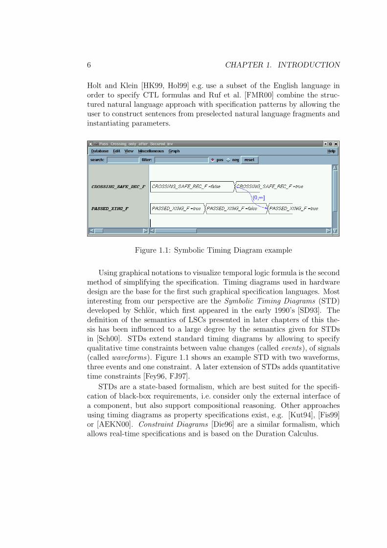
Figure 1.1: Symbolic Timing Diagram example
Using graphical notations to visualize temporal logic formula is the secondmethod of simplifying the specification. Timing diagrams used in hardwaredesign are the base for the first such graphical specification languages. Mostinteresting from our perspective are the Symbolic Timing Diagrams (STD)developed by Schlor, which first appeared in the early 1990’s [SD93]. Thedefinition of the semantics of LSCs presented in later chapters of this the-sis has been influenced to a large degree by the semantics given for STDsin [Sch00]. STDs extend standard timing diagrams by allowing to specifyqualitative time constraints between value changes (called events), of signals(called waveforms). Figure 1.1 shows an example STD with two waveforms,three events and one constraint. A later extension of STDs adds quantitativetime constraints [Fey96, FJ97].
STDs are a state-based formalism, which are best suited for the specifi-cation of black-box requirements, i.e. consider only the external interface ofa component, but also support compositional reasoning. Other approachesusing timing diagrams as property specifications exist, e.g. [Kut94], [Fis99]or [AEKN00]. Constraint Diagrams [Die96] are a similar formalism, whichallows real-time specifications and is based on the Duration Calculus.
7
Specification of Communication Properties
The specification formalisms in the preceding section have been developedwith a single component in mind. The expressivity of most approaches alsoallows to state properties about several components, but they are not tai-lored to this particular use case. With respect to the increasing number ofembedded controllers, which are used today and which often also exchangeinformation and commands among each other, an appropriate graphical for-malism is needed in order to meet the changed demands. Ideally, such aformalism is not limited to being a graphical front-end for temporal logic,but is suited also for other use cases, as elaborated below.
activate_rec
ack_sndack_rec
activate_snd
status_req_sndstatus_req_rec
safe_sndsafe_rec
msc activateCrossing
Train Comm Crossing
Safe
T1(50)
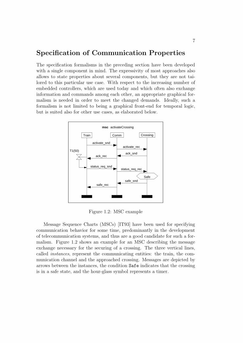
Figure 1.2: MSC example
Message Sequence Charts (MSCs) [IT93] have been used for specifyingcommunication behavior for some time, predominantly in the developmentof telecommunication systems, and thus are a good candidate for such a for-malism. Figure 1.2 shows an example for an MSC describing the messageexchange necessary for the securing of a crossing. The three vertical lines,called instances, represent the communicating entities: the train, the com-munication channel and the approached crossing. Messages are depicted byarrows between the instances, the condition Safe indicates that the crossingis in a safe state, and the hour-glass symbol represents a timer.
8 CHAPTER 1. INTRODUCTION
This example demonstrates the intuitiveness of these basic MSC con-structs, which motivates their application for the requirement capture in theearly development phases, where they are used to document typical inter-actions, often referred to as scenarios. This is also the major use case forSequence Diagrams (SDs), which are a very similar graphical descriptionwithin the UML and are applied to the same end there. Today, such scenar-ios serve two purposes: gaining a better understanding of the behavior of thedeveloped application, and documentation. They often also record simula-tion or test traces. More advanced use cases are conceivable, however, whichreuse the early scenarios in later stages of the development process and thusprovide an added value. The following use cases show great promise:
Model Synthesis Starting from a set of scenarios, which identify the en-tities comprising the system under design (SUD) and describe theirtypical interactions, a first cut of a model is synthesized. From the com-munication behavior shown in the MSCs or SDs a preliminary modelstructure and behavioral description is derived, which can be extendedmanually.
Existential Check Once a model exists it can be checked, if the function-ality specified by the early scenarios is possible in the current model,i.e. if it is able to fulfill each behavior described in a scenario at leastonce. A failed check indicates a fundamental error. This check servesas an early and easy to use debugging aid.
Model Testing When a largely stable model exists and a simulator is avail-able, MSCs/SDs can serve as watchdogs monitoring a user-driven sim-ulation session. Deviations from the specified scenarios are detectedand reported. Additionally MSCs/SDs can be used to drive the simu-lation without user interaction by providing the required input stimuliand observing, if the expected model reactions ensue. This use caseis another step toward a reference model and is also ideally suited forregression testing, where a set of MSCs/SDs are re-run after a changeto the model in order to ensure that the basic original functionality isstill guaranteed.
Formal Verification MSCs/SDs can be used to state communication pro-tocols between different entities and employ them for formal verifica-tion.
9
Test Vector Generation Existing scenarios from earlier phases in the de-velopment or also newly generated ones can be used to automaticallygenerate test vectors for integration testing of several communicatingembedded controllers.
All of the abovementioned use cases demand a formal foundation in orderto be realized by corresponding tools. Neither MSCs nor SDs fully complywith this demand. For MSCs a formal semantics exists, but several impor-tant issues are covered only inadequately or not at all. Liveness properties,e.g. that a message must arrive at its destination, can for instance not beexpressed in the formal semantics of MSCs. Only safety properties are ex-pressible, i.e. that the receipt of a message may only occur after sending. ForSequence Diagrams no formal semantics has been defined so far. Moreover,both languages are lacking expressiveness wrt. to the envisioned advanceduse cases. For the verification and model testing use cases e.g. it is vitallyimportant to know when the specified communication behavior should beobserved, i.e. when the chart is active. A more detailed introduction andcriticism of MSCs and SDs in this respect is presented in chapter 3. Ain-depth treatment of the state-of-the-art regarding the abovementioned ad-vances use cases is given in the chapters dealing with the individual languageconstructs of LSCs.
In summary we can state that in general the intuitiveness and visualappeal of MSCs and SDs is very well suited for the abovementioned use cases,but they are lacking expressiveness and an adequate formal semantics. Thisis where Live Sequence Charts, the central subject of this thesis, come intoplay. Damm and Harel noted the potential of MSCs and SDs to become morethan scenario descriptions, if given a sound and more expressive basis, andproposed Live Sequence Charts (LSCs) in [DH98] as an extension of MSCsand SDs, which addresses these shortcomings. This work is the starting pointfor the present thesis, where the basic ideas of Damm and Harel are renderedmore precise and treated more completely than in [DH98].
The fundamental idea of LSCs is the distinction between mandatory andpossible behavior, where conventional MSCs and SDs are considered as con-sisting of possible elements only and mandatory elements constitute the en-hancements of expressiveness offered by LSCs. This concept is applied toalmost all language constructs: entire charts, instance lines, messages, con-ditions, etc. On the chart level this allows the distinction between existentialand universal LSC specifications, the former being the scenario view of MSCs
10 CHAPTER 1. INTRODUCTION
and SDs (there exists a run, which conforms to the chart) and the latter al-lowing the specification of protocols, which have to be obeyed by all runs ofa system. For instance lines and messages mandatory means that livenessproperties can be specified, i.e. points along an instance line must be reachedand messages must be received once sent. This important feature is also thesource of the name of Live Sequence Charts. The expressive power of LSCsis additionally enhanced by truly supporting conditions by associating themwith a boolean expression (making them “first-class citizens” in the wordsof [DH98]), instead of the informal treatment in MSCs or their absence inSDs. Conditions in LSCs are not limited to single points in time, but mayconstrain a number of contiguous time points, in which case they are calledlocal invariants. Additionally, LSCs allow to specify the activation point ofa chart by an activation condition. The full set of features is explained inmore detail in chapters 4 - 9.
The goal of this thesis is the development of a language for the easy, intu-itive, graphical specification of interactions between communicating entities.This language are Live Sequence Charts. The first task in this respect isthe definition of the language constructs required to express the propertiesnecessary for a more prominent role of sequence charts4 in the developmentprocess. This involves a non-trivial trade-off between retaining as much in-tuitiveness as possible on the one hand and providing as much expressivepower as necessary on the other. The second major task is the definition of asuitable formal semantics, which unambiguously expresses the meaning of allfeatures and their combinations and thus allows the automated processing ofLSCs.
Another point is essential in order to successfully apply any formalism ormethod in general, and LSCs in particular, in the real world: An indicationhas to be given in which phases of the development the formalism in questionshould be applied and to which end. Answering this question is the third goalof this thesis. The final task is the evaluation of the LSC language by applyingit to one of the abovementioned advanced use cases: formal verification. Theevaluation should demonstrate, if the expressiveness is sufficient and if thesemantics is appropriate and useful in practice. This proof of concept willbe done by using LSCs for property specification for the formal verificationof Statemate designs.
4We will use the term ‘sequence chart’ to denote the sum of all dialects, be it MSCs,SDs, LSCs, . . . .
11
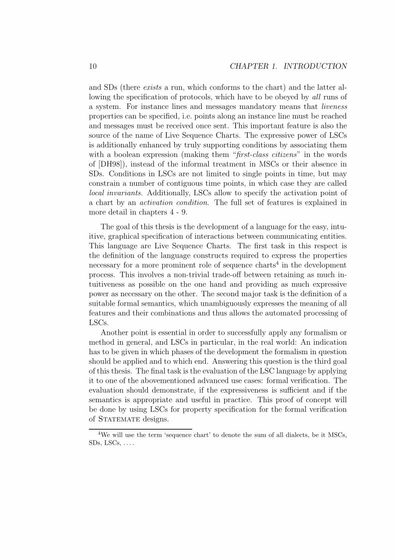
Formal Verification of Statemate Designs
This section briefly introduces the Statemate tool and notations andalso gives a short overview over the Statemate Verification Environment(STVE), into which the tools dealing with LSCs are prototypically integrated.
Statemate
Statemate is a CASE-tool, distributed by I-Logix, Inc., USA, which allowsto build an abstract model of an SUD, e.g. an embedded controller. It offersto capture several views onto the SUD, the most important ones being thefunctional decomposition and the behavioral description. Other views likethe modeling of continuous aspects or physical distribution of componentsare possible as well; the details are described e.g. in [HLN+90] or [HP96].Here only the former two aspects are explained as the STVE is based onthese.
Figure 1.3: Top level Activity Chart
12 CHAPTER 1. INTRODUCTION
Activity Charts
The functional decomposition of an SUD is modeled by Activity Charts,whereas the behavioral description is given by Statecharts. Figure 1.3 onthe preceding page shows an example for a top-level Activity Chart for thetrain control system, which is discussed in more detail in chapter 2. Eachfunctional unit, called activity in Statemate, is represented by a solid linebox, e.g. TRAIN or CROSSING in figure 1.3. The environment is represented byexternal activities depicted by dashed line rectangles, e.g. DRIVER or BARRIER,which provide input stimuli or accept outputs of the model. Activities canbe structured into a hierarchy, where each Activity Chart represents onelevel of the hierarchy. The top-level Activity Chart in figure 1.3 for instancecontains the three activities shown, which in turn are further decomposedinto other Activity Charts, indicated by the ‘@’ in front of the activity name.The activities TRAIN and CROSSING are truly decomposed further as shownin figures 2.3 on page 28 and 2.10 on page 37 in section 2.2, whereas theActivity Chart for COMMUNICATION contains only the behavioral descriptionof this component.
On each level of hierarchy a control activity can be specified, which isresponsible for controlling, i.e. starting, stopping, etc., the other activitiespresent. The control activity is depicted by solid line box with rounded cor-ners (e.g. SPEED CONTROL CTRL in figure 2.3 on page 28). If no control activityis specified, as is the case in the Activity Chart in figure 1.3, all activities atthis level of hierarchy are activated at system start. A control activity locatedon a level without any other activities, e.g. SPEED CONTROL CTRL, is one ofthe possibilities offered by Statemate for the specification of behavior.
Information exchange between activities is depicted by arrows leadingfrom the sender to the receiver. The user can distinguish data and controlflows, represented by solid, resp. dashed arrows. Several individual commu-nications leading from one sender to the same receiver can be combined intoa single arrow, called an information flow.
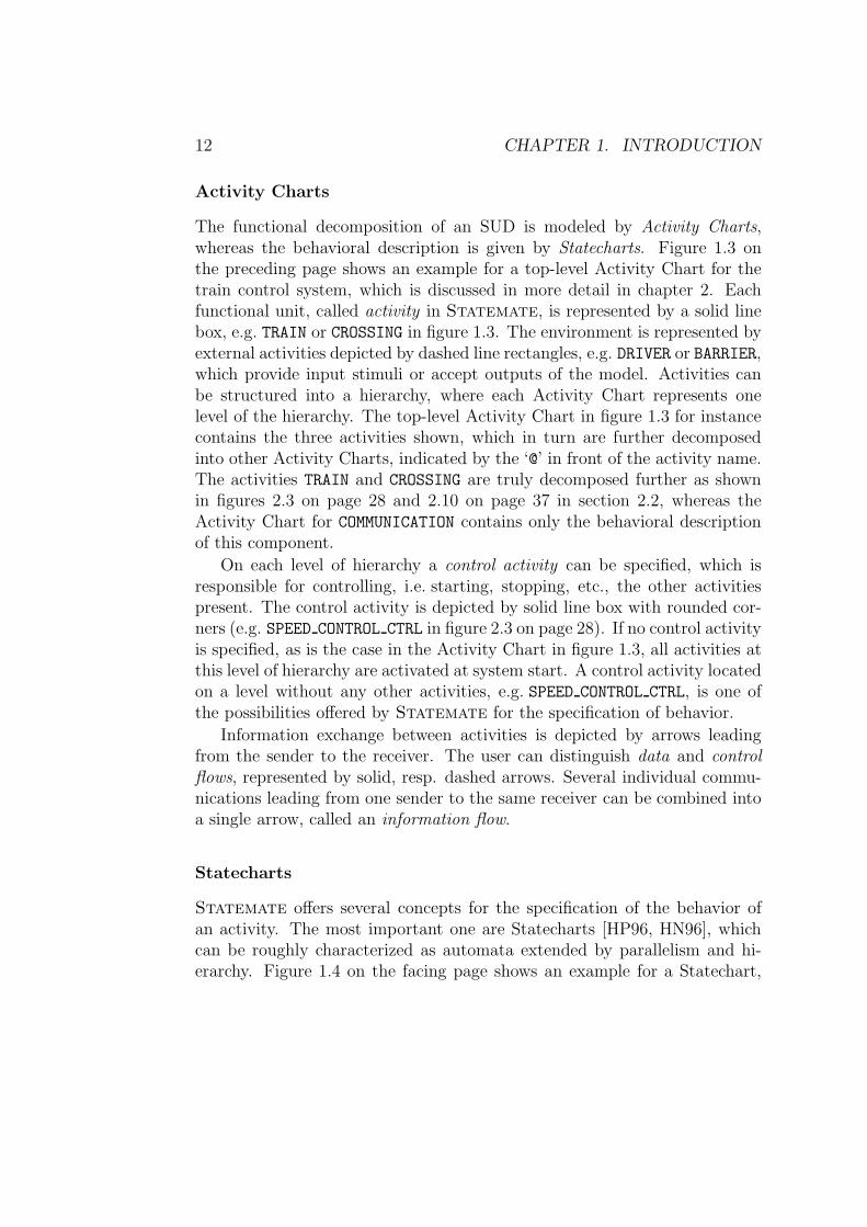
Statecharts
Statemate offers several concepts for the specification of the behavior ofan activity. The most important one are Statecharts [HP96, HN96], whichcan be roughly characterized as automata extended by parallelism and hi-erarchy. Figure 1.4 on the facing page shows an example for a Statechart,
13
Figure 1.4: Statechart example
again taken from the model of the train control system. The StatechartSPEED CONTROL CTRL is split into two parallel parts, called AND-States inStatemate terminology, indicated by the dashed line separating sub-statesCOMPUTE SPEED and SUPERVISE SPEED. The latter is further structured intothree sub-states, so-called OR-states. States, which are not decomposed, arecalled basic states. All sub-states of an AND-state are active, when the gov-erning AND-state is active, i.e. both COMPUTE SPEED and SUPERVISE SPEED
are active when SPEED CONTROL CTRL is active, whereas only exactly oneof the OR-states at each level of hierarchy may be active at a time, i.e. ifSUPERVISE SPEED is active either FREE RUN or FORCE BRAKE or FORCE STOP
is active. The entire Statechart is active, if the activity it is contained in isactive.
14 CHAPTER 1. INTRODUCTION
When a Statechart is active it can react on changes to system variablesby taking transitions between states. Each transition is annotated by
trigger[guard]/action
consisting of a trigger, which determines when the transition is possiblyenabled, a boolean expression guard, which further restricts the enablednessof the transition, and an action part containing the ensuing consequences. Atransition is enabled, if the source state is active, the trigger is observed andthe guard evaluates to true. An enabled transition need not fire, since theremay be other transition, which are enabled concurrently. There are priorityrules determining which enabled transition is actually fired, but not all casescan be covered by these rules, so that non-deterministic situations can arise.If a transition is fired, control changes to the target state and the actions areexecuted, which can consist of the generation of events, variable assignments,control commands for other activities, e.g. st!(TIMER) or sp!(TIMER) forstarting, resp. stopping activity TIMER.
Which state of a Statechart or decomposed state is active initially is de-termined by a default transition, which is graphically depicted as a transitionwithout a source state; state FREE RUN e.g. is initially activated in figure 1.4.
Variables in Statemate are typed and the user may choose from severaldata types, one of the most important ones being Event, which is a booleansignal visible for one step (execution cycle). Other available types are condi-tion and data items, the latter comprising integer, real, etc.; see [HP96] formore details. Other modeling constructs will be introduced by example whenpresenting the Statemate for the train control case study in section 2.2.
Statemate Simulation Semantics
Part of the Statemate tool is a simulator, which allows the interactive exe-cution of the model. Simulation runs can be recorded in Simulation ControlPrograms (SCP) to be replayed later. The simulator supports two executionmodels: synchronous and asynchronous semantics, which differ in the un-derlying time model and the points in time when the embedded controllercommunicates with its environment.
In the synchronous semantics the model accepts inputs from the envi-ronment every step, whereas in the asynchronous semantics new inputs areconsumed only when all computations in reaction to the previous inputs havebeen completed, i.e. a stable state is reached, where no further transition can
15
be fired without new input stimuli. In the asynchronous semantics reactionto one set of input stimuli thus may entail several internal steps, which do notconsume time; time only passes when the system has reached a stable stateand synchronizes with its environment. The transition from one stable stateto the next is called a superstep. The asynchronous semantics is often alsoreferred to as superstep semantics, the synchronous one as step semantics.
Statemate Verification Environment
LogicTemporal
Pattern AnalysesSymbolic TimingDiagrams (STDs)
Counter Example Visualization
FSM
Statemate
VIS/Prover
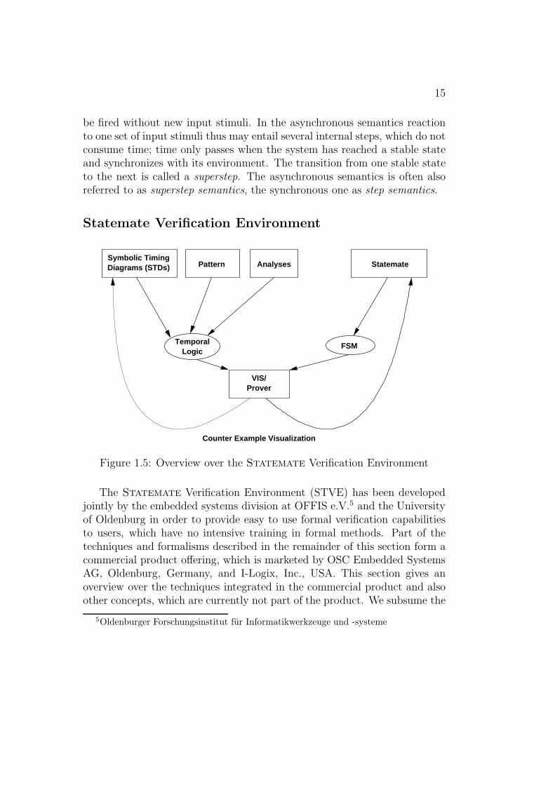
Figure 1.5: Overview over the Statemate Verification Environment
The Statemate Verification Environment (STVE) has been developedjointly by the embedded systems division at OFFIS e.V.5 and the Universityof Oldenburg in order to provide easy to use formal verification capabilitiesto users, which have no intensive training in formal methods. Part of thetechniques and formalisms described in the remainder of this section form acommercial product offering, which is marketed by OSC Embedded SystemsAG, Oldenburg, Germany, and I-Logix, Inc., USA. This section gives anoverview over the techniques integrated in the commercial product and alsoother concepts, which are currently not part of the product. We subsume the
5Oldenburger Forschungsinstitut fur Informatikwerkzeuge und -systeme
16 CHAPTER 1. INTRODUCTION
entire set of features and techniques under the term Statemate VerificationEnvironment. Figure 1.5 on the page before shows the general organizationof the STVE.
The offered techniques are grouped into different skill levels ranging fromanalyses, which can be employed by ordinary designers familiar with State-mate to full-fledged property specification and verification capabilities. Theincrease of expert knowledge required is accompanied by an increase of ex-pressive power: the more knowledge is needed to apply a technique, the morecomplex properties can be expressed.
The techniques offered are grouped into three categories: robustnesschecks, pattern-based verification and STD-based verification. The robust-ness checks are simple, but formal analyses, which can be used by a typicalStatemate user. They comprise checks/analyses for
• non-deterministic situations:
– concurrently enabled transitions
– multiple writer (two or more activities simultaneously write a dataitem)
– read-write hazards (a data item is read and written simultane-ously)
– range violations (a data item is assigned an out-of-range value)
• reachability
– reachability of basic states
– reachability of state configurations (sets of basic states)
– reachability of transitions
– reachability of specific values for data items
Note that the check for a non-deterministic choice between concurrentlyenabled transitions only reports those situations, which are not already re-solved by the Statemate priority rules for transitions. These analyses areintended to be used for debugging purposes as the model is developed byanswering questions like: “Are all states of the model reachable?”, “Is it pos-sible to observe value ‘7’ at output o1?”, or “Are there situations, where —
17
after applying the priority rules — more than one transition is concurrentlyenabled?”.
There are two core verification engines which can be used alternatively:the VIS model checker ([Gro96a, Gro96b]) and a bounded model checkerbased on the SAT checker ProverCL. By exploiting the counter examplegeneration capabilities of the VIS witnesses are produced, which lead intoexactly those situations, which have been checked by the robustness analy-sis, provided such a situation exists. The general goal of these analyses thusis falsification, i.e. the expectation is that a witness exists, e.g. how to reacha certain basic state. This can be exploited by using reachability-based modelchecking with early termination6 [Gro96a, Gro96b]. Instead of employingthe standard backward-oriented fix-point iteration (see e.g. [CGP99]) thisstrategy checks the formula while performing a forward-oriented reachabilityanalysis. If the formula does not hold, the reachability analysis is aborted(early termination), because a counter example has been found. If the for-mula indeed fails, this strategy generally performs better than the fix-pointiteration, since only part of the reachable states need to be considered.
Falsification is also the prime use case for the practical application ofbounded model checking [BCCZ99], which is very efficient for these cases.When a checked property does not hold, SAT-checkers, which form the coreof bounded model checkers, are typically more efficient than standard modelcheckers. The STVE therefore offers bounded model checking via integrationof the SAT solver ProverCL [SS98] of Prover Technologies, Sweden, insteadof the VIS for robustness checks and other situations when a counter exampleis expected. Note that both reachability-based and bounded model checkingare limited to check invariant formulas of the form ‘AG(p)’.7
More information on the robustness checks of the STVE are found in[BBHW00, BDW00, OSC02b, BDKW01].
The pattern-based verification is a oriented towards certification, in-stead of falsification, i.e. the specified properties are expected to hold onthe model. The STVE offers a library of pre-defined parameterized patterns,which allow to express a set of typical properties. Each pattern is instan-
6The term ”reachability” used here is a different one than the one used in the abovechecks. The term here refers to reachable states in the finite state machine (FSM) gener-ated for the Statemate design, whereas reachability as used above refers to Statemateitems (basic states, transitions, etc.).
7The bounded model checking procedure described in [BCCZ99] also considers otherformulas, but in practice globally formulas are used almost exclusively.
18 CHAPTER 1. INTRODUCTION
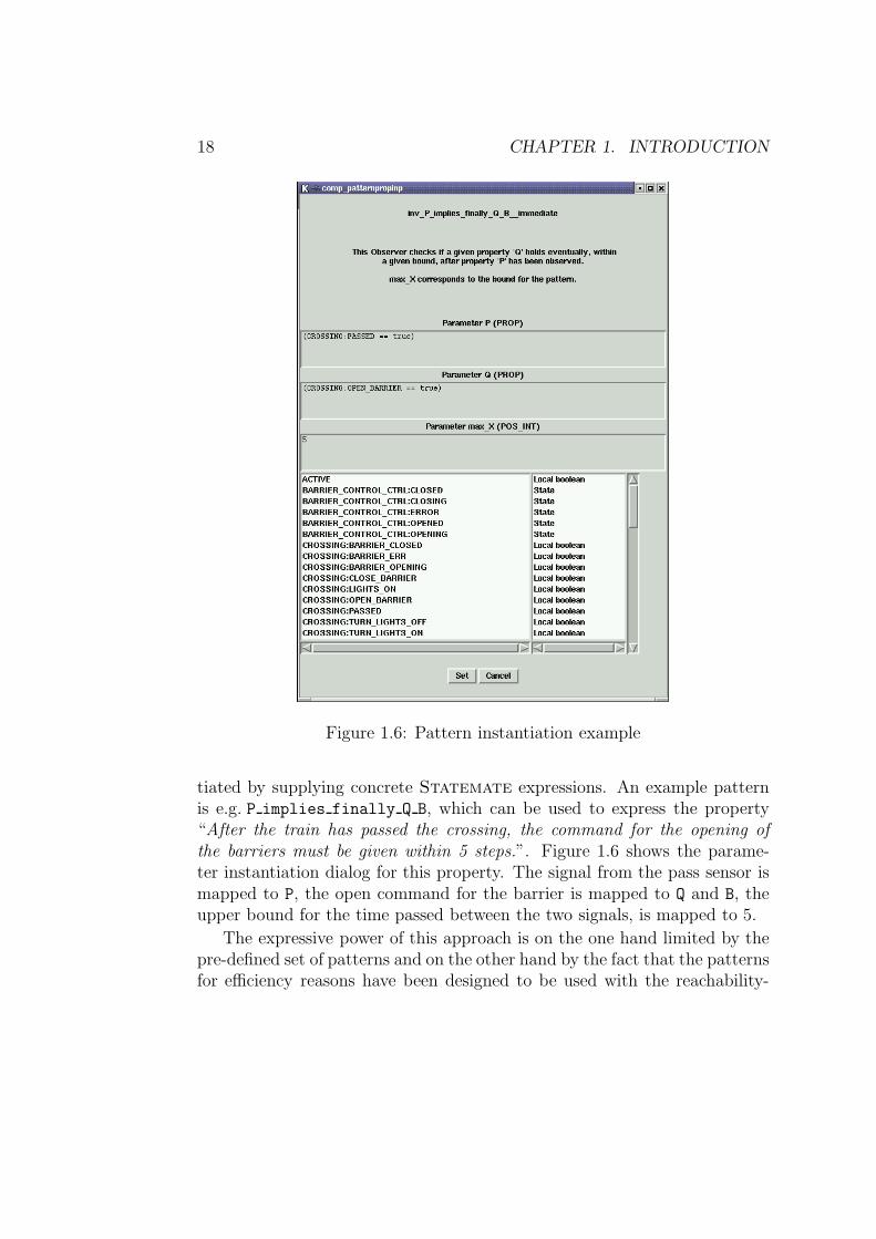
Figure 1.6: Pattern instantiation example
tiated by supplying concrete Statemate expressions. An example patternis e.g. P implies finally Q B, which can be used to express the property“After the train has passed the crossing, the command for the opening ofthe barriers must be given within 5 steps.”. Figure 1.6 shows the parame-ter instantiation dialog for this property. The signal from the pass sensor ismapped to P, the open command for the barrier is mapped to Q and B, theupper bound for the time passed between the two signals, is mapped to 5.
The expressive power of this approach is on the one hand limited by thepre-defined set of patterns and on the other hand by the fact that the patternsfor efficiency reasons have been designed to be used with the reachability-
19
based method. This entails that, in addition to safety properties, boundedliveness properties may be expressed as the example pattern demonstrates,but no unbounded liveness requirements.More information on the STVE patterns is available in [OSC02a].
If more flexibility in stating requirements is desired or unbounded live-ness properties are to be expressed, Symbolic Timing Diagrams (STDs[Sch00, FJ97]) are offered, which allow to specify completely user-definedproperties. Figure 1.1 on page 6 shows an example STD, which has beenspecified for the crossing component of the train control system. The re-quirement is formulated over the interface objects CROSSING SAFE REC F andPASSED XING F and expresses that the crossing may only be passed by thetrain after it has indicated its safe state. Properties stated as STDs arechecked using the standard fix-point iteration-based model check algorithm.More information on the application of STDs within the STVE can be foundin [BW98, BBD+99, DDK99, KM00, DK01].
The overview shown in figure 1.5 on page 15 illustrates the general orga-nization of the STVE. The Statemate design to be verified is transformedautomatically into a finite state machine (right hand side of figure 1.5) andthe property to be checked is translated into a temporal logic formula (lefthalf of figure 1.5). The translation of STDs is split into two phases: first asymbolic automaton is derived for an STD, which in turn is transformed intoa temporal logic formula.
If a property specified as an STD or pattern is violated by the modelor a witness for a robustness check is found, the (bounded) model checkergenerates an error path, which can be visualized and examined in two ways.The preferred and most natural way is to translate it into an SCP in orderto execute in the Statemate simulator. Alternatively the error path can bevisualized as an STD.
For more information about the different formalisms and techniquescontained in the STVE the reader is referred to the following refer-ences: [Bro99] describes the FSM generation for Statemate designs,[BDW00, BDKW01, BBHW00, OSC02b] provide more details about theanalyses, the pattern-based approach is described in [OSC02a], and informa-tion on formal verification of Statemate designs using STDs can be foundin [BW98, DDK99, KM00, DK01]. Details about the technologies underlyingthe STVE are contained in [BBD+99, BBB+99, Bie03, Wit03].
20 CHAPTER 1. INTRODUCTION
Organization of this Thesis
Chapter 2 introduces the train control case study, which serves as a runningexample throughout this thesis. This case study deals with a radio-basedsignaling system for the control of level crossings. This chapter contains ageneral introduction and a detailed description of the Statemate model,which will also be used for obtaining experimental results in chapter 11.
The language of Live Sequence Charts is motivated by both the visual ap-peal and lack of expressiveness and formal rigor of Message Sequence Chartsand UML’s Sequence Diagrams as has been expounded above. Chapter 3gives an overview over the two sequence charts dialects, describing the majorfeatures, historical development and discussing the shortcomings wrt. theadvanced use cases briefly presented above. The complete set of featuresof the LSC language, along with the definition of the formal semantics, ispresented incrementally in the following chapters. Chapter 4 begins with thebasic LSC features, whose motivation, graphical representation and informalmeaning are described.
The semantics of an LSC is defined in terms of an automaton. The re-lation between the embedded controller being developed (the SUD) and theLSC specification is established by considering runs of the system and deter-mining, if they are accepted by the automaton. The SUDs, whose propertiesare to be specified by LSCs, operate for an indeterminate amount of time(theoretically forever), so that the automata used for the semantics defini-tion must be able to deal with infinite runs. Chapter 5 introduces a suitableautomata format, derived from Buchi automata and also defines a corre-sponding timed variant thereof. Defining the semantics of LSCs in termsof Buchi automata allows to easily derive temporal logic formulas due tothe well-known relationship between (a sub-class of) Buchi automata andLTL. The temporal logic formulas are essential for later formal verificationactivities.
Chapter 6 defines a formal syntax for the LSC constructs introducedin chapter 4, upon which the algorithm for the generation of the automa-ton operates. The basic algorithm defined here is extended in the followingchapters. The complete semantics of an LSC is then defined on the basisof the generated automaton incorporating the activation and quantificationinformation.
Chapter 7 extends the basic features by additionally considering timingconstraints and extending the automaton generation algorithm to produce
21
a timed automaton. Chapter 8 deals with a feature, which is essential forthe use case of formal verification: assumptions. Since the environment ofan SUD is already part of the LSC, in form of one or more environmentinstances, assumptions about the expected environment behavior are easilyspecified within an LSC by using elements on dedicated instances.
Chapter 9 enhances the activation information not only allowing to con-sider one point in time, via the activation condition, in order to determineif an LSC is to be activated or not. Additionally a sequence of messagesforming a pre-chart may now trigger the activation of the actual LSC. Thepre-chart semantics is again defined in terms of an automaton.
Chapter 10 addresses the third task specified above and proposes amethodology of how LSCs can be embedded into a model-based develop-ment process. The focus is on a re-use of LSCs from early stages in thedesign process.
The practical application of LSCs to the use case of formal verificationis presented in chapter 11. The Statemate Verification Environment iscovered in more detail and the integration of the LSC tools is described. Themajor part of this chapter is taken up by the experimental results. Chapter 12concludes this work with a summary and identification of directions for futurework.
Appendix A summarizes all LSCs used in the verification of the traincontrol system, including the corresponding automata. Appendix B lists thecontents of all information flows used in the Statemate model for the traincontrol system and appendix C contains the grammar of the textual LSCrepresentation.

22 CHAPTER 1. INTRODUCTION
Chapter 2
Sample Application: A
Radio-based Signaling System
This chapter introduces the case study, which will be used as a runningexample throughout this thesis. Section 2.1 gives a short introduction to thegeneral subject before the Statemate model of the case study is presentedin section 2.2. This Statemate model will also be used to evaluate theconcepts and tools described in the remainder of this work; cf. chapter 11.
2.1 General Description
The control of level crossings, crossings for short, is currently carried out bywayside hardware, for example sensors, which announce an approaching trainto a crossing, signals, which for instance indicate the status of the crossingto the train driver, etc. This solution is rather inflexible, since the hardwareis permanently installed and must be able to handle different trains varyingin speed, length, etc. Another drawback is the high amount of maintenanceinvolved to keep signals, sensors and wiring operational. International railtraffic additionally raises demands for more flexibility, since almost everyEuropean country uses different signaling technology, so that trains can noteasily cross borders. This has prompted railway companies to look for better,more flexible and efficient solutions for the control of trains, crossings, etc.There exist efforts on the European level with the objective of harmonizingand facilitating international rail traffic in Europe: the ERTMS/ETCS (Eu-ropean Rail Traffic Management System/ European Train Control System)
23
24 CHAPTER 2. SAMPLE APPLICATION
will use radio transmission, among other measures, for the communicationbetween trains and the operations center (then called radio block controller).The German railway company Deutsche Bahn investigated a more advancedconcept, which proposes to use a radio connection also for the communicationbetween train and crossing and points. This allows more flexibility inasmuchas each train can contact a crossing depending on its specific information,a slow train would e.g. announce itself later than a faster train. This solu-tion also entails lower maintenance effort, since the involved components arelocated on the train and directly at the crossing, instead of being dispersedalong the track.
EnvCrossingTrain
activate
ack
red_on
yellow_on
lower_barrier
closed
status_req
safe
train_passed
raise_barrier
opened
switch_off_lights
Invariantactivation_point_reachedsecuring_all
AM:AC:LSC
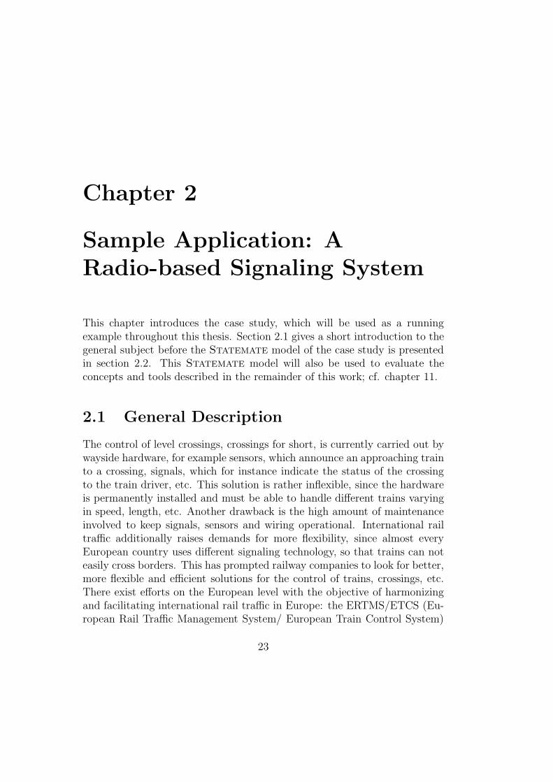
Figure 2.1: Existential LSC showing the typical interaction between trainand crossing
2.1. GENERAL DESCRIPTION 25
There are several different strategies used in the traditional control ofcrossings by means of wayside equipment, which serve as blueprints for theradio-based approach. This case study considers the radio-based crossingcontrol according to the guarding signal strategy. Figure 2.1 shows an exis-tential LSC depicting the typical interaction between train and crossing forthis strategy. Even without a detailed understanding of all the features ofthe LSC language, the graphical nature of this representation is sufficient tobe used as an illustration of the protocol between train and crossing.
Once the activation point is reached, indicated by the second row in theLSC header, the train activates the crossing. The activation point is the latestpoint at which the train can initiate the securing of the crossing, if it is to bepassed without braking. In the hard-wired control this point was given by afixed sensor, which sent a signal to the crossing. In the radio-based versionthis point can be determined dynamically. The exact position of this pointmust consider the delays for communication setup, message transmission, thetime necessary to secure the crossing, an additional safety interval and thespeed and position of the train. The crossing acknowledges the receipt ofthe activation request and starts the securing procedure by switching on firstthe yellow and then the red light of the traffic lights in order to warn thecar traffic. Then the command to close the barriers is given and once thebarriers are indeed closed, the crossing is in a secured state.
After the amount of time has passed, which in ordinary circumstancesis needed to secure the crossing, the train requests a status report fromthe crossing. Here, the crossing responds with the report safe. Should thecrossing not be in a safe state when the status request arrives, no responseis given. In the hard-wired control this corresponds to the crossing settingthe guarding signal to go in the safe case, and leaving it set to stop in theunsafe case.
A pass sensor determines when the train has passed the crossing andsends a corresponding signal to the crossing controller. Then the crossingis returned into its normal state, i.e. the barriers are opened again and thetraffic lights are switched off.
Before a train can approach and contact a crossing, it needs to knowthe position of the crossing. This information is stored in a track chartalong with other details about the track, like maximal velocity, position ofcrossings, points, stations, etc. Once the train has been granted movementauthorization for a track segment, it looks up the relevant information inthe track chart and places control points at all potentially dangerous points,
26 CHAPTER 2. SAMPLE APPLICATION
which can e.g. be track segments with a lowered maximally allowed speed,crossings, points, stations, or the end of the assigned track segment. Witheach control point a target speed is associated, which must be observed; fornot secured crossings or not set points for instance this speed is zero, sothat the train e.g. has to stop in front of a crossing. Control points due tocrossings, points, stations or the end of the assigned track segment requiresome action on the part of the train: a crossing needs to be secured beforeit can be passed, a switch must be set to the right track, the train shouldstop at a station it is supposed to service, and movement authorization for asubsequent track segment must be requested before reaching the end of thecurrently assigned segment.
The control points are considered by the train in the calculation of themaximal velocity for each point in time. This speed profile is the basis forthe speed supervision, which controls that the train does not go faster thanallowed by track, train and control points. Once a control point has becomeirrelevant, e.g. because a crossing has been secured and it is no longer neces-sary that the train stops, it is disregarded for the maximal speed computationand thus no longer restricts the train’s velocity.
This case study focuses on one aspect of the entire set of tasks necessaryfor radio-controlled train operation: the control of level crossings. Points,stations, etc. are neglected and it is assumed that movement authorizationhas been granted. The considered type of crossing guards a single track andits barriers cover only one side of the street.
2.2 STATEMATE Model
The Statemate model of the radio-controlled crossing bases on a model,which has been developed in [KT00], but has been slightly adapted to ourneeds in this thesis. Earlier versions have been partly described in [DDK99,KM00, DK01]. The model presented here uses the asynchronous simulationsemantics of Statemate, a variation using the synchronous semantics existsas well, but is not described in detail here, since the differences are only minor.
2.2.1 Activity Chart SYSTEM
Figure 2.2 on the facing page shows the top level Activity Chart (SYSTEM)of the radio-based crossing control. The two main activities are TRAIN and
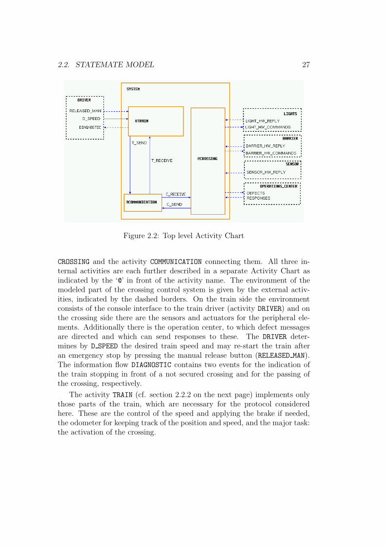
2.2. STATEMATE MODEL 27
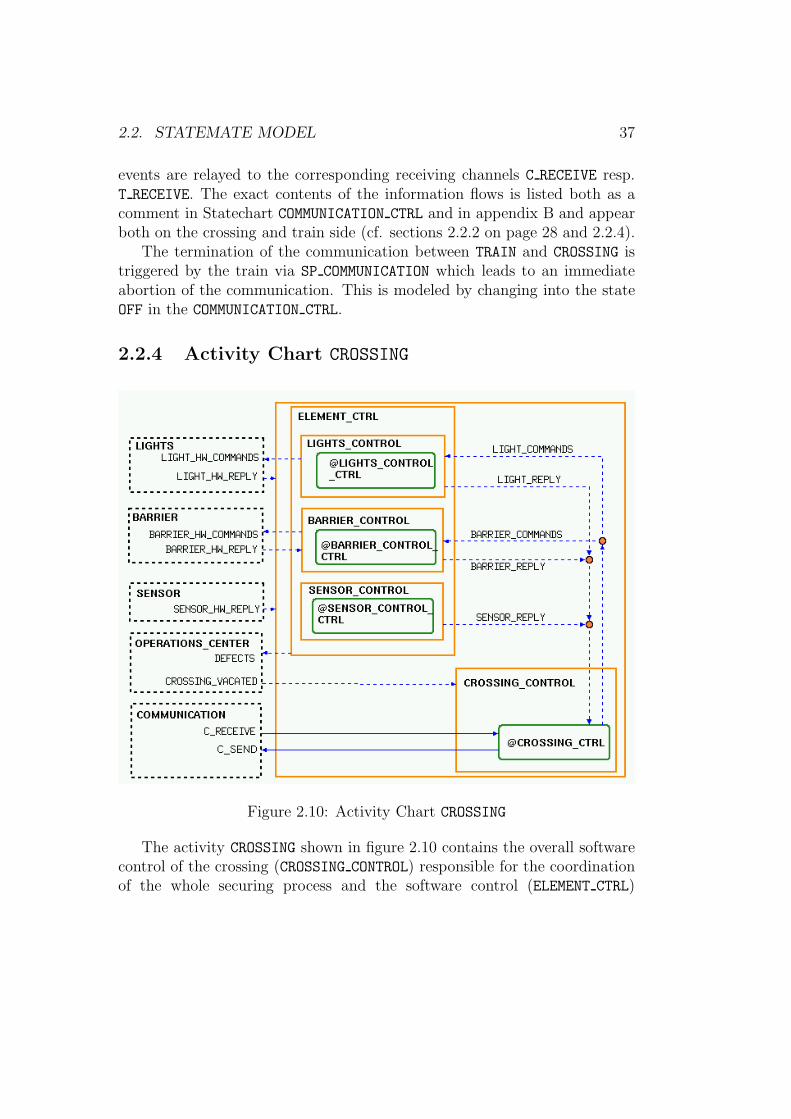
Figure 2.2: Top level Activity Chart
CROSSING and the activity COMMUNICATION connecting them. All three in-ternal activities are each further described in a separate Activity Chart asindicated by the ‘@’ in front of the activity name. The environment of themodeled part of the crossing control system is given by the external activ-ities, indicated by the dashed borders. On the train side the environmentconsists of the console interface to the train driver (activity DRIVER) and onthe crossing side there are the sensors and actuators for the peripheral ele-ments. Additionally there is the operation center, to which defect messagesare directed and which can send responses to these. The DRIVER deter-mines by D SPEED the desired train speed and may re-start the train afteran emergency stop by pressing the manual release button (RELEASED MAN).The information flow DIAGNOSTIC contains two events for the indication ofthe train stopping in front of a not secured crossing and for the passing ofthe crossing, respectively.
The activity TRAIN (cf. section 2.2.2 on the next page) implements onlythose parts of the train, which are necessary for the protocol consideredhere. These are the control of the speed and applying the brake if needed,the odometer for keeping track of the position and speed, and the major task:the activation of the crossing.
28 CHAPTER 2. SAMPLE APPLICATION
The implementation of a crossing in activity CROSSING (cf. sec-tion 2.2.4 on page 37) contains sub-controllers for all peripheral elements(lights, barrier, pass sensor) as well as the overall control for securing thecrossing.
The information flow between TRAIN and CROSSING is established bymeans of activity COMMUNICATION (cf. section 2.2.3 on page 36). The infor-mation exchange takes place via the information flows T SEND and T RECEIVE
between TRAIN and COMMUNICATION, respectively C SEND and C RECEIVE
between CROSSING and COMMUNICATION. The signals sent in T SEND andC SEND are relayed by COMMUNICATION to the corresponding receive chan-nel (C RECEIVE, resp. T RECEIVE). The exact contents of information flowsis listed in appendix B.
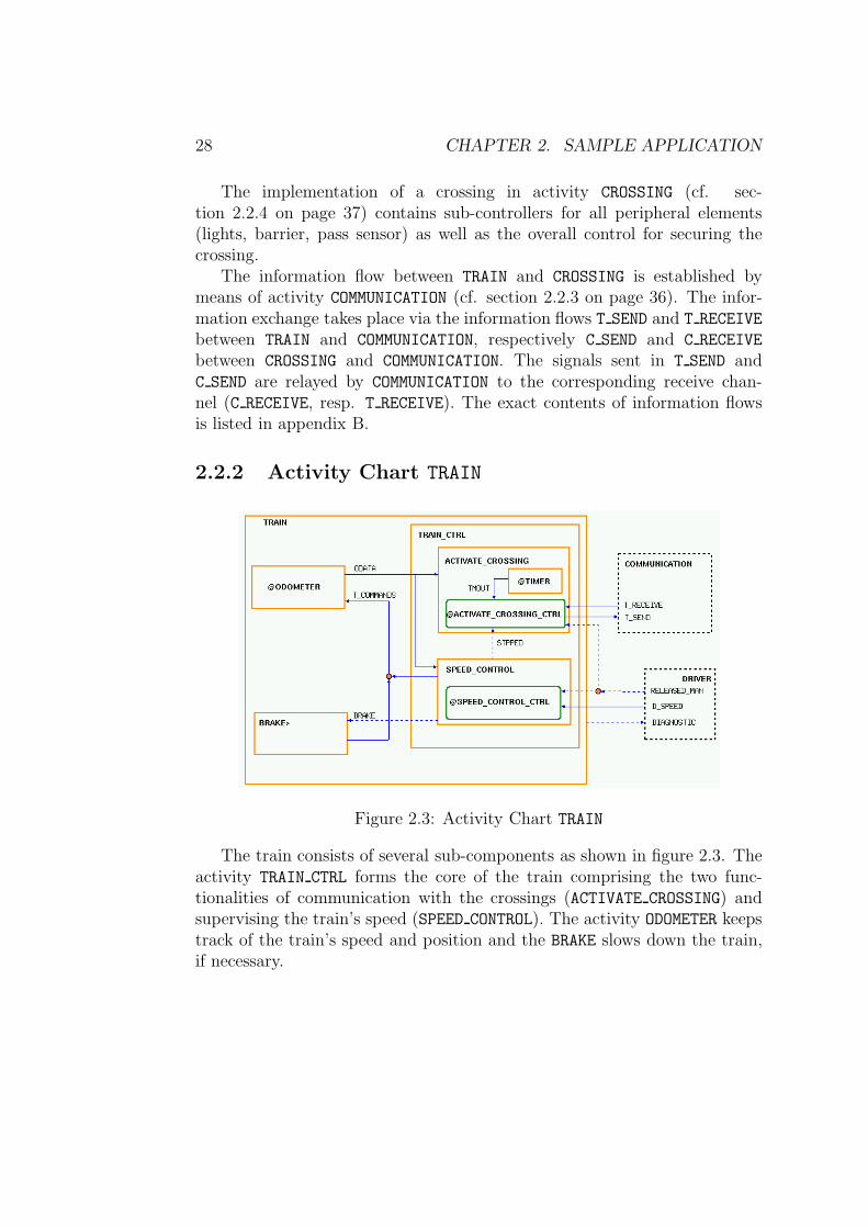
2.2.2 Activity Chart TRAIN
Figure 2.3: Activity Chart TRAIN
The train consists of several sub-components as shown in figure 2.3. Theactivity TRAIN CTRL forms the core of the train comprising the two func-tionalities of communication with the crossings (ACTIVATE CROSSING) andsupervising the train’s speed (SPEED CONTROL). The activity ODOMETER keepstrack of the train’s speed and position and the BRAKE slows down the train,if necessary.
2.2. STATEMATE MODEL 29
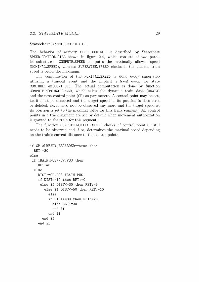
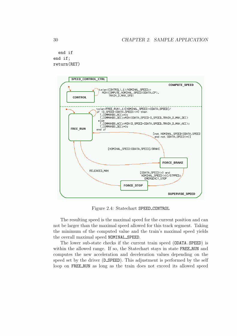
Statechart SPEED CONTROL CTRL
The behavior of activity SPEED CONTROL is described by StatechartSPEED CONTROL CTRL shown in figure 2.4, which consists of two paral-lel sub-states: COMPUTE SPEED computes the maximally allowed speed(NOMINAL SPEED), whereas SUPERVISE SPEED checks if the current trainspeed is below the maximum.
The computation of the NOMINAL SPEED is done every super-steputilizing a timeout event and the implicit entered event for stateCONTROL: en(CONTROL). The actual computation is done by functionCOMPUTE NOMINAL SPEED, which takes the dynamic train data (ODATA)and the next control point (CP) as parameters. A control point may be set,i.e. it must be observed and the target speed at its position is thus zero,or deleted, i.e. it need not be observed any more and the target speed atits position is set to the maximal value for this track segment. All controlpoints in a track segment are set by default when movement authorizationis granted to the train for this segment.
The function COMPUTE NOMINAL SPEED checks, if control point CP stillneeds to be observed and if so, determines the maximal speed dependingon the train’s current distance to the control point:
if CP.ALREADY_REGARDED==true then
RET:=30
else
if TRAIN.POS>=CP.POS then
RET:=0
else
DIST:=CP.POS-TRAIN.POS;
if DIST<=10 then RET:=0
else if DIST<=30 then RET:=5
else if DIST<=50 then RET:=10
else
if DIST<=80 then RET:=20
else RET:=30
end if
end if
end if
end if
30 CHAPTER 2. SAMPLE APPLICATION
end if
end if;
return(RET)
Figure 2.4: Statechart SPEED CONTROL
The resulting speed is the maximal speed for the current position and cannot be larger than the maximal speed allowed for this track segment. Takingthe minimum of the computed value and the train’s maximal speed yieldsthe overall maximal speed NOMINAL SPEED.
The lower sub-state checks if the current train speed (ODATA.SPEED) iswithin the allowed range. If so, the Statechart stays in state FREE RUN andcomputes the new acceleration and deceleration values depending on thespeed set by the driver (D SPEED). This adjustment is performed by the selfloop on FREE RUN as long as the train does not exceed its allowed speed
2.2. STATEMATE MODEL 31
as computed by sub-state COMPUTE SPEED (condition part of the transitionannotation of the self loop). The implemented algorithm is fairly simple: Ifthe speed set by the driver is lower than the current train speed, the train isdecelerated by the difference, otherwise it is accelerated. If the two speedsare equal, the train is neither accelerated nor decelerated.
If the train speed is greater than the allowed speed, state FREE RUN isexited, FORCE BRAKE is entered and the brake is activated. Once the speed isless than the maximal speed again and the train has not stopped, the State-chart returns to FREE RUN. If the NOMINAL SPEED and the actual train speedare both zero, the train has stopped in front of a still active control point,state FORCE STOP is entered and SPEED CONTROL CTRL emits the event STPPEDto ACTIVATE CROSSING CTRL and EMERGENCY STOP to the driver. Note thatonly those stops are covered by STPPED, which result from NOMINAL SPEED
dropping to zero. If the train stops for other reasons, it may resume its courseon its own without intervention by the driver. In the former case, however,the driver has to manually confirm that the crossing may be passed safely(RELEASE MAN) in order to continue. SPEED CONTROL CTRL then switches backinto the normal behavior of state FREE RUN.
Statechart ACTIVATE CROSSING CTRL
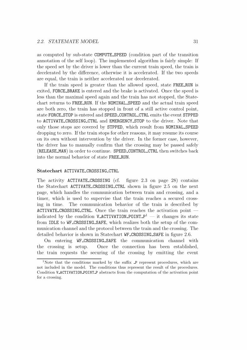
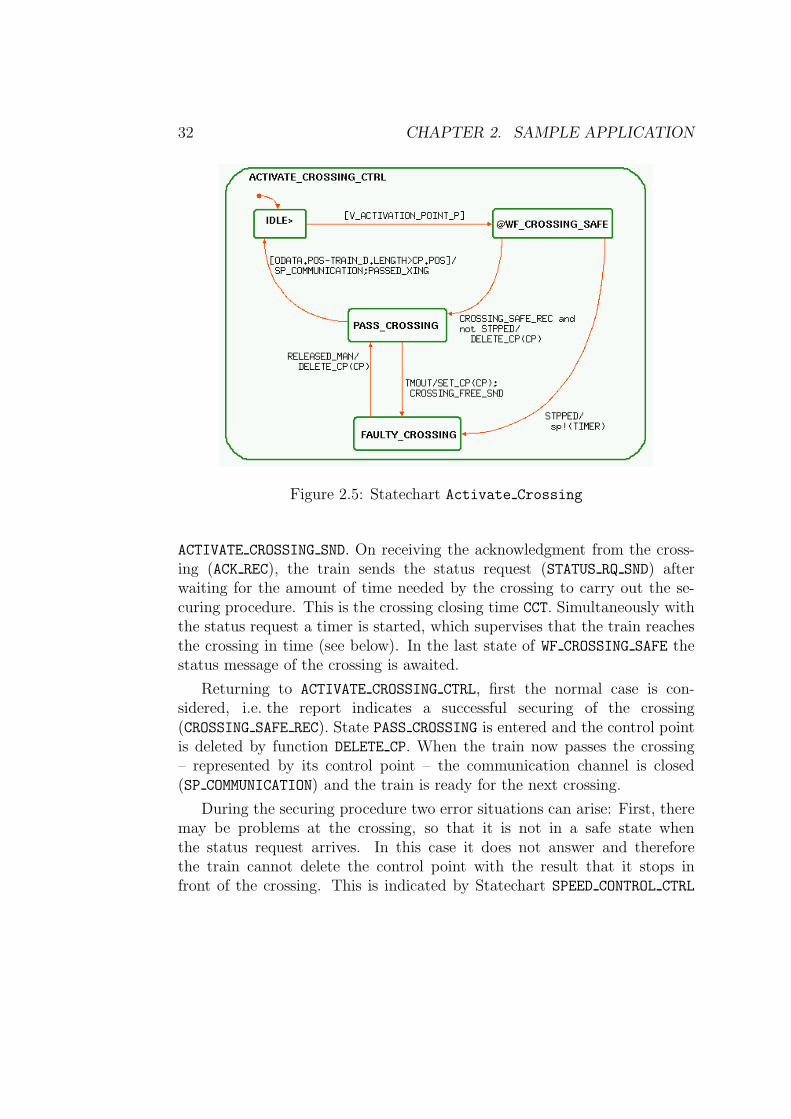
The activity ACTIVATE CROSSING (cf. figure 2.3 on page 28) containsthe Statechart ACTIVATE CROSSING CTRL shown in figure 2.5 on the nextpage, which handles the communication between train and crossing, and atimer, which is used to supervise that the train reaches a secured cross-ing in time. The communication behavior of the train is described byACTIVATE CROSSING CTRL. Once the train reaches the activation point —indicated by the condition V ACTIVATION POINT P1 — it changes its statefrom IDLE to WF CROSSING SAFE, which realizes both the setup of the com-munication channel and the protocol between the train and the crossing. Thedetailed behavior is shown in Statechart WF CROSSING SAFE in figure 2.6.
On entering WF CROSSING SAFE the communication channel withthe crossing is setup. Once the connection has been established,the train requests the securing of the crossing by emitting the event
1Note that the conditions marked by the suffix P represent procedures, which arenot included in the model. The conditions thus represent the result of the procedures.Condition V ACTIVATION POINT P abstracts from the computation of the activation pointfor a crossing.
32 CHAPTER 2. SAMPLE APPLICATION
Figure 2.5: Statechart Activate Crossing
ACTIVATE CROSSING SND. On receiving the acknowledgment from the cross-ing (ACK REC), the train sends the status request (STATUS RQ SND) afterwaiting for the amount of time needed by the crossing to carry out the se-curing procedure. This is the crossing closing time CCT. Simultaneously withthe status request a timer is started, which supervises that the train reachesthe crossing in time (see below). In the last state of WF CROSSING SAFE thestatus message of the crossing is awaited.
Returning to ACTIVATE CROSSING CTRL, first the normal case is con-sidered, i.e. the report indicates a successful securing of the crossing(CROSSING SAFE REC). State PASS CROSSING is entered and the control pointis deleted by function DELETE CP. When the train now passes the crossing– represented by its control point – the communication channel is closed(SP COMMUNICATION) and the train is ready for the next crossing.
During the securing procedure two error situations can arise: First, theremay be problems at the crossing, so that it is not in a safe state whenthe status request arrives. In this case it does not answer and thereforethe train cannot delete the control point with the result that it stops infront of the crossing. This is indicated by Statechart SPEED CONTROL CTRL
2.2. STATEMATE MODEL 33
Figure 2.6: Statechart WF CROSSING SAFE
with the event STPPED triggering the transition from WF CROSSING SAFE toFAULTY CROSSING. Since the train has stopped already, the timer becomesirrelevant and is stopped. In this situation the driver has to manually con-firm that the crossing can be safely passed (RELEASE MAN) entering statePASS CROSSING and deleting the control point in order to allow the train topass it.
The second error situation arises when the crossing has answered the sta-tus request but the train is unable to pass it within the maximal barrierclosed time. This is indicated by the event TMOUT sent by the timer result-ing in changing from state PASS CROSSING to FAULTY CROSSING, setting thecontrol point again via the function SET CP and notifying the crossing thatthe train will not reach it in time (event CROSSING FREE SND). Again thissituation has to be resolved by the driver.
34 CHAPTER 2. SAMPLE APPLICATION
Figure 2.7: Statechart TIMER CTRL
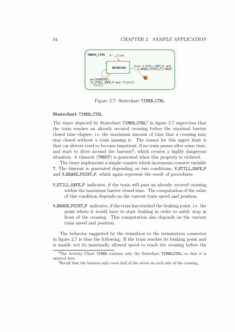
Statechart TIMER CTRL
The timer depicted by Statechart TIMER CTRL2 in figure 2.7 supervises thatthe train reaches an already secured crossing before the maximal barrierclosed time elapses, i.e. the maximum amount of time that a crossing maystay closed without a train passing it. The reason for this upper limit isthat car drivers tend to become impatient, if no train passes after some time,and start to drive around the barriers3, which creates a highly dangeroussituation. A timeout (TMOUT) is generated when this property is violated.
The timer implements a simple counter which increments counter variableT. The timeout is generated depending on two conditions, V STILL SAFE P
and V BRAKE POINT P, which again represent the result of procedures:
V STILL SAFE P indicates, if the train will pass an already secured crossingwithin the maximum barrier closed time. The computation of the valueof this condition depends on the current train speed and position.
V BRAKE POINT P indicates, if the train has reached the braking point, i.e. thepoint where it would have to start braking in order to safely stop infront of the crossing. This computation also depends on the currenttrain speed and position.
The behavior suggested by the transition to the termination connectorin figure 2.7 is thus the following: If the train reaches its braking point andis unable wrt its maximally allowed speed to reach the crossing before the
2The Activity Chart TIMER contains only the Statechart TIMER CTRL, so that it isomitted here.
3Recall that the barriers only cover half of the street on each side of the crossing.
2.2. STATEMATE MODEL 35
maximum barrier closed time elapses, the timeout is generated and the timeris stopped.
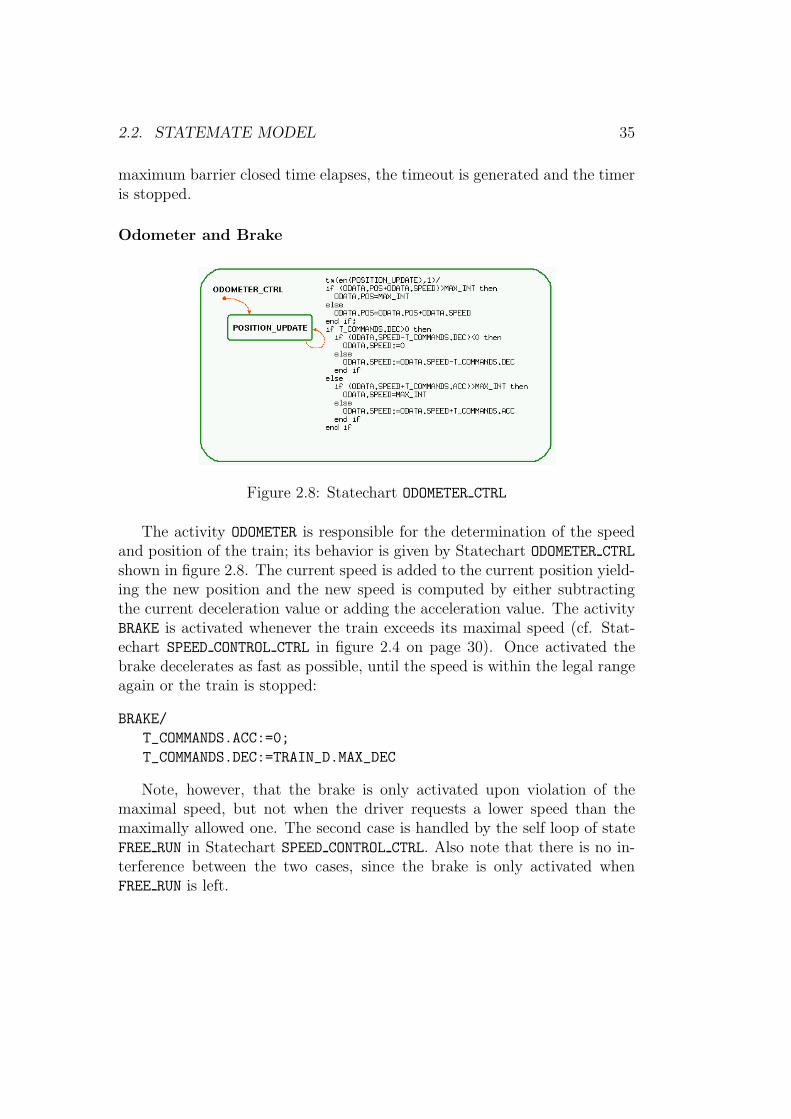
Odometer and Brake
Figure 2.8: Statechart ODOMETER CTRL
The activity ODOMETER is responsible for the determination of the speedand position of the train; its behavior is given by Statechart ODOMETER CTRL
shown in figure 2.8. The current speed is added to the current position yield-ing the new position and the new speed is computed by either subtractingthe current deceleration value or adding the acceleration value. The activityBRAKE is activated whenever the train exceeds its maximal speed (cf. Stat-echart SPEED CONTROL CTRL in figure 2.4 on page 30). Once activated thebrake decelerates as fast as possible, until the speed is within the legal rangeagain or the train is stopped:
BRAKE/
T_COMMANDS.ACC:=0;
T_COMMANDS.DEC:=TRAIN_D.MAX_DEC
Note, however, that the brake is only activated upon violation of themaximal speed, but not when the driver requests a lower speed than themaximally allowed one. The second case is handled by the self loop of stateFREE RUN in Statechart SPEED CONTROL CTRL. Also note that there is no in-terference between the two cases, since the brake is only activated whenFREE RUN is left.
36 CHAPTER 2. SAMPLE APPLICATION
2.2.3 Activity Chart COMMUNICATION
Figure 2.9: Statechart COMMUNICATION CTRL
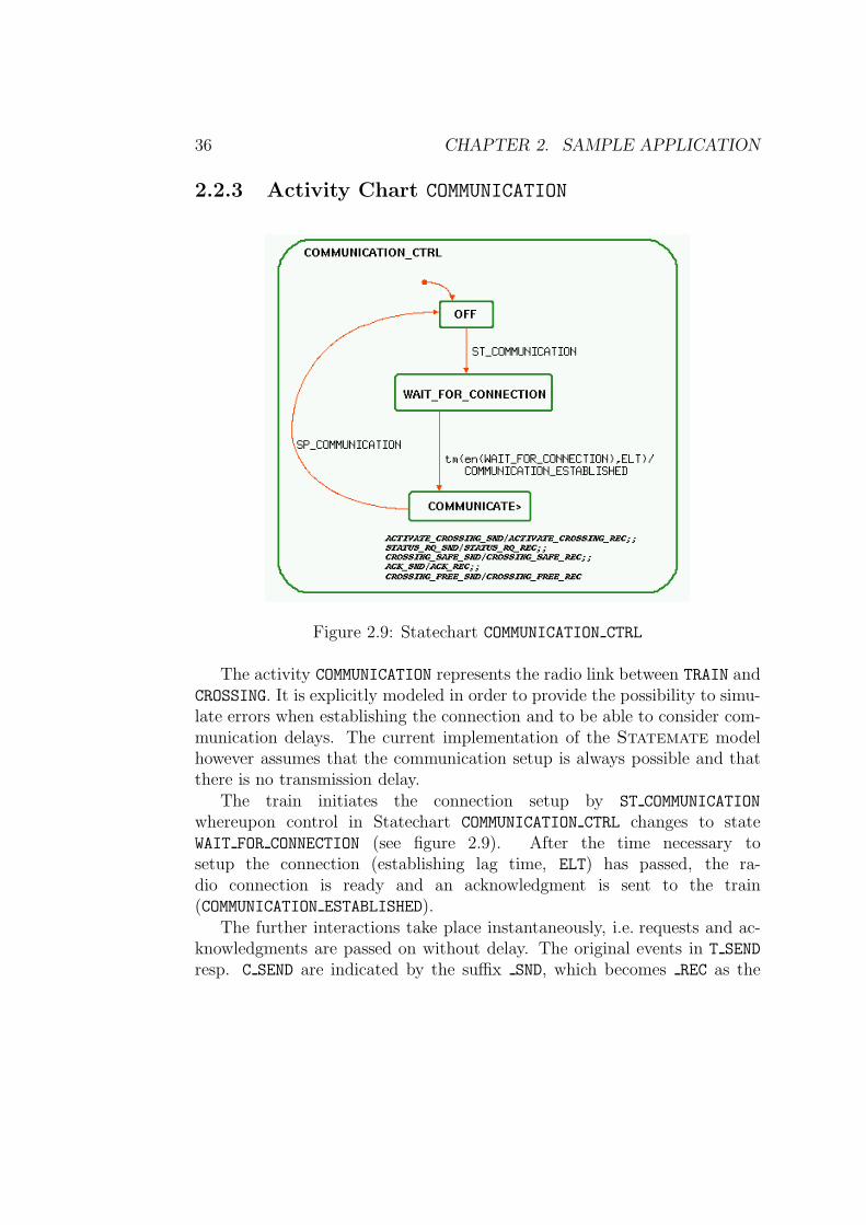
The activity COMMUNICATION represents the radio link between TRAIN andCROSSING. It is explicitly modeled in order to provide the possibility to simu-late errors when establishing the connection and to be able to consider com-munication delays. The current implementation of the Statemate modelhowever assumes that the communication setup is always possible and thatthere is no transmission delay.
The train initiates the connection setup by ST COMMUNICATION
whereupon control in Statechart COMMUNICATION CTRL changes to stateWAIT FOR CONNECTION (see figure 2.9). After the time necessary tosetup the connection (establishing lag time, ELT) has passed, the ra-dio connection is ready and an acknowledgment is sent to the train(COMMUNICATION ESTABLISHED).
The further interactions take place instantaneously, i.e. requests and ac-knowledgments are passed on without delay. The original events in T SEND
resp. C SEND are indicated by the suffix SND, which becomes REC as the
2.2. STATEMATE MODEL 37
events are relayed to the corresponding receiving channels C RECEIVE resp.T RECEIVE. The exact contents of the information flows is listed both as acomment in Statechart COMMUNICATION CTRL and in appendix B and appearboth on the crossing and train side (cf. sections 2.2.2 on page 28 and 2.2.4).
The termination of the communication between TRAIN and CROSSING istriggered by the train via SP COMMUNICATION which leads to an immediateabortion of the communication. This is modeled by changing into the stateOFF in the COMMUNICATION CTRL.
2.2.4 Activity Chart CROSSING
Figure 2.10: Activity Chart CROSSING
The activity CROSSING shown in figure 2.10 contains the overall softwarecontrol of the crossing (CROSSING CONTROL) responsible for the coordinationof the whole securing process and the software control (ELEMENT CTRL)
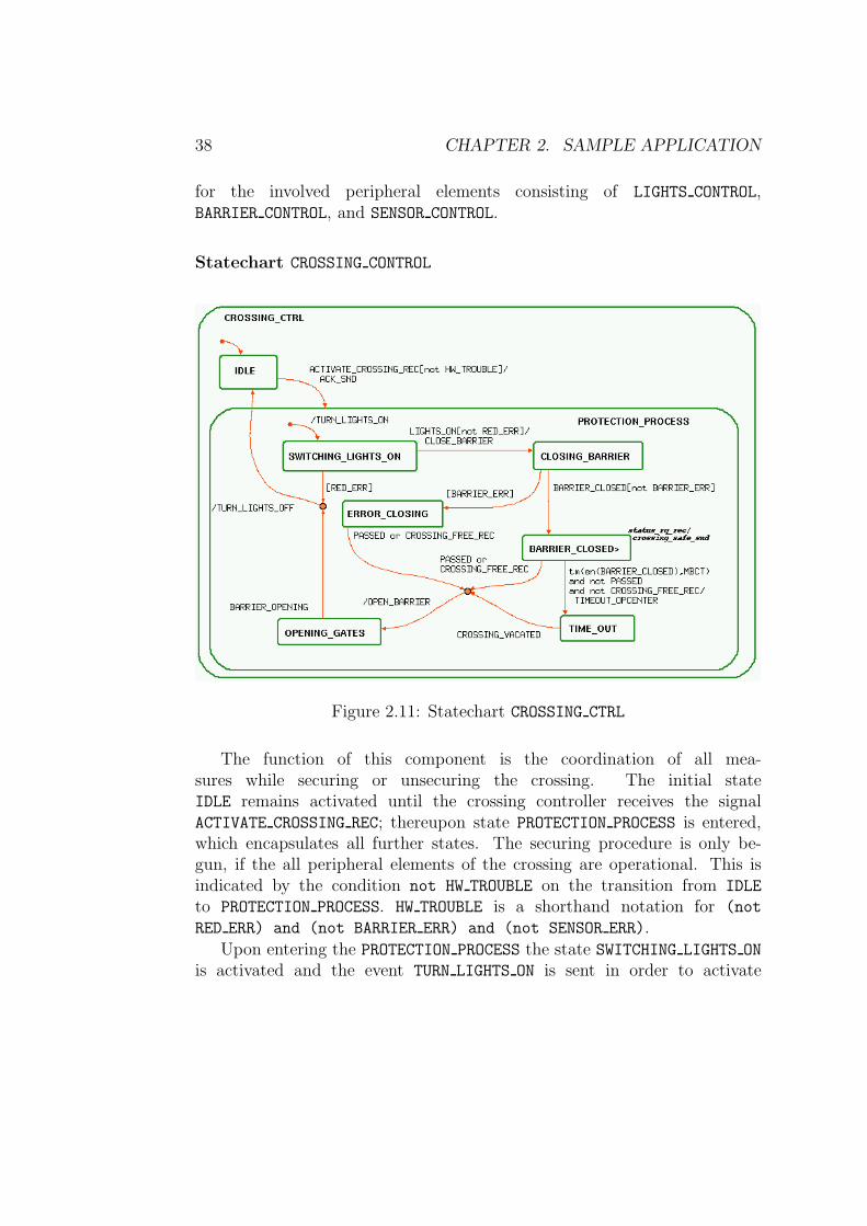
38 CHAPTER 2. SAMPLE APPLICATION
for the involved peripheral elements consisting of LIGHTS CONTROL,BARRIER CONTROL, and SENSOR CONTROL.
Statechart CROSSING CONTROL
Figure 2.11: Statechart CROSSING CTRL
The function of this component is the coordination of all mea-sures while securing or unsecuring the crossing. The initial stateIDLE remains activated until the crossing controller receives the signalACTIVATE CROSSING REC; thereupon state PROTECTION PROCESS is entered,which encapsulates all further states. The securing procedure is only be-gun, if the all peripheral elements of the crossing are operational. This isindicated by the condition not HW TROUBLE on the transition from IDLE
to PROTECTION PROCESS. HW TROUBLE is a shorthand notation for (not
RED ERR) and (not BARRIER ERR) and (not SENSOR ERR).Upon entering the PROTECTION PROCESS the state SWITCHING LIGHTS ON
is activated and the event TURN LIGHTS ON is sent in order to activate
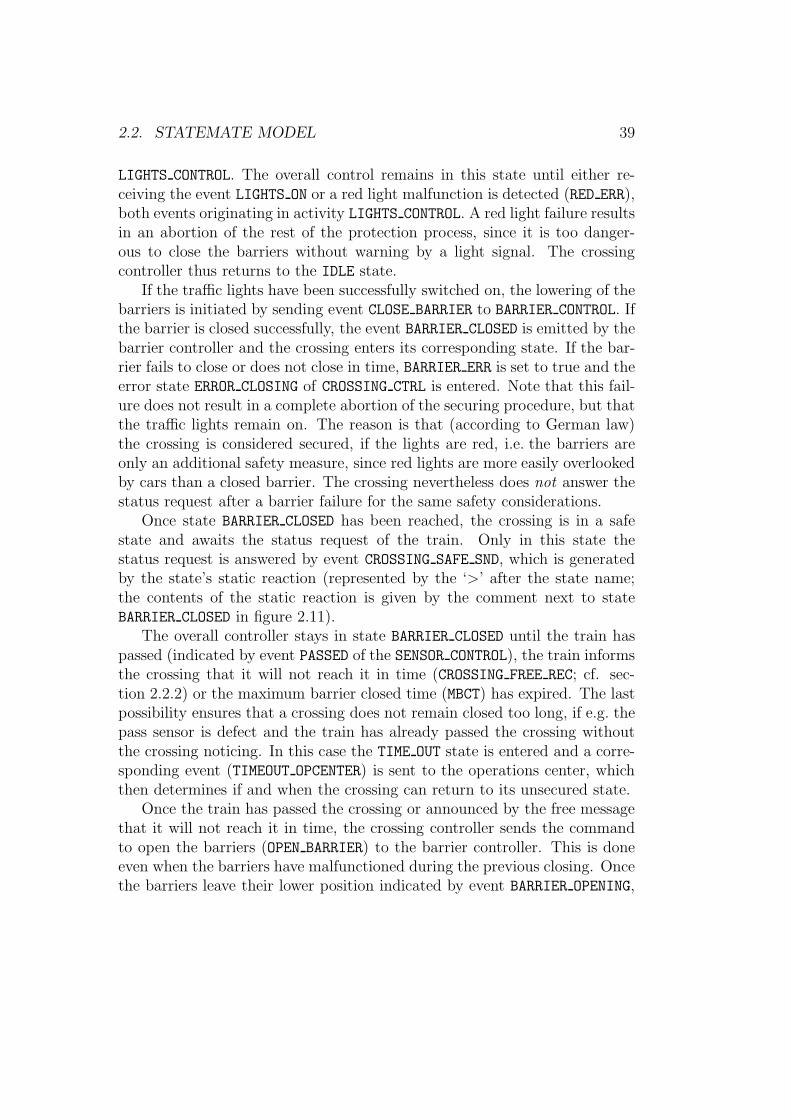
2.2. STATEMATE MODEL 39
LIGHTS CONTROL. The overall control remains in this state until either re-ceiving the event LIGHTS ON or a red light malfunction is detected (RED ERR),both events originating in activity LIGHTS CONTROL. A red light failure resultsin an abortion of the rest of the protection process, since it is too danger-ous to close the barriers without warning by a light signal. The crossingcontroller thus returns to the IDLE state.
If the traffic lights have been successfully switched on, the lowering of thebarriers is initiated by sending event CLOSE BARRIER to BARRIER CONTROL. Ifthe barrier is closed successfully, the event BARRIER CLOSED is emitted by thebarrier controller and the crossing enters its corresponding state. If the bar-rier fails to close or does not close in time, BARRIER ERR is set to true and theerror state ERROR CLOSING of CROSSING CTRL is entered. Note that this fail-ure does not result in a complete abortion of the securing procedure, but thatthe traffic lights remain on. The reason is that (according to German law)the crossing is considered secured, if the lights are red, i.e. the barriers areonly an additional safety measure, since red lights are more easily overlookedby cars than a closed barrier. The crossing nevertheless does not answer thestatus request after a barrier failure for the same safety considerations.
Once state BARRIER CLOSED has been reached, the crossing is in a safestate and awaits the status request of the train. Only in this state thestatus request is answered by event CROSSING SAFE SND, which is generatedby the state’s static reaction (represented by the ‘>’ after the state name;the contents of the static reaction is given by the comment next to stateBARRIER CLOSED in figure 2.11).
The overall controller stays in state BARRIER CLOSED until the train haspassed (indicated by event PASSED of the SENSOR CONTROL), the train informsthe crossing that it will not reach it in time (CROSSING FREE REC; cf. sec-tion 2.2.2) or the maximum barrier closed time (MBCT) has expired. The lastpossibility ensures that a crossing does not remain closed too long, if e.g. thepass sensor is defect and the train has already passed the crossing withoutthe crossing noticing. In this case the TIME OUT state is entered and a corre-sponding event (TIMEOUT OPCENTER) is sent to the operations center, whichthen determines if and when the crossing can return to its unsecured state.
Once the train has passed the crossing or announced by the free messagethat it will not reach it in time, the crossing controller sends the commandto open the barriers (OPEN BARRIER) to the barrier controller. This is doneeven when the barriers have malfunctioned during the previous closing. Oncethe barriers leave their lower position indicated by event BARRIER OPENING,
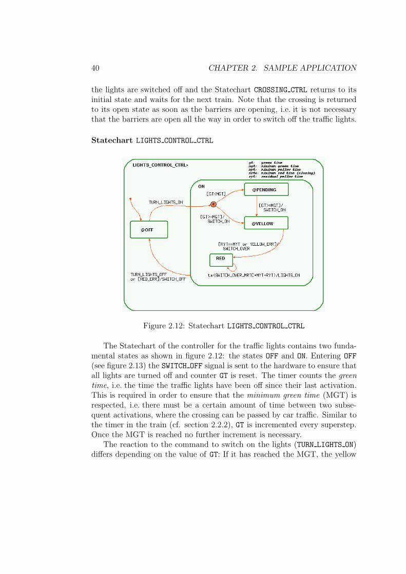
40 CHAPTER 2. SAMPLE APPLICATION
the lights are switched off and the Statechart CROSSING CTRL returns to itsinitial state and waits for the next train. Note that the crossing is returnedto its open state as soon as the barriers are opening, i.e. it is not necessarythat the barriers are open all the way in order to switch off the traffic lights.
Statechart LIGHTS CONTROL CTRL
Figure 2.12: Statechart LIGHTS CONTROL CTRL
The Statechart of the controller for the traffic lights contains two funda-mental states as shown in figure 2.12: the states OFF and ON. Entering OFF
(see figure 2.13) the SWITCH OFF signal is sent to the hardware to ensure thatall lights are turned off and counter GT is reset. The timer counts the greentime, i.e. the time the traffic lights have been off since their last activation.This is required in order to ensure that the minimum green time (MGT) isrespected, i.e. there must be a certain amount of time between two subse-quent activations, where the crossing can be passed by car traffic. Similar tothe timer in the train (cf. section 2.2.2), GT is incremented every superstep.Once the MGT is reached no further increment is necessary.
The reaction to the command to switch on the lights (TURN LIGHTS ON)differs depending on the value of GT: If it has reached the MGT, the yellow
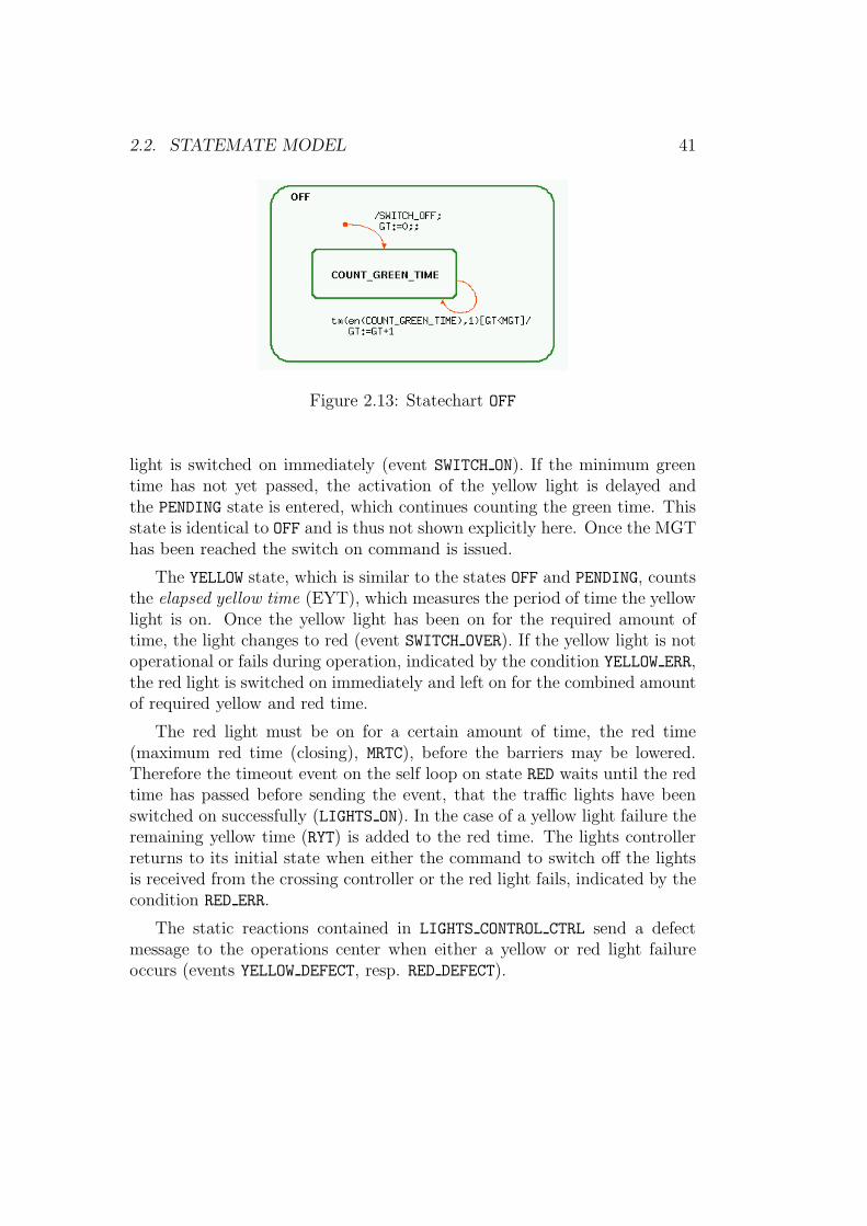
2.2. STATEMATE MODEL 41
Figure 2.13: Statechart OFF
light is switched on immediately (event SWITCH ON). If the minimum greentime has not yet passed, the activation of the yellow light is delayed andthe PENDING state is entered, which continues counting the green time. Thisstate is identical to OFF and is thus not shown explicitly here. Once the MGThas been reached the switch on command is issued.
The YELLOW state, which is similar to the states OFF and PENDING, countsthe elapsed yellow time (EYT), which measures the period of time the yellowlight is on. Once the yellow light has been on for the required amount oftime, the light changes to red (event SWITCH OVER). If the yellow light is notoperational or fails during operation, indicated by the condition YELLOW ERR,the red light is switched on immediately and left on for the combined amountof required yellow and red time.
The red light must be on for a certain amount of time, the red time(maximum red time (closing), MRTC), before the barriers may be lowered.Therefore the timeout event on the self loop on state RED waits until the redtime has passed before sending the event, that the traffic lights have beenswitched on successfully (LIGHTS ON). In the case of a yellow light failure theremaining yellow time (RYT) is added to the red time. The lights controllerreturns to its initial state when either the command to switch off the lightsis received from the crossing controller or the red light fails, indicated by thecondition RED ERR.
The static reactions contained in LIGHTS CONTROL CTRL send a defectmessage to the operations center when either a yellow or red light failureoccurs (events YELLOW DEFECT, resp. RED DEFECT).
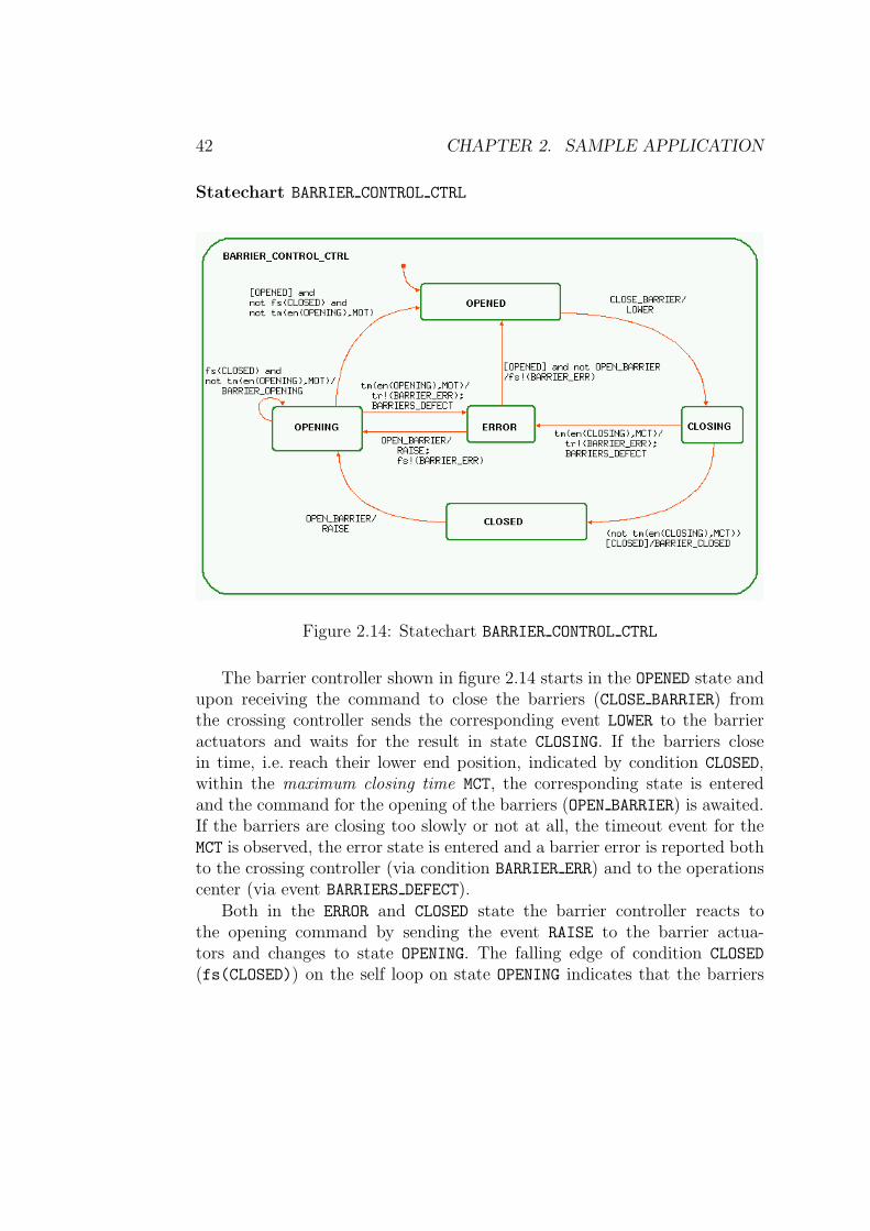
42 CHAPTER 2. SAMPLE APPLICATION
Statechart BARRIER CONTROL CTRL
Figure 2.14: Statechart BARRIER CONTROL CTRL
The barrier controller shown in figure 2.14 starts in the OPENED state andupon receiving the command to close the barriers (CLOSE BARRIER) fromthe crossing controller sends the corresponding event LOWER to the barrieractuators and waits for the result in state CLOSING. If the barriers closein time, i.e. reach their lower end position, indicated by condition CLOSED,within the maximum closing time MCT, the corresponding state is enteredand the command for the opening of the barriers (OPEN BARRIER) is awaited.If the barriers are closing too slowly or not at all, the timeout event for theMCT is observed, the error state is entered and a barrier error is reported bothto the crossing controller (via condition BARRIER ERR) and to the operationscenter (via event BARRIERS DEFECT).
Both in the ERROR and CLOSED state the barrier controller reacts tothe opening command by sending the event RAISE to the barrier actua-tors and changes to state OPENING. The falling edge of condition CLOSED
(fs(CLOSED)) on the self loop on state OPENING indicates that the barriers
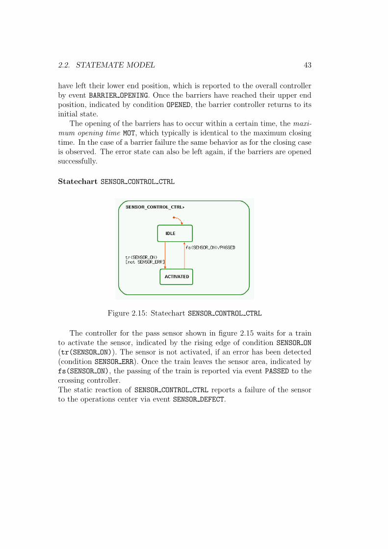
2.2. STATEMATE MODEL 43
have left their lower end position, which is reported to the overall controllerby event BARRIER OPENING. Once the barriers have reached their upper endposition, indicated by condition OPENED, the barrier controller returns to itsinitial state.
The opening of the barriers has to occur within a certain time, the maxi-mum opening time MOT, which typically is identical to the maximum closingtime. In the case of a barrier failure the same behavior as for the closing caseis observed. The error state can also be left again, if the barriers are openedsuccessfully.
Statechart SENSOR CONTROL CTRL
Figure 2.15: Statechart SENSOR CONTROL CTRL
The controller for the pass sensor shown in figure 2.15 waits for a trainto activate the sensor, indicated by the rising edge of condition SENSOR ON
(tr(SENSOR ON)). The sensor is not activated, if an error has been detected(condition SENSOR ERR). Once the train leaves the sensor area, indicated byfs(SENSOR ON), the passing of the train is reported via event PASSED to thecrossing controller.The static reaction of SENSOR CONTROL CTRL reports a failure of the sensorto the operations center via event SENSOR DEFECT.

44 CHAPTER 2. SAMPLE APPLICATION
Chapter 3
Message Sequence Charts and
Sequence Diagrams
In the development of computer systems visual languages are becoming in-creasingly popular due to their graphical appeal, as developers are moreinclined to draw diagrams in order to design a system than to write cryp-tic lines of code. Especially the telecommunications domain has been usingvisual languages for many years. In this field the language of Message Se-quence Charts, which captures information exchange in communication sys-tems, has its origin. It has been adopted in other fields as well in orderto specify message exchange between entities. Most notable is the inclusionof an object-oriented variant of Message Sequence Charts, called SequenceDiagrams, into the UML standard. In this chapter we will give an introduc-tion to both sequence chart variants, starting with Message Sequence Chartsin section 3.1 and followed by Sequence Diagrams in section 3.2, and high-light their inadequacies barring a more prominent role in the design process.These shortcomings have led to the definition of a variant which addressesand remedies these deficiencies: Live Sequence Charts, which are introducedin chapter 4.
3.1 Message Sequence Charts
Message Sequence Charts (MSCs) are standardized and maintained by theInternational Telecommunications Union (ITU). Prior to their standardiza-tion there existed several precursors, like Time Sequence Diagrams, Arrow
45
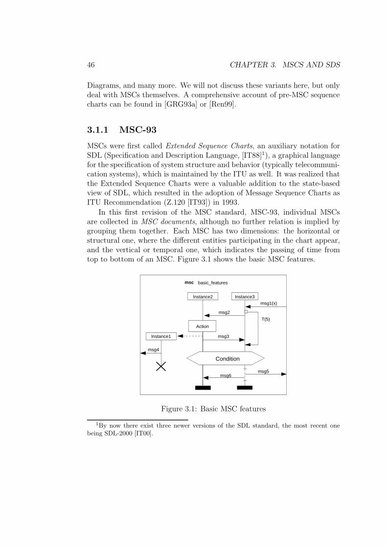
46 CHAPTER 3. MSCS AND SDS
Diagrams, and many more. We will not discuss these variants here, but onlydeal with MSCs themselves. A comprehensive account of pre-MSC sequencecharts can be found in [GRG93a] or [Ren99].
3.1.1 MSC-93
MSCs were first called Extended Sequence Charts, an auxiliary notation forSDL (Specification and Description Language, [IT88]1), a graphical languagefor the specification of system structure and behavior (typically telecommuni-cation systems), which is maintained by the ITU as well. It was realized thatthe Extended Sequence Charts were a valuable addition to the state-basedview of SDL, which resulted in the adoption of Message Sequence Charts asITU Recommendation (Z.120 [IT93]) in 1993.
In this first revision of the MSC standard, MSC-93, individual MSCsare collected in MSC documents, although no further relation is implied bygrouping them together. Each MSC has two dimensions: the horizontal orstructural one, where the different entities participating in the chart appear,and the vertical or temporal one, which indicates the passing of time fromtop to bottom of an MSC. Figure 3.1 shows the basic MSC features.
msc basic_features
Instance3
msg2
msg6
Condition
T(5)
Instance2
Instance1
Action
msg1(x)
msg3
msg5
msg4
Figure 3.1: Basic MSC features
1By now there exist three newer versions of the SDL standard, the most recent onebeing SDL-2000 [IT00].
3.1. MESSAGE SEQUENCE CHARTS 47
The entities involved in the communication are represented by verticallines called instances, which consist of an instance head symbol (empty rect-angle) carrying the instance name, the instance axis and an instance endsymbol (filled rectangle); cf. figure 3.1. Due to the close relation betweenMSCs and SDL instances often represent entities of the SDL design, like pro-cesses, blocks, etc., although this is not required. On the instance axis theactions carried out by the entity represented by the instance appear; theseactions are called events and can e.g. be messages, conditions or timers. Theevents of one instance axis are totally ordered from top to bottom unlessthey are contained in a coregion. An ordering between events on different in-stances is enforced only by messages; see below for more detailed descriptionsof these concepts.
The environment is represented by the frame enclosing the MSC. Notethat the instance head and end do not correspond to the creation and de-struction of the model entity represented by the instance. They just markthe points in time where the corresponding design entities start, resp. stop totake part in the communication described in the MSC. There exist separateconstructs for expressing creation and destruction of entities (see below).
Information exchange between entities is represented by messages, whichare depicted by arrows; all communication is asynchronous. As shown infigure 3.1, messages can be exchanged between two instances or between aninstance and the environment. Each message consists of two distinct events:a send event and a receive event. Messages are the only way to establish anordering between events of two different instances, since obviously a messagemust be sent before it can be received. A message has a name and may alsocarry parameters, cf. msg1 in figure 3.1. Only one message may be sent orreceived by each instance at one point in time.
Conditions are used to represent system states, which are described tex-tually. They are depicted by hexagonal shapes and can refer, i.e. be attached,to one or more instances. Instance axes of instances, which are not participat-ing in a condition, but which cross the condition symbol are drawn throughthe hexagon, whereas the axes of participating instances are suspended. Infigure 3.1 e.g. the condition refers to both Instance2 and Instance3. Condi-tions can be used to define possible continuations of MSCs: An MSC endingwith a condition connected e.g. can be continued in another MSC, whichstarts with the same condition.
MSCs also allow to express time properties in the form of timers, withthree possible actions:
48 CHAPTER 3. MSCS AND SDS
1. setting a timer to a value
2. resetting the timer
3. observing a timeout
Timer set events are depicted by a small square attached to an instanceand may be named; cf. T in figure 3.1. The duration of the timer canoptionally be specified in parenthesis. A timer set event is always connectedto either a timer reset or timeout event by means of a vertical line whichemanates from the timer set square, runs in parallel to the instance axis andis connected to the instance axis once again by an arrow, which indicatesthe timeout or reset event. A timeout event is rendered as a solid arrow, areset event by a dashed arrow. Figure 3.1 on page 46 shows an example fora timeout event.
Process creation is depicted by a dashed message arrow leading from thecreating instance to the created one. Process termination is depicted by alarge X terminating the instance line; cf. Instance1 in figure 3.1 for anexample. Local actions, i.e. activity internal to an entity, are depicted by arectangle, which contains a textual description of the action.
The total order among the events on one instance may be suspended bya coregion. All events within a coregion are completely unordered, i.e. theymay occur in any order, but not simultaneously. A coregion is depicted bya dashed segment of an instance axis. In figure 3.1 the send events of themessages msg5 and msg6 are contained in the coregion of Instance3 andmay therefore be sent in any order.
The only structuring mechanism offered by MSC-93 is the refinementof an instance into sub-entities, called decomposition. This is not depictedgraphically, but just indicated by the key word decomposed followed by thename of the chart, which shows the refined structure and behavior, belowthe instance head.
Several different approaches to define a semantics for MSC-93 havebeen undertaken: automata-based [LL92b, LL92a, LL95], Petri-net-based [GRG93b] and by process algebra [MR94]. A short overview ofthese approaches can again be found in [GRG93a]. From these semanticsthe one based on process algebra was chosen to become the official semanticspublished by the ITU in [IT95].
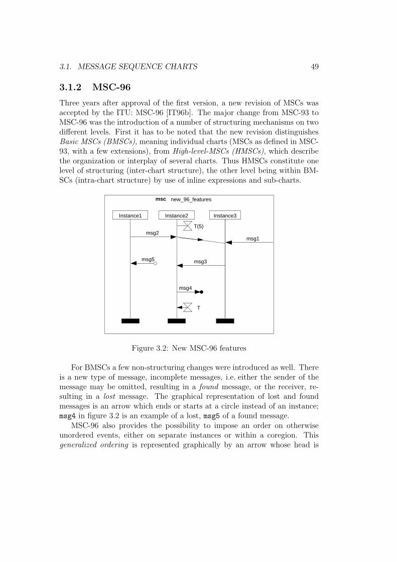
3.1. MESSAGE SEQUENCE CHARTS 49
3.1.2 MSC-96
Three years after approval of the first version, a new revision of MSCs wasaccepted by the ITU: MSC-96 [IT96b]. The major change from MSC-93 toMSC-96 was the introduction of a number of structuring mechanisms on twodifferent levels. First it has to be noted that the new revision distinguishesBasic MSCs (BMSCs), meaning individual charts (MSCs as defined in MSC-93, with a few extensions), from High-level-MSCs (HMSCs), which describethe organization or interplay of several charts. Thus HMSCs constitute onelevel of structuring (inter-chart structure), the other level being within BM-SCs (intra-chart structure) by use of inline expressions and sub-charts.
msc new_96_features
Instance2
T(5)
Instance1 Instance3
msg2
T
msg1
msg3
msg4
msg5
Figure 3.2: New MSC-96 features
For BMSCs a few non-structuring changes were introduced as well. Thereis a new type of message, incomplete messages, i.e. either the sender of themessage may be omitted, resulting in a found message, or the receiver, re-sulting in a lost message. The graphical representation of lost and foundmessages is an arrow which ends or starts at a circle instead of an instance;msg4 in figure 3.2 is an example of a lost, msg5 of a found message.
MSC-96 also provides the possibility to impose an order on otherwiseunordered events, either on separate instances or within a coregion. Thisgeneralized ordering is represented graphically by an arrow whose head is
50 CHAPTER 3. MSCS AND SDS
not positioned at the end but in the middle. Figure 3.2 shows an exam-ple of ordering two otherwise unrelated message receive events on differentinstances: The receipt of msg2 should precede the receipt of msg1.
The appearance of timer has been altered in the new standard as well:the old timer set symbol has been replaced by a more intuitive hour-glasssymbol, the timer reset symbol by an X similar to the process terminationsymbol, but connected to the instance axis by a vertical line, and a timeoutis now indicated by an hour-glass symbol which is connected via an arrowto the instance axis. Moreover, different timer events related to the sametimer can now be decoupled from each other – i.e. they need no longer beconnected by a vertical line, but are identified by the timer name – and maythus appear in different charts. A timer e.g. may be set in one chart and thecorresponding timeout may be observed in another MSC. Figure 3.2 showsthe setting of timer T and the respective timeout event.
Intra-chart Structure
The intra-chart category of structuring mechanisms offered by MSC-96 con-tains two new possibilities to structure Basic MSCs, in addition to the in-stance decomposition of MSC-93. The first of those are inline expressions,the second are MSC references. The former are represented graphically by abox, which encloses those instances and events, which take part in the inlineexpression. Inline expressions come in different flavors indicated by a keyword in the upper left corner of the box:
loop: Describes the iteration of the communication sequence shown in thebox. Both bounded and unbounded iterations are allowed; for boundedones a lower and an upper bound may be specified. Figure 3.3 showsan example where msg1 is send and received at least 2 and at most 7times.
alt: Several alternative continuations of the chart can be specified. Whichalternative is taken is determined by which event is observed first af-ter entering the inline expression. In case of a common prefix amongthe alternatives, the common prefix is executed first and the first dif-fering event determines the alternative. The different alternatives areseparated by dashed horizontal lines; see figure 3.4 on page 52 for anexample. Here there are three possible continuations after the sending
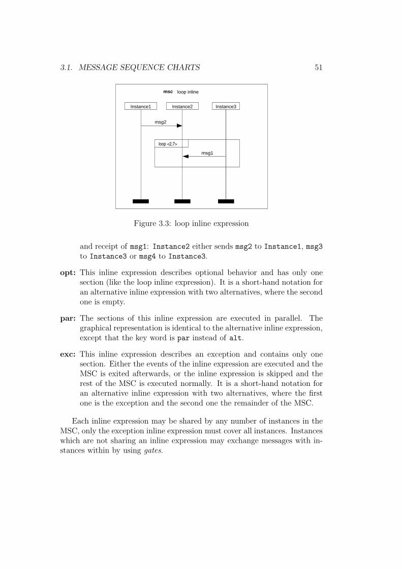
3.1. MESSAGE SEQUENCE CHARTS 51
msc loop inline
Instance1 Instance2 Instance3
msg2
msg1
loop <2,7>
Figure 3.3: loop inline expression
and receipt of msg1: Instance2 either sends msg2 to Instance1, msg3to Instance3 or msg4 to Instance3.
opt: This inline expression describes optional behavior and has only onesection (like the loop inline expression). It is a short-hand notation foran alternative inline expression with two alternatives, where the secondone is empty.
par: The sections of this inline expression are executed in parallel. Thegraphical representation is identical to the alternative inline expression,except that the key word is par instead of alt.
exc: This inline expression describes an exception and contains only onesection. Either the events of the inline expression are executed and theMSC is exited afterwards, or the inline expression is skipped and therest of the MSC is executed normally. It is a short-hand notation foran alternative inline expression with two alternatives, where the firstone is the exception and the second one the remainder of the MSC.
Each inline expression may be shared by any number of instances in theMSC, only the exception inline expression must cover all instances. Instanceswhich are not sharing an inline expression may exchange messages with in-stances within by using gates.
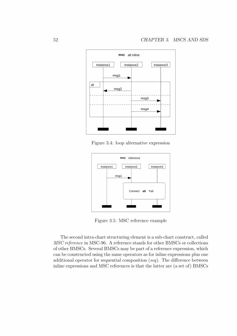
52 CHAPTER 3. MSCS AND SDS
msc alt inline
Instance1 Instance2 Instance3
msg2
msg3
msg4
alt
msg1
Figure 3.4: loop alternative expression
referencemsc
Instance3Instance1 Instance2
alt Fail
msg1
Connect
Figure 3.5: MSC reference example
The second intra-chart structuring element is a sub-chart construct, calledMSC reference in MSC-96. A reference stands for other BMSCs or collectionsof other BMSCs. Several BMSCs may be part of a reference expression, whichcan be constructed using the same operators as for inline expressions plus oneadditional operator for sequential composition (seq). The difference betweeninline expressions and MSC references is that the latter are (a set of) BMSCs
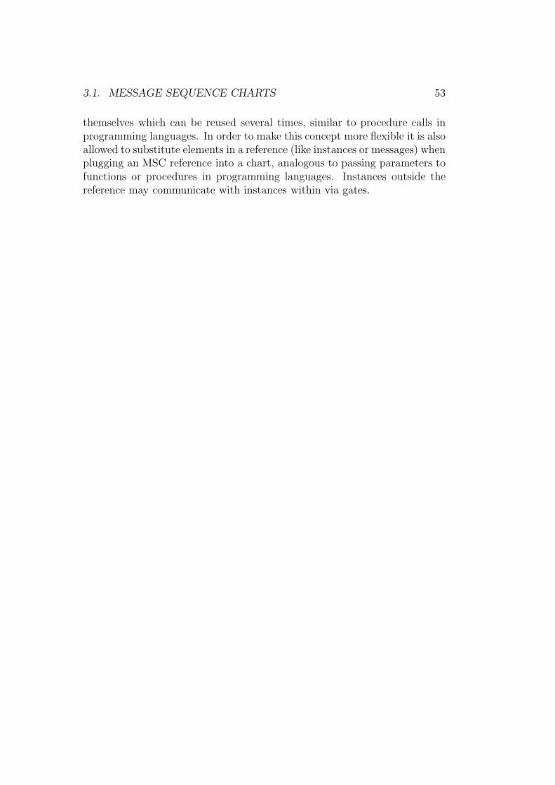
3.1. MESSAGE SEQUENCE CHARTS 53
themselves which can be reused several times, similar to procedure calls inprogramming languages. In order to make this concept more flexible it is alsoallowed to substitute elements in a reference (like instances or messages) whenplugging an MSC reference into a chart, analogous to passing parameters tofunctions or procedures in programming languages. Instances outside thereference may communicate with instances within via gates.
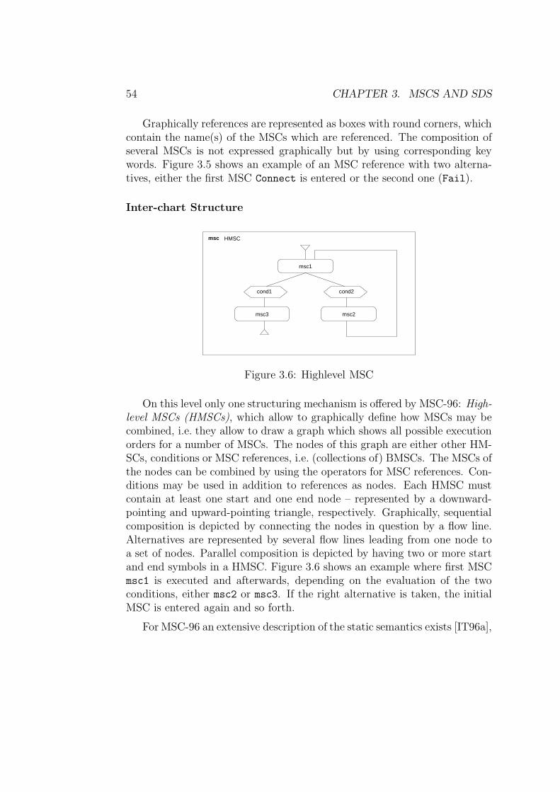
54 CHAPTER 3. MSCS AND SDS
Graphically references are represented as boxes with round corners, whichcontain the name(s) of the MSCs which are referenced. The composition ofseveral MSCs is not expressed graphically but by using corresponding keywords. Figure 3.5 shows an example of an MSC reference with two alterna-tives, either the first MSC Connect is entered or the second one (Fail).
Inter-chart Structure
msc HMSC
msc1
msc3 msc2
cond1 cond2
Figure 3.6: Highlevel MSC
On this level only one structuring mechanism is offered by MSC-96: High-level MSCs (HMSCs), which allow to graphically define how MSCs may becombined, i.e. they allow to draw a graph which shows all possible executionorders for a number of MSCs. The nodes of this graph are either other HM-SCs, conditions or MSC references, i.e. (collections of) BMSCs. The MSCs ofthe nodes can be combined by using the operators for MSC references. Con-ditions may be used in addition to references as nodes. Each HMSC mustcontain at least one start and one end node – represented by a downward-pointing and upward-pointing triangle, respectively. Graphically, sequentialcomposition is depicted by connecting the nodes in question by a flow line.Alternatives are represented by several flow lines leading from one node toa set of nodes. Parallel composition is depicted by having two or more startand end symbols in a HMSC. Figure 3.6 shows an example where first MSCmsc1 is executed and afterwards, depending on the evaluation of the twoconditions, either msc2 or msc3. If the right alternative is taken, the initialMSC is entered again and so forth.
For MSC-96 an extensive description of the static semantics exists [IT96a],
3.1. MESSAGE SEQUENCE CHARTS 55
but the definition of the dynamic semantics required more effort and time. Itis a remodeled and extended variant of [IT95], i.e. it is again defined in termsof process algebra. Initially worked out in [Ren99], it was approved by theITU as [IT98] in 1998. In the meantime between the publication of MSC-96and the publication of its semantics, other suggestions for a semantics weremade, based on Petri-Nets [Hey00] [KPE00], rewriting logic [Kos97], Dura-tion Calculus [GDO98] and streams [Kru00]; there also exists an alternativeprocess algebra characterization [GHRW98, GHN+98]. These works mostlydo not cover the complete set of MSC-96 features, but concretize differentopen points of MSCs, like time and sequential composition.
3.1.3 MSC-2000
The latest revision of the MSC standard, MSC-2000 [IT99], was publishedat the end of 1999. While the major additions of MSC-96 were structuringmechanisms, MSC-2000 focuses on extending MSCs with object-oriented fea-tures and adding data. The MSC document containing individual MSCs hasbeen extended to include several object-oriented features, like inheritance orvirtual references, plus a number of declarations (messages, instances, . . . )in the style of programming languages. These new organizational featuresare mostly non-graphical.
MSC-2000 also allows the specification of method calls and replies, similarto Sequence Diagrams, although they do not need to be synchronous (cf.section 3.2). The section of the instance which is carrying out the methodcall, is indicated by broadening the instance axis into a thin, filled rectangle,identical to the activation in SDs (see section 3.2). Moreover, the instanceaxis of the calling and waiting instance is marked by an empty rectangle.The method call is additionally distinguished from normal, asynchronousmessages by the keyword call. Every method call must be matched bycorresponding reply message represented by a dashed arrow; see figure 3.7for an example. In addition to the normal, asynchronous messages of theformer versions of the MSC standard MSC-2000 thus offers the possibility ofsynchronous and asynchronous method calls.
MSC-2000 allows the user to declare a data language to be included,so that variables of this data domain can be used in the MSCs. This isparticularly useful in conjunction with conditions, where it is now possibleto associate boolean expressions with a condition; they are called guarding
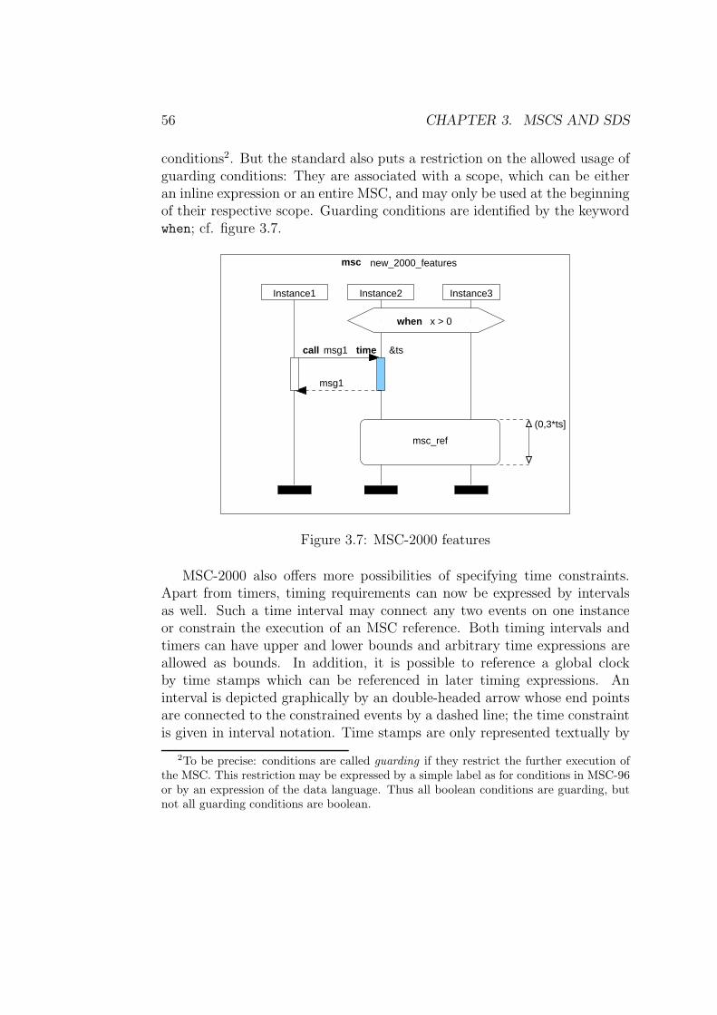
56 CHAPTER 3. MSCS AND SDS
conditions2. But the standard also puts a restriction on the allowed usage ofguarding conditions: They are associated with a scope, which can be eitheran inline expression or an entire MSC, and may only be used at the beginningof their respective scope. Guarding conditions are identified by the keywordwhen; cf. figure 3.7.
new_2000_featuresmsc
Instance2Instance1 Instance3
msg1call
msg1
msc_ref
time &ts
(0,3*ts]
when x > 0
Figure 3.7: MSC-2000 features
MSC-2000 also offers more possibilities of specifying time constraints.Apart from timers, timing requirements can now be expressed by intervalsas well. Such a time interval may connect any two events on one instanceor constrain the execution of an MSC reference. Both timing intervals andtimers can have upper and lower bounds and arbitrary time expressions areallowed as bounds. In addition, it is possible to reference a global clockby time stamps which can be referenced in later timing expressions. Aninterval is depicted graphically by an double-headed arrow whose end pointsare connected to the constrained events by a dashed line; the time constraintis given in interval notation. Time stamps are only represented textually by
2To be precise: conditions are called guarding if they restrict the further execution ofthe MSC. This restriction may be expressed by a simple label as for conditions in MSC-96or by an expression of the data language. Thus all boolean conditions are guarding, butnot all guarding conditions are boolean.
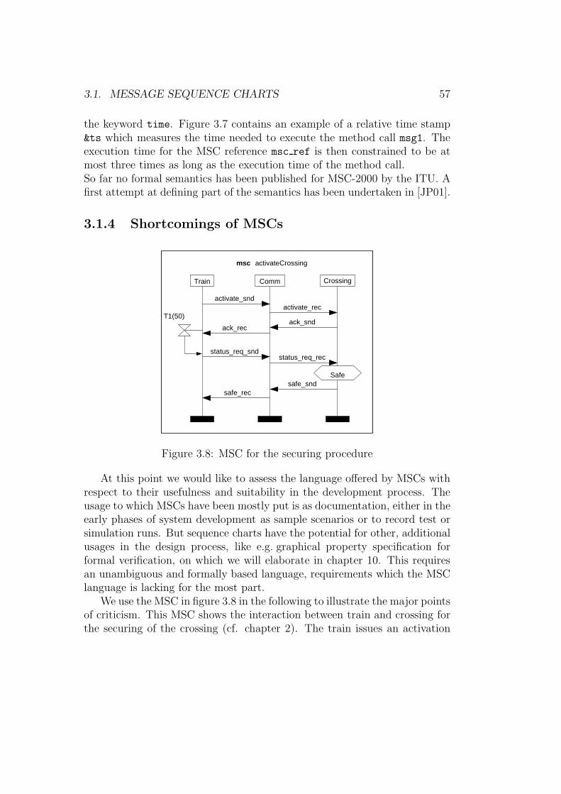
3.1. MESSAGE SEQUENCE CHARTS 57
the keyword time. Figure 3.7 contains an example of a relative time stamp&ts which measures the time needed to execute the method call msg1. Theexecution time for the MSC reference msc ref is then constrained to be atmost three times as long as the execution time of the method call.So far no formal semantics has been published for MSC-2000 by the ITU. Afirst attempt at defining part of the semantics has been undertaken in [JP01].
3.1.4 Shortcomings of MSCs
activate_rec
ack_sndack_rec
activate_snd
status_req_sndstatus_req_rec
safe_sndsafe_rec
msc activateCrossing
Train Comm Crossing
Safe
T1(50)
Figure 3.8: MSC for the securing procedure
At this point we would like to assess the language offered by MSCs withrespect to their usefulness and suitability in the development process. Theusage to which MSCs have been mostly put is as documentation, either in theearly phases of system development as sample scenarios or to record test orsimulation runs. But sequence charts have the potential for other, additionalusages in the design process, like e.g. graphical property specification forformal verification, on which we will elaborate in chapter 10. This requiresan unambiguous and formally based language, requirements which the MSClanguage is lacking for the most part.
We use the MSC in figure 3.8 in the following to illustrate the major pointsof criticism. This MSC shows the interaction between train and crossing forthe securing of the crossing (cf. chapter 2). The train issues an activation
58 CHAPTER 3. MSCS AND SDS
command, which is immediately acknowledged, and after waiting for 50 unitsof time, it requests the status of the crossing. If the crossing has been securedsuccessfully, it answers by sending the corresponding message. All messagesare exchanged via radio link represented by the communication component.
The formal semantics given by the ITU ([IT95, IT98]) defines the seman-tics only in terms of allowed sequences of events, without indicating, if thebehavior specified by an MSC is mandatory or not. The major points ofcriticism are detailed in the following:
1. An MSC shows only one sample run of the system, one scenario. TheMSC in figure 3.8 thus expresses that it is possible for a train to ordera crossing to be secured. But the intended meaning of this MSC isnot to specify a possible, sample behavior, but rather to express amandatory protocol between train and crossing: Every train shouldcontact every crossing along its way and secure it, i.e. every systemrun should conform to the behavior specified in the MSC.
2. An MSC does not state explicitly when the behavior it describes shouldbe observed, i.e. there is no indication of when the MSC should beactivated. People familiar with the application may know that thetrain should activate the crossing once it reaches the correspondingactivation point, but the MSC does not reflect this hidden knowledge.It would e.g. allow the train to activate all crossings along its way atthe start of its trip or even when it has already passed the crossing.
The guarding data conditions of MSC-2000 can be used to specify theactivation point of an MSC by placing them at the beginning of an MSCand expressing the system state characterizing the activation point bythe boolean expression, although sequences of messages, which acti-vates a chart, can not be specified.
3. The MSC semantics offers no distinction, whether progress is enforcedor not. The intention of the MSC in figure 3.8 e.g. is that the crossingdoes send the safe message, if it has been secured. Thus progress alongthe instance line should be enforced, but the semantics in [IT95] onlydefine permitted sequences of events; the occurrence of an event cannot be enforced. Likewise, we do expect all messages, which are sentin our example MSC, to arrive at their destination. This too can notbe expressed according to the MSC semantics. Using the terms coined
3.1. MESSAGE SEQUENCE CHARTS 59
by Lamport [Lam77] MSCs can only express safety (nothing bad everhappens), but not liveness properties (something good will happeneventually).
Bounded liveness is theoretically expressible by using timers, but sincetimer durations are not covered by the semantics (see below), this isonly true on an informal level.
4. MSCs do not allow more than one event to happen at the same time.In the example MSC we would like to express that 50 time units passbetween the reception of the acknowledgment and the sending of thestatus request, i.e. we want the timer to start counting when the ac-knowledgment arrives and the timeout to occur simultaneously withthe sending of the status request. Likewise, the condition expressingthe safe state of the crossing should be evaluated when the status re-quest arrives at the crossing, i.e. the crossing is required to be in thesecured state at this point. Neither can be expressed in MSCs.
Simultaneity is now available for timing annotations as the ex-ample in figure 3.7 shows, but it is still not possible to enforcee.g. simultaneousness of a message and a condition or of several mes-sages.
5. Conditions in MSCs have no formal semantics, but are either gluepoints, which indicate possible concatenations of MSCs, or ”guard”alternatives in HMSCs. In the words of [IT95]: ”The semantics of achart containing conditions is simply the semantics of the chart withthe conditions deleted from it.”. This is obviously not the way to treatconditions from a more formal point of view. In MSC-2000 conditionshave been upgraded to some degree due to the introduction of data,which allow boolean conditions. But these guarding conditions do notsolve the problem completely, since they are restricted to be placed atthe beginning of their scope. It is thus not possible to have booleanconditions in arbitrary locations of a chart, so the extension for con-ditions as offered by MSC-2000 is not completely satisfactory. Evenmore so, since no semantics for the latest revision of the standard isavailable so far.
The missing semantics also entail that the meaning of a violated con-dition is unclear: is this an error or not? In the example MSC the
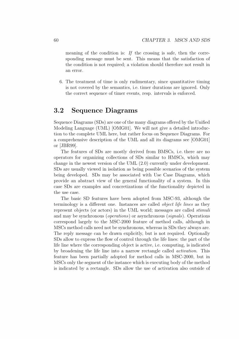
60 CHAPTER 3. MSCS AND SDS
meaning of the condition is: If the crossing is safe, then the corre-sponding message must be sent. This means that the satisfaction ofthe condition is not required; a violation should therefore not result inan error.
6. The treatment of time is only rudimentary, since quantitative timingis not covered by the semantics, i.e. timer durations are ignored. Onlythe correct sequence of timer events, resp. intervals is enforced.
3.2 Sequence Diagrams
Sequence Diagrams (SDs) are one of the many diagrams offered by the UnifiedModeling Language (UML) [OMG01]. We will not give a detailed introduc-tion to the complete UML here, but rather focus on Sequence Diagrams. Fora comprehensive description of the UML and all its diagrams see [OMG01]or [JBR99].
The features of SDs are mostly derived from BMSCs, i.e. there are nooperators for organizing collections of SDs similar to HMSCs, which maychange in the newest version of the UML (2.0) currently under development.SDs are usually viewed in isolation as being possible scenarios of the systembeing developed. SDs may be associated with Use Case Diagrams, whichprovide an abstract view of the general functionality of a system. In thiscase SDs are examples and concretizations of the functionality depicted inthe use case.
The basic SD features have been adopted from MSC-93, although theterminology is a different one. Instances are called object life lines as theyrepresent objects (or actors) in the UML world; messages are called stimuliand may be synchronous (operations) or asynchronous (signals). Operationscorrespond largely to the MSC-2000 feature of method calls, although inMSCs method calls need not be synchronous, whereas in SDs they always are.The reply message can be drawn explicitly, but is not required. OptionallySDs allow to express the flow of control through the life lines: the part of thelife line where the corresponding object is active, i.e. computing, is indicatedby broadening the life line into a narrow rectangle called activation. Thisfeature has been partially adopted for method calls in MSC-2000, but inMSCs only the segment of the instance which is executing body of the methodis indicated by a rectangle. SDs allow the use of activation also outside of
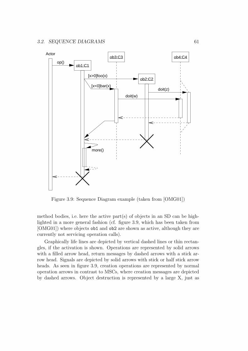
3.2. SEQUENCE DIAGRAMS 61
ob1:C1
ob3:C3
ob2:C2
ob4:C4Actor
op()
[x>0]foo(x)
[x<0]bar(x)doit(z)
doit(w)
more()
Figure 3.9: Sequence Diagram example (taken from [OMG01])
method bodies, i.e. here the active part(s) of objects in an SD can be high-lighted in a more general fashion (cf. figure 3.9, which has been taken from[OMG01]) where objects ob1 and ob2 are shown as active, although they arecurrently not servicing operation calls).
Graphically life lines are depicted by vertical dashed lines or thin rectan-gles, if the activation is shown. Operations are represented by solid arrowswith a filled arrow head, return messages by dashed arrows with a stick ar-row head. Signals are depicted by solid arrows with stick or half stick arrowheads. As seen in figure 3.9, creation operations are represented by normaloperation arrows in contrast to MSCs, where creation messages are depictedby dashed arrows. Object destruction is represented by a large X, just as
62 CHAPTER 3. MSCS AND SDS
process termination in MSCs. Figure 3.9 also shows that stimuli may beguarded, so that it is possible to specify alternatives. This corresponds toan alternative inline expression or a reference in MSCs. A duplication oflife lines is offered to express alternatives or concurrent activities (e.g. ob4 infigure 3.9).
caller exchange receiver
{b.receiveTime -a.sendTime < 1 sec}
a:lift_receiver
b:dial_tone
c:dial_digit
d:route
ringing_tone phone_rings
answer_phone
stop_ringingstop_ringing< 1 sec
{c.receiveTime -b.sendTime < 10 sec}
{d.receiveTime -d.sendTime < 5 sec}
Figure 3.10: Sequence Diagram example with time (taken from [OMG01])
SDs also offer timing constraints, which may be stated either graphicallyor textually. The graphical representation is similar to the time intervals ofMSC-2000, except that the annotation is not necessarily in interval format,but may be expressed textually as well, see figure 3.10 (also taken from[OMG01]). In order to use the textual representation it is necessary to tagthe stimuli with a symbolic name, by which they can be referenced in theconstraint. Specific time points of a stimulus can be defined and referenced,e.g. a.sendTime in figure 3.10. The actual constraint is written in curlybraces and can be expressed in any language, the one predefined by theUML standard for this purpose is the Object Constraint Language (OCL),see [OMG01].
3.2. SEQUENCE DIAGRAMS 63
The UML standard defines a semantics for SDs in terms of the UML metamodel, which eventually is defined in terms of itself, but until now no officialformal semantics for either the complete UML or SDs is available, althoughseveral propositions have been made for different parts of the UML, someof which are shortly presented in the following. Several works have takena meta-modeling approach, trying to define a common domain in which thedifferent diagram types of the UML can be mapped: see e.g. works by the pre-cise UML group3 [EFLR99, EBF+98, EK99] and [GR99]. [RACH00] presentan algebraic semantics for class and state diagrams, [LP99] define an oper-ational semantics for state diagrams, including consistency checks by modelchecking, [LMM99a, LMM99b] follow a very similar approach. [FHD+99]translate SDs into timed automata in order to check their timing consis-tency, but do not consider the complete set of features. [DJPV03] define asemantics for a kernel UML language, which covers class and state diagramsand also takes the action language into account.
Shortcomings of Sequence Diagrams
The points of criticism raised for MSCs in section 3.1.4 hold as well for SDs,as they are existential in nature, make no statement about the activationand do not allow the distinction whether progress is enforced or not. Simul-taneousness is expressible for timing annotations by the interval notation orby the timing labels. Conditions in the sense of MSCs do not exist in SDs,the only construct coming close are the guard expressions on messages (cf.figure 3.9). These allow to express simultaneousness, but cover only condi-tions on the sender’s side. Simultaneous sending and/or receipt of severalmessages is not discussed in [OMG01]. The major drawback of SDs, however,is the absence of a formal semantics.
So in conclusion we can say that neither MSCs nor SDs provide the ex-pressiveness and formal rigor, which is needed for sequence charts to be usedfor more advanced use cases. This motivates the introduction of a sequencechart dialect which remedies these shortcomings: Live Sequence Charts.
3www.cs.york.ac.uk/puml

64 CHAPTER 3. MSCS AND SDS
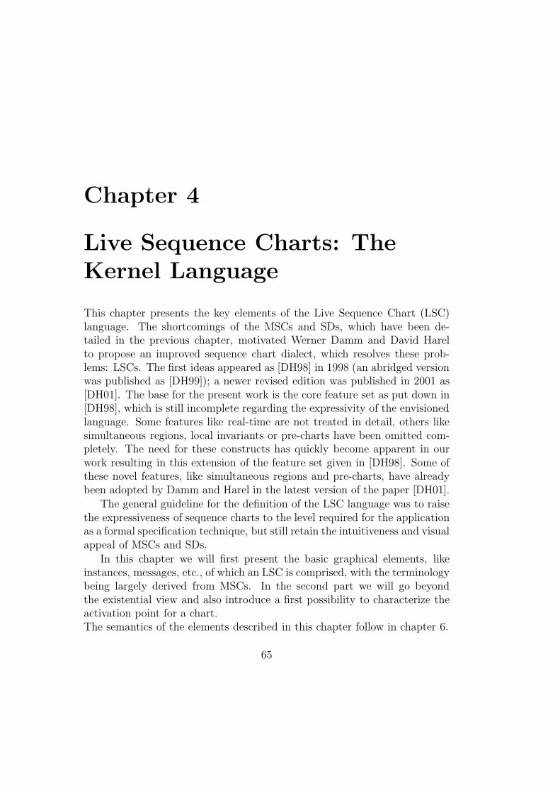
Chapter 4
Live Sequence Charts: The
Kernel Language
This chapter presents the key elements of the Live Sequence Chart (LSC)language. The shortcomings of the MSCs and SDs, which have been de-tailed in the previous chapter, motivated Werner Damm and David Harelto propose an improved sequence chart dialect, which resolves these prob-lems: LSCs. The first ideas appeared as [DH98] in 1998 (an abridged versionwas published as [DH99]); a newer revised edition was published in 2001 as[DH01]. The base for the present work is the core feature set as put down in[DH98], which is still incomplete regarding the expressivity of the envisionedlanguage. Some features like real-time are not treated in detail, others likesimultaneous regions, local invariants or pre-charts have been omitted com-pletely. The need for these constructs has quickly become apparent in ourwork resulting in this extension of the feature set given in [DH98]. Some ofthese novel features, like simultaneous regions and pre-charts, have alreadybeen adopted by Damm and Harel in the latest version of the paper [DH01].
The general guideline for the definition of the LSC language was to raisethe expressiveness of sequence charts to the level required for the applicationas a formal specification technique, but still retain the intuitiveness and visualappeal of MSCs and SDs.
In this chapter we will first present the basic graphical elements, likeinstances, messages, etc., of which an LSC is comprised, with the terminologybeing largely derived from MSCs. In the second part we will go beyondthe existential view and also introduce a first possibility to characterize theactivation point for a chart.The semantics of the elements described in this chapter follow in chapter 6.
65
66 CHAPTER 4. LSCS: THE KERNEL LANGUAGE
4.1 Basic LSC Features
The basic idea of LSCs is to allow a distinction between mandatory andpossible behavior, i.e. most LSC elements can be designated to belong to ei-ther one category or the other. This distinction is also expressed graphically,which contributes largely to the easy understanding of LSC specifications.Mandatory elements are depicted by solid lines, possible ones by dashedlines. The basic features described in this section are:
• instances, which represent the participants for the communication,
• messages sent between the instances,
• temperatures indicating progress along instances and messages,
• conditions describing particular states of the instances at a certainpoint in time,
• local invariants, which are conditions which hold for a period of time
• coregions and simultaneous regions, which express ordering informationon instances.
4.1.1 Instances and Messages
Instances and messages are the elementary building blocks of LSCs. Thegraphical representation for instances has been adopted from MSCs, i.e. LSCinstances consist of an instance head carrying the instance name, an instanceaxis and an instance end, as the example LSC in figure 4.1 shows. As forMSCs and SDs, the horizontal dimension is the structural dimension and thevertical dimension corresponds to the time dimension.
Deviating from MSCs we depict the environment by an instance of itsown rather than the border of the LSC. When using LSCs for formal veri-fication, an explicit environment instance offers the possibility of expressingassumptions on the behavior of the environment within the LSC by employ-ing the same elements as for the other instances (see chapter 8 for details).Graphically, environment instances are denoted by a shaded instance headsymbol; see figure 4.1.
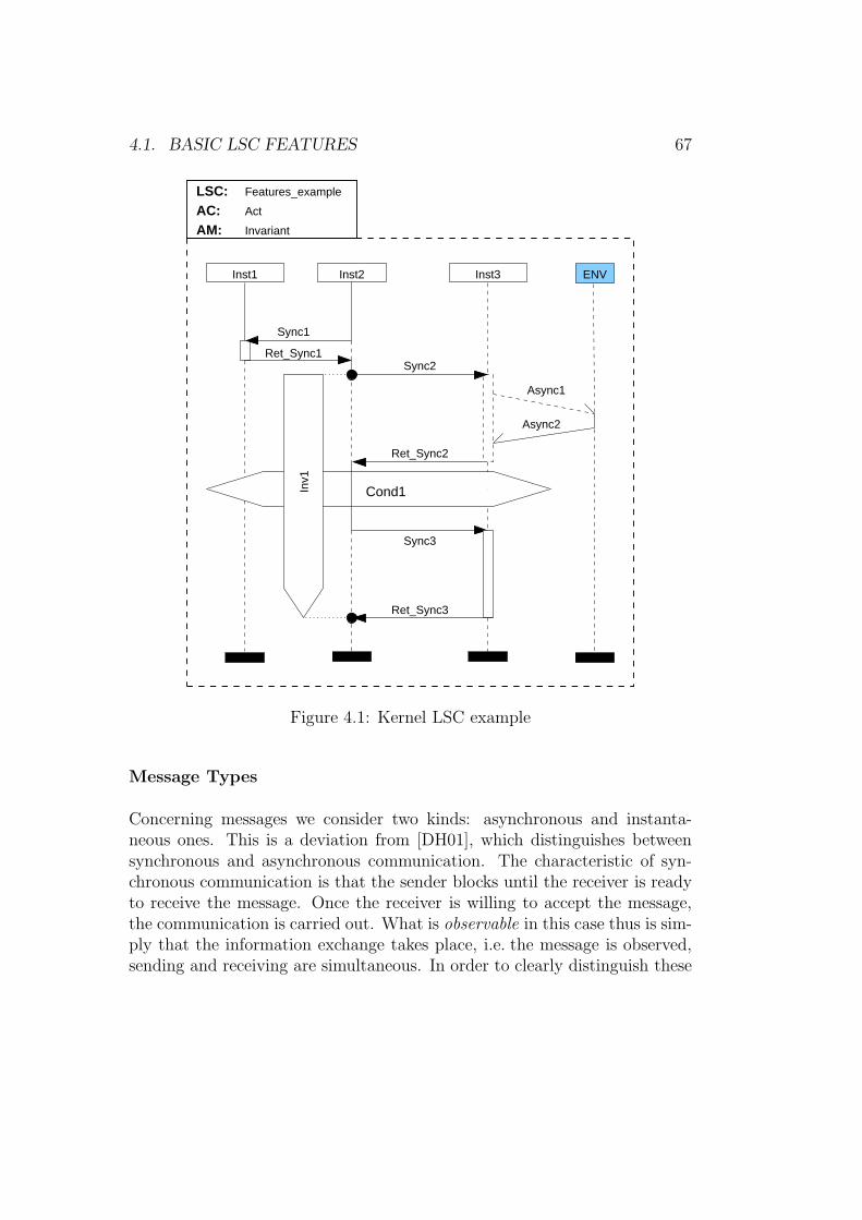
4.1. BASIC LSC FEATURES 67
Inst2 Inst3
Sync3
Inst1 ENV
AC:AM: Invariant
Features_exampleLSC:Act
Async1
Async2
Ret_Sync2
Ret_Sync3
Sync2
Cond1Inv1
Sync1
Ret_Sync1
Figure 4.1: Kernel LSC example
Message Types
Concerning messages we consider two kinds: asynchronous and instanta-neous ones. This is a deviation from [DH01], which distinguishes betweensynchronous and asynchronous communication. The characteristic of syn-chronous communication is that the sender blocks until the receiver is readyto receive the message. Once the receiver is willing to accept the message,the communication is carried out. What is observable in this case thus is sim-ply that the information exchange takes place, i.e. the message is observed,sending and receiving are simultaneous. In order to clearly distinguish these
68 CHAPTER 4. LSCS: THE KERNEL LANGUAGE
concepts, we rather use the term instantaneous than synchronous. Sincethe time dimension in LSCs is the vertical one, a delay on the senders sidebetween trying to send a message and acceptance of this request by the re-ceiver should be expressed on the instance axis as a progress requirement.The same line of thought has been used in the context of Message FlowGraphs by Ladkin and Leue [LL95].
AC:AM: Invariant
Inst2
AmbiguityLSC:Act
Inst3
Sync2()
Inst1
Sync1()
(a) ambiguous LSC
AC:AM: Invariant
Inst2
AmbiguityLSC:Act
Inst3Inst1
Sync2
Ret_Sync2
Sync1
Ret_Sync1
(b) possible resolution
Figure 4.2: Ambiguity example
Operation calls, e.g. in UML or method calls in MSC-2000, are thus rep-resented by two instantaneous messages: the method call and the returnmessage. For method calls in LSCs we require the return message to be in-cluded explicitly, because otherwise confusion arises whether messages andother elements following a method call receipt are part of the method body.Consider the LSC in figure 4.2(a). It is not immediately clear whether oper-ation call Sync2 should be considered as taking place after the completion ofthe preceeding operation call or if it is part of the body of operation Sync1.Requiring the user to explicitly include the return message clarifies the sit-uation. Figure 4.2(b) shows how the second interpretation would look like.Consequently we require to explicitly include the return message for eachoperation invocation.[DH01] does not explicitly address the question of method calls or returns.
For the graphical representation of messages we use an SD-like notation:asynchronous messages are visualized by half stick arrows, instantaneousmessages by arrows with solid heads; see figure 4.1. Instantaneous messages
4.1. BASIC LSC FEATURES 69
have to be drawn horizontally to indicate simultaneity of sending and receiv-ing, while asynchronous ones are drawn slanted to indicate the passage oftime between sending and receipt. Note that both types of messages consistof a sending and receiving event. The pairing of operation call and returnis indicated graphically by widening the instance axis on the receiver sideinto a thin rectangle which marks the operation body, as for method calls inMSC-2000; see figures 4.1 and 4.2(b) for examples. A graphical representa-tion of activations, i.e. explicitly showing the flow of control by enlarging thecorresponding instance axis segments, as done in SDs is not provided, sincethis is not the focus of LSCs.
Progress
One deficiency of both MSCs and SDs is their inability to enforce progress,as mentioned in section 3.1.4. LSCs overcome this drawback by associatinga temperature with both locations1 and messages. The temperature canbe either hot or cold, the former indicating that progress is enforced. Theanalogy here is that one cannot remain at a hot location for an infinite amountof time, because then one would burn ones feet. This obviously requires thata hot location has to be left, i.e. the following location has to be reached.At a cold location one can stay forever without harming ones feet, i.e. thefollowing location need not be reached. In terms of messages this means thata hot message has to be delivered, whereas a cold message may be lost alongthe way. Progress information is thus expressed by the temperatures of themessages and along the instance lines. The meaning of the temperatures issummarized in table 4.1.
hot coldlocation location has to be left may stay infinitely long
i.e. next locations has to be reached at locationmessage message has to be received message may be lost
once sent
Table 4.1: Temperatures for messages and locations
1Locations are those points on an instance axis, where some event is attached,e.g. sending or receipt of a message, conditions, etc. In chapter 6 we give a formal definitionof a location.
70 CHAPTER 4. LSCS: THE KERNEL LANGUAGE
Graphically hot temperatures are represented by solid lines, cold onesby dashed lines. This means that e.g. a hot location is depicted by a solidinstance axis segment, which starts at this location and ends either at thenext cold location or the instance end. In figure 4.1 for example the locationof the sending of message Sync2 is cold and the next location (the receiptof the return message) is hot, so that the instance axis segment in betweenthem is dashed. Note that also the rectangle representing operation bodiesis rendered either solid or dashed depending on the location temperatures.Analogously are messages depicted by solid or dashed arrows depending ontheir temperature; see figure 4.1 for examples. Note that the completion ofoperation calls is indicated by location temperatures, not by the messagetemperature. The request for operation Sync2 in figure 4.1 thus must bereceived, but the operation need not be completed.
It is recommended that only those locations are annotated with a hottemperature, whose instance is responsible for achieving the progress. Thereceiving instance of a method call e.g. is responsible for generating a corre-sponding return message, so only this location is assigned a hot temperature,not the sending one. Conforming to this convention yields LSCs, which showa focus of control, similar to the activation of object life lines in SDs.
We will gradually transform the MSC of figure 3.8 on page 57, which weused to illustrate the shortcomings of MSCs and SDs in chapter 3, into anLSC as we introduce the LSC features. Figure 4.3 shows the first step of thistransformation with temperatures added for locations and messages. Notethat all final location temperatures are cold, because once all events on aninstance axis have been observed, no progress need be enforced. All messagesare instantaneous, since we are considering a Statemate model, where noasynchronous communication is possible.
4.1.2 Conditions
In order to make statements about the state of the system boolean conditionsreferring to attributes or data items of the involved entities are used. Notethat we are using symbolic names instead of concrete expressions in our LSCexamples, since the unwinding algorithm presented in chapter 6 operates onpropositions rather than concrete model elements. Graphically, conditionsare represented as in MSCs by an elongated hexagon (see figure 4.1 or fig-ure 4.3).
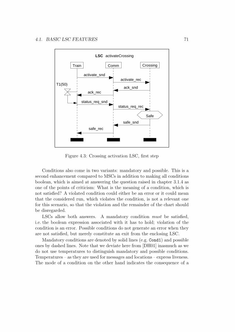
4.1. BASIC LSC FEATURES 71
activate_rec
ack_snd
activate_snd
status_req_recstatus_req_snd
safe_rec
safe_snd
LSC activateCrossing
Train Comm Crossing
ack_rec
Safe
T1(50)
Figure 4.3: Crossing activation LSC, first step
Conditions also come in two variants: mandatory and possible. This is asecond enhancement compared to MSCs in addition to making all conditionsboolean, which is aimed at answering the question raised in chapter 3.1.4 asone of the points of criticism: What is the meaning of a condition, which isnot satisfied? A violated condition could either be an error or it could meanthat the considered run, which violates the condition, is not a relevant onefor this scenario, so that the violation and the remainder of the chart shouldbe disregarded.
LSCs allow both answers. A mandatory condition must be satisfied,i.e. the boolean expression associated with it has to hold; violation of thecondition is an error. Possible conditions do not generate an error when theyare not satisfied, but merely constitute an exit from the enclosing LSC.
Mandatory conditions are denoted by solid lines (e.g. Cond1) and possibleones by dashed lines. Note that we deviate here from [DH01] inasmuch as wedo not use temperatures to distinguish mandatory and possible conditions.Temperatures – as they are used for messages and locations – express liveness.The mode of a condition on the other hand indicates the consequence of a
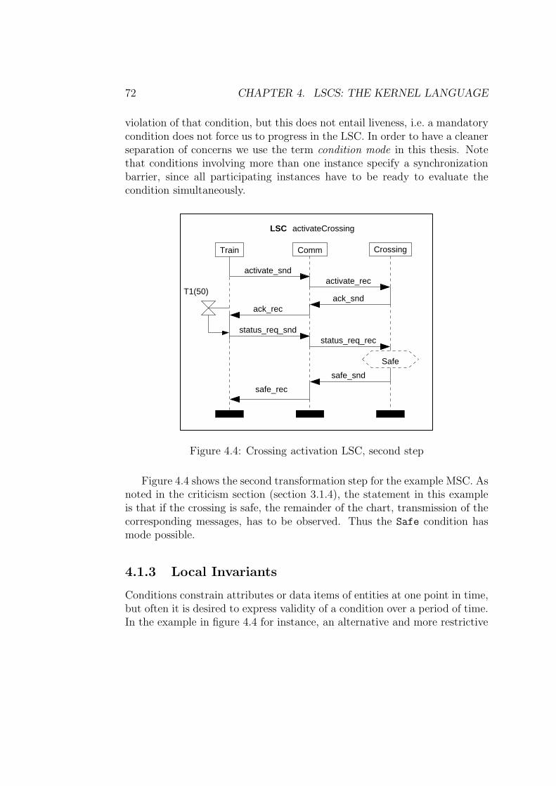
72 CHAPTER 4. LSCS: THE KERNEL LANGUAGE
violation of that condition, but this does not entail liveness, i.e. a mandatorycondition does not force us to progress in the LSC. In order to have a cleanerseparation of concerns we use the term condition mode in this thesis. Notethat conditions involving more than one instance specify a synchronizationbarrier, since all participating instances have to be ready to evaluate thecondition simultaneously.
activate_rec
ack_snd
activate_snd
status_req_rec
ack_rec
status_req_snd
safe_rec
safe_snd
LSC activateCrossing
Train Comm Crossing
Safe
T1(50)
Figure 4.4: Crossing activation LSC, second step
Figure 4.4 shows the second transformation step for the example MSC. Asnoted in the criticism section (section 3.1.4), the statement in this exampleis that if the crossing is safe, the remainder of the chart, transmission of thecorresponding messages, has to be observed. Thus the Safe condition hasmode possible.
4.1.3 Local Invariants
Conditions constrain attributes or data items of entities at one point in time,but often it is desired to express validity of a condition over a period of time.In the example in figure 4.4 for instance, an alternative and more restrictive
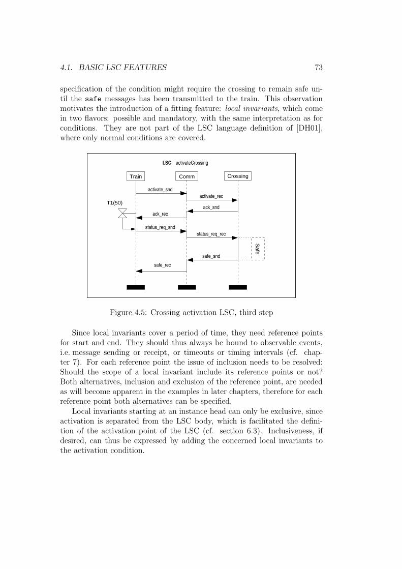
4.1. BASIC LSC FEATURES 73
specification of the condition might require the crossing to remain safe un-til the safe messages has been transmitted to the train. This observationmotivates the introduction of a fitting feature: local invariants, which comein two flavors: possible and mandatory, with the same interpretation as forconditions. They are not part of the LSC language definition of [DH01],where only normal conditions are covered.
LSC activateCrossing
CommTrain
activate_rec
ack_snd
activate_snd
status_req_rec
Crossing
ack_rec
status_req_snd
safe_rec
safe_snd
Safe
T1(50)
Figure 4.5: Crossing activation LSC, third step
Since local invariants cover a period of time, they need reference pointsfor start and end. They should thus always be bound to observable events,i.e. message sending or receipt, or timeouts or timing intervals (cf. chap-ter 7). For each reference point the issue of inclusion needs to be resolved:Should the scope of a local invariant include its reference points or not?Both alternatives, inclusion and exclusion of the reference point, are neededas will become apparent in the examples in later chapters, therefore for eachreference point both alternatives can be specified.
Local invariants starting at an instance head can only be exclusive, sinceactivation is separated from the LSC body, which is facilitated the defini-tion of the activation point of the LSC (cf. section 6.3). Inclusiveness, ifdesired, can thus be expressed by adding the concerned local invariants tothe activation condition.
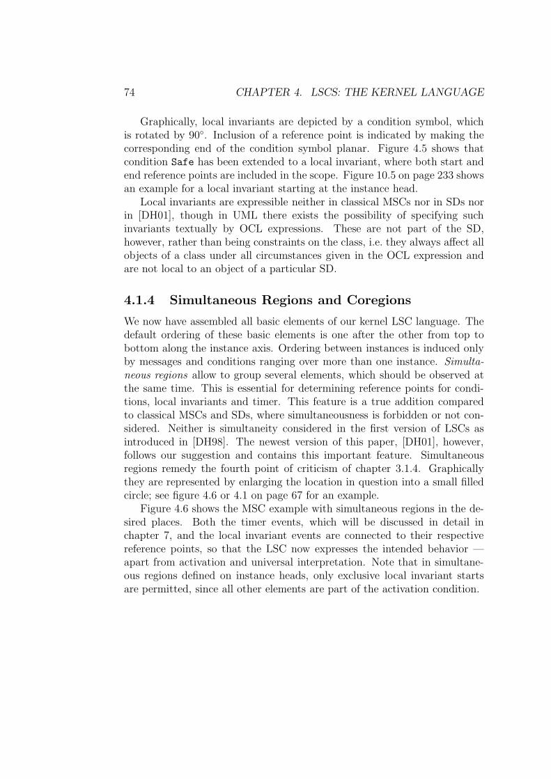
74 CHAPTER 4. LSCS: THE KERNEL LANGUAGE
Graphically, local invariants are depicted by a condition symbol, whichis rotated by 90◦. Inclusion of a reference point is indicated by making thecorresponding end of the condition symbol planar. Figure 4.5 shows thatcondition Safe has been extended to a local invariant, where both start andend reference points are included in the scope. Figure 10.5 on page 233 showsan example for a local invariant starting at the instance head.
Local invariants are expressible neither in classical MSCs nor in SDs norin [DH01], though in UML there exists the possibility of specifying suchinvariants textually by OCL expressions. These are not part of the SD,however, rather than being constraints on the class, i.e. they always affect allobjects of a class under all circumstances given in the OCL expression andare not local to an object of a particular SD.
4.1.4 Simultaneous Regions and Coregions
We now have assembled all basic elements of our kernel LSC language. Thedefault ordering of these basic elements is one after the other from top tobottom along the instance axis. Ordering between instances is induced onlyby messages and conditions ranging over more than one instance. Simulta-neous regions allow to group several elements, which should be observed atthe same time. This is essential for determining reference points for condi-tions, local invariants and timer. This feature is a true addition comparedto classical MSCs and SDs, where simultaneousness is forbidden or not con-sidered. Neither is simultaneity considered in the first version of LSCs asintroduced in [DH98]. The newest version of this paper, [DH01], however,follows our suggestion and contains this important feature. Simultaneousregions remedy the fourth point of criticism of chapter 3.1.4. Graphicallythey are represented by enlarging the location in question into a small filledcircle; see figure 4.6 or 4.1 on page 67 for an example.
Figure 4.6 shows the MSC example with simultaneous regions in the de-sired places. Both the timer events, which will be discussed in detail inchapter 7, and the local invariant events are connected to their respectivereference points, so that the LSC now expresses the intended behavior —apart from activation and universal interpretation. Note that in simultane-ous regions defined on instance heads, only exclusive local invariant startsare permitted, since all other elements are part of the activation condition.
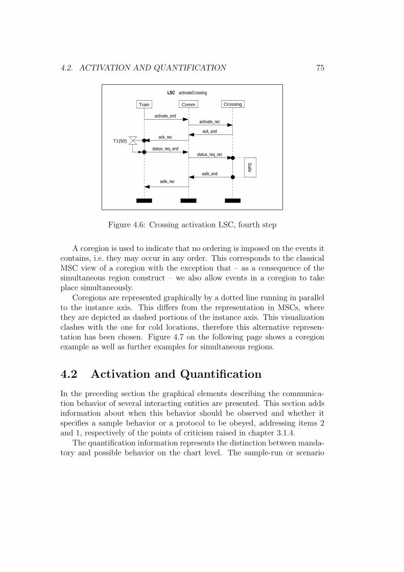
4.2. ACTIVATION AND QUANTIFICATION 75
activateCrossing
Safe
LSC
safe_snd
safe_rec
Train
activate_rec
Comm
ack_snd
activate_snd
status_req_rec
Crossing
ack_rec
status_req_snd
T1(50)
Figure 4.6: Crossing activation LSC, fourth step
A coregion is used to indicate that no ordering is imposed on the events itcontains, i.e. they may occur in any order. This corresponds to the classicalMSC view of a coregion with the exception that – as a consequence of thesimultaneous region construct – we also allow events in a coregion to takeplace simultaneously.
Coregions are represented graphically by a dotted line running in parallelto the instance axis. This differs from the representation in MSCs, wherethey are depicted as dashed portions of the instance axis. This visualizationclashes with the one for cold locations, therefore this alternative represen-tation has been chosen. Figure 4.7 on the following page shows a coregionexample as well as further examples for simultaneous regions.
4.2 Activation and Quantification
In the preceding section the graphical elements describing the communica-tion behavior of several interacting entities are presented. This section addsinformation about when this behavior should be observed and whether itspecifies a sample behavior or a protocol to be obeyed, addressing items 2and 1, respectively of the points of criticism raised in chapter 3.1.4.
The quantification information represents the distinction between manda-tory and possible behavior on the chart level. The sample-run or scenario
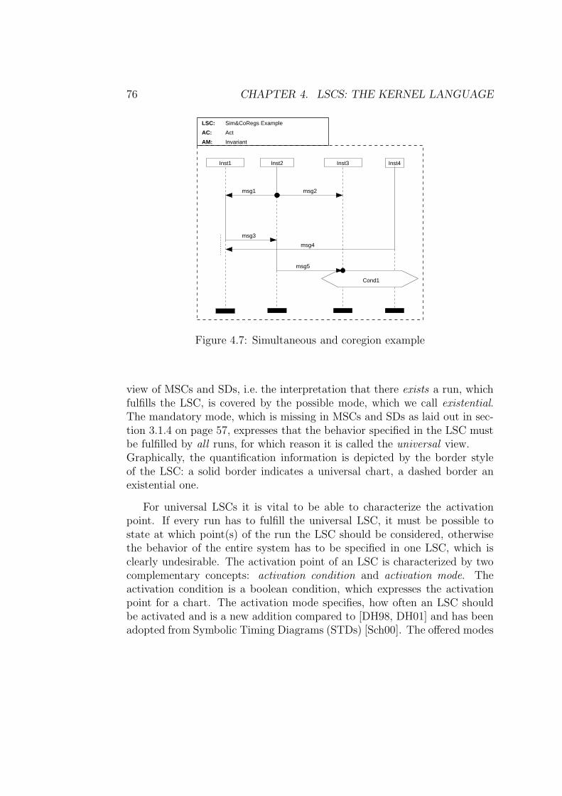
76 CHAPTER 4. LSCS: THE KERNEL LANGUAGE
AC:
AM: Invariant
Inst2
Sim&CoRegs ExampleLSC:
Act
Inst3Inst1
msg2
Inst4
Cond1
msg1
msg3
msg4
msg5
Figure 4.7: Simultaneous and coregion example
view of MSCs and SDs, i.e. the interpretation that there exists a run, whichfulfills the LSC, is covered by the possible mode, which we call existential.The mandatory mode, which is missing in MSCs and SDs as laid out in sec-tion 3.1.4 on page 57, expresses that the behavior specified in the LSC mustbe fulfilled by all runs, for which reason it is called the universal view.Graphically, the quantification information is depicted by the border styleof the LSC: a solid border indicates a universal chart, a dashed border anexistential one.
For universal LSCs it is vital to be able to characterize the activationpoint. If every run has to fulfill the universal LSC, it must be possible tostate at which point(s) of the run the LSC should be considered, otherwisethe behavior of the entire system has to be specified in one LSC, which isclearly undesirable. The activation point of an LSC is characterized by twocomplementary concepts: activation condition and activation mode. Theactivation condition is a boolean condition, which expresses the activationpoint for a chart. The activation mode specifies, how often an LSC shouldbe activated and is a new addition compared to [DH98, DH01] and has beenadopted from Symbolic Timing Diagrams (STDs) [Sch00]. The offered modes
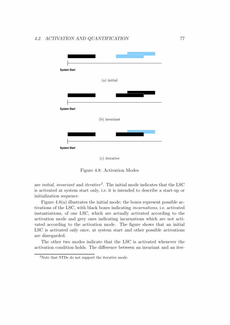
4.2. ACTIVATION AND QUANTIFICATION 77
System Start
(a) initial
System Start
(b) invariant
System Start
(c) iterative
Figure 4.8: Activation Modes
are initial, invariant and iterative2. The initial mode indicates that the LSCis activated at system start only, i.e. it is intended to describe a start-up orinitialization sequence.
Figure 4.8(a) illustrates the initial mode; the boxes represent possible ac-tivations of the LSC, with black boxes indicating incarnations, i.e. activatedinstantiations, of one LSC, which are actually activated according to theactivation mode and grey ones indicating incarnations which are not acti-vated according to the activation mode. The figure shows that an initialLSC is activated only once, at system start and other possible activationsare disregarded.
The other two modes indicate that the LSC is activated whenever theactivation condition holds. The difference between an invariant and an iter-
2Note that STDs do not support the iterative mode.
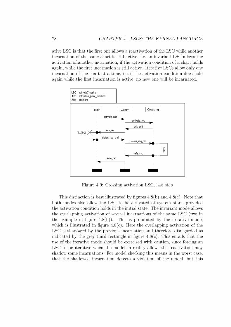
78 CHAPTER 4. LSCS: THE KERNEL LANGUAGE
ative LSC is that the first one allows a reactivation of the LSC while anotherincarnation of the same chart is still active. i.e. an invariant LSC allows theactivation of another incarnation, if the activation condition of a chart holdsagain, while the first incarnation is still active. Iterative LSCs allow only oneincarnation of the chart at a time, i.e. if the activation condition does holdagain while the first incarnation is active, no new one will be incarnated.
activateCrossingLSC
Safe
activation_point_reached
Comm
ack_snd
activate_snd
status_req_rec
Crossing
AC:
Invariant
Train
activate_rec
ack_rec
status_req_snd
safe_rec
safe_snd
AM:
T1(50)
Figure 4.9: Crossing activation LSC, last step
This distinction is best illustrated by figures 4.8(b) and 4.8(c). Note thatboth modes also allow the LSC to be activated at system start, providedthe activation condition holds in the initial state. The invariant mode allowsthe overlapping activation of several incarnations of the same LSC (two inthe example in figure 4.8(b)). This is prohibited by the iterative mode,which is illustrated in figure 4.8(c). Here the overlapping activation of theLSC is shadowed by the previous incarnation and therefore disregarded asindicated by the grey third rectangle in figure 4.8(c). This entails that theuse of the iterative mode should be exercised with caution, since forcing anLSC to be iterative when the model in reality allows the reactivation mayshadow some incarnations. For model checking this means in the worst case,that the shadowed incarnation detects a violation of the model, but this
4.2. ACTIVATION AND QUANTIFICATION 79
counter example is never found, because this incarnation is shadowed by theprevious incarnation, which is not violated. The use of iterative LSCs forproperty specification for formal verification is thus prohibited and will notbe considered in our application example. For other use cases, e.g. testing,however, the iterative mode does make sense.
Activation mode and condition are not depicted graphically, but are ex-pressed textually at the top of an LSC together with the name, using theacronyms AM and AC respectively. For examples for activation mode, condi-tion and quantification see figures 4.1, 4.7 and 4.9. Figure 4.9 shows the finalresult of the stepwise transformation of the MSC of figure 3.8 into an LSC.

80 CHAPTER 4. LSCS: THE KERNEL LANGUAGE
Chapter 5
Automata-Theoretic
Foundation
The base for the definition of the formal semantics of LSCs is a variation oftimed Buchi automata. We chose Buchi automata for several reasons: First,we use LSCs to describe the communication behavior of reactive systems,i.e. systems which must be able to accept and react to input signals at anytime. These systems are typically designed to operate forever, at least the-oretically, which means that runs of reactive systems are infinite. Thereforeclassical finite automata are not sufficient for our purpose. Buchi automata([Tho90]) are one possible solution as they accept infinite words. The secondreason for choosing Buchi automata over other variants of automata on infi-nite words is that there is a close relationship between Buchi automata andlinear time temporal logic (LTL) [Tho90, Eme90]. Since the main applicationfield for LSCs in this thesis is property specification for formal verification,this is a major advantage. The third reason is that Buchi automata allow toeasily express liveness properties via their acceptance criterion.
This line of reasoning has also been employed in the definition of theformal semantics of Symbolic Timing Diagrams (STDs) by Schlor in [Sch00],where the semantics of STDs are given in terms of a Buchi automaton variant.This variant, called Symbolic Automaton in [Sch00], extends classical Buchiautomata by allowing expressions over an assertion language as transitionlabels. Since this extension is a vital addition for our semantics definition ofLSCs, as will become apparent later, we are using this type of automaton aswell and further extend it to be able to cope also with quantitative timing,which is not considered in [Sch00].
81
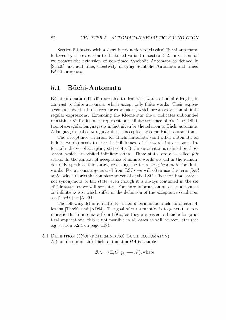
82 CHAPTER 5. AUTOMATA-THEORETIC FOUNDATION
Section 5.1 starts with a short introduction to classical Buchi automata,followed by the extension to the timed variant in section 5.2. In section 5.3we present the extension of non-timed Symbolic Automata as defined in[Sch00] and add time, effectively merging Symbolic Automata and timedBuchi automata.
5.1 Buchi-Automata
Buchi automata ([Tho90]) are able to deal with words of infinite length, incontrast to finite automata, which accept only finite words. Their expres-siveness is identical to ω-regular expressions, which are an extension of finiteregular expressions. Extending the Kleene star the ω indicates unboundedrepetition: aω for instance represents an infinite sequence of a’s. The defini-tion of ω-regular languages is in fact given by the relation to Buchi automata:A language is called ω-regular iff it is accepted by some Buchi automaton.
The acceptance criterion for Buchi automata (and other automata oninfinite words) needs to take the infiniteness of the words into account. In-formally the set of accepting states of a Buchi automaton is defined by thosestates, which are visited infinitely often. These states are also called fairstates. In the context of acceptance of infinite words we will in the remain-der only speak of fair states, reserving the term accepting state for finitewords. For automata generated from LSCs we will often use the term finalstate, which marks the complete traversal of the LSC. The term final state isnot synonymous to fair state, even though it is always contained in the setof fair states as we will see later. For more information on other automataon infinite words, which differ in the definition of the acceptance condition,see [Tho90] or [AD94].
The following definition introduces non-deterministic Buchi automata fol-lowing [Tho90] and [AD94]. The goal of our semantics is to generate deter-ministic Buchi automata from LSCs, as they are easier to handle for prac-tical applications; this is not possible in all cases as will be seen later (seee.g. section 6.2.4 on page 118).
5.1 Definition ((Non-deterministic) Buchi Automaton)A (non-deterministic) Buchi automaton BA is a tuple
BA = (Σ, Q, q0,−→, F ),where
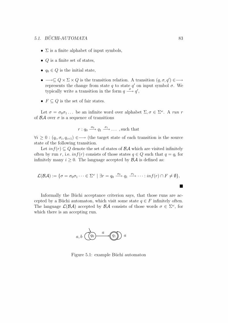
5.1. BUCHI-AUTOMATA 83
• Σ is a finite alphabet of input symbols,
• Q is a finite set of states,
• q0 ∈ Q is the initial state,
• −→⊆ Q×Σ×Q is the transition relation. A transition (q, σ, q′) ∈−→represents the change from state q to state q′ on input symbol σ. Wetypically write a transition in the form q
σ−→ q′,
• F ⊆ Q is the set of fair states.
Let σ = σ0σ1 . . . be an infinite word over alphabet Σ, σ ∈ Σω. A run rof BA over σ is a sequence of transitions
r : q0σ0−→ q1
σ1−→ . . . , such that
∀i ≥ 0 : (qi, σi, qi+1) ∈−→ (the target state of each transition is the sourcestate of the following transition.
Let inf(r) ⊆ Q denote the set of states of BA which are visited infinitelyoften by run r, i.e. inf(r) consists of those states q ∈ Q such that q = qi forinfinitely many i ≥ 0. The language accepted by BA is defined as:
L(BA) := {σ = σ0σ1 · · · ∈ Σω | ∃r = q0σ0−→ q1
σ1−→ · · · : inf(r) ∩ F 6= ∅},
�
Informally the Buchi acceptance criterion says, that those runs are ac-cepted by a Buchi automaton, which visit some state q ∈ F infinitely often.The language L(BA) accepted by BA consists of those words σ ∈ Σω, forwhich there is an accepting run.
q0a, b q1 aa
Figure 5.1: example Buchi automaton
84 CHAPTER 5. AUTOMATA-THEORETIC FOUNDATION
Example 5.1 (Buchi automata)Figure 5.1 shows an example of a Buchi automaton. The initial state ismarked by a transition without a source state and fair states by a doubleborder. In this example there is only one fair state, q1. The automatonaccepts the language (a+ b)∗aω. �
5.2 Timed Buchi Automata
When the occurrence times of the letters of words are important, timedlanguages are used and consequently a corresponding type of automaton isneeded: a timed automaton. We only consider timed Buchi automata here,there also exist variants for finite automata and other timed automata oninfinite words (see [AD94]). For the definition of timed Buchi automata weloosely follow the lead of [AD94] here, inasmuch as we associate an occur-rence time to each symbol of a word, yielding timed words. In contrast to[AD94], however, we only consider discrete time instead of dense time as thisis sufficient for our purpose. Time is represented by a sequence of time valuesfrom the set of non-negative natural numbers: τi ∈ N, which has to satisfytwo constraints: time only advances and time never stands still:
5.2 Definition (Timed Word)A time sequence τ = τ0τ1τ2 . . . is an infinite sequence of time values τi ∈ N
for which the following holds:
1. τi < τi+1, ∀i ≥ 0 (τ is strictly monotonically increasing).
2. ∀t ∈ N ∃i ≥ 1 : τi > t (time always progresses)
A timed word over an alphabet Σ is then a pair (σ, τ), where σ = σ0σ1 . . .is an infinite word and τ = τ0τ1 . . . is a time sequence. The time value τidenotes the occurrence time of input symbol σi. �
In the untimed case the behavior of the automaton depends only on theinput symbols, i.e. being in some state the next states of an automaton aredetermined by the current input symbol. In order for an automaton to alsoaccept timed words it needs a means to count time, since the choice of thenext states also depends on the occurrence time of the input symbols inquestion. This is realized by clocks, which can be set to zero on any transition
5.2. TIMED BUCHI AUTOMATA 85
of the automaton and count the time since their last reset. This allows forthe introduction of clock constraints on transitions – i.e. a transition mayonly be taken, if all its clock constraints are satisfied – forcing the inputword to obey certain timing requirements. Thus time is introduced into anautomaton by adding a (finite) set of clocks and augmenting transitions byclock resets and clock constraints formulated over this set of clocks.
Before giving the formal definition of a timed automaton it is necessary todetermine which are legal expressions for clock constraints and how the valueof the clocks is resolved. For our purposes it is sufficient to allow comparisonof clock values to constants, conjunction and disjunction of clock constraints.
5.3 Definition (Clock Constraint)Let C be a set of clocks. A clock constraint γ ∈ Φ(C) is defined as
γ := ǫ | x < c | x ≤ c | x = c | x > c | x ≥ c | γ1 ∧ γ2 | γ1 ∨ γ2,
where x ∈ C and c ∈ N. ǫ represents the empty clock constraint.A clock interpretation ν assigns to each clock x ∈ C a value of the time
domain:ν : C −→ N
The set of all clock interpretations is defined as I.The valuation of a clock constraint is defined by
J·K(·) : Φ(C) × I −→ B
JǫK(ν) := true
Jx < cK(ν) := ν(x) < c
Jx ≤ cK(ν) := ν(x) ≤ c
Jx > cK(ν) := ν(x) > c
Jx ≥ cK(ν) := ν(x) ≥ c
Jx = cK(ν) := ν(x) = c
Jγ1 ∧ γ2K(ν) := Jγ1K(ν) ∧ Jγ2K(ν)
Jγ1 ∨ γ2K(ν) := Jγ1K(ν) ∨ Jγ2K(ν)
Let ν+ t be the clock interpretation, which adds t to all clocks: ν+ t := ∀x ∈C : (ν + t)(x) = ν(x) + t. �
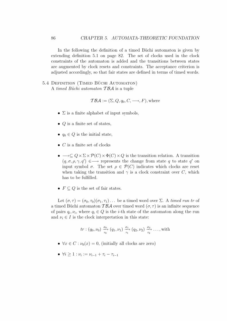
86 CHAPTER 5. AUTOMATA-THEORETIC FOUNDATION
In the following the definition of a timed Buchi automaton is given byextending definition 5.1 on page 82. The set of clocks used in the clockconstraints of the automaton is added and the transitions between statesare augmented by clock resets and constraints. The acceptance criterion isadjusted accordingly, so that fair states are defined in terms of timed words.
5.4 Definition (Timed Buchi Automaton)A timed Buchi automaton T BA is a tuple
T BA := (Σ, Q, q0, C,−→, F ),where
• Σ is a finite alphabet of input symbols,
• Q is a finite set of states,
• q0 ∈ Q is the initial state,
• C is a finite set of clocks
• −→⊆ Q×Σ×P(C)×Φ(C)×Q is the transition relation. A transition(q, σ, ρ, γ, q′) ∈−→ represents the change from state q to state q′ oninput symbol σ. The set ρ ∈ P(C) indicates which clocks are resetwhen taking the transition and γ is a clock constraint over C, whichhas to be fulfilled.
• F ⊆ Q is the set of fair states.
Let (σ, τ) = (σ0, τ0)(σ1, τ1) . . . be a timed word over Σ. A timed run tr ofa timed Buchi automaton T BA over timed word (σ, τ) is an infinite sequenceof pairs qi, νi, where qi ∈ Q is the i-th state of the automaton along the runand νi ∈ I is the clock interpretation in this state:
tr : (q0, ν0)σ0−→τ0
(q1, ν1)σ1−→τ1
(q2, ν2)σ2−→τ2
. . . ,with
• ∀x ∈ C : ν0(x) = 0, (initially all clocks are zero)
• ∀i ≥ 1 : νi := νi−1 + τi − τi−1
5.3. SYMBOLIC AUTOMATA 87
• ∀i ≥ 0 ∃ (qi, σi, ρi, γi, qi+1) ∈−→: JγiK(νi) = true ∧ ∀x ∈ ρi : νi+1(x) =0 ∧ ∀x 6∈ ρi : νi+1(x) = νi(x) + τi − τi−1
(the target state of each transition is the source state of the followingtransition, the transition respects all its clock constraints, resets allappropriate clocks and all clocks, which are not reset, correctly advancethe time).
Let inf(tr) ⊆ Q denote the set of states of T BA which are visited in-finitely often by timed run tr, i.e. inf(tr) consists of those states q ∈ Q suchthat q = qi for infinitely many i ≥ 0. The language accepted by T BA isdefined as the set of timed words, for which there is an accepting run ofT BA:
L(T BA) := {(σ, τ) | ∃tr = (q0, ν0)σ0−→τ0
(q1, ν1)σ1−→τ1
· · · : inf(tr) ∩ F 6= ∅}
�
q0a q1a
q2 a
b, x := 0
c, x < 4
Figure 5.2: example timed Buchi automaton
Example 5.2Figure 5.2 shows an example of a timed Buchi automaton, which accepts thelanguage {(σ, τ) | σ ∈ a+(ba∗c)ω ∧ ∀i ∃j > i : σi = b ⇒ σj = c ∧ τj < τi + 4}.
�
5.3 Symbolic Automata
The automata described so far operate on single input symbols only, sincethey allow but one element of Σ per transition. In order to be able to de-scribe the communication behavior of a system, it is necessary to allow morethan one observation at a time. Symbolic Timing Diagrams faced the same
88 CHAPTER 5. AUTOMATA-THEORETIC FOUNDATION
problem, which in [Sch00] is solved by the extension of Buchi automata tosymbolic automata, where a run is extended to a computation sequence refer-ring to valuations of system variables and formulas are allowed as transitionannotations in the automaton. We adopt this strategy for the LSC semanticsdefinition and therefore use symbolic automata.
[Sch00] does not consider quantitative timing for STDs, so that symbolicautomata are untimed. We consequently extend the definition of symbolic au-tomata to also encompass (discrete) time, similar to timed Buchi automata.First, we extend the notion of a timed word to a timed symbolic word (calleda computation sequence in [Sch00]).
5.5 Definition (Timed Symbolic Word)Let V be a set of typed variables, DOM the domain of variables v ∈ V andθ : V −→ DOM a valuation, which assigns to each v ∈ V a value of itsdomain. Furthermore let τ be a time sequence.
A symbolic word then is an infinite sequence θ = θ0θ1θ2 . . .
A timed symbolic word then is a pair (θ, τ) = (θ0, τ0)(θ1, τ1)(θ2, τ2) . . . , whereτi denotes the occurrence time of valuation θi. �
In order to refer to the occurrence of several communication events it isnecessary to extend the timed Buchi automata to allow formulas:
5.6 Definition (Formula over Σ)Let Σ ⊆ V be a set of boolean variables. A formula ψ over Σ is a booleanexpression produced by the following rules:
ψ := σ | ¬ψ | (ψ) | ψ1 ∧ ψ2 | ψ1 ∨ ψ2
with σ ∈ Σ.The set of all formulas over Σ is denoted by BExprΣ. �
5.7 Definition (Validity of a formula)Let θ be a valuation and ψ a formula. The validity of ψ with respect to θ,denoted θ |= ψ is defined as follows:
5.3. SYMBOLIC AUTOMATA 89
θ |= σ := θ(σ) = true
θ |= ¬ψ := not θ |= ψ
θ |= (ψ) := θ |= ψ
θ |= ψ1 ∧ ψ2 := θ |= ψ1 and θ |= ψ2
θ |= ψ1 ∨ ψ2 := θ |= ψ1 or θ |= ψ2
�
We can now define in extension of definition 5.4 on page 86 a timed symbolicautomaton:
5.8 Definition ((Non-deterministic) Timed Symbolic Automaton)A timed symbolic automaton T SA is a tuple
T SA := (Σ, Q, q0, C,−→, F ),
where
• Σ is a finite alphabet of input symbols (variables),
• Q is a finite set of states,
• q0 ∈ Q is the initial state,
• C is a finite set of clocks
• −→⊆ Q × BExprΣ × P(C) × Φ(C) × Q is the transition relation. Atransition (q, ψ, ρ, γ, q′) ∈−→ represents the change from state q tostate q′ while satisfying formula ψ. The set ρ ∈ P(C) indicates whichclocks are reset when taking the transition and γ is a clock constraintover C, which has to be fulfilled.
• F ⊆ Q is the set of fair states.
A timed run tsr of a timed symbolic automaton T SA over a timed symbolicword (θ, τ) is an infinite sequence of pairs (qi, νi), where qi ∈ Q is the i-thstate of the automaton along the run, νi ∈ I is the clock interpretation inthis state:
tsr : (q0, ν0)θ0−→τ0
(q1, ν1)θ1−→τ1
(q2, ν2)θ2−→τ2
. . . ,with
90 CHAPTER 5. AUTOMATA-THEORETIC FOUNDATION
• ∀x ∈ C : ν0(x) = 0, (initially all clocks are zero)
• ∀i ≥ 1 : νi := νi−1 + τi − τi−1
• ∀i ≥ 0 ∃ (qi, ψi, ρi, γi, qi+1) ∈−→: θi |= ψi ∧ JγiK(νi) = true ∧ ∀x ∈ ρi :νi+1(x) = 0 ∧ ∀x 6∈ ρi : νi+1(x) = νi(x) + τi − τi−1
(the target state of each transition is the source state of the followingtransition, the boolean expression annotating the transition is evalu-ated to true, the transition respects all its clock constraints, resets allappropriate clocks and all clocks, which are not reset, correctly advancethe time).
Let inf(tsr) ⊆ Q denote the set of states of T SA which are visitedinfinitely often by timed run tsr, i.e. inf(tsr) consists of those states q ∈ Qsuch that q = qi for infinitely many i ≥ 0. The language accepted by T SAis defined as:
L(T SA) := {(θ, τ) |∃ tsr = q0θ0−→τ0
q1θ1−→τ1
q2θ2−→τ2
· · · : inf(tsr) ∩ F 6= ∅}
�
The definition of the semantics for pre-charts requires a finite automaton(cf. chapter 9), so that here a finite variant of timed symbolic automaton isintroduced as well. This timed finite automaton is similar to a timed symbolicautomaton, except for the definition of acceptance.
5.9 Definition (Timed Finite Automaton)A timed finite automaton T FA is a tuple
T FA := (Σ, Q, q0, C,−→, F ),
where
• Σ is a finite alphabet of input symbols (variables),
• Q is a finite set of states,
• q0 ∈ Q is the initial state,
• C is a finite set of clocks
5.3. SYMBOLIC AUTOMATA 91
• −→⊆ Q × BExprΣ × P(C) × Φ(C) × Q is the transition relation. Atransition (q, ψ, ρ, γ, q′) ∈−→ represents the change from state q tostate q′ on formula ψ. The set ρ ∈ P(C) indicates which clocks arereset when taking the transition and γ is a clock constraint over C,which has to be fulfilled.
• F ⊆ Q is the set of accepting states.
Let (θ, τ) be a finite timed word: (θ, τ) = (θ0, τ0) . . . (θn, τn). A finite timedrun tfr of a timed finite automaton T FA over (θ, τ) is a finite sequence ofpairs (qi, νi), where qi ∈ Q is the i-th state of the automaton along the run,νi ∈ I is the clock interpretation in this state:
tfr : (q0, ν0)θ0−→τ0
. . .θn−→τn
(qn+1, νn+1),with
• ∀x ∈ C : ν0(x) = 0, (initially all clocks are zero)
• ∀1 ≤ i ≤ n+ 1 : νi := νi−1 + τi − τi−1
• ∀0 ≤ i ≤ n ∃ (qi, ψi, ρi, γi, qi+1) ∈−→: θi |= ψi ∧ JγiK(νi) = true ∧ ∀x ∈ρi : νi+1(x) = 0 ∧ ∀x 6∈ ρi : νi+1(x) = νi(x) + τi − τi−1
(the target state of each transition is the source state of the followingtransition, the boolean expression annotating the transition is evalu-ated to true, the transition respects all its clock constraints, resets allappropriate clocks and all clocks, which are not reset, correctly advancethe time).
A finite timed word is accepted by T FA, iff qn+1 ∈ F . The languageaccepted by T FA is defined as:
L(T FA) := {(θ, τ) |∃ tfr = (q0, ν0)θ0−→τ0
. . .θn−→τn
(qn+1, νn+1) : qn+1 ∈ F}
�
Relation between Buchi Automata and Linear Temporal Logic
There is a well-known relation between ω-regular languages, i.e. Buchi au-tomata, and linear time temporal logic (LTL): star-free ω-regular languagesare identical in expressiveness to LTL [Eme90]. Schlor [Sch00] constructively
92 CHAPTER 5. AUTOMATA-THEORETIC FOUNDATION
shows that this property holds for symbolic automata by defining a trans-lation from symbolic automata to LTL. Wittke [Wit03] additionally consid-ers STDs with quantitative timing constraints. The results of these worksform the base for the application of LSCs to formal verification consideredlater in this thesis. The formal basis for the LSC semantics are symbolicautomata, however, the reader is referred to the above works for a descrip-tion of the translation to LTL. Note that both of these approaches requirethat the automaton to be translated contains at most trivial loops, i.e. selfloops on states. Automata fulfilling this property are called partially orderedin [Sch00] and flat in [Wit03]. The algorithm for unwinding LSCs into timedsymbolic automata ensures that this requirement is respected as will becomeapparent later.
Chapter 6
Semantics of the LSC Kernel
Language
This chapter introduces the semantics of the LSC features presented in chap-ter 4. The definition of the semantics is split into two phases: the definitionof the semantics for the kernel behavior of an LSC in terms of a symbolicautomaton, and the treatment of quantification, activation condition andmode, since these bits of information can be handled much more efficientlyafter the core automaton has been generated. Especially the invariant modewould complicate the automaton generation procedure considerably, since areactivation of the automaton must be possible in every state. This wouldentail a very complex construction algorithm, since for every state of the coreautomaton the product of the core automaton with itself would have to becomputed. Thus we will first generate only the core automaton, disregardingpossible reactivations.
The procedure of deriving an automaton from an LSCs, which we callunwinding, is inspired by the semantics definition for Symbolic Timing Di-agrams presented in [Sch00], which has been taken as a blue print for thesemantics definition in [DH01]. The semantics given in [DH01], however, usea symbolic transition system, the so-called skeleton automaton, as a semanti-cal framework. The unwinding algorithm presented in this chapter operateson a propositional level in order to be independent of the particulars of aspecific modeling language and its expression language.A preliminary and incomplete version of the formal semantics presented inthis chapter has been published in [KW01].
Before giving the details of the unwinding algorithm we define the formal
93
94 CHAPTER 6. SEMANTICS OF THE LSC KERNEL LANGUAGE
syntax of LSC elements in section 6.1, which is the starting point for thetranslation from an LSC into a timed symbolic automaton presented in sec-tion 6.2. Since time is introduced later in chapter 7, the automaton does notcontain clocks or clock constraints. Activation and Quantification informa-tion is incorporated in section 6.3. We conclude this chapter with a reviewof related work in section 6.4.
6.1 Formal Syntax
This section defines the syntax of the LSC elements introduced in chapter 4.This definition is the base for all further extensions in the following chapters.An LSC consists of several components: the body of the LSC — i.e. theinstances and events defined on it —, the activation condition and mode, thequantification and the pre-chart, which is not discussed here, but is dealt within detail in chapter 9. There is also a (possibly empty) set of assumptionslinked to an LSC, which is discussed in chapter 8. In the remainder of thissection the focus is on the body of the LSC, the other information is dealtwith in section 6.3.
6.1 Definition (LSC)An LSC is a tuple L = (l, assumptions, ac, pch, amode, quant), with
• l : the body of LSC
• assumptions : a set of assumptions
• ac : the activation condition
• pch : the pre-chart
• amode : the activation mode
• quant : the quantification
�
An LSC body consists of a number of instances, which are collected inthe set Inst(l). In the following let l denote the body of an LSC L, and leti ∈ Inst(l) denote some instance of l. The basic blocks (atoms) of which anLSC body is comprised are the following:
6.1. FORMAL SYNTAX 95
• instance heads
• instance ends
• sending a message
• receiving a message
• condition atom (local to one instance)
• start of a local invariant
• end of a local invariant
The atoms carry the progress information of each instance (cf. sec-tion 6.2.1 on page 103) and are organized according to their positioningon the instance axes. The atoms are thus instance-wise collected in sets:
• Msgsnd(i) : set of message send atoms
• Msgrcv(i) : set of message receive atoms
• Conds(i) : set of condition atoms1
• LI starts(i) : set of start atoms of local invariants
• LI ends(i) : set of end atoms of local invariants
There is only one instance head atom, denoted by ⊥i, and one instanceend atom, denoted by ⊤i, for each instance i, so that it is not necessary tohave sets for these atoms on the instance level. Collecting all atoms of theLSC body according to type yields the following sets:
• Instheads(l) :=⋃
i∈Inst(l){⊥i}
• Instends(l) :=⋃
i∈Inst(l){⊤i}
• Msgsnd(l) :=⋃
i∈Inst(l)Msgsnd(i)
• Msgrcv(l) :=⋃
i∈Inst(l)Msgrcv(i)
1Note that a condition atom is local to one instance. A condition shared by severalinstances consists of one condition atom on each participating instance.
96 CHAPTER 6. SEMANTICS OF THE LSC KERNEL LANGUAGE
• Conds(l) :=⋃
i∈Inst(l)Conds(i)
• LI starts(l) :=⋃
i∈Inst(l) LI starts(i)
• LI ends(l) :=⋃
i∈Inst(l) LI ends(i)
Collecting all atoms of an instance, resp. of the entire body yields the sets:
Atoms(i) := {⊥i} ∪Msgsnd(i) ∪Msgrcv(i) ∪Conds(i) ∪LI starts(i) ∪LI ends(i) ∪{⊤i}
Atoms(l) := Instheads(l) ∪Msgsnd(l) ∪Msgrcv(l) ∪Conds(l) ∪LI starts(l)∪LI ends(l) ∪Instends(l)
The atoms of each instance are ordered from top to bottom as drawn in theLSC2 and thus have a graphical position, given by the function position(a)for a ∈ Atoms(i).
6.2 Definition (Atom Position)Let a, a′, a′′ ∈ Atoms(i) and a ≺i a
′ denote the order of a and a′ as drawn oninstance i. The function position(·) assigns a natural number to each atoma ∈ Atoms(l) of LSC body l. This number is called position of a.
position : Atoms(l) −→ N0
position(a) :=
0 if ∀a′ 6= a : a′ 6≺i a
1 + position(a′) if a′ ≺i a ∧ ¬∃a′′ ∈ Atoms(i) :
a′ ≺i a′′ ≺i a
�
2This total order can be disrupted by a coregion as discussed later.
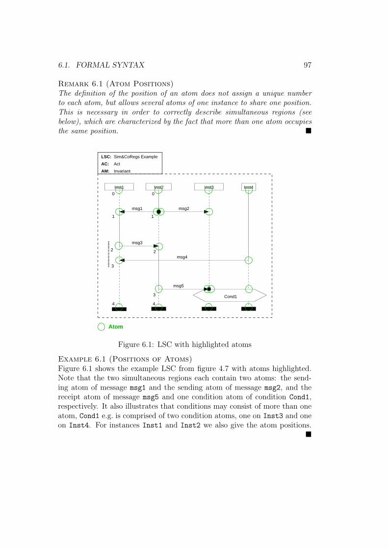
6.1. FORMAL SYNTAX 97
Remark 6.1 (Atom Positions)The definition of the position of an atom does not assign a unique numberto each atom, but allows several atoms of one instance to share one position.This is necessary in order to correctly describe simultaneous regions (seebelow), which are characterized by the fact that more than one atom occupiesthe same position. �
AC:
AM:
Inst2
LSC:
Inst3Inst1
msg2
Inst4
Cond1
Sim&CoRegs Example
Act
Invariant
1
2
3
4
0 0
1
2
3
4
msg1
msg3
msg4
msg5
Atom
Figure 6.1: LSC with highlighted atoms
Example 6.1 (Positions of Atoms)Figure 6.1 shows the example LSC from figure 4.7 with atoms highlighted.Note that the two simultaneous regions each contain two atoms: the send-ing atom of message msg1 and the sending atom of message msg2, and thereceipt atom of message msg5 and one condition atom of condition Cond1,respectively. It also illustrates that conditions may consist of more than oneatom, Cond1 e.g. is comprised of two condition atoms, one on Inst3 and oneon Inst4. For instances Inst1 and Inst2 we also give the atom positions.
�
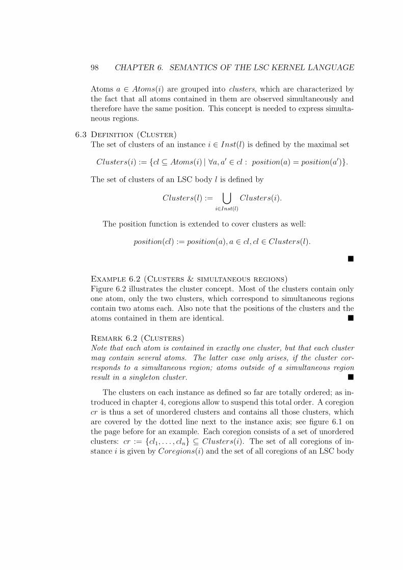
98 CHAPTER 6. SEMANTICS OF THE LSC KERNEL LANGUAGE
Atoms a ∈ Atoms(i) are grouped into clusters, which are characterized bythe fact that all atoms contained in them are observed simultaneously andtherefore have the same position. This concept is needed to express simulta-neous regions.
6.3 Definition (Cluster)The set of clusters of an instance i ∈ Inst(l) is defined by the maximal set
Clusters(i) := {cl ⊆ Atoms(i) | ∀a, a′ ∈ cl : position(a) = position(a′)}.
The set of clusters of an LSC body l is defined by
Clusters(l) :=⋃
i∈Inst(l)
Clusters(i).
The position function is extended to cover clusters as well:
position(cl) := position(a), a ∈ cl, cl ∈ Clusters(l).
�
Example 6.2 (Clusters & simultaneous regions)Figure 6.2 illustrates the cluster concept. Most of the clusters contain onlyone atom, only the two clusters, which correspond to simultaneous regionscontain two atoms each. Also note that the positions of the clusters and theatoms contained in them are identical. �
Remark 6.2 (Clusters)Note that each atom is contained in exactly one cluster, but that each clustermay contain several atoms. The latter case only arises, if the cluster cor-responds to a simultaneous region; atoms outside of a simultaneous regionresult in a singleton cluster. �
The clusters on each instance as defined so far are totally ordered; as in-troduced in chapter 4, coregions allow to suspend this total order. A coregioncr is thus a set of unordered clusters and contains all those clusters, whichare covered by the dotted line next to the instance axis; see figure 6.1 onthe page before for an example. Each coregion consists of a set of unorderedclusters: cr := {cl1, . . . , cln} ⊆ Clusters(i). The set of all coregions of in-stance i is given by Coregions(i) and the set of all coregions of an LSC body
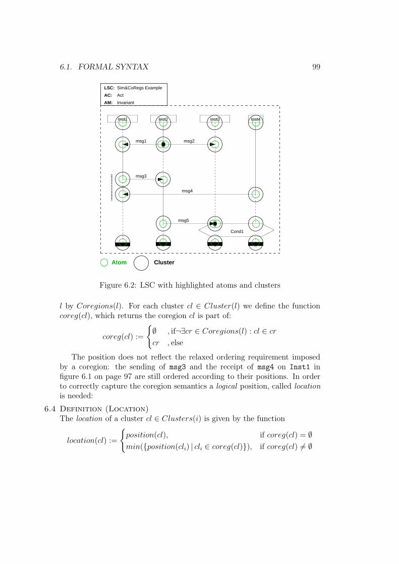
6.1. FORMAL SYNTAX 99
AC:
AM:
Inst2
LSC:
Inst3Inst1
msg2
Inst4
Cond1
Sim&CoRegs Example
Act
Invariant
msg1
msg3
msg4
msg5
Atom Cluster
Figure 6.2: LSC with highlighted atoms and clusters
l by Coregions(l). For each cluster cl ∈ Cluster(l) we define the functioncoreg(cl), which returns the coregion cl is part of:
coreg(cl) :=
{
∅ , if¬∃cr ∈ Coregions(l) : cl ∈ cr
cr , else
The position does not reflect the relaxed ordering requirement imposedby a coregion: the sending of msg3 and the receipt of msg4 on Inst1 infigure 6.1 on page 97 are still ordered according to their positions. In orderto correctly capture the coregion semantics a logical position, called locationis needed:
6.4 Definition (Location)The location of a cluster cl ∈ Clusters(i) is given by the function
location(cl) :=
{
position(cl), if coreg(cl) = ∅
min({position(cli) | cli ∈ coreg(cl)}), if coreg(cl) 6= ∅
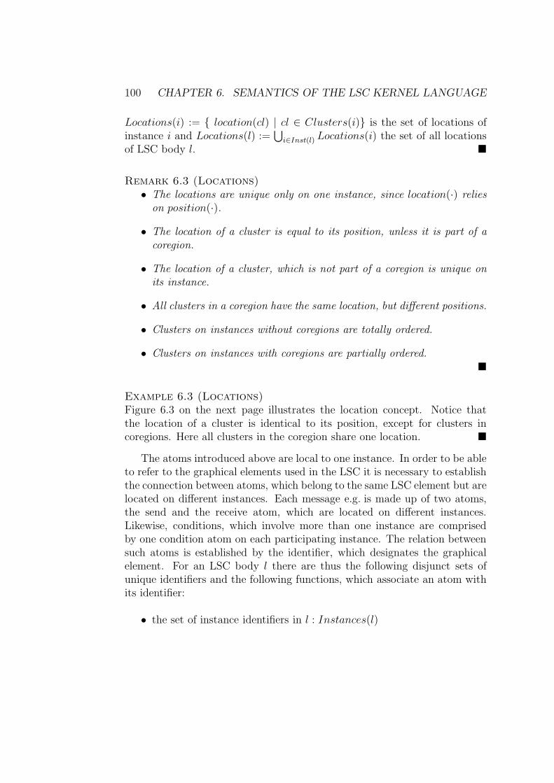
100 CHAPTER 6. SEMANTICS OF THE LSC KERNEL LANGUAGE
Locations(i) := { location(cl) | cl ∈ Clusters(i)} is the set of locations ofinstance i and Locations(l) :=
⋃
i∈Inst(l) Locations(i) the set of all locationsof LSC body l. �
Remark 6.3 (Locations)• The locations are unique only on one instance, since location(·) relies
on position(·).
• The location of a cluster is equal to its position, unless it is part of acoregion.
• The location of a cluster, which is not part of a coregion is unique onits instance.
• All clusters in a coregion have the same location, but different positions.
• Clusters on instances without coregions are totally ordered.
• Clusters on instances with coregions are partially ordered.�
Example 6.3 (Locations)Figure 6.3 on the next page illustrates the location concept. Notice thatthe location of a cluster is identical to its position, except for clusters incoregions. Here all clusters in the coregion share one location. �
The atoms introduced above are local to one instance. In order to be ableto refer to the graphical elements used in the LSC it is necessary to establishthe connection between atoms, which belong to the same LSC element but arelocated on different instances. Each message e.g. is made up of two atoms,the send and the receive atom, which are located on different instances.Likewise, conditions, which involve more than one instance are comprisedby one condition atom on each participating instance. The relation betweensuch atoms is established by the identifier, which designates the graphicalelement. For an LSC body l there are thus the following disjunct sets ofunique identifiers and the following functions, which associate an atom withits identifier:
• the set of instance identifiers in l : Instances(l)
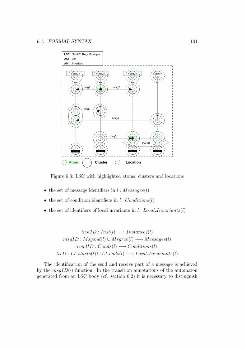
6.1. FORMAL SYNTAX 101
AC:
AM:
Inst2
LSC:
Inst3Inst1
msg2
Inst4
Cond1
Sim&CoRegs Example
Act
Invariant
msg1
msg3
msg4
msg5
Atom Cluster Location
Figure 6.3: LSC with highlighted atoms, clusters and locations
• the set of message identifiers in l : Messages(l)
• the set of condition identifiers in l : Conditions(l)
• the set of identifiers of local invariants in l : Local Invariants(l)
instID : Inst(l) −→ Instances(l)
msgID : Msgsnd(l) ∪Msgrcv(l) −→Messages(l)
condID : Conds(l) −→ Conditions(l)
liID : LI starts(l) ∪ LI ends(l) −→ Local Invariants(l)
The identification of the send and receive part of a message is achievedby the msgID(·) function. In the transition annotations of the automatongenerated from an LSC body (cf. section 6.2) it is necessary to distinguish
102 CHAPTER 6. SEMANTICS OF THE LSC KERNEL LANGUAGE
send and receive atoms, therefore the set of message labels MsgLabels(l) isintroduced, including the function msgLabel(m), which associates a messagelabel with each m ∈ Msgsnd(l) ∪ Msgrcv(l). Sending of message m1 isrepresented by the label !m1, receipt by ?m1.
msgLabel : Msgsnd(l) ∪Msgrcv(l) −→MsgLabels(l)
msgLabel(m) :=
{
!msgID(m) if m ∈Msgsnd(l)
?msgID(m) if m ∈Msgrcv(l)
Furthermore is it necessary to access the properties of messages, condi-tions and local invariants. For messages the relevant properties are tem-perature and type (instantaneous or asynchronous), for conditions and localinvariants the mode (mandatory or possible). The progress information alongeach instance is associated with the atoms of this instance, so that the domainof function temp(·) below is the union of message identifiers and atoms. Theproperties for messages and conditions on the other hand pertain to the LSCelements, represented by the corresponding identifiers, and not the atoms.The situation for the mode of local invariants is identical to that of condi-tions, i.e. this information is tied to the LSC element. The information, if alocal invariant atom is included in the simultaneous region, which containsit, on the other hand pertains to the individual atom, so that the incl func-tion is defined on the set of local invariant atoms rather than on the set ofidentifiers.
temp : Messages(l) ∪Atoms(l) −→ {hot, cold}
sync type : Messages(l) −→ {async, instant}
mode : Conditions(l) ∪ Local Invariants(l) −→ {mandatory, possible}
incl : LI starts(l) ∪ LI ends(l) −→ B
The treatment of liveness requirements in the formal semantics in the nextsection is tied to locations, so that the atom temperature has to be lifted tothe location level. An intermediate step to achieve this is to first lift it tothe Cluster level, which in fact determines the temperature of simultaneousregions. Analogously to the cut temperature computation in section 6.2.3 onpage 117 one hot atom overrides the temperature of all other atoms in asimultaneous regions.
6.2. FORMAL SEMANTICS 103
temp : Clusters(l) −→ {hot, cold}
temp(cl) :=
{
cold, if ∀a ∈ cl : temp(a) = cold
hot, else
The temperature function is extended analogously to locations, so thatcoregions can be treated correctly. Since no ordering exists between theatoms of a coregion, no progress between them can be enforced, so that asingle temperature is associated with a coregion. In the remainder we onlyapply the temp(·) function to message identifiers and locations, so that noconfusion should arise.
temp : Locations(l) −→ {hot, cold}
temp(loc) :=
cold, if ∀cl ∈ Clusters(l) : location(cl) = loc ∧
temp(cl) = cold
hot, else
6.2 Formal Semantics
In this section we describe the generation of the automaton from an LSC. Wefirst construct the basic structure and then discuss several semantical issues,which influence the final automaton, before completing the procedure.
6.2.1 Basic Automaton Construction
The unwinding approach has been adopted from the definition of the seman-tics of Symbolic Timing Diagrams [Sch00, Fey96, FJ97]. The general ideais to define a cut through the LSC starting at the top and moving this cutdownward until we reach all instance ends, while respecting the partial orderimposed by the LSC. Cuts become states in the automaton and the tran-sition relation of the automaton encodes the successor relation among thecuts. Ordering among the atoms in an LSC is induced by the following rules:
1. atoms (clusters) along each instance axis are totally ordered (unlessthey are part of a coregion)
2. a message has to be sent before it can be received
104 CHAPTER 6. SEMANTICS OF THE LSC KERNEL LANGUAGE
3. conditions ranging over several instances (shared conditions) enforcesynchronization between the involved instances
These rules determine when an LSC element is enabled, i.e. when it is readyto be unwound:An atom is enabled when
1. all its predecessors along the instance axis have already be unwound
2. the corresponding message send atom has already been unwound (ifthe atom is a message receive atom of an asynchronous message) or isbeing unwound simultaneously (if the atom is part of an instantaneousmessage)
3. all other condition atoms belonging to the same condition are alsoenabled (if the atom is a shared condition)
The first rule demands a computation of all predecessors on the instanceaxis for each atom. It is actually sufficient to only conduct a local com-putation of the immediate predecessor of each atom, since this relation istransitive: If the immediate predecessor of a cluster cl has been unwound,then immediate predecessor of cl must have been unwound, and so on. Theformal definition of the function computing the immediate predecessor is:
6.5 Definition (Immediate Predecessor)
predecessor : Clusters(i) −→ P(Clusters(i))
predecessor(cl) :=
{
∅ , if∃ a ∈ cl : a = ⊥i ∨ a = ⊤i
CL , else, where
CL := {cl′ ∈ Clusters(i) | location(cl′) < location(cl) ∧
¬∃ cl′′ ∈ Clusters(i) :
location(cl′) < location(cl′′) < location(cl) }
�
The function predecessor(cl) looks along one instance for the location,which is immediately above the cluster cl and returns the clusters boundto that location. If the element bound to the predecessor location is not a
6.2. FORMAL SEMANTICS 105
coregion, the returned set of clusters contains a single cluster. Otherwise allclusters of the coregion are returned. For clusters containing instance head orend atoms no predecessor is returned, since an instance head does not have apredecessor and instance end atoms are not unwound by the algorithm (seebelow).
The second and third rule above involve more than one instance and thusrequire to also take clusters of other instances into account. The messagesend and receive atom for an instantaneous message have to be unwoundsimultaneously, and all condition atoms of a condition must be unwound atthe same time. This synchronization of clusters is expressed by the relation≈.
6.6 Definition (Equivalence of Clusters)Let cl, cl′ ∈ Clusters(l). The relation ≈ on Clusters(l) is defined as:
cl ≈ cl′ ⇔ ∃ a ∈ cl ∃ a′ ∈ cl′ :
cl = cl′ ∨ sharedConds(a, a′) ∨ instMsgs(a, a′)
∨ transitivity(a, a′)
where
sharedConds(a, a′) := a, a′ ∈ Conds(l) ∧ condID(a) = condID(a′)
instMsgs(a, a′) := a ∈Msgsnd(l) ∧ a′ ∈Msgrcv(l)
∧ msgID(a) = msgID(a′)
∧ sync type(msgID(a)) = instant
transitivity(a, a′) := a, a′ ∈ syncAtoms(l)
∧ ∃cl′′ ∈ Clusters(l) ∃ai, aj ∈ cl′′ : |cl′′| > 1
∧ (sharedConds(a, ai) ∨ instMsgs(a, ai))
∨ (sharedConds(a′, aj) ∨ instMsgs(a′, aj))
syncAtoms(l) := {a ∈ Atoms(l)|a ∈ Conds(l)∨
(a ∈Msgsnd(l) ∨ a ∈Msgrcv(l))
∧ sync type(msgID(a)) = instant}
The classes defined by ≈ are called simultaneous classes. SimClasses(l) :={ scl ⊆ Clusters(l) | ∀ cl, cl′ ∈ scl : cl ≈ cl′ } is the set of simultaneousclasses of l. �
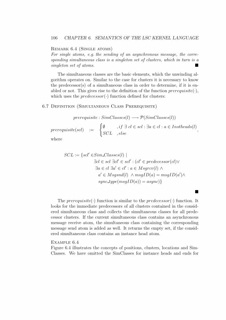
106 CHAPTER 6. SEMANTICS OF THE LSC KERNEL LANGUAGE
Remark 6.4 (Single atoms)For single atoms, e.g. the sending of an asynchronous message, the corre-sponding simultaneous class is a singleton set of clusters, which in turn is asingleton set of atoms. �
The simultaneous classes are the basic elements, which the unwinding al-gorithm operates on. Similar to the case for clusters it is necessary to knowthe predecessor(s) of a simultaneous class in order to determine, if it is en-abled or not. This gives rise to the definition of the function prerequisite(·),which uses the predecessor(·) function defined for clusters:
6.7 Definition (Simultaneous Class Prerequisite)
prerequisite : SimClasses(l) −→ P(SimClasses(l))
prerequisite(scl) :=
{
∅ , if ∃ cl ∈ scl : ∃a ∈ cl : a ∈ Instheads(l)
SCL , else,
where
SCL := {scl′ ∈Sim Classes(l) |
∃cl ∈ scl ∃cl′ ∈ scl′ : (cl′ ∈ predecessor(cl)∨
∃a ∈ cl ∃a′ ∈ cl′ : a ∈Msgrcv(l) ∧
a′ ∈Msgsnd(l) ∧msgID(a) = msgID(a′)∧
sync type(msgID(a)) = async)}
�
The prerequisite(·) function is similar to the predecessor(·) function. Itlooks for the immediate predecessors of all clusters contained in the consid-ered simultaneous class and collects the simultaneous classes for all prede-cessor clusters. If the current simultaneous class contains an asynchronousmessage receive atom, the simultaneous class containing the correspondingmessage send atom is added as well. It returns the empty set, if the consid-ered simultaneous class contains an instance head atom.
Example 6.4Figure 6.4 illustrates the concepts of positions, clusters, locations and Sim-Classes. We have omitted the SimClasses for instance heads and ends for
6.2. FORMAL SEMANTICS 107
AC:AM: Invariant
Inst2
Sim&CoRegs ExampleLSC:Act
Inst3Inst1
msg2
Inst4
Cond1
msg1
msg3
msg5
msg4
Atom Cluster Location
SimClass
Figure 6.4: LSC with positions, locations and SimClasses
readability’s sake; in these cases the SimClasses contain only one cluster, seetable 6.1.
The predecessor computation is obvious, we therefore concentrate on theprerequisites. Atoms are named after their corresponding identifiers, messagesend atoms are characterized by prefixing the identifier with a ‘!’, messagereceive atoms with a ‘?’. Table 6.1 shows the simultaneous classes and theirprerequisites for this example.
The multitude of braces in the prerequisites is due to the nested sets.A single atom is not enclosed in braces (e.g. ?msg1), but is enclosed in acluster, which is a set of atoms (e.g. {?msg1}). Simultaneous regions resultin clusters with more than one element (e.g. {!msg1,!msg2}). The clustersare part of a SimClass, which is a set of clusters (e.g. {{!msg3}, {?msg3} }).When considering the prerequisites another level of braces is added, since
108 CHAPTER 6. SEMANTICS OF THE LSC KERNEL LANGUAGE
SimClass Prerequisite
{{⊥Inst1}} ∅{{⊥Inst2}} ∅{{⊥Inst3}} ∅{{⊥Inst4}} ∅
{ {?msg1},{!msg1,!msg2},{?msg2} } { {{⊥Inst1}}, {{⊥Inst2}}, {{⊥Inst3}} }{ {!msg3}, {?msg3} } { {{?msg1},{!msg1,!msg2},{?msg2}} }{ {?msg4}, {!msg4} } { {{?msg1},{!msg1,!msg2},{?msg2}},
{{⊥Inst4}} }{ {!msg5}, {?msg5, cond1} } {{{!msg3},{?msg3}},{{?msg4},{!msg4}}}
{{⊤Inst1}} ∅{{⊤Inst2}} ∅{{⊤Inst3}} ∅{{⊤Inst4}} ∅
Table 6.1: Prerequisites for the LSC in figure 6.4
prerequisites are sets of SimClasses. Notice that all elements of the coregionshare part of their prerequisites, which is due to the fact that coregions aretreated as a single location. �
A cut through the LSC is used to keep track of the progress of the un-winding procedure. It represents the borderline between already unwoundelements and those which still have to be considered. The elements directlybelow the cut are those, which are currently enabled. Cuts are representedby a tuple containing one cluster of each instance:
6.8 Definition (Cut)A cut Cut ⊆ Clusters(i1) × · · · × Clusters(in), for Inst(l) = {i1, . . . , in} isa tuple (cli1 , . . . , clin), clij ∈ Clusters(ij), 1 ≤ j ≤ n = |Inst(l)|.
Let Cuts(l) be the set of all possible cuts of LSC body l. �
The unwinding algorithm requires a number of other auxiliary sets andconstructs, which are collected in a tuple called phase. Each phase charac-terizes one unwinding step and consequently corresponds to a state in theresulting automaton. Possible transitions from one phase to another corre-spond to transitions of the automaton.
6.2. FORMAL SEMANTICS 109
6.9 Definition (Phase)A phase is a tuple Phase := (Ready,History, Cut), with
• History ⊆ SimClasses(l) : the set of simultaneous classes which havealready been unwound
• Ready ⊆ SimClasses(l) : the set of simultaneous classes, which arecurrently enabled to be unwound
• Cut : the current cut as defined in definition 6.8.
Let Phases(l) be the set of all phases of LSC body l. �
Since several simultaneous classes may be enabled concurrently, e.g. dueto a coregion, each ready set may contain more than one simultaneous class.In this case all combinations of elements of the ready set lead to valid suc-cessor phases and thus have to be taken into consideration. All possiblecombinations correspond to the powerset of the ready set; the set of simul-taneous classes, which is currently chosen to be unwound, is called the firedset Fired ⊆ P(SimClasses(l)). Thus, for each phase Phasei there exist kfired sets Firedik , with k = |P(Readyi)|. Let Firedsets(l) be the set of allfired sets in l.
Example 6.5 (Fired set)Let the current ready set consist of simultaneous classes a and b, thusReadyi = (a, b). The resulting fired sets are Firedi1 = ∅, F iredi2 ={a}, F iredi3 = {b}, and Firedi3 = {a, b}}. �
The unwinding algorithm starts at the top of the LSC body and computesthe initial phase Phase0, which is given by
Phase0 =(Ready0, History0, Cut0),
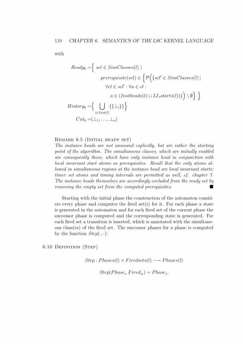
110 CHAPTER 6. SEMANTICS OF THE LSC KERNEL LANGUAGE
with
Ready0 ={
scl ∈ SimClasses(l) |
prerequisite(scl) ∈{
P(
{scl′ ∈ SimClasses(l) |
∀cl ∈ scl′ : ∀a ∈ cl :
a ∈ (Instheads(l) ∪ LI starts(l))})
\ ∅} }
History0 ={
⋃
i∈Inst(l)
{{⊥i}}}
Cut0 =(⊥1, . . . ,⊥n)
Remark 6.5 (Initial ready set)The instance heads are not unwound explicitly, but are rather the startingpoint of the algorithm. The simultaneous classes, which are initially enabledare consequently those, which have only instance head in conjunction withlocal invariant start atoms as prerequisites. Recall that the only atoms al-lowed in simultaneous regions at the instance head are local invariant starts;timer set atoms and timing intervals are permitted as well, cf. chapter 7.The instance heads themselves are accordingly excluded from the ready set byremoving the empty set from the computed prerequisites. �
Starting with the initial phase the construction of the automaton consid-ers every phase and computes the fired set(s) for it. For each phase a stateis generated in the automaton and for each fired set of the current phase thesuccessor phase is computed and the corresponding state is generated. Foreach fired set a transition is inserted, which is annotated with the simultane-ous class(es) of the fired set. The successor phases for a phase is computedby the function Step(·, ·):
6.10 Definition (Step)
Step : Phases(l) × Firedsets(l) −→ Phases(l)
Step(Phasei, F iredik) = Phasej ,
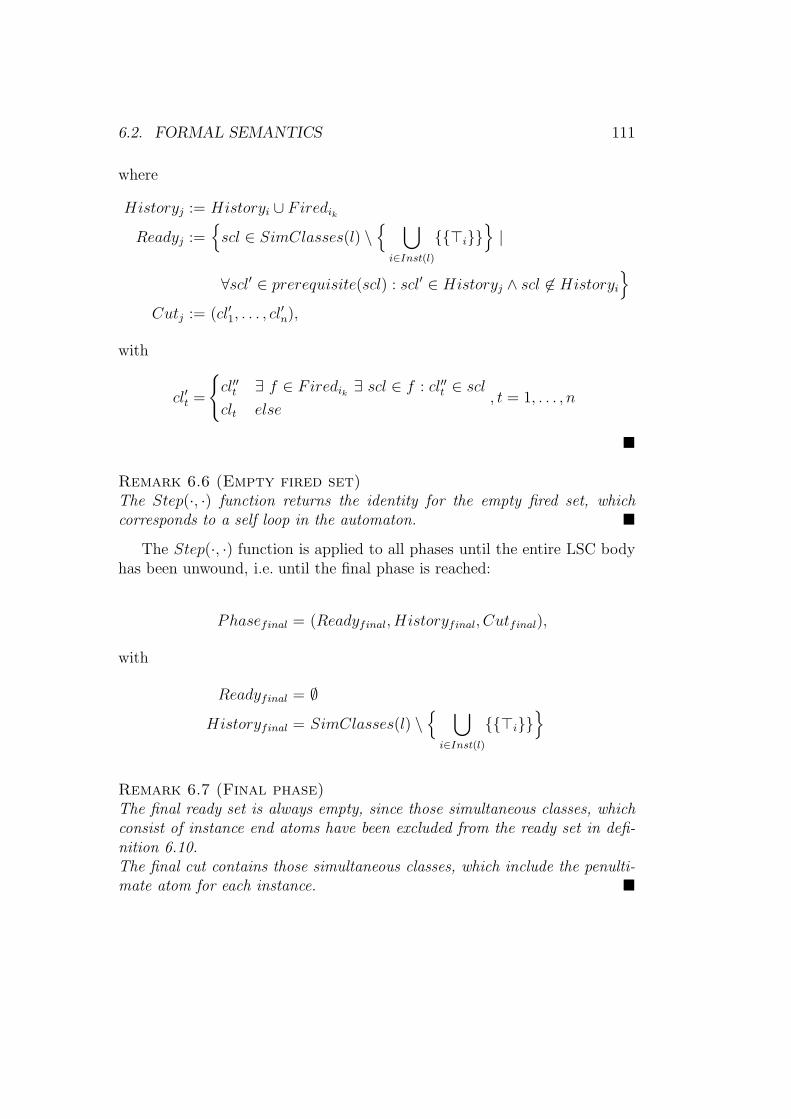
6.2. FORMAL SEMANTICS 111
where
Historyj := Historyi ∪ Firedik
Readyj :={
scl ∈ SimClasses(l) \{
⋃
i∈Inst(l)
{{⊤i}}}
|
∀scl′ ∈ prerequisite(scl) : scl′ ∈ Historyj ∧ scl 6∈ Historyi
}
Cutj := (cl′1, . . . , cl′n),
with
cl′t =
{
cl′′t ∃ f ∈ Firedik ∃ scl ∈ f : cl′′t ∈ scl
clt else, t = 1, . . . , n
�
Remark 6.6 (Empty fired set)The Step(·, ·) function returns the identity for the empty fired set, whichcorresponds to a self loop in the automaton. �
The Step(·, ·) function is applied to all phases until the entire LSC bodyhas been unwound, i.e. until the final phase is reached:
Phasefinal = (Readyfinal, Historyfinal, Cutfinal),
with
Readyfinal = ∅
Historyfinal = SimClasses(l) \{
⋃
i∈Inst(l)
{{⊤i}}}
Remark 6.7 (Final phase)The final ready set is always empty, since those simultaneous classes, whichconsist of instance end atoms have been excluded from the ready set in defi-nition 6.10.The final cut contains those simultaneous classes, which include the penulti-mate atom for each instance. �
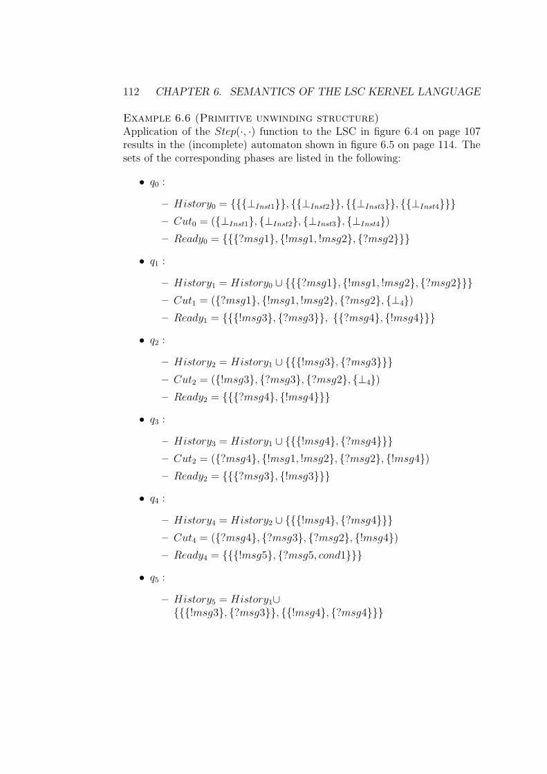
112 CHAPTER 6. SEMANTICS OF THE LSC KERNEL LANGUAGE
Example 6.6 (Primitive unwinding structure)Application of the Step(·, ·) function to the LSC in figure 6.4 on page 107results in the (incomplete) automaton shown in figure 6.5 on page 114. Thesets of the corresponding phases are listed in the following:
• q0 :
– History0 = {{{⊥Inst1}}, {{⊥Inst2}}, {{⊥Inst3}}, {{⊥Inst4}}}
– Cut0 = ({⊥Inst1}, {⊥Inst2}, {⊥Inst3}, {⊥Inst4})
– Ready0 = {{{?msg1}, {!msg1, !msg2}, {?msg2}}}
• q1 :
– History1 = History0 ∪ {{{?msg1}, {!msg1, !msg2}, {?msg2}}}
– Cut1 = ({?msg1}, {!msg1, !msg2}, {?msg2}, {⊥4})
– Ready1 = {{{!msg3}, {?msg3}}, {{?msg4}, {!msg4}}}
• q2 :
– History2 = History1 ∪ {{{!msg3}, {?msg3}}}
– Cut2 = ({!msg3}, {?msg3}, {?msg2}, {⊥4})
– Ready2 = {{{?msg4}, {!msg4}}}
• q3 :
– History3 = History1 ∪ {{{!msg4}, {?msg4}}}
– Cut2 = ({?msg4}, {!msg1, !msg2}, {?msg2}, {!msg4})
– Ready2 = {{{?msg3}, {!msg3}}}
• q4 :
– History4 = History2 ∪ {{{!msg4}, {?msg4}}}
– Cut4 = ({?msg4}, {?msg3}, {?msg2}, {!msg4})
– Ready4 = {{{!msg5}, {?msg5, cond1}}}
• q5 :
– History5 = History1∪{{{!msg3}, {?msg3}}, {{!msg4}, {?msg4}}}
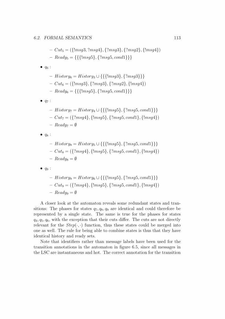
6.2. FORMAL SEMANTICS 113
– Cut5 = ({!msg3, ?msg4}, {?msg3}, {?msg2}, {!msg4})
– Ready5 = {{{!msg5}, {?msg5, cond1}}}
• q6 :
– History6 = History3 ∪ {{{!msg3}, {?msg3}}}
– Cut6 = ({!msg3}, {?msg3}, {?msg2}, {!msg4})
– Ready6 = {{{!msg5}, {?msg5, cond1}}}
• q7 :
– History7 = History4 ∪ {{{!msg5}, {?msg5, cond1}}}
– Cut7 = ({?msg4}, {!msg5}, {?msg5, cond1}, {!msg4})
– Ready7 = ∅
• q8 :
– History8 = History5 ∪ {{{!msg5}, {?msg5, cond1}}}
– Cut8 = ({?msg4}, {!msg5}, {?msg5, cond1}, {!msg4})
– Ready8 = ∅
• q9 :
– History9 = History6 ∪ {{{!msg5}, {?msg5, cond1}}}
– Cut9 = ({?msg4}, {!msg5}, {?msg5, cond1}, {!msg4})
– Ready9 = ∅
A closer look at the automaton reveals some redundant states and tran-sitions: The phases for states q7, q8, q9 are identical and could therefore berepresented by a single state. The same is true for the phases for statesq4, q5, q6, with the exception that their cuts differ. The cuts are not directlyrelevant for the Step(·, ·) function, thus these states could be merged intoone as well. The rule for being able to combine states is thus that they haveidentical history and ready sets.
Note that identifiers rather than message labels have been used for thetransition annotations in the automaton in figure 6.5, since all messages inthe LSC are instantaneous and hot. The correct annotation for the transition
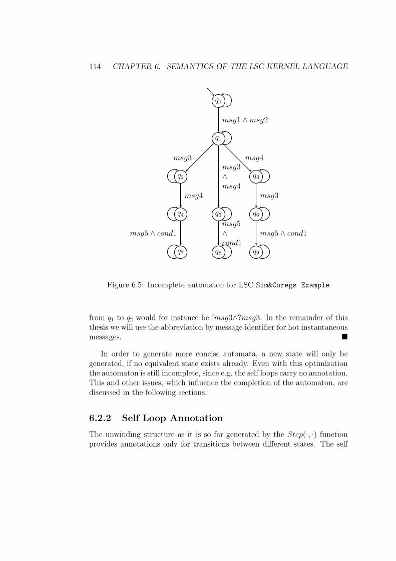
114 CHAPTER 6. SEMANTICS OF THE LSC KERNEL LANGUAGE
q0
q1
msg1 ∧msg2
q2
msg3
q3
msg4
q4
msg4
q5
msg3∧msg4
q6
msg3
q7
msg5 ∧ cond1
q8
msg5∧cond1
q9
msg5 ∧ cond1
Figure 6.5: Incomplete automaton for LSC Sim&Coregs Example
from q1 to q2 would for instance be !msg3∧?msg3. In the remainder of thisthesis we will use the abbreviation by message identifier for hot instantaneousmessages. �
In order to generate more concise automata, a new state will only begenerated, if no equivalent state exists already. Even with this optimizationthe automaton is still incomplete, since e.g. the self loops carry no annotation.This and other issues, which influence the completion of the automaton, arediscussed in the following sections.
6.2.2 Self Loop Annotation
The unwinding structure as it is so far generated by the Step(·, ·) functionprovides annotations only for transitions between different states. The self
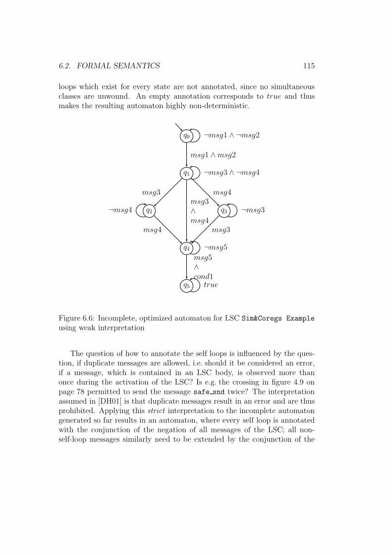
6.2. FORMAL SEMANTICS 115
loops which exist for every state are not annotated, since no simultaneousclasses are unwound. An empty annotation corresponds to true and thusmakes the resulting automaton highly non-deterministic.
q0 ¬msg1 ∧ ¬msg2
q1 ¬msg3 ∧ ¬msg4
msg1 ∧msg2
q2¬msg4
msg3
q3 ¬msg3
msg4
q4 ¬msg5
msg3∧msg4
msg4 msg3
q5 true
msg5∧cond1
Figure 6.6: Incomplete, optimized automaton for LSC Sim&Coregs Example
using weak interpretation
The question of how to annotate the self loops is influenced by the ques-tion, if duplicate messages are allowed, i.e. should it be considered an error,if a message, which is contained in an LSC body, is observed more thanonce during the activation of the LSC? Is e.g. the crossing in figure 4.9 onpage 78 permitted to send the message safe snd twice? The interpretationassumed in [DH01] is that duplicate messages result in an error and are thusprohibited. Applying this strict interpretation to the incomplete automatongenerated so far results in an automaton, where every self loop is annotatedwith the conjunction of the negation of all messages of the LSC; all non-self-loop messages similarly need to be extended by the conjunction of the
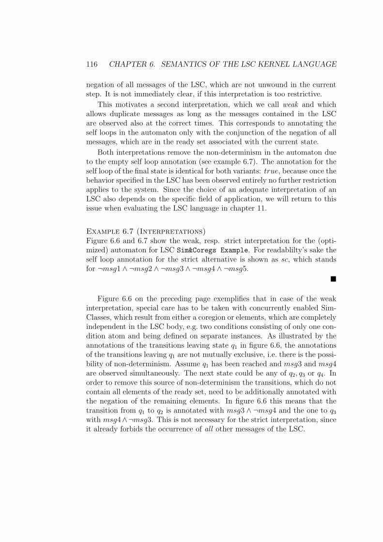
116 CHAPTER 6. SEMANTICS OF THE LSC KERNEL LANGUAGE
negation of all messages of the LSC, which are not unwound in the currentstep. It is not immediately clear, if this interpretation is too restrictive.
This motivates a second interpretation, which we call weak and whichallows duplicate messages as long as the messages contained in the LSCare observed also at the correct times. This corresponds to annotating theself loops in the automaton only with the conjunction of the negation of allmessages, which are in the ready set associated with the current state.
Both interpretations remove the non-determinism in the automaton dueto the empty self loop annotation (see example 6.7). The annotation for theself loop of the final state is identical for both variants: true, because once thebehavior specified in the LSC has been observed entirely no further restrictionapplies to the system. Since the choice of an adequate interpretation of anLSC also depends on the specific field of application, we will return to thisissue when evaluating the LSC language in chapter 11.
Example 6.7 (Interpretations)Figure 6.6 and 6.7 show the weak, resp. strict interpretation for the (opti-mized) automaton for LSC Sim&Coregs Example. For readablilty’s sake theself loop annotation for the strict alternative is shown as sc, which standsfor ¬msg1 ∧ ¬msg2 ∧ ¬msg3 ∧ ¬msg4 ∧ ¬msg5.
�
Figure 6.6 on the preceding page exemplifies that in case of the weakinterpretation, special care has to be taken with concurrently enabled Sim-Classes, which result from either a coregion or elements, which are completelyindependent in the LSC body, e.g. two conditions consisting of only one con-dition atom and being defined on separate instances. As illustrated by theannotations of the transitions leaving state q1 in figure 6.6, the annotationsof the transitions leaving q1 are not mutually exclusive, i.e. there is the possi-bility of non-determinism. Assume q1 has been reached and msg3 and msg4are observed simultaneously. The next state could be any of q2, q3 or q4. Inorder to remove this source of non-determinism the transitions, which do notcontain all elements of the ready set, need to be additionally annotated withthe negation of the remaining elements. In figure 6.6 this means that thetransition from q1 to q2 is annotated with msg3 ∧ ¬msg4 and the one to q3with msg4∧¬msg3. This is not necessary for the strict interpretation, sinceit already forbids the occurrence of all other messages of the LSC.
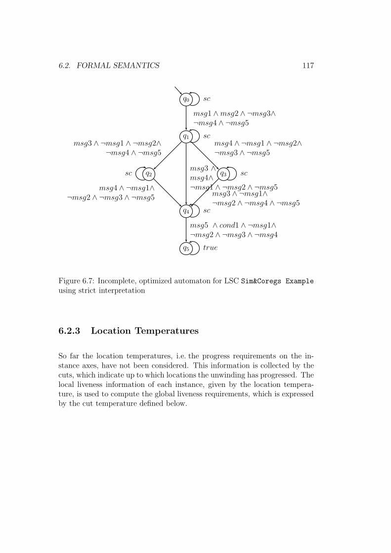
6.2. FORMAL SEMANTICS 117
q0 sc
q1 sc
msg1 ∧msg2 ∧ ¬msg3∧¬msg4 ∧ ¬msg5
q2sc
msg3 ∧ ¬msg1 ∧ ¬msg2∧¬msg4 ∧ ¬msg5
q3 sc
msg4 ∧ ¬msg1 ∧ ¬msg2∧¬msg3 ∧ ¬msg5
q4 sc
msg3 ∧msg4∧¬msg1 ∧ ¬msg2 ∧ ¬msg5msg4 ∧ ¬msg1∧
¬msg2 ∧ ¬msg3 ∧ ¬msg5 msg3 ∧ ¬msg1∧¬msg2 ∧ ¬msg4 ∧ ¬msg5
q5 true
msg5 ∧ cond1 ∧ ¬msg1∧¬msg2 ∧ ¬msg3 ∧ ¬msg4
Figure 6.7: Incomplete, optimized automaton for LSC Sim&Coregs Example
using strict interpretation
6.2.3 Location Temperatures
So far the location temperatures, i.e. the progress requirements on the in-stance axes, have not been considered. This information is collected by thecuts, which indicate up to which locations the unwinding has progressed. Thelocal liveness information of each instance, given by the location tempera-ture, is used to compute the global liveness requirements, which is expressedby the cut temperature defined below.
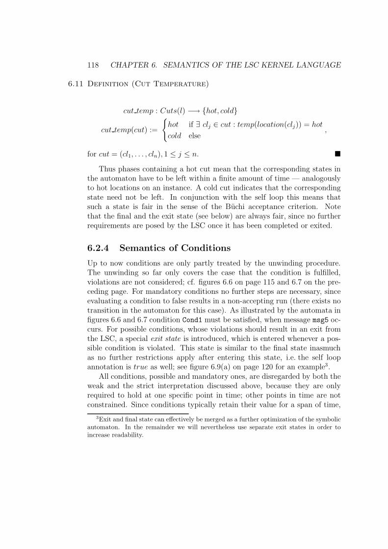
118 CHAPTER 6. SEMANTICS OF THE LSC KERNEL LANGUAGE
6.11 Definition (Cut Temperature)
cut temp : Cuts(l) −→ {hot, cold}
cut temp(cut) :=
{
hot if ∃ clj ∈ cut : temp(location(clj)) = hot
cold else,
for cut = (cl1, . . . , cln), 1 ≤ j ≤ n. �
Thus phases containing a hot cut mean that the corresponding states inthe automaton have to be left within a finite amount of time — analogouslyto hot locations on an instance. A cold cut indicates that the correspondingstate need not be left. In conjunction with the self loop this means thatsuch a state is fair in the sense of the Buchi acceptance criterion. Notethat the final and the exit state (see below) are always fair, since no furtherrequirements are posed by the LSC once it has been completed or exited.
6.2.4 Semantics of Conditions
Up to now conditions are only partly treated by the unwinding procedure.The unwinding so far only covers the case that the condition is fulfilled,violations are not considered; cf. figures 6.6 on page 115 and 6.7 on the pre-ceding page. For mandatory conditions no further steps are necessary, sinceevaluating a condition to false results in a non-accepting run (there exists notransition in the automaton for this case). As illustrated by the automata infigures 6.6 and 6.7 condition Cond1 must be satisfied, when message msg5 oc-curs. For possible conditions, whose violations should result in an exit fromthe LSC, a special exit state is introduced, which is entered whenever a pos-sible condition is violated. This state is similar to the final state inasmuchas no further restrictions apply after entering this state, i.e. the self loopannotation is true as well; see figure 6.9(a) on page 120 for an example3.
All conditions, possible and mandatory ones, are disregarded by both theweak and the strict interpretation discussed above, because they are onlyrequired to hold at one specific point in time; other points in time are notconstrained. Since conditions typically retain their value for a span of time,
3Exit and final state can effectively be merged as a further optimization of the symbolicautomaton. In the remainder we will nevertheless use separate exit states in order toincrease readability.
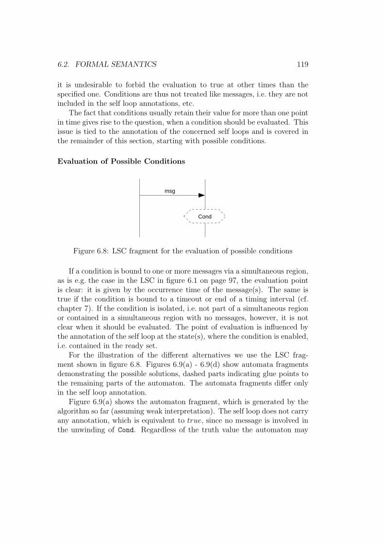
6.2. FORMAL SEMANTICS 119
it is undesirable to forbid the evaluation to true at other times than thespecified one. Conditions are thus not treated like messages, i.e. they are notincluded in the self loop annotations, etc.
The fact that conditions usually retain their value for more than one pointin time gives rise to the question, when a condition should be evaluated. Thisissue is tied to the annotation of the concerned self loops and is covered inthe remainder of this section, starting with possible conditions.
Evaluation of Possible Conditions
Cond
msg
Figure 6.8: LSC fragment for the evaluation of possible conditions
If a condition is bound to one or more messages via a simultaneous region,as is e.g. the case in the LSC in figure 6.1 on page 97, the evaluation pointis clear: it is given by the occurrence time of the message(s). The same istrue if the condition is bound to a timeout or end of a timing interval (cf.chapter 7). If the condition is isolated, i.e. not part of a simultaneous regionor contained in a simultaneous region with no messages, however, it is notclear when it should be evaluated. The point of evaluation is influenced bythe annotation of the self loop at the state(s), where the condition is enabled,i.e. contained in the ready set.
For the illustration of the different alternatives we use the LSC frag-ment shown in figure 6.8. Figures 6.9(a) - 6.9(d) show automata fragmentsdemonstrating the possible solutions, dashed parts indicating glue points tothe remaining parts of the automaton. The automata fragments differ onlyin the self loop annotation.
Figure 6.9(a) shows the automaton fragment, which is generated by thealgorithm so far (assuming weak interpretation). The self loop does not carryany annotation, which is equivalent to true, since no message is involved inthe unwinding of Cond. Regardless of the truth value the automaton may
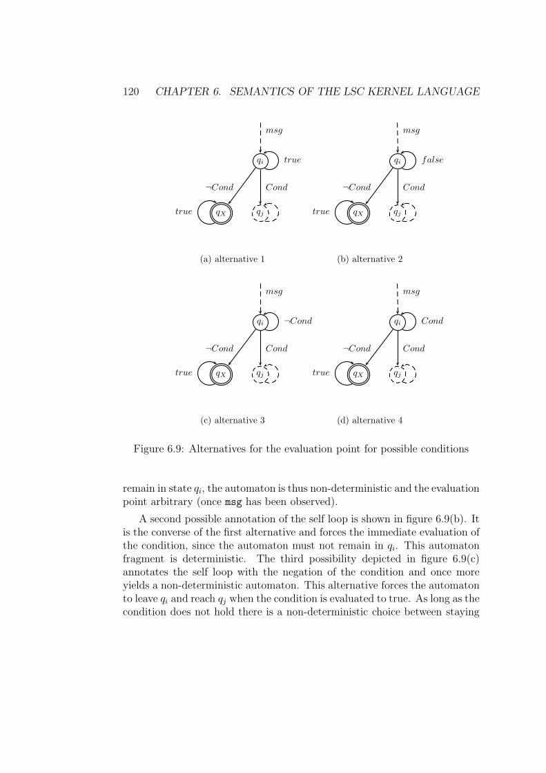
120 CHAPTER 6. SEMANTICS OF THE LSC KERNEL LANGUAGE
qi
msg
true
qj
Cond
qXtrue
¬Cond
(a) alternative 1
qi
msg
false
qj
Cond
qXtrue
¬Cond
(b) alternative 2
qi
msg
¬Cond
qj
Cond
qXtrue
¬Cond
(c) alternative 3
qi
msg
Cond
qj
Cond
qXtrue
¬Cond
(d) alternative 4
Figure 6.9: Alternatives for the evaluation point for possible conditions
remain in state qi, the automaton is thus non-deterministic and the evaluationpoint arbitrary (once msg has been observed).
A second possible annotation of the self loop is shown in figure 6.9(b). Itis the converse of the first alternative and forces the immediate evaluation ofthe condition, since the automaton must not remain in qi. This automatonfragment is deterministic. The third possibility depicted in figure 6.9(c)annotates the self loop with the negation of the condition and once moreyields a non-deterministic automaton. This alternative forces the automatonto leave qi and reach qj when the condition is evaluated to true. As long as thecondition does not hold there is a non-deterministic choice between staying
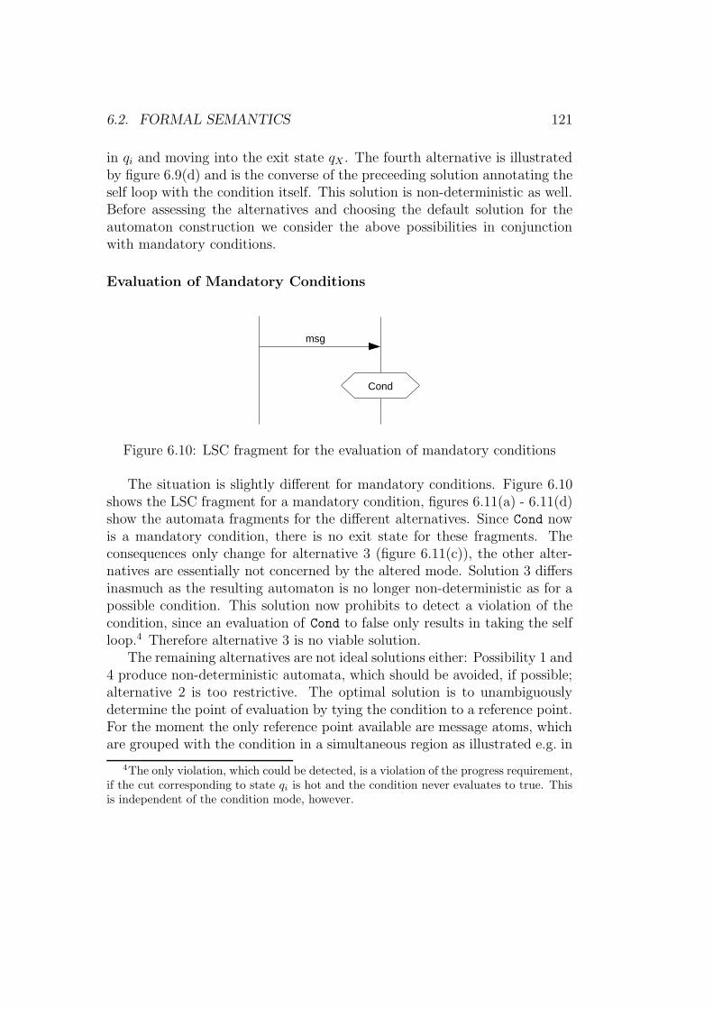
6.2. FORMAL SEMANTICS 121
in qi and moving into the exit state qX . The fourth alternative is illustratedby figure 6.9(d) and is the converse of the preceeding solution annotating theself loop with the condition itself. This solution is non-deterministic as well.Before assessing the alternatives and choosing the default solution for theautomaton construction we consider the above possibilities in conjunctionwith mandatory conditions.
Evaluation of Mandatory Conditions
Cond
msg
Figure 6.10: LSC fragment for the evaluation of mandatory conditions
The situation is slightly different for mandatory conditions. Figure 6.10shows the LSC fragment for a mandatory condition, figures 6.11(a) - 6.11(d)show the automata fragments for the different alternatives. Since Cond nowis a mandatory condition, there is no exit state for these fragments. Theconsequences only change for alternative 3 (figure 6.11(c)), the other alter-natives are essentially not concerned by the altered mode. Solution 3 differsinasmuch as the resulting automaton is no longer non-deterministic as for apossible condition. This solution now prohibits to detect a violation of thecondition, since an evaluation of Cond to false only results in taking the selfloop.4 Therefore alternative 3 is no viable solution.
The remaining alternatives are not ideal solutions either: Possibility 1 and4 produce non-deterministic automata, which should be avoided, if possible;alternative 2 is too restrictive. The optimal solution is to unambiguouslydetermine the point of evaluation by tying the condition to a reference point.For the moment the only reference point available are message atoms, whichare grouped with the condition in a simultaneous region as illustrated e.g. in
4The only violation, which could be detected, is a violation of the progress requirement,if the cut corresponding to state qi is hot and the condition never evaluates to true. Thisis independent of the condition mode, however.
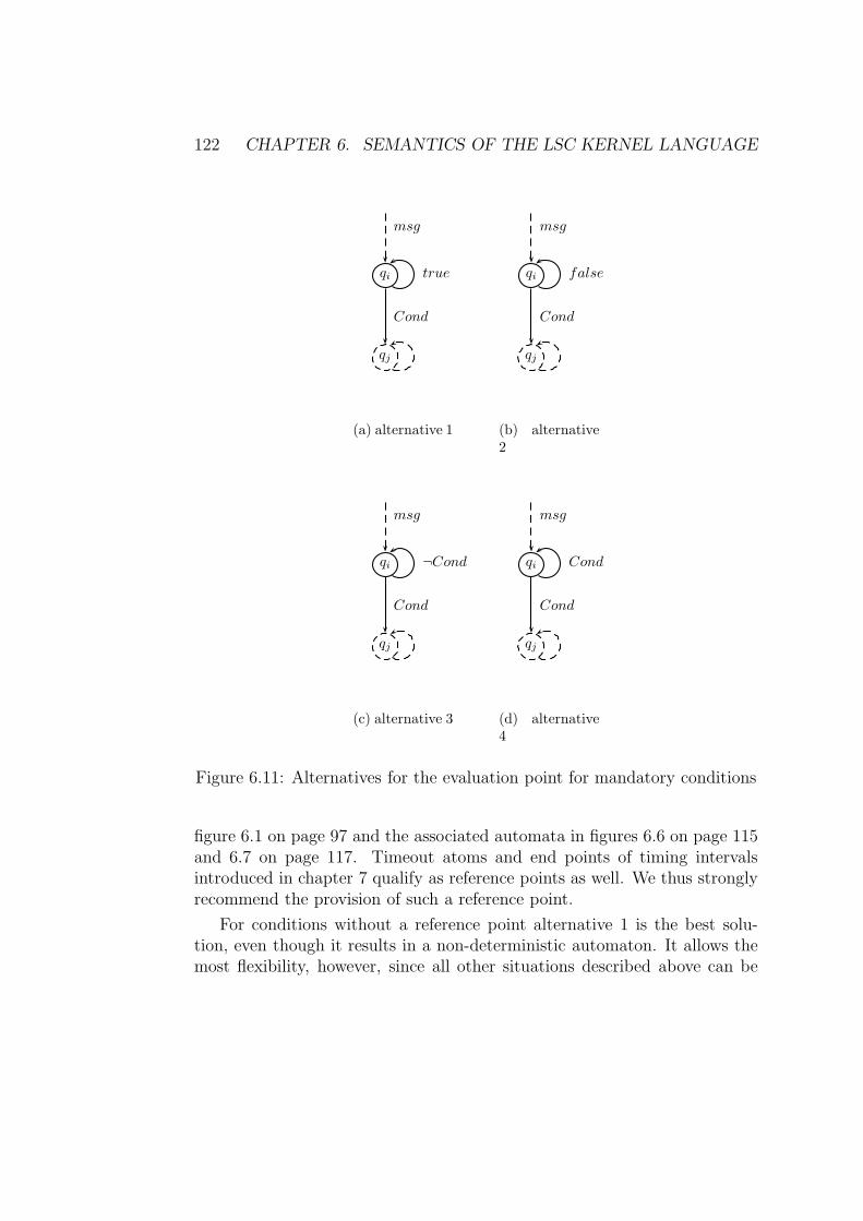
122 CHAPTER 6. SEMANTICS OF THE LSC KERNEL LANGUAGE
qi
msg
true
qj
Cond
(a) alternative 1
qi
msg
false
qj
Cond
(b) alternative2
qi
msg
¬Cond
qj
Cond
(c) alternative 3
qi
msg
Cond
qj
Cond
(d) alternative4
Figure 6.11: Alternatives for the evaluation point for mandatory conditions
figure 6.1 on page 97 and the associated automata in figures 6.6 on page 115and 6.7 on page 117. Timeout atoms and end points of timing intervalsintroduced in chapter 7 qualify as reference points as well. We thus stronglyrecommend the provision of such a reference point.
For conditions without a reference point alternative 1 is the best solu-tion, even though it results in a non-deterministic automaton. It allows themost flexibility, however, since all other situations described above can be
6.2. FORMAL SEMANTICS 123
expressed by using appropriate local invariants, etc. This is not the case forthe other alternatives.
Remark 6.8 (Tying possible conditions to messages)If a possible condition has a reference point in the form of a message, thismessage must also be included in the annotation of the transition, which leadsinto the exit state. Assume for instance that the mode of Cond1 in the LSCin figure 6.1 were possible. Then there would be a transition from state q4 tothe exit state annotated by ”¬Cond1 ∧msg5” in the automata in figures 6.6and 6.7. �
6.2.5 Message Temperatures
So far message temperatures have been assumed to be hot, for which thesemantical treatment is clear: if the send atom has been observed, the receiveatom must also be observed. The intuitive semantics of a cold message isthat it need not be received. For instantaneous messages the situation isclear: Since sending and receipt happen simultaneously, only the send atom isunwound. For asynchronous messages, however, there exist different optionshow to formally define the semantics:
• Alternative 1: The receiving instance is not allowed to progress be-yond the receiving atom for this message, i.e. no atoms below the re-ceiving atom may be observed before the message arrives.
• Alternative 2a: The receiving instance is allowed to progress beyondthe receiving atom without actually receiving the message. If the mes-sage does arrive later on, the LSC is exited without generating an error,similar to a violated cold condition.
• Alternative 2b: The receiving instance is allowed to progress be-yond the receiving atom without actually receiving the message. Ifthe message does arrive later on, this constitutes an error, similar to amandatory condition.
• Alternative 2c: The receiving instance is allowed to progress beyondthe receiving atom without actually receiving the message and a latearrival of the message is ignored.
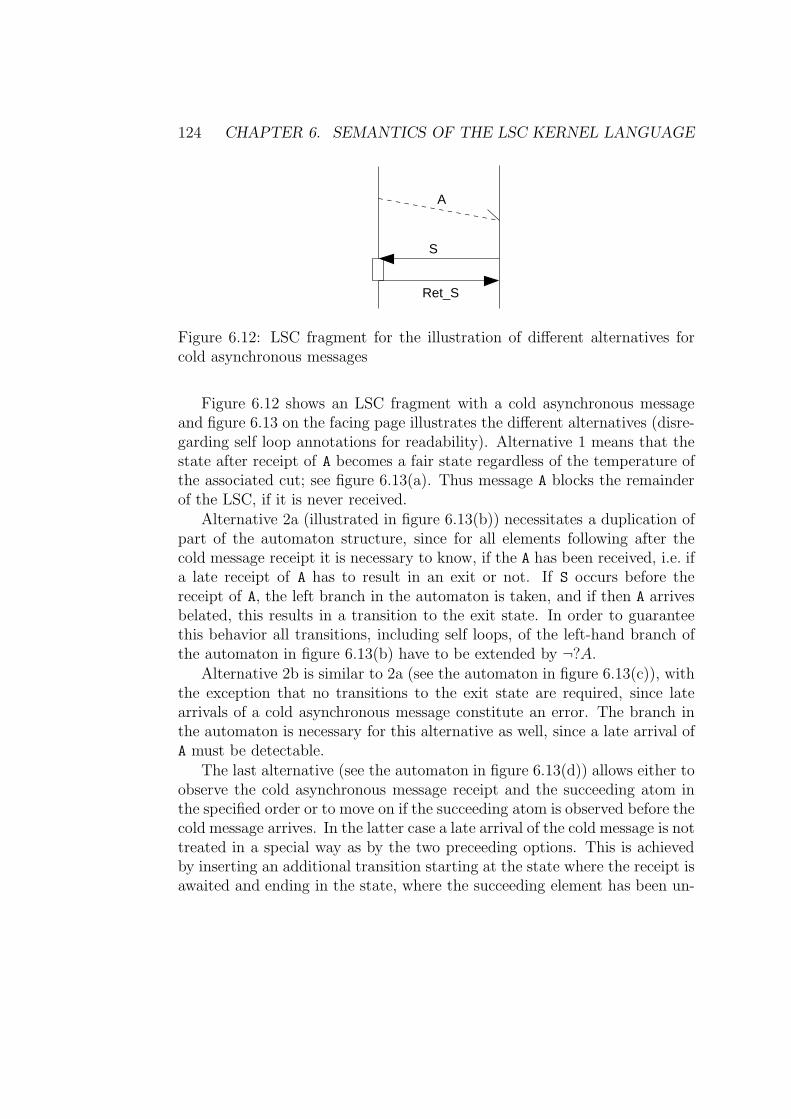
124 CHAPTER 6. SEMANTICS OF THE LSC KERNEL LANGUAGE
A
S
Ret_S
Figure 6.12: LSC fragment for the illustration of different alternatives forcold asynchronous messages
Figure 6.12 shows an LSC fragment with a cold asynchronous messageand figure 6.13 on the facing page illustrates the different alternatives (disre-garding self loop annotations for readability). Alternative 1 means that thestate after receipt of A becomes a fair state regardless of the temperature ofthe associated cut; see figure 6.13(a). Thus message A blocks the remainderof the LSC, if it is never received.
Alternative 2a (illustrated in figure 6.13(b)) necessitates a duplication ofpart of the automaton structure, since for all elements following after thecold message receipt it is necessary to know, if the A has been received, i.e. ifa late receipt of A has to result in an exit or not. If S occurs before thereceipt of A, the left branch in the automaton is taken, and if then A arrivesbelated, this results in a transition to the exit state. In order to guaranteethis behavior all transitions, including self loops, of the left-hand branch ofthe automaton in figure 6.13(b) have to be extended by ¬?A.
Alternative 2b is similar to 2a (see the automaton in figure 6.13(c)), withthe exception that no transitions to the exit state are required, since latearrivals of a cold asynchronous message constitute an error. The branch inthe automaton is necessary for this alternative as well, since a late arrival ofA must be detectable.
The last alternative (see the automaton in figure 6.13(d)) allows either toobserve the cold asynchronous message receipt and the succeeding atom inthe specified order or to move on if the succeeding atom is observed before thecold message arrives. In the latter case a late arrival of the cold message is nottreated in a special way as by the two preceeding options. This is achievedby inserting an additional transition starting at the state where the receipt isawaited and ending in the state, where the succeeding element has been un-
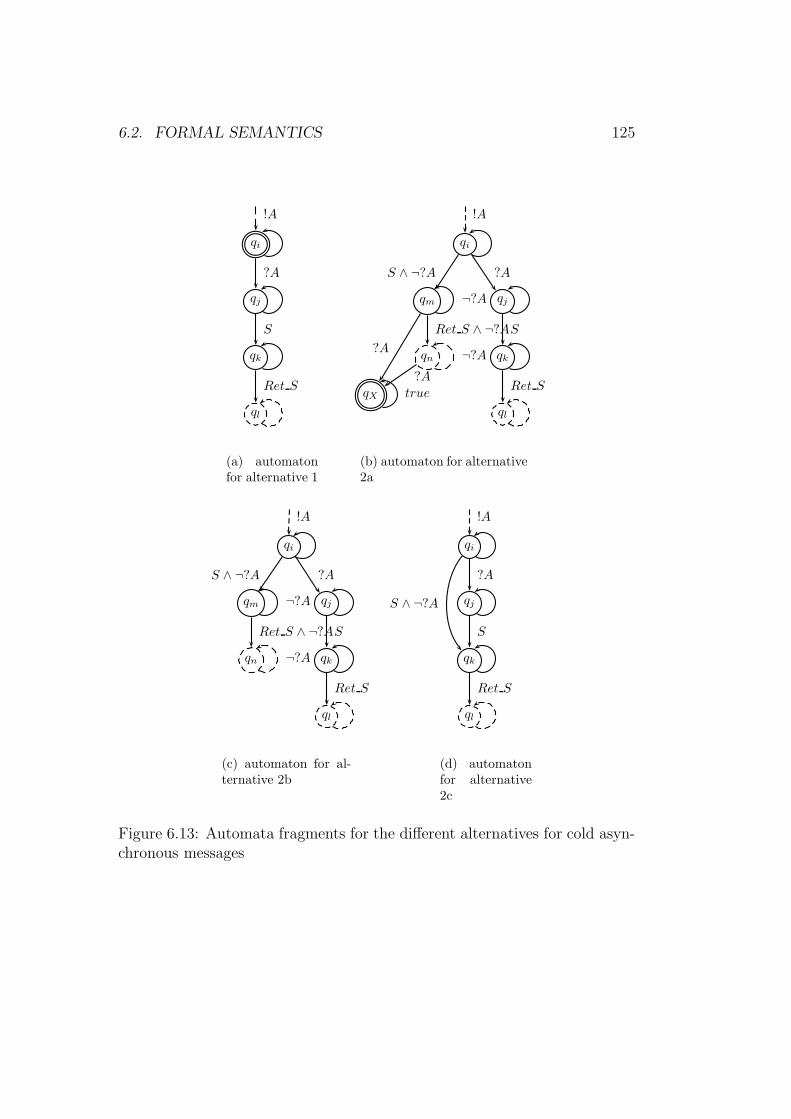
6.2. FORMAL SEMANTICS 125
qi
!A
qj
?A
qk
S
ql
Ret S
(a) automatonfor alternative 1
qi
!A
qj
?A
qm ¬?A
S ∧ ¬?A
qn ¬?A
Ret S ∧ ¬?A
qk
S
ql
Ret SqX true
?A
?A
(b) automaton for alternative2a
qi
!A
qj
?A
qm ¬?A
S ∧ ¬?A
qn ¬?A
Ret S ∧ ¬?A
qk
S
ql
Ret S
(c) automaton for al-ternative 2b
qi
!A
qj
?A
qk
S
S ∧ ¬?A
ql
Ret S
(d) automatonfor alternative2c
Figure 6.13: Automata fragments for the different alternatives for cold asyn-chronous messages
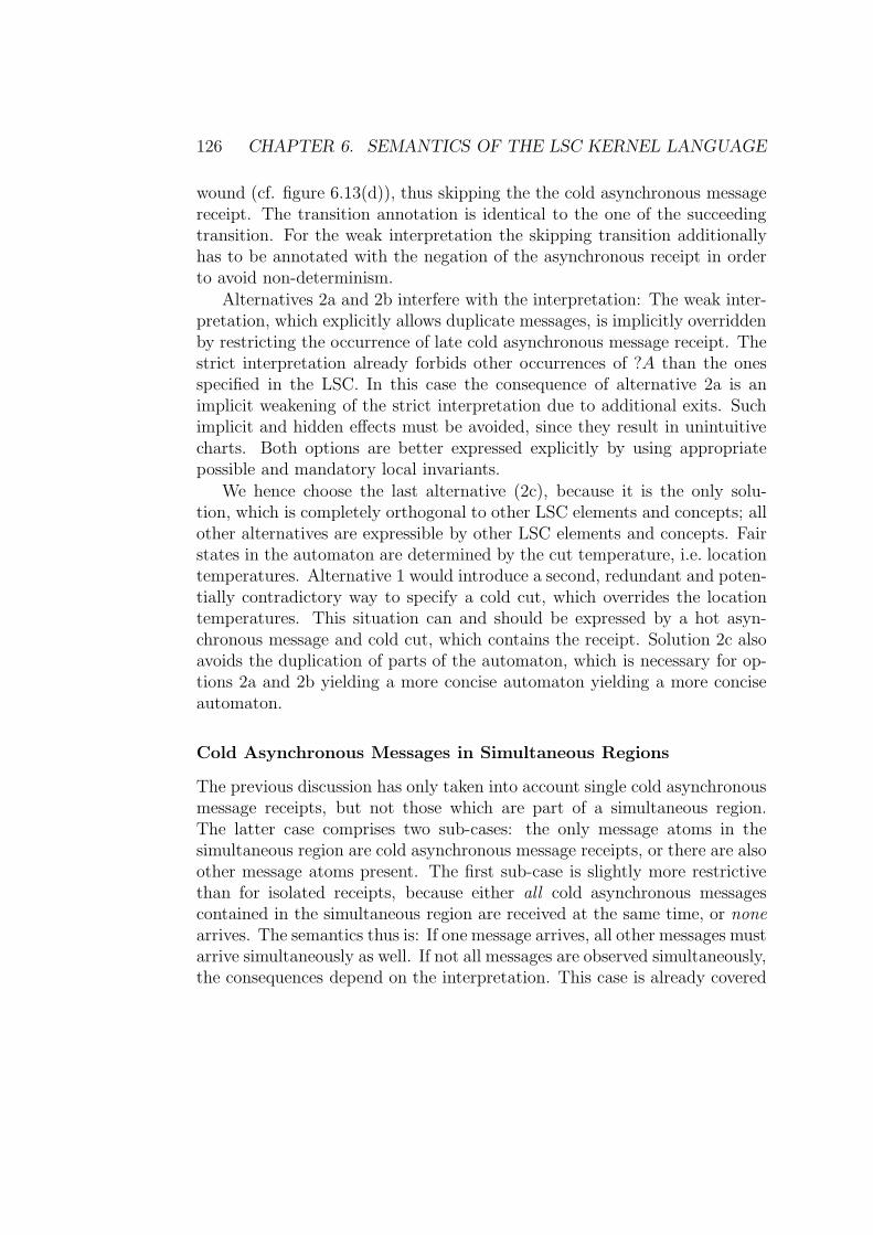
126 CHAPTER 6. SEMANTICS OF THE LSC KERNEL LANGUAGE
wound (cf. figure 6.13(d)), thus skipping the the cold asynchronous messagereceipt. The transition annotation is identical to the one of the succeedingtransition. For the weak interpretation the skipping transition additionallyhas to be annotated with the negation of the asynchronous receipt in orderto avoid non-determinism.
Alternatives 2a and 2b interfere with the interpretation: The weak inter-pretation, which explicitly allows duplicate messages, is implicitly overriddenby restricting the occurrence of late cold asynchronous message receipt. Thestrict interpretation already forbids other occurrences of ?A than the onesspecified in the LSC. In this case the consequence of alternative 2a is animplicit weakening of the strict interpretation due to additional exits. Suchimplicit and hidden effects must be avoided, since they result in unintuitivecharts. Both options are better expressed explicitly by using appropriatepossible and mandatory local invariants.
We hence choose the last alternative (2c), because it is the only solu-tion, which is completely orthogonal to other LSC elements and concepts; allother alternatives are expressible by other LSC elements and concepts. Fairstates in the automaton are determined by the cut temperature, i.e. locationtemperatures. Alternative 1 would introduce a second, redundant and poten-tially contradictory way to specify a cold cut, which overrides the locationtemperatures. This situation can and should be expressed by a hot asyn-chronous message and cold cut, which contains the receipt. Solution 2c alsoavoids the duplication of parts of the automaton, which is necessary for op-tions 2a and 2b yielding a more concise automaton yielding a more conciseautomaton.
Cold Asynchronous Messages in Simultaneous Regions
The previous discussion has only taken into account single cold asynchronousmessage receipts, but not those which are part of a simultaneous region.The latter case comprises two sub-cases: the only message atoms in thesimultaneous region are cold asynchronous message receipts, or there are alsoother message atoms present. The first sub-case is slightly more restrictivethan for isolated receipts, because either all cold asynchronous messagescontained in the simultaneous region are received at the same time, or nonearrives. The semantics thus is: If one message arrives, all other messages mustarrive simultaneously as well. If not all messages are observed simultaneously,the consequences depend on the interpretation. This case is already covered
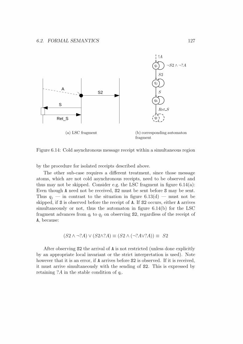
6.2. FORMAL SEMANTICS 127
AS2
S
Ret_S
(a) LSC fragment
qi ¬S2 ∧ ¬?A
!A
qj
S2
qk
S
ql
Ret S
(b) corresponding automatonfragment
Figure 6.14: Cold asynchronous message receipt within a simultaneous region
by the procedure for isolated receipts described above.
The other sub-case requires a different treatment, since those messageatoms, which are not cold asynchronous receipts, need to be observed andthus may not be skipped. Consider e.g. the LSC fragment in figure 6.14(a):Even though A need not be received, S2 must be sent before S may be sent.Thus qj — in contrast to the situation in figure 6.13(d) — must not beskipped, if S is observed before the receipt of A. If S2 occurs, either A arrivessimultaneously or not, thus the automaton in figure 6.14(b) for the LSCfragment advances from qi to qj on observing S2, regardless of the receipt ofA, because:
(S2 ∧ ¬?A) ∨ (S2∧?A) ≡ (S2 ∧ (¬?A∨?A)) ≡ S2
After observing S2 the arrival of A is not restricted (unless done explicitlyby an appropriate local invariant or the strict interpretation is used). Notehowever that it is an error, if A arrives before S2 is observed. If it is received,it must arrive simultaneously with the sending of S2. This is expressed byretaining ?A in the stable condition of qi.
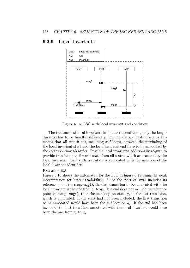
128 CHAPTER 6. SEMANTICS OF THE LSC KERNEL LANGUAGE
6.2.6 Local Invariants
Invariant
Inst2
Local Inv Example
ActAC:
AM:
Inst1
LSC:
Inst3
msg2
Inv1
Cond1
msg3
msg4
msg1
Figure 6.15: LSC with local invariant and condition
The treatment of local invariants is similar to conditions, only the longerduration has to be handled differently. For mandatory local invariants thismeans that all transitions, including self loops, between the unwinding ofthe local invariant start and the local invariant end have to be annotated bythe corresponding identifier. Possible local invariants additionally require toprovide transitions to the exit state from all states, which are covered by thelocal invariant. Each such transition is annotated with the negation of thelocal invariant identifier.
Example 6.8Figure 6.16 shows the automaton for the LSC in figure 6.15 using the weakinterpretation for better readability. Since the start of Inv1 includes itsreference point (message msg1), the first transition to be annotated with thelocal invariant is the one from q1 to q2. The end does not include its referencepoint (message msg4), thus the self loop on state q4 is the last transition,which is annotated. If the start had not been included, the first transitionto be annotated would have been the self loop on q2. If the end had beenincluded, the last transition annotated with the local invariant would havebeen the one from q4 to q5.
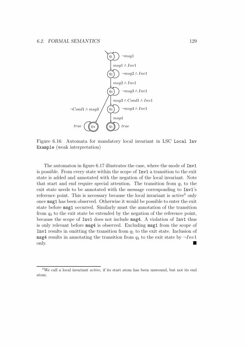
6.2. FORMAL SEMANTICS 129
q1 ¬msg1
q2 ¬msg2 ∧ Inv1
msg1 ∧ Inv1
q3 ¬msg3 ∧ Inv1
msg2 ∧ Inv1
q4 ¬msg4 ∧ Inv1
msg3 ∧Cond1 ∧ Inv1
q5 true
msg4
qXtrue
¬Cond1 ∧msg3
Figure 6.16: Automata for mandatory local invariant in LSC Local Inv
Example (weak interpretation)
The automaton in figure 6.17 illustrates the case, where the mode of Inv1is possible. From every state within the scope of Inv1 a transition to the exitstate is added and annotated with the negation of the local invariant. Notethat start and end require special attention. The transition from q1 to theexit state needs to be annotated with the message corresponding to Inv1’sreference point. This is necessary because the local invariant is active5 onlyonce msg1 has been observed. Otherwise it would be possible to enter the exitstate before msg1 occurred. Similarly must the annotation of the transitionfrom q4 to the exit state be extended by the negation of the reference point,because the scope of Inv1 does not include msg4. A violation of Inv1 thusis only relevant before msg4 is observed. Excluding msg1 from the scope ofInv1 results in omitting the transition from q1 to the exit state. Inclusion ofmsg4 results in annotating the transition from q4 to the exit state by ¬Inv1only. �
5We call a local invariant active, if its start atom has been unwound, but not its endatom.
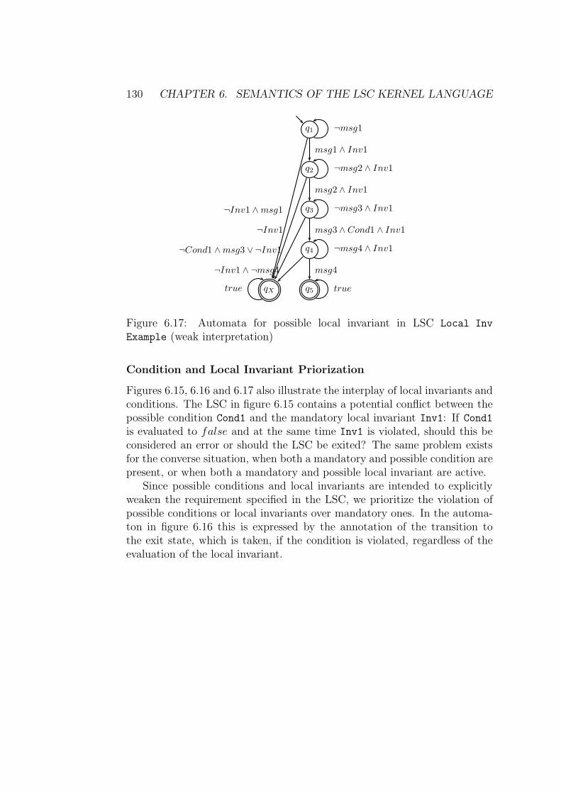
130 CHAPTER 6. SEMANTICS OF THE LSC KERNEL LANGUAGE
q1 ¬msg1
q2 ¬msg2 ∧ Inv1
msg1 ∧ Inv1
q3 ¬msg3 ∧ Inv1
msg2 ∧ Inv1
q4 ¬msg4 ∧ Inv1
msg3 ∧ Cond1 ∧ Inv1
q5 true
msg4
qXtrue
¬Cond1 ∧msg3 ∨ ¬Inv1
¬Inv1 ∧msg1
¬Inv1
¬Inv1 ∧ ¬msg4
Figure 6.17: Automata for possible local invariant in LSC Local Inv
Example (weak interpretation)
Condition and Local Invariant Priorization
Figures 6.15, 6.16 and 6.17 also illustrate the interplay of local invariants andconditions. The LSC in figure 6.15 contains a potential conflict between thepossible condition Cond1 and the mandatory local invariant Inv1: If Cond1is evaluated to false and at the same time Inv1 is violated, should this beconsidered an error or should the LSC be exited? The same problem existsfor the converse situation, when both a mandatory and possible condition arepresent, or when both a mandatory and possible local invariant are active.
Since possible conditions and local invariants are intended to explicitlyweaken the requirement specified in the LSC, we prioritize the violation ofpossible conditions or local invariants over mandatory ones. In the automa-ton in figure 6.16 this is expressed by the annotation of the transition tothe exit state, which is taken, if the condition is violated, regardless of theevaluation of the local invariant.
6.2. FORMAL SEMANTICS 131
6.2.7 The Unwinding Algorithm
The unwinding algorithm needs as input an LSC body l, including the setsand functions defined in the preceding sections, and the interpretation (weakor strict). The result is a timed symbolic automaton T SA = (Σ, Q, q0, C,−→, F ). Since no timing information is considered at this point, the set ofclocks is empty for the moment and all transitions will carry no clock resetor constraints. Some auxiliary functions are needed, which are indicated bysmall capitals font and whose behavior is described below. Algorithm 6.1shows the main routine of the unwinding procedure.
Algorithm 6.1, lines 1 – 16: Initialization First the stable condi-tion sc is constructed in line 2, which is only possible beforehand, if theinterpretation is strict, because only then are all stable conditions identi-cal6. The auxiliary function Neg Conjunct takes a set of identifiers andconstructs the conjunction of the negation of all elements of this set. Ifthe set contains only one element, only the negation of this element is re-turned. Thus Neg Conjunct({msg1, msg2}) produces ¬msg1 ∧ ¬msg2,Neg Conjunct({msg1}) yields ¬msg1.
The set of properties, from which the transition annotations are built, ismade up of the identifiers used in the LSC (line 4). Note that message labelsare used instead of message identifiers, because for asynchronous messagesthere need to be two annotations for each message, one for the sending andone for the receipt. In addition to the identifiers also constants true and falseare allowed. The set of clocks is empty (line 5). phases in line 6 is the setof phases and is initialized to the initial phase Phase0 (cf. definition 6.9 onpage 109), which also becomes the first state in Q and the initial state (lines 7and 8). Function State establishes the relation between automaton statesand phases by assigning a unique state name to a phase, e.g. q0 for the initialphase. If the phase has already been assigned a name, the existing one isreturned. If the initial cut is cold, then the set of fair states is initializedwith Q (line 10), which at this point only contains q0, otherwise F is empty(line 12). Note that the exit node is always included to keep the algorithmsimple. In practice it is only added when needed. The transition relation isinitialized with the self loop of the exit state in line 14.
6The stable conditions may be not identical in the end due to local invariants, but thebase remains the same.
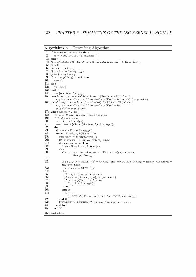
132 CHAPTER 6. SEMANTICS OF THE LSC KERNEL LANGUAGE
Algorithm 6.1 Unwinding Algorithm1: if interpretation = strict then
2: sc := Neg Conjunct(MsgLabels(l))3: end if
4: Σ := MsgLabels(l) ∪ Conditions(l) ∪ Local Invariants(l) ∪ {true, false}5: C := ∅6: phases := {Phase0}7: Q := {State(Phase0), qX}8: q0 := State(Phase0)9: if cut temp(Cut0) = cold then
10: F := Q
11: else
12: F := {qX}13: end if
14: −→:= {(qX , true, ∅, ǫ, qX)}15: poss invs0 := {li ∈ Local Invariants(l) | ∃scl ∃cl ∈ scl ∃a, a′ ∈ cl :
a ∈ Instheads(l) ∧ a′ ∈ LI starts(l) ∧ liID(a′) = li ∧ mode(a′) = possible}16: mand invs0 := {li ∈ Local Invariants(l) | ∃scl ∃cl ∈ scl ∃a, a′ ∈ cl :
a ∈ Instheads(l) ∧ a′ ∈ LI starts(l) ∧ liID(a′) = li∧mode(a′) = mandatory}
17: while phases 6= ∅ do
18: let ph = (Readyi, Historyi, Cuti) ∈ phases
19: if Readyi = ∅ then
20: F := F ∪ {State(ph)}21: −→:=−→ ∪ {(State(ph), true, ∅, ǫ,State(ph))}22: else
23: Generate Exits(Readyi , ph)24: for all F iredik
∈ P(Readyi) do
25: successor := Step(ph,F iredik)
26: let successor = (Readyj , Historyj , Cutj)27: if successor = ph then
28: Insert Self Loop(ph, Readyi)29: else
30: TransitionAnnot :=Construct Transition(ph, successor,
Readyi, F iredik)
31:32: if ∃q ∈ Q with State−1(q) = (Readyx, Historyx, Cutx) : Readyi = Readyx ∧ Historyi =
Historyx then
33: successor := State−1(q)34: else
35: Q := Q ∪ {State(successor)}36: phases := (phases \ {ph}) ∪ {successor}37: if cut temp(Cuti) = cold then
38: F := F ∪ {State(ph)}39: end if
40: end if
41: −→:=−→ ∪{(State(ph), T ransitionAnnot, ∅, ǫ,State(successor))}
42: end if
43: Insert Skip Transition(TransitionAnnot, ph, successor)44: end for
45: end if
46: end while

6.2. FORMAL SEMANTICS 133
Two sets are associated with each phase Phasei: poss invsi andmand invsi, which contain the identifiers of all possible, resp. mandatorylocal invariants, which are active in this phase. The initial sets poss invs0
and mand invs0 are initialized with those local invariants, whose start atomsare attached to an instance head (lines 15 and 16).
Algorithm 6.1, lines 18 – 47: Main Part The remainder of algo-rithm 6.1 iterates over the list of accumulated phases and computes the suc-cessors for each by applying the step function of definition 6.10 on page 110.As long as the list of phases is not empty (line 17) a phase ph is taken fromthe list (line 18) and unwound.
Algorithm 6.1, lines 19 – 21: Final State Line 19 checks, if the currentphase is the final phase, which is indicated by an empty ready set. The finalphase need not be unwound using the step function, since it does not have asuccessor. Thus it is sufficient to add the name corresponding to the phaseto the set of fair states7 (line 20) and to insert the true-annotated self loopto the transition relation (line 21). Note the empty clock reset list and clockconstraint.
Algorithm 6.1, lines 23 – 46: Computing Successors If the currentphase is not the final one, the step function needs to be applied for all firedsets Firedik computed for ready set Readyi (lines 24 – 26). Before the succes-sors are computed the transition to the exit state is generated, if needed, inline 23 by the function Generate Exits, which is shown in algorithm 6.2 onpage 135.
If the successor is identical to the current phase, this means that theself loop for the corresponding state must be generated, which is handledby function Insert Self Loop (line 28) and which is described in algo-rithm 6.3 on page 137. If the successor phase is different from the currentphase, the annotation of the transition to the successor phase is generatedby function Construct Transition in line 30; for the behavior of thisfunction refer to algorithm 6.4 on page 138.
Lines 32 and 33 implement the optimization introduced in section 6.2.1:If there already is an equivalent state in Q, this state is used as successor(line 33), otherwise a new state is generated and inserted into Q (line 35),
7Recall that the final state is always fair.
134 CHAPTER 6. SEMANTICS OF THE LSC KERNEL LANGUAGE
the old phase is removed from the phases list and the new phase is appended(line 36), and the state is added to the set of fair states, if the correspondingcut is cold (lines 37, 38). The function State−1 is the inverse of functionState, i.e. it returns the phase associated with a state in Q.
In line 41 the transition is generated and added to −→. Line 43 containsthe treatment for cold asynchronous message receipts, if they require theinserting of a skipping transition as described in section 6.2.5 on page 123.This is handled by function Insert Skip Transition, which is describedin algorithm 6.5 on page 139.
Algorithm 6.2 on the next page creates the transition to the exit state foreach unwound phase, i.e. it is executed only once for each phase. It consistsof three major parts: checking for possible conditions and local invariants insimultaneous regions (lines 2 – 25), handling possible conditions, which arenot part of a simultaneous region (lines 27 – 29) and generating the transitionto the exit state (lines 30 – 32). The annotation for the transition to the exitstate is initialized to true in line 1.
Algorithm 6.2, lines 2 – 5: Possible Conditions in Simulta-
neous Regions First, the simultaneous regions contained in the cur-rent ready set are checked for possible conditions. The auxiliary func-tion SimClasses(SimRegs(Readyi)) returns the set of simultaneous classesin Readyi, which contain a simultaneous region, i.e. the set of clus-ters, which contain more than one atom each. The auxiliary functionPoss CondIDs(scl) similarly returns the set of condition atom identifiers,which are contained in SimClass scl and whose mode is possible. If suchidentifiers exist, i.e. the set returned by Poss CondIDs(scl) is not empty(line 3), the conjunction of the negation of these identifiers is disjunctivelyadded to the annotation of the transition to the exit state ExitAnnot (line 4)conjoined with the conjunction of all message identifiers contained in thesame simultaneous region. The auxiliary function MsgLabels(scl) returnsthe set of labels of messages contained in SimClass scl. This implementsthe semantics for possible conditions within simultaneous regions describedin remark 6.8 on page 123: the evaluation point of a condition bound to amessage via a simultaneous region is given by the occurrence of this message.The procedure described here is the generalization to a number of possibleconditions and several messages contained in a simultaneous region. Notethat the elements within one simultaneous region are assembled conjunc-
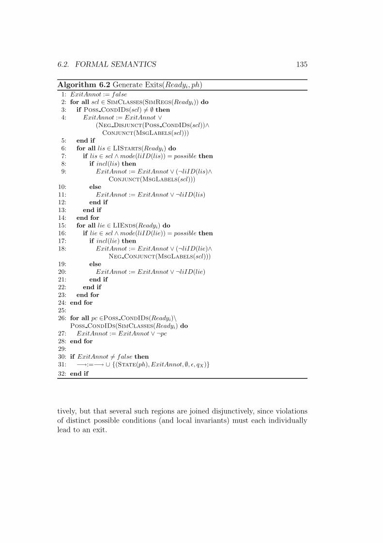
6.2. FORMAL SEMANTICS 135
Algorithm 6.2 Generate Exits(Readyi, ph)1: ExitAnnot := false
2: for all scl ∈ SimClasses(SimRegs(Readyi)) do
3: if Poss CondIDs(scl) 6= ∅ then
4: ExitAnnot := ExitAnnot ∨(Neg Disjunct(Poss CondIDs(scl))∧
Conjunct(MsgLabels(scl)))5: end if
6: for all lis ∈ LIStarts(Readyi) do
7: if lis ∈ scl ∧mode(liID(lis)) = possible then
8: if incl(lis) then
9: ExitAnnot := ExitAnnot ∨ (¬liID(lis)∧Conjunct(MsgLabels(scl)))
10: else
11: ExitAnnot := ExitAnnot ∨ ¬liID(lis)12: end if
13: end if
14: end for
15: for all lie ∈ LIEnds(Readyi) do
16: if lie ∈ scl ∧mode(liID(lie)) = possible then
17: if incl(lie) then
18: ExitAnnot := ExitAnnot ∨ (¬liID(lie)∧Neg Conjunct(MsgLabels(scl)))
19: else
20: ExitAnnot := ExitAnnot ∨ ¬liID(lie)21: end if
22: end if
23: end for
24: end for
25:26: for all pc ∈Poss CondIDs(Readyi)\
Poss CondIDs(SimClasses(Readyi) do
27: ExitAnnot := ExitAnnot ∨ ¬pc28: end for
29:30: if ExitAnnot 6= false then
31: −→:=−→ ∪ {(State(ph), ExitAnnot, ∅, ǫ, qX)}
32: end if
tively, but that several such regions are joined disjunctively, since violationsof distinct possible conditions (and local invariants) must each individuallylead to an exit.
136 CHAPTER 6. SEMANTICS OF THE LSC KERNEL LANGUAGE
Algorithm 6.2, lines 6 – 14: Possible Local Invariant Starts Theauxiliary function LIStarts(Readyi) returns the set of local invariant startatoms of Readyi. Only the possible ones, which are contained in the currentsimultaneous region, are of interest here (line 7). If they also include thesimultaneous region they are bound to (line 8), the exit transition needs to beannotated not only with the negation of the local invariant, but also with themessage identifiers of their simultaneous region as described in example 6.8 onpage 128 (line 9). If they are non-inclusive the negation of the local invariantidentifier is sufficient (line 11).
Algorithm 6.2, lines 15 – 24: Possible Local Invariant Ends Asimilar treatment is necessary for possible local invariant ends, since theyalso need a special treatment, if they include the simultaneous region theyare bound to. As explained in example 6.8 on page 128 it is necessary toadditionally annotate the negation of the local invariant identifier with thenegation of the messages contained in the currently considered simultaneousregion (line 18).
Algorithm 6.2, lines 26 – 28: Isolated Possible Conditions All pos-sible conditions, which are not part of a simultaneous region (line 26) requireonly their disjunctive inclusion into the annotation of the exit transition(line 27).
Algorithm 6.2, lines 30 – 32: Exit Transition Generation The gen-eration of a transition to the exit state is only necessary, if any possiblecondition or local invariant is present in the current ready set, indicated bya non-empty, i.e. other than false, ExitAnnot (line 30). If this is the case,the transition to the exit state is added to the transition relation (line 31).
Algorithm 6.3 Algorithm 6.3 on the next page generates the self loop fora state and adds it to the transition relation. For simplicity’s sake the twosets of active local invariants are joined in line 1. If the interpretation isstrict, then the base stable condition has already been computed and onlythe conjunction of the active local invariants needs to be added (line 3). Forthe weak interpretation it has to be checked, if there are any messages in theready set (line 5). The auxiliary function MsgLabels is an extension of thecorresponding auxiliary function defined in algorithm 6.2. If Readyi contains
6.2. FORMAL SEMANTICS 137
Algorithm 6.3 Insert Self Loop(ph,Readyi)1: let invsi = poss invsi ∪mand invsi
2: if interpretation = strict then
3: −→:=−→ ∪ {(State(ph), sc ∧ Conjunct(invsi), ∅, ǫ,State(ph))}4: else
5: if MsgLabels(Readyi) 6= ∅ then
6: −→:=−→ ∪ {(State(ph),Neg Conjunct(MsgLabels(Readyi)) ∧ Conjunct(invsi),∅, ǫ,State(ph))}
7: else
8: −→:=−→ ∪{(State(ph), true ∧ Conjunct(invsi), ∅, ǫ,State(ph))}
9: end if
10: end if
at least one message, the conjunction of the negation of their identifiers isused for the transition annotation, in addition to the conjunction of activelocal invariants (line 6). If no messages are present in Readyi the annotationis simply true plus the conjunction of active local invariants (line 8).
Algorithm 6.4 Algorithm 6.4 on the following page constructs the an-notation for the transition corresponding to the currently unwound fired setand computes the new sets of active local invariants. The starting pointfor these sets, poss invsj and mand invsj , are the current sets (lines 1, 2).First the local invariants, whose end atoms are unwound in this step have tobe considered, since these local invariants must not appear in the transitionannotation and thus have to be removed first. This is done by function Han-dle Local Invariant Ends (line 4), which returns the first part of thetransition annotation and adjusts the set of active local invariants and whosebehavior is detailed by algorithm 6.6. Lines 6 – 8 introduce some abbrevi-ations for the set of all active local invariants, the set of identifiers of coldmessage receipts contained in the current fired set, and the set of messagelabels contained in simultaneous regions of Firedik. The auxiliary functionSimRegs(Firedik) yields the simultaneous regions contained in the fired set,i.e. those clusters, which are comprised of more than one atom, ColdMsgR-cvLabels(Firedik) returns the set of message labels of cold asynchronousmessage receipt atoms in Firedik . If cold message receipts are present inthe current fired set, the transition annotation is extended appropriately bythe function Generate Main Annotation (line 10), which is presented
138 CHAPTER 6. SEMANTICS OF THE LSC KERNEL LANGUAGE
Algorithm 6.4 transAnnot Construct Transition(ph, successor, Readyi,Firedik)1: mand invsj := mand invsi
2: poss invsj := poss invsi
3:4: transAnnot := Handle Local Invariant Ends(true,
F iredik, Readyi, j)
5:6: let invsj = poss invsj ∪mand invsj
7: let cmr = ColdMsgRcvLabels(Firedik)
8: let msr = MsgLabels(SimRegs(Firedik))
9: if cmr 6= ∅ then
10: transAnnot :=Generate Main Annotation(Firedik, cmr,
msr, invsj, transAnnot)11: end if
12: if interpretation = strict then
13: transAnnot := transAnnot ∧Neg Conjunct(MsgLabels(l) \ MsgLabels(Firedik
))14: end if
15: if |SimClasses(Readyi)| > 1 ∧ interpretation = weak then
16: transAnnot := transAnnot∧Neg Conjunct(MsgLabels(Readyi \ MsgLabels(Firedik
)))17: end if
18:19: transAnnot :=Handle Local Invariant Starts(transAnnot,
F iredik, Readyi, j)
20:
21: return transAnnot
in detail in algorithm 6.8 on page 140.
In case of the strict interpretation the transition must contain the con-junction of the negation of all message labels of the LSC, which are notunwound in the current step, which is done in line 13. If the current readyset contains more than one SimClass, which means that either (part of) acoregion is unwound or independent LSC elements, the transitions leavingthe current state ph have to be made deterministic — as motivated in sec-tion 6.2.2 on page 116 — by adding the negation of all elements, which arenot unwound, but are in the ready set (line 16).
Finally, the local invariant starts contained in the current fired set haveto be considered and added to the transition annotation. This is handled byfunction Handle Local Invariant Starts in line 19, which is described
6.2. FORMAL SEMANTICS 139
by algorithm 6.7 on the following page.
Algorithm 6.5 Insert Skip Transition(TransitionAnnot, ph, successor)
1: for all (qx, ψ,State−1(ph)) ∈−→ do
2: let (Readyx, Historyx, Cutx) = State−1(qx)3: if ColdMsgRcvs(Readyx) =Atoms(Readyx) then
4: −→:=−→ ∪ (qx, T ransitionAnnot∧Neg Conjunct(ColdMsgRcvLabels)(Readyx),State(successor))
5: end if
6: end for
Algorithm 6.5 Algorithm 6.5 generates the transitions, which skip thereceipt of cold asynchronous message receipts as explained in detail in sec-tion 6.2.5. The strategy is to examine all transitions leading to the state,for which a successor has just been computed (line 1), and find those statesimmediately preceding the one for the current phase ph, which only containcold message receipt atoms (line 3). The auxiliary functions ColdMsgR-cvs(Readyx), resp. Atoms(Readyx) return the set of cold message receiveatoms, resp. all atoms of the ready set. These states are the ones fromwhich a skipping transition originates and thus a correspondingly annotatedtransition is added to −→ (line 4). As described in section 6.2.5 the annota-tion consists of the annotation of the currently considered transition (fromState−1(ph) to State−1(successor)).
Algorithm 6.6 TransAnnot Handle Local InvariantEnds(TransAnnot, F iredik , Readyi, j)
1: for all lie ∈ LIEnds(Readyi) do
2: if incl(lie) then
3: TransAnnot := TransAnnot ∧ liID(lie)4: end if
5: if mode(liID(lie)) = mandatory then
6: mand invsj := mand invsj \ {liID(lie)}7: else
8: poss invsj := poss invsj \ {liID(lie)}9: end if
10: end for
11: return TransAnnot
140 CHAPTER 6. SEMANTICS OF THE LSC KERNEL LANGUAGE
Algorithm 6.6 Algorithm 6.6 on the preceding page conjunctively addsthe identifiers of all local invariant end atoms to the annotation of the cur-rent transition (line 3), if they are inclusive (line 2). Non-inclusive ones areautomatically handled by not being in the set of active local invariants. Allare removed from the respective sets for the successor phase (lines 5 – 8).
Algorithm 6.7 TransAnnot Handle Local InvariantStarts(TransAnnot, F iredik , Readyi, j)
1: for all lis ∈ LIStarts(Readyi) do
2: if incl(lis) then
3: TransAnnot := TransAnnot ∧ liID(lis)4: end if
5: if mode(liID(lis)) = mandatory then
6: mand invsj := mand invsj ∪ {liID(lis)}7: else
8: poss invsj := poss invsj ∪ {liID(lis)}9: end if
10: end for
11: return TransAnnot
Algorithm 6.7 Algorithm 6.7 is the dual of algorithm 6.6 and likewiseadds inclusive local invariants to the current transition (lines 2, 3) and addsall unwound local invariants to the respective sets of active local invariantsfor the next phase (lines 5 – 9).
Algorithm 6.8 transAnnot Generate Main Annotation(Firedik , cmr,msr, invsj , transAnnot)
1: let msgs = MsgLabels(Firedik) \ ColdInstLabels(Firedik
)2:3: if (cmr ⊂ msr) then
4: transAnnot := transAnnot ∧ Conjunct((msgs \ cmr)∪ CondIDs(Firedik
) ∪ invsj)5: else
6: transAnnot := transAnnot ∧ Conjunct(msgs ∪CondIDs(Firedik
) ∪ invsj)7: end if
8: return transAnnot
6.3. ACTIVATION AND QUANTIFICATION 141
Algorithm 6.8 Algorithm 6.8 on the facing page constructs the mainpart of the transition annotation and also takes care of cold message re-ceipts, except for the skipping transition, which is handled by function In-sert Skip Transition described in algorithm 6.5 on page 139. Cold in-stantaneous messages are taken care of in line 1, where they are removedfrom the set of labels of fired messages; the auxiliary function ColdInst-Labels(Firedik) returns the labels of all cold instantaneous messages in thecurrent fired set.
Then it is checked, whether asynchronous cold message receipts have tobe considered for the transition annotation. They can be neglected, if theyare contained in a simultaneous region, which also contains other messages(cf. page 126). This is expressed by the strict subset requirement in line 3.In this case the cold message receipts (cmr) are disregarded for the transitionannotation (line 4), otherwise they are included (line 6). In both cases thecondition identifiers and the active local invariants are added, if present.
6.3 Activation and Quantification
The symbolic automaton generated by the unwinding algorithm in the pre-ceding section defines the behavior of the LSC body, disregarding the acti-vation point, mode and quantification information. In order to define thesemantics of the entire LSC the system, whose behavior is specified by theLSC, is needed; we call this the reference system of the LSC. In this sectionwe introduce an abstract representation of such a reference system, which isused to define the complete semantics of an LSC.
6.3.1 Reference System
Informally, a system consists of a set of functional units, which are hierarchi-cally organized, i.e. there are several levels of hierarchy, each consisting of aset of functional units, which may be decomposed into sub-units and so on.Each functional unit has a set of ports, which form its interface, the interfacesof different units are connected by channels. Information from unit to unitis passed along the channels, which can be delaying. Each unit also imple-ments a behavior, whose concrete realization is unimportant for this thesis.Figure 6.18 shows an example with three levels of hierarchy. Functional unitsare depicted as boxes, channels by lines between units, interfaces by channels
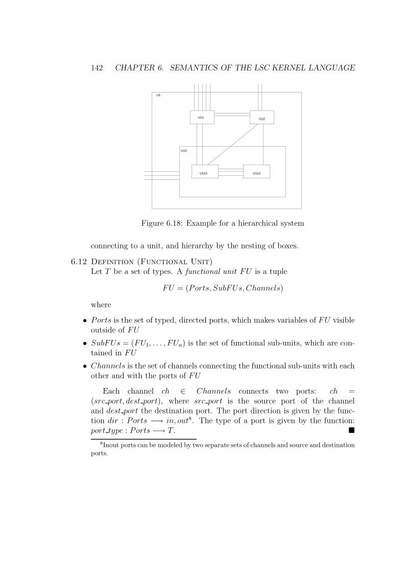
142 CHAPTER 6. SEMANTICS OF THE LSC KERNEL LANGUAGE
U1
U11 U12
U13
U111 U112
Figure 6.18: Example for a hierarchical system
connecting to a unit, and hierarchy by the nesting of boxes.
6.12 Definition (Functional Unit)Let T be a set of types. A functional unit FU is a tuple
FU = (Ports, SubFUs, Channels)
where
• Ports is the set of typed, directed ports, which makes variables of FU visibleoutside of FU
• SubFUs = (FU1, . . . , FUn) is the set of functional sub-units, which are con-tained in FU
• Channels is the set of channels connecting the functional sub-units with eachother and with the ports of FU
Each channel ch ∈ Channels connects two ports: ch =(src port, dest port), where src port is the source port of the channeland dest port the destination port. The port direction is given by the func-tion dir : Ports −→ in, out8. The type of a port is given by the function:port type : Ports −→ T . �
8Inout ports can be modeled by two separate sets of channels and source and destinationports.
6.3. ACTIVATION AND QUANTIFICATION 143
6.13 Definition (Well-formedness of a Functional Unit)A functional unit FU is well-formed iff
1. ∀ch ∈ Channels : port type(src port) = port type(dest port) (Ports mustbe type compatible.)
2. ∀ch ∈ Channels : dir(src port) 6= dir(dest port) (A channel may only con-nect an in port with an out port and vice versa.)
3. ∀ch = (src port, dest port), ch′ = (src port′, dest port′) ∈ Channels :dest port 6= dest port′ (No multiple senders.)
�
6.14 Definition (Reference System)A reference system S is a well-formed functional unit: S =(Ports, SubFUs, Channels). �
Each functional unit contains internal variables, which may be made vis-ible to other units or the outside world via the units’ ports. The ports aretyped according to the type of the variable, which is associated with the port.The concrete types and nature of the variables is again abstracted from forour purposes. The observables of the system thus are those variables, whichare made available via ports. The domain of variables, and hence of theports, of reference system S is denoted by DOMS. Valuation
θ : (Ports ∪ PortsFU1∪ · · · ∪ PortsFUn
) −→ DomS
assigns to each port p ∈ Ports ∪ PortsFU1∪ · · · ∪ PortsFUn
the value of thevariable associated with p. A sequence of such valuations makes up a run ofreference system (cf. section 5.3):
6.15 Definition (Reference System Run)Let PropS := {p ⊲ v | p ∈ Ports ∪ PortsFU1
∪ · · · ∪ PortsFUn, v ∈ DOMS ∨
v ∈∈ Ports∪PortsFU1∪· · ·∪PortsFUn
,⊲∈ {=, <,>,≤,≥}} be the set of allpropositions over ports of reference system S = (Ports, SubFUs, Channels)and let τ = τ0τ1τ2 . . . be a time sequence.
A timed run tr of reference system S is an infinite sequence of pairs(θ, τ) : tr = (θ0, τ0)(θ1, τ1)(θ2, τ2) . . .The i-th valuation of timed run tr is denoted by tri = (θi, τi) and the suffix
of a timed run tr, which starts at the i-th valuation is denoted by−→tri =
144 CHAPTER 6. SEMANTICS OF THE LSC KERNEL LANGUAGE
(θi, τi)(θi+1, τi+1) . . . The finite segment of a timed run, starting at the i-thvaluation and ending at the j-th, is denoted by trj
i = (θi, τi) . . . (θj , τj)The satisfaction of a formula ψ ∈ BExprPropS
over basic propositions overports of S by the i-th valuation of tr is denoted by tri |= ψ.Runs(S) is the set of all timed runs of reference system S. �
6.3.2 Complete Semantics
The complete semantics of an LSC is defined in terms of the runs, which areproduced by the system and accepted by the automaton of the LSC. The un-winding algorithm operates on the identifiers, which are associated with theunwound LSCs elements, and therefore the generated symbolic automatonis annotated with formulas over these identifiers. The final step in relatingthe LSC to the reference system is taken by mapping identifiers to concretedesign elements.
Since environment instances have to be mapped to the reference systemitself — which represents the border between the environment and the ac-tual system under development — the function envInst(·) is introduced. Itreturns true, if an instance is an environment instance and false, if it is anormal instance:
envInst : Instances(l) −→ B
The mapping function map for an LSC L and a reference system S assignsa functional unit to each instance identifier, and a proposition over ports ofS to each message label and condition and local invariant identifier:
• map(i) = FUj, for i ∈ Inst(l) with envInst(i) = false, FUj ∈SubFUs, 1 ≤ j ≤ n
• map(i) = FU , for i ∈ Inst(l) with envInst(i) = true
• map(label) = p, for label ∈ MsgLabels(l) ∪ Conditions(l) ∪Local Invariants(l), p ∈ PropS := {p ⊲ v | p ∈ Ports ∪ PortsFU1
∪· · ·∪PortsFUn
, v ∈ DOMS∨v ∈∈ Ports∪PortsFU1∪· · ·∪PortsFUn
,⊲∈{=, <,>,≤,≥}}
Message labels should be mapped to ports of suitable types, suitable inthis context meaning event-based, since messages in LSCs express dynamic
6.3. ACTIVATION AND QUANTIFICATION 145
information exchange. Mapping a message e.g. to an integer port is typi-cally not appropriate; mapping a message to a value change of an integerport is suitable. Complementarily, should conditions be mapped to staticexpressions, as they represent properties which are stable for several pointsin time. Local invariants belong to both categories, since they express bothstatic and dynamic properties. Consequently, their mapping may consist ofevent-based and static parts. The concrete definition of map(·) depends onthe reference system; see section 6.3.3 on the following page for an example.
For a symbolic automaton T SA we thus denote the substitution of allidentifiers by their corresponding proposition by map(T SA), the acceptedlanguage is consequently denoted by L(map(T SA)).
The exact definition of the relation between both types of runs dependson the activation mode and quantification. Initial LSCs are activated atsystem start, whereas invariant and iterative LSCs are activated wheneverthe activation condition is true. Iterative LSCs allow only one incarnation ofan LSC at a time, i.e. such an LSC may not be reactivated.
Recall from definition 6.1 on page 94 the formal LSC definition: L =(l, assumptions, ac, pch, amode, quant). We assume here that the set of as-sumptions is empty and no pre-chart is specified in order to focus on the LSCconstructs presented in this chapter. The semantics is extended to deal withassumptions and pre-charts in chapters 8 and 9, respectively.
6.16 Definition (Satisfaction of an LSC)Let L = (l, ∅, ac, ǫ, amode, quant) be an LSC, T SAl the timed symbolicautomaton generated for LSC body l by the unwinding algorithm, and S thecorresponding reference system.
L is existentially satisfied by S, denoted S |=∃ L, iff quant = existential ∧∃tr ∈ Runs(S) : tr |=∃ L, where
tr |=∃ Liff
tr0 |= ac ∧−→tr1 ∈ L(map(T SAl)) amode = initial
∃i : tri |= ac∧−−→tri+1 ∈ L(map(T SAl)) amode = invariant
∃i : tri |= ac ∧ ¬active(L)∧−−→tri+1 ∈ L(map(T SAl)) amode = iterative
146 CHAPTER 6. SEMANTICS OF THE LSC KERNEL LANGUAGE
L is universally satisfied by S, denoted S |=∀ L,iff quant = universal∧∀tr ∈Runs(S) : tr |=∀ L, where
tr |=∀ Liff
tr0 |= ac⇒−→tr1 ∈ L(map(T SAl)) amode = initial
∀i : tri |= ac⇒−−→tri+1 ∈ L(map(T SAl)) amode = invariant
∀i : tri |= ac ∧ ¬active(L) ⇒−−→tri+1 ∈ L(map(T SAl)) amode = iterative
withthe predicate active(L) is true, if there is another active incarnation of L,which has not yet reached its final or exit state.
�
Note that for the universal satisfaction of an LSC a satisfaction of theactivation condition only implies the satisfaction of the LSC body. Thisis due to the fact that in the universal quantification all states of all runshave to be checked for activation: a conjunction as in the case of existentialsatisfaction would require every state of every run to satisfy the activationcondition, which is not the intended semantics. The consequence of theimplication is that an LSC may be universally satisfied, even though it isnever activated. For practical applications it is thus recommended to checkfor a satisfied universal LSC, if it is activated at least once. One such checkis e.g. to check the universal LSC for existential satisfaction.
6.3.3 Implications on the Interpretation
The types of the ports of the reference system have an impact on the inter-pretation of the LSC, since the LSC messages, conditions and local invari-ants use these ports. We will use Statemate as example in this section,but the argument is valid independently of a particular modeling language.We thus first give an informal overview of the mapping of LSC elements toStatemateelements: the functional units are activities, so that instancesare mapped to activities and environment instances to environment activi-ties. The channels are represented by information, control and data flows,and the ports by the data items and events contained in them.
6.3. ACTIVATION AND QUANTIFICATION 147
Conditions should therefore be mapped to data items and conditions,whereas messages should be mapped to events, explicit or derived ones. Thelatter type of events are derived from data items and conditions by observingactions on these. For data items events expressing the writing or change ofa data item are available — e.g. changed(int x) which is true when thevalue of integer data item int x changes. For conditions derived events forobserving the falling and rising edge are available.
Example 6.9In LSC securing yerr in figure A.33 on page 326 message switch2yellow ise.g. mapped to event SWITCH ON (SWITCH ON = TRUE) and message opening
is mapped to condition CLOSED (false(CLOSED), falling edge of CLOSED). �
For the strict interpretation only certain types are usable, since duplicatemessages are forbidden. Assume e.g. that a message is mapped to a portcond of type (Statemate) condition and the expression cond = true. Sincetypically cond is true for more than a single point in time, the correspondingLSC is immediately violated in the strict interpretation. The same holds forinteger data types and other data items. Thus, such data types must not beused in the strict interpretation, unless it can be guaranteed, that during theactivation of the LSC(s) in question the expected value is observed only atone single point in time, which is generally not the case.
A similar situation arises when messages are mapped to often recurringevents, like e.g. in Statemate implicit signals indicating that a data itemhas been written or changed. Assume for instance that int x is an inte-ger and that it is incremented every two steps. Mapping a message to theport representing the implicit signal changed(int x) results in immediateviolations in the strict interpretation. Consequently, no two messages of anLSC may be mapped to the same port or expression when this LSC is tobe interpreted strictly. Furthermore, in order to be able to use the strictinterpretation every message must be mapped to an expression, which iscompletely disjunct from expressions other messages of the same LSC aremapped to. Consider for instance two messages msg1 and msg2, which areboth mapped to the same port, say integer int x and expressions int x <
7 and int x > 2, respectively. Since the truth valuations of the two expres-sions are not disjunct, both expressions become true when int x is e.g. setto 4, immediately violating an LSC, which contains both messages and isinterpreted strictly. For the weak interpretation there is no restriction onwhich ports to choose for a message, since duplicate messages are allowed.
148 CHAPTER 6. SEMANTICS OF THE LSC KERNEL LANGUAGE
Therefore caution has to be exercised, if the strict interpretation is to beused. Otherwise unexpected or unwanted violations of the LSC will result.
Another source of undesired behavior are cold cuts. In the weak interpre-tation cold cuts should be used with care, because once a cold cut is reachedthe LSC is essentially deactivated. The message(s) expected at this point areeither observed and the LSC continues or they are never observed withoutany further restrictions (from the interpretation) on the subsequent behaviorof the system. Cold cuts in combination with the strict interpretation arealso potentially dangerous, since if the system never exhibits behavior, whichprompt the automaton to leave the state corresponding to the cold cut, allmessages contained in the LSC are forbidden forever. This may not be thebehavior intended by the specifier, so cold cuts should be used with care inany case.
6.3.4 Well-formedness Rules
In conclusion we here summarize the well-formedness rules, which have beenidentified in this chapter and in chapter 4. Henceforth we assume that allLSCs are well-formed.
1. Instantaneous messages may not cross other instantaneous ones.
2. For each method call there is a return message and vice versa.
3. On an instance axis which has emitted a method call there are nomessages either sent or received between the call and the return.
4. Every local invariant start or end atom must be encapsulated in asimultaneous region.
5. Simultaneous regions involving an instance head may only contain thestart of a local invariant.
6. Every condition should be bound to at least one hot message.
6.4. RELATED WORK 149
6.4 Related Work
In this section we relate our approach to other work from the literature,which either extend the feature set as given by MSCs or SDs and/or provideformal characterizations for standard or extended sequence charts. Chapter4 has already highlighted the points, where the language of LSCs presentedin this thesis differs from the one proposed in [DH98, DH01]. In this sectionwe thus focus on the differences of the formal semantics.
The semantics of LSCs as defined in [DH01] are similar to our approachdue to the characterization by a symbolic transition system called skeletonautomaton, which is vaguely similar to our symbolic automaton, but differsin definition of acceptance of a run. It is encoded into different parts of theskeleton automaton and is defined on the one hand by reaching either thefinal or the exit state and on the other hand by stopping somewhere alongthe way as long as all progress requirements, which are collected in separateset, have been met. Our notion of acceptance in contrast hinges only on oneconcept: the set of fair states of the generated symbolic automaton.
The skeleton automaton includes an explicit error state, called abort,which is implicit in the symbolic automaton. The abort state does not cap-ture all violations of the LSC, since unfulfilled liveness requirements are de-tected via a different mechanism, a set of promises.
Whereas the automaton of [DH01] defines a pure interleaving semantics,the symbolic automaton additionally allows in certain circumstances morethan one instance to advance in a step. For concurrently enabled LSC ele-ments the latter solution is more appropriate, since simultaneity is explicitlysupported by simultaneous regions.
[DH01] only considers the strict interpretation, which is not formalized.All messages appearing in an LSC are collected in a list, which may addition-ally contain other messages, which are forbidden during activation of the LSC(forbidden messages). Such additional forbidden messages are not explicitlytreated in our approach, but can be easily added by using mandatory localinvariants. This moreover allows the selective prohibition of messages withinspecific segments of the LSC only. Cold asynchronous message receipts aretreated identically to our approach, i.e. they are ignored.
The evaluation point for isolated conditions is not considered in detailin [DH01], it is rather left open, when such a condition is evaluated, whichcorresponds to the default solution of our approach.
150 CHAPTER 6. SEMANTICS OF THE LSC KERNEL LANGUAGE
Bontemps [Bon01] gives a semantics definition for LSCs, which closelyfollows [DH01], but constructs a finite automaton. The semantics cover onlya subset of the LSC features leaving out conditions, local invariants, simul-taneous regions and time. In addition to existential and universal quantifica-tion [Bon01] considers also a third possibility, called no-stories, which simplyis the negation of the existential quantification.
There are other approaches, which aim at defining a richer, more expres-sive variant of MSCs or a suitable formal semantics. Kruger [Kru00] takesup some of the ideas presented in [DH98] and enhances (a subset of) MSC-96with a number of concepts; a formal semantics based on streams is also pro-vided. Among the new concepts is the possibility to specify quantificationinformation, i.e. to designate MSCs as existential or universal, in the samefashion as in [DH98]. In addition to these two modes (called interpretationsin [Kru00]) an exact mode, which forbids all behavior not explicitly specifiedin the MSC, and the negation of an MSC are introduced.
There is no possibility to distinguish between mandatory and possibleelements within the chart in this approach; all messages must be observed,i.e. all locations and messages are hot in LSC terminology. The underlyingcommunication paradigm is synchronous, i.e. there is no distinction betweenthe points of sending and receiving of a message, although a potential in-terpretation for asynchronous message exchange is offered, which assumesthat messages are buffered by the channels they are sent on, similar to anevent queue in UML. Conditions are not given a semantics directly, but canbe modeled by guarded MSCs, i.e. MSCs, which are guarded by a booleancondition. Since the final MSC may be composed from smaller parts, whichare MSCs themselves, this concept can be used to give meaning to conditionsand also to model activation conditions. The use of an activation conditionis not required though, so that in general the point of activation is not re-solved. If an MSC starts with a guard, this would correspond to the invariantactivation mode; other activation modes are not considered.
Local invariants, simultaneous regions and an activation mode are notcovered in [Kru00]. Duplicate messages are not constrained, except in theexact interpretation. Thus for all modes except the exact the interpretation— in our terminology — is weak, whereas the constraint imposed by theexact mode is more restrictive than our strict interpretation, since only thosesystem behaviors are allowed, which are explicitly specified in the LSC. Thislevel of strictness is unnecessary for our approach, since we do not aim atspecifying the entire behavior of a system in one LSC.
6.4. RELATED WORK 151
The (to our knowledge) first to bring together liveness and MSCs wereLadkin and Leue [LL92b, LL92a, LL95], who define a formal, automata-based semantics for part of MSC-93. Their approach to derive an automatonfrom an MSC is similar to the one presented in this chapter, although theset of features covered is much smaller, since they only consider messages.9
A construct similar to a cut, called global system state, and a transitionrelation on these states is used to generate the automaton. Liveness is addedto the generated automaton by manually designating states as fair in thesense of Buchi automata. These liveness properties are not expressible in thegraphical MSC representation, but added only as a finishing touch on thegenerated automaton.
Firley et al. [FHD+99] translate Sequence Diagrams with timing annota-tions into timed automata in order to check the SDs for timing consistencyusing the UPPAAL model checker [LPY97]. Inspired by [DH99] they distin-guish between mandatory and optional behavior on the chart level, whichnevertheless differs from the LSC concept of quantification. There existsalso a third type of behavior, called If-Then-Behavior, which is similar topre-charts and therefore covered in section 9.3 on page 218.
The goal in [FHD+99] is to check, if a given SD is consistent with respectto its timing constraints. This property only requires one run of the system,which completely traverses the entire SD. The quantification, in our termi-nology, is thus always existential. Given the fact that no liveness properties,no conditions and no local invariants can be specified within the consid-ered SDs, the notion of existential satisfaction is slightly different than inour approach. [FHD+99] always require the complete traversal of the SD,which is not necessarily required in our existential interpretation, where theLSC is also fulfilled, if a possible condition or local invariant is evaluated tofalse or we get stuck in a cold cut forever. The timed automata constructedin [FHD+99] thus do not contain an exit state; in contrast to our timedsymbolic automata they do have an explicit error state, however.
The distinction between mandatory and optional SD behavior corre-sponds rather to strict, resp. weak interpretation of LSCs. The issue ofactivating the SD is addressed partly, again depending on the SD behavior.Mandatory SDs are activated when the first message is observed, optionaland If-Then-SDs are activated non-deterministically on observation of the
9Asynchronous ones in the MSC-93 case, but also synchronous ones in the more generalcase of Message Flow Graphs, which are similar to MSCs.
152 CHAPTER 6. SEMANTICS OF THE LSC KERNEL LANGUAGE
first message.10 Since the quantification is inherently existential in this ap-proach, there exists no possibility for multiple or concurrent activations of anSD. The non-deterministic activation for optional and If-Then-SDs, however,allows to consider SD incarnations other than the first.
Within an SD there is no distinction between mandatory and possiblebehavior, so that no progress is enforceable. The timing constraints in amandatory SD allow to express bounded liveness requirements, however, butin the other SD types progress is not required. Conditions and local invari-ant are not covered and messages are limited to synchronous ones, whichadditionally have to totally ordered.
Padilla and Jonsson [JP01] define a formal semantics for MSC-2000, whichis given as an abstract execution machine, which is constructed according toa set of production rules from an MSC and is intended to serve either as amonitor or generator of test sequences. They consider boolean conditions,which has become possible due to the introduction of data in MSC-2000.The question of what the consequence of a violated condition is, is resolvedby waiting for the rising edge. The issues of activation, simultaneity andprogress are not covered.
There are several approaches, which are concerned with adding timinginformation to MSCs and SDs. These approaches allow to specify a limitedversion of liveness by placing upper or exact bounds on the occurrence timesof messages, etc. Typically it is not clear, if the elements constrained by thetime bound must occur within the allotted time or whether, if they occur,it has to be within the time bound. Some also allow to use ∞ as an upperbound, so that real liveness can be specified, although the semantics providedare of varying degrees of formalization. We will discuss these approaches inmore detail in the section 7.3 on page 167.
10Activation on observation of the first message works in this case, because only SDswith totally ordered messages are considered.
Chapter 7
Adding Time
Being able to specify time constraints in property specifications is a keypoint, especially but not exclusively in the field of safety-critical systems,where a timely behavior is essential. One essential property of an airbagcontroller e.g. is that it activates the firing capsule within a certain amountof time after a crash has been detected. As presented in chapter 3 both MSCsand SDs provide constructs for the expression of time like timer or timingintervals, although the semantics, if existing, do not treat time quantitatively,as criticized in sections 3.1.4 and 3.2.
LSCs allow the specification of time constraints either in form of an MSC-style timer or in interval notation, with a lower and an upper bound. Thesemantics of the time constraints is defined by using a timed symbolic au-tomaton instead of an untimed one and associating a clock with each timeconstraint. Transitions containing elements constrained by a timer or timinginterval are annotated with a corresponding clock constraint.
This chapter is structured in the following manner: section 7.1 introducesthe time constraints used in LSCs, the formal syntax and semantics are givenin section 7.2. This chapter concludes with a comparison to the other worksdealing with time in sequence charts in section 7.3.
7.1 Time Constraints in LSCs
Formulating requirements about the behavior of a system over time is essen-tial for most modern computer systems and even more so for safety-criticalsystems. The LSC in figure 4.9 on page 78 shows an example from our train
153
154 CHAPTER 7. ADDING TIME
systems application: the train is required to issue a status request to thecrossing a certain amount of time after receiving the acknowledgment for theactivation message.
As presented in chapter 3 several constructs for expressing time require-ments are available in MSCs and SDs: MSCs offer timers and in MSC-2000also an interval notation and time stamps (absolute and relative) are intro-duced, SDs provide an interval-like graphical notation and textual capabilitesfor the specification of timing requirements. The timing constructs chosenfor LSCs are based on MSC-96-style timers and the interval notation. Theintuitiveness of the graphical representation of timers and timing intervals inMSCs motivated us to use these constructs.
The graphical representation of timers is identical to the one given inMSC-96 and MSC-2000, i.e. the setting of a timer is represented by an hourglass symbol, which is annotated by a name and a duration; a timeout symbolis represented by an hour glass symbol, which is connected to the instanceaxis by an arrow; a timer reset is represented by a large X, which is connectedto the instance axis by a simple line. The relation between a timer set andits corresponding query (timeout or reset) is established either by a verticalline, which connects the two symbols or by using the same name for settingthe timer and the query. In the former case the second hour glass symbol canbe omitted for a timeout. The second alternative (identification via name)offers more flexibility in placing timer atoms and thus increases readability.Figure 7.1 gives an example. T1 shows a timeout, which is connected to itstimer setting by a vertical line; T2 shows an example, where the timer resetis identified with its corresponding timer set by the name instead of a line.Note that resetting a timer implies that in the meantime the timer has notexpired, i.e. no timeout has occurred. As for MSCs there may be at most onetimer reset or timeout per timer set and they are confined to one instance.
Timing intervals express quantitative local liveness properties, since theyrefer to neighboring atoms. They are used to give both a minimum anda maximum delay between two directly consecutive atoms. The delimitingatoms (or rather clusters) can either be located on the same instance axis,one directly after the other, or be the sending and receipt of an asynchronousmessage. They deviate in this respect from the intervals available in UMLSDs and MSC-2000, which can connect arbitrary clusters. These more gen-eral intervals can, however, be modeled by timers and can thus be seen asshorthand notations. We therefore restrict the timing features in this thesisto the basic ones introduced above.
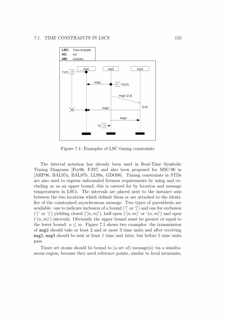
7.1. TIME CONSTRAINTS IN LSCS 155
Inst2
Act
LSC: Timer Example
InvariantAM:AC:
Inst3Inst1
msg2
T2
msg1
msg3
T2(12)
msg4
[2,3]
T1(7)
[1,5)
Figure 7.1: Examples of LSC timing constraints
The interval notation has already been used in Real-Time SymbolicTiming Diagrams [Fey96, FJ97] and also been proposed for MSC-96 in[AHP96, BAL97a, BAL97b, LL99a, GDO98]. Timing constraints in STDsare also used to express unbounded liveness requirements by using and ex-cluding ∞ as an upper bound; this is catered for by location and messagetemperatures in LSCs. The intervals are placed next to the instance axisbetween the two locations which delimit them or are attached to the identi-fier of the constrained asynchronous message. Two types of parenthesis areavailable: one to indicate inclusion of a bound (‘[’ or ‘]’) and one for exclusion(‘(’ or ‘)’) yielding closed (’[n,m]’), half-open (‘[n,m)’ or ‘(n,m]’) and open(‘(n,m)’) intervals. Obviously the upper bound must be greater or equal tothe lower bound: n ≤ m. Figure 7.1 shows two examples: the transmissionof msg2 should take at least 2 and at most 3 time units and after receivingmsg2, msg3 should be sent at least 1 time unit later, but before 5 time unitspass.
Timer set atoms should be bound to (a set of) message(s) via a simulta-neous region, because they need reference points, similar to local invariants,
156 CHAPTER 7. ADDING TIME
as pointed out in our criticism of MSCs in section 3.1.4 on page 57. The mosttypical use case for timers is that they are set when some event is observed,e.g. the receipt of a message, and some reaction is expected within a certainspan of time. The situation is slightly different for timeouts and timer resets:Timeouts are observable themselves, so that they need no reference point,but can rather act as reference points themselves. They can thus be used todelimit local invariants, conditions and other timer sets, and of course mes-sages. Timer resets can not be used as reference points, since they do notindicate a specific point in time. They may nevertheless be used in isolation,since this allows the expression of upper bounds: Since they indicate that theassociated timer has not yet expired, this means that the occurrence times ofall atoms between the timer set and reset occur before the timer expires. Thereference points of timing intervals are clear, since they are always bound totwo adjacent locations.
As figure 7.1 illustrates for T1, timer sets can be associated with an in-stance head in order to express timing constraints, which measure time fromthe point of activation. Timing intervals may also be attached to instanceheads just like they are attached to other locations.
Timing intervals, due to being constrained to two adjacent locations, areintended for local constraints, whereas timers are intended to range overlarger parts of an instance. Timers ranging over several instances are gen-erally conceivable, but require more care, since it is not immediately clear,if the timer is always set before it is queried. We thus constrain the use oftimer to one instance.
7.2 Formal Semantics
Before the unwinding algorithm is adapted to handle timer and timing in-tervals in section 7.2.2 these constructs are added to the abstract syntaxrepresentation in section 7.2.1.
7.2.1 Formal Syntax
Analogous to the atoms defined in section 6.1 on page 94 we introduce the fol-lowing sets for the timer atoms of LSC body l and instance i ∈ Instances(l),respectively:
• T imer Set(i), T imer Set(l) : sets of timer set atoms
7.2. FORMAL SEMANTICS 157
• T imer Reset(i), T imer Reset(l) : sets of timer reset atoms
• T imeouts(i), T imeouts(l) : sets of timeout atoms
We collect all timer related atoms in the sets
T imer(i) := T imer Set(i) ∪ T imer Reset(i) ∪ T imeouts(i)
T imer(l) := T imer Set(l) ∪ T imer Reset(l) ∪ T imeouts(l)
These sets have to be added to the set of atoms of an instance, resp. entireLSC body:
Atoms(i) := {⊥i} ∪Msgsnd(i) ∪Msgrcv(i) ∪Conds(i) ∪LI starts(i) ∪LI ends(i) ∪T imer(i)∪{⊤i}
Atoms(l) := Instheads(l) ∪Msgsnd(l) ∪Msgrcv(l) ∪Conds(l) ∪LI starts(l)∪LI ends(l) ∪T imer(l)∪Instends(l)
As for most other atoms it is necessary to be able to identify timers and maptimer atoms to their corresponding identifier. The set of timer identifiersis given by T imerIDs(l). Moreover, the duration of a timer needs to beknown. Timing intervals are not handled by atoms of their own, since theyare not observable entities to be unwound. Thus mappings from locationsand asynchronous message sendings to timing intervals are defined, whichprovide the information on upper and lower bounds and if they are inclusive.Timing intervals are attached to the location of the first cluster. There arethus the following functions:
158 CHAPTER 7. ADDING TIME
timID : T imer(l) −→ T imerIDs(l)
duration : T imerIDs(l) −→ N
lowBound : Locations(l) ∪AsyncMsgSnd(l) −→ ǫ ∪N
lowIncl : Locations(l) ∪AsyncMsgSnd(l) −→ B
upBound : Locations(l) ∪AsyncMsgSnd(l) −→ ǫ ∪N
upIncl : Locations(l) ∪AsyncMsgSnd(l) −→ B
The set AsyncMsgSnd(l) is the set of all asynchronous message sendatoms: {m ∈ Msgsnd(l) | sync type(msgID(m))) = async}. The functionslowBound(·) and upBound(·) give the lower, resp. upper bound of a timinginterval. They return ǫ, if there is no timing interval associated with thelocation or message. The functions lowIncl(·) and upIncl(·) return true, ifthe respective bound is inclusive.
Well-formedness Rules
1. Timer set atoms must be bound to a cluster of an observable atom.
2. A timer must be set before it expires or is reset.
3. For each timer set atom there is at most one reset or timeout atom.
4. The upper bound of a timing interval must be greater or equal to itslower bound.
The first rule is motivated by the fact that — similar to local invariants—there has to be a reference point for the start of a timer, as has been remarkedin section 3.1.4 on page 57. Note that a timeout atom can be a referencepoint, since it identifies a single point in time, whereas a timer reset can not.Timer resets may be used in isolation in order to specify a lower bound.
7.2. FORMAL SEMANTICS 159
7.2.2 The Timed Unwinding Algorithm
So far the semantics of the presented LSC elements were expressible in anuntimed symbolic automaton, whereas now we need the time properties in-troduced in section 5.3. The timed unwinding algorithm extends the onepresented in section 6.2.7 by incorporating the timing features introducedabove and producing a timed symbolic automaton. The general idea is toassociate a clock with every timer and timing interval, which is set to zerowhen the corresponding timer is set or the location of the timing interval isreached. When the timer is either reset or a timeout is observed or the loca-tion following the one with the timing interval is reached, a clock constraint isplaced on the corresponding transitions in the automaton, which reflects thenature and duration of the timer or timing interval. For a timeout atom thismeans that the value of the associated clock must be equal to the durationof the timer. For a timer reset atom the clock must be strictly less than thetimer duration, because no timeout has been observed so far, i.e. the clockmust not have reached its maximal value. For timing intervals the clock mustbe equal to or greater than the lower bound and less than or equal to theupper bound depending on the type of interval (open, closed). Note thattiming intervals and timer atoms which are bound via a simultaneous regionto some observable do not alter the structure of the TBA. Only when a timeratom occurs without a simultaneous region the structure is changed; then anew node and a new transition are inserted.
Recall from definition 5.8 on page 89 that a set C of clocks is needed fora timed symbolic automaton. We use variables z0, z1, . . . to denote clocks,with the number of clocks for an automaton being the sum of timer set atomsplus locations, which carry a timing interval annotation, plus the number ofasynchronous message send atoms, which are guarded by an interval.
Time Constraints and Exits
Clock constraints do not only influence the transitions, on which they ap-pear, they also have an impact on transitions to the exit state, which startin the same state as the constrained transition. Consider e.g. the LSC infigure 7.2 on the following page and the corresponding automaton shown infigure 7.3 on the next page. The clock z0 associated with the timing intervalis reset when observing msg1 and the transition from q1 to q2 is constrainedby a clock constraint corresponding to the interval. Additionally, the tran-
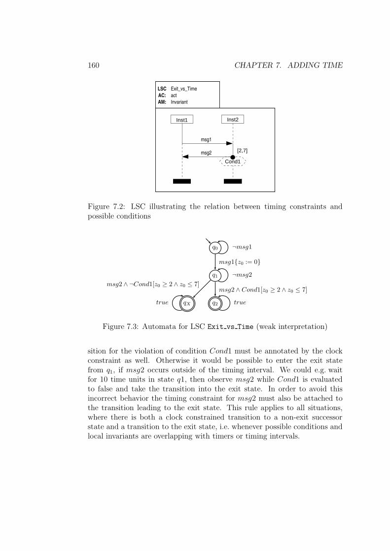
160 CHAPTER 7. ADDING TIME
AM: Invariant
AC: act
LSC Exit_vs_Time
Inst1 Inst2
msg1
msg2 [2,7]
Cond1
Figure 7.2: LSC illustrating the relation between timing constraints andpossible conditions
q0 ¬msg1
q1 ¬msg2
msg1{z0 := 0}
q2 true
msg2 ∧ Cond1[z0 ≥ 2 ∧ z0 ≤ 7]
qXtrue
msg2 ∧ ¬Cond1[z0 ≥ 2 ∧ z0 ≤ 7]
Figure 7.3: Automata for LSC Exit vs Time (weak interpretation)
sition for the violation of condition Cond1 must be annotated by the clockconstraint as well. Otherwise it would be possible to enter the exit statefrom q1, if msg2 occurs outside of the timing interval. We could e.g. waitfor 10 time units in state q1, then observe msg2 while Cond1 is evaluatedto false and take the transition into the exit state. In order to avoid thisincorrect behavior the timing constraint for msg2 must also be attached tothe transition leading to the exit state. This rule applies to all situations,where there is both a clock constrained transition to a non-exit successorstate and a transition to the exit state, i.e. whenever possible conditions andlocal invariants are overlapping with timers or timing intervals.
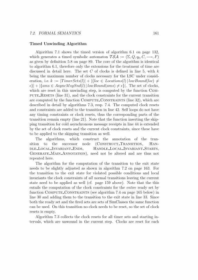
7.2. FORMAL SEMANTICS 161
Timed Unwinding Algorithm
Algorithm 7.1 shows the timed version of algorithm 6.1 on page 132,which generates a timed symbolic automaton T SA := (Σ, Q, q0, C,−→, F )as given by definition 5.8 on page 89. The core of the algorithm is identicalto algorithm 6.1, therefore only the extensions for the treatment of time arediscussed in detail here. The set C of clocks is defined in line 5, with kbeing the maximum number of clocks necessary for the LSC under consid-eration, i.e. k := |T imerSets(l)| + |{loc ∈ Locations(l) | lowBound(loc) 6=ǫ}| + |{ams ∈ AsyncMsgSnd(l) | lowBound(ams) 6= ǫ}|. The set of clocks,which are reset in this unwinding step, is computed by the function Com-pute Resets (line 31), and the clock constraints for the current transitionare computed by the function Compute Constraints (line 32), which aredescribed in detail by algorithms 7.3, resp. 7.4. The computed clock resetsand constraints are added to the transition in line 42. Self loops do not haveany timing constraints or clock resets, thus the corresponding parts of thetransition remain empty (line 21). Note that the function inserting the skip-ping transition for cold asynchronous message receipts in line 44 is extendedby the set of clock resets and the current clock constraints, since these haveto be applied to the skipping transition as well.
The algorithms, which construct the annotation of the tran-sition to the successor node (Construct Transition, Han-dle Local Invariant Ends, Handle Local Invariant Starts,Generate Main Annotation), need not be altered and are thus notrepeated here.
The algorithm for the computation of the transition to the exit stateneeds to be slightly adjusted as shown in algorithm 7.2 on page 163. Forthe transition to the exit state for violated possible conditions and localinvariants the clock constraints of all normal transitions leaving the currentstate need to be applied as well (cf. page 159 above). Note that the thisentails the computation of the clock constraints for the entire ready set byfunction Compute Constraints (see algorithm 7.4 on page 165 below) inline 30 and adding them to the transition to the exit state in line 33. Sinceboth the ready set and the fired sets are sets of SimClasses the same functioncan be used. On this transition no clock needs to be reset, so the set of clockresets is empty.
Algorithm 7.3 collects the clock resets for all timer sets and starting in-tervals, which are unwound in the current step. Clocks are reset for each
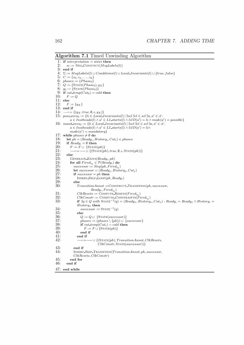
162 CHAPTER 7. ADDING TIME
Algorithm 7.1 Timed Unwinding Algorithm1: if interpretation = strict then
2: sc := Neg Conjunct(MsgLabels(l))3: end if
4: Σ := MsgLabels(l) ∪ Conditions(l) ∪ Local Invariants(l) ∪ {true, false}5: C := {z0, z1, . . . , zk}6: phases := {Phase0}7: Q := {State(Phase0), qX}8: q0 := {State(Phase0)}9: if cut temp(Cut0) = cold then
10: F := Q
11: else
12: F := {qX}13: end if
14: −→:= {(qX , true, ∅, ǫ, qX)}15: poss invs0 := {li ∈ Local Invariants(l) | ∃scl ∃cl ∈ scl ∃a, a′ ∈ cl :
a ∈ Instheads(l) ∧ a′ ∈ LI starts(l) ∧ liID(a′) = li ∧ mode(a′) = possible}16: mand invs0 := {li ∈ Local Invariants(l) | ∃scl ∃cl ∈ scl ∃a, a′ ∈ cl :
a ∈ Instheads(l) ∧ a′ ∈ LI starts(l) ∧ liID(a′) = li∧mode(a′) = mandatory}
17: while phases 6= ∅ do
18: let ph = (Readyi, Historyi, Cuti) ∈ phases
19: if Readyi = ∅ then
20: F := F ∪ {State(ph)}21: −→:=−→ ∪ {(State(ph), true, ∅, ǫ,State(ph))}22: else
23: Generate Exits(Readyi , ph)24: for all F iredik
∈ P(Readyi) do
25: successor := Step(ph,F iredik)
26: let successor = (Readyj , Historyj , Cutj)27: if successor = ph then
28: Insert Self Loop(ph, Readyi)29: else
30: TransitionAnnot :=Construct Transition(ph, successor,
Readyi, F iredik)
31: ClkResets := Compute Resets(F iredik)
32: ClkConstr := Compute Constraints(F iredik)
33: if ∃q ∈ Q with State−1(q) = (Readyx, Historyx, Cutx) : Readyi = Readyx ∧ Historyi =Historyx then
34: successor := State−1(q)35: else
36: Q := Q ∪ {State(successor)}37: phases := (phases \ {ph}) ∪ {successor}38: if cut temp(Cuti) = cold then
39: F := F ∪ {State(ph)}40: end if
41: end if
42: −→:=−→ ∪ {(State(ph), T ransitionAnnot, ClkResets,
ClkConstr,State(successor))}43: end if
44: Insert Skip Transition(TransitionAnnot, ph, successor,
ClkResets, ClkConstr)45: end for
46: end if
47: end while
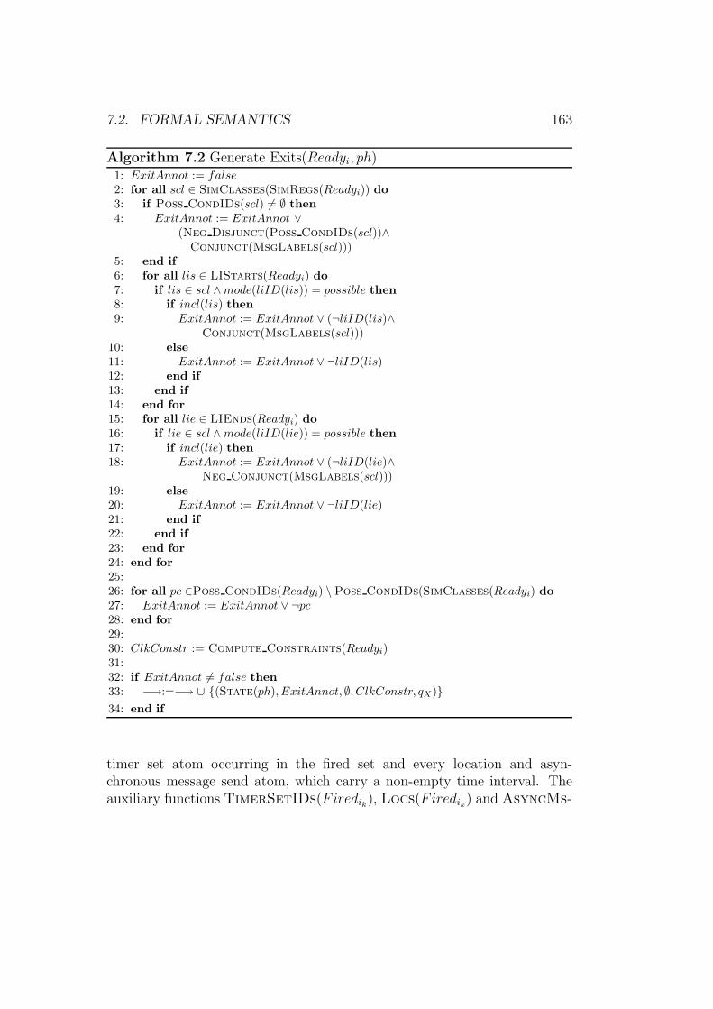
7.2. FORMAL SEMANTICS 163
Algorithm 7.2 Generate Exits(Readyi, ph)1: ExitAnnot := false
2: for all scl ∈ SimClasses(SimRegs(Readyi)) do
3: if Poss CondIDs(scl) 6= ∅ then
4: ExitAnnot := ExitAnnot ∨(Neg Disjunct(Poss CondIDs(scl))∧
Conjunct(MsgLabels(scl)))5: end if
6: for all lis ∈ LIStarts(Readyi) do
7: if lis ∈ scl ∧mode(liID(lis)) = possible then
8: if incl(lis) then
9: ExitAnnot := ExitAnnot ∨ (¬liID(lis)∧Conjunct(MsgLabels(scl)))
10: else
11: ExitAnnot := ExitAnnot ∨ ¬liID(lis)12: end if
13: end if
14: end for
15: for all lie ∈ LIEnds(Readyi) do
16: if lie ∈ scl ∧mode(liID(lie)) = possible then
17: if incl(lie) then
18: ExitAnnot := ExitAnnot ∨ (¬liID(lie)∧Neg Conjunct(MsgLabels(scl)))
19: else
20: ExitAnnot := ExitAnnot ∨ ¬liID(lie)21: end if
22: end if
23: end for
24: end for
25:26: for all pc ∈Poss CondIDs(Readyi) \ Poss CondIDs(SimClasses(Readyi) do
27: ExitAnnot := ExitAnnot ∨ ¬pc28: end for
29:30: ClkConstr := Compute Constraints(Readyi)31:32: if ExitAnnot 6= false then
33: −→:=−→ ∪ {(State(ph), ExitAnnot, ∅, ClkConstr, qX)}
34: end if
timer set atom occurring in the fired set and every location and asyn-chronous message send atom, which carry a non-empty time interval. Theauxiliary functions TimerSetIDs(Firedik), Locs(Firedik) and AsyncMs-
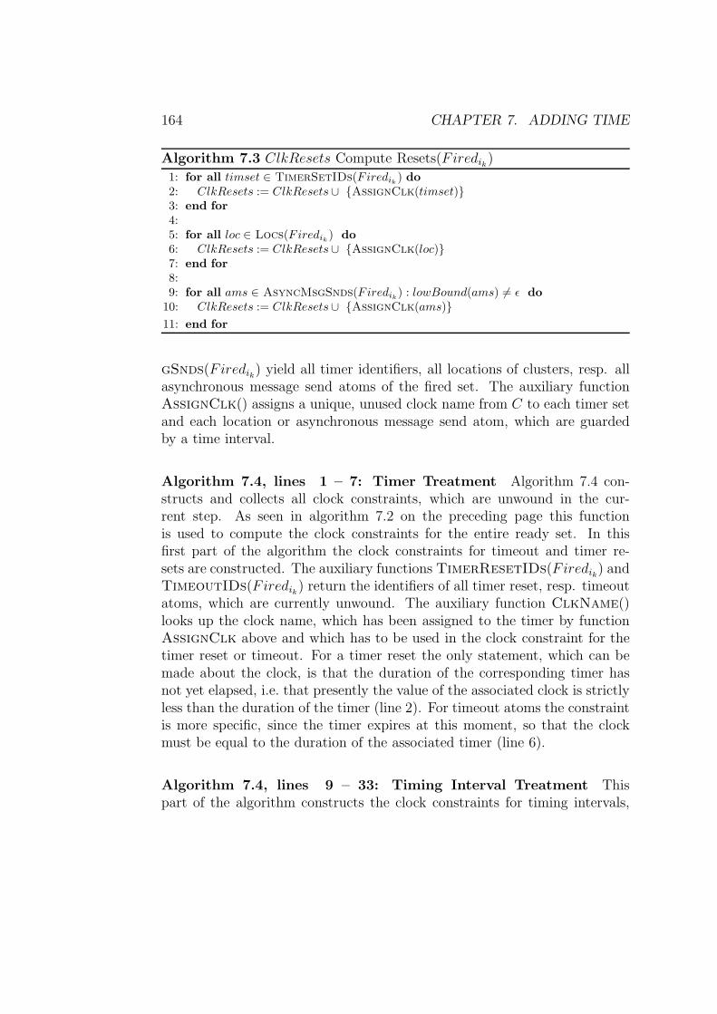
164 CHAPTER 7. ADDING TIME
Algorithm 7.3 ClkResets Compute Resets(Firedik)
1: for all timset ∈ TimerSetIDs(Firedik) do
2: ClkResets := ClkResets∪ {AssignClk(timset)}3: end for
4:5: for all loc ∈ Locs(Firedik
) do
6: ClkResets := ClkResets∪ {AssignClk(loc)}7: end for
8:9: for all ams ∈ AsyncMsgSnds(Firedik
) : lowBound(ams) 6= ǫ do
10: ClkResets := ClkResets∪ {AssignClk(ams)}
11: end for
gSnds(Firedik) yield all timer identifiers, all locations of clusters, resp. allasynchronous message send atoms of the fired set. The auxiliary functionAssignClk() assigns a unique, unused clock name from C to each timer setand each location or asynchronous message send atom, which are guardedby a time interval.
Algorithm 7.4, lines 1 – 7: Timer Treatment Algorithm 7.4 con-structs and collects all clock constraints, which are unwound in the cur-rent step. As seen in algorithm 7.2 on the preceding page this functionis used to compute the clock constraints for the entire ready set. In thisfirst part of the algorithm the clock constraints for timeout and timer re-sets are constructed. The auxiliary functions TimerResetIDs(Firedik) andTimeoutIDs(Firedik) return the identifiers of all timer reset, resp. timeoutatoms, which are currently unwound. The auxiliary function ClkName()looks up the clock name, which has been assigned to the timer by functionAssignClk above and which has to be used in the clock constraint for thetimer reset or timeout. For a timer reset the only statement, which can bemade about the clock, is that the duration of the corresponding timer hasnot yet elapsed, i.e. that presently the value of the associated clock is strictlyless than the duration of the timer (line 2). For timeout atoms the constraintis more specific, since the timer expires at this moment, so that the clockmust be equal to the duration of the associated timer (line 6).
Algorithm 7.4, lines 9 – 33: Timing Interval Treatment Thispart of the algorithm constructs the clock constraints for timing intervals,
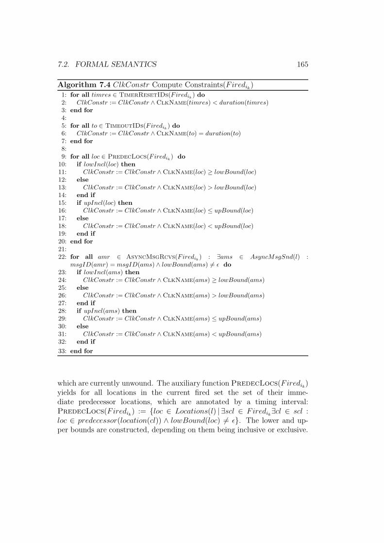
7.2. FORMAL SEMANTICS 165
Algorithm 7.4 ClkConstr Compute Constraints(Firedik)
1: for all timres ∈ TimerResetIDs(Firedik) do
2: ClkConstr := ClkConstr ∧ ClkName(timres) < duration(timres)3: end for
4:5: for all to ∈ TimeoutIDs(Firedik
) do
6: ClkConstr := ClkConstr ∧ ClkName(to) = duration(to)7: end for
8:9: for all loc ∈ PredecLocs(Firedik
) do
10: if lowIncl(loc) then
11: ClkConstr := ClkConstr ∧ ClkName(loc) ≥ lowBound(loc)12: else
13: ClkConstr := ClkConstr ∧ ClkName(loc) > lowBound(loc)14: end if
15: if upIncl(loc) then
16: ClkConstr := ClkConstr ∧ ClkName(loc) ≤ upBound(loc)17: else
18: ClkConstr := ClkConstr ∧ ClkName(loc) < upBound(loc)19: end if
20: end for
21:22: for all amr ∈ AsyncMsgRcvs(Firedik
) : ∃ams ∈ AsyncMsgSnd(l) :msgID(amr) = msgID(ams) ∧ lowBound(ams) 6= ǫ do
23: if lowIncl(ams) then
24: ClkConstr := ClkConstr ∧ ClkName(ams) ≥ lowBound(ams)25: else
26: ClkConstr := ClkConstr ∧ ClkName(ams) > lowBound(ams)27: end if
28: if upIncl(ams) then
29: ClkConstr := ClkConstr ∧ ClkName(ams) ≤ upBound(ams)30: else
31: ClkConstr := ClkConstr ∧ ClkName(ams) < upBound(ams)32: end if
33: end for
which are currently unwound. The auxiliary function PredecLocs(Firedik)yields for all locations in the current fired set the set of their imme-diate predecessor locations, which are annotated by a timing interval:PredecLocs(Firedik) := {loc ∈ Locations(l) | ∃scl ∈ Firedik∃cl ∈ scl :loc ∈ predecessor(location(cl)) ∧ lowBound(loc) 6= ǫ}. The lower and up-per bounds are constructed, depending on them being inclusive or exclusive.
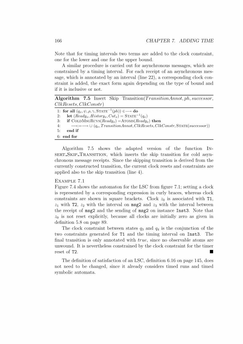
166 CHAPTER 7. ADDING TIME
Note that for timing intervals two terms are added to the clock constraint,one for the lower and one for the upper bound.
A similar procedure is carried out for asynchronous messages, which areconstrained by a timing interval. For each receipt of an asynchronous mes-sage, which is annotated by an interval (line 22), a corresponding clock con-straint is added, the exact form again depending on the type of bound andif it is inclusive or not.
Algorithm 7.5 Insert Skip Transition(TransitionAnnot, ph, successor,ClkResets, ClkConstr)
1: for all (qx, ψ, ρ, γ,State−1(ph)) ∈−→ do
2: let (Readyx, Historyx, Cutx) = State−1(qx)3: if ColdMsgRcvs(Readyx) =Atoms(Readyx) then
4: −→:=−→ ∪ (qx, T ransitionAnnot, ClkResets, ClkConstr,State(successor))5: end if
6: end for
Algorithm 7.5 shows the adapted version of the function In-sert Skip Transition, which inserts the skip transition for cold asyn-chronous message receipts. Since the skipping transition is derived from thecurrently constructed transition, the current clock resets and constraints areapplied also to the skip transition (line 4).
Example 7.1Figure 7.4 shows the automaton for the LSC from figure 7.1; setting a clockis represented by a corresponding expression in curly braces, whereas clockconstraints are shown in square brackets. Clock z0 is associated with T1,z1 with T2, z2 with the interval on msg2 and z3 with the interval betweenthe receipt of msg2 and the sending of msg2 on instance Inst3. Note thatz0 is not reset explicitly, because all clocks are initially zero as given indefinition 5.8 on page 89.
The clock constraint between states q3 and q4 is the conjunction of thetwo constraints generated for T1 and the timing interval on Inst3. Thefinal transition is only annotated with true, since no observable atoms areunwound. It is nevertheless constrained by the clock constraint for the timerreset of T2. �
The definition of satisfaction of an LSC, definition 6.16 on page 145, doesnot need to be changed, since it already considers timed runs and timedsymbolic automata.
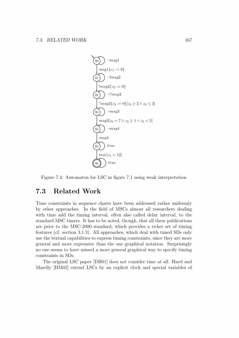
7.3. RELATED WORK 167
q0 ¬msg1
q1 ¬!msg2
msg1{z1 := 0}
q2 ¬?msg2
!msg2{z2 := 0}
q3 ¬msg3
?msg2{z3 := 0}[z2 ≥ 2 ∧ z2 ≤ 3]
q4 ¬msg4
msg3[z0 = 7 ∧ z3 ≥ 1 ∧ z3 < 5]
q5 true
msg4
q6 true
true[z1 < 12]
Figure 7.4: Automaton for LSC in figure 7.1 using weak interpretation
7.3 Related Work
Time constraints in sequence charts have been addressed rather uniformlyby other approaches. In the field of MSCs almost all researchers dealingwith time add the timing interval, often also called delay interval, to thestandard MSC timers. It has to be noted, though, that all these publicationsare prior to the MSC-2000 standard, which provides a richer set of timingfeatures (cf. section 3.1.3). All approaches, which deal with timed SDs onlyuse the textual capabilities to express timing constraints, since they are moregeneral and more expressive than the one graphical notation. Surprisinglyno one seems to have missed a more general graphical way to specify timingconstraints in SDs.
The original LSC paper [DH01] does not consider time at all. Harel andMarelly [HM02] extend LSCs by an explicit clock and special variables of
168 CHAPTER 7. ADDING TIME
domain time. Time variables are assigned the current clock value and can bequeried within conditions. Their approach is similar to the one we propose forspecifying timing constraints in terms of supersteps in Statemate’s asyn-chronous semantics (cf. section 11.3), except that their counter is unbounded,which is unsuitable for model checking. By using conditions [HM02] areable to encode complex timing constraints more concisely. The distinctionbetween mandatory and possible conditions allows to specify assumptionsabout the time behavior of the environment with the same effect as plac-ing timing constraints on the environment axis in our LSCs (cf. chapter 8).However, we feel that our graphical representation of timing constraints ismore intuitive.
Alur et al. [AHP96] extend MSC-96 by time intervals on subsequent lo-cations and (asynchronous) messages, but do not provide a formal semanticsfor either untimed or timed MSCs. Infinity is allowed as an upper bound,thus allowing to specify unbounded liveness, which is covered by locationand message temperatures in our approach. The focus of this article is theanalysis of MSCs, including the checking for timing consistency. The usedmethod is a conversion of the MSC into a graph, whose nodes are the events(atoms in LSC terminology) of the MSC. Edges are inserted for all timing an-notations, with unannotated messages and instance segments being assignedthe default interval (0,∞), and weighted according to the upper bounds forthe occurrence of each pair of events. Timing consistency is then checkedby computing negative cost cycles in this graph, where the existence of anegative cost cycle between two events means that there is no run, whichcan fulfill the timing constraints imposed by the MSC. This kind of checkcorresponds to the existential verification of LSCs (cf. chapter 10).
Leue and Ben-Abdallah [BAL97a, BAL97b] use the same approach as[AHP96] for basic MSCs and extend it to HMSCs by checking every path,i.e. every possible concatenation of basic MSCs in the HMSC graph, for tim-ing consistency. All three approaches also consider other consistency checksmore concerned with implementation issues, e.g. detection of process diver-gence, influence of queuing strategies, etc.
Grabowski et al. [GDO98] also extend MSC-96 by time intervals and de-fine the semantics in terms of Duration Calculus formulae via translation ofMSCs into a set of Constraint Diagrams. They also allow to express un-bounded liveness by assuming a default interval of (0,∞) between orderedevents. The time model is dense time.
7.3. RELATED WORK 169
Lilius and Li [LL99a] do not provide a formal semantics for MSCs, butrather check, if an MSC is timing consistent or not. Each timing constraint,expressed by a timer or an interval, is translated into a linear inequality, thusyielding a set of linear inequalities. The problem of checking, if all timingannotations of the MSC are consistent, is then reduced to finding a solutionfor this group of linear inequalities, which can be solved efficiently by linearprogramming. The MSC is timing consistent, if a solution exists. [LL99a]deal with HMSCs in the same manner as [BAL97a, BAL97b]. The sameapproach is applied to Sequence Diagrams in [LL99b].
Firley et al. [FHD+99] also propose a timing consistency check for SDsvia translation into timed automata, which can be analyzed by the UPPAALmodel checker. The timing annotations used are the textual ones proposed inthe UML standard [OMG01], i.e. labels are used to identify message send andreceive events and from these labels textual constraints are formulated. Thetiming constraints result in clocks, which are reset and queried, in the timedautomaton, similar to timed symbolic automata. As detailed in section 6.4 onpage 149 UPPAAL is employed to find out, if it is possible to reach thefinal state of the timed automaton constructed from the SD. This procedurecorresponds to the formal verification of existential LSCs we propose.
Seemann and von Gudenberg [SvG98] also use SD-style textual timingconstraints and check SDs for timing consistency, but use the negative costcycle procedure of [AHP96].

170 CHAPTER 7. ADDING TIME
Chapter 8
Integrated Assumption
Treatment
Modern computer systems typically are not stand-alone installations, butare deployed in a certain context. The train control system which serves asour running example e.g. relies on input from sensors like the informationthat the train has passed the crossing. On the other hand it controls otherentities external to the currently developed ones, like the train brake or thebarrier. Thus a system is developed with this context or environment inmind. Typically, assumptions about the possible values and combination ofinput signals in this environment are made. For the crossing we e.g. assumethat the barrier can not be simultaneously open and closed. The environmentcan represent a number of things:
• Other soft- or hardware components, which are either part of the devel-oped system or are completely external. The communication channelfor instance belongs to the environment, if we look at the train in iso-lation, but it still belongs to the system under design. The operationcenter on the other hand is an external environmental component.
• Sensors or actuators which gather information, resp. affect the realworld.
• Persons, which interact with the system.
When verifying a system under design, the model checker plays the roleof the environment and supplies the inputs of the model. Since the model
171
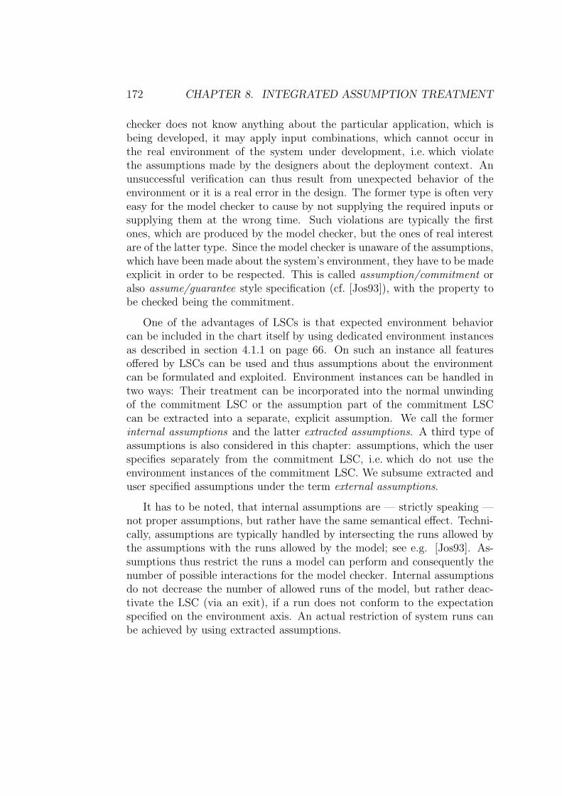
172 CHAPTER 8. INTEGRATED ASSUMPTION TREATMENT
checker does not know anything about the particular application, which isbeing developed, it may apply input combinations, which cannot occur inthe real environment of the system under development, i.e. which violatethe assumptions made by the designers about the deployment context. Anunsuccessful verification can thus result from unexpected behavior of theenvironment or it is a real error in the design. The former type is often veryeasy for the model checker to cause by not supplying the required inputs orsupplying them at the wrong time. Such violations are typically the firstones, which are produced by the model checker, but the ones of real interestare of the latter type. Since the model checker is unaware of the assumptions,which have been made about the system’s environment, they have to be madeexplicit in order to be respected. This is called assumption/commitment oralso assume/guarantee style specification (cf. [Jos93]), with the property tobe checked being the commitment.
One of the advantages of LSCs is that expected environment behaviorcan be included in the chart itself by using dedicated environment instancesas described in section 4.1.1 on page 66. On such an instance all featuresoffered by LSCs can be used and thus assumptions about the environmentcan be formulated and exploited. Environment instances can be handled intwo ways: Their treatment can be incorporated into the normal unwindingof the commitment LSC or the assumption part of the commitment LSCcan be extracted into a separate, explicit assumption. We call the formerinternal assumptions and the latter extracted assumptions. A third type ofassumptions is also considered in this chapter: assumptions, which the userspecifies separately from the commitment LSC, i.e. which do not use theenvironment instances of the commitment LSC. We subsume extracted anduser specified assumptions under the term external assumptions.
It has to be noted, that internal assumptions are — strictly speaking —not proper assumptions, but rather have the same semantical effect. Techni-cally, assumptions are typically handled by intersecting the runs allowed bythe assumptions with the runs allowed by the model; see e.g. [Jos93]. As-sumptions thus restrict the runs a model can perform and consequently thenumber of possible interactions for the model checker. Internal assumptionsdo not decrease the number of allowed runs of the model, but rather deac-tivate the LSC (via an exit), if a run does not conform to the expectationspecified on the environment axis. An actual restriction of system runs canbe achieved by using extracted assumptions.
8.1. INTERNAL ASSUMPTIONS 173
Internal assumptions are presented in section 8.1, while external assump-tions are discussed in section 8.2, with extracted assumptions being the focusin section 8.2.1 and user specified ones in section 8.2.2. The semantics of anLSC with associated external assumptions is defined in section 8.3. Thischapter closes with a review of related work in section 8.4.
8.1 Internal Assumptions
Internal assumptions aim at not allowing the model checker to violate anLSC specification by simply applying unexpected inputs. The expected en-vironment behavior is specified by the user on the dedicated environmentinstances using the normal LSC features (cf. section 4.1.1 on page 66). Theway to achieve this goal is to treat wrong behaviors of the environment not aserrors, but as a deactivation of the LSC, i.e. if the environment does not con-form to the expected behavior (as given by the elements on the environmentinstance axes), this is treated as an exit from the LSC, similar to possibleconditions or possible local invariants. Thus the model checker has to fulfillthe assumptions expressed on the environment instances in order to progressthrough the automaton and possibly find a real error in the model.
Barrier Crossing
AM: Invariant
AC: Lights_on
LSC securing_barrier
lower
close_barrier
barrier_closed
closed
Env
[1,1]
Figure 8.1: LSC for the Crossing component specifying the barrier closing
Figure 8.1 shows an example from the train control system case study: theprotocol for successfully closing the barrier. Once the lights have been turned
174 CHAPTER 8. INTEGRATED ASSUMPTION TREATMENT
on (AC: Lights on) the crossing controller instructs the barrier controller toclose the barrier, which in turn sends the signal to the barrier actuator, whichis part of the environment. As is indicated by the hot part of the environmentaxis and the attached timing interval, the barrier is expected to be closedafter one time unit and this result must be reported back to the crossingcontroller. The environment axis thus expresses the assumption that thebarrier is operational and closes in time. Making the LSC robust against amisbehaving environment in this case means that the LSC is deactivated, ifthe closed message does not arrive at all or not within the given interval(which would typically be captured in a seprate LSC). The special treatmentnecessary for each LSC element defined on the environment instance is listedin the following:
instantaneous messages Need no special treatment, since it is either ob-served or not. The occurrence of an instantaneous message can berequired only by a hot location temperature. In the strict interpreta-tion messages sent by the environment must not result in an error, ifthey occur at a time when they are not supposed to. The correct treat-ment rather is to exit from the LSC. This means that for each state inthe automaton, where such a message is not supposed to be observed,a transition to the exit state must be added.
asynchronous messages sent from the environment Need no specialtreatment. As for instantaneous messages the location temperatureindicates, if a message must be sent. The message temperature is al-ways hot, since an assumption about a message, which need not arrive,is useless. In the strict interpretation the same treatment as for instan-taneous messages is necessary.
asynchronous messages received by the environment The messagetemperature is set to cold, because the environment can not be forcedto receive the message. In the strict interpretation the same treatmentas for the previous message types is necessary.
conditions All conditions on the environment instance are treated as pos-sible ones, since the environment can not be forced to satisfy a givencondition. Thus, exits are inserted into the automaton for all conditionsdefined on the environment axis regardless of their mode.
8.1. INTERNAL ASSUMPTIONS 175
local invariants They are treated as possible ones, analogously to condi-tions.
timer and timing intervals Timing constraints of the environment, whichare violated, are treated as exits from the LSC. This means that addi-tional transitions to the exit node are inserted into the automaton andare annotated by the negation of the constraints.
Recall that timing intervals of the form [n,m] constrain two clusters,e.g. two messages, and translate into a clock constraint of the form[z3 ≥ n∧z3 ≤ m] in the automaton. This timing annotation is violated,if the second atom, e.g. msgX occurs either too early or too late, whichtranslates into the following annotation for the transition to the exitstate: msgX[z3 < n ∨ z3 > m]. Open and half-open timing intervalsare treated analogously.
Timeouts result in clock constraints of the form [z1 = dur], where duris the duration given for the timer. Assuming that the timeout is boundto some message msgX this leads to an annotation of the correspondingexit transition of msgX[z1 < dur ∨ z1 > dur]. Timer resets result inclock constraints of the form [z1 < dur], which leads to an annotationof the corresponding exit transition of msgX[z1 ≥ dur].
location temperatures Location temperatures are set to cold, becauseprogress of the environment can not be enforced. The system underdevelopment can e.g. not force the environment to respond to a request;this requires an explicit assumption (see section 8.2.1 on page 195 be-low).
simultaneous regions A simultaneous region is violated, if not all mes-sages of this region are observed simultaneously; other LSC elementsare already taken care of by the procedures described above. Thus,whenever only a strict subset of messages of the simultaneous regionis observed, this should result in an exit, if one of the missing mes-sages should have been sent by the environment. The same treatmentis necessary for simultaneous regions, which are not defined on the en-vironment axis, but which contain messages sent by the environment.
coregions No special treatment necessary.
176 CHAPTER 8. INTEGRATED ASSUMPTION TREATMENT
8.1.1 Adjustment of the Formal Semantics
Since the treatment of LSC elements differs depending on the type of instanceaxis (environment or normal) they appear on, this information has to bemade available to the unwinding algorithm. This is done by the functionenvInst(·), which returns true, if an instance is an environment instanceand false, if it is a normal instance:
envInst : Instances(l) −→ B
For convenience’s sake similar functions are defined for atoms, resp. clustersof each instance:
isEnv : Atoms(i) −→ B
isEnv(a) :=
{
true if envInst(i) = true
false else, a ∈ Atoms(i)
isEnv : Clusters(i) −→ B
isEnv(cl) :=
{
true if ∃a ∈ cl : isEnv(a) = true
false else, cl ∈ Clusters(i)
Since hot location temperatures on the environment instance must betreated as cold, the computation of the cut temperature has to be adjustedaccordingly. This ensures that the model checker can not violate the propertysimply by doing nothing, provided progress only hinges on the environmentinstance(s). If progress is additionally required by the commitment part ofthe LSC, then this may still result in a violation depending on the systembehavior. This exemplifies the benefit of assigned a hot temperature only tothose locations of an LSC, which are actually responsible for progressing.
Thus the function cut temp(·) (cf. definition 6.11 on page 117), whichcomputes the cut temperature and thus determines the set of fair states,is extended in the following manner: A hot location temperature is onlyregarded, if the location is not situated on the environment instance.
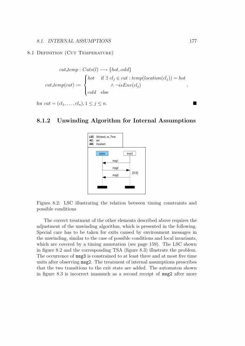
8.1. INTERNAL ASSUMPTIONS 177
8.1 Definition (Cut Temperature)
cut temp : Cuts(l) −→ {hot, cold}
cut temp(cut) :=
hot if ∃ clj ∈ cut : temp(location(clj)) = hot
∧ ¬isEnv(clj)
cold else
,
for cut = (cl1, . . . , cln), 1 ≤ j ≤ n. �
8.1.2 Unwinding Algorithm for Internal Assumptions
ENV Inst1
AM: Invariant
AC: act
LSC Strictexit_vs_Time
msg1
msg2
msg3[3,5]
Figure 8.2: LSC illustrating the relation between timing constraints andpossible conditions
The correct treatment of the other elements described above requires theadjustment of the unwinding algorithm, which is presented in the following.Special care has to be taken for exits caused by environment messages inthe unwinding, similar to the case of possible conditions and local invariants,which are covered by a timing annotation (see page 159). The LSC shownin figure 8.2 and the corresponding TSA (figure 8.3) illustrate the problem.The occurrence of msg3 is constrained to at least three and at most five timeunits after observing msg2. The treatment of internal assumptions prescribesthat the two transitions to the exit state are added. The automaton shownin figure 8.3 is incorrect inasmuch as a second receipt of msg2 after more
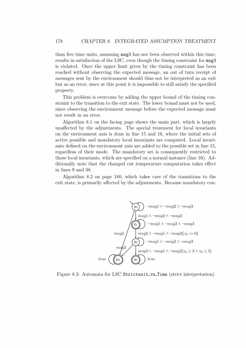
178 CHAPTER 8. INTEGRATED ASSUMPTION TREATMENT
than five time units, assuming msg3 has not been observed within this time,results in satisfaction of the LSC, even though the timing constraint for msg3is violated. Once the upper limit given by the timing constraint has beenreached without observing the expected message, an out of turn receipt ofmessages sent by the environment should thus not be interpreted as an exitbut as an error, since at this point it is impossible to still satisfy the specifiedproperty.
This problem is overcome by adding the upper bound of the timing con-straint to the transition to the exit state. The lower bound must not be used,since observing the environment message before the expected message mustnot result in an error.
Algorithm 8.1 on the facing page shows the main part, which is largelyunaffected by the adjustments. The special treatment for local invariantson the environment axis is done in line 15 and 16, where the initial sets ofactive possible and mandatory local invariants are computed. Local invari-ants defined on the environment axis are added to the possible set in line 15,regardless of their mode. The mandatory set is consequently restricted tothose local invariants, which are specified on a normal instance (line 16). Ad-ditionally note that the changed cut temperature computation takes effectin lines 9 and 38.
Algorithm 8.2 on page 180, which takes care of the transitions to theexit state, is primarily affected by the adjustments. Because mandatory con-
q0 ¬msg1 ∧ ¬msg2 ∧ ¬msg3
q1 ¬msg1 ∧ ¬msg2 ∧ ¬msg3
msg1 ∧ ¬msg2 ∧ ¬msg3
q2 ¬msg1 ∧ ¬msg2 ∧ ¬msg3
msg2 ∧ ¬msg1 ∧ ¬msg3{z0 := 0}
q3 true
msg3 ∧ ¬msg1 ∧ ¬msg2[z0 ≥ 3 ∧ z0 ≤ 5]
qXtrue
msg2
msg2
Figure 8.3: Automata for LSC Strictexit vs Time (strict interpretation)
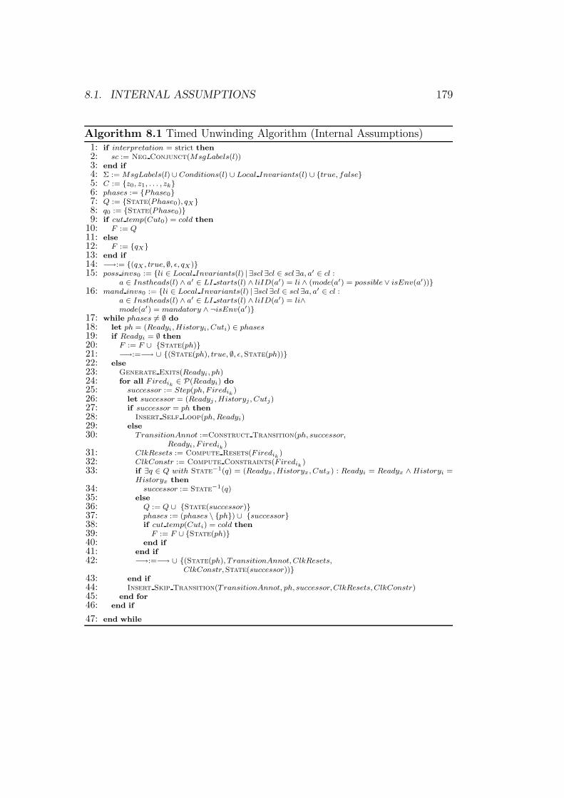
8.1. INTERNAL ASSUMPTIONS 179
Algorithm 8.1 Timed Unwinding Algorithm (Internal Assumptions)1: if interpretation = strict then
2: sc := Neg Conjunct(MsgLabels(l))3: end if
4: Σ := MsgLabels(l) ∪ Conditions(l) ∪ Local Invariants(l) ∪ {true, false}5: C := {z0, z1, . . . , zk}6: phases := {Phase0}7: Q := {State(Phase0), qX}8: q0 := {State(Phase0)}9: if cut temp(Cut0) = cold then
10: F := Q
11: else
12: F := {qX}13: end if
14: −→:= {(qX , true, ∅, ǫ, qX)}15: poss invs0 := {li ∈ Local Invariants(l) | ∃scl ∃cl ∈ scl ∃a, a′ ∈ cl :
a ∈ Instheads(l) ∧ a′ ∈ LI starts(l) ∧ liID(a′) = li ∧ (mode(a′) = possible ∨ isEnv(a′))}16: mand invs0 := {li ∈ Local Invariants(l) | ∃scl ∃cl ∈ scl∃a, a′ ∈ cl :
a ∈ Instheads(l) ∧ a′ ∈ LI starts(l) ∧ liID(a′) = li∧mode(a′) = mandatory ∧ ¬isEnv(a′)}
17: while phases 6= ∅ do
18: let ph = (Readyi, Historyi, Cuti) ∈ phases
19: if Readyi = ∅ then
20: F := F ∪ {State(ph)}21: −→:=−→ ∪ {(State(ph), true, ∅, ǫ,State(ph))}22: else
23: Generate Exits(Readyi, ph)24: for all F iredik
∈ P(Readyi) do
25: successor := Step(ph,F iredik)
26: let successor = (Readyj , Historyj , Cutj)27: if successor = ph then
28: Insert Self Loop(ph, Readyi)29: else
30: TransitionAnnot :=Construct Transition(ph, successor,
Readyi, F iredik)
31: ClkResets := Compute Resets(F iredik)
32: ClkConstr := Compute Constraints(F iredik)
33: if ∃q ∈ Q with State−1(q) = (Readyx , Historyx, Cutx) : Readyi = Readyx ∧ Historyi =Historyx then
34: successor := State−1(q)35: else
36: Q := Q ∪ {State(successor)}37: phases := (phases \ {ph}) ∪ {successor}38: if cut temp(Cuti) = cold then
39: F := F ∪ {State(ph)}40: end if
41: end if
42: −→:=−→ ∪ {(State(ph), T ransitionAnnot, ClkResets,
ClkConstr,State(successor))}43: end if
44: Insert Skip Transition(TransitionAnnot, ph, successor,ClkResets, ClkConstr)45: end for
46: end if
47: end while
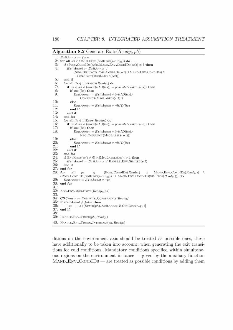
180 CHAPTER 8. INTEGRATED ASSUMPTION TREATMENT
Algorithm 8.2 Generate Exits(Readyi, ph)1: ExitAnnot := false
2: for all scl ∈ SimClasses(SimRegs(Readyi)) do
3: if (Poss CondIDs(scl)∪Mand Env CondIDs(scl)) 6= ∅ then
4: ExitAnnot := ExitAnnot ∨(Neg Disjunct(Poss CondIDs(scl) ∪ Mand Env CondIDs)∧
Conjunct(MsgLabels(scl)))5: end if
6: for all lis ∈ LIStarts(Readyi) do
7: if lis ∈ scl ∧ (mode(liID(lis)) = possible ∨ isEnv(lis)) then
8: if incl(lis) then
9: ExitAnnot := ExitAnnot ∨ (¬liID(lis)∧Conjunct(MsgLabels(scl)))
10: else
11: ExitAnnot := ExitAnnot ∨ ¬liID(lis)12: end if
13: end if
14: end for
15: for all lie ∈ LIEnds(Readyi) do
16: if lie ∈ scl ∧ (mode(liID(lie)) = possible ∨ isEnv(lie)) then
17: if incl(lie) then
18: ExitAnnot := ExitAnnot ∨ (¬liID(lie)∧Neg Conjunct(MsgLabels(scl)))
19: else
20: ExitAnnot := ExitAnnot ∨ ¬liID(lie)21: end if
22: end if
23: end for
24: if EnvMsgs(scl) 6= ∅) ∧ |MsgLabels(scl)| > 1 then
25: ExitAnnot := ExitAnnot ∨ Handle Env SimReg(scl)26: end if
27: end for
28: for all pc ∈ (Poss CondIDs(Readyi) ∪ Mand Env CondIDs(Readyi)) \(Poss CondIDs(SimRegs(Readyi)) ∪ Mand Env CondIDs(SimRegs(Readyi))) do
29: ExitAnnot := ExitAnnot ∨ ¬pc
30: end for
31:32: Add Env Msg Exits(Readyi , ph)33:34: ClkConstr := Compute Constraints(Readyi)35: if ExitAnnot 6= false then
36: −→:=−→ ∪ {(State(ph), ExitAnnot, ∅, ClkConstr, qX)}37: end if
38:39: Handle Env Timer(ph, Readyi)
40: Handle Env Timing Intervals(ph, Readyi)
ditions on the environment axis should be treated as possible ones, thesehave additionally to be taken into account, when generating the exit transi-tions for cold conditions. Mandatory conditions specified within simultane-ous regions on the environment instance — given by the auxiliary functionMand Env CondIDs — are treated as possible conditions by adding them
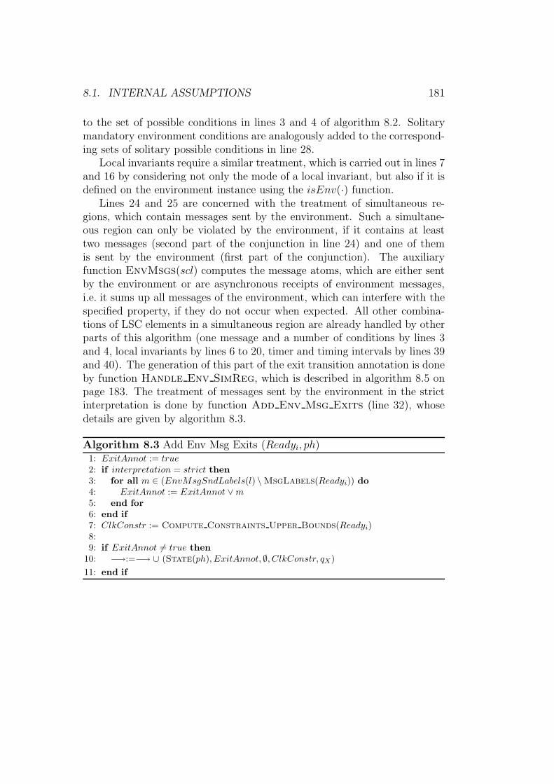
8.1. INTERNAL ASSUMPTIONS 181
to the set of possible conditions in lines 3 and 4 of algorithm 8.2. Solitarymandatory environment conditions are analogously added to the correspond-ing sets of solitary possible conditions in line 28.
Local invariants require a similar treatment, which is carried out in lines 7and 16 by considering not only the mode of a local invariant, but also if it isdefined on the environment instance using the isEnv(·) function.
Lines 24 and 25 are concerned with the treatment of simultaneous re-gions, which contain messages sent by the environment. Such a simultane-ous region can only be violated by the environment, if it contains at leasttwo messages (second part of the conjunction in line 24) and one of themis sent by the environment (first part of the conjunction). The auxiliaryfunction EnvMsgs(scl) computes the message atoms, which are either sentby the environment or are asynchronous receipts of environment messages,i.e. it sums up all messages of the environment, which can interfere with thespecified property, if they do not occur when expected. All other combina-tions of LSC elements in a simultaneous region are already handled by otherparts of this algorithm (one message and a number of conditions by lines 3and 4, local invariants by lines 6 to 20, timer and timing intervals by lines 39and 40). The generation of this part of the exit transition annotation is doneby function Handle Env SimReg, which is described in algorithm 8.5 onpage 183. The treatment of messages sent by the environment in the strictinterpretation is done by function Add Env Msg Exits (line 32), whosedetails are given by algorithm 8.3.
Algorithm 8.3 Add Env Msg Exits (Readyi, ph)1: ExitAnnot := true
2: if interpretation = strict then
3: for all m ∈ (EnvMsgSndLabels(l) \ MsgLabels(Readyi)) do
4: ExitAnnot := ExitAnnot ∨m5: end for
6: end if
7: ClkConstr := Compute Constraints Upper Bounds(Readyi)8:9: if ExitAnnot 6= true then
10: −→:=−→ ∪ (State(ph), ExitAnnot, ∅, ClkConstr, qX)
11: end if
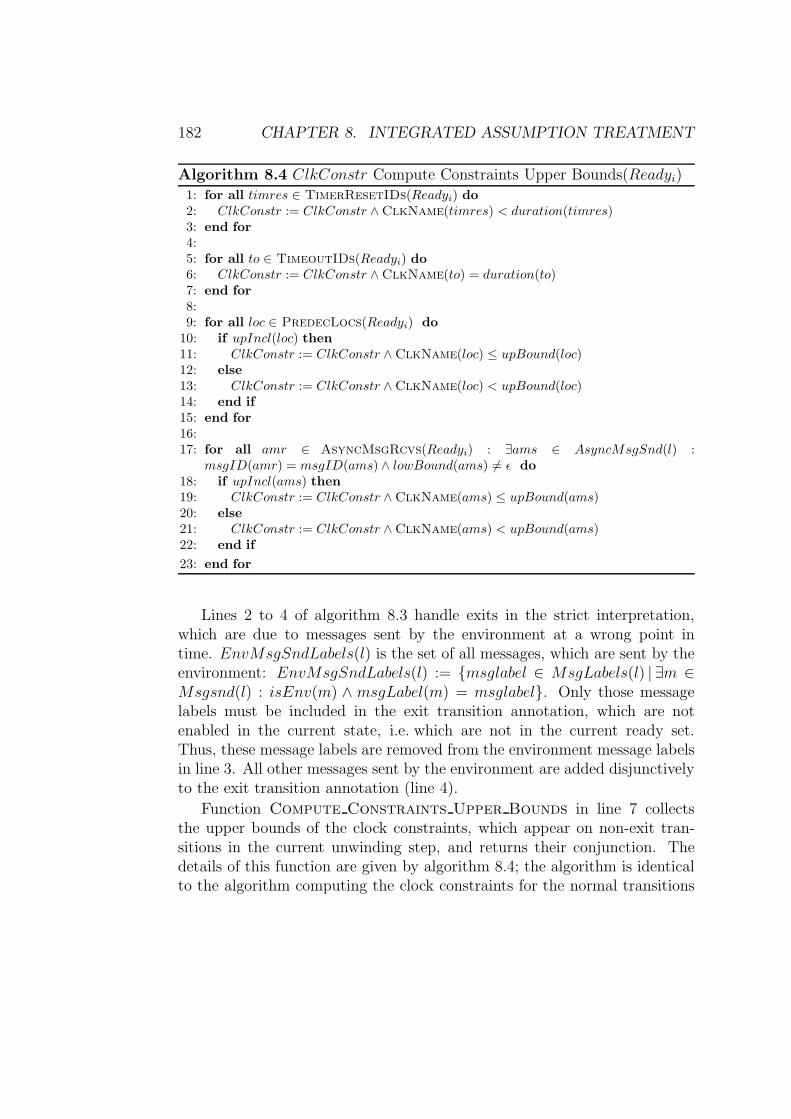
182 CHAPTER 8. INTEGRATED ASSUMPTION TREATMENT
Algorithm 8.4 ClkConstr Compute Constraints Upper Bounds(Readyi)1: for all timres ∈ TimerResetIDs(Readyi) do
2: ClkConstr := ClkConstr ∧ ClkName(timres) < duration(timres)3: end for
4:5: for all to ∈ TimeoutIDs(Readyi) do
6: ClkConstr := ClkConstr ∧ ClkName(to) = duration(to)7: end for
8:9: for all loc ∈ PredecLocs(Readyi) do
10: if upIncl(loc) then
11: ClkConstr := ClkConstr ∧ ClkName(loc) ≤ upBound(loc)12: else
13: ClkConstr := ClkConstr ∧ ClkName(loc) < upBound(loc)14: end if
15: end for
16:17: for all amr ∈ AsyncMsgRcvs(Readyi) : ∃ams ∈ AsyncMsgSnd(l) :
msgID(amr) = msgID(ams) ∧ lowBound(ams) 6= ǫ do
18: if upIncl(ams) then
19: ClkConstr := ClkConstr ∧ ClkName(ams) ≤ upBound(ams)20: else
21: ClkConstr := ClkConstr ∧ ClkName(ams) < upBound(ams)22: end if
23: end for
Lines 2 to 4 of algorithm 8.3 handle exits in the strict interpretation,which are due to messages sent by the environment at a wrong point intime. EnvMsgSndLabels(l) is the set of all messages, which are sent by theenvironment: EnvMsgSndLabels(l) := {msglabel ∈ MsgLabels(l) | ∃m ∈Msgsnd(l) : isEnv(m) ∧ msgLabel(m) = msglabel}. Only those messagelabels must be included in the exit transition annotation, which are notenabled in the current state, i.e. which are not in the current ready set.Thus, these message labels are removed from the environment message labelsin line 3. All other messages sent by the environment are added disjunctivelyto the exit transition annotation (line 4).
Function Compute Constraints Upper Bounds in line 7 collectsthe upper bounds of the clock constraints, which appear on non-exit tran-sitions in the current unwinding step, and returns their conjunction. Thedetails of this function are given by algorithm 8.4; the algorithm is identicalto the algorithm computing the clock constraints for the normal transitions
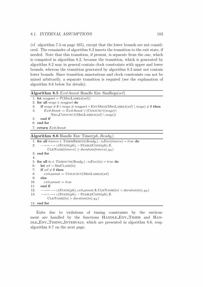
8.1. INTERNAL ASSUMPTIONS 183
(cf. algorithm 7.4 on page 165), except that the lower bounds are not consid-ered. The remainder of algorithm 8.3 inserts the transition to the exit state, ifneeded. Note that this transition, if present, is separate from the one, whichis computed in algorithm 8.2, because the transition, which is generated byalgorithm 8.2 may in general contain clock constraints with upper and lowerbounds, whereas the transition generated by algorithm 8.3 must not containlower bounds. Since transition annotations and clock constraints can not bemixed arbitrarily, a separate transition is required (see the explanation ofalgorithm 8.6 below for details).
Algorithm 8.5 ExitAnnot Handle Env SimRegs(scl)1: let msgpset = P(MsgLabels(scl))2: for all msgs ∈ msgpset do
3: if msgs 6= ∅ ∧msgs 6= msgpset ∧ EnvMsgs(MsgLabels(scl) \msgs) 6= ∅ then
4: ExitAnnot := ExitAnnot ∨ (Conjunct(msgs)∧Neg Conjunct(MsgLabels(scl) \msgs))
5: end if
6: end for
7: return ExitAnnot
Algorithm 8.6 Handle Env Timer(ph,Readyi)1: for all timres ∈ TimerResets(Readyi) : isEnv(timres) = true do
2: −→:=−→ ∪(State(ph),¬ StableCond(ph), ∅,ClkName(timres) ≥ duration(timres), qX)
3: end for
4:5: for all to ∈ Timeouts(Readyi) : isEnv(to) = true do
6: let scl = SimClass(to)7: if scl 6= ∅ then
8: exit annot := Conjunct(MsgLabels(scl)9: else
10: exit annot := true
11: end if
12: −→:=−→ ∪(State(ph), exit annot, ∅,ClkName(to) < duration(to), qX)13: −→:=−→ ∪(State(ph),¬ StableCond(ph), ∅,
ClkName(to) > duration(to), qX)
14: end for
Exits due to violations of timing constraints by the environ-ment are handled by the functions Handle Env Timer and Han-dle Env Timing Intervals, which are presented in algorithm 8.6, resp.algorithm 8.7 on the next page.
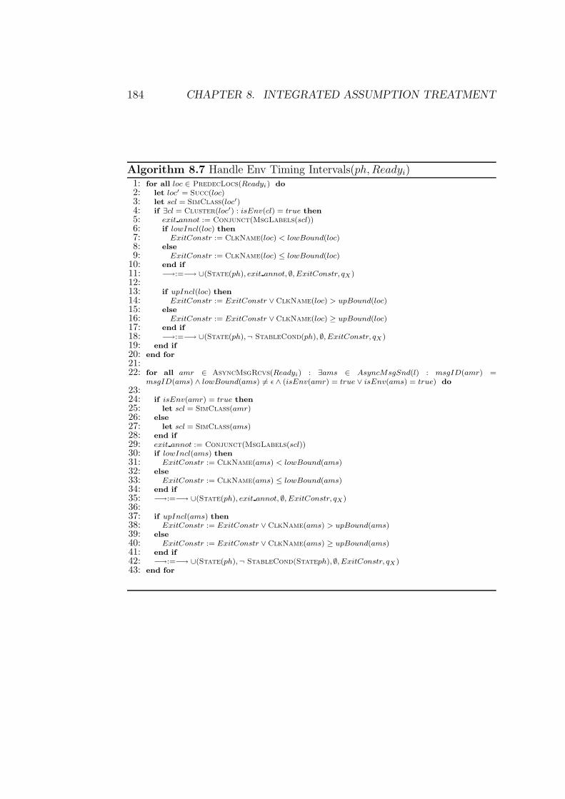
184 CHAPTER 8. INTEGRATED ASSUMPTION TREATMENT
Algorithm 8.7 Handle Env Timing Intervals(ph,Readyi)1: for all loc ∈ PredecLocs(Readyi) do
2: let loc′ = Succ(loc)3: let scl = SimClass(loc′)4: if ∃cl = Cluster(loc′) : isEnv(cl) = true then
5: exit annot := Conjunct(MsgLabels(scl))6: if lowIncl(loc) then
7: ExitConstr := ClkName(loc) < lowBound(loc)8: else
9: ExitConstr := ClkName(loc) ≤ lowBound(loc)10: end if
11: −→:=−→ ∪(State(ph), exit annot, ∅, ExitConstr, qX)12:13: if upIncl(loc) then
14: ExitConstr := ExitConstr ∨ ClkName(loc) > upBound(loc)15: else
16: ExitConstr := ExitConstr ∨ ClkName(loc) ≥ upBound(loc)17: end if
18: −→:=−→ ∪(State(ph),¬ StableCond(ph), ∅, ExitConstr, qX)19: end if
20: end for
21:22: for all amr ∈ AsyncMsgRcvs(Readyi) : ∃ams ∈ AsyncMsgSnd(l) : msgID(amr) =
msgID(ams) ∧ lowBound(ams) 6= ǫ ∧ (isEnv(amr) = true ∨ isEnv(ams) = true) do
23:24: if isEnv(amr) = true then
25: let scl = SimClass(amr)26: else
27: let scl = SimClass(ams)28: end if
29: exit annot := Conjunct(MsgLabels(scl))30: if lowIncl(ams) then
31: ExitConstr := ClkName(ams) < lowBound(ams)32: else
33: ExitConstr := ClkName(ams) ≤ lowBound(ams)34: end if
35: −→:=−→ ∪(State(ph), exit annot, ∅, ExitConstr, qX)36:37: if upIncl(ams) then
38: ExitConstr := ExitConstr ∨ ClkName(ams) > upBound(ams)39: else
40: ExitConstr := ExitConstr ∨ ClkName(ams) ≥ upBound(ams)41: end if
42: −→:=−→ ∪(State(ph),¬ StableCond(Stateph), ∅, ExitConstr, qX)43: end for
8.1. INTERNAL ASSUMPTIONS 185
Algorithm 8.5 on page 183 generates the part of the exit transition an-notation, which deals with simultaneous regions, which depend on messagessent by the environment. If the environment does not send the messages itis supposed to send within the considered simultaneous region1, this shouldresult in a transition to the exit state. This means that all combinations ofmessages, which are part of the simultaneous region, have to be considered.Therefore the powerset of all messages in the current simultaneous region iscomputed in line 1. Each set of the powerset corresponds to one combina-tion of messages and is interpreted here as the occurrence of the messagescontained in the set. All messages, which are missing from the set, i.e. thecomplementary set, is interpreted as messages, which are not observed.
The empty set and the set containing all messages can be ignored, asthey correspond to the self loop, resp. the good case. Since only violationscaused by the environment should lead to an exit, it is sufficient to add acorresponding annotation, if one of the messages sent by the environmentis missing (line 3). If this is the case, the observed messages (msgs) arerecorded positively in the exit transition annotation and all other messagesin a negated form (line 4).
Algorithm 8.6 on page 183 constructs the exits for timing constraints,which are due to timeouts and timer resets and which are violated by theenvironment. The first part (lines 1 to 2) considers violated timer resets,the second part (lines 5 to 13) violated timeouts. The transition annotationis the negation of the stable condition and the clock constraint for the exittransition is the negation of the normal constraint for a timer reset (line 2;also cf. algorithm 7.4 on page 165). The annotation is the negation of thestable condition rather than the single label of the message to which thetimer refers, because otherwise in the strict interpretation the occurrence ofany message contained in the LSC would lead to an undesired error, oncethe upper bound given by the timer reset is violated. The auxiliary func-tion StableCond(ph) returns the annotation of the self loop on the statecorresponding to the current phase.
The treatment of violated timeouts is different inasmuch as it requires twoseparate transitions to the exit state, each carrying one part of the negationof the original clock constraint. The computation of the transition annota-
1We are using the term simultaneous region here out of convenience, although weare actually dealing with the SimClass, which contains the simultaneous region underconsideration.
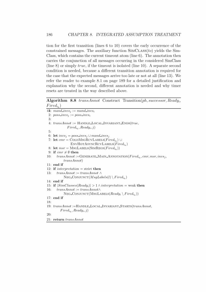
186 CHAPTER 8. INTEGRATED ASSUMPTION TREATMENT
tion for the first transition (lines 6 to 10) covers the early occurrence of theconstrained messages. The auxiliary function SimClass(to) yields the Sim-Class, which contains the current timeout atom (line 6). The annotation thencarries the conjunction of all messages occurring in the considered SimClass(line 8) or simply true, if the timeout is isolated (line 10). A separate secondcondition is needed, because a different transition annotation is required forthe case that the expected messages arrive too late or not at all (line 13). Werefer the reader to example 8.1 on page 189 for a detailed justification andexplanation why the second, different annotation is needed and why timerresets are treated in the way described above.
Algorithm 8.8 transAnnot Construct Transition(ph, successor, Readyi,Firedik)44:1: mand invsj := mand invsi
2: poss invsj := poss invsi
3:4: transAnnot := Handle Local Invariant Ends(true,
F iredik, Readyi, j)
5:6: let invsj = poss invsj ∪mand invsj
7: let cmr = ColdMsgRcvLabels(Firedik) ∪
EnvHotAsyncRcvLabels(Firedik)
8: let msr = MsgLabels(SimRegs(Firedik))
9: if cmr 6= ∅ then
10: transAnnot :=Generate Main Annotation(Firedik, cmr,msr, invsj,
transAnnot)11: end if
12: if interpretation = strict then
13: transAnnot := transAnnot ∧Neg Conjunct(MsgLabels(l) \ Firedik
)14: end if
15: if |SimClasses(Readyi)| > 1 ∧ interpretation = weak then
16: transAnnot := transAnnot∧Neg Conjunct(MsgLabels(Readyi \ Firedik
))17: end if
18:19: transAnnot :=Handle Local Invariant Starts(transAnnot,
F iredik, Readyi, j)
20:
21: return transAnnot
8.1. INTERNAL ASSUMPTIONS 187
Different transition annotations, which are associated with distinct clockconstraints, always require separate transitions. Assume for instance thatthere are two messages, msgX andmsgY , with clock constraints clkconstrX,resp. clkconstrY . Considered in isolation the transition annotation wouldbe msgX[clkconstrX], resp. msgY [clkconstrY ] or more explicitly msgX ∧clkconstrX, resp. msgY ∧ clkconstrY . Using a single transition for bothmessages including clock constraints, i.e. disjunctively adding annotationsand constraints would result for instance in (msgX∨msgY )∧(clkconstrX ∨clkconstrY ). This is incorrect, since the association of each message to itsconstraint is lost. The correct annotation should read (msgX∧clkconstrX)∨(msgY ∧clkconstrY ) and can only be expressed by two separate transitions;cf. example 8.1.
Algorithm 8.7 on page 184 constructs the exit transitions for violatedtiming intervals. The basic procedure is similar to the one used in algo-rithm 8.6 on page 183, although the concrete execution is slightly different.As in algorithm 7.4 on page 165 the function PredecLocs(Readyi) yieldsfor all locations in the current ready set the set of their immediate prede-cessor locations, which are annotated by a timing interval (line 1). In line 2the location, which marks the end of the timing interval, i.e. the successor ofloc, is computed by the auxiliary function Succ(loc), which is used to findthe SimClass containing this location (line 3). Line 4 determines if there isa cluster (given by the auxiliary function Cluster(loc′); line 4) defined onthe environment instance in this location. The SimClass is needed for thetransition annotation (line 5).
Since a timing interval is always bound to two locations, the annotationcannot be empty as for timer resets or timeouts. Similar to the treatment ofviolated timeouts, two separate transitions to the exit state are needed (seeexample 8.1 on page 189 for the details). The clock constraint for the casewhere the lower bound is violated is constructed in lines 6 to 9, dependingon the nature of the interval (open, half-open, closed). The constraint isthe negation of the normal constraint, as for timer resets and timeouts. Thecorresponding transition is added to −→ in line 11. The transition for the casewhere the upper bound is violated is constructed analogously in lines 13 to 18.The treatment for timing intervals of asynchronous messages is analogous;the transition annotation depends on the message atom, which is defined onthe environment instance (lines 22 to 42).
Algorithm 8.8 on the facing page shows the adjusted version of the algo-rithm for the construction of the transition to the successor state. Only a
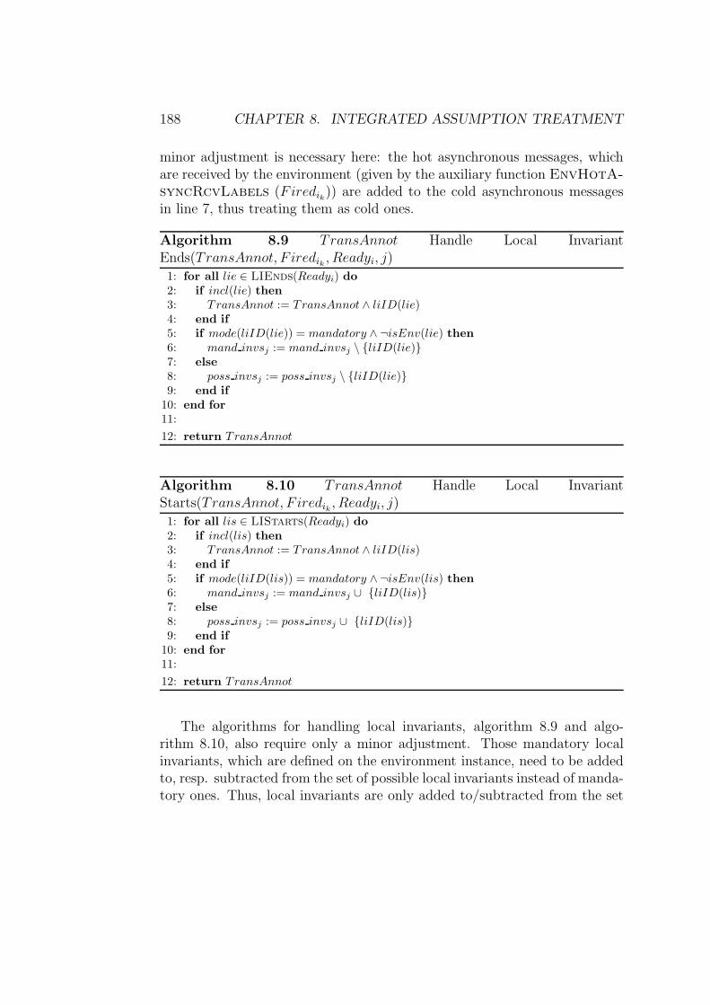
188 CHAPTER 8. INTEGRATED ASSUMPTION TREATMENT
minor adjustment is necessary here: the hot asynchronous messages, whichare received by the environment (given by the auxiliary function EnvHotA-syncRcvLabels (Firedik)) are added to the cold asynchronous messagesin line 7, thus treating them as cold ones.
Algorithm 8.9 TransAnnot Handle Local InvariantEnds(TransAnnot, F iredik , Readyi, j)
1: for all lie ∈ LIEnds(Readyi) do
2: if incl(lie) then
3: TransAnnot := TransAnnot ∧ liID(lie)4: end if
5: if mode(liID(lie)) = mandatory ∧ ¬isEnv(lie) then
6: mand invsj := mand invsj \ {liID(lie)}7: else
8: poss invsj := poss invsj \ {liID(lie)}9: end if
10: end for
11:
12: return TransAnnot
Algorithm 8.10 TransAnnot Handle Local InvariantStarts(TransAnnot, F iredik , Readyi, j)
1: for all lis ∈ LIStarts(Readyi) do
2: if incl(lis) then
3: TransAnnot := TransAnnot ∧ liID(lis)4: end if
5: if mode(liID(lis)) = mandatory ∧ ¬isEnv(lis) then
6: mand invsj := mand invsj ∪ {liID(lis)}7: else
8: poss invsj := poss invsj ∪ {liID(lis)}9: end if
10: end for
11:
12: return TransAnnot
The algorithms for handling local invariants, algorithm 8.9 and algo-rithm 8.10, also require only a minor adjustment. Those mandatory localinvariants, which are defined on the environment instance, need to be addedto, resp. subtracted from the set of possible local invariants instead of manda-tory ones. Thus, local invariants are only added to/subtracted from the set
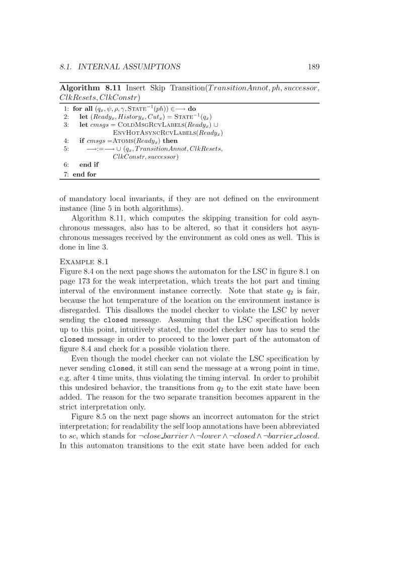
8.1. INTERNAL ASSUMPTIONS 189
Algorithm 8.11 Insert Skip Transition(TransitionAnnot, ph, successor,ClkResets, ClkConstr)
1: for all (qx, ψ, ρ, γ,State−1(ph)) ∈−→ do
2: let (Readyx, Historyx, Cutx) = State−1(qx)3: let cmsgs = ColdMsgRcvLabels(Readyx) ∪
EnvHotAsyncRcvLabels(Readyx)4: if cmsgs =Atoms(Readyx) then
5: −→:=−→ ∪ (qx, T ransitionAnnot, ClkResets,ClkConstr, successor)
6: end if
7: end for
of mandatory local invariants, if they are not defined on the environmentinstance (line 5 in both algorithms).
Algorithm 8.11, which computes the skipping transition for cold asyn-chronous messages, also has to be altered, so that it considers hot asyn-chronous messages received by the environment as cold ones as well. This isdone in line 3.
Example 8.1Figure 8.4 on the next page shows the automaton for the LSC in figure 8.1 onpage 173 for the weak interpretation, which treats the hot part and timinginterval of the environment instance correctly. Note that state q2 is fair,because the hot temperature of the location on the environment instance isdisregarded. This disallows the model checker to violate the LSC by neversending the closed message. Assuming that the LSC specification holdsup to this point, intuitively stated, the model checker now has to send theclosed message in order to proceed to the lower part of the automaton offigure 8.4 and check for a possible violation there.
Even though the model checker can not violate the LSC specification bynever sending closed, it still can send the message at a wrong point in time,e.g. after 4 time units, thus violating the timing interval. In order to prohibitthis undesired behavior, the transitions from q2 to the exit state have beenadded. The reason for the two separate transition becomes apparent in thestrict interpretation only.
Figure 8.5 on the next page shows an incorrect automaton for the strictinterpretation; for readability the self loop annotations have been abbreviatedto sc, which stands for ¬close barrier∧¬lower∧¬closed∧¬barrier closed.In this automaton transitions to the exit state have been added for each
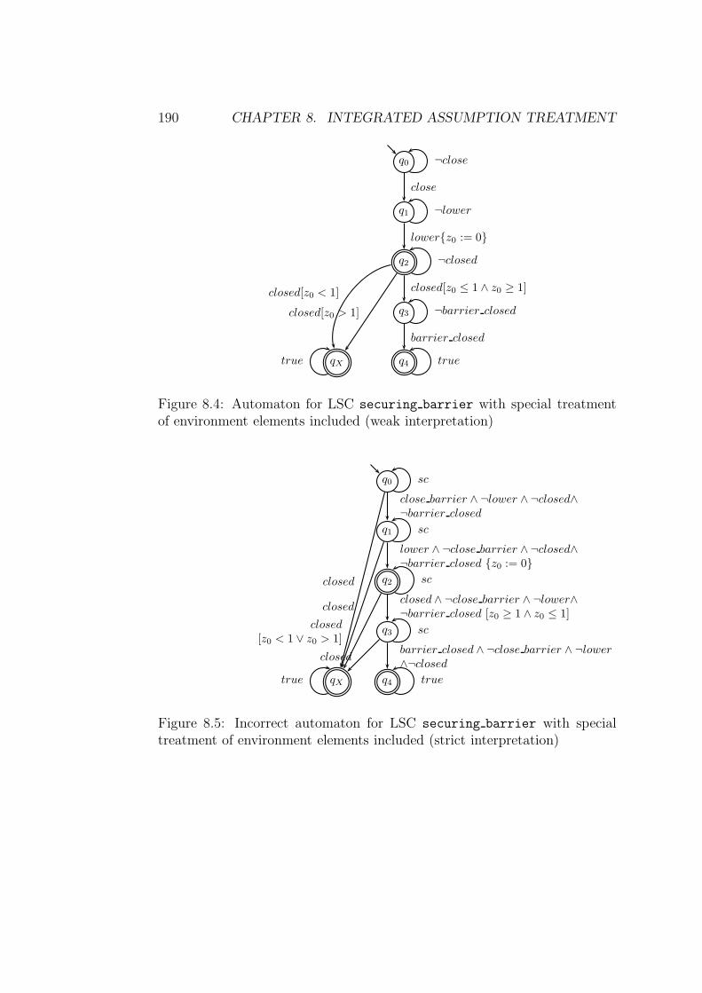
190 CHAPTER 8. INTEGRATED ASSUMPTION TREATMENT
q0 ¬close
q1 ¬lower
close
q2 ¬closed
lower{z0 := 0}
q3 ¬barrier closed
closed[z0 ≤ 1 ∧ z0 ≥ 1]
q4 true
barrier closed
qXtrue
closed[z0 < 1]
closed[z0 > 1]
Figure 8.4: Automaton for LSC securing barrier with special treatmentof environment elements included (weak interpretation)
q0 sc
q1 sc
close barrier ∧ ¬lower ∧ ¬closed∧¬barrier closed
q2 sc
lower ∧ ¬close barrier ∧ ¬closed∧¬barrier closed {z0 := 0}
q3 sc
closed ∧ ¬close barrier ∧ ¬lower∧¬barrier closed [z0 ≥ 1 ∧ z0 ≤ 1]
q4 true
barrier closed ∧ ¬close barrier ∧ ¬lower∧¬closed
qXtrue
closed
closed
closed
closed
[z0 < 1 ∨ z0 > 1]
Figure 8.5: Incorrect automaton for LSC securing barrier with specialtreatment of environment elements included (strict interpretation)
8.1. INTERNAL ASSUMPTIONS 191
state, in which the closed message should not occur (q0, q1, and q2). Notethat the transition from q2 is due to the timing interval and not because ofthe strict interpretation; without the timing interval this transition would bemissing.
This transition is the incorrect part of the automaton, since it should berepresented by two separate transitions as in the automaton of figure 8.4. Itis used here to demonstrate that the straight-forward way to represent a vio-lation of the timing interval by simply negating the original clock constraintas done here, is insufficient when using the strict interpretation. Consider thesituation that the automaton in figure 8.5 has progressed to state q2, i.e. thatwe are waiting to observe closed within the given time bound. In the weakinterpretation there was no problem, if the environment never sent closed,since q2 is an fair state. In the strict interpretation the case is different,because the stable condition expressed by the self loop annotation can be vi-olated by other messages. Assume e.g. that the automaton in figure 8.5 hasremained in state q2 for five time units and now we observe barrier closed:We have a violation of the property even though the environment did notobey the (internal) assumption expressed by the timing constraint.
In order to prohibit this undesired behavior by the model checker, weexploit the knowledge that after the time given by the upper bound of thetiming interval has passed, the LSC can not be fulfilled anymore regardlessof the occurrence of the required message. Once more time has passed thanallowed by the upper bound, without observing the expected message fromthe environment (closed in our example), in the strict interpretation theoccurrence of any message, which is present in the LSC, causes an error as alate effect of the not sent environment message. Consequently a violation ofthe stable condition of the state, where the environment message is expected,should lead to an exit, if this occurs after the time given by the upper boundhas elapsed. In our example this results in a transition to the exit state withannotation ¬sc[z0 > 1] or more explicitly: close barrier ∨ lower ∨ closed ∨barrier closed[z0 > 1].
A second transition to the exit state is required for a violation of the lowerbound, since here a different annotation and a different clock constraint isrequired. Before the time for the lower bound elapses only the occurrenceof the environment message must result in an exit. Should any of the othermessages in the LSC be observed in this time span, the consequence must bean error (in the strict interpretation). In our example here the annotation ofthe first transition thus reads closed[z0 < 1]. This strategy is correct for the
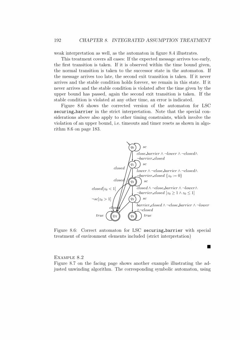
192 CHAPTER 8. INTEGRATED ASSUMPTION TREATMENT
weak interpretation as well, as the automaton in figure 8.4 illustrates.This treatment covers all cases: If the expected message arrives too early,
the first transition is taken. If it is observed within the time bound given,the normal transition is taken to the successor state in the automaton. Ifthe message arrives too late, the second exit transition is taken. If it neverarrives and the stable condition holds forever, we remain in this state. If itnever arrives and the stable condition is violated after the time given by theupper bound has passed, again the second exit transition is taken. If thestable condition is violated at any other time, an error is indicated.
Figure 8.6 shows the corrected version of the automaton for LSCsecuring barrier in the strict interpretation. Note that the special con-siderations above also apply to other timing constraints, which involve theviolation of an upper bound, i.e. timeouts and timer resets as shown in algo-rithm 8.6 on page 183.
q0 sc
q1 sc
close barrier ∧ ¬lower ∧ ¬closed∧¬barrier closed
q2 sc
lower ∧ ¬close barrier ∧ ¬closed∧¬barrier closed {z0 := 0}
q3 sc
closed ∧ ¬close barrier ∧ ¬lower∧¬barrier closed [z0 ≥ 1 ∧ z0 ≤ 1]
q4 true
barrier closed ∧ ¬close barrier ∧ ¬lower∧¬closed
qXtrue
closed
closed
closed
closed[z0 < 1]
¬sc[z0 > 1]
Figure 8.6: Correct automaton for LSC securing barrier with specialtreatment of environment elements included (strict interpretation)
�
Example 8.2Figure 8.7 on the facing page shows another example illustrating the ad-justed unwinding algorithm. The corresponding symbolic automaton, using
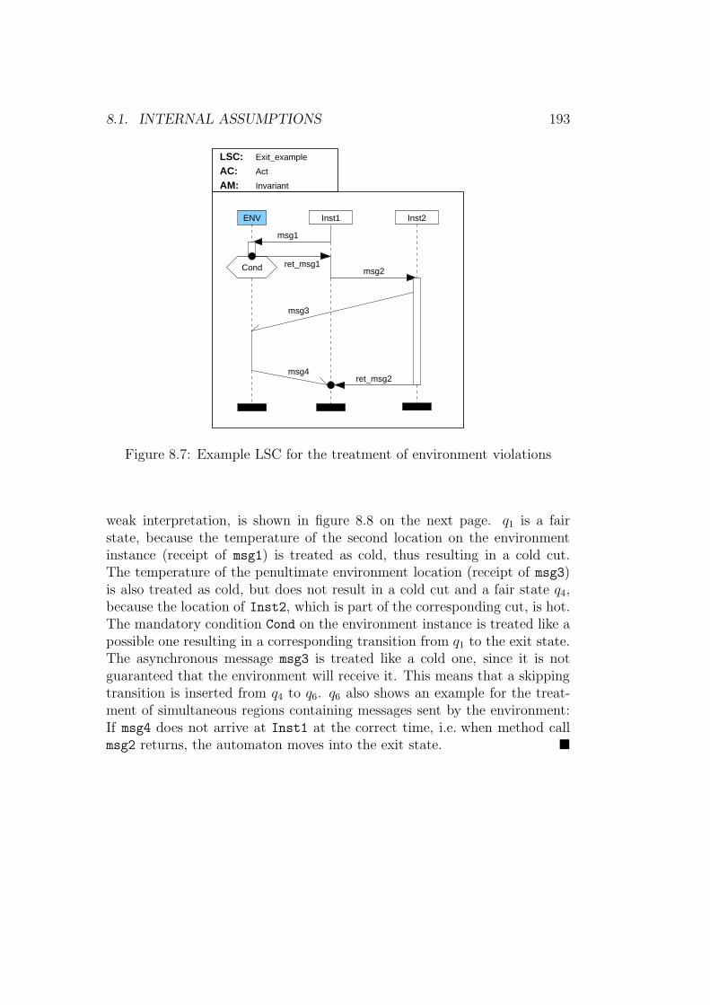
8.1. INTERNAL ASSUMPTIONS 193
ENV Inst1 Inst2
msg3
msg4
Cond
AC:AM: Invariant
Exit_exampleLSC:Act
msg2
ret_msg2
msg1
ret_msg1
Figure 8.7: Example LSC for the treatment of environment violations
weak interpretation, is shown in figure 8.8 on the next page. q1 is a fairstate, because the temperature of the second location on the environmentinstance (receipt of msg1) is treated as cold, thus resulting in a cold cut.The temperature of the penultimate environment location (receipt of msg3)is also treated as cold, but does not result in a cold cut and a fair state q4,because the location of Inst2, which is part of the corresponding cut, is hot.The mandatory condition Cond on the environment instance is treated like apossible one resulting in a corresponding transition from q1 to the exit state.The asynchronous message msg3 is treated like a cold one, since it is notguaranteed that the environment will receive it. This means that a skippingtransition is inserted from q4 to q6. q6 also shows an example for the treat-ment of simultaneous regions containing messages sent by the environment:If msg4 does not arrive at Inst1 at the correct time, i.e. when method callmsg2 returns, the automaton moves into the exit state. �
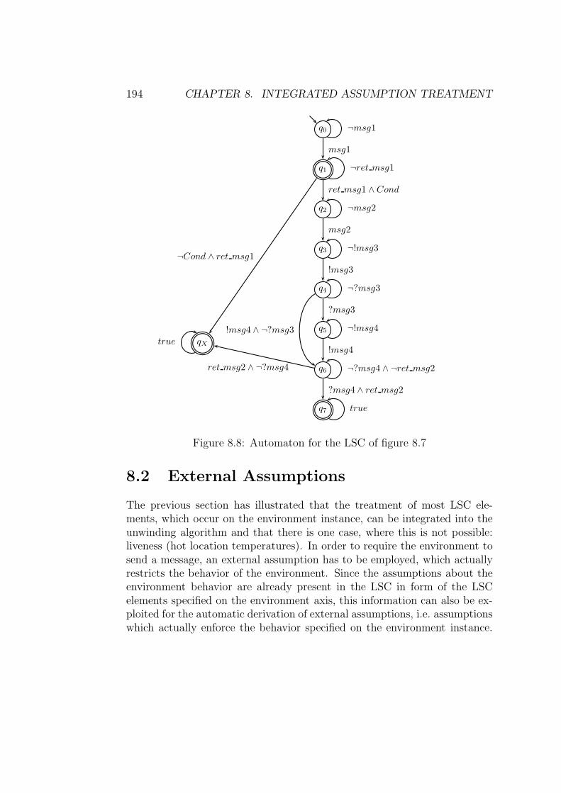
194 CHAPTER 8. INTEGRATED ASSUMPTION TREATMENT
q0 ¬msg1
q1 ¬ret msg1
msg1
q2 ¬msg2
ret msg1 ∧Cond
q3 ¬!msg3
msg2
q4 ¬?msg3
!msg3
q5 ¬!msg4
?msg3
q6 ¬?msg4 ∧ ¬ret msg2
!msg4
q7 true
?msg4 ∧ ret msg2
qXtrue
¬Cond ∧ ret msg1
ret msg2 ∧ ¬?msg4
!msg4 ∧ ¬?msg3
Figure 8.8: Automaton for the LSC of figure 8.7
8.2 External Assumptions
The previous section has illustrated that the treatment of most LSC ele-ments, which occur on the environment instance, can be integrated into theunwinding algorithm and that there is one case, where this is not possible:liveness (hot location temperatures). In order to require the environment tosend a message, an external assumption has to be employed, which actuallyrestricts the behavior of the environment. Since the assumptions about theenvironment behavior are already present in the LSC in form of the LSCelements specified on the environment axis, this information can also be ex-ploited for the automatic derivation of external assumptions, i.e. assumptionswhich actually enforce the behavior specified on the environment instance.
8.2. EXTERNAL ASSUMPTIONS 195
Section 8.2.1 describes how this is realized by extracting an assumption LSCfrom the originally specified commitment LSC, whereas section 8.2.2 intro-duces external assumption LSCs, which are explicitly specified by the user.
8.2.1 Extracting Assumptions from LSCs
The assumptions extracted from a commitment LSC are represented by anLSC as well, although of a slightly restricted type. Such assumption LSCscontain only two instances, one for the environment and one for the systemunder development. This is sufficient, since assumptions are concerned withthe items observable at the interface between the system and its environment.The environment can only observe and influence the system behavior via thisinterface, all internal actions are hidden from it. The extraction thus involvesthe hiding of internal communication and internal elements, i.e. only thoseelements of the commitment LSC are extracted into the assumption LSC,which either have originally been specified on the environment instance orare messages leading to or coming from the environment. The environmentinstance axis of the commitment LSC is consequently retained in the assump-tion LSC and all other elements are projected onto the external interface ofthe system represented by the system instance axis.
For the message atoms, which are projected onto the system axis, thequestion of their ordering arises. In the case of instantaneous messages theposition of the complementary message atom on the system instance is easilydetermined, since the positions of both the sending and receiving atom andcluster are identical. In the case of asynchronous messages the position ofthe complementary message atoms is more difficult to determine, becausethe positions of one can not be derived from the position of the other. Theobservance of the complementary atoms, however, is not necessary in theassumption LSC, since only the message atoms on the environment instancecarry relevant information. The fact that messages received have been sentearlier by the system or that messages sent to the system are eventually re-ceived is non-essential in this view. Messages received by the environmentprovide ordering information for the sending of messages and validity of con-ditions and local invariants. But the concrete ordering of the atoms/clusterson the system instance is irrelevant in the assumption, so that the positionof the complementary message atoms is in this case copied from the corre-sponding atom on the environment axis and all clusters of the system axis areplaced into a coregion, if the environment instance contains at least one asyn-
196 CHAPTER 8. INTEGRATED ASSUMPTION TREATMENT
chronous message atom. Care has to be taken when an asynchronous messageatom is part of a simultaneous region on the environment axis. In this casethe complementary asynchronous message atoms must not be placed in asimultaneous region on the system axis, since no simultaneity between send-ing and receipt is enforced for asynchronous messages. The complementarymessage atom is then placed either in a not already occupied cluster abovethe current one for complementary message sends or below for receipts. In-stantaneous messages are not affected, because their point of observation isstill uniquely determined by the position of the corresponding atom on theenvironment axis.
The role of the environment axis in an assumption LSC differs from theone in a commitment LSC. In the former the behavior specified on the envi-ronment axis has to be guaranteed, whereas it is only expected in the latter.The environment axis in an external assumption is therefore not treated dif-ferently than a normal instance axis. The elements used on the system axis ofan extracted assumption are needed by the environment to determine whento send which messages, etc. Therefore only messages, simultaneous regionsand coregions will appear on the system axis of an extracted assumption.Hence all location temperatures on the newly introduced system instanceare cold, because liveness requirements on the system are expressed in thecommitment LSC.Assumption extraction is performed for each environment instance axis ofthe commitment LSC, i.e. for each environment instance an assumption LSCis derived.
Assumption Extraction Algorithm
The extracted assumption LSCs obviously share the activation information ofthe commitment, i.e. take over the activation mode and activation condition.The quantification is always universal, because assumptions express universalconstraints on the behavior of the environment.
Recall from definition 6.1 on page 94 that an LSC is a tupleL = (l, assumptions, ac, pch, amode, quant). The (possibly empty)set assumptions contains the assumption LSCs linked to commitmentLSC l. The extraction algorithm thus constructs from a commitmentLSC Lcomm = (lcomm, assumptions, ac, pch, amode, quant) a new LSCLass = (lass, ∅, ac, pch, amode, universal) for each environment instanceof Lcomm and adds it to the set of assumptions of Lcomm: Lcomm =(lcomm, assumptions ∪ {Lass}, ac, pch, amode, quant).
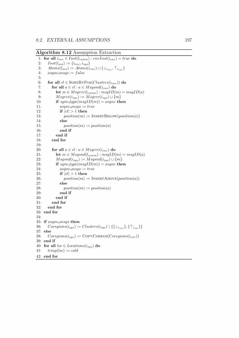
8.2. EXTERNAL ASSUMPTIONS 197
Algorithm 8.12 Assumption Extraction1: for all ienv ∈ Inst(lcomm) : envInst(ienv) = true do
2: Inst(lass) := {ienv, isys}3: Atoms(lass) := Atoms(ienv) ∪ {⊥isys
,⊤isys}
4: async msgs := false
5:6: for all cl ∈ SortByPos(Clusters(ienv)) do
7: for all a ∈ cl : a ∈Msgsnd(ienv) do
8: let m ∈Msgrcv(lcomm) : msgID(m) = msgID(a)9: Msgrcv(isys) := Msgrcv(isys) ∪ {m}
10: if sync type(msgID(m)) = async then
11: async msgs := true
12: if |cl| > 1 then
13: position(m) := InsertBelow(position(a))14: else
15: position(m) := position(a)16: end if
17: end if
18: end for
19:20: for all a ∈ cl : a ∈Msgrcv(ienv) do
21: let m ∈Msgsnd(lcomm) : msgID(m) = msgID(a)22: Msgsnd(isys) := Msgsnd(isys) ∪ {m}23: if sync type(msgID(m)) = async then
24: async msgs := true
25: if |cl| > 1 then
26: position(m) := InsertAbove(position(a))27: else
28: position(m) := position(a)29: end if
30: end if
31: end for
32: end for
33: end for
34:35: if async msgs then
36: Coregions(isys) := Clusters(isys) \ {{⊥isys}, {⊤isys
}}37: else
38: Coregions(isys) := CopyCoregs(Coregions(ienv))39: end if
40: for all loc ∈ Locations(isys) do
41: temp(loc) := cold
42: end for
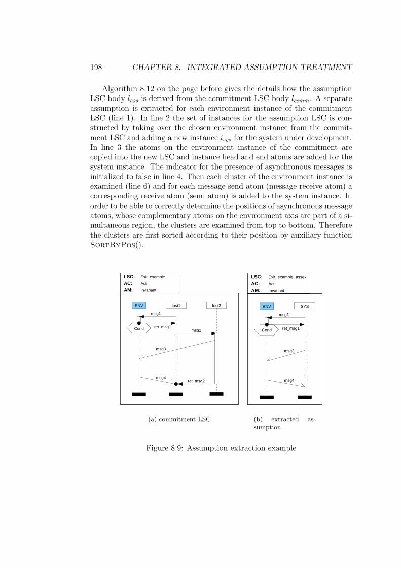
198 CHAPTER 8. INTEGRATED ASSUMPTION TREATMENT
Algorithm 8.12 on the page before gives the details how the assumptionLSC body lass is derived from the commitment LSC body lcomm. A separateassumption is extracted for each environment instance of the commitmentLSC (line 1). In line 2 the set of instances for the assumption LSC is con-structed by taking over the chosen environment instance from the commit-ment LSC and adding a new instance isys for the system under development.In line 3 the atoms on the environment instance of the commitment arecopied into the new LSC and instance head and end atoms are added for thesystem instance. The indicator for the presence of asynchronous messages isinitialized to false in line 4. Then each cluster of the environment instance isexamined (line 6) and for each message send atom (message receive atom) acorresponding receive atom (send atom) is added to the system instance. Inorder to be able to correctly determine the positions of asynchronous messageatoms, whose complementary atoms on the environment axis are part of a si-multaneous region, the clusters are examined from top to bottom. Thereforethe clusters are first sorted according to their position by auxiliary functionSortByPos().
ENV Inst1 Inst2
msg3
msg4
Cond
AC:AM: Invariant
Exit_exampleLSC:Act
msg2
ret_msg2
msg1
ret_msg1
(a) commitment LSC
AC:AM: Invariant
Exit_example_assexLSC:Act
ENV SYS
msg3
msg4
Cond
msg1
ret_msg1
(b) extracted as-sumption
Figure 8.9: Assumption extraction example
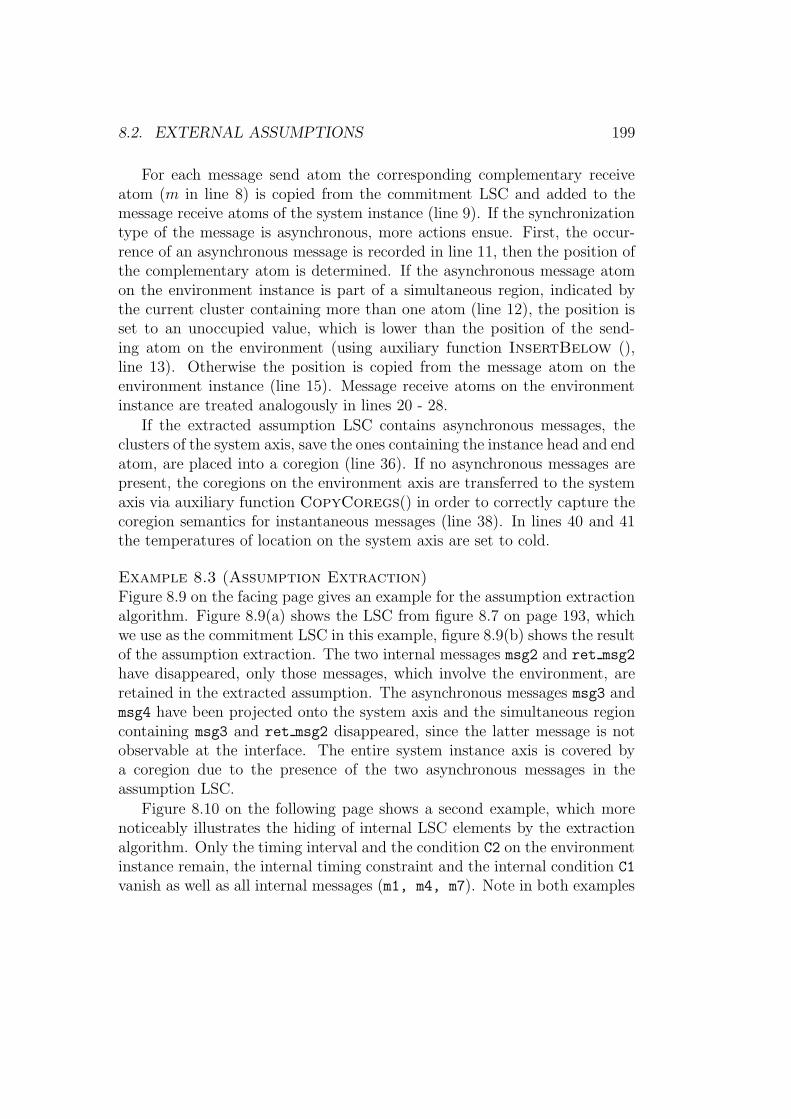
8.2. EXTERNAL ASSUMPTIONS 199
For each message send atom the corresponding complementary receiveatom (m in line 8) is copied from the commitment LSC and added to themessage receive atoms of the system instance (line 9). If the synchronizationtype of the message is asynchronous, more actions ensue. First, the occur-rence of an asynchronous message is recorded in line 11, then the position ofthe complementary atom is determined. If the asynchronous message atomon the environment instance is part of a simultaneous region, indicated bythe current cluster containing more than one atom (line 12), the position isset to an unoccupied value, which is lower than the position of the send-ing atom on the environment (using auxiliary function InsertBelow (),line 13). Otherwise the position is copied from the message atom on theenvironment instance (line 15). Message receive atoms on the environmentinstance are treated analogously in lines 20 - 28.
If the extracted assumption LSC contains asynchronous messages, theclusters of the system axis, save the ones containing the instance head and endatom, are placed into a coregion (line 36). If no asynchronous messages arepresent, the coregions on the environment axis are transferred to the systemaxis via auxiliary function CopyCoregs() in order to correctly capture thecoregion semantics for instantaneous messages (line 38). In lines 40 and 41the temperatures of location on the system axis are set to cold.
Example 8.3 (Assumption Extraction)Figure 8.9 on the facing page gives an example for the assumption extractionalgorithm. Figure 8.9(a) shows the LSC from figure 8.7 on page 193, whichwe use as the commitment LSC in this example, figure 8.9(b) shows the resultof the assumption extraction. The two internal messages msg2 and ret msg2
have disappeared, only those messages, which involve the environment, areretained in the extracted assumption. The asynchronous messages msg3 andmsg4 have been projected onto the system axis and the simultaneous regioncontaining msg3 and ret msg2 disappeared, since the latter message is notobservable at the interface. The entire system instance axis is covered bya coregion due to the presence of the two asynchronous messages in theassumption LSC.
Figure 8.10 on the following page shows a second example, which morenoticeably illustrates the hiding of internal LSC elements by the extractionalgorithm. Only the timing interval and the condition C2 on the environmentinstance remain, the internal timing constraint and the internal condition C1
vanish as well as all internal messages (m1, m4, m7). Note in both examples
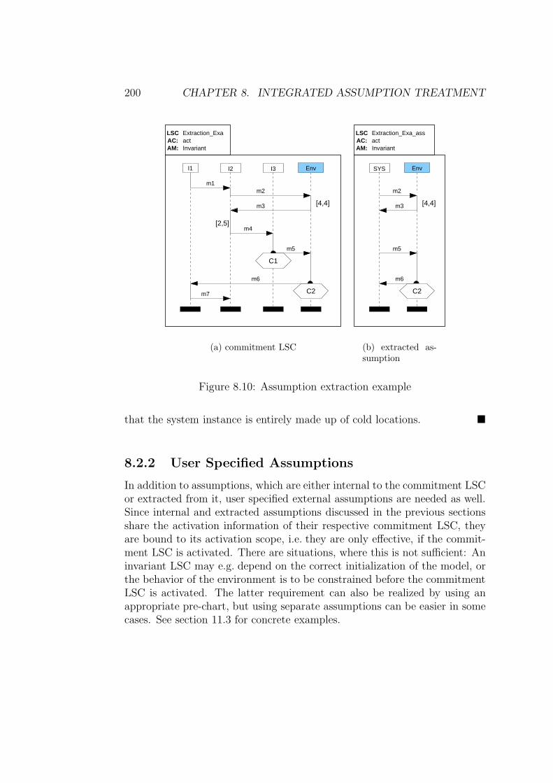
200 CHAPTER 8. INTEGRATED ASSUMPTION TREATMENT
Invariantact
I1
LSCAC:AM:
Extraction_Exa
m1
I3 EnvI2
m2
m3
[2,5]m4
C1
[4,4]
C2
m5
m6
m7
(a) commitment LSC
Invariantact
LSCAC:AM:
Extraction_Exa_ass
SYS Env
[4,4]
C2
m5
m6
m3
m2
(b) extracted as-sumption
Figure 8.10: Assumption extraction example
that the system instance is entirely made up of cold locations. �
8.2.2 User Specified Assumptions
In addition to assumptions, which are either internal to the commitment LSCor extracted from it, user specified external assumptions are needed as well.Since internal and extracted assumptions discussed in the previous sectionsshare the activation information of their respective commitment LSC, theyare bound to its activation scope, i.e. they are only effective, if the commit-ment LSC is activated. There are situations, where this is not sufficient: Aninvariant LSC may e.g. depend on the correct initialization of the model, orthe behavior of the environment is to be constrained before the commitmentLSC is activated. The latter requirement can also be realized by using anappropriate pre-chart, but using separate assumptions can be easier in somecases. See section 11.3 for concrete examples.
8.3. SEMANTICS OF EXTERNAL ASSUMPTIONS 201
User specified assumptions are identical to extracted assumptions, exceptthat they are not derived automatically from the commitment LSC. Theyhence contain exactly two instance axes, environment and system, since theenvironment can only observe communication at the interface to the system.Similarly, only messages, simultaneous regions and coregions should be usedon the system axis and all location temperatures should be cold.
8.3 Semantics of External Assumptions
The semantics of internal assumptions is already taken care of by the modifiedunwinding algorithm presented in section 8.1. The semantics of externalassumptions is expressed as a restriction of the system under design, sincethey disallow certain runs of the system. Technically these restrictions neednot only concern the behavior of the environment, i.e. constrain input signals,but may in general restrict any variable of the system under design. Greatcare has to be exerted when constraining system variables in assumptions,because prohibiting — via assumptions — certain runs of the system, whichare actually possible in the system, means that model check results becomeuntrustworthy. In the worst case a violation of a property, which has beenspecified as an LSC, is only possible in the part of the system behavior, whichhas been disallowed by such an assumption, so that the property seems tohold, but is in reality not guaranteed when considering the complete system.For this reason we only allow assumptions about inputs in the practicalapplication of LSCs.
Since assumptions, both extracted and user specified, are expressed asLSCs, their semantics is defined by unwinding them into a timed symbolicautomaton, as for commitment LSCs. Because assumptions express theexpected environment behavior, i.e. are formulated from the environment’spoint of view, there is no treatment for internal assumptions in the unwindingalgorithm, i.e. both instances are treated as normal ones.
It is therefore necessary to know, whether an LSC is an assumption or acommitment. This is indicated by the usagemode, which can have the valuescomm or ass. The usage mode is an additional input for the unwindingalgorithm, which comes into play when determining which LSC elementsshould be treated as belonging to the environment: in a commitment LSCthese are the elements defined on the environment instance, in an assumptionLSC no special treatment of these elements is necessary. Thus only the
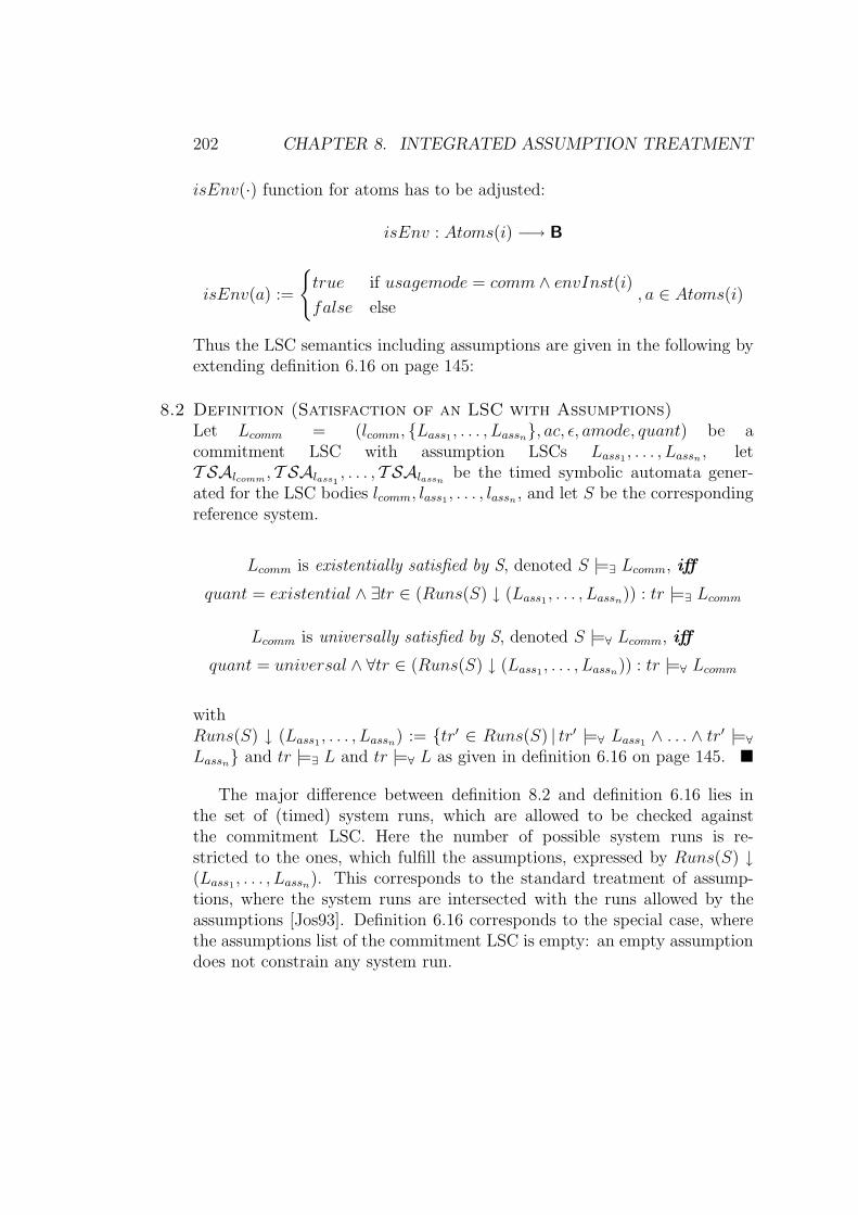
202 CHAPTER 8. INTEGRATED ASSUMPTION TREATMENT
isEnv(·) function for atoms has to be adjusted:
isEnv : Atoms(i) −→ B
isEnv(a) :=
{
true if usagemode = comm ∧ envInst(i)
false else, a ∈ Atoms(i)
Thus the LSC semantics including assumptions are given in the following byextending definition 6.16 on page 145:
8.2 Definition (Satisfaction of an LSC with Assumptions)Let Lcomm = (lcomm, {Lass1
, . . . , Lassn}, ac, ǫ, amode, quant) be a
commitment LSC with assumption LSCs Lass1, . . . , Lassn
, letT SAlcomm
, T SAlass1, . . . , T SAlassn
be the timed symbolic automata gener-ated for the LSC bodies lcomm, lass1
, . . . , lassn, and let S be the corresponding
reference system.
Lcomm is existentially satisfied by S, denoted S |=∃ Lcomm, iff
quant = existential ∧ ∃tr ∈ (Runs(S) ↓ (Lass1, . . . , Lassn
)) : tr |=∃ Lcomm
Lcomm is universally satisfied by S, denoted S |=∀ Lcomm, iff
quant = universal ∧ ∀tr ∈ (Runs(S) ↓ (Lass1, . . . , Lassn
)) : tr |=∀ Lcomm
withRuns(S) ↓ (Lass1
, . . . , Lassn) := {tr′ ∈ Runs(S) | tr′ |=∀ Lass1
∧ . . . ∧ tr′ |=∀
Lassn} and tr |=∃ L and tr |=∀ L as given in definition 6.16 on page 145. �
The major difference between definition 8.2 and definition 6.16 lies inthe set of (timed) system runs, which are allowed to be checked againstthe commitment LSC. Here the number of possible system runs is re-stricted to the ones, which fulfill the assumptions, expressed by Runs(S) ↓(Lass1
, . . . , Lassn). This corresponds to the standard treatment of assump-
tions, where the system runs are intersected with the runs allowed by theassumptions [Jos93]. Definition 6.16 corresponds to the special case, wherethe assumptions list of the commitment LSC is empty: an empty assumptiondoes not constrain any system run.
8.4. RELATED WORK 203
8.4 Related Work
To our knowledge there are no other approaches, which deal with integratedassumptions in sequence charts. Kruger [Kru00] considers external assump-tions, which are not represented graphically, however. Assumptions appearin the context of the decomposition of a global specification, given in termsof an extended MSC (MSC-96), into local specifications of the participatinginstances. For each local specification the other instances of the MSC arepart of its environment and therefore the desired behavior of this instanceis only guaranteed, if the other instances conform to their role in the globalspecification. No concrete application, like e.g. model checking, is presented,however.
The basic approach is similar to our extraction procedure: One instance issingled out and the message exchanges of the entire MSC are projected ontothe interface between the chosen instance and the remaining instances. Butwhereas in our case the commitment part is the entire LSC and the assump-tion part becomes another LSC, the result of [Kru00] is not an MSC, butrather sets of textual properties for both the commitment and the assump-tion part. The properties are further divided into a safety and a liveness part,while in our approach there is only one assumption containing all individualproperties. In contrast to our work [Kru00] does not allow the possibility tospecify assumptions about the environment of an entire chart.

204 CHAPTER 8. INTEGRATED ASSUMPTION TREATMENT
Chapter 9
Upgrading Activation:
Pre-charts
So far the activation of an LSC is guarded by activation condition and mode.It turns out that these constructs do not always sufficiently characterize theactivation point of a property specification. Often it is necessary to knowmore about the history of a run, before being able to decide, whether theLSC should be activated. There may be e.g. more than one way for a runto arrive at a certain system state (characterized by a condition), but theLSC should only be activated, if the run has followed a specific “route”. Weare for instance only interested in activating an LSC, when no errors haveoccurred so far. This motivates the introduction of pre-charts which allowto specify a prefix of a run acting as a trigger for the actual LSC.
The formal semantics of a pre-chart is defined by an altered unwindingalgorithm yielding a second automaton, in addition to the one for the LSCitself. The pre-chart automaton acts as a filter on the system runs lettingonly those pass, which fulfill the pre-chart.
Section 9.1 introduces the pre-chart concept in detail, whereas the formalsemantics is presented in section 9.2. As usual we close this chapter with adiscussion of related work in section 9.3.
9.1 Pre-charts
This chapter deals once more with the issue of when an LSC is activated.So far two means for specifying the activation point have been presented in
205
206 CHAPTER 9. UPGRADING ACTIVATION: PRE-CHARTS
section 4.2 on page 75: activation condition and activation mode. The formerspecifies a single point in time, at which the LSC is activated. Depending onthe activation mode the LSC may be activated a number of times, if this pointis reached more than once. Such a single point in time is not always sufficientfor triggering an LSC, since there may be several distinct possibilities to reacha system state, where the activation condition holds. Consider for instancethe LSC in figure 9.1, which repeats the LSC for successfully closing thebarrier of the train control system of figure 8.1 on page 173. There are twobasic ways to arrive at the state, where the signal lights on is sent: thebarrier was operational in the previous securing cycle or there was an error,either during closing or opening. In the latter case the securing procedurefor the next train will not be able to successfully secure the crossing, i.e. theprotocol shown in the LSC in figure 9.1 does not hold. In order to successfullyverify that the barrier is closed, the prerequisite is thus that the barrierhas been successfully opened during the previous securing procedure. Thisrequires that a sequence of messages must be observed, i.e. several points intime, instead of only one.
Barrier Crossing
AM: Invariant
AC: Lights_on
LSC securing_barrier
lower
close_barrier
barrier_closed
closed
Env
[1,1]
Figure 9.1: LSC for the Crossing component specifying the barrier closing
9.1. PRE-CHARTS 207
Pre-charts take care of this requirement by allowing to specify a prefixor history, which must be fulfilled by a run in order to activate the LSC. Apre-chart is essentially an LSC, i.e. all language constructs can be used in apre-chart, but its semantics is different, since the message sequence of thepre-chart is not required to hold in the system, but rather must be observedbefore activating the actual LSC.
Pre-charts do not replace the activation condition, but extend it; the acti-vation condition in the presence of a pre-chart indicates the starting point ofthe prefix. The pre-chart may be empty as has been assumed in the previoussections. The informal semantics of an LSC with pre-chart is consequently:If the activation condition holds and afterwards the pre-chart is completed,then the LSC is activated. The key point here is that the pre-chart has to betraversed completely in order to activate the LSC. This explicitly disallowsactivation of the actual LSC, if the pre-chart is exited, e.g. due to a violatedpossible condition. Thus, only when the entire prefix described in the pre-chart has been observed is the LSC considered. A violation of the pre-chartconsequently is not a violation of the actual LSC, but rather means that theLSC is not activated.
Graphically pre-charts are represented by a large possible condition sym-bol covering the pre-chart elements. The pre-chart is placed above the actualLSC. Figure 9.2 shows LSC securing barrier (cf. figure 9.1), extended byan appropriate pre-chart. The new activation condition is the opening com-mand for the barrier actuator (raise barrier). Since the goal is to requirea successful opening of the barrier in order to check the LSC describing theclosing procedure for the following train, the environment must send themessages opening and open as shown at the beginning of the pre-chart. Thetime bounds between the instance head and opening, resp. opening andopen ensure that both barrier and crossing controller return to their initialstates: The barrier controller in the Statemate model (cf. section 2.2.4)must receive the open message at most two steps after the event to raisethe barrier (RAISE) has been issued in order to return to its initial state(OPENED). Because the barrier has to first leave its closed position (eventBARRIER OPENING, to which the opening message is mapped) before it canreach its upper end position, the tight timing as given on the environmentaxis of the LSC in figure 9.2 is necessary. Once the barrier and crossing con-troller have returned to their respective initial states, the message originallyactivating the LSC in figure 9.1, lights on, should be sent triggering theactivation of the actual LSC. Another requirement for the prefix is that the
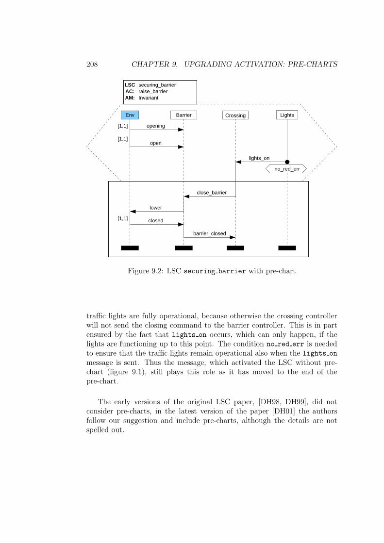
208 CHAPTER 9. UPGRADING ACTIVATION: PRE-CHARTS
BarrierEnv
AM: InvariantAC: raise_barrierLSC securing_barrier
LightsCrossing
lights_on
opening
open
close_barrier
lower
closed
barrier_closed
[1,1]
[1,1]
[1,1]
no_red_err
Figure 9.2: LSC securing barrier with pre-chart
traffic lights are fully operational, because otherwise the crossing controllerwill not send the closing command to the barrier controller. This is in partensured by the fact that lights on occurs, which can only happen, if thelights are functioning up to this point. The condition no red err is neededto ensure that the traffic lights remain operational also when the lights on
message is sent. Thus the message, which activated the LSC without pre-chart (figure 9.1), still plays this role as it has moved to the end of thepre-chart.
The early versions of the original LSC paper, [DH98, DH99], did notconsider pre-charts, in the latest version of the paper [DH01] the authorsfollow our suggestion and include pre-charts, although the details are notspelled out.
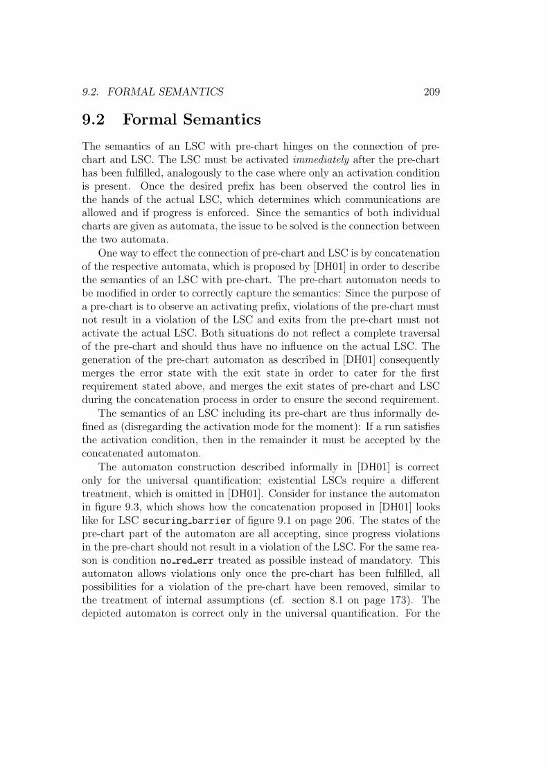
9.2. FORMAL SEMANTICS 209
9.2 Formal Semantics
The semantics of an LSC with pre-chart hinges on the connection of pre-chart and LSC. The LSC must be activated immediately after the pre-charthas been fulfilled, analogously to the case where only an activation conditionis present. Once the desired prefix has been observed the control lies inthe hands of the actual LSC, which determines which communications areallowed and if progress is enforced. Since the semantics of both individualcharts are given as automata, the issue to be solved is the connection betweenthe two automata.
One way to effect the connection of pre-chart and LSC is by concatenationof the respective automata, which is proposed by [DH01] in order to describethe semantics of an LSC with pre-chart. The pre-chart automaton needs tobe modified in order to correctly capture the semantics: Since the purpose ofa pre-chart is to observe an activating prefix, violations of the pre-chart mustnot result in a violation of the LSC and exits from the pre-chart must notactivate the actual LSC. Both situations do not reflect a complete traversalof the pre-chart and should thus have no influence on the actual LSC. Thegeneration of the pre-chart automaton as described in [DH01] consequentlymerges the error state with the exit state in order to cater for the firstrequirement stated above, and merges the exit states of pre-chart and LSCduring the concatenation process in order to ensure the second requirement.
The semantics of an LSC including its pre-chart are thus informally de-fined as (disregarding the activation mode for the moment): If a run satisfiesthe activation condition, then in the remainder it must be accepted by theconcatenated automaton.
The automaton construction described informally in [DH01] is correctonly for the universal quantification; existential LSCs require a differenttreatment, which is omitted in [DH01]. Consider for instance the automatonin figure 9.3, which shows how the concatenation proposed in [DH01] lookslike for LSC securing barrier of figure 9.1 on page 206. The states of thepre-chart part of the automaton are all accepting, since progress violationsin the pre-chart should not result in a violation of the LSC. For the same rea-son is condition no red err treated as possible instead of mandatory. Thisautomaton allows violations only once the pre-chart has been fulfilled, allpossibilities for a violation of the pre-chart have been removed, similar tothe treatment of internal assumptions (cf. section 8.1 on page 173). Thedepicted automaton is correct only in the universal quantification. For the
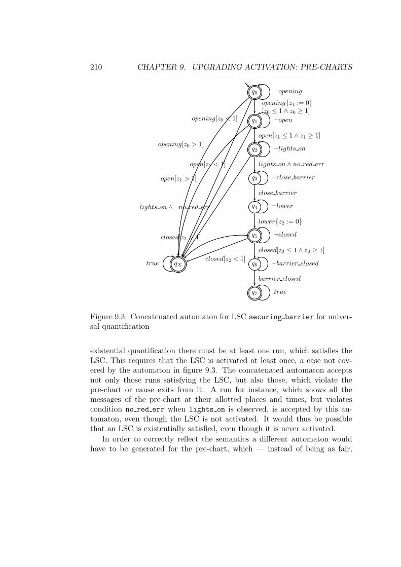
210 CHAPTER 9. UPGRADING ACTIVATION: PRE-CHARTS
q0 ¬opening
q1 ¬open
opening{z1 := 0}[z0 ≤ 1 ∧ z0 ≥ 1]
q2 ¬lights on
open[z1 ≤ 1 ∧ z1 ≥ 1]
q3 ¬close barrier
lights on ∧ no red err
q4 ¬lower
close barrier
q5 ¬closed
lower{z2 := 0}
q6 ¬barrier closed
closed[z2 ≤ 1 ∧ z2 ≥ 1]
q7 true
barrier closed
qXtrue
opening[z0 < 1]
opening[z0 > 1]
open[z1 < 1]
open[z1 > 1]
lights on ∧ ¬no red err
closed[z2 < 1]
closed[z2 > 1]
Figure 9.3: Concatenated automaton for LSC securing barrier for univer-sal quantification
existential quantification there must be at least one run, which satisfies theLSC. This requires that the LSC is activated at least once, a case not cov-ered by the automaton in figure 9.3. The concatenated automaton acceptsnot only those runs satisfying the LSC, but also those, which violate thepre-chart or cause exits from it. A run for instance, which shows all themessages of the pre-chart at their allotted places and times, but violatescondition no red err when lights on is observed, is accepted by this au-tomaton, even though the LSC is not activated. It would thus be possiblethat an LSC is existentially satisfied, even though it is never activated.
In order to correctly reflect the semantics a different automaton wouldhave to be generated for the pre-chart, which — instead of being as fair,
9.2. FORMAL SEMANTICS 211
q0 ¬opening
q1 ¬open
opening{z1 := 0}[z0 ≤ 1 ∧ z0 ≥ 1]
q2 ¬lights on
open[z1 ≤ 1 ∧ z1 ≥ 1]
q3 ¬close barrier
lights on ∧ no red err
q4 ¬lower
close barrier
q5 ¬closed
lower{z2 := 0}
q6 ¬barrier closed
closed[z2 ≤ 1 ∧ z2 ≥ 1]
q7 true
barrier closedqXtrue
closed[z2 < 1]
closed[z2 > 1]
Figure 9.4: Concatenated automaton for LSC securing barrier for exis-tential quantification
i.e. accepting, as possible as the one shown in figure 9.3 — needs to be asunfair as possible in order to reach the actual LSC part of the concatenatedautomaton, which is shown in figure 9.4. Removing the states belonging tothe pre-chart from the set of fair states in combination with omitting alltransitions to the exit state in the pre-chart ensures that the pre-chart mustbe traversed. All runs which do not fulfill the pre-chart result in an error,which is inconsequential in the existential quantification as long as there isone run, which activates and satisfies the LSC.
The drawback of this approach is thus that a different automaton con-struction is required depending on the quantification. In order to avoid thisunnecessary dependency, we use a different approach, which does not rely
212 CHAPTER 9. UPGRADING ACTIVATION: PRE-CHARTS
on the quantification. Our approach builds on the fact that a pre-chart de-scribes only a finite sequence of messages: from the time when the activationcondition holds until the pre-chart is traversed completely. This means thata finite (timed) run and consequently a finite (timed) automaton are suf-ficient to recognize an activating prefix. The only accepting state of thisfinite automaton is the final state representing the complete traversal of thepre-chart.
In definition 9.1 on page 215 below we will see that pre-charts are treateduniformly in the semantics, independent of the quantification, thus effecting asimpler treatment of pre-charts in the semantics. The pre-chart automatonis separated from the LSC automaton and treated in the same manner asthe activation condition. For universally quantified LSCs this results in thefollowing informally stated implication: If the activation condition holds andthe pre-chart is fulfilled, then the LSC is considered. Our approach thusyields a clearer separation of concerns between activation and satisfactionof an LSC. The concatenation approach of [DH01] mixes both aspects andresults in a more complex semantics.
Since pre-charts only observe, if the desired prefix is part of a run, there isno need for internal assumptions, i.e. to treat environment axes in a specialway for the unwinding. The effect of internal assumptions is guaranteed bythe fact that the actual LSC is only activated once the complete pre-charthas been traversed. Thus, no exit state is needed.
The treatment of extracted assumptions for the LSC does not needto be adjusted in the presence of a pre-chart. The required syn-chronization with the activation of the actual LSC is already incor-porated into the assumption extraction described in section 8.2.1 onpage 195. Recall that for the assumption extraction an assumption LSCLass = (lass, ∅, ac, pch, amode, universal) is generated for a commitment LSCLcomm = (lcomm, assumptions, ac, pch, amode, quant). In particular, the ex-tracted assumption inherits the pre-chart of its commitment LSC. The correctactivation of the extracted assumption is thus guaranteed.
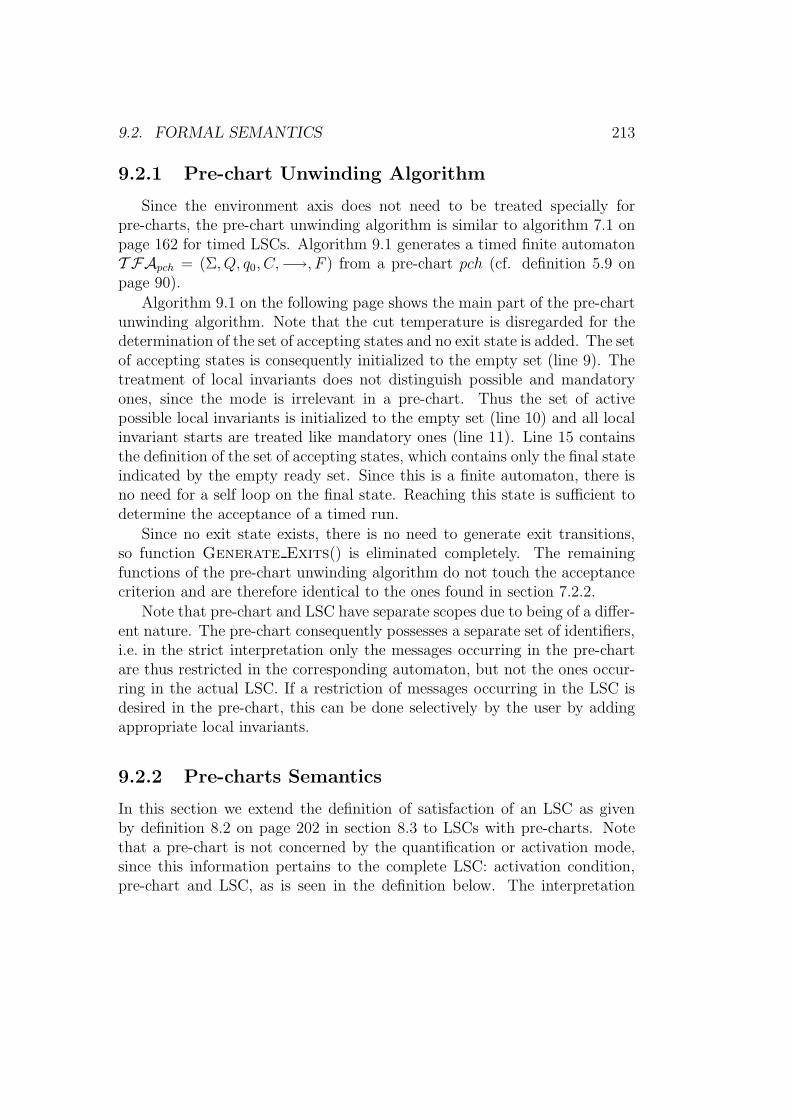
9.2. FORMAL SEMANTICS 213
9.2.1 Pre-chart Unwinding Algorithm
Since the environment axis does not need to be treated specially forpre-charts, the pre-chart unwinding algorithm is similar to algorithm 7.1 onpage 162 for timed LSCs. Algorithm 9.1 generates a timed finite automatonT FApch = (Σ, Q, q0, C,−→, F ) from a pre-chart pch (cf. definition 5.9 onpage 90).
Algorithm 9.1 on the following page shows the main part of the pre-chartunwinding algorithm. Note that the cut temperature is disregarded for thedetermination of the set of accepting states and no exit state is added. The setof accepting states is consequently initialized to the empty set (line 9). Thetreatment of local invariants does not distinguish possible and mandatoryones, since the mode is irrelevant in a pre-chart. Thus the set of activepossible local invariants is initialized to the empty set (line 10) and all localinvariant starts are treated like mandatory ones (line 11). Line 15 containsthe definition of the set of accepting states, which contains only the final stateindicated by the empty ready set. Since this is a finite automaton, there isno need for a self loop on the final state. Reaching this state is sufficient todetermine the acceptance of a timed run.
Since no exit state exists, there is no need to generate exit transitions,so function Generate Exits() is eliminated completely. The remainingfunctions of the pre-chart unwinding algorithm do not touch the acceptancecriterion and are therefore identical to the ones found in section 7.2.2.
Note that pre-chart and LSC have separate scopes due to being of a differ-ent nature. The pre-chart consequently possesses a separate set of identifiers,i.e. in the strict interpretation only the messages occurring in the pre-chartare thus restricted in the corresponding automaton, but not the ones occur-ring in the actual LSC. If a restriction of messages occurring in the LSC isdesired in the pre-chart, this can be done selectively by the user by addingappropriate local invariants.
9.2.2 Pre-charts Semantics
In this section we extend the definition of satisfaction of an LSC as givenby definition 8.2 on page 202 in section 8.3 to LSCs with pre-charts. Notethat a pre-chart is not concerned by the quantification or activation mode,since this information pertains to the complete LSC: activation condition,pre-chart and LSC, as is seen in the definition below. The interpretation
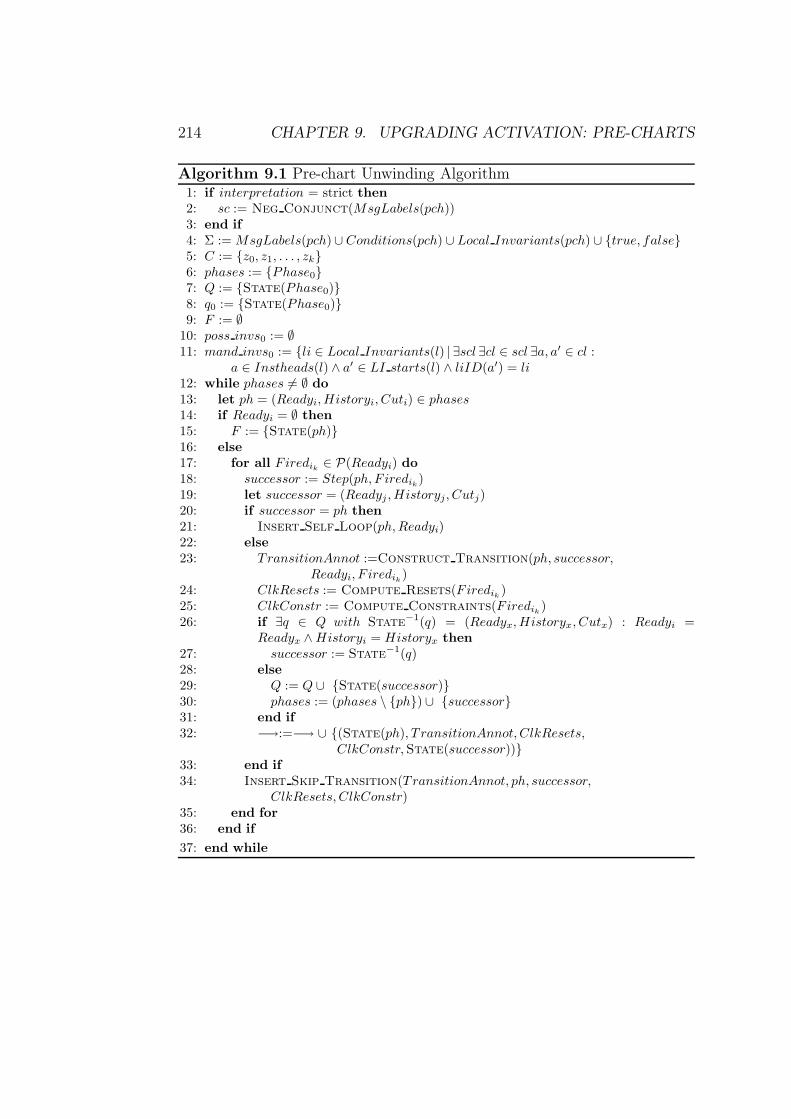
214 CHAPTER 9. UPGRADING ACTIVATION: PRE-CHARTS
Algorithm 9.1 Pre-chart Unwinding Algorithm1: if interpretation = strict then
2: sc := Neg Conjunct(MsgLabels(pch))3: end if
4: Σ := MsgLabels(pch)∪ Conditions(pch) ∪ Local Invariants(pch) ∪ {true, false}5: C := {z0, z1, . . . , zk}6: phases := {Phase0}7: Q := {State(Phase0)}8: q0 := {State(Phase0)}9: F := ∅
10: poss invs0 := ∅11: mand invs0 := {li ∈ Local Invariants(l) | ∃scl ∃cl ∈ scl ∃a, a′ ∈ cl :
a ∈ Instheads(l) ∧ a′ ∈ LI starts(l) ∧ liID(a′) = li
12: while phases 6= ∅ do
13: let ph = (Readyi, Historyi, Cuti) ∈ phases
14: if Readyi = ∅ then
15: F := {State(ph)}16: else
17: for all Firedik∈ P(Readyi) do
18: successor := Step(ph, F iredik)
19: let successor = (Readyj , Historyj, Cutj)20: if successor = ph then
21: Insert Self Loop(ph,Readyi)22: else
23: TransitionAnnot :=Construct Transition(ph, successor,Readyi, F iredik
)24: ClkResets := Compute Resets(Firedik
)25: ClkConstr := Compute Constraints(Firedik
)26: if ∃q ∈ Q with State−1(q) = (Readyx, Historyx, Cutx) : Readyi =
Readyx ∧Historyi = Historyx then
27: successor := State−1(q)28: else
29: Q := Q ∪ {State(successor)}30: phases := (phases \ {ph}) ∪ {successor}31: end if
32: −→:=−→ ∪ {(State(ph), T ransitionAnnot, ClkResets,ClkConstr,State(successor))}
33: end if
34: Insert Skip Transition(TransitionAnnot, ph, successor,ClkResets, ClkConstr)
35: end for
36: end if
37: end while
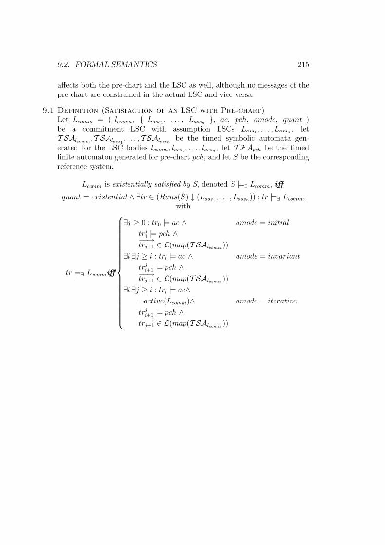
9.2. FORMAL SEMANTICS 215
affects both the pre-chart and the LSC as well, although no messages of thepre-chart are constrained in the actual LSC and vice versa.
9.1 Definition (Satisfaction of an LSC with Pre-chart)Let Lcomm = ( lcomm, { Lass1
, . . . , Lassn}, ac, pch, amode, quant )
be a commitment LSC with assumption LSCs Lass1, . . . , Lassn
, letT SAlcomm
, T SAlass1, . . . , T SAlassn
be the timed symbolic automata gen-erated for the LSC bodies lcomm, lass1
, . . . , lassn, let T FApch be the timed
finite automaton generated for pre-chart pch, and let S be the correspondingreference system.
Lcomm is existentially satisfied by S, denoted S |=∃ Lcomm, iff
quant = existential ∧ ∃tr ∈ (Runs(S) ↓ (Lass1, . . . , Lassn
)) : tr |=∃ Lcomm,with
tr |=∃ Lcommiff
∃j ≥ 0 : tr0 |= ac ∧ amode = initial
trj1 |= pch ∧
−−→trj+1 ∈ L(map(T SAlcomm
))
∃i ∃j ≥ i : tri |= ac ∧ amode = invariant
trji+1 |= pch ∧
−−→trj+1 ∈ L(map(T SAlcomm
))
∃i ∃j ≥ i : tri |= ac∧
¬active(Lcomm)∧ amode = iterative
trji+1 |= pch ∧
−−→trj+1 ∈ L(map(T SAlcomm
))
216 CHAPTER 9. UPGRADING ACTIVATION: PRE-CHARTS
Lcomm is universally satisfied by S, denoted S |=∀ Lcomm, iff
quant = universal ∧ ∀tr ∈ (TRuns(S) ↓ (Lass1, . . . , Lassn
)) : tr |=∀ Lcomm,with
tr |=∀ Lcommiff
∀j ≥ 0 : tr0 |= ac ∧ amode = initial
trj1 |= pch⇒
−−→trj+1 ∈ L(map(T SAlcomm
))
∀i ∀j ≥ i : tri |= ac ∧ amode = invariant
trji+1 |= pch⇒
−−→trj+1 ∈ L(map(T SAlcomm
))
∀i ∀j ≥ i : tri |= ac∧
¬active(Lcomm)∧ amode = iterative
trji+1 |= pch⇒
−−→trj+1 ∈ L(map(T SAlcomm
))
with
• trji+1 |= pch denoting the satisfaction of pch by trj
i+1 :
trji+1 |= pch iff trj
i+1 ∈ L(map(T FApch)),
• (Runs(S) ↓ (Lass1, . . . , Lassn
)) as given by definition 8.2 on page 202,active(L) and L(map(T SAl)) as given by definition 6.16 on page 145.
�
For existential satisfaction of an LSC all three components must hold,i.e. for at least one run the activation condition must be evaluated to trueand the pre-chart must be fulfilled and the LSC must be satisfied. For uni-versal satisfaction of an LSC the pre-chart is placed on the left-hand sideof the implication: If the activation condition holds and the pre-chart isfulfilled, then the actual LSC must be satisfied. For existential satisfactionthe implication is simply exchanged for a conjunction. The pre-chart is thustreated in an identical manner to the activation condition.
The transition from the pre-chart to the LSC upon complete traversal isachieved using index j, which marks the valuation of timed run tr reachingthe final state in the pre-chart automaton and thus the transition into theLSC. The next valuation j + 1 is the first step of run tr, which is within
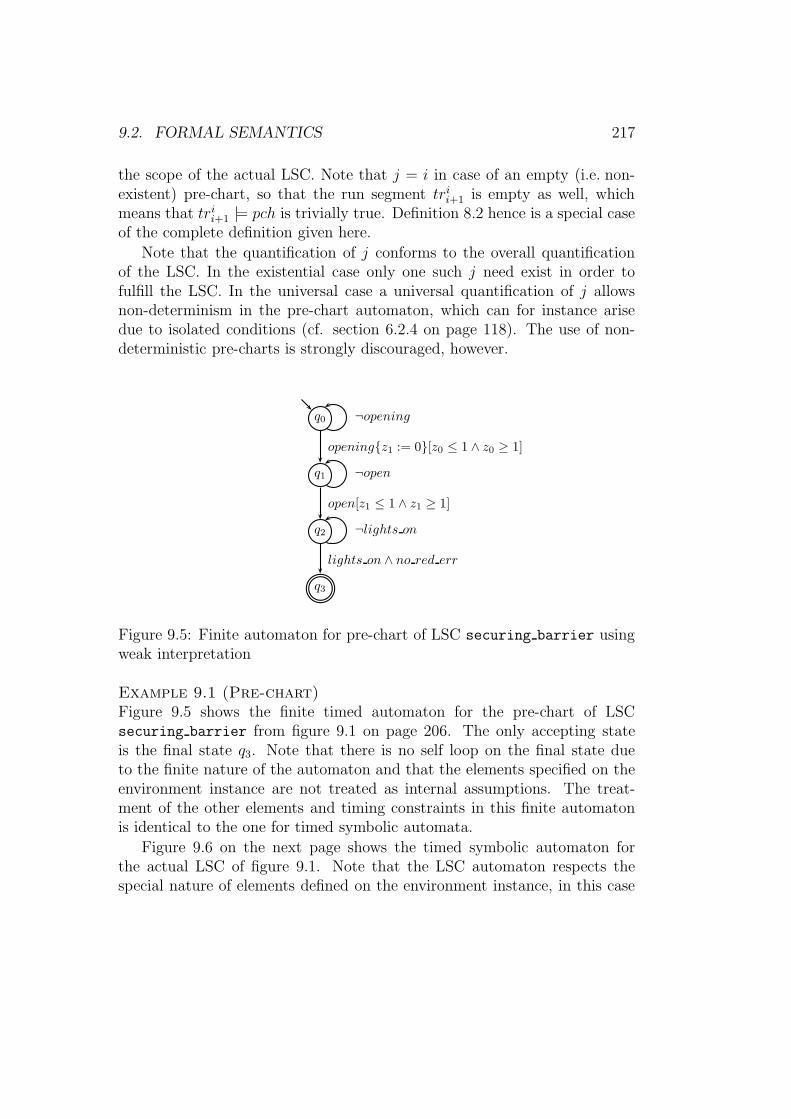
9.2. FORMAL SEMANTICS 217
the scope of the actual LSC. Note that j = i in case of an empty (i.e. non-existent) pre-chart, so that the run segment tri
i+1 is empty as well, whichmeans that tri
i+1 |= pch is trivially true. Definition 8.2 hence is a special caseof the complete definition given here.
Note that the quantification of j conforms to the overall quantificationof the LSC. In the existential case only one such j need exist in order tofulfill the LSC. In the universal case a universal quantification of j allowsnon-determinism in the pre-chart automaton, which can for instance arisedue to isolated conditions (cf. section 6.2.4 on page 118). The use of non-deterministic pre-charts is strongly discouraged, however.
q0 ¬opening
q1 ¬open
opening{z1 := 0}[z0 ≤ 1 ∧ z0 ≥ 1]
q2 ¬lights on
open[z1 ≤ 1 ∧ z1 ≥ 1]
q3
lights on ∧ no red err
Figure 9.5: Finite automaton for pre-chart of LSC securing barrier usingweak interpretation
Example 9.1 (Pre-chart)Figure 9.5 shows the finite timed automaton for the pre-chart of LSCsecuring barrier from figure 9.1 on page 206. The only accepting stateis the final state q3. Note that there is no self loop on the final state dueto the finite nature of the automaton and that the elements specified on theenvironment instance are not treated as internal assumptions. The treat-ment of the other elements and timing constraints in this finite automatonis identical to the one for timed symbolic automata.
Figure 9.6 on the next page shows the timed symbolic automaton forthe actual LSC of figure 9.1. Note that the LSC automaton respects thespecial nature of elements defined on the environment instance, in this case
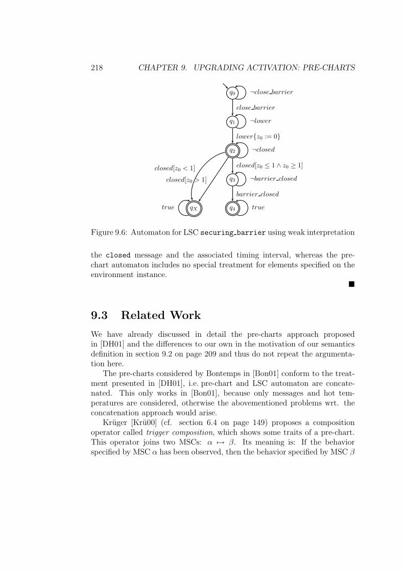
218 CHAPTER 9. UPGRADING ACTIVATION: PRE-CHARTS
q0 ¬close barrier
q1 ¬lower
close barrier
q2 ¬closed
lower{z0 := 0}
q3 ¬barrier closed
closed[z0 ≤ 1 ∧ z0 ≥ 1]
q4 true
barrier closed
qXtrue
closed[z0 < 1]
closed[z0 > 1]
Figure 9.6: Automaton for LSC securing barrier using weak interpretation
the closed message and the associated timing interval, whereas the pre-chart automaton includes no special treatment for elements specified on theenvironment instance.
�
9.3 Related Work
We have already discussed in detail the pre-charts approach proposedin [DH01] and the differences to our own in the motivation of our semanticsdefinition in section 9.2 on page 209 and thus do not repeat the argumenta-tion here.
The pre-charts considered by Bontemps in [Bon01] conform to the treat-ment presented in [DH01], i.e. pre-chart and LSC automaton are concate-nated. This only works in [Bon01], because only messages and hot tem-peratures are considered, otherwise the abovementioned problems wrt. theconcatenation approach would arise.
Kruger [Kru00] (cf. section 6.4 on page 149) proposes a compositionoperator called trigger composition, which shows some traits of a pre-chart.This operator joins two MSCs: α 7→ β. Its meaning is: If the behaviorspecified by MSC α has been observed, then the behavior specified by MSC β
9.3. RELATED WORK 219
is inevitable. This notion is similar to the pre-chart concept presented in thissection, but not identical as the trigger composition operator expresses rathera liveness requirement than a history of behavior, since β need not startimmediately after the completion of α. This is a key property of pre-charts,which can not be expressed by the MSC language presented in [Kru00]. Thetrigger composition rather corresponds to a liveness requirement, i.e. a hotcut, in LSCs.
Firley et al. [FHD+99] (cf. section 6.4 on page 149) present a pre-chart-like concept as well, called If-Then-Behavior, which is applied to SDs. Itcorresponds more closely to pre-charts than the trigger composition, sincethe second SD is entered immediately after the first one is completed. Theconnection between the first and second SD is established by concatenation,which does not provoke the problem with the quantification described insection 9.2, since SDs are viewed only existentially in [FHD+99].
220 CHAPTER 9. UPGRADING ACTIVATION: PRE-CHARTS
Chapter 10
Embedding LSCs into the
Development Process
The practical usefulness of a language not only depends on its immediateproperties like features, graphical representation or expressiveness, but alsoon guidelines how and when to apply it. The users need to know for whichtasks in the design process the language is intended and how it should beapplied to get the best results. Hence, in addition to the description of thelanguage and its meaning (syntax and semantics) a methodology should beprovided, which indicates what the primary use cases of this language are.After introducing the language features and defining their semantics in thepreceding chapters, this chapter presents such a methodology for LSCs on thebasis of a model-based development process. There are several standardizedprocess models, like the waterfall model [Roy70], spiral model [Boe88] orV-model [ESt97], to name but a few.
Regardless of the particular process model there are recurring commonphases. Since we do not want to focus on a specific development process, welook at an abstract process model, which consists of these typical, recurringdevelopment phases. In section 10.1 we thus introduce such an abstractprocess model and its phases. We assume that the process is model-basedand focus on the phases on the use case of formal verification and the phasesaffected thereby. Section 10.2 outlines our methodology by embedding LSCsinto this abstract development process. We conclude this chapter with areview of related work in section 10.3.
221
222 CHAPTER 10. LSCS IN THE DEVELOPMENT PROCESS
10.1 Abstract Development Process
Phase 1: Initial System Analysis Phase embedded controller devel-opment typically starts with a textual requirements specification, which de-scribes the basic functionality using natural language. It also contains non-functional constraints like timing requirements, side conditions due to limitedresources, interoperability demands, etc. For the documentation of the majorfunctionality Use Case Diagrams are often used.
Phase 2: Architectural Design Phase The Architectural Design Phaseis concerned with structuring the system under design (SUD). Based on theresults of the previous phase the SUD is decomposed in a top-down manner,iteratively breaking the complete system down into sub-components. Simul-taneously the interfaces, including the interface between the system itselfand its environment, and the connections between the different sub-systemsare defined. In a model-based development process the functional decom-position of the system can e.g. be represented by classes (if for instance theUML is employed) or activities (if Statemate is used). The system struc-ture, including connections between entities, is then for example modeled byClass, Collaboration or Sequence Diagrams or Activity Charts. The result isa model of the hierarchical system architecture with defined interfaces andconnections.
Phase 3: Behavioral Design Phase Assuming a model-based process,the detailed behavior of each sub-system is modeled in this phase. This modelcan be analyzed, simulated and verified, depending on the tool support. ForStatemate designs the behavioral specification is given as Statecharts, inthe UML State Diagrams are typically used. The goal of this phase is areference model, which has been thoroughly analyzed and implements thekey properties specified in the requirements document. It thus serves as areference for the following phases, which is the most important advantage ofa model-based development process.
Phase 4: Implementation Phase This phase entails the actual imple-mentation of the SUD in hard- and software. The tasks to be performedhere are thus primarily the partitioning into software and hardware partsand the derivation of code (manually or automatically). The model, which
10.2. ADVANCED USE CASES FOR LSCS 223
is the outcome of the previous phase, serves as a reference against which theimplementation is measured. The particular steps in this phase strongly de-pend on the type of application being developed and the tools used; severalmodeling tools e.g. offer automatic code generation capabilities.
Phase 5: Test Phase The goal of this phase is to ensure that the im-plementation generated in the previous phase is free of any major errorsand meets the initially specified requirements. This entails first testing eachsub-system in isolation (module test) and later in conjunction with other sub-systems (integration testing). For embedded controllers prototypes, realizedeither in hard- or software, are often hooked up to the physical environmentthey are built for (hardware or software in the loop testing). The final partof this stage is the acceptance test, where the conformance of the completesystem to the customer’s requirements is demonstrated. Note that in mostprocess models this phase consists of several individual phases.
10.2 Advanced Use Cases for LSCs
In this section we outline the methodology for embedding LSCs into a model-based development process, with special attention to the use case of formalverification. We use the abstract development process introduced in the pre-vious section as a guideline through the methodology. In the Initial SystemAnalysis Phase LSCs are typically not used, since LSCs are not intended forspecifying non-functional requirements, except timing information. More-over, the structure of the SUD is only developed in the following phase,which constitutes the first use case for LSCs:
10.2.1 Capturing Typical System Interactions
At the beginning of Architectural Design Phase existential LSCs are used forthe illustration of the major use cases, similar to the use Sequence Diagramsare put to in the UML. During elaboration of the use cases in the form ofLSCs the primary participants are identified and become instances in theLSC. In this manner a first view of the system architecture evolves and thusthe first level of hierarchy is created.
By allowing to capture the typical communication scenarios as LSCs thedesigner is supported in identifying the entities needed for the realization
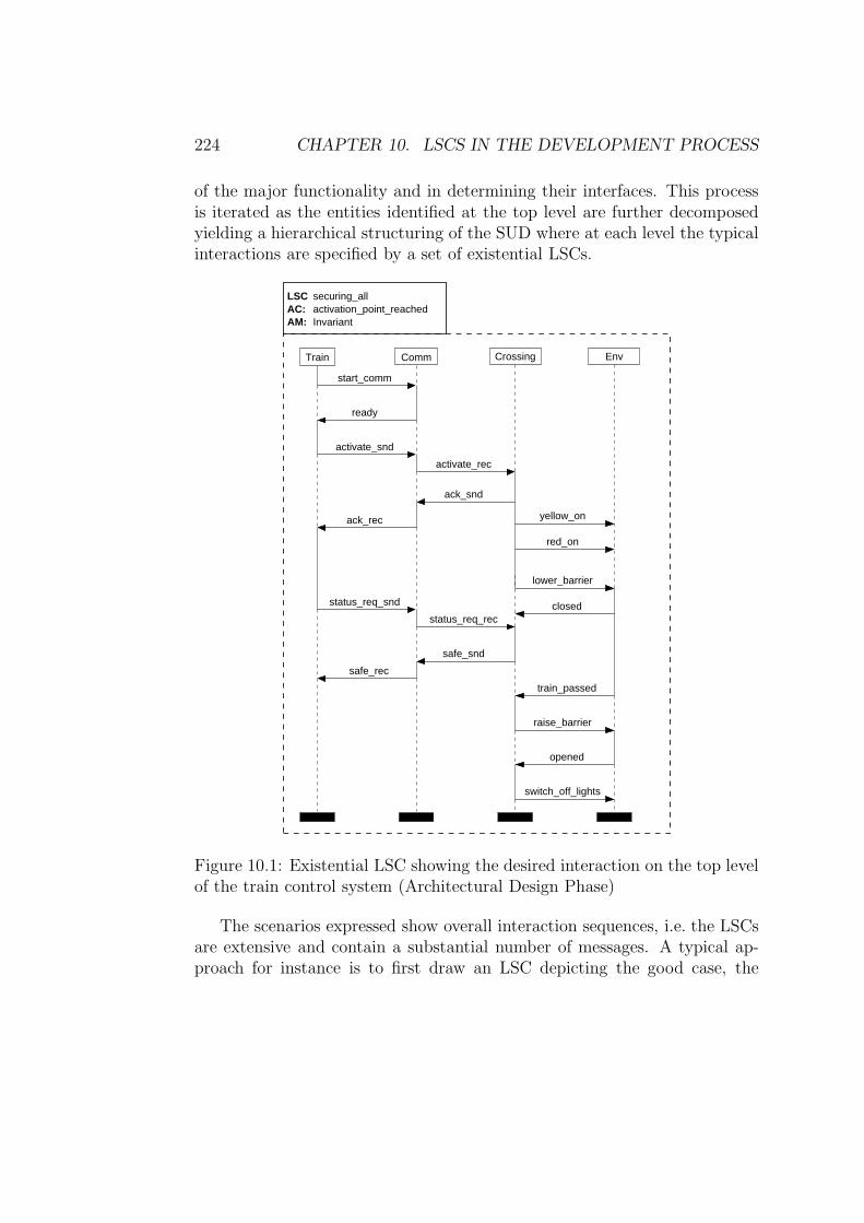
224 CHAPTER 10. LSCS IN THE DEVELOPMENT PROCESS
of the major functionality and in determining their interfaces. This processis iterated as the entities identified at the top level are further decomposedyielding a hierarchical structuring of the SUD where at each level the typicalinteractions are specified by a set of existential LSCs.
EnvCommTrain Crossing
start_comm
ready
activate_snd
activate_rec
ack_snd
safe_rec
safe_snd
status_req_rec
status_req_snd
train_passed
raise_barrier
opened
switch_off_lights
closed
lower_barrier
yellow_on
red_on
ack_rec
Invariantactivation_point_reachedsecuring_all
AM:AC:LSC
Figure 10.1: Existential LSC showing the desired interaction on the top levelof the train control system (Architectural Design Phase)
The scenarios expressed show overall interaction sequences, i.e. the LSCsare extensive and contain a substantial number of messages. A typical ap-proach for instance is to first draw an LSC depicting the good case, the
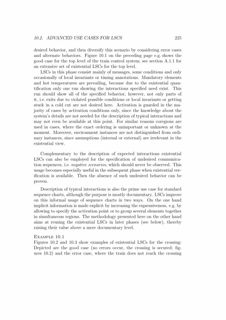
10.2. ADVANCED USE CASES FOR LSCS 225
desired behavior, and then diversify this scenario by considering error casesand alternate behaviors. Figure 10.1 on the preceding page e.g. shows thegood case for the top level of the train control system; see section A.1.1 foran extensive set of existential LSCs for the top level.
LSCs in this phase consist mainly of messages, some conditions and onlyoccasionally of local invariants or timing annotations. Mandatory elementsand hot temperatures are prevailing, because due to the existential quan-tification only one run showing the interactions specified need exist. Thisrun should show all of the specified behavior, however, not only parts ofit, i.e. exits due to violated possible conditions or local invariants or gettingstuck in a cold cut are not desired here. Activation is guarded in the ma-jority of cases by activation conditions only, since the knowledge about thesystem’s details are not needed for the description of typical interactions andmay not even be available at this point. For similar reasons coregions areused in cases, where the exact ordering is unimportant or unknown at themoment. Moreover, environment instances are not distinguished from ordi-nary instances, since assumptions (internal or external) are irrelevant in theexistential view.
Complementary to the description of expected interactions existentialLSCs can also be employed for the specification of undesired communica-tion sequences, i.e. negative scenarios, which should never be observed. Thisusage becomes especially useful in the subsequent phase when existential ver-ification is available. Then the absence of such undesired behavior can beproven.
Description of typical interactions is also the prime use case for standardsequence charts, although the purpose is mostly documentary. LSCs improveon this informal usage of sequence charts in two ways. On the one handimplicit information is made explicit by increasing the expressiveness, e.g. byallowing to specify the activation point or to group several elements togetherin simultaneous regions. The methodology presented here on the other handaims at reusing the existential LSCs in later phases (see below), therebyraising their value above a mere documentary level.
Example 10.1Figures 10.2 and 10.3 show examples of existential LSCs for the crossing:Depicted are the good case (no errors occur, the crossing is secured; fig-ures 10.2) and the error case, where the train does not reach the crossing
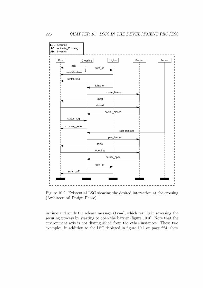
226 CHAPTER 10. LSCS IN THE DEVELOPMENT PROCESS
AM: InvariantAC: Activate_CrossingLSC securing
Env Lights
ack
BarrierCrossing
turn_on
switch2yellow
switch2red
lights_on
status_req
crossing_safe
barrier_closed
lower
closed
barrier_open
raise
opening
turn_off
switch_off
open_barrier
Sensor
train_passed
close_barrier
Figure 10.2: Existential LSC showing the desired interaction at the crossing(Architectural Design Phase)
in time and sends the release message (free), which results in reversing thesecuring process by starting to open the barrier (figure 10.3). Note that theenvironment axis is not distinguished from the other instances. These twoexamples, in addition to the LSC depicted in figure 10.1 on page 224, show
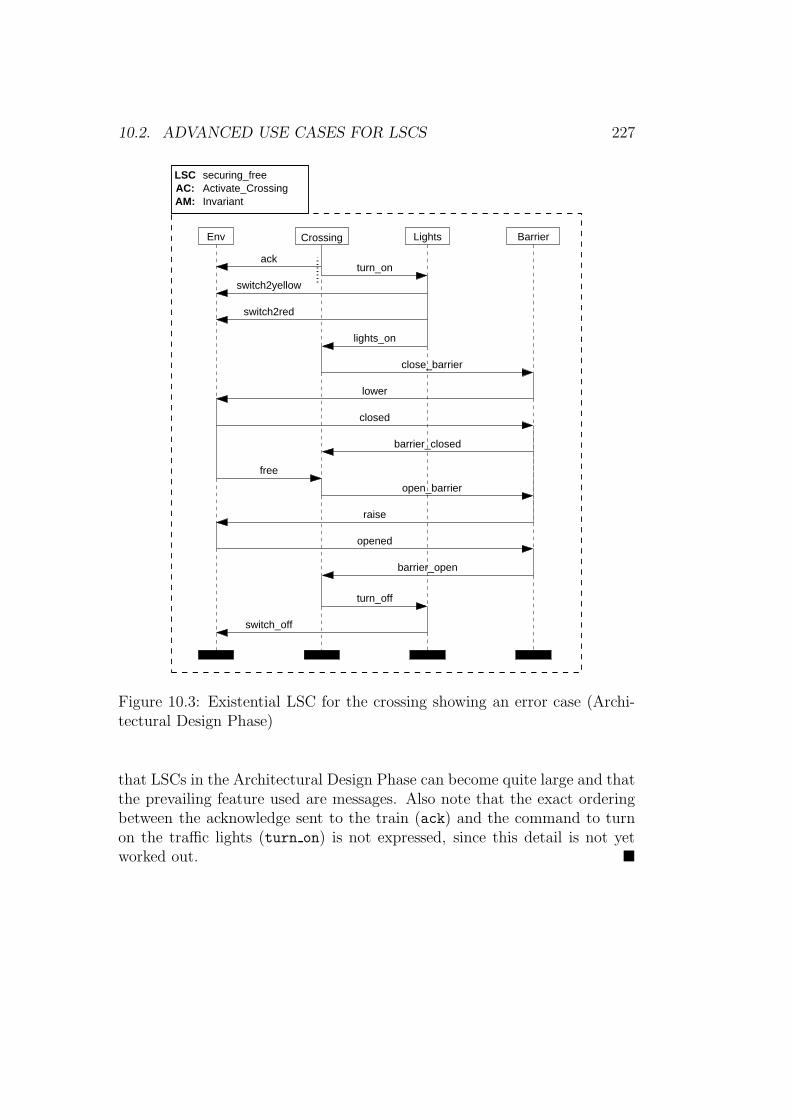
10.2. ADVANCED USE CASES FOR LSCS 227
AM: InvariantAC: Activate_CrossingLSC securing_free
Env Lights
ack
BarrierCrossing
turn_on
switch2yellow
switch2red
lights_on
lower
closed
barrier_closed
free
open_barrier
barrier_open
opened
turn_off
switch_off
raise
close_barrier
Figure 10.3: Existential LSC for the crossing showing an error case (Archi-tectural Design Phase)
that LSCs in the Architectural Design Phase can become quite large and thatthe prevailing feature used are messages. Also note that the exact orderingbetween the acknowledge sent to the train (ack) and the command to turnon the traffic lights (turn on) is not expressed, since this detail is not yetworked out. �
228 CHAPTER 10. LSCS IN THE DEVELOPMENT PROCESS
10.2.2 Debugging by Existential Verification
At the end of the Architectural Design Phase the system architecture isknown and for each hierarchy level a set of existential LSCs has been drawnto capture the typical communications between (sub-)systems/entities at thislevel. The next step is to define the behavior of each entity and thus ofthe complete system, which is done in the Behavioral Design Phase. In amodel-based development process the goal is to produce a reference modelfor the subsequent phases. Steps toward this goal are simulation, analysisand formal verification. We present those related to LSCs in this and thefollowing section.
Once a suitable portion of the behavior has been modeled, the existentialLSCs specified in the previous phase can be reused for verification. Sincethese LSCs are existential, it is checked if the part of the system constructedso far, is indeed capable of performing the typical communication sequence atleast once. Or in other words: Is there at least one run, which conforms to thespecified scenario? We call this use case existential verification. This checkcan be applied as the model is built, i.e. the model need not be complete.The developer decides if and when existential verification is to be applied,which LSCs are to be checked, etc.
Existential verification can hence be employed as a debugging aid early inthe development in order to verify that the current state of the SUD modelis able to perform the basic interactions as specified by the existential LSCs.The LSCs created in the previous phase can be used directly without anymodifications, allowing a facile reuse.
Negative scenarios are verified in the same way as normal existentialLSCs, only the result is interpreted differently. If a negative scenario isproven to be possible in the model, this indicates an error, since the absenceof the specified interaction sequence is expected. Checking negative scenariosis thus performed at the same stage as universal verification, i.e. at the endof the Behavioral Design Phase when the model has reached a mature andstable state.
10.2. ADVANCED USE CASES FOR LSCS 229
10.2.3 From Scenarios to Protocol Specifications
Modularization of Existential LSCs
Existential verification, potentially in conjunction with simulation and anal-ysis of the model, increases the confidence in the correctness of the modelbeing built compared to a traditional design process. These measures do notensure, however, that a requirement is fulfilled under all circumstances, sincenot all possible cases are covered. This can be achieved by formally verifyingkey properties specified as universal LSCs, which is applied towards the endof the Behavioral Design Phase, i.e. when the model is mature and stable.
The question at this point is where do these universal LSCs come from.The existential LSCs specified in the Architectural Design Phase alreadycontain these key properties. The aim is thus to reuse these LSCs for thespecification of the properties to be model checked. Since such existentialLSCs tend to be rather large as the LSCs in figures 10.1 - 10.3 illustrate(see also sections A.1.1, A.2.1 and A.3.1), the relevant protocols have to beidentified and extracted.
The procedure for producing smaller, more concise universal LSCs fromextensive existential LSCs is guided by identifying fragments belonging to-gether, i.e. forming one sub-protocol, one property. A first indication in thisdirection is gained by recognizing identical or similar parts in a set of ex-istential LSCs. The existential LSCs produced in the preceding phase arenot completely disjunct, but partially overlapping, since an LSC showing agood case, is often complemented by others, which describe potential errorsituations. The LSCs in figure 10.2 on page 226 and figure 10.3 on page 227for instance are largely identical. At the developers discretion the overlap-ping parts are factored out yielding a number of shorter, core communicationsequences. We call this extraction of universal protocols from an existentialLSC modularization.
Strengthening the LSCs
Before the extracted sub-protocols can be verified they have to be adjustedto the changed usage. In a first step the quantification is changed to uni-versal and environment instances, if present, are distinguished from normalinstances in order to enable the consideration of internal and extracted as-sumptions. Generally, other modifications have to be applied as well toenable formal verification of the extracted universal LSCs. We refer to this
230 CHAPTER 10. LSCS IN THE DEVELOPMENT PROCESS
second part of the transformation from existential scenarios to universal pro-tocol specifications as strengthening. The strengthening activities can also beviewed as a generalization, since general behavior is deduced from particularruns.
The typical interaction sequences created in the previous phase can usu-ally be expressed by basic LSC features, mostly messages. As the aim nowis to prove that the specified interaction is executed under all circumstances,more information and precision is needed, requiring more advanced features.Mandatory conditions or timing constraints, are e.g. added and indeterminedordering of messages expressed e.g. by coregions is made more precise by re-quiring a specific order or employing simultaneous regions.
In order to prove that the model conforms to the behavior specified bya universal LSC, generally the environment actions have to be restrictedin addition to specifying more precise charts. The assumptions effectingthese restrictions can be grouped into two categories: Assumptions ensuringreactions of the environment and assumptions expressing case distinctions.The former category comprises hot locations and timing annotations on theenvironment axis. The latter category of assumptions is used to focus on aspecific behavior of the SUD. In order to successfully verify that the barriersare closed, the barriers have to be operational, i.e. the system behavior hasto be restricted to this case. Conditions and local invariants are typicallyused for this purpose. Both internal and external assumptions can be used,although it is recommended to use internal assumptions if possible, sincethey are more intuitive due to the fact that they are contained directly inthe commitment LSC.
Activation conditions of universal LSCs often need to be made more pre-cise, i.e. more restricted, in order to rule out undesired activations of theLSC. For some charts it will become apparent that more information aboutthe history of a run is needed in order to determine, if the LSC should be ac-tivated. Activation conditions are thus in such cases extended to pre-charts.
The process of model checking the resulting LSC specifications typicallyrequires several iterations, in which the mentioned strengthening actions areperformed incrementally. First the commitment side of an LSC is strength-ened in conjunction with some basic restrictions of the environment. If thespecified property does not hold, there is either an error in the model orthe LSC is not precise enough. In the first case the model is corrected andthe proof is executed again. Each change to the model moreover requires
10.2. ADVANCED USE CASES FOR LSCS 231
a re-assessment of the other LSCs, i.e. it has to be determined, if they areaffected by the altered model behavior. In the second case the LSC has tobe analyzed and corrected, e.g. by adding an assumption.
Care has to be taken when specifying assumptions in order to be consis-tent with the initial requirements. Before an assumption is added to a com-mitment LSC the designer has to determine that the assumption is valid,i.e. conforms to the initial requirements document and is justified by theenvironment.
The result of this phase is a model, which serves as a reference for the fur-ther steps in the development process. The verification activities describedabove are an important step towards such a reference model, in addition toother measures like simulation and analysis. The reference model constitutesan early, virtual integration of the components of which the SUD is com-prised. Existential and universal LSC-based verification allows to check theintegration and interplay of the individual components prior to their imple-mentation.
Note that verification does not ensure the complete correctness of themodel, but only wrt. the specified properties. If the specified and verifiedproperties cover all the requirements stated in the initial document or if thoserequirements are complete themselves, has to be determined in a differentway. Such considerations are beyond the scope of this thesis.
Example 10.2 (Modularization and Strengthening)In this example we illustrate part of the modularization and strengtheningprocess described above at the level of the crossing component of the traincontrol system. For the strengthening we will not present all intermediateversions of the universal LSCs, but rather only show the final one.
The LSCs in figures 10.2 on page 226 and 10.3 on page 227 show two of theexistential LSCs for this component, more can be found in section A.3.1 in theappendix. LSC securing (figure 10.2) shows the good case, the remainingones describe error scenarios, which are identical in large parts. A naturalmodularization is to separate the activities necessary for a train approachingthe crossing from those for a train, which has already passed the crossing.This cuts off the lower part of the LSCs, from message open barrier ondownward; figure 10.4 shows the resulting already strengthened, universalLSC.
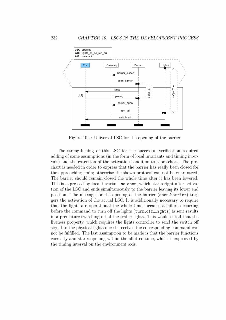
232 CHAPTER 10. LSCS IN THE DEVELOPMENT PROCESS
Barrier Lights
AM: InvariantAC:LSC
Env Crossing
openinglights_on_no_red_err
open_barrier
turn_off
raise
barrier_open
barrier_closed
opening
switch_off
no_red_err
no_open[1,1]
Figure 10.4: Universal LSC for the opening of the barrier
The strengthening of this LSC for the successful verification requiredadding of some assumptions (in the form of local invariants and timing inter-vals) and the extension of the activation condition to a pre-chart. The pre-chart is needed in order to express that the barrier has really been closed forthe approaching train; otherwise the shown protocol can not be guaranteed.The barrier should remain closed the whole time after it has been lowered.This is expressed by local invariant no open, which starts right after activa-tion of the LSC and ends simultaneously to the barrier leaving its lower endposition. The message for the opening of the barrier (open barrier) trig-gers the activation of the actual LSC. It is additionally necessary to requirethat the lights are operational the whole time, because a failure occurringbefore the command to turn off the lights (turn off lights) is sent resultsin a premature switching off of the traffic lights. This would entail that theliveness property, which requires the lights controller to send the switch offsignal to the physical lights once it receives the corresponding command cannot be fulfilled. The last assumption to be made is that the barrier functionscorrectly and starts opening within the allotted time, which is expressed bythe timing interval on the environment axis.
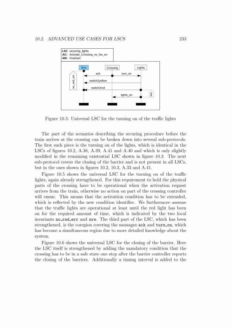
10.2. ADVANCED USE CASES FOR LSCS 233
AM: InvariantAC: Activate_Crossing_no_hw_errLSC
Env Lights
ack
Crossing
switch2yellow
switch2red
lights_on
turn_on
securing_lights
no_r
ed_e
rr
nre
Figure 10.5: Universal LSC for the turning on of the traffic lights
The part of the scenarios describing the securing procedure before thetrain arrives at the crossing can be broken down into several sub-protocols.The first such piece is the turning on of the lights, which is identical in theLSCs of figures 10.2, A.38, A.39, A.41 and A.40 and which is only slightlymodified in the remaining existential LSC shown in figure 10.3. The nextsub-protocol covers the closing of the barrier and is not present in all LSCs,but in the ones shown in figures 10.2, 10.3, A.33 and A.41.
Figure 10.5 shows the universal LSC for the turning on of the trafficlights, again already strengthened. For this requirement to hold the physicalparts of the crossing have to be operational when the activation requestarrives from the train, otherwise no action on part of the crossing controllerwill ensue. This means that the activation condition has to be extended,which is reflected by the new condition identifier. We furthermore assumethat the traffic lights are operational at least until the red light has beenon for the required amount of time, which is indicated by the two localinvariants no red err and nre. The third part of the LSC, which has beenstrengthened, is the coregion covering the messages ack and turn on, whichhas become a simultaneous region due to more detailed knowledge about thesystem.
Figure 10.6 shows the universal LSC for the closing of the barrier. Herethe LSC itself is strengthened by adding the mandatory condition that thecrossing has to be in a safe state one step after the barrier controller reportsthe closing of the barriers. Additionally a timing interval is added to the
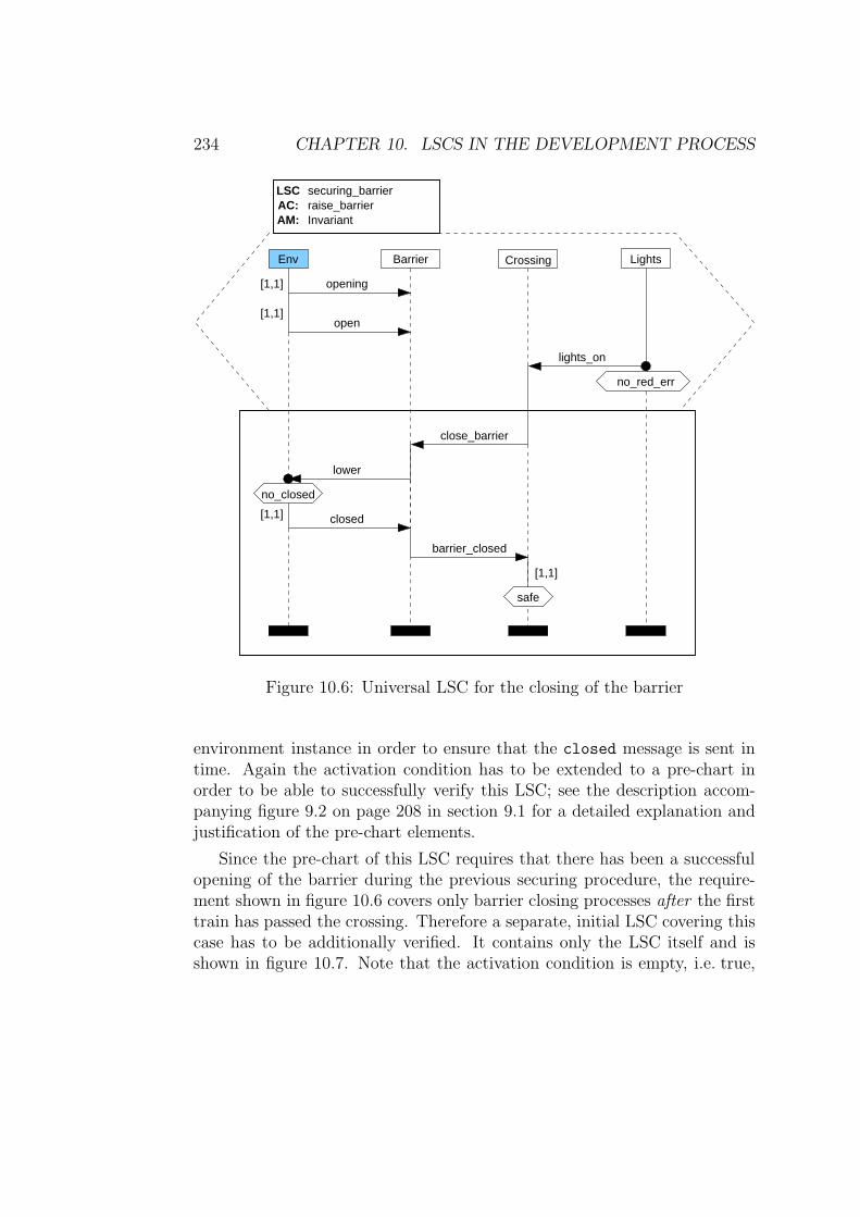
234 CHAPTER 10. LSCS IN THE DEVELOPMENT PROCESS
Env
AM: InvariantAC: raise_barrierLSC securing_barrier
LightsCrossing
lights_on
opening
open
close_barrier
lower
Barrier
closed
barrier_closed
[1,1]
[1,1]
no_red_err
[1,1]
safe
[1,1]
no_closed
Figure 10.6: Universal LSC for the closing of the barrier
environment instance in order to ensure that the closed message is sent intime. Again the activation condition has to be extended to a pre-chart inorder to be able to successfully verify this LSC; see the description accom-panying figure 9.2 on page 208 in section 9.1 for a detailed explanation andjustification of the pre-chart elements.
Since the pre-chart of this LSC requires that there has been a successfulopening of the barrier during the previous securing procedure, the require-ment shown in figure 10.6 covers only barrier closing processes after the firsttrain has passed the crossing. Therefore a separate, initial LSC covering thiscase has to be additionally verified. It contains only the LSC itself and isshown in figure 10.7. Note that the activation condition is empty, i.e. true,
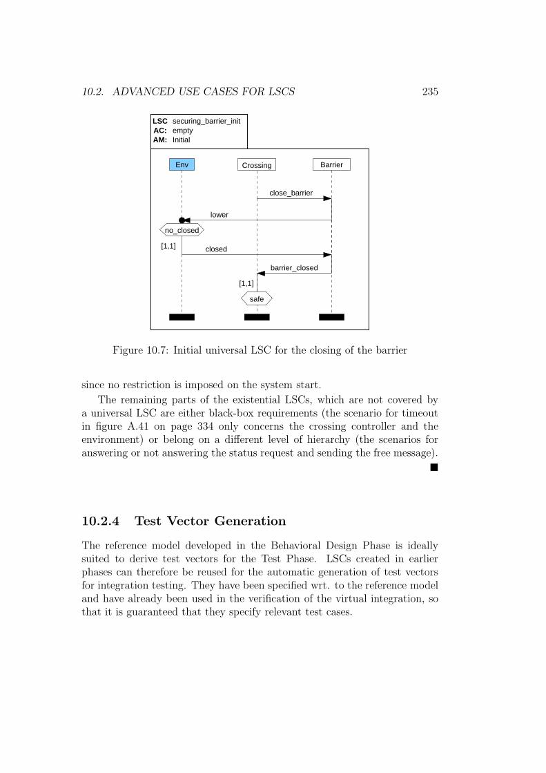
10.2. ADVANCED USE CASES FOR LSCS 235
barrier_closed
closed
AM: InitialAC:LSC securing_barrier_init
Env Crossing
empty
close_barrier
lower
Barrier
no_closed
safe
[1,1]
[1,1]
Figure 10.7: Initial universal LSC for the closing of the barrier
since no restriction is imposed on the system start.
The remaining parts of the existential LSCs, which are not covered bya universal LSC are either black-box requirements (the scenario for timeoutin figure A.41 on page 334 only concerns the crossing controller and theenvironment) or belong on a different level of hierarchy (the scenarios foranswering or not answering the status request and sending the free message).
�
10.2.4 Test Vector Generation
The reference model developed in the Behavioral Design Phase is ideallysuited to derive test vectors for the Test Phase. LSCs created in earlierphases can therefore be reused for the automatic generation of test vectorsfor integration testing. They have been specified wrt. to the reference modeland have already been used in the verification of the virtual integration, sothat it is guaranteed that they specify relevant test cases.
236 CHAPTER 10. LSCS IN THE DEVELOPMENT PROCESS
10.3 Related Work
Damm and Harel [DH01] outline some use cases for LSCs using a UML-based development process as an example. They also advocate the use ofexistential LSCs in order to add more contents to Use Case Diagrams andfurther develop those LSCs during the object analysis phase, which corre-sponds to the Architectural Design Phase and partly the Behavioral DesignPhase. They propose testing and formal verification activities as well, whichlargely coincide with the ones presented here, since both are inspired by thesame activities at OFFIS. While advocating a transition from existential touniversal LSCs to be used for formal verification, no details on how thistransition is to be achieved are offered.
In [KL01, BKL01] we have presented an LSC-based approach for testingUML designs modeled with Rhapsody. The basic idea is that during a simula-tion session a watchdog is generated, which monitors if a set of user-specifiedproperties, given in the form of LSCs, is satisfied. The simulation can eitherbe conducted by the user or it can be driven automatically according to thespecified LSCs exploiting the activation information and designated environ-ment instances offered by LSCs. In the latter case the required inputs aregenerated according to the LSCs.
Once a set of LSCs has been compiled it can be employed for regressiontesting, i.e. if the model is changed, e.g. by adding new functionality, this setof LSCs can be rerun in order to check, if the extensions have impaired theoriginal functionality. The LSCs used in this simulation-based testing arealso ideal candidates for the derivation of test vectors for integration testing.
In [KRK02] we have investigated a similar approach, which deals withsimulation-based testing of system-level hardware designs, implemented inSystemC. Here LSCs serve as a graphical front-end for LTL formulas, whichare monitored in parallel to the simulation of a SystemC implementation ofthe SUD by the checker presented in [RHTR01].
Harel and Marelly have proposed a different use case for LSCs describedin [Har00, HKMP02, HM02, MHK02]. The basic idea of this approach, calledPlay-In/Play-Out, is to play in the desired interactions in the ArchitecturalDesign Phase and use LSCs to record them. The key point is that no modelrepresentation exists at this time, so that the play in procedure is carriedout via a mock-up graphical user interface. Once a set of LSCs (universaland existential) has been recorded in this way they can be used as behaviorspecifications, which monitor a user-guided simulation (play-out). This ap-
10.3. RELATED WORK 237
proach is intended to be used at the beginning of the development processto generate the basic system interactions in an easy and intuitive way. Theview of this approach is an operational one, whereas the purpose of LSCs aspresented here is a denotational description of the behavior of an SUD.
[HKMP02] additionally use model checking in order to check the consis-tency of several universal LSCs. This check is also used to find a sequenceof steps (a superstep), which leads to another stable system state, i.e. a sit-uation where new inputs are required in order for the system to advancefurther. This approach is similar to our existential verification, except that[HKMP02] consider several LSCs and are limited to one superstep.
Another advanced use case for LSCs, described by Harel and Kuglerin [HK01, HK02], is bridging the gap between requirements, specified byLSCs, and a behavioral model by automatically synthesizing a first-cutmodel from LSCs. [HK02] outline an algorithm to automatically generatestate charts from LSCs in an object-oriented system. Similar approachesexist for MSCs as well: Leue et al. [LMR98] synthesize ROOM state chartsfrom MSCs, Kruger et al. derive Statecharts from MSCs in [KGSB99], andKruger generates finite state machines from extended MSCs in [Kru00]. Inthe telecommunications field there are several approaches dealing with syn-thesis of an SDL model from MSCs, e.g. [RKG97] or [Man01].
Bunker and Gopalakrishnan [BG01, BG02] use LSCs for the specificationand formal verification of a hardware protocol. The properties to be verifiedare derived by hand from the requirements document and a set of simpleproof obligations is derived manually from the LSC. The application used asan example is small enough, so that a direct creation of universal LSCs ispossible and no need for an elaborate design process is considered.
Mauw et al. [MRW00] present a methodology for the application of MSCs,which is not limited to a specific process, but is described in terms of an ab-stract design flow. They also advocate the use of MSCs in the early phases inorder to capture the typical use cases, which is the classical field of applicationfor MSCs. Other use cases are the recording and monitoring of simulationruns, reusing MSCs as test vectors and recording execution traces. No formaltreatment of MSCs is assumed and the only (informal) verification activityconsidered is comparison between MSCs from different phases. The exactnature or basis of such comparisons is not presented and neither is the con-crete relation between the MSCs from different phases, which in [MRW00]have different views (black-box or grey-box) depending on the phase.
238 CHAPTER 10. LSCS IN THE DEVELOPMENT PROCESS
The embedding of MSCs into a development process presentedin [MRW00] is, in summary, less tight than our proposal for LSCs givenin this chapter. We achieve a greater reuse of LSCs from previous in laterphases of the development process, thereby reducing the development effortnecessary and gaining a better integration of LSCs, especially across phaseboundaries. The enhanced expressiveness and formal foundation of LSCsyields even more added value, in particular wrt. formal verification.
Existential verification of MSCs against an SDL model is offered by someSDL tools Telelogic e.g. offers a check to determine if a SDL model containsthe communications shown in an MSC ([Ek98]). There are also numerousapproaches to using MSCs for the specification of test cases. We refer theinterested reader to [MRW00].
Chapter 11
Assessment of the LSC
Language
In this chapter we explore the applicability and usability of the languageof LSCs and the proposed methodology as presented in the previous chap-ters. We take a closer look here at the advanced use case of specificationof properties for formal verification; more concretely the application field isthe formal verification of Statemate designs. The sample application usedis the train control system introduced in chapter 2. The LSCs presented inthis chapter have been developed according to the methodology described inchapter 10. First existential LSCs have been specified, which are used forexistential verification and from which universal ones have been derived asexpounded in section 10.2.3.
The technical basis for the evaluation presented here is the StatemateVerification Environment (STVE), which has been presented in the chapter 1on page 15. Section 11.1 outlines the prototypical integration of the toolssupporting LSCs into the STVE (subsection 11.1.1) and deals with the par-ticulars of specifying properties for Statemate designs in the synchronous(subsection 11.1.2) and asynchronous (subsection 11.1.3) simulation seman-tics. Section 11.2 presents the the existential and universal LSCs specified forthe train control system and section 11.3 presents the experimental results.Section 11.4 concludes this chapter with an overall assessment of the LSClanguage.
239
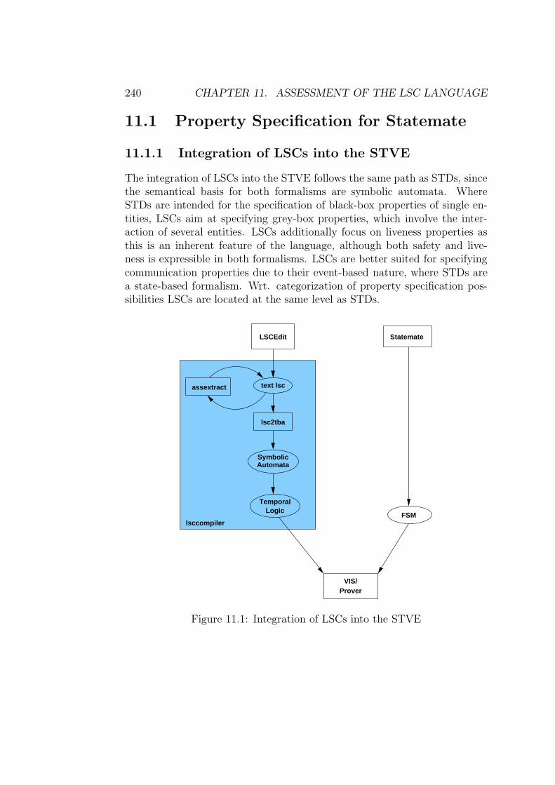
240 CHAPTER 11. ASSESSMENT OF THE LSC LANGUAGE
11.1 Property Specification for Statemate
11.1.1 Integration of LSCs into the STVE
The integration of LSCs into the STVE follows the same path as STDs, sincethe semantical basis for both formalisms are symbolic automata. WhereSTDs are intended for the specification of black-box properties of single en-tities, LSCs aim at specifying grey-box properties, which involve the inter-action of several entities. LSCs additionally focus on liveness properties asthis is an inherent feature of the language, although both safety and live-ness is expressible in both formalisms. LSCs are better suited for specifyingcommunication properties due to their event-based nature, where STDs area state-based formalism. Wrt. categorization of property specification pos-sibilities LSCs are located at the same level as STDs.
Statemate
FSMLogic
Temporal
AutomataSymbolic
lsc2tba
LSCEdit
assextract text lsc
lsccompiler
VIS/Prover
Figure 11.1: Integration of LSCs into the STVE
11.1. PROPERTY SPECIFICATION FOR STATEMATE 241
Figure 11.1 gives an overview of the LSC tools and their interplay with therest of the STVE; rectangles in this picture represent tools and ellipses for-mats. An editor, LSCEdit, is available to draw and manipulate LSCs, whichare stored in a textual syntax derived from the textual representation of MSC-96; see appendix C for the grammar of the textual LSC representation. Thetextual LSC is the basis for all further treatment of the LSCs. If applicable,the tool assextract performs the extraction of assumptions as describedin section 8.2.1 on page 195 and adds the resulting assumption LSC(s) tothe textual representation of the commitment LSC. The tool lsc2tba im-plements the unwinding algorithms for assumptions, commitments and pre-charts as defined in the preceding chapters. Both tools are integrated intothe lsccompiler, indicated by the shaded part of figure 11.1, which con-trols the entire generation of a temporal logic formula from an LSC, therebycomprising both LSC-specific tools and tools, which are already part of theSTVE and are responsible for the generation of temporal logic formula fromsymbolic automata and the treatment of assumptions, which are already partof the STVE. The tasks performed by lsccompiler for a commitment LSCL are thus:
1. Extract assumptions from L using assextract, if necessary.
2. Unwind all assumptions associated with L using lsc2tba.
3. Perform STVE assumption treatment using symbolic automata gener-ated from assumptions.
4. Unwind pre-chart pch of L using lsc2tba, if necessary.
5. Unwind L using lsc2tba.
6. Generate temporal logic formula from the symbolic automaton for L.
The lsccompiler produces the formats and files required by the STVE.The subsequent steps necessary for the verification of LSCs (restriction ofthe system runs to the ones conforming to the assumptions, observance ofthe prefix given by the pre-chart and the actual model checking run) are thusalready part of the existing STVE machinery and are not presented here. Adescription of the technical details of the STVE is out of the scope of thisthesis and can be found in [Wit03].Note that both the lsccompiler and lsc2tba are parameterized to supportboth the weak or the strict interpretation.
242 CHAPTER 11. ASSESSMENT OF THE LSC LANGUAGE
11.1.2 Property Specification for Synchronous Models
This subsection deals with the particulars of Statemate designs, whichare modeled using the synchronous simulation semantics. Recall that inthis semantics the SUD accepts inputs and produces outputs in every step(execution cycle) and time passes between two steps. Note that the treatmentof time is not part of the Statemate semantics, but is left to the toolsoperating on the Statemate design like e.g. the simulator (cf. [HN96]).Time annotations consequently are interpreted in terms of steps by the STVEand in LSCs as well, i.e. timers and timing intervals in LSCs refer to steps.
There are two other peculiarities, which affect property specification withLSCs: All communication in Statemate step models is instantaneous andthere is no notion of a lossy channel, so that messages can not be lost. LSCsspecified for a Statemate model therefore only contain hot instantaneousmessages. Note that this is also true for asynchronous models, because only asingle controller (embedded controller) at a time can be modeled in State-mate. If several embedded controllers are contained in one Statematemodel, they are treated as on single controller, i.e. the communications be-tween individual controllers are considered to be internal, i.e. are step-based.
Notice that all messages occurring in the LSCs for the train control system(cf. section 11.2) refer to events in order to use them for both the weakand the strict interpretation (cf. the remarks on page 146). This includesboth normal Statemate events and derived events like changed and writtenevents for data items and rising or falling edges of conditions.
11.1.3 Property Specification for Asynchronous Mod-
els
The asynchronous simulation semantics of Statemate proves to be morecomplicated than the step semantics. Recall that in the asynchronous (orsuperstep) semantics the modeled controller accepts inputs from the envi-ronment, which trigger a series of internal steps necessary to produce theoutputs, and new inputs are accepted when the controller once again reachesa stable state. The transition from one stable state to the next is a super-step. All internal steps do not consume time; time is advanced when thesystem reaches a stable state, i.e. after completion of the current superstep.Figure 11.2 on the next page illustrates the concepts of steps and supersteps:the circles represent global system states, large circles denote stable states,
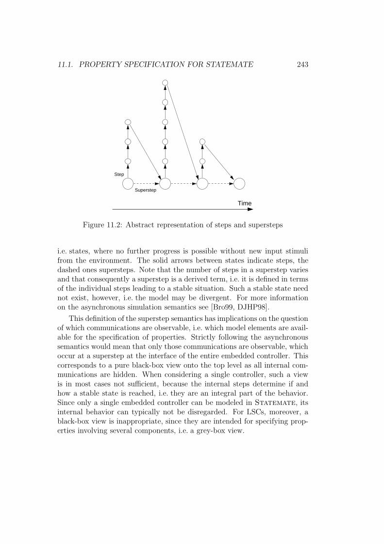
11.1. PROPERTY SPECIFICATION FOR STATEMATE 243
Step
Time
Superstep
Figure 11.2: Abstract representation of steps and supersteps
i.e. states, where no further progress is possible without new input stimulifrom the environment. The solid arrows between states indicate steps, thedashed ones supersteps. Note that the number of steps in a superstep variesand that consequently a superstep is a derived term, i.e. it is defined in termsof the individual steps leading to a stable situation. Such a stable state neednot exist, however, i.e. the model may be divergent. For more informationon the asynchronous simulation semantics see [Bro99, DJHP98].
This definition of the superstep semantics has implications on the questionof which communications are observable, i.e. which model elements are avail-able for the specification of properties. Strictly following the asynchronoussemantics would mean that only those communications are observable, whichoccur at a superstep at the interface of the entire embedded controller. Thiscorresponds to a pure black-box view onto the top level as all internal com-munications are hidden. When considering a single controller, such a viewis in most cases not sufficient, because the internal steps determine if andhow a stable state is reached, i.e. they are an integral part of the behavior.Since only a single embedded controller can be modeled in Statemate, itsinternal behavior can typically not be disregarded. For LSCs, moreover, ablack-box view is inappropriate, since they are intended for specifying prop-erties involving several components, i.e. a grey-box view.
244 CHAPTER 11. ASSESSMENT OF THE LSC LANGUAGE
The basic granularity of observability in the superstep semantics conse-quently still is a step. This creates the paradoxical situation that sequential-ity of internal communications must be expressible, while assuming that allinternal communication occurs at the same point in time. Messages in LSCsthus refer to both internal and external communication raising the questionwhat timing annotations in LSCs should refer to: steps or supersteps? Wehave decided to let them still refer to steps, since this is the only consistentchoice. Steps constitute the finest level of granularity and also form the se-mantical foundation (cf. [DJHP98]), with supersteps being derived from thisbase.
Supersteps can be referenced in LSCs, since the model representation inthe STVE includes an output (event stable), which indicates a stable state,i.e. a superstep boundary. Quantitatively dealing with supersteps is oftendesired, since this allows to state requirements on timed behavior as time isassociated with supersteps. Recall, however, that time itself is not part of theformal semantics of Statemate, so that we choose to allow the formulationof timing constraints in terms of supersteps by counting them.
In the remainder of this subsection we investigate how timing constraintsreferring to supersteps can be specified in LSCs. Two approaches are con-ceivable: explicit usage of the signal indicating stabilization of the model inLSCs and introduction of a dedicated counter into the model, which countssupersteps and can be referred to in the LSCs.
The first alternative requires the user to explicitly indicate the points,where a stable state in the model is reached, by including the stable eventin the LSC. By explicitly referring to this event in an LSC specificationit is possible to count supersteps. This explicit enumeration approach isillustrated in figure 11.3 on the facing page, which shows the adaption ofLSC securing yellow err (cf. figure 11.13 on page 259) to the superstepsemantics. Figure 11.3 depicts the situation where the yellow light is out oforder, but the red light is still operational and is switched on immediatelyafter detecting the failure of the yellow light. The red light has to be on forthe combined duration required for yellow and red light.
The stable event is represented by mandatory conditions rather then mes-sages, since several identically mapped messages would bar the usage of suchLSCs in the strict interpretation. Note that the required six1 supersteps be-
1The differing number compared to the LSC for the step semantics, which requires sevensteps (cf. figure 11.13 on page 259), is due to the fact that the delay between occurrence
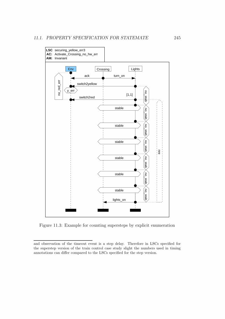
11.1. PROPERTY SPECIFICATION FOR STATEMATE 245
AM: InvariantAC: Activate_Crossing_no_hw_errLSC
Env Lights
ack
Crossing
switch2yellow
turn_on
securing_yellow_err3
switch2red
lights_on
y_err
stable
stable
stable
stable
stable
stable
no_stab
nre
no_stabno_stab
no_stabno_stab
no_stabno_stab
[1,1]no_r
ed_e
rr
Figure 11.3: Example for counting supersteps by explicit enumeration
and observation of the timeout event is a step delay. Therefore in LSCs specified forthe superstep version of the train control case study slight the numbers used in timingannotations can differ compared to the LSCs specified for the step version.
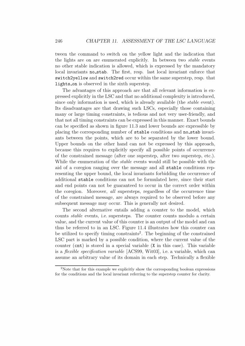
246 CHAPTER 11. ASSESSMENT OF THE LSC LANGUAGE
tween the command to switch on the yellow light and the indication thatthe lights are on are enumerated explicitly. In between two stable eventsno other stable indication is allowed, which is expressed by the mandatorylocal invariants no stab. The first, resp. last local invariant enforce thatswitch2yellow and switch2red occur within the same superstep, resp. thatlights on is observed in the sixth superstep.
The advantages of this approach are that all relevant information is ex-pressed explicitly in the LSC and that no additional complexity is introduced,since only information is used, which is already available (the stable event).Its disadvantages are that drawing such LSCs, especially those containingmany or large timing constraints, is tedious and not very user-friendly, andthat not all timing constraints can be expressed in this manner. Exact boundscan be specified as shown in figure 11.3 and lower bounds are expressible byplacing the corresponding number of stable conditions and no stab invari-ants between the points, which are to be separated by the lower bound.Upper bounds on the other hand can not be expressed by this approach,because this requires to explicitly specify all possible points of occurrenceof the constrained message (after one superstep, after two superstep, etc.).While the enumeration of the stable events would still be possible with theaid of a coregion ranging over the message and all stable conditions rep-resenting the upper bound, the local invariants forbidding the occurrence ofadditional stable conditions can not be formulated here, since their startand end points can not be guaranteed to occur in the correct order withinthe coregion. Moreover, all supersteps, regardless of the occurrence timeof the constrained message, are always required to be observed before anysubsequent message may occur. This is generally not desired.
The second alternative entails adding a counter to the model, whichcounts stable events, i.e. supersteps. The counter counts modulo a certainvalue, and the current value of this counter is an output of the model and canthus be referred to in an LSC. Figure 11.4 illustrates how this counter canbe utilized to specify timing constraints2. The beginning of the constrainedLSC part is marked by a possible condition, where the current value of thecounter (cnt) is stored in a special variable (X in this case). This variableis a flexible specification variable [ACS99, Wit03], i.e. a variable, which canassume an arbitrary value of its domain in each step. Technically a flexible
2Note that for this example we explicitly show the corresponding boolean expressionsfor the conditions and the local invariant referring to the superstep counter for clarity.
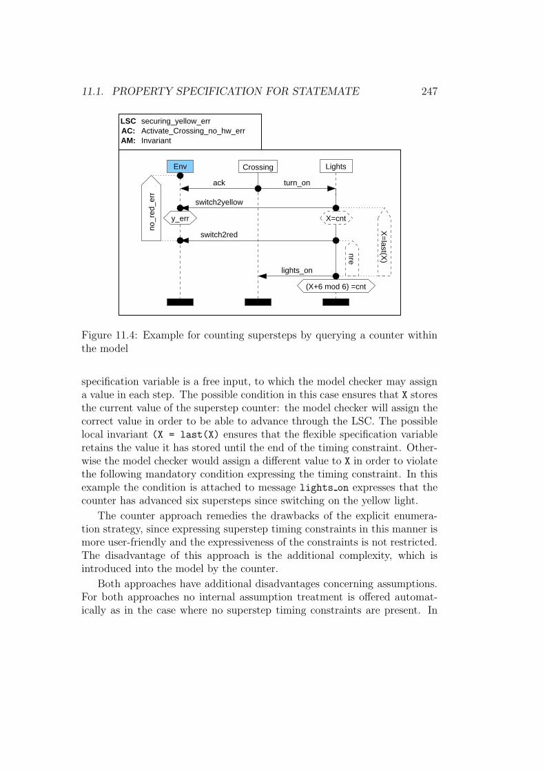
11.1. PROPERTY SPECIFICATION FOR STATEMATE 247
AM: InvariantAC: Activate_Crossing_no_hw_errLSC
Env Lights
ack
Crossing
switch2yellow
turn_on
securing_yellow_err
switch2red
lights_on
y_err X=cnt
(X+6 mod 6) =cnt
no_r
ed_e
rr
nre
X=
last(X)
Figure 11.4: Example for counting supersteps by querying a counter withinthe model
specification variable is a free input, to which the model checker may assigna value in each step. The possible condition in this case ensures that X storesthe current value of the superstep counter: the model checker will assign thecorrect value in order to be able to advance through the LSC. The possiblelocal invariant (X = last(X) ensures that the flexible specification variableretains the value it has stored until the end of the timing constraint. Other-wise the model checker would assign a different value to X in order to violatethe following mandatory condition expressing the timing constraint. In thisexample the condition is attached to message lights on expresses that thecounter has advanced six supersteps since switching on the yellow light.
The counter approach remedies the drawbacks of the explicit enumera-tion strategy, since expressing superstep timing constraints in this manner ismore user-friendly and the expressiveness of the constraints is not restricted.The disadvantage of this approach is the additional complexity, which isintroduced into the model by the counter.
Both approaches have additional disadvantages concerning assumptions.For both approaches no internal assumption treatment is offered automat-ically as in the case where no superstep timing constraints are present. In
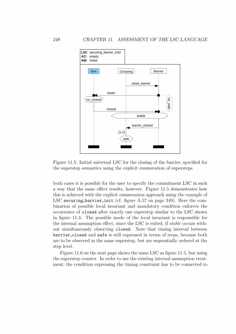
248 CHAPTER 11. ASSESSMENT OF THE LSC LANGUAGE
barrier_closed
AM: InitialAC:LSC securing_barrier_init2
Env Crossing
empty
close_barrier
Barrier
closed
lower
safe
[1,1]
no_closed
stable
no_stab
Figure 11.5: Initial universal LSC for the closing of the barrier, specified forthe superstep semantics using the explicit enumeration of supersteps
both cases it is possible for the user to specify the commitment LSC in sucha way that the same effect results, however. Figure 11.5 demonstrates howthis is achieved with the explicit enumeration approach using the example ofLSC securing barrier init (cf. figure A.57 on page 349). Here the com-bination of possible local invariant and mandatory condition enforces theoccurrence of closed after exactly one superstep similar to the LSC shownin figure 11.3. The possible mode of the local invariant is responsible forthe internal assumption effect, since the LSC is exited, if stable occurs with-out simultaneously observing closed. Note that timing interval betweenbarrier closed and safe is still expressed in terms of steps, because bothare to be observed in the same superstep, but are sequentially ordered at thestep level.
Figure 11.6 on the next page shows the same LSC as figure 11.5, but usingthe superstep counter. In order to use the existing internal assumption treat-ment, the condition expressing the timing constraint has to be connected to
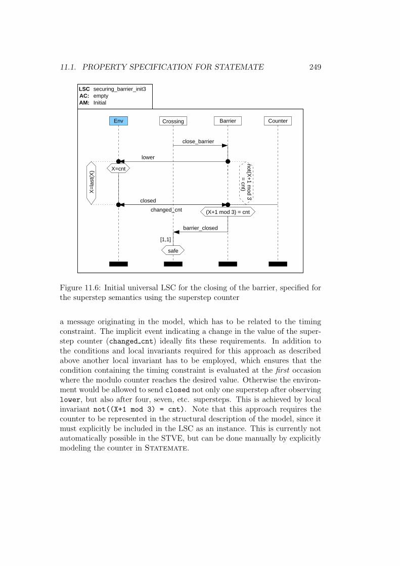
11.1. PROPERTY SPECIFICATION FOR STATEMATE 249
AM: InitialAC:LSC securing_barrier_init3
empty
Env Crossing
close_barrier
lower
CounterBarrier
closed
barrier_closed
changed_cnt
X=cnt
safe
[1,1]
X=
last
(X)
(X+1 mod 3) = cnt
= cnt)
not(X+
1 mod 3
Figure 11.6: Initial universal LSC for the closing of the barrier, specified forthe superstep semantics using the superstep counter
a message originating in the model, which has to be related to the timingconstraint. The implicit event indicating a change in the value of the super-step counter (changed cnt) ideally fits these requirements. In addition tothe conditions and local invariants required for this approach as describedabove another local invariant has to be employed, which ensures that thecondition containing the timing constraint is evaluated at the first occasionwhere the modulo counter reaches the desired value. Otherwise the environ-ment would be allowed to send closed not only one superstep after observinglower, but also after four, seven, etc. supersteps. This is achieved by localinvariant not((X+1 mod 3) = cnt). Note that this approach requires thecounter to be represented in the structural description of the model, since itmust explicitly be included in the LSC as an instance. This is currently notautomatically possible in the STVE, but can be done manually by explicitlymodeling the counter in Statemate.
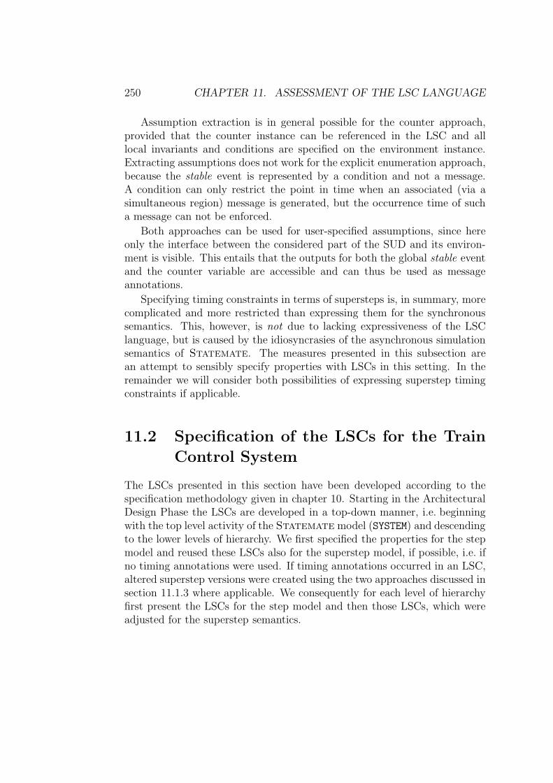
250 CHAPTER 11. ASSESSMENT OF THE LSC LANGUAGE
Assumption extraction is in general possible for the counter approach,provided that the counter instance can be referenced in the LSC and alllocal invariants and conditions are specified on the environment instance.Extracting assumptions does not work for the explicit enumeration approach,because the stable event is represented by a condition and not a message.A condition can only restrict the point in time when an associated (via asimultaneous region) message is generated, but the occurrence time of sucha message can not be enforced.
Both approaches can be used for user-specified assumptions, since hereonly the interface between the considered part of the SUD and its environ-ment is visible. This entails that the outputs for both the global stable eventand the counter variable are accessible and can thus be used as messageannotations.
Specifying timing constraints in terms of supersteps is, in summary, morecomplicated and more restricted than expressing them for the synchronoussemantics. This, however, is not due to lacking expressiveness of the LSClanguage, but is caused by the idiosyncrasies of the asynchronous simulationsemantics of Statemate. The measures presented in this subsection arean attempt to sensibly specify properties with LSCs in this setting. In theremainder we will consider both possibilities of expressing superstep timingconstraints if applicable.
11.2 Specification of the LSCs for the Train
Control System
The LSCs presented in this section have been developed according to thespecification methodology given in chapter 10. Starting in the ArchitecturalDesign Phase the LSCs are developed in a top-down manner, i.e. beginningwith the top level activity of the Statemate model (SYSTEM) and descendingto the lower levels of hierarchy. We first specified the properties for the stepmodel and reused these LSCs also for the superstep model, if possible, i.e. ifno timing annotations were used. If timing annotations occurred in an LSC,altered superstep versions were created using the two approaches discussed insection 11.1.3 where applicable. We consequently for each level of hierarchyfirst present the LSCs for the step model and then those LSCs, which wereadjusted for the superstep semantics.
11.2. LSCS FOR THE TRAIN CONTROL SYSTEM 251
The existential LSCs specified for SYSTEM are collected in appendix A.1.1.They show the basic interactions between the activities identified at thislevel (TRAIN, COMMUNICATION and CROSSING; cf. section 2.2.1) and theirenvironment. The LSC in figure A.1 on page 298 shows the good case, wherethe crossing is secured as desired and the train passes it without needing tostop. The remaining LSCs show different error situations: figure A.2 and A.3depict the consequences of a yellow, resp. and red light failure, figure A.5show a failure of the barrier, figure A.7 exemplifies the situation, where thetrain realizes that it will not reach the crossing in time and thus sends thefreeing message, and figure A.8 on page 305 finally depicts a timeout at thecrossing, e.g. resulting from a defect pass sensor. The LSCs describing thered light and barrier failure have been characterized in two slightly differentways: One only describing the desired interactions (figures A.3 and A.5), theother additionally prohibiting the sending of the safe message in response tothe status request (figures A.4 and A.6). The LSC dealing with exceeding themaximum barrier closed time also comes in two variants, one with (figure A.8)and one without a timer (figure A.9) enforcing the MBCT in the LSC.
CrossingCommTrain
start_comm
ready
activate_snd
activate_rec
no_s
topp
ed
Invariantactivation_point_reachedsecuring_all_comm_setup
AM:AC:LSC
Figure 11.7: Universal LSCs for establishing the communication channel
The modularization and strengthening of these existential LSCs resultsin the universal LSCs shown in figures 11.7 - 11.10. Figure 11.7 shows thecommon prefix of all existential LSCs, the establishing of the communication
252 CHAPTER 11. ASSESSMENT OF THE LSC LANGUAGE
channel between train and crossing. Since this part of the protocol is as-sumed to be failsafe in the model, the only strengthening measure needed isto exclude that the train stops due to a not secured crossing before even theactivation command has been transmitted. Such a behavior would indicatea severe problem in the speed supervision or localization components or ac-tivation point calculation of the train, which are assumed to work correctlyhere. The corresponding assumption is being taken care of by local invariantno stopped on the Train instance.
This commitment LSC requires two external assumptions. The first in-hibits the arbitrary reactivation of the LSC by ensuring that the activationcondition (reaching the activation point), which is indicated by a messagesent by the environment, does not occur again as the train is already ap-proaching a crossing. The corresponding assumption LSC is shown in fig-ure A.24 on page 318. Note that this property is not expressible by aninternal assumption, i.e. a local invariant forbidding the recurrence of theactivation condition. The effect of such a local invariant would be that thefirst, correct activation of the LSC is terminated by a recurring activationcondition, but since the securing procedure has been initiated within themodel, the corresponding protocol would be executed correctly, showing thedesired communication sequence. The still active second incarnation, how-ever, would not recognize this, because it has been activated out of turn anddid not observe the prefix of the current message exchange. Therefore anexternal assumption, either extracted or user-specified, is necessary. In thiscase a user-specified assumption is employed, because there is no environmentinstance present in the commitment LSC.
The second external assumption LSC (no activation point ass) shownin figure A.26 on page 319 is necessary in order to restrict the occurrence ofthe activation condition to a point in time, where the system is operational,i.e. after the initialization step. Since the first message (start comm) mustoccur eventually due to the hot instance head location, it is essential that thecommitment LSC is not activated in step zero, where in real life no activationpoint can be reported. The assumption LSC consequently forbids the initialreport of reaching the activation point and therefore also its activation modeis initial. This assumption is again not expressible within the commitmentLSC, since the activation modes of the commitment LSC is invariant, whereasa restriction of the initial state is required as an assumption. Note that theassumption LSC effectively contains no messages, since only the initial stateis of interest, which is restricted by the activation condition.
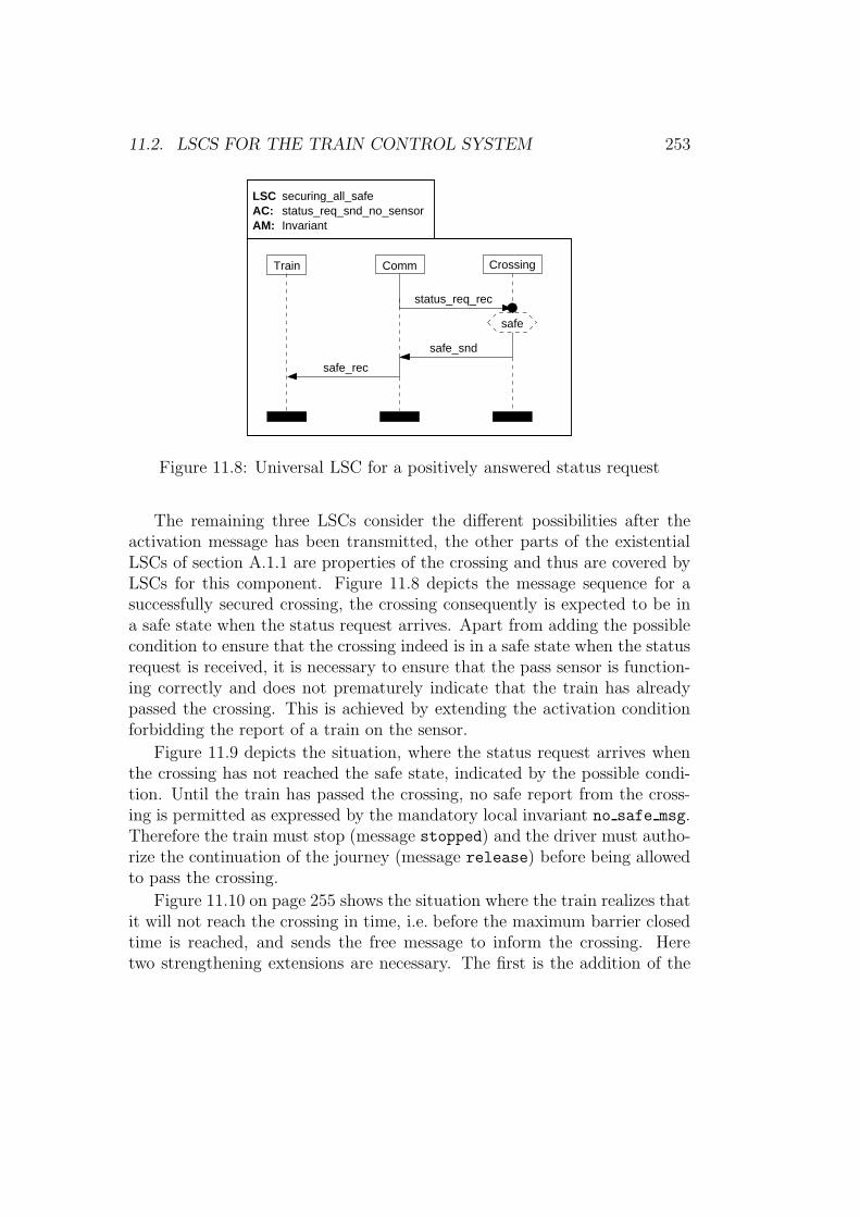
11.2. LSCS FOR THE TRAIN CONTROL SYSTEM 253
CommTrain Crossing
safe_rec
safe_snd
status_req_rec
safe
Invariantstatus_req_snd_no_sensorsecuring_all_safe
AM:AC:LSC
Figure 11.8: Universal LSC for a positively answered status request
The remaining three LSCs consider the different possibilities after theactivation message has been transmitted, the other parts of the existentialLSCs of section A.1.1 are properties of the crossing and thus are covered byLSCs for this component. Figure 11.8 depicts the message sequence for asuccessfully secured crossing, the crossing consequently is expected to be ina safe state when the status request arrives. Apart from adding the possiblecondition to ensure that the crossing indeed is in a safe state when the statusrequest is received, it is necessary to ensure that the pass sensor is function-ing correctly and does not prematurely indicate that the train has alreadypassed the crossing. This is achieved by extending the activation conditionforbidding the report of a train on the sensor.
Figure 11.9 depicts the situation, where the status request arrives whenthe crossing has not reached the safe state, indicated by the possible condi-tion. Until the train has passed the crossing, no safe report from the cross-ing is permitted as expressed by the mandatory local invariant no safe msg.Therefore the train must stop (message stopped) and the driver must autho-rize the continuation of the journey (message release) before being allowedto pass the crossing.
Figure 11.10 on page 255 shows the situation where the train realizes thatit will not reach the crossing in time, i.e. before the maximum barrier closedtime is reached, and sends the free message to inform the crossing. Heretwo strengthening extensions are necessary. The first is the addition of the
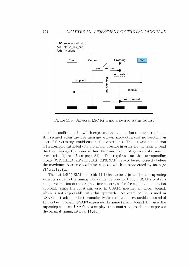
254 CHAPTER 11. ASSESSMENT OF THE LSC LANGUAGE
Comm Crossing
status_req_rec
ENVTrain
train_passed
stopped
release
not_safe
no_s
afem
sg
Invariantstatus_req_sndsecuring_all_stop
AM:AC:LSC
Figure 11.9: Universal LSC for a not answered status request
possible condition safe, which expresses the assumption that the crossing isstill secured when the free message arrives, since otherwise no reaction onpart of the crossing would ensue; cf. section 2.2.4. The activation conditionis furthermore extended to a pre-chart, because in order for the train to sendthe free message the timer within the train first must generate its timeoutevent (cf. figure 2.7 on page 34). This requires that the correspondinginputs (V STILL SAFE P and V BRAKE POINT P) have to be set correctly beforethe maximum barrier closed time elapses, which is represented by messageETA violation.
The last LSC (USAF1 in table 11.1) has to be adjusted for the superstepsemantics due to the timing interval in the pre-chart. LSC USAF2 containsan approximation of the original time constraint for the explicit enumerationapproach, since the constraint used in USAF1 specifies an upper bound,which is not expressible with this approach. An exact bound is used inUSAF2 instead; in order to complexity for verification reasonable a bound of15 has been chosen. USAF3 expresses the same (exact) bound, but uses thesuperstep counter. USAF4 also employs the counter approach, but expressesthe original timing interval [1,40].
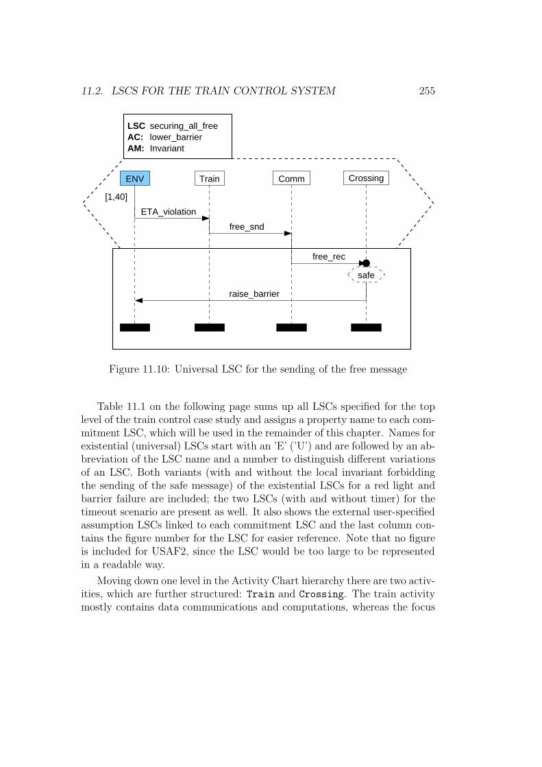
11.2. LSCS FOR THE TRAIN CONTROL SYSTEM 255
ETA_violation
ENV Train Comm
free_snd
Crossing
free_rec
raise_barrier
[1,40]
lower_barrierAC:LSC securing_all_free
InvariantAM:
safe
Figure 11.10: Universal LSC for the sending of the free message
Table 11.1 on the following page sums up all LSCs specified for the toplevel of the train control case study and assigns a property name to each com-mitment LSC, which will be used in the remainder of this chapter. Names forexistential (universal) LSCs start with an ’E’ (’U’) and are followed by an ab-breviation of the LSC name and a number to distinguish different variationsof an LSC. Both variants (with and without the local invariant forbiddingthe sending of the safe message) of the existential LSCs for a red light andbarrier failure are included; the two LSCs (with and without timer) for thetimeout scenario are present as well. It also shows the external user-specifiedassumption LSCs linked to each commitment LSC and the last column con-tains the figure number for the LSC for easier reference. Note that no figureis included for USAF2, since the LSC would be too large to be representedin a readable way.
Moving down one level in the Activity Chart hierarchy there are two activ-ities, which are further structured: Train and Crossing. The train activitymostly contains data communications and computations, whereas the focus
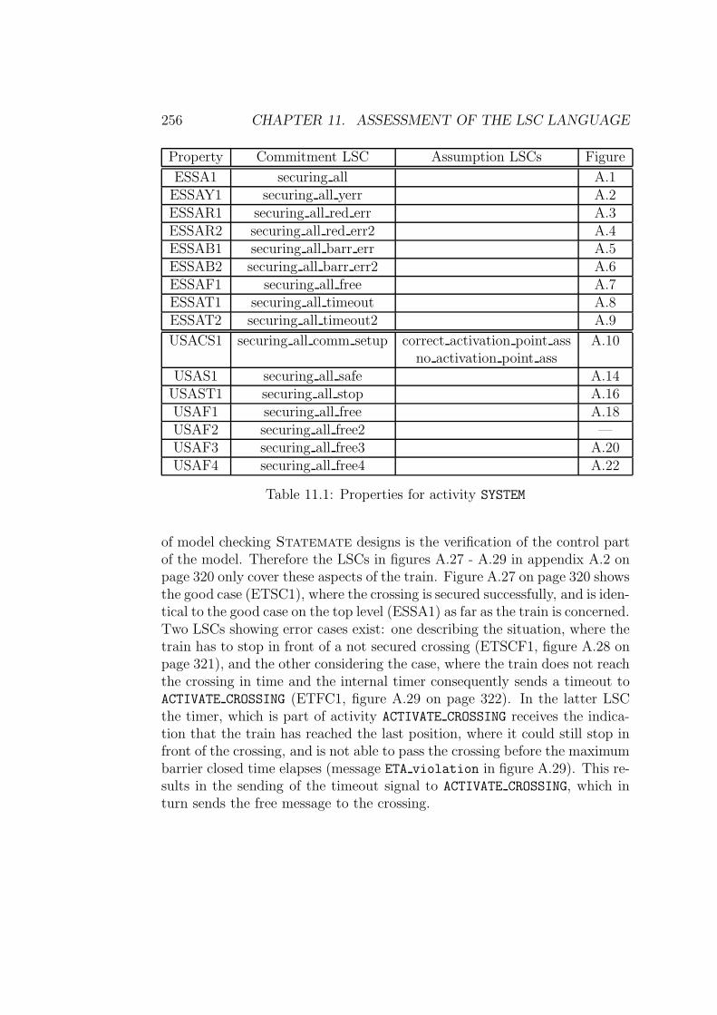
256 CHAPTER 11. ASSESSMENT OF THE LSC LANGUAGE
Property Commitment LSC Assumption LSCs Figure
ESSA1 securing all A.1ESSAY1 securing all yerr A.2ESSAR1 securing all red err A.3ESSAR2 securing all red err2 A.4ESSAB1 securing all barr err A.5ESSAB2 securing all barr err2 A.6ESSAF1 securing all free A.7ESSAT1 securing all timeout A.8ESSAT2 securing all timeout2 A.9
USACS1 securing all comm setup correct activation point ass A.10no activation point ass
USAS1 securing all safe A.14USAST1 securing all stop A.16USAF1 securing all free A.18USAF2 securing all free2 —USAF3 securing all free3 A.20USAF4 securing all free4 A.22
Table 11.1: Properties for activity SYSTEM
of model checking Statemate designs is the verification of the control partof the model. Therefore the LSCs in figures A.27 - A.29 in appendix A.2 onpage 320 only cover these aspects of the train. Figure A.27 on page 320 showsthe good case (ETSC1), where the crossing is secured successfully, and is iden-tical to the good case on the top level (ESSA1) as far as the train is concerned.Two LSCs showing error cases exist: one describing the situation, where thetrain has to stop in front of a not secured crossing (ETSCF1, figure A.28 onpage 321), and the other considering the case, where the train does not reachthe crossing in time and the internal timer consequently sends a timeout toACTIVATE CROSSING (ETFC1, figure A.29 on page 322). In the latter LSCthe timer, which is part of activity ACTIVATE CROSSING receives the indica-tion that the train has reached the last position, where it could still stop infront of the crossing, and is not able to pass the crossing before the maximumbarrier closed time elapses (message ETA violation in figure A.29). This re-sults in the sending of the timeout signal to ACTIVATE CROSSING, which inturn sends the free message to the crossing.
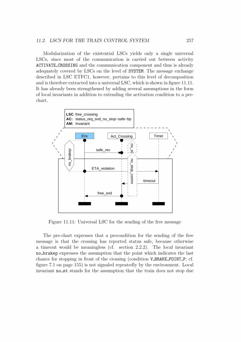
11.2. LSCS FOR THE TRAIN CONTROL SYSTEM 257
Modularization of the existential LSCs yields only a single universalLSCs, since most of the communication is carried out between activityACTIVATE CROSSING and the communication component and thus is alreadyadequately covered by LSCs on the level of SYSTEM. The message exchangedescribed in LSC ETFC1, however, pertains to this level of decompositionand is therefore extracted into a universal LSC, which is shown in figure 11.11.It has already been strengthened by adding several assumptions in the formof local invariants in addition to extending the activation condition to a pre-chart.
timeout
free_snd
status_req_snd_no_stop−safe−bp
Act_Crossing TimerEnv
safe_rec
ETA_violation
Invariant
free_crossing
AM:AC:LSC
no_stop_comm
no_st
no_b
rake
p
Figure 11.11: Universal LSC for the sending of the free message
The pre-chart expresses that a precondition for the sending of the freemessage is that the crossing has reported status safe, because otherwisea timeout would be meaningless (cf. section 2.2.2). The local invariantno brakep expresses the assumption that the point which indicates the lastchance for stopping in front of the crossing (condition V BRAKE POINT P; cf.figure 7.1 on page 155) is not signaled repeatedly by the environment. Localinvariant no st stands for the assumption that the train does not stop due
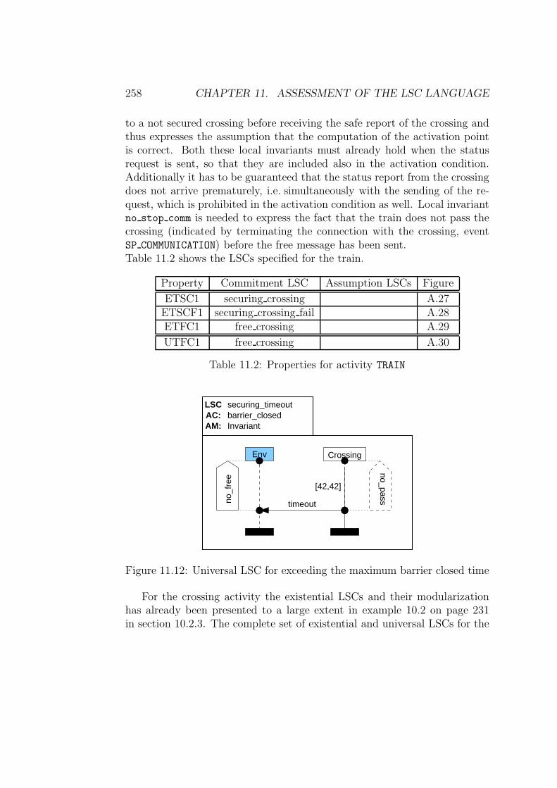
258 CHAPTER 11. ASSESSMENT OF THE LSC LANGUAGE
to a not secured crossing before receiving the safe report of the crossing andthus expresses the assumption that the computation of the activation pointis correct. Both these local invariants must already hold when the statusrequest is sent, so that they are included also in the activation condition.Additionally it has to be guaranteed that the status report from the crossingdoes not arrive prematurely, i.e. simultaneously with the sending of the re-quest, which is prohibited in the activation condition as well. Local invariantno stop comm is needed to express the fact that the train does not pass thecrossing (indicated by terminating the connection with the crossing, eventSP COMMUNICATION) before the free message has been sent.Table 11.2 shows the LSCs specified for the train.
Property Commitment LSC Assumption LSCs Figure
ETSC1 securing crossing A.27ETSCF1 securing crossing fail A.28ETFC1 free crossing A.29
UTFC1 free crossing A.30
Table 11.2: Properties for activity TRAIN
Env Crossing
AM: InvariantAC:LSC securing_timeout
barrier_closed
timeoutno_f
ree
[42,42]
no_pass
Figure 11.12: Universal LSC for exceeding the maximum barrier closed time
For the crossing activity the existential LSCs and their modularizationhas already been presented to a large extent in example 10.2 on page 231in section 10.2.3. The complete set of existential and universal LSCs for the
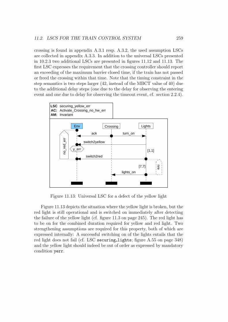
11.2. LSCS FOR THE TRAIN CONTROL SYSTEM 259
crossing is found in appendix A.3.1 resp. A.3.2, the used assumption LSCsare collected in appendix A.3.3. In addition to the universal LSCs presentedin 10.2.3 two additional LSCs are presented in figures 11.12 and 11.13. Thefirst LSC expresses the requirement that the crossing controller should reportan exceeding of the maximum barrier closed time, if the train has not passedor freed the crossing within that time. Note that the timing constraint in thestep semantics is two steps larger (42, instead of the MBCT value of 40) dueto the additional delay steps (one due to the delay for observing the enteringevent and one due to delay for observing the timeout event, cf. section 2.2.4).
AM: InvariantAC: Activate_Crossing_no_hw_errLSC
Env Lights
ack
Crossing
switch2yellow
turn_on
securing_yellow_err
switch2red
lights_on
y_err [1,1]
no_r
ed_e
rr
nre[7,7]
Figure 11.13: Universal LSC for a defect of the yellow light
Figure 11.13 depicts the situation where the yellow light is broken, but thered light is still operational and is switched on immediately after detectingthe failure of the yellow light (cf. figure 11.3 on page 245). The red light hasto be on for the combined duration required for yellow and red light. Twostrengthening assumptions are required for this property, both of which areexpressed internally: A successful switching on of the lights entails that thered light does not fail (cf. LSC securing lights; figure A.55 on page 348)and the yellow light should indeed be out of order as expressed by mandatorycondition yerr.
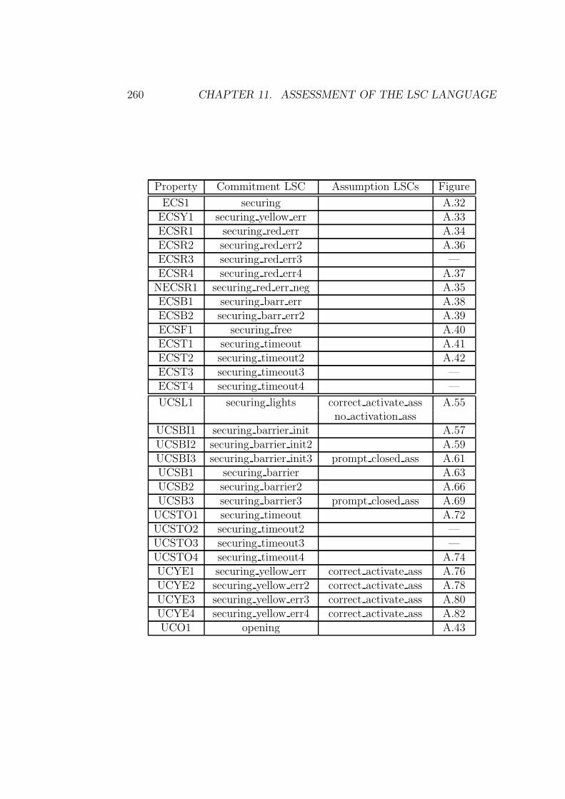
260 CHAPTER 11. ASSESSMENT OF THE LSC LANGUAGE
Property Commitment LSC Assumption LSCs Figure
ECS1 securing A.32ECSY1 securing yellow err A.33ECSR1 securing red err A.34ECSR2 securing red err2 A.36ECSR3 securing red err3 —ECSR4 securing red err4 A.37
NECSR1 securing red err neg A.35ECSB1 securing barr err A.38ECSB2 securing barr err2 A.39ECSF1 securing free A.40ECST1 securing timeout A.41ECST2 securing timeout2 A.42ECST3 securing timeout3 —ECST4 securing timeout4 —
UCSL1 securing lights correct activate ass A.55no activation ass
UCSBI1 securing barrier init A.57UCSBI2 securing barrier init2 A.59UCSBI3 securing barrier init3 prompt closed ass A.61UCSB1 securing barrier A.63UCSB2 securing barrier2 A.66UCSB3 securing barrier3 prompt closed ass A.69
UCSTO1 securing timeout A.72UCSTO2 securing timeout2 —UCSTO3 securing timeout3 —UCSTO4 securing timeout4 A.74UCYE1 securing yellow err correct activate ass A.76UCYE2 securing yellow err2 correct activate ass A.78UCYE3 securing yellow err3 correct activate ass A.80UCYE4 securing yellow err4 correct activate ass A.82UCO1 opening A.43
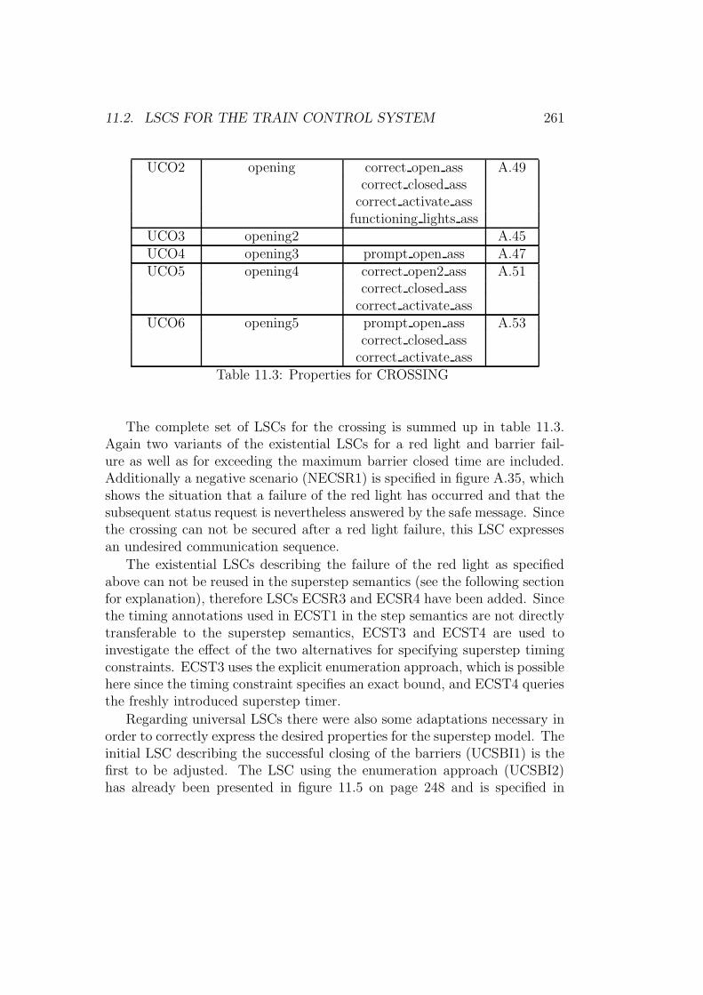
11.2. LSCS FOR THE TRAIN CONTROL SYSTEM 261
UCO2 opening correct open ass A.49correct closed ass
correct activate assfunctioning lights ass
UCO3 opening2 A.45UCO4 opening3 prompt open ass A.47UCO5 opening4 correct open2 ass A.51
correct closed asscorrect activate ass
UCO6 opening5 prompt open ass A.53correct closed ass
correct activate assTable 11.3: Properties for CROSSING
The complete set of LSCs for the crossing is summed up in table 11.3.Again two variants of the existential LSCs for a red light and barrier fail-ure as well as for exceeding the maximum barrier closed time are included.Additionally a negative scenario (NECSR1) is specified in figure A.35, whichshows the situation that a failure of the red light has occurred and that thesubsequent status request is nevertheless answered by the safe message. Sincethe crossing can not be secured after a red light failure, this LSC expressesan undesired communication sequence.
The existential LSCs describing the failure of the red light as specifiedabove can not be reused in the superstep semantics (see the following sectionfor explanation), therefore LSCs ECSR3 and ECSR4 have been added. Sincethe timing annotations used in ECST1 in the step semantics are not directlytransferable to the superstep semantics, ECST3 and ECST4 are used toinvestigate the effect of the two alternatives for specifying superstep timingconstraints. ECST3 uses the explicit enumeration approach, which is possiblehere since the timing constraint specifies an exact bound, and ECST4 queriesthe freshly introduced superstep timer.
Regarding universal LSCs there were also some adaptations necessary inorder to correctly express the desired properties for the superstep model. Theinitial LSC describing the successful closing of the barriers (UCSBI1) is thefirst to be adjusted. The LSC using the enumeration approach (UCSBI2)has already been presented in figure 11.5 on page 248 and is specified in
262 CHAPTER 11. ASSESSMENT OF THE LSC LANGUAGE
such a way that the effect of an internal assumption is achieved (cf. theexplanation accompanying figure 11.5). The counter approach is not appli-cable in this case, since no internal assumption treatment can be effected(cf. explanation accompanying figure 11.6 on page 249). Therefore the user-specified assumption LSC prompt closed ass (figure A.95 on page 378) islinked to the original commitment LSC (without the timing interval) yield-ing property UCSBI3 (figure A.61 on page 353). Since the timing intervalspecifies an exact bound and requires only one superstep delay, we use theexplicit inclusion of the stable event in this assumption. The invariant LSCsecuring barrier (UCSB1) is treated analogously resulting in LSCs UCSB2for the enumeration approach and UCSB3 using the superstep counter (forthe timing intervals in the pre-chart) and assumption prompt closed ass
(for the timing interval in the commitment LSC).
The LSCs dealing with the timeout due to the elapsed maximum barrierclosed time (UCSTO1) and considering a failure of the yellow light (UCYE1)both exist also in a version, which omits the timing intervals: UCSTO2and UCYE2, respectively. UCSTO1 and UCYE1 moreover result in twovariations for the superstep semantics as well: UCSTO3 and UCYE3 for theenumeration and UCSTO4 and UCYE4 for the counter approach.
The LSC specifying the return of the crossing to its idle state after atrain has passed comes in two versions: one using a pre-chart (UCO1, cf.figure 10.4 on page 232) and one expressing the restrictions of the pre-chartby a set of user-specified assumptions (UCO2). Each version results in twoLSCs in the asynchronous simulation semantics, one using explicit enumer-ation, the other an assumption (prompt open ass, similar to the one usedfor UCSBI3, cf. figure A.97 on page 378) for the specification of the tim-ing constraint on the environment. UCO3 (figure A.46 on page 339) andUCO4 (figure A.48 on page 341) thus both come equipped with a pre-chart,UCO5 (figure A.52 on page 345) and UCO6 (figure A.54 on page 347) usethe assumptions linked to UCO2 instead; UCO3 and UCO5 use the enumer-ation approach, whereas UCO4 and UCO6 additionally link the assumptionLSC prompt open ass. Since this assumption covers the behavior speci-fied by assumption LSC correct closed ass, the latter is substituted byprompt open ass in UCO6, yielding a total of four assumptions.
11.3. VERIFICATION RESULTS 263
11.3 Verification Results
11.3.1 General Considerations
For the verification of existential LSCs the chosen strategy is to produce awitness for the LSC, rather than just reporting true or false as a result. Awitness is more useful to the designer than the statement that there existsa run satisfying the LSC, since it can be viewed as a timing diagram oralso executed in the Statemate simulator, thus allowing to examine thewitness and compare it to the original existential LSC. The goal of verifyingexistential LSCs is consequently falsification, so that for this use case both thereachability-based approach and bounded model checking can be employed.For universal LSCs only the standard model checking technique can be used.
If the existential verification of an LSC fails, no indication is given bythe model checker as to what the problem is, which is an inherent problem,since the counter example is the entire model. In this case the strategy is tomanually shorten the LSC in order to find out which part of the LSC is notsatisfiable. We expect this situation to be a rare case, however.
Note that the strategy for the witness generation differs from the formalsemantics of existential satisfaction (cf. definition 9.1 on page 215). The wit-ness is generated for one legal run, if one exists: the complete traversal of theLSC, whereas the formal semantics also allows runs, which exit due to vio-lated possible conditions or local invariants and which get stuck in a cold cut.We feel that a complete traversal is much more useful and informative andtherefore only consider an LSC existentially verified, if all communicationshave been observed.
For the verification of the LSCs specified for the train control system wehave in some cases used an optimization called data abstraction offered bythe STVE. In real life models control and data are not clearly separated asthe radio-based crossing control application shows. Since the data part of amodel typically heavily contributes to the overall complexity, it is desirable toexclude it from the model, if possible. Data abstraction allows to selectivelyremove data parts from the model, constructing an abstract model. Note thatnot the entire variable is removed by this approach, but some informationabout it is retained in the abstract model. There are several strategies, whichgovern how much and which information is kept. One possibility e.g. is toconvert a data item into an input, which simplifies calculations involving this
264 CHAPTER 11. ASSESSMENT OF THE LSC LANGUAGE
data item while at the same time loosing accuracy. The selection of whichvariables should be abstracted is made by the user.
Data abstraction is an over-approximating technique, i.e. in the abstractmodel more behavior is allowed than in the original model. This entails thata property, which is proved on the abstract model, is true in the original oneas well. A property, which is violated on the abstract model, on the otherhand may still be satisfied in the original one, since the violation might bedue to the added behavior. Therefore data abstraction can not be employedfor falsification, i.e. existential verification in our context.For more information on abstraction techniques see [BBD+99] and [Bie03].
In the following the model checker run times for the LSCs listed in ta-bles 11.1, 11.2 and 11.3 are presented. All results have been produced ona SUN Blade 1000 equipped with a 750 Mhz UltraSparc processors and 2.5GB RAM running Solaris 8. The VIS version used is 1.3. The run timesare pure processing time used by the model checker, compilation times forthe generation of the FSM and the formula are not included. The run timesare measured in seconds and a timeout of five hours is enforced, after whichthe model check run is aborted. The used commitment and user-specifiedassumption LSCs and the corresponding symbolic automata are collected inappendix A. All universal LSCs have additionally been checked to ensurethat they are activated at least once.
The results are considered separately for existential and universal LSCsin sections 11.3.2 and 11.3.3, which are each split into subsections for theassessment of LSCs for the step and superstep version of the train controlsystem model.Note that for all model check runs using the standard fix-point algorithmthe reachability computation on the FSM level has been activated, becausewithout it the proofs took decidedly more time.
11.3.2 Existential Verification Results
Synchronous Semantics
The verification times for the top level (SYSTEM) are shown in tables 11.4 onthe facing page for the weak interpretation and 11.5 on page 266 for thestrict interpretation. Both tables present the run times in seconds for thethree different technologies: standard model checking (column headed byTime mc), reachability-based model checking (column Time rb) and bounded
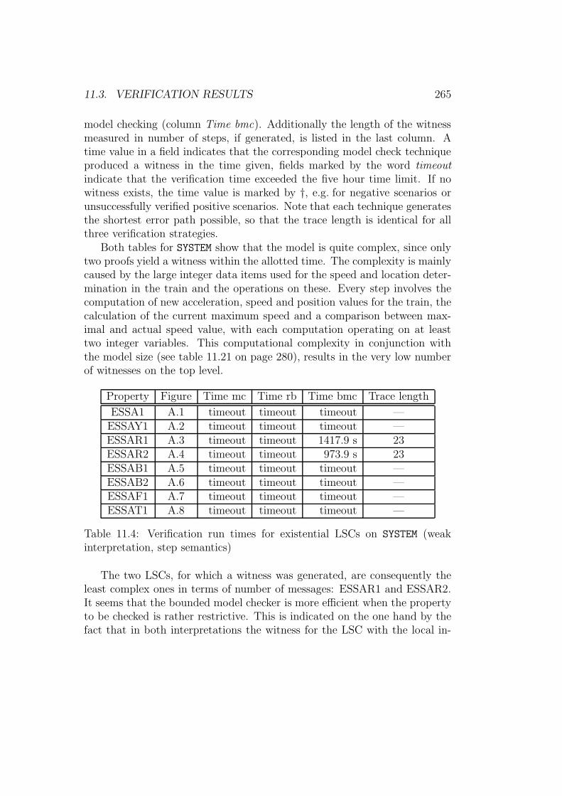
11.3. VERIFICATION RESULTS 265
model checking (column Time bmc). Additionally the length of the witnessmeasured in number of steps, if generated, is listed in the last column. Atime value in a field indicates that the corresponding model check techniqueproduced a witness in the time given, fields marked by the word timeoutindicate that the verification time exceeded the five hour time limit. If nowitness exists, the time value is marked by †, e.g. for negative scenarios orunsuccessfully verified positive scenarios. Note that each technique generatesthe shortest error path possible, so that the trace length is identical for allthree verification strategies.
Both tables for SYSTEM show that the model is quite complex, since onlytwo proofs yield a witness within the allotted time. The complexity is mainlycaused by the large integer data items used for the speed and location deter-mination in the train and the operations on these. Every step involves thecomputation of new acceleration, speed and position values for the train, thecalculation of the current maximum speed and a comparison between max-imal and actual speed value, with each computation operating on at leasttwo integer variables. This computational complexity in conjunction withthe model size (see table 11.21 on page 280), results in the very low numberof witnesses on the top level.
Property Figure Time mc Time rb Time bmc Trace length
ESSA1 A.1 timeout timeout timeout —ESSAY1 A.2 timeout timeout timeout —ESSAR1 A.3 timeout timeout 1417.9 s 23ESSAR2 A.4 timeout timeout 973.9 s 23ESSAB1 A.5 timeout timeout timeout —ESSAB2 A.6 timeout timeout timeout —ESSAF1 A.7 timeout timeout timeout —ESSAT1 A.8 timeout timeout timeout —
Table 11.4: Verification run times for existential LSCs on SYSTEM (weakinterpretation, step semantics)
The two LSCs, for which a witness was generated, are consequently theleast complex ones in terms of number of messages: ESSAR1 and ESSAR2.It seems that the bounded model checker is more efficient when the propertyto be checked is rather restrictive. This is indicated on the one hand by thefact that in both interpretations the witness for the LSC with the local in-
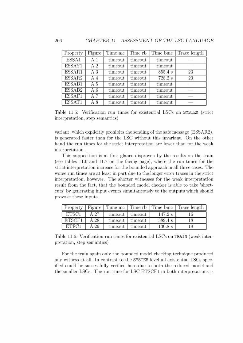
266 CHAPTER 11. ASSESSMENT OF THE LSC LANGUAGE
Property Figure Time mc Time rb Time bmc Trace length
ESSA1 A.1 timeout timeout timeout —ESSAY1 A.2 timeout timeout timeout —ESSAR1 A.3 timeout timeout 855.4 s 23ESSAR2 A.4 timeout timeout 728.2 s 23ESSAB1 A.5 timeout timeout timeout —ESSAB2 A.6 timeout timeout timeout —ESSAF1 A.7 timeout timeout timeout —ESSAT1 A.8 timeout timeout timeout —
Table 11.5: Verification run times for existential LSCs on SYSTEM (strictinterpretation, step semantics)
variant, which explicitly prohibits the sending of the safe message (ESSAR2),is generated faster than for the LSC without this invariant. On the otherhand the run times for the strict interpretation are lower than for the weakinterpretation.
This supposition is at first glance disproven by the results on the train(see tables 11.6 and 11.7 on the facing page), where the run times for thestrict interpretation increase for the bounded approach in all three cases. Theworse run times are at least in part due to the longer error traces in the strictinterpretation, however. The shorter witnesses for the weak interpretationresult from the fact, that the bounded model checker is able to take ’short-cuts’ by generating input events simultaneously to the outputs which shouldprovoke these inputs.
Property Figure Time mc Time rb Time bmc Trace length
ETSC1 A.27 timeout timeout 147.2 s 16ETSCF1 A.28 timeout timeout 389.4 s 18ETFC1 A.29 timeout timeout 130.8 s 19
Table 11.6: Verification run times for existential LSCs on TRAIN (weak inter-pretation, step semantics)
For the train again only the bounded model checking technique producedany witness at all. In contrast to the SYSTEM level all existential LSCs spec-ified could be successfully verified here due to both the reduced model andthe smaller LSCs. The run time for LSC ETSCF1 in both interpretations is
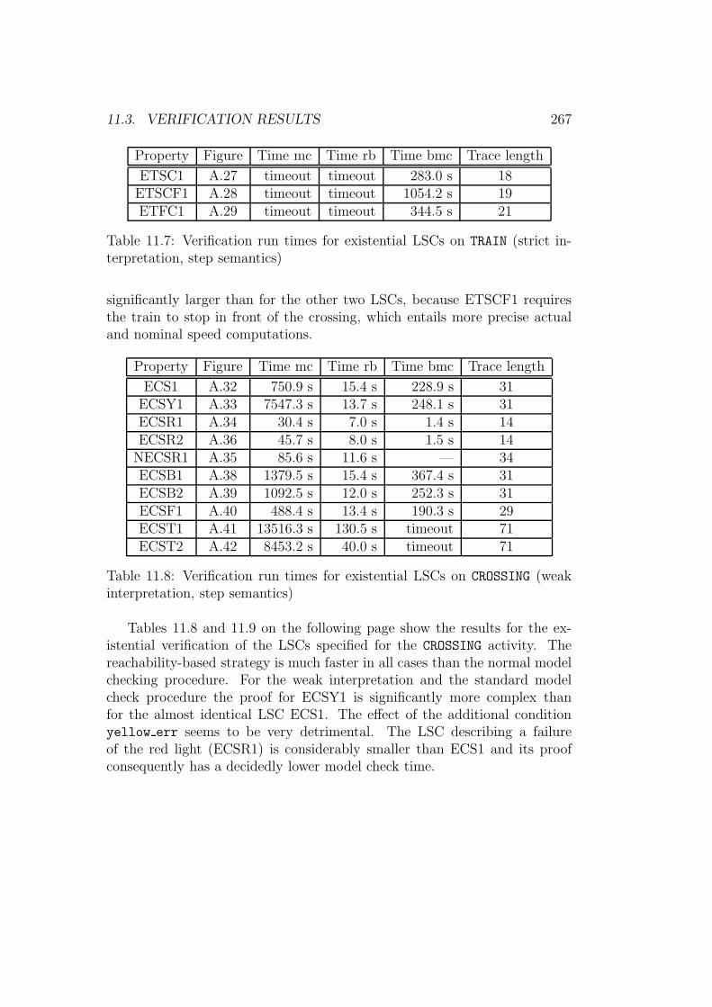
11.3. VERIFICATION RESULTS 267
Property Figure Time mc Time rb Time bmc Trace length
ETSC1 A.27 timeout timeout 283.0 s 18ETSCF1 A.28 timeout timeout 1054.2 s 19ETFC1 A.29 timeout timeout 344.5 s 21
Table 11.7: Verification run times for existential LSCs on TRAIN (strict in-terpretation, step semantics)
significantly larger than for the other two LSCs, because ETSCF1 requiresthe train to stop in front of the crossing, which entails more precise actualand nominal speed computations.
Property Figure Time mc Time rb Time bmc Trace length
ECS1 A.32 750.9 s 15.4 s 228.9 s 31ECSY1 A.33 7547.3 s 13.7 s 248.1 s 31ECSR1 A.34 30.4 s 7.0 s 1.4 s 14ECSR2 A.36 45.7 s 8.0 s 1.5 s 14
NECSR1 A.35 85.6 s 11.6 s — 34ECSB1 A.38 1379.5 s 15.4 s 367.4 s 31ECSB2 A.39 1092.5 s 12.0 s 252.3 s 31ECSF1 A.40 488.4 s 13.4 s 190.3 s 29ECST1 A.41 13516.3 s 130.5 s timeout 71ECST2 A.42 8453.2 s 40.0 s timeout 71
Table 11.8: Verification run times for existential LSCs on CROSSING (weakinterpretation, step semantics)
Tables 11.8 and 11.9 on the following page show the results for the ex-istential verification of the LSCs specified for the CROSSING activity. Thereachability-based strategy is much faster in all cases than the normal modelchecking procedure. For the weak interpretation and the standard modelcheck procedure the proof for ECSY1 is significantly more complex thanfor the almost identical LSC ECS1. The effect of the additional conditionyellow err seems to be very detrimental. The LSC describing a failureof the red light (ECSR1) is considerably smaller than ECS1 and its proofconsequently has a decidedly lower model check time.
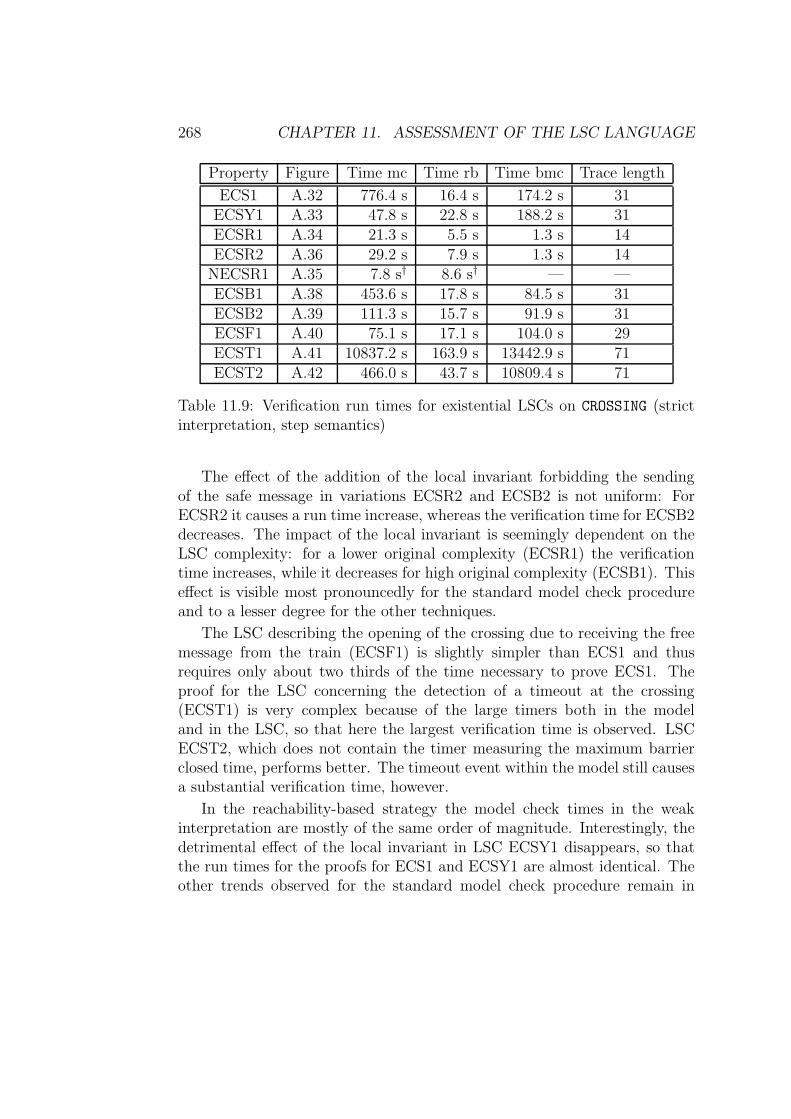
268 CHAPTER 11. ASSESSMENT OF THE LSC LANGUAGE
Property Figure Time mc Time rb Time bmc Trace length
ECS1 A.32 776.4 s 16.4 s 174.2 s 31ECSY1 A.33 47.8 s 22.8 s 188.2 s 31ECSR1 A.34 21.3 s 5.5 s 1.3 s 14ECSR2 A.36 29.2 s 7.9 s 1.3 s 14
NECSR1 A.35 7.8 s† 8.6 s† — —ECSB1 A.38 453.6 s 17.8 s 84.5 s 31ECSB2 A.39 111.3 s 15.7 s 91.9 s 31ECSF1 A.40 75.1 s 17.1 s 104.0 s 29ECST1 A.41 10837.2 s 163.9 s 13442.9 s 71ECST2 A.42 466.0 s 43.7 s 10809.4 s 71
Table 11.9: Verification run times for existential LSCs on CROSSING (strictinterpretation, step semantics)
The effect of the addition of the local invariant forbidding the sendingof the safe message in variations ECSR2 and ECSB2 is not uniform: ForECSR2 it causes a run time increase, whereas the verification time for ECSB2decreases. The impact of the local invariant is seemingly dependent on theLSC complexity: for a lower original complexity (ECSR1) the verificationtime increases, while it decreases for high original complexity (ECSB1). Thiseffect is visible most pronouncedly for the standard model check procedureand to a lesser degree for the other techniques.
The LSC describing the opening of the crossing due to receiving the freemessage from the train (ECSF1) is slightly simpler than ECS1 and thusrequires only about two thirds of the time necessary to prove ECS1. Theproof for the LSC concerning the detection of a timeout at the crossing(ECST1) is very complex because of the large timers both in the modeland in the LSC, so that here the largest verification time is observed. LSCECST2, which does not contain the timer measuring the maximum barrierclosed time, performs better. The timeout event within the model still causesa substantial verification time, however.
In the reachability-based strategy the model check times in the weakinterpretation are mostly of the same order of magnitude. Interestingly, thedetrimental effect of the local invariant in LSC ECSY1 disappears, so thatthe run times for the proofs for ECS1 and ECSY1 are almost identical. Theother trends observed for the standard model check procedure remain in
11.3. VERIFICATION RESULTS 269
effect. ECSR1 is still proven in less time than any of the other LSCs, eventhough the advantage is not as great, and ECST1 remains the most complexproof task. The omission of the timer again has a beneficial effect comparedto ECSTO1 without reaching the low run times of the other LSCs.
The bounded model check approach performs rather poorly compared tothe reachability-based technique. Only for the smallest LSCs (ECSR1 andECSR2) it produces a small gain, for all other proof tasks the run times aremuch larger and the proofs for the LSCs involving the observing of the max-imum barrier closed time do not even yield a result within the allotted time.Except for ECST1 and ECST2 the run times are still significantly better thanfor the standard model check procedure, however. The key point for the be-havior of the bounded model check approach is the length of the witness:Short witnesses are easily found by bounded model checking, whereas longones require an increased amount of time, since more iterations of bounded-FSM generation and SAT-checker runs are necessary. This effect can beobserved for all verification runs for existential LSCs in the step semantics.For the crossing the fastest times for bounded model checking are achievedfor LSCs resulting in the shortest witnesses and the worst results are seenfor LSCs producing the longest error paths, e.g. ECST1. For the train andthe complete system the witnesses found by bounded model checking are rel-atively short, compared to the trace lengths for most LSCs on the crossinglevel.
The overall effect of the strict interpretation (table 11.9) on the normalmodel checking procedure is beneficent, all run times improve save the onefor ECS1, which slightly increases. For this technique the more restrictiveformula limits the search space for the backward-oriented model check algo-rithm, so that it is kept more closely to the desired path, i.e. the witness.This effect is visible most pronouncedly for the proof of LSC ECSY1, whoserun time is reduced by a factor of almost 160.
For the reachability-based method the change in interpretation is almostunnoticeable in the run times, since the forward-oriented technique does nothave as much variability in finding the witness as the backward strategy,because it starts forward from the initial state. The verification times for thereachability-based method consequently almost uniformly increase slightlydue to the more complex formula.
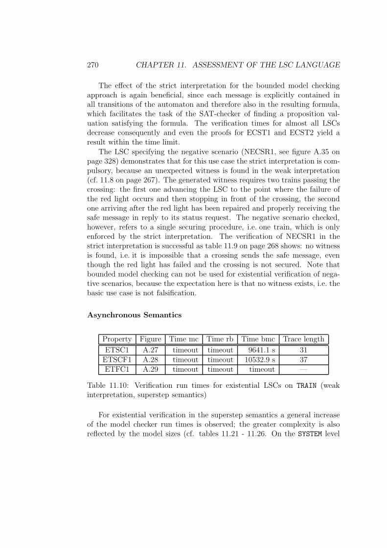
270 CHAPTER 11. ASSESSMENT OF THE LSC LANGUAGE
The effect of the strict interpretation for the bounded model checkingapproach is again beneficial, since each message is explicitly contained inall transitions of the automaton and therefore also in the resulting formula,which facilitates the task of the SAT-checker of finding a proposition val-uation satisfying the formula. The verification times for almost all LSCsdecrease consequently and even the proofs for ECST1 and ECST2 yield aresult within the time limit.
The LSC specifying the negative scenario (NECSR1, see figure A.35 onpage 328) demonstrates that for this use case the strict interpretation is com-pulsory, because an unexpected witness is found in the weak interpretation(cf. 11.8 on page 267). The generated witness requires two trains passing thecrossing: the first one advancing the LSC to the point where the failure ofthe red light occurs and then stopping in front of the crossing, the secondone arriving after the red light has been repaired and properly receiving thesafe message in reply to its status request. The negative scenario checked,however, refers to a single securing procedure, i.e. one train, which is onlyenforced by the strict interpretation. The verification of NECSR1 in thestrict interpretation is successful as table 11.9 on page 268 shows: no witnessis found, i.e. it is impossible that a crossing sends the safe message, eventhough the red light has failed and the crossing is not secured. Note thatbounded model checking can not be used for existential verification of nega-tive scenarios, because the expectation here is that no witness exists, i.e. thebasic use case is not falsification.
Asynchronous Semantics
Property Figure Time mc Time rb Time bmc Trace length
ETSC1 A.27 timeout timeout 9641.1 s 31ETSCF1 A.28 timeout timeout 10532.9 s 37ETFC1 A.29 timeout timeout timeout —
Table 11.10: Verification run times for existential LSCs on TRAIN (weakinterpretation, superstep semantics)
For existential verification in the superstep semantics a general increaseof the model checker run times is observed; the greater complexity is alsoreflected by the model sizes (cf. tables 11.21 - 11.26. On the SYSTEM level
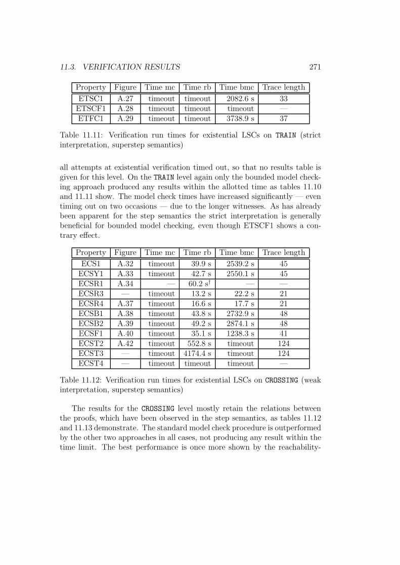
11.3. VERIFICATION RESULTS 271
Property Figure Time mc Time rb Time bmc Trace length
ETSC1 A.27 timeout timeout 2082.6 s 33ETSCF1 A.28 timeout timeout timeout —ETFC1 A.29 timeout timeout 3738.9 s 37
Table 11.11: Verification run times for existential LSCs on TRAIN (strictinterpretation, superstep semantics)
all attempts at existential verification timed out, so that no results table isgiven for this level. On the TRAIN level again only the bounded model check-ing approach produced any results within the allotted time as tables 11.10and 11.11 show. The model check times have increased significantly — eventiming out on two occasions — due to the longer witnesses. As has alreadybeen apparent for the step semantics the strict interpretation is generallybeneficial for bounded model checking, even though ETSCF1 shows a con-trary effect.
Property Figure Time mc Time rb Time bmc Trace length
ECS1 A.32 timeout 39.9 s 2539.2 s 45ECSY1 A.33 timeout 42.7 s 2550.1 s 45ECSR1 A.34 — 60.2 s† — —ECSR3 — timeout 13.2 s 22.2 s 21ECSR4 A.37 timeout 16.6 s 17.7 s 21ECSB1 A.38 timeout 43.8 s 2732.9 s 48ECSB2 A.39 timeout 49.2 s 2874.1 s 48ECSF1 A.40 timeout 35.1 s 1238.3 s 41ECST2 A.42 timeout 552.8 s timeout 124ECST3 — timeout 4174.4 s timeout 124ECST4 — timeout timeout timeout —
Table 11.12: Verification run times for existential LSCs on CROSSING (weakinterpretation, superstep semantics)
The results for the CROSSING level mostly retain the relations betweenthe proofs, which have been observed in the step semantics, as tables 11.12and 11.13 demonstrate. The standard model check procedure is outperformedby the other two approaches in all cases, not producing any result within thetime limit. The best performance is once more shown by the reachability-
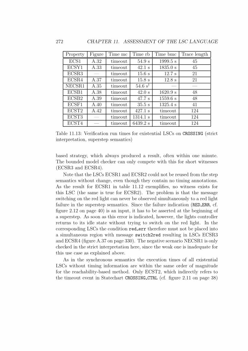
272 CHAPTER 11. ASSESSMENT OF THE LSC LANGUAGE
Property Figure Time mc Time rb Time bmc Trace length
ECS1 A.32 timeout 54.9 s 1999.5 s 45ECSY1 A.33 timeout 42.1 s 1835.0 s 45ECSR3 — timeout 15.6 s 12.7 s 21ECSR4 A.37 timeout 15.8 s 12.8 s 21
NECSR1 A.35 timeout 54.6 s† — —ECSB1 A.38 timeout 42.0 s 1620.9 s 48ECSB2 A.39 timeout 47.7 s 1559.6 s 48ECSF1 A.40 timeout 35.5 s 1325.4 s 41ECST2 A.42 timeout 427.1 s timeout 124ECST3 — timeout 1314.1 s timeout 124ECST4 — timeout 6439.2 s timeout 124
Table 11.13: Verification run times for existential LSCs on CROSSING (strictinterpretation, superstep semantics)
based strategy, which always produced a result, often within one minute.The bounded model checker can only compete with this for short witnesses(ECSR3 and ECSR4).
Note that the LSCs ECSR1 and ECSR2 could not be reused from the stepsemantics without change, even though they contain no timing annotations.As the result for ECSR1 in table 11.12 exemplifies, no witness exists forthis LSC (the same is true for ECSR2). The problem is that the messageswitching on the red light can never be observed simultaneously to a red lightfailure in the superstep semantics. Since the failure indication (RED ERR, cf.figure 2.12 on page 40) is an input, it has to be asserted at the beginning ofa superstep. As soon as this error is indicated, however, the lights controllerreturns to its idle state without trying to switch on the red light. In thecorresponding LSCs the condition red err therefore must not be placed intoa simultaneous region with message switch2red resulting in LSCs ECSR3and ECSR4 (figure A.37 on page 330). The negative scenario NECSR1 is onlychecked in the strict interpretation here, since the weak one is inadequate forthis use case as explained above.
As in the synchronous semantics the execution times of all existentialLSCs without timing information are within the same order of magnitudefor the reachability-based method. Only ECST2, which indirectly refers tothe timeout event in Statechart CROSSING CTRL (cf. figure 2.11 on page 38)
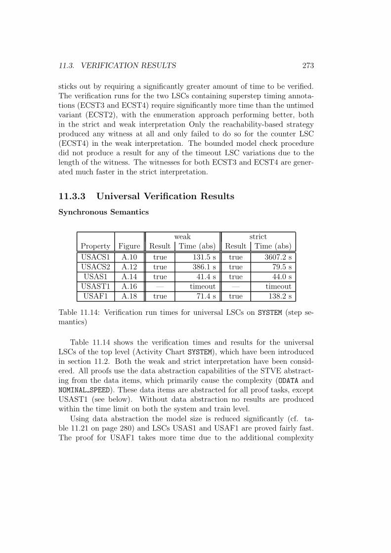
11.3. VERIFICATION RESULTS 273
sticks out by requiring a significantly greater amount of time to be verified.The verification runs for the two LSCs containing superstep timing annota-tions (ECST3 and ECST4) require significantly more time than the untimedvariant (ECST2), with the enumeration approach performing better, bothin the strict and weak interpretation Only the reachability-based strategyproduced any witness at all and only failed to do so for the counter LSC(ECST4) in the weak interpretation. The bounded model check proceduredid not produce a result for any of the timeout LSC variations due to thelength of the witness. The witnesses for both ECST3 and ECST4 are gener-ated much faster in the strict interpretation.
11.3.3 Universal Verification Results
Synchronous Semantics
weak strictProperty Figure Result Time (abs) Result Time (abs)
USACS1 A.10 true 131.5 s true 3607.2 sUSACS2 A.12 true 386.1 s true 79.5 sUSAS1 A.14 true 41.4 s true 44.0 s
USAST1 A.16 — timeout — timeoutUSAF1 A.18 true 71.4 s true 138.2 s
Table 11.14: Verification run times for universal LSCs on SYSTEM (step se-mantics)
Table 11.14 shows the verification times and results for the universalLSCs of the top level (Activity Chart SYSTEM), which have been introducedin section 11.2. Both the weak and strict interpretation have been consid-ered. All proofs use the data abstraction capabilities of the STVE abstract-ing from the data items, which primarily cause the complexity (ODATA andNOMINAL SPEED). These data items are abstracted for all proof tasks, exceptUSAST1 (see below). Without data abstraction no results are producedwithin the time limit on both the system and train level.
Using data abstraction the model size is reduced significantly (cf. ta-ble 11.21 on page 280) and LSCs USAS1 and USAF1 are proved fairly fast.The proof for USAF1 takes more time due to the additional complexity
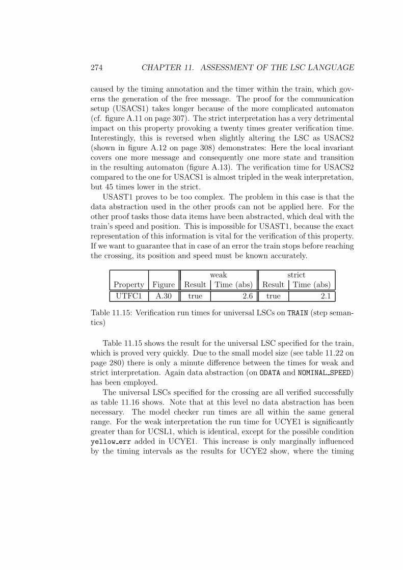
274 CHAPTER 11. ASSESSMENT OF THE LSC LANGUAGE
caused by the timing annotation and the timer within the train, which gov-erns the generation of the free message. The proof for the communicationsetup (USACS1) takes longer because of the more complicated automaton(cf. figure A.11 on page 307). The strict interpretation has a very detrimentalimpact on this property provoking a twenty times greater verification time.Interestingly, this is reversed when slightly altering the LSC as USACS2(shown in figure A.12 on page 308) demonstrates: Here the local invariantcovers one more message and consequently one more state and transitionin the resulting automaton (figure A.13). The verification time for USACS2compared to the one for USACS1 is almost tripled in the weak interpretation,but 45 times lower in the strict.
USAST1 proves to be too complex. The problem in this case is that thedata abstraction used in the other proofs can not be applied here. For theother proof tasks those data items have been abstracted, which deal with thetrain’s speed and position. This is impossible for USAST1, because the exactrepresentation of this information is vital for the verification of this property.If we want to guarantee that in case of an error the train stops before reachingthe crossing, its position and speed must be known accurately.
weak strictProperty Figure Result Time (abs) Result Time (abs)
UTFC1 A.30 true 2.6 true 2.1
Table 11.15: Verification run times for universal LSCs on TRAIN (step seman-tics)
Table 11.15 shows the result for the universal LSC specified for the train,which is proved very quickly. Due to the small model size (see table 11.22 onpage 280) there is only a minute difference between the times for weak andstrict interpretation. Again data abstraction (on ODATA and NOMINAL SPEED)has been employed.
The universal LSCs specified for the crossing are all verified successfullyas table 11.16 shows. Note that at this level no data abstraction has beennecessary. The model checker run times are all within the same generalrange. For the weak interpretation the run time for UCYE1 is significantlygreater than for UCSL1, which is identical, except for the possible conditionyellow err added in UCYE1. This increase is only marginally influencedby the timing intervals as the results for UCYE2 show, where the timing
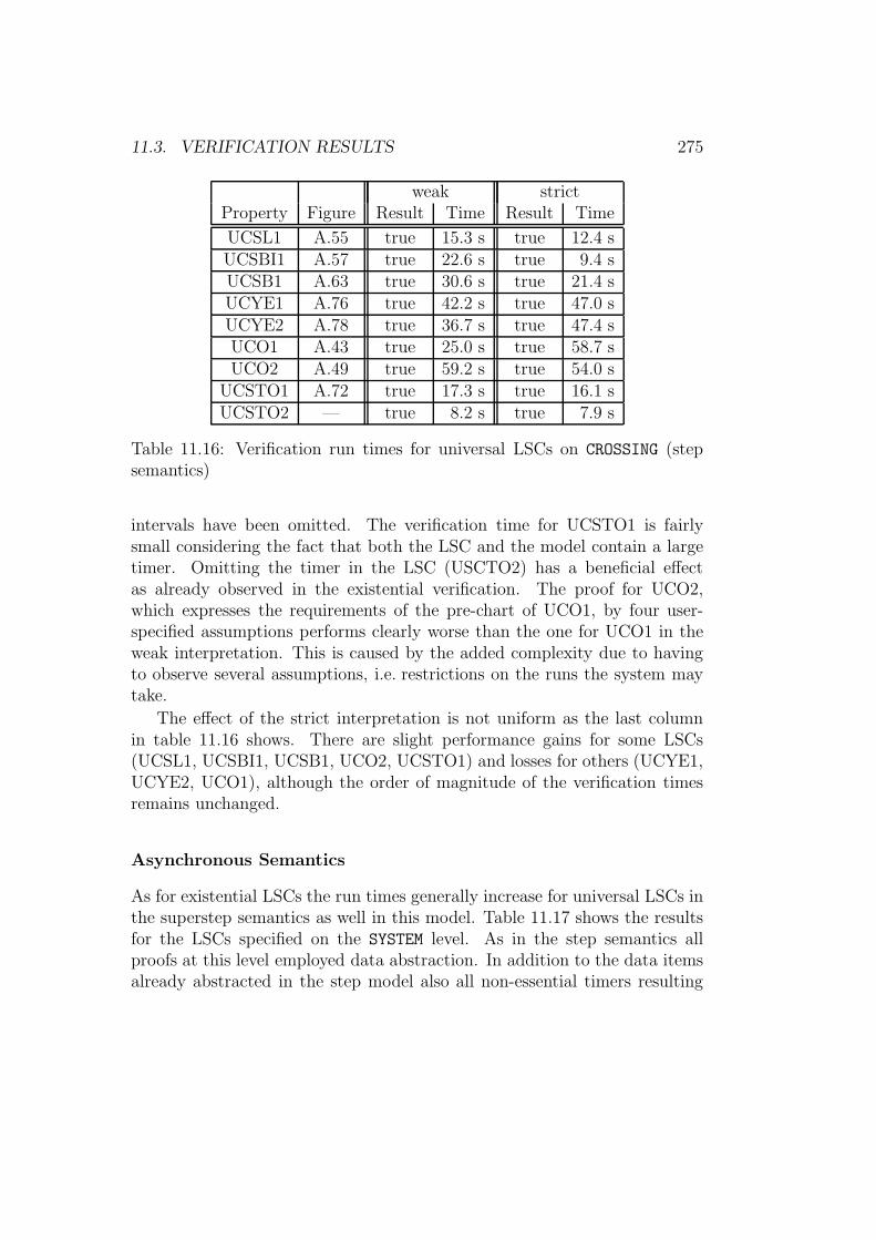
11.3. VERIFICATION RESULTS 275
weak strictProperty Figure Result Time Result Time
UCSL1 A.55 true 15.3 s true 12.4 sUCSBI1 A.57 true 22.6 s true 9.4 sUCSB1 A.63 true 30.6 s true 21.4 sUCYE1 A.76 true 42.2 s true 47.0 sUCYE2 A.78 true 36.7 s true 47.4 sUCO1 A.43 true 25.0 s true 58.7 sUCO2 A.49 true 59.2 s true 54.0 s
UCSTO1 A.72 true 17.3 s true 16.1 sUCSTO2 — true 8.2 s true 7.9 s
Table 11.16: Verification run times for universal LSCs on CROSSING (stepsemantics)
intervals have been omitted. The verification time for UCSTO1 is fairlysmall considering the fact that both the LSC and the model contain a largetimer. Omitting the timer in the LSC (USCTO2) has a beneficial effectas already observed in the existential verification. The proof for UCO2,which expresses the requirements of the pre-chart of UCO1, by four user-specified assumptions performs clearly worse than the one for UCO1 in theweak interpretation. This is caused by the added complexity due to havingto observe several assumptions, i.e. restrictions on the runs the system maytake.
The effect of the strict interpretation is not uniform as the last columnin table 11.16 shows. There are slight performance gains for some LSCs(UCSL1, UCSBI1, UCSB1, UCO2, UCSTO1) and losses for others (UCYE1,UCYE2, UCO1), although the order of magnitude of the verification timesremains unchanged.
Asynchronous Semantics
As for existential LSCs the run times generally increase for universal LSCs inthe superstep semantics as well in this model. Table 11.17 shows the resultsfor the LSCs specified on the SYSTEM level. As in the step semantics allproofs at this level employed data abstraction. In addition to the data itemsalready abstracted in the step model also all non-essential timers resulting
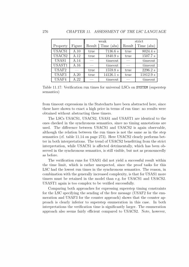
276 CHAPTER 11. ASSESSMENT OF THE LSC LANGUAGE
weak strictProperty Figure Result Time (abs) Result Time (abs)
USACS1 A.10 true 7136.6 s true 8024.4 sUSACS2 A.12 true 1840.9 s true 1507.7 sUSAS1 A.14 — timeout — timeout
USAST1 A.16 — timeout — timeoutUSAF2 — true 1559.8 s true 2296.2 sUSAF3 A.20 true 14126.1 s true 11812.9 sUSAF4 A.22 — timeout — timeout
Table 11.17: Verification run times for universal LSCs on SYSTEM (superstepsemantics)
from timeout expressions in the Statecharts have been abstracted here, sincethese have shown to exact a high price in terms of run time: no results wereobtained without abstracting these timers.
The LSCs USACS1, USACS2, USAS1 and USAST1 are identical to theones checked in the synchronous semantics, since no timing annotations areused. The difference between USACS1 and USACS2 is again observable,although the relation between the run times is not the same as in the stepsemantics (cf. table 11.14 on page 273). Here USACS2 clearly performs bet-ter in both interpretations. The trend of USACS2 benefitting from the strictinterpretation, while USACS1 is affected detrimentally, which has been ob-served in the synchronous semantics, is still visible, but not as pronouncedlyas before.
The verification runs for USAS1 did not yield a successful result withinthe time limit, which is rather unexpected, since the proof tasks for thisLSC had the lowest run times in the synchronous semantics. The reason, incombination with the generally increased complexity, is that for USAS1 moretimers must be retained in the model than e.g. for USACS1 and USACS2.USAST1 again is too complex to be verified successfully.
Comparing both approaches for expressing superstep timing constraintsfor the LSC specifying the sending of the free message (USAF2 for the enu-meration and USAF3 for the counter approach) shows that the counter ap-proach is clearly inferior to superstep enumeration in this case. In bothinterpretations the verification time is significantly larger. The enumerationapproach also seems fairly efficient compared to USACS2. Note, however,
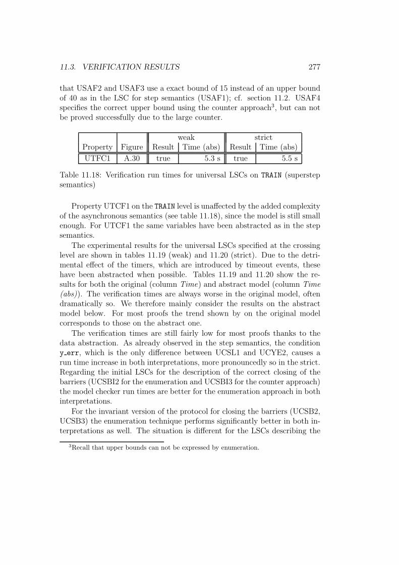
11.3. VERIFICATION RESULTS 277
that USAF2 and USAF3 use a exact bound of 15 instead of an upper boundof 40 as in the LSC for step semantics (USAF1); cf. section 11.2. USAF4specifies the correct upper bound using the counter approach3, but can notbe proved successfully due to the large counter.
weak strictProperty Figure Result Time (abs) Result Time (abs)
UTFC1 A.30 true 5.3 s true 5.5 s
Table 11.18: Verification run times for universal LSCs on TRAIN (superstepsemantics)
Property UTCF1 on the TRAIN level is unaffected by the added complexityof the asynchronous semantics (see table 11.18), since the model is still smallenough. For UTCF1 the same variables have been abstracted as in the stepsemantics.
The experimental results for the universal LSCs specified at the crossinglevel are shown in tables 11.19 (weak) and 11.20 (strict). Due to the detri-mental effect of the timers, which are introduced by timeout events, thesehave been abstracted when possible. Tables 11.19 and 11.20 show the re-sults for both the original (column Time) and abstract model (column Time(abs)). The verification times are always worse in the original model, oftendramatically so. We therefore mainly consider the results on the abstractmodel below. For most proofs the trend shown by on the original modelcorresponds to those on the abstract one.
The verification times are still fairly low for most proofs thanks to thedata abstraction. As already observed in the step semantics, the conditiony err, which is the only difference between UCSL1 and UCYE2, causes arun time increase in both interpretations, more pronouncedly so in the strict.Regarding the initial LSCs for the description of the correct closing of thebarriers (UCSBI2 for the enumeration and UCSBI3 for the counter approach)the model checker run times are better for the enumeration approach in bothinterpretations.
For the invariant version of the protocol for closing the barriers (UCSB2,UCSB3) the enumeration technique performs significantly better in both in-terpretations as well. The situation is different for the LSCs describing the
3Recall that upper bounds can not be expressed by enumeration.
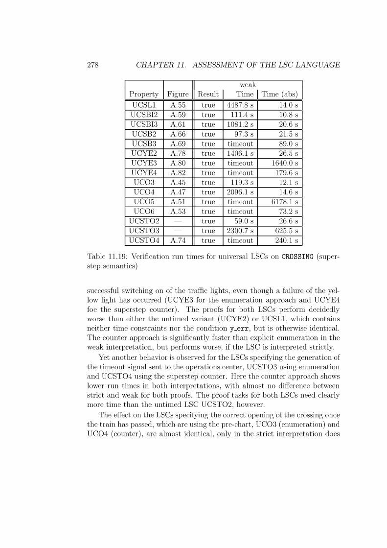
278 CHAPTER 11. ASSESSMENT OF THE LSC LANGUAGE
weakProperty Figure Result Time Time (abs)
UCSL1 A.55 true 4487.8 s 14.0 sUCSBI2 A.59 true 111.4 s 10.8 sUCSBI3 A.61 true 1081.2 s 20.6 sUCSB2 A.66 true 97.3 s 21.5 sUCSB3 A.69 true timeout 89.0 sUCYE2 A.78 true 1406.1 s 26.5 sUCYE3 A.80 true timeout 1640.0 sUCYE4 A.82 true timeout 179.6 sUCO3 A.45 true 119.3 s 12.1 sUCO4 A.47 true 2096.1 s 14.6 sUCO5 A.51 true timeout 6178.1 sUCO6 A.53 true timeout 73.2 s
UCSTO2 — true 59.0 s 26.6 sUCSTO3 — true 2300.7 s 625.5 sUCSTO4 A.74 true timeout 240.1 s
Table 11.19: Verification run times for universal LSCs on CROSSING (super-step semantics)
successful switching on of the traffic lights, even though a failure of the yel-low light has occurred (UCYE3 for the enumeration approach and UCYE4foe the superstep counter). The proofs for both LSCs perform decidedlyworse than either the untimed variant (UCYE2) or UCSL1, which containsneither time constraints nor the condition y err, but is otherwise identical.The counter approach is significantly faster than explicit enumeration in theweak interpretation, but performs worse, if the LSC is interpreted strictly.
Yet another behavior is observed for the LSCs specifying the generation ofthe timeout signal sent to the operations center, UCSTO3 using enumerationand UCSTO4 using the superstep counter. Here the counter approach showslower run times in both interpretations, with almost no difference betweenstrict and weak for both proofs. The proof tasks for both LSCs need clearlymore time than the untimed LSC UCSTO2, however.
The effect on the LSCs specifying the correct opening of the crossing oncethe train has passed, which are using the pre-chart, UCO3 (enumeration) andUCO4 (counter), are almost identical, only in the strict interpretation does
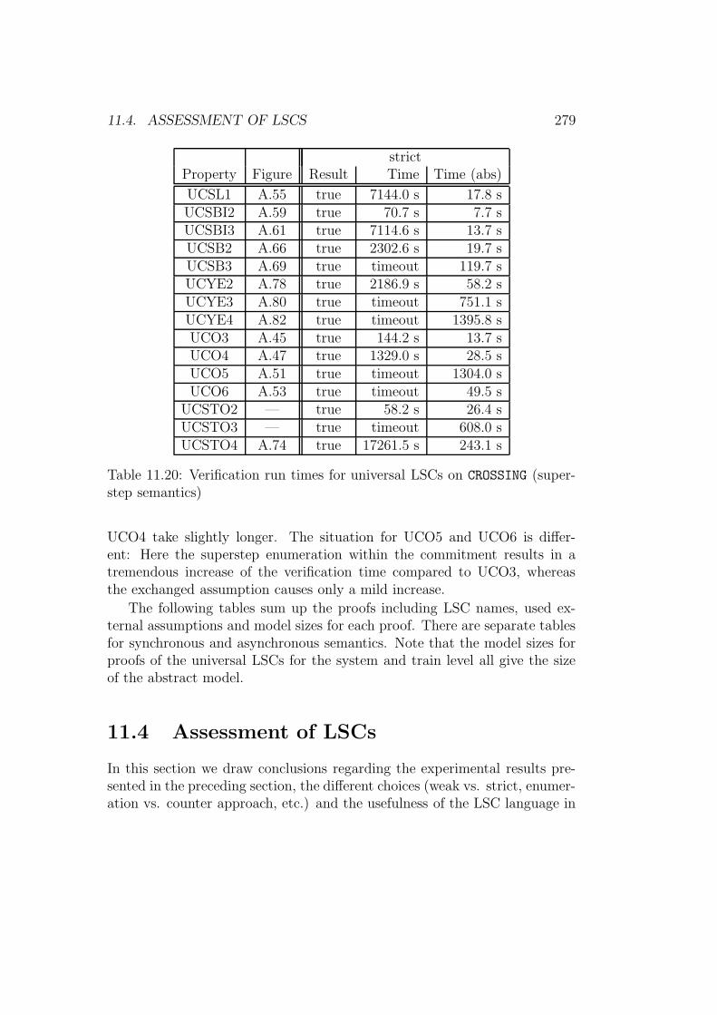
11.4. ASSESSMENT OF LSCS 279
strictProperty Figure Result Time Time (abs)
UCSL1 A.55 true 7144.0 s 17.8 sUCSBI2 A.59 true 70.7 s 7.7 sUCSBI3 A.61 true 7114.6 s 13.7 sUCSB2 A.66 true 2302.6 s 19.7 sUCSB3 A.69 true timeout 119.7 sUCYE2 A.78 true 2186.9 s 58.2 sUCYE3 A.80 true timeout 751.1 sUCYE4 A.82 true timeout 1395.8 sUCO3 A.45 true 144.2 s 13.7 sUCO4 A.47 true 1329.0 s 28.5 sUCO5 A.51 true timeout 1304.0 sUCO6 A.53 true timeout 49.5 s
UCSTO2 — true 58.2 s 26.4 sUCSTO3 — true timeout 608.0 sUCSTO4 A.74 true 17261.5 s 243.1 s
Table 11.20: Verification run times for universal LSCs on CROSSING (super-step semantics)
UCO4 take slightly longer. The situation for UCO5 and UCO6 is differ-ent: Here the superstep enumeration within the commitment results in atremendous increase of the verification time compared to UCO3, whereasthe exchanged assumption causes only a mild increase.
The following tables sum up the proofs including LSC names, used ex-ternal assumptions and model sizes for each proof. There are separate tablesfor synchronous and asynchronous semantics. Note that the model sizes forproofs of the universal LSCs for the system and train level all give the sizeof the abstract model.
11.4 Assessment of LSCs
In this section we draw conclusions regarding the experimental results pre-sented in the preceding section, the different choices (weak vs. strict, enumer-ation vs. counter approach, etc.) and the usefulness of the LSC language in
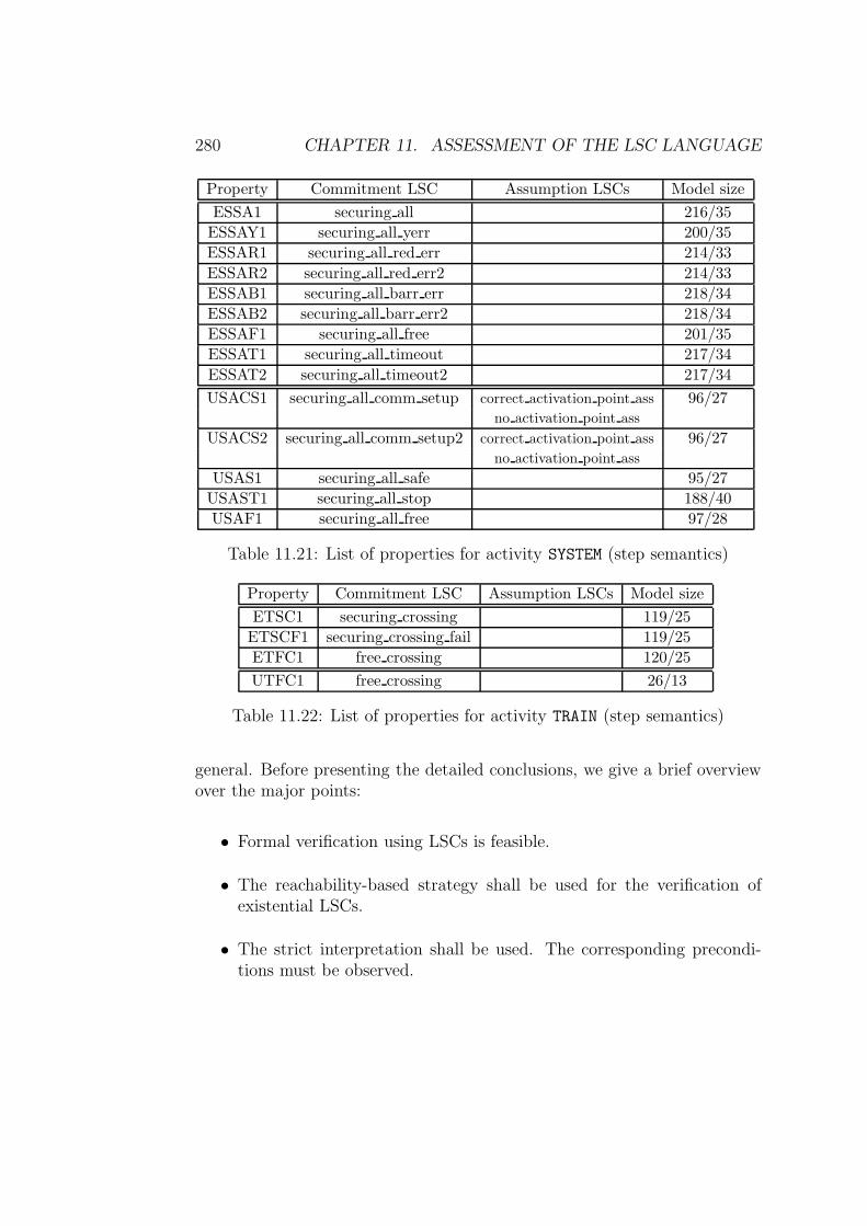
280 CHAPTER 11. ASSESSMENT OF THE LSC LANGUAGE
Property Commitment LSC Assumption LSCs Model size
ESSA1 securing all 216/35
ESSAY1 securing all yerr 200/35
ESSAR1 securing all red err 214/33
ESSAR2 securing all red err2 214/33
ESSAB1 securing all barr err 218/34
ESSAB2 securing all barr err2 218/34
ESSAF1 securing all free 201/35
ESSAT1 securing all timeout 217/34
ESSAT2 securing all timeout2 217/34
USACS1 securing all comm setup correct activation point ass 96/27no activation point ass
USACS2 securing all comm setup2 correct activation point ass 96/27no activation point ass
USAS1 securing all safe 95/27
USAST1 securing all stop 188/40
USAF1 securing all free 97/28
Table 11.21: List of properties for activity SYSTEM (step semantics)
Property Commitment LSC Assumption LSCs Model size
ETSC1 securing crossing 119/25
ETSCF1 securing crossing fail 119/25
ETFC1 free crossing 120/25
UTFC1 free crossing 26/13
Table 11.22: List of properties for activity TRAIN (step semantics)
general. Before presenting the detailed conclusions, we give a brief overviewover the major points:
• Formal verification using LSCs is feasible.
• The reachability-based strategy shall be used for the verification ofexistential LSCs.
• The strict interpretation shall be used. The corresponding precondi-tions must be observed.
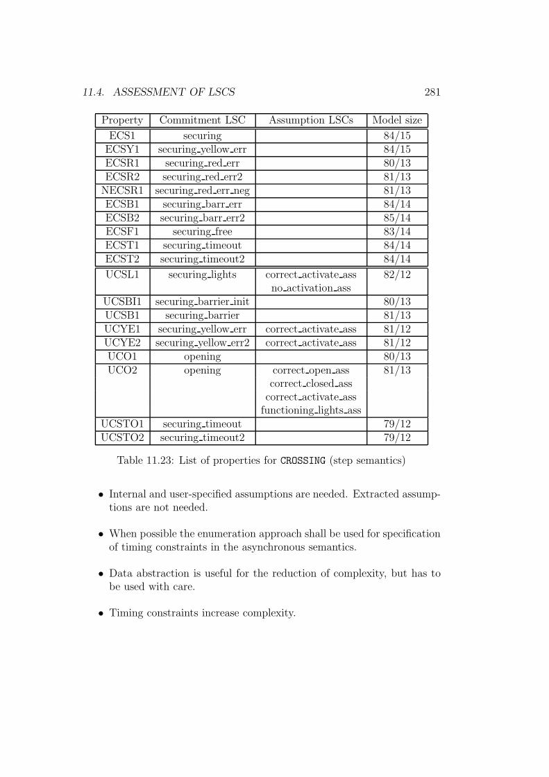
11.4. ASSESSMENT OF LSCS 281
Property Commitment LSC Assumption LSCs Model size
ECS1 securing 84/15ECSY1 securing yellow err 84/15ECSR1 securing red err 80/13ECSR2 securing red err2 81/13
NECSR1 securing red err neg 81/13ECSB1 securing barr err 84/14ECSB2 securing barr err2 85/14ECSF1 securing free 83/14ECST1 securing timeout 84/14ECST2 securing timeout2 84/14
UCSL1 securing lights correct activate ass 82/12no activation ass
UCSBI1 securing barrier init 80/13UCSB1 securing barrier 81/13UCYE1 securing yellow err correct activate ass 81/12UCYE2 securing yellow err2 correct activate ass 81/12UCO1 opening 80/13UCO2 opening correct open ass 81/13
correct closed asscorrect activate ass
functioning lights assUCSTO1 securing timeout 79/12UCSTO2 securing timeout2 79/12
Table 11.23: List of properties for CROSSING (step semantics)
• Internal and user-specified assumptions are needed. Extracted assump-tions are not needed.
• When possible the enumeration approach shall be used for specificationof timing constraints in the asynchronous semantics.
• Data abstraction is useful for the reduction of complexity, but has tobe used with care.
• Timing constraints increase complexity.
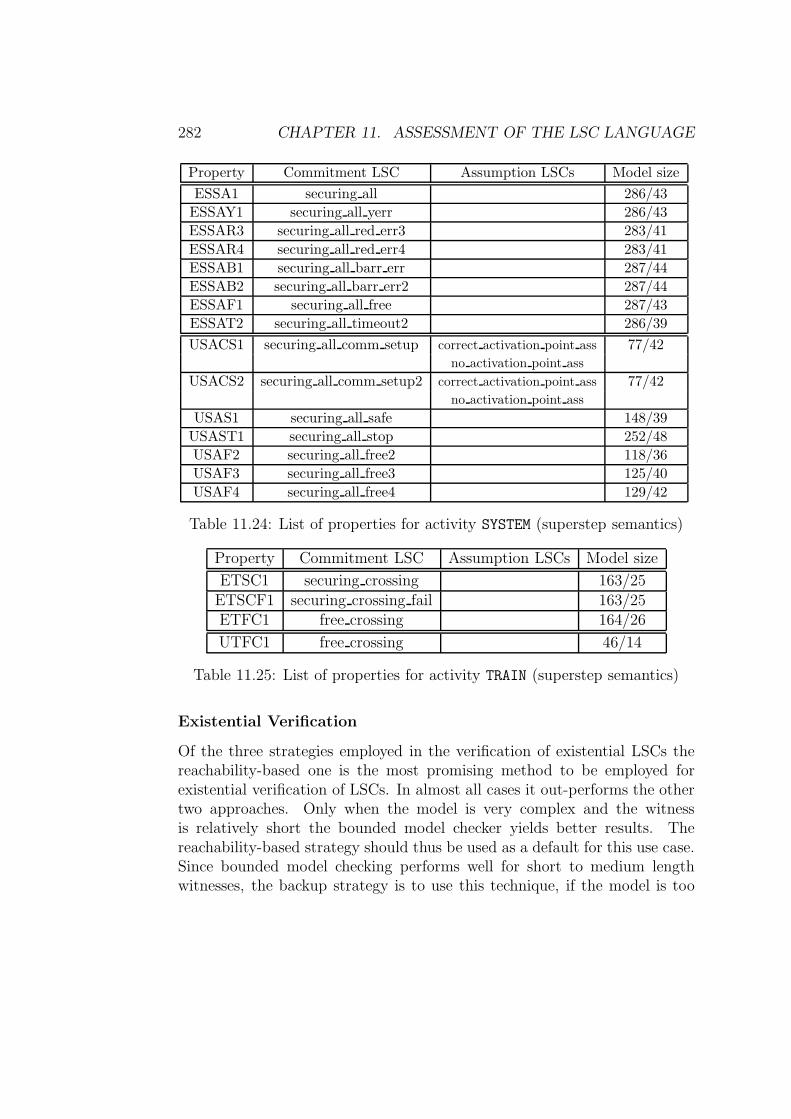
282 CHAPTER 11. ASSESSMENT OF THE LSC LANGUAGE
Property Commitment LSC Assumption LSCs Model size
ESSA1 securing all 286/43
ESSAY1 securing all yerr 286/43
ESSAR3 securing all red err3 283/41
ESSAR4 securing all red err4 283/41
ESSAB1 securing all barr err 287/44
ESSAB2 securing all barr err2 287/44
ESSAF1 securing all free 287/43
ESSAT2 securing all timeout2 286/39
USACS1 securing all comm setup correct activation point ass 77/42no activation point ass
USACS2 securing all comm setup2 correct activation point ass 77/42no activation point ass
USAS1 securing all safe 148/39
USAST1 securing all stop 252/48
USAF2 securing all free2 118/36
USAF3 securing all free3 125/40
USAF4 securing all free4 129/42
Table 11.24: List of properties for activity SYSTEM (superstep semantics)
Property Commitment LSC Assumption LSCs Model size
ETSC1 securing crossing 163/25ETSCF1 securing crossing fail 163/25ETFC1 free crossing 164/26
UTFC1 free crossing 46/14
Table 11.25: List of properties for activity TRAIN (superstep semantics)
Existential Verification
Of the three strategies employed in the verification of existential LSCs thereachability-based one is the most promising method to be employed forexistential verification of LSCs. In almost all cases it out-performs the othertwo approaches. Only when the model is very complex and the witnessis relatively short the bounded model checker yields better results. Thereachability-based strategy should thus be used as a default for this use case.Since bounded model checking performs well for short to medium lengthwitnesses, the backup strategy is to use this technique, if the model is too
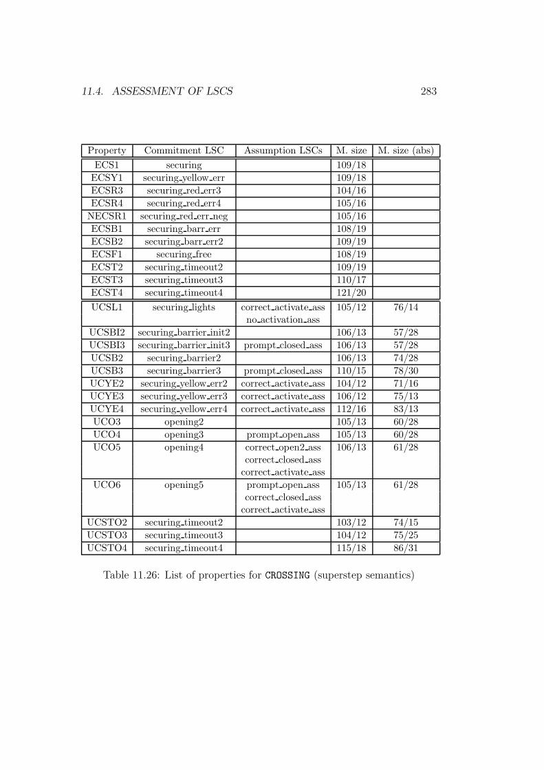
11.4. ASSESSMENT OF LSCS 283
Property Commitment LSC Assumption LSCs M. size M. size (abs)
ECS1 securing 109/18
ECSY1 securing yellow err 109/18
ECSR3 securing red err3 104/16
ECSR4 securing red err4 105/16
NECSR1 securing red err neg 105/16
ECSB1 securing barr err 108/19
ECSB2 securing barr err2 109/19
ECSF1 securing free 108/19
ECST2 securing timeout2 109/19
ECST3 securing timeout3 110/17
ECST4 securing timeout4 121/20
UCSL1 securing lights correct activate ass 105/12 76/14no activation ass
UCSBI2 securing barrier init2 106/13 57/28
UCSBI3 securing barrier init3 prompt closed ass 106/13 57/28
UCSB2 securing barrier2 106/13 74/28
UCSB3 securing barrier3 prompt closed ass 110/15 78/30
UCYE2 securing yellow err2 correct activate ass 104/12 71/16
UCYE3 securing yellow err3 correct activate ass 106/12 75/13
UCYE4 securing yellow err4 correct activate ass 112/16 83/13
UCO3 opening2 105/13 60/28
UCO4 opening3 prompt open ass 105/13 60/28
UCO5 opening4 correct open2 ass 106/13 61/28correct closed ass
correct activate ass
UCO6 opening5 prompt open ass 105/13 61/28correct closed ass
correct activate ass
UCSTO2 securing timeout2 103/12 74/15
UCSTO3 securing timeout3 104/12 75/25
UCSTO4 securing timeout4 115/18 86/31
Table 11.26: List of properties for CROSSING (superstep semantics)
284 CHAPTER 11. ASSESSMENT OF THE LSC LANGUAGE
complex and the expected length of the witness is short.
Interpretation
Our expectation regarding the effect of the strict compared to the weakinterpretation was that the larger formula resulting from the former wouldlead to noticeably increased model checker run times. The experimentalresults show that this expectation is fulfilled for only a small number ofproperties, e.g. USACS2 in the step semantics or UCYE4. In the majorityof cases the verification times increased only slightly or even decreased. Apossible reason for this effect could be that the inclusion of all message labelsin every transition of the symbolic automaton constitutes almost an invariantproperty resulting in a formula, which is easier to check, since all containedpropositions are similar. This supposition is supported by LSC USACS2:the extension of the local invariant to cover one more message in comparisonto USACS1 yields a more uniform automaton (cf. figures A.11 on page 307and A.15 on page 309) and a reduced run time in the strict interpretation.
Our decision for a default interpretation goes in favor of strict interpreta-tion. This choice is motivated by several reasons. First, there is the issue ofwitnesses of differing lengths, which has become apparent on the train level.Even though the short-cuts taken in the weak interpretation in these casesdo not constitute errors, witnesses showing the correct sequence of cause andeffect better conform to the real world and the intuition of the user. Thesecond argument for the strict interpretation are negative scenarios, whichrequire this interpretation in order not to generate undesired witnesses. Asimilar problem — the satisfaction of an LSC by two trains — can also arisefor ordinary existential LSCs. Here the strict interpretation is better suitedas well, since then no witness is generated in this case, which directly in-dicates that there is a problem. The third reason for choosing the strictinterpretation is that it better fits the intuition of the user. Additionally theperformance figures do not bar the use of the strict interpretation as statedabove.
Having made this decision in favor of the strict interpretation, let us em-phasize again, however, that there are preconditions, which must be fulfilled(cf. also the remarks on page 146):
11.4. ASSESSMENT OF LSCS 285
1. The message mappings must be unique.
2. There must be only one active incarnation of the same LSC at eachpoint in time.
Assumptions
The conclusion for assumptions is that internal assumptions are very usefuland intuitive, since they are specified directly within the commitment LSCusing the same elements, which make up the commitment. User-specified as-sumptions are likewise indispensable (cf. e.g. USACS1 or USL1). Extractedassumptions were not needed for the successful verification of the LSCs spec-ified. In retrospective, we expect them to be used only rarely, since they areintended to be used mostly for enforcing unbounded liveness requirements onthe environment. This will typically not be sufficient to guarantee livenessproperties on the commitment side, because for embedded controllers a re-sponse from the environment often must occur within a certain time frame.For this reason there is e.g. no unbounded liveness requirement expressed onan environment instance in the LSCs for the radio-based crossing controlsystem. The barriers for instance have to be closed within a certain amountof time in order for the crossing to operate correctly.
Statemate Semantics
With respect to the superstep semantics we can state that for our case studythe verification times are always worse than in the step semantics. Thisstatement can not be generalized, however, since the model at hand is in effectnot very modular, i.e. there is a large degree of interdependence betweendifferent activities (cf. [Bie03]). Thus, most of the synchronization betweenall activities, which is necessary for the stabilization of the complete part ofthe model considered in the verification, is contained in the verified model,increasing the complexity of the verification task. More modular models areexpected to show better performance figures. Regardless of the modularity,however, it can be said that timeout events, and presumably also scheduledactions, have a detrimental impact on the model check performance.
286 CHAPTER 11. ASSESSMENT OF THE LSC LANGUAGE
Enumeration vs. Superstep Counter Approach
Regarding the issue of which approach to expressing timing constraints inthe superstep semantics should be used, no clear trend can be discerned.On the complete model USAF2 and USAF3 show that the counter approachperforms much worse than explicit enumeration, which is corroborated byUCSB2 and UCSB3 on the crossing level. In both these examples the timingconstraints are located in the pre-chart, whereas a contrary effect is observedfor UCSTO3 and UCSTO4, where the timing constraint is part of the com-mitment. UCYE3 and UCYE4, where the constraint is also located in theactual LSCs, show a mixed picture, which in the weak interpretation is iden-tical to the behavior observed for UCSTO3 and UCSTO4, but is reversed inthe strict interpretation.
From a performance point of view therefore the explicit enumeration ap-proach is to be used for timing constraints, if it can be applied. This is notalways possible, since this approach can only express lower and exact bounds.In these cases, however, it is a viable optimization; otherwise the generallyapplicable counter approach must be used.
Abstraction
For universal LSCs the verification complexity can be reduced by applyingdata abstraction as done for the proofs on the system and train level andon crossing in the superstep semantics. It has proven to be very useful asthe experimental results show, especially on the crossing component in thesuperstep semantics (cf. tables 11.19 on page 278 and 11.20), but it has tobe noted that this technique has some limitations. The selection of whichvariables should be abstracted is done by the user and requires a thoroughunderstanding of the model. Care has to be taken not to abstract a variable,whose precise value is essential for the verified property. This is even moreimportant for the verification of liveness properties, since typically concreteand precise values of involved variables must be available in order to even-tually produce a certain result. When abstracting variables in the superstepsemantics additional care has to be exercised, because not only those vari-ables, whose value actually contributes to the checked property, have to behandled with caution, but also those, which influence the stabilization of themodel. Abstracting a variable of the latter type results in a diverging model,which then does guarantee no liveness requirement.
11.4. ASSESSMENT OF LSCS 287
Timing Annotations
The conclusion regarding timing constraints, irrespective of the semantics,is that they result in a more complex verification task. The effect is rathermild in the step semantics, where in the best case there is little differencein the performance between the timed and untimed variant of the checkedLSC (e.g. UCYE1 vs. UCYE2 in the step semantics) and in the worst casethe verification time is increased by factor four (ECST1 vs. ECST2). Inthe superstep semantics there is a substantial increase, however, rangingfrom roughly six times to over sixty times longer run time for the timedvariants. Only those timing annotations should thus be used in LSCs, whichare absolutely necessary, in order to increase performance. The same advicecan be given regarding timers in the Statemate model, i.e. timeout eventsand scheduled actions, which also have a detrimental impact on model checkerrun times, especially in the superstep semantics.
Activation
The possibility to explicitly characterize the activation point of a chart is akey benefit of LSCs, especially for formal verification. For the experimentalresults the invariant activation mode has been used predominantly, althoughthe initial mode has proven useful in a number of occasions, e.g. to restrictthe initial system state via initial assumptions or to cover the first occurrenceof a protocol (UCSBI1 - UCSBI3). Pre-charts have also demonstrated thatthey are a profitable feature for the easy and intuitive specification of arequired history of a desired protocol (cf. LSCs UCSB1 - UCSB3 and UCO1,UCO3, UCO4). Care has to be taken with pre-charts as well as assumptions,however, that they are compatible with the original requirements.
Mandatory vs. Possible
The distinction between mandatory and possible elements in an LSC mas-sively enhance the expressiveness of LSCs compared to MSCs or SDs. As theexperimental results show the distinction of existential and universal charts isan integral element for the smooth integration of LSCs into a model-based de-velopment process. The capability of discriminating mandatory and possibleconditions and local invariants is indispensable for expressing requirementsand internal assumptions. In this context simultaneous regions have proven
288 CHAPTER 11. ASSESSMENT OF THE LSC LANGUAGE
to be extremely useful for tying together messages and conditions and forproviding reference points for timers and local invariants.
Hot and cold location temperatures allow to intuitively mark the in-stances, which are responsible for progress. No assessment of message tem-peratures and asynchronous messages can be done, since all communicationin Statemate is instantaneous and messages can not be lost. But we expectcold messages to be useful in rare cases only, especially when considering for-mal verification. Typically either both sending and receipt of a message is ofinterest or the message is omitted altogether.
Methodology
Taking a more general view on LSCs we can state that the graphical spec-ification of interactions between communicating entities (activities in thiscase) is extremely helpful in the early phases of the design process in orderto thoroughly understand a system’s basic functionality. Even though LSCsare not necessarily required for this purpose — MSCs and SDs can be usedas well — the increased expressiveness of LSCs adds more substance to earlyscenarios by allowing to state information more explicitly. A very importantfeature in this context is the activation condition, which requires the de-signer to explicitly characterize the situation triggering the scenario which isdescribed. Another key advantage of LSCs over the other two sequence chartdialects are local invariants, which allow to forbid the occurrence of messagesin a specific part of the chart, e.g. LSCs ECSR2 or ECSB2, which explicitlycontain the prohibition of sending the safe message after a failure of the redlight or the barrier. Such side conditions are only implicitly contained in SDsor MSCs, by not including them. The enhanced expressiveness of LSCs thusallows to make property specifications more precise, while at the same timeretaining the intuitiveness and visual appeal of standard sequence charts.
The subsequent phases of the development process capitalize both on theadditional precision and information contained in the early existential LSCsand on the formal semantics. Existential verification reuses the early scenarioand provides valuable feedback to the designer in the form of early indicationsthat the model contains the basic communication behavior as specified in theexistential LSCs. Existential verification profits from the explicitly specifiedside conditions, because the checking is more focused.
Even though existential verification did yield few results for the top levelof the train control system model, we still feel that this technique is valu-
11.4. ASSESSMENT OF LSCS 289
able in general, since it allows to check for the existence of deep interactionsequences, thus exploiting one of the major advantages of model-based de-velopment process: virtual integration. The complexity problems are to adegree inherent due to the long message sequences, which consequently re-quire a deep exploration of the model. Chapter 12 offers some suggestions,how to reduce the verification complexity for both existential and universalLSCs.
The modularization of existential LSCs into universal ones and the sub-sequent strengthening of the latter allows a further reuse of the existentialLSCs created in earlier phases of development. This smooth transition touniversal protocol specifications is another very important benefit offered byLSCs and the accompanying methodology.
For the formal verification of universal LSCs the capability to expressassumptions about environment behavior directly within the LSCs has provento be extraordinarily useful. From the user’s point of view it is convenient andnatural to specify assumptions not only in the same graphical formalism, butwithin the same chart. Especially internal assumptions play a key role in thestrengthening of universal LSCs: most assumptions used in the verificationof the LSCs for the train control system have been expressed internally. Anequally positive effect can be asserted for pre-charts, which allow an easyand intuitive specification of a prefix of the actual LSC. The experimentalresults show that the use of pre-charts is superior to employing user-specifiedassumptions both wrt. ease of use and efficiency (cf. LSCs UCO1 -UCO5).
Expressiveness
Compared to the patterns provided by the STVE LSCs offer more expressive-ness like true liveness, local invariants, pre-charts and an arbitrary number ofmessages, conditions, etc. Another advantage of LSCs is their visual appealand intuitiveness, whereas the patterns are represented in a non-graphicalway. The downside to the enhanced expressiveness, however, is the decreasedperformance when model checking LSCs. Additionally more expert knowl-edge is required to specify properties as LSCs than as patterns.
STDs in comparison to LSCs are similar in terms of expressiveness andthe required expert knowledge, but are focused on single components and area state-based formalism, whereas LSCs are event-based. Protocols involvingseveral components are expressible in STDs, but separate STDs, one percomponent, are needed and a rather complicated compositional verification
290 CHAPTER 11. ASSESSMENT OF THE LSC LANGUAGE
approach must be employed. LSCs are better suited to describe communica-tion sequences involving several components due to their event-based nature.Long interaction sequences is moreover more naturally and more easily spec-ified with LSCs.
A development process based on the STVE and LSCs should use all avail-able analyses and checks at the appropriate time. While the model is beingconstructed the STVE robustness checks are employed, possibly in conjunc-tion with existential verification of LSCs once an adequate part of the be-havior has been modeled. Patterns are then used to verify simple propertiesexploiting their greater efficiency, and STDs and universal LSCs are usedfor the specification and verification of more complex properties. STDs arebest suited for black-box requirements, whereas LSCs are ideal for livenessproperties involving more than one component (grey-box requirements).
It has to be noted, though, that the successful verification of universalLSCs can be time consuming due to the potential iterations of (unsuccessful)verification run, problem analysis and changing the LSC or the model. Forobtaining the experimental results for universal LSCs presented in the pre-vious section up to three iterations were necessary. This drawback of LSCsdoes not outweigh the advantages like intuitiveness and enhanced expres-sive power, especially since each iteration gives the specifier more knowledgeabout the behavior of the considered (sub-)system, which can be reused whenverifying other, similar LSCs.
In conclusion we can say that LSCs are very well suited for the specifica-tion of communication protocols, especially those involving liveness require-ments. The use case of formal verification, which has been considered indetail here, seems a promising field of application, in particular in combina-tion with the associated methodology, which eases the task of property spec-ification by partly reusing LSCs, which have been created in earlier phasesof the development process. Both the universal and existential verificationshow promise to become valuable additions to a model-based developmentprocess. The experimental results presented in this thesis serve as a proofof concept, but also indicate that the model check performance has to beimproved before LSC-based formal verification can take root in everydayindustrial development.
Chapter 12
Conclusion and Outlook
The incentive of this thesis has been the upgrade of standard sequence chartsin order to play a more prominent role in the development of electronic controlsystems. In the introduction we have outlined the most important advanceduse cases, like formal verification and automatic test vector generation, whichtranscend the applications of todays sequence charts: documentation of typ-ical interactions and visualization of test or simulation traces. A detailedlook at the two standardized sequence charts, Message Sequence Charts andUML’s Sequence Diagrams, revealed that these, in their present form, arenot well suited to meet the challenges posed by the envisioned advanced usecases. Both MSCs and SDs lack expressivity and a sound formal base, whichmotivates the definition of the language of Live Sequence Charts carried outin this work involving the fixing of the language features and their syntax aswell as providing their formal semantics. We have performed the definitionof both syntax and semantics incrementally, starting with the core featuresand step by step adding more advanced concepts.
The kernel language of LSCs comprises the basic elements, which makeup a chart like instances, messages and conditions. We have defined thesemantical basis in a constructive way by translating an LSC into a variationof a timed Buchi automaton. The relation to the system, whose behavioris described by the LSC, is established by relating the runs of the systemto those accepted by the automaton. We have extended this definition ofthe basic features bit by bit to include the more advanced concepts of time,pre-charts and assumptions.
With the syntax and semantics of LSCs in place we have added the thirdvital building block: an application methodology, which outlines how and
291
292 CHAPTER 12. CONCLUSION AND OUTLOOK
where the created language should be employed. Here we laid special empha-sis on the seamless reusability of LSCs and the use case of formal verification.We concluded with the experimental results we have obtained in the formalverification of a radio-based train control system, which has already servedas a running example throughout this work. The practical application ofLSCs to the advanced use case of formal verification has demonstrated theusefulness and viability of the features and semantics of LSCs, even thoughsome complexity problems were encountered.
Outlook
The high model checking complexity observed for a number of the LSCsin the experimental results section is somewhat inherent. The purpose ofLSCs is to specify the communication behavior between several components,so that components can not be considered in isolation. This entails a non-trivial base complexity depending on the number and size of the involvedcomponents. The reduction of complexity wrt. model checking is thus animportant direction for future work.
For universal LSCs data abstraction has already been applied in severalof the proofs in section 11.3. This optimization requires a high degree ofuser interaction and knowledge about the system, since the variables to beabstracted have to be chosen by the user. Bienmuller [Bie03] presents anapproach, which does not require the user to select the variables to be ab-stracted, but tries to determine them automatically. At first a very coarseabstraction is used and it is checked, if the property holds. If this is notthe case the abstraction is refined and the procedure is iterated until a trueresult is obtained or no further abstractions are possible. The entire pro-cess is guided by a heuristic, which combines standard backward cone-of-influence (COI) computation and a similar forward-oriented strategy. Thebackward-COI depends on the outputs used in the checked property, whereasthe forward-COI regards the inputs. In [Bie03] this approach has successfullybeen applied to properties specified as patterns in the STVE.
This automated abstraction technique seems promising to help reducethe complexity for verification of universal LSCs and additionally increaseuser-friendliness. The applicability of this approach hinges on the possibilityto automatically determine which propositions of the property are inputsand which are outputs, which is easy for patterns. In order to transfer this
293
technique to LSCs as well, information about inputs and outputs used inthe chart must be made available to the tool performing the automatedabstraction.
Another possibility for complexity reduction is the automatic decompo-sition of grey-box requirements specified as LSCs into local black-box prop-erties, which can be proven on the involved components. Key idea here isthat the decomposition already guarantees one of the tasks, which have to beperformed for compositional reasoning: the proof that the sum of the localrequirements indeed implies the global grey-box requirement. Questions tobe investigated for this approach comprise:
• Is a decomposition possible for invariant LSCs? Due to overlappingincarnations it is not clear, if the decomposed view correctly reflectsthe global behavior.
• What is the best representation for the decomposed local requirements?They could e.g. be represented as LSCs, STDs, TSAs, temporal logicor yet another format.
• How are the decomposed properties triggered/activated? Is the ac-tivation condition used for triggering all local requirements? Is thesynchronized activation necessary and if so, how is it achieved?
• How should pre-charts be treated?
• Are there restrictions on the features, which may be used in the globalLSC? Can e.g. synchronization for shared conditions be guaranteed?
For the verification of existential LSCs a possible optimization is thepartitioning of the entire LSC into smaller segments, each of which forms aseparate verification task. The idea hence is to first find a witness for theinitial segment, record the current global state of the FSM once it has beenfound and use this state as a fresh start point — forgetting the first witness— for the generation of the witness for the second segment and so on. Inthis way long existential LSCs can be broken down into smaller fragments,which are checked decidedly faster. The witness for the complete LSCs thenhas to be assembled from the witnesses for the fragments.
Regarding a further extension of the set of LSC features it is interesting toconsider the inclusion of structuring elements, like e.g. sub-charts and loops.
294 CHAPTER 12. CONCLUSION AND OUTLOOK
These constructs have been mentioned in the original LSC paper [DH98],albeit without a formal definition. The use of such operational constructs forformal verification purposes, where the manner of specification of interactionsis rather declarative, is doubtful. For other purposes, e.g. testing, they canbe useful, however. An exhaustive treatment of sub-charts encompasses alsothe relation between elements within and outside of the sub-chart and ifan interference between internal and external elements should be allowed,e.g. messages crossing the sub-chart boundary. Furthermore bounded and/orunbounded loops should be considered in this context as well as instancerefinement similar to instance decomposition in MSCs.
Another direction of further work deals with the improvement of prop-erty specification for Statemate models using the superstep semantics. Theview offered by Statemate does not lend itself to property specification withLSCs as the evaluation has shown. Statemate in the asynchronous seman-tics allows to only model one embedded controller, whose internals are givenby the Activity Charts and Statecharts thereby mixing internal and externalcommunication. A more natural view wrt. LSCs would be to model severalembedded controllers and only allow to refer to messages sent between them,thus disregarding any internal communication of the individual embeddedcontrollers. Franzle et al. [FNMD03] propose such an interpretation andprovides an according formal semantics. On this basis applications bettersuited to property specification with LSCs are conceivable like system-leveltesting, i.e. testing the interplay of several embedded controllers.
Other application contexts for LSCs are possible as well, like e.g. UML,which already contains Sequence Diagrams. While the LSC language as pre-sented in this work considers the basic elements, which are necessary in orderto specify protocols as LSCs also within a UML context, the concrete rela-tions between LSC and model elements still have to be defined. Whereas thismapping is fairly simple and obvious in the case of Statemate, more efforthas to be invested for the practical application of LSCs in the UML world.A UML model is generally not as persistent as a Statemate model, whichdoes not change its structure during its lifetime. One of the key features ofobject-orientation is the dynamic creation and destruction of objects, whichentails that the structure of the model and the relation between objects inthe model change over time as new objects are created, old ones are destroyedand associations between objects are redirected. There are additional ques-tions to be resolved, like e.g. how sending and receipt of an event are to beinterpreted in the UML model in view of an event queue, or the mapping
295
of LSC instances to model objects in the presence of relative identifications,e.g. of the form crossing->itsTrain.
We have undertaken a first attempt at providing such a relationin [KW02], albeit without referring to a formal representation of a UMLmodel. In the context of ongoing efforts at the University of Oldenburg andOFFIS, Damm and Westphal [DW03] provide a more precise and formal def-inition of the relation of LSC to model elements basing on the semantics fora subset of the UML presented in [DJPV03].
The highly dynamic nature of UML models makes the formal verificationa challenging field of research involving the definition of a formal semantics,the investigation of new verification strategies in order to cope with changingand even unbounded models, and the development of a fitting format forspecifying properties. LSCs seem a very natural choice for the last task andit will be interesting to see how this area evolves.

296 CHAPTER 12. CONCLUSION AND OUTLOOK
Appendix A
LSCs for the Radio-based Train
Control System
This chapter collects the LSCs, which have been specified and verified forthe train control system. For universal and assumption LSCs additionallythe generated timed symbolic automata are included. Some LSCs have beenomitted when they were too large to be included (e.g. due to a large tim-ing constraint in the superstep semantics using the explicit enumeration ap-proach).
297
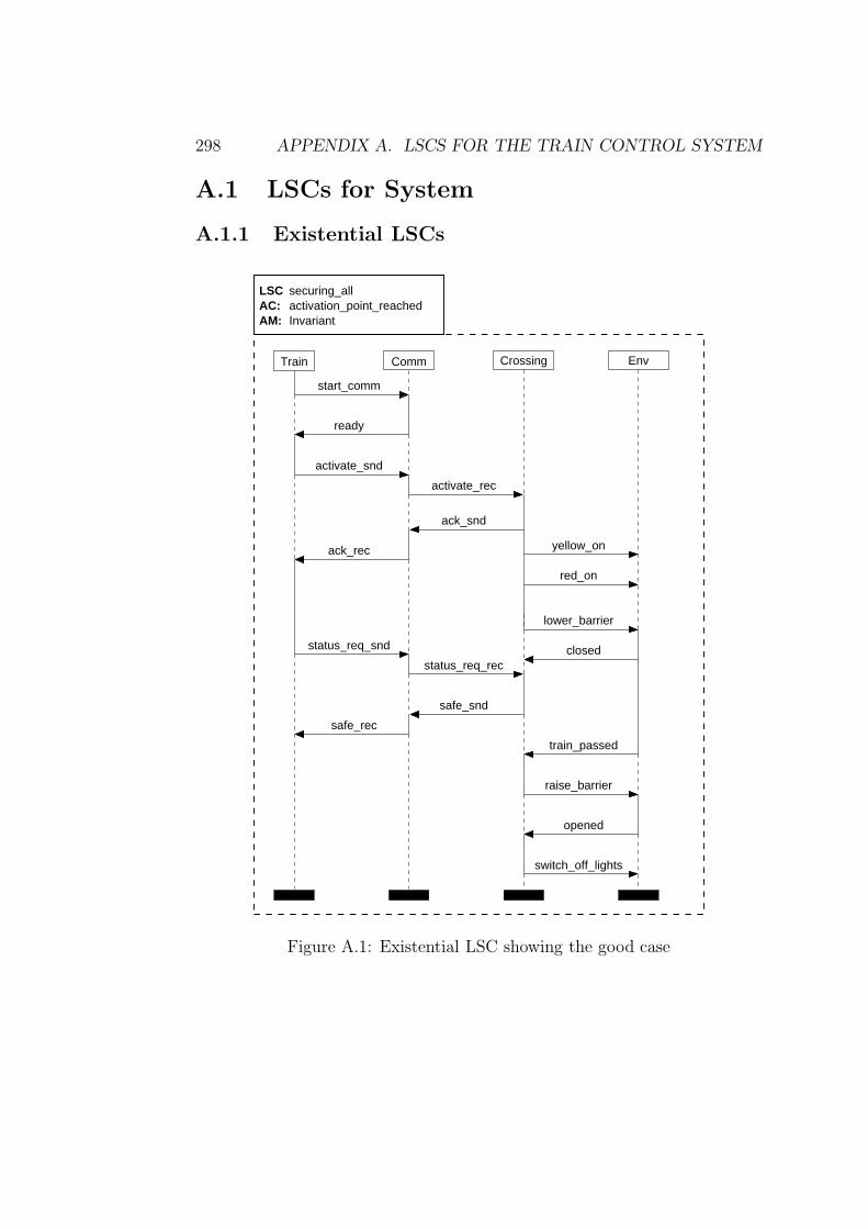
298 APPENDIX A. LSCS FOR THE TRAIN CONTROL SYSTEM
A.1 LSCs for System
A.1.1 Existential LSCs
EnvCommTrain Crossing
start_comm
ready
activate_snd
activate_rec
ack_snd
safe_rec
safe_snd
status_req_rec
status_req_snd
train_passed
raise_barrier
opened
switch_off_lights
closed
lower_barrier
yellow_on
red_on
ack_rec
Invariantactivation_point_reachedsecuring_all
AM:AC:LSC
Figure A.1: Existential LSC showing the good case
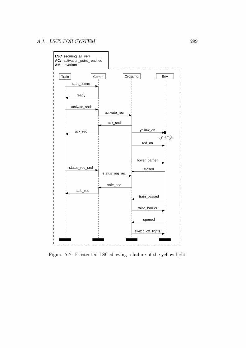
A.1. LSCS FOR SYSTEM 299
Env
safe_rec
safe_snd
status_req_rec
status_req_snd
train_passed
raise_barrier
opened
switch_off_lights
closed
lower_barrier
red_on
CommTrain Crossing
start_comm
ready
activate_snd
activate_rec
ack_snd
yellow_onack_rec
y_err
Invariantactivation_point_reached
AM:AC:LSC securing_all_yerr
Figure A.2: Existential LSC showing a failure of the yellow light
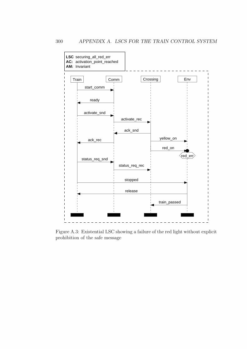
300 APPENDIX A. LSCS FOR THE TRAIN CONTROL SYSTEM
EnvCommTrain Crossing
start_comm
ready
activate_snd
activate_rec
ack_snd
train_passed
yellow_on
red_on
ack_rec
status_req_rec
status_req_snd
stopped
release
red_err
Invariantactivation_point_reachedsecuring_all_red_err
AM:AC:LSC
Figure A.3: Existential LSC showing a failure of the red light without explicitprohibition of the safe message
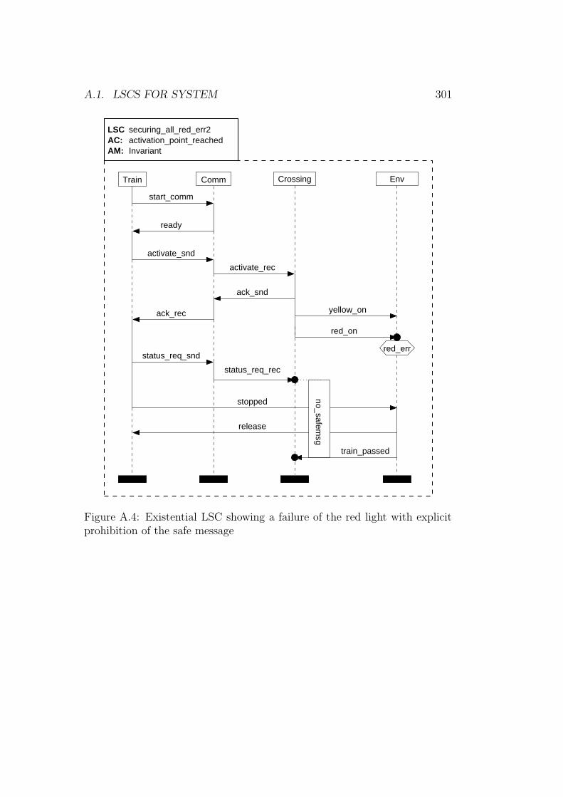
A.1. LSCS FOR SYSTEM 301
EnvCommTrain Crossing
start_comm
ready
activate_snd
activate_rec
ack_snd
ack_rec
status_req_rec
status_req_snd
stopped
release
train_passed
red_on
yellow_on
red_err
no_safemsg
Invariantactivation_point_reachedsecuring_all_red_err2
AM:AC:LSC
Figure A.4: Existential LSC showing a failure of the red light with explicitprohibition of the safe message
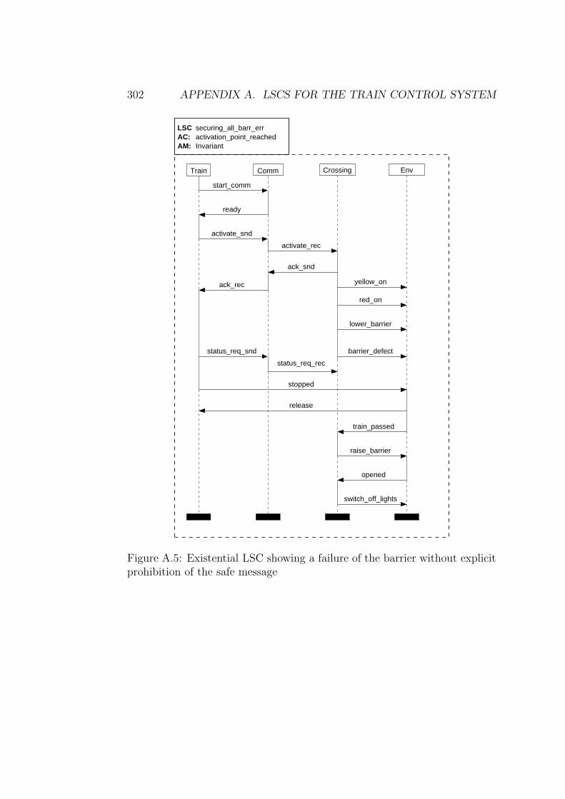
302 APPENDIX A. LSCS FOR THE TRAIN CONTROL SYSTEM
EnvCommTrain Crossing
start_comm
ready
activate_snd
activate_rec
ack_snd
yellow_on
red_on
ack_rec
lower_barrier
status_req_rec
status_req_snd barrier_defect
train_passed
raise_barrier
opened
switch_off_lights
stopped
release
Invariantactivation_point_reachedsecuring_all_barr_err
AM:AC:LSC
Figure A.5: Existential LSC showing a failure of the barrier without explicitprohibition of the safe message
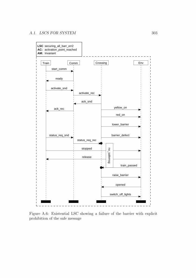
A.1. LSCS FOR SYSTEM 303
EnvCommTrain Crossing
start_comm
ready
activate_snd
activate_rec
ack_snd
ack_rec
status_req_rec
status_req_snd
stopped
release
train_passed
raise_barrier
switch_off_lights
opened
barrier_defect
lower_barrier
red_on
yellow_on
no_safemsg
Invariantactivation_point_reachedsecuring_all_barr_err2
AM:AC:LSC
Figure A.6: Existential LSC showing a failure of the barrier with explicitprohibition of the safe message
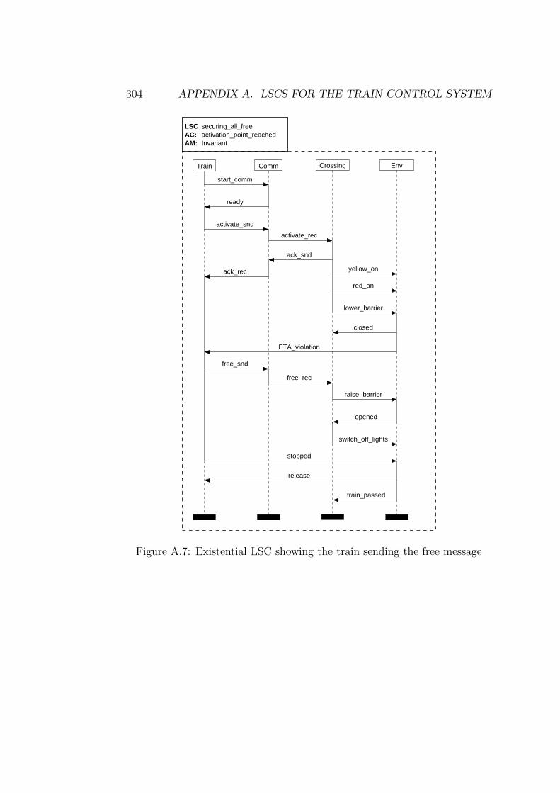
304 APPENDIX A. LSCS FOR THE TRAIN CONTROL SYSTEM
Env
free_snd
free_rec
raise_barrier
switch_off_lights
opened
release
stopped
train_passed
CommTrain Crossing
start_comm
ready
activate_snd
activate_rec
ack_snd
yellow_on
red_on
ack_rec
lower_barrier
closed
ETA_violation
Invariantactivation_point_reachedsecuring_all_free
AM:AC:LSC
Figure A.7: Existential LSC showing the train sending the free message
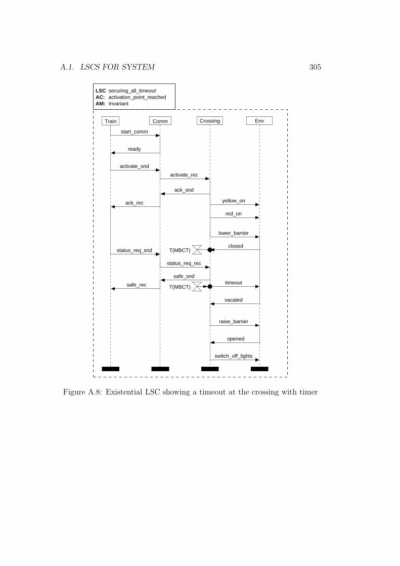
A.1. LSCS FOR SYSTEM 305
EnvCommTrain Crossing
start_comm
ready
activate_snd
activate_rec
ack_snd
closed
lower_barrier
yellow_on
red_on
ack_rec
timeout
raise_barrier
opened
switch_off_lights
vacated
safe_rec
safe_snd
status_req_snd
status_req_rec
Invariantactivation_point_reachedsecuring_all_timeout
AM:AC:LSC
T(MBCT)
T(MBCT)
Figure A.8: Existential LSC showing a timeout at the crossing with timer
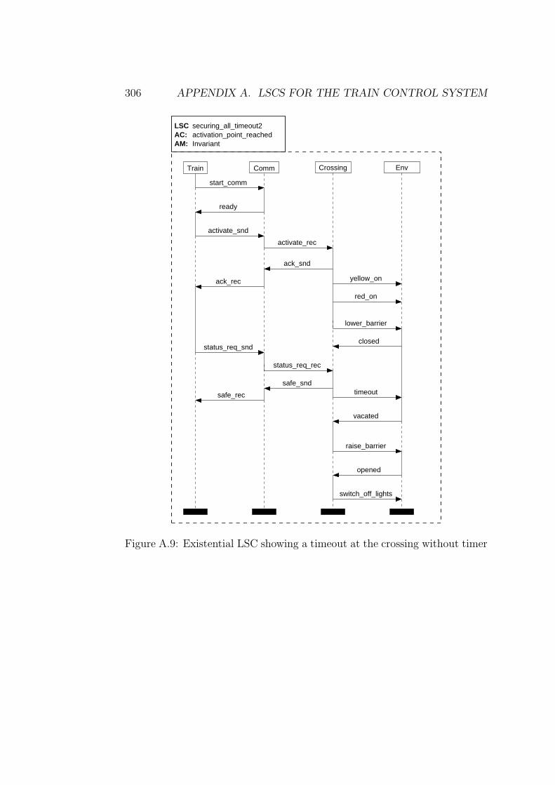
306 APPENDIX A. LSCS FOR THE TRAIN CONTROL SYSTEM
EnvCommTrain Crossing
start_comm
ready
activate_snd
activate_rec
ack_snd
closed
lower_barrier
yellow_on
red_on
ack_rec
timeout
raise_barrier
opened
switch_off_lights
vacated
safe_rec
safe_snd
status_req_snd
status_req_rec
Invariantactivation_point_reachedsecuring_all_timeout2
AM:AC:LSC
Figure A.9: Existential LSC showing a timeout at the crossing without timer
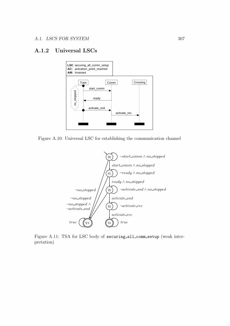
A.1. LSCS FOR SYSTEM 307
A.1.2 Universal LSCs
CrossingCommTrain
start_comm
ready
activate_snd
activate_rec
no_s
topp
edInvariantactivation_point_reachedsecuring_all_comm_setup
AM:AC:LSC
Figure A.10: Universal LSC for establishing the communication channel
q0 ¬start comm ∧ no stopped
q1 ¬ready ∧ no stopped
start comm ∧ no stopped
q2 ¬activate snd ∧ no stopped
ready ∧ no stopped
q3 ¬activate rec
activate snd
q4 true
activate rec
qXtrue
¬no stopped
¬no stopped
¬no stopped ∧¬activate snd
Figure A.11: TSA for LSC body of securing all comm setup (weak inter-pretation)
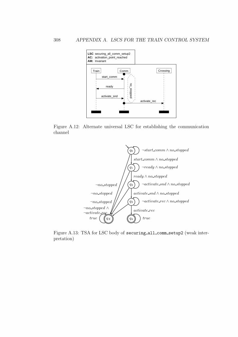
308 APPENDIX A. LSCS FOR THE TRAIN CONTROL SYSTEM
CrossingCommTrain
start_comm
ready
activate_snd
activate_rec
Invariantactivation_point_reachedsecuring_all_comm_setup2
AM:AC:LSC
no_stopped
Figure A.12: Alternate universal LSC for establishing the communicationchannel
q0 ¬start comm ∧ no stopped
q1 ¬ready ∧ no stopped
start comm ∧ no stopped
q2 ¬activate snd ∧ no stopped
ready ∧ no stopped
q3 ¬activate rec ∧ no stopped
activate snd ∧ no stopped
q4 true
activate rec
qXtrue
¬no stopped
¬no stopped
¬no stopped
¬no stopped ∧¬activate rec
Figure A.13: TSA for LSC body of securing all comm setup2 (weak inter-pretation)
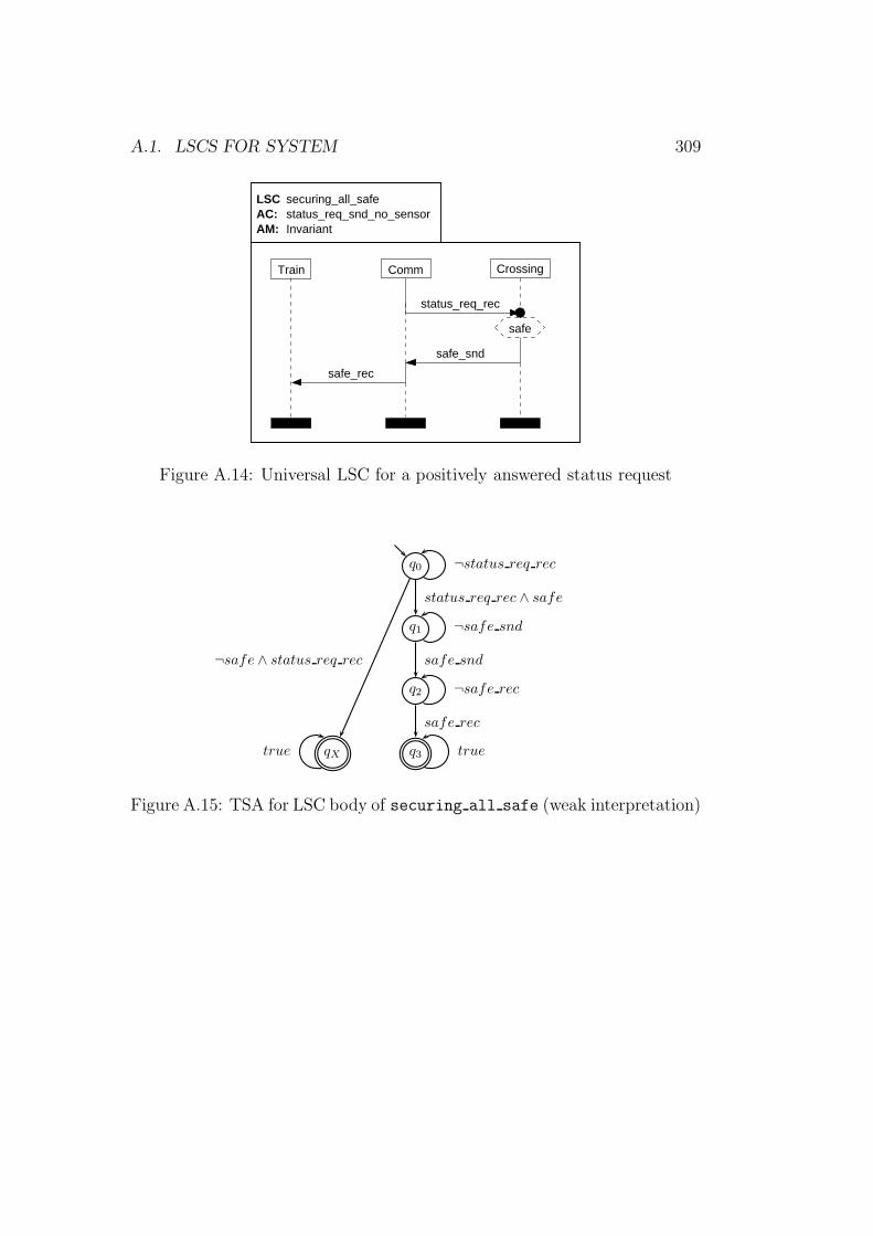
A.1. LSCS FOR SYSTEM 309
CommTrain Crossing
safe_rec
safe_snd
status_req_rec
safe
Invariantstatus_req_snd_no_sensorsecuring_all_safe
AM:AC:LSC
Figure A.14: Universal LSC for a positively answered status request
q0 ¬status req rec
q1 ¬safe snd
status req rec ∧ safe
q2 ¬safe rec
safe snd
q3 true
safe rec
qXtrue
¬safe ∧ status req rec
Figure A.15: TSA for LSC body of securing all safe (weak interpretation)
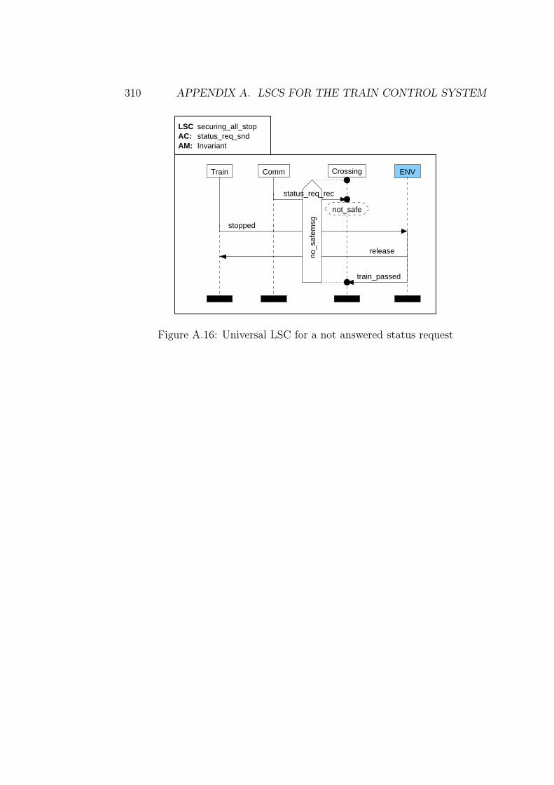
310 APPENDIX A. LSCS FOR THE TRAIN CONTROL SYSTEM
Comm Crossing
status_req_rec
ENVTrain
train_passed
stopped
release
not_safe
no_s
afem
sg
Invariantstatus_req_sndsecuring_all_stop
AM:AC:LSC
Figure A.16: Universal LSC for a not answered status request
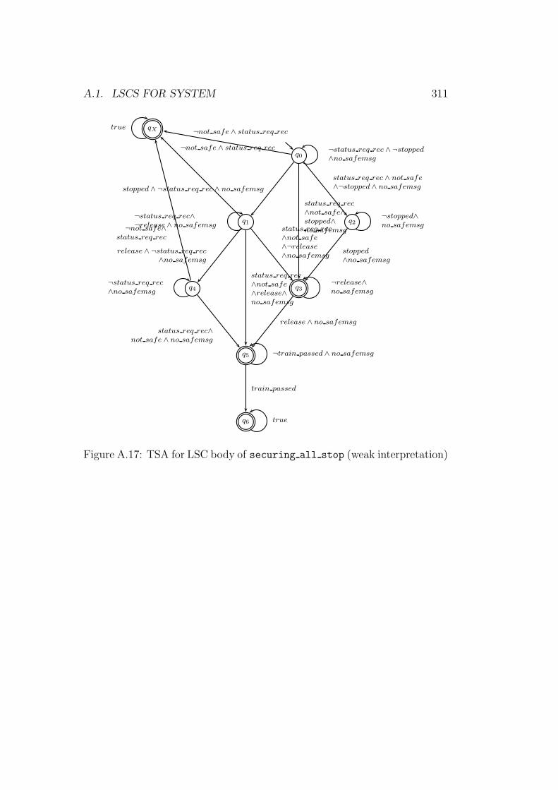
A.1. LSCS FOR SYSTEM 311
q0
¬status req rec ∧ ¬stopped
∧no safemsg
q1
¬status req rec∧¬release ∧ no safemsg
stopped ∧ ¬status req rec ∧ no safemsg
q2
¬stopped∧no safemsg
status req rec ∧ not safe
∧¬stopped ∧ no safemsg
q3
¬release∧no safemsg
status req rec
∧not safe
∧¬release
∧no safemsgstopped
∧no safemsg
status req rec
∧not safe∧stopped∧no safemsg
q4
¬status req rec
∧no safemsg
release ∧ ¬status req rec
∧no safemsg
q5 ¬train passed ∧ no safemsg
status req rec
∧not safe
∧release∧no safemsg
release ∧ no safemsg
status req rec∧not safe ∧ no safemsg
q6 true
train passed
qXtrue¬not safe ∧ status req rec
¬not safe ∧ status req rec
¬not safe∧status req rec
Figure A.17: TSA for LSC body of securing all stop (weak interpretation)
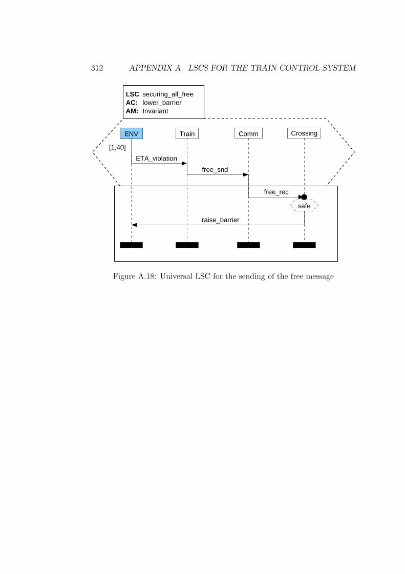
312 APPENDIX A. LSCS FOR THE TRAIN CONTROL SYSTEM
ETA_violation
ENV Train Comm
free_snd
Crossing
free_rec
raise_barrier
[1,40]
lower_barrierAC:LSC securing_all_free
InvariantAM:
safe
Figure A.18: Universal LSC for the sending of the free message
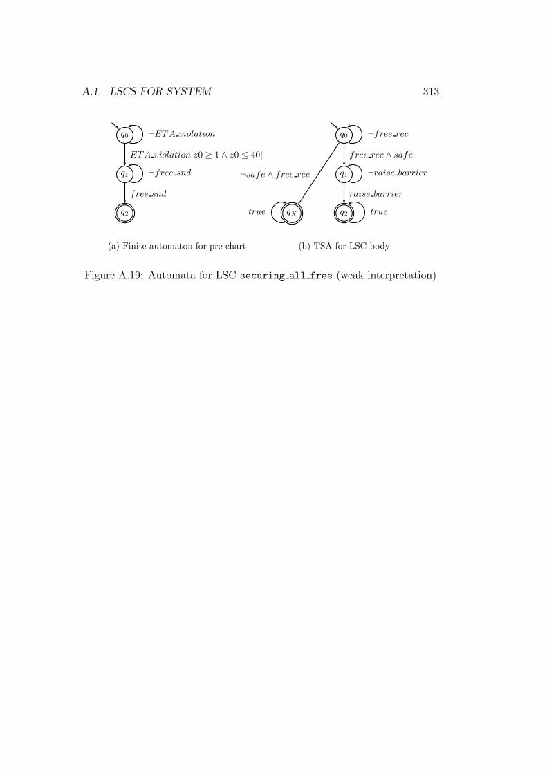
A.1. LSCS FOR SYSTEM 313
q0 ¬ETA violation
q1 ¬free snd
ETA violation[z0 ≥ 1 ∧ z0 ≤ 40]
q2
free snd
(a) Finite automaton for pre-chart
q0 ¬free rec
q1 ¬raise barrier
free rec ∧ safe
q2 true
raise barrier
qXtrue
¬safe ∧ free rec
(b) TSA for LSC body
Figure A.19: Automata for LSC securing all free (weak interpretation)
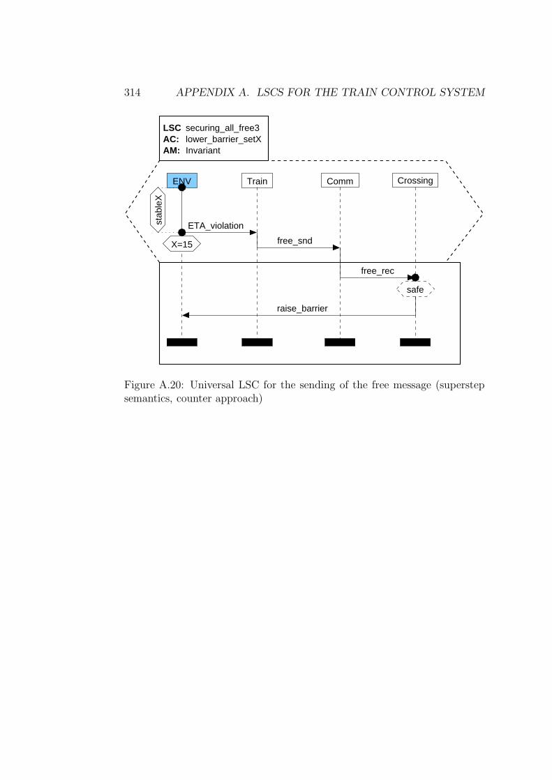
314 APPENDIX A. LSCS FOR THE TRAIN CONTROL SYSTEM
free_snd
free_rec
raise_barrier
ENV Train Comm Crossing
ETA_violation
lower_barrier_setXAC:LSC securing_all_free3
InvariantAM:st
able
X
X=15
safe
Figure A.20: Universal LSC for the sending of the free message (superstepsemantics, counter approach)
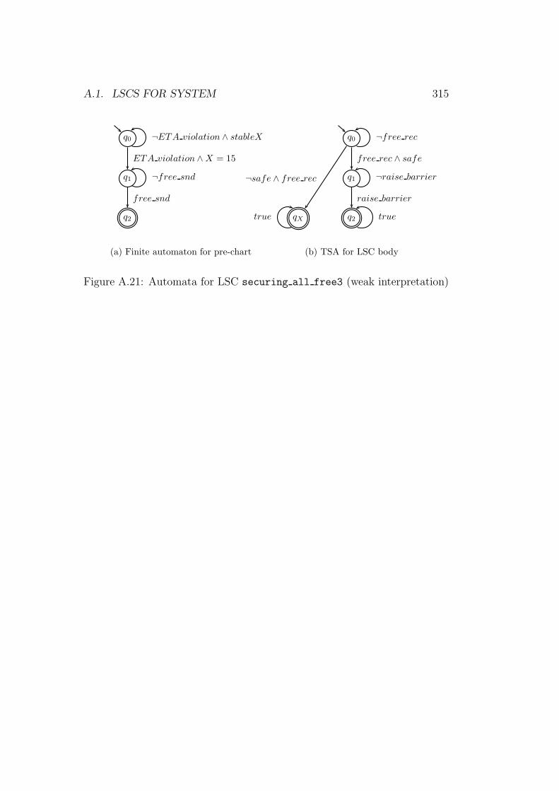
A.1. LSCS FOR SYSTEM 315
q0 ¬ETA violation ∧ stableX
q1 ¬free snd
ETA violation ∧X = 15
q2
free snd
(a) Finite automaton for pre-chart
q0 ¬free rec
q1 ¬raise barrier
free rec ∧ safe
q2 true
raise barrier
qXtrue
¬safe ∧ free rec
(b) TSA for LSC body
Figure A.21: Automata for LSC securing all free3 (weak interpretation)
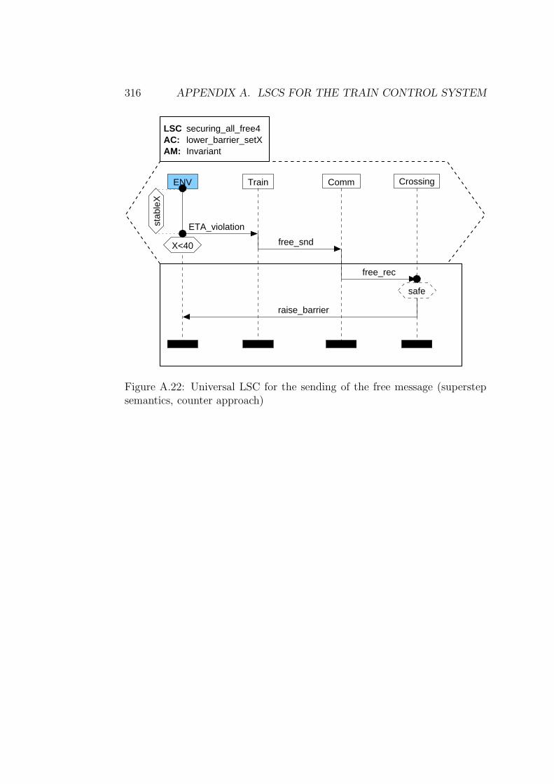
316 APPENDIX A. LSCS FOR THE TRAIN CONTROL SYSTEM
free_snd
free_rec
raise_barrier
ENV Train Comm Crossing
ETA_violationstab
leX
X<40
lower_barrier_setXAC:LSC securing_all_free4
InvariantAM:
safe
Figure A.22: Universal LSC for the sending of the free message (superstepsemantics, counter approach)

A.1. LSCS FOR SYSTEM 317
q0 ¬ETA violation ∧ stableX
q1 ¬free snd
ETA violation ∧X < 40
q2
free snd
(a) Finite automaton for pre-chart
q0 ¬free rec
q1 ¬raise barrier
free rec ∧ safe
q2 true
raise barrier
qXtrue
¬safe ∧ free rec
(b) TSA for LSC body
Figure A.23: Automata for LSC securing all free4 (weak interpretation)
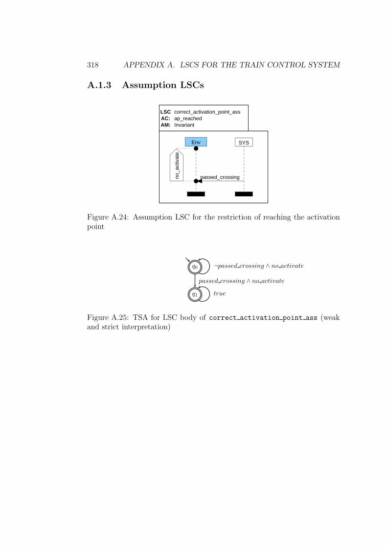
318 APPENDIX A. LSCS FOR THE TRAIN CONTROL SYSTEM
A.1.3 Assumption LSCs
ap_reachedLSCAC:
correct_activation_point_ass
InvariantAM:
Env SYS
passed_crossingno_a
ctiv
ate
Figure A.24: Assumption LSC for the restriction of reaching the activationpoint
q0 ¬passed crossing ∧ no activate
q1 true
passed crossing ∧ no activate
Figure A.25: TSA for LSC body of correct activation point ass (weakand strict interpretation)
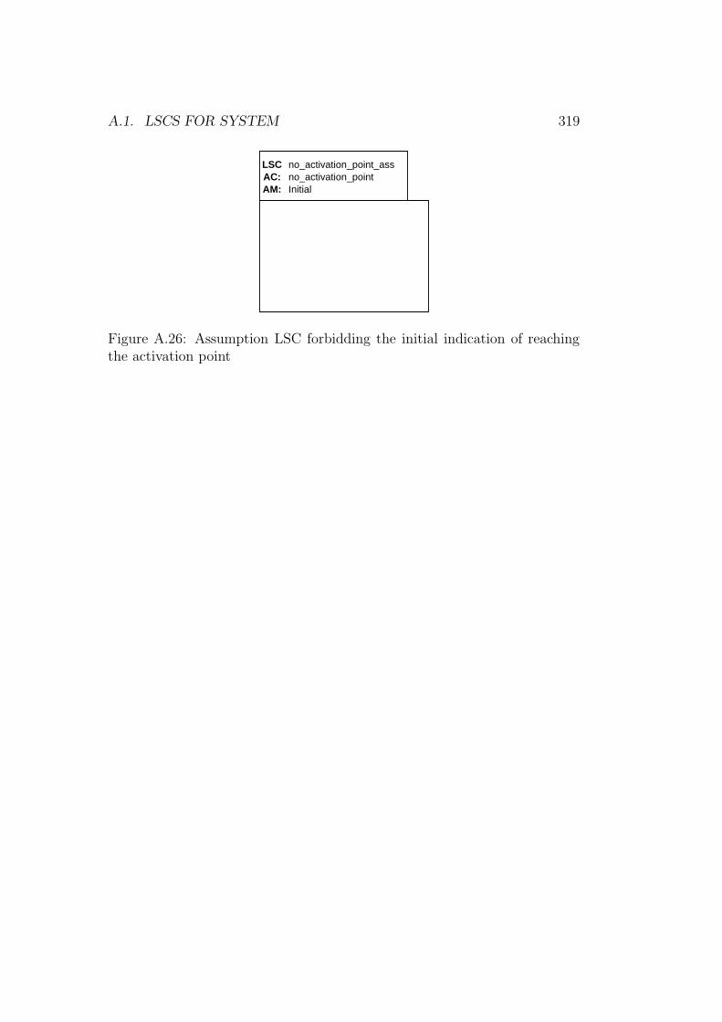
A.1. LSCS FOR SYSTEM 319
no_activation_pointLSCAC:
no_activation_point_ass
InitialAM:
Figure A.26: Assumption LSC forbidding the initial indication of reachingthe activation point
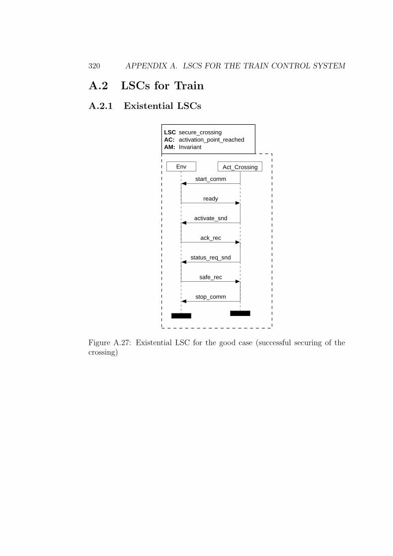
320 APPENDIX A. LSCS FOR THE TRAIN CONTROL SYSTEM
A.2 LSCs for Train
A.2.1 Existential LSCs
Env Act_Crossing
safe_rec
status_req_snd
ack_rec
activate_snd
ready
start_comm
stop_comm
Invariantactivation_point_reachedsecure_crossing
AM:AC:LSC
Figure A.27: Existential LSC for the good case (successful securing of thecrossing)
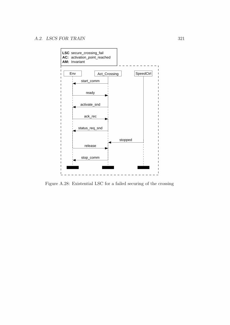
A.2. LSCS FOR TRAIN 321
Env Act_Crossing
status_req_snd
ack_rec
activate_snd
ready
start_comm
SpeedCtrl
stopped
stop_comm
release
Invariantactivation_point_reachedsecure_crossing_fail
AM:AC:LSC
Figure A.28: Existential LSC for a failed securing of the crossing
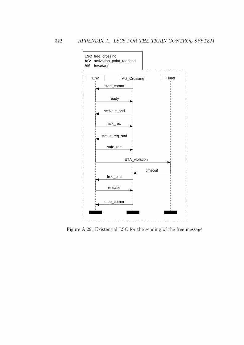
322 APPENDIX A. LSCS FOR THE TRAIN CONTROL SYSTEM
Env
timeout
free_snd
release
stop_comm
ETA_violation
Act_Crossing
status_req_snd
ack_rec
activate_snd
ready
start_comm
Timer
safe_rec
Invariantactivation_point_reachedfree_crossing
AM:AC:LSC
Figure A.29: Existential LSC for the sending of the free message
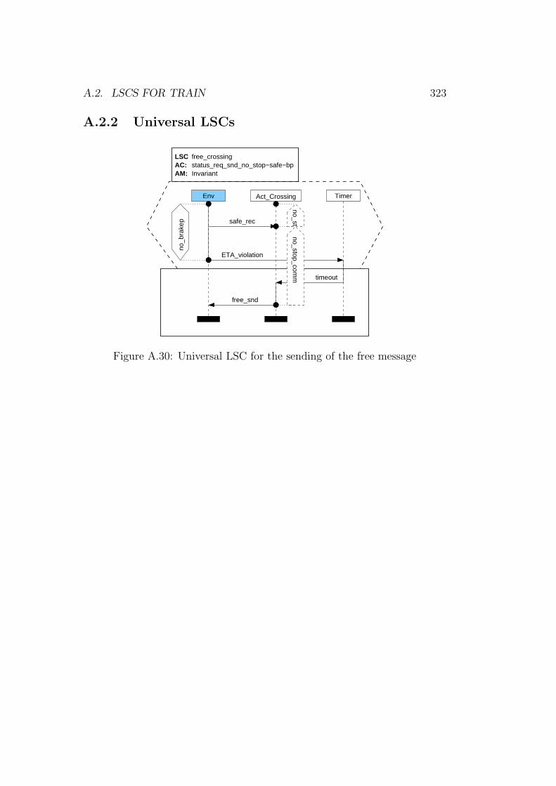
A.2. LSCS FOR TRAIN 323
A.2.2 Universal LSCs
timeout
free_snd
status_req_snd_no_stop−safe−bp
Act_Crossing TimerEnv
safe_rec
ETA_violation
Invariant
free_crossing
AM:AC:LSC
no_stop_comm
no_st
no_b
rake
p
Figure A.30: Universal LSC for the sending of the free message
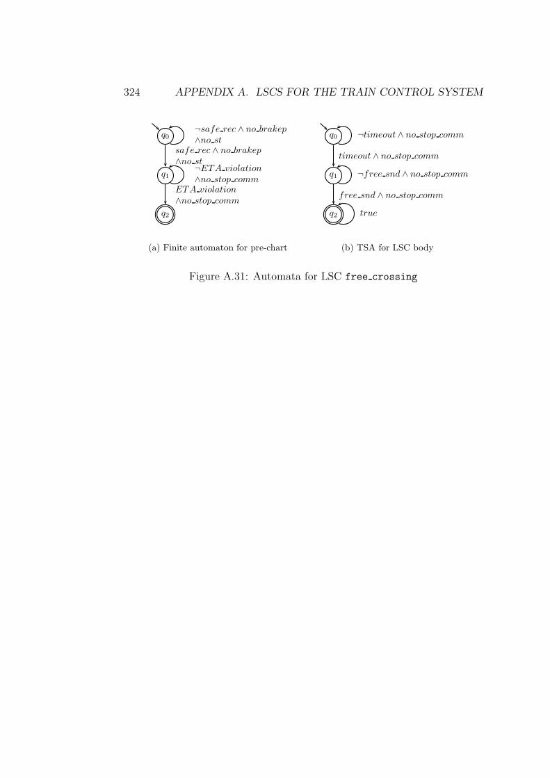
324 APPENDIX A. LSCS FOR THE TRAIN CONTROL SYSTEM
q0¬safe rec ∧ no brakep∧no st
q1¬ETA violation
∧no stop comm
safe rec ∧ no brakep∧no st
q2
ETA violation
∧no stop comm
(a) Finite automaton for pre-chart
q0 ¬timeout ∧ no stop comm
q1 ¬free snd ∧ no stop comm
timeout ∧ no stop comm
q2 true
free snd ∧ no stop comm
(b) TSA for LSC body
Figure A.31: Automata for LSC free crossing

A.3. LSCS FOR CROSSING 325
A.3 LSCs for Crossing
A.3.1 Existential LSCs
AM: InvariantAC: Activate_CrossingLSC securing
Env Lights
ack
BarrierCrossing
turn_on
switch2yellow
switch2red
lights_on
status_req
crossing_safe
barrier_closed
lower
closed
barrier_open
raise
opening
turn_off
switch_off
open_barrier
Sensor
train_passed
close_barrier
Figure A.32: Existential LSC for the good case (successful securing of thecrossing)
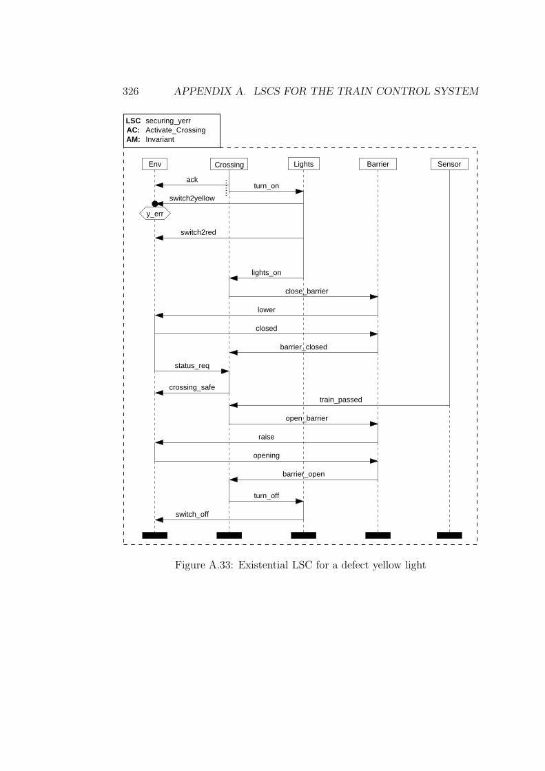
326 APPENDIX A. LSCS FOR THE TRAIN CONTROL SYSTEM
AM: InvariantAC: Activate_CrossingLSC securing_yerr
Env Lights
ack
BarrierCrossing
turn_on
switch2yellow
Sensor
lights_on
status_req
crossing_safe
barrier_closed
lower
closed
barrier_open
raise
opening
turn_off
switch_off
open_barrier
train_passed
close_barrier
switch2red
y_err
Figure A.33: Existential LSC for a defect yellow light
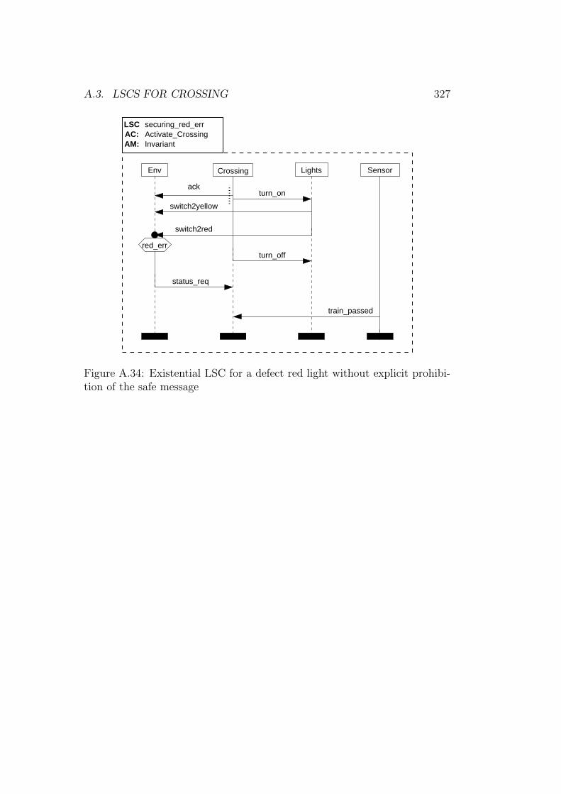
A.3. LSCS FOR CROSSING 327
AM: InvariantAC: Activate_CrossingLSC securing_red_err
Env Lights
ack
Crossing
turn_on
switch2yellow
switch2red
train_passed
status_req
turn_off
Sensor
red_err
Figure A.34: Existential LSC for a defect red light without explicit prohibi-tion of the safe message
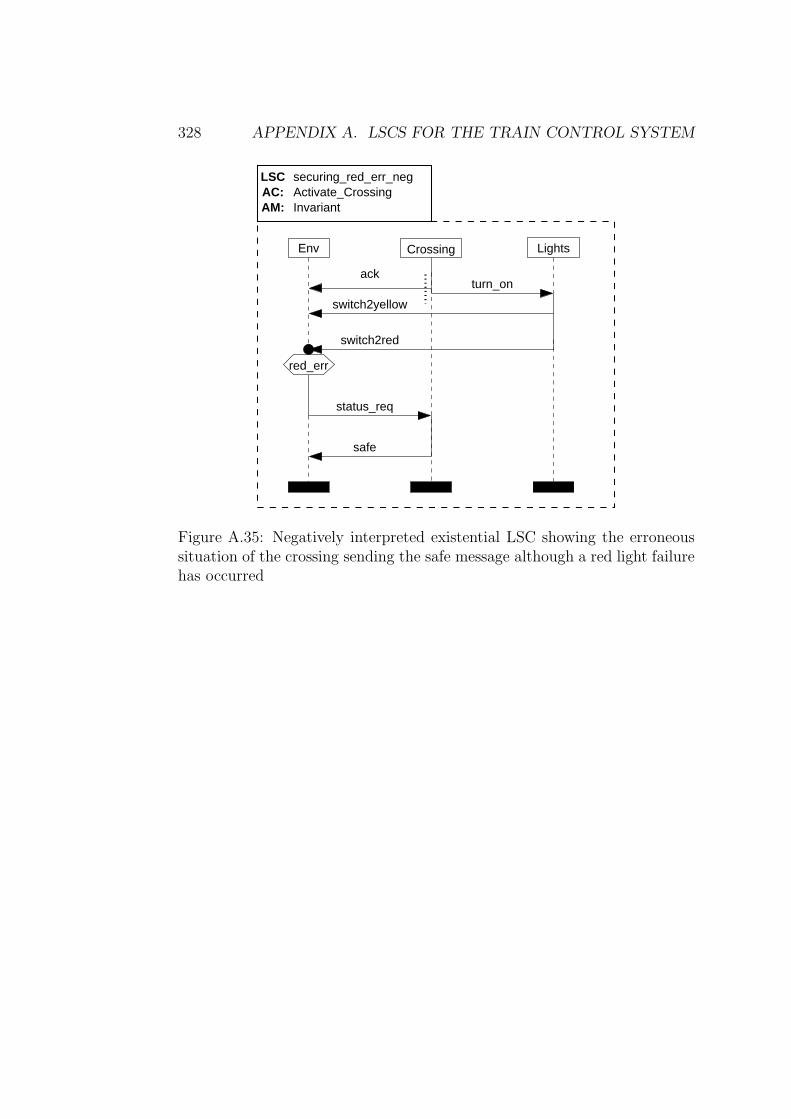
328 APPENDIX A. LSCS FOR THE TRAIN CONTROL SYSTEM
AM: InvariantAC: Activate_CrossingLSC securing_red_err_neg
Env Lights
ack
Crossing
turn_on
switch2yellow
switch2red
status_req
safe
red_err
Figure A.35: Negatively interpreted existential LSC showing the erroneoussituation of the crossing sending the safe message although a red light failurehas occurred
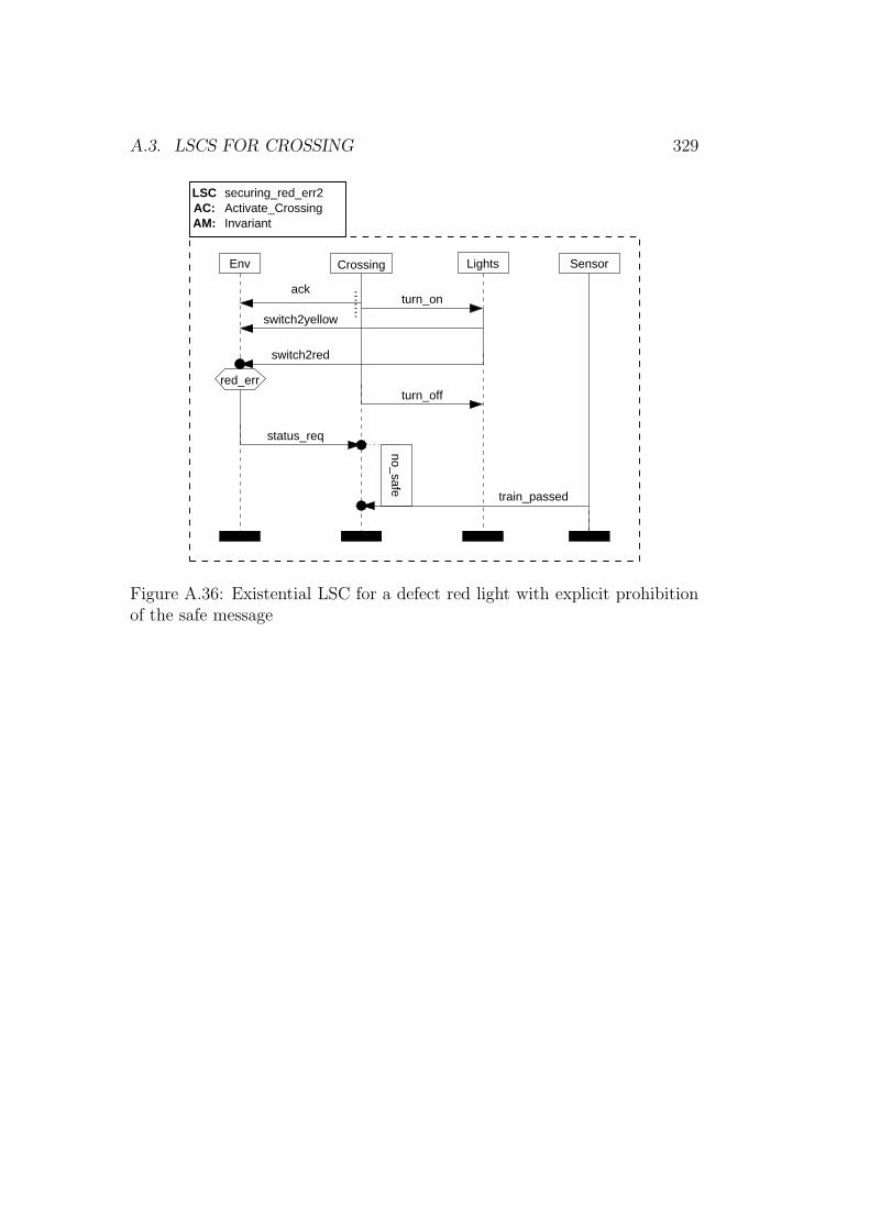
A.3. LSCS FOR CROSSING 329
AM: InvariantAC: Activate_CrossingLSC securing_red_err2
Env Lights
ack
Crossing
turn_on
switch2yellow
switch2red
status_req
turn_off
Sensor
train_passed
red_err
no_safe
Figure A.36: Existential LSC for a defect red light with explicit prohibitionof the safe message
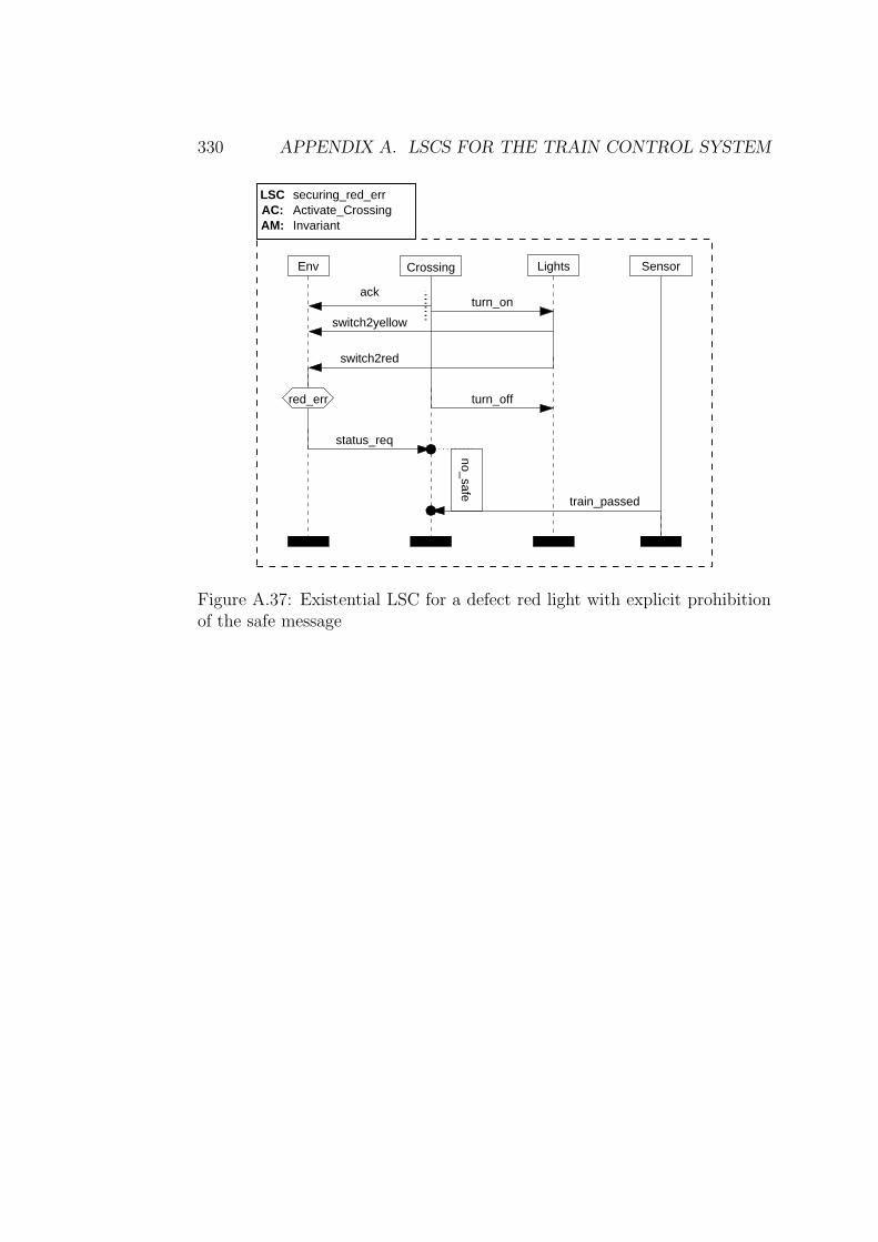
330 APPENDIX A. LSCS FOR THE TRAIN CONTROL SYSTEM
AM: InvariantAC: Activate_CrossingLSC securing_red_err
Env Lights
ack
Crossing
turn_on
switch2yellow
switch2red
status_req
turn_off
Sensor
train_passed
red_errno_safe
Figure A.37: Existential LSC for a defect red light with explicit prohibitionof the safe message
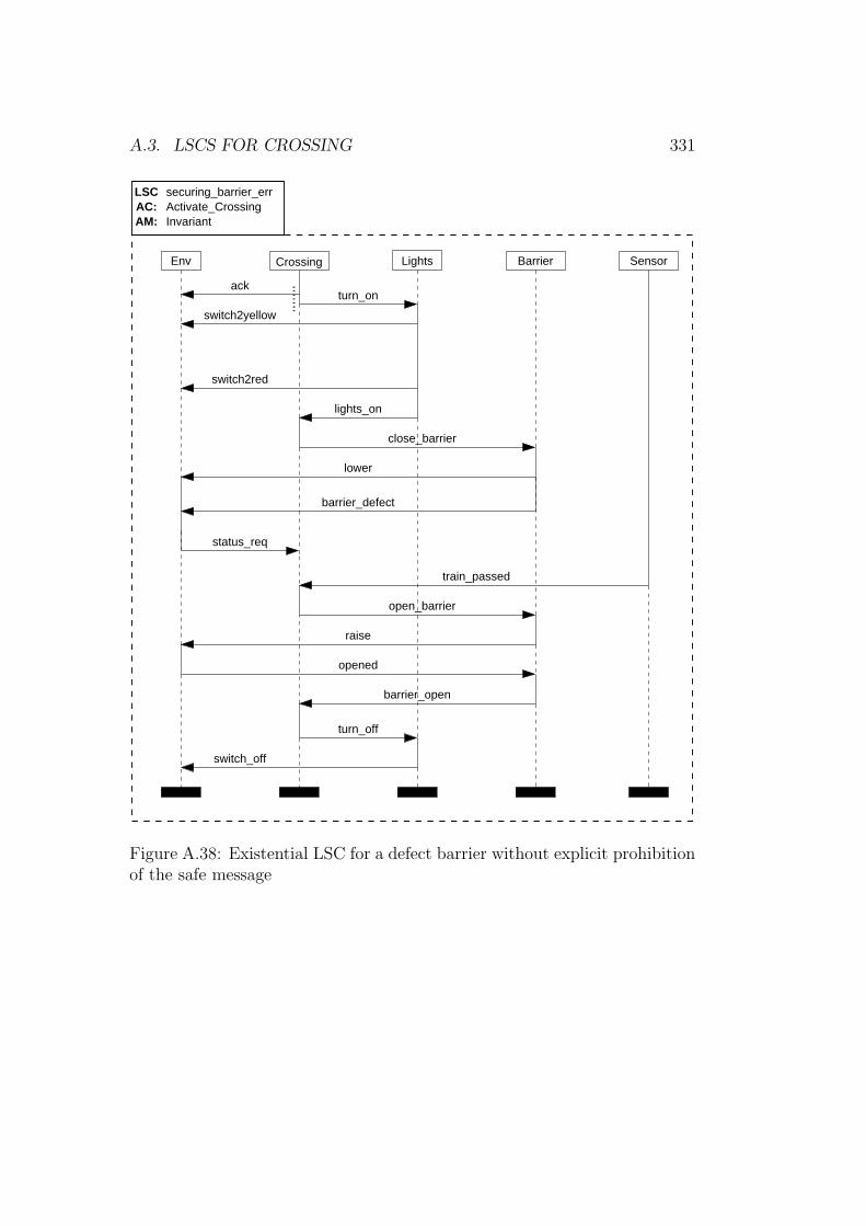
A.3. LSCS FOR CROSSING 331
status_req
AM: InvariantAC: Activate_CrossingLSC securing_barrier_err
Env Lights
ack
BarrierCrossing
turn_on
switch2yellow
barrier_open
raise
opened
turn_off
switch_off
open_barrier
Sensor
train_passed
switch2red
lights_on
lower
close_barrier
barrier_defect
Figure A.38: Existential LSC for a defect barrier without explicit prohibitionof the safe message
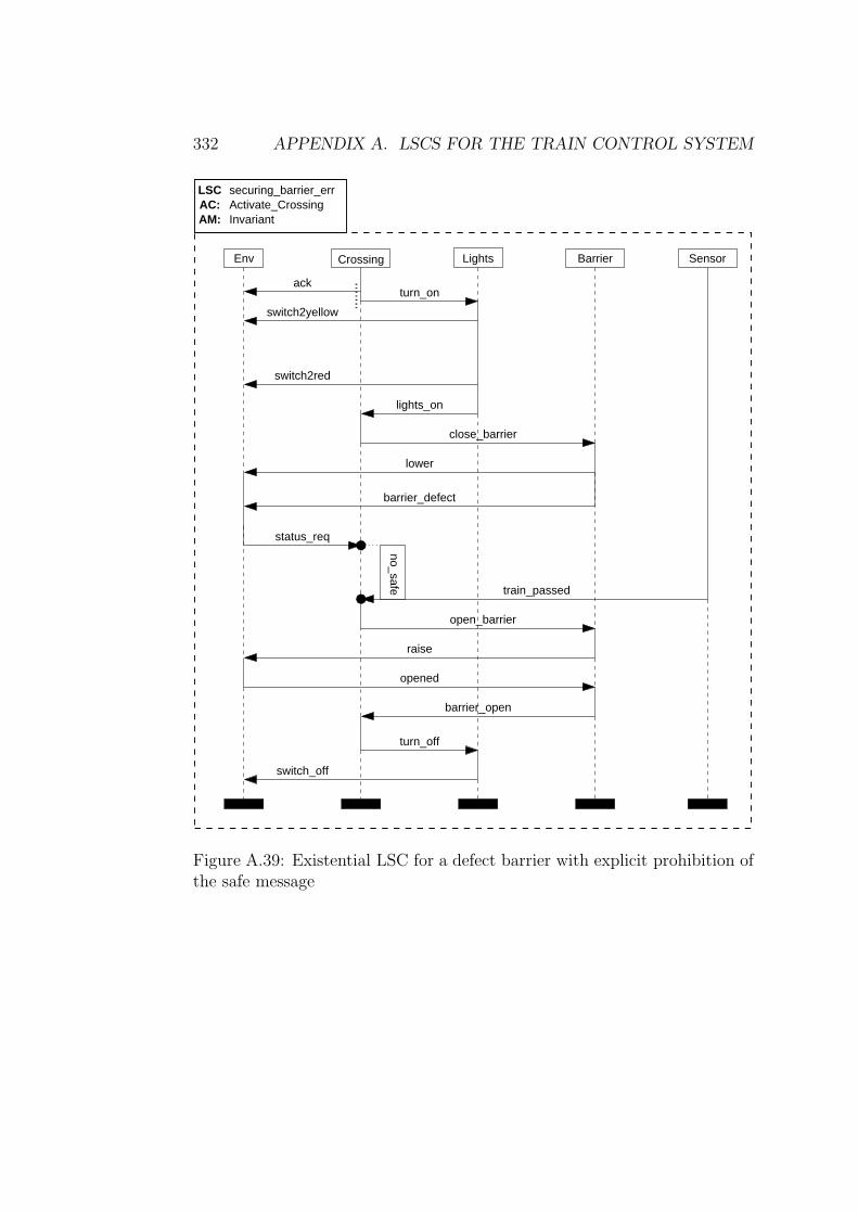
332 APPENDIX A. LSCS FOR THE TRAIN CONTROL SYSTEM
status_req
barrier_open
raise
opened
turn_off
switch_off
open_barrier
train_passed
AM: InvariantAC: Activate_CrossingLSC securing_barrier_err
Env Lights
ack
BarrierCrossing
turn_on
switch2yellow
Sensor
switch2red
lights_on
lower
close_barrier
barrier_defect
no_safe
Figure A.39: Existential LSC for a defect barrier with explicit prohibition ofthe safe message
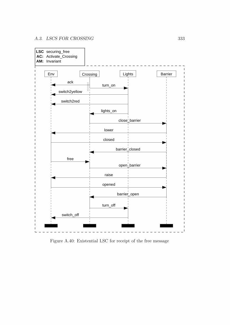
A.3. LSCS FOR CROSSING 333
AM: InvariantAC: Activate_CrossingLSC securing_free
Env Lights
ack
BarrierCrossing
turn_on
switch2yellow
switch2red
lights_on
lower
closed
barrier_closed
free
open_barrier
barrier_open
opened
turn_off
switch_off
raise
close_barrier
Figure A.40: Existential LSC for receipt of the free message
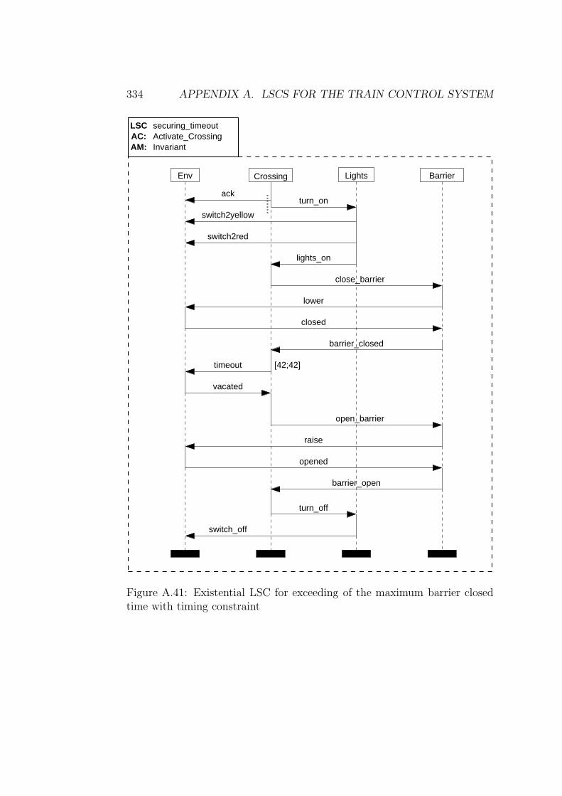
334 APPENDIX A. LSCS FOR THE TRAIN CONTROL SYSTEM
AM: InvariantAC: Activate_CrossingLSC securing_timeout
Env Lights
ack
BarrierCrossing
turn_on
switch2yellow
switch2red
lights_on
lower
closed
barrier_closed
timeout
barrier_open
raise
opened
turn_off
switch_off
open_barrier
vacated
close_barrier
[42;42]
Figure A.41: Existential LSC for exceeding of the maximum barrier closedtime with timing constraint
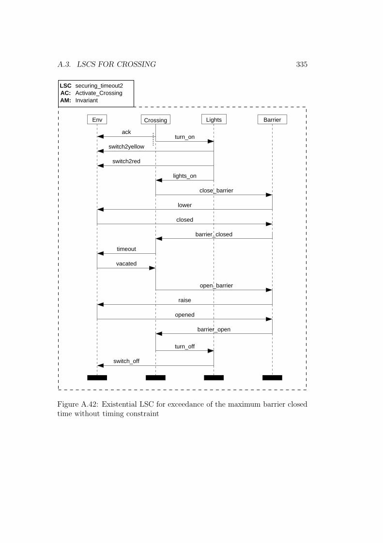
A.3. LSCS FOR CROSSING 335
AM: InvariantAC: Activate_CrossingLSC securing_timeout2
Env Lights
ack
BarrierCrossing
turn_on
switch2yellow
switch2red
lights_on
lower
closed
barrier_closed
timeout
barrier_open
raise
opened
turn_off
switch_off
open_barrier
vacated
close_barrier
Figure A.42: Existential LSC for exceedance of the maximum barrier closedtime without timing constraint
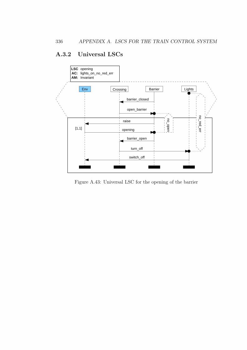
336 APPENDIX A. LSCS FOR THE TRAIN CONTROL SYSTEM
A.3.2 Universal LSCs
Barrier Lights
AM: InvariantAC:LSC
Env Crossing
openinglights_on_no_red_err
open_barrier
turn_off
raise
barrier_open
barrier_closed
opening
switch_off
no_red_err
no_open[1,1]
Figure A.43: Universal LSC for the opening of the barrier
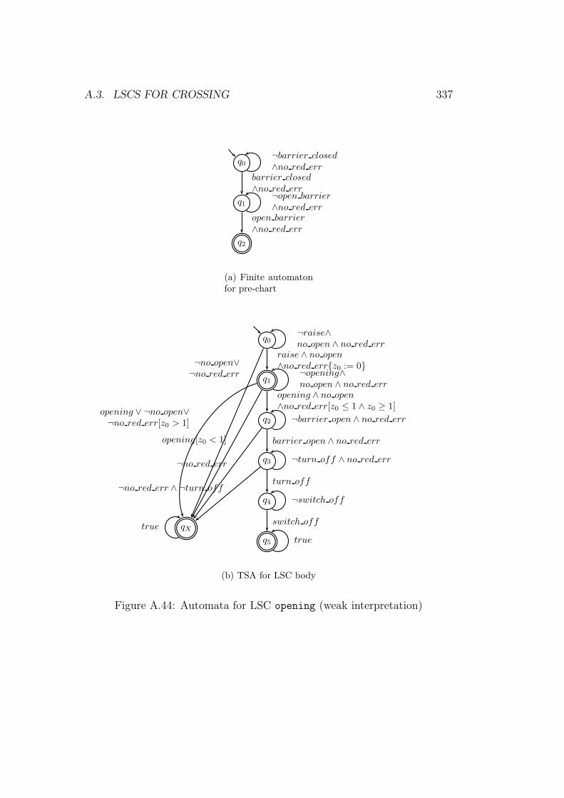
A.3. LSCS FOR CROSSING 337
q0¬barrier closed∧no red err
q1¬open barrier∧no red err
barrier closed
∧no red err
q2
open barrier
∧no red err
(a) Finite automatonfor pre-chart
q0¬raise∧no open ∧ no red err
q1¬opening∧no open ∧ no red err
raise ∧ no open∧no red err{z0 := 0}
q2 ¬barrier open ∧ no red err
opening ∧ no open∧no red err[z0 ≤ 1 ∧ z0 ≥ 1]
q3 ¬turn off ∧ no red err
barrier open ∧ no red err
q4 ¬switch off
turn off
q5 true
switch offqXtrue
¬no open∨¬no red err
opening ∨ ¬no open∨¬no red err[z0 > 1]
opening[z0 < 1]
¬no red err
¬no red err ∧ ¬turn off
(b) TSA for LSC body
Figure A.44: Automata for LSC opening (weak interpretation)
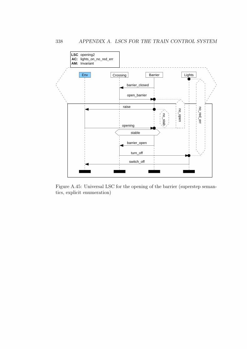
338 APPENDIX A. LSCS FOR THE TRAIN CONTROL SYSTEM
Barrier Lights
turn_off
switch_off
AM: InvariantAC:LSC
Env Crossing
opening2lights_on_no_red_err
open_barrier
raise
barrier_closed
opening
barrier_open
no_stab
no_open
no_red_err
stable
Figure A.45: Universal LSC for the opening of the barrier (superstep seman-tics, explicit enumeration)
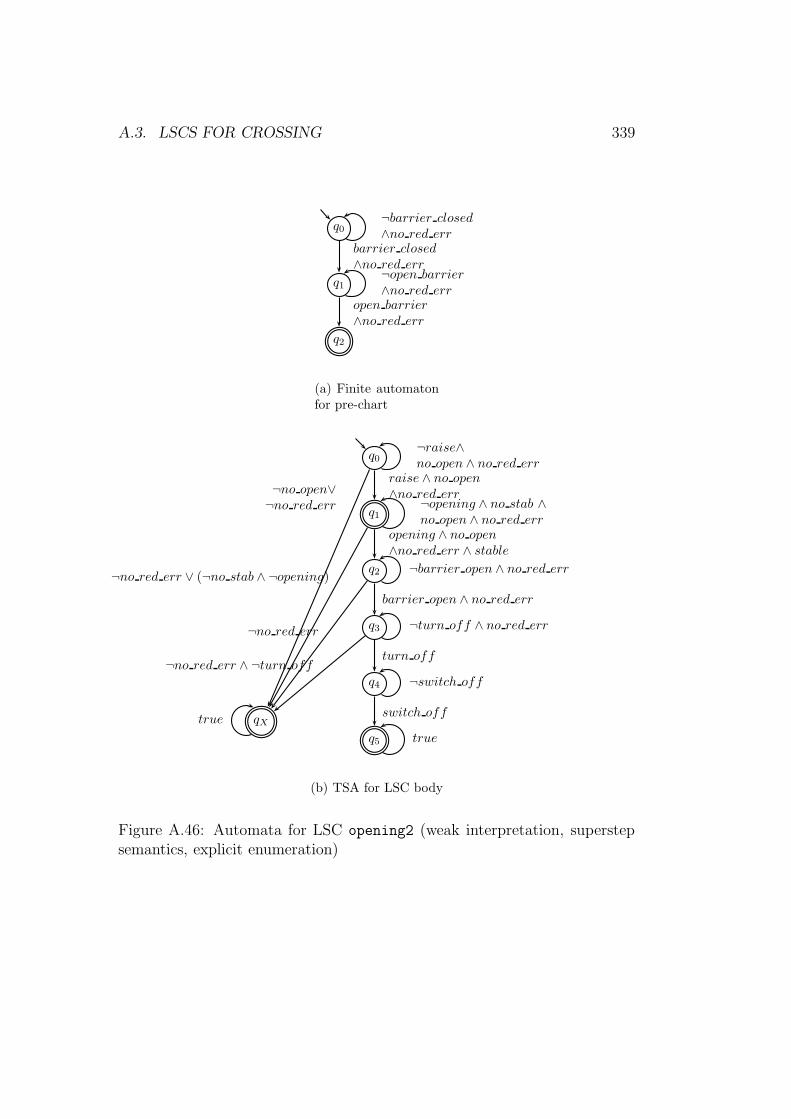
A.3. LSCS FOR CROSSING 339
q0¬barrier closed∧no red err
q1¬open barrier∧no red err
barrier closed
∧no red err
q2
open barrier
∧no red err
(a) Finite automatonfor pre-chart
q0¬raise∧no open ∧ no red err
q1¬opening ∧ no stab ∧no open ∧ no red err
raise ∧ no open∧no red err
q2 ¬barrier open ∧ no red err
opening ∧ no open∧no red err ∧ stable
q3 ¬turn off ∧ no red err
barrier open ∧ no red err
q4 ¬switch off
turn off
q5 true
switch offqXtrue
¬no open∨¬no red err
¬no red err ∨ (¬no stab ∧ ¬opening)
¬no red err
¬no red err ∧ ¬turn off
(b) TSA for LSC body
Figure A.46: Automata for LSC opening2 (weak interpretation, superstepsemantics, explicit enumeration)
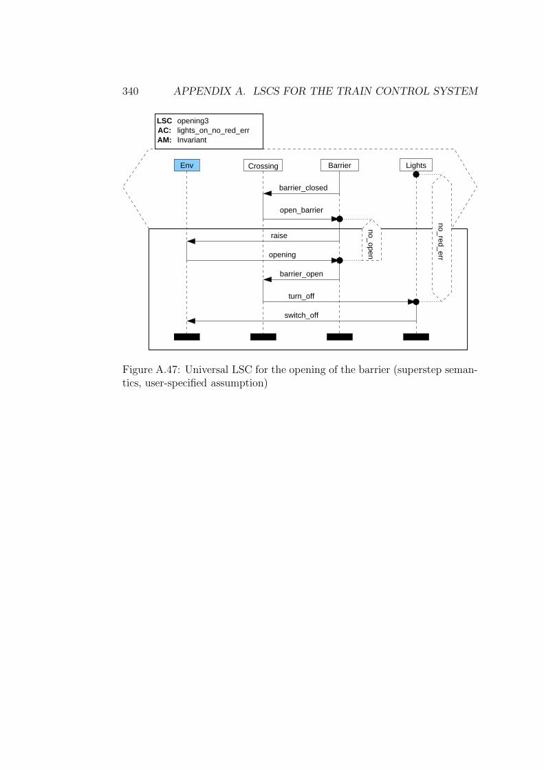
340 APPENDIX A. LSCS FOR THE TRAIN CONTROL SYSTEM
Barrier Lights
AM: InvariantAC:LSC
Env Crossing
opening3lights_on_no_red_err
open_barrier
turn_off
raise
barrier_open
barrier_closed
opening
switch_off
no_red_err
no_open
Figure A.47: Universal LSC for the opening of the barrier (superstep seman-tics, user-specified assumption)
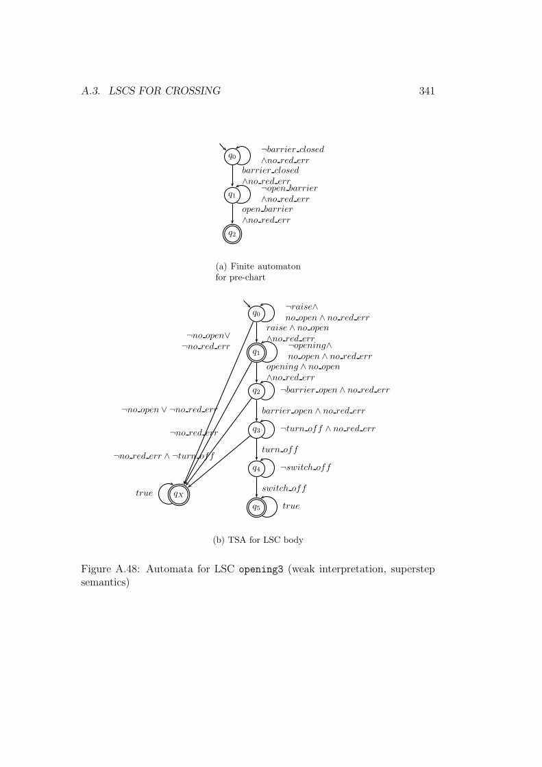
A.3. LSCS FOR CROSSING 341
q0¬barrier closed∧no red err
q1¬open barrier∧no red err
barrier closed
∧no red err
q2
open barrier
∧no red err
(a) Finite automatonfor pre-chart
q0¬raise∧no open ∧ no red err
q1¬opening∧no open ∧ no red err
raise ∧ no open∧no red err
q2 ¬barrier open ∧ no red err
opening ∧ no open∧no red err
q3 ¬turn off ∧ no red err
barrier open ∧ no red err
q4 ¬switch off
turn off
q5 true
switch offqXtrue
¬no open∨¬no red err
¬no open ∨ ¬no red err
¬no red err
¬no red err ∧ ¬turn off
(b) TSA for LSC body
Figure A.48: Automata for LSC opening3 (weak interpretation, superstepsemantics)
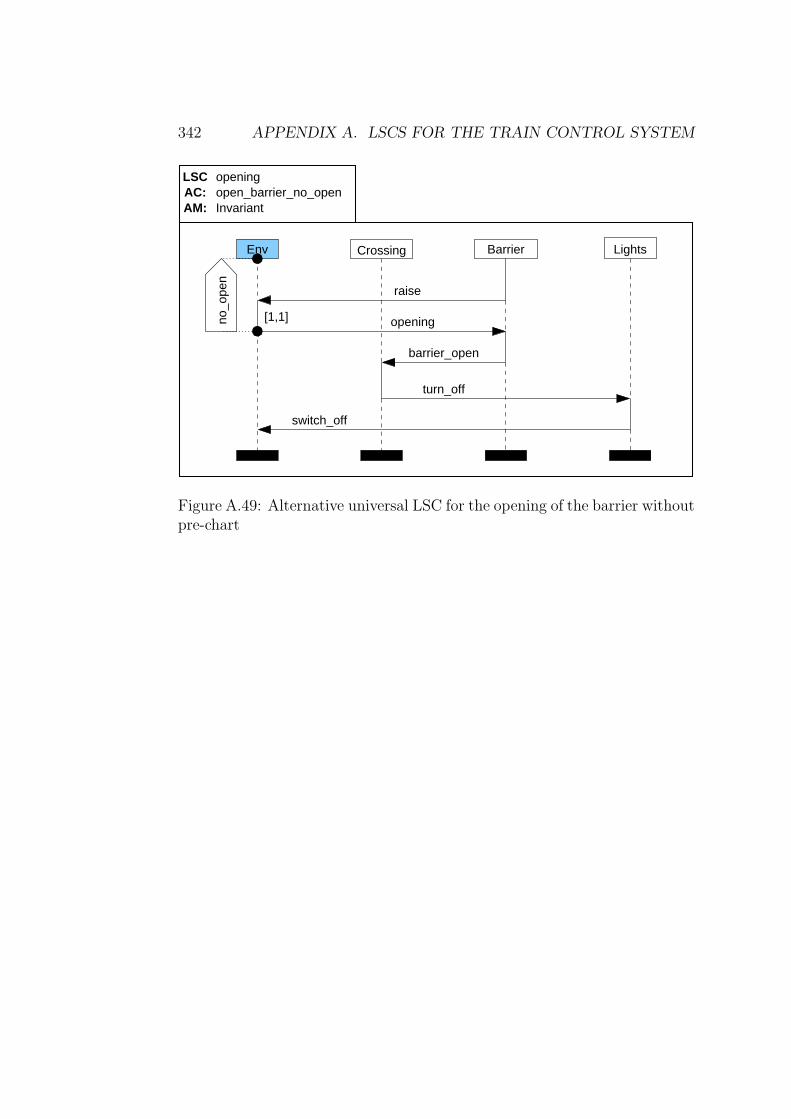
342 APPENDIX A. LSCS FOR THE TRAIN CONTROL SYSTEM
Barrier Lights
AM: InvariantAC:LSC opening
open_barrier_no_open
Env Crossing
turn_off
switch_off
raise
barrier_open
opening[1,1]no_o
pen
Figure A.49: Alternative universal LSC for the opening of the barrier withoutpre-chart
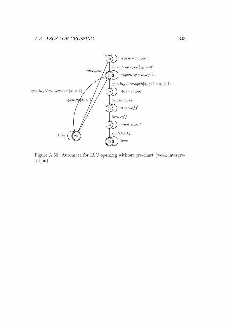
A.3. LSCS FOR CROSSING 343
q0 ¬raise ∧ no open
q1 ¬opening ∧ no open
raise ∧ no open{z0 := 0}
q2 ¬barrier ope
opening ∧ no open[z0 ≤ 1 ∧ z0 ≥ 1]
q3 ¬turn off
barrier open
q4 ¬switch off
turn off
q5 true
switch offqXtrue
¬no open
opening ∨ ¬no open ∨ [z0 > 1]
opening[z0 < 1]
Figure A.50: Automata for LSC opening without pre-chart (weak interpre-tation)
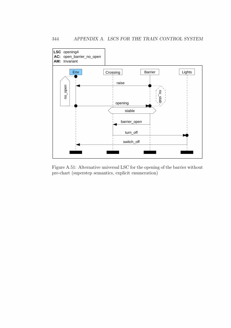
344 APPENDIX A. LSCS FOR THE TRAIN CONTROL SYSTEM
Barrier Lights
raise
opening
barrier_open
turn_off
switch_off
Env Crossing
AM: InvariantAC:LSC opening4
open_barrier_no_open
no_stab
stable
no_o
pen
Figure A.51: Alternative universal LSC for the opening of the barrier withoutpre-chart (superstep semantics, explicit enumeration)
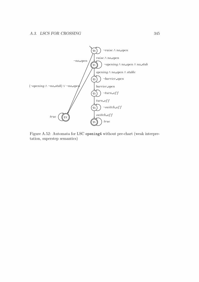
A.3. LSCS FOR CROSSING 345
q0 ¬raise ∧ no open
q1 ¬opening ∧ no open ∧ no stab
raise ∧ no open
q2 ¬barrier open
opening ∧ no open ∧ stable
q3 ¬turn off
barrier open
q4 ¬switch off
turn off
q5 true
switch offqXtrue
¬no open
(¬opening ∧ ¬no stab) ∨ ¬no open
Figure A.52: Automata for LSC opening4 without pre-chart (weak interpre-tation, superstep semantics)
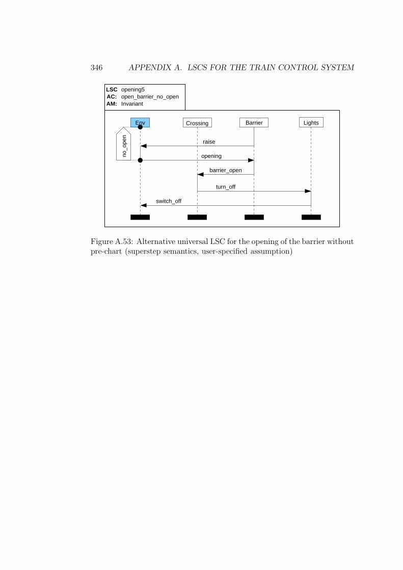
346 APPENDIX A. LSCS FOR THE TRAIN CONTROL SYSTEM
Barrier LightsEnv Crossing
turn_off
switch_off
raise
barrier_open
opening
AM: InvariantAC:LSC opening5
open_barrier_no_open
no_o
pen
Figure A.53: Alternative universal LSC for the opening of the barrier withoutpre-chart (superstep semantics, user-specified assumption)
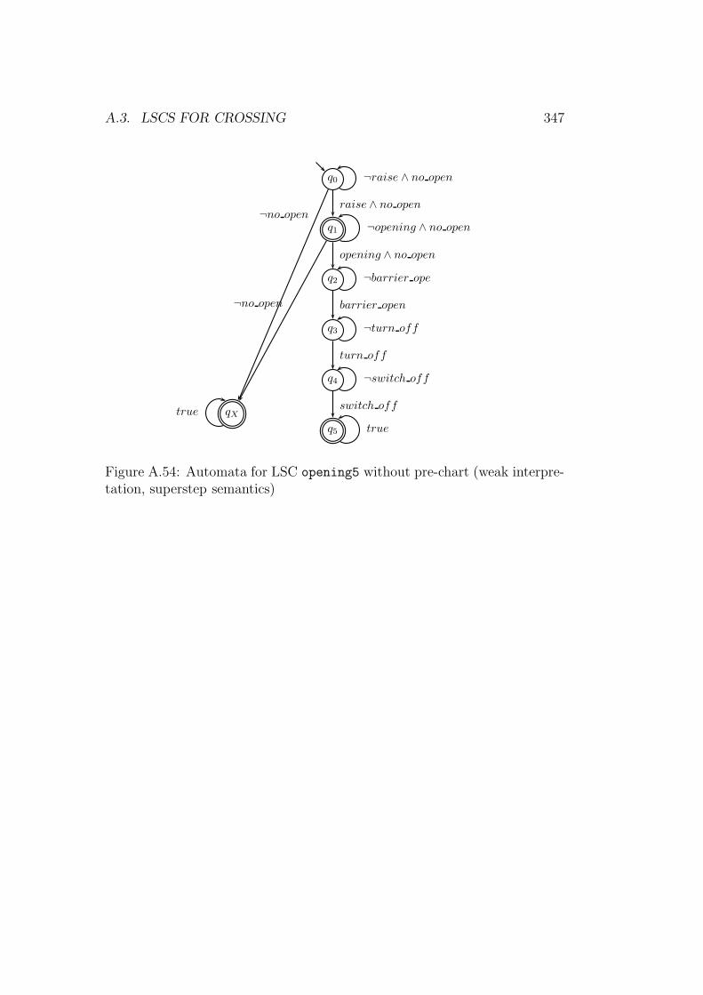
A.3. LSCS FOR CROSSING 347
q0 ¬raise ∧ no open
q1 ¬opening ∧ no open
raise ∧ no open
q2 ¬barrier ope
opening ∧ no open
q3 ¬turn off
barrier open
q4 ¬switch off
turn off
q5 true
switch offqXtrue
¬no open
¬no open
Figure A.54: Automata for LSC opening5 without pre-chart (weak interpre-tation, superstep semantics)
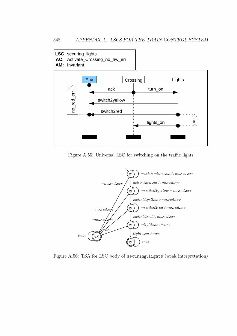
348 APPENDIX A. LSCS FOR THE TRAIN CONTROL SYSTEM
AM: InvariantAC: Activate_Crossing_no_hw_errLSC
Env Lights
ack
Crossing
switch2yellow
switch2red
lights_on
turn_on
securing_lights
no_r
ed_e
rr
nre
Figure A.55: Universal LSC for switching on the traffic lights
q0 ¬ack ∧ ¬turn on ∧ no red err
q1 ¬switch2yellow ∧ no red err
ack ∧ turn on ∧ no red err
q2 ¬switch2red ∧ no red err
switch2yellow ∧ no red err
q3 ¬lights on ∧ nre
switch2red ∧ no red err
q4 true
lights on ∧ nreqXtrue
¬no red err
¬no red err
¬no red err
¬nre
Figure A.56: TSA for LSC body of securing lights (weak interpretation)

A.3. LSCS FOR CROSSING 349
barrier_closed
closed
AM: InitialAC:LSC securing_barrier_init
Env Crossing
empty
close_barrier
lower
Barrier
no_closed
safe
[1,1]
[1,1]
Figure A.57: Initial universal LSC for the closing of the barrier
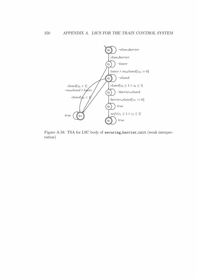
350 APPENDIX A. LSCS FOR THE TRAIN CONTROL SYSTEM
q0 ¬close barrier
q1 ¬lower
close barrier
q2 ¬closed
lower ∧ no closed{z0 := 0}
q3 ¬barrier closed
closed[z0 ≥ 1 ∧ z0 ≤ 1]
q4 true
barrier closed{z1 := 0}
q5 true
safe[z1 ≥ 1 ∧ z1 ≤ 1]qXtrue
¬no closed ∧ lower
closed[z0 < 1]
closed[z0 > 1]
Figure A.58: TSA for LSC body of securing barrier init (weak interpre-tation)
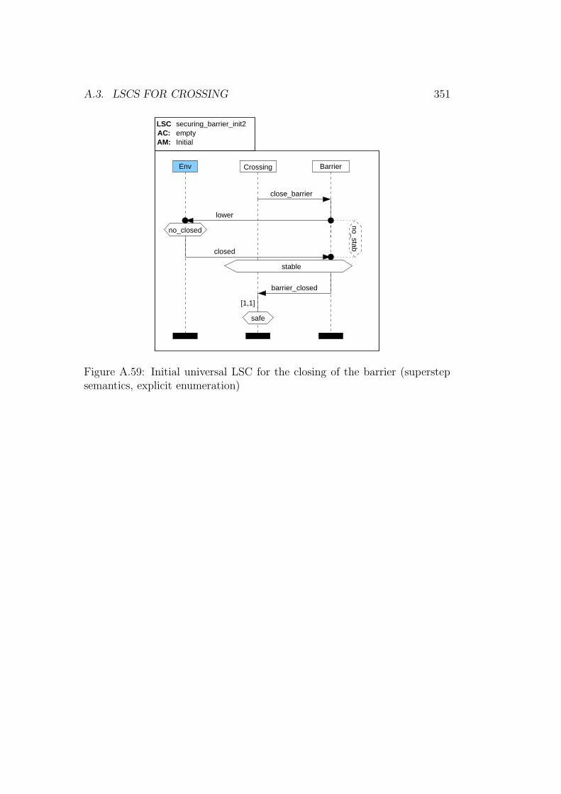
A.3. LSCS FOR CROSSING 351
barrier_closed
AM: InitialAC:LSC securing_barrier_init2
Env Crossing
empty
close_barrier
Barrier
closed
lower
safe
[1,1]
no_closed
stable
no_stab
Figure A.59: Initial universal LSC for the closing of the barrier (superstepsemantics, explicit enumeration)
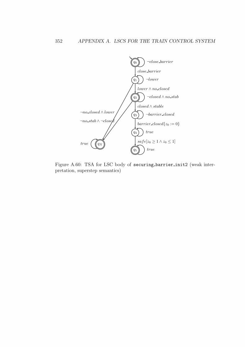
352 APPENDIX A. LSCS FOR THE TRAIN CONTROL SYSTEM
q0 ¬close barrier
q1 ¬lower
close barrier
q2 ¬closed ∧ no stab
lower ∧ no closed
q3 ¬barrier closed
closed ∧ stable
q4 true
barrier closed{z0 := 0}
q5 true
safe[z0 ≥ 1 ∧ z0 ≤ 1]qXtrue
¬no closed ∧ lower
¬no stab ∧ ¬closed
Figure A.60: TSA for LSC body of securing barrier init2 (weak inter-pretation, superstep semantics)
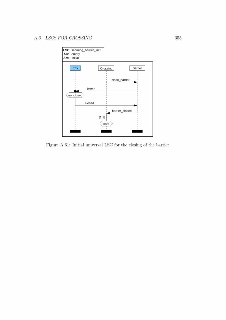
A.3. LSCS FOR CROSSING 353
barrier_closed
closed
AM: InitialAC:LSC securing_barrier_init3
Env Crossing
empty
close_barrier
lower
Barrier
no_closed
safe
[1,1]
Figure A.61: Initial universal LSC for the closing of the barrier
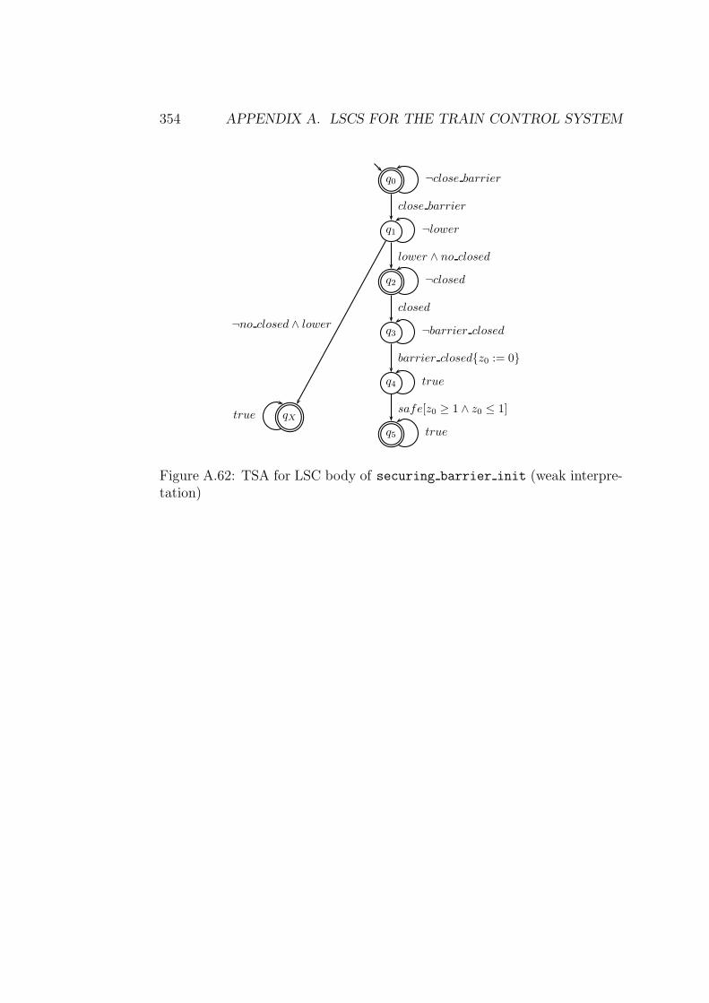
354 APPENDIX A. LSCS FOR THE TRAIN CONTROL SYSTEM
q0 ¬close barrier
q1 ¬lower
close barrier
q2 ¬closed
lower ∧ no closed
q3 ¬barrier closed
closed
q4 true
barrier closed{z0 := 0}
q5 true
safe[z0 ≥ 1 ∧ z0 ≤ 1]qXtrue
¬no closed ∧ lower
Figure A.62: TSA for LSC body of securing barrier init (weak interpre-tation)
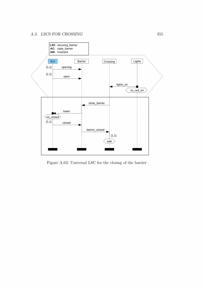
A.3. LSCS FOR CROSSING 355
Env
AM: InvariantAC: raise_barrierLSC securing_barrier
LightsCrossing
lights_on
opening
open
close_barrier
lower
Barrier
closed
barrier_closed
[1,1]
[1,1]
no_red_err
[1,1]
safe
[1,1]
no_closed
Figure A.63: Universal LSC for the closing of the barrier
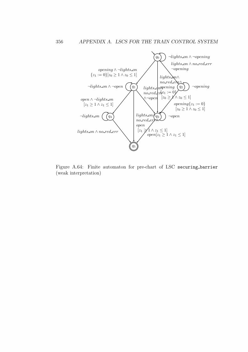
356 APPENDIX A. LSCS FOR THE TRAIN CONTROL SYSTEM
q0 ¬lights on ∧ ¬opening
q1¬lights on ∧ ¬open
opening ∧ ¬lights on{z1 := 0}[z0 ≥ 1 ∧ z0 ≤ 1]
q2 ¬opening
lights on ∧ no red err¬opening
q3 ¬open
lights on∧no red err
∧¬open
opening{z1 := 0}[z0 ≥ 1 ∧ z0 ≤ 1]
lights on∧no red err∧opening
{z1 := 0}[z0 ≥ 1 ∧ z0 ≤ 1]
q4¬lights on
open ∧ ¬lights on[z1 ≥ 1 ∧ z1 ≤ 1]
q5
lights on∧no red err∧open
[z1 ≥ 1 ∧ z1 ≤ 1]open[z1 ≥ 1 ∧ z1 ≤ 1]
lights on ∧ no red err
Figure A.64: Finite automaton for pre-chart of LSC securing barrier
(weak interpretation)
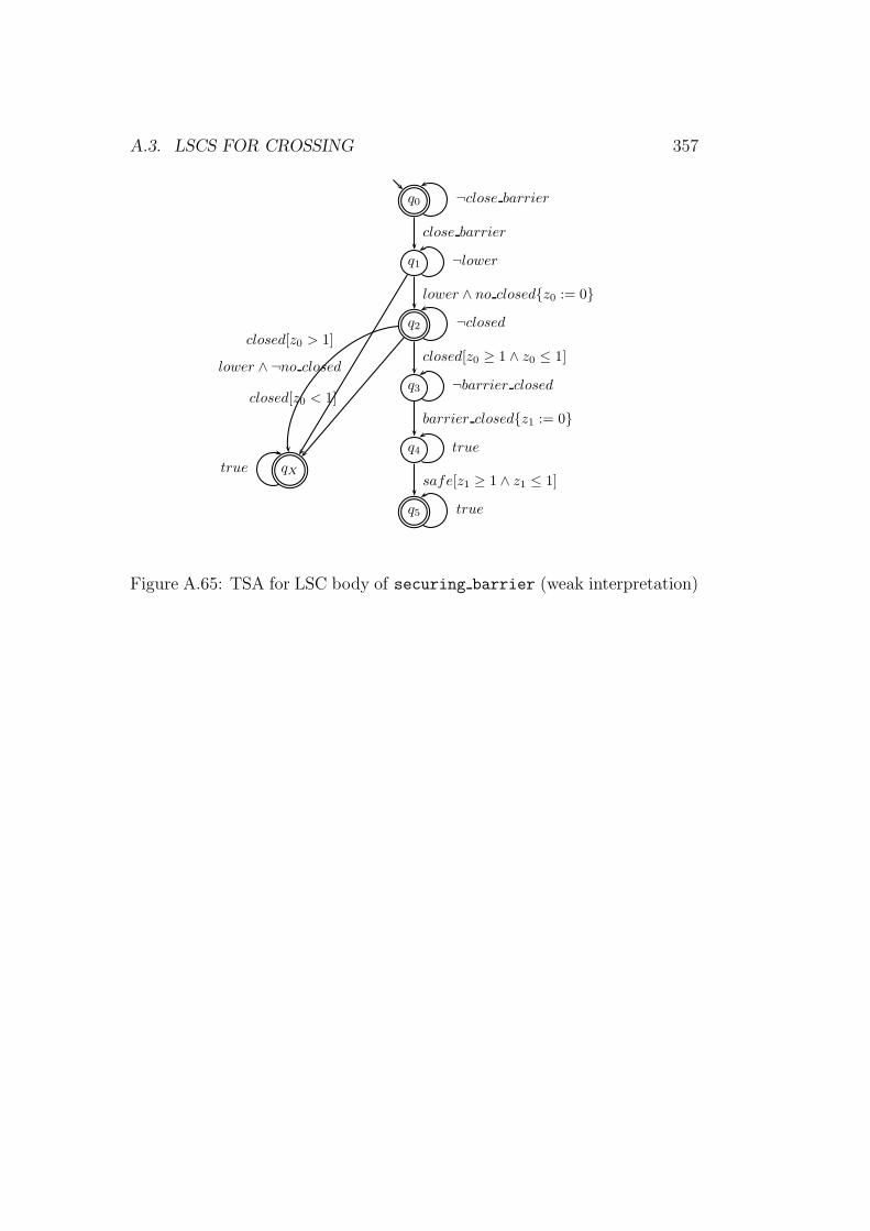
A.3. LSCS FOR CROSSING 357
q0 ¬close barrier
q1 ¬lower
close barrier
q2 ¬closed
lower ∧ no closed{z0 := 0}
q3 ¬barrier closed
closed[z0 ≥ 1 ∧ z0 ≤ 1]
q4 true
barrier closed{z1 := 0}
q5 true
safe[z1 ≥ 1 ∧ z1 ≤ 1]qXtrue
lower ∧ ¬no closed
closed[z0 < 1]
closed[z0 > 1]
Figure A.65: TSA for LSC body of securing barrier (weak interpretation)
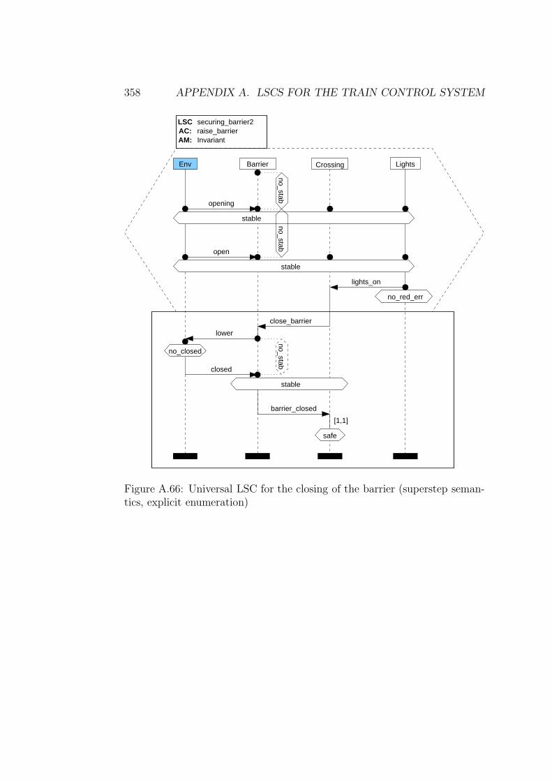
358 APPENDIX A. LSCS FOR THE TRAIN CONTROL SYSTEM
Env
AM: InvariantAC: raise_barrierLSC securing_barrier2
LightsBarrier Crossing
opening
open
lights_on
lower
closed
barrier_closed
close_barrier
stable
no_closed
no_stabno_stab
stable
no_stab
no_red_err
stable
[1,1]
safe
Figure A.66: Universal LSC for the closing of the barrier (superstep seman-tics, explicit enumeration)
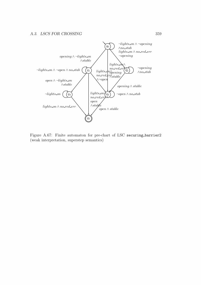
A.3. LSCS FOR CROSSING 359
q0¬lights on ∧ ¬opening∧no stab
q1¬lights on ∧ ¬open ∧ no stab
opening ∧ ¬lights on∧stable
q2¬opening∧no stab
lights on ∧ no red err¬opening
q3 ¬open ∧ no stab
lights on∧no red err
∧¬open
opening ∧ stable
lights on∧no red err∧opening
∧stable
q4¬lights on
open ∧ ¬lights on∧stable
q5
lights on∧no red err∧open
∧stableopen ∧ stable
lights on ∧ no red err
Figure A.67: Finite automaton for pre-chart of LSC securing barrier2
(weak interpretation, superstep semantics)
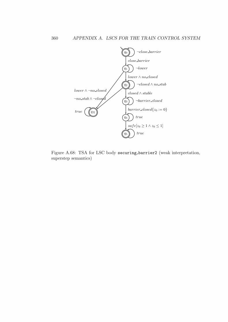
360 APPENDIX A. LSCS FOR THE TRAIN CONTROL SYSTEM
q0 ¬close barrier
q1 ¬lower
close barrier
q2 ¬closed ∧ no stab
lower ∧ no closed
q3 ¬barrier closed
closed ∧ stable
q4 true
barrier closed{z0 := 0}
q5 true
safe[z0 ≥ 1 ∧ z0 ≤ 1]
qXtrue
lower ∧ ¬no closed
¬no stab ∧ ¬closed
Figure A.68: TSA for LSC body securing barrier2 (weak interpretation,superstep semantics)
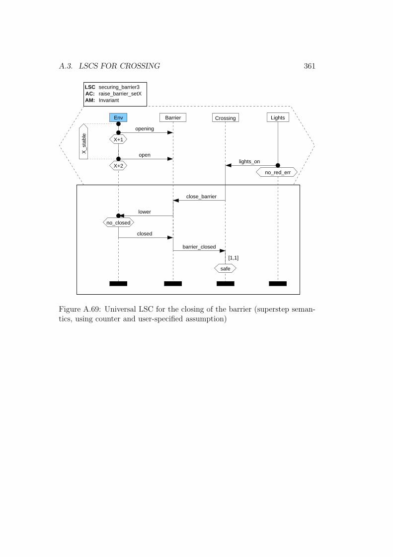
A.3. LSCS FOR CROSSING 361
AM: InvariantAC: raise_barrier_setXLSC securing_barrier3
Env LightsCrossing
lights_on
opening
close_barrier
lower
Barrier
closed
barrier_closed
open
X+1
no_red_err
safe
[1,1]
no_closed
X_s
tabl
e
X+2
Figure A.69: Universal LSC for the closing of the barrier (superstep seman-tics, using counter and user-specified assumption)
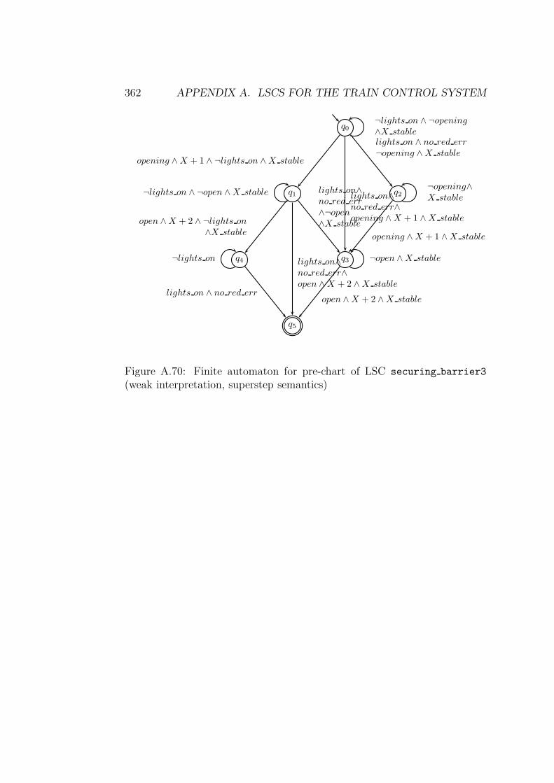
362 APPENDIX A. LSCS FOR THE TRAIN CONTROL SYSTEM
q0¬lights on ∧ ¬opening∧X stable
q1¬lights on ∧ ¬open ∧X stable
opening ∧X + 1 ∧ ¬lights on ∧X stable
q2¬opening∧X stable
lights on ∧ no red err¬opening ∧X stable
q3 ¬open ∧X stable
lights on∧no red err
∧¬open∧X stable
opening ∧X + 1 ∧X stable
lights on∧no red err∧opening ∧X + 1 ∧X stable
q4¬lights on
open ∧X + 2 ∧ ¬lights on∧X stable
q5
lights on∧no red err∧open ∧X + 2 ∧X stable
open ∧X + 2 ∧X stablelights on ∧ no red err
Figure A.70: Finite automaton for pre-chart of LSC securing barrier3
(weak interpretation, superstep semantics)
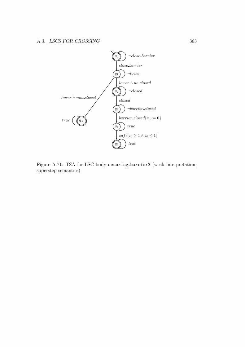
A.3. LSCS FOR CROSSING 363
q0 ¬close barrier
q1 ¬lower
close barrier
q2 ¬closed
lower ∧ no closed
q3 ¬barrier closed
closed
q4 true
barrier closed{z0 := 0}
q5 true
safe[z0 ≥ 1 ∧ z0 ≤ 1]
qXtrue
lower ∧ ¬no closed
Figure A.71: TSA for LSC body securing barrier3 (weak interpretation,superstep semantics)
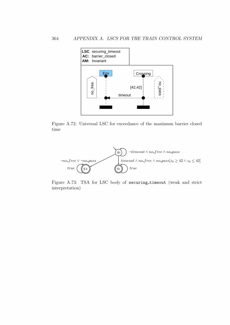
364 APPENDIX A. LSCS FOR THE TRAIN CONTROL SYSTEM
Env Crossing
AM: InvariantAC:LSC securing_timeout
barrier_closed
timeoutno_f
ree
[42,42]
no_pass
Figure A.72: Universal LSC for exceedance of the maximum barrier closedtime
q0 ¬timeout ∧ no free ∧ no pass
q1 true
timeout ∧ no free ∧ no pass[z0 ≥ 42 ∧ z0 ≤ 42]
qXtrue
¬no free ∨ ¬no pass
Figure A.73: TSA for LSC body of securing timeout (weak and strictinterpretation)
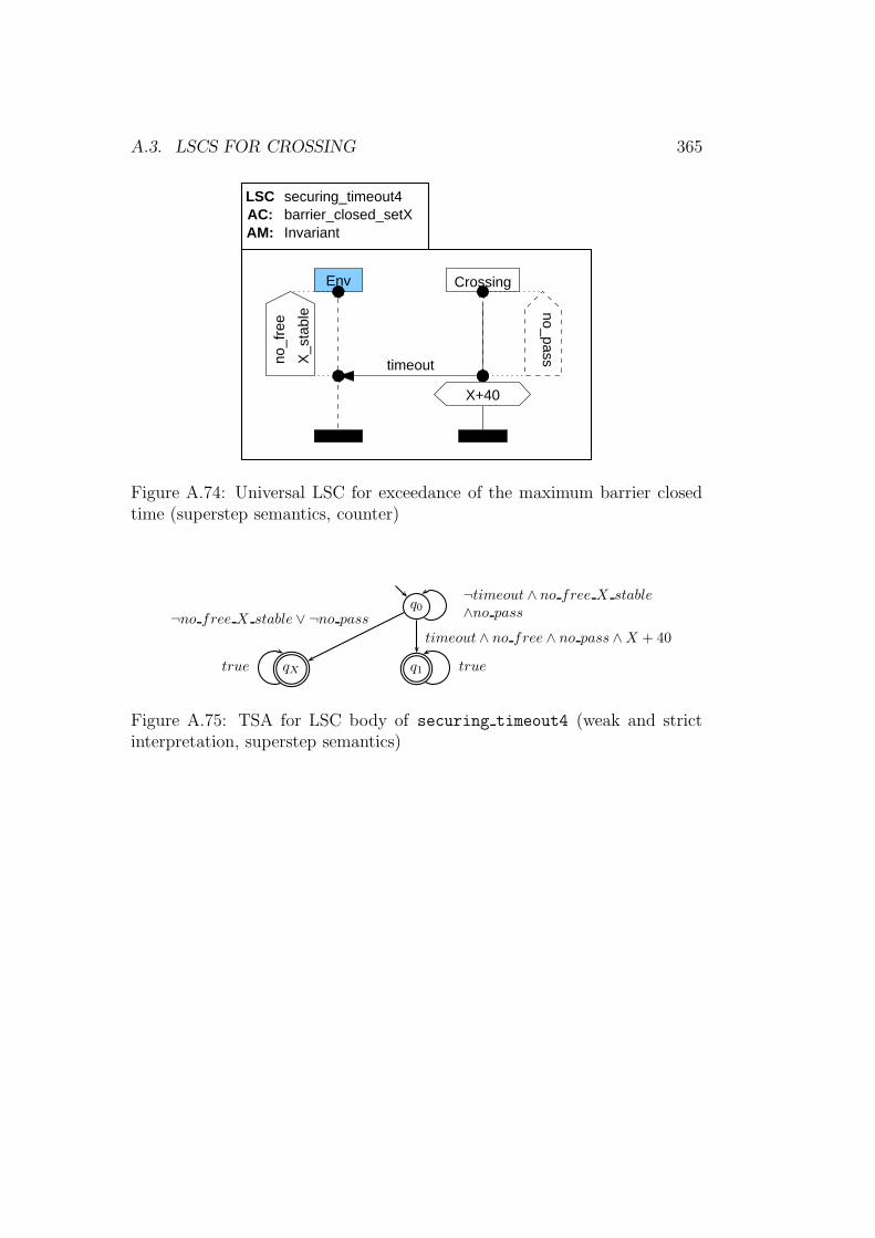
A.3. LSCS FOR CROSSING 365
Env Crossing
AM: InvariantAC:LSC securing_timeout4
barrier_closed_setX
timeoutno_f
ree
X_s
tabl
e
X+40
no_pass
Figure A.74: Universal LSC for exceedance of the maximum barrier closedtime (superstep semantics, counter)
q0¬timeout ∧ no free X stable
∧no pass
q1 true
timeout ∧ no free ∧ no pass ∧X + 40
qXtrue
¬no free X stable ∨ ¬no pass
Figure A.75: TSA for LSC body of securing timeout4 (weak and strictinterpretation, superstep semantics)
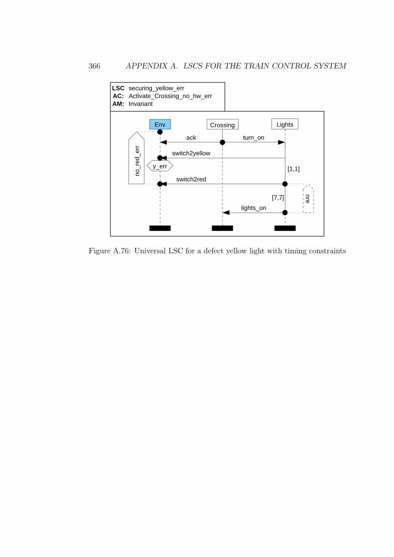
366 APPENDIX A. LSCS FOR THE TRAIN CONTROL SYSTEM
AM: InvariantAC: Activate_Crossing_no_hw_errLSC
Env Lights
ack
Crossing
switch2yellow
turn_on
securing_yellow_err
switch2red
lights_on
y_err [1,1]
no_r
ed_e
rr
nre[7,7]
Figure A.76: Universal LSC for a defect yellow light with timing constraints
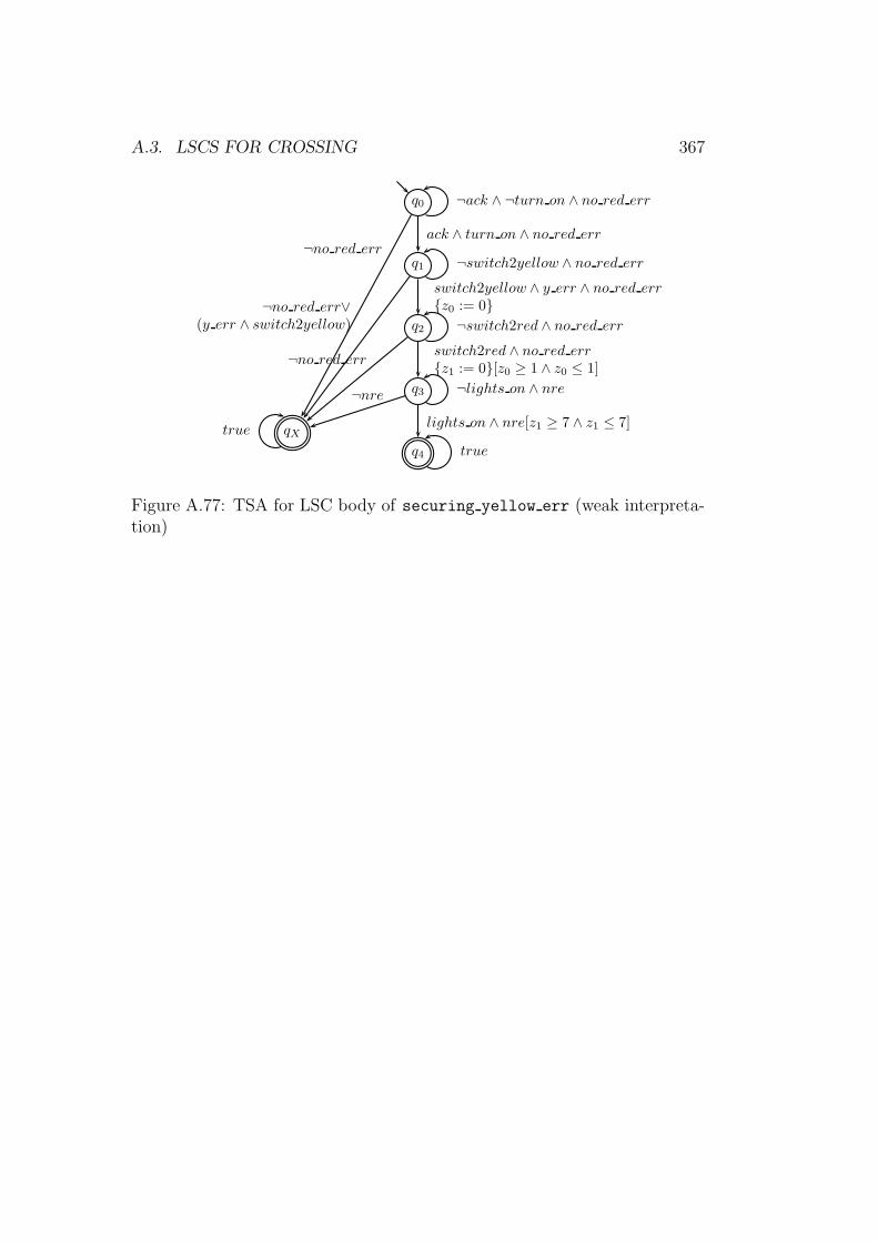
A.3. LSCS FOR CROSSING 367
q0 ¬ack ∧ ¬turn on ∧ no red err
q1 ¬switch2yellow ∧ no red err
ack ∧ turn on ∧ no red err
q2 ¬switch2red ∧ no red err
switch2yellow ∧ y err ∧ no red err{z0 := 0}
q3 ¬lights on ∧ nre
switch2red ∧ no red err{z1 := 0}[z0 ≥ 1 ∧ z0 ≤ 1]
q4 true
lights on ∧ nre[z1 ≥ 7 ∧ z1 ≤ 7]qXtrue
¬no red err
¬no red err∨(y err ∧ switch2yellow)
¬no red err
¬nre
Figure A.77: TSA for LSC body of securing yellow err (weak interpreta-tion)
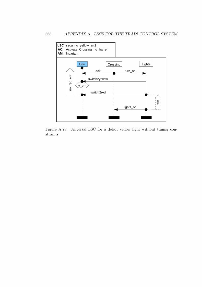
368 APPENDIX A. LSCS FOR THE TRAIN CONTROL SYSTEM
AM: InvariantAC: Activate_Crossing_no_hw_errLSC
Env Lights
ack
Crossing
switch2yellow
turn_on
securing_yellow_err2
switch2red
lights_on
y_err
no_r
ed_e
rr
nre
Figure A.78: Universal LSC for a defect yellow light without timing con-straints
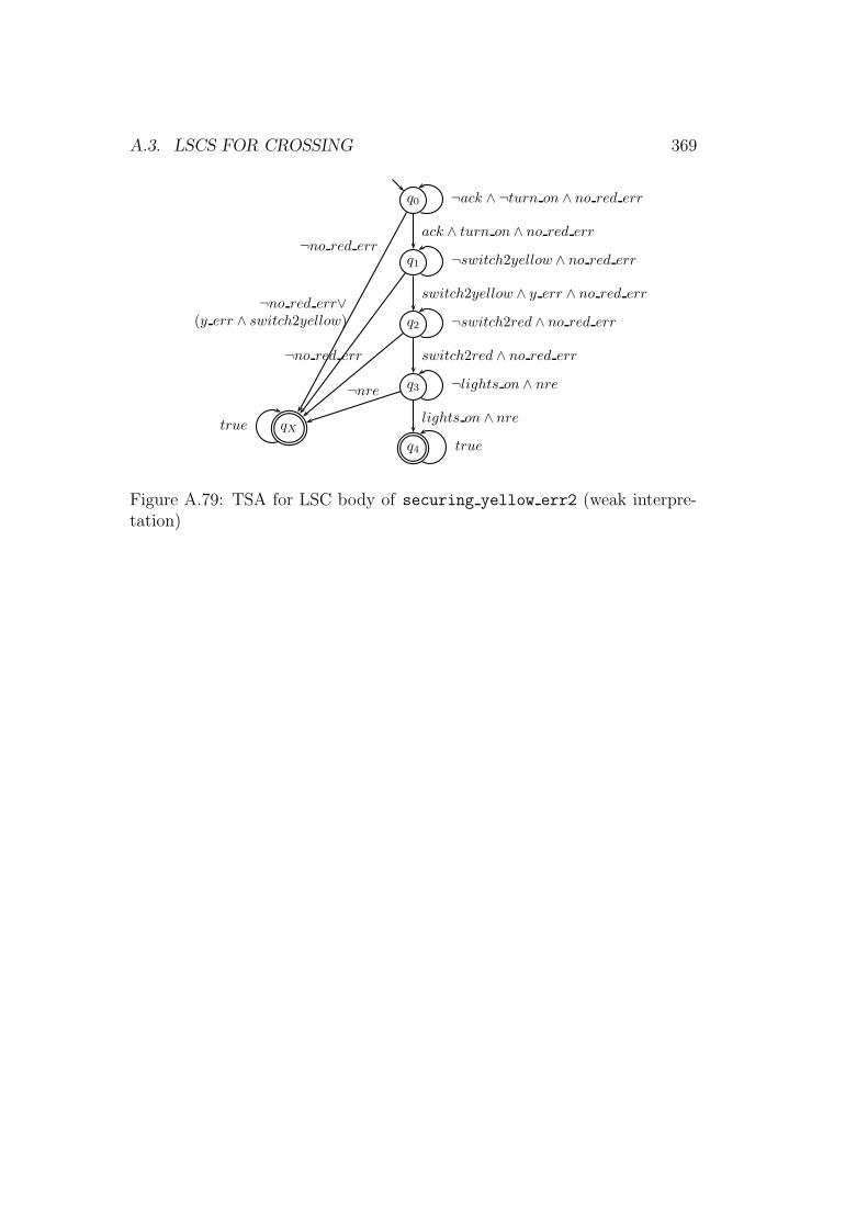
A.3. LSCS FOR CROSSING 369
q0 ¬ack ∧ ¬turn on ∧ no red err
q1 ¬switch2yellow ∧ no red err
ack ∧ turn on ∧ no red err
q2 ¬switch2red ∧ no red err
switch2yellow ∧ y err ∧ no red err
q3 ¬lights on ∧ nre
switch2red ∧ no red err
q4 true
lights on ∧ nreqXtrue
¬no red err
¬no red err∨(y err ∧ switch2yellow)
¬no red err
¬nre
Figure A.79: TSA for LSC body of securing yellow err2 (weak interpre-tation)
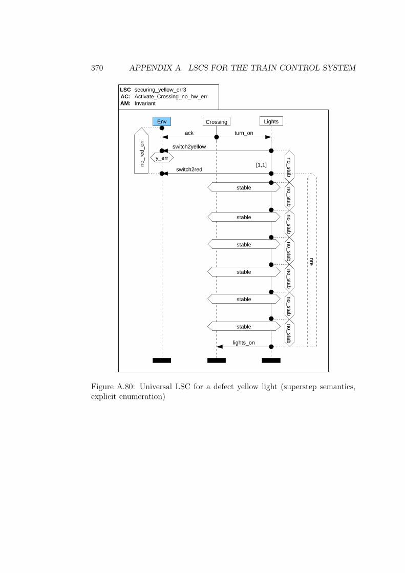
370 APPENDIX A. LSCS FOR THE TRAIN CONTROL SYSTEM
AM: InvariantAC: Activate_Crossing_no_hw_errLSC
Env Lights
ack
Crossing
switch2yellow
turn_on
securing_yellow_err3
switch2red
lights_on
y_err
stable
stable
stable
stable
stable
stable
no_stab
nre
no_stabno_stab
no_stabno_stab
no_stabno_stab
[1,1]no_r
ed_e
rr
Figure A.80: Universal LSC for a defect yellow light (superstep semantics,explicit enumeration)
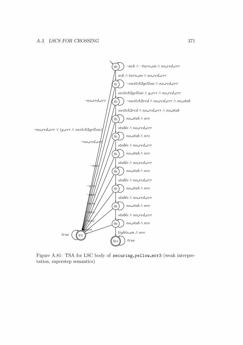
A.3. LSCS FOR CROSSING 371
q0 ¬ack ∧ ¬turn on ∧ no red err
q1 ¬switch2yellow ∧ no red err
ack ∧ turn on ∧ no red err
q2 ¬switch2red ∧ no red err ∧ no stab
switch2yellow ∧ y err ∧ no red err
q3 no stab ∧ nre
switch2red ∧ no red err ∧ no stab
q4 no stab ∧ nre
stable ∧ no red err
q5 no stab ∧ nre
stable ∧ no red err
q6 no stab ∧ nre
stable ∧ no red err
q7 no stab ∧ nre
stable ∧ no red err
q8 no stab ∧ nre
stable ∧ no red err
q9 no stab ∧ nre
stable ∧ no red err
q10 true
lights on ∧ nreqXtrue
¬no red err
¬no red err ∨ (y err ∧ switch2yellow)
¬no red err
¬nre
¬nre
¬nre
¬nre
¬nre
¬nre
¬nre
Figure A.81: TSA for LSC body of securing yellow err3 (weak interpre-tation, superstep semantics)
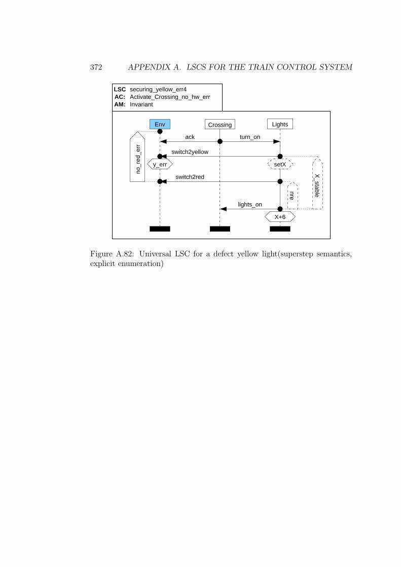
372 APPENDIX A. LSCS FOR THE TRAIN CONTROL SYSTEM
AM: InvariantAC: Activate_Crossing_no_hw_errLSC
Env Lights
ack
Crossing
switch2yellow
turn_on
securing_yellow_err4
switch2red
lights_on
y_err setX
X+6
no_r
ed_e
rr
nre
X_stable
Figure A.82: Universal LSC for a defect yellow light(superstep semantics,explicit enumeration)
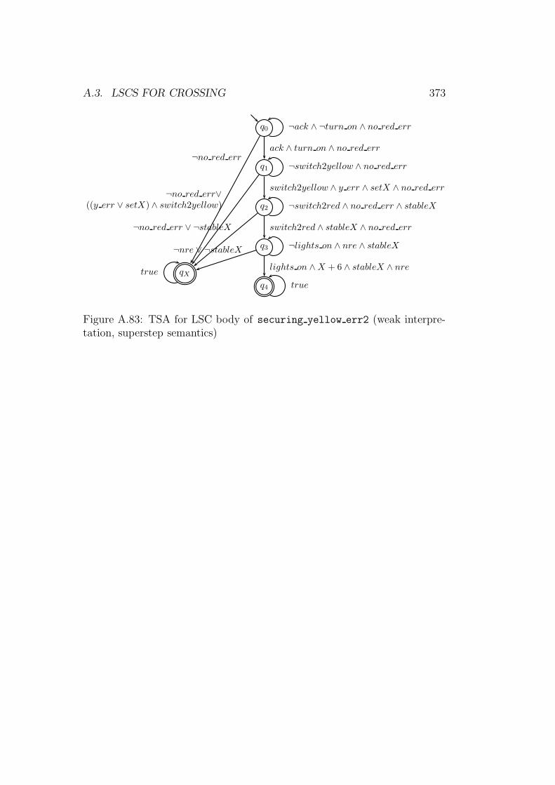
A.3. LSCS FOR CROSSING 373
q0 ¬ack ∧ ¬turn on ∧ no red err
q1 ¬switch2yellow ∧ no red err
ack ∧ turn on ∧ no red err
q2 ¬switch2red ∧ no red err ∧ stableX
switch2yellow ∧ y err ∧ setX ∧ no red err
q3 ¬lights on ∧ nre ∧ stableX
switch2red ∧ stableX ∧ no red err
q4 true
lights on ∧X + 6 ∧ stableX ∧ nreqXtrue
¬no red err
¬no red err∨((y err ∨ setX) ∧ switch2yellow)
¬no red err ∨ ¬stableX
¬nre ∨ ¬stableX
Figure A.83: TSA for LSC body of securing yellow err2 (weak interpre-tation, superstep semantics)
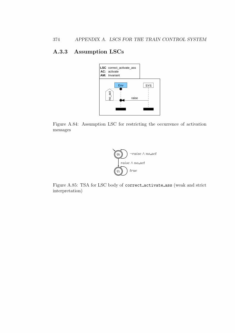
374 APPENDIX A. LSCS FOR THE TRAIN CONTROL SYSTEM
A.3.3 Assumption LSCs
activateLSCAC:
correct_activate_ass
InvariantAM:
Env SYS
raiseno_a
ct
Figure A.84: Assumption LSC for restricting the occurrence of activationmessages
q0 ¬raise ∧ no act
q1 true
raise ∧ no act
Figure A.85: TSA for LSC body of correct activate ass (weak and strictinterpretation)
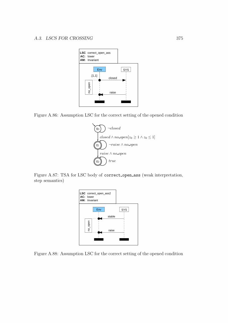
A.3. LSCS FOR CROSSING 375
lowerLSCAC:
correct_open_ass
InvariantAM:
Env SYS
closed
raise
.[1,1]
no_o
pen
Figure A.86: Assumption LSC for the correct setting of the opened condition
q0 ¬closed
q1 ¬raise ∧ no open
closed ∧ no open[z0 ≥ 1 ∧ z0 ≤ 1]
q2 true
raise ∧ no open
Figure A.87: TSA for LSC body of correct open ass (weak interpretation,step semantics)
stable
raise
lowerLSCAC:
InvariantAM:
Env SYS
correct_open_ass2
no_o
pen
Figure A.88: Assumption LSC for the correct setting of the opened condition
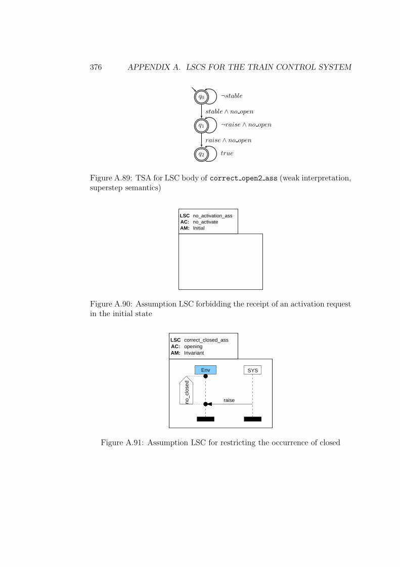
376 APPENDIX A. LSCS FOR THE TRAIN CONTROL SYSTEM
q0 ¬stable
q1 ¬raise ∧ no open
stable ∧ no open
q2 true
raise ∧ no open
Figure A.89: TSA for LSC body of correct open2 ass (weak interpretation,superstep semantics)
no_activateLSCAC:
no_activation_ass
InitialAM:
Figure A.90: Assumption LSC forbidding the receipt of an activation requestin the initial state
openingLSCAC:
correct_closed_ass
InvariantAM:
Env SYS
raiseno_c
lose
d
Figure A.91: Assumption LSC for restricting the occurrence of closed
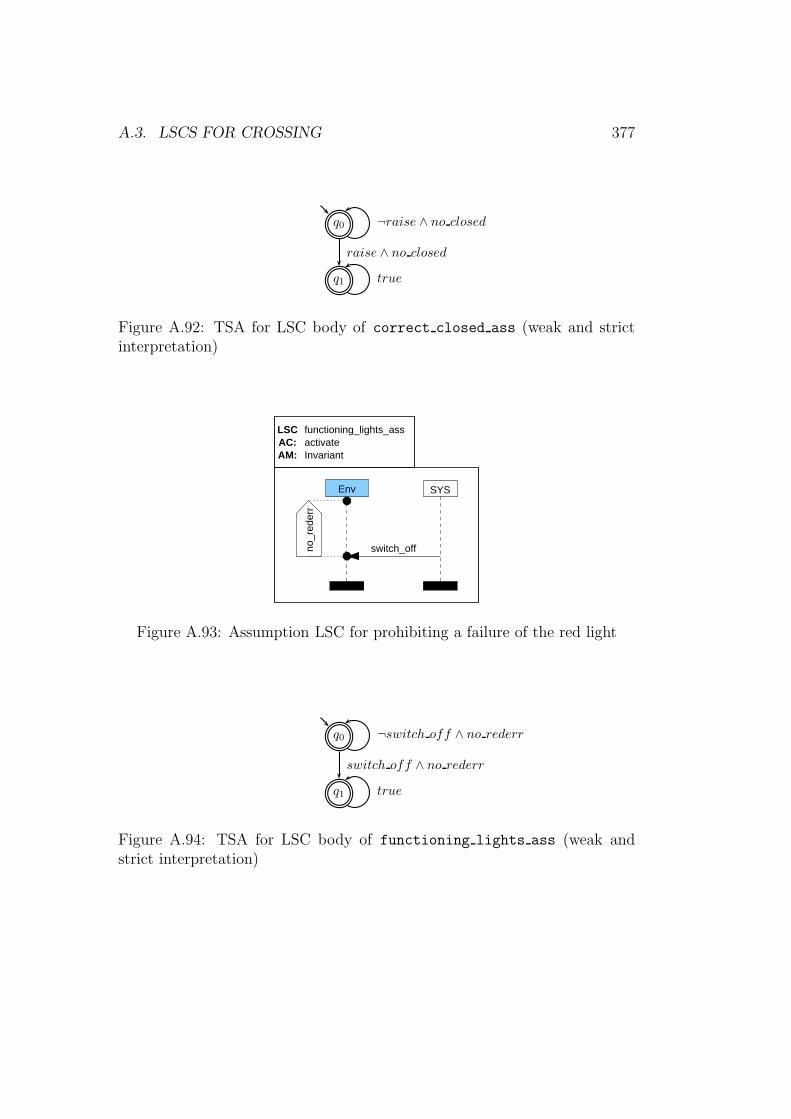
A.3. LSCS FOR CROSSING 377
q0 ¬raise ∧ no closed
q1 true
raise ∧ no closed
Figure A.92: TSA for LSC body of correct closed ass (weak and strictinterpretation)
activateLSCAC:
functioning_lights_ass
InvariantAM:
Env SYS
switch_offno_r
eder
r
Figure A.93: Assumption LSC for prohibiting a failure of the red light
q0 ¬switch off ∧ no rederr
q1 true
switch off ∧ no rederr
Figure A.94: TSA for LSC body of functioning lights ass (weak andstrict interpretation)
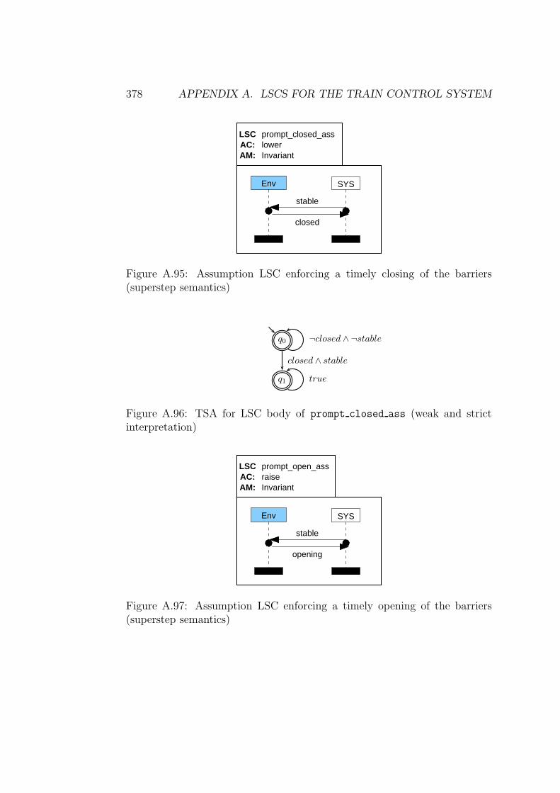
378 APPENDIX A. LSCS FOR THE TRAIN CONTROL SYSTEM
Env SYS
stable
closed
lowerLSCAC:
prompt_closed_ass
InvariantAM:
Figure A.95: Assumption LSC enforcing a timely closing of the barriers(superstep semantics)
q0 ¬closed ∧ ¬stable
q1 true
closed ∧ stable
Figure A.96: TSA for LSC body of prompt closed ass (weak and strictinterpretation)
raiseLSCAC:
InvariantAM:
prompt_open_ass
Env SYS
stable
opening
Figure A.97: Assumption LSC enforcing a timely opening of the barriers(superstep semantics)
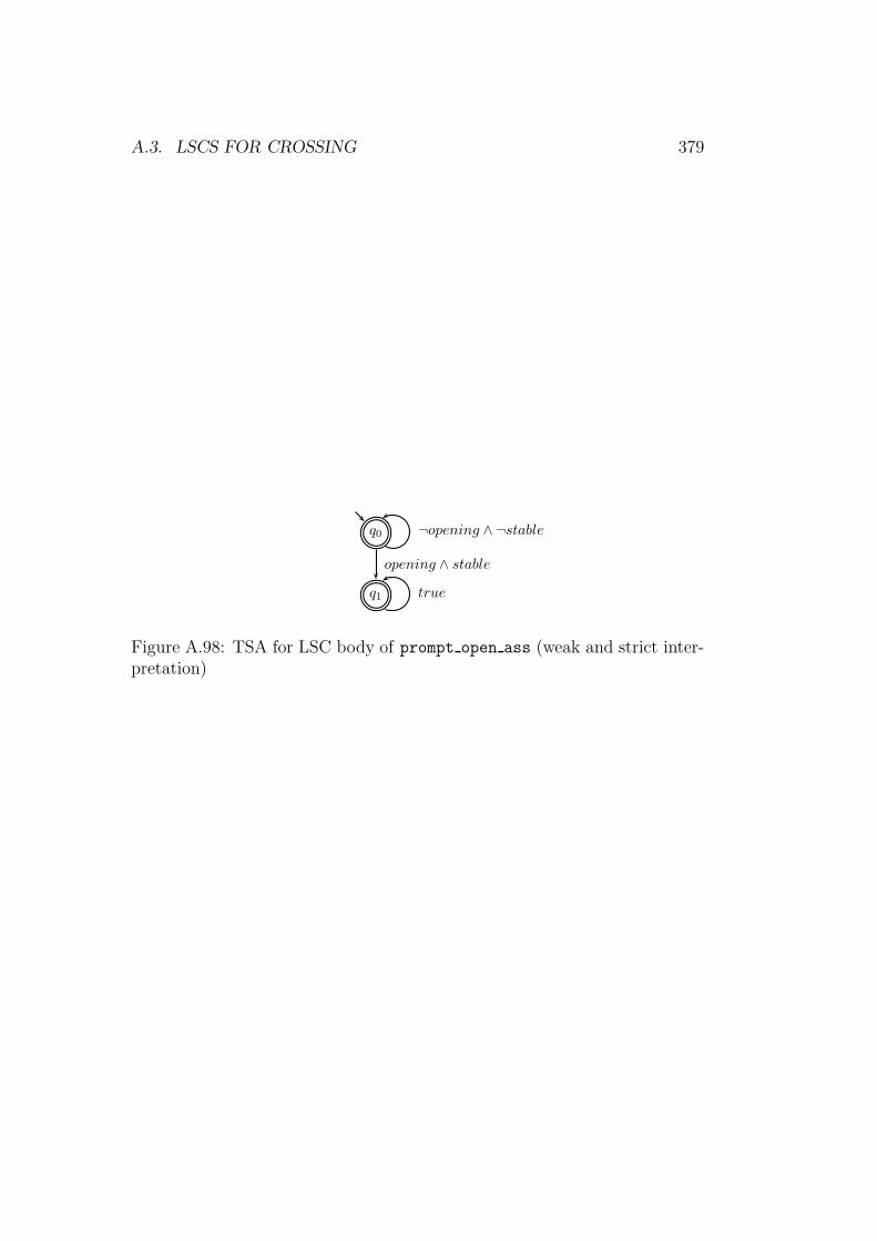
A.3. LSCS FOR CROSSING 379
q0 ¬opening ∧ ¬stable
q1 true
opening ∧ stable
Figure A.98: TSA for LSC body of prompt open ass (weak and strict inter-pretation)

380 APPENDIX A. LSCS FOR THE TRAIN CONTROL SYSTEM
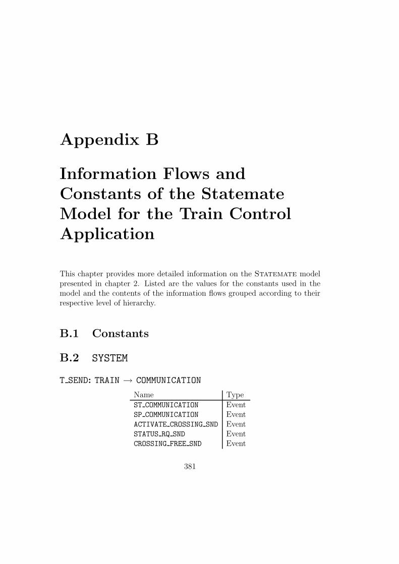
Appendix B
Information Flows and
Constants of the Statemate
Model for the Train Control
Application
This chapter provides more detailed information on the Statemate modelpresented in chapter 2. Listed are the values for the constants used in themodel and the contents of the information flows grouped according to theirrespective level of hierarchy.
B.1 Constants
B.2 SYSTEM
T SEND: TRAIN → COMMUNICATION
Name TypeST COMMUNICATION EventSP COMMUNICATION EventACTIVATE CROSSING SND EventSTATUS RQ SND EventCROSSING FREE SND Event
381
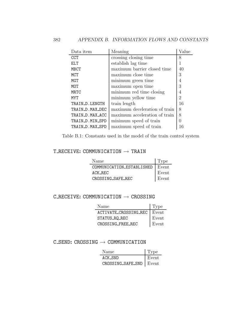
382 APPENDIX B. INFORMATION FLOWS AND CONSTANTS
Data item Meaning ValueCCT crossing closing time 8ELT establish lag time 1MBCT maximum barrier closed time 40MCT maximum close time 3MGT minimum green time 4MOT maximum open time 3MRTC minimum red time closing 4MYT minimum yellow time 2TRAIN D.LENGTH train length 16TRAIN D.MAX DEC maximum deceleration of train 8TRAIN D.MAX ACC maximum acceleration of train 8TRAIN D.MIN SPD minimum speed of train 0TRAIN D.MAX SPD maximum speed of train 16
Table B.1: Constants used in the model of the train control system
T RECEIVE: COMMUNICATION → TRAIN
Name TypeCOMMUNICATION ESTABLISHED EventACK REC EventCROSSING SAFE REC Event
C RECEIVE: COMMUNICATION → CROSSING
Name TypeACTIVATE CROSSING REC EventSTATUS RQ REC EventCROSSING FREE REC Event
C SEND: CROSSING → COMMUNICATION
Name TypeACK SND EventCROSSING SAFE SND Event
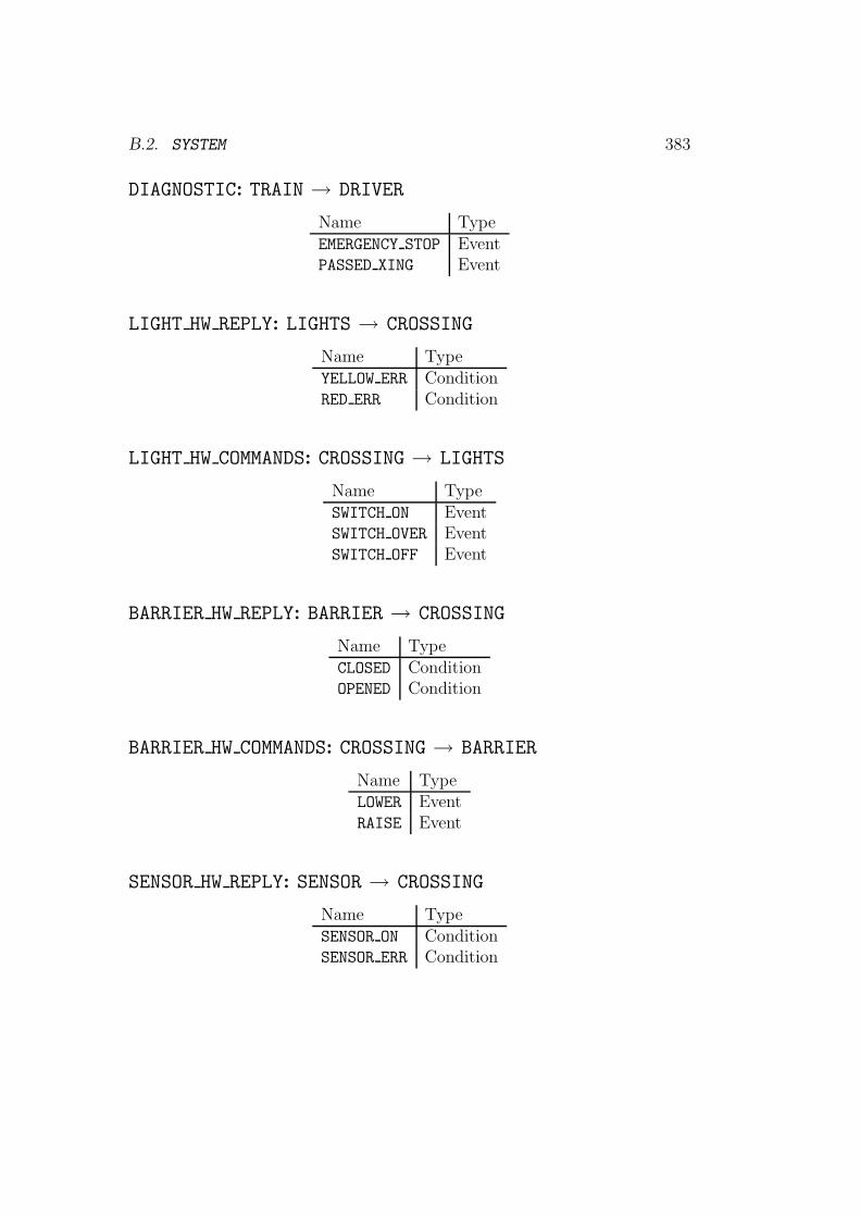
B.2. SYSTEM 383
DIAGNOSTIC: TRAIN → DRIVER
Name TypeEMERGENCY STOP EventPASSED XING Event
LIGHT HW REPLY: LIGHTS → CROSSING
Name TypeYELLOW ERR ConditionRED ERR Condition
LIGHT HW COMMANDS: CROSSING → LIGHTS
Name TypeSWITCH ON EventSWITCH OVER EventSWITCH OFF Event
BARRIER HW REPLY: BARRIER → CROSSING
Name TypeCLOSED ConditionOPENED Condition
BARRIER HW COMMANDS: CROSSING → BARRIER
Name TypeLOWER EventRAISE Event
SENSOR HW REPLY: SENSOR → CROSSING
Name TypeSENSOR ON ConditionSENSOR ERR Condition
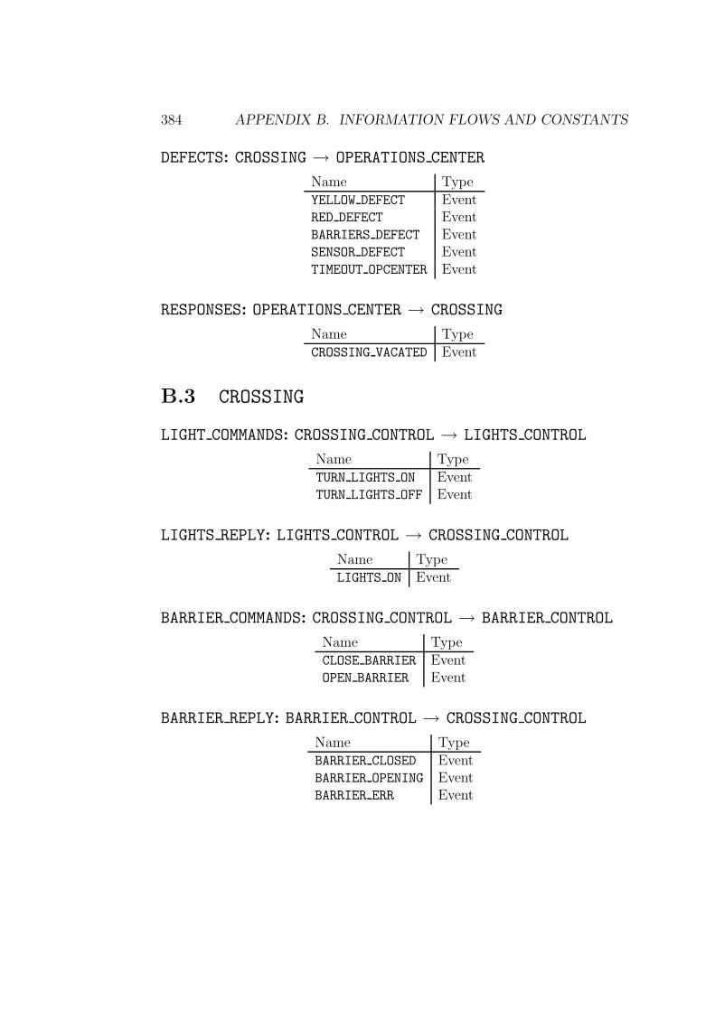
384 APPENDIX B. INFORMATION FLOWS AND CONSTANTS
DEFECTS: CROSSING → OPERATIONS CENTER
Name TypeYELLOW DEFECT EventRED DEFECT EventBARRIERS DEFECT EventSENSOR DEFECT EventTIMEOUT OPCENTER Event
RESPONSES: OPERATIONS CENTER → CROSSING
Name TypeCROSSING VACATED Event
B.3 CROSSING
LIGHT COMMANDS: CROSSING CONTROL → LIGHTS CONTROL
Name TypeTURN LIGHTS ON EventTURN LIGHTS OFF Event
LIGHTS REPLY: LIGHTS CONTROL → CROSSING CONTROL
Name TypeLIGHTS ON Event
BARRIER COMMANDS: CROSSING CONTROL → BARRIER CONTROL
Name TypeCLOSE BARRIER EventOPEN BARRIER Event
BARRIER REPLY: BARRIER CONTROL → CROSSING CONTROL
Name TypeBARRIER CLOSED EventBARRIER OPENING EventBARRIER ERR Event
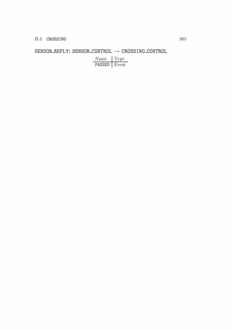
B.3. CROSSING 385
SENSOR REPLY: SENSOR CONTROL → CROSSING CONTROL
Name TypePASSED Event
386 APPENDIX B. INFORMATION FLOWS AND CONSTANTS
Appendix C
LSC Grammar
<lsc document> ::= <document head> <live sequence chart>*
<end> ::= [ <comment> ] ;
<comment> ::= comment <character string>
<text definition> ::= text <character string> <end>
<document head> ::= { mscdocument | lscdocument }
<lsc document name> <end>
<identifier> ::= <name>
<live sequence chart> ::= { [ universal | existential ] }
[ lsc_kind ]
{ lsc | msc } <lsc head> <lsc body>
{ endlsc | endmsc } <end>
<lsc_kind> ::= prechart | assumption
<lsc head> ::= <lsc name> <end>
[ activation condition : condexpr <string>
endexpr activation mode <mode name> ]
[ assumption <assumption list> ]
<assumption list> ::= <lsc name>+
<lsc body> ::= <lsc statement>*
387
388 APPENDIX C. LSC GRAMMAR
<lsc statement> ::= <text definition> [ end ]
| <event definition> [ end ]
| <old instance head statement>
<instance event list> [ end ]
<text definition> ::= text <character string> <end>
<event definition> ::= <instance name> : <instance event list>
| <instance name list> :
<multi instance event list>
<instance event list> ::= { <instance event> } +
<instance event> ::= { <orderable event> |
<non-orderable event> }
<end> [ <delay> ]
<orderable event> ::= [ { hot | cold } ]
{ <message event>
| <timer statement>
| <action>
| <sim region> }
[ <layout info> ]
<layout info> ::= <character string>
<non-orderable event> ::= [ { hot | cold } ]
{ { <coregion>
| <shared condition>
| <shared lsc reference>
| <instance head statement>
| <instance end statement> }
[ <layout info> ]
| empty }
<instance name list> ::= <instance name> {, <instance name> }*
| all
<multi instance event list> ::= { <multi instance event> <end> } +
<multi instance event> ::= <condition> | <lsc reference>
| <inline expr>
<old instance head statement> ::= instance [ { hot | cold } ]
<instance name> [ <sim region> ]
389
[ <layout info> ] <end> [ <delay> ]
<instance head statement> ::= instance
<instance end statement> ::= endinstance
<message event> ::= { <message output> | <message input> } [ <delay> ]
<message output> ::= out [ { hot | cold } ] [ { sync | async } ]
<msg identification> to <input address>
<message input> ::= in [ { hot | cold } ] [ { sync | async } ]
<msg identification> from <output address>
<msg identification> ::= <message name> [ , <message instance name> ]
[ ( <parameter list> ) ]
<parameter list> ::= <parameter name> [ , <parameter list> ]
<output address> ::= <instance name>
<input address> ::= <instance name>
<shared condition> ::= <condition identification> <shared>
<condition identification> ::= condition { [ hot | cold ] }
<condition name list> :
condexpr <string> endexpr
<condition name list> ::= <condition name>{ , <condition name> }*
<shared> ::= shared { [ <shared instance list> ] | all }
<shared instance list> ::= <instance name> [, <shared instance list> ]
<condition> ::= <condition identification>
<timer statement> ::= <set> | <reset> | <timeout>
<set> ::= set <timer name> [ , <timer instance name> ]
[ (<duration name>) ]
<reset> ::= reset <timer name> [ , <timer instance name> ]
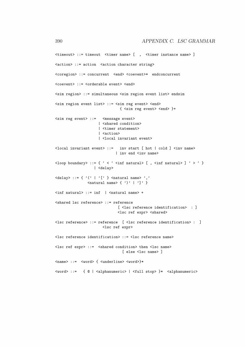
390 APPENDIX C. LSC GRAMMAR
<timeout> ::= timeout <timer name> [ , <timer instance name> ]
<action> ::= action <action character string>
<coregion> ::= concurrent <end> <coevent>* endconcurrent
<coevent> ::= <orderable event> <end>
<sim region> ::= simultaneous <sim region event list> endsim
<sim region event list> ::= <sim reg event> <end>
{ <sim reg event> <end> }+
<sim reg event> ::= <message event>
| <shared condition>
| <timer statement>
| <action>
| <local invariant event>
<local invariant event> ::= inv start [ hot | cold ] <inv name>
| inv end <inv name>
<loop boundary> ::= { ‘ < ‘ <inf natural> [ , <inf natural> ] ‘ > ‘ }
| <delay>
<delay> ::= { ’(’ | ’[’ } <natural name> ’,’
<natural name> { ’)’ | ’]’ }
<inf natural> ::= inf | <natural name> +
<shared lsc reference> ::= reference
[ <lsc reference identification> : ]
<lsc ref expr> <shared>
<lsc reference> ::= reference [ <lsc reference identification> : ]
<lsc ref expr>
<lsc reference identification> ::= <lsc reference name>
<lsc ref expr> ::= <shared condition> then <lsc name>
[ else <lsc name> ]
<name> ::= <word> { <underline> <word>}*
<word> ::= { @ | <alphanumeric> | <full stop> }* <alphanumeric>
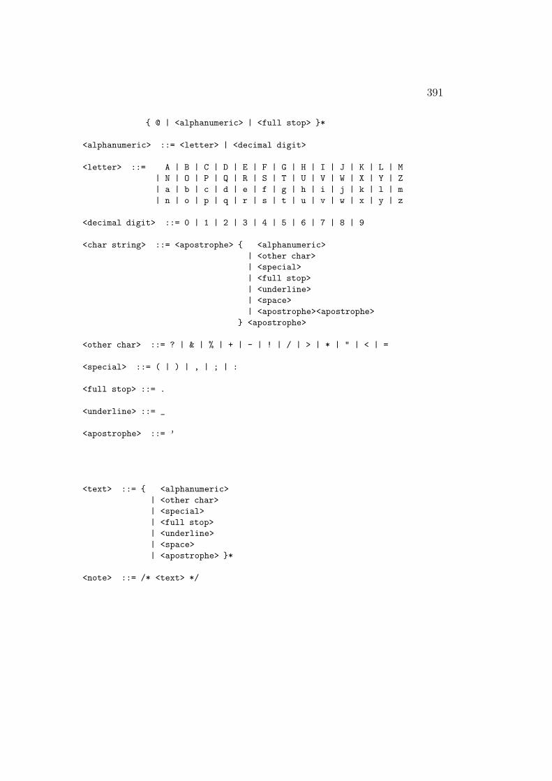
391
{ @ | <alphanumeric> | <full stop> }*
<alphanumeric> ::= <letter> | <decimal digit>
<letter> ::= A | B | C | D | E | F | G | H | I | J | K | L | M
| N | O | P | Q | R | S | T | U | V | W | X | Y | Z
| a | b | c | d | e | f | g | h | i | j | k | l | m
| n | o | p | q | r | s | t | u | v | w | x | y | z
<decimal digit> ::= 0 | 1 | 2 | 3 | 4 | 5 | 6 | 7 | 8 | 9
<char string> ::= <apostrophe> { <alphanumeric>
| <other char>
| <special>
| <full stop>
| <underline>
| <space>
| <apostrophe><apostrophe>
} <apostrophe>
<other char> ::= ? | & | % | + | - | ! | / | > | * | " | < | =
<special> ::= ( | ) | , | ; | :
<full stop> ::= .
<underline> ::= _
<apostrophe> ::= ’
<text> ::= { <alphanumeric>
| <other char>
| <special>
| <full stop>
| <underline>
| <space>
| <apostrophe> }*
<note> ::= /* <text> */

392 APPENDIX C. LSC GRAMMAR
Bibliography
[ACS99] A. Allara, S. Comai, and R. Schlor. System Verification usingUser-Friendly Interfaces. In Design, Automation and Test in Eu-rope / User Forum, pages 167–172. IEEE Computer Society Press,1999.
[AD94] Rajeev Alur and David Dill. A Theory of Timed Automata. The-oretical Computer Science, 126(2):183–236, 1994.
[AEKN00] N. Amla, E.A. Emerson, R.P. Kurshan, and K.S. Namjoshi.Model Checking Synchronous Timing Diagrams. In ProceedingsFormal Methods in Computer-Aided Design (FMCAD), LNCS,pages 283–298. Springer Verlag, 2000.
[AHP96] R. Alur, G.J. Holzmann, and D. Peled. An analyzer for Mes-sage Sequence Charts. In T. Margaria and B. Steffen, editors,Proceedings 2nd International Worshop on Tools and Algorithmsfor the Construction and Analysis of Systems, TACAS96, volume1055 of Lecture Notes in Computer Science, pages 35–48, Passau,Germany, March 1996. Springer Verlag.
[BAL97a] H. Ben-Abdallah and S. Leue. Expressing and analyzing timingconstraints in message sequence chart specifications. Technical Re-port 97-04, Department of Electrical and Computer Engineering,University of Waterloo, April 1997.
[BAL97b] H. Ben-Abdallah and S. Leue. Timing constraints in MessageSequence Chart specifications. In T. Mizuno, N. Shiratori, T. Hi-gashino, and A. Togashi, editors, Formal Description Techniquesand Protocol Specification, Testing and Verification. Proceedings
393
394 BIBLIOGRAPHY
of FORTE X and PSTV XVII ’97, pages 91–106, Osaka, 1997.Chapman & Hall.
[BBB+99] Tom Bienmuller, Jurgen Bohn, Henning Brinkmann, Udo Brock-meyer, Werner Damm, Hardi Hungar, and Peter Jansen. Verifi-cation of Automotive Control Units. In Ernst-Rudiger Olderogand Bernd Steffen, editors, Correct System Design, number 1710in LNCS, pages 319–341. Springer Verlag, 1999.
[BBD+99] Tom Bienmuller, Udo Brockmeyer, Werner Damm, Gert Dohmen,Claus Eßmann, Hans-Jurgen Holberg, Hardi Hungar, BernhardJosko, Rainer Schlor, Gunnar Wittich, Hartmut Wittke, GeoffreyClements, John Rowlands, and Eric Sefton. Formal Verificationof an Avionics Application using Abstraction and Symbolic ModelChecking. In Felix Redmill and Tom Anderson, editors, TowardsSystem Safety – Proceedings of the Seventh Safety-critical SystemsSymposium, Huntingdon, UK, pages 150–173. Safety-Critical Sys-tems Club, Springer Verlag, 1999.
[BBHW00] Tom Bienmuller, Udo Brockmeyer, Hans Jurgen Holberg, andHartmut Wittke. Automatic Debugging for STATEMATE De-signs, 2000. 8. Deutsches Anwenderforum fur STATEMATE Mag-num.
[BCCZ99] Armin Biere, Alessandro Cimatti, Edmund Clarke, and YunshanZhu. Symbolic model checking without BDDs. In W. R. Cleave-land, editor, Tools and Algorithms for the Construction and Anal-ysis of Systems. Part of European Conferences on Theory andPractice of Software, ETAPS’99, Amsterdam, volume 1579 ofLNCS, pages 193–207. Springer-Verlag, 1999.
[BCM+92] J.R. Burch, E.M. Clarke, K. McMillan, D. L. Dill, and L. J.Hwang. Symbolic Model Checking: 1020 States and Beyond. In-formation and Computation, 98(2):142–170, June 1992.
[BDKW01] Tom Bienmuller, Werner Damm, Jochen Klose, and Hart-mut Wittke. Formale Analyse und Verifikation von StatemateEntwurfen. it+ti, 43(1), 2001.
BIBLIOGRAPHY 395
[BDW00] Tom Bienmuller, Werner Damm, and Hartmut Wittke. TheSTATEMATE Verification Environment – Making it real. InE. Allen Emerson and A. Prasad Sistla, editors, 12th internationalConference on Computer Aided Verification, CAV, number 1855in LNCS, pages 561–567. Springer Verlag, 2000.
[BG01] Annette Bunker and Ganesh Gopalakrishnan. Using live sequencecharts for hardware protocol specification and compliance verifi-cation. In IEEE International High Level Design Validation andTest Workshop. IEEE Computer Society Press, November 2001.
[BG02] Annette Bunker and Ganesh Gopalakrishnan. Verifying a VCI BusInterface Model Using an LSC-based Specification. In H. Ehrig,B. J. Kramer, and A. Ertas, editors, Proceedings of the Sixth Bi-ennial World Conference on Integrated Design and Process Tech-nology, page 48. Society of Design and Process Science, June 2002.
[Bie03] Tom Bienmuller. Reducing Complexity for the Verification ofStatemate Designs. PhD thesis, Carl von Ossietzky UniversitatOldenburg, 2003.
[Bit00] Friedemann Bitsch. Classification of Safety Requirements for For-mal Verification of Software Models of Industrial Automation Sys-tems. In Proceedings of the 13th Conference on Software and Sys-tems Engineering and their Applications - ICSSEA 2000, 2000.
[Bit01] Friedemann Bitsch. Safety patterns — the key to formal specifica-tion of safety requirements. Lecture Notes in Computer Science,2187, 2001.
[BKL01] Udo Brockmeyer, Jochen Klose, and Marc Lettrari. UML Valida-tion Suite. In J. Tretmans and E. Brinksma, editors, Proceedingsof FATES’01 - Formal Approaches to Testing of Software, 2001.
[Boe88] Barry W. Boehm. A Spiral Model of Software Development andEnhancement. IEEE Computer, 21(5):61–72, 1988.
[Bon01] Yves Bontemps. Automated verification of state-based specifica-tions against scenarios. Master’s thesis, University of Namur, June2001.
396 BIBLIOGRAPHY
[Bro99] Udo Brockmeyer. Verifikation von STATEMATE Designs. PhDthesis, Carl-von-Ossietzky Universitat Oldenburg, Oldenburg,Dezember 1999.
[BW98] U. Brockmeyer and G. Wittich. Tamagotchis Need Not Die – Ver-ification of STATEMATE Designs. In Bernhard Steffen, editor,Tools and Algorithms for the Construction and Analysis of Sys-tems, volume 1384 of Lecture Notes in Computer Science, pages217–231, 1998.
[CE81] E.M. Clarke and E.A. Emerson. Design and Synthesis of Syn-chronization Skeletons using Branching Time Temporal Logic. InD. Kozen, editor, Proceedings of the Workshop on Logics of Pro-grams, volume 131 of Lecture Notes in Computer Science, pages52–71, Yorktown Heights, New York, May 1981. Springer-Verlag.
[CEN01] CENELEC. EN 50128, Railway Applications, Communications,Signaling and Processing Systems - Software for Railway Controland Protection Systems. European Committee for ElectrotechnicalStandardization, 2001.
[CGP99] Edmund M. Clarke, Orna Grumberg, and Doron A. Peled. ModelChecking. The MIT Press, Cambridge, Massachusetts, 1999.
[DAC98] Matthew B. Dwyer, George S. Avrunin, and James C. Corbett.Property specification patterns for finite-state verification. InMark Ardis, editor, Proceedings of the 2nd Workshop on FormalMethods in Software Practice (FMSP-98), pages 7–15, New York,1998. ACM Press.
[DAC99] Matthew B. Dwyer, George S. Avrunin, and James C. Corbett.Patterns in property specifications for finite-state verification. InProceedings of the 1999 International Conference on Software En-gineering (ICSE’99), pages 411–421, New York, 1999. Associationfor Computing Machinery.
[DDK99] W. Damm, G. Dohmen, and J. Klose. Secure Decentralized Con-trol of Railway Crossings. In S. Gnesi and D. Latella, editors,Fourth International ERCIM Workshop on Formal Methods in In-dustrial Critical Systems, 1999.
BIBLIOGRAPHY 397
[DH98] W. Damm and D. Harel. LSCs: Breathing Life into MessageSequence Charts. Technical Report CS98-09, The Weizmann In-stitute of Science, Rehovot, Israel, July 1998.
[DH99] W. Damm and D. Harel. LSCs: Breathing Life into Message Se-quence Charts. In FMOODS’99 IFIP TC6/WG6.1 Third Inter-national Conference on Formal Methods for Open Object-BasedDistributed Systems, 1999.
[DH01] W. Damm and D. Harel. LSCs: Breathing Life into MessageSequence Charts. Formal Methods in System Design, 19(1):45 –80, July 2001.
[Die96] C. Dietz. Graphical formalization of real-time requirements. InB. Jonsson and J. Parrow, editors, Formal Techniques in Real-Time and Fault-Tolerant Systems, number 1135 in Lecture Notesin Computer Science, pages 366–385. Springer Verlag, 1996.
[DJHP98] Werner Damm, Bernhard Josko, Hardi Hungar, and Amir Pnueli.A compositional real-time semantics of STATEMATE designs. InW.-P. de Roever, H. Langmaack, and A. Pnueli, editors, Pro-ceedings COMPOS’97, Lecture Notes in Computer Science 1536.Springer-Verlag, 1998.
[DJPV03] W. Damm, B. Josko, A. Pnueli, and A. Votintseva. Understand-ing UML: A Formal Semantics of Concurrency and Communi-cation in Real-Time UML. In Proceedings of the First Interna-tional Symposium on Formal Methods for Components and Objects(FMCO’02), 2003. to appear.
[DK01] Werner Damm and Jochen Klose. Verification of a Radio-basedSignaling System Using the Statemate Verification Environment.Formal Methods in System Design, 19(2), 2001.
[DP60] Martin Davis and Hilary Putnam. A computing procedure forquantification theory. Journal of the ACM, 7(3):201–215, July1960.
[DW03] W. Damm and B. Westphal. Live and Let Die: LSC-based Ver-ification of UML-Models. In Proceedings of the First Interna-
398 BIBLIOGRAPHY
tional Symposium on Formal Methods for Components and Objects(FMCO’02), 2003. to appear.
[EBF+98] A. Evans, J-M. Bruel, R. France, K. Lano, and B. Rumpe. Makinguml precise. In OOPSLA’98 Workshop on “Formalizing UML.Why and How?” 10 Seiten, Vancouver, Canada. October 1998.OOPSLA’98, 1998.
[EFLR99] Andy Evans, Robert France, Kevin Lano, and Bernhard Rumpe.The uml as a formal modeling notation. In Jean Bezivin andPierre-Alain Muller, editors, The Unified Modeling Language -Workshop UML’98: Beyond the Notation. Springer Verlag Berlin,LNCS, 1999.
[Ek98] Anders Ek. Automatic Debugging of Communicating SystemsUsing the Tau SDL Validator. Telelogic White Paper, 1998.http://www.telelogic.com.
[EK99] Andy Evans and Stuart Kent. Core meta-modelling semantics ofuml: the puml approach. In R. France and B. Rumpe, editors,UML’99 - The Unified Modeling Language: Beyond the Standard,number 1723 in Lecture Notes in Computer Science. Springer-Verlag, 1999.
[Eme90] E. Allen Emerson. Temporal and modal logic. In Jan van Leeuwen,editor, Handbook of Theoretical Computer Science, Volume B:Formal Models and Semantics, pages 995–1072. Elsevier SciencePublishers, 1990.
[ESt97] Bundesministerium des Inneren EStdIT. V-Model, DevelopmentStandard for IT-Systems of the federal Republic of Germany, 1997.
[Fey96] Konrad Feyerabend. Realtime Symbolic Timing Diagrams. Tech-nical report, Carl von Ossietzky Universitat Oldenburg, 1996.
[FHD+99] Thomas Firley, Michaela Huhn, Karsten Diethers, ThomasGehrke, and Ursula Goltz. Timed sequence diagrams and tool-based analysis - a case study. In R. France and B. Rumpe, editors,UML’99 - The Unified Modeling Language: Beyond the Standard,number 1723 in Lecture Notes in Computer Science. Springer-Verlag, 1999.
BIBLIOGRAPHY 399
[Fis99] K. Fisler. Timing Diagrams: Formalization and Formal Verifica-tion. Journal of Logic, Language and Information, 8(3), 1999.
[FJ97] Konrad Feyerabend and Bernhard Josko. A visual formalism forreal time requirement specifications. In Proceedings of the 4th In-ternational AMAST Workshop on Real-Time Systems and Con-currentand Distributed Software, ARTS’97, Lecture Notes in Com-puter Science 1231, pages 156–168, 1997.
[FMR00] S. Flake, W. Muller, and J. Ruf. Structured English for ModelChecking Specification. In Methoden und Beschreibungssprachenzur Modellierung und Verifikation von Schaltungen und Systemen,GI/ITG/GMM Workshop, 2000.
[FNMD03] Martin Franzle, Jurgen Niehaus, Alexander Metzner, and WernerDamm. A semantics for distributed execution of STATEMATE.Submitted to International Journal on Formal Aspects of Comput-ing (FAC), Special Issue on Semantic Foundations of EngineeringDesign Languages, to appear., 2003.
[GDO98] V. Grabowski, C. Dietz, and E.R. Olderog. Semantics for timedMessage Sequence Charts via constraints diagrams. In Y. Lahav,A. Wolisz, J. Fischer, and E. Holz, editors, Proceedings of the 1stWorkshop of the SDL Forum Society on SDL and MSC, number104 in Informatik-Berichte, pages 251–260, Berlin, Germany, June1998. Humboldt-Universitat zu Berlin.
[GHN+98] T. Gehrke, M. Huhn, P. Niebert, A. Rensink, and H. Wehrheim. Aprocess algebra semantics for Message Sequence Charts includingconditions. In H. Konig and Langendorfer, editors, Proceedingsof the 8th GI/ITG-Workshop Formale Beschreibungstechniken furverteilte Systeme (FBT’98), pages 185–196, Cottbus, June 1998.
[GHRW98] T. Gehrke, M. Huhn, A. Rensink, and H. Wehrheim. An al-gebraic semantics for Message Sequence Chart documents. InS. Budkowski, A. Cavalli, and E. Najm, editors, Formal Descrip-tion Techniques and Protocol Specification, Testing and Verifica-tion (FORTE/PSTV’98), pages 3–18. Kluwer Academic Publish-ers, 1998.
400 BIBLIOGRAPHY
[GR99] Martin Große-Rhode. On a reference model for the formalizationand integration of software specification languages. Bulletin of theEATCS No 68, The Formal Specification Column, Part 8, pages81–89, June 1999.
[GRG93a] P. Graubmann, E. Rudolph, and J. Grabowski. The Standard-ization of Message Sequence Charts. In Proceedings of the IEEESoftware Engineering Standards Symposium (SESS’93), pages 48–63, Brighton, UK, September 1993. IEEE Computer Society.
[GRG93b] P. Graubmann, E. Rudolph, and J. Grabowski. Towards a PetriNet based semantics definition for Message Sequence Charts. InO. Færgemand and A. Sarma, editors, SDL’93 – Using Objects,Proceedings of the Sixth SDL Forum, pages 179–190, Darmstadt,October 1993. Elsevier Science Publishers/North Holland.
[Gro96a] The VIS Group. VIS : A System for Verification and Synthesis.In 8th international Conference on Computer Aided Verification,number 1102 in LNCS, 1996. VIS 1.3 is available from the VIShome-page: http://www-cad.eecs.Berkeley.EDU/~vis.
[Gro96b] The VIS Group. VIS: A System for Verification and Synthesis. InFMCAD, 1996.
[Har00] David Harel. From Play-In Scenarios to Code: An AchievableDream. In International Conference on Fundamental Approachesto Software Engineering (FASE), volume 1783 of Lecture Notes inComputer Science. Springer Verlag, 2000.
[Hey00] S. Heymer. A semantics for MSC based on Petri-Net components.In S. Graf, C. Jard, and Y. Lahav, editors, SAM2000. 2nd Work-shop on SDL and MSC, pages 262–275, Col de Porte, Grenoble,June 2000.
[HK99] Alexander Holt and Ewan Klein. A semantically-derived subset ofEnglish for hardware verification. In Proc. 37th Annual Meeting ofthe Association for Computational Linguistics: Maryland, USA,pages 451–456. Association for Computational Linguistics, 1999.
BIBLIOGRAPHY 401
[HK01] David Harel and Hillel Kugler. Synthesizing State-based ObjectSystems from LSC Specifications. In Proceedings of the 5th Inter-national Conference on Implementation and Application of Au-tomata (CIAA 2000), volume 2088 of Lecture Notes in ComputerScience, pages 1 – 33. Springer Verlag, 2001.
[HK02] David Harel and Hillel Kugler. Synthesizing State-based ObjectSystems from LSC Specifications. International Journal of Foun-dations of Computer Science, 13(1):5 – 51, 2002.
[HKMP02] David Harel, Hillel Kugler, Rami Marelly, and Amir Pnueli.Smart Play-Out of Behavioral Requirements. In Proceedings ofthe 4th International Conference on Formal Methods in Computer-Aided Design (FMCAD’02), pages 378–398, 2002.
[HLN+90] D. Harel, H. Lachover, A. Naamad, A. Pnueli, M. Politi, R. Sher-man, A. Shtull-Trauring, and M. Trakhtenbrot. STATEMATE:A working environment for the development of complex reactivesystems. IEEE Transactions on Software Engineering, 16:403 –414, 1990.
[HM02] David Harel and Rami Marelly. Playing with Time: On the Spec-ification and Execution of Time-Enriched LSCs. In Proceedings10th IEEE/ACM Int. Symp. on Modeling, Analysis and Simula-tion of Computer and Telecommunication Systems (MASCOTS2002), 2002.
[HN96] D. Harel and A. Naamad. The STATEMATE semantics of state-charts. ACM Transactions on Software Engineering and Method-ology, 5(4), 1996.
[Hol99] Alexander Holt. Formal verification with natural language specifi-cations: guidelines, experiments and lessons so far. South AfricanComputer Journal, 24:253–257, 1999.
[HP96] David Harel and Michal Politi. Modeling Reactive Systems withStatecharts: The STATEMATE Approach. Part No. D–1100–43.i-Logix Inc., Three Riverside Drive, Andover, MA 01810, June1996.
402 BIBLIOGRAPHY
[IT88] ITU-T. ITU-T Recommendation Z.100: Specification and De-scription Language (SDL). ITU-T, Geneva, 1988.
[IT93] ITU-T. ITU-T Recommendation Z.120: Message Sequence Chart(MSC). ITU-T, Geneva, 1993.
[IT95] ITU-T. ITU-T Annex B to Recommendation Z.120: AlgebraicSemantics of Message Sequence Charts. ITU-T, Geneva, 1995.
[IT96a] ITU-T. ITU-T Annex C to Recommendation Z.120: Static Se-mantics of Message Sequence Charts. ITU-T, Geneva, 1996.
[IT96b] ITU-T. ITU-T Recommendation Z.120: Message Sequence Chart(MSC). ITU-T, Geneva, October 1996.
[IT98] ITU-T. ITU-T Annex B to Recommendation Z.120: Formal Se-mantics of Message Sequence Charts. ITU-T, Geneva, 1998.
[IT99] ITU-T. ITU-T Recommendation Z.120: Message Sequence Chart(MSC). ITU-T, Geneva, 1999.
[IT00] ITU-T. ITU-T Recommendation Z.100: Specification and De-scription Language (SDL). ITU-T, Geneva, 2000.
[JBR99] I. Jacobsen, G. Booch, and J. Rumbaugh. The Unified SoftwareDevelopment Process. Addison-Wesley, 1999.
[Jos93] Bernhard Josko. Modular specification and verification of reac-tive systems. Carl von Ossietzky Universitat Oldenburg, 1993.Habiltationsschrift.
[JP01] B. Jonsson and G. Padilla. An execution semantics for MSC-2000.In SDL’01: Meeting UML, Lecture Notes in Computer Science,Copenhagen, June 2001. Springer Verlag.
[KGSB99] I. Kruger, R. Grosu, P. Scholz, and M. Broy. From MSCs tostatecharts. In Franz J. Rammig, editor, Distributed and ParallelEmbedded Systems, proceedings DIPES’98, pages 61–71. KluwerAcademic Publishers, 1999.
BIBLIOGRAPHY 403
[KL01] Jochen Klose and Marc Lettrari. Scenario-based Monitoring andTesting of Real-time UML models. In M. Gogolla and C. Kobryn,editors, UML 2001 - The Unified Modeling Language: ModelingLanguages, Concepts, and Tools, volume 2185 of LNCS. SpringerVerlag, 2001.
[KM00] Jochen Klose and Adam Moik. Modellierung der FORMS-Fallstudien mit Statemate. In Eckehard Schnieder, editor,FORMS2000 - Formale Techniken fur die Eisenbahnsicherung,number 441 in Fortschritt-Berichte VDI Reihe 12. VDI Verlag,2000.
[Kos97] P. Kosiuczenko. Time in message sequence charts: A formal ap-proach. In C. Lengauer, M. Griebl, and S. Gorlatch, editors, Eu-roPar’97: Parallel Processing, number 1300 in Lecture Notes inComputer Science. Springer Verlag, 1997.
[KPE00] Olaf Kluge, Julia Padberg, and Hartmut Ehrig. Modeling TrainControl Systems: From Message Sequence Charts to Petri Nets.In Eckehard Schnieder, editor, FORMS2000 - Formale Technikenfur die Eisenbahnsicherung, number 441 in Fortschritt-BerichteVDI Reihe 12. VDI Verlag, 2000.
[KRK02] Jochen Klose, Juergen Ruf, and Thomas Kropf. A Visual Ap-proach to Validating System Level Designs. In 15.th InternationalSymposioum on System Synthesis (ISSS), pages 186 – 191, Kyoto,Japan, 2002. IEEE Computer Society Press.
[Kru00] Ingolf Kruger. Distributed System Design with Message SequenceCharts. PhD thesis, Technical University of Munich, 2000.
[KT00] Jochen Klose and Andreas Thums. The State-mate Reference Model of the Reference Case Study’Verkehrsleittechnik’. Technical report, Universityof Augsburg, 2000. http://www.Informatik.Uni-Augsburg.DE/swt/formosa/RefVL/bericht.ps.gz.
[Kut94] George Kutty. A Graphical Environment for Temporal Reasoning.PhD thesis, Deptartment of Electrical and Computer Engineering,University of California, Santa Barbara, 1994.
404 BIBLIOGRAPHY
[KW01] Jochen Klose and Hartmut Wittke. An Automata Based Repre-sentation of Live Sequence Charts. In Tiziana Margaria and WangYi, editors, Proceedings of TACAS 2001, number 2031 in LNCS.Springer Verlag, 2001.
[KW02] Jochen Klose and Bernd Westphal. Relating LSC Specificationsto UML Models. In Proceedings INT2002- International Work-shop on Integration of Specification Techniques for Applicationsin Engineering, 2002.
[Lam77] Leslie Lamport. Proving the Correctness of Multiprocess Pro-grams. IEEE Transactions on Software Engineering, 3(2), 1977.
[LL92a] P.B. Ladkin and S. Leue. An analysis of Message Sequence Charts.Technical Report IAM-92-013, University of Berne, Institute forInformatics and Applied Mathematics, 1992.
[LL92b] P.B. Ladkin and S. Leue. An automaton interpretation of MessageSequence Charts. Technical Report IAM 92-012, University ofBerne, Institute for Informatics and Applied Mathematics, 1992.
[LL95] P.B. Ladkin and S. Leue. Interpreting Message Flow Graphs.Formal Aspects of Computing, 7(5):473–509, 1995.
[LL99a] Xuandong Li and Johan Lilius. Timing analysis of message se-quence charts. Technical Report 255, Turku Center for ComputerScience, March 1999.
[LL99b] Xuandong Li and Johan Lilius. Timing analysis of uml sequencediagrams. In R. France and B. Rumpe, editors, UML’99 - TheUnified Modeling Language: Beyond the Standard, number 1723in Lecture Notes in Computer Science. Springer-Verlag, 1999.
[LMM99a] Diego Latella, Istvan Maijzik, and Mieke Massink. Towards aformal operational semantics of uml statechart diagrams. In 3rdInternational Conference on Formal Methods for Open Object-Oriented Distributed Systems, Lecture Notes in Computer Science.Kluwer Academic Publishers, 1999.
[LMM99b] Diego Latella, Istvan Majzik, and Mieke Massink. AutomaticVerification of a Behavioural Subset of UML Statechart Diagrams
BIBLIOGRAPHY 405
Using the SPIN Model-checker. Formal Aspects of Computing,11(6):637–664, 1999.
[LMR98] S. Leue, L. Mehrmann, and M. Rezai. Synthesizing ROOM mod-els from Message Sequence Chart specifications. Technical Report98-06, Department of Electrical and Computer Engineering, Uni-versity of Waterloo, April 1998.
[LP99] Johan Lilius and Ivan Porres Paltor. Formalising uml state ma-chines for model checking. In R. France and B. Rumpe, editors,UML’99 - The Unified Modeling Language: Beyond the Standard,number 1723 in Lecture Notes in Computer Science. Springer-Verlag, 1999.
[LPY97] Kim G. Larsen, Paul Pettersson, and Wang Yi. Uppaal in aNutshell. Int. Journal on Software Tools for Technology Transfer,1(1–2):134–152, October 1997.
[Man01] Nikolai Mansurov. Automatic synthesis of SDL from MSC andits applications in forward and reverse engineering. ComputerLanguages, 27(1–3):115–136, 2001.
[McM93] Kenneth L. McMillan. Symbolic Model Checking. Kluwer Aca-demic Publishers, 1993.
[MHK02] Rami Marelly, David Harel, and Hillel Kugler. Multiple In-stances and Symbolic Variables in Executable Sequence Charts.In Proceedings of the 17th Annual ACM Conference on Object-Oriented Programming, Systems, Languages and Applications(OOPSLA’02), pages 83–100, 2002.
[MP92] Zohar Manna and Amir Pnueli. The Temporal Logic of Reactiveand Concurrent Systems, Specification. Springer Verlag, 1992.
[MR94] S. Mauw and M.A. Reniers. An algebraic semantics of Basic Mes-sage Sequence Charts. The Computer Journal, 37(4):269–277,1994.
[MRW00] S. Mauw, M.A. Reniers, and T.A.C. Willemse. Message SequenceCharts in the software engineering process. In S.K. Chang, editor,
406 BIBLIOGRAPHY
Handbook of Software Engineering and Knowledge Engineering.World Scientific, 2000.
[OMG01] OMG. Unified Modeling Language Specification,Version 1.4. Object Management Group, 2001.http://www.omg.org/docs/formal/01-09-67.pdf.
[OS97] Sam Owre and Natarajan Shankar. The formal semantics of PVS.Technical Report SRI-CSL-97-2, Computer Science Laboratory,SRI International, Menlo Park, CA, August 1997.
[OSC02a] OSC Group and I-Logix. Statemate MAGNUM Model CertifierPattern Library User Guide, 2002.
[OSC02b] OSC Group and I-Logix. Statemate MAGNUM Model Checker &Model Certifier User Guide 2.0, 2002.
[QS82] J. P. Queille and J. Sifakis. Specification and verification of concur-rent systems in CESAR. In Proc. 5th Int’l Symp. on Programming,Lecture Notes in Computer Science, Vol. 137, pages 337–371. SV,1982.
[RACH00] G. Reggio, E. Astesiano, C. Choppy, and H. Hussmann.Analysing uml active classes and associated state machines - alightweight formal approach. In T. Maibaum, editor, FASE, Fun-damental Approaches to Software Engineering, number 1783 inLecture Notes in Computer Science, pages 127–146. Springer-Verlag, 2000.
[Ren99] M.A. Reniers. Message Sequence Chart: Syntax and Semantics.PhD thesis, Eindhoven University of Technology, June 1999.
[RHTR01] J. Ruf, D. W. Hoffmann, T.Kropf, and W. Rosenstiel. Simulation-guided property checking based on multi-valued ar-automata. InDesign Automation and Test in Europe (DATE). IEEE Conm-puter Society Press, 2001.
[RKG97] G. Robert, F. Khendek, and P. Grogono. Deriving an SDL specifi-cation with a given architecture from a set of MSCs. In A. Cavalliand A. Sarma, editors, SDL’97: Time for Testing – SDL, MSCand Trends, Proceedings of the Eighth SDL Forum, pages 197–212,
BIBLIOGRAPHY 407
Evry, France, September 1997. Elsevier Science Publishers/NorthHolland.
[Roy70] Winston W. Royce. Managing the Development of Large Soft-ware Systems: Concepts and techniques. In WESCON TechnicalPapers, v. 14, pages A/1–1–A/1–9, Los Angeles, August 1970.WESCON. Reprinted in Proceedings of the Ninth InternationalConference on Software Engineering, 1987, pp. 328–338.
[Sch00] Rainer Schlor. Symbolic Timing Diagrams : A Visual Formalismfor Model Verification. PhD thesis, Universitat Oldenburg, 2000.
[SD93] R. Schlor and W. Damm. Specification and verification of system-level hardware designs using timing diagrams. In Proceedings ofthe European Conference on Design Automation with the EuropeanEvent in ASIC Design, pages 518–524. IEEE Computer SocietyPress, 1993.
[SS98] Mary Sheeran and Gunnar Stalmarck. A tutorial on Stalmarck’sproof procedure for propositional logic. In Ganesh Gopalakrishnanand Phillip J. Windley, editors, Proceedings Formal Methods inComputer-Aided Design, FMCAD’98, Palo Alto/CA, USA, vol-ume 1522 of Lecture Notes in Computer Science, pages 82–99,1998.
[SvG98] J. Seemann and J. Wolff von Gudenberg. Extension of UML se-quence diagrams for realtime systems. In Proceedings Interna-tional UML Workshop, Mulhouse, June 1998.
[Tho90] Wolfgang Thomas. Automata on Infinite Objects. In J. vanLeeuwen, editor, Handbook of Theoretical Computer Science, Vol.B. Elsevier, 1990.
[Wit03] Hartmut Wittke. A Framework for Specification Verification forComplex Embedded Systems. PhD thesis, Carl von Ossietzky Uni-versitat Oldenburg, 2003. to appear.