Download pdf - Business Cycle Accountingとその応用...Business Cycle Accounting with Misspeciﬁed Wedges 景気循環会計とは？景気循環会計とは？Chari, Kehoe and McGrattan (2007)

Business Cycle Accounting とその応用

稲葉　大 †

† キヤノングローバル戦略研究所

CIGSワークショップ9/29/2010

Inaba (2010) BCA とその応用 CIGS 1 / 42

Outline

.

. .1 Business Cycle Accounting with Misspecified Wedges

景気循環会計とは？BCAの問題点と実証上の有効性

.

. .

2 Business cycle accountingによる日米の比較

.

. .

3 Collateral constraint as an amplification mechanismIntroduction先行研究本稿のモデルシミュレーション結論

.

. .

4 今後の研究


Business Cycle Accounting with Misspecified Wedges

An Application of Business Cycle Accounting withMisspecified Wedges

joint with Kengo Nutahara25th Annual Congress of the European Economic Association in Glasgow.


Business Cycle Accounting with Misspecified Wedges 景気循環会計とは？

景気循環会計とは？

Chari, Kehoe and McGrattan (2007) (以下 CKM)により開発

景気循環要因を 4つの要素に分け，重要性を評価する手法

時間と共に変化する 4つの外生変数を持った，プロトタイプ・モデル(後述)を構築

.

.

.

1 efficiency wedge（生産性） At,

.

.

.

2 labor wedge（労働所得税のようなもの） τℓ,t,

.

.

.

3 investment wedge（投資税のようなもの） τx,t,

.

.

.

4 government wedge（政府支出） gt.

モデルがマクロデータを説明できるように，wedgeを計測．

景気変動を各 wedgeの影響ごとに要因分解する (wedgedecomposition).



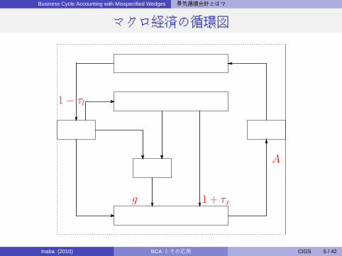
マクロ経済の循環図

家計企業

政府

生産

生産要素市場要素への支払

所得

財市場

消費

租税

金融市場

貯蓄

投資政府支出

財政赤字

売上1 + τx

1 − τl

g

A



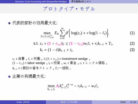
プロトタイプ・モデル

代表的家計の効用最大化:

max{ct ,ℓt ,it}∞t=0

E0

∞∑t=0

βt[log(ct) + ν log(1− ℓt)

], (1)

s.t. ct + (1+ τx,t)it ≤ (1− τℓ,t)wtℓt + rtkt−1 + Tt, (2)

kt = (1− δ)kt−1 + it, (3)

ct：消費，ℓt：労働，1/(1+ τx,t)：investment wedge，(1− τℓ,t)：labor wedge，it：投資，wt：賃金，r t：レンタル価格，

kt−1：t期初の資本ストック，Tt:一括税．

企業の利潤最大化:

maxkt−1,ℓt

Atkαt−1ℓ

1−αt − rtkt−1 − wtℓt.



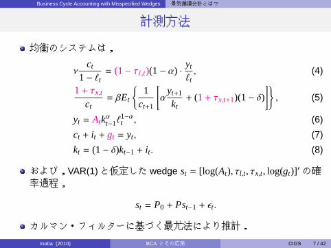
計測方法

均衡のシステムは，

νct

1− ℓt= (1− τℓ,t)(1− α) ·

yt

ℓt, (4)

1+ τx,t

ct= βEt

{1

ct+1

[α

yt+1

kt+ (1+ τx,t+1)(1− δ)

]}, (5)

yt = Atkαt−1ℓ

1−αt , (6)

ct + it + gt = yt, (7)

kt = (1− δ)kt−1 + it. (8)

および，VAR(1)と仮定した wedge st = [log(At), τl,t, τx,t, log(gt)]′の確率過程，

st = P0 + Pst−1 + ϵt.

カルマン・フィルターに基づく最尤法により推計．



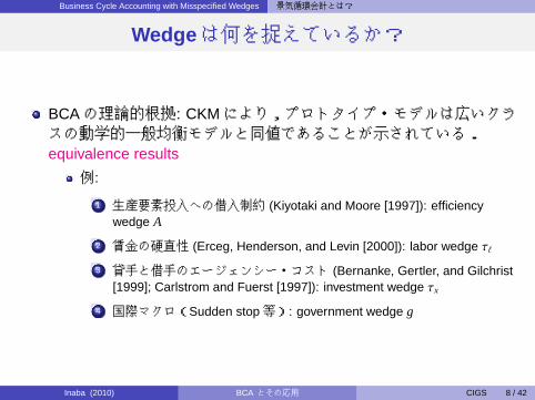
Wedgeは何を捉えているか？

BCAの理論的根拠: CKMにより，プロトタイプ・モデルは広いクラスの動学的一般均衡モデルと同値であることが示されている．equivalence results

例:

.

.

.

1 生産要素投入への借入制約 (Kiyotaki and Moore [1997]): efficiencywedge A

.

.

.

2 賃金の硬直性 (Erceg, Henderson, and Levin [2000]): labor wedge τℓ

.

.

.

3 貸手と借手のエージェンシー・コスト (Bernanke, Gertler, and Gilchrist[1999]; Carlstrom and Fuerst [1997]): investment wedge τx

.

.

.

4 国際マクロ（Sudden stop等）: government wedge g



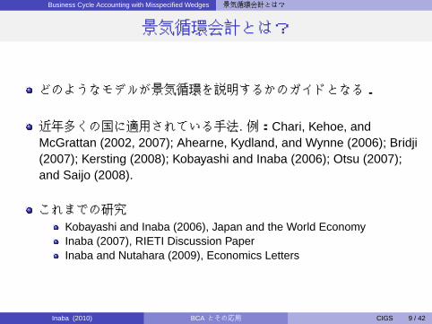
景気循環会計とは？

どのようなモデルが景気循環を説明するかのガイドとなる．

近年多くの国に適用されている手法. 例：Chari, Kehoe, andMcGrattan (2002, 2007); Ahearne, Kydland, and Wynne (2006); Bridji(2007); Kersting (2008); Kobayashi and Inaba (2006); Otsu (2007);and Saijo (2008).

これまでの研究Kobayashi and Inaba (2006), Japan and the World EconomyInaba (2007), RIETI Discussion PaperInaba and Nutahara (2009), Economics Letters


Business Cycle Accounting with Misspecified Wedges BCA の問題点と実証上の有効性

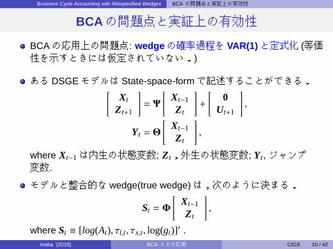
BCAの問題点と実証上の有効性

BCAの応用上の問題点: wedge の確率過程を VAR(1)と定式化 (等価性を示すときには仮定されていない．)

ある DSGEモデルは State-space-formで記述することができる．[Xt

Zt+1

]= Ψ

[Xt−1

Zt

]+

[0

Ut+1

],

Yt = Θ

[Xt−1

Zt

],

where Xt−1は内生の状態変数; Zt，外生の状態変数; Yt,ジャンプ変数.

モデルと整合的な wedge(true wedge)は，次のように決まる．

St = Φ

[Xt−1

Zt

],

where St ≡ [log(At), τl,t, τx,t, log(gt)]′ .

一方 BCAでは，Wedgeの確率過程が VAR(1)と定式化．Inaba (2010) BCA とその応用 CIGS 10 / 42


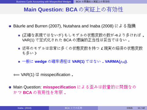
Main Question: BCA の実証上の有効性

Baurle and Burren (2007), Nutahara and Inaba (2008)による指摘

(正確な表現ではないが)もしモデルの状態変数の数が４より多ければ，VAR(1)で定式化された BCAの理論的正当性は妥当ではない．

近年のモデルは非常に多くの状態変数を持つ．（現実の経済の状態変数も多い）

一般に wedge の確率過程は VAR(1) ではない．VARMA( p,q).

⇐= VAR(1)はmisspecification．

Main Question: misspecification による歪みは数量的に問題なのか？ BCA の有用性を考察．



何を行ったか？：BCAの実証上の有用性を調べる．

.

..

1 あるたくさんの状態変数を持った動学的一般均衡モデルを用いる．

.

.

.

2 このモデルで発生させた人工データに BCAを適用.

.

.

.

3 BCAで測った wedgeについて，モデルの持つ trueの wedgeと比較（要因分解についても比較）

.

.

.

4 結果: それらのズレは小さく，応用上の問題点はあるものの BCAは有効である．



A DSGE model

Medium-scale DSGE economy a la Smets and Wouters (2007)

何故 SWのモデルなのか？

“State-of-the-art”で，政策シミュレーションに利用されるモデル

上述の BCAの理論的正当性が妥当しないケース

モデルの特徴

.

.

.

1 消費の習慣形成

.

.

.

2 投資の調整費用 (flow specification)

.

.

.

3 価格及び名目賃金の硬直性

.

.

.

4 資本稼働率

.

.

.

5 (forward-looking)テイラー・ルール

.

.

.

6 多くの外生ショック;技術ショック，投資特殊的技術ショック，リスク・プレミアム・ショック，マークアップ・ショック，財政政策のショック，金融政策のショック.



検証の手続き

Smets and Wouters (2007)モデルからデータを発生させる．10,000期間（250年）

データに BCAを適用．観測値： ct, it, ℓt, yt を利用Kalman filterに基づく MLwedgeの計測，GDPの要因分解

結果の比較trueと計測された wedgeとの値の比較wedgeによる GDPの要因分解の比較



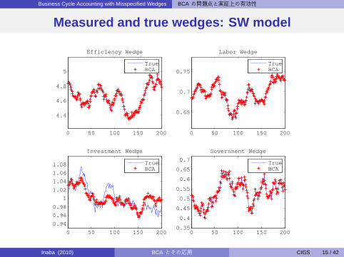
Measured and true wedges: SW model

0 50 100 150 200

4.4

4.6

4.8

5

Efficiency Wedge

TrueBCA

0 50 100 150 200

0.65

0.7

0.75

Labor Wedge

TrueBCA

0 50 100 150 200

0.94

0.96

0.98

1

1.02

1.04

1.06

1.08

Investment Wedge

TrueBCA

0 50 100 150 2000.35

0.4

0.45

0.5

0.55

0.6

0.65

0.7

Government Wedge

TrueBCA



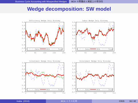
Wedge decomposition: SW model

0 50 100 150 2002.7

2.8

2.9

3

3.1

3.2

3.3

3.4

3.5

3.6Efficiency Wedge Only Economy

Data BCA True

0 50 100 150 2002.7

2.8

2.9

3

3.1

3.2

3.3

3.4

3.5

3.6Labor Wedge Only Economy

Data BCA True

0 50 100 150 2002.7

2.8

2.9

3

3.1

3.2

3.3

3.4

3.5

3.6Investment Wedge Only Economy

Data BCA True

0 50 100 150 2002.7

2.8

2.9

3

3.1

3.2

3.3

3.4

3.5

3.6Government Wedge Only Economy

Data BCA True



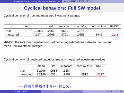
Cyclical behaviors: Full SW modelCyclical behavior of true and measured investment wedges

mean std autocorr. corr. w/ yt corr. w/ true RMSE

true 1.0003 .0258 .9651 -.2876 – –measured .9974 .0208 .9791 -.0858 .8449 .0141

∗RMSE: the root mean squared error of percentage-deviations between the true andmeasured investment wedges.

Cyclical behavior of predicted output by true and measured investment wedges

mean std autocorr. corr. w/ true RMSE

true 3.2206 .0554 .9384 – –measured 3.2146 .0361 .9702 .6812 .0127

=⇒両者の乖離は小さい (約１％).Inaba (2010) BCA とその応用 CIGS 17 / 42


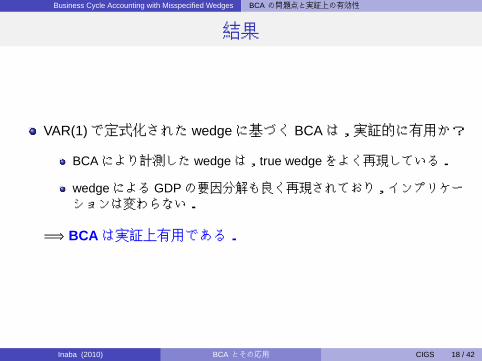
結果

VAR(1)で定式化された wedgeに基づく BCAは，実証的に有用か？

BCAにより計測した wedgeは，true wedgeをよく再現している．

wedgeによる GDPの要因分解も良く再現されており，インプリケーションは変わらない．

=⇒ BCA は実証上有用である．



実際の応用：Business cycle accounting による日米の比較


Business cycle accounting による日米の比較

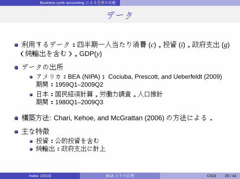
データ

利用するデータ：四半期一人当たり消費 (c)，投資 (i)，政府支出 (g)（純輸出を含む），GDP(y)

データの出所アメリカ：BEA (NIPA)； Cociuba, Prescott, and Ueberfeldt (2009)期間：1959Q1–2009Q2

日本：国民経済計算，労働力調査，人口推計期間：1980Q1–2009Q3

構築方法: Chari, Kehoe, and McGrattan (2006)の方法による．

主な特徴投資：公的投資を含む純輸出：政府支出に計上



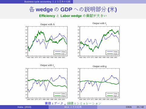
各wedge のGDPへの説明部分 (米)Efficiency と Labor wedge の貢献が大きい

1960 1965 1970 1975 1980 1985 1990 1995 2000 200524

25

26

27

28

29

30

31

32

33Output with A

YdataYeff

1960 1965 1970 1975 1980 1985 1990 1995 2000 200524

25

26

27

28

29

30

31

32

33

Output with τl

YdataYtaul

1960 1965 1970 1975 1980 1985 1990 1995 2000 200524

25

26

27

28

29

30

31

32

33

Output with τx

YdataYtaux

1960 1965 1970 1975 1980 1985 1990 1995 2000 200524

25

26

27

28

29

30

31

32

33Output with g

YdataYgov

青線：データ，緑線：シミュレーションInaba (2010) BCA とその応用 CIGS 21 / 42


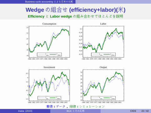
Wedgeの組合せ (efficiency+labor)( 米)Efficiency と Labor wedge の組み合わせでほとんどを説明

1960 1965 1970 1975 1980 1985 1990 1995 2000 2005

18

19

20

21

22

23

Consumption

Cdata

Cefflab

1960 1965 1970 1975 1980 1985 1990 1995 2000 2005

0.23

0.24

0.25

0.26

0.27

0.28

0.29

0.3

Labor

Ldata

Lefflab

1960 1965 1970 1975 1980 1985 1990 1995 2000 2005

3.5

4

4.5

5

5.5

6

6.5

Investment

Idata

Iefflab

1960 1965 1970 1975 1980 1985 1990 1995 2000 200524

25

26

27

28

29

30

31

32

Output

Ydata

Yefflab



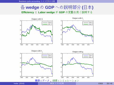
各wedge のGDPへの説明部分 (日本)Efficiency と Labor wedge が GDPの変動を良く説明する

1980 1985 1990 1995 2000 200510

11

12

13

14

15Output with A

YdataYeff

1980 1985 1990 1995 2000 200510

11

12

13

14

15

Output with τl

YdataYtaul

1980 1985 1990 1995 2000 200510

11

12

13

14

15

Output with τx

YdataYtaux

1980 1985 1990 1995 2000 200510

11

12

13

14

15Output with g

YdataYgov



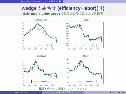
wedge の組合せ (efficiency+labor)( 日)Efficiency と Labor wedge の組み合わせでほとんどを説明

1980 1985 1990 1995 2000 2005

6

6.2

6.4

6.6

6.8

7

7.2

7.4

7.6

Consumption

Cdata

Cefflab

1980 1985 1990 1995 2000 2005

0.28

0.29

0.3

0.31

0.32

0.33

0.34

0.35

0.36

0.37

Labor

Ldata

Lefflab

1980 1985 1990 1995 2000 20051.5

2

2.5

3

3.5

4

4.5

5

5.5

Investment

Idata

Iefflab

1980 1985 1990 1995 2000 2005

10

11

12

13

14

15

Output

Ydata

Yefflab



まとめ

GDPの変動は，efficiency wedgeと labor wedgeによりほとんど説明される．

investment wedgeおよび government wedgeは，ほとんど説明力を持たない．

BCAによる実証結果から，efficiency wedge以外に labor wedgeが重要であると判断できる．


Collateral constraint as an amplification mechanism

Collateral constraint as an amplification mechanismjoint with Keiichiro Kobayashi

日本経済学会　秋季大会報告論文


Collateral constraint as an amplification mechanism Introduction

Introduction

問い：金融制約は，景気変動を増幅するか？

先行研究：消費の平準化を目的とした借入に担保制約Kiyotaki and Moore (1997)：増幅する

Kocherlakota (2000) and Cordoba and Ripoll (2004)：通常の関数形およびパラメーターでは増幅しない．

本稿では，

生産要素支払い（特に労働）へ担保制約を導入（labor wedgeが生じ，BCAの実証結果と整合的）

通常のパラメーターで，景気変動の増幅を示した.

意義：景気循環における担保制約の量的な重要性を指摘.


Collateral constraint as an amplification mechanism Introduction

関連するこれまでの研究

Kobayashi and Inaba, (2006), ”Irrational exuberance’ in the PigouCycle under Collateral Constraints”

Kobayashi and Inaba, (2006), ”Borrowing Constraints and ProtractedRecessions”

Kobayashi and Inaba, (2007), ”Debt-Ridden Equilibria”

Kobayashi, Nakajima, and Inaba, (2010), ”Collateral Constraint andNews Driven Cycles”


Collateral constraint as an amplification mechanism 先行研究

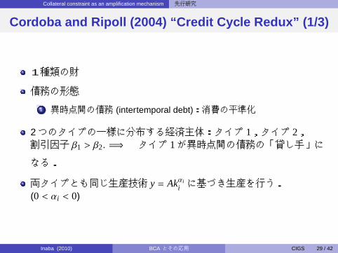
Cordoba and Ripoll (2004) “Credit Cycle Redux” (1/3)

１種類の財

債務の形態

.

.

.

1 異時点間の債務 (intertemporal debt)：消費の平準化

2つのタイプの一様に分布する経済主体：タイプ 1，タイプ 2，割引因子 β1 > β2. =⇒ 　タイプ 1が異時点間の債務の「貸し手」に

なる．

両タイプとも同じ生産技術 y = Akαii に基づき生産を行う．

(0 < αi < 0)



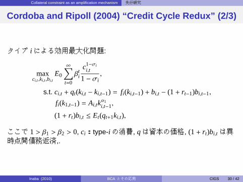
Cordoba and Ripoll (2004) “Credit Cycle Redux” (2/3)

タイプ iによる効用最大化問題:

maxci,t ,ki,t ,bi,t

E0

∞∑t=0

βti

c1−σii,t

1− σi,

s.t. ci,t + qt(ki,t − ki,t−1) = fi(ki,t−1) + bi,t − (1+ rt−1)bi,t−1,

fi(k1,t−1) = Ai,tkα1i,t−1,

(1+ rt)bi,t ≤ Et(qt+1ki,t),

ここで 1 > β1 > β2 > 0, ci：type-iの消費, qは資本の価格, (1+ rt)bi,tは異時点間債務返済,.



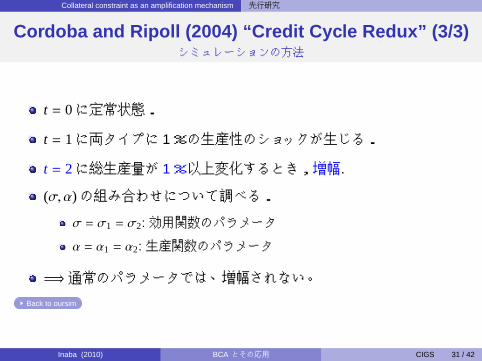
Cordoba and Ripoll (2004) “Credit Cycle Redux” (3/3)シミュレーションの方法

t = 0に定常状態．

t = 1に両タイプに 1％の生産性のショックが生じる．

t = 2に総生産量が 1％以上変化するとき，増幅.

(σ, α)の組み合わせについて調べる．

σ = σ1 = σ2: 効用関数のパラメータ

α = α1 = α2: 生産関数のパラメータ

=⇒通常のパラメータでは、増幅されない。

..

Back to oursim


Collateral constraint as an amplification mechanism 本稿のモデル

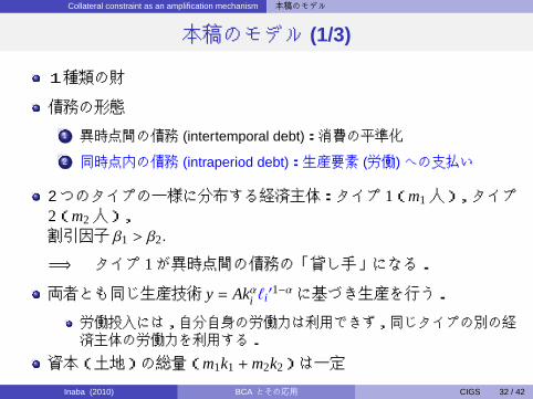
本稿のモデル (1/3)

１種類の財

債務の形態

.

..

1 異時点間の債務 (intertemporal debt)：消費の平準化

.

.

.

2 同時点内の債務 (intraperiod debt)：生産要素 (労働)への支払い

2つのタイプの一様に分布する経済主体：タイプ 1（m1人），タイプ2（m2人），割引因子 β1 > β2.

=⇒ 　タイプ 1が異時点間の債務の「貸し手」になる．

両者とも同じ生産技術 y = Akαi ℓi′1−αに基づき生産を行う．

労働投入には，自分自身の労働力は利用できず，同じタイプの別の経済主体の労働力を利用する．

資本（土地）の総量（m1k1 +m2k2）は一定



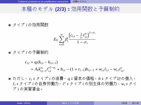
本稿のモデル (2/3)：効用関数と予算制約

タイプ iの効用関数

E0

∞∑t=0

βti

(ci,t − 1

γiℓγii,t

)1−σi

1− σi

タイプ iの予算制約

ci,t + qt(ki,t − ki,t−1)

= Atkαii,t−1ℓ

′1−αii,t + bi,t − (1+ rt−1)bi,t−1 + wi,tℓi,t − wi,tℓ

′i,t.

ただし、ci：タイプ iの消費、q：資本の価格、b：タイプ２の借入、ℓi：タイプ iの自身労働力、ℓ′：タイプ iの別主体の労働力、wi：タイプ iの実質賃金。



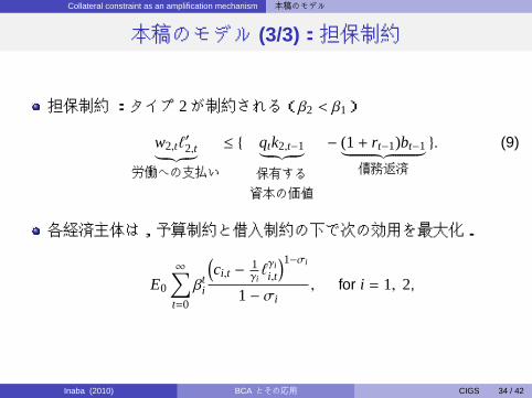
本稿のモデル (3/3)：担保制約

担保制約：タイプ 2が制約される（β2 < β1）

w2,tℓ′2,t︸︷︷︸

労働への支払い

≤ { qtk2,t−1︸︷︷︸保有する

資本の価値

− (1+ rt−1)bt−1︸︷︷︸債務返済

}. (9)

各経済主体は，予算制約と借入制約の下で次の効用を最大化．

E0

∞∑t=0

βti

(ci,t − 1

γiℓγii,t

)1−σi

1− σi, for i = 1, 2,


Collateral constraint as an amplification mechanism シミュレーション

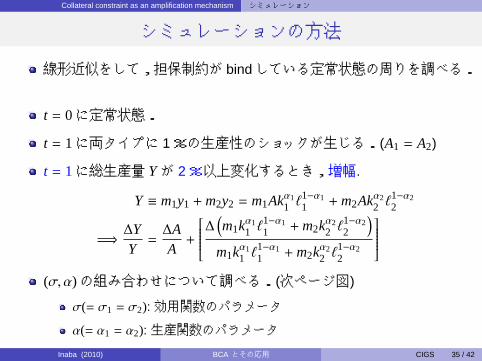
シミュレーションの方法

線形近似をして，担保制約が bindしている定常状態の周りを調べる．

t = 0に定常状態．

t = 1に両タイプに 1％の生産性のショックが生じる．(A1 = A2)

t = 1に総生産量 Yが 2％以上変化するとき，増幅.

Y ≡ m1y1 +m2y2 = m1Akα11 ℓ

1−α11 +m2Akα2

2 ℓ1−α22

=⇒ ∆YY=∆AA+

∆(m1kα1

1 ℓ1−α11 +m2kα2

2 ℓ1−α22

)m1kα1

1 ℓ1−α11 +m2kα2

2 ℓ1−α22

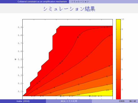
(σ, α)の組み合わせについて調べる．(次ページ図)

σ(= σ1 = σ2): 効用関数のパラメータ

α(= α1 = α2): 生産関数のパラメータ



シミュレーション結果

2.52.52.5

2.5

2.5

2.5

2.5

333

3

3

3

3

444

4

4

4

55

5

5

5

77

7

7

1010

10

σ

α

0.5 1 1.5 2 2.5 3 3.5 4

0.1

0.2

0.3

0.4

0.5

0.6

0.7

0.8

0.9

3

4

5

6

7

8

9

10

Figure: Region where the elasticity to the TFP shock is greater than 2.

Notes: The utility function is the same as that of CR.



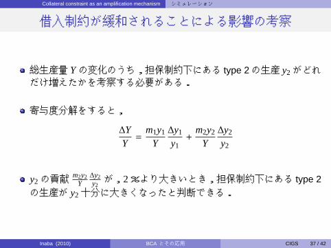
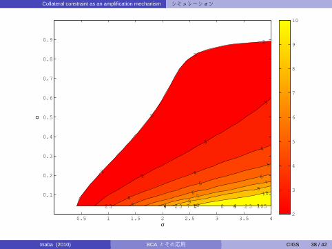
借入制約が緩和されることによる影響の考察

総生産量 Yの変化のうち，担保制約下にある type 2の生産 y2がどれだけ増えたかを考察する必要がある．

寄与度分解をすると，

∆YY=

m1y1

Y∆y1

y1+

m2y2

Y∆y2

y2

y2の貢献m2y2

Y∆y2y2が，2％より大きいとき，担保制約下にある type 2

の生産が y2十分に大きくなったと判断できる．



222

2

2

2

2

333

3

3

3

44

4

4

4

555

5

5

66

6

6

77

7

7

88

8

1010

10

σ

α

0.5 1 1.5 2 2.5 3 3.5 4

0.1

0.2

0.3

0.4

0.5

0.6

0.7

0.8

0.9

2

3

4

5

6

7

8

9

10

Figure: Region where the contribution of y2 is more than two.Inaba (2010) BCA とその応用 CIGS 38 / 42


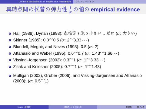
異時点間の代替の弾力性 1σの値の empirical evidence

Hall (1988), Dynan (1993): 点推定（米）小さい，ゼロ (σ: 大きい)

Skinner (1985): 0.3～0.5 (σ: 2～3.33· · · )Blundell, Meghir, and Neves (1993): 0.5 (σ: 2)

Attanasio and Weber (1995): 0.6～0.7 (σ: 1.43～1.66· · · )Vissing-Jorgensen (2002): 0.3～1 (σ: 1～3.33· · · )Ziliak and Kniesner (2005): 0.7～1 (σ: 1～1.43)

Mulligan (2002), Gruber (2006), and Vissing-Jorgensen and Attanasio(2003): (σ: 0.5～1)


Collateral constraint as an amplification mechanism 結論

結論

金融制約は，景気循環を増幅し得る．

景気循環における担保制約の量的な重要性を指摘．

特に，生産要素支払への担保制約の重要性．


今後の研究

Outline

.

. .1 Business Cycle Accounting with Misspecified Wedges

景気循環会計とは？BCAの問題点と実証上の有効性

.

. .

2 Business cycle accountingによる日米の比較

.

. .

3 Collateral constraint as an amplification mechanismIntroduction先行研究本稿のモデルシミュレーション結論

.

. .

4 今後の研究


今後の研究

今後の研究

BCAを国際経済版に拡張し，international macroeconomicsのモデルの同定への利用の可能性を探る．

BCAに投資特殊的技術進歩，または非定常性なショックを導入し，それらのショックが景気循環に与える影響を考察する．

Occasionally Binding Collateral Constraint:

担保制約が bindしたり，しなかったりといった occasionally bindingを考慮することで，より大きな増幅効果を期待できる．

上記モデルに基づいて，ベイズ推定によってマクロデータからパラメータを推計し，現実の景気変動に金融制約がどの程度有効であったかをモデルベースで実証分析を行う．
