
GRS - A - 3234
Validierung von Com-putational Fluid Dynamics Methoden für Reaktorsicher-heitsanalysen (ECORA) Abschlussbericht
Gesellschaft für Anlagen-und Reaktorsicherheit (GRS) mbH
Abschlussbericht/ Final Report Reaktorsicherheitsforschungs-Vorhabens Nr.:/ Reactor Safety Research-Project No.:
RS 1135 Vorhabenstitel / Project Title:
Validierung von Computational Fluid Dynamics Methoden für Reaktorsicherheitsanalysen (ECORA) Evaluation of Computational Fluid Dynamics Methods for Reactor Safety Analysis (ECORA) Autor / Authors:
M. Scheuerer
Berichtszeitraum / Publication Date: November 2004
Anmerkung: Das diesem Bericht zugrunde lie-gende F&E-Vorhaben wurde im Auftrag des Bundesministeriums für Wirtschaft und Arbeit (BMWA) unter dem Kennzeichen RS 1135durchgeführt. Die Verantwortung für den Inhalt dieser Veröffentlichung liegt beim Auftragnehmer.
GRS - A - 3234
I
Kurzfassung
Im Rahmen der Reaktorsicherheitsforschung des BMWA, Forschungsschwerpunkt
"Transientenanalyse und Unfallabläufe" wurde das Vorhaben RS 1135 mit dem Titel
„Validierung von Computational Fluid Dynamic Methoden für Reaktoranalysen
(ECORA)“ durchgeführt. Dieses Vorhaben ist Teilprojekt eines Vorhabens der
Europäischen Union auf Kostenteilungsbasis „ECORA, Evaluation of Computational
Fluid Dynamics Methods for Reactor Safety Analysis“ im 5. EU-Rahmenprogramm. Die
Ergebnisse des Projekts stehen auf der ECORA-Webseite unter
http://domino.grs.de/ecora/ecora.nsf zur Verfügung
Ziel der Vorhaben ECORA und RS1135 ist es, die Anwendungsmöglichkeiten und
Leitungsfähigkeit von Computational Fluid Dynamics (CFD) Software-Programmen zu
ermitteln, Strömungen und Wärmeübergangsvorgänge im Primärkreis und im
Sicherheitsbehälter von Kernreaktoren zu simulieren. Dreidimensionale Strömungs-
effekte in diesen Kraftwerkskomponenten haben große Bedeutung und können von
den klassischen Systemcodes nur beschränkt simuliert werden. Daher wurden im
Forschungsvorhaben ECORA-RS1135 Anwendungsbereiche detaillierter dreidimensio-
naler CFD-Rechnungen ermittelt und Empfehlungen für die Verbesserung der Modelle
erarbeitet.
Die Bewertung der CFD Softwarepakete beinhaltet die Ermittlung und Einführung von
Richtlinien zur Anwendung (Best Practice Guidelines, BPG) und legt Standards für die
Anwendung von CFD-Software und die Bewertung von CFD-Ergebnissen für
Sicherheitsanalysen fest. Damit ist auf europäischer Ebene eine Basis für eine
optimale Anwendung von CFD Verfahren und die formale Beurteilung von CFD
Berechnungen festgelegt. Die BPG-Regeln werden im Laufe des Projekts für die CFD-
Strömungsberechnungen im Primärsystem und im Sicherheitsbehälter von
Kernreaktoren angewendet.
II
Es wurde eine umfassende Bewertung bereits vorhandener CFD Simulationen
dreidimensionaler Strömungen im LWR Primärkreis und deren Validierung anhand von
experimentellen Daten durchgeführt, Modelle zur verbesserten Simulation von PTS-
Phänomenen ausgewählt und in das CFX- and NEPTUNE Programm implementiert.
Zur Veranschaulichung der CFD Programm-Optimierung für PTS-Analysen durch
Implementierung und Validierung verbesserter Turbulenz- und Zweiphasenmodelle
wurden qualitätskontrollierte CFD Simulationen für ausgewählte UPTF-Experimente
berechnet. Darüber hinaus wurden CFD-Analysen im Reaktorsicherheitsbehälter für
ausgewählte SETH-PANDA Experiment durchgeführt. Die Erfahrungen und Ergebnisse
wurden schließlich in einer umfassenden Bewertung von CFD-Anwendungen auf dem
Gebiet der Reaktorsicherheit zusammengefasst und dokumentiert.
III
Abstract
In the frame of reactor safety research of BMWA, with emphasis on “Transient and
accident analysis”, the project “RS 1135” was financed with the title: “Evaluation of
Computational Fluid Dynamics Methods for Reactor Safety Analysis (ECORA)”. It is
part of the European project on the basis of a shared cost action in the frame of the 5th
European framework programme. The project results are made availabe via internet at
http://domino.grs.de/ecora/ecora.nsf.
The objective of the ECORA project is to evaluate the capabilities of Computational
Fluid Dynamics (CFD) software packages for simulating flows in the primary system
and containment of nuclear reactors. The interest in the application of CFD methods
arises from the importance of three-dimensional flow effects in these reactor
components, which one-dimensional system codes cannot predict. Therefore, the
ECORA project will identify application areas for detailed three-dimensional CFD
calculations and make recommendations for software improvements.
The software assessment includes the establishment of Best Practice Guidelines
(BPG) and standards regarding the use of CFD software and the evaluation of CFD
results for safety analysis. Quality criteria for the application of CFD software are
standardised. CFD results are only accepted after these quality criteria are satisfied.
Thus, a general basis for assessing merits and weaknesses of particular models and
codes is formed on a European basis. CFD simulations having an accepted quality
level will increase confidence in the application of CFD-tools.
In addition, a comprehensive and systematic software engineering approach for
extending and customising CFD codes for nuclear safety analyses has been
formulated and applied. The adaptation of CFD software for nuclear reactor flow
simulations is shown by implementing enhanced two-phase flow, turbulence, and
energy transfer models relevant for Pressurized Thermal Shock (PTS) applications into
the CFX, and Neptune software. An analysis of selected UPTF and PANDA
experiments was performed to validate CFD software in relation to PTS phenomena in
the primary system and severe accident management in the containment.

IV
V
Inhaltsverzeichnis
1 Vorbemerkung........................................................................................... 1
2 Einleitung................................................................................................... 2
3 Arbeitsprogramm ...................................................................................... 4
4 Durchgeführte Arbeiten............................................................................ 6
5 Zusammenfassung und Schlussfolgerung........................................... 12
6 Abbildungen ............................................................................................ 13
7 Literatur.................................................................................................... 18
7.1 Vorhabensberichte (Deliverables) ............................................................. 18
7.2 Veröffentlichungen .................................................................................... 20
8 Verteiler.................................................................................................... 23
Anhang Final Technical Report

1
1 Vorbemerkung
Im Rahmen der Reaktorsicherheitsforschung des BMWA, Forschungsschwerpunkt
"Transientenanalyse und Unfallabläufe" wurde das Vorhaben „RS 1135“ mit dem Titel
„Validierung von Computational Fluid Dynamic Methoden für Reaktoranalysen“
durchgeführt. Dieses Vorhaben ist Teilprojekt eines Vorhabens der Europäischen
Union auf Kostenteilungsbasis „ECORA, Evaluation of Computational Fluid Dynamics
Methods for Reactor Safety Analysis“ im 5. EU-Rahmenprogramm.
Am Vorhaben waren 12 Partner beteiligt: GRS als Projekt-Koordinator, AEA
Technology GmbH (Deutschland), Serco Insurances plc (Großbritannien), Atomic
Energy Research Institute (Ungarn), Commissariat a l'Energie Atomique (Frankreich),
Groupe Electricite de France (Frankreich), Forschungszentrum Rossendorf (Deutsch-
land), Nuclear Research and Consultancy Group (Niederlande), Nuclear Research In-
stitute Rez plc (Tschechische Republik), Paul Scherrer Institut (Schweiz), Vattenfall Ut-
veckling AB (Schweden), VTT Processes (Finnland).
Die Vorhaben ECORA und RS1135 begannen am 31.10.2001 und sollten am
30.9.2004 enden. Das EU-Vorhaben ECORA wurde bis 31.12.2004 verlängert.
Abweichend davon wurde das BMWA-Vorhaben RS 1135 nur bis 30.11.2004
verlängert. Zum Vorhaben gibt es einen ausführlichen Abschlussbericht, der in der
vollständigen Originalversion beiliegt.
2
2 Einleitung
Im Rahmen des Vorhabens ECORA - RS1135 wurden Computational Fluid Dynamics
(CFD) Programme für Anwendungen auf dem Gebiet der Reaktorsicherheit umfassend
bewertet. Zu diesem Zweck wurden Richtlinien (Best Practice Guidelines, BPG) zur
optimalen Handhabung und Weiterentwicklung und zum effizienten Einsatz von CFD
Verfahren erarbeitet, und künftige Anwendungsbereiche dreidimensionaler Strömungs-
berechnungen identifiziert. Es wurde eine umfassende Bewertung bereits vorhandener
CFD Simulationen dreidimensionaler Strömungen im LWR Primärkreis und deren
Validierung anhand von experimentellen Daten durchgeführt. PTS-Phänomene und
deren Modellierung werden im Detail untersucht. Es wuden Modelle zur verbesserten
Simulation von PTS-Phänomenen ausgewählt und in das CFX-Programm
implementiert. Die Handhabung des Programms wurde speziell für die Anwendung auf
dem Gebiet der Reaktorsicherheit angepasst. Zur Veranschaulichung der CFD
Programm-Optimierung für PTS-Analysen wurden verbesserte Turbulenz- und
Zweiphasenmodelle implementiert und validiert und qualitätskontrollierte CFD
Simulationen für ausgewählte UPTF-Experimente durchgeführt.
Um dieses Ziel zu erreichen, wurden im Prokjekt die folgenden messbaren
Arbeitsschritte durchgeführt:
• Festlegung von Richtlinien (BPGs) für die optimale Anwendung von CFD-Verfahren
und die formale Beurteilung von CFD-Berechnungen und Experimenten. In diesem
Arbeitsschritt wurde die Grundlage für eine konsistente und systematische
Vorgehensweise bei der Bewertung und Interpretation von CFD-Berechnungen
gelegt. Die BPG-Regeln wurden im Laufe des Projekts für die CFD-
Strömungsberechnungen im Primärsystem und im Sicherheitsbehälter von
Kernreaktoren angewendet.
• Bewertung der Möglichkeiten, Schwierigkeiten und Grenzen von CFD-Methoden
zur Strömumgsberechnung im Primärsystem und im Sicherheitsbehälter von
Leichtwasserreaktoren, mit Schwerpunkt der Untersuchungen auf Vermischungs-
phänomene unter PTS-Bedingungen
• Festlegung von Anforderungen an Experimente für die Verifikation und Validierung
von CFD-Programmen für Strömungen im Primärsystem und im Sicherheitsbehälter
von Leichtwasserreaktoren
• Identifizierung, Implementierung und Validierung verbesserter Turbulenz- und
Zweiphasenmodelle für die Simulation von PTS-Phänomenen im Primärkreis von
Druckwasserreaktoren
3
• Die Erfahrungen und Ergebnisse wurden schließlich in einer umfassenden
Bewertung von CFD-Anwendungen auf dem Gebiet der Reaktorsicherheit
zusammengefasst und dokumentiert. Dabei werden auch der Bedarf und Leitlinien
für zukünftige CFD-Entwicklungen vorgegeben
Das Forschungsvorhaben verbesserte das Verständnis der Möglichkeiten, aber auch
der Einschränkungen von CFD und war nützlich, die Möglichkeiten von CFD in
realistischem Licht zu sehen. Die Ergebnisse von ECORA-RS1135 werden im Projekt
NURESIM des 6. europäischen Rahmenprogramms weiterverwendet. Die
Verbesserung an den Modellen und Rechenprogrammteilen sind in den Codes CFX-5
und NEPTUNE implementiert. Diese CFD-Systeme sind öffentlich verfügbar. die Pro-
jektergebnisse stehen auf der ECORA-Webseite zur Verfügung unter
http://domino.grs.de/ecora/ecora.nsf.
4
3 Arbeitsprogramm
Das Vorhaben ECORA-RS1135 begann mit der Festlegung von Richtlinien für die
korrekte Anwendung (Best Practice Guidelines, BPG) von CFD-Codes und die
Beurteilung von Rechenergebnissen und von experimentellen Daten. Die Regeln, die
in diesem Arbeitspaket 1 (WP 1) aufgestellt wurden, verhalfen zu einem
systematischen und konsistenten Ansatz zur Begutachtung, Interpretation und
Bewertung von CFD-Ergebnissen für Strömungen im Primärkreis und im
Sicherheitsbehälter von Kernreaktoren.
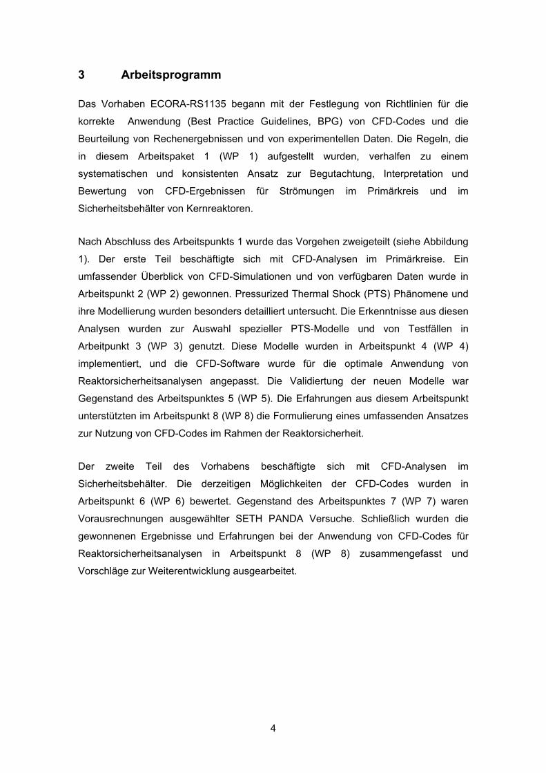
Nach Abschluss des Arbeitspunkts 1 wurde das Vorgehen zweigeteilt (siehe Abbildung
1). Der erste Teil beschäftigte sich mit CFD-Analysen im Primärkreise. Ein
umfassender Überblick von CFD-Simulationen und von verfügbaren Daten wurde in
Arbeitspunkt 2 (WP 2) gewonnen. Pressurized Thermal Shock (PTS) Phänomene und
ihre Modellierung wurden besonders detailliert untersucht. Die Erkenntnisse aus diesen
Analysen wurden zur Auswahl spezieller PTS-Modelle und von Testfällen in
Arbeitpunkt 3 (WP 3) genutzt. Diese Modelle wurden in Arbeitspunkt 4 (WP 4)
implementiert, und die CFD-Software wurde für die optimale Anwendung von
Reaktorsicherheitsanalysen angepasst. Die Validiertung der neuen Modelle war
Gegenstand des Arbeitspunktes 5 (WP 5). Die Erfahrungen aus diesem Arbeitspunkt
unterstützten im Arbeitspunkt 8 (WP 8) die Formulierung eines umfassenden Ansatzes
zur Nutzung von CFD-Codes im Rahmen der Reaktorsicherheit.
Der zweite Teil des Vorhabens beschäftigte sich mit CFD-Analysen im
Sicherheitsbehälter. Die derzeitigen Möglichkeiten der CFD-Codes wurden in
Arbeitspunkt 6 (WP 6) bewertet. Gegenstand des Arbeitspunktes 7 (WP 7) waren
Vorausrechnungen ausgewählter SETH PANDA Versuche. Schließlich wurden die
gewonnenen Ergebnisse und Erfahrungen bei der Anwendung von CFD-Codes für
Reaktorsicherheitsanalysen in Arbeitspunkt 8 (WP 8) zusammengefasst und
Vorschläge zur Weiterentwicklung ausgearbeitet.
5
Abbildung 1: Projektstruktur
WP 8: CFD-Bewer-tung und Weiterent-wicklung
WP 1: Best Practice Guidelines
WP 2: Analysen im Primärkreis
WP 3: Modelle und Testfälle
WP 4: Software Entwicklung
WP 5: Software Validierung, UPTF Experimente
WP 6: Analysen im Containment
WP 7: Voraus-rechnung SETH-PANDA Versuche
6
4 Durchgeführte Arbeiten
Die GRS ist Koordinator des gesamten ECORA Projektes, an dem 12 Partner aus 9
europäischen Ländern beteiligt sind. Die Aufgaben des Koordinators beinhaltet die
fachliche und administrative Koordination des Vorhabens. Im Rahmen dieser Aufgabe
wurde das ECORA Projekt als ersters europäisches Projekt ISO 9001:2000 zertifiziert.
Darüberhinaus hat die GRS wesentliche Beiträge zur Auswahl von PTS-relevanten
Modellen und Testfällen in WP3, zur Berechnung von Validierungstestfällen in WP4
und WP5, zur Bewertung vorhandener CFD-Simulationen für Containmentströmungen
und zur Vorausrechnung von ausgewählten PANDA SETH Experimenten in WP8
geleistet.
Eines der wichtigsten Ziele im ECORA Projekt ist die Erarbeitung von Richtlinien zur
optimalen Handhabung und Weiterentwicklung und zum effizienten Einsatz von CFD
Verfahren. Die ECORA BPGs wurden zu Beginn des Projekts erstellt, siehe /1/. Sie
wurden im Laufe des Projekts konsequent für die CFD-Berechnungen von Strömungen
im Primärsystem und im Sicherheitsbehälter von Kernreaktoren angewendet und auf
Grund der gewonnenen Erfahrungen aktualisiert. Die Koordinatoren der EU-Projekte
ERCOFTAC/QNET-CFD, FLOMIX-R, ASTAR und ITEM haben Kopien der ECORA
BPGs erhalten mit der Vereinbarung, ihre Erfahrungen bei der Anwendung der BPGs
in eine Verbesserung der Richtlinien einfließen zu lassen. Die Teilnahme der ECORA
Partner in der gemeinsam koordinierten ASTAR Konferenz, die am 17. – 18.
September 2003 bei der GRS stattfand, vertiefte den Erfahrungsaustausch. Ein
gemeinsames Arbeitstreffen von ECORA und FLOMIX-R fand am 15. – 16. März 2004
statt. Darüber hinaus wurde die GRS als Koordinator eingeladen, ECORA und die
BPGs im Rahmen der Abschlusskonferenz des EU-Projekts QNET-CFD vorzustellen.
Weiterhin ist die GRS in der OECD/NEA Arbeitsgruppe „CFD Issues“ vertreten. Die
OECD will Richtlinien für die Anwendung von CFD in der Reaktorsicherheit
veröffentlichen, die sich stark an den ECORA BPGs anlehnen.
Ein umfassender Bericht über vorhandene CFD Analysen im Primärkreis von LWR
wurde erstellt, siehe /2/. Die behandelten Themen sind: CFD Simulationen von
Strömungen im Reaktorkern, Borvermischung und asymmetrischer Loop - Betrieb, PTS
und andere Anwendungen von CFD-Programmen zur Simulation der Thermo-Hydraulik
im Reaktorkühlsystem. Verschiedene Turbulenzmodelle und numerischer Verfahren
wurden bewertet und der Bedarf für effizientere Modelle und Algorithmen wurde
diskutiert. Analog dazu fasst der Übersichtsbericht „Review of Experimental Data Base
7
on Mixing in Primary Loop Applications and Future Needs“ /3/ Experimente zusammen,
die zur Untersuchung der Kühlmittelvermischung im Primärkreis von Kernreaktoren
ausgeführt wurden. Der Bericht „Review of Two-Phase Flow Modelling Capabilities and
Recommendations“ /4/ umfasst die Beschreibung prinzipieller Ansätze für die
Modellierung von Zweiphasenströmungen und die Realisierung der Modelle in den
kommerziellen CFD-Programmen CFX. FLUENT, STAR-CD, PHOENIX, und im „in-
house“ Code NEPTUNE. Die Möglichkeiten von CFD-Analysen in der
Reaktorsicherheit und deren Anforderungen an physikalische Modelle und numerische
Verfahren wurden unter Einbeziehung der Schlussfolgerungen aus dem EURO-
FASTNET Projekt und den neuesten OECD/NEA Übersichtsberichten zu diesem
Thema zusammengestellt.
Die wichtigsten physikalischen Phänomene, die die Temperaturverteilung in der Wand
des Reaktordruckbehälters bestimmen, einschließlich der Zweiphasen-,
Phasenübergangs- und Turbulenz-Effekte wurden identifiziert und in /5/ dokumentiert.
Der Bericht beinhaltet eine Liste relevanter PTS-Phänomene, eine Tabelle
ausgewählter Testfälle und eine Zuordnung der Testfälle zu den jeweiligen ECORA
Partnern. Die Testfälle sind in Einzeleffekt-Test unterteilt, die zur ersten Verifikation
und Validierung von CFD-Programmen eingesetzt werden. Testfälle mit kombinierten
Phänomenen beinhalten dagegen bereits industriell relevante Geometrien und
Randbedingungen.
Ausgewählte physikalische Modelle, die zur Simulation von PTS-relevanten
Zweiphasenströmungen mit Phasenübergang und freien Oberflächen benötigt werden,
sind ausführlich im Bericht „Selection of PTS-Relevant Verification Physical Models“
(siehe /6/) beschrieben. Diese Modelle sind die Ausgangsbasis für die Simulation der
ECORA Testfälle.
Es wurden zwei Verifikationstestfälle VER01: „Oscillating Manometer“ und VER02:
„Liquid Sloshing“ mit den CFD-Programmen CFX und NEPTUNE nachgerechnet.
Beide Testfälle behandeln Zweiphasenströmungen mit freien Oberflächen und ohne
Phasenübergang. Sie dienen in erster Linie der Verifikation, d.h. der Überprüfung der
korrekten Implementierung und der Robustheit des numerischen Verfahrens, siehe /7/.
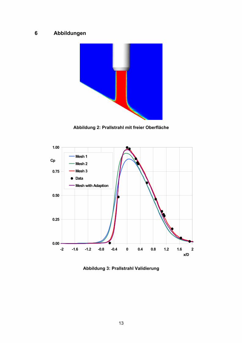
Die Ergebnisse und Bewertungen der Validierungstestfälle ECORA VAL01, VAL02,
VAL03 und VAL04 wurden in /8/ dokumentiert. Die Berechnungen für den Testfall
VAL03 wurden von der GRS mit dem CFD-Programm CFX-5 durchgeführt. Es handelt
8
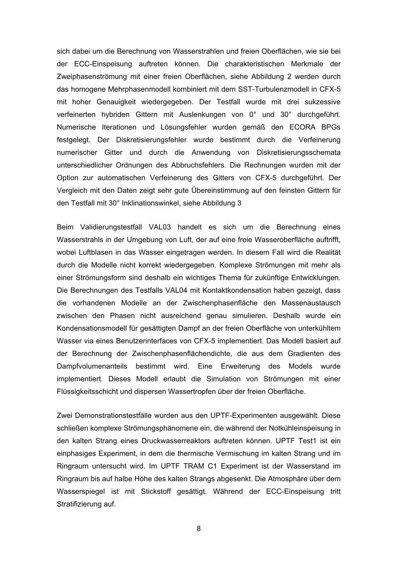
sich dabei um die Berechnung von Wasserstrahlen und freien Oberflächen, wie sie bei
der ECC-Einspeisung auftreten können. Die charakteristischen Merkmale der
Zweiphasenströmung mit einer freien Oberflächen, siehe Abbildung 2 werden durch
das homogene Mehrphasenmodell kombiniert mit dem SST-Turbulenzmodell in CFX-5
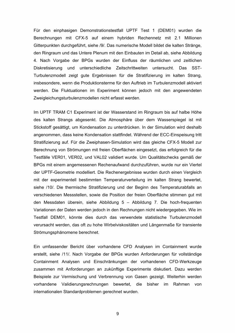
mit hoher Genauigkeit wiedergegeben. Der Testfall wurde mit drei sukzessive
verfeinerten hybriden Gittern mit Auslenkungen von 0° und 30° durchgeführt.
Numerische Iterationen und Lösungsfehler wurden gemäß den ECORA BPGs
festgelegt. Der Diskretisierungsfehler wurde bestimmt durch die Verfeinerung
numerischer Gitter und durch die Anwendung von Diskretisierungsschemata
unterschiedlicher Ordnungen des Abbruchsfehlers. Die Rechnungen wurden mit der
Option zur automatischen Verfeinerung des Gitters von CFX-5 durchgeführt. Der
Vergleich mit den Daten zeigt sehr gute Übereinstimmung auf den feinsten Gittern für
den Testfall mit 30° Inklinationswinkel, siehe Abbildung 3
Beim Validierungstestfall VAL03 handelt es sich um die Berechnung eines
Wasserstrahls in der Umgebung von Luft, der auf eine freie Wasseroberfläche auftrifft,
wobei Luftblasen in das Wasser eingetragen werden. In diesem Fall wird die Realität
durch die Modelle nicht korrekt wiedergegeben. Komplexe Strömungen mit mehr als
einer Strömungsform sind deshalb ein wichtiges Thema für zukünftige Entwicklungen.
Die Berechnungen des Testfalls VAL04 mit Kontaktkondensation haben gezeigt, dass
die vorhandenen Modelle an der Zwischenphasenfläche den Massenaustausch
zwischen den Phasen nicht ausreichend genau simulieren. Deshalb wurde ein
Kondensationsmodell für gesättigten Dampf an der freien Oberfläche von unterkühltem
Wasser via eines Benutzerinterfaces von CFX-5 implementiert. Das Modell basiert auf
der Berechnung der Zwischenphasenflächendichte, die aus dem Gradienten des
Dampfvolumenanteils bestimmt wird. Eine Erweiterung des Models wurde
implementiert. Dieses Modell erlaubt die Simulation von Strömungen mit einer
Flüssigkeitsschicht und dispersen Wassertropfen über der freien Oberfläche.
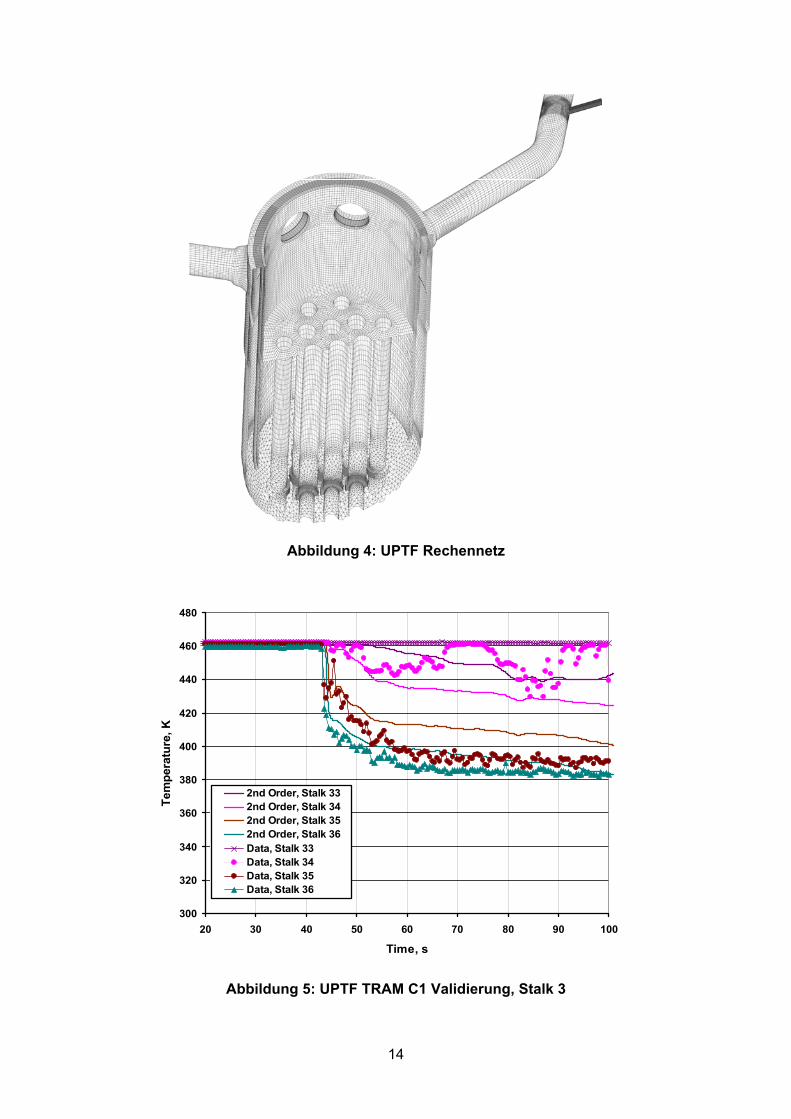
Zwei Demonstrationstestfälle wurden aus den UPTF-Experimenten ausgewählt. Diese
schließen komplexe Strömungsphänomene ein, die während der Notkühleinspeisung in
den kalten Strang eines Druckwasserreaktors auftreten können. UPTF Test1 ist ein
einphasiges Experiment, in dem die thermische Vermischung im kalten Strang und im
Ringraum untersucht wird. Im UPTF TRAM C1 Experiment ist der Wasserstand im
Ringraum bis auf halbe Höhe des kalten Strangs abgesenkt. Die Atmosphäre über dem
Wasserspiegel ist mit Stickstoff gesättigt. Während der ECC-Einspeisung tritt
Stratifizierung auf.
9
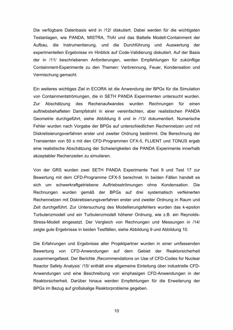
Für den einphasigen Demonstrationstestfall UPTF Test 1 (DEM01) wurden die
Berechnungen mit CFX-5 auf einem hybriden Rechennetz mit 2.1 Millionen
Gitterpunkten durchgeführt, siehe /9/. Das numerische Modell bildet die kalten Stränge,
den Ringraum und das Untere Plenum mit den Einbauten im Detail ab, siehe Abbildung
4. Nach Vorgabe der BPGs wurden der Einfluss der räumlichen und zeitlichen
Diskretisierung und unterschiedliche Zeitschrittweiten untersucht. Das SST-
Turbulenzmodell zeigt gute Ergebnissen für die Stratifizierung im kalten Strang,
insbesondere, wenn die Produktionsterme für den Auftrieb im Turbulenzmodell aktiviert
werden. Die Fluktuationen im Experiment können jedoch mit den angewendeten
Zweigleichungsturbulenzmodellen nicht erfasst werden.
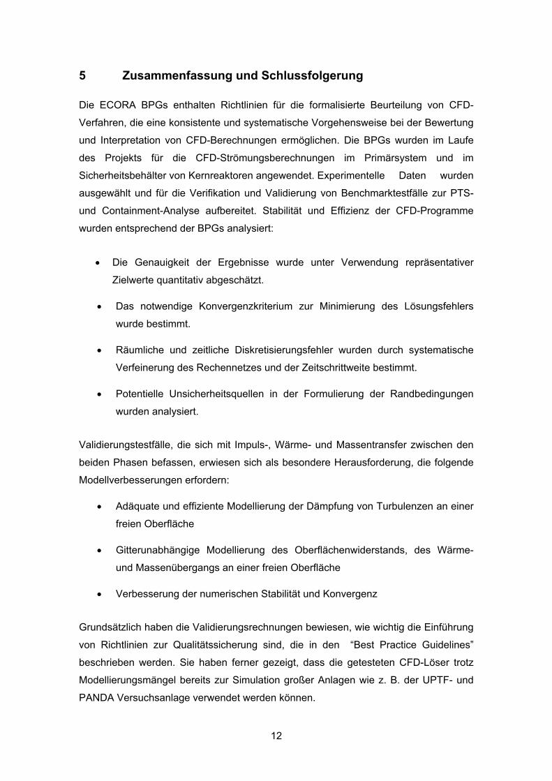
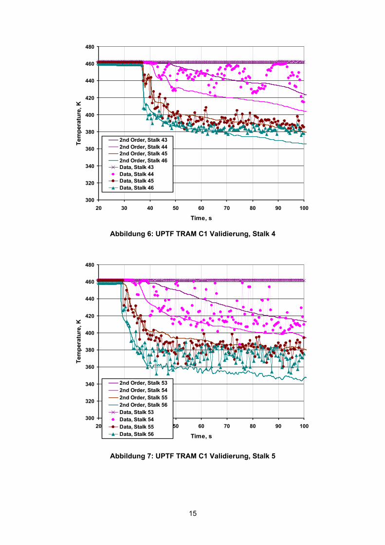
Im UPTF TRAM C1 Experiment ist der Wasserstand im Ringraum bis auf halbe Höhe
des kalten Strangs abgesenkt. Die Atmosphäre über dem Wasserspiegel ist mit
Stickstoff gesättigt, um Kondensation zu unterdrücken. In der Simulation wird deshalb
angenommen, dass keine Kondensation stattfindet. Während der ECC-Einspeisung tritt
Stratifizierung auf. Für die Zweiphasen-Simulation wird das gleiche CFX-5 Modell zur
Berechnung von Strömungen mit freien Oberflächen eingesetzt, das erfolgreich für die
Testfälle VER01, VER02, und VAL02 validiert wurde. Um Qualitätschecks gemäß der
BPGs mit einem angemessenen Rechenaufwand durchzuführen, wurde nur ein Viertel
der UPTF-Geometrie modelliert. Die Rechenergebnisse wurden durch einen Vergleich
mit der experimentell bestimmten Temperaturverteilung im kalten Strang bewertet,
siehe /10/. Die thermische Stratifizierung und der Beginn des Temperaturabfalls an
verschiedenen Messstellen, sowie die Position der freien Oberfläche stimmen gut mit
den Messdaten überein, siehe Abbildung 5 – Abbildung 7. Die hoch-frequenten
Variationen der Daten werden jedoch in den Rechnungen nicht wiedergegeben. Wie im
Testfall DEM01, könnte dies durch das verwendete statistische Turbulenzmodell
verursacht werden, das oft zu hohe Wirbelviskositäten und Längenmaße für transiente
Strömungsphänomene berechnet.
Ein umfassender Bericht über vorhandene CFD Analysen im Containment wurde
erstellt, siehe /11/. Nach Vorgabe der BPGs wurden Anforderungen für vollständige
Containment Analysen und Einschränkungen der vorhandenen CFD-Werkzeuge
zusammen mit Anforderungen an zukünftige Experimente diskutiert. Dazu werden
Beispiele zur Vermischung und Verbrennung von Gasen gezeigt. Weiterhin werden
vorhandene Validierungsrechnungen bewertet, die bisher im Rahmen von
internationalen Standardproblemen gerechnet wurden.
10
Die verfügbare Datenbasis wird in /12/ diskutiert. Dabei werden für die wichtigsten
Testanlagen, wie PANDA, MISTRA, ThAI und das Battelle Modell-Containment der
Aufbau, die Instrumentierung, und die Durchführung und Auswertung der
experimentellen Ergebnisse im Hinblick auf Code-Validierung diskutiert. Auf der Basis
der in /11/ beschriebenen Anforderungen, werden Empfehlungen für zukünftige
Containment-Experimente zu den Themen: Verbrennung, Feuer, Kondensation und
Vermischung gemacht.
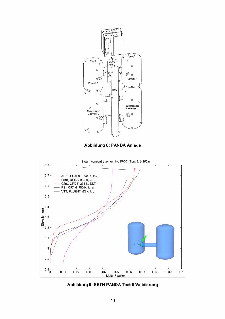
Ein weiteres wichtiges Ziel in ECORA ist die Anwendung der BPGs für die Simulation
von Containmentströmungen, die in SETH PANDA Experimenten untersucht wurden.
Zur Abschätzung des Rechenaufwandes wurden Rechnungen für einen
auftriebsbehafteten Dampfstrahl in einer vereinfachten, aber realistischen PANDA
Geometrie durchgeführt, siehe Abbildung 8 und in /13/ dokumentiert. Numerische
Fehler wurden nach Vorgabe der BPGs auf unterschiedlichen Rechennetzen und mit
Diskretisierungsverfahren erster und zweiter Ordnung bestimmt. Die Berechnung der
Transienten von 50 s mit den CFD-Programmen CFX-5, FLUENT und TONUS ergab
eine realistische Abschätzung der Schwierigkeiten die PANDA Experimente innerhalb
akzeptabler Rechenzeiten zu simulieren.
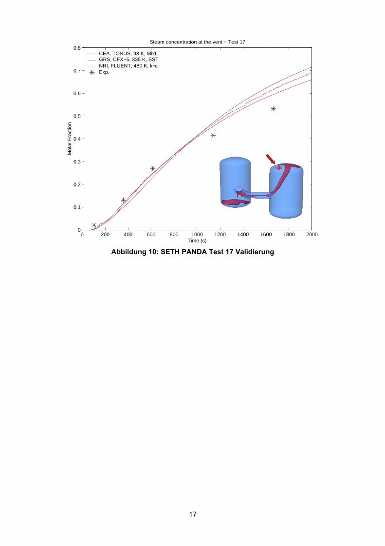
Von der GRS wurden zwei SETH PANDA Experimente Test 9 und Test 17 zur
Bewertung mit dem CFD-Programme CFX-5 berechnet. In beiden Fällen handelt es
sich um schwerkraftgetriebene Auftriebsströmungen ohne Kondensation. Die
Rechnungen wurden gemäß der BPGs auf drei systematisch verfeinerten
Rechennetzen mit Diskretisierungsverfahren erster und zweiter Ordnung in Raum und
Zeit durchgeführt. Zur Untersuchung des Modellierungsfehlers wurden das k-epsilon
Turbulenzmodell und ein Turbulenzmodell höherer Ordnung, wie z.B. ein Reynolds-
Stress-Modell eingesetzt. Der Vergleich von Rechnungen und Messungen in /14/
zeigte gute Ergebnisse in beiden Testfällen, siehe Abbildung 9 und Abbildung 10.
Die Erfahrungen und Ergebnisse aller Projektpartner wurden in einer umfassenden
Bewertung von CFD-Anwendungen auf dem Gebiet der Reaktorsicherheit
zusammengefasst. Der Berichte ‚Recommendations on Use of CFD-Codes for Nuclear
Reactor Safety Analysis’ /15/ enthält eine allgemeine Einleitung über industrielle CFD-
Anwendungen und eine Beschreibung von einphasigen CFD-Anwendungen in der
Reaktorsicherheit. Darüber hinaus werden Empfehlungen für die Erweiterung der
BPGs im Bezug auf großskalige Reaktorprobleme gegeben.

11
Im Bericht ‚Recommendations for CFD Development and Customisation’ /16/ werden
Vorschläge zur Verbesserung der Modellierung der Geometrie, des numerischen
Gitters und des Pre- und Postprozessing gemacht. Im Abschnitt über einphasige CFD-
Anwendungen werden Verbesserungen im Bezug auf physikalische Modelle und
numerische Effizienz vorgeschlagen. Die Empfehlungen für CFD-Entwicklungen auf
dem Gebiet der Zweiphasenströmungen heben die Notwendigkeit hervor physikalische
Modelle zu verbessern, z.B. für freie Oberflächen mit Phasenübergang.
12
5 Zusammenfassung und Schlussfolgerung
Die ECORA BPGs enthalten Richtlinien für die formalisierte Beurteilung von CFD-
Verfahren, die eine konsistente und systematische Vorgehensweise bei der Bewertung
und Interpretation von CFD-Berechnungen ermöglichen. Die BPGs wurden im Laufe
des Projekts für die CFD-Strömungsberechnungen im Primärsystem und im
Sicherheitsbehälter von Kernreaktoren angewendet. Experimentelle Daten wurden
ausgewählt und für die Verifikation und Validierung von Benchmarktestfälle zur PTS-
und Containment-Analyse aufbereitet. Stabilität und Effizienz der CFD-Programme
wurden entsprechend der BPGs analysiert:
• Die Genauigkeit der Ergebnisse wurde unter Verwendung repräsentativer
Zielwerte quantitativ abgeschätzt.
• Das notwendige Konvergenzkriterium zur Minimierung des Lösungsfehlers
wurde bestimmt.
• Räumliche und zeitliche Diskretisierungsfehler wurden durch systematische
Verfeinerung des Rechennetzes und der Zeitschrittweite bestimmt.
• Potentielle Unsicherheitsquellen in der Formulierung der Randbedingungen
wurden analysiert.
Validierungstestfälle, die sich mit Impuls-, Wärme- und Massentransfer zwischen den
beiden Phasen befassen, erwiesen sich als besondere Herausforderung, die folgende
Modellverbesserungen erfordern:
• Adäquate und effiziente Modellierung der Dämpfung von Turbulenzen an einer
freien Oberfläche
• Gitterunabhängige Modellierung des Oberflächenwiderstands, des Wärme-
und Massenübergangs an einer freien Oberfläche
• Verbesserung der numerischen Stabilität und Konvergenz
Grundsätzlich haben die Validierungsrechnungen bewiesen, wie wichtig die Einführung
von Richtlinien zur Qualitätssicherung sind, die in den “Best Practice Guidelines”
beschrieben werden. Sie haben ferner gezeigt, dass die getesteten CFD-Löser trotz
Modellierungsmängel bereits zur Simulation großer Anlagen wie z. B. der UPTF- und
PANDA Versuchsanlage verwendet werden können.
13
6 Abbildungen
Abbildung 2: Prallstrahl mit freier Oberfläche
0.00
0.25
0.50
0.75
1.00
-2 -1.6 -1.2 -0.8 -0.4 0 0.4 0.8 1.2 1.6 2x/D
CpMesh 1
Mesh 2
Mesh 3
Data
Mesh with Adaption
Abbildung 3: Prallstrahl Validierung
14
Abbildung 4: UPTF Rechennetz
300
320
340
360
380
400
420
440
460
480
20 30 40 50 60 70 80 90 100
Time, s
Tem
pera
ture
, K
2nd Order, Stalk 332nd Order, Stalk 342nd Order, Stalk 352nd Order, Stalk 36Data, Stalk 33Data, Stalk 34Data, Stalk 35Data, Stalk 36
Abbildung 5: UPTF TRAM C1 Validierung, Stalk 3
15
Abbildung 6: UPTF TRAM C1 Validierung, Stalk 4
300
320
340
360
380
400
420
440
460
480
20 30 40 50 60 70 80 90 100
Time, s
Tem
pera
ture
, K
2nd Order, Stalk 532nd Order, Stalk 542nd Order, Stalk 552nd Order, Stalk 56Data, Stalk 53Data, Stalk 54Data, Stalk 55Data, Stalk 56
Abbildung 7: UPTF TRAM C1 Validierung, Stalk 5
300
320
340
360
380
400
420
440
460
480
20 30 40 50 60 70 80 90 100
Time, s
Tem
pera
ture
, K
2nd Order, Stalk 432nd Order, Stalk 442nd Order, Stalk 452nd Order, Stalk 46Data, Stalk 43Data, Stalk 44Data, Stalk 45Data, Stalk 46
16
Abbildung 8: PANDA Anlage
Abbildung 9: SETH PANDA Test 9 Validierung
17
Abbildung 10: SETH PANDA Test 17 Validierung
0 200 400 600 800 1000 1200 1400 1600 1800 20000
0.1
0.2
0.3
0.4
0.5
0.6
0.7
0.8
Mol
ar F
ract
ion
Time (s)
Steam concentration at the vent − Test 17
CEA, TONUS, 93 K, MixL GRS, CFX−5, 335 K, SST NRI, FLUENT, 480 K, k−εExp.
18
7 Literatur
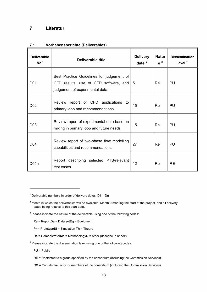
7.1 Vorhabensberichte (Deliverables)
Deliverable No1
Deliverable title Delivery
date 2 Natur
e 3 Dissemination
level 4
D01
Best Practice Guidelines for judgement of
CFD results, use of CFD software, and
judgement of experimental data.
5 Re PU
D02 Review report of CFD applications to
primary loop and recommendations 15 Re PU
D03 Review report of experimental data base on
mixing in primary loop and future needs 15 Re PU
D04 Review report of two-phase flow modelling
capabilities and recommendations 27 Re PU
D05a Report describing selected PTS-relevant
test cases 12 Re RE
1 Deliverable numbers in order of delivery dates: D1 – Dn
2 Month in which the deliverables will be available. Month 0 marking the start of the project, and all delivery dates being relative to this start date.
3 Please indicate the nature of the deliverable using one of the following codes:
Re = ReportDa = Data setEq = Equipment
Pr = Prototype Si = Simulation Th = Theory
De = Demonstrator Me = MethodologyO = other (describe in annex)
4 Please indicate the dissemination level using one of the following codes:
PU = Public
RE = Restricted to a group specified by the consortium (including the Commission Services).
CO = Confidential, only for members of the consortium (including the Commission Services).
19
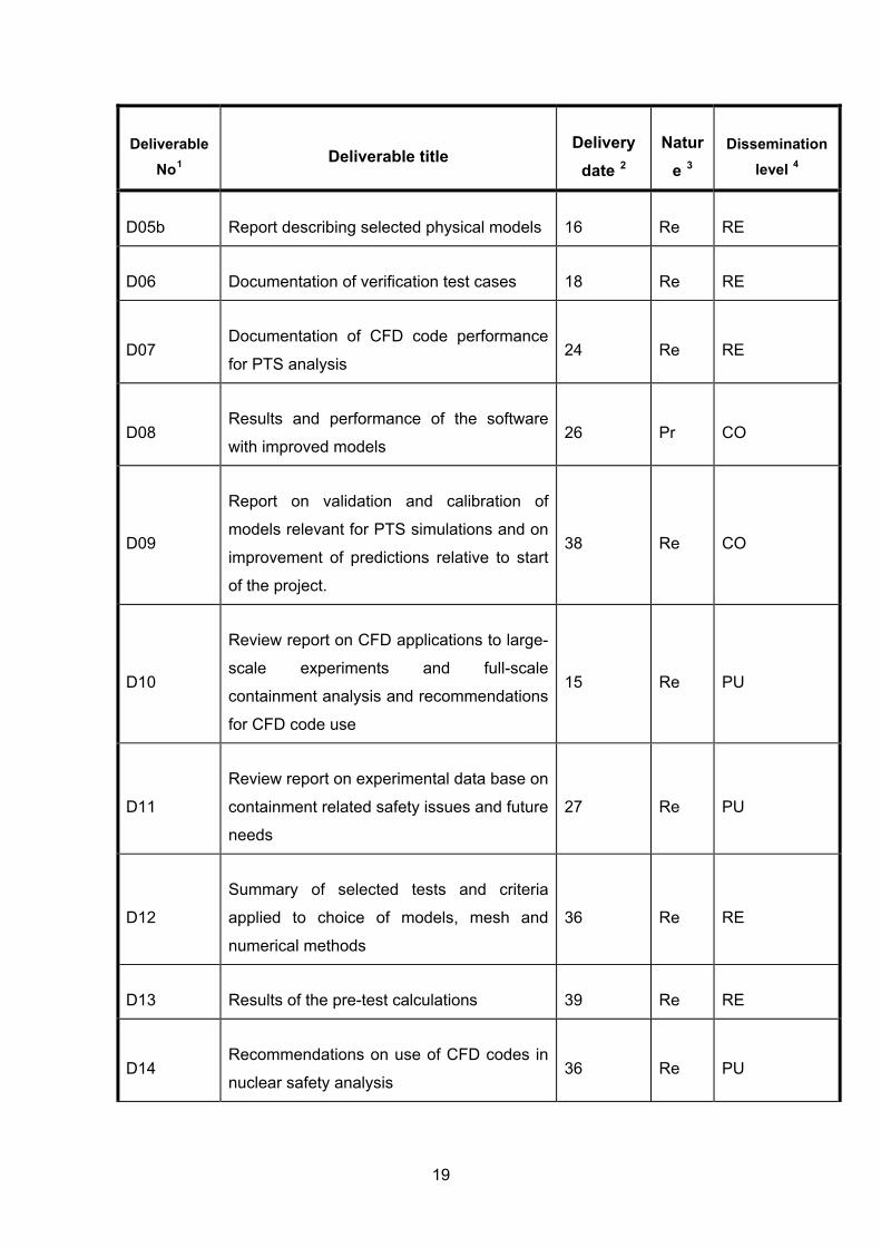
Deliverable No1
Deliverable title Delivery
date 2 Natur
e 3 Dissemination
level 4
D05b Report describing selected physical models 16 Re RE
D06 Documentation of verification test cases 18 Re RE
D07 Documentation of CFD code performance
for PTS analysis 24 Re RE
D08 Results and performance of the software
with improved models 26 Pr CO
D09
Report on validation and calibration of
models relevant for PTS simulations and on
improvement of predictions relative to start
of the project.
38 Re CO
D10
Review report on CFD applications to large-
scale experiments and full-scale
containment analysis and recommendations
for CFD code use
15 Re PU
D11
Review report on experimental data base on
containment related safety issues and future
needs
27 Re PU
D12
Summary of selected tests and criteria
applied to choice of models, mesh and
numerical methods
36 Re RE
D13 Results of the pre-test calculations 39 Re RE
D14 Recommendations on use of CFD codes in
nuclear safety analysis 36 Re PU
20
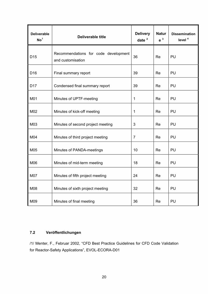
Deliverable No1
Deliverable title Delivery
date 2 Natur
e 3 Dissemination
level 4
D15 Recommendations for code development
and customisation 36 Re PU
D16 Final summary report 39 Re PU
D17 Condensed final summary report 39 Re PU
M01 Minutes of UPTF-meeting 1 Re PU
M02 Minutes of kick-off meeting 1 Re PU
M03 Minutes of second project meeting 3 Re PU
M04 Minutes of third project meeting 7 Re PU
M05 Minutes of PANDA-meetings 10 Re PU
M06 Minutes of mid-term meeting 18 Re PU
M07 Minutes of fifth project meeting 24 Re PU
M08 Minutes of sixth project meeting 32 Re PU
M09 Minutes of final meeting 36 Re PU
7.2 Veröffentlichungen
/1/ Menter, F., Februar 2002, “CFD Best Practice Guidelines for CFD Code Validation
for Reactor-Safety Applications”, EVOL-ECORA-D01
21
/2/ Muhlbauer, P., März 2003, “Review of CFD Applications in Primary Loop and
Recommendations”, EVOL-ECORA-D02
/3/ Muhlbauer, P., August 2003, “Review of Experimental Database on Mixing in
Primary Loop and Future Needs”, EVOL-ECORA-D03
/4/ Muhlbauer, P., Februar 2004, “Review of Two-phase Flow Modelling Capabilities
and Recommendations”, EVOL-ECORA-D04
/5/ Scheuerer, M., Dezember 2002, “Selection of PTS-Relevant Test Cases”, GRS
mbH, Garching, EVOL-ECORA-D05a
/6/ Pigny, S., Juni 2003, “Selection of PTS-Relevant Physical Models”, EVOL-ECORA-
D05b
/7/ Pigny, S., August 2003, “PTS-Relevant Verification Test Cases”, EVOL-ECORA-
D06
/8/ Egorov, Y., September 2004, “Validation of CFD Codes with PTS-Relevant Test
Cases”, EVOL-ECORA-D07
/9/ Willemsen, S., November 2004, “Demonstration Test Case: ECORA DEM01 UPTF
Test 1, Run 21”, EVOL-ECORA-D9.1
/10/ Scheuerer, M., August 2004, “Demonstration Test Case: ECORA DEM02 UPTF
TRAM C1, Run 21a2”, EVOL-ECORA-D9.2
/11/ Heitsch, M., August 2003, “Review of CFD Applications to Containment Related
Phenomena”, EVOL-ECORA-D10
/12/ Heitsch, M., Dezember 2004, “Experimental Data Base on Containment Related
Safety Issues and Future Needs”, EVOL-ECORA-D11
/13/ Andreani, M., September 2004, “Summary of Selected Tests and Criteria applied
to Choice of Models, Mesh and Numerical Methods”, EVOL-ECORA-D12
/14/ Andreani, M., März 2005, “Results of the pre-test calculations (of two PANDA-
SETH tests)”, EVOL-ECORA-D 13

22
/15/ Bestion, D., September 2004, “Recommendation on use of CFD Codes for Nuclear
Reactor Safety Analysis”, EVOL-ECORA-D14
/16/ Bestion, D., September 2004, “Recommendation for CFD Development and
Customisation”, EVOL-ECORA-D15
23
8 Verteiler
BMWA Referat IX B 4 1 x GRS-FB
Internationale Verteilung 40 xProjektbegleiter (wof) 3 x GRS
Geschäftsführung (hah, ldr) je 1 xBereichsleiter (ban, brw, erl, erv, lim, prg, tes) je 1 xAbteilungsleiter (all, gls, lab, poi, bea) je 1 xProjektbetreuung (kgl, scc) je 1 xProjektleiterin (bam) 1 xInformationsverarbeitung (nit) 1 xAutorin (bam) 3 x Gesamtauflage
64 Exemplare
1
EUROPEAN COMMISSION 5th EURATOM FRAMEWORK PROGRAMME 1998-2002 KEY ACTION: NUCLEAR FISSION
ECORA
CONTRACT N° FIKS-CT-2001-00154
Final Technical Report
Authors: Martina Scheuerer GRS, Germany Michele Andreani PSI, Switzerland Dominique Bestion CEA, France Yury Egorov ANSYS, Germany Matthias Heitsch GRS, Germany Florian Menter ANSYS, Germany Petr Muhlbauer NRI, Czech Republic Sylvain Pigny CEA, France Carla Schwäger GRS, Germany Sander Willemsen NRG, Netherlands
Dissemination level: CO: confidential, only for partners of the ECORA project
January, 2005 EVOL– ECORA – D 16
2
Final Technical Report
CONTRACT N°: FIKS-CT-2001-00154 PROJECT N°: ACRONYM: ECORA TITLE: Evaluation of Computational Fluid Dynamics methods for Reactor Safety Analysis PROJECT CO-ORDINATOR: Gesellschaft für Anlagen- und Reaktorsicherheit GmbH PARTNERS: AEA Technology GmbH Germany Serco Insurances plc U.K. Atomic Energy Research Institute Hungary Commissariat a l'Energie Atomique France Groupe Electricite de France France Forschungszentrum Rossendorf Inc Germany Nuclear Research and Consultancy Group Netherlands Nuclear Research Institute Rez plc Czech Republic Paul Scherrer Institute Switzerland Vattenfall Utveckling AB Sweden VTT Processes Finland EC Contribution: EUR 753 480.00 Total Project Value: EUR 1 623 822.00 Starting Date: 1 October 2001 Duration: 36 months
3
CONTENTS
1 OBJECTIVES AND SCOPE ............................................................................................................. 10
1.1 Socio-Economic Objectives and Strategic Aspects ..................................................................... 10 1.2 Scientific/Technological Objectives............................................................................................ 10 1.3 Contribution to EU Policy ........................................................................................................... 11
2 WORK PROGRAMME AND RESULTS ........................................................................................ 13
2.1 Establishment of Best Practice Guidelines (WP 1) ..................................................................... 14 2.1.1 General Aspects ...................................................................................................................... 14 2.1.2 Errors in CFD Simulations ..................................................................................................... 14 2.1.3 Existing CFD Simulations and Experimental Data................................................................. 15 2.1.4 ECORA Specific Considerations and Templates.................................................................... 15 2.1.5 Appliction of the BPG to the ECORA Test Cases.................................................................. 16
2.2 Evaluation of CFD Analysis of Primary Loop (WP 2)................................................................ 18 2.2.1 Flow and Heat Transfer in Nuclear Reactor Cores ................................................................. 18 2.2.2 Pressurized Thermal Shocks................................................................................................... 19 2.2.3 Boron Dilution and Non-Symmetric Loop Operation ............................................................ 20
2.3 Definition of Physical Models and Test Cases for PTS-Analysis (WP 3)................................... 24 2.3.1 Selection of PTS-Relevant Test Cases.................................................................................... 24 2.3.2 Selection of PTS-Relevant Physical Models .......................................................................... 26 2.3.3 Calculation of PTS-Relevant Verification Test Cases ............................................................ 27
2.4 Software Development and Verification (WP 4)......................................................................... 28 2.4.1 VAL01: Impinging Jet with Heat Transfer............................................................................. 28 2.4.2 VAL02: Impinging Water Jet in Air Environment ................................................................. 30 2.4.3 VAL03: Jet Impingement on a Free Surface .......................................................................... 32 2.4.4 VAL04: Contact Condensation in Stratified Steam-Water Flow............................................ 35
2.5 Software Validation (WP 5) ........................................................................................................ 39 2.5.1 The Upper Plenum Test Facility (UPTF)................................................................................ 40 2.5.2 Single-Phase Calculations....................................................................................................... 41 2.5.3 Two-Phase Calculations ......................................................................................................... 46 2.5.4 Conclusions............................................................................................................................. 50
2.6 Evaluation of CFD Analysis of Containment (WP 6) ................................................................. 50 2.6.1 Validation of CFD for Containment Phenomena.................................................................... 51 2.6.2 Evaluation of the Available Database..................................................................................... 60 2.6.3 Conclusions............................................................................................................................. 66
2.7 Pre-Test Analysis of Selected SETH PANDA Tests (WP 7) ...................................................... 67 2.7.1 The scoping exercise............................................................................................................... 70 2.7.2 Definition of the CFD simulations.......................................................................................... 72 2.7.3 Main results of the pre-test analyses....................................................................................... 76 2.7.4 Conclusions............................................................................................................................. 91
2.8 Evaluation of Application of CFD Codes to Reactor Safety (WP 8) .......................................... 93 2.8.1 Use of Single-Phase CFD ....................................................................................................... 93 2.8.2 Use of Two-Phase Flow CFD................................................................................................. 97 2.8.3 Recommendations for Code Customisation.......................................................................... 101 2.8.4 Recommendations for Single-Phase CFD Development ...................................................... 104 2.8.5 Recommendations for Two-Phase CFD Development ......................................................... 105
4
3 MANAGEMENT AND COORDINATION ASPECTS................................................................. 108
3.1 Communication between Partners ............................................................................................. 108 3.2 Contractual Matters ................................................................................................................... 108 3.3 Meetings .................................................................................................................................... 108 3.4 Time and Financial Management .............................................................................................. 108 3.5 Quality Management ................................................................................................................. 109 3.6 List of Deliverables ................................................................................................................... 109 3.7 Comparison of Planned Activities and Actual Work ................................................................ 112 3.8 Cooperation with Other Projects/Programmes .......................................................................... 116
3.8.1 Exchange of Best Practice Guidelines .................................................................................. 116 3.8.2 Establishment of a Network of European Centres of Competence for CFD Codes in Nuclear Safety .............................................................................................................................................. 116 3.8.3 Organisation of a POST-FISA Workshop ............................................................................ 116
3.9 Dissemination and Use of the Results ....................................................................................... 117
4 REFERENCES.................................................................................................................................. 118
5
List of Figures
Figure 1: Organizational structure of ECORA................................................................... 13 Figure 2: Plume direction and stratification in the FORTUM test facility without and with
flow in the side loops.................................................................................................. 20 Figure 3: ROCOM model of a RPV................................................................................... 21 Figure 4: Gidropress facility – model of the reactor. ......................................................... 22 Figure 5: UM 2x4 loop with position of thermocouples. ................................................... 23 Figure 6: Vattenfall test facility: reactor vessel ................................................................. 24 Figure 7: PTS-relevant flow phenomena............................................................................ 25 Figure 8: Impinging jet geometry....................................................................................... 29 Figure 9: Nusselt number distribution with discretisation of second order accuracy ........ 30 Figure 10: Geometry for test case VAL02 ......................................................................... 31 Figure 11: Distribution of the pressure coefficient along the surface ................................ 31 Figure 12: Experimental setup ........................................................................................... 32 Figure 13: Comparison of the numerical (left) and experimental (right) void fraction
profile as a function of the depth below the initial water surface, along the centre line of the nozzle ............................................................................................................... 33
Figure 14: Void fraction map at different successive times............................................... 34 Figure 15: Radial profiles of void fraction at 1 mm depth, mesh 1 and mesh 2. ............... 34 Figure 16: Radial profiles of void fraction at 1 mm depth, mesh 3. .................................. 35 Figure 17: Schematic of the stratified flow in a 2-D duct .................................................. 36 Figure 18: Water temperature profiles at the measurement station, NEPTUNE results: top
- lower Reynolds number of steam; bottom - higher Reynolds number of steam...... 37 Figure 19: Water temperature profiles at the measurement station, CFX-5 results: top –
lower Reynolds number of steam; bottom – higher Reynolds number of steam. ...... 38 Figure 20: Layout of the Upper Plenum Test Facility........................................................ 40 Figure 21: Location of the key temperature measurement positions, and probe numbering.
.................................................................................................................................... 41 Figure 22: Vessel and fluid temperatures on the vessel and cold leg walls (left) and a
cross-section through the middle of the cold leg with ECC injection (right). ........... 43 Figure 23: Stalk 3 results of the CFX-5 reference calculation (left) and UPTF experiment
(right). For legend see Figure 21. ............................................................................... 44 Figure 24: Level 750 mm results of the CFX-5 reference calculation (left) and UPTF
experiment (right). For legend see Figure 21. ............................................................ 44 Figure 25: Level 4500 mm results of the CFX-5 reference calculation (left) and UPTF
experiment (right). For legend see Figure 21. ............................................................ 44 Figure 26: Vessel and fluid temperatures on the vessel and cold leg walls (right) and a
cross-section through the middle of the cold leg with ECC injection (left)............... 45 Figure 27: Temperature on the last stalk before down comer (left) and on level 750 mm
(right) (for legend see Figure 21, T31 = Stalk 3 position 1) ...................................... 46 Figure 28: Water velocity at Stalk 5 (for position 3 and 5 see Figure 21) ......................... 48 Figure 29: Iso-surface of constant velocity (0.3 m/s), coloured by temperature (left) and
Velocity vectors and temperature distribution at = 50 s (right) ................................ 48 Figure 30: Water temperature distribution at Stalk 3 (left) and Stalk 4 (right) (legend as
defined in Figure 21). ................................................................................................. 49 Figure 31: Gas distribution after 600 s of helium inflow................................................... 55
6
Figure 32: Helium transient 2 m away from the jet axis (RNG k-ε model)....................... 56 Figure 33: Axial profile through the jet (RNG k-ε model) ................................................ 57 Figure 34: TONUS (v98D) predictions for the AECL LSGMF helium test, using the RNG
k-ε model. (courtesy of IRSN) ................................................................................... 59 Figure 35: The PANDA facility. ........................................................................................ 68 Figure 36: Configuration for the two PANDA tests selected for the ECORA project. ..... 70 Figure 37: Test 9. Steam concentration distribution at 250 s along a horizontal line
crossing the plume...................................................................................................... 81 Figure 38: Test 9. Steam concentration vertical distribution in the interconnecting pipe at
250 s. .......................................................................................................................... 83 Figure 39: Test 9. Steam concentration vertical distribution in Drywell1 at various times.
.................................................................................................................................... 84 Figure 40: Test 9. Steam concentration vertical distribution in Drywell 2 at various times.
.................................................................................................................................... 85 Figure 41: Test 17. Gas temperature distribution on a horizontal line crossing the jet. .... 87 Figure 42: Test 17. Steam concentration vertical distribution in the interconnecting pipe at
500s. ........................................................................................................................... 88 Figure 43: Test 17. Steam concentration at the vent (top of DW2). .................................. 89 Figure 44: Test 17. Steam concentration vertical distribution in Drywell 1 at 1000 s....... 90 Figure 45: Test 17. Steam concentration vertical distribution in Drywell 2 at 1000 s....... 91
7
List of Tables
Table I: PTS test case matrix.............................................................................................. 26 Table II: Overview of the performed CFX-5 computations for UPTF Test 1.................... 42 Table III: Overview of the performed CFX-5 computations for UPTF TRAM C1........... 47 Table IV: Summary of containment phenomena................................................................ 51 Table V: Summary of available CFD applications ............................................................ 53 Table VI: Summary of relevance and specific difficulties (beyond common drawbacks of
integral tests discussed in the text) of PANDA data .................................................. 61 Table VII: Main areas of required experimental work....................................................... 66 Table VIII: Initial conditions.............................................................................................. 73 Table IX: Matrix of simulations......................................................................................... 75 Table X: Definition of tasks for the various organizations ................................................ 76 Table XI: Summary of simulations for Step 1 of Test 9 .................................................... 78 Table XII: Summary of simulations for Step 1 of Test 17 ................................................. 79 Table XIII: Summary of simulations for Step 2 of Tests 9 and 17 .................................... 79 Table XIV: List of deliverables........................................................................................ 109 Table XV: Man power and progress follow-up table October 2001 - December 2004 ... 112

8
LIST OF ABBREVIATIONS AND SYMBOLS
ABWR Advanced Boiling Water Reactor BDBA Beyond Design Basis Accident BPG Best Practice Guidelines BWR Boiling Water Reactor CFD Computational Fluid Dynamics CHF Critical Heat Flux DNB Departure from Nuclear Boiling ECC Emergency Core Cooling EPR European Pressurised water Reactor ERCOFTAC European Research Community for Flow, Turbulence and Combustion FWP Framework Programme GCR Gas Cooled Reactor IAEA International Atomic Energy Agency LES Large Eddy Simulation LMFBR Liquid Metal Fast Breeder Reactor LOCA Loss Of Coolant Accident LWR Light Water Reactor NEA Nuclear Energy Agency OECD Organisation for Economic Co-operation and Development PTS Pressurized Thermal Shock PWR Pressurized Water Reactor RANS Reynolds Averaged Navier Stokes equations RPV Reactor Pressure Vessel RSM Reynolds stress model SST Shear Stress Transport model FEFV Finite-Element-Finite –Volume UPTF Upper Plenum Test Facility URANS Unsteady Reynolds Averaged Navier Stokes equations VVER Russian type of pressurised water reactor
9
EXECUTIVE SUMMARY
The objective of the ECORA project is to evaluate the capabilities of Computational Fluid Dynam-ics (CFD) software packages for simulating flows in the primary system and containment of nu-clear reactors. The interest in the application of CFD methods arises from the importance of three-dimensional flow effects in these reactor components, which one-dimensional system codes cannot predict. Therefore, the ECORA project will identify application areas for detailed three-dimensional CFD calculations and make recommendations for software improvements. The software assessment includes the establishment of Best Practice Guidelines (BPG) and stan-dards regarding the use of CFD software and the evaluation of CFD results for safety analysis. Quality criteria for the application of CFD software are standardised. CFD results are only ac-cepted after these quality criteria are satisfied. Thus, a general basis for assessing merits and weaknesses of particular models and codes is formed on a European basis. CFD simulations hav-ing an accepted quality level will increase confidence in the application of CFD-tools. In addition, a comprehensive and systematic software engineering approach for extending and cus-tomising CFD codes for nuclear safety analyses has been formulated and applied. The adaptation of CFD software for nuclear reactor flow simulations is shown by implementing enhanced two-phase flow, turbulence, and energy transfer models relevant for Pressurized Thermal Shock (PTS) applications into the CFX, and Neptune software. An analysis of selected UPTF and PANDA ex-periments was performed to validate CFD software in relation to PTS phenomena in the primary system and severe accident management in the containment. The following results have been achieved: • The ECORA BPGs (see Ref. [1]) were applied in the European projects FLOMIX-R, ASTAR
and ITEM. In common workshops and project meetings BPG calculations were presented and discussed (see Refs. [2] and [3]).
• Surveys of existing CFD calculations and experimental data for primary loop (see Refs. [4], [5], [6]) and containment flows (see Refs. [7], [8]) have been performed.
• Relevant flow phenomena and models and methods for the simulation of PTS-relevant flows are documented in Refs [9] and [10]. The implemented models were verified by calculating se-lected test cases following the ECORA BPGs, see Ref. [11].
• Simulations for PTS-relevant single-phase flow and two-phase flow validation and demonstra-tion test cases have been performed according to BPGs. They are documented in Refs. [12] and [13].
• A prototype of the CFD code CFX-5 containing newly implemented and improved models was made available to the ECORA partners.
• Test cases from the SETH PANDA experiments were selected and scoping calculations for a buoyant steam jet were performed (see Ref. [14]) following the ECORA BPGs.
• Pre-test calculations were made for the SETH PANDA experiments Test 9 and Test 17, a comparison with experiments is documented in Ref. [15].
• A comprehensive analysis on the use of CFD codes in nuclear reactor applications and rec-ommendations for code development and customisation is documented in Refs. [16] and [17]
• In October 2003, the ECORA project was audited and successfully certified for the interna-tional ISO 9001:2000 standard.
• During the Final Meeting at NRG, Petten, the partners agreed to proceed with a follow-up ac-tion of this project to achieve the sustainability of the ECORA results, see Ref. [18].
10
1 OBJECTIVES AND SCOPE
1.1 Socio-Economic Objectives and Strategic Aspects
The major objectives of the ECORA project are to consolidate the use of CFD methods in nuclear safety analysis by providing an overview of the state-of-the-art of their capabili-ties for safety-relevant applications, and to define CFD code improvements that are neces-sary for nuclear engineering applications. CFD codes were tested in a concerted validation exercise. This assessment produced requirements for improving the CFD codes used in ECORA. The increase in predictive power and better understanding of PTS and contain-ment flows, which were primarily investigated in the project, provide a firmer basis for the development and practical implementation of engineered safety features and accident management measures. This will allow for higher safety, achieved at reduced cost. The ECORA project was a multi-disciplinary research effort, which brought together highly skilled experts from different engineering fields. The consortium comprised ther-mal-hydraulic experts, code developers, safety experts and engineers from the nuclear in-dustry, as well as CFD experts. The development of internationally verified and validated methods and practices helps to improve the analysis of potential accident situations and of operating conditions. It will also contribute to a better management of the plant lifetime. In ECORA, CFD quality criteria were standardized before the application of CFD soft-ware, and results were only accepted once the set quality criteria have been met. This stan-dardization was done on a European basis. The ‘certified’ results form a more rational ba-sis for assessing merits and weaknesses of particular models and codes than individual na-tional efforts. Achievement of an accepted quality level also increases confidence in the results, and reduces the amount of overlapping research. This, in turn, leads to cost sav-ings on a European basis, and allows concentration on progressing the state-of-the-art rather than on double-checking results on a national basis. Further benefit to EC policies comes from the involvement of non-nuclear users interested in the application of CFD software for thermal-hydraulic two-phase flow problems. For instance, the same procedures and largely similar models can be used for improved simu-lations of coal and oil combustion in fossil power engineering and of cavitation in hydrau-lic power plants. The chemical and process industry has a major interest in a deeper un-derstanding of multi-phase flow mixing and reactions. Hence, the interest of several non-nuclear industry branches will further promote an effective application of the acquired knowledge and of the developed software.
1.2 Scientific/Technological Objectives
The objectives of the ECORA project were to assess the capabilities of current CFD soft-ware packages for safety analyses of existing installations and evolutionary reactors, to es-tablish guidelines for their correct use, to identify perspective application areas for three-dimensional flow calculations, and to indicate necessary code improvements for simula-tions of safety-relevant accident scenarios. The assessment included the validation of CFD
11
codes with respect to severe accident management in the containment and to PTS phe-nomena in the primary system of PWRs. Moreover, the feasibility of tailoring CFD codes for reactor safety analysis was demonstrated by implementation, verification and valida-tion of selected physical models relevant for PTS analysis. In the verification step the cor-rect programming and implementation of the models was checked. In the validation step, the numerical results were compared to experimental data for reactor-safety relevant phe-nomena. Furthermore, requirements were formulated for customized versions of CFD packages with features tailored to the needs of the nuclear industry. The project had several measurable objectives and steps to reach this goal: • Establishment of Best Practice Guidelines for ensuring high-quality results and for the
formalised judgement of CFD calculations and experimental data • Assessment of the potential, of difficulties, and of limitations of CFD methods for
flows in the primary system and in LWR containments, with special emphasis on mix-ing phenomena such as PTS
• Definition of experimental needs for the verification and validation of CFD software for flows in the primary system and in LWR containments
• Identification of improvements and extensions to the current CFD packages that are necessary for primary loop and containment flow analysis
• Implementation and validation of improved turbulence and two-phase flow models for the simulation of PTS phenomena in PWR primary systems
• Comprehensive evaluation of the application of CFD codes for reactor safety applica-tions
• Identification of research needs for customising CFD software for nuclear application needs
The project helped to improve understanding of merits and limitations of CFD for reactor safety analysis. It also contributes to the definition of realistic expectations regarding these methods. The ECORA results are used within the proposed 6th framework project NURE-SIM. Model and code improvements are implemented into CFX-5 and NEPTUNE which are publicly available.
1.3 Contribution to EU Policy
The ECORA project contributes to the main research objectives of the programme. It ad-dresses the issue of improved methods for the assessment of operational safety of existing installations. It contributes towards maintaining and enhancing the high level of expertise and competence of the European industry in nuclear technology. Because of the wide range of possible applications of CFD, the project contributes to all three research areas, plant life extension, severe accident management, and evolutionary concepts. Plant life extension: The assessment of the capabilities of CFD codes to predict the re-sponse of materials under operational thermal transients and hypothetical accident condi-tions contributes to develop a technical basis for the continued safe operation of nuclear reactors. Predictions of the integrity of equipment and structures of reactor pressure vessels require accurate knowledge of the thermal loads. The thermal loads are strongly influenced by the
12
thermal-hydraulic conditions in the main coolant pipes, and in the downcomer of the reac-tor pressure vessel. CFD simulations of the flow in the pipes and in the pressure vessels of the primary system help to locate critical positions in these systems, and improve monitor-ing, inspection and maintenance of nuclear reactors. Severe accident management: The evaluation of the capabilities of CFD codes to predict the distribution of steam, hydrogen and non-condensable gases released during a hypo-thetical severe accident contribute to the understanding of these phenomena, to the defini-tion of effective accident management strategies, and to the development of accident miti-gating features. The OECD/NEA group of experts on Containment Thermal-Hydraulics and Hydrogen Distribution [OECD, 1999] has identified a lack of momentum and species concentration transport data from separate-effect and coupled-effect tests as one of the main difficulties in assessing the capabilities of CFD codes. In order to fill the gap several experimental programs in large-scale facilities have been proposed, where high quality data will be obtained to provide a database for CFD code validation. In the ECORA pro-ject, calculations of the SETH PANDA tests, organized by the OECD/NEA/CSNI, were used for assessment of the capabilities of the CFD codes. Evolutionary concepts: The assessment of best-estimate analytical tools is an important element in the investigation of cost reducing and safety-enhancing improvements of cur-rently used technology. Enhancing confidence in advanced analytical tools allows devel-opment of upscale strategies from laboratory scale to reactor conditions. The assessment of CFD codes in the frame of the ECORA project is an important contribution to the more accurate evaluation of the merits of evolutionary concepts.
13
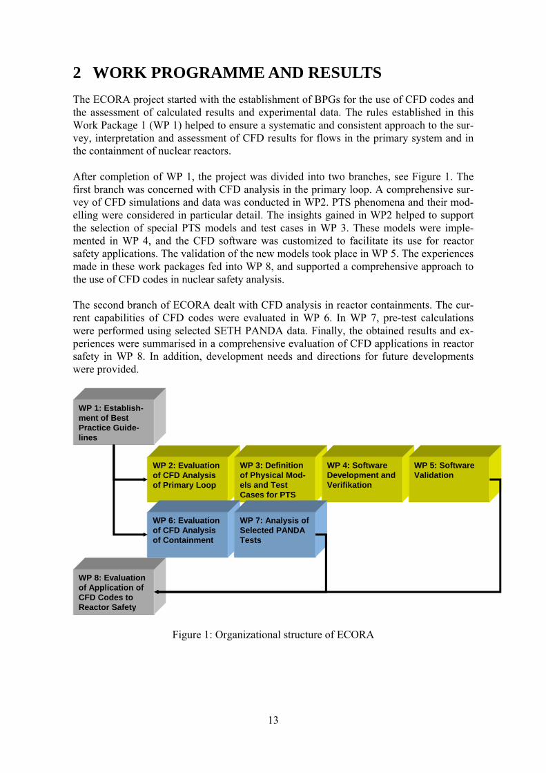
2 WORK PROGRAMME AND RESULTS The ECORA project started with the establishment of BPGs for the use of CFD codes and the assessment of calculated results and experimental data. The rules established in this Work Package 1 (WP 1) helped to ensure a systematic and consistent approach to the sur-vey, interpretation and assessment of CFD results for flows in the primary system and in the containment of nuclear reactors. After completion of WP 1, the project was divided into two branches, see Figure 1. The first branch was concerned with CFD analysis in the primary loop. A comprehensive sur-vey of CFD simulations and data was conducted in WP2. PTS phenomena and their mod-elling were considered in particular detail. The insights gained in WP2 helped to support the selection of special PTS models and test cases in WP 3. These models were imple-mented in WP 4, and the CFD software was customized to facilitate its use for reactor safety applications. The validation of the new models took place in WP 5. The experiences made in these work packages fed into WP 8, and supported a comprehensive approach to the use of CFD codes in nuclear safety analysis. The second branch of ECORA dealt with CFD analysis in reactor containments. The cur-rent capabilities of CFD codes were evaluated in WP 6. In WP 7, pre-test calculations were performed using selected SETH PANDA data. Finally, the obtained results and ex-periences were summarised in a comprehensive evaluation of CFD applications in reactor safety in WP 8. In addition, development needs and directions for future developments were provided.
Figure 1: Organizational structure of ECORA
WP 8: Evaluation of Application of CFD Codes to Reactor Safety
WP 1: Establish-ment of Best Practice Guide-lines
WP 2: Evaluation of CFD Analysis of Primary Loop
WP 3: Definition of Physical Mod-els and Test Cases for PTS
WP 4: Software Development and Verifikation
WP 5: Software Validation
WP 6: Evaluation of CFD Analysis of Containment
WP 7: Analysis of Selected PANDA Tests
14
2.1 Establishment of Best Practice Guidelines (WP 1)
2.1.1 General Aspects
One of the central aspects of the ECORA project was the definition and application of Best Practice Guidelines (BPG) for CFD code validation for reactor safety applications. It is to be emphasised that the purpose of this activity, was the combination of “Best Prac-tice” and “Validation”. No attempt was made to provide guidelines for the use of CFD codes for industrial reactor safety applications. The reason for this restriction was that the numerous physical phenomena and the associated physical models have to be tested (vali-dated) against simpler building-block experiments, to demonstrate their proper formula-tion and modelling accuracy before they can be applied with confidence to more complex applications. Validation of physical model formulations requires a strict discrimination be-tween errors resulting from the model formulation and errors from other sources. A sec-ond and equally important outcome of the application of BPG is the resulting information on the computational resources required for an accurate solution. This is of major impor-tance for the estimation of the computing times and hardware requirements for the appli-cation of CFD tools to complex industrial applications. It also serves as a basis for the separation of industrial applications, which can be handled by today’s CFD techniques, and those which are not within reach due to excessive CPU/Memory requirements. At the start of the project, BPG have been compiled in a report (D01-best-practice-guidelines.doc) by AEA Technology GmbH (now ANSYS Germany GmbH) and submit-ted for review to the partners in this work package. Comments of the partners have been included in the document. The BPG were then provided to all partners to serve as a basis for the test case simulations within the project. It was clear from the start of the present work package that the application of BPG in any rigorous way would be limited to the less complex cases within the project. Nevertheless, it was required from all partners to follow the procedures as far as possible for their vali-dation studies. As detailed below, the BPG have been applied successfully to a number of the ECORA test cases.
2.1.2 Errors in CFD Simulations
A central aspect of the BPG was the identification of all potential errors, which can influ-ence the accuracy of a CFD simulation for the validation cases. The discussion identified the following sources of error: • Numerical errors. • Model errors. • User errors. • Software errors. • Application uncertainties.
15
Numerical errors result from the differences between the exact equations and the discre-tised equations solved by the CFD code. For consistent discretisation schemes, these er-rors can be reduced by an increased spatial grid density and/or by smaller time steps. Modelling errors result from the necessity to describe flow phenomena like turbulence, combustion, and multi-phase flows by empirical models. For turbulent flows, the necessity for using empirical models derives from the excessive computational effort to solve the exact model equations with a Direct Numerical Simulation (DNS) approach. Turbulence models are therefore required to bridge the gap between the real flow and the statistically averaged equations. Other examples are combustion models and models for interpenetrat-ing continua, e.g. two-fluid models for two-phase flows. User errors result from inadequate use of CFD software. They are usually a result of insuf-ficient expertise by the CFD user. They can be reduced or avoided by additional training and experience in combination with a high quality project management and by provision and use of Best Practice Guidelines and associated checklists. Software errors are the result of an inconsistency between the documented equations and the actual implementation in the CFD software. They are usually a result of programming errors. Application uncertainties are related to insufficient information to define a CFD simula-tion. A typical example is insufficient information on the boundary conditions, etc.. In addition to the general description of the sources of errors in CFD simulations, strate-gies for their omission/quantifications are given in the report in the form of guidelines.
2.1.3 Existing CFD Simulations and Experimental Data
In order to be able to utilize also information from other sources, a section on the evalua-tion of existing CFD simulations was added. The application of these guidelines allows the judgement of the quality of CFD simulation carried out by other groups/projects. The central aspect in a validation exercise is the availability of high-quality experimental data. It is not sufficient to only investigate sources of errors in the CFD simulations, but to also categorise and quantify the errors in the experiments. A chapter was included in the report, which gives information concerning the selection of experiments for verification, validation and demonstration of CFD codes for reactor safety applications. Examples have been given as to appropriate experiments for the different phases of CFD code/model evaluation.
2.1.4 ECORA Specific Considerations and Templates
Specific considerations for the application of the BPG to the ECORA project have been written. They discuss the different phases of the test case set-up, from geometry genera-tion to grid generation to boundary conditions. Small sections for the selection of physical models have been included (turbulence models and multiphase models). In addition, the chapters in the report relevant for the CFD simulation and the reporting have been listed.
16
In the appendix, an example for the structure of the test case selection report has been added. It structures the process of test case selection according to:
• The goals of the simulation. • The description of the test case. • Quality assessment of the test case. • Recommendations for CFD simulation. • Conclusions of the suitability of the test case.
Also in the appendix, a template for the structure of a report for the evaluation of existing CFD results has been included. Finally, the structure proposed for validation reports within the ECORA project has been defined, which was intended as a guideline for the preparation of test case reports within the project. The structure was set-up in a way that all aspects discussed in the BPG were addressed in the report.
2.1.5 Appliction of the BPG to the ECORA Test Cases
It was clear from the start that the strict application of the BPG would not be feasible for all test cases in the project, due to the large computing resources required. However, it was also agreed that validation studies, without the consideration of the BPG would be of very limited value. The BPG guidelines were therefore applied to all validation studies within the ECORA project, albeit on a different level of detail. Examples of the comprehensive application of the BPG are summarized in the present re-port (Chapter 2.3, 2.4): Verification (Chap. 2.3)
• VER01: Oscillating Manometer • VER02: Liquid Sloshing
Validation (Chap. 2.4)
• VAL01: Impinging single phase jet with heat transfer • VAL02: Impinging water jet in air environment • VAL03: Impinging jet on a free surface • VAL04: Contact condensation in stratified steam-water flow
The main conclusions from the application of the BPG were that some of the cases could be carried out in full consistency with the define procedures (VER01, VAL01 VAL02). Particularly for VAL01 and VAL02, consistent grid refinement procedures could be em-ployed, resulting in a reliable comparison with the experimental data. For both cases, the agreement with the data was very high. For other cases, the best practice procedures revealed convergence or modelling problems. In case VER02, good quantitative agreement between measurements and simulation could be obtained. However, grid and time step refinement resulted in an increasing resolution of flow details (inclusion of air bubbles in water), which prevented a convergence to a well defined solution. This is a typical situation for flows with free surfaces, where grid
17
refinement eventually results in additional flow details, which might not be desired within the simulation. For VAL03, the jet impingement resulted in substantially too high air-entrainment into the water with different codes (see chapter 2.4.3). This is a result of the deficiency of the physical models in the impingement region. The results indicate a need for refined two-phase modelling in this region. In addition, it was observed that the numerical accuracy deteriorated under grid refinement. This is most likely also a result of the unphysical be-haviour of the models in the impingement region. The simulation of the flow with contact condensation resulted in a qualitatively good com-parison with the data, when all physical aspects were included in the simulation. The cur-rent formulation of the condensation models would however require an even finer resolu-tion of the free surface than possible in the simulations. For the complex applications, involving parts of actual reactors (or models thereof) the BPG could only be applied in a limited fashion. This was expected from the start, as the computing requirements, particularly for transient simulations are already very large. However, even for these cases, important information on the uncertainties in the simula-tion and the comparison with the data could be obtained. For the UPTF test case, it was shown in a sensitivity study that the use of a porous media approach to simulate the piping in the lower plenum, resulted in oscillations in the simulation, which were not present in the experiments. The detailed geometric modelling of the lower plenum resulted in a stabi-lization of the simulations. Tests with different spatial and temporal discretisation schemes proved some sensitivity of the simulations to the details of the numerical formulation. This is an indication that additional grid resolution would be required, which was currently not feasible due to limited computer resources. A time step corresponding to 1≈CFL was needed in the downcomer. Improvements in the prediction have been observed with inclu-sion of buoyancy modifications in the turbulence model. Comments on the feasibility of the BPG were provided by PSI. They address the use of BPG in complex geometries with multiple physical phenomena. Particularly for transient flows, the estimates show that the strict application of the procedures is currently not fea-sible. Other issues, like geometry reduction and boundary layer resolution are also dis-cussed. It is important to note that the cases where the application of the BPG proved not straight-forward should not be used as an argument against the procedures. The information on model-, convergence- or principle deficiencies of today’s CFD formulations are an essen-tial basis for future improvements, particularly in multi-phase flow simulations. One could also argue that areas, where no sensitivity studies to numerical or other uncertainties can be performed, are outside the realm of reliable CFD simulations today. However, with the increase of computing power and advanced strategies (statistical) for uncertainty analysis, more and more of these cases will be tractable.
18
2.2 Evaluation of CFD Analysis of Primary Loop (WP 2)
Within the WP2, a survey of CFD practices of available CFD applications, and of experi-mental data for primary loop applications was conducted. The survey included, but was not limited to, PTS, boron dilution scenarios, steam line break, and flow distribution at the entrance to the core. Particularly, CFD calculations and comparison of the results with ex-perimental data on slug mixing and flow distribution obtained within the 5th FWP project FLOMIX-R, and International Standard Problems (ISP-43) were integrated into this sur-vey. Basic fluid dynamic problems related to turbulent and transient mixing of velocity and temperature fields were considered. The lessons learned from the various analyses were compared and summarized, and con-clusions on the simulation of phenomena controlled by mixing were drawn. The results of the EUROFASTNET project in relation to limitations and proposed improvements for physical modelling of two-phase flows were considered, The merits of the various turbu-lence models and numerical schemes were evaluated, and the need to implement more ac-curate and efficient models and numerical methods was established. Sensitivity studies of the impact of grid nodalisation, numerical schemes and turbulence models on the numeri-cal results were reviewed. Requirements for additional experiments were also identified. The calculation times for full-scale calculations were estimated and compared with the ca-pabilities of current computers expected to become available within the next decade. This gave a realistic picture of the future possibilities of CFD analyses, and of restrictions posed by simulation time and memory requirements. The current perspective on the appli-cation of CFD methods to more complex situations including two-phase flows was evalu-ated. Research needs were defined for developing customized versions of the codes. As an example of established development needs, PTS phenomena and related modelling were considered in more detail.
2.2.1 Flow and Heat Transfer in Nuclear Reactor Cores
In the field of single-phase flow and heat transfer in nuclear reactor cores, two main prob-lem areas can be identified: coolant mixing in the rod-to-rod and rod-to-wall gaps, and ef-fects of spacers (mainly mixing wanes) on coolant mixing. Both these problems are im-portant also to application of subchannel codes, which are the main tools used in thermal-hydraulic analyses of nuclear reactor cores. Coolant mixing is introduced into these codes by means of semi-empirical correlations for “mixing coefficients” and these correlations are dependent on geometry and other parameters of corresponding experiments. Applica-tion of CFD-type codes could decrease the number of needed experiments or provide data, which is difficult or even impossible to measure. In the case of two-phase flow, determi-nation of critical heat flux is the most important. The role of CFD codes here is more dif-ficult, since modelling of two-phase flows suitable for these codes is not mature enough to be used with confidence. Nevertheless, there are several papers treating this problem. The rod-to-rod or rod-to-wall gap mixing is very probably an unsteady phenomenon caused by a system of large-scale vortices in the gaps. Application of LES models of tur-bulence and, therefore, unsteady approach is natural, but requirements put on hardware are so large that engineering models of turbulence applied to steady cases will be used in pre-sent and future analyses. Here, various models with anisotropic turbulent viscosity are un-
19
der development. Several high-quality experiments in either rod bundles or topologically similar geometries are also available. Examples of such experiments and CFD analyses are mentioned in Refs. [4], and [5]. The effects of spacers are even more difficult to simulate. Again, it is in fact an unsteady phenomenon with vortex shedding and strong 3-D effects. Moreover, there is a problem with formulation of suitable boundary conditions. Experimental results are scarce due to confidential nature of most mixing vane designs. Nevertheless, there are some sources of information available and it is possible that after some time, when the concrete form of mixing vanes loose their commercial value, the corresponding results of measurements will be made public under some acceptable conditions.
2.2.2 Pressurized Thermal Shocks
Pressurized thermal shock is a complex phenomenon involving among others mixing of both forced and buoyant jets/plumes, jet impingement on curved surfaces, plunging jets, and interaction of parallel jets/plumes. In WP 3, some experiments focused on these sepa-rate phenomena were used for verification/validation of CFD computer codes. In WP 2, attention was paid to European experimental facilities where “integral” tests were per-formed. These include German UPTF and HDR facilities, and Finnish FORTUM (former IVO) facility simulating the VVER-440 Loviisa reactor vessel. As for the former two fa-cilities, it is possible to download the data from some tests, but most tests are confidential. Data from several tests on the FORTUM facility was made available within the FLOMIX-R project and a number of CFD analyses were performed in an attempt to find the most suitable approach to this problem. Both ECORA and FLOMIX-R results indicate that it is important to model in a realistic way the structures in lower plenum if such structures are present, since behaviour of the cold plume in reactor downcomer is affected by this mod-elling. As to the selection of computational domain, the tests on the FORTUM facility showed that cold plume from one loop moved along all available perimeter (180 deg) of the downcomer, see Figure 2. Stabilizing effect of flow in the side loops as also shown in Fig. 2 was also reproduced in CFD simulations performed within the FLOMIX-R project. Results of the demonstration calculation of one UPTF test within ECORA WP 5 also indi-cated that precise modelling of reactor inlet nozzle is important. When attempting an analysis of real “industrial” case, one is facing further problems not included in the experiments: it is not clear what region of primary circuit is affected by the HPI in such a way that behaviour of the cold plume in reactor downcomer changes, it is not clear what part of the injected water goes in the direction of RPV, it is not clear how to transform inlet and outlet “boundary conditions” taken over from thermal-hydraulic analy-sis performed by means of a 1-D system code into boundary conditions suitable for a CFD code, it is not clear how to initialize solution in order to fit the situation at the time of start of HPI. Real transients are more complicated than tests; there are very unsteady time courses of HPI water flow rates and temperatures, background flow in the cold leg with velocity small enough to enable formation of cold plumes during some time intervals, but then too large or having reverse direction during some other time intervals. Some of these questions can be answered when new measurements are made on experimental facilities including a model of pump and loop seals.
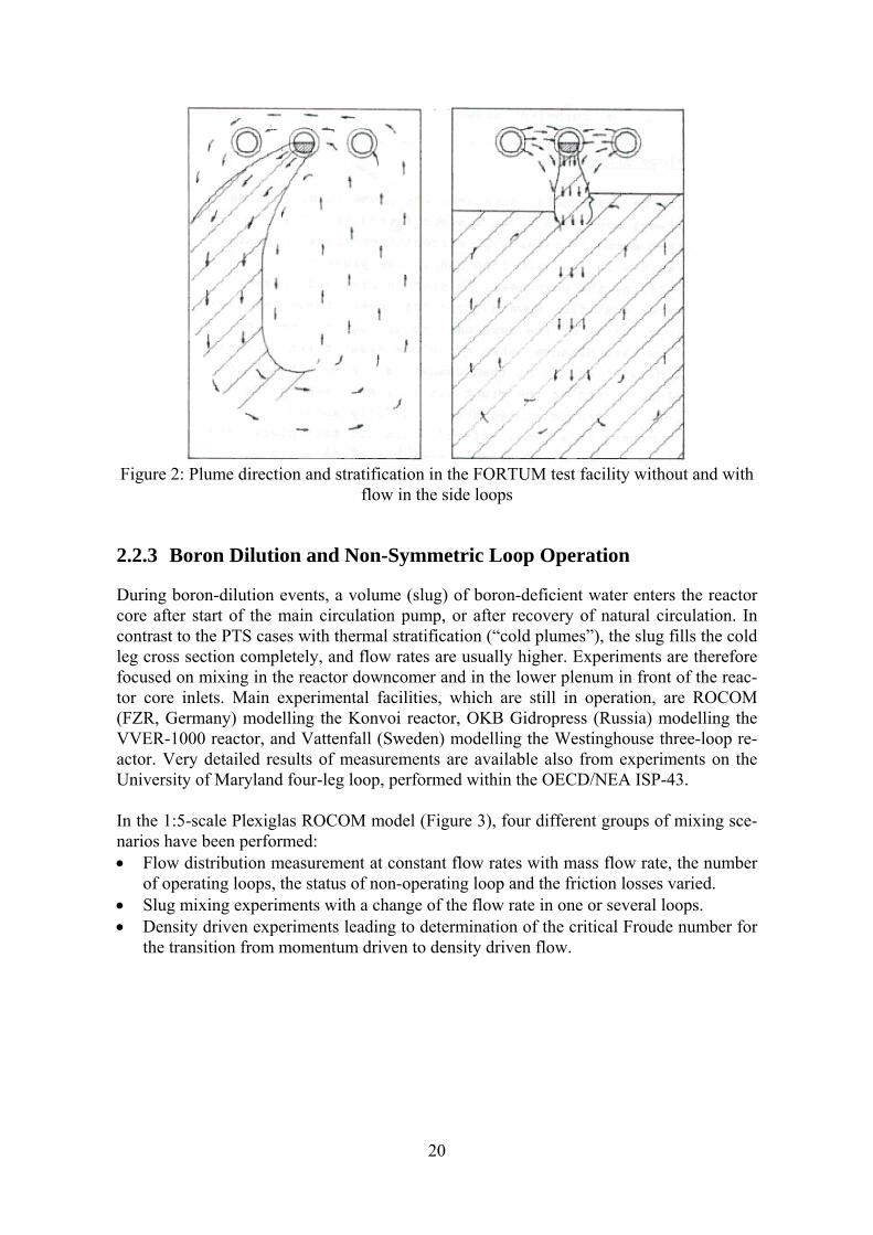
20
Figure 2: Plume direction and stratification in the FORTUM test facility without and with flow in the side loops
2.2.3 Boron Dilution and Non-Symmetric Loop Operation
During boron-dilution events, a volume (slug) of boron-deficient water enters the reactor core after start of the main circulation pump, or after recovery of natural circulation. In contrast to the PTS cases with thermal stratification (“cold plumes”), the slug fills the cold leg cross section completely, and flow rates are usually higher. Experiments are therefore focused on mixing in the reactor downcomer and in the lower plenum in front of the reac-tor core inlets. Main experimental facilities, which are still in operation, are ROCOM (FZR, Germany) modelling the Konvoi reactor, OKB Gidropress (Russia) modelling the VVER-1000 reactor, and Vattenfall (Sweden) modelling the Westinghouse three-loop re-actor. Very detailed results of measurements are available also from experiments on the University of Maryland four-leg loop, performed within the OECD/NEA ISP-43. In the 1:5-scale Plexiglas ROCOM model (Figure 3), four different groups of mixing sce-narios have been performed: • Flow distribution measurement at constant flow rates with mass flow rate, the number
of operating loops, the status of non-operating loop and the friction losses varied. • Slug mixing experiments with a change of the flow rate in one or several loops. • Density driven experiments leading to determination of the critical Froude number for
the transition from momentum driven to density driven flow.
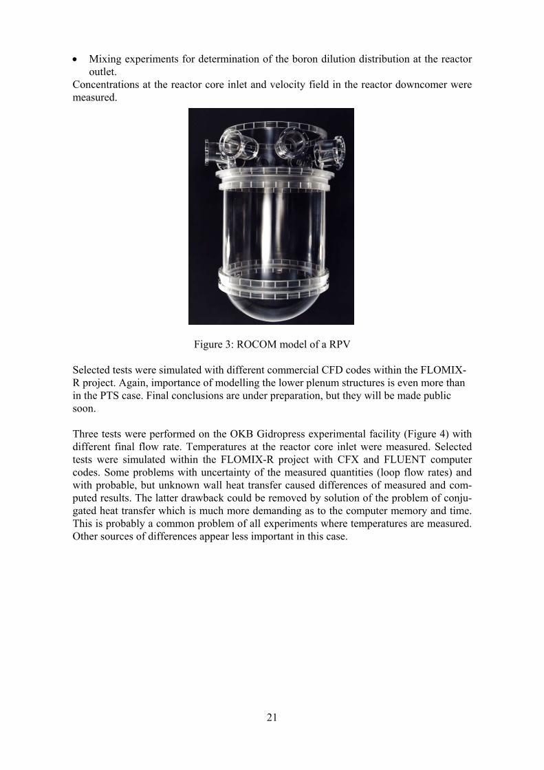
21
• Mixing experiments for determination of the boron dilution distribution at the reactor outlet.
Concentrations at the reactor core inlet and velocity field in the reactor downcomer were measured.
Figure 3: ROCOM model of a RPV
Selected tests were simulated with different commercial CFD codes within the FLOMIX-R project. Again, importance of modelling the lower plenum structures is even more than in the PTS case. Final conclusions are under preparation, but they will be made public soon. Three tests were performed on the OKB Gidropress experimental facility (Figure 4) with different final flow rate. Temperatures at the reactor core inlet were measured. Selected tests were simulated within the FLOMIX-R project with CFX and FLUENT computer codes. Some problems with uncertainty of the measured quantities (loop flow rates) and with probable, but unknown wall heat transfer caused differences of measured and com-puted results. The latter drawback could be removed by solution of the problem of conju-gated heat transfer which is much more demanding as to the computer memory and time. This is probably a common problem of all experiments where temperatures are measured. Other sources of differences appear less important in this case.
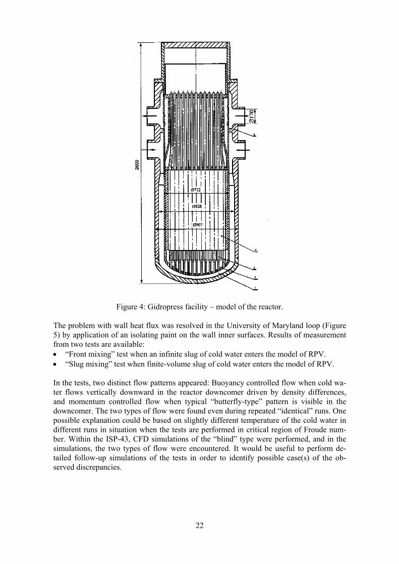
22
Figure 4: Gidropress facility – model of the reactor.
The problem with wall heat flux was resolved in the University of Maryland loop (Figure 5) by application of an isolating paint on the wall inner surfaces. Results of measurement from two tests are available: • “Front mixing” test when an infinite slug of cold water enters the model of RPV. • “Slug mixing” test when finite-volume slug of cold water enters the model of RPV. In the tests, two distinct flow patterns appeared: Buoyancy controlled flow when cold wa-ter flows vertically downward in the reactor downcomer driven by density differences, and momentum controlled flow when typical “butterfly-type” pattern is visible in the downcomer. The two types of flow were found even during repeated “identical” runs. One possible explanation could be based on slightly different temperature of the cold water in different runs in situation when the tests are performed in critical region of Froude num-ber. Within the ISP-43, CFD simulations of the “blind” type were performed, and in the simulations, the two types of flow were encountered. It would be useful to perform de-tailed follow-up simulations of the tests in order to identify possible case(s) of the ob-served discrepancies.
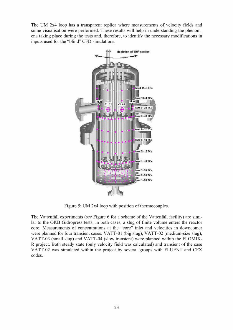
23
The UM 2x4 loop has a transparent replica where measurements of velocity fields and some visualisation were performed. These results will help in understanding the phenom-ena taking place during the tests and, therefore, to identify the necessary modifications in inputs used for the “blind” CFD simulations.
Figure 5: UM 2x4 loop with position of thermocouples.
The Vattenfall experiments (see Figure 6 for a scheme of the Vattenfall facility) are simi-lar to the OKB Gidropress tests; in both cases, a slug of finite volume enters the reactor core. Measurements of concentrations at the “core” inlet and velocities in downcomer were planned for four transient cases: VATT-01 (big slug), VATT-02 (medium-size slug), VATT-03 (small slug) and VATT-04 (slow transient) were planned within the FLOMIX-R project. Both steady state (only velocity field was calculated) and transient of the case VATT-02 was simulated within the project by several groups with FLUENT and CFX codes.
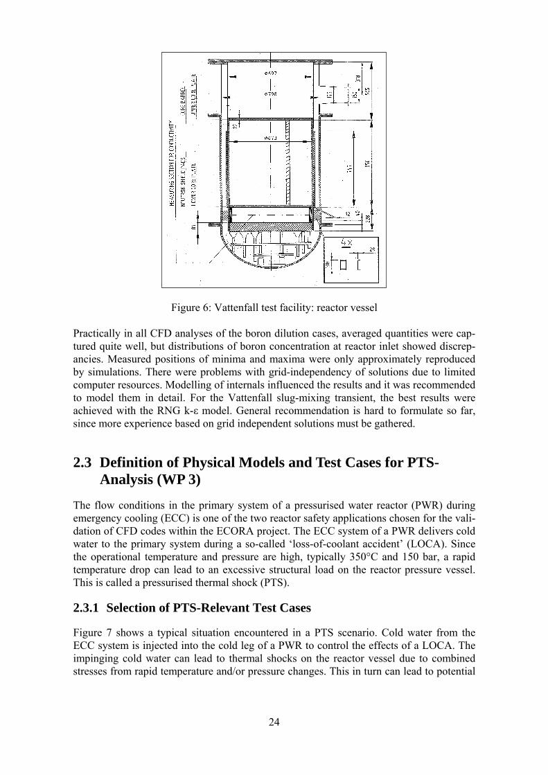
24
Figure 6: Vattenfall test facility: reactor vessel
Practically in all CFD analyses of the boron dilution cases, averaged quantities were cap-tured quite well, but distributions of boron concentration at reactor inlet showed discrep-ancies. Measured positions of minima and maxima were only approximately reproduced by simulations. There were problems with grid-independency of solutions due to limited computer resources. Modelling of internals influenced the results and it was recommended to model them in detail. For the Vattenfall slug-mixing transient, the best results were achieved with the RNG k-ε model. General recommendation is hard to formulate so far, since more experience based on grid independent solutions must be gathered.
2.3 Definition of Physical Models and Test Cases for PTS-Analysis (WP 3)
The flow conditions in the primary system of a pressurised water reactor (PWR) during emergency cooling (ECC) is one of the two reactor safety applications chosen for the vali-dation of CFD codes within the ECORA project. The ECC system of a PWR delivers cold water to the primary system during a so-called ‘loss-of-coolant accident’ (LOCA). Since the operational temperature and pressure are high, typically 350°C and 150 bar, a rapid temperature drop can lead to an excessive structural load on the reactor pressure vessel. This is called a pressurised thermal shock (PTS).
2.3.1 Selection of PTS-Relevant Test Cases
Figure 7 shows a typical situation encountered in a PTS scenario. Cold water from the ECC system is injected into the cold leg of a PWR to control the effects of a LOCA. The impinging cold water can lead to thermal shocks on the reactor vessel due to combined stresses from rapid temperature and/or pressure changes. This in turn can lead to potential
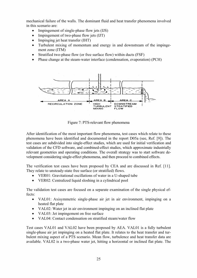
25
mechanical failure of the walls. The dominant fluid and heat transfer phenomena involved in this scenario are:
• Impingement of single-phase flow jets (IJS) • Impingement of two-phase flow jets (IJT) • Impinging jet heat transfer (IHT) • Turbulent mixing of momentum and energy in and downstream of the impinge-
ment zone (ITM) • Stratified two-phase flow (or free surface flow) within ducts (FSF) • Phase change at the steam-water interface (condensation, evaporation) (PCH)
Figure 7: PTS-relevant flow phenomena
After identification of the most important flow phenomena, test cases which relate to these phenomena have been identified and documented in the report D05a (see, Ref. [9]). The test cases are subdivided into single-effect studies, which are used for initial verification and validation of the CFD software, and combined-effect studies, which approximate industrially relevant geometries and operating conditions. The overall strategy was to start software de-velopment considering single-effect phenomena, and then proceed to combined effects. The verification test cases have been proposed by CEA and are discussed in Ref. [11]. They relate to unsteady-state free surface (or stratified) flows.
• VER01: Gravitational oscillations of water in a U-shaped tube • VER02: Centralized liquid sloshing in a cylindrical pool
The validation test cases are focused on a separate examination of the single physical ef-fects:
• VAL01: Axisymmetric single-phase air jet in air environment, impinging on a heated flat plate
• VAL02: Water jet in air environment impinging on an inclined flat plate • VAL03: Jet impingement on free surface • VAL04: Contact condensation on stratified steam/water flow
Test cases VAL01 and VAL02 have been proposed by AEA. VAL01 is a fully turbulent single-phase air jet impinging on a heated flat plate. It relates to the heat transfer and tur-bulent mixing aspect of a PTS scenario. Mean flow, turbulence and heat transfer data are available. VAL02 is a two-phase water jet, hitting a horizontal or inclined flat plate. The
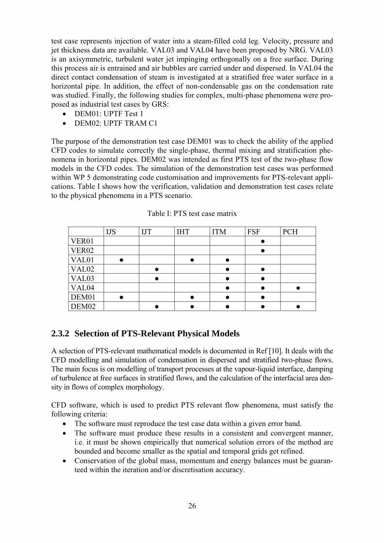
26
test case represents injection of water into a steam-filled cold leg. Velocity, pressure and jet thickness data are available. VAL03 and VAL04 have been proposed by NRG. VAL03 is an axisymmetric, turbulent water jet impinging orthogonally on a free surface. During this process air is entrained and air bubbles are carried under and dispersed. In VAL04 the direct contact condensation of steam is investigated at a stratified free water surface in a horizontal pipe. In addition, the effect of non-condensable gas on the condensation rate was studied. Finally, the following studies for complex, multi-phase phenomena were pro-posed as industrial test cases by GRS:
• DEM01: UPTF Test 1 • DEM02: UPTF TRAM C1
The purpose of the demonstration test case DEM01 was to check the ability of the applied CFD codes to simulate correctly the single-phase, thermal mixing and stratification phe-nomena in horizontal pipes. DEM02 was intended as first PTS test of the two-phase flow models in the CFD codes. The simulation of the demonstration test cases was performed within WP 5 demonstrating code customisation and improvements for PTS-relevant appli-cations. Table I shows how the verification, validation and demonstration test cases relate to the physical phenomena in a PTS scenario.
Table I: PTS test case matrix
IJS IJT IHT ITM FSF PCH VER01 ● VER02 ● VAL01 ● ● ● VAL02 ● ● ● VAL03 ● ● ● VAL04 ● ● ● DEM01 ● ● ● ● DEM02 ● ● ● ● ●
2.3.2 Selection of PTS-Relevant Physical Models
A selection of PTS-relevant mathematical models is documented in Ref [10]. It deals with the CFD modelling and simulation of condensation in dispersed and stratified two-phase flows. The main focus is on modelling of transport processes at the vapour-liquid interface, damping of turbulence at free surfaces in stratified flows, and the calculation of the interfacial area den-sity in flows of complex morphology. CFD software, which is used to predict PTS relevant flow phenomena, must satisfy the following criteria:
• The software must reproduce the test case data within a given error band. • The software must produce these results in a consistent and convergent manner,
i.e. it must be shown empirically that numerical solution errors of the method are bounded and become smaller as the spatial and temporal grids get refined.
• Conservation of the global mass, momentum and energy balances must be guaran-teed within the iteration and/or discretisation accuracy.
27
• The software must be robust. However, a mathematical convergence proof for three-dimensional CFD methods, which could be used as an absolute benchmark for robustness does not exist. Therefore, robustness of the CFD methods can only be defined in a statistical sense. For instance, a code is said to be ‚robust’ if it runs and converges for more than 80 % of the test cases it is subject to.
The ‘optimum’ CFD software needs to satisfy the above requirements, at the same mini-mizing computing time and computer memory demands.
2.3.3 Calculation of PTS-Relevant Verification Test Cases
The two verification test cases have been calculated with CFX-5 and Neptune. The results are documented in Ref. [11]. The purpose of these test cases was to check robustness and accu-racy of the numerical methods. Different factors influencing accuracy of the results were identified and analysed separately. 2.3.3.1 VER01: Oscillating Manometer The first verification test case VER01 is the oscillating manometer documented in Ref. [19]. It consists in calculating the motion of one liquid phase in a U-shaped tube. The tube is closed at both ends. Initially, it contains water in its upper part and air in its lower part. The liquid level is the same in the two parts of the pipe. The initial velocity of the liquid is non zero with a uniform value. In this case the two phases are mechanically uncoupled. Gravity forces are present. The motion of a volume fraction front has to be represented without diffusion. Therefore, stratified flows must be correctly calculated. The problem deals not only with the numerical features, but also with physical modelling. The test case is useful to investigate the accuracy of mass balance and the ability of the code to con-serve total pressure along a stream line. Though the manometer problem is a good test of front-capturing capabilities, as they exist in hyperbolic numerical schemes, parabolic/elliptic solvers cope adequately with the prob-lem, provided second-order differencing schemes are utilised, and there is sufficient mesh resolution. Additionally, there are positive benefits from employing an explicit interface-tracking technique. Satisfactory results are obtained with the Neptune and CFX 4 and CFX-5 codes. 2.3.3.2 VER02: Liquid Sloshing The test deals with an experiment in which the main phenomenon is free surface oscilla-tions. The flow is transient, the fluid is water in an air environment. A cylindrical pool is divided into two concentric parts. Initially, the water column in the inner cylinder is higher than the water level in the external cylinder. Initially, the water column is released and a sloshing motion of the liquid between the symmetry axis and the outer wall of the cylindrical pool is initiated. The main goal of the simulation is to compute the free surface flow and to predict the motion of the free surface correctly. The original test case is documented in Ref. [20] A cylindrical water column with a diameter of 11 cm and an ini-tial height of 20 cm, is centred in a cylindrical pool with an outer diameter of 44 cm. The initial water level in the pool is 5 cm (D1X-3 experiment). The water sloshing is initiated by lifting quickly the sheet around the inner cylinder. The test case is useful to investigate the following numerical features:
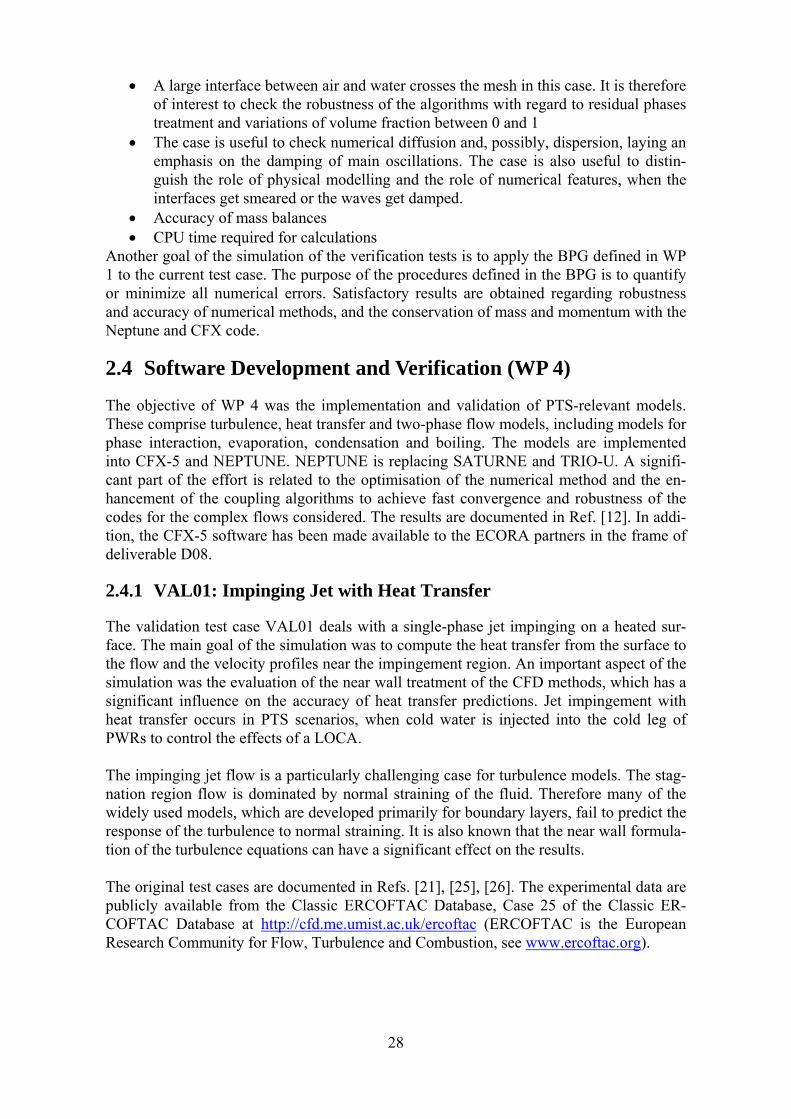
28
• A large interface between air and water crosses the mesh in this case. It is therefore of interest to check the robustness of the algorithms with regard to residual phases treatment and variations of volume fraction between 0 and 1
• The case is useful to check numerical diffusion and, possibly, dispersion, laying an emphasis on the damping of main oscillations. The case is also useful to distin-guish the role of physical modelling and the role of numerical features, when the interfaces get smeared or the waves get damped.
• Accuracy of mass balances • CPU time required for calculations
Another goal of the simulation of the verification tests is to apply the BPG defined in WP 1 to the current test case. The purpose of the procedures defined in the BPG is to quantify or minimize all numerical errors. Satisfactory results are obtained regarding robustness and accuracy of numerical methods, and the conservation of mass and momentum with the Neptune and CFX code.
2.4 Software Development and Verification (WP 4)
The objective of WP 4 was the implementation and validation of PTS-relevant models. These comprise turbulence, heat transfer and two-phase flow models, including models for phase interaction, evaporation, condensation and boiling. The models are implemented into CFX-5 and NEPTUNE. NEPTUNE is replacing SATURNE and TRIO-U. A signifi-cant part of the effort is related to the optimisation of the numerical method and the en-hancement of the coupling algorithms to achieve fast convergence and robustness of the codes for the complex flows considered. The results are documented in Ref. [12]. In addi-tion, the CFX-5 software has been made available to the ECORA partners in the frame of deliverable D08.
2.4.1 VAL01: Impinging Jet with Heat Transfer
The validation test case VAL01 deals with a single-phase jet impinging on a heated sur-face. The main goal of the simulation was to compute the heat transfer from the surface to the flow and the velocity profiles near the impingement region. An important aspect of the simulation was the evaluation of the near wall treatment of the CFD methods, which has a significant influence on the accuracy of heat transfer predictions. Jet impingement with heat transfer occurs in PTS scenarios, when cold water is injected into the cold leg of PWRs to control the effects of a LOCA. The impinging jet flow is a particularly challenging case for turbulence models. The stag-nation region flow is dominated by normal straining of the fluid. Therefore many of the widely used models, which are developed primarily for boundary layers, fail to predict the response of the turbulence to normal straining. It is also known that the near wall formula-tion of the turbulence equations can have a significant effect on the results. The original test cases are documented in Refs. [21], [25], [26]. The experimental data are publicly available from the Classic ERCOFTAC Database, Case 25 of the Classic ER-COFTAC Database at http://cfd.me.umist.ac.uk/ercoftac (ERCOFTAC is the European Research Community for Flow, Turbulence and Combustion, see www.ercoftac.org).
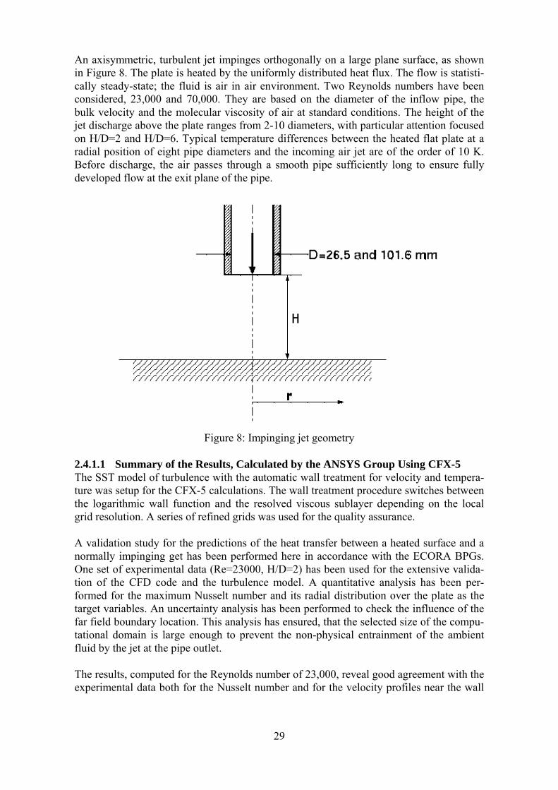
29
An axisymmetric, turbulent jet impinges orthogonally on a large plane surface, as shown in Figure 8. The plate is heated by the uniformly distributed heat flux. The flow is statisti-cally steady-state; the fluid is air in air environment. Two Reynolds numbers have been considered, 23,000 and 70,000. They are based on the diameter of the inflow pipe, the bulk velocity and the molecular viscosity of air at standard conditions. The height of the jet discharge above the plate ranges from 2-10 diameters, with particular attention focused on H/D=2 and H/D=6. Typical temperature differences between the heated flat plate at a radial position of eight pipe diameters and the incoming air jet are of the order of 10 K. Before discharge, the air passes through a smooth pipe sufficiently long to ensure fully developed flow at the exit plane of the pipe.
Figure 8: Impinging jet geometry
2.4.1.1 Summary of the Results, Calculated by the ANSYS Group Using CFX-5 The SST model of turbulence with the automatic wall treatment for velocity and tempera-ture was setup for the CFX-5 calculations. The wall treatment procedure switches between the logarithmic wall function and the resolved viscous sublayer depending on the local grid resolution. A series of refined grids was used for the quality assurance. A validation study for the predictions of the heat transfer between a heated surface and a normally impinging get has been performed here in accordance with the ECORA BPGs. One set of experimental data (Re=23000, H/D=2) has been used for the extensive valida-tion of the CFD code and the turbulence model. A quantitative analysis has been per-formed for the maximum Nusselt number and its radial distribution over the plate as the target variables. An uncertainty analysis has been performed to check the influence of the far field boundary location. This analysis has ensured, that the selected size of the compu-tational domain is large enough to prevent the non-physical entrainment of the ambient fluid by the jet at the pipe outlet. The results, computed for the Reynolds number of 23,000, reveal good agreement with the experimental data both for the Nusselt number and for the velocity profiles near the wall
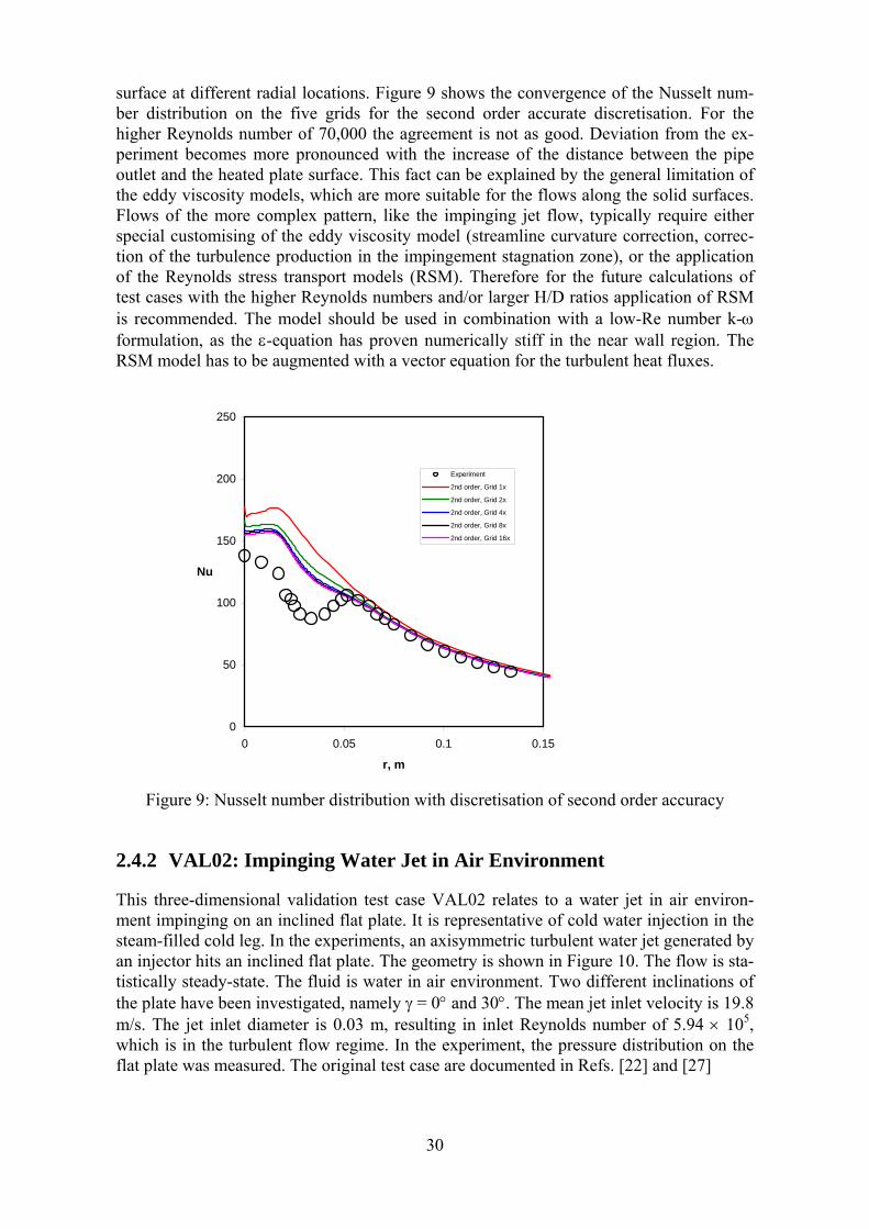
30
surface at different radial locations. Figure 9 shows the convergence of the Nusselt num-ber distribution on the five grids for the second order accurate discretisation. For the higher Reynolds number of 70,000 the agreement is not as good. Deviation from the ex-periment becomes more pronounced with the increase of the distance between the pipe outlet and the heated plate surface. This fact can be explained by the general limitation of the eddy viscosity models, which are more suitable for the flows along the solid surfaces. Flows of the more complex pattern, like the impinging jet flow, typically require either special customising of the eddy viscosity model (streamline curvature correction, correc-tion of the turbulence production in the impingement stagnation zone), or the application of the Reynolds stress transport models (RSM). Therefore for the future calculations of test cases with the higher Reynolds numbers and/or larger H/D ratios application of RSM is recommended. The model should be used in combination with a low-Re number k-ω formulation, as the ε-equation has proven numerically stiff in the near wall region. The RSM model has to be augmented with a vector equation for the turbulent heat fluxes.
0
50
100
150
200
250
0 0.05 0.1 0.15
r, m
Nu
Experiment
2nd order, Grid 1x
2nd order, Grid 2x
2nd order, Grid 4x
2nd order, Grid 8x
2nd order, Grid 16x
Figure 9: Nusselt number distribution with discretisation of second order accuracy
2.4.2 VAL02: Impinging Water Jet in Air Environment
This three-dimensional validation test case VAL02 relates to a water jet in air environ-ment impinging on an inclined flat plate. It is representative of cold water injection in the steam-filled cold leg. In the experiments, an axisymmetric turbulent water jet generated by an injector hits an inclined flat plate. The geometry is shown in Figure 10. The flow is sta-tistically steady-state. The fluid is water in air environment. Two different inclinations of the plate have been investigated, namely γ = 0° and 30°. The mean jet inlet velocity is 19.8 m/s. The jet inlet diameter is 0.03 m, resulting in inlet Reynolds number of 5.94 × 10⁵, which is in the turbulent flow regime. In the experiment, the pressure distribution on the flat plate was measured. The original test case are documented in Refs. [22] and [27]
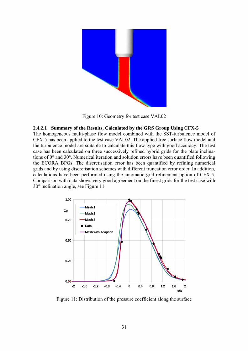
31
Figure 10: Geometry for test case VAL02 2.4.2.1 Summary of the Results, Calculated by the GRS Group Using CFX-5 The homogeneous multi-phase flow model combined with the SST-turbulence model of CFX-5 has been applied to the test case VAL02. The applied free surface flow model and the turbulence model are suitable to calculate this flow type with good accuracy. The test case has been calculated on three successively refined hybrid grids for the plate inclina-tions of 0° and 30°. Numerical iteration and solution errors have been quantified following the ECORA BPGs. The discretisation error has been quantified by refining numerical grids and by using discretisation schemes with different truncation error order. In addition, calculations have been performed using the automatic grid refinement option of CFX-5. Comparison with data shows very good agreement on the finest grids for the test case with 30° inclination angle, see Figure 11.
0.00
0.25
0.50
0.75
1.00
-2 -1.6 -1.2 -0.8 -0.4 0 0.4 0.8 1.2 1.6 2x/D
CpMesh 1
Mesh 2
Mesh 3
Data
Mesh with Adaption
Figure 11: Distribution of the pressure coefficient along the surface
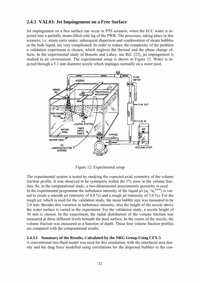
32
2.4.3 VAL03: Jet Impingement on a Free Surface
Jet impingement on a free surface can occur in PTS scenario, when the ECC water is in-jected into a partially steam-filled cold leg of the PWR. The processes, taking place in this scenario, i.e. steam carry under, subsequent dispersion and condensation of steam bubbles in the bulk liquid, are very complicated. In order to reduce the complexity of the problem a validation experiment is chosen, which neglects the thermal and the phase change ef-fects. In the experimental study of Bonetto and Lahey, see Ref. [23], jet impingement is studied in air environment. The experimental setup is shown in Figure 12. Water is in-jected through a 5.1 mm diameter nozzle which impinges normally on a water pool.
Figure 12: Experimental setup
The experimental system is tested by studying the expected axial symmetry of the volume fraction profile. It was observed to be symmetric within the 1% error in the volume frac-tion. So, in the computational study, a two-dimensional axisymmetric geometry is used. In the experimental programme the turbulence intensity of the liquid jet (uL’/uL
mean) is var-ied to create a smooth jet (intensity of 0.8 %) and a rough jet (intensity of 3.0 %). For the rough jet, which is used for the validation study, the mean bubble size was measured to be 2.0 mm. Besides this variation in turbulence intensity, also the height of the nozzle above the water surface is varied in the experiment. For the validation study, a nozzle height of 30 mm is chosen. In the experiment, the radial distribution of the volume fraction was measured at three different levels beneath the pool surface. In the centre of the nozzle, the volume fraction was measured as a function of depth. These four volume fraction profiles are compared with the computational results. 2.4.3.1 Summary of the Results, Calculated by the NRG Group Using CFX-5 A conventional two-fluid model was used for this simulation, with the interfacial area den-sity and the drag force modelled using correlations for the dispersed bubbles in the con-
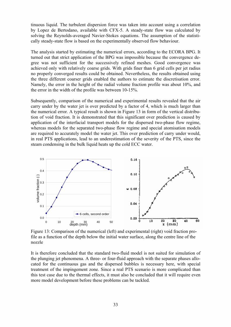
33
tinuous liquid. The turbulent dispersion force was taken into account using a correlation by Lopez de Bertodano, available with CFX-5. A steady-state flow was calculated by solving the Reynolds-averaged Navier-Stokes equations. The assumption of the statisti-cally steady-state flow is based on the experimentally observed flow behaviour. The analysis started by estimating the numerical errors, according to the ECORA BPG. It turned out that strict application of the BPG was impossible because the convergence de-gree was not sufficient for the successively refined meshes. Good convergence was achieved only with relatively coarse grids. With grids finer than 6 grid cells per jet radius no properly converged results could be obtained. Nevertheless, the results obtained using the three different coarser grids enabled the authors to estimate the discretisation error. Namely, the error in the height of the radial volume fraction profile was about 10%, and the error in the width of the profile was between 10-15%. Subsequently, comparison of the numerical and experimental results revealed that the air carry under by the water jet is over predicted by a factor of 4, which is much larger than the numerical error. A typical result is shown in Figure 13 in form of the vertical distribu-tion of void fraction. It is demonstrated that this significant over prediction is caused by application of the interfacial transport models for the dispersed two-phase flow regime, whereas models for the separated two-phase flow regime and special atomisation models are required to accurately model the water jet. This over prediction of carry under would, in real PTS applications, lead to an underestimation of the severity of the PTS, since the steam condensing in the bulk liquid heats up the cold ECC water.
Figure 13: Comparison of the numerical (left) and experimental (right) void fraction pro-file as a function of the depth below the initial water surface, along the centre line of the nozzle It is therefore concluded that the standard two-fluid model is not suited for simulation of the plunging jet phenomena. A three- or four-fluid approach with the separate phases allo-cated for the continuous gas and the dispersed bubbles is necessary here, with special treatment of the impingement zone. Since a real PTS scenario is more complicated than this test case due to the thermal effects, it must also be concluded that it will require even more model development before these problems can be tackled.
0.0
0.1
0.2
0.3
0.4
0.5
0 10 20 30 40 50depth (mm)
volu
me
fract
ion
(-)
6 cells, second order
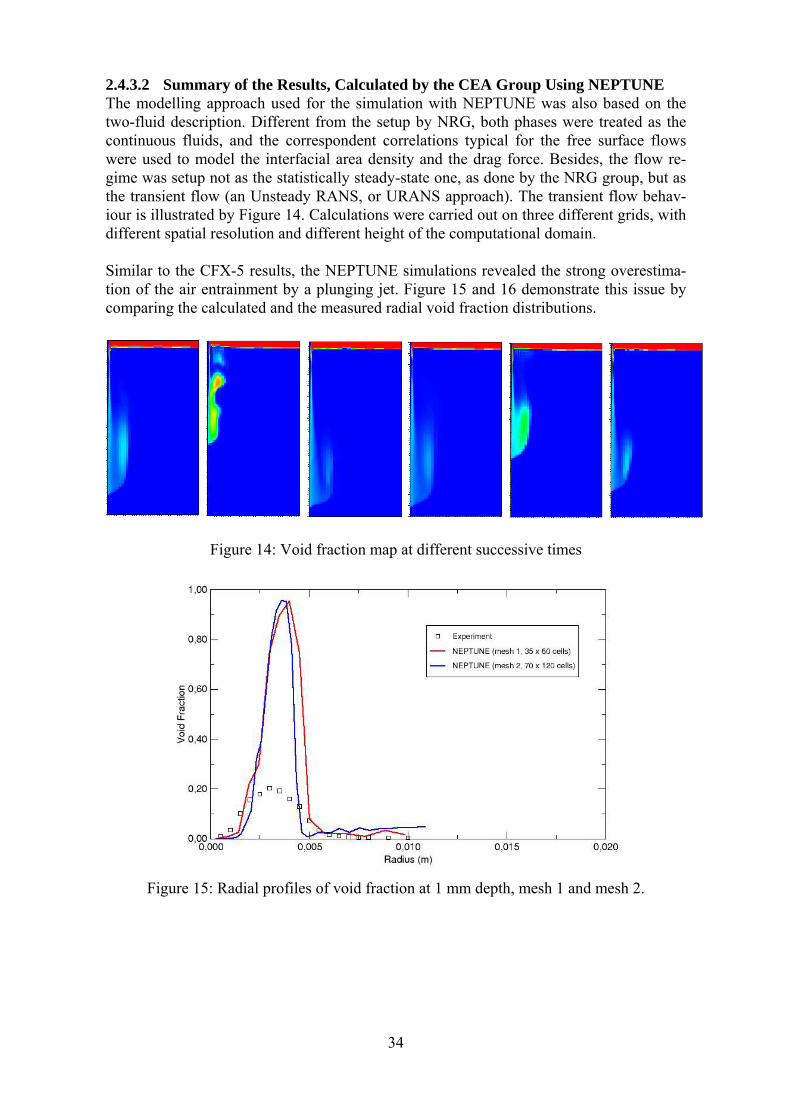
34
2.4.3.2 Summary of the Results, Calculated by the CEA Group Using NEPTUNE The modelling approach used for the simulation with NEPTUNE was also based on the two-fluid description. Different from the setup by NRG, both phases were treated as the continuous fluids, and the correspondent correlations typical for the free surface flows were used to model the interfacial area density and the drag force. Besides, the flow re-gime was setup not as the statistically steady-state one, as done by the NRG group, but as the transient flow (an Unsteady RANS, or URANS approach). The transient flow behav-iour is illustrated by Figure 14. Calculations were carried out on three different grids, with different spatial resolution and different height of the computational domain. Similar to the CFX-5 results, the NEPTUNE simulations revealed the strong overestima-tion of the air entrainment by a plunging jet. Figure 15 and 16 demonstrate this issue by comparing the calculated and the measured radial void fraction distributions.
Figure 14: Void fraction map at different successive times
Figure 15: Radial profiles of void fraction at 1 mm depth, mesh 1 and mesh 2.
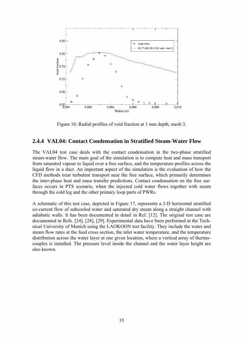
35
Figure 16: Radial profiles of void fraction at 1 mm depth, mesh 3.
2.4.4 VAL04: Contact Condensation in Stratified Steam-Water Flow
The VAL04 test case deals with the contact condensation in the two-phase stratified steam-water flow. The main goal of the simulation is to compute heat and mass transport from saturated vapour to liquid over a free surface, and the temperature profiles across the liquid flow in a duct. An important aspect of the simulation is the evaluation of how the CFD methods treat turbulent transport near the free surface, which primarily determines the inter-phase heat and mass transfer predictions. Contact condensation on the free sur-faces occurs in PTS scenario, when the injected cold water flows together with steam through the cold leg and the other primary loop parts of PWRs. A schematic of this test case, depicted in Figure 17, represents a 2-D horizontal stratified co-current flow of subcooled water and saturated dry steam along a straight channel with adiabatic walls. It has been documented in detail in Ref. [12]. The original test case are documented in Refs. [24], [28], [29]. Experimental data have been performed at the Tech-nical University of Munich using the LAOKOON test facility. They include the water and steam flow rates at the feed cross section, the inlet water temperature, and the temperature distribution across the water layer at one given location, where a vertical array of thermo-couples is installed. The pressure level inside the channel and the water layer height are also known.

36
Adiabatic wall
Steam
Water
Thermocouples
Adiabatic wall 790mm
128mm
31mm
Figure 17: Schematic of the stratified flow in a 2-D duct
According to the experimental evidence this flow is stationary and two-dimensional. The Reynolds number of water was in the range between 20,000 and 30,000. Two co-current flow regimes were selected, which differ in the steam Reynolds number value, namely 5.1⋅105 and 3.4⋅105 at the inlet. The pressure level was close to 7 bar in the higher Rey-nolds number case, and 4 bar in the lower Reynolds number case. Due to the carefully de-signed inlet and outlet of water the free surface is plane and horizontal everywhere. No waves were visually observed in the experiment. During the condensation the latent heat of phase transition is released and fully consumed for heating up the initially sub-cooled water. The correspondent temperature gradient, normal to the free surface, develops in water. Therefore the condensation rate is limited by the transport rate of heat from the free surface to the bulk water flow. 2.4.4.1 Summary of the Results, Calculated by the EDF Group Using NEPTUNE A model of condensation, used by the EDF group, was based on a modified interface re-newal concept by Hughes and Duffey in Ref. [30]. A small parametric study was done for the high Reynolds number configuration in order to better understand the behaviour of the condensation model. Figure 18 shows the water temperature profiles at the measurement section. The computa-tion curve of the water temperature is in a good agreement with the experimental data. Near the channel bottom, the water temperature obtained with the Neptune CFD code is colder than expected, which might be caused by the weakness of the k-ε turbulence model near a wall and by the too small turbulent diffusion.
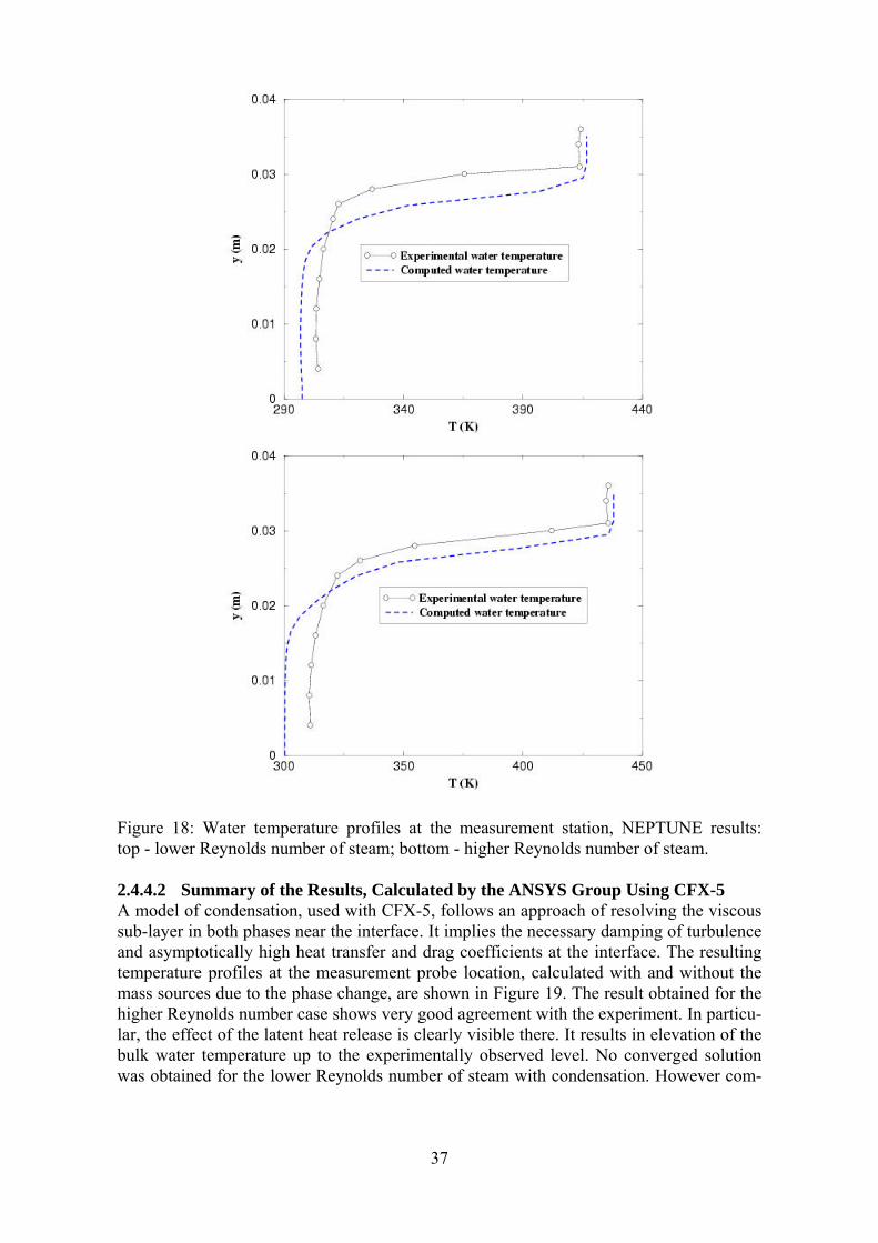
37
Figure 18: Water temperature profiles at the measurement station, NEPTUNE results: top - lower Reynolds number of steam; bottom - higher Reynolds number of steam. 2.4.4.2 Summary of the Results, Calculated by the ANSYS Group Using CFX-5 A model of condensation, used with CFX-5, follows an approach of resolving the viscous sub-layer in both phases near the interface. It implies the necessary damping of turbulence and asymptotically high heat transfer and drag coefficients at the interface. The resulting temperature profiles at the measurement probe location, calculated with and without the mass sources due to the phase change, are shown in Figure 19. The result obtained for the higher Reynolds number case shows very good agreement with the experiment. In particu-lar, the effect of the latent heat release is clearly visible there. It results in elevation of the bulk water temperature up to the experimentally observed level. No converged solution was obtained for the lower Reynolds number of steam with condensation. However com-
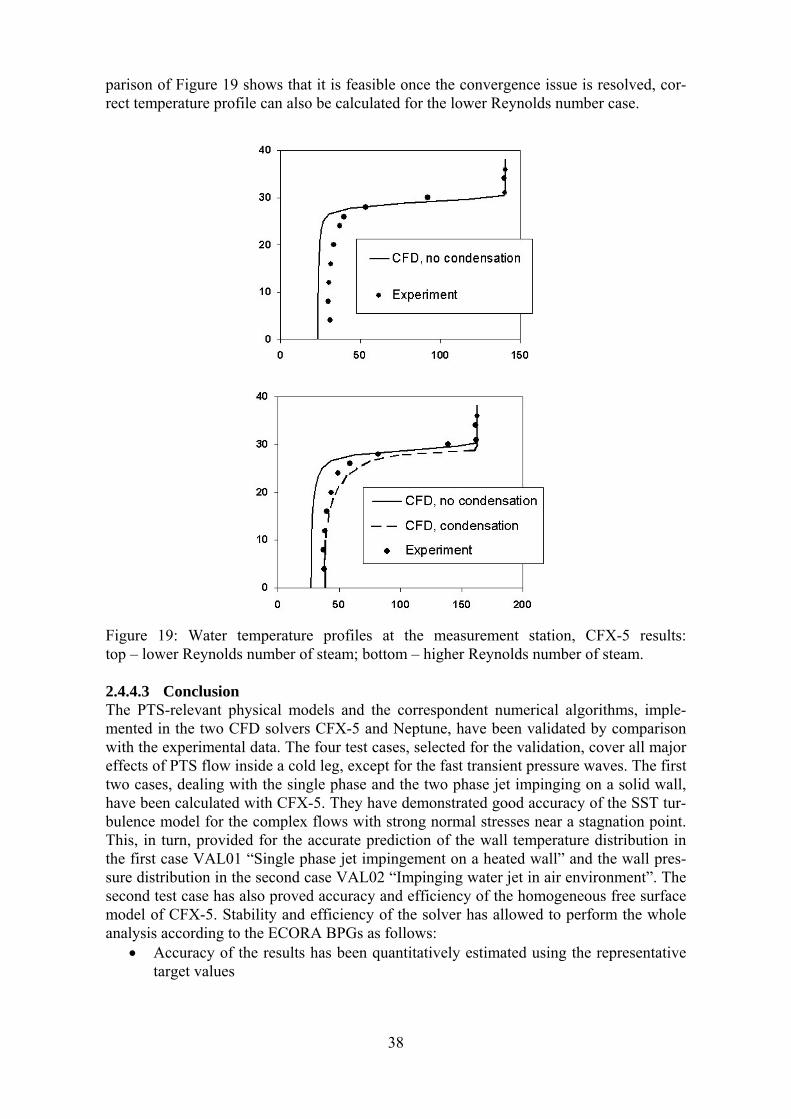
38
parison of Figure 19 shows that it is feasible once the convergence issue is resolved, cor-rect temperature profile can also be calculated for the lower Reynolds number case.
Figure 19: Water temperature profiles at the measurement station, CFX-5 results: top – lower Reynolds number of steam; bottom – higher Reynolds number of steam. 2.4.4.3 Conclusion The PTS-relevant physical models and the correspondent numerical algorithms, imple-mented in the two CFD solvers CFX-5 and Neptune, have been validated by comparison with the experimental data. The four test cases, selected for the validation, cover all major effects of PTS flow inside a cold leg, except for the fast transient pressure waves. The first two cases, dealing with the single phase and the two phase jet impinging on a solid wall, have been calculated with CFX-5. They have demonstrated good accuracy of the SST tur-bulence model for the complex flows with strong normal stresses near a stagnation point. This, in turn, provided for the accurate prediction of the wall temperature distribution in the first case VAL01 “Single phase jet impingement on a heated wall” and the wall pres-sure distribution in the second case VAL02 “Impinging water jet in air environment”. The second test case has also proved accuracy and efficiency of the homogeneous free surface model of CFX-5. Stability and efficiency of the solver has allowed to perform the whole analysis according to the ECORA BPGs as follows:
• Accuracy of the results has been quantitatively estimated using the representative target values
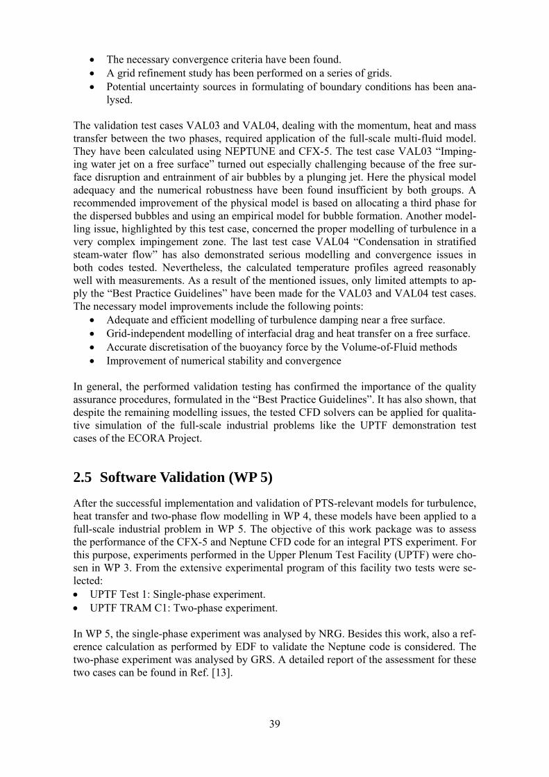
39
• The necessary convergence criteria have been found. • A grid refinement study has been performed on a series of grids. • Potential uncertainty sources in formulating of boundary conditions has been ana-
lysed. The validation test cases VAL03 and VAL04, dealing with the momentum, heat and mass transfer between the two phases, required application of the full-scale multi-fluid model. They have been calculated using NEPTUNE and CFX-5. The test case VAL03 “Imping-ing water jet on a free surface” turned out especially challenging because of the free sur-face disruption and entrainment of air bubbles by a plunging jet. Here the physical model adequacy and the numerical robustness have been found insufficient by both groups. A recommended improvement of the physical model is based on allocating a third phase for the dispersed bubbles and using an empirical model for bubble formation. Another model-ling issue, highlighted by this test case, concerned the proper modelling of turbulence in a very complex impingement zone. The last test case VAL04 “Condensation in stratified steam-water flow” has also demonstrated serious modelling and convergence issues in both codes tested. Nevertheless, the calculated temperature profiles agreed reasonably well with measurements. As a result of the mentioned issues, only limited attempts to ap-ply the “Best Practice Guidelines” have been made for the VAL03 and VAL04 test cases. The necessary model improvements include the following points:
• Adequate and efficient modelling of turbulence damping near a free surface. • Grid-independent modelling of interfacial drag and heat transfer on a free surface. • Accurate discretisation of the buoyancy force by the Volume-of-Fluid methods • Improvement of numerical stability and convergence
In general, the performed validation testing has confirmed the importance of the quality assurance procedures, formulated in the “Best Practice Guidelines”. It has also shown, that despite the remaining modelling issues, the tested CFD solvers can be applied for qualita-tive simulation of the full-scale industrial problems like the UPTF demonstration test cases of the ECORA Project.
2.5 Software Validation (WP 5)
After the successful implementation and validation of PTS-relevant models for turbulence, heat transfer and two-phase flow modelling in WP 4, these models have been applied to a full-scale industrial problem in WP 5. The objective of this work package was to assess the performance of the CFX-5 and Neptune CFD code for an integral PTS experiment. For this purpose, experiments performed in the Upper Plenum Test Facility (UPTF) were cho-sen in WP 3. From the extensive experimental program of this facility two tests were se-lected: • UPTF Test 1: Single-phase experiment. • UPTF TRAM C1: Two-phase experiment. In WP 5, the single-phase experiment was analysed by NRG. Besides this work, also a ref-erence calculation as performed by EDF to validate the Neptune code is considered. The two-phase experiment was analysed by GRS. A detailed report of the assessment for these two cases can be found in Ref. [13].
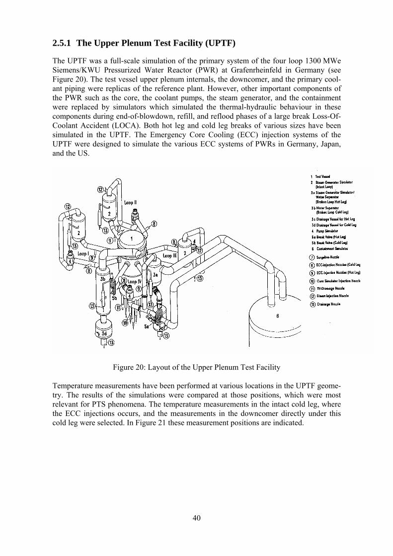
40
2.5.1 The Upper Plenum Test Facility (UPTF)
The UPTF was a full-scale simulation of the primary system of the four loop 1300 MWe Siemens/KWU Pressurized Water Reactor (PWR) at Grafenrheinfeld in Germany (see Figure 20). The test vessel upper plenum internals, the downcomer, and the primary cool-ant piping were replicas of the reference plant. However, other important components of the PWR such as the core, the coolant pumps, the steam generator, and the containment were replaced by simulators which simulated the thermal-hydraulic behaviour in these components during end-of-blowdown, refill, and reflood phases of a large break Loss-Of-Coolant Accident (LOCA). Both hot leg and cold leg breaks of various sizes have been simulated in the UPTF. The Emergency Core Cooling (ECC) injection systems of the UPTF were designed to simulate the various ECC systems of PWRs in Germany, Japan, and the US.
Figure 20: Layout of the Upper Plenum Test Facility Temperature measurements have been performed at various locations in the UPTF geome-try. The results of the simulations were compared at those positions, which were most relevant for PTS phenomena. The temperature measurements in the intact cold leg, where the ECC injections occurs, and the measurements in the downcomer directly under this cold leg were selected. In Figure 21 these measurement positions are indicated.
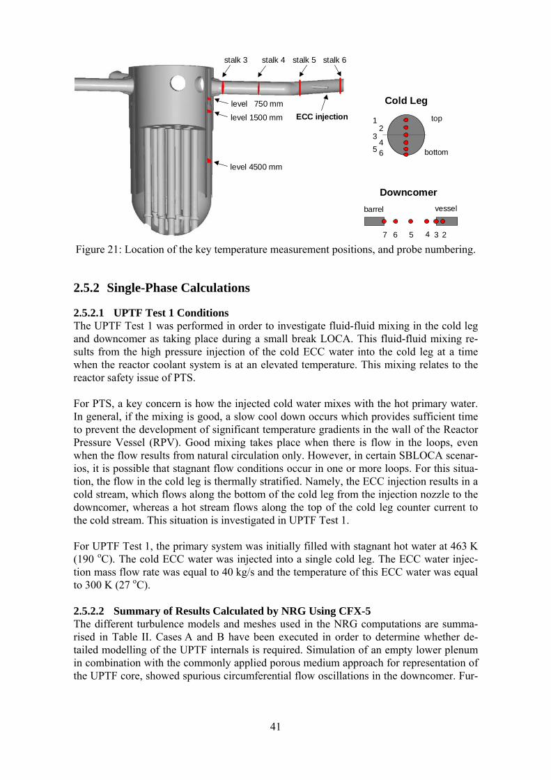
41
stalk 3 stalk 4
level 750 mm
level 1500 mm
level 4500 mm
stalk 5 stalk 6
ECC injection
23
45 6 bottom
top1
Cold Leg
23457 6
vesselbarrel
Downcomer
Figure 21: Location of the key temperature measurement positions, and probe numbering.
2.5.2 Single-Phase Calculations
2.5.2.1 UPTF Test 1 Conditions The UPTF Test 1 was performed in order to investigate fluid-fluid mixing in the cold leg and downcomer as taking place during a small break LOCA. This fluid-fluid mixing re-sults from the high pressure injection of the cold ECC water into the cold leg at a time when the reactor coolant system is at an elevated temperature. This mixing relates to the reactor safety issue of PTS. For PTS, a key concern is how the injected cold water mixes with the hot primary water. In general, if the mixing is good, a slow cool down occurs which provides sufficient time to prevent the development of significant temperature gradients in the wall of the Reactor Pressure Vessel (RPV). Good mixing takes place when there is flow in the loops, even when the flow results from natural circulation only. However, in certain SBLOCA scenar-ios, it is possible that stagnant flow conditions occur in one or more loops. For this situa-tion, the flow in the cold leg is thermally stratified. Namely, the ECC injection results in a cold stream, which flows along the bottom of the cold leg from the injection nozzle to the downcomer, whereas a hot stream flows along the top of the cold leg counter current to the cold stream. This situation is investigated in UPTF Test 1. For UPTF Test 1, the primary system was initially filled with stagnant hot water at 463 K (190 oC). The cold ECC water was injected into a single cold leg. The ECC water injec-tion mass flow rate was equal to 40 kg/s and the temperature of this ECC water was equal to 300 K (27 oC). 2.5.2.2 Summary of Results Calculated by NRG Using CFX-5 The different turbulence models and meshes used in the NRG computations are summa-rised in Table II. Cases A and B have been executed in order to determine whether de-tailed modelling of the UPTF internals is required. Simulation of an empty lower plenum in combination with the commonly applied porous medium approach for representation of the UPTF core, showed spurious circumferential flow oscillations in the downcomer. Fur-
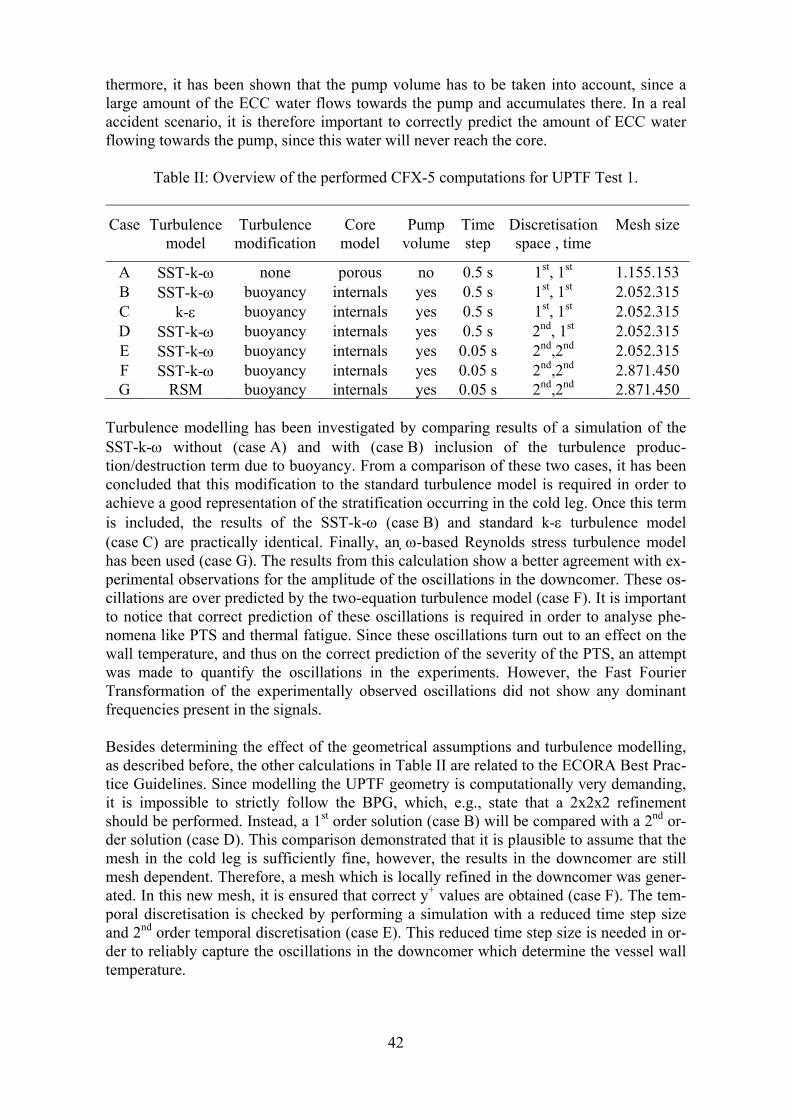
42
thermore, it has been shown that the pump volume has to be taken into account, since a large amount of the ECC water flows towards the pump and accumulates there. In a real accident scenario, it is therefore important to correctly predict the amount of ECC water flowing towards the pump, since this water will never reach the core.
Table II: Overview of the performed CFX-5 computations for UPTF Test 1.
Case
Turbulence model
Turbulence modification
Core model
Pump volume
Timestep
Discretisation space , time
Mesh size
A SST-k-ω none porous no 0.5 s 1st, 1st 1.155.153 B SST-k-ω buoyancy internals yes 0.5 s 1st, 1st 2.052.315 C k-ε buoyancy internals yes 0.5 s 1st, 1st 2.052.315 D SST-k-ω buoyancy internals yes 0.5 s 2nd, 1st 2.052.315 E SST-k-ω buoyancy internals yes 0.05 s 2nd,2nd 2.052.315 F SST-k-ω buoyancy internals yes 0.05 s 2nd,2nd 2.871.450 G RSM buoyancy internals yes 0.05 s 2nd,2nd 2.871.450
Turbulence modelling has been investigated by comparing results of a simulation of the SST-k-ω without (case A) and with (case B) inclusion of the turbulence produc-tion/destruction term due to buoyancy. From a comparison of these two cases, it has been concluded that this modification to the standard turbulence model is required in order to achieve a good representation of the stratification occurring in the cold leg. Once this term is included, the results of the SST-k-ω (case B) and standard k-ε turbulence model (case C) are practically identical. Finally, an ω-based Reynolds stress turbulence model has been used (case G). The results from this calculation show a better agreement with ex-perimental observations for the amplitude of the oscillations in the downcomer. These os-cillations are over predicted by the two-equation turbulence model (case F). It is important to notice that correct prediction of these oscillations is required in order to analyse phe-nomena like PTS and thermal fatigue. Since these oscillations turn out to an effect on the wall temperature, and thus on the correct prediction of the severity of the PTS, an attempt was made to quantify the oscillations in the experiments. However, the Fast Fourier Transformation of the experimentally observed oscillations did not show any dominant frequencies present in the signals. Besides determining the effect of the geometrical assumptions and turbulence modelling, as described before, the other calculations in Table II are related to the ECORA Best Prac-tice Guidelines. Since modelling the UPTF geometry is computationally very demanding, it is impossible to strictly follow the BPG, which, e.g., state that a 2x2x2 refinement should be performed. Instead, a 1st order solution (case B) will be compared with a 2nd or-der solution (case D). This comparison demonstrated that it is plausible to assume that the mesh in the cold leg is sufficiently fine, however, the results in the downcomer are still mesh dependent. Therefore, a mesh which is locally refined in the downcomer was gener-ated. In this new mesh, it is ensured that correct y+ values are obtained (case F). The tem-poral discretisation is checked by performing a simulation with a reduced time step size and 2nd order temporal discretisation (case E). This reduced time step size is needed in or-der to reliably capture the oscillations in the downcomer which determine the vessel wall temperature.
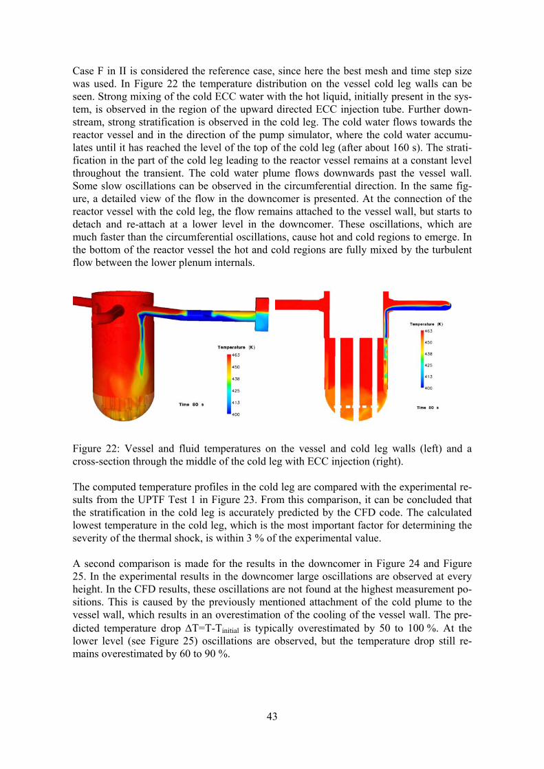
43
Case F in II is considered the reference case, since here the best mesh and time step size was used. In Figure 22 the temperature distribution on the vessel cold leg walls can be seen. Strong mixing of the cold ECC water with the hot liquid, initially present in the sys-tem, is observed in the region of the upward directed ECC injection tube. Further down-stream, strong stratification is observed in the cold leg. The cold water flows towards the reactor vessel and in the direction of the pump simulator, where the cold water accumu-lates until it has reached the level of the top of the cold leg (after about 160 s). The strati-fication in the part of the cold leg leading to the reactor vessel remains at a constant level throughout the transient. The cold water plume flows downwards past the vessel wall. Some slow oscillations can be observed in the circumferential direction. In the same fig-ure, a detailed view of the flow in the downcomer is presented. At the connection of the reactor vessel with the cold leg, the flow remains attached to the vessel wall, but starts to detach and re-attach at a lower level in the downcomer. These oscillations, which are much faster than the circumferential oscillations, cause hot and cold regions to emerge. In the bottom of the reactor vessel the hot and cold regions are fully mixed by the turbulent flow between the lower plenum internals.
Figure 22: Vessel and fluid temperatures on the vessel and cold leg walls (left) and a cross-section through the middle of the cold leg with ECC injection (right). The computed temperature profiles in the cold leg are compared with the experimental re-sults from the UPTF Test 1 in Figure 23. From this comparison, it can be concluded that the stratification in the cold leg is accurately predicted by the CFD code. The calculated lowest temperature in the cold leg, which is the most important factor for determining the severity of the thermal shock, is within 3 % of the experimental value. A second comparison is made for the results in the downcomer in Figure 24 and Figure 25. In the experimental results in the downcomer large oscillations are observed at every height. In the CFD results, these oscillations are not found at the highest measurement po-sitions. This is caused by the previously mentioned attachment of the cold plume to the vessel wall, which results in an overestimation of the cooling of the vessel wall. The pre-dicted temperature drop ΔT=T-Tinitial is typically overestimated by 50 to 100 %. At the lower level (see Figure 25) oscillations are observed, but the temperature drop still re-mains overestimated by 60 to 90 %.
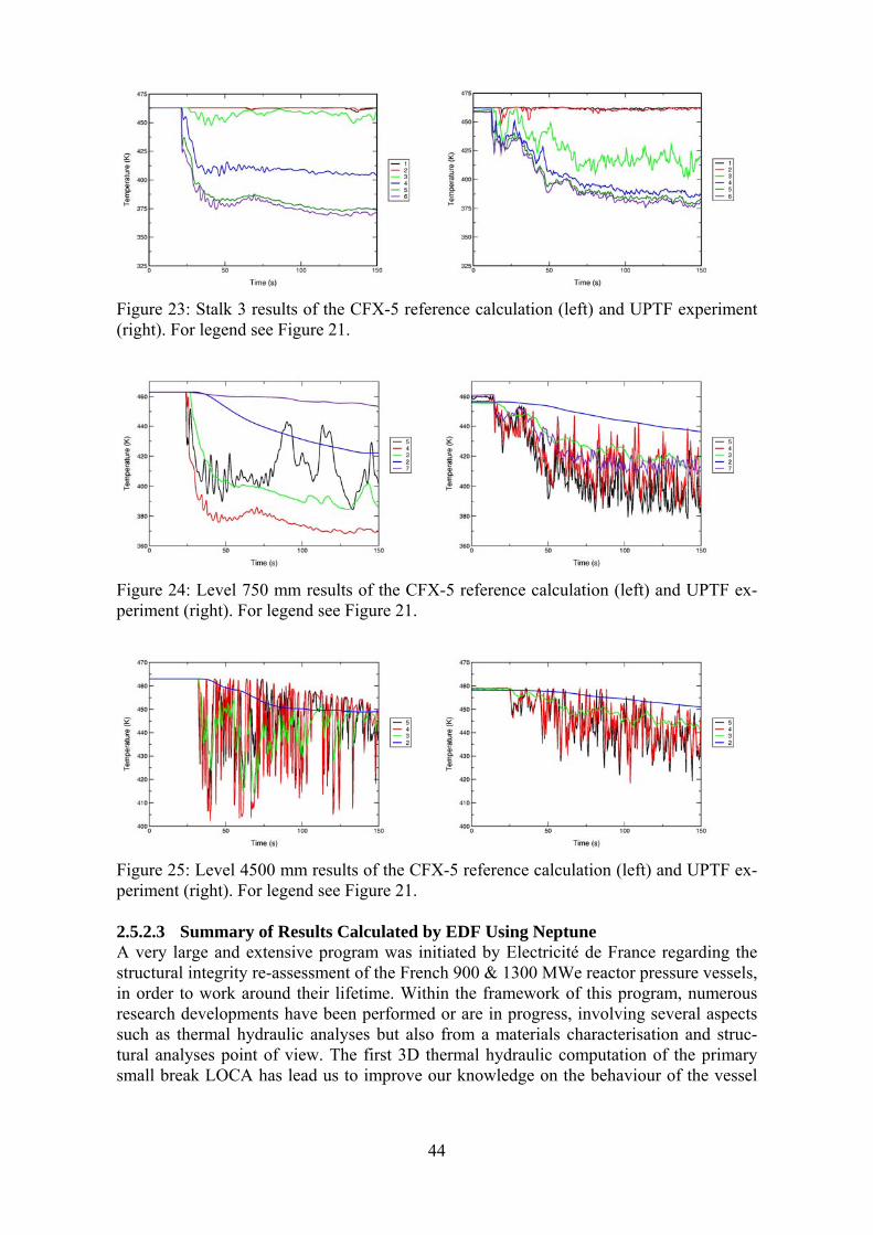
44
Figure 23: Stalk 3 results of the CFX-5 reference calculation (left) and UPTF experiment (right). For legend see Figure 21.
Figure 24: Level 750 mm results of the CFX-5 reference calculation (left) and UPTF ex-periment (right). For legend see Figure 21.
Figure 25: Level 4500 mm results of the CFX-5 reference calculation (left) and UPTF ex-periment (right). For legend see Figure 21. 2.5.2.3 Summary of Results Calculated by EDF Using Neptune A very large and extensive program was initiated by Electricité de France regarding the structural integrity re-assessment of the French 900 & 1300 MWe reactor pressure vessels, in order to work around their lifetime. Within the framework of this program, numerous research developments have been performed or are in progress, involving several aspects such as thermal hydraulic analyses but also from a materials characterisation and struc-tural analyses point of view. The first 3D thermal hydraulic computation of the primary small break LOCA has lead us to improve our knowledge on the behaviour of the vessel
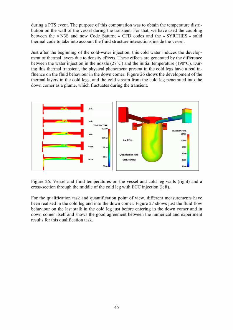
45
during a PTS event. The purpose of this computation was to obtain the temperature distri-bution on the wall of the vessel during the transient. For that, we have used the coupling between the « N3S and now Code_Saturne » CFD codes and the « SYRTHES » solid thermal code to take into account the fluid structure interactions inside the vessel. Just after the beginning of the cold-water injection, this cold water induces the develop-ment of thermal layers due to density effects. These effects are generated by the difference between the water injection in the nozzle (27°C) and the initial temperature (190°C). Dur-ing this thermal transient, the physical phenomena present in the cold legs have a real in-fluence on the fluid behaviour in the down comer. Figure 26 shows the development of the thermal layers in the cold legs, and the cold stream from the cold leg penetrated into the down comer as a plume, which fluctuates during the transient.
Figure 26: Vessel and fluid temperatures on the vessel and cold leg walls (right) and a cross-section through the middle of the cold leg with ECC injection (left). For the qualification task and quantification point of view, different measurements have been realised in the cold leg and into the down comer. Figure 27 shows just the fluid flow behaviour on the last stalk in the cold leg just before entering in the down comer and in down comer itself and shows the good agreement between the numerical and experiment results for this qualification task.
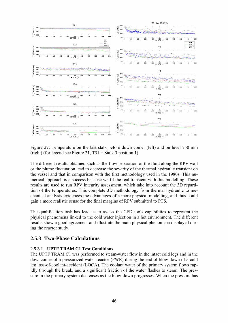
46
Figure 27: Temperature on the last stalk before down comer (left) and on level 750 mm (right) (for legend see Figure 21, T31 = Stalk 3 position 1) The different results obtained such as the flow separation of the fluid along the RPV wall or the plume fluctuation lead to decrease the severity of the thermal hydraulic transient on the vessel and that in comparison with the first methodology used in the 1980s. This nu-merical approach is a success because we fit the real transient with this modelling. These results are used to run RPV integrity assessment, which take into account the 3D reparti-tion of the temperatures. This complete 3D methodology from thermal hydraulic to me-chanical analysis evidences the advantages of a more physical modelling, and thus could gain a more realistic sense for the final margins of RPV submitted to PTS. The qualification task has lead us to assess the CFD tools capabilities to represent the physical phenomena linked to the cold water injection in a hot environment. The different results show a good agreement and illustrate the main physical phenomena displayed dur-ing the reactor study.
2.5.3 Two-Phase Calculations
2.5.3.1 UPTF TRAM C1 Test Conditions The UPTF TRAM C1 was performed to steam-water flow in the intact cold legs and in the downcomer of a pressurized water reactor (PWR) during the end of blow-down of a cold leg loss-of-coolant-accident (LOCA). The coolant water of the primary system flows rap-idly through the break, and a significant fraction of the water flashes to steam. The pres-sure in the primary system decreases as the blow-down progresses. When the pressure has
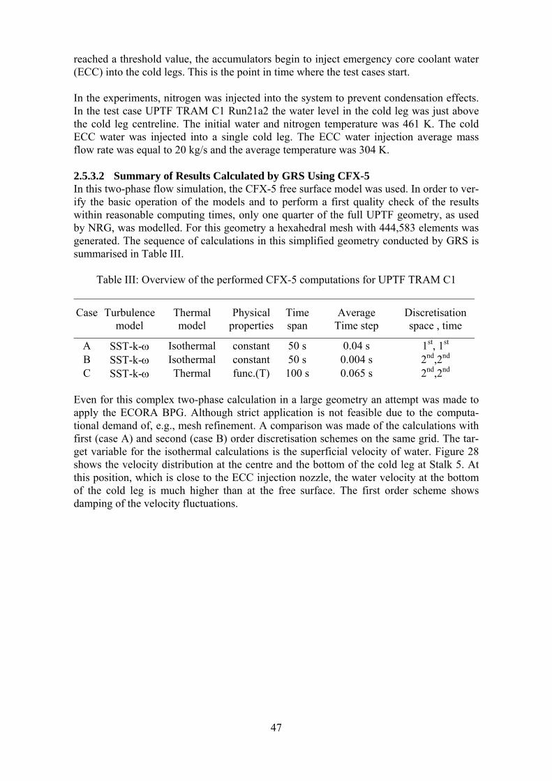
47
reached a threshold value, the accumulators begin to inject emergency core coolant water (ECC) into the cold legs. This is the point in time where the test cases start. In the experiments, nitrogen was injected into the system to prevent condensation effects. In the test case UPTF TRAM C1 Run21a2 the water level in the cold leg was just above the cold leg centreline. The initial water and nitrogen temperature was 461 K. The cold ECC water was injected into a single cold leg. The ECC water injection average mass flow rate was equal to 20 kg/s and the average temperature was 304 K. 2.5.3.2 Summary of Results Calculated by GRS Using CFX-5 In this two-phase flow simulation, the CFX-5 free surface model was used. In order to ver-ify the basic operation of the models and to perform a first quality check of the results within reasonable computing times, only one quarter of the full UPTF geometry, as used by NRG, was modelled. For this geometry a hexahedral mesh with 444,583 elements was generated. The sequence of calculations in this simplified geometry conducted by GRS is summarised in Table III.
Table III: Overview of the performed CFX-5 computations for UPTF TRAM C1
Case
Turbulence model
Thermal model
Physical properties
Time span
Average Time step
Discretisation space , time
A SST-k-ω Isothermal constant 50 s 0.04 s 1st, 1st B SST-k-ω Isothermal constant 50 s 0.004 s 2nd,2nd C SST-k-ω Thermal func.(T) 100 s 0.065 s 2nd,2nd
Even for this complex two-phase calculation in a large geometry an attempt was made to apply the ECORA BPG. Although strict application is not feasible due to the computa-tional demand of, e.g., mesh refinement. A comparison was made of the calculations with first (case A) and second (case B) order discretisation schemes on the same grid. The tar-get variable for the isothermal calculations is the superficial velocity of water. Figure 28 shows the velocity distribution at the centre and the bottom of the cold leg at Stalk 5. At this position, which is close to the ECC injection nozzle, the water velocity at the bottom of the cold leg is much higher than at the free surface. The first order scheme shows damping of the velocity fluctuations.
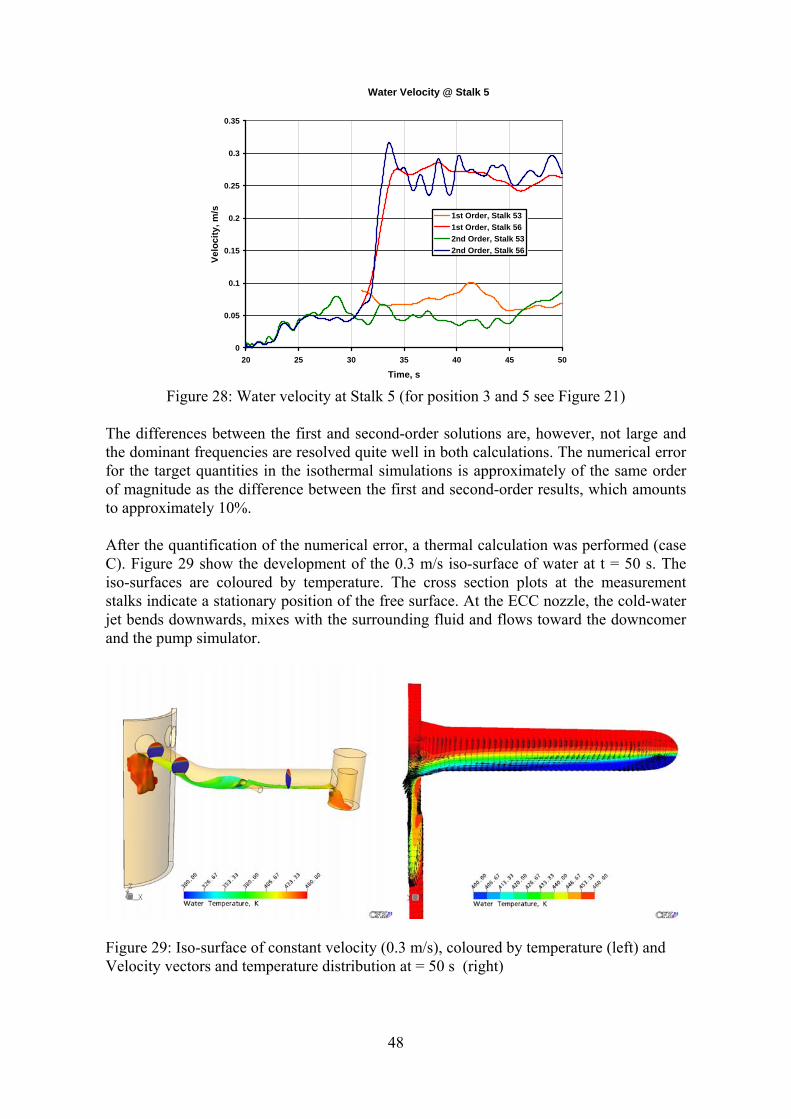
48
Water Velocity @ Stalk 5
0
0.05
0.1
0.15
0.2
0.25
0.3
0.35
20 25 30 35 40 45 50
Time, s
Velo
city
, m/s 1st Order, Stalk 53
1st Order, Stalk 562nd Order, Stalk 532nd Order, Stalk 56
Figure 28: Water velocity at Stalk 5 (for position 3 and 5 see Figure 21)
The differences between the first and second-order solutions are, however, not large and the dominant frequencies are resolved quite well in both calculations. The numerical error for the target quantities in the isothermal simulations is approximately of the same order of magnitude as the difference between the first and second-order results, which amounts to approximately 10%. After the quantification of the numerical error, a thermal calculation was performed (case C). Figure 29 show the development of the 0.3 m/s iso-surface of water at t = 50 s. The iso-surfaces are coloured by temperature. The cross section plots at the measurement stalks indicate a stationary position of the free surface. At the ECC nozzle, the cold-water jet bends downwards, mixes with the surrounding fluid and flows toward the downcomer and the pump simulator.
Figure 29: Iso-surface of constant velocity (0.3 m/s), coloured by temperature (left) and Velocity vectors and temperature distribution at = 50 s (right)
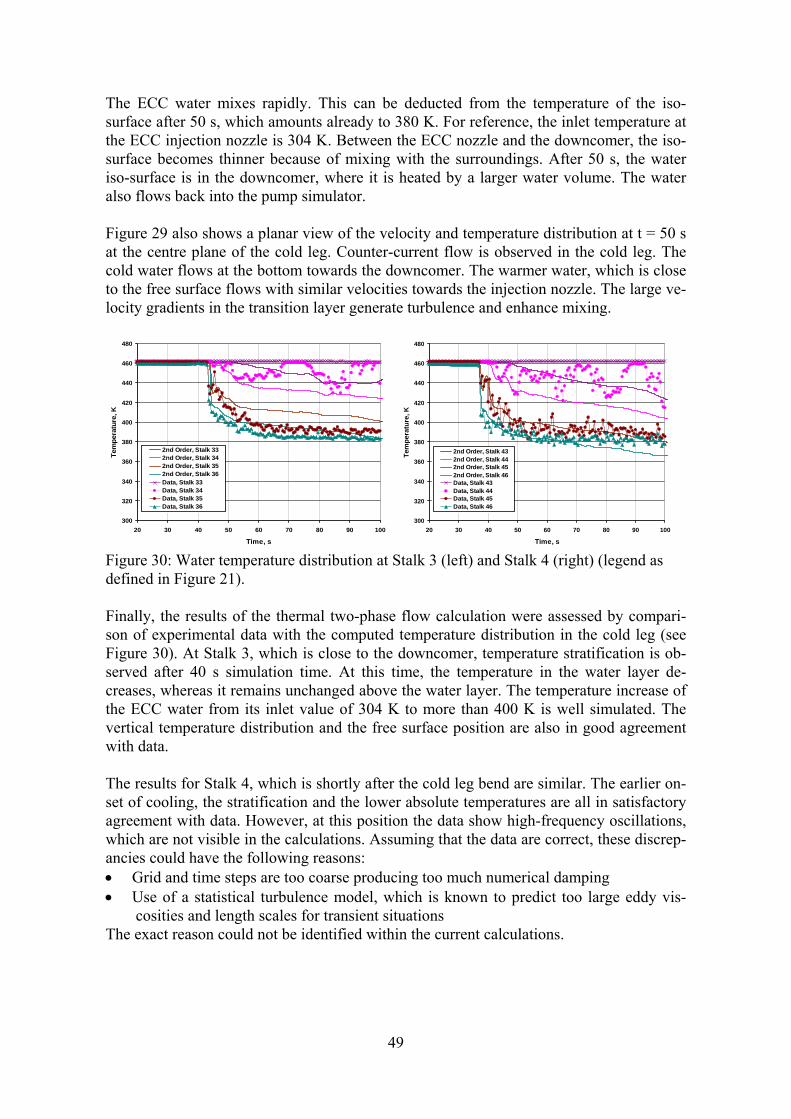
49
The ECC water mixes rapidly. This can be deducted from the temperature of the iso-surface after 50 s, which amounts already to 380 K. For reference, the inlet temperature at the ECC injection nozzle is 304 K. Between the ECC nozzle and the downcomer, the iso-surface becomes thinner because of mixing with the surroundings. After 50 s, the water iso-surface is in the downcomer, where it is heated by a larger water volume. The water also flows back into the pump simulator. Figure 29 also shows a planar view of the velocity and temperature distribution at t = 50 s at the centre plane of the cold leg. Counter-current flow is observed in the cold leg. The cold water flows at the bottom towards the downcomer. The warmer water, which is close to the free surface flows with similar velocities towards the injection nozzle. The large ve-locity gradients in the transition layer generate turbulence and enhance mixing.
300
320
340
360
380
400
420
440
460
480
20 30 40 50 60 70 80 90 100
Time, s
Tem
pera
ture
, K
2nd Order, Stalk 332nd Order, Stalk 342nd Order, Stalk 352nd Order, Stalk 36Data, Stalk 33Data, Stalk 34Data, Stalk 35Data, Stalk 36
300
320
340
360
380
400
420
440
460
480
20 30 40 50 60 70 80 90 100
Time, s
Tem
pera
ture
, K
2nd Order, Stalk 432nd Order, Stalk 442nd Order, Stalk 452nd Order, Stalk 46Data, Stalk 43Data, Stalk 44Data, Stalk 45Data, Stalk 46
Figure 30: Water temperature distribution at Stalk 3 (left) and Stalk 4 (right) (legend as defined in Figure 21). Finally, the results of the thermal two-phase flow calculation were assessed by compari-son of experimental data with the computed temperature distribution in the cold leg (see Figure 30). At Stalk 3, which is close to the downcomer, temperature stratification is ob-served after 40 s simulation time. At this time, the temperature in the water layer de-creases, whereas it remains unchanged above the water layer. The temperature increase of the ECC water from its inlet value of 304 K to more than 400 K is well simulated. The vertical temperature distribution and the free surface position are also in good agreement with data. The results for Stalk 4, which is shortly after the cold leg bend are similar. The earlier on-set of cooling, the stratification and the lower absolute temperatures are all in satisfactory agreement with data. However, at this position the data show high-frequency oscillations, which are not visible in the calculations. Assuming that the data are correct, these discrep-ancies could have the following reasons: • Grid and time steps are too coarse producing too much numerical damping • Use of a statistical turbulence model, which is known to predict too large eddy vis-
cosities and length scales for transient situations The exact reason could not be identified within the current calculations.
50
2.5.4 Conclusions
In this work package, the performance of CFX-5 and the Neptune CFD codes have been assessed for prediction of the PTS phenomena occurring in an integral PTS experiment. For this purpose, the experimental data from the full-scale Upper Plenum Test Facility has been compared with results from the CFD codes. The following conclusions have been drawn: • The single-phase flow calculation with CFX-5 and Neptune showed good agreement
for the prediction of the thermal mixing and stratification phenomena occurring in the cold leg. A detailed study with CFX-5 showed that the CFD model does not accurately capture the flow behaviour in the downcomer.
• The two-phase flow calculation with CFX-5 showed satisfactory results for the predic-tion of the two-phase flow and thermal stratification in the cold leg.
• For a large demonstration case as this UPTF geometry, it is impossible to strictly fol-low the ECORA BPG. However, comparison of first and second order discretisation scheme solutions (as performed in the both the single and two-phase CFX-5 calcula-tion) can be used to estimate the numerical error.
The largest discrepancies in both the single and two-phase calculations are observed for quickly fluctuating flow phenomena. Although no definite conclusions can be drawn at this stage, it is highly probably that the use of statistical turbulence models is the cause for this discrepancy. The state-of-the-art in turbulence modelling now includes more refined approaches like Large Eddy Simulations (LES), hybrid RANS – LES approaches called Detached Eddy Simulation (DES), or even Scale-Adaptive Simulation (SAS). These mod-els have hardly been investigated for NRS application, but show great potential for this important class of problems. Since the BPG could not be strictly applied for the UPTF cases, the risk exists that the outcome of ECORA will be that the BPG are only applicable to small scale problems of no interest to realistic large scale NRS problems. It is our opinion that the establishment of ‘quality and trust’ in CFD in general, and NRS CFD in particular, starts with an accepted and applied quality document; the BPG. Therefore, it is of the highest importance to estab-lish practical BPG for these large scale cases. These final and most complex demonstration cases in the ECORA project are not only a challenge for the available models, but also for the available computer power. Notice that both the single and two-phase CFX-5 cases required several weeks computation time on parallel computers. Therefore, in order to use CFD calculations for reactor safety applica-tions of the type investigated in the work package, an important task is a reduction of cal-culation times by, e.g., using adaptive algorithms in space and time. Another important is-sue that has to be addressed is the application of BPG for these large scale calculations.
2.6 Evaluation of CFD Analysis of Containment (WP 6)
The main objective of WP 6 is the evaluation of the current CFD codes with respect to their potential for analysing containment flows. A second step in this work package is the assessment of the available experimental database combined with recommendations for future experiments.
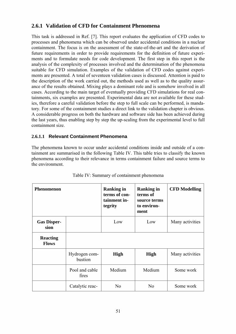
51
2.6.1 Validation of CFD for Containment Phenomena
This task is addressed in Ref. [7]. This report evaluates the application of CFD codes to processes and phenomena which can be observed under accidental conditions in a nuclear containment. The focus is on the assessment of the state-of-the-art and the derivation of future requirements in order to provide requirements for the definition of future experi-ments and to formulate needs for code development. The first step in this report is the analysis of the complexity of processes involved and the determination of the phenomena suitable for CFD simulation. Examples of the validation of CFD codes against experi-ments are presented. A total of seventeen validation cases is discussed. Attention is paid to the description of the work carried out, the methods used as well as to the quality assur-ance of the results obtained. Mixing plays a dominant role and is somehow involved in all cases. According to the main target of eventually providing CFD simulations for real con-tainments, six examples are presented. Experimental data are not available for these stud-ies, therefore a careful validation before the step to full scale can be performed, is manda-tory. For some of the containment studies a direct link to the validation chapter is obvious. A considerable progress on both the hardware and software side has been achieved during the last years, thus enabling step by step the up-scaling from the experimental level to full containment size. 2.6.1.1 Relevant Containment Phenomena The phenomena known to occur under accidental conditions inside and outside of a con-tainment are summarised in the following Table IV. This table tries to classify the known phenomena according to their relevance in terms containment failure and source terms to the environment.
Table IV: Summary of containment phenomena
Phenomenon Ranking in terms of con-tainment in-tegrity
Ranking in terms of source terms to environ-ment
CFD Modelling
Gas Disper-sion
Low Low Many activities
Reacting Flows
Hydrogen com-bustion
High High Many activities
Pool and cable fires
Medium Medium Some work
Catalytic reac- No No Some work
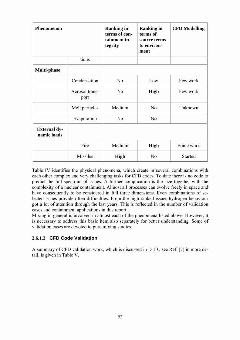
52
Phenomenon Ranking in terms of con-tainment in-tegrity
Ranking in terms of source terms to environ-ment
CFD Modelling
tions
Multi-phase
Condensation No Low Few work
Aerosol trans-port
No High Few work
Melt particles Medium No Unknown
Evaporation No No
External dy-namic loads
Fire Medium High Some work
Missiles High No Started
Table IV identifies the physical phenomena, which create in several combinations with each other complex and very challenging tasks for CFD codes. To date there is no code to predict the full spectrum of issues. A further complication is the size together with the complexity of a nuclear containment. Almost all processes can evolve freely in space and have consequently to be considered in full three dimensions. Even combinations of se-lected issues provide often difficulties. From the high ranked issues hydrogen behaviour got a lot of attention through the last years. This is reflected in the number of validation cases and containment applications in this report. Mixing in general is involved in almost each of the phenomena listed above. However, it is necessary to address this basic item also separately for better understanding. Some of validation cases are devoted to pure mixing studies. 2.6.1.2 CFD Code Validation A summary of CFD validation work, which is discussed in D 10 , see Ref. [7] in more de-tail, is given in Table V.
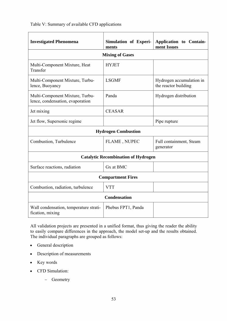
53
Table V: Summary of available CFD applications
Investigated Phenomena Simulation of Experi-ments
Application to Contain-ment Issues
Mixing of Gases
Multi-Component Mixture, Heat Transfer
HYJET
Multi-Component Mixture, Turbu-lence, Buoyancy
LSGMF Hydrogen accumulation in the reactor building
Multi-Component Mixture, Turbu-lence, condensation, evaporation
Panda Hydrogen distribution
Jet mixing CEASAR
Jet flow, Supersonic regime Pipe rupture
Hydrogen Combustion
Combustion, Turbulence FLAME , NUPEC Full containment, Steam generator
Catalytic Recombination of Hydrogen
Surface reactions, radiation Gx at BMC
Compartment Fires
Combustion, radiation, turbulence VTT
Condensation
Wall condensation, temperature strati-fication, mixing
Phebus FPT1, Panda
All validation projects are presented in a unified format, thus giving the reader the ability to easily compare differences in the approach, the model set-up and the results obtained. The individual paragraphs are grouped as follows:
• General description
• Description of measurements
• Key words
• CFD Simulation:
− Geometry
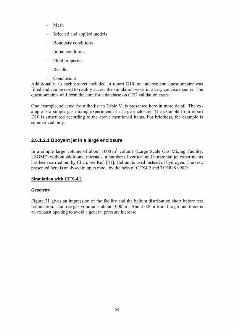
54
− Mesh
− Selected and applied models
− Boundary conditions
− Initial conditions
− Fluid properties
− Results
− Conclusions Additionally, to each project included in report D10, an independent questionnaire was filled and can be used to readily access the simulation work in a very concise manner. The questionnaires will form the core for a database on CFD validation cases. One example, selected from the list in Table V, is presented here in more detail. The ex-ample is a simple gas mixing experiment in a large enclosure. The example from report D10 is structured according to the above mentioned items. For briefness, the example is summarized only.
2.6.1.2.1 Buoyant jet in a large enclosure In a simple large volume of about 1000 m3 volume (Large Scale Gas Mixing Facility, LSGMF) without additional internals, a number of vertical and horizontal jet experiments has been carried out by Chan, see Ref. [41]. Helium is used instead of hydrogen. The test, presented here is analysed in open mode by the help of CFX4.2 and TONUS v98D. Simulation with CFX-4.2 Geometry Figure 31 gives an impression of the facility and the helium distribution short before test termination. The free gas volume is about 1000 m3. About 0.8 m from the ground there is an exhaust opening to avoid a general pressure increase.
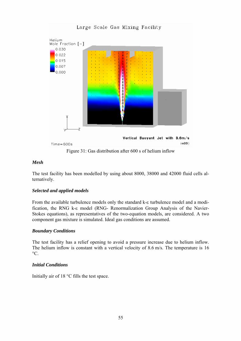
55
Figure 31: Gas distribution after 600 s of helium inflow
Mesh The test facility has been modelled by using about 8000, 38000 and 42000 fluid cells al-ternatively. Selected and applied models From the available turbulence models only the standard k-ε turbulence model and a modi-fication, the RNG k-ε model (RNG- Renormalization Group Analysis of the Navier-Stokes equations), as representatives of the two-equation models, are considered. A two component gas mixture is simulated. Ideal gas conditions are assumed. Boundary Conditions The test facility has a relief opening to avoid a pressure increase due to helium inflow. The helium inflow is constant with a vertical velocity of 8.6 m/s. The temperature is 16 °C. Initial Conditions Initially air of 18 °C fills the test space.
56
Fluid Properties Air and helium properties are specified at constant temperature. Results The low inflow speed might imply a more homogeneous distribution of helium, but it clearly stratifies. Two cross beams at the ceiling along the depth of the facility influence the flow field locally. The relief opening is located low enough and helium losses are unlikely. It turned out, that 38000 cells give a grid-converged solution. It is known, that the standard k-ε turbulence model overestimates the rate of spread from round jets by 30 %. This behaviour leads to lower concentrations in the jet and higher values in the vi-cinity. An increase from the standard value of C1=1.44 to 1.6 in the k-ε model has also been tested. For the position 1.2 m above the bottom it augments the prediction but for other locations not. A more general improvement can be achieved by use of the RNG model. With this model, there is still too low helium at the measurement point, but at other spots the simulation meets the recorded data quite well. Figure 32 shows the transient of helium 2 m away from the jet axis at two elevations of 8.9 m and 10.6 m (close to the ceil-ing).
Large Scale Gas Mixing Facility (AECL)
Experiment: Jet diameter=0.05m, Jet speed=8.6m/s,no obstruction plate.CFX: RNG k-e Model
CFX Helium Mole Fraction Predictions
0.00 200.00 400.00 600.00100.00 300.00 500.00
Time [s]
0.00
1.00
2.00
3.00
4.00
Hel
ium
Mol
e Fr
actio
n [%
] Probes Lance -Outside Jet-(xm,6.15m,5.1m), m09
Test P9 (x=8.92m)CFX P9Test P10 (x=10.65m)CFX P10
Figure 32: Helium transient 2 m away from the jet axis (RNG k-ε model)
There, a little more helium then measured is predicted. Another way of analysing the simulation is to look at the vertical distribution of helium above the gas release opening.
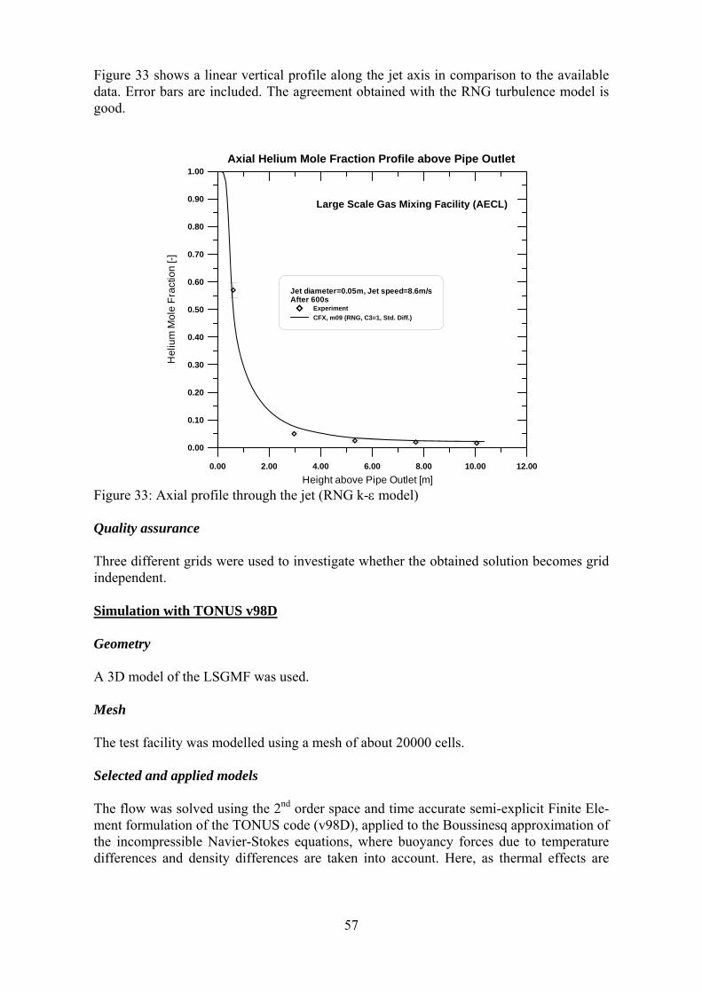
57
Figure 33 shows a linear vertical profile along the jet axis in comparison to the available data. Error bars are included. The agreement obtained with the RNG turbulence model is good.
Large Scale Gas Mixing Facility (AECL)
Axial Helium Mole Fraction Profile above Pipe Outlet
0.00 2.00 4.00 6.00 8.00 10.00 12.00Height above Pipe Outlet [m]
0.00
0.10
0.20
0.30
0.40
0.50
0.60
0.70
0.80
0.90
1.00H
eliu
m M
ole
Frac
tion
[-]
Jet diameter=0.05m, Jet speed=8.6m/sAfter 600s
ExperimentCFX, m09 (RNG, C3=1, Std. Diff.)
Figure 33: Axial profile through the jet (RNG k-ε model) Quality assurance Three different grids were used to investigate whether the obtained solution becomes grid independent. Simulation with TONUS v98D Geometry A 3D model of the LSGMF was used. Mesh The test facility was modelled using a mesh of about 20000 cells. Selected and applied models The flow was solved using the 2nd order space and time accurate semi-explicit Finite Ele-ment formulation of the TONUS code (v98D), applied to the Boussinesq approximation of the incompressible Navier-Stokes equations, where buoyancy forces due to temperature differences and density differences are taken into account. Here, as thermal effects are
58
small, the latter term is almost solely responsible for the buoyancy force, with two gas components taken into account, air and helium. As far as turbulence modelling is con-cerned, as in the CFX computation, both the standard k-ε model and the RNG k-ε models were compared. Boundary conditions Helium is injected at the rate of 3 g/s for a period of 600 s and with a temperature of 20 oC. The gas mixture is allowed to flow out to ensure that the total pressure in the vol-ume remains constant. Initial conditions The initial conditions are still air at 20 oC. Fluid properties Air and helium have constant properties (viscosity and heat conductivity). Results The results of the TONUS computation with the RNG k-ε model are shown in Figure 34. The same conclusions concerning the standard k-ε model and its RNG version were drawn from the computation of this test case compared with the CFX simulation. The standard model tended to be overly diffusive and the RNG version gave a much better prediction compared to the experimental data.
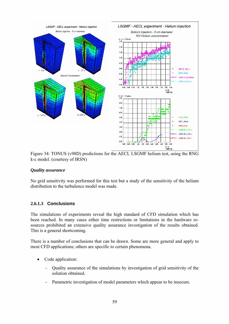
59
Figure 34: TONUS (v98D) predictions for the AECL LSGMF helium test, using the RNG k-ε model. (courtesy of IRSN) Quality assurance No grid sensitivity was performed for this test but a study of the sensitivity of the helium distribution to the turbulence model was made.
2.6.1.3 Conclusions The simulations of experiments reveal the high standard of CFD simulation which has been reached. In many cases either time restrictions or limitations in the hardware re-sources prohibited an extensive quality assurance investigation of the results obtained. This is a general shortcoming. There is a number of conclusions that can be drawn. Some are more general and apply to most CFD applications; others are specific to certain phenomena.
• Code application:
− Quality assurance of the simulations by investigation of grid sensitivity of the solution obtained.
− Parametric investigation of model parameters which appear to be insecure.
60
− Follow Best Practice Guidelines developed in WP1.
− Derive uncertainty bands when possible.
• Future Needs:
• Hardware needs:
− More powerful computers (clusters or shared memory multiprocessors) for lar-ger meshes to better resolve turbulent flows and to run over longer problem times. A full severe accident scenario may require several hours of problem time to be covered.
• Software needs:
− More robust parallel solvers.
− Dynamic grid adaptation for premixed combustion of hydrogen.
− Coupling with heat conduction, radiation, neutronics, structural mechanics.
• Physical models:
− More developed combustion models.
− Combination of phenomena: combustion – structural response, condensation, radiation – fires or standing flames.
− Advanced turbulence modelling.
− Multi-phase model improvements
• Experimental needs:
− Special CFD related instrumentation including flow field, species concentra-tions.
− Denser grids of data recording for more comprehensive code comparisons.
− Precise control of boundary conditions.
2.6.2 Evaluation of the Available Database
The available database is analysed in D11 see Ref. [8] Major recent test facilities like PANDA, MISTRA, ThAI and Battelle Model Containment are discussed and evaluated in more detail. As representatives, PANDA, MISTRA and ThAI activities are summarised in the following sections. PANDA A broad variety of experiments have been conducted and are currently carried out in the PANDA tests facility, and the relevance of the collected data for CFD codes validation is
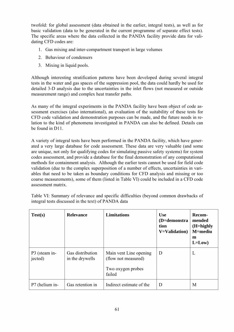
61
twofold: for global assessment (data obtained in the earlier, integral tests), as well as for basic validation (data to be generated in the current programme of separate effect tests). The specific areas where the data collected in the PANDA facility provide data for vali-dating CFD codes are:
1. Gas mixing and inter-compartment transport in large volumes
2. Behaviour of condensers
3. Mixing in liquid pools.
Although interesting stratification patterns have been developed during several integral tests in the water and gas spaces of the suppression pool, the data could hardly be used for detailed 3-D analysis due to the uncertainties in the inlet flows (not measured or outside measurement range) and complex heat transfer paths.
As many of the integral experiments in the PANDA facility have been object of code as-sessment exercises (also international), an evaluation of the suitability of these tests for CFD code validation and demonstration purposes can be made, and the future needs in re-lation to the kind of phenomena investigated in PANDA can also be defined. Details can be found in D11.
A variety of integral tests have been performed in the PANDA facility, which have gener-ated a very large database for code assessment. These data are very valuable (and some are unique, not only for qualifying codes for simulating passive safety systems) for system codes assessment, and provide a database for the final demonstration of any computational methods for containment analysis. Although the earlier tests cannot be used for field code validation (due to the complex superposition of a number of effects, uncertainties in vari-ables that need to be taken as boundary conditions for CFD analysis and missing or too coarse measurements), some of them (listed in Table VI) could be included in a CFD code assessment matrix. Table VI: Summary of relevance and specific difficulties (beyond common drawbacks of integral tests discussed in the text) of PANDA data
Test(s) Relevance Limitations Use (D=demonstration V=Validation)
Recom-mended (H=highly M=medium L=Low)
P3 (steam in-jected)
Gas distribution in the drywells
Main vent Line opening (flow not measured)
Two oxygen probes failed
D L
P7 (helium in- Gas retention in Indirect estimate of the D M
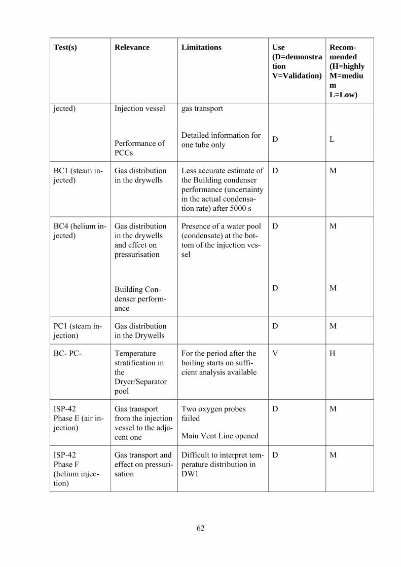
62
Test(s) Relevance Limitations Use (D=demonstration V=Validation)
Recom-mended (H=highly M=medium L=Low)
jected) Injection vessel
Performance of PCCs
gas transport
Detailed information for one tube only
D
L
BC1 (steam in-jected)
Gas distribution in the drywells
Less accurate estimate of the Building condenser performance (uncertainty in the actual condensa-tion rate) after 5000 s
D M
BC4 (helium in-jected)
Gas distribution in the drywells and effect on pressurisation
Building Con-denser perform-ance
Presence of a water pool (condensate) at the bot-tom of the injection ves-sel
D
D
M
M
PC1 (steam in-jection)
Gas distribution in the Drywells
D M
BC- PC- Temperature stratification in the Dryer/Separator pool
For the period after the boiling starts no suffi-cient analysis available
V H
ISP-42 Phase E (air in-jection)
Gas transport from the injection vessel to the adja-cent one
Two oxygen probes failed
Main Vent Line opened
D M
ISP-42 Phase F (helium injec-tion)
Gas transport and effect on pressuri-sation
Difficult to interpret tem-perature distribution in DW1
D M
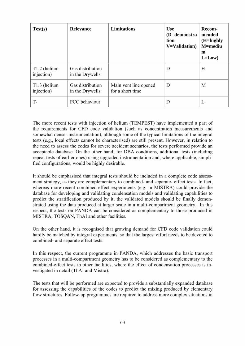
63
Test(s) Relevance Limitations Use (D=demonstration V=Validation)
Recom-mended (H=highly M=medium L=Low)
T1.2 (helium injection)
Gas distribution in the Drywells
D H
T1.3 (helium injection)
Gas distribution in the Drywells
Main vent line opened for a short time
D M
T- PCC behaviour D L
The more recent tests with injection of helium (TEMPEST) have implemented a part of the requirements for CFD code validation (such as concentration measurements and somewhat denser instrumentation), although some of the typical limitations of the integral tests (e.g., local effects cannot be characterised) are still present. However, in relation to the need to assess the codes for severe accident scenarios, the tests performed provide an acceptable database. On the other hand, for DBA conditions, additional tests (including repeat tests of earlier ones) using upgraded instrumentation and, where applicable, simpli-fied configurations, would be highly desirable.
It should be emphasised that integral tests should be included in a complete code assess-ment strategy, as they are complementary to combined- and separate- effect tests. In fact, whereas more recent combined-effect experiments (e.g. in MISTRA) could provide the database for developing and validating condensation models and validating capabilities to predict the stratification produced by it, the validated models should be finally demon-strated using the data produced at larger scale in a multi-compartment geometry. In this respect, the tests on PANDA can be considered as complementary to those produced in MISTRA, TOSQAN, ThAI and other facilities.
On the other hand, it is recognised that growing demand for CFD code validation could hardly be matched by integral experiments, so that the largest effort needs to be devoted to combined- and separate effect tests.
In this respect, the current programme in PANDA, which addresses the basic transport processes in a multi-compartment geometry has to be considered as complementary to the combined-effect tests in other facilities, where the effect of condensation processes is in-vestigated in detail (ThAI and Mistra).
The tests that will be performed are expected to provide a substantially expanded database for assessing the capabilities of the codes to predict the mixing produced by elementary flow structures. Follow-up programmes are required to address more complex situations in
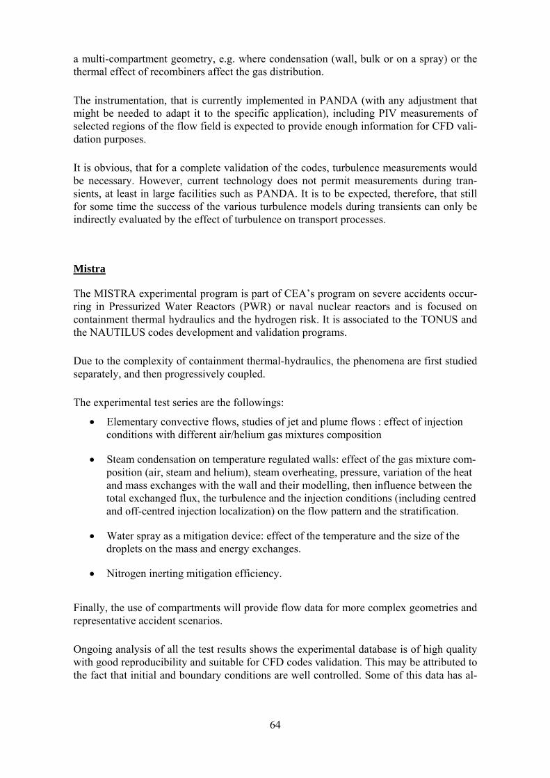
64
a multi-compartment geometry, e.g. where condensation (wall, bulk or on a spray) or the thermal effect of recombiners affect the gas distribution.
The instrumentation, that is currently implemented in PANDA (with any adjustment that might be needed to adapt it to the specific application), including PIV measurements of selected regions of the flow field is expected to provide enough information for CFD vali-dation purposes.
It is obvious, that for a complete validation of the codes, turbulence measurements would be necessary. However, current technology does not permit measurements during tran-sients, at least in large facilities such as PANDA. It is to be expected, therefore, that still for some time the success of the various turbulence models during transients can only be indirectly evaluated by the effect of turbulence on transport processes.
Mistra
The MISTRA experimental program is part of CEA’s program on severe accidents occur-ring in Pressurized Water Reactors (PWR) or naval nuclear reactors and is focused on containment thermal hydraulics and the hydrogen risk. It is associated to the TONUS and the NAUTILUS codes development and validation programs.
Due to the complexity of containment thermal-hydraulics, the phenomena are first studied separately, and then progressively coupled.
The experimental test series are the followings:
• Elementary convective flows, studies of jet and plume flows : effect of injection conditions with different air/helium gas mixtures composition
• Steam condensation on temperature regulated walls: effect of the gas mixture com-position (air, steam and helium), steam overheating, pressure, variation of the heat and mass exchanges with the wall and their modelling, then influence between the total exchanged flux, the turbulence and the injection conditions (including centred and off-centred injection localization) on the flow pattern and the stratification.
• Water spray as a mitigation device: effect of the temperature and the size of the droplets on the mass and energy exchanges.
• Nitrogen inerting mitigation efficiency.
Finally, the use of compartments will provide flow data for more complex geometries and representative accident scenarios.
Ongoing analysis of all the test results shows the experimental database is of high quality with good reproducibility and suitable for CFD codes validation. This may be attributed to the fact that initial and boundary conditions are well controlled. Some of this data has al-
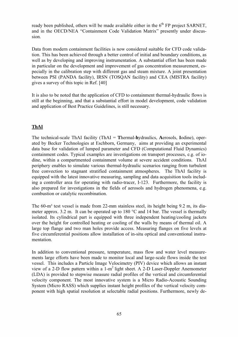
65
ready been published, others will be made available either in the 6th FP project SARNET, and in the OECD/NEA “Containment Code Validation Matrix” presently under discus-sion.
Data from modern containment facilities is now considered suitable for CFD code valida-tion. This has been achieved through a better control of initial and boundary conditions, as well as by developing and improving instrumentation. A substantial effort has been made in particular on the development and improvement of gas concentration measurement, es-pecially in the calibration step with different gas and steam mixture. A joint presentation between PSI (PANDA facility), IRSN (TOSQAN facility) and CEA (MISTRA facility) gives a survey of this topic in Ref. [40]
It is also to be noted that the application of CFD to containment thermal-hydraulic flows is still at the beginning, and that a substantial effort in model development, code validation and application of Best Practice Guidelines, is still necessary.
ThAI
The technical-scale ThAI facility (ThAI = Thermal-hydraulics, Aerosols, Iodine), oper-ated by Becker Technologies at Eschborn, Germany, aims at providing an experimental data base for validation of lumped parameter and CFD (Computational Fluid Dynamics) containment codes. Typical examples are investigations on transport processes, e.g. of io-dine, within a compartmented containment volume at severe accident conditions. ThAI periphery enables to simulate various thermal-hydraulic scenarios ranging from turbulent free convection to stagnant stratified containment atmospheres. The ThAI facility is equipped with the latest innovative measuring, sampling and data acquisition tools includ-ing a controller area for operating with radio-tracer, I-123. Furthermore, the facility is also prepared for investigations in the fields of aerosols and hydrogen phenomena, e.g. combustion or catalytic recombination.
The 60-m³ test vessel is made from 22-mm stainless steel, its height being 9.2 m, its dia-meter approx. 3.2 m. It can be operated up to 180 °C and 14 bar. The vessel is thermally isolated. Its cylindrical part is equipped with three independent heating/cooling jackets over the height for controlled heating or cooling of the walls by means of thermal oil. A large top flange and two man holes provide access. Measuring flanges on five levels at five circumferential positions allow installation of in-situ optical and conventional instru-mentation.
In addition to conventional pressure, temperature, mass flow and water level measure-ments large efforts have been made to monitor local and large-scale flows inside the test vessel. This includes a Particle Image Velocimetry (PIV) device which allows an instant view of a 2-D flow pattern within a 1-m2 light sheet. A 2-D Laser-Doppler Anemometer (LDA) is provided to stepwise measure radial profiles of the vertical and circumferential velocity component. The most innovative system is a Micro Radio-Acoustic Sounding System (Micro RASS) which supplies instant height profiles of the vertical velocity com-ponent with high spatial resolution at selectable radial positions. Furthermore, newly de-
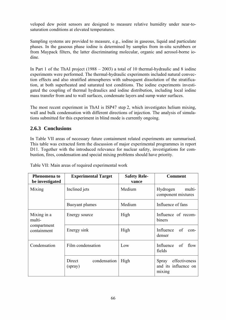
66
veloped dew point sensors are designed to measure relative humidity under near-to-saturation conditions at elevated temperatures.
Sampling systems are provided to measure, e.g., iodine in gaseous, liquid and particulate phases. In the gaseous phase iodine is determined by samples from in-situ scrubbers or from Maypack filters, the latter discriminating molecular, organic and aerosol-borne io-dine.
In Part 1 of the ThAI project (1988 – 2003) a total of 10 thermal-hydraulic and 8 iodine experiments were performed. The thermal-hydraulic experiments included natural convec-tion effects and also stratified atmospheres with subsequent dissolution of the stratifica-tion, at both superheated and saturated test conditions. The iodine experiments investi-gated the coupling of thermal hydraulics and iodine distribution, including local iodine mass transfer from and to wall surfaces, condensate layers and sump water surfaces.
The most recent experiment in ThAI is ISP47 step 2, which investigates helium mixing, wall and bulk condensation with different directions of injection. The analysis of simula-tions submitted for this experiment in blind mode is currently ongoing.
2.6.3 Conclusions
In Table VII areas of necessary future containment related experiments are summarised. This table was extracted form the discussion of major experimental programmes in report D11. Together with the introduced relevance for nuclear safety, investigations for com-bustion, fires, condensation and special mixing problems should have priority. Table VII: Main areas of required experimental work
Phenomena to be investigated
Experimental Target Safety Rele-vance
Comment
Inclined jets Medium Hydrogen multi-component mixtures
Mixing
Buoyant plumes Medium Influence of fans
Energy source High Influence of recom-biners
Mixing in a multi-compartment containment Energy sink High Influence of con-
denser
Film condensation Low Influence of flow fields
Condensation
Direct condensation (spray)
High Spray effectiveness and its influence on mixing
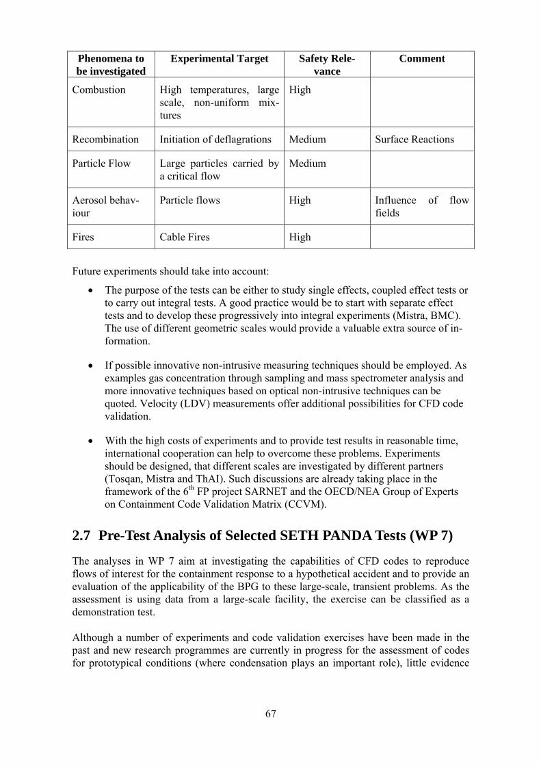
67
Phenomena to be investigated
Experimental Target Safety Rele-vance
Comment
Combustion High temperatures, large scale, non-uniform mix-tures
High
Recombination Initiation of deflagrations Medium Surface Reactions
Particle Flow Large particles carried by a critical flow
Medium
Aerosol behav-iour
Particle flows High Influence of flow fields
Fires Cable Fires High
Future experiments should take into account:
• The purpose of the tests can be either to study single effects, coupled effect tests or to carry out integral tests. A good practice would be to start with separate effect tests and to develop these progressively into integral experiments (Mistra, BMC). The use of different geometric scales would provide a valuable extra source of in-formation.
• If possible innovative non-intrusive measuring techniques should be employed. As examples gas concentration through sampling and mass spectrometer analysis and more innovative techniques based on optical non-intrusive techniques can be quoted. Velocity (LDV) measurements offer additional possibilities for CFD code validation.
• With the high costs of experiments and to provide test results in reasonable time, international cooperation can help to overcome these problems. Experiments should be designed, that different scales are investigated by different partners (Tosqan, Mistra and ThAI). Such discussions are already taking place in the framework of the 6th FP project SARNET and the OECD/NEA Group of Experts on Containment Code Validation Matrix (CCVM).
2.7 Pre-Test Analysis of Selected SETH PANDA Tests (WP 7)
The analyses in WP 7 aim at investigating the capabilities of CFD codes to reproduce flows of interest for the containment response to a hypothetical accident and to provide an evaluation of the applicability of the BPG to these large-scale, transient problems. As the assessment is using data from a large-scale facility, the exercise can be classified as a demonstration test. Although a number of experiments and code validation exercises have been made in the past and new research programmes are currently in progress for the assessment of codes for prototypical conditions (where condensation plays an important role), little evidence
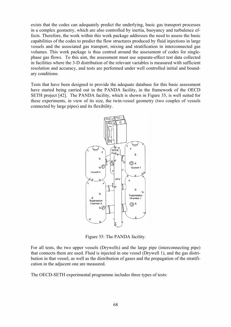
68
exists that the codes can adequately predict the underlying, basic gas transport processes in a complex geometry, which are also controlled by inertia, buoyancy and turbulence ef-fects. Therefore, the work within this work package addresses the need to assess the basic capabilities of the codes to predict the flow structures produced by fluid injections in large vessels and the associated gas transport, mixing and stratification in interconnected gas volumes. This work package is thus centred around the assessment of codes for single-phase gas flows. To this aim, the assessment must use separate-effect test data collected in facilities where the 3-D distribution of the relevant variables is measured with sufficient resolution and accuracy, and tests are performed under well controlled initial and bound-ary conditions. Tests that have been designed to provide the adequate database for this basic assessment have started being carried out in the PANDA facility, in the framework of the OECD SETH project [42]. The PANDA facility, which is shown in Figure 35, is well suited for these experiments, in view of its size, the twin-vessel geometry (two couples of vessels connected by large pipes) and its flexibility.
Figure 35: The PANDA facility. For all tests, the two upper vessels (Drywells) and the large pipe (interconnecting pipe) that connects them are used. Fluid is injected in one vessel (Drywell 1), and the gas distri-bution in that vessel, as well as the distribution of gases and the propagation of the stratifi-cation in the adjacent one are measured. The OECD-SETH experimental programme includes three types of tests:
69
• Horizontal jets: moderate velocity jets, with steam or steam/helium injections in one vessel, both vessels being initially filled with a mixture of air and steam or with pure steam, respectively.
• Near-wall plumes: a low-momentum steam flow enters one vessel at short dis-tance from the wall, both vessels being initially filled with air or a mixture of steam and air. This series includes both horizontal and vertical injection condi-tions
• Free plumes: low-momentum flows injected vertically along the axis of one vessel. Steam or a mixture of steam and helium are injected in vessels filled with air or a mixture of air and steam.
Most tests are performed with a constant pressure boundary condition, prescribing the pressure at the outlet (vent), and under conditions for which no condensation is expected: a moderately superheated gas is injected in an ambient where both gas and walls are at a temperature slightly above the saturation temperature at the prescribed pressure. The pro-gramme includes, however, some tests with condensation. Measurements include pressure, injection and vent flow rates, fluid and wall temperatures, gas concentrations, and veloci-ties at selected locations. PIV measurements are also foreseen for specific regions. These measurements have been carried out for the first test made available to the ECORA pro-ject. The typical test duration for all tests is a few thousands seconds, which is a computa-tional challenge for simulations with CFD codes and high-quality meshes. Additional in-formation on the experimental programme, its rationale and the available instrumentation is included in D12, see Ref. [14]. Two tests without condensation (identified by number 9 and 17, respectively) belonging to the near-wall plumes series have been selected, using criteria discussed in D12. These two tests (the schematics of which is shown in Fig. 36) address two conditions of special inter-est, one with a very low-momentum injection (Test 9) and one with higher (but still low) momentum injection (Test 17). Both tests feature horizontal injection of steam close to the wall of one of the two initially air-filled vessels. The two tests lead to different jet penetrations sp and flow structures in the fluid receiving vessel. Indeed, Test 17 was expected to result in a highly-buoyant jet, with axis detached from both walls, producing anti-clockwise circulation in Drywell1. Test 9, instead, is ex-pected to result in a near-wall plume and clockwise circulation. This experimental set-up produces a flow condition where the buoyancy force acts perpendicular to the initial iner-tia of the injected flow, which has been investigated little in the past and is specially chal-lenging for the codes. The main aspects of the tests on which the assessment of the codes is focused are:
• Flow structure in fluid–receiving vessel (Drywell 1, DW1) • Steam transport through the interconnecting pipe and to the vent • Flow structure in the adjacent vessel (Drywell 2, DW2) • Steam stratification in DW1 • Steam stratification in DW2
To establish standards for the evaluation of the capabilities of the codes, the BPG should be applied. However, due to the large computational overhead that they impose, the appli-
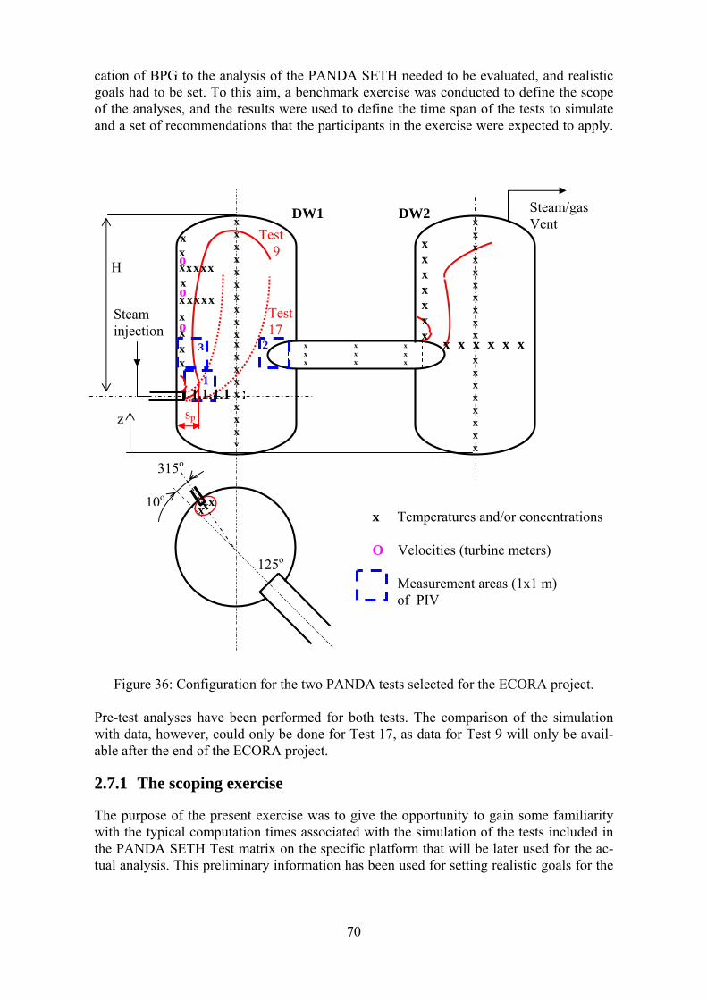
70
cation of BPG to the analysis of the PANDA SETH needed to be evaluated, and realistic goals had to be set. To this aim, a benchmark exercise was conducted to define the scope of the analyses, and the results were used to define the time span of the tests to simulate and a set of recommendations that the participants in the exercise were expected to apply.
Figure 36: Configuration for the two PANDA tests selected for the ECORA project. Pre-test analyses have been performed for both tests. The comparison of the simulation with data, however, could only be done for Test 17, as data for Test 9 will only be avail-able after the end of the ECORA project.
2.7.1 The scoping exercise
The purpose of the present exercise was to give the opportunity to gain some familiarity with the typical computation times associated with the simulation of the tests included in the PANDA SETH Test matrix on the specific platform that will be later used for the ac-tual analysis. This preliminary information has been used for setting realistic goals for the
x x
x 10o
o
x
xxxx
x
xxxx
x
z
Steam injection
Steam/gas Vent
x
x x x
x x x x x x x x x x x x x x x x x x x
x x x
x x x
x x x
x x x x x x x x x x x x x
xx x x x x x x x x x x x x x x x x
o
x Temperatures and/or concentrations O Velocities (turbine meters) Measurement areas (1x1 m) of PIV
sp
o
x x
1.1.1.1 x
H
1
2 3
Test 17
Test 9
DW1 DW2
125o
315o
71
analysis to be carried out in the frame of WP 7 of the project ECORA, as well as for the final selection of the tests (injection velocities). The detailed information on the scoping exercise is included in D12. Due to the exploratory character of the simulation, the analysis for typical conditions could be limited to a simplified geometry (one vessel and half interconnecting pipe only) and boundary conditions. The exercise proposed, however, was intended to be representa-tive of the real case. It was thus proposed to study the first period of a representative tran-sient (relevant to condition of Test 17, but with a reduced initial temperature to increase buoyancy) in a “box” geometry, where the volume of the vessel and the most important linear dimensions (hydraulic diameter of the injection pipe, distance of the injection from the opposite wall, height of the connecting pipe, height of the vessel) were maintained. Details of the geometry, as well as initial and boundary conditions are given in D12. It was proposed to calculate 50 s. At this time (according to the calculations performed with the CFX-4 and GOTHIC codes), some steam was expected to flow into the intercon-necting pipe. Due to the different codes used (with structured and unstructured mesh), a mesh was not recommended. It was suggested, however, that a basic mesh with at least 100’000 cells should be used, where the cross section of the inlet pipe is represented by at least a 4x4 subdivision. The results with this mesh had to be compared with those obtained using a refined mesh, to check that mesh-independent results can be obtained (at least to a certain extent) and to verify that with a realistic mesh and one refinement a sufficiently accurate estimate of the relevant variables can be achieved, with the computing resource that can be used within the scope of the project. Each participant in the exercise was asked to produce and compare the results at t=50 s with the two meshes for temperature and steam concentration distributions along various lines (target variables). For each variable, the RMS of the difference of the distributions obtained with the two meshes had to be given.
( )
N
ff
ffdifferenceRMS
N
∑ −
−= 1
221
min,1max,1 ||1
where f1 and f2 are the values of the variables at N points for the calculations with the coarse and fine mesh, respectively, for each prescribed line. The benchmark test was calculated by the seven partners in WP7 (PSI, GRS, VTT, Vat-tenfall, CEA, AEKI and NRI) using the four codes that will be assessed using the SETH data, i.e., CFX-4, CFX-5, FLUENT and TONUS. Additionally, calculations with the GOTHIC code are also reported, as most of the pre-test calculations for defining the test conditions for the SETH project have been carried out using this code. The results showed that large computation times were required for the simulation with the refined mesh, and small time steps were necessary for achieving a sufficiently accurate so-lution. From the RMS of the difference of the distributions on the four lines selected,
72
which have been calculated using two (or more meshes) or different order differencing methods it also resulted that no mesh-independent results could be obtained with the meshes used, and a large sensitivity in the results exists with respect to the mesh used. Es-pecially the steam distribution in the interconnecting pipe was affected by a large sensitiv-ity to mesh numerical methods and turbulence models used. This suggested that successful simulations of the SETH tests can only be achieved with an adequate resolution of the flow domain, and that for achieving some evidence that convergence has been achieved the calculations would need to be carried out with a third mesh. Moreover, the expectation was confirmed that the choice of the turbulence model would substantially affect the re-sults. The practical indications resulting from the scoping test exercise can be summarized as follows:
• The currently available computer resources are not sufficient for a complete analysis of the entire transient of Tests 17 and 9 using the BPG. Indeed, simula-tions of up to thousands seconds using increasingly fine mesh to obtain con-verged solutions appears to be not possible. Simulations with only one, “practi-cal mesh”, seems to be the only realistic option
• The BPG can only be applied to a portion of the transient. For a short transient, it is possible to perform the sensitivity studies aiming at evaluating the various er-rors and the accuracy of the simulation
• Therefore, the validation exercise could be conveniently divided in two steps: o Step 1: a short transient should be analysed using, to any practical extent,
the BPG. o Step 2: provided that the solution using a “practical mesh” is sufficiently
close to that obtained with the finest mesh used in Step 1, the entire tran-sient will be calculated with that mesh. The criterion used for deciding whether Step 2 has to be carried out will be the convergence of one of the target variables (see below) within certain acceptance limits, to be pre-scribed.
• In view of the difficulties to predict accurately the steam concentration in the in-terconnecting pipe, this variable has a crucial role in the simulation, as it “inte-grates” the errors in the simulation of the flow and transport processes in the Drywell 1. Therefore, the end of Step 1 is conveniently defined by the time at which the steam concentration of the air-steam mixture that is flowing through the interconnecting time is sufficiently high to be detected with confidence. This time, evaluated with the GOTHIC code, was expected to be about 70 s for Test 17 and between 200 and 250 s for Test 9.
2.7.2 Definition of the CFD simulations
Specifications for the pre-test analyses were given for: geometry, simulation times, initial and boundary conditions, sensitivity studies, as well as for the variables to submit. All these specifications are included in D12, and only the essential parameters are reported here.
73
2.7.2.1 General definition As discussed above, in consideration of the large computational time needed for running the transients and the number of calculations that are required for complying with the Best Practice Guidelines, it was decided to have two steps in the simulation:
1. Step 1: perform the simulation according to the BPG for a short transient, until the time steam can be measured in the center of the interconnecting pipe. For the two tests, this time is expected to be:
o Test 17: 70 s o Test 9: 250 s
2. Step 2: the calculation with the largest “practical” mesh will be extended to the time when the stratification front in Drywell 2 propagates below the intercon-necting pipe. This simulation will be performed only if the simulations of Step 1 will show that the calculation of the target variables (discussed below) with the largest “practical” mesh (intermediate mesh) and the finest mesh do not differ by more than 5%,. In the two tests, the time of this event was expected to be:
o Test 17: 1000 to 2000 s o Test 9: 4000 to 5000 s
The two tests are started from the same initial conditions, which are given in Table VIII.
Table VIII: Initial conditions Variable Value Pressure 130 kPa Wall Temperature 108 oC Fluid Temperature 108 oC Air Partial Pressure 130 kPa Steam negligible amount
For both tests, the pressure can be assumed to be constant and equal to 130 kPa. Fluid will be vented to the atmosphere through a pipe connected to a flange at the top of Drywell 2 . The temperature of the steam injected will be 140 oC. The steam mass flow rates (actually controlled in the experiments) for the two tests are: Test 17: G= 65 g/s Test 9: G=14 g/s which result in the following injection velocities: Test 17: Vin= 4.926 m/s Test 9: Vin=1.061 m/s
74
The tests are started by opening the valve upstream of the injection nozzle (see D12), so that the prescribed mass flow rate will be reached within a certain transient time. As the valve opening time is shorter than 4 seconds, and the actual transient could not be estimated at the time the specifications for the pre-test analysis were given, it was recom-mended to use for the simulation a linear increase of the inlet flow rate over 4 seconds time. 2.7.2.2 Sensitivity studies The strict application of the BPG would result in a computational effort that is hardly af-fordable with the current computer power. Especially a systematic refinement of the mesh (at least in two steps), which would allow the formal definition of the discretisation error, cannot be envisaged, as it would lead (starting from a coarse mesh of about 105 cells and halving twice each cell in all three directions x, y and z) to a fine mesh of a few million cells. It was therefore recommended to refine the mesh according to the experience of the user, and to evaluate the convergence of the simulations using the trends of the target variables. It was therefore excluded that the same mesh could be used by all participants in the vali-dation exercise, or strict criteria could be prescribed for establishing the mesh. Also the guideline to verify that the results obtained are independent of the prescribed ac-curacy (time step or tolerance on residuals) was somewhat relaxed, and such independ-ence was required to be verified for one mesh. As regards the truncation error, experience shows that it may not be always possible to get converged solutions with both single and double precision. Therefore, the investigation on the effect of the precision on the results was suggested only. In summary, it was required to perform the following calculations:
• Use three meshes (coarse, intermediate, fine) • Study the effect of time step (tolerance on residuals) for at least one mesh (in-
termediate mesh), using at least three time steps • If applicable, study the effect of precision
The only model that was expected to have an effect on the calculated results is the turbu-lence model (and, to some extent, the associated wall treatment). This implies that the validation exercise included simulations with at least two turbulence models. As the stan-dard high-Reynolds number k-ε model is currently the industrial standard for large-scale calculations, all participants were asked to provide simulations with this model. The criteria defined in the BPG regarding the appropriate wall treatment for the various turbulence models and the associated requirements for the mesh close to the walls had to be applied. For each of the tests, the matrix of the simulations is given in Table IX below. Simulations for the entire transient (Step 2) had to be carried out only if the results of the calculations for Step 1 (early period of the transient) showed that the simulations per-
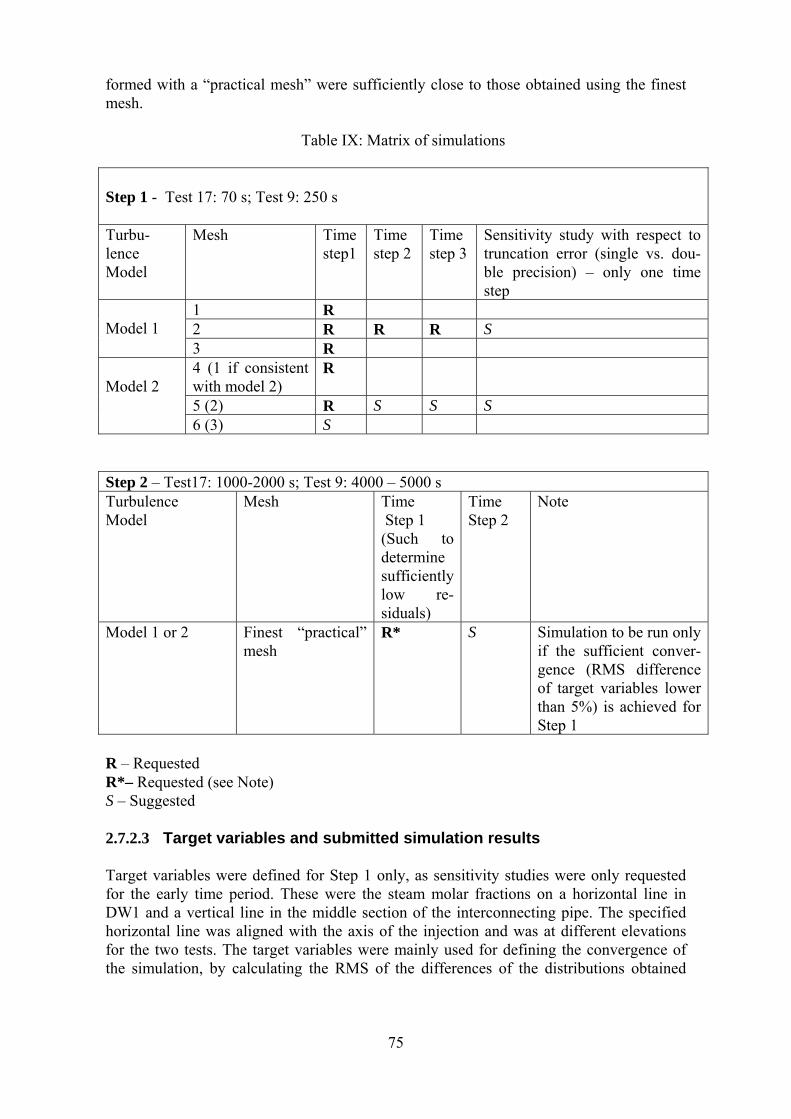
75
formed with a “practical mesh” were sufficiently close to those obtained using the finest mesh.
Table IX: Matrix of simulations Step 1 - Test 17: 70 s; Test 9: 250 s Turbu-lence Model
Mesh Time step1
Time step 2
Time step 3
Sensitivity study with respect to truncation error (single vs. dou-ble precision) – only one time step
1 R 2 R R R S
Model 1
3 R 4 (1 if consistent with model 2)
R
5 (2) R S S S
Model 2
6 (3) S Step 2 – Test17: 1000-2000 s; Test 9: 4000 – 5000 s Turbulence Model
Mesh Time Step 1 (Such to determine sufficiently low re-siduals)
Time Step 2
Note
Model 1 or 2 Finest “practical” mesh
R* S Simulation to be run only if the sufficient conver-gence (RMS difference of target variables lower than 5%) is achieved for Step 1
R – Requested R*– Requested (see Note) S – Suggested 2.7.2.3 Target variables and submitted simulation results Target variables were defined for Step 1 only, as sensitivity studies were only requested for the early time period. These were the steam molar fractions on a horizontal line in DW1 and a vertical line in the middle section of the interconnecting pipe. The specified horizontal line was aligned with the axis of the injection and was at different elevations for the two tests. The target variables were mainly used for defining the convergence of the simulation, by calculating the RMS of the differences of the distributions obtained
76
with the increasingly fine meshes and did not all correspond to variables actually meas-ured in the test. Two types of results had to be extracted for the simulations for comparison with data:
1. Time evolution of temperatures and concentrations at selected locations. 2. Distributions of temperature and steam concentration along a number of lines
(both horizontal and vertical) at the end of the simulation and at a number of in-termediate times (see Ref. [14] for details).
It has to be taken into account that due to the long times required to take a concentration measurement (15 s) and the consequent long cycling times between two measurements at the same location, the comparison of calculated distributions of steam fraction with ex-perimental values is possible only over long time periods, as it is expected that changes in time are very slow. As a consequence, only temperature distributions can be compared with test data for Step 1 of both tests. For each of the models used, the RMS of the differ-ences of the distributions obtained with the two finest meshes (not only the target vari-ables) had also to be provided. 2.7.2.4 Definition of tasks for the various organizations Seven organizations submitted simulations with 4 codes: CFX-4, CFX-5, FLUENT and TONUS. As the FLUENT code was intended to be used by four organizations, the work has been distributed in order to get the maximum output. Table X below summarizes the tasks as-signed to each of the WP7 partners:
Table X: Definition of tasks for the various organizations Organisa-tion
PSI CEA GRS AEKI NRI Vatten-fall
VTT
code CFX-4 TONUS CFX-5 FLUENT Test 17 X X X X X Test 9 X X X X
2.7.3 Main results of the pre-test analyses
The pre-test calculations revealed that the application of the BPG (though reduced in scope) to the analyses of the transient problem in the large-scale geometry of the PANDA facility resulted in a severe computational challenge. Therefore, an overview of the simu-lations performed and the statistics of the simulation is presented first. The code-to-code comparison for selected results is then presented, which includes, for Test 17 only, the comparison with experimental data. The data for Test 9 will be only available later in 2005, and could not be used for the assessment of the codes within the ECORA project.
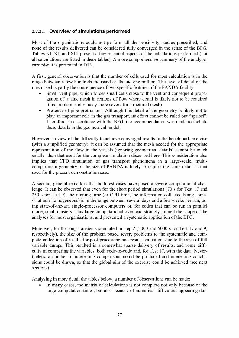
77
2.7.3.1 Overview of simulations performed Most of the organisations could not perform all the sensitivity studies prescribed, and none of the results delivered can be considered fully converged in the sense of the BPG. Tables XI, XII and XIII present a few essential aspects of the calculations performed (not all calculations are listed in these tables). A more comprehensive summary of the analyses carried-out is presented in D13. A first, general observation is that the number of cells used for most calculation is in the range between a few hundreds thousands cells and one million. The level of detail of the mesh used is partly the consequence of two specific features of the PANDA facility:
• Small vent pipe, which forces small cells close to the vent and consequent propa-gation of a fine mesh in regions of flow where detail is likely not to be required (this problem is obviously more severe for structured mesh)
• Presence of pipe protrusions. Although this detail of the geometry is likely not to play an important role in the gas transport, its effect cannot be ruled out “apriori”. Therefore, in accordance with the BPG, the recommendation was made to include these details in the geometrical model.
However, in view of the difficulty to achieve converged results in the benchmark exercise (with a simplified geometry), it can be assumed that the mesh needed for the appropriate representation of the flow in the vessels (ignoring geometrical details) cannot be much smaller than that used for the complete simulation discussed here. This consideration also implies that CFD simulation of gas transport phenomena in a large-scale, multi-compartment geometry of the size of PANDA is likely to require the same detail as that used for the present demonstration case. A second, general remark is that both test cases have posed a severe computational chal-lenge. It can be observed that even for the short period simulations (70 s for Test 17 and 250 s for Test 9), the running time (or CPU time, the information collected being some-what non-homogeneous) is in the range between several days and a few weeks per run, us-ing state-of-the-art, single-processor computers or, for codes that can be run in parallel mode, small clusters. This large computational overhead strongly limited the scope of the analyses for most organisations, and prevented a systematic application of the BPG. Moreover, for the long transients simulated in step 2 (2000 and 5000 s for Test 17 and 9, respectively), the size of the problem posed severe problems to the systematic and com-plete collection of results for post-processing and result evaluation, due to the size of full variable dumps. This resulted in a somewhat sparse delivery of results, and some diffi-culty in comparing the variables, both code-to-code and, for Test 17, with the data. Never-theless, a number of interesting comparisons could be produced and interesting conclu-sions could be drawn, so that the global aim of the exercise could be achieved (see next sections). Analysing in more detail the tables below, a number of observations can be made:
• In many cases, the matrix of calculations is not complete not only because of the large computation times, but also because of numerical difficulties appearing dur-
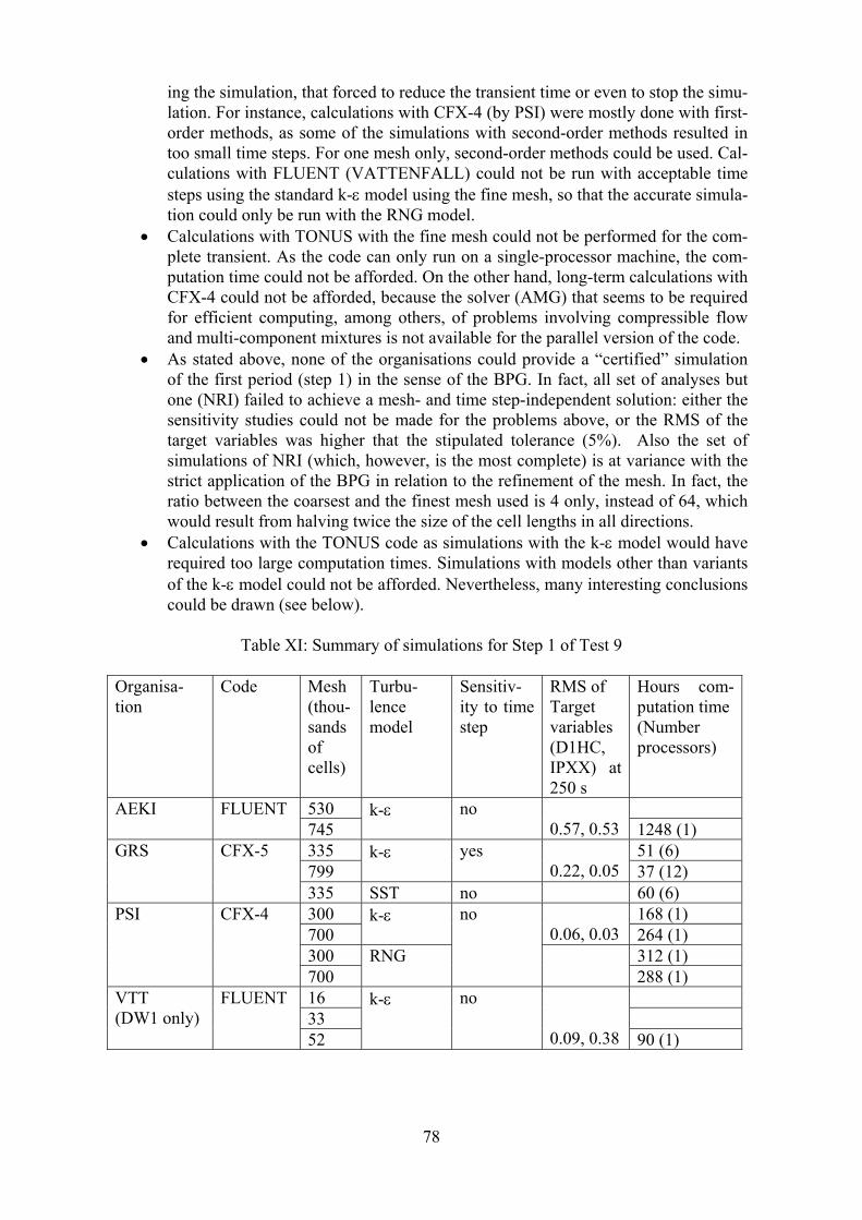
78
ing the simulation, that forced to reduce the transient time or even to stop the simu-lation. For instance, calculations with CFX-4 (by PSI) were mostly done with first-order methods, as some of the simulations with second-order methods resulted in too small time steps. For one mesh only, second-order methods could be used. Cal-culations with FLUENT (VATTENFALL) could not be run with acceptable time steps using the standard k-ε model using the fine mesh, so that the accurate simula-tion could only be run with the RNG model.
• Calculations with TONUS with the fine mesh could not be performed for the com-plete transient. As the code can only run on a single-processor machine, the com-putation time could not be afforded. On the other hand, long-term calculations with CFX-4 could not be afforded, because the solver (AMG) that seems to be required for efficient computing, among others, of problems involving compressible flow and multi-component mixtures is not available for the parallel version of the code.
• As stated above, none of the organisations could provide a “certified” simulation of the first period (step 1) in the sense of the BPG. In fact, all set of analyses but one (NRI) failed to achieve a mesh- and time step-independent solution: either the sensitivity studies could not be made for the problems above, or the RMS of the target variables was higher that the stipulated tolerance (5%). Also the set of simulations of NRI (which, however, is the most complete) is at variance with the strict application of the BPG in relation to the refinement of the mesh. In fact, the ratio between the coarsest and the finest mesh used is 4 only, instead of 64, which would result from halving twice the size of the cell lengths in all directions.
• Calculations with the TONUS code as simulations with the k-ε model would have required too large computation times. Simulations with models other than variants of the k-ε model could not be afforded. Nevertheless, many interesting conclusions could be drawn (see below).
Table XI: Summary of simulations for Step 1 of Test 9
Organisa-tion
Code Mesh (thou-sands of cells)
Turbu-lence model
Sensitiv-ity to time step
RMS of Target variables (D1HC, IPXX) at 250 s
Hours com-putation time (Number processors)
530 AEKI FLUENT 745
k-ε no 0.57, 0.53 1248 (1)
335 51 (6) 799
k-ε
yes
0.22, 0.05 37 (12)
GRS CFX-5
335 SST no 60 (6) 300 168 (1) 700
k-ε 0.06, 0.03 264 (1)
300 312 (1)
PSI CFX-4
700 RNG
no
288 (1)
16 33
VTT (DW1 only)
FLUENT
52
k-ε no 0.09, 0.38 90 (1)
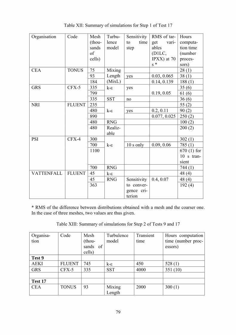
79
Table XII: Summary of simulations for Step 1 of Test 17 Organisation Code Mesh
(thou-sands of cells)
Turbu-lence model
Sensitivity to time step
RMS of tar-get vari-ables (D1LC, IPXX) at 70 s *
Hours computa-tion time (number proces-sors)
75 28 (1) 93 yes 0.03, 0.065 38 (1)
CEA TONUS
184
Mixing Length (MixL) 0.14, 0.139 188 (1)
335 35 (6) 799
k-ε yes 0.19, 0.05 61 (6)
GRS CFX-5
335 SST no 36 (6) 235 55 (2) 480 yes 0.2, 0.11 90 (2) 890
k-ε 0.077, 0.025 250 (2)
480 RNG 100 (2)
NRI FLUENT
480 Realiz-able
200 (2)
300 302 (1) 700 10 s only 0.09, 0.06 785 (1) 1100
k-ε
670 (1) for 10 s tran-sient
PSI CFX-4
700 RNG 744 (1) 45 k-ε 48 (4) 45 48 (4)
VATTENFALL FLUENT
363 RNG Sensitivity
to conver-gence cri-terion
0.4, 0.07 192 (4)
* RMS of the difference between distributions obtained with a mesh and the coarser one. In the case of three meshes, two values are thus given.
Table XIII: Summary of simulations for Step 2 of Tests 9 and 17 Organisa-tion
Code Mesh (thou-sands of cells)
Turbulence model
Transient time
Hours computation time (number proc-essors)
Test 9 AEKI FLUENT 745 k-ε 450 528 (1) GRS CFX-5 335 SST 4000 351 (10) Test 17 CEA TONUS 93 Mixing
Length 2000 300 (1)
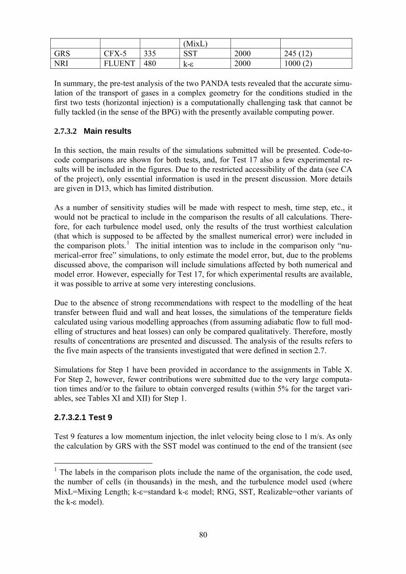
80
(MixL) GRS CFX-5 335 SST 2000 245 (12) NRI FLUENT 480 k-ε 2000 1000 (2) In summary, the pre-test analysis of the two PANDA tests revealed that the accurate simu-lation of the transport of gases in a complex geometry for the conditions studied in the first two tests (horizontal injection) is a computationally challenging task that cannot be fully tackled (in the sense of the BPG) with the presently available computing power. 2.7.3.2 Main results In this section, the main results of the simulations submitted will be presented. Code-to-code comparisons are shown for both tests, and, for Test 17 also a few experimental re-sults will be included in the figures. Due to the restricted accessibility of the data (see CA of the project), only essential information is used in the present discussion. More details are given in D13, which has limited distribution. As a number of sensitivity studies will be made with respect to mesh, time step, etc., it would not be practical to include in the comparison the results of all calculations. There-fore, for each turbulence model used, only the results of the trust worthiest calculation (that which is supposed to be affected by the smallest numerical error) were included in the comparison plots.1 The initial intention was to include in the comparison only “nu-merical-error free” simulations, to only estimate the model error, but, due to the problems discussed above, the comparison will include simulations affected by both numerical and model error. However, especially for Test 17, for which experimental results are available, it was possible to arrive at some very interesting conclusions. Due to the absence of strong recommendations with respect to the modelling of the heat transfer between fluid and wall and heat losses, the simulations of the temperature fields calculated using various modelling approaches (from assuming adiabatic flow to full mod-elling of structures and heat losses) can only be compared qualitatively. Therefore, mostly results of concentrations are presented and discussed. The analysis of the results refers to the five main aspects of the transients investigated that were defined in section 2.7. Simulations for Step 1 have been provided in accordance to the assignments in Table X. For Step 2, however, fewer contributions were submitted due to the very large computa-tion times and/or to the failure to obtain converged results (within 5% for the target vari-ables, see Tables XI and XII) for Step 1. 2.7.3.2.1 Test 9 Test 9 features a low momentum injection, the inlet velocity being close to 1 m/s. As only the calculation by GRS with the SST model was continued to the end of the transient (see
1 The labels in the comparison plots include the name of the organisation, the code used, the number of cells (in thousands) in the mesh, and the turbulence model used (where MixL=Mixing Length; k-ε=standard k-ε model; RNG, SST, Realizable=other variants of the k-ε model).
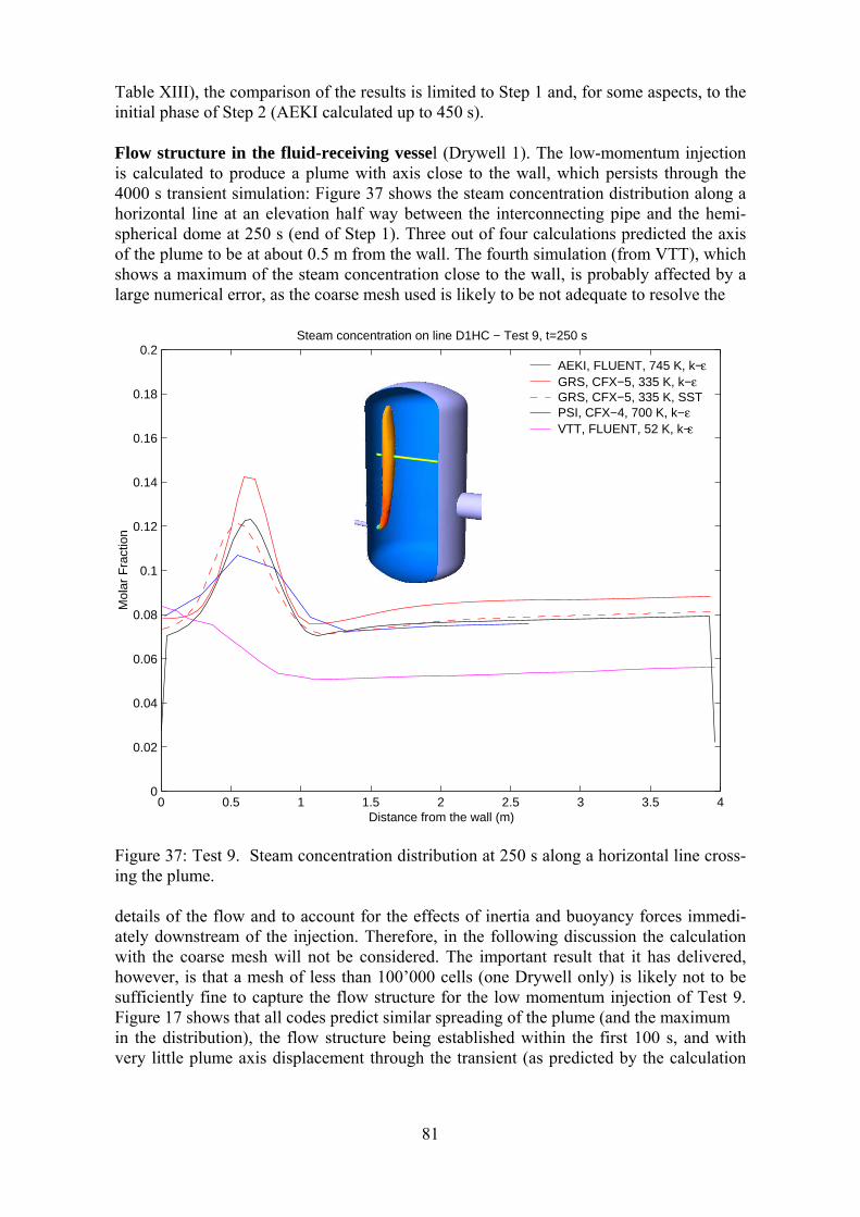
81
Table XIII), the comparison of the results is limited to Step 1 and, for some aspects, to the initial phase of Step 2 (AEKI calculated up to 450 s). Flow structure in the fluid-receiving vessel (Drywell 1). The low-momentum injection is calculated to produce a plume with axis close to the wall, which persists through the 4000 s transient simulation: Figure 37 shows the steam concentration distribution along a horizontal line at an elevation half way between the interconnecting pipe and the hemi-spherical dome at 250 s (end of Step 1). Three out of four calculations predicted the axis of the plume to be at about 0.5 m from the wall. The fourth simulation (from VTT), which shows a maximum of the steam concentration close to the wall, is probably affected by a large numerical error, as the coarse mesh used is likely to be not adequate to resolve the
0 0.5 1 1.5 2 2.5 3 3.5 40
0.02
0.04
0.06
0.08
0.1
0.12
0.14
0.16
0.18
0.2
Mol
ar F
ract
ion
Distance from the wall (m)
Steam concentration on line D1HC − Test 9, t=250 s
AEKI, FLUENT, 745 K, k−εGRS, CFX−5, 335 K, k−ε GRS, CFX−5, 335 K, SST PSI, CFX−4, 700 K, k−ε VTT, FLUENT, 52 K, k−ε
Figure 37: Test 9. Steam concentration distribution at 250 s along a horizontal line cross-ing the plume. details of the flow and to account for the effects of inertia and buoyancy forces immedi-ately downstream of the injection. Therefore, in the following discussion the calculation with the coarse mesh will not be considered. The important result that it has delivered, however, is that a mesh of less than 100’000 cells (one Drywell only) is likely not to be sufficiently fine to capture the flow structure for the low momentum injection of Test 9. Figure 17 shows that all codes predict similar spreading of the plume (and the maximum in the distribution), the flow structure being established within the first 100 s, and with very little plume axis displacement through the transient (as predicted by the calculation
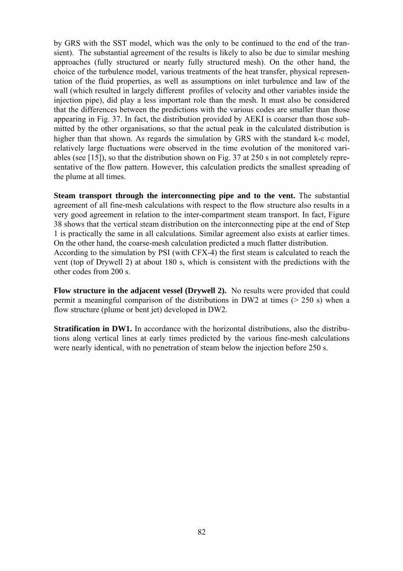
82
by GRS with the SST model, which was the only to be continued to the end of the tran-sient). The substantial agreement of the results is likely to also be due to similar meshing approaches (fully structured or nearly fully structured mesh). On the other hand, the choice of the turbulence model, various treatments of the heat transfer, physical represen-tation of the fluid properties, as well as assumptions on inlet turbulence and law of the wall (which resulted in largely different profiles of velocity and other variables inside the injection pipe), did play a less important role than the mesh. It must also be considered that the differences between the predictions with the various codes are smaller than those appearing in Fig. 37. In fact, the distribution provided by AEKI is coarser than those sub-mitted by the other organisations, so that the actual peak in the calculated distribution is higher than that shown. As regards the simulation by GRS with the standard k-ε model, relatively large fluctuations were observed in the time evolution of the monitored vari-ables (see [15]), so that the distribution shown on Fig. 37 at 250 s in not completely repre-sentative of the flow pattern. However, this calculation predicts the smallest spreading of the plume at all times. Steam transport through the interconnecting pipe and to the vent. The substantial agreement of all fine-mesh calculations with respect to the flow structure also results in a very good agreement in relation to the inter-compartment steam transport. In fact, Figure 38 shows that the vertical steam distribution on the interconnecting pipe at the end of Step 1 is practically the same in all calculations. Similar agreement also exists at earlier times. On the other hand, the coarse-mesh calculation predicted a much flatter distribution. According to the simulation by PSI (with CFX-4) the first steam is calculated to reach the vent (top of Drywell 2) at about 180 s, which is consistent with the predictions with the other codes from 200 s. Flow structure in the adjacent vessel (Drywell 2). No results were provided that could permit a meaningful comparison of the distributions in DW2 at times (> 250 s) when a flow structure (plume or bent jet) developed in DW2. Stratification in DW1. In accordance with the horizontal distributions, also the distribu-tions along vertical lines at early times predicted by the various fine-mesh calculations were nearly identical, with no penetration of steam below the injection before 250 s.
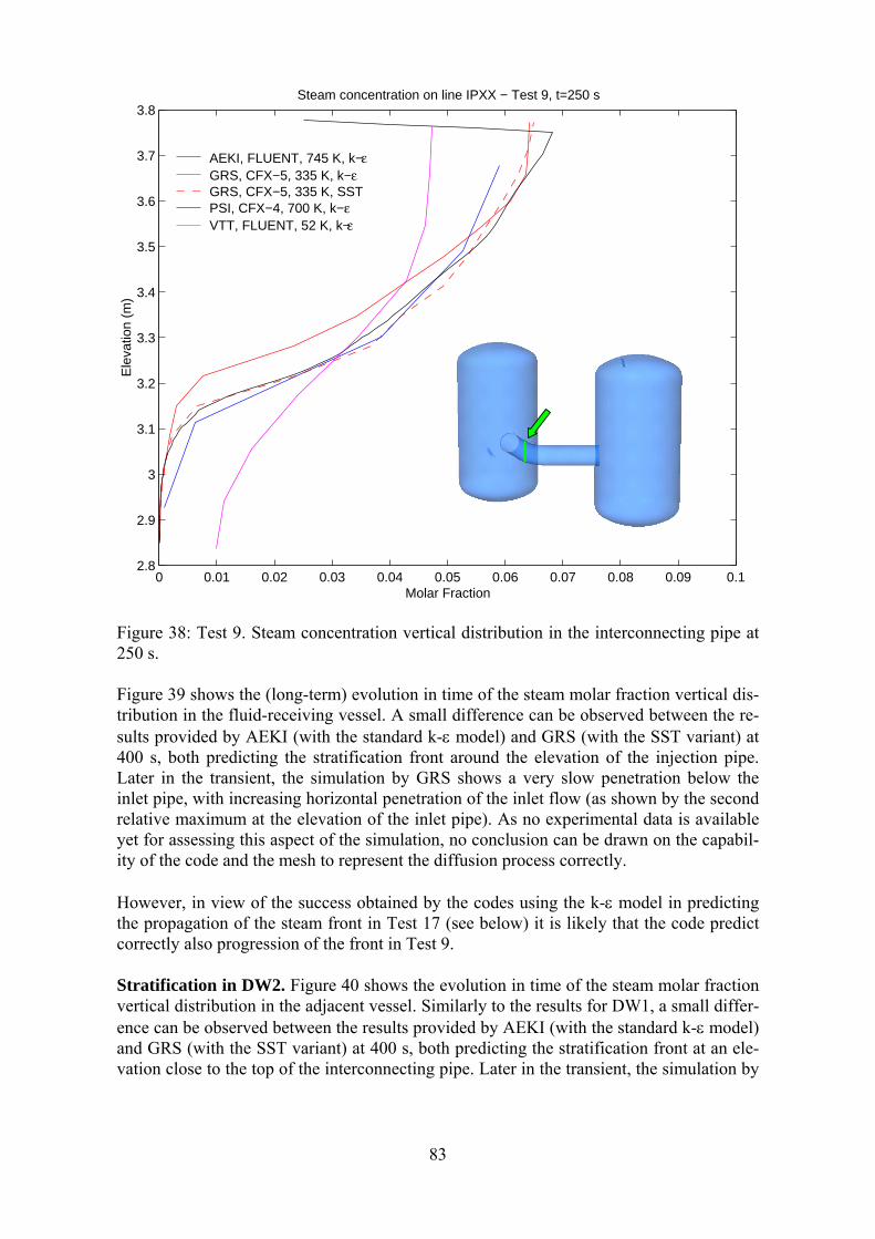
83
0 0.01 0.02 0.03 0.04 0.05 0.06 0.07 0.08 0.09 0.12.8
2.9
3
3.1
3.2
3.3
3.4
3.5
3.6
3.7
3.8
Molar Fraction
Ele
vatio
n (m
)
Steam concentration on line IPXX − Test 9, t=250 s
AEKI, FLUENT, 745 K, k−εGRS, CFX−5, 335 K, k−ε GRS, CFX−5, 335 K, SST PSI, CFX−4, 700 K, k−ε VTT, FLUENT, 52 K, k−ε
Figure 38: Test 9. Steam concentration vertical distribution in the interconnecting pipe at 250 s. Figure 39 shows the (long-term) evolution in time of the steam molar fraction vertical dis-tribution in the fluid-receiving vessel. A small difference can be observed between the re-sults provided by AEKI (with the standard k-ε model) and GRS (with the SST variant) at 400 s, both predicting the stratification front around the elevation of the injection pipe. Later in the transient, the simulation by GRS shows a very slow penetration below the inlet pipe, with increasing horizontal penetration of the inlet flow (as shown by the second relative maximum at the elevation of the inlet pipe). As no experimental data is available yet for assessing this aspect of the simulation, no conclusion can be drawn on the capabil-ity of the code and the mesh to represent the diffusion process correctly. However, in view of the success obtained by the codes using the k-ε model in predicting the propagation of the steam front in Test 17 (see below) it is likely that the code predict correctly also progression of the front in Test 9. Stratification in DW2. Figure 40 shows the evolution in time of the steam molar fraction vertical distribution in the adjacent vessel. Similarly to the results for DW1, a small differ-ence can be observed between the results provided by AEKI (with the standard k-ε model) and GRS (with the SST variant) at 400 s, both predicting the stratification front at an ele-vation close to the top of the interconnecting pipe. Later in the transient, the simulation by
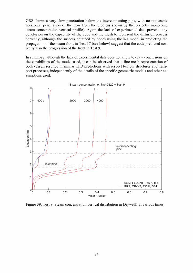
84
GRS shows a very slow penetration below the interconnecting pipe, with no noticeable horizontal penetration of the flow from the pipe (as shown by the perfectly monotonic steam concentration vertical profile). Again the lack of experimental data prevents any conclusion on the capability of the code and the mesh to represent the diffusion process correctly, although the success obtained by codes using the k-ε model in predicting the propagation of the steam front in Test 17 (see below) suggest that the code predicted cor-rectly also the progression of the front in Test 9. In summary, although the lack of experimental data does not allow to draw conclusions on the capabilities of the model used, it can be observed that a fine-mesh representation of both vessels resulted in similar CFD predictions with respect to flow structures and trans-port processes, independently of the details of the specific geometric models and other as-sumptions used.
0 0.1 0.2 0.3 0.4 0.5 0.6 0.7 0.80
1
2
3
4
5
6
7
8
inlet pipe
interconnectingpipe
400 s 2000 3000 4000
Molar Fraction
Ele
vatio
n (m
)
Steam concentration on line D120 − Test 9
AEKI, FLUENT, 745 K, k−εGRS, CFX−5, 335 K, SST
Figure 39: Test 9. Steam concentration vertical distribution in Drywell1 at various times.
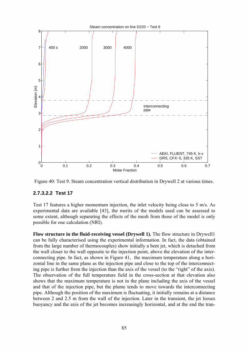
85
0 0.1 0.2 0.3 0.4 0.5 0.6 0.70
1
2
3
4
5
6
7
8
interconnectingpipe
400 s 2000 3000 4000
Molar Fraction
Ele
vatio
n (m
)
Steam concentration on line D220 − Test 9
AEKI, FLUENT, 745 K, k−εGRS, CFX−5, 335 K, SST
Figure 40: Test 9. Steam concentration vertical distribution in Drywell 2 at various times.
2.7.3.2.2 Test 17 Test 17 features a higher momentum injection, the inlet velocity being close to 5 m/s. As experimental data are available [43], the merits of the models used can be assessed to some extent, although separating the effects of the mesh from those of the model is only possible for one calculation (NRI). Flow structure in the fluid-receiving vessel (Drywell 1). The flow structure in Drywell1 can be fully characterised using the experimental information. In fact, the data (obtained from the large number of thermocouples) show initially a bent jet, which is detached from the wall closer to the wall opposite to the injection point, above the elevation of the inter-connecting pipe. In fact, as shown in Figure 41, the maximum temperature along a hori-zontal line in the same plane as the injection pipe and close to the top of the interconnect-ing pipe is further from the injection than the axis of the vessel (to the “right” of the axis). The observation of the full temperature field in the cross-section at that elevation also shows that the maximum temperature is not in the plane including the axis of the vessel and that of the injection pipe, but the plume tends to move towards the interconnecting pipe. Although the position of the maximum is fluctuating, it initially remains at a distance between 2 and 2.5 m from the wall of the injection. Later in the transient, the jet looses buoyancy and the axis of the jet becomes increasingly horizontal, and at the end the tran-
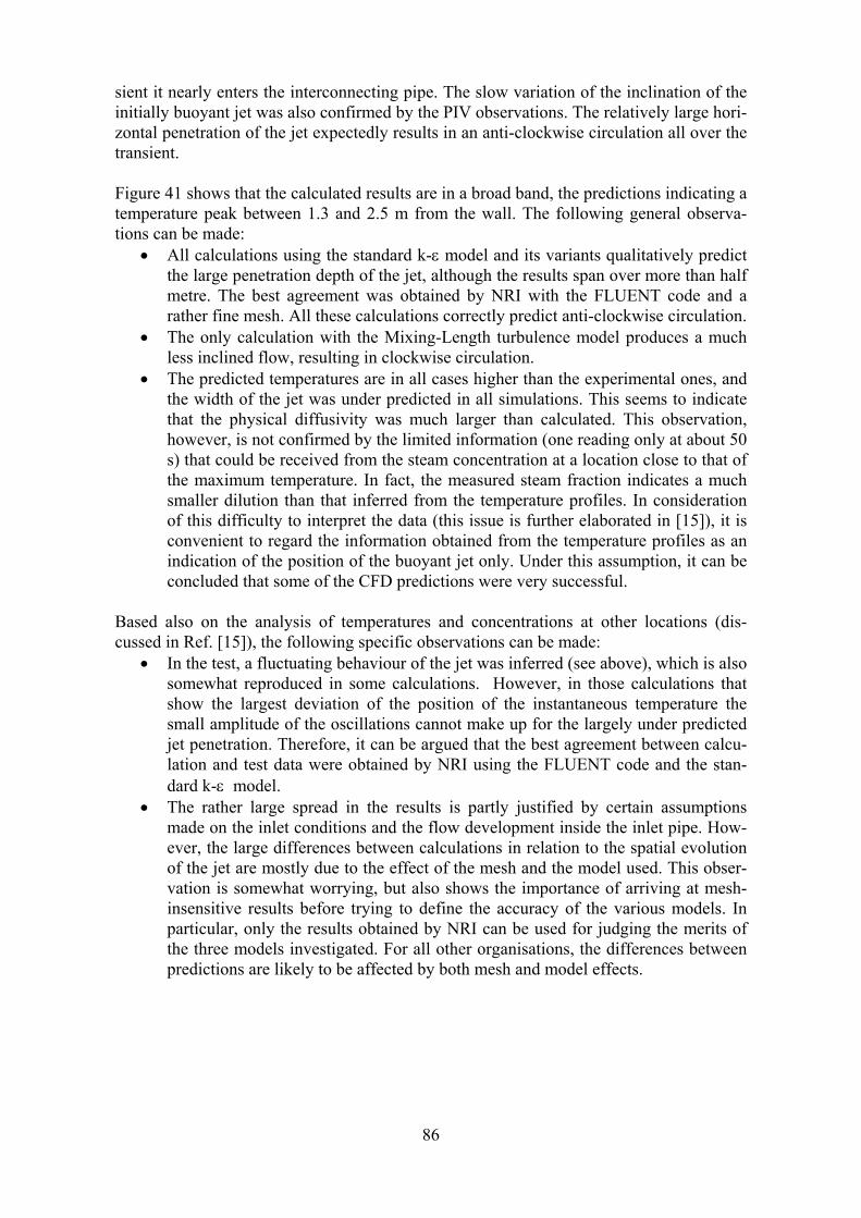
86
sient it nearly enters the interconnecting pipe. The slow variation of the inclination of the initially buoyant jet was also confirmed by the PIV observations. The relatively large hori-zontal penetration of the jet expectedly results in an anti-clockwise circulation all over the transient. Figure 41 shows that the calculated results are in a broad band, the predictions indicating a temperature peak between 1.3 and 2.5 m from the wall. The following general observa-tions can be made:
• All calculations using the standard k-ε model and its variants qualitatively predict the large penetration depth of the jet, although the results span over more than half metre. The best agreement was obtained by NRI with the FLUENT code and a rather fine mesh. All these calculations correctly predict anti-clockwise circulation.
• The only calculation with the Mixing-Length turbulence model produces a much less inclined flow, resulting in clockwise circulation.
• The predicted temperatures are in all cases higher than the experimental ones, and the width of the jet was under predicted in all simulations. This seems to indicate that the physical diffusivity was much larger than calculated. This observation, however, is not confirmed by the limited information (one reading only at about 50 s) that could be received from the steam concentration at a location close to that of the maximum temperature. In fact, the measured steam fraction indicates a much smaller dilution than that inferred from the temperature profiles. In consideration of this difficulty to interpret the data (this issue is further elaborated in [15]), it is convenient to regard the information obtained from the temperature profiles as an indication of the position of the buoyant jet only. Under this assumption, it can be concluded that some of the CFD predictions were very successful.
Based also on the analysis of temperatures and concentrations at other locations (dis-cussed in Ref. [15]), the following specific observations can be made:
• In the test, a fluctuating behaviour of the jet was inferred (see above), which is also somewhat reproduced in some calculations. However, in those calculations that show the largest deviation of the position of the instantaneous temperature the small amplitude of the oscillations cannot make up for the largely under predicted jet penetration. Therefore, it can be argued that the best agreement between calcu-lation and test data were obtained by NRI using the FLUENT code and the stan-dard k-ε model.
• The rather large spread in the results is partly justified by certain assumptions made on the inlet conditions and the flow development inside the inlet pipe. How-ever, the large differences between calculations in relation to the spatial evolution of the jet are mostly due to the effect of the mesh and the model used. This obser-vation is somewhat worrying, but also shows the importance of arriving at mesh-insensitive results before trying to define the accuracy of the various models. In particular, only the results obtained by NRI can be used for judging the merits of the three models investigated. For all other organisations, the differences between predictions are likely to be affected by both mesh and model effects.
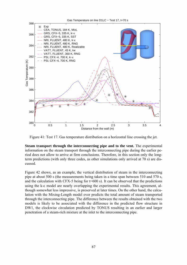
87
0 0.5 1 1.5 2 2.5 3 3.5 4380
382
384
386
388
390
392
394
396
398G
as T
empe
ratu
re (
K)
Distance from the wall (m)
Gas Temperature on line D1LC − Test 17, t=70 s
Exp CEA, TONUS, 184 K, MixL GRS, CFX−5, 335 K, k−ε GRS, CFX−5, 335 K, SST NRI, FLUENT, 480 K, k−εNRI, FLUENT, 480 K, RNG NRI, FLUENT, 480 K, RealizableVATT, FLUENT, 45 K, k−εVATT, FLUENT, 360 K, RNG PSI, CFX−4, 700 K, k−ε PSI, CFX−4, 700 K, RNG
Figure 41: Test 17. Gas temperature distribution on a horizontal line crossing the jet. Steam transport through the interconnecting pipe and to the vent. The experimental information on the steam transport through the interconnecting pipe during the earlier pe-riod does not allow to arrive at firm conclusions. Therefore, in this section only the long-term predictions (with only three codes, as other simulations only arrived at 70 s) are dis-cussed. Figure 42 shows, as an example, the vertical distribution of steam in the interconnecting pipe at about 500 s (the measurements being taken in a time span between 510 and 570 s, and the calculation with CFX-5 being for t=600 s). It can be observed that the predictions using the k-ε model are nearly overlapping the experimental results. This agreement, al-though somewhat less impressive, is preserved at later times. On the other hand, the calcu-lation with the Mixing-Length model over predicts the total amount of steam transported through the interconnecting pipe. The difference between the results obtained with the two models is likely to be associated with the difference in the predicted flow structure in DW1, the clockwise circulation predicted by TONUS resulting in an earlier and larger penetration of a steam-rich mixture at the inlet to the interconnecting pipe.
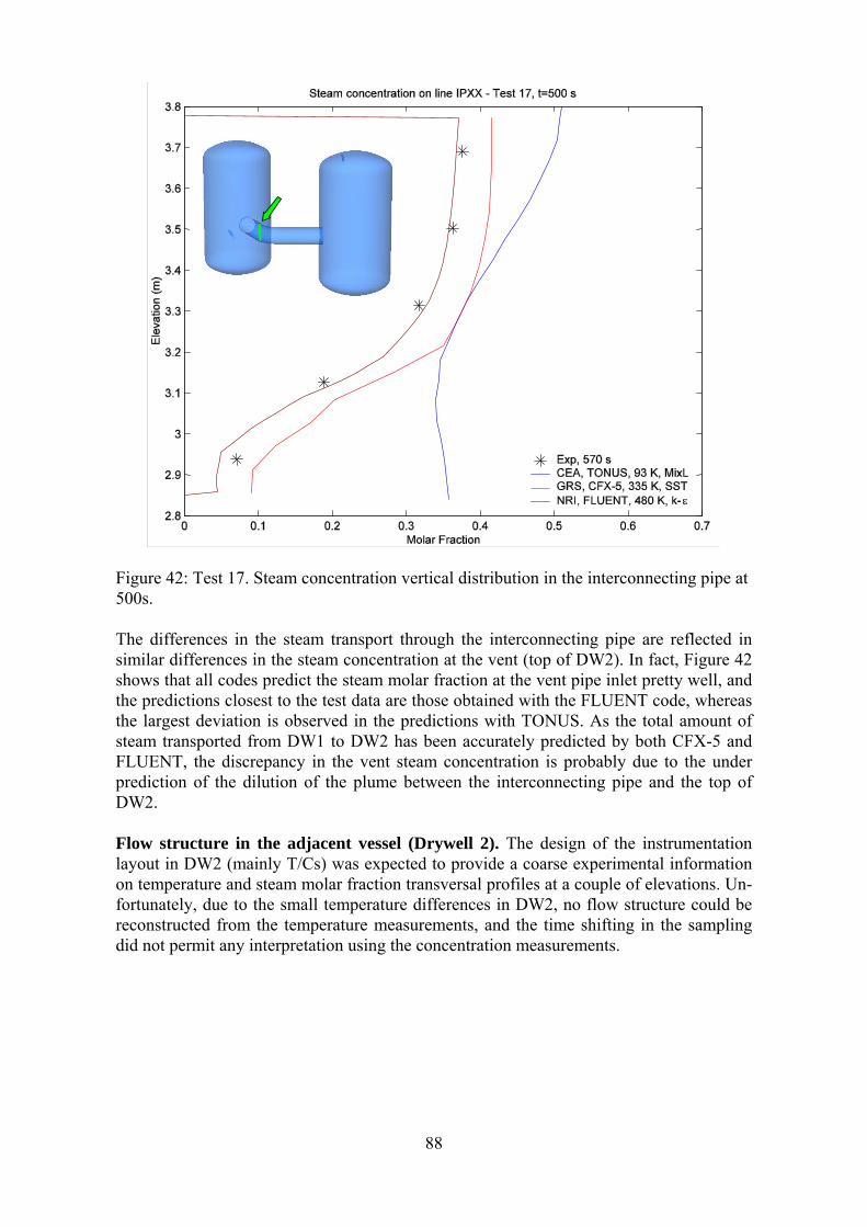
88
Figure 42: Test 17. Steam concentration vertical distribution in the interconnecting pipe at 500s. The differences in the steam transport through the interconnecting pipe are reflected in similar differences in the steam concentration at the vent (top of DW2). In fact, Figure 42 shows that all codes predict the steam molar fraction at the vent pipe inlet pretty well, and the predictions closest to the test data are those obtained with the FLUENT code, whereas the largest deviation is observed in the predictions with TONUS. As the total amount of steam transported from DW1 to DW2 has been accurately predicted by both CFX-5 and FLUENT, the discrepancy in the vent steam concentration is probably due to the under prediction of the dilution of the plume between the interconnecting pipe and the top of DW2. Flow structure in the adjacent vessel (Drywell 2). The design of the instrumentation layout in DW2 (mainly T/Cs) was expected to provide a coarse experimental information on temperature and steam molar fraction transversal profiles at a couple of elevations. Un-fortunately, due to the small temperature differences in DW2, no flow structure could be reconstructed from the temperature measurements, and the time shifting in the sampling did not permit any interpretation using the concentration measurements.
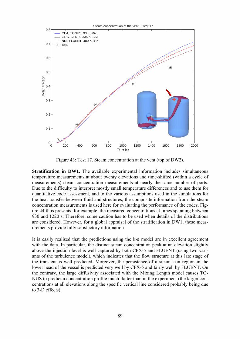
89
Figure 43: Test 17. Steam concentration at the vent (top of DW2).
Stratification in DW1. The available experimental information includes simultaneous temperature measurements at about twenty elevations and time-shifted (within a cycle of measurements) steam concentration measurements at nearly the same number of ports. Due to the difficulty to interpret mostly small temperature differences and to use them for quantitative code assessment, and to the various assumptions used in the simulations for the heat transfer between fluid and structures, the composite information from the steam concentration measurements is used here for evaluating the performance of the codes. Fig-ure 44 thus presents, for example, the measured concentrations at times spanning between 930 and 1220 s. Therefore, some caution has to be used when details of the distributions are considered. However, for a global appraisal of the stratification in DW1, these meas-urements provide fully satisfactory information. It is easily realised that the predictions using the k-ε model are in excellent agreement with the data. In particular, the distinct steam concentration peak at an elevation slightly above the injection level is well captured by both CFX-5 and FLUENT (using two vari-ants of the turbulence model), which indicates that the flow structure at this late stage of the transient is well predicted. Moreover, the persistence of a steam-lean region in the lower head of the vessel is predicted very well by CFX-5 and fairly well by FLUENT. On the contrary, the large diffusivity associated with the Mixing Length model causes TO-NUS to predict a concentration profile much flatter than in the experiment (the larger con-centrations at all elevations along the specific vertical line considered probably being due to 3-D effects).
0 200 400 600 800 1000 1200 1400 1600 1800 20000
0.1
0.2
0.3
0.4
0.5
0.6
0.7
0.8
Mol
ar F
ract
ion
Time (s)
Steam concentration at the vent − Test 17
CEA, TONUS, 93 K, MixL GRS, CFX−5, 335 K, SST NRI, FLUENT, 480 K, k−εExp.
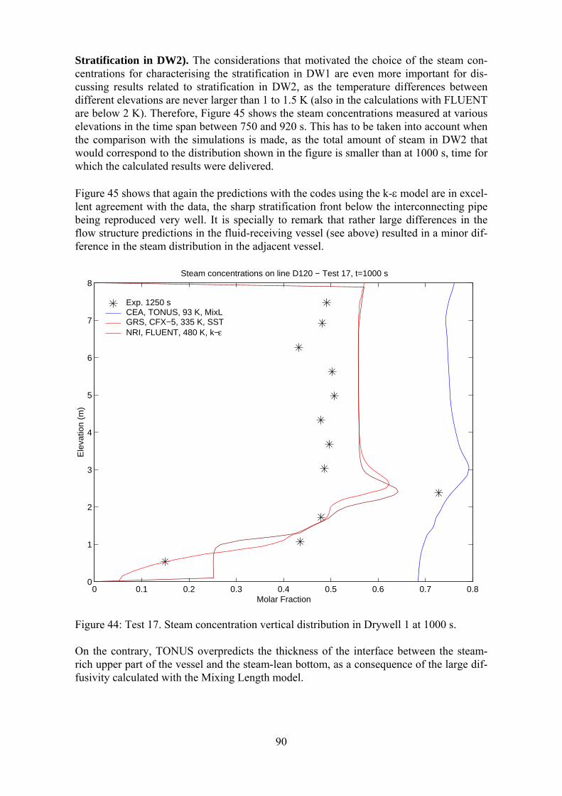
90
Stratification in DW2). The considerations that motivated the choice of the steam con-centrations for characterising the stratification in DW1 are even more important for dis-cussing results related to stratification in DW2, as the temperature differences between different elevations are never larger than 1 to 1.5 K (also in the calculations with FLUENT are below 2 K). Therefore, Figure 45 shows the steam concentrations measured at various elevations in the time span between 750 and 920 s. This has to be taken into account when the comparison with the simulations is made, as the total amount of steam in DW2 that would correspond to the distribution shown in the figure is smaller than at 1000 s, time for which the calculated results were delivered. Figure 45 shows that again the predictions with the codes using the k-ε model are in excel-lent agreement with the data, the sharp stratification front below the interconnecting pipe being reproduced very well. It is specially to remark that rather large differences in the flow structure predictions in the fluid-receiving vessel (see above) resulted in a minor dif-ference in the steam distribution in the adjacent vessel.
0 0.1 0.2 0.3 0.4 0.5 0.6 0.7 0.80
1
2
3
4
5
6
7
8
Molar Fraction
Ele
vatio
n (m
)
Steam concentrations on line D120 − Test 17, t=1000 s
Exp. 1250 s CEA, TONUS, 93 K, MixL GRS, CFX−5, 335 K, SST NRI, FLUENT, 480 K, k−ε
Figure 44: Test 17. Steam concentration vertical distribution in Drywell 1 at 1000 s. On the contrary, TONUS overpredicts the thickness of the interface between the steam-rich upper part of the vessel and the steam-lean bottom, as a consequence of the large dif-fusivity calculated with the Mixing Length model.
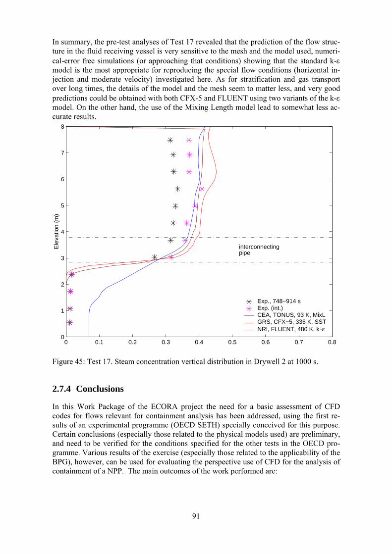
91
In summary, the pre-test analyses of Test 17 revealed that the prediction of the flow struc-ture in the fluid receiving vessel is very sensitive to the mesh and the model used, numeri-cal-error free simulations (or approaching that conditions) showing that the standard k-ε model is the most appropriate for reproducing the special flow conditions (horizontal in-jection and moderate velocity) investigated here. As for stratification and gas transport over long times, the details of the model and the mesh seem to matter less, and very good predictions could be obtained with both CFX-5 and FLUENT using two variants of the k-ε model. On the other hand, the use of the Mixing Length model lead to somewhat less ac-curate results.
0 0.1 0.2 0.3 0.4 0.5 0.6 0.7 0.80
1
2
3
4
5
6
7
8
interconnectingpipe
Ele
vatio
n (m
)
Exp., 748−914 s Exp. (int.) CEA, TONUS, 93 K, MixL GRS, CFX−5, 335 K, SST NRI, FLUENT, 480 K, k−ε
Figure 45: Test 17. Steam concentration vertical distribution in Drywell 2 at 1000 s.
2.7.4 Conclusions
In this Work Package of the ECORA project the need for a basic assessment of CFD codes for flows relevant for containment analysis has been addressed, using the first re-sults of an experimental programme (OECD SETH) specially conceived for this purpose. Certain conclusions (especially those related to the physical models used) are preliminary, and need to be verified for the conditions specified for the other tests in the OECD pro-gramme. Various results of the exercise (especially those related to the applicability of the BPG), however, can be used for evaluating the perspective use of CFD for the analysis of containment of a NPP. The main outcomes of the work performed are:
92
• The accurate analysis of the flows produced by the injection of buoyant fluid in large-size, interconnected vessels is a computationally challenging task, which requires very large computer resources. For the relatively milder conditions of the low-momentum injection prescribed for one of the two tests investigated here (for which experimental data are not available yet), the mesh required for obtaining sufficiently trustworthy results seem to be larger than hundred thou-sands cells. For the more severe conditions of a higher-momentum injection, sensitivity studies could be made only for a short transient, and these lead to the conclusions that approximately mesh-insensitive results can be achieved with a few hundred thousands cells. The need for such a large mesh and the long times of the transients investigated result in a very large computation times.
• Due to the large computational overhead of the analysis, the BPG had to be re-duced in scope, with goals defined by means of a scoping exercise (with a sim-plified geometry). In particular, it was proposed to use the BPG for the initial phase of the transient, and use the mesh “certified” for the short-term also for the long-term calculation. This approach, obviously, can only be proposed for transients where boundary conditions and the main variables are expected to change monotonically and slowly (as, for instance, in the case of a continuous build-up of a gas). Notwithstanding the reduced scope, the BPG could not fully be applied by any organisation. In a strict sense, simulations using a mesh with about 106 cells were not proved to have achieved mesh-insensitivity.
• The simulation of the flow in the fluid-receiving vessel is the most intriguing task, and the results are very sensitive to mesh and model choice. As only one simulation was based on the use of a “certified” mesh, it is not possible at pre-sent to speculate on whether the differences between codes would be drastically reduced if all mesh-independent results were provided. On the other hand, the steam transport between vessels and the long-term stratification seems to be less sensitive to the quality of the mesh. The success of the simulation (against ex-perimental data) performed with an approximately “certified” mesh seem to confirm that the application of a systematic sensitivity study (along the lines of the BPG) has a high “pay-off”.
• On the other hand, the adequate predictions obtained with a mesh of similar size, but not supported by sensitivity studies and evaluation of the accuracy, could lead to the wrong conclusions that the use of a “good” mesh according to engineering judgement and careful choice of numerical methods and time step could be sufficient to produce a trustworthy result. The occasional success of the “traditional approach” should not distract the attention from the need to estab-lish rigorous guidelines.
• The use of the standard k-ε turbulence model produced unexpectedly good re-sults, and was the only (in association with a “certified” mesh) to reproduce all aspects of the only test for which experimental results are available. Variants of the model also produced very good results in relation to stratification and gas transport. On the other hand, the simpler Mixing Length model produced results of much lesser accuracy in relation to all aspects of the transient, the flow struc-ture in the fluid-receiving vessel being totally missed.
93
In relation to the objective of WP 7 in the more general framework of the ECORA project, namely the evaluation of CFD methods for reactor safety analysis, the following conclu-sions can be drawn:
• The flows analysed in the framework of the ECORA project do not include all the physics (principally condensation is not included) of prototypical applica-tions However, the success obtained in the simulation of the separate-effect tests considered here using appropriate mesh and models can greatly improve the confidence in the methods for containment analysis. The assessment of the code using other tests of the OECD-SETH programme is therefore an important step in building this confidence.
• The accurate prediction of the flow structure in the compartment (vessel) where the fluid is injected (in an NPP, as the result of a leak) does not seem to be a pre-requisite for acceptable prediction of inter-compartment transport and stratifica-tion. Therefore, in principle, to strive for mesh-independent results in relation to the flow structure could result in “over killing” the problem. However, in ab-sence of data or detailed analyses for similar conditions, the use of a unique mesh which does not resolve properly the flow structure in the fluid-receiving compartment could lead to simulations of unpredictable accuracy.
• The applications of the BPG to full containment analysis is out of reach with the currently available computer power, although the use of large computer clusters (provided that the code is written for parallel computing) could permit occasion-ally full-scope analyses of reference scenarios.
• In general, CFD codes seem to be capable to give reliable answers on issues relevant for containment integrity evaluation (such as inter-compartment mass transport mainly investigated here). Moreover, as advanced (and more computa-tionally intensive) turbulence models may not be needed, the use of the BPG for “certified” simulations could become feasible within a relatively short time.
2.8 Evaluation of Application of CFD Codes to Reactor Safety (WP 8)
2.8.1 Use of Single-Phase CFD
Reactor Safety Analysis related to both Pressurised Water Reactors (western type and VVER type) or Boiling Water Reactors mainly relied on system codes where the primary (and secondary) flows are modelled with a rather coarse nodalisation including about 103 mesh points or “control volumes”. However some safety issues were clearly identified where a much finer resolution of the simulation tools was required. These issues are often related to situations where the 3D aspects of the flow and the geometrical effects have a significant influence on the safety criterion. Turbulent mixing is a common feature of these flows and the degree of mixing controls the result which directly affects the safety. Single phase CFD tools are then required which may model small scale mixing phenom-ena with a fine space resolution including 105 to 107 mesh points. The experimental inves-tigation may also give the answer to the safety problem if the industrial geometry is strictly respected. Reliable simulation tools, after having been validated for each basic flow process and for some prototypic geometry, may allow much rapid answer to a new
94
problem and/or a new geometry. Such single phase CFD tools exist and are commonly used in many industrial sectors and are now applied for Nuclear Reactor Safety or for de-sign purposes. The principal interest of industrial computational fluid dynamics consists mainly in the capability to obtain at a lower cost, valuable information on some physical phenomena. Numerical simulations of industrial processes enable to test virtually any configuration, from both qualitative and quantitative points of view, and thus to evaluate and/or dis-criminate different designs according to pre-determined criteria. These criteria may be linked to economical or technological constraints, and/or to safety and environmental is-sues. Concerning safety issues in the nuclear industry, CFD has now been recognized as an important tool, as discussed in the IAEA/NEA workshop of November 2002. In order to produce trustworthy studies on various problems, both “in house” and “com-mercial” software for thermal hydraulics and industrial fluid mechanics were developed and validated. Commercial codes such as CFX and FLUENT are widely and increasingly used in nuclear reactor safety applications. In the nuclear reactor community, for example, the SATURNE code is developed at EDF and the TRIO-U code and CAST3M code are developed at CEA for single phase flow whereas the NEPTUNE platform developed by CEA and EDF includes a two phase flow CFD tool. Two-phase models are also available in commercial codes. A multi-year validation study of the multi-phase capability in CFX-5 for reactor safety applications is currently carried out in a German research project co-ordinated by GRS (CFD Kompetenzverbund Reaktorsicherheit - German CFD Network in Nuclear Technology). In the 6th Framework Programme, the NURESIM proposal will be an integrated project aiming at developing a common nuclear reactor simulation platform, which will also include two-phase CFD modules. All these codes are engaged in a qualifi-cation process in the field of nuclear thermal hydraulics in order to ensure that the soft-ware is effectively able to produce relevant results in a clearly defined application field. Developing and testing the tools has required intensive work on complex physical model-ling and numerics, both domains being closely linked in the CFD field. In parallel, ex-perimental data bases are created, including Separate Effect Tests and some real size in-dustry-like experiments; they are used to validate the physical modelling implemented in the codes. A comprehensive measurement data base on turbulent mixing inside the reactor pressure vessel has been created within the EC project FLOMIX-R on fluid mixing and flow distribution in the primary circuit of PWR. This data base gained from experiments at various test facilities representing different types of European reactors (German KON-VOI, Westinghouse and Framatome –ANP PWRs, VVER) is made available for CFD code validation purposes. Although the design of the first PWRs was mainly based on an experimental approach in particular for evaluating the loads applied on the structures, present numerical tools are now able to model the structures even with complex geometry using a 3D numerical model and to solve the complex physical aspects of the flows. Different flow features take place in normal operating conditions, like jet impact, flow reversal, piping swirl effect, and in accidental conditions, buoyancy effects or dilution problems are encountered, either in the primary system or in the reactor containment in the event of a Loss of Coolant Ac-cident. Now, for the new reactors such as the EPR, the experimental approach is coupled to the numerical approach to provide elements required by the design.
95
Although not addressed in the framework of the ECORA project, other thermal-hydraulic phenomena require the use of CFD for safety assessment: for example, hydrogen combus-tion issues (addressed in the 4th FP projects HDC (see, Ref. [31] and HYCOM (see Ref. [32]) or the 5th FP EXPRO (http://batchelor.uc3m.es/expro/expro.html), as well as phe-nomena representative of Generation IV reactors such as Gas-Cooled Reactors (Decay heat removal phenomena, depressurisations, thermal fatigue, etc) – see for example Refs. [33] and [34] or also the proceedings of the HTR-2002 conference for examples of appli-cation of CFD to such problems. The development of Best Practice Guidelines for those particular applications is also needed, and would prove beneficial to the overall quality of the simulations. 2.8.1.1 Nuclear Reactor Safety Problems where Single Phase CFD is Recommended A good maturity of both the tool and the user is reached or can be reached in a reasonable term and single phase CFD can be a very powerful tool for better understanding physical behaviour and one may recommend using it for in a number of flow configurations en-countered in safety analyses:.
• Boron dilution • Mixing of cold and hot water in Steam Line Break event • Hot-leg temperature heterogeneity • PTS (pressurised thermal shock) • Counter-current flow of hot steam in hot leg for severe accident investigations of a
possible “Induced Break” • Thermal fatigue (e.g. T-junction) • Hydrogen distribution and combustion in containment
In addition to these problems related to the present generation of water reactors, there is also a number of issues for advanced (including Gas-Cooled) reactors. One may give a few examples:
• Natural circulation in LMFBRs • Coolability & Flow induced vibration of APWR radial reflector • Flow in lower plenum of ABWR • Depressurisation of a GCR • Decay heat removal in a GCR • Thermal loading on structures, etc. • Containment integrity (peak pressure) during the long-term cooling of innovative
reactors with passive safety systems, particularly in a BDBA scenarios, see Ref. [44].
2.8.1.2 How to adjust the ECORA BPG to Large Scale and Reactor Problems Although CFD is being used extensively both inside and outside the nuclear community, still the credibility of many CFD simulations is being discussed. Part of the discussion re-volves around the physical difficulties of modelling the effect of, for instance, turbulence. However, another part of the discussion relates to the accuracy of the numerical discretisa-tion in CFD simulations. Difficulties that still exist in this area are amply demonstrated by the many CFD validation exercises involving blind test cases, where only sufficient in-formation is made available to allow a CFD model to be set up and run, but the full test re-sults are not available. The results of such exercises can be highly user-dependent even when the same software and models are used. The ERCOFTAC special interest group on
96
“Quality and Trust in Industrial CFD” has identified that production of BPG in Ref. [35] would reduce these errors and enhance the credibility of CFD. The ECORA project has embraced this notion and, with the ERCOFTAC BPG as a basis, a BPG for nuclear safety applications was created at the beginning of the project (see Ref. [1]). The emphasis of the ECORA BPG is on validation, which basically means that small scale simulations are per-formed and, by comparison with experimental data, the extent to which the model accu-rately represents reality is assessed. In this chapter the experience gained by using the BPG, for both small scale and large scale problems, will be summarised and recommenda-tions for adjusting them will be given. In the BPG, the following potential sources for errors or uncertainties are defined:
• Numerical errors; difference between the exact equations and the discretised equa-tions (Spatial and temporal discretisation error, iteration error);
• Model errors; error in the applied models, e.g. turbulence models; • Application uncertainties; lack of information of the application, e.g. boundary
condition or details of the geometry; • User errors; inadequate use of the CFD code by the user, e.g. oversimplification of
the problem; • Software errors; any inconsistency in the software package, e.g. coding errors.
In order to be able to determine the model error separately, which is required for meaning-ful subsequent model improvement, the other errors have to be minimised. Within the ECORA project this has been done for the following single-phase cases:
• PTS Validation 1: Jet impingement with heat transfer (see, Ref. [12]; application of the ECORA BPG was successfully performed for this validation case PTS
• Demonstration 1: Upper Plenum Test Facility (UPTF) liquid-liquid mixing (see Ref. [13]; application of the BPG has been successful for the majority of the guide-lines. However, since the initial mesh used for this large demonstration case al-ready contained over 2 million cells, it was not possible to obtain a solution on ‘three (or more) grids using the same topology or, for unstructured meshes, with a uniform refinement over all cells as stated in the BPG.
• Containment Demonstration: Analysis of PANDA test (see, Ref. [15]). The BPG could not be applied strictly, but insight into the sensitivity of the numerical solu-tions to some parameters could be assessed.
2.8.1.3 Recommendations All the BPG could be applied for the small scale validation case in the project. Also, the strict use of the majority of the BPG for a large scale demonstration case has given insight in the errors in this simulation. However, obtaining a solution on three successively re-fined grids turned out to be impossible, due to the expected computational demand of these calculations. So, the BPG have to be adapted adjusted and extended to be applicable for large scale problems and reactor problems. This is a general recommendation that can be drawn from first attempts to apply BPG to large scale problems such as PANDA or UPTF at the end of ECORA project. Such an extension of the BPG requires further work and cannot be established during ECORA project but first suggestions emerged from ECORA members:
• When global mesh refinement is not possible, it is recommended to perform calcu-lations with first and second order discretisation on the same mesh,
97
• It is also recommended to perform calculations on multiple meshes with local grid-refinement in areas which are the most sensitive to solution change although this may be difficult for transient flows where the areas of the flow with high gradients can change in time.
• For large-scale problems with multiple parameters, it might also be recommended to incorporate into the BPG a “Design of Experiments” methodology to limit the cost of evaluating the different types of errors in CFD computations.
• For the specific class of flows relevant to containment analysis as studied in ECORA project, the application of the BPG (though relaxed as regards the number of sensitivity studies required) seems to be feasible for the initial period of the transient. A two-step approach can be proposed, namely the application of the BPG to a portion of the transient to “qualify” the finest “practical mesh” that can be afforded for the complete transient. In this approach, the use of three succes-sively refined mesh is affordable, and sufficiently converged results can be achieved, although this can imply a large effort in optimising the mesh. Finally, the use of advanced (and highly computing intensive) turbulence models may be not necessary for defining the uncertainty range due to the choice of the turbulence model. Previous experience of similar flows should help to select the models for estimating model errors.
It should however be noted, that the range of applications, where the strict application of BPG is feasible, will continuously expand with the ever increasing computing power. Rec-ommendations for reduced BPG procedures should therefore be considered as a temporary solution, which will gradually converge back to the strict application of the procedures. For three-dimensional single-phase flows, this should be possible within the next decade, at least for validation studies.
2.8.2 Use of Two-Phase Flow CFD
The EC project EUROFASTNET, which was a pre-runner to ECORA, has identified in-dustrial needs for three-dimensional simulation of nuclear reactor thermo-hydraulics. These include safety, performance, design, availability and increase of life span of nuclear reactors (see Ref. [36]). The requirements with the highest industrial priority are fuel per-formance, fluid-structure interaction, thermal shocks due to safety injection and stratifica-tion in circuits. As a consequence, the ‘Extension of CFD Codes to Two-Phase Safety Problems’ has become the subject of Writing Groups on CFD Issues, which has been es-tablished by the OECD/NEA. The report produced by this Writing Group (see, Ref. [37]) covers a wide range of NRS problems in pressurized water reactors (PWR), boiling water reactors (BWR), steam generators, heat exchangers, containment flows and components with three-dimensional structures like spacer grids. High priority is given to critical heat flux conditions in the core, to two-phase pressurized thermal shocks (PTS), and to thermal fatigue and stratification in the primary system of PWRs. The reports in Refs. [36] and [37] embrace all aspects of two-phase flow CFD in NRS. In the ASTAR project, some test cases of interest for two-phase flow modelling were inves-tigated, and BPG were also applied to produce better quality solutions (see, Ref. [38]) and (see, Ref. [39]). In the ECORA project, only a subset of the cases described in Ref. [37] was investigated, namely the CFD simulation of flows in the primary system and con-tainment of PWRs. Two-phase flow phenomena were studied for PTS-relevant flow con-
98
ditions during the injection of emergency core cooling water into the cold leg of PWRs. The following discussion will be focussed on these topics. 2.8.2.1 Nuclear Reactor Safety Problems where Two-Phase CFD is Recommended Two-phase CFD tools are far less mature than single phase tools. However, it is recom-mended to further develop such tools for a number of nuclear safety issues. Due to the lower maturity, the activity should include:
• Identification of the relevant basic phenomena which need to be modelled for a given application
• Assessment of the model including verification, validation and demonstration tests • Definition of new R&D work for a more detailed validation, for a better numerical
efficiency, and a better accuracy and reliability of predictions Such a process has been applied within ECORA to the two-phase PTS scenario as summa-rized here below. In a typical PTS scenario, cold water is injected into the cold leg of a PWR during the refill phase of a LOCA. The injected water mixes with the hot fluid pre-sent in the cold leg. Depending on the size of the break, either single- or two-phase condi-tions prevail between the injection nozzle and the downcomer. There may be stratification of cold water on the bottom of the cold leg with counter-current flow of hot water or steam on top of the cold-water layer. Condensation phenomena take place at the free surfaces of the cooling water jet and of the stratified flow. These depend strongly on the turbulence in the fluid. As a consequence of the emergency cooling water injection, a stream of cold wa-ter penetrates into the downcomer. The path and characteristics of this cold-water jet de-pends on the flow conditions and on the detailed cold leg, downcomer geometry. Thermal shocks can occur on the reactor vessel walls due to the thermal and mechanical stresses arising from the rapid temperature and pressure changes at the cold-water jet edge. This, in turn, can lead to mechanical failure of the walls. The dominant fluid and heat transfer phenomena involved in the two-phase flow scenarios described above are:
• Impingement of two-phase flow jets • Impinging jet heat transfer • Turbulent mixing of momentum and energy in and downstream of the impinge-
ment zone • Stratified two-phase flow (or free surface flow) within ducts • Phase change, like condensation at the steam-water interface
These phenomena were investigated in ECORA. The respective test cases which were cal-culated in ECORA are documented in Ref. [9]. The ECORA test cases were subdivided into verification, validation and demonstration tests. A detailed description of the results is given in Ref. [12]. The validation tests included jet impingement with heat transfer, water jet impingement in an air environment, and contact condensation in a stratified steam-water flow. It was shown that turbulence model formulations based on the ω-length scale equation are well suited for the simulation of impinging jet flows. The characteristics of the free surface wa-ter jet flow were also adequately represented by the free surface flow models. The simulations of the contact condensation have shown that standard interfacial mass transfer models are not sufficient to predict this phenomenon accurately. However, an im-proved condensation model, implemented in CFX-5, which identifies the free surface by
99
calculating the gradient of the volume fraction, and damps the turbulence at such identi-fied free surface shows satisfactory agreement with data. In summary, the calculations in ECORA have shown a satisfactory performance of the employed CFD codes for single-phase flow problems, and for two-phase flow problems with single dominant interface morphology. This includes free surface flows, or bubbly flows. However, for cases with more than one morphology, for instance for a jet imping-ing on free surface flow with bubble entrainment or for the transition of bubble to churn flow, the available two-phase models show poor results and need to be improved. The same is true for multi-phase flows with heat transfer and mass transfer at the interface. For the latter, the numerical schemes and the physical models need enhancements. A prerequi-site for these model improvements is, however, the provision of adequate experimental data to develop, calibrate and validate these models. The test calculations in ECORA have also shown that the calculation times for typical PWR assemblies (cold legs, downcomer, lower plenum, core, and hot legs, see Ref. [13] are still very large (order of weeks on current parallel machines). Improvements in the numerical methods, and advancements like error-based grid and time-step adaptation, are therefore necessary to make CFD a tool for comparing and assessing different scenarios in NRS. The ECORA project has made a contribution to the assessment of the state-of-the-art of two-phase flow CFD in NRS. Also, a number of useful model improvements have been made in ECORA. It is, however, still difficult to ‘recommend NRS problems’ for CFD. If a problem is suitable or not depends on the accuracy expectations and on the computa-tional investments one is willing to make. As said above, many two-phase flow problems with single morphologies (free surfaces, bubble flows, droplet flows, water jets, …) can be predicted quite well. However, there are still large uncertainties for flows with more than one morphology, and for flows with mass transfer at the interface (condensation, boiling, cavitation). Also, calculation times for these kinds of flows may become prohibi-tive. Therefore, while many of the flows described in Table I of Ref. [37] can now be tackled from a research and development perspective, the available CFD codes are not yet sufficiently mature for a day-to-day industrial application. Independent of the test case and the problem at hand, ECORA has shown that the applica-tion of the Best Practice Guidelines developed as part of the project, can substantially re-duce uncertainties, lead to more valid conclusions about model performance vs. perform-ance of the numerical method, and can therefore help to accelerate development and pro-gress of three-dimensional CFD in NRS. A similar approach should be followed for other important issues with two-phase flow such as:
• DNB, dry-out and CHF investigations • Direct contact condensation : ECC injection or steam discharge in a pool • Condensation induced water hammer • Pool heat exchangers: thermal stratification and mixing problems • Corrosion, erosion and deposition • Two-phase flow in valves, safety valves • Flow oscillations in BWRs • Steam generator tube vibration
100
• Pipe Flow with cavitation
2.8.2.2 How to adjust the ECORA BPG to Reactor Relevant Two-Phase Problems Two-phase CFD is much less mature than single phase CFD. The flows are much more complex and myriads of basic phenomena may take place at various scales. Thus it is clear that the physical modelling will have to be improved over a long time period. Fundamen-tal questions related to the averaging or filtering of equations are not yet as clearly formal-ised as they are for RANS or LES methods in single phase. This makes that the separation between physics and numerical aspects is not always well defined. This lack of maturity is also reflected in the Best Practice Guidelines which cannot be as clearly defined as in sin-gle phase flows. One may expect that new ideas about extension of BPG to two-phase will emerge in parallel to the progress in modelling and understanding of two-phase flows. The transport equations solved in multi-phase flow codes are much more complex than those of single-phase flow codes. The potential of numerical methods in multi-phase codes is thus difficult to estimate a priori and the analysis of many computational results is needed to evaluate all required numerical capabilities. The same is true concerning the validation of the various physical closure laws. Comments to the application of the BPG to real two-phase flow situations are made based on the experience gained during the ECORA project. 2.8.2.2.1 Filtering of Basic Equations The physical filtering of basic equations due to averaging should be clearly distinguished from the numerical filtering due to the discretisation. Phenomena which are larger than the physical filter scale can be simulated with more or less numerical accuracy but phenom-ena which are smaller than the physical filter scale should be clearly modelled by closure laws. It is a necessary condition for allowing mesh refinements up to convergence. An-other approach could be to benefit from mesh refinement for simulating smaller scale phe-nomena (like in Ref. [23]), but this should be clearly identified as an extension of the Large Eddy Simulation approach to two-phase CFD and the classical mesh convergence method is no more relevant. 2.8.2.2.2 Verification The best verification tests use analytical solutions for simple cases, but analytical solu-tions are practically never available in two-phase flow. Simple experimental test cases are often used instead and the ECORA project selected two tests cases, the Oscillating Ma-nometer and the Sloshing (see, Ref. [11]). Such test cases should be representative of a re-actor application with one physical phenomenon being dominant. A perfect agreement with the data is not required, but the differences between the simulations and the data must respect some predetermined criteria. The verification tests must be diverse enough to check all aspects of the implementation and to allow the examination of many criteria about the coherence of algorithms with the physics of phenomena, the robustness of the algorithms, the residual phases treatment, the accuracy with regard to numerical diffusion dissipation and dispersion, the preservation of mass and energy. 2.8.2.2.3 Physical Validation Before selecting a matrix of physical validation for a given application, one must identify all relevant basic phenomena which need to be modelled. As far as possible each basic phenomenon should be validated separately using single effect tests.
101
2.8.2.2.4 Control of Discretisation Errors In both single phase and two-phase CFD codes, the effect of truncation has an important influence on the transport terms. First order upwind differencing of the convective terms yields truncation errors 0 (Δx) with leading term proportional to f(2) Δx. This term then contributes artificially to the diffusion (numerical diffusion). Such schemes also enhance the dissipation property of the numerical algorithm. In two-phase systems, source terms may play the dominant role and the truncation error on these algebraic source terms can be of prime importance. Interfacial transfers of heat, mass and momentum are modelled by strongly non linear stiff source terms in some flow conditions. Most codes use zero order centred space discretisation of these terms, which results in a truncation error of order 1. In the same way the time discretisation of stiff source terms is of prime importance when the associated relaxation time constants are very small. The real order of the numerical method can be obtained by plotting the logarithm of the error for a target variable, versus the logarithm of the cell size. 2.8.2.2.5 Concluding Remark Finalising BPG in two-phase applications could not be achieved within the ECORA pro-ject, and ECORA strongly recommends further investigations on this topic.
2.8.3 Recommendations for Code Customisation
The fluid flow problems considered in ECORA, as well as information gathered at meet-ings with other European projects like ASTAR and FLOMIX-R, have shown that CFD applications in nuclear reactor safety are focussed on internal flows. Examples are the sin-gle and multi-phase flows in hot and cold legs, downcomers, pressure vessels and con-tainments. In ECORA, Best Practice Guidelines have been developed for these flow cate-gories. Customisations of CFD software are also recommended, which encompass these BPGs. The recommended customisation of the CFD codes can facilitate the set-up of CFD calculations and the interpretation of the CFD results, as well as optimise the solution process. The net result will be higher result quality, an increased trust in the results, and reduced user influence. 2.8.3.1 Geometry Model The first step in performing a CFD calculation is the generation of a geometry model. This geometry model must include all the details influencing the flow. For instance, calcula-tions in ECORA and FLOMIX-R have shown that only a detailed modelling of the struc-tures in the lower plenum and at the core entrance will lead to realistic flow predictions. Since many reactor components are geometrically similar for European pressure reactors, parameterized geometry models could be provided for such components. These parameter-ised models could then be quickly adjusted to different applications by changing the ap-propriate dimensions. Pre-made models for cold and hot legs, ECC-nozzles, downcomers, and core structures could then be combined in a modular fashion using a solid (or volume) modeller. The recommendations for code customisation can be summarised as follows:
• Provision of parameterised solid models for typical reactor components like cold legs, hot legs, downcomers, lower plenums, reactor cores, ECC nozzles, and con-tainments. A pre-requisite for this customisation is the acceptance of a common standard for geometry transfer, which supports parameterisation.
102
• Provision of a part library, which can be used to build modular reactor models more efficiently.
2.8.3.2 Mesh Generation After the geometry of the flow domain is available, it needs to be meshed. As stated above, NRS applications involve mainly internal flows. These require special care in order to obtain proper resolution of the walls. The generated grids should also be scalable, which means that their quality should not change when the mesh size is changed. Genera-tion of such high-quality grids can be aided by the following customisations:
• Guidance about which element types (tetrahedral, hexahedral, prisms, …) are rec-ommended for which reactor component and application
• Provision of pre-designed, scalable hexahedral block structures for typical NRS components, like downcomers, hot and cold legs, etc.
• Estimators for the required near-wall resolution based on typical flow parameters like Reynolds or Peclet numbers
• Development of grid-quality metrics, including recommendations and information on grid density, skewness, aspect ratios, expansion factors
• Construction of vertical applications for generating meshes in typical reactor com-ponents using the BPGs developed in ECORA
2.8.3.3 Physical Models and Boundary Conditions One of the major results of ECORA BPGs was the selection of state-of-the-art physical models for predicting turbulent flows, turbulent heat transfer, and multi-phase flows in NRS applications. A logical customisation of the applied CFD software is therefore to en-capsulate the best models for specific applications in ‘Application Libraries’. Typical ap-plications could be pressurized thermal shocks, Boron mixing, buoyant flows in contain-ments, etc. The same principle could then be extended to boundary condition setting and to numerical control parameters. Customisations for boundary conditions could include recommended values for positioning of inlet and outlet boundaries, turbulence quantities at inlet cross sections, preferred outlet boundary condition settings, guidance on the general near-wall treatment for given geometries, and the use of rough or smooth wall boundary conditions. Customisation of the numerical control parameters could provide guidance about time-step sizes for given applications, choice of convergence criteria, and recommendations on appropriate spatial and temporal discretisation schemes. These customisations would narrow the physical model, boundary condition and numeri-cal control parameter choices for novice users on the basis of the expertise of experienced users. The result would be higher and more consistent result quality. Another recommendation is the customisation of material data (fluid and solid properties). These could be shared for typical fluids like steam/water, nitrogen, hydrogen, and typical solids used for reactor walls and claddings. 2.8.3.4 Solver Run and Quality Control
Extensions and customisations for the CFD flow solver and for quality control are recom-mended in the following areas:
103
• Most calculations in NRS are for transient, three-dimensional flows. A major issue for these flows are the long calculation times. A much-needed extension of current CFD codes is, therefore, to provide algorithms for adaptive time stepping. These algorithms should adjust the time steps to either preserve a given numerical accu-racy (solution error-based adaptation) or maintain a given iterative convergence level per time step. By using small time steps only when they are needed, and by increasing the time-steps otherwise, calculation times can be minimized for a given result quality.
• A logical extension of the above would be to also adapt the spatial grid during transient runs. In this way, a given amount of grid points could be used in the most efficient manner, or a given accuracy could be maintained by adding and with-drawing grid points from critical zones. It is, however, recognized that spatial, transient adaptation is a rather complex development project.
• A very helpful feature for monitoring transient CFD runs would be to post-process results during the calculation. In other words, the flow solver should continuously feed information to the post-processor. Anomalies and problems with transient flow calculations, or discrepancies to data could then be recognized immediately and countermeasures could be taken. This would be more efficient than the cur-rently used sequential processing of solver and post-processor.
• Post-Processing and Analysis • Customisations for efficient post-processing and analysis of NRS calculations,
which extend the currently available functionality, are: • Easy creation of post-processing surfaces at a given distance from boundaries
(lofted surfaces), for instance in the centre of downcomers or in the interior of hot and cold legs
• Easy definition of surface normals and cutting planes based on these surface nor-mals; examples are cutting planes normal to the path of hot and cold legs
• Provision of macros for calculating values which are relevant for NRS, like the po-sition as a function of time of maximum and minimum temperatures or concentra-tions or of maximum and minimum temperature, pressure or concentration gradi-ents (relevant for fatigue and structural analysis)
• Possibility to transfer mechanical (forces, moments) and thermal loads (tempera-tures, heat fluxes) to structural mechanics and fatigue software
• Allowance for two-way fluid structure interaction in order to follow transient de-velopment of cracks and other structural failures
• Provision of project data management software to keep track of the large amount of data and runs typically involved in NRS applications
The priorities given below are based on the ‘return-on-investment’ criterion. This means they are ranked by their ‘added value’ for given finite amounts of funding and time. Using this criterion, it is recommended to perform work in the following sequence:
• Provision of application libraries • Post-processing enhancements • Solver enhancements (adaptive time steps, on-line post-processing) • Mesh generation templates • Generation of parameterized geometry models and geometry model data bases
104
2.8.4 Recommendations for Single-Phase CFD Development
Single phase CFD tools are already mature for being applied to many Nuclear Reactor safety issues. The need for some further developments was identified . 2.8.4.1 Extension of the Scope of Single Phase CFD Applications Extension to porous media: Many reactor applications require a modelling of some reac-tor components with CFD in open medium (e.g. downcomer , lower plenum, upper ple-num in a Pressure vessel) and a modelling of some other components (reactor core) with a porous body approach. Since turbulent mixing is often a main concern (in Steam Line Break, boron mixing,…) the physical coupling between turbulence description in the open medium and in the porous body requires further modelling effort and validation. Coupling with other disciplines: Many reactor applications require coupling of CFD with simulations tools for neutron kinetics, fuel thermo-mechanics and structure mechan-ics. Such coupling should be made easier by a standardisation of the code architecture and of module interfaces. This is a major objective of the NURESIM Integrated Project. 2.8.4.2 Improvements of the Physical Modelling Using either RANS or LES turbulence models requires the use of wall functions in order to avoid too fine meshes in all wall boundary layers. Such wall functions for momentum and energy equations exist and are well established for some ideal cases but might be im-proved in more complex situations such as a natural circulation (or mixed forced-natural convection) boundary layer, in presence of an impinging jet or of a flow detachment and for heated boundary layer with strong variations of physical properties. Large Eddy Simulation now often replaces RANS models to benefit from the capacity to predict large scale fluctuations or for transients where time scales related to mean value variations and to large eddies are similar. Being more recently developed, LES still re-quire some improvements about wall functions, low Reynolds number zones, the control of the numerical viscosity. High Reynolds number flows could be better treated by devel-oping a coupling between RANS and LES or using a hybrid method which combine the advantages of RANS and LES. 2.8.4.3 Improvements of the Numerical Efficiency of the Solvers The main limitation of present CFD tools is still the large CPU time which is required for industrial applications. Any further progress in the efficiency of the numerical schemes will be welcome for all users. Adaptative Mesh Refinement methods should be generalised since they provide a better accuracy with a minimum increase of CPU time. In particular similar methods should be developed for LES. However LES+Parallel+Adaptation does not seem efficient, as adap-tation would be required for every time step. Grid nodes would cluster around each single resolved eddy. Turbulent structures are best resolved on a “uniform” grid. An alternative would be an adaptation based on the averaged quantities. In most codes a first generation of solvers used Finite Volume Finite difference methods with structured meshing and staggered grids. These methods were very stable, robust,
105
could preserve mass and energy and solve the momentum balance with a reasonable accu-racy. The present generation of solvers prefers Finite Volume methods with body fitted meshing and co-localised grids. These methods offer new capabilities to be adapted to complex geometry, can also preserve mass and energy but may lose a little accuracy. At-tempts to combine advantages of both and more generally to improve accuracy and ro-bustness are in progress, such as the Finite-Element-Finite –Volume (FEFV) method. It is recommended to continue the development of robust numerical schemes with higher resolution and sharper interface prediction capabilities on given grids
2.8.5 Recommendations for Two-Phase CFD Development
Two phase CFD tools are not yet very mature and require long term developments on many aspects. Physical modelling will require a long term effort and numerical scheme capabilities can still be better evaluated with respect to the requirements. Many applica-tions of two-phase CFD also require a coupling with other thermal hydraulic modules and with other disciplines. Then recommendations for further R&D on two phase CFD are given. 2.8.5.1 Improving the Predictive Capability by Improved Physical Modelling Present two-phase CFD tools have already proven reasonable predictive capabilities for some specific applications where the flow regime is a priori well known but cannot be used as a black box without knowing what are the main basic flow processes to capture. Modelling in two phase CFD tool includes several aspects:
• Selection of the system of equations and of the averaging procedure • Identification of local flow structure , which can be dispersed liquid, dispersed gas,
separate-phase, or a mixture of them. • Modelling wall transfers through wall functions • Modelling turbulent transfers • Modelling interfacial heat and mass transfers • Modelling source terms of additional equations such as interfacial area, bubble
number density,…)
For all these aspects further R&D is required. • No clear definition of what is the space and time filtering of basic equations has
been formulated so far. The Bonetto-Lahey test case demonstrated that the choice of the space resolution of the model is of prime importance. More theoretical work is necessary to specify what can be simulated and what should be modelled.
• An identification of the local flow configuration has to be based on calculated lo-cal variables. Still no universal approach exists and this prevents CFD from being a simulation tool capable of covering the whole range of flow regimes.
Modelling of pure bubbly flows:
• The turbulence modelling seems to be presently limited to extrapolations of the single phase k-epsilon models by adding interfacial production terms. The limits of such approaches have already been reached and multi-scale approaches are neces-sary to take account of the different nature of the turbulence produced in wall shear layers and the turbulence produced in bubble wakes.
106
• Identification of the interface structure is now currently using a transport equation for a bubble number density or an interfacial area concentration. However coales-cence and break-up phenomena have to be modelled and further modelling effort is required for improving the available models Moreover several additional equations would be necessary in poly-dispersed bubbly flows to characterize the bubble size spectrum. Further work is still required for having reliable closure relations for such additional equations
• If expression for drag and virtual mass forces tend to converge, lift and turbulent diffusion forces are still tuned from experiment to another. This indicates that more generic models are still to be developed.
• Wall functions for momentum and energy equations are still taken from single phase flow whereas flow processes near the wall are significantly different in two-phase flow.
Modelling of pure droplet flows:
• Identification of the interface structure is now currently using a transport equation for a droplet number density or an interfacial area concentration. However several additional equations would be necessary in poly-dispersed droplet flows to charac-terize the droplet size spectrum. Further work is still required for having reliable closure relations for such additional equations. The identification of all possible mechanisms for droplet break up or coalescence still requires further investiga-tions.
• Turbulent diffusion forces require more generic models and the modelling of drop-let deposition upon vertical films or on free surface also requires further investiga-tions.
• Wall functions for momentum and energy equations are still taken from single phase flow whereas flow processes near the wall are significantly different in two-phase flow.
Modelling of free surface flows:
• The interface structure of a stratified flow with a free surface may be influenced by friction forces, surface tension, wave propagation, condensation or vaporization, turbulence of both the gas flow and the liquid flow. The most difficult part is the prediction of the local wave structure since it is the result of local perturbations but also of propagation from everywhere in the flow domain.
• Turbulent diffusion controls heat and mass transfers at the free surface. Present models for the interfacial turbulence are not so well established than for wall shear layers. Complex interactions between turbulence and waves exist, which are not yet well understood.
• Droplet entrainment from the wave crests are not presently modelled with ade-quate accuracy for such a local scale modelling.
• Breaking of waves with entrainment of bubbles below the free surface plays a role in the interfacial transfers and also requires a specific effort.
Considering the two-phase PTS issue which was investigated in ECORA, progress has been obtained for modelling some physical processes
• Interfacial transfer of momentum and heat & mass at a free surface • Effects of turbulent diffusion upon condensation
107
• Turbulence production below the jet • Turbulence production in wall shear layers & in interfacial shear layer
Further effort should be directed to the modelling of the following physical processes:
• Entrainment of steam bubbles below the water level • Condensation on the jet itself before mixing • Interactions between interfacial waves , interfacial turbulence production and con-
densation • Effects of temperature stratification upon turbulent diffusion • Interface configuration in top of downcomer • Flow separation or not in downcomer at cold leg nozzle • Heat transfers with cold leg and RPV walls
2.8.5.2 Concluding Remarks As a conclusion two-phase modelling with CFD is a complex problem and the codes are far from mature. There are numerous areas where the models are deficient and it is impor-tant to prioritise these, to enable the most important safety issues to be addressed as soon as possible. The safety community should therefore:
• prioritise the safety issues • identify the dominant phenomena for which reliable two-phase CFD models are
needed • advise the code developers accordingly • plan future validation tests accordingly
108
3 MANAGEMENT AND COORDINATION ASPECTS
3.1 Communication between Partners
The communication between partners of the ECORA consortium is managed via the ECORA web site at http://domino.grs.de/ecora/ecora.nsf. It contains links to project part-ners, a project description, announcement of meetings, presentations, reports and docu-ments. This information has different levels of confidentiality. It is accessible via user name and password. In parallel, the intensive flow and exchange of information via e-mail, phone and personal communication is an indicator of the good and effective cooperation level.
3.2 Contractual Matters
The Unified Consortium Agreement (UCA) with a special confidentiality agreement for the use of selected UPTF experiments and PANDA data has been signed by all ECORA partners. Due to the late submission of some deliverables, in particular because of the delay of the final evaluation of the SETH-PANDA calculations, the GRS Project coordinator was al-lowed to prolong the contract to submit the final summary reports before end of December 2004.
3.3 Meetings
Following the milestones within the work plan seven common meetings took place at the partners’ headquarters. The first additional meeting for discussion of PTS relevant test cases and UPTF confidentiality issues has been arranged at GRS, Garching, on 16 October 2001 and the second special meeting on PANDA tests has been held at PSI, Villigen, on 23 September 2002. During the final Meeting at NRG, Petten, the partners agreed to pro-ceed with a follow-up action of this project to achieve the sustainability of the ECORA re-sults [18]. The minutes including presentations are posted at the ECORA web/site: http://domino.grs.de/ecora/ecora.nsf in the UPTF and PANDA User Forum, respectively. These are protected by special passwords.
3.4 Time and Financial Management
The project and financial coordination is running in line with the scheduled resources. A delay in the deliverable D13 of WP 8 and, as a consequence, the final reports D16 and D17, see section 3.1 , was anticipated and approved by the responsible EC officer. The data initially selected for the pre-test analysis in WP 8 were two tests (one with low momentum injection and one with high momentum injection) from the experimental pro-gramme included in the OECD-SETH project. However, due to a delay in the delivery and installation of hardware components in the PANDA facility, the two tests (the first in the
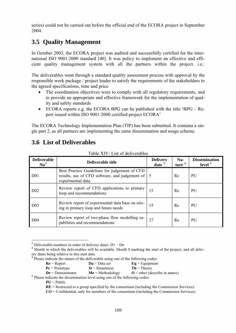
109
series) could not be carried out before the official end of the ECORA project in September 2004.
3.5 Quality Management
In October 2003, the ECORA project was audited and successfully certified for the inter-national ISO 9001:2000 standard [40]. It was policy to implement an effective and effi-cient quality management system with all the partners within the project. i.e.: The deliverables went through a standard quality assessment process with approval by the responsible work package / project leader to satisfy the requirements of the stakeholders to the agreed specifications, time and price
• The coordination objectives were to comply with all regulatory requirements, and to provide an appropriate and effective framework for the implementation of qual-ity and safety standards
• ECORA reports e.g. the ECORA BPG can be published with the title ‘BPG – Re-port issued within ISO 9001:2000 certified project ECORA’
The ECORA Technology Implementation Plan (TIP) has been submitted. It contains a sin-gle part 2, as all partners are implementing the same dissemination and usage scheme.
3.6 List of Deliverables
Table XIV: List of deliverables Deliverable
No2 Deliverable title Delivery date 3
Na-ture 4
Disseminationlevel 5
D01 Best Practice Guidelines for judgement of CFD results, use of CFD software, and judgement of experimental data.
5 Re PU
D02 Review report of CFD applications to primary loop and recommendations 15 Re PU
D03 Review report of experimental data base on mix-ing in primary loop and future needs 15 Re PU
D04 Review report of two-phase flow modelling ca-pabilities and recommendations 27 Re PU
2 Deliverable numbers in order of delivery dates: D1 – Dn 3 Month in which the deliverables will be available. Month 0 marking the start of the project, and all deliv-ery dates being relative to this start date. 4 Please indicate the nature of the deliverable using one of the following codes: Re = Report Da = Data set Eq = Equipment Pr = Prototype Si = Simulation Th = Theory De = Demonstrator Me = Methodology O = other (describe in annex) 5 Please indicate the dissemination level using one of the following codes: PU = Public RE = Restricted to a group specified by the consortium (including the Commission Services). CO = Confidential, only for members of the consortium (including the Commission Services).
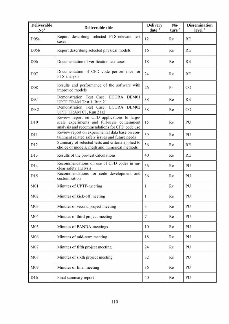
110
Deliverable No2 Deliverable title Delivery
date 3 Na-
ture 4 Dissemination
level 5
D05a Report describing selected PTS-relevant test cases 12 Re RE
D05b Report describing selected physical models 16 Re RE
D06 Documentation of verification test cases 18 Re RE
D07 Documentation of CFD code performance for PTS analysis 24 Re RE
D08 Results and performance of the software with improved models 26 Pr CO
D9.1 Demonstration Test Case: ECORA DEM01 UPTF TRAM Test 1, Run 21 38 Re RE
D9.2 Demonstration Test Case: ECORA DEM02 UPTF TRAM C1, Run 21a2 38 Re CO
D10 Review report on CFD applications to large-scale experiments and full-scale containment analysis and recommendations for CFD code use
15 Re PU
D11 Review report on experimental data base on con-tainment related safety issues and future needs 39 Re PU
D12 Summary of selected tests and criteria applied to choice of models, mesh and numerical methods 36 Re RE
D13 Results of the pre-test calculations 40 Re RE
D14 Recommendations on use of CFD codes in nu-clear safety analysis 36 Re PU
D15 Recommendations for code development and customisation 36 Re PU
M01 Minutes of UPTF-meeting 1 Re PU
M02 Minutes of kick-off meeting 1 Re PU
M03 Minutes of second project meeting 3 Re PU
M04 Minutes of third project meeting 7 Re PU
M05 Minutes of PANDA-meetings 10 Re PU
M06 Minutes of mid-term meeting 18 Re PU
M07 Minutes of fifth project meeting 24 Re PU
M08 Minutes of sixth project meeting 32 Re PU
M09 Minutes of final meeting 36 Re PU
D16 Final summary report 40 Re PU

111
Deliverable No2 Deliverable title Delivery
date 3 Na-
ture 4 Dissemination
level 5
D17 Condensed final summary report 40 Re PU
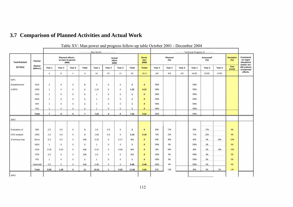
112
3.7 Comparison of Planned Activities and Actual Work
Table XV: Man power and progress follow-up table October 2001 - December 2004 - - - - - - - - - Man-Month - - - - - - - - - - - - - - - - - - Technical Progress % - - - - - - -
Planned efforts - at start of period
(MM)
Actual effort (MM)
Devia-
tion (MM)
Planned
(%)
Assessed*
(%)
Deviation
(%)
Year 1 Year 2 Year 3 Total Year 1 Year 2 Year 3 Total Totals Year 1 Year 2 Year 3 Year 1 Year 2 Year 3 Year (now)
Task/Subtask
(N°/title)
Partner
(Name/ abbrev.)
a b c d a1 b1 c1 d1 d1-d a/d b/d c/d a1/d1 b1/d1 c1/d1
Comments on major
deviations and/or mo-difi-cations of planned
efforts.
WP1
Establishment AEA 2 0 0 2 2 0 0 2 0 100% 100%
of BPG GRS 1 0 0 1 1.22 0 0 1.22 0.22 100% 100%
CEA 1 0 0 1 1 0 0 1 0 100% 100%
NRG 1 0 0 1 1 0 0 1 0 100% 100%
NRI 1 0 0 1 1 0 0 1 0 100% 100%
PSI 1 0 0 1 1 0 0 1 0 100% 100%
Total 7 0 0 7 7.22 0 0 7.22 0.22 100% 100%
WP2
Evaluation of NRI 2.5 0.5 0 3 2.5 0.5 0 3 0 83% 17% 83% 17% 0%
CFD analysis GRS 1.5 0.5 0 2 1.68 0.5 0 2.18 0.18 75% 25% 77% 23% 0%
of primary loop Serco 0.3 0.2 0 0.5 0.33 0 0.17 0.5 0 60% 40% 66% 0% 34% -34%
AEKI 1 0 0 1 1 0 0 1 0 100% 0% 100% 0% 0%
CEA 0.25 0.25 0 0.5 0.42 0 0.08 0.5 0 50% 50% 84% 0% 16% -16%
FZR 2.5 0 0 2.5 2.5 0 0 2.5 0 100% 0% 100% 0% 0%
PSI 1 0 0 1 1 0 0 1 0 100% 0% 100% 0% 0%
Vattenfall 0.5 0 0 0.5 0.98 0 0 0.98 0.48 100% 0% 100% 0% 0%
Total 9.55 1.45 0 11 10.41 1 0.25 11.66 0.66 87% 13% 89% 9% 2% -2%
WP3
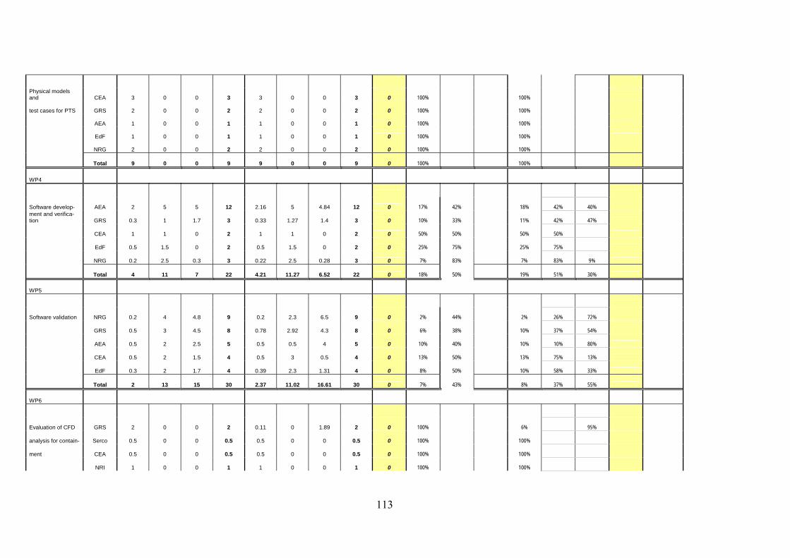
113
Physical models and CEA 3 0 0 3 3 0 0 3 0 100% 100%
test cases for PTS GRS 2 0 0 2 2 0 0 2 0 100% 100%
AEA 1 0 0 1 1 0 0 1 0 100% 100%
EdF 1 0 0 1 1 0 0 1 0 100% 100%
NRG 2 0 0 2 2 0 0 2 0 100% 100%
Total 9 0 0 9 9 0 0 9 0 100% 100%
WP4
Software develop- AEA 2 5 5 12 2.16 5 4.84 12 0 17% 42% 18% 42% 40% ment and verifica-tion GRS 0.3 1 1.7 3 0.33 1.27 1.4 3 0 10% 33% 11% 42% 47%
CEA 1 1 0 2 1 1 0 2 0 50% 50% 50% 50%
EdF 0.5 1.5 0 2 0.5 1.5 0 2 0 25% 75% 25% 75%
NRG 0.2 2.5 0.3 3 0.22 2.5 0.28 3 0 7% 83% 7% 83% 9%
Total 4 11 7 22 4.21 11.27 6.52 22 0 18% 50% 19% 51% 30%
WP5
Software validation NRG 0.2 4 4.8 9 0.2 2.3 6.5 9 0 2% 44% 2% 26% 72%
GRS 0.5 3 4.5 8 0.78 2.92 4.3 8 0 6% 38% 10% 37% 54%
AEA 0.5 2 2.5 5 0.5 0.5 4 5 0 10% 40% 10% 10% 80%
CEA 0.5 2 1.5 4 0.5 3 0.5 4 0 13% 50% 13% 75% 13%
EdF 0.3 2 1.7 4 0.39 2.3 1.31 4 0 8% 50% 10% 58% 33%
Total 2 13 15 30 2.37 11.02 16.61 30 0 7% 43% 8% 37% 55%
WP6
Evaluation of CFD GRS 2 0 0 2 0.11 0 1.89 2 0 100% 6% 95%
analysis for contain- Serco 0.5 0 0 0.5 0.5 0 0 0.5 0 100% 100%
ment CEA 0.5 0 0 0.5 0.5 0 0 0.5 0 100% 100%
NRI 1 0 0 1 1 0 0 1 0 100% 100%
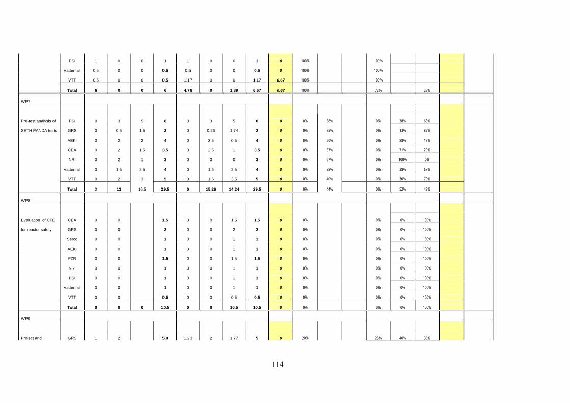
114
PSI 1 0 0 1 1 0 0 1 0 100% 100%
Vattenfall 0.5 0 0 0.5 0.5 0 0 0.5 0 100% 100%
VTT 0.5 0 0 0.5 1.17 0 0 1.17 0.67 100% 100%
Total 6 0 0 6 4.78 0 1.89 6.67 0.67 100% 72% 28%
WP7
Pre-test analysis of PSI 0 3 5 8 0 3 5 8 0 0% 38% 0% 38% 63%
SETH PANDA tests GRS 0 0.5 1.5 2 0 0.26 1.74 2 0 0% 25% 0% 13% 87%
AEKI 0 2 2 4 0 3.5 0.5 4 0 0% 50% 0% 88% 13%
CEA 0 2 1.5 3.5 0 2.5 1 3.5 0 0% 57% 0% 71% 29%
NRI 0 2 1 3 0 3 0 3 0 0% 67% 0% 100% 0%
Vattenfall 0 1.5 2.5 4 0 1.5 2.5 4 0 0% 38% 0% 38% 63%
VTT 0 2 3 5 0 1.5 3.5 5 0 0% 40% 0% 30% 70%
Total 0 13 16.5 29.5 0 15.26 14.24 29.5 0 0% 44% 0% 52% 48%
WP8
Evaluation of CFD CEA 0 0 1.5 0 0 1.5 1.5 0 0% 0% 0% 100%
for reactor safety GRS 0 0 2 0 0 2 2 0 0% 0% 0% 100%
Serco 0 0 1 0 0 1 1 0 0% 0% 0% 100%
AEKI 0 0 1 0 0 1 1 0 0% 0% 0% 100%
FZR 0 0 1.5 0 0 1.5 1.5 0 0% 0% 0% 100%
NRI 0 0 1 0 0 1 1 0 0% 0% 0% 100%
PSI 0 0 1 0 0 1 1 0 0% 0% 0% 100%
Vattenfall 0 0 1 0 0 1 1 0 0% 0% 0% 100%
VTT 0 0 0.5 0 0 0.5 0.5 0 0% 0% 0% 100%
Total 0 0 0 10.5 0 0 10.5 10.5 0 0% 0% 0% 100%
WP9
Project and GRS 1 2 5.0 1.23 2 1.77 5 0 20% 25% 40% 35%
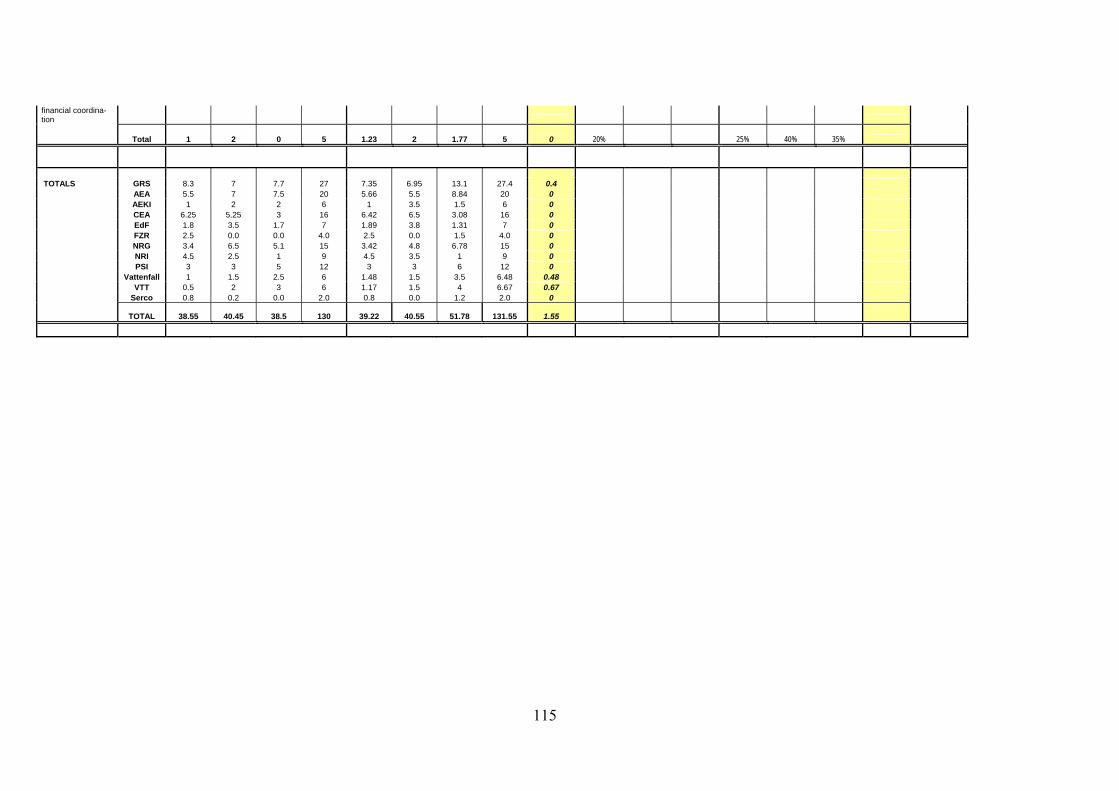
115
financial coordina-tion
Total 1 2 0 5 1.23 2 1.77 5 0 20% 25% 40% 35%
TOTALS GRS 8.3 7 7.7 27 7.35 6.95 13.1 27.4 0.4 AEA 5.5 7 7.5 20 5.66 5.5 8.84 20 0 AEKI 1 2 2 6 1 3.5 1.5 6 0 CEA 6.25 5.25 3 16 6.42 6.5 3.08 16 0 EdF 1.8 3.5 1.7 7 1.89 3.8 1.31 7 0 FZR 2.5 0.0 0.0 4.0 2.5 0.0 1.5 4.0 0 NRG 3.4 6.5 5.1 15 3.42 4.8 6.78 15 0 NRI 4.5 2.5 1 9 4.5 3.5 1 9 0 PSI 3 3 5 12 3 3 6 12 0 Vattenfall 1 1.5 2.5 6 1.48 1.5 3.5 6.48 0.48 VTT 0.5 2 3 6 1.17 1.5 4 6.67 0.67 Serco 0.8 0.2 0.0 2.0 0.8 0.0 1.2 2.0 0
TOTAL 38.55 40.45 38.5 130 39.22 40.55 51.78 131.55 1.55

116
3.8 Cooperation with Other Projects/Programmes
3.8.1 Exchange of Best Practice Guidelines
Representatives of the projects ERCOFTAC/QNET-CFD, FLOMIX-R, ASTAR and ITEM expressed strong interest to cooperate with ECORA. The technical coordinators of these projects have obtained copies of the ECORA BPGs with the stipulation to return general comments on the BPGs, and to report about any experience gained in applying the BPGs. Many ECORA partners have contributed to the ASTAR conference which took place on 17 – 18 September 2003 at GRS. ASTAR has a new deliverable, the AS-TAR BPGs, which will feed into the ECORA BPGs. FLOMIX-R and ITEM also used templates from the ECORA BPGs for the description of numerical and experimental test cases. A common ECORA/FLOMIX-R workshop took place on 15 – 16 March 2004 or-ganised by CFX Germany. Several FLOMIX-R simulations of Boron dilution mixing were presented where the ECORA BPGs had been successfully applied. In addition, the ECORA BPGs have been presented at the OECD/NEA writing groups on CFD issues in NRS which want to issue similar guidelines for the use of CFD in NRS.
3.8.2 Establishment of a Network of European Centres of Competence for CFD Codes in Nuclear Safety
An EoI for CORE-NET was submitted in June 2002. It was aiming at the establishment of a Network of European Centres of Competence for CFD codes in nuclear reactor safety at the end of the ECORA project. The goal of the network is the establishment, maintenance and extension of the ECORA BPGs, the achievement of a consensus on key technical issues related to the use of CFD software for reactor safety analysis, the distil-lation of requirements for CFD software, and the transformation of these requirements into software solutions. However, the initial intention to organise a network for CFD in NRS will not be realised because it was decided to focus the efforts on NURESIM. In order to discuss the possible integration of the EoI for CORE-NET into the proposed 6th framework project NURE-SIM, a special meeting was organised immediately after the ECORA mid-term meeting with the ECORA partners and the EC Scientific Manager Georges Van Goethem. The subject of investigating PTS-relevant flows will be continued in the NURESIM project as ‘situation target PTS’. A German CFD-network for CFD applications in nuclear reactor safety has been initiated by GRS in February 2003. Its major objectives is the improvement of three-dimensional flow simulations by assessing and extending the numerical and physical models in CFD codes for nuclear reactor safety applications, in particular for two-phase flows. The CFD Network already benefits from the input and work performed within the ECORA project, building on the models and methods implemented in CFX-5. Its consortium includes partners from the ECORA and FLOMIX-R project.
3.8.3 Organisation of a POST-FISA Workshop
A POST-FISA workshop on ‘advanced multi-physics computations in nuclear reactor safety’ was organised by the ECORA coordinators. The objectives of this workshop were the discussion of nuclear reactor safety simulation challenges from the industrial, regula-
117
tory and utility point of view. Representatives of European and US nuclear reactor safety organisations presented the state-of-the-art of nuclear reactor simulation tools, and de-scribed current development challenges and on-going research programmes. The presen-tations related to the fields of computational fluid dynamics (CFD), computational neu-tronics, system codes, multi-scale methods, and to the coupling of these methods for multi-physics applications. Collaboration opportunities were identified for multi-physics simulation platforms, and for the assessment of mathematical models in nuclear reactor safety. Finally, the importance of quality assurance guidelines for simulations was dis-cussed using the example of the ERCOFTAC and ECORA CFD Best Practise Guidelines The workshop was attended by 30 participants. In the first part of the workshop technical lectures were given on the use of numerical simulation tools in nuclear reactor safety (NRS), with an emphasis on three-dimensional CFD simulations. The second part of the workshop consisted of a round-table discussion on a collaboration framework relating to computational reactor physics and CFD for nuclear reactor safety.
3.9 Dissemination and Use of the Results
Documentation is made available via the Internet to achieve a high degree of topicality and to be in a position to maintain and extend the BPGs and related documents during and beyond the project term. The ECORA website at http://domino.grs.de/ecora/ecora.nsf contains the project documents and the results from the validation test cases including the experimental data. The main findings and conclu-sions of the project are presented in publications and conferences, e.g. FISA conference, ASTAR and ANSYS-FZR workshop on multi-phase flows. The ECORA paper presented at the FISA 2003 conference is published in the Journal for Nuclear Engineering and De-sign. The models developed within the project are implemented in industrial and commercial CFD software packages and will therefore be easily accessible by industry and research institutions. Implementation in industrial software packages will guarantee that the mod-els will be maintained and refined after the project. The work performed in ECORA improves understanding of merits and limitations of CFD, and contributes to define realistic goals of these methods in safety analysis. Addi-tionally, the project aims at reinforcing the network among the European Centres of Competence on CFD, to achieve consensus and common understanding on key techni-cal/scientific issues related to the use of CFD methods for reactor safety analysis. The gathered experience has an impact on plant life management programmes as well as on the competitiveness of the European nuclear electricity generating industry, of re-search organisations and of engineering support organisations. To achieve these objec-tives, it is necessary to propose new and innovative solutions for nuclear energy produc-tion and safety. Multi-national, multi-disciplinary efforts involving research organisa-tions, designers, vendors and utilities are an effective way to achieve these objectives. The ECORA project represents a specific contribution in the area of CFD to a global European research initiative. It is aimed at providing the European nuclear industry with improved thermal-hydraulic flow prediction capabilities to study and to optimise reactor components in a cost-effective way, thus reducing the necessity to resort to increasingly expensive full-scale experiments.
118
4 REFERENCES
[1] Menter, F., “CFD Best Practice Guidelines for CFD Code Validation for Reactor-Safety Applications”, EVOL-ECORA-D01 (2002)
[2] Scheuerer, M., “Minutes of the Project Meeting M5”, EVOL-ECORA-M07 (2003)
[3] Scheuerer, M. “Minutes of the Joint ECORA/FLOMIX-R Project Meeting 15/16 March 2004, Großhartpenning/Bavaria, Germany”, EVOL-ECORA-M08 (2004)
[4] Muhlbauer, P., “Review of CFD Applications in Primary Loop and Recommenda-tions”, EVOL-ECORA-D02 (2003)
[5] Muhlbauer, P., “Review of Experimental Database on Mixing in Primary Loop and Future Needs”, EVOL-ECORA-D03 (2003)
[6] Muhlbauer, P., “Review of Two-Phase Modelling Capabilities of CFD computer codes and Feasibility of Transient Simulations”, EVOL-ECORA-D04 (2004)
[7] Heitsch, M., “Review of CFD Applications to Containment Related Phenomena”, EVOL-ECORA-D10 (2003)
[8] Heitsch, M., “Review of CFD Experimental Data Base on Containment Related Safety Issues and Future Needs”, EVOL-ECORA-D11 (2004)
[9] Scheuerer, M., “Selection of PTS-Relevant Test Cases”, EVOL-ECORA-D05a (2003)
[10] Pigny, S., “Selection of PTS-Relevant Physical Models”, EVOL-ECORA-D05b (2003)
[11] Pigny, S., “PTS-Relevant Verification Test Cases”, EVOL-ECORA-D06 (2003)
[12] Egorov, Y., “Validation of CFD Codes with PTS-Relevant Test Cases”, EVOL-ECORA-D07 (2004)
[13] Willemsen, S., “Validation and Calibration of Models Relevant for PTS Simulations”, EVOL-ECORA-D09 (2004)
[14] Andreani, M., “Summary of Selected tests and Criteria Applied to Choice of Models, Mesh and Numerical Methods”, EVOL-ECORA-D12 (2004)
[15] Andreani, M., “Results of the Pre-Test Calculations”, EVOL-ECORA-D13 (2004)
[16] Bestion, D., “Recommendation on use of CFD Codes for Nuclear Reactor Safety Analysis”, EVOL-ECORA-D14 (2004)
[17] Bestion, D., “Recommendation for CFD Development and Customisation”, EVOL-ECORA-D15 (2004)
[18] Scheuerer, M., Schwaeger C., “Minutes of the Final Project Meeting M9”, EVOL-ECORA-M09 (2004)
[19] Ransom, V. H., ‘Numerical Benchmark Test No. 2.1 : Faucet Flow’, Journal of Multi-phase Science and Technology, Volume 6, Hewitt G. F., Delhaye J. M., Zuber M., Eds., Hemisphere Publishing Corporation (1992)
[20] Maschek W., Roth A., Kirstahler M., Meyer L., ‘Simulation Experiments for Cen-tralized Liquid Sloshing Motions’, KfK report No 5090 (1992)
119
[21] Baughn, J. W., Shimizu, S. S.‚ ‘Heat Transfer Measurements from a Surface with Uniform Heat Flux and a Fully Developed Impinging Jet’, Journal of Heat Transfer, Vol. 111, pp. 1096 – 1098 (1998)
[22] Kvicinsky, S., Kueny, J.-L., Avellan, F., 2002, ‘Numerical and Experimental Analysis of Free Surface Flow in a 3D Non-rotating Pelton Bucket’, 9th Interna-tional Symposium on Transport Phenomena and Dynamics of Rotating Machinery, Honolulu, Hawaii, U.S.A., Paper FD 18/FD-125, pp. 1 – 8 (2002)
[23] Bonetto F. and Lahey R. T. Jr, “An Experimental Study on Air Carry under due to a Plunging Liquid Jet”, Int. J. Multiphase Flow, Vol. 19, No 2, pp. 281-294 (1993)
[24] Goldbrunner, M., Karl, J., Hein, D., 2000, Experimental Investigation of Heat Transfer Phenomena during Direct Contact Condensation in the Presence of Non Condensable Gas by Means of Linear Raman Spectroscopy, 10th International Sym-posium on Laser Techniques Applied to Fluid Mechanics, Lisbon (2000)
[25] Cooper, D., Jackson, D. C., Launder, B. E., Liao, G. X., ‘Impinging Jet Studies for Turbulence Model Assessment. Part I: Flow-Field Experiments’, Int. Journal of Heat Mass Transfer, Vol. 36, pp. 2675 – 2684 (1993)
[26] Yan, X., Baughn, J. W., Mesbah, M., ‘The Effect of Reynolds Number on the Heat Transfer Distribution from a Flat Plate to an Impinging Jet’, ASME, HTD-Vol. 226, Fundamental and Applied Heat Transfer Research for Gas Turbines, pp. 1 – 7 (1992)
[27] Kvicinsky, S., ‘Mèthode d’Analyse des Ecoulements 3D à Surface Libre: Applica-tion aux Turbines Pelton’, PhD Thesis, EPFL Lausanne (2002)
[28] Ruile, H., Direktkontaktkondensation in geschichteten Zweiphasenströmungen, Fortschr.-Ber. VDI, Reihe 19, Nr. 88, Düsseldorf, VDI Verlag (1996)
[29] Hein, D., Ruile, H., Karl, J., 1995, Kühlmittelerwärmung bei Direktkontaktkonden-sation an horizontalen Schichten und vertikalen Streifen zur Quantifizierung des druckbelasteten Thermoschocks, BMFT Forschungsvorhaben 1500906, Abschluß-bericht, Lehrstuhl für Thermische Kraftanlagen, TU München (in German)
[30] Hughes, E. D., Duffey, R. B., 1991, “Direct contact condensation and momentum transfer in turbulent separated flows”, Int. J. Multiphase Flow, Vol. 17, pp. 599-619 (1991)
[31] Bielert, U., Breitung, W., Kotchourko, A., Royl, P., Scholtyssek, W., Veser, A., Beccantini, A., Dabbene, F., Paillère, H., Studer, E., Huld, T., Wilkening, H., Edlin-ger, B., Poruba, C., Movahed, M., “Multidimensional simulation of hydrogen dis-tribution and turbulent combustion in severe accidents”, Nucl. Eng. Design, Vol. 209, pp. 165-172, 4th FP Project HDC (2001)
[32] Bielert, U., Breitung, W., Dorofeev, S., Kotchourko, A., Redlinger, R., Scholtyssek, W., L’Heriteau, J.-P., Pailhories, P., Petit, P., Eyink, J., Movahed, M., Petzold, K-G, Heitsch, M., Alekseev, V., Denkevits, A., Efimenko, A., Kuznetsov, M., Okun, M., Huld, T., Baraldi, D., “Integral large scale experiments on hydrogen combus-tion for severe accident code validation – Project HYCOM”, Proc. FISA 2003, Luxembourg, 10-12 November 2003
[33] IAEA-TECDOC-1163, Heat transport and afterheat removal for gas cooled reactors under accident conditions (2000)
[34] IAEA-TECDOC-1382, Evaluation of high temperature gas cooled reactor perform-ance: benchmark analysis related to initial testing of the HTTR and HTR-10 (2003)
120
[35] Casey, M. and Wintergerste W., “Best Practice Guidelines”, ERCOFTAC Special Interest Group on Quality and Trust in Industrial CFD, report (2000)
[36] Bestion, D., Latrobe, A., Paillere, H., Laporta, A., Teschendorff, V., Staedtke, H., Aksan, N., D’Auria, F., Vihavainen, j., Meloni, P., Hewitt, G., Lillington, J., Mavko, B., Prosek, A., Macek, J., Malacka, M., Camous, F., Fichot, F., Monhardt, D., “European Project for Future Adavances in Science and Technology for Nuclear Engineering Thermal-Hydraulics (EUROFASTNET)”, Final Report (2002)
[37] Bestion, D., Anglart, H., Smith, B.L., Royen, J., Andreani, M., Mahaffy, J., Kasa-hara, F., Watanabe, T., Komen, E., Muhlbauer, P., Laurien, E., Morii, T., “Exten-sion of CFD Codes to Two-Phase Safety Problems”, Organisation for Economic Co-operation and Development/Nuclear Energy Agency OECD/NEA Report Draft Version, (2004)
[38] De Cachard, F., Garcia-Cascales, J.R., Deconinck, H., Franchello, G., Graf, U., Kumbaro, A., Mimouni, S., Paillère, H., Ricchiuto, Romenski, E., Romstedt, P., Smith, B., Städtke, H., Toro, E.F., Worth, B., “The ASTAR Project – Status and Perspective”, Proc. NURETH-10 Conference, Seoul, Korea, 5-9 October (2003)
[39] Romstedt, P., “ASTAR Contribution to the ECORA Best Practice Guidelines”, AS-TAR Deliverable D19 (2003)
[40] Auban, O., et al., “Implementation of gas concentration measurement systems using mass spectrometry in containment thermal-hydraulics test facilities : different ap-proaches for calibration and measurement with steam/air/helium mixtures”, Pro-ceeding of the 10th International Topical Meeting on Nuclear Reactor Thermal Hy-draulics (NURETH-10), Seoul, Korea, October 5-9, 2003.
[41] Chan, C. K., Jones, S. C., “Gas Mixing Experiments in a Large Enclosure”, AECL Whiteshell Laboratories, Pinawa, Manitoba, Canada, 1997.
[42] Yadigaroglu, G., Andreani, M., Dreier, J. and Coddington, P “Trends and Needs in Experimentation and Numerical Simulation for LWR Safety”, Nuclear Engineering and Design, 221, 205-223 (2003).
[43] OECD/SETH Project, Large-scale investigation of gas mixing and stratification, PANDA Test 17-1, Quick-Look Report, Jan. 2005.
[44] Wichers, V. A. Malo, J.Y., Straflinger, J., Heitsch, M., Preusser, G., Tuomainen, M., Huggenberger, M., “Testing and Enhanced Modelling of Passive Evolutionary Systems Technology for Containment Cooling (TEMPEST)”, Proc. FISA 2003, Luxembourg, 10-12 November 2003
Recommended