Embed Size (px)
Citation preview
281
Learning Objectives � Identify situations in
which, based on the levels of measurement of the independent and dependent variables, analysis of variance is appropriate.
� Explain between- and within-group variances and how they can be compared to make a judgment about the presence or absence of group effects.
� Explain the F statistic conceptually.
� Explain what the null and alternative hypotheses predict.
� Use raw data to solve equations and conduct five-step hypothesis tests.
� Explain measures of association and why they are necessary.
� Use SPSS to run analysis of variance and interpret the output.
CHAPTER
12 Hypothesis Testing With Three or More Population MeansAnalysis of Variance
In Chapter 11, you learned how to determine whether a two-class categorical variable exerts an impact on a continuous
outcome measure: This is a case in which a two-population t test for differences between means is appropriate. In many situations, though, a categorical independent variable (IV) has more than two classes. The proper hypothesis-testing technique to use when the IV is categorical with three or more classes and the dependent variable (DV) is continuous is analysis of variance (ANOVA).
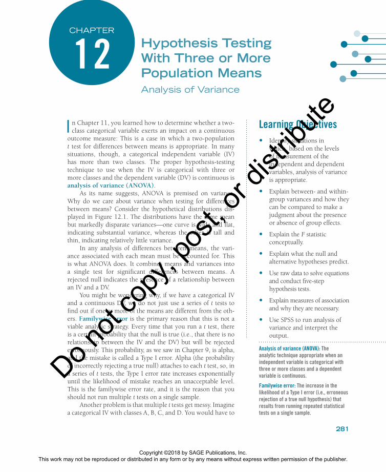
As its name suggests, ANOVA is premised on variance. Why do we care about variance when testing for differences between means? Consider the hypothetical distributions dis-played in Figure 12.1. The distributions have the same mean but markedly disparate variances—one curve is wide and flat, indicating substantial variance, whereas the other is tall and thin, indicating relatively little variance.
In any analysis of differences between means, the vari-ance associated with each mean must be accounted for. This is what ANOVA does. It combines means and variances into a single test for significant differences between means. A rejected null indicates the presence of a relationship between an IV and a DV.
You might be wondering why, if we have a categorical IV and a continuous DV, we do not just use a series of t tests to find out if one or more of the means are different from the oth-ers. Familywise error is the primary reason that this is not a viable analytic strategy. Every time that you run a t test, there is a certain probability that the null is true (i.e., that there is no relationship between the IV and the DV) but will be rejected erroneously. This probability, as we saw in Chapter 9, is alpha, and the mistake is called a Type I error. Alpha (the probability of incorrectly rejecting a true null) attaches to each t test, so, in a series of t tests, the Type I error rate increases exponentially until the likelihood of mistake reaches an unacceptable level. This is the familywise error rate, and it is the reason that you should not run multiple t tests on a single sample.
Another problem is that multiple t tests get messy. Imagine a categorical IV with classes A, B, C, and D. You would have to
Analysis of variance (ANOVA): The analytic technique appropriate when an independent variable is categorical with three or more classes and a dependent variable is continuous.
Familywise error: The increase in the likelihood of a Type I error (i.e., erroneous rejection of a true null hypothesis) that results from running repeated statistical tests on a single sample.
Do not
copy
, pos
t, or d
istrib
ute
Copyright ©2018 by SAGE Publications, Inc. This work may not be reproduced or distributed in any form or by any means without express written permission of the publisher.
282 Part III | Hypothesis Testing
run a separate t test for each combination (AB, AC, AD, BC, BD, CD). That is a lot of t tests! The results would be cumbersome and difficult to interpret.
The ANOVA test solves the problems of familywise error and overly complicated output because ANOVA analyzes all classes on the IV simultaneously. One test is all it takes. This simplifies the process and makes for cleaner results.
ANOVA: Different Types of Variances
There are two types of variance analyzed in ANOVA. Both are based on the idea of groups, which are the classes on the IV. If an IV was political orientation measured as liberal, moderate, or conservative, then liberals would be a group, moderates would be a group, and conservatives would be a group. Groups are central to ANOVA.
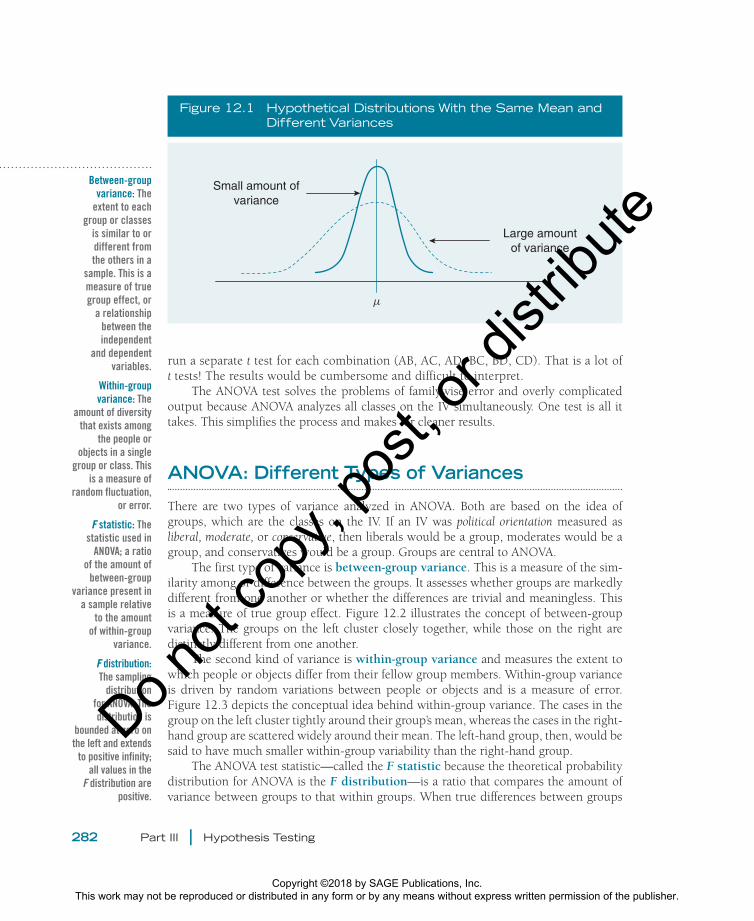
The first type of variance is between-group variance. This is a measure of the sim-ilarity among or difference between the groups. It assesses whether groups are markedly different from one another or whether the differences are trivial and meaningless. This is a measure of true group effect. Figure 12.2 illustrates the concept of between-group variance. The groups on the left cluster closely together, while those on the right are distinctly different from one another.
The second kind of variance is within-group variance and measures the extent to which people or objects differ from their fellow group members. Within-group variance is driven by random variations between people or objects and is a measure of error. Figure 12.3 depicts the conceptual idea behind within-group variance. The cases in the group on the left cluster tightly around their group’s mean, whereas the cases in the right-hand group are scattered widely around their mean. The left-hand group, then, would be said to have much smaller within-group variability than the right-hand group.
The ANOVA test statistic—called the F statistic because the theoretical probability distribution for ANOVA is the F distribution—is a ratio that compares the amount of variance between groups to that within groups. When true differences between groups
Figure 12.1 Hypothetical Distributions With the Same Mean and Different Variances
Large amountof variance
Small amount ofvariance
µ
Between-group variance: The
extent to each group or classes
is similar to or different from the others in a
sample. This is a measure of true group effect, or
a relationship between the independent
and dependent variables.
Within-group variance: The
amount of diversity that exists among
the people or objects in a single
group or class. This is a measure of
random fluctuation, or error.
F statistic: The statistic used in
ANOVA; a ratio of the amount of
between-group variance present in
a sample relative to the amount
of within-group variance.
F distribution: The sampling
distribution for ANOVA. The distribution is
bounded at zero on the left and extends
to positive infinity; all values in the
F distribution are positive.
Do not
copy
, pos
t, or d
istrib
ute
Copyright ©2018 by SAGE Publications, Inc. This work may not be reproduced or distributed in any form or by any means without express written permission of the publisher.
Chapter 12 | Hypothesis Testing With Three or More Population Means 283
Figure 12.2 Small and Large Between-Group Variability
Small Between-Group Variability Large Between-Group Variability
x2x1x2x1
Figure 12.3 Small and Large Within-Group Variability
Large Within-Group VariabilitySmall Within-Group Variability
x1 x2
substantially outweigh the random fluctuations present within each group, the F statistic will be large and the null hypothesis that there is no IV–DV relationship will be rejected in favor of the alternative hypothesis that there is an association between the two vari-ables. When between-group variance is small relative to within-group variance, the F statistic will be small, and the null will be retained.
An example might help illustrate the concept behind the F statistic. Suppose we wanted to test the effectiveness of a mental-health treatment program on recidi-vism rates in a sample of probationers. We gather three samples: treatment-program completers, people who started the program and dropped out, and those who did not participate in the program at all. Our DV is the number of times each person is rearrested within 2 years of the end of the probation sentence. There will be some random fluctuations within each group; not everybody is going to have the same recidivism score. This is white noise or, more formally, within-group variance—in any sample of people, places, or objects, there will be variation. What we are attempt-ing to discern is whether the difference between the groups outweighs the random
Do not
copy
, pos
t, or d
istrib
ute
Copyright ©2018 by SAGE Publications, Inc. This work may not be reproduced or distributed in any form or by any means without express written permission of the publisher.
284 Part III | Hypothesis Testing
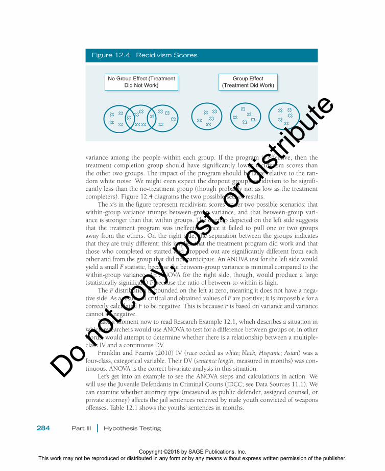
variance among the people within each group. If the program is effective, then the treatment-completion group should have significantly lower recidivism scores than the other two groups. The impact of the program should be large relative to the ran-dom white noise. We might even expect the dropout group’s recidivism to be signifi-cantly less than the no-treatment group (though probably not as low as the treatment completers). Figure 12.4 diagrams the two possible sets of results.
The x’s in the figure represent recidivism scores under two possible scenarios: that within-group variance trumps between-group variance, and that between-group vari-ance is stronger than that within groups. The overlap depicted on the left side suggests that the treatment program was ineffective, since it failed to pull one or two groups away from the others. On the right side, the separation between the groups indicates that they are truly different; this implies that the treatment program did work and that those who completed or started and dropped out are significantly different from each other and from the group that did not participate. An ANOVA test for the left side would yield a small F statistic, because the between-group variance is minimal compared to the within-group variance. An ANOVA for the right side, though, would produce a large (statistically significant) F because the ratio of between-to-within is high.
The F distribution is bounded on the left at zero, meaning it does not have a nega-tive side. As a result, all critical and obtained values of F are positive; it is impossible for a correctly calculated F to be negative. This is because F is based on variance and variance cannot be negative.
Take a moment now to read Research Example 12.1, which describes a situation in which researchers would use ANOVA to test for a difference between groups or, in other words, would attempt to determine whether there is a relationship between a multiple- class IV and a continuous DV.
Franklin and Fearn’s (2010) IV (race coded as white; black; Hispanic; Asian) was a four-class, categorical variable. Their DV (sentence length, measured in months) was con-tinuous. ANOVA is the correct bivariate analysis in this situation.
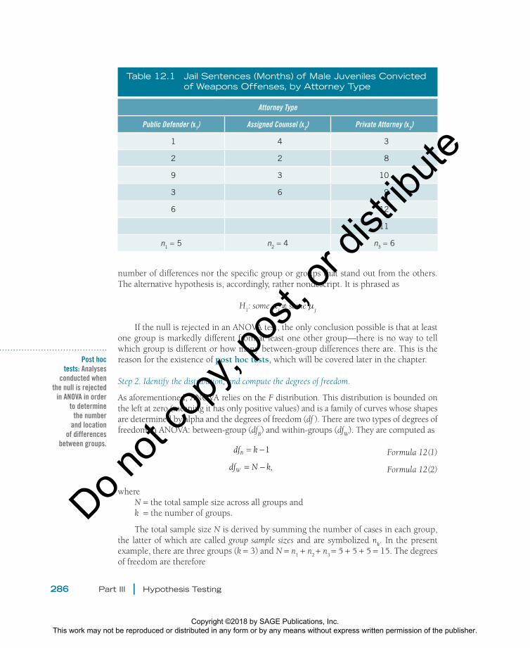
Let’s get into an example to see the ANOVA steps and calculations in action. We will use the Juvenile Defendants in Criminal Courts (JDCC; see Data Sources 11.1). We can examine whether attorney type (measured as public defender, assigned counsel, or private attorney) affects the jail sentences received by male youth convicted of weapons offenses. Table 12.1 shows the youths’ sentences in months.
Figure 12.4 Recidivism Scores
Group Effect(Treatment Did Work)
No Group Effect (TreatmentDid Not Work)
Do not
copy
, pos
t, or d
istrib
ute
Copyright ©2018 by SAGE Publications, Inc. This work may not be reproduced or distributed in any form or by any means without express written permission of the publisher.
Chapter 12 | Hypothesis Testing With Three or More Population Means 285
Research Example 12.1
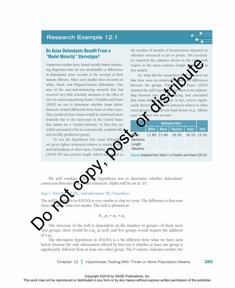
Do Asian Defendants Benefit From a “Model Minority” Stereotype?Numerous studies have found racially based sentenc-ing disparities that are not attributable to differences in defendants’ prior records or the severity of their instant offenses. Most such studies have focused on white, black, and Hispanic/Latino defendants. One area of the race-and-sentencing research that has received very little scholarly attention is the effect of race on sentencing among Asians. Franklin and Fearn (2010) set out to determine whether Asian defen-dants are treated differently from those of other races. They predicted that Asians would be sentenced more leniently due to the stereotype in the United States that Asians are a “model minority,” in that they are widely presumed to be an economically, academically, and socially productive group.
To test the hypothesis that Asian defendants are given lighter sentences relative to similarly situ-ated defendants of other races, Franklin and Fearn’s (2010) DV was sentence length, which was coded as
the number of months of incarceration imposed on offenders sentenced to jail or prison. The research-ers reported the statistics shown in the table with respect to the mean sentence length across race in this sample.
So, what did the researchers find? It turned out that there were no statistically significant differences between the groups. Franklin and Fearn (2010) retained the null hypothesis that there is no relation-ship between race and sentencing, and concluded that Asian defendants do not, in fact, receive signifi-cantly shorter jail or prison sentences relative to other racial groups once relevant legal factors (e.g., offense type) are taken into account
Defendant Race
White Black Hispanic Asian Total
Mean Sentence Length (Months)
11.80 17.40 16.50 16.10 15.50
Source: Adapted from Table 1 in Franklin and Fearn (2010).
We will conduct a five-step hypothesis test to determine whether defendants’ conviction histories affect their sentences. Alpha will be set at .01.
Step 1. State the null (H0) and alternative (H
1) hypotheses.
The null hypothesis in ANOVA is very similar to that in t tests. The difference is that now there are more than two means. The null is phrased as
H0: µ
1 = µ
2 = µ
3
The structure of the null is dependent on the number of groups—if there were four groups, there would be a µ
4 as well, and five groups would require the addition
of a µ5.
The alternative hypothesis in ANOVA is a bit different from what we have seen before because the only information offered by this test is whether at least one group is significantly different from at least one other group. The F statistic indicates neither the
Do not
copy
, pos
t, or d
istrib
ute
Copyright ©2018 by SAGE Publications, Inc. This work may not be reproduced or distributed in any form or by any means without express written permission of the publisher.
286 Part III | Hypothesis Testing
number of differences nor the specific group or groups that stand out from the others. The alternative hypothesis is, accordingly, rather nondescript. It is phrased as
H1: some µ
i ≠ some µ
j
If the null is rejected in an ANOVA test, the only conclusion possible is that at least one group is markedly different from at least one other group—there is no way to tell which group is different or how many between-group differences there are. This is the reason for the existence of post hoc tests, which will be covered later in the chapter.
Step 2. Identify the distribution, and compute the degrees of freedom.
As aforementioned, ANOVA relies on the F distribution. This distribution is bounded on the left at zero (meaning it has only positive values) and is a family of curves whose shapes are determined by alpha and the degrees of freedom (df ). There are two types of degrees of freedom in ANOVA: between-group (df
B) and within-groups (df
W). They are computed as
df kB = −1 Formula 12(1)
df N k,W = − Formula 12(2)
where N = the total sample size across all groups andk = the number of groups.
The total sample size N is derived by summing the number of cases in each group, the latter of which are called group sample sizes and are symbolized n
k. In the present
example, there are three groups (k = 3) and N = n1 + n
2 + n
3 = 5 + 5 + 5 = 15. The degrees
of freedom are therefore
Table 12.1 Jail Sentences (Months) of Male Juveniles Convicted of Weapons Offenses, by Attorney Type
Attorney Type
Public Defender (x1) Assigned Counsel (x2) Private Attorney (x3)
1 4 3
2 2 8
9 3 10
3 6 9
6 12
11
n1 = 5 n2 = 4 n3 = 6
Post hoc tests: Analyses
conducted when the null is rejected
in ANOVA in order to determine
the number and location
of differences between groups.
Do not
copy
, pos
t, or d
istrib
ute
Copyright ©2018 by SAGE Publications, Inc. This work may not be reproduced or distributed in any form or by any means without express written permission of the publisher.
Chapter 12 | Hypothesis Testing With Three or More Population Means 287
dfB = 3 − 1 = 2
dfW
= 15 − 3 = 12
Step 3. Identify the critical value and state the decision rule.
The F distribution is located in Appendix E. There are different distributions for differ-ent alpha levels, so take care to ensure that you are looking at the correct one! You will find the between-group df across the top of the table and the within-group df down the side. The critical value is located at the intersection of the proper column and row. With α = .01, df
B = 2, and df
W = 12, F
crit = 6.93. The decision rule is that if F
obt > 6.93, the
null will be rejected. The decision rule in ANOVA is always phrased using a greater than inequality because the F distribution contains only positive values, so the critical region is always in the right-hand tail.
Step 4. Compute the obtained value of the test statistic.
Step 4 entails a variety of symbols and abbreviations, all of which are listed and defined in Table 12.2. Stop for a moment and study this chart. You will need to know these symbols and what they mean in order to understand the concepts and formulas about to come.
You already know that each group has a sample size (nk) and that the entire
sample has a total sample size (N). Each group also has its own mean (xk), and the entire sample has a grand mean (xG). These sample sizes and means, along with other numbers that will be discussed shortly, are used to calculate the three types of sums of squares. The sums of squares are then used to compute mean squares, which, in turn, are used to derive the obtained value of F. We will first take a look at the for-mulas for the three types of sums of squares: total (SS
T), between-group (SS
B), and
within-group (SSW
).
SS xx
NTi k
i k= ∑∑ − ∑ ∑22( )
Formula 12(3)
Table 12.2 Elements of ANOVA
Sample Sizes Means Sums of Squares Mean Squares
nk = the sample size of group k; the number of cases in each group
xk = group mean; each group’s mean on the DV
SSB = between-groups sums of squares
MSB = between-groups mean squares
N = the total sample size across all groups
xG = the grand mean; the mean for the entire sample regardless of group
SSW = within-groups sums of squaresSST = total sums of squares; SSB + SSW = SST
MSW = within-groups mean squares
Do not
copy
, pos
t, or d
istrib
ute
Copyright ©2018 by SAGE Publications, Inc. This work may not be reproduced or distributed in any form or by any means without express written permission of the publisher.

288 Part III | Hypothesis Testing
where
iΣ = the sum of all scores i in group k,
kΣ = the sum of each group total across all groups in the sample,
x = the raw scores, and
N = the total sample size across all groups.
SS n x xBk
k k G= ∑ −( )2 Formula 12(4)
where
nk = the number of cases in group k,
xk = the mean of group k, and
xG = the grand mean across all groups.
SSw = SS
T - SS
B Formula 12(5)
The double summation signs in the SST formula are instructions to sum sums. The
i subscript denotes individual scores and k signifies groups, so the double sigmas direct you to first sum the scores within each group and to then add up all the group sums to form a single sum representing the entire sample.
Sums of squares are measures of variation. They calculate the amount of variation that exists within and between the groups’ raw scores, squared scores, and means. The SS
B formula should look somewhat familiar—in Chapters 4 and 5, we calculated devia-
tion scores by subtracting the sample mean from each raw score. Here, we are going to subtract the grand mean from each group mean. See the connection? This strategy pro-duces a measure of variation. The sums of squares provide information about the level of variability within each group and between the groups.
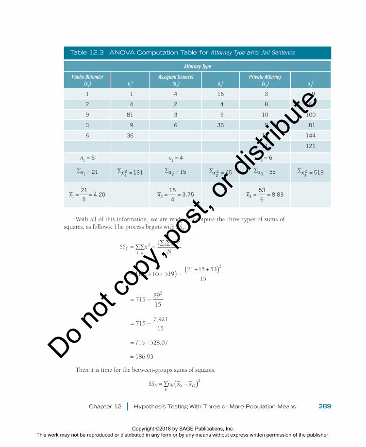
The easiest way to compute the sums of squares is to use a table. What we ultimately want from the table are (a) the sums of the raw scores for each group, (b) the sums of each group’s squared raw scores, and (c) each group’s mean. All of these numbers are displayed in Table 12.3.
We also need the grand mean, which is computed by summing all of the raw scores across groups and dividing by the total sample size N, as such:
x
x
NGi k= ∑ ∑
Formula 12(6)
Here,
xG =+ ++ +
= =21 15 53
5 4 6
89
155 93.
Do not
copy
, pos
t, or d
istrib
ute
Copyright ©2018 by SAGE Publications, Inc. This work may not be reproduced or distributed in any form or by any means without express written permission of the publisher.
Chapter 12 | Hypothesis Testing With Three or More Population Means 289
With all of this information, we are ready to compute the three types of sums of squares, as follows. The process begins with SS
T:
SS x
x
NTi k
i k= ∑∑ − ∑ ∑22( )
= + +( ) −
+ +( )131 65 519
21 15 53
15
2
= −715
89
15
2
= −715
7 921
15
,
= −715 528 07.
= 186.93
Then it is time for the between-groups sums of squares:
SS n x xBk
k k G= ∑ −( )2
Table 12.3 ANOVA Computation Table for Attorney Type and Jail Sentence
Attorney Type
Public Defender (x1) x1
2
Assigned Counsel(x2) x2
2
Private Attorney(x3) x3
2
1 1 4 16 3 9
2 4 2 4 8 64
9 81 3 9 10 100
3 9 6 36 9 81
6 36 12 144
11 121
n1 = 5 n2 = 4 n3 = 6
∑ =x1 21 ∑ =x12 131 ∑ =x2 15 ∑ =x
22 65 ∑x3 53= ∑x
32 519=
x1
21
54.20= = x2
15
43.75= = x3
53
68.83= =
Do not
copy
, pos
t, or d
istrib
ute
Copyright ©2018 by SAGE Publications, Inc. This work may not be reproduced or distributed in any form or by any means without express written permission of the publisher.

290 Part III | Hypothesis Testing
= 5(4.20 - 5.93)2 = 4(3.75 - 5.93)2 + 6(8.83 - 5.93)2
= 5(-1.73)2 + 4(-2.18)2 + 6(2.90)2
= 5(2.99) + 4(4.75) + 6(8.41)
= 14.95 + 19.00 + 50.46
= 84.41
Next, we calculate the within-groups sums of squares:
SSW
= SST - SS
B = 186.93 − 84.41 = 102.52
A great way to help you check your math as you go through Step 4 of ANOVA is to remember that the final answers for any of the sums of squares, mean squares, or F
obt
will never be negative. If you get a nega-tive number for any of your final answers
in Step 4, you will know immediately that you made a calculation error, and you should go back and locate the mistake. Can you identify the reason why all final answers are positive? Hint: The answer is in the formulas.
Learning Check 12.1
We now have what we need to compute the mean squares (symbolized MS). Mean squares transform sums of squares (measures of variation) into variances by dividing SS
B and SS
w by their respective degrees of freedom, df
B and df
w. This is a method
of standardization. The mean squares formulas are
MSSS
kBB=
−1 Formula 12(7)
MSSS
N kWW=−
Formula 12(8)
Plugging in our numbers,
MSB =−
=84 41
3 142 21
..
MSW =−
=102 52
15 38 54
..
We now have what we need to calculate Fobt
. The F statistic is the ratio of between-group variance to within-group variance and is computed as
Do not
copy
, pos
t, or d
istrib
ute
Copyright ©2018 by SAGE Publications, Inc. This work may not be reproduced or distributed in any form or by any means without express written permission of the publisher.

Chapter 12 | Hypothesis Testing With Three or More Population Means 291
FMS
MSobtB
W
= Formula 12(9)
Inserting the numbers from the present example,
Fobt = =42 21
8 544 94
.
..
Step 4 is done! Fobt
= 4.94.
Step 5. Make a decision about the null hypothesis and state the substantive conclusion.
The decision rule stated that if the obtained value exceeded 6.93, the null would be rejected. With an F
obt of 4.94, the null is retained. The substantive conclusion is that
there is no significant difference between the groups in terms of sentence length received. In other words, male juvenile weapons offenders’ jail sentences do not vary as a function of the type of attorney they had. That is, attorney type does not influence jail sentences. This finding makes sense. Research is mixed with regard to whether privately retained attorneys (who cost defendants a lot of money) really are better than publicly funded defense attorneys (who are provided to indigent defendants for free). While there is a popular assumption that privately retained attorneys are better, the reality is that publicly funded attorneys are frequently as or even more skilled than private ones are.
We will go through another ANOVA example. If you are not already using your cal-culator to work through the steps as you read and make sure you can replicate the results obtained here in the book, start doing so. This is an excellent way to learn the material.
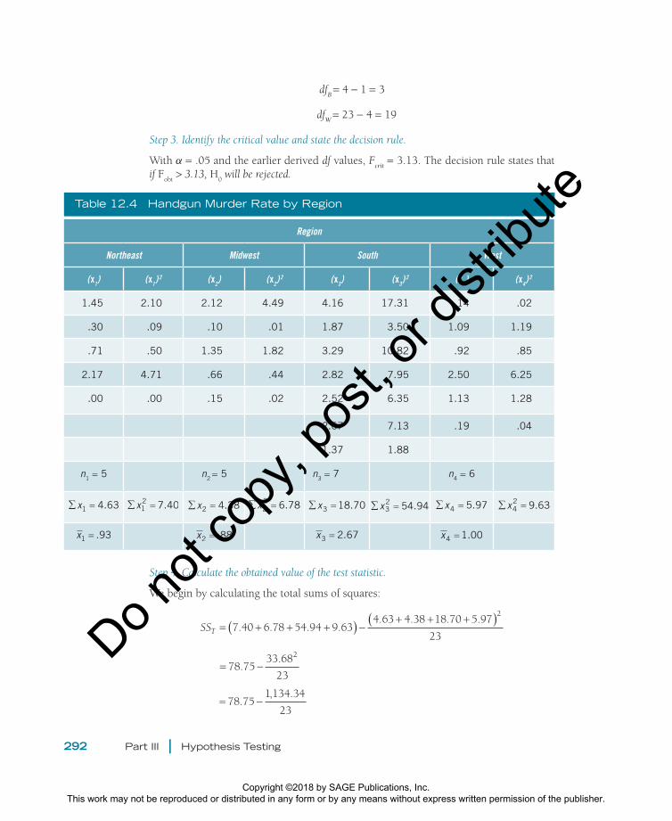
For the second example, we will study handguns and murder rates. Handguns are a prevalent murder weapon and, in some locations, they account for more deaths than all other modalities combined. In criminal justice and criminology researchers’ ongoing efforts to learn about violent crime, the question arises as to whether there are geograph-ical differences in handgun-involved murders. Uniform Crime Report (UCR) data can be used to find out whether there are significant regional differences in handgun murder rates (calculated as the number of murders by handgun per 100,000 residents in each state). A random sample of states was drawn, and the selected states were divided by region. Table 12.4 contains the data in the format that will be used for computations. Alpha will be set at .05.
Step 1. State the null (H0) and alternative (H
1) hypotheses.
H0: µ
1 = µ
2 = µ
3 = µ
4
H1: some µ
i ≠ some µ
j
Step 2. Identify the distribution and compute the degrees of freedom.
This being an ANOVA, the F distribution will be employed. There are four groups, so k = 4. The total sample size is N = 5 + 5 + 7 + 6 = 23. Using Formulas 12(1) and 12(2), the degrees of freedom are
Do not
copy
, pos
t, or d
istrib
ute
Copyright ©2018 by SAGE Publications, Inc. This work may not be reproduced or distributed in any form or by any means without express written permission of the publisher.
292 Part III | Hypothesis Testing
dfB = 4 - 1 = 3
dfW
= 23 - 4 = 19
Step 3. Identify the critical value and state the decision rule.
With α = .05 and the earlier derived df values, Fcrit
= 3.13. The decision rule states that if F
obt > 3.13, H
0 will be rejected.
Table 12.4 Handgun Murder Rate by Region
Region
Northeast Midwest South West
(x1) (x1)2 (x2) (x2)
2 (x3) (x3)2 (x4) (x4)
2
1.45 2.10 2.12 4.49 4.16 17.31 .14 .02
.30 .09 .10 .01 1.87 3.50 1.09 1.19
.71 .50 1.35 1.82 3.29 10.82 .92 .85
2.17 4.71 .66 .44 2.82 7.95 2.50 6.25
.00 .00 .15 .02 2.52 6.35 1.13 1.28
2.67 7.13 .19 .04
1.37 1.88
n1 = 5 n2 = 5 n3 = 7 n4 = 6
∑ =x1 4.63 ∑ =x12 7.40 ∑ =x2 4.38 ∑ =x2
2 6.78 ∑ =x3 18.70 ∑ =x32 54.94 ∑ =x4 5.97 ∑ =x4
2 9.63
x1 .93= x2 .88= x3 2.67= x4 1.00=
Step 4. Calculate the obtained value of the test statistic.
We begin by calculating the total sums of squares:
SST = + + +( ) −+ + +( )
7 40 6 78 54 94 9 634 63 4 38 18 70 5 97
23
2
. . . .. . . .
= −78 75
33 68
23
2
..
= −78 75
1 134 34
23.
, .
Do not
copy
, pos
t, or d
istrib
ute
Copyright ©2018 by SAGE Publications, Inc. This work may not be reproduced or distributed in any form or by any means without express written permission of the publisher.
Chapter 12 | Hypothesis Testing With Three or More Population Means 293
= 78.75 - 49.32
= 29.43
Before computing the between-groups sums of squares, we need the grand mean:
xG =+ + +
= =4 63 4 38 18 70 5 97
23
33 68
231 46
. . . . ..
Now SSB can be calculated:
SSB = −( ) + −( ) + −( ) + −( )5 93 1 46 5 88 1 46 7 2 67 1 46 6 1 00 1 462 2 2 2
. . . . . . . .
= 5(-.53)2 + 5(-.58)2 + 7(1.21)2 + 6(-.46)2
= 5(.28) + 5(.34) + 7(1.46) + 6(.21)
= 1.40 + 1.70 + 10.22 + 1.26
= 14.58
Next, we calculate the within-groups sums of squares:
SSw = 29.43 -14.58 = 14.85
Plugging our numbers into Formulas 12(7) and 12(8) for mean squares gives
MSB =
−=
14 58
4 14 86
..
MSW =−
=14 85
23 478
..
Finally, using Formula 12(9) to derive Fobt
,
Fobt = =
4 86
786 23
.
..
This is the obtained value of the test statistic. Fobt
= 6.23, and Step 4 is complete.
Step 5. Make a decision about the null and state the substantive conclusion.
In Step 3, the decision rule stated that if Fobt
turned out to be greater than 3.13, the null would be rejected. Since F
obt ended up being 6.23, the null is indeed rejected.
The substantive interpretation is that there is a significant difference across regions in the handgun-murder rate.
Do not
copy
, pos
t, or d
istrib
ute
Copyright ©2018 by SAGE Publications, Inc. This work may not be reproduced or distributed in any form or by any means without express written permission of the publisher.
294 Part III | Hypothesis Testing
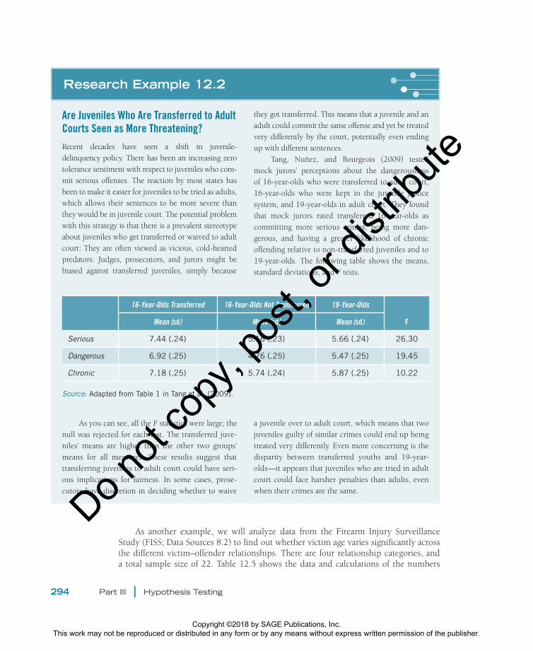
Research Example 12.2
Are Juveniles Who Are Transferred to Adult Courts Seen as More Threatening?Recent decades have seen a shift in juvenile- delinquency policy. There has been an increasing zero tolerance sentiment with respect to juveniles who com-mit serious offenses. The reaction by most states has been to make it easier for juveniles to be tried as adults, which allows their sentences to be more severe than they would be in juvenile court. The potential problem with this strategy is that there is a prevalent stereotype about juveniles who get transferred or waived to adult court: They are often viewed as vicious, cold-hearted predators. Judges, prosecutors, and jurors might be biased against transferred juveniles, simply because
they got transferred. This means that a juvenile and an adult could commit the same offense and yet be treated very differently by the court, potentially even ending up with different sentences.
Tang, Nuñez, and Bourgeois (2009) tested mock jurors’ perceptions about the dangerousness of 16-year-olds who were transferred to adult court, 16-year-olds who were kept in the juvenile justice system, and 19-year-olds in adult court. They found that mock jurors rated transferred 16-year-olds as committing more serious crimes, being more dan-gerous, and having a greater likelihood of chronic offending relative to non-transferred juveniles and to 19-year-olds. The following table shows the means, standard deviations, and F tests.
16-Year-Olds Transferred 16-Year-Olds Not Transferred 19-Year-Olds
FMean (sd) Mean (sd) Mean (sd)
Serious 7.44 (.24) 5.16 (.23) 5.66 (.24) 26.30
Dangerous 6.92 (.25) 4.76 (.25) 5.47 (.25) 19.45
Chronic 7.18 (.25) 5.74 (.24) 5.87 (.25) 10.22
Source: Adapted from Table 1 in Tang et al. (2009).
As you can see, all the F statistics were large; the null was rejected for each test. The transferred juve-niles’ means are higher than the other two groups’ means for all measures. These results suggest that transferring juveniles to adult court could have seri-ous implications for fairness. In some cases, prose-cutors have discretion in deciding whether to waive
a juvenile over to adult court, which means that two juveniles guilty of similar crimes could end up being treated very differently. Even more concerning is the disparity between transferred youths and 19-year-olds—it appears that juveniles who are tried in adult court could face harsher penalties than adults, even when their crimes are the same.
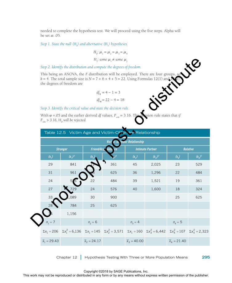
As another example, we will analyze data from the Firearm Injury Surveillance Study (FISS; Data Sources 8.2) to find out whether victim age varies significantly across the different victim–offender relationships. There are four relationship categories, and a total sample size of 22. Table 12.5 shows the data and calculations of the numbers
Do not
copy
, pos
t, or d
istrib
ute
Copyright ©2018 by SAGE Publications, Inc. This work may not be reproduced or distributed in any form or by any means without express written permission of the publisher.
Chapter 12 | Hypothesis Testing With Three or More Population Means 295
needed to complete the hypothesis test. We will proceed using the five steps. Alpha will be set at .05.
Step 1. State the null (H0) and alternative (H
1) hypotheses.
H0: µ
1 = µ
2 = µ
3 = µ
4
H1: some µ
i ≠ some µ
j
Step 2. Identify the distribution and compute the degrees of freedom.
This being an ANOVA, the F distribution will be employed. There are four groups, so k = 4. The total sample size is N = 7 + 6 + 4 + 5 = 22. Using Formulas 12(1) and 12(2), the degrees of freedom are
dfB
= 4 - 1 = 3
dfW
= 22 - 4 = 18
Step 3. Identify the critical value and state the decision rule.
With α =.05 and the earlier derived df values, Fcrit
= 3.16. The decision rule states that if F
obt > 3.16, H
0 will be rejected.
Table 12.5 Victim Age and Victim–Offender Relationship
Victim–Offender Relationship
Stranger Friend/Acquaintance Intimate Partner Relative
(x1) (x1)2 (x2) (x2) 2 (x3) (x3) 2 (x4) (x4)
2
29 841 19 361 45 2,025 23 529
31 961 25 625 36 1,296 22 484
24 576 22 484 39 1,521 19 361
27 729 24 576 40 1,600 18 324
33 1,089 30 900 25 625
28 784 25 625
34 1,156
n1 = 7 n2 = 6 n3 = 4 n4 = 5
Σx1 206= Σx12 6,136= Σx1 145= Σx2
2 3,571= Σx1 160= Σx32 6,442= Σx4
2 107= Σx42 2,323=
x1 29.43= x2 24.17= x3 40.00= x4 21.40=
Do not
copy
, pos
t, or d
istrib
ute
Copyright ©2018 by SAGE Publications, Inc. This work may not be reproduced or distributed in any form or by any means without express written permission of the publisher.

296 Part III | Hypothesis Testing
Step 4. Calculate the obtained value of the test statistic.
The total sums of squares for the data in Table 12.5 is
SS x
x
NTi k
i k= ∑∑ − ∑ ∑22( )
= + + +( ) −+ + +( )
6 136 3 571 6 442 2 323206 145 160 107
22
2
, , , ,
= −18 472
618 00
22
2
,.
= −18 472
381 924
22,
,
= 18,472 - 17360.18
= 1,111.82
Next, we need the grand mean:
xx
NGi k= ∑ ∑ =
+ + += =
206 145 160 107
22
618 00
2228 09
..
Now SSB can be calculated:
SS n x xBk
k k G= ∑ −( )2
= −( ) + −( ) + −( ) + −7 29 43 28 09 6 24 17 28 09 4 40 00 28 09 5 21 40 282 2 2
. . . . . . . ..092( )
= 7(1.34)2 + 6(-3.92)2 + 4(11.91)2 + 5(-6.69)2
= 7(1.80) + 6(15.37) + 4(141.85) + 5(44.76)
= 12.60 + 92.22 + 567.40 + 223.80
= 896.02
Next, we calculate the within-groups sums of squares:
SSw = 1,111.82 - 896.02 = 215.80
And the mean squares are
MS
SS
kBB=
−=
−=
1
896 02
4 1298 67
..
MSSS
N kWW=−
=−
=215 80
22 411 99
..
Do not
copy
, pos
t, or d
istrib
ute
Copyright ©2018 by SAGE Publications, Inc. This work may not be reproduced or distributed in any form or by any means without express written permission of the publisher.
Chapter 12 | Hypothesis Testing With Three or More Population Means 297
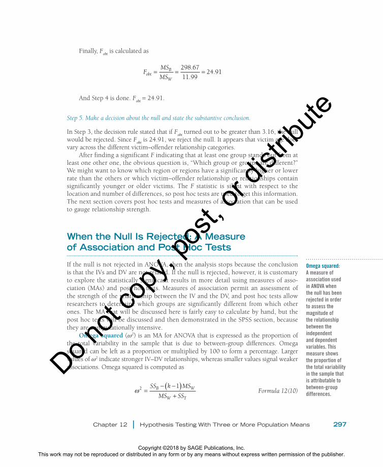
Finally, Fobt
is calculated as
FMS
MSobtB
W
= = =298 67
11 9924 91
.
..
And Step 4 is done. Fobt
= 24.91.
Step 5. Make a decision about the null and state the substantive conclusion.
In Step 3, the decision rule stated that if Fobt
turned out to be greater than 3.16, the null would be rejected. Since F
obt is 24.91, we reject the null. It appears that victim age does
vary across the different victim–offender relationship categories.After finding a significant F indicating that at least one group stands out from at
least one other one, the obvious question is, “Which group or groups are different?” We might want to know which region or regions have a significantly higher or lower rate than the others or which victim–offender relationship or relationships contain significantly younger or older victims. The F statistic is silent with respect to the location and number of differences, so post hoc tests are used to get this information. The next section covers post hoc tests and measures of association that can be used to gauge relationship strength.
When the Null Is Rejected: A Measure of Association and Post Hoc Tests
If the null is not rejected in ANOVA, then the analysis stops because the conclusion is that the IVs and DV are not related. If the null is rejected, however, it is customary to explore the statistically significant results in more detail using measures of asso-ciation (MAs) and post hoc tests. Measures of association permit an assessment of the strength of the relationship between the IV and the DV, and post hoc tests allow researchers to determine which groups are significantly different from which other ones. The MA that will be discussed here is fairly easy to calculate by hand, but the post hoc tests will be discussed and then demonstrated in the SPSS section, because they are computationally intensive.
Omega squared (ω2) is an MA for ANOVA that is expressed as the proportion of the total variability in the sample that is due to between-group differences. Omega squared can be left as a proportion or multiplied by 100 to form a percentage. Larger values of ω2 indicate stronger IV–DV relationships, whereas smaller values signal weaker associations. Omega squared is computed as
ω2 1=
− −( )+
SS k MS
MS SSB W
W T
Formula 12(10)
Omega squared: A measure of association used in ANOVA when the null has been rejected in order to assess the magnitude of the relationship between the independent and dependent variables. This measure shows the proportion of the total variability in the sample that is attributable to between-group differences.
Do not
copy
, pos
t, or d
istrib
ute
Copyright ©2018 by SAGE Publications, Inc. This work may not be reproduced or distributed in any form or by any means without express written permission of the publisher.
298 Part III | Hypothesis Testing
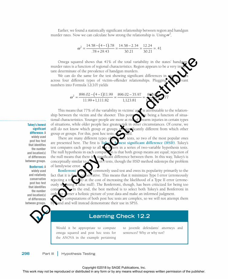
Earlier, we found a statistically significant relationship between region and handgun murder rates. Now we can calculate how strong the relationship is. Using ω2,
ω2 14 58 4 1 78
78 29 43
14 58 2 34
30 21
12 24
30 2141=
− −( )+
=−
= =. .
. .
. .
.
.
..
Omega squared shows that 41% of the total variability in the states’ handgun- murder rates is a function of regional characteristics. Region appears to be a very impor-tant determinate of the prevalence of handgun murders.
We can do the same for the test showing significant differences in victims’ ages across four different types of victim–offender relationships. Plugging the relevant numbers into Formula 12(10) yields
ω2 896 02 4 1 11 99
11 99 1 111 82
896 02 35 97
1 123 81
86=
− −( )+
=−
=. .
. , .
. .
, .
00 05
1 123 8177
.
, ..=
This means that 77% of the variability in victims’ ages is attributable to the relation-ship between the victim and the shooter. This points to age being a function of situa-tional characteristics. Younger people are more at risk of firearm injuries in certain types of situations, while older people face greater risk in other circumstances. Of course, we still do not know which group or groups are significantly different from which other group or groups. For this, post hoc tests are needed.
There are many different types of post hoc tests, so two of the most popular ones are presented here. The first is Tukey’s honest significant difference (HSD). Tukey’s test compares each group to all the others in a series of two-variable hypothesis tests. The null hypothesis in each comparison is that both group means are equal; rejection of the null means that there is a significant difference between them. In this way, Tukey’s is conceptually similar to a series of t tests, though the HSD method sidesteps the problem of familywise error.
Bonferroni is another commonly used test and owes its popularity primarily to the fact that it is fairly conservative. This means that it minimizes Type I error (erroneously rejecting a true null) at the cost of increasing the likelihood of a Type II error (errone-ously retaining a false null). The Bonferroni, though, has been criticized for being too conservative. In the end, the best method is to select both Tukey’s and Bonferroni in order to garner a holistic picture of your data and make an informed judgment.
The computations of both post hoc tests are complex, so we will not attempt them by hand and will instead demonstrate their use in SPSS.
Tukey’s honest significant
difference: A widely used
post hoc test that identifies
the number and location(s) of differences
between groups.
Bonferroni: A widely used
and relatively conservative post hoc test
that identifies the number
and location(s) of differences
between groups.
Would it be appropriate to compute omega squared and post hoc tests for the ANOVA in the example pertaining
to juvenile defendants’ attorneys and sentences? Why or why not?
Learning Check 12.2Do not
copy
, pos
t, or d
istrib
ute
Copyright ©2018 by SAGE Publications, Inc. This work may not be reproduced or distributed in any form or by any means without express written permission of the publisher.
Chapter 12 | Hypothesis Testing With Three or More Population Means 299
Research Example 12.3
Does Crime Vary Spatially and Temporally in Accordance With Routine Activities Theory?Crime varies across space and time; in other words, there are places and times it is more (or less) likely to occur. Routine activities theory has emerged as one of the most prominent explanations for this variation. Numerous studies have shown that the characteristics of places can attract or prevent crime and that large-scale patterns of human behavior shape the way crime occurs. For instance, a tavern in which negligent bartenders fre-quently sell patrons too much alcohol might generate alcohol-related fights, car crashes, and so on. Likewise, when schools let out for summer break, cities experi-ence a rise in the number of unsupervised juveniles, many of whom get into mischief. Most of this research, however, has been conducted in Western nations. De Melo, Pereira, Andresen, and Matias (2017) extended the study of spatial and temporal variation in crime rates to Campinas, Brazil, to find out if crime appears to vary along these two dimensions. They broke crime down by type and ran ANOVAs to test for temporal variation across different units of time (season, month, day of week, hour of day). The table displays the results for the ANOVAs that were statistically significant. (Nonsignifi-cant findings have been omitted.)
Unit of Time Crime F value p Value
Season Homicide 3.252 .059
Day of week Homicide 3.821 .009
Robbery 16.77 .000
Unit of Time Crime F value p Value
Burglary 3.88 .009
Theft 39.98 .000
Hour of day Homicide 3.05 .000
Rape 3.14 .000
Robbery 98.02 .000
Burglary 18.09 .000
Theft 101.00 .000
Source: Adapted from Table 1 in De Melo et al. (2017).
As the table shows, homicide rates vary somewhat across month. Post hoc tests showed that the summer months experienced spikes in homicide, likely because people are outdoors more often when the weather is nice, which increases the risk for violent victimiza-tion and interpersonal conflicts. None of the variation across month was statistically significant (which is why there are no rows for this unit of time in the table). There was significant temporal variation across weeks and hours. Post hoc tests revealed interesting findings across crime type. For example, homicides are more likely to occur on weekends (since people are out and about more during weekends than during weekdays), while burglaries are more likely to happen on week-days (since people are at work). The variation across hours of the day was also significant for all crime types, but the pattern was different within each one. For instance, crimes of violence were more common in late evenings and into the night, while burglary was most likely to occur during the daytime hours.
SPSS
Let us revisit the question asked in Example 2 regarding whether handgun murder rates vary by region. To run an ANOVA in SPSS, follow the steps depicted in Figure 12.5. Use the Analyze Compare Means One-Way ANOVA sequence to bring up the dialog box on the left side in Figure 12.5 and then select the variables you want to use.
Do not
copy
, pos
t, or d
istrib
ute
Copyright ©2018 by SAGE Publications, Inc. This work may not be reproduced or distributed in any form or by any means without express written permission of the publisher.
300 Part III | Hypothesis Testing
Move the IV to the Factor space and the DV to the Dependent List. Then click Post Hoc and select the Bonferroni and Tukey tests. Click Continue and OK to produce the output shown in Figure 12.6.
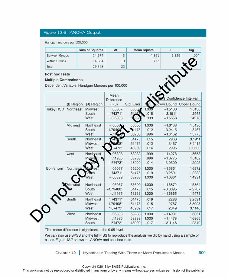
The first box of the output shows the results of the hypothesis test. You can see the sums of squares, df, and mean squares for within groups and between groups. There are also total sums of squares and total degrees of freedom. The number in the F column is F
obt. Here, you can see that F
obt = 6.329. When we did the calculations
by hand, we got 6.23. Our hand calculations had some rounding error, but this did not affect the final decision regarding the null because you can also see that the significance value (the p value) is .004, which is less than .05, the value at which α was set. The null hypothesis is rejected in the SPSS context just like it was in the hand calculations.
The next box in the output shows the Tukey and Bonferroni post hoc tests. The difference between these tests is in the p values in the Sig. column. In the present case, those differences are immaterial because the results are the same across both types of tests. Based on the asterisks that flag significant results and the fact that the p values associated with the flagged numbers are less than .05, it is apparent that the South is the region that stands out from the others. Its mean is significantly greater than all three of the other regions’ means. The Northeast, West, and Midwest do not differ significantly from one another, as evidenced by the fact that all of their p values are greater than .05.
Figure 12.5 Running an ANOVA in SPSS
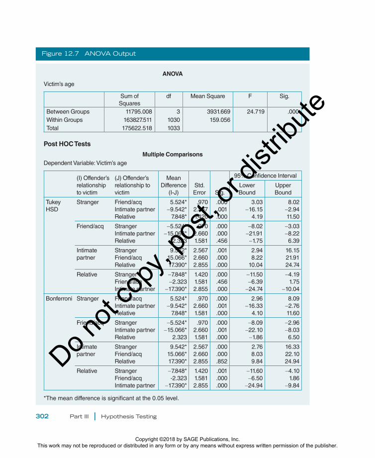
In Figure 12.7, you can see that the Fobt
SPSS produces (24.719) is nearly identical to the 12.91 we arrived at by hand. Looking at Tukey’s and Bonferroni, it appears that the categories “relative” and “friend/acquaintance” are the only ones that do not differ significantly from one another. In the full data set, the mean age of victims shot by rel-atives is 21.73 and that for the ones shot by friends and acquaintances is 24.05. These means are not significantly different from each other, but they are both distinct from the means for stranger-perpetrated shootings (mean age of 29.58) and intimate-partner shootings (39.12).
Do not
copy
, pos
t, or d
istrib
ute
Copyright ©2018 by SAGE Publications, Inc. This work may not be reproduced or distributed in any form or by any means without express written permission of the publisher.
Chapter 12 | Hypothesis Testing With Three or More Population Means 301
Post hoc Tests
Multiple Comparisons
Dependent Variable: Handgun Murders per 100,000
(I) Region (J) Region
Mean Difference
(I- J) Std. Error Sig.
95% Confidence Interval
Lower Bound Upper BoundTukey HSD Northeast Midwest
SouthWest
.05037−1.74371*
-0.6898
.55600
.51475
.53233
1.000.015.999
−1.5130−3.1911−1.5658
1.6138−.29631.4278
Midwest NortheastSouthWest
−.05037−1.79408*
−.11935
.55600
.51475
.53233
1.000.012.996
−1.6138−3.2415−1.6162
1.5130−.34671.3775
South NortheastMidwestWest
1.74371*1.79408*1.67473*
.51475
.51475
.48909
.015
.012
.014
.2963
.3467
.2995
3.19113.24153.0500
west NortheastMidwestSouth
.06898.11935
−1.67473*
.53233
.53233
.48909
.999
.996.014
−1.4278−1.3775−3.0500
1.56581.6162−.2995
Bonferroni Northeast MidwestSouthWest
.05037−1.74371*
−.06899
.55600
.51475
.53233
1.000.019
1.000
−1.5864−3.2591−1.6361
1.6872−.22831.4991
Midwest NortheastSouthWest
−05037−1.79408*
−.11935
.55600
.51475
.53233
1.000.015
1.000
−1.6872−3.3095−1.6865
1.5864−.27871.4478
South NortheastMidwestWest
1.74371*1.79408*1.67473*
.51475
.51475
.48909
.019
.015
.017
.2283
.2787
.2349
3.25913.30953.1146
West NortheastMidwestSouth
.06898.11935
−1.67473*
.53233
.53233
.48909
1.0001.000.017
−1.4981−1.4478−3.1146
1.63611.6865−.2349
*The mean difference is significant at the 0.05 level.
We can also use SPSS and the full FISS to reproduce the analysis we did by hand using a sample of cases. Figure 12.7 shows the ANOVA and post hoc tests.
Figure 12.6 ANOVA Output
Handgun murders per 100,000
Sum of Squares df Mean Square F Sig
Between Groups 14.674 3 4.891 6.329 .004
Within Groups 14.684 19 .773
Total 29.358 22
Do not
copy
, pos
t, or d
istrib
ute
Copyright ©2018 by SAGE Publications, Inc. This work may not be reproduced or distributed in any form or by any means without express written permission of the publisher.
302 Part III | Hypothesis Testing
Figure 12.7 ANOVA Output
ANOVA
Victim’s age
Sum of Squares
df Mean Square F Sig.
Between Groups 11795.008 3 3931.669 24.719 .000Within Groups 163827.511 1030 159.056Total 175622.518 1033
Post HOC Tests
Multiple ComparisonsDependent Variable: Victim’s age
(I) Offender’s relationship to victim
(J) Offender’s relationship to victim
Mean Difference
(I-J)Std. Error Sig.
95% Confidence Interval
Lower Bound
Upper Bound
Tukey HSD
Stranger Friend/acqIntimate partnerRelative
5.524*-9.542*
7.848*
.9702.5671.420
.000.001.000
3.03-16.15
4.19
8.02-2.9411.50
Friend/acq StrangerIntimate partnerRelative
-5.524*-15.066*
2.323
.9702.6601.581
.000
.000
.456
-8.02-21.91
-1.75
-3.03-8.226.39
Intimate partner
StrangerFriend/acqRelative
9.542*15.066*17.390*
2.5672.6602.855
.001.000.000
2.948.22
10.04
16.1521.9124.74
Relative StrangerFriend/acqIntimate partner
-7.848*-2.323
-17.390*
1.4201.5812.855
.000
.456
.000
-11.50-6.39
-24.74
-4.191.75
-10.04
Bonferroni Stranger Friend/acqIntimate partnerRelative
5.524*-9.542*
7.848*
.9702.6601.581
.000.001.000
2.96-16.33
4.10
8.09-2.7611.60
Friend/acq StrangerIntimate partnerRelative
-5.524*-15.066*
2.323
.9702.6601.581
.000.001.000
-8.09-22.10
-1.86
-2.96-8.036.50
Intimate partner
StrangerFriend/acqRelative
9.542*15.066*17.390*
2.5672.6602.855
.000
.000
.852
2.768.039.84
16.3322.1024.94
Relative StrangerFriend/acqIntimate partner
-7.848*-2.323
-17.390*
1.4201.5812.855
.001.000.000
-11.60-6.50
-24.94
-4.101.86
-9.84
*The mean difference is significant at the 0.05 level.
Do not
copy
, pos
t, or d
istrib
ute
Copyright ©2018 by SAGE Publications, Inc. This work may not be reproduced or distributed in any form or by any means without express written permission of the publisher.
Chapter 12 | Hypothesis Testing With Three or More Population Means 303
CHAPTER SUMMARY
This chapter taught you what to do when you have a categorical IV with three or more classes and a con-tinuous DV. A series of t tests in such a situation is not viable because of the familywise error rate. In an analysis of variance, the researcher conducts multi-ple between-group comparisons in a single analysis. The F statistic compares between-group variance to within-group variance to determine whether between-group variance (a measure of true effect) substantially outweighs within-group variance (a measure of error). If it does, the null is rejected; if it does not, the null is retained.
The ANOVA F, though, does not indicate the size of the effect, so this chapter introduced you to an MA that allows for a determination of the strength of a relationship. This measure is omega squared (w2), and it is used only when the null has been rejected—there is no sense in examining the strength of an IV–DV relationship that you just said does not exist! Omega squared is interpreted as the proportion of the variability in the DV that is attributable to the
IV. It can be multiplied by 100 to be interpreted as a percentage.
The F statistic also does not offer information about the location or number of differences between groups. When the null is retained, this is not a problem because a retained null means that there are no differences between groups; however, when the null is rejected, it is desirable to gather more information about which group or groups differ from which others. This is the reason for the existence of post hoc tests. This chap-ter covered Tukey’s HSD and Bonferroni, which are two of the most commonly used post hoc tests in criminal justice and criminology research. Bonferroni is a con-servative test, meaning that it is more difficult to reject the null hypothesis of no difference between groups. It is a good idea to run both tests and, if they produce dis-crepant information, make a reasoned judgment based on your knowledge of the subject matter and data. Together, MAs and post hoc tests can help you glean a comprehensive and informative picture of the relation-ship between the independent and dependent variables.
THINKING CRITICALLY
1. What implications does the relationship between shooting victims’ ages and these victims’ relationships with their shooters have for efforts to prevent firearm violence? For each of the four categories of victim–offender relationship, consider the mean age of victims and devise a strategy that could be used to reach people of this age group and help them lower their risks of firearm victimization.
2. A researcher is evaluating the effectiveness of a substance abuse treatment program for jail
inmates. The researcher categorizes inmates into three groups: those who completed the program, those who started it and dropped out, and those who never participated at all. He follows up with all people in the sample six months after their release from jail and asks them whether or not they have used drugs since being out. He codes drug use as 0 = no and 1 = yes. He plans to analyze the data using an ANOVA. Is this the correct analytic approach? Explain your answer.
REVIEW PROBLEMS
1. A researcher wants to know whether judges’ gender (measured as male; female) affects the severity of sentences they impose on convicted defendants (measured as months of incarceration). Answer the following questions:
a. What is the independent variable?
b. What is the level of measurement of the independent variable?
c. What is the dependent variable?
Do not
copy
, pos
t, or d
istrib
ute
Copyright ©2018 by SAGE Publications, Inc. This work may not be reproduced or distributed in any form or by any means without express written permission of the publisher.

304 Part III | Hypothesis Testing
d. What is the level of measurement of the dependent variable?
e. What type of hypothesis test should the researcher use?
2. A researcher wants to know whether judges’ gender (measured as male; female) affects the types of sentences they impose on convicted criminal defendants (measured as jail; prison; probation; fine; other). Answer the following questions:
a. What is the independent variable?
b. What is the level of measurement of the independent variable?
c. What is the dependent variable?
d. What is the level of measurement of the dependent variable?
e. What type of hypothesis test should the researcher use?
3. A researcher wishes to find out whether arrest deters domestic violence offenders from committing future acts of violence against intimate partners. The researcher measures arrest as arrest; mediation; separation; no action and recidivism as number of arrests for domestic violence within the next 3 years. Answer the following questions:
a. What is the independent variable?
b. What is the level of measurement of the independent variable?
c. What is the dependent variable?
d. What is the level of measurement of the dependent variable?
e. What type of hypothesis test should the researcher use?
4. A researcher wishes to find out whether arrest deters domestic violence offenders from committing future acts of violence against intimate partners. The researcher measures arrest as arrest; mediation; separation; no action and recidivism as whether these offenders were arrested for domestic violence within the next
2 years (measured as arrested; not arrested). Answer the following questions:
a. What is the independent variable?
b. What is the level of measurement of the independent variable?
c. What is the dependent variable?
d. What is the level of measurement of the dependent variable?
e. What type of hypothesis test should the researcher use?
5. A researcher wants to know whether poverty affects crime. The researcher codes neighborhoods as being lower-class, middle-class, or upper-class and obtains the crime rate for each area (measured as the number of index offenses per 10,000 residents). Answer the following questions:
a. What is the independent variable?
b. What is the level of measurement of the independent variable?
c. What is the dependent variable?
d. What is the level of measurement of the dependent variable?
e. What type of hypothesis test should the researcher use?
6. A researcher wants to know whether the prevalence of liquor-selling establishments (such as bars and convenience stores) in neighborhoods affects crime in those areas. The researcher codes neighborhoods as having 0–1, 2–3, 4–5, or 6+ liquor-selling establishments. The researcher also obtains the crime rate for each area (measured as the number of index offenses per 10,000 residents). Answer the following questions:
a. What is the independent variable?
b. What is the level of measurement of the independent variable?
c. What is the dependent variable?
d. What is the level of measurement of the dependent variable?
e. What type of hypothesis test should the researcher use?
Do not
copy
, pos
t, or d
istrib
ute
Copyright ©2018 by SAGE Publications, Inc. This work may not be reproduced or distributed in any form or by any means without express written permission of the publisher.
Chapter 12 | Hypothesis Testing With Three or More Population Means 305
7. Explain within-groups variance and between-groups variance. What does each of these concepts represent or measure?
8. Explain the F statistic in conceptual terms. What does it measure? Under what circumstances will F be small? Large?
9. Explain why the F statistic can never be negative.
10. When the null hypothesis in an ANOVA test is rejected, why are MA and post hoc tests necessary?
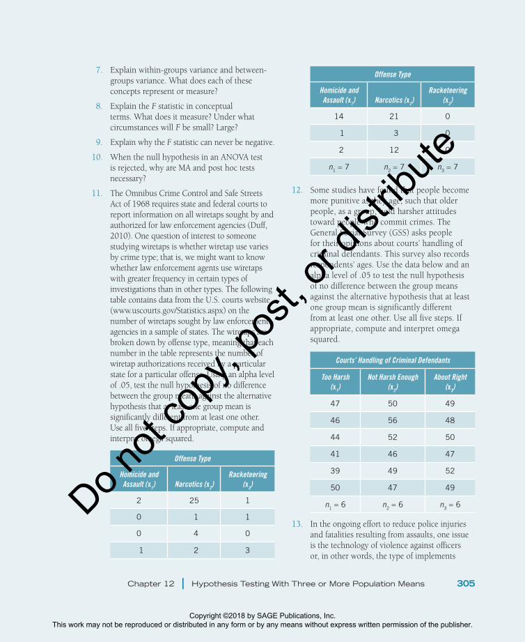
11. The Omnibus Crime Control and Safe Streets Act of 1968 requires state and federal courts to report information on all wiretaps sought by and authorized for law enforcement agencies (Duff, 2010). One question of interest to someone studying wiretaps is whether wiretap use varies by crime type; that is, we might want to know whether law enforcement agents use wiretaps with greater frequency in certain types of investigations than in other types. The following table contains data from the U.S. courts website (www.uscourts.gov/Statistics.aspx) on the number of wiretaps sought by law enforcement agencies in a sample of states. The wiretaps are broken down by offense type, meaning that each number in the table represents the number of wiretap authorizations received by a particular state for a particular offense. Using an alpha level of .05, test the null hypothesis of no difference between the group means against the alternative hypothesis that at least one group mean is significantly different from at least one other. Use all five steps. If appropriate, compute and interpret omega squared.
Offense Type
Homicide and Assault (x1) Narcotics (x2)
Racketeering (x3)
2 25 1
0 1 1
0 4 0
1 2 3
Offense Type
Homicide and Assault (x1) Narcotics (x2)
Racketeering (x3)
14 21 0
1 3 0
2 12 0
n1 = 7 n2 = 7 n3 = 7
12. Some studies have found that people become more punitive as they age, such that older people, as a group, hold harsher attitudes toward people who commit crimes. The General Social Survey (GSS) asks people for their opinions about courts’ handling of criminal defendants. This survey also records respondents’ ages. Use the data below and an alpha level of .05 to test the null hypothesis of no difference between the group means against the alternative hypothesis that at least one group mean is significantly different from at least one other. Use all five steps. If appropriate, compute and interpret omega squared.
Courts’ Handling of Criminal Defendants
Too Harsh(x1)
Not Harsh Enough(x2)
About Right(x3)
47 50 49
46 56 48
44 52 50
41 46 47
39 49 52
50 47 49
n1 = 6 n2 = 6 n3 = 6
13. In the ongoing effort to reduce police injuries and fatalities resulting from assaults, one issue is the technology of violence against officers or, in other words, the type of implements
Do not
copy
, pos
t, or d
istrib
ute
Copyright ©2018 by SAGE Publications, Inc. This work may not be reproduced or distributed in any form or by any means without express written permission of the publisher.
306 Part III | Hypothesis Testing
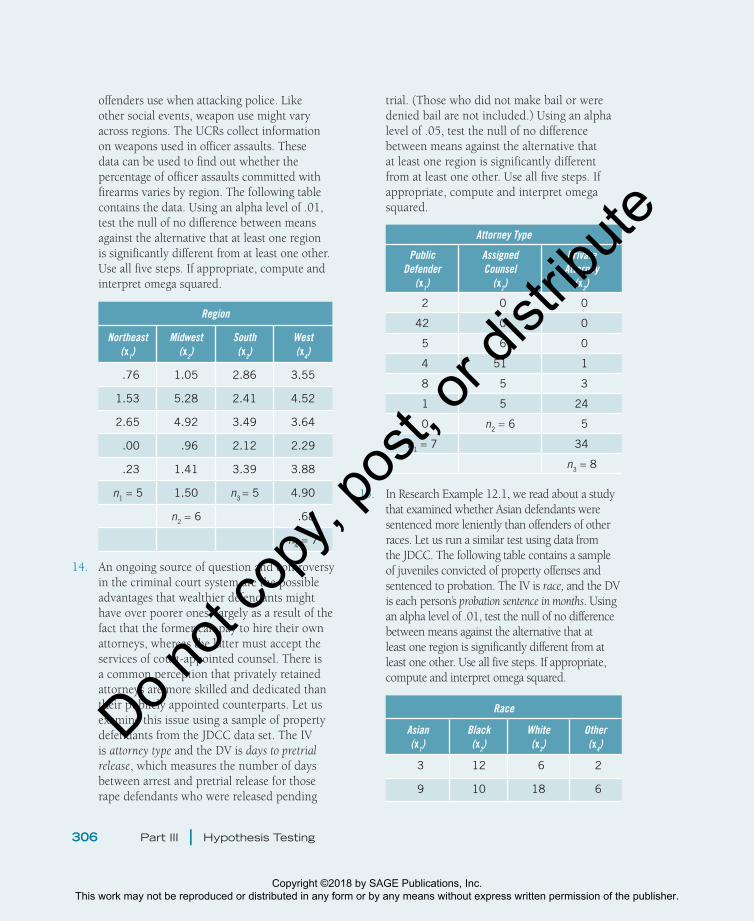
offenders use when attacking police. Like other social events, weapon use might vary across regions. The UCRs collect information on weapons used in officer assaults. These data can be used to find out whether the percentage of officer assaults committed with firearms varies by region. The following table contains the data. Using an alpha level of .01, test the null of no difference between means against the alternative that at least one region is significantly different from at least one other. Use all five steps. If appropriate, compute and interpret omega squared.
Region
Northeast(x1)
Midwest(x2)
South(x3)
West(x4)
.76 1.05 2.86 3.55
1.53 5.28 2.41 4.52
2.65 4.92 3.49 3.64
.00 .96 2.12 2.29
.23 1.41 3.39 3.88
n1 = 5 1.50 n3 = 5 4.90
n2 = 6 .68
n4 = 7
14. An ongoing source of question and controversy in the criminal court system are the possible advantages that wealthier defendants might have over poorer ones, largely as a result of the fact that the former can pay to hire their own attorneys, whereas the latter must accept the services of court-appointed counsel. There is a common perception that privately retained attorneys are more skilled and dedicated than their publicly appointed counterparts. Let us examine this issue using a sample of property defendants from the JDCC data set. The IV is attorney type and the DV is days to pretrial release, which measures the number of days between arrest and pretrial release for those rape defendants who were released pending
trial. (Those who did not make bail or were denied bail are not included.) Using an alpha level of .05, test the null of no difference between means against the alternative that at least one region is significantly different from at least one other. Use all five steps. If appropriate, compute and interpret omega squared.
Attorney Type
Public Defender
(x1)
Assigned Counsel
(x2)
Private Attorney
(x3)
2 0 0
42 0 0
5 6 0
4 51 1
8 5 3
1 5 24
0 n2 = 6 5
n1 = 7 34
n3 = 8
15. In Research Example 12.1, we read about a study that examined whether Asian defendants were sentenced more leniently than offenders of other races. Let us run a similar test using data from the JDCC. The following table contains a sample of juveniles convicted of property offenses and sentenced to probation. The IV is race, and the DV is each person’s probation sentence in months. Using an alpha level of .01, test the null of no difference between means against the alternative that at least one region is significantly different from at least one other. Use all five steps. If appropriate, compute and interpret omega squared.
Race
Asian(x1)
Black(x2)
White(x3)
Other(x4)
3 12 6 2
9 10 18 6
Do not
copy
, pos
t, or d
istrib
ute
Copyright ©2018 by SAGE Publications, Inc. This work may not be reproduced or distributed in any form or by any means without express written permission of the publisher.
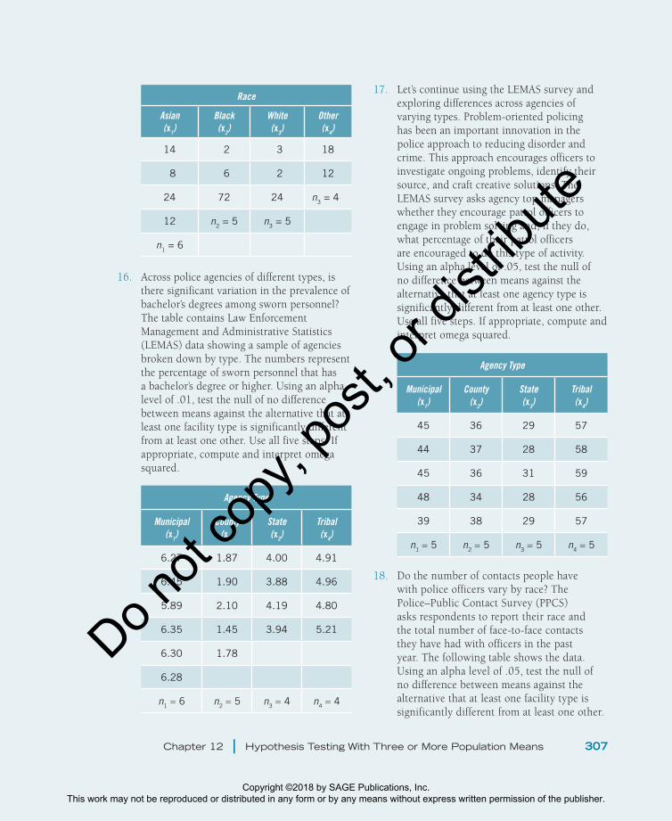
Chapter 12 | Hypothesis Testing With Three or More Population Means 307
Race
Asian(x1)
Black(x2)
White(x3)
Other(x4)
14 2 3 18
8 6 2 12
24 72 24 n3 = 4
12 n2 = 5 n3 = 5
n1 = 6
16. Across police agencies of different types, is there significant variation in the prevalence of bachelor’s degrees among sworn personnel? The table contains Law Enforcement Management and Administrative Statistics (LEMAS) data showing a sample of agencies broken down by type. The numbers represent the percentage of sworn personnel that has a bachelor’s degree or higher. Using an alpha level of .01, test the null of no difference between means against the alternative that at least one facility type is significantly different from at least one other. Use all five steps. If appropriate, compute and interpret omega squared.
Agency Type
Municipal(x1)
County(x2)
State(x3)
Tribal(x4)
6.27 1.87 4.00 4.91
6.45 1.90 3.88 4.96
5.89 2.10 4.19 4.80
6.35 1.45 3.94 5.21
6.30 1.78
6.28
n1 = 6 n2 = 5 n3 = 4 n4 = 4
17. Let’s continue using the LEMAS survey and exploring differences across agencies of varying types. Problem-oriented policing has been an important innovation in the police approach to reducing disorder and crime. This approach encourages officers to investigate ongoing problems, identify their source, and craft creative solutions. The LEMAS survey asks agency top managers whether they encourage patrol officers to engage in problem solving and, if they do, what percentage of their patrol officers are encouraged to do this type of activity. Using an alpha level of .05, test the null of no difference between means against the alternative that at least one agency type is significantly different from at least one other. Use all five steps. If appropriate, compute and interpret omega squared.
Agency Type
Municipal(x1)
County(x2)
State(x3)
Tribal(x4)
45 36 29 57
44 37 28 58
45 36 31 59
48 34 28 56
39 38 29 57
n1 = 5 n2 = 5 n3 = 5 n4 = 5
18. Do the number of contacts people have with police officers vary by race? The Police–Public Contact Survey (PPCS) asks respondents to report their race and the total number of face-to-face contacts they have had with officers in the past year. The following table shows the data. Using an alpha level of .05, test the null of no difference between means against the alternative that at least one facility type is significantly different from at least one other.
Do not
copy
, pos
t, or d
istrib
ute
Copyright ©2018 by SAGE Publications, Inc. This work may not be reproduced or distributed in any form or by any means without express written permission of the publisher.
308 Part III | Hypothesis Testing
Use all five steps. If appropriate, compute and interpret omega squared.
Race
White(x1)
Black(x2)
Other(x3)
5.13 6.03 1.74
5.00 5.90 1.70
4.98 6.10 2.00
5.20 6.18 1.61
5.10 6.00 n3 = 4
5.15 n2 = 5
n1 = 6
19. Are there race differences among juvenile defendants with respect to the length of time it takes them to acquire pretrial release? The data set JDCC for Chapter 12.sav (edge .sagepub.com/gau3e) can be used to test for whether time-to-release varies by race for juveniles accused of property crimes. The variables are race and days. Using SPSS, run an ANOVA with race as the IV and days as the DV. Select the appropriate post hoc tests.
a. Identify the obtained value of F.
b. Would you reject the null at an alpha of .01? Why or why not?
c. State your substantive conclusion about whether there is a relationship between race and days to release for juvenile property defendants.
d. If appropriate, interpret the post hoc tests to identify the location and total number of significant differences.
e. If appropriate, compute and interpret omega squared.
20. Are juvenile property offenders sentenced differently depending on the file mechanism
used to waive them to adult court? The data set JDCC for Chapter 12.sav (edge.sagepub .com/gau3e) contains the variables file and jail, which measure the mechanism used to transfer each juvenile to adult court (discretionary, direct file, or statutory) and the number of months in the sentences of those sent to jail on conviction. Using SPSS, run an ANOVA with file as the IV and jail as the DV. Select the appropriate post hoc tests.
a. Identify the obtained value of F.
b. Would you reject the null at an alpha of .05? Why or why not?
c. State your substantive conclusion about whether there is a relationship between attorney type and days to release for juvenile defendants.
d. If appropriate, interpret the post hoc tests to identify the location and total number of significant differences.
e. If appropriate, compute and interpret omega squared.
21. The data set FISS for Chapter 12.sav (edge .sagepub.com/gau3e) contains the FISS variables capturing shooters’ intentions (accident, assault, and police involved) and victims’ ages. Using SPSS, run an ANOVA with intent as the IV and age as the DV. Select the appropriate post hoc tests.
a. Identify the obtained value of F.
b. Would you reject the null at an alpha of .05? Why or why not?
c. State your substantive conclusion about whether victim age appears to be related to shooters’ intentions.
d. If appropriate, interpret the post hoc tests to identify the location and total number of significant differences.
e. If appropriate, compute and interpret omega squared.
Do not
copy
, pos
t, or d
istrib
ute
Copyright ©2018 by SAGE Publications, Inc. This work may not be reproduced or distributed in any form or by any means without express written permission of the publisher.
Chapter 12 | Hypothesis Testing With Three or More Population Means 309
KEY TERMS
Analysis of variance (ANOVA) 281
Familywise error 281Between-group variance 282
Within-group variance 282F statistic 282F distribution 282Post hoc tests 286
Omega squared 297Tukey’s honest significant
difference (HSD) 298Bonferroni 298
GLOSSARY OF SYMBOLS AND ABBREVIATIONS INTRODUCED IN THIS CHAPTER
F The statistic and sampling distribution for ANOVA
nk The sample size of group k
N The total sample size across all groups
xk The mean of group k
xG The grand mean across all cases in all groups
SSB Between-groups sums of squares; a measure of true group effect
SSW Within-groups sums of squares; a measure of error
SST Total sums of squares; equal to SSB + SSw
MSB Between-group mean square; the variance between groups and a measure of true group effect
MSW Within-group mean square; the variance within groups and a measure of error
ω2 A measure of association that indicates the proportion of the total variability that is due to between-group differences
Do not
copy
, pos
t, or d
istrib
ute
Copyright ©2018 by SAGE Publications, Inc. This work may not be reproduced or distributed in any form or by any means without express written permission of the publisher.

Do not
copy
, pos
t, or d
istrib
ute
Copyright ©2018 by SAGE Publications, Inc. This work may not be reproduced or distributed in any form or by any means without express written permission of the publisher.


![Statistische Tests (Signi kanztests) · Statistische Tests (Signi kanztests) [testing statistical hypothesis] Pr ufen und Bewerten von Hypothesen (Annahmen, Vermutungen) uber die](https://img.pdfslide.org/doc/110x75/5b7bc6a57f8b9a73728b569a/statistische-tests-signi-kanztests-statistische-tests-signi-kanztests-testing.jpg)