24.03.2015

Bibliographische Beschreibung

Löbel, Franziska

Identification of Prostate Cancer Metabolomic Markers by 1H HRMAS NMR Spectroscopy and

Quantitative Immunohistochemistry

Universität Leipzig, Dissertation

98 S.¹, 112 Lit.², 40 Abb.3, 11 Tab.4, 3 Anl.5

Referat:

Die vorliegende Studie präsentiert und evaluiert einen diagnostischen Ansatz zur quantitativen

Bestimmung von metabolomischen Markern von Prostatakrebs, basierend auf der Durchführung von

"1H High Resolution Magic Angle Spinning Nuclear Magnetic Resonance Spectroscopy" (1H HRMAS

NMR Spektroskopie) und quantitativer Immunhistochemie.

Durch Untersuchung von Gewebsproben von Prostatakrebspatienten mittels 1H HRMAS NMR

Spektroskopie und anschließender Korrelation der Ergebnisse mit quantitativ bestimmten Resultaten

immunhistochemischer Färbeverfahren können die Metaboliten Phosphocholin und Zitrat in der

vorliegenden Patientenkohorte als potentielle metabolomische Marker von Prostatakrebs identifiziert

werden. Eine Validierung der vorgestellten diagnostischen Methode erfolgt durch vergleichende

Analysen qualitativer und quantitativer konventioneller histopathologischer Untersuchungen.

Die Anwendung des präsentierten diagnostischen Ansatzes erfolgt zusätzlich zur Bestimmung von

potentiellen metabolomischen Markern von rezidivierenden Prostatakrebserkrankungen.

1 Seitenzahl insgesamt 2 Zahl der im Literaturverzeichnis ausgewiesenen Literaturangaben 3 Anzahl der in der Arbeit veröffentlichten Abbildungen 4 Gesamtanzahl der abgebildeten Tabellen 5 Anzahl der Anhänge

��

�

�

�

�

�

Part of this work was presented at the “Annual meeting of the Society for European Magnetic

Resonance in Medicine and Biology (ESMRMB)” in Lisbon, October 2012

�

�

��

�

Table of Contents

Table of Contents .................................................................................................................................... 3

Glossary ................................................................................................................................................... 5

1 Introduction ..................................................................................................................................... 7

1. 1 Prostate Cancer ........................................................................................................................ 7

1. 2 Detection of Prostate Cancer – State of the Art....................................................................... 7

1. 2. 1 Prostate- Specific Antigen Test and Digital Rectal Examination .................................... 8

1.2.2 Radiographic Methods in PCa Detection ........................................................................ 8

1.2.3 Transrectal Core Biopsies and Histopathological Analysis........................................... 10

1.2.4 Histopathological Grading of Prostate Cancer: GLEASON Score ............................... 11

1.3 Challenges and Need for New Approaches in PCa Diagnostic Management ....................... 12

2 Scientific Background I: Nuclear Magnetic Resonance,1H HRMAS NMR Spectroscopy and Metabolomic Profiles .................................................................................................................... 13

2.1 Nuclear Magnetic Resonance ............................................................................................... 13

2.1.1 Spin Precession .............................................................................................................. 15

2.1.2 Magnetic Resonance ...................................................................................................... 16

2.1.3 Chemical Shift and J- coupling ..................................................................................... 16

2.2 Nuclear Magnetic Resonance Spectroscopy.......................................................................... 19

2.2.1 Magic Angle Spinning and 1H HRMAS NMR Spectroscopy ...................................... 19

2.2.2 MAS Spinning Rates and Spinning Side Bands ........................................................... 20

2. 3 Metabolomics, Metabolite Profiles and Clinical Utility ........................................................ 22

3 Scientific Background II: Immunohistochemistry of Prostate Cancer .......................................... 26

4 Aims of the Study .......................................................................................................................... 29

5 Material and Methods .................................................................................................................... 31

5.1 Prostate Tissue Samples and Patient Demographics ............................................................. 31

5.2 1H HRMAS NMR Spectroscopy ........................................................................................... 31

5.2.1 Sample Preparation ........................................................................................................ 32

5.2.2 Spectroscopy Scan ......................................................................................................... 32

5.2.3 Data Processing ............................................................................................................. 33

5.3 Immunohistochemistry .......................................................................................................... 37

5.3.1 Immunohistochemistry Material and Equipment .......................................................... 37

5.3.2. Immunohistochemistry Protocol ................................................................................... 37

5. 3. 3 Prostate Immunomarker Stability after 1H HRMAS NMR Spectroscopy ..................... 41

5.3.4 Qualitative IHC Analysis ............................................................................................. 42

5. 3.5 Quantitative IHC Analysis ............................................................................................ 43

��

�

5.3.5.1 Quantitative IHC Slide Review .................................................................................. 43

5.3.5.2 Computer-Automated Quantitative IHC Analysis ..................................................... 43

5.3 Quantitative Histopathology ................................................................................................. 49

5. 4 Identification of Prostate Cancer Metabolomic Markers ..................................................... 50

5. 5 Patient Outcomes and Recurrence Categories ...................................................................... 50

5.6 Statistical Analysis ............................................................................................................... 51

6 Results ........................................................................................................................................... 52

6. 1 Patient demographics ........................................................................................................... 52

6. 2 Spectroscopy Results ............................................................................................................ 53

6. 3 Immunohistochemistry ......................................................................................................... 56

6. 3. 1 Evaluation of Prostate Immunomarker Stability after 1H HRMAS MRS ..................... 56

6. 3. 2 Qualitative Immunohistochemistry ............................................................................... 59

6. 4 Quantitative Immunohistochemistry .................................................................................... 65

6. 4. 1 Quantitative IHC Slide Review ..................................................................................... 65

6. 4. 2 Computer-Automated Quantitative IHC Evaluation using QIAP ................................. 67

6. 5 Quantitative Histopathology .................................................................................................. 69

6. 6 Identification of Prostate Cancer Metabolomic Markers using QIAP ................................... 72

6. 7 Patient Outcomes and Recurrence ......................................................................................... 74

7 Discussion ..................................................................................................................................... 77

8 Summary / Abstract ....................................................................................................................... 86

9 Zusammenfassung ......................................................................................................................... 89

10 References ..................................................................................................................................... 92

11 Erklärung über die eigenständige Abfassung der Arbeit ............................................................... 99

12 Danksagung ................................................................................................................................. 100

13 Lebenslauf und Publikationsverzeichnis ..................................................................................... 101

Appendix ............................................................................................................................................. 103

A.1 Immunostaining protocols 103

A.2 Spectral Intensities Measured by 1H HRMAS MRS in 51 Samples ................................... 105

A.3 Graphs for Correlations of Spectral Intensities and CaE% determined by QIAP in 34 Additional Regions of Interest............................................................................................. 110

�

�

��

�

Glossary

ABC Avidin-Biotin-Peroxidase-Complex

ADC Apparent diffusion coefficient

ADT Androgen deprivation therapy

Ala Alanine

AMACR Alpha-Methylacyl-CoA-Racemace

BCIP 5-Bromo-4-chloro-3-indolyl phosphate

BPH Benign Prostate Hyperplasia

Cit Citrate

CK Cytokeratin

CPMG Carr- Purcell-Meiboom-Gill pulse sequence

Cr Creatine

DAB 3,3'-Diaminobenzidine

DANTE Delay alternating with nutation for tailored excitation

DAPI 4´,6-Diamidino-2-phenylindole

DER Digital Rectal Examination

EDTA Ethylenediaminetetraacetic acid

FID Free induction decay

FLAIR Fluid attenuated inversion recovery

fMRI Functional Magnetic Resonance Imaging

GBM Glioblastoma multiforme

GC-MS Gas-chromatography mass spectrometry

GPC Glycerophosphocholine

GS Gleason score

H&E Hematoxlin & Eosin

HIER Heat Induced Epitope Retrieval

HMWCK High Molecular Weight Cytokeratin

HRMAS High Resolution Magic Angle Spinning

IHC Immunohistochemistry

IRB Institutional Review Board

Lac Lactate

LC-MS Liquid-chromatography mass spectrometry

MAS Magic Angle Spinning

��

�

MGH Massachusetts General Hospital

MRI Magnetic Resonance Imaging

MRS Nuclear Magnetic Resonance Spectroscopy

NBT Nitro blue tetrazolium chloride

NMR

OS

Nuclear Magnetic Resonance

Overall survival

PBS Phosphate Buffered Saline

Pcho Phophocholine

PCa Prostate Cancer

PIER Proteolytic Induced Epitope Retrieval

PIN Prostate Intraepithelial Neoplasia

PSA Prostate Specific Antigen

QIAP

SD

Quantitative Immunohistochemistry Analysis Program

Standard deviation

SSB Spinning side bands

T1 Spin-lattice relaxation time

T2 Spin-spin relaxation time

TE Transient Echo

TMS Trimethylsilan

TRIS Trisaminomethane

TRUS Transrectal Ultrasound Guided Biopsy

�

��

�

1 Introduction

1. 1 Prostate Cancer

Prostate cancer (PCa) is the most frequently diagnosed malignant disease among adult males

in the USA and the second leading cause of cancer-related deaths in men [1]. Worldwide, the

5-year prevalence of PCa has been calculated at more than 3.9 million cases [2]. The

distribution of incidence is very heterogeneous and highest rates are found in industrialized

countries, especially of Northern America, Western and Northern Europe and Australia. With

233,000 newly diagnosed cases and about 29,480 cancer associated deaths among males in

the USA estimated for 2013, PCa presents a tremendous and significant health problem [1].

The lifetime risk of developing PCa for American men is approximately 15%. However,

autopsies have revealed microscopic prostate carcinomas in up to 29% in the age group of

30- 40 year old men and 64% in age group 60- 70 years. At 80 years of age, as many as 80%

of all men show small carcinomas [3].The risk of developing PCa is known to be related to

genetic factors, diet, lifestyle and androgens. Furthermore, studies indicated that infection or

inflammation of the prostate may also trigger PCa development and that environmental

carcinogens might promote PCa progression [3]. High risk groups have been identified within

the population, including African Americans as well as men with one or more first-degree

relatives diagnosed with PCa at an early age [1].

Histology indicates that more than 95% of PCas are unevenly distributed, epithelially derived

adenocarcinomas of which more than 75% are located in the peripheral zone, 10-15% in the

transition zone and less than 15% in the central zone of the prostate [4]. This cancer tends to

metastasize to the bones, especially the lumbar spine, pelvis and femur. Bone metastases can

be found in up to 70% of patients with advanced PCa [5]. In general, this malignancy is

characterized by a relatively slow growth rate of the primary tumor, compared to malignant

transformations of other organs [6]. Given the mostly indolent clinical behavior of PCa, an

early and accurate diagnosis is crucial, in order to provide an adequate treatment for this

highly prevalent disease.

�

1. 2 Detection of Prostate Cancer – State of the Art

The detection of PCa according to the screening guidelines of the American Cancer Society

includes a serum Prostate-Specific Antigen (PSA) test and annual Digital Rectal Examination

(DRE) for men older than 50 years. High risk groups are subjected to earlier screening tests at

��

�

an age of 45 years [7]. Clinical tools that are administered to symptomatic patients in order to

detect PCa are transrectal ultrasound (TRUS) and, less frequently, Magnetic Resonance

Imaging (MRI) [4]. The gold standard of modern PCa diagnosis, however, is the

histopathological examination of transrectal ultrasound-guided core biopsies [8].

1. 2. 1 Prostate- Specific Antigen Test and Digital Rectal Examination

Despite the high prevalence of PCa in the USA, the 5-year relative survival rate for localized

or locally advanced disease is nearly 100% [7]. This is mainly due to the development of

prostate-specific antigen (PSA) screening tests in the 1990s, which resulted in a remarkable

increase in the incidence of early diagnosed PCas [9]. PSA is a glycoprotein produced by the

cells of the prostate gland and added to the ejaculate, where it functions as a liquefier of the

semen. Although there is no true PSA cut-off point distinguishing cancer from non-cancerous

conditions, an elevated level of PSA (> 4 ng/ml) in the serum has been shown to correlate

with the occurrence of PCa. However, while PSA is prostate specific, it is not cancer specific:

benign prostate hyperplasia (BPH) and prostatitis are conditions that are known to increase

serum PSA levels, thereby leading to diagnostic uncertainty [10, 11]. While significantly

increasing the number of early PCa diagnoses, the PSA screening lacks the ability to

distinguish more aggressive and malignant tumors from indolent cases, leading to

overdiagnosis and overtreatment [12, 13]. Even though studies indicated that PSA-based

screening might reduce mortality rates [14, 15], recent systematic reviews failed to find

significant evidence for that [16].

DRE, a routine clinical method used to screen for suspicious prostate structures, is another

insufficient diagnostic tool, due to its lack of specificity and high investigator-dependence.

Benign conditions, such as BPH, can cause abnormal test results, leading to further diagnosis

and, oftentimes, unnecessary intervention. Only about 25-50% of abnormal findings in DRE

can ultimately be verified as PCa [10].

1.2.2 Radiographic Methods in PCa Detection

Radiographic methods for PCa diagnostics are commonly conducted on patients with elevated

PSA levels and abnormal findings in DRE.

Magnetic Resonance Imaging (MRI) represents a non-invasive approach to obtain images of

anatomical structures in the prostate. For that, the patient is placed in a large superconducting

magnet- the MRI scanner- at field strengths of 1.5 or 3 Tesla. A combination of pelvic and

��

�

endorectal coils is used for induction of a current that can then be translated into anatomical

images. More detailed information on the scientific background of magnetic resonance is

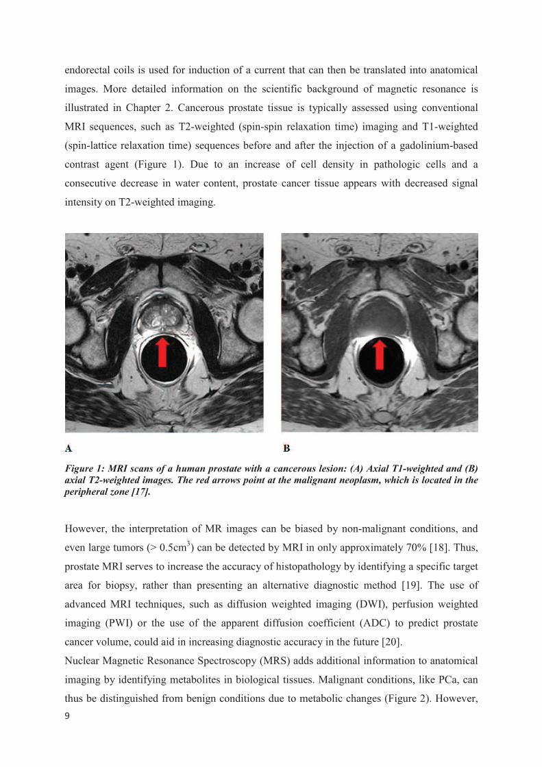
illustrated in Chapter 2. Cancerous prostate tissue is typically assessed using conventional

MRI sequences, such as T2-weighted (spin-spin relaxation time) imaging and T1-weighted

(spin-lattice relaxation time) sequences before and after the injection of a gadolinium-based

contrast agent (Figure 1). Due to an increase of cell density in pathologic cells and a

consecutive decrease in water content, prostate cancer tissue appears with decreased signal

intensity on T2-weighted imaging.

Figure 1: MRI scans of a human prostate with a cancerous lesion: (A) Axial T1-weighted and (B)

axial T2-weighted images. The red arrows point at the malignant neoplasm, which is located in the

peripheral zone [17].

However, the interpretation of MR images can be biased by non-malignant conditions, and

even large tumors (> 0.5cm3) can be detected by MRI in only approximately 70% [18]. Thus,

prostate MRI serves to increase the accuracy of histopathology by identifying a specific target

area for biopsy, rather than presenting an alternative diagnostic method [19]. The use of

advanced MRI techniques, such as diffusion weighted imaging (DWI), perfusion weighted

imaging (PWI) or the use of the apparent diffusion coefficient (ADC) to predict prostate

cancer volume, could aid in increasing diagnostic accuracy in the future [20].

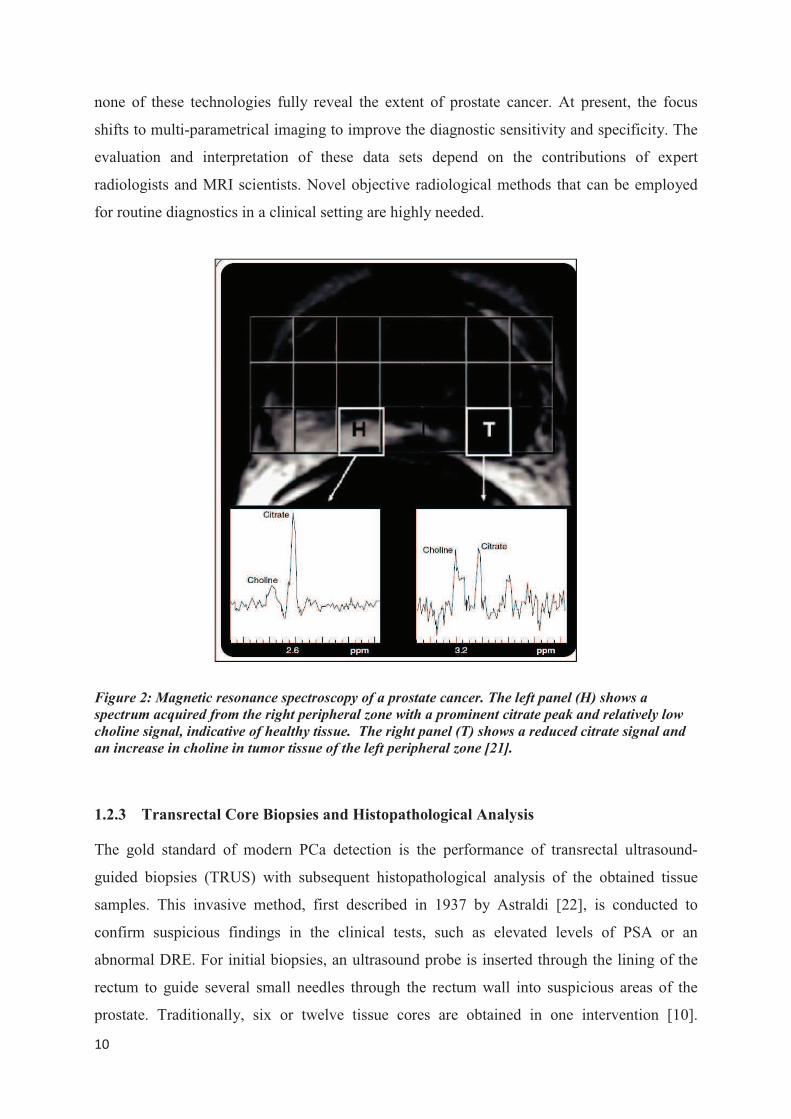
Nuclear Magnetic Resonance Spectroscopy (MRS) adds additional information to anatomical

imaging by identifying metabolites in biological tissues. Malignant conditions, like PCa, can

thus be distinguished from benign conditions due to metabolic changes (Figure 2). However,

���

�

none of these technologies fully reveal the extent of prostate cancer. At present, the focus

shifts to multi-parametrical imaging to improve the diagnostic sensitivity and specificity. The

evaluation and interpretation of these data sets depend on the contributions of expert

radiologists and MRI scientists. Novel objective radiological methods that can be employed

for routine diagnostics in a clinical setting are highly needed.

Figure 2: Magnetic resonance spectroscopy of a prostate cancer. The left panel (H) shows a

spectrum acquired from the right peripheral zone with a prominent citrate peak and relatively low

choline signal, indicative of healthy tissue. The right panel (T) shows a reduced citrate signal and

an increase in choline in tumor tissue of the left peripheral zone [21].

1.2.3 Transrectal Core Biopsies and Histopathological Analysis

The gold standard of modern PCa detection is the performance of transrectal ultrasound-

guided biopsies (TRUS) with subsequent histopathological analysis of the obtained tissue

samples. This invasive method, first described in 1937 by Astraldi [22], is conducted to

confirm suspicious findings in the clinical tests, such as elevated levels of PSA or an

abnormal DRE. For initial biopsies, an ultrasound probe is inserted through the lining of the

rectum to guide several small needles through the rectum wall into suspicious areas of the

prostate. Traditionally, six or twelve tissue cores are obtained in one intervention [10].

���

�

Unfortunately, this method shows low sensitivity, a high sampling error and high false-

negative rates, detecting PCa in only 22-34% of the initial biopsy [23, 24]. For the

histopathological evaluation of core biopsies, the GLEASON score is used and will be further

described in the subsequent section.

1.2.4 Histopathological Grading of Prostate Cancer: GLEASON Score

The GLEASON score describes a histopathological grading system developed by Donald

Gleason, which is used in prostate cancer staging, to determine prognosis and guide

therapy[25]. Based on tissue obtained from prostate biopsies or prostatectomies, histological

grades are assigned to the most common and second most common patterns that appear in the

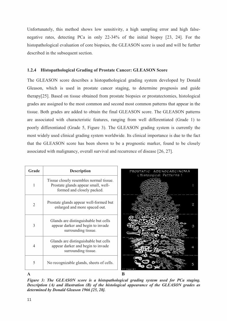
tissue. Both grades are added to obtain the final GLEASON score. The GLEASON patterns

are associated with characteristic features, ranging from well differentiated (Grade 1) to

poorly differentiated (Grade 5, Figure 3). The GLEASON grading system is currently the

most widely used clinical grading system worldwide. Its clinical importance is due to the fact

that the GLEASON score has been shown to be a prognostic marker, found to be closely

associated with malignancy, overall survival and recurrence of disease [26, 27].

A B

Figure 3: The GLEASON score is a histopathological grading system used for PCa staging.

Description (A) and illustration (B) of the histological appearance of the GLEASON grades as

determined by Donald Gleason 1966 [25, 28].

Grade Description

1 Tissue closely resembles normal tissue.

Prostate glands appear small, well-formed and closely packed.

2 Prostate glands appear well-formed but

enlarged and more spaced out.

3 Glands are distinguishable but cells appear darker and begin to invade

surrounding tissue.

4 Glands are distinguishable but cells appear darker and begin to invade

surrounding tissue.

5 No recognizable glands, sheets of cells.

���

�

1.3 Challenges and Need for New Approaches in PCa Diagnostic Management

About 158,000 prostatectomy procedures are performed each year in the USA because of

clinical suspicion of PCa [29]. Radical treatment procedures, like prostatectomies, often

result in impotence and /or incontinence of urine, causing enormous impact on the quality of

life for patients [30].

While routine diagnostic methods, most importantly the PSA screening test, have greatly

improved early diagnosis and led to a tremendous increase in early onset of treatment, they

are also responsible for a substantial number of unnecessary interventions in a tumor type that

often exhibits indolent, slow growth. About 67% of the cancers managed with radical

procedures would never have led to the patient’s death and, therefore, would not have

required such a radical treatment [31-33].

None of the currently available diagnostic tools has the potential to accurately distinguish

between highly aggressive and malignant tumors, which require consequent treatment, and

indolent low malignant cases, which can be managed by regular observation without reaching

clinical significance during the patient’s lifetime.

Therefore, new diagnostic methods to determine biological status, malignant potential, and

extent of the disease are urgently needed in order to optimize diagnosis and ultimately

minimize healthcare costs.

“High Resolution Magic Angle Spinning Nuclear Magnetic Resonance Spectroscopy”

(1H HRMAS MRS), a method introduced for intact biological tissue analysis in 1996 [34, 35],

has proven to be a candidate to address the current challenges present in PCa diagnostics [36].

This method measures metabolomic profiles while preserving tissue architecture for

subsequent evaluations of histopathology [37]. To date, metabolomic profiles established by 1H HRMAS MRS have been evaluated and validated using conventional histopathology as the

reference standard. In contrast to conventional histopathology, immunohistochemistry (IHC)

presents an objective and observer-independent diagnostic method [38, 39]. Since IHC has the

potential to provide more objective, accurate and quantitative measures of tissue pathology

than routine histopathology, the present study attempted to establish a novel quantitative and

observer-independent diagnostic approach by exploring the potential of prostate cancer

immunomarkers to quantify metabolomic profiles established by 1H HRMAS MRS.

�

���

�

2 Scientific Background I: Nuclear Magnetic Resonance,1H HRMAS

NMR Spectroscopy and Metabolomic Profiles

2.1 Nuclear Magnetic Resonance

Nuclear magnetic resonance (NMR) describes a physical phenomenon that is based on the

fact that several atomic nuclei have intrinsic magnetic moments and can therefore absorb and

re-emit electromagnetic radiation when placed in a magnetic field.

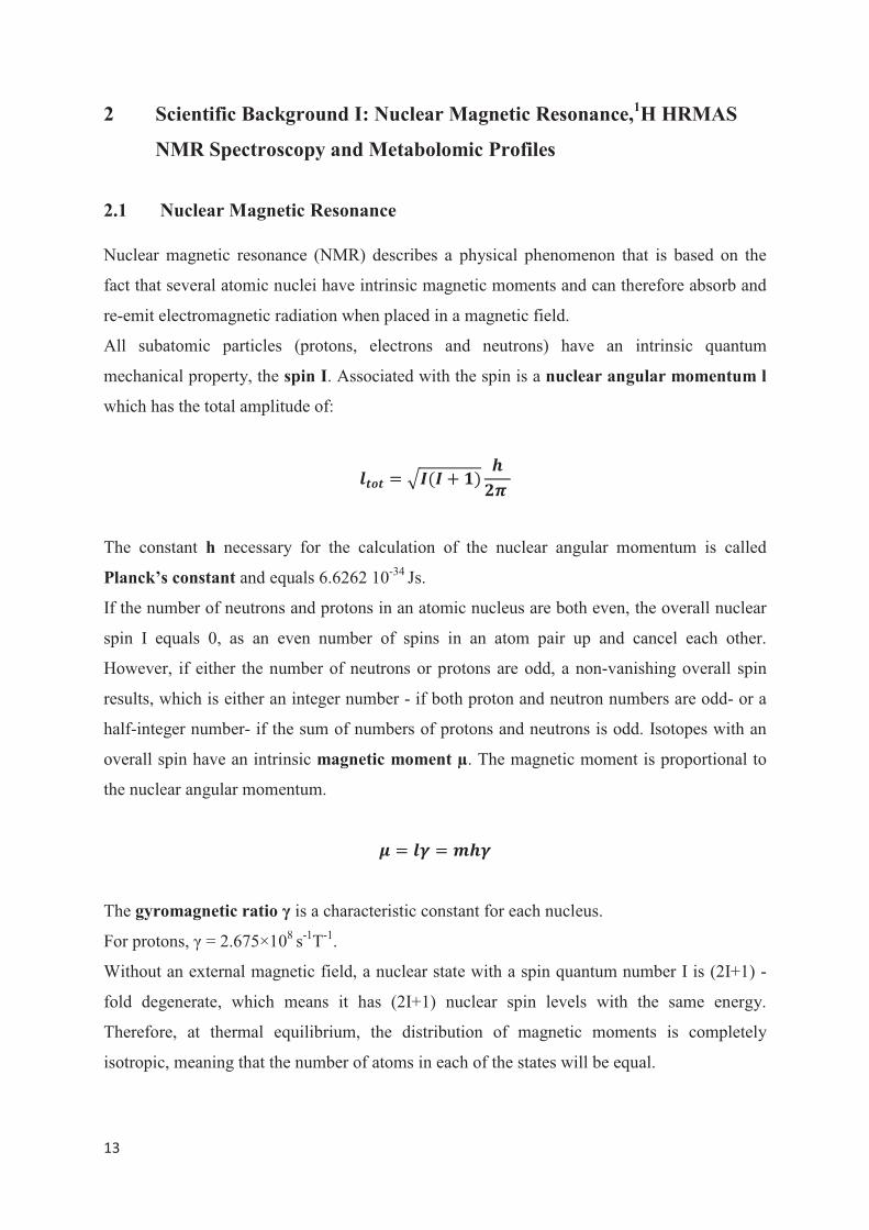
All subatomic particles (protons, electrons and neutrons) have an intrinsic quantum

mechanical property, the spin I. Associated with the spin is a nuclear angular momentum l

which has the total amplitude of:

���� � ���� � ������

The constant h necessary for the calculation of the nuclear angular momentum is called

Planck’s constant and equals 6.6262 10-34 Js.

If the number of neutrons and protons in an atomic nucleus are both even, the overall nuclear

spin I equals 0, as an even number of spins in an atom pair up and cancel each other.

However, if either the number of neutrons or protons are odd, a non-vanishing overall spin

results, which is either an integer number - if both proton and neutron numbers are odd- or a

half-integer number- if the sum of numbers of protons and neutrons is odd. Isotopes with an

overall spin have an intrinsic magnetic moment µ. The magnetic moment is proportional to

the nuclear angular momentum.

� � �� � ���

The gyromagnetic ratio � is a characteristic constant for each nucleus.

For protons, � = 2.675×108 s-1T-1.

Without an external magnetic field, a nuclear state with a spin quantum number I is (2I+1) -

fold degenerate, which means it has (2I+1) nuclear spin levels with the same energy.

Therefore, at thermal equilibrium, the distribution of magnetic moments is completely

isotropic, meaning that the number of atoms in each of the states will be equal.

���

�

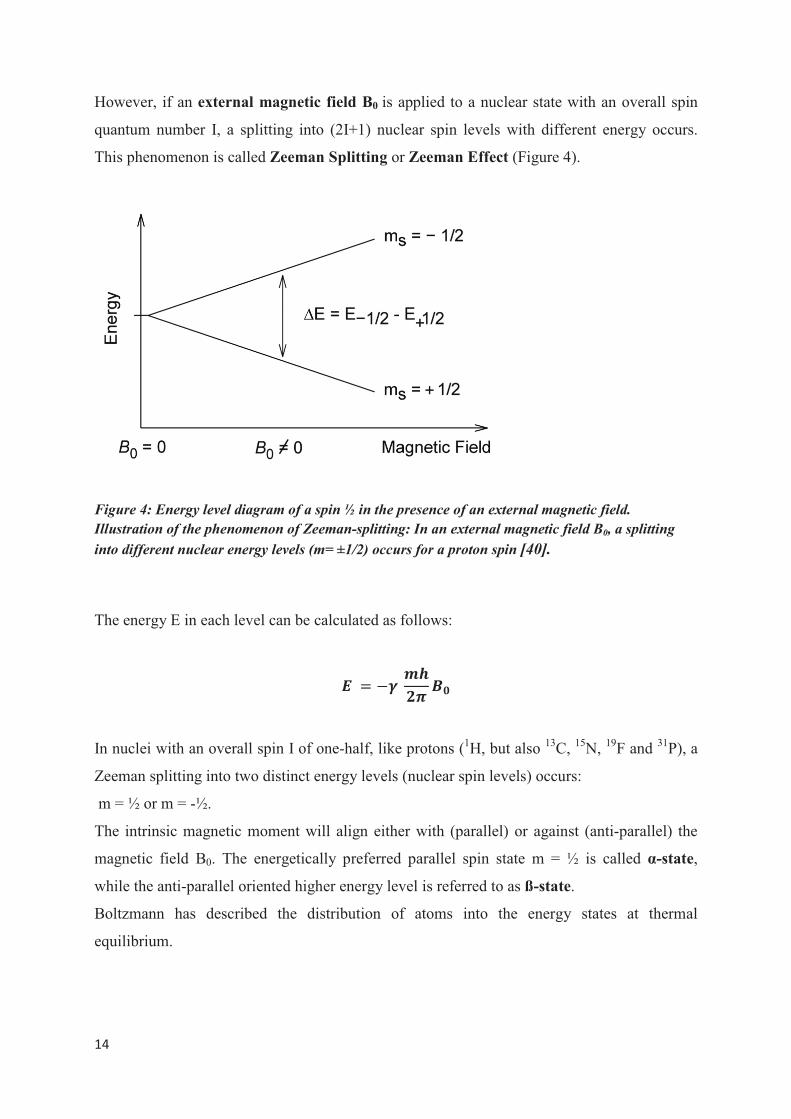
However, if an external magnetic field B0 is applied to a nuclear state with an overall spin

quantum number I, a splitting into (2I+1) nuclear spin levels with different energy occurs.

This phenomenon is called Zeeman Splitting or Zeeman Effect (Figure 4).

Figure 4: Energy level diagram of a spin ½ in the presence of an external magnetic field.

Illustration of the phenomenon of Zeeman-splitting: In an external magnetic field B0, a splitting

into different nuclear energy levels (m= ±1/2) occurs for a proton spin [40].

The energy E in each level can be calculated as follows:

�� � �������

��

In nuclei with an overall spin I of one-half, like protons (1H, but also 13C, 15N, 19F and 31P), a

Zeeman splitting into two distinct energy levels (nuclear spin levels) occurs:

m = ½ or m = -½.

The intrinsic magnetic moment will align either with (parallel) or against (anti-parallel) the

magnetic field B0. The energetically preferred parallel spin state m = ½ is called �-state,

while the anti-parallel oriented higher energy level is referred to as ß-state.

Boltzmann has described the distribution of atoms into the energy states at thermal

equilibrium.

���

�

The number of atoms N1 in the anti-parallel state � and N0 in the parallel state � at a

designated temperature T can be calculated through the Boltzmann distribution equation:

��

��� ����

��������

The Boltzmann constant k equals 1.3806 10-23 J/K.

For positive �, the lower-energy state � is slightly more populated than the higher-energy

level �. The sum of the angular momentums creates a macroscopic magnetization, which is

used in NMR spectroscopy. The differences in the population of the α and β energy levels is

called spin polarization, and represents a necessary requirement for NMR spectroscopy.

Higher �, lower temperature and a greater magnetic field strength B0 contribute to a greater

energy level separation and enhance the sensitivity of the NMR spectra.

2.1.1 Spin Precession

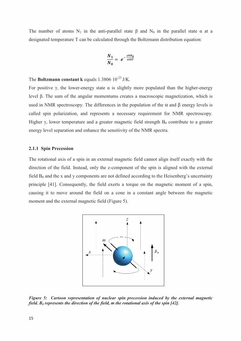
The rotational axis of a spin in an external magnetic field cannot align itself exactly with the

direction of the field. Instead, only the z-component of the spin is aligned with the external

field B0 and the x and y components are not defined according to the Heisenberg’s uncertainty

principle [41]. Consequently, the field exerts a torque on the magnetic moment of a spin,

causing it to move around the field on a cone in a constant angle between the magnetic

moment and the external magnetic field (Figure 5).

Figure 5: Cartoon representation of nuclear spin precession induced by the external magnetic

field. B0 represents the direction of the field, m the rotational axis of the spin [42].

���

�

This motion is called precession and its frequency is referred to as Larmor frequency �0.

�� � �����

2.1.2 Magnetic Resonance

In the presence of a static magnetic field, which produces spin polarization, a radio frequency

field of a proper frequency can induce a transition of a nucleus from the lower energy level to

the higher energy state. This transition, also referred to as “spin flip”, requires absorption of

radio frequency energy. The absorption of energy, called “resonance”, can only occur at a

resonance frequency equal to the Larmor frequency �0. The resonance frequency is directly

proportional to the field strength of the external magnetic field B0. The spectrometer used in

the present study operated at the field strength of 14.1 Tesla, providing a resonance frequency

of 600 MHz.

During an NMR experiment, the excess spins in an orientation parallel to the external

magnetic field give rise to a microscopic magnetization. This magnetization is flipped into the

x-y-plane and due to the rotation, caused by the Larmor frequency, induces a voltage in the

receiver coil, which can then be read off as the NMR signal. This produces a radio frequency

signal that is measured in NMR spectroscopy. During the relaxation process, the transverse

magnetization relaxes back into equilibrium, leading to the characteristic decreasing voltage

in the receiver coil, called free induction decay (FID). Subsequently, a Fourier transformation

produces the NMR spectrum that can then be used for qualitative or quantitative evaluation.

2.1.3 Chemical Shift and J- coupling

The use of NMR spectroscopy in organic chemistry is based on the close relationship between

information that can be obtained through NMR spectra and the molecular structures of the

chemical compounds. Two quantities are measurable in NMR spectroscopy, the “chemical

shift” and “J coupling”. These parameters explain a characteristic change of resonance

frequency of a chemical compound that is the basis for molecular structure analysis. Each

nuclear isotope in a homogenous magnetic field would be expected to provide a single narrow

peak at the Larmor frequency of that field. However, the Larmor frequency of a given nucleus

is influenced by the electronic structure of its atomic environment. Electrons surrounding the

proton in a covalent bond are magnetic. They, therefore, in response to the external magnetic

field, generate a secondary field which shields the nucleus from the external field. Thus,

���

�

different magnetically inequivalent nuclear spins resonate at slightly different field strengths.

This phenomenon is called chemical shift. Chemical shifts are very small compared to the

actual field strength of the external magnetic field and are commonly referred to as parts per

million (ppm). They are displayed in relative units, using a reference compound. Most

commonly, tetramethylsilane (TMS) serves as reference compound; its chemical shift equals

zero by definition. TMS spins have a very strong shielding. Because of that, the vast majority

of chemical compounds have a positive chemical shift when referenced to TMS.

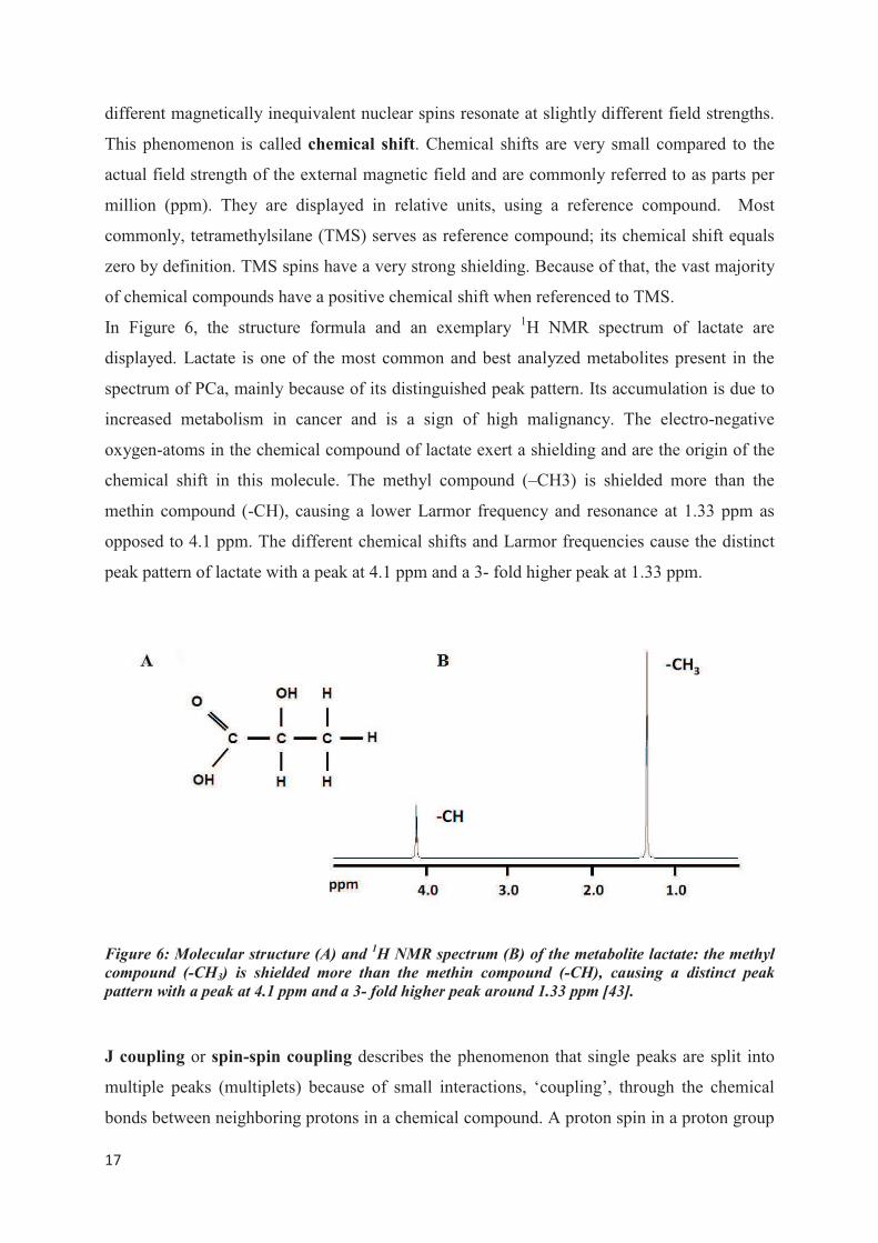
In Figure 6, the structure formula and an exemplary 1H NMR spectrum of lactate are

displayed. Lactate is one of the most common and best analyzed metabolites present in the

spectrum of PCa, mainly because of its distinguished peak pattern. Its accumulation is due to

increased metabolism in cancer and is a sign of high malignancy. The electro-negative

oxygen-atoms in the chemical compound of lactate exert a shielding and are the origin of the

chemical shift in this molecule. The methyl compound (–CH3) is shielded more than the

methin compound (-CH), causing a lower Larmor frequency and resonance at 1.33 ppm as

opposed to 4.1 ppm. The different chemical shifts and Larmor frequencies cause the distinct

peak pattern of lactate with a peak at 4.1 ppm and a 3- fold higher peak at 1.33 ppm.

Figure 6: Molecular structure (A) and 1H NMR spectrum (B) of the metabolite lactate: the methyl

compound (-CH3) is shielded more than the methin compound (-CH), causing a distinct peak

pattern with a peak at 4.1 ppm and a 3- fold higher peak around 1.33 ppm [43].

J coupling or spin-spin coupling describes the phenomenon that single peaks are split into

multiple peaks (multiplets) because of small interactions, ‘coupling’, through the chemical

bonds between neighboring protons in a chemical compound. A proton spin in a proton group

���

�

in the chemical compound can have two possible orientations, either aligned or opposed to an

applied magnetic field. Opposed spins have the effect of altering the magnetic field

experienced by the neighboring protons. Therefore, a single peak is split into two peaks by

one single coupling proton. In case of a greater number of coupled equivalent protons in a

neighboring group, the variety of spin direction combinations increases. Hence, two coupling

protons result in a triplet peak with an intensity ratio of 1:2:1, as there is only one spin

combination of the two spins causing an upfield and a downfield shift, whereas there are two

ways of generating the inner peak, characterized by no shift. Coupling to three protons results

in eight possible spin combinations and produces a quartet split with an intensity ratio of

1:3:3:1. In general, if a nuclear spin is coupled to n equivalent spins of one-half, its peak is

split into an (n+1)- fold multiplet with an amplitude ratio proportional to the binomial

coefficients nCr (r = 0, 1, …, n). The spacing between the peaks of a multiplet is always

constant, characterized by the coupling constant J, which is independent of the applied

magnetic field. Therefore, a multiplet can always be recognized by its closely spaced

chemical shift peaks. Equivalent nuclei (spins of a distinct proton group with equivalent

binding characteristics) do not interact with each other and do not cause a splitting. Below in

Figure 7, the characteristic structure of the lactate NMR spectrum is demonstrated. The proton

of the methin-compound (-CH) is coupling to the methyl-compound (-CH3). It therefore splits

into a quartet peak with an amplitude ratio of 1:3:3:1. The lactate methyl peak is split into a

double peak by coupling to the methin compounds.

Figure 7: Illustration of scalar coupling of NMR lines of lactate: (A) Splitting of the methin peak

into a quartet with intensity ratio of 1:3:3:1 by coupling with the methyl group, (B) splitting of the

methyl peak into a doublet with an intensity ratio of 1:1 (B) [43].

���

�

2.2 Nuclear Magnetic Resonance Spectroscopy

In nuclear magnetic resonance (NMR) spectroscopy, radio-frequency signals emitted by spins

that are transitioning back to their original low-energy state are being displayed in a spectrum,

as a function of their resonance frequency. Peak integrals in the spectrum correlate with the

number of spins in the sample giving rise to this specific signal. Therefore, quantitative

information about the chemical compounds present in a scanned sample can be obtained

through NMR spectroscopy. High field NMR spectrometers have been shown to provide

spectra with a high resolution and a low signal-to-noise-ratio.

2.2.1 Magic Angle Spinning and 1H HRMAS NMR Spectroscopy

“Magic Angle Spinning” (MAS) was first described in 1958 by E. Andrew, A. Bradbury, and

R. Eades [44] and independently in 1959 by I. J. Lowe [45], and is a technique that was

originally developed for solid-state NMR spectroscopy studies.

In NMR of liquid samples, anisotropic interactions between nuclei are usually averaged out

by the isotropic rotational diffusion. In more solid-like structures, such as biological tissues,

the molecules undergo motions in restricted geometries, which give rise to anisotropic effects,

such as dipolar couplings, quadrupolar interactions or chemical shift anisotropy. These effects

result in spectral line broadening, that renders a clear distinction of different metabolites

impossible.

By mechanically rotating (spinning) the sample at an angle of � =54.74° with respect to the

direction of the external magnetic field, the anisotropic interactions can be averaged to zero,

as all anisotropic interaction Hamiltonians are scaled by the factor ½(3cos2�-1). This

procedure mimics the fast isotropic tumbling of the molecules in solution that leads to the

averaging of all anisotropic interactions. The angle of � =54.74° is called the “magic angle”.

Rapid spinning of a sample at the magic angle can reduce the spectral line-broadening and

results in highly resolved spectra (Figure 8). This spectroscopy method is therefore named

“1H High Resolution Magic Angle Spinning Nuclear Magnetic Resonance Spectroscopy”

(1H HRMAS MRS).

���

�

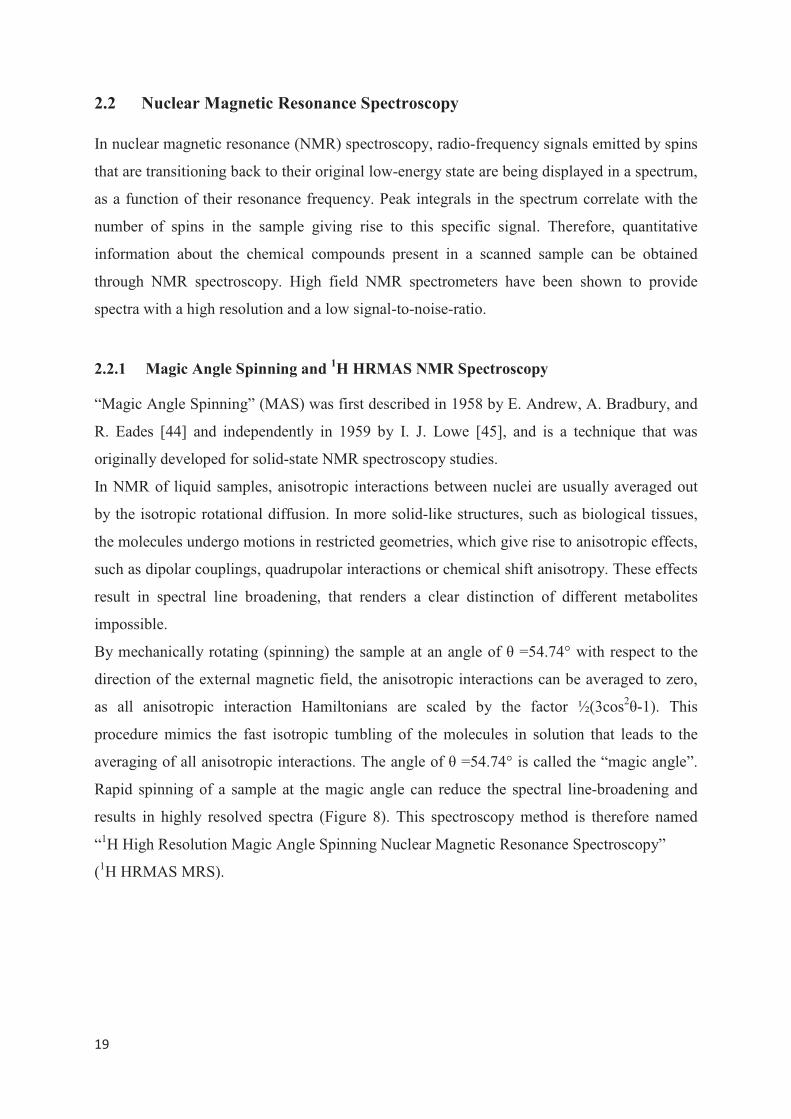
Figure 8: Principle of magic-angle spinning: The sample (blue) is rotated with high frequency

within the external magnetic field (B0). The axis of rotation is tilted by the magic angle �m with

respect to the direction of B0[42].

In 1996, Cheng et al. reported the use of 1H HRMAS MRS on intact human tissue samples for

the first time [34]. They were able to show that using this method on biological tissue

samples, it is possible to omit the destruction of tissue architecture, while at the same time

spectral line-broadening can be minimized and spectral resolution can be increased [46].

Subsequent histopathological analysis can be performed following an 1H HRMAS MRS

experiment to investigate correlations between these biochemical spectra and the pathology of

a sample [47, 48]. Since 1997, multiple studies have been performed in order to improve the

technique of 1H HRMAS MRS and evaluate its clinical applicability. This method has been

shown to be highly reproducible, with the potential to be computer- automated [34, 35, 47,

49,50].

2.2.2 MAS Spinning Rates and Spinning Side Bands

Fast spinning at the magic angle is necessary to average out anisotropic effects and decrease

spectral line broadening. Spinning rates for 1H HRMAS MRS on biological tissues are

commonly around 1 kHz or higher. With the smallest rotors, a spinning rate up to 70kHz and

higher is possible. However, fast spinning increases the risk of destructing tissue architecture.

To preserve a better tissue quality for subsequent pathological evaluation, a reduction of

sample spinning rates has proven to be useful. Spinning rates of 600Hz or 700Hz have been

shown to minimize the destruction of tissue architecture through HRMAS centrifugation

while at the same time providing equally good spectral information as higher spinning rates

[37].

���

�

At slow-rate spinning, single pulse spectra are dominated by a large water peak and its

“spinning sidebands”, originating from the oriented water in the tissue. Spinning sidebands

describe signals that appear as additional peaks in the spectrum on either side of a large

genuine peak. They are caused by the chemical shift anisotropy and appear at distances to the

genuine peak that are multiples of the spinning frequency [51]. In biological tissues, residual

anisotropic interactions are very weak and spinning side bands are typically not observed.

However, if present, special rotor-synchronized suppression methods, like the TOSS pulse

sequence protocol, can be used to effectively suppress spinning sidebands. Also, by applying

a simple minimum function (Min(A, B), described below) on two spectra acquired at different

but close spinning rates ( for example 600Hz and 700Hz), spinning-sideband-free spectra can

be produced [52].

In biological tissues, water is normally three orders of magnitude more abundant than other

metabolites. In order to recover metabolites that overlap the strong baseline of the water

resonance, suppression of the water signal is necessary during the acquisition of NMR

spectra. The elimination of the water signal without losing other resonances is challenging

[53]. Various water suppression protocols have been suggested, among them a DANTE (delay

alternating with nutation for tailored excitation) pulse sequence protocol.

While preventing tissue damage by HRMAS centrifugation, slow-rate spinning has been

shown to be sensitive enough for the purpose of disease diagnosis.

�

���

�

2. 3 Metabolomics, Metabolite Profiles and Clinical Utility

Metabolomics has been defined as the study of the metabolome, which represents “the

complete set of metabolites or low-molecular-weight intermediates, which are context

dependent, varying according to the physiological, developmental or pathological state of the

cell, tissue, organ or organism” [54]. This evolving field of science uses fundamental

analytical techniques to study the global variation of metabolites by examining the underlying

biochemistry of cellular processes. It profiles the metabolites present at the very moment of

analysis. Metabolites can best be described as molecules that are products, reactants,

intermediates or waste products generated during the execution of signals that a cell is

receiving. Thus, each cellular process has its own metabolic signature and the analysis of

metabolite concentrations can be used to create a metabolic profile that may function as a

biomarker for the process [21]. Different techniques can be used to explore the metabolome

and create metabolic profiles, including Mass Spectrometry (MS) and NMR spectroscopy.

While MS is a highly sensitive method that rapidly provides extensive metabolic information,

it requires extensive sample preparation (separation, extraction). NMR, on the other hand, has

the ability to rapidly identify and quantify the majority of metabolites present in a sample,

with only minimal sample preparation. Due to the characteristic chemical shift of a given

chemical compound, the spectral peak pattern is uniquely characteristic for that metabolite,

making it possible to identify and quantify the metabolites present in a sample. The metabolite

concentration can be determined by measuring the area under the associated peaks. Certain

metabolites play a crucial role in the characterization of malignant transformations in the

prostate and can be assessed by using MR spectroscopy. For instance, in healthy prostate

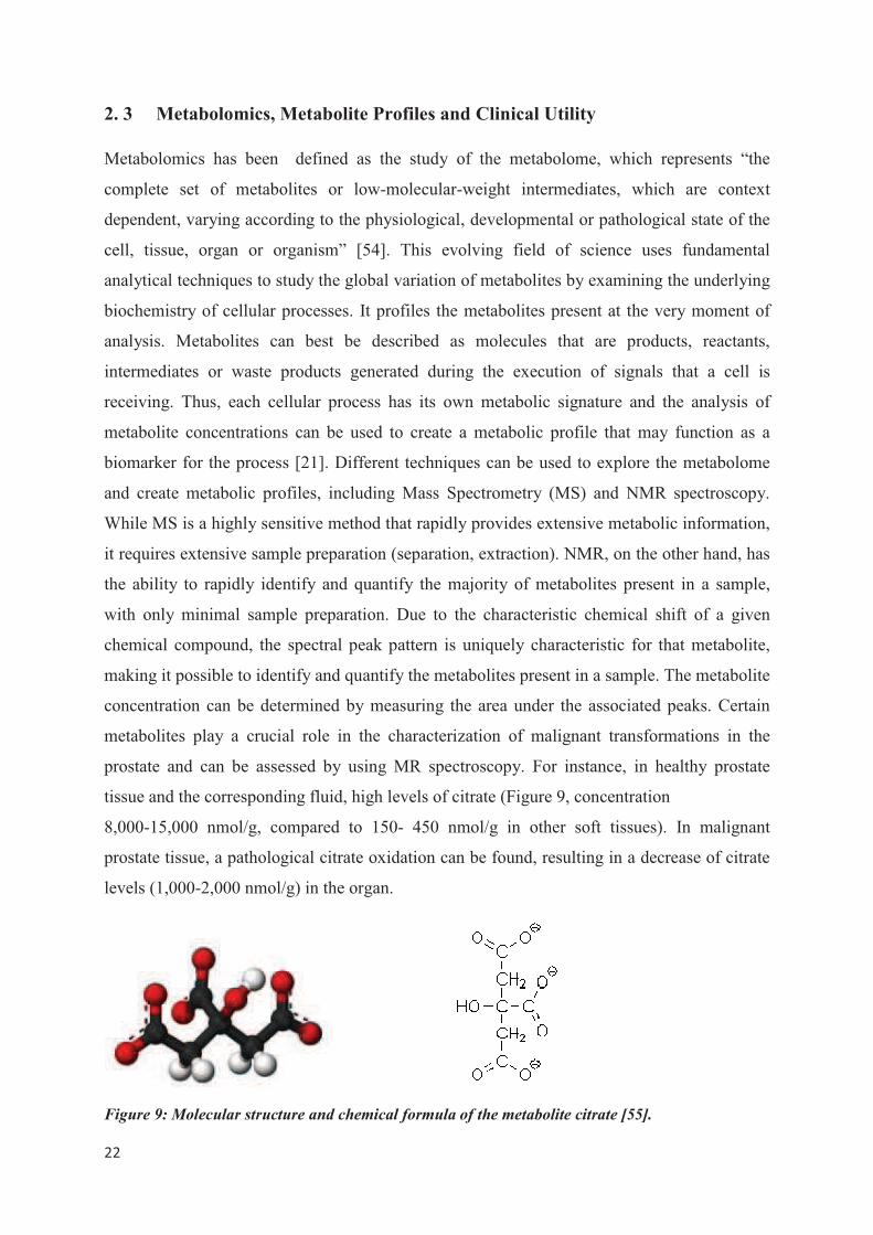
tissue and the corresponding fluid, high levels of citrate (Figure 9, concentration

8,000-15,000 nmol/g, compared to 150- 450 nmol/g in other soft tissues). In malignant

prostate tissue, a pathological citrate oxidation can be found, resulting in a decrease of citrate

levels (1,000-2,000 nmol/g) in the organ.

Figure 9: Molecular structure and chemical formula of the metabolite citrate [55].

���

�

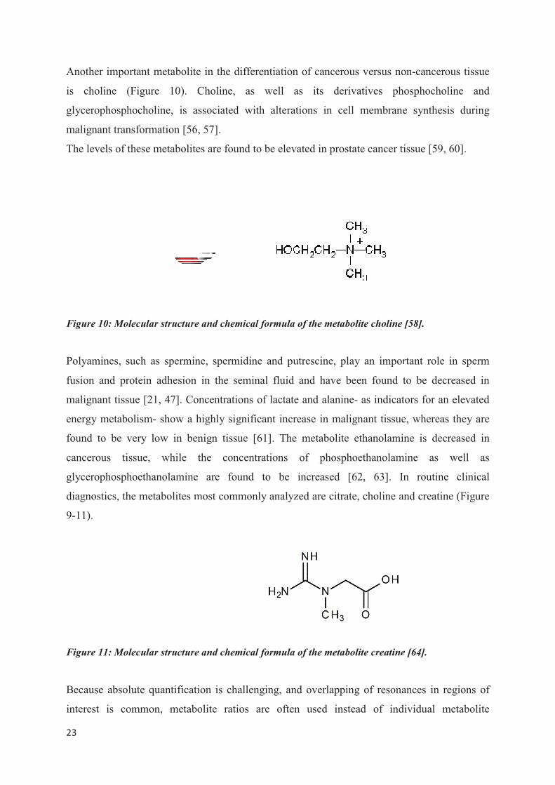
Another important metabolite

is choline (Figure 10). C

glycerophosphocholine, is as

malignant transformation [56,

The levels of these metabolites

Figure 10: Molecular structure

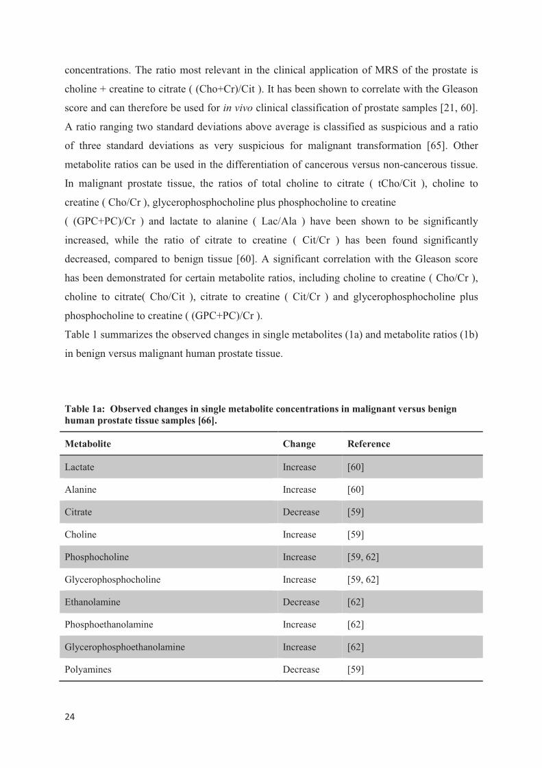
Polyamines, such as spermine

fusion and protein adhesion i

malignant tissue [21, 47]. Con

energy metabolism- show a h

found to be very low in ben

cancerous tissue, while th

glycerophosphoethanolamine

diagnostics, the metabolites m

9-11).

Figure 11: Molecular structure

Because absolute quantificatio

interest is common, metabo

e in the differentiation of cancerous versus no

Choline, as well as its derivatives ph

ssociated with alterations in cell membran

57].

s are found to be elevated in prostate cancer t

and chemical formula of the metabolite choline

e, spermidine and putrescine, play an impor

in the seminal fluid and have been found

ncentrations of lactate and alanine- as indicat

highly significant increase in malignant tissue

nign tissue [61]. The metabolite ethanolami

the concentrations of phosphoethanolam

are found to be increased [62, 63]. I

most commonly analyzed are citrate, choline a

and chemical formula of the metabolite creatine

on is challenging, and overlapping of resona

olite ratios are often used instead of ind

on-cancerous tissue

hosphocholine and

ne synthesis during

tissue [59, 60].

e [58].

ortant role in sperm

to be decreased in

ators for an elevated

e, whereas they are

ine is decreased in

mine as well as

In routine clinical

and creatine (Figure

e [64].

nances in regions of

dividual metabolite

���

�

concentrations. The ratio most relevant in the clinical application of MRS of the prostate is

choline + creatine to citrate ( (Cho+Cr)/Cit ). It has been shown to correlate with the Gleason

score and can therefore be used for in vivo clinical classification of prostate samples [21, 60].

A ratio ranging two standard deviations above average is classified as suspicious and a ratio

of three standard deviations as very suspicious for malignant transformation [65]. Other

metabolite ratios can be used in the differentiation of cancerous versus non-cancerous tissue.

In malignant prostate tissue, the ratios of total choline to citrate ( tCho/Cit ), choline to

creatine ( Cho/Cr ), glycerophosphocholine plus phosphocholine to creatine

( (GPC+PC)/Cr ) and lactate to alanine ( Lac/Ala ) have been shown to be significantly

increased, while the ratio of citrate to creatine ( Cit/Cr ) has been found significantly

decreased, compared to benign tissue [60]. A significant correlation with the Gleason score

has been demonstrated for certain metabolite ratios, including choline to creatine ( Cho/Cr ),

choline to citrate( Cho/Cit ), citrate to creatine ( Cit/Cr ) and glycerophosphocholine plus

phosphocholine to creatine ( (GPC+PC)/Cr ).

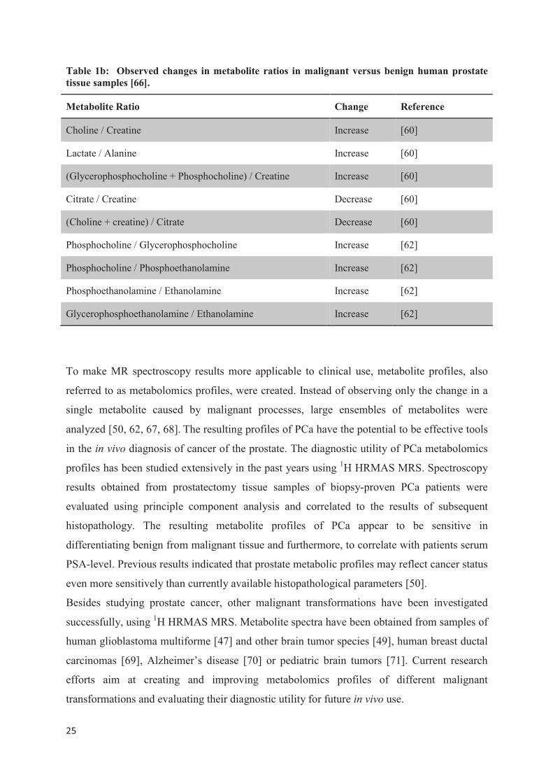
Table 1 summarizes the observed changes in single metabolites (1a) and metabolite ratios (1b)

in benign versus malignant human prostate tissue.

Table 1a: Observed changes in single metabolite concentrations in malignant versus benign

human prostate tissue samples [66].

Metabolite Change Reference

Lactate Increase [60]

Alanine Increase [60]

Citrate Decrease [59]

Choline Increase [59]

Phosphocholine Increase [59, 62]

Glycerophosphocholine Increase [59, 62]

Ethanolamine Decrease [62]

Phosphoethanolamine Increase [62]

Glycerophosphoethanolamine Increase [62]

Polyamines Decrease [59]

���

�

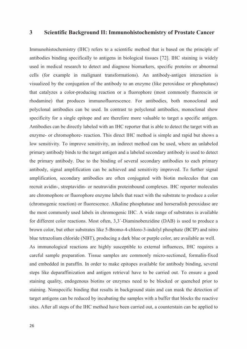
Table 1b: Observed changes in metabolite ratios in malignant versus benign human prostate

tissue samples [66].

Metabolite Ratio Change Reference

Choline / Creatine Increase [60]

Lactate / Alanine Increase [60]

(Glycerophosphocholine + Phosphocholine) / Creatine Increase [60]

Citrate / Creatine Decrease [60]

(Choline + creatine) / Citrate Decrease [60]

Phosphocholine / Glycerophosphocholine Increase [62]

Phosphocholine / Phosphoethanolamine Increase [62]

Phosphoethanolamine / Ethanolamine Increase [62]

Glycerophosphoethanolamine / Ethanolamine Increase [62]

To make MR spectroscopy results more applicable to clinical use, metabolite profiles, also

referred to as metabolomics profiles, were created. Instead of observing only the change in a

single metabolite caused by malignant processes, large ensembles of metabolites were

analyzed [50, 62, 67, 68]��The resulting profiles of PCa have the potential to be effective tools

in the in vivo diagnosis of cancer of the prostate. The diagnostic utility of PCa metabolomics

profiles has been studied extensively in the past years using 1H HRMAS MRS. Spectroscopy

results obtained from prostatectomy tissue samples of biopsy-proven PCa patients were

evaluated using principle component analysis and correlated to the results of subsequent

histopathology. The resulting metabolite profiles of PCa appear to be sensitive in

differentiating benign from malignant tissue and furthermore, to correlate with patients serum

PSA-level. Previous results indicated that prostate metabolic profiles may reflect cancer status

even more sensitively than currently available histopathological parameters [50].

Besides studying prostate cancer, other malignant transformations have been investigated

successfully, using 1H HRMAS MRS. Metabolite spectra have been obtained from samples of

human glioblastoma multiforme [47] and other brain tumor species [49], human breast ductal

carcinomas [69], Alzheimer’s disease [70] or pediatric brain tumors [71]. Current research

efforts aim at creating and improving metabolomics profiles of different malignant

transformations and evaluating their diagnostic utility for future in vivo use.

���

�

3 Scientific Background II: Immunohistochemistry of Prostate Cancer

Immunohistochemistry (IHC) refers to a scientific method that is based on the principle of

antibodies binding specifically to antigens in biological tissues [72]. IHC staining is widely

used in medical research to detect and diagnose biomarkers, specific proteins or abnormal

cells (for example in malignant transformations). An antibody-antigen interaction is

visualized by the conjugation of the antibody to an enzyme (like peroxidase or phosphatase)

that catalyzes a color-producing reaction or a fluorophore (most commonly fluorescin or

rhodamine) that produces immunofluorescence. For antibodies, both monoclonal and

polyclonal antibodies can be used. In contrast to polyclonal antibodies, monoclonal show

specificity for a single epitope and are therefore more valuable to target a specific antigen.

Antibodies can be directly labeled with an IHC reporter that is able to detect the target with an

enzyme- or chromophore- reaction. This direct IHC method is simple and rapid but shows a

low sensitivity. To improve sensitivity, an indirect method can be used, where an unlabeled

primary antibody binds to the target antigen and a labeled secondary antibody is used to detect

the primary antibody. Due to the binding of several secondary antibodies to each primary

antibody, signal amplification can be achieved and sensitivity improved. To further signal

amplification, secondary antibodies are often conjugated with biotin molecules that can

recruit avidin-, streptavidin- or neutravidin proteinbound complexes. IHC reporter molecules

are chromophore or fluorophore enzyme labels that react with the substrate to produce a color

(chromogenic reaction) or fluorescence. Alkaline phosphatase and horseradish peroxidase are

the most commonly used labels in chromogenic IHC. A wide range of substrates is available

for different color reactions. Most often, 3,3`-Diaminobenzidine (DAB) is used to produce a

brown color, but other substrates like 5-Bromo-4-chloro-3-indolyl phosphate (BCIP) and nitro

blue tetrazolium chloride (NBT), producing a dark blue or purple color, are available as well.

As immunological reactions are highly susceptible to external influences, IHC requires a

careful sample preparation. Tissue samples are commonly micro-sectioned, formalin-fixed

and embedded in paraffin. In order to make epitopes available for antibody binding, several

steps like deparaffinization and antigen retrieval have to be carried out. To ensure a good

staining quality, endogenous biotins or enzymes need to be blocked or quenched prior to

staining. Nonspecific binding that results in background stain and can mask the detection of

target antigens can be reduced by incubating the samples with a buffer that blocks the reactive

sites. After all steps of the IHC method have been carried out, a counterstain can be applied to

���

�

provide a contrast that helps to enhance the detection of the primary stain. Common

counterstains include Hematoxylin, 4´,6-diamidino-2-phenylindole (DAPI) or Methyl Green.

Immunohistochemical methods have been proven useful in the diagnosis of different

malignant transformations, including prostate cancer [38, 39,73] and have been increasingly

incorporated in basic diagnosis.

A cytoplasmic protein involved in the beta-oxidation of branched-chain fatty acids, P504S,

also known as AMACR (alpha-methylacyl-CoA racemase), shows high expression in prostate

cancer and a modest expression in benign prostate tissue. It can therefore be used as an

immunomarker to differentiate between cancerous and non-cancerous glands [74-76].

Another protein, CK903, also known as 34-beta-E12 (high molecular weight cytokeratin), is

highly expressed in the cytoplasm of basal cells of healthy prostate glands, whereas it cannot

be found in cancerous tissue. It functions as a marker of benign prostate tissue [77]. The

tumor suppressor protein p63 is a basal cell marker that can be used to stain nuclei of benign

prostate gland epithelium. p63 belongs to the same family of tumor suppressor proteins like

p53 and p73 and has been suspected to be the original family member, with p53 and p73

being derived from it [78]. p63 gene encodes for 2 protein isoforms, one of which (TAp63)

plays an important role in apoptotic function [79]. With the help of p63-antibodies it is

possible to differentiate between prostate adenocarcinoma and benign prostate tissue, as

malignant glands do not have basal cells that could be stained. Also, p63 immunostaining can

be used to differentiate between urothelial cancer (high expression) and PCa (no expression)

in cases where a clinical differentiation seems difficult [80]. By combining IHC stainings of

P504S with those of CK903 and p63, cancerous prostate samples can be differentiated from

both normal prostate tissue and benign lesions. While P504S has a positive expression in both

PCa and Prostate Intraepithelial Neoplasia (PIN), the stainings for both CK903 and p63 are

negative in PCa and positive in PIN, making a differentiation between cancer and PIN

possible. Benign prostate hyperplasia (BPH) is a benign transformation of the prostate. BPH

is a relatively common disease in older men and is not classified as precancerous lesion.

While non-cancerous prostate tissue stains positive for CK903 and p63, BPH does not [81].

Therefore, IHC is a useful tool for the differentiation of cancerous from non-cancerous

conditions, but also malignant from benign transformations or preliminary stages.

Besides using the mentioned immunomarkers separately on suspicious prostate tissue, they

can also be combined as a triple-cocktail-staining with a single- or double chromogen

���

�

reaction, making it possible to obtain immunohistochemical information from the very same

tissue [73, 82].

Compared to conventional histopathologic examinations, IHC has several advantages in the

diagnosis of PCa. Conventional histopathologic analysis of suspicious tissue after prostate

needle biopsy or prostatectomy is commonly carried out using a Hematoxylin & Eosin

staining procedure. Subsequently, the stained tissue slides have to be analyzed by a

pathologist with fundamental knowledge on prostate tissue pathology. In contrast, IHC

provides objective pathology results, based on the fact that staining occurs only in tissue that

expressed the targeted antigens. Using the immunomarkers P504S (AMACR), CK903 and

p63, it is possible to obtain an objective differentiation of tissue pathology in suspicious

prostate tissue. The chromogenic reaction that is part of the visualization in IHC also yields

the opportunity for a computer automated evaluation. DAB produces a dark brown color that

provides a good enough contrast between benign and malignant tissue. A specifically

designed computer program could be used to measure cancerous and non-cancerous tissue

distribution in a sample through the detection of dark versus light tissue areas. IHC therefore

has the potential to allow objective and fast evaluation of large numbers of tissue samples,

minimizing intra- and inter-observer- variability.

���

�

4 Aims of the Study

Current methods for prostate cancer diagnosis are not satisfying and overdiagnosis and

overtreatment are very common, due to the insufficiency of state-of-the-art diagnostic tools to

accurately distinguish between highly aggressive and malignant cancers and more indolent

cases. Novel, observer-independent and quantitative diagnostic methods for PCa are urgently

needed. This study aims to establish a novel approach for identification of PCa biomarkers, by

quantification of metabolomic profiles measured from prostate tissue by 1H HRMAS MRS.

It has been demonstrated that 1H HRMAS MRS does not destroy the tissue architecture of a

sample, thus allowing for unbiased subsequent histopathological evaluation of a scanned

tissue piece [16, 49]. In previous studies of prostate cancer metabolomics, conventional

histopathology was commonly used as reference standard [16], due to its facile utility and

broad clinical applicability. Immunohistochemistry, in contrast, presents a more accurate and

objective diagnostical method than conventional histopathology, and yields the potential to be

computer automated. Therefore, this study aims to explore the potential of three prostate

immunomarkers- P504S (Alpha-Methylacyl-CoA-Racemace), CK903 (high-molecular weight

cytokeratin) and p63- as tools for quantitative analysis of immunohistochemistry performed

on the same tissue samples.

To achieve this aim, a quantitative IHC analysis program was developed to automatically and

objectively determine the percentage of cancerous and benign glands in a prostate tissue

sample. Additionally, this project aims to confirm the validity of the presented approach by

using a conventional histopathological evaluation and a quantitative IHC analysis performed

by an experienced pathologist. This study aims to use these quantitative measures of tissue

pathology obtained from IHC to identify PCa biomarkers in a metabolomic profile measured

with 1H HRMAS MRS in the same sample. For that, correlations of spectral intensities with

the results of quantitative IHC analysis will be examined.

In an attempt to explore the stability and utility of the proposed immunomarkers for use

following 1H HRMAS MRS, the presented project aims to compare the quality and

evaluability of immunostainings of tissue sections that have been subjected to 1H HRMAS

MRS to samples from the same prostate that have not undergone spectroscopic procedures, in

a subset of the sample cohort.

To further explore the potential of our novel approach, this study aims to investigate the

utility of it to identify metabolomic biomarkers of PCa recurrence. For that, patient outcomes

���

�

and recurrence five years after initial diagnosis will be obtained and correlated to the results

of 1H HRMAS MRS to identify metabolomic markers of recurrence in the dataset.

���

�

5 Material and Methods

Tissue acquisition, medical record review and all experiments performed in this study were

approved by the Institutional Review Board (IRB) of the Massachusetts General Hospital

(MGH) and in accordance with the Health Insurance Portability and Accountability Act

(HIPAA).

5.1 Prostate Tissue Samples and Patient Demographics

Human prostate tissue specimens were prospectively collected from 51 biopsy-proven PCa

patients who underwent prostatectomy surgery at the Department of Urology at the MGH in

Boston, between January of 2007 and December of 2008. The tissue samples were collected

from the operating suite, instantly frozen and stored at a temperature of -80°Celsius prior to

the experiments.

The patient medical records were reviewed to determine important demographic information,

including: patient’s age at surgery, pre-operative PSA-levels, final histopathological

diagnosis, including GLEASON grades, and adjuvant treatment, if administered (defined as

any additional treatment in a time-period of less than 6 months before or after surgery).

5.2 1H HRMAS NMR Spectroscopy

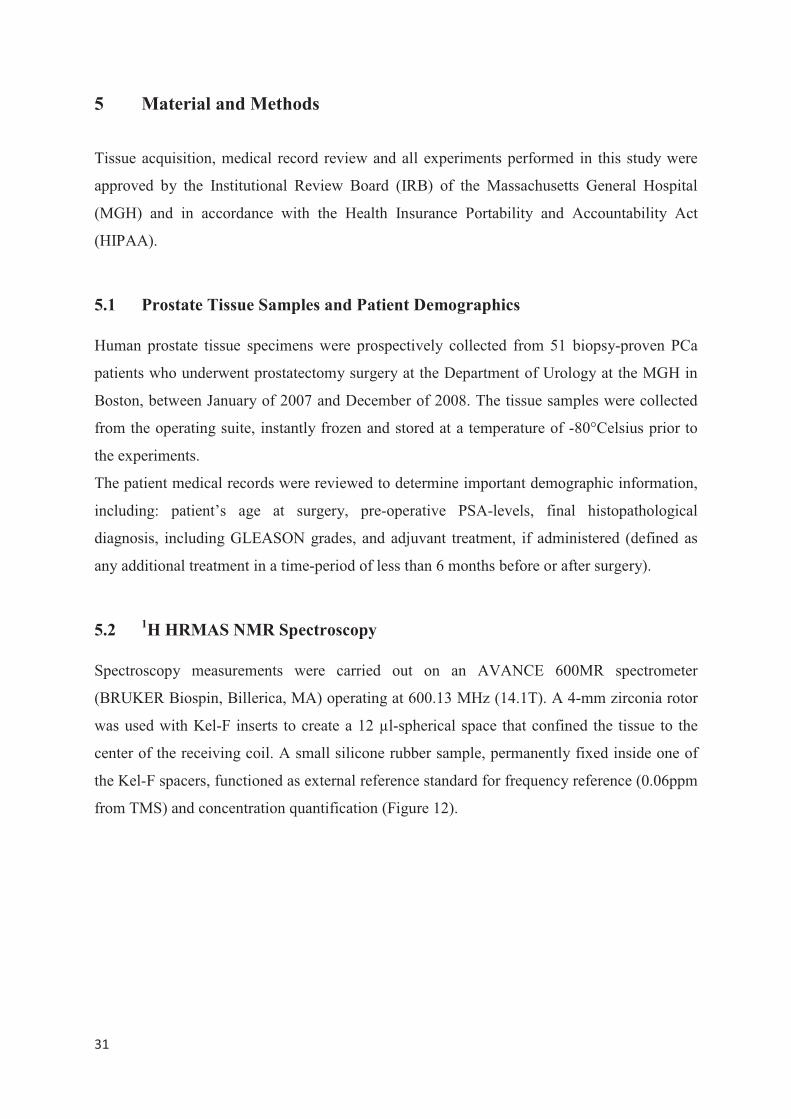
Spectroscopy measurements were carried out on an AVANCE 600MR spectrometer

(BRUKER Biospin, Billerica, MA) operating at 600.13 MHz (14.1T). A 4-mm zirconia rotor

was used with Kel-F inserts to create a 12 µl-spherical space that confined the tissue to the

center of the receiving coil. A small silicone rubber sample, permanently fixed inside one of

the Kel-F spacers, functioned as external reference standard for frequency reference (0.06ppm

from TMS) and concentration quantification (Figure 12).

���

�

Figure 12: BRUKER Biospin

Biomedical Imaging”, Massachu

5.2.1 Sample Preparation

The sample preparation was p

the spectrometer. The prostate

(-80 degrees Celsius). To p

specimens were stored on dr

(approximately 10mg) was cu

carefully placed into the rotor

micro weight scale. Dependin

D2O were added for 2H field l

marked at the bottom with a pe

5.2.2 Spectroscopy Scan

After adjusting the magic angl

tissue preservation, with the re

phase adjustments as well as s

was regulated by a MAS contr

spinning frequencies of 600H

AVANCE III 600MHz spectrometer at the “M

usetts General Hospital / Harvard Medical Scho

performed at room temperature in a preparati

e tissue samples were collected from the stora

prevent tissue destruction during the prepa

dry ice at all times during handling. A sm

ut from each sample, using a scalpel with a

r. The weight of the sample in the rotor was

ng on the total weight of the tissue piece, bet

locking. The rotor was carefully closed with

ermanent marker, and placed into the probe.

gle, MR spectra were recorded at a temperatu

resonance frequency centered on the water re

shimming were performed if necessary. The

trolling interface. Water suppressed spectra w

Hz and 700Hz. A rotor synchronized DANTE

Martinos Center for

ool, Boston

ion area adjacent to

age freezer

aration process, the

mall piece of tissue

a blade size 10, and

as measured using a

etween 2 and 8µl of

h a screw and a cap,

ure of 4°C for better

esonance. Lock and

e rotor-spinning rate

were recorded using

E (delay alternating

���

�

with nutation for tailored excitation) pulse sequence (1000 DANTE pulses of 1.5µs, 8.4° flip

angle) [37] for water suppression was used in combination with a Carr-Purcell-Meiboom-Gill

(CPMG) pulse sequence at short TE (30ms). A repetition time of 5s and an average 32

transients were used.

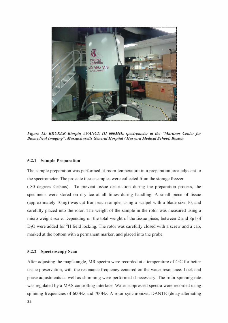
The CPMG pulse starts with a 90° pulse which flips the magnetization in the x-y-plane. Then,

during the decay that follows, some spins slow down due to lower local field strength, while

others speed up. T2* decay refers to an exponential decrease in signal strength compared to

T2 decay, due to inhomogeneity of the magnet. In the CPMG pulse sequence, a series of 180°

pulses is applied, which make it possible to refocus the T2* signal and remove inhomogeneity

effects in order to correct pulse-accuracy errors (Figure 13).

Figure 13: Carr-Purcell-Meiboom-Gill pulse sequence (echo train acquisition): after an initial 90°

pulse, multiple 180°pulses are applied to refocus inhomogenous line broadening of the nuclear

spins. This technique is used to self-correct accuracy errors in T2- (spin-spin relaxation) weighted

imaging [83].

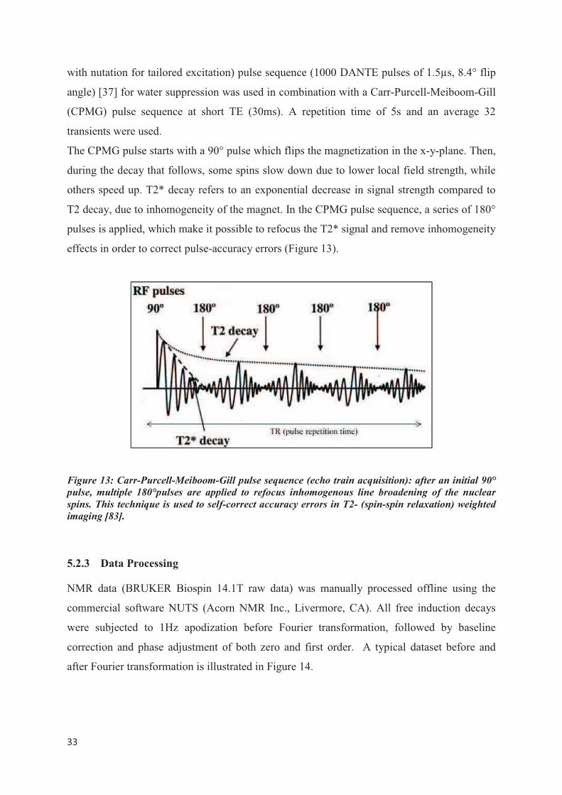
5.2.3 Data Processing

NMR data (BRUKER Biospin 14.1T raw data) was manually processed offline using the

commercial software NUTS (Acorn NMR Inc., Livermore, CA). All free induction decays

were subjected to 1Hz apodization before Fourier transformation, followed by baseline

correction and phase adjustment of both zero and first order. A typical dataset before and

after Fourier transformation is illustrated in Figure 14.

���

�

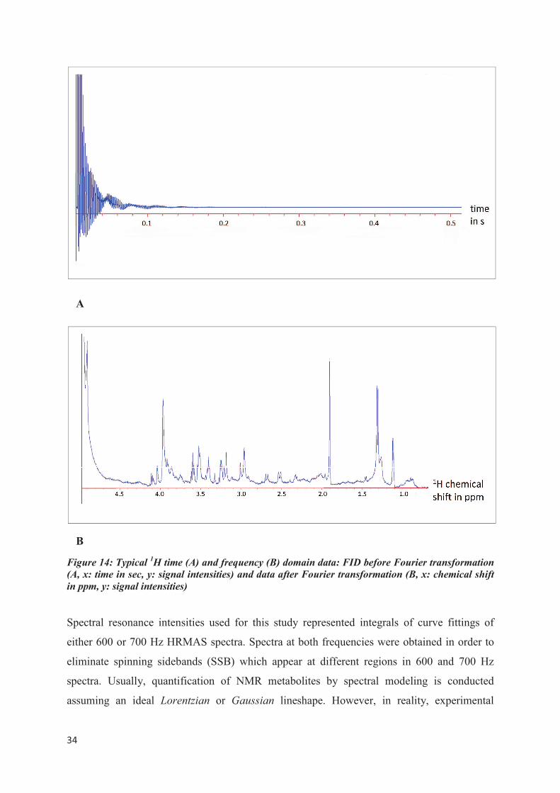
B

Figure 14: Typical 1H time (A) and frequency (B) domain data: FID before Fourier transformation

(A, x: time in sec, y: signal intensities) and data after Fourier transformation (B, x: chemical shift

in ppm, y: signal intensities)

Spectral resonance intensities used for this study represented integrals of curve fittings of

either 600 or 700 Hz HRMAS spectra. Spectra at both frequencies were obtained in order to

eliminate spinning sidebands (SSB) which appear at different regions in 600 and 700 Hz

spectra. Usually, quantification of NMR metabolites by spectral modeling is conducted

assuming an ideal Lorentzian or Gaussian lineshape. However, in reality, experimental

A

���

�

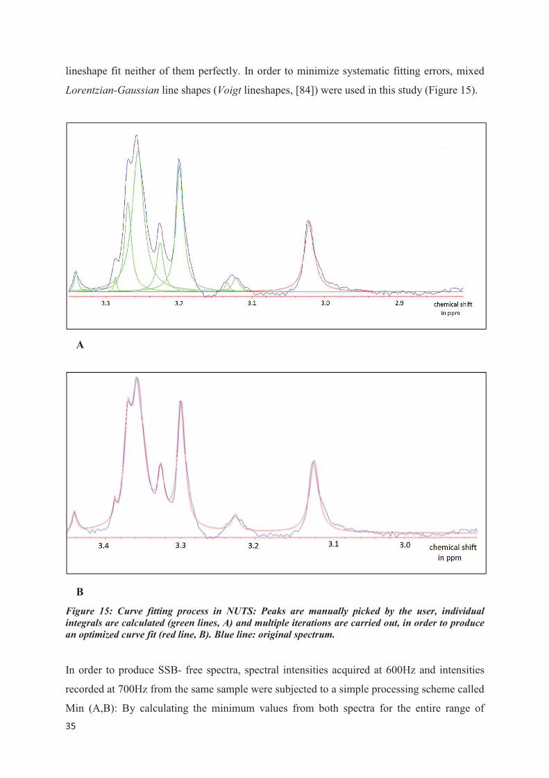
lineshape fit neither of them perfectly. In order to minimize systematic fitting errors, mixed

Lorentzian-Gaussian line shapes (Voigt lineshapes, [84]) were used in this study (Figure 15).

Figure 15: Curve fitting process in NUTS: Peaks are manually picked by the user, individual

integrals are calculated (green lines, A) and multiple iterations are carried out, in order to produce

an optimized curve fit (red line, B). Blue line: original spectrum.

In order to produce SSB- free spectra, spectral intensities acquired at 600Hz and intensities

recorded at 700Hz from the same sample were subjected to a simple processing scheme called

Min (A,B): By calculating the minimum values from both spectra for the entire range of

A

B

���

�

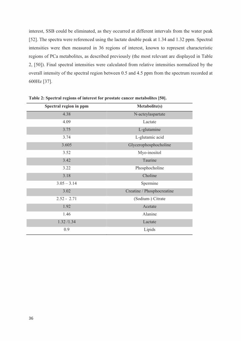
interest, SSB could be eliminated, as they occurred at different intervals from the water peak

[52]. The spectra were referenced using the lactate double peak at 1.34 and 1.32 ppm. Spectral

intensities were then measured in 36 regions of interest, known to represent characteristic

regions of PCa metabolites, as described previously (the most relevant are displayed in Table

2, [50]). Final spectral intensities were calculated from relative intensities normalized by the

overall intensity of the spectral region between 0.5 and 4.5 ppm from the spectrum recorded at

600Hz [37].

Table 2: Spectral regions of interest for prostate cancer metabolites [50].

Spectral region in ppm Metabolite(s)

4.38 N-acteylaspartate

4.09 Lactate

3.75 L-glutamine

3.74 L-glutamic acid

3.605 Glycerophosphocholine

3.52 Myo-inositol

3.42 Taurine

3.22 Phosphocholine

3.18 Choline

3.05 – 3.14 Spermine

3.02 Creatine / Phosphocreatine

2.52 - 2.71 (Sodium-) Citrate

1.92 Acetate

1.46 Alanine

1.32 /1.34 Lactate

0.9 Lipids

���

�

5.3 Immunohistochemistry

5.3.1 Immunohistochemistry Material and Equipment

The immunomarkers P504S, CK903 and p63 were chosen for this study, as their specificity

and utility as well as their clinical applicability have been demonstrated multiple times in the

literature [73, 82, 85]. As primary antibodies, rabbit monoclonal anti-human AMACR

(P504S), mouse monoclonal anti-human CK903 and mouse monoclonal anti-human p63 were

used. Biotinylated anti-rabbit IgG and biotinylated anti-mouse IgG were applied as secondary

antibodies. For the visualization of the immune reaction, a single color reaction was

performed, using 3,3`-Diaminobenzidine (DAB). DAB was chosen for visualization, because

of its characteristic dark brown color, which facilitates qualitative evaluation and furthermore,

yields the potential for computer- automated quantitative evaluation. A summary of all

materials and chemicals used for IHC can be found in Table 3.

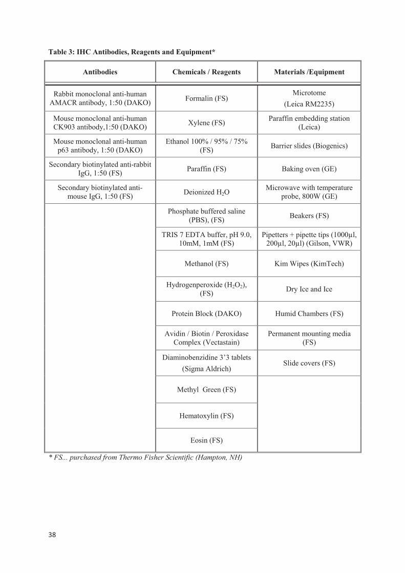
5.3.2. Immunohistochemistry Protocol

An IHC staining protocol was established in our laboratory according to antibody/reagent

specifications. Effectiveness and specificity experiments were carried out using confirmed

PCa tissue as positive control. Different incubation times and antibody dilutions were tested

to identify the best possible staining conditions. The following IHC protocol illustrates the

optimized algorithm for the immunostaining experiments in this study.

���

�

Table 3: IHC Antibodies, Reagents and Equipment*

Antibodies Chemicals / Reagents Materials /Equipment

Rabbit monoclonal anti-human AMACR antibody, 1:50 (DAKO)

Formalin (FS) Microtome

(Leica RM2235)

Mouse monoclonal anti-human CK903 antibody,1:50 (DAKO)

Xylene (FS) Paraffin embedding station

(Leica)

Mouse monoclonal anti-human p63 antibody, 1:50 (DAKO)

Ethanol 100% / 95% / 75% (FS)

Barrier slides (Biogenics)

Secondary biotinylated anti-rabbit IgG, 1:50 (FS)

Paraffin (FS) Baking oven (GE)

Secondary biotinylated anti-mouse IgG, 1:50 (FS)

Deionized H2O Microwave with temperature

probe, 800W (GE)

Phosphate buffered saline (PBS), (FS)

Beakers (FS)

TRIS 7 EDTA buffer, pH 9.0, 10mM, 1mM (FS)

Pipetters + pipette tips (1000µl, 200µl, 20µl) (Gilson, VWR)

Methanol (FS) Kim Wipes (KimTech)

Hydrogenperoxide (H2O2), (FS)

Dry Ice and Ice

Protein Block (DAKO) Humid Chambers (FS)

Avidin / Biotin / Peroxidase Complex (Vectastain)

Permanent mounting media (FS)

Diaminobenzidine 3’3 tablets

(Sigma Aldrich) Slide covers (FS)

Methyl Green (FS)

Hematoxylin (FS)

Eosin (FS)

* FS... purchased from Thermo Fisher Scientific (Hampton, NH)

���

�

5.3.2.1 Sample Preparation

After completion of NMR spectroscopy, the prostate tissue samples were removed from the

rotor, fixed in a formalin bath overnight and embedded in paraffin. Small tissue sections

(5µm) were cut using a microtome and transferred instantly on barrier glass slides.

The slides had to be baked at a temperature of 60°C for 2 hours, in order to insure tissue

adherence. They were then deparaffinized and rehydrated according to the following steps:

- Xylene 3 x 5 min

- Ethanol 100% 2 x 5 min

- Ethanol 95% 1 x 5 min

- Ethanol 70% 1 x 5 min

- Deionized H2O 2 x 5 min

To ensure hydration and prevent tissue sections from drying out, slides were either incubated

with a target solution or kept in a buffer solution at all times. Three adjacent slides were used

for immunostaining with the designated primary antibodies. A fourth adjacent slide was left

for staining with Hematoxylin & Eosin (see section Qualitative Histopathology).

5. 3.2.2 Antigen Retrieval, Quenching of Endogenous Peroxidases and Protein Block

To improve the demonstration of antigens, an antigen retrieval step was required prior to the

application of the primary antibodies. During formalin-fixation, methylene bridges are formed

that cross-link proteins, therefore masking antigenic sites. Antigen retrieval, a method

discovered in the early 1990`s [86] is a non-enzymatic pretreatment to break down these

protein-cross links, thereby uncovering hidden epitopes [87, 88]. The technique most

commonly used is called “Heat Induced Epitope Retrieval (HIER)”. Formalin-fixed, paraffin-

embedded tissue slides are heated in a specific antigen retrieval solution for a designated time.

Microwave, steamer, autoclave or water bath serve as suitable heating devices. Citrate buffer

(pH 6.0) and TRIS/EDTA (pH 9.0) or EDTA (pH 8.0) buffer solutions are suitable for most

antigens [89]. An alternative approach for unmasking antigenic sites is “Proteolytic Induced

Epitope Retrieval (PIER)” which uses enzyme digestion. Effective reagents include proteinase

K, trypsin, chymotrypsin, pepsin and other proteases. The enzymatic method tends to be much

gentler, but sometimes may destroy tissue morphology [90].

Heat induced epitope retrieval using TRIS/EDTA buffer solution (pH 9.0,10mM/1mM) for

P504S (AMACR) and citrate buffer (pH 6.0, 0.1M) for CK903 and p63 respectively were

���

�

identified as suitable antigen retrieval solutions for this study in preliminary experiments.

Deparaffinized and rehydrated tissue slides had to be immersed into the determined retrieval

solutions and heated in a commercial microwave (800W, 199°C) for 30 minutes. Afterwards,

the slides had to cool down in a tap water bath for 15 minutes.

Endogenous peroxidase activity in cells or tissue sections used for IHC may cause high, non-

specific background staining, due to catalyzation of chromogenic or chemiluminescent

substrates. To improve the staining quality in this study, the non-specific background staining

was reduced by quenching (irreversible inactivation) of endogenous peroxidases. For that,

tissue slides were immersed into deionized H2O and PBS for 5 minutes each. Then, 3% H2O2

in methanol was applied to sections for 10 minutes. Slides were washed in deionized H2O

again for 5 minutes.

To enhance the detection of a target antigen in IHC procedures, an Avidin-Biotin-Complex

(ABC) has been proven useful. Biotin, a coenzyme in many biological reactions, has a strong

binding affinity with avidin and can thus be conjugated to antibodies for labeling purposes.

However, free or labeled avidin not only binds to conjugated biotin but also to endogenous

biotin, thus causing high background staining in tissues rich in endogenous biotin [91].

Therefore, a biotin block (protein block step) is necessary to ensure good staining quality.

Protein blocking was performed using a commercially available protein block solution. As

protein block is highly susceptible to high temperatures, the block solution had to be stored on

ice during use and kept refrigerated. Tissue slides were incubated with the protein block

solution in a closed humid chamber for 10 minutes at room temperature. The solution was

shaken off after the incubation.

5.3.2. 3 Antibody Application

During the entire immunostaining process, all antibodies had to be stored on ice to prevent

destruction. Three adjacent tissue slides were incubated for 75 minutes with the primary

antibodies (200µl). Following the primary incubation, the liquids were tapped off, slides were

rinsed and then buffer washed with PBS for 5 minutes. The next incubation step involved

staining with biotinylated secondary antibodies for 30 minutes. The third incubation step, an

Avidin-/Biotin-/Peroxidase- complex (ABC) was applied to all three slides for 30 minutes

5.3.2.4 Visualization and Counterstain

All tissue slides were incubated with 250µl DAB per slide for 10 minutes. For best color

results, the DAB solution had to be prepared 24 hours prior to use and stored in a dark

���

�

environment, as DAB is highly light-sensitive. After DAB-application, the tissue slides were

rinsed in deionized H2O (3x 6 dips) and counterstained with Methyl Green for 2 minutes.

Tissue dehydrationwas performed using the following solutions:

- Ethanol 100% 10 dips

- Ethanol 100% 10 dips

- Ethanol 100% 10 dips

- Xylene 5 min

- Xylene 5 min

All slides were covered with permanent mounting media and slipped with cover slides while

still wet. The slides were left to dry overnight, before they could be examined with a

microscope. Table A1 in the Appendix section summarizes the staining process for the three

antibodies used in this study.

5. 3. 3 Prostate Immunomarker Stability after 1H HRMAS NMR Spectroscopy

Previous studies demonstrated that 1H HRMAS MRS does not destroy the tissue architecture

of a sample, thus allowing for unbiased subsequent histopathological evaluation of a scanned

tissue piece [16, 49]. However, until now, the immunohistological potential and quality of

previously scanned tissue has not been evaluated.

In an attempt to verify that the quality and assessability of the proposed prostate

immunomarkers, P504S, CK903 and p63, was not impacted by prior performance of 1H HRMAS MRS, and that these markers were suitable for post-spectroscopic IHC, 28 paired

prostate tissue sections from 14 samples were studied. Of each sample, one tissue section

(“scanned”) was subjected to 1H HRMAS MRS scanning before subsequent performance of

IHC, using the designated immunomarkers on three adjacent tissue slides. The second section

of each sample (“unscanned”) was processed with IHC, without prior 1H HRMAS MRS. To

ensure comparability of the IHC results, the “scanned” and “unscanned” sections from each

sample were processed and immunostained simultaneously. Following the IHC procedure, the

immunostaining quality and evaluability was judged for each tissue slide by an experienced

pathologist using a 5-point scale (1 = poorest possible staining quality, 5 = highest possible

staining quality). The evaluation of quality was based on staining intensity, preservation of

tissue architecture and amount of background staining. Ultimately, the quality scores of all

���

�

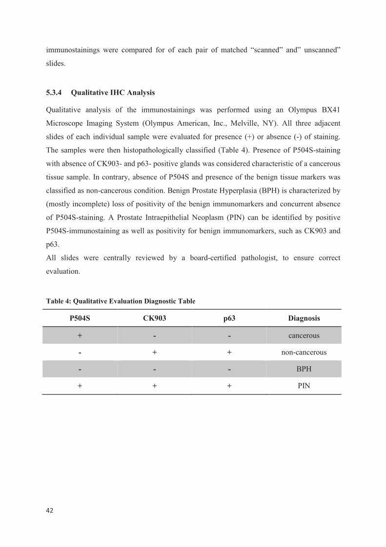
immunostainings were compared for of each pair of matched “scanned” and” unscanned”

slides.

5.3.4 Qualitative IHC Analysis

Qualitative analysis of the immunostainings was performed using an Olympus BX41

Microscope Imaging System (Olympus American, Inc., Melville, NY). All three adjacent

slides of each individual sample were evaluated for presence (+) or absence (-) of staining.

The samples were then histopathologically classified (Table 4). Presence of P504S-staining

with absence of CK903- and p63- positive glands was considered characteristic of a cancerous

tissue sample. In contrary, absence of P504S and presence of the benign tissue markers was

classified as non-cancerous condition. Benign Prostate Hyperplasia (BPH) is characterized by

(mostly incomplete) loss of positivity of the benign immunomarkers and concurrent absence

of P504S-staining. A Prostate Intraepithelial Neoplasm (PIN) can be identified by positive

P504S-immunostaining as well as positivity for benign immunomarkers, such as CK903 and

p63.

All slides were centrally reviewed by a board-certified pathologist, to ensure correct

evaluation.

Table 4: Qualitative Evaluation Diagnostic Table

P504S CK903 p63 Diagnosis

+ - - cancerous

- + + non-cancerous

- - - BPH

+ + + PIN

���

�

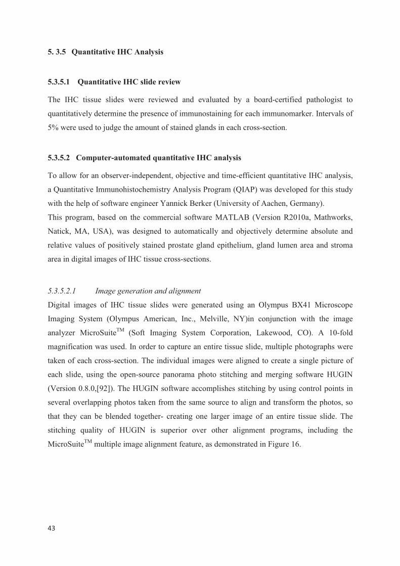
5. 3.5 Quantitative IHC Analysis

5.3.5.1 Quantitative IHC slide review

The IHC tissue slides were reviewed and evaluated by a board-certified pathologist to

quantitatively determine the presence of immunostaining for each immunomarker. Intervals of

5% were used to judge the amount of stained glands in each cross-section.

5.3.5.2 Computer-automated quantitative IHC analysis

To allow for an observer-independent, objective and time-efficient quantitative IHC analysis,

a Quantitative Immunohistochemistry Analysis Program (QIAP) was developed for this study

with the help of software engineer Yannick Berker (University of Aachen, Germany).

This program, based on the commercial software MATLAB (Version R2010a, Mathworks,

Natick, MA, USA), was designed to automatically and objectively determine absolute and

relative values of positively stained prostate gland epithelium, gland lumen area and stroma

area in digital images of IHC tissue cross-sections.

5.3.5.2.1 Image generation and alignment

Digital images of IHC tissue slides were generated using an Olympus BX41 Microscope

Imaging System (Olympus American, Inc., Melville, NY)in conjunction with the image

analyzer MicroSuiteTM (Soft Imaging System Corporation, Lakewood, CO). A 10-fold

magnification was used. In order to capture an entire tissue slide, multiple photographs were

taken of each cross-section. The individual images were aligned to create a single picture of

each slide, using the open-source panorama photo stitching and merging software HUGIN

(Version 0.8.0,[92]). The HUGIN software accomplishes stitching by using control points in

several overlapping photos taken from the same source to align and transform the photos, so

that they can be blended together- creating one larger image of an entire tissue slide. The

stitching quality of HUGIN is superior over other alignment programs, including the

MicroSuiteTM multiple image alignment feature, as demonstrated in Figure 16.

���

�

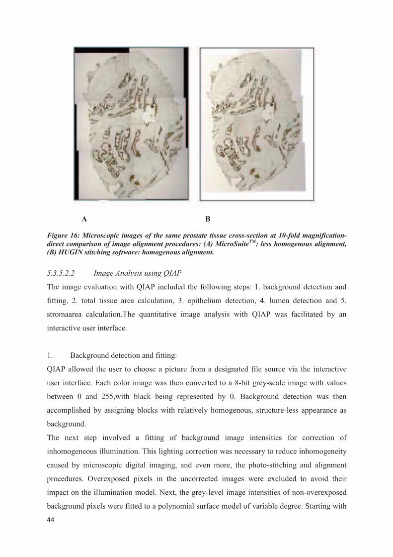
Figure 16: Microscopic images

direct comparison of image alig

(B) HUGIN stitching software: h

5.3.5.2.2 Image Analysis

The image evaluation with QI

fitting, 2. total tissue area ca

stromaarea calculation.The q

interactive user interface.

1. Background detection a

QIAP allowed the user to cho

user interface. Each color ima

between 0 and 255,with bla

accomplished by assigning bl

background.

The next step involved a

inhomogeneous illumination. T

caused by microscopic digita

procedures. Overexposed pix

impact on the illumination mo

background pixels were fitted

A

s of the same prostate tissue cross-section at 10

gnment procedures: (A) MicroSuiteTM

: less hom

homogenous alignment.

s using QIAP

QIAP included the following steps: 1. backgr

alculation, 3. epithelium detection, 4. lume

quantitative image analysis with QIAP was

and fitting:

oose a picture from a designated file source

age was then converted to a 8-bit grey-scale

ack being represented by 0. Background d

locks with relatively homogenous, structure-

fitting of background image intensities

This lighting correction was necessary to red

al imaging, and even more, the photo-stitch

xels in the uncorrected images were exclu

odel. Next, the grey-level image intensities o

d to a polynomial surface model of variable de

B

0-fold magnification-

mogenous alignment,

round detection and

en detection and 5.

s facilitated by an

e via the interactive

e image with values

detection was then

-less appearance as

for correction of

duce inhomogeneity

hing and alignment

uded to avoid their

of non-overexposed

egree. Starting with

���

�

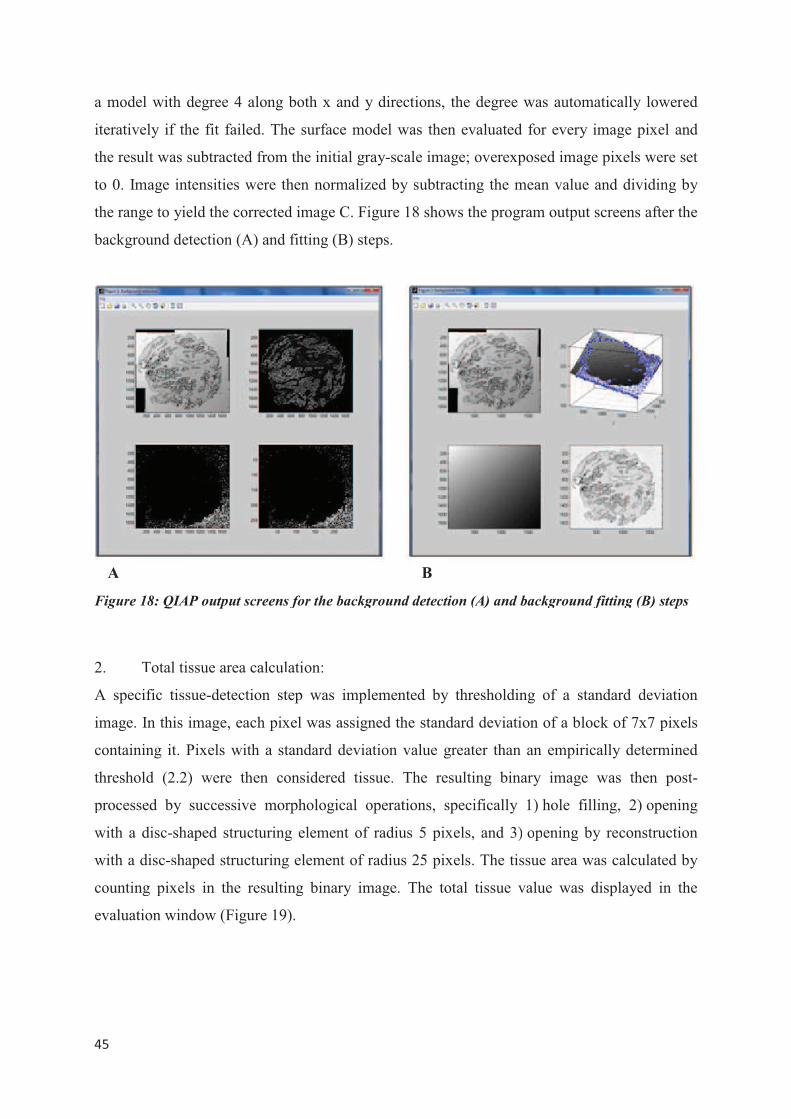
a model with degree 4 along

iteratively if the fit failed. Th

the result was subtracted from

to 0. Image intensities were th

the range to yield the corrected

background detection (A) and

Figure 18: QIAP output screens

2. Total tissue area calcul

A specific tissue-detection st

image. In this image, each pix

containing it. Pixels with a st

threshold (2.2) were then co

processed by successive mor

with a disc-shaped structuring

with a disc-shaped structuring

counting pixels in the resulti

evaluation window (Figure 19

A

both x and y directions, the degree was aut

he surface model was then evaluated for eve

m the initial gray-scale image; overexposed im

then normalized by subtracting the mean val

d image C. Figure 18 shows the program outp

fitting (B) steps.

s for the background detection (A) and backgrou

lation:

tep was implemented by thresholding of a

xel was assigned the standard deviation of a b

tandard deviation value greater than an emp

onsidered tissue. The resulting binary ima

rphological operations, specifically 1) hole

g element of radius 5 pixels, and 3) opening

g element of radius 25 pixels. The tissue area

ing binary image. The total tissue value wa

9).

B

tomatically lowered

ery image pixel and

mage pixels were set

lue and dividing by

put screens after the

und fitting (B) steps

standard deviation

block of 7x7 pixels

pirically determined

age was then post-

filling, 2) opening

g by reconstruction

a was calculated by

as displayed in the

���

�

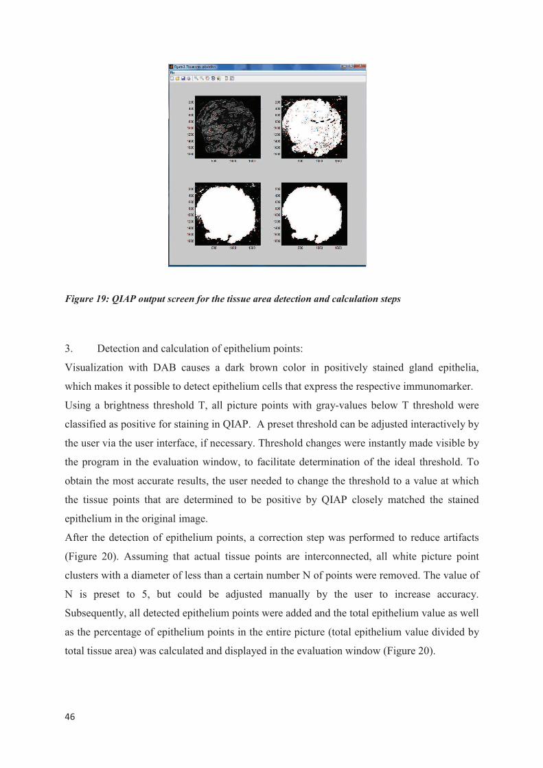
Figure 19: QIAP output screen for the tissue area detection and calculation steps

3. Detection and calculation of epithelium points:

Visualization with DAB causes a dark brown color in positively stained gland epithelia,

which makes it possible to detect epithelium cells that express the respective immunomarker.

Using a brightness threshold T, all picture points with gray-values below T threshold were

classified as positive for staining in QIAP. A preset threshold can be adjusted interactively by

the user via the user interface, if necessary. Threshold changes were instantly made visible by

the program in the evaluation window, to facilitate determination of the ideal threshold. To

obtain the most accurate results, the user needed to change the threshold to a value at which

the tissue points that are determined to be positive by QIAP closely matched the stained

epithelium in the original image.

After the detection of epithelium points, a correction step was performed to reduce artifacts

(Figure 20). Assuming that actual tissue points are interconnected, all white picture point

clusters with a diameter of less than a certain number N of points were removed. The value of

N is preset to 5, but could be adjusted manually by the user to increase accuracy.

Subsequently, all detected epithelium points were added and the total epithelium value as well

as the percentage of epithelium points in the entire picture (total epithelium value divided by

total tissue area) was calculated and displayed in the evaluation window (Figure 20).

���

�

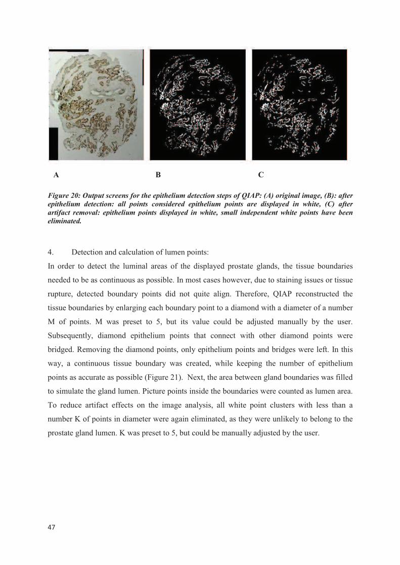
Figure 20: Output screens for th

epithelium detection: all points

artifact removal: epithelium po

eliminated.

4. Detection and calculati

In order to detect the lumina

needed to be as continuous as

rupture, detected boundary p

tissue boundaries by enlarging

M of points. M was preset

Subsequently, diamond epith

bridged. Removing the diamo

way, a continuous tissue bou

points as accurate as possible (

to simulate the gland lumen. P

To reduce artifact effects on

number K of points in diamete

prostate gland lumen. K was p

A

he epithelium detection steps of QIAP: (A) origi

ts considered epithelium points are displayed

oints displayed in white, small independent whi

ion of lumen points:

al areas of the displayed prostate glands, the

possible. In most cases however, due to stain

points did not quite align. Therefore, QIAP

g each boundary point to a diamond with a dia

to 5, but its value could be adjusted man

helium points that connect with other dia

ond points, only epithelium points and bridge

undary was created, while keeping the num

(Figure 21). Next, the area between gland bo

Picture points inside the boundaries were cou

n the image analysis, all white point cluster

ter were again eliminated, as they were unlike

preset to 5, but could be manually adjusted by

B C

inal image, (B): after

d in white, (C) after

hite points have been

e tissue boundaries

ning issues or tissue

P reconstructed the

iameter of a number

nually by the user.

amond points were

es were left. In this

mber of epithelium

oundaries was filled

unted as lumen area.

rs with less than a

kely to belong to the

y the user.

���

�

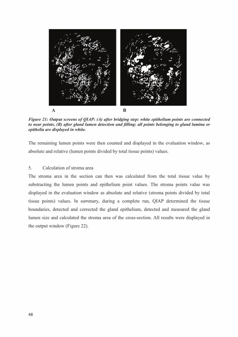
Figure 21: Output screens of QI

to near points, (B) after gland lu

epithelia are displayed in white.

The remaining lumen points w

absolute and relative (lumen p

5. Calculation of stroma a

The stroma area in the sect

substracting the lumen point

displayed in the evaluation w

tissue points) values. In sum

boundaries, detected and corr

lumen size and calculated the

the output window (Figure 22)

A

QIAP: (A) after bridging step: white epithelium p

lumen detection and filling: all points belonging

were then counted and displayed in the eva

points divided by total tissue points) values.

area

tion can then was calculated from the tot

ts and epithelium point values. The stroma

window as absolute and relative (stroma poin

mmary, during a complete run, QIAP dete

rected the gland epithelium, detected and m

e stroma area of the cross-section. All results

).

B

points are connected

g to gland lumina or

aluation window, as

tal tissue value by

a points value was

nts divided by total

termined the tissue

measured the gland

s were displayed in

���

�

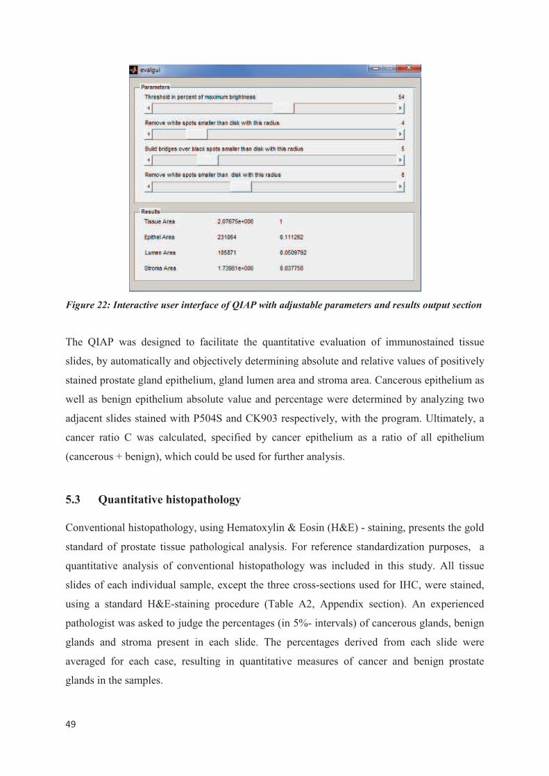
Figure 22: Interactive user interface of QIAP with adjustable parameters and results output section

The QIAP was designed to facilitate the quantitative evaluation of immunostained tissue

slides, by automatically and objectively determining absolute and relative values of positively

stained prostate gland epithelium, gland lumen area and stroma area. Cancerous epithelium as

well as benign epithelium absolute value and percentage were determined by analyzing two

adjacent slides stained with P504S and CK903 respectively, with the program. Ultimately, a

cancer ratio C was calculated, specified by cancer epithelium as a ratio of all epithelium

(cancerous + benign), which could be used for further analysis.

5.3 Quantitative histopathology

Conventional histopathology, using Hematoxylin & Eosin (H&E) - staining, presents the gold

standard of prostate tissue pathological analysis. For reference standardization purposes, a

quantitative analysis of conventional histopathology was included in this study. All tissue

slides of each individual sample, except the three cross-sections used for IHC, were stained,

using a standard H&E-staining procedure (Table A2, Appendix section). An experienced

pathologist was asked to judge the percentages (in 5%- intervals) of cancerous glands, benign

glands and stroma present in each slide. The percentages derived from each slide were

averaged for each case, resulting in quantitative measures of cancer and benign prostate

glands in the samples.

���

�

For future referencing purposes, a quantitative analysis of each complete sample is not time-

efficient and manageable. Therefore, one aim of this study was to determine whether it would

be feasible to use only one adjacent tissue slide of each case for referencing purposes. For

that, the results of quantitative histopathology analysis of a single adjacent slide were

compared to the averaged percentages of the corresponding case. �

�

5. 4 Identification of Prostate Cancer Metabolomic Markers

In order to identify potential metabolomic markers of prostate cancer, relative spectral

intensities obtained from 1H HRMAS MRS had to be referenced against histopathological

results obtained from the corresponding tissue samples. In previous studies, conventional

histopathology was commonly used as reference standard [16], due to its broad clinical utility

and applicability. The present study shows a novel approach to identify metabolomic markers

of PCa, by using quantitative IHC as reference standard instead of conventional

histopathology.

For that, the spectral intensities of 36 regions of interest (described in 4.2.3.) of each case

were correlated with a cancer ratio calculated from quantitative IHC of the same tissue

sample. The cancer ratio was defined as percentage of cancer epithelium (as determined by

QIAP) divided by the amount of all epithelia, cancerous as well as benign (by QIAP), and

served as measure for quantitative pathology as determined by IHC. The correlation between

cancer ratio and the corresponding spectral intensities from each sample was performed using

a linear regression model.

5. 5 Patient Outcomes and Recurrence Categories

Five years after the initial diagnosis and surgery, the patient medical records were reviewed

again retrospectively, in order to evaluate the patients’ outcome. Any adjuvant treatment

administered was recorded as well as clinical signs of recurrence or metastasis. Furthermore,

the date of last follow-up, PSA-levels as well as vital status at last follow-up were determined.

Overall survival (OS) was calculated as time from initial diagnosis to death, or date of last-

follow up in survivors. Recurrence was classified into four categories, according to their

presence und absence of PSA-elevation, clinical symptoms and metastases (Table 5).

���

�

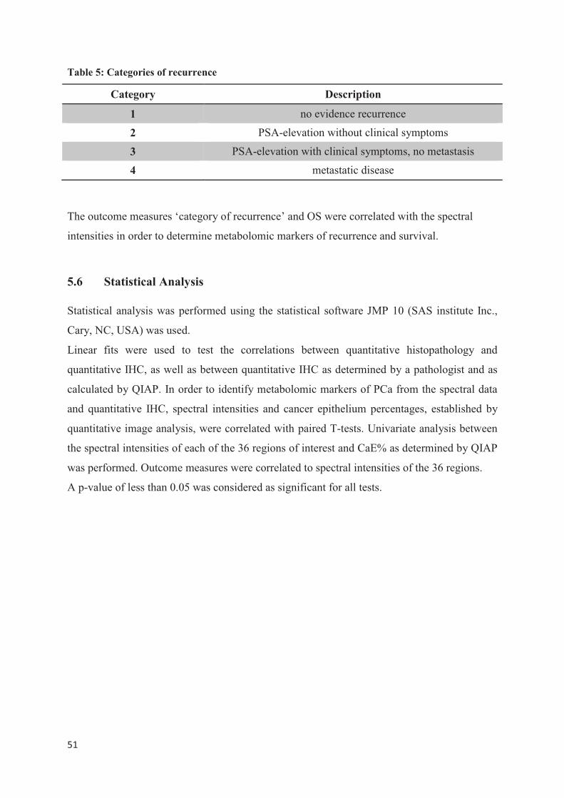
Table 5: Categories of recurrence

Category Description

1 no evidence recurrence

2 PSA-elevation without clinical symptoms

3 PSA-elevation with clinical symptoms, no metastasis

4 metastatic disease

The outcome measures ‘category of recurrence’ and OS were correlated with the spectral

intensities in order to determine metabolomic markers of recurrence and survival.

5.6 Statistical Analysis

Statistical analysis was performed using the statistical software JMP 10 (SAS institute Inc.,

Cary, NC, USA) was used.

Linear fits were used to test the correlations between quantitative histopathology and

quantitative IHC, as well as between quantitative IHC as determined by a pathologist and as

calculated by QIAP. In order to identify metabolomic markers of PCa from the spectral data

and quantitative IHC, spectral intensities and cancer epithelium percentages, established by

quantitative image analysis, were correlated with paired T-tests. Univariate analysis between

the spectral intensities of each of the 36 regions of interest and CaE% as determined by QIAP

was performed. Outcome measures were correlated to spectral intensities of the 36 regions.

A p-value of less than 0.05 was considered as significant for all tests.

�

���

�

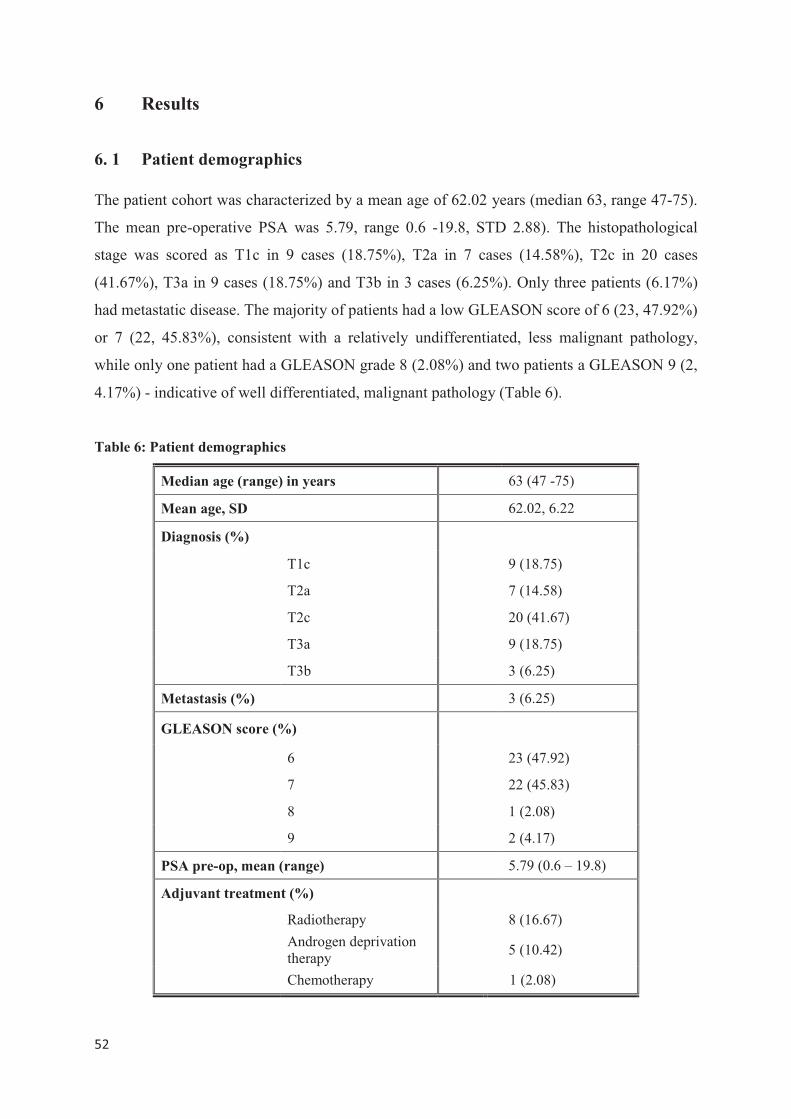
6 Results

6. 1 Patient demographics

The patient cohort was characterized by a mean age of 62.02 years (median 63, range 47-75).

The mean pre-operative PSA was 5.79, range 0.6 -19.8, STD 2.88). The histopathological

stage was scored as T1c in 9 cases (18.75%), T2a in 7 cases (14.58%), T2c in 20 cases

(41.67%), T3a in 9 cases (18.75%) and T3b in 3 cases (6.25%). Only three patients (6.17%)

had metastatic disease. The majority of patients had a low GLEASON score of 6 (23, 47.92%)

or 7 (22, 45.83%), consistent with a relatively undifferentiated, less malignant pathology,

while only one patient had a GLEASON grade 8 (2.08%) and two patients a GLEASON 9 (2,

4.17%) - indicative of well differentiated, malignant pathology (Table 6).

Table 6: Patient demographics

Median age (range) in years 63 (47 -75)

Mean age, SD 62.02, 6.22

Diagnosis (%)

T1c 9 (18.75)

T2a 7 (14.58)

T2c 20 (41.67)

T3a 9 (18.75)

T3b 3 (6.25)

Metastasis (%) 3 (6.25)

GLEASON score (%)

6 23 (47.92)

7 22 (45.83)

8 1 (2.08)

9 2 (4.17)

PSA pre-op, mean (range) 5.79 (0.6 – 19.8)

Adjuvant treatment (%)

Radiotherapy 8 (16.67)

Androgen deprivation therapy

5 (10.42)

Chemotherapy 1 (2.08)

���

�

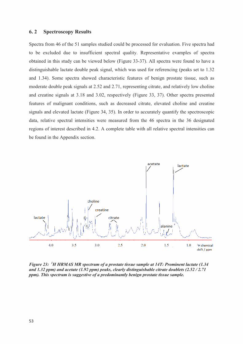
6. 2 Spectroscopy Result

Spectra from 46 of the 51 sam

to be excluded due to insuf

obtained in this study can be v

distinguishable lactate double

and 1.34). Some spectra show

moderate double peak signals

and creatine signals at 3.18 a

features of malignant conditi

signals and elevated lactate (F

data, relative spectral intensit

regions of interest described in

be found in the Appendix secti

Figure 23: 1H HRMAS MR spe

and 1.32 ppm) and acetate (1.92

ppm). This spectrum is suggestiv

ts

mples studied could be processed for evaluatio

ufficient spectral quality. Representative ex

viewed below (Figure 33-37). All spectra we

peak signal, which was used for referencing

owed characteristic features of benign prost

at 2.52 and 2.71, representing citrate, and rel

and 3.02, respectively (Figure 33, 37). Othe

ions, such as decreased citrate, elevated ch

Figure 34, 35). In order to accurately quantif

ties were measured from the 46 spectra in

in 4.2. A complete table with all relative spec

tion.

ectrum of a prostate tissue sample at 14T: Promi

2 ppm) peaks, clearly distinguishable citrate doub

ve of a predominantly benign prostate tissue sam

on. Five spectra had

xamples of spectra

ere found to have a

g (peaks set to 1.32

tate tissue, such as

latively low choline

er spectra presented

holine and creatine

fy the spectroscopic

n the 36 designated

ectral intensities can

inent lactate (1.34

blets (2.52 / 2.71

mple.

���

�

+

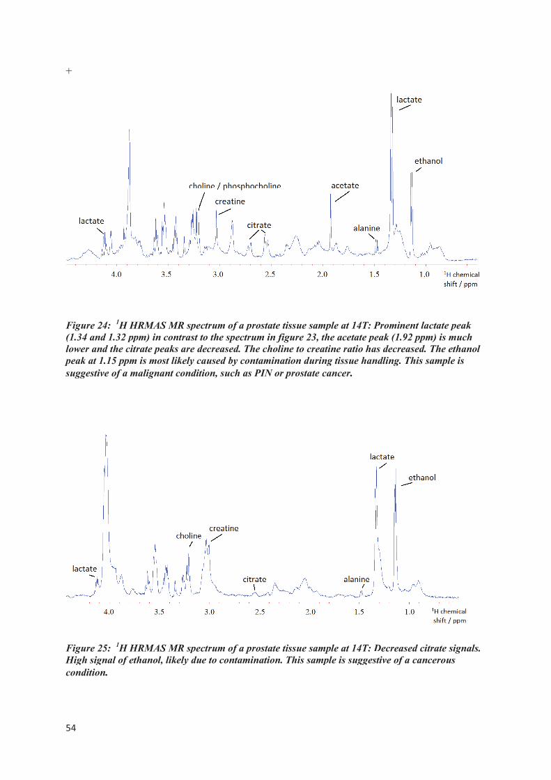
Figure 24: 1H HRMAS MR spe

(1.34 and 1.32 ppm) in contrast t

lower and the citrate peaks are d

peak at 1.15 ppm is most likely c

suggestive of a malignant condit

�

Figure 25: 1H HRMAS MR spe

High signal of ethanol, likely du

condition. �

�

ectrum of a prostate tissue sample at 14T: Promi

to the spectrum in figure 23, the acetate peak (1

decreased. The choline to creatine ratio has decr

caused by contamination during tissue handling.

ition, such as PIN or prostate cancer.

ectrum of a prostate tissue sample at 14T: Decrea

ue to contamination. This sample is suggestive of

inent lactate peak

1.92 ppm) is much

reased. The ethanol

g. This sample is

�

eased citrate signals.

of a cancerous

���

�

�

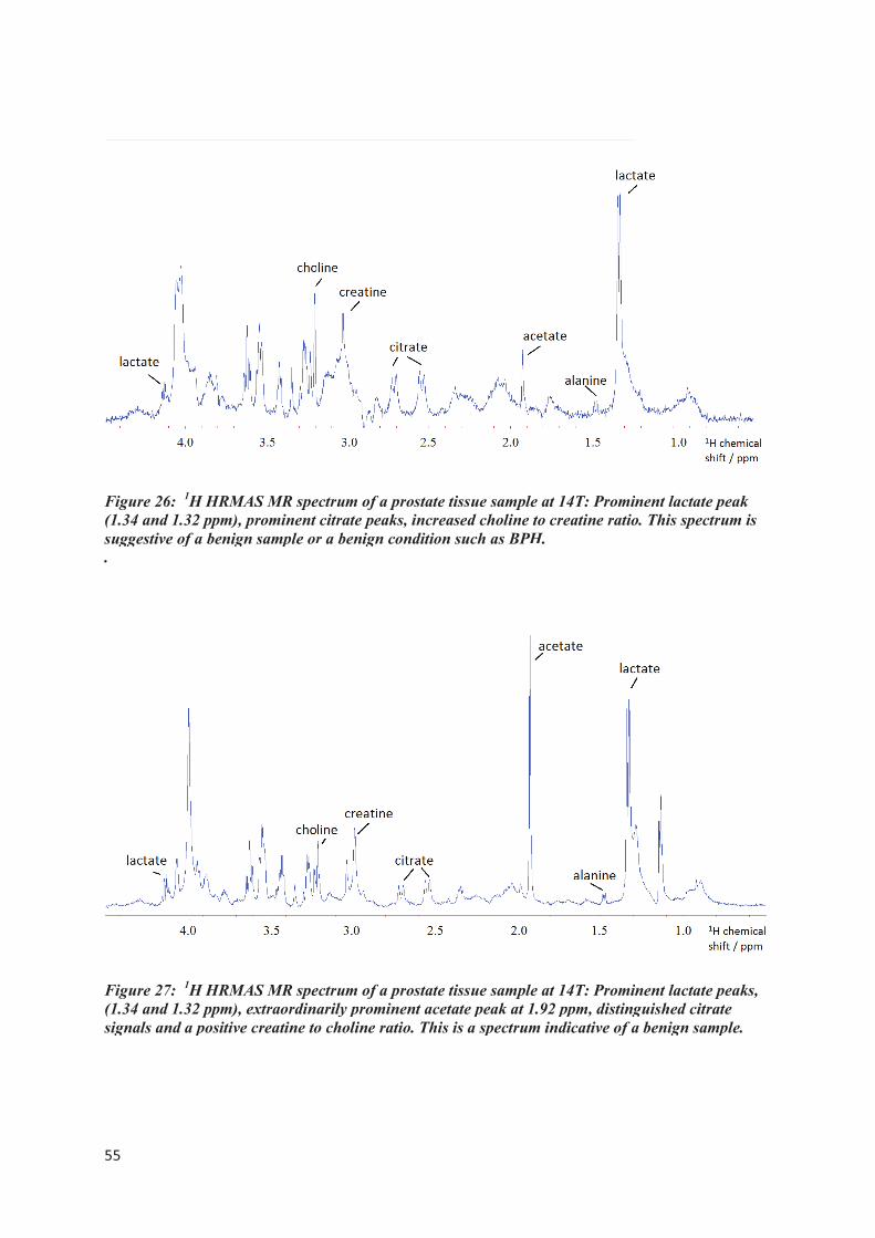
Figure 26: 1H HRMAS MR spe

(1.34 and 1.32 ppm), prominent

suggestive of a benign sample or

.

Figure 27: 1H HRMAS MR spe

(1.34 and 1.32 ppm), extraordina

signals and a positive creatine to

�

�

ectrum of a prostate tissue sample at 14T: Promi

citrate peaks, increased choline to creatine ratio

r a benign condition such as BPH.

ectrum of a prostate tissue sample at 14T: Promi

arily prominent acetate peak at 1.92 ppm, disting

o choline ratio. This is a spectrum indicative of a

�

inent lactate peak

o. This spectrum is

�

inent lactate peaks,

nguished citrate

a benign sample.

���

�

6. 3 Immunohistochemistry

6. 3. 1 Evaluation of Prostate Immunomarker Stability after 1H HRMAS MRS

Three cases of 28 paired tissue samples, which were studied for the evaluation of prostate

immunomarker stability after 1H HRMAS MRS, had to be excluded from further analyses

due to insufficient gland epithelium in the cross-sections (stroma tissue only).

The remaining 11 cases were used for the evaluation of quality and accessibility by the

pathologist.

P504S- positive staining, indicative of cancerous tissue, appeared in a distinct light brown,

granular staining pattern in the tissue slides. CK903 on the other hand caused a clear, dark

brown staining in the cytoplasm of benign epithelium basal cells, leaving cancerous tissue

unstained. P63, known as a basal cell marker, stained nuclei of benign prostate gland

epithelium only. Due to its scattered nuclear staining pattern and the extensive background

staining in most slides, the evaluation of this marker was complicated. Figure 28 illustrates

the appearance of the three chosen prostate immunomarkers, P504S, CK903 and p63, in

“unscanned” versus “scanned” tissue sections of the same prostate sample.

The evaluation of quality was based on staining intensity, amount of background staining and

similar criteria, using a 5- point scale. Table 6 summarizes the findings in the 28 paired tissue

samples.

���

�

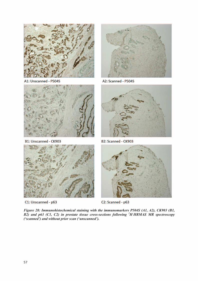
Figure 28: Immunohistochemical staining with the immunomarkers P504S (A1, A2), CK903 (B1,

B2) and p63 (C1, C2) in prostate tissue cross-sections following 1H HRMAS MR spectroscopy

(‘scanned’) and without prior scan (‘unscanned’).

���

�

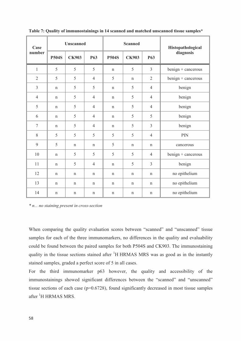
Table 7: Quality of immunostainings in 14 scanned and matched unscanned tissue samples*

Case

number

Unscanned Scanned Histopathological

diagnosis P504S CK903 P63 P504S CK903 P63

1 5 5 5 n 5 3 benign + cancerous

2 5 5 4 5 n 2 benign + cancerous

3 n 5 5 n 5 4 benign

4 n 5 4 n 5 4 benign

5 n 5 4 n 5 4 benign

6 n 5 4 n 5 5 benign

7 n 5 4 n 5 3 benign

8 5 5 5 5 5 4 PIN

9 5 n n 5 n n cancerous

10 n 5 5 5 5 4 benign + cancerous

11 n 5 4 n 5 3 benign

12 n n n n n n no epithelium

13 n n n n n n no epithelium

14 n n n n n n no epithelium

* n... no staining present in cross-section

When comparing the quality evaluation scores between “scanned” and “unscanned” tissue

samples for each of the three immunomarkers, no differences in the quality and evaluability

could be found between the paired samples for both P504S and CK903. The immunostaining

quality in the tissue sections stained after 1H HRMAS MRS was as good as in the instantly

stained samples, graded a perfect score of 5 in all cases.

For the third immunomarker p63 however, the quality and accessibility of the

immunostainings showed significant differences between the “scanned” and “unscanned”

tissue sections of each case (p=0.6728), found significantly decreased in most tissue samples

after 1H HRMAS MRS.

���

�

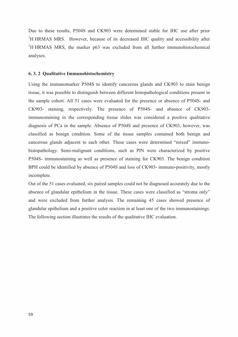
Due to these results, P504S and CK903 were determined stable for IHC use after prior 1H HRMAS MRS. However, because of its decreased IHC quality and accessibility after 1H HRMAS MRS, the marker p63 was excluded from all further immunohistochemical

analyses.

6. 3. 2 Qualitative Immunohistochemistry

Using the immunomarker P504S to identify cancerous glands and CK903 to stain benign

tissue, it was possible to distinguish between different histopathological conditions present in

the sample cohort. All 51 cases were evaluated for the presence or absence of P504S- and

CK903- staining, respectively. The presence of P504S- and absence of CK903-

immunostaining in the corresponding tissue slides was considered a positive qualitative

diagnosis of PCa in the sample. Absence of P504S and presence of CK903, however, was

classified as benign condition. Some of the tissue samples contained both benign and

cancerous glands adjacent to each other. These cases were determined “mixed” immuno-

histopathology. Semi-malignant conditions, such as PIN were characterized by positive

P504S- immunostaining as well as presence of staining for CK903. The benign condition

BPH could be identified by absence of P504S and loss of CK903- immuno-positivity, mostly

incomplete.

Out of the 51 cases evaluated, six paired samples could not be diagnosed accurately due to the

absence of glandular epithelium in the tissue. These cases were classified as “stroma only”

and were excluded from further analysis. The remaining 45 cases showed presence of

glandular epithelium and a positive color reaction in at least one of the two immunostainings.

The following section illustrates the results of the qualitative IHC evaluation.

���

�

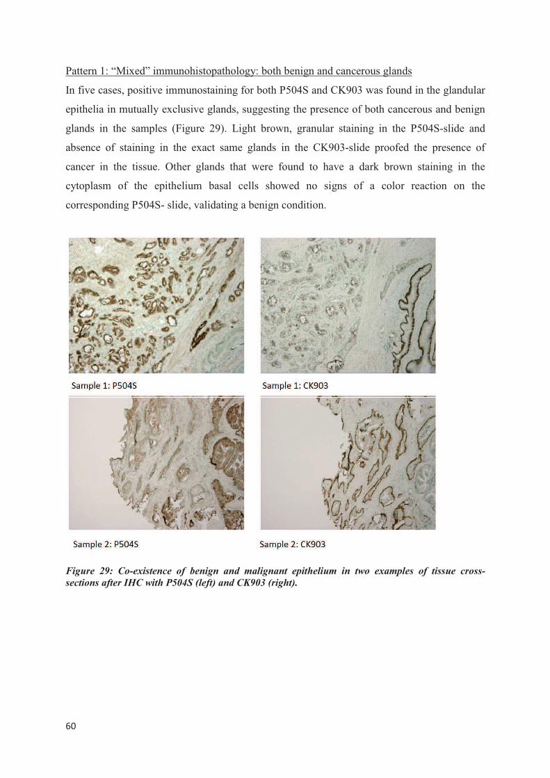
Pattern 1: “Mixed” immunohistopathology: both benign and cancerous glands

In five cases, positive immunostaining for both P504S and CK903 was found in the glandular

epithelia in mutually exclusive glands, suggesting the presence of both cancerous and benign

glands in the samples (Figure 29). Light brown, granular staining in the P504S-slide and

absence of staining in the exact same glands in the CK903-slide proofed the presence of

cancer in the tissue. Other glands that were found to have a dark brown staining in the

cytoplasm of the epithelium basal cells showed no signs of a color reaction on the

corresponding P504S- slide, validating a benign condition.

Figure 29: Co-existence of benign and malignant epithelium in two examples of tissue cross-

sections after IHC with P504S (left) and CK903 (right).

���

�

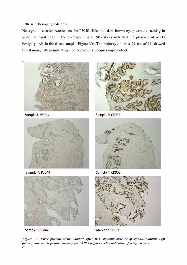
Pattern 2: Benign glands only

No signs of a color reaction on the P504S slides but dark brown cytoplasmatic staining in

glandular basal cells in the corresponding CK903 slides indicated the presence of solely

benign glands in the tissue sample (Figure 30). The majority of cases, 28 out of 44, showed

this staining pattern indicating a predominantly benign sample cohort.

Figure 30: Three prostate tissue samples after IHC showing absence of P504S- staining (left

panels) and clearly positive staining for CK903 (right panels), indicative of benign tissue.

���

�

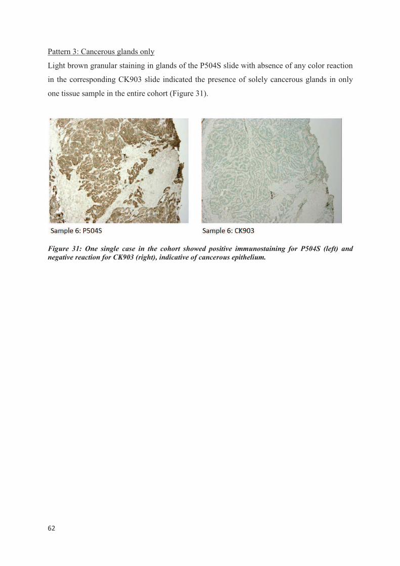
Pattern 3: Cancerous glands only

Light brown granular staining in glands of the P504S slide with absence of any color reaction

in the corresponding CK903 slide indicated the presence of solely cancerous glands in only

one tissue sample in the entire cohort (Figure 31).

Figure 31: One single case in the cohort showed positive immunostaining for P504S (left) and

negative reaction for CK903 (right), indicative of cancerous epithelium.

���

�

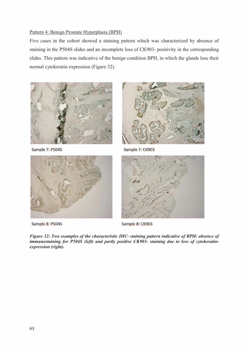
Pattern 4: Benign Prostate Hyperplasia (BPH)

Five cases in the cohort showed a staining pattern which was characterized by absence of

staining in the P504S slides and an incomplete loss of CK903- positivity in the corresponding

slides. This pattern was indicative of the benign condition BPH, in which the glands lose their

normal cytokeratin expression (Figure 32).

Figure 32: Two examples of the characteristic IHC- staining pattern indicative of BPH: absence of

immunostaining for P504S (left) and partly positive CK903- staining due to loss of cytokeratin-

expression (right).

���

�

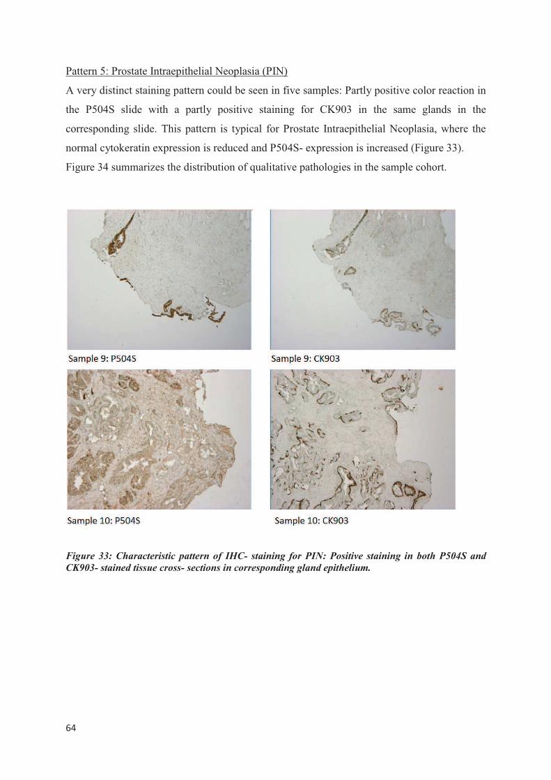
Pattern 5: Prostate Intraepithelial Neoplasia (PIN)

A very distinct staining pattern could be seen in five samples: Partly positive color reaction in

the P504S slide with a partly positive staining for CK903 in the same glands in the

corresponding slide. This pattern is typical for Prostate Intraepithelial Neoplasia, where the

normal cytokeratin expression is reduced and P504S- expression is increased (Figure 33).

Figure 34 summarizes the distribution of qualitative pathologies in the sample cohort.

Figure 33: Characteristic pattern of IHC- staining for PIN: Positive staining in both P504S and

CK903- stained tissue cross- sections in corresponding gland epithelium.

���

�

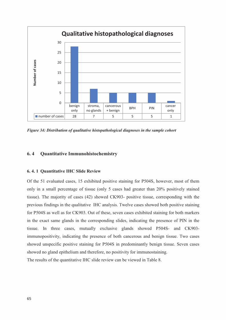
Figure 34: Distribution of qualitative histopathological diagnoses in the sample cohort

6. 4 Quantitative Immunohistochemistry

6. 4. 1 Quantitative IHC Slide Review

Of the 51 evaluated cases, 15 exhibited positive staining for P504S, however, most of them

only in a small percentage of tissue (only 5 cases had greater than 20% positively stained

tissue). The majority of cases (42) showed CK903- positive tissue, corresponding with the

previous findings in the qualitative IHC analysis. Twelve cases showed both positive staining

for P504S as well as for CK903. Out of these, seven cases exhibited staining for both markers

in the exact same glands in the corresponding slides, indicating the presence of PIN in the

tissue. In three cases, mutually exclusive glands showed P504S- and CK903-

immunopositivity, indicating the presence of both cancerous and benign tissue. Two cases

showed unspecific positive staining for P504S in predominantly benign tissue. Seven cases

showed no gland epithelium and therefore, no positivity for immunostaining.

The results of the quantitative IHC slide review can be viewed in Table 8.

�

�

�

�������

����

��������

���������

����������

����������� ���

�������

�����

��������������� �� � � � � �

�

�

��

��

��

��

��

���������������

���������������������������������������

���

�

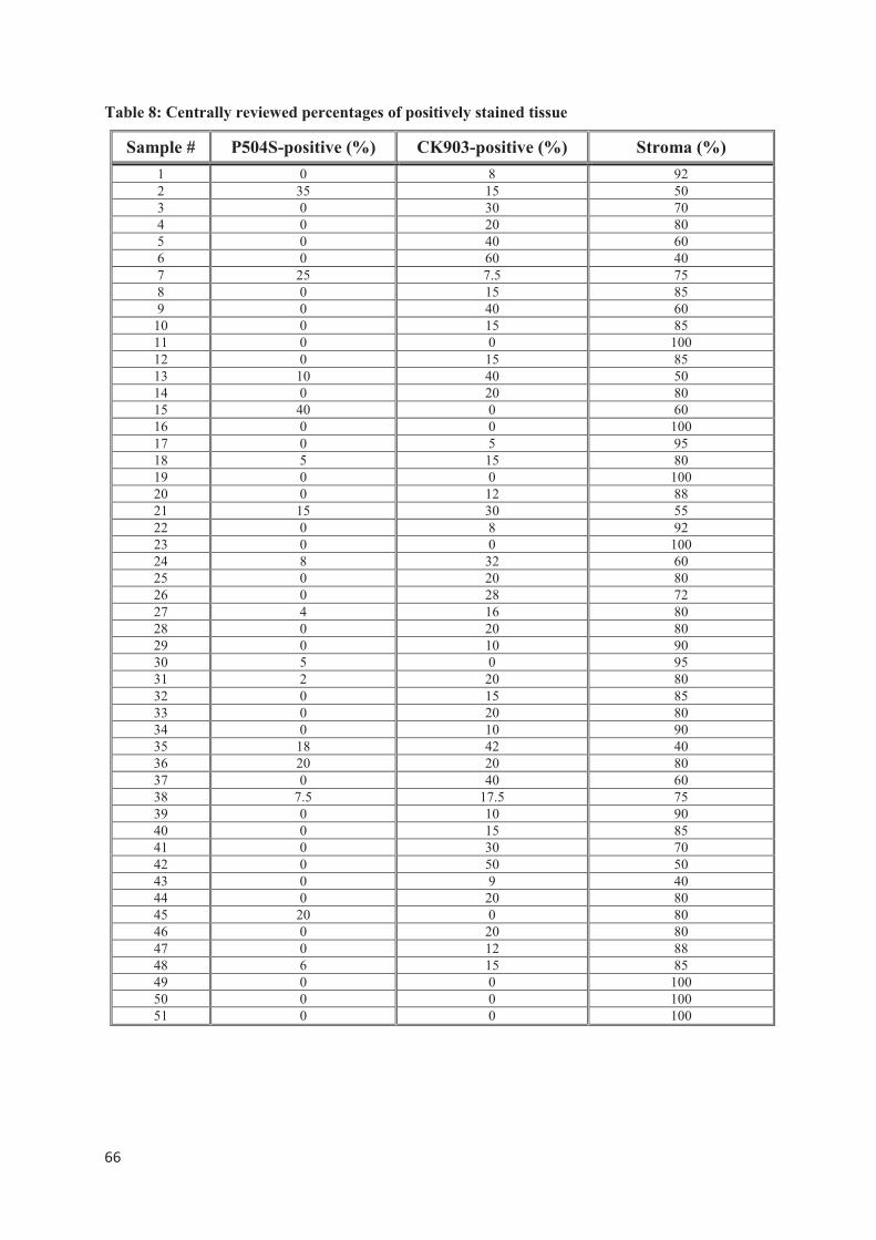
Table 8: Centrally reviewed percentages of positively stained tissue

Sample # P504S-positive (%) CK903-positive (%) Stroma (%)

1 0 8 92 2 35 15 50 3 0 30 70 4 0 20 80 5 0 40 60 6 0 60 40 7 25 7.5 75 8 0 15 85 9 0 40 60

10 0 15 85 11 0 0 100 12 0 15 85 13 10 40 50 14 0 20 80 15 40 0 60 16 0 0 100 17 0 5 95 18 5 15 80 19 0 0 100 20 0 12 88 21 15 30 55 22 0 8 92 23 0 0 100 24 8 32 60 25 0 20 80 26 0 28 72 27 4 16 80 28 0 20 80 29 0 10 90 30 5 0 95 31 2 20 80 32 0 15 85 33 0 20 80 34 0 10 90 35 18 42 40 36 20 20 80 37 0 40 60 38 7.5 17.5 75 39 0 10 90 40 0 15 85 41 0 30 70 42 0 50 50 43 0 9 40 44 0 20 80 45 20 0 8046 0 20 80 47 0 12 88 48 6 15 85 49 0 0 100 50 0 0 100 51 0 0 100

���

�

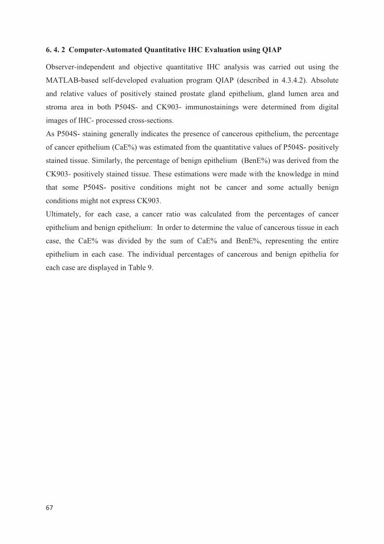
6. 4. 2 Computer-Automated Quantitative IHC Evaluation using QIAP

Observer-independent and objective quantitative IHC analysis was carried out using the

MATLAB-based self-developed evaluation program QIAP (described in 4.3.4.2). Absolute

and relative values of positively stained prostate gland epithelium, gland lumen area and

stroma area in both P504S- and CK903- immunostainings were determined from digital

images of IHC- processed cross-sections.

As P504S- staining generally indicates the presence of cancerous epithelium, the percentage

of cancer epithelium (CaE%) was estimated from the quantitative values of P504S- positively

stained tissue. Similarly, the percentage of benign epithelium (BenE%) was derived from the

CK903- positively stained tissue. These estimations were made with the knowledge in mind

that some P504S- positive conditions might not be cancer and some actually benign

conditions might not express CK903.

Ultimately, for each case, a cancer ratio was calculated from the percentages of cancer

epithelium and benign epithelium: In order to determine the value of cancerous tissue in each

case, the CaE% was divided by the sum of CaE% and BenE%, representing the entire

epithelium in each case. The individual percentages of cancerous and benign epithelia for

each case are displayed in Table 9.

���

�

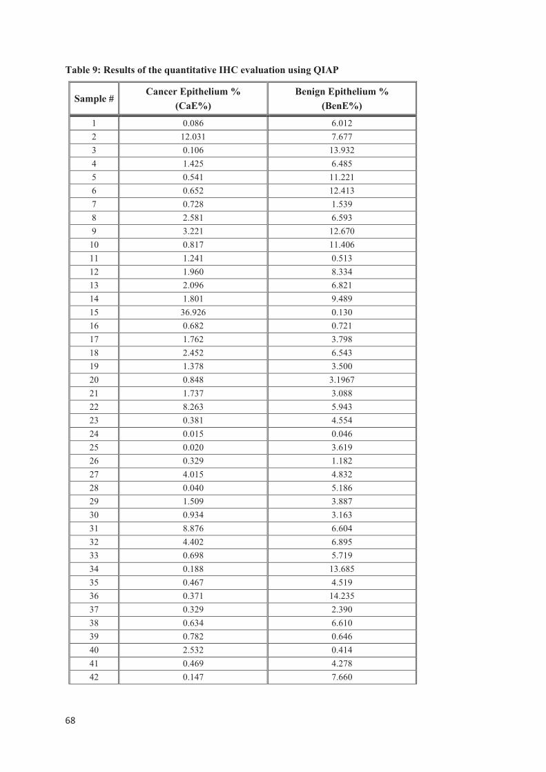
Table 9: Results of the quantitative IHC evaluation using QIAP

Sample #Cancer Epithelium %

(CaE%)

Benign Epithelium %

(BenE%)

1 0.086 6.012

2 12.031 7.677

3 0.106 13.932

4 1.425 6.485

5 0.541 11.221

6 0.652 12.413

7 0.728 1.539

8 2.581 6.593

9 3.221 12.670

10 0.817 11.406

11 1.241 0.513

12 1.960 8.334

13 2.096 6.821

14 1.801 9.489

15 36.926 0.130

16 0.682 0.721

17 1.762 3.798

18 2.452 6.543

19 1.378 3.500

20 0.848 3.1967

21 1.737 3.088

22 8.263 5.943

23 0.381 4.554

24 0.015 0.046

25 0.020 3.619

26 0.329 1.182

27 4.015 4.832

28 0.040 5.186

29 1.509 3.887

30 0.934 3.163

31 8.876 6.604

32 4.402 6.895

33 0.698 5.719

34 0.188 13.685

35 0.467 4.519

36 0.371 14.235

37 0.329 2.390

38 0.634 6.610

39 0.782 0.646

40 2.532 0.414

41 0.469 4.278

42 0.147 7.660

���

�

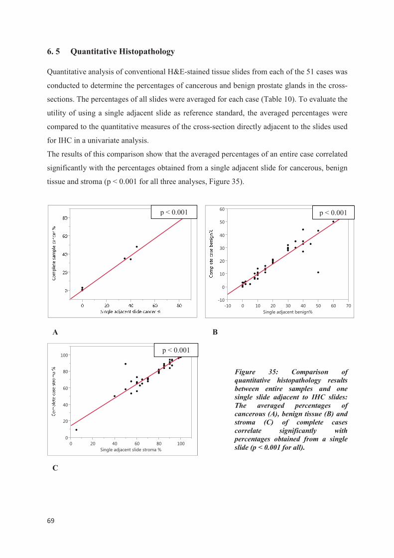
6. 5 Quantitative Histopathology

Quantitative analysis of conventional H&E-stained tissue slides from each of the 51 cases was

conducted to determine the percentages of cancerous and benign prostate glands in the cross-

sections. The percentages of all slides were averaged for each case (Table 10). To evaluate the

utility of using a single adjacent slide as reference standard, the averaged percentages were

compared to the quantitative measures of the cross-section directly adjacent to the slides used

for IHC in a univariate analysis.

The results of this comparison show that the averaged percentages of an entire case correlated

significantly with the percentages obtained from a single adjacent slide for cancerous, benign

tissue and stroma (p < 0.001 for all three analyses, Figure 35).

Figure 35: Comparison of

quantitative histopathology results

between entire samples and one

single slide adjacent to IHC slides:

The averaged percentages of

cancerous (A), benign tissue (B) and

stroma (C) of complete cases

correlate significantly with

percentages obtained from a single

slide (p < 0.001 for all).

p < 0.001

A B

���

�

��

��

��

��

��

��

��� � �� �� �� �� �� �� ��

�����������������������

p < 0.001

�

��

��

��

��

���

� �� �� �� �� ���

������������������������������

C

p < 0.001

���

�

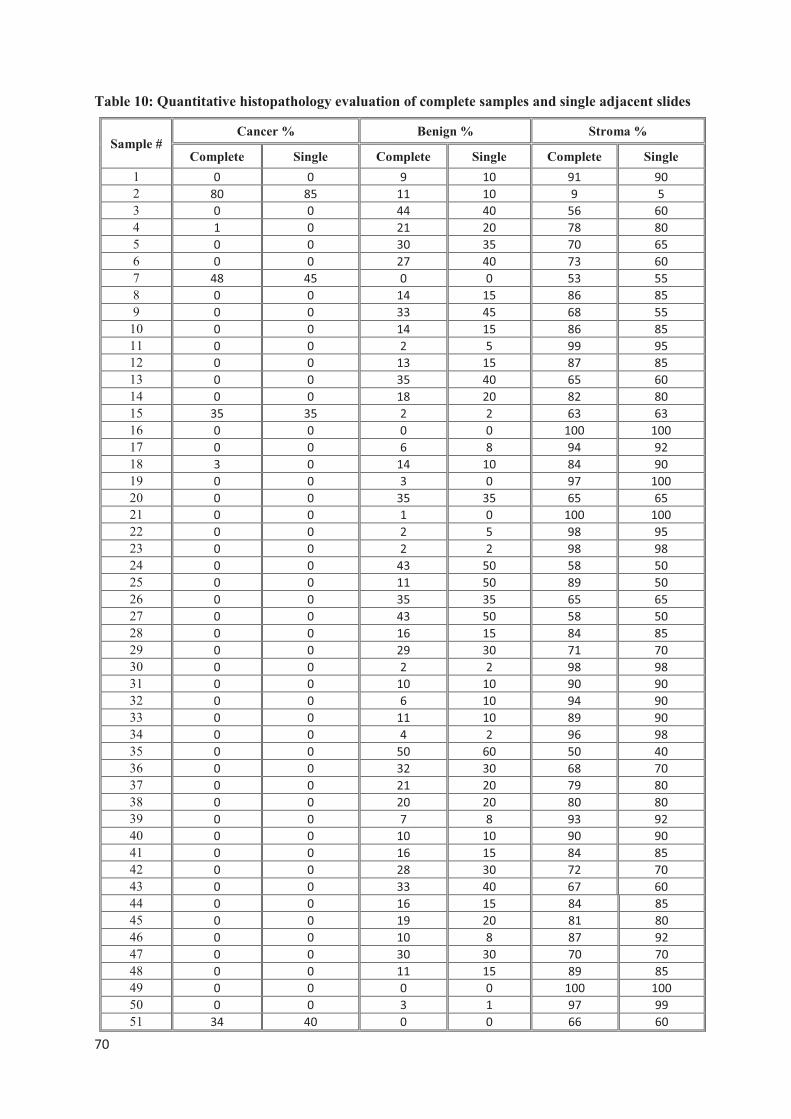
Table 10: Quantitative histopathology evaluation of complete samples and single adjacent slides

Sample # Cancer % Benign % Stroma %

Complete Single Complete Single Complete Single

1 �� �� �� ��� ��� ���

2 ��� ��� ��� ��� �� ��

3 �� �� ��� ��� ��� ���

4 �� �� ��� ��� ��� ���

5 �� �� ��� ��� ��� ���

6 �� �� ��� ��� ��� ���

7 ��� ��� �� �� ��� ���

8 �� �� ��� ��� ��� ���

9 �� �� ��� ��� ��� ���

10 �� �� ��� ��� ��� ���

11 �� �� �� �� ��� ���

12 �� �� ��� ��� ��� ���

13 �� �� ��� ��� ��� ���

14 �� �� ��� ��� ��� ���

15 ��� ��� �� �� ��� ���

16 �� �� �� �� ���� ����

17 �� �� �� �� ��� ���

18 �� �� ��� ��� ��� ���

19 �� �� �� �� ��� ����

20 �� �� ��� ��� ��� ���

21 �� �� �� �� ���� ����

22 �� �� �� �� ��� ���

23 �� �� �� �� ��� ���

24 �� �� ��� ��� ��� ���

25 �� �� ��� ��� ��� ���

26 �� �� ��� ��� ��� ���

27 �� �� ��� ��� ��� ���

28 �� �� ��� ��� ��� ���

29 �� �� ��� ��� ��� ���

30 �� �� �� �� ��� ���

31 �� �� ��� ��� ��� ���

32 �� �� �� ��� ��� ���

33 �� �� ��� ��� ��� ���

34 �� �� �� �� ��� ���

35 �� �� ��� ��� ��� ���

36 �� �� ��� ��� ��� ���

37 �� �� ��� ��� ��� ���

38 �� �� ��� ��� ��� ���

39 �� �� �� �� ��� ���

40 �� �� ��� ��� ��� ���

41 �� �� ��� ��� ��� ���

42 �� �� ��� ��� ��� ���

43 �� �� ��� ��� ��� ���

44 �� �� ��� ��� ��� ���

45 �� �� ��� ��� ��� ���

46 �� �� ��� �� ��� ���

47 �� �� ��� ��� ��� ���

48 �� �� ��� ��� ��� ���

49 �� �� �� �� ���� ����

50 �� �� �� �� ��� ���

51 ��� ��� �� �� ��� ���

���

�

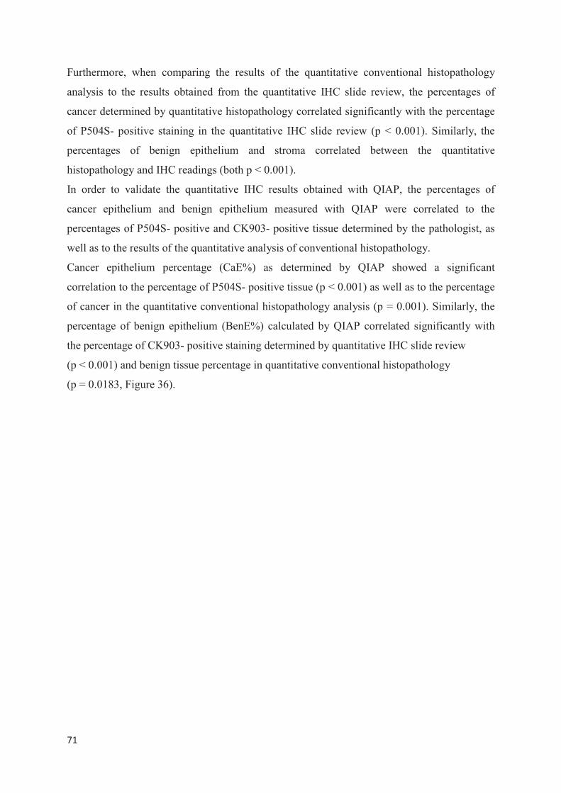
Furthermore, when comparing the results of the quantitative conventional histopathology

analysis to the results obtained from the quantitative IHC slide review, the percentages of

cancer determined by quantitative histopathology correlated significantly with the percentage

of P504S- positive staining in the quantitative IHC slide review (p < 0.001). Similarly, the

percentages of benign epithelium and stroma correlated between the quantitative

histopathology and IHC readings (both p < 0.001).

In order to validate the quantitative IHC results obtained with QIAP, the percentages of

cancer epithelium and benign epithelium measured with QIAP were correlated to the

percentages of P504S- positive and CK903- positive tissue determined by the pathologist, as

well as to the results of the quantitative analysis of conventional histopathology.

Cancer epithelium percentage (CaE%) as determined by QIAP showed a significant

correlation to the percentage of P504S- positive tissue (p < 0.001) as well as to the percentage

of cancer in the quantitative conventional histopathology analysis (p = 0.001). Similarly, the

percentage of benign epithelium (BenE%) calculated by QIAP correlated significantly with

the percentage of CK903- positive staining determined by quantitative IHC slide review

(p < 0.001) and benign tissue percentage in quantitative conventional histopathology

(p = 0.0183, Figure 36).

���

�

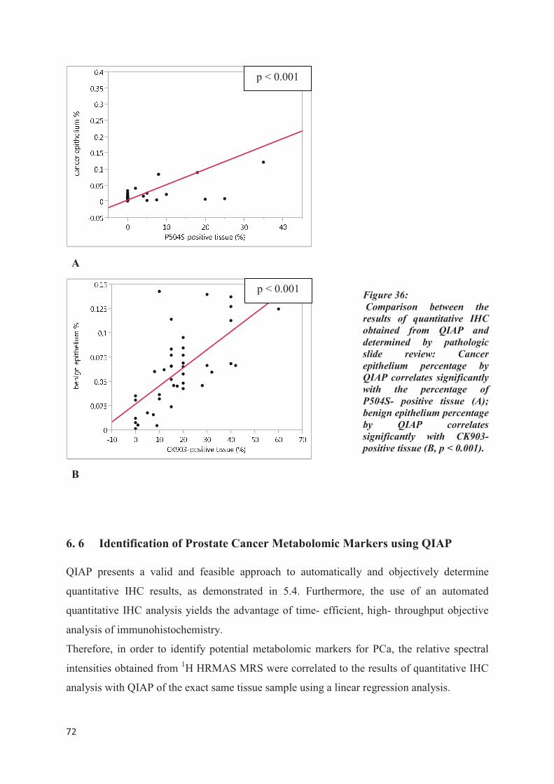
Figure 36:

Comparison between the

results of quantitative IHC

obtained from QIAP and

determined by pathologic

slide review: Cancer

epithelium percentage by

QIAP correlates significantly

with the percentage of

P504S- positive tissue (A);

benign epithelium percentage

by QIAP correlates

significantly with CK903-

positive tissue (B, p < 0.001).

�

6. 6 Identification of Prostate Cancer Metabolomic Markers using QIAP

QIAP presents a valid and feasible approach to automatically and objectively determine

quantitative IHC results, as demonstrated in 5.4. Furthermore, the use of an automated

quantitative IHC analysis yields the advantage of time- efficient, high- throughput objective

analysis of immunohistochemistry.

Therefore, in order to identify potential metabolomic markers for PCa, the relative spectral

intensities obtained from 1H HRMAS MRS were correlated to the results of quantitative IHC

analysis with QIAP of the exact same tissue sample using a linear regression analysis.

A

B

p < 0.001

p < 0.001

���

�

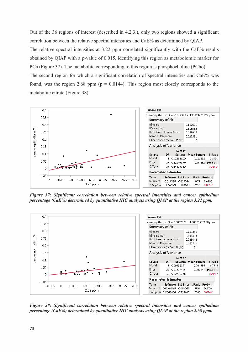
Out of the 36 regions of interest (described in 4.2.3.), only two regions showed a significant

correlation between the relative spectral intensities and CaE% as determined by QIAP.

The relative spectral intensities at 3.22 ppm correlated significantly with the CaE% results

obtained by QIAP with a p-value of 0.015, identifying this region as metabolomic marker for

PCa (Figure 37). The metabolite corresponding to this region is phosphocholine (PCho).

The second region for which a significant correlation of spectral intensities and CaE% was

found, was the region 2.68 ppm (p = 0.0144). This region most closely corresponds to the

metabolite citrate (Figure 38).

Figure 37: Significant correlation between relative spectral intensities and cancer epithelium

percentage (CaE%) determined by quantitative IHC analysis using QIAP at the region 3.22 ppm.

Figure 38: Significant correlation between relative spectral intensities and cancer epithelium

percentage (CaE%) determined by quantitative IHC analysis using QIAP at the region 2.68 ppm.

���

�

The remaining 34 regions of interest did not show any correlation between spectral intensities

and percentage of cancer epithelium. All graphs including the corresponding p- values for the

correlation can be found in the Appendix section.

In particular, the spectral intensities at the metabolomic region for lactate (1.32 – 1.34 ppm,

p = 0.5334) as well as for creatine / phosphocreatine (3.03 ppm, p = 0.7427) did not correlate

significantly with the percentage of cancer epithelium. Similarly, no significant correlations

could be found in other common metabolites in prostate cancer, such as the regions 3.75 ppm,

representing glutamine (p = 0.7545), 3.74 ppm, representing glutamate (p = 0.6097), or

3.05- 3.09 ppm, the metabolomic region of spermine (p = 0.6025).

6. 7 Patient Outcomes and Recurrence

The outcomes of the patients in our cohort were determined 5 years following the initial

diagnosis and prostatectomy surgery. For four patients, no follow- up data was available.

Two additional patients were followed for less than one year, considering them lost for

follow- up. The remaining 45 patients were followed for an average time of 53.34 months

(4.45 years), median follow- up 64.93 months (5.41 years), with a range between 14.53 and

78.43 months (1.21 and 6.54 years). During the follow- up time, 14 patients received adjuvant

treatment: radiotherapy in 8 cases (16.67%), androgen-deprivation therapy in 5 cases

(10.42%) and chemotherapy in 1 case (2.08%). Table 11 summarizes the outcome results.

Recurrence (PSA-elevation and / or new onset of clinical symptoms) was found in 11 patients

(22.92%). However, the vast majority of patients (44, 97.78%) were alive at the time of last

follow- up, with only one death found in the cohort. According to the classification of

recurrence, 34 patients (75.56%) classified as recurrence category 1 (no recurrence), 7

patients (15.56% ) belonged to the category 2 group (PSA-elevation without new clinical

symptoms) and 4 patients (8.89%) were classified as category 4 (metastatic disease). No

patients exhibited PSA-elevation and new onset of clinical symptoms (category 3, Figure 39).

���

�

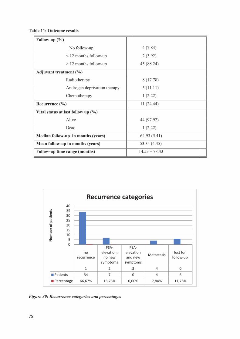
Table 11: Outcome results

Follow-up (%)

4 (7.84) No follow-up

< 12 months follow-up 2 (3.92)

> 12 months follow-up 45 (88.24)

Adjuvant treatment (%)

Radiotherapy 8 (17.78)

Androgen deprivation therapy 5 (11.11)

Chemotherapy 1 (2.22)

Recurrence (%) 11 (24.44)

Vital status at last follow up (%)

Alive 44 (97.92)

Dead 1 (2.22)

Median follow-up in months (years) 64.93 (5.41)

Mean follow-up in months (years) 53.34 (4.45)

Follow-up time range (months) 14.53 – 78.43

Figure 39: Recurrence categories and percentages

���

����������

����

�����������

�������

��������

����

����������

��������

��������

�������������������

����������

� � � � �

�������� �� � � � �

���������� ������ ������ ����� ����� ������

�

�

��

��

��

��

��

��

��

������������������

���������������������

���

�

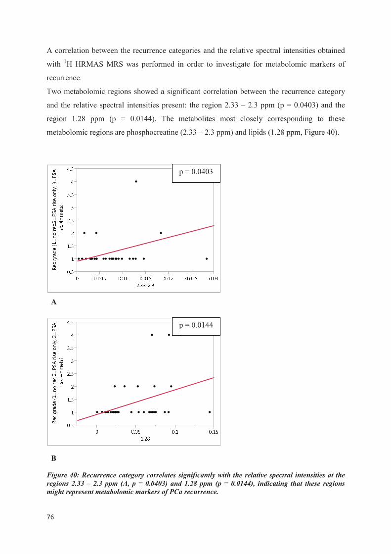
A correlation between the recurrence categories and the relative spectral intensities obtained

with 1H HRMAS MRS was performed in order to investigate for metabolomic markers of

recurrence.

Two metabolomic regions showed a significant correlation between the recurrence category

and the relative spectral intensities present: the region 2.33 – 2.3 ppm (p = 0.0403) and the

region 1.28 ppm (p = 0.0144). The metabolites most closely corresponding to these

metabolomic regions are phosphocreatine (2.33 – 2.3 ppm) and lipids (1.28 ppm, Figure 40).

Figure 40: Recurrence category correlates significantly with the relative spectral intensities at the

regions 2.33 – 2.3 ppm (A, p = 0.0403) and 1.28 ppm (p = 0.0144), indicating that these regions

might represent metabolomic markers of PCa recurrence.

p = 0.0144

p = 0.0403

B

A

���

�

7 Discussion

Summary of findings

In this study, a novel approach to identify metabolomic markers of prostate cancer was

estanlished, using prostate immunomarkers to quantify PCa metabolomic profiles measured

from prostate tissue by 1H HRMAS MRS.

In a first step, the potential of three prostate immunomarkers- P504S, CK903 and p63- to

serve as tools for quantitative analysis of immunohistochemistry following 1H HRMAS MRS

was explored. This study aimed to verify that both quality and accessibility of the prostate

immunomarkers used for the quantitative analysis were not impacted by prior 1H HRMAS

MR scanning, to ensure that these markers were suitable for post- spectroscopic IHC. For that,

the quality and accessibility of immunostainings in prostate tissue samples that had undergone

HRMAS 1HMR spectroscopy were analyzed and compared to “unscanned” tissue sections

from the same samples. In this investigation, the immunomarkers P504S and CK903 showed

equally excellent immunostaining quality in both “scanned” and “unscanned” tissue samples,

indicating that these markers are stable for immunohistochemical use following 1H HRMAS

MRS. The prostate immunomarker p63, however, showed significantly decreased quality of

immunostaining after prior 1H HRMAS MRS, suggesting that this marker might not be useful

for IHC analysis after 1H HRMAS MRS.

Using the 1H HRMAS MRS- stable immunomarkers P504S and CK903, quantitative

measures of the percentage of cancer present in the immunostained tissue sections were

obtained, using the newly developed MATLAB-based quantitative image analysis program

QIAP. The quantitative IHC results were validated, using quantitative measures of

conventional histopathology and IHC judged by a pathologist.

The percentage of cancerous (CaE%) and benign epithelia (BenE%) measured by QIAP

correlated significantly with the results for cancer and benign tissue in the conventional

histopathology slide review (p= 0.001 and p = 0.0183, respectively). Furthermore, CaE% and

BenE% correlated significantly with the quantitative evaluation of cancer and benign tissue

percentages as determined by the pathologist (p< 0.001 for both), indicating that the results of

quantitative IHC measurements obtained with the program QIAP are valid and valuable for

quantitative IHC analysis.

Ultimately, in an attempt to validate the utility of quantitative IHC to identify metabolomic

markers or PCa, relative spectral intensities obtained by 1H HRMAS MR spectroscopy were

���

�

correlated to the quantitative measures of cancer epithelium determined from immunostained

slides of the same prostate sample, using QIAP.

Out of 36 regions investigated, two regions showed a statistically significant correlation

between quantitative IHC results and spectral intensities: 3.22 ppm (p = 0.0150) and 2.68 ppm

(p = 0.0144). The metabolites corresponding to these regions, phosphocholine (PCho, 3.22

ppm) and citrate (2.68 ppm) therefore have the potential to serve as metabolomic markers of

cancerous epithelium in prostate tissue.

Furthermore, patient outcomes five years after their initial surgery were obtained and PCa

recurrence categories were identified in our cohort. Using the newly established quantitative

IHC approach to identify metabolomic markers, metabolomic markers of recurrence could be

identified in this study. Two metabolomic regions presented a significant correlation between

recurrence grade and the relative spectral intensities: the region 2.33 – 2.3 ppm

(p = 0.0403) and the region 1.28 ppm (p = 0.0144). The metabolites most closely

corresponding to these metabolomic regions are phosphocreatine (2.33 – 2.3 ppm) and lipids

(1.28 ppm). These results suggest that these metabolites could represent metabolomic markers

of recurrence in PCa patients.

Interpretation of the results

The comparison of the quality and evaluability of immunostainings following 1H HRMAS

MRS with those of “unscanned” tissue sections from the same prostate samples supports the

hypothesis that the prostate tissue architecture remains intact during an 1H HRMAS MRS

experiment. Multiple previous studies have established this knowledge [16, 37].

The equally excellent staining qualities in the stainings with the immunomarkers P504S and

CK903 indicate that the immunologic potential is indeed preserved during a scan. These

findings suggest that both markers, P504S and CK903, are stable for immunohistochemical

use on prostate tissue samples previously studied by 1H HRMAS MRS.

In contrast, the quality and evaluability of the immunostainings with p63 were significantly

decreased following 1H HRMAS MRS, indicating that this immunomarker might be

susceptible to damage induced during the process of 1H HRMAS MRS scanning or post-

procession, or might lose its immunologic potential during the spectroscopy experiment. As

the quality and the diagnostical value of p63-immunostainings appear to be altered through

spectroscopy procedures, this immunomarker seems to be unuseful for IHC following 1H

HRMAS MRS. The results of this study indicate that, although the tissue architecture remains

stable after 1H HRMAS MRS, not all immunohistochemical procedures are feasible following

���

�

spectroscopic procedures. Prior to analyzing tissue scanned samples with IHC, the proposed

immunomarker should therefore be tested for stability during the spectroscopic analysis.

Ultimately, the quantitative analysis of combined immunostainings with P504S and CK903

on adjacent tissue cross- sections presents a suitable diagnostic approach to quantitatively

evaluate prostate tissue pathologic conditions and distinguish between benign and cancerous

conditions in prostate tissue. While P504S indicates the presence of cancerous tissue, CK903

identifies benign glands. Thus, the combination of these complementary antibodies highly

increases the diagnostic value of the prostate cancer immunostaining.

The significant correlations between the results of quantitative IHC analysis using the

evaluation program QIAP and the results of a quantitative IHC review by an experienced

pathologist strongly confirm that the program QIAP presents a valuable and valid method to

determine quantitative measures of IHC. The fact that the results of QIAP also correlate

significantly with the results of a quantitative conventional histopathology analysis further

validates the utility of QIAP for quantitative pathological analysis. These findings show that

QIAP presents a valid, objective and computer-automated approach for quantitative IHC

analysis.

Using quantitative IHC analysis and metabolomic profiles obtained with 1H HRMAS MRS,

two metabolomic regions that significantly correlated with quantitative measures of cancerous

epithelium in the samples were identified. The two metabolites corresponding to these

regions, PCho and citrate, therefore could be identified as metabolomic markers of prostate

cancer conditions in our cohort. PCho is a ubiquitous metabolite, mostly present in cell

membranes, and involved in the pathway of choline synthesis. PCa causes high cell

proliferation and an increase in cell membrane synthesis, which results in elevated choline

levels and an elevation of choline synthesis meta-products, like PCho, glycerophosphocholine

and free choline [93]. Although PCho is an unspecific metabolite, its increased concentration

in cancerous conditions might contribute to its potential as a metabolomic marker of PCa.

Citrate is a metabolite highly characteristic of healthy prostate tissue and prostate fluids.

Under normal conditions, high levels of citrate are generally found. Malignant conditions,

such as PCa, cause a pathological oxidation of citrate in the KREBS cycle, resulting in a

significant decrease of citrate levels. A decrease in the citrate signals as well as in the

citrate/creatine- and (choline + creatine)/citrate- ratios in prostate spectroscopy are commonly

acknowledged indicators of the presence of cancer. The identification of citrate as a

metabolomic marker of PCa seems therefore plausible. A quantification of citrate seems to be

���

�

a feasible approach and could potentially increase the diagnostic value of prostate

spectroscopy.

Comparison of the results with findings of other studies

Multiple previous studies have focused on creating metabolomic profiles for PCa, using NMR

spectroscopy [61, 94] and mass spectrometry methods [67, 95]. However, due to technical

challenges in this field, previous results are highly diverse and different metabolites have been

proposed as potential biomarkers for PCa [36, 96-98].

The association between changes in choline-containing metabolites and malignant

transformation is well established [99]. Increased expression of genes involved in choline

metabolism and transport, such as choline kinase, kinase have been found in different cancers,

including breast cancer or high- grade gliomas [100, 101], but also PCa. Choline and choline

compounds have been shown to be increased in prostatectomy as well as prostate biopsy

specimen in cancer patients versus matched benign tissue samples [60, 68]. Also, previous ex

vivo studies have found increased Pcho levels to be associated with increased PSA and higher

GLEASON score, indicating the importance of this biomarker for the detection and

classification of prostate cancer [50, 60]. PCho is a metabolite involved in the pathway of

choline synthesis. Because of its association to alterations in cell membrane synthesis, choline

levels are increased in PCa, resulting in an elevation of choline synthesis meta-products, like

PCho, glycerophosphocholine and free choline [93]. Not only increased cell proliferation, but

also changes in tumor microenvironment, like hypoxia or shifts of pH, account for alterations

in choline metabolite levels� ��� ����� ��� ������ ���������� �������������� ������� ��������

���������� ���������������������������������������

Other metabolites have been suggested to present biomarkers of PCa in past studies. Lactate

and alanine are known to be increased in PCa, due to enhanced glycolytic activity and the

Warburg effect [61, 68]. However, these biomarkers are unspecific metabolites which are

altered in multiple cancer types, thereby reducing their potential to be PCa specific

biomarkers. With p- values of 0.5334 (region 1.32 – 1.34 ppm) and 0.7828 (region 1.46 ppm)

respectively, the spectroscopic regions corresponding to lactate and alanine did not show

significant correlations to CaE% in the present study. With the established dataset, it was not

possible to identify these metabolites as biomarkers for PCa.

In contrast to the unspecific metabolites mentioned before, decreased levels of citrate, zinc

and spermine are associated more specifically with prostate cancer [103].

���

�

Decreased levels of citrate have previously been observed in prostate cancer tissue by ex vivo

MRS [68] and measurements of citrate signals and metabolite ratios including citrate have

successfully been incorporated into routine clinical diagnostics [104, 105]. In accordance with

the results of this study, citrate has been suggested to present a PCa biomarker in a previous

study using ex vivo1H HRMAS MRS [50]. In a recent study, citrate was additionally found to

be associated with cancer aggressiveness. The authors reported a negative correlation between

citrate levels and the GLEASON score as well as significant differences between low grade

and high grade PCa, indicating that citrate concentrations measured by MRS have the

potential to distinguish between highly aggressive and indolent PCa cases [106].

Besides changes in citrate levels, a decrease of polyamine signals has been found to be

associated with PCa [50]. Significantly lower concentrations of spermine have been reported

in high grade compared to low grade PCa, suggesting spermine to be a discriminative

biomarker for PCa aggressiveness [106]. Polyamines, especially spermine, have a strong

potential for incorporation into clinical practice. In the present study, an association between

cancer epithelium percentage and spectral intensities for the region of spermine (3.05 – 3.09

ppm, p = 0.6025) could not be confirmed.

Other metabolomic biomarkers described in the literature include myo-inositol, taurine,

valine-leucine, glutamine and hydroxybutyrate [63]. None of these metabolites could be

identified using the presented novel approach, most likely due to the predominantly benign

nature of the sample set. A recent study using LC/ GC-MS to identify PCa metabolomic

markers, found six metabolites that were associated with PCa and its progression: sarcosine,

uracil, kynurenine, glycerol-3-phosphate, leucine and proline [67]. Among them, sarcosine

demonstrated the most pronounced differences, suggesting its strong potential as a biomarker

for PCa and leading to further extensive investigations of this metabolite [107-109]. In the

present study, none of these recently suggested metabolomic biomarkers could be confirmed

to be associated with PCa when using quantitative IHC as investigative tool. Multiple reasons

and limitations of our aporoach might account for that, which will be illustrated in the

following section.

Limitations of the study

Limitations of this study are due in part to the heterogenous sample cohort with

predominantly benign tissues. Out of each prostatectomy sample, only a small amount of

tissue was studied, therefore not guaranteeing definitive evaluation of the cancerous portion.

Also, the sample cohort contained preliminary stages of malignant conditions, such as BPH or

���

�

PIN. Because of this, a clear evaluation of metabolite markers for cancer was difficult to

realize. In order to establish validate prostate cancer metabolomics profiles, more cases with

predominantly cancerous conditions would need to be studied.

Due to difficulties in spectroscopy or quantitative image evaluation, only 42 out of the 51

cases could be subjected to quantitative analysis, substantially reducing the sample cohort.

The MATLAB-based evaluation program used for the quantitative image evaluation is a self-

developed pioneer image evaluation program. Therefore, the results of this method have to be

considered with caution. Further improvements of the program are necessary in the future. For

instance, image brightness should be adjusted and a fixed, and a user- independent threshold

for each immunomarker employed. To ensure program improvement, bigger sample sizes

need to be evaluated using this device. First and foremost, the current results should be

validated using a larger sample cohort of predominantly cancerous tissue. Also, a cumulative

analysis of the tissue samples, including all cross- sections of each individual sample, would

be useful. Ultimately, a 3- dimensional sample analysis seems to be desirable, as it allows full

analysis of all tissue components.

This study was performed ex vivo, using a 600MHz MR spectrometer. Translation of the

results into an in vivo clinical application is challenging. Routine clinical scanners usually

have field strengths of 3T or 1.5T, and thus provide a lower spectral resolution and more

prominent baseline noise than high field spectrometers. 7T in vivo scanners provide more

accurate results and could help overcoming these challenges, but are not available for routine

clinical diagnostics in most centers. To date, the strongest MR scanner available for in vivo

use in human subjects has a field strength of 10.5T and is located at the University of

Minnesota in Duluth, MN, USA [110].The NeuroSpin facility in France is currently

constructing an 11.7T whole- body human scanner which is expected to be available for

research purposes in 2014 [111]. Due to artifacts and side effects experienced by the subjects,

the use of even stronger magnets will not be possible in the near future, thus impairing a

direct translation of the 14.1T spectroscopy results established in this study into an in vivo

application. Besides, spectroscopy is more time- consuming, more difficult to evaluate and

more expensive than other methods.

Magic Angle Spinning, the central method used in this study, is a highly optimized technique

which enables an extremely high resolution in an ex vivo setting. However, MAS can never be

performed in humans, as a human body would not be able to tolerate spinning in a scanner.

Therefore, the extremely high resolution achieved in with a MAS- rotor will never be

reproducible in an in vivo application.

���

�

Ultimately, in order to establish clinical applicability of our results, metabolomic profiles

established by ex vivo1H HRMAS MRS would have to be translated into an in vivo setting,

while at the same time increasing the quality of low field spectroscopy and reducing scan time

and costs.

As part of our investigations, patient outcomes were determined 5 years after prostatectomy.

Early identified and correctly treated prostate cancer has a very favorable prognosis, with a

5-year-survival time of close to 100% [112]. Therefore, at the time of last follow-up, the vast

majority of patients in our cohort were still alive, limiting the conclusions that could be drawn

from correlations of spectroscopy and outcome measures.

Strengths

Despite those limitations, the presented approach using quantitative evaluation of IHC clearly

yields great potential for clinical applicability. In contrast to conventional histopathology

using H&E staining, IHC is an objective, observer- independent method and has the potential

to be computer- automated. Through visualization of immunohistochemical reactions with

DAB, subsequent quantitative, in contrast to qualitative, evaluation is possible, as shown by

this study. Using this approach, high- throughput evaluation of large cohorts of

immunostained prostate tissue samples could be possible, realizing the establishment of valid

and accurate metabolomic profiles that could then be used in a clinical setting. These

metabolomic profiles could aid in accurate differentiation between benign and malignant

conditions, as well as between low and high grade cancer. Ultimately, objective and

extremely fast evaluation of prostatectomy- specimen or biopsies could be feasible in the

future, without the need for an independent pathologist. A translation of metabolomics

profiles established with our method into an in vivo setting is possible, and could present a

non- invasive diagnostic approach for accurate classification of disease, even in a pre-

operative setting. Longitudinal, non-invasive monitoring of PCa patients would be possible,

and recurrent disease could be better distinguished from other non- malignant conditions.

In this study, the patient outcome and recurrence categories were determined and correlated in

order to identify metabolomic markers of recurrence. The vast majority of patients (88.24%)

were followed tightly for the entire time- period of 5 years, adding great additional value to

the results of spectrocopy and IHC.

���

�

Outlook

Given the exploratory nature of the study, the presented findings must be considered in a

hypothesis generating context. Further studies are needed to verify the identified prostate

cancer metabolomic markers phosphocholine and citrate, as well as to establish the clinical

applicability of this novel method. A high- throughput analysis of a large cohort of PCa

samples (e.g. biopsies or prostatectomy samples) with this novel approach could aid in the

development of accurate metabolomics profiles to differentiate several conditions, such as

highly aggressive cancer from indolent cases or precursor lesions. Even an objective, accurate

staging could be accomplished, by differentiating biopsy samples or prostatectomy samples

according to metabolomics profiles of different GLEASON grades. A future aim should be a

translation of metabolomic profiles of PCa into an in vivo setting. Ultimately, a non-invasive

approach to longitudinally monitor disease status and help to identify recurrence in PCa

patients would be of great clinical importance.

The patients enrolled in this study were followed for 5 years after initial surgery to determine

outcome and recurrence. A prospective patient follow- up for an even longer time (10 years or

more) could add additional knowledge to and determine more accurate measures of outcome

and survival. In order to improve PCa metabolomics profiles and confirm previous results of

metabolomic predictors of aggressive behavior, these outcomes could be correlated with 1H HRMAS MRS results as well as quantitative pathology using IHC in future studies.

Conclusion

In this study, a novel method was introduced that allows for an observer- independent,

quantitative analysis of IHC to help establish metabolomic profiles and identify metabolomic

markers of PCa from spectral intensities obtained with 1H HRMAS MRS. The combination of 1H HRMAS MRS and IHC has the potential to serve as faster, more accurate, observer-

independent diagnostic tool. 1H HRMAS MRS could become a useful tool in the diagnostics

of PCa. Biopsies of patients that are suspected of having PCa could be subjected to 1H HRMAS MRS and the results compared to pre-established cancer profiles. Thus, a

differentiation between highly malignant and aggressive conditions that requires radical

therapy or rather low malignant, non-aggressive tumors that can be treated with “watchful

waiting”, would be possible. A prospective in vivo application of PCa metabolite profiles and

metabolomic markers could serve as highly sensitive, non- invasive diagnostic tool.

���

�

Observer- independent, computer- automated tissue evaluation could help to avoid

overtreatment and reduce complications and risks from invasive methods for PCa patients in

the future.

�

���

�

8 Summary / Abstract

Background

Prostate cancer (PCa) is the most frequently diagnosed malignant disease among adult males

in the USA and the second leading cause of cancer deaths in men. Due to the lack of

diagnostic tools that are able to differentiate highly malignant and aggressive cases from

indolent tumors, overtreatment has become very common in the era of prostate specific

antigen (PSA) screening. New diagnostical methods to determine biological status,

malignancy, aggressiveness and extent of PCA are urgently needed. 1H High Resolution

Magic Angle Spinning Nuclear Magnetic Resonance Spectroscopy (1H HRMAS MRS) can be

used to establish PCa metabolomic profiles while preserving tissue architecture for

subsequent histopathological analysis. Immunohistochemistry (IHC), as opposed to

conventional histopathology methods, has the potential to provide objective, more accurate

and quantitative knowledge of tissue pathology. This diagnostic- accuracy study sought to

evaluate a novel approach to quantitatively identify metabolomic markers of PCa by

exploring the potential of PCa immunomarkers to quantify metabolomic profiles established

by 1H HRMAS MRS.

Material and Methods

1H HRMAS MRS was performed on tissue samples of 51 prostate cancer patients using a

14.1 T BRUKER NMR spectrometer with a rotor synchronized CPMG pulse sequence.

Spectral intensities of 36 regions of interest were measured as integrals of curve fittings with

Lorentzian-Gaussian line shapes. Immunohistochemistry (IHC) was carried out following the

spectroscopy scan, using three prostate immunomarkers to identify cancerous and benign

glands: P504S (Alpha-methylacyl-CoA-racemace), CK903 (high-molecular weight

cytokeratin) and p63.The immunostaining quality following 1H HRMAS MRS was evaluated

and compared to unscanned sections of the same sample, to verify the stability and

accessibility of the proposed immunomarkers. IHC images were automatically and

quantitatively evaluated, using a quantitative image analysis program (QIAP), to determine

the percentage of cancerous and benign epithelia in the cross- sections. The results of the

program were validated by a correlation to the results of a quantitative IHC review and

quantitative conventional histopathology analysis performed by an experienced pathologist.

���

�

Ultimately, spectral intensities and the cancer epithelium percentage, obtained from

quantitative immunohistochemistry, were correlated in order to validate PCa metabolomics

markers identified by 1H HRMAS MRS.

Patient outcomes and incidence of recurrence were determined by retrospective review of

medical records five years after initial surgery. States of recurrence were correlated to spectral

intensities to explore potential metabolomics markers of recurrence in the cohort.

Results

Immunostainings with P504S and CK903 showed excellent staining quality and accessibility

following 1H HRMAS MRS, making these markers suitable for our novel quantitative

approach to determine metabolomics profiles of PCa. In contrast, the quality of p63 IHC was

impaired after previously performed spectroscopy.

IHC using the immunomarkers P504S and CK903 on adjacent slides presents a feasible

quantitative diagnostic method to distinguish between benign and cancerous conditions in

prostate tissue. The cancer epithelium percentage as determined by QIAP showed a

significant correlation to the results of quantitative IHC analysis performed by a pathologist

(p < 0.001), as well as to a quantitative conventional histopathology review (p = 0.001). The

same was true for the benign epithelium percentage (p < 0.001 and p = 0.0183), validating our

novel approach.

Two metabolomic regions showed a significant correlation between relative spectral

intensities and the cancer epithelium percentage as determined by QIAP: 3.22 ppm

(p = 0.015) and 2.68 ppm (p = 0.0144). The metabolites corresponding to these regions,

phosphocholine and citrate, could be identified as metabolomic markers of PCa in our cohort.

45 patients were followed for more than 12 months. Of these, 97.8%were still alive five years

after initial surgery. 11 patients (24.4%) experienced a recurrence during the follow- up time.

The categories of recurrence showed a correlation to the spectral intensities of two regions,

2.33 – 2.3 ppm (p = 0.0403) and 1.28 ppm (p = 0.0144), corresponding to the metabolites

phosphocreatine and lipids.

Conclusion

This study introduces a method that allows an observer-independent, quantitative analysis of

IHC to help establish metabolomic profiles and identify metabolomic markers of PCa from

spectral intensities obtained with 1H HRMAS NMR Spectroscopy. The immunomarkers

P504S and CK903 have been found suitable IHC analysis following 1H HRMAS MRS. A

���

�

prospective in vivo application of PCa metabolite profiles and metabolomic markers

determined by our analysis could serve as highly sensitive, non- invasive diagnostic tool. This

observer- independent, computer- automated, quantitative analysis could help to distinguish

highly aggressive tumors from low-malignant conditions, avoid overtreatment and reduce

risks and complications for cancer patients in the future. However, further studies are needed

to verify the identified PCa metabolomic markers and to establish clinical applicability.

�

�

���

�

9 Zusammenfassung

Einführung

Prostatakrebs ist eine häufigsten Krebserkrankungen in den USA und die zweithäufigste

malignom- assoziierte Todesursache männlicher Patienten weltweit. Seit der Einführung des

Prostata- spezifischen Antigen (PSA)- Screeningtests wird diese Krebsart in früheren Stadien

diagnostiziert und therapiert, wodurch die Mortalitätsrate in den letzten Jahren deutlich

reduziert werden konnte. Da moderne diagnostische Methoden bislang jedoch nicht

ausreichend in der Lage sind, suffizient zwischen hochmalignen und weniger aggressiven

Varianten dieses bösartigen Krebsleidens zu unterscheiden, werden häufig auch Patienten

aggressiv therapiert, deren niedriggradiges Prostatakarzinom keine klinische Relevanz gehabt

hätte. Es besteht daher ein großes wissenschaftliches Interesse an der Entwicklung neuer

diagnostischer Methoden zur akkuraten Bestimmung von biologischem Status, Malignität,

Aggressivität und Ausmaß einer Prostatakrebserkrankung. "1H High Resolution Magic Angle Spinning Nuclear Magnetic Resonance Spectroscopy" (1H

HRMAS MRS) ist eine vielversprechende diagnostische Methode, welche es ermöglicht,

metabolomische Profile von Prostatakrebs zu erstellen, ohne die Gewebsstruktur der

analysierten Proben zu zerstören. Durch anschließende histopathologische Begutachtung

lassen sich die erstellten Metabolitprofile validieren und evaluieren.

Im Gegensatz zu konventionellen histopathologischen Methoden können durch

immunhistochemische Verfahren dabei objektivere, akkuratere und quantifizierbare

histopathologische Erkenntnisse gewonnen werden.

Die vorliegende Studie präsentiert einen neuentwickelten diagnostischen Ansatz zur

quantitativen Bestimmung von metabolomischen Markern von Prostatakrebs, basierend auf

der Durchführung von 1H HRMAS NMR Spektroskopie und quantitativer

Immunhistochemie.

Material und Methoden

Einundfünfzig Gewebsproben von Prostatakrebspatienten wurden mittels 1H HRMAS MRS

an einem 14.1 T BRUKER NMR Spektrometer unter Einsatz einer CPMG-Pulssequenz

untersucht. Spektrale Intensitäten in 36 Metabolitregionen wurden gemessen. Anschließend

wurden die analysierten Gewebeproben mit drei Immunfärbemarkern für sowohl malignes

(P504S, Alpha-methylacyl-CoA-racemase) als auch benignes (CK903, High-molecular

weight cytokeratin, und p63) Prostatagewebe angefärbt und quantitativ mit Hilfe eines

���

�

Bildanalyseprogramms (QIAP) ausgewertet. Die Anwendbarkeit und Auswertbarkeit der

genannten Immunomarker nach Spektroskopie wurde evaluiert und mit der Färbungsqualität

von nicht- gescannten Schnitten verglichen.

Die Resultate der automatischen Auswertung durch QIAP konnten durch einen erfahrenen

Pathologen in einer quantitativen Analyse der Immunfärbungen sowie konventioneller

histologischer Färbungen derselben Gewebsproben validiert werden. Die spektralen

Intensitäten aus den Messungen mit 1H HRMAS MRS wurden mit den korrespondierenden

Ergebnissen der quantitativen Auswertung der Immunfärbungen korreliert, um

metabolomische Marker von Prostatakrebs zu identifizieren.

Der klinische Verlauf und die Rezidivrate der Patienten wurden 5 Jahre nach der initialen

Prostatektomie retrospektiv bestimmt. Rezidivkategorien wurden erstellt und mit den

bestimmten spektralen Intensitäten korreliert, um metabolomische Marker für das Auftreten

von Prostatakrebsrezidiven zu identifizieren.

Ergebnisse

Die Immunfärbungen mit P504S und CK903 zeigten exzellente Qualität und Auswertbarkeit

nach vorheriger 1H HRMAS MRS. Beide Marker eigneten sich zur Durchführung von

quantitativer Immunhistochemie an spektroskopierten Gewebeproben. Im Gegensatz dazu war

die Qualität der Immunfärbungen mit p63 nach Spektroskopie vermindert. Quantitative

Immunfärbungen unter Einsatz der Immunmarker P504S und CK903 stellten eine praktikable

diagnostische Methode dar, um zwischen malignen und benignem Prostatagewebe zu

unterscheiden.

Der Anteil von bösartig verändertem Prostatagewebe, bestimmt durch QIAP, korrelierte

signifikant mit den Ergebnissen der quantitativen Analyse der Immunfärbungen durch den

Pathologen (p < 0.001), sowie mit der quantitativen Auswertung der konventionellen

histopathologischen Färbung (p = 0.001). Ebenso ließ sich die Bestimmung des Anteils von

benignem Gewebe mit QIAP zu den Ergebnissen der pathologischen Analyse korrelieren

(p < 0.001 und p = 0.0183).

Für zwei metabolomische Regionen konnte ein signifikante Korrelation zwischen relativen

spektralen Intensitäten, bestimmt mit 1H HRMAS NMR Spektroskopie, und dem Anteil von

malignem Epithelium in derselben Gewebeprobe, ermittelt durch QIAP, festgestellt werden:

3.22 ppm (p = 0.015) und 2.68 ppm (p = 0.0144). Die zu diesen Regionen korrespondierenden

Metaboliten, Phosphocholin und Zitrat, konnten als potentielle metabolomische Marker für

Prostatakrebs identifiziert werden.

���

�

Die retrospektiven Analyse der klinischen Daten der Patienten fünf Jahre nach Prostatektomie

ergab eine Überlebensrate von 97.8%. Elf dieser Patienten (24.4%) erlitten ein Rezidiv ihrer

Erkrankung. Die bestimmten Rezidivkategorien korrelierten signifikant mit zwei

metabolomischen Regionen (2.33 – 2.3 ppm, p = 0.0403 und 1.28 ppm, p = 0.0144), welche

zu den Metaboliten Phosphokreatin und Lipiden korrespondierten.

Schlussfolgerung

Die vorliegende Studie präsentiert einen diagnostischen Ansatz zur objektiven und

quantitativen Bestimmung metabolomischer Marker von Prostatakrebs unter Verwendung von 1H HRMAS MRS und Immunhistochemie.

P504S und CK903 eignen sich als Immunmarker für quantitative Immunfärbungen nach

vorheriger Durchführung von 1H HRMAS MRS.

Die Metaboliten Phosphocholin und Zitrat konnten in der vorliegenden Patientenkohorte als

potentielle metabolomische Marker für Prostatakrebs identifiziert werden.

Eine mögliche in vivo Anwendung der gefundenen metabolomischen Marker könnte als

hochsensitives, objektives und nicht- invasives diagnostisches Werkzeug der

Prostatakrebsdiagnostik dienen. Der vorliegende untersucherunabhängige, automatisierte und

quantitative diagnostischer Ansatz hat das Potential, zwischen hochmalignen und weniger

aggressiven Krebsfällen zu unterscheiden und somit unnötige Risiken und Komplikationen

für Prostatakrebspatienten zu reduzieren.

Weitere Untersuchungen sind notwendig, um die identifizierten metabolomischen Marker zu

verifizieren und eine klinische Anwendung zu etablieren.

�

���

�

10 References

1. Jemal, A., et al., Global cancer statistics. CA Cancer J Clin, 2011. 61(2): p. 69-90.

2. Cancer, I.A.f.R.o., Facts Sheets Cancer.

2014(http://globocan.iarc.fr/Pages/fact_sheets_cancer.aspx).

3. Nelson, W.G., A.M. De Marzo, and W.B. Isaacs, Prostate cancer. N Engl J Med, 2003.

349(4): p. 366-81.

4. Carroll, P.R., Lee, K., Fuks, Z., Kantoff, P., Cancer of the Prostate. , in Cancer: Principle and

Practise of Oncology., V. DeVita, Hellman, S., Rosenberg, S., Editor. 2001, Lippincott

Williams & Wilkins: Philadelphia.

5. Roodman, G.D., Mechanisms of bone metastasis. N Engl J Med, 2004. 350(16): p. 1655-64.

6. McNeal, J.E., Prostatic microcarcinomas in relation to cancer origin and the evolution to

clinical cancer. Cancer, 1993. 71(3 Suppl): p. 984-91.

7. Siegel, R., D. Naishadham, and A. Jemal, Cancer statistics, 2013. CA Cancer J Clin, 2013.

63(1): p. 11-30.

8. Steiner, H., et al., Clinical and pathologic features of prostate cancer detected after repeat

false-negative biopsy in a screening population. Prostate, 2004. 58(3): p. 277-82.

9. Welch, H.G. and P.C. Albertsen, Prostate cancer diagnosis and treatment after the

introduction of prostate-specific antigen screening: 1986-2005. J Natl Cancer Inst, 2009.

101(19): p. 1325-9.

10. DeVita, V., Hellman, S., Rosenberg, S., Cancer: Principles and Practise of Oncology. 7th ed.

2005, Philadelphia: Lippinscott Williams & Wilkins.

11. Draisma, G., et al., Lead time and overdiagnosis in prostate-specific antigen screening:

importance of methods and context. J Natl Cancer Inst, 2009. 101(6): p. 374-83.

12. Pound, C.R., et al., Natural history of progression after PSA elevation following radical

prostatectomy. JAMA, 1999. 281(17): p. 1591-7.

13. Shibata, A., J. Ma, and A.S. Whittemore, Prostate cancer incidence and mortality in the

United States and the United Kingdom. J Natl Cancer Inst, 1998. 90(16): p. 1230-1.

14. Bangma, C.H., S. Roemeling, and F.H. Schroder, Overdiagnosis and overtreatment of early

detected prostate cancer. World J Urol, 2007. 25(1): p. 3-9.

15. Schroder, F.H., PSA screening--a review of recent studies. Eur J Cancer, 2009. 45 Suppl 1: p.

402-4.

16. Burns, M.A., et al., Quantitative pathology in tissue MR spectroscopy based human prostate

metabolomics. Technol Cancer Res Treat, 2004. 3(6): p. 591-8.

17. Prostata-Center, Treatment of Prostate Cancer: Precise and Safe. 2014(http://www.prostate-

center.org/Prostate_Cancer_Treatment/3D-Biopsy.htm).

���

�

18. Coakley, F.V., et al., Prostate cancer tumor volume: measurement with endorectal MR and

MR spectroscopic imaging. Radiology, 2002. 223(1): p. 91-7.

19. Akin, O. and H. Hricak, Imaging of prostate cancer. Radiol Clin North Am, 2007. 45(1): p.

207-22.

20. Mazaheri, Y., et al., Prostate cancer: identification with combined diffusion-weighted MR

imaging and 3D 1H MR spectroscopic imaging--correlation with pathologic findings.

Radiology, 2008. 246(2): p. 480-8.

21. Jordan, K.W. and L.L. Cheng, NMR-based metabolomics approach to target biomarkers for

human prostate cancer. Expert Rev Proteomics, 2007. 4(3): p. 389-400.

22. A., A., Diagnosis of cancer of the prostate: biopsy by rectal route. The Urologic and

Cutaneous Review, 1937. 41(421).

23. Djavan, B., et al., Prospective evaluation of prostate cancer detected on biopsies 1, 2, 3 and 4:

when should we stop? J Urol, 2001. 166(5): p. 1679-83.

24. Roehl, K.A., J.A. Antenor, and W.J. Catalona, Serial biopsy results in prostate cancer

screening study. J Urol, 2002. 167(6): p. 2435-9.

25. Gleason, D.F., Classification of prostatic carcinomas. Cancer Chemother Rep, 1966. 50(3): p.

125-8.

26. Humphrey, P.A., Gleason grading and prognostic factors in carcinoma of the prostate. Mod

Pathol, 2004. 17(3): p. 292-306.

27. Delahunt, B., et al., Gleason grading: past, present and future. Histopathology, 2012. 60(1):

p. 75-86.

28. Wikipedia, Gleason score. 2014(http://en.wikipedia.org/wiki/File:Gleasonscore.jpg).

29. Prevention, C.f.D.C.a., National Hospital Discharge Survey 2010. 2009

(http://www.cdc.gov/nchs/data/nhds/4procedures/2009pro4_numberrate.pdf).

30. Ransohoff, D.F., M. McNaughton Collins, and F.J. Fowler, Why is prostate cancer screening

so common when the evidence is so uncertain? A system without negative feedback. Am J

Med, 2002. 113(8): p. 663-7.

31. Gore, J.L., et al., Survivorship beyond convalescence: 48-month quality-of-life outcomes after

treatment for localized prostate cancer. J Natl Cancer Inst, 2009. 101(12): p. 888-92.

32. Potosky, A.L., et al., Five-year outcomes after prostatectomy or radiotherapy for prostate

cancer: the prostate cancer outcomes study. J Natl Cancer Inst, 2004. 96(18): p. 1358-67.

33. Schover, L.R., et al., Defining sexual outcomes after treatment for localized prostate

carcinoma. Cancer, 2002. 95(8): p. 1773-85.

34. Cheng, L.L., et al., Enhanced resolution of proton NMR spectra of malignant lymph nodes

using magic-angle spinning. Magn Reson Med, 1996. 36(5): p. 653-8.

���

�

35. Cheng, L.L., et al., Quantitative neuropathology by high resolution magic angle spinning

proton magnetic resonance spectroscopy. Proc Natl Acad Sci U S A, 1997. 94(12): p. 6408-

13.

36. Decelle, E.A. and L.L. Cheng, High-resolution magic angle spinning (1) H MRS in prostate

cancer. NMR Biomed, 2014. 27(1): p. 90-9.

37. Taylor, J.L., et al., High-resolution magic angle spinning proton NMR analysis of human

prostate tissue with slow spinning rates. Magn Reson Med, 2003. 50(3): p. 627-32.

38. Shi, X., E. Gong, and X. Wu, Alpha-methylacyl-CoA racemase/P504S overexpression in

colorectal carcinoma is correlated with tumor differentiation. Appl Immunohistochem Mol

Morphol, 2007. 15(2): p. 175-80.

39. Kuefer, R., et al., alpha-Methylacyl-CoA racemase: expression levels of this novel cancer

biomarker depend on tumor differentiation.Am J Pathol, 2002. 161(3): p. 841-8.

40. UCDavis, C., Zeeman

effect.2014(http://chemwiki.ucdavis.edu/@api/deki/files/9303/Zeeman_Effect.jpg).

41. Heisenberg, W., Ueber den anschaulichen Inhalt der quantentheoretischen Kinematik und

Mechanik.Zeitschrift fuer Physik, 1927. 43(3-4): p. 172-198.

42. Wikipedia, Magic Angle

Spinning.2014(http://en.wikipedia.org/wiki/File:MagicAngleSpinning.svg).

43. Melkus, G., Development and application of spectroscopic 1H-NMR methods for in vivo

characterisation of xenograft tumor models at 17.6 T, F.f.P.u.A. Universität Würzburg, Editor.

2009: Würzburg.

44. Andrew, E.A., Bradbury, A., Eades, R.G., Nuclear Magnetic Resonance Spectra from Crystal

rotated at High Speed. Nature, 1958. 182(4650): p. 1659.

45. Lowe, I.J., Free Induction Decays of Rotating Solids. Physical Reviwe Letters, 1959. 2(7): p.

285 - 287.

46. Jordan, K.W., et al., Evaluation of Tissue Metabolites with High Resolution Magic Angle

Spinning MR Spectroscopy Human Prostate Samples After Three-Year Storage at -80 degrees

C. Biomark Insights, 2007. 2: p. 147-54.

47. Cheng, L.L., et al., Quantification of microheterogeneity in glioblastoma multiforme with ex

vivo high-resolution magic-angle spinning (HRMAS) proton magnetic resonance

spectroscopy. Neuro Oncol, 2000. 2(2): p. 87-95.

48. Cheng, L.L., et al., Non-destructive quantitation of spermine in human prostate tissue samples

using HRMAS 1H NMR spectroscopy at 9.4 T. FEBS Lett, 2001. 494(1-2): p. 112-6.

49. Cheng, L.L., et al., Correlation of high-resolution magic angle spinning proton magnetic

resonance spectroscopy with histopathology of intact human brain tumor specimens. Cancer

Res, 1998. 58(9): p. 1825-32.

���

�

50. Cheng, L.L., et al., Metabolic characterization of human prostate cancer with tissue magnetic

resonance spectroscopy. Cancer Res, 2005. 65(8): p. 3030-4.

51. M.H., L., Spin dynamics: basic of nuclear magnetic resonance. 2nd ed. 2008, West Sussesx,

England: John Wiley & Sons, Ltd.

52. Burns, M.A., et al., Reduction of spinning sidebands in proton NMR of human prostate tissue

with slow high-resolution magic angle spinning. Magn Reson Med, 2005. 54(1): p. 34-42.

53. Chen, G.Y., et al., [Assessment of P504S immunohistochemistry in diagnosis and differential

diagnosis of prostatic adenocarcinoma]. Zhonghua Bing Li Xue Za Zhi, 2004. 33(5): p. 419-

23.

54. Oliver, S., Functional Genomics: all the king's horses and all the king's men can put Humpty

together again. Mol Cell, 2003. 12(6): p. 1343-4.

55. Wikipedia. Citrate. 2014 http://en.wikipedia.org/wiki/File:Citrate-3D-balls.png].

56. Glunde, K., M.A. Jacobs, and Z.M. Bhujwalla, Choline metabolism in cancer: implications for

diagnosis and therapy. Expert Rev Mol Diagn, 2006. 6(6): p. 821-9.

57. Glunde, K. and N.J. Serkova, Therapeutic targets and biomarkers identified in cancer choline

phospholipid metabolism. Pharmacogenomics, 2006. 7(7): p. 1109-23.

58. Wikipedia. Choline. 2014 http://en.wikipedia.org/wiki/File:Choline-cation-3D-balls.png].

59. Swanson, M.G., et al., Proton HR-MAS spectroscopy and quantitative pathologic analysis of

MRI/3D-MRSI-targeted postsurgical prostate tissues. Magn Reson Med, 2003. 50(5): p. 944-

54.

60. van Asten, J.J., et al., High resolution magic angle spinning NMR spectroscopy for metabolic

assessment of cancer presence and Gleason score in human prostate needle biopsies.

MAGMA, 2008. 21(6): p. 435-42.

61. Tessem, M.B., et al., Evaluation of lactate and alanine as metabolic biomarkers of prostate

cancer using 1H HR-MAS spectroscopy of biopsy tissues. Magn Reson Med, 2008. 60(3): p.

510-6.

62. Santos, C.F., et al., Metabolic, pathologic, and genetic analysis of prostate tissues:

quantitative evaluation of histopathologic and mRNA integrity after HR-MAS spectroscopy.

NMR Biomed, 2010. 23(4): p. 391-8.

63. Swanson, M.G., et al., Quantification of choline- and ethanolamine-containing metabolites in

human prostate tissues using 1H HR-MAS total correlation spectroscopy. Magn Reson Med,

2008. 60(1): p. 33-40.

64. Wikipedia. Creatine. 2014 http://en.wikipedia.org/wiki/File:Creatine-3D-balls.png].

65. Males, R.G., et al., Clinical application of BASING and spectral/spatial water and lipid

suppression pulses for prostate cancer staging and localization by in vivo 3D 1H magnetic

resonance spectroscopic imaging. Magn Reson Med, 2000. 43(1): p. 17-22.

���

�

66. Kurth, J., E. Defeo, and L.L. Cheng, Magnetic resonance spectroscopy: a promising tool for

the diagnostics of human prostate cancer? Urol Oncol, 2011. 29(5): p. 562-71.

67. Sreekumar, A., et al., Metabolomic profiles delineate potential role for sarcosine in prostate

cancer progression. Nature, 2009. 457(7231): p. 910-4.

68. Swanson, M.G., et al., Quantitative analysis of prostate metabolites using 1H HR-MAS

spectroscopy. Magn Reson Med, 2006. 55(6): p. 1257-64.

69. Cheng, L.L., et al., Evaluating human breast ductal carcinomas with high-resolution magic-

angle spinning proton magnetic resonance spectroscopy. J Magn Reson, 1998. 135(1): p. 194-

202.

70. Cheng, L.L., et al., Quantification of neurons in Alzheimer and control brains with ex vivo

high resolution magic angle spinning proton magnetic resonance spectroscopy and

stereology. Magn Reson Imaging, 2002. 20(7): p. 527-33.

71. Tzika, A.A., et al., Biochemical characterization of pediatric brain tumors by using in vivo

and ex vivo magnetic resonance spectroscopy. J Neurosurg, 2002. 96(6): p. 1023-31.

72. Ramos-Vara, J.A., Technical aspects of immunohistochemistry. Vet Pathol, 2005. 42(4): p.

405-26.

73. Jiang, Z., et al., Using an AMACR (P504S)/34betaE12/p63 cocktail for the detection of small

focal prostate carcinoma in needle biopsy specimens. Am J Clin Pathol, 2005. 123(2): p. 231-

6.

74. Carswell, B.M., et al., Detection of prostate cancer by alpha-methylacyl CoA racemase

(P504S) in needle biopsy specimens previously reported as negative for malignancy.

Histopathology, 2006. 48(6): p. 668-73.

75. Beach, R., et al., P504S immunohistochemical detection in 405 prostatic specimens including

376 18-gauge needle biopsies. Am J Surg Pathol, 2002. 26(12): p. 1588-96.

76. Jiang, Z., et al., Discovery and clinical application of a novel prostate cancer marker: alpha-

methylacyl CoA racemase (P504S). Am J Clin Pathol, 2004. 122(2): p. 275-89.

77. Koenig, C., et al., Carcinoma Arising in Microglandular Adenosis: An Immunohistochemical

Analysis of 20 Intraepithelial and Invasive Neoplasms. Int J Surg Pathol, 2000. 8(4): p. 303-

315.

78. Wu, M., et al., p63 and TTF-1 immunostaining. A useful marker panel for distinguishing small

cell carcinoma of lung from poorly differentiated squamous cell carcinoma of lung. Am J Clin

Pathol, 2003. 119(5): p. 696-702.

79. Deutsch, G.B., et al., Quality control in oocytes: domain-domain interactions regulate the

activity of p63. Cell Cycle, 2011. 10(12): p. 1884-5.

80. Ud Din, N., A. Qureshi, and S. Mansoor, Utility of p63 immunohistochemical stain in

differentiating urothelial carcinomas from adenocarcinomas of prostate. Indian J Pathol

Microbiol, 2011. 54(1): p. 59-62.

���

�

81. Jiang, Z., et al., P504S/alpha-methylacyl-CoA racemase: a useful marker for diagnosis of

small foci of prostatic carcinoma on needle biopsy. Am J Surg Pathol, 2002. 26(9): p. 1169-

74.

82. Tacha, D.E. and R.T. Miller, Use of p63/P504S monoclonal antibody cocktail in

immunohistochemical staining of prostate tissue. Appl Immunohistochem Mol Morphol,

2004. 12(1): p. 75-8.

83. Iomonitoring. MR Physics. 2014 http://www.iomonitoring.pro/mrphysics.htm].

84. Marshall, I., et al., Use of Voigt lineshape for quantification of in vivo 1H spectra. Magn

Reson Med, 1997. 37(5): p. 651-7.

85. Kumaresan, K., et al., Diagnostic utility of alpha-methylacyl CoA racemase (P504S) &

HMWCK in morphologically difficult prostate cancer. Diagn Pathol, 2010. 5: p. 83.

86. Shi, S.R., M.E. Key, and K.L. Kalra, Antigen retrieval in formalin-fixed, paraffin-embedded

tissues: an enhancement method for immunohistochemical staining based on microwave oven

heating of tissue sections. J Histochem Cytochem, 1991. 39(6): p. 741-8.

87. Leong, T.Y. and A.S. Leong, How does antigen retrieval work? Adv Anat Pathol, 2007.

14(2): p. 129-31.

88. Shi, S.R., R.J. Cote, and C.R. Taylor, Antigen retrieval immunohistochemistry: past, present,

and future. J Histochem Cytochem, 1997. 45(3): p. 327-43.

89. Shi, S.R., R.J. Cote, and C.R. Taylor, Antigen retrieval techniques: current perspectives. J

Histochem Cytochem, 2001. 49(8): p. 931-7.

90. D'Amico, F., E. Skarmoutsou, and F. Stivala, State of the art in antigen retrieval for

immunohistochemistry. J Immunol Methods, 2009. 341(1-2): p. 1-18.

91. Dakshinamurti, K. and S.P. Mistry, Amino acid incorporation and biotin deficiency. J Biol

Chem, 1963. 238: p. 297-301.

92. Sourceforge. Hugin - Panorama photo stitcher. 2013 http://hugin.sourceforge.net/].

93. Koppenol, W.H., P.L. Bounds, and C.V. Dang, Otto Warburg's contributions to current

concepts of cancer metabolism. Nat Rev Cancer, 2011. 11(5): p. 325-37.

94. Kurhanewicz, J., et al., Combined magnetic resonance imaging and spectroscopic imaging

approach to molecular imaging of prostate cancer. J Magn Reson Imaging, 2002. 16(4): p.

451-63.

95. McDunn, J.E., et al., Metabolomic signatures of aggressive prostate cancer. Prostate, 2013.

73(14): p. 1547-60.

96. DeFeo, E.M., et al., A decade in prostate cancer: from NMR to metabolomics. Nat Rev Urol,

2011. 8(6): p. 301-11.

97. DeFeo, E.M. and L.L. Cheng, Characterizing human cancer metabolomics with ex vivo 1H

HRMAS MRS. Technol Cancer Res Treat, 2010. 9(4): p. 381-91.

���

�

98. Spur, E.M., E.A. Decelle, and L.L. Cheng, Metabolomic imaging of prostate cancer with

magnetic resonance spectroscopy and mass spectrometry. Eur J Nucl Med Mol Imaging,

2013. 40 Suppl 1: p. S60-71.

99. Glunde, K. and Z.M. Bhujwalla, Metabolic tumor imaging using magnetic resonance

spectroscopy. Semin Oncol, 2011. 38(1): p. 26-41.

100. Glunde, K., et al., MRS and MRSI guidance in molecular medicine: targeting and monitoring

of choline and glucose metabolism in cancer. NMR Biomed, 2011. 24(6): p. 673-90.

101. Righi, V., et al., 1H HR-MAS and genomic analysis of human tumor biopsies discriminate

between high and low grade astrocytomas. NMR Biomed, 2009. 22(6): p. 629-37.

102. Moestue, S.A., et al., Glycerophosphocholine (GPC) is a poorly understood biomarker in

breast cancer. Proc Natl Acad Sci U S A, 2012. 109(38): p. E2506; author reply E2507.

103. Costello, L.C., et al., Zinc causes a shift toward citrate at equilibrium of the m-aconitase

reaction of prostate mitochondria. J Inorg Biochem, 2000. 78(2): p. 161-5.

104. Verma, S., et al., Prostate MRI and 3D MR spectroscopy: how we do it. AJR Am J

Roentgenol, 2010. 194(6): p. 1414-26.

105. Kobus, T., et al., In vivo assessment of prostate cancer aggressiveness using magnetic

resonance spectroscopic imaging at 3 T with an endorectal coil. Eur Urol, 2011. 60(5): p.

1074-80.

106. Giskeodegard, G.F., et al., Spermine and citrate as metabolic biomarkers for assessing

prostate cancer aggressiveness. PLoS One, 2013. 8(4): p. e62375.

107. Jentzmik, F., et al., Sarcosine in urine after digital rectal examination fails as a marker in

prostate cancer detection and identification of aggressive tumours. Eur Urol, 2010. 58(1): p.

12-8; discussion 20-1.

108. Cao, D.L., et al., Efforts to resolve the contradictions in early diagnosis of prostate cancer: a

comparison of different algorithms of sarcosine in urine. Prostate Cancer Prostatic Dis, 2011.

14(2): p. 166-72.

109. Wu, H., et al., GC/MS-based metabolomic approach to validate the role of urinary sarcosine

and target biomarkers for human prostate cancer by microwave-assisted derivatization. Anal

Bioanal Chem, 2011. 401(2): p. 635-46.

110. Startribune. Giant magnet makes U attractive to brain mapping researchers.

http://www.startribune.com/lifestyle/health/235171471.html 2013 [cited 2014 02.03.2014].

111. Nature. Brain imaging: fMRI 2.0. http://www.nature.com/news/brain-imaging-fmri-2-0-

1.10365 2012 [cited 2014 02.03.2014].

112. Siegel, R., et al., Cancer statistics, 2014. CA Cancer J Clin, 2014. 64(1): p. 9-29.

�

���

�

11 Erklärung über die eigenständige Abfassung der Arbeit

Hiermit erkläre ich, dass ich die vorliegende Arbeit selbständig und ohne unzulässige Hilfe

oder Benutzung anderer als der angegebenen Hilfsmittel angefertigt habe. Ich versichere, dass

Dritte von mir weder unmittelbar noch mittelbar geldwerte Leistungen für Arbeiten erhalten

haben, die im Zusammenhang mit dem Inhalt der vorgelegten Dissertation stehen, und dass

die vorgelegte Arbeit weder im Inland noch im Ausland in gleicher oder ähnlicher Form einer

anderen Prüfungsbehörde zum Zweck einer Promotion oder eines anderen Prüfungsverfahrens

vorgelegt wurde. Alles aus anderen Quellen und von anderen Personen übernommene

Material, das in der Arbeit verwendet wurde oder auf das direkt Bezug genommen wird,

wurde als solches kenntlich gemacht. Insbesondere wurden alle Personen genannt, die direkt

an der Entstehung der vorliegenden Arbeit beteiligt waren.

.................................. ...................................................

Datum Unterschrift �

�

�

�

�

�

�

����

�

12 Danksagung

Diese Arbeit wäre in der vorliegenden Form niemals ohne die tatkräftige Unterstützung einer

Reihe von Personen möglich gewesen, bei denen ich mich hiermit herzlichst bedanken

möchte. Ein großes Dankeschön geht daher an:

Meinen Promotionsbetreuer, Professor Daniel Huster vom Institut für Medizinische Physik

und Biophysik an der Universität Leipzig, welcher mir beständig bei der Abfassung der

Arbeit zur Seite stand.

Professor Leo L. Cheng, Leiter des Radiopathology Laboratory des Massachusetts General

Hospitals in Boston, für die Möglichkeit zum Erlernen der Hochfeldspektroskopie, die

Bereitstellung eines Laborplatzes und jederzeit ausreichenden Arbeitsmaterialien, aber vor

allem für den wissenschaftlichen Freiraum und die intellektuelle Unterstützung bei der

Entwicklung und Durchführung eines eigenständigen Forschungsprojektes.

Yannick Berker für seine enorme Hilfe bei der Erstellung des Auswertungsprogramms für die

Immunhistochemie.

Johannes Nowak und Piet Habbel für die Gelegenheit zum Forschungsaufenthalt in Boston.

Den Mitgliedern des Cheng- Labors, sowie den Teams der Abteilungen für Pathologie am

Brigham and Women’s Hospital und Massachusetts General Hospital.

Dr. Thomas Riemer vom Institut für Medizinische Physik für seine ausführlichen

Korrekturhinweise zum NMR-Kapitel.

Andreas Maxeiner und Süleyman Bilal für unermüdliche Unterstützung und Freundschaft

während des Aufenthaltes in Boston.

Meine Schwester Ulrike, Jan Sedlacik und Julius Chapiro für die wissenschaftliche

Unterstützung bei der Erstellung der Arbeit, hervorragende Korrekturhinweise, sowie

jederzeit motivierende Worte.

Und schließlich möchte ich mich ganz besonders bei meinen Eltern bedanken, die mir ein

Medizinstudium und den Forschungsaufenthalt in Boston ermöglichten und mir in jeder

Lebenslage unterstützend zur Seite standen. Ihnen möchte ich die vorliegende Arbeit widmen.

Vielen Dank!

�

13 Lebenslauf und Publikationsverzeichnis

101

102

����

�

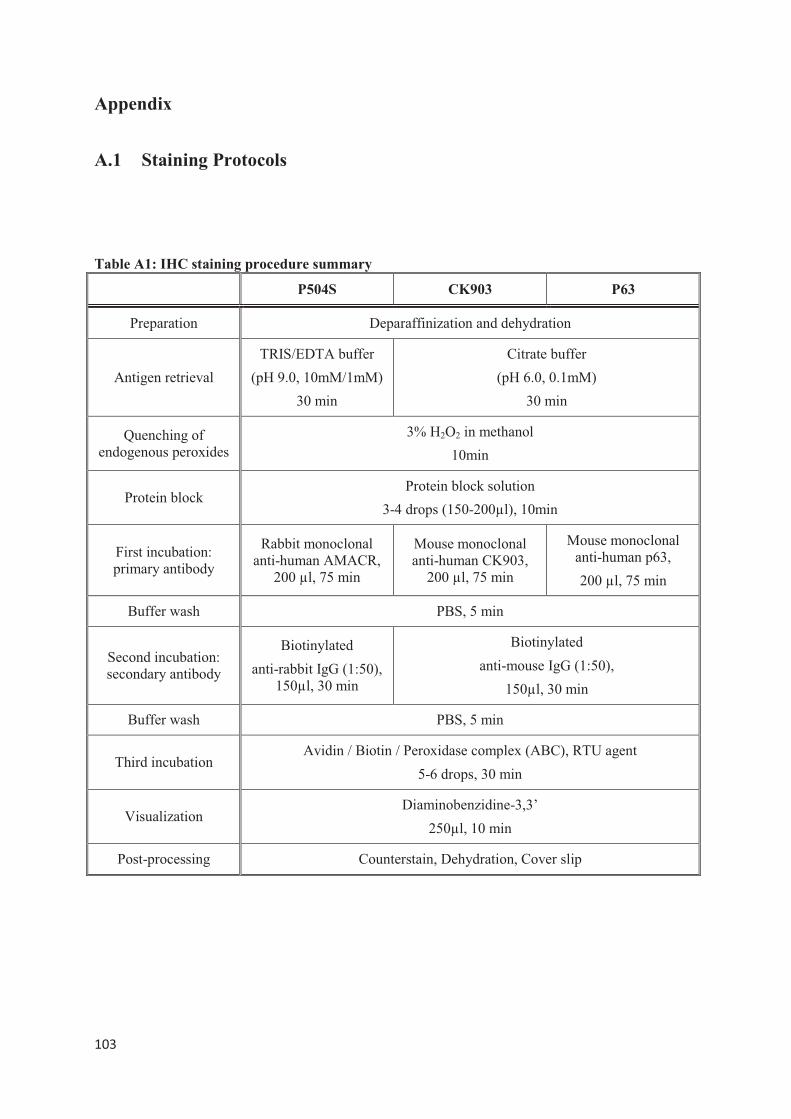
Appendix

A.1 Staining Protocols

Table A1: IHC staining procedure summary

P504S CK903 P63

Preparation Deparaffinization and dehydration

Antigen retrieval

TRIS/EDTA buffer

(pH 9.0, 10mM/1mM)

30 min

Citrate buffer

(pH 6.0, 0.1mM)

30 min

Quenching of endogenous peroxides

3% H2O2 in methanol

10min

Protein block Protein block solution

3-4 drops (150-200µl), 10min

First incubation: primary antibody

Rabbit monoclonal anti-human AMACR,

200 µl, 75 min

Mouse monoclonal anti-human CK903,

200 µl, 75 min

Mouse monoclonal anti-human p63,

200 µl, 75 min

Buffer wash PBS, 5 min

Second incubation: secondary antibody

Biotinylated

anti-rabbit IgG (1:50), 150µl, 30 min

Biotinylated

anti-mouse IgG (1:50),

150µl, 30 min

Buffer wash PBS, 5 min

Third incubation Avidin / Biotin / Peroxidase complex (ABC), RTU agent

5-6 drops, 30 min

Visualization Diaminobenzidine-3,3’

250µl, 10 min

Post-processing Counterstain, Dehydration, Cover slip

����

�

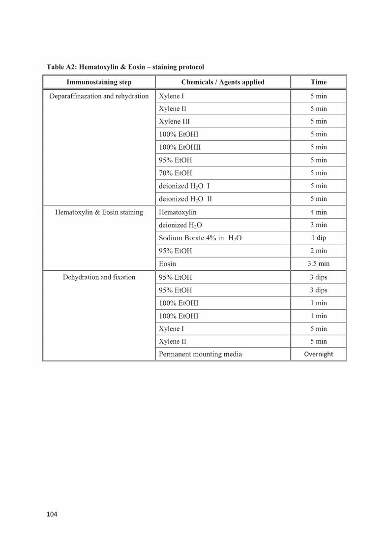
Table A2: Hematoxylin & Eosin – staining protocol

Immunostaining step Chemicals / Agents applied Time

Deparaffinazation and rehydration Xylene I 5 min

Xylene II 5 min�

Xylene III 5 min�

100% EtOHI 5 min�

100% EtOHII 5 min�

95% EtOH 5 min�

70% EtOH 5 min�

deionized H2O I 5 min

deionized H2O II 5 min

Hematoxylin & Eosin staining Hematoxylin 4 min

deionized H2O 3 min�

Sodium Borate 4% in H2O 1 dip�

95% EtOH 2 min�

Eosin 3.5 min�

Dehydration and fixation 95% EtOH 3 dips�

95% EtOH 3 dips�

100% EtOHI 1 min�

100% EtOHI 1 min�

Xylene I 5 min

Xylene II 5 min

Permanent mounting media ����������

�

�

�

����

�

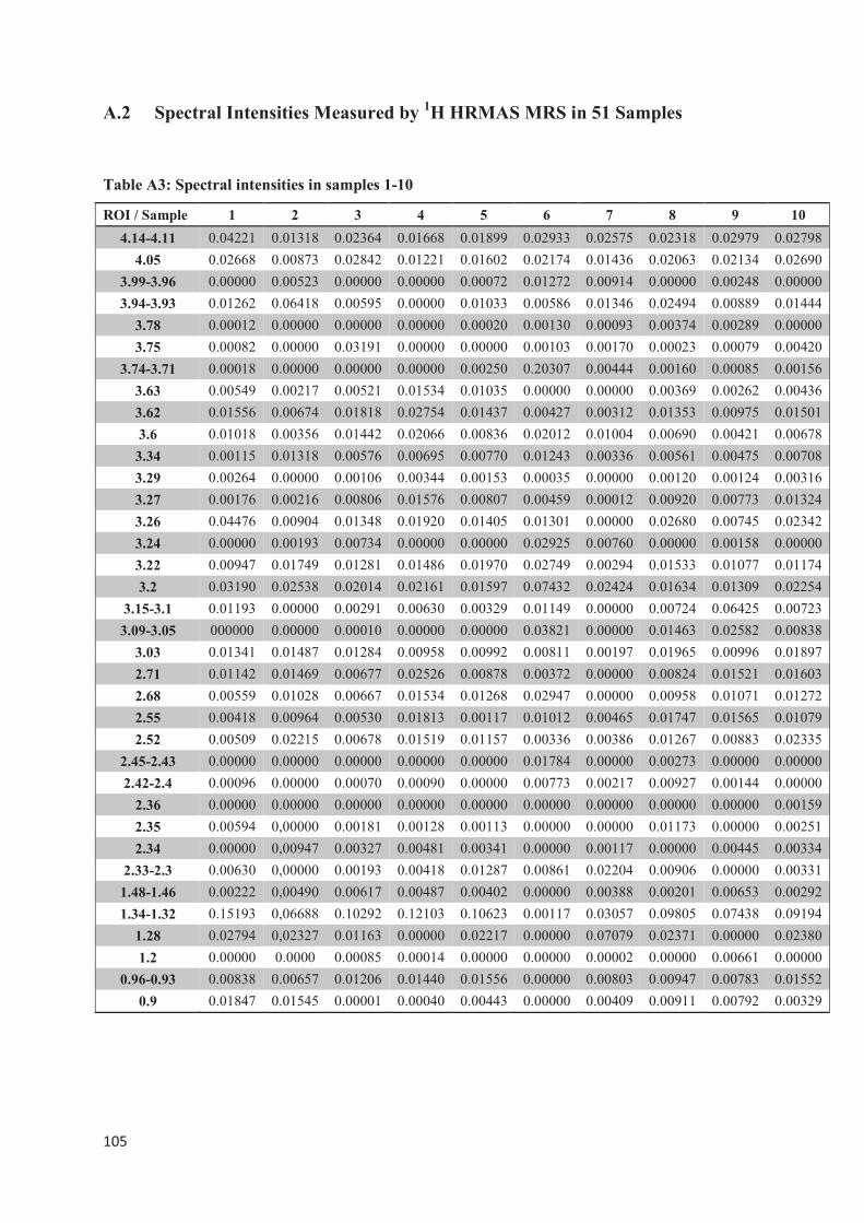
A.2 Spectral Intensities Measured by 1H HRMAS MRS in 51 Samples

�

Table A3: Spectral intensities in samples 1-10

ROI / Sample 1 2 3 4 5 6 7 8 9 10

4.14-4.11 0.04221 0.01318 0.02364 0.01668 0.01899 0.02933 0.02575 0.02318 0.02979 0.02798

4.05 0.02668 0.00873 0.02842 0.01221 0.01602 0.02174 0.01436 0.02063 0.02134 0.02690

3.99-3.96 0.00000 0.00523 0.00000 0.00000 0.00072 0.01272 0.00914 0.00000 0.00248 0.00000

3.94-3.93 0.01262 0.06418 0.00595 0.00000 0.01033 0.00586 0.01346 0.02494 0.00889 0.01444

3.78 0.00012 0.00000 0.00000 0.00000 0.00020 0.00130 0.00093 0.00374 0.00289 0.00000

3.75 0.00082 0.00000 0.03191 0.00000 0.00000 0.00103 0.00170 0.00023 0.00079 0.00420

3.74-3.71 0.00018 0.00000 0.00000 0.00000 0.00250 0.20307 0.00444 0.00160 0.00085 0.00156

3.63 0.00549 0.00217 0.00521 0.01534 0.01035 0.00000 0.00000 0.00369 0.00262 0.00436

3.62 0.01556 0.00674 0.01818 0.02754 0.01437 0.00427 0.00312 0.01353 0.00975 0.01501

3.6 0.01018 0.00356 0.01442 0.02066 0.00836 0.02012 0.01004 0.00690 0.00421 0.00678

3.34 0.00115 0.01318 0.00576 0.00695 0.00770 0.01243 0.00336 0.00561 0.00475 0.00708

3.29 0.00264 0.00000 0.00106 0.00344 0.00153 0.00035 0.00000 0.00120 0.00124 0.00316

3.27 0.00176 0.00216 0.00806 0.01576 0.00807 0.00459 0.00012 0.00920 0.00773 0.01324

3.26 0.04476 0.00904 0.01348 0.01920 0.01405 0.01301 0.00000 0.02680 0.00745 0.02342

3.24 0.00000 0.00193 0.00734 0.00000 0.00000 0.02925 0.00760 0.00000 0.00158 0.00000

3.22 0.00947 0.01749 0.01281 0.01486 0.01970 0.02749 0.00294 0.01533 0.01077 0.01174

3.2 0.03190 0.02538 0.02014 0.02161 0.01597 0.07432 0.02424 0.01634 0.01309 0.02254

3.15-3.1 0.01193 0.00000 0.00291 0.00630 0.00329 0.01149 0.00000 0.00724 0.06425 0.00723

3.09-3.05 000000 0.00000 0.00010 0.00000 0.00000 0.03821 0.00000 0.01463 0.02582 0.00838

3.03 0.01341 0.01487 0.01284 0.00958 0.00992 0.00811 0.00197 0.01965 0.00996 0.01897

2.71 0.01142 0.01469 0.00677 0.02526 0.00878 0.00372 0.00000 0.00824 0.01521 0.01603

2.68 0.00559 0.01028 0.00667 0.01534 0.01268 0.02947 0.00000 0.00958 0.01071 0.01272

2.55 0.00418 0.00964 0.00530 0.01813 0.00117 0.01012 0.00465 0.01747 0.01565 0.01079

2.52 0.00509 0.02215 0.00678 0.01519 0.01157 0.00336 0.00386 0.01267 0.00883 0.02335

2.45-2.43 0.00000 0.00000 0.00000 0.00000 0.00000 0.01784 0.00000 0.00273 0.00000 0.00000

2.42-2.4 0.00096 0.00000 0.00070 0.00090 0.00000 0.00773 0.00217 0.00927 0.00144 0.00000

2.36 0.00000 0.00000 0.00000 0.00000 0.00000 0.00000 0.00000 0.00000 0.00000 0.00159

2.35 0.00594 0,00000 0.00181 0.00128 0.00113 0.00000 0.00000 0.01173 0.00000 0.00251

2.34 0.00000 0,00947 0.00327 0.00481 0.00341 0.00000 0.00117 0.00000 0.00445 0.00334

2.33-2.3 0.00630 0,00000 0.00193 0.00418 0.01287 0.00861 0.02204 0.00906 0.00000 0.00331

1.48-1.46 0.00222 0,00490 0.00617 0.00487 0.00402 0.00000 0.00388 0.00201 0.00653 0.00292

1.34-1.32 0.15193 0,06688 0.10292 0.12103 0.10623 0.00117 0.03057 0.09805 0.07438 0.09194

1.28 0.02794 0,02327 0.01163 0.00000 0.02217 0.00000 0.07079 0.02371 0.00000 0.02380

1.2 0.00000 0.0000 0.00085 0.00014 0.00000 0.00000 0.00002 0.00000 0.00661 0.00000

0.96-0.93 0.00838 0.00657 0.01206 0.01440 0.01556 0.00000 0.00803 0.00947 0.00783 0.01552

0.9 0.01847 0.01545 0.00001 0.00040 0.00443 0.00000 0.00409 0.00911 0.00792 0.00329

�

����

�

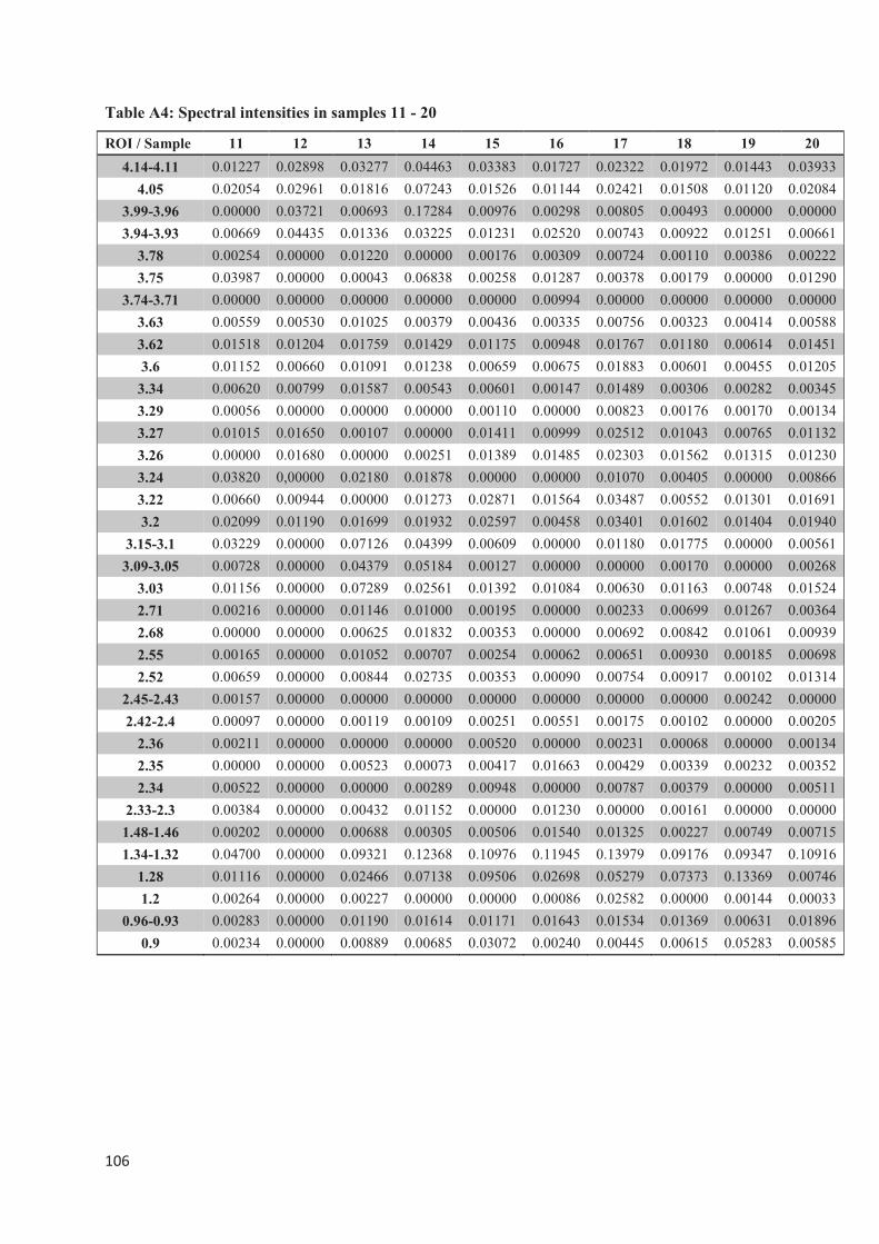
Table A4: Spectral intensities in samples 11 - 20

ROI / Sample 11 12 13 14 15 16 17 18 19 20

4.14-4.11 0.01227 0.02898 0.03277 0.04463 0.03383 0.01727 0.02322 0.01972 0.01443 0.03933

4.05 0.02054 0.02961 0.01816 0.07243 0.01526 0.01144 0.02421 0.01508 0.01120 0.02084

3.99-3.96 0.00000 0.03721 0.00693 0.17284 0.00976 0.00298 0.00805 0.00493 0.00000 0.00000

3.94-3.93 0.00669 0.04435 0.01336 0.03225 0.01231 0.02520 0.00743 0.00922 0.01251 0.00661

3.78 0.00254 0.00000 0.01220 0.00000 0.00176 0.00309 0.00724 0.00110 0.00386 0.00222

3.75 0.03987 0.00000 0.00043 0.06838 0.00258 0.01287 0.00378 0.00179 0.00000 0.01290

3.74-3.71 0.00000 0.00000 0.00000 0.00000 0.00000 0.00994 0.00000 0.00000 0.00000 0.00000

3.63 0.00559 0.00530 0.01025 0.00379 0.00436 0.00335 0.00756 0.00323 0.00414 0.00588

3.62 0.01518 0.01204 0.01759 0.01429 0.01175 0.00948 0.01767 0.01180 0.00614 0.01451

3.6 0.01152 0.00660 0.01091 0.01238 0.00659 0.00675 0.01883 0.00601 0.00455 0.01205

3.34 0.00620 0.00799 0.01587 0.00543 0.00601 0.00147 0.01489 0.00306 0.00282 0.00345

3.29 0.00056 0.00000 0.00000 0.00000 0.00110 0.00000 0.00823 0.00176 0.00170 0.00134

3.27 0.01015 0.01650 0.00107 0.00000 0.01411 0.00999 0.02512 0.01043 0.00765 0.01132

3.26 0.00000 0.01680 0.00000 0.00251 0.01389 0.01485 0.02303 0.01562 0.01315 0.01230

3.24 0.03820 0,00000 0.02180 0.01878 0.00000 0.00000 0.01070 0.00405 0.00000 0.00866

3.22 0.00660 0.00944 0.00000 0.01273 0.02871 0.01564 0.03487 0.00552 0.01301 0.01691

3.2 0.02099 0.01190 0.01699 0.01932 0.02597 0.00458 0.03401 0.01602 0.01404 0.01940

3.15-3.1 0.03229 0.00000 0.07126 0.04399 0.00609 0.00000 0.01180 0.01775 0.00000 0.00561

3.09-3.05 0.00728 0.00000 0.04379 0.05184 0.00127 0.00000 0.00000 0.00170 0.00000 0.00268

3.03 0.01156 0.00000 0.07289 0.02561 0.01392 0.01084 0.00630 0.01163 0.00748 0.01524

2.71 0.00216 0.00000 0.01146 0.01000 0.00195 0.00000 0.00233 0.00699 0.01267 0.00364

2.68 0.00000 0.00000 0.00625 0.01832 0.00353 0.00000 0.00692 0.00842 0.01061 0.00939

2.55 0.00165 0.00000 0.01052 0.00707 0.00254 0.00062 0.00651 0.00930 0.00185 0.00698

2.52 0.00659 0.00000 0.00844 0.02735 0.00353 0.00090 0.00754 0.00917 0.00102 0.01314

2.45-2.43 0.00157 0.00000 0.00000 0.00000 0.00000 0.00000 0.00000 0.00000 0.00242 0.00000

2.42-2.4 0.00097 0.00000 0.00119 0.00109 0.00251 0.00551 0.00175 0.00102 0.00000 0.00205

2.36 0.00211 0.00000 0.00000 0.00000 0.00520 0.00000 0.00231 0.00068 0.00000 0.00134

2.35 0.00000 0.00000 0.00523 0.00073 0.00417 0.01663 0.00429 0.00339 0.00232 0.00352

2.34 0.00522 0.00000 0.00000 0.00289 0.00948 0.00000 0.00787 0.00379 0.00000 0.00511

2.33-2.3 0.00384 0.00000 0.00432 0.01152 0.00000 0.01230 0.00000 0.00161 0.00000 0.00000

1.48-1.46 0.00202 0.00000 0.00688 0.00305 0.00506 0.01540 0.01325 0.00227 0.00749 0.00715

1.34-1.32 0.04700 0.00000 0.09321 0.12368 0.10976 0.11945 0.13979 0.09176 0.09347 0.10916

1.28 0.01116 0.00000 0.02466 0.07138 0.09506 0.02698 0.05279 0.07373 0.13369 0.00746

1.2 0.00264 0.00000 0.00227 0.00000 0.00000 0.00086 0.02582 0.00000 0.00144 0.00033

0.96-0.93 0.00283 0.00000 0.01190 0.01614 0.01171 0.01643 0.01534 0.01369 0.00631 0.01896

0.9 0.00234 0.00000 0.00889 0.00685 0.03072 0.00240 0.00445 0.00615 0.05283 0.00585

�

�

�

�

�

����

�

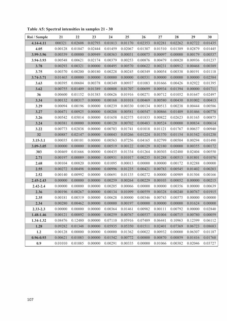
Table A5: Spectral intensities in samples 21 - 30

Roi / Sample 21 22 23 24 25 26 27 28 29 30

4.14-4.11 000321 0.02608 0.02793 0.01813 0.01170 0.02353 0.02281 0.02262 0.02722 0.01435

4.05 0.00128 0.01847 0.02444 0.01459 0.02067 0.01307 0.01510 0.01389 0.02879 0.01445

3.99-3.96 0.00339 0.00000 0.00949 0.00363 0.00031 0.00075 0.00097 0.00000 0.00179 0.00537

3.94-3.93 0.00548 0.00621 0.02174 0.00379 0.00253 0.00876 0.00479 0.00820 0.00936 0.01237

3.78 0.00293 0.00321 0.00000 0.00495 0.00570 0.00622 0.00231 0.00912 0.00468 0.00389

3.75 0.00370 0.00200 0.00180 0.00228 0.00245 0.00349 0.00054 0.00338 0.00191 0.01118

3.74-3.71 0.01465 0.00000 0.00000 0.00000 0.00000 0.00531 0.00000 0.00000 0.00000 0.02584

3.63 0.00395 0.00604 0.00378 0.00349 0.00937 0.01083 0.01666 0.00426 0.02922 0.01395

3.62 0.00755 0.01409 0.01389 0.00808 0.01707 0.00699 0.00934 0.01394 0.00000 0.01711

36 0.00600 0.01152 0.01383 0.00626 0.01916 0.00271 0.00712 0.01052 0.01647 0.02497

3.34 0.00132 0.00317 0.00000 0.00168 0.01018 0.00469 0.00580 0.00430 0.01002 0.00413

3.29 0.00094 0.00196 0.00000 0.00239 0.00330 0.00134 0.00513 0.00238 0.00444 0.00586

3.27 0.00471 0.00925 0.00000 0.00208 0.00581 0.00547 0.00866 0.01409 0.01466 0.00778

3.26 0.00542 0.05014 0.00000 0.01658 0.02375 0.01833 0.00822 0.02623 0.01165 0.00875

3.24 0.00381 0.00000 0.00000 0.00120 0.00702 0.00483 0.00524 0.00000 0.00834 0.00614

3.22 0.00773 0.02838 0.00000 0.00703 0.01741 0.01018 0.01121 0.01767 0.00637 0.00940

32 0.00887 0.02147 0.00000 0.00043 0.03266 0.01224 0.01370 0.01154 0.01542 0.01238

3.15-3.1 0.00035 0.00101 0.00000 0.00563 0.07256 0.04165 0.02799 0.00504 0.00294 0.01490

3.09-3.05 0.00000 0.00000 0.00000 0.00519 0.00122 0.00129 0.02180 0.00000 0.00355 0.00172

303 0.00469 0.01666 0.00000 0.00435 0.01334 0.01264 0.00303 0.02480 0.02404 0.00550

2.71 0.00197 0.00089 0.00000 0.00931 0.01017 0.00235 0.01288 0.00513 0.01801 0.01076

2.68 0.00104 0.00820 0.00000 0.01095 0.00013 0.00000 0.00000 0.00172 0.02288 0.00000

2.55 0.00272 0.00498 0.00000 0.00996 0.01235 0.00421 0.00783 0.00545 0.01402 0.00203

2.52 0.00140 0.00992 0.00000 0.00691 0.01135 0.00272 0.00000 0.00909 0.01504 0.00166

2.45-2.43 0.00000 0.00000 0.00000 0.00259 0.00264 0.00229 0.00103 0.00052 0.00000 0.00215

2.42-2.4 0.00000 0.00000 0.00000 0.00205 0.00066 0.00000 0.00000 0.00356 0.00000 0.00639

2.36 0.00196 0.00267 0.00000 0.00134 0.01099 0.00559 0.00328 0.00240 0.00767 0.01915

2.35 0.00181 0.00319 0.00000 0.00628 0.00000 0.00346 0.00743 0.00575 0.00000 0.00000

2.34 0.00280 0.00462 0.00000 0.00000 0.00197 0.00000 0.00000 0.00000 0.01624 0.00000

2.33-2.3 0.00000 0.00000 0.00000 0.00364 0.01461 0.00982 0.00111 0.00792 0.00000 0.02840

1.48-1.46 0.00121 0.00892 0.00000 0.00259 0.00767 0.00537 0.01004 0.00715 0.00780 0.00059

1.34-1.32 0.08476 0.12480 0.00000 0.07110 0.05916 0.07489 0.06441 0.10963 0.12399 0.06112

1.28 0.09282 0.01348 0.00000 0.05935 0.05350 0.01511 0.02401 0.07369 0.06723 0.08683

1.2 0.00128 0.00000 0.00000 0.00000 0.01362 0.00022 0.00932 0.00000 0.06307 0.01187

0.96-0.93 0.00621 0.01083 0.00000 0.01542 0.00772 0.00800 0.00870 0.00859 0.01416 0.01768

0.9 0.01010 0.01085 0.00000 0.00291 0.00335 0.00000 0.01066 0.00382 0.02046 0.03727

�

�

�

�

�

����

�

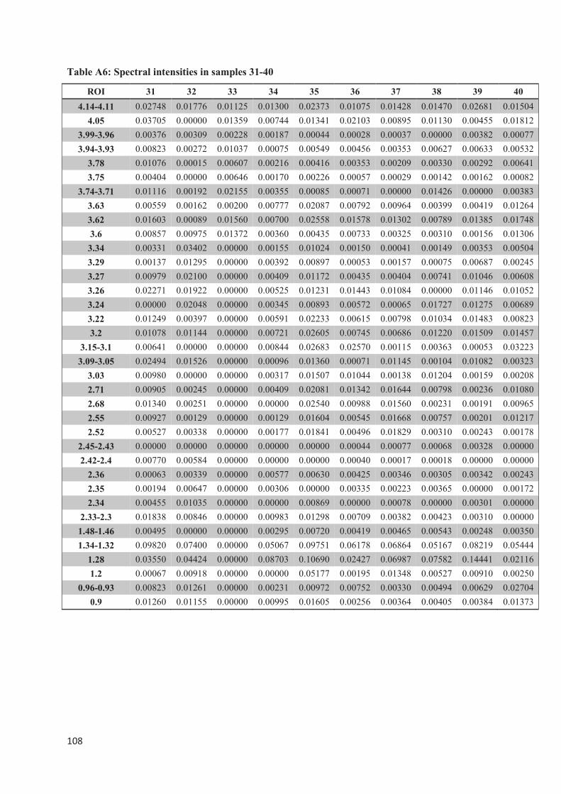
Table A6: Spectral intensities in samples 31-40

ROI 31 32 33 34 35 36 37 38 39 40

4.14-4.11 0.02748 0.01776 0.01125 0.01300 0.02373 0.01075 0.01428 0.01470 0.02681 0.01504

4.05 0.03705 0.00000 0.01359 0.00744 0.01341 0.02103 0.00895 0.01130 0.00455 0.01812

3.99-3.96 0.00376 0.00309 0.00228 0.00187 0.00044 0.00028 0.00037 0.00000 0.00382 0.00077

3.94-3.93 0.00823 0.00272 0.01037 0.00075 0.00549 0.00456 0.00353 0.00627 0.00633 0.00532

3.78 0.01076 0.00015 0.00607 0.00216 0.00416 0.00353 0.00209 0.00330 0.00292 0.00641

3.75 0.00404 0.00000 0.00646 0.00170 0.00226 0.00057 0.00029 0.00142 0.00162 0.00082

3.74-3.71 0.01116 0.00192 0.02155 0.00355 0.00085 0.00071 0.00000 0.01426 0.00000 0.00383

3.63 0.00559 0.00162 0.00200 0.00777 0.02087 0.00792 0.00964 0.00399 0.00419 0.01264

3.62 0.01603 0.00089 0.01560 0.00700 0.02558 0.01578 0.01302 0.00789 0.01385 0.01748

3.6 0.00857 0.00975 0.01372 0.00360 0.00435 0.00733 0.00325 0.00310 0.00156 0.01306

3.34 0.00331 0.03402 0.00000 0.00155 0.01024 0.00150 0.00041 0.00149 0.00353 0.00504

3.29 0.00137 0.01295 0.00000 0.00392 0.00897 0.00053 0.00157 0.00075 0.00687 0.00245

3.27 0.00979 0.02100 0.00000 0.00409 0.01172 0.00435 0.00404 0.00741 0.01046 0.00608

3.26 0.02271 0.01922 0.00000 0.00525 0.01231 0.01443 0.01084 0.00000 0.01146 0.01052

3.24 0.00000 0.02048 0.00000 0.00345 0.00893 0.00572 0.00065 0.01727 0.01275 0.00689

3.22 0.01249 0.00397 0.00000 0.00591 0.02233 0.00615 0.00798 0.01034 0.01483 0.00823

3.2 0.01078 0.01144 0.00000 0.00721 0.02605 0.00745 0.00686 0.01220 0.01509 0.01457

3.15-3.1 0.00641 0.00000 0.00000 0.00844 0.02683 0.02570 0.00115 0.00363 0.00053 0.03223

3.09-3.05 0.02494 0.01526 0.00000 0.00096 0.01360 0.00071 0.01145 0.00104 0.01082 0.00323

3.03 0.00980 0.00000 0.00000 0.00317 0.01507 0.01044 0.00138 0.01204 0.00159 0.00208

2.71 0.00905 0.00245 0.00000 0.00409 0.02081 0.01342 0.01644 0.00798 0.00236 0.01080

2.68 0.01340 0.00251 0.00000 0.00000 0.02540 0.00988 0.01560 0.00231 0.00191 0.00965

2.55 0.00927 0.00129 0.00000 0.00129 0.01604 0.00545 0.01668 0.00757 0.00201 0.01217

2.52 0.00527 0.00338 0.00000 0.00177 0.01841 0.00496 0.01829 0.00310 0.00243 0.00178

2.45-2.43 0.00000 0.00000 0.00000 0.00000 0.00000 0.00044 0.00077 0.00068 0.00328 0.00000

2.42-2.4 0.00770 0.00584 0.00000 0.00000 0.00000 0.00040 0.00017 0.00018 0.00000 0.00000

2.36 0.00063 0.00339 0.00000 0.00577 0.00630 0.00425 0.00346 0.00305 0.00342 0.00243

2.35 0.00194 0.00647 0.00000 0.00306 0.00000 0.00335 0.00223 0.00365 0.00000 0.00172

2.34 0.00455 0.01035 0.00000 0.00000 0.00869 0.00000 0.00078 0.00000 0.00301 0.00000

2.33-2.3 0.01838 0.00846 0.00000 0.00983 0.01298 0.00709 0.00382 0.00423 0.00310 0.00000

1.48-1.46 0.00495 0.00000 0.00000 0.00295 0.00720 0.00419 0.00465 0.00543 0.00248 0.00350

1.34-1.32 0.09820 0.07400 0.00000 0.05067 0.09751 0.06178 0.06864 0.05167 0.08219 0.05444

1.28 0.03550 0.04424 0.00000 0.08703 0.10690 0.02427 0.06987 0.07582 0.14441 0.02116

1.2 0.00067 0.00918 0.00000 0.00000 0.05177 0.00195 0.01348 0.00527 0.00910 0.00250

0.96-0.93 0.00823 0.01261 0.00000 0.00231 0.00972 0.00752 0.00330 0.00494 0.00629 0.02704

0.9 0.01260 0.01155 0.00000 0.00995 0.01605 0.00256 0.00364 0.00405 0.00384 0.01373

�

�

�

�

�

����

�

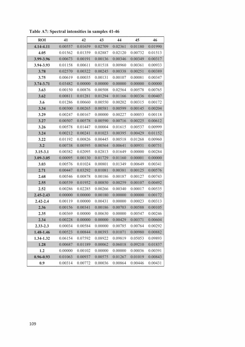
Table A7: Spectral intensities in samples 41-46

ROI 41 42 43 44 45 46

4.14-4.11 0.00557 0.01659 0.02709 0.02361 0.01180 0.01990

4.05 0.01562 0.01359 0.02887 0.02120 0.00732 0.01513

3.99-3.96 0.00673 0.00191 0.00136 0.00346 0.00349 0.00317

3.94-3.93 0.01158 0.00611 0.01518 0.00960 0.00361 0.00933

3.78 0.02570 0.00322 0.00245 0.00338 0.00251 0.00389

3.75 0.00619 0.00035 0.00131 0.00107 0.00081 0.00347

3.74-3.71 0.03482 0.00000 0.00000 0.00000 0.00000 0.00000

3.63 0.00150 0.00876 0.00508 0.02564 0.00578 0.00765

3.62 0.00811 0.01281 0.01294 0.01166 0.00336 0.00407

3.6 0.01286 0.00660 0.00550 0.00202 0.00315 0.00172

3.34 0.00300 0.00265 0.00581 0.00599 0.00145 0.00204

3.29 0.00247 0.00167 0.00000 0.00227 0.00053 0.00118

3.27 0.00507 0.00578 0.00590 0.00716 0.00225 0.00612

3.26 0.00578 0.01447 0.00004 0.01615 0.00537 0.00999

3.24 0.00212 0.00241 0.01023 0.00395 0.00429 0.01152

3.22 0.01192 0.00826 0.00445 0.00518 0.01268 0.00960

3.2 0.00738 0.00595 0.00564 0.00641 0.00931 0.00751

3.15-3.1 0.00382 0.02095 0.02813 0.01649 0.00000 0.00284

3.09-3.05 0.00095 0.00130 0.01729 0.01160 0.00001 0.00000

3.03 0.00576 0.01024 0.00801 0.01349 0.00649 0.00341

2.71 0.00447 0.03292 0.01081 0.00381 0.00125 0.00576

2.68 0.00546 0.00878 0.00186 0.00187 0.00127 0.00743

2.55 0.00539 0.01952 0.00850 0.00259 0.00107 0.00492

2.52 0.00286 0.02285 0.00266 0.00340 0.00017 0.00535

2.45-2.43 0.00000 0.00000 0.00180 0.00000 0.00000 0.00172

2.42-2.4 0.00119 0.00000 0.00431 0.00000 0.00023 0.00313

2.36 0.00156 0.00341 0.00186 0.00703 0.00588 0.00105

2.35 0.00369 0.00000 0.00630 0.00000 0.00547 0.00246

2.34 0.00228 0.00000 0.00000 0.00429 0.00371 0.00604

2.33-2.3 0.00034 0.00584 0.00000 0.00785 0.00764 0.00292

1.48-1.46 0.00523 0.00844 0.00393 0.01071 0.00980 0.00882

1.34-1.32 0.06154 0.07592 0.08922 0.09819 0.05053 0.09893

1.28 0.00687 0.01189 0.00062 0.06018 0.09210 0.01837

1.2 0.00000 0.00102 0.00000 0.00000 0.00036 0.00391

0.96-0.93 0.01063 0.00937 0.00575 0.01267 0.01019 0.00843

0.9 0.00314 0.00772 0.00036 0.00864 0.00446 0.00431

�

�

����

�

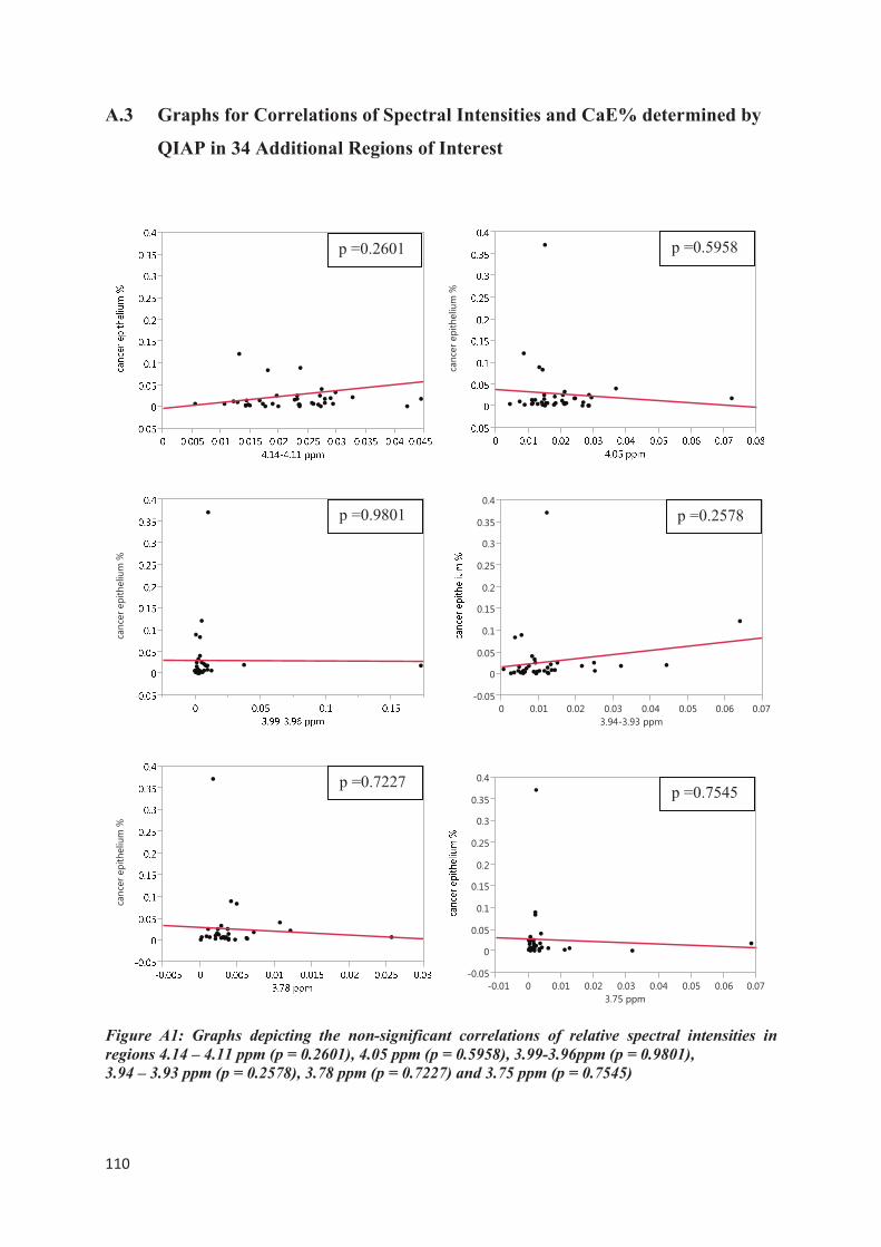
A.3 Graphs for Correlations of Spectral Intensities and CaE% determined by

QIAP in 34 Additional Regions of Interest

Figure A1: Graphs depicting the non-significant correlations of relative spectral intensities in

regions 4.14 – 4.11 ppm (p = 0.2601), 4.05 ppm (p = 0.5958), 3.99-3.96ppm (p = 0.9801),

3.94 – 3.93 ppm (p = 0.2578), 3.78 ppm (p = 0.7227) and 3.75 ppm (p = 0.7545)

�������������������

�������������������

�������������������

�����

�

����

���

����

���

����

���

����

���

� ���� ���� ���� ���� ���� ���� ����

�������������

�����

�

����

���

����

���

����

���

����

���

����� � ���� ���� ���� ���� ���� ���� ����

��������

p =0.2601 p =0.5958

p =0.9801 p =0.2578

p =0.7227 p =0.7545

����

�

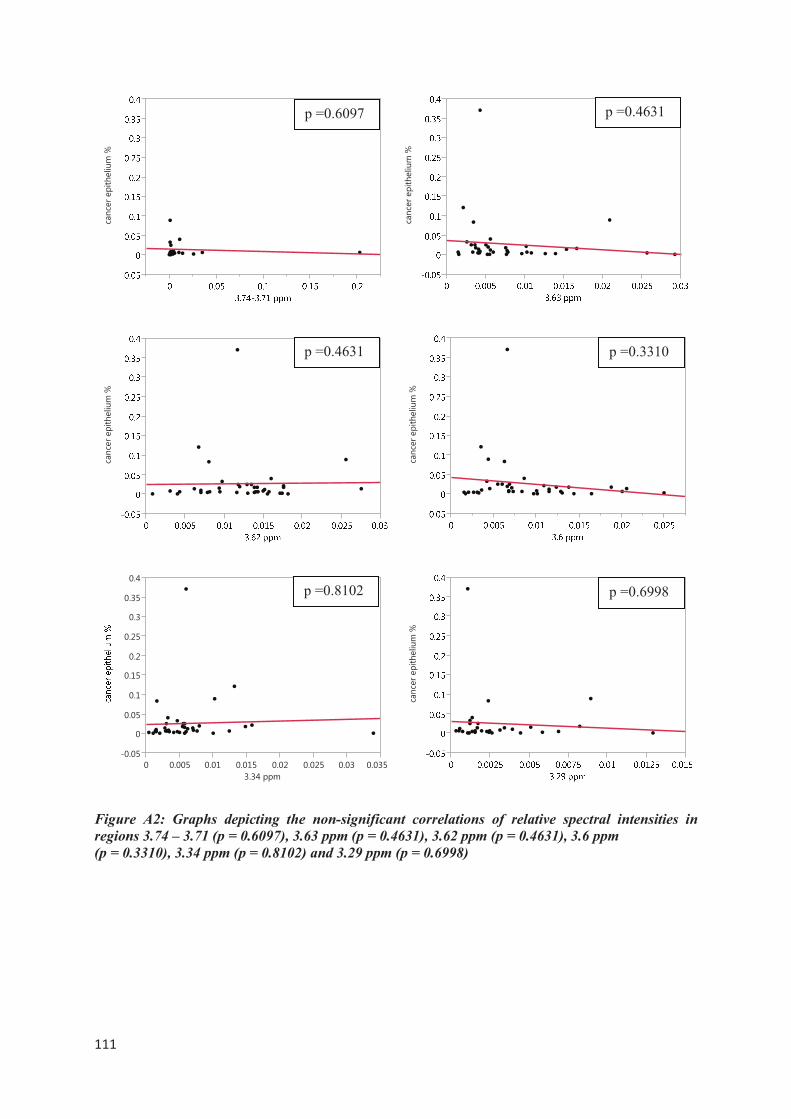
Figure A2: Graphs depicting the non-significant correlations of relative spectral intensities in

regions 3.74 – 3.71 (p = 0.6097), 3.63 ppm (p = 0.4631), 3.62 ppm (p = 0.4631), 3.6 ppm

(p = 0.3310), 3.34 ppm (p = 0.8102) and 3.29 ppm (p = 0.6998)

�������������������

�������������������

�����

�

����

���

����

���

����

���

����

���

� ����� ���� ����� ���� ����� ���� �����

��������

p =0.6097

�������������������

p =0.4631

p =0.4631

�������������������

p =0.3310

p =0.8102

�������������������

p =0.6998

����

�

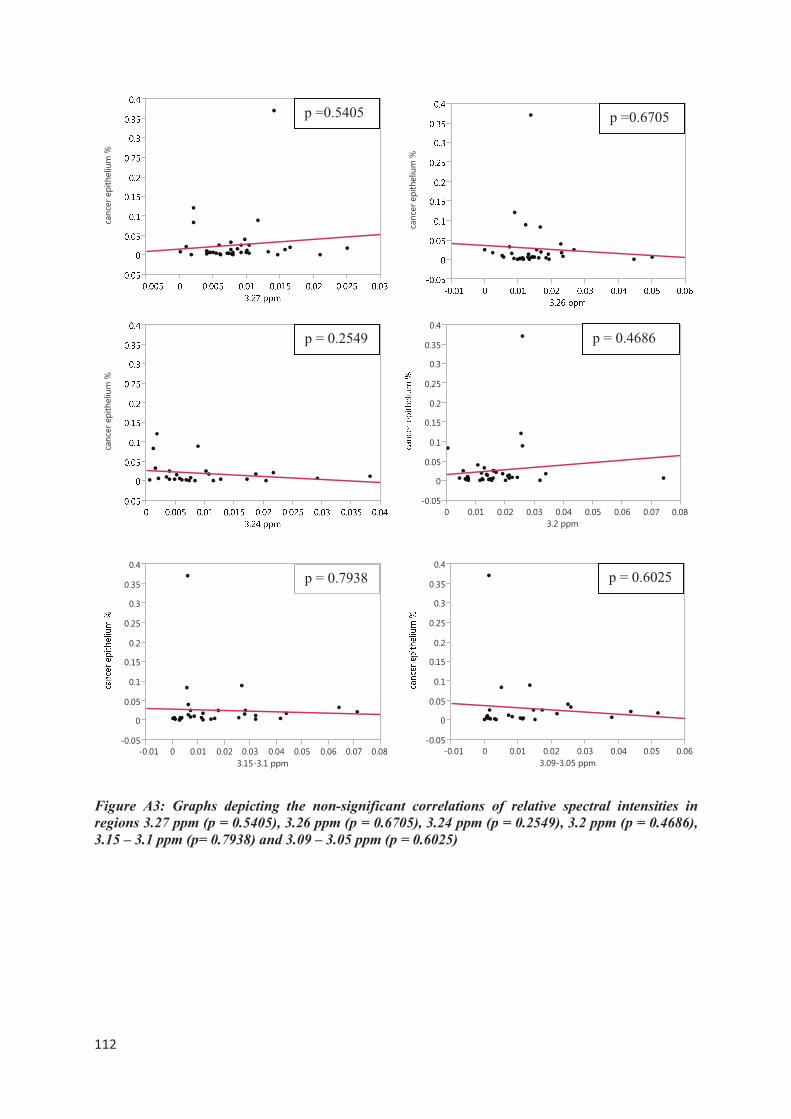
Figure A3: Graphs depicting the non-significant correlations of relative spectral intensities in

regions 3.27 ppm (p = 0.5405), 3.26 ppm (p = 0.6705), 3.24 ppm (p = 0.2549), 3.2 ppm (p = 0.4686),

3.15 – 3.1 ppm (p= 0.7938) and 3.09 – 3.05 ppm (p = 0.6025)

�������������������

�������������������

�����

�

����

���

����

���

����

���

����

���

����� � ���� ���� ���� ���� ���� ���� ���� ����

������������

p =0.5405

�������������������

p =0.6705

p = 0.2549

�����

�

����

���

����

���

����

���

����

���

� ���� ���� ���� ���� ���� ���� ���� ����

�������

p = 0.7938

p = 0.4686

�����

�

����

���

����

���

����

���

����

���

����� � ���� ���� ���� ���� ���� ����

�������������

p = 0.6025

����

�

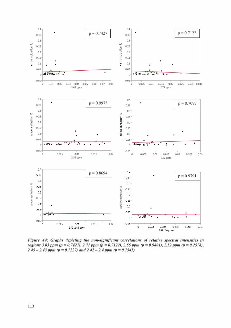
Figure A4: Graphs depicting the non-significant correlations of relative spectral intensities in

regions 3.03 ppm (p = 0.7427), 2.71 ppm (p = 0.7122), 2.55 ppm (p = 0.9801), 2.52 ppm (p = 0.2578),

2.45 – 2.43 ppm (p = 0.7227) and 2.42 – 2.4 ppm (p = 0.7545)

�����

�

����

���

����

���

����

���

����

���

� ���� ���� ���� ���� ���� ���� ���� ����

��������

�����

�

����

���

����

���

����

���

����

���

� ����� ���� ����� ����

��������

�������������������

p = 0.8694

�������������������

p = 0.9791

�����

�

����

���

����

���

����

���

����

���

� ����� ���� ����� ���� ����� ���� �����

��������

p = 0.7427 p = 0.7122

p = 0.9975

�����

�

����

���

����

���

����

���

����

���

� ����� ���� ����� ���� ����� ����

��������

p = 0.7097

����

�

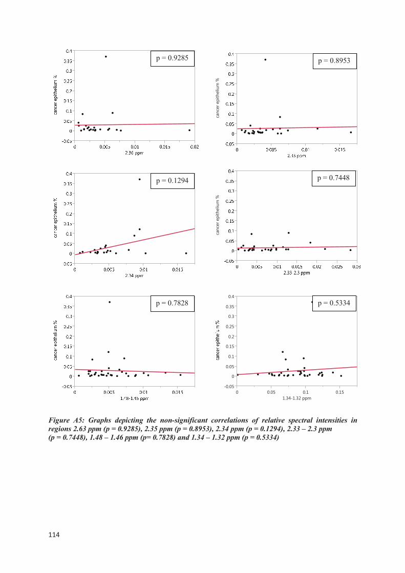
Figure A5: Graphs depicting the non-significant correlations of relative spectral intensities in

regions 2.63 ppm (p = 0.9285), 2.35 ppm (p = 0.8953), 2.34 ppm (p = 0.1294), 2.33 – 2.3 ppm

(p = 0.7448), 1.48 – 1.46 ppm (p= 0.7828) and 1.34 – 1.32 ppm (p = 0.5334)

p = 0.9285

�������������������

p = 0.8953

p = 0.1294

�������������������

p = 0.7448

p = 0.7828

�����

�

����

���

����

���

����

���

����

���

� ���� ��� ����

�������������

p = 0.5334

����

�

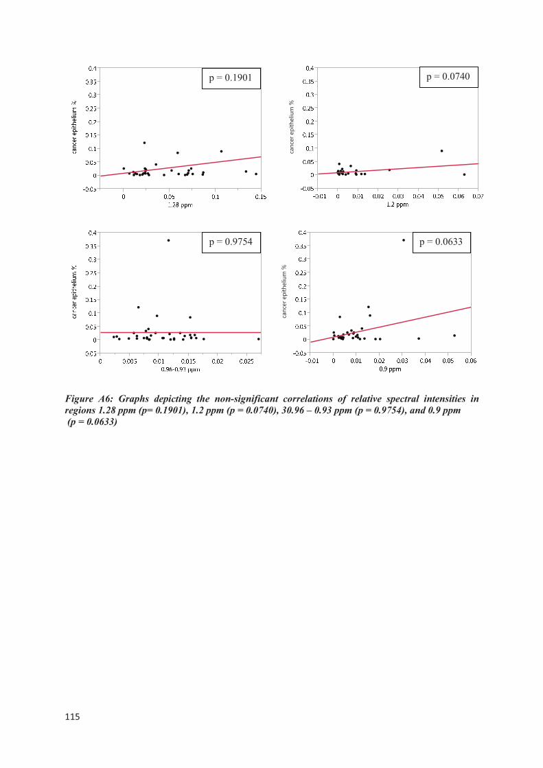
Figure A6: Graphs depicting the non-significant correlations of relative spectral intensities in

regions 1.28 ppm (p= 0.1901), 1.2 ppm (p = 0.0740), 30.96 – 0.93 ppm (p = 0.9754), and 0.9 ppm

(p = 0.0633)

p = 0.1901

�������������������

p = 0.0740

p = 0.9754

�������������������

p = 0.0633