Embed Size (px)
Citation preview
Demonstration Of A Power Ampliier Linearization Based On Digital Predistortion In Mobile Wimax Application 175
Demonstration Of A Power Ampliier Linearization Based On Digital Predistortion In Mobile Wimax Application
Pooria Varahram, Somayeh Mohammady, M. Nizar Hamidon, Roslina M. Sidek and Sabira Khatun
x
DEMONSTRATION OF A POWER AMPLIFIER LINEARIZATION BASED
ON DIGITAL PREDISTORTION IN MOBILE WIMAX APPLICATION
Pooria Varahram, Somayeh Mohammady,
M. Nizar Hamidon, Roslina M. Sidek and Sabira Khatun University Putra Malaysia
Malaysia
1. Introduction
Spectrally efficient linear modulation techniques are used in the third generation systems and their performance is strongly dependent on the linearity of the transmission system, Also, the efficiency of the amplifier to be used has to be maximized, which means that it must work near saturation. Newer transmission formats, with wide bandwidths, such as multi carrier wideband code division multiple access (WCDMA), wireless local area network (WLAN), worldwide interoperability for microwave access (WiMAX), are especially vulnerable to PA nonlinearities, due to their high peak-to-average power ratio, corresponding to large fluctuations in their signal envelopes. In order to comply with spectral masks imposed by regulatory bodies and to reduce BER, PA linearization is necessary. A number of linearization techniques have been reported in recent years (Cripps, 1999;Kennington, 2000; kim & Konstantinou, 2001;Wright & Durtler 1992;Woo, et al. 2007; Nagata, 1989). One technique that can potentially compensate for power amplifier (PA) nonlinearities in such an environment is the adaptive digital predistortion technique. The concept is based on inserting a non-linear function (the inverse function of the amplifier) between the input signal and the amplifier to produce a linear output. The digital predistortion (DPD) requires to be adaptive because of variation in power amplifier nonlinearity with time, temperature and different operating channels and so on. Another limitation of predistortion is the dependence of amplifier’s transfer characteristic’s on the frequency content of the signal or defined as changes of the amplitude and phase in distortion components due to past signal values, that is called memory effects. The memory effects compensation is an important issue of the DPD algorithm in addition to correction of power amplifier (PA) nonlinearity especially when the signal bandwidth increases. Many studies are involved in this technique but many of them suffer from limitations in bandwidth, precision or stability (Cavers, 1990;Wright & Durtler 1992;Nagata, 1989). In this reseach a new technique of adaptive digital predistortion that is the combination of two techniques, the gain based predistorter (Cavers, 1990) and memory polynomial model
9
www.intechopen.com
Advanced Microwave and Millimeter Wave Technologies: Semiconductor Devices, Circuits and Systems176
(Ding, et al. 2004) is presented. Both previous techniques have demonstrated acceptable results but both have disadvantages. In memory polynomial predistortion the complexity of extracting the coefficients of predistortion function decrease the capability of linearization and so it needs to apply other method like (Raich, et al. 2003) for implementing it. In complex gain predistortion method (Cavers, 1990) the memory effects that cause dynamic AM-AM and AM-PM are not considered. So here the main objective is not only to demonstrate the capability of this new method to overcome for such disadvantages, but also to show that with applying this technique all the memory contents of power amplifier that is modeled with memory polynomial is compensated. for validating this technique several simulations are applied. The adaptation is based on linear convergence method in the simulations. For simplicity the effects of the quadrature modulator and demodulator and A/D and D/A is not considered. The LUT size is 10 bit and addressing the LUT is based on the input amplitude. It will be shown that with applying this method all the memory contents of the power amplifier especially the one that cause dynamic AM/AM and AM/PM are compensated. Simulation and results are examined based on Motorola’s MRF1806 1.9 GHz LDMOS PA with 13 dB gain and 60W output power. To demonstrating the results several tests are shown with Mobile WiMAX signal. Finally the actual power amplifier from Mini Circuit ZVE-8G with 30 dB gain is used and tested with agilent equipments to verify the proposed algorithm. 2. Predistortion technique
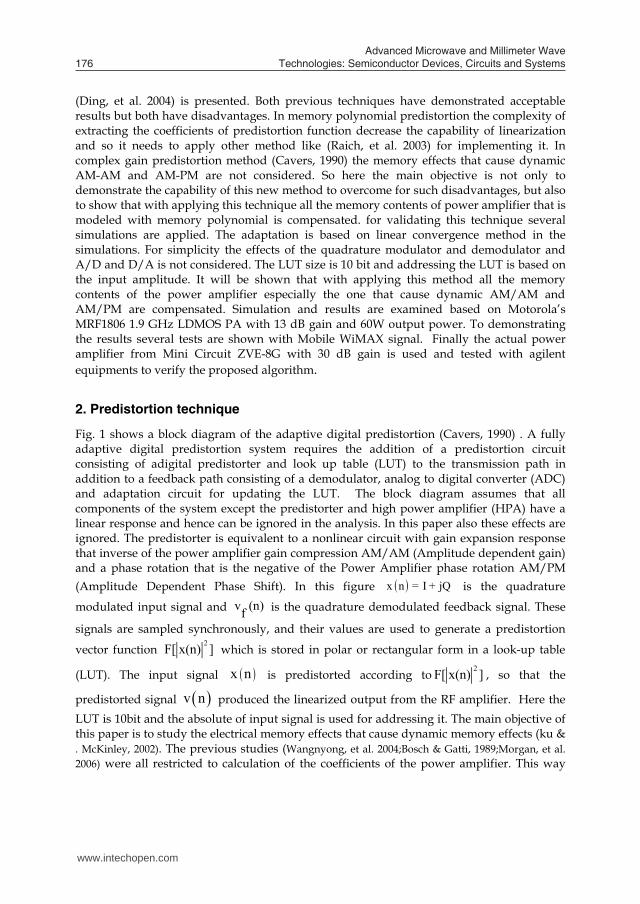
Fig. 1 shows a block diagram of the adaptive digital predistortion (Cavers, 1990) . A fully adaptive digital predistortion system requires the addition of a predistortion circuit consisting of adigital predistorter and look up table (LUT) to the transmission path in addition to a feedback path consisting of a demodulator, analog to digital converter (ADC) and adaptation circuit for updating the LUT. The block diagram assumes that all components of the system except the predistorter and high power amplifier (HPA) have a linear response and hence can be ignored in the analysis. In this paper also these effects are ignored. The predistorter is equivalent to a nonlinear circuit with gain expansion response that inverse of the power amplifier gain compression AM/AM (Amplitude dependent gain) and a phase rotation that is the negative of the Power Amplifier phase rotation AM/PM (Amplitude Dependent Phase Shift). In this figure x n = I + jQ is the quadrature
modulated input signal and v (n)f is the quadrature demodulated feedback signal. These
signals are sampled synchronously, and their values are used to generate a predistortion
vector function 2F[ x(n) ] which is stored in polar or rectangular form in a look-up table
(LUT). The input signal x n is predistorted according to 2F[ x(n) ] , so that the
predistorted signal v n produced the linearized output from the RF amplifier. Here the LUT is 10bit and the absolute of input signal is used for addressing it. The main objective of this paper is to study the electrical memory effects that cause dynamic memory effects (ku & . McKinley, 2002). The previous studies (Wangnyong, et al. 2004;Bosch & Gatti, 1989;Morgan, et al. 2006) were all restricted to calculation of the coefficients of the power amplifier. This way
needs a lot of computation and therefore takes a lot of processor time and also never can be implemented when the number of coefficients increases.
Fig. 1. Adaptive digital predistortion block The technique that is proposed here doesn’t have that drawback. It even claims that can linearized the dynamic memory effects in wideband applications. This method will be discussed in details in section III. One of the other important things in studying the predistortion method is that the predistortion attempts to add 3rd and 5th order intermodulation products to the input signals that cancels out the 3rd and 5th order intermodulation products added by the PA, thus the bandwidth of the predistorted signal must be three times greater than the bandwidth of the input signals to be able to represent up to 5th order intermodulation products. In the real world the predistorted signals are fed into a DAC and then low pass filtered at the Nyquist rate (half the input sample rate), the predistorted signal must have a sample rate of at least six times that of the original input signals. Thus in simulations the input signals are interpolated by a factor of six before being fed into the predistorter. In the next section the new technique of predistortion is discussed.
3. Complex gain predistortion
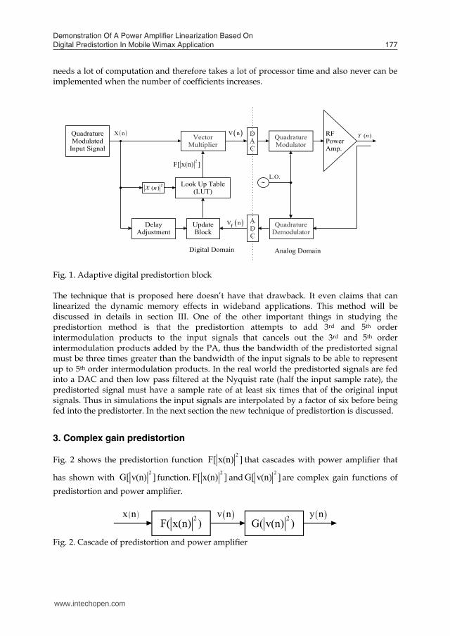
Fig. 2 shows the predistortion function 2F[ x(n) ] that cascades with power amplifier that
has shown with 2G[ v(n) ] function.
2F[ x(n) ] and2G[ v(n) ] are complex gain functions of
predistortion and power amplifier.
2F( x(n) ) 2G( v(n) ) v n y n x n
Fig. 2. Cascade of predistortion and power amplifier
QuadratureModulator
Look Up Table(LUT)
QuadratureModulated
Input Signal
VectorMultiplier
DAC
QuadratureDemodulator
L.O.~
ADC
UpdateBlock
DelayAdjustment
RFPowerAmp.
Analog DomainDigital Domain
( )Y n
( )X n 2
V n
fV n
X n
2F[ x(n) ]
www.intechopen.com
Demonstration Of A Power Ampliier Linearization Based On Digital Predistortion In Mobile Wimax Application 177
(Ding, et al. 2004) is presented. Both previous techniques have demonstrated acceptable results but both have disadvantages. In memory polynomial predistortion the complexity of extracting the coefficients of predistortion function decrease the capability of linearization and so it needs to apply other method like (Raich, et al. 2003) for implementing it. In complex gain predistortion method (Cavers, 1990) the memory effects that cause dynamic AM-AM and AM-PM are not considered. So here the main objective is not only to demonstrate the capability of this new method to overcome for such disadvantages, but also to show that with applying this technique all the memory contents of power amplifier that is modeled with memory polynomial is compensated. for validating this technique several simulations are applied. The adaptation is based on linear convergence method in the simulations. For simplicity the effects of the quadrature modulator and demodulator and A/D and D/A is not considered. The LUT size is 10 bit and addressing the LUT is based on the input amplitude. It will be shown that with applying this method all the memory contents of the power amplifier especially the one that cause dynamic AM/AM and AM/PM are compensated. Simulation and results are examined based on Motorola’s MRF1806 1.9 GHz LDMOS PA with 13 dB gain and 60W output power. To demonstrating the results several tests are shown with Mobile WiMAX signal. Finally the actual power amplifier from Mini Circuit ZVE-8G with 30 dB gain is used and tested with agilent equipments to verify the proposed algorithm. 2. Predistortion technique
Fig. 1 shows a block diagram of the adaptive digital predistortion (Cavers, 1990) . A fully adaptive digital predistortion system requires the addition of a predistortion circuit consisting of adigital predistorter and look up table (LUT) to the transmission path in addition to a feedback path consisting of a demodulator, analog to digital converter (ADC) and adaptation circuit for updating the LUT. The block diagram assumes that all components of the system except the predistorter and high power amplifier (HPA) have a linear response and hence can be ignored in the analysis. In this paper also these effects are ignored. The predistorter is equivalent to a nonlinear circuit with gain expansion response that inverse of the power amplifier gain compression AM/AM (Amplitude dependent gain) and a phase rotation that is the negative of the Power Amplifier phase rotation AM/PM (Amplitude Dependent Phase Shift). In this figure x n = I + jQ is the quadrature
modulated input signal and v (n)f is the quadrature demodulated feedback signal. These
signals are sampled synchronously, and their values are used to generate a predistortion
vector function 2F[ x(n) ] which is stored in polar or rectangular form in a look-up table
(LUT). The input signal x n is predistorted according to 2F[ x(n) ] , so that the
predistorted signal v n produced the linearized output from the RF amplifier. Here the LUT is 10bit and the absolute of input signal is used for addressing it. The main objective of this paper is to study the electrical memory effects that cause dynamic memory effects (ku & . McKinley, 2002). The previous studies (Wangnyong, et al. 2004;Bosch & Gatti, 1989;Morgan, et al. 2006) were all restricted to calculation of the coefficients of the power amplifier. This way
needs a lot of computation and therefore takes a lot of processor time and also never can be implemented when the number of coefficients increases.
Fig. 1. Adaptive digital predistortion block The technique that is proposed here doesn’t have that drawback. It even claims that can linearized the dynamic memory effects in wideband applications. This method will be discussed in details in section III. One of the other important things in studying the predistortion method is that the predistortion attempts to add 3rd and 5th order intermodulation products to the input signals that cancels out the 3rd and 5th order intermodulation products added by the PA, thus the bandwidth of the predistorted signal must be three times greater than the bandwidth of the input signals to be able to represent up to 5th order intermodulation products. In the real world the predistorted signals are fed into a DAC and then low pass filtered at the Nyquist rate (half the input sample rate), the predistorted signal must have a sample rate of at least six times that of the original input signals. Thus in simulations the input signals are interpolated by a factor of six before being fed into the predistorter. In the next section the new technique of predistortion is discussed.
3. Complex gain predistortion
Fig. 2 shows the predistortion function 2F[ x(n) ] that cascades with power amplifier that
has shown with 2G[ v(n) ] function.
2F[ x(n) ] and2G[ v(n) ] are complex gain functions of
predistortion and power amplifier.
2F( x(n) ) 2G( v(n) ) v n y n x n
Fig. 2. Cascade of predistortion and power amplifier
QuadratureModulator
Look Up Table(LUT)
QuadratureModulated
Input Signal
VectorMultiplier
DAC
QuadratureDemodulator
L.O.~
ADC
UpdateBlock
DelayAdjustment
RFPowerAmp.
Analog DomainDigital Domain
( )Y n
( )X n 2
V n
fV n
X n
2F[ x(n) ]
www.intechopen.com
Advanced Microwave and Millimeter Wave Technologies: Semiconductor Devices, Circuits and Systems178
As proposed in (Ding, et al. 2004) the equivalent discrete baseband PA model considering memory effects and baseband nonlinearity can be represented with a memory polynomial model which is a special case of Volterra series as below:
Odd
QK 2(k-1)kq
k =1 q = 0y(n) = a v(n- q) v(n- q) (1)
where v n is the discrete input complex signal of power amplifier after predistortion block and y n is the discrete output complex envelope signal. K is the order of nonlinearity and Q is the memory length. This model considers only odd-order nonlinear terms due to bandpass nonlinear characteristics that cause intermodulation distortion. In (1) v n also can be represented as below:
2v(n) = x(n)F[ x(n) ] (2)
where x n is the discrete input complex and
2F[ x(n) ] is the complex gain of the predistortion block. Equation (1) can be simplified as below:
Odd
Q K2(k-1)
kqq = 0 k =1
y(n) = v(n- q) a v(n- q) (3)
Where the function 2
qG ( v(n- q) ) can be represented as:
Odd
K2 2(k-1)
q kqk=1
G [ v(n- q) ] = a v(n- q) (4)
Then (3) is as below:
Q
2 2 2q 0 1
q=0
y(n) = v(n- q)G [ v(n- q) ] = v(n)G [ v(n) ] + v(n-1)G [ v(n-1) ] + .. (5)
This equation demonstrates that the memory contents of the power amplifier are not only appeared in the coefficients kqa of the (1), but it also can be shown as the complex function, which means that the memory effects are appeared in the function
2qG [ v(n) ] . Previous
efforts only tried to extract the kqa to compensate for such memory effects but here it will be shown that without having the coefficients also the memory effects can be compensated and even the compensation is better and includes all the memory (Varahram, et al. 2009).
From (2) for finding the function 2F[ x(n) ] , first it is assumed that Q=0 or the power amplifier is memoryless thus from (5) it can be conculded:
20y(n) = v(n)G [ v(n) ] (6)
Ideally the power amplifier should satisfy the below condition for having the linear output.
y(n) = Gx(n) (7) Where G is the linear gain of power amplifier. replacing (5) in (7) then:
Q2
qq=0
y(n) = v(n- q)G [ v(n) ] = Gx(n) (8)
With assuming Q=0 and replacing the v(n) in (6) and with considering that the quadrature modulator is a perfect unity gain device the optimum predistorter characteristic, denoted by
2F[ x(n) ] , would satisfy:
22 2
0x(n)F[ x(n) ]G [ x(n)F[ x(n) ] ] = Gx(n) (9)
Then the optimum value of the predistortion complex gain is calculated from below iterative equation:
2
2 2 ii+1 i error2
0
F[ x(n) ]F [ x(n) ] = F[ x(n) ] - V (n)
v(n)G [ v(n) ] (10)
where errorV (n) = y(n) - Gx(n) (11)
Now assume that the power amplifier includes one memory or Q=1 then after some simplification, equation below will be generated:
22 1
2 20 0
v(n-1)G [ v(n-1) ]GF( x(n) ) = -G [ v(n) ] x(n)G [ v(n) ]
(12)
The second fraction of (12) indicates the memory effects of the power amplifier. If Q increases then the elements in (12) also will increase. The iterative solution for (12) is:
2 2 22 2 i i 1
i+1 i error2 20 0
21
20
F[ x(n) ] F[ x(n) ]v(n-1)G [ v(n-1) ]F ( x(n) ) = F[ x(n) ] - V (n) +
v(n)G [ v(n) ] v(n)G ( v(n) )
v(n-1)G [ v(n-1) ]-
x(n)G [ v(n) ]
(13)
This equation can be simplified as below:
www.intechopen.com
Demonstration Of A Power Ampliier Linearization Based On Digital Predistortion In Mobile Wimax Application 179
As proposed in (Ding, et al. 2004) the equivalent discrete baseband PA model considering memory effects and baseband nonlinearity can be represented with a memory polynomial model which is a special case of Volterra series as below:
Odd
QK 2(k-1)kq
k =1 q = 0y(n) = a v(n- q) v(n- q) (1)
where v n is the discrete input complex signal of power amplifier after predistortion block and y n is the discrete output complex envelope signal. K is the order of nonlinearity and Q is the memory length. This model considers only odd-order nonlinear terms due to bandpass nonlinear characteristics that cause intermodulation distortion. In (1) v n also can be represented as below:
2v(n) = x(n)F[ x(n) ] (2)
where x n is the discrete input complex and
2F[ x(n) ] is the complex gain of the predistortion block. Equation (1) can be simplified as below:
Odd
Q K2(k-1)
kqq = 0 k =1
y(n) = v(n- q) a v(n- q) (3)
Where the function 2
qG ( v(n- q) ) can be represented as:
Odd
K2 2(k-1)
q kqk=1
G [ v(n- q) ] = a v(n- q) (4)
Then (3) is as below:
Q
2 2 2q 0 1
q=0
y(n) = v(n- q)G [ v(n- q) ] = v(n)G [ v(n) ] + v(n-1)G [ v(n-1) ] + .. (5)
This equation demonstrates that the memory contents of the power amplifier are not only appeared in the coefficients kqa of the (1), but it also can be shown as the complex function, which means that the memory effects are appeared in the function
2qG [ v(n) ] . Previous
efforts only tried to extract the kqa to compensate for such memory effects but here it will be shown that without having the coefficients also the memory effects can be compensated and even the compensation is better and includes all the memory (Varahram, et al. 2009).
From (2) for finding the function 2F[ x(n) ] , first it is assumed that Q=0 or the power amplifier is memoryless thus from (5) it can be conculded:
20y(n) = v(n)G [ v(n) ] (6)
Ideally the power amplifier should satisfy the below condition for having the linear output.
y(n) = Gx(n) (7) Where G is the linear gain of power amplifier. replacing (5) in (7) then:
Q2
qq=0
y(n) = v(n- q)G [ v(n) ] = Gx(n) (8)
With assuming Q=0 and replacing the v(n) in (6) and with considering that the quadrature modulator is a perfect unity gain device the optimum predistorter characteristic, denoted by
2F[ x(n) ] , would satisfy:
22 2
0x(n)F[ x(n) ]G [ x(n)F[ x(n) ] ] = Gx(n) (9)
Then the optimum value of the predistortion complex gain is calculated from below iterative equation:
2
2 2 ii+1 i error2
0
F[ x(n) ]F [ x(n) ] = F[ x(n) ] - V (n)
v(n)G [ v(n) ] (10)
where errorV (n) = y(n) - Gx(n) (11)
Now assume that the power amplifier includes one memory or Q=1 then after some simplification, equation below will be generated:
22 1
2 20 0
v(n-1)G [ v(n-1) ]GF( x(n) ) = -G [ v(n) ] x(n)G [ v(n) ]
(12)
The second fraction of (12) indicates the memory effects of the power amplifier. If Q increases then the elements in (12) also will increase. The iterative solution for (12) is:
2 2 22 2 i i 1
i+1 i error2 20 0
21
20
F[ x(n) ] F[ x(n) ]v(n-1)G [ v(n-1) ]F ( x(n) ) = F[ x(n) ] - V (n) +
v(n)G [ v(n) ] v(n)G ( v(n) )
v(n-1)G [ v(n-1) ]-
x(n)G [ v(n) ]
(13)
This equation can be simplified as below:
www.intechopen.com
Advanced Microwave and Millimeter Wave Technologies: Semiconductor Devices, Circuits and Systems180
22 2 i
i+1 i error20
2 2 22 21 i i
i+1 i error2 20 0
F[ x(n) ]F ( x(n) ) = F[ x(n) ] - V (n)
v(n)G [ v(n) ]
v(n-1)G [ v(n-1) ] F[ x(n) ] F[ x(n) ]1( - ) = F ( x(n) ) = F[ x(n) ] - V (n)v(n) x(n)G [ v(n) ] v(n)G [ v(n) ]
(14)
The function
2F[ x(n) ] in (14) is similar to (10) when the power amplifier has no memory. This formula can be extended to more memory and is still valid. Simulations and results will prove the validity of this equation later. Memory polynomial method was very complicated and it couldn't calculate all the coefficients in the volterra series and only could compensate for 2 or 3 memory length but this method proves that it can compensate all the memory contents of the power amplifier. The important parameter in (14) is the gain factor which is the only difference between (10)
and (13) and it is the2F[ x(n) ] over 2
0v(n)G ( v(n) ) . In the case of having memory, 2
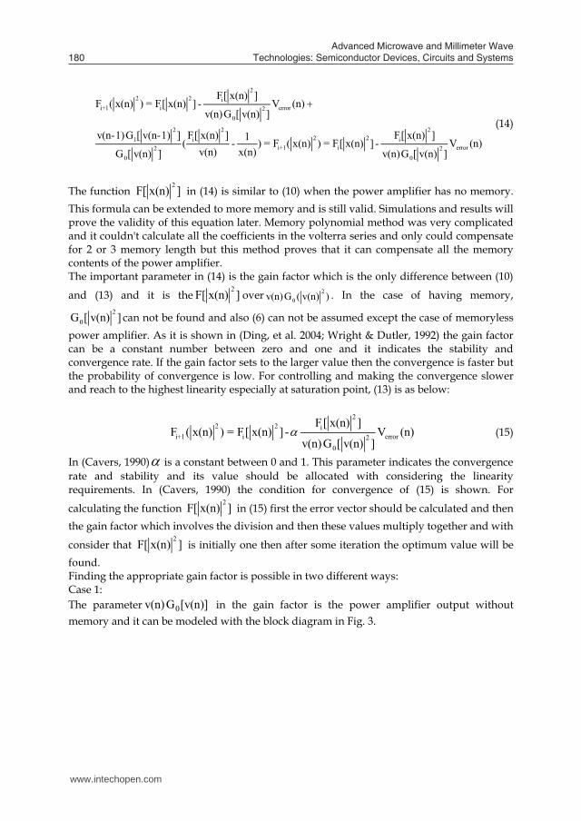
0G [ v(n) ] can not be found and also (6) can not be assumed except the case of memoryless power amplifier. As it is shown in (Ding, et al. 2004; Wright & Dutler, 1992) the gain factor can be a constant number between zero and one and it indicates the stability and convergence rate. If the gain factor sets to the larger value then the convergence is faster but the probability of convergence is low. For controlling and making the convergence slower and reach to the highest linearity especially at saturation point, (13) is as below:
2
2 2 ii+1 i error2
0
F[ x(n) ]F ( x(n) ) = F[ x(n) ] - V (n)
v(n)G [ v(n) ] (15)
In (Cavers, 1990) is a constant between 0 and 1. This parameter indicates the convergence rate and stability and its value should be allocated with considering the linearity requirements. In (Cavers, 1990) the condition for convergence of (15) is shown. For
calculating the function 2F[ x(n) ] in (15) first the error vector should be calculated and then
the gain factor which involves the division and then these values multiply together and with
consider that 2F[ x(n) ] is initially one then after some iteration the optimum value will be
found. Finding the appropriate gain factor is possible in two different ways: Case 1: The parameter 0v(n)G [v(n)] in the gain factor is the power amplifier output without memory and it can be modeled with the block diagram in Fig. 3.
Fig. 3. predistortion block with memory compensation(case 1) But it is still needed to know the characteristic of the power amplifier without memory. It is possible to initially calculate the coefficients of the power amplifier without memory and save it in LUT and then calculate the gain factor, but this way takes a lot of space and processing time. Because of this reason it is better to study case 2.
Case 2:
In this case the simplification could be done as below:
2 2
2 2 2 20 0 0
F[ x(n) ] F[ x(n) ] 1=v(n)G [ v(n) ] x(n)F[ x(n) ]G [ v(n) ] x(n)G [ v(n) ]
(16)
It can be assumed that th function 2F[ x(n) ] is initially equal to one then:
2 200 0
1 1 1= =y (n)x(n)G [ v(n) ] x(n)G [ x(n) ]
(17)
Where 0y (n) is the power amplifier output without memory and this is different from y(n) which includes memory. As the target is:
0y (n) = Gx(n) (18) So the diagram in Fig. 4 will be reached which is the simplest method for linearizing the power amplifier with memory. And equation below will be the final predistortion adaptation that will be used in whole simulations:
(19)
AddressGeneration
DelayAdj.
LUTF(x(n))
( )v n( )x n ( )y n
G
. 1Z
Stability
. QZ 2[ ( ) ]QG v n Q
21[ ( 1) ]G v n
20[ ( ) ]G v n
Power Amplifier with memory
20[ ( ) ]G v n
2 2i+1 i error
1F ( x(n) ) = F[ x(n) ] - V (n)( )Gx n
www.intechopen.com
Demonstration Of A Power Ampliier Linearization Based On Digital Predistortion In Mobile Wimax Application 181
22 2 i
i+1 i error20
2 2 22 21 i i
i+1 i error2 20 0
F[ x(n) ]F ( x(n) ) = F[ x(n) ] - V (n)
v(n)G [ v(n) ]
v(n-1)G [ v(n-1) ] F[ x(n) ] F[ x(n) ]1( - ) = F ( x(n) ) = F[ x(n) ] - V (n)v(n) x(n)G [ v(n) ] v(n)G [ v(n) ]
(14)
The function
2F[ x(n) ] in (14) is similar to (10) when the power amplifier has no memory. This formula can be extended to more memory and is still valid. Simulations and results will prove the validity of this equation later. Memory polynomial method was very complicated and it couldn't calculate all the coefficients in the volterra series and only could compensate for 2 or 3 memory length but this method proves that it can compensate all the memory contents of the power amplifier. The important parameter in (14) is the gain factor which is the only difference between (10)
and (13) and it is the2F[ x(n) ] over 2
0v(n)G ( v(n) ) . In the case of having memory, 2
0G [ v(n) ] can not be found and also (6) can not be assumed except the case of memoryless power amplifier. As it is shown in (Ding, et al. 2004; Wright & Dutler, 1992) the gain factor can be a constant number between zero and one and it indicates the stability and convergence rate. If the gain factor sets to the larger value then the convergence is faster but the probability of convergence is low. For controlling and making the convergence slower and reach to the highest linearity especially at saturation point, (13) is as below:
2
2 2 ii+1 i error2
0
F[ x(n) ]F ( x(n) ) = F[ x(n) ] - V (n)
v(n)G [ v(n) ] (15)
In (Cavers, 1990) is a constant between 0 and 1. This parameter indicates the convergence rate and stability and its value should be allocated with considering the linearity requirements. In (Cavers, 1990) the condition for convergence of (15) is shown. For
calculating the function 2F[ x(n) ] in (15) first the error vector should be calculated and then
the gain factor which involves the division and then these values multiply together and with
consider that 2F[ x(n) ] is initially one then after some iteration the optimum value will be
found. Finding the appropriate gain factor is possible in two different ways: Case 1: The parameter 0v(n)G [v(n)] in the gain factor is the power amplifier output without memory and it can be modeled with the block diagram in Fig. 3.
Fig. 3. predistortion block with memory compensation(case 1) But it is still needed to know the characteristic of the power amplifier without memory. It is possible to initially calculate the coefficients of the power amplifier without memory and save it in LUT and then calculate the gain factor, but this way takes a lot of space and processing time. Because of this reason it is better to study case 2.
Case 2:
In this case the simplification could be done as below:
2 2
2 2 2 20 0 0
F[ x(n) ] F[ x(n) ] 1=v(n)G [ v(n) ] x(n)F[ x(n) ]G [ v(n) ] x(n)G [ v(n) ]
(16)
It can be assumed that th function 2F[ x(n) ] is initially equal to one then:
2 200 0
1 1 1= =y (n)x(n)G [ v(n) ] x(n)G [ x(n) ]
(17)
Where 0y (n) is the power amplifier output without memory and this is different from y(n) which includes memory. As the target is:
0y (n) = Gx(n) (18) So the diagram in Fig. 4 will be reached which is the simplest method for linearizing the power amplifier with memory. And equation below will be the final predistortion adaptation that will be used in whole simulations:
(19)
AddressGeneration
DelayAdj.
LUTF(x(n))
( )v n( )x n ( )y n
G
. 1Z
Stability
. QZ 2[ ( ) ]QG v n Q
21[ ( 1) ]G v n
20[ ( ) ]G v n
Power Amplifier with memory
20[ ( ) ]G v n
2 2i+1 i error
1F ( x(n) ) = F[ x(n) ] - V (n)( )Gx n
www.intechopen.com
Advanced Microwave and Millimeter Wave Technologies: Semiconductor Devices, Circuits and Systems182
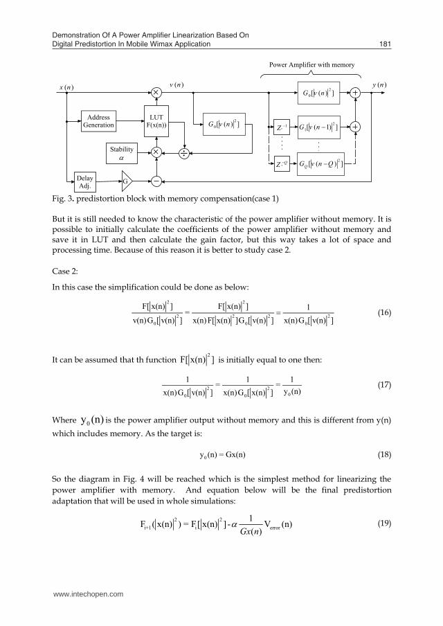
Fig. 4. predistortion block with memory compensation(case 2) The only drawback that is remaining is to calculate the inverse of the input data which after finding it and multiplied with error vector then the LUT contents could be updated. So in implementation the main concern is the division part which the main issue in implementation and it leaves for future work. In (15) with two or three iterations convergence is achieved and it will be shown that as compared with the indirect learning architecture method that is proposed in (Ding, 2004), the efficiency improves more and it is less complex. It will be shown that if the case 1 is applied in simulations the speed of convergence is more than case 2 which requires more iterations to convergence. The only time consuming part for implementing this method is the calculation of the gain factor which requires the inverse of the input signal. The predistorter is assumed to be implemented as a lookup table (LUT) of complex gain values (Cavers, 1990) that here is 10bit, indexed by the squared magnitude, as shown in Fig. 3. It is also possible to index by magnitude, or any other monotonic function of magnitude, depending on the regions of amplifier characteristic that need the greatest accuracy of representation. However, these considerations do not enter the analysis of the present paper. Also to help evaluate the performance of the DPD a figure for in-band distortion as well as out of band distortion which is measured with adjacent-channel-leakage-ratio (ACLR) is calculated. This involves calculating the error vector magnitude (EVM) in transmitter, which is given by the following equation
errorrms( V (n) )EVM =
rms( (x(n) ) (20)
where errorV (n) is from (11) and x n is the input signal.
4. Simulations and results
In order to validate the proposed method several simulations are done. MATLAB is applied for simulations. The power amplifier is ZVE-8G from Mini-Circuit suitable for CDMA applications. The input signal which is generated from Matlab is passed to agilent signal
PA withmemory
AddressGeneration
Delay Adj.
LUT
( )v n( )x n ( )y n
G
Calculatethe Inverse
2F[ x(n) ]
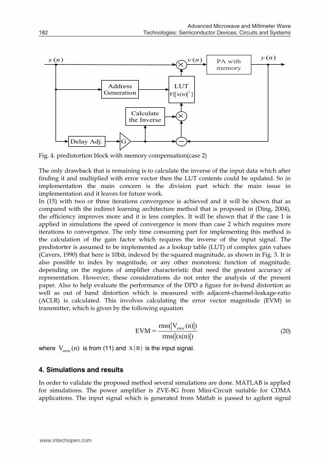
generator which will be upconvert the signal and pass it to the power amplifier. The power amplifier is wideband from 2 GHz to 8 GHz with 30 dB gain. Here the PA is working at 2.4 GHz. The input signal is QPSK with sample rate of 1 Mbps and the root rate cosine filter with alfa equal to 0.35. The output signal of the PA is connected to the attenuator for bring down the output power below the input power of the equipment. For receiving part of the measurement, the 89600S VXI equipment from agilent is used, which the main task is to downconvert the signal to IF frequency. The photograph of this experimental setup is shown in Fig. 5. The VSA software in PC will capture the data of the PA. The captured data can then import to Matlab for further analysis. Synchronization is used in order to achieve a complete coordination among the signal that is sent and the signal taken into Matlab.
Fig. 5. the experimental setup for testing digital predistortion These samples are used to model the power amplifier based on (1) which is the memory polynomial method. The extracted coefficients that include the memory effects are shown in table 1. In Fig. 6 the AM-AM and AM-PM characteristics of this power amplifier are shown. It can be seen the scattering of samples in this figure that is because of the memory effects. It can be shown that when the memory effects are more these samples will be scattered more, and then the digital predistortion technique should be designed based on it. It is clear in Fig. 6a that the AM-AM characteristic is not linear when the input amplitude is increased. And also in Fig. 6b the curve bends too. This is because of the nonlinear characteristics of the power amplifier. All the input and output samples in the simulations are normalized. For modeling the memory effects of the power amplifiers authors in (Ku & Kenney, 2003) proposed a method for modeling the power amplifiers with memory. This method that is based on the spars delay taps is actually able to take into account all the memory effects of the power amplifier. The memory effect modeling ratio (MEMR) was used to show the amount of memory that this method can model. The power amplifier from mini circuit has MEMR=0.62 and the one in (Ku & Kenney, 2003) has MEMR=1 and these coefficients are shown in table 1. previous researches could present the comparison of the power amplifier with MEMR that is less than one. Here the presented method is successfully tested with
www.intechopen.com
Demonstration Of A Power Ampliier Linearization Based On Digital Predistortion In Mobile Wimax Application 183
Fig. 4. predistortion block with memory compensation(case 2) The only drawback that is remaining is to calculate the inverse of the input data which after finding it and multiplied with error vector then the LUT contents could be updated. So in implementation the main concern is the division part which the main issue in implementation and it leaves for future work. In (15) with two or three iterations convergence is achieved and it will be shown that as compared with the indirect learning architecture method that is proposed in (Ding, 2004), the efficiency improves more and it is less complex. It will be shown that if the case 1 is applied in simulations the speed of convergence is more than case 2 which requires more iterations to convergence. The only time consuming part for implementing this method is the calculation of the gain factor which requires the inverse of the input signal. The predistorter is assumed to be implemented as a lookup table (LUT) of complex gain values (Cavers, 1990) that here is 10bit, indexed by the squared magnitude, as shown in Fig. 3. It is also possible to index by magnitude, or any other monotonic function of magnitude, depending on the regions of amplifier characteristic that need the greatest accuracy of representation. However, these considerations do not enter the analysis of the present paper. Also to help evaluate the performance of the DPD a figure for in-band distortion as well as out of band distortion which is measured with adjacent-channel-leakage-ratio (ACLR) is calculated. This involves calculating the error vector magnitude (EVM) in transmitter, which is given by the following equation
errorrms( V (n) )EVM =
rms( (x(n) ) (20)
where errorV (n) is from (11) and x n is the input signal.
4. Simulations and results
In order to validate the proposed method several simulations are done. MATLAB is applied for simulations. The power amplifier is ZVE-8G from Mini-Circuit suitable for CDMA applications. The input signal which is generated from Matlab is passed to agilent signal
PA withmemory
AddressGeneration
Delay Adj.
LUT
( )v n( )x n ( )y n
G
Calculatethe Inverse
2F[ x(n) ]
generator which will be upconvert the signal and pass it to the power amplifier. The power amplifier is wideband from 2 GHz to 8 GHz with 30 dB gain. Here the PA is working at 2.4 GHz. The input signal is QPSK with sample rate of 1 Mbps and the root rate cosine filter with alfa equal to 0.35. The output signal of the PA is connected to the attenuator for bring down the output power below the input power of the equipment. For receiving part of the measurement, the 89600S VXI equipment from agilent is used, which the main task is to downconvert the signal to IF frequency. The photograph of this experimental setup is shown in Fig. 5. The VSA software in PC will capture the data of the PA. The captured data can then import to Matlab for further analysis. Synchronization is used in order to achieve a complete coordination among the signal that is sent and the signal taken into Matlab.
Fig. 5. the experimental setup for testing digital predistortion These samples are used to model the power amplifier based on (1) which is the memory polynomial method. The extracted coefficients that include the memory effects are shown in table 1. In Fig. 6 the AM-AM and AM-PM characteristics of this power amplifier are shown. It can be seen the scattering of samples in this figure that is because of the memory effects. It can be shown that when the memory effects are more these samples will be scattered more, and then the digital predistortion technique should be designed based on it. It is clear in Fig. 6a that the AM-AM characteristic is not linear when the input amplitude is increased. And also in Fig. 6b the curve bends too. This is because of the nonlinear characteristics of the power amplifier. All the input and output samples in the simulations are normalized. For modeling the memory effects of the power amplifiers authors in (Ku & Kenney, 2003) proposed a method for modeling the power amplifiers with memory. This method that is based on the spars delay taps is actually able to take into account all the memory effects of the power amplifier. The memory effect modeling ratio (MEMR) was used to show the amount of memory that this method can model. The power amplifier from mini circuit has MEMR=0.62 and the one in (Ku & Kenney, 2003) has MEMR=1 and these coefficients are shown in table 1. previous researches could present the comparison of the power amplifier with MEMR that is less than one. Here the presented method is successfully tested with
www.intechopen.com
Advanced Microwave and Millimeter Wave Technologies: Semiconductor Devices, Circuits and Systems184
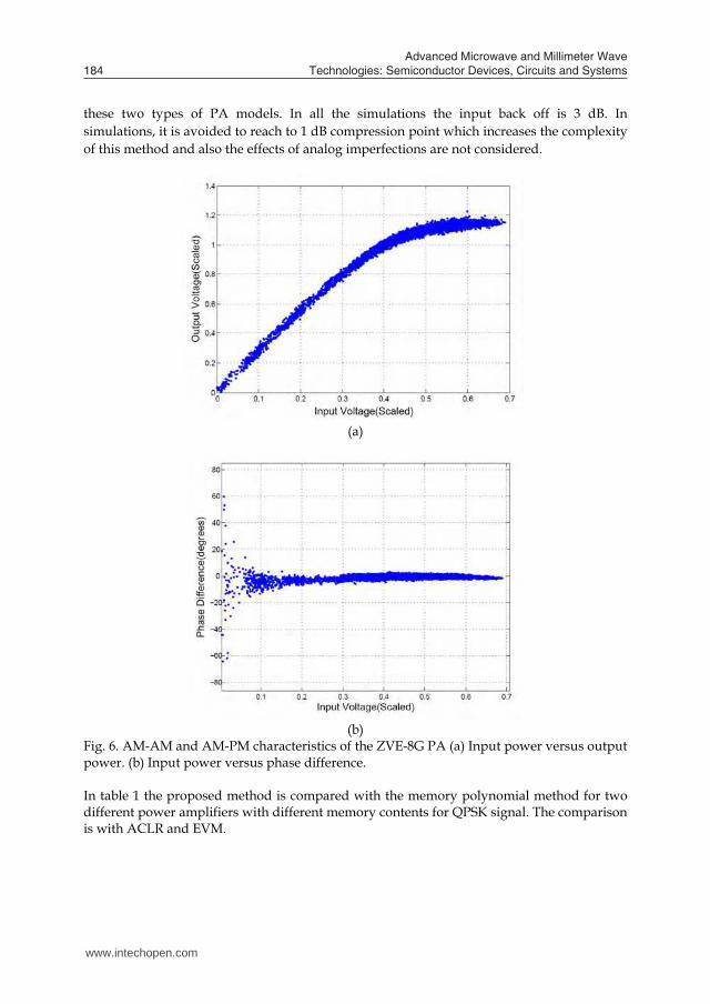
these two types of PA models. In all the simulations the input back off is 3 dB. In simulations, it is avoided to reach to 1 dB compression point which increases the complexity of this method and also the effects of analog imperfections are not considered.
(a)
(b) Fig. 6. AM-AM and AM-PM characteristics of the ZVE-8G PA (a) Input power versus output power. (b) Input power versus phase difference. In table 1 the proposed method is compared with the memory polynomial method for two different power amplifiers with different memory contents for QPSK signal. The comparison is with ACLR and EVM.
Table 1. Comparison of the two predistortion techniques for different power amplifiiers with QPSK signal
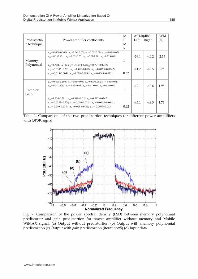
Fig. 7. Comparison of the power spectral density (PSD) between memory polynomial predistorter and gain predistortion for power amplifier without memory and Mobile WiMAX signal. (a) Output without predistortion (b) Output with memory polynomial predistortion (c) Output with gain predistortion (iteration=5) (d) Input data
Predistortion technique
Power amplifier coefficients
M E M R
ACLR(dBc) Left Right
EVM (%)
Memory Polynomial
10 11 12 13
30 31 32 33
a =0.9800-0.300i; a =0.06+0.03i; a =0.02+0.08i; a =-0.01+0.02i;a =-0.3+0.42i; a =-0.02+0.05i; a =-0.01-0.08i; a =0.02-0.01i;
1
-39.1
-40.2
2.55
10 11 12
30 31 32
50 51 52
a =1.524-0.211i; a =0.349+0.32i;a =-0.797-0.0247i;a =-0.0355+0.72i; a =-0.010-0.012i; a =-0.0065+0.0042i;a =-0.019-0.004i; a =0.009-0.019i; a =-0.0069+0.013i;
0.62
-41.2
-42.5
2.25
Complex Gain
10 11 12 13
30 31 32 33
a =0.9800-0.300i; a =0.06+0.03i; a =0.02+0.08i; a =-0.01+0.02i;a =-0.3+0.42i; a =-0.02+0.05i; a =-0.01-0.08i; a =0.02-0.01i;
1
-42.1
-40.6
1.95
10 11 12
30 31 32
50 51 52
a =1.524-0.211i; a =0.349+0.32i; a =-0.797-0.0247i;a =-0.0355+0.72i; a =-0.010-0.012i; a =-0.0065+0.0042i;a =-0.019-0.004i; a =0.009-0.019i; a =-0.0069+0.013i;
0.62
-45.1
-48.3
1.73
www.intechopen.com
Demonstration Of A Power Ampliier Linearization Based On Digital Predistortion In Mobile Wimax Application 185
these two types of PA models. In all the simulations the input back off is 3 dB. In simulations, it is avoided to reach to 1 dB compression point which increases the complexity of this method and also the effects of analog imperfections are not considered.
(a)
(b) Fig. 6. AM-AM and AM-PM characteristics of the ZVE-8G PA (a) Input power versus output power. (b) Input power versus phase difference. In table 1 the proposed method is compared with the memory polynomial method for two different power amplifiers with different memory contents for QPSK signal. The comparison is with ACLR and EVM.
Table 1. Comparison of the two predistortion techniques for different power amplifiiers with QPSK signal
Fig. 7. Comparison of the power spectral density (PSD) between memory polynomial predistorter and gain predistortion for power amplifier without memory and Mobile WiMAX signal. (a) Output without predistortion (b) Output with memory polynomial predistortion (c) Output with gain predistortion (iteration=5) (d) Input data
Predistortion technique
Power amplifier coefficients
M E M R
ACLR(dBc) Left Right
EVM (%)
Memory Polynomial
10 11 12 13
30 31 32 33
a =0.9800-0.300i; a =0.06+0.03i; a =0.02+0.08i; a =-0.01+0.02i;a =-0.3+0.42i; a =-0.02+0.05i; a =-0.01-0.08i; a =0.02-0.01i;
1
-39.1
-40.2
2.55
10 11 12
30 31 32
50 51 52
a =1.524-0.211i; a =0.349+0.32i;a =-0.797-0.0247i;a =-0.0355+0.72i; a =-0.010-0.012i; a =-0.0065+0.0042i;a =-0.019-0.004i; a =0.009-0.019i; a =-0.0069+0.013i;
0.62
-41.2
-42.5
2.25
Complex Gain
10 11 12 13
30 31 32 33
a =0.9800-0.300i; a =0.06+0.03i; a =0.02+0.08i; a =-0.01+0.02i;a =-0.3+0.42i; a =-0.02+0.05i; a =-0.01-0.08i; a =0.02-0.01i;
1
-42.1
-40.6
1.95
10 11 12
30 31 32
50 51 52
a =1.524-0.211i; a =0.349+0.32i; a =-0.797-0.0247i;a =-0.0355+0.72i; a =-0.010-0.012i; a =-0.0065+0.0042i;a =-0.019-0.004i; a =0.009-0.019i; a =-0.0069+0.013i;
0.62
-45.1
-48.3
1.73
www.intechopen.com
Advanced Microwave and Millimeter Wave Technologies: Semiconductor Devices, Circuits and Systems186
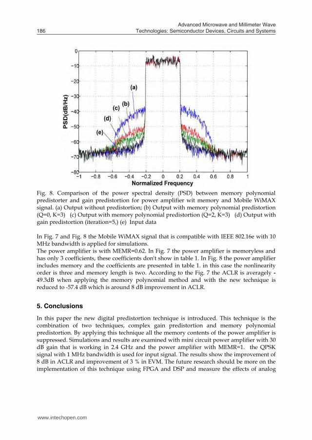
Fig. 8. Comparison of the power spectral density (PSD) between memory polynomial predistorter and gain predistortion for power amplifier wit memory and Mobile WiMAX signal. (a) Output without predistortion; (b) Output with memory polynomial predistortion (Q=0, K=3) (c) Output with memory polynomial predistortion (Q=2, K=3) (d) Output with gain predistortion (iteration=5,) (e) Input data In Fig. 7 and Fig. 8 the Mobile WiMAX signal that is compatible with IEEE 802.16e with 10 MHz bandwidth is applied for simulations. The power amplifier is with MEMR=0.62. In Fig. 7 the power amplifier is memoryless and has only 3 coefficients, these coefficients don't show in table 1. In Fig. 8 the power amplifier includes memory and the coefficients are presented in table 1. in this case the nonlinearity order is three and memory length is two. According to the Fig. 7 the ACLR is averagely -49.3dB when applying the memory polynomial method and with the new technique is reduced to -57.4 dB which is around 8 dB improvement in ACLR. 5. Conclusions
In this paper the new digital predistortion technique is introduced. This technique is the combination of two techniques, complex gain predistortion and memory polynomial predistortion. By applying this technique all the memory contents of the power amplifier is suppressed. Simulations and results are examined with mini circuit power amplifier with 30 dB gain that is working in 2.4 GHz and the power amplifier with MEMR=1. the QPSK signal with 1 MHz bandwidth is used for input signal. The results show the improvement of 8 dB in ACLR and improvement of 3 % in EVM. The future research should be more on the implementation of this technique using FPGA and DSP and measure the effects of analog
imperfection that cause reduction in efficiency in practical implementation and add that effects in the simulations.
6. References
Bosch W. and Gatti G. (1989). “Measurement and simulation of memory effects in predistortion linearizers,” IEEE Trans. Microwave Theory Tech., vol. 37, pp. 1885–1890, Dec. 1989
Cavers J. K. (1990). “Amplifier Linearization Using a Digital Predistorter with Fast Adaptation and Low Memory Requirements”, IEEE Transaction on vehicular technology, vol 39, no.4, pp. 374-382,Nov 1990.
Cripps S.C. (1999). RF Power Amplifiers for Wireless Communications. Norwood, MA: Artech House, 1999.
Ding L., Zhou G. T, Morgan D. R., Ma Z., Kenney J. S, Kim J., and Giardina C. R (2004). “A robust predistorter constructed using memory polynomials,” IEEE Trans. Commun., vol. 52, pp. 159–165, Jan. 2004.
Kenington P. B. (2000). High-Linearity RF Amplifier Design. Norwood, MA: Artech House, 2000.
Kim J. and Konstantinou K. (2001). “Digital predistortion of wideband signals based on power amplifier model with memory,” Electron. Lett., vol. 37, no. 23, pp. 1417–1418, Nov. 2001
Ku H. and Kenney J. S. (2003). “Behavioral modeling of nonlinear RF power amplifiers considering memory effects,” IEEE Trans. Microw. Theory Tech., vol. 51, no. 12, pp. 2495–2504, Dec. 2003.
Ku H., and McKinley M. D. (2002). “Quantifying Memory Effects in RF Power Amplifiers,” IEEE Trans. Microw. Theory Tech, vol. 50, no. 12, December 2002.
Morgan D. R., Z. Ma, Kim J., Zierdt M. G., and Pastalan J. (2006). “A generalized memory polynomial model for digital predistortion of RF power amplifiers,” IEEE Trans. Signal Process., vol. 54, no. 10, pp. 3852–3860, Oct. 2006
Nagata Y. (1989). “Linear amplification techniques for digital mobile communications,” in Proc. IEEE 39th Veh. Technol. Conf., 1989, pp. 159–164.
Raich R., Qian H., and Zhou G. T. (2003). “Digital baseband predistortion of nonlinear power amplifiers using orthogonal polynomials,” in Proc. IEEE Int. Con f. Acoust, Speech, Signal Processing, pp. 689–692, Apr. 2003.
Varahram P., Mohammady S., Hamidon M. N., Sidek R. M., Khatun S., (2009). “Digital Predistortion Technique for Compensating Memory Effects of Power Amplifiers in Wideband Applications,” Journal of ELECTRICAL ENGINEERING, VOL. 60, NO. 3, 2009.
Wangnyong W., Miller M., and Kenney J. S. (2004). “Predistortion Linearization System for High Power Amplifiers”, IEEE MTT-S Digest, pp. 677-680, 2004 .
Woo Y. Y., Kim J., Yi J., Hong S., Kim I., Moon J., and Kim B. (2007). “Adaptive digital feedback predistortion technique for linearizing power amplifiers,” IEEE Trans. Microw. Theory Tech., vol. 55, no. 5, pp. 932–940, May 2007.
Woo Y. Y., Kim J., Hong S., Kim I., Moon J., Yi J., and Kim B. (2007). “A new adaptive digital predistortion technique employing feedback technique,” in IEEE MTT-S Int. Microw. Symp. Dig., Jun., pp. 1445–1448.
www.intechopen.com
Demonstration Of A Power Ampliier Linearization Based On Digital Predistortion In Mobile Wimax Application 187
Fig. 8. Comparison of the power spectral density (PSD) between memory polynomial predistorter and gain predistortion for power amplifier wit memory and Mobile WiMAX signal. (a) Output without predistortion; (b) Output with memory polynomial predistortion (Q=0, K=3) (c) Output with memory polynomial predistortion (Q=2, K=3) (d) Output with gain predistortion (iteration=5,) (e) Input data In Fig. 7 and Fig. 8 the Mobile WiMAX signal that is compatible with IEEE 802.16e with 10 MHz bandwidth is applied for simulations. The power amplifier is with MEMR=0.62. In Fig. 7 the power amplifier is memoryless and has only 3 coefficients, these coefficients don't show in table 1. In Fig. 8 the power amplifier includes memory and the coefficients are presented in table 1. in this case the nonlinearity order is three and memory length is two. According to the Fig. 7 the ACLR is averagely -49.3dB when applying the memory polynomial method and with the new technique is reduced to -57.4 dB which is around 8 dB improvement in ACLR. 5. Conclusions
In this paper the new digital predistortion technique is introduced. This technique is the combination of two techniques, complex gain predistortion and memory polynomial predistortion. By applying this technique all the memory contents of the power amplifier is suppressed. Simulations and results are examined with mini circuit power amplifier with 30 dB gain that is working in 2.4 GHz and the power amplifier with MEMR=1. the QPSK signal with 1 MHz bandwidth is used for input signal. The results show the improvement of 8 dB in ACLR and improvement of 3 % in EVM. The future research should be more on the implementation of this technique using FPGA and DSP and measure the effects of analog
imperfection that cause reduction in efficiency in practical implementation and add that effects in the simulations.
6. References
Bosch W. and Gatti G. (1989). “Measurement and simulation of memory effects in predistortion linearizers,” IEEE Trans. Microwave Theory Tech., vol. 37, pp. 1885–1890, Dec. 1989
Cavers J. K. (1990). “Amplifier Linearization Using a Digital Predistorter with Fast Adaptation and Low Memory Requirements”, IEEE Transaction on vehicular technology, vol 39, no.4, pp. 374-382,Nov 1990.
Cripps S.C. (1999). RF Power Amplifiers for Wireless Communications. Norwood, MA: Artech House, 1999.
Ding L., Zhou G. T, Morgan D. R., Ma Z., Kenney J. S, Kim J., and Giardina C. R (2004). “A robust predistorter constructed using memory polynomials,” IEEE Trans. Commun., vol. 52, pp. 159–165, Jan. 2004.
Kenington P. B. (2000). High-Linearity RF Amplifier Design. Norwood, MA: Artech House, 2000.
Kim J. and Konstantinou K. (2001). “Digital predistortion of wideband signals based on power amplifier model with memory,” Electron. Lett., vol. 37, no. 23, pp. 1417–1418, Nov. 2001
Ku H. and Kenney J. S. (2003). “Behavioral modeling of nonlinear RF power amplifiers considering memory effects,” IEEE Trans. Microw. Theory Tech., vol. 51, no. 12, pp. 2495–2504, Dec. 2003.
Ku H., and McKinley M. D. (2002). “Quantifying Memory Effects in RF Power Amplifiers,” IEEE Trans. Microw. Theory Tech, vol. 50, no. 12, December 2002.
Morgan D. R., Z. Ma, Kim J., Zierdt M. G., and Pastalan J. (2006). “A generalized memory polynomial model for digital predistortion of RF power amplifiers,” IEEE Trans. Signal Process., vol. 54, no. 10, pp. 3852–3860, Oct. 2006
Nagata Y. (1989). “Linear amplification techniques for digital mobile communications,” in Proc. IEEE 39th Veh. Technol. Conf., 1989, pp. 159–164.
Raich R., Qian H., and Zhou G. T. (2003). “Digital baseband predistortion of nonlinear power amplifiers using orthogonal polynomials,” in Proc. IEEE Int. Con f. Acoust, Speech, Signal Processing, pp. 689–692, Apr. 2003.
Varahram P., Mohammady S., Hamidon M. N., Sidek R. M., Khatun S., (2009). “Digital Predistortion Technique for Compensating Memory Effects of Power Amplifiers in Wideband Applications,” Journal of ELECTRICAL ENGINEERING, VOL. 60, NO. 3, 2009.
Wangnyong W., Miller M., and Kenney J. S. (2004). “Predistortion Linearization System for High Power Amplifiers”, IEEE MTT-S Digest, pp. 677-680, 2004 .
Woo Y. Y., Kim J., Yi J., Hong S., Kim I., Moon J., and Kim B. (2007). “Adaptive digital feedback predistortion technique for linearizing power amplifiers,” IEEE Trans. Microw. Theory Tech., vol. 55, no. 5, pp. 932–940, May 2007.
Woo Y. Y., Kim J., Hong S., Kim I., Moon J., Yi J., and Kim B. (2007). “A new adaptive digital predistortion technique employing feedback technique,” in IEEE MTT-S Int. Microw. Symp. Dig., Jun., pp. 1445–1448.
www.intechopen.com

Advanced Microwave and Millimeter Wave Technologies: Semiconductor Devices, Circuits and Systems188
Wright A. S. and Durtler W. G. (1992). “Experimental performance of an adaptive digital linearized power amplifier,” IEEE Trans. Veh. Technol., vol. 41, no. 4, pp. 395–400, Nov.
www.intechopen.com
Advanced Microwave and Millimeter Wave TechnologiesSemiconductor Devices Circuits and SystemsEdited by Moumita Mukherjee
ISBN 978-953-307-031-5Hard cover, 642 pagesPublisher InTechPublished online 01, March, 2010Published in print edition March, 2010
InTech EuropeUniversity Campus STeP Ri Slavka Krautzeka 83/A 51000 Rijeka, Croatia Phone: +385 (51) 770 447
InTech ChinaUnit 405, Office Block, Hotel Equatorial Shanghai No.65, Yan An Road (West), Shanghai, 200040, China
Phone: +86-21-62489820 Fax: +86-21-62489821
This book is planned to publish with an objective to provide a state-of-the-art reference book in the areas ofadvanced microwave, MM-Wave and THz devices, antennas and systemtechnologies for microwavecommunication engineers, Scientists and post-graduate students of electrical and electronics engineering,applied physicists. This reference book is a collection of 30 Chapters characterized in 3 parts: AdvancedMicrowave and MM-wave devices, integrated microwave and MM-wave circuits and Antennas and advancedmicrowave computer techniques, focusing on simulation, theories and applications. This book provides acomprehensive overview of the components and devices used in microwave and MM-Wave circuits, includingmicrowave transmission lines, resonators, filters, ferrite devices, solid state devices, transistor oscillators andamplifiers, directional couplers, microstripeline components, microwave detectors, mixers, converters andharmonic generators, and microwave solid-state switches, phase shifters and attenuators. Several applicationsarea also discusses here, like consumer, industrial, biomedical, and chemical applications of microwavetechnology. It also covers microwave instrumentation and measurement, thermodynamics, and applications innavigation and radio communication.
How to referenceIn order to correctly reference this scholarly work, feel free to copy and paste the following:
Pooria Varahram, Somayeh Mohammady, M. Nizar Hamidon, Roslina M. Sidek and Sabira Khatun (2010).Demonstration of a Power Amplifier Linearization Based on Digital Predistortion in Mobile Wimax Application,Advanced Microwave and Millimeter Wave Technologies Semiconductor Devices Circuits and Systems,Moumita Mukherjee (Ed.), ISBN: 978-953-307-031-5, InTech, Available from:http://www.intechopen.com/books/advanced-microwave-and-millimeter-wave-technologies-semiconductor-devices-circuits-and-systems/demonstration-of-a-power-amplifier-linearization-based-on-digital-predistortion-in-mobile-wimax-appl
www.intechopen.com

Fax: +385 (51) 686 166www.intechopen.com
Fax: +86-21-62489821

© 2010 The Author(s). Licensee IntechOpen. This chapter is distributedunder the terms of the Creative Commons Attribution-NonCommercial-ShareAlike-3.0 License, which permits use, distribution and reproduction fornon-commercial purposes, provided the original is properly cited andderivative works building on this content are distributed under the samelicense.


![„Klima schützen – Kohle stoppen!“ Demonstration zur ... · [Medien-Info zur internen Planung] „Klima schützen – Kohle stoppen!“ Demonstration zur Weltklimakonferenz](https://img.pdfslide.org/doc/110x75/5d4d0eaf88c993c96c8ba1a0/klima-schuetzen-kohle-stoppen-demonstration-zur-medien-info.jpg)