Embed Size (px)
Citation preview
Accessing Relational and Higher DatabasesThrough
Database Set Predicatesin
Logic Programming Languages
INAUGURAL-DISSERTATION
ZUR
ERLANGUNG DER PHILOSOPHISCHEN DOKTORWÜRDE
VORGELEGT DER
PHILOSOPHISCHEN FAKULTÄT II
DER
UNIVERSITÄT ZÜRICH
VON
Christoph Draxler
AUS
Österreich
BEGUTACHTET VON DEN HERREN
PROF. Dr. K. Bauknecht
PROF. Dr. K. Dittrich
PROF. Dr. G. Gottlob
ZÜRICH 1991


Hiermit erkläre ich, daß ich zur Abfassung der Dissertation keine anderen als die darin angege-benen Hilfsmittel herangezogen habe.
Zürich, 6.5.91
Lebenslauf
Name: Draxler
Vornamen: Christoph Johannes
geboren: 27. Dezember 1960 in Dortmund/BRD
Staatsangehörigkeit: österreichische
Ausbildung
Nov. 1979 - Mai 1986 Studium der Informatik mit Nebenfach Linguistik (Diplom)an der Technischen Universität München
Diplomarbeit bei Prof. Dr. M. Paul: “Programmsystem zurUnterstützung eines Experten im Bereich der Graphentheoriebei der Lösung von Problemen, die auf Algorithmen vom TypWarshall- oder Ford/Fulkerson führen”
Nov. 1979 - Juni 1988 Studium der französischen Philologie, Hauptfach Literatur-wissenschaft mit Nebenfach Linguistik (Magister)an der Ludwig-Maximilians-Universität München
Magisterarbeit bei Prof. Dr. I. Nolting-Hauff: “Computerunt-erstützte Dramenanalyse — Weiterentwicklung der Mathema-tischen Dramenanalyse und Anwendung der Methode auf dreiausgewählte französische Dramen des 17. und 20. Jahrhun-derts”
seit Juli 1987 Doktorand und Assistent bei Prof. Bauknecht am Institut fürInformatik der Universität Zürich
Besuch der Vorlesungen/Seminare der Dozenten
Prof. Dr. K. BauknechtProf. Dr. K. DittrichProf. Dr. R. PfeifferProf. Dr. L. RichterProf. Dr. H. SchauerProf. Dr. P. StuckiPD Dr. M. HessPD Dr. E. MumprechtDr. M. DomenigDr. N. E. Fuchs
Sept. 1989 - Nov. 1989 Forschungsaufenthalt beim European Computer-Industry Re-search Centre ECRC in München
Mai 1991 Dissertation bei Prof. Dr. K. Bauknecht, Prof. Dr. K. Dittrichund Prof. Dr. G. Gottlob (TU Wien)
Zusammenfassung
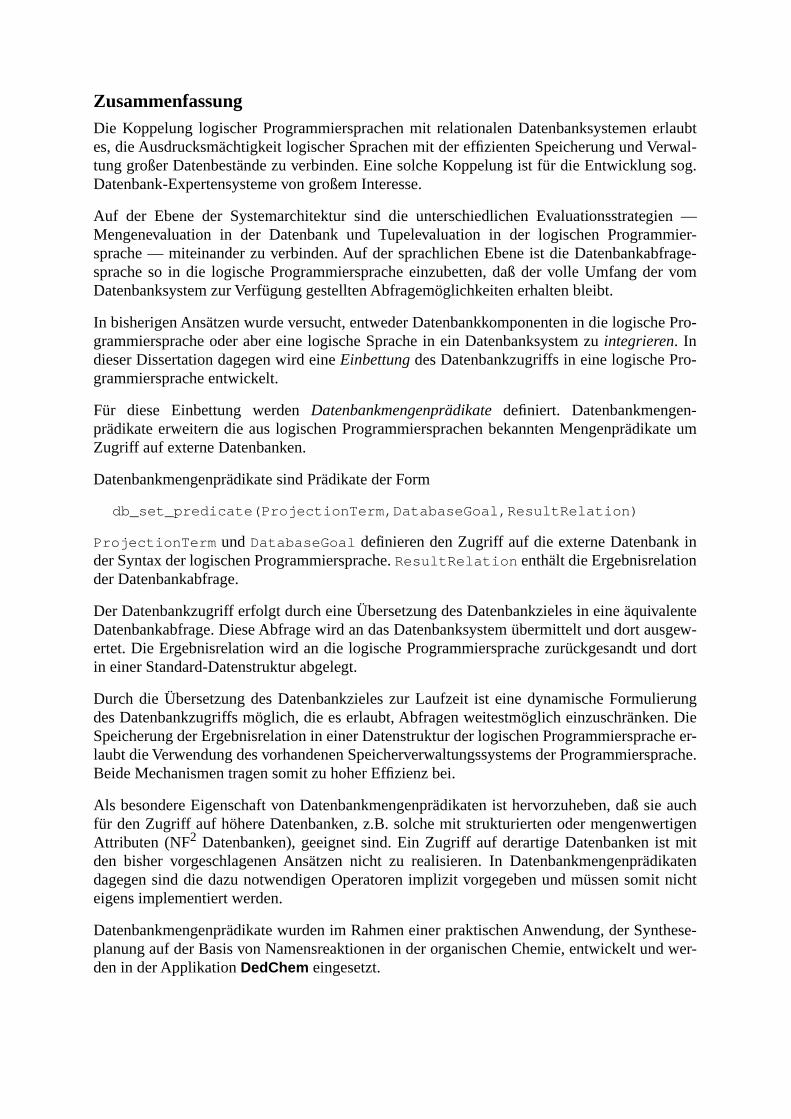
Die Koppelung logischer Programmiersprachen mit relationalen Datenbanksystemen erlaubtes, die Ausdrucksmächtigkeit logischer Sprachen mit der effizienten Speicherung und Verwal-tung großer Datenbestände zu verbinden. Eine solche Koppelung ist für die Entwicklung sog.Datenbank-Expertensysteme von großem Interesse.
Auf der Ebene der Systemarchitektur sind die unterschiedlichen Evaluationsstrategien —Mengenevaluation in der Datenbank und Tupelevaluation in der logischen Programmier-sprache — miteinander zu verbinden. Auf der sprachlichen Ebene ist die Datenbankabfrage-sprache so in die logische Programmiersprache einzubetten, daß der volle Umfang der vomDatenbanksystem zur Verfügung gestellten Abfragemöglichkeiten erhalten bleibt.
In bisherigen Ansätzen wurde versucht, entweder Datenbankkomponenten in die logische Pro-grammiersprache oder aber eine logische Sprache in ein Datenbanksystem zu
integrieren
. Indieser Dissertation dagegen wird eine
Einbettung
des Datenbankzugriffs in eine logische Pro-grammiersprache entwickelt.
Für diese Einbettung werden
Datenbankmengenprädikate
definiert. Datenbankmengen-prädikate erweitern die aus logischen Programmiersprachen bekannten Mengenprädikate umZugriff auf externe Datenbanken.
Datenbankmengenprädikate sind Prädikate der Form
db_set_predicate(ProjectionTerm,DatabaseGoal,ResultRelation)
ProjectionTerm
und
DatabaseGoal
definieren den Zugriff auf die externe Datenbank inder Syntax der logischen Programmiersprache.
ResultRelation
enthält die Ergebnisrelationder Datenbankabfrage.
Der Datenbankzugriff erfolgt durch eine Übersetzung des Datenbankzieles in eine äquivalenteDatenbankabfrage. Diese Abfrage wird an das Datenbanksystem übermittelt und dort ausgew-ertet. Die Ergebnisrelation wird an die logische Programmiersprache zurückgesandt und dortin einer Standard-Datenstruktur abgelegt.
Durch die Übersetzung des Datenbankzieles zur Laufzeit ist eine dynamische Formulierungdes Datenbankzugriffs möglich, die es erlaubt, Abfragen weitestmöglich einzuschränken. DieSpeicherung der Ergebnisrelation in einer Datenstruktur der logischen Programmiersprache er-laubt die Verwendung des vorhandenen Speicherverwaltungssystems der Programmiersprache.Beide Mechanismen tragen somit zu hoher Effizienz bei.
Als besondere Eigenschaft von Datenbankmengenprädikaten ist hervorzuheben, daß sie auchfür den Zugriff auf höhere Datenbanken, z.B. solche mit strukturierten oder mengenwertigenAttributen (NF
2
Datenbanken), geeignet sind. Ein Zugriff auf derartige Datenbanken ist mitden bisher vorgeschlagenen Ansätzen nicht zu realisieren. In Datenbankmengenprädikatendagegen sind die dazu notwendigen Operatoren implizit vorgegeben und müssen somit nichteigens implementiert werden.
Datenbankmengenprädikate wurden im Rahmen einer praktischen Anwendung, der Synthese-planung auf der Basis von Namensreaktionen in der organischen Chemie, entwickelt und wer-den in der Applikation
DedChem
eingesetzt.
Abstract
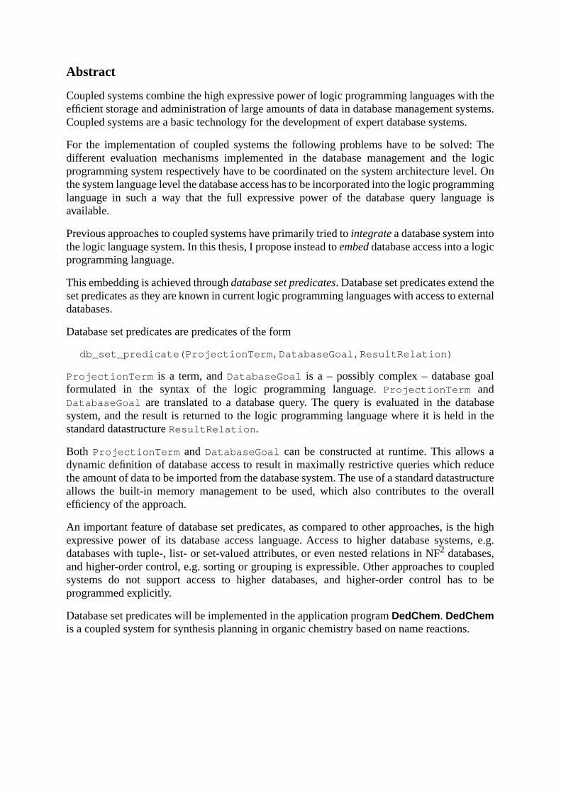
Coupled systems combine the high expressive power of logic programming languages with theefficient storage and administration of large amounts of data in database management systems.Coupled systems are a basic technology for the development of expert database systems.
For the implementation of coupled systems the following problems have to be solved: Thedifferent evaluation mechanisms implemented in the database management and the logicprogramming system respectively have to be coordinated on the system architecture level. Onthe system language level the database access has to be incorporated into the logic programminglanguage in such a way that the full expressive power of the database query language isavailable.
Previous approaches to coupled systems have primarily tried to
integrate
a database system intothe logic language system. In this thesis, I propose instead to
embed
database access into a logicprogramming language.
This embedding is achieved through
database set predicates
. Database set predicates extend theset predicates as they are known in current logic programming languages with access to externaldatabases.
Database set predicates are predicates of the form
db_set_predicate(ProjectionTerm,DatabaseGoal,ResultRelation)
ProjectionTerm
is a term, and
DatabaseGoal
is a – possibly complex – database goalformulated in the syntax of the logic programming language.
ProjectionTerm
and
DatabaseGoal
are translated to a database query. The query is evaluated in the databasesystem, and the result is returned to the logic programming language where it is held in thestandard datastructure
ResultRelation
.
Both
ProjectionTerm
and
DatabaseGoal
can be constructed at runtime. This allows adynamic definition of database access to result in maximally restrictive queries which reducethe amount of data to be imported from the database system. The use of a standard datastructureallows the built-in memory management to be used, which also contributes to the overallefficiency of the approach.
An important feature of database set predicates, as compared to other approaches, is the highexpressive power of its database access language. Access to higher database systems, e.g.databases with tuple-, list- or set-valued attributes, or even nested relations in NF
2
databases,and higher-order control, e.g. sorting or grouping is expressible. Other approaches to coupledsystems do not support access to higher databases, and higher-order control has to beprogrammed explicitly.
Database set predicates will be implemented in the application program
DedChem
.
DedChem
is a coupled system for synthesis planning in organic chemistry based on name reactions.
i
Table of Contents
1. Introduction 1
1.1 Theoretical level ......................................................................................................................... 11.2 Conceptual level ......................................................................................................................... 31.3 Implementation level .................................................................................................................. 41.4 Contributions of the thesis.......................................................................................................... 41.5 Position of the thesis on the three levels..................................................................................... 51.6 Limitations of the thesis ............................................................................................................. 51.7 Structure of the thesis ................................................................................................................. 6
— Theory —
2. Logic programming and the relational database model 11
2.1 Relational database model ........................................................................................................ 11Relational algebra ..................................................................................................................... 12SQL........................................................................................................................................... 14
2.2 First-order predicate logic ........................................................................................................ 16Evaluation of logic programs ................................................................................................... 17Abstract interpreter ................................................................................................................... 21Prolog ....................................................................................................................................... 23
2.3 Relationship between logic and the relational database model ................................................ 26Logic languages and relational database model ....................................................................... 27Representation of relational algebra in the logic programming language................................ 28
— Concept —
3. Coupled systems 33
3.1 General structure of coupled systems....................................................................................... 33Embedding vs. integration........................................................................................................ 34Physical and logical level ......................................................................................................... 35Description of coupled systems on the physical level.............................................................. 36Description of coupled systems on the logical level ................................................................ 37Database access procedure ....................................................................................................... 37
ii
3.2 Interface .................................................................................................................................... 38Physical level interface............................................................................................................. 38Logical level interface .............................................................................................................. 39
4. Framework for coupled systems 41
4.1 Two-dimensional framework ................................................................................................... 414.2 Qualitative criteria for coupled systems ................................................................................... 43
Efficiency ................................................................................................................................. 44Implementation effort ............................................................................................................... 44Independence ............................................................................................................................ 44Expressive power...................................................................................................................... 44Naturalness ............................................................................................................................... 45
4.3 Summary................................................................................................................................... 45
5. Application of the framework 47
5.1 Sample application ................................................................................................................... 475.2 PROSQL................................................................................................................................... 485.3 Quintus Prolog.......................................................................................................................... 485.4 CGW and PRIMO .................................................................................................................... 495.5 KB-Prolog................................................................................................................................. 505.6 System by Nussbaum ............................................................................................................... 515.7 Prolog-SQL coupling by Danielsson and Barklund ................................................................. 515.8 EKS-V1 .................................................................................................................................... 525.9 Other work................................................................................................................................ 525.10 Application of the framework................................................................................................... 545.11 Discussion................................................................................................................................. 54
Improving efficiency ................................................................................................................ 54Maximum independence........................................................................................................... 58Summary................................................................................................................................... 59
5.12 Requirements for a new approach ............................................................................................ 61
6. Database Set Predicates 63
6.1 Set predicates............................................................................................................................ 63Set predicate definition............................................................................................................. 64Set predicate semantics............................................................................................................. 64Implementation of set predicates in Prolog .............................................................................. 67Abstract implementation of set predicates................................................................................ 68Representation of set predicates ............................................................................................... 69
iii
6.2 Database set predicates............................................................................................................. 70Definition.................................................................................................................................. 70Operational semantics of database set predicates..................................................................... 70Database access language......................................................................................................... 71Implementation schema............................................................................................................ 72Application of database set predicates...................................................................................... 73
6.3 Discussion................................................................................................................................. 76System architecture and coordination of evaluations ............................................................... 76Memory requirements............................................................................................................... 80Portability ................................................................................................................................. 83Restriction of queries................................................................................................................ 84Higher-order control ................................................................................................................. 89Relationship between the built-in set predicates and database set predicates .......................... 91Implementation of other approaches with database set predicates........................................... 92
6.4 Summary................................................................................................................................... 94
— Implementation —
7. Implementation of Database Set Predicates 99
7.1 System architecture and requirements for database set predicates........................................... 99System architecture................................................................................................................... 99Database set predicates implementation requirements........................................................... 100
7.2 Translation from Prolog to SQL............................................................................................. 100Representation of schema information ................................................................................... 101Translation of database access requests.................................................................................. 102SQL compiler ......................................................................................................................... 105Comprehensive Example........................................................................................................ 110
7.3 Realization of the communication channel and its interfaces ................................................ 111Inter-process communication ................................................................................................. 112Communication via procedure calls ....................................................................................... 113Comparison of methods.......................................................................................................... 115
8. A Real-World Application: Synthesis Planning with
DedChem
119
8.1 Introduction ............................................................................................................................ 119Name reactions ....................................................................................................................... 119Synthesis tree.......................................................................................................................... 121A first implementation of
synthesis
/3 .............................................................................. 121
iv
8.2
DedChem
— a coupled system for synthesis planning........................................................... 123Database for substance classes, superclasses and name reactions.......................................... 124Database set predicates for database access ........................................................................... 124Interactive planning ................................................................................................................ 127Adding higher-order control to the database access............................................................... 127Delegation of tests to the database system ............................................................................. 130
8.3 Discussion............................................................................................................................... 130
9. Outlook 133
9.1 Increasing the expressive power of the database access language ......................................... 133Tuple-, list-, and set-valued attributes .................................................................................... 133NF
2
databases ......................................................................................................................... 1359.2 Updates through database set predicates ................................................................................ 137
Implicit updates ...................................................................................................................... 138Explicit updates ...................................................................................................................... 140Summary................................................................................................................................. 140
10. Conclusion 143
Acknowledgments 145
References 147
Author Index 153
1
1
Introduction
The field of logic and databases aims at combining the sound theoretical foundation and the
powerful and universal formalism of logic with the efficient and safe administration of large
amounts of data of databases. Two major working areas have evolved, deductive databases
[Gallaire/Minker 78, Gallaire et al. 84, Minker 88 b, Lloyd 87] and persistent logic programming
languages [Appelrath 85, Jasper 90].
The field of logic and databases can be described on three levels: theory, concept and
implementation.
1.1 Theoretical level
On the theoretical level the relationship between formal logic and logic programming on the one
side and database models on the other side is analyzed.
A formal logic system consists of a logic language, a set of axioms formulated in the logic
language, and a set of inference rules that allow the derivation of theorems from the axioms of the
system.
Formal logic systems can be ordered hierarchically according to their expressive power. In
propositional logic it is only possible to prove statements about complete sentences. First-order
predicate logic introduces variables that stand for individuals. Universal or existential
quantification of variables allows to express the relationships that hold between variables in a first-
order sentence. Higher-order logic systems such as second order predicate logic, temporal logic
[Kröger 87], or modal logic [Gabbay/Guenthner 84], extend predicate logic with quantification
over predicates, the notion of time, and reasoning under uncertainty. However, for a large class of
high-level applications the expressive power of first-order predicate logic is fully sufficient
[Kowalski 79, Genesereth/Nilsson 87]. Often, all that is required is higher-order syntax to facilitate
the formulation of special problems, but even in such cases the semantics of first-order predicate
logic suffices [Chen et al. 90].
1. Introduction
2
The major appeal of using first-order predicate logic as a programming language are its correctness
and completeness properties. With these properties it is possible to
prove
correct a program written
in a first-order predicate logic language.
Two developments opened the way for logic programming. The first was the proposal of the
resolution rule by Robinson [Robinson 65], a sound and complete inference rule that made possible
first-order predicate logic systems with only one inference rule and without non-logical axioms.
The second development was the restriction of the logic language to Horn clauses. For Horn clause
languages intuitive declarative and procedural semantics were proposed by Kowalski [Kowalski
79].
A logic program may be seen as a theory of first-order predicate logic. Its axioms, written as Horn
clauses, capture the knowledge about the application either extensionally in facts, or intensionally
through rules. The program is executed by providing a goal, i.e. a theorem that is to be proved
through the application of the inference rules. If the proof succeeds, then the variable bindings
computed during the evaluation are returned as a solution.
The classical relational database model can also be considered as a first-order predicate logic
system [Gallaire/Minker 78, Kowalski 81, Parsaye 83, Gallaire et al. 84]. The axioms of this system
consist of the database relation tables, and queries correspond to theorems. The evaluation of a
query in the relational database model amounts to retrieving those columns and rows from the
database relations that match the query conditions.
Despite their common foundations in first-order predicate logic there are two main differences
between the relational database model and a logic programming language system, namely the
different
• expressive power of the respective languages and the
• evaluation mechanisms employed in the respective system implementations.
Everything that can be expressed in the relational database model can also be expressed in a Horn
clause language because each relational operator can be represented as a Horn clause. A formal
system based on Horn clauses is thus said to be relationally complete. However, because recursion
is expressible in Horn clause languages but not in the relational database model, the expressive
power of Horn clause systems is greater than that of the relational database model.
In the relational database model an operation is defined over relations as a whole, and the result of
an operation is again a relation [Codd 70]. Logic programming systems are theorem provers. In
general they are based on resolution with the standard unification procedure in which each variable
is bound to at most one atomic value. A proof returns the bindings of a single tuple. The evaluation
in database systems is thus set-oriented, as compared to tuple-oriented in logic programming
systems.
Conceptual level
3
1.2 Conceptual level
In the context of logic and databases a coupled system is a system that couples a logic
programming language with one or more database systems. The database systems provide
persistent data storage and efficient access to large amounts of data, while the logic language
provides the expressive power that is needed for the implementation of the application.
The conceptual level describes the pragmatics of coupling a logic programming language with
external databases. It contains the requirements that an approach to coupled systems is designed to
meet, and criteria to define the structure and quality of coupled systems. The general techniques
employed in an approach are also described on this level.
There exist two main techniques to coupling a logic programming language with external
databases: integration and embedding [Bever 86]. In an integrated coupled system, access to a
database system is included in the programming language definition already. With embedding,
access to databases is added to existing programming language through language or run time
system modifications. Both techniques can be described in more detail by distinguishing a logical
– or system language – and a physical – or system architecture – level [Bocca 86]. Together with
the degree of coupling on both levels this results in structural criteria that may adequately describe
the structure of coupled systems.
Qualitative criteria, such as expressive power, efficiency, implementation effort, or the
independence of the external database system and the logic programming language, describe the
properties of an approach to coupled systems and may be used to compare different approaches.
Dependencies exist between structural and qualitative criteria. The overall efficiency of a coupled
system is determined by the degree of coupling on the physical level, and integration of the
database language into the logic programming language.
Similar dependencies also hold among the qualitative criteria themselves. A trade-off exists
between expressive power and efficiency because the evaluation of a high-level language is
computationally more demanding than that of languages with restricted expressive power.
The architecture of a coupled system is determined by the application requirements the system is
designed to meet. Constraints of such a kind are the types of external databases that are to be
accessed, the access privileges to these databases, the availability of resources, and others. These
constraints are not inherent to coupled systems, but they define the structure and thus to a large
extent also the properties of a particular approach to coupled systems.
Because of the dependencies between external constraints, structural criteria, and the properties of
a coupled system, any approach to coupled system is necessarily a compromise. This explains the
variety of approaches, and it implies that any comparison of coupled systems must take into
account the original system requirements.
1. Introduction
4
1.3 Implementation level
On the implementation level the low-level implementation details of an approach to coupled
systems are described. Such low-level details are the programming language used to implement a
coupled system, the actual encoding of the interface mechanisms defined on the conceptual level,
and information about the interaction of a coupled system with the underlying file system of an
operating system environment.
1.4 Contributions of the thesis
The main contribution of the thesis is the proposal of a new approach to coupled systems, namely
database set predicates
. Database set predicates extend the definition of the set predicates [Warren
82] found in logic programming languages with access to arbitrary external relational or higher
databases.
• The general idea of database set predicates is to
embed
— instead of integrate — database
access into the logic programming language evaluation.
The primary distinguishing feature of database set predicates is that database access is fully
embedded into the logic language. In other approaches either the database is integrated into the
logic language system, or there coexist distinct languages for the application program and the
database access.
A second distinguishing feature is that result relations as a whole are captured in a standard
datastructure of the logic language. In other approaches, either the evaluation strategy of the
logic language system is changed to match that of the database, or relations retrieved from the
database system are either asserted into the logic language workspace — which effectively is a
modification of the logic program — or their contents are returned to the logic programming
language one record at a time — which causes considerable administration overhead and/or
requires the use of a dedicated buffering mechanism to temporarily store the result relation.
Finally, database set predicates may be used to simulate most of the other approaches to
coupling databases to a logic programming language.
Furthermore, a graphical two-dimensional framework based on the structure of coupled systems
and a set of qualitative criteria are proposed for the classification of coupled systems. The main
properties of a coupled system can be derived automatically from the position that this system
occupies in the matrix. This framework is used to describe the approaches to coupled systems
which have been developed so far, and to motivate the current approach.
In the thesis an example from the world of flight connections and airplanes is used because it is
highly intuitive. However, database set predicates were developed as part of a practical application.
Position of the thesis on the three levels
5
This application is described in a chapter of its own because the application domain, organic
chemistry, has so-far not been considered amenable to deductive database systems.
The specific task of the application is synthesis planning. Synthesis planning consists of finding a
sequence of reactions so that a given substance can be produced. The requirements of the
application exceed the expressive power of most current deductive database systems based on
Datalog because it requires functions to build tree structures to adequately represent synthesis
plans.
1.5 Position of the thesis on the three levels
The three levels theory, concept and implementation will now serve to position the thesis in the
research field.
On the theoretical level database set predicates are higher-order language constructs because they
refer to sets and functions. Function symbols are used as term constructors and are necessary for
the datastructure that holds the result relation of the database query evaluation. However, the
semantics of set predicates in general, and of database set predicates in particular, is within the
semantics of first-order predicate logic [Warren 82, Chen et al. 90].
On the conceptual level database set predicates embed access to external databases. The same
language is used to access external databases and to implement application programs, and standard
datastructures are used to collect the result relations produced by the set-oriented database
evaluation.
Database set predicates implement a physically loosely and logically tightly coupled system. The
logic programming language and the relational database systems are separate systems connected
through a communication channel. Database access requests are dynamically translated to database
queries. These queries are transmitted to the database system and evaluated there. The result
relation is returned as a whole back to logic programming language where it is placed in a list
datastructure.
On the implementation level the actual implementation of database set predicates in Prolog and
SQL is outlined.
1.6 Limitations of the thesis
Database set predicates have certain limitations which are briefly outlined here. A more detailed
discussion and a description of how to overcome these limitations is given in the appropriate
chapters.
1. Introduction
6
These main limitations are
• high memory requirements,
• restriction of the database access language to the expressive power of relational database
languages, and
• read-only access to the external database.
Of these, only the high memory demand is a limitation inherent to database set predicates. Both the
language restriction and the read-only access are limitations of this thesis.
Storing entire result relations in a standard datastructure of the logic programming language
potentially requires the allocation of large amounts of main memory in the logic programming
language. Memory demand is reduced through small result relations. With database set predicates
memory demand can be reduced through the formulation of maximally restrictive queries that yield
minimal result relations. Furthermore, because a standard datastructure is used, the built-in
memory management mechanisms, including garbage collection, can be used to deallocate
memory as soon as the datastructure is no longer needed.
In this thesis, database set predicates are restricted to such database access requests that can be
directly translated to a single relational query. However, access to more powerful databases is
expressible by database set predicates, with the only limitation that the database access language
be a first-order logic language (see [Lloyd 87, Ullman 88, Marti 89, Vieille/Lefêbvre 89] for a
discussion and definition of
allowed
databases). In Chapter nine, access to NF
2
databases is
discussed in detail.
In this thesis, database set predicates are restricted to read-only access to external databases. It is
argued that for many applications, especially in the case of physically loosely coupled systems,
updates are not necessary or even not allowed. However, it is possible to express updates through
database set predicates either implicitly by calling them with the database goal expressing the
update conditions and a fully instantiated third argument containing the update values, or explicitly
through reserved database update commands. The use of database set predicates for updates is
discussed in Chapter nine.
1.7 Structure of the thesis
The thesis is divided into three main parts, roughly corresponding to the description levels theory,
concept and implementation.
Part one deals with the theoretical level. Chapter two is a brief introduction of the theory of first-
order predicate logic and logic programming. In this chapter the relationship between the relational
database model and Horn clause logic is described.
Part two corresponds to the conceptual level. Chapter three contains the terminology relevant to
coupled systems. Chapter four contains the graphical framework and presents the structural and
qualitative criteria for coupled systems. Chapter five gives an overview and a discussion of existing

Structure of the thesis
7
coupled systems. From this discussion database set predicates are motivated. In chapter six, set
predicates as they are known in logic programming languages, and their extension to database set
predicates, are presented. In this chapter the specific properties of database set predicates are
discussed in detail.
In part three the implementation level is dealt with. Chapter seven describes the translation of
Prolog database goals to SQL and discusses the communication channel. Chapter eight contains a
sample application from organic chemistry. Extending database set predicates to access higher
databases and the incorporation of database updates is discussed in Chapter nine. In Chapter ten, a
conclusion summarizes the work presented.

8

Part I
Theory

10
11
2
Logic programming and the relational database model
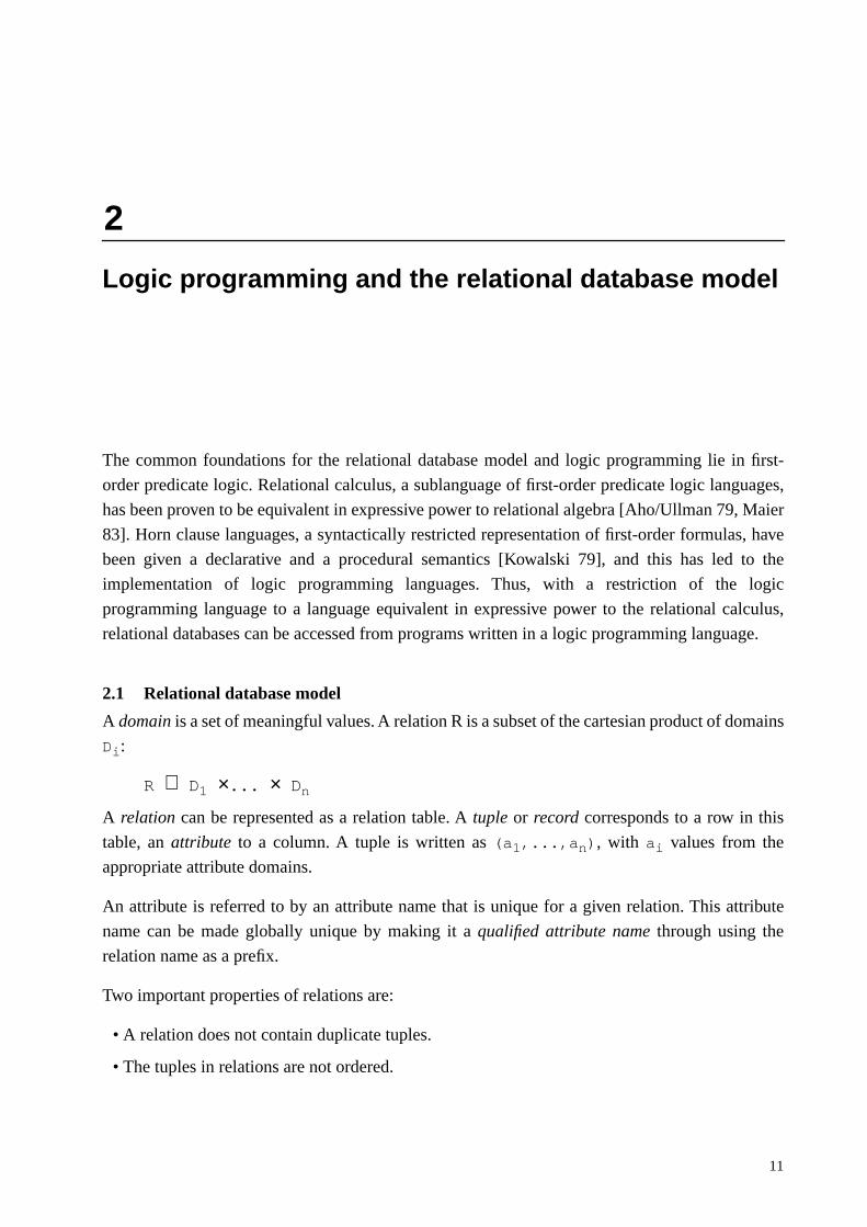
The common foundations for the relational database model and logic programming lie in first-
order predicate logic. Relational calculus, a sublanguage of first-order predicate logic languages,
has been proven to be equivalent in expressive power to relational algebra [Aho/Ullman 79, Maier
83]. Horn clause languages, a syntactically restricted representation of first-order formulas, have
been given a declarative and a procedural semantics [Kowalski 79], and this has led to the
implementation of logic programming languages. Thus, with a restriction of the logic
programming language to a language equivalent in expressive power to the relational calculus,
relational databases can be accessed from programs written in a logic programming language.
2.1 Relational database model
A
domain
is a set of meaningful values. A relation R is a subset of the cartesian product of domains
D
i
:
R
⊆
D
1
×
...
×
D
n
A relation can be represented as a relation table. A tuple or record corresponds to a row in this
table, an attribute to a column. A tuple is written as (a1,...,an), with ai values from the
appropriate attribute domains.
An attribute is referred to by an attribute name that is unique for a given relation. This attribute
name can be made globally unique by making it a qualified attribute name through using the
relation name as a prefix.
Two important properties of relations are:
• A relation does not contain duplicate tuples.
• The tuples in relations are not ordered.

2. Logic programming and the relational database model
12
The first property means that no two tuples in a relation are the same. The second property means
that any representation of a relation displays just one possible ordering of tuples — any other
ordering is just as valid.
A relation is in first normal form (1. NF) if its attributes are atomic values.
2.1.1 Relational algebra
The relational algebra consists of the standard set operations
• union,
• intersection,
• difference
In relational algebra, these set operations are restricted to union-compatible relations. Two
relations R and S are union-compatible if they both have the same number of attributes, and the i-
th attribute of either relation must be based on the same domain Di (the attributes must not
necessarily have the same attribute name in both relations).
The following operations are defined specifically for the relational database model:
• The selection operation selects from a relation R all those tuples that match a given selection
condition.
Selection is written as σcond(R), where cond is the selection condition.
• The projection of the relation R on attributes A1,...,An is the set of all tuples that contain only
the values of the attributes specified by the projection operator.
Projection is written as πattlist(R), where attlist is a list of attributes to project on.
• A join concatenates the tuples of two relations R and S for all those tuples for which a join
condition holds between pairs of attributes from both R and S.
A join is written as R[attr θ atts]S, where θ expresses the condition that holds
between attributes of R and attributes of S.
A special case is the natural join, where the condition that must hold is the equality of the
attribute values of both relations. Only one of the attributes of the equality comparison is
retained in the resulting relation.
Relational algebra is a closed system: each operation is defined over relations, and the result of an
operation is again a relation. Because of this closure property, the operations of the relational
algebra can be nested to result in complex relational expressions.
Example
Flight and Plane are two relation tables defined as
Flight := (flightno × departure × destination × plane)Plane := (type × seats)
The domain of flightno is the set of flight numbers, the common domain of departure and
Relational database model
13
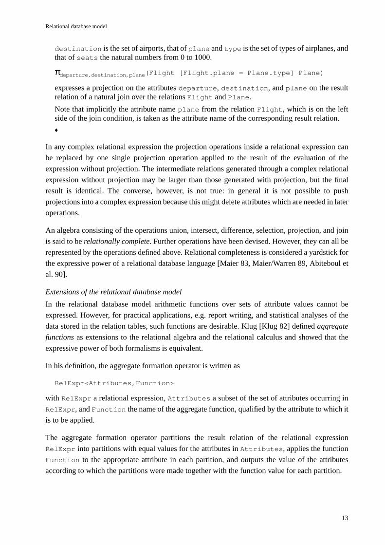
destination is the set of airports, that of plane and type is the set of types of airplanes, andthat of seats the natural numbers from 0 to 1000.
πdeparture,destination,plane(Flight [Flight.plane = Plane.type] Plane)
expresses a projection on the attributes departure, destination, and plane on the resultrelation of a natural join over the relations Flight and Plane.
Note that implicitly the attribute name plane from the relation Flight, which is on the leftside of the join condition, is taken as the attribute name of the corresponding result relation.
♦
In any complex relational expression the projection operations inside a relational expression can
be replaced by one single projection operation applied to the result of the evaluation of the
expression without projection. The intermediate relations generated through a complex relational
expression without projection may be larger than those generated with projection, but the final
result is identical. The converse, however, is not true: in general it is not possible to push
projections into a complex expression because this might delete attributes which are needed in later
operations.
An algebra consisting of the operations union, intersect, difference, selection, projection, and join
is said to be relationally complete. Further operations have been devised. However, they can all be
represented by the operations defined above. Relational completeness is considered a yardstick for
the expressive power of a relational database language [Maier 83, Maier/Warren 89, Abiteboul et
al. 90].
Extensions of the relational database model
In the relational database model arithmetic functions over sets of attribute values cannot be
expressed. However, for practical applications, e.g. report writing, and statistical analyses of the
data stored in the relation tables, such functions are desirable. Klug [Klug 82] defined aggregate
functions as extensions to the relational algebra and the relational calculus and showed that the
expressive power of both formalisms is equivalent.
In his definition, the aggregate formation operator is written as
RelExpr<Attributes,Function>
with RelExpr a relational expression, Attributes a subset of the set of attributes occurring in
RelExpr, and Function the name of the aggregate function, qualified by the attribute to which it
is to be applied.
The aggregate formation operator partitions the result relation of the relational expression
RelExpr into partitions with equal values for the attributes in Attributes, applies the function
Function to the appropriate attribute in each partition, and outputs the value of the attributes
according to which the partitions were made together with the function value for each partition.
2. Logic programming and the relational database model
14
Example
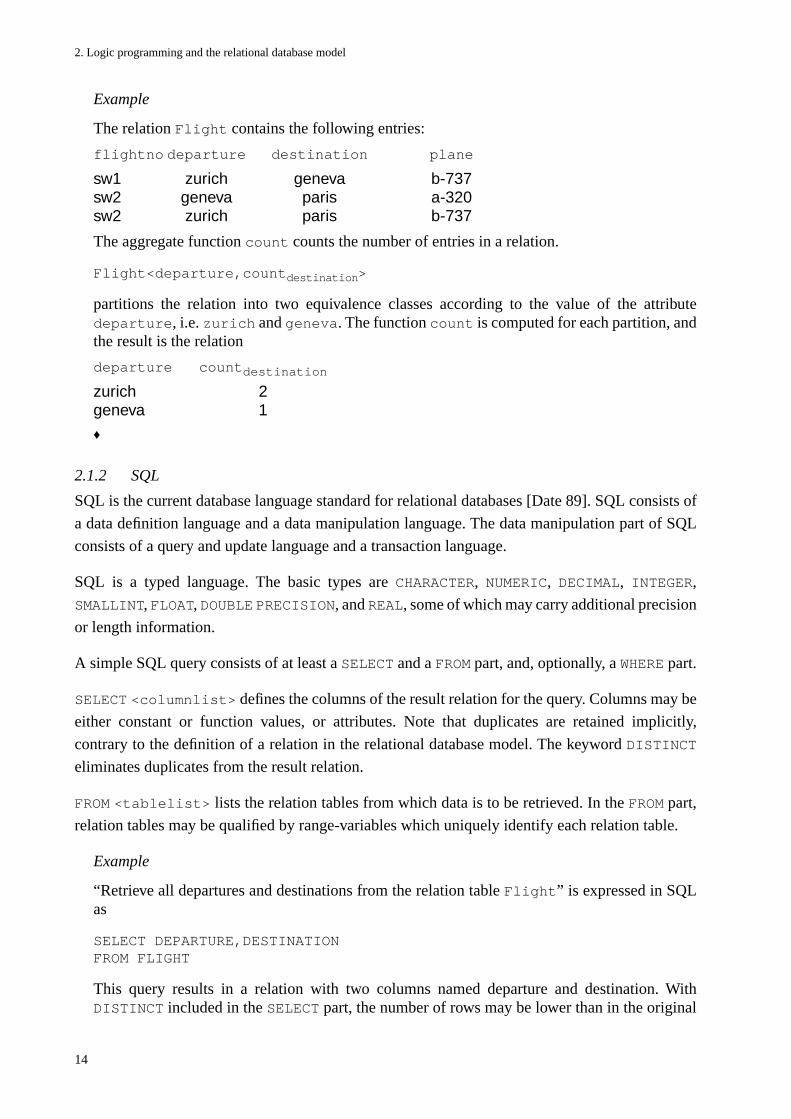
The relation Flight contains the following entries:
flightno departure destination plane
sw1 zurich geneva b-737sw2 geneva paris a-320sw2 zurich paris b-737
The aggregate function count counts the number of entries in a relation.
Flight<departure,countdestination>
partitions the relation into two equivalence classes according to the value of the attributedeparture, i.e. zurich and geneva. The function count is computed for each partition, andthe result is the relation
departure countdestination
zurich 2geneva 1
♦
2.1.2 SQL
SQL is the current database language standard for relational databases [Date 89]. SQL consists of
a data definition language and a data manipulation language. The data manipulation part of SQL
consists of a query and update language and a transaction language.
SQL is a typed language. The basic types are CHARACTER, NUMERIC, DECIMAL, INTEGER,
SMALLINT, FLOAT, DOUBLE PRECISION, and REAL, some of which may carry additional precision
or length information.
A simple SQL query consists of at least a SELECT and a FROM part, and, optionally, a WHERE part.
SELECT <columnlist> defines the columns of the result relation for the query. Columns may be
either constant or function values, or attributes. Note that duplicates are retained implicitly,
contrary to the definition of a relation in the relational database model. The keyword DISTINCT
eliminates duplicates from the result relation.
FROM <tablelist> lists the relation tables from which data is to be retrieved. In the FROM part,
relation tables may be qualified by range-variables which uniquely identify each relation table.
Example
“Retrieve all departures and destinations from the relation table Flight” is expressed in SQLas
SELECT DEPARTURE,DESTINATIONFROM FLIGHT
This query results in a relation with two columns named departure and destination. WithDISTINCT included in the SELECT part, the number of rows may be lower than in the original
Relational database model
15
relation due to the elimination of duplicate entries.
♦
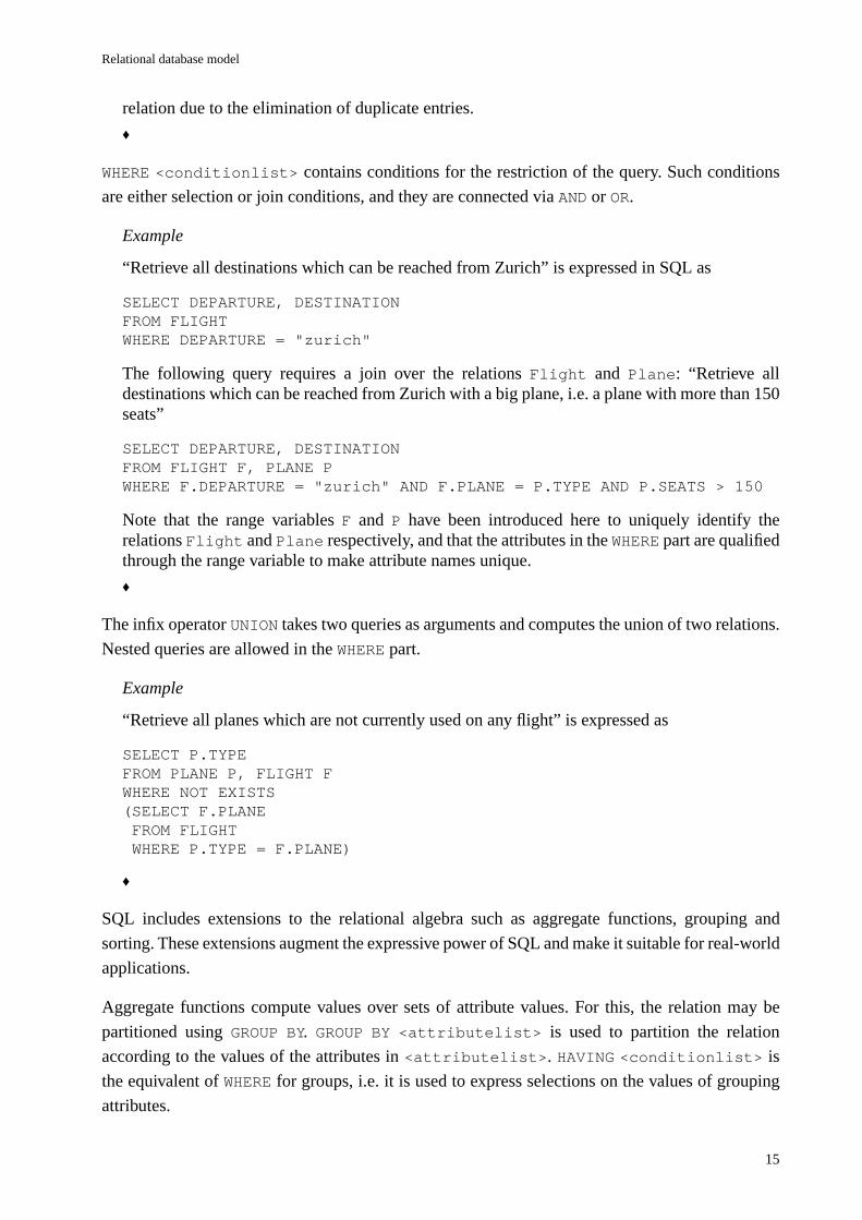
WHERE <conditionlist> contains conditions for the restriction of the query. Such conditions
are either selection or join conditions, and they are connected via AND or OR.
Example
“Retrieve all destinations which can be reached from Zurich” is expressed in SQL as
SELECT DEPARTURE, DESTINATIONFROM FLIGHTWHERE DEPARTURE = "zurich"
The following query requires a join over the relations Flight and Plane: “Retrieve alldestinations which can be reached from Zurich with a big plane, i.e. a plane with more than 150seats”
SELECT DEPARTURE, DESTINATIONFROM FLIGHT F, PLANE PWHERE F.DEPARTURE = "zurich" AND F.PLANE = P.TYPE AND P.SEATS > 150
Note that the range variables F and P have been introduced here to uniquely identify therelations Flight and Plane respectively, and that the attributes in the WHERE part are qualifiedthrough the range variable to make attribute names unique.
♦
The infix operator UNION takes two queries as arguments and computes the union of two relations.
Nested queries are allowed in the WHERE part.
Example
“Retrieve all planes which are not currently used on any flight” is expressed as
SELECT P.TYPEFROM PLANE P, FLIGHT FWHERE NOT EXISTS(SELECT F.PLANE FROM FLIGHT WHERE P.TYPE = F.PLANE)
♦
SQL includes extensions to the relational algebra such as aggregate functions, grouping and
sorting. These extensions augment the expressive power of SQL and make it suitable for real-world
applications.
Aggregate functions compute values over sets of attribute values. For this, the relation may be
partitioned using GROUP BY. GROUP BY <attributelist> is used to partition the relation
according to the values of the attributes in <attributelist>. HAVING <conditionlist> is
the equivalent of WHERE for groups, i.e. it is used to express selections on the values of grouping
attributes.
2. Logic programming and the relational database model
16
The SQL aggregate functions are min, max, avg, sum, and count. An aggregate function may
occur as the sole entry in the SELECT part, or together with other aggregate functions only.
ORDER BY <columnlist> sorts the result relation according to the values of the columns specified
in the list.
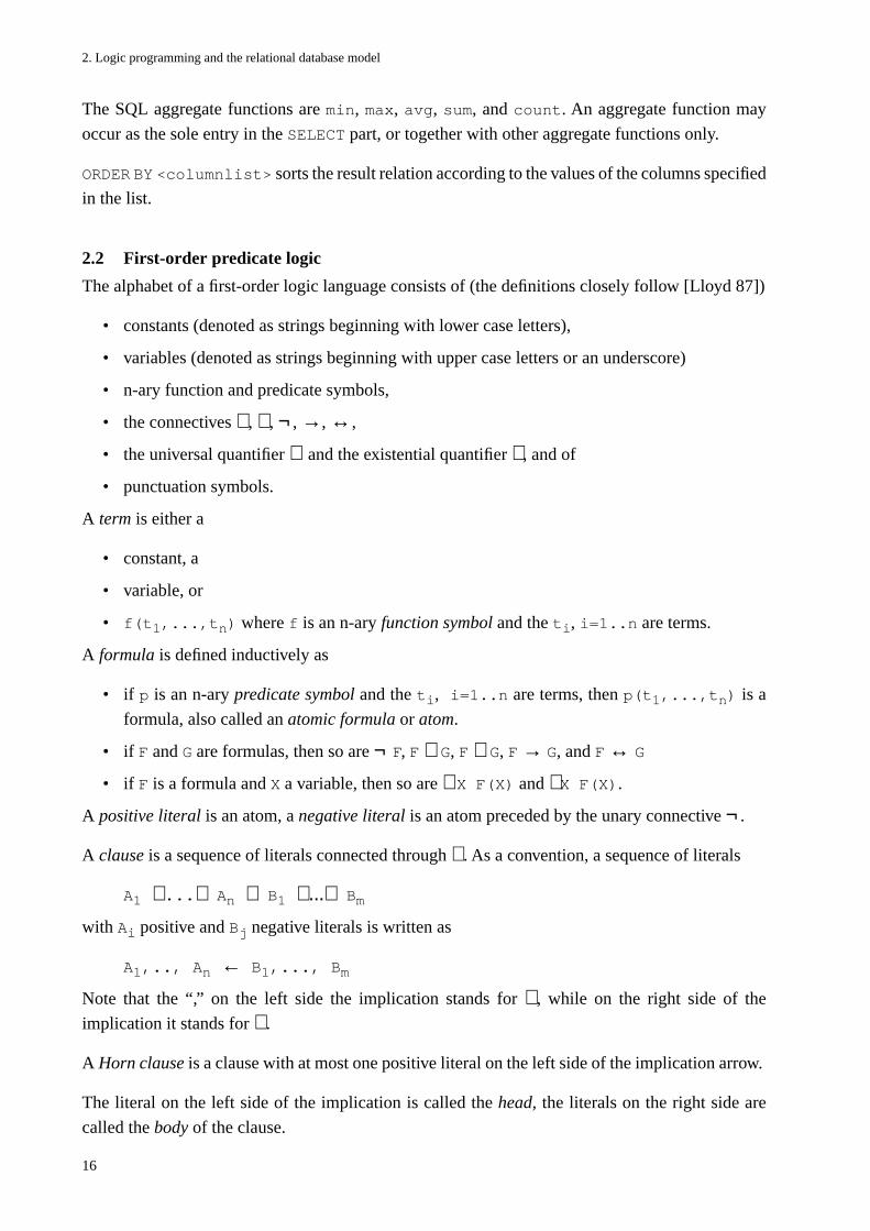
2.2 First-order predicate logic
The alphabet of a first-order logic language consists of (the definitions closely follow [Lloyd 87])
• constants (denoted as strings beginning with lower case letters),
• variables (denoted as strings beginning with upper case letters or an underscore)
• n-ary function and predicate symbols,
• the connectives ∧ , ∨ , ¬ , →, ↔,
• the universal quantifier ∀ and the existential quantifier ∃ , and of
• punctuation symbols.
A term is either a
• constant, a
• variable, or
• f(t1,...,tn) where f is an n-ary function symbol and the ti, i=1..n are terms.
A formula is defined inductively as
• if p is an n-ary predicate symbol and the ti, i=1..n are terms, then p(t1,...,tn) is a
formula, also called an atomic formula or atom.
• if F and G are formulas, then so are ¬ F, F ∧ G, F ∨ G, F → G, and F ↔ G
• if F is a formula and X a variable, then so are ∀ X F(X) and ∃ X F(X).
A positive literal is an atom, a negative literal is an atom preceded by the unary connective ¬ .
A clause is a sequence of literals connected through ∨ . As a convention, a sequence of literals
A1 ∨ ...∨ An ∨ B1 ∨...∨ Bm
with Ai positive and Bj negative literals is written as
A1,.., An ← B1,..., Bm
Note that the “,” on the left side the implication stands for ∨ , while on the right side of the
implication it stands for ∧ .
A Horn clause is a clause with at most one positive literal on the left side of the implication arrow.
The literal on the left side of the implication is called the head, the literals on the right side are
called the body of the clause.
First-order predicate logic
17
A program clause is either a
• unit clause, a clause with an empty body: p ←. (also written as p.)
• rule, a clause of the form: p ← qm,...,qn.
• goal, a clause with an empty head: ← qm,...,qn.
A clause is ground if it does not contain variables. A fact is ground unit clause. A goal is a simple
goal if it contains only one literal, a complex goal otherwise.
All variables in a program clause are assumed to be universally quantified. This assumption is
permitted because the existential quantifier for a variable X can be replaced by a Skolem function
which takes as arguments the universally quantified variables that determine the value of X. Under
this assumption, the universal quantifiers can be omitted.
A rule is range-restricted if all the variables in its head also occur positively in its body. In the rest
of the thesis only range-restricted rules will be considered.
A predicate is a set of clauses with common predicate symbol and arity. The extension of a
predicate is the set of facts with the same predicate symbol and arity, whereas the intension is given
through its rules. A predicate is defined extensionally if its definition consists of facts only, and
intensionally otherwise.
A rule p ← q1,...,qn is recursive if it contains in its body a literal qi with the same predicate
symbol and arity as p.
A predicate p is recursive if it contains a recursive rule. Two predicates p and q are mutually
recursive if p contains q in the body of a rule (“p calls q”), and q contains p in the body of a rule.
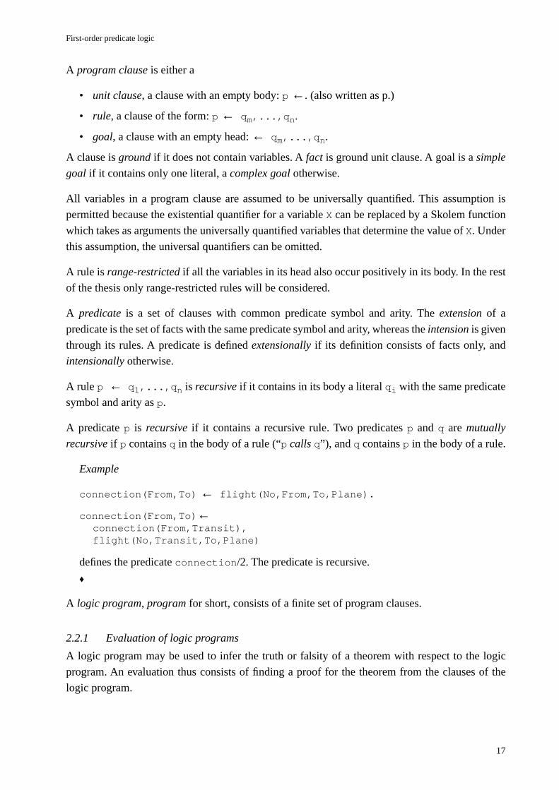
Example
connection(From,To) ← flight(No,From,To,Plane).
connection(From,To)← connection(From,Transit),flight(No,Transit,To,Plane)
defines the predicate connection/2. The predicate is recursive.
♦
A logic program, program for short, consists of a finite set of program clauses.
2.2.1 Evaluation of logic programs
A logic program may be used to infer the truth or falsity of a theorem with respect to the logic
program. An evaluation thus consists of finding a proof for the theorem from the clauses of the
logic program.
2. Logic programming and the relational database model
18
Substitution and Unification
During the construction of a proof variable bindings are computed in which a variable v is bound
to a term t. Such a variable binding is written as v/t. A substitution is a set of variable bindings
vi/ti, where the distinct variables vi of a term are bound to a term ti with vi ≠ ti and vj ≠ vifor i ≠ j.
The application of a substitution to a clause yields an instance of a clause.
Example
The application of the substitution {X/geneva} to flight(sw1,zurich,X,b-737) iswritten as
flight(sw1,zurich,X,b-737) {X/geneva}
and yields the ground instance
flight(sw1,zurich,geneva,b-737).
♦
Unification is the process of making two formulas syntactically identical through a substitution. If
there exists such a substitution or unifier, then there also exists a unique most general unifier (mgu).
A unifier θ for a set of formulas F is an mgu for F if there exists for any other unifier σ of F a
substitution γ such that σ = θγ.
Example
The mgu of the following two clauses
flight(sw1,zurich,X,b-737) and
flight(Y,zurich,Z,b-737)
is {Y/sw1,X/Z}.
♦
An evaluation can be either top-down, starting with the original goal and using resolution, bottom-
up, starting with the program clauses in a fixed-point computation, or a combination of both.
In a top-down evaluation the starting point of the evaluation is the goal to be proved. In each
evaluation step the goal is replaced through the subgoals of a clause that can be unified with the
goal. This evaluation strategy is also called backward chaining because the direction of evaluation
goes from rule head to the body in the opposite direction of the “←” implication.
In a bottom-up evaluation the starting point of the evaluation is the set of facts. In each evaluation
step a the set of facts is augmented with the heads of rules whose bodies evaluate to true. The
evaluation ends if the original goal is included in the set of derived facts. The direction of evaluation
follows the “←” implication, and it is thus also called forward chaining.
First-order predicate logic
19
Top-down evaluation with SLD resolution
Top-down evaluation relies on the resolution rule [Robinson 65], a sound and complete inference
rule, to derive new clauses from the clauses stored in the program. This derivation is commonly
done through a refutation theorem prover. A refutation proof adds the negation of the clauses that
are to be proved to the set of program clauses and tries to derive a contradiction. If such a
contradiction can be found, then the negation of the clauses to be proved is false, hence the clauses
are true.
SLD resolution is a refutation proof procedure for logic programs. The general procedure of SLD
resolution is as follows:
• The original goal is taken as the first resolvent.
• In a derivation step, a clause from the resolvent is selected through a selection function. For
this selected clause a program clause is chosen and the most general unifier of the two clauses
is computed. In the current resolvent, the selected clause is replaced by the body of the
program clause and the most general unifier is applied to the current resolvent.
• Derivation continues until the empty resolvent is reached which is the case when a proof has
been constructed.
The resolvent may actually become smaller in each derivation step. If a rule has been chosen from
the program clauses, the new resolvent will contain at least as many goals as the previous resolvent.
However, if a fact is chosen, the new resolvent contains less goals than the previous one because
the selected goal is deleted from the resolvent, and there is no clause body to add.
In each derivation step variable bindings are computed. Any variable in a goal may thus receive a
binding during the proof. In fact, except for programs where the existence of a proof suffices, the
variable bindings are the results one really is interested in.
A solution is the set of bindings for the goal variables computed during the proof of a goal. An
instantiation is the application of a solution to a term.
Note that there may exist more than one proof for a given goal, each resulting in a solution. The set
of all solutions to a goal is called the solution set.
SLD tree
An SLD resolution can be represented as an SLD tree. The root of the SLD tree contains the
original goal. A node represents a resolvent and an edge corresponds to one derivation step in the
resolution. In each derivation step exactly one clause from possibly many clauses whose heads can
be unified with the selected goal is chosen through a search rule.
Each node in the SLD tree is labelled with the current resolvent. The selected goal for the next
derivation step is underlined. A goal for which there is no unifiable clause is called a failure node,
a branch in the SLD tree with a failure node as its leaf is a failure branch. A branch with the empty
2. Logic programming and the relational database model
20
resolvent as its leaf is a success branch. Each edge in the SLD tree is labelled with the most general
unifier mgu of the derivation step.
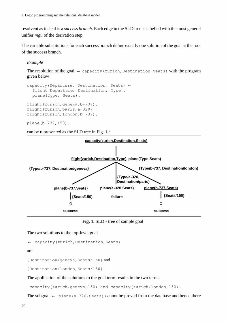
The variable substitutions for each success branch define exactly one solution of the goal at the root
of the success branch.
Example
The resolution of the goal ← capacity(zurich,Destination,Seats) with the programgiven below
capacity(Departure, Destination, Seats) ← flight(Departure, Destination, Type),plane(Type, Seats).
flight(zurich,geneva,b-737).flight(zurich,paris,a-320).flight(zurich,london,b-737).
plane(b-737,150).
can be represented as the SLD tree in Fig. 1.:
The two solutions to the top-level goal
← capacity(zurich,Destination,Seats)
are
{Destination/geneva,Seats/150} and
{Destination/london,Seats/150}.
The application of the solutions to the goal term results in the two terms
capacity(zurich,geneva,150) and capacity(zurich,london,150).
The subgoal ← plane(a-320,Seats) cannot be proved from the database and hence there
capacity(zurich,Destination,Seats)
flight(zurich,Destination,Type), plane(Type,Seats)
plane(b-737,Seats)
◊
{Type/b-737, Destination/london}
{Seats/150}
success
{Type/b-737, Destination/geneva}
plane(b-737,Seats)
Fig. 1. SLD - tree of sample goal
failure
plane(a-320,Seats)
{Seats/150}
◊success
{Type/a-320, Destination/paris}
First-order predicate logic
21
is no solution for capacity(zurich,paris,...).
♦
2.2.2 Abstract interpreter
The proof procedure informally described above is now presented as an abstract interpreter for
logic programs (the empty resolvent is denoted by the symbol ◊. A fact is a clause with an empty
body, written as ClauseHead ← ◊).
prove(◊).
prove(CurrentResolvent)← select_goal(CurrentResolvent,Goal),select_clause(Goal,(ClauseHead ← ClauseBody),Unifier),replace_goal(Goal,CurrentResolvent,ClauseBody,ReducedResolvent),apply(Unifier,ReducedResolvent,NewResolvent),prove(NewResolvent).
In this interpreter, variable substitutions are not represented explicitly. Only the most general
unifier is shown to make its application to the whole resolvent visible.
Example
The logic program consists of the following clauses:
flight(sw1,zurich,geneva,b-737).flight(sw2,zurich,paris,a-320).flight(sw5,paris,london,b-737).
connection(From,To) ← flight(_,From,To,_).
connection(From,To) ← flight(_,From,Transit,_),connection(Transit,To).
The goal to be proved is ← connection(zurich,X).
This goal is supplied to the abstract interpreter prove as the first resolvent which then becomesprove(connection(zurich,X)).
select_goal(connection(zurich,X),Goal) is called. There is only one goal in theresolvent and hence it must be selected. Goal thus becomes connection(zurich,X).select_clause tries to find a matching clause for the current goal and computes the mostgeneral unifier.
In this case, assume that the first connection clause has been chosen. The most general unifierof connection(zurich,X) and connection(From,To) is {From/zurich,To/X}.
connection(zurich,X) is now deleted from the resolvent, and the body of the programclause is added to the resolvent which now becomes flight(_,From,To,_). The unifier isapplied to the resolvent to result in flight(_,zurich,X,_) as the new resolvent.
The derivation continues with the new resolvent through a recursive call toprove(flight(_,zurich, X,_)). The matching clauses for the resolvent are the first twoprogram clauses.
2. Logic programming and the relational database model
22
Assume that the second clause is chosen. The unifier of the resolvent flight(_,zurich,X,_) and flight(sw2,zurich,paris,a-320) is {X/paris}. The use of the anonymousvariable _ indicates that its binding is of no interest and thus it is neglected. However, thebinding of X is returned.
The resolvent now becomes the empty resolvent ◊ because flight(sw2,zurich,paris,a-320) is a fact. The call to prove with the empty resolvent terminates the proof procedure.
As a result, the variable bindings for the variables of the original goal are returned. The solutionto the goal ← connection(zurich, X) is {X/paris}.
♦
This abstract interpreter does not specify
• which goal to select from the current resolvent, nor
• where to place the body of the unified clause in the resolvent.
In the above example program clauses were chosen arbitrarily. The problem of selecting a goal
from the resolvent did not arise because at any time there was at most one goal in the resolvent. In
an actual implementation of a logic programming language the selection of a goal from the current
resolvent is defined through a computation rule or selection function in the abstract interpreter. The
replacement of a goal in the resolvent through its body is defined through the search rule.
In terms of a proof tree, the computation rule determines how to construct the tree, whereas the
search rule determines how to traverse the tree in the course of a proof. In SLD resolution, the
search rule always selects the first subgoal in the resolvent, and the computation rule always places
the body of the selected clause before any other goal in the resolvent which results in a depth-first
construction of the SLD tree.
Note that success or failure to prove a goal in a finite number of steps is independent of the
computation rule, but requires a fair search rule, i.e. a search rule which guarantees that all clauses
are tried [Lloyd 87].
Negation as failure
SLD resolution can be enhanced through a restricted form of negation to result in SLDNF
resolution. Negation as failure, denoted by the symbol not, is a weaker form of negation than full
negation of first-order predicate logic, or even negation under the closed world assumption [Reiter
78]. not G expresses only “G cannot be proved” rather than “G is not true” [Clark 78].
Negation as failure is safe, i.e. it yields the same result as negation under the closed world
assumption, only for goals whose arguments are all bound. With unbound variables in the negated
goal negation as failure does not yield the expected result but instead the computation flounders.
First-order predicate logic
23
Example
The following clauses are given:
railroad_station(zurich).railroad_station(berne).
airport(zurich).
Suppose one wants to find those cities that do not have an airport, but are railroad stations.
← not airport(City), railroad_station(City).
The expected answer is City = berne, but instead the goal fails. The reason for this is that notairport(City) calls airport(City), which succeeds with City being bound to a value.not turns the success into a failure and undoes any variable binding, and thus the whole queryfails.
Reordering the subgoals in such a way that the variables occurring in the negated subgoal arebound by positive subgoals gives the expected result:
← railroad_station(City), not airport(City).
City = berne
♦
For a detailed discussion of negation and negation as failure see the book by Lloyd [Lloyd 87], or
the article by Shepherdson [Shepherdson 88].
2.2.3 Prolog
Prolog is a programming language based on Horn clause logic. Its development was motivated by
Kowalski´s research result that Horn clauses have a declarative as well as a procedural reading
[Kowalski 79].
A Horn clause
A ← Bm,…, Bn, 0 ≤ m ≤ n
can either be read declaratively as
A is valid if Bm ∧…∧ Bn is valid.
or procedurally as
To achieve A, do Bm, …, do Bn.
The procedural (or operational) semantics of Horn clauses is the basis of all implementations of
logic programming languages. Note that this procedural semantics does not prescribe a particular
order in which the subgoals in the body of the clause are to be evaluated.
2. Logic programming and the relational database model
24
Prolog was defined by Colmerauer and Roussel [Roussel 75] at the University of Marseille and a
first interpreter was implemented there. A Prolog compiler was first implemented by Warren and
Pereira in Edinburgh [Warren 83].
The following syntax definition of Prolog follows the de-facto standard “Edinburgh” syntax as
defined in [Clocksin/Mellish 87].
• A constant is either an atom, or a number. An atom is written as a sequence of characters,
beginning with a lower case letter, and delimited by a space or a punctuation mark.
Alternatively, if the atom is to begin with a capital letter, or contain punctuation marks or
spaces, it can be enclosed in single quotes. Numbers are denoted by a sequence of digits
including sign, decimal point or exponent symbol.
• A variable is denoted as a sequence of characters beginning with capital letters or an
underscore.
• A structure (also called compound term) consists of a functor and a set of arguments
enclosed in parentheses. Each functor is assigned an arity, and a functor is uniquely
identified by the pair functor/arity. A functor is an atom, and the arguments are terms.
A special structure is the list. The empty list is written as [], and [Head|Tail] denotes a list
with the first element the variable Head. The vertical bar separates the elements on the left of the
bar from the rest of the list, which is a list itself, represented by the variable Tail.
Example
john mary ‘Loves’ 1234 are constants,Head Tail _x are variables,loves(john,X) is a compound term with the first argument a constant, the second argumenta variable,[john,loves,mary] is a list with three constant elements.
♦
Program clauses are also terms. Facts are simple compound terms, rules are terms with the binary
functor “:-”, and goals are denoted by the unary functor “?-”.
Operators are functors with a predefined meaning (which can be redefined). The set of Prolog
operators includes
• =/2, which succeeds if its two arguments can be unified,
• comparison operators, e.g. >/2, =</2, @</2,…, which succeed if the specified comparison
holds between the two arguments. Note that for comparison operations all arguments must
be bound.
• is/2, which succeeds if the argument on the left side can be unified with the result of the
evaluation of the arithmetic expression on the right side,
• arithmetic operators, e.g. +/2, -/2, */2, //2.
First-order predicate logic
25
The inference engine of Prolog is a concretization of the abstract interpreter presented in section
2.2.2. Prolog implements SLDNF resolution with a left-to-right computation rule, and a depth-first
search rule. This means that the computation rule selects the leftmost subgoal from the current
resolvent and that the search rule replaces this subgoal with the body of the program clause it was
unified with successfully.
The depth-first computation rule together with the search rule can be implemented with a stack
datastructure which holds the current resolvent. This implementation is space efficient because the
maximum length of the stack is equal to the depth of the SLD tree of the original goal. The top
element of the stack corresponds to the left-most subgoal in the resolvent. Replacing the left-most
goal from the resolvent by the body of the unifying clause amounts to popping the top element off
the stack, and pushing the body of the unifying clause into the stack.
Note that this search rule may lead to non-terminating evaluations with mutually or left recursive
predicates. The search rule is only correct, but not complete. There may exist a proof for a given
goal, but due to its fixed search rule Prolog fails to find this proof.
Example
The following program succeeds if there exists a connection between Departure andDestination via Route.
flight(sw1,zurich,geneva,b-737).flight(sw2,geneva,paris,a-320).flight(sw3,paris,london,b-737).flight(sw4,zurich,london,b-747).
connection(Departure,Destination,Route):-connect(Departure,Destination,[],Route).
connect(Departure,Destination,SoFar,[Destination,Departure|SoFar]):-flight(_,Departure,Destination,_).
connect(Departure,Destination,SoFar,Route):-flight(_,Departure,Transit,_),not member(Transit,SoFar),connect(Transit,Destination,[Departure|SoFar],Route).
The program is started through the goal
?- connection(zurich,london,Route).
Route = [london,paris,geneva,zurich];Route = [london,zurich]
Further solutions can be computed by forcing Prolog to backtrack. Entering a semicolon ; willforce the current evaluation to fail and start the search for another solution. If there exist furthersolutions, they will be displayed, otherwise the evaluation fails with a system dependentmessage, e.g.
no more solutions.
2. Logic programming and the relational database model
26
The program can also be run “backwards”, e.g. by supplying only the route. The goal
?- connection(Departure,Destination,[london,paris,geneva,zurich]).
succeeds with
Departure = zurichDestination = london;
no more solutions.
In fact, the program runs safely with any instantiation pattern (also called mode) of itsarguments.
♦
Prolog features non-logical extensions which make it a general purpose programming language,
but which do not have a declarative semantics.
• Extra-logical predicates achieve side effects during their evaluation. Typical examples are I/O
predicates such as read/1 or write/1, dynamic database update predicates such as assert/1
or retract/1, or predicates that retrieve clauses from the program code, e.g. clause/2.
• Meta-level predicates query the state of a proof, treat variables as objects of the language, and
allow the conversion of datastructures to goals [Sterling/Shapiro 86]. var/1 and nonvar/1
succeed if their argument is a variable respectively not a variable. Comparison of nonground
terms is expressible by ==/2, which succeeds if its arguments are identical (which is stronger
than unifiable: ?- 5=X will succeed and unify X with 5, but ?- 5==X will fail). The predicate
call/1 converts its argument into a goal, and succeeds if the evaluation of this goal succeeds.
• Control predicates affect the procedural behavior of a program. The cut, written as !/1,
commits the evaluation to the current clause. Alternatives for the current clause, and
alternatives for the goals before the !/1 in a clause are not tried. The cut thus amounts to
pruning subtrees in the SLD tree.
The if-then-else construct of procedural language is defined through the cut. It is written as -
>/2, and can be defined as
->(P,(Q;_)) :- call(P),!,call(Q).->(_,(_;R)) :- call(R).
Prolog is the most widespread logic programming language today. Various implementations, many
of which have extensions to allow co-routining, delayed evaluation, safe negation, higher-order
constructs etc. are commercially available, or in the public domain. The international standards
committee is currently establishing a Prolog standard [Scowen 90].
2.3 Relationship between logic and the relational database model
First-order predicate logic languages feature negation, recursion, and function symbols. Through
successive restrictions the expressive power of logic languages can be reduced. A first restriction,
namely the elimination of function symbols, results in the language known as Datalog [Ullman 88,
Relationship between logic and the relational database model
27
Gardarin/Valduriez 88]. In a second restriction only non-recursive clauses are allowed. With this
restriction the expressive power of the language is equivalent to that of relational calculus, and
hence, with relational algebra [Aho/Ullman 79, Parsaye 83, Maier 83].
Note that negation is needed to express in relational calculus the difference operation of relational
algebra. In the context of databases the closed world assumption is very natural, and therefore full
negation of first-order predicate logic is not required.
2.3.1 Logic languages and relational database model
Any relational algebra operation may be expressed in a relational calculus formula, and any
formula of the relational calculus can be represented through Horn clauses. Thus it is possible to
express any relational algebra operation in a logic programming language based on Horn clauses.
However, the converse is not true because the expressive power of an unrestricted logic
programming language is greater than that of relational calculus or algebra.
With a suitable restriction the expressive power of the logic programming language can be made
equal to the expressive power of relational algebra. Such a restriction is of particular interest in the
context of logic and databases because it allows a direct access to relational databases through the
logic programming language and therefore does not require an extra language for accessing the
database.
In practice, this results in application programs which use the restricted logic programming
language for accessing relational databases, and which use the unrestricted logic programming
language for the application itself.
For each data object of the relational database model there is an appropriate construct in the logic
language:
• A domain corresponds to a set of constants,
• A relation table corresponds to an extensionally defined predicate, i.e. a set of facts.
The relation name is mapped to a predicate symbol, the number of attributes is equal to the
arity of a predicate, and each relation attribute is mapped to a predicate argument via a
mapping function. Attribute values are atomic constants, i.e. they have no internal structure.
• A database query corresponds to a non-recursive goal.
Note that in actual implementations of a logic programming language the order of tuples in a
relation may be significant, whereas in relational database systems no particular order of records
is assumed. Consequently, if a logic program is to access data stored in external relational
databases, it must be guaranteed that the order of database records is of no relevance to the logic
program.
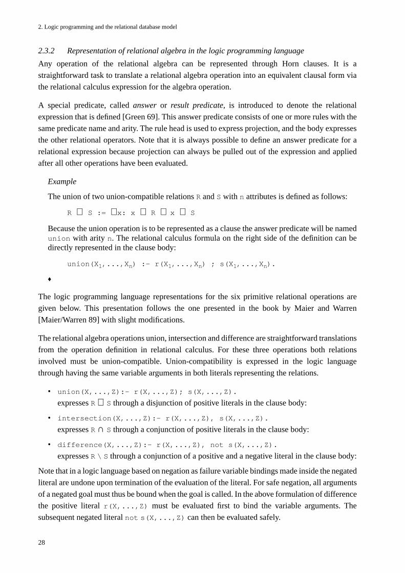
2. Logic programming and the relational database model
28
2.3.2 Representation of relational algebra in the logic programming language
Any operation of the relational algebra can be represented through Horn clauses. It is a
straightforward task to translate a relational algebra operation into an equivalent clausal form via
the relational calculus expression for the algebra operation.
A special predicate, called answer or result predicate, is introduced to denote the relational
expression that is defined [Green 69]. This answer predicate consists of one or more rules with the
same predicate name and arity. The rule head is used to express projection, and the body expresses
the other relational operators. Note that it is always possible to define an answer predicate for a
relational expression because projection can always be pulled out of the expression and applied
after all other operations have been evaluated.
Example
The union of two union-compatible relations R and S with n attributes is defined as follows:
R ∪ S := ∀ x: x ∈ R ∨ x ∈ S
Because the union operation is to be represented as a clause the answer predicate will be namedunion with arity n. The relational calculus formula on the right side of the definition can bedirectly represented in the clause body:
union(X1,...,Xn) :- r(X1,...,Xn) ; s(X1,...,Xn).
♦
The logic programming language representations for the six primitive relational operations are
given below. This presentation follows the one presented in the book by Maier and Warren
[Maier/Warren 89] with slight modifications.
The relational algebra operations union, intersection and difference are straightforward translations
from the operation definition in relational calculus. For these three operations both relations
involved must be union-compatible. Union-compatibility is expressed in the logic language
through having the same variable arguments in both literals representing the relations.
• union(X,...,Z):- r(X,...,Z); s(X,...,Z).
expresses R ∪ S through a disjunction of positive literals in the clause body:
• intersection(X,...,Z):- r(X,...,Z), s(X,...,Z).
expresses R ∩ S through a conjunction of positive literals in the clause body:
• difference(X,...,Z):- r(X,...,Z), not s(X,...,Z).
expresses R \ S through a conjunction of a positive and a negative literal in the clause body:
Note that in a logic language based on negation as failure variable bindings made inside the negated
literal are undone upon termination of the evaluation of the literal. For safe negation, all arguments
of a negated goal must thus be bound when the goal is called. In the above formulation of difference
the positive literal r(X,...,Z) must be evaluated first to bind the variable arguments. The
subsequent negated literal not s(X,...,Z) can then be evaluated safely.
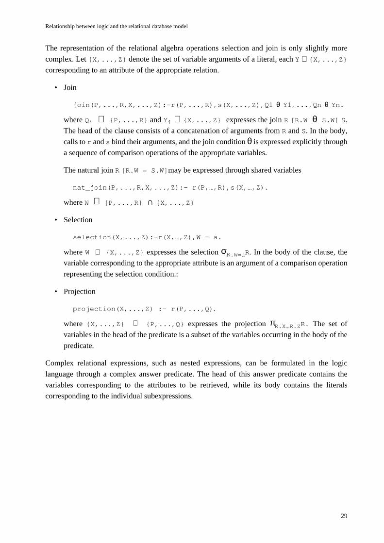
Relationship between logic and the relational database model
29
The representation of the relational algebra operations selection and join is only slightly more
complex. Let {X,...,Z} denote the set of variable arguments of a literal, each Y ∈ {X,...,Z}
corresponding to an attribute of the appropriate relation.
• Join
join(P,...,R,X,...,Z):-r(P,...,R),s(X,...,Z),Q1 θ Y1,...,Qn θ Yn.
where Qi ∈ {P,...,R} and Yi ∈ {X,...,Z} expresses the join R [R.W θ S.W] S.
The head of the clause consists of a concatenation of arguments from R and S. In the body,
calls to r and s bind their arguments, and the join condition θ is expressed explicitly through
a sequence of comparison operations of the appropriate variables.
The natural join R [R.W = S.W]may be expressed through shared variables
nat_join(P,...,R,X,...,Z):- r(P,…,R),s(X,…,Z).
where W ⊆ {P,...,R} ∩ {X,...,Z}
• Selection
selection(X,...,Z):-r(X,…,Z),W = a.
where W ∈ {X,...,Z} expresses the selection σR.W=aR. In the body of the clause, the
variable corresponding to the appropriate attribute is an argument of a comparison operation
representing the selection condition.:
• Projection
projection(X,...,Z) :- r(P,...,Q).
where {X,...,Z} ⊆ {P,...,Q} expresses the projection πR.X…R.ZR. The set of
variables in the head of the predicate is a subset of the variables occurring in the body of the
predicate.
Complex relational expressions, such as nested expressions, can be formulated in the logic
language through a complex answer predicate. The head of this answer predicate contains the
variables corresponding to the attributes to be retrieved, while its body contains the literals
corresponding to the individual subexpressions.
2. Logic programming and the relational database model
30
Example
The projection on the attributes departure, destination, plane applied to the result of ajoin over the common attribute plane of Flight and type of Plane is expressed in relationalalgebra as
πdeparture,destination,planeFlight[Flight.plane=Plane.type]PlaneIn the logic programming language this operation is expressed as the Horn clause
proj_join(Departure,Destination,Plane):-flight(FlightNo,Departure,Destination,Plane),plane(Plane,Seats).
♦
With a clausal representation of the relational algebra it is possible to formulate any relational
query in a logic programming language. A restriction of the logic programming language to the
above clauses results in the Horn clause equivalent of relational calculus, with the expressive power
equal to that of relational algebra. Effectively, the language defined here corresponds to Datalog
with negation, but without recursion [Ullman 88, Gardarin/Valduriez 88, Ceri et al. 90].

Part II
Concept

32
33
3
Coupled systems
A coupled system consists of a programming language system connected to an external database
system. The database is accessed prior to or during the evaluation of application programs written
in the programming language.
In the remainder of this thesis, coupled systems are restricted to logic programming language
systems coupled to external relational database systems.
3.1 General structure of coupled systems
The clauses of a logic program can be stored either internally in the logic language system
workspace in main memory, or externally in a relational database system on secondary memory. A
logic program in a coupled system may have a subset of its program clauses stored internally, and
the rest of the clauses stored externally in a relational database system.
• A program predicate, or simply predicate if the reference is clear from the context, is a
predicate the clauses of which are stored internally in the logic language system workspace.
• A database predicate is a predicate the clauses of which are stored in an external database.
Note that — with the exception of comparison operations and arithmetic functions — a predicate
must either be a program predicate or a database predicate, but not both. This is no restriction since
a predicate p that violates this condition can always be redefined through renaming the externally
stored definition to p´ and adding a call to p´ to the definition of p [Bancilhon/Ramakrishnan 86].
The standard comparison operators for constant values, e.g. “>”, “<“, “=” etc., can be thought of
as relation tables with two attributes corresponding to the operands. n-ary arithmetic functions can
be thought of as n+1-ary relation tables with n attributes for the operands and one result attribute.
Comparison operations and arithmetic functions are thus database predicates as well as program
predicates.
3. Coupled systems
34
• A database fact is an extensionally defined database predicate.
• A database goal is a clause with an empty head which contains in its body only calls to
database predicates.
• A base conjunction is a conjunction of database goals.
Any sequence of database goals can be split into disjunctions of base conjunctions.
In coupled systems a complex goal may contain both goals and database goals in any order. For
efficiency reasons it is desirable to achieve as long as possible base conjunctions. This is always
possible through reordering program goals and database goals [Ceri et al. 90].
3.1.1 Embedding vs. integration
In his thesis on embedding database access into high-level procedural programming languages,
Bever [Bever 86] discerns two basic methods of coupling a database system with a programming
language system: integration vs. embedding.
• Integration means that the programming language system is extended to incorporate database
system features. Integration requires extending the programming language through database
language constructs, and entails modifications of the programming language compiler and the
runtime system.
• Embedding means that the database access is implementable entirely through language
constructs provided by the programming language. Embedding database access into a
programming language allows the programming language and the database language to be
chosen independently, and does not require modifications of the programming language
compiler.
He defines two forms of embedding: type embedding (Typeinbettung) and language embedding
(Spracheinbettung).
Type embedding is schema dependent since only the current database schema is represented by
datastructures of the programming language. Language embedding is schema independent, and the
database language itself is represented by programming language constructs. An instance of a
language embedding, the representation of an actual database schema, is thus a concretization of
the abstract language embedding.
Bever lists the following requirements for the embedding of database access into programming
languages.
• Independence of database language and programming languages
• No modification of the programming language compiler
• Database type and view definition also by the programming language
• Static type checking
General structure of coupled systems
35
• Programming language representation of data objects not in the responsibility of the
application programmer
• Orthogonality
• Prevention of redundant tests in the database system.
Clearly, these requirements are coined for procedural programming languages. For logic
programming languages these requirements have to be modified:
• Logic programming languages are often untyped languages, and the database access language
is a sublanguage of the logic programming language.
Type checking for accessing the database or retrieving data is thus not always feasible in
untyped languages.
• In logic programming languages there is no distinction between program and data: program
clauses are terms. This allows the dynamic definition of database access in the logic
programming language itself.
Static analysis of database access is not sufficient. Instead, database access requests and the
data retrieved from the database system must be interpreted.
• Furthermore, the dynamic properties of logic programming languages allow language
extensions without modifications of the language compiler.
The distinction of embedding an integration gives a rather general characterization of coupled
systems. It relates to the database system and the logic programming system as a whole and is not
specific enough to capture the system architecture nor the system languages.
3.1.2 Physical and logical level
In his discussion of coupled systems Bocca [Bocca 86] separates language issues from system
architecture issues. He distinguishes between a physical level, which relates to the system
architecture of a coupled system, and a logical level, which relates to the system languages.
Bocca uses the terms integration and coupling to describe the degree of coupling on the physical
level, and close coupling and loose coupling for the logical level.
In his terminology, integration means that a database system and a logic programming language
are integrated in one single system. Coupling means that both systems run independently of each
other. A closely coupled system is a system in which the programming language is also the data
manipulation language of the database. A loosely coupled system is a system in which the
programming language and the data manipulation language are different languages.
In this thesis, I prefer to use loose and tight for both the logical and the physical level because these
terms adequately reflect the fact that there is a smooth transition from integration to coupling on
either level. In the following, a coupled system is thus always described by giving the degree of
coupling on both levels as in “physically loosely and logically tightly coupled system”.
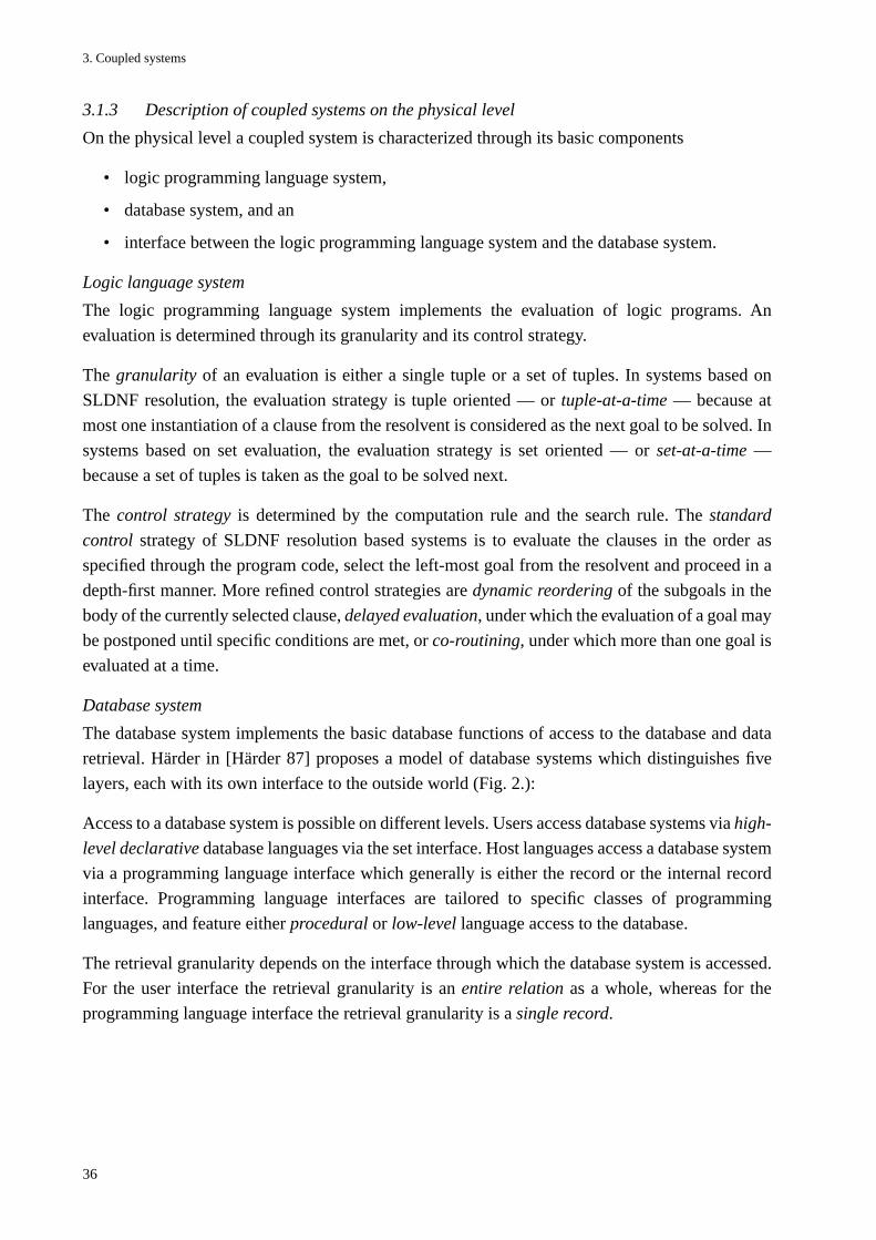
3. Coupled systems
36
3.1.3 Description of coupled systems on the physical level
On the physical level a coupled system is characterized through its basic components
• logic programming language system,
• database system, and an
• interface between the logic programming language system and the database system.
Logic language system
The logic programming language system implements the evaluation of logic programs. An
evaluation is determined through its granularity and its control strategy.
The granularity of an evaluation is either a single tuple or a set of tuples. In systems based on
SLDNF resolution, the evaluation strategy is tuple oriented — or tuple-at-a-time — because at
most one instantiation of a clause from the resolvent is considered as the next goal to be solved. In
systems based on set evaluation, the evaluation strategy is set oriented — or set-at-a-time —
because a set of tuples is taken as the goal to be solved next.
The control strategy is determined by the computation rule and the search rule. The standard
control strategy of SLDNF resolution based systems is to evaluate the clauses in the order as
specified through the program code, select the left-most goal from the resolvent and proceed in a
depth-first manner. More refined control strategies are dynamic reordering of the subgoals in the
body of the currently selected clause, delayed evaluation, under which the evaluation of a goal may
be postponed until specific conditions are met, or co-routining, under which more than one goal is
evaluated at a time.
Database system
The database system implements the basic database functions of access to the database and data
retrieval. Härder in [Härder 87] proposes a model of database systems which distinguishes five
layers, each with its own interface to the outside world (Fig. 2.):
Access to a database system is possible on different levels. Users access database systems via high-
level declarative database languages via the set interface. Host languages access a database system
via a programming language interface which generally is either the record or the internal record
interface. Programming language interfaces are tailored to specific classes of programming
languages, and feature either procedural or low-level language access to the database.
The retrieval granularity depends on the interface through which the database system is accessed.
For the user interface the retrieval granularity is an entire relation as a whole, whereas for the
programming language interface the retrieval granularity is a single record.
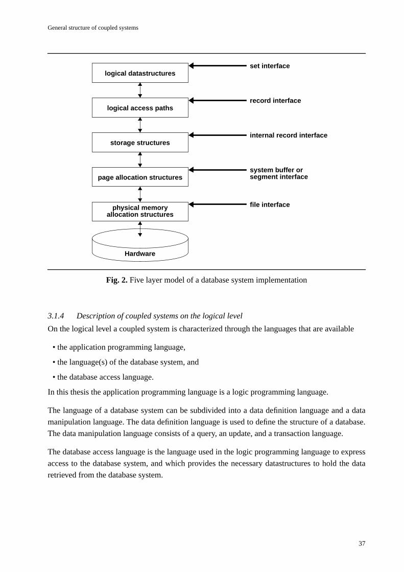
General structure of coupled systems
37
3.1.4 Description of coupled systems on the logical level
On the logical level a coupled system is characterized through the languages that are available
• the application programming language,
• the language(s) of the database system, and
• the database access language.
In this thesis the application programming language is a logic programming language.
The language of a database system can be subdivided into a data definition language and a data
manipulation language. The data definition language is used to define the structure of a database.
The data manipulation language consists of a query, an update, and a transaction language.
The database access language is the language used in the logic programming language to express
access to the database system, and which provides the necessary datastructures to hold the data
retrieved from the database system.
logical datastructures
logical access paths
storage structures
page allocation structures
physical memoryallocation structures
set interface
record interface
internal record interface
system buffer or
file interface
Hardware
Fig. 2. Five layer model of a database system implementation
segment interface
3. Coupled systems
38
3.1.5 Database access procedure
The general database access procedure is as follows: The logic language system issues a database
access request to the database interface in the logic programming language system. The request is
transmitted through a communication channel to the appropriate interface of the database system.
The database evaluates the database access request and returns the result of the evaluation through
the communication channel to the logic programming language system where it is placed in a
datastructure in the application program.
In coupled systems database access is possible either by a pre-processor or at load-time before the
evaluation, or at runtime during the evaluation of an application program. In standard terminology
the terms static and dynamic are used for access at load time and access at runtime respectively.
With pre-processor database access the application program is scanned for database predicates by
a pre-processor before the evaluation of the program. The relation tables corresponding to the
database predicates are then added to the application program through the assertion of new clauses.
With static database access database goals must be defined at load time already. An access path
for these database goals is then established by the loading mechanism of the logic language system,
and data is retrieved from the database system at runtime.
With dynamic database access the database system is accessed only upon the occurrence of a
database predicate during the evaluation of the logic program. Generally, dynamic database access
is achieved through the translation of database goals to the query language of the database system
at runtime.
3.2 Interface
On either level there exists an interface between the logic programming system and the database
system. This interface is determined by the type of coupling, integration or embedding.
On the physical level a general interface provides the basic functionalities
• communication,
• data conversion,
• database access, and
• coordination of evaluations.
On the logical level the interface is defined by the
• database access language, and the
• mode of database access.
Interface
39
3.2.1 Physical level interface
The communication channel connects the logic programming system to the database system. In
physically tightly coupled systems this communication channel is an internal system bus. In
physically loosely coupled systems the communication channel may be an operating system device
such as a pipe or a stream.
Data conversion translates from one low-level data representation to another. In physically tightly
coupled systems there is in general no need for a data conversion mechanism because the logic
programming component and the database component use the same data. In physically loosely
coupled systems the logic programming language system and the database system each access their
own data, and the exchange of data necessitates data conversion. Generally, the exchange of data
is restricted to such values that can be represented in both systems.
The database access mechanism implements the database access and the data retrieval via the
database interface. For procedural database access via the internal record interface this requires
access to low-level information in the database system dictionary, e.g. internal relation or attribute
names, or the position of attribute values in records. Procedural access via the record interface
requires the creation and use of a database cursor. For non-procedural database access the database
is accessed through queries formulated in the database query language.
The coordination mechanism monitors the flow of control and coordinates the programming
language and the database system evaluations. Two cases can be distinguished: either the
granularity of the logic language evaluation and the retrieval granularity of the database system are
the same, or they are different. In the first case the coordination mechanism simply passes the data
retrieved from the database system on to the logic language system. With different granularities,
relations retrieved from the database system are stored in temporary buffers, pipes, or files from
which they are returned to the logic language a tuple at a time.
3.2.2 Logical level interface
The database access language within the logic programming language is either an extension or a
sublanguage of the logic programming language. In the first case, special constructs are introduced
into database goals for accessing the database, e.g. relational algebra operators, or existing
datastructures are given a new semantics, e.g. atoms which represent a database query. In the
second case, the database access language consists of the logic programming language restricted
in such a way that it is equivalent in expressive power to the database language.
In single relation access only one relation table can be accessed through a database goal, whereas
in view access multiple relation tables can be accessed. With single relation access only the
relational algebra operations selection and projection can be directly evaluated in the database
system. Any other relational operation has to be implemented on top of this single relation access
in the logic programming system. With view access in principle any relational algebra operation
can be directly evaluated in the database system.
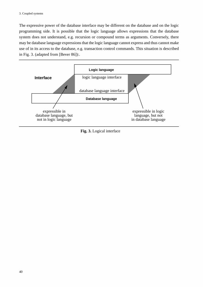
3. Coupled systems
40
The expressive power of the database interface may be different on the database and on the logic
programming side. It is possible that the logic language allows expressions that the database
system does not understand, e.g. recursion or compound terms as arguments. Conversely, there
may be database language expressions that the logic language cannot express and thus cannot make
use of in its access to the database, e.g. transaction control commands. This situation is described
in Fig. 3. (adapted from [Bever 86]):.
expressible in logicexpressible inlanguage, but not
in database languagedatabase language, butnot in logic language
Interface
Database language
Logic language
logic language interface
database language interface
Fig. 3. Logical interface
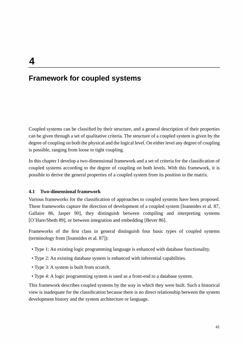
41
4
Framework for coupled systems
Coupled systems can be classified by their structure, and a general description of their properties
can be given through a set of qualitative criteria. The structure of a coupled system is given by the
degree of coupling on both the physical and the logical level. On either level any degree of coupling
is possible, ranging from loose to tight coupling.
In this chapter I develop a two-dimensional framework and a set of criteria for the classification of
coupled systems according to the degree of coupling on both levels. With this framework, it is
possible to derive the general properties of a coupled system from its position in the matrix.
4.1 Two-dimensional framework
Various frameworks for the classification of approaches to coupled systems have been proposed.
These frameworks capture the direction of development of a coupled system [Ioannides et al. 87,
Gallaire 86, Jasper 90], they distinguish between compiling and interpreting systems
[O´Hare/Sheth 89], or between integration and embedding [Bever 86].
Frameworks of the first class in general distinguish four basic types of coupled systems
(terminology from [Ioannides et al. 87]):
• Type 1: An existing logic programming language is enhanced with database functionality.
• Type 2: An existing database system is enhanced with inferential capabilities.
• Type 3: A system is built from scratch.
• Type 4: A logic programming system is used as a front-end to a database system.
This framework describes coupled systems by the way in which they were built. Such a historical
view is inadequate for the classification because there is no direct relationship between the system
development history and the system architecture or language.
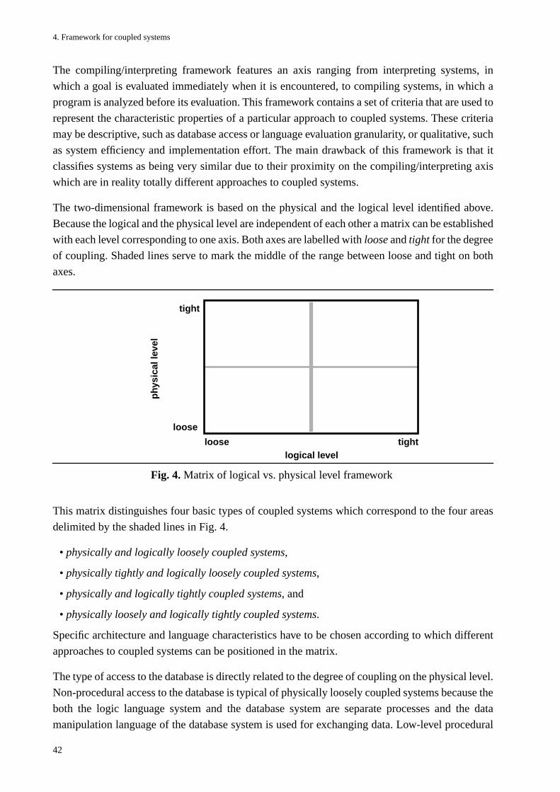
4. Framework for coupled systems
42
The compiling/interpreting framework features an axis ranging from interpreting systems, in
which a goal is evaluated immediately when it is encountered, to compiling systems, in which a
program is analyzed before its evaluation. This framework contains a set of criteria that are used to
represent the characteristic properties of a particular approach to coupled systems. These criteria
may be descriptive, such as database access or language evaluation granularity, or qualitative, such
as system efficiency and implementation effort. The main drawback of this framework is that it
classifies systems as being very similar due to their proximity on the compiling/interpreting axis
which are in reality totally different approaches to coupled systems.
The two-dimensional framework is based on the physical and the logical level identified above.
Because the logical and the physical level are independent of each other a matrix can be established
with each level corresponding to one axis. Both axes are labelled with loose and tight for the degree
of coupling. Shaded lines serve to mark the middle of the range between loose and tight on both
axes.
This matrix distinguishes four basic types of coupled systems which correspond to the four areas
delimited by the shaded lines in Fig. 4.
• physically and logically loosely coupled systems,
• physically tightly and logically loosely coupled systems,
• physically and logically tightly coupled systems, and
• physically loosely and logically tightly coupled systems.
Specific architecture and language characteristics have to be chosen according to which different
approaches to coupled systems can be positioned in the matrix.
The type of access to the database is directly related to the degree of coupling on the physical level.
Non-procedural access to the database is typical of physically loosely coupled systems because the
both the logic language system and the database system are separate processes and the data
manipulation language of the database system is used for exchanging data. Low-level procedural
Fig. 4. Matrix of logical vs. physical level framework
phy
sica
l lev
el
logical level
loose
tight
loose tight
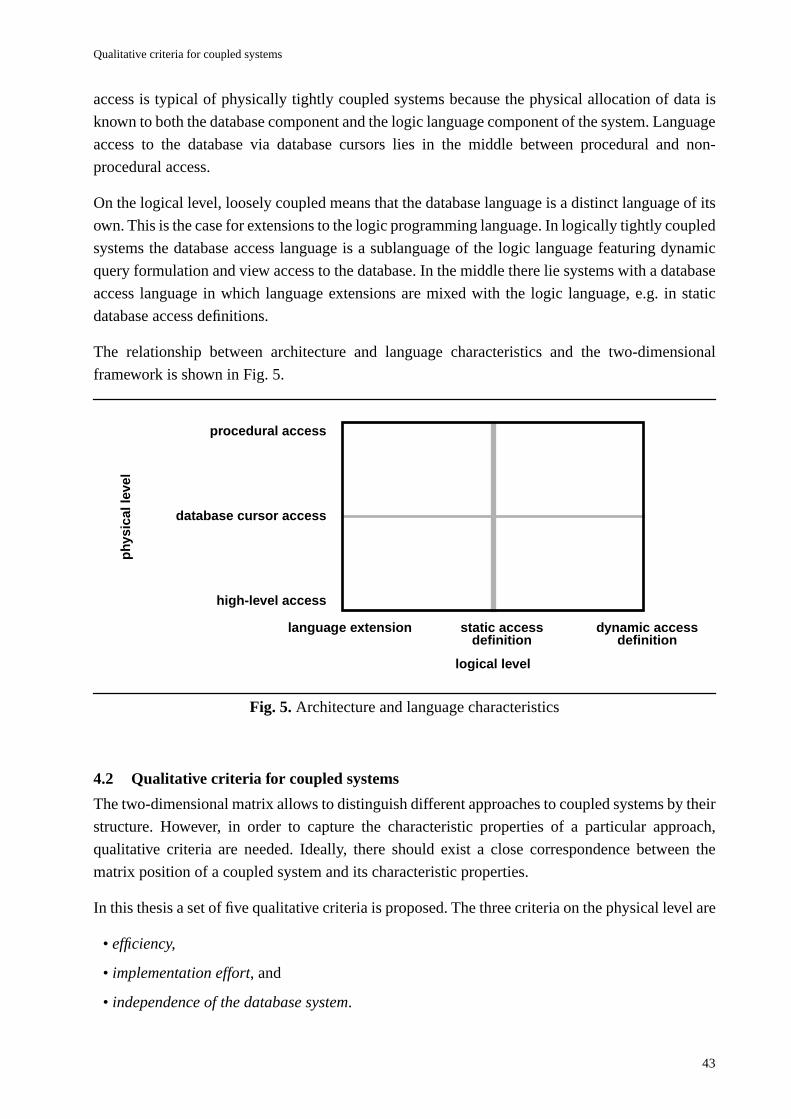
Qualitative criteria for coupled systems
43
access is typical of physically tightly coupled systems because the physical allocation of data is
known to both the database component and the logic language component of the system. Language
access to the database via database cursors lies in the middle between procedural and non-
procedural access.
On the logical level, loosely coupled means that the database language is a distinct language of its
own. This is the case for extensions to the logic programming language. In logically tightly coupled
systems the database access language is a sublanguage of the logic language featuring dynamic
query formulation and view access to the database. In the middle there lie systems with a database
access language in which language extensions are mixed with the logic language, e.g. in static
database access definitions.
The relationship between architecture and language characteristics and the two-dimensional
framework is shown in Fig. 5.
4.2 Qualitative criteria for coupled systems
The two-dimensional matrix allows to distinguish different approaches to coupled systems by their
structure. However, in order to capture the characteristic properties of a particular approach,
qualitative criteria are needed. Ideally, there should exist a close correspondence between the
matrix position of a coupled system and its characteristic properties.
In this thesis a set of five qualitative criteria is proposed. The three criteria on the physical level are
• efficiency,
• implementation effort, and
• independence of the database system.
Fig. 5. Architecture and language characteristics
phy
sica
l lev
el
high-level access
database cursor access
procedural access
language extension static access dynamic access
logical level
definition definition
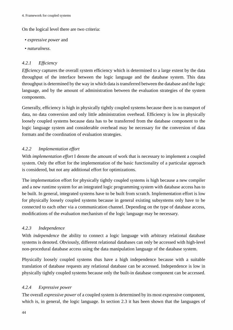
4. Framework for coupled systems
44
On the logical level there are two criteria:
• expressive power and
• naturalness.
4.2.1 Efficiency
Efficiency captures the overall system efficiency which is determined to a large extent by the data
throughput of the interface between the logic language and the database system. This data
throughput is determined by the way in which data is transferred between the database and the logic
language, and by the amount of administration between the evaluation strategies of the system
components.
Generally, efficiency is high in physically tightly coupled systems because there is no transport of
data, no data conversion and only little administration overhead. Efficiency is low in physically
loosely coupled systems because data has to be transferred from the database component to the
logic language system and considerable overhead may be necessary for the conversion of data
formats and the coordination of evaluation strategies.
4.2.2 Implementation effort
With implementation effort I denote the amount of work that is necessary to implement a coupled
system. Only the effort for the implementation of the basic functionality of a particular approach
is considered, but not any additional effort for optimizations.
The implementation effort for physically tightly coupled systems is high because a new compiler
and a new runtime system for an integrated logic programming system with database access has to
be built. In general, integrated systems have to be built from scratch. Implementation effort is low
for physically loosely coupled systems because in general existing subsystems only have to be
connected to each other via a communication channel. Depending on the type of database access,
modifications of the evaluation mechanism of the logic language may be necessary.
4.2.3 Independence
With independence the ability to connect a logic language with arbitrary relational database
systems is denoted. Obviously, different relational databases can only be accessed with high-level
non-procedural database access using the data manipulation language of the database system.
Physically loosely coupled systems thus have a high independence because with a suitable
translation of database requests any relational database can be accessed. Independence is low in
physically tightly coupled systems because only the built-in database component can be accessed.
4.2.4 Expressive power
The overall expressive power of a coupled system is determined by its most expressive component,
which is, in general, the logic language. In section 2.3 it has been shown that the languages of
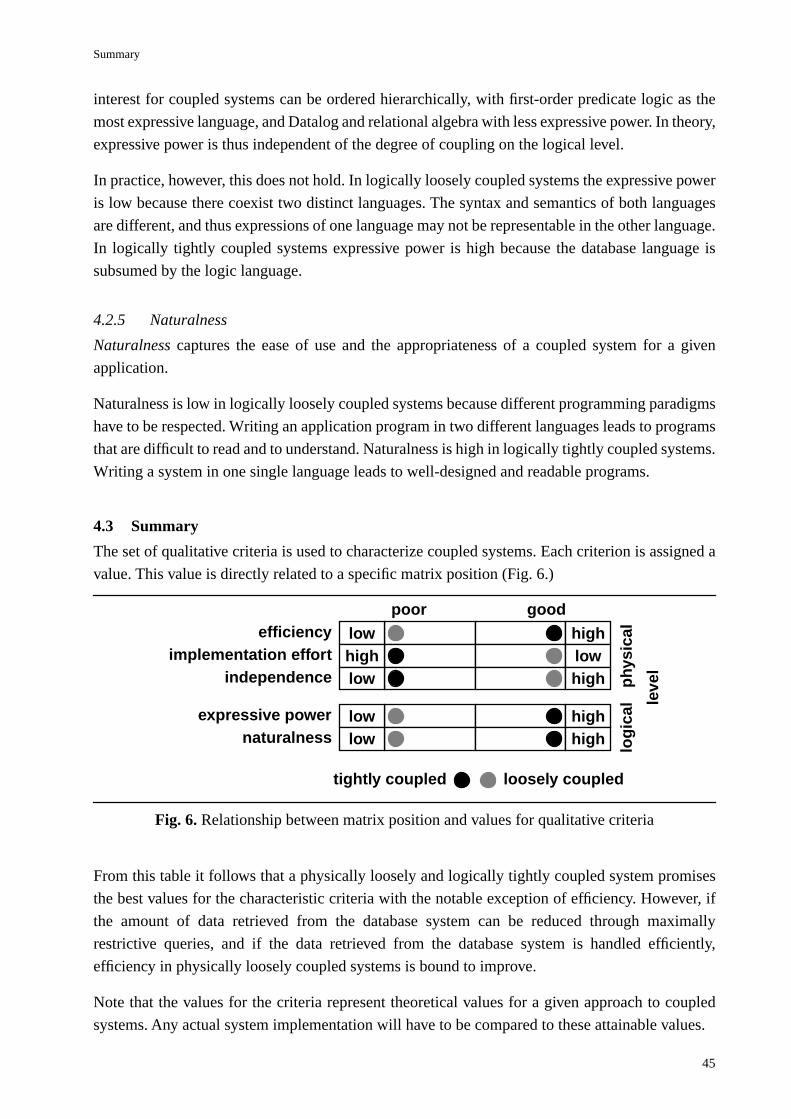
Summary
45
interest for coupled systems can be ordered hierarchically, with first-order predicate logic as the
most expressive language, and Datalog and relational algebra with less expressive power. In theory,
expressive power is thus independent of the degree of coupling on the logical level.
In practice, however, this does not hold. In logically loosely coupled systems the expressive power
is low because there coexist two distinct languages. The syntax and semantics of both languages
are different, and thus expressions of one language may not be representable in the other language.
In logically tightly coupled systems expressive power is high because the database language is
subsumed by the logic language.
4.2.5 Naturalness
Naturalness captures the ease of use and the appropriateness of a coupled system for a given
application.
Naturalness is low in logically loosely coupled systems because different programming paradigms
have to be respected. Writing an application program in two different languages leads to programs
that are difficult to read and to understand. Naturalness is high in logically tightly coupled systems.
Writing a system in one single language leads to well-designed and readable programs.
4.3 Summary
The set of qualitative criteria is used to characterize coupled systems. Each criterion is assigned a
value. This value is directly related to a specific matrix position (Fig. 6.)
From this table it follows that a physically loosely and logically tightly coupled system promises
the best values for the characteristic criteria with the notable exception of efficiency. However, if
the amount of data retrieved from the database system can be reduced through maximally
restrictive queries, and if the data retrieved from the database system is handled efficiently,
efficiency in physically loosely coupled systems is bound to improve.
Note that the values for the criteria represent theoretical values for a given approach to coupled
systems. Any actual system implementation will have to be compared to these attainable values.
efficiency low highimplementation effort high low
independence low high
expressive power low highnaturalness low high
tightly coupled loosely coupled
phy
sica
llo
gic
al
leve
l
Fig. 6. Relationship between matrix position and values for qualitative criteria
poor good

46
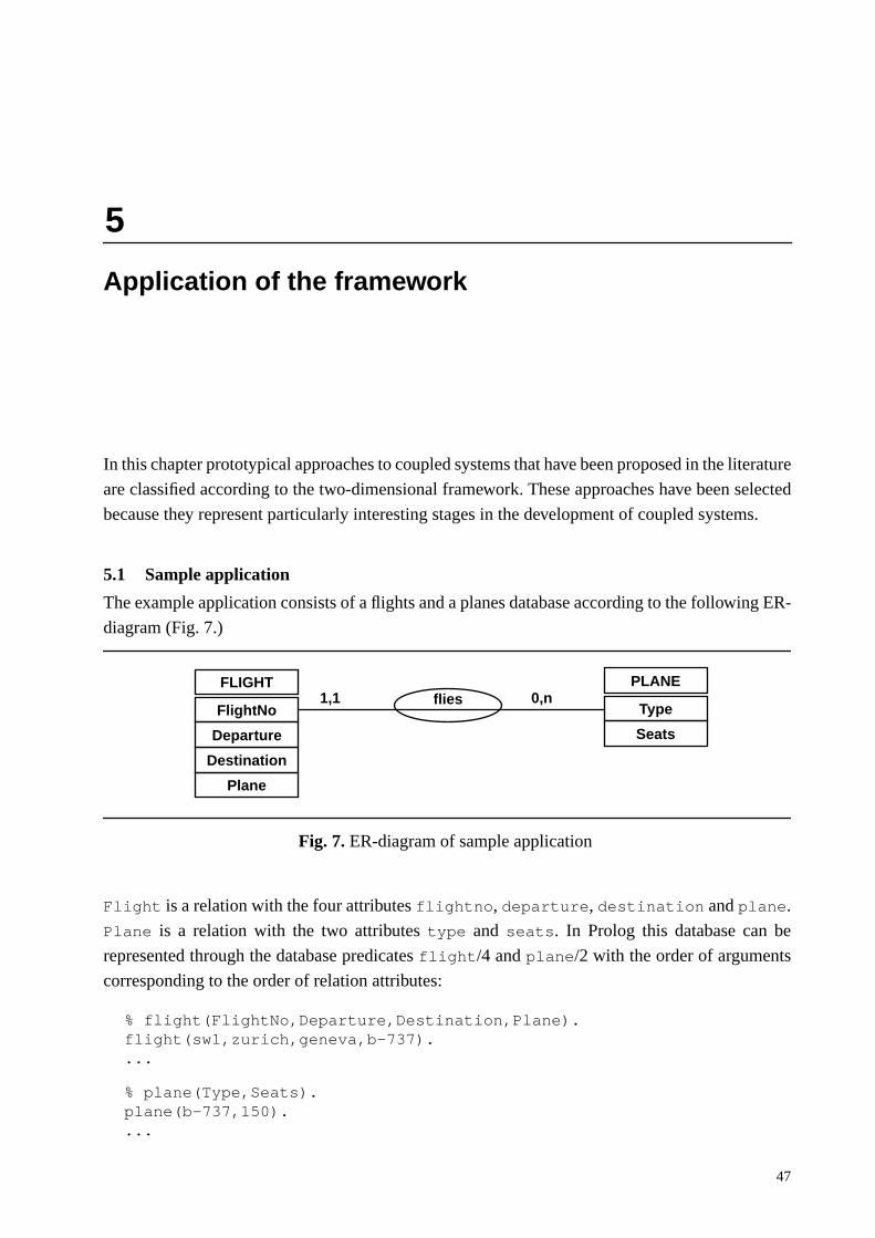
47
5
Application of the framework
In this chapter prototypical approaches to coupled systems that have been proposed in the literature
are classified according to the two-dimensional framework. These approaches have been selected
because they represent particularly interesting stages in the development of coupled systems.
5.1 Sample application
The example application consists of a flights and a planes database according to the following ER-
diagram (Fig. 7.)
Flight is a relation with the four attributes flightno, departure, destination and plane.
Plane is a relation with the two attributes type and seats. In Prolog this database can be
represented through the database predicates flight/4 and plane/2 with the order of arguments
corresponding to the order of relation attributes:
% flight(FlightNo,Departure,Destination,Plane). flight(sw1,zurich,geneva,b-737)....
% plane(Type,Seats).plane(b-737,150)....
FLIGHT PLANE
FlightNo
Departure
Destination
Type
Plane
Seats
flies 0,n1,1
Fig. 7. ER-diagram of sample application
5. Application of the framework
48
5.2 PROSQL
PROSQL [Chang/Walker 86] connects a Prolog system with an SQL relational database system.
Database predicates have the reserved predicate name sql/1. The only argument to an sql/1
clause is an atomic value that represents an SQL command.
In PROSQL database access is static, and database predicates must precede any predicates that
operate on the data retrieved from the database:
?- sql(’ SELECT FLIGHTNO, DEPARTURE, DESTINATION, PLANE FROM FLIGHT’) flight(FNo, Departure, Destination, Plane).
When a database predicate is encountered the atom is transmitted to the database where it is
interpreted as a query. The current Prolog evaluation is suspended until the result of the operation
is returned. Any result relation is asserted into the Prolog workspace as a predicate under the name
of the first relation in the from-part of a query. Only then any data retrieved from the database can
be accessed by subsequent Prolog predicates.
PROSQL is a physically and logically loosely coupled system because Prolog and the SQL
database system are separate processes that communicate with each other, and because two
different languages are present in the system.
5.3 Quintus Prolog
Quintus offers a database interface for different database systems such as Unify or Oracle
[Quintus]. Note that although I present only Quintus Prolog here most other commercial Prolog
implementations offer a database interface similar to the approach of Quintus Prolog.
The database access of Quintus Prolog is both static view and static single relation access. Update
access is allowed through reserved predicates.
Single relation access is defined through the predicate db/3. The third argument of db/3 defines a
mapping from a Prolog term to a relation table. A db/3 fact must precede any access to an external
database:
db(flight,example,flight(’FLIGHTNO’:string,’DEPARTURE’:string,’DESTINATION’:string,’TYPE’:string)).
The actual database access follows Prolog syntax and operational semantics. The goal
?- flight(FlightNo, Departure, Destination, Plane)
is a legal database goal.
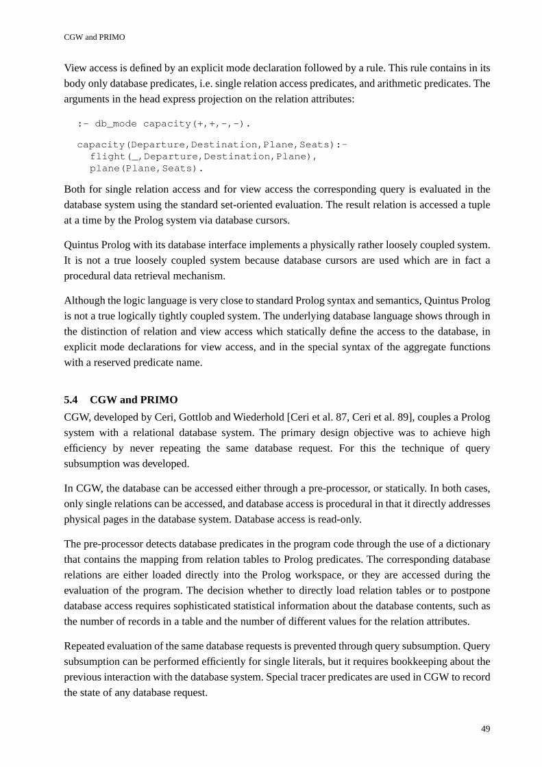
CGW and PRIMO
49
View access is defined by an explicit mode declaration followed by a rule. This rule contains in its
body only database predicates, i.e. single relation access predicates, and arithmetic predicates. The
arguments in the head express projection on the relation attributes:
:- db_mode capacity(+,+,-,-).
capacity(Departure,Destination,Plane,Seats):-flight(_,Departure,Destination,Plane),plane(Plane,Seats).
Both for single relation access and for view access the corresponding query is evaluated in the
database system using the standard set-oriented evaluation. The result relation is accessed a tuple
at a time by the Prolog system via database cursors.
Quintus Prolog with its database interface implements a physically rather loosely coupled system.
It is not a true loosely coupled system because database cursors are used which are in fact a
procedural data retrieval mechanism.
Although the logic language is very close to standard Prolog syntax and semantics, Quintus Prolog
is not a true logically tightly coupled system. The underlying database language shows through in
the distinction of relation and view access which statically define the access to the database, in
explicit mode declarations for view access, and in the special syntax of the aggregate functions
with a reserved predicate name.
5.4 CGW and PRIMO
CGW, developed by Ceri, Gottlob and Wiederhold [Ceri et al. 87, Ceri et al. 89], couples a Prolog
system with a relational database system. The primary design objective was to achieve high
efficiency by never repeating the same database request. For this the technique of query
subsumption was developed.
In CGW, the database can be accessed either through a pre-processor, or statically. In both cases,
only single relations can be accessed, and database access is procedural in that it directly addresses
physical pages in the database system. Database access is read-only.
The pre-processor detects database predicates in the program code through the use of a dictionary
that contains the mapping from relation tables to Prolog predicates. The corresponding database
relations are either loaded directly into the Prolog workspace, or they are accessed during the
evaluation of the program. The decision whether to directly load relation tables or to postpone
database access requires sophisticated statistical information about the database contents, such as
the number of records in a table and the number of different values for the relation attributes.
Repeated evaluation of the same database requests is prevented through query subsumption. Query
subsumption can be performed efficiently for single literals, but it requires bookkeeping about the
previous interaction with the database system. Special tracer predicates are used in CGW to record
the state of any database request.

5. Application of the framework
50
Before actually accessing the external database, this tracer predicate is checked to find out whether
the current database request — or a more general one — has already been answered. If so, a fact
queried(database_predicate).
exists in the workspace, and the corresponding relation is already stored in the workspace where it
can be accessed by the Prolog system. If the current database request has not yet been fully
evaluated a tracer fact contains the address of the last page that has been read in:
tracer(database_predicate,current_db_page).
The request is evaluated in the database system and the results of the evaluation are asserted into
the Prolog workspace. A new tracer fact with the address of the most recently fetched database page
is asserted into the workspace.
Query subsumption implies that part of the extension of a predicate is already in the workspace,
and that further clauses are added during the evaluation. These clauses must be accessible
immediately for the evaluation to be correct. However, this violates the logical update principle
[Lindholm/O’Keefe 87] which states that a predicate may not be modified while it is being
accessed to prevent unpredictable program behavior.
Because of its low-level procedural access to the database, CGW is a physically rather tightly
coupled system. It is not a true logically tightly coupled system because tracer predicates are
visible and because database access is defined statically.
PRIMO [Gozzi et al. 90] is a successor system to CGW. Its main design objective has been to
provide a portable Prolog - database coupling through modules. PRIMO connects any Prolog
system with any SQL database system provided that the Prolog system has an interface to the
operating system. Query subsumption is retained from CGW, and access to a maximum of two
relations for join-operations is included.
PRIMO is a physically loosely coupled system because database access is non-procedural using
the SQL query language. However, it is not a true logically tightly coupled system because the
reserved predicate name retrieve must be used for database access, because tracer predicates are
visible, and because database access is defined statically.
5.5 KB-Prolog
KB-Prolog [Bocca et al. 89 a] integrates a Prolog system with the grid-file database system BANG
[Freeston 88]. In KB-Prolog, relations are considered to be primitive datastructures.
Database access in KB-Prolog is static, and database updates are allowed. Two different database
access methods exist, relational algebra and a retrieval predicate with the reserved name
retr_tup/2.
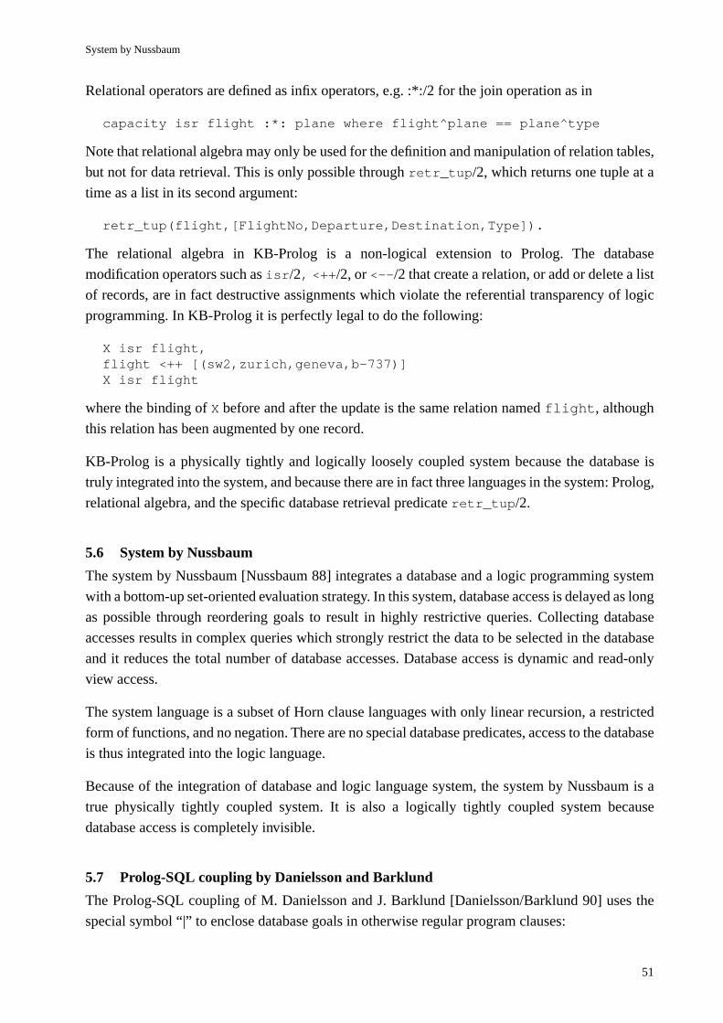
System by Nussbaum
51
Relational operators are defined as infix operators, e.g. :*:/2 for the join operation as in
capacity isr flight :*: plane where flight^plane == plane^type
Note that relational algebra may only be used for the definition and manipulation of relation tables,
but not for data retrieval. This is only possible through retr_tup/2, which returns one tuple at a
time as a list in its second argument:
retr_tup(flight,[FlightNo,Departure,Destination,Type]).
The relational algebra in KB-Prolog is a non-logical extension to Prolog. The database
modification operators such as isr/2, <++/2, or <--/2 that create a relation, or add or delete a list
of records, are in fact destructive assignments which violate the referential transparency of logic
programming. In KB-Prolog it is perfectly legal to do the following:
X isr flight,flight <++ [(sw2,zurich,geneva,b-737)]X isr flight
where the binding of X before and after the update is the same relation named flight, although
this relation has been augmented by one record.
KB-Prolog is a physically tightly and logically loosely coupled system because the database is
truly integrated into the system, and because there are in fact three languages in the system: Prolog,
relational algebra, and the specific database retrieval predicate retr_tup/2.
5.6 System by Nussbaum
The system by Nussbaum [Nussbaum 88] integrates a database and a logic programming system
with a bottom-up set-oriented evaluation strategy. In this system, database access is delayed as long
as possible through reordering goals to result in highly restrictive queries. Collecting database
accesses results in complex queries which strongly restrict the data to be selected in the database
and it reduces the total number of database accesses. Database access is dynamic and read-only
view access.
The system language is a subset of Horn clause languages with only linear recursion, a restricted
form of functions, and no negation. There are no special database predicates, access to the database
is thus integrated into the logic language.
Because of the integration of database and logic language system, the system by Nussbaum is a
true physically tightly coupled system. It is also a logically tightly coupled system because
database access is completely invisible.
5.7 Prolog-SQL coupling by Danielsson and Barklund
The Prolog-SQL coupling of M. Danielsson and J. Barklund [Danielsson/Barklund 90] uses the
special symbol “|” to enclose database goals in otherwise regular program clauses:
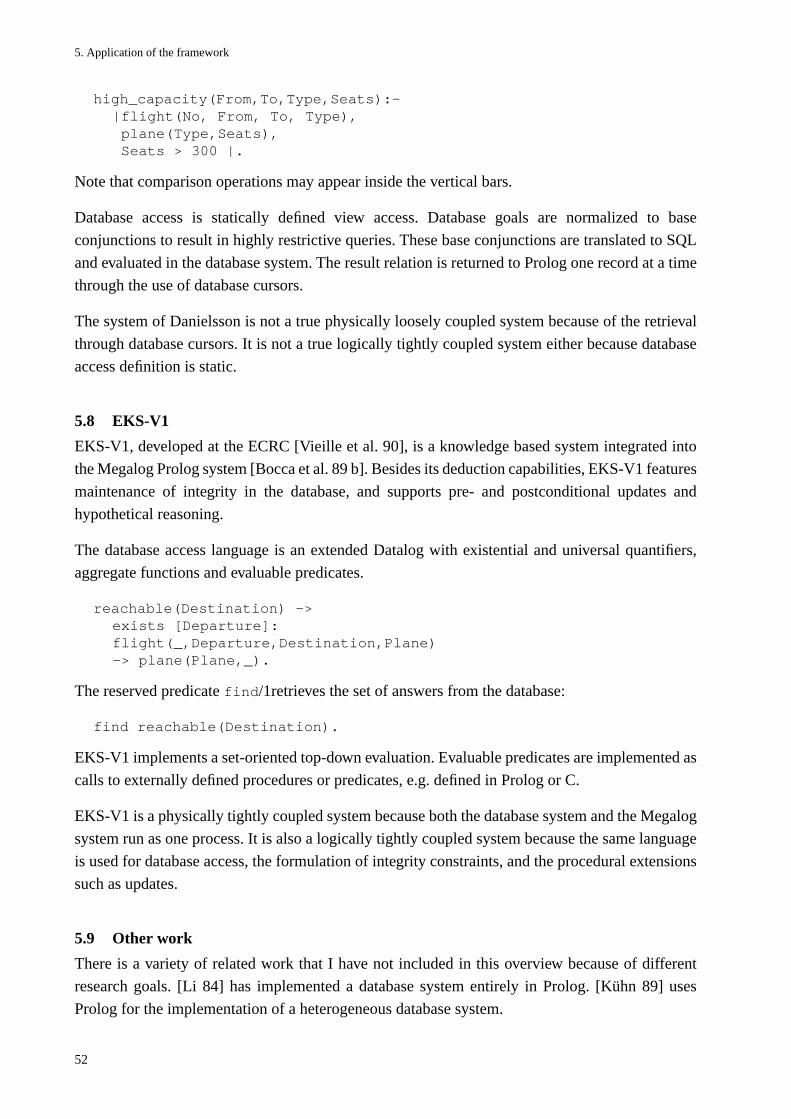
5. Application of the framework
52
high_capacity(From,To,Type,Seats):-|flight(No, From, To, Type), plane(Type,Seats), Seats > 300 |.
Note that comparison operations may appear inside the vertical bars.
Database access is statically defined view access. Database goals are normalized to base
conjunctions to result in highly restrictive queries. These base conjunctions are translated to SQL
and evaluated in the database system. The result relation is returned to Prolog one record at a time
through the use of database cursors.
The system of Danielsson is not a true physically loosely coupled system because of the retrieval
through database cursors. It is not a true logically tightly coupled system either because database
access definition is static.
5.8 EKS-V1
EKS-V1, developed at the ECRC [Vieille et al. 90], is a knowledge based system integrated into
the Megalog Prolog system [Bocca et al. 89 b]. Besides its deduction capabilities, EKS-V1 features
maintenance of integrity in the database, and supports pre- and postconditional updates and
hypothetical reasoning.
The database access language is an extended Datalog with existential and universal quantifiers,
aggregate functions and evaluable predicates.
reachable(Destination) ->exists [Departure]:flight(_,Departure,Destination,Plane)-> plane(Plane,_).
The reserved predicate find/1retrieves the set of answers from the database:
find reachable(Destination).
EKS-V1 implements a set-oriented top-down evaluation. Evaluable predicates are implemented as
calls to externally defined procedures or predicates, e.g. defined in Prolog or C.
EKS-V1 is a physically tightly coupled system because both the database system and the Megalog
system run as one process. It is also a logically tightly coupled system because the same language
is used for database access, the formulation of integrity constraints, and the procedural extensions
such as updates.
5.9 Other work
There is a variety of related work that I have not included in this overview because of different
research goals. [Li 84] has implemented a database system entirely in Prolog. [Kühn 89] uses
Prolog for the implementation of a heterogeneous database system.
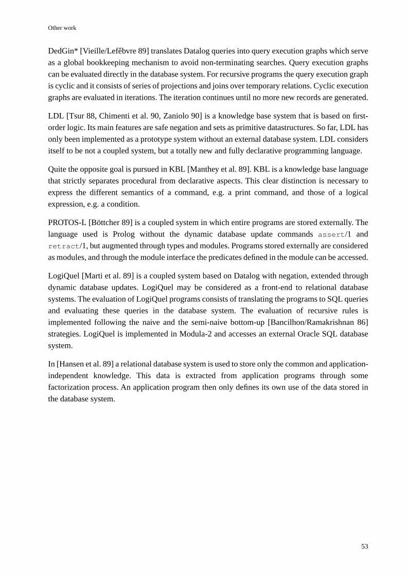
Other work
53
DedGin* [Vieille/Lefêbvre 89] translates Datalog queries into query execution graphs which serve
as a global bookkeeping mechanism to avoid non-terminating searches. Query execution graphs
can be evaluated directly in the database system. For recursive programs the query execution graph
is cyclic and it consists of series of projections and joins over temporary relations. Cyclic execution
graphs are evaluated in iterations. The iteration continues until no more new records are generated.
LDL [Tsur 88, Chimenti et al. 90, Zaniolo 90] is a knowledge base system that is based on first-
order logic. Its main features are safe negation and sets as primitive datastructures. So far, LDL has
only been implemented as a prototype system without an external database system. LDL considers
itself to be not a coupled system, but a totally new and fully declarative programming language.
Quite the opposite goal is pursued in KBL [Manthey et al. 89]. KBL is a knowledge base language
that strictly separates procedural from declarative aspects. This clear distinction is necessary to
express the different semantics of a command, e.g. a print command, and those of a logical
expression, e.g. a condition.
PROTOS-L [Böttcher 89] is a coupled system in which entire programs are stored externally. The
language used is Prolog without the dynamic database update commands assert/1 and
retract/1, but augmented through types and modules. Programs stored externally are considered
as modules, and through the module interface the predicates defined in the module can be accessed.
LogiQuel [Marti et al. 89] is a coupled system based on Datalog with negation, extended through
dynamic database updates. LogiQuel may be considered as a front-end to relational database
systems. The evaluation of LogiQuel programs consists of translating the programs to SQL queries
and evaluating these queries in the database system. The evaluation of recursive rules is
implemented following the naive and the semi-naive bottom-up [Bancilhon/Ramakrishnan 86]
strategies. LogiQuel is implemented in Modula-2 and accesses an external Oracle SQL database
system.
In [Hansen et al. 89] a relational database system is used to store only the common and application-
independent knowledge. This data is extracted from application programs through some
factorization process. An application program then only defines its own use of the data stored in
the database system.
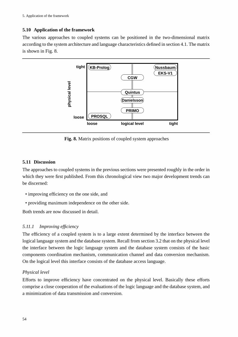
5. Application of the framework
54
5.10 Application of the framework
The various approaches to coupled systems can be positioned in the two-dimensional matrix
according to the system architecture and language characteristics defined in section 4.1. The matrix
is shown in Fig. 8.
5.11 Discussion
The approaches to coupled systems in the previous sections were presented roughly in the order in
which they were first published. From this chronological view two major development trends can
be discerned:
• improving efficiency on the one side, and
• providing maximum independence on the other side.
Both trends are now discussed in detail.
5.11.1 Improving efficiency
The efficiency of a coupled system is to a large extent determined by the interface between the
logical language system and the database system. Recall from section 3.2 that on the physical level
the interface between the logic language system and the database system consists of the basic
components coordination mechanism, communication channel and data conversion mechanism.
On the logical level this interface consists of the database access language.
Physical level
Efforts to improve efficiency have concentrated on the physical level. Basically these efforts
comprise a close cooperation of the evaluations of the logic language and the database system, and
a minimization of data transmission and conversion.
Fig. 8. Matrix positions of coupled system approaches
phy
sica
l lev
el
logical level
loose
tight
loose tight
KB-Prolog
PROSQLPRIMO
Nussbaum
CGW
Quintus
Danielsson
EKS-V1
Discussion
55
Coordination of evaluation strategies
A coordination of evaluation strategies can be achieved in two ways: either through an explicit
coordination mechanism in the interface, or by changing the evaluation strategy in one system
component to match that of the other.
The development of techniques for the coordination of evaluations has been the following: from
• asserting relations into main memory workspace to
• temporarily storing relations in buffers, to
• using procedural database access, and finally to a
• full integration with a uniform evaluation strategy.
Asserting relations into main memory workspace
Asserting the extension of database predicates into the logic language workspace, also known as
cacheing of data, effectively hides the database evaluation from the logic language system. The
database evaluation returns a relation which is asserted as a sequence of program clauses into the
workspace of the logic language. The evaluation of the logic language does not distinguish between
such asserted clauses and other program clauses. Asserting result relations into the workspace is
implemented in PROSQL, CGW and PRIMO.
Asserting relations in the internal workspace of the logic language is an extremely time and space
consuming operation because clause indexes have to be updated and each clause has to be stored
explicitly. A second problem is that assertions are not undone upon backtracking. Once memory is
allocated it cannot be released automatically which almost inevitably leads to workspace overflow.
Buffering result relations
Buffers are operating system devices that temporarily store result relations. The rationale behind
using buffers is that the database writes a whole result relation into the buffer at once, whereas the
logic language system retrieves only one tuple at a time from the buffer. This approach is
implemented in Educe [Bocca 86], which uses pipes as buffers, and in BERMUDA [Ioannides et
al. 87], where temporary files are used.
The major problem of buffers is that their size and number is limited. If a buffer is too small to hold
a relation, then either data is lost, or the database evaluation has to be suspended until the buffer
has been emptied which causes administration overhead. If buffers are too big, valuable system
resources are wasted. With only one buffer, subsequent database requests may overwrite the current
buffer contents. Upon backtracking, the previous buffer contents cannot be restored and must be
recalculated. Associating a proprietary buffer to each individual database request would in
principle solve this problem. However, the number of buffers is always finite, and the number of
database requests may exceed the number of buffers. This is especially true in recursive
evaluations, where the number of recursion steps is not known in advance.
5. Application of the framework
56
Procedural database access
Procedural access to the database system can be subdivided into low-level access via the internal
record interface or even the segment interface, and access through database cursors via the record
interface.
Direct access to relations via the segment interface has been implemented in CGW. Direct access
returns to the logic language systems one physical page at a time, from which the requested records
have to be extracted. This reduces the retrieval granularity from whole relations to physical pages
which contain only a few records and only small amounts of data must thus be stored temporarily.
The major problems of direct access are that the precision of retrieval is low because the position
of a record on a particular page is independent of its attribute values, and that only single relations
can be accessed.
Database cursors are retrieval mechanisms which are provided by relational database systems for
high-level procedural programming languages. A database cursor provides a single-record
interface for the retrieval of data from the database system.
In Quintus Prolog and the Prolog-SQL coupling by Danielsson each invocation of a database
predicate is assigned a database cursor. The query corresponding to the body of the predicate is
evaluated in the database system at the first call to the predicate. The current values of the cursor
are returned via the argument variables of the database predicate. New values are fetched from the
database upon backtracking, and the predicate fails when the cursor has reached the end of the
result relation.
The major advantages of database cursors are that they are provided and supported by the database
system, and that the granularity of data retrieval matches the granularity of the logic language
evaluation. The main problem with cursors is that only a finite number is available in the database
system which leads to similar problems as with using buffers. A second problem is that for the logic
language evaluation mechanism the treatment of database cursors differs from that of internal
pointers. The runtime system of the logic language thus has to be modified to incorporate database
cursors.
Full integration
The previous techniques are employed when there are separate evaluations in both the logic
language system and the database system. However, coupled systems are possible in which there
exists a uniform evaluation. In such a system, database and logic language are simply
subcomponents of a physically tightly coupled, or integrated, system. The evaluation in a
physically tightly coupled system may either be tuple-oriented as in KB-Prolog, or set-oriented as
in the system by Nussbaum or EKS-V1.
A uniform evaluation in a coupled system does not cause any coordination overhead and it is thus
bound to be efficient. However, the implementation effort for a uniform evaluation is extremely
high. Furthermore, a uniform evaluation strategy may directly affect the expressive power of a
Discussion
57
coupled system. Currently only systems with languages of restricted expressive power, e.g. the
system by Nussbaum, which is restricted to linear recursive languages without negation, or
DedGin*, which is restricted to Datalog, have been implemented with a set-oriented evaluation
strategy.
Communication channel
The effects of the type of communication channel that exists between the logic language system
and the database system on the efficiency should be clear. The efficiency of the communication
channel is determined by the transmission speed of the channel, and by the amount of data
transferred through the channel.
The communication channel in coupled systems has evolved from an external slow channel
between two distinct systems to a quick internal bus in physically tightly coupled systems.
Efficiency can be increased by reducing the amount of data to be transferred. In PROSQL, whole
relations are transferred. In Educe and MU-Prolog [Naish 87] the communication channel also
serves as a buffer. In CGW only a few physical pages, and in Quintus Prolog only a few records
need to be transferred in the best case. However, with a more sophisticated coordination of
evaluations the ratio of control information versus actual data deteriorates.
Data conversion
In physically loosely coupled systems data conversion is always only necessary because different
data formats are used in both the logic language and the database system. Data conversion is
expensive, and it is thus desirable to have as little conversion as necessary. The data conversion
mechanism is thus best situated only on one end of the communication channel, either in the logic
programming language system or the database system. In the systems presented above, the data
conversion component can be found on the logic language system side.
In physically tightly coupled systems there is in general no need for a data conversion mechanism
because the same data is accessed by the database and the logic language component.
Logical level
The interface on the logical level also has a great effect on the efficiency of the coupled system as
a whole. Two main contributions to improving efficiency can be discerned,
• query restriction, and
• language integration.
Query restriction
Query restriction depends on the database access language and the dynamic aspects of database
access definition. In PROSQL queries are part of the program code. Because SQL statements are
included as atomic constants in the application program queries cannot be restricted dynamically.
A next step is to propagate variable bindings and constant values to the database system. This
propagation of variable bindings is currently supported in most coupled systems, either with single
relation or with view access.
5. Application of the framework
58
Single relation access in general is not powerful enough to effectively restrict queries. In the
following example with employee/2 as database predicate
retrieve(Person):-employee(Person,Salary),Salary < 100.000.
all records are retrieved, although only a few database records satisfy the comparison. In Educe
conditions are allowed as extra arguments to database goals to restrict queries.
With view access, the amount of data to be retrieved can effectively be reduced through relational
operations such as difference, intersection or through exploiting join-selectivity. Furthermore it is
possible to express selection conditions through comparison operations as in the example above.
Finally, with dynamic access definition, maximally restrictive queries are possible because not only
the current variable bindings, but also additional information from the current state of the
evaluation can be used. Currently, dynamic access definition has only been implemented in
physically tightly coupled systems with delayed evaluation such as the systems of
[Cuppens/Demolombe 86] or [Nussbaum 88].
Language integration
Language integration also contributes to efficiency. In logically loosely coupled systems, as in
PROSQL or KB-Prolog, data manipulated by the database language is not directly accessible to the
logic language system. In PROSQL, SQL commands are considered to be atomic constants by the
Prolog system, and data has to be asserted into the workspace to be accessible to the application
program. In KB-Prolog, relational algebra is used for the manipulation of relations, but to actually
retrieve data a special predicate must be used. Thus, in both systems a shift between different
language paradigms is necessary which reduces efficiency.
In systems in which database access is a sublanguage of the logic language such problems occur
to a much lesser degree. However, the language restriction to single relation access, as in CGW or
BERMUDA, or to two relations, as in PRIMO, forces the logic language system to perform
evaluations that could have been done more efficiently in the database system, even to recompute
relations. In general, this is true for any static database access definition.
Of the systems presented above, only EKS-V1, Quintus Prolog, and the system by Danielsson
support aggregate functions, the latter two merely in a weaker form because grouping on attributes
cannot be expressed. Only EKS-V1 can express higher-order constructs such as grouping, sorting,
or structured attributes.
5.11.2 Maximum independence
The independence of a coupled system of a particular database system implementation is possible
only through a non-procedural access to the database system. For this, two techniques have been
developed, namely
Discussion
59
• a modular interface to various database systems, or
• the translation of database requests to high-level database query languages.
Modular interface for database access
With a modular interface to the database system, an additional layer is inserted between the logic
language system and the database system. This layer is implemented through an access module to
the database system. With specific modules different database systems can be accessed. The actual
access to a database system is then implemented in the corresponding module. This technique is
employed in PRIMO, a variation of it is used in commercial Prolog systems.
The major problem of a modular interface is that this interface lies underneath the logic
programming language. The implementation of a database access module thus requires knowledge
about low-level implementation details of the logic language system. Furthermore, the interface
module is in general implemented in a different language which requires further language
interfaces.
Translation of database requests
The second technique translates directly from the logic language to a high-level database query
language without an intermediate interface. Each time a database predicate is called, the
corresponding goals are translated to a query or a sequence of queries in the database language.
The actual database access is performed through an interface to communication devices in the
operating system, streams, or through calls to externally defined procedures. Translating database
predicates to SQL is done in the Prolog-SQL system by Danielsson.
The advantage of translation is that database queries can be formulated dynamically, and that the
translation procedure itself can be written in the logic language. The major drawback is that a
translation is necessary for every call to a database predicate, which may be rather time-consuming
5.11.3 Summary
From this overview of approaches to coupled systems the following two observations can be made:
• The predominant design objective in coupled systems, once their feasibility had been
demonstrated, was to improve efficiency.
• Only recently, the independence of a coupled system of a particular database system has been
given more weight.
Efficiency has been the primary concern in the development of coupled systems. Any
improvements have been achieved through an ever tighter physical coupling of the logic language
system and the database system. This has lead to physically tightly coupled systems, or, in the
terminology of Bever, to an integration of a database system into the logic programming system.
A first consequence of this development is that with every step in the direction of a tighter physical
coupling the implementation effort grows. A second consequence is that independence is lost
because only the built-in database can be accessed.
5. Application of the framework
60
Independence has been a design goal of its own only since about 1986 with the proliferation of
commercial Prolog implementations and the definition of SQL as the standard database language.
Independence requires that the logic language and the database system be separate systems, and
that a particular implementation of a database system be replaceable by another one. This is only
possible in physically loosely coupled systems. In addition to that physically loosely coupled
systems may exploit the high functionality of current database management systems, such as multi-
user access, and they allow easy access to data already stored in existing databases.
It has been shown that a database access language which is a sublanguage of the logic
programming language contributes to the overall system efficiency because it allows maximal
restriction of queries. It also contributes to achieve maximal independence, because with the
database access language a sublanguage of the logic programming language there is no
predilection for a specific database system. Logically tightly coupled systems thus combine high
efficiency with independence.
Requirements for a new approach
61
5.12 Requirements for a new approach
The development of a new approach to coupled systems is motivated by the following
observations:
• A powerful database access language is necessary to effectively combine the full capacities of
database systems with the high expressive power of logic language systems.
Hence, arithmetic functions, aggregate functions, structured attributes, and the application of
higher-order control such as grouping or sorting must be expressible in the database access
language.
• In current systems, efficiency has primarily been improved through tight physical coupling.
Less effort has been devoted to the logical level although a tight logical coupling would allow
the formulation of maximally restrictive queries and thus contribute to improve the overall
efficiency.
Hence, the database access language is to be a sublanguage of the logic programming
language.
• Today many commercial or public domain databases store large amounts of information
relevant to new applications. These database services are offered on a variety of machines and
they allow access through high-level query languages.
Hence, independence is a crucial requirement.
• Furthermore, it should be possible to access this information from existing systems and
applications.
Hence, the new approach must be implementable and downward compatible with existing
logic programming language systems.
A physically loosely and logically tightly coupled system with the database access language a
sublanguage of the logic language for efficiency, with set-oriented data retrieval to allow the
application of higher-order control, and with non-procedural database access for independence is
thus desirable.

62
63
6
Database Set Predicates
Set predicates are higher-order extensions of programming languages based on first-order
predicate logic. They retain all solutions to a goal as a set (or a bag) of variable instantiations. This
property will be exploited to extend the definition of set predicates to result in database set
predicates.
Database set predicates extend the traditional set predicates with access to external databases. The
basic concept of database set predicates is that the evaluation of the goal to be proved is performed
by the database system, and that the result relation of the database evaluation is captured by a
standard datastructure of the logic language. This way
• the set-oriented evaluation of database systems is embedded into the standard tuple-oriented
evaluation of logic language systems, and
• the logic language itself is used for accessing the external database system.
Although only Prolog set predicates are presented, this discussion is not restricted to Prolog but
applies to set predicates in general and other logic languages based on tuple oriented evaluation.
6.1 Set predicates
Set predicates were originally proposed and implemented by D.H.D. Warren [Warren 82] as
higher-order extensions to Prolog.
With standard SLDNF resolution a solution, i.e. a variable instantiation, is returned as the result of
a successful proof of a goal. The search for further solutions is initiated through forced failure after
a solution has been returned to the top-level goal. However, because any variable bindings are
undone upon failure of a goal, it is not possible to collect all solutions for a given goal without
resorting to extra-logical or control predicates. This problem is overcome through set predicates –
also called all-solutions predicates – which retain all solutions to a goal in a datastructure for
further processing.
6. Database Set Predicates
64
6.1.1 Set predicate definition
Set predicates are of the following form:
set_predicate(Template,Goal,Instantiations)
set_predicate is name of the predicate. In most Prolog implementations, set_predicate is
findall, bagof, and/or setof.
• Template is a term.
• Goal is an arbitrary goal which may include control predicates, system predicates, extra-
logical predicates, etc. Note that this allows set predicates to be nested.
Variables in Goal may be explicitly quantified through the existential quantifier ^/2 which
takes a variable as its first and a goal as its second argument.
• Instantiations is a list of template instances.
Example
In the goal
?- setof(Destination, Plane^flight(Departure,Destination,Plane),Destinations)
Destination is the template term, Plane^flight(Departure,Destination, Plane)is the goal argument with the existentially quantified variable Plane. Destinations is unifiedwith a list that contains all instantiations of the template variable Destination which aresolutions to the goal argument.
♦
6.1.2 Set predicate semantics
Set predicates must be called with the first two arguments partially instantiated terms, and the third
argument an uninstantiated variable or an instantiated list:
set_predicate(+Template, +Goal, ?Instantiations).
If set_predicate is called with the third argument an uninstantiated variable, then this variable
is instantiated with a list of template term instantiations computed by the successful evaluation of
the goal argument. With the third argument instantiated, set_predicate/3 only succeeds if this
argument is unifiable with the list of template instantiations as computed by the evaluation of the
goal argument.
findall/3 on the one side and setof/3 and bagof/3 on the other side differ in their treatment of
• quantification and
• finite failure of goal arguments.
The difference between setof/3 and bagof/3 is that the list of variable instantiations in setof/3
is sorted and does not contain duplicate entries.
Set predicates
65
Quantification
In Horn clause languages, variables in a clause are considered to be universally quantified. Because
the body of a clause consists of negated literals, variables that occur only in the body of a clause
are said to be existentially quantified. The binding of such existentially quantified variables is of
no interest outside of the clause.
In set predicates a variable is free if it is neither bound when the set predicate is called nor does it
occur in the Template. findall/3 considers the free variables in Goal to be existentially
quantified, whereas they are implicitly universally quantified in setof/3 and bagof/3.
Consequently, findall/3 yields only one list of template instantiations, whereas setof/3 and
bagof/3 produce different lists of template instantiations for each binding of the free variables in
Goal. This means that findall/3 is deterministic and fails upon backtracking, whereas setof/3
and bagof/3 attempt to compute the next solution with a different binding of the free variables.
Example
In the example database
flight(zurich, geneva, b-737).flight(zurich, paris, a-320).flight(zurich, london, b-737).
findall/3 produces the following results (forced backtracking through ; after each solution):
?-findall((Departure,Destination), flight(Departure,Destination,Type),List).
List = [(zurich,geneva),(zurich,paris),(zurich,london)];
no more solutions
Contrast this to the result of
?-setof((Departure,Destination), flight(Departure,Destination,Type),List)
Type = a-320, List = [(zurich, paris)];
Type = b-737, List = [(zurich,geneva),(zurich,london)];
no more solutions
The variable Type in the goal argument of the two top-level goals is free. In findall/3 thisleads to only one list being returned, regardless of the binding for Type. With setof/3 eachbinding for Type results in a separate list.
♦
Quantification information can be made explicit in setof/3 and bagof/3.
6. Database Set Predicates
66
Example
With the variable Type existentially quantified setof/3 yields a sorted list that contains thesame entries as computed by findall/3:
?-setof((Departure,Destination), Type^flight(Departure,Destination,Type),List).
List = [(zurich,geneva),(zurich,london),(zurich,paris)];
no more solutions
♦
Finite failure of goal arguments
The result of a set predicate is only defined if the evaluation of its goal argument terminates. If the
goal argument fails finitely, then findall/3 succeeds with an empty list, whereas bagof/3 and
setof/3 fail altogether [Maier/Warren 89, O’Keefe 90].
The reason for this lies in the treatment of the free variables in the goal argument. If bagof/3 or
setof/3 would succeed with an empty list although the goal could not be proved, subsequent goals
would expect the free variables in the goal to be bound. However, because the goal failed, all
variable bindings are undone, and thus no binding of a free variable can be returned.
findall/3 leaves unbound any free variables, and hence subsequent goals always expect a
variable that is free in the goal argument of findall/3 to be unbound.
Declarative semantics
Set predicates have been the source of some controversy because they are a higher-order extension
to first-order languages. It is not possible to give a declarative first-order semantics for findall/3
and bagof/3 since they depend heavily on the control strategy of the logic language evaluation.
Because of this dependency both predicates can be used to define meta-logical predicates which
cannot be defined in pure first-order logic languages, e.g. var/1 or negation as failure [Naish 86].
However, setof/3 can be given a declarative semantics because the result of the predicate is a set,
and the order of set elements is independent of the order in which the individual solutions were
computed [Naish 86]:
setof(Template,Goal,Instantiations)↔ ∀ X(∃ L1,...,Ln(Goal ∧ X = Template)↔ element(X,Instantiations)) ∧ sorted(Instantiations)
with L1,...,Ln variables in Goal which also occur in Template.
In Prolog, the set of solutions is represented as a sorted list without duplicate elements.
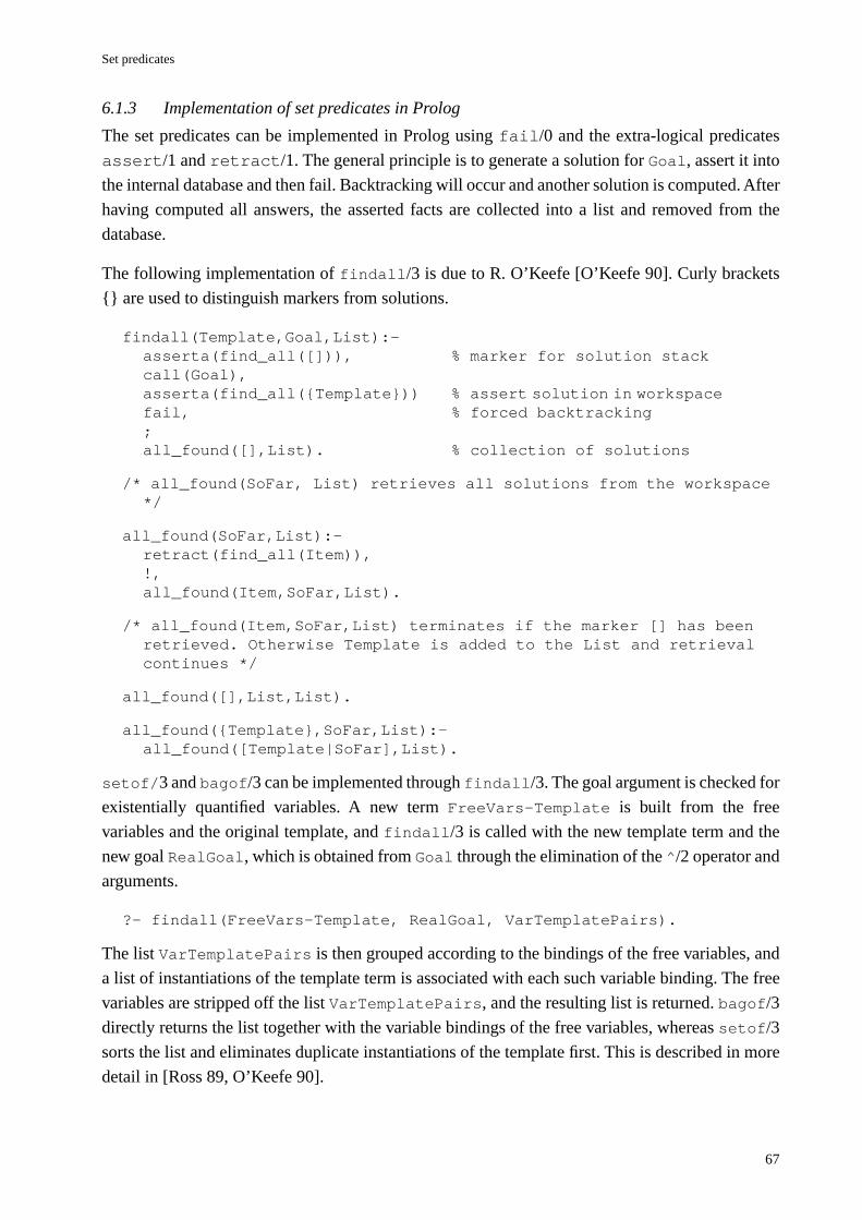
Set predicates
67
6.1.3 Implementation of set predicates in Prolog
The set predicates can be implemented in Prolog using fail/0 and the extra-logical predicates
assert/1 and retract/1. The general principle is to generate a solution for Goal, assert it into
the internal database and then fail. Backtracking will occur and another solution is computed. After
having computed all answers, the asserted facts are collected into a list and removed from the
database.
The following implementation of findall/3 is due to R. O’Keefe [O’Keefe 90]. Curly brackets
{} are used to distinguish markers from solutions.
findall(Template,Goal,List):-asserta(find_all([])), % marker for solution stackcall(Goal),asserta(find_all({Template})) % assert solution in workspacefail, % forced backtracking;all_found([],List). % collection of solutions
/* all_found(SoFar, List) retrieves all solutions from the workspace */
all_found(SoFar,List):-retract(find_all(Item)),!,all_found(Item,SoFar,List).
/* all_found(Item,SoFar,List) terminates if the marker [] has been retrieved. Otherwise Template is added to the List and retrieval continues */
all_found([],List,List).
all_found({Template},SoFar,List):-all_found([Template|SoFar],List).
setof/3 and bagof/3 can be implemented through findall/3. The goal argument is checked for
existentially quantified variables. A new term FreeVars-Template is built from the free
variables and the original template, and findall/3 is called with the new template term and the
new goal RealGoal, which is obtained from Goal through the elimination of the ̂ /2 operator and
arguments.
?- findall(FreeVars-Template, RealGoal, VarTemplatePairs).
The list VarTemplatePairs is then grouped according to the bindings of the free variables, and
a list of instantiations of the template term is associated with each such variable binding. The free
variables are stripped off the list VarTemplatePairs, and the resulting list is returned. bagof/3
directly returns the list together with the variable bindings of the free variables, whereas setof/3
sorts the list and eliminates duplicate instantiations of the template first. This is described in more
detail in [Ross 89, O’Keefe 90].
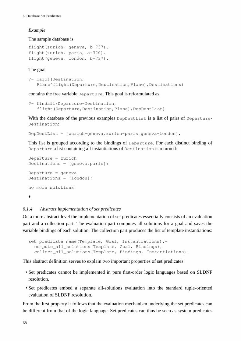
6. Database Set Predicates
68
Example
The sample database is
flight(zurich, geneva, b-737).flight(zurich, paris, a-320).flight(geneva, london, b-737).
The goal
?- bagof(Destination, Plane^flight(Departure,Destination,Plane),Destinations)
contains the free variable Departure. This goal is reformulated as
?- findall(Departure-Destination, flight(Departure,Destination,Plane),DepDestList)
With the database of the previous examples DepDestList is a list of pairs of Departure-Destination:
DepDestList = [zurich-geneva,zurich-paris,geneva-london].
This list is grouped according to the bindings of Departure. For each distinct binding ofDeparture a list containing all instantiations of Destination is returned:
Departure = zurichDestinations = [geneva,paris];
Departure = genevaDestinations = [london];
no more solutions
♦
6.1.4 Abstract implementation of set predicates
On a more abstract level the implementation of set predicates essentially consists of an evaluation
part and a collection part. The evaluation part computes all solutions for a goal and saves the
variable bindings of each solution. The collection part produces the list of template instantiations:
set_predicate_name(Template, Goal, Instantiations):-compute_all_solutions(Template, Goal, Bindings),collect_all_solutions(Template, Bindings, Instantiations).
This abstract definition serves to explain two important properties of set predicates:
• Set predicates cannot be implemented in pure first-order logic languages based on SLDNF
resolution.
• Set predicates embed a separate all-solutions evaluation into the standard tuple-oriented
evaluation of SLDNF resolution.
From the first property it follows that the evaluation mechanism underlying the set predicates can
be different from that of the logic language. Set predicates can thus be seen as system predicates
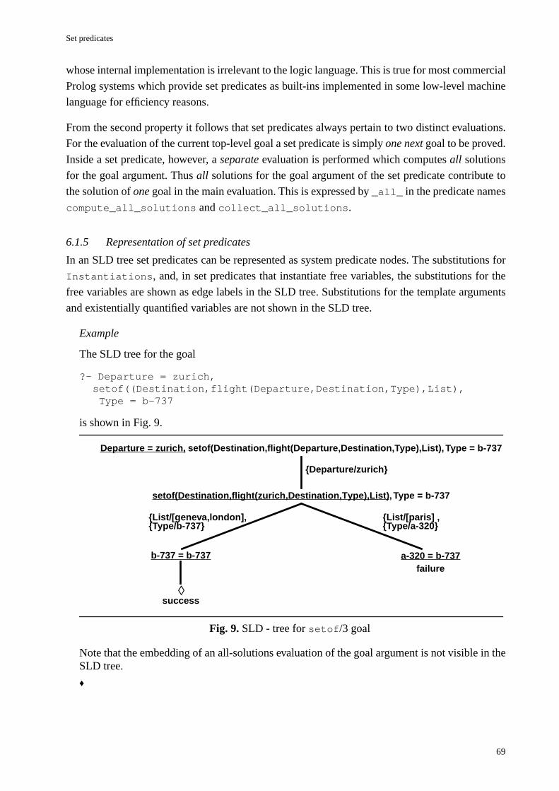
Set predicates
69
whose internal implementation is irrelevant to the logic language. This is true for most commercial
Prolog systems which provide set predicates as built-ins implemented in some low-level machine
language for efficiency reasons.
From the second property it follows that set predicates always pertain to two distinct evaluations.
For the evaluation of the current top-level goal a set predicate is simply one next goal to be proved.
Inside a set predicate, however, a separate evaluation is performed which computes all solutions
for the goal argument. Thus all solutions for the goal argument of the set predicate contribute to
the solution of one goal in the main evaluation. This is expressed by _all_ in the predicate names
compute_all_solutions and collect_all_solutions.
6.1.5 Representation of set predicates
In an SLD tree set predicates can be represented as system predicate nodes. The substitutions for
Instantiations, and, in set predicates that instantiate free variables, the substitutions for the
free variables are shown as edge labels in the SLD tree. Substitutions for the template arguments
and existentially quantified variables are not shown in the SLD tree.
Example
The SLD tree for the goal
?- Departure = zurich,setof((Destination,flight(Departure,Destination,Type),List), Type = b-737
is shown in Fig. 9.
Note that the embedding of an all-solutions evaluation of the goal argument is not visible in theSLD tree.
♦
setof(Destination,flight(zurich,Destination,Type),List), Type = b-737
b-737 = b-737 a-320 = b-737
◊
failure
success
{Type/b-737} {Type/a-320}{List/[geneva,london], {List/[paris] ,
Departure = zurich, setof(Destination,flight(Departure,Destination,Type),List), Type = b-737
{Departure/zurich}
Fig. 9. SLD - tree for setof/3 goal
6. Database Set Predicates
70
6.2 Database set predicates
Database set predicates are an extension of set predicates. Database set predicates access external
database systems for the proof of their goal argument.
6.2.1 Definition
A database set predicate is a predicate of the form
db_set_predicate(ProjectionTerm,DatabaseGoal,ResultRelation).
where
• db_set_predicate is one of db_setof or db_findall.
The prefix “db_” distinguishes database set predicates from the built-in set predicates (see
section 6.3.6 for a discussion of the relationship between set predicates and database set
predicates).
• ProjectionTerm is a term.
• DatabaseGoal is a database goal as defined in section 3.1.
DatabaseGoal is the goal argument of the database set predicate, and it is evaluated in an
external database system.
• ResultRelation is a list.
It contains the result relation of the database evaluation of DatabaseGoal.
The above definition closely follows the definition of Prolog set predicates. However, it is to be
seen as a generic definition only. As such it merely defines the basic arguments and the
relationships that hold between them, the exact syntactical form of database set predicates
depending on the language actually used.
6.2.2 Operational semantics of database set predicates
Like set predicates, database set predicates are called with the first two arguments partially
instantiated terms, and the third argument an uninstantiated variable or an instantiated list.
db_set_predicate(+ProjectionTerm,+DatabaseGoal,?ResultRelation).
The basic operational semantics of database set predicates is that the database goal is evaluated in
the external database system, and not by the logic language system.
The general database access procedure is as follows: when a database set predicate is encountered,
• ProjectionTerm and DatabaseGoal of the database set predicate are translated to the
equivalent query in a non-procedural database language.
• The query is written into the communication channel that connects the logic language system
with the database system.
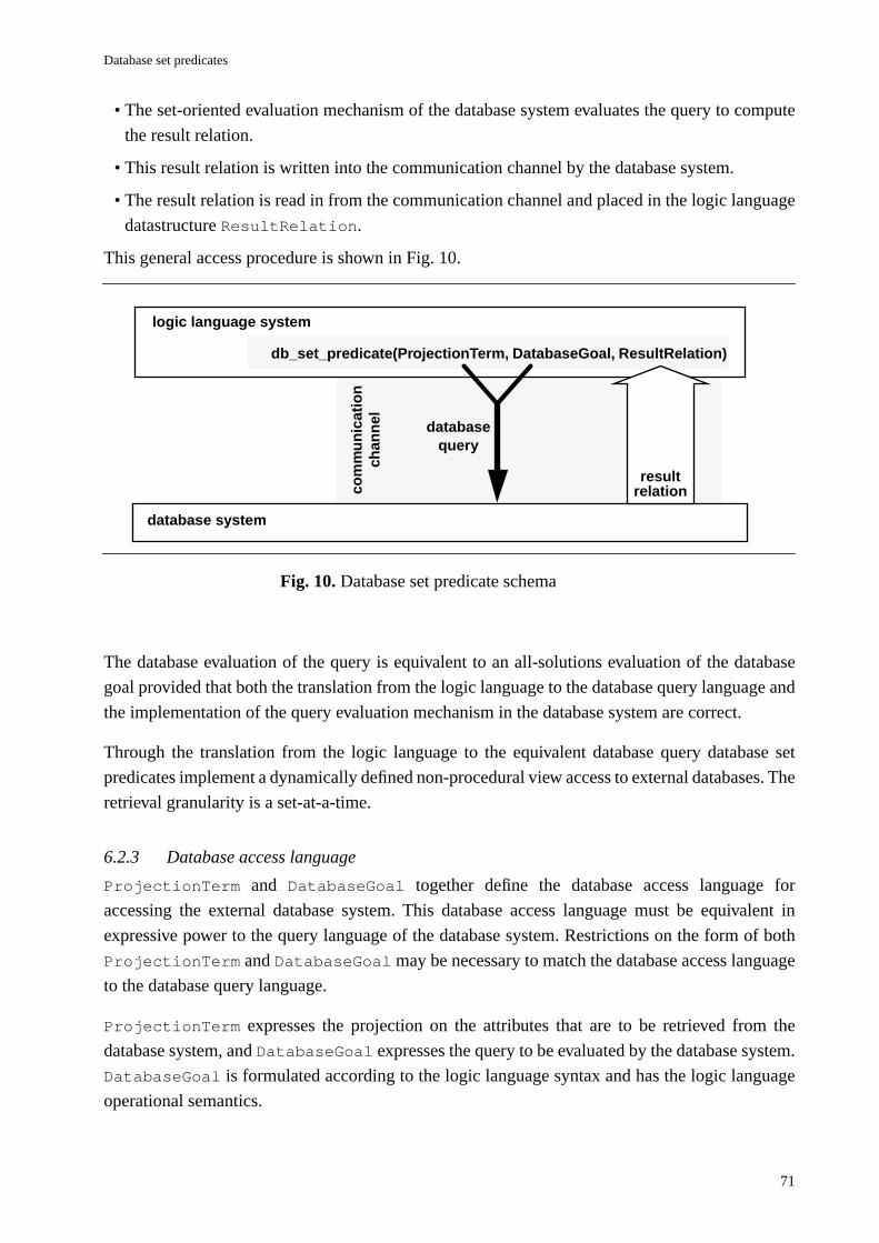
Database set predicates
71
• The set-oriented evaluation mechanism of the database system evaluates the query to compute
the result relation.
• This result relation is written into the communication channel by the database system.
• The result relation is read in from the communication channel and placed in the logic language
datastructure ResultRelation.
This general access procedure is shown in Fig. 10.
The database evaluation of the query is equivalent to an all-solutions evaluation of the database
goal provided that both the translation from the logic language to the database query language and
the implementation of the query evaluation mechanism in the database system are correct.
Through the translation from the logic language to the equivalent database query database set
predicates implement a dynamically defined non-procedural view access to external databases. The
retrieval granularity is a set-at-a-time.
6.2.3 Database access language
ProjectionTerm and DatabaseGoal together define the database access language for
accessing the external database system. This database access language must be equivalent in
expressive power to the query language of the database system. Restrictions on the form of both
ProjectionTerm and DatabaseGoal may be necessary to match the database access language
to the database query language.
ProjectionTerm expresses the projection on the attributes that are to be retrieved from the
database system, and DatabaseGoal expresses the query to be evaluated by the database system.
DatabaseGoal is formulated according to the logic language syntax and has the logic language
operational semantics.
databasequery
logic language system
db_set_predicate(ProjectionTerm, DatabaseGoal, ResultRelation)
database system
result
com
mu
nic
atio
nch
ann
el
Fig. 10. Database set predicate schema
relation
6. Database Set Predicates
72
In SLDNF logic programming languages, variable arguments are bound by successful positive
literals, negated literals do not return the bindings of variables, and all arguments of comparison
operations and the input arguments of arithmetic functions must be bound when.the comparison or
arithmetic literal is called.
Example
flight/4 and plane/2 are database predicates.
?- flight(No,Departure,Destination,Plane),plane(Plane,Seats),Seats > 150.
is a database goal.
?- flight(No,Departure,Destination,Plane), plane(Plane,Seats), X is Seats + 4, X > 150.
is again a database goal because the input arguments to the addition are bound, and subsequentlythe arguments of the comparison operation are bound.
♦
6.2.4 Implementation schema
Database set predicates are implemented according to the following schema:
db_set_predicate(ProjectionTerm,DatabaseGoal,ResultRelation):-database_goal(DatabaseGoal),translate(ProjectionTerm,DatabaseGoal,QueryTerm),evaluate_in_db(QueryTerm,DBResult),make_list(DBResult,ProjectionTerm,DatabaseGoal,ResultRelation).
In the abstract definition of set predicates of section 6.1.4 the subgoal compute_all_
solutions/3 is implemented through database_goal/1, translate/3 and evaluate_in_
db/2. collect_all_solutions/3 is implemented through make_list/4.
database_goal/1 succeeds deterministically if the goal argument of the database set predicate
is a legal database goal.
translate/3 succeeds deterministically if its input arguments ProjectionTerm and
DatabaseGoal can be translated to a database query which is represented as the term QueryTerm
in the logic language. This translation is correct, i.e. it succeeds for legal database goals, and fails
otherwise.
translate(ProjectionTerm,DatabaseGoal,QueryTerm):-translate_goal(DatabaseGoal,RelationalExpression),translate_template(ProjectionTerm,Projections),QueryTerm = query(Projections,RelationalExpression).
Note that there may be more than one equivalent database query for a given projection term and
database goal. However, the predicate must be deterministic to prevent queries from being re-
translated upon backtracking. This imposes the task of query optimization on the database system.
Database set predicates
73
For efficiency reasons, database_goal/1 and translate/3 may be implemented in a single
predicate.
evaluate_in_db/2 implements the interface to the database system. Its input argument is a term
representing the database query, and its output argument is a term that captures the resulting
relation. This datastructure may be partial or complete, and it may be any appropriate structured
term such as a list, or a tree.
evaluate_in_db/2 writes the query term into the communication channel that connects the logic
language system to the external database system. The query is evaluated in the database system and
the result relation is sent back to evaluate_in_db/2 where it is placed in an appropriate
datastructure.
evaluate_in_db(QueryTerm,ResultRelation):-open_communication(OutChannel,InChannel),send_to_db(QueryTerm,OutChannel),% database evaluation here - receive result relationread_from_db(InChannel,ResultRelation),close_communication(OutChannel,InChannel).
make_list/4 takes as input the projection term, the database goal, and the datastructure
containing the result relation. From these it generates a list of instantiated template terms. With free
variables in the database goal make_list/4 may be non-deterministic because for each variable
binding there may exist a distinct list of instantiated template terms.
make_list(DBResult,Template,DatabaseGoal,ResultList):-free_vars(Template,DatabaseGoal,FreeVars-TemplateVars),group(DBResult,FreeVars-TemplateVars,ResultList).
The subgoals database_goal/1, translate/3, and make_list/4 can be implemented in a
logic programming language with extra-logical predicates such as the Prolog built-ins var/1,
functor/3 and arg/3. evaluate_in_db/2 refers to some evaluation mechanism outside the
logic programming language, and hence it requires the ability to access this evaluation mechanism,
e.g. through procedure calls or I/O to communication devices (see section 7.3 for details).
database_goal/1, translate/3, and evaluate_in_db/2 are all deterministic. This means
that database goal and template term are translated to the database query only once, and that this
query is evaluated only once.
6.2.5 Application of database set predicates
Database set predicates retrieve a set (or bag) of instantiations of the projection term from the
database system and store it in a list. Generally, for the evaluation to continue, selecting elements
from the set is necessary.
This selection is achieved through selection predicates. A selection predicate may be deterministic
and extract only one single element from the list, or it may return one element after the other upon
backtracking until the last element has been extracted, e.g. as in element/2
6. Database Set Predicates
74
element([Element],Element).
element([_|Rest],Element]):-element(Rest,Element)
Database set predicates are most commonly used in a combination with a selection predicate as in
?- ...,db_set_predicate(ProjectionTerm,DatabaseGoal,ResultRelation),element(Element,ResultRelation),process(Element),...
A combination of a database set predicate with a selection predicate can be used in any application
program that accesses an external database. In such programs a call to a database predicate p is
replaced by a combination of a database set predicate and a selection predicate. The goal argument
of the database set predicate calls p, and the template term contains the variables which are
required for the continuation of the program.
Example
In the following flight/4 is a database predicate.
Flight connections from Departure to some Destination are searched for. flight/4 is thuscalled with Departure bound and No, Destination, and Type uninstantiated variables.
?- ..., flight(No,Departure,Destination,Type),...
In database set predicates the call to flight/4 is the goal argument.
?- ...,db_set_predicate(Next,flight(No,Departure,Next,Type),Nexts),element(Nexts,Destination),...
The database set predicate is followed by the selection predicate element/2 which extractsfrom the list Nexts the bindings retrieved from the database for the variable Destination.
♦
Replacing the database goal through a database set predicate plus a selection predicate does not
seem to be a particularly economic way of expressing database accesses. However, the result
relation retrieved is minimal because only those attributes corresponding to variables in the
projection term are retrieved, as compared to retrieving the whole relation when the database
predicate is called directly.
Example
The database goal from the previous example is to be restricted. Now all flight connections witha small plane, i.e. a plane with less than 100 seats, from the current Departure to someDestination are searched for. For this a join operation of the database predicate plane/2 and
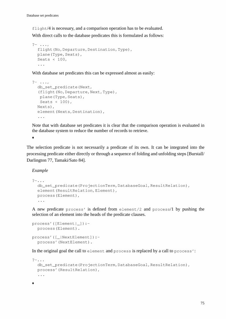
Database set predicates
75
flight/4 is necessary, and a comparison operation has to be evaluated.
With direct calls to the database predicates this is formulated as follows:
?- ...,flight(No,Departure,Destination,Type),plane(Type,Seats),Seats < 100,...
With database set predicates this can be expressed almost as easily:
?- ...,db_set_predicate(Next,(flight(No,Departure,Next,Type), plane(Type,Seats), Seats < 100),Nexts),element(Nexts,Destination),...
Note that with database set predicates it is clear that the comparison operation is evaluated inthe database system to reduce the number of records to retrieve.
♦
The selection predicate is not necessarily a predicate of its own. It can be integrated into the
processing predicate either directly or through a sequence of folding and unfolding steps [Burstall/
Darlington 77, Tamaki/Sato 84].
Example
?-...db_set_predicate(ProjectionTerm,DatabaseGoal,ResultRelation),element(ResultRelation,Element),process(Element),...
A new predicate process’ is defined from element/2 and process/1 by pushing theselection of an element into the heads of the predicate clauses.
process’([Element|_]):-process(Element).
process’([_|NextElement]):-process’(NextElement).
In the original goal the call to element and process is replaced by a call to process’:
?-...db_set_predicate(ProjectionTerm,DatabaseGoal,ResultRelation),process’(ResultRelation),...
♦
6. Database Set Predicates
76
6.3 Discussion
The implications of using database set predicates to access external databases in coupled systems
are now discussed. On the physical level, this discussion covers the
• system architecture and the coordination of evaluations,
• memory management, and
• portability.
On the logical level, the
• restriction of the database queries and the
• applicability of higher-order control
are discussed.
Two further issues, namely the
• relationship between database set predicates and the standard set predicates and
• implementation of other database access techniques with database set predicates
are presented in the final two subsections.
6.3.1 System architecture and coordination of evaluations
Database set predicates implement a physically loosely coupled system with a client/server
architecture. In this architecture, the logic language system is a client requesting services from the
database system which acts as a server.
In contrast to other approaches to coupled systems which integrate access to the external database
system into the logic language evaluation, database set predicates embed the set-oriented database
evaluation into the tuple-oriented evaluation of a logic programming language system. Note that
through embedding an external evaluation any of the existing optimizing techniques available in
the existing evaluation mechanism, e.g. co-routining, can be exploited. This is of particular interest
in data-intensive applications such as coupled systems.
Within their client/server architecture, database set predicates promise an efficient access to the
database evaluation because
• the number of individual database accesses is reduced,
• both systems retain their proper evaluation strategies, and
• there is no interference between the database and the logic language evaluation.
These three aspects relate directly to the flow of control in database set predicates.
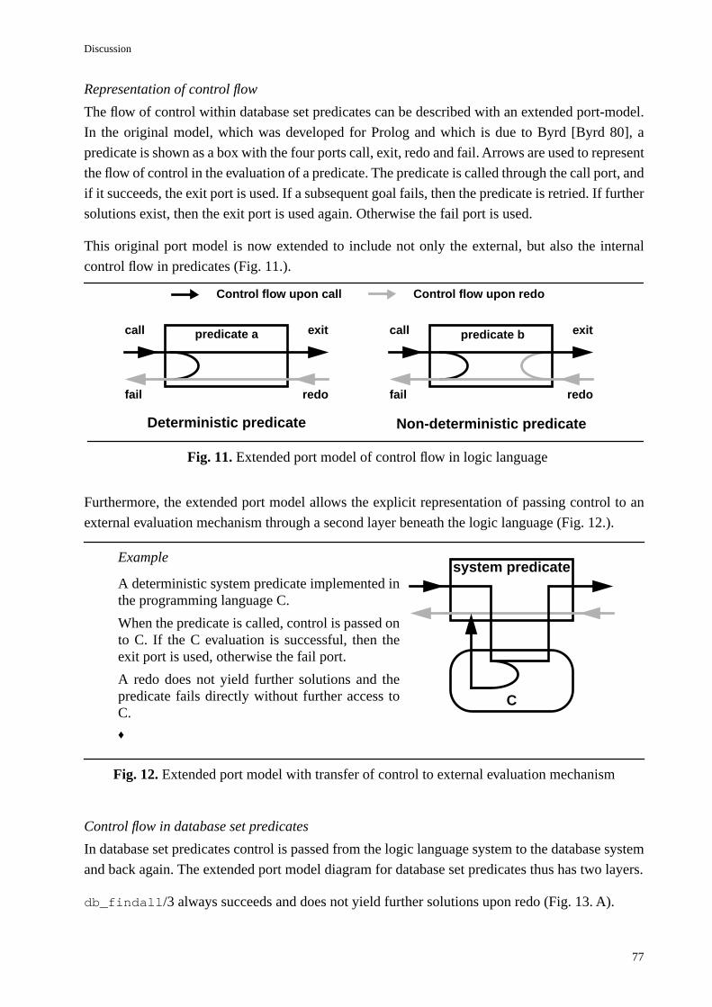
Discussion
77
Representation of control flow
The flow of control within database set predicates can be described with an extended port-model.
In the original model, which was developed for Prolog and which is due to Byrd [Byrd 80], a
predicate is shown as a box with the four ports call, exit, redo and fail. Arrows are used to represent
the flow of control in the evaluation of a predicate. The predicate is called through the call port, and
if it succeeds, the exit port is used. If a subsequent goal fails, then the predicate is retried. If further
solutions exist, then the exit port is used again. Otherwise the fail port is used.
This original port model is now extended to include not only the external, but also the internal
control flow in predicates (Fig. 11.).
Furthermore, the extended port model allows the explicit representation of passing control to an
external evaluation mechanism through a second layer beneath the logic language (Fig. 12.).
Control flow in database set predicates
In database set predicates control is passed from the logic language system to the database system
and back again. The extended port model diagram for database set predicates thus has two layers.
db_findall/3 always succeeds and does not yield further solutions upon redo (Fig. 13. A).
call exit
redofail
predicate acall exit
redofail
Non-deterministic predicateDeterministic predicate
Control flow upon call Control flow upon redo
Fig. 11. Extended port model of control flow in logic language
predicate b
Fig. 12. Extended port model with transfer of control to external evaluation mechanism
Example
A deterministic system predicate implemented inthe programming language C.
When the predicate is called, control is passed onto C. If the C evaluation is successful, then theexit port is used, otherwise the fail port.
A redo does not yield further solutions and thepredicate fails directly without further access toC.
♦
C
system predicate
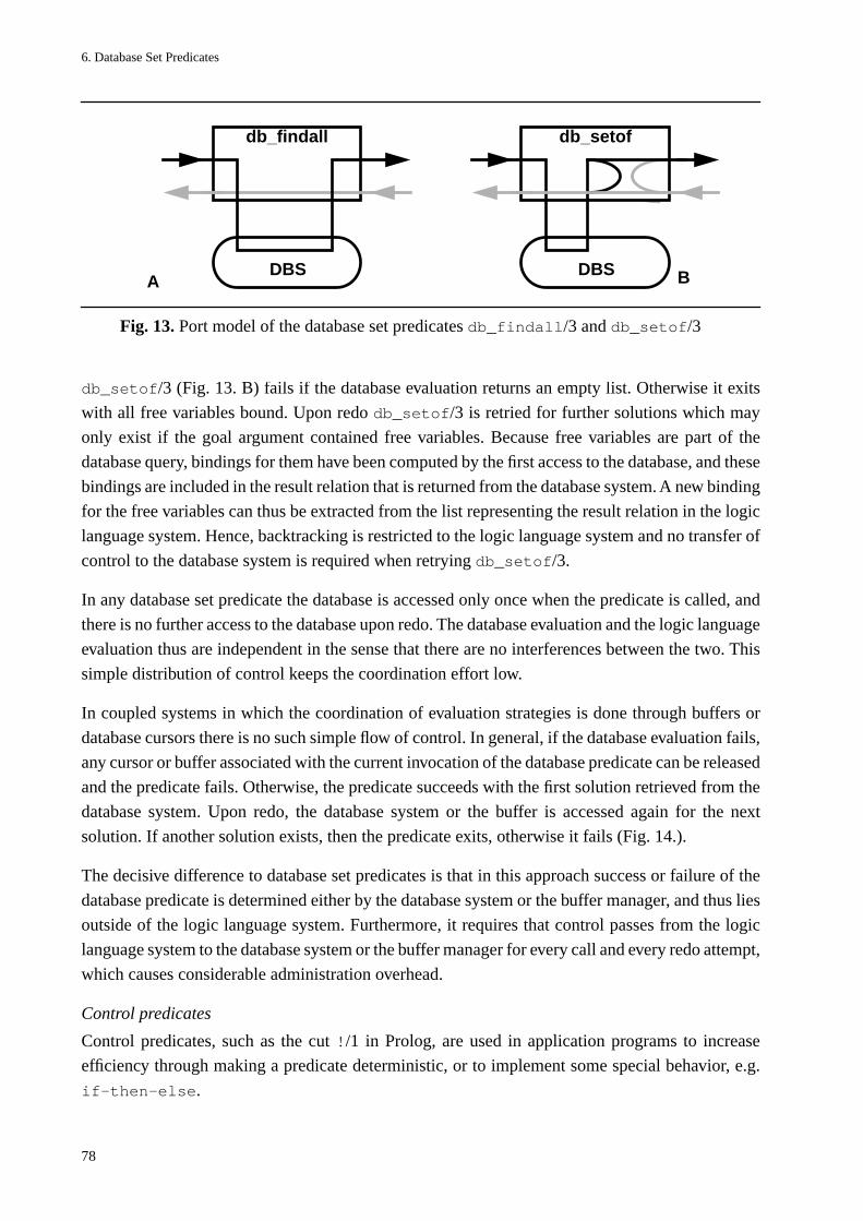
6. Database Set Predicates
78
db_setof/3 (Fig. 13. B) fails if the database evaluation returns an empty list. Otherwise it exits
with all free variables bound. Upon redo db_setof/3 is retried for further solutions which may
only exist if the goal argument contained free variables. Because free variables are part of the
database query, bindings for them have been computed by the first access to the database, and these
bindings are included in the result relation that is returned from the database system. A new binding
for the free variables can thus be extracted from the list representing the result relation in the logic
language system. Hence, backtracking is restricted to the logic language system and no transfer of
control to the database system is required when retrying db_setof/3.
In any database set predicate the database is accessed only once when the predicate is called, and
there is no further access to the database upon redo. The database evaluation and the logic language
evaluation thus are independent in the sense that there are no interferences between the two. This
simple distribution of control keeps the coordination effort low.
In coupled systems in which the coordination of evaluation strategies is done through buffers or
database cursors there is no such simple flow of control. In general, if the database evaluation fails,
any cursor or buffer associated with the current invocation of the database predicate can be released
and the predicate fails. Otherwise, the predicate succeeds with the first solution retrieved from the
database system. Upon redo, the database system or the buffer is accessed again for the next
solution. If another solution exists, then the predicate exits, otherwise it fails (Fig. 14.).
The decisive difference to database set predicates is that in this approach success or failure of the
database predicate is determined either by the database system or the buffer manager, and thus lies
outside of the logic language system. Furthermore, it requires that control passes from the logic
language system to the database system or the buffer manager for every call and every redo attempt,
which causes considerable administration overhead.
Control predicates
Control predicates, such as the cut !/1 in Prolog, are used in application programs to increase
efficiency through making a predicate deterministic, or to implement some special behavior, e.g.
if-then-else.
Fig. 13. Port model of the database set predicates db_findall/3 and db_setof/3
A BDBS
db_findall db_setof
DBS
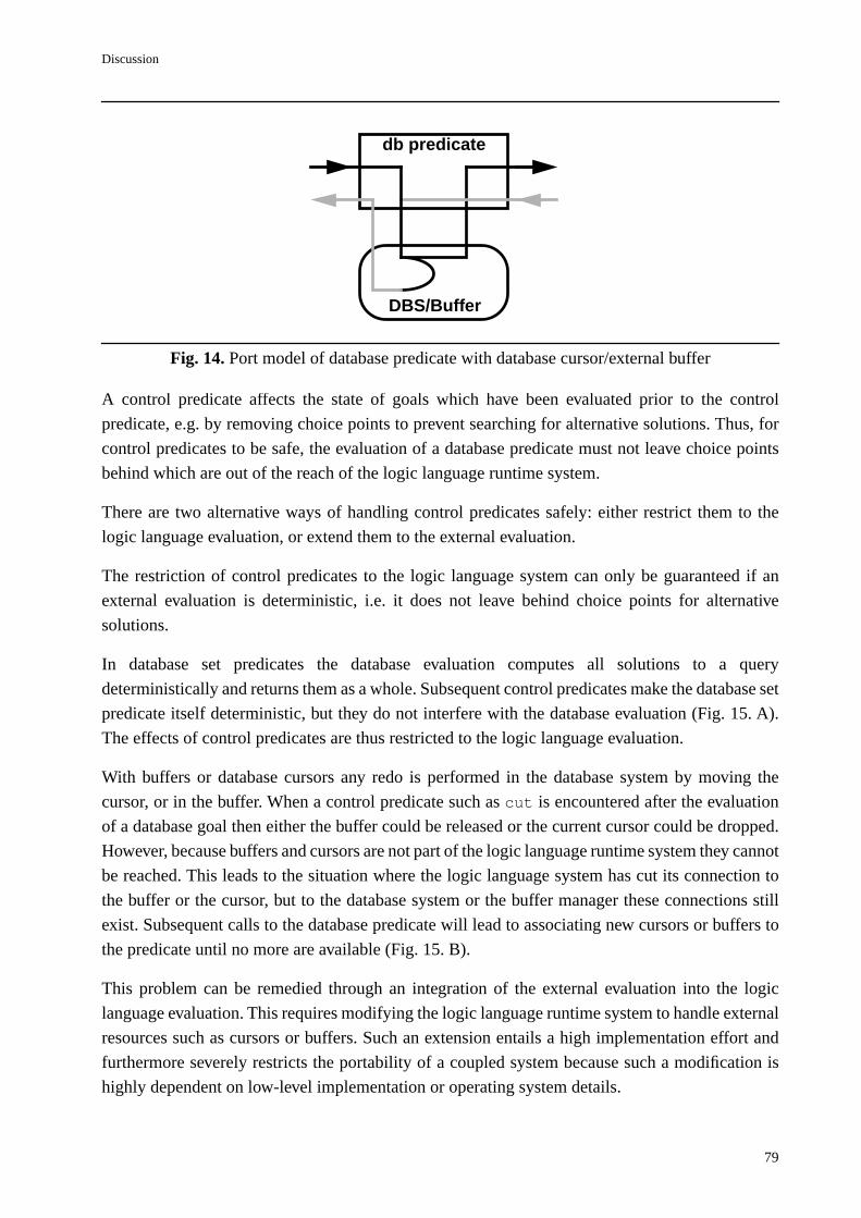
Discussion
79
A control predicate affects the state of goals which have been evaluated prior to the control
predicate, e.g. by removing choice points to prevent searching for alternative solutions. Thus, for
control predicates to be safe, the evaluation of a database predicate must not leave choice points
behind which are out of the reach of the logic language runtime system.
There are two alternative ways of handling control predicates safely: either restrict them to the
logic language evaluation, or extend them to the external evaluation.
The restriction of control predicates to the logic language system can only be guaranteed if an
external evaluation is deterministic, i.e. it does not leave behind choice points for alternative
solutions.
In database set predicates the database evaluation computes all solutions to a query
deterministically and returns them as a whole. Subsequent control predicates make the database set
predicate itself deterministic, but they do not interfere with the database evaluation (Fig. 15. A).
The effects of control predicates are thus restricted to the logic language evaluation.
With buffers or database cursors any redo is performed in the database system by moving the
cursor, or in the buffer. When a control predicate such as cut is encountered after the evaluation
of a database goal then either the buffer could be released or the current cursor could be dropped.
However, because buffers and cursors are not part of the logic language runtime system they cannot
be reached. This leads to the situation where the logic language system has cut its connection to
the buffer or the cursor, but to the database system or the buffer manager these connections still
exist. Subsequent calls to the database predicate will lead to associating new cursors or buffers to
the predicate until no more are available (Fig. 15. B).
This problem can be remedied through an integration of the external evaluation into the logic
language evaluation. This requires modifying the logic language runtime system to handle external
resources such as cursors or buffers. Such an extension entails a high implementation effort and
furthermore severely restricts the portability of a coupled system because such a modification is
highly dependent on low-level implementation or operating system details.
Fig. 14. Port model of database predicate with database cursor/external buffer
db predicate
DBS/Buffer
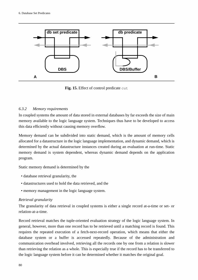
6. Database Set Predicates
80
6.3.2 Memory requirements
In coupled systems the amount of data stored in external databases by far exceeds the size of main
memory available to the logic language system. Techniques thus have to be developed to access
this data efficiently without causing memory overflow.
Memory demand can be subdivided into static demand, which is the amount of memory cells
allocated for a datastructure in the logic language implementation, and dynamic demand, which is
determined by the actual datastructure instances created during an evaluation at run-time. Static
memory demand is system dependent, whereas dynamic demand depends on the application
program.
Static memory demand is determined by the
• database retrieval granularity, the
• datastructures used to hold the data retrieved, and the
• memory management in the logic language system.
Retrieval granularity
The granularity of data retrieval in coupled systems is either a single record at-a-time or set- or
relation-at-a-time.
Record retrieval matches the tuple-oriented evaluation strategy of the logic language system. In
general, however, more than one record has to be retrieved until a matching record is found. This
requires the repeated execution of a fetch-next-record operation, which means that either the
database system or a buffer is accessed repeatedly. Because of the administration and
communication overhead involved, retrieving all the records one by one from a relation is slower
than retrieving the relation as a whole. This is especially true if the record has to be transferred to
the logic language system before it can be determined whether it matches the original goal.
A B
Fig. 15. Effect of control predicate cut
db set predicate
DBS
db predicate
DBS/Buffer
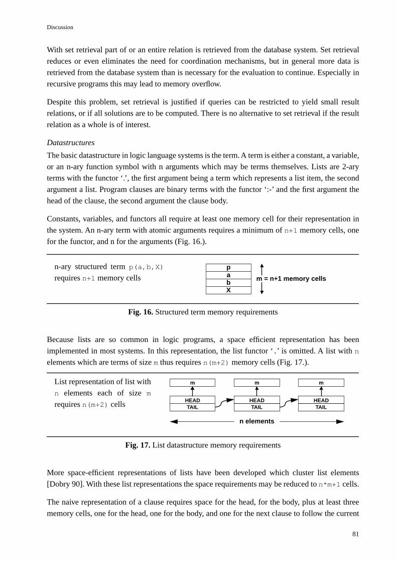
Discussion
81
With set retrieval part of or an entire relation is retrieved from the database system. Set retrieval
reduces or even eliminates the need for coordination mechanisms, but in general more data is
retrieved from the database system than is necessary for the evaluation to continue. Especially in
recursive programs this may lead to memory overflow.
Despite this problem, set retrieval is justified if queries can be restricted to yield small result
relations, or if all solutions are to be computed. There is no alternative to set retrieval if the result
relation as a whole is of interest.
Datastructures
The basic datastructure in logic language systems is the term. A term is either a constant, a variable,
or an n-ary function symbol with n arguments which may be terms themselves. Lists are 2-ary
terms with the functor ‘.’, the first argument being a term which represents a list item, the second
argument a list. Program clauses are binary terms with the functor ‘:-’ and the first argument the
head of the clause, the second argument the clause body.
Constants, variables, and functors all require at least one memory cell for their representation in
the system. An n-ary term with atomic arguments requires a minimum of n+1 memory cells, one
for the functor, and n for the arguments (Fig. 16.).
Because lists are so common in logic programs, a space efficient representation has been
implemented in most systems. In this representation, the list functor ‘.’ is omitted. A list with n
elements which are terms of size m thus requires n(m+2) memory cells (Fig. 17.).
More space-efficient representations of lists have been developed which cluster list elements
[Dobry 90]. With these list representations the space requirements may be reduced to n*m+1 cells.
The naive representation of a clause requires space for the head, for the body, plus at least three
memory cells, one for the head, one for the body, and one for the next clause to follow the current
ap
bX
m = n+1 memory cells
Fig. 16. Structured term memory requirements
n-ary structured term p(a,b,X)
requires n+1 memory cells
Fig. 17. List datastructure memory requirements
m m m
TAIL TAILTAILHEAD HEAD HEAD
n elements
List representation of list with
n elements each of size m
requires n(m+2) cells
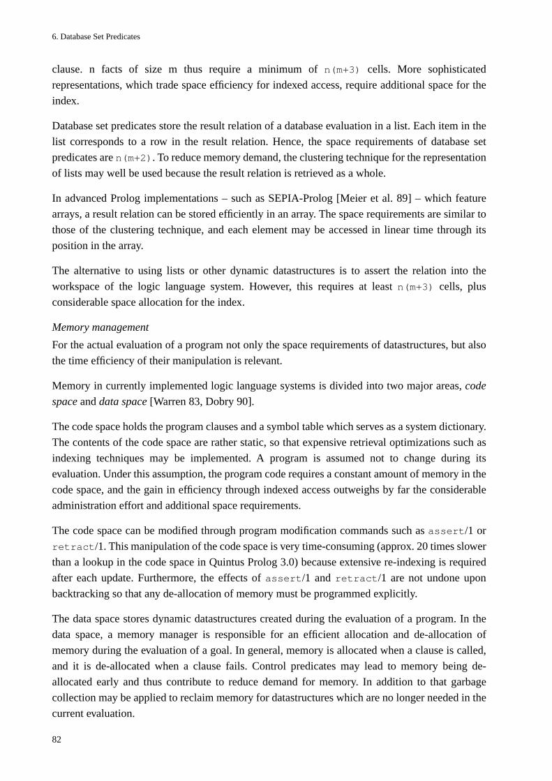
6. Database Set Predicates
82
clause. n facts of size m thus require a minimum of n(m+3) cells. More sophisticated
representations, which trade space efficiency for indexed access, require additional space for the
index.
Database set predicates store the result relation of a database evaluation in a list. Each item in the
list corresponds to a row in the result relation. Hence, the space requirements of database set
predicates are n(m+2). To reduce memory demand, the clustering technique for the representation
of lists may well be used because the result relation is retrieved as a whole.
In advanced Prolog implementations – such as SEPIA-Prolog [Meier et al. 89] – which feature
arrays, a result relation can be stored efficiently in an array. The space requirements are similar to
those of the clustering technique, and each element may be accessed in linear time through its
position in the array.
The alternative to using lists or other dynamic datastructures is to assert the relation into the
workspace of the logic language system. However, this requires at least n(m+3) cells, plus
considerable space allocation for the index.
Memory management
For the actual evaluation of a program not only the space requirements of datastructures, but also
the time efficiency of their manipulation is relevant.
Memory in currently implemented logic language systems is divided into two major areas, code
space and data space [Warren 83, Dobry 90].
The code space holds the program clauses and a symbol table which serves as a system dictionary.
The contents of the code space are rather static, so that expensive retrieval optimizations such as
indexing techniques may be implemented. A program is assumed not to change during its
evaluation. Under this assumption, the program code requires a constant amount of memory in the
code space, and the gain in efficiency through indexed access outweighs by far the considerable
administration effort and additional space requirements.
The code space can be modified through program modification commands such as assert/1 or
retract/1. This manipulation of the code space is very time-consuming (approx. 20 times slower
than a lookup in the code space in Quintus Prolog 3.0) because extensive re-indexing is required
after each update. Furthermore, the effects of assert/1 and retract/1 are not undone upon
backtracking so that any de-allocation of memory must be programmed explicitly.
The data space stores dynamic datastructures created during the evaluation of a program. In the
data space, a memory manager is responsible for an efficient allocation and de-allocation of
memory during the evaluation of a goal. In general, memory is allocated when a clause is called,
and it is de-allocated when a clause fails. Control predicates may lead to memory being de-
allocated early and thus contribute to reduce demand for memory. In addition to that garbage
collection may be applied to reclaim memory for datastructures which are no longer needed in the
current evaluation.
Discussion
83
With database set predicates the result relation retrieved from the external database is stored as a
dynamic datastructure in the data space of the logic language system. The built-in memory
manager thus can be exploited to reduce space demand and increase time efficiency. Furthermore,
memory is allocated and de-allocated implicitly, and it is guaranteed that memory is only allocated
as long as it is needed in the current evaluation.
6.3.3 Portability
An approach to coupled systems is said to be portable if it can be implemented on a variety of
machines, under various operating systems, and for different logic languages and database
systems.
Portability is determined by the specific system resources that are required. A coupled system is
thus portable if its implementation requires only such resources which are already provided as
standard features in both the logic language system or the database system.
In coupled systems portability is achieved by
• restricting the exchange of data between the logic language system and the database system to
high-level standard interfaces.
Any modification of the runtime system of the logic language, the use of auxiliary interfaces, or
low-level database access, prevents a system from being easily portable.
The system resources required by database set predicates are an interface to a communication
device of the operating system from both the logic language system and the database system.
Currently available logic language systems in general provide such an interface via built-in
predicates which allow reading from and writing to files or streams. Commercial database systems
also provide similar interfaces either for direct user access or for programming languages.
Database set predicates access external databases in a non-procedural manner through queries
formulated in a high-level query language. A query is generated from the goal argument of a
database set predicate in a translation procedure. This translation procedure can be implemented
entirely in the logic language itself without any need to resort other languages. Furthermore,
because a database goal is translated directly to an equivalent query there are no intermediate
translations to be performed as is the case with a distinct module interface as in PRIMO. Finally,
a high-level programming language such as a logic language greatly facilitates the implementation
of a translation procedure. Thus, adapting a given translation procedure to different database
languages, extending it to include new features, or porting it to another machine is straightforward
(see section 7.2 for details of the translation procedure).
Embedding an external database evaluation into the logic language evaluation requires adequate
datastructures to capture the data retrieved from the external database. In database set predicates,
data retrieved from the external database is interpreted and placed in a list of terms, the arguments
of which are ground values. This interpretation is done by the logic language system, and it can be
6. Database Set Predicates
84
implemented entirely in the logic language, or the built-in tokenizer, which is provided to parse
user input, may be used.
In systems using buffers or database cursors, managing these external resources requires major
modifications of the logic language runtime system. Because a runtime system is in general written
in low-level languages and not accessible to programmers, incorporating these modifications is
difficult.
6.3.4 Restriction of queries
In coupled systems a subset or an extension of the logic language is used to access the external
database system. In database set predicates the database access language is a subset of the logic
language. Maximally restrictive queries can be formulated which minimize the amount of data
retrieved from the database system. This reduces the cost of transport, may prevent memory
overflow and thus increases efficiency.
In logic languages, various techniques can be employed to achieve maximally restrictive queries:
• propagating variable bindings into the queries,
• exploiting join selectivity,
• dynamic database access definition, and
• independent selection and projection expressions.
The first two have been used in other approaches to coupled systems already and thus will only be
sketched. Dynamic database access definition is new only in physically loosely coupled systems,
whereas independent selection and projection expressions are new in the context of coupled
systems in general.
Database set predicates allow all four techniques to be employed to effectively restrict queries as
strong as possible. The word of warning of section 6.3.2 that set retrieval is only justified if result
relations are small directly relates to this section. It will be shown that in fact result relations
retrieved through database set predicates are minimal and that database set predicates are thus an
efficient means of implementing coupled systems.
Propagating variable bindings into queries
The arguments of database goals are constants and variables, or terms containing constants and
variables. Each argument is mapped to an attribute in a database table. In the query corresponding
to the database goal unbound variable arguments are mapped to attribute names and variable
arguments bound to constants are mapped to comparison operations with the appropriate attribute
name as one argument, and the constant value as the second argument. This comparison operation
serves as a selection condition to restrict the query.
Discussion
85
Example
The database goal
?- ...,flight(FlightNo,Departure,Destination,Plane).
with Departure bound to the constant value zurich is equivalent to the relational algebraexpression
σFLIGHT.Departure=zurich(FLIGHT)
♦
The propagation of variable bindings into database queries allows queries to be restricted
dynamically at runtime and thus serve to restrict the amount of data to be retrieved to those tuples
which are really needed for the evaluation to continue.
Propagating variable bindings is only possible if the language used for database access and the
logic language have common constructs through which the variable bindings can be exchanged. In
PROSQL SQL commands are treated as atoms whose internal structure is not accessible through
the Prolog system. The database access language and the logic language are completely separated,
and thus propagation of bindings is not feasible in PROSQL. The same is true for KB-Prolog where
the relational algebra expressions may not contain variables. In most other systems propagation of
bindings is provided.
In database set predicates the propagation of variable bindings is achieved during the translation of
the template term and the database goal.
Exploiting join selectivity
The most commonly used form of a join is the natural join which implies an equality comparison
over at least one attribute from both argument relations as the join condition. Join operations can
be used to restrict queries because the comparison operation also serves as a selection condition for
the two relations.
Join operations require at least two relations as input arguments. Self-joins, which are joins over
only one relation table, are only a special case of the general join. In coupled systems joins can be
performed in the logic language system or in the database system. It is very expensive to perform
joins in the logic language system because both relations involved have to be retrieved from the
database system prior to the evaluation of the join. Performing joins in the database is much more
efficient because database systems support join operations through e.g. indexed access to records,
and because only the result relation need be retrieved.
In coupled systems with single relation access to the database joins can only be performed in the
logic language system. For joins to be performed in the database view access to the database is
necessary.
6. Database Set Predicates
86
In the logic language natural join is expressed through shared variables in the individual subgoals
of a database goal. More general join operations are expressed through comparison operations over
two variables from distinct subgoals.
Example
The database goal
?- flight(FlightNo,zurich,Destination,Type), plane(Type,Seats).
is equivalent to the following natural join
FLIGHT [FLIGHT.Plane = PLANE.Type] PLANE
The database goal
?-flight(FlightNo,Departure,Destination,Type_1),plane(Type_2, Seats),Type_1 < Type_2.
is equivalent to the following join with < comparison over the attribute PlaneTypes.
FLIGHT [FLIGHT.Plane < PLANE.Type] PLANE
With single relation access both relations FLIGHT and PLANE have to be retrieved from thedatabase system for the evaluation of the join. With view access the join is evaluated in thedatabase system, and only the result relation is retrieved.
♦
Note that exploiting join-selectivity is not restricted to two relations. On the contrary, with more
relations involved the selectivity potential of a join improves.
In database set predicates join selectivity can be fully exploited because the database goal may
consist of an arbitrary number of conjunctive or disjunctive database subgoals. Database goals with
disjunction are split into as large as possible base conjunctions connected through disjunction via
transformations according to de Morgan’s laws.
In coupled systems, such as CGW or BERMUDA, where database access is restricted to single
relation access, join selectivity cannot be exploited. In PRIMO joins are evaluated in the database
system, but the relations involved are asserted into the workspace as distinct relations. Therefore
any join must be performed twice - once in the database system, and again in the logic language
system.
Dynamic database access definition
In physically loosely coupled systems access to the database is either defined
• statically as part of the program code, or
• dynamically through datastructures.
With static database access definition database predicates are program clauses. These clauses are
mapped to query skeletons which may be instantiated with current variable bindings. This mapping
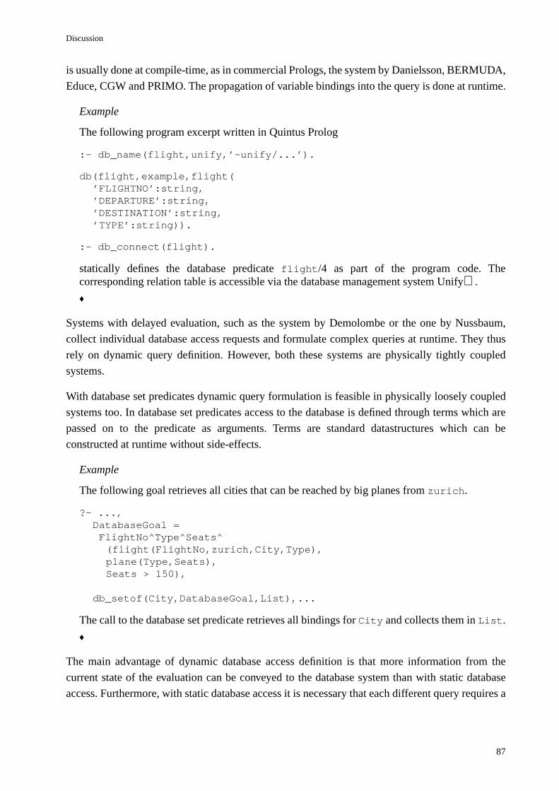
Discussion
87
is usually done at compile-time, as in commercial Prologs, the system by Danielsson, BERMUDA,
Educe, CGW and PRIMO. The propagation of variable bindings into the query is done at runtime.
Example
The following program excerpt written in Quintus Prolog
:- db_name(flight,unify,’~unify/...’).
db(flight,example,flight(’FLIGHTNO’:string,’DEPARTURE’:string,’DESTINATION’:string,’TYPE’:string)).
:- db_connect(flight).
statically defines the database predicate flight/4 as part of the program code. Thecorresponding relation table is accessible via the database management system Unify .
♦
Systems with delayed evaluation, such as the system by Demolombe or the one by Nussbaum,
collect individual database access requests and formulate complex queries at runtime. They thus
rely on dynamic query definition. However, both these systems are physically tightly coupled
systems.
With database set predicates dynamic query formulation is feasible in physically loosely coupled
systems too. In database set predicates access to the database is defined through terms which are
passed on to the predicate as arguments. Terms are standard datastructures which can be
constructed at runtime without side-effects.
Example
The following goal retrieves all cities that can be reached by big planes from zurich.
?- ...,DatabaseGoal = FlightNo^Type^Seats^
(flight(FlightNo,zurich,City,Type),plane(Type,Seats),Seats > 150),
db_setof(City,DatabaseGoal,List),...
The call to the database set predicate retrieves all bindings for City and collects them in List.
♦
The main advantage of dynamic database access definition is that more information from the
current state of the evaluation can be conveyed to the database system than with static database
access. Furthermore, with static database access it is necessary that each different query requires a
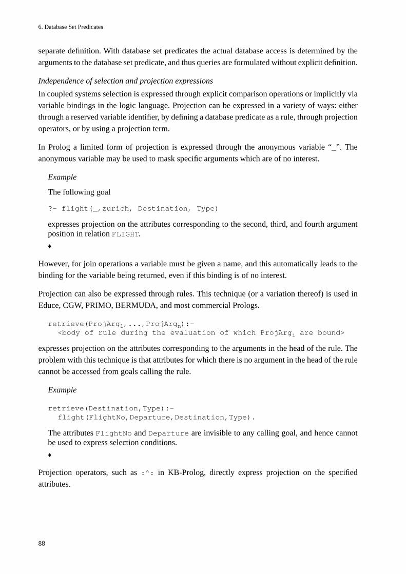
6. Database Set Predicates
88
separate definition. With database set predicates the actual database access is determined by the
arguments to the database set predicate, and thus queries are formulated without explicit definition.
Independence of selection and projection expressions
In coupled systems selection is expressed through explicit comparison operations or implicitly via
variable bindings in the logic language. Projection can be expressed in a variety of ways: either
through a reserved variable identifier, by defining a database predicate as a rule, through projection
operators, or by using a projection term.
In Prolog a limited form of projection is expressed through the anonymous variable “_”. The
anonymous variable may be used to mask specific arguments which are of no interest.
Example
The following goal
?- flight(_,zurich, Destination, Type)
expresses projection on the attributes corresponding to the second, third, and fourth argumentposition in relation FLIGHT.
♦
However, for join operations a variable must be given a name, and this automatically leads to the
binding for the variable being returned, even if this binding is of no interest.
Projection can also be expressed through rules. This technique (or a variation thereof) is used in
Educe, CGW, PRIMO, BERMUDA, and most commercial Prologs.
retrieve(ProjArg1,...,ProjArgn):-<body of rule during the evaluation of which ProjArgi are bound>
expresses projection on the attributes corresponding to the arguments in the head of the rule. The
problem with this technique is that attributes for which there is no argument in the head of the rule
cannot be accessed from goals calling the rule.
Example
retrieve(Destination,Type):-flight(FlightNo,Departure,Destination,Type).
The attributes FlightNo and Departure are invisible to any calling goal, and hence cannotbe used to express selection conditions.
♦
Projection operators, such as :^: in KB-Prolog, directly express projection on the specified
attributes.
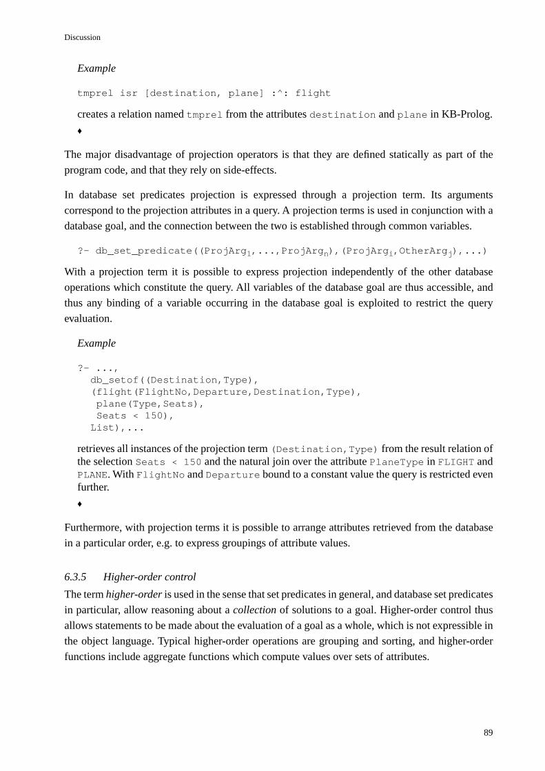
Discussion
89
Example
tmprel isr [destination, plane] :^: flight
creates a relation named tmprel from the attributes destination and plane in KB-Prolog.
♦
The major disadvantage of projection operators is that they are defined statically as part of the
program code, and that they rely on side-effects.
In database set predicates projection is expressed through a projection term. Its arguments
correspond to the projection attributes in a query. A projection terms is used in conjunction with a
database goal, and the connection between the two is established through common variables.
?- db_set_predicate((ProjArg1,...,ProjArgn),(ProjArgi,OtherArgj),...)
With a projection term it is possible to express projection independently of the other database
operations which constitute the query. All variables of the database goal are thus accessible, and
thus any binding of a variable occurring in the database goal is exploited to restrict the query
evaluation.
Example
?- ...,db_setof((Destination,Type),(flight(FlightNo,Departure,Destination,Type), plane(Type,Seats), Seats < 150),List),...
retrieves all instances of the projection term (Destination,Type) from the result relation ofthe selection Seats < 150 and the natural join over the attribute PlaneType in FLIGHT andPLANE. With FlightNo and Departure bound to a constant value the query is restricted evenfurther.
♦
Furthermore, with projection terms it is possible to arrange attributes retrieved from the database
in a particular order, e.g. to express groupings of attribute values.
6.3.5 Higher-order control
The term higher-order is used in the sense that set predicates in general, and database set predicates
in particular, allow reasoning about a collection of solutions to a goal. Higher-order control thus
allows statements to be made about the evaluation of a goal as a whole, which is not expressible in
the object language. Typical higher-order operations are grouping and sorting, and higher-order
functions include aggregate functions which compute values over sets of attributes.
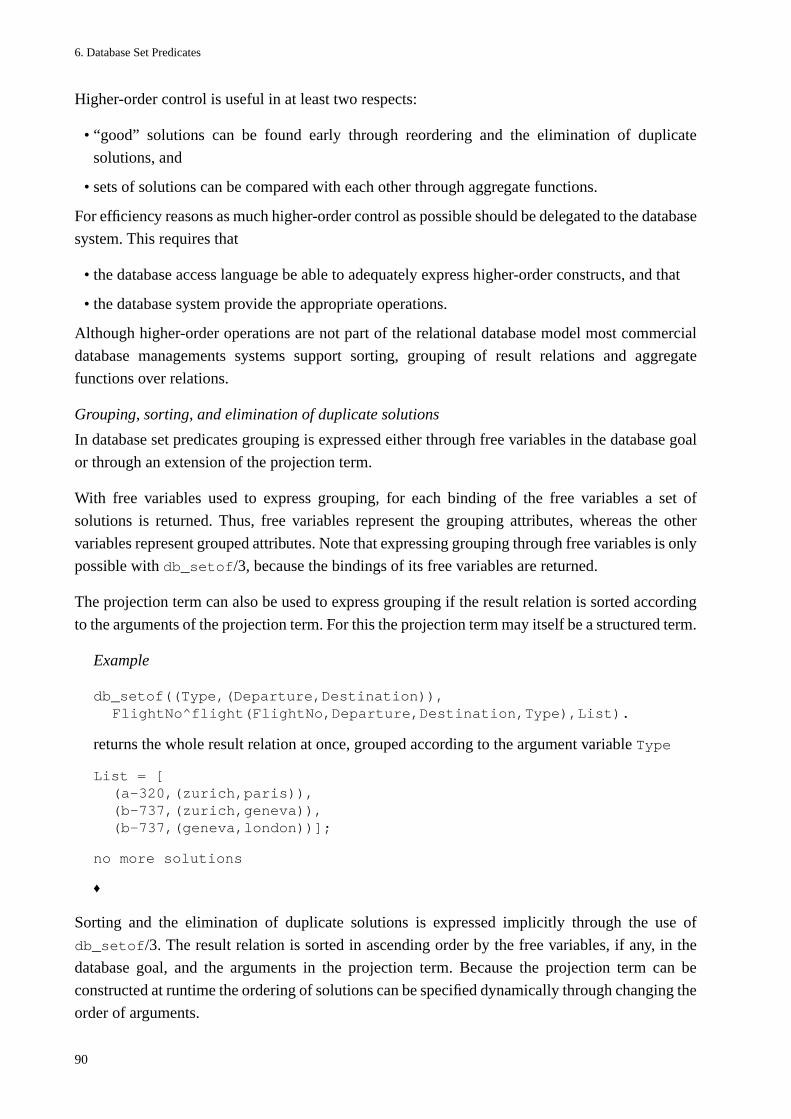
6. Database Set Predicates
90
Higher-order control is useful in at least two respects:
• “good” solutions can be found early through reordering and the elimination of duplicate
solutions, and
• sets of solutions can be compared with each other through aggregate functions.
For efficiency reasons as much higher-order control as possible should be delegated to the database
system. This requires that
• the database access language be able to adequately express higher-order constructs, and that
• the database system provide the appropriate operations.
Although higher-order operations are not part of the relational database model most commercial
database managements systems support sorting, grouping of result relations and aggregate
functions over relations.
Grouping, sorting, and elimination of duplicate solutions
In database set predicates grouping is expressed either through free variables in the database goal
or through an extension of the projection term.
With free variables used to express grouping, for each binding of the free variables a set of
solutions is returned. Thus, free variables represent the grouping attributes, whereas the other
variables represent grouped attributes. Note that expressing grouping through free variables is only
possible with db_setof/3, because the bindings of its free variables are returned.
The projection term can also be used to express grouping if the result relation is sorted according
to the arguments of the projection term. For this the projection term may itself be a structured term.
Example
db_setof((Type,(Departure,Destination)),FlightNo^flight(FlightNo,Departure,Destination,Type),List).
returns the whole result relation at once, grouped according to the argument variable Type
List = [(a-320,(zurich,paris)),(b-737,(zurich,geneva)),(b-737,(geneva,london))];
no more solutions
♦
Sorting and the elimination of duplicate solutions is expressed implicitly through the use of
db_setof/3. The result relation is sorted in ascending order by the free variables, if any, in the
database goal, and the arguments in the projection term. Because the projection term can be
constructed at runtime the ordering of solutions can be specified dynamically through changing the
order of arguments.
Discussion
91
Aggregate functions
Aggregate functions compute values over collections — or aggregates — of attribute values.
Typical aggregate functions are sum(), avg(), count(), min(), and max() which compute the sum,
the average, the number, the minimum and the maximum of given attributes.
In database set predicates calls to aggregate functions are ternary subgoals in the database goal. The
predicate symbol of such a subgoal is mapped to the function name in the database system. The
first argument of the subgoal is mapped to the attribute over which the function is to be computed,
the second argument specifies the relation, and the third argument receives the result value of the
function evaluation. Because this value is of interest the variable in the result position of the
aggregate function subgoal must also occur in the projection term.
Example
“Find the smallest plane in the database”
db_setof(MinSeats,min(Seats,Plane^plane(Plane,Seats),MinSeats),List).
returns
List = [150];
no more solutions
MinSeats, which is the function value of interest, occurs in the database goal as the resultargument of the aggregate function subgoal min/3, and in the projection term.
With Plane a free variable, the result of the function would be grouped by the correspondingattribute values. For the aggregate function to be computed over the whole relation, Plane mustbe existentially quantified.
♦
In some database languages, e.g. QUEL [Held et al. 75], aggregate functions may have complex
input argument arguments, e.g. arithmetic expressions over attributes, or they may even be nested.
Such complex or nested aggregate functions can also be represented in the logic language and
hence also in database set predicates.
6.3.6 Relationship between the built-in set predicates and database set predicates
The main difference between the built-in and database set predicates lies in the constraints on the
goal argument:
• the extension of a predicate called in the goal argument must be stored either externally, or
internally only, and
• the goal argument may contain calls to either database predicates or program predicates only.
Under these two constraints, database set predicates can be used in parallel to the built-in set
predicates of logic languages.
6. Database Set Predicates
92
This can be achieved by a mutually exclusive test in the clauses defining the set predicates. This
test serves to select the appropriate set predicate definition. A suitable test is whether the goal
argument is in fact a valid database goal. If so, then the goal argument can be proved from database
predicates in an external database evaluation. Otherwise it must be proved from program
predicates.
Example
findall/3 is redefined as follows (with the database set predicate db_findall/3 renamed tofindall/3):
findall(Template, Goal, List):-not database_goal(Goal),/* built-in implementation of findall */...
findall(Template, Database_Goal, List):-database_goal(Database_Goal),/* database set predicate implementation */...
The first clause of findall/3 succeeds if the goal can be proved from the clauses stored in theinternal workspace. The second clause succeeds if the goal can be proved using facts stored inthe external database system. Either clause returns an empty list if the goal argument could notbe proved.
♦
If set predicates and database set predicates are used in parallel in a program the physical allocation
of data accessed through these predicates must not be known to the programmer. With the database
schema information accessible through the program it is thus possible to build a prototype that
accesses only the internal workspace, and then, in the final version, relocate the database to an
external database system without changing the program.
6.3.7 Implementation of other approaches with database set predicates
In the introduction it was claimed that database set predicates can simulate most other techniques
developed so far for the coordination of evaluation strategies in coupled systems. This is shown by
example for asserting result relations into workspace, and for single tuple retrieval. Both these
approaches rely on the constraint that data is stored either externally or internally, but not both.
With the subsumption technique this assumption could be dropped — the extension of a database
predicate is stored externally, but part of it is also held internally for efficient access.
Asserting relations
Asserting relations into the workspace can be represented with database set predicates through
retrieving the set of solutions of a database predicate, and asserting, one by one, each instantiated
tuple.
Discussion
93
retrieve_and_assert(DatabaseGoal):-db_set_predicate(DatabaseGoal,DatabaseGoal,RelationList),assert_all(RelationList).
assert_all([]).
assert_all([Head|Tail]):-asserta(Head),assert_all(Tail).
Redundant clauses can be avoided through an additional check before asserting a clause into the
workspace. The second clause of assert_all/1 is modified accordingly. Note that the check
consists of a meta-variable which is instantiated with a goal.
assert_all([Head|Tail]):-/* check that clause Head does not already exist in workspace */ call(Head) -> true,! ; asserta(Head),assert_all(Tail).
Asserting relations into the workspace is best employed once in an application program prior to
any access to the data stored externally.
Single tuple interface
A single-tuple interface to the database system can be implemented with database set predicates in
the following way: a new clause with an appropriately chosen name is added to the program. The
head of the clause contains an argument for each attribute to be retrieved from the database. The
body of the clause contains a call of a database set predicate with the arguments of the head as the
template and a database goal that contains at least these arguments. The selection predicate
element/2 returns one tuple at a time from the result relation upon backtracking.
retrieve_tuple(Arg1,...,Argn):-db_set_pred((Arg1,...,Argn),db_goal(Arg1,...,Argn),ResultRelation),element(RelationList,(Arg1,...,Argn)).
Note that this definition can be modified to yield a very general single tuple database interface by
replacing the n arguments in the head through only one argument which may be a term representing
a goal. This term is also used as the projection term and the database goal of the database set
predicate, and it is used as the selection mask in element/2:
retrieve_tuple(Goal):-db_set_pred(Goal,Goal,ResultRelation),element(ResultRelation,Goal,).
With this definition, any term representing a database request can be executed in the logic program.
Note that this definition makes use of the fact that the template variables and the existentially
quantified variables in the database goal remain unbound after the execution of the database set
predicate.
6. Database Set Predicates
94
Subsumption
The subsumption technique was primarily developed to replace the number of expensive individual
accesses to external databases through cheap lookup in the internal workspace. Upon the first
occurrence of a database goal its extension is loaded into workspace, so that for further requests it
can be accessed efficiently. Query subsumption is used to test whether data has to be fetched from
the database system, or is simply searched for in the logic language workspace.
Query subsumption requires tracer predicates that record which queries have been evaluated in the
database already. With database set predicates query subsumption can be implemented according
to the following definition:
subsumption_access(Goal):-tracer(Goal,Tracer),subsumes(Tracer,Goal), % Goal extension is in workspace already!, % to prevent second clause from being triedcall(Goal).
subsumption_access(Goal):-% Goal not yet answered by database evaluationdb_set_pred(Goal,Goal,List),% permanently store tuples retrieved from dbassert_all(List),% update tracer recordmodify_tracer(Goal),call(Goal).
Note that the second clause of subsumption_access/2 relies on the immediate update of the
internal workspace. As in the original model proposed by [Ceri et al. 87] the tracers are updated
through modify_tracer/1. Tracers are asserted in front of each other so that the tracers for every
query are organized as a stack. Care must be taken to prevent backtracking into the second clause
of subsumption_access/1 to prevent the modification of tracers other than the current tracer.
6.4 Summary
With database set predicates both the logic language system and the external database system are
completely independent, communicating with each other only upon request from the application
program written in the logic language. Database access is defined dynamically, and the database
access language is a subset of the logic language. Database set predicates thus implement a true
physically loosely and logically tightly coupled system (Fig. 18.).
On the physical level efficiency is achieved through a simple flow of control that does not cause
coordination overhead, efficient datastructures, and automatic memory management by the logic
language system. On the logical level efficiency is achieved through maximally restrictive queries.
Set retrieval, which is a source of inefficiency in other approaches because of the expensive storage
of result relations, contributes to efficiency in database set predicates because it minimizes the
number of individual database accesses, and allows the application of higher-order control to the
current evaluation.
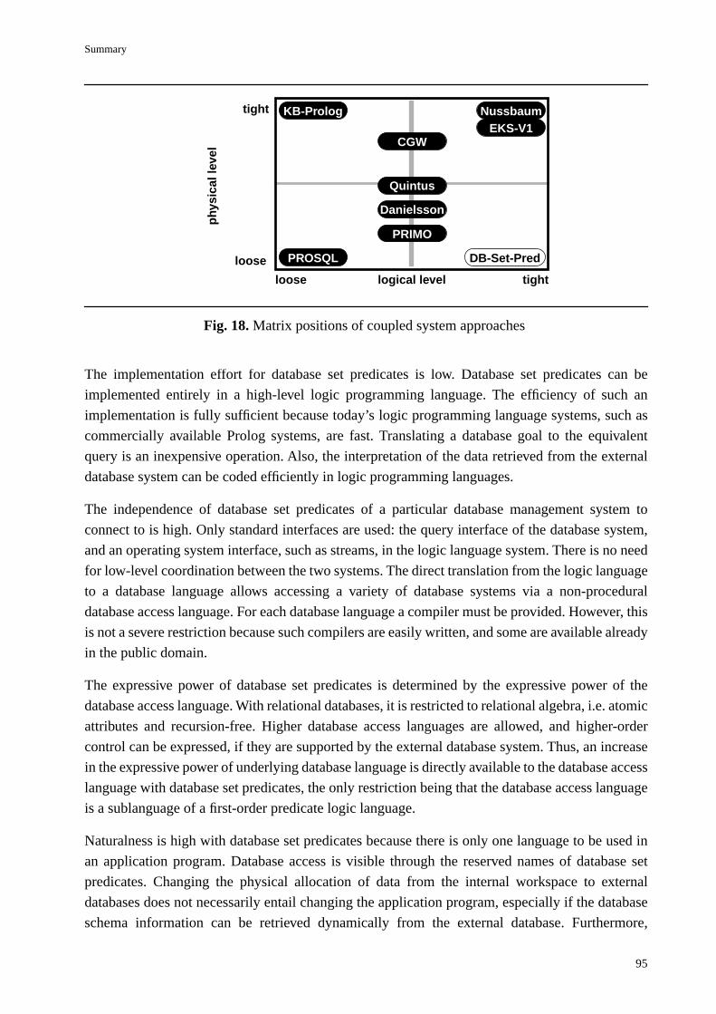
Summary
95
The implementation effort for database set predicates is low. Database set predicates can be
implemented entirely in a high-level logic programming language. The efficiency of such an
implementation is fully sufficient because today’s logic programming language systems, such as
commercially available Prolog systems, are fast. Translating a database goal to the equivalent
query is an inexpensive operation. Also, the interpretation of the data retrieved from the external
database system can be coded efficiently in logic programming languages.
The independence of database set predicates of a particular database management system to
connect to is high. Only standard interfaces are used: the query interface of the database system,
and an operating system interface, such as streams, in the logic language system. There is no need
for low-level coordination between the two systems. The direct translation from the logic language
to a database language allows accessing a variety of database systems via a non-procedural
database access language. For each database language a compiler must be provided. However, this
is not a severe restriction because such compilers are easily written, and some are available already
in the public domain.
The expressive power of database set predicates is determined by the expressive power of the
database access language. With relational databases, it is restricted to relational algebra, i.e. atomic
attributes and recursion-free. Higher database access languages are allowed, and higher-order
control can be expressed, if they are supported by the external database system. Thus, an increase
in the expressive power of underlying database language is directly available to the database access
language with database set predicates, the only restriction being that the database access language
is a sublanguage of a first-order predicate logic language.
Naturalness is high with database set predicates because there is only one language to be used in
an application program. Database access is visible through the reserved names of database set
predicates. Changing the physical allocation of data from the internal workspace to external
databases does not necessarily entail changing the application program, especially if the database
schema information can be retrieved dynamically from the external database. Furthermore,
Fig. 18. Matrix positions of coupled system approaches
phy
sica
l lev
el
logical level
loose
tight
loose tight
KB-Prolog
PROSQL
PRIMO
Nussbaum
CGW
Quintus
Danielsson
DB-Set-Pred
EKS-V1
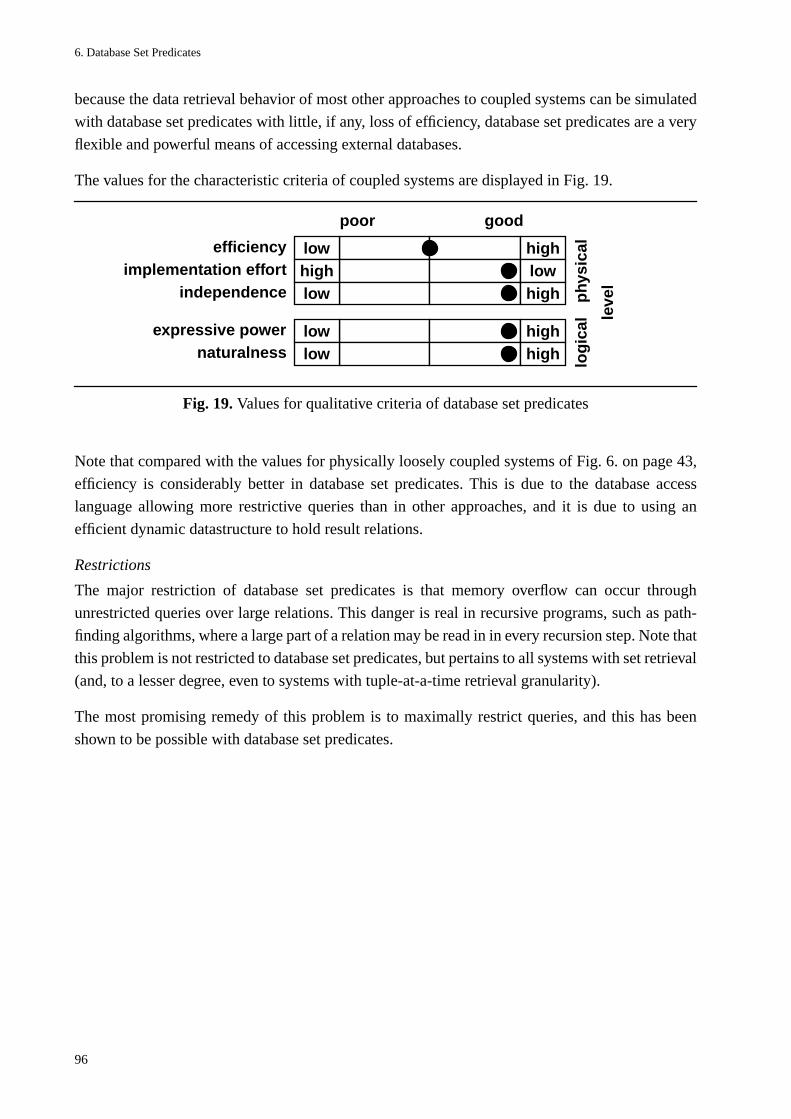
6. Database Set Predicates
96
because the data retrieval behavior of most other approaches to coupled systems can be simulated
with database set predicates with little, if any, loss of efficiency, database set predicates are a very
flexible and powerful means of accessing external databases.
The values for the characteristic criteria of coupled systems are displayed in Fig. 19.
Note that compared with the values for physically loosely coupled systems of Fig. 6. on page 43,
efficiency is considerably better in database set predicates. This is due to the database access
language allowing more restrictive queries than in other approaches, and it is due to using an
efficient dynamic datastructure to hold result relations.
Restrictions
The major restriction of database set predicates is that memory overflow can occur through
unrestricted queries over large relations. This danger is real in recursive programs, such as path-
finding algorithms, where a large part of a relation may be read in in every recursion step. Note that
this problem is not restricted to database set predicates, but pertains to all systems with set retrieval
(and, to a lesser degree, even to systems with tuple-at-a-time retrieval granularity).
The most promising remedy of this problem is to maximally restrict queries, and this has been
shown to be possible with database set predicates.
efficiency low highimplementation effort high low
independence low high
expressive power low highnaturalness low high
phy
sica
llo
gic
al
leve
l
Fig. 19. Values for qualitative criteria of database set predicates
poor good

Part III
Implementation

98
99
7
Implementation of Database Set Predicates
In the remainder of the thesis the logic programming language will be Prolog and the database
system is an SQL system. Prolog has been chosen because it is the most widespread logic
programming language implementation, and SQL because it is the current relational database
language standard.
7.1 System architecture and requirements for database set predicates
Database set predicates can be implemented efficiently in existing Prolog systems provided that
either calls to externally defined procedures are supported, or accessing operating system
communication devices is allowed. Most commercial Prolog system implementations provide one
of the above mechanisms. The database system must also feature a programming language
interface, or an interface to the communication devices of the operating system. Again, most
commercially available database systems feature such an interface.
7.1.1 System architecture
Database set predicates implement a physically loosely and logically tightly coupled system in
which access to the external database is embedded into the logic language. The general architecture
of a coupled system based on database set predicates is a programming language system connected
to an external database system through a bi-directional communication channel (Fig. 10. on page
71).
In this architecture the Prolog system is simply another user to the database management system.
An application program must have the access privileges for each relation table and view that it
accesses, and it must register with the database system through a login procedure. This login
procedure can be executed when the application program is loaded into the Prolog system, when
the communication channel to the external database is established, or prior to the first database
access request.
7. Implementation of Database Set Predicates
100
7.1.2 Database set predicates implementation requirements
The implementation of database set predicates requires that a
• database access request be translated to the equivalent SQL query, and that the
• result of the database evaluation be retrieved and placed in a Prolog list datastructure.
Translating the database access request and the result relation retrieved from the database system
can be implemented in standard Prolog. In fact, logic languages are well-suited for the
implementation of interpreters and compilers [Warren 80, Sterling/Shapiro 86].
This translation of a database access request to the database query requires meta-level access to the
object language, and it entails extensive term manipulation. The meta-logical predicates such as
var/1, functor/3, arg/3, or =../2 test whether a token of the database access request is a
variable, extract the functor or an argument of a term, or transform a term into a list respectively.
Furthermore, in order to allow the assignment of unique identifiers to tokens, a generator of
symbols, e.g. the built-in predicate gensym/2, is needed.
For the connection to the database system there are two possibilities: communication through
procedure calls, or inter-process communication. Communication via procedure calls is possible
only in Prolog systems which allow predicates to be defined externally as procedures in a
procedural programming language and provide a calling mechanism to such procedures. Inter-
process communication requires access to operating system communication devices such as
streams or pipes.
The retrieval of data from the database system, and the construction of a list to capture the result
relation depends to a large extent on the type of communication between the two systems. With
communication through procedure calls high-level Prolog datastructures can be exchanged with
the database system as procedure arguments, and therefore only standard term manipulation is
needed. With inter-process communication, data exchange is possible only on the basis of single
characters, and hence low-level I/O predicates such as get/1 and put/1 must be used to read in or
write out single characters, and extra-logical predicates such as name/2 to construct terms from
sequences of characters.
7.2 Translation from Prolog to SQL
ProjectionTerm and DatabaseGoal are translated to an equivalent SQL query. This
translation is based on the
• schema information of the database to be accessed, and a
• translation procedure for the database access request.
The database schema information is application dependent. For each database accessed schema
information must be available. The translation procedure is independent of an application program,
but dependent on the database access language in the logic language and the target database query
language.
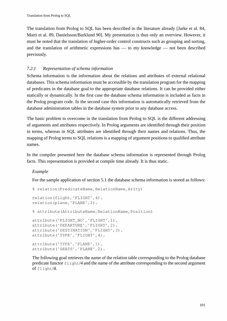
Translation from Prolog to SQL
101
The translation from Prolog to SQL has been described in the literature already [Jarke et al. 84,
Marti et al. 89, Danielsson/Barklund 90]. My presentation is thus only an overview. However, it
must be noted that the translation of higher-order control constructs such as grouping and sorting,
and the translation of arithmetic expressions has — to my knowledge — not been described
previously.
7.2.1 Representation of schema information
Schema information is the information about the relations and attributes of external relational
databases. This schema information must be accessible by the translation program for the mapping
of predicates in the database goal to the appropriate database relations. It can be provided either
statically or dynamically. In the first case the database schema information is included as facts in
the Prolog program code. In the second case this information is automatically retrieved from the
database administration tables in the database system prior to any database access.
The basic problem to overcome in the translation from Prolog to SQL is the different addressing
of arguments and attributes respectively. In Prolog arguments are identified through their position
in terms, whereas in SQL attributes are identified through their names and relations. Thus, the
mapping of Prolog terms to SQL relations is a mapping of argument positions to qualified attribute
names.
In the compiler presented here the database schema information is represented through Prolog
facts. This representation is provided at compile time already. It is thus static.
Example
For the sample application of section 5.1 the database schema information is stored as follows:
% relation(PredicateName,RelationName,Arity)
relation(flight,’FLIGHT’,4).relation(plane,’PLANE’,2).
% attribute(AttributeName,RelationName,Position)
attribute(’FLIGHT_NO’,’FLIGHT’,1).attribute(’DEPARTURE’,’FLIGHT’,2).attribute(’DESTINATION’,’FLIGHT’,3).attribute(’TYPE’,’FLIGHT’,4).
attribute(’TYPE’,’PLANE’,1).attribute(’SEATS’,’PLANE’,2).
The following goal retrieves the name of the relation table corresponding to the Prolog databasepredicate functor flight/4 and the name of the attribute corresponding to the second argumentof flight/4.
7. Implementation of Database Set Predicates
102
?- relation(flight,Table,_),attribute(Table,Attribute,2).
Table = ’FLIGHT’Attribute = ’DEPARTURE’
♦
Note that type information could be included in the schema description in an additional argument.
Such type information can only be used to check already during the translation whether a constant
argument complies with the type of the corresponding database attribute. For the retrieval from the
database such type information cannot be utilized because Prolog is an untyped language.
Example
Type information can be stored along with the attribute descriptions in attribute/4:
attribute(’FLIGHT_NO’,’FLIGHT’,1,’CHAR(5)’).
♦
With typed logic languages, e.g. Gödel [Hill/Lloyd 91], type information could and should be
exploited to facilitate detecting errors as soon as possible.
7.2.2 Translation of database access requests
In database set predicates implemented in Prolog and accessing relational databases, the database
access language is a restricted sublanguage of Prolog equivalent in expressive power to relational
calculus.
A database access request consists of a projection term and a database goal.
• A projection term is a term. Each variable in the projection term must also occur in the
database goal.
Note that the projection term may be an arbitrarily complex term.
The database goal expresses the query to be evaluated by the database system. For relational
databases, the operators union, intersection, difference, selection and join must be expressed
through the database goal.
• A database goal contains positive or negative literals L1,…,Ln, n ≥ 1, connected through the
logical connectives “,” and “;” such that
- Li is a database predicate, a comparison operation, or an arithmetic or aggregate function,
- at least one Li is a positive database predicate,
- all input arguments of functions are bound,
- all arguments of comparison operations are bound.
The functor of a database predicate is mapped to the appropriate relation table name, and each of
the predicate arguments is assigned a relation attribute. The comparison operations in the database
goal must be expressible in SQL. This is true for the standard comparison operations >, <, =, etc.
Translation from Prolog to SQL
103
The allowed functors for aggregate functions are sum, avg, min, max, and count. Arithmetic
functions are written using the functor is/2 in infix position as in X is ArithmeticExpression
with ArithmeticExpression an evaluable arithmetic expression. Again, all arithmetic
functions used in the database goal must be expressible in SQL.
Due to the order of execution imposed by the Prolog control strategy a complex database goal has
as the first subgoal at least one call to a positive database predicate to return bindings for the
variable arguments, followed by negated goals, comparison operations, or functions.
SQL queries
Recall from section 2.1.2 that an SQL query consists of at least a SELECT and a FROM part, with
optional WHERE, GROUP BY, and ORDER BY parts. The keyword DISTINCT, which is used to
eliminate duplicate entries in the result relation, is also optional. Optional parts are enclosed in
curly brackets in the following simplified SQL grammar.
SELECT {DISTINCT} <columnlist>FROM <tablelist>{WHERE <conditionlist>}{GROUP BY <columnlist>}{ORDER BY <columnlist>}
<tablelist> is a list of relation table names with range variables, <columnlist> a list of
constants or relation attributes qualified through relation names or range variables which uniquely
identify a relation, and <conditionlist> a list of comparison operations or subqueries. The
items in <tablelist> and <columnlist> are separated by commas, whereas the logical
connectives ∧ and ∨ , written as AND and OR, are used in <conditionlist>.
Translation of database access requests to SQL queries
The translation of database access requests to SQL queries is done according to the following
informal translation rules.
• A conjunction of database goals is translated to a single SQL query.
• Disjunctions of database goals are translated to several SQL queries connected through the
UNION operator.
• Negated database goals are translated to negated existential subqueries (NOT EXISTS
<subquery>) in the WHERE part.
• Goal functors other than comparison operators and function symbols are translated to
relation names and assigned a unique identifier (range variable) in the FROM part of the
query.
• Comparison operations and functions are translated to the equivalent SQL comparisons and
functions over relation attributes or constant values.
7. Implementation of Database Set Predicates
104
• Variables in the projection term are translated to attribute names in the SELECT part of the
query. These attributes are qualified by range variables. Variables occurring only once in the
database goal are not translated.
• Shared variables, i.e. variables occurring in at least two base calls in the database goal, are
translated to join-conditions in the WHERE part.
• Constant values in the database goal translate to comparison operations of the appropriate
qualified relation attribute and the constant value in the WHERE part.
• Constants in the projection term are not translated.
Translation of higher-order constructs
Depending on the database set predicate additional rules may be used. For example, db_setof/3
returns a result relation for each binding of the free variables in the database goal, duplicates are
eliminated from the result relation, and the result relation is sorted. This requires the use of a
GROUP BY and an ORDER BY part in the query.
• Free variables, i.e. variables occurring only in the database goal, are translated to qualified
attributes in the GROUP BY part.
• Free variables and the variables occurring in the projection term are translated to qualified
attributes in the ORDER BY part. The order in which the free variables and the projection
term variables occur determines the order according to which the result relation is sorted.
• The keyword DISTINCT is added to the SELECT part of the query.
With these rules, the translation of higher-order constructs to SQL is achieved.
Translation of aggregate functions
Aggregate functions may only appear in the SELECT part of an SQL query. In database set
predicates this is expressed by a projection term which contains a variable to hold the result of the
aggregate function, and a database goal with the aggregate function represented through a ternary
term, the functor of which is one of min, max, avg, count, sum (see section 6.3.5 for an example).
The translation of aggregate functions is as follows:
• Aggregate functions, written as relations in the database goal, are translated to the
corresponding aggregate functions in the SELECT part.
Optimization
In general, query optimization is left to the query optimizer of the database management system.
However, one specific optimization is applicable during the translation already.
• Disjunctions of simple database goals need not always be translated to separate queries
interconnected through UNION.
If the disjunction concerns only comparison operations, then these comparison operations
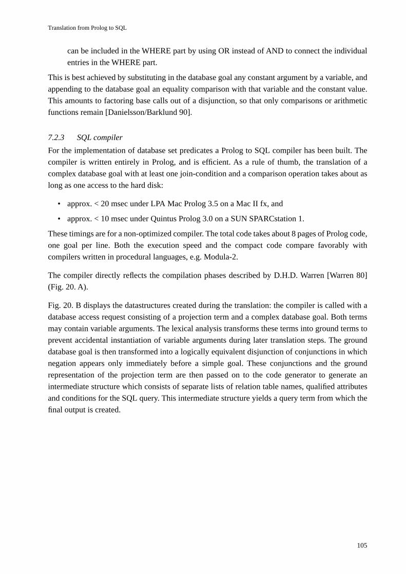
Translation from Prolog to SQL
105
can be included in the WHERE part by using OR instead of AND to connect the individual
entries in the WHERE part.
This is best achieved by substituting in the database goal any constant argument by a variable, and
appending to the database goal an equality comparison with that variable and the constant value.
This amounts to factoring base calls out of a disjunction, so that only comparisons or arithmetic
functions remain [Danielsson/Barklund 90].
7.2.3 SQL compiler
For the implementation of database set predicates a Prolog to SQL compiler has been built. The
compiler is written entirely in Prolog, and is efficient. As a rule of thumb, the translation of a
complex database goal with at least one join-condition and a comparison operation takes about as
long as one access to the hard disk:
• approx. < 20 msec under LPA Mac Prolog 3.5 on a Mac II fx, and
• approx. < 10 msec under Quintus Prolog 3.0 on a SUN SPARCstation 1.
These timings are for a non-optimized compiler. The total code takes about 8 pages of Prolog code,
one goal per line. Both the execution speed and the compact code compare favorably with
compilers written in procedural languages, e.g. Modula-2.
The compiler directly reflects the compilation phases described by D.H.D. Warren [Warren 80]
(Fig. 20. A).
Fig. 20. B displays the datastructures created during the translation: the compiler is called with a
database access request consisting of a projection term and a complex database goal. Both terms
may contain variable arguments. The lexical analysis transforms these terms into ground terms to
prevent accidental instantiation of variable arguments during later translation steps. The ground
database goal is then transformed into a logically equivalent disjunction of conjunctions in which
negation appears only immediately before a simple goal. These conjunctions and the ground
representation of the projection term are then passed on to the code generator to generate an
intermediate structure which consists of separate lists of relation table names, qualified attributes
and conditions for the SQL query. This intermediate structure yields a query term from which the
final output is created.
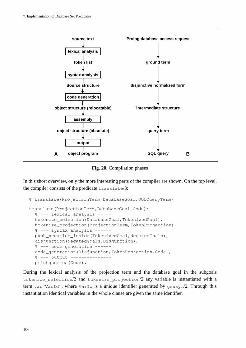
7. Implementation of Database Set Predicates
106
In this short overview, only the more interesting parts of the compiler are shown. On the top level,
the compiler consists of the predicate translate/3:
% translate(ProjectionTerm,DatabaseGoal,SQLQueryTerm)
translate(ProjectionTerm,DatabaseGoal,Code):-% --- lexical analysis -----tokenize_selection(DatabaseGoal,TokenizedGoal),tokenize_projection(ProjectionTerm,TokenProjection),% --- syntax analysis ------push_negation_inside(TokenizedGoal,NegatedGoals),disjunction(NegatedGoals,Disjunction),% --- code generation ------code_generation(Disjunction,TokenProjection,Code),% --- output ---------------printqueries(Code).
During the lexical analysis of the projection term and the database goal in the subgoals
tokenize_selection/2 and tokenize_projection/2 any variable is instantiated with a
term var(VarId), where VarId is a unique identifier generated by gensym/2. Through this
instantiation identical variables in the whole clause are given the same identifier.
source text
lexical analysis
Token list
syntax analysis
Source structure
code generation
object structure (relocatable)
assembly
object structure (absolute)
output
object program
Prolog database access request
ground term
disjunctive normalized form
SQL query
intermediate structure
Fig. 20. Compilation phases
A B
query term
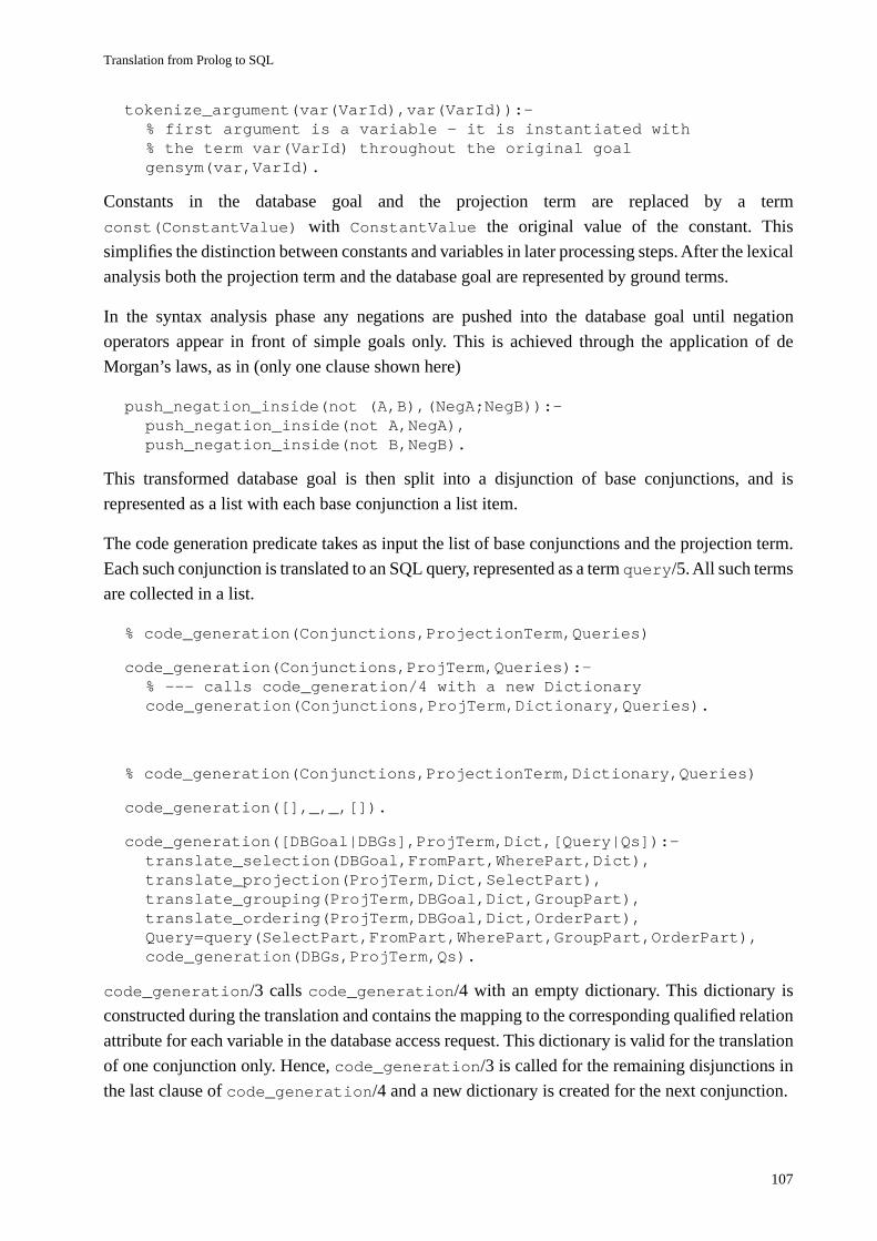
Translation from Prolog to SQL
107
tokenize_argument(var(VarId),var(VarId)):-% first argument is a variable - it is instantiated with% the term var(VarId) throughout the original goalgensym(var,VarId).
Constants in the database goal and the projection term are replaced by a term
const(ConstantValue) with ConstantValue the original value of the constant. This
simplifies the distinction between constants and variables in later processing steps. After the lexical
analysis both the projection term and the database goal are represented by ground terms.
In the syntax analysis phase any negations are pushed into the database goal until negation
operators appear in front of simple goals only. This is achieved through the application of de
Morgan’s laws, as in (only one clause shown here)
push_negation_inside(not (A,B),(NegA;NegB)):-push_negation_inside(not A,NegA),push_negation_inside(not B,NegB).
This transformed database goal is then split into a disjunction of base conjunctions, and is
represented as a list with each base conjunction a list item.
The code generation predicate takes as input the list of base conjunctions and the projection term.
Each such conjunction is translated to an SQL query, represented as a term query/5. All such terms
are collected in a list.
% code_generation(Conjunctions,ProjectionTerm,Queries)
code_generation(Conjunctions,ProjTerm,Queries):-% --- calls code_generation/4 with a new Dictionarycode_generation(Conjunctions,ProjTerm,Dictionary,Queries).
% code_generation(Conjunctions,ProjectionTerm,Dictionary,Queries)
code_generation([],_,_,[]).
code_generation([DBGoal|DBGs],ProjTerm,Dict,[Query|Qs]):-translate_selection(DBGoal,FromPart,WherePart,Dict),translate_projection(ProjTerm,Dict,SelectPart),translate_grouping(ProjTerm,DBGoal,Dict,GroupPart),translate_ordering(ProjTerm,DBGoal,Dict,OrderPart),Query=query(SelectPart,FromPart,WherePart,GroupPart,OrderPart),code_generation(DBGs,ProjTerm,Qs).
code_generation/3 calls code_generation/4 with an empty dictionary. This dictionary is
constructed during the translation and contains the mapping to the corresponding qualified relation
attribute for each variable in the database access request. This dictionary is valid for the translation
of one conjunction only. Hence, code_generation/3 is called for the remaining disjunctions in
the last clause of code_generation/4 and a new dictionary is created for the next conjunction.
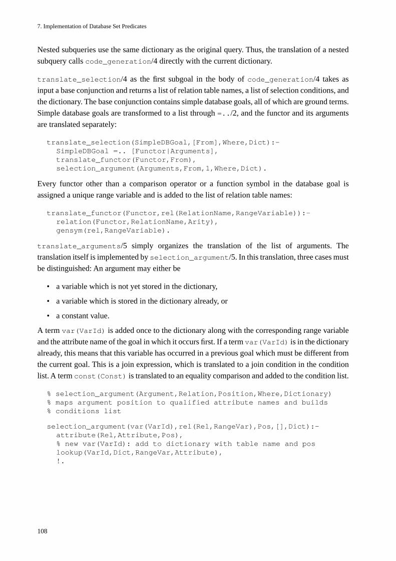
7. Implementation of Database Set Predicates
108
Nested subqueries use the same dictionary as the original query. Thus, the translation of a nested
subquery calls code_generation/4 directly with the current dictionary.
translate_selection/4 as the first subgoal in the body of code_generation/4 takes as
input a base conjunction and returns a list of relation table names, a list of selection conditions, and
the dictionary. The base conjunction contains simple database goals, all of which are ground terms.
Simple database goals are transformed to a list through =../2, and the functor and its arguments
are translated separately:
translate_selection(SimpleDBGoal,[From],Where,Dict):-SimpleDBGoal =.. [Functor|Arguments],translate_functor(Functor,From),selection_argument(Arguments,From,1,Where,Dict).
Every functor other than a comparison operator or a function symbol in the database goal is
assigned a unique range variable and is added to the list of relation table names:
translate_functor(Functor,rel(RelationName,RangeVariable)):-relation(Functor,RelationName,Arity),gensym(rel,RangeVariable).
translate_arguments/5 simply organizes the translation of the list of arguments. The
translation itself is implemented by selection_argument/5. In this translation, three cases must
be distinguished: An argument may either be
• a variable which is not yet stored in the dictionary,
• a variable which is stored in the dictionary already, or
• a constant value.
A term var(VarId) is added once to the dictionary along with the corresponding range variable
and the attribute name of the goal in which it occurs first. If a term var(VarId) is in the dictionary
already, this means that this variable has occurred in a previous goal which must be different from
the current goal. This is a join expression, which is translated to a join condition in the condition
list. A term const(Const) is translated to an equality comparison and added to the condition list.
% selection_argument(Argument,Relation,Position,Where,Dictionary)% maps argument position to qualified attribute names and builds% conditions list
selection_argument(var(VarId),rel(Rel,RangeVar),Pos,[],Dict):-attribute(Rel,Attribute,Pos),% new var(VarId): add to dictionary with table name and poslookup(VarId,Dict,RangeVar,Attribute),!.
Translation from Prolog to SQL
109
selection_argument(var(VarId),rel(Rel,RangeVar),Pos,JoinCond,Dict):-% var(VarId) in dictionary already: equality test in WHERE partlookup(VarId,Dict,PrevRangeVar,PrevAtt),PrevRangeVar \= RangeVar,attribute(Rel,Attribute,Pos),JoinCond = [comp(att(RangeVar,Attribute),=,att(PrevRangeVar,PrevAtt))].
selection_argument(const(Const),rel(Rel,RangeVar),Pos,CompOp,Dict):-% translate to test: attribute = constant valueattribute(Rel,Attribute,Pos),CompOp = [comp(att(RangeVar,Attribute),=,const(Const))].
The translation of comparison operations and arithmetic functions follows the translation of simple
database goals. The main difference is that the operands may be evaluable expressions instead of
simply variables or constant values. Such evaluable expressions, which may contain variables, are
not evaluated by Prolog. Instead, they are translated to SQL evaluable expressions with the
variables replaced by relation attributes.
The projection term is translated by translate_projection/3. The input arguments are ground
representation of the projection term and the dictionary. The result is a list of qualified attribute
names in a list in the argument SelectPart. The projection term may only contain variables
which also occur in the database goal too. Because the database goal is translated prior to the
projection term, and because the dictionary contains all variables occurring positively in the
database goal, the mapping of all variables occurring in the projection term is already contained in
the dictionary. The translation of the projection term is thus straightforward: constant values are
added to the list unchanged, and variables are substituted by qualified attribute names.
translate_projection(ProjectionTerm,Dictionary,SelectList):-ProjectionTerm =.. [Functor|Arguments],projection_arguments(Arguments,SelectList,Dictionary).
projection_arguments/3 organizes the translation of projection term arguments by working
through the list of arguments recursively. The translation itself is performed by
projection_argument/3.
projection_argument(var(VarId),att(RangeVar,Attribute),Dict):-lookup(VarId,Dictionary,RangeVar,Attribute).
projection_argument(const(Const),const(Const),_).
For the GROUP BY and the ORDER BY part of the final query the free variables in the database goal
must be handled. This is done in translate_grouping/4 and translate_ordering/4.
Unfortunately SQL places severe restrictions on the use of groupings. Only such attributes may be
included in the SELECT part of a grouped query that have a single value for each grouping attribute.
This effectively restricts the use of grouping to aggregate functions which compute one single
value for a grouped attribute.
7. Implementation of Database Set Predicates
110
In the last two subgoals of code_generation/4 the query term for the current conjunction of
database goals is constructed, and the recursive call to code_generation/3 continues the
computation with the next conjunction of goals.
7.2.4 Comprehensive Example
The database request is:
“Retrieve from the database the departures and destinations connected by flights with largeplanes, i.e. planes with more than 150 seats. Print the departures, destinations, planes and therespective number of seats in alphabetical order”.
With database set predicates, this request is written as:
?- db_setof((Departure,Destination,Plane,Seats),FlightNo^(flight(FlightNo,Departure,Destination,Plane), plane(Plane,Seats), Seats > Bound),
List).
Although Bound is a variable, it must be bound to a constant value, in this case 150, prior to the
call of the database set predicate. Otherwise the comparison operation would have an unbound
operand.
The projection term is
(Departure,Destination,Plane,Seats)
and the database goal is
FlightNo^(flight(FlightNo,Departure,Destination,Plane), plane(Plane,Seats), Seats > 150)
The projection term and the database goal are translated to the following ground representation by
the lexical analysis:
(var(var1),var(var2),var(var3),var(var4))
and
var(var0)^(flight(var(var0),var(var(1),var(var2),var(var3)), plane(var(var3),var(var4)), var(var4) > const(150))
The syntax analysis leaves the ground representation of the database goal unchanged because it
does not contain disjunction or negation. The list of base conjunctions thus contains only one entry,
namely the database goal.
Realization of the communication channel and its interfaces
111
The ground representations of the projection term and the database goal serve as input to
code_generation/3. The result of the code generation is a list containing only one query term
with five list arguments (for the SELECT, FROM, WHERE, GROUP BY and ORDER BY part of
the final query). f and p are range variables which uniquely identify the relation tables flight
and plane.
[query( [att(f,departure),att(f,destination),att(f,plane),att(p,seats)], [rel(flight,f),rel(plane,p)], [comp(att(f,plane),=,att(p,type)),comp(att(p,seats),>,const(150)], [], [att(f,departure),att(f,destination),att(f,plane),att(p,seats)])]
The final output of the compiler is the following SQL query:
SELECT DISTINCT f.departure,f.destination,f.plane,p.seatsFROM flight f, plane pWHERE f.plane = p.type and p.seats > 150ORDER BY f.departure,f.destination,f.plane,p.seats
Any instantiation of a template variable would lead to a more restrictive query. With Departure
bound to the constant zurich, the query would be
SELECT DISTINCT zurich,f.destination,f.plane,p.seatsFROM flight f, plane pWHERE f.departure = "zurich" and f.plane = p.type and p.seats > 150ORDER BY zurich,f.destination,f.plane,p.seats
♦
7.3 Realization of the communication channel and its interfaces
In a physically loosely coupled system a Prolog system is connected to an external database system
via a communication channel. This communication channel can be realized through either
• procedure calls or
• inter-process communication
Ideally, the communication channel is completely hidden from the Prolog system, and only Prolog
datastructures are written into or read from the communication channel. For database set predicates
this would mean that the subgoal evaluate_in_db/2 writes a term into the communication
channel, and retrieves a list of instantiated terms from the channel. In practice, however, database
systems do not offer a direct interface to Prolog (or to declarative languages in general), and thus
the communication channel has to be programmed explicitly.
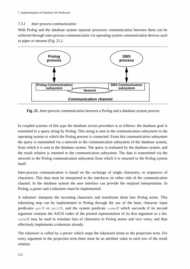
7. Implementation of Database Set Predicates
112
7.3.1 Inter-process communication
With Prolog and the database system separate processes communication between them can be
achieved through inter-process communication via operating system communication devices such
as pipes or streams (Fig. 21.).
In coupled systems of this type the database access procedure is as follows: the database goal is
translated to a query string by Prolog. This string is sent to the communication subsystem in the
operating system to which the Prolog process is connected. From this communication subsystem
the query is transmitted via a network to the communication subsystem of the database system,
from which it is sent to the database system. The query is evaluated by the database system, and
the result relation is returned to the communication subsystem. The data is transmitted via the
network to the Prolog communication subsystem from which it is returned to the Prolog system
itself.
Inter-process communication is based on the exchange of single characters, or sequences of
characters. This data must be interpreted in the interfaces on either side of the communication
channel. In the database system the user interface can provide the required interpretation. In
Prolog, a parser and a tokenizer must be implemented.
A tokenizer interprets the incoming characters and transforms them into Prolog terms. This
tokenizing step can be implemented in Prolog through the use of the basic character input
predicates get/1 or get0/1, and the system predicate name/2 which succeeds if its second
argument contains the ASCII codes of the printed representation of its first argument in a list.
name/2 may be used to translate lists of characters to Prolog atoms and vice versa, and thus
effectively implements a tokenizer already.
The tokenizer is called by a parser which maps the tokenized terms to the projection term. For
every argument in the projection term there must be an attribute value in each row of the result
relation.
Prolog DBS
Communication channel
Fig. 21. Inter-process communication between a Prolog and a database system process
processprocess
Network
Prolog Communicationsubsystem
DBS Communicationsubsystem
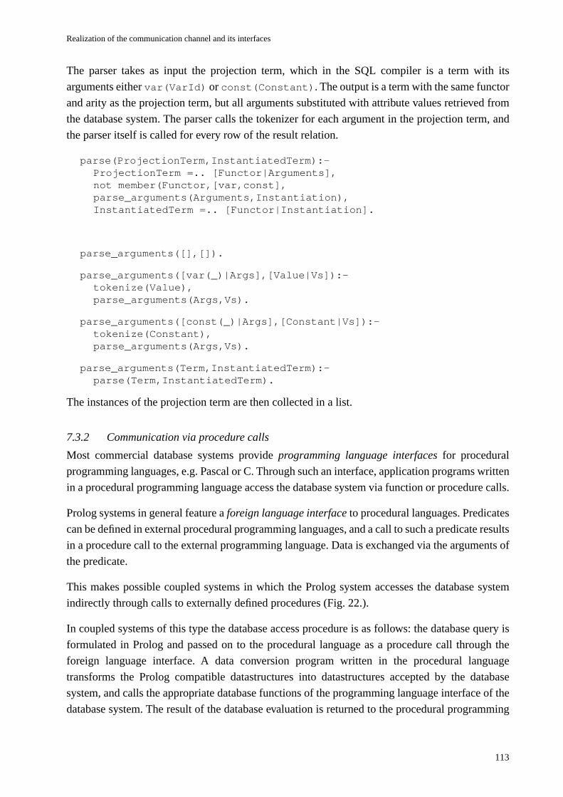
Realization of the communication channel and its interfaces
113
The parser takes as input the projection term, which in the SQL compiler is a term with its
arguments either var(VarId) or const(Constant). The output is a term with the same functor
and arity as the projection term, but all arguments substituted with attribute values retrieved from
the database system. The parser calls the tokenizer for each argument in the projection term, and
the parser itself is called for every row of the result relation.
parse(ProjectionTerm,InstantiatedTerm):-ProjectionTerm =.. [Functor|Arguments],not member(Functor,[var,const],parse_arguments(Arguments,Instantiation),InstantiatedTerm =.. [Functor|Instantiation].
parse_arguments([],[]).
parse_arguments([var(_)|Args],[Value|Vs]):-tokenize(Value),parse_arguments(Args,Vs).
parse_arguments([const(_)|Args],[Constant|Vs]):-tokenize(Constant),parse_arguments(Args,Vs).
parse_arguments(Term,InstantiatedTerm):-parse(Term,InstantiatedTerm).
The instances of the projection term are then collected in a list.
7.3.2 Communication via procedure calls
Most commercial database systems provide programming language interfaces for procedural
programming languages, e.g. Pascal or C. Through such an interface, application programs written
in a procedural programming language access the database system via function or procedure calls.
Prolog systems in general feature a foreign language interface to procedural languages. Predicates
can be defined in external procedural programming languages, and a call to such a predicate results
in a procedure call to the external programming language. Data is exchanged via the arguments of
the predicate.
This makes possible coupled systems in which the Prolog system accesses the database system
indirectly through calls to externally defined procedures (Fig. 22.).
In coupled systems of this type the database access procedure is as follows: the database query is
formulated in Prolog and passed on to the procedural language as a procedure call through the
foreign language interface. A data conversion program written in the procedural language
transforms the Prolog compatible datastructures into datastructures accepted by the database
system, and calls the appropriate database functions of the programming language interface of the
database system. The result of the database evaluation is returned to the procedural programming
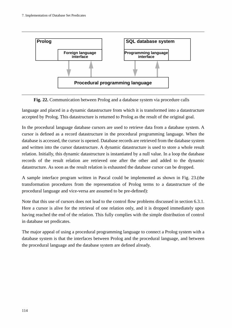
7. Implementation of Database Set Predicates
114
language and placed in a dynamic datastructure from which it is transformed into a datastructure
accepted by Prolog. This datastructure is returned to Prolog as the result of the original goal.
In the procedural language database cursors are used to retrieve data from a database system. A
cursor is defined as a record datastructure in the procedural programming language. When the
database is accessed, the cursor is opened. Database records are retrieved from the database system
and written into the cursor datastructure. A dynamic datastructure is used to store a whole result
relation. Initially, this dynamic datastructure is instantiated by a null value. In a loop the database
records of the result relation are retrieved one after the other and added to the dynamic
datastructure. As soon as the result relation is exhausted the database cursor can be dropped.
A sample interface program written in Pascal could be implemented as shown in Fig. 23.(the
transformation procedures from the representation of Prolog terms to a datastructure of the
procedural language and vice-versa are assumed to be pre-defined):
Note that this use of cursors does not lead to the control flow problems discussed in section 6.3.1.
Here a cursor is alive for the retrieval of one relation only, and it is dropped immediately upon
having reached the end of the relation. This fully complies with the simple distribution of control
in database set predicates.
The major appeal of using a procedural programming language to connect a Prolog system with a
database system is that the interfaces between Prolog and the procedural language, and between
the procedural language and the database system are defined already.
Foreign language Programming languageinterfaceinterface
Prolog SQL database system
Procedural programming language
Fig. 22. Communication between Prolog and a database system via procedure calls
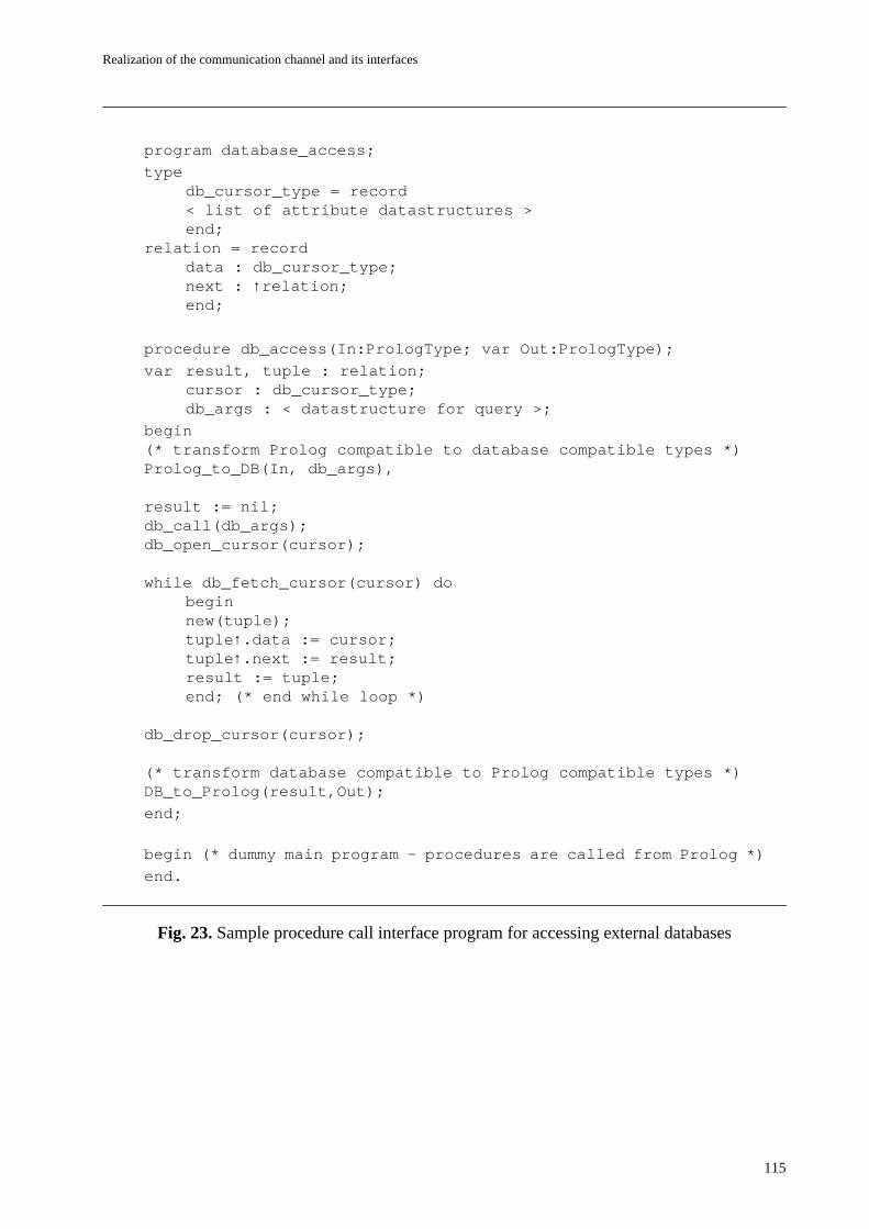
Realization of the communication channel and its interfaces
115
program database_access;
typedb_cursor_type = record < list of attribute datastructures > end;
relation = recorddata : db_cursor_type;next : ↑relation;end;
procedure db_access(In:PrologType; var Out:PrologType);
var result, tuple : relation;cursor : db_cursor_type;db_args : < datastructure for query >;
begin(* transform Prolog compatible to database compatible types *)Prolog_to_DB(In, db_args),
result := nil;db_call(db_args);db_open_cursor(cursor);
while db_fetch_cursor(cursor) dobeginnew(tuple);tuple↑.data := cursor;tuple↑.next := result;result := tuple;end; (* end while loop *)
db_drop_cursor(cursor);
(* transform database compatible to Prolog compatible types *)DB_to_Prolog(result,Out);
end;
begin (* dummy main program - procedures are called from Prolog *)
end.
Fig. 23. Sample procedure call interface program for accessing external databases
7. Implementation of Database Set Predicates
116
7.3.3 Comparison of methods
Communication via procedure calls and inter-process communication are two fundamentally
different concepts.
• With communication via procedure calls the coupled system effectively is a single operating
system process, whereas with inter-process communication there are several operating system
processes which may run in parallel. Potentially, even a distributed coupled system is
implementable by having the processes run on different machines.
• With communication via procedure calls, the level of data exchange is that of Prolog terms,
whereas with inter-process communication data is exchanged on the level of character
sequences which must be interpreted.
Data conversion
The problem of data conversion between Prolog and database data formats occurs independently
of the approach to communication.
Prolog systems generally are tagged architectures. A small fragment of the memory allocated for
a data item contains a tag with type information, the rest is used for the value itself. In database
systems, type information is held in the schema, and the full width of a machine word can be used
for the representation of a value. This difference in the number of bits available in the database
system and Prolog leads to different value ranges, and to different precisions in the computation of
real or floating point numbers. The range of values must thus be restricted to the largest common
range of values.
A second problem is that some datastructures of the one system are not known in the other. For
example, SQL features a multitude of different number formats, whereas most Prolog systems only
distinguish between floating point numbers and integers. Consequently, some datastructures may
not be adequately represented, or different datastructures of the database system are represented
through identical datastructures in Prolog.
These problems are common to both types of communication. With a procedure call interface they
are perhaps more severe because there is an additional data conversion step in the procedural
language. Clearly, this additional interface increases the likelihood of data conversion problems.
Efficiency and flexibility
Efficiency and flexibility are dependent on the approach to communication. With inter-process
communication the amount of data handled is larger by approximately an order of magnitude than
with procedure calls because sequences of individual characters are considered instead of high-
level terms. The interpretation of data is performed on both sides of the communication channel,
but for this efficient built-in conversion mechanisms can be used.
With procedure calls three conversions are necessary: from the internal representation of the
database system to an appropriate datastructure in the procedural language, from this
representation to one suitable for Prolog, and from this representation in the procedural language
Realization of the communication channel and its interfaces
117
to true Prolog terms. The first and the last data conversion is provided by the programming
language interface in the database system and the foreign language interface in Prolog respectively.
However, the transformation of database system compatible datastructures to those accepted by
Prolog (and vice versa) must be programmed explicitly.
The major difference between the two approaches is that database access through procedure calls
must be defined statically at compile time already whereas with inter-process communication
database access is defined dynamically at runtime.
In a procedural language a record datastructure serves to capture the data retrieved by the database
cursor. This record datastructure is defined statically as part of the program. As a consequence, a
different cursor type definition is necessary for every different projection on database relation
tables. Using a procedural language as an interface to the database system thus makes sense when
the projection on database attributes is known at compile time already. This is not the case with
database set predicates, because both the projection term and the database goal are constructed
dynamically. Hence, communicating via procedure calls severely restricts the dynamic query
formulation capacities of database set predicates.
This problem is further aggravated by the fact that the datastructures used in the foreign language
interface in the Prolog system and those of the programming language interface in the database
system are highly system dependent and thus in the general case not portable.
With inter-process communication, a parser combines the tokenized input from the database
system to complex terms which are instantiations of the projection term with database values.
Because term construction can be done dynamically, constructing different terms in which the
database values are stored is possible at runtime. However, parser and tokenizer must be defined
statically or be provided by the Prolog runtime system.
Conclusion
The dichotomy between procedure call and inter-process communication can be expressed in terms
of dependencies: system implementation dependency vs. operating system dependency.
For every combination of a Prolog system and a database system implementation the procedure call
interface has to be defined anew. Currently, there is neither a standard for a programming language
interface for relational database systems, nor for foreign language interfaces in Prolog systems.
Porting a database set predicate implementation to a different configuration of a Prolog and a
database system thus implies considerable implementation effort and may even require
modifications in the application program because of the static database access definition.
With inter-process communication the presence of operating system communication devices
determines whether a particular implementation of database set predicates can be ported to other
machines. The Prolog and the database system do not communicate with each other directly, but
only with the interface to the operating system communication devices. Thus, replacing one
database system for another one has no effects on the Prolog system (modifications, if any, are

118
restricted to the parser and tokenizer which must parse the data retrieved from the database
system).
119
8
A Real-World Application: Synthesis Planning with DedChem
8.1 Introduction
I now present a real-world problem which is handled elegantly with a coupled system based on
database set predicates. The application domain is organic chemistry, and the task is that of
planning the synthesis of a specific substance class on the basis of name reactions. A synthesis plan
contains the reactions that are necessary to synthesize a given substance, the order in which the
individual reactions must be performed, and the intermediate substances which are synthesized as
by-products during the synthesis.
Synthesis planning corresponds to computing the transitive closure of a reaction relation under
application dependent constraints. The synthesis plan itself may be represented as a tree structure,
with the nodes standing for intermediate substances, and the edges standing for reactions.
A coupled system based on Prolog provides the required expressive power for the representation
of the reaction relation, the synthesis plan, and for the implementation of the deduction component
to compute the transitive closure. The ease of implementation in a single high-level logic language
implies a logically tightly coupled system. Practical constraints, e.g. access to a variety of reaction
databases, demand a physically loosely coupled system.
8.1.1 Name reactions
Name reactions are reaction prototypes or reaction schemes which are so commonly used that they
are referred to by their name — often the name of the persons that discovered the reaction —
instead of the substance classes involved. Name reactions thus describe standardized reactions
which have proven to be useful in practice.
Name reactions abstract from concrete reactions in that they are defined for substance classes, not
individual substances. A name reaction thus produces a certain substance class, the product, from
one or two substance classes, the educts.
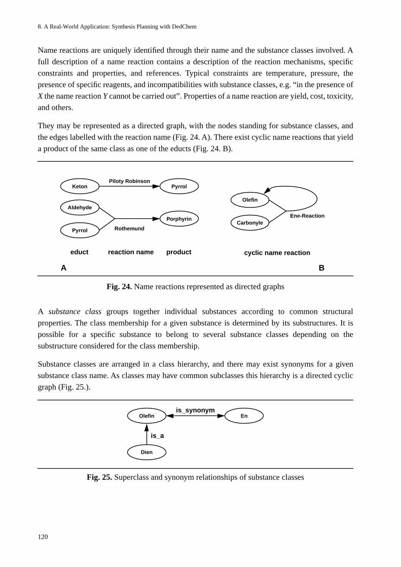
8. A Real-World Application: Synthesis Planning with DedChem
120
Name reactions are uniquely identified through their name and the substance classes involved. A
full description of a name reaction contains a description of the reaction mechanisms, specific
constraints and properties, and references. Typical constraints are temperature, pressure, the
presence of specific reagents, and incompatibilities with substance classes, e.g. “in the presence of
X the name reaction Y cannot be carried out”. Properties of a name reaction are yield, cost, toxicity,
and others.
They may be represented as a directed graph, with the nodes standing for substance classes, and
the edges labelled with the reaction name (Fig. 24. A). There exist cyclic name reactions that yield
a product of the same class as one of the educts (Fig. 24. B).
A substance class groups together individual substances according to common structural
properties. The class membership for a given substance is determined by its substructures. It is
possible for a specific substance to belong to several substance classes depending on the
substructure considered for the class membership.
Substance classes are arranged in a class hierarchy, and there may exist synonyms for a given
substance class name. As classes may have common subclasses this hierarchy is a directed cyclic
graph (Fig. 25.).
Fig. 24. Name reactions represented as directed graphs
Piloty Robinson
Rothemund
educt reaction name product
Pyrrol
Ene-ReactionPorphyrin
Aldehyde
Keton Pyrrol
Carbonyle
Olefin
cyclic name reaction
A B
Fig. 25. Superclass and synonym relationships of substance classes
Dien
Olefin En
is_a
is_synonym
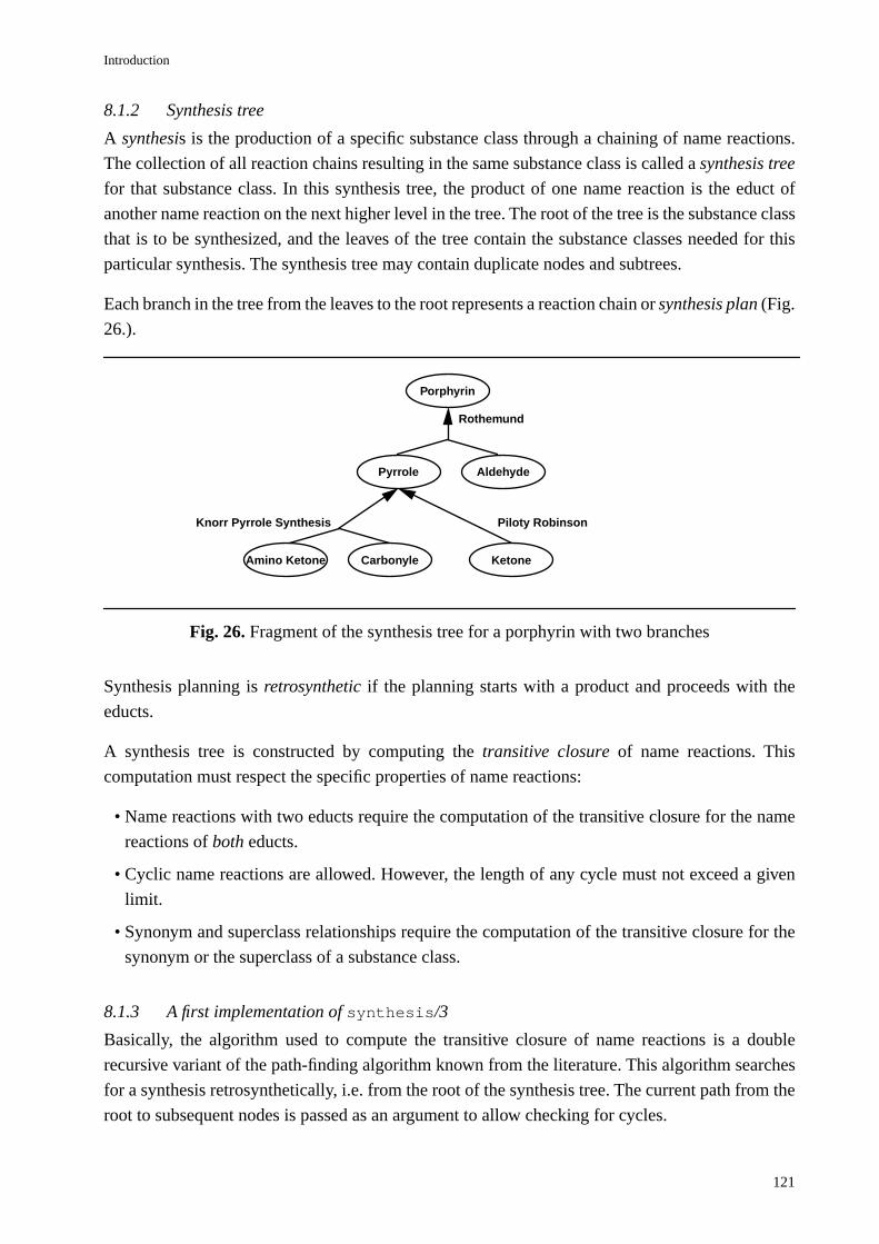
Introduction
121
8.1.2 Synthesis tree
A synthesis is the production of a specific substance class through a chaining of name reactions.
The collection of all reaction chains resulting in the same substance class is called a synthesis tree
for that substance class. In this synthesis tree, the product of one name reaction is the educt of
another name reaction on the next higher level in the tree. The root of the tree is the substance class
that is to be synthesized, and the leaves of the tree contain the substance classes needed for this
particular synthesis. The synthesis tree may contain duplicate nodes and subtrees.
Each branch in the tree from the leaves to the root represents a reaction chain or synthesis plan (Fig.
26.).
Synthesis planning is retrosynthetic if the planning starts with a product and proceeds with the
educts.
A synthesis tree is constructed by computing the transitive closure of name reactions. This
computation must respect the specific properties of name reactions:
• Name reactions with two educts require the computation of the transitive closure for the name
reactions of both educts.
• Cyclic name reactions are allowed. However, the length of any cycle must not exceed a given
limit.
• Synonym and superclass relationships require the computation of the transitive closure for the
synonym or the superclass of a substance class.
8.1.3 A first implementation of synthesis/3
Basically, the algorithm used to compute the transitive closure of name reactions is a double
recursive variant of the path-finding algorithm known from the literature. This algorithm searches
for a synthesis retrosynthetically, i.e. from the root of the synthesis tree. The current path from the
root to subsequent nodes is passed as an argument to allow checking for cycles.
Fig. 26. Fragment of the synthesis tree for a porphyrin with two branches
Piloty Robinson
Rothemund
Pyrrole
Porphyrin
Aldehyde
KetoneAmino Ketone Carbonyle
Knorr Pyrrole Synthesis
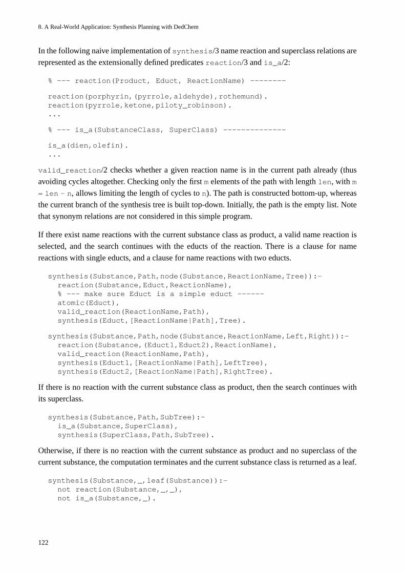
8. A Real-World Application: Synthesis Planning with DedChem
122
In the following naive implementation of synthesis/3 name reaction and superclass relations are
represented as the extensionally defined predicates reaction/3 and is_a/2:
% --- reaction(Product, Educt, ReactionName) --------
reaction(porphyrin,(pyrrole,aldehyde),rothemund).reaction(pyrrole,ketone,piloty_robinson)....
% --- is_a(SubstanceClass, SuperClass) --------------
is_a(dien,olefin)....
valid_reaction/2 checks whether a given reaction name is in the current path already (thus
avoiding cycles altogether. Checking only the first m elements of the path with length len, with m
= len - n, allows limiting the length of cycles to n). The path is constructed bottom-up, whereas
the current branch of the synthesis tree is built top-down. Initially, the path is the empty list. Note
that synonym relations are not considered in this simple program.
If there exist name reactions with the current substance class as product, a valid name reaction is
selected, and the search continues with the educts of the reaction. There is a clause for name
reactions with single educts, and a clause for name reactions with two educts.
synthesis(Substance,Path,node(Substance,ReactionName,Tree)):-reaction(Substance,Educt,ReactionName),% --- make sure Educt is a simple educt ------ atomic(Educt),valid_reaction(ReactionName,Path),synthesis(Educt,[ReactionName|Path],Tree).
synthesis(Substance,Path,node(Substance,ReactionName,Left,Right)):-reaction(Substance,(Educt1,Educt2),ReactionName),valid_reaction(ReactionName,Path),synthesis(Educt1,[ReactionName|Path],LeftTree),synthesis(Educt2,[ReactionName|Path],RightTree).
If there is no reaction with the current substance class as product, then the search continues with
its superclass.
synthesis(Substance,Path,SubTree):-is_a(Substance,SuperClass),synthesis(SuperClass,Path,SubTree).
Otherwise, if there is no reaction with the current substance as product and no superclass of the
current substance, the computation terminates and the current substance class is returned as a leaf.
synthesis(Substance,_,leaf(Substance)):-not reaction(Substance,_,_),not is_a(Substance,_).
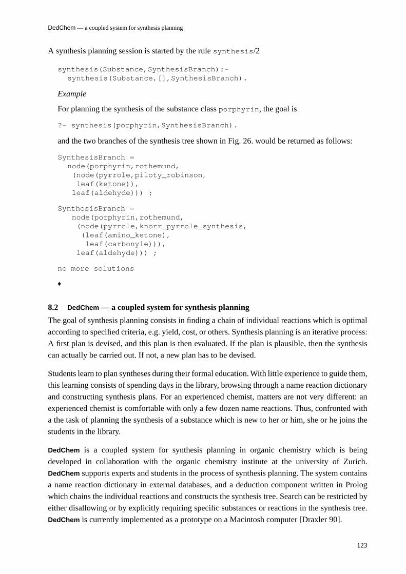
DedChem — a coupled system for synthesis planning
123
A synthesis planning session is started by the rule synthesis/2
synthesis(Substance,SynthesisBranch):-synthesis(Substance,[],SynthesisBranch).
Example
For planning the synthesis of the substance class porphyrin, the goal is
?- synthesis(porphyrin,SynthesisBranch).
and the two branches of the synthesis tree shown in Fig. 26. would be returned as follows:
SynthesisBranch = node(porphyrin,rothemund, (node(pyrrole,piloty_robinson, leaf(ketone)), leaf(aldehyde))) ;
SynthesisBranch = node(porphyrin,rothemund, (node(pyrrole,knorr_pyrrole_synthesis, (leaf(amino_ketone), leaf(carbonyle))), leaf(aldehyde))) ;
no more solutions
♦
8.2 DedChem — a coupled system for synthesis planning
The goal of synthesis planning consists in finding a chain of individual reactions which is optimal
according to specified criteria, e.g. yield, cost, or others. Synthesis planning is an iterative process:
A first plan is devised, and this plan is then evaluated. If the plan is plausible, then the synthesis
can actually be carried out. If not, a new plan has to be devised.
Students learn to plan syntheses during their formal education. With little experience to guide them,
this learning consists of spending days in the library, browsing through a name reaction dictionary
and constructing synthesis plans. For an experienced chemist, matters are not very different: an
experienced chemist is comfortable with only a few dozen name reactions. Thus, confronted with
a the task of planning the synthesis of a substance which is new to her or him, she or he joins the
students in the library.
DedChem is a coupled system for synthesis planning in organic chemistry which is being
developed in collaboration with the organic chemistry institute at the university of Zurich.
DedChem supports experts and students in the process of synthesis planning. The system contains
a name reaction dictionary in external databases, and a deduction component written in Prolog
which chains the individual reactions and constructs the synthesis tree. Search can be restricted by
either disallowing or by explicitly requiring specific substances or reactions in the synthesis tree.
DedChem is currently implemented as a prototype on a Macintosh computer [Draxler 90].
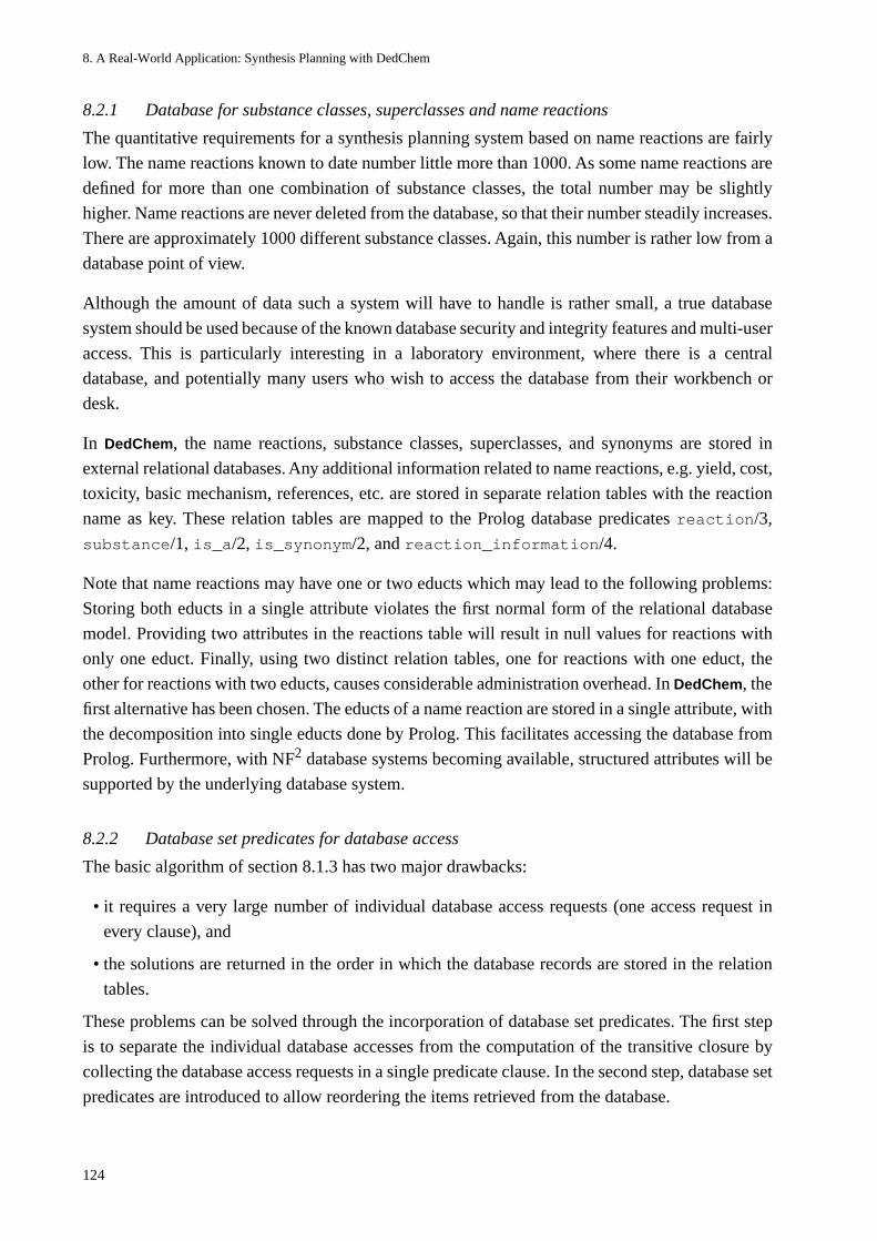
8. A Real-World Application: Synthesis Planning with DedChem
124
8.2.1 Database for substance classes, superclasses and name reactions
The quantitative requirements for a synthesis planning system based on name reactions are fairly
low. The name reactions known to date number little more than 1000. As some name reactions are
defined for more than one combination of substance classes, the total number may be slightly
higher. Name reactions are never deleted from the database, so that their number steadily increases.
There are approximately 1000 different substance classes. Again, this number is rather low from a
database point of view.
Although the amount of data such a system will have to handle is rather small, a true database
system should be used because of the known database security and integrity features and multi-user
access. This is particularly interesting in a laboratory environment, where there is a central
database, and potentially many users who wish to access the database from their workbench or
desk.
In DedChem, the name reactions, substance classes, superclasses, and synonyms are stored in
external relational databases. Any additional information related to name reactions, e.g. yield, cost,
toxicity, basic mechanism, references, etc. are stored in separate relation tables with the reaction
name as key. These relation tables are mapped to the Prolog database predicates reaction/3,
substance/1, is_a/2, is_synonym/2, and reaction_information/4.
Note that name reactions may have one or two educts which may lead to the following problems:
Storing both educts in a single attribute violates the first normal form of the relational database
model. Providing two attributes in the reactions table will result in null values for reactions with
only one educt. Finally, using two distinct relation tables, one for reactions with one educt, the
other for reactions with two educts, causes considerable administration overhead. In DedChem, the
first alternative has been chosen. The educts of a name reaction are stored in a single attribute, with
the decomposition into single educts done by Prolog. This facilitates accessing the database from
Prolog. Furthermore, with NF2 database systems becoming available, structured attributes will be
supported by the underlying database system.
8.2.2 Database set predicates for database access
The basic algorithm of section 8.1.3 has two major drawbacks:
• it requires a very large number of individual database access requests (one access request in
every clause), and
• the solutions are returned in the order in which the database records are stored in the relation
tables.
These problems can be solved through the incorporation of database set predicates. The first step
is to separate the individual database accesses from the computation of the transitive closure by
collecting the database access requests in a single predicate clause. In the second step, database set
predicates are introduced to allow reordering the items retrieved from the database.
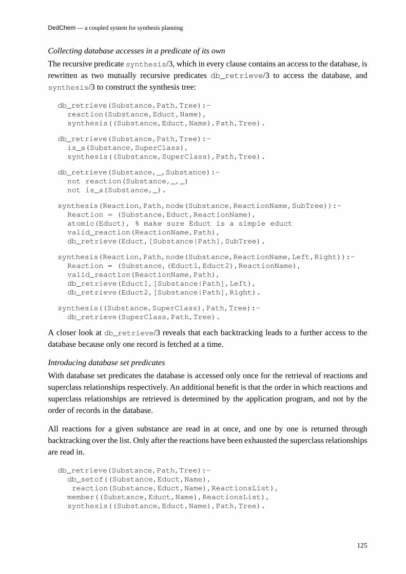
DedChem — a coupled system for synthesis planning
125
Collecting database accesses in a predicate of its own
The recursive predicate synthesis/3, which in every clause contains an access to the database, is
rewritten as two mutually recursive predicates db_retrieve/3 to access the database, and
synthesis/3 to construct the synthesis tree:
db_retrieve(Substance,Path,Tree):-reaction(Substance,Educt,Name),synthesis((Substance,Educt,Name),Path,Tree).
db_retrieve(Substance,Path,Tree):-is_a(Substance,SuperClass),synthesis((Substance,SuperClass),Path,Tree).
db_retrieve(Substance,_,Substance):-not reaction(Substance,_,_)not is_a(Substance,_).
synthesis(Reaction,Path,node(Substance,ReactionName,SubTree)):-Reaction = (Substance,Educt,ReactionName),atomic(Educt), % make sure Educt is a simple eductvalid_reaction(ReactionName,Path),db_retrieve(Educt,[Substance|Path],SubTree).
synthesis(Reaction,Path,node(Substance,ReactionName,Left,Right)):-Reaction = (Substance,(Educt1,Educt2),ReactionName),valid_reaction(ReactionName,Path),db_retrieve(Educt1,[Substance|Path],Left),db_retrieve(Educt2,[Substance|Path],Right).
synthesis((Substance,SuperClass),Path,Tree):-db_retrieve(SuperClass,Path,Tree).
A closer look at db_retrieve/3 reveals that each backtracking leads to a further access to the
database because only one record is fetched at a time.
Introducing database set predicates
With database set predicates the database is accessed only once for the retrieval of reactions and
superclass relationships respectively. An additional benefit is that the order in which reactions and
superclass relationships are retrieved is determined by the application program, and not by the
order of records in the database.
All reactions for a given substance are read in at once, and one by one is returned through
backtracking over the list. Only after the reactions have been exhausted the superclass relationships
are read in.
db_retrieve(Substance,Path,Tree):-db_setof((Substance,Educt,Name), reaction(Substance,Educt,Name),ReactionsList),member((Substance,Educt,Name),ReactionsList),synthesis((Substance,Educt,Name),Path,Tree).
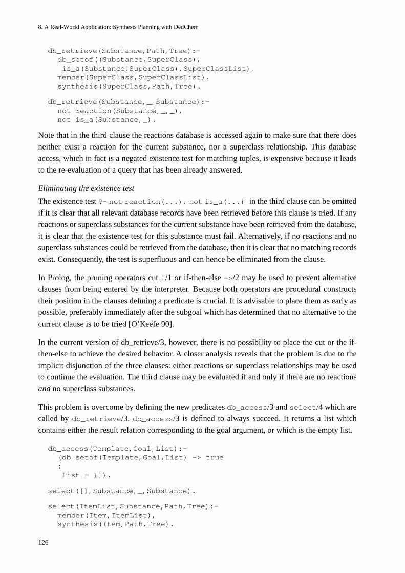
8. A Real-World Application: Synthesis Planning with DedChem
126
db_retrieve(Substance,Path,Tree):-db_setof((Substance,SuperClass), is_a(Substance,SuperClass),SuperClassList),member(SuperClass,SuperClassList),synthesis(SuperClass,Path,Tree).
db_retrieve(Substance,_,Substance):-not reaction(Substance,_,_),not is_a(Substance,_).
Note that in the third clause the reactions database is accessed again to make sure that there does
neither exist a reaction for the current substance, nor a superclass relationship. This database
access, which in fact is a negated existence test for matching tuples, is expensive because it leads
to the re-evaluation of a query that has been already answered.
Eliminating the existence test
The existence test ?- not reaction(...), not is_a(...) in the third clause can be omitted
if it is clear that all relevant database records have been retrieved before this clause is tried. If any
reactions or superclass substances for the current substance have been retrieved from the database,
it is clear that the existence test for this substance must fail. Alternatively, if no reactions and no
superclass substances could be retrieved from the database, then it is clear that no matching records
exist. Consequently, the test is superfluous and can hence be eliminated from the clause.
In Prolog, the pruning operators cut !/1 or if-then-else ->/2 may be used to prevent alternative
clauses from being entered by the interpreter. Because both operators are procedural constructs
their position in the clauses defining a predicate is crucial. It is advisable to place them as early as
possible, preferably immediately after the subgoal which has determined that no alternative to the
current clause is to be tried [O’Keefe 90].
In the current version of db_retrieve/3, however, there is no possibility to place the cut or the if-
then-else to achieve the desired behavior. A closer analysis reveals that the problem is due to the
implicit disjunction of the three clauses: either reactions or superclass relationships may be used
to continue the evaluation. The third clause may be evaluated if and only if there are no reactions
and no superclass substances.
This problem is overcome by defining the new predicates db_access/3 and select/4 which are
called by db_retrieve/3. db_access/3 is defined to always succeed. It returns a list which
contains either the result relation corresponding to the goal argument, or which is the empty list.
db_access(Template,Goal,List):-(db_setof(Template,Goal,List) -> true; List = []).
select([],Substance,_,Substance).
select(ItemList,Substance,Path,Tree):-member(Item,ItemList),synthesis(Item,Path,Tree).
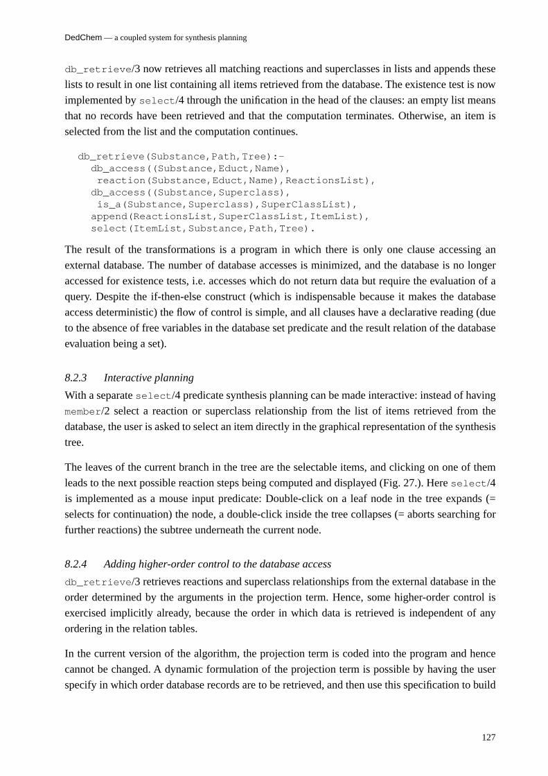
DedChem — a coupled system for synthesis planning
127
db_retrieve/3 now retrieves all matching reactions and superclasses in lists and appends these
lists to result in one list containing all items retrieved from the database. The existence test is now
implemented by select/4 through the unification in the head of the clauses: an empty list means
that no records have been retrieved and that the computation terminates. Otherwise, an item is
selected from the list and the computation continues.
db_retrieve(Substance,Path,Tree):-db_access((Substance,Educt,Name), reaction(Substance,Educt,Name),ReactionsList),db_access((Substance,Superclass), is_a(Substance,Superclass),SuperClassList),append(ReactionsList,SuperClassList,ItemList),select(ItemList,Substance,Path,Tree).
The result of the transformations is a program in which there is only one clause accessing an
external database. The number of database accesses is minimized, and the database is no longer
accessed for existence tests, i.e. accesses which do not return data but require the evaluation of a
query. Despite the if-then-else construct (which is indispensable because it makes the database
access deterministic) the flow of control is simple, and all clauses have a declarative reading (due
to the absence of free variables in the database set predicate and the result relation of the database
evaluation being a set).
8.2.3 Interactive planning
With a separate select/4 predicate synthesis planning can be made interactive: instead of having
member/2 select a reaction or superclass relationship from the list of items retrieved from the
database, the user is asked to select an item directly in the graphical representation of the synthesis
tree.
The leaves of the current branch in the tree are the selectable items, and clicking on one of them
leads to the next possible reaction steps being computed and displayed (Fig. 27.). Here select/4
is implemented as a mouse input predicate: Double-click on a leaf node in the tree expands (=
selects for continuation) the node, a double-click inside the tree collapses (= aborts searching for
further reactions) the subtree underneath the current node.
8.2.4 Adding higher-order control to the database access
db_retrieve/3 retrieves reactions and superclass relationships from the external database in the
order determined by the arguments in the projection term. Hence, some higher-order control is
exercised implicitly already, because the order in which data is retrieved is independent of any
ordering in the relation tables.
In the current version of the algorithm, the projection term is coded into the program and hence
cannot be changed. A dynamic formulation of the projection term is possible by having the user
specify in which order database records are to be retrieved, and then use this specification to build
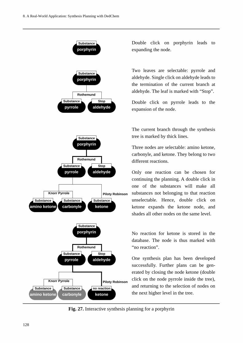
8. A Real-World Application: Synthesis Planning with DedChem
128
Piloty Robinson
Rothemund
Knorr Pyrrole
pyrrole
Substance
carbonyle
Substance
ketone
Substance
amino ketone
Substance
porphyrin
Substance
porphyrin
Substance
Rothemund
pyrrole
Substance
aldehyde
Stop
porphyrin
Substance
aldehyde
Stop
Double click on porphyrin leads to
expanding the node.
Two leaves are selectable: pyrrole and
aldehyde. Single click on aldehyde leads to
the termination of the current branch at
aldehyde. The leaf is marked with “Stop”.
Double click on pyrrole leads to the
expansion of the node.
The current branch through the synthesis
tree is marked by thick lines.
Three nodes are selectable: amino ketone,
carbonyle, and ketone. They belong to two
different reactions.
Only one reaction can be chosen for
continuing the planning. A double click in
one of the substances will make all
substances not belonging to that reaction
unselectable. Hence, double click on
ketone expands the ketone node, and
shades all other nodes on the same level.
Piloty Robinson
Rothemund
Knorr Pyrrole
pyrrole
Substance
carbonyle
Substance
ketone
no reaction
amino ketone
Substance
porphyrin
Substance
aldehyde
Stop
No reaction for ketone is stored in the
database. The node is thus marked with
“no reaction”.
One synthesis plan has been developed
successfully. Further plans can be gen-
erated by closing the node ketone (double
click on the node pyrrole inside the tree),
and returning to the selection of nodes on
the next higher level in the tree.
Fig. 27. Interactive synthesis planning for a porphyrin
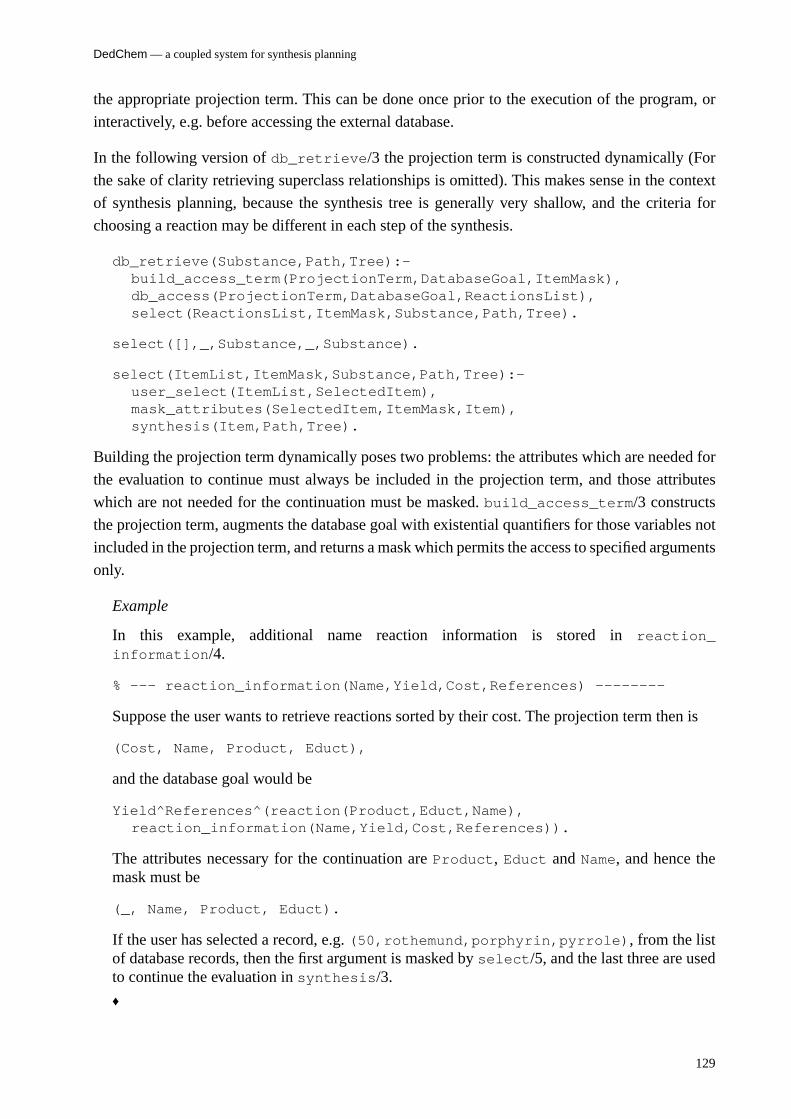
DedChem — a coupled system for synthesis planning
129
the appropriate projection term. This can be done once prior to the execution of the program, or
interactively, e.g. before accessing the external database.
In the following version of db_retrieve/3 the projection term is constructed dynamically (For
the sake of clarity retrieving superclass relationships is omitted). This makes sense in the context
of synthesis planning, because the synthesis tree is generally very shallow, and the criteria for
choosing a reaction may be different in each step of the synthesis.
db_retrieve(Substance,Path,Tree):-build_access_term(ProjectionTerm,DatabaseGoal,ItemMask),db_access(ProjectionTerm,DatabaseGoal,ReactionsList),select(ReactionsList,ItemMask,Substance,Path,Tree).
select([],_,Substance,_,Substance).
select(ItemList,ItemMask,Substance,Path,Tree):-user_select(ItemList,SelectedItem),mask_attributes(SelectedItem,ItemMask,Item),synthesis(Item,Path,Tree).
Building the projection term dynamically poses two problems: the attributes which are needed for
the evaluation to continue must always be included in the projection term, and those attributes
which are not needed for the continuation must be masked. build_access_term/3 constructs
the projection term, augments the database goal with existential quantifiers for those variables not
included in the projection term, and returns a mask which permits the access to specified arguments
only.
Example
In this example, additional name reaction information is stored in reaction_information/4.
% --- reaction_information(Name,Yield,Cost,References) --------
Suppose the user wants to retrieve reactions sorted by their cost. The projection term then is
(Cost, Name, Product, Educt),
and the database goal would be
Yield^References^(reaction(Product,Educt,Name), reaction_information(Name,Yield,Cost,References)).
The attributes necessary for the continuation are Product, Educt and Name, and hence themask must be
(_, Name, Product, Educt).
If the user has selected a record, e.g. (50,rothemund,porphyrin,pyrrole), from the listof database records, then the first argument is masked by select/5, and the last three are usedto continue the evaluation in synthesis/3.
♦
8. A Real-World Application: Synthesis Planning with DedChem
130
Note that build_access_term/3 and mask_attributes/3 require extensive term
manipulation. This term manipulation is possible entirely within Prolog.
8.2.5 Delegation of tests to the database system
In the introduction to section 8.2 I mentioned restricting the search space by explicitly requiring or
disallowing specific substances or reactions in the synthesis tree. In the code fragments shown,
only legal_reaction/2, which checks that there is no cycle in the reaction chain, can be found.
Preventing specific reactions or substance classes from being used in a synthesis can be added
easily: a list of reactions and substances which are not to be used is held in an extra argument.
legal_reaction/2 is then extended to legal_reaction/3 and checks that no selected reaction
or substance is on that list.
This immediately leads to the following remark: if a particular reaction or substance class is not to
be used in the synthesis plan, why not prevent it from being retrieved from the database in the first
place instead of doing that in Prolog? At least part — if not all — of the checking which is currently
done by legal_reaction/3 should be delegated to the database system to reduce the number of
database records retrieved.
The answer is that relational database languages are not powerful enough. Structured attributes,
lists, or sets cannot be represented adequately in the relational database model if the 1. NF is to be
respected. Thus everything that cannot be expressed in the database access language must be
programmed and evaluated in Prolog. With more powerful database languages more work can be
delegated to the database system. For example, with a HDBL [Pistor/Traunmüller 85] database
system connected to Prolog, passing a list of values to the database system for the restriction of
queries is possible because lists are primitive datastructures provided by HDBL.
8.3 Discussion
The application presented in this chapter is by no means trivial. Extensive rewriting of the original
naive algorithm was necessary to reduce the number of database accesses, and to exploit the full
capacities of database set predicates. Such rewriting is common practice when optimizing a given
program.
Here, a clean distribution of control has been achieved by isolating database access in a single
predicate and through the use of database set predicates. The resulting code is efficient without
compromising too much on clarity.
In DedChem, the strategy for constructing a synthesis plan is different from the evaluation strategy
of the underlying Prolog system. The Prolog evaluation strategy is depth first and left to right. The
strategy for constructing plans is still depth first, but the user may select freely from the set of
allowed next reactions and synonyms. This selection has distinct advantages: the number of
possible next steps is known, and an optimized selection based on the comparison with alternatives
is supported. Note that this selection from a set of items retrieved from the database is only possible
Discussion
131
with database set predicates because of the set retrieval, the sorting of the result relation, and the
dynamic datastructure used to hold the result relation.
The presentation of DedChem shows that a full-fledged programming language is needed to cover
all relevant aspects of the application: user I/O, database access, and the application program itself.
Prolog was designed to be a programming language, with I/O and system predicates etc. The
Prolog programming environments available today feature comfortable interface libraries. There is
thus no need to resort to other languages for implementing user-friendly interfaces. The same is
true for database access: database set predicates can be implemented in Prolog, and they can be
added to any existing Prolog system. Hence no other language is needed for accessing external
databases.
Programming the application itself is facilitated by the high-level declarative language Prolog.
Database set predicates embed database access into the logic programming language, and
therefore, despite their being used as a means to increase efficiency, they contribute to programs
which are easy to read and understand.

132
133
9
Outlook
Database set predicates are not restricted to accessing relational database systems. Access to more
powerful database models, e.g. nested relations database systems, is also expressible.
9.1 Increasing the expressive power of the database access language
The relational database model requires the domains of its attributes to be atomic. This is a very
severe restriction which makes using relational database systems almost impossible for a large
class of practical applications.
Extensions to the relational database model have been proposed which feature a higher expressive
power. A first extension is to allow attributes which are collections of atomic values, e.g. tuples,
lists, or sets. A second extension are nested relations, i.e. relation tables the arguments of which
may themselves be relations. Such extensions are known as NF2 (non first normal form) databases.
NF2 databases allow a more natural way of expressing data dependencies through a grouping of
attributes, and they support efficient storage in that they express clustering conditions.
In contrast to the other approaches to coupled systems, database set predicates may access such
higher database systems.
9.1.1 Tuple-, list-, and set-valued attributes
In this extension of the classical relational database model attributes may be collections of atomic
values. The relational algebra and calculus were extended to set-valued attributes by [Özsoyoglu
et al. 87]. Other collection constructors, such as tuples, or lists are easily incorporated.
• A tuple attribute consists of an n-ary term with a functor. Each argument of the term must
be an atomic value.
• A list attribute consists of a list of finite length. This list contains only atomic values.
• A set attribute consists of a finite set of atomic values.
9. Outlook
134
Constructor operators and operations to retrieve the individual values from such a collection can
be defined in the logic language. Collections are commonly constructed by explicitly providing the
elements that belong to the particular collection and unifying them with a logical variable, e.g.
Example
Tuple = f(zurich,geneva) for tuplesList = [zurich,geneva,geneva] for listsSet = {zurich,geneva} for sets.
♦
The retrieval of individual elements is possible through pattern matching and unification for tuples,
and a selection predicate for lists and sets.
Example
Tuple = (Item1,Item2) for tuplesmember(Item,List) for listselement(Set,Element) or subset(Subset,Set) for sets.
♦
For each of these operations an equivalent operation must be defined in the database system to be
accessed. In fact, most commercial relational database system implementations provide such
operations (which implies that the 1. NF may be violated in these systems). Typical examples are
substring searches, which may be used to retrieve individual values stored in a string, or date
arithmetic, which requires the separate treatment of days, months, and years.
Example
In the reactions database incompatibilities between name reactions and substance classes maybe stored as an attribute of a name reaction, with incompatibilities a set of substance classnames.
% --- reaction(Product, Educt, ReactionName, Incompatibilities) --reaction(porphyrin, ketone, rothemund, {carbonyle, en, olefin}).
In a synthesis only such reactions may be used which are compatible with the substance classesin the current branch of the synthesis tree. In order to exclude incompatible substances as earlyas possible, the appropriate restriction is evaluated in the database system already:
?- ... /* Branch bound by previous goals */db_setof((Product,Educt,Name),(reaction(Product,Educt,Name,Incompatibilities), not subset(Incompatibilities,Branch)),List).
subset/2 is translated to the equivalent operation in the database system, and the queryrestriction is performed in the database system already.
♦
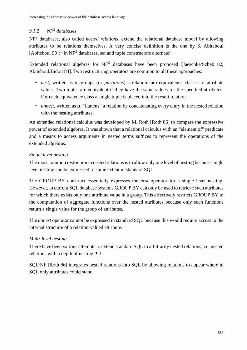
Increasing the expressive power of the database access language
135
9.1.2 NF2 databases
NF2 databases, also called nested relations, extend the relational database model by allowing
attributes to be relations themselves. A very concise definition is the one by S. Abiteboul
[Abiteboul 90]: “In NF2 databases, set and tuple constructors alternate”.
Extended relational algebras for NF2 databases have been proposed [Jaeschke/Schek 82,
Abiteboul/Bidoit 84]. Two restructuring operators are common to all these approaches:
• nest, written as ν, groups (or partitions) a relation into equivalence classes of attribute
values. Two tuples are equivalent if they have the same values for the specified attributes.
For each equivalence class a single tuple is placed into the result relation.
• unnest, written as µ, “flattens” a relation by concatenating every entry in the nested relation
with the nesting attributes.
An extended relational calculus was developed by M. Roth [Roth 86] to compare the expressive
power of extended algebras. It was shown that a relational calculus with an “element of” predicate
and a means to access arguments in nested terms suffices to represent the operations of the
extended algebras.
Single level nesting
The most common restriction in nested relations is to allow only one level of nesting because single
level nesting can be expressed to some extent in standard SQL.
The GROUP BY construct essentially expresses the nest operator for a single level nesting.
However, in current SQL database systems GROUP BY can only be used to retrieve such attributes
for which there exists only one attribute value in a group. This effectively restricts GROUP BY to
the computation of aggregate functions over the nested attributes because only such functions
return a single value for the group of attributes.
The unnest operator cannot be expressed in standard SQL because this would require access to the
internal structure of a relation-valued attribute.
Multi-level nesting
There have been various attempts to extend standard SQL to arbitrarily nested relations, i.e. nested
relations with a depth of nesting ≥ 1.
SQL/NF [Roth 86] integrates nested relations into SQL by allowing relations to appear where in
SQL only attributes could stand.
9. Outlook
136
Example
The nested relation flight is defined as
“Retrieve all departures and their corresponding destinations” is expressed in SQL/NF as
SELECT departure,SELECT cityFROM destination
FROM flight
The SELECT-part of the outer query contains a relation specification instead of an attributename.
♦
Accessing NF2 databases through database set predicates
Single-level nested relations can be accessed through database set predicates with a standard
database goal which contains terms as arguments in subgoals. Multi-level nesting requires that
database set predicates be nested, i.e. a database set predicate must appear in the database goal of
another database set predicate.
The ν and µ operators are expressed through the quantification of variables in the database goal. νis expressed by using free variables for those attributes which form the equivalence classes, and
projection term variables for the other attributes; µ by including all variables of the database goal
in the projection term.
Example
Single level nested relations can be accessed by database set predicates with standard databasegoals.
db_setof(City,Plane^flight(Departure,destination(City,Plane)),List)
retrieves a list of Destinations for every binding of Departure.
db_setof((Departure,City),Plane^flight(Departure,destination(City,Plane)),List)
retrieves a list of tuples (Departure,Destination).
♦
Flight
DepartureCity Plane
Destination
Fig. 28. Schema of the NF2 table flight
Updates through database set predicates
137
In the examples above the nest operator was applied to relational database tables only. For the
retrieval of data from NF2 databases the predicate element/2, which selects an element from a set,
must be used to select individual attribute values from nested relations.
Example
Retrieving the number of seats available for the individual flight connections is expressed asfollows (with plane/2 a database predicate mapped to the relation table Plane with attributestype and seats):
db_setof((City,Seats),Destination^Plane^(flight(Departure,Destination), element(Destination,(City,Plane)), plane(Plane,Seats)),Result).
The projection term contains those variables corresponding to the attributes one is interested in,i.e. destination and seats. flight/2 in the database goal retrieves in its second argumentthe nested relation corresponding to the database attributes departure and destination.From this nested relation single tuples, represented through the term (City,Plane), areselected through element/2. For each of these tuples a join over the attribute plane and typerespectively is performed to retrieve the number of seats. This join is expressed through theshared variable Plane in element/2 and plane/2 respectively. The result relation is held inthe variable Result.
The variable Departure is free, and hence the solutions to the database set predicate aredistinct lists of instantiated terms for each binding of Departure.
♦
Translating NF2 queries
The translation of database access requests to SQL/NF closely follows the procedure described in
section 7.2. The free variables are translated to nesting attributes and thus the goals they occur in
belong to the outer query. The other variables are translated to nested attributes and hence the goals
without free variables form a query of their own in the SELECT-part of the outer query.
The translation to other database languages, such as HDBL [Pistor/Traunmüller 85], may be more
difficult if these languages have constructs which cannot be represented directly in the logic
language. For example, HDBL distinguishes between lists and sets. Prolog does not know sets, and
hence they are represented as lists in most application programs. For a translation to HDBL it must
be known which Prolog lists translate to HDBL lists, and which Prolog lists translate to HDBL sets.
Additional information about the type of an attribute must thus be provided by the schema
description. However, the translation procedure itself then is no longer independent of the database
schema.
9.2 Updates through database set predicates
In the previous chapters, database set predicates have been restricted to read-only access to external
databases. This restriction is due to their close relationship with the Prolog set predicates.
9. Outlook
138
Prolog set predicates may be called with either the first two arguments, or with all three arguments
instantiated. With the third argument a variable this variable is instantiated with the list of solutions
to the goal argument. With the third argument bound to a list, the set predicates test whether the
result of the all-solutions evaluation can be unified with this list. It is not possible, however, to
evaluate set predicates “backwards”, i.e. to instantiate the template and the goal terms with
solutions from the list argument.
In Prolog this restriction makes sense because running set predicates backwards implies that the
instantiations of the goal argument be derivable from the list argument, and this is not guaranteed
for arbitrary goal arguments since they may contain predicates which cannot be run backwards, e.g.
control or system predicates, or predicates with side-effects. A second problem is that it may not
be possible to determine the binding for every variable in the body of the rules called by the subgoal
because they are not “visible”. This problem is known as the view update problem in the context
of databases.
In database set predicates updates can be expressed either implicitly through “inverting” the proof
procedure, or explicitly through update commands in the goal argument. In either case, the list
argument of the database set predicate is fully instantiated, whereas the template and the goal
argument are partially instantiated terms.
9.2.1 Implicit updates
Expressing updates implicitly amounts to inverting the proof procedure: instead of computing
solutions from a given program, the program is constructed from the solutions supplied as input.
In database set predicates, the projection term and the database goal thus serve as program schemes
which are materialized through the instantiations supplied by the list argument. This is possible
provided that
• the database goal consists of a conjunction of positive base calls only, and that
• the arguments of the database goal are either constants, free variables which must be bound
when the predicate is called, or variables which also occur in the projection term.
The semantics of updates through database set predicates requires the definition of the scope of
update, and the mode of update.
The scope of update is determined by the free variables of the goal argument and is restricted to
those tuples whose attribute values of the attributes corresponding to the free variables are equal to
the instantiated free variables in the database goal. If there are no free variables in the goal
argument, then the scope of update is the whole relation.
The mode of update is to replace these tuples by the ones supplied through the list argument of the
database set predicate.
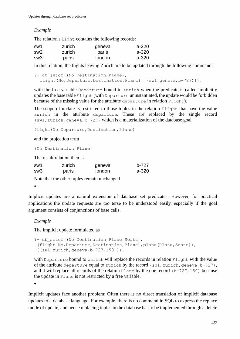
Updates through database set predicates
139
Example
The relation Flight contains the following records:
sw1 zurich geneva a-320sw2 zurich paris a-320sw3 paris london a-320
In this relation, the flights leaving Zurich are to be updated through the following command:
?- db_setof((No,Destination,Plane),flight(No,Departure,Destination,Plane),[(sw1,geneva,b-727)]).
with the free variable Departure bound to zurich when the predicate is called implicitlyupdates the base table Flight (with Departure uninstantiated, the update would be forbiddenbecause of the missing value for the attribute departure in relation Flight).
The scope of update is restricted to those tuples in the relation Flight that have the valuezurich in the attribute departure. These are replaced by the single record(sw1,zurich,geneva,b-727) which is a materialization of the database goal
flight(No,Departure,Destination,Plane)
and the projection term
(No,Destination,Plane)
The result relation then is
sw1 zurich geneva b-727sw3 paris london a-320
Note that the other tuples remain unchanged.
♦
Implicit updates are a natural extension of database set predicates. However, for practical
applications the update requests are too terse to be understood easily, especially if the goal
argument consists of conjunctions of base calls.
Example
The implicit update formulated as
?- db_setof((No,Destination,Plane,Seats), (flight(No,Departure,Destination,Plane),plane(Plane,Seats)), [(sw1,zurich,geneva,b-727,150)]).
with Departure bound to zurich will replace the records in relation Flight with the valueof the attribute departure equal to zurich by the record (sw1,zurich,geneva,b-727),and it will replace all records of the relation Plane by the one record (b-727,150) becausethe update in Plane is not restricted by a free variable.
♦
Implicit updates face another problem: Often there is no direct translation of implicit database
updates to a database language. For example, there is no command in SQL to express the replace
mode of update, and hence replacing tuples in the database has to be implemented through a delete
9. Outlook
140
command with a search condition, and a subsequent insertion of the values supplied through the
list argument of the database set predicate.
9.2.2 Explicit updates
With explicit updates, the database access language is extended through either
• a new database set predicate, or
• database update commands in the goal argument.
In the first case, the database set predicate db_update/3 is introduced. The arguments of
db_update/3 are the same as in the other database set predicates, and the operational semantics
is that of the implicit update described above.
Introducing a new database set predicate for updates would allow the other database set predicates
to retain their operational semantics even with the third argument instantiated, and it would make
updates to the database explicit without any dependency on the underlying database manipulation
language.
In the second case update commands are included in the goal argument of database set predicates
as the reserved predicates replace/1, delete/1, and insert/1 which take as argument a base
call.
Example
?- db_setof((No,Destination,Plane),insert(flight(No,Departure,Destination,Plane)),[(sw1,geneva,b-727)]).
with Departure bound to zurich will insert into the relation FLIGHT the record(sw1,zurich,geneva,b-727) to the previous entries in the relation table.
♦
Generally, these reserved predicate names are chosen to reflect the commands of the underlying
database manipulation language. However, this makes visible the underlying database
manipulation language and hence violates the principle of embedding. Furthermore, the burden of
choosing the appropriate method for database updates is placed on the application programmer.
9.2.3 Summary
It must be noted that the problem of integrating updates into logic programs has not yet been solved
satisfactorily. From a theoretic point of view, updates to the database are an extension of the set of
axioms of the logic theory. Augmenting the set of axioms entails non-monotonicity: theorems can
now be proved that could not be proved before.
In logic programming, updating the set of axioms is achieved through side-effects which implies a
permanent change of the program code. Backtracking at later stages does not undo the program
Updates through database set predicates
141
code modification, so that although the original goal failed, the set of axioms is changed. A solution
may be the approach taken in Gödel where the current database is passed on as a context argument
during the evaluation. Database updates lead to the definition of a new context for subsequent
goals. Upon failure, any database update is undone, and the proof continues with the previous
database context [Hill/Lloyd 91]. Database set predicates also have a natural update semantics in
that any backtracking is performed on the list datastructure that holds the result relation read in
when the goal was called for the first time — subsequent database updates have no effects on this
list. This semantics follows the defensible semantics for assert and retract as proposed by Lindholm
and O’Keefe [Lindholm/O’Keefe 87].
In the context of physically loosely coupled systems the update problem is particularly acute
because with multi-user access updates to the database may occur which cannot be controlled by
the current application program and hence may lead to unpredictable results. However, this
problem pertains to multi-user database systems in general, and suitable mechanisms such as
locking must be applied.
In practice, the introduction of a specific database set predicate for updates is a reasonable way of
integrating updates into logic programming languages, because it distinguishes database updates
from data retrieval in the program code, but does not require a separate database access language.
Furthermore, the translation procedure, which is different for retrieval and update, is determined
explicitly by the predicate name, and not implicitly through the instantiation pattern of the
arguments.

142
143
10
Conclusion
Database set predicates embed access to external databases into logic programming languages
based on SLDNF resolution. This embedding is achieved through a physically loose and logically
tight coupling of the logic programming language and the database system.
On the physical level, the database evaluation is embedded into the logic language evaluation by
confining access to and retrieval from the external database to the standard set-oriented data
manipulation language interface of the database system. In previous approaches to physically
loosely coupled systems the external database is accessed via the procedural programming
language interface of the database system one record at a time to match the tuple-oriented
evaluation strategy of the logic programming language.
On the logical level, access to the database is embedded into the logic programming language
through the powerful term and list datastructure primitives provided by the logic programming
language which allow the adequate representation of any database query and its corresponding
result relation. In previous approaches to logically tightly coupled systems in which the logic
programming language is the sole language, this language is restricted in its expressive power to
Datalog with negation and arithmetics, and the database itself must respect the allowedness
constraints on the form of its predicates.
The high expressive power of the database access language of database set predicates stems from
the ability to discern variable quantifications, and the independence of the projection term and the
database goal. This expressive power contributes to efficiency through maximally restrictive
queries, it permits exploiting the full capabilities of external database systems, including the
computation of aggregate functions and the expression of higher order control such as grouping
and sorting, and it supports access to higher database systems, such as databases with non-atomic
attributes or even NF2 databases.
Database set predicates can be implemented on top of most commercial Prolog systems in Prolog
itself. In fact, writing an efficient compiler to translate database access requests to a database query

10. Conclusion
144
is a straightforward task in the high level declarative language Prolog. For the communication
between the logic programming language system and the database system all that is required are
low level stream I/O predicates for inter-process communication, or a foreign language interface
for communication through procedure calls. Both mechanisms are supported in most commercial
Prolog environments.
Database set predicates have two distinct advantages for practical applications. They support a
declarative style of programming without compromising on efficiency, and their inherent
independence of a particular database system implementation allows accessing a multitude of
different database systems. The importance of this last feature for high level applications, e.g.
knowledge base and/or expert system applications, cannot be overestimated.
145
AcknowledgmentsI thank Prof. Dr. K. Bauknecht for his generous support not only of this thesis but also of my work
in general, and Prof. Dr. G. Gottlob and Prof. Dr. K. Dittrich for their reviewing my thesis. Their
critical remarks helped me clarify a number of issues.
I thank my colleagues Dr. Norbert Fuchs, Dr. Rolf Stadler, and Markus Fromherz for their
suggestions, corrections, and continuing discussions. Without their help and encouragement I
could not have written this thesis.
I thank Volker Küchenhoff of ECRC for his thorough review of the thesis and his critical, but
always highly constructive remarks. His experience in the field was of invaluable help to me.
Furthermore, I thank Prof. Dr. Robert Marti of ETH Zurich for his information on the compilation
to SQL, Ina Kraan for her hint which led to the introduction of selection predicates, and Dr. Chris
Mellish whose review of a paper of mine made me realize that access to higher databases is
expressible in a very natural way through database set predicates.

146
147
References
[Abiteboul/Bidoit 84] S. Abiteboul, N. Bidoit: Non first normal form relations torepresent hierarchically organized data. In: Proceedings of theThird ACM SIGACT-SIGMOD Symposium on Principles ofDatabase Systems, Waterloo, April 1984
[Abiteboul et al. 90] S. Abiteboul, C. Beeri, M. Gyssens, D. van Gucht: AnIntroduction to the Completeness of Languages for ComplexObjects and Nested Relations. in: [Abiteboul 90]
[Abiteboul 90] S. Abiteboul (Ed.) Proceedings of ICDT 90, Paris, LNCS No470, Springer Verlag, Berlin, 1990
[Aho/Ullman 79] A. Aho, J. Ullman: Universality of Data Retrieval Languages.ACM Symposium on Principles of Programming Languages,1979
[Appelrath 85] H.J. Appelrath: Von Datenbanken zu Expertensystemen, IFBNr. 102, Springer Verlag, 1985
[Appelrath et al. 89] H.-J. Appelrath, A. Cremers, H. Schiltknecht (Eds): PrologTools for Building Expert Systems, Workshop proceedings,Morcote, 1989
[Bancilhon/Ramakrishnan 86] F.Bancilhon, R. Ramakrishnan: An Amateurs introduction toRecursive Query Processing. In: ACM SIGMOD’86, 1986
[Bever 86] M. Bever: Einbettung von Datenbanksprachen in höhereProgram-miersprachen. Reihe 10: Informatik/Kommuni-kationstechnik, VDI Verlag, Düsseldorf, 1986
[Bocca 86] J. Bocca: EDUCE - A Marriage of Convenience: Prolog and aRelational DBS. Proceedings Third Symposium on LogicProgramming, Salt Lake City, 1986
[Bocca et al. 89 a] J. Bocca, M. Dahmen, G. Macartney: KB-Prolog User Guide.Technical Report, ECRC Munich, 1989
[Bocca et al. 89 b] J. Bocca, M. Dahmen, M. Freeston, G. Macartney, P. Pearson:KB-Prolog, A Prolog for very large Knowledge Bases. In:[Williams 89]
[Böttcher 89] S. Böttcher: The Architecture of the PROTOS-L System. in:[Appelrath et al.89]
[Ceri et al. 87] S. Ceri, G. Gottlob, G. Wiederhold. Interfacing relationaldatabases and Prolog efficiently. in: [Kershberg 87]
[Ceri et al. 89] S. Ceri, G. Gottlob, G. Wiederhold: Efficient Database Accessfrom Prolog. IEEE Transactions on Software Engineering, Vol15 No 2, 1989
[Ceri et al. 90] S. Ceri, G. Gottlob, L. Tanca: Logic Programming andDatabases. Springer Verlag, 1990
[Chimenti et al. 90] D. Chimenti, R. Gamboa, R. Krishnamurthy, S. Naqvi, S. Tsur,C. Zaniolo: The LDL System Prototype. in: IEEE Transactionson Knowledge and Data Engineering, Vol 2, No 1, March 1990
[Chang/Walker 84] C.L. Chang, A. Walker: PROSQL: A Prolog programminginterface with SQL/DS. in: [Kershberg 86]

148
[Chen et al. 90] W. Chen, M. Kifer, D. Warren: HiLog: A First-OrderSemantics of Higher-Order Logic Programming Constructs.Proceedings of NACLP 90, Austin, 1990
[Clark 78] K. Clark. Negation as Failure. in: [Gallaire/Minker 78]
[Clocksin/Mellish 87] W. Clocksin, C. Mellish: Programming in Prolog. 3rd Edition,Springer Verlag, 1987
[Codd 70] E. F. Codd: A Relational Model for Large Shared Data Banks.in: CACM, Vol 13, No 6, 1970
[Cuppens/Demolombe 86] F. Cuppens, R. Demolombe: A Prolog-Relational DBMSInterface Using Delayed Evaluation. Workshop on IntegratingLogic Programming and Databases, Venice, 1986
[Danielsson/Barklund 90] M. Danielsson, J. Barklund: Persistent Data Storage forProlog. Proceedings of DEXA 90, Vienna, 1990
[Date 89] C. Date: The SQL Standard, Addison Wesley, 1989
[Dobry 90] T. P. Dobry: A High Performance Architecture for Prolog.Kluwer Academic Publishers, Boston, 1990
[Draxler 90] C. Draxler: Logic Programming and Databases — anOverview Over Coupled Systems and a New Approach Basedon Set Predicates. Institutsbericht 90.09 Institut für Informatik,Universität Zürich, 1990
[Freeston 88] M. Freeston: Grid files for efficient Prolog clause access. in: P.Gray, R. Lucas (Eds): Prolog and Databases, Ellis Horwood,1988
[Gabbay/Guenthner 84] D. Gabbay, F. Guenthner (Eds): Handbook of PhilosophicalLogic, Vol 2. Extensions of Classical Logic. Reidel, Dordrecht,1984
[Gallaire/Minker 78] H. Gallaire, J. Minker: Logic and Databases. Plenum Press,1978
[Gallaire et al. 84] H. Gallaire, J. Minker, J.M. Nicolas: Logic and Databases: aDeductive Approach. in: Computing Surveys, Vol 16, No 2,June 1984
[Gardarin/Valduriez 89] G. Gardarin, P. Valduriez: Relational Databases andKnowledge Bases. Addison Wesley, 1989
[Genesereth/Nilsson 87] Genesereth, N. Nilsson: Foundations of Artificial Intelligence.Morgan Kaufman, 1987
[Gozzi et al. 90] F. Gozzi, M. Lugli, S. Ceri: An Overview of PRIMO: APortable Interface between Prolog and Relational Databases.Information Systems, Vol 15, No 5, 1990
[Green 69] C. Green: Theorem Proving by Resolution as a Basis forQuestion-Answering Systems. In: Machine Intelligence 4,Edinburgh University Press, 1969
[Hansen et al. 89] M. Hansen, B. Hansen, P. Lucas, P. van Emde Boas:Integrating Relational Databases and Constraint Languages.in: Computing Languages, Vol 14, No 2, Maxwell PergamonMacmillan, 1989
149
[Held et al. 75] G. Held, M. Stonebraker, E. Wong: INGRES - a RelationalDatabase System. Proc. NCC 44, May 1975
[Härder 87] Th. Härder: Realisierung von operationalen Schnittstellen. in:[Lockemann/Schmidt 87]
[Hill/Lloyd 91] P. Hill, J. Lloyd: the Gödel Report. Technical Report TR 91 02,Department of Computer Science, University of Bristol, 1991
[Ioannides et al. 88] Y. Ioannides, J. Chen, M. Friedman, M. Tsangaris:BERMUDA - An architectural perspective on interfacingProlog to a database machine. Second Intl. Conference onExpert Database Systems, L. Kershberg (editor). Benjamin-Cummings, 1988
[Jaeschke/Schek 82] G. Jaeschke, H.-J. Schek: Remarks on the algebra of non firstnormal form relations. In: Proceedings of the ACM SIGACT-SIGMOD Symposium on Principles of Database Systems, LosAngeles, March 1982
[Jarke et al. 84] M. Jarke, J. Clifford, Y. Vassiliou: An Optimizing Prolog Front-End to a Relational Query System. Proceedings SIGMOD,Boston, 1984
[Jasper 90] H. Jasper: Datenbankunterstützung für Prolog-Programmier-umgebungen, Dissertation, Berichte aus dem FachbereichInformatik der Universität Oldenburg, Nr. 5/90, November1990
[Kershberg 86] L. Kershberg (ed): Proceedings First Workshop on ExpertDatabase Systems, Charleston, Benjamin-Cummings, 1986
[Kershberg 87] L. Kershberg (ed): Proceedings First Intl. Conference onExpert Database Systems, Charleston, Benjamin-Cummings,1987
[Klug 82] A. Klug: Equivalence of Relational Algebra and RelationalCalculus Query Languages Having Aggregate Functions.Journal of the ACM, Vol 29, No 3, July 1982
[Kowalski 79] R. Kowalski: Logic for Problem Solving. North Holland,Amsterdam, 1979
[Kowalski 82] R. Kowalski: Logic and Databases. Research Report 82/25,Dept. of Computing, Imperial College of Science andTechnology, London 1982
[Korth/Roth 90] H. Korth, M. Roth: Query Languages for Nested RelationalDatabases. in: S. Abiteboul (Ed.) Proceedings ICDT 90, Paris,Lecture Notes No 470, Springer Verlag, Berlin, 1990
[Kröger 87] F. Kröger: Temporal Logics of Programs. Springer, 1987
[Kühn 89] E. Kühn: Implementierung von Multi-Datenbanksystemen inProlog. Dissertation Technische Universität Wien, April 1989
[Li 84] D.Li: A Prolog Database System. Research Studies Press, JohnWiley & Sons Ltd., 1984
[Lindholm/O’Keefe 87] T. G. Lindholm, R. A. O’Keefe, Efficient Implementation of aDefensible Semantics for Dynamic Prolog Code, 4thInternational Logic Programming Conference, ed. Jean-LouisLassez, MIT Press, Cambridge MA, 1987
150
[Lloyd 87] J. Lloyd: Foundations of Logic Programming. 2nd Edition,Springer Verlag, 1987
[Lockemann/Schmidt 87] P. Lockemann, J. Schmidt (Eds): Datenbank-Handbuch.Springer Verlag, 1987
[Maier 83] D. Maier: The Theory of Relational Databases. PitmanPublishers, London, 1983
[Maier 84] D. Maier: Databases and the Fifth Generation Project: IsProlog a Database language? Proceedings SIGMODConference, 1984
[Maier/Warren 89] D. Maier, D.S.D. Warren: Computing with Logic. Benjamin-Cummings, 1989
[Manthey et al. 89] R. Manthey, V. Küchenhoff, M. Wallace: KBL: DesignProposal of a conceptual language for EKS. ECRC TechnicalReport TR-KB-29, Jan. 89, Munich, 1989
[Marcus 86] C. Marcus: Prolog Programming. Addison Wesley, 1986
[Marti et al. 89] R. Marti, C. Wieland, B. Wüthrich: Adding Inferencing to aRelational Database Management System. Proceedings ofBTW 89, Zurich, IFB No 204, Springer Verlag, Berlin, 1989
[Meier et al. 89] M. Meier, A. Aggoun, D. Chan, P. Dufresne, R. Enders, D.Henry de Villeneuve, A. Herold, P. Kay, B. Perez, E. vanRossum, J. Schimpf: SEPIA – an Extendible Prolog System.in: Proceedings of the 11th World Computer Congress IFIP‘89, San Francisco, 1989
[Minker 88 a] J. Minker (ed): Foundations of Deductive Databases and LogicProgramming. Morgan Kaufman, 1988
[Minker 88 b] J. Minker: Perspectives in Deductive Databases. in: Journal ofLogic Programming, No 5, Elsevier Science Publishing Co.New York, 1988
[Naish 86] L. Naish: Negation and Control in Prolog. Springer LectureNotes in Computer Science, No 238. Springer Verlag, 1986
[Nussbaum 88] M. Nussbaum: Delayed evaluation in logic programming: aninference mechanism for large knowledge bases. Diss No 8542ETH Zurich, 1988
[O’Hare/Sheth 89] A. O’Hare, A. Sheth: The Interpreted-Compiled Range ofAI/DB Systems. in: ACM SIGMOD Record, Vol 18, No 1,March, 1989
[O’Keefe 83] R. O’Keefe: Prolog Compared with Lisp? Sigplan Notices, Vol18, No 5, May 1983
[O’Keefe 90] R. O’Keefe: The Craft of Prolog. MIT Press, 1990
[Özsoyoglu et al. 87] G. Özsoyoglu, Z. Özsoyoglu, V. Matos: Extending RelationalAlgebra and Relational Calculus with Set-Valued Attributesand Aggregate Functions. Transactions on Database Systems,Vol 12, No 4, Dec. 1987
[Pistor/Traunmüller 85] P. Pistor, R. Traunmüller: A Database Language for Sets, Listsand Tables. Technical Report 85.10.004, IBM HeidelbergScientific Center, 1985
151
[Parsaye 83] K. Parsaye: Logic Programming and Relational Databases.IEEE Computer Society Database Engineering Bulletin, Vol 6No4, Dec. 1983
[Pereira/Shieber 87] F. Pereira, St. Shieber: Prolog and Natural-Language Analysis.Center for the study of language and information CSLI, MenloPark, 1987
[Quintus 87] Quintus Prolog Database Interface manual. Quintus Inc.,Sunnyvale
[Reiter 78] R. Reiter: On Closed World Databases. In: [Gallaire/Minker78]
[Robinson 65] J. Robinson: A Machine-oriented Logic Based on theResolution Principle. JACM, Vol 12, 1965
[Ross 89] P. Ross: Advanced Prolog. Addison Wesley, 1989
[Roth 86] M. Roth: Theory of Non-First Normal Form RelationalDatabases. Ph.D. thesis, University of Texas, Austin, 1986
[Roussel 75] Ph. Roussel: Prolog: Manuel de Référence et Utilisation.Technical Report, Groupe d’Intelligence Artificielle,Université d’Aix-Marseille II, Marseille 1975
[Scowen 90] R. S. Scowen: Prolog - Draft for working draft 4.0 (WG17N64). International Organization for Standardization, NationalPhysical Laboratory, Teddington, England 1990
[Shepherdson 88] J. Shepherdson: Negation in Logic Programming. in: [Minker88 a]
[Sterling/Shapiro 86] L. Sterling, E. Shapiro: The Art of Prolog. MIT Press, 1986
[Thayse 89] A. Thayse: From Modal Logic to Deductive Databases. JohnWiley and Sons, Chichester, 1989
[Tsur 88] S. Tsur: LDL - A technology for the realization of tightlycoupled expert database systems. in: IEEE Expert, Fall 1988
[Ullman 88] J. Ullman: Principles of Database and Knowledge-BaseSystems, Vol I. Computer Science Press, 1988
[Vieille/Lefêbvre 89] L. Vieille, A. Lefêbvre: Deductive Database Systems and theDedGin* query evaluator. 7th British National Conference onDatabases, Edinburgh, 1989
[Vieille et al. 90] L. Vieille, P. Bayer, V. Küchenhoff, A. Lefêbvre: EKS-V1, AShort Overview. AAAI 90 Workshop on Knowledge BaseManagement Systems, Boston, July 1990
[Warren 80] D.H.D. Warren: Logic Programming and Compiler Writing.Software Practice and Experience, Vol 10, No 11, 1980
[Warren 82] D.H.D. Warren: Higher-order extensions to Prolog: are theyneeded? in: Machine Intelligence 10, Ellis Horwood, 1982
[Williams 89] M. Williams (ed): 7th British National Conference onDatabases, Edinburgh, June 1989
[Zaniolo 90] C. Zaniolo: Deductive Databases - Theory meets Practice.Proceedings EDBT ‘90, Venice, LNCS No 416, SpringerVerlag, Berlin, 1990

152

153
A
Abiteboul 13, 135Aho 11, 27Appelrath 1
B
Bancilhon 33, 53Barklund 51, 101, 105Bever 3, 34, 40, 41Bidoit 135Bocca 3, 35, 50, 52, 55Böttcher 53Burstall 75Byrd 77
C
Ceri 30, 34, 49, 94Chang 48Chen 1, 5Chimenti 53Clark 22Clocksin 24Codd 2Cuppens 58
D
Danielsson 51, 101, 105Darlington 75Date 14Demolombe 58Dobry 81, 82Draxler 123
F
Freeston 50
G
Gabbay 1Gallaire 1, 2, 41Gardarin 27, 30Genesereth 1Gozzi 50Green 28Guenthner 1
H
Hansen 53Härder 36Held 91Hill 102, 141
I
Ioannides 41, 55
J
Jaeschke 135Jarke 101Jasper 1, 41
K
Klug 13Kowalski 1, 2, 11, 23Kröger 1Kühn 52
L
Lefêbvre 6, 53Li 52Lindholm 50, 141Lloyd 1, 6, 16, 22, 23, 102, 141
M
Maier 13, 27, 28, 66Manthey 53Marti 6, 53, 101Meier 82Mellish 24Minker 1
N
Naish 57, 66Nilsson 1Nussbaum 51, 58
O
O´Hare 41O’Keefe 50, 66, 67, 126, 141Özsoyoglu 133
Author Index

154
P
Parsaye 2, 27
Pistor 130, 137
R
Ramakrishnan 33, 53
Reiter 22
Robinson 2, 19
Ross 67
Roth 135
Roussel 24
S
Sato 75
Schek 135
Scowen 26
Shapiro 26, 100
Shepherdson 23
Sheth 41
Sterling 26, 100
T
Tamaki 75
Traunmüller 130
Tsur 53
U
Ullman 6, 11, 26, 27, 30
V
Valduriez 27, 30
Vieille 6, 52, 53
W
Walker 48
Warren 82
Warren D.H.D. 5, 24, 63, 100, 105
Warren D.S. 13, 28, 66
Z
Zaniolo 53


![Grails - Weiterführende Themen zu Internet- und WWW ... · Ubersicht uber Grails [1] Groovy Programming Language Hibernate: object-relational mapping Hyperthreaded Structured Query](https://img.pdfslide.org/doc/110x75/5e057486962f635dfe22e75a/grails-weiterfhrende-themen-zu-internet-und-www-ubersicht-uber-grails-1.jpg)