Applied Probability and Stochastic Processes

Bearbeitet vonRichard M. Feldman, Ciriaco Valdez-Flores

1. Auflage 2010. Buch. xv, 397 S. HardcoverISBN 978 3 642 05155 5

Format (B x L): 15,5 x 23,5 cmGewicht: 1670 g

Weitere Fachgebiete > Mathematik > Stochastik

Zu Inhaltsverzeichnis

schnell und portofrei erhältlich bei

Die Online-Fachbuchhandlung beck-shop.de ist spezialisiert auf Fachbücher, insbesondere Recht, Steuern und Wirtschaft.Im Sortiment finden Sie alle Medien (Bücher, Zeitschriften, CDs, eBooks, etc.) aller Verlage. Ergänzt wird das Programmdurch Services wie Neuerscheinungsdienst oder Zusammenstellungen von Büchern zu Sonderpreisen. Der Shop führt mehr

als 8 Millionen Produkte.

Chapter 5Markov Chains

Many decisions must be made within the context of randomness. Random failuresof equipment, fluctuating production rates, and unknown demands are all part ofnormal decision making processes. In an effort to quantify, understand, and predictthe effects of randomness, the mathematical theory of probability and stochasticprocesses has been developed, and in this chapter, one special type of stochasticprocess called a Markov chain is introduced. In particular, a Markov chain has theproperty that the future is independent of the past given the present. These processesare named after the probabilist A. A. Markov who published a series of papers start-ing in 1907 which laid the theoretical foundations for finite state Markov chains.

An interesting example from the second half of the 19th century is the so-calledGalton-Watson process [1]. (Of course, since this was before Markov’s time, Galtonand Watson did not use Markov chains in their analyses, but the process they studiedis a Markov chain and serves as an interesting example.) Galton, a British scientistand first cousin of Charles Darwin, and Watson, a clergyman and mathematician,were interested in answering the question of when and with what probability woulda given family name become extinct. In the 19th century, the propagation or extinc-tion of aristocratic family names was important, since land and titles stayed withthe name. The process they investigated was as follows: At generation zero, theprocess starts with a single ancestor. Generation one consists of all the sons of theancestor (sons were modeled since it was the male that carried the family name).The next generation consists of all the sons of each son from the first generation(i.e., grandsons to the ancestor), generations continuing ad infinitum or until extinc-tion. The assumption is that for each individual in a generation, the probability ofhaving zero, one, two, etc. sons is given by some specified (and unchanging) prob-ability mass function, and that mass function is identical for all individuals at anygeneration. Such a process might continue to expand or it might become extinct,and Galton and Watson were able to address the questions of whether or not ex-tinction occurred and, if extinction did occur, how many generations would it take.The distinction that makes a Galton-Watson process a Markov chain is the fact thatat any generation, the number of individuals in the next generation is completelyindependent of the number of individuals in previous generations, as long as the

R.M. Feldman, C. Valdez-Flores, Applied Probability and Stochastic Processes, 2nd ed., 141DOI 10.1007/978-3-642-05158-6 5, c© Springer-Verlag Berlin Heidelberg 2010

142 5 Markov Chains

number of individuals in the current generation are known. It is processes with thisfeature (the future being independent of the past given the present) that will be stud-ied next. They are interesting, not only because of their mathematical elegance, butalso because of their practical utilization in probabilistic modeling.

5.1 Basic Definitions

In this chapter we study a special type of discrete parameter stochastic process thatis one step more complicated than a sequence of i.i.d. random variables; namely,Markov chains. Intuitively, a Markov chain is a discrete parameter process in whichthe future is independent of the past given the present. For example, suppose that wedecided to play a game with a fair, unbiased coin. We each start with five penniesand repeatedly toss the coin. If it turns up heads, then you give me a penny; if tails, Igive you a penny. We continue until one of us has none and the other has ten pennies.The sequence of heads and tails from the successive tosses of the coin would forman i.i.d. stochastic process; the sequence representing the total number of penniesthat you hold would be a Markov chain. To see this, assume that after several tosses,you currently have three pennies. The probability that after the next toss you willhave four pennies is 0.5 and knowledge of the past (i.e., how many pennies you hadone or two tosses ago) does not help in calculating the probability of 0.5. Thus, thefuture (how many pennies you will have after the next toss) is independent of thepast (how many pennies you had several tosses ago) given the present (you currentlyhave three pennies).

Another example of the Markov property comes from Mendelian genetics.Mendel in 1865 demonstrated that the seed color of peas was a genetically con-trolled trait. Thus, knowledge about the gene pool of the current generation of peasis sufficient information to predict the seed color for the next generation. In fact,if full information about the current generation’s genes are known, then knowingabout previous generations does not help in predicting the future; thus, we wouldsay that the future is independent of the past given the present.

Definition 5.1. The stochastic process X = {Xn;n = 0,1, · · ·} with discrete statespace E is a Markov chain if the following holds for each j ∈ E and n = 0,1, · · ·

Pr{Xn+1 = j|X0 = i0,X1 = i1, · · · ,Xn = in} = Pr{Xn+1 = j|Xn = in} ,

for any set of states i0, · · · , in in the state space. Furthermore, the Markov chain issaid to have stationary transition probabilities if

Pr{X1 = j|X0 = i} = Pr{Xn+1 = j|Xn = i} .

��

The first equation in Definition 5.1 is a mathematical statement of the Markovproperty. To interpret the equation, think of time n as the present. The left-hand-side

5.1 Basic Definitions 143

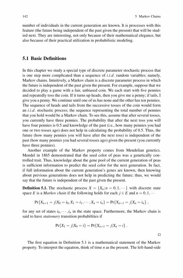
Fig. 5.1 State diagram for theMarkov chain of Example 5.1

��

0��

1

�1.0

�0.1

�

�� 0.9

is the probability of going to state j next, given the history of all past states. Theright-hand-side is the probability of going to state j next, given only the presentstate. Because they are equal, we have that the past history of states provides noadditional information helpful in predicting the future if the present state is known.The second equation (i.e., the stationary property) simply indicates that the proba-bility of a one-step transition does not change as time increases (in other words, theprobabilities are the same in the winter and the summer).

In this chapter it is always assumed that we are working with stationary transitionprobabilities. Because the probabilities are stationary, the only information neededto describe the process are the initial conditions (a probability mass function for X0)and the one-step transition probabilities. A square matrix is used for the transitionprobabilities and is often denoted by the capital letter P, where

P(i, j) = Pr{X1 = j|X0 = i} . (5.1)

Since the matrix P contains probabilities, it is always nonnegative (a matrix is non-negative if every element of it is nonnegative) and the sum of the elements withineach row equals one. In fact, any nonnegative matrix with row sums equal to one iscalled a Markov matrix.

Example 5.1. Consider a farmer using an old tractor. The tractor is often in the repairshop but it always takes only one day to get it running again. The first day out of theshop it always works but on any given day thereafter, independent of its previoushistory, there is a 10% chance of it not working and thus being sent back to theshop. Let X0,X1, · · · be random variables denoting the daily condition of the tractor,where a one denotes the working condition and a zero denotes the failed condition.In other words, Xn = 1 denotes that the tractor is working on day n and Xn = 0denotes it being in the repair shop on day n. Thus, X0,X1, · · · is a Markov chainwith state space E = {0,1} and with Markov matrix

P =01

[0 1

0.1 0.9

]

.

(Notice that the state space is sometimes written to the left of the matrix to help inkeeping track of which row refers to which state.) ��

In order to develop a mental image of the Markov chain, it is very helpful todraw a state diagram (Fig. 5.1) of the Markov matrix. In the diagram, each state isrepresented by a circle and the transitions with positive probabilities are representedby an arrow. Until the student is very familiar with Markov chains, we recommendthat state diagrams be drawn for any chain that being discussed.

144 5 Markov Chains

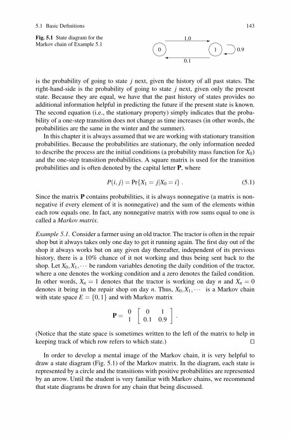
Fig. 5.2 State diagram for theMarkov chain of Example 5.2

��

a��

b

��

c

��������

0.5

��

��

��

0.75

�

0.25

�

0.25

�0.5

0.75�

Example 5.2. A salesman lives in town ‘a’ and is responsible for towns ‘a’, ‘b’, and‘c’. Each week he is required to visit a different town. When he is in his home town,it makes no difference which town he visits next so he flips a coin and if it is headshe goes to ‘b’ and if tails he goes to ‘c’. However, after spending a week away fromhome he has a slight preference for going home so when he is in either towns ‘b’ or‘c’ he flips two coins. If two heads occur, then he goes to the other town; otherwisehe goes to ‘a’. The successive towns that he visits form a Markov chain with statespace E = {a,b,c} where the random variable Xn equals a, b, or c according to hislocation during week n. The state diagram for this system is given in Fig. 5.2 andthe associated Markov matrix is

P =abc

⎡

⎣0 0.50 0.50

0.75 0 0.250.75 0.25 0

⎤

⎦ .

��

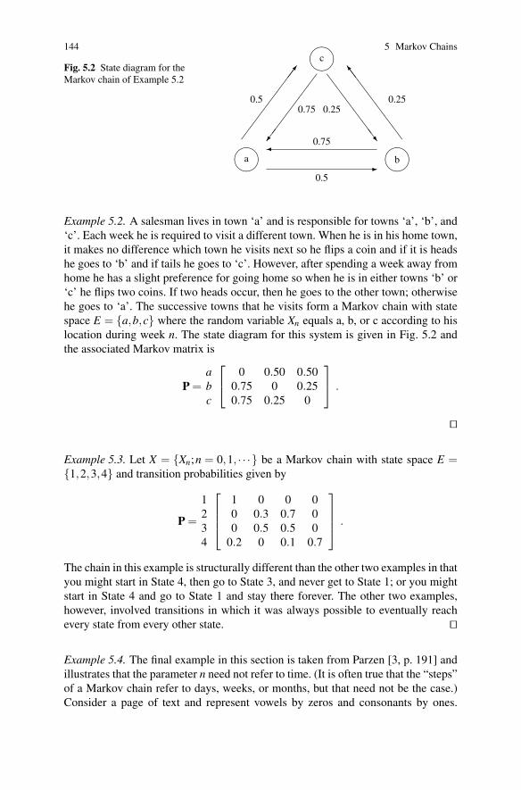
Example 5.3. Let X = {Xn;n = 0,1, · · ·} be a Markov chain with state space E ={1,2,3,4} and transition probabilities given by

P =

1234

⎡

⎢⎢⎣

1 0 0 00 0.3 0.7 00 0.5 0.5 0

0.2 0 0.1 0.7

⎤

⎥⎥⎦ .

The chain in this example is structurally different than the other two examples in thatyou might start in State 4, then go to State 3, and never get to State 1; or you mightstart in State 4 and go to State 1 and stay there forever. The other two examples,however, involved transitions in which it was always possible to eventually reachevery state from every other state. ��

Example 5.4. The final example in this section is taken from Parzen [3, p. 191] andillustrates that the parameter n need not refer to time. (It is often true that the “steps”of a Markov chain refer to days, weeks, or months, but that need not be the case.)Consider a page of text and represent vowels by zeros and consonants by ones.

5.2 Multistep Transitions 145

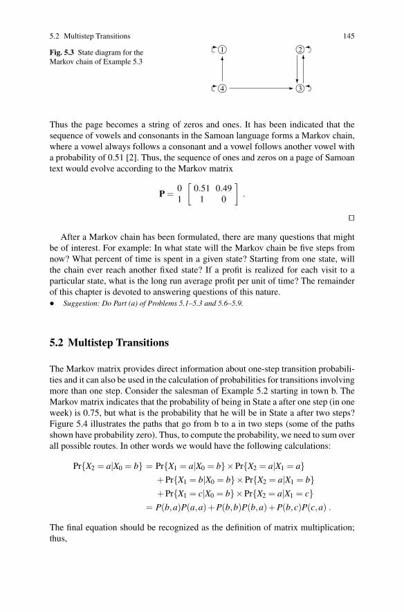
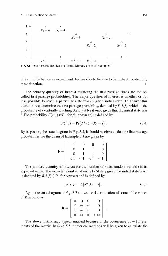
Fig. 5.3 State diagram for theMarkov chain of Example 5.3

4

1

�

���

���

3

2

�

���

�

��

�

�

Thus the page becomes a string of zeros and ones. It has been indicated that thesequence of vowels and consonants in the Samoan language forms a Markov chain,where a vowel always follows a consonant and a vowel follows another vowel witha probability of 0.51 [2]. Thus, the sequence of ones and zeros on a page of Samoantext would evolve according to the Markov matrix

P =01

[0.51 0.49

1 0

]

.

��

After a Markov chain has been formulated, there are many questions that mightbe of interest. For example: In what state will the Markov chain be five steps fromnow? What percent of time is spent in a given state? Starting from one state, willthe chain ever reach another fixed state? If a profit is realized for each visit to aparticular state, what is the long run average profit per unit of time? The remainderof this chapter is devoted to answering questions of this nature.• Suggestion: Do Part (a) of Problems 5.1–5.3 and 5.6–5.9.

5.2 Multistep Transitions

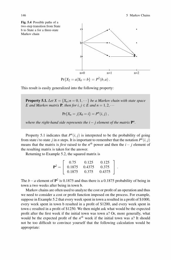
The Markov matrix provides direct information about one-step transition probabili-ties and it can also be used in the calculation of probabilities for transitions involvingmore than one step. Consider the salesman of Example 5.2 starting in town b. TheMarkov matrix indicates that the probability of being in State a after one step (in oneweek) is 0.75, but what is the probability that he will be in State a after two steps?Figure 5.4 illustrates the paths that go from b to a in two steps (some of the pathsshown have probability zero). Thus, to compute the probability, we need to sum overall possible routes. In other words we would have the following calculations:

Pr{X2 = a|X0 = b} = Pr{X1 = a|X0 = b}×Pr{X2 = a|X1 = a}+Pr{X1 = b|X0 = b}×Pr{X2 = a|X1 = b}+Pr{X1 = c|X0 = b}×Pr{X2 = a|X1 = c}

= P(b,a)P(a,a)+P(b,b)P(b,a)+P(b,c)P(c,a) .

The final equation should be recognized as the definition of matrix multiplication;thus,

146 5 Markov Chains

Fig. 5.4 Possible paths of atwo-step transition from Stateb to State a for a three-stateMarkov chain

n=0 n=1 n=2

�

�

�

�

�

�

�

�

�

a

b

c

� �

�������� �

��������

��������

Pr{X2 = a|X0 = b} = P2(b,a) .

This result is easily generalized into the following property:

Property 5.1. Let X = {Xn;n = 0,1, · · ·} be a Markov chain with state spaceE and Markov matrix P, then for i, j ∈ E and n = 1,2, · · ·

Pr{Xn = j|X0 = i} = Pn(i, j) ,

where the right-hand side represents the i− j element of the matrix Pn.

Property 5.1 indicates that Pn(i, j) is interpreted to be the probability of goingfrom state i to state j in n steps. It is important to remember that the notation Pn(i, j)means that the matrix is first raised to the nth power and then the i− j element ofthe resulting matrix is taken for the answer.

Returning to Example 5.2, the squared matrix is

P2 =

⎡

⎣0.75 0.125 0.125

0.1875 0.4375 0.3750.1875 0.375 0.4375

⎤

⎦ .

The b−a element of P2 is 0.1875 and thus there is a 0.1875 probability of being intown a two weeks after being in town b.

Markov chains are often used to analyze the cost or profit of an operation and thuswe need to consider a cost or profit function imposed on the process. For example,suppose in Example 5.2 that every week spent in town a resulted in a profit of $1000,every week spent in town b resulted in a profit of $1200, and every week spent intown c resulted in a profit of $1250. We then might ask what would be the expectedprofit after the first week if the initial town was town a? Or, more generally, whatwould be the expected profit of the nth week if the initial town was a? It shouldnot be too difficult to convince yourself that the following calculation would beappropriate:

5.2 Multistep Transitions 147

E[Profit for week n] = Pn(a,a)×1000+Pn(a,b)×1200+Pn(a,c)×1250 .

We thus have the following property.

Property 5.2. Let X = {Xn;n = 0,1, · · ·} be a Markov chain with state spaceE, Markov matrix P, and profit function f (i.e., each time the chain visits statei, a profit of f (i) is obtained). The expected profit at the nth step is given by

E[ f (Xn)|X0 = i] = Pnf(i) .

Note again that in the right-hand side of the equation, the matrix Pn is multipliedby the vector f first and then the ith component of the resulting vector is taken as theanswer. Thus, in Example 5.2, we have that the expected profit during the secondweek given that the initial town was a is

E[ f (X2)|X0 = a] = 0.75×1000+0.125×1200+0.125×1250

= 1056.25.

Up until now we have always assumed that the initial state was known. However,that is not always the situation. The manager of the traveling salesman might notknow for sure the location of the salesman; instead, all that is known is a probabilitymass function describing his initial location. Again, using Example 5.2, supposethat we do not know for sure the salesman’s initial location but know that there is a50% chance he is in town a, a 30% chance he is in town b, and a 20% chance he isin town c. We now ask, what is the probability that the salesman will be in town anext week? The calculations for that are

Pr{X1 = a} = 0.50×0+0.30×0.75+0.20×0.75 = 0.375 .

These calculations generalize to the following.

Property 5.3. Let X = {Xn;n = 0,1, · · ·} be a Markov chain with state spaceE, Markov matrix P, and initial probability vector μμμ (i.e., μ(i) = Pr{X0 = i}).Then

Prμ{Xn = j} = μμμPn( j) .

It should be noticed that μ is a subscript to the probability statement on the left-hand side of the equation. The purpose for the subscript is to insure that there is noconfusion over the given conditions. And again when interpreting the right-hand-side of the equation, the vector μμμ is multiplied by the matrix Pn first and then the jth

element is taken from the resulting vector.The last two properties can be combined, when necessary, into one statement.

148 5 Markov Chains

Property 5.4. Let X = {Xn;n = 0,1, · · ·} be a Markov chain with state spaceE, Markov matrix P, initial probability vector μμμ , and profit function f. Theexpected profit at the nth step is given by

Eμ [ f (Xn)] = μμμPnf .

Returning to Example 5.2 and using the initial probabilities and profit functiongiven above, we have that the expected profit in the second week is calculated to be

μμμP2f = (0.50,0.30,0.20)

⎡

⎣0.75 0.125 0.125

0.1875 0.4375 0.3750.1875 0.375 0.4375

⎤

⎦

⎛

⎝100012001250

⎞

⎠

= 1119.375 .

Example 5.5. A market analysis concerning consumer behavior in auto purchaseshas been conducted. Body styles traded-in and purchased have been recorded by aparticular dealer with the following results:

Number of Customers Trade275 sedan for sedan180 sedan for station wagon45 sedan for convertible80 station wagon for sedan

120 station wagon for station wagon150 convertible for sedan50 convertible for convertible

These data are believed to be representative of average consumer behavior, and it isassumed that the Markov assumptions are appropriate.

We shall develop a Markov chain to describe the changing body styles over thelife of a customer. (Notice, for purposes of instruction, we are simplifying the pro-cess by assuming that the age of the customer does not affect the customer’s choiceof a body style.) We define the Markov chain to be the body-style of the automo-bile that the customer has immediately after a trade-in, where the state space isE = {s,w,c} with s for the sedan, w for the wagon, and c for the convertible. Of500 customers who have a sedan, 275 will stay with the sedan during the next trade;therefore, the s-s element of the transition probability matrix will be 275/500. Thus,the Markov matrix for the “body style” Markov chain is

P =

s

w

c

⎡

⎢⎣

275/500 180/500 45/500

80/200 120/200 0

150/200 0 50/200

⎤

⎥⎦ =

⎡

⎢⎣

0.55 0.36 0.09

0.40 0.60 0.0

0.75 0.0 0.25

⎤

⎥⎦ .

5.3 Classification of States 149

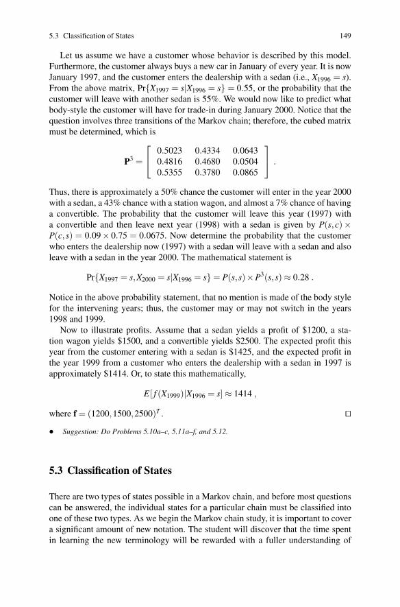
Let us assume we have a customer whose behavior is described by this model.Furthermore, the customer always buys a new car in January of every year. It is nowJanuary 1997, and the customer enters the dealership with a sedan (i.e., X1996 = s).From the above matrix, Pr{X1997 = s|X1996 = s} = 0.55, or the probability that thecustomer will leave with another sedan is 55%. We would now like to predict whatbody-style the customer will have for trade-in during January 2000. Notice that thequestion involves three transitions of the Markov chain; therefore, the cubed matrixmust be determined, which is

P3 =

⎡

⎣0.5023 0.4334 0.06430.4816 0.4680 0.05040.5355 0.3780 0.0865

⎤

⎦ .

Thus, there is approximately a 50% chance the customer will enter in the year 2000with a sedan, a 43% chance with a station wagon, and almost a 7% chance of havinga convertible. The probability that the customer will leave this year (1997) witha convertible and then leave next year (1998) with a sedan is given by P(s,c)×P(c,s) = 0.09× 0.75 = 0.0675. Now determine the probability that the customerwho enters the dealership now (1997) with a sedan will leave with a sedan and alsoleave with a sedan in the year 2000. The mathematical statement is

Pr{X1997 = s,X2000 = s|X1996 = s} = P(s,s)×P3(s,s) ≈ 0.28 .

Notice in the above probability statement, that no mention is made of the body stylefor the intervening years; thus, the customer may or may not switch in the years1998 and 1999.

Now to illustrate profits. Assume that a sedan yields a profit of $1200, a sta-tion wagon yields $1500, and a convertible yields $2500. The expected profit thisyear from the customer entering with a sedan is $1425, and the expected profit inthe year 1999 from a customer who enters the dealership with a sedan in 1997 isapproximately $1414. Or, to state this mathematically,

E[ f (X1999)|X1996 = s] ≈ 1414 ,

where f = (1200,1500,2500)T . ��

• Suggestion: Do Problems 5.10a–c, 5.11a–f, and 5.12.

5.3 Classification of States

There are two types of states possible in a Markov chain, and before most questionscan be answered, the individual states for a particular chain must be classified intoone of these two types. As we begin the Markov chain study, it is important to covera significant amount of new notation. The student will discover that the time spentin learning the new terminology will be rewarded with a fuller understanding of

150 5 Markov Chains

Markov chains. Furthermore, a good understanding of the dynamics involved forMarkov chains will greatly aid in the understanding of the entire area of stochasticprocesses.

Two random variables that will be extremely important denote “first passagetimes” and “number of visits to a fixed state”. To describe these random variables,consider a fixed state, call it State j, in the state space for a Markov chain. The firstpassage time is a random variable, denoted by T j, that equals the time (i.e., numberof steps) it takes to reach the fixed state for the first time. Mathematically, the firstpassage time random variable is defined by

T j = min{n ≥ 1 : Xn = j} , (5.2)

where the minimum of the empty set is taken to be +∞. For example, in Exam-ple 5.3, if X0 = 1 then T 2 = ∞, i.e., if the chain starts in State 1 then it will neverreach State 2.

The number of visits to a state is a random variable, denoted by N j, that equalsthe total number of visits (including time zero) that the Markov chain makes to thefixed state throughout the life of the chain. Mathematically, the “number of visits”random variable is defined by

N j =∞

∑n=0

I(Xn, j) , (5.3)

where I is the identity matrix. The identity matrix is used simply as a “counter”.Because the identity has ones on the diagonal and zeroes off the diagonal, it followsthat I(Xn, j) = 1 if Xn = j; otherwise, it is zero. It should be noted that the summationin (5.3) starts at n = 0; thus, if X0 = j then N j must be at least one.

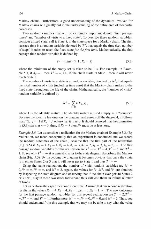
Example 5.6. Let us consider a realization for the Markov chain of Example 5.3. (Byrealization, we mean conceptually that an experiment is conducted and we recordthe random outcomes of the chain.) Assume that the first part of the realization(Fig. 5.5) is X0 = 4,X1 = 4,X2 = 4,X3 = 3,X4 = 2,X5 = 3,X6 = 2, · · · . The firstpassage random variables for this realization are T 1 = ∞,T 2 = 4,T 3 = 3,and T 4 =1. To see why T 1 = ∞, it is easiest to refer to the state diagram describing the Markovchain (Fig. 5.3). By inspecting the diagram it becomes obvious that once the chainis in either States 2 or 3 that it will never get to State 1 and thus T 1 = ∞.

Using the same realization, the number of visits random variables are N1 =0,N2 = ∞,N3 = ∞, and N4 = 3. Again, the values for N1,N2, and N3 are obtainedby inspecting the state diagram and observing that if the chain ever gets to States 2or 3 it will stay in those two states forever and thus will visit them an infinite numberof times.

Let us perform the experiment one more time. Assume that our second realizationresults in the values X0 = 4,X1 = 4,X2 = 1,X3 = 1,X4 = 1, · · · . The new outcomesfor the first passage random variables for this second realization are T 1 = 2,T 2 =∞,T 3 = ∞,and T 4 = 1. Furthermore, N1 = ∞,N2 = 0,N3 = 0,and N4 = 2. Thus, youshould understand from this example that we may not be able to say what the value

5.3 Classification of States 151

1

2

3

4

T 4 = 1 T 3 = 3 T 2 = 4

X1 = 4 X2 = 4

X3 = 3

X4 = 2

X5 = 3

X6 = 2

× × ×

×

×

×

×

·· ·

Fig. 5.5 One Possible Realization for the Markov chain of Example5.1

of T j will be before an experiment, but we should be able to describe its probabilitymass function. ��

The primary quantity of interest regarding the first passage times are the so-called first passage probabilities. The major question of interest is whether or notit is possible to reach a particular state from a given initial state. To answer thisquestion, we determine the first passage probability, denoted by F(i, j), which is theprobability of eventually reaching State j at least once given that the initial state wasi. The probability F(i, j) (“F” for first passage) is defined by

F(i, j) = Pr{T j < ∞|X0 = i} . (5.4)

By inspecting the state diagram in Fig. 5.3, it should be obvious that the first passageprobabilities for the chain of Example 5.3 are given by

F =

⎡

⎢⎢⎣

1 0 0 00 1 1 00 1 1 0

< 1 < 1 < 1 < 1

⎤

⎥⎥⎦ .

The primary quantity of interest for the number of visits random variable is itsexpected value. The expected number of visits to State j given the initial state was iis denoted by R(i, j) (“R” for returns) and is defined by

R(i, j) = E[N j|X0 = i] . (5.5)

Again the state diagram of Fig. 5.3 allows the determination of some of the valuesof R as follows:

R =

⎡

⎢⎢⎣

∞ 0 0 00 ∞ ∞ 00 ∞ ∞ 0∞ ∞ ∞ < ∞

⎤

⎥⎥⎦ .

The above matrix may appear unusual because of the occurrence of ∞ for ele-ments of the matrix. In Sect. 5.5, numerical methods will be given to calculate the

152 5 Markov Chains

values of the R and F matrices; however, the values of ∞ are obtained by an under-standing of the structures of the Markov chain and not through specific formulas.For now, our goal is to develop an intuitive understanding of these processes; there-fore, the major concern for the F matrix is whether an element is zero or one, andthe concern for the R matrix is whether an element is zero or infinity. As mightbe expected, there is a close relation between R(i, j) and F(i, j) as is shown in thefollowing property.

Property 5.5. Let R(i, j) and F(i, j) be as defined in (5.5) and (5.4), respec-tively. Then

R(i, j) =

⎧⎪⎨

⎪⎩

11−F( j, j) for i = j,

F(i, j)1−F( j, j) for i �= j;

,

where the convention 0/0 = 0 is used.

The above discussion utilizing Example 5.3 should help to point out that there is abasic difference between States 1, 2 or 3 and State 4 of the example. Consider that ifthe chain ever gets to State 1 or to State 2 or to State 3 then that state will continuallyreoccur. However, even if the chain starts in State 4, it will only stay there a finitenumber of times and will eventually leave State 4 never to return. These ideas giverise to the terminology of recurrent and transient states. Intuitively, a state is calledrecurrent if, starting in that state, it will continuously reoccur; and a state is calledtransient if, starting in that state, it will eventually leave that state never to return.Or equivalently, a state is recurrent if, starting in that state, the chain must (i.e., withprobability one) eventually return to the state at least once; and a state is transientif, starting in that state, there is a chance (i.e., with probability greater than zero)that the chain will leave the state and never return. The mathematical definitions arebased on these notions developed above.

Definition 5.2. A state j is called transient if F( j, j) < 1. Equivalently, state j istransient if R( j, j) < ∞. ��

Definition 5.3. A state j is called recurrent if F( j, j) = 1. Equivalently, state j isrecurrent if R( j, j) = ∞. ��

From the above two definitions, a state must either be transient or recurrent. Adictionary1 definition for the word transient is “passing esp. quickly into and outof existence”. Thus, the use of the word is justified since transient states will onlyoccur for a finite period of time. For a transient state, there will be a time after whichthe transient state will never again be visited. A dictionary1 definition for recurrentis “returning or happening time after time”. So again the mathematical concept of a

1 Webster’s Ninth New Collegiate Dictionary, (Springfield, MA: Merriam-Webster, Inc., 1989)

5.3 Classification of States 153

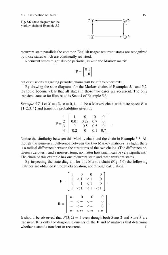
Fig. 5.6 State diagram for theMarkov chain of Example 5.7

4

1

�

���

���

3

2

�

���

�

��

�

�

�

recurrent state parallels the common English usage: recurrent states are recognizedby those states which are continually revisited.

Recurrent states might also be periodic, as with the Markov matrix

P =[

0 11 0

]

but discussions regarding periodic chains will be left to other texts.By drawing the state diagrams for the Markov chains of Examples 5.1 and 5.2,

it should become clear that all states in those two cases are recurrent. The onlytransient state so far illustrated is State 4 of Example 5.3.

Example 5.7. Let X = {Xn;n = 0,1, · · ·} be a Markov chain with state space E ={1,2,3,4} and transition probabilities given by

P =

1234

⎡

⎢⎢⎣

1 0 0 00.01 0.29 0.7 0

0 0.5 0.5 00.2 0 0.1 0.7

⎤

⎥⎥⎦ .

Notice the similarity between this Markov chain and the chain in Example 5.3. Al-though the numerical difference between the two Markov matrices is slight, thereis a radical difference between the structures of the two chains. (The difference be-tween a zero term and a nonzero term, no matter how small, can be very significant.)The chain of this example has one recurrent state and three transient states.

By inspecting the state diagram for this Markov chain (Fig. 5.6) the followingmatrices are obtained (through observation, not through calculation):

F =

⎡

⎢⎢⎣

1 0 0 01 < 1 < 1 01 1 < 1 01 < 1 < 1 < 1

⎤

⎥⎥⎦ .

R =

⎡

⎢⎢⎣

∞ 0 0 0∞ < ∞ < ∞ 0∞ < ∞ < ∞ 0∞ < ∞ < ∞ < ∞

⎤

⎥⎥⎦ .

It should be observed that F(3,2) = 1 even though both State 2 and State 3 aretransient. It is only the diagonal elements of the F and R matrices that determinewhether a state is transient or recurrent. ��

154 5 Markov Chains

� � �����

���

Step 1 Step 2

��

good

��

scrap

��

���

��

���

�����

���

�

0.7

0.10.2

0.1

0.05

0.8

0.05

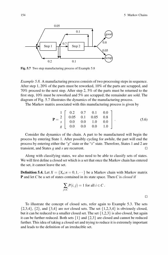
Fig. 5.7 Two step manufacturing process of Example 5.8

Example 5.8. A manufacturing process consists of two processing steps in sequence.After step 1, 20% of the parts must be reworked, 10% of the parts are scrapped, and70% proceed to the next step. After step 2, 5% of the parts must be returned to thefirst step, 10% must be reworked and 5% are scrapped; the remainder are sold. Thediagram of Fig. 5.7 illustrates the dynamics of the manufacturing process.

The Markov matrix associated with this manufacturing process is given by

P =

12sg

⎡

⎢⎢⎣

0.2 0.7 0.1 0.00.05 0.1 0.05 0.80.0 0.0 1.0 0.00.0 0.0 0.0 1.0

⎤

⎥⎥⎦ . (5.6)

Consider the dynamics of the chain. A part to be manufactured will begin theprocess by entering State 1. After possibly cycling for awhile, the part will end theprocess by entering either the “g” state or the “s” state. Therefore, States 1 and 2 aretransient, and States g and s are recurrent. ��

Along with classifying states, we also need to be able to classify sets of states.We will first define a closed set which is a set that once the Markov chain has enteredthe set, it cannot leave the set.

Definition 5.4. Let X = {Xn;n = 0,1, · · ·} be a Markov chain with Markov matrixP and let C be a set of states contained in its state space. Then C is closed if

∑j∈C

P(i, j) = 1 for all i ∈C .

��

To illustrate the concept of closed sets, refer again to Example 5.3. The sets{2,3,4}, {2}, and {3,4} are not closed sets. The set {1,2,3,4} is obviously closed,but it can be reduced to a smaller closed set. The set {1,2,3} is also closed, but againit can be further reduced. Both sets {1} and {2,3} are closed and cannot be reducedfurther. This idea of taking a closed set and trying to reduce it is extremely importantand leads to the definition of an irreducible set.

5.3 Classification of States 155

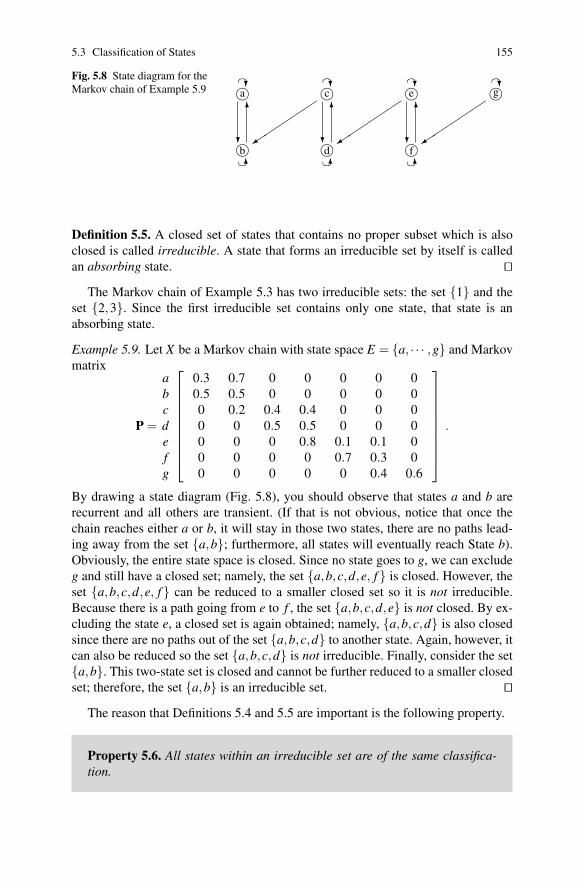
Fig. 5.8 State diagram for theMarkov chain of Example 5.9

b

a

d

c

f

e g

�

�

�

�

�

�

� ��

� ��

� ��

� ��

� ��

� �� � ��

��

����

��

����

��

����

Definition 5.5. A closed set of states that contains no proper subset which is alsoclosed is called irreducible. A state that forms an irreducible set by itself is calledan absorbing state. ��

The Markov chain of Example 5.3 has two irreducible sets: the set {1} and theset {2,3}. Since the first irreducible set contains only one state, that state is anabsorbing state.

Example 5.9. Let X be a Markov chain with state space E = {a, · · · ,g} and Markovmatrix

P =

abcdefg

⎡

⎢⎢⎢⎢⎢⎢⎢⎢⎣

0.3 0.7 0 0 0 0 00.5 0.5 0 0 0 0 00 0.2 0.4 0.4 0 0 00 0 0.5 0.5 0 0 00 0 0 0.8 0.1 0.1 00 0 0 0 0.7 0.3 00 0 0 0 0 0.4 0.6

⎤

⎥⎥⎥⎥⎥⎥⎥⎥⎦

.

By drawing a state diagram (Fig. 5.8), you should observe that states a and b arerecurrent and all others are transient. (If that is not obvious, notice that once thechain reaches either a or b, it will stay in those two states, there are no paths lead-ing away from the set {a,b}; furthermore, all states will eventually reach State b).Obviously, the entire state space is closed. Since no state goes to g, we can excludeg and still have a closed set; namely, the set {a,b,c,d,e, f} is closed. However, theset {a,b,c,d,e, f} can be reduced to a smaller closed set so it is not irreducible.Because there is a path going from e to f , the set {a,b,c,d,e} is not closed. By ex-cluding the state e, a closed set is again obtained; namely, {a,b,c,d} is also closedsince there are no paths out of the set {a,b,c,d} to another state. Again, however, itcan also be reduced so the set {a,b,c,d} is not irreducible. Finally, consider the set{a,b}. This two-state set is closed and cannot be further reduced to a smaller closedset; therefore, the set {a,b} is an irreducible set. ��

The reason that Definitions 5.4 and 5.5 are important is the following property.

Property 5.6. All states within an irreducible set are of the same classifica-tion.

156 5 Markov Chains

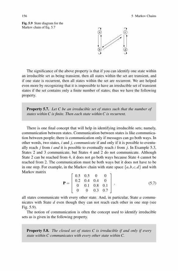
Fig. 5.9 State diagram for theMarkov chain of Eq. 5.7

b

a

d

c

�

�

�

�

� ��

� ��

� ��

� ��

��

����������

The significance of the above property is that if you can identify one state withinan irreducible set as being transient, then all states within the set are transient, andif one state is recurrent, then all states within the set are recurrent. We are helpedeven more by recognizing that it is impossible to have an irreducible set of transientstates if the set contains only a finite number of states; thus we have the followingproperty.

Property 5.7. Let C be an irreducible set of states such that the number ofstates within C is finite. Then each state within C is recurrent.

There is one final concept that will help in identifying irreducible sets; namely,communication between states. Communication between states is like communica-tion between people; there is communication only if messages can go both ways. Inother words, two states, i and j, communicate if and only if it is possible to eventu-ally reach j from i and it is possible to eventually reach i from j. In Example 5.3,States 2 and 3 communicate, but States 4 and 2 do not communicate. AlthoughState 2 can be reached from 4, it does not go both ways because State 4 cannot bereached from 2. The communication must be both ways but it does not have to bein one step. For example, in the Markov chain with state space {a,b,c,d} and withMarkov matrix

P =

⎡

⎢⎢⎣

0.5 0.5 0 00.2 0.4 0.4 00 0.1 0.8 0.10 0 0.3 0.7

⎤

⎥⎥⎦ , (5.7)

all states communicate with every other state. And, in particular, State a commu-nicates with State d even though they can not reach each other in one step (seeFig. 5.9).

The notion of communication is often the concept used to identify irreduciblesets as is given in the following property.

Property 5.8. The closed set of states C is irreducible if and only if everystate within C communicates with every other state within C.

5.4 Steady-State Behavior 157

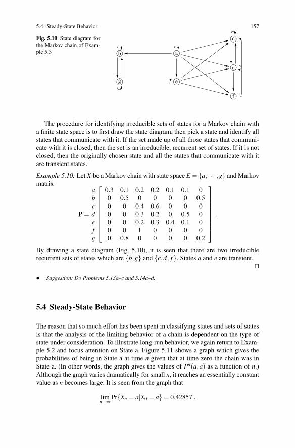
Fig. 5.10 State diagram forthe Markov chain of Exam-ple 5.3

g

b

�

�

� ��

� ��

e

a

� ��

���

�

�

f

d

c

� ��

���

�

�

�

�

��

���������

������������������

���������

������������������

The procedure for identifying irreducible sets of states for a Markov chain witha finite state space is to first draw the state diagram, then pick a state and identify allstates that communicate with it. If the set made up of all those states that communi-cate with it is closed, then the set is an irreducible, recurrent set of states. If it is notclosed, then the originally chosen state and all the states that communicate with itare transient states.

Example 5.10. Let X be a Markov chain with state space E = {a, · · · ,g} and Markovmatrix

P =

abcdefg

⎡

⎢⎢⎢⎢⎢⎢⎢⎢⎣

0.3 0.1 0.2 0.2 0.1 0.1 00 0.5 0 0 0 0 0.50 0 0.4 0.6 0 0 00 0 0.3 0.2 0 0.5 00 0 0.2 0.3 0.4 0.1 00 0 1 0 0 0 00 0.8 0 0 0 0 0.2

⎤

⎥⎥⎥⎥⎥⎥⎥⎥⎦

.

By drawing a state diagram (Fig. 5.10), it is seen that there are two irreduciblerecurrent sets of states which are {b,g} and {c,d, f}. States a and e are transient.

��• Suggestion: Do Problems 5.13a–c and 5.14a–d.

5.4 Steady-State Behavior

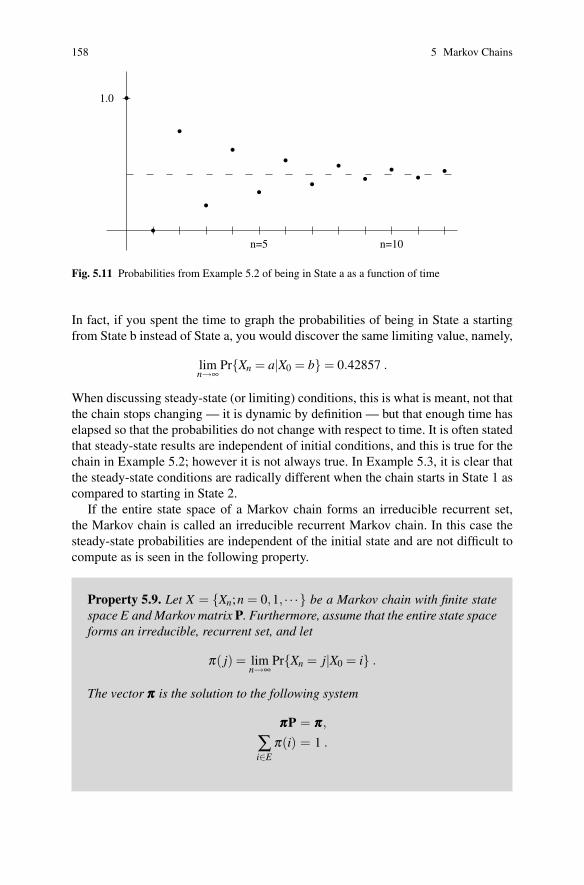
The reason that so much effort has been spent in classifying states and sets of statesis that the analysis of the limiting behavior of a chain is dependent on the type ofstate under consideration. To illustrate long-run behavior, we again return to Exam-ple 5.2 and focus attention on State a. Figure 5.11 shows a graph which gives theprobabilities of being in State a at time n given that at time zero the chain was inState a. (In other words, the graph gives the values of Pn(a,a) as a function of n.)Although the graph varies dramatically for small n, it reaches an essentially constantvalue as n becomes large. It is seen from the graph that

limn→∞

Pr{Xn = a|X0 = a} = 0.42857 .

158 5 Markov Chains

1.0

n=5 n=10

�

�

�

�

�

�

�

�

�

��

��

Fig. 5.11 Probabilities from Example 5.2 of being in State a as a function of time

In fact, if you spent the time to graph the probabilities of being in State a startingfrom State b instead of State a, you would discover the same limiting value, namely,

limn→∞

Pr{Xn = a|X0 = b} = 0.42857 .

When discussing steady-state (or limiting) conditions, this is what is meant, not thatthe chain stops changing — it is dynamic by definition — but that enough time haselapsed so that the probabilities do not change with respect to time. It is often statedthat steady-state results are independent of initial conditions, and this is true for thechain in Example 5.2; however it is not always true. In Example 5.3, it is clear thatthe steady-state conditions are radically different when the chain starts in State 1 ascompared to starting in State 2.

If the entire state space of a Markov chain forms an irreducible recurrent set,the Markov chain is called an irreducible recurrent Markov chain. In this case thesteady-state probabilities are independent of the initial state and are not difficult tocompute as is seen in the following property.

Property 5.9. Let X = {Xn;n = 0,1, · · ·} be a Markov chain with finite statespace E and Markov matrix P. Furthermore, assume that the entire state spaceforms an irreducible, recurrent set, and let

π( j) = limn→∞

Pr{Xn = j|X0 = i} .

The vector πππ is the solution to the following system

πππP = πππ,

∑i∈E

π(i) = 1 .

5.4 Steady-State Behavior 159

To illustrate the determination of πππ , observe that the Markov chain of Exam-ple 5.2 is irreducible, recurrent. Applying Property 5.9, we obtain

0.75πb + 0.75πc = πa

0.5πa + 0.25πc = πb

0.5πa + 0.25πb = πc

πa + πb + πc = 1 .

There are four equations and only three variables, so normally there would not be aunique solution; however, for an irreducible Markov matrix there is always exactlyone redundant equation from the system formed by πππP =πππ . Thus, to solve the abovesystem, arbitrarily choose one of the first three equations to discard and solve theremaining 3 by 3 system (never discard the final or norming equation) which yields

πa =37, πb =

27, πc =

27

.

Property 5.9 cannot be directly applied to the chain of Example 5.3 because thestate space is not irreducible. All irreducible, recurrent sets must be identified andgrouped together and then the Markov matrix is rearranged so that the irreduciblesets are together and transient states are last. In such a manner, the Markov matrixfor a chain can always be rewritten in the form

P =

⎡

⎢⎢⎢⎢⎢⎣

P1

P2

P3. . .

B1 B2 B3 · · · Q

⎤

⎥⎥⎥⎥⎥⎦

. (5.8)

After a chain is in this form, each submatrix Pi is a Markov matrix and can beconsidered as an independent Markov chain for which Property 5.9 is applied.

The Markov matrix of Example 5.3 is already in the form of (5.8). Since State 1 isabsorbing (i.e., an irreducible set of one state), its associated steady-state probabilityis easy; namely, π1 = 1. States 2 and 3 form an irreducible set so Property 5.9 canbe applied to the submatrix from those states resulting in the following system:

0.3π2 + 0.5π3 = π2

0.7π2 + 0.5π3 = π3

π2 + π3 = 1

which yields (after discarding one of the first two equations)

π2 =5

12and π3 =

712

.

The values π2 and π3 are interpreted to mean that if a snapshot of the chain istaken a long time after it started and if it started in States 2 or 3, then there is a 5/12

160 5 Markov Chains

probability that the picture will show the chain in State 2 and a 7/12 probability thatit will be in State 3. Another interpretation of the steady-state probabilities is thatif we recorded the time spent in States 2 and 3, then over the long run the fractionof time spent in State 2 would equal 5/12 and the fraction of time spent in State3 would equal 7/12. These steady-state results are summarized in the followingproperty.

Property 5.10. Let X = {Xn;n = 0,1, · · ·} be a Markov chain with finite statespace with k distinct irreducible sets. Let the �th irreducible set be denoted byC�, and let P� be the Markov matrix restricted to the �th irreducible set (as inEq. 5.8). Finally, let F be the matrix of first passage probabilities.

• If State j is transient,

limn→∞

Pr{Xn = j|X0 = i} = 0 .

• If State i and j both belong to the �th irreducible set,

limn→∞

Pr{Xn = j|X0 = i} = π( j)

where

πππP� = πππ and

∑i∈C�

π(i) = 1 .

• If State j is recurrent and i is not in its irreducible set,

limn→∞

Pr{Xn = j|X0 = i} = F(i, j)π( j) ,

where πππ is determined as above.• If State j is recurrent and X0 is in the same irreducible set as j,

limn→∞

1n

n−1

∑m=0

I(Xm, j) = π( j) ,

where I is the identity matrix.• If State j is recurrent,

E[T j|X0 = j] =1

π( j).

The intuitive idea of the second to last item in the above property is obtainedby considering the role that the identity matrix plays in the left-hand-side of the

5.4 Steady-State Behavior 161

equation. As mentioned previously, the identity matrix acts as a counter so that thesummation on the left-hand-side of the equation is the total number of visits that thechain makes to state j. Thus, the equality indicates that the fraction of time spentin State j is equal to the steady-state probability of being in State j. This propertyis called the Ergodic Property. The last property indicates that the reciprocal ofthe long-run probabilities equals the expected number of steps to return to the state.Intuitively, this is as one would expect it, since the higher the probability, the quickerthe return.

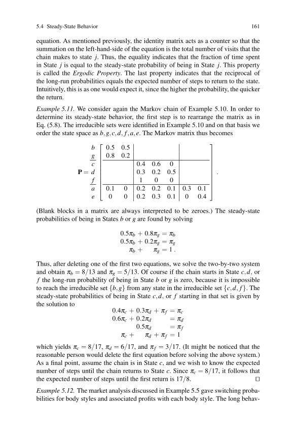
Example 5.11. We consider again the Markov chain of Example 5.10. In order todetermine its steady-state behavior, the first step is to rearrange the matrix as inEq. (5.8). The irreducible sets were identified in Example 5.10 and on that basis weorder the state space as b,g,c,d, f ,a,e. The Markov matrix thus becomes

P =

bgcdfae

⎡

⎢⎢⎢⎢⎢⎢⎢⎢⎣

0.5 0.50.8 0.2

0.4 0.6 00.3 0.2 0.51 0 0

0.1 0 0.2 0.2 0.1 0.3 0.10 0 0.2 0.3 0.1 0 0.4

⎤

⎥⎥⎥⎥⎥⎥⎥⎥⎦

.

(Blank blocks in a matrix are always interpreted to be zeroes.) The steady-stateprobabilities of being in States b or g are found by solving

0.5πb + 0.8πg = πb

0.5πb + 0.2πg = πg

πb + πg = 1 .

Thus, after deleting one of the first two equations, we solve the two-by-two systemand obtain πb = 8/13 and πg = 5/13. Of course if the chain starts in State c,d, orf the long-run probability of being in State b or g is zero, because it is impossibleto reach the irreducible set {b,g} from any state in the irreducible set {c,d, f}. Thesteady-state probabilities of being in State c,d, or f starting in that set is given bythe solution to

0.4πc + 0.3πd + π f = πc

0.6πc + 0.2πd = πd

0.5πd = π f

πc + πd + π f = 1

which yields πc = 8/17, πd = 6/17, and π f = 3/17. (It might be noticed that thereasonable person would delete the first equation before solving the above system.)As a final point, assume the chain is in State c, and we wish to know the expectednumber of steps until the chain returns to State c. Since πc = 8/17, it follows thatthe expected number of steps until the first return is 17/8. ��Example 5.12. The market analysis discussed in Example 5.5 gave switching proba-bilities for body styles and associated profits with each body style. The long behav-

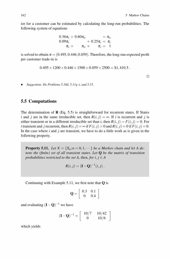
162 5 Markov Chains

ior for a customer can be estimated by calculating the long-run probabilities. Thefollowing system of equations

0.36πs + 0.60πw = πw

0.09πs + 0.25πc = πc

πs + πw + πc = 1

is solved to obtain π = (0.495,0.446,0.059). Therefore, the long-run expected profitper customer trade-in is

0.495×1200+0.446×1500+0.059×2500 = $1,410.5 .

��

• Suggestion: Do Problems 5.10d, 5.11g–i, and 5.15.

5.5 Computations

The determination of R (Eq. 5.5) is straightforward for recurrent states. If Statesi and j are in the same irreducible set, then R(i, j) = ∞. If i is recurrent and j iseither transient or in a different irreducible set than i, then R(i, j) = F(i, j) = 0. Fori transient and j recurrent, then R(i, j) = ∞ if F(i, j) > 0 and R(i, j) = 0 if F(i, j)= 0.In the case where i and j are transient, we have to do a little work as is given in thefollowing property.

Property 5.11. Let X = {Xn;n = 0,1, · · ·} be a Markov chain and let A de-note the (finite) set of all transient states. Let Q be the matrix of transitionprobabilities restricted to the set A, then, for i, j ∈ A

R(i, j) = (I−Q)−1(i, j) .

Continuing with Example 5.11, we first note that Q is

Q =[

0.3 0.10 0.4

]

and evaluating (I−Q)−1 we have

(I−Q)−1 =[

10/7 10/420 10/6

]

which yields

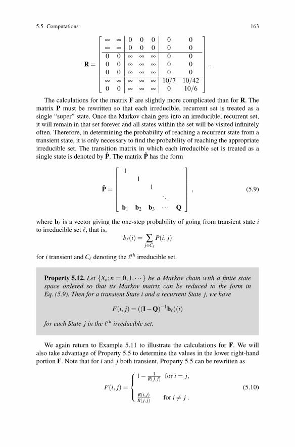
5.5 Computations 163

R =

⎡

⎢⎢⎢⎢⎢⎢⎢⎢⎣

∞ ∞ 0 0 0 0 0∞ ∞ 0 0 0 0 00 0 ∞ ∞ ∞ 0 00 0 ∞ ∞ ∞ 0 00 0 ∞ ∞ ∞ 0 0∞ ∞ ∞ ∞ ∞ 10/7 10/420 0 ∞ ∞ ∞ 0 10/6

⎤

⎥⎥⎥⎥⎥⎥⎥⎥⎦

.

The calculations for the matrix F are slightly more complicated than for R. Thematrix P must be rewritten so that each irreducible, recurrent set is treated as asingle “super” state. Once the Markov chain gets into an irreducible, recurrent set,it will remain in that set forever and all states within the set will be visited infinitelyoften. Therefore, in determining the probability of reaching a recurrent state from atransient state, it is only necessary to find the probability of reaching the appropriateirreducible set. The transition matrix in which each irreducible set is treated as asingle state is denoted by P̂. The matrix P̂ has the form

P̂ =

⎡

⎢⎢⎢⎢⎢⎣

11

1. . .

b1 b2 b3 · · · Q

⎤

⎥⎥⎥⎥⎥⎦

, (5.9)

where b� is a vector giving the one-step probability of going from transient state ito irreducible set �, that is,

b�(i) = ∑j∈C�

P(i, j)

for i transient and C� denoting the �th irreducible set.

Property 5.12. Let {Xn;n = 0,1, · · ·} be a Markov chain with a finite statespace ordered so that its Markov matrix can be reduced to the form inEq. (5.9). Then for a transient State i and a recurrent State j, we have

F(i, j) = ((I−Q)−1b�)(i)

for each State j in the �th irreducible set.

We again return to Example 5.11 to illustrate the calculations for F. We willalso take advantage of Property 5.5 to determine the values in the lower right-handportion F. Note that for i and j both transient, Property 5.5 can be rewritten as

F(i, j) =

⎧⎪⎨

⎪⎩

1− 1R( j, j) for i = j,

R(i, j)R( j, j) for i �= j .

(5.10)

164 5 Markov Chains

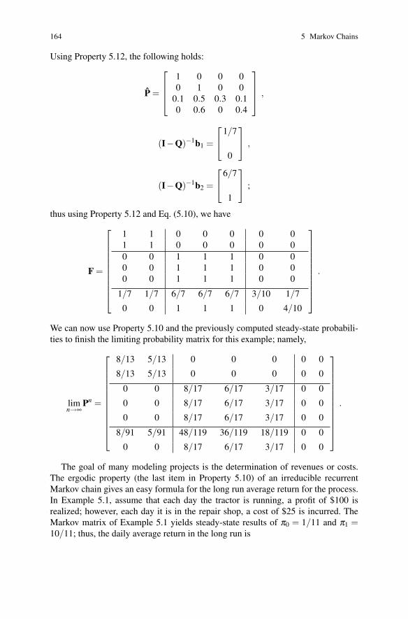
Using Property 5.12, the following holds:

P̂ =

⎡

⎢⎢⎣

1 0 0 00 1 0 0

0.1 0.5 0.3 0.10 0.6 0 0.4

⎤

⎥⎥⎦ ,

(I−Q)−1b1 =

⎡

⎣1/7

0

⎤

⎦ ,

(I−Q)−1b2 =

⎡

⎣6/7

1

⎤

⎦ ;

thus using Property 5.12 and Eq. (5.10), we have

F =

⎡

⎢⎢⎢⎢⎢⎢⎢⎢⎢⎣

1 1 0 0 0 0 01 1 0 0 0 0 00 0 1 1 1 0 00 0 1 1 1 0 00 0 1 1 1 0 0

1/7 1/7 6/7 6/7 6/7 3/10 1/7

0 0 1 1 1 0 4/10

⎤

⎥⎥⎥⎥⎥⎥⎥⎥⎥⎦

.

We can now use Property 5.10 and the previously computed steady-state probabili-ties to finish the limiting probability matrix for this example; namely,

limn→∞

Pn =

⎡

⎢⎢⎢⎢⎢⎢⎢⎢⎢⎢⎢⎣

8/13 5/13 0 0 0 0 0

8/13 5/13 0 0 0 0 0

0 0 8/17 6/17 3/17 0 0

0 0 8/17 6/17 3/17 0 0

0 0 8/17 6/17 3/17 0 0

8/91 5/91 48/119 36/119 18/119 0 0

0 0 8/17 6/17 3/17 0 0

⎤

⎥⎥⎥⎥⎥⎥⎥⎥⎥⎥⎥⎦

.

The goal of many modeling projects is the determination of revenues or costs.The ergodic property (the last item in Property 5.10) of an irreducible recurrentMarkov chain gives an easy formula for the long run average return for the process.In Example 5.1, assume that each day the tractor is running, a profit of $100 isrealized; however, each day it is in the repair shop, a cost of $25 is incurred. TheMarkov matrix of Example 5.1 yields steady-state results of π0 = 1/11 and π1 =10/11; thus, the daily average return in the long run is

5.5 Computations 165

−25× 111

+100× 1011

= 88.64 .

This intuitive result is given in the following property.

Property 5.13. Let X = {Xn;n = 0,1, · · ·} be an irreducible Markov chainwith finite state space E and with steady-state probabilities given by the vectorπππ . Let the vector f be a profit function (i.e., f (i) is the profit received for eachvisit to State i). Then (with probability one) the long-run average profit perunit of time is

limn→∞

1n

n−1

∑k=0

f (Xk) = ∑j∈E

π( j) f ( j) .

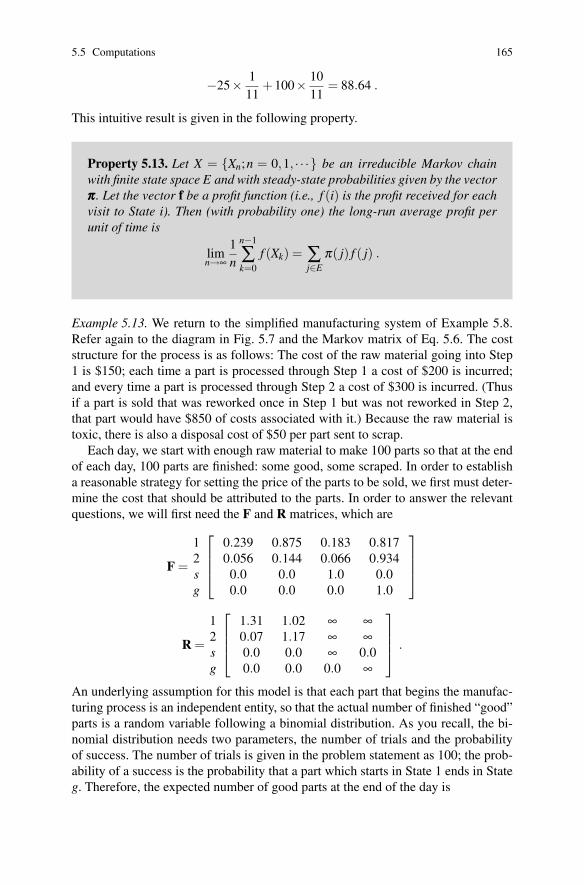
Example 5.13. We return to the simplified manufacturing system of Example 5.8.Refer again to the diagram in Fig. 5.7 and the Markov matrix of Eq. 5.6. The coststructure for the process is as follows: The cost of the raw material going into Step1 is $150; each time a part is processed through Step 1 a cost of $200 is incurred;and every time a part is processed through Step 2 a cost of $300 is incurred. (Thusif a part is sold that was reworked once in Step 1 but was not reworked in Step 2,that part would have $850 of costs associated with it.) Because the raw material istoxic, there is also a disposal cost of $50 per part sent to scrap.

Each day, we start with enough raw material to make 100 parts so that at the endof each day, 100 parts are finished: some good, some scraped. In order to establisha reasonable strategy for setting the price of the parts to be sold, we first must deter-mine the cost that should be attributed to the parts. In order to answer the relevantquestions, we will first need the F and R matrices, which are

F =

12sg

⎡

⎢⎢⎣

0.239 0.875 0.183 0.8170.056 0.144 0.066 0.934

0.0 0.0 1.0 0.00.0 0.0 0.0 1.0

⎤

⎥⎥⎦

R =

12sg

⎡

⎢⎢⎣

1.31 1.02 ∞ ∞0.07 1.17 ∞ ∞0.0 0.0 ∞ 0.00.0 0.0 0.0 ∞

⎤

⎥⎥⎦ .

An underlying assumption for this model is that each part that begins the manufac-turing process is an independent entity, so that the actual number of finished “good”parts is a random variable following a binomial distribution. As you recall, the bi-nomial distribution needs two parameters, the number of trials and the probabilityof success. The number of trials is given in the problem statement as 100; the prob-ability of a success is the probability that a part which starts in State 1 ends in Stateg. Therefore, the expected number of good parts at the end of the day is

166 5 Markov Chains

100×F(1,g) = 81.7 .

The cost per part started is given by

150+200×R(1,1)+300×R(1,2)+50×F(1,s) = 727.15 .

Therefore, the cost which should be associated to each part sold is

(100×727.15)/81.7 = $890/part sold .

A rush order for 100 parts from a very important customer has just been received,and there are no parts in inventory. Therefore, we wish to start tomorrow’s produc-tion with enough raw material to be 95% confident that there will be at least 100good parts at the end of the day. How many parts should we plan on starting tomor-row morning? Let the random variable Nn denote the number of finished parts thatare good given that the day started with enough raw material for n parts. From theabove discussion, the random variable Nn has a binomial distribution where n is thenumber of trials and F(1,g) is the probability of success. Therefore, the question ofinterest is to find n such that Pr{Nn ≥ 100} = 0.95. Hopefully, you also recall thatthe binomial distribution can be approximated by the normal distribution; therefore,define X to be a normally distributed random variable with mean nF(1,g) and vari-ance nF(1,g)F(1,s). We now have the following equation:

Pr{Nn ≥ 100} ≈ Pr{X > 99.5}= Pr{Z > (99.5−0.817n)/

√0.1495n} = 0.95

where Z is normally distributed with mean zero and variance one. Thus, using eitherstandard statistical tables or the Excel function =NORMSINV(0.05), we have that

99.5−0.817n√0.1495n

= −1.645 .

The above equation is solved for n. Since it becomes a quadratic equation, there aretwo roots: n1 = 113.5 and n2 = 130.7. We must take the second root (why?), andwe round up; thus, the day must start with enough raw material for 131 parts. ��

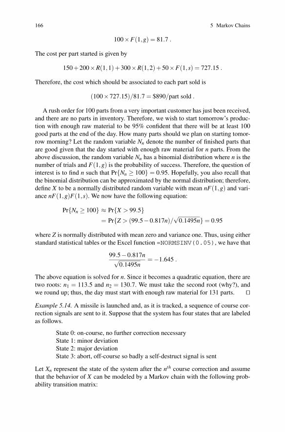
Example 5.14. A missile is launched and, as it is tracked, a sequence of course cor-rection signals are sent to it. Suppose that the system has four states that are labeledas follows.

State 0: on-course, no further correction necessaryState 1: minor deviationState 2: major deviationState 3: abort, off-course so badly a self-destruct signal is sent

Let Xn represent the state of the system after the nth course correction and assumethat the behavior of X can be modeled by a Markov chain with the following prob-ability transition matrix:

5.5 Computations 167

P =

0123

⎡

⎢⎢⎣

1.0 0.0 0.0 0.00.5 0.25 0.25 0.00.0 0.5 0.25 0.250.0 0.0 0.0 1.0

⎤

⎥⎥⎦ .

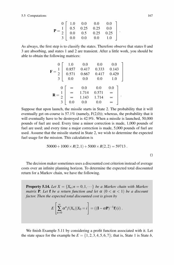
As always, the first step is to classify the states. Therefore observe that states 0 and3 are absorbing, and states 1 and 2 are transient. After a little work, you should beable to obtain the following matrices:

F =

0123

⎡

⎢⎢⎣

1.0 0.0 0.0 0.00.857 0.417 0.333 0.1430.571 0.667 0.417 0.429

0.0 0.0 0.0 1.0

⎤

⎥⎥⎦

R =

0123

⎡

⎢⎢⎣

∞ 0.0 0.0 0.0∞ 1.714 0.571 ∞∞ 1.143 1.714 ∞

0.0 0.0 0.0 ∞

⎤

⎥⎥⎦ .

Suppose that upon launch, the missile starts in State 2. The probability that it willeventually get on-course is 57.1% (namely, F(2,0)); whereas, the probability that itwill eventually have to be destroyed is 42.9%. When a missile is launched, 50,000pounds of fuel are used. Every time a minor correction is made, 1,000 pounds offuel are used; and every time a major correction is made, 5,000 pounds of fuel areused. Assume that the missile started in State 2, we wish to determine the expectedfuel usage for the mission. This calculation is

50000+1000×R(2,1)+5000×R(2,2) = 59713 .

��

The decision maker sometimes uses a discounted cost criterion instead of averagecosts over an infinite planning horizon. To determine the expected total discountedreturn for a Markov chain, we have the following.

Property 5.14. Let X = {Xn;n = 0,1, · · ·} be a Markov chain with Markovmatrix P. Let f be a return function and let α (0 < α < 1) be a discountfactor. Then the expected total discounted cost is given by

E

[∞

∑n=0

αn f (Xn)|X0 = i

]

= ((I−αP)−1f)(i) .

We finish Example 5.11 by considering a profit function associated with it. Letthe state space for the example be E = {1,2,3,4,5,6,7}; that is, State 1 is State b,

168 5 Markov Chains

State 2 is State g, etc. Let f be the profit function with f = (500,450,400,350,300,350,200); that is, each visit to State 1 produces $500, each visit to State 2 produces$450, etc. If the chain starts in States 1 or 2, then the long-run average profit perperiod is

500× 813

+450× 513

= $480.77 .

If the chain starts in States 3, 4, or 5, then the long-run average profit per period is

400× 817

+350× 617

+300× 317

= $364.71 .

If the chain starts in State 6, then the expected value of the long-run average wouldbe a weighted average of the two ergodic results, namely,

480.77× 17

+364.71× 67

= $381.29 ,

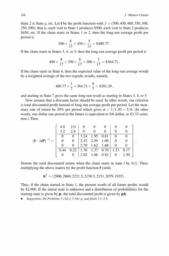
and starting in State 7 gives the same long-run result as starting in States 3, 4, or 5.Now assume that a discount factor should be used. In other words, our criterion

is total discounted profit instead of long-run average profit per period. Let the mon-etary rate of return be 20% per period which gives α = 1/1.20 = 5/6. (In otherwords, one dollar one period in the future is equivalent to 5/6 dollar, or 83.33 cents,now.) Then

(I−αP)−1 =

⎡

⎢⎢⎢⎢⎢⎢⎢⎢⎣

4.0 2.0 0 0 0 0 03.2 2.8 0 0 0 0 00 0 3.24 1.95 0.81 0 00 0 2.32 2.59 1.08 0 00 0 2.70 1.62 1.68 0 0

0.44 0.22 1.76 1.37 0.70 1.33 0.170 0 2.02 1.66 0.82 0 1.50

⎤

⎥⎥⎥⎥⎥⎥⎥⎥⎦

.

Denote the total discounted return when the chain starts in state i by h(i). Then,multiplying the above matrix by the profit function f yields

hT = (2900,2860,2221.5,2158.5,2151,2079,1935) .

Thus, if the chain started in State 1, the present worth of all future profits wouldbe $2,900. If the initial state is unknown and a distribution of probabilities for thestarting state is given by μμμ , the total discounted profit is given by μμμh.• Suggestion: Do Problems 5.13d–f, 5.14e–g, and finish 5.1–5.9.

Appendix 169

Appendix

We close the chapter with a brief look at the use of Excel for analyzing Markovchains. We will consider both the matrix operations involved in the computations ofSection 5.5 and the use of random numbers for simulating Markov chains.

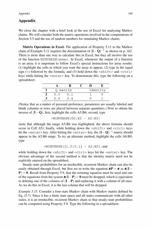
Matrix Operations in Excel. The application of Property 5.11 to the Markovchain of Example 5.11 requires the determination of (I−Q)−1 as shown on p. 162.There is more than one way to calculate this in Excel, but they all involve the useof the function MINVERSE(array). In Excel, whenever the output of a functionis an array it is important to follow Excel’s special instructions for array results:(1) highlight the cells in which you want the array to appear, (2) type in the equalsign (=) followed by the formula, and (3) hold down the <shift> and <ctrl>keys while hitting the <enter> key. To demonstrate this, type the following on aspreadsheet:

A B C D E1 Q matrix Identity2 0.3 0.1 1 03 0.0 0.4 0 1

(Notice that as a matter of personal preference, parameters are usually labeled andblank columns or rows are placed between separate quantities.) Now to obtain theinverse of (I−Q), first, highlight the cells A5:B6; second, type

=MINVERSE(D2:E3 - A2:B3)

(note that although the range A5:B6 was highlighted, the above formula shouldoccur in Cell A5); finally, while holding down the <shift> and <ctrl> keyshit the <enter> key. After hitting the <enter> key, the (I−Q)−1 matrix shouldappear in the A5:B6 range. To try an alternate method, highlight the cells A8:B9,type

=MINVERSE({1,0;0,1} - A2:B3), and

while holding down the <shift> and <ctrl> keys hit the <enter> key. Theobvious advantage of the second method is that the identity matrix need not beexplicitly entered on the spreadsheet.

Steady-state probabilities for an irreducible, recurrent Markov chain can also beeasily obtained through Excel, but first we re-write the equation πππP = πππ as πππ(I−P) = 0. Recall from Property 5.9, that the norming equation must be used and oneof the equations from the system πππ(I−P) = 0 must be dropped, which is equivalentto deleting one of the columns of (I−P) and replacing it with a column of all ones.As we do this in Excel, it is the last column that will be dropped.

Example 5.15. Consider a four-state Markov chain with Markov matrix defined byEq. (5.7). Since it has a finite state space and all states communicate with all otherstates, it is an irreducible, recurrent Markov chain so that steady-state probabilitiescan be computed using Property 5.9. Type the following in a spreadsheet:

170 5 Markov Chains

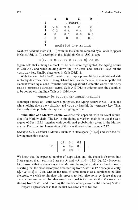
A B C D1 P matrix2 0.5 0.5 0 03 0.2 0.4 0.4 04 0 0.1 0.8 0.15 0 0 0.3 0.767 Modified I-P matrix

Next, we need the matrix (I−P) with the last column replaced by all ones to appearin Cells A8:D11. To accomplish this, highlight Cells A8:C11, type

={1,0,0;0,1,0;0,0,1;0,0,0}-A2:C5(again note that although a block of 12 cells were highlighted, the typing occursin Cell A8), and while holding down the <shift> and <ctrl> keys hit the<enter> key. Finally, place ones in Cells D8:D11.

With the modified (I−P) matrix, we simply pre-multiply the right-hand sidevector by its inverse, where the right-hand side is a vector of all zeros except the lastelement which equals one (from the norming equation). Center the words "Steadystate probabilities" across Cells A13:D13 in order to label the quantitiesto be computed, highlight Cells A14:D14, type

=MMULT({0,0,0,1},MINVERSE(A8:D11))(although a block of 4 cells were highlighted, the typing occurs in Cell A14), andwhile holding down the <shift> and <ctrl> keys hit the <enter> key. Thus,the steady-state probabilities appear in highlighted cells. ��

Simulation of a Markov Chain. We close this appendix with an Excel simula-tion of a Markov chain. The key to simulating a Markov chain is to use the tech-niques of Sect. 2.3.1 together with conditional probabilities given in the Markovmatrix. The Excel implementation of this was illustrated in Example 2.12.

Example 5.16. Consider a Markov chain with state space {a,b,c} and with the fol-lowing transition matrix:

P =

⎡

⎣0.8 0.1 0.10.4 0.6 0.00.0 0.0 1.0

⎤

⎦ .

We know that the expected number of steps taken until the chain is absorbed intoState c given that it starts in State a is R(a,a)+ R(a,b) = 12.5 (Eq. 5.5). However,let us assume that as a new student of Markov chains, our confidence level is low inasserting that the mean absorption time starting from State a is 12.5 (or equivalently,E[T c|X0 = a] = 12.5). One of the uses of simulation is as a confidence builder;therefore, we wish to simulate this process to help give some evidence that ourcalculations are correct. In other words, our goal is to simulate this Markov chainstarting from State a and recording the number of steps taken until reaching State c.

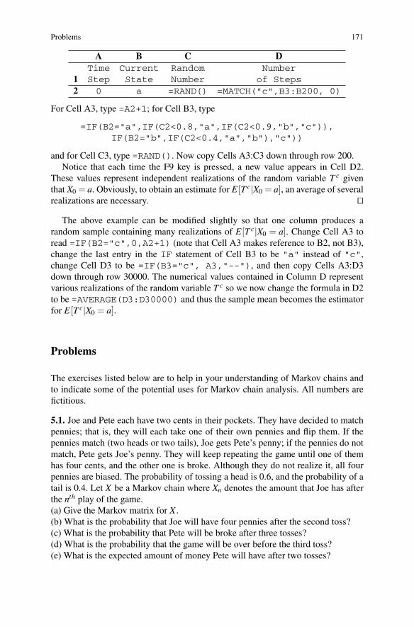
Prepare a spreadsheet so that the first two rows are as follows:

Problems 171

A B C DTime Current Random Number

1 Step State Number of Steps2 0 a =RAND() =MATCH("c",B3:B200, 0)

For Cell A3, type =A2+1; for Cell B3, type

=IF(B2="a",IF(C2<0.8,"a",IF(C2<0.9,"b","c")),IF(B2="b",IF(C2<0.4,"a","b"),"c"))

and for Cell C3, type =RAND(). Now copy Cells A3:C3 down through row 200.Notice that each time the F9 key is pressed, a new value appears in Cell D2.

These values represent independent realizations of the random variable T c giventhat X0 = a. Obviously, to obtain an estimate for E[T c|X0 = a], an average of severalrealizations are necessary. ��

The above example can be modified slightly so that one column produces arandom sample containing many realizations of E[T c|X0 = a]. Change Cell A3 toread =IF(B2="c",0,A2+1) (note that Cell A3 makes reference to B2, not B3),change the last entry in the IF statement of Cell B3 to be "a" instead of "c",change Cell D3 to be =IF(B3="c", A3,"--"), and then copy Cells A3:D3down through row 30000. The numerical values contained in Column D representvarious realizations of the random variable T c so we now change the formula in D2to be =AVERAGE(D3:D30000) and thus the sample mean becomes the estimatorfor E[T c|X0 = a].

Problems

The exercises listed below are to help in your understanding of Markov chains andto indicate some of the potential uses for Markov chain analysis. All numbers arefictitious.

5.1. Joe and Pete each have two cents in their pockets. They have decided to matchpennies; that is, they will each take one of their own pennies and flip them. If thepennies match (two heads or two tails), Joe gets Pete’s penny; if the pennies do notmatch, Pete gets Joe’s penny. They will keep repeating the game until one of themhas four cents, and the other one is broke. Although they do not realize it, all fourpennies are biased. The probability of tossing a head is 0.6, and the probability of atail is 0.4. Let X be a Markov chain where Xn denotes the amount that Joe has afterthe nth play of the game.(a) Give the Markov matrix for X .(b) What is the probability that Joe will have four pennies after the second toss?(c) What is the probability that Pete will be broke after three tosses?(d) What is the probability that the game will be over before the third toss?(e) What is the expected amount of money Pete will have after two tosses?

172 5 Markov Chains

(f) What is the probability that Pete will end up broke?(g) What is the expected number of tosses until the game is over?

5.2. At the start of each week, the condition of a machine is determined by measur-ing the amount of electrical current it uses. According to its amperage reading, themachine is categorized as being in one of the following four states: low, medium,high, failed. A machine in the low state has a probability of 0.05, 0.03, and 0.02 ofbeing in the medium, high, or failed state, respectively, at the start of the next week.A machine in the medium state has a probability of 0.09 and 0.06 of being in thehigh or failed state, respectively, at the start of the next week (it cannot, by itself, goto the low state). And, a machine in the high state has a probability of 0.1 of beingin the failed state at the start of the next week (it cannot, by itself, go to the lowor medium state). If a machine is in the failed state at the start of a week, repair isimmediately begun on the machine so that it will (with probability 1) be in the lowstate at the start of the following week. Let X be a Markov chain where Xn is thestate of the machine at the start of week n.(a) Give the Markov matrix for X .(b) A new machine always starts in the low state. What is the probability that themachine is in the failed state three weeks after it is new?(c) What is the probability that a machine has at least one failure three weeks afterit is new?(d) On the average, how many weeks per year is the machine working?(e) Each week that the machine is in the low state, a profit of $1,000 is realized;each week that the machine is in the medium state, a profit of $500 is realized; eachweek that the machine is in the high state, a profit of $400 is realized; and the weekin which a failure is fixed, a cost of $700 is incurred. What is the long-run averageprofit per week realized by the machine?(f) A suggestion has been made to change the maintenance policy for the machine.If at the start of a week the machine is in the high state, the machine will be takenout of service and repaired so that at the start of the next week it will again be in thelow state. When a repair is made due to the machine being in the high state insteadof a failed state, a cost of $600 is incurred. Is this new policy worthwhile?

5.3. We are interested in the movement of patients within a hospital. For purposesof our analysis, we shall consider the hospital to have three different types of rooms:general care, special care, and intensive care. Based on past data, 60% of arrivingpatients are initially admitted into the general care category, 30% in the special carecategory, and 10% in intensive care. A “general care” patient has a 55% chance ofbeing released healthy the following day, a 30% of remaining in the general careroom, and a 15% of being moved to the special care facility. A “special care” pa-tient has a 10% chance of being released the following day, a 20% chance of beingmoved to general care, a 10% chance of being upgraded to intensive care, and a5% chance of dying during the day. An “intensive care” patient is never releasedfrom the hospital directly from the intensive care unit (ICU), but is always movedto another facility first. The probabilities that the patient is moved to general care,special care, or remains in intensive care are 5%, 30%, or 55%, respectively. Let X

Problems 173

be a Markov chain where X0 is the type of room that an admitted patient initiallyuses, and Xn is the room category of that patient at the end of day n.(a) Give the Markov matrix for X .(b) What is the probability that a patient admitted into the intensive care room even-tually leaves the hospital healthy?(c) What is the expected number of days that a patient, admitted into intensive care,will spend in the ICU?(d) What is the expected length of stay for a patient admitted into the hospital as ageneral care patient?(e) During a typical day, 100 patients are admitted into the hospital. What is theaverage number of patients in the ICU?

5.4. Consider again the manufacturing process of Example 5.8. New productionplans call for an expected production level of 2000 good parts per month. (In otherwords, enough raw material must be used so that the expected number of good partsproduced each month is 2000.) For a capital investment and an increase in operatingcosts, all rework and scrap can be eliminated. The sum of the capital investment andoperating cost increase is equivalent to an annual cost of $5 million. Is it worthwhileto increase the annual cost by $5 million in order to eliminate the scrap and rework?

5.5. Assume the description of the manufacturing process of Example 5.8 is for theprocess at Branch A of the manufacturing company. Branch B of the same companyhas been closed. Branch B had an identical process and they had 1000 items in stockthat had been through Step 1 of the process when they were shut down. Because theprocess was identical, these items can be fed into Branch A’s process at the startof Step 2. (However, since the process was identical there is still a 5% chance thatafter finishing Step 2 the item will have to be reworked at Step 1, a 10% chance theitem will have to be reworked at Step 2, and a 5% chance that the item will haveto be scrapped.) Branch A purchases these (partially completed) items for a totalof $300,000, and they will start processing at Step 2 of Branch A’s system. AfterBranch A finishes processing this batch of items, they must determine the cost ofthese items so they will know how much to charge customers in order to recoverthe cost. (They may want to give a discount.) Your task is to determine the cost thatwould be attributed to each item shipped.

5.6. The manufacture of a certain type of electronic board consists of four steps:tinning, forming, insertion, and solder. After the forming step, 5% of the parts mustbe retinned; after the insertion step, 20% of the parts are bad and must be scrapped;and after the solder step, 30% of the parts must be returned to insertion and 10%must be scrapped. (We assume that when a part is returned to a processing step, it istreated like any other part entering that step.) Figure 5.12 gives a schematic showingthe flow of a job through the manufacturing steps.(a) Model this process using Markov chains and give its Markov matrix.(b) If a batch of 100 boards begins this manufacturing process, what is the expectednumber that will end up scraped?(c) How many boards should we start with if the goal is to have the expected number

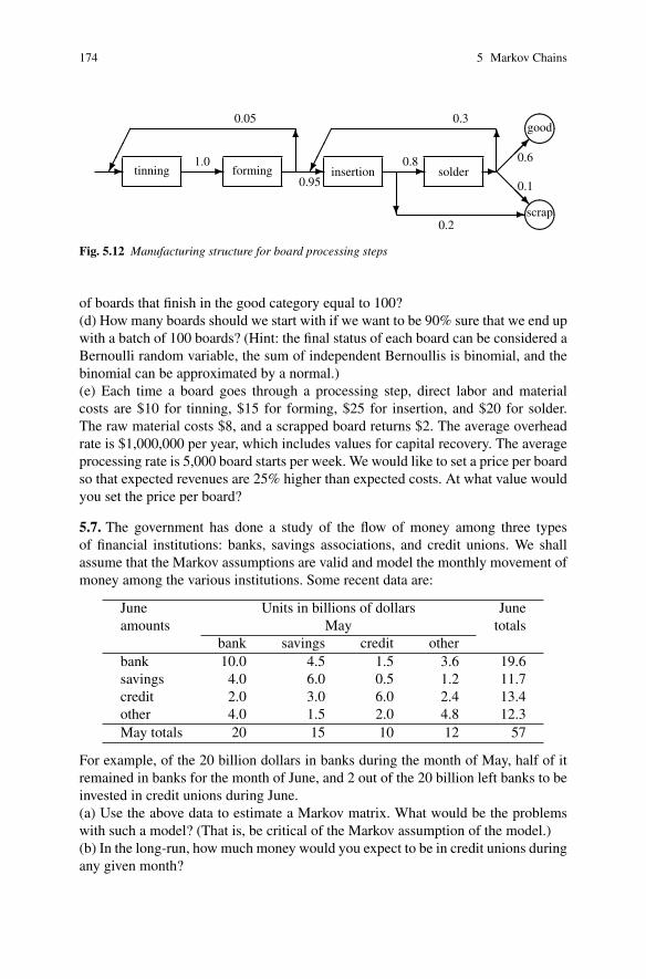
174 5 Markov Chains

� � � � �����

���

tinning forming insertion solder

��

good

��

scrap

��

�

��

�

� �

1.0

0.05

0.95

0.8

0.2

0.3

0.6

0.1

Fig. 5.12 Manufacturing structure for board processing steps

of boards that finish in the good category equal to 100?(d) How many boards should we start with if we want to be 90% sure that we end upwith a batch of 100 boards? (Hint: the final status of each board can be considered aBernoulli random variable, the sum of independent Bernoullis is binomial, and thebinomial can be approximated by a normal.)(e) Each time a board goes through a processing step, direct labor and materialcosts are $10 for tinning, $15 for forming, $25 for insertion, and $20 for solder.The raw material costs $8, and a scrapped board returns $2. The average overheadrate is $1,000,000 per year, which includes values for capital recovery. The averageprocessing rate is 5,000 board starts per week. We would like to set a price per boardso that expected revenues are 25% higher than expected costs. At what value wouldyou set the price per board?

5.7. The government has done a study of the flow of money among three typesof financial institutions: banks, savings associations, and credit unions. We shallassume that the Markov assumptions are valid and model the monthly movement ofmoney among the various institutions. Some recent data are:

June Units in billions of dollars Juneamounts May totals

bank savings credit otherbank 10.0 4.5 1.5 3.6 19.6savings 4.0 6.0 0.5 1.2 11.7credit 2.0 3.0 6.0 2.4 13.4other 4.0 1.5 2.0 4.8 12.3May totals 20 15 10 12 57

For example, of the 20 billion dollars in banks during the month of May, half of itremained in banks for the month of June, and 2 out of the 20 billion left banks to beinvested in credit unions during June.(a) Use the above data to estimate a Markov matrix. What would be the problemswith such a model? (That is, be critical of the Markov assumption of the model.)(b) In the long-run, how much money would you expect to be in credit unions duringany given month?

Problems 175

(c) How much money would you expect to be in banks during August of the sameyear that the above data were collected?

5.8. Within a certain market area, there are two brands of soap that most peopleuse: “super soap” and “cheap soap”, with the current market split evenly betweenthe two brands. A company is considering introducing a third brand called “extraclean soap”, and they have done some initial studies of market conditions. Theirestimates of weekly shopping patterns are as follows: If a customer buys super soapthis week, there is a 75% chance that next week the super soap will be used again, a10% chance that extra clean will be used and a 15% chance that the cheap soap willbe used. If a customer buys the extra clean this week, there is a fifty-fifty chance thecustomer will switch, and if a switch is made it will always be to super soap. If acustomer buys cheap soap this week, it is equally likely that next week the customerwill buy any of the three brands.(a) Assuming that the Markov assumptions are good, use the above data to estimatea Markov matrix. What would be the problems with such a model?(b) What is the long-run market share for the new soap?(c) What will be the market share of the new soap two weeks after it is introduced?(d) The market consists of approximately one million customers each week. Eachpurchase of super soap yields a profit of 15 cents; a purchase of cheap soap yieldsa profit of 10 cents; and a purchase of extra clean will yield a profit of 25 cents.Assume that the market was at steady-state with the even split between the twoproducts. The initial advertising campaign to introduce the new brand was $100,000.How many weeks will it be until the $100,000 is recovered from the added revenueof the new product?(e) The company feels that with these three brands, an advertising campaign of$30,000 per week will increase the weekly total market by a quarter of a millioncustomers? Is the campaign worthwhile? (Use a long-term average criterion.)

5.9. A small company sells high quality laser printers and they use a simple periodicinventory ordering policy. If there are two or fewer printers in inventory at the endof the day on Friday, the company will order enough printers so that there will befive printers in stock at the start of Monday. (It only takes the weekend for printersto be delivered from the wholesaler.) If there are more than two printers at the endof the week, no order is placed. Weekly demand data has been analyzed yielding theprobability mass function for weekly demand as Pr{D = 0} = 0.05, Pr{D = 1} =0.1, Pr{D = 2} = 0.2, Pr{D = 3} = 0.4, Pr{D = 4} = 0.1, Pr{D = 5} = 0.1, andPr{D = 6} = 0.05. Let X be a Markov chain where Xn is the inventory at the end ofweek n. (Note: backorders are not accepted.)(a) Give the Markov matrix for X .(b) If at the end of week 1 there were five items in inventory, what is the probabilitythat there will be five items in inventory at the end of week 2?(c) If at the end of week 1 there were five items in inventory, what is the probabilitythat there will be five items in inventory at the end of week 3?(d) What is the expected number of times each year that an order is placed?(e) Each printer sells for $1,800. Each time an order is placed, it costs $500 plus

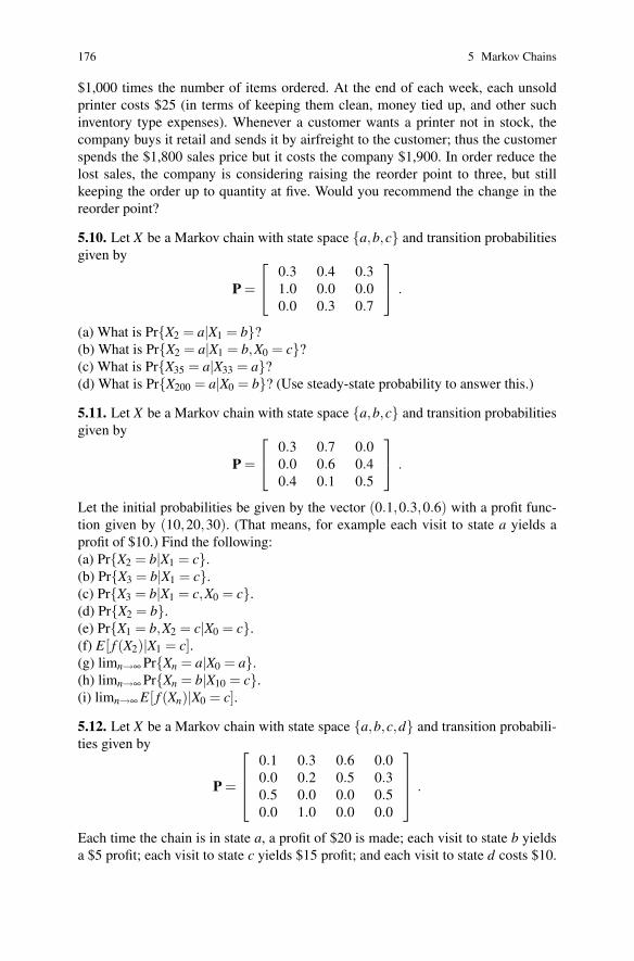
176 5 Markov Chains

$1,000 times the number of items ordered. At the end of each week, each unsoldprinter costs $25 (in terms of keeping them clean, money tied up, and other suchinventory type expenses). Whenever a customer wants a printer not in stock, thecompany buys it retail and sends it by airfreight to the customer; thus the customerspends the $1,800 sales price but it costs the company $1,900. In order reduce thelost sales, the company is considering raising the reorder point to three, but stillkeeping the order up to quantity at five. Would you recommend the change in thereorder point?

5.10. Let X be a Markov chain with state space {a,b,c} and transition probabilitiesgiven by

P =

⎡

⎣0.3 0.4 0.31.0 0.0 0.00.0 0.3 0.7

⎤

⎦ .

(a) What is Pr{X2 = a|X1 = b}?(b) What is Pr{X2 = a|X1 = b,X0 = c}?(c) What is Pr{X35 = a|X33 = a}?(d) What is Pr{X200 = a|X0 = b}? (Use steady-state probability to answer this.)

5.11. Let X be a Markov chain with state space {a,b,c} and transition probabilitiesgiven by

P =

⎡

⎣0.3 0.7 0.00.0 0.6 0.40.4 0.1 0.5

⎤

⎦ .

Let the initial probabilities be given by the vector (0.1,0.3,0.6) with a profit func-tion given by (10,20,30). (That means, for example each visit to state a yields aprofit of $10.) Find the following:(a) Pr{X2 = b|X1 = c}.(b) Pr{X3 = b|X1 = c}.(c) Pr{X3 = b|X1 = c,X0 = c}.(d) Pr{X2 = b}.(e) Pr{X1 = b,X2 = c|X0 = c}.(f) E[ f (X2)|X1 = c].(g) limn→∞ Pr{Xn = a|X0 = a}.(h) limn→∞ Pr{Xn = b|X10 = c}.(i) limn→∞ E[ f (Xn)|X0 = c].

5.12. Let X be a Markov chain with state space {a,b,c,d} and transition probabili-ties given by

P =

⎡

⎢⎢⎣

0.1 0.3 0.6 0.00.0 0.2 0.5 0.30.5 0.0 0.0 0.50.0 1.0 0.0 0.0

⎤

⎥⎥⎦ .

Each time the chain is in state a, a profit of $20 is made; each visit to state b yieldsa $5 profit; each visit to state c yields $15 profit; and each visit to state d costs $10.

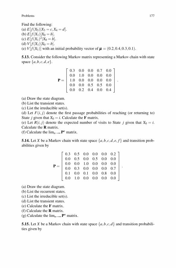
Problems 177

Find the following:(a) E[ f (X5)|X3 = c,X4 = d].(b) E[ f (X1)|X0 = b].(c) E[ f (X1)2|X0 = b].(d) V [ f (X1)|X0 = b].(e) V [ f (X1)] with an initial probability vector of μμμ = (0.2,0.4,0.3,0.1).

5.13. Consider the following Markov matrix representing a Markov chain with statespace {a,b,c,d,e}.

P =

⎡

⎢⎢⎢⎢⎣

0.3 0.0 0.0 0.7 0.00.0 1.0 0.0 0.0 0.01.0 0.0 0.0 0.0 0.00.0 0.0 0.5 0.5 0.00.0 0.2 0.4 0.0 0.4

⎤

⎥⎥⎥⎥⎦

.

(a) Draw the state diagram.(b) List the transient states.(c) List the irreducible set(s).(d) Let F(i, j) denote the first passage probabilities of reaching (or returning to)State j given that X0 = i. Calculate the F matrix.(e) Let R(i, j) denote the expected number of visits to State j given that X0 = i.Calculate the R matrix.(f) Calculate the limn→∞ Pn matrix.

5.14. Let X be a Markov chain with state space {a,b,c,d,e, f} and transition prob-abilities given by

P =

⎡

⎢⎢⎢⎢⎢⎢⎣

0.3 0.5 0.0 0.0 0.0 0.20.0 0.5 0.0 0.5 0.0 0.00.0 0.0 1.0 0.0 0.0 0.00.0 0.3 0.0 0.0 0.0 0.70.1 0.0 0.1 0.0 0.8 0.00.0 1.0 0.0 0.0 0.0 0.0

⎤

⎥⎥⎥⎥⎥⎥⎦

.

(a) Draw the state diagram.(b) List the recurrent states.(c) List the irreducible set(s).(d) List the transient states.(e) Calculate the F matrix.(f) Calculate the R matrix.(g) Calculate the limn→∞ Pn matrix.

5.15. Let X be a Markov chain with state space {a,b,c,d} and transition probabili-ties given by

178 5 Markov Chains

P =

⎡

⎢⎢⎣

0.3 0.7 0.0 0.00.5 0.5 0.0 0.00.0 0.0 1.0 0.00.1 0.1 0.2 0.6

⎤

⎥⎥⎦ .

(a) Find limn→∞ Pr{Xn = a|X0 = a}.(b) Find limn→∞ Pr{Xn = a|X0 = b}.(c) Find limn→∞ Pr{Xn = a|X0 = c}.(d) Find limn→∞ Pr{Xn = a|X0 = d}.

5.16. Consider a Markov chain with state space {a,b,c} and with the followingtransition matrix:

P =

⎡

⎣0.35 0.27 0.380.82 0.00 0.181.00 0.00 0.00

⎤

⎦ .

(a) Given that the Markov chain starts in State b, estimate through simulation theexpected number of steps until the first return to State b.(b) The expected return time to a state should equal the reciprocal of the long-run probability of being in that state. Estimate through simulation and analyticallythe steady-state probability and compare it to your answer to Part (a). Explain anydifferences.

5.17. Consider a Markov chain with state space {a,b,c} and with the followingtransition matrix:

P =

⎡

⎣0.3 0.5 0.20.1 0.2 0.70.8 0.0 0.2

⎤

⎦ .

Each visit to State a results in a profit of $5, each visit to State b results in a profitof $10, and each visit to State c results in a profit of $12. Write a computer programthat will simulate the Markov chain so that an estimate of the expected profit perstep can be made. Assume that the chain always starts in State a. The simulationshould involve accumulating the profit from each step; then the estimate per simu-lation run is the cumulative profit divided by the number of steps in the run.(a) Let the estimate be based on 10 replications, where each replication has 25 steps.The estimate is the average value over the 10 replicates. Record both the overall av-erage and the range of the averages.(b) Let the estimate be based on 10 replications, where each replication has 1000steps. Compare the estimates and ranges for parts (a) and (b) and explain any differ-ences.

References

1. Galton, F., and Watson, H.W. (1875). On the Probability of the Extinction of Families, J. An-thropol. Soc. London, 4:138–144.

References 179

2. Miller, G.A. (1952). Finite Markov Processes in Psychology, Psychometrika 17:149–167.3. Parzen, E. (1962). Stochastic Processes, Holden-Day, Inc., Oakland, CA.

http://www.springer.com/978-3-642-05155-5