Probability and Quantum Symmetries. II. The Theorem of ...gfm.cii.fc.ul.pt/people/jczambrini/JMathPhys-47-062107.pdf · Probability and Quantum Symmetries. II. The Theorem of Nœther

Po

I

wbstitoc

sofrutristics

JOURNAL OF MATHEMATICAL PHYSICS 47, 062107 �2006�

0

Downloaded

robability and Quantum Symmetries. II. The Theoremf Nœther in quantum mechanics

S. AlbeverioInstitut für Angewandte Mathematics, Abt. für Wahrsch.und Mathematische Statistik 53115 Bonn, Wegelerstasse 6, Germany

J. Rezende and J.-C. ZambriniGrupo de Física-Matemática (GFMUL), Universidade de Lisboa,Av. Prof. Gama Pinto 2, P-1649-003 Lisboa, Portugal

�Received 30 December 2005; accepted 1 April 2006; published online 26 June 2006�

For the largest class of physical systems having a classical analog, a new rigorous,but not probabilistic, Lagrangian version of nonrelativistic quantum mechanics isgiven, in terms of a notion of regularized action function. As a consequence of thestudy of the symmetries of this action, an associated Nœther theorem is obtained.All the quantum symmetries resulting from the canonical quantization procedurefollow in this way, as well as a number of symmetries which are new even for thecase of the simplest systems. The method is based on the study of a correspondingLie algebra and an analytical continuation in the time parameter of the probabilisticconstruction given in paper I of this work. Generically, the associated quantum firstintegrals are time dependent and the probabilistic model provides a natural inter-pretation of the new symmetries. Various examples illustrate the physical relevanceof our results. © 2006 American Institute of Physics. �DOI: 10.1063/1.2199087�

. INTRODUCTION

This paper is the continuation of the one, referred hereafter simply as paper I, whose subtitleas the “Theorem of Nœther in Schrödinger’s Euclidean quantum mechanics.”1 There, a proba-ilistic �i.e., “Euclidean”� generalization of Nœther’s theorem of classical mechanics was pre-ented, for a class of Lagrangians quadratic in the velocities, and involving a special family ofime-symmetric R3-valued diffusion processes. At the end of paper I, our physical motivation wasndicated: after an appropriate analytic continuation in the time parameters, the main conclusion ofhe construction was preserved as a theorem on quantum symmetries, in the Heisenberg picture. Inther words, although the probabilistic content of the theorem of Nœther was destroyed by thisontinuation in time, its geometrical one survived.

The purpose of this second paper is to describe in a detailed way the reason of this apparentlyurprising conclusion. This will provide us with a new Lagrangian version of the quantum theoryf such a class of systems. The symmetries of the associated new concept of regularized actionunctional will be expressed as a quantum version of the theorem of Nœther. All the unusualegularizations introduced on the quantum side will correspond to the ones given for free with thenderlying diffusion process, whose probability measures make sense only in the Euclidean set-ing. In point of fact, it will be shown that the corresponding symbolic “quantum diffusions” ineal time have all the properties of the heuristic ones manipulated by Feynman in his famous pathntegral method.2 In this sense, our indirect method is very much along the line of Feynman’space–time approach. It will be shown that we obtain many more quantum symmetries in this wayhan using the usual theorems on quantum symmetries, even for the simplest class of elementaryntegrable systems. Those “new” quantum symmetries are the keys of basic relations with sto-hastic analysis. A general argument of Lie group theory assures us, in fact, that all quantumymmetries arise in this way.

The organization of this work is as follows.

47, 062107-1022-2488/2006/47�6�/062107/61/$23.00 © 2006 American Institute of Physics

29 Jul 2008 to 194.117.6.7. Redistribution subject to AIP license or copyright; see http://jmp.aip.org/jmp/copyright.jsp

http://dx.doi.org/10.1063/1.2199087

http://dx.doi.org/10.1063/1.2199087

http://dx.doi.org/10.1063/1.2199087

ttNd

ppam

s

dnhs

dafHf

m

ia

ssodpf

I

=s

w

s

062107-2 Albeverio, Rezende, and Zambrini J. Math. Phys. 47, 062107 �2006�

Downloaded

Section II introduces the notions �implicit in Feyman’s approach� of �complex-valued� space–ime observables associated with a family of regular quantum observables and of quantum deriva-ives along a state. Although these quantum derivatives are not observables in the sense of Voneumann, they constitute a key tool of our construction. Under the quantum expectation, suchifferential operators behave like derivations.

Then, we define the concept of quantum conditional expectation in a state, given a space–timeoint. In spite of the fact that this concept shares a number of properties with its counterpart inrobability theory, we show why it is not a conditional expectation in the probabilistic sense. Thessociated “quantum diffusions” are precisely the ones introduced by Feynman in time discretizedanner.

Section III is devoted to the definition of the regularized action function for this class ofystems and its relations with quantum dynamics.

The study of the symmetries of this quantum action is the subject of Sec. IV. In particular, theefinition of the invariance of the action corresponds to a natural regularization of the classicalotion. The symmetry group of the underlying Schrödinger equation is used in an essential wayere, and the regular concept of constant observable of the motion is adapted to our calculus onpace–time observable �or quantum calculus, for short�.

In Sec. V the construction is specialized to the case of Hamiltonians which are polynomials ofegrees �2 in the position and momentum observables. This is the case where all the calculationsre explicit. Although this class is supposed to be completely known, our method provides, evenor the most elementary systems, more symmetries than the traditional approach. For generalamiltonians the main results hold true; but no explicit basis of the symmetry algebra can be

ound, in general and, therefore, the method is more indirect.Section VI is devoted to the analysis of the content of our Nœther theorem in a Riemannian

anifold.In Sec. VII we come back to the relation of what we did with the ideas of Feynman and show

n what sense the content of the present paper is a natural counterpart of paper I, where stochasticnalysis is involved in an essential way.

Finally, the last section is devoted to a short collection of explicit examples of quantumymmetries with some emphasis on those not directly accessible to regular methods. Of course, asoon as we know it, the theorem of Nœther in quantum mechanics can be verified without any usef our detour via probability theory and stochastic analysis. However, it is argued in favor of thisetour for the intuition it provides, in the same sense as Feynman’s path integral approach hasroved to be very useful for the discovery of many new aspects of quantum theory. A short Errataor paper I will conclude the present work.

I. THE CONCEPT OF QUANTUM MECHANICAL CONDITIONAL EXPECTATION

Let H be a self-adjoint, lower bounded Hamiltonian operator in the Hilbert space HL2�Rn ,dx� of square integrable complex-valued function over Rn. Consider the one-parameter,

trongly continuous groups of unitary operators Ut :H→H , t�R,

Ut = e−�i/��tH,

ith the reduced Planck constant �. Then for any � in the definition domain DH�H of H,

�t = Ut� , �2.1�

olves the Schrödinger equation with the initial condition �:

i ��t

�t= H�t,

�2.2�
�0 = � .

DoD�

I

sl

c

ticD

t

H

w

o

062107-3 Theorem of Nœther in quantum mechanics J. Math. Phys. 47, 062107 �2006�

Downloaded

Let consider a one-parameter family A�t� , t�R, of self-adjoint operators in H. Assume that

A�t��HDH and A�t�DH�DH, so that the commutators �A�t� ,H�=A�t�H−HA�t� are well definedn DH. Let 0�T�� and define DT

A�t��DA�t� by DA�t�=�T��t�0DA�t+�t�. In particular we haveA�t��DA�t�. If A�t� is weakly differentiable on DA�t� with respect to the time parameter t�0,T�,then we can compute

lim�t↓0

��,A�t + �t� − A�t�

�t�� t

A��,�� .

t exists for any ��H ,��DA�t�, where �· , · � denotes the scalar product in H, and is linear in the

econd vector. Provided that DA�t� is dense in H ,tA :HDA�t�→C is a densely defined sesqui-

inear form.Now let us define, for �t�H and �t�DA�t� , I�,��t�= ��t ,A�t��t�.When �t�DA�t� and �t is the solution of �2.2� with �t�DA�t� ,T� t�0 and �t�0, we can

ompute the relative time increment of I�,��t� as follows:

I�,��t,�t� �I�,��t + �t� − I�,��t�

�t

=1

�t��t+�t,A�t + �t��t+�t� − ��t,A�t + �t��t+�t�

+ ��t,A�t + �t��t+�t� − ��t,A�t��t+�t�

+ ��t,A�t��t+�t� − ��t,A�t��t�� .

If, in addition, �t=Ut� with �0��D�H� then the strong derivative �t˙ of �t with respect to

exists and �t˙ = �1/ i� �H�t. But, by assumption, H�t�DA�t�. This, inserted in the above relative

ncrement of I�,��t� gives, when �t↓0, using the strong differentiability of �t ,�t, the strongontinuity of A�t��t on DA�t�, the fact that �t+�t�DA�t� and that A�t� is weakly differentiable onA�t�,

lim�t↓0

I�,��t,�t� = ��t,A�t��t� + tA��t,�t� + ��t,A�t��t� .

By �2.2�, the corresponding equation for �t and the further assumption DA�t��HDH, we seehat the latter relation can be rewritten as

lim�t↓0

I�,��t,�t� = � 1

i�H�t,A�t��t� + t

A��t,�t� + ��t,1

i�A�t�H�t� .

Since A�t�DH�DH by assumption, and so A�t��t�DH, this reduces, by the self-adjointness of, to

1

i��t,�A�t�,H��t� + �t

A��t,�t� =d

dt��t,A�t��t� , �2.3�

here we used the definitions of I�,��t ,�t�, I�,��t�, and �tA��t ,�t�.

We shall denote by D��t ,�t� the sesquilinear form on left-hand side �lhs� of �2.3�. So

D��t,�t� =d

dt��t,A�t��t� . �2.4�

We recall that for T� t�0, D��t, �t� is well defined if �t�DA�t� and A�t�DH�DH.Definition II.1: Let � be in H and such that �t�DA�t�. The complex-valued space–time

A
bservable a�t�x , t� associated with the family of quantum observable A�t� in the state �t is defined

f

dH

w

A

t

w

T

A

idt


Downloaded

or all x�Rn , t�R ,s . t .�t�x��0, by

a�t

A �x,t� ��A�t��t��x��t�x�

. �2.5�

We shall consider, for any x , t, versions of �t�x� jointly measurable in t�R, x�Rn, andenote them again by �t�x�. For x , t such that �t�x�=0 we set a�t

A �x , t��0. Therefore, for any �t inand �t in DA�t� we have

��t,A�t��t� = ��Nt��c�tA�t��t dx + �

Nt��tA�t��t dx = �

�Nt��c�tA�t��t dx ,

here Nt�= x�Rn �t�x�=0� , �Nt

��c=Rn−Nt�.

Using �2.5�, it is clear that, by construction,

��t,A�t��t� =� �t�ta�t

A dx . �2.6�

ssumption on the zeroes of the wave function

We shall need that Nt� has zero Lebesgue measure. Sufficient conditions for this are known in

erms of assumption on H. See Sec. V.Using �2.3� and �2.4� and our assumption that Nt

� has zero Lebesgue measure, we get

D��t,�t� =1

i��t,�A�t�,H��t� + t

A��t,�t� =1

i��

�Nt��c�t�t

1

�t�A�t�,H��t dx + t

A/�t��t�t,�t� ,

�2.7�

here we have defined tA/�t, for f / �t�H and g�DA�t�, by

tA/�t�f ,g� � lim

�t↓0� f ,

1

�t�A�t + �t� − A�t�

�t g� .

Now suppose that, in the strong sense on DA�t�, there exist a linear operator �A�t� /�t such that

lim�t↓0

A�t + �t� − A�t��t

�t =�A

�t�t��t, 0� t� T .

hen, for ��H ,�t�DA�t�, using the definition of tA��t ,�t�,

��t,�A

�t�t��t� = t

A��t,�t� .

lso, for any �t�DA�t�,

� �A

�t�t� +

1

i��A�t�,H��t

s well defined �recall that we have assumed HDH�DA�t� and A�t�DH�DH�. According to theefinition �2.5�, a�t

A .�t=A�t��t is also well defined. Therefore in the sense of the identification of
he corresponding Bochner integrals,

ft

i

N

U

F

we

aaos

f�

d

t

f


Downloaded

�

�t�a�t

A · �t� =�A

�t�t��t +

1

i�A�t�H�t,

or any �t�DA�t� and Lebesgue a.e. t� �0,T� �recalling our assumption that DA�t��HDH�. Fromhis it follows that

� �

�t−

1

i�H��a�t

A · �t�

s well defined and coincides, for Lebesgue a.e. t, with

� �A

�t+

1

i��A�t�,H��t.

ow for any x� �Nt��c we defined Dta�t

A by

�Dta�t

A ��x� =1

�t� �

�t−

1

i�H��a�t

A · �t��x� . �2.8�

sing the relation above, we get first on �Nt��c but then in the L2�Rn�-sense

Dta�t

A =1

�t� �A

�t+

1

i��A�t�,H��t. �2.9�

rom this, for all �0=��DH we obtain

��t,�Dta�t

A ��t� = ��t,� �A

�t+

1

i��A�t�,H��t� =

d

dt��t,A�t��t� ,

here �2.7� and �2.9� have been used. All equalities hold first for Lebesgue a.e. t but can bextended to all t if both sides of the equalities are continuous in t.

In summary, we have proved the following:Proposition II.2:Let H be a self-adjoint operator in H=L2�Rn ,dx� and A�t� a one-parameter family of self-

djoint operators in H with A�t�DH�DH and DA�t��HDH. For ��DH, consider �t=e−�i/��tH�nd assume that Nt

� has a zero Lebesgue measure. Suppose that �A�t� /�t exists in the strong sensen DA�t�. Define Dta�t

A by equations �2.8� and �2.9�. Then, for any ��DH and �t�DA�t�,with �t

atisfying �2.2�, we have

d

dt��t,A�t��t� = ��t,�Dta�t

A ��t� , �2.10�

or Lebesgue a.e. t�R. If both sides of �2.10� are continuous in t, then �2.10� holds for all tR.

Corollary II.3:If A�t� is a quantum constant of motion of the system with Hamiltonian H, defined on a dense

omain D�H, in the sense that

� �A

�t�t� +

1

i��A�t�,H��X = 0 for any X � D ,

hen the space–time observable associated with A�t� satisfies

Dta�t

A = 0,

A
or all �t�D �t�.

Ad

m

A

�

�

�

�"

S


Downloaded

Proof: By �2.9� we have Dta�t

A = �1/�t�A�t��t=0, for

A�t� ��A

�t�t� +

1

i��A�t�,H� .

˙ �t� is a closable operator since A�t�, ��A /�t��t� and H are all symmetric, defined on a commonomain.

By approximation of �t�DA�t� through vectors in D, and since A�t� is a quantum constant of

otion, we see that A¯ �t��t=0, where the overbar denotes the closure. Since �t is in the domain of

˙ �t�, the conclusion follows. �

Remarks:

1� If we call quantum space–time observable any operator-valued map �x , t�→g�x , t� measur-able in the sense that �x , t�→ � ,g�x , t�� is measurable for �H ,��D a dense domainand g�x , t� self-adjoint in H, we can define Dt, t�R, on the set of such observables g by

Dtg �1

�t� �

�t−

1

i�H��g�t� , �2.11�

whenever the right-hand side �rhs� makes sense �with �g�t��x��g�x , t��t��x��. Then, for g=a�t

A , Dta�t

A coincides with �2.9�. If g�t�DH, �g /�t exists in the strong sense on DH andD�g/�t�DH, then the rhs of �2.11� is well defined �for �t�DH�. However, we are going toshow that there is a more natural definition of Dt regarded as differential operator denselydefined in an associated Hilbert space.

2� Dt, acting on space–time functions a�t

A , for example, should not be confused with the familiarHeisenberg derivative D acting on the family of self-adjoint operators A�t� and definedheuristically by

DA�t� =�A

�t�t� +

1

i��A�t�,H� .

Indeed, according to �2.9�, the relation between these two derivatives is Dta�t

A

= �1/�t��DA�t��t�. In particular, Heisenberg’s derivative D does not depend on the state �t.In order to avoid any confusion, from now on we shall call Dt the quantum derivative along�t.

3� Consider two arbitrary observables A and H, time independent and with DA=DH=D, acommon dense domain in H, invariant under A and H. We say that A and H commute, andwrite �A ,H�=0 whenever for any f , g bounded and Borel measurable one has f�A�g�H�−g�H�f�A�=0.

A necessary and sufficient condition for this property is, for example, that

�ei��/��A,ei�t/��H� = 0 " �, t � R .

cf., for example, Ref. 3�. If A is essentially self-adjoint on a domain D, invariant under ei�t/��H,t�R, then A and H commute if

A�t�� ei�t/��HAe−i�t/��H� = A�, " �� D and t � R .

o it suffices indeed to show that


w

iaw

ltL

�tt

c

w

ot

id

u�

R


Downloaded

d

dt� ,ei�t/��HAe−i�t/��H�� =

d

dt� t,A�t�

=� t,1

i��A�t�,H��t�

=0

ith

t � e−i�t/��H , Xt � e−i�t/��H�, and " �, in D = DH � DA,

n order to prove that A and H commute �in the sense of the above-mentioned sufficient condition�nd therefore that A�t� is a constant of motion. According to the Corollary II.3, when this holds,e have Dta�t

A =0.Lemma II.4:Let �t be the solution of the Schrödinger equation �2.2� with initial condition � in L2�Rn� and

et Nt� be a zero Lebesgue measure set. Then the quantum derivative Dt along the solution �t of

he Schrödinger equation �2.2� with initial condition � is a densely defined differential operator in2�Rn , �t�x�2 dx�.

Proof: Let �t be the solution of the Schrödinger equation �2.2� with the initial condition �L2�Rn ,dx��H and consider the weighted Hilbert space L2�Rn , �t�x�2 dx�. Since, by assump-

ion, Nt� has zero Lebesgue measure, the two Hilbert spaces are unitarily equivalent through the

ransformation

U�t: L2�Rn, �t�x�2 dx� → L2�Rn,dx� ,

g � g�t.

Let K be the space of R-indexed families of functions f = �f �t��t�R with each f �t� stronglyontinuously differentiable from R into H, such that

�

�tf �t� � lim

�t↓0

f �t+�t� − f �t�

�t� H ,

here the limit is taken in the strong H sense. Let us define the partial differential operator

Q =�

�t−

1

i�H

n the subset KH of K consisting of those �f �t��t�R such that the mapping x�Rn� f �t��x� belongso DH for all t�R. We can also define the Hilbert space W1

2�R ,H�, consisting of the functionsf = �f �t��t�R, with f �K such that f �t��x� , �� /�t�f �t��x��L2�R ,dt� for dx a.e., x�Rn. The operator iQs well defined on KH

0 �f �t��KH , t� f �t��C01�R��. This operator is symmetric in W1

2�Rn ,H�, on aense domain KH

S �DS �S for “Schrödinger”�, independent of time.Let Kt be the “tth copy” of L2�Rn ,dx� so that f �t��Kt for any t�R. Let us consider the image

nder U�t

−1 of Kt. U�t

−1Kt is made of all functions of the form f �t��x� /�t�x�, with f �t��Kt andx , t��Nt

�.

U�t

−1 can be extended to an operator U�t

−1 from K into L2�Rn , �t�x�2 dx�, defined by

�U�t

−1f �s��x� =f �s��x��t�x�

, �x,t� � Nt�, s � R .

2 n 2 ˜ −1 2 n 2 2 n
estricted to L �R , �t�x� dx� ,U�tis unitary from L �R , �t�x� dx� to L �R ,dx�, since

a

o

s

W

t

w

C

�


Downloaded

�U�t

−1f �s��L2�Rn,�t�x�2 dx� = �f �s��L2�Rn,dx�, " s,t � R ,

nd its inverse is U�tf �s�=�t f

�s�.

We can look at the image of the operator Qt in K under U�t

−1 as an operator Qt whose action

n elements of L2�Rn , �t�x�2 dx� is given by U�t

−1QtU�t=Qt on D�L2�Rn , �t�x�2 dx� ,D being

uch that U�tD�DQt. Since iQt= i� /�t− �1/ � �H is symmetric on the dense domain DS of

12�R ,H�, this means that iQt is symmetric on the dense domain U�t

−1DS in L2�RnR ,dx dt�. On

his domain, Qt is given by

QtU�t

−1f =1

�t� �

�t−

1

i�H� f ,

ith f = �f �t��t�R�DS.DS contains, for example, the subset DS

0 consisting of all families f = �f �t��t�R such thatf �t��·� as well as �� /�t�f �t��·� are both in C0

��Rn� �if DH�C0��Rn��.

Setting h= U�t

−1f for f �DS0 we see that

Qth =1

�t� �

�t−

1

i�H��th� .

omparing with �2.11�, this means that, on U�t

−1DS0 we have indeed

Qt = Dt. �2.12�

�

Remarks:

1� Suppose that H is the Hamiltonian for a unit mass and charged particle in an electromagneticfield, i.e., H=−��2 /2��−�i / � �A�2+V on C0

��Rn� or

H = −�2

2� + i � A · � +

i�

2� · A +

1

2�A�2 + V , �2.13�

where A :Rn�Rn is the vector potential and V :Rn�R the scalar potential, both continuous,A being C1, and such that H has a unique self-adjoint extension, also denoted by H �cf., forexample, Ref. 4 for sufficient conditions such that this holds�. In this case, using �2.11�, weobtain explicitly a quantum derivative along �t �in the sense of Lemma II.4� given by

Dt =�

�t+ �− i �

��t

�t− A� · �−

i�

2� �2.14�

on the domain of functions of the form � ·DS, which is dense in L2�Rn , �t�x�2 dx�. Accord-ing to our Remark 1 after Corollary II.3, Dt is also defined on a larger set of functions inL2�Rn , �t�x�2 dx�. For example, denoting by q the function

Rn R → Rn, " t, we have Dtq = i ��t

�t− A

�x,t� � x

which is well defined, provided

� �t�x�x�H�t��x�dx� � .

This is the case under weak restrictions on the vector and scalar potentials A and V.


�

�

n

q

as

q

cv

I

i


Downloaded

2� We shall also need the complex conjugate of the operator Dt, denoted by Dt. On complexspace–time observables of the form a�t

A , one has, by definition,

Dta�t

A =1

�t� �

�t+

1

i�H��ta�t

A � .

Proceeding as before in connection with �2.12�, i.e., considering vectors h of the form U�t

−1f ,with f �DS

0, we have

Dth =1

�t� �

�t+

1

i�H��th� . �2.15�

In particular, when the Hamiltonian H is of the form �2.13�, Dt reduces on U�t

−1DS0 to the

differential operator

Dt =�

�t+ �i �

��t

�t

− A� · � +i�

2� �2.16�

defined on the elements U�t

−1DS0�t�R of W1

2�Rn ,H�. These elements form a dense domain ofW1

2�Rn ,H�, as discussed in the proof of the Lemma II.4. Using the terminology introduced

there, Dt will simply be called the quantum derivative along �t.3� It follows clearly from �2.11� and �2.15� that

Dtg = Dtg ,

where the lhs denotes the complex conjugate of Dtg.

Motivated by Born’s probabilistic interpretation of the wave function, let us introduce theatural definition.

Definition II.5: Let f = �f �t��t�R, with f �t��·� in L1�Rn , �t�x�2 dx� and f �t� measurable in t. Theuantum �absolute� expectation of f in the state �t solving �2.1�, denoted by �f��t

, is the integral

�f��t=� f �t��x��t�x�2 dx �2.17�

nd we shall refer to �t�x�2 as the density �with respect to dx� of the quantum probability in thetate �t.

The terminology chosen for Dt and Dt is due to the crucial observation that, under thisuantum expectation, these differential operators behave like derivations.

Proposition II.6:

Let f = �f �t��t�R, g= �g�t��t�R be in the domains of the quantum derivatives Dt and Dt and withompact support in the space variables. Then �f ·g��t

is differentiable with respect to the timeariable and the following Leibniz rule holds:

d

dt�f · g��t

= �Dtf · g + f · Dtg��t. �2.18�

n particular,

d

dt�f��t

= �Dtf��t= �Dtf��t

. �2.19�

Corollary II.7:If f , g have supports with respect to the time variable strictly contained in the interior of an

nterval �t0 , t1� for some t0 , t1�R, then Dt+=−Dt where + denotes the adjoint with respect to

2 n
�t�x� dx dt on R �t0 , t1�.

Tc

dt

s

wHo

ws

L

�


Downloaded

Proof: Integrating �2.18�, we obtain

�t0

t1

�Dtf · g��tdt = − �

t0

t1

�f · Dtg��tdt .

�

Proof of Proposition II.6: By definition, �d /dt��f ·g��tdenotes

lim�t↓0

�f �t+�t�g�t+�t��t+�t− �f �t�g�t��t

�t.

The term under lim�t↓0 means explicitly

1

�t�� f �t+�t�g�t+�t��t+�t�x�2 dx −� f �t�g�t��t�x�2 dx

=1

�t�� f �t+�t� − f �t��g�t+�t��t+�t�x�2 dx

+� f �t��g�t+�t� − g�t��x�t+�t2 dx

+� f �t�g�t��t+�t�x�2 − �t�x�2�dx .

he first term on the rhs converges, when �t↓0, to �� f �t�g�t��x� �t�x�2 dx by the dominatedonvergence theorem and the hypothesis that f �t� is strongly differentiable in L2�Rn ,dx� �here we

enote �� /�t�f �t� by f �t� for simplicity�. Similarly we see that the second term of the rhs convergeso �f �t�g�t� �t�x�2 dx.

For the third term we use again the dominated convergence theorem and the fact that, in thetrong L2�Rn ,dx� sense,

d

dt�t2 =

d

dt�t · �t = −

1

i�H�t · �t + �t

1

i�H�t,

here the Schrödinger equation has been used, together with the fact that �t ·H�t as well as�t ·�t are in L1�Rn ,dx� and f �t� ,g�t� have compact support as functions of the space variable. Inther words the rhs above becomes

� � f �t�g�t� + f �t�g�t� + f �t�g�t�� 1

i�

H�t

�t−

1

i�

H�t

�t��x��t�x�2 dx

=� �Dtf�t� · g�t� + f �t�Dtg

�t��x��t�x�2 dx ,

here the definition of Dt , Dt have been used together with the self-adjointness of H, in order toimplify the term involving H�f �t��t�.

The second part of the calculation follows from the first one by approaching in the2�Rn , �t�x�2 dx�-norm f �t�=1, respectively, g�t�=1 through C0

��Rn� functions. �

Remarks:

1� When the Hamiltonian H is of the explicit form �2.13�, the relation �2.18� can be given a
more illuminating form if we use exclusively one of the quantum derivatives,

�

H

f

�td

d

b

c

f�

U

T

w

t�


Downloaded

d

dt�f · g��t

= ��Dtf� · g + f�Dtg��t− i � ��f · �g��t

�2.20�

=��Dtf� · g + f�Dtg��t+ i � ��f · �g��t

. �2.21�

Proof: This follows directly from Proposition II.6, using the explicit expressions �2.14� and

2.16� of Dt and Dt available for the Hamiltonian �2.13�. �

�2� Relations like �2.20� and �2.21� hold, in fact, also without integration with respect to�t�x�2 dx.

Proposition II.8:For f ,g in a dense domain of the form �t ·DS�L2�Rn , �t�x�2 dx� (cf. Lemma II.4) and an

amiltonian of the form �2.13�, one has

Dt�f · g� = �Dtf� · g + f�Dtg� − i � �f · �g , �2.20��

Dt�f · g� = �Dtf� · g + f�Dtg� + i � �f · �g , �2.21��

or any �t ,x� such that �t�x��0.Proof: Equations �2.20� and �2.21� can be written, for any �t=Ut�, and any �t ,x� s.t.

�t ,x��0,�A�x , t� �t�x�2 dx=0 with A�x , t�= D�f ·g�− �Dtf�g− f�Dtg�− i��f ·�g, and so equa-ions �2.20�� and �2.21�� hold a.e. with respect to dx. Alternatively, one can use directly theefinitions �2.14� and �2.16� to show that the conclusion holds. �

Equations �2.20�� and �2.21�� show that the quantum derivatives behave, in fact, like quantumeformations of derivatives in the �commutative� algebra of families of functions f = �f �t��t�R with

f �t��C0�Rn�. To regard Dt and Dt as quantum deformations of derivations will prove, later on, toe a very natural interpretation.

Now we are going to introduce the quantum counterpart of the probabilistic concept ofonditional expectation given a space point x�Rn in the past time t�0.

Definition II.9:Let g= �g��R be complex valued, measurable functions defined on Rn and such that g��

�·��·��L2�Rn ,dx� where, as before, ��=U��. For 0� t�� and �t ,x� such that �t�x��0 �or,

or short, �t ,x� “�-admissible”� let us define the quantum conditional expectation Mt,x� in the state

, given �t ,x� and evaluated at g�� by

Mt,x� �g�� = ��t�x��−1�U�−t�g��x� . �2.22�

Let us first assume that the Hamiltonian H is time-independent and that the evolution group

�−t has an integral kernel, denoted by

k�x,� − t,q� = �e−�i/��−t�H��x,q�, x,q � Rn, � � t .

hen the definition �2.22� means

Mt,x� �g�� = ��t�x��−1� k�x,� − t,q�g��q��q�dq , �2.22��

hich is well defined for any �-admissible �t ,x��R+Rn. We shall denote by

p�t,x,�,dq� = ��t�x��−1k�x,� − t,q��q�dq, t� �, x,q � Rn, �2.23�

he integral kernel associated with �2.22�� and refer to it as the forward quantum transition kernel
“forward” because the conditioning x is in the past t�� and also because the initial quantum

p�

�

E

f

ic

t

�


Downloaded

robability density �t�x�2 is propagated towards the future by p�. More precisely since, for �t the kernel k�x ,�− t ,q� coincides with the retarded �or “casual”� propagator

k+�x,� − t,q� = �� − t��e−�i/��−t�H��x,q� ,

where � is Heaviside’s distribution� i.e., the distribution solving

�− i ��

��+ H�k+�x,� − t,q� = − i � ��q − x�� − t� ,

q. �2.23� means that

p�t,x,�,dq� = ��t�x��−1k+�x,� − t,q��q�dq . �2.23��

Let us observe that sufficient conditions for the existence of k and therefore p as continuousunctions in all the variable are known; cf., e.g., Refs. 5, 6, and 60.

We remark that when H is time dependent, Eq. �2.23� still holds with k replaced by thentegral kernel of the two-parameter family of unitary operators U�t ,��, t ,��R defining theorresponding time evolution.

The main properties of the quantum conditional expectation of Definition 2.9 are expressed byhe following:

Proposition II.10:For all �-admissible �t ,x��RRn and g= �g��R as in �2.22��, with �� t,

�1� the quantum mechanical conditional expectation is linear: if �i�C and gi= �gi��R ,

i=1,2 as above,

Mt,x� ��1g1

�� + �2g2�� = �1Mt,x

� �g1�� + �2Mt,x

� �g2��;

�2� Mt,x� ��=�, ��C;

�3� Mt,x� �g��=g�t��x�, �� t;

�4� �Mt��g��= �g��, �� t;

�5� when Ms,x� �g1

�s�g2�t��, s� t, is well defined, then

Ms,x� �g1

�s�g2�t�� = g1

�s��x�Ms,x� �g2

�t�� .

Proof: This follows from direct computations using the definitions �2.17� and �2.22�. �

Remarks:

1� We shall also need, for the same class of g= �g��R as in Proposition II.10, and any

�-admissible �t ,x��RRn, the definition �2.22� with � replaced by � and U�−t replaced byU�−t, 0�� t, i.e.,

M�t,x�g�� = ��t�x��−1�Ut−��g��x� . �2.24�

The properties of M�t,x are, of course, similar to the ones of Mt,x

� .Let us stress that, for the latter quantum conditional expectation in the state �, the condi-tioning x is lying in the future of the time interval under consideration �i.e., t��; this justifiesour alteration of notation with respect to �2.22��. For this reason, we shall occasionally callbackward �respectively, forward� the conditional expectation �2.24� �respectively �2.22��when a confusion is possible between these two concepts. When needed, we shall denote byp�� ,dq , t ,x� the backward quantum transition kernel associated with �2.24�, i.e.,

−1
p��,dq,t,x� = ��q�k−�q,t − �,x��x�� dq, � � t , �2.25�

�

e

w

s

wt

i

p

w

s

�


Downloaded

for any �t ,x� �-admissible. Here, we denote by k− the advanced propagator defined in termsof the causal one by

k−�x1,s − u,x2� = k+�x2,u − s,x1� . �2.26�

2� Comparing the definitions �2.23�� and �2.25�, it is clear that the relation between the forwardand backward quantum transition kernels can be expressed as

p�t,x,s,y� = p�s,y,t,x�, s� t, x,y � Rn. �2.27�

Definition II.11:Let f = �f �t��t�R, �g�s��s�R as in the definitions �2.22�� and �2.23�. The quantum �absolute�

xpectation of their product f �t� ·g�s� in the state �, for t�s, is defined by

�f �t�g�s�� = �Ms,·� �f �t�� · g�s��s

�2.28�

=�f �t�M�t,·�g�s��t

, �2.28��

hen Ms,·� �f �t�� ·g�s��L2��s�x�2 dx� and f �t�M�

t,·�g�s��L2��t�q�2 dq�.The consistency of this definition is verified by observing that equation �2.28� reduces, after

implification, to

� � �s�x�g�s��x�k�x,t − s,q�f �t��q��t�q�dq dx ,

hen the integral kernel �2.23�� exists �since t�s�. On the other hand, using the forward condi-ional expectation of �2.28��, this absolute expectation in the state �t reduces to

� � �s�x�g�s��x�k−�x,t − s,q�f �t��q��t�q�dq dx ,

.e., to the same expression as before, by definition of the advanced propagator k− when t�s.This duality with respect to the time parameter suggests to introduce the following two-

arameters family of operators Ps,t* ,s� t associated with quantum conditional expectations:

Ps,t* :L2��s�x�2 dx� → L2��t�q�2 dq�

�2.29�

g�s��·� �� g�s��x�p�s,dx,t,q� � M�t,q�g�s�� ,

here the backward transition kernel �2.25� has been introduced and its “time reversed” familyPt,s, s� t,

Pt,s:L2��t�q�2 dq� → L2��s�x�2 dx� ,

�2.29��

f �t��·� �� f �t��q�p�s,x,t,dq� � Ms,x� �f �t�� ,

o that the equality between �2.28� and �2.28�� can be rewritten as

��Pt,sf�t�� · g�s��s

= �f �t� · �Ps,t* g�s��t

. �2.30�

The properties of the operators Ps,t* �or Pt,s� for s� t are as follows:

a� Ps,t* are linear operators; as a map from R+R+ into densely defined, bounded operators

2 2 2 2 *
from L ��s�x� dx� into L ��t�q� dq�, �s , t�� Ps,t is continuous;

��

��

iMf

q

�

�

s

�

�

�


Downloaded

b� �Ps,t* g�s��L2��t�q�2 dq�= �g�s��L2��s�x�2 dx�;

c� Ps,t* 1�s�=1�t� where 1�s� is the function identically 1 in L2��s�x�2 dx� �with 1�t� the same in

L2��t�q�2 dq�� and Pt,s1�t�=1�s�;d� Ps,s

* �Id, the identity operator from L2��s�x�2 dx� into L2��s�x�2 dx�;e� Pt,u

* · Ps,t* = Ps,u

* , s� t�u;

f� Ps,t* · Pt,s=1�t� and Pt,s · Ps,t

* =1�s�.

We may summarize the situation as follows:Proposition II.12:The two-parameters family of bounded operators Ps,t

* and Pt,s are dual from L2��s�x�2 dx�nto L2��t�q�2 dq� in the sense that for any f �t��DPt,s

and g�s��DPs,t* , the relation �2.30� holds.

oreover, the properties �a� to �f� are satisfied �where �a� to �e� have their natural counterpartsor Pt,s�.

The proof follows directly from the definitions �2.23�� and �2.25� of the forward and backwarduantum transition kernels.

Remarks:

1� Let f �s��·� be non-negative in L2��s�x�2 dx�. Then, clearly Ps,t* does not, in general, transform

f �s��·� into a non-negative element of L2��t�q�2 dq� since the backward quantum transitionkernel p is not even real. In particular, p�s , · , t ,q� is not a measure, although it sharesmanifestly a number of properties with probability measures.

2� The equality between �2.28� and �2.28�� can be rewritten infinitesimally using the quantum

derivatives Dt and Dt. To do this, we need another property of these derivatives, which willbe the first result of the next section.

Let Ps,t* and Pt,s a pair of 2-parameters family of operators satisfying the properties of Propo-

ition II.12 and p , p, respectively, their associated quantum transition kernels.Definition II.13:The two dual kernels define a quantum diffusion if "s� t ,x�Rn ,�0, we have

1� p�s ,x , t ,S�x�c�=o�t−s�, where S�x�c is the complement of the sphere S�x� of radius andcenter x.

2� There is a Cn-valued function B�x ,s� s.t.,

�S�x�

�q − x�p�s,x,t,dq� = B�x,s��t − s� + o�t − s� .

There is an nn complex-valued function C�x ,s� s.t.

�S�x�

�q − x��q − x�Tp�s,x,t,dq� = C�x,s��t − s� + o�t − s� .

C will be called the quantum diffusion matrix and B the �forward� drift of the quantumdiffusion.

3� There is a Cn-valued function B�x , t� s.t.

�S�x�

�q − x�p�s,dx,t,q� = B�q,t��t − s� + o�t − s� ,

and an nn complex-valued function C�x ,s� s.t.

�S �x�

�q − x��q − x�Tp�s,dx,t,q� = C�q,t��t − s� + o�t − s� .


C

wiSvd

w

g

Ur


Downloaded

These properties are satisfied, e.g., for the kernels associated with the Hamiltonians �2.13�ompare also Refs. 5 and 6. Indeed we have the following.

Proposition II.14:Let H be of the form �2.13� and its associated kernel k be such that

lim�s↓0

1

�s� �q − x�R�q,x,�s�k�x,�s,q�dq = 0,

here R�q ,x ,�s�=0��q−x�2�+0��s�2 is a term in the Taylor expansion of the integrand of B�x ,s�n the proof below. Let �q , t��RnR be �-admissible, where �t is a regular solution of thechrödinger equation for H, admitting a Taylor expansion in powers of the space and timeariables around �t�q�. Then a quantum diffusion corresponds to this solution, whose drifts andiffusion matrix are, respectively, given by

B�q,t� = i ��t

�t

�q� − A�q� ,

B�q,t� = − i ��t

�t�q� − A�q� , �2.31�

C�q,t� = C�q,t� = i � 1 ,

here 1 denotes the nn identity matrix.Proof: By �3� and �2.23�,

B�x,s� = lim�s↓0

1

�s�

s�x��q − x�p�s,x,s + �s,q�dq

= lim�s↓0

1

�s�

s�x��q − x��s�x��−1k�x,�s,q��s+�s�q�dq

= lim�s↓0

1

�s�

s�x��q − x��1 +

��s

�s

�x��q − x� +�˙

s

�s

�x��s + O��q − x�2� + O��s2� k�x,�s,q�dq .

We can easily verify the following properties of the integral kernel k�x ,� ,q� of the evolutionroup U� for the Hamiltonian �2.13�:

lim�↓0

1

��1 − �Rn

k�x,�,q�dq =1

2� · A�x� +

i

2��A�x��2 +

i

�V�x� ,

lim�↓0

1

��

Rn�q − x�k�x,�,q�dq = A�x� ,

lim�↓0

1

��

Rn�q − x��q − x�Tk�x,�,q�dq = i � 1 .

sing these in the above rhs of the expression of B�x ,s� we obtain the expected result. The otheresults follow in a similar way. �

Proposition II.15:
Let ��t /�t and A�q� be given and continuous, for a Hamiltonian of the form �2.13�. Assume

tte

�

�

�

�

ftt


Downloaded

hat, in the representations �2.29� and �2.29��, the partial derivatives with respect to �t ,q� �respec-ively �s ,x�� of the quantum conditional expectations are well defined and continuous, and can bexchanged with the integrals. Then the quantum equation of Kolmogorov for the transition kernel

p for s� t�R, x ,y�Rn, is given by

a�

−� p

�s�s,x,t,q� =

i�

2

�2p

�xj � xj �s,x,t,q� + �i �� j�t

�t

�q� − Aj�q��

�xj p�s,x,t,q� �2.32�

�with the usual summation convention over the indices j�. Equivalently, regarded as a func-tion of the past variable, p is the fundamental solution of

Dsu = 0, for u � DDs, �2.33�

with Ds defined in �2.16�.b� If all the involved partial derivatives exist and are continuous, p, regarded as a function of

the future variables, solves the quantum Fokker-Planck equation

� p

�t�s,x,t,q� =

i�

2

�2p

�qj � qj �s,x,t,q� −�

�qj��i �� j�t

�t

�q� − Aj�q�� p�s,x,t,q� .

�2.34�

Similarly, the transition kernel p�s ,x , t ,q� solvesc�

−�p

�s�s,x,t,q� = −

i�

2

�2p

�xj � xj �s,x,t,q� + �− i �� j�t

�t�q� − Aj�q��

�xj p�s,x,t,q� .

�2.35�

So that p is the fundamental solution of

Dsv = 0 for v � DDs, �2.36�

with Ds given by �2.14� and the following backward quantum Fokker-Planck equation holds:d�

�p

�t�s,x,t,y� = −

i�

2

�2p

�qj � qj �s,x,t,y� −�

�qj��− i �� j�t

�t�q� − Aj�q��p�s,x,t,y� .

�2.37�

Proof: �a� Let us consider �2.29��

�Pt,sf�t��x� =� f �t��q�p�s,x,t,dq� � u�s,x�, s� t ,

or any f �t� of compact support in the class used to define �2.22�. By hypothesis, we can differen-iate with respect to �s ,x� under the integral sign. Using Proposition II.12 �c� and the properties of
he quantum transition kernels before Proposition II.14,

wOq

S

��

N

U

A

c


Downloaded

u�s1,x� − u�s2,x� = �S�x�

�u�s2,q� − u�s2,x��p�s1,x,s2,q�dq + o�s2 − s1�

=�S�x�

��q − x� � u�s2,x�+ �q − x��q − x�T1

2�2u�s2,x� + R� p dq + o�s2 − s1�

=��u�s2,x��S�x�

�q − x�p�s1,x,s2,q�dq

+1

2�2u�s2,x��

S�x��q − x��q − x�Tp�s1,x,s2,q� dq + R �s2 − s1� + o�s2 − s1�

=�B�x,s2� � u�s2,x� +1

2C�s2,x��2u�s2,x� + R �s2 − s1� + o�s2 − s1� ,

here B and C have been computed in Proposition II.14 and R�R�s1 ,s2 ,q ,x� is a remainder�q−x2�. Dividing by �s2−s1� and taking lims2↓s, lims1↑s one verifies that u�s ,x� solves theuantum Fokker-Planck equation �2.34�.

According to �2.29��, the boundary condition of this equation is provided by

u�s,x� − f �s��x� = �S�x�

�f �t��q� − f �s��x��p�s,x,t,q�dq + o�t − s� .

o

lims↑t

u�s,x� � lims↑t

Ms,x� �f �t�� = f �t��x� . �2.33��

b� Let f �t� be of compact support, twice continuously differentiable in the class used to define2.22�. As before, one verifies that

lims1↑s,s2↓s

1

s2 − s1�� f �s2��q�p�s1,x,s2,q�dq − f �s��x� = B�x,s� � f �s��x� +

1

2C�x,s��2f �s��x� .

�2.38�

ow let us write

�

�t� f �t��q�p�s,x,t,q�dq = lim

s1↑t,s2↓t

1

s2 − s1� �p�s,x,s2,q� − p�s,x,s1,q��f �t��q�dq

= lims1↑t,s2↓t

� p�s,x,s1,q�� 1

s2 − s1� f �s2��z�p�s1,q,s2,z�dz − f �s2��q� dq .

sing �2.38� this reduces to

� p�s,x,t,q��B�q,t� � f �t��q� +1

2C�q,t��2f �t��q� dq .

fter integration by parts, we get

� �

�tp�s,x,t,q� · f �t��q�dq =� dq f �t��q��− �q�p�s,x,t,q�B�q,t� −

1

2�q�C�q,t�p�s,x,t,q�� .

�

Introducing B, C of Proposition II.14, �2.34� holds since f �t� is arbitrary in the chosen dense
lass.

t

o

Ao

B

Ie

I

iq

d

w

I


Downloaded

Starting from �2.29�, one proves �c� and �d� in the same way.Proposition II.16:Under the same conditions as in Proposition II. 15, the density of the quantum probability in

he state �t ,��x , t� dx= �t�x�2 dx, solves the continuity equation

��

�t+ � j� i�

2��t�

j�t − �t�j�t� − Aj� = 0,

r

��

�t+ � j� i�

2 �� j�t

�t

−� j�t

�t− Aj�� = 0. �2.39�

Proof: It follows from the definition �2.23�� of the forward quantum transition kernelp�s ,x , t ,q� that, if ��s��dx� denotes the quantum probability density at time s� t, then

��q,t� =� ��s��dx�p�s,x,t,q� . �2.40�

pplying the integration with respect to ��s��dx� to the quantum Fokker-Planck equation �2.34�ne can see that ��q , t� satisfies the same equation, namely

��

�t= − � j��i �

� j�t

�t

− A�� +i�

2�� . �2.41�

ut the quantum probability density � is also propagated backward in time by the transition kernelp solving �2.37�. This means that � solves as well

��

�t= − � j��− i �

� j�t

�t− A�� −

i�

2�� . �2.42�

t follows that � also solves the average of �2.41� and �2.42�, i.e., the usual quantum continuityquation �2.39�, as claimed. �

II. THE QUANTUM ACTION FUNCTION AND ITS DYNAMICAL CONTENT

Let us show first why, in relation with the quantum conditional expectation in a given state, it

s legitimate to call D� a quantum �time� derivative. The next proposition can be regarded as auantum version of the fundamental theorem of calculus.

Proposition III.1: Let f = �f ��R be any function continuous in the time variable �, and in the

omain of D�. Then, for any t�u we have

Mt,x� ��

t

u

D� f �� d� = Mt,x� �f �u�� − f �t��x� , �3.1�

here D� is defined by �2.15�, for � replaced by �.

Proof: By the definition �2.22� of Mt,x� , the lhs of �3.1�, for �t ,x� �-admissible, is

��t�x��−1��t

u

U�−t�D� f �� · ��d��x� .

¯
ntroducing the definition �2.15� of D�, this means

Bo

S

B

Ttd

"

f

N

tr

t

s


Downloaded

��t�x��−1��t

u

U�−t · � 1

��

��+

1

i�H�� f �� · �� d��x�

= ��t�x��−1��t

u

U�−t��

��+

1

i�H�� · f ��d� �x� .

y an integration by parts with respect to d� and using the self-adjointness of H in L2�Rn ,dx� webtain

��t�x��−1�− �t

u � �

��U�−t�� f ��d� + U�−t�� f ��

t

u

�x� +1

i��

t

u

�HU�−t�� f ��d�� .

ince U�−t solves, for �� t, �� /��U�−t�= �1/ i� �HU�−t� for all � in DH, this reduces to

��t�x��−1U�−t�� f ��tu = ��t�x��−1Uu−t��uf �t��x� − �t�x�f �t��x�� .

y definition of the quantum conditional expectation, this is the rhs of Eq. �3.1�. �

Remark:When U� admits an integral kernel k, as in Sec. II, then the lhs of Eq. �3.1� becomes

��t�x��−1�t

T � k�x,� − t,q�D� f ��q��q�dq d� .

he integration by parts with respect to d� mentioned in Proposition III.1 is done using the facthat k coincides with the retarded �or causal� distribution k+ solving, for �� t, in the sense ofistributions

�− i ��

��+ H�k+�x,� − t,q� = − i � ��q − x�� − t� .

�

Corollary III.2:Let f = �f �t��t�R strongly continuously differentiable from R into L2�Rn ,dx�, with f �t��·��DH,

t. Assume that �Hf �t��t�R is continuous in the time variable t. Then

Dt f �t��x� = lim�t↓0

Mt,x� � f �t+�t��·� − f �t��x�

�t . �3.2�

Proof: By Proposition III.1 for u= t+�t and property �3� of Proposition II.10,

�tMt,x� �Dt*f �t*�� = Mt,x

� �f �t+�t��·� − f �t��x�� , �3.3�

or some t*� t. The lhs is

�t��t�x��−1Ut*−t��

�t* +1

i�H��t*f �t*�� .

ow f �t*��DH and H��t*f �t*��= �t*Hf �t*�→t*→t�tHf �t�=H��t f�t��. By Lemma II.4 �� /�t*�f �t*� is con-

inuous in time, thus limt*→t Mt,x� �Dt*f �t*�� exists. After division by �t, the rhs limit of �3.3� is the

hs of �3.2�.Corollary III.2 provides another proof of Proposition II.14 regarding the forward quantum

ransition kernel p.Corollary III.3:Let us assume that f = �f ��R is as before and, moreover, admits a Taylor expansion up to the

n
econd order around a �-admissible �t ,x��RR . Then if the Hamiltonian H is of the form

�

a

wi

“

U

P�

w

IH

a

wo

I

�


Downloaded

2.13�, equation �3.2� implies, for f �t��x�=x,

Dtx = lim�t↓0

Mt,x� � f �t+�t��·� − x

�t = i �

��t

�t

�x� − A�x� , �3.4�

nd

lim�t↓0

Mt,x� � �f �t+�t��·� − x�2

�t = i � 1 , �3.5�

here �f �t+�t��·�−x�2 refers to the tensor product �f �t+�t��·�−x� � �f �t+�t��·�−x� and 1 is the nndentity matrix.

In equations �3.4� and �3.5� the dummy variable �·� is the one denoted by q in �2.23��. All suchquantum moments” of order higher than 2 vanish.

Proof: Let us consider the Taylor expansion up to the second order,

Mt,x� �f �t+�t��q� − f �t��x�� = Mt,x

� � � f

�t�x,t� � t + �q − x� · �f�x,t�

+1

2�i,j

��qi − xi��qj − xj��2f

�xi � xj �x,t� + o��t� .

sing the linearity of the quantum conditional expectation, as well as the properties �3� and �5� of

roposition II.15, the conclusion follows from the comparison with the explicit form �2.16� of Dt

with � replacing �� for the Hamiltonian �2.13�. �

In a similar way one proves the following.Proposition III.4:Let f = �f ��R be continuous in the time variable � and in the domain of D�. Then, "t�s,

M�t,x��

s

t

D�f��d� = f �t��x� − M�

t,x�f �s�� , �3.6�

here D� is defined by �2.11�, with � replaced by �.Corollary III.5:Under the same conditions as in Corollary III.2 we have

Dtf�t��x� = lim

�t↓0M�

t,x� f �t��x� − f �t−�t��·��t

. �3.7�

f f admits a Taylor expansion up to the second order around a �-admissible �t ,x��RRn, withas in �2.13� we have, for f �t��x�=x,

Dtx = lim�t↓0

M�t,x� x − f �t−�t��·�

�t = − i �

��t

�t�x� − A�x� , �3.8�

nd

lim�t↓0

M�t,x� �x − f �t−�t��·��2

�t = i � 1 , �3.9�

here �·� is the dummy space variable of the definition �2.24�. As before, all such moments ofrder higher than 2 vanish.

As mentioned in Remark 2 after Proposition II.12, in the conditions of Propositions III.1 andII.4, the definitions of the quantum �absolute� expectation of f �t� ·g�s� in the state �, t�s, given in

¯
2.28� and �2.28�� can be reexpressed in terms of the quantum derivatives Dt and Dt as follows.

r

ie

f

W

im

u

m

Wal


Downloaded

Corollary III.6:

�f �t�g�s�� =�Ms,·� ��

s

t

D�f�� d� · g�s� + f �s�g�s��

�s

=� f �t�g�t� − f �t�M�t,·��

s

t

D�g�� d� �

�t

, t� s .

This relation could define, actually, the proper concept of time-dependent Dirichlet formelevant to quantum dynamics �or its Euclidean counterpart—cf. Ref. 7�.

Let us apply the Proposition III.1 to a f = �f ��R in the domain of D� which is, in fact, timendependent and of the form f ��·�=F�·� for some regular F. Then the lhs of �3.1� can be madexplicit using �2.16� for the Hamiltonian �2.13�, as well as �3.4�,

Mt,x� �

t

T

D�F d� = Mt,x� �

t

T �D�q · �F +i�

2�F�d� = Mt,x

� �F�·�� − F�x� . �3.10�

This relation clearly displays a quantum deformation of the fundamental theorem of calculusor line integrals along C1 trajectories

�:�t,T� � R → Rn

�� q�� .

e shall henceforth denote the lhs of �3.10� by

Mt,x� �

t

T

� F � dq �3.11�

n order to remind ourselves that it coincides simply with the rhs of �3.10� but involves theentioned deformation of the classical calculus.

Using �3.6� instead of �3.1�, we shall write as well, when s� t,

M�t,x�

s

t

� F � dq = F�x� − M�t,x�F�·�� , �3.11��

nderstanding now the lhs as

M�t,x�

s

t �D�q · �F −i�

2�F�d� . �3.10��

More generally, for any A :Rn→Rn regular such that

Mt,x� �

t

T �D�q · A +i�

2� A�d� �3.12�

akes sense, we shall denote the expression �3.12� simply by

Mt,x� �

t

T

A � dq . �3.13�

e preserve, however, the boundary value in the time variable, in order to stress that �3.13� is onlyshort notation for �3.12� and that, in particular, no assumption on the existence of some under-

ying continuous trajectories � �q�� is made. The same remark applies to


sc

ai

f�b

Iwr

cw

wSl

it

wbT


Downloaded

M�t,x��

s

t

A � dq = M�t,x�

s

t �D�q · A −i�

2� · A�d� , �3.13��

o, with the conventions �3.13� and �3.13��, this “quantum calculus” satisfies the rules of thelassical �Riemann-Stieltjes� calculus.

Let us come back to the special Lagrangian system whose quantum Hamiltonian is �2.13�, i.e.,unit mass and charge particle in an electromagnetic field. Its associated classical action SL with

nitial condition S�s� is defined by

SL�x,t� = S�s��q�s�� + ��1

2q2 + q · A − V�q��d� , �3.14�

or s� t. It is a real valued function of x�Rn, t�R and a functional along a bundle of solutionsin C2��s , t� ;Rn� :��q�� of the classical Lagrangian equations of motion, with the mixed

oundary conditions on �s , t�,

q�s� = � �S�s�

�q�

q�s�and q�t� = x .

t is well known �cf., e.g., Ref. 8� that for t−s small enough �and A and V as in �2.13��, SL is aell-defined function. Notice that the Lagrangian L of SL �i.e., the integrand of �3.14�� can be

ewritten as

��

L d� = ��1

2q2 − V�q��d� + �

�

A dq . �3.15�

We are going to show that, using various regularizations provided by the quantum mechanicalonditional expectation, we can define a quantization of the above classical action functional SL

hich will prove to be natural later on.For any �� ,q��-admissible, let us define

S�q,�� = − i � ln ��q� , �3.16�

here �� is a regular solution of the Schrödinger equation �2.2� with Hamiltonian �2.1�, such that= �S��R is continuous in the domain of D�. �We may choose the principal determination of the

ogarithm in the definition �3.16�.�According to �3.8�, we observe that

D� q = �S�q,�� − A�q� �3.17�

s an element of L2�Rn , ��q�2 dq� when ��2 dq�� as well as �A2�q� ��q�2 dq��. Usinghe definition �2.14� for our situation, we compute

D�S�q,�� =�S

��+ �− i �

��

− A� · �S −i�

2�S =

1

2�D� q�2 −

i�

2� · A + A · D�q − V�q� ,

�3.18�

here the relation �3.16� and the fact �i solves the Schrödinger equation with H as in �2.13� haveeen used. The rhs of �3.18� is interpreted as the Lagrangian L�D� q ,q� of our quantum system.hen, by Proposition III.4,

M�t,x��

s

t �1

2�D�q�2 − V�q��d� + �

s

t �A · D�q −i�

2� · A�d� = S�x,t� − M�

t,x�S�s��·�� .

With the convention �3.13�, this means that we have defined a regularized action function by


tp

far

"e

pk

Pt

Ad

ruHst�

o


Downloaded

S�x,t� = M�t,x�S�s��·�� + M�

t,x��s

t �1

2�D�q�2 − V�q��d� + M�

t,x��s

t

A � dq , �3.19�

o be compared with the corresponding classical action �3.14� and �3.15�. The relation �3.19�rovides us with an exact representation of the solution �t of the Schrödinger equation.

Theorem III.7:Let �t be the solution of the Cauchy problem in L2�Rn ,dx� , t�s,

i ��t

�t= H�t,

�s�x� = e�i/��S�s��x� � DH, with S�s� such that S�s� = − i � ln �s�x� exists ,

or H=−��2 /2��−�i� �A�2+V, with A,V continuous as in Remark 1 after Lemma II.4. We alsossume that ��q�2 dq�� and �A2 ��q�2 dq�� , "��s. Then the following exact integralepresentation of the solution �t holds:

�t�x� = exp� i

�M�

t,x��s

t �1

2�D�q�2 − V�q��d� + �

s

t

A � dq + S�s��·� � = e�i/��S�x,t�, �3.20�

�t ,x��-admissible, where S is the (complex-valued) solution of the quantum Hamilton Jacobiquation on Rn �s ,� �

�S

�t+

1

2��S − A�2 + V +

i�

2� · A −

i�

2�S = 0,

�3.21�S�s��x� = − i � ln �s�x� .

Remark: The kinetic energy term in �3.20� �i.e., the term with V=0,A=0� involves the scalarroduct of real vectors and not an Hermitian product. So, since D�q is a complex function, theinetic energy term is, in general, a complex function, denoted here by �D�q�2.

Proof: When t=s the representation �3.20� holds trivially, according to the property �3� ofroposition II.10 of the quantum mechanical conditional expectation. When t�s, using the rela-

ion �3.17�, Eq. �3.18� means

�S

�t+ ��S − A� · �S −

i�

2�S =

1

2��S − A�2 −

i�

2� · A + A · ��S − A� − V .

fter simplification, this reduces to �3.21�. The integral representation �3.20� follows from theefinition �3.16� and the relation �3.19�.

Remarks: We shall interpret �3.20� as a rigorous substitute for Feynman’s path integral rep-esentation of the wave function �t.

2 Like this one, �3.20� is built in term of the Lagrangian of thenderlying classical system. We are going to need this for our study of quantum symmetries.owever, the mathematical status of �3.20� is quite distinct from Feynman’s heuristic �and, in

ome cases, rigorous9,10 sum over a path space, as it involves in an essential way the regulariza-ions provided by the quantum conditional expectation and no underlying path space whatsoevercf. Sec. VII�.

Corollary III.8:

Let �t be the solution of the boundary problem in L2�Rn ,dx� which is complex conjugate to the
ne of Theorem III.7,

T

w

Dc

hfu

o�

a

S


Downloaded

� − i ��t

�t= H�t, 0� t� T,H as in Theorem III.7,

�T�x� = e�i/��S�T��x�.�

hen the following representation holds under the same assumptions as Theorem III.7:

�t�x� = exp� i

�M�t,x��

t

T �1

2�D�q�2 − V�q��d� + �

t

T

A � dq + S�T��·� � = e�i/��S�x,t�,

�3.22�here S solves the equation adjoint to �3.21� on Rm �−� ,T�,

−� S

�t+

1

2�− �S − A�2 + V −

i�

2� · A −

i�

2�S = 0,

�3.23�S�x,T� = S�T��x� = − i � ln �T�x� .

Proof: Starting from the logarithmic transformation of �3.22�, Eq. �2.16� shows that¯�q=−�S−A. Also DiS�q ,��=−�1/2��D�q�2+V�q�− D�q ·A− �i� /2��. A reduces to �3.23�. The

onclusion follows from the definition �3.10� and Proposition III.1. �

Notice the change of signs in the two Hamilton-Jacobi equation �3.21� and �3.23�. In theeuristic classical limit �=0, this is a well-known observation when the action is computed as aunction of the future or past configurations �Ref. 11�. This limit could be computed rigorouslysing, e.g., the methods of Ref. 12.

Also notice that, up to the convention �3.10� and �3.11� and the fact that the classical norm q2f �3.14� is replaced by the square of a complex-valued quantum derivative, the Lagrangian of3.22� is indeed the classical one, but evaluated on regularized variables.

The regularized action �3.19� used in our integral representation �3.20� satisfies the followingdditivity property along an admissible family of states �� , s��u.

Corollary III.9:For any t� �s ,u� and under the conditions of Theorem III.7,

M�u,z��

s

t

L d� + A � dq + M�u,z��

t

u

L d� + A � dq = M�u,z��

s

t

L d� + A � dq .

Proof: According to the property �c� of the operator P* defined by �2.29�, using �3.19�, and for�s� like in the definition �3.21�,

Pt,u* · Ps,t

* �S�s�� = M�u,z�M�

t,·�S�s��

=M�u,z�S�t��·� − M�

t,·��s

t

Ld� + A � dq =M�

u,z�S�t��·�� − M�u,z�M�

t,·��s

t

Ld� + A � dq =S�u��z� − M�

u,z��t

u

L d� + A � dq − M�u,z��

s

t

L d� + A � dq =Ps,u

* �S�s��

=S�u��z� − M�u,z��

s

u

L d� + A � dq .

�


o

c

l�

U

Wt�

�C

aL

w

w

fti


Downloaded

Let us see what the fundamental gauge invariance of quantum mechanics means in the contextf our integral representation �3.20�.

Proposition III.10:Let �t be the solution of the Cauchy problem of Theorem III.7. Let �= ��R be real

ontinuous and differentiable in the domain of D�. Then the gauge transformation

A � A� = A + �� ,

�3.24�

V � V� = V −��

��

eaves the form of the Schrödinger equation invariant provided that the integral representation3.20� becomes

�t�x� � �t��x� = exp� i

�M�

t,x��s

t �1

2�D�q�2 − V�q��d� + �

s

t

A � dq+ �s

t

D��d� + �S�s� + ��s��·� � .

�3.25�

Proof: According to �2.14�, for �t replaced by t, and �3.11�,

M�t,x��

s

t

D�� d� = M�

t,x��s

t

� � � dq + �s

t ��

��d� = ��t��x� − M�

t,x��t��·�� . �3.26�

sing the representation of �t�x� in Theorem III.7 and �3.26�, the representation �3.25� reduces to

�t��x� = �t�x�e�i/��X�t��x�. �3.27�

hen the starting wave function �t is subject to the phase transformation �3.27�, it is well knowhat the Schrödinger equation is form invariant under the gauge transformation �3.24�. And indeed,3.25� coincides with the representation �3.20� of �t��x� in term of V� and A� defined by �3.24�.

�

We shall need, later on, a dynamical characterization of what plays, for our regularized action3.19�, the role of the critical points of the classical action �3.15�, regarded as a functional of the

2 path � :��q��.Proposition III.11:For the action �3.19�, the regularized equations of motion and conservation of energy in the

dmissible state �� solving the Schrödinger equation �2.2� with Hamiltonian H �2.13� in2�R3 ,dq� are, respectively, when D�q is in the domain of D�,

D�D�q = − rot A Ù D�Z −i�

2rot�rot A� − �V , �3.28�

hen Ù denotes the exterior product in Rn and

D�h��H �q,�� =

�h��H

��, �3.29�

here h��H is the space–time observable associated by �2.5� with the Hamiltonian �2.13�, i.e.,

h��H =

1

2p2 − p · A +

i�

2� · �A − p� +

1

2A2 + V

or p the vector pj =−i� �� j�� /��=Bj −Aj , j=1,2 ,3 and B�q ,��=D�q. In �3.29�, �h��H /�� denotes

he space–time observable associated with �H /��, i.e., here, �V /��. In particular, for V timeH H
ndependent, h�� is a quantum martingale along ��, i.e., D�h��=0.

cgq

wcp“=rHa�

io

v

F

b

ia−ic

fH

IO

H


Downloaded

Proof: According to �2.14�, we have D�q=−i� �� /��−A. If D�q is in the domain of D� wean compute D�D�q. Using the fact that �� solves the Schrödinger equation of Theorem III.7 oneets, after some simplification, the rhs of �3.28�. Alternatively, taking the gradient � of theuantum Hamilton-Jacobi equation �3.21� and, by �3.17�,

D�q = �S�q,�� − A�q� � B�q,�� ,

here we introduced the notation B=−i� �� /��−A for the space–time observable a��P−A asso-

iated by �2.5� with the quantum velocity observable P−A�Q� �P being the momentum and Q theosition observable�. We verify that the resulting equation coincides with �3.28�. The additionalquantum” deformation on the rhs of �3.28� comes from the vector identity in R3 :�� ·A�rot�rot A�+�A for the potential vector A. Besides this extra term, the rhs of �3.28� is the quantum

egularization of the classical Lorentz force acting, at the singular limit �=0, on the system withamiltonian �2.13� �cf. remark below�. Concerning �3.29�, the space–time energy function h

ssociated with the Hamiltonian �2.13� is, by �2.5�, �H�� /�� for ��DH. After substitution in2.11� and using the fact that i� �� /��=H��, we obtain the conclusion. �

Remark: Using D�, as defined in �3.2�, instead of D�, we would find that

D�D�q = D�q Ù rot A +i�

2rot�rot A� − �V , �3.30�

nstead of �3.28�. In particular, only the average of D�D�q and D�D�q can provide a regularizationf the classical Lorentz force free of quantum corrections but involving, instead, the symmetric

elocity �1/2��D�q+ D�q�, namely

12 �D�D�q + D�D�q� = 1

2 �D�q + D�q� Ù rot A − �V . �3.31�

Let us stress that our quantum calculus over space–time observables is perfectly commutative.or example, −rot AÙD�q=D�qÙ rot A in contrast with its operator counterpart,

− rot A Ù �P − A� = �P − A� Ù rot A + i � rot�rot A� , �3.32�

ut the quantum correction associated with the noncommutativity of the operators reappears now

n �3.28� as a consequence of the definition �2.14� of D�. Also we remark that the use of both D�

nd D� is really necessary for our quantum calculus. For example, as expressed by �3.32�,rot AÙq and qÙ rot A differ after canonical quantization and, in fact, they do not even define,

ndividually, symmetric operators. So our symmetrization leading to �3.31� is the space–timeounterpart of the canonical �symmetrized� Lorentz equations of motion13

d2Q

d�2 =1

2��P − A� Ù rot A − rot A Ù �P − A�� − �V , �3.33�

or Q and P, respectively, the position and momentum quantum observables in the sense ofeisenberg.

V. SYMMETRIES OF THE QUANTUM ACTION FUNCTION AND THE THEOREMF NŒTHER

Let Rn be the configuration manifold of the classical system associated with the quantumamiltonian H of �2.2�. The corresponding Lagrangian is

L:Rn Rn R → R

�4.1�˙ ˙
�q,q,t� � L�q,q,t� .

r

w

t

Ii

w

Ni

c

t

wt

wt

tu

go

gi


Downloaded

Let us consider a one-parameter local Lie group of transformations of the extended configu-ation space RnR, of the form

U�:Rn R → Rn R

�q,t� � �Q,�� ,

here

Q = q + �X�q,t� + o��; � = t + �T�t� + o��; �4.2�

he generators X :RnR→Rn and T :R→R are real analytical functions and � is a real parameter.Let us write the action function �3.19� associated with the special Hamiltonian H of Theorem

II.7. With an appropriate choice of the gauge ��t��x� �Proposition III.10�, we can get rid of thenitial condition in the representation �3.19� for, say, s= t0 and t= t1,

SL�x,t1� = M�t1,x��

t0

t1 �1

2�Dt q�2 − V�q��dt + �

t0

t1

A � dq �4.3�

here � denotes the underlying solution of the associated Cauchy problem of Theorem III.7.In analogy with the concept of invariance of the action involved in the classical Theorem of

œther14 we want to use the change of space–time variables, defined by �4.2�, for defining thenvariance of our regularized action �4.3�.

Let us assume the existence of a further, complex analytic, generator ��t� in the domain of D�,alled the “divergence.”

Definition IV.1: The action �4.3� is divergence invariant under the one-parameter group ofransformations �4.2� if, any interval �t0 , t1�, we have

M�t1,x1��

t0

t1 �1

2�D�q�2 − V�q��dt + �

t0

t1

A � dq + �M�t1,x1��

t0

t1

D��t�dt

= M�

�1,Q1��0

�1 �1

2�D�Q�2 − V�Q��d� + �

�0

�1

A � dQ + o�� , �4.4�

here � denotes the associated solution of the same Cauchy problem as in Theorem III.7 but forhe new space–time variables �Q ,�� resulting from the transformation U�.

We remark that the definition �4.2� implies, up to the first order in �,

q + �X�q,t� = Q , �4.5�

here Q refers to the new configuration at the new time � �we do not denote Q by Q� only to avoidhe suggestion that paths ��Q� are involved�.

Clearly, the invariance condition �4.4� can only hold under severe restrictions on the genera-

ions X ,T, and �. These conditions are easier to find in terms of the two solutions � and � of thenderlying Cauchy problem.

First, Proposition III.10 suggests that the addition in �4.4� of the divergence term Dt��t� to the

iven Lagrangian should correspond to a relation similar to �3.27� between � and �. So, to the firstrder in the parameter �, it should hold that

� = � − �i

�� · � . �4.6�

Now let us consider �4.2� and �4.6� together with the linear generator of the associated localroup of transformations of the Schrödinger equation �2.2� �as before, Einstein’s sum convention
s used�

g

at

w�

Db

�a

t

s

t

c

(

�

�

�

w


Downloaded

L = Xj �

�xj + T�

�t+

i

��, j = 1, . . . ,n .

For further purposes, it will be more natural to consider, instead, the formal symmetryenerator

N�t� = − i � L = Xj�x,t��− i ��

�xj� − T�t��i ��

�t� + ��x,t� , �4.7�

s well as the Schrödinger partial differential operator �cf. �2.2��, already used in Lemma II.4 �upo a factor i�,

Q = i�

�t−

1

�H . �4.8�

Definition IV.2: N�t� is a symmetry operator for the Schrödinger equation �2.2� provided

�N�t�,Q� = �N�x,t�Q , �4.9�

here the complex analytic function �N�x , t� will depend, in general, on N�t� and is s.t.

NQDQ�L2�RnR ,dx dt�.The domain DQ of Q has been defined in Lemma II.4. For the time being, we assume that

Q�QDQ and N�t�DQ�DQ so that the lhs commutator of �4.9� is well defined on DQ. We shalle more specific about DN in Sec. V.

In Refs. 15 and 67 it was shown that, in the algebraic sense, we have the following:

A symmetry operator N�t� generates a group, mapping solutions of the Schrödinger equation

2.2� into other solutions. The collection g of such symmetry operators N�t� is a complex Lie

lgebra, i.e., if N1 , N2�g, then �1� �1N1+�2N2�g , "�1, �2�C, �2� �N1 , N2��g.The formal symmetry group G�exp g of Eq. �2.2� results from products of formal exponen-

ials of symmetry operators; it is a local Lie group.Let us stress that, in order to make this claim analytical rigorous, we have first to define the

ymmetrization N�t� of such a formal generator N�t� then a self-adjoint extension N�t� and finally

he unitary group generated by N�t�. This will be done in Sec. V.For a given Hamiltonian H, the property �4.9� implies the explicit conditions on the coeffi-

ients X ,T, and � that we are looking for.Proposition IV.3:

N�t� is a symmetry operator for the Schrödinger equation in L2�Rn�, with Hamiltonian �2.13�where V may depend on time), if and only if

1�

dT

dt� jk =

�Xk

�xj +�Xj

�xk , 1� j, k� n ,

2�

�Xj

�t= −

��

�xj −1

2

dT

dtAj − Xk�Aj

�xk ,

3�

��

�t− Aj ��

�xj −i�

2�� = Xj �

�xj� i�

2� · A +

1

2A2 + V� +

dT

dt� i�

2� · A +

1

2A2 + V� + T

�V

�t,

here Einstein’s sum convention has been used, �. A denotes the divergence of the vector field A


a

f

I

r

I

tc

ti

O

f

Btvf

Ha�W

c

d


Downloaded

nd n is the dimension of the configuration space of the underlying classical system.

Remark: If we allow space–dependent time transformation �= t+�T�q , t�+o�� in �4.2� then,

or the associated N�t� to be a symmetry operator it is necessary, in addition to �1�, �2�, �3�, that

�T

�xj = 0, j = 1, . . . ,n .

n other words, our initial choice of T=T�t� was not a restriction.Proof: Using the definitions �4.7� and �4.8�, the conclusion follows from �4.9�, after a labo-

ious computation. One verifies that the coefficient �N�x , t� in �4.9� is

�N�x,t� = −dT

dt�t� . �4.10�

n particular �N is not space dependent. �

Notice that the “determining equations” �1�–�4� �Ref. 16� for the coefficients Xj ,T, and � ofhe symmetry operator �4.7� are linear. We shall come back later to discuss their integrabilityonditions.

According to Theorem III.7, when N is a symmetry operator for �2.2� with Hamiltonian H of

he form �2.13�, � solves the same Schrödinger equation but in the new variables �Q ,��. Thereforet follows from �3.16� and �3.19� that

− i � ln ��Q,�� = M�

�,Q��0

� �1

2�DsQ�2 − V�Q��ds + �

�0

�

A � dQ .

n the other hand, taken together, the relations �4.2� and �4.6� defining the Lie groups of trans-

ormation around the identity �=0 mean that � and � are related, up to the first order in �, by

��q,t�exp�−i�

��q,t�� = ��q + �X�q,t�,t + �T�t�� .

y considering �−i� ln� of this equality for the principal determination of ln, taking into accounthe relation �4.5�, valid for � small enough, as well as the representations �3.20� and �3.26�, weerify that the invariance condition �4.4� of the action �4.3� is satisfied. In other words, theollowing proposition holds.

Proposition IV.4:When the determining equations �1�–�3� are satisfied for the Schrödinger equation with

amiltonian �2.13� i.e., when the operator N of �4.7� is a symmetry operator for this equation, thessociated action �4.3� is divergence invariant under the Lie groups of transformations defined by4.2� and �4.6�.

e shall need:Proposition IV.5:Let us denote by L=L�Dtq ,q , t� the Lagrangian involved in �3.18�–�3.20�. Then, a necessary

ondition for the divergence invariance �4.4� of the action is that

�L

�tT +

�L

�qj Xj +

�L

��Dtq� j�DtXj − �Dtq� j dT

dt� + L

dT

dt= − Dt� . �4.11�

Proof: For the Hamiltonian of Theorem III.7 we have, according to the definition �2.14� of Dt,2 n 2
ensely defined in L �R , �t�x� dx�,

w

B

I

t

ce

�

f

s

w

�

t

�g

at


Downloaded

DtXj =

�Xj

�t+ Bk�Xj

�qk −i�

2�Xj , �4.12�

here

Bk = − i ��k�t

�t− Ak, k = 1, . . . ,n .

y �1� and �2� of Proposition IV.3,

DtXj = −

��

�qj −1

2

dT

dtAj − Xk�Aj

�qk + Bk�Xj

�qk .

n particular,

DtXj = − �Dtq� j dT

dt= i �

� j�t

�t·

1

2

dT

dt−

��

�qj − Xk�Aj

�qk +1

2Bk� �Xj

�qk −�Xk

�qj � .

After substitution of L�Dtq ,q , t�= �1/2��Dtq�2+A ·Dtq− �i� /2�� ·A−V in �4.11� we verifyhat this relation reduces to the condition �3� of Proposition IV.3 and therefore to one of the

onditions ensuring that the generator N of �4.7� is a symmetry operator for the Schrödingerquation of Theorem III.7. �

Proposition IV.6:

When the generator N�t� is a symmetry operator for the Schrödinger equation �2.2� s.t.

�t , N�t��t� is well defined and the assumption for �4.9� is satisfied, then we have "�t�DN�t�,

d

dt��t,N�t��t� = 0.

Proof: The equation �2.3� for A�t�= N�t� holds even when the members of the one-parameter

amily of operators N�t� are not self-adjoint as long as H is, and if the N�t� are densely defined and

uch that ��t , N�t��t� makes sense.Then, for any �t�DN�t�, using �2.3� for �t=�t,

d

dt��t,N�t��t� =� �t� �N�t�

�t+

i

��H,N�t��t dx

=− i� �tQ�N�t��t� − N�t�Q�t�dx ,

here the operator −iQ= �� /�t�− �1/ i� �H� of Lemma II.4 has been introduced.

On the other hand, it follows from the definition �4.9� that when N is a symmetry operator for

2.2� then Q�t=0ÞQ�N�t��t�=0. So the conclusion follows. �

Let us prove a stronger version of Proposition IV.6 �without expectation� in terms of space–ime observables.

Theorem IV.7 (Theorem of Nœther):When N�t� is a symmetry operator for the Schrödinger equation �2.2� with Hamiltonian

2.13�, and when the action �4.3� is divergence invariant under the Lie group of transformations

enerated by N�t�, the associated space–time observable n�t

N in the state �t satisfies Dtn�t

N =0, for

ll �t-admissible elements in DN�t�. In this case we shall say that n�t

N is a quantum martingale forhis Schrödinger equation.

N
Proof: According to the definition �4.7�, writing n instead of n�tfor simplicity, we have

wt

b

ws

s

O

U

W

A

B

w

A


Downloaded

Dtn�x,t� = Dt�Xjpj − Th + ��x,t� , �4.13�

here the space–time functions associated with N, the momentum observable Pj and the Hamil-onian observable H of �2.13� have been introduced.

Using the relation �4.12� and Proposition II.8, the derivative of the scalar product in �4.13� cane written as

Dt�Xjpj� = �DtXj�pj + Xj�Dtpj� − i �

�Xj

�xk

�pj

�xk , �4.14�

here we notice the quantum deformation of Leibniz rule. Since pj =−i� �� j�t /�t�, �pj /�xk isymmetric in j and k, so

Dt�Xjpj� = �DtXj�pj + Xj�Dtpj� − i �

1

2� �Xk

�xj +�Xj

�xj � �pj

�xk

=�DtXj�pj + Xj�Dtpj� −

�2

2

dT

dt��t

�t− ��t

�t�2� ,

ince, by �1� of Proposition IV.3,

�Xk

�xj +�Xj

�xk =dT

dt� jk. �4.15�

n the other hand, coming back to �4.13�, we have

h = −�2

2

��t

�t+ i �

��

�· A +

i�

2� · A +

1

2A2 + V . �4.16�

sing �2.11� it is easy to verify �cf. also Proposition III.11� that

Dth =�V

�t. �4.17�

e have already found, in Proposition IV.5, that

DtXj = �Dtq�idT

dt+ i �

� j�t

�t·

1

2

dT

dt−

��

�xj − Xk�Aj

�xk .

lso, by �3� of Proposition IV.3,

Dt� = � ��

�t− Aj ��

�xj −i�

2�� − i �

� j�t

�t

��

�xj

=Xj �

�xj� i�

2� · A +

1

2A2 + V� +

dT

dt� i�

2� · A +

1

2A2 + V�+ T

�V

�t− i �

� j�t

�t

��

�xj .

y �3.28�, we also have, since pj = �Dtq� j +Aj,

Dtpj = �Dtq Ù rot A� j −i�

2rot�rot A� j − � jV + DtAj ,

here

DtAj = �− i ��t

�t· ��Aj − �A · ��Aj −

i�

2�Aj .

fter substitution of all this in


w

So

w

H

ws

w

oH

as

Sam

t

tN


Downloaded

Dtn = �DtXj�pj + Xj�Dtpj� −

�2

2��t

�t− ��t

�t�2 − hDtT − Dth · T + Dt� ,

e obtain, indeed, zero. �

Let us come back to the explicit definition �4.7� of a symmetry operator N�t� for thechrödinger equation �2.2�. Introducing the definitions of the momentum and energy quantumbservables P and H �in Heisenberg’s picture� we observe that

N�t� = XjPj − TH + � , �4.18�

here the coefficients Xj, T, and � solve the partial differential equations of Proposition IV.3.Let us denote by Q�t� the time �Heisenberg� evolution of the position observable under an

amiltonian H of the form �2.13�. Then we define the following symmetrization of N�t�:

N�t� = Xj�Q�t�,t� � Pj�t� − T�t�H�t� + ��Q�t�,t� , �4.19�

here � denotes Jordan’s multiplication of operators, i.e., C �B= �1/2��CB+BC�. Then the phase �hould be redefined by

� = � +i�

2� · X . �4.20�

Proceeding heuristically, without worrying about domains �cf. Sec. V for precise definitions�,e see that by the Corollary II.3 and Theorem IV.7, n�t

N satisfies

Dtn�t

N =1

�t� �N

�t+

1

i��N,H��t = 0, �4.21�

r, equivalently, for n�t

N . So we can also verify, using the definition �4.19� of N�t�, the followingeisenberg equations of motion for the Hamiltonian �2.13�:

dQ

dt= P − A�Q� ,

dP

dt= �P,H� =

1

2�P − A� Ù rot A − rot A Ù �P − A�� − �V +

1

i��A,H� , �4.22�

dH

dt=

�H

�t,

nd the equations �1�, �2�, and �3� of Proposition IV.3, that N�t� is indeed a constant of motion, i.e.,atisfies

�N�t��t

+1

i��N�t�,H� = 0. �4.23�

o we have heuristically checked that the family of operators N�t� defined by �4.19� in terms ofny solution Xj ,T ,�s� of the system of determining equations of Proposition IV.3 are constants ofotion of the system with Hamiltonian H �2.13�, associated with the Lie groups of space–time

ransformations generated by N�t�.From now on, we shall refer to N�t� as above as a Nœtherian operator. We must now prove

hat any Nœtherian operator is indeed a respectable quantum observable, in the sense of Von
eumann.

V

A

t

bd

Hic

i

St

ce

ww

�rc

fsf

Liatd


Downloaded

. STUDY OF THE NŒTHERIAN OPERATORS

. Quadratic Hamiltonians

We shall start from the special class of Hamiltonian observables used in Theorem III.7, i.e., ofhe form

H�Q,P,t� = 12 �P − A�Q��2 + V�Q,t� on C0

��Rn� �5.1�

ut where, in addition, H is a real-valued polynomial of degree �2 in Q and P, which may be timeependent.

Let us denote by Hc the classical observable �or symbol� on the phase space R2nR to which�HW is associated by the Weyl calculus17 of pseudodifferential operators. The set of quadratic

nhomogeneous polynomials in q , p on R2n, denoted by IQ�2n�, constitutes a Lie algebra under thelassical Poisson bracket of observables

Fc,Gc� = �j=1

n�Fc

�qj

�Gc

�pj−

�Fc

�pj

�Gc

�qj . �5.2�

Since the algebra generated under �5.2� by IQ�2n� and any additional polynomial of order �2s the set of all polynomials, IQ�2n� will be maximal for our purpose.

Let us consider a smooth family of initial conditions ��DH�L2�Rn ,dx� ,��R, for thechrödinger equation of a quadratic Hamiltonian �5.1�, such that �0=�. The infinitesimal genera-

or N of the associated one-parameter group in DH is defined formally by

N� =� d

d��

�=0. �5.3�

Using the notation �4.7� for the symmetry operator N�t� of this Schrödinger equation, weonsider the family of transformations N of the initial conditions � such that, under the quantumvolution generated by the quadratic Hamiltonian H,

�N��t�x� = N�t��t�x� , �5.4�

here, as before, �t denotes the solution of the above-mentioned Cauchy problem of Schrödingerith initial condition ��DH.

On the other hand, the �“Weyl”� quantization �−i / � �FW�Q , P� of any observable F�q , p�IQ�2n� provides a linear map between Lie algebras, preserving the Lie bracket operation, i.e., a

epresentation of such quadratic polynomials by skew-symmetric operators, such that Dirac’sorrespondence holds,

�FW�Q,P�,GW�Q,P�� =i

�Fc,Gc�W�Q,P� �5.5�

or Q and P the quantum position and momentum observables, respectively. We consider first theimplest quadratic Hamiltonian �5.1�, i.e., the free case A=V=0. This will prove to be sufficientor any quadratic case �cf. Proposition V.4�.

Proposition V.1:The above (faithful) representation of IQ�2n� can be exponentiated to a representation of a

ie group, called the inhomogeneous (or extended) metaplectic group and denoted iMp�n�, whichs the semidirect product of Mp�n�, the (“metaplectic”) group generated by the quadratic observ-bles and Wn, the Heisenberg group generated by the linear and constant observables. In par-icular, any generator N satisfying �5.4� belongs to the inhomogeneous metaplectic algebra,enoted by imp�n�.

Proof: Let us denote by k0�q , t ,x� the propagator of the free Schrödinger equation �2.2� �i.e.,


ww

wf

d

ctt+

ots

rTt

"

dl

ntsa


Downloaded

ith H=H0 in �5.1�, where A=V=0�. Using the definition �4.7� of N�t�, the rhs of Eq. �5.4� can beritten as

�Rn��q��Xj�x,t��− i �

�k0

�xj � − T�t�i ��k0

�t+ ��x,t�k0��q,t,x�dq

=�Rn�i � Xj�x,t�

��q��qj + T�t�

�2

2

�2��q��qj�2 + ��x,t��k0�q,t,x�dq ,

here the space translation invariance of k0 has been used. Taking limt↓0, this provides theollowing explicit form of N defined on C0

��Rn� by �5.4�:

N = − Xj�Q,0�Pj − 12T�0�Pj

2 + ��Q,0� . �5.6�

�

Clearly, the maximal Lie algebra generated by such infinitesimal operators is a subalgebra,enoted by Gs�n�, of the above-mentioned Weyl quantization of IQ�2n�.

Equivalently, each Xj�x ,0� can be an inhomogeneous polynomial of degree 1, T�0� is aonstant and ��x ,0� an inhomogeneous polynomial of degree 2. Taking into account the restric-ions imposed by �5.4� and the special form of our free Schrödinger equation, one computes thathe dimension of this �“symmetry”� Lie algebra Gs�n� of skew-symmetric operators is �n /2��n3�+4= l.

Here is a basis of Gs�n�, for j ,k=1,2 , . . . ,n:

Bs�n� = �i,iqk, ��

�qk ,i�k

�qk�2,i�2

2 �k

�2

��qk�2�,� ��k

qk �

�qk +�

2n, � �qj �

�qk − qk �

�qj�� .

�5.7�

We shall denote by N j , j=1,2 , . . . , �n /2��n+3�+4� l, the skew-Hermitian operators of Bs�n�n L2�Rn�. A necessary condition for exponentiating this representation of the Lie algebra Gs�n� ishat all the generators N j should be essentially skew-adjoint on a common domain in the Hilbertpaces. We shall use the following general result of Nelson18 �cf. also Ref. 19�:

Let G be a simply connected Lie group with an �-dimensional Lie algebra G, and a givenepresentation of G by unbounded skew-Hermitian operators N j , j=1, . . . ,�, on a Hilbert space H.hen this representation of G arises by differentiation of a unique unitary representation of G if

here is dense set vectors � in the domain of any product N j1, . . . ,N jm

and such that

�N j1¯ N jm

��Hm!

� CKm, �5.8�

m�N and "ji� 1, . . . , � �, for C ,K two positive constants. Such a ��H is called “analytic forN j� j=1

� .”In our case we have the following.Lemma V.2:The finite linear combinations of the Hermite functions on Rn (i.e., the products of one-

imensional Hermite functions) are analytic vectors for any products N j1. . .N jm

of the generatorsisted in the basis �5.7� of Gs�n�.

Proof: Since the set of finite linear combinations of Hermite functions is dense in L2�Rn�, oneeeds only to show that each Hermite function is an analytic vector for any N j1¯N jm. Instead ofhe standard basic i , iqk , �� /�qk� ,k=1, . . . ,n, used in �5.7� for the Heisenberg algebra �of con-tant and linear observables in q and p�, consider the linear combinations called creation and
nnihilation operators:

Evqoo

dtmH

wn

fo

wg

c

ofI


Downloaded

�i,Ak �1�2

�qk + ��

�qk�, Ak+ �

1�2

�qk − ��

�qk�� . �5.9�

xpressing the Hermite function in terms of Ak+, one shows that those functions are analytical

ectors for qk and −i� �� /�qk� �see, e.g., Ref. 4, p. 204�. On the other hand, the operators of Bs�n�uadratic in q and p are generated by all possible double products of creation and annihilationperators and it is known that the Hermite functions are analytic vectors as well for such quadraticbservables �Ref. 19, p. 190�. �

So there is indeed a unique representation of a Lie group Gs�n� whose infinitesimal version �orifferential� is the symmetry algebra Gs�n�. The representation is included in the so-called ex-ended metaplectic representation19 which is the semidirect product of the n�2n+1�-dimensional

etaplectic group Mp�n�, generated by all quadratic observables, and the �2n+1�-dimensionaleisenberg group Wn generated by the constant and liner observable.

In particular, let us consider matrices D in the symplectic Lie algebra Sp�2n�, i.e., of the form

D = �WT Z

Y − W� , �5.10�

here Y and Z are nn real matrices of the form Y =�1 ,Z=�1, with � ,� two real constants, 1 then identity matrix, and W is a nn real matrix of the form

W =�� − W21 − W31 . . . . . . − Wn1

W21 � − W32 . . . . . . − Wn2

W32 W32 � . . . . . . − Wn3

� � �� − Wnn−1

Wn1 Wn2 . . . . . . Wnn−1 �

� �5.11�

or � a constant. Then we use the faithful representation of Sp�2n� by skew-Hermitian quadraticperators associated with the names of Segal, Shale, and Weil,20

D � − iPDW�Q,P� � �

i�2

2

�2

�qk2 − � qkWjk

�

�qj −�

2n� + �

i

2qk

2, �5.12�

hich is the infinitesimal version of the representation of some elements M� of the symplecticroups Sp�2n� by unitary groups U� ,��R, on L2�Rn�,

M� = e�D � U� = e�PDW�Q,P�.

On the classical side, each M� is a one-parameter group of linear difeomorphisms of thelassical phase space R2n, whose associated quadratic Hamiltonian vector field vD is defined by

vD�Fc� =d

d�Fc�M��q,p��=0 = �WTq + �p��qFc + ��q − Wp��pFc = �pPD

c · �qFc − �qPDc · �pFc

= Fc,PDc � �5.13�

n any Fc in the Schwartz space of smooth and rapidly decreasing functions, which are C� vectorsor the metaplectic representation. Equation �5.13� holds since the classical observable PD

c in
Q�2n� associated with D�Sp�2n� is

Nd

hr

w

o

i

�tda�

f

t

a

op

ies


Downloaded

PDc �q,p� =

�

2p2 + qWp −

�

2q2. �5.14�

otice that the only additional constant term in the representation �5.12� with respect to �5.14� isue to the Weyl �Jordan� symmetrization of the classical qWp term in �5.14�.

The relation D�Sp�2n��vD preserves the respective Lie parentheses, i.e., is a Lie algebraomomorphism. As mentioned before, the Heisenberg algebra Wn adds to the previous picture theepresentation of the linear observable on R2n,

ap − bq + c � − i � ak�

�qk− bkq

k + c , �5.15�

here a ,b�Rn and c�R, so that, finally, the classical quadratic observable

PDc �q,p� =

�

2p2 + qWp −

�

2q2 + ap − bq + c �5.16�

f Hamiltonian vector field vP associated with the �affine� equation of Hamilton,

�q

p� = � �pPc

− �qPc � = �WT �1

�1 − W��q

p� + �a

b� ,

s quantized, according to Weyl, by

PDW�Q,P� = −

�

2�2 �2

�qk2 − i � qkWjk

�

�qj−�

2qk

2 − i � ak�

�qk− bkq

k + �c −i�

2n�� 5.17�

with the usual convention of summing over repeated indices�. We can now be more specific abouthe comments at the beginning of this section: The Lie algebra IQ�2n� associated with the semi-irect product of the metaplectic group Mp�n� and the Heisenberg group Wn is isomorphic to thelgebra of all polynomial observables of degree �2 on R2n equipped with the Poisson bracket5.2� and the representation of the classical observables is Weyl quantization procedure.

Let us observe that some subgroups of Sp�2n� have, under this representation, explicit integralormulations. We will not need them here. See Ref. 19 for some particular cases.

In particular, let us consider D= �0 1

0 0 ��Sp�2n�, i.e., the case �=1,�=0,W=0 in �5.14�. So

he associated classical observable reduces to our free Hamiltonian

PAc �q,p� = 1

2 p2 � H0�p� ,

nd its Weyl quantization is, of course,

PAW�Q,P� = −

i

�H0�P�

r iN�2n+3� in term of the �2n+3�th element of the basis Bs�n� �5.7�. Denoting the associatedarameter � by t, let us consider

Ut = etPAW

= e−�i/��tH0, t � R,

.e., the strongly continuous unitary group evolution in L2�Rn�, solving the free Schrödingerquation, and defined on DH0

. This groups acts on the symmetry algebra Gs�n� generated by the
ymmetry operators N j , j=1, ¯ �n /2��n+3�+4 via the adjoint representation

SDtvm

wi

tooV

t

=

�f

t

io

B

B

w

ffi


Downloaded

N � UtNUt � N�t� . �5.18�

ince this representation sends analytic vectors into analytic vectors, the domains are preserved,

N=DN�t�. In other words, although H0 and the operators −iN are unbounded symmetric opera-ors, they are essentially self-adjoint and defined on a common dense invariant domain of analyticectors in L2�Rn�. By a variant of the commutator theorem,4 the Baker-Campbell-Hausdorff for-ula still holds. The image of the basis Bs�n� under �5.18� is, therefore, computed as follows:

�i,iqk − t ��

�qk , ��

�qk ,i�k

�qk�2 − 2t��k

qk ��

�qk +�

2n� − 2t2 �

�

�t, �

�

�t,

��k

qk �

�qk +�

2n + 2t �

�

�t, � �qj �

�qk − qk �

�qj�� , �5.19�

here j ,k=1, ¯ ,n. We shall denote by Nj�t� , j=1, ¯ ,�, any of those �= �n /2��n+3��4 result-ng skew-symmetric operators.

Theorem V.3:For fixed t�R, let us define by UtV0

j ��U−t=Vtj��, ��R, a one-parameter family of opera-

ors in L2�Rn�, with V0j ��=e��/��Nj and Vt

j��=e��/��Nj�t�, Nj�t� being any of the skew-symmetricperators of �5.19�, image under the adjoint representation �5.18� of the one-parameter group ofperators V0

j ��, j=1, . . . ,�, generated by the basis �5.7� of the symmetry algebra Gs�n�. Then, the

tj�� are symmetry operators of the free, Schrödinger equation i� �� /�t��t=H0�t in L2�Rn�, i.e.,

hey map any regular solution �t of this equation in another solution of the same equation �t

Vtj��t, and the iNj�t� are constant observables of the free quantum system.Proof: Let us consider �t=Ut�, ��DH for Ut=e−�i/��tH0, t�R. Then Vt

j��t�e−�i/��tH0��,�R, is, by construction, solution of the same free Schrödinger equation, for the one-parameter

amily of initial conditions in DH�L2�Rn� defined by ��e��/��Nj�.It follows from the definition of Vt

j�� and the computation of �� /��=0 in the relation abovehat

�N j��t�x� = Nj�t��t�x�, j = 1, . . . ,n

2�n + 3� + 4, �5.20�

s the infinitesimal version of this relation, as required by the definition �5.4� of a symmetryperator.

Now by �5.18�, Ut N jUt−1= Nj�t�. Proceeding like in Sec. II �or observing, as before, that the

aker-Campbell-Hausdorff formula holds here�, we see that

d

dt��t,Nj�t��t� = ��t,� �Nj

�t+

1

i��Nj,H0��t� .

ut, by definition �4.9� of a symmetry operator N�t� for the free Schrödinger operator

Q�t � �i�

�t−

1

�H0��t, �5.21�

e had

�N�t�,Q��t = �NQ�t = 0 �5.22�

or any �t�DN�t� �in the notations of Proposition II.2�. In particular, for any Nj�t� as before we
nd, by Proposition IV.6,

i

tc

ws

w

e

f

s

Na

i

T

ht


Downloaded

id

dt��t,Nj�t��t� = 0, �5.23�

.e., that iNj�t� is a constant observable of the free Schrödinger equation. �

Any quadratic Hamiltonian H of the form �5.1� can, in fact, be handled in the same way sincehe infinitesimal generators of Bs�n� �cf. �5.7�� form a vector space. Let us see how, in the specialase n=2 for the simplicity of the illustration �and notations�.

Proposition V.4:All Schrödinger equations in L2�R2�, of the form

i ��

�t�t = �−

�2

2� + c1��x1�2 + �x2�2� + c2�− i �

�

�x1� + c3�− i ��

�x2� + c4�− i � �x1 �

�x2 − x2 �

�x1��+ c5x1 + c6x2 + c7�− i � �x1 �

�x1 + x2 �

�x2�� + c8 �t, �5.24�

ith ck�R such that the Hamiltonian is essentially self-adjoint on C0��R2�, have isomorphic

ymmetry algebras and are equivalent to the free equation

i ��

�t�t = H0�t, �5.25�

here H0 is the two-dimensional free Hamiltonian

H0 = −�2

2� �2

��x1�2 +�2

��x2�2� .

Proof: Given in Ref. 15. �

In order to illustrate this isomorphism, let us consider the following linear combination oflements of Gs�2� �using the notations of �5.7��:

N = − N6 +1

2N7 = i�−

�2

2� +

1

2��x1�2 + �x2�2�� iH0s. �5.26�

H0s is the Hamiltonian observable of the isotropic two-dimensional harmonic oscillator. So,or any ��DH0s

,

�t�x� = �e−�i/��tH0s��x� �5.27�

olves in L2�R2�

i ��t

�t= H0s�t,

�0�x� = ��x� .

�5.28�

ow pick any N j, j=1, . . . ,9 in Bs�2�, the basis �5.7� of the free symmetry algebra Gs�2�. Then,ccording to �5.18�, but now for Ut

0s=exp�−�i / � �tH0s�,

Nj0s�t� = Ut

0sN j�Ut0s�−1 �5.29�

s a symmetry generator of the harmonic oscillator, for the same reason as in Theorem V.3.

herefore iNj0s�t� is a constant observable of the quantum harmonic oscillator �5.28�. All such

armonic symmetry operators Nj0s�t�, j=1, . . . ,9, are linear combinations of the N j in Bs�2�, with

k
ime-dependent coefficients denoted by X �x , t�, k=1,2 ,T�t� and ��x , t� in �4.7�.

tt

i

Nt

C

iop

Swe

a

Ft

qs

o


Downloaded

By Proposition IV.3, we already know the system of partial differential equations solved byhese coefficients Xk, T, and � regarded as functions. In our case, since V�q�= 1

2 ��x1�2+ �x2�2� andhe vector field A in �5.26� vanishes, they reduce to

�X1

�x2 +�X2

�x1 = 0,�X1

�x1 +�X2

�x2 =dT

dt,

�Xj

�t= −

��

�xj , j = 1,2,

��

�t−

i�

2�� = X1x1 + X2x2 +

dT

dt·

1

2��x1�2 + �x2�2� .

�5.30�

In particular, instead of solving �5.30�, we could use the Baker-Campbell-Hausdorff formulan �5.29�, for N j any explicit element of the free basis Bs�2� of �5.7�. Let us take, for example,

4= �� /�x1. According to �5.19� this generator is invariant under �5.18�, i.e., N4�t�= �� /�x1. Onhe other hand, under �5.29� we obtain, on C0

��R2�,

N40s�t� = exp�−

i

�tH0s�N4 exp� i

�tH0s� = �1 −

t2

2!+

t4

4!− ¯ ��

�x1� − x1�t −t3

3!+

t5

5!− ¯ � .

omparing with the general form �4.7�, this means that the coefficients of N40s�t� are, respectively,

X1�x,t� = cos t, X2�x,t� = 0, T�t� = 0, ��x,t� = x1 sin t . �5.31�

One verifies easily that �5.31� makes up a solution of the system �5.30�. In other words,

cos t · P1�t� + sin t · Q1�t� �5.32�

s a constant of motion of the quantum harmonic oscillator. This can also be easily verifiedtherwise: Consider the solution of the equation of motion of this system, in the Heisenbergicture. Those �linear� equations are, for j=1,2,

�Qj�t�Pj�t�

� =��t��Qj

Pj�, with ��t� = � cos t sin t

− sin t cos t� � SO�2� . �5.33�

In particular, the �constant� operators which are initial conditions of this solution are given by

�Qj

Pj� = �cos t − sin t

sin t cos t��Qj�t�

Pj�t��, j = 1,2. �5.34�

o the constant of motion �5.32� provided by Nœther’s theorem coincides, in this elementary case,ith the initial momentum P1 of the solution �5.33�. Another trivial example of symmetry gen-

rator is

cos tQ2�t� − sin tP2�t� � Q2, �5.35�

ssociated with the following solution of the system �5.30�

X1�x,t� = 0, X2�x,t� = − sin t, T�t� = 0, ��x,t� = x2 cos t .

ortunately, many nontrivial examples follow as well from this constructions �cf. Sec. VIII�. Inhis way, the free basis Bs�2� allows us to compute the basis of the symmetry Lie algebra of any

uadratic Hamiltonian of the form �5.24� and then their associated symmetry operators N�t�. Weummarize this result �in two dimensions, for simplicity� as follows.

Proposition V.5:Let us consider any essentially self-adjoint quadratic Hamiltonian HQ in L2�R2�, as in the rhs

f equation �5.24�, i.e., resulting from a linear combination of elements of Gs�2�. For any �


�Nt

ic

Ide

L

odp

w

aes

tH

C�ifc

i

H

dtt


Downloaded

DHQ, �t= �e−�i/��tHQ��x� solves the Cauchy problem for the associated Schrödinger equation. If

j, j=1, . . . ,9, denotes any element of the basis Bs�2� of the free symmetry algebra Gs�2� then, onhe dense invariant domain of analytic vectors of Lemma V.2,

NjHQ�t� = Ut

QN j�UtQ�−1 �5.36�

s a symmetry generator of the HQ-system, where UtQ, t�R, denotes the one-parameter strongly

ontinuous group of unitary operators

UtQ = e−�i/��tHQ:L2�R2� → L2�R2� .

n particular, iNjHQ�t� is a constant of the motion of the HQ-system. By construction, the time-

ependent coefficients Xj�x , t� ,T�t� and ��x , t� of this constant observable solve the system ofquations of Proposition IV.3, for the quadratic Hamiltonian HQ.

Moreover, if Wt denotes the one-parameter, strongly continuous, group of unitary operators in2�R2� defined by

Wt = UtQ · e�i/��tH0 �5.37�

n the invariant domain of Lemma V.2, and for H0 as in �5.25�, then Wt provides the time-ependent canonical transformation from the free system �5.25� to the one of Hamiltonian HQ. Inarticular, we have

HQ = WtH0Wt−1 + i �

dWt

dtWt

−1. �5.38�

Proof: The Hamiltonian defined by the rhs of �5.24� is of the general quadratic form �5.18�ith

� = 1, W21 = − c4, � = − 2c1, a1 = c2, a2 = c3,

b1 = − c5, b2 = − c6, � = c7, c − i � c7 = c8�5.39�

nd results indeed from a linear combination of elements of Gs�2�. Let HQ denote a self-adjointxtension of this �lower-bounded� operator in L2�R2�. By Stone’s theorem, Ut

Q=e−�i/��tHQ is atrongly continuous unitary group of evolution in L2�Rn� solving the associated Schrödinger equa-

ion. Using �5.36�, any N j �Bs�2� , j=1, . . . ,9, evolves into a symmetry generator NjHQ�t� of the

Q-system, as in the above-mentioned example.

Let us define a time-dependent unitary operator Wt on the invariant domain of Lemma V.2 by

Wt = UtQe�i/��tH0.

learly, if �t is a solution of the free Schrödinger equation �5.25� with initial condition �0=�DH0

then t=Wt�t solves the Schrödinger equation with quadratic potential HQ and the samenitial condition. Equivalently, an HQ-solution t is given by a quadrature from a solution �t of theree equation. �One could also introduce an extra unitary generator M acting as well on the initialondition �, so that

Wt� = UtQMe�i/��tH0

s unitary.�Then, it is well known that such a time-dependent unitary transformation Wt the Hamiltonian

0 is transformed into HQ given by �5.38�. Precisely, this goes as follows.Let us write HQ=H0+ �HQ−H0� and denoted by DQ the above-mentioned common dense

omain of analytic vectors of H0 and HQ. Then HQ=UtQH0�Ut

Q�−1+UtQ�HQ−H0��Ut

Q�−1 on DQ. Byhe definition �5.37� of Wt this is also HQ=WtH0Wt

−1+UtQ�HQ−H0��Ut

Q�−1 on DQ. Now on DQ �in2 n
he strong L �R � sense�

s

r

k

fW

+t

w

fl

B

cfc

taoH

tat�t

i

V

wm


Downloaded

i �dWt

dt· Wt

−1 = ihd

dt�Ut

Qe�i/��tH0�e−�i/��tH0�UtQ�−1

=HQ − UtQH0�Ut

Q�−1

=UtQ�HQ − H0��Ut

Q�−1,

o HQ=WtH0Wt−1+ i� �dWt /dt�Wt

−1 on DQ.Since DQ is a domain of essential self-adjointness, this implies �5.38�. �

Let us make a remark on the problem of the zeroes set Nt�= x�Rn �t�x�=0�.

As mentioned in Sec. II, our construction �see the definitions �2.5� and �2.14�, for example�equires to consider �t ,x�-admissible states �, i.e., such that �t�x��0.

The study of the zeroes of �t�x� amounts to investigate the wave front set WF of the integralernel of Schrödinger,

k�x,t,y� = kernel�e−�i/��tH��x,y�

or fixed initial configuration x and time t. This problem has been considered by Zelditch21 andeinstein22 for H slight perturbations of a quadratic Hamiltonian HQ.

For example, in the case of the classical harmonic oscillator Hamiltonian PAc �q , p�= �1/2�p2

��2 /2�q2 �i.e., the case �=1,�=−�2 and W=0 in �5.14�� the initial zero �cf. Mehler formula� ofhe associated �t reappears at times k� /� and positions �−1�kx=y ,k�Z.

For more about this, see also Fujiwara �Ref. 23�.Under bounded perturbations with bounded derivative, the singularities of �t behave as if H

as the harmonic Hamiltonian, i.e., the wave front sets are stable under these weak perturbations.The study of these singularities is made using the geometry of the underlying Hamiltonian

ow on the classical phase space.

. General Hamiltonians

When the Hamiltonian H of our given quantum system is not of the quadratic form HQ

onsidered in Sec. V A �cf., for example, Proposition V.5�, the symmetry operators N�t� definedormally in �4.19� with coefficients X ,T ,� solving the PDE of Proposition IV.3 are still quantumonstants of motion.

However, Dirac’s correspondence �5.5� does not hold anymore and the metaplectic represen-ation used in Sec. V B is of no help. In general, no explicit basis of the associated symmetrylgebra can be found. But since, by hypothesis, the coefficients X ,T, and � of the symmetryperator N�t� are analytic functions, it is easy to show that N�t� is well defined for a large class ofamiltonians H.

Proposition V.6: Let us consider H=−��2 /2��+V, with V :Rn→R as in the Kato-Rellichheorem, so that H is self-adjoint in L2�R2�. Let X :RnR→Rn ,� :RnR→C and T :R→R benalytic functions, respectively, of the form X�q , t�=�n=0

� �n�t�qn, with �n real-valued smooth func-ions, ��q , t�=�n=0

� �n�t�qn with �n complex-valued and smooth. If �n=0� �n�t� �QnP� �� and

n=0� �n�t� �Qn� �� , "��A�H�, the set of analytic vectors for H, then the Nœtherian symme-

ry operator

N�t� = Xj�Q�t�,t� � Pj�t� − T�t�H�t� + ��Q�t�,t� �5.40�

s a densely defined operator in L2�Rn�.

I. THE QUANTUM THEOREM OF NŒTHER IN A RIEMANNIAN MANIFOLD

Let us consider now a classical system like the one of Sec. IV but with a configuration spacehich is, instead of Rn, any n-dimensional smooth Riemannian manifold M, with positive-definite
etric tensor gi,j.

d

f

wLm

a

s

w

ad

Sdv

i�

f

TD�


Downloaded

The state � of the associated quantum system evolves in L2�M ,dM�, with volume elementM�q�=�g dq, where g=det�gij�, according to

i ��t

�t= H�t �6.1�

or the Hamiltonian of the form �2.13�

H = −�2

2� j� j + i � Aj� j +

i�

2�kA

k +1

2�A�2 + V , �6.2�

here � · � denotes the Riemannian norm and � j is the covariant derivative with respect to theevi-Civita connection. Let us recall that for this connection, the Christoffel symbols are sym-etric: � jk

i =�kji , i.e., we are in the torsion-free case.

Conditions on the vector and scalar potentials V and A ensuring the self-adjointness of H ondense domain of L2�M ,�gdq� are known; see, e.g., Refs. 24–27.

The relevant one-parameter group U� ,��R, of transformations of the extended configurationpace will be denoted, like in the flat case, by

U�:M R,�qi,t� � �Q�i = qi + �Xi�q,t� + o��,�� = t + �T�t� + o�� , �6.3�

here qi are local configuration coordinates and

X:M R → M, T:R → R ,

re real analytic. For g any scalar field on MR such that g�t�DH and such that g exists, let usefine, like in �2.11�, the quantum derivative along �t by

Dtg =1

�t� �

�t−

1

i�H��g�t� . �6.4�

Introducing �6.1� and �6.2�, this means that

Dtg = � �

�t+ �− i �

� j�t

�t− Aj�� j −

i�

2� j� j�g . �6.5�

ince this can be interpreted as a quantum deformation of the classical “absolute” �or “intrinsic”�erivative of the scalar g along a smooth continuous curve qj =qj�t�, we shall define Dtq

j by theector

Dtqj = − i �

� j�t�q��t�q�

− Aj�q� � Bj�q,t� , �6.6�

n analogy with what we have done in the proof of Theorem III.7 of Sec. III. Choosing, like in Eq.3.16�, g�q ,��=S�q ,��, with

S�q,�� = − i � ln ��q� �6.7�

or any � ,q �-admissible solution of the Schrödinger equation �6.1�, we can compute

D�S�q,�� =1

2D�q

jD�qj −i�

2� jA

j + AjD�qj − V�q� . �6.8�

he rhs of �6.8� defines the Lagrangian L�D�q ,q� associated with the quantum system �6.1�.efining, for any g= �g�s��s�R complex-valued, measurable and such that g�s��·��s�·�

2
L �M ,dM�, the �forward� quantum conditional expectation in the state � by

w

wsf

w�

t

aE

te

�

�

�

−


Downloaded

E�t,x�g�s�� =� g�s��p�s,�,t,x�dM�� , �6.9�

here, for any �t ,x� �-admissible, s� t,

p�s,�,t,x�dM�� = �s��k−��,t − s,x��t�x��−1 dM�� 6.10�

ith k− the advanced propagator of the Schrödinger equation �6.1�, one verifies that Theorem III.7till holds. So, canceling the boundary term without loss of generality, the regularized actionunctional �6.3� becomes

SL�x,t1� = M�t1,x��

t0

t1 �1

2�Dtq�2 − V�q��dt + �

t0

t1 �AjDqj −i�

2� jA

j�dt = M�

t1,x��t0

t1 �1

2�Dtq�2 − V�q��dt + �

t0

t1

A � dq , �6.11�

here we have used on M the same notations as in the Euclidean case of equations �3.10� and3.11�.

Given an additional analytic generator � :MR→C, called the divergence, the invariance ofhe action �6.11� �up to this divergence term� is defined as in �4.4�.

The formal symmetry operator on M becomes, instead of �4.7�,

N�t� = Xj�x,t��− i � � j� − T�t��i ��

�t� + ��x,t� , �6.12�

nd it is defined by the same commutation property �4.9� with the Schrödinger equation as in theuclidean case. This property implies the following conditions on X ,T, and �.

Proposition VI.1:

N�t� is a symmetry operator for the Schrödinger equation �6.1� in L2�M ,dM�, with Hamil-onian �6.2� �where V may depend smoothly on time� if and only if the following determiningquations hold:

1�

dT

dtgjk = � jXk + �kXj ,

2�

�Xj

�t= − � j� −

1

2

dT

dtAj − Xk�kA

j ,

3�

��

�t− Aj� j� −

i�

2� j�

j� = Xj� j� i�

2�kA

k +1

2�A�2 + V�

+dT

dt� i�

2�kA

k +1

2�A�2 + V� + T

�V

�t.

Proof: This is based on a simple computation of �N�t� ,Q�=�N�x , t�Q, where Q= �� /�t�
�i / � �H with the Hamiltonian �6.2�. Like in the flat Euclidean case, one finds that

�

I

fl

�

tv

o“o

(

w

Rg

a

pg


Downloaded

�N�x,t� = −dT

dt�t� . �6.13�

�

Remark: As in the flat Euclidean case, if we allow space-dependent time transformations in

6.3�, a further condition is needed for N�t� to be a symmetry operator for �6.1�. This is

� jT = 0. �6.14�

n other words �6.3� is indeed the most general space–time transformation for our purpose.The integrability conditions of the determining equations �1�–�3� are not as obvious as in the

at Euclidean case, but they have already been investigated.28

When the determining equations �1�–�3� hold, the divergence invariance of the action �6.11�in the sense of the relation �4.4�� is guaranteed by construction.

In order to obtain the general form of the invariance of the Lagrangian under our groups ofransformations �Proposition IV.5� we need first to define the quantum derivative along �t of aector field Y j on MR.

In classical mechanics on a Riemannian manifold M, it is well known that the time derivativef the velocity field is, in general, not a tensor. In consequence, the acceleration is defined as theabsolute” �or “intrinsic”� derivative of the velocity.29 The result is indeed a contravariant tensorf rank one.

Definition VI.2: Let Rkj be the Ricci tensor of the Riemannian manifold M. Then the quantum

“absolute”) derivative of the complex-valued vector field Y, on MR is defined by

DtYj =

�Y j

�t+ Bk�kY

j −i�

2��k�kY

j + RkjYk� , �6.15�

here Bk is given by �6.6�.To be short, we shall denote simply by � the operator �k�k+R, so that

DtYj =

�Y j

�t+ Bk�kY

j −i�

2� Y j . �6.15��

On scalars and covariant vectors, the Laplacian � coincides with the Laplace-Kodaira-deham operator.30 One easily shows that this Laplacian commutes with the gradient and the diver-ence, i.e., for g a scalar field as before,

� j � g = � � jg ,

nd for Y a vector field,

� j � Y j = � � jYj .

Notice, in contrast, that �� j� j ,�i� is not zero, in general.Proposition VI.3:Let L�Dtq ,q , t� be the Lagrangian, defined by the rhs of �6.8�, of the quantum system, when the

otential V is allowed to be a smooth function of the time. A necessary condition for the diver-ence invariance of the action functional �6.11� is

�L

�tT +

�L

�qj Xj +

�L

��Dtq� j�DtXj − �Dtq� j dT

dt� + L

dT

dt= − Dt� . �6.16�


P

Fw

U

wR

a

A�

I

Ng

T�u

qq

wHm

W


Downloaded

roof:

DtXj =

�Xj

�t+ Bk�kX

j −i�

2��k�kX

j + RkjXk� . �6.17�

rom the determining equation �1� �Proposition VI.1� and �dT /dt�= �2/n�� jXj �where n=dim M�

e have

�l�kXj + �l� jXk = 0.

sing this in the Ricci identity we get

�l�kXj = Rkjlm Xm, �6.18�

here Rkjlm denotes the Riemannian-Christoffel curvature tensor. The rhs of �6.18� coincides with

kn,jlXn, so

�n�kXj = gn,lRkn,jlXn

nd

�k�kXj = − Rk

jXk. �6.19�

fter introduction of the determining equation �2� �Proposition VI.1� and of �6.19� in the definition6.17� we obtain

DtXj = − � j� −

1

2

dT

dt· Aj − Xk�kA

j + Bj�kXj .

n particular,

DtXj − �Dtq� j dT

dt= − � j� −

1

2

dT

dt· Aj − Xk�kA

j −1

2Bj dT

dt+

1

2Bk��kX

j − � jXk� . �6.20�

ow consider the invariance condition �6.16�. Using the rhs of �6.8� as a definition of the La-rangian �for V smoothly time dependent� this condition means explicitly, after simplification,

��

�t− Aj� j� −

i�

2� j�

j� = Xj� j� i�

2�kA

k +1

2�A�2 + V +

dT

dt� i�

2�kA

k +1

2�A�2 + V� + T

�V

�t.

his is the determining equation �3� of Proposition VI.1 and, therefore, the invariance condition6.16� constitutes indeed a necessary condition for the divergence invariance of the action �6.11�nder the Lie group of transformations �6.13�. �

The main results of the flat case are, now, easily generalized. Using the definition of theuantum derivative along �t of the scalar field S defined by �6.7�, one verifies that S solves theuantum Hamilton-Jacobi equation on MR,

�S

�t+

1

2��S − A�2 + V +

i�

2� jA

j −i�

2� j� jS = 0, �6.21�

here the same remark as after �3.21� applies, as far as our notations are concerned. The quantumamilton-Jacobi equation �6.21� provides us with a direct derivation of the regularized equation ofotion generalizing �3.28� and the Riemannian version of conservation of energy �3.29�.

Let us compute

� jS = Bj + Aj . �6.22�

e first notice that


SB−

O

F�

N

A

s

Ai

I�s

wh

A

L


Downloaded

� j12 ��S − A�2 = 1

2� j�BkBk�=Bk�kBj + �� jBk − �kBj�Bk.

ince, for the Levi-Civita connection, there is no torsion, � jBk−�kBj is the exterior derivative of

k, generalizing the curl operator of Proposition III.11. By �6.22� this coincides with −�� jAk

�kAj� so

� j12 ��S − A�2 = Bk�kBj − �� jAk − �kAj�Bk. �6.23�

n the other hand, as observed after �6.15��, �� ,� j�S=0 implies that

� j�k�kS = �k�k� jS + Rj

k�kS .

inally, using �6.15� and �6.22�, the covariant derivative of the quantum Hamilton-Jacobi equation6.21� reduces to

DtDtqj = − �� jAk − �kAj�Bk −i�

2�� j�kA

k − �Aj� − � jV . �6.24�

ow let us consider the space–time observable of energy h�t

H associated with �6.2�, namely

h�t

H =H�t

�t= −

�2

2

� j�t

�t

� j�t

�t−�2

2� j�� j�t

�t� + i � Aj� j�t

�t+

i�

2�kA

k +1

2A2 + V . �6.25�

ccording to �6.6�, it is consistent to denote the space–time momentum by

pj = Bj + Aj , �6.26�

o that the energy becomes

h�t

H =1

2p2 − Ajpj +

i�

2� jAj −

i�

2� jpj +

1

2A2 + V . �6.25��

ssociated with the quantum Hamilton-Jacobi equation �6.21� we notice the following integrabil-ty condition:

� jh�t

H = −�Bj

�t. �6.27�

ndeed, from the definition �2.5� and Schrödinger equation �6.1�, h�t

H =−�� /�t�S, where the relation6.7� has been used. In other words, according to �6.6�, the relation �6.27� holds. Since the energypace–time observable is a scalar, its quantum derivative along �t is given by �6.5�,

Dth�t

H =�h

�t− Bj�Bj

�t+

i�

2� j�Bj

�t, �6.28�

here the integrability condition �6.27� was used. On the other hand, by the definition �6.25�� of

�t

H ,

�H�t

H

�t= Bj�Bj

�t−

i�

2� j�Bj

�t+

�V

�t.

fter substitution in �6.28� we obtain the conservation of the energy

Dth�t

H =�V

�t. �6.29�

et us collect this information in the


sL

a

Ii

t

L

w

atm

as

V

fHr

titvs

wu


Downloaded

Proposition VI.4:For the action functional SL defined by �6.11�, the regularized equation of motion and con-

ervation of energy in an admissible state �t, solution of the Schrödinger equation �6.1� in2�M ,�gdq�, are given respectively by

DtDtqj = − �� jAk − �kAj�Bk −i�

2�� j�kA

k − � Aj� − � jV �6.30�

nd

Dth�t

H =�V

�t. �6.31�

n particular, when the scalar potential V is time independent, the energy space–time observables a quantum martingale.

More generally, one shows, like in the flat case �cf. Ref. 31 and 32 for the probabilistic case�,he following.

Theorem VI.5 (Theorem of Nœther):Let us consider the Jordan symmetrization of the formal symmetry operator N�t� in

2�M ,dM� defined in �6.12�, i.e., the Nœtherian operator

N�t� = Xj�Q�t�,t� � Pj�t� − T�t�H�t� + ��Q�t�,t� , �6.32�

here � denotes Jordan’s multiplication of operators,

� = � +i�

2� jX

j �6.33�

nd X, T, and � are solutions of the determining equations �1�, �2�, and �3� of Proposition VI.1, forhe symmetry groups of the Schrödinger equation �6.1�. In �6.32� Pj and H are, respectively, theomentum and Hamiltonian observable in Heisenberg’s picture [cf. �6.26� and �6.2�].

Then N�t� is a quantum constant observable, densely defined on DN�t��L2�M ,dM� and thessociated space–time (scalar) observable n�t

N is a quantum martingale, i.e., Dtn�t

N =0, "�t admis-ible.

II. QUANTUM PHYSICS, FEYNMAN PATH INTEGRAL AND STOCHASTIC ANALYSIS

Von Neumann axiomatization of quantum mechanics in Hilbert space is the mathematicalorm of the original version of this theory.33 It can be regarded as a generalization of classicalamiltonian mechanics, where the commutative algebra of the �real� observables in phase space is

eplaced by a noncommutative one.It is well known that there is no mathematically rigorous Lagrangian version of quantum

heory. To construct such a framework was precisely one of Feynman’s original motivations.2 But,n spite of its success �founded on its extraordinary heuristic power�, Feynman’s path integralheory still cannot be regarded as such a satisfactory framework, from the mathematical point ofiew. Let us recall that Feynman represents the solution of the initial value problem �2.2� by theymbolic expression

�t�x� = ��t,x

��0��e�i/��S��;t�D� , �7.1�

here �t,x denotes the path space ��C��0, t� ,Rn� ��t�=x�. S�� ; t� is the action functional of the
nderlying classical Lagrangian system. For example, when H is as in �2.13�, with A=0,

D

a

i

p�

sp=

imfvo

�

Be

w

camp

pm


Downloaded

S��;t� = �0

t �1

2��2 − V��d�� S0��;t� − �

0

t

V��d� , �7.2�

� is the heuristic “flat measure” on the path space �t,x �used as a Lebesgue measure�

D� = �0��t

d�� ,

nd

e�i/��S��;t� � e−�i/��0t V��d�e�i/��S0��;t�

s a complex weight.Note that to make sense of the kinetic energy term in S0 one should a priori assume that the

aths �� are absolutely continuous and in the Cameron-Martin Hilbert space HCM withfinite� norm

��,��H = �0

t

��2d� . �7.3�

Using Lie-Trotter’s formula, Nelson has shown that the rhs of �7.1� can be reinterpreted as thetrong limit j→� in L2�Rn� of a discretization of the time interval 0� t1� t2�¯� tj = t alongolygonal paths interpolating linearly between the corresponding configurations ��tk�=xk, k1, . . . , j ,��t�=x. But the heuristic expression for the limit of

e�i/��S0��,t� ��t1,. . .,tj=t�

d�� 7.4�

s not �-additive �cf. Ref. 18� and therefore cannot be used for the construction of a basic complexeasure on �t,x. However, it is possible, but very hard, to construct a rigorous �nonprobabilistic�

unctional calculus on path space, using the time discretization approximation �cf. Ref. 34�. Forarious other approaches, cf. also Ref. 35. Let us see �in the free case, for simplicity� how the lackf complex measure is reinterpreted in our distinct construction.

We consider a finite product of complex-valued functions like the ones used in our definition2.28�,

F = fn�t� · fn−1

�tj−1�¯ f1

�t1�, n � N, t� tj−1 � tj−2 � ¯ � t1. �7.5�

y iteration of the argument used there for only two such functions, the quantum �absolute�xpectation of F in the state � becomes

�f j�t�¯ f1

�t1�� =� �t1�x1�f1

�t1��x1�k0�x1,t2 − t1,x2�f2�t2��x2�k0�x2,t3 − t2,x3� ¯ k0�xj−1,t − tj−1,xj�

f j�t��xj��t�xj�dx1 ¯ dxj , �7.6�

here k0�x , t−s ,y� denotes the integral kernel of the evolution group Ut−s when V=0.The rhs of �7.6� is a multilinear functional of f1

�t1� , . . . , f j�t� which is well defined. But the

orresponding finite additive measure is not �-additive �the proof goes back to Cameron.36 Seelso Ref. 37� and, therefore, there is no way to look at such an additive measure as the path spaceeasure of some diffusion process, i.e., a Markovian stochastic process with continuous sample

aths �→��.What we have called the forward quantum transition kernel p in �2.23�, for example, is not

ositive in contrast with a crucial requirement of the existence proof of such a probability38
easure. However, regarded only as defining a continuous complex-valued functional on a

rfR

sai

w

c��bm

wtfs

ttpdb

�l

ps�ifbp

pahos

sm


Downloaded

easonable domain of integrable functions and satisfying some basic properties needed otherwiseor quantum theory, the limit of �7.4� makes sense and allows to obtain a number of results �seeefs. 39, 40, 37, 41, 42, and 61�.

If we are insistent about interpreting Feynman’s type of formula �7.1� as an integral over apace of continuous paths, the traditional way, in mathematical physics, is to appeal to Kac’spproach �but cf. also Refs. 62–66�. First one replaces Schrödinger’s initial value problem �2.2� byts “Euclidean” �or “imaginary time”� counterpart, say

− ��*

�t= H�* �7.7�

ith a bounded continuous initial condition � in L2�Rn�. Then the counterpart of �7.4�, i.e.,

e−�1/��S0��;t� ��t1,¯. . .,tj=t�

d�� , �7.8�

onverges to the Wiener measure with diffusion coefficient �, denoted by dMW� , on the path space

t,x �cf., e.g., Ref. 38�. The measure MW� has support on continuous but not differentiable paths

in particular MW� �HCM�=0� so neither the first factor in �7.8� nor the second one are well defined

ut their product is. After a discrete absorption of the a.s. singular kinetic energy term in theeasure, the probabilistic counterpart of �7.1� is Feynman-Kac formula,43

�t*�x� = �

�t,x��0��e−�1/��0

t V��d�dMW��=Et,x��W�0��e−�1/��0t V�W��d�� , �7.9�

here the last expression adopts the probabilities notation for the conditional expectation givenhat the Wiener process satisfies W�t�=x �our superscript t ,x indicates that the condition lies in theuture of the time interval of integration�, as well as another notation ��

* for the solution of �7.7�tressing its dependence on the initial condition �.

The process W�� is used exclusively as a technical tool in �7.9�. We shall not insist here onhe fact, underlined time and time again44,45 that its �irreversible� dynamical properties have littleo do with the �reversible� ones of free quantum dynamics. There is no surprise here: the wayrobability theory enters in �7.7�–�7.9� has nothing to do with the way it enters in quantumynamics, where, in particular, no direct probabilistic concept of conditional expectation is definedut Born interpretation of �t is fundamental to the absolute expectation.

The above-mentioned support of MW� makes rather tricky the construction of any “stochastic

Euclidean� Lagrangian calculus” along the line suggested by Feynman in Ref. 2, since the irregu-arities of the “quantum paths” turn any classical action functional into a divergent one.

Any quantum observable should be defined as a function of the basic underlying “stochasticrocess.” It is easy to check �see Chap. 7 of Ref. 2� that Feynman’s implicit relation betweenelf-adjoint operators in Hilbert space and associated “random variables” is precisely of our form2.5� �although formulated by the authors in the time discretized context, i.e., before taking limj→�

n the above-mentioned construction, in order to avoid flagrant singularities�. But the specific rulesor handling these “random variables” are not established at all in Ref. 2. Their calculus seems toe plagued by the same kind of singularities as in naive computations along the paths of diffusionrocesses before the advent of Itô’s calculus.

The first problem is, of course, that the precise nature of the underlying formal stochasticrocess itself �for a given H� is never specified. This may be due to the fact that, after thebove-mentioned nonexistence proof of the “Feynman’s process,” the specific properties it shouldave were not, understandably, investigated. Is it clear, for example, that this process should be thene associated with the real time version of the Wiener measure or, instead, of the counterpart ofome measure absolutely continuous with respect to the Wiener measure?

Also even if, given a quantum observable A, one admits �2.5� as a rule for the associatedpace–time observable, there are, of course, many other candidates providing the same quantum
echanical expectation ��t ,A�t��t�. For example, Feynman gives two distinct space–time observ-

ansti

atc

aci

tue

tt

d

opt

t�

f

b

Tt

w


Downloaded

bles for the Hamiltonian H of the form �2.13� with zero vector potential �Ref. 2, p. 194�. He doesot indicate any way to choose which of those is more natural, for instance as defining the properpace–time counterpart of the quantum constant of motion. It is also worthwhile to observe herehat Feynman’s path integral approach does not provide, curiously, any Nœther Theorem althoughts whole point is to be a Lagrangian approach.

Nevertheless, Feynman’s formal computations suggest that the abelian nature of the classicallgebra of observables should be preserved under quantization but that other basic rules of New-onian calculus should be “deformed in �” so as to preserve the compatibility with regular �non-ommutative� quantum mechanics in Hilbert space.

The point of our present work has been to investigate systematically the properties of thebove-mentioned “process,” beyond what Feynman did, without ever using what it certainlyannot provide, a well-defined probability measure on the path space, compatible with Bornnterpretation of the wave function �t and all quantum mechanical predictions.

Our main improvement with respect to Feynman’s original framework is the introduction ofhe quantum version�s� of conditional expectation�s� for his heuristic process. Indeed, this suppliess with a natural regularization of the many divergent terms in his formal computation, forxample the kinetic energy term �cf. �3.20�� of the classical action function.

Introducing the quantum derivatives along an L2-state associated with this quantum condi-ional expectation, our calculus of space–time observables follows directly, as well as the defini-ion of quantum martingale, underlying Nœther theorem.

The key deformations of the rules of the classical calculus are, therefore, the ones of theerivations, given by Proposition II.8.

With this procedure, we have embedded regular quantum mechanics �more precisely, the classf elementary systems considered here� into a framework which, we claim, is much closer torobability theory and stochastic analysis than Feynman’s path integral approach and, a fortiori,han quantum theory in Hilbert space.

Let us now recall why this claim is justified.A solution of the Cauchy problems for Schrödinger’s equation can be regarded as the value on

he imaginary axis of a solution of the heat equation �7.7�. This is the famous “Euclidean” relationor “Wick rotation”�

��x,− it� = ��*�x,t� �7.10�

or any ��DH�L2�Rn�.Let us restrict ourselves, for a fixed T�0, to � in the dense set of vectors in L2�Rn�, denoted

y D�e�T/2�H�, such that

�n=0

�1

n!�Hn��2tn � � , " t � I = �−

T

2,T

2 .

hen, together with the solution of �7.7�, we can consider the solution, in the strong L2-sense ofhe adjoint equation with respect to the time parameter

��

�t= H��, t � I

��· ,0� = ��·� ,

�7.11�

here the overbar denotes, now, the complex conjugate.
Clearly we have

i�f

oF

a

E

aHeo

w

=o=w

td�

Ljw�

i

s

Ir


Downloaded

�Rn��

*�x,t�dx = ��22, �7.12�

n a striking analogy with Born’s “probabilistic” interpretation of the associated wave function �t

cf. definition �2.17��. This observation is due to Schrödinger �cf. Refs. 44 and 45� and lies at theoundations of Euclidean quantum mechanics.

The identity �7.12� suggests the introduction of various Hilbert spaces associated with the pairf heat equations �7.7�–�7.11� and allowing to mimic what happens in regular quantum mechanics.or each t� I, consider the solution space of �7.7�, namely

t* � t

*�Rn� = ��*�t�,�� D�e�T/2�H�� ,

nd define

Ut−1: t

* → D�e�T/2�H� ,

��*�t� � � .

�7.13�

quation �7.12� suggests as well the definition of the following scalar product in t*:

��1

* �t��2

* �t��t = �Ut−1��1

* �t�Ut−1��2

* �t��2 = ��1�2�2, �7.14�

nd to complete t* with respect to �· · �t. The resulting space, denoted by t

*, is called forwardilbert space. As a matter of fact, � t

* , �· · �t� is unitarily equivalent to �L2 , �· · �2� since Ut−1 can be

xtended unitarily from t* onto L2. Using Ut, the Euclidean version of Heisenberg time evolution

f observables will be, for any densely defined A,

A−tF = Ut AUt

−1, t � I , �7.15�

here F stands for forward �space�.So the familiar �Heisenberg’s� quantum formulas will be valid, but without the factor i

�−1. For the same reason, the observables, in this framework, are densely defined normalperators �not necessarily self-adjoint�. For example, the momentum observable in 0

*�Rn�L2�Rn� is defined as −�� on its usual domain. A symmetric construction for equation �7.11�ould introduce another one-parameter family of �“backward”� Hilbert space, t.

Before continuing, it is worth stressing that the “reciprocal” analytical continuation in time ofhe above construction adds nothing to regular quantum theory. Since the analytical vectors areense in L2�Rn� and e−�i/��tH�L2�Rn��=L2�Rn� " t, the real time version of the key restriction �D�e�T/2�H� disappears since

D�ei�T/2�H� = L2�Rn�, " T � R .

et us see that the probabilistic interpretation suggested by �7.12� and �7.14� is indeed fullyustified on positive vectors in t

*, if e−�t/��H is positively preserving. For H as in Theorem III.7,ith A=0, this is the case when V belongs to a subset of a class of potentials introduced by Kato

cf. Ref. 45�. The integral kernel of e−�1/��t−s�H in L2�Rn�, denoted by

h�x,t − s,q� , �7.16�

s, then, known to be jointly continuous and strictly positive.For ��0 fixed as before, and �s

*�·�=��*�· ,s�, the Euclidean counterpart of the quantum tran-

ition kernel �2.25� becomes

q*��,dq,t,x� = ��*�q�h�q,t − �,x��t

*�x��−1 dq, � � t in I . �7.17�

n contrast with �2.25�, q* satisfies all the properties of the backward transition probability of a
eal-valued Markov process in I, for a given final probability distribution pT/2�y�dy.

q

nduR

h�d

w

MtF

aN

�r

oaB

t

w

a


Downloaded

For another fixed ��0, and �t�·�=��· , t� in t�Rn� one gets the Euclidean version of theuantum transition kernel �2.23�, i.e.,

q�t,x,�,dq� = �t−1�x�h�x,� − t,q��q�dq, t� � in I, �7.18�

amely the �forward� transition probability of a Markov process for a given initial probabilityistribution p−T/2�x�dx. The existence of this Markov process Zt , t� I, introduced in 1984–1985nder the name of Bernstein diffusion45 has been proved since then in more general settings �seeef. 46 for a recent review, using the tools of statistical physics�.

Notice that the quantum problem of the zeroes of the wave function disappears here since, byypothesis on the potential V, exp�−�1/ � ��t−s�H� is positivity preserving. Using �7.17� and7.18�, one verifies easily that Zt, t� I, is a real valued inhomogeneous diffusion process whoserifts and diffusion matrix are given by the Euclidean version of Proposition II.14, i.e.,

B*�q,t� = − ��t

*

�t* �q� ,

B�q,t� = ��t

�t�q� , �7.19�

C�q,t� = C*�q,t� = � 1 ,

ith 1 the nn identity matrix.The particularity of such diffusions is that, in contrast with the traditional one-sided notion of

arkov processes, they take seriously the fact that the Markov property itself is invariant underime reversal. If Pt denotes the �-algebra generated by the past of Zt, i.e., Pt=�Zs ,s� I ,s� t� and

t the future, Ft= Zu ,u� I ,u� t�, then, for any events A�Pt and B�Ft,38

P�ABNt� = P�ANt� · P�BNt� �7.20�

lmost surely, where Nt denotes the present �Zt� and P�·Nt� is the conditional probability given

t.The time symmetry of Zt , t� I, shows up in the multiplicative aspect of the integrand of

7.12�, for a pair of positive analytic vectors � ,��, since Eqs. �7.7� and �7.11� are formally timeeversed of each other.

The Euclidean version of the relation �2.5� between operators in Hilbert space and space–timebservables provides us with well-defined random variables, functions of Zt. For example, thebove-mentioned momentum observable at time t corresponds to −� ��t

* /�t*��Zt�, i.e., the drift

*�zk , t� already known by �7.19�.It follows that the Euclidean counterparts of the quantum derivatives �2.14� and �2.16� along

he quantum state �t and �t are given, respectively, by

Dt* =

�

�t+ L*, �7.21�

Dt =�

�t+ L , �7.22�

here L* and L are backward and forward generators of Zt , t� I, namely the elliptic operators

L* = − ��t

*

�t* · �−

�

2� , �7.21��

nd


Te

a

witq

Ri

i

ko

ifTTb

TSkp

ap

it

epipo


Downloaded

L = ��t

�t· � +

�

2� . �7.22��

he derivatives �7.21� and �7.22� are better defined as limits �whenever they exist� of conditionalxpectations, for f smooth real valued with compact support on Rn+1, namely

Dt*f�Zt,t� = lim

�t↓0Et� f�Zt,t� − f�Zt−�t,t − �t�

�t �7.23�

nd

Dtf�Zt,t� = lim�t↓0

Et� f�Zt+�t,t + �t� − f�Zt,t��t

, �7.24�

here Et denotes the conditional expectation given Zt in the future or in the past of the timenterval, computed in terms of the kernels �7.17� or �7.18�, respectively. These conditional expec-ations make sense from the probabilistic viewpoint, since the process Zt does, in contrast with ouruantum definitions �2.24� and �2.22�.

Let us stress that, although the definitions �7.23� and �7.24� coincide with Nelson’s ones inef. 47, the processes Zt have little in common with the ones introduced by him in order to

nterpret probabilistically �2.2� �cf. Ref. 44 for more about that�.By definition of Dt

* and Dt, notice that f�Zt , t� is an Ft �respectively, Pt� martingale if and onlyf Dt

*f�Zt , t�=0 �respectively, Dtf�Zt , t�=0�.The probabilistic counterpart of Proposition III.1, involving the derivative �7.24�, is generally

nown in stochastic analysis, as Dynkin’s formula �cf., e.g., Ref. 48�. The fact that the counterpartf �3.4�, using �7.23�, holds as well is due to the time symmetry of Bernstein measures.

The infinitesimal operators Dt and Dt* are keystones of Itô’s stochastic calculus.49,68 Although

t is not as widely known in mathematical physics as it should, this calculus can indeed beormulated in a time-symmetric way as well as with respect to the usual increasing filtration Pt.his requires the introduction of the time-reversed filtration Ft, �Refs. 45, 47, and 50�, used here.he quantum deformations �2.20�� and �2.21�� of Leibniz rule �for our class of Hamiltonians�ecome, respectively, in stochastic analysis, for f ,g smooth and real valued,

Dt�f · g� = �Dtf� · g + f�Dtg� + � �f · �g , �7.25�

Dt*�f · g� = �Dt

*f� · g + f�Dt*g� − � �f · �g , �7.26�

he relations �3.13� and �3.13�� are the quantum counterparts of the relations between Itô andtratonovich stochastic integrals �also denoted by � �Ref. 50�� with respect to Pt and Ft. It is wellnown that the latter relation had already been discovered by Feynman in his path integral ap-roach to quantum theory.2,44

Using this, one shows that positive solutions of the two adjoint heat equations �7.7� and �7.11�dmit two path integral representations in terms of Zt , t� I. These are the probabilistic counter-arts of the integral representations �3.20� and �3.22�.

The study of the symmetries of the action functionals involved in these path integrals resultsn the probabilistic version of the quantum theorem of Nœther, proved in paper I, which is in facthe origin of the present Lagrangian formulation of quantum theory for elementary systems.

One can further develop Feynman’s ideas using the rigorous tools of stochastic analysis.69 Forxample, his functional calculus2 is well defined for the class of Bernstein diffusions and allows torove the Euclidean version of his heuristic results.51 The aim of Euclidean quantum mechanics,n the sense of Refs. 44 and 45 and for the present paper, is to transfer along this line, as much asossible of mathematical structures from stochastic analysis to regular quantum theory. The point
f this indirect approach is to make the best of the irreducible probabilistic content of this theory

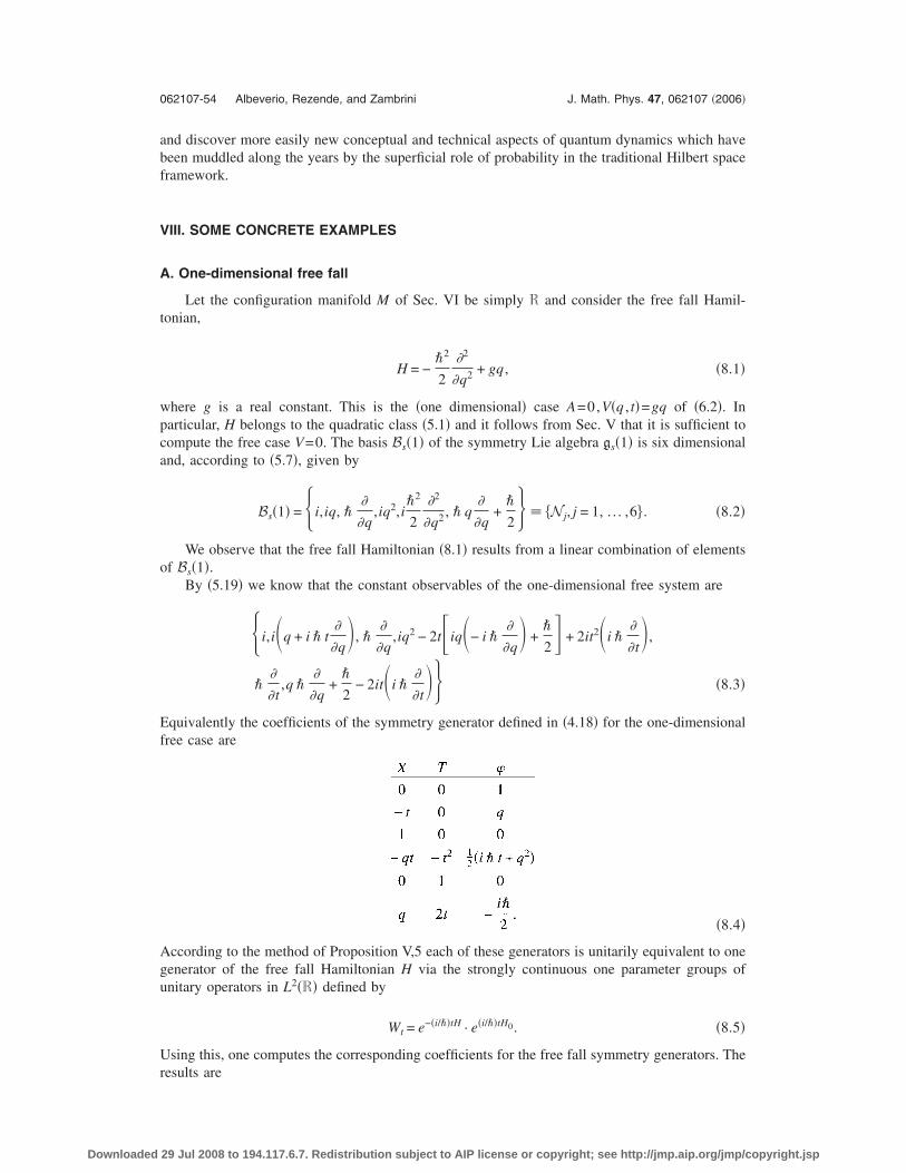
abf

V

A

t

wpca

o

Ef

Agu

Ur


Downloaded

nd discover more easily new conceptual and technical aspects of quantum dynamics which haveeen muddled along the years by the superficial role of probability in the traditional Hilbert spaceramework.

III. SOME CONCRETE EXAMPLES

. One-dimensional free fall

Let the configuration manifold M of Sec. VI be simply R and consider the free fall Hamil-onian,

H = −�2

2

�2

�q2 + gq , �8.1�

here g is a real constant. This is the �one dimensional� case A=0,V�q , t�=gq of �6.2�. Inarticular, H belongs to the quadratic class �5.1� and it follows from Sec. V that it is sufficient toompute the free case V=0. The basis Bs�1� of the symmetry Lie algebra gs�1� is six dimensionalnd, according to �5.7�, given by

Bs�1� = �i,iq, ��

�q,iq2,i

�2

2

�2

�q2 , � q�

�q+�

2� � N j, j = 1, . . . ,6� . �8.2�

We observe that the free fall Hamiltonian �8.1� results from a linear combination of elementsf Bs�1�.

By �5.19� we know that the constant observables of the one-dimensional free system are

�i,i�q + i � t�

�q�, �

�

�q,iq2 − 2t�iq�− i �

�

�q� +

�

2 + 2it2�i �

�

�t�,

��

�t,q �

�

�q+�

2− 2it�i �

�

�t�� 8.3�

quivalently the coefficients of the symmetry generator defined in �4.18� for the one-dimensionalree case are

�8.4�

ccording to the method of Proposition V,5 each of these generators is unitarily equivalent to oneenerator of the free fall Hamiltonian H via the strongly continuous one parameter groups ofnitary operators in L2�R� defined by

Wt = e−�i/��tH · e�i/��tH0. �8.5�

sing this, one computes the corresponding coefficients for the free fall symmetry generators. The
esults are

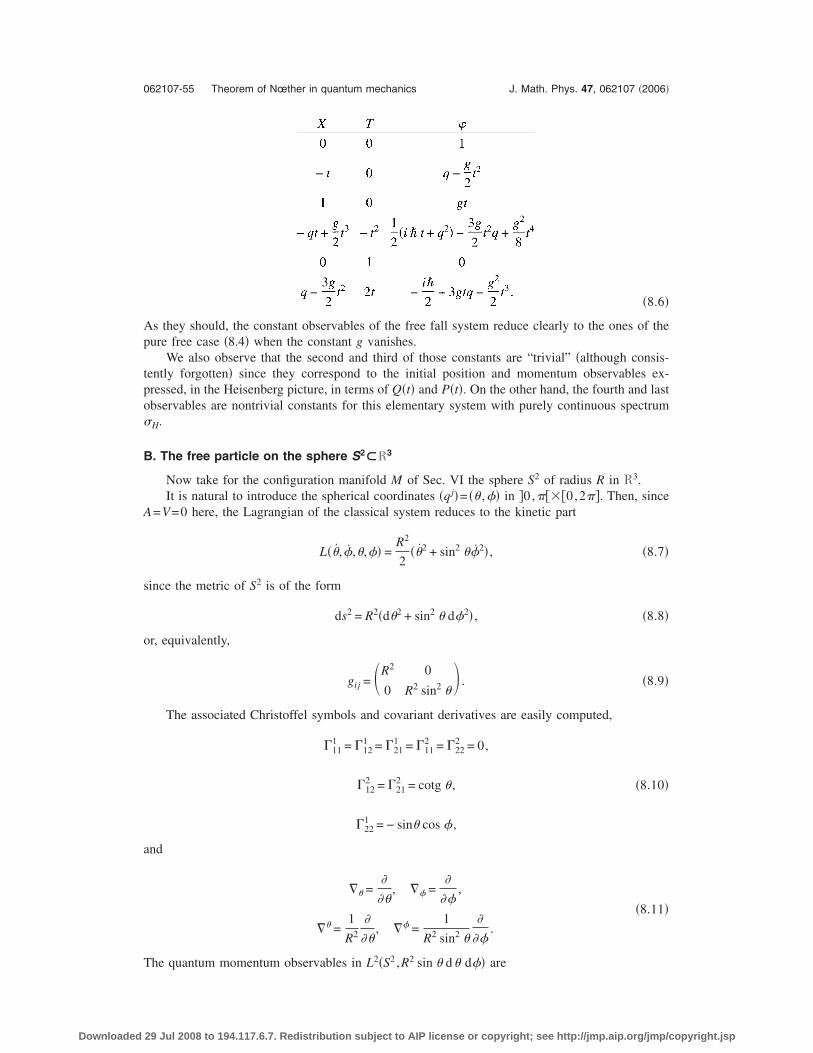
Ap

tpo�

B

A

s

o

a

T


Downloaded

�8.6�

s they should, the constant observables of the free fall system reduce clearly to the ones of theure free case �8.4� when the constant g vanishes.

We also observe that the second and third of those constants are “trivial” �although consis-ently forgotten� since they correspond to the initial position and momentum observables ex-ressed, in the Heisenberg picture, in terms of Q�t� and P�t�. On the other hand, the fourth and lastbservables are nontrivial constants for this elementary system with purely continuous spectrum

H.

. The free particle on the sphere S2£R3

Now take for the configuration manifold M of Sec. VI the sphere S2 of radius R in R3.It is natural to introduce the spherical coordinates �qj�= �� , � in �0,��0,2��. Then, since

=V=0 here, the Lagrangian of the classical system reduces to the kinetic part

L��, ,�, � =R2

2��2 + sin2 � 2� , �8.7�

ince the metric of S2 is of the form

ds2 = R2�d�2 + sin2 � d 2� , �8.8�

r, equivalently,

gij = �R2 0

0 R2 sin2 �� . �8.9�

The associated Christoffel symbols and covariant derivatives are easily computed,

�111 = �12

1 = �211 = �11

2 = �222 = 0,

�122 = �21

2 = cotg � , �8.10�

�221 = − sin� cos ,

nd

�� =�

��, � =

�

� ,

�� =1

R2

�

��, � =

1

R2 sin2 �

�

� .

�8.11�

2 2 2
he quantum momentum observables in L �S ,R sin � d� d � are

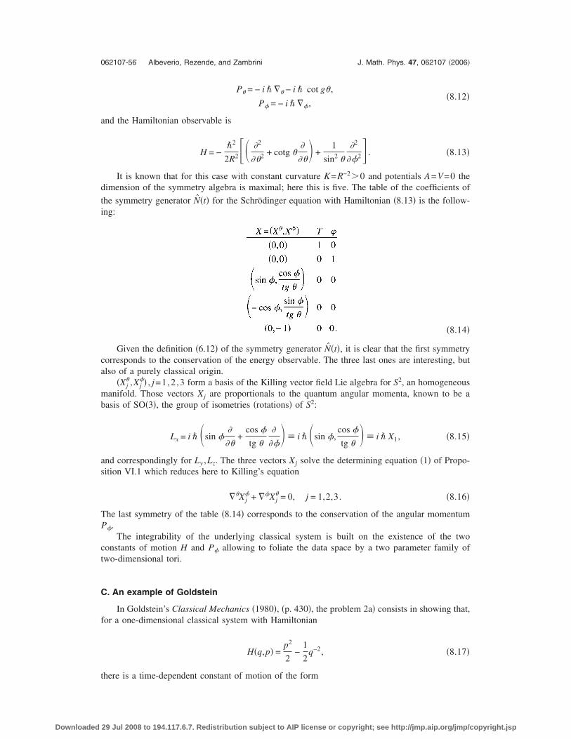
a

d

ti

ca

mb

as

T

ct

C

f

t


Downloaded

P� = − i � �� − i � cot g� ,

P = − i � � ,�8.12�

nd the Hamiltonian observable is

H = −�2

2R2�� 2

��2 + cotg ��

�� +

1

sin2 �

�2

� 2 . �8.13�

It is known that for this case with constant curvature K=R−2�0 and potentials A=V=0 theimension of the symmetry algebra is maximal; here this is five. The table of the coefficients of

he symmetry generator N�t� for the Schrödinger equation with Hamiltonian �8.13� is the follow-ng:

�8.14�

Given the definition �6.12� of the symmetry generator N�t�, it is clear that the first symmetryorresponds to the conservation of the energy observable. The three last ones are interesting, butlso of a purely classical origin.

�Xj� ,Xj

� , j=1,2 ,3 form a basis of the Killing vector field Lie algebra for S2, an homogeneousanifold. Those vectors Xj are proportionals to the quantum angular momenta, known to be a

asis of SO�3�, the group of isometries �rotations� of S2:

Lx = i � �sin �

��+

cos

tg �

�

� � � i � �sin ,

cos

tg �� i � X1, �8.15�

nd correspondingly for Ly ,Lz. The three vectors Xj solve the determining equation �1� of Propo-ition VI.1 which reduces here to Killing’s equation

��Xj + � Xj

� = 0, j = 1,2,3. �8.16�

he last symmetry of the table �8.14� corresponds to the conservation of the angular momentumP .

The integrability of the underlying classical system is built on the existence of the twoonstants of motion H and P allowing to foliate the data space by a two parameter family ofwo-dimensional tori.

. An example of Goldstein

In Goldstein’s Classical Mechanics �1980�, �p. 430�, the problem 2a� consists in showing that,or a one-dimensional classical system with Hamiltonian

H�q,p� =p2

2−

1

2q−2, �8.17�

here is a time-dependent constant of motion of the form


T

Tltc

D

t

I

w

D

I

S

ugcfcadaAuwm

ii


Downloaded

n =q

2p − tH . �8.18�

his is the case where M =R ,A�q�=0, V�q�=− 12q−2and �8.18� shows that

X�q,t� =q

2, T�t� = t, ��q,t� = 0.

he determining equations �1� and �2� of Proposition IV.3 are trivially satisfied and the “classicalimit �=0” of �3� holds as well, so n is indeed a �classical� constant of motion. Let us recall thathere is nothing exotic about time-dependent classical first integrals, as shown by the ones asso-iated with Galilean boosts.

. Lewis and Riesenfeld invariant

This is a quantum invariant, discovered in 1969 �Ref. 52� for the harmonic oscillator withime-dependent frequency, i.e., with classical Hamiltonian �M =R�

H�q,p,t� =1

2p2 +

�2�t�2

q2. �8.19�

t can be shown that this invariant is of the form �6.32�, with

X�q,t� =T

2q, ��q,t� = −

T

4q2, T�t� = �2�t� ,

here ��t� solves the nonlinear equation

� + �2�t�� −1

�3 = 0.

etails can be found in Ref. 53.

X. CONCLUSIONS

Our framework is founded on a dynamic reinterpretation of the symmetry group of thechrödinger equation, itself very close to the one of the associated heat equation.

Given the fact that this group was computed by Lie around 1890, a number of the tools wesed here are, indeed, quite old. The free Lie algebra can be found in most of the textbooks on Lieroups analysis of PDE published since 1970 �for example Refs. 15, 16, and 54�, often withommentaries about the obscure physical interpretation of most explicitly time-dependent trans-ormations, notably those presented as trivial in our Section V. Kuwabara’s result28 �1984� �dis-overed by us after the redaction of the present work was almost finished� is especially relevant,s it shows that the Lie algebraic structure for quantum �and classical� symmetries is time-ependent. He found, in particular, the form �6.12� of the symmetry operator, without regarding its a consequence of a Nœther theorem or trying to relate it with a Lagrangian framework.lthough we could not find a clear statement that the associated quantum first integrals should benderstood in the sense of the Heisenberg picture of quantum dynamics, such a statement mayell already exist in the vast literature on the subject, but is certainly not common knowledge inathematical or theoretical physics.

The specific contribution of our indirect Euclidean approach lies, curiously, in the physicalnterpretation it provides of many time-dependent symmetries, through their elementary meaning

69
n stochastic analysis.

t�s

oa

at

w

a

p

af

o�

osadtSc�p

p

Rm


Downloaded

The simplest illustration is provided by the one-dimensional �n=1� free case �A=V=0� and

he symmetry associated with the coefficients X=−t ,T=0,�=x of the symmetric generator N�t� in4.7�, corresponding to a simple solution of the system of equations of Proposition IV.3. Thisymmetry corresponds to the one-parameter family of solutions

��x,t� = e�i/��x−��2/2�t��x − �t,t�, �� R �9.1�

f the free equation i� �� /�t�=−��2 /2��, quite familiar in the context of the Galilean invari-nce of this equation.55

Let us rewrite �9.1� as

��x,t� = �e�N�t��x,t� , �9.2�

nd expand in � this expression when � is the trivial �unnormalizable� free solution if �t=1. Onhis “state,” the space–time observables of momentum and energy vanish and the one associated

ith N�t� reduces to the phase � �cf. �4.18��. We find

��x,t� = 1 + �x +�2

2!�x2 + i � t� −

�3

3!�x3 + 3i � tx� + ¯ . �9.3�

By successive taking of �� /�� at �=0 we obtain a collection of constant space–time observ-

bles n1Nn

�x , t��n�x , t� ,n�N, each, indeed, solution of Dt�n=0.

Now N�t�= �−tP�t�+Q�t�� itself is certainly a trivial quantum first integral, namely the initialosition observable �since Q�t� and P�t� are solutions of the free Heisenberg equation of motion�nd the Nn�t� ,n�N, reduce to the successive powers of this trivial dynamical information on theree quantum system.

On the Euclidean side, we are dealing instead of �9.1� with the one parameter family

��q,t� = e�1/��q−��2/2�t��q − �t,t�, �� R �9.4�

f �positive� solutions of the free heat equation �7.11�. It corresponds to the Euclidean counterpartcf. paper I�

NE�t� = t�

�q− q �9.5�

f the real time symmetry generator N�t�. The above unphysical state �t turns into the trivialolution �t=1 of the free equation �7.11� whose probabilistic role becomes fundamental. Indeed,ccording to �7.19� and �7.22�� the associated well-defined diffusion Zt reduces to the one-imensional Wiener process with diffusion coefficient �. Notice that the corresponding solution ofhe free adjoint heat equation �7.7� is, then, the integral kernel �t

*=h0�x , t ,q� of this equation.ince the relation between �t and �t

* is manifestly not the Euclidean counterpart of a complexonjugacy, this means that for the Wiener process itself, the time invariance of the lhs of �7.12�with an appropriate pair of positive boundary conditions� is the basis of our probabilistic inter-retation of a complex quantum probability amplitude.

Now let us consider

h��q,t� =��

�q,t� . �9.6�

If Zt is the diffusion, of law P, built from � using �7.19�, it is easy to show that h� is a strictlyositive Pt-martingale of Zt, i.e., satisfies Dt h��Zt , t�=0. Denoting by Zt

� the new diffusion, of lawP�, built from ��, one shows easily that P� is absolutely continuous with respect to P, with

adon-Nikodym derivative dP� /dP=h�. In the case of the Wiener process, h� is the exponential44,49
artingale of this process, a basic tool dating back to the foundations of stochastic analysis.

Tnmt

t

cm

pmws

X

�

�

1

1

1

1

1

1

1

1

1

1

2


Downloaded

he family of Pt-martingales resulting from the successive taking of derivatives � /�� at �=0,amely 1,q ,q2− � t ,q3−3� tq , . . . �, coincides with the familiar Wick product of the Brownianotion56 which is, therefore, reinterpreted as the probabilistic counterpart of the above-mentioned

rivial dynamical information on the free quantum system provided by Nœther’s theorem.Thus stochastic analysis may help, indeed, to understand some conventional aspects of quan-

um dynamics.The version of Euclidean quantum mechanics advocated in paper I is known to be valid for a

lass of Hamiltonians much larger than the one considered here �cf. Ref. 57� and it is expected thatany ideas expressed here will survive in more general contexts �cf. Refs. 70 and 71�.

Although, as shown here, the Riemannian formulation of our results is quite natural, theroper geometrical framework of this method is distinct. It should be regarded, in fact, as defor-ation of classical contact geometry.58 This viewpoint also has serious computational advantageshen adopted in the Euclidean context where the probability measures make sense, and quantum

ymmetries are reinterpreted as symmetries of families of diffusion processes.

. ERRATA FOR PAPER I

1� In Proposition 3.6 of Ref. 1 �cf. also Ref. 59�, the term � −Xq ·B, i.e., the variation of thedrift, is ambiguous. It should be understood as

�

�qi −�Xk

�qi Bk

�where the summation convention is used�.2� The “illustration of the central role of time symmetry,” mentioned in p. 331 of Ref. 1 is

wrong: the function n�q , t� �respectively n*�q , t�� solves our heat equation �7.11� �respec-tively, �7.7�� and so are Pt �respectively, Ft� martingales of the starting process Zt, t� I. Butthey are not strictly positive and so cannot be used as h-functions, in the sense of Doob’s

h-transform. However, when the Nœtherian symmetry operator N is positivity preserving,

��q , t�=e−�N��q , t�, where � is the positive solution of �7.11� associated with Zt, is aone-parameter family of solutions of the same equation. Then h��q , t�= �� /��q , t� is, in-deed, the positive martingale needed for the h-transform producing the family of Bernsteindiffusions Zt

� associated with this symmetry �cf. Conclusion here, Sec. 6, Part 2 of Ref. 44,and Refs. 31, 32, and 58 for much more�.

1 M. Thieullen and J.-C. Zambrini, Ann. I.H.P. Phys. Theor. 67�3�, 297 �1997�.2 R. Feynman and A. R. Hibbs, Quantum Mechanics and Path Integrals �McGraw-Hill, New York, 1965�.3 W. Thirring, A Course in Mathematical Physics Vol. 3: Quantum Mechanics of Atoms and Molecules �Springer-Verlag,New York, 1981�.

4 M. Reed and B. Simon, Fourier Analysis, Self-Adjointness �Academic, New York, 1975�.5 T. Tsuchida, Nagoya Math. J. 136, 157 �1994�.6 D. Fujiwara and T. Tsuchida, J. Math. Soc. Jpn. 49, 299 �1997�.7 Y. Oshima, “Time dependent Dirichlet form and its applications to a transformation of space–time processes,” DirichletForms and Stochastic Processes �de Gruyter, New York, 1993�, pp. 305–320.

8 V. Arnold, Méthodes Mathématiques de la Mécanique Classique �Mir, Moscow, 1976�.9 S. Albeverio and R. Høegh-Krohn, Mathematical Theory of Feynman Path Integrals, Lect. Notes Math. 523 �Springer,New York, 1976�. New edition, with S. Mazzucchi, in preparation, Springer, Berlin �2006�.

0 S. Albeverio and Z. Brzeźniak, J. Funct. Anal. 113, 177 �1993�.1 B. S. DeWitt, Rev. Mod. Phys. 29, 377 �1957�.2 S. Albeverio, A. M. Boutet de Monvel-Berthier, and Z. Brzeźniak, Potential Anal. 4, 469 �1995�.3 L. Shiff, Quantum Mechanics �McGraw-Hill, Kogakusha Tokyo, 1968�.4 V. M. Alekseev, V. M. Tikhomirov, and S. V. Fomin, Commande Optimale �Mir, Moscow, 1982�.5 W. Miller, Symmetry and Separation of Variables �Addison-Wesley, Reading, MA, 1977�.6 P. J. Olver, Applications of Lie Groups to Differential Equations �Springer-Verlag, New York, 1986�.7 V. Guillemin and S. Sternberg, Symplectic Techniques in Physics �Cambridge University Press, Cambridge, 1984�.8 E. Nelson, Ann. Math. 70, 572 �1959�.9 G. B. Folland, Harmonic Analysis in Phase Space �Princeton University Press, Princeton, NJ, 1989�.0
R. Berndt, An Introduction to Symplectic Geometry, Grad. Stud. Math. 26 �American Mathematical Society, Providence,

2

2

2

2

2

2

2

2

2

3

3

3

3

3

3

3

3

3

3

4

4

4

4

4

4

4

4

4

4

5

5

5

5

5

5

5

5

5

5

6

6

6

6

6

6

6

6


Downloaded

RI, 2001�.1 S. Zelditch, Commun. Math. Phys. 90, 1 �1993�.2 A. Weinstein, Am. J. Math. 107, 1 �1985�.3 D. Fujiwara, Duke Math. J. 47, 559 �1980�.4 Y. Colin de Verdière, Chem. Phys. 105, 327 �1986�.5 H. Tamura, Nagoya Math. J. 105, 40 �1987�.6 A. Mohamed and J. Nourrigat, J. Math. Pures Appl. 70, 87 �1991�.7 H. Matsumoto, “The asymptotic distributions of the eigenvalues for the Schrödinger operators with magnetic fields,”in Asymptotic Problems in Probability Theory: Wiener Functionals and Asymptotics, edited by K. D. Elworthy andN. Ikeda, Pitman Lecture Notes, 284 �Longman, Harlow, 1993�, pp. 169–193.

8 R. Kuwabara, Rep. Math. Phys. 19, 27 �1984�.9 B. Doubrovine, S. Novikov, and A. Fomenko, Géométrie Contemporaine, 1st ed. �Mir, Moscow, 1982�.0 R. Abraham and J. E. Marsden, Foundations of Mechanics, 2nd ed. �Benjamin, Reading, MA, 1978�.1 T. Kolsrud, “Quantum constants of motion and the heat Lie algebra in a Riemanniann manifold,” Trita-Mat, 1996,Stockholm �unpublished�.

2 J.-C. Zambrini, “Probability and quantum symmetries in a Riemannian manifold,” in Progress in Probability, edited byR. Dalang, M. Dozzi, and F. Russo �Birkhäuser, Boston, 1999�, Vol. 45.

3 J. Von Neumann, Mathematical Foundations of Quantum Mechanics �Princeton University Press, Princeton, NJ, 1955�.4 N. Kumano-go, Bull. Sci. Math. 128, 197 �2004�.5 “The Mathematical Legacy of R. P. Feynman,” in Stochastic Analysis and Mathematical Physics, edited by R. Rebolledo,J. Rezende, and J.-C. Zambrini �World Scientific, Singapore, 2004�.

6 R. H. Cameron, J. Math. Phys. 39, 126 �1960�.7 S. Albeverio, “Wiener and Feynman path integrals and their applications,” Proceedings of Symposium in Applied Math-ematics �American Mathematical Society, Providence, RI�, Vol. 52 �1997�.

8 A. D. Wentzell, A Course in the Theory of Stochastic Processes �McGraw-Hill, New York, 1981�.9 S. Albeverio, A. Hahn, and A. Sengupta, “Rigorous Feynman path integrals with applications to quantum theory, gaugefields and topological invariants,” in Ref. 35.

0 S. Albeverio and S. Mazzucchi, J. Stat. Phys. 115, 191 �2004�.1 J. Rezende, Commun. Math. Phys. 101, 187 �1985�.2 G. W. Johnson and M. L. Lapidus, The Feynman Integral and Feynman’s Operational Calculus �Oxford UniversityPress, Oxford, 2000�.

3 M. Kac, “On some connections between probability theory and differential and integral equations,” Proceedings of 2ndBerkeley Symposium on Probability and Statistics, edited by J. Neyman �University of California Press, Berkeley, 1951�.

4 K.-L. Chung and J.-C. Zambrini, Introduction to Quantum Time and Quantum Randomness, 2nd ed. �Word Scientific,Singapore, 2003�.

5 S. Albeverio, K. Yasue, and J.-C. Zambrini, Ann. I.H.P. Phys. Theor. 49, 259 �1989�.6 A. B. Cruzeiro, W. Liming, and J.-C. Zambrini, “Bernstein processes associated with a Markov process,” in StochasticAnalysis and Mathematical Physics, edited by R. Rebolledo, Santiago, �Birkhäuser, Boston, 2000�.

7 E. Nelson, Dynamical Theories of Brownian Motion, Math. Notes �Princeton University Press, Princeton, NJ, 1967�.8 L. C. G. Rogers and D. Williams, Diffusions, Markov Processes, and Martingales, Vol. 2, Itô Calculus �Wiley, Chich-ester, 1987�.

9 K. Itô and H. P. McKean, Jr., Diffusion Processes and Their Sample Paths �Springer, Berlin, 1965�.0 K. Itô, “Extension of Stochastic Integrals,” in Proceedings of International Symposium in Stochastic DifferentialEquations—Kyoto 1976, edited by K. Itô, �Kinokuniya, Tokyo, 1976�.

1 A. B. Cruzeiro and J.-C. Zambrini, J. Funct. Anal. 96, 62 �1991�.2 H. R. Lewis and W. B. Riesenfeld, J. Math. Phys. 10, 1458 �1969�.3 J.-C. Zambrini, “A special time–dependent quantum invariant and a general theorem on quantum symmetries,”in Stochastic Analysis and Mathematical Physics �Anestoc’ 96�, edited by R. Rebolledo �World Scientific, Singapore,1996�.

4 N. H. Ibragimov, CRC Handbook of Lie Group Analysis of Differential Equations �CRC Press, Boca Raton, FL�, Vol. 2�1994�.

5 A. Galindo, P. Pascual, “Quantum mechanics I,” Texts and Monographs in Physics �Springer-Verlag, New York, 1990�.6 B. Simon, “The P� �2 Euclidean (quantum) field theory, Princeton Series in Physics,” �Princeton University Press, NJ,1974�.

7 N. Privault and J.-C. Zambrini, Ann. I.H.P. Probab. Stat. 40, 599 �2004�.8 P. Lescot and J.-C. Zambrini, “Probabilistic deformation of contact geometry, diffusion processes and their quadratures,”Seminar on Stochastic Analysis, Random Fields and Applications V, Ascona �Birkhäuser, Boston�, to appear.

9 M. Thieullen and J.-C. Zambrini, Probab. Theory Relat. Fields 107, 401 �1997�.0 K. Yajima, Commun. Math. Phys. 181, 605 �1996�.1 S. Albeverio and S. Mazzucchi, J. Funct. Anal. 221, 83 �2005�.2 G. Ben Arous and F. Castell, J. Funct. Anal. 137, 243 �1996�.3 M. De Faria, J. Potthoff, and L. Streit, J. Math. Phys. 32, 2123 �1991�.4 D. Elworthy and A. Truman, Ann. I.H.P. Phys. Theor. 41, 115 �1984�.5 M. Grothaus, D. Khandekar, J. L. da Silva, and L. Streit, J. Math. Phys. 38, 3278 �1997�.6 V. N. Kolokoltsov, Semiclassical Analysis for Diffusions and Stochastic Processes, Lect. Notes Math. 1724 �Springer,Berlin, 2000�.

7 T. Hida, Brownian Motion �Springer-Verlag, New York, 1980�.


6

6

7

7


Downloaded

8 N. Ikeda and S. Watanabe, Stochastic Differential Equations and Diffusion Processes �North-Holland, Amsterdam,1981�.

9 P. Malliavin, Stochastic Analysis, Grund. der Math. Wiss 313 �Springer-Verlag, Berlin, 1997�.0 S. Albeverio, “Theory of Dirichlet forms and applications,” in S. Albeverio, W. Schachermayer, and M. Talagrand,Lectures on Probability Theory and Statistics �Ecole d’Eté de Probabilités de Saint-Flour XXX-2000�, edited byP. Bernard, Lect. Notes Math. 1816 �Springer, New York, 2003�, pp. 4–110.

1 T. Kolsrud, “Position dependent NLS hierarchies: Involutivity, commutation relations, renormalisation and classicalinvariants,” to appear in Bull. Sci. Math.


Documents

Probability and Quantum Symmetries. II. The Theorem of ...gfm.cii.fc.ul.pt/people/jczambrini/JMathPhys-47-062107.pdf · Probability and Quantum Symmetries. II. The Theorem of Nœther