Embed Size (px)
Citation preview
Master Thesis im Rahmen des
Universitätslehrganges „Geographical Information Science & Systems“ (UNIGIS MSc) am Zentrum für GeoInformatik (Z_GIS)
der Paris Lodron-Universität Salzburg
zum Thema
„Biomass-mapping of alpine grassland with APEX imaging
spectrometry data“
vorgelegt von
Dipl. Ing. Maja Rapp U1509, UNIGIS MSc Jahrgang 2010
Zur Erlangung des Grades „Master of Science (Geographical Information Science & Systems) – MSc(GIS)”
Gutachter:
Ao. Univ. Prof. Dr. Josef Strobl Zürich, 30.03.1013

I
EIDESSTATTLICHE ERKLÄRUNG
Ich erkläre hiermit an Eides statt, dass ich die vorliegende Thesis selbständig und ohne
unzulässige fremde Hilfe angefertigt habe. Die verwendeten Quellen sind vollständig
zitiert.
Datum: 30.03.2013 Unterschrift:
II
ABSTRACT
Today remote sensing is a standard technique for mapping land cover in high spatial
resolution over large areas. Not only land cover but also the quality and quantity of
vegetation can be classified by the analysis of imaging spectroscopy data. In the Swiss
National Park (SNP) we use data from the Airborne Prism Experiment (APEX) imaging
spectrometer to expand the possibilities of vegetation analysis in alpine territories. The
high spectral and spatial resolution of APEX data allows the correlation of the
measured reflection with ground truth data.
In this work a standard Normalized Differenced Vegetation Index (NDVI) and an
optimized simple ratio index (SRI) with selected bands were generated to model the
biomass content of the alpine grassland of one particular valley in the SNP, the Val
Trupchun.
The correlation between biomass insitu measurements and SRIs was non-linear, most
likely due to sensor saturation. Our optimal SRI improved the model quality compared
to the NDVI model. All computed models underestimated high biomass values above
600 g/m2. The model accuracy of 57% was good considering the challenging terrain.
However, several factors showed that the model was relatively unstable due to
parameter input settings and external factors. Differences in APEX data between strips
induced an important effect, due to different illumination/view angles. The variability
analysis investigating the sample plot location demonstrated that small-scale
geometrical shifts were insignificant compared to the overall model accuracy. The
biomass prediction map showed plausible values for the grassland with high
concentrations around former alps. High biomass sources were linked to former
anthropogenic land use, dominant vegetation structure and to preferred ungulate
habitat today.
The high-resolution map is now a useful basis for future research in the SNP to
investigate forage amount and analyse ungulate habitat pattern in Val Trupchun. This a

welcoming issue for ungulate research, which is an important research area of the
SNP.
IV
TABLE OF CONTENTS
ABSTRACT ..................................................................................................................................... III
LIST OF FIGURES .............................................................................................................................. VI
LIST OF TABLES .............................................................................................................................VIII
ACKNOWLEDGEMENTS ..................................................................................................................... IX
1 INTRODUCTION ..................................................................................................................... 10
1.1 Motivation......................................................................................................................... 11
1.2 Objective ........................................................................................................................... 11
1.3 Methodology ..................................................................................................................... 12
1.4 Structure ........................................................................................................................... 12
2 BACKGROUND ...................................................................................................................... 14
2.1 Research in the Swiss National Park ................................................................................. 14
2.2 Imaging Spectroscopy of vegetation ................................................................................. 16
2.2.2 Spectral indices.......................................................................................................... 22
2.2.3 State of the art in biomass estimation using VIs ....................................................... 23
2.3 Apex .................................................................................................................................. 25
3 METHODOLOGY .................................................................................................................... 29
3.1 The study area ................................................................................................................... 29
3.2 Field data collection .......................................................................................................... 30
3.3 Image acquisition and pre-processing .............................................................................. 32
3.4 Data analysis ..................................................................................................................... 33
4 RESULTS .............................................................................................................................. 37
4.1 Field sample results........................................................................................................... 37
4.2 Regression of biomass and standard NDVI ....................................................................... 38
4.3 Regression of Biomass and Optimal Simple Ratio Index ................................................... 40
4.4 Regression of biomass and narrowband sri ...................................................................... 44
4.5 Biomass map ..................................................................................................................... 46
4.6 Different reflectance values between strips ..................................................................... 51
4.7 Variability of sample plot location .................................................................................... 53
5 DISCUSSION ......................................................................................................................... 55
5.1 Biomass reference............................................................................................................. 55
5.2 Comparison of NDVI and optimal SRI ............................................................................... 55
5.3 Uncertainty Analysis ......................................................................................................... 56
5.3.1 Different reflectance values between strips ............................................................. 57
5.3.2 Variability of sample plot location............................................................................. 59
6 CONCLUSION ........................................................................................................................ 61
7 OUTLOOK ............................................................................................................................ 62
8 LIST OF REFERENCES ............................................................................................................... 63
9 GLOSSARY ........................................................................................................................... 69
10 APPENDIX ............................................................................................................................ 71
V
LIST OF FIGURES
Figure 1: Working schematic of imaging spectroscopy (Image: www.apex-esa.org, last accessed
20.03.2013) ................................................................................................................................................ 17
Figure 2: Typical spectral signature of vegetation, water and bare soil (Image: Remote Sensing,
fundamental Concepts, from http://www.remote-sensing.net, last accessed on 06.12.2012). ............... 19
Figure 3: Canopy reflectance effects dependant with different LAI and MLA (Image: ENVI user guide,
http://geol.hu/data/online_help/Understanding_Vegetation_and_Its_Reflectance_Properties.html#wp1
159169, last accessed on 20.03.2013) ....................................................................................................... 21
Figure 4: Changes in reflectance between dead and dry vegetation across the optical spectrum (Image:
ENVI user guide, http://geol.hu/data/online_help/Understanding_Vegetation_and_Its_Reflectance_
Properties.html#wp1159 169, last accessed on 20.03.2013). ................................................................... 22
Figure 5: Picture of the Dornier DO-228 on which the sensor was installed, and the APEX sensor (Images
from RSL, University of Zurich) ................................................................................................................... 27
Figure 6: Overview of APEX subsystems (image from Schaepman et al., 2003). ....................................... 27
Figure 7: Overview of the study site Val Trupchun and its historical park boarders ................................. 29
Figure 8: Locations of the 25 sample plots in Val Trupchun, where 1x1 m of vegetation was clipped. .... 31
Figure 9: Apex ground truth plot design 2010 ........................................................................................... 32
Figure 10: Overview of the study site and the 4 flight strips (S_42, S_52, S_62 and S_72) ....................... 33
Figure 11: Regression between the standard NDVI derived from APEX reflectance spectra from bands at
809 and 664 nm and the wet weight biomass calibration sample data .................................................... 39
Figure 12: Regression between the predicted biomass value calculated from the NDVI model calibration
and the true biomass value of the validation sample plots ....................................................................... 40
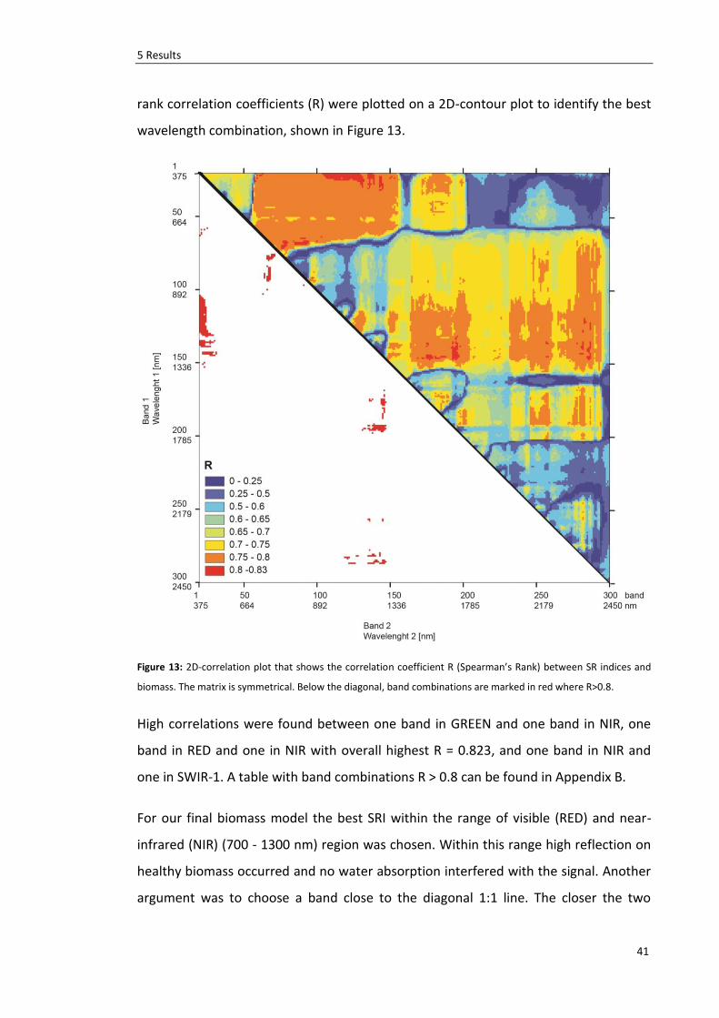
Figure 13: 2D-correlation plot that shows the correlation coefficient R (Spearman’s Rank) between SR
indices and biomass. The matrix is symmetrical. Below the diagonal, band combinations are marked in
red where R>0.8. ........................................................................................................................................ 41
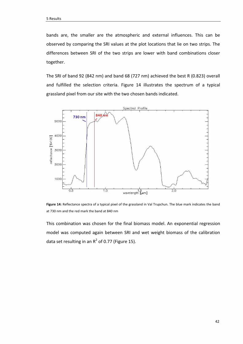
Figure 14: Reflectance spectra of a typical pixel of the grassland in Val Trupchun. The blue mark
indicates the band at 730 nm and the red mark the band at 840 nm ....................................................... 42
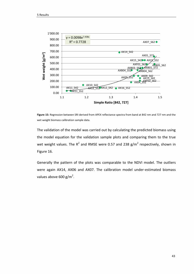
Figure 15: Regression between SRI derived from APEX reflectance spectra from band at 842 nm and 727
nm and the wet weight biomass calibration sample data. ........................................................................ 43
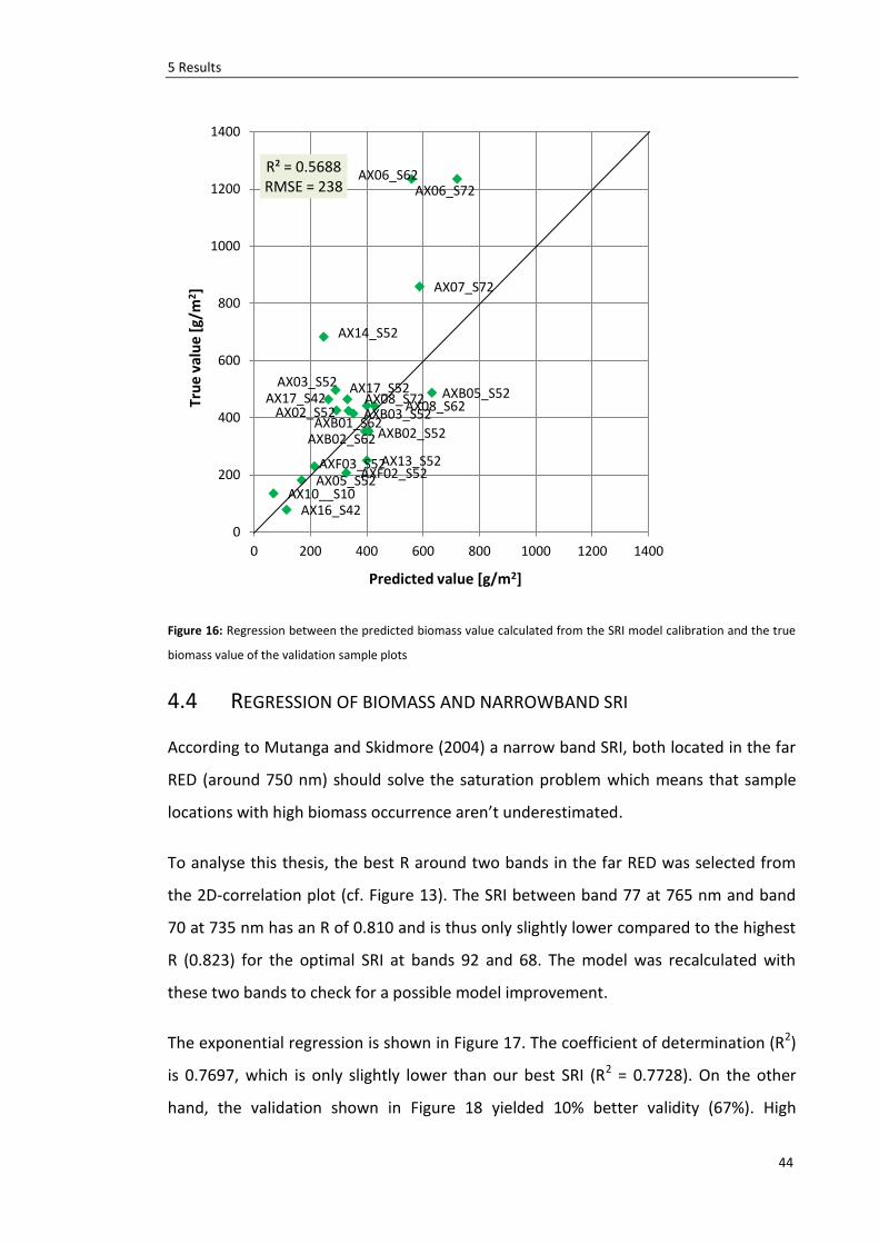
Figure 16: Regression between the predicted biomass value calculated from the SRI model calibration
and the true biomass value of the validation sample plots ....................................................................... 44
Figure 17: Regression between SRI derived from APEX reflectance spectra from band at 765 nm and 735
nm and the wet weight biomass calibration sample data ......................................................................... 45
Figure 18: Regression between the predicted biomass value and the true biomass value for the
prediction model SRI765 nm, 735 nm ................................................................................................................. 45
Figure 19: Biomass map of Val Trupchun overlain on a graphical relief shading ...................................... 47
Figure 20: Detailed biomass map and monkshood occurrence of the grassland around Alp Trupchun ... 48
Figure 21: Detail map of Alp Purcher with special herb/grass type ........................................................... 49
Figure 22: Detailed map of the bottom south slope in the back of the valley with high biomass sources 50
Figure 23: Histogram of the biomass map of Val Trupchun....................................................................... 51
Figure 24: Scatter plot of the optimal SRI values of all sample plots on APEX strip a against strip b ........ 52
Figure 25: Scatter plot of the narrow band SRI values of all sample plots on APEX strip a against strip b 52
Figure 26: Biomass discrepancy predicted for the sample plot locations between implementation of
average reflection of 3x3 vs. 5x5 APEX pixels as reference values. ........................................................... 54
Figure 27: Multiple view angle imaging of vegetation using airborne sensors carried on overlapping
flight-paths using wide field-of-view sensors to obtain cross-track data. The highlighted area can be
viewed at three different angles (image from Jones & Vaughan, 2010). ................................................... 58
Figure 28: Schematic of plot AX12 (left) and AX09 (right) overlain by the APEX image. The APEX image is
oriented in a northerly direction, whereas the plots have been measured in direction to the slope. The
dots indicate the true mid points and the corners of the plot, respectively, the green square indicates
the 3x3 APEX pixels, the blue square the 5x5 APEX pixel implemented for modelling. ............................ 60
Figure 29: Map of the entrance of Val Trupchun with plots AX101, AX06, AXB01, AX06 and AX07
indicated ..................................................................................................................................................... 71
Figure 30: Detailed map of the middle part of Val Trupchun, Dschembrina, God Malgöletta and God
Trupchun with AXF02, AXB02, AXB03, AXB04 and AXB05 indicated ......................................................... 71
Figure 31: Map of the Alp Trupchun and the north slope of the valley with plot AXF03, AX02, AX03, AX04
and AX05 .................................................................................................................................................... 72
Figure 32: Map of the inner most part of the valley and the south slope of the valley with plots indicated
.................................................................................................................................................................... 72

VII
LIST OF TABLES
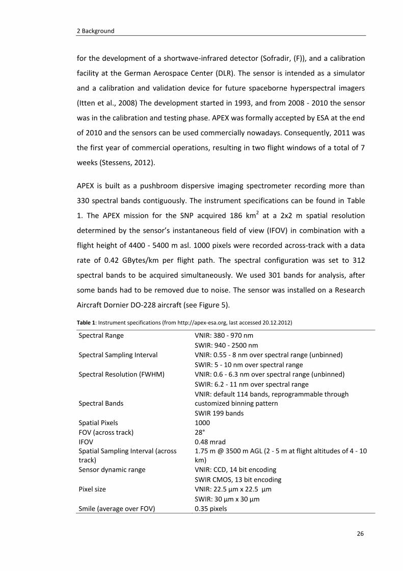
Table 1: Instrument specifications (from http://apex-esa.org, last accessed 20.12.2012) ....................... 26
Table 2: Overview of the raw data of all biomass samples ........................................................................ 38
Table 3: Overview of the calibration and validation data set selection (random) ..................................... 73
Table 4: Correlation hotspots with R > 0.8 from 2D contour plot ............................................................. 73
Table 5: Calculation results of different reflectance values between stripes and effect on biomass
prediction ................................................................................................................................................... 74
VIII
ACKNOWLEDGEMENTS
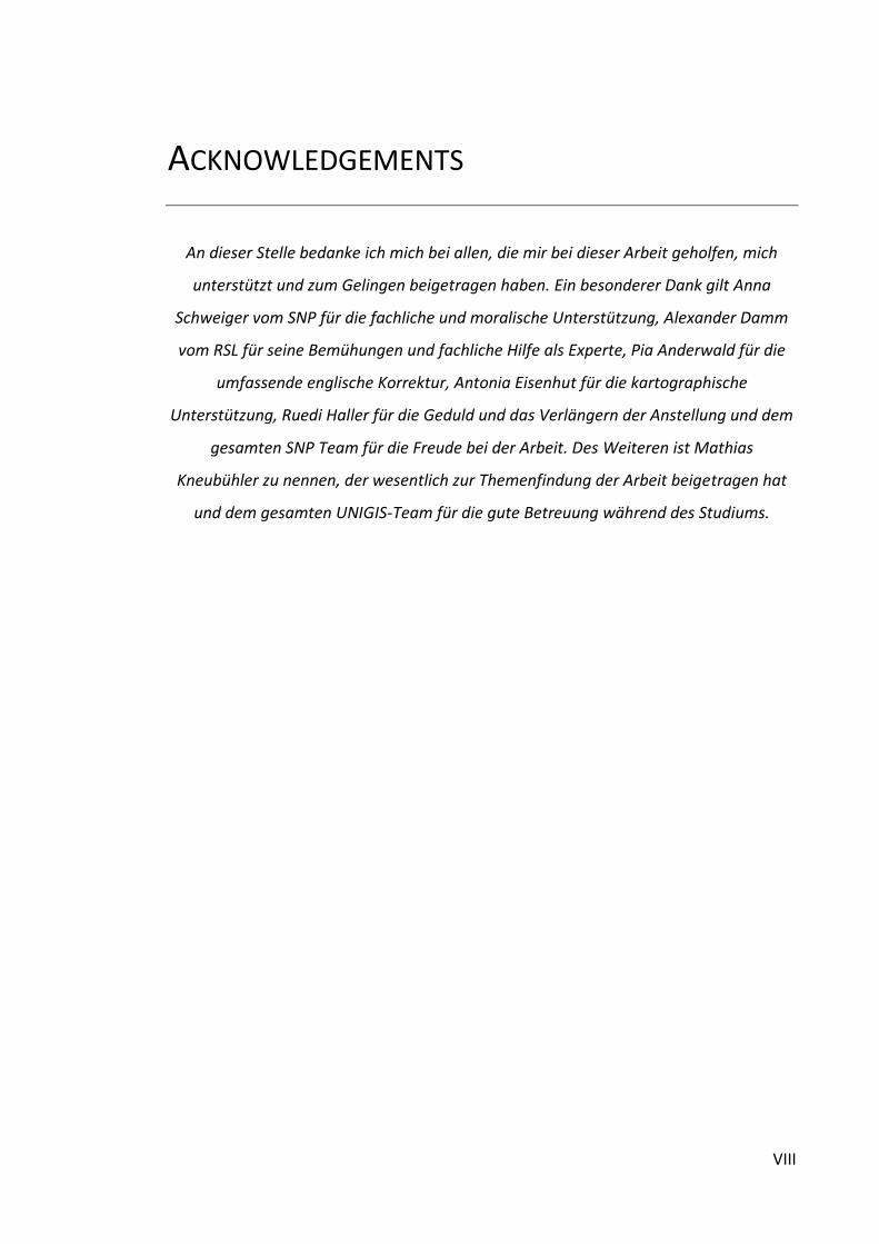
An dieser Stelle bedanke ich mich bei allen, die mir bei dieser Arbeit geholfen, mich
unterstützt und zum Gelingen beigetragen haben. Ein besonderer Dank gilt Anna
Schweiger vom SNP für die fachliche und moralische Unterstützung, Alexander Damm
vom RSL für seine Bemühungen und fachliche Hilfe als Experte, Pia Anderwald für die
umfassende englische Korrektur, Antonia Eisenhut für die kartographische
Unterstützung, Ruedi Haller für die Geduld und das Verlängern der Anstellung und dem
gesamten SNP Team für die Freude bei der Arbeit. Des Weiteren ist Mathias
Kneubühler zu nennen, der wesentlich zur Themenfindung der Arbeit beigetragen hat
und dem gesamten UNIGIS-Team für die gute Betreuung während des Studiums.
10
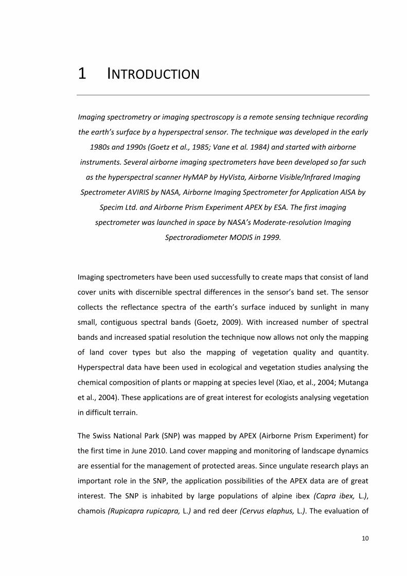
1 INTRODUCTION
Imaging spectrometry or imaging spectroscopy is a remote sensing technique recording
the earth’s surface by a hyperspectral sensor. The technique was developed in the early
1980s and 1990s (Goetz et al., 1985; Vane et al. 1984) and started with airborne
instruments. Several airborne imaging spectrometers have been developed so far such
as the hyperspectral scanner HyMAP by HyVista, Airborne Visible/Infrared Imaging
Spectrometer AVIRIS by NASA, Airborne Imaging Spectrometer for Application AISA by
Specim Ltd. and Airborne Prism Experiment APEX by ESA. The first imaging
spectrometer was launched in space by NASA’s Moderate-resolution Imaging
Spectroradiometer MODIS in 1999.
Imaging spectrometers have been used successfully to create maps that consist of land
cover units with discernible spectral differences in the sensor’s band set. The sensor
collects the reflectance spectra of the earth’s surface induced by sunlight in many
small, contiguous spectral bands (Goetz, 2009). With increased number of spectral
bands and increased spatial resolution the technique now allows not only the mapping
of land cover types but also the mapping of vegetation quality and quantity.
Hyperspectral data have been used in ecological and vegetation studies analysing the
chemical composition of plants or mapping at species level (Xiao, et al., 2004; Mutanga
et al., 2004). These applications are of great interest for ecologists analysing vegetation
in difficult terrain.
The Swiss National Park (SNP) was mapped by APEX (Airborne Prism Experiment) for
the first time in June 2010. Land cover mapping and monitoring of landscape dynamics
are essential for the management of protected areas. Since ungulate research plays an
important role in the SNP, the application possibilities of the APEX data are of great
interest. The SNP is inhabited by large populations of alpine ibex (Capra ibex, L.),
chamois (Rupicapra rupicapra, L.) and red deer (Cervus elaphus, L.). The evaluation of
1 Introduction
11
vegetation quantity and quality can provide important information on forage
abundance and its spatial distribution. A water content map of the valley of Trupchun
(Val Trupchun) has already been produced using APEX data (Kneubühler, 2011). The
mapping of biomass content of the grassland serves as an additional valuable input
feature for the investigation of ungulate habitat patterns.
1.1 MOTIVATION
The high alpine territory of the SNP is challenging for vegetation analysis. As field
sampling is difficult and time consuming due to the hard accessibility of the terrain,
traditional field research is limited. Not only are time and accessibility restricted, but
the personnel effort in the field would also require substantial financial resources.
Furthermore, reliable estimates are restricted to local scales only, whereas ecologists
require estimates at landscape scale. Remote sensing is therefore a great technique for
an area-wide interpretation of vegetation at high spatial resolution.
Ungulate research has a long tradition in the SNP and therefore the analysis of
vegetation quality and quantity is an essential issue. Because ungulates need to spend
most of their time grazing, the (local) composition of forage can explain their spatial
distribution (Van Langenvelde & Prins, 2008). Together with other vegetation
parameters such as water, nutrition and fibre content, the biomass model serves as a
valuable input for the analysis of ungulate habitat and movement patterns.
1.2 OBJECTIVE
The aim of this MSc thesis is to generate a biomass map of the grassland of one
particular valley of the SNP (Val Trupchun) with APEX imaging spectrometry data from
June 2010. A semi-empirical method is implemented in the modelling process. First, a
standard normalized-differenced-vegetation-index (NDVI) is calculated and compared
with insitu biomass samples. To achieve a better model, a large number of simple ratio
vegetation indices (SRI) are developed from the hyperspectral data and regressed
against the ground truth data. Model validation is carried out by independent sample
plots. The best model is taken to predict the grassland biomass in Val Trupchun.
1 Introduction
12
The produced biomass map is analysed for plausibility relating to the former land use
of the Val Trupchun. Furthermore the model is tested for stability and accuracy by
investigating the APEX data at the overlapping zones of the different strips and
analysed by the variability of the sample plot locations. A comprehensive discussion is
carried out to analyse the modelling approach for accuracy, uncertainty and
possibilities for improvement.
The study area of Val Trupchun was chosen due to its substantial cover of grassland
and high population of ungulates. Imaging spectroscopy induces a large data volume
and therefore the handling has its limitations. The whole territory of the park would be
unfeasible for this modelling approach. As the territory is complex and variable at fine
spatial scales, many insitu samples are required to obtain a useful and satisfactory
prediction model. Therefore the method used here not only requires strong computing
power but also substantial effort in the field.
1.3 METHODOLOGY
The APEX data is provided geometrically, atmospherically and radiometrically
corrected by the Remote Sensing Laboratory of the University of Zurich (RSL) using the
standard procedures ATCOR-4 (Schläpfer & Richter, 2002) and PARGE (Schläpfer &
Richter, 2002). A semi-empirical modelling approach is carried out to obtain the
biomass prediction map. Different model settings are tested to optimise model
accuracy. The detailed methodology of pixel-based modelling of the biomass map is
explained in chapter 3.
For data preparation and modelling the software ENVI 4.7 (Environment for
Visualisation of Images) in combination with IDL (Interactive Data Language) by ITT VIS
was used. For the cartography and simple GIS analysis the software ArcGIS 10.0 by ESRI
was applied.
1.4 STRUCTURE
This MSc thesis has been carried out at the Swiss National Park in collaboration with
the Remote Sensing Laboratories of the University of Zurich (RSL).
1 Introduction
13
In the first chapter, an introduction to imaging spectrometry and background
information about the Swiss National Park, the Valley of Trupchun and the APEX
project is given. Chapter 3 explains the methodology of the modelling approach. In
chapter 4, the results are presented, first the model variables and then the resulting
prediction map. Furthermore results related to the model stability, accuracy and
saturation are shown. The results are discussed in chapter 5. Different model
parameters are reviewed here and a comprehensive uncertainty analysis is carried out.
Finally, conclusions are derived from the study and an outlook to further potential
studies is provided.
14
2 BACKGROUND
Due to their high spectral and spatial resolution, image spectrometers serve many
applications over a broad range of scientific fields such as e.g. in ecology, limnology,
geology, atmospheric sciences, natural hazard and disaster management, and
materials detection. Application examples are mapping of soil composition, total
suspended matter in lakes, plant pigments and non-pigments (water, protein,
chlorophyll, lignin, cellulose, nitrogen, etc.), vegetation structure, hydrocarbon content,
net and gross primary production, aerosol concentration and atmospheric water
vapour. The technique is therefore a valuable tool in the management of nature parks.
2.1 RESEARCH IN THE SWISS NATIONAL PARK
The Swiss National Park (SNP) was founded in 1914 as a strict nature reserve and is the
oldest national park in the Alps. The park is situated in the canton of Graubünden
covering an area of 170 km2, which is the largest protected area in Switzerland. It is the
country’s only national park and is classified as a category I nature reserve (highest
protection level - strict nature reserve /wilderness area) with the IUCN (International
Union for the Conservation of Nature). The territory encompasses an alpine landscape
extending over altitudes between about 1400 to 3200 meters above sea level (asl.)
with a rich flora and fauna. Research is one official mission of the park so that the
territory is available for the analysis of natural processes and ecosystems in the
absence of human influence. Scientists from various research institutes use this open-
air laboratory to gain further knowledge of alpine species and habitats. Minimal
human disturbance and the availability of results from earlier projects carried out
during many years offer ideal conditions for a variety of research activities.
As ecological and ungulate research have a long tradition in the SNP, many valuable
long-term data series and publications are available. Since 1917, the vegetation has
been monitored on more than 150 permanent plots (Braun-Blanquet et al., 1931;
2 Background
15
Stüssi, 1970). In 1968 an analogue vegetation map of part of the SNP was produced in
cartography work by Trepp/Campell at a scale of 1:10’000 (Trepp & Campbell, 1968).
In 1992, Zoller published a vegetation map of the entire SNP (Zoller, 1992). It was
based on observation plots and field trips, and mapped at a 1:50’000 scale. An
interpretation of colour infra-red aerial images was conducted over the whole territory
of the SNP as part of the project Alpine Habitat Diversity (HABITALP1) in 2006. A
common coded interpretation key was developed to map area-wide standardized
delimitation of land use types at a 1:5’000 scale. The interpretation allowed not only
the classification of the habitats, but also assignment of the dominant vegetation
species.
Until now, vegetation mapping has been based on the interpretation of single plots
and visual observations, which enables only limited interpolations over large areas.
The HABITALP project has been the first study with a standardized method to classify
vegetation types area-wide from aerial images. Not only is a classification of habitat
types possible with the APEX data, but also pixel-based modelling of vegetation
composition at a scale of 2 x 2 meters.
Ungulate research in the National Park also has a long history. The SNP is inhabited by
large populations of alpine ibex (Capra ibex, L.), chamois (Rupicapra rupicapra, L.) and
red deer (Cervus elaphus, L.). Population counts have been carried out since the
1920’s. Extensive ungulate projects began in the 1990’s. With the assistance of
telemetry and GPS radio collaring, the movement of individual animals can be
recorded and graphically represented. Results from ungulate counts and GIS
movement tracks in combination with vegetation studies will provide information
regarding the forage availability and migration patterns of ungulate populations.
Despite the 100 years of protection, traces from the former land use can still be found
on subalpine and alpine grassland. Cattle and sheep grazed the territory of the SNP for
1 HABITALP – Alpine Habitat Diversity Project. INTERREG III B Alpenraumprogramm 2002-2006,
http://habitalp.de, (last accessed on 20.03.2013)
2 Background
16
several centuries until 1914 (Parolini, 1995). As a result, tall-herb communities
dependent on nutrient enrichment from the excreta of cattle or sheep can still be
found on several former pastures in the SNP (Braun-Blanquet, 1931; Braun-Blanquet et
al., 1954; Pictet, 1942; Stüssi, 1970; Krüsi et al., 1995; Achermann et al., 2000).
2.2 IMAGING SPECTROSCOPY OF VEGETATION
Imaging spectroscopy is similar to colour photography, but the spectrometer acquires
for each pixel many bands of light intensity data from the spectrum, instead of just the
three bands of the RGB model. The sensor collects simultaneously spatially
coregistered images in many spectrally contiguous bands.
The term hyperspectral imaging is often used interchangeably with imaging
spectroscopy. Due to its heavy use in military related applications, the civil world has
developed a slight preference for using the term imaging spectroscopy2.
Imaging spectrometers such as APEX sample contiguously in the optical part of the
electromagnetic spectrum using dozens to hundreds of narrow spectral bands. For
each image pixel, the sensor acquires the reflectance of the earth’s surface from the
ultraviolet through the visible to the near- and mid-infrared (i.e. 250 - 2500 nm) part of
the electromagnetic spectrum at a high spatial resolution. The data allows the analysis
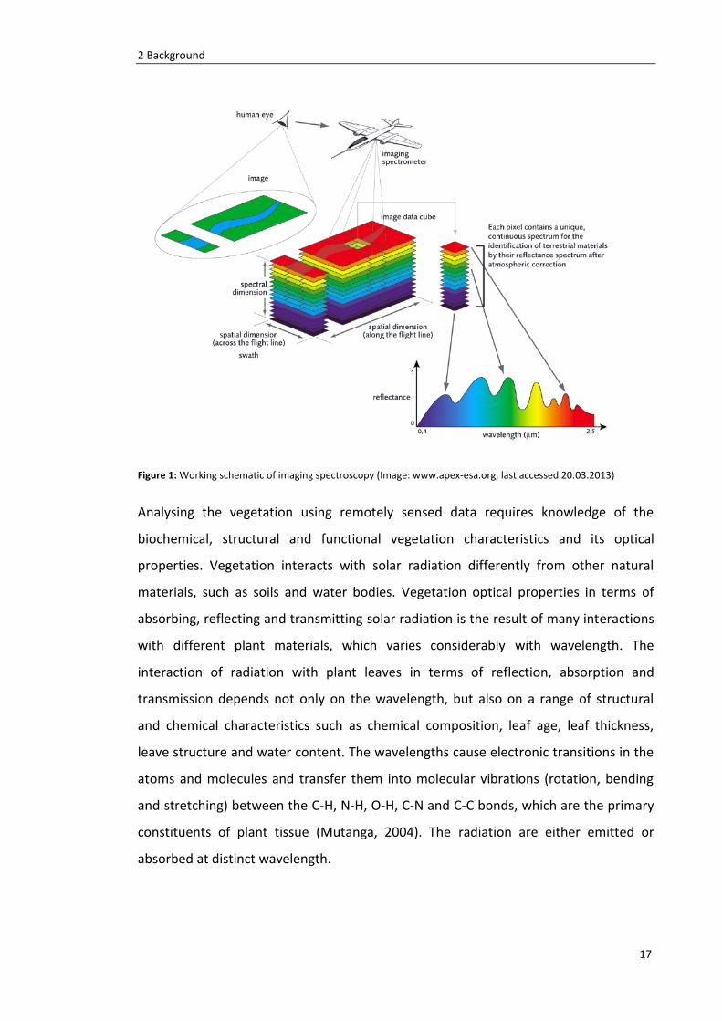
of useful and precise quantitative information about the environment. In Figure 1, a
schematic of the function of imaging spectrometry is illustrated.
2From Wikipedia, Imaging spectroscopy. http://en.wikipedia.org/wiki/Imaging_spectroscopy, last
accessed on 20.03.2013
2 Background
17
Figure 1: Working schematic of imaging spectroscopy (Image: www.apex-esa.org, last accessed 20.03.2013)
Analysing the vegetation using remotely sensed data requires knowledge of the
biochemical, structural and functional vegetation characteristics and its optical
properties. Vegetation interacts with solar radiation differently from other natural
materials, such as soils and water bodies. Vegetation optical properties in terms of
absorbing, reflecting and transmitting solar radiation is the result of many interactions
with different plant materials, which varies considerably with wavelength. The
interaction of radiation with plant leaves in terms of reflection, absorption and
transmission depends not only on the wavelength, but also on a range of structural
and chemical characteristics such as chemical composition, leaf age, leaf thickness,
leave structure and water content. The wavelengths cause electronic transitions in the
atoms and molecules and transfer them into molecular vibrations (rotation, bending
and stretching) between the C-H, N-H, O-H, C-N and C-C bonds, which are the primary
constituents of plant tissue (Mutanga, 2004). The radiation are either emitted or
absorbed at distinct wavelength.
2 Background
18
Water, pigments, nutrients and carbon are each expressed in the reflected optical
spectrum from 400 nm to 2500 nm, with often overlapping, but spectrally distinct,
reflectance behaviours. The absorption characteristics of these compounds determine
the optical properties, which as a result are then visible in e.g. the reflectance spectra.
These known signatures allow scientists to combine reflectance measurements at
different wavelengths to enhance specific vegetation characteristics3.
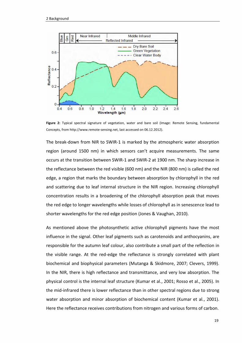
The typical characteristics of healthy green vegetation over the wavelength range from
400-2500 nm are shown in Figure 2. The optical spectrum is divided into four distinct
wavelength regions (Lillesand & Kiefer, 1994):
1. Visible: 400 nm - 700 nm
a. Blue: 400 - 500 nm
b. Green: 500 - 600 nm
c. Red: 600 - 700 nm
2. Near-infrared (NIR): 700 nm - 1300 nm
3. Shortwave infrared 2 (SWIR-1): 1300 nm - 1900 nm
4. Shortwave infrared 2 (SWIR-2): 1900 nm - 2500 nm
3 From ENVI User’s Guide: Vegetation Indices. http://geol.hu/data/online_help/Understanding_
Vegetation_and_Its_Reflectance_Properties.html, last accessed on 20.03.2013.
2 Background
19
Figure 2: Typical spectral signature of vegetation, water and bare soil (Image: Remote Sensing, fundamental
Concepts, from http://www.remote-sensing.net, last accessed on 06.12.2012).
The break-down from NIR to SWIR-1 is marked by the atmospheric water absorption
region (around 1500 nm) in which sensors can’t acquire measurements. The same
occurs at the transition between SWIR-1 and SWIR-2 at 1900 nm. The sharp increase in
the reflectance between the red visible (600 nm) and the NIR (800 nm) is called the red
edge, a region that marks the boundary between absorption by chlorophyll in the red
and scattering due to leaf internal structure in the NIR region. Increasing chlorophyll
concentration results in a broadening of the chlorophyll absorption peak that moves
the red edge to longer wavelengths while losses of chlorophyll as in senescence lead to
shorter wavelengths for the red edge position (Jones & Vaughan, 2010).
As mentioned above the photosynthetic active chlorophyll pigments have the most
influence in the signal. Other leaf pigments such as carotenoids and anthocyanins, are
responsible for the autumn leaf colour, also contribute a small part of the reflection in
the visible range. At the red-edge the reflectance is strongly correlated with plant
biochemical and biophysical parameters (Mutanga & Skidmore, 2007; Clevers, 1999).
In the NIR, there is high reflectance and transmittance, and very low absorption. The
physical control is the internal leaf structure (Kumar et al., 2001; Rosso et al., 2005). In
the mid-infrared there is lower reflectance than in other spectral regions due to strong
water absorption and minor absorption of biochemical content (Kumar et al., 2001).
Here the reflectance receives contributions from nitrogen and various forms of carbon.
2 Background
20
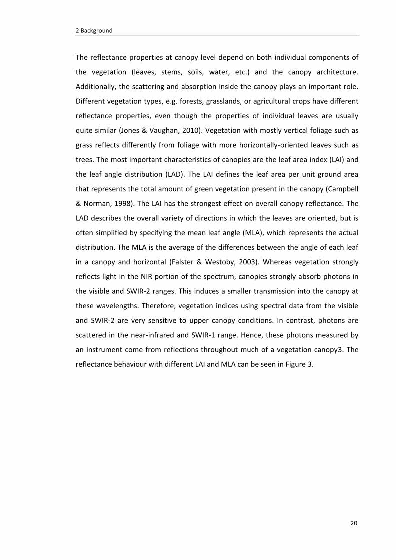
The reflectance properties at canopy level depend on both individual components of
the vegetation (leaves, stems, soils, water, etc.) and the canopy architecture.
Additionally, the scattering and absorption inside the canopy plays an important role.
Different vegetation types, e.g. forests, grasslands, or agricultural crops have different
reflectance properties, even though the properties of individual leaves are usually
quite similar (Jones & Vaughan, 2010). Vegetation with mostly vertical foliage such as
grass reflects differently from foliage with more horizontally-oriented leaves such as
trees. The most important characteristics of canopies are the leaf area index (LAI) and
the leaf angle distribution (LAD). The LAI defines the leaf area per unit ground area
that represents the total amount of green vegetation present in the canopy (Campbell
& Norman, 1998). The LAI has the strongest effect on overall canopy reflectance. The
LAD describes the overall variety of directions in which the leaves are oriented, but is
often simplified by specifying the mean leaf angle (MLA), which represents the actual
distribution. The MLA is the average of the differences between the angle of each leaf
in a canopy and horizontal (Falster & Westoby, 2003). Whereas vegetation strongly
reflects light in the NIR portion of the spectrum, canopies strongly absorb photons in
the visible and SWIR-2 ranges. This induces a smaller transmission into the canopy at
these wavelengths. Therefore, vegetation indices using spectral data from the visible
and SWIR-2 are very sensitive to upper canopy conditions. In contrast, photons are
scattered in the near-infrared and SWIR-1 range. Hence, these photons measured by
an instrument come from reflections throughout much of a vegetation canopy3. The
reflectance behaviour with different LAI and MLA can be seen in Figure 3.
2 Background
21
Figure 3: Canopy reflectance effects dependant with different LAI and MLA (Image: ENVI user guide,
http://geol.hu/data/online_help/Understanding_Vegetation_and_Its_Reflectance_Properties.html#wp1159169,
last accessed on 20.03.2013)
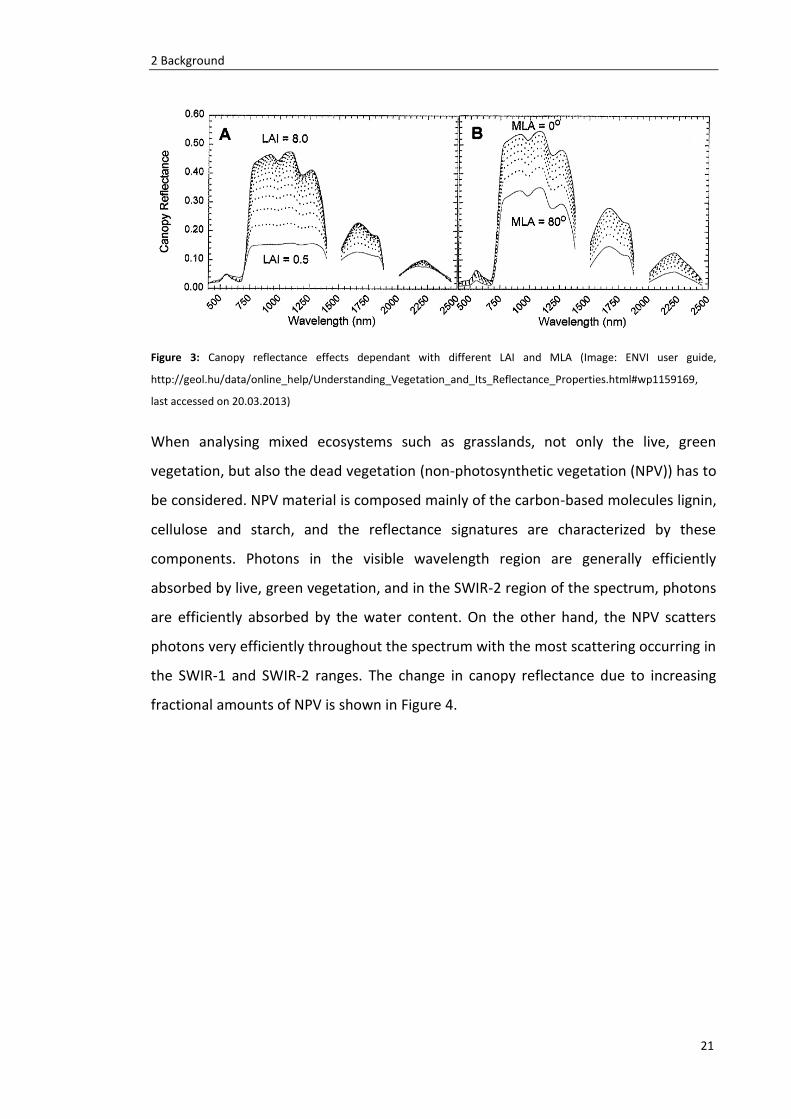
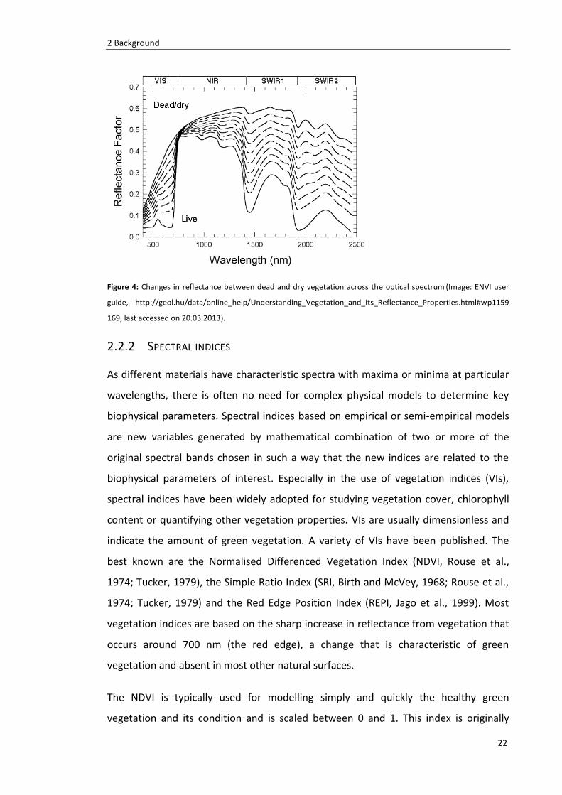
When analysing mixed ecosystems such as grasslands, not only the live, green
vegetation, but also the dead vegetation (non-photosynthetic vegetation (NPV)) has to
be considered. NPV material is composed mainly of the carbon-based molecules lignin,
cellulose and starch, and the reflectance signatures are characterized by these
components. Photons in the visible wavelength region are generally efficiently
absorbed by live, green vegetation, and in the SWIR-2 region of the spectrum, photons
are efficiently absorbed by the water content. On the other hand, the NPV scatters
photons very efficiently throughout the spectrum with the most scattering occurring in
the SWIR-1 and SWIR-2 ranges. The change in canopy reflectance due to increasing
fractional amounts of NPV is shown in Figure 4.
2 Background
22
Figure 4: Changes in reflectance between dead and dry vegetation across the optical spectrum (Image: ENVI user
guide, http://geol.hu/data/online_help/Understanding_Vegetation_and_Its_Reflectance_Properties.html#wp1159
169, last accessed on 20.03.2013).
2.2.2 SPECTRAL INDICES
As different materials have characteristic spectra with maxima or minima at particular
wavelengths, there is often no need for complex physical models to determine key
biophysical parameters. Spectral indices based on empirical or semi-empirical models
are new variables generated by mathematical combination of two or more of the
original spectral bands chosen in such a way that the new indices are related to the
biophysical parameters of interest. Especially in the use of vegetation indices (VIs),
spectral indices have been widely adopted for studying vegetation cover, chlorophyll
content or quantifying other vegetation properties. VIs are usually dimensionless and
indicate the amount of green vegetation. A variety of VIs have been published. The
best known are the Normalised Differenced Vegetation Index (NDVI, Rouse et al.,
1974; Tucker, 1979), the Simple Ratio Index (SRI, Birth and McVey, 1968; Rouse et al.,
1974; Tucker, 1979) and the Red Edge Position Index (REPI, Jago et al., 1999). Most
vegetation indices are based on the sharp increase in reflectance from vegetation that
occurs around 700 nm (the red edge), a change that is characteristic of green
vegetation and absent in most other natural surfaces.
The NDVI is typically used for modelling simply and quickly the healthy green
vegetation and its condition and is scaled between 0 and 1. This index is originally
2 Background
23
introduced by Rouse et al. (1974) in order to separate green vegetation from its
background soil brightness using Landsat MSS digital data. Today it is also used to
quantify the photosynthetic capacity of plant canopies. It is expressed as the difference
between the near infrared and red bands normalized by the sum of those bands. It
retains the ability to minimize topographic effects while producing a linear
measurement scale.
The SRI has the same field of application and is calculated by simply dividing the
reflectance values of the near infrared band by those of the red band. The contrast
between the red and infrared bands clearly results, with high index values being
produced by combinations of low red (because of absorption by chlorophyll) and high
infrared (as a result of leaf structure) reflectance (Birth & McVey, 1968). Because of
the ratio problems of variable illumination as a result of topography are minimized to
some extent.
The REPI is a narrowband reflectance measurement that is sensitive to changes in
chlorophyll content. Increased chlorophyll concentration broadens the absorption
feature and moves the red edge to longer wavelengths. This index is commonly used
for crop monitoring, yield prediction, photosynthesis modelling or canopy stress.
With the advent of imaging spectroscopy and the availability of the large amount of
narrow spectral bands, vegetation indices can be individually designed for a specific
vegetation property and a specific territory. By correlating the results of the VIs with
on site field data, the optimal VI is chosen to model the desired vegetation property.
The advantage of the index implementing two to many bands is to minimize the
sensitivity to irradiance, illumination and to other factors such as variation in
atmospheric transmission. The disadvantage of empirical models and VIs is that the
structural property of the vegetation can’t be modelled. Especially for dense canopies
(high biomass) the VI have its limitations due to saturation.
2.2.3 STATE OF THE ART IN BIOMASS ESTIMATION USING VIS
The quantification of vegetation parameters is an important task in climate and
ecosystem research, biomass production (food, fibre and fuel) and when investigating
2 Background
24
land-atmosphere interactions. Accurate characterization of vegetation properties and
temporal dynamics are therefore needed for many land-cover models that are used as
prediction maps. These maps can provide detailed spatial information on biomass
distribution which is useful in the management of protected areas, research of animal
distributions and grazing effects, ecological process and habitat modelling, and when
studying the effects of natural and man-made disturbances.
Grasslands belong to the earth’s most wide-spread land cover types and represent the
forage source for livestock and wild herbivores (Mutanga & Skidmore, 2004). Studies
using hyperspectral data to estimate biomass by relating field data to vegetation
indices have been carried out under controlled laboratory conditions (Mutanga &
Skidmore, 2004). The biomass production of mixed grassland ecosystems under
natural conditions has been investigated in several studies using hyperspectral data
(Rahman & Gamon, 2004; Mirik et al., 2005; Tarr et al., 2005; Beeri et al., 2007; Cho et
al., 2007; Psomas et al., 2009). These studies show the complexity of the spectral
response of mixed grasslands, especially in the presence of a high fraction of NPV and
exposed soil (Beeri et al., 2007; He et al., 2006; Boschetti et al., 2007), grazing impact
(Numata et al. 2007), and canopy architecture complexity due to mixed species
composition and phenology (Cho et al., 2007; Numata et al. 2008). Mirik (2005)
estimated total and live biomass with hyperspectral 1-m resolution data by SRI and
NDVI indices. The SRI or NDVI with the best relationships for biomass were found in
the NIR part of the spectrum for band 1 and the visible part of the spectrum for Bands
2 with an R2 = 0.88. Beeri et al. (2007) also estimated forage quantity and quality using
hyperspectral imagery for northern mixed-grass prairie. A narrow band NDVI (802 nm,
673 nm) was calculated from HyMap imagery and regressed against ground truth data
resulting in an R2 = 0.78. Cho et al. (2007) also showed an estimation of green
grass/herb biomass from airborne hyperspectral imagery using spectral indices. The
NDVI and REPI were calculated from HyMap data and correlated with ground truth
samples. NDVIs involving far red-edge bands in the 725 - 800 nm range produced
higher coefficients compared with traditional NDVIs computed from red and NIR
bands. Another study showed that narrow-band NDVI resulted in the best models to
2 Background
25
predict aboveground biomass of dry grassland sites by field spectroradiometer
(Psomas et al., 2009).
Using grass (Cenchrus ciliaris) grown in the greenhouse, Mutanga & Skidmore (2004)
showed that narrow-band NDVI computed from 740 and 755 nm (both in the far RED)
solved the saturation problem when estimating grass biomass at high canopy cover.
The NDVIs of all possible band combinations were calculated and compared to the
standard NDVI.
Identification of hyperspectral vegetation indices for pasture characterization has been
analysed by calculating SRIs and NDVIs using all combinations of bands and regressing
them against field data (Fava et al., 2009). SRIs involving bands in NIR (770 - 930 nm)
and in the red edge (720 - 740 nm) yielded the best performance for biomass. Another
conclusion was that SRIs always performed better than NDVIs, but the combination
ranges evidenced by the two indices were the same.
Another study analysing vegetation biomass in river floodplains using imaging
spectroscopy showed that regression models with VIs and field measurements could
be improved when differences in vegetation structure were taken into account
(Kooistra et al., 2006). Better regression models have been achieved for individual
plant functional types (grassland, shrub, mixed herbaceous and softwood forest).
To conclude, there have been numerous attempts to model biomass with
hyperspectral data by using vegetation indices, but to our knowledge, no study exist
that uses this technique for biomass modelling of alpine grassland.
2.3 APEX
The Airborne Prism Experiment (APEX) is an airborne imaging spectrometer developed
under the scientific lead of a Swiss-Belgian collaboration between the Remote Sensing
Laboratories (RSL, University of Zurich (CH)) and the Flemish Institute for Technological
Research VITO (B) on behalf of the European Space Agency (ESA) PRODEX programme.
The industrial consortium is headed by RUAG Aerospace (CH) with subcontractors such
as OIP Sensor Systems (B) and Netcetera AG (CH). Special contracts were issued by ESA
2 Background
26
for the development of a shortwave-infrared detector (Sofradir, (F)), and a calibration
facility at the German Aerospace Center (DLR). The sensor is intended as a simulator
and a calibration and validation device for future spaceborne hyperspectral imagers
(Itten et al., 2008) The development started in 1993, and from 2008 - 2010 the sensor
was in the calibration and testing phase. APEX was formally accepted by ESA at the end
of 2010 and the sensors can be used commercially nowadays. Consequently, 2011 was
the first year of commercial operations, resulting in two flight windows of a total of 7
weeks (Stessens, 2012).
APEX is built as a pushbroom dispersive imaging spectrometer recording more than
330 spectral bands contiguously. The instrument specifications can be found in Table
1. The APEX mission for the SNP acquired 186 km2 at a 2x2 m spatial resolution
determined by the sensor’s instantaneous field of view (IFOV) in combination with a
flight height of 4400 - 5400 m asl. 1000 pixels were recorded across-track with a data
rate of 0.42 GBytes/km per flight path. The spectral configuration was set to 312
spectral bands to be acquired simultaneously. We used 301 bands for analysis, after
some bands had to be removed due to noise. The sensor was installed on a Research
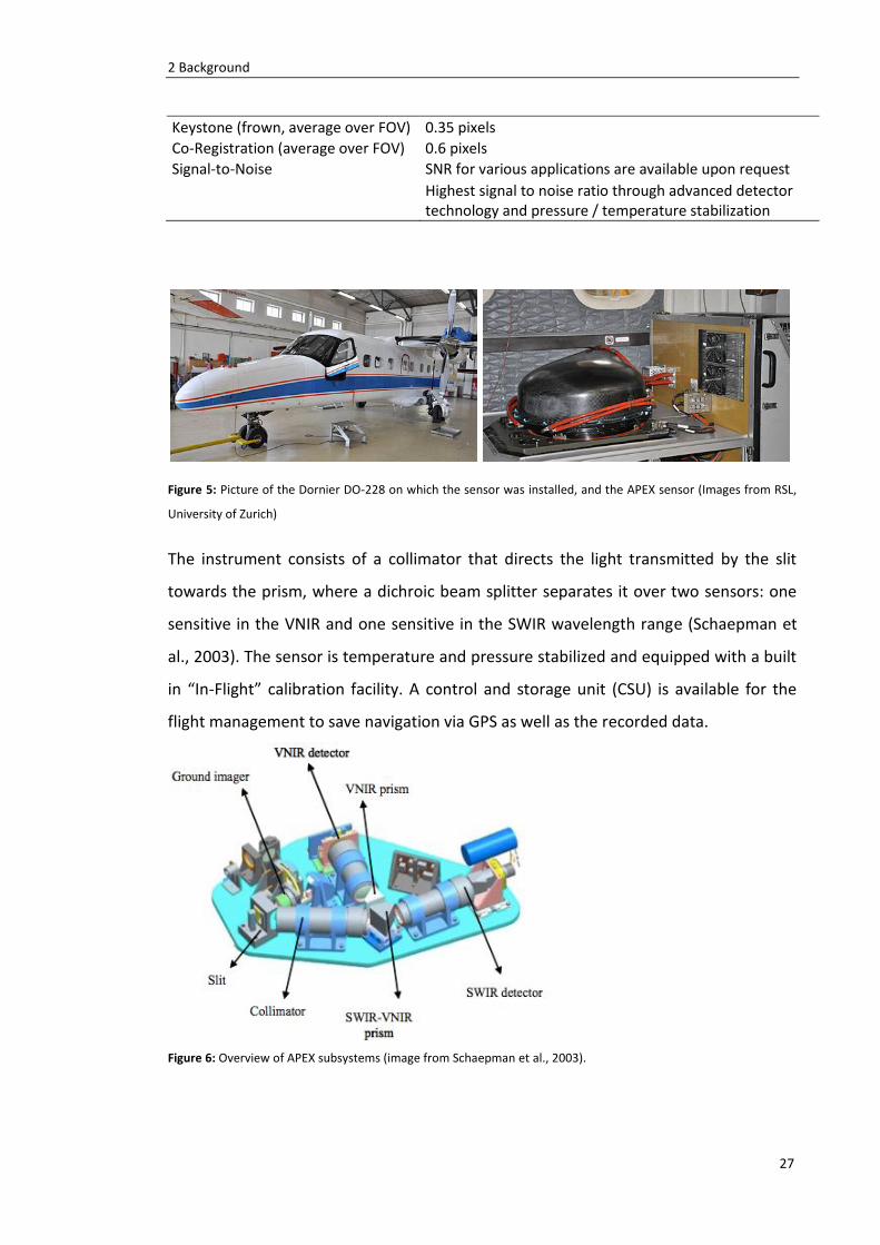
Aircraft Dornier DO-228 aircraft (see Figure 5).
Table 1: Instrument specifications (from http://apex-esa.org, last accessed 20.12.2012)
Spectral Range VNIR: 380 - 970 nm SWIR: 940 - 2500 nm Spectral Sampling Interval VNIR: 0.55 - 8 nm over spectral range (unbinned) SWIR: 5 - 10 nm over spectral range Spectral Resolution (FWHM) VNIR: 0.6 - 6.3 nm over spectral range (unbinned) SWIR: 6.2 - 11 nm over spectral range
Spectral Bands VNIR: default 114 bands, reprogrammable through customized binning pattern
SWIR 199 bands Spatial Pixels 1000 FOV (across track) 28° IFOV 0.48 mrad Spatial Sampling Interval (across track)
1.75 m @ 3500 m AGL (2 - 5 m at flight altitudes of 4 - 10 km)
Sensor dynamic range VNIR: CCD, 14 bit encoding SWIR CMOS, 13 bit encoding Pixel size VNIR: 22.5 μm x 22.5 μm SWIR: 30 μm x 30 μm Smile (average over FOV) 0.35 pixels
2 Background
27
Keystone (frown, average over FOV) 0.35 pixels Co-Registration (average over FOV) 0.6 pixels Signal-to-Noise SNR for various applications are available upon request
Highest signal to noise ratio through advanced detector technology and pressure / temperature stabilization
Figure 5: Picture of the Dornier DO-228 on which the sensor was installed, and the APEX sensor (Images from RSL,
University of Zurich)
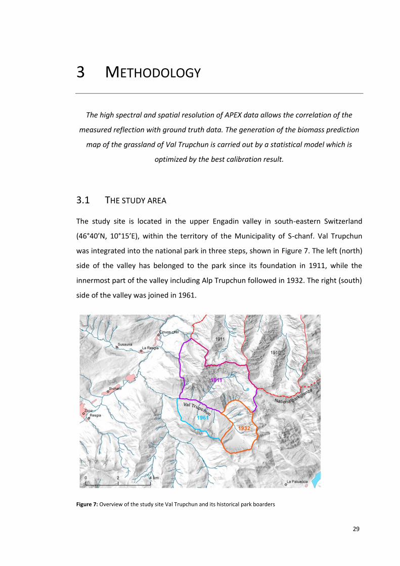
The instrument consists of a collimator that directs the light transmitted by the slit
towards the prism, where a dichroic beam splitter separates it over two sensors: one
sensitive in the VNIR and one sensitive in the SWIR wavelength range (Schaepman et
al., 2003). The sensor is temperature and pressure stabilized and equipped with a built
in “In-Flight” calibration facility. A control and storage unit (CSU) is available for the
flight management to save navigation via GPS as well as the recorded data.
Figure 6: Overview of APEX subsystems (image from Schaepman et al., 2003).

2 Background
28
The external facilities are the Calibration Home Base (CHB) for instrument calibration,
which is located at the DLR in Germany, and a data processing and archiving facility
(PAF) for operational product generation, which is managed by VITO (Jehle et al.,
2010).
29
3 METHODOLOGY
The high spectral and spatial resolution of APEX data allows the correlation of the
measured reflection with ground truth data. The generation of the biomass prediction
map of the grassland of Val Trupchun is carried out by a statistical model which is
optimized by the best calibration result.
3.1 THE STUDY AREA
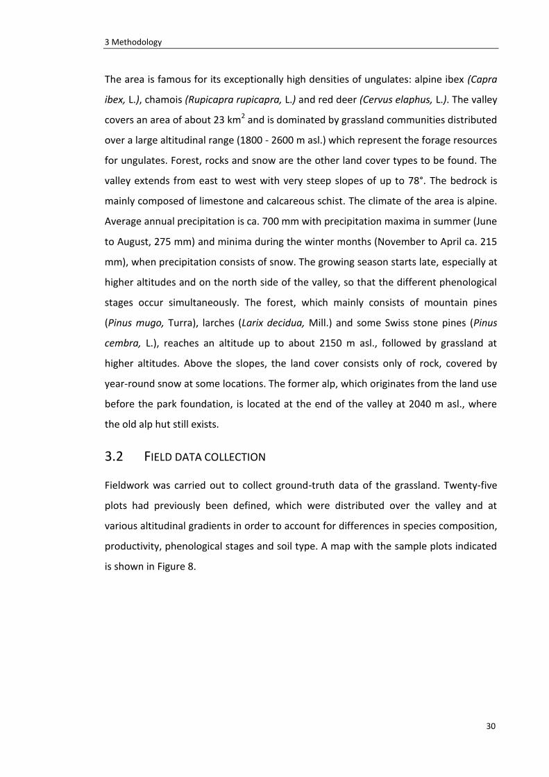
The study site is located in the upper Engadin valley in south-eastern Switzerland
(46°40’N, 10°15’E), within the territory of the Municipality of S-chanf. Val Trupchun
was integrated into the national park in three steps, shown in Figure 7. The left (north)
side of the valley has belonged to the park since its foundation in 1911, while the
innermost part of the valley including Alp Trupchun followed in 1932. The right (south)
side of the valley was joined in 1961.
Figure 7: Overview of the study site Val Trupchun and its historical park boarders
3 Methodology
30
The area is famous for its exceptionally high densities of ungulates: alpine ibex (Capra
ibex, L.), chamois (Rupicapra rupicapra, L.) and red deer (Cervus elaphus, L.). The valley
covers an area of about 23 km2 and is dominated by grassland communities distributed
over a large altitudinal range (1800 - 2600 m asl.) which represent the forage resources
for ungulates. Forest, rocks and snow are the other land cover types to be found. The
valley extends from east to west with very steep slopes of up to 78°. The bedrock is
mainly composed of limestone and calcareous schist. The climate of the area is alpine.
Average annual precipitation is ca. 700 mm with precipitation maxima in summer (June
to August, 275 mm) and minima during the winter months (November to April ca. 215
mm), when precipitation consists of snow. The growing season starts late, especially at
higher altitudes and on the north side of the valley, so that the different phenological
stages occur simultaneously. The forest, which mainly consists of mountain pines
(Pinus mugo, Turra), larches (Larix decidua, Mill.) and some Swiss stone pines (Pinus
cembra, L.), reaches an altitude up to about 2150 m asl., followed by grassland at
higher altitudes. Above the slopes, the land cover consists only of rock, covered by
year-round snow at some locations. The former alp, which originates from the land use
before the park foundation, is located at the end of the valley at 2040 m asl., where
the old alp hut still exists.
3.2 FIELD DATA COLLECTION
Fieldwork was carried out to collect ground-truth data of the grassland. Twenty-five
plots had previously been defined, which were distributed over the valley and at
various altitudinal gradients in order to account for differences in species composition,
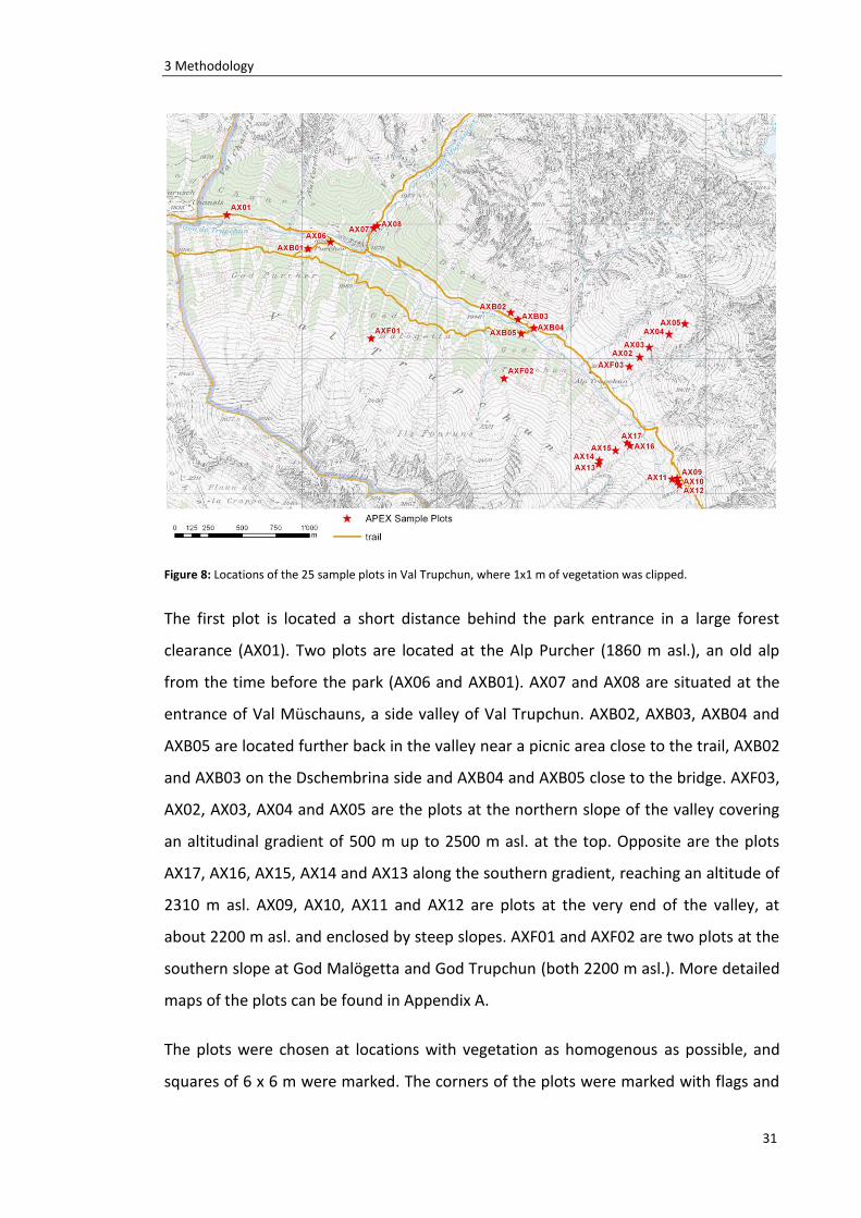
productivity, phenological stages and soil type. A map with the sample plots indicated
is shown in Figure 8.
3 Methodology
31
Figure 8: Locations of the 25 sample plots in Val Trupchun, where 1x1 m of vegetation was clipped.
The first plot is located a short distance behind the park entrance in a large forest
clearance (AX01). Two plots are located at the Alp Purcher (1860 m asl.), an old alp
from the time before the park (AX06 and AXB01). AX07 and AX08 are situated at the
entrance of Val Müschauns, a side valley of Val Trupchun. AXB02, AXB03, AXB04 and
AXB05 are located further back in the valley near a picnic area close to the trail, AXB02
and AXB03 on the Dschembrina side and AXB04 and AXB05 close to the bridge. AXF03,
AX02, AX03, AX04 and AX05 are the plots at the northern slope of the valley covering
an altitudinal gradient of 500 m up to 2500 m asl. at the top. Opposite are the plots
AX17, AX16, AX15, AX14 and AX13 along the southern gradient, reaching an altitude of
2310 m asl. AX09, AX10, AX11 and AX12 are plots at the very end of the valley, at
about 2200 m asl. and enclosed by steep slopes. AXF01 and AXF02 are two plots at the
southern slope at God Malögetta and God Trupchun (both 2200 m asl.). More detailed
maps of the plots can be found in Appendix A.
The plots were chosen at locations with vegetation as homogenous as possible, and
squares of 6 x 6 m were marked. The corners of the plots were marked with flags and
3 Methodology
32
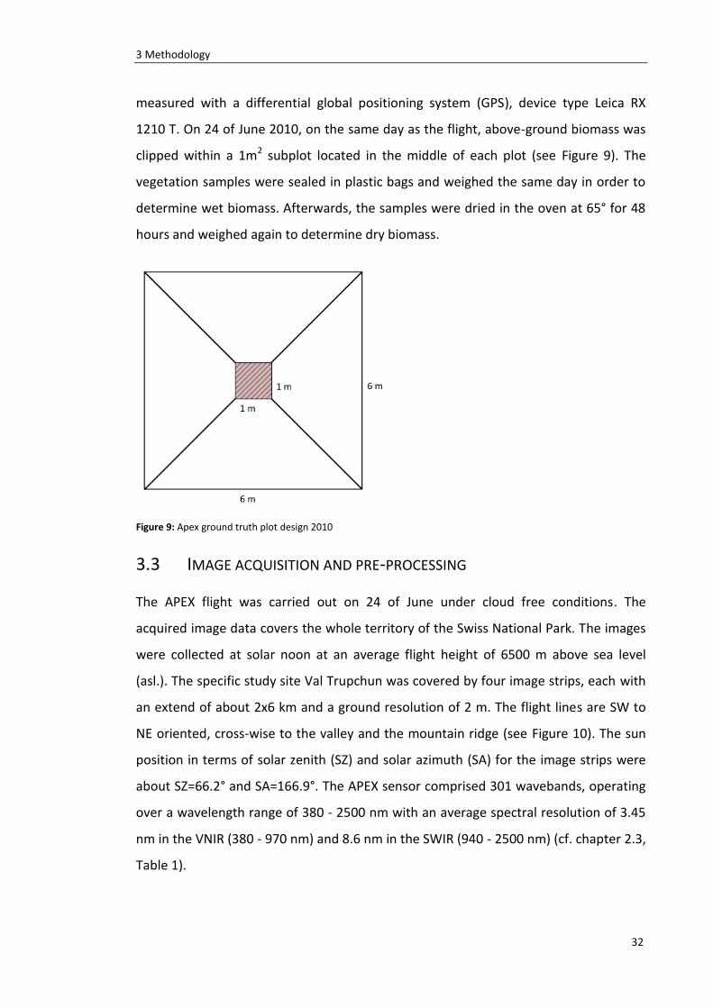
measured with a differential global positioning system (GPS), device type Leica RX
1210 T. On 24 of June 2010, on the same day as the flight, above-ground biomass was
clipped within a 1m2 subplot located in the middle of each plot (see Figure 9). The
vegetation samples were sealed in plastic bags and weighed the same day in order to
determine wet biomass. Afterwards, the samples were dried in the oven at 65° for 48
hours and weighed again to determine dry biomass.
Figure 9: Apex ground truth plot design 2010
3.3 IMAGE ACQUISITION AND PRE-PROCESSING
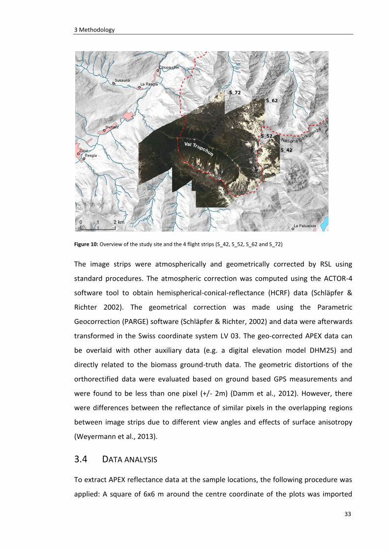
The APEX flight was carried out on 24 of June under cloud free conditions. The
acquired image data covers the whole territory of the Swiss National Park. The images
were collected at solar noon at an average flight height of 6500 m above sea level
(asl.). The specific study site Val Trupchun was covered by four image strips, each with
an extend of about 2x6 km and a ground resolution of 2 m. The flight lines are SW to
NE oriented, cross-wise to the valley and the mountain ridge (see Figure 10). The sun
position in terms of solar zenith (SZ) and solar azimuth (SA) for the image strips were
about SZ=66.2° and SA=166.9°. The APEX sensor comprised 301 wavebands, operating
over a wavelength range of 380 - 2500 nm with an average spectral resolution of 3.45
nm in the VNIR (380 - 970 nm) and 8.6 nm in the SWIR (940 - 2500 nm) (cf. chapter 2.3,
Table 1).
3 Methodology
33
Figure 10: Overview of the study site and the 4 flight strips (S_42, S_52, S_62 and S_72)
The image strips were atmospherically and geometrically corrected by RSL using
standard procedures. The atmospheric correction was computed using the ACTOR-4
software tool to obtain hemispherical-conical-reflectance (HCRF) data (Schläpfer &
Richter 2002). The geometrical correction was made using the Parametric
Geocorrection (PARGE) software (Schläpfer & Richter, 2002) and data were afterwards
transformed in the Swiss coordinate system LV 03. The geo-corrected APEX data can
be overlaid with other auxiliary data (e.g. a digital elevation model DHM25) and
directly related to the biomass ground-truth data. The geometric distortions of the
orthorectified data were evaluated based on ground based GPS measurements and
were found to be less than one pixel (+/- 2m) (Damm et al., 2012). However, there
were differences between the reflectance of similar pixels in the overlapping regions
between image strips due to different view angles and effects of surface anisotropy
(Weyermann et al., 2013).
3.4 DATA ANALYSIS
To extract APEX reflectance data at the sample locations, the following procedure was
applied: A square of 6x6 m around the centre coordinate of the plots was imported
3 Methodology
34
into the ENVI 4.7 software. This square corresponded to 9 pixels (3x3 pixels) of the
APEX data from which the average reflectance was extracted as reference value. There
were plots lying on more than one strip because of the overlapping zone, so that two
reference reflectance values were available for one sample. These values were
considered as independent measurement points. Consequently, there were 43
measurement points available, from which 18 points were double (same ground truth
biomass value, but different reference reflectance).
The biomass samples were divided into two groups, one used for the calibration (22
points), and one for the validation (21 points) of the model using a stratified random
sampling approach. An empirical model was developed based on the 22 calibration
samples. The standard NDVI was calculated based on band 50 (664.3 nm) and band 86
(808.8 nm) by using the following formula:
where R is the reflectance at the specific wavelength.
The calculated NDVI was regressed against the calibration biomass samples in an
exponential regression to obtain the coefficient of determination (R2) for calibration.
An exponential (instead of linear) regression can be implemented due to the large
volume scattering of vegetation that induces sensor saturation at high densities.
Since APEX provides more bands in the red (600 - 700 nm) and NIR (700 - 1300 nm), we
tested if calibration results could be improved by calculating simple ratio vegetation
indices (SRI) with all possible combinations of 301 bands and regressing them against
the calibration data set.
where Ra and Rb is the reflectance at wavelength a and b, respectively.
Spearman’s rank correlation coefficients (R) resulting from the regression analysis
were plotted on a 2D-contour plot to evaluate R characteristic patterns and identify

3 Methodology
35
the best wavelength combination. This procedure allowed the selection of optimal
bands to be used in the calculation of the index. Band combinations with maximized
correlation with biomass were chosen, considering cause effect relationships between
spectral bands and underlying absorption and scattering processes. For the final model
we chose the best SRI within the range of the visible (RED) for the first band and near-
infrared (NIR) (700 - 1300 nm) region for the second band. Within this range, high
reflection occurs on healthy biomass, and no water absorption interferes with the
signal. With the chosen SRI we computed an exponential regression model to predict
and map biomass content.
Predictive performance of the biomass model was computed with the independent
validation data set. The coefficient of determination (R2) and the root mean square
error (RMSE) were calculated to compare the predicted with the observed values.
Secondly, a SRI model was calculated with another band selection to test the problem
of underestimation in the region of high biomass, usually occurring with NDVI and SRI
models with a broad band selection. Two narrow bands in the far RED were chosen as
this should solve the saturation problem according to Mutanga and Skidmore (2004).
Furthermore an investigation about the APEX data regarding the overlapping zone
between two strips was carried out. As SRI values on overlapping regions vary slightly
between the strips, the different SRI from plots located on more than one strip are
analysed in a scatterplot.
Then an analysis about the variability of the APEX pixel location is conducted. The
average SRI at the sample plot locations were extracted for the 5x5 pixels around the
centre coordinate and compared to the result of 3x3 pixels. This value was converted
by the SRI biomass model equation to analyse the difference with respect to the
biomass prediction. The biomass discrepancy predicted for the sample plot locations
are compared and discussed in a histogram.
The biomass prediction model is only valid for grassland. A linear spectral unmixing
method (LSU) was performed to separate different land cover classes and to extract
3 Methodology
36
the grassland. LSU is a classification approach that can be used for hyperspectral
imagery based on the materials’ spectral characteristics. The reflectance at each pixel
of the image is assumed to be a linear combination of the reflectance of each material
present within the pixel (Boardman, 1989). The measured spectrum of a mixed pixel is
decomposed into the set of corresponding fractions (endmembers) that indicate the
proportion of each endmember present in the pixel. Pure training pixels were manually
defined for grassland, rock, snow and forest in selecting homogenous pixels as regions
of interest. The linear unmixing method is then assigning each pixel into the
predefined classes based on the abundance values of each endmember. The unmixing
result has a data range (representing endmember abundance) from 0 - 1. 50% has
been taken as abundance for extracting grassland.
37
4 RESULTS
For the calibration data set, 22 sample plots were randomly chosen out of 43
independent reflection reference values from all sample plots. The plots lying in
overlapping regions of two strips were taken as independent reflection references, as
different reflectance values were available. A table with the specific calibration and
validation points of all sample plots can be found in Appendix. For all correlations
between biomass sample and APEX reflectance spectra, the comparison was carried
out using the wet weight of the biomass samples. The wet weight achieved overall
better R2 compared to the dry weight.
4.1 FIELD SAMPLE RESULTS
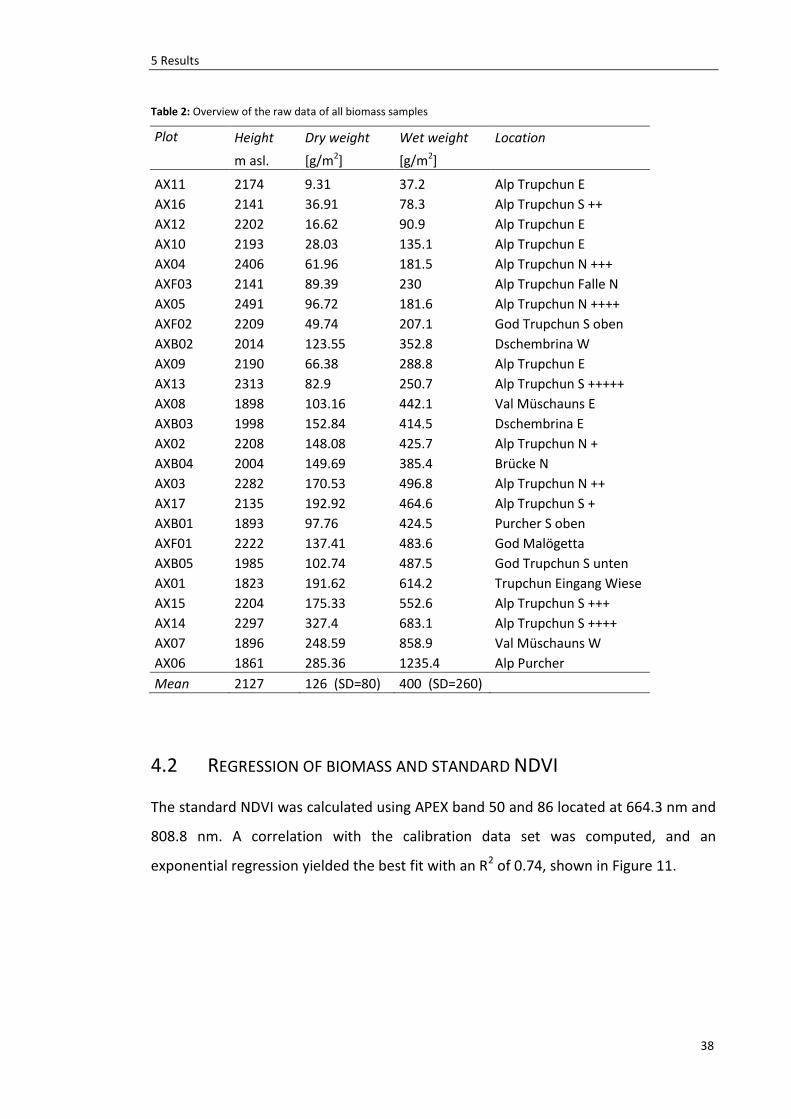
In Table 2 the results of the field campaign can be found. The dry and the wet weight
of all 25 biomass samples are listed. The samples were overall in a reasonable range
with a mean average of 400 g/m2 (SD = 80 g/m2) for the wet weight and 126 g/m2 for
the dry weight (SD = 260 g/m2). The minimum was found at Alp Trupchun East (37
g/m2). High biomass was found especially on former alp sites, at Alp Purcher (AX06),
Alp Trupchun (AX14) and at the entrance of Val Müschauns (AX07).
5 Results
38
Table 2: Overview of the raw data of all biomass samples
Plot Height Dry weight Wet weight Location
m asl. [g/m2] [g/m2]
AX11 2174 9.31 37.2 Alp Trupchun E AX16 2141 36.91 78.3 Alp Trupchun S ++ AX12 2202 16.62 90.9 Alp Trupchun E AX10 2193 28.03 135.1 Alp Trupchun E AX04 2406 61.96 181.5 Alp Trupchun N +++ AXF03 2141 89.39 230 Alp Trupchun Falle N AX05 2491 96.72 181.6 Alp Trupchun N ++++
AXF02 2209 49.74 207.1 God Trupchun S oben AXB02 2014 123.55 352.8 Dschembrina W AX09 2190 66.38 288.8 Alp Trupchun E AX13 2313 82.9 250.7 Alp Trupchun S +++++ AX08 1898 103.16 442.1 Val Müschauns E AXB03 1998 152.84 414.5 Dschembrina E
AX02 2208 148.08 425.7 Alp Trupchun N + AXB04 2004 149.69 385.4 Brücke N AX03 2282 170.53 496.8 Alp Trupchun N ++ AX17 2135 192.92 464.6 Alp Trupchun S + AXB01 1893 97.76 424.5 Purcher S oben
AXF01 2222 137.41 483.6 God Malögetta AXB05 1985 102.74 487.5 God Trupchun S unten AX01 1823 191.62 614.2 Trupchun Eingang Wiese AX15 2204 175.33 552.6 Alp Trupchun S +++ AX14 2297 327.4 683.1 Alp Trupchun S ++++ AX07 1896 248.59 858.9 Val Müschauns W AX06 1861 285.36 1235.4 Alp Purcher
Mean 2127 126 (SD=80) 400 (SD=260)
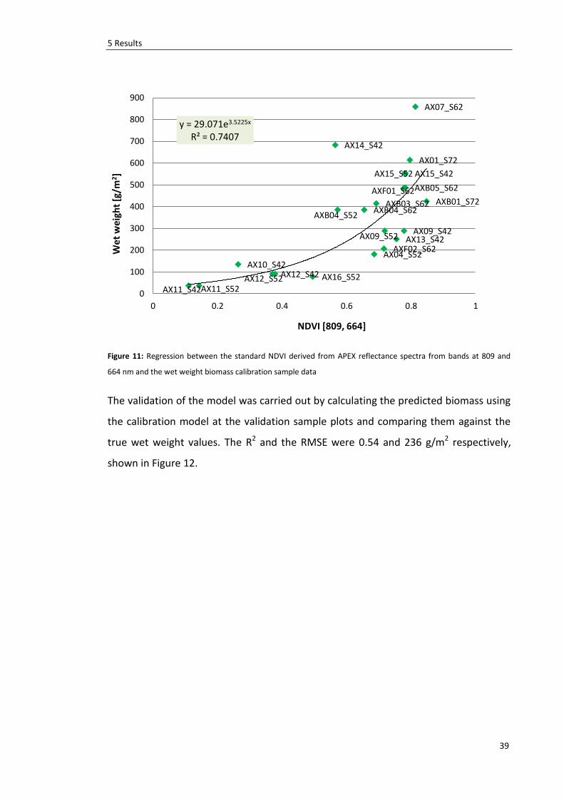
4.2 REGRESSION OF BIOMASS AND STANDARD NDVI
The standard NDVI was calculated using APEX band 50 and 86 located at 664.3 nm and
808.8 nm. A correlation with the calibration data set was computed, and an
exponential regression yielded the best fit with an R2 of 0.74, shown in Figure 11.
5 Results
39
Figure 11: Regression between the standard NDVI derived from APEX reflectance spectra from bands at 809 and
664 nm and the wet weight biomass calibration sample data
The validation of the model was carried out by calculating the predicted biomass using
the calibration model at the validation sample plots and comparing them against the
true wet weight values. The R2 and the RMSE were 0.54 and 236 g/m2 respectively,
shown in Figure 12.
AX01_S72
AX04_S52
AX07_S62
AX09_S42 AX09_S52
AX10_S42
AX11_S42 AX11_S52
AX12_S42 AX12_S52
AX13_S42
AX14_S42
AX15_S42 AX15_S52
AX16_S52
AXB01_S72 AXB03_S62 AXB04_S52
AXB04_S62
AXB05_S62 AXF01_S62
AXF02_S62
y = 29.071e3.5225x R² = 0.7407
0
100
200
300
400
500
600
700
800
900
0 0.2 0.4 0.6 0.8 1
Wet
wei
ght
[g/m
2]
NDVI [809, 664]
5 Results
40
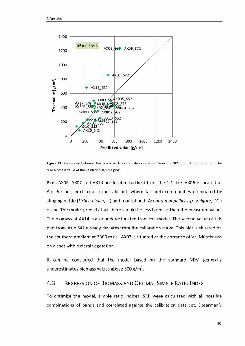
Figure 12: Regression between the predicted biomass value calculated from the NDVI model calibration and the
true biomass value of the validation sample plots
Plots AX06, AX07 and AX14 are located furthest from the 1:1 line. AX06 is located at
Alp Purcher, next to a former alp hut, where tall-herb communities dominated by
stinging nettle (Urtica dioica, L.) and monkshood (Aconitum napellus ssp. Vulgare, DC.)
occur. The model predicts that there should be less biomass than the measured value.
The biomass at AX14 is also underestimated from the model. The second value of this
plot from strip S42 already deviates from the calibration curve. This plot is situated on
the southern gradient at 2300 m asl. AX07 is situated at the entrance of Val Müschauns
on a spot with ruderal vegetation.
It can be concluded that the model based on the standard NDVI generally
underestimates biomass values above 600 g/m2.
4.3 REGRESSION OF BIOMASS AND OPTIMAL SIMPLE RATIO INDEX
To optimize the model, simple ratio indices (SRI) were calculated with all possible
combinations of bands and correlated against the calibration data set. Spearman’s
AX16_S42
AX17_S42 AX02_S52
AX03_S52
AX05_S52 AX10_S52
AX13_S52
AX14_S52
AX17_S52
AXB02_S52
AXB03_S52
AXB05_S52
AXF02_S52 AXF03_S52
AX06_S62
AX08_S62 AXB01_S62 AXB02_S62
AX06_S72
AX07_S72
AX08_S72
R² = 0.5393
0
200
400
600
800
1000
1200
1400
0 200 400 600 800 1000 1200 1400
Tru
e va
lue
[g/m
2]
Predicted value [g/m2]
5 Results
41
rank correlation coefficients (R) were plotted on a 2D-contour plot to identify the best
wavelength combination, shown in Figure 13.
Figure 13: 2D-correlation plot that shows the correlation coefficient R (Spearman’s Rank) between SR indices and
biomass. The matrix is symmetrical. Below the diagonal, band combinations are marked in red where R>0.8.
High correlations were found between one band in GREEN and one band in NIR, one
band in RED and one in NIR with overall highest R = 0.823, and one band in NIR and
one in SWIR-1. A table with band combinations R > 0.8 can be found in Appendix B.
For our final biomass model the best SRI within the range of visible (RED) and near-
infrared (NIR) (700 - 1300 nm) region was chosen. Within this range high reflection on
healthy biomass occurred and no water absorption interfered with the signal. Another
argument was to choose a band close to the diagonal 1:1 line. The closer the two
5 Results
42
bands are, the smaller are the atmospheric and external influences. This can be
observed by comparing the SRI values at the plot locations that lie on two strips. The
differences between SRI of the two strips are lower with band combinations closer
together.
The SRI of band 92 (842 nm) and band 68 (727 nm) achieved the best R (0.823) overall
and fulfilled the selection criteria. Figure 14 illustrates the spectrum of a typical
grassland pixel from our site with the two chosen bands indicated.
Figure 14: Reflectance spectra of a typical pixel of the grassland in Val Trupchun. The blue mark indicates the band
at 730 nm and the red mark the band at 840 nm
This combination was chosen for the final biomass model. An exponential regression
model was computed again between SRI and wet weight biomass of the calibration
data set resulting in an R2 of 0.77 (Figure 15).
5 Results
43
Figure 15: Regression between SRI derived from APEX reflectance spectra from band at 842 nm and 727 nm and the
wet weight biomass calibration sample data.
The validation of the model was carried out by calculating the predicted biomass using
the model equation for the validation sample plots and comparing them to the true
wet weight values. The R2 and RMSE were 0.57 and 238 g/m2 respectively, shown in
Figure 16.
Generally the pattern of the plots was comparable to the NDVI model. The outliers
were again AX14, AX06 and AX07. The calibration model under-estimated biomass
values above 600 g/m2.
AX01_S72
AX04_S52
AX07_S62
AX09_S42 AX09_S52
AX10_S42 AX11_S42
AX11_S52 AX12_S42 AX12_S52
AX13_S42
AX14_S42
AX15_S42 AX15_S52
AX16_S52
AXB01_S72 AXB03_S62 AXB04_S52 AXB04_S62
AXB05_S62 AXF01_S62
AXF02_S62
y = 0.0098e7.438x R² = 0.7728
0.00
100.00
200.00
300.00
400.00
500.00
600.00
700.00
800.00
900.00
1'000.00
1.1 1.2 1.3 1.4 1.5
Wet
wei
ght
[g/m
2]
Simple Ratio [842, 727]
5 Results
44
Figure 16: Regression between the predicted biomass value calculated from the SRI model calibration and the true
biomass value of the validation sample plots
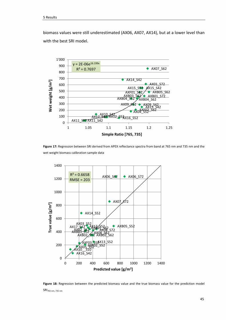
4.4 REGRESSION OF BIOMASS AND NARROWBAND SRI
According to Mutanga and Skidmore (2004) a narrow band SRI, both located in the far
RED (around 750 nm) should solve the saturation problem which means that sample
locations with high biomass occurrence aren’t underestimated.
To analyse this thesis, the best R around two bands in the far RED was selected from
the 2D-correlation plot (cf. Figure 13). The SRI between band 77 at 765 nm and band
70 at 735 nm has an R of 0.810 and is thus only slightly lower compared to the highest
R (0.823) for the optimal SRI at bands 92 and 68. The model was recalculated with
these two bands to check for a possible model improvement.
The exponential regression is shown in Figure 17. The coefficient of determination (R2)
is 0.7697, which is only slightly lower than our best SRI (R2 = 0.7728). On the other
hand, the validation shown in Figure 18 yielded 10% better validity (67%). High
AX16_S42
AX17_S42 AX02_S52
AX03_S52
AX05_S52 AX10__S10
AX13_S52
AX14_S52
AX17_S52
AXB02_S52
AXB03_S52
AXB05_S52
AXF02_S52 AXF03_S52
AX06_S62
AX08_S62 AXB01_S62
AXB02_S62
AX06_S72
AX07_S72
AX08_S72
R² = 0.5688 RMSE = 238
0
200
400
600
800
1000
1200
1400
0 200 400 600 800 1000 1200 1400
Tru
e va
lue
[g/m
2]
Predicted value [g/m2]
5 Results
45
biomass values were still underestimated (AX06, AX07, AX14), but at a lower level than
with the best SRI model.
Figure 17: Regression between SRI derived from APEX reflectance spectra from band at 765 nm and 735 nm and the
wet weight biomass calibration sample data
Figure 18: Regression between the predicted biomass value and the true biomass value for the prediction model
SRI765 nm, 735 nm
AX01_S72
AX04_S52
AX07_S62
AX09_S42 AX09_S52
AX10_S42
AX11_S42 AX11_S52 AX12_S42 AX12_S52
AX13_S42
AX14_S42
AX15_S42 AX15_S52
AX16_S52
AXB01_S72 AXB03_S62 AXB04_S52 AXB04_S62
AXB05_S62 AXF01_S62
AXF02_S62
y = 2E-06e16.199x R² = 0.7697
0
100
200
300
400
500
600
700
800
900
1'000
1 1.05 1.1 1.15 1.2 1.25
Wet
wei
ght
[g/m
2]
Simple Ratio [765, 735]
AX16_S42
AX17_S42 AX02_S52
AX03_S52
AX05_S52 AX10__S10
AX13_S52
AX14_S52
AX17_S52
AXB02_S52 AXB03_S52
AXB05_S52
AXF02_S52 AXF03_S52
AX06_S62
AX08_S62
AXB01_S62
AXB02_S62
AX06_S72
AX07_S72
AX08_S72
R² = 0.6658 RMSE = 203
0
200
400
600
800
1000
1200
1400
0 200 400 600 800 1000 1200 1400
Tru
e va
lue
[g/m
2]
Predicted value [g/m2]
5 Results
46
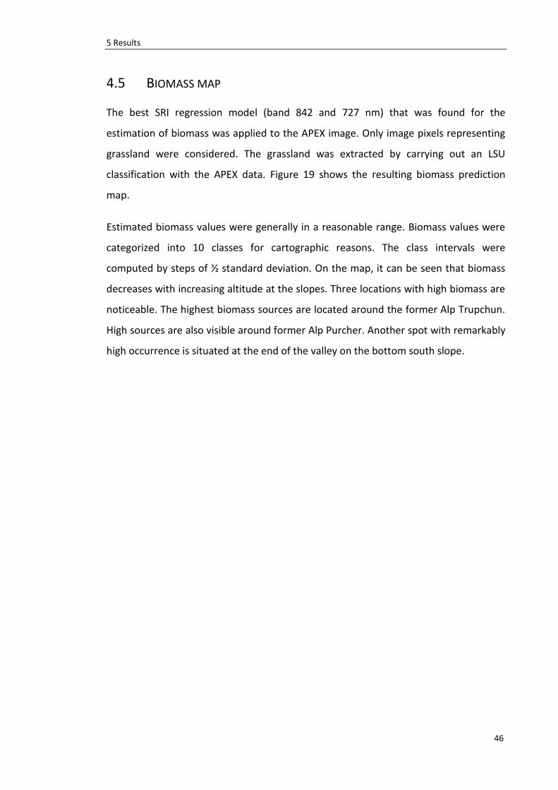
4.5 BIOMASS MAP
The best SRI regression model (band 842 and 727 nm) that was found for the
estimation of biomass was applied to the APEX image. Only image pixels representing
grassland were considered. The grassland was extracted by carrying out an LSU
classification with the APEX data. Figure 19 shows the resulting biomass prediction
map.
Estimated biomass values were generally in a reasonable range. Biomass values were
categorized into 10 classes for cartographic reasons. The class intervals were
computed by steps of ½ standard deviation. On the map, it can be seen that biomass
decreases with increasing altitude at the slopes. Three locations with high biomass are
noticeable. The highest biomass sources are located around the former Alp Trupchun.
High sources are also visible around former Alp Purcher. Another spot with remarkably
high occurrence is situated at the end of the valley on the bottom south slope.
5 Results
47
Figure 19: Biomass map of Val Trupchun overlain on a graphical relief shading
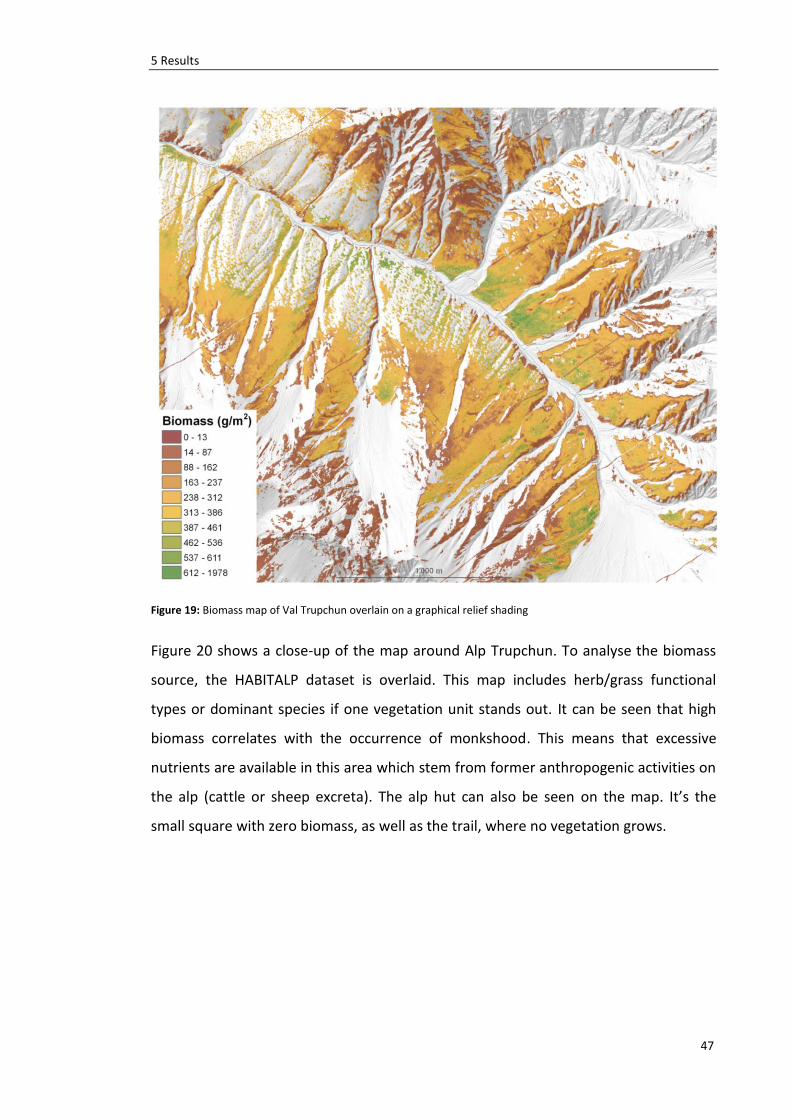
Figure 20 shows a close-up of the map around Alp Trupchun. To analyse the biomass
source, the HABITALP dataset is overlaid. This map includes herb/grass functional
types or dominant species if one vegetation unit stands out. It can be seen that high
biomass correlates with the occurrence of monkshood. This means that excessive
nutrients are available in this area which stem from former anthropogenic activities on
the alp (cattle or sheep excreta). The alp hut can also be seen on the map. It’s the
small square with zero biomass, as well as the trail, where no vegetation grows.
5 Results
48
Figure 20: Detailed biomass map and monkshood occurrence of the grassland around Alp Trupchun
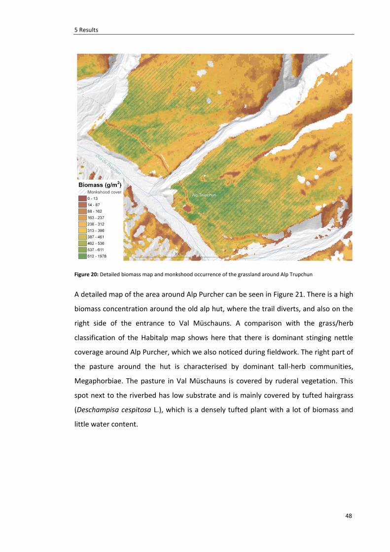
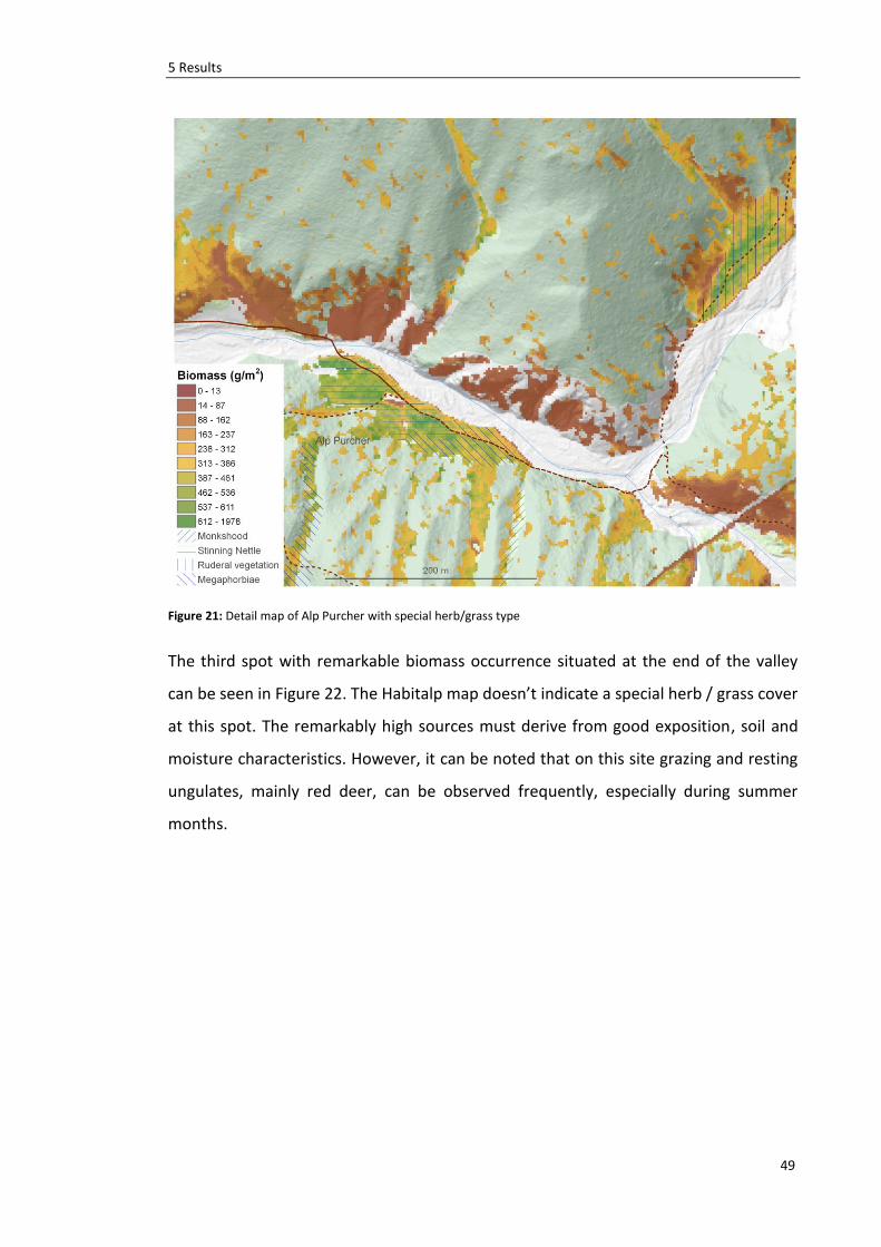
A detailed map of the area around Alp Purcher can be seen in Figure 21. There is a high
biomass concentration around the old alp hut, where the trail diverts, and also on the
right side of the entrance to Val Müschauns. A comparison with the grass/herb
classification of the Habitalp map shows here that there is dominant stinging nettle
coverage around Alp Purcher, which we also noticed during fieldwork. The right part of
the pasture around the hut is characterised by dominant tall-herb communities,
Megaphorbiae. The pasture in Val Müschauns is covered by ruderal vegetation. This
spot next to the riverbed has low substrate and is mainly covered by tufted hairgrass
(Deschampisa cespitosa L.), which is a densely tufted plant with a lot of biomass and
little water content.
5 Results
49
Figure 21: Detail map of Alp Purcher with special herb/grass type
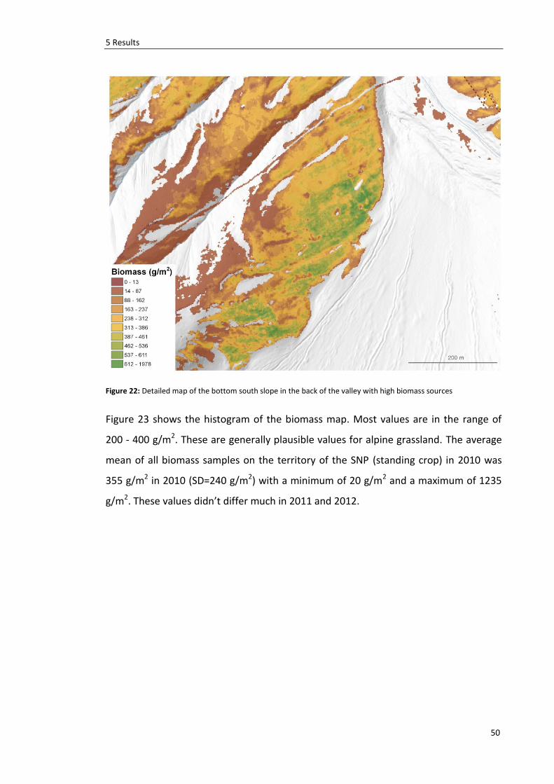
The third spot with remarkable biomass occurrence situated at the end of the valley
can be seen in Figure 22. The Habitalp map doesn’t indicate a special herb / grass cover
at this spot. The remarkably high sources must derive from good exposition, soil and
moisture characteristics. However, it can be noted that on this site grazing and resting
ungulates, mainly red deer, can be observed frequently, especially during summer
months.
5 Results
50
Figure 22: Detailed map of the bottom south slope in the back of the valley with high biomass sources
Figure 23 shows the histogram of the biomass map. Most values are in the range of
200 - 400 g/m2. These are generally plausible values for alpine grassland. The average
mean of all biomass samples on the territory of the SNP (standing crop) in 2010 was
355 g/m2 in 2010 (SD=240 g/m2) with a minimum of 20 g/m2 and a maximum of 1235
g/m2. These values didn’t differ much in 2011 and 2012.
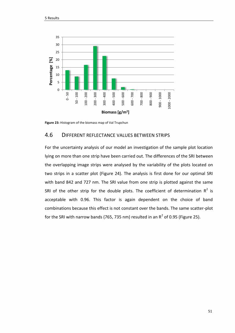
5 Results
51
Figure 23: Histogram of the biomass map of Val Trupchun
4.6 DIFFERENT REFLECTANCE VALUES BETWEEN STRIPS
For the uncertainty analysis of our model an investigation of the sample plot location
lying on more than one strip have been carried out. The differences of the SRI between
the overlapping image strips were analysed by the variability of the plots located on
two strips in a scatter plot (Figure 24). The analysis is first done for our optimal SRI
with band 842 and 727 nm. The SRI value from one strip is plotted against the same
SRI of the other strip for the double plots. The coefficient of determination R2 is
acceptable with 0.96. This factor is again dependent on the choice of band
combinations because this effect is not constant over the bands. The same scatter-plot
for the SRI with narrow bands (765, 735 nm) resulted in an R2 of 0.95 (Figure 25).
0
5
10
15
20
25
30
35
0 -
50
50
- 1
00
10
0 -
20
0
20
0 -
30
0
30
0 -
40
0
40
0 -
50
0
50
0 -
60
0
60
0 -
70
0
70
0 -
80
0
80
0 -
90
0
90
0 -
10
00
10
00
- 2
00
0
Pe
rcen
tage
[%
]
Biomass [g/m2]
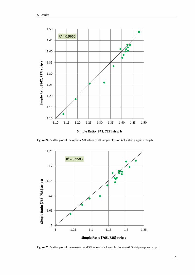
5 Results
52
Figure 24: Scatter plot of the optimal SRI values of all sample plots on APEX strip a against strip b
Figure 25: Scatter plot of the narrow band SRI values of all sample plots on APEX strip a against strip b
R² = 0.9666
1.10
1.15
1.20
1.25
1.30
1.35
1.40
1.45
1.50
1.10 1.15 1.20 1.25 1.30 1.35 1.40 1.45 1.50
Sim
ple
Rat
io [
84
2, 7
27
] st
rip
a
Simple Ratio [842, 727] strip b
R² = 0.9503
1
1.05
1.1
1.15
1.2
1.25
1 1.05 1.1 1.15 1.2 1.25
Sim
ple
Rat
io [
76
5, 7
35
] st
rip
a
Simple Ratio [765, 735] strip b
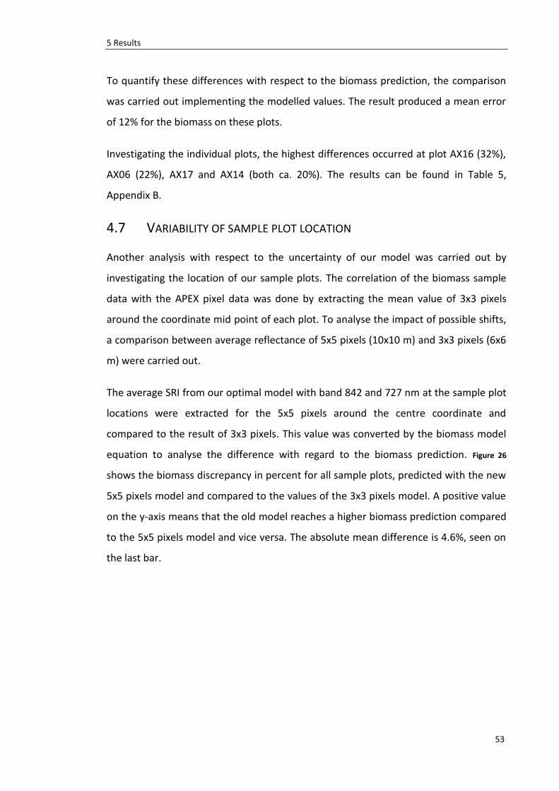
5 Results
53
To quantify these differences with respect to the biomass prediction, the comparison
was carried out implementing the modelled values. The result produced a mean error
of 12% for the biomass on these plots.
Investigating the individual plots, the highest differences occurred at plot AX16 (32%),
AX06 (22%), AX17 and AX14 (both ca. 20%). The results can be found in Table 5,
Appendix B.
4.7 VARIABILITY OF SAMPLE PLOT LOCATION
Another analysis with respect to the uncertainty of our model was carried out by
investigating the location of our sample plots. The correlation of the biomass sample
data with the APEX pixel data was done by extracting the mean value of 3x3 pixels
around the coordinate mid point of each plot. To analyse the impact of possible shifts,
a comparison between average reflectance of 5x5 pixels (10x10 m) and 3x3 pixels (6x6
m) were carried out.
The average SRI from our optimal model with band 842 and 727 nm at the sample plot
locations were extracted for the 5x5 pixels around the centre coordinate and
compared to the result of 3x3 pixels. This value was converted by the biomass model
equation to analyse the difference with regard to the biomass prediction. Figure 26
shows the biomass discrepancy in percent for all sample plots, predicted with the new
5x5 pixels model and compared to the values of the 3x3 pixels model. A positive value
on the y-axis means that the old model reaches a higher biomass prediction compared
to the 5x5 pixels model and vice versa. The absolute mean difference is 4.6%, seen on
the last bar.
5 Results
54
Figure 26: Biomass discrepancy predicted for the sample plot locations between implementation of average
reflection of 3x3 vs. 5x5 APEX pixels as reference values.
-30
-20
-10
0
10
20
30
AX
09
AX
10
AX
11
AX
12
AX
13
AX
14
AX
15
AX
16
AX
17
AX
06
AX
07
AX
08
AX
B0
1
AX
B0
2
AX
B0
3
AX
B0
4
AX
B0
5
AX
F01
AX
F02
AX
02
AX
03
AX
04
AX
05
AX
F03
AX
01
Ab
solu
te m
ean
Bio
mas
s d
iscr
epan
ce [
%]
55
5 DISCUSSION
In general high correlations with biomass ground truth were found. The optimized
model was generated by implementing the best SRI. In the following discussion we
found that the best calibration doesn’t bring the best validation result. Many factors
showed that the model validation vary strongly with different model input settings.
5.1 BIOMASS REFERENCE
The biomass field data was available as wet and dry weight. The regression analyses
showed that wet weight correlated better with APEX data than dry weight. The
reflection of the actual vegetation cover showed high volume scattering due to the
water content and the leaf architecture. It makes more sense to correlate reflectance
with wet weight because many different plant types are found within one plot and the
water content of the different plants isn’t constant.
We were not able to distinguish between dead and live biomass, i.e. between
photosynthetically active (PV) and non-active vegetation (NPV). We tried not to sample
the dead material, but as the grassland is very mixed and weedy, this was difficult to
accomplish. At some plots there was only very little grass coverage (especially on the
higher plots due to the late start of the growing season), so that all available material
had to be cut.
5.2 COMPARISON OF NDVI AND OPTIMAL SRI
NDVI and SR indices are functionally related (Liang, 2005), however SR indices are
often used in mountainous regions (Boschetti et al., 2007) since they enhance the
contrast between soil and vegetation, minimize the effects of the illumination
conditions (Baret and Guyot, 1991) and reduce shadow effects (Boschetti et al., 2007).
Additionally, the presented results indicate a better performance of the optimal SRI
compared to the NDVI and an improved the predictive accuracy of the SRI for biomass.
5 Discussion
56
The coefficient of determination R2 increased from 0.74 for the standard NDVI to 0.77
for the SRI model. The validation is also slightly improved from 0.54 to 0.56 (R2). The
quality of the model with an accuracy of 57% is good regarding the challenging terrain
with slopes up to 78°. This means that 57% of the variation in biomass on an
independent test data set could be explained by the model.
Both models are non-linear and underestimate high biomass values (above 600 g/m2).
Such bias can be caused by random noise or fundamentally non-linear relationship in
the true physical relationship (Geladi et al., 1999). Another reason is saturation of NIR
reflectance in dense vegetation, which frequently affects NDVI and slightly less SR
indices. Broad bands for VIs, one in RED and one in NIR, have been shown to saturate
at high biomass or high LAI (Mutanga & Skidmore, 2004). For our SRI we chose two
closer bands (730 vs. 840 nm), still located in RED and NIR.
However, the saturation effect should only occur typically in multilayer vegetation
such as forests or agricultural crops, with LAI > 4 (Baret & Guyot, 1991). The grassland
of Val Trupchun would probably have a LAI around 3. Nevertheless, our SRI model still
underestimates high biomass. Based on this fact the model was recalculated using two
narrow bands, both located in the far RED, as this should solve the saturation problem
according to Mutanga and Skidmore (2004). The coefficient of determination (R2)
between band 77 at 765 nm and band 70 at 735 nm is 0.7697, which is only slightly
lower than our best SRI (R2 = 0.7728). On the other hand, the validation yielded 10%
better validity (67%). It can be concluded that high biomass values were still
underestimated, but at a lower level when avoiding the NIR domain.
5.3 UNCERTAINTY ANALYSIS
The 57% accuracy of the SRI model (842/747) validation means that 57% of the
biomass variance can be explained. This is a comparatively good validation for such a
complex terrain conducted with completely independent plots. However, several
factors showed that the model is relatively instable. The selection of the band
combination is one important factor that influences the model accuracy, as illustrated
by the example with the narrow band SR index (765/735) in the far RED. The best
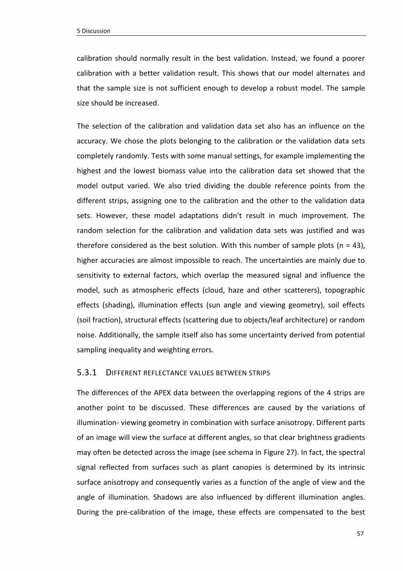
5 Discussion
57
calibration should normally result in the best validation. Instead, we found a poorer
calibration with a better validation result. This shows that our model alternates and
that the sample size is not sufficient enough to develop a robust model. The sample
size should be increased.
The selection of the calibration and validation data set also has an influence on the
accuracy. We chose the plots belonging to the calibration or the validation data sets
completely randomly. Tests with some manual settings, for example implementing the
highest and the lowest biomass value into the calibration data set showed that the
model output varied. We also tried dividing the double reference points from the
different strips, assigning one to the calibration and the other to the validation data
sets. However, these model adaptations didn’t result in much improvement. The
random selection for the calibration and validation data sets was justified and was
therefore considered as the best solution. With this number of sample plots (n = 43),
higher accuracies are almost impossible to reach. The uncertainties are mainly due to
sensitivity to external factors, which overlap the measured signal and influence the
model, such as atmospheric effects (cloud, haze and other scatterers), topographic
effects (shading), illumination effects (sun angle and viewing geometry), soil effects
(soil fraction), structural effects (scattering due to objects/leaf architecture) or random
noise. Additionally, the sample itself also has some uncertainty derived from potential
sampling inequality and weighting errors.
5.3.1 DIFFERENT REFLECTANCE VALUES BETWEEN STRIPS
The differences of the APEX data between the overlapping regions of the 4 strips are
another point to be discussed. These differences are caused by the variations of
illumination- viewing geometry in combination with surface anisotropy. Different parts
of an image will view the surface at different angles, so that clear brightness gradients
may often be detected across the image (see schema in Figure 27). In fact, the spectral
signal reflected from surfaces such as plant canopies is determined by its intrinsic
surface anisotropy and consequently varies as a function of the angle of view and the
angle of illumination. Shadows are also influenced by different illumination angles.
During the pre-calibration of the image, these effects are compensated to the best
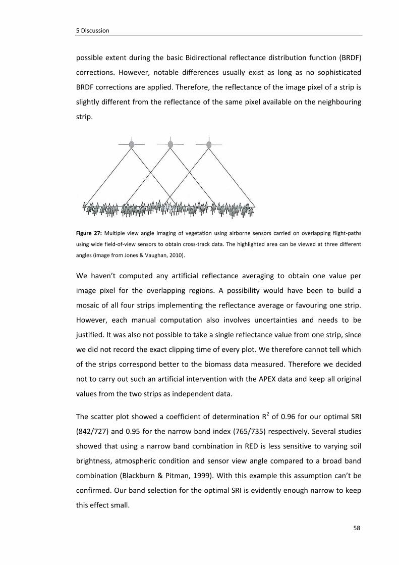
5 Discussion
58
possible extent during the basic Bidirectional reflectance distribution function (BRDF)
corrections. However, notable differences usually exist as long as no sophisticated
BRDF corrections are applied. Therefore, the reflectance of the image pixel of a strip is
slightly different from the reflectance of the same pixel available on the neighbouring
strip.
Figure 27: Multiple view angle imaging of vegetation using airborne sensors carried on overlapping flight-paths
using wide field-of-view sensors to obtain cross-track data. The highlighted area can be viewed at three different
angles (image from Jones & Vaughan, 2010).
We haven’t computed any artificial reflectance averaging to obtain one value per
image pixel for the overlapping regions. A possibility would have been to build a
mosaic of all four strips implementing the reflectance average or favouring one strip.
However, each manual computation also involves uncertainties and needs to be
justified. It was also not possible to take a single reflectance value from one strip, since
we did not record the exact clipping time of every plot. We therefore cannot tell which
of the strips correspond better to the biomass data measured. Therefore we decided
not to carry out such an artificial intervention with the APEX data and keep all original
values from the two strips as independent data.
The scatter plot showed a coefficient of determination R2 of 0.96 for our optimal SRI
(842/727) and 0.95 for the narrow band index (765/735) respectively. Several studies
showed that using a narrow band combination in RED is less sensitive to varying soil
brightness, atmospheric condition and sensor view angle compared to a broad band
combination (Blackburn & Pitman, 1999). With this example this assumption can’t be
confirmed. Our band selection for the optimal SRI is evidently enough narrow to keep
this effect small.
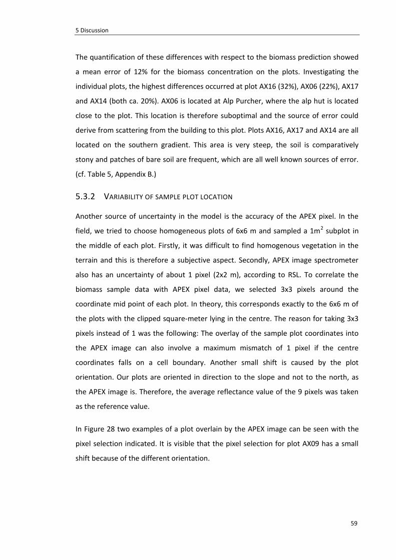
5 Discussion
59
The quantification of these differences with respect to the biomass prediction showed
a mean error of 12% for the biomass concentration on the plots. Investigating the
individual plots, the highest differences occurred at plot AX16 (32%), AX06 (22%), AX17
and AX14 (both ca. 20%). AX06 is located at Alp Purcher, where the alp hut is located
close to the plot. This location is therefore suboptimal and the source of error could
derive from scattering from the building to this plot. Plots AX16, AX17 and AX14 are all
located on the southern gradient. This area is very steep, the soil is comparatively
stony and patches of bare soil are frequent, which are all well known sources of error.
(cf. Table 5, Appendix B.)
5.3.2 VARIABILITY OF SAMPLE PLOT LOCATION
Another source of uncertainty in the model is the accuracy of the APEX pixel. In the
field, we tried to choose homogeneous plots of 6x6 m and sampled a 1m2 subplot in
the middle of each plot. Firstly, it was difficult to find homogenous vegetation in the
terrain and this is therefore a subjective aspect. Secondly, APEX image spectrometer
also has an uncertainty of about 1 pixel (2x2 m), according to RSL. To correlate the
biomass sample data with APEX pixel data, we selected 3x3 pixels around the
coordinate mid point of each plot. In theory, this corresponds exactly to the 6x6 m of
the plots with the clipped square-meter lying in the centre. The reason for taking 3x3
pixels instead of 1 was the following: The overlay of the sample plot coordinates into
the APEX image can also involve a maximum mismatch of 1 pixel if the centre
coordinates falls on a cell boundary. Another small shift is caused by the plot
orientation. Our plots are oriented in direction to the slope and not to the north, as
the APEX image is. Therefore, the average reflectance value of the 9 pixels was taken
as the reference value.
In Figure 28 two examples of a plot overlain by the APEX image can be seen with the
pixel selection indicated. It is visible that the pixel selection for plot AX09 has a small
shift because of the different orientation.
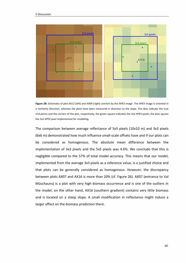
5 Discussion
60
Figure 28: Schematic of plot AX12 (left) and AX09 (right) overlain by the APEX image. The APEX image is oriented in
a northerly direction, whereas the plots have been measured in direction to the slope. The dots indicate the true
mid points and the corners of the plot, respectively, the green square indicates the 3x3 APEX pixels, the blue square
the 5x5 APEX pixel implemented for modelling.
The comparison between average reflectance of 5x5 pixels (10x10 m) and 3x3 pixels
(6x6 m) demonstrated how much influence small-scale offsets have and if our plots can
be considered as homogenous. The absolute mean difference between the
implementation of 3x3 pixels and the 5x5 pixels was 4.6%. We conclude that this is
negligible compared to the 57% of total model accuracy. This means that our model,
implemented from the average 3x3 pixels as a reference value, is a justified choice and
that plots can be generally considered as homogenous. However, the discrepancy
between plots AX07 and AX16 is more than 20% (cf. Figure 26). AX07 (entrance to Val
Müschauns) is a plot with very high biomass occurrence and is one of the outliers in
the model; on the other hand, AX16 (southern gradient) contains very little biomass
and is located on a steep slope. A small modification in reflectance might induce a
larger effect on the biomass prediction there.
61
6 CONCLUSION
Imaging spectroscopy techniques permit not only the classification of vegetation, but
also the quantitative mapping of different vegetation variables due to their high
spectral and spatial resolution. This study demonstrates the utility of vegetation
indices involving APEX bands for estimating biomass in alpine grasslands.
SRI and NDVI models were suitable for the modelling of biomass prediction maps
implementing biophysical parameters. We found that the correlation between biomass
insitu measurements and SRIs was non-linear, most likely due to sensor saturation. Our
optimal SRI improved the model quality compared to a standard NDVI model. All
computed models underestimated high biomass values above 600 g/m2. The model
accuracy of 57% was good considering the challenging terrain. However, several
factors showed that the model was relatively unstable due to parameter input settings
and external factors. Differences in APEX data between strips induced an important
effect, due to different illumination/view angles. The quantification regarding biomass
prediction due to these differences produced a mean error of 12% for the sample
plots. The variability analysis investigating the sample plot location demonstrated that
small-scale geometrical shifts were insignificant compared to the overall model
accuracy.
The biomass prediction map showed plausible values for the grassland with high
concentrations around the former Alp Trupchun, Alp Purcher and on the south slope at
the end of the valley. We found that high biomass sources were linked to former
anthropogenic land use, dominant vegetation structure and to preferred ungulate
habitat today.
The high-resolution map is now a useful basis for future research in the SNP to
investigate forage amount and analyse ungulate habitat pattern in Val Trupchun.
62
7 OUTLOOK
The generated biomass prediction map can be used for future research in Val
Trupchun. This work was carried out within the scope of a PhD thesis at the Swiss
National Park analysing ungulate habitat patterns relating to biophysical and
biochemical parameters. The APEX campaigns have been continued during the years
2011 and 2012.
The model produced is applicable only for the study area, since semi-empirical. These
predictive models are site- and sensor-specific and unsuitable for application to other
areas or to different seasons. With this model we tried to predict another area of the
SNP, the grassland of Il Fuorn, which is located ca. 15 km north-east, and didn’t find
suitable agreement with insitu measurements. This finding highlights the importance
of local models, based on local measurements for small scales in complex terrain.
Moreover, our model is only valid for the time of the image, which was June. To
analyse temporal changes for biomass, the APEX campaign should be carried out
several times a year.
The main proposal for a model improvement based on this work is to increase the
number of sample plots in the study area. With more samples covering the full range
of biomass concentrations, we suppose that the model accuracy and stability will
improve. Another possibility would be to clip more than 1 m2 per sample plot to get
more than one sample out of one plot. Thus, small-scale variability could be improved,
too. However, all improvement proposals would require a lot more effort in the field
which is a limiting factor.
For the APEX campaign carried out in June 2012, 100 sample plots have been
implemented. Modelling results aren’t available yet, we are curious!
63
8 LIST OF REFERENCES
Achermann, G., Schütz, M., Krüsi, B. O., 2000. Tall-herb communities in the Swiss
National Park: Long-term development of the vegetation. Nationalpark-Forschung
in der Schweiz, Band 89.
Baret, F., Guyot, G., 1991. Potentials and limits of vegetation indices for LAI and APAR
assessment. Remote Sensing of Environment, 35, pp. 161-173.
Beeri, O., Phillips, R., Hendrickson, J., Frank, A. B., Kronberg, S., 2007. Estimating forage
quantity and quality using aerial hyperspectral imagery for northern mixed-grass
prairie. Remote Sensing of Environment, 110, pp. 216-225.
Birth, G. S., McVey, G. R., 1968. Measuring the colour of growing turf with a
reflectance spectrophotometer. Agronomy Journal 60, pp 640-643.
Blackburn, G. A., Pitman, J. I., 1999. Biophysical controls on the directional spectral
reflectance properties of bracken (Pteridium aquilinum) canopies: results of a field
experiment. International Journal of Remote Sensing, 20(11), pp. 2265-2282.
Boardman, J. W., 1989. Inversion of imaging spectrometry data using singular value
decomposition: Proceedings, IGARSS’89, 12th Canadian Symposium on Remote
Sensing 4, pp. 2069-2072.
Boschetti, M., Bocchi, S., Brivio, P. A., 2007. Assessment of pasture production in the
Italian Alps using spectrometric and remote sensing information. Agriculture,
Ecosystems Environment, 118(1-4), pp. 267-272.
Braun-Blanquet, J., Brunies, S., Campell, K., Frey, E., Jenny, H., Meylan, Cli. & Pallmann,
H., 1931. Vegetationsentwicklung im Schweiz. Nationalpark. Ergebnisse der
Untersuchung von Dauerbeobachtungsflächen, 1. Dokumente zur Untersuchung
des Schweizer Nationalparks. Jahresberichte der Nationalforschenden Gesellschaft
Graubündens, 69, pp. 3-82.
Braun-Blanquet, J., Pallmann, H., Bach, R., 1954. Planzensoziologische und
bodenkundliche Untersuchungen im Schweizerischen Nationalpark und seinen
Nachbargebieten. II Vegetation und Böden der Wald- und Zwergstrauch-
gesellschaften (Vaccinio-Piceetalia). Ergebnisse der wissenschaftlichen
Untersuchungen des schweizerischen Nationalparks. Band 4, Kapitel 28.
10 List of references
64
Cho, M. A., Skidmore, A., Corsi, F., van Wieren, S. E., Sobhan, I., 2007. Estimation of
green grass/herb biomass from airborne hyperspectral imagery using spectral
indices and partial least squares regression. International Journal of Applied Earth
Observation and Geoinformation 9, pp. 414-424.
Clevers, J. G. P. W., 1999. The use of imaging spectrometry for agricultural applications.
ISPRS Journal of Photogrammetry and Remote Sensing 54 (5), pp. 299-304.
Damm, A., Kneubühler, M., Schaepman, M. E., Rascher, U., 2012. Evaluation of gross
primary production (GPP) variability over several ecosystems in Switzerland using
sun-induced chlorophyll fluorescence derived from APEX data. Proc, IGARSS 2012,
Munich (D), July 22-27 2012, pp. 7133-7136.
Falster, D. S, Westoby, M., 2003. Leaf size and angle vary widely across species: what
consequences for light interception? New Phytologist 158, pp. 509-525.
Fava, F., Colombo, R., Bocchi, S., Meroni, M., Sitzia, M., Fois, N., Zucca, C., 2009.
Identification of hyperspectral vegetation indices for Mediterranean pasture
characterization. International Journal of Applied Earth Observation and
Geoinformation 11, pp. 233-243.
Geladi, P., Hadjiiski, L., Hopke, P., 1999. Multiple regression for environmental data:
nonlinearities and prediction bias. Chemometrics Intell. Lab. Syst. 47 (2), pp 165-
173.
Goetz, A. F. H., 2009. Three decades of hyperspectral remote sensing of the Earth: A
personal view. Remote Sensing of Environment, 113 (Supplement 1), pp. S5–S16.
Goetz, A. F. H., Vane, G., Solomon, J., & Rock, B. N., 1985. Imaging spectrometry for
Earth remote sensing. Science, 228, pp. 1147−1153.
He, Y., Guo, X.L., Wilmshurst, J., 2006. Studying mixed grassland ecosystems I: suitable
hyperspectral vegetation indices. Canadian Journal of Remote Sensing 32, pp. 98-
107.
Itten, K., Dell’Endice, F., Hueni, A., Kneubühler, M., Schläpfer, D., Odermatt, D., Seidel,
F., Huber, S., Schopfer, J., Kellenberger, T., Bühler, Y., D’Odorico, P., Nieke, J.,
Alberti, E., Meuleman, K., 2008. Sensors 8, pp. 6235-6259.
Jago, R. A., Cutler, M. E. J., Curran, P. J., 1999. Estimating Canopy Chlorophyll
Concentration from Field and Airbonre Spectra. Remote Sensing of Environment
68, pp. 217-224.
10 List of references
65
Jehle, M., Hueni, A., Damm, A., D’Odorico, P., Weyermann, J., Kneubühler, M.,
Schläpfer, D., Schaepman, M. E., 2010. APEX - current status, performance and
product generation. IEEE Sensors 2010, Waikoloa (HI), pp. 533-537.
Jones, H. G., Vaughan, R. A., 2010. Remote sensing of vegetation. Principles,
Techniques, and applications. Oxford University Press Inc, New York.
Kneubühler, M., Damm, A., Mundava, Ch., Weyermann, J., Hueni, A., Risch, A. C.,
Schütz, M., Schweiger, A., Haller, R., Filli, F., Schaepman, M. E., 2011. Imaging
Spectrometry for Ecological Studies in a High Mountain Environment. In EARSeL
7th SIG-Imaging Spectroscopy Workshop, Edinburgh, Scotland, 11-13 April.
Kooistra, L., Suarez Barranco, M. D., van Dobben, H. & Schaepman, M. E., 2006.
Monitoring Vegetation Biomass in River Floodplains using Imaging Spectroscopy.
ISPRS Mid Term Symposium: From Pixels to Processes, Enschede (NL), Kerle, N. &
Skidmore, A. (Eds.), ISPRS, p. 5, CD-ROM.
Krüsi, B. O., Schütz, M., Wildi, O., Grömiger, H., 1995. Huftiere, Vegetationsdynamik
und botanische Vielfalt im Nationalpark. Cratschla 32, pp 12-25.
Kumar, L., Schmidt, K. S., Dury, S., Skidmore A. K., 2001. Review of hyperspectral
remote sensing and vegetation Science. In: Van der Meer, F.D., De Jong, S.M. (eds)
Imaging spectrometry: basic principles and prospective applications. Kluwer,
Dordrecht, The Netherlands.
Liang, S., 2004. Quantitative remote sensing of land surfaces. Hoboken: Wiley,
Hoboken.
Lillesand, T. M., Kiefer, R. W., 1994. Remote sensing and image interpretation, 3rd ed.
New York: John Wiley and Sons, Inc.
Mirik, M., Norland, J. E., Crabtree, R. L., and Biondini, M. E., 2005a. Hyperspectral one-
meter-resolution remote sensing in Yellowstone National Park, Wyoming: I. Forage
nutritional values. Rangeland Ecology and Management 58, pp. 452-458.
Mirik, M., Norland, J. E., Crabtree, R. L., Biondini, M. E., 2005b. Hyperspectral one-
meter-resolution remote sensing in Yellowstone National Park, Wyoming: II.
Biomass. Rangeland Ecology and Management 58, pp. 459-465.
Mutanga, O., Skidmore, A. K., 2004. Integrating imaging spectroscopy and neural
networks to map grass quality in the Kruger National Park, South Africa. Remote
Sensing of Environment 90, pp. 104-115.
10 List of references
66
Mutanga, O., Skidmore, A. K., 2004. Narrow band vegetation indices overcome the
saturation problem in biomass estimation. International Journal of Remote
Sensing, Vol. 25, pp. 3999-4014.
Mutanga, O., Skidmore, A. K., 2007. Red edge shift and biochemical content in grass
canopies. ISPRS Journal of Photogrammetry and Remote Sensing 62, pp. 34-42.
Mutanga, O., Skidmore, A. K., Prins, H. H. T., 2004. Predicting in situ pasture quality in
the Kruger National Park, South Africa, using continuum-removed absorption
features. Remote Sensing of Environment, 89, pp. 393-408.
Numata, I., Roberts, D. A., Chadwick, O. A., Schimel, J., Galvao, J., Soares, J. V., 2008.
Evaluation of hyperspectral data for pasture estimate in the Brazilian Amazon
using field and imaging spectrometers. Remote Sensing of Environment, 112, pp.
1569-1583.
Numata, I., Roberts, D. A., Chadwick, O. A., Schimel, J., Sampaio, F. R., Leonidas, F. C.,
Soares, J. V., 2007. Characterization of pasture biophysical properties and the
impact of grazing intensity using remotely sensed data. Remote Sensing of
Environment, 109, pp. 314-327.
Parolini, J. D., 1995. Zur Geschichte der Waldnutzung im Gebiet des Schweizerischen
Nationalparks. PhD Thesis ETH Zurich, Nr. 1187.
Pictet, A., 1942. Les Macrolépidoptères du parc national Suisse et des régions
limitrophes. Ergebnisse der wissenschaftlichen Untersuchungen des
schweizerischen Nationalparks. Band 1, Kapitel 8.
Psomas, A., 2009. Hyperspectral remote sensing for ecological analyses of grasslands
ecosystems. Spectral separability and derivation of NPP related biophysical and
biochemical parameters. Dissertation, University of Zurich.
Rahman A. F., Gamon J. A., 2004. Detecting biophysical properties of a semi-arid
grassland and distinguishing burned from unburned areas with hyperspectral
reflectance. Journal of Arid Environments 58(4), pp. 597-610.
Rosso, P. H., Ustin, S. L., Hastings, A., 2005. Mapping marshland vegetation of San
Francisco Bay, California, using hyperspectral data. Int. Journal of Remote Sensing,
Vol. 26, Nr. 23, pp. 5169-5191.
Rouse, J. W., Haas, R. H., Schell, J. A., Deering, D. W., Harlan, J C., 1974. Monitoring the
vernal advancement and retrogradation (greenwave effect) of natural vegetation.
NASA/GSFC Final report, Greenbelt, MD, USA.
10 List of references
67
Schaepman, M., Schläpfer, D., Kaiser, J., Brazile, J., Itten, K., 2003. APEX-Airborne Prism
Experiment: Dispersive Pushbroom Imaging Spectrometer for Environmental
Monitoring. 3rd EARSeL Workshop on Imaging Spectroscopy, Proc. CD_ROM.
Schläpfer, D., Richter, R., 2002. Geo-atmospheric processing of airborne imaging
spectrometry data. Part 1: parametric orthorectification. International Journal of
Remote Sensing, Vol. 23, pp. 2609-2630.
Stessens, J., 2012. BruHyp 2012, conference slides, p. 24.
Stüssi, B., 1970. Naturbedingte Entwicklung subalpiner Weiderasen auf Alp La Schera
im Schweizer Nationalpark während der Reservatsperiode 1939-1965. Ergebnisse
der wissenschaftlichen Untersuchungen im schweizerischen Nationalpark, 13.
Tarr, A. B., Moore, K. J., Dixon, P. M., 2005. Spectral reflectance as a covariate for
estimating pasture productivity and composition. Crop Science, 45(3), pp. 996-
1003.
Trepp, W., Campell, E., 1968. Vegetationskarte des Schweizerischen Nationalpark.
Nationalparkforschung in der Schweiz, Band 11, Heft 58
Tucker, C. J., 1979. Red and photographic infrared linear combinations for monitoring
vegetation. Remote Sensing of Environment 8, pp 127-150.
Vane, G., Chrisp, M., Emmark, H., Macenka, S., Solomon, J., 1984. Airborne Visible
Infrared Imaging Spectrometer (AVIRIS): An Advanced Tool for Earth Remote
Sensing. European Space Agency. Special Publication, ESA SP, 2, 751.
Van Langevelde, F., Prins, H. H. T., 2008. Introduction to resource ecology. In Prins, H.
H. T., and Van Langevelde, F. (eds.). Resource Ecology, Spatial and Temporal
Dynamics of Foraging. Springer, Dordrecht, pp 1-6.
Weyermann, J., Damm, A., Kneubühler, M., Schaepman, M. E., 2013. Correction of
reflectance anisotropy effects of vegetation on airborne spectroscopy data and
derived products. IEEE Transactions on Geosciences and Remote Sensing.
Xiao, Q., Ustin, S. L., McPherson, E. G., 2004. AVRIS data and mulitple-masking
techniques to map urban tree species. International Journal of Remote Sensing,
Vol. 25, No. 24, pp. 5637-5654.
Zoller, H., 1992. Vegetationskarte des Schweizerischen Nationalparks und seiner
Umgebung. Nationalpark-Forschung in der Schweiz, Band 85.

10 List of references
68
Campbell, G. S., Norman, J. M., 1998. An introduction to environmental biophysics. 2nd
ed., Springer, New York, pp. 286.
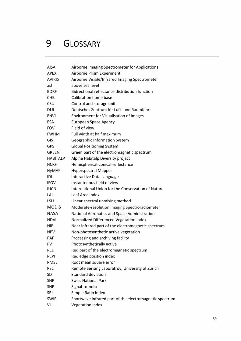
69
9 GLOSSARY
AISA Airborne Imaging Spectrometer for Applications
APEX Airborne Prism Experiment
AVIRIS Airborne Visible/Infrared Imaging Spectrometer
asl above sea level
BDRF Bidrectional reflectance distribution function
CHB Calibration home base CSU Control and storage unit DLR Deutsches Zentrum für Luft- und Raumfahrt ENVI Environment for Visualisation of Images ESA European Space Agency FOV Field of view FWHM Full width at half maximum GIS Geographic Information System GPS Global Positioning System GREEN Green part of the electromagnetic spectrum HABITALP Alpine Habitalp Diversity project
HCRF Hemispherical-conical-reflectance HyMAP Hyperspectral Mapper
IDL Interactive Data Language IFOV Instantenous field of view IUCN International Union for the Conservation of Nature LAI Leaf Area index LSU Linear spectral unmixing method
MODIS Moderate-resolution Imaging Spectroradiometer
NASA National Aeronatics and Space Administration NDVI Normalized Differenced Vegetation index NIR Near infrared part of the electromagnetic spectrum
NPV Non-photosynthetic active vegetation
PAF Processing and archiving facility PV Photosynthetically active RED Red part of the electromagnetic spectrum REPI Red edge position index RMSE Root mean square error RSL Remote Sensing Laboratroy, University of Zurich SD Standard deviation
SNP Swiss National Park SNP Signal-to-noise SRI Simple Ratio index
SWIR Shortwave infrared part of the electromagnetic spectrum VI Vegetation index

10 Glossary
70
VIS Visible part of the electromagnetic spectrum VITO Vision on Technology
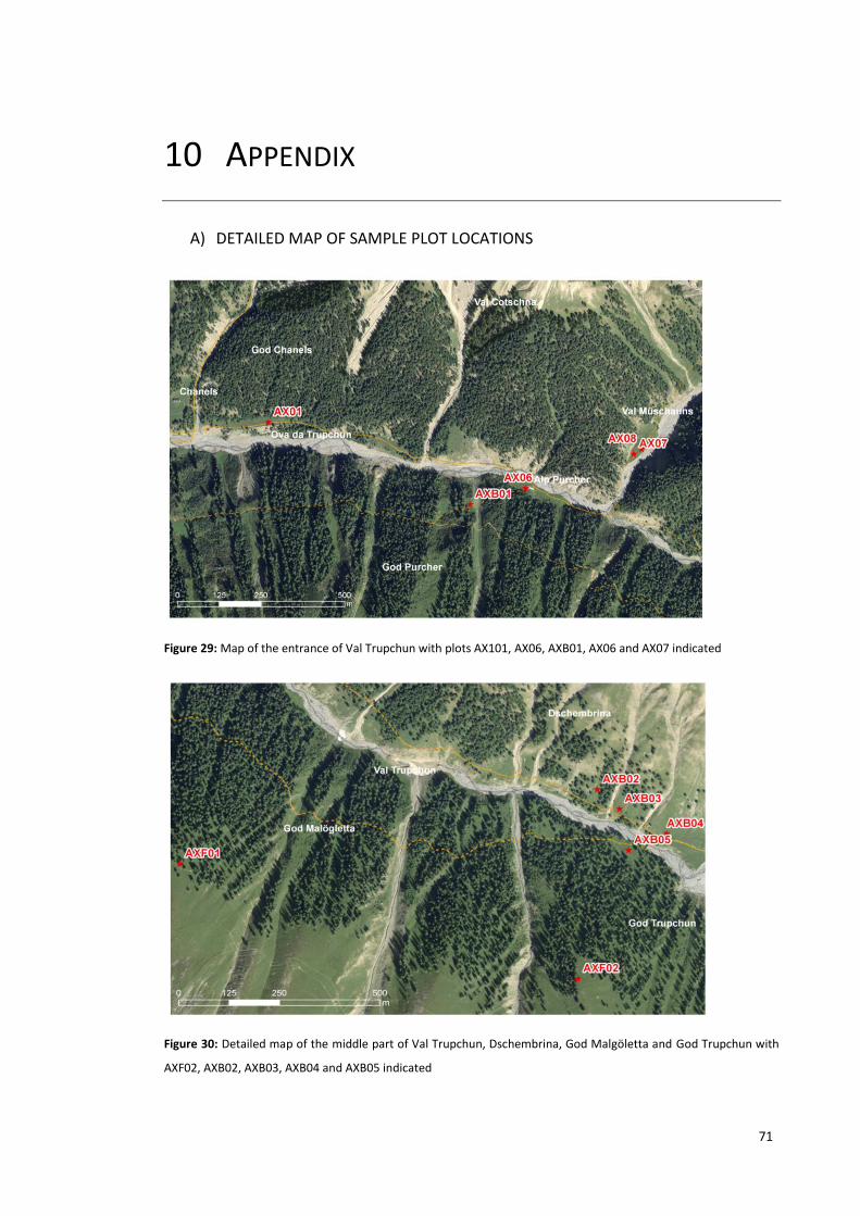
71
10 APPENDIX
A) DETAILED MAP OF SAMPLE PLOT LOCATIONS
Figure 29: Map of the entrance of Val Trupchun with plots AX101, AX06, AXB01, AX06 and AX07 indicated
Figure 30: Detailed map of the middle part of Val Trupchun, Dschembrina, God Malgöletta and God Trupchun with
AXF02, AXB02, AXB03, AXB04 and AXB05 indicated
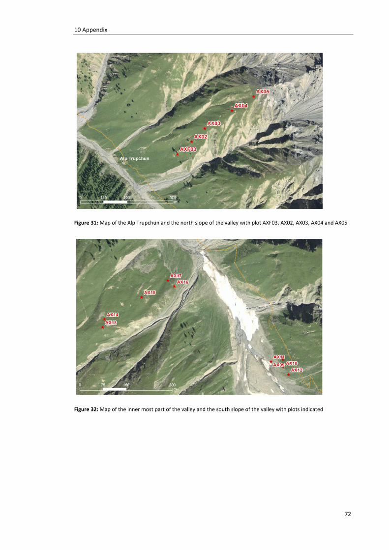
10 Appendix
72
Figure 31: Map of the Alp Trupchun and the north slope of the valley with plot AXF03, AX02, AX03, AX04 and AX05
Figure 32: Map of the inner most part of the valley and the south slope of the valley with plots indicated
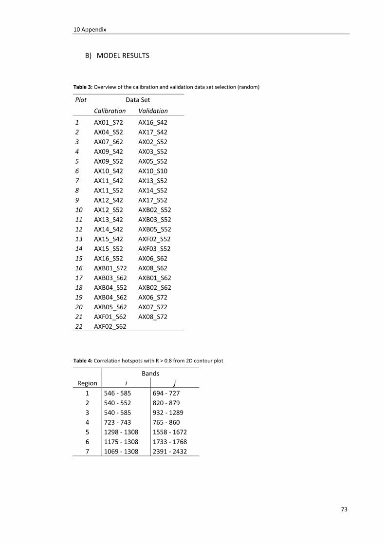
10 Appendix
73
B) MODEL RESULTS
Table 3: Overview of the calibration and validation data set selection (random)
Plot Data Set
Calibration Validation
1 AX01_S72 AX16_S42 2 AX04_S52 AX17_S42 3 AX07_S62 AX02_S52 4 AX09_S42 AX03_S52
5 AX09_S52 AX05_S52 6 AX10_S42 AX10_S10 7 AX11_S42 AX13_S52 8 AX11_S52 AX14_S52 9 AX12_S42 AX17_S52 10 AX12_S52 AXB02_S52 11 AX13_S42 AXB03_S52 12 AX14_S42 AXB05_S52 13 AX15_S42 AXF02_S52 14 AX15_S52 AXF03_S52 15 AX16_S52 AX06_S62
16 AXB01_S72 AX08_S62 17 AXB03_S62 AXB01_S62 18 AXB04_S52 AXB02_S62 19 AXB04_S62 AX06_S72 20 AXB05_S62 AX07_S72 21 AXF01_S62 AX08_S72 22 AXF02_S62
Table 4: Correlation hotspots with R > 0.8 from 2D contour plot
Bands Region i j
1 546 - 585 694 - 727 2 540 - 552 820 - 879 3 540 - 585 932 - 1289 4 723 - 743 765 - 860 5 1298 - 1308 1558 - 1672 6 1175 - 1308 1733 - 1768 7 1069 - 1308 2391 - 2432

10 Appendix
74
Table 5: Calculation results of different reflectance values between stripes and effect on biomass prediction
Plot SRI stripe a SRI stripe b Biomass a Biomass b Difference biom. Difference
[g/m2] [g/m2] [g/m2] [%]
AX06 0.8895 0.8948 667.2 679.8 12.6 1.9 AX07 0.8134 0.8161 510.2 515.1 4.8 0.9 AX08 0.7794 0.8116 452.6 507.1 54.4 10.7 AX09 0.7781 0.7182 450.7 364.9 -85.7 -23.5 AX10 0.2638 0.2881 73.6 80.2 6.6 8.2 AX11 0.1103 0.1427 42.9 48.1 5.2 10.8
AX12 0.3784 0.3700 110.2 107.0 -3.2 -3.0 AX13 0.7548 0.7488 415.1 406.4 -8.7 -2.1 AX14 0.5649 0.5744 212.6 219.9 7.2 3.3 AX15 0.7830 0.7798 458.4 453.4 -5.0 -1.1 AX16 0.3930 0.4948 116.1 166.1 50.1 30.1
AX17 0.6224 0.6899 260.4 330.3 69.9 21.2 AXB01 0.8581 0.8479 597.3 576.2 -21.1 -3.7 AXB02 0.6916 0.7283 332.2 378.0 45.8 12.1 AXB03 0.6519 0.6921 288.9 332.8 43.9 13.2 AXB04 0.5722 0.6546 218.1 291.7 73.6 25.2 AXB05 0.8366 0.7820 553.7 456.9 -96.8 -21.2
AXF02 0.6933 0.7158 334.2 361.8 27.6 7.6
absolute mean 11.1