Embed Size (px)
Citation preview
Image Segmentation
Computação Visual e Multimédia
10504: Mestrado em Engenharia Informática
Chap. 6 — Image Segmentation
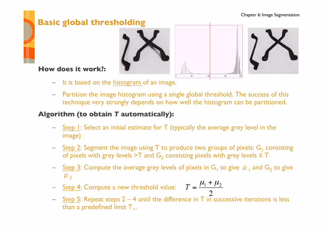
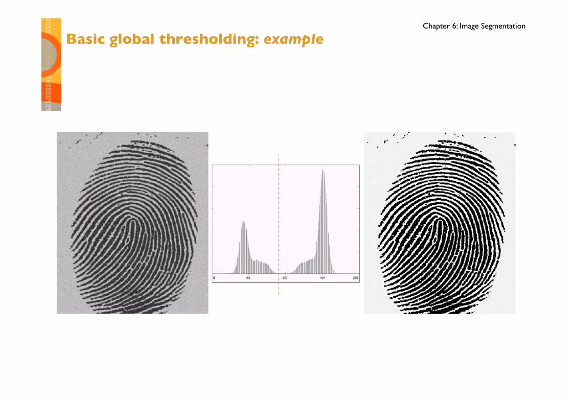
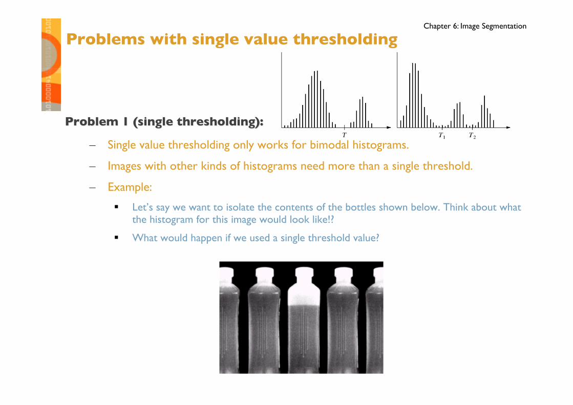
Chapter 6: Image Segmentation
Outline
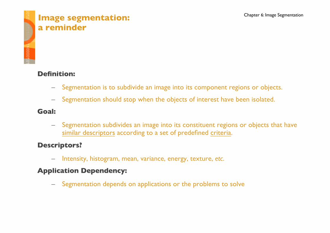
Chapter 6: Image Segmentation Image segmentation:���a reminder
Chapter 6: Image Segmentation
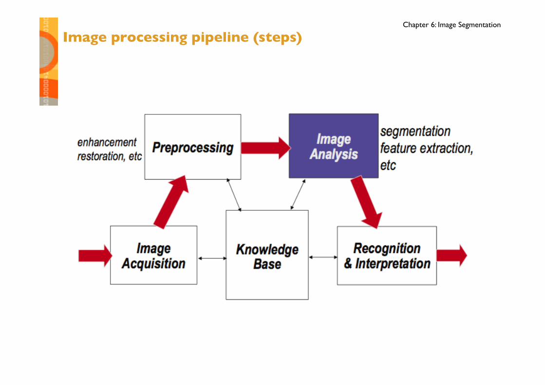
Image processing pipeline (steps)
Chapter 6: Image Segmentation
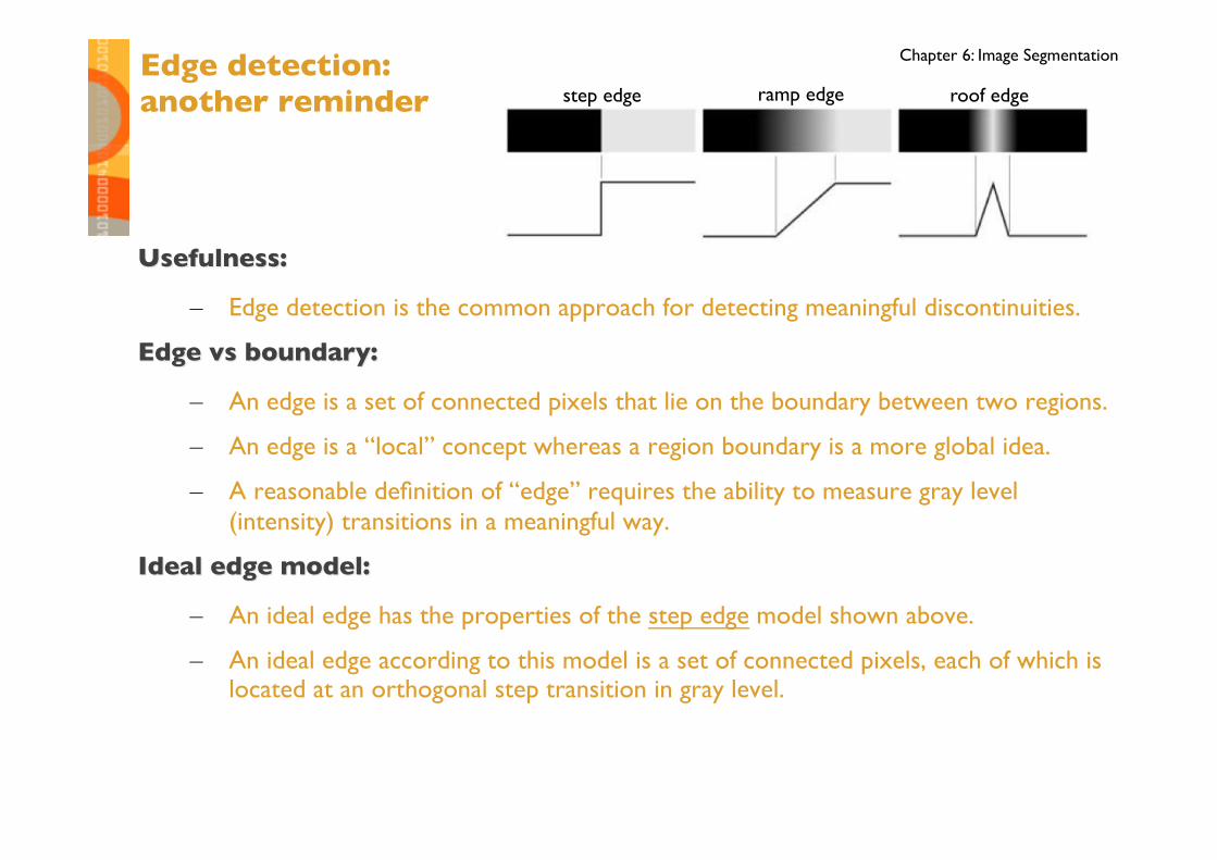
Chapter 6: Image Segmentation Edge detection:���another reminder ramp edge roof edge step edge
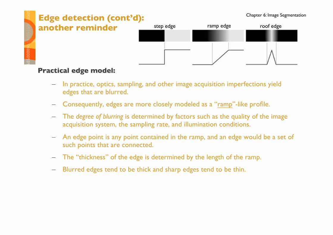
Chapter 6: Image Segmentation Edge detection (cont’d):���another reminder ramp edge roof edge step edge
Chapter 6: Image Segmentation Edge detection (cont’d):���still another reminder
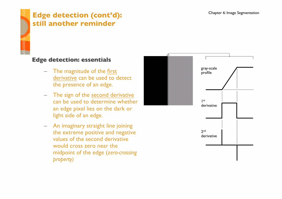
gray-scale profile
1st derivative
2nd derivative
Chapter 6: Image Segmentation
Edge segments
How to link edge segments into longer edges?
edge detection edge linking
Chapter 6: Image Segmentation
Edge linking
http
://eu
clid
.ii.m
etu.
edu.
tr/~
ion5
28/d
emo/
lect
ures
/6/4
/inde
x.ht
ml
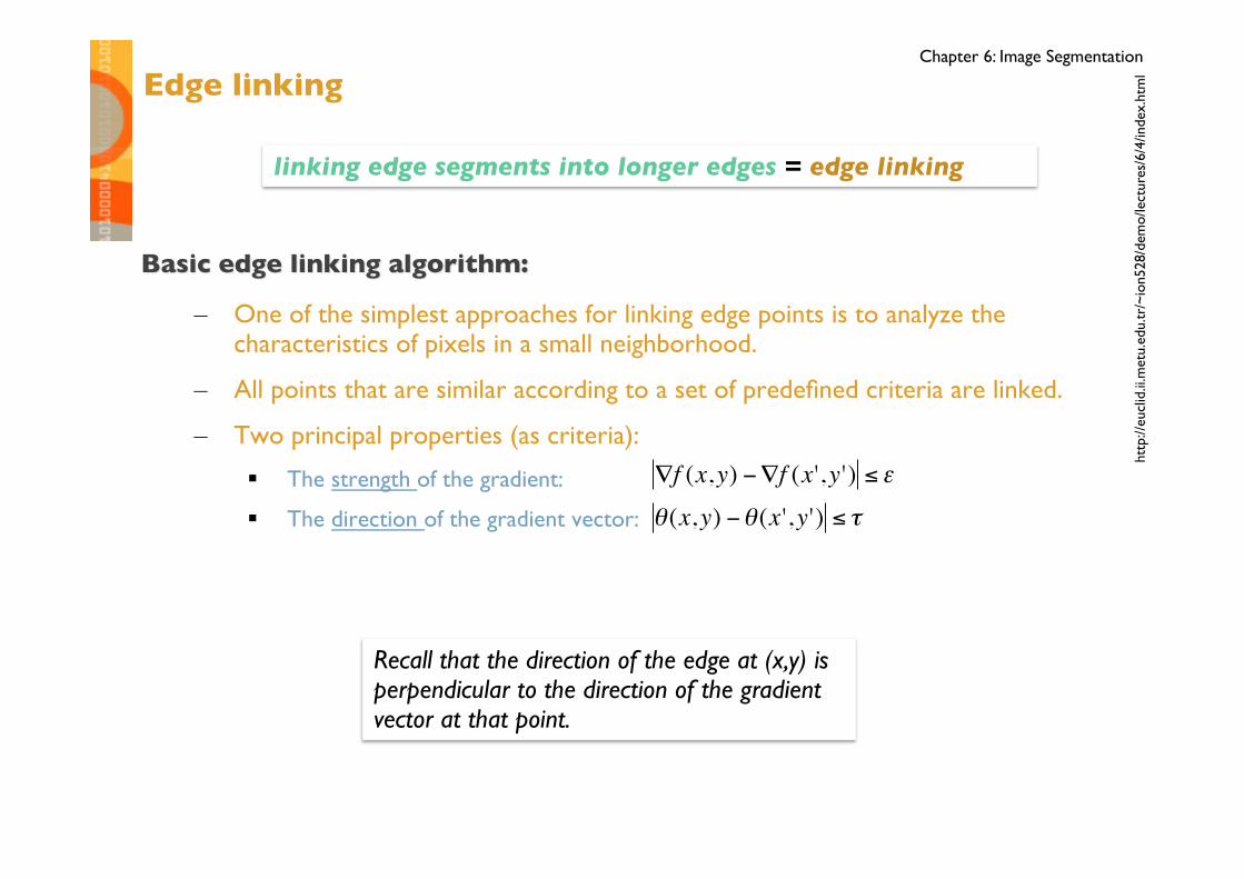
linking edge segments into longer edges = edge linking
€
∇f (x,y) −∇f (x',y ') ≤ ε
€
θ (x,y) −θ (x ',y') ≤ τ
Recall that the direction of the edge at (x,y) is perpendicular to the direction of the gradient vector at that point.
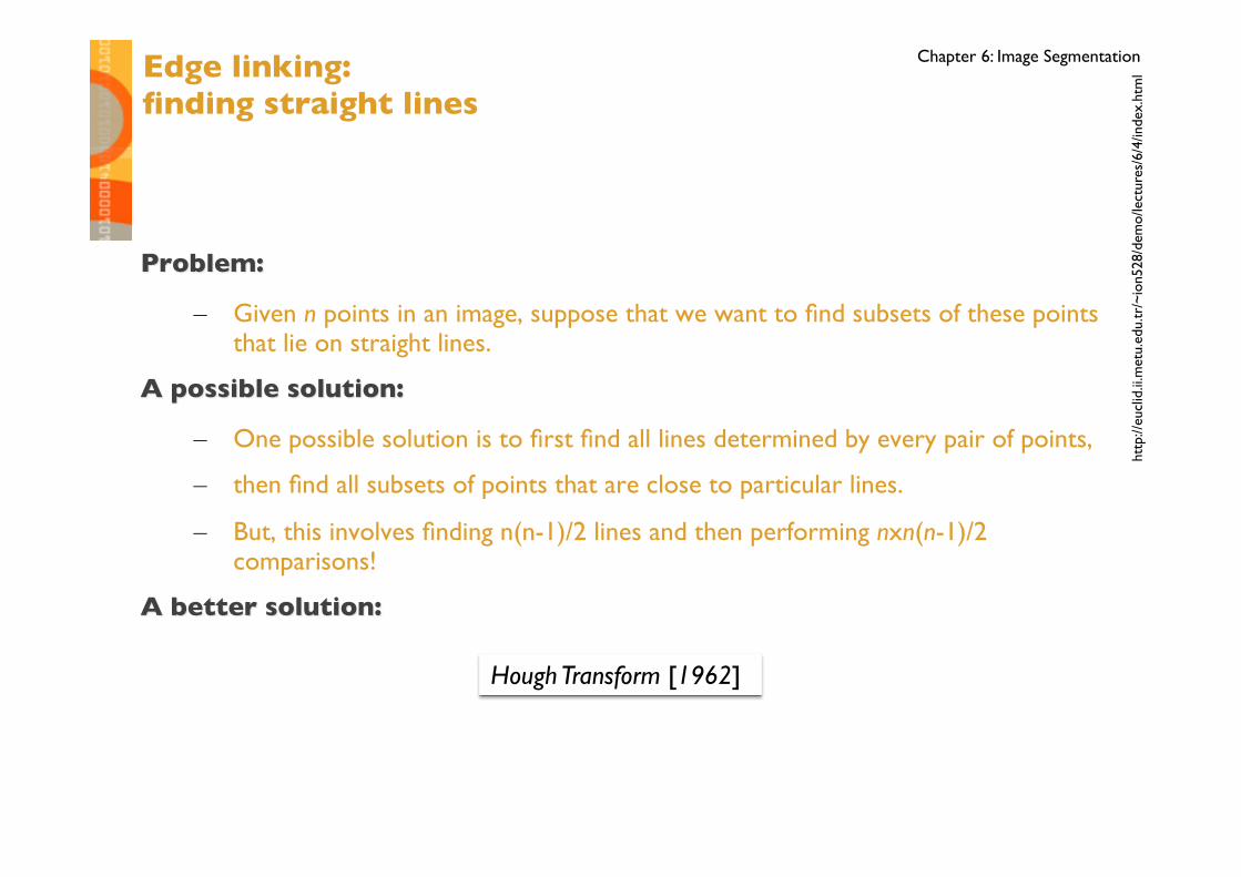
Chapter 6: Image Segmentation Edge linking: ���finding straight lines
http
://eu
clid
.ii.m
etu.
edu.
tr/~
ion5
28/d
emo/
lect
ures
/6/4
/inde
x.ht
ml
Hough Transform [1962]
Chapter 6: Image Segmentation
Hough transform
Chapter 6: Image Segmentation
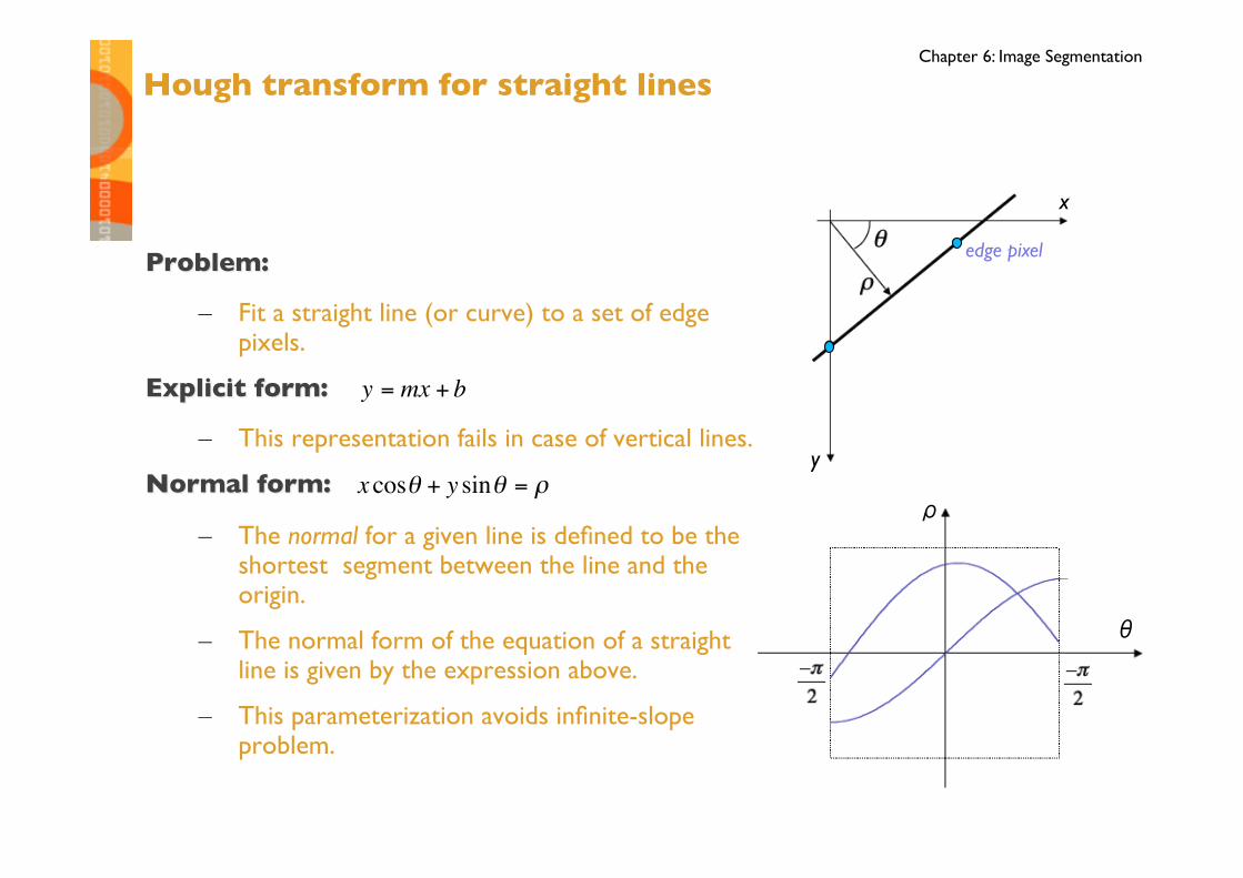
Hough transform for straight lines
€
y = mx + b
€
x cosθ + y sinθ = ρ
edge pixel
x
y
ρ
θ
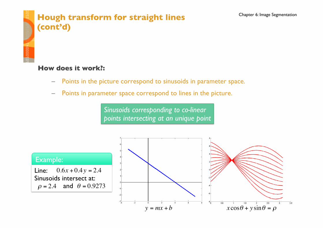
Chapter 6: Image Segmentation Hough transform for straight lines���(cont’d)
€
y = mx + b
€
x cosθ + y sinθ = ρ
Sinusoids corresponding to co-linear points intersecting at an unique point
Example: Line: Sinusoids intersect at: and
€
0.6x + 0.4y = 2.4
€
ρ = 2.4
€
θ = 0.9273
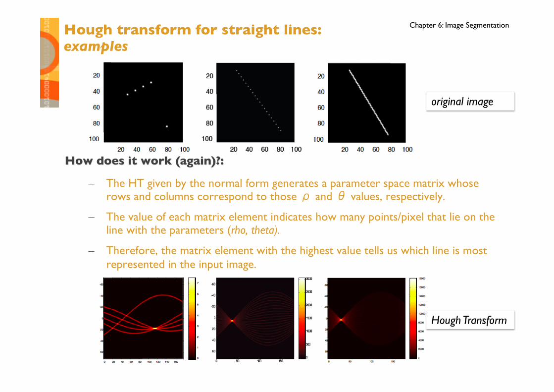
Chapter 6: Image Segmentation Hough transform for straight lines:���examples
Hough Transform
original image
Chapter 6: Image Segmentation
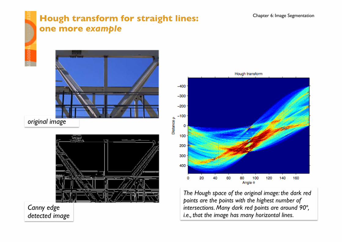
Canny edge detected image
original image
Hough transform for straight lines:���one more example
The Hough space of the original image: the dark red points are the points with the highest number of intersections. Many dark red points are around 90º, i.e., that the image has many horizontal lines.
Chapter 6: Image Segmentation
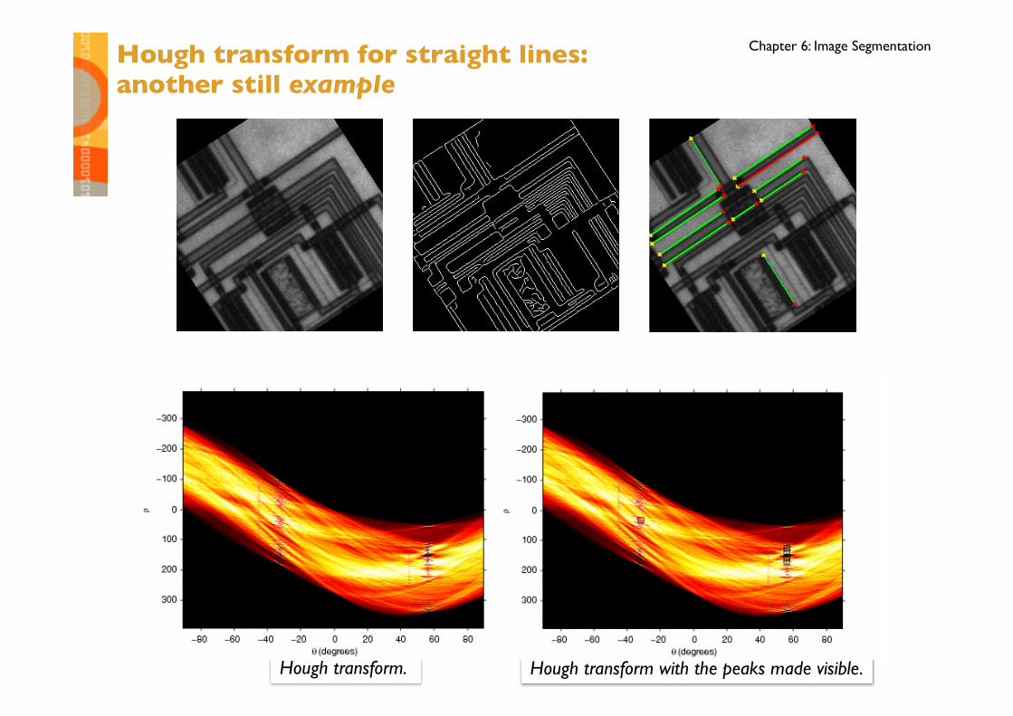
Hough transform with the peaks made visible. Hough transform.
Hough transform for straight lines:���another still example
Chapter 6: Image Segmentation
Hough transform algorithm
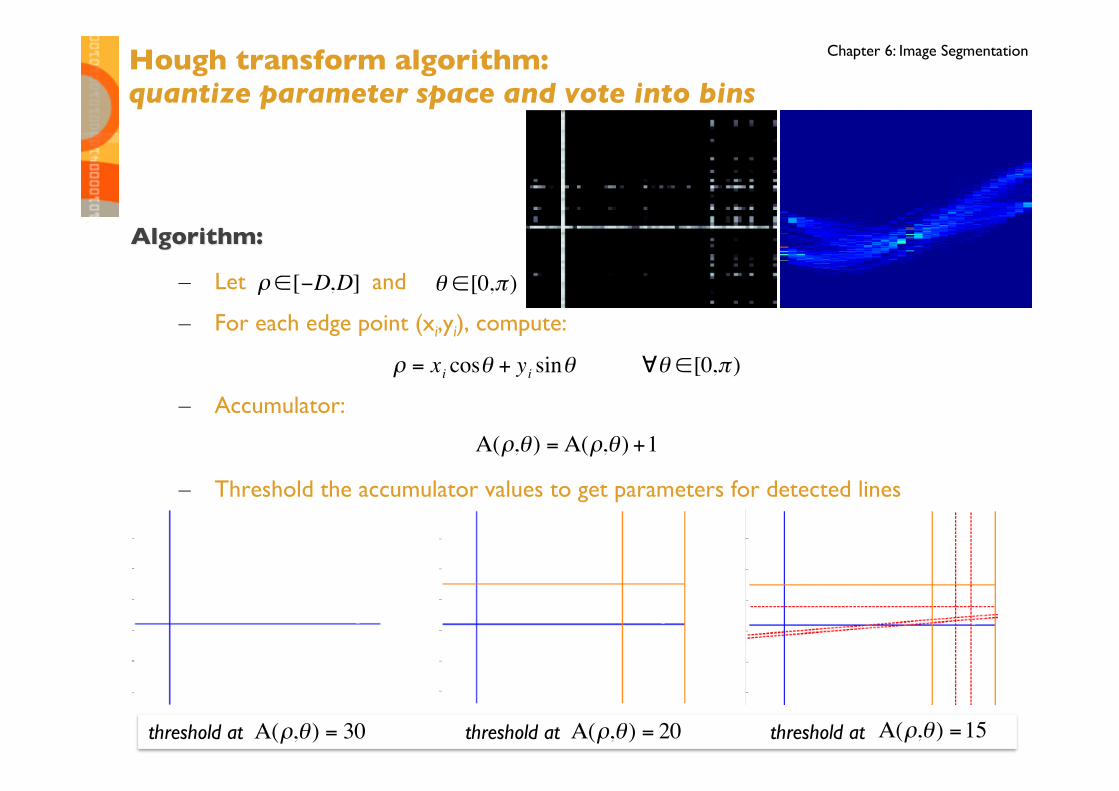
Chapter 6: Image Segmentation Hough transform algorithm:���quantize parameter space and vote into bins
€
ρ ∈[−D,D]
€
θ ∈[0,π )
€
ρ = xi cosθ + yi sinθ ∀θ ∈[0,π )
€
Α(ρ,θ ) = Α(ρ,θ ) +1
threshold at threshold at threshold at
€
Α(ρ,θ ) = 30
€
Α(ρ,θ ) = 20
€
Α(ρ,θ ) =15
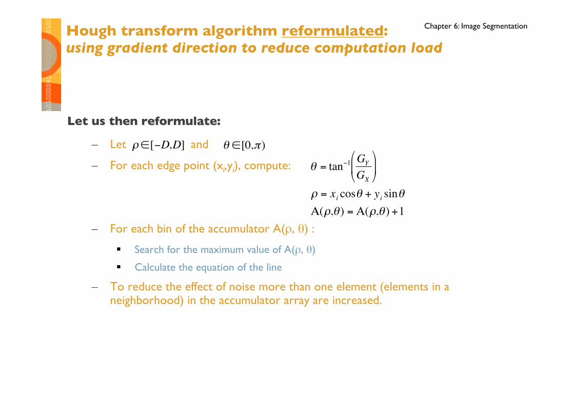
Chapter 6: Image Segmentation Hough transform algorithm reformulated:���using gradient direction to reduce computation load
€
ρ ∈[−D,D]
€
θ ∈[0,π )
€
θ = tan−1 GY
GX
⎛
⎝ ⎜
⎞
⎠ ⎟
ρ = xi cosθ + yi sinθΑ(ρ,θ ) = Α(ρ,θ ) +1
Chapter 6: Image Segmentation
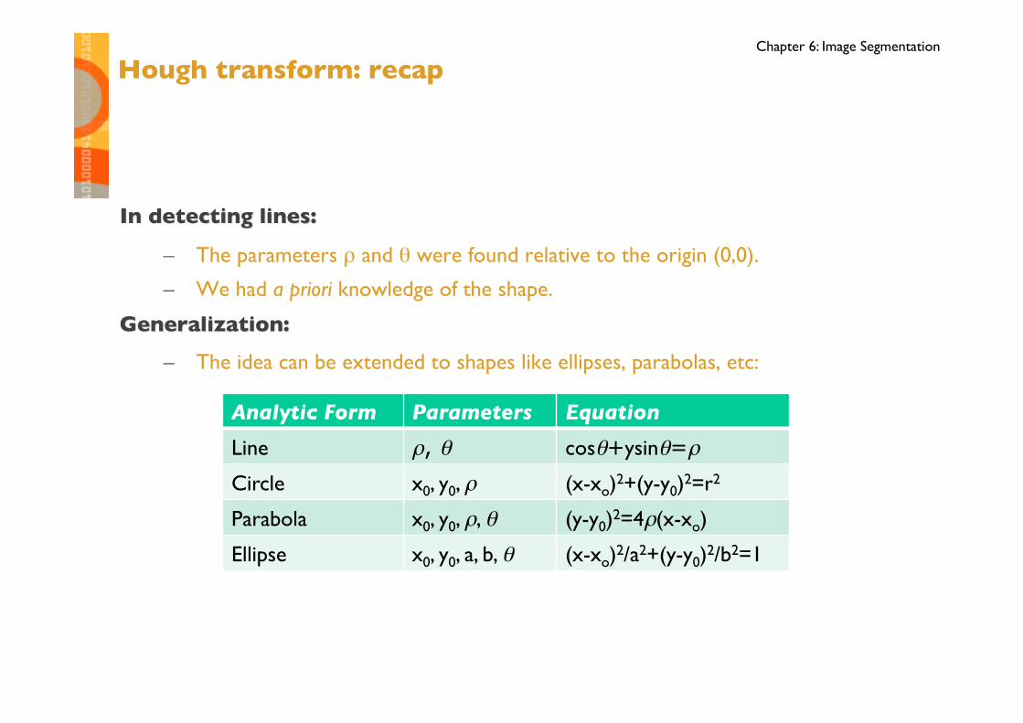
Hough transform: recap
Analytic Form Parameters Equation
Line ρ, θ cosθ+ysinθ=ρ
Circle x0, y0, ρ (x-xo)2+(y-y0)2=r2
Parabola x0, y0, ρ, θ (y-y0)2=4ρ(x-xo)
Ellipse x0, y0, a, b, θ (x-xo)2/a2+(y-y0)2/b2=1
Chapter 6: Image Segmentation
A classification for image segmentation techniques
Chapter 6: Image Segmentation
Chapter 6: Image Segmentation
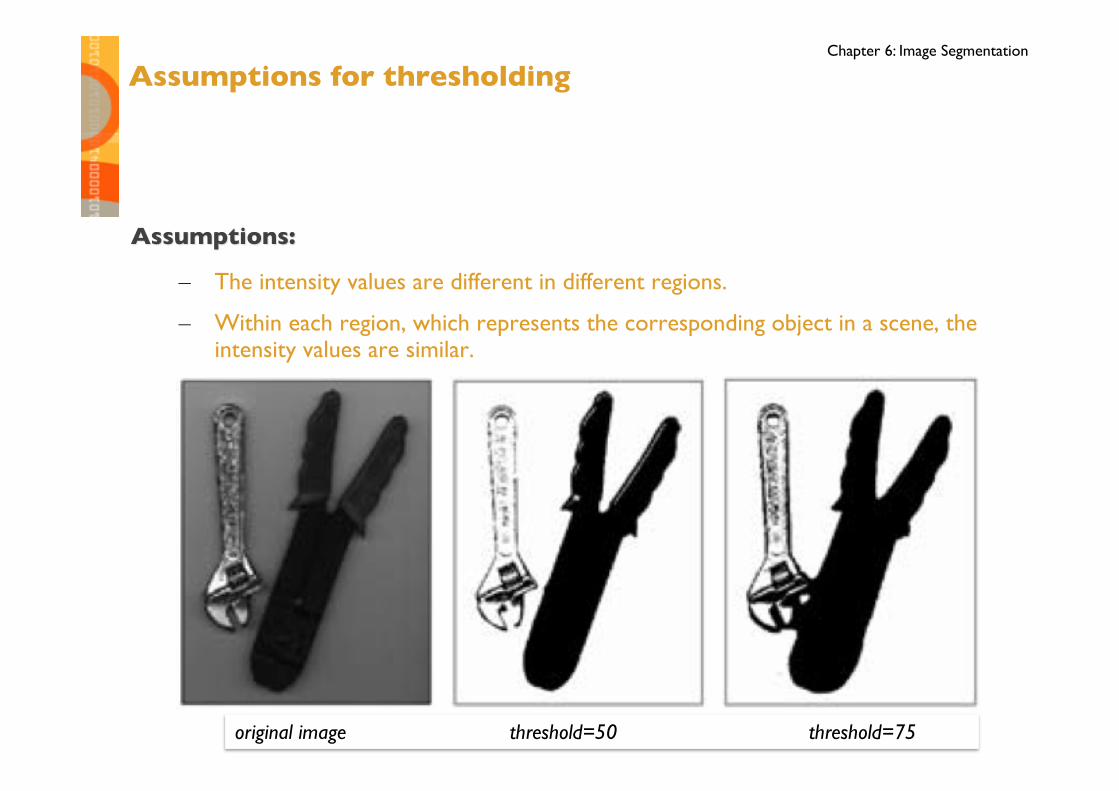
Assumptions for thresholding
original image threshold=50 threshold=75
Chapter 6: Image Segmentation
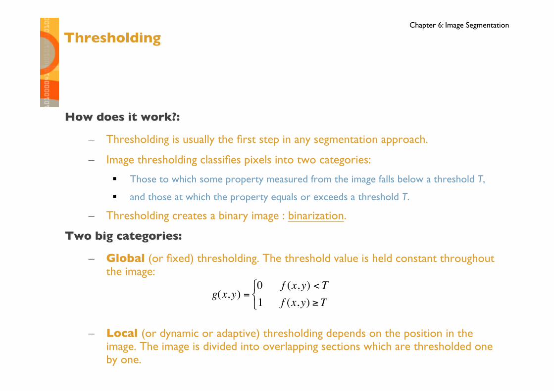
Thresholding
€
g(x,y) =0 f (x,y) < T1 f (x,y) ≥T⎧ ⎨ ⎩
Chapter 6: Image Segmentation
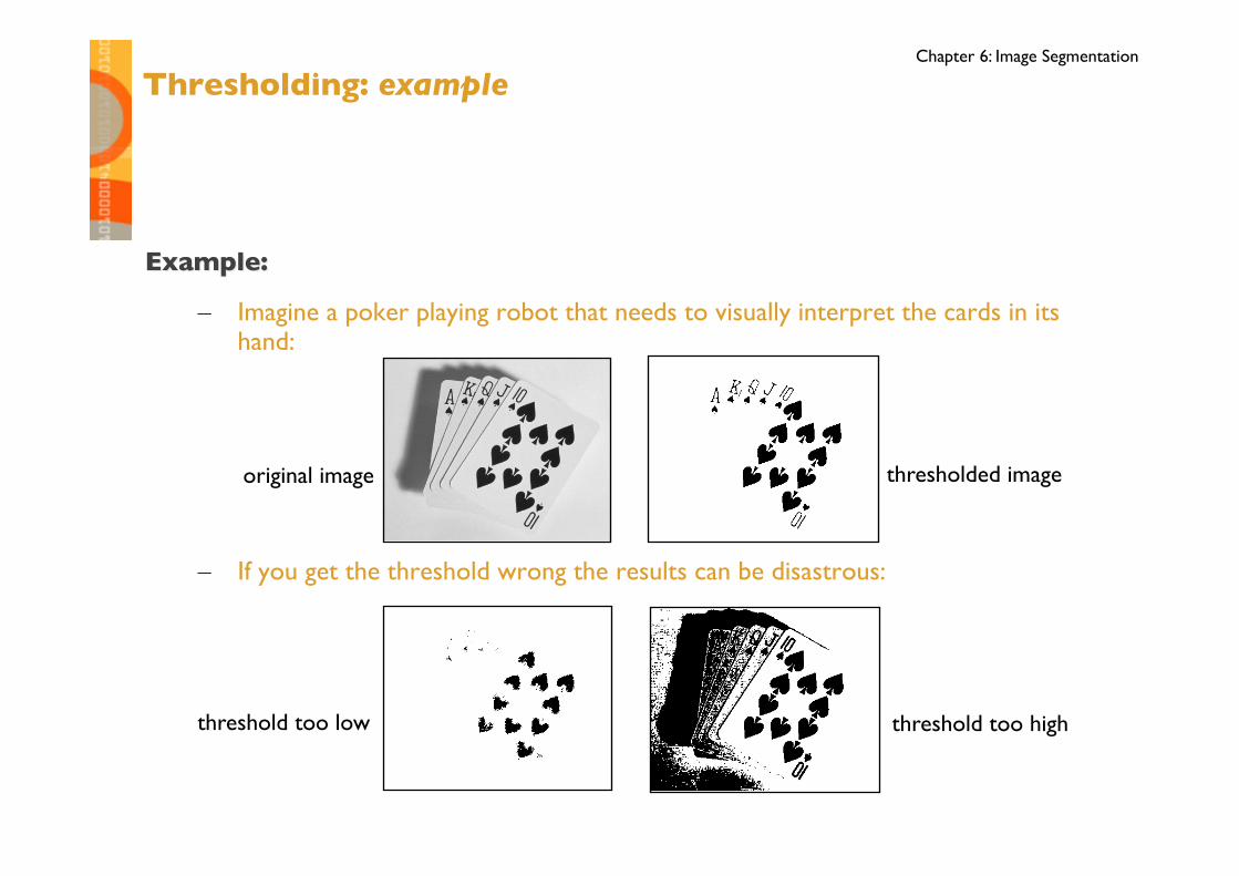
Thresholding: example
original image thresholded image
threshold too low threshold too high
Chapter 6: Image Segmentation
Basic global thresholding
Chapter 6: Image Segmentation
Basic global thresholding: example
Chapter 6: Image Segmentation
Problems with single value thresholding
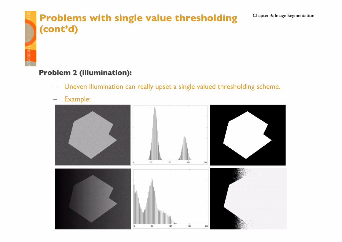
Chapter 6: Image Segmentation Problems with single value thresholding���(cont’d)
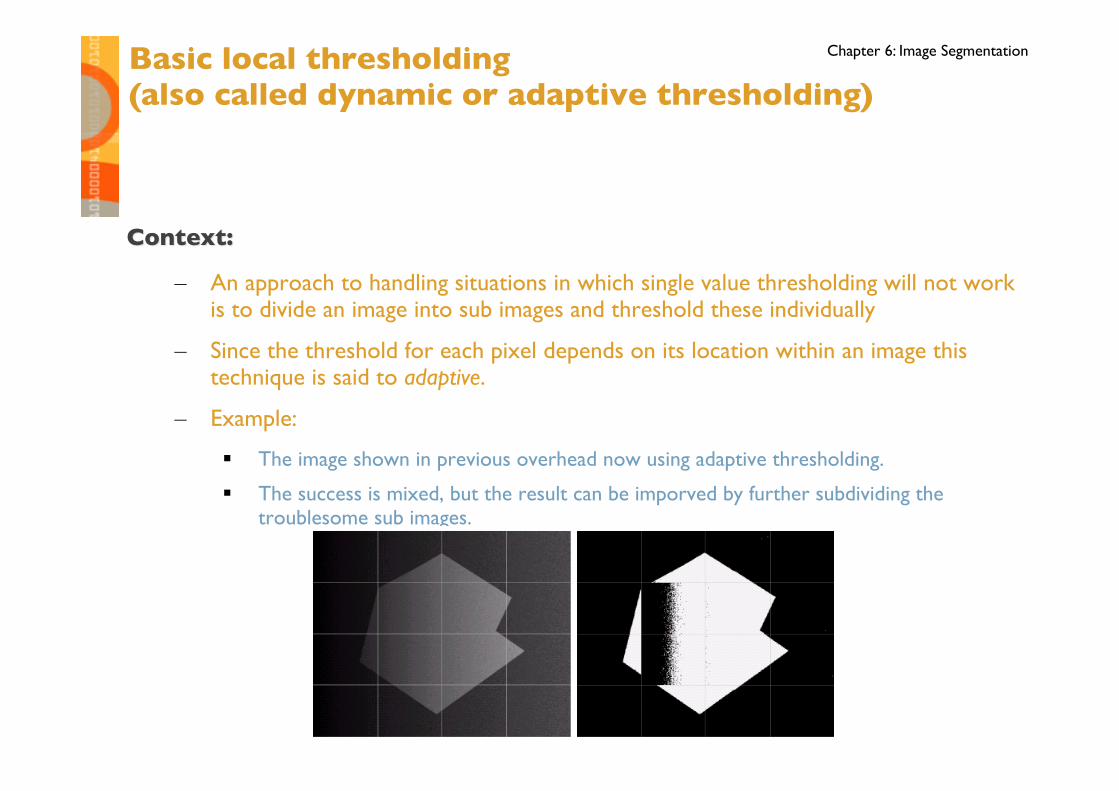
Chapter 6: Image Segmentation Basic local thresholding���(also called dynamic or adaptive thresholding)
Chapter 6: Image Segmentation
Summary: