Closest Pair of Points

Computational Geometry, WS 2006/07Lecture 9, Part II

Prof. Dr. Thomas OttmannKhaireel A. Mohamed

Algorithmen & Datenstrukturen, Institut für InformatikFakultät für Angewandte WissenschaftenAlbert-Ludwigs-Universität Freiburg

Computational Geometry, WS 2006/07Prof. Dr. Thomas Ottmann 2

Overview

• Motivation• Closest Pair algorithms

– Improving the naïve runtime– Divide and Conquer– Scan Line

• Analyses

Computational Geometry, WS 2006/07Prof. Dr. Thomas Ottmann 3

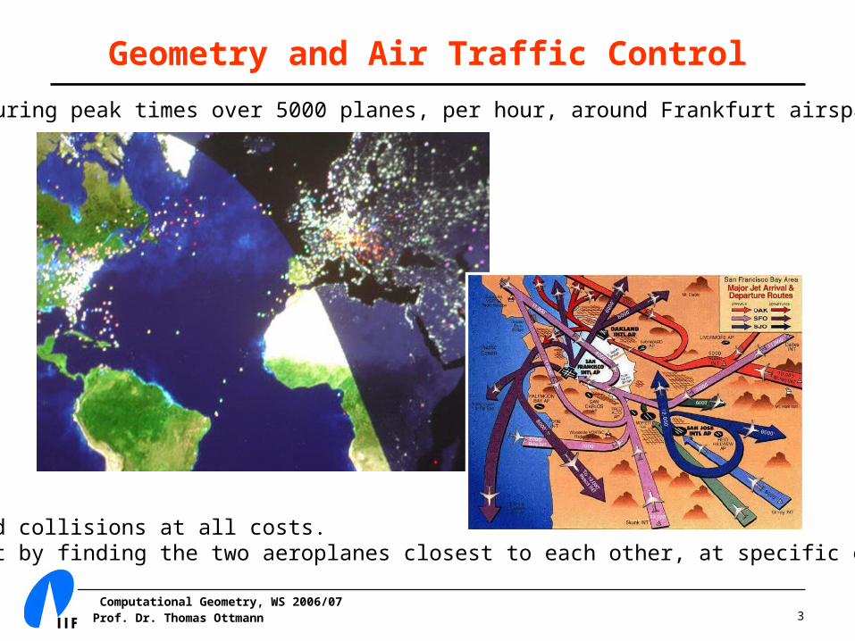
Geometry and Air Traffic Control

» Avoid collisions at all costs.» Start by finding the two aeroplanes closest to each other, at specific elevations.

» During peak times over 5000 planes, per hour, around Frankfurt airspace.

Computational Geometry, WS 2006/07Prof. Dr. Thomas Ottmann 4

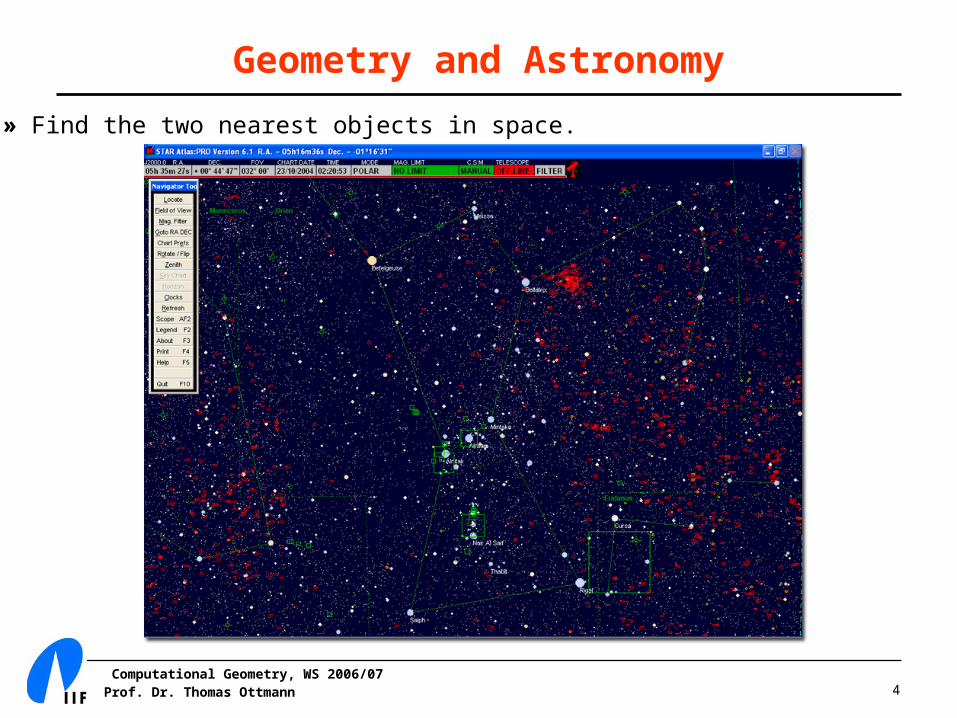
Geometry and Astronomy

» Find the two nearest objects in space.

Computational Geometry, WS 2006/07Prof. Dr. Thomas Ottmann 5

Search Quickly… and Why?

» Find the two nearest objects in space.

Computational Geometry, WS 2006/07Prof. Dr. Thomas Ottmann 6

Problem Description

• Input: A set S of n points in the plane.• Output: The pair of points with the shortest Euclidean distance

between them.

• Other applications in fundamental geometric primitive:– Graphics, computer vision, geographic information systems, molecular

modeling

– Special case of nearest neighbour, Euclidean MST, Voronoi

Computational Geometry, WS 2006/07Prof. Dr. Thomas Ottmann 7

Closest Pair of Points

• Naïve method: Brute force.– Check all pair of points p and q with Θ(n2) comparisons.

• 1D version– Simple if all points are on a single line.

– Run time O(n log n)

Key to reducing quadratic runtime of the naïve method:

Simply don´t visit each point n times.

Computational Geometry, WS 2006/07Prof. Dr. Thomas Ottmann 8

Algorithm: DAC – Divide

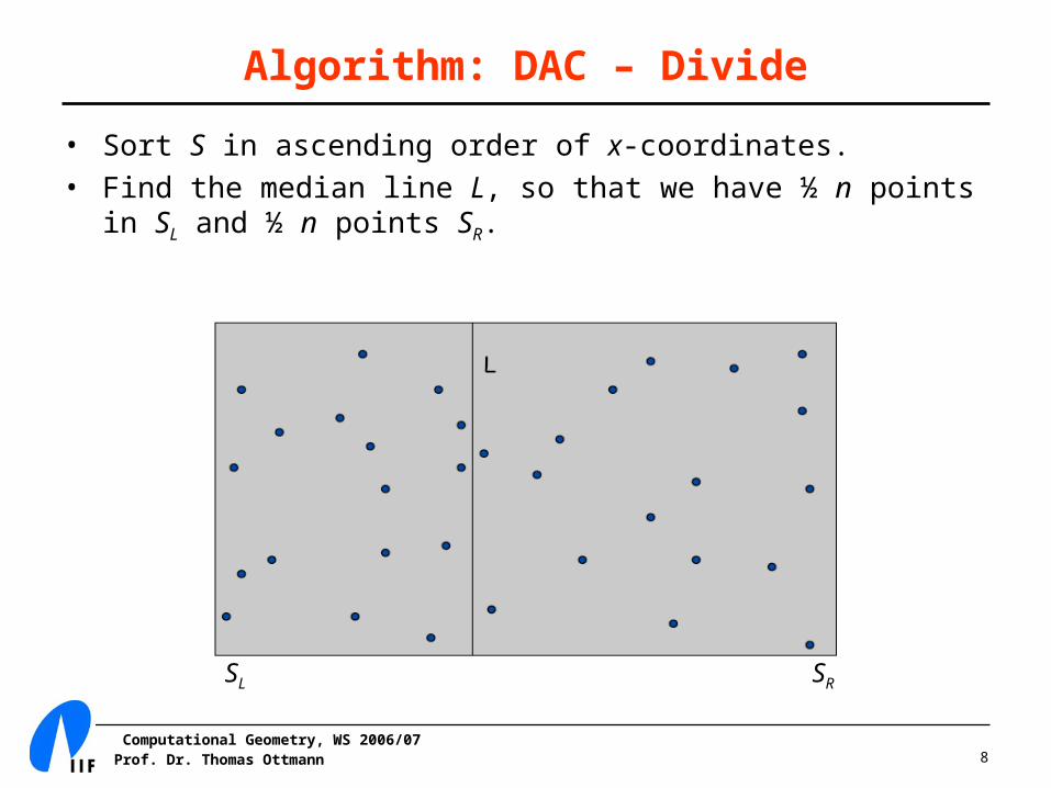
• Sort S in ascending order of x-coordinates.

• Find the median line L, so that we have ½ n points in SL and ½ n points SR.

SL SR

Computational Geometry, WS 2006/07Prof. Dr. Thomas Ottmann 9

Algorithm: DAC – Conquer

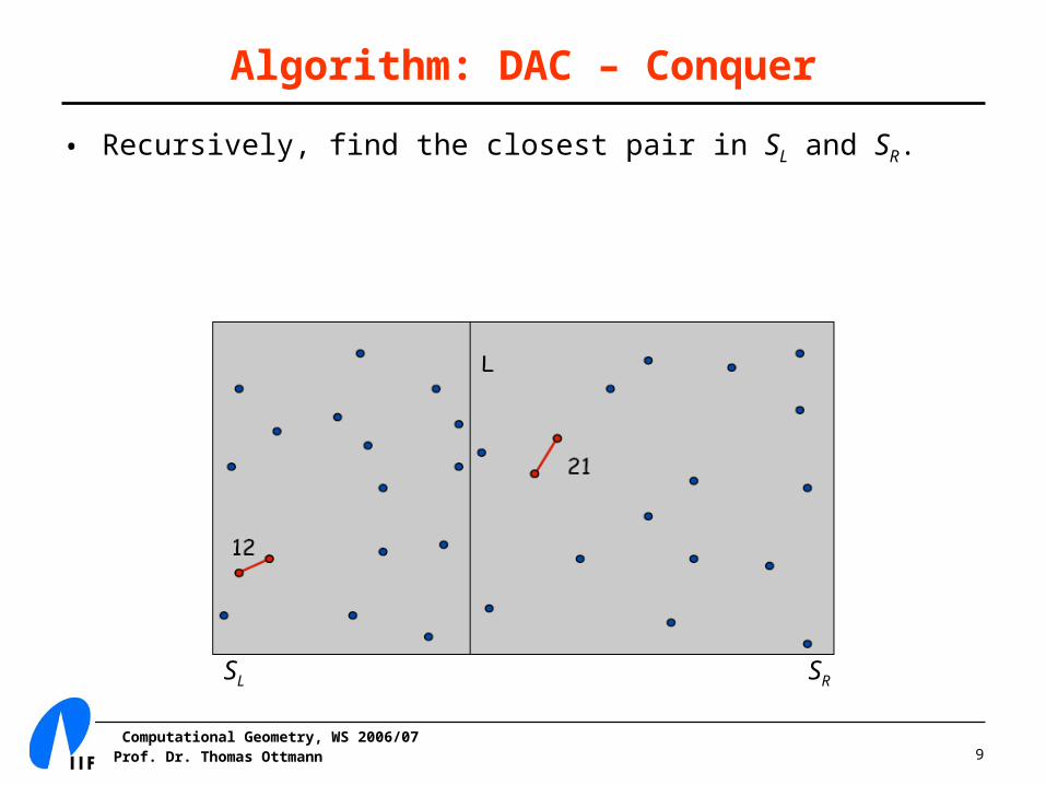
• Recursively, find the closest pair in SL and SR.

SL SR

Computational Geometry, WS 2006/07Prof. Dr. Thomas Ottmann 10

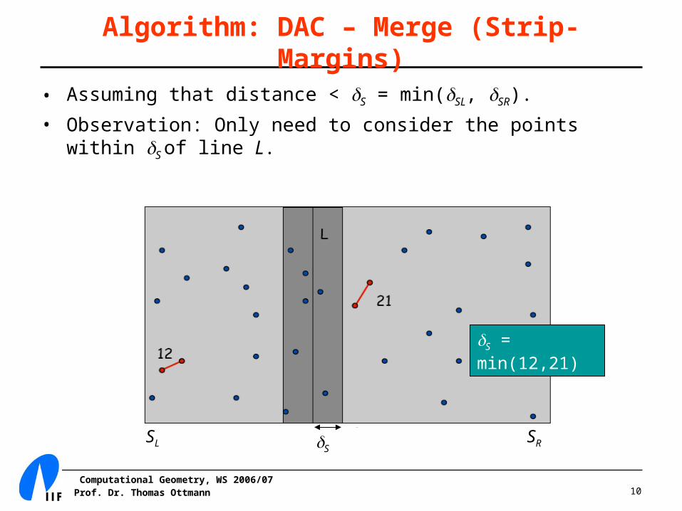
Algorithm: DAC – Merge (Strip-Margins)

• Assuming that distance < S = min(SL, SR).

• Observation: Only need to consider the points within S of line L.

SL SRS

S = min(12,21)

Computational Geometry, WS 2006/07Prof. Dr. Thomas Ottmann 11

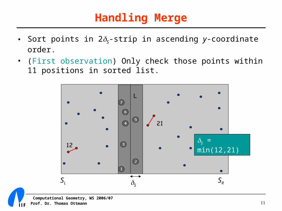
Handling Merge

• Sort points in 2S-strip in ascending y-coordinate order.

• (First observation) Only check those points within 11 positions in sorted list.

SL SRS

S = min(12,21)

Computational Geometry, WS 2006/07Prof. Dr. Thomas Ottmann 12

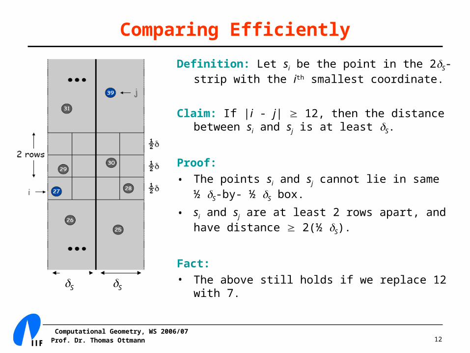
Comparing Efficiently

Definition: Let si be the point in the 2S-strip with the ith smallest coordinate.

Claim: If |i - j| 12, then the distance between si and sj is at least S.

Proof:

• The points si and sj cannot lie in same ½ S-by- ½ S box.

• si and sj are at least 2 rows apart, and have distance 2(½ S).

Fact:

• The above still holds if we replace 12 with 7.SS

Computational Geometry, WS 2006/07Prof. Dr. Thomas Ottmann 13

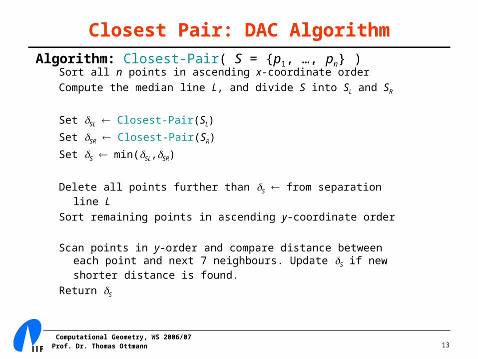
Closest Pair: DAC Algorithm

Algorithm: Closest-Pair( S = {p1, …, pn} )Sort all n points in ascending x-coordinate order

Compute the median line L, and divide S into SL and SR

Set SL Closest-Pair(SL)

Set SR Closest-Pair(SR)

Set S min(SL,SR)

Delete all points further than S from separation line L

Sort remaining points in ascending y-coordinate order

Scan points in y-order and compare distance between each point and next 7 neighbours. Update S if new shorter distance is found.

Return S

Computational Geometry, WS 2006/07Prof. Dr. Thomas Ottmann 14

Closest Pair: DAC Analysis

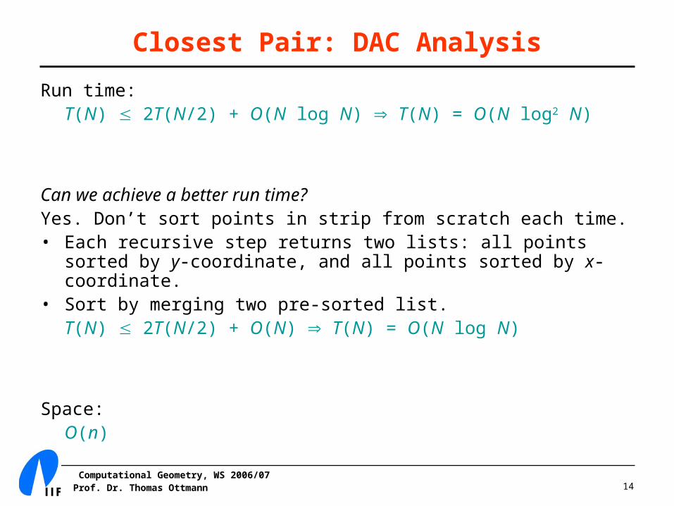
Run time:T(N) 2T(N/2) + O(N log N) T(N) = O(N log2 N)

Can we achieve a better run time?Yes. Don’t sort points in strip from scratch each time.• Each recursive step returns two lists: all points sorted by y-

coordinate, and all points sorted by x-coordinate.• Sort by merging two pre-sorted list.

T(N) 2T(N/2) + O(N) T(N) = O(N log N)

Space:O(n)

Computational Geometry, WS 2006/07Prof. Dr. Thomas Ottmann 15

Algorithm: Scan-Line

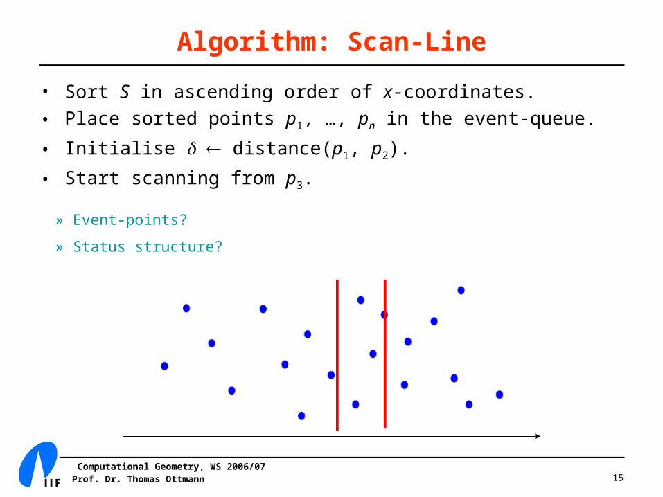
• Sort S in ascending order of x-coordinates.

• Place sorted points p1, …, pn in the event-queue.

• Initialise distance(p1, p2).

• Start scanning from p3.

» Event-points?

» Status structure?

Computational Geometry, WS 2006/07Prof. Dr. Thomas Ottmann 16

The Status-Structure

• Maintain the status-structure (-slab): – Insert the new event-point pi.

– Remove all points that are greater than distance to the left of the current event-point pi.

– All points in the status structure are maintained in ascending y-coordinate order.

Computational Geometry, WS 2006/07Prof. Dr. Thomas Ottmann 17

The Status-Structure

• Maintain the status-structure (-slab): – Insert the new event-point pi.

– Remove all points that are greater than distance to the left of the current event-point pi.

– All points in the status structure are maintained in ascending y-coordinate order.

– Perform the ‘Efficient Comparison’, as described earlier, BUT only between the new event point pi and at most 7 other nearest points to pi.

– Update if a shorter distance is found.

Computational Geometry, WS 2006/07Prof. Dr. Thomas Ottmann 18

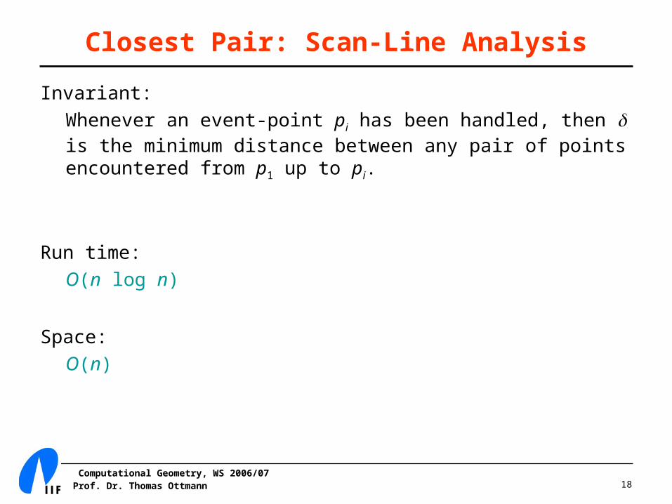
Closest Pair: Scan-Line Analysis

Invariant:

Whenever an event-point pi has been handled, then is the minimum distance between any pair of points encountered from p1 up to pi.

Run time:

O(n log n)

Space:

O(n)

Computational Geometry, WS 2006/07Prof. Dr. Thomas Ottmann 19

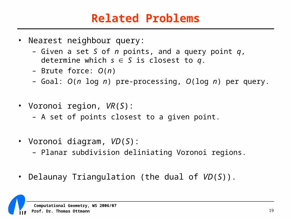
Related Problems

• Nearest neighbour query:– Given a set S of n points, and a query point q,

determine which s S is closest to q.

– Brute force: O(n)

– Goal: O(n log n) pre-processing, O(log n) per query.

• Voronoi region, VR(S): – A set of points closest to a given point.

• Voronoi diagram, VD(S):– Planar subdivision deliniating Voronoi regions.

• Delaunay Triangulation (the dual of VD(S)).