Embed Size (px)
Citation preview

Cold atom physics usingultra-thin optical fibres
Dissertation
zurErlangung des Doktorgrades (Dr. rer. nat.)
derMathematisch-Naturwissenschaftlichen Fakultat
derRheinischen Friedrich-Wilhelms-Universitat Bonn
vorgelegt von
Guillem Sague Cassany
aus
Barcelona
Bonn 2008

Angefertigt mit Genehmigungder Mathematisch-Naturwissenschaftlichen Fakultatder Rheinischen Friedrich-Wilhelms-Universitat Bonn
1. Gutachter: Prof. Dr. Dieter Meschede2. Gutachter: Prof. Dr. Arno Rauschenbeutel
Tag der Promotion: 15.12.2008Erscheinungsjahr: 2009
Dieser Forschungsbericht ist auf dem Hochschulschriftenserver der ULBBonn http://hss.ulb.uni-bonn.de/diss_online elektronisch publiziert.


Dedicat al meu germa Joan.

Summary/Zusammenfassung
In this thesis I present experiments concerning the investigation and manipulation of coldneutral atoms using ultra-thin optical fibres with a diameter smaller than the wavelengthof the guided light. In such a fibre-field configuration the guided light exhibits a largeevanescent field that penetrates into the free-space surrounding the fibre thus enablingto couple laser cooled atoms to the fibre mode. By trapping and cooling caesium atomsin a magneto-optical trap formed around the fibre I investigated the interaction of theatoms with the evanescent field at sub-micrometre distances from the fibre surface.
Chapters 1 and 2 provide the theoretical foundations of this work. Chapter 1 describesthe propagation of light in optical fibres. The general solution of the Maxwell’s equationsin the fibre that complements the description is provided in Appendix A. In Chapter 2,the theory of the interaction of atoms with time-varying electric fields is described.
In Chapter 3 the resonant interaction of laser cooled caesium atoms with the evanescentfield of a probe laser launched through a 500-nm diameter fibre is studied. A detailedanalysis of the atomic absorption at sub-micrometre distances from the fibre surfaceis given. I have performed Monte-Carlo simulations of atomic trajectories inside thecold atom cloud surrounding the fibre. From the simulations, the atomic density atthe vicinity of the fibre is deduced and the absorbance profiles of the atoms measuredduring the experiments can be modelled. By carefully investigating the linewidths ofthese profiles, clear evidence of dipole forces, van der Waals interaction, and a significantenhancement of the spontaneous emission rate of the atoms is found.
The atomic spontaneous emission into the guided mode of a 500-nm diameter opticalfibre is the focus of Chapter 4. Here, I show that the fibre can be used as an efficienttool to collect and guide the spontaneous emission of the atoms.
The dipole force induced by the evanescent field on the atoms is the central idea of theexperiments performed in Chapter 5. I have built a new version of the experimentalsetup that opens the route towards atom trapping in the evanescent field in an array ofsurface microtraps around the fibre. Such traps are created by the combination of twolaser fields with opposite sign of the detuning with respect to the excitation frequencyof the atoms. The first experimental results reporting the influence of the two-colourevanescent field on the spectral properties of the atoms are presented.
Die vorliegende Arbeit berichtet uber Experimente zur Untersuchung und Manipulationkalter neutraler Atome mittels ultradunner Glasfasern, deren Durchmesser kleiner als dieWellenlange des gefuhrten Lichts ist. In dieser Konfiguration besitzt die gefuhrte Faser-mode ein starkes evaneszentes Feld, das in den freien Raum um die Faser hineinreichtund damit die Kopplung kalter Casiumatome ermoglicht.
Die Kapitel 1 und 2 liefern die theoretischen Grundlagen dieser Dissertation. In Kapitel 1werden die Eigenschaften der Lichtleitung in Glasfasern beschrieben. Die allgemeineLosung der Maxwellgleichungen in der Faser liefert Anhang A. In Kapitel 2 wird dieTheorie der Wechselwirkung neutraler Atome mit einem zeitabhangigen elektrischenFeld behandelt.
In Kapitel 3 wird die Wechselwirkung lasergekulter Atome mit dem evaneszenten Feldresonanter Laserstrahlung untersucht, die in einer Glasfaser mit einem Durchmesservon 500 nm geleitet wird. Es wird eine detaillierte Analyse der atomaren Absorption ineiner Submikrometerentfernung von der Faseroberflache prasentiert. Ich habe Monte-Carlo Simulationen von Trajektorien der lasergekuhlten Atome durchgefuhrt. Darauskann die atomare Dichte in der Nahe der Faser abgeleitet werden. Dies erlaubt dieModellierung der gemessenen atomaren Absorbanzkurven. Eine sorfaltige Untersuchungder Linienbreite solcher Absorbanzkurven liefert eine deutliche Signatur lichtinduzierterDipolkrafte, der van der Waals Kraft und einer Erhohung der spontanen Emissionsrateder Atome.
Die spontane Emission in die Mode einer ultradunnen Glasfaser steht im Zentrum vonKapitel 4. Hier untersuche ich die Effizienz solcher Fasern als Werkzeug zum Sammelnund Ubertragen atomarer spontanen Emission.
Die durch das evaneszente Feld induzierte Dipolkraft ist der Kerngedanke des Exper-iments von Kapitel 5. Ich habe eine erweiterte Version des expereimentellen Aufbausentwickelt, die den Weg zum Fangen von Casiumatomen im evaneszenten Feld der Fasergeebnet hat. Solche Fallen bestehen aus einer Kombination von zwei Lasern mit entge-gengesetzter Verstimmung gegenuber der atomaren Anregungsfrequenz. Zudem werdendie ersten Messungen des spektralen Einflusses des zweifarbigen evaneszenten Feldes aufdie kalte Atomwolke prasentiert.
Parts of this thesis have been published in the following journal articles:
1. G. Sague, E. Vetsch, W. Alt, D. Meschede and A. Rauschenbeutel, Cold Atom
Physics Using Ultra-Thin Optical Fibers: Light-Induced Dipole Forces and Surface
Interactions, Phys. Rev. Lett. 99, 163602 (2007).
2. G. Sague, A. Baade and A. Rauschenbeutel, Blue-detuned evanescent field surface
traps for neutral atoms based on mode interference in ultra-thin optical fibres, NewJ. Phys. 10 113008 (2008).
Contents
Introduction 1
1 Light propagation in step-index optical fibres 3
1.1 Ray propagation in optical fibres . . . . . . . . . . . . . . . . . . . . . . 4
1.1.1 Numerical aperture of a fibre . . . . . . . . . . . . . . . . . . . . 4
1.1.2 Hybrid and Transverse modes . . . . . . . . . . . . . . . . . . . . 5
1.2 Solutions for the fields in an optical fibre . . . . . . . . . . . . . . . . . . 6
1.2.1 The fundamental HE11 mode: Rotating polarisation . . . . . . . 10
1.2.2 The fundamental HE11 mode: Quasi-linear polarisation . . . . . 18
1.2.3 Evanescent field strength in the HE11 mode: Quasi-linear polari-sation . . . . . . . . . . . . . . . . . . . . . . . . . . . . . . . . . 21
1.2.4 The TE01 mode . . . . . . . . . . . . . . . . . . . . . . . . . . . . 22
1.3 Tapered optical fibres (TOF’s) . . . . . . . . . . . . . . . . . . . . . . . 26
1.3.1 Flame-pulling of optical fibres . . . . . . . . . . . . . . . . . . . . 27
1.3.2 Measurement of the transmission . . . . . . . . . . . . . . . . . . 28
1.3.3 Measurement of the local diameter and the surface quality of a TOF 30
2 Theory of the atom-field interaction 33
2.1 Classical model of the atom-field interaction . . . . . . . . . . . . . . . . 33
2.1.1 Scattering rate . . . . . . . . . . . . . . . . . . . . . . . . . . . . 34
2.1.2 Dipole force . . . . . . . . . . . . . . . . . . . . . . . . . . . . . . 35
2.2 Near-resonant atom-field interaction . . . . . . . . . . . . . . . . . . . . 35
2.2.1 Scattering rate . . . . . . . . . . . . . . . . . . . . . . . . . . . . 36
2.2.2 Dipole force . . . . . . . . . . . . . . . . . . . . . . . . . . . . . . 37
2.3 Far detuned atom-field interaction . . . . . . . . . . . . . . . . . . . . . 38
2.3.1 Semiclassical approach . . . . . . . . . . . . . . . . . . . . . . . . 38
2.3.2 Light shifts in multilevel atoms . . . . . . . . . . . . . . . . . . . 39
3 Evanescent field spectroscopy on cold caesium atoms 41
3.1 Introduction . . . . . . . . . . . . . . . . . . . . . . . . . . . . . . . . . . 41
3.2 Experimental setup . . . . . . . . . . . . . . . . . . . . . . . . . . . . . . 42
3.3 A caesium magneto-optical trap around an ultra-thin optical fibre . . . 45
3.3.1 Magneto-optical trap for caesium atoms . . . . . . . . . . . . . . 46
3.3.2 Tools for embedding and manipulating an ultra-thin optical fibrein UHV . . . . . . . . . . . . . . . . . . . . . . . . . . . . . . . . 51
3.3.3 Positioning of the fibre and the MOT . . . . . . . . . . . . . . . 55
3.4 Tools for atom detection . . . . . . . . . . . . . . . . . . . . . . . . . . . 57
3.5 Experimental sequence . . . . . . . . . . . . . . . . . . . . . . . . . . . . 58
3.5.1 Timing sequence of the experiment . . . . . . . . . . . . . . . . . 59
3.6 Experimental results . . . . . . . . . . . . . . . . . . . . . . . . . . . . . 60
3.6.1 Data analysis . . . . . . . . . . . . . . . . . . . . . . . . . . . . . 60
3.6.2 Absorbance on resonance as a function of the probe power . . . . 62
3.6.3 Time-of-flight measurements of the cold atom cloud using a TOF 63
3.6.4 Frequency-dependent absorbance of the cold atom cloud . . . . . 64
3.6.5 Linewidths vs incident power: Light-induced dipole forces andatom-surface interactions . . . . . . . . . . . . . . . . . . . . . . 67
3.7 Model for the interaction of cold atoms with the evanescent field . . . . 69
3.7.1 Reduced model . . . . . . . . . . . . . . . . . . . . . . . . . . . . 69
3.7.2 Surface interactions between a neutral atom and a dielectric fibre 71
3.7.3 Monte-Carlo simulations of the relative density of the atom cloud 78
3.7.4 Modelling of the absorbance profiles . . . . . . . . . . . . . . . . 81
3.8 Comparison between the model and the experimental results . . . . . . 83
4 Probing the fluorescence of laser cooled atoms 89
4.1 Emission rate into the guided mode . . . . . . . . . . . . . . . . . . . . . 93
5 Towards atom-trapping in evanescent field dipole traps 97
5.1 Two-colour evanescent field dipole trap . . . . . . . . . . . . . . . . . . . 98
5.1.1 Linearly polarised fields . . . . . . . . . . . . . . . . . . . . . . . 98
5.1.2 Circularly polarised fields . . . . . . . . . . . . . . . . . . . . . . 104
5.2 Experimental Setup . . . . . . . . . . . . . . . . . . . . . . . . . . . . . 106
5.2.1 Polarisation maintaining TOF . . . . . . . . . . . . . . . . . . . 108
5.2.2 Dipole lasers . . . . . . . . . . . . . . . . . . . . . . . . . . . . . 113
5.3 Experimental results . . . . . . . . . . . . . . . . . . . . . . . . . . . . . 114
5.3.1 Light-induced shifts . . . . . . . . . . . . . . . . . . . . . . . . . 114
Conclusions 117
6 Outlook 119
6.1 External dipole trap to approach the atoms to the fibre . . . . . . . . . 119
6.2 Blue-detuned evanescent field traps based on two-mode interference . . 122
6.2.1 Modal dispersion and polarisation configuration . . . . . . . . . . 122
6.2.2 HE11+TE01 trap . . . . . . . . . . . . . . . . . . . . . . . . . . . 123
A Maxwell’s equations in a step-index circular optical fibre 127
List of Figures 137
List of Tables 139
Bibliography 141
Acknowledgements 149

Introduction
The interaction of light and matter at the fundamental level, where a single photonefficiently interacts with a single atom, has been one of the main research topics inquantum optics over the last decades [1–3]. Since the absorption cross-section of thean atom on resonance is on the order of the wavelength of the absorbed light (∼ λ2)such interaction is in general very weak [4]. Many approaches have been conceived toenhance this interaction. One possibility is to use high atomic densities to store singlephotons in a whole ensemble of atoms as a collective single-photon excitation [5–7]. An-other possibility is to modify, tailor or store the light field used for the interaction. Inthis context, one of the most widely used approaches to tackle the problem is the useof resonant structures [8–10]: One photon trapped in a high finesse resonator, passesthrough the position of the atom a few million times before leaking out from the cavity,thereby increasing the coupling probability [11]. Moreover, the use of dielectric struc-tures such as microspheres or microtoroids to store the light propagating in whisperinggallery modes has undergone high development in recent years [12, 13]. This approachhas, in addition, the advantage that such dielectric structures are cheap, robust andscalable [14], which is a necessary condition for building a quantum computer [15].
Nevertheless, the 3-dimensional confinement is not a requirement to increase the inter-action between light and matter using tailored light fields. For example, a laser beamwhich is strongly focused at the position of the atom also leads to an enhanced atom-photon coupling [16]. This method has, however, some limitations due to, e. g., thenon-uniformity of the polarisation of the field at the focus [17]. Indeed, the photon thatinduces an absorption with 100% probability must reproduce the spatial, temporal andpolarisation properties of the atomic radiation. This requirement has been assessed in arecent theoretical proposal where a laser beam is focused in such a way that the emissionpattern of a classical dipole is reproduced at the focal point of a parabolic mirror [18].
Waveguides and prisms are also suited to tailor light fields and use them to coupleatoms. In this case, the interaction takes place in the optical near field close to thesurface of the dielectric [19], leading to modified spectral and radiative properties of theatoms [20]. The evanescent field arising from the internal reflection of a laser beam in aprism has been used in several experiments to investigate and cool alkali atoms at a fewmicrometres above the surface of the dielectric [21–23]. Many other efforts have beenfocused on the mechanical control of atoms using the strong non-dissipative forces arising
2 Introduction
in non-resonant evanescent fields. Evanescent wave mirrors for neutral atoms [24, 25]and atom trapping above dielectric waveguides [26–28] are some examples. The latterhas not been yet experimentally demonstrated.
Optical fibres also count among the dielectric structures that enable tailoring of thepropagation properties of the light. The light guided in the core of a standard telecom-munications optical fibre is isolated from the environment allowing low loss transmissionover long distances [29]. This property has not only been used in telecommunicationsbut also in quantum optics experiments to, e. g., demonstrate the quantum interferenceof two indistinguishable photons [30] or to transmit quantum cryptography keys encodedin the polarisation of the emitted photons [31]. On the other hand, the use of opticalfibres to enhance and control the interaction between light and matter is an innovativeaspect that has recently attracted much attention [32–35]. In this work I demonstratethat ultra-thin optical fibres are good candidates for this issue.
Standard telecommunication optical fibres can be tapered in our custom-made pullingfacility at the University of Mainz down to diameters as small as 100 nm [36]. Suchtapered optical fibres (TOF) offer a strong transverse confinement of the guided modewhile exhibiting a pronounced evanescent field surrounding the fibre [37]. This allows toefficiently couple atoms to the guided fibre mode at sub-micrometre distances from thefibre surface [35]. I have built an experimental setup that allows to couple laser-cooledcaesium atoms to the evanescent field by inserting the waist of a 500-nm diameter TOFinto a magneto-optical trap (MOT). A rigorous analysis of the resonant interaction ofthe atoms with the evanescent field as a function of the probe laser power shows clearevidence of light-induced dipole forces and surface interactions (Chapter 3). The latterincludes the van der Waals (v.d.W.) potential and a significant enhancement of thespontaneous emission rate of the atoms near the fibre surface.
Moreover, an ultra-thin optical fibre can be used to probe the fluorescence of laser-cooledatoms in the MOT. The experimental results demonstrate the efficiency of the TOF asa tool to collect and guide the spontaneous emission of the atoms (Chapter 4). Themeasured spontaneous emission rate into the guided mode at the surface of the fibre is,in addition, in good agreement with the theoretical calculations published in [38].
In the last part of my work I describe a new version of the experiment that enables tocouple two additional far-detuned lasers into the fibre following the theoretical proposalfrom [39] (Chapter 5). When the laser fields have two opposite signs of the detuning withrespect to the atomic transition frequency, a two-colour dipole trap for caesium atomsin the evanescent field of an ultra-thin optical fibre can be created. This opens the routetowards atom trapping and manipulation using ultra-thin optical fibres. The creationof ensembles of fibre-coupled atoms at a fixed distance from the fibre surface, is a verypromising framework for slow light experiments [40], or the realisation of two-photongates in non-linear media [41].
Chapter 1
Light propagation in step-indexoptical fibres
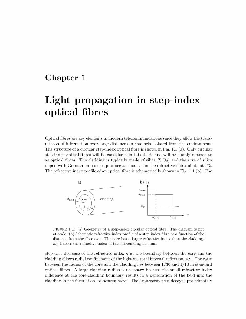
Optical fibres are key elements in modern telecommunications since they allow the trans-mission of information over large distances in channels isolated from the environment.The structure of a circular step-index optical fibre is shown in Fig. 1.1 (a). Only circularstep-index optical fibres will be considered in this thesis and will be simply referred toas optical fibres. The cladding is typically made of silica (SiO2) and the core of silicadoped with Germanium ions to produce an increase in the refractive index of about 1%.The refractive index profile of an optical fibre is schematically shown in Fig. 1.1 (b). The
core cladding
acore
acore
aclad
aclad
ncore
nclad
n0
n
r
a) b)
Figure 1.1: (a) Geometry of a step-index circular optical fibre. The diagram is notat scale. (b) Schematic refractive index profile of a step-index fibre as a function of thedistance from the fibre axis. The core has a larger refractive index than the cladding.n0 denotes the refractive index of the surrounding medium.
step-wise decrease of the refractive index n at the boundary between the core and thecladding allows radial confinement of the light via total internal reflection [42]. The ratiobetween the radius of the core and the cladding lies between 1/30 and 1/10 in standardoptical fibres. A large cladding radius is necessary because the small refractive indexdifference at the core-cladding boundary results in a penetration of the field into thecladding in the form of an evanescent wave. The evanescent field decays approximately
4 Light propagation in step-index optical fibres
exponentially inside the cladding, allowing part of the light to axially propagate outsidethe core. The presence of light outside the core is one of the theoretical foundations ofthis work and will be extensively treated in the next Chapters. The typical parametersof a standard fibre with the single-mode cut-off at 760 nm (see Sect. 1.2) are shown inTable 1.1. The parameter Θ in Eq. 1.1 is referred to as the numerical aperture of the
Single mode fibre
aclad = 62.5 µm2 µm ≤ acore ≤ 5 µm
nclad = 1.452 (fused quarz)0.06 ≤ Θ ≤ 0.15
Table 1.1: Typical parameters and dimensions of a standard fibre with single-modecutoff at 760 nm. Since the refractive index of silica is frequency dependent [43], thevalue for nclad has been calculated at a wavelength of 852 nm.
fibre and plays a similar role as the numerical aperture of a lens (see Fig. 1.2).
Θ =√
n2core − n2
clad. (1.1)
1.1 Ray propagation in optical fibres
In this section some fundamental properties of light propagation inside optical fibres willbe discussed in the frame of geometric optics: The coupling of light into an optical fibre,characterised by its numerical aperture (NA) (Sec. 1.1.1), and the nature of the differentmodes of propagation in the fibre (Sec. 1.1.2) determined by the exact solutions of theMaxwell equations. Geometric optics provides useful tools for intuitively understandingthese basic principles of light propagation in optical fibres. However, due to the wavecharacter of light some of the features from single-mode and ultra-thin optical fibres,cannot be explained using this interpretation [29]. One should thus keep in mind thatthe results exposed in this section are rather qualitative.
1.1.1 Numerical aperture of a fibre
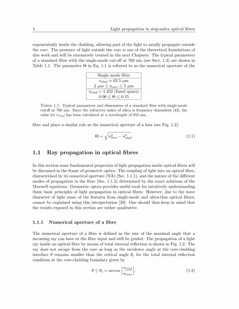
The numerical aperture of a fibre is defined as the sine of the maximal angle that aincoming ray can have at the fibre input and still be guided. The propagation of a lightray inside an optical fibre by means of total internal reflection is shown in Fig. 1.2. Theray does not escape from the core as long as the incidence angle at the core-claddinginterface θ remains smaller than the critical angle θc for the total internal reflectioncondition at the core-cladding boundary given by
θ ≤ θc = arccos[nclad
ncore
]
. (1.2)
1.1 Ray propagation in optical fibres 5
ncore
nclad
n0
θθ0
Figure 1.2: Schematic of the propagation of a light ray in an optical fibre.
Snell’s law determines θ for a given incidence angle θ0 at the fibre input,
n0 sin[θ0] = ncore sin[θ]. (1.3)
Combining Eqns. (1.2) and (1.3), and assuming n0 = 1 the condition for a ray to beguided when entering the fibre reads
sin[θ0] ≤√
n2core − n2
clad. (1.4)
1.1.2 Hybrid and Transverse modes
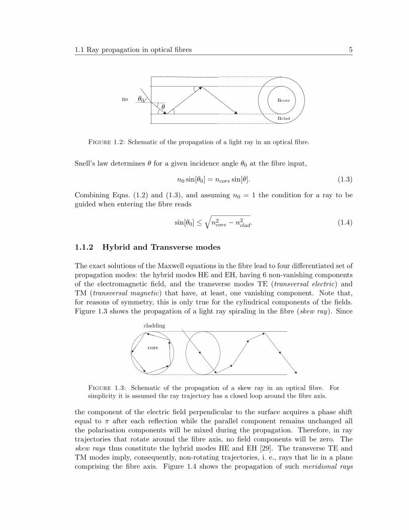
The exact solutions of the Maxwell equations in the fibre lead to four differentiated set ofpropagation modes: the hybrid modes HE and EH, having 6 non-vanishing componentsof the electromagnetic field, and the transverse modes TE (transversal electric) andTM (transversal magnetic) that have, at least, one vanishing component. Note that,for reasons of symmetry, this is only true for the cylindrical components of the fields.Figure 1.3 shows the propagation of a light ray spiraling in the fibre (skew ray). Since
core
cladding
Figure 1.3: Schematic of the propagation of a skew ray in an optical fibre. Forsimplicity it is assumed the ray trajectory has a closed loop around the fibre axis.
the component of the electric field perpendicular to the surface acquires a phase shiftequal to π after each reflection while the parallel component remains unchanged allthe polarisation components will be mixed during the propagation. Therefore, in raytrajectories that rotate around the fibre axis, no field components will be zero. Theskew rays thus constitute the hybrid modes HE and EH [29]. The transverse TE andTM modes imply, consequently, non-rotating trajectories, i. e., rays that lie in a planecomprising the fibre axis. Figure 1.4 shows the propagation of such meridional rays
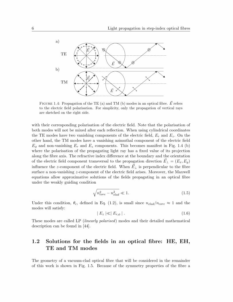
6 Light propagation in step-index optical fibres
TE
TM
~E
~E
~E
~E
a)
b)
Figure 1.4: Propagation of the TE (a) and TM (b) modes in an optical fibre. ~E refersto the electric field polarisation. For simplicity, only the propagation of vertical raysare sketched on the right side.
with their corresponding polarisation of the electric field. Note that the polarisation ofboth modes will not be mixed after each reflection. When using cylindrical coordinatesthe TE modes have two vanishing components of the electric field, Er and Ez. On theother hand, the TM modes have a vanishing azimuthal component of the electric fieldEφ and non-vanishing Er and Ez components. This becomes manifest in Fig. 1.4 (b)where the polarisation of the propagating light ray has a fixed value of its projectionalong the fibre axis. The refractive index difference at the boundary and the orientationof the electric field component transversal to the propagation direction ~E⊥ = (Ex, Ey)
influence the z-component of the electric field. When ~E⊥ is perpendicular to the fibresurface a non-vanishing z-component of the electric field arises. Moreover, the Maxwellequations allow approximative solutions of the fields propagating in an optical fibreunder the weakly guiding condition
√
n2core − n2
clad ≪ 1. (1.5)
Under this condition, θc, defined in Eq. (1.2), is small since nclad/ncore ≈ 1 and themodes will satisfy:
| Ez |≪| Er,φ | . (1.6)
These modes are called LP (linearly polarised) modes and their detailed mathematicaldescription can be found in [44].
1.2 Solutions for the fields in an optical fibre: HE, EH,TE and TM modes
The geometry of a vacuum-clad optical fibre that will be considered in the remainderof this work is shown in Fig. 1.5. Because of the symmetry properties of the fibre a
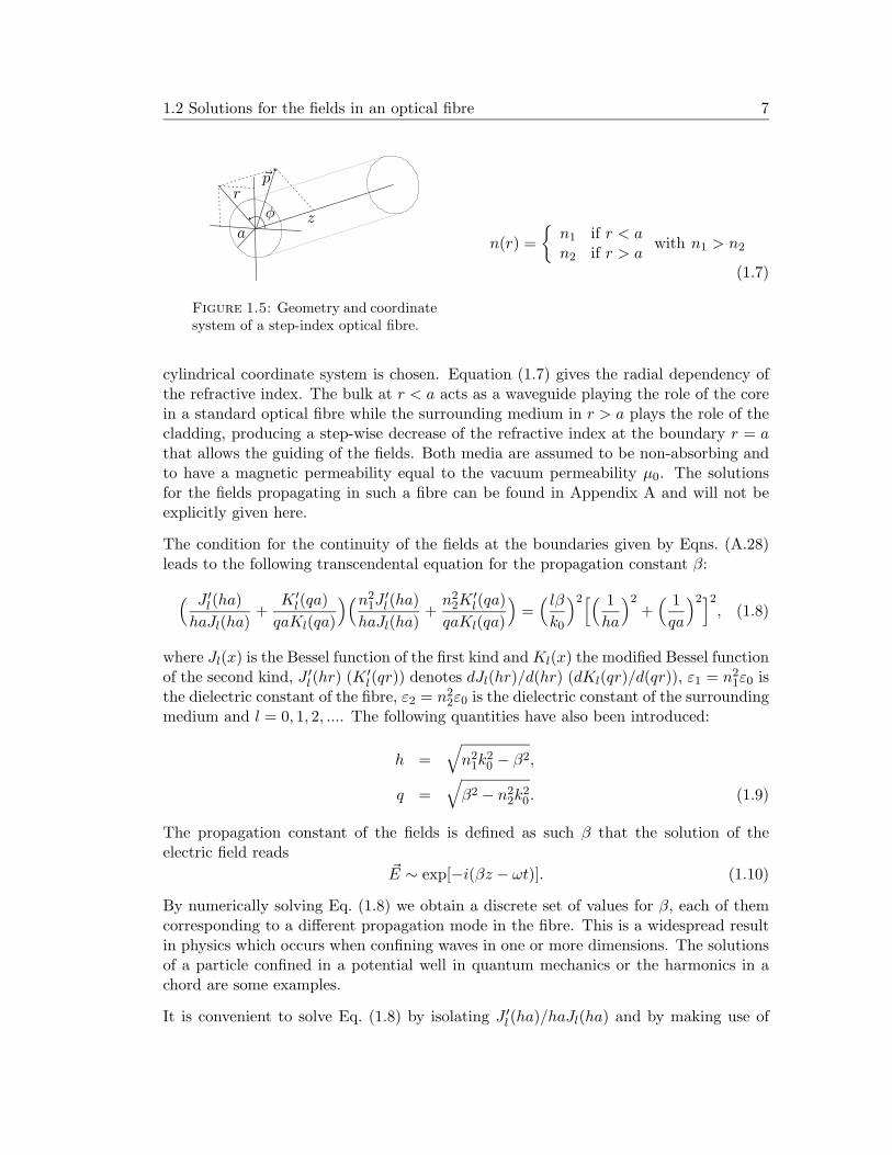
1.2 Solutions for the fields in an optical fibre 7
a
r~p
φ z
Figure 1.5: Geometry and coordinatesystem of a step-index optical fibre.
n(r) =
{
n1 if r < an2 if r > a
with n1 > n2
(1.7)
cylindrical coordinate system is chosen. Equation (1.7) gives the radial dependency ofthe refractive index. The bulk at r < a acts as a waveguide playing the role of the corein a standard optical fibre while the surrounding medium in r > a plays the role of thecladding, producing a step-wise decrease of the refractive index at the boundary r = athat allows the guiding of the fields. Both media are assumed to be non-absorbing andto have a magnetic permeability equal to the vacuum permeability µ0. The solutionsfor the fields propagating in such a fibre can be found in Appendix A and will not beexplicitly given here.
The condition for the continuity of the fields at the boundaries given by Eqns. (A.28)leads to the following transcendental equation for the propagation constant β:
( J ′l (ha)
haJl(ha)+
K ′l(qa)
qaKl(qa)
)(n21J
′l (ha)
haJl(ha)+n2
2K′l(qa)
qaKl(qa)
)
=( lβ
k0
)2[( 1
ha
)2+
( 1
qa
)2]2, (1.8)
where Jl(x) is the Bessel function of the first kind andKl(x) the modified Bessel functionof the second kind, J ′
l (hr) (K ′l(qr)) denotes dJl(hr)/d(hr) (dKl(qr)/d(qr)), ε1 = n2
1ε0 isthe dielectric constant of the fibre, ε2 = n2
2ε0 is the dielectric constant of the surroundingmedium and l = 0, 1, 2, .... The following quantities have also been introduced:
h =√
n21k
20 − β2,
q =√
β2 − n22k
20. (1.9)
The propagation constant of the fields is defined as such β that the solution of theelectric field reads
~E ∼ exp[−i(βz − ωt)]. (1.10)
By numerically solving Eq. (1.8) we obtain a discrete set of values for β, each of themcorresponding to a different propagation mode in the fibre. This is a widespread resultin physics which occurs when confining waves in one or more dimensions. The solutionsof a particle confined in a potential well in quantum mechanics or the harmonics in achord are some examples.
It is convenient to solve Eq. (1.8) by isolating J ′l (ha)/haJl(ha) and by making use of
8 Light propagation in step-index optical fibres
the relations
J ′l (x) = Jl−1(x) −
l
xJl(x),
K ′l(x) = −1
2[Kl−1(x) +Kl+1(x)], (1.11)
to obtainJl−1(ha)
haJl(ha)=
(n21 + n2
2
2n21
)Kl−1(qa) +Kl+1(qa)
2qaKl(qa)+
l
(ha)2±R, (1.12)
with
R =[(n2
1 − n22
2n21
)2(Kl−1(qa) +Kl+1(qa)
2qaKl(qa)
)2+
( lβ
n1k0
)2( 1
(qa)2+
1
(ha)2
)2]1/2. (1.13)
The ± signs in Eq. (1.12) stem from Eq. (1.8), which is quadratic in J ′l (ha)/haJl(ha),
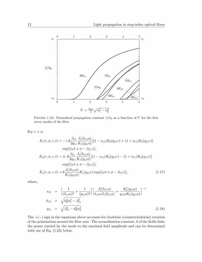
leading to two different sets of modes, the HE (−) and EH (+). This designation isbased on the contribution of Ez and Hz to the mode: Ez is larger (smaller) than Hz forthe EH (HE) modes [44]. Within each set of modes exist different solutions dependingon the value l. Hence, the modes are labelled as EHlm and HElm where m accountsfor the different solutions of Eq. (1.12) for a fixed l. Two special cases are those withl = 0: TM, for the solutions EH0m, and TE, for the solutions HE0m. The differentiatednaming of these solutions stems from the special propagation properties of the TM andTE modes explained in Sec. 1.1.
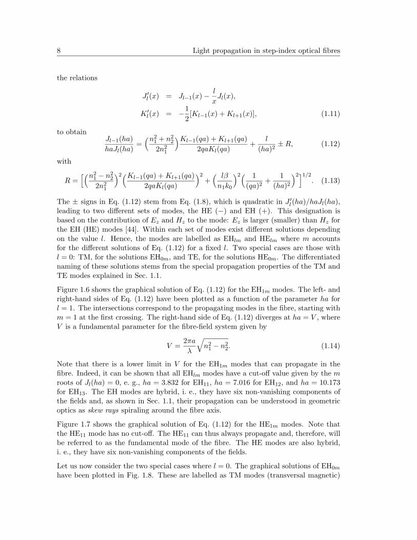
Figure 1.6 shows the graphical solution of Eq. (1.12) for the EH1m modes. The left- andright-hand sides of Eq. (1.12) have been plotted as a function of the parameter ha forl = 1. The intersections correspond to the propagating modes in the fibre, starting withm = 1 at the first crossing. The right-hand side of Eq. (1.12) diverges at ha = V , whereV is a fundamental parameter for the fibre-field system given by
V =2πa
λ
√
n21 − n2
2. (1.14)
Note that there is a lower limit in V for the EH1m modes that can propagate in thefibre. Indeed, it can be shown that all EHlm modes have a cut-off value given by the mroots of Jl(ha) = 0, e. g., ha = 3.832 for EH11, ha = 7.016 for EH12, and ha = 10.173for EH13. The EH modes are hybrid, i. e., they have six non-vanishing components ofthe fields and, as shown in Sec. 1.1, their propagation can be understood in geometricoptics as skew rays spiraling around the fibre axis.
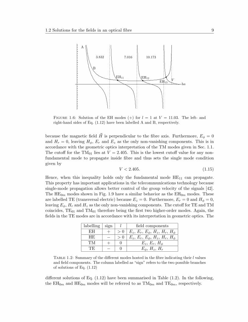
Figure 1.7 shows the graphical solution of Eq. (1.12) for the HE1m modes. Note thatthe HE11 mode has no cut-off. The HE11 can thus always propagate and, therefore, willbe referred to as the fundamental mode of the fibre. The HE modes are also hybrid,i. e., they have six non-vanishing components of the fields.
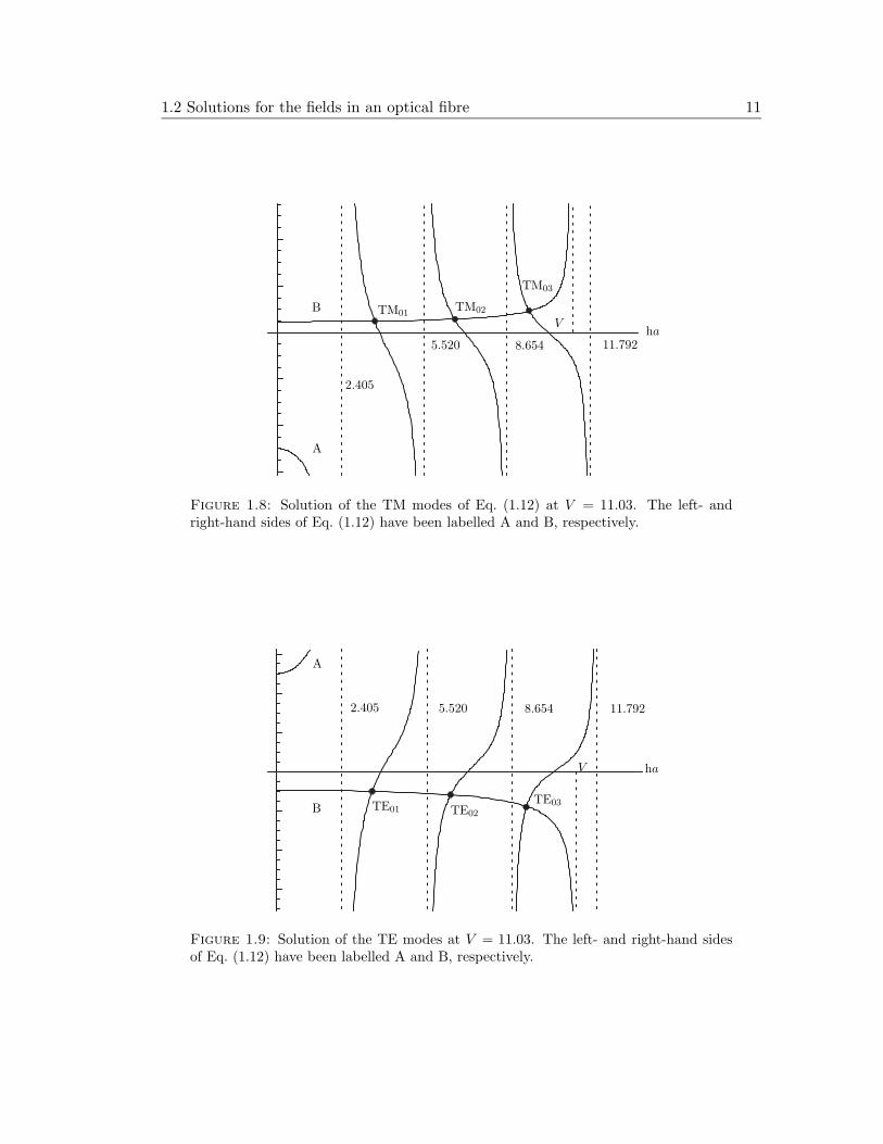
Let us now consider the two special cases where l = 0. The graphical solutions of EH0m
have been plotted in Fig. 1.8. These are labelled as TM modes (transversal magnetic)
1.2 Solutions for the fields in an optical fibre 9
A
B
EH11 EH12
EH13
3.832 7.016 10.173
Vha
Figure 1.6: Solution of the EH modes (+) for l = 1 at V = 11.03. The left- andright-hand sides of Eq. (1.12) have been labelled A and B, respectively.
because the magnetic field ~H is perpendicular to the fibre axis. Furthermore, Eφ = 0and Hr = 0, leaving Hφ, Er and Ez as the only non-vanishing components. This is inaccordance with the geometric optics interpretation of the TM modes given in Sec. 1.1.The cutoff for the TM01 lies at V = 2.405. This is the lowest cutoff value for any non-fundamental mode to propagate inside fibre and thus sets the single mode conditiongiven by
V < 2.405. (1.15)
Hence, when this inequality holds only the fundamental mode HE11 can propagate.This property has important applications in the telecommunications technology becausesingle-mode propagation allows better control of the group velocity of the signals [42].The HE0m modes shown in Fig. 1.9 have a similar behavior as the EH0m modes. Theseare labelled TE (transversal electric) because Ez = 0. Furthermore, Er = 0 and Hφ = 0,leaving Eφ, Hr andHz as the only non-vanishing components. The cutoff for TE and TMcoincides, TE01 and TM01 therefore being the first two higher-order modes. Again, thefields in the TE modes are in accordance with its interpretation in geometric optics. The
labelling sign l field components
EH + > 0 Ez, Er, Eφ, Hz, Hr, Hφ
HE − > 0 Ez, Er, Eφ, Hz, Hr, Hφ
TM + 0 Ez, Er, Hφ
TE − 0 Eφ, Hz, Hr
Table 1.2: Summary of the different modes hosted in the fibre indicating their l valuesand field components. The column labelled as “sign” refers to the two possible branchesof solutions of Eq. (1.12)
different solutions of Eq. (1.12) have been summarised in Table (1.2). In the following,the EH0m and HE0m modes will be referred to as TM0m and TE0m, respectively.
10 Light propagation in step-index optical fibres
A
B HE11 HE12HE13
HE14
3.832 7.016 10.173 13.323
Vha
Figure 1.7: Solution of the HE modes (−) for l = 1 at V = 11.03. The left- andright-hand sides of Eq. (1.12) have been labelled A and B, respectively.
Let us now examine the dependence of the propagation constant β as a function ofthe parameter V shown in Fig. 1.10. Here, the single-mode and multi-mode regimescan be clearly distinguished. The first two excited modes TE01 and TM01 appear forV ≥ 2.405. When decreasing (increasing) the V parameter, β/k0 tends to n2 (n1). Thisillustrates the fact that by decreasing the radius of the fibre or increasing the wavelengthof the light, the fields will penetrate more into the surrounding medium. In the inversesituation, the fields will be guided mostly in the bulk.
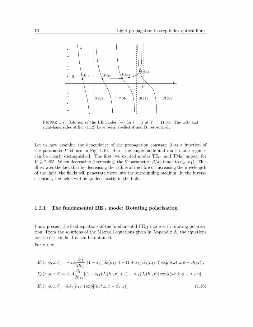
1.2.1 The fundamental HE11 mode: Rotating polarisation
I now present the field equations of the fundamental HE11 mode with rotating polarisa-tion. From the solutions of the Maxwell equations given in Appendix A, the equationsfor the electric field ~E can be obtained.
For r < a:
Er(r, φ, z, t) = − iAβ11
2h11[(1 − s11)J0(h11r) − (1 + s11)J2(h11r)] exp[i(ωt± φ− β11z)],
Eφ(r, φ, z, t) = ±Aβ11
2h11[(1 − s11)J0(h11r) + (1 + s11)J2(h11r)] exp[i(ωt± φ− β11z)],
Ez(r, φ, z, t) =AJ1(h11r) exp[i(ωt± φ− β11z)]. (1.16)
1.2 Solutions for the fields in an optical fibre 11
A
B TM01TM02
TM03
2.405
5.520 8.654 11.792
Vha
Figure 1.8: Solution of the TM modes of Eq. (1.12) at V = 11.03. The left- andright-hand sides of Eq. (1.12) have been labelled A and B, respectively.
A
B TE01 TE02
TE03
2.405 5.520 8.654 11.792
V ha
Figure 1.9: Solution of the TE modes at V = 11.03. The left- and right-hand sidesof Eq. (1.12) have been labelled A and B, respectively.
12 Light propagation in step-index optical fibres
HE11
TM01
TE01
HE21 HE12
HE31
EH11
β/k0
V = 2πaλ
√
n21 − n2
2
n1n1
n2n2
0
0
1
1
2
2
3
3
4
4
5
5
Figure 1.10: Normalised propagation constant β/k0 as a function of V for the firstseven modes of the fibre.
For r > a:
Er(r, φ, z, t) = − iAβ11
2q11
J1(h11a)
K1(q11a)[(1 − s11)K0(q11r) + (1 + s11)K2(q11r)]
exp[i(ωt± φ− β11z)],
Eφ(r, φ, z, t) = ±Aβ11
2q11
J1(h11a)
K1(q11a)[(1 − s11)K0(q11r) − (1 + s11)K2(q11r)]
exp[i(ωt± φ− β11z)],
Ez(r, φ, z, t) =AJ1(h11a)
K1(q11a)K1(q11r) exp[i(ωt± φ− β11z)], (1.17)
where,
s11 =[ 1
(h11a)2+
1
(q11a)2
][ J ′1(h11a)
h11aJ1(h11a)+
K ′1(q11a)
q11aK1(q11a)
]−1
h11 =√
k20n
21 − β2
11
q11 =√
β211 − k2
0n22 (1.18)
The +(−) sign in the equations above accounts for clockwise (counterclockwise) rotationof the polarisation around the fibre axis. The normalisation constant A of the fields linksthe power carried by the mode to the maximal field amplitude and can be determinedwith use of Eq. (1.23) below.
1.2 Solutions for the fields in an optical fibre 13
0.25
0.25
0.25
0.25x (µm)
0.500.50
0.50
0.50
y(µ
m)
0
0
0
0
-0.25
-0.25
-0.25
-0.25-0.50
-0.50
-0.50-0.50
Figure 1.11: Field plot of the electric field com-ponent perpendicular to the fibre axis ~E⊥ in theHE11 mode for rotating polarisation at t = 0 andz = 0. The following parameters have been as-sumed: n1 = 1.452, n2 = 1, a = 250 nm andλ = 852 nm.
0.25
0.25
0.25
0.25x (µm)
0.500.50
0.50
0.50
y(µ
m)
0
0
0
0
-0.25
-0.25
-0.25
-0.25-0.50
-0.50
-0.50-0.50
Figure 1.12: Field plot of ~E⊥ in the HE11 modefor rotating polarisation at t = π/4ω and z = 0for the same parameters as in Fig. 1.11.
0.25
0.25
0.25
0.25x (µm)
0.500.50
0.50
0.50
y(µ
m)
0
0
0
0
-0.25
-0.25
-0.25
-0.25-0.50
-0.50
-0.50-0.50
Figure 1.13: Field plot of ~E⊥ in the HE11 modefor rotating polarisation at t = π/2ω and z = 0for the same parameters as in Fig. 1.11.
0.25
0.25
0.25
0.25x (µm)
0.500.50
0.50
0.50
y(µ
m)
0
0
0
0
-0.25
-0.25
-0.25
-0.25-0.50
-0.50
-0.50-0.50
Figure 1.14: Field plot of ~E⊥ in the HE11 modefor rotating polarisation at t = 3π/4ω and z = 0for the same parameters as in Fig. 1.11.
14 Light propagation in step-index optical fibres
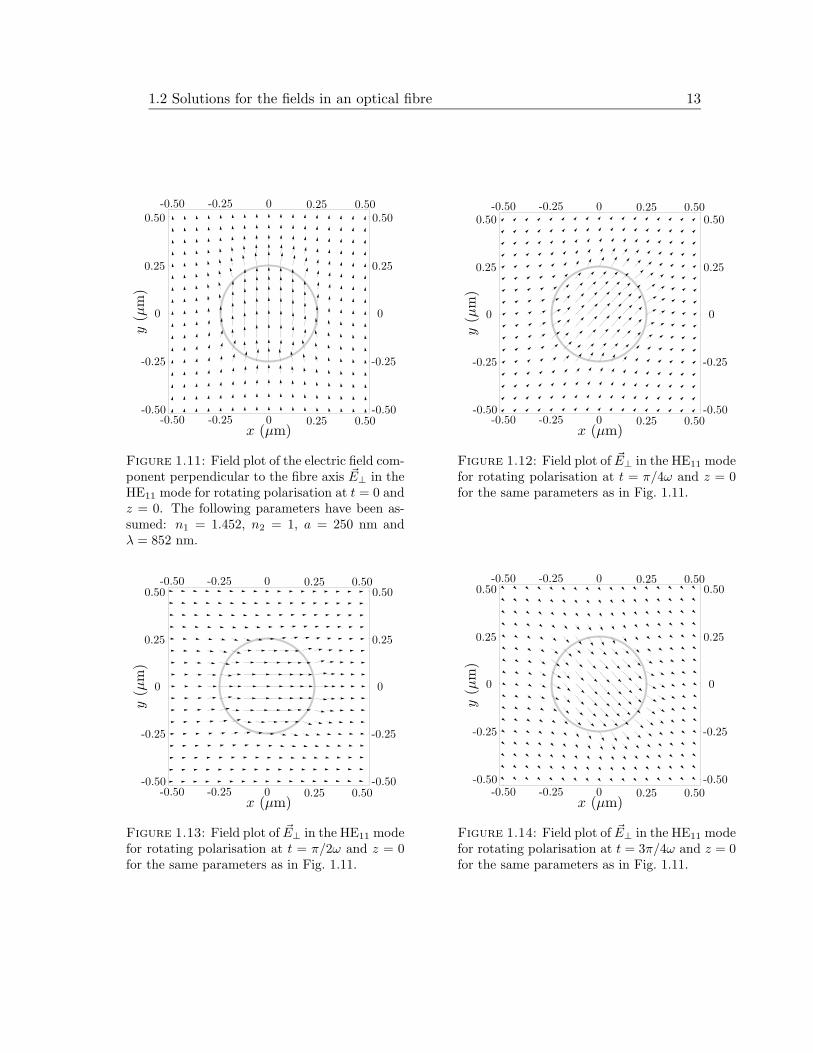
Figures 1.11, 1.12, 1.13 and 1.14 are vector plots of the electric field component transver-sal to the fibre axis ~E⊥ = (Ex, Ey) at z = 0 and t = 0, t = π/4ω, t = 2π/4ω andt = 3π/4ω, respectively. The fibre surface is indicated by a grey circle. The calculationshave been performed for a fibre of pure silica (n1 = 1.452) with a radius a = 250 nm,surrounded by vacuum (n2 = 1) at a wavelength of λ = 852 nm. These fibre and wave-length parameters correspond to the experiments presented in Chaps. 3, 4, and 5. Asexpected, ~E⊥ rotates in time with respect to the fibre axis. However, the rotation is notperfectly circular but elliptical and the ellipticity is position dependent. The position ofmaximal ellipticity is located at the surface of the fibre. This stems from the boundaryconditions for the electric field [37], which lead to a discontinuity in the Er componentat the fibre surface. This produces a radial orientation of the ellipse, its long (short)axis being oriented perpendicular (parallel) to the fibre surface, which becomes apparentwhen comparing the point (0 µm, 0.25 µm) in Figs. 1.11 and 1.13.
The absolute value of the squared electric field averaged over one oscillation period∣
∣ ~E(r)∣
∣
2in the HE11 mode is given by
∣
∣ ~E(r)∣
∣
2
in=A2β2
11
2h211
[
(1 − s11)2J2
0 (h11r) + (1 + s11)2J2
2 (h11r) + 2h2
11
β211
J21 (h11r)
]
, (1.19)
∣
∣ ~E(r)∣
∣
2
out=A2β2
11
2q211
J21 (h11a)
K21 (q11a)
[
(1 − s11)2K2
0 (q11r) + (1 + s11)2K2
2 (q11r) + 2q211β2
11
K21 (q11r)
]
,
(1.20)where | ~E(r)|2in (| ~E(r)|2out) denotes the time-averaged squared electric field inside (out-
side) the fibre. Since the above equations do not depend on φ, the distribution of∣
∣ ~E(r)∣
∣
2
is cylindrically symmetric. This stems from the averaging of the squared ~E field overone oscillation period. As shown in Figs. 1.11 – 1.14, the electric field propagating inthe fibre is, in general, not cylindrically symmetric because the polarisation of the fieldbrakes the symmetry. However, for rotating polarisation, averaging over one periodwashes out this symmetry breaking.
Equations (1.19) and (1.20) are useful for estimating the relative strength of the z-component of the electric field ~E yielding |Ez(r = a)|2in/| ~E(r = a)|2in = 0.2 and |Ez(r =
a)|2out/| ~E(r = a)|2out = 0.1. This feature does not exist in free propagating beams, where~E and ~H are perpendicular to the propagation vector ~k. Again, the discontinuity atthe boundary is produced by the Er component of the field because, although Ez iscontinuous at the surface,
∣
∣ ~E(r)∣
∣
2is not.
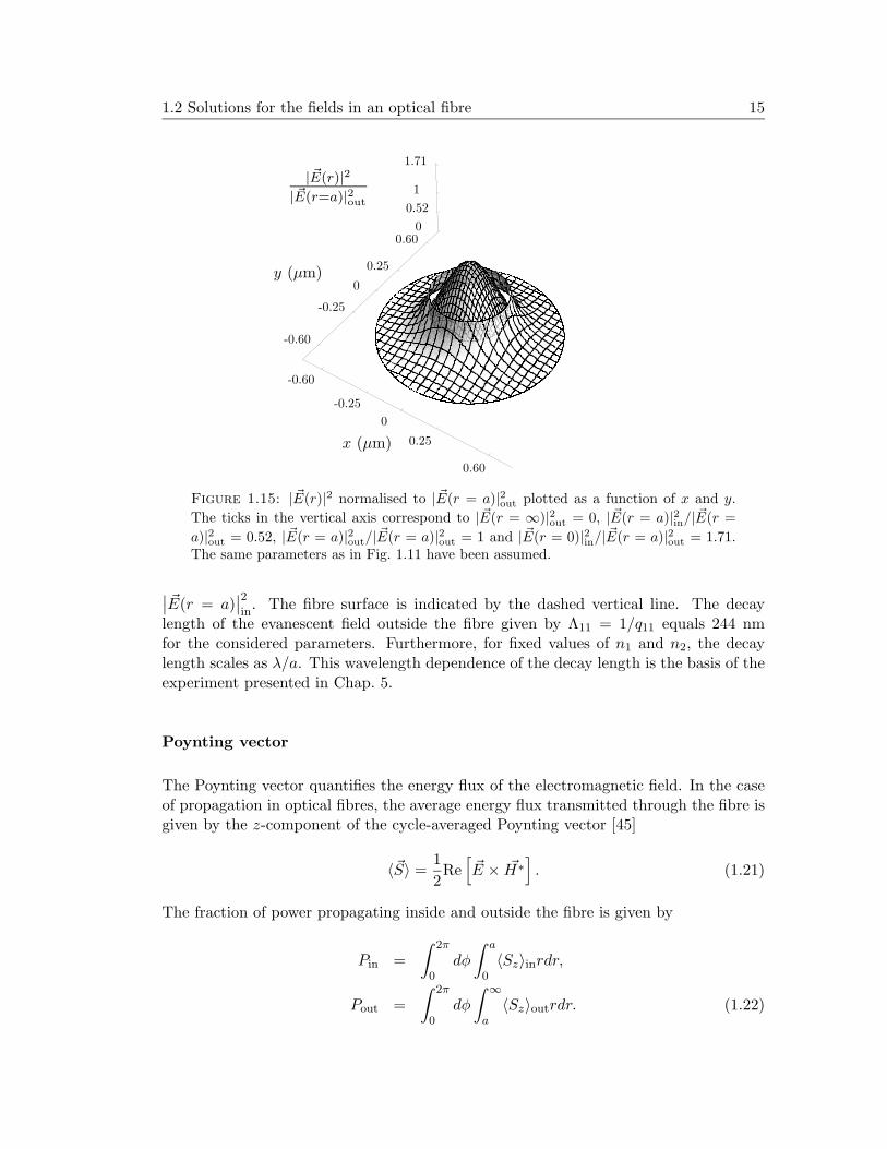
Figure 1.15 shows the distribution of∣
∣ ~E(r)∣
∣
2
in(inside) and
∣
∣ ~E(r)∣
∣
2
out(outside) normalised
to the value∣
∣ ~E(r = a)∣
∣
2
out(surface) as a function of x and y. The regions where r < a
and r > a can be clearly identified due to the discontinuity at the boundary r = a.This strong discontinuity arises from the large refractive index difference between thebulk and the surrounding medium and from the strong radial confinement of the fieldwhen λ > a. The strength of the evanescent field
∣
∣ ~E(r)∣
∣
2
outaround the fibre is apparent
in Fig. 1.16:∣
∣ ~E(r = a)∣
∣
2
outis about 58% of
∣
∣ ~E(r = 0)∣
∣
2
inand almost twice as large as
1.2 Solutions for the fields in an optical fibre 15
0.25
0.25
-0.25
-0.25
-0.60
-0.60
0
0
0
0.60
0.60
x (µm)
y (µm)
1.71
0.52
1| ~E(r)|2
| ~E(r=a)|2out
Figure 1.15: | ~E(r)|2 normalised to | ~E(r = a)|2out plotted as a function of x and y.
The ticks in the vertical axis correspond to | ~E(r = ∞)|2out = 0, | ~E(r = a)|2in/| ~E(r =
a)|2out = 0.52, | ~E(r = a)|2out/| ~E(r = a)|2out = 1 and | ~E(r = 0)|2in/| ~E(r = a)|2out = 1.71.The same parameters as in Fig. 1.11 have been assumed.
∣
∣ ~E(r = a)∣
∣
2
in. The fibre surface is indicated by the dashed vertical line. The decay
length of the evanescent field outside the fibre given by Λ11 = 1/q11 equals 244 nmfor the considered parameters. Furthermore, for fixed values of n1 and n2, the decaylength scales as λ/a. This wavelength dependence of the decay length is the basis of theexperiment presented in Chap. 5.
Poynting vector
The Poynting vector quantifies the energy flux of the electromagnetic field. In the caseof propagation in optical fibres, the average energy flux transmitted through the fibre isgiven by the z-component of the cycle-averaged Poynting vector [45]
〈~S〉 =1
2Re
[
~E × ~H∗]
. (1.21)
The fraction of power propagating inside and outside the fibre is given by
Pin =
∫ 2π
0dφ
∫ a
0〈Sz〉inrdr,
Pout =
∫ 2π
0dφ
∫ ∞
a〈Sz〉outrdr. (1.22)
16 Light propagation in step-index optical fibres
0.25r (µm)
1.71
1
0.52
| ~E(r)|2
| ~E(r=a)|2out
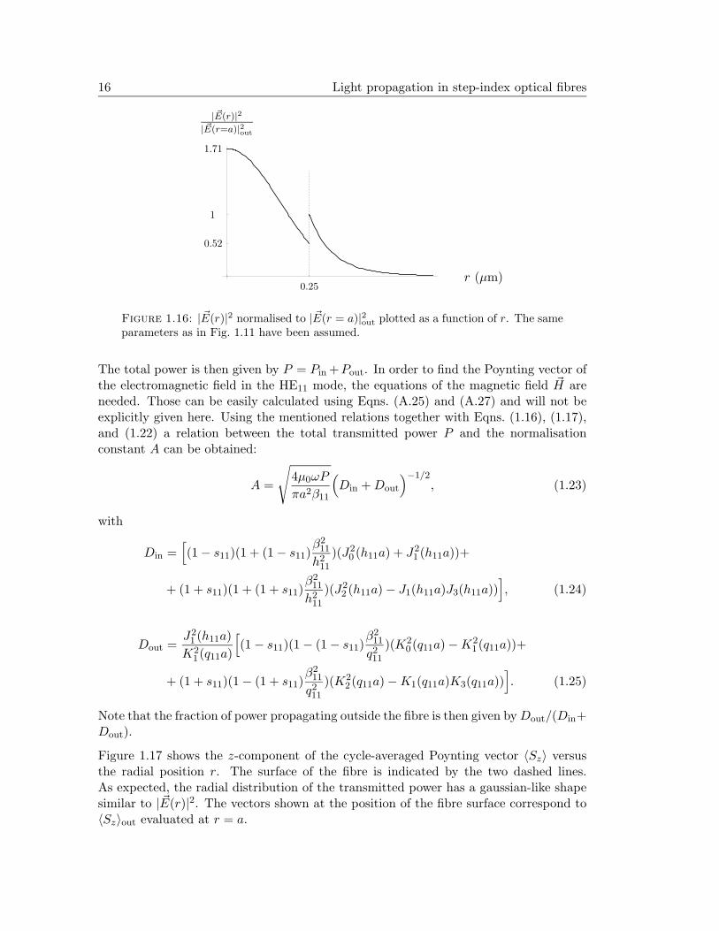
Figure 1.16: | ~E(r)|2 normalised to | ~E(r = a)|2out plotted as a function of r. The sameparameters as in Fig. 1.11 have been assumed.
The total power is then given by P = Pin +Pout. In order to find the Poynting vector ofthe electromagnetic field in the HE11 mode, the equations of the magnetic field ~H areneeded. Those can be easily calculated using Eqns. (A.25) and (A.27) and will not beexplicitly given here. Using the mentioned relations together with Eqns. (1.16), (1.17),and (1.22) a relation between the total transmitted power P and the normalisationconstant A can be obtained:
A =
√
4µ0ωP
πa2β11
(
Din +Dout
)−1/2, (1.23)
with
Din =[
(1 − s11)(1 + (1 − s11)β2
11
h211
)(J20 (h11a) + J2
1 (h11a))+
+ (1 + s11)(1 + (1 + s11)β2
11
h211
)(J22 (h11a) − J1(h11a)J3(h11a))
]
, (1.24)
Dout =J2
1 (h11a)
K21 (q11a)
[
(1 − s11)(1 − (1 − s11)β2
11
q211)(K2
0 (q11a) −K21 (q11a))+
+ (1 + s11)(1 − (1 + s11)β2
11
q211)(K2
2 (q11a) −K1(q11a)K3(q11a))]
. (1.25)
Note that the fraction of power propagating outside the fibre is then given byDout/(Din+Dout).
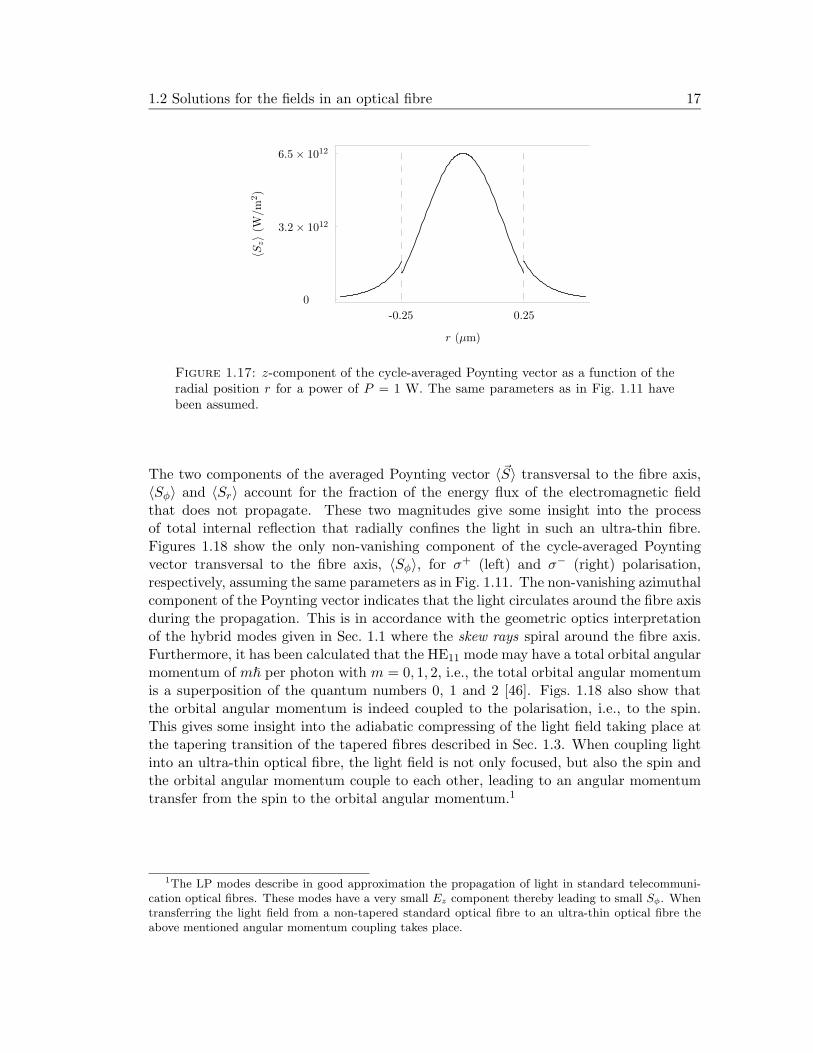
Figure 1.17 shows the z-component of the cycle-averaged Poynting vector 〈Sz〉 versusthe radial position r. The surface of the fibre is indicated by the two dashed lines.As expected, the radial distribution of the transmitted power has a gaussian-like shapesimilar to | ~E(r)|2. The vectors shown at the position of the fibre surface correspond to〈Sz〉out evaluated at r = a.
1.2 Solutions for the fields in an optical fibre 17
0.25
〈Sz〉(
W/m
2)
6.5 × 10¹²
3.2 × 10¹²
r (µm)
0
-0.25
Figure 1.17: z-component of the cycle-averaged Poynting vector as a function of theradial position r for a power of P = 1 W. The same parameters as in Fig. 1.11 havebeen assumed.
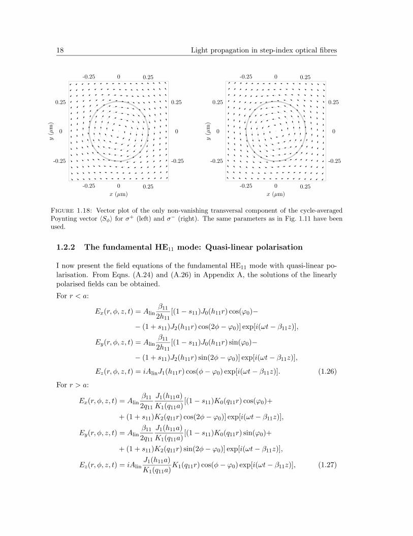
The two components of the averaged Poynting vector 〈~S〉 transversal to the fibre axis,〈Sφ〉 and 〈Sr〉 account for the fraction of the energy flux of the electromagnetic fieldthat does not propagate. These two magnitudes give some insight into the processof total internal reflection that radially confines the light in such an ultra-thin fibre.Figures 1.18 show the only non-vanishing component of the cycle-averaged Poyntingvector transversal to the fibre axis, 〈Sφ〉, for σ+ (left) and σ− (right) polarisation,respectively, assuming the same parameters as in Fig. 1.11. The non-vanishing azimuthalcomponent of the Poynting vector indicates that the light circulates around the fibre axisduring the propagation. This is in accordance with the geometric optics interpretationof the hybrid modes given in Sec. 1.1 where the skew rays spiral around the fibre axis.Furthermore, it has been calculated that the HE11 mode may have a total orbital angularmomentum of mℏ per photon with m = 0, 1, 2, i.e., the total orbital angular momentumis a superposition of the quantum numbers 0, 1 and 2 [46]. Figs. 1.18 also show thatthe orbital angular momentum is indeed coupled to the polarisation, i.e., to the spin.This gives some insight into the adiabatic compressing of the light field taking place atthe tapering transition of the tapered fibres described in Sec. 1.3. When coupling lightinto an ultra-thin optical fibre, the light field is not only focused, but also the spin andthe orbital angular momentum couple to each other, leading to an angular momentumtransfer from the spin to the orbital angular momentum.1
1The LP modes describe in good approximation the propagation of light in standard telecommuni-cation optical fibres. These modes have a very small Ez component thereby leading to small Sφ. Whentransferring the light field from a non-tapered standard optical fibre to an ultra-thin optical fibre theabove mentioned angular momentum coupling takes place.
18 Light propagation in step-index optical fibres
0.25
0.25
0.25
0.25
x (µm)
y(µ
m)
0
0
0
0
-0.25
-0.25
-0.25
-0.25
0.25
0.25
0.25
0.25
x (µm)
y(µ
m)
0
0
0
0
-0.25
-0.25
-0.25
-0.25
Figure 1.18: Vector plot of the only non-vanishing transversal component of the cycle-averagedPoynting vector 〈Sφ〉 for σ+ (left) and σ− (right). The same parameters as in Fig. 1.11 have beenused.
1.2.2 The fundamental HE11 mode: Quasi-linear polarisation
I now present the field equations of the fundamental HE11 mode with quasi-linear po-larisation. From Eqns. (A.24) and (A.26) in Appendix A, the solutions of the linearlypolarised fields can be obtained.
For r < a:
Ex(r, φ, z, t) = Alinβ11
2h11[(1 − s11)J0(h11r) cos(ϕ0)−
− (1 + s11)J2(h11r) cos(2φ− ϕ0)] exp[i(ωt− β11z)],
Ey(r, φ, z, t) = Alinβ11
2h11[(1 − s11)J0(h11r) sin(ϕ0)−
− (1 + s11)J2(h11r) sin(2φ− ϕ0)] exp[i(ωt− β11z)],
Ez(r, φ, z, t) = iAlinJ1(h11r) cos(φ− ϕ0) exp[i(ωt− β11z)]. (1.26)
For r > a:
Ex(r, φ, z, t) = Alinβ11
2q11
J1(h11a)
K1(q11a)[(1 − s11)K0(q11r) cos(ϕ0)+
+ (1 + s11)K2(q11r) cos(2φ− ϕ0)] exp[i(ωt− β11z)],
Ey(r, φ, z, t) = Alinβ11
2q11
J1(h11a)
K1(q11a)[(1 − s11)K0(q11r) sin(ϕ0)+
+ (1 + s11)K2(q11r) sin(2φ− ϕ0)] exp[i(ωt− β11z)],
Ez(r, φ, z, t) = iAlinJ1(h11a)
K1(q11a)K1(q11r) cos(φ− ϕ0) exp[i(ωt− β11z)], (1.27)
1.2 Solutions for the fields in an optical fibre 19
where q11, h11 and s11 have been defined in Sec. 1.2.1. The angle ϕ0 accounts for thepolarisation direction, ϕ0 = 0 leading to x-polarisation of the transverse ~E field andϕ0 = π/2 to y-polarisation. The normalisation constant Alin is related to the maximumamplitude of the electric field and satisfies the relation Alin =
√2A, where A is the global
constant of the fields with rotating polarisation given in Sec. 1.2.1. Using Eq. (1.23), therelation between Alin and the total power transmitted through the fibre can be obtained.
0.25
0.25
0.25
0.25
x (µm)
0.50
0.50
0.50
0.50
-0.50
-0.50
-0.50
-0.50
y(µ
m)
0
0
0
0
-0.25
-0.25
-0.25
-0.25
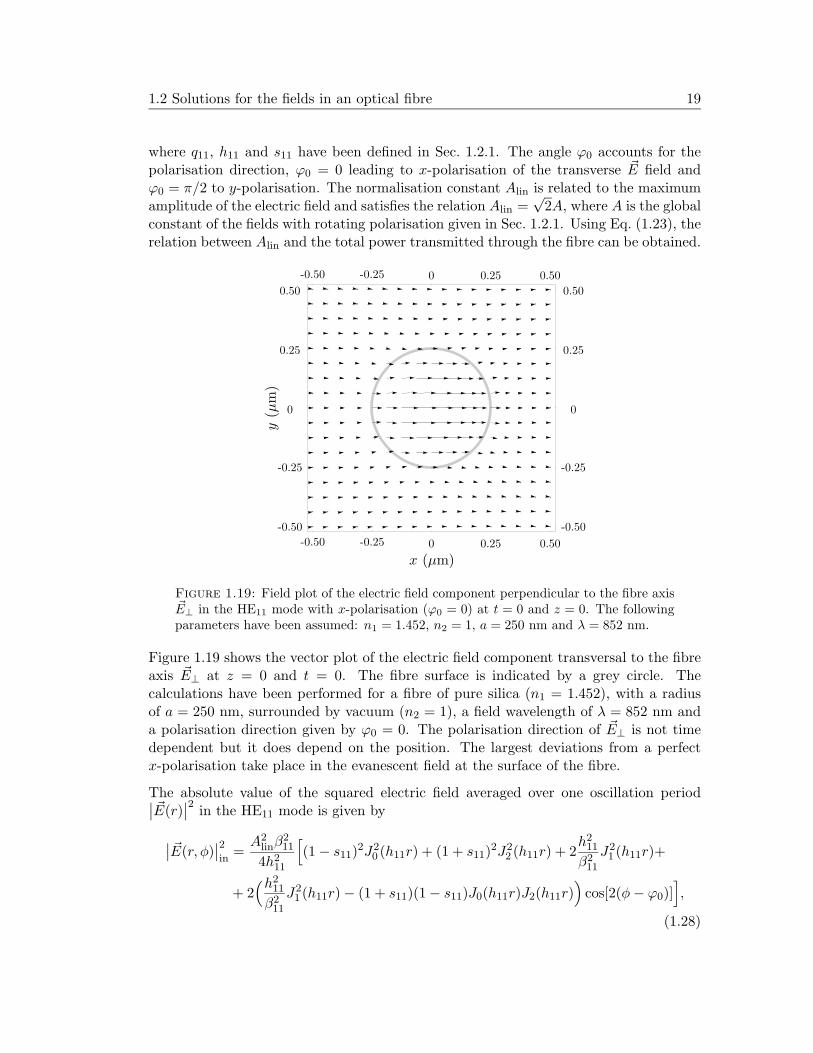
Figure 1.19: Field plot of the electric field component perpendicular to the fibre axis~E⊥ in the HE11 mode with x-polarisation (ϕ0 = 0) at t = 0 and z = 0. The followingparameters have been assumed: n1 = 1.452, n2 = 1, a = 250 nm and λ = 852 nm.
Figure 1.19 shows the vector plot of the electric field component transversal to the fibreaxis ~E⊥ at z = 0 and t = 0. The fibre surface is indicated by a grey circle. Thecalculations have been performed for a fibre of pure silica (n1 = 1.452), with a radiusof a = 250 nm, surrounded by vacuum (n2 = 1), a field wavelength of λ = 852 nm anda polarisation direction given by ϕ0 = 0. The polarisation direction of ~E⊥ is not timedependent but it does depend on the position. The largest deviations from a perfectx-polarisation take place in the evanescent field at the surface of the fibre.
The absolute value of the squared electric field averaged over one oscillation period∣
∣ ~E(r)∣
∣
2in the HE11 mode is given by
∣
∣ ~E(r, φ)∣
∣
2
in=A2
linβ211
4h211
[
(1 − s11)2J2
0 (h11r) + (1 + s11)2J2
2 (h11r) + 2h2
11
β211
J21 (h11r)+
+ 2(h2
11
β211
J21 (h11r) − (1 + s11)(1 − s11)J0(h11r)J2(h11r)
)
cos[2(φ− ϕ0)]]
,
(1.28)
20 Light propagation in step-index optical fibres
∣
∣ ~E(r, φ)∣
∣
2
out=A2
linβ211
4q211
J21 (h11a)
K21 (q11a)
[
(1 − s11)2K2
0 (q11r) + (1 + s11)2K2
2 (q11r) + 2q211β2
11
K21 (q11r)+
+ 2( q211β2
11
K21 (q11r) + (1 + s11)(1 − s11)K0(q11r)K2(q11r)
)
cos[2(φ− ϕ0)]]
,
(1.29)
where | ~E(r)|2in (| ~E(r)|2out) denotes the time-averaged squared electric field inside (out-side) the fibre. Similarly to the case of rotating polarisation, the equations above canbe used to estimate the strength of Ez, leading to |Ez(r = a, φ = 0)|2in/| ~E(r = a, φ =
0)|2in = 0.6 and to |Ez(r = a, φ = 0)|2out/| ~E(r = a, φ = 0)|2out = 0.25 at the fibre sur-
face [37]. Note that Ez vanishes where ~E⊥ is parallel to the fibre surface and reachesits maximum value where ~E⊥ is perpendicular to it. This is in accordance with the rayoptics interpretation given in Sec. 1.1.
0
0
0
0.25
0.25
-0.25
-0.250.5
0.5
-0.5-0.5
y (µm)
11.04
x (µm)
0.21
| ~E(r,φ)|2
| ~E(r=a,φ=0)|2out
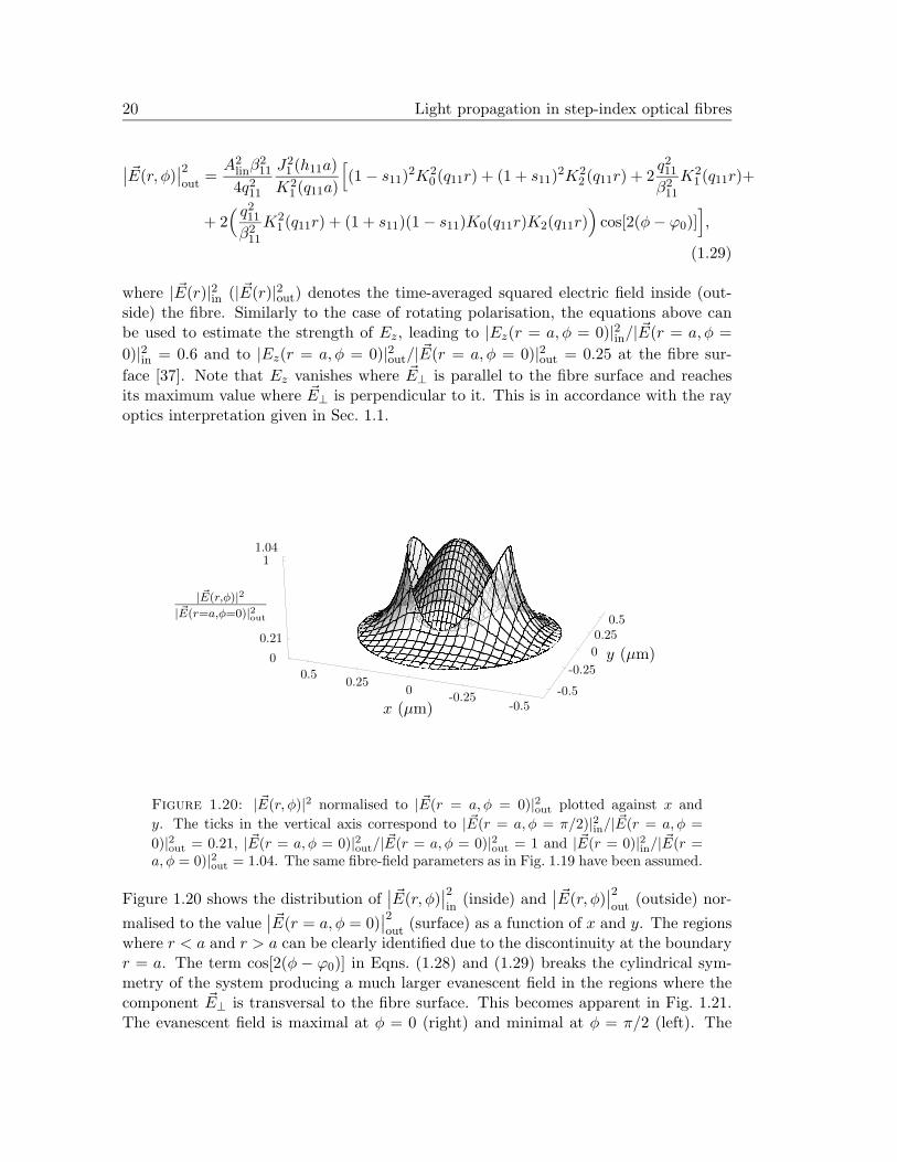
Figure 1.20: | ~E(r, φ)|2 normalised to | ~E(r = a, φ = 0)|2out plotted against x and
y. The ticks in the vertical axis correspond to | ~E(r = a, φ = π/2)|2in/| ~E(r = a, φ =
0)|2out = 0.21, | ~E(r = a, φ = 0)|2out/| ~E(r = a, φ = 0)|2out = 1 and | ~E(r = 0)|2in/| ~E(r =a, φ = 0)|2out = 1.04. The same fibre-field parameters as in Fig. 1.19 have been assumed.
Figure 1.20 shows the distribution of∣
∣ ~E(r, φ)∣
∣
2
in(inside) and
∣
∣ ~E(r, φ)∣
∣
2
out(outside) nor-
malised to the value∣
∣ ~E(r = a, φ = 0)∣
∣
2
out(surface) as a function of x and y. The regions
where r < a and r > a can be clearly identified due to the discontinuity at the boundaryr = a. The term cos[2(φ − ϕ0)] in Eqns. (1.28) and (1.29) breaks the cylindrical sym-metry of the system producing a much larger evanescent field in the regions where thecomponent ~E⊥ is transversal to the fibre surface. This becomes apparent in Fig. 1.21.The evanescent field is maximal at φ = 0 (right) and minimal at φ = π/2 (left). The
1.2 Solutions for the fields in an optical fibre 21
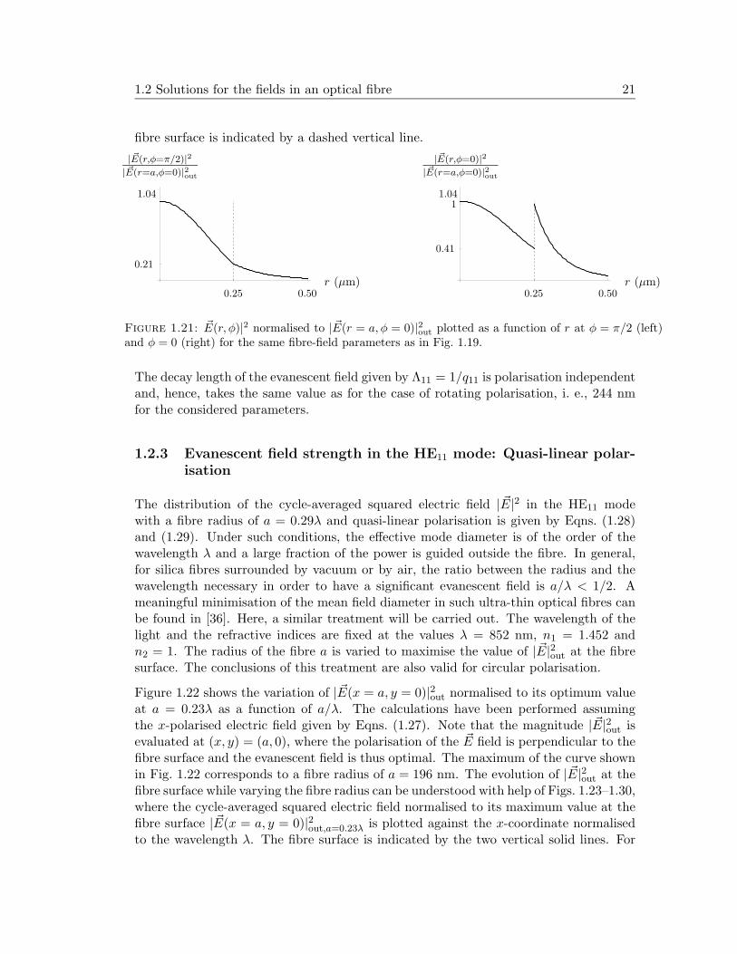
fibre surface is indicated by a dashed vertical line.
0.25 0.50r (µm)
1.04
0.21
| ~E(r,φ=π/2)|2
| ~E(r=a,φ=0)|2out
1
0.25 0.50r (µm)
0.41
1.04
| ~E(r,φ=0)|2
| ~E(r=a,φ=0)|2out
Figure 1.21: ~E(r, φ)|2 normalised to | ~E(r = a, φ = 0)|2out plotted as a function of r at φ = π/2 (left)and φ = 0 (right) for the same fibre-field parameters as in Fig. 1.19.
The decay length of the evanescent field given by Λ11 = 1/q11 is polarisation independentand, hence, takes the same value as for the case of rotating polarisation, i. e., 244 nmfor the considered parameters.
1.2.3 Evanescent field strength in the HE11 mode: Quasi-linear polar-isation
The distribution of the cycle-averaged squared electric field | ~E|2 in the HE11 modewith a fibre radius of a = 0.29λ and quasi-linear polarisation is given by Eqns. (1.28)and (1.29). Under such conditions, the effective mode diameter is of the order of thewavelength λ and a large fraction of the power is guided outside the fibre. In general,for silica fibres surrounded by vacuum or by air, the ratio between the radius and thewavelength necessary in order to have a significant evanescent field is a/λ < 1/2. Ameaningful minimisation of the mean field diameter in such ultra-thin optical fibres canbe found in [36]. Here, a similar treatment will be carried out. The wavelength of thelight and the refractive indices are fixed at the values λ = 852 nm, n1 = 1.452 andn2 = 1. The radius of the fibre a is varied to maximise the value of | ~E|2out at the fibresurface. The conclusions of this treatment are also valid for circular polarisation.
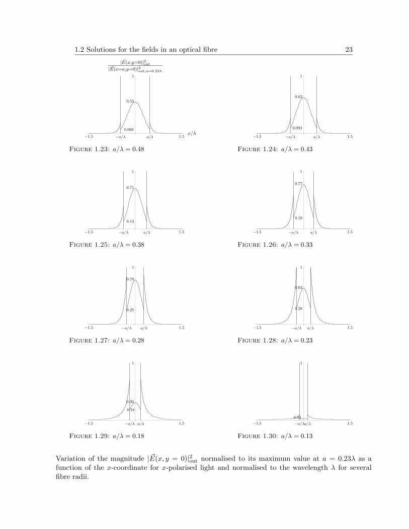
Figure 1.22 shows the variation of | ~E(x = a, y = 0)|2out normalised to its optimum valueat a = 0.23λ as a function of a/λ. The calculations have been performed assumingthe x-polarised electric field given by Eqns. (1.27). Note that the magnitude | ~E|2out isevaluated at (x, y) = (a, 0), where the polarisation of the ~E field is perpendicular to thefibre surface and the evanescent field is thus optimal. The maximum of the curve shownin Fig. 1.22 corresponds to a fibre radius of a = 196 nm. The evolution of | ~E|2out at thefibre surface while varying the fibre radius can be understood with help of Figs. 1.23–1.30,where the cycle-averaged squared electric field normalised to its maximum value at thefibre surface | ~E(x = a, y = 0)|2out,a=0.23λ is plotted against the x-coordinate normalisedto the wavelength λ. The fibre surface is indicated by the two vertical solid lines. For
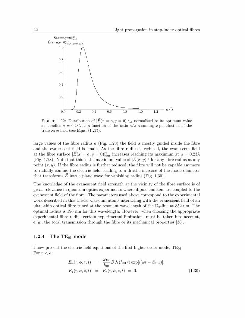
22 Light propagation in step-index optical fibres
| ~E(x=a,y=0)|2out
| ~E(x=a,y=0)|2out,a=0.23λ
1.0
1.0
0.8
0.8
0.6
0.6
0.4
0.4
0.2
0.20.0 1.2a/λ
Figure 1.22: Distribution of | ~E(x = a, y = 0)|2out normalised to its optimum valueat a radius a = 0.23λ as a function of the ratio a/λ assuming x-polarisation of thetransverse field (see Eqns. (1.27)).
large values of the fibre radius a (Fig. 1.23) the field is mostly guided inside the fibreand the evanescent field is small. As the fibre radius is reduced, the evanescent fieldat the fibre surface | ~E(x = a, y = 0)|2out increases reaching its maximum at a = 0.23λ(Fig. 1.28). Note that this is the maximum value of | ~E(x, y)|2 for any fibre radius at anypoint (x, y). If the fibre radius is further reduced, the fibre will not be capable anymoreto radially confine the electric field, leading to a drastic increase of the mode diameterthat transforms ~E into a plane wave for vanishing radius (Fig. 1.30).
The knowledge of the evanescent field strength at the vicinity of the fibre surface is ofgreat relevance in quantum optics experiments where dipole emitters are coupled to theevanescent field of the fibre. The parameters used above correspond to the experimentalwork described in this thesis: Caesium atoms interacting with the evanescent field of anultra-thin optical fibre tuned at the resonant wavelength of the D2-line at 852 nm. Theoptimal radius is 196 nm for this wavelength. However, when choosing the appropriateexperimental fibre radius certain experimental limitations must be taken into account,e. g., the total transmission through the fibre or its mechanical properties [36].
1.2.4 The TE01 mode
I now present the electric field equations of the first higher-order mode, TE01.For r < a:
Eφ(r, φ, z, t) =ωµ0
h01BJ1(h01r) exp[i(ωt− β01z)],
Ez(r, φ, z, t) = Er(r, φ, z, t) = 0. (1.30)
1.2 Solutions for the fields in an optical fibre 23
1
x/λ
| ~E(x,y=0)|2out
| ~E(x=a,y=0)|2out,a=0.23λ
−1.5 1.5
0.55
0.066
a/λ−a/λ
Figure 1.23: a/λ = 0.48
1
−1.5 1.5
0.62
0.093
a/λ−a/λ
Figure 1.24: a/λ = 0.43
1
−1.5 1.5
0.71
0.13
a/λ−a/λ
Figure 1.25: a/λ = 0.38
1
−1.5 1.5
0.77
0.19
a/λ−a/λ
Figure 1.26: a/λ = 0.33
1
−1.5 1.5
0.78
0.25
a/λ−a/λ
Figure 1.27: a/λ = 0.28
1
−1.5 1.5
0.63
0.28
a/λ−a/λ
Figure 1.28: a/λ = 0.23
1
−1.5 1.5
0.30
0.18
a/λ−a/λ
Figure 1.29: a/λ = 0.18
1
−1.5 1.5
0.03
a/λ−a/λ
Figure 1.30: a/λ = 0.13
Variation of the magnitude | ~E(x, y = 0)|2out normalised to its maximum value at a = 0.23λ as afunction of the x-coordinate for x-polarised light and normalised to the wavelength λ for severalfibre radii.
24 Light propagation in step-index optical fibres
For r > a:
Eφ(r, φ, z, t) = −ωµ0
q01
J0(h01a)
K0(q01a)BK1(q01r) exp[i(ωt− β01z)],
Ez(r, φ, z, t) = Er(r, φ, z, t) = 0, (1.31)
where,
h01 =√
k20n
21 − β2
01,
q01 =√
β201 − k2
0n22. (1.32)
β01 denotes propagation constant of the TE01 mode given by Eq. (1.8) and B the nor-malisation constant of the electric field which can be determined using Eq. (1.35) below.
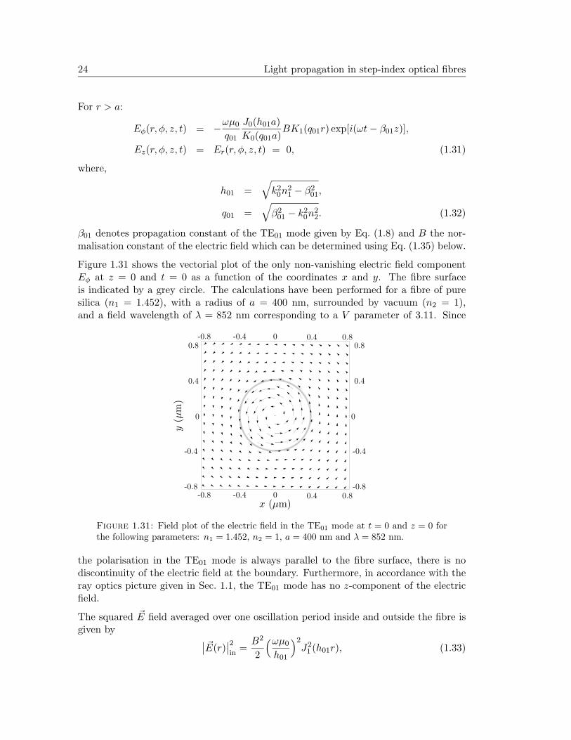
Figure 1.31 shows the vectorial plot of the only non-vanishing electric field componentEφ at z = 0 and t = 0 as a function of the coordinates x and y. The fibre surfaceis indicated by a grey circle. The calculations have been performed for a fibre of puresilica (n1 = 1.452), with a radius of a = 400 nm, surrounded by vacuum (n2 = 1),and a field wavelength of λ = 852 nm corresponding to a V parameter of 3.11. Since
-0.8
-0.8
-0.8-0.8
0.80.8
0.8
0.8
-0.4
-0.4
-0.4
-0.4
0.4
0.4
0.4
0.4x (µm)
y(µ
m)
00
0
0
Figure 1.31: Field plot of the electric field in the TE01 mode at t = 0 and z = 0 forthe following parameters: n1 = 1.452, n2 = 1, a = 400 nm and λ = 852 nm.
the polarisation in the TE01 mode is always parallel to the fibre surface, there is nodiscontinuity of the electric field at the boundary. Furthermore, in accordance with theray optics picture given in Sec. 1.1, the TE01 mode has no z-component of the electricfield.
The squared ~E field averaged over one oscillation period inside and outside the fibre isgiven by
∣
∣ ~E(r)∣
∣
2
in=B2
2
(ωµ0
h01
)2J2
1 (h01r), (1.33)