Embed Size (px)
Citation preview
D I P L O M A R B E I T
Asymptotic behavior of the Weyl m-function for one-dimensionalSchrodinger operators with measure-valued potentials
unter der Anleitung von
Univ.Prof. Dr. Gerald Teschlder Universitat Wien und in Zusammenarbeit mit
Ass.Univ.Prof. Dr. Annemarie Lugerder Stockholm University
eingereicht an der Technischen Universitat Wien,Fakultat fur Mathematik und Geoinformatik
durch
Tobias Wohrer
Johann-Nepomuk-Berger-Platz 6/5, 1160 Wien
September 15, 2014
Abstract
We consider the Sturm-Liouville differential expression with measure-valued coefficients
τf =d
dρ
(−dfdζ
+
∫f dχ
)and introduce the Weyl m-function for self-adjoint realizations. We further look at the specialcase of one-dimensional Schrodinger operators with measure-valued potentials. For this case wedevelop the asymptotic behavior
m(z) = −√−z −
∫ x
0e−2√−zy dχ(y) + o
(1√−z
)of the Weyl m-function for large z.
1
Introduction
The Sturm-Liouville theory, which essentially is the theory of ordinary differential equations ofsecond order, was initiated in the 1830’s by Charles Francois Sturm who soon collaborated withJoseph Liouville. This theory has been a field of interest ever since, with many applicationsmost notably in physics. Especially the modern field of quantum mechanics broadly employsthe Sturm-Liouville theory in combination with spectral theory. In the one-dimensional casethe Sturm-Liouville eigenvalue problem coincides with the one-dimensional time-independentSchrodinger equation Hψ(x) = Eψ(x). A popular introduction problem for physics students is
a model with a potential of the form V (x) = −~2m δ(x) were δ(x) describes a point charge. This
leads to a jump condition for the first derivative of solutions of the Schrodinger equation whichis not covered by the classical Sturm-Liouville theory.
In this thesis we look at a generalization of the classical Sturm-Liouville differential expressionτ1 which covers such point charge potentials as well as many other generalized potentials ofinterest. The derivatives are extended as Radon–Nikodym derivatives to the expression
τ1f =d
d%
(−dfdζ
+
∫f dχ
),
with measures %, ζ and χ not necessarily absolutely continuous with respect to the Lebesguemeasure.Our starting point is the paper of [1], published by Gerald Teschl and Jonathan Eckhardt in2013. From this paper we explain the basic theory of the differential expression τ1. This includesan existence and uniqueness result for the initial value problem, categorizing interval endpointregularities and looking for self-adjoint realizations of τ1. The methods we use to develop thisresults are very similar to the classical Sturm-Liouville theory methods with the difference thatwe have to use the tools of measure theory, i.e. the Radon–Nikodym theorem and integrationby parts for Lebesgue-Stieltjes integrals. The main effort lies in finding self-adjoint realizationsof τ1 in a Hilbert space as those correspond to possibly multi-valued linear relations. For cer-tain self-adjoint realizations S of τ1 we introduce the Weyl m-function, which is a Nevanlinnafunction containing the spectral information of S.
Equipped with this apparatus of our generalized Sturm-Liouville expression we examine the one-dimensional Schrodinger operator with measure-valued potential. This potential is describedby the measure χ resulting in the differential expression
τ2f =
(−f ′ +
∫f dχ
)′.
In this thesis we will develop a new improved estimate for the asymptotic behavior of the Weylm-function corresponding to τ2. We do this by first describing a fundamental system of thedifferential equation (τ2 − z)u = 0 as solutions of integral equations. This integral equationsallow us to extract an asymptotic estimate for their solutions. Then we find an asymptoticestimate for the Weyl m-function with the help of the Weyl circles, as done in the classical caseby F. Atkinson in [3]. Combining this two estimates leads to or final estimate for the asymptoticbehavior of the Weyl function given as
m(z) = −√−z −
∫ x
0e−2√−zy dχ(y) + o
(1√−z
)as Im(z)→ +∞.This result is valuable for inverse Sturm-Liouville problems which examines the possibility to
2
get information about the self-adjoint realization of a differential expression τ (i.e. its potential)by only possessing its spectral information (i.e. its Weyl m-function).
Acknowledgement
First I want to thank my supervisor Gerald Teschl for his great suggestions and support onwriting this thesis, as well as for sparking my interest in this field of mathematics through hisexcellent book [4]. I also thank my co-supervisor Annemarie Luger for her devoted supportduring my stay at Stockholm University.
Furthermore I want to thank my family for their incredible support throughout the years of mystudies. I am indebted to all my friends for their constant support especially Albert Fandl, OliverLeingang and Alexander Beigl for their help on mathematical questions. Last but not least, Iwant to express my appreciation for my girlfriend Ana Svetel, who was always understandingand a big source of motivation.
3
Contents
Abstract . . . . . . . . . . . . . . . . . . . . . . . . . . . . . . . . . . . . . . . . . . . . 1Introduction . . . . . . . . . . . . . . . . . . . . . . . . . . . . . . . . . . . . . . . . . . 2
1 Preliminaries and notations 51.1 Measures . . . . . . . . . . . . . . . . . . . . . . . . . . . . . . . . . . . . . . . . 51.2 Absolutely continuous functions . . . . . . . . . . . . . . . . . . . . . . . . . . . . 71.3 Asymptotic behavior of functions . . . . . . . . . . . . . . . . . . . . . . . . . . . 81.4 Nevanlinna functions . . . . . . . . . . . . . . . . . . . . . . . . . . . . . . . . . . 9
2 Linear relations 102.1 The basics . . . . . . . . . . . . . . . . . . . . . . . . . . . . . . . . . . . . . . . . 102.2 Self-adjoint linear relations . . . . . . . . . . . . . . . . . . . . . . . . . . . . . . 112.3 Self-adjoint extensions of linear relations . . . . . . . . . . . . . . . . . . . . . . . 13
3 Linear measure differential equations 153.1 Initial value problems . . . . . . . . . . . . . . . . . . . . . . . . . . . . . . . . . 153.2 Properties of solutions . . . . . . . . . . . . . . . . . . . . . . . . . . . . . . . . . 21
4 Sturm-Liouville equations with measure-valued coefficients 244.1 Consistency with the classical Sturm-Liouville problem . . . . . . . . . . . . . . . 244.2 Generalized cases . . . . . . . . . . . . . . . . . . . . . . . . . . . . . . . . . . . . 254.3 Solutions of initial value problems . . . . . . . . . . . . . . . . . . . . . . . . . . 264.4 Regularity of τ . . . . . . . . . . . . . . . . . . . . . . . . . . . . . . . . . . . . . 324.5 The Sturm-Liouville operator on L2((a, b); %) . . . . . . . . . . . . . . . . . . . . 354.6 Weyl’s alternative and the deficiency index of Tmin . . . . . . . . . . . . . . . . . 494.7 Self-adjoint realizations of τ . . . . . . . . . . . . . . . . . . . . . . . . . . . . . . 534.8 The Weyl m-function . . . . . . . . . . . . . . . . . . . . . . . . . . . . . . . . . . 55
5 Asymptotics of the Weyl m-function 575.1 The Weyl m-function for S . . . . . . . . . . . . . . . . . . . . . . . . . . . . . . 575.2 The one-dimensional Schrodinger operator with measure-valued potential . . . . 59
References 73
4
1 Preliminaries and notations
We gather some basic definitions and theorems of analysis that will be used throughout thisthesis. It might fill some gaps of the knowledge that is needed for this thesis and serve as astandardized reference point for implications later on.
1.1 Measures
We recapitulate some basic measure theory and define a set function which is a complex measurefor all compact subsets.
Definition 1.1. Let Ω be a set and A be a σ-algebra on Ω. A function µ : A → C iscalled complex measure if for all sequences (En) with pairwise disjoint En ∈ A, we have
µ
( ∞∑n=1
En
)=∞∑n=1
µ(En).
Starting from such a complex measure we can construct a positive finite measure.
Definition 1.2. Let (Ω,A) be a set equipped with a σ-algebra and let µ : A → C be acomplex measure on Ω. Then we call
|µ|(A) := sup
∞∑j=1
|µ(Aj)| : Aj ∈ A,⋃∞
k=1Ak = A
the variation of µ.
The variation of a complex measure µ is always a positive finite measure and we have the in-equality |µ|(A) ≤ |µ(A)| for A ∈ A.We want measures which are finite on all compact sets, thus we need the set on which ourmeasure is operating equipped with a topology.
Definition 1.3. Let (X, T ) be a topological space. We call the σ-algebra created by T theBorel-σ-algebra on X and denote B(X) := Aσ(T ). If D ⊆ X and TD the subspace topology wedenote B(D) := Aσ(TD).
We have the equality B(D) = Aσ(T ) ∩D
Definition 1.4. Let (X, T ) be a topological Hausdorff space. A measure µ : B(X)→ [0,+∞]is called a positive Borel measure if µ(K) < +∞ for all compact K ⊆ X.
The property of (X, T ) to be Hausdorff is needed in order for compact sets to be closed. HenceK ∈ B(X) for all K ⊆ X, K compact.We can extend this definition to complex measures and as those are finite-valued everywherewe only need to specify the underlying σ-algebra.
Definition 1.5. Let (X, T ) be a topological space and µ a complex measure on X. Wecall µ a complex Borel measure if it is defined on the σ-algebra B(X), i.e. µ : B(X)→ C.
5
If (X, T ) is a topological Hausdorff space and µ is a complex Borel measure then the mapping|µ| : B(X) → [0,+∞) is a finite measure, and therefore |µ|(K) < ∞ for all complex K ⊆ X,hence |µ| is a positive Borel measure.
Definition 1.6. Let (X, T ) be a local compact Hausdorff space. We say
µ :⋃K⊆X
Kcompact
B(K)→ C
is a locally finite complex Borel measure if for all K ⊆ X, K compact, the restricted measureµ|B(K) is a complex measure.
Again from the Hausdorff property follows that compact K satisfy K ∈ B(X) and thusB(K1) ⊆ B(K2) for K1 ⊆ K2 which means (µ |B(K2)) |B(K1)= µ |B(K1). Hence the defini-tion above makes sense.The locally compactness assures that for every point x ∈ X we find a compact set Kx withx ∈ Kx which we need for the definition of the support below.Note that if µ is a locally finite complex Borel measure and K is compact then the measure|µ∣∣B(K)| is a finite positive Borel measure on K.
Definition 1.7. Let (X, T ) be a topological space and µ : B(X) → C be a complex mea-sure on X. The support of µ is defined as
supp(µ) := x ∈ X | ∀Nx ∈ T with x ∈ Nx : |µ|(Nx) > 0.
If (X, T ) is a locally compact Hausdorff space and µ a locally finite complex Borel measure onX, then the support of µ is defined as
supp(µ) :=⋃K⊆X
K compact
suppµ|B(K).
Definition 1.8. Let µ, ν be complex measures on (X,A). We call µ absolutely continuous withrespect to ν, denoted as µ ν, if for all A ∈ A with |ν|(A) = 0 follows that |µ|(A) = 0.
Now we will focus our interest on intervals on the real line.
Definition 1.9. Let [α, β] be a real finite interval and let µ be a complex Borel measureon [α, β]. We call a function f : [α, β]→ C satisfying
f(c)− f(d) = µ([c, d)) for all c, d ∈ [α, β], c < d
a distribution function of µ.
Note that in this definition we have the half-open interval [c, d) with the right endpoint excludedin contrast to most literature were the left endpoint is chosen to be excluded. Our definitionleads to the distribution function being left-continuous. Every measure has a distribution func-tion which is unique up to an additive constant.
6
1.2 Absolutely continuous functions
Combining the theorem of Radon–Nikodym with the distribution function of an absolutely con-tinuous measure leads to a generalization of the fundamental theorem of calculus.
Definition 1.10. Let [α, β] be a finite interval and µ a complex Borel measure on [α, β].We call a function f : [α, β] → C absolutely continuous with respect to µ if f is a distributionfunction to some complex Borel measure ν on [α, β] satisfying ν µ. We denote the set ofabsolutely continuous functions with respect to µ as AC([α, β];µ).
From the theorem of Radon–Nikodym follows that f ∈ AC([α, β];µ) if and only if f can bewritten as
f(x) = f(c) +
∫ x
ch dµ, x ∈ [α, β],
with h ∈ L1([α, β];µ) and some c ∈ [α, β]. The integral is defined as
∫ x
ch dµ =
∫[c,x) h dµ c < x,
0 c = x,
−∫[x,c) h dµ c > x,
corresponding to the left-continuously defined distribution functions. With this notation asthe basis, we denote
∫ xc+ :=
∫(c,x) and
∫ x+c+ :=
∫(c,x]. The function h is the Radon–Nikodym
derivative of f with respect to µ and we also write dfdµ := h. It is uniquely defined in L1([α, β];µ).
From the integral representation of f ∈ AC([α, β];µ) follows, that the right-hand limit existsfor all x ∈ [α, β). Indeed we have
f(x+) := limε0
f(x+ ε) = f(x) + limε0
∫ x+ε
xh dµ.
Now by definition of our integral range this means we integrate over
limε0
[x, x+ ε) =⋂ε≥0
[x, x+ ε) = x
and getf(x+) = f(x) + h(x)µ(x). (1.1)
As f is left-continuous we also see from this identity that f can only be discontinuous at a pointx if µ(x) 6= 0. |µ| is a finite measure so µ can at most have countable many points with mass,so f ∈ AC([α, β];µ) can at most have countable many points of discontinuity in the form ofjumps.Functions f ∈ AC([α, β];µ) are of bounded variation, that means if P is the set of all partitionsP of [α, β] (with α = t1 < t2, . . . < tn(P ) = β) we have
V βα (f) := sup
P∈P
n(P )∑i=1
|f(ti+1)− f(ti)| <∞.
As any two points in [α, β] are part of some partition, we have for all y ∈ [α, β]
|f(y)| ≤ |f(c)|+ |f(y)− f(c)| ≤ |f(c)|+ V βα (f) <∞.
7
Thus any f ∈ AC([α, β];µ) is bounded in [α, β].
We want to extend the idea of absolutely continuous functions to intervals of infinite length.
Definition 1.11. Let (a, b) be an arbitrary interval with −∞ ≤ a < b ≤ +∞ and let µbe a locally finite complex Borel measure. A function f : (a, b) → C is called locally ab-solutely continuous with respect to µ if for all finite intervals [α, β] ⊆ (a, b) with α < β therestricted function f |[α,β] is absolutely continuous with respect to µ|B([α,β]). In this case wewrite f ∈ ACloc((a, b);µ).
From the definition and the above stated results follows that f is locally absolutely continuouswith respect to µ if and only if we can write f in the form
f(x) = f(c) +
∫ x
c
df
dµdµ, x ∈ (a, b) (1.2)
with dfdµ ∈ L
1loc((a, b);µ) and some c ∈ (a, b).
For locally absolutely continuous functions we have a variation of the integration by partsformula which will be one of the most prominent tools used in this thesis. For proof and sur-rounding theory we refer to [17], Section 16.
Lemma 1.12. Let (a, b) be an arbitrary interval with −∞ ≤ a < b ≤ +∞ and let µ andν be locally finite complex Borel measures on (a, b) with distribution functions F and G respec-tively. Then we have the identity∫ β
αF (x) dν(x) = [FG]βα −
∫ β
αG(x+) dµ(x), α, β ∈ (a, b) (1.3)
where [FG]βα := F (β)G(β)− F (α)G(α).
Note that if the measures have the explicit form
µ(B) :=
∫Bf dλ and ν(B) :=
∫Bg dλ
for B ∈ B((a, b)) with f, g ∈ L1loc((a, b);λ) we get the classical integration by parts formula.
This follows as ν has no point mass since λ has none. Thus G is continuous, i.e. G(x+) = G(x)for all x ∈ (a, b) and we get∫ β
αF (x)g(x) dλ(x) = [FG]βα −
∫ α
βG(x)f(x) dλ(x) α, β ∈ (a, b).
1.3 Asymptotic behavior of functions
Definition 1.13. Let f : R→ C and g : R→ C be two functions. We write
f(x) = O(g(x)) as x→ +∞
if and only if there exist two positive constants x0 and M such that
|f(x)| ≤M |g(x)| for all x > x0.
8
We writef(x) = o(g(x)) as x→ +∞
if and only if for every constant ε > 0 there exists some x0(ε) > 0 such that
|f(x)| ≤ ε|g(x)| for all x > x0(ε).
We see immediately from the definition that from f(x) = o(g(x)) as x→ +∞ it always followsthat f(x) = O(g(x)) as x→ +∞. If g is a function for which there exists some constant R > 0such that g(x) 6= 0 for all x > R we have the equivalences
f(x) = O(g(x)) as x→ +∞ ⇐⇒ lim supx→+∞
f(x)
g(x)< +∞
and
f(x) = o(g(x)) as x→ +∞ ⇐⇒ limx→+∞
f(x)
g(x)= 0
We can formulate these equivalences in a more practical way as
f(x) = O(g(x)) as x→ +∞ ⇐⇒ f(x) = g(x)D(x)
and
f(x) = o(g(x)) as x→ +∞ ⇐⇒ f(x) = g(x)ε(x)
for some function D : R → C for which there exist positive constants x0 and C such that|D(x)| ≤ C for x > x0 and some function ε : R→ C which satisfies limx→+∞ ε(x) = 0.
1.4 Nevanlinna functions
Definition 1.14. We call a function f : C+ → C+ which is analytic a Nevanlinna function.
Theorem 1.15. Let f : C+ → C be an analytic function. Then f is a Nevanlinna function ifand only if it has the representation
f(z) = c1 + c2z +
∫R
(1
λ− z− λ
1 + λ2
)dµ(λ). (1.4)
with c1, c2 ∈ R, c2 ≥ 0 and µ a positive Borel measure satisfying∫R
dµ(λ)
1 + λ2<∞.
For proof we refer to [14], Chapter 2, Theorem 2.
Proposition 1.16. A Nevanlinna function f with representation (1.4) satisfies
limy→+∞
f(iy)
iy= c2.
For proof see [14], Chapter 2, Theorem 3.
9
2 Linear relations
In this section we will give a short introduction to the theory of linear relations similarly as in[1], Appendix B and state some results that we will need for later use. For a good introductionto linear relations we refer to the manuscript [16] and for further theory we refer to the books[12], [11].
The theory of linear relations is a generalization of the theory of linear operators. One motivationfor this theory is the example of operators T for which the element T ∗ or T−1 is multi-valuedand thus not an operator. In contrast to linear operators inverting some linear relation T isalways possible and convenient and the adjoint T ∗ always exists. Specifically we will see thatthe realization of the Sturm-Liouville differential expression in a Hilbert space which we willexamine in Section 4 can have a multi-valued part.
2.1 The basics
We start with two linear spaces X and Y over C and want to look at the cartesian product ofthose two spaces denoted as X × Y . If X and Y are topological vector spaces we view X × Ywith respect to the product topology. We write the elements as (x, y) ∈ X ×Y with x ∈ X andy ∈ Y . We introduce linear relations as subspaces of product spaces of this kind.
Definition 2.1. T is called a linear relation of X into Y if it is a linear subspace of X×Y . Wedenote this with T ∈ LR(X,Y ). We denote T as the closure of T in X × Y . A linear relationT is called a closed linear relation if it satisfies T = T .
Linear relations are indeed a generalization of linear operators. To see this we look at a linearsubspace D ⊆ X and a linear operator T : D → Y . We can identify the linear operator T withits graph, given as graph(T ) = (x, Tx) | x ∈ D ⊆ X × Y . Because of the linearity propertiesof T the graph of T is a linear subspace of X × Y . We see that every linear operator can beidentified with a linear relation. As we know that a closed operator is an operator for which itsgraph is closed in X × Y , a closed operator corresponds to a closed linear relation.
Motivated by the theory of linear operators we make the following definitions, for which the firstthree are identical with the classical definitions if T is a linear relation resembling the graph ofa linear operator.
Definition 2.2. If T ∈ LR(X,Y ) we define the domain, range, kernel and multi-valued part ofT as
domT := x ∈ X | ∃y ∈ Y : (x, y) ∈ T,ranT := y ∈ Y | ∃x ∈ X : (x, y) ∈ T,kerT := x ∈ X | (x, 0) ∈ T,
mulT := y ∈ Y | (0, y) ∈ T.
If T is the graph of an operator then mulT = 0 has to be true in order for the operator to bewell-defined. For T ∈ LR(X,Y ) with mulT = 0 and (x, y1), (x, y2) ∈ T we get (0, y1−y2) ∈ Tand y1 = y2 follows. We see that T is the graph of an operator if and only if mulT = 0.
10
Now we want to introduce operations between linear relations again motivated by operatortheory.
Definition 2.3. For T, S ∈ LR(X,Y ) and λ ∈ C we define
T + S := (x, y) ∈ X × Y | ∃y1, y2 ∈ Y : (x, y1) ∈ S, (x, y2) ∈ T, y1 + y2 = y
andλT := (x, y) ∈ X × Y | ∃y0 ∈ C : (x, y0) ∈ T, y = λy0.
If T ∈ LR(X,Y ) and S ∈ LR(Y, Z) for some linear space Z we define
ST := (x, z) ∈ X × Z | ∃y ∈ Y : (x, y) ∈ T, (y, z) ∈ S
andT−1 := (y, x) ∈ Y ×X | (x, y) ∈ T.
It is easy to check that the above defined subspaces are linear relations in their overlying productspaces. If W is another linear space and R ∈ LR(W,X) we have
S(TR) = (ST )R and (ST )−1 = T−1S−1.
We also have the easily understood identities
dom(T−1) = ranT and ran(T−1) = domT.
From the definition of the multi-valued part we see that T−1 is the graph of an operator if andonly if kerT = 0.
2.2 Self-adjoint linear relations
Now we want to develop a theory for self-adjoint linear relations similarly to the theory of self-adjoint operators. As mentioned before the adjoint of a linear relation always exists even if thedomain of the linear relation is not densely defined.
From now on assume X and Y are Hilbert spaces with inner product 〈·, ·〉X and 〈·, ·〉Y .
Definition 2.4. If T is a linear relation of X into Y we call
T ∗ := (y, x) ∈ Y ×X | ∀(u, v) ∈ T : 〈x, u〉X = 〈y, v〉Y
the adjoint of T .
The adjoint of a linear relation is a closed linear relation and similar to the adjoint of an operatorwe have
T ∗∗ = T , kerT ∗ = (ranT )⊥ and mulT ∗ = (domT )⊥. (2.1)
If S ∈ LR(X,Y ) is another linear relation we have
T ⊆ S =⇒ S∗ ⊆ T ∗.
The proofs for this and similar properties can be found for example in [16], page 61f or in [11],page 15f.
11
Spectral properties
From now on let T be a linear relation of X into X. We will only distinguish the terms operatorand graph of an operator if not clear in the context. B(X,Y ) will denote the set of boundedlinear operators of X into Y and abbriviate B(X) := B(X,X).
The definition of spectrum, subsets of the spectrum and resolvent are the same as in the oper-ator theory. Additionally we have the points of regular type.
Definition 2.5. Let T be a closed linear relation. Then we call the set
ρ(T ) := z ∈ C | (T − z)−1 ∈ B(X)
the resolvent set of T . We denote Rz(T ) := (T − z)−1 and call the mapping
ρ(T )→ B(X),
z 7→ Rz(T )
the resolvent of T . The spectrum of T is defined as the complement of ρ(T ) in C and we denote
σ(T ) := C\ρ(T ).
The setr(T ) := z ∈ C | (T − z)−1 ∈ B(ran(T − z), X)
is called the points of regular type of T .
The inclusion ρ(T ) ⊆ r(T ) holds for every closed linear relation T and we have r(T ) = r(T ).
Theorem 2.6. Let T be a linear relation on X. Then for every connected Ω ⊆ r(T ) wehave
dim ran(T − λ)⊥ = const.
for λ ∈ Ω.
For proof see for example [16], Corollary 3.2.20.
Definition 2.7. A linear relation T is said to be symmetric provided that T ⊆ T ∗. A linearrelation S is said to be self-adjoint provided S = S∗ holds.
If T is a symmetric linear relation we have C\R ⊆ r(T ). If S is a self-adjoint linear relation itis closed, the spectrum is real and from (2.1) one sees that
mulS = (domS)⊥ and kerS = (ranS)⊥.
In particular we see that if S is densely defined mulS = 0 holds and S is a linear operator.So a self-adjoint linear relation is an operator if and only if it is densely defined. Furthermorefor D := domS the linear relation
SD := S ∩ (D ×D)
is a self-adjoint operator in the Hilbert space (D, 〈·, ·〉|D). The following results will show thatS and SD have many spectral properties in common.
12
Lemma 2.8. Let S be a self-adjoint linear relation, SD defined as above and P the orthogonalprojection onto D. Then we have
σ(S) = σ(SD)
andRzf = (SD − z)−1Pf, f ∈ X, z ∈ ρ(S).
Moreover the eigenvalues and the corresponding eigenspaces are identical.
Proof.For all z ∈ C we have the equality
(ran(S − z)) ∩ D = y ∈ X | ∃x ∈ X : (x, y) ∈ S − z ∩ D= y ∈ D | ∃x ∈ D : (x, y) ∈ S − z= ran(SD − z)
and the orthogonal equivalent
ker(S − z) = ker(SD − z).
Thus S and SD have the same spectrum as well as the same point spectrum and eigenspaces.Let z ∈ ρ(S), f ∈ X and set g := (S− z)−1f , then (g, f) ∈ S− z and therefore g ∈ D. If f ∈ Dwe have (g, f) ∈ SD − z which means (SD − z)−1f = g. If f ∈ D⊥ = domS⊥ = dom(S − z)⊥ =mul(S − z) then g = 0 follows.
2.3 Self-adjoint extensions of linear relations
As in the theory of operators on a Hilbert space our goal is to find self-adjoint linear relationsas extensions of symmetric linear relations in X.
Definition 2.9. S is called an (n dimensional) extension to a linear relation T if T ⊆ S (withS/T = n). S is said to be a self-adjoint extension if it is an extension of T and self-adjoint. Fora closed symmetric linear relation the linear relations
N±(T ) = (x, y) ∈ T ∗ | y = ±ix ⊆ T ∗
are called deficiency spaces of T . The deficiency indices of T are defined as
n±(T ) := dim N±(T ) ∈ [0,∞].
Note first that because of (x,±ix) ∈ T ∗ =⇒ x ∈ ker(T ∗ ∓ i) the signs of the deficiency indicesare consistent with the classical definition and second that N±(T ) are operators with
dom(N±(T )) = ker(T ∗ ∓ i) = ran(T ± i)⊥.
Furthermore one has an analog result of the first von Neumann formula.
Theorem 2.10. Let T be a closed symmetric linear relation in X ×X. Then we have
T ∗ = T ⊕N+(T )⊕N−(T )
13
where the sums are orthogonal with respect to the usual inner product
〈(f1, f2), (g1, g2)〉X×X = 〈f1, g1〉X + 〈f2, g2〉X , (f1, f2), (g1, g2) ∈ X ×X.
For proof we refer to [13] Theorem 6.1. An immediate consequence of the first von Neumannformula is the following corollary.
Corollary 2.11. If T is a closed symmetric linear relation then T is self-adjoint if and only ifn+(T ) = n−(T ) = 0.
As in the operator case there exists a self-adjoint extension of some closed symmetric linearrelation T if the deficiency subspaces of T are of the same dimension.
Theorem 2.12. The closed symmetric linear relation T has a self-adjoint extension if andonly if n+(T ) = n−(T ). In this case all self-adjoint extensions S of T are of the form
S = T ⊕ (I − V )N+(T ) (2.2)
where V : N+(T ) → N−(T ) is an isometry. Conversely, for each such isometry V the linearrelation S given by (2.2) is self-adjoint.
For proof we refer to [13] Theorem 6.2.
Corollary 2.13. Let T be a closed symmetric linear relation. If n−(T ) = n+(T ) ∈ n ∈ N, thenthe self-adjoint extensions of T are precisely the n-dimensional symmetric extensions of T .
Proof.Let S be a self-adjoint extension of T . By Theorem 2.12 we have S = T ⊕ (I − V )N+(T ) withV an isometry from N+(T ) onto N−(T ). Since dim(I − V )N+(T ) = dimN−(T ) = n the linearrelation S is an n-dimensional extension of T .
Conversely, assume that S is an n-dimensional symmetric extension of T , i.e. S = T +N forsome n-dimensional symmetric subspace N . We show dimN±(S) = 0 and use Corollary 2.11.The linear relation N ± i is given as the set
N ± i = (f, g ± if) ∈ X ×X | ∃g ∈ X : (f, g) ∈ N
and thereforeran(N ± i) = (g ± if) ∈ X | ∃g : (f, g) ∈ N.
Since ±i ∈ r(N) we have0 = mul(N ± i)−1 = ker(N ± i)
so the mapping
N → ran(N ± i)(f, g) 7→ (g ± if)
is bijective and we getdim ran(N ± i) = dim(N) = n.
14
From i ∈ r(T ) follows that ran(T ± i) is closed and hence
n = dim ran(T ± i)⊥ = dimX/ ran(T ± i).
We getran(S ± i) = ran(T ± i)+ ran(N ± i) = X.
Hence we have dimN±(S) = 0 and therefore S = S∗ by Corollary 2.11.
3 Linear measure differential equations
In this section we introduce the theory for linear measure differential equations as done in thepaper [1], Appendix A.
The methods we use to develop the basic theory for linear measure differential equations for lo-cally finite Borel measures is very similar to the classical case where the measure coincides withthe Lebesgue measure. As our solutions can now have countable infinitely many jumps, we haveto introduce an additional condition to our equation parameters in order to get unique solutions.
3.1 Initial value problems
Let (a, b) be an arbitrary interval in R with interval endpoints −∞ ≤ a < b ≤ +∞ and let ωbe a positive Borel measure on (a, b). We look at a matrix-valued function M : (a, b) → Cn×nwith measurable components and a vector-valued function F : (a, b) → Cn with measurablecomponents. Additionally we assume the functions M and F to be locally integrable, thatmeans ∫
K‖M‖ dω <∞ and
∫K‖F‖ dω <∞
for all compact sets K ⊆ (a, b). Here ‖ · ‖ denotes the norm on Cn as well as the correspondingoperator norm on Cn×n.
Definition 3.1. For c ∈ (a, b) and Yc ∈ Cn some function Y : (a, b) → Cn is called a so-lution of the initial value problem
dY
dω= MY + F, Y (c) = Yc, (3.1)
if the components Yi of Y satisfy Yi ∈ ACloc((a, b);ω) and their Radon–Nikodym derivativessatisfy the differential equation in (3.1) almost everywhere with respect to ω and Y satisfies thegiven initial value at c.
Lemma 3.2. A function Y : (a, b)→ Cn is a solution of the initial value problem (3.1) if andonly if it is a solution of the integral equation
Y (x) = Yc +
∫ x
cMY + F dω, x ∈ (a, b). (3.2)
15
Proof.This follows immediately from the calculus for absolute continuous functions (see equation(1.2)). If Y is a solution of the initial value problem (3.1) we can write
Y (x) = Y (c) +
∫ x
c
dY
dωdω = Yc +
∫ x
cMY + F dω.
Conversely a function satisfying (3.1) solves the initial value problem by definition of the inte-gral and the calculus for absolutely continuous functions.
Remark 3.3.
If Y is a solution of the initial value problem (3.1), it’s components are absolutely contin-uous and we can write
Y (x0+) = limx→x0+
Y (x) = Y (x0) + limx→x0+
∫ x
x0
MY + F dω.
We get (remember (1.1))
Y (x0+) = Y (x0) + (M(x0)Y (x0) + F (x0))ω(x0). (3.3)
Similarly we can take the right-hand limit of the lower integral boundary and get
Y (x) = limc→x0+
Y (c) +
∫ x
cMY + F dω
= Y (x0+) + limc→x0+
∫[c,x)
MY + F dω = Y (x0+) +
∫(x0,x)
MY + F dω
Using the notation of our integral range from the preliminaries this means
Y (x) = Y (x0+) +
∫ x
x0+MY + F dω. (3.4)
In order to get an explicit estimate for the growth of our solutions Y we will introduce a varia-tion of the Gronwall lemma known from the theory of ODEs. For the proof of this lemma wecite a variant of the substitution rule for Lebesgue-Stieltjes integrals from [8].
Lemma 3.4. Let H : [c, d] → R be increasing and let g be a bounded measurable functionon the range of H, then we have∫ d
cg(H(x)) dH(x) ≤
∫ H(d)
H(c)g(y) dλ(y). (3.5)
Lemma 3.5. Let c ∈ (a, b) and v ∈ L1loc((a, b);ω) be real-valued, such that
0 ≤ v(x) ≤ K +
∫ x
cv dω, x ∈ [c, b)
16
for some constant K ≥ 0. Then v can be estimated by
v(x) ≤ Ke∫ xc dω, x ∈ [c, b).
Similarly for
0 ≤ v(x) ≤ K +
∫ c+
x+v dω, x ∈ (a, c]
follows the estimate
v(x) ≤ Ke∫ c+x+ dω.
Proof.Applying Lemma 3.4 by setting g(x) := xn and the increasing function H(x) :=
∫ xc dω, which
means dH = 1dω, we get the inequality∫ x
cHn dω ≤
∫ H(x)
H(c)yn dλ(y) =
[yn+1
n+ 1
]H(x)
y=H(c)
=Hn+1(x)
n+ 1(3.6)
for n ∈ N0. We will need this inequality to prove that
v(x) ≤ Kn∑k=0
H(x)k
k!+H(x)n
n!
∫ x
cv dω
for each n ∈ N0.For n = 0 this is the assumption of the lemma. Otherwise (with help of inequality (3.6) to getto third and fourth line) we inductively get
v(x) ≤K +
∫ x
cv dω
≤K +
∫ x
c
(K
n∑k=0
H(t)k
k!+H(t)n
n!
∫ t
cv dω
)dω(t)
≤K
(1 +
n∑k=0
∫ x
c
H(t)k
k!dω(t)
)+H(x)n+1
(n+ 1)!
∫ x
cv dω
≤K
(1 +
n∑k=0
H(x)k+1
(k + 1)!
)+H(x)n+1
(n+ 1)!
∫ x
cv dω
=Kn+1∑k=0
H(x)k
k!+H(x)n+1
(n+ 1)!
∫ x
cv dω.
Taking the limit n→∞ for fixed x ∈ [c, b) leads to
v(x) ≤ KeH(x) + limn→∞
H(x)n+1
(n+ 1)!
∫ x
cv dω = Ke
∫ xc v dω,
where limn→∞H(x)n+1
(n+1)! = 0 since the partial sums of this sequence converge. Similarly one can
start from the estimate for x ∈ (a, c] and accordingly adjust the proof from above to get thedesired result.
17
Now we want to examine the existence and uniqueness of solutions of the initial value problem.In the classical case where ω = λ has no point mass, we know from the theory of ordinary dif-ferential equations, that a unique solution is guaranteed for every initial value problem withoutfurther conditions. As our measure can have point-mass and therefore a solution of the initialvalue problem Y can have points of discontinuity we need to add one assumption in order to getuniqueness and existence of Y for the whole interval. The proof will show that this assumptionis only needed for the left-hand side of the initial value c of the interval (a, b).
Theorem 3.6. The initial value problem (3.1) has a unique solution for each c ∈ (a, b) andYc ∈ Cn if and only if the matrix
I + ω(x)M(x) (3.7)
is invertible for all x ∈ (a, b).
Proof.First we assume that (3.1) has a unique solution for c ∈ (a, b), Yc ∈ Cn. If the matrix (3.7) wasnot invertible for some x0 ∈ (a, b), its columns would be linearly dependent and so we wouldhave two vectors v1, v2 ∈ Cn\0, v1 6= v2 with
(I + ω(x0))M(x0)v1 = (I + ω(x0))M(x0)v2.
Now by assumption we can find solutions of our differential equation Y1 and Y2 going throughthese vectors v1 and v2 respectively, i.e.
Y1(x0) = v1 and Y2(x0) = v2.
From v1 6= v2 follows that Y1 6= Y2. By (3.3) we can write
Y (x0+) = Y (x0) + (M(x0)Y (x0) + F (x0))ω(x0)= (I +M(x0)ω(x0))Y (x0) + F (x0)ω(x0).
It follows that
Y1(x0+)− F (x0)ω(x0) = (I +M(x0)ω(x0))Y1(x0)= (I +M(x0)ω(x0))Y2(x0)= Y2(x0+)− F (x0)ω(x0)
and hence Y1(x0+) = Y2(x0+). Now using (3.4) for our two solutions Y1 and Y2 we get theestimate
‖Y1(x)− Y2(x)‖ =
∥∥∥∥Y1(x0+) +
∫ x
x0+MY1 + F dω − Y2(x0+)−
∫ x
x0+MY2 + F dω
∥∥∥∥≤∫ x
x0+‖MY1 −MY2‖ dω ≤
∫ x
x0+‖M‖‖Y1 − Y2‖ dω.
Applying the Gronwall lemma with dω replaced by ‖M‖dω and with K = 0 we get
‖Y1(x)− Y2(x)‖ ≤ Ke∫ xx0+‖M‖ dω
= 0
and hence Y1(x) = Y2(x) for x ∈ (x0, b). So both functions are solutions for the same initialvalue problem at some c ∈ (x0, b), but since Y1 6= Y2 this is a contradiction to our assumption.
18
For the other implication we assume the matrix (3.7) is invertible for all x ∈ (a, b) and letc, α, β ∈ (a, b) with α < c < β.
Uniqueness:To prove the uniqueness we assume Y is a solution of the homogenous system with Yc = 0. Weget
‖Y (x)‖ ≤∫ x
c‖M(t)‖‖Y (t)‖ dω(t), x ∈ [c, β).
The Gronwall lemma implies that Y (x) = 0 for all x ∈ [c, β). To the left-hand side of point cwe have
Y (x) = −∫ c
xMY dω = −
∫ c
x+MY dω −M(x)Y (x)ω(x)
and thus
(I +M(x)ω(x))Y (x) = −∫ c
x+MY dω.
As the matrix on the left side is invertible by assumption, we can write the solution as
Y (x) = −(I +M(x)ω(x))−1∫ c
x+MY dω
for x ∈ (α, c). Adding the point c to the integration range after performing the triangle inequal-ity leads to
‖Y (x)‖ ≤ ‖(I +M(x)ω(x))−1‖∫ c+
x+‖M‖‖Y ‖ dω, x ∈ (α, c). (3.8)
Since ‖M‖ is locally integrable, we have ‖M(x)ω(x)‖ ≤ 12 for all but finitely many x ∈ [α, c].
For those x we have
‖(I +M(x)ω(x))−1‖ =
∥∥∥∥∥∞∑n=0
(−M(x)ω(x))n∥∥∥∥∥
≤∞∑n=0
‖M(x)‖nω(x)n ≤∞∑n=0
1
2n=
1
1− 12
= 2
and we get an estimate ‖(I + M(x)ω(x))−1‖ ≤ K for all x ∈ [α, c) with some K ≥ 2 as onlyfinitely many x can lead to values bigger than 2. Now we can perform the Gronwall lemma to(3.8) and arrive at Y (x) = 0 for all x ∈ (α, c) and the uniqueness is proven for all x ∈ (α, β).This is true for all α, β ∈ (a, b) with α < c < β. So for a point x ∈ (a, b) we find an interval(α, β) including x with the properties from before. It follows that we have uniqueness on thewhole interval (a, b).
ExistenceTo prove the existence of a solution we construct the solution through successive approximation.We define
Y0(x) := Yc +
∫ x
cF dω, x ∈ [c, β)
and inductively for each n ∈ N through
Yn(x) :=
∫ x
cMYn−1 dω, x ∈ [c, β).
19
We will show that these functions are bounded by
‖Yn(x)‖ ≤ supt∈[c,x)
‖Y0(t)‖1
n!
(∫ x
c‖M‖ dω
)n, x ∈ [c, β).
For n = 0 this is true. For n > 0 we use (3.6) with ‖M‖dω as the measure to calculateinductively
‖Yn(x)‖ ≤∫ x
c‖M(t)‖‖Yn−1(t)‖ dω(t)
≤ supt∈[c,x)
‖Y0(t)‖1
(n− 1)!
∫ x
c
(∫ t
c‖M‖ dω
)n−1‖M(t)‖ dω(t)
≤ supt∈[c,x)
‖Y0(t)‖1
(n− 1)!
1
n
(∫ x
c‖M‖ dω
)n= sup
t∈[c,x)‖Y0(t)‖
1
n!
(∫ x
c‖M‖ dω
)n.
Hence the sum Y (x) :=∑∞
n=0 Yn(x) converges absolutely and uniformly for x ∈ [c, β) and wehave
Y (x) = Y0(x) +∞∑n=1
∫ x
cMYn−1 dω = Yc +
∫ x
cMY + F dω
for all x ∈ [c, β). Now we will extend the solution to the left of c. Since ‖M‖ is locally integrableω(x)‖M(x)‖ ≥ 1
2 is only true for finitely many points. We can divide the interval (α, c) insubintervals with those endpoints and then further divide those subintervals in finitely many sothat we get points xk such that α = x−N < x−N+1 < . . . < x0 = c with∫
(xk,xk+1)‖M‖ dω < 1
2.
Now we take k such that −N < k < 0 and assume Y is a solution on [xk, β). We show that Ycan be extended to a solution on [xk−1, β). We define
Z0(x) := Y (xk) +
∫ x
xk
F dω, x ∈ (xk−1, xk]
and inductively
Zn(x) :=
∫ x
xk
MZn−1 dω, x ∈ (xk−1, xk]
for n > 0. Again one can show inductively that for each n ∈ N and x ∈ (xk−1, xk] thesefunctions are bounded by
‖Zn(x)‖ ≤
(‖Y (xk)‖+
∫[xk−1,xk)
‖F‖ dω
)1
2n. (3.9)
Hence we may extend Y onto (xk−1, xk) by
Y (x) :=∞∑n=0
Zn(x), x ∈ (xk−1, xk),
20
where the sum converges uniformly and absolutely. For this reason we can show that Y is asolution of (3.1) in the same way as above for x ∈ (xk−1, β). If we set
Y (xk−1) := (I + ω(xk−1)M(xk−1))−1(Y (xk−1+)− ω(xk−1)F (xk−1),
then one can show that Y satisfies the integral equation (3.2) for all x ∈ [xk−1, β). After finitelymany steps we arrive at a solution Y satisfying the integral equation (3.2) for all x ∈ (α, β). IfYc, F,M are real, all the quantities in the proof are real-valued and we get a real-valued solution.
3.2 Properties of solutions
We assume M to be dependent on an additional complex variable z and look into the behaviorof solutions of our initial value problem with respect to this z. Furthermore we will look intothe behavior of the solutions if we assume additional regularity of our equation parameters closeto the endpoints.
Corollary 3.7. Let M1,M2 : (a, b)→ Cn×n be measurable functions on (a, b) such that‖M1(·)‖, ‖M2(·)‖ ∈ L1
loc((a, b);ω). Assume for z ∈ C
(I + (M1(x) + zM2(x))ω(x))
is invertible for all x ∈ (a, b). If for z ∈ C some function Y (z, ·) is the unique solution of theinitial value problem
dY
dω= (M1 + zM2)Y + F, Y (c) = Yc
for c ∈ (a, b), Yc ∈ Cn. Then for each x ∈ (a, b) the function z 7→ Y (z, x) is analytic.
Proof.We show that the construction of the solution from Theorem 3.6 yields analytic solutions. Forc, α, β ∈ (a, b) with α < c < β and for x ∈ [c, β) the functions z 7→ Yn(z, x) are polynomial in zfor n ∈ N0. Furthermore the sum
∑Yn(z, ·) can be estimated with
‖∞∑n=0
Yn(z, x)‖ ≤ supt∈[c,x)
‖Y0(t)‖∞∑n=0
1
n!
(∫ x
c‖M1 + zM2‖ dω
)n≤ sup
t∈[c,x)‖Y0(t)‖e
∫ xc ‖M1‖+|z|‖M2‖ dω.
It follows that the sum converges locally uniformly in z. This proves that for x ∈ [c, β) thefunction z 7→ Y (z, x) is analytic.For the left side of c we fix R > 0. Then there are points xk as in the proof of Theorem 3.6,such that ∫
(xk,xk+1)‖M1 + zM2‖ dω <
1
2, −N ≤ k ≤ 0, |z| < R.
It is sufficient to prove the following implication: if z 7→ Y (z, xk) is analytic =⇒ the functionz 7→ Y (z, x) is analytic for x ∈ [xk−1, xk). With the notation of the proof of Theorem 3.6 itfollows that for each x ∈ (xk−1, xk) the function z 7→ Zn(z, x) is analytic and bounded for zwith |z| < R. From the bound (3.9) follows that for x ∈ (xk−1, xk) the sum
∑∞n=0 Zn(z, x)
21
converges uniformly for z with |z| < R. Hence for those x the function z 7→ Y (z, x) is analytic.Furthermore from Theorem 3.6 we have the identity
Y (z, xk−1) = (I + (M1(xk−1) + zM2(xk−1))ω(xk−1))−1(Y (z, xk−1+)− F (xk−1)ω(xk−1))
which is analytic in z since Y (z, xk−1+) is the limit of analytic and locally bounded functions.
Corollary 3.8. Assume the matrix (I +M(x)ω(x)) is invertible for all x ∈ (a, b). Then theinitial value problem for c ∈ (a, b), Yc ∈ Cn, stated as
dY
dω= MY + F, Y (c+) = Yc (3.10)
has a unique solution. If M,F and Yc are real, then the solution Y is real.
Proof.Every solution Y of our differential equation is of the form
Y (x) = v +
∫ x
cMY + Fdω
for some c ∈ (a, b), v ∈ Cn. From Y (c+) = Yc follows that
v = (I +M(c)ω(c))−1(Yc − F (c)ω(c)).
Because of that, the initial value problem (3.10) stated in this Corollary can be written as aninitial value problem with initial value at c
dY
dω= MY + F, Y (c) = (I +M(c)ω(c))−1(Yc − F (c)ω(c))
which has a unique solution by Theorem 3.6.
Remark 3.9.Starting from the initial value problem
dY
dω= MY + F, Y (c) = (I +M(c)ω(c))−1(Yc − F (c)ω(c)) (3.11)
shows that (3.10) and the initial value problem (3.11) are equivalent.
Finally we will show, that we can extend every solution of the initial value problem to theendpoints, in case that M and F are integrable on the whole interval (a, b).
Theorem 3.10. Assume ‖M(·)‖ and ‖F (·)‖ are integrable with respect to ω over (a, c) forsome c ∈ (a, b) and Y is a solution of the initial value problem (3.1). Then the limit
Y (a) := limx→a+
Y (x)
exists and is finite. A similar result holds for the endpoint b.
Proof.By assumption there is some c ∈ (a, b) such that∫ c
a+‖M‖ dω ≤ 1
2.
22
Boundedness:We first prove that ‖Y ‖ is bounded near a. If it was not, there is a monotone sequence(xn) ∈ (a, c), xn a, such that ‖Y (xn)‖ ≥ ‖Y (x)‖, x ∈ [xn, c]. Since Y is a solution ofthe integral equation, we get
‖Y (xn)‖ ≤ ‖Y (c)‖+
∫ c
xn
‖M‖‖Y ‖ dω +
∫ c
xn
‖F‖ dω
≤ ‖Y (c)‖+ ‖Y (xn)‖∫ c
xn
‖M‖ dω +
∫ c
a+‖F‖ dω
≤ ‖Y (c)‖+
∫ c
a+‖F‖ dω +
1
2‖Y (xn)‖.
Hence ‖Y (xn)‖ ≤ 2‖Y (c)‖ + 2∫ ca+ ‖F‖ dω which is a contradiction to the assumption that
‖Y (xn)‖ is unbounded. It follows that ‖Y (·)‖ is bounded near a by some constant K.
Cauchy-sequence:Now it follows that
‖Y (x)− Y (y)‖ =
∥∥∥∥∫ x
yMY + F dω
∥∥∥∥≤ K
∫ x
y‖M‖ dω +
∫ x
y‖F‖ dω
for all x, y ∈ (a, c), x < y, which shows that for all sequences xn → a the set Y (xn) is a Cauchy-sequence.
Remark 3.11.
Under the regularity assumptions of Theorem 3.10 one can show (with almost the sameproof as in Theorem 3.6) that there is always a unique solution to the initial value problem
dY
dω= MY + F, Y (a) = Ya
without additional assumptions.
If ‖M(·)‖ and ‖F (·)‖ are integrable near b, then furthermore one has to assume, that thematrix (I + M(x)ω(x)) is invertible for all x ∈ (a, b) in order to get a unique solutionto the initial value problem
dY
dω= MY + F, Y (b) = Yb,
in a similar way is in the proof of Theorem 3.6.
Under the assumptions of Corollary 3.7 we see that Y (z, x+) is analytic for each x ∈ (a, b).Since Y (z, x) is locally uniformly bounded in x and z this follows from
Y (z, x+) = limξx
, Y (z, ξ) z ∈ C.
23
Furthermore the proof of Corollary 3.8 reveals that, if for each z ∈ C the function Y (z, ·)is the solution of the initial value problem
dY
dω= (M1 + zM2)Y + F, Y (c+) = Yc,
then the function z 7→ Y (z, x) as well as z 7→ Y (z, x+) are analytic for each x ∈ (a, b).
4 Sturm-Liouville equations with measure-valued coefficients
Let (a, b) be an arbitrary interval in R with interval endpoints −∞ ≤ a < b ≤ +∞ and let %, ζ, χbe locally finite complex Borel measures on (a, b). Furthermore we assume that supp(ζ) = (a, b).We want to look at a linear differential expression which is informally given as
τf =d
d%
(−dfdζ
+
∫f dχ
).
To define the maximal domain for which τ makes sense we fix some c ∈ (a, b) and get
Dτ :=
f ∈ ACloc((a, b); ζ)
∣∣∣∣ (x 7→ −dfdζ (x) +
∫ x
cf dχ
)∈ ACloc((a, b); %)
We will see below, that the definition of τf is independent of the chosen constant c for Dτ .Since the expression
f1 :=
(x 7→ −df
dζ(x) +
∫ x
cf dχ
), x ∈ (a, b)
is an equivalence class of functions equal almost everywhere with respect to ζ, the notationf1 ∈ ACloc((a, b); %) has to be understood in the sense, that there exists some representativeof f1, which lies in ACloc((a, b); %). From the assumption supp(ζ) = (a, b) follows, that thisrepresentative is unique. We then set τf ∈ L1
loc((a, b); %) to be the Radon–Nikodym derivativeof this function f1 with respect to %. The definition of τf is independent of the c ∈ (a, b) set inDτ , since the corresponding functions f1 only differ by an additive constant.
Definition 4.1. We denote the Radon–Nikodym derivative with respect to ζ of some functionf ∈ Dτ by
f [1] :=df
dζ∈ L1
loc((a, b); ζ).
The function f [1] is called the first quasi-derivative of f .
4.1 Consistency with the classical Sturm-Liouville problem
We show that our differential expression is consistent with the classical Sturm-Liouville problemstated by the expression
τclassicf(x) :=1
r(x)
(−(p(x)f ′(x))′ + f(x)q(x)
), x ∈ (a, b),
24
with the assumptions 1p , q, r ∈ L
1loc((a, b);λ) and p > 0, r > 0. The maximal domain of functions
for which this expression makes sense is
Dclassic := f ∈ ACloc((a, b);λ) | pf ′ ∈ ACloc((a, b);λ).
We set the measures of τ as
%(B) :=∫B r dλ, ζ(B) :=
∫B
1p dλ, χ(B) :=
∫B q dλ, B ∈ B((a, b)).
We see that %, ζ, χ λ and it is also true that λ %, ζ. Indeed if we take K ⊂ (a, b), compactand look at B ∈ B(K) for which ζ(B) = 0, we get
0 = ζ(B) =
∫B
1
p(x)dλ(x) ≥ inf
K
1
pλ(B) ≥ 0.
Hence λ(B) = 0 and the same argument works for %. Because of this we can write
dλ
d%(x) =
(d%
dλ
)−1(x) =
1
r(x),
dλ
dζ(x) =
(dζ
dλ
)−1(x) = p(x).
Now we can write
f1(x) = − dfdλ
(x)dλ
dζ(x) +
∫ x
cfq dλ = −f ′(x)p(x) +
∫ x
cfq dλ
and we see that f1 ∈ ACloc((a, b); %) ⇐⇒ pf ′ ∈ ACloc((a, b);λ). From ζ λ ζ followsf ∈ ACloc((a, b); ζ) ⇐⇒ f ∈ ACloc((a, b);λ). This means Dτ = Dclassic and for f ∈ Dτ wearrive at
(τf)(x) =d
d%
(t 7→ −df
dζ(t) +
∫ t
cf dχ
)(x)
=1
r(x)(−(p(x)f ′(x))′ + f(x)q(x))
= τclassicf(x).
4.2 Generalized cases
Now we want to look at some generalized cases by modifying the classical case from abovethrough adding Dirac measures centered at a point c ∈ (a, b) denoted by δc.
We add a point mass α to ζ from the classical case
%(B) :=∫B r dλ, ζ(B) :=
∫B
1p dλ+ αδc, χ(B) :=
∫B q dλ, B ∈ B((a, b)).
For f ∈ Dτ follows f ∈ ACloc((a, b); ζ) and this means we can write
f(x) = f(c) +
∫ x
c
df
dζdζ = f(c) +
∫ x
cf [1]
1
pdλ+ α
∫ x
cf [1] dδc
= f(c) +
∫ x
cf [1]
1
pdλ+
αf [1](c) x > c,
0 x ≤ c.
It follows, that we get the jump condition
f(c+)− f(c) = αf [1](c).
25
Similarly we can add a point mass α to χ
%(B) :=∫B r dλ, ζ(B) :=
∫B
1p dλ, χ(B) :=
∫B q dλ+ αδc, B ∈ B((a, b)).
In this case f1 has the form
f1(x) = −dfdζ
(x) +
∫ x
cfq dλ+ α
∫ x
cf dδc(x)
= −dfdζ
(x) +
∫ x
cfq dλ+
αf(c) x > c,
0 x ≤ c.
Since we need f for which f1 ∈ ACloc((a, b); %), there needs to be a continuous represen-tative of f1, which leads to the jump condition
αf(c) = f [1](c+)− f [1](c).
4.3 Solutions of initial value problems
For the results for initial value problems of our Sturm-Liouville equation we can rewrite thisone-dimensional equation of second order into a two-dimensional differential equation of firstorder and use Theorem 3.6 with ω = |%|+ |ζ|+ |χ|. First we define, what we consider a solutionof our Sturm-Liouville initial value problem similar to Section 1.
Definition 4.2. For g ∈ L1loc((a, b); %), c ∈ (a, b) and z, d1, d2 ∈ C some function f : (a, b)→ C
is called a solution of the initial value problem
(τ − z)f = g with f(c) = d1, f[1](c) = d2 (4.1)
if f ∈ Dτ , the differential equation is satisfied almost everywhere with respect to % and thegiven initial values at c are satisfied.
Theorem 4.3. For every function g ∈ L1loc((a, b); %) there exists a unique solution f of the
initial value problem(τ − z)f = g with f(c) = d1, f
[1](c) = d2
for each z ∈ C, c ∈ (a, b) and d1, d2 ∈ C, if and only if
%(x)ζ(x) = 0 and χ(x)ζ(x) 6= 1 (4.2)
for all x ∈ (a, b). If in addition all measures as well as g, d1, d2 and z are real, then the solutionis real.
Proof.For a function f ∈ Dτ which satisfies the initial values from (4.1), the following equivalenceholds
((τ − z)f)(x) = g(x)
d
d%
(t 7→ −f [1](t) +
∫ t
cf dχ
)(x) = zf(x) + g(x)
−f [1](x) + f [1](c)︸ ︷︷ ︸d2
+
∫ x
cf dχ =
∫ x
c(zf + g) d%
f [1](x) = d2 +
∫ x
cf dχ−
∫ x
c(zf + g) d%.
26
Therefore some function f ∈ Dτ is a solution of (4.1) if and only if for each x ∈ (a, b)
f(x) = d1 +
∫ x
cf [1] dζ,
f [1](x) = d2 +
∫ x
cf dχ−
∫ x
c(zf + g) d%.
Now we set ω := |%|+ |ζ|+ |χ|. Hence %, ζ, χ ω holds and we set m12 := dζdω ,m21 := d(χ−z%)
dω
and f2 := −d(g%)dω . Then the above equations can be written as(
f(x)
f [1](x)
)=
(d1d2
)+
∫ x
c
(0 m12
m21 0
)︸ ︷︷ ︸
=:M
(f
f [1]
)dω +
∫ x
c
(0f2
)dω.
Applying Theorem 3.6 leads to a unique solution of (4.1), if and only if
I + ω(x)(
0 m12
m21 0
)(x) =
(1 ζ(x)
χ(x)− z%(x) 1
)is invertible for all x ∈ (a, b). From
det(I + ω(x)M(x)) = 1− ζ(x)χ(x) + zζ(x)%(x) 6= 0
for all z ∈ C follow the conditions (4.2).
Remark 4.4.Note that if g ∈ L1
loc((a, b); %) and (4.2) holds for all x ∈ (a, b), then there is also a uniquesolution of the initial value problem
(τ − z)f = g; with f(c+) = d1, f[1](c+) = d2
for every z ∈ C, c ∈ (a, b), d1, d2 ∈ C by Corollary 3.8.
In the following we will always assume that
ζ(x)%(x) = ζ(x)χ(x) = 0 (4.3)
for all x ∈ (a, b). This is stronger than needed for Theorem 4.3, but will be neccessary for theLagrange identity below.
Remark 4.5.From assumption (4.3) follows that for f ∈ Dτ we have∫ β
αf1(t+) dζ(t) =
∫ β
αf1(t) dζ(t), (4.4)∫ β
αf(t+) dχ(t) =
∫ β
αf(t) dχ(t), (4.5)
for α, β ∈ (a, b), α < β.
To show this we defineS := x ∈ (α, β) : %(x) 6= 0.
27
f ∈ Dτ implies f1 ∈ ACloc((a, b); %) and therefore f1 can only have jumps in points x with%(x) 6= 0, i.e. x ∈ (α, β) : f1(x+) 6= f1(x) ⊆ S. Now since % is a locally finite complexBorel measure S can have at most countable infinitely many elements. From assumption (4.3)follows that ζ(S) = 0, which means
0 =
∫Sf1(t+) dζ(t) =
∫Sf1(t) dζ(t)
and (4.4) follows. A similar argument follows for (4.5) with f and χ.
Definition 4.6. For f, g ∈ Dτ we define the Wronski determinant
W (f, g)(x) := f(x)g[1](x)− f [1](x)g(x)
for x ∈ (a, b).
The Wronski determinant is well defined as it is absolutely continuous with respect to % by thenext Remark 4.8.
Proposition 4.7. For each f, g ∈ Dτ and α, β ∈ (a, b) the Lagrange identity∫ β
α(g(x)τf(x)− f(x)τg(x)) d%(x) = W (f, g)(β)−W (f, g)(α) (4.6)
holds.
Proof.Let f, g ∈ Dτ and α, β ∈ (a, b) be fixed. By definition of Dτ the function g is a distributionfunction of g[1]ζ. The function
f1(x) = −f [1](x) +
∫ x
αf dχ, x ∈ (a, b)
is a distribution function of (τf)%. Hence by applying the integration by parts formula (1.3)setting F = g, dµ = g[1]dζ and G = f1, dν = τfd%, we get∫ β
αg(t)τf(t) d%(t) = [f1(t)g(t)]βt=α −
∫ β
αf1(t+)g[1](t) dζ(t).
We use (4.4) from the above remark to replace the f1(t+) with f1(t) on the right hand side.By performing integration by parts using formula (1.3) with F =
∫ tα f dχ, dµ = fdχ and G =
g, dν = g[1]dζ and then using (4.5) from the last Remark we get∫ β
αf1(t)g
[1](t) dζ(t) =
∫ β
α
∫ t
αf dχ g[1](t) dζ(t)−
∫ β
αf [1](t)g[1](t) dζ(t)
=
[g(t)
∫ t
αf dχ
]βt=α
−∫ β
αg(t+)f(t) dχ−
∫ β
αf [1](t)g[1](t) dζ(t)
= g(β)
∫ β
αf dχ−
∫ β
αg(t)f(t) dχ−
∫ β
αf [1]g[1](t) dζ(t).
28
Note that the last two integrals are symmetric with respect to f and g. By inserting theidentities from above it follows that∫ β
αgτf − fτg d% = [f1(t)g(t)]βt=α − [g1(t)f(t)]βt=α − g(β)
∫ β
αf dχ+ f(β)
∫ β
αg dχ
= [−f [1](t)g(t)]βt=α +
[∫ t
αf dχ g(t)
]βt=α
− [−g[1](t)f(t)]βt=α−
−[∫ t
αg dχf(t)
]βt=α
− g(β)
∫ β
αf dχ+ f(β)
∫ β
αg dχ
= [−f [1](t)g(t)]βt=α +
∫ β
αf dχ g(β)− [−g[1](t)f(t)]βt=α−
−∫ β
αg dχ f(β)− g(β)
∫ β
αf dχ+ f(β)
∫ β
αg dχ
= W (f, g)(β)−W (f, g)(α).
Remark 4.8.
As a consequence of the Lagrange identity we see, that for f, g ∈ Dτ the functionW (f, g)(x) is absolutely continuous with respect to %, with
dW (f, g)
d%= gτf − fτg.
Furthermore if u1, u2 ∈ Dτ are two solutions of (τ − z)u = 0 the Lagrange identity shows,that W (u1, u2) is constant for all x ∈ (a, b). We have
W (u1, u2) 6= 0 ⇐⇒ u1, u2 are linearly independent.
If u1 = cu2 the Wronskian W (u1, u2) vanishes obviously. Conversly W (u1, u2) = 0 means,that the vectors (
u1(x)
u[1]1 (x)
)and
(u2(x)
u[1]2 (x)
)are linearly dependent for each x ∈ (a, b). So we have some complex valued function hwith (
u1(x)
u[1]1 (x)
)= h(x)
(u2(x)
u[1]2 (x)
)x ∈ (a, b).
The functions u2h and u2h(c) both satisfy the initial value problem with initial values
d1 = u1(c) and d2 = u[1]1 (c) at c. Now since the initial value problem has a unique solution
h(x) = h(c) for all x ∈ (a, b) follows. This means the solutions u1 and u2 are linearlydependent if W (u1, u2) 6= 0.
Definition 4.9. For every z ∈ C we call two linearly independent solutions of (τ − z)u = 0 afundamental system of (τ − z)u = 0.
29
From Theorem 4.3 follows, that there exist solutions for two linearly independent initial values.Because the Wronskian is constant for all x ∈ (a, b), a fundamental system always exists.
Proposition 4.10. Let z ∈ C and u1, u2 be a fundamental system of (τ − z)u = 0. Fur-thermore, let c ∈ (a, b), d1, d2 ∈ C, g ∈ L1
loc((a, b); %). Then there exist c1, c2 ∈ C, such that thesolution f of
(τ − z)f = g with f(c) = d1, f[1](c) = d2
is given by
f(x) = c1u1(x) + c2u2(x) +
∫ x
c
u1(x)u2(t)− u2(x)u1(t)
W (u1, u2)g(t) d%(t),
f [1](x) = c1u[1]1 (x) + c2u
[1]2 (x) +
∫ x
c
u[1]1 (x)u2(t)− u[1]2 (x)u1(t)
W (u1, u2)g(t) d%(t)
for each x ∈ (a, b). If u1, u2 is the fundamental system with
u1(c) = 1, u[1]1 (c) = 0 and u2(c) = 0, u
[1]2 (c) = 1
then c1 = d1 and c2 = d2.
Proof.For c ∈ (a, b) we set
h1(x) := u1(x)
∫ x
cu2g d%, h2(x) := u2(x)
∫ x
cu1g d%, h(x) := h1(x)− h2(x)
with x ∈ (a, b). We show that (τ − z)h = W (u1, u2)g by showing that the integrated equation
h[1](α)− h[1](β) +
∫ β
αh dχ− z
∫ β
αh d% = W (u1, u2)
∫ β
αg d%
is satisfied with the help of integration by parts.
First integration by parts shows that∫ β
α
(u[1]1 (x)
∫ x
cu2g d%− u[1]2 (x)
∫ x
cu1g d%
)dζ =
=
[u1(x)
∫ x
cu2g d%− u2(x)
∫ x
cu1g d%
]βx=α
−∫ β
αu1(x)u2(x)g(x)− u2(x)u1(x)g(x) d%︸ ︷︷ ︸
=0
= h(β)− h(α)
for all α, β ∈ (a, b) with α < β. This means h is a distribution function with ζ-density
h[1](x) = u[1]1 (x)
∫ x
cu2g d%− u[1]2 (x)
∫ x
cu1g d%, x ∈ (a, b). (4.7)
From (τ − z)u1 = 0 follows the identity
u[1]1 (x)− u[1]1 (c) =
∫ x
cu1 dχ− z
∫ x
cu1 d%. (4.8)
30
By first using integration by parts and then (4.8) twice, we calculate for h1∫ β
αh1 dχ− z
∫ β
αh1 d% =
=
∫ β
αu1(x)
∫ x
cu2g d% dχ(x)− z
∫ β
αu1(x)
∫ x
cu2g d% d%(x)
=
[∫ x
cu1 dχ
∫ x
cu2g d%− z
∫ x
cu1 d%
∫ x
cu2g d%
]βx=α
−
−∫ β
α
(∫ x
cu1 dχu2(x)g(x)− z
∫ x
cu1 d% u2(x)g(x)
)d%(x)
=
[(∫ x
cu1 dχ− z
∫ x
cu1 d%
)∫ x
cu2g d%
]βx=α
−
−∫ β
α
(∫ x
cu1 dχ− z
∫ x
cu1 d%
)u2(x)g(x) d%(x)
=
[(u[1]1 (x)− u[1]1 (c)
)∫ x
cu2g d%
]βx=α
−∫ β
α(u
[1]1 (x)− u[1]1 (c))u2(x)g(x) d%
= u[1]1 (β)
∫ β
cu2g d%− u[1]1 (α)
∫ α
cu2g d%−
∫ β
αu2u
[1]1 g d%
for all α, β ∈ (a, b) with α < β. The same is true for h2 with u1 and u2 changing places. Hencefor h it follows with (4.7) that∫ β
αh dχ− z
∫ β
αh d% = h[1](β)− h[1](α) +W (u1, u2)
∫ β
αg d%.
Hence h is a solution of (τ − z)h = W (u1, u2)g and therefore the function f , given in the claim,is a solution of (τ − z)f = g.
To show that we can find c1, c2 ∈ C such that for some d1, d2 ∈ C the initial values f(c) = d1and f [1](c) = d2 are satisfied, we set
c1 :=d1u
[1]2 (c)− d2u2(c)W (u1, u2)
and c2 :=u1(c)d2 − u[1]1 (c)d1
W (u1, u2).
We calculate
f(c) = c1u1(c) + c2u2(c)
=1
W (u1, u2)
[(d1u
[1]2 (c)− d2u2(c)
)u1(c) +
(u1(c)d2 − u[1]1 (c)d1
)u2(c)
]
=1
W (u1, u2)d1
u[1]2 (c)u1(c)− u[1]1 (c)u2(c)︸ ︷︷ ︸=W (u1,u2)
+1
W (u1, u2)d2
u1(c)u2(c)− u2(c)u1(c)︸ ︷︷ ︸=0
= d1
and a similiar calculation holds for f [1](c) = d2.
The following Proposition will be needed later in Section 5.
31
Proposition 4.11. For all functions f1, f2, f3, f4 ∈ Dτ we have the Plucker identity
W (f1, f2)W (f3, f4) +W (f1, f3)W (f2, f4) +W (f1, f4)W (f2, f3) = 0.
Proof.The left-hand side is equal to the determinant of the clearly not invertible matrix
1
2
f1 f2 f3 f4
f[1]1 f
[1]2 f
[1]3 f
[1]4
f1 f2 f3 f4
f[1]1 f
[1]2 f
[1]3 f
[1]4
.
4.4 Regularity of τ
Definition 4.12. We say τ is regular at a, if |%|((a, c]), |ζ|((a, c]) and |χ|((a, c]) are finite forone (and hence for all1) c ∈ (a, b). Similarly one defines regularity at the endpoint b. Finallywe say that τ is regular, if τ is regular at both endpoints, i.e. if |%|, |ζ| and |χ| are finite.
Theorem 4.13. Let τ be regular at a, z ∈ C and g ∈ L1((a, c); %) for each c ∈ (a, b). Then forevery solution f of (τ − z)f = g the limits
f(a) := limx→a+
f(x) and f [1](a) := limx→a+
f [1](x)
exist and are finite. For each d1, d2 ∈ C there exists a unique solution of
(τ − z)f = g with f(a) = d1, f[1](a) = d2.
Furthermore, if all measures as well as g, d1, d2 and z are real, then the solution is real. Similarresults hold for the right endpoint b.
Proof.The first part of the proof is an immediate consequence of Theorem 3.10 applied to the two-dimensional integral equation of the proof of Theorem 4.3. From Proposition 4.10 we infer, thatall solutions of (τ − z)f = g are given by
f(x) = c1u1(x) + c2u2(x) + f0(x), x ∈ (a, b),
where c1, c2 ∈ C, u1, u2 are a fundamental system of (τ − z)u = 0 and f0 is some solutionof (τ − z)f = g. Now since W (u1, u2) is constant and doesn’t vanish for x ∈ (a, b) we getW (u1, u2)(a) 6= 0. It follows that(
u1(a)
u[1]1 (a)
)and
(u2(a)
u[1]2 (a)
)1since the measures are finite on all [c1, c2] with c1, c2 ∈ (a, b)
32
are linearly independent and there is exactly one choice for the coefficients c1, c2, such that thesolution f satisfies the initial value at a.If g, d1, d2 and z are real then u1, u2 and f0 can be chosen real and hence c1 and c2 are real.
Remark 4.14.Under the assumptions of Theorem 4.13 one can see that Proposition 4.10 remains valid evenin the case, when c = a (respectively c = b) with essentially the same proof.
Theorem 4.15. Let g ∈ L1loc((a, b); %), c ∈ (a, b), d1, d2 ∈ C and for each z ∈ C, let f(z, ·) be
the unique solution of
(τ − z)f = g, with f(c) = d1, f[1](c) = d2.
Then for each point x ∈ (a, b) the functions z 7→ f(z, x) and z 7→ f [1](z, x) are entire functionsof order at most 1
2 in z. Moreover, for each α, β ∈ (a, b) with α < β there are constants C,B ∈ Rsuch that
|f(z, x)|+ |f [1](z, x)| ≤ CeB√|z|, x ∈ [α, β], z ∈ C. (4.9)
Proof.As done in the proof of Theorem 4.3, we can write the initial value problem as a two dimensionalintegral equation with ω := |%|+ |ζ|+ |χ| of the form(
f(x)
f [1](x)
)=
(d1d2
)+
∫ x
c
((0 dζ
dωdχdω 0
)+ z
(0 0
− d%dω 0
))(f(x)
f [1](x)
)dω +
∫ x
c
(0
d(g%)dω
)dω.
Since all the matrix coefficients are locally integrable with respect to ω and (3.7) is satisfied bythe general assumption (4.3) we can apply Theorem 3.7. Therefore the functions z 7→ f(z, x)and z 7→ f [1](z, x) are analytic for all z ∈ C.
By choosing W (u1, u2) = 1 we know from Proposition 4.10 that a solution f(z, ·) of (τ−z)f = gis given by
f(z, x) = u1(z, x)
(c1 +
∫ x
cu2(z, ·)g d%
)− u2(z, x)
(c2 +
∫ x
cu1(z, ·)g d%
)≤ |u1(z, x)|
(|c1|+
∫ x
c|g| d|%| sup
t∈[c,x)|u2(z, t)|
)+
+ |u2(z, x)|
(|c2|+
∫ x
c|g| d|%| sup
t∈[c,x)|u1(z, t)|
).
Because∫ xc |g| d|%| is a constant in z, it is sufficient to look at solutions of the homogeneous
system for the asymptotics. Using the integration by parts formula (1.3) with F = f(z, ·), dµ =f [1](z, ·)dζ and the complex conjugate G = f(z, ·)∗, dν = f [1](z, ·)∗dζ, we get
f(z, x)f(z, x)∗ = f(z, c)f(z, c)∗ +
∫ x
c
(f(z, ·)f [1](z, ·)∗ + f [1](z, ·)f(z, ·)∗
)dζ.
As we assume g = 0, the differential equation implies
f [1](z, x) = f [1](z, c) +
∫ x
cf(z, ·) dχ− z
∫ x
cf(z, ·) d% = f [1](z, c) +
∫ x
cf(z, ·) dκ
33
with κ := χ− z%. With this identity we get
f [1](z, x)f [1](z, x)∗ =
(f [1](z, c) +
∫ x
cf(z, ·) dκ
)(f [1](z, c) +
∫ x
cf(z, ·) dκ
)∗= f [1](z, c)f [1](z, c)∗ +
∫ x
c
(f [1](z, c) +
∫ t
cf(z, ·) dκ
)f(z, t)∗ dκ(t)+
+
∫ x
cf(z, t)
(f [1](z, c) +
∫ x
cf(z, ·) dκ
)∗dκ(t)
= |f [1](z, c)|2 +
∫ x
cf [1](z, t)f(z, t)∗ + f(z, t)f [1]∗(z, t) dκ(t).
Putting all the parts together we compute for |z| ≥ 1 and ω = |%|+ |ζ|+ |χ| as above
v(z, x) := |z||f(z, x)|2 + |f [1](z, x)|2
= v(z, c) + |z|∫ x
c(f(z, ·)f [1]∗(z, ·) + f(z, ·)∗f [1](z, ·)) dζ+
+
∫ x
cf [1](z, ·)f(z, ·)∗ + f(z, ·)f [1](z, ·)∗ dχ− z
∫ x
cf [1](z, ·)f(z, ·)∗ + f(z, ·)f [1](z, ·)∗ dζ
≤ v(z, c) + |z|∫ x
c2 Re(f(z, ·)∗f [1](z, ·)) dω.
With the fact (a− b)2 ≥ 0, a, b ∈ R we get the estimate
2 Re(f(z, x)∗f [1](z, x))| ≤ |z||f(z, x)|2 + |f [1](z, x)|2√|z|
=v(z, x)√|z|
which gives us the upper bound for v(z, ·)
v(z, x) ≤ v(z, c) +
∫ x
cv(z, ·)
√|z| dω x ∈ [c, b).
Now an application of the Gronwall Lemma 3.5 leads to
v(z, x) ≤ v(z, c)e∫ xc
√|z| dω x ∈ [c, b).
For x ∈ (a, c) we have
v(z, x) ≤ v(z, c) +
∫ c
x+v(z, ·)
√|z| dω
and hence again by the Gronwall Lemma we get
v(z, x) ≤ v(z, c)e∫ cx+
√|z| dω, x ∈ (a, c).
So with
B1 :=
∫ xc dω x ≥ c∫ cx+ dω x < c
we get for each x ∈ (a, b)
v(z, x) ≤ v(z, c)eB1
√|z| = (|z||d1|2 + |d2|2)eB1
√|z| ≤ (|d1|2 + |d2|2)e(B1+1)
√|z|
and we see, that the claim of the theorem is proven.
34
The following Corollary extends the analytic properties of solutions of the initial value problemfor right-hand limits as well as interval endpoints (mind the included point a in the second caseof initial values), if we assume regularity at the endpoints.
Corollary 4.16. Let the assumptions of Theorem 4.15 be satisfied. Additionally let τ beregular at a and g ∈ L1((a, c); %) for c ∈ (a, b). Let f(z, ·) be the solution of the initial valueproblem
(τ − z)f = g
with initial valuesf(z, c) = d1, f
[1](z, c) = d2 c ∈ (a, b)
orf(z, c+) = d1, f
[1](z, c+) = d2 c ∈ [a, b).
Then for each x ∈ (a, b) the functions z 7→ f(z, x), z 7→ f [1](z, x) and for each x ∈ [a, b) thefunctions z 7→ f(z, x+), z 7→ f [1](z, x+) are entire functions. They are of order at most 1
2 andsatisfy the asymptotics (4.9) where α can also be set as a.
Proof.The right-hand limits of f(z, x) and f [1](z, x) for x ∈ (a, b) are entire functions as mentionedin Remark 3.11. Since the upper bound of f(z, ·) holds for all x ∈ [α, β), this upper boundremains true for the right-hand limits, so the asymptotic behavior is the same. With theregularity assumptions for τ and g the proof of Theorem 4.15 can be extended for α = a andwe get the asymptotic behavior for [a, β) and therefore also the right-hand limits f(z, a) andf [1](z, a) are analytic.
4.5 The Sturm-Liouville operator on L2((a, b); %)
Now we want to introduce linear operators in the Hilbert space L2((a, b); %) as realizations ofthe differential expression τ . To this end we gather the assumptions on the measures we alreadyput into action and introduce some new ones, which will be needed for further results.
Definition 4.17. We say that some interval (α, β) is a gap of supp(%) if (α, β) ⊆ (a, b)\ supp(%)and α, β ∈ supp(%). We introduce the abbreviations
α% := inf supp(%) and β% := sup supp(%).
Hypothesis 4.18. The following requirements for the measures shall be fulfilled for the rest ofthe paper
(A1) The measure % is non-negative-valued.
(A2) The measure χ is real-valued.
(A3) The measure ζ is real-valued and supported on the whole interval;
supp(ζ) = (a, b).
(A4) The measure ζ has no point mass in common with % or χ;
ζ(x)%(x) = 0 and ζ(x)χ(x) = 0, x ∈ (a, b).
35
(A5) The measures %, χ, ζ have the following property: For each gap (α, β) of supp(%) andevery function f ∈ Dτ with the outer limits f(α−) = f(β+) = 0 it follows that f(x) = 0,x ∈ (α, β).
(A6) The measure % is supported on more than one point.
The assumptions (A3) and (A4) have already been introduced above. We need the non-negativity of %, in order to be able to get a positive definite inner product for L2((a, b); %) later.The real-valuedness of the measures imply a real-valued differential expression, i.e. (τf)∗ = τf∗,f ∈ Dτ . Assumption (A5) is important for Proposition 4.22 and Proposition 4.23 to hold. As itis a rather implicit requirement for the measures it is not immediately clear if this requirement issatisfied for a usefull class of measures. But the following lemma will show that this assumptionis satisfied for a large class of measures. (A6) is needed as otherwise L1((a, b); %) would only beone-dimensional and hence the Proposition 4.22 does not hold in this case as all solutions arelinearly dependent. We refer to [1], Appendix C for the one dimensional case.
Lemma 4.19. If for each gap (α, β) of supp(%) the measures ζ|(α,β) and χ|(α,β) are ei-ther both non-negative valued or both non-positive valued, then (A5) is satisfied.
Proof.Let (α, β) be a gap of supp(%) and f ∈ Dτ satisfy f(α−) = f(β+) = 0. Since f is left-continuouswe have ∫ β
αf∗τf d% = 0
and we calculate similarly to the first two calculations in the proof of Proposition 4.7 withg = f∗
f(β)∗τf(β)%(β) =
∫ β+
αf∗τf d%
= [f1(t)f(t)∗]β+t=α︸ ︷︷ ︸=0
−∫ β+
αf1f
[1]∗ dζ
=
∫ β+
α|f |2 dχ+
∫ β+
α|f [1]|2 dζ.
The left-hand side vanishes, since either %(β) = 0 or f is continuous at β by (A4). So ifthe measures share the same sign on (α, β), this means that f [1] = 0 ζ−a.e. and because ofthe left-continuity of f [1] and the condition (A3), this means f [1](x) = 0, x ∈ (α, β). There-
fore f(d) − f(c) =∫ dc f
[1] dζ = 0 for c, d ∈ (α, β), i.e. f is constant in (α, β). Now from
f(β) + f [1](β)ζ(β) = f(β+) = 0 follows, that f vanishes in (α, β).
Now we start constructing our linear operator on L2((a, b); %). Thus we have to embed functionsf ∈ Dτ into L2((a, b); %). Functions f ∈ Dτ are left-continuous with at most countable-infinitelymany jumps (since Dτ ⊆ ACloc((a, b); ζ), see Section 1, Equation (1.1)), but the support of %can be very small and because of that the equivalence classes of functions equal almost every-where with respect to %, which we denote as [f ]%, can be very big. Thus an injective embeddingDτ → L2((a, b); %) is hardly possible. Nonetheless below we will see that there is an embedding
36
Dτ → L2((a, b); %) × L2((a, b); %) which is injective. To emphasize the difference between ele-ments of the two sets Dτ and L2((a, b); %), we will use the equivalence class notation for elementsof L2((a, b); %) from now on.
We begin by defining a linear relation on L1loc((a, b); %) which we will restrict later in order to
get a linear relation on L2((a, b); %). This linear relation is given as
Tloc := ([f ]%, [τf ]%) | f ∈ Dτ .
Note that this linear relation is in fact a subset of L1loc((a, b); %) × L1
loc((a, b); %) as f ∈ Dτ islocally bounded (see Section 1, Subsection 1.2) and [τf ]% ∈ L1
loc((a, b); %) by the definition ofthe Radon–Nikodym derivative of f1 with respect to %.
We will show that the map Dτ → Tloc, f 7→ ([f ]%, [τf ]%) is bijective and for that we need somelemmas first.
Lemma 4.20. Let f : (a, b) → C satisfy f = 0 almost everywhere with respect to %, i.e.f ∈ [0]%. If f is left-continuous, then f(x) = 0 for all 2 x ∈ supp(%). If f ∈ Dτ and (α, β) is agap of supp(%), then f(α−) = f(β+) = 0.
Proof.Let x ∈ supp(%) and assume f(x) 6= 0. Since f is left-continuous, there exists some d < x suchthat f(y) 6= 0 for all y ∈ (d, x]. As f(x) = 0 a.e. with respect to %, this interval can have nomass with respect to %, i.e. %((d, x]) = 0. Thus (d, x) ⊆ supp(%)c which contradicts x ∈ supp(%)
as this means we can find some ε > 0 such that (x− ε, x+ ε) ⊆ supp(%).
If f ∈ [0]% and additionally f ∈ Dτ , then f is left-continuous and f(α−) = f(α). Assumef(α) 6= 0 then there exists some d < α such that f(y) 6= 0 for y ∈ (d, α]. As above this means(d, α) ⊆ supp(%)c follows. Since (α, β) is a gap we have α ∈ supp(%) with (d, α) ∪ (α, β) ⊆supp(%)c and hence %(α) 6= 0 which contradicts f ∈ [0]% because we assumed f(α) 6= 0.
Now assume f(β+) 6= 0, then there exists some d > β, such that f(y) 6= 0, y ∈ (β, d), whichmeans (β, d) ⊆ supp(%)c, so % has point mass at β and therefore f(β) = 0 as f ∈ [0]%. Now by(A4) we get that ζ can have no point mass at β. As f ∈ Dτ implies f ∈ ACloc((a, b); ζ) thiswould mean f is continuous at β, i.e. f(β+) = f(β) = 0 which is a contradiction.
In the following lemma we show which elements of Dτ lie in the equivalence class [0]%, whichwe will need to prove the injectivity of our bijection between Dτ and Tloc.
Lemma 4.21. Let f ∈ Dτ . Then f ∈ [0]%, if and only if there exist ca, cb ∈ C such that
f(x) =
caua(x) x ∈ (a, α%],
0 x ∈ (α%, β%],
cbub(x) x ∈ (β%, b),
(4.10)
for ua, ub ∈ Dτ solutions of the initial value problem
τu = 0 with ua(α%−) = 0, u[1]a (α%−) = 1
and ub(β%+) = 0, u[1]b (β%+) = 1.
2supp(%) is the biggest open set contained in supp(%).
37
In this case the identity[τf ]% = [1α%ca − 1β%cb]%
holds.
Proof.The property f ∈ [0]% means f = 0 a.e. with respect to %. Obviously f(x) = 0 for all x withpoint mass and with Lemma 4.20 we also have f(x) = 0 for x ∈ supp(%). If (α, β) is a gap ofsupp(%), Lemma 4.20 yields f(α−) = f(β+) = 0 and therefore f(x) = 0 for all x ∈ [α, β] by(A5).It follows, that for all remaining boundary points of supp(%) with f(x) 6= 0, x ∈ (α%, β%), thereexists a monotonous sequence x−n x with (x−n ) ∈ supp(%). If x−n ∈ supp(%), again withLemma 4.20, f(x−n ) = 0 follows. If x−n 6∈ supp(%), there exists a gap of one side of x−n andhence either f(x−n−) = 0 or f(x−n+) = 0. So for every n ∈ N there is some tn < x such that|x−n − tn| < 1
n and |f(tn)| < 1n . With the triangle inequality follows that tn → x hence there
exists some monotonous subsequence (tnk) x satisfying
f(x−) = limk→∞
f(tnk) = 0.
A similar argument for (x+n ) ∈ supp(%), x+n x yields f(x+) = 0. We arrive at f(x) = f(x+) =0 for x ∈ (α%, β%).
Outside of [α%, β%] we have∫ dc τf d% =
∫ dc 0 d% = 0 for c, d < α% or c, d > β% and therefore f is
a solution of τf = 0 outside [α%, β%]. And according to Proposition 4.10 f is of the form
f(x) =
caua(x) x ∈ (a, α%),
cbub(x) x ∈ (β%, b),
for some ca, cb ∈ C, ua, ub ∈ Dτ solutions of τu = 0. The initial values follow similar to Lemma4.20.It remains to show, that f(α%) = f(β%) = 0. For that assume f is not continuous in α%, i.e.ζ(α%) 6= 0. Then from (A4) it follows that f [1] is continuous at α%. Hence f [1](α%) = 0. Butthis yields
f(α%−) = f(α%+)−∫ α%+
α%
f [1] dζ = f(α%+)︸ ︷︷ ︸=0
− f [1](α%)︸ ︷︷ ︸=0
ζ(α%) = 0,
which means f(α%) = 0. Similarly one shows that f(β%) = 0 and we are finished with the firstpart of the claim.
Now we want to compute τf for f ∈ Dτ with f = 0 a.e. with respect to %. From integratingthe differential expression, we get the identity
τf(α%)%(α%) = f [1](α%)− f [1](α%+)︸ ︷︷ ︸=0
+ f(α%)︸ ︷︷ ︸=0
χ(α%)
= f [1](α%).
If % has mass in α%, we have
τf(α%) =f [1](α%)
%(α%)=u[1]a (α%−)ca%(α%)
=ca
%(α%).
38
A similar argument leads to τf(β%) = − cb%(β%) and we arrive at
τf = ca1α% − cb1β%a.e. with respect to %.
Now we arrive at the main result which will allow us to construct an operator on L2((a, b); %)later.
Proposition 4.22. The linear map
Dτ → Tloc
f 7→ ([f ]%, [τf ]%)
is bijective.
Proof.The mapping is linear as τ is linear and surjective by definition of Tloc.To show injectivity, let f ∈ Dτ be such, that f ∈ [0]% and [τf ]% = [0]%. By Lemma 4.21 we know,that for every c ∈ (α%, β%), we have f(c) = f [1](c) = 0. Now since the initial value problem forτf = 0 a.e. with respect to %, with f(c) = f [1](c) = 0 has a unique solution by Theorem 4.3, weget f = 0 as an element of Dτ .
By the above proposition, every element f ∈ Tloc has the form ([f ]%, [τf ]%) for a uniquely definedf ∈ Dτ and we can identify f with f .
If α% = a we view the condition that % has no mass at α% from the next proposition triviallysatisfied, similarly for b.
Proposition 4.23. The multi-valued part of Tloc is given as
mul(Tloc) = span
[1α%]%, [1β%]%.
In particular
dim mul(Tloc) =
0, if % has neither mass in α% nor β%,
1, if % has either mass in α% or β%,
2, if % has mass in α% and β%.
Hence Tloc is an operator, if and only if % has neither mass in α% nor β%.
Proof.Let [g]% ∈ mul(Tloc). This implies ([0]%, [g]%) ∈ Tloc by definition and from the above remark,we know that there exists a unique representative f ∈ Dτ , such that ([0]%, [g]%) = ([f ]%, [τf ]%).From Lemma 4.21 we know, that the possible f ∈ Dτ , which satisfy this, are of the form (4.10).By the second result of Lemma 4.21, we get the inclusion
[τf ]% ⊆ span
[1α%]%, [1β%]%.
To show the opposite inclusion, consider the function
f(x) =
ua(x) x ∈ (a, α%],
0 x ∈ (α%, b),
39
with ua as in Lemma 4.21. We can write f as
f(x) = −∫ x
α%
u[1]a (t)1(a,α%](t) dζ(t)
and it is easy to see, that f ∈ Dτ . Therefore f ∈ [0]% and [τf ]% = [1α%]% by Lemma 4.21,which means ([0]%, [1α%]%) ∈ Tloc and therefore [1α%]% ∈ mul(Tloc).
Similarly one shows that [1β%]% ∈ mul(Tloc). Note that if % has no mass at α%, we have[1α%]% = [0]% and the same for β%, which finishes the proof.
Definition 4.24. For f, g ∈ Tloc with f = ([f ]%, [τf ]%), g = ([g]%, [τg]%) we define the Wronskianof Tloc as
W (f, g)(x) := f(x)g[1](x)− f [1](x)g(x), x ∈ (a, b).
Remark 4.25.
The Lagrange identity (Proposition 4.7) of Tloc then takes the form
W (f, g)(β)−W (f, g)(α) = W (f, g)(β)−W (f, g)(α)
=
∫ β
α(gτf − fτg) d%
by (4.6).
By applying Theorem 4.3 to get to the last equality, we have
ran(Tloc−z) =
[g]% ∈ L1loc((a, b); %) | ∃[h]% ∈ L1
loc((a, b); %) : ([h]%, [g]%) ∈ Tloc−z
=
[g]% ∈ L1loc((a, b); %) | ∃f ∈ Dτ : ([f ]%, [(τ − z)f ]%) = ([f ]%, [g]%)
=
[g]% ∈ L1loc((a, b); %) | ∃f ∈ Dτ : [(τ − z)f ]% = [g]%
= L1
loc((a, b); %)
for each z ∈ C.
We also have
dim ker(Tloc−z) = dim
[f ]% ∈ L1loc((a, b); %) | ([f ]%, [0]%) ∈ Tloc−z
= dim f ∈ Dτ | [(τ − z)f ]% = [0]% = 2
for each z ∈ C by Proposition 4.10.
Now we want to restrict the differential relation Tloc in order to get a linear relation on theHilbert space L2((a, b); %) with the scalar product
〈f, g〉 :=
∫ b
afg∗ d%.
40
To this end we define the maximal linear relation Tmax on L2((a, b); %) by
Tmax :=
([f ]%, [τf ]%) ∈ Tloc | [f ]%, [τf ]% ∈ L2((a, b); %).
In general Tmax doesn’t have to be an operator because all elements of
mul(Tloc) = span
[1α%]%, [1β%]%
are square-integrable and this means
mul(Tmax) = mul(Tloc).
If f ∈ Dτ has compact support, then f is of bounded variation and therefore bounded (seeSection 1, Subsection 1.2) and [f ]% ∈ L2((a, b); %) follows.
Now let T0 be the restriction of Tmax defined as
T0 := ([f ]%, [τf ]%) ∈ Tloc | f ∈ Dτ , supp(f) is compact in (a, b)⊆ L2((a, b); %)× L2((a, b); %).
We will prove later that T0 is an operator, i.e. mul(T0) = 0. Because the differential expres-sion τ satisfies (τf)∗ = τf∗ by Hypothesis 4.18 the elements of the relations T0 and Tmax
satisfy ([f ]%, [τf ]%)∗ := ([f ]∗%, [τf ]∗%) = ([f∗]%, [τf
∗]%). This means that for every f ∈ Tmax followsf∗ ∈ Tmax and for every f ∈ T0 follows f∗ ∈ T0.
Definition 4.26. We say that some %-measureable function [f ]% lies in L2((a, b); %) near aif [f |(a,c)]% ∈ L2((a, c); %) for all c ∈ (a, b). We say some ([f ]%, [τf ]%) lies in Tmax near a if both[f ]% and [τf ]% lie in L2((a, b); %) near a. Similarly we define [f ]% lies in L2((a, b); %) near b and([f ]% , [τf ]%) lies in Tmax near b.
Before we look at the adjoints of the introduced operators, we collect similar results as for Dτ :extension of the solutions to the endpoints with additional regularity requirements, Wronski-determinant and Lagrange-identity.
Proposition 4.27. Let τ be regular at a and ([f ]%, [τf ]%) lie in Tmax near a. Then both limits
f(a) := limx→a
f(x) and f [1](a) := limx→a
f [1](x)
exist and are finite. A similar result holds at b.
Proof.If ([f ]%, [τf ]%) lies in Tmax near a, we have [τf |(a,c)]% ∈ L2((a, c); %). Since τ is regular themeasure %|(a,c) is a finite measure and therefore [τf |(a,c)]% ∈ L1((a, c); %) for each c ∈ (a, b).Hence we have [(τ − z)f |(a,c)]% ∈ L1((a, c); %) and the limits exist by Theorem 4.13.
Definition 4.28. Let f, g ∈ Tloc. For convinience we denote
W (f, g)(a) := limα→a
W (f, g)(α) and W (f, g)(b) := limβ→b
W (f, g)(β)
and for c, d ∈ [a, b] we denote
W dc (f, g) := W (f, g)(d)−W (f, g)(c).
41
Lemma 4.29. Let f = ([f ]% , [τf ]%), g = ([g]% , [τg]%) ∈ Tloc both lie in Tmax near a. Then thelimit W (f, g∗)(a) exists and is finite. If additionally τ is regular at a we have
W (f, g∗)(a) = f(a)g[1](a)∗ − f [1](a)g(a)∗.
A similar result holds at b. Furthermore if f = ([f ]% , [τf ]%), g = ([g]% , [τg]%) ∈ Tmax then wehave the identity
〈[τf ]%, [g]%〉 − 〈[f ]%, [τg]%〉 = W ba(f, g∗). (4.11)
Proof.By Proposition 4.7 we have for all f = ([f ]% , [τf ]%), g = ([g]% , [τg]%) ∈ Tloc and all α, β ∈ (a, b)the Lagrange identity
W βα (f, g∗) = W (f, g∗)(β)−W (f, g∗)(α) =
∫ β
αg∗τf − f(τg)∗ d%. (4.12)
If f, g lie in Tmax near a this means that the right-hand side of (4.11) is finite for all α < βin (a, b) and that the limit α → a on the right-hand side of (4.11) exists and is finite for allβ ∈ (a, b). It follows that W (f, g∗)(a) exists and is finite. Combining the first result andProposition 4.27 leads to the second claim.Similarly one can see that the limit β → b exists and is finite. Now taking the limits α→ a andβ → b one after the other leads to the third claim.
In order to determine the adjoint of T0 defined as
T ∗0 = ([f ]%, [g]%) ∈ L2((a, b); %)× L2((a, b); %) | ∀([u]%, [v]%) ∈ T0 : 〈f, v〉 = 〈g, u〉
we need the following basic lemma from linear algebra.
Lemma 4.30. Let V be a vector space over C and F1, . . . , Fn, F ∈ V ∗. Then
F ∈ spanF1, . . . , Fn ⇐⇒n⋂i=1
kerFi ⊆ kerF.
Proof.If F =
∑nj=1 αjFj for some αj ∈ C we clearly have
⋂ni=1 kerFi ⊆ kerF.
Conversely we define F (x) := (F1(x), . . . , Fn(x)) ∈ Cn. We have ker F =⋂ni=1 kerFi. Therefore
from F (x1) = F (x2) follows that F (x1) = F (x2). Hence the function
g0 : ran F → Cg0(F (x)) := F (x)
is well defined. We extend g0 linearly to a function g : Cn → C which has the form g(y1, . . . , yn) =∑nj=1 αjyj for some αj ∈ C. We arrive at
F (x) = g0(F (x)) = g(F (x)) =n∑j=1
αjFj(x)
for all x ∈ V .
42
Theorem 4.31. T0 is symmetric and the adjoint of T0 is Tmax.
Proof.First we show the inclusion Tmax ⊆ T ∗0 . Let ([f ]% , [τf ]%) ∈ Tmax. From Lemma 4.29 we get forall ([g]% , [τg]%) ∈ T0 that
〈[τf ]%, [g]%〉 − 〈[f ]%, [τg]%〉 = limβ→b
W (([f ]% , [τf ]%), ([g]% , [τg]%)∗)(β)−
− limα→a
W (([f ]% , [τf ]%), ([g]% , [τg]%)∗)(α)
= limβ→b
(f(β)g[1]∗(β)− f [1](β)g(β)∗
)−
− limα→a
(f(α)g[1]∗(α)− f [1](α)g(α)∗)
).
The right-hand side of this equation is zero since f and g have compact support in (a, b). Asan immediate consequence we get ([f ]% , [τf ]%) ∈ T ∗0 .
For the other inclusion T ∗0 ⊆ Tmax let ([f ]%, [f2]%) ∈ T ∗0 and f ∈ Dτ be the solution of τ f =f2. We know that ([f ]%, [f2]%) = ([f ]%, [τ f ]%) ∈ Tloc by Proposition 4.22. Now we show that([f ]%, [f2]%) ∈ Tloc. For that we define the subspace
L2c((a, b); %) := [f ]% ∈ L2((a, b); %) | ∃f ∈ [f ]% : supp(f) is compact in (a, b).
On this subspace of L2((a, b); %) we define the following linear functionals
l : L2c((a, b); %)→ C
l(g) :=
∫ b
a(f − f)∗g d%
and for u1, u2 solutions of τu = 0 with W (u1, u2) = 1
li : L2c((a, b); %)→ C
li(g) :=
∫ b
au∗i g d%, i = 1, 2.
To apply Lemma 4.30 we want to show that ker l1 ∩ ker l2 ⊆ ker l. For that take [g]% ∈ ker l1 ∩ker l2. Then there exists an interval [α, β] ⊆ (a, b) such that
0 = li(g) =
∫ b
a1[α,β]gui d% for i = 1, 2.
We define the function
u(x) := u1(x)
∫ x
au2g d%+ u2(x)
∫ b
xu1g d%
= u1(x)
∫ x
a1[α,β]u2g d%+ u2(x)
∫ t
x1[α,β]u1g d%.
From the definition of u we see that u is a solution of τu = g by Proposition 4.10 and from thesecond line and g ∈ ker l1 ∩ ker l2 follows that u has compact support. Hence ([u]%, [τu]%) ∈ T0.
43
Applying the Lagrange identity for u with compact support and using the definition of theadjoint we get ∫ b
a(f − f)∗g d% =
∫ b
a(f − f)∗τu d%
= 〈τu, f〉 − 〈τu, f〉= 〈u, f2〉 − 〈u, τ f〉 = 〈u, f2〉 − 〈u, f2〉 = 0.
It follows that g ∈ ker l. Now applying Lemma 4.30 there are c1, c2 ∈ C such that∫ b
a(f − f + c1u1 + c2u2)
∗g d% = 0
for each function g ∈ L2c((a, b); %) which leads to [f ]% = [f+c1u1+c2u2]%. From f+c1u1+c2u2 ∈
Dτ and [τ(f + c1u1 + c2u2)]% = [f2]% follows ([f + c1u1 + c2u2]%, [f2]%) = ([f ]%, [f2]%) ∈ Tloc bythe definition of Tloc and ([f ]%, [f2]%) ∈ Tmax follows . Hence T ∗0 = Tmax and since T0 ⊆ Tmax
by definition we see that T0 is symmetric.
Since T0 is symmetric by the last theorem we can define the closure of T0 as
Tmin := T0 = T ∗∗0 = T ∗max.
Since every adjoint linear relation is closed we know that Tmax is closed and T0 ⊆ Tmax yieldsTmin = T ∗max ⊆ Tmax and T ∗min = T ∗∗max = Tmax so Tmin is symmetric again. In order to deter-mine Tmin we need the following lemma.
Lemma 4.32. Let ([fa]%, [τfa]%) lie in Tmax near a and ([fb]%, [τfb]%) lie in Tmax near b.Then there exists a function f ∈ Dτ with ([f ]%, [τf ]%) ∈ Tmax such that f = fa near a andf = fb near b.
Proof.To connect fa and fb we will fix an initial value problem close to a and vary g so that we get thedesired values of our solution close to b. To achieve that we will use Proposition 4.10 to showthat there are two linearly independent functionals dependent on g determining our solution.
Let u1, u2 be a fundamental system of τu = 0 with W (u1, u2) = 1. We define on L2((a, b); %)the linear functionals
Fα,βj (g) :=
∫ β
αujg d% for j = 1, 2 and α < β, α, β ∈ (a, b).
Assume there exists some c ∈ C such that for all α < β, α, β ∈ (a, b) we have Fα,β1 (g) = cFα,β2 (g)for all g ∈ L2((a, b); %), i.e.∫ β
α(u1 − cu2)g d% = 0 for α < β, α, β ∈ (a, b), g ∈ L2((a, b); %).
Therefore [u1]% = [cu2]% follows and hence ([u1]%, [τu1]%) = ([u1]%, [0]%) = ([cu2]%, [0]%) =([cu2]%, [τcu2]%). As the representation in Dτ is unique this means u1(x) = cu2(x) for allx ∈ (a, b). This is a contradiction to W (u1, u2) = 1.
44
It follows that there exists α0 < β0, α0, β0 ∈ (a, b) such that F1 := Fα0,β01 and F2 := Fα0,β0
2 arelinearly independent, i.e. there exist g1, g2 ∈ L2((a, b); %) such that F1(g1) = 1, F2(g1) = 0 andF1(g2) = 0, F2(g2) = 1. Now we want to show that there exists some u ∈ Dτ which satisfies
u(α0) = fa(α0), u[1](α0) = f [1]a (α0), u(β0) = fb(β0), u
[1](β0) = f[1]b (β0).
From Proposition 4.10 we know that for every g ∈ L2((a, b); %) ⊆ L1loc((a, b); %) there exists a
solution u ∈ Dτ of τu = g with the initial values u(α0) = fa(α0), u[1](α0) = f
[1]a (α0) of the form
u(x) = c1u1(x) + c2u2(x) + u1(x)Fα0,x2 (g)− u2(x)Fα0,x
1 (g)
u[1](x) = c1u[1]1 (x) + c2u
[1]2 (x) + u
[1]1 F
α0,x2 (g)− u[1]2 (x)Fα0,x
1 (g)
with c1, c2 ∈ C and u1, u2 as stated in Proposition 4.10. In order for u, u[1] to satisfy the valuesof β0 we need a solution (F2(g), F1(g)) of the linear equation system(
u1(β0) −u2(β0)u[1]1 (β0) −u[1]2 (β0)
)(F2(g)F1(g)
)=
(fb(β0)− c1u1(β0)− c2u2(β0)
f[1]b (β0)− c1u[1]1 (β0)− c2u[1]2 (β0).
)
Now since u1, u2 satisfy W (u1, u2) = 1 the matrix on the left-hand side is invertible and sinceF1 and F2 are linearly independent it is possible to find a function g ∈ L2((a, b); %) such that(F2(g), F1(g)) is a solution of the linear equation system. Hence u ∈ Dτ with the desiredproperties exists. Now the function f defined by
f(x) =
fa(x) x ∈ (a, α0],
u(x) x ∈ (α0, β0],
fb(x) x ∈ (β0, b),
has the claimed properties.
Theorem 4.33. The minimal relation Tmin is given by
Tmin = f ∈ Tmax | ∀g ∈ Tmax : W (f, g)(a) = W (f, g)(b) = 0.
Furthermore, Tmin is an operator, i.e.
dim mul(Tmin) = 0.
Proof.We define M := f ∈ Tmax | ∀g ∈ Tmax : W (f, g)(a) = W (f, g)(b) = 0 and show Tmin ⊆M first.
Let ([f ]%, [τf ]%) ∈ Tmin. As Tmin = T ∗max we have the identity
〈[τf ]%, [g]%〉 = 〈[f ]%, [τg]%〉
for all ([g]%, [τg]%) ∈ Tmax. As Tmin = T ∗max ⊆ Tmax the Lagrange identity (4.11) holds for([f ]%, [τf ]%) and all ([g]%, [τg]%) ∈ Tmax. We get
0 = 〈[τf ]%, [g]%〉 − 〈[f ]%, [τg]%〉 = W (f, g∗)(b)−W (f, g∗)(a)
45
for all ([g]%, [τg]%) ∈ Tmax. Now we want to apply Lemma 4.32 to some ([g]%, [τg]%) ∈ Tmax
by setting fa := g∗ and fb := 0 as elements of Dτ . As for these fa and fb the correspondingelements in Tloc lie in Tmax, we have some ([g]%, [τ g]%) ∈ Tmax which satisfies g∗ = g near a andg = 0 near b. Therefore we get
−W (([f ]%, [τf ]%), ([g]%, [τg]%))(a) = −W (f, g)(a)
= W (f, 0)(b)−W (f, g)(a)
= W (f, g∗)(b)−W (f, g∗)(a)
= 0.
Similarly one sees that W (([f ]%, [τf ]%), ([g]%, [τg]%))(b) = 0 for all ([g]%, [τg]%) ∈ Tmax and wearrive at Tmin ⊆M .
Conversely if ([f ]%, [τf ]%) ∈M ⊆ Tmax the Lagrange-identity yields for each ([g]%, [τg]%) ∈ Tmax
〈[τf ]%, [g]%〉 − 〈[f ]%, [τg]%〉 = W (f, g∗)(b)−W (f, g∗)(a) = 0
and hence ([f ]%, [τf ]%) ∈ T ∗max = Tmin and we arrive at Tmax = M .
To show that Tmin is an operator let f ∈ Dτ such that f ∈ [0]% and ([f ]%, [τf ]%) ∈ Tmax. FromLemma 4.21 we know that f is of the form
f(x) =
caua(x) x ∈ (a, α%],
0 x ∈ (α%, β%],
cbub(x) x ∈ (β%, b).
If α% = a or if %(α%) = 0 we have ([f ]%, [τf ]%) = ([0]%, [0]%) left of β% and therefore f(x) = 0left of β%. So let α% > a and %(α%) 6= 0. Since ([f ]%, [τf ]%) ∈ Tmax we know from the firstpart of the proof that for all fundamental systems u1, u2 of τu = 0 we have W (f, uj)(a) = 0.Since W (u, u) is constant for all solutions of τu = 0 we have
W (f, uj)(x) = W (caua, uj)(x) = const.
for all x ∈ (a, α%). Thus we get
0 = limx→a
W (f, uj)(x) = limx→α%−
W (f, uj)(x) = limx→α%−
f(x)u[1]j (x)− f [1]xuj(x) = −cauj(α%).
Since this can only be true for all fundamental systems of τu = 0 if ca = 0 we get f(x) = 0 forall x ∈ (a, α%]. Similarly one proves that f(x) = 0 for all x ∈ (β%, b) and therefore f(x) = 0 forall x ∈ (a, b). So we arrive at mul(Tmin) = 0.
Lemma 4.34. If τ is regular at a and c1, c2 ∈ C then there exists some ([f ]%, [τf ]%) ∈ Tmax
such that f(a) = c1 and f [1](a) = c2. A similar result holds at b.
Proof.If τ is regular at a and z ∈ C, we can find some solution f ∈ Dτ of the initial value problemof (τ − z)f = 0 with f(a) = c1 and f [1](a) = c2. Since %|(a,c) is a finite measure and f is
locally bounded on [a, c) as it is of bounded variation (see Preliminaries) it follows that f lies inL2((a, b); %) near a. Since τ f = zf we have ([f ]%, [τ f ]%) ∈ Tmax near a. Now applying Lemma
46
4.32 by setting fa = f and fb = 0 yields some ([f ]%, [τf ]%) ∈ Tmax such that f(a) = c1 andf [1](a) = c2.
Corollary 4.35. If τ is regular at a and ([f ]%, [τf ]%) ∈ Tmax then we have
f(a) = f [1](a) = 0 ⇐⇒ ∀([g]%, [τg]%) ∈ Tmax : W (f, g)(a) = 0.
A similar result holds for b.
Proof.If τ is regular at a we have
W (f, g)(a) = f(a)g[1](a)− f [1](a)g(a)
so the implication =⇒ follows immediately.
Conversely let c1, c2 ∈ C. As τ is regular we can find some ([g]%, [τg]%) ∈ Tmax such thatg(a) = c1 and g[1](a) = c2 by Lemma 4.34. It follows that
0 = W (f, g)(a) = f(a)c2 − f [1](a)c1.
As c1, c2 ∈ C was arbitrary this means means f(a) = f [1](a) = 0. Similarly one shows the resultfor b.
Corollary 4.36. If α% > a and ([f ]%, [τf ]%) ∈ Tmax then we have
f(α%−) = f [1](α%−) = 0 ⇐⇒ ∀([g]%, [τg]%) ∈ Tmax : W (f, g)(a) = 0
In this case f(x) = f [1](x) = 0 for all x ∈ (a, α%]. A similar result holds for b.
Proof.If α% > a and two elements ([f ]%, [τf ]%), ([g]%, [τg]%) lie in Tmax near a, we have for all x ∈ (a, α%)
W bx(f, g) =
∫ b
x(gτf − fτg) d% =
∫ b
a(gτf − fτg) d% = W b
a(f, g).
Therefore W (f, g)(x) is constant for all x ∈ (a, α%) and we have
W (f, g)(a) = limx→α%−
f(x)g[1](x)− f [1](x)g(x)
and the implication =⇒ follows immediately.
For the other implication note that the assumption α% > a means, that for every solution u ofτu = 0 the elment ([u]%, [τu]%) lies in Tmax near a. A similar argument as in Corollary 4.35, nowwith initial values at x ∈ (a, α%), leads to f(x) = f [1](x) = 0 for each x ∈ (a, α%) and thereforealso for the left-hand side limit at α%.
By the last Corollary we can characterize the minimal Operator Tmin by restricting Tmax tothose elements which are zero at the boundary points if τ is regular.
47
Corollary 4.37. If τ is regular or if α% > a and β% < b then we have
Tmin = ([f ]%, [τf ]%) ∈ Tmax | f(a) = f [1](a) = f(b) = f [1](b) = 0.
Proof.The characterization follows immediately from Theorem 4.33 in combination with 4.35 and 4.36.
Remark 4.38.
Note that all functions f ∈ Dτ with ([f ]%, [τf ]%) ∈ Tmin vanish outside of (α%, β%) byCorollary 4.36.
dom(Tmin) is dense in L2((a, b); %) if and only if %(α%) = %(β%) = 0. This is true sincewe have
dom(Tmin)⊥ = mul(Tmin∗) = mul(T ∗∗max) = mul(Tmax) = span[1α%]%, [1β%]%.
dom(Tmax) is dense in L2((a, b); %). This follows from
dom(Tmax)⊥ = mul(T ∗max) = mul(Tmin) = 0.
The next theorem shows that Tmin always has self-adjoint extensions.
Theorem 4.39. The deficiency indices of the minimal relation Tmin are equal and at mosttwo, i.e.
n(Tmin) := dim ran(Tmin−i)⊥ = dim ran(Tmin +i)⊥ ≤ 2.
Proof.We have the inclusion
ran(Tmin±i)⊥ = ker(Tmax∓i) ⊆ ker(Tloc∓i)
and from Remark 4.25 we know that dim ker(Tloc∓i) = 2. To show the equality we rememberthat we have
([f ]%, [τf ]%) ∈ Tmax =⇒ ([f∗]%, [τf∗]%) = ([f ]%, [τf ]%)
∗ ∈ Tmax
as already noted. Hence if ([f ]%, [0]%) ∈ Tmin±i it follows that ([f∗]%, [0]%) = ([f ]%, [0]%)∗ ∈
Tmin∓i. Therefore the mapping
∗ : ker(Tmin +i)→ ker(Tmin−i)[f ]% → [f∗]%
is a conjugate-linear isometry and hence the deficiency indices are equal.
48
4.6 Weyl’s alternative and the deficiency index of Tmin
In this section we want to categorize the different cases of endpoint regularity of solutions of(τ − z)u = 0 for z ∈ C. We will see that if τ is regular at one endpoint the solutions of(τ − z)u = 0 lie in L2((a, b); %) near this endpoint for all z ∈ C.
By the following theorem we see that it is sufficient to look at one z0 ∈ C to know the regularityof solutions of (τ − z)u = 0 for all z ∈ C.
Theorem 4.40. If there exists some z0 ∈ C such that all solutions of (τ − z0)u = 0 lie inL2((a, b); %) near a then for all z ∈ C all solutions of (τ − z)u = 0 lie in L2((a, b); %) near a. Asimilar result holds at the endpoint b.
Proof.If u1, u2 is a fundamental system of (τ − z0)u = 0 with W (u1, u2) = 1, then u1 and u2 lie inL2((a, b); %) near a by assumption. Thus for each z ∈ C there is some c ∈ (a, b) such that thefunction v := |u1|+ |u2| satisfies
|z − z0|∫ c
av2 d% ≤ 1
2. (4.13)
Now let z ∈ C and u be a solution of (τ − z)u = 0. Then we get (τ − z0)u = (z − z0)u with(z − z0)u ∈ L1
loc((a, b); %). By Proposition 4.10 with g set as g = (z − z0)u we get for eachx ∈ (a, b)
u(x) = c1u1(x) + c2u2(x) + (z − z0)∫ x
c(u1(x)u2(t)− u2(x)u1(t))u(t) d%(t)
for some c1, c2 ∈ C and c ∈ (a, b) such that (4.13) holds. It follows that
|u(x)| ≤ max|c1|, |c2|︸ ︷︷ ︸K:=
v(x) + |z − z0|∫ c
x(|u1(x)u2(t)|+ |u2(x)u1(t)|)|u(t)|d%(t)
≤ Kv(x) + |z − z0|∫ c
x(|u1(x)u2(t)|+ |u1(t)u2(x)|+ |u1(x)u1(t)|+ |u2(x)u2(t)|)|u(t)| d%(t)
≤ Kv(x) + |z − z0|v(x)
∫ c
xv(t)|u(t)| d%(t)
for x ∈ (a, c). Furthermore with the fact that (a + b)2 ≤ 2a2 + 2b2 for a, b ∈ R and theCauchy-Schwarz inequality we get
|u(x)|2 ≤ 2Kv(x)2 + 2|z − z0|2v(x)2(∫ c
xv(t)|u(t)| d%(t)
)2
≤ 2Kv(x)2 + 2|z − z0|2v(x)2(∫ c
xv2 d%
)(∫ c
x|u|2 d%
)for x ∈ (a, c). Now an integration yields for each s ∈ (a, c)∫ c
s|u|2 d% ≤ 2K2
∫ c
av2 d%+ 2|z − z0|2
∫ c
s
[v(x)2
(∫ c
xv2 d%
)(∫ c
x|u|2 d%
)]d%(x)
≤ 2K2
∫ c
av2 d%+ 2|z − z0|2
∫ c
s
[v(x)2
(∫ c
sv2 d%
)(∫ c
s|u|2d%
)]d%(x)
≤ 2K2
∫ c
av2 d%+ 2|z − z0|2
(∫ c
sv2 d%
)2(∫ c
s|u|2 d%
).
49
Now we use the estimate (4.13) and get∫ c
s|u|2 d% ≤ 2K2
∫ c
av2 d%+
1
2
∫ c
s|u|2 d%.
Rearranging this leads to∫ c
s|u|2 d% ≤ 4K2
∫ c
sv2 d% ≤ 4K2
∫ c
av2 d% < +∞
Since s ∈ (a, c) was arbitrary the claim follows.
The last theorem suggests to distinguish between two possible cases of regularity with respectto all z ∈ C.
Definition 4.41. We say τ is in the limit-circle (l.c.) case at a, if for each z ∈ C all so-lutions of (τ − z) = 0 lie in L2((a, b); %) near a. Furthermore we say τ is in the limit-point(l.p.) case at a, if for each z ∈ C there is some solution of (τ − z)u = 0 which does not lie inL2((a, b); %) near a.
The motivation for the terms “limit-point” and “limit-circle” stem from the original proof fromH. Weyl for the Weyl alternative (see [2] section 13.3 or Lemma 5.9 of this thesis). He showedthat near an endpoint all solution parameters of a self-adjoint realization lie on a circle whicheither stays a circle or shrinks to a point as the endpoint is approached.
As an immediate consequence of Theorem 4.40 we get
Corollary 4.42. (Weyl’s alternative) Each boundary point τ is either in the l.c. case or inthe l.p. case.
Notice that the case in which a specific τ is at an endpoint is dependent on the properties ofthe measures %, ζ, χ. We will now develop some possibilities to check in what case τ is at anendpoint and further examine the l.p. case.
Proposition 4.43. If τ is regular at a or if % has no weight near a, i.e. α% > a then τis in the l.c. case at a. A similar result holds at b.
Proof.If τ is regular at a each solution f ∈ Dτ can be continuously extended to the endpoint a byTheorem 4.13. Since %|(a,c) is a finite measure and f is locally bounded (as it is locally ofbounded variation) it follows that f lies in L2((a, b); %) near a. If α% > a for each c ∈ (a, b) andsome d ∈ (a, α%) we get∫ c
a|u|2 d% =
∫ d
a|u|2 d%︸ ︷︷ ︸=0
+
∫ c
d|u|2 d% ≤ %([d, c]) sup
t∈[d,c]|u(t)| <∞.
This means that u lies in L2((a, b); %) near a.
50
Remember (see Section 2) that the set r(Tmin) of points of regular type of Tmin consists ofall z ∈ C such that (Tmin−z)−1 : ran(Tmin−z) → L2((a, b); %) is a bounded operator withran(Tmin−z) ⊆ L2((a, b); %) not neccessarily defined on the whole space L2((a, b); %). SinceTmin is symmetric we have C\R ⊆ r(Tmin). Recall from Section 2, that dim ran(Tmin−z)⊥ isconstant on every connected component of r(Tmin) and thus
dim ker(Tmax−z∗) = dim ran(Tmin−z)⊥ = n(Tmin)
for every z ∈ r(Tmin).
Lemma 4.44. For each z ∈ r(Tmin) there is a non-trivial solution of the equation (τ−z)u = 0which lies in L2((a, b); %) near a. A similar result holds at b.
Proof.Let z ∈ r(Tmin). First we prove the case in which we assume that τ is regular at b: Assume thatτ has no non-trivial solution of (τ − z)u = 0 which lies in L2((a, b); %) near the other endpointa. Thus there is certainly no non-trivial solution f for which ([f ]%, [τf ]%) ∈ Tmax. And we get
0 = dim ker(Tmax−z) = dim ran(Tmin−z∗)⊥ = n(Tmin).
Hence Tmin is self-adjoint by Corollary 2.11, i.e.
Tmin = T ∗min = Tmax .
Now we can use Lemma 4.34 with c1 = 1 and c2 = 0 and we get some ([f ]%, [τf ]%) ∈ Tmax whichsatisfies f(b) = 1 and f [1](b) = 0. As ([f ]%, [τf ]%) ∈ Tmin Theorem 4.33 yields
W (([f ]%, [τf ]%), ([g]%, [τg]%))(b) = 0 ∀([g]%, [τg]%) ∈ Tmax .
But by characterization of Tmax of Corollary 4.35 it follows that f(b) = f [1](b) = 0 which isa contradiction to our specific f . Therefore there always exists some non-trivial solution of(τ − z)f = 0 for which ([f ]%, [τf ]%) lies in Tmax near a if τ is regular at b.
Now the general case: We take some c ∈ (a, b) and consider the minimal relation Tc inL2((a, c); %) induced by τ |(a,c) and show that z ∈ r(Tmin) implies z ∈ r(Tc). Since τ |(a,c) is
regular at c, each ([fc]%, [τfc]%) ∈ Tc satisfies fc(c) = f[1]c (c) = 0. Because of that we can ex-
tend each fc ∈ Dτc with ([fc]%, [τfc]%) ∈ Tc continuously with zero to some function f ∈ Dτ ,i.e. [fc]% ∈ domTc implies [f ]% ∈ dom Tmin. We will use the operator notation for Tmin andTc (which is possible as they have trivial multi-valued part by Theorem 4.33) and denote theHilbert space norm on L2((a, c); %) as ‖ · ‖c. As z ∈ r(Tmin) we get
‖(Tc − z)[fc]%‖c = ‖(Tmin−z)[f ]%‖ ≤ K‖[f ]%‖ = K‖[fc]%‖c
for some constant K > 0. Now since the solutions of the equations (τ |(a,c) − z)u = 0 for z ∈ Care exactly the solutions of (τ − z)u = 0 restricted to (a, c) (remember the construction ofsolutions from the proof of Theorem 3.6) the claim follows from the first part.
Corollary 4.45. If z ∈ r(Tmin) and τ is in the l.p. case at a, then there is a unique non-trivialsolution of (τ − z)u = 0 (up to scalar multiple), which lies in L2((a, b); %) near a. A similarresult holds at b.
51
Proof.If there were two linearly independent solutions in L2((a, b); %) near a, then τ would already bein the l.c. case at a.
Lemma 4.46. τ is in the l.p. case at a if and only if
W (f, g)(a) = 0 ∀f, g ∈ Tmax .
τ is in the l.c. case at a if and only if there exists f, g ∈ Tmax such that
W (f, f∗)(a) = 0 and W (f, g)(a) 6= 0.
A similar result holds at b.
Proof.Let τ be in the l.c. case at a and u1, u2 be a fundamental system of τu = 0 with W (u1, u2) = 1.As all variables are real-valued the fundamental system is real-valued. Then both ([u1]%, [τu1]%)and ([u2]%, [τu2]%) lie in Tmax near a. Applying Lemma 4.32 yields ([f ]%, [τf ]%), ([g]%, [τg]%) ∈Tmax such that f = u1 near a, f = 0 near b and g = u2 near a, g = 0 near b. Thus we have
W (f, g)(a) = W (u1, u2) = 1
and since u1 is realW (f, f∗)(a) = W (u1, u
∗1)(a) = W (u1, u1) = 0.
We have shown the right-hand implication of the l.c. case and the left-hand implication of thel.p. case.
Now assume τ is in the l.p. case at a and regular at b. By Corollary 4.45 we have dim ker(Tmin−i) =1 and by the first von Neumann formula (Theorem 2.10)
Tmax = T ∗min = Tmin⊕N+(Tmin)⊕N−(Tmin).
Hence Tmax is a two-dimensional extension of Tmin. By Lemma 4.34 we can find ([f ]%, [τ f ]%) ∈Tmax with f(b) = c1 and f [1](b) = c2. Now with Lemma 4.32 we can find ([f ]%, [τf ]%) ∈ Tmax
with f = 0 near a and f = f near b. This way we can find ([v]%, [τv]%), ([w]%, [τw]%) ∈ Tmax
such that v = w = 0 near a and v(b) = 1, v[1](b) = 0 and w(b) = 0, w[1](b) = 1. By Corollary4.37 v and w are linearly independent modulo Tmin and do not lie in Tmin. Hence we can write
Tmax = Tmin + spanv, w.
Now that means for each ([f ]%, [τf ]%), ([g]%, [τg]%) ∈ Tmax we have some ([f0]%, [τf0]%), ([g0]%, [τg0]%) ∈Tmin such that
f = f0 + c1v + c2w and g = g0 + d1v + d2w.
Hence f = f0 near a and g = g0 near a and therefore
W (f, g)(a) = W (f0, g0)(a) = 0.
Now if τ is not regular at b we take some c ∈ (a, b). Then for each ([f ]%, [τf ]%) ∈ Tmax thefunction f |(a,c) lies in the maximal relation induced by τ |(a,c). Since τ |(a,c) is regular at c wecan apply the first part of the proof. This proves the right-hand implication of the l.p. case andthe left-hand implication of the l.c. case.
52
Lemma 4.47. Let τ be in the l.p. case at both endpoints and z ∈ C\R. Then there is nonon-trivial solution u of (τ − z)u = 0 such that ([u]%, [τu]%) ∈ Tmax.
Proof.If [u]% ∈ L2((a, b); %) such that u is a solution of (τ−z)u = 0 then u∗ is a solution of (τ−z∗)u = 0and both ([u]%, [τu]%) and ([u∗]%, [τu
∗]%) lie in Tmax. Now the Lagrange identity yields for eachα, β ∈ (a, b), α < β
W (u, u∗)(β)−W (u, u∗)(α) =
∫ β
α(u∗τu− uτu∗) d%
=
∫ β
α(zuu∗ − uz∗u∗) d%
= 2i Im(z)
∫ β
α|u|2 d%.
As α → a and β → b the left-hand side converges to zero by Lemma 4.46 and the right-handside converges to 2i Im(z)‖u‖2, hence ‖u‖ = 0.
Now we can collect the results for the different endpoint scenarios of τ by looking at the defi-ciency index of our minimal relation Tmin.
Theorem 4.48. The deficiency index of the minimal relation is given by
n(Tmin) =
0 if τ is in the l.c. case at no boundary point,
1 if τ is in the l.c. case at exactly one boundary point,
2 if τ is in the l.c. case at both boundary points.
Proof.If τ is in the l.c. case at both endpoints for all solutions u of (τ−i)u = 0 the elements ([u]%, [τu]%)lie in Tmax by definition of the l.c. cases and the fact that all solutions are locally integrable. Itfollows that n(Tmin) = dim ker(Tmax−i) = 2.
If τ is in the l.c. case at exactly one endpoint there is exactly one non-trivial solution u of(τ − i)u = 0 for which ([u]%, [τu]%) ∈ Tmax by Corollary 4.45.
If τ is in the l.p. case at both endpoints, we have ker(Tmax−i) = 0 by Lemma 4.47 and hencen(Tmin) = 0.
4.7 Self-adjoint realizations of τ
As we have seen in Proposition 4.22 we can always identify an element f ∈ Tloc with some ele-ment f ∈ Dτ . As it is now mostly clear from the context what element we mean we will no longerdifferentiate the two elements in notation and write f ∈ Tloc for some element ([f ]%, [τf ]%) ∈ Tloc
for convenience and simplicity. We use the same simplified notation for all the restricted linearrelations of Tloc.
53
Theorem 4.49. Let S ⊆ Tmax be a linear relation. Then S is self-adjoint if and only ifit is of the form
S = f ∈ Tmax | ∀g ∈ S : W ba(f, g∗) = 0.
Proof.We define S0 := f ∈ Tmax | ∀g ∈ S : W b
a(f, g∗) = 0 and first assume that S is self-adjoint:Take f ∈ S then we have
〈τf, g〉 = 〈f, τg〉, ∀g ∈ S.
Since S ⊆ Tmax the Lagrange identity (4.11) holds and therefore
0 = 〈τf, g〉 − 〈f, τg〉 = W ba(f, g∗)
for all g ∈ S. It follows that f ∈ S0, so S ⊆ S0. If f ∈ S0 the definition of S0 and the Lagrangeidentity (S0 ⊆ Tmax) yields
0 = W ba(f, g∗) = 〈τf, g〉 − 〈f, τg〉
for all g ∈ S. By the definition of the adjoint this means f ∈ S∗ and as S is self-adjoint byassumption we have f ∈ S and arrive at S = S0.
Conversely, we assume that S = S0. Again from the Lagrange identity follows that for f ∈ Swe have
〈τf, g〉 = 〈f, τg〉
for all g ∈ S, hence S is symmetric. From T0 ⊆ S0 = S follows S∗ ⊆ T ∗0 = Tmax so for f ∈ S∗we get
0 = 〈τf, g〉 − 〈f, τg〉 = W ba(f, g∗)
for all g ∈ S, hence f ∈ S0 = S and we arrive at S∗ = S.
From now on we look at the specific case in which τ is regular at a and in the l.p. case at b.The restriction of τ to be in the l.p. case at b grants more convenient boundary conditions forthe self-adjoint realizations and is better suited to understand the concept. We refer to [1],Section 6f for the case where τ is in the l.c. case at b, which works very similarly but with moreparameters for the boundary conditions.
Theorem 4.50. Let τ be regular at a and in the l.p. case at b and let S be a linear rela-tion with S ⊆ Tmax. Then S is self-adjoint if and only if
S = f ∈ Tmax | f(a) cosϕ− f [1](a) sinϕ = 0
for some ϕ ∈ [0, π).
For proof we refer to [1], Proposition 7.1 and Theorem 7.3.
4.8 The Weyl m-function
General assumption: From now on let τ be regular at a and in the l.p. case at b. Further-more we denote S as the self-adjoint realization of τ with Dirichlet boundary conditions, i.e.S := f ∈ Tmax | f(a) = 0
54
For z ∈ C we denote θ(z, ·) and φ(z, ·) as the solutions of (τ − z)u = 0 with the initial values
θ(z, a) = 1, θ[1](z, a) = 0 and φ(z, a) = 0, φ[1](z, a) = 1.
For all z ∈ C the functions θ(z, ·), φ(z, ·) are a fundamental system of (τ − z)u = 0 satisfyingW (θ(z, ·), φ(z, ·)) = 1 and φ(z, ·) satisfies the boundary condition of the self-adjoint realizationS of τ , i.e. φ(z, ·) lies in S near a. Note that for λ ∈ R the solutions θ(λ, ·) and φ(λ, ·) arereal-valued by Theorem 4.3 as all parameters are real.
Definition 4.51. The function m(z) : ρ(S)→ C is defined such that the solutions
ψ(z, x) = θ(z, x) +m(z)φ(z, x), z ∈ ρ(S), x ∈ (a, b)
lie in L2((a, b); %) and is called Weyl m-function. For z ∈ ρ(S) we call ψ(z, ·) the Weyl solutionsof S.
Remark 4.52.
From Theorem 4.48 follows, that m(z) and thus ψ(z, x) are well defined, as for our specificτ there is always a solution in Tmax and therefore in L2((a, b); %). As mentioned φ(z, ·)satisfies the boundary conditions at a, i.e. lies in S near a and now the Weyl solutionψ(z, ·) satisfies L2((a, b); %) near b, i.e. ψ(z, ·) lies in S near b.
The solutions ψ(z, ·) and φ(z, ·) are linearly independent: Assume they are not, thenψ(z, a) = h(z)φ(z, a) = 0 for some function h : ρ(S) → C and ψ(z, ·) would be aneigenfunction for z ∈ ρ(S) which is a contradiction to the definition of ρ(S).
W (φ(z, ·), ψ(z, ·)) 6= 0 as the two functions are linear independent solutions of (τ−z)u = 0.
As our initial values for θ and φ are real-valued and the equation (τ − z)θ(z, x) = 0implies (τ − z∗)θ(z, x)∗ = 0 we have θ(z, x)∗ = θ(z∗, x) and similarly φ(z, x)∗ = φ(z∗, x)and ψ(z, x)∗ = ψ(z∗, x).
If ϕ ∈ (0, π) and a self-adjoint realization of τ is given as the linear relationSϕ := f ∈ Tmax | f(a) cosϕ − f [1](a) sinϕ (see Theorem 4.50) then we can define theWeyl m-function of Sϕwith the solutions of (τ − z)u = 0 satisfying
θ(z, a) = cosϕ, θ[1](z, a) = − sinϕ and φ(z, a) = sinϕ, φ[1](z, a) = cosϕ
for z ∈ C.
For z ∈ C\R the solution φ(z, ·) does not vanish for x > a.To show this suppose there exists some z ∈ C\R and x > 0 such that φ(z, x) = 0. Welook at the restricted differential expression τ |[α,x] which is regular at both endpoints.There exists a self-adjoint realization S[α,x] of τ with Dirichlet boundary conditions (see[1], Theorem 7.6), i.e. S[α,x] := f ∈ Tmax,[α,x] | f(a) = 0, f(x) = 0. Since φ(z, ·) satisfiesboth boundary conditions of S[α,x] we have φ(z, ·)|[α,x] ∈ S[α,x]. The function φ(z, ·) is asolution of (τ |[α,x] − z)u = 0 which means it is an eigenfunction to the eigenvalue z. Asz ∈ C\R this is a contradiction to the self-adjointness of S[α,x].
55
Theorem 4.53. The Weyl m-function m : ρ(S)→ C is a Nevanlinna function on C+ satisfying
m(z∗) = m(z)∗, z ∈ ρ(S).
Proof.For the proof of analyticity we refer to [1], Theorem 9.2.
The property m(z∗) = m(z)∗ for z ∈ ρ(S): With the last Remark we have
ψ(z∗, x) = ψ(z, x)∗ = (θ(z, x) +m(z)φ(z, x))∗ = θ(z∗, x) +m(z)∗φ(z∗, x).
Since the Weyl solution and m are uniquely defined, m(z)∗ = m(z∗) must hold true.
To show that m is a Nevanlinna function, we show that
Im(m(z))
Im(z)= ‖ψ(z, ·)‖2 > 0 for z ∈ C\R.
First we compute for z, z1, z2 ∈ C\R
ψ(z, a) = θ(z, a) +m(z)φ(z, a) = 1,
ψ[1](z, a) = θ[1](z, a) +m(z)φ[1](z, a) = m(z).
and therefore
W (ψ(z1, ·), ψ(z2, ·))(a) = m(z2)−m(z1).
Since ψ(z, ·) lies in Tmax near b, Lemma 4.46 yields
W (ψ(z1, ·), ψ(z2, ·))(b) = 0.
With the Lagrange identity (see equation (4.11)) we get for z1, z2 ∈ C\R that
(z1 − z2)∫ b
aψ(z1, ·)ψ(z2, ·) d% =
∫ b
aψ(z2, ·)τψ(z1, ·)− ψ(z1, ·)τψ(z2) d% =
= W ba(ψ(z1, ·), ψ(z2, ·)) = −W (ψ(z1, ·), ψ(z2, ·))(a) = m(z1)−m(z2).
Now using the above identity by setting z1 = z and z2 = z∗ and the properties ψ(z, ·)∗ = ψ(z∗, ·)and m(z)∗ = m(z∗) as already proven, we get
‖ψ(z, ·)‖2 =
∫ b
aψ(z, ·)ψ(z∗, ·) d% =
m(z)−m(z∗)
z − z∗=
Im(m(z))
Im(z).
Since ψ(z, ·) is a non-trivial solution of (τ − z)u = 0 for all z ∈ C\R we arrive at Im(m(z))Im(z) > 0,
hence the function m is a Nevanlinna function.
56
5 Asymptotics of the Weyl m-function
In this section we examine the behavior of the Weyl m-function for Im(z)→ +∞. This can behelpful in order to get information about the measure χ by only looking at the Weyl m-functionof S. We will start with describing the asymptotics in terms of the fundamental system θ, φ.Then develop further estimates for the asymptotic behavior with help of integral equations forθ, φ and the Weyl circles.
5.1 The Weyl m-function for S
Before we focus on further results for the Weyl m-function we need some tools that we willquote from [1].
Definition 5.1. With the same notation as above we call the function
G(z, x, y) :=
φ(z, y)ψ(z, x) y ≤ x,φ(z, x)ψ(z, y) y > x,
for x, y ∈ (a, b) and z ∈ ρ(S) the Green function of S.
From the definition we see that for x, y ∈ (a, b) the function z 7→ G(z, x, y) is analytic in ρ(S)and that G(z, x, ·) ∈ domS. The Green function is of general interest as it is the core functionof the resolvent Rz. For z ∈ ρ(S) we have the identity
Rzg(x) =
∫ b
aG(z, x, y)g(y) d%(y), x ∈ (a, b), g ∈ L2((a, b); %).
For proof see [1], Theorem 8.3.
We give a quick summary of the Fourier transform associated with the self-adjoint realizationS of τ . For the basic concept we refer to [4], Section 9.3. and a detailed discussion in regard ofour measure-valued differential expression τ can be found in [1], Section 10.
As the Weyl m-function is a Nevanlinna function by Theorem 4.53 there exists a unique positiveBorel measure µ on R so that the Weyl m-function has the representation
m(z) = c1 + zc2 +
∫R
(1
λ− z− λ
1 + λ2
)dµ(λ)
for some c1, c2 ∈ R with c2 ≥ 0. From a variation of the Stieltjes-inversion formula (see [1],Lemma 10.1) follows that this positive Borel measure µ can be extracted from the Weyl m-function via
µ((λ1, λ2]) = limδ0
limε0
1
π
∫ λ2+δ
λ1+δIm(m(t+ iε)) dλ(t)
with λ1, λ2 ∈ R, λ1 < λ2. Denoting D := domS (from Section 2 we know that S ∩ (D × D) isan operator) and φ(λ, ·) as above we can construct an isometric linear operator F by
F : D → L2(R;µ)
Ff(λ) := limα→a
limβ→b
∫ β
αφ(λ, x)f(x) d%(x).
57
This Fourier transformation F (in the simple case τ = d2
dx2with (a, b) = (0,+∞) we get the
classical one-dimensional Fourier transformation) with respect to S satisfies
FG(z, x, ·)(λ) =φ(λ, x)
λ− z∈ L2(R;µ) (5.1)
and as F is an isometry we have the equality
‖G(z, x, ·)‖2 =
∥∥∥∥(λ 7→ φ(λ, x)
λ− z
)∥∥∥∥2L2(R;µ)
(5.2)
for x ∈ (a, b), z ∈ C\R.
With the help of these tools we can now calculate the first estimate for the asymptotic behaviorof the Weyl m-function as an expression of the fundamental system θ, φ. The proof is done in asimilar manner as the proof in the paper [6], Lemma A.1. which covers distributional potentials.
Theorem 5.2. With the notation from above the Weyl m-function satisfies the asymptoticbehavior
m(z) = − θ(z, x)
φ(z, x)+ o
(z
φ(z, x)2
), x ∈ (a, b)
as Im(z)→ +∞.
Proof.We first show that z 7→ G(z, x, x) is a Nevanlinna function (see Theorem 1.15) with c2 = 0.
Let z ∈ C\R and u be a solution of τu = zu then u∗ is a solution of τu = z∗u and the Lagrangeidentity (see equation (4.11)) yields
− 2i Im(z)
∫ x
a|u|2 d% = W x
a (u, u∗). (5.3)
Note that for u ∈ S we have W (u, u∗)(a) = W (u, u∗)(b) = 0 by Lemma 4.46. With help ofequation (5.3) we calculate for z ∈ C\R , x ∈ (a, b) (with abbreviating φ(x) := φ(z, x) andψ(x) := ψ(z, x))
Im(z)
∫ b
a|G(z, x, y)|2 d%(y) =
= |ψ(z, x)|2 Im(z)
∫ x
a|φ(z, y)|2 d%(y) + |φ(z, x)|2 Im(z)
∫ b
x|ψ(x, y)|2 d%(y)
= |ψ(z, x)|2(− 1
2iW xa (φ, φ∗)
)+ |φ(z, x)|2
(− 1
2iW bx(ψ,ψ∗)
)=
1
2i
[−ψ(x)∗ψ(x)
(φ(x)φ[1](x)∗ − φ[1](x)φ(x)∗
)+ φ(x)∗φ(x)
(ψ(x)ψ[1]∗(x)− ψ[1](x)ψ(x)∗
)]=
1
2i
[−G(z, x, x)ψ∗φ[1]∗ +G∗(z, x, x)ψ(x)φ[1](x)+
+G(z, x, x)φ(x)∗ψ[1](x)∗ −G(z, x, x)∗φ(x)ψ[1](x)]
=1
2i
G(z, x, x)W (φ∗, ψ∗)(x)︸ ︷︷ ︸=1
−G(z, x, x)∗W (φ, ψ)(x)︸ ︷︷ ︸=1
= ImG(z, x, x).
58
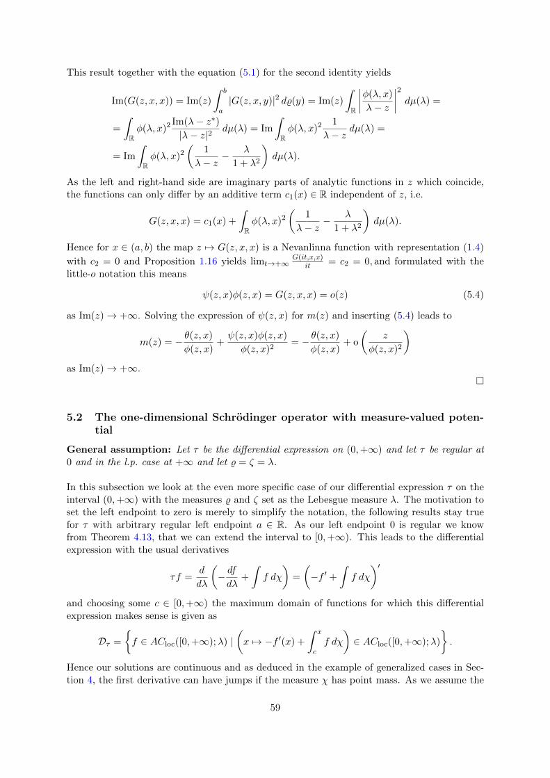
This result together with the equation (5.1) for the second identity yields
Im(G(z, x, x)) = Im(z)
∫ b
a|G(z, x, y)|2 d%(y) = Im(z)
∫R
∣∣∣∣φ(λ, x)
λ− z
∣∣∣∣2 dµ(λ) =
=
∫Rφ(λ, x)2
Im(λ− z∗)|λ− z|2
dµ(λ) = Im
∫Rφ(λ, x)2
1
λ− zdµ(λ) =
= Im
∫Rφ(λ, x)2
(1
λ− z− λ
1 + λ2
)dµ(λ).
As the left and right-hand side are imaginary parts of analytic functions in z which coincide,the functions can only differ by an additive term c1(x) ∈ R independent of z, i.e.
G(z, x, x) = c1(x) +
∫Rφ(λ, x)2
(1
λ− z− λ
1 + λ2
)dµ(λ).
Hence for x ∈ (a, b) the map z 7→ G(z, x, x) is a Nevanlinna function with representation (1.4)
with c2 = 0 and Proposition 1.16 yields limt→+∞G(it,x,x)
it = c2 = 0, and formulated with thelittle-o notation this means
ψ(z, x)φ(z, x) = G(z, x, x) = o(z) (5.4)
as Im(z)→ +∞. Solving the expression of ψ(z, x) for m(z) and inserting (5.4) leads to
m(z) = − θ(z, x)
φ(z, x)+ψ(z, x)φ(z, x)
φ(z, x)2= − θ(z, x)
φ(z, x)+ o
(z
φ(z, x)2
)as Im(z)→ +∞.
5.2 The one-dimensional Schrodinger operator with measure-valued poten-tial
General assumption: Let τ be the differential expression on (0,+∞) and let τ be regular at0 and in the l.p. case at +∞ and let % = ζ = λ.
In this subsection we look at the even more specific case of our differential expression τ on theinterval (0,+∞) with the measures % and ζ set as the Lebesgue measure λ. The motivation toset the left endpoint to zero is merely to simplify the notation, the following results stay truefor τ with arbitrary regular left endpoint a ∈ R. As our left endpoint 0 is regular we knowfrom Theorem 4.13, that we can extend the interval to [0,+∞). This leads to the differentialexpression with the usual derivatives
τf =d
dλ
(− dfdλ
+
∫f dχ
)=
(−f ′ +
∫f dχ
)′and choosing some c ∈ [0,+∞) the maximum domain of functions for which this differentialexpression makes sense is given as
Dτ =
f ∈ ACloc([0,+∞);λ) |
(x 7→ −f ′(x) +
∫ x
cf dχ
)∈ ACloc([0,+∞);λ)
.
Hence our solutions are continuous and as deduced in the example of generalized cases in Sec-tion 4, the first derivative can have jumps if the measure χ has point mass. As we assume the
59
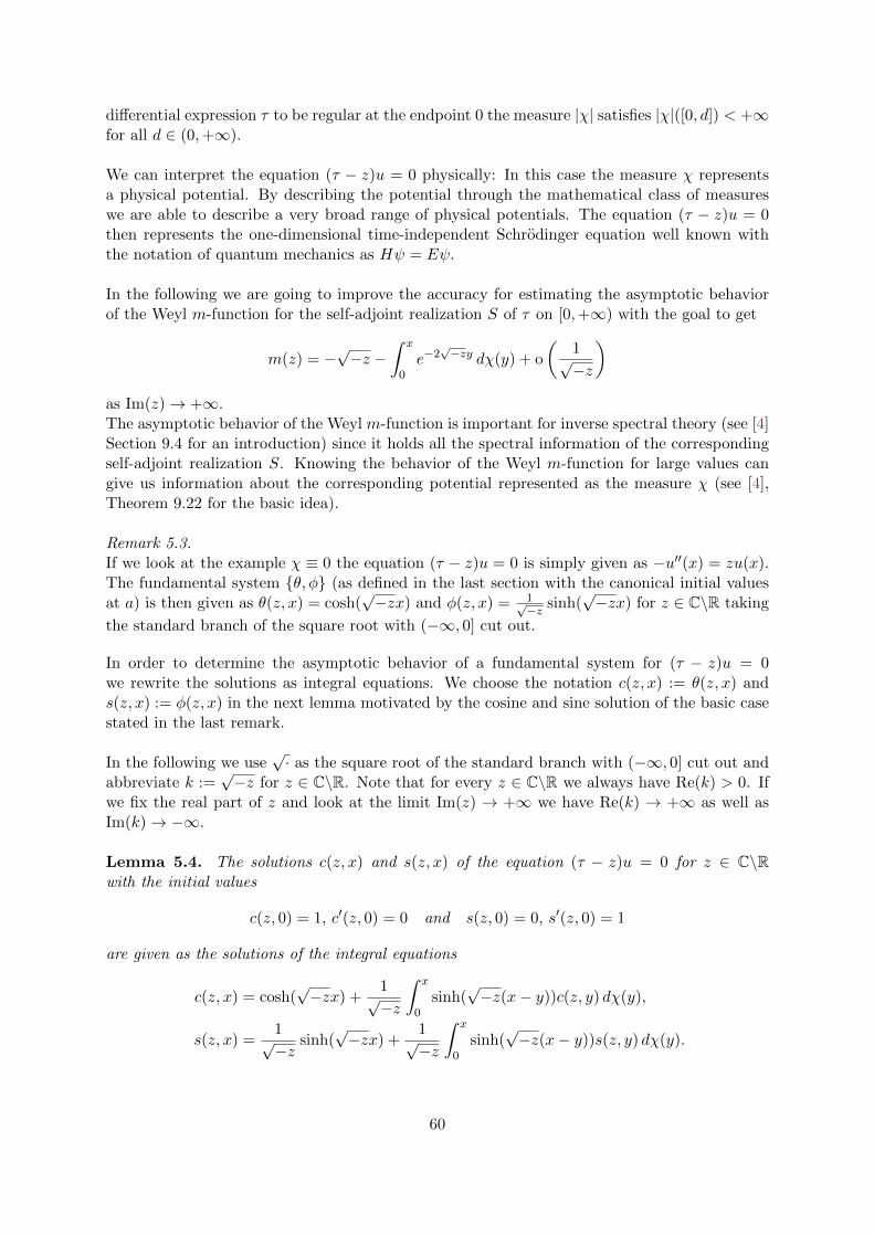
differential expression τ to be regular at the endpoint 0 the measure |χ| satisfies |χ|([0, d]) < +∞for all d ∈ (0,+∞).
We can interpret the equation (τ − z)u = 0 physically: In this case the measure χ representsa physical potential. By describing the potential through the mathematical class of measureswe are able to describe a very broad range of physical potentials. The equation (τ − z)u = 0then represents the one-dimensional time-independent Schrodinger equation well known withthe notation of quantum mechanics as Hψ = Eψ.
In the following we are going to improve the accuracy for estimating the asymptotic behaviorof the Weyl m-function for the self-adjoint realization S of τ on [0,+∞) with the goal to get
m(z) = −√−z −
∫ x
0e−2√−zy dχ(y) + o
(1√−z
)as Im(z)→ +∞.The asymptotic behavior of the Weyl m-function is important for inverse spectral theory (see [4]Section 9.4 for an introduction) since it holds all the spectral information of the correspondingself-adjoint realization S. Knowing the behavior of the Weyl m-function for large values cangive us information about the corresponding potential represented as the measure χ (see [4],Theorem 9.22 for the basic idea).
Remark 5.3.If we look at the example χ ≡ 0 the equation (τ − z)u = 0 is simply given as −u′′(x) = zu(x).The fundamental system θ, φ (as defined in the last section with the canonical initial valuesat a) is then given as θ(z, x) = cosh(
√−zx) and φ(z, x) = 1√
−z sinh(√−zx) for z ∈ C\R taking
the standard branch of the square root with (−∞, 0] cut out.
In order to determine the asymptotic behavior of a fundamental system for (τ − z)u = 0we rewrite the solutions as integral equations. We choose the notation c(z, x) := θ(z, x) ands(z, x) := φ(z, x) in the next lemma motivated by the cosine and sine solution of the basic casestated in the last remark.
In the following we use√· as the square root of the standard branch with (−∞, 0] cut out and
abbreviate k :=√−z for z ∈ C\R. Note that for every z ∈ C\R we always have Re(k) > 0. If
we fix the real part of z and look at the limit Im(z) → +∞ we have Re(k) → +∞ as well asIm(k)→ −∞.
Lemma 5.4. The solutions c(z, x) and s(z, x) of the equation (τ − z)u = 0 for z ∈ C\Rwith the initial values
c(z, 0) = 1, c′(z, 0) = 0 and s(z, 0) = 0, s′(z, 0) = 1
are given as the solutions of the integral equations
c(z, x) = cosh(√−zx) +
1√−z
∫ x
0sinh(
√−z(x− y))c(z, y) dχ(y),
s(z, x) =1√−z
sinh(√−zx) +
1√−z
∫ x
0sinh(
√−z(x− y))s(z, y) dχ(y).
60
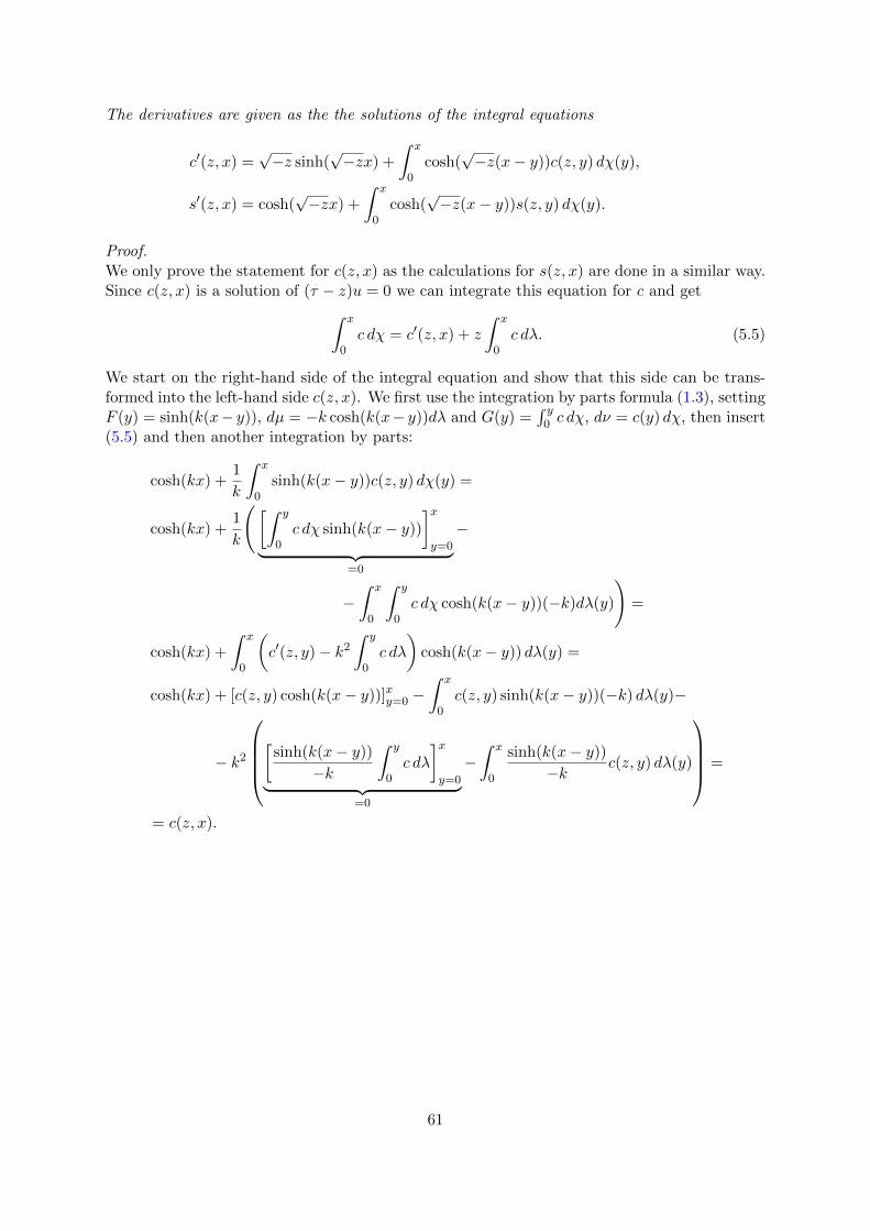
The derivatives are given as the the solutions of the integral equations
c′(z, x) =√−z sinh(
√−zx) +
∫ x
0cosh(
√−z(x− y))c(z, y) dχ(y),
s′(z, x) = cosh(√−zx) +
∫ x
0cosh(
√−z(x− y))s(z, y) dχ(y).
Proof.We only prove the statement for c(z, x) as the calculations for s(z, x) are done in a similar way.Since c(z, x) is a solution of (τ − z)u = 0 we can integrate this equation for c and get∫ x
0c dχ = c′(z, x) + z
∫ x
0c dλ. (5.5)
We start on the right-hand side of the integral equation and show that this side can be trans-formed into the left-hand side c(z, x). We first use the integration by parts formula (1.3), settingF (y) = sinh(k(x− y)), dµ = −k cosh(k(x− y))dλ and G(y) =
∫ y0 c dχ, dν = c(y) dχ, then insert
(5.5) and then another integration by parts:
cosh(kx) +1
k
∫ x
0sinh(k(x− y))c(z, y) dχ(y) =
cosh(kx) +1
k
([∫ y
0c dχ sinh(k(x− y))
]xy=0︸ ︷︷ ︸
=0
−
−∫ x
0
∫ y
0c dχ cosh(k(x− y))(−k)dλ(y)
)=
cosh(kx) +
∫ x
0
(c′(z, y)− k2
∫ y
0c dλ
)cosh(k(x− y)) dλ(y) =
cosh(kx) + [c(z, y) cosh(k(x− y))]xy=0 −∫ x
0c(z, y) sinh(k(x− y))(−k) dλ(y)−
− k2
[
sinh(k(x− y))
−k
∫ y
0c dλ
]xy=0︸ ︷︷ ︸
=0
−∫ x
0
sinh(k(x− y))
−kc(z, y) dλ(y)
=
= c(z, x).
61
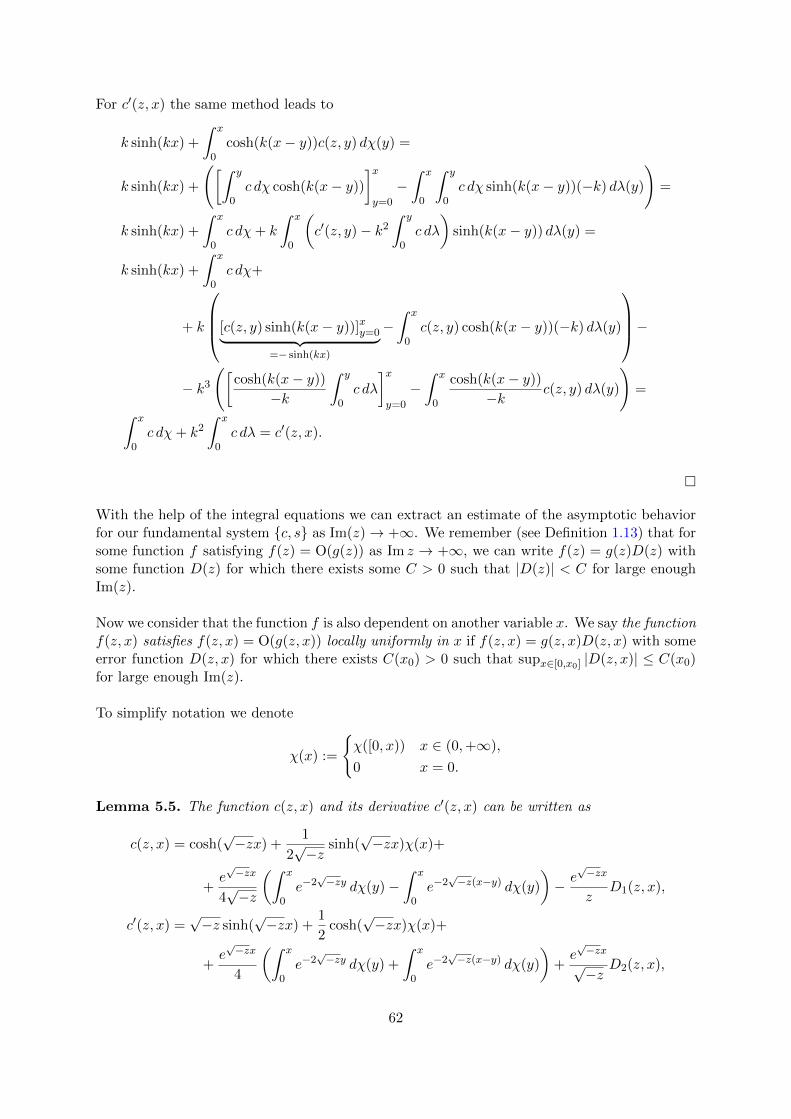
For c′(z, x) the same method leads to
k sinh(kx) +
∫ x
0cosh(k(x− y))c(z, y) dχ(y) =
k sinh(kx) +
([∫ y
0c dχ cosh(k(x− y))
]xy=0
−∫ x
0
∫ y
0c dχ sinh(k(x− y))(−k) dλ(y)
)=
k sinh(kx) +
∫ x
0c dχ+ k
∫ x
0
(c′(z, y)− k2
∫ y
0c dλ
)sinh(k(x− y)) dλ(y) =
k sinh(kx) +
∫ x
0c dχ+
+ k
[c(z, y) sinh(k(x− y))]xy=0︸ ︷︷ ︸=− sinh(kx)
−∫ x
0c(z, y) cosh(k(x− y))(−k) dλ(y)
−− k3
([cosh(k(x− y))
−k
∫ y
0c dλ
]xy=0
−∫ x
0
cosh(k(x− y))
−kc(z, y) dλ(y)
)=∫ x
0c dχ+ k2
∫ x
0c dλ = c′(z, x).
With the help of the integral equations we can extract an estimate of the asymptotic behaviorfor our fundamental system c, s as Im(z)→ +∞. We remember (see Definition 1.13) that forsome function f satisfying f(z) = O(g(z)) as Im z → +∞, we can write f(z) = g(z)D(z) withsome function D(z) for which there exists some C > 0 such that |D(z)| < C for large enoughIm(z).
Now we consider that the function f is also dependent on another variable x. We say the functionf(z, x) satisfies f(z, x) = O(g(z, x)) locally uniformly in x if f(z, x) = g(z, x)D(z, x) with someerror function D(z, x) for which there exists C(x0) > 0 such that supx∈[0,x0] |D(z, x)| ≤ C(x0)for large enough Im(z).
To simplify notation we denote
χ(x) :=
χ([0, x)) x ∈ (0,+∞),
0 x = 0.
Lemma 5.5. The function c(z, x) and its derivative c′(z, x) can be written as
c(z, x) = cosh(√−zx) +
1
2√−z
sinh(√−zx)χ(x)+
+e√−zx
4√−z
(∫ x
0e−2√−zy dχ(y)−
∫ x
0e−2√−z(x−y) dχ(y)
)− e
√−zx
zD1(z, x),
c′(z, x) =√−z sinh(
√−zx) +
1
2cosh(
√−zx)χ(x)+
+e√−zx
4
(∫ x
0e−2√−zy dχ(y) +
∫ x
0e−2√−z(x−y) dχ(y)
)+e√−zx√−z
D2(z, x),
62
with error functions Di(z, x) satisfying Di(z, x) = O(1) as Im(z) → +∞ locally uniform in xfor i = 1, 2.
The function s(z, x) and its derivative s′(z, x) can be written as
s(z, x) =1√−z
sinh(√−zx)− 1
2zcosh(
√−zx)χ(x)+
+e√−zx
4z
(∫ x
0e−2√−zy dχ(y) +
∫ x
0e−2√−z(x−y) dχ(y)
)+e√−zx
√−z3
D3(z, x),
s′(z, x) = cosh(√−zx) +
1
2√−z
sinh(√−zx)χ(x)−
− e√−zx
4√−z
(∫ x
0e−2√−zy dχ(y)−
∫ x
0e−2√−z(x−y) dχ(y)
)− e
√−zx
zD4(z, x),
with error functions Di(z, x) satisfying Di(z, x) = O(1) as Im(z) → +∞ locally uniform in xfor i = 3, 4.
Proof.Let x0 > 0. First we define c(z, x) := e−kxc(z, x) and show that there exists some C0(x0) ≥ 0such that
|c(z, x)| ≤ C0(x0), z ∈ C\[0,+∞), x ∈ [0, x0].
For that we use the integral equation for c from the last lemma (Lemma 5.4) to write
c(z, x) = e−kxc(z, x)
= e−kx cosh(kx) +1
k
∫ x
0e−kx sinh(k(x− y))c(z, y) dχ(y)
=1 + e−2kx
2+
∫ x
0
1− e−2k(x−y)
2kc(z, y) dχ(y). (5.6)
We show that the solution of this integral equation is bounded for all z ∈ C\[0,+∞), x ∈ [0, x0].We define inductively
ϕ0(z, x) =1 + e−2kx
2and ϕn+1(z, x) =
∫ x
0
1− e−2k(x−y)
2kϕn(z, y) dχ(y)
and claim
|ϕn(z, x)| ≤ xn
n!
(∫ x
0d|χ|
)n, n ≥ 0.
For n = 0 this is true and with the estimate∣∣∣∣1− e−2kx2k
∣∣∣∣ =
∣∣∣∣∫ x
0e−2kt dt
∣∣∣∣ ≤ x
63
as well as the substitution rule from Lemma 3.4 (similarly as in (3.6)) we inductively have
|ϕn+1(z, x)| ≤∫ x
0
∣∣∣∣∣1− e−2k(x−y)2k
∣∣∣∣∣ ynn!
(∫ y
0d|χ|
)nd|χ|(y)
≤∫ x
0(x− y)
xn
n!
(∫ y
0d|χ|
)nd|χ|(y)
≤ xn+1
n!
∫ x
0
(∫ y
0d|χ|
)nd|χ|(y)
≤ xn+1
(n+ 1)!
(∫ x
0d|χ|
)n+1
.
It follows thatN∑n=0
|ϕn(z, x)| ≤N∑n=0
xn
n!
(∫ x
0d|χ|
)n≤ ex
∫ x0 d|χ| ≤ ex0
∫ x00 d|χ| =: C0(x0) (5.7)
for all N ∈ N and therefore the series ϕ(z, x) :=∑∞
n=0 ϕn(z, x) converges uniformly for z ∈C\[0,+∞) , x ∈ [0, x0]. Going back to the definition of ϕn we have
N∑n=0
ϕn(z, x) =1 + e−2kx
2+
N∑n=1
∫ x
0
1− e−2k(x−y)
2kϕn−1(z, y) dχ(y)
=1 + e−2kx
2+
∫ x
0
1− e−2k(x−y)
2k
N−1∑n=0
ϕn(z, y) dχ(y).
Taking the limit N → +∞ which commutes with the integral due to the uniform convergenceleads to
ϕ(z, x) =1 + e−2kx
2+
∫ x
0
1− e−2k(x−y)
2kϕ(z, y) dχ(y).
Since the solution of this integral equation is unique by the Gronwall lemma (Lemma 3.5) wehave c(z, x) = ϕ(z, x) and we see that the function c(z, x) satisfies
|c(z, x)| ≤ C0(x0), z ∈ C\[0,+∞), x ∈ [0, x0].
Next we show that the function c(z, x) has the asymptotic behavior stated in the lemma.
To this end we first write
c(z, x) = ekxc(z, x)
= cosh(kx) +ekx
k
∫ x
0
1− e−2k(x−y)
2c(z, y) dχ(y)︸ ︷︷ ︸
D(z,x):=
.
The function D(z, x) satisfies
supx∈[0,x0]
|D(z, x)| = supx∈[0,x0]
∣∣∣∣∣∫ x
0
1− e−2k(x−y)
2c(z, y) dχ(y)
∣∣∣∣∣≤ ex0
∫ x00 d|χ|
∫ x0
0d|χ| =: C(x0) (5.8)
64
for all z ∈ C\[0,+∞). Reinserting this into our integral equation for c(z, x) leads to
c(z, x) = cosh(kx) +1
k
∫ x
0sinh(k(x− y))
(cosh(ky) +
eky
kD(z, y)
)dχ(y)
= cosh(kx) +ekx
4k
∫ x
0(1− e−2k(x−y))(1 + e−2ky) dχ(y)+
+ekx
k2
∫ x
0
1− e−2k(x−y)
2D(z, y) dχ(y)︸ ︷︷ ︸
D1(z,x):=
= cosh(kx) +ekx
4k
∫ x
0(1− e−2kx + e−2ky − e−2k(x−y)) dχ(y) +
ekx
k2D1(z, x)
= cosh(kx) +1
2ksinh(kx)χ(x)+
+ekx
4k
(∫ x
0e−2ky dχ(y)−
∫ x
0e−2k(x−y) dχ(y)
)+ekx
k2D1(z, x).
The function D1(z, x) satisfies
supx∈[0,x0]
|D1(z, x)| = supx∈[0,x0]
∣∣∣∣∣∫ x
0
1− e−2k(x−y)
2D(z, y) dχ(y)
∣∣∣∣∣≤ C(x0)
∫ x0
0d|χ| := C1(x0)
for all z ∈ C\[0,+∞) and we arrive at the desired asymptotic for c(z, x). The other asymptoticsare calculated similarly.
Remark 5.6.Note that the integral terms of last lemma
I1(z, x) :=
∫ x
0e−2ky dχ(y) and I2(z, x) :=
∫ x
0e−2k(x−y) dχ(y)
both are uniformly bounded in z ∈ C\[0,+∞). Applying the dominated convergence theoremto I1(z, x) for x ∈ (0,+∞) leads to
I1(z, x) =
∫0
1 dχ(y) +
∫(0,x)
e−2ky dχ(y) = χ(0) + o(1) (5.9)
as Im(z)→ +∞ as well as
I2(z, x) =
∫ x
0e−2k(x−y) dχ(y) = o(1)
as Im(z)→ +∞.
We will calculate better estimates for the error functions of Lemma 5.5 with the help of thedominated convergence theorem.
65
Lemma 5.7. For x ∈ (0,+∞) the error functions of Lemma 5.5 can be further estimatedas
Di(z, x) =1
8
∫(0,x)
(χ(y) + χ(0)
)dχ(y) + o(1), i = 1, 2,
Di(z, x) =1
8
∫(0,x)
(χ(y)− χ(0)
)dχ(y) + o(1), i = 3, 4,
as Im(z)→ +∞.
Proof.Let x > 0 be fixed. We continue with the notation introduced in the proof of Lemma 5.5 andcalculate the estimate for the error function D1(z, x) of the solution c(z, x).
First note that we have
c(z, x) =1 + e−2kx
2+
1
kD(z, x)
where D(z, x) satisfies supx∈[0,x0] |D(z, x)| ≤ C(x0) as Im(z)→ +∞ for x0 ∈ (0,+∞) by (5.8).
Reinserting this into the definition of the function D(z, x) leads to
D(z, x) =
∫ x
0
1− e−2k(x−y)
2c(z, y) dχ(y)
=1
4
∫ x
0(1− e−2k(x−y))(1 + e−2ky)︸ ︷︷ ︸
f(z,y):=
dχ(y) +1
2k
∫ x
0(1− e−2k(x−y))D(z, y) dχ(y)︸ ︷︷ ︸
F (z,x):=
.
Now as the function f(z, y) is locally uniformly bounded and since f(z, y) → 1 + 10(y) asIm(z)→ +∞ we can apply the dominated convergence theorem and get
D(z, x) =
14
(χ(x) + χ(0)
)+ 1
2kF (z, x) x > 0
0 x = 0
where the integral F (z, x) satisfies F (z, x) = O(1) locally uniformly in x as Im(z)→ +∞. Fromthe proof of Lemma 5.5 we know that the error function D1(z, x) is defined as
D1(z, x) =1
2
∫ x
0(1− e−2k(x−y))D(z, y) dχ(y).
If we now insert the calculation for D(z, x) from above and apply the dominated convergencetheorem again we get
D1(z, x) =1
2
∫(0,x)
(1− e−2k(x−y))(
1
4(χ(y) + χ(0) +
1
2kF (z, y)
)dχ(y)
=1
8
∫(0,x)
(χ(y) + χ(0)
)dχ(y) + o(1)
as Im(z)→ +∞.
The estimates for the error functions of c′(z, x), s(z, x) and s′(z, x) are calculated in a similarmanner.
66
We introduce circles discovered by Weyl which he used for the original proof of the Weyl alter-native. Given a self-adjoint realization S of the differential expression τ , we know the solutionsof the equation (τ − z)u = 0, which lie in the domain of S, satisfy certain boundary conditions(see Theorem 4.50). This solutions can be parameterized on circles called Weyl circles.
Definition 5.8. For x ∈ (0,+∞) we denote
q(z, x) := −W (c(z), s(z)∗)(x)
W (s(z), s(z)∗)(x), r(z, x) :=
1
|W (s(z), s(z)∗)(x)|.
This functions are called Weyl-center and Weyl-radius respectively.
We denote the open disk centered at q ∈ C with radius r > 0 as Ur(q) := z ∈ C | |z − q| < r.The next Lemma is based on the original proof of the Weyl alternative, which can be found forexample in [2] after Theorem 13.18.
Lemma 5.9. The Weyl-function satisfies m(z) ∈ Ur(z,x)(q(z, x)) for all x ∈ (0,+∞). Forz ∈ C+ and x ∈ (0,+∞) some m ∈ C satisfies the equivalences
m ∈ Ur(z,x)(q(z, x)) ⇐⇒ c′(z, x) +ms′(z, x)
c(z, x) +ms(z, x)∈ C+
m ∈(Ur(z,x)(q(z, x))
)c⇐⇒ c′(z, x) +ms′(z, x)
c(z, x) +ms(z, x)∈ C−.
Proof.For fixed z ∈ C+ we define
f, g(x) :=1
z∗ − zW (f∗, g)(x).
If u is a solution of (τ − z)u = 0 the Lagrange identity (see equation (4.11)) yields u, u(x)−u, u(c) =
∫ xc |u|
2 dλ. Hence the function x 7→ u, u(x) is increasing. Since c, c(0) =s, s(0) = 0, the functions x 7→ c, c(x) and x 7→ s, s(x) are positive and increasing forx ∈ (0,+∞). For an arbitrary solution u of (τ − z)u = 0 we have the identity
u, u(x) =1
2 Im(z∗)W (u∗, u)(z) =
Im(u∗u′)
Im(z∗)=|u(x)|2
Im(z∗)Im
(u′(x)
u(x)
). (5.10)
For m ∈ C we have
c+ms, c+ms(x) = c, c(x) +m∗s, c(x) +mc, s(x) + |m|2s, s(x) =
= s, s(x)
(|m|2 +
(mc, s(x))∗ +mc, s(x)
s, s(x)+|c, s(x)|2
|s, s(x)|2−
− c, c(x)2s, s(x)− c, c(x)s, s(x)
s, s(x)2︸ ︷︷ ︸=:h(z,x)
= s, s(x)
(∣∣∣∣∣m−(−c, s(x)
s, s(x)︸ ︷︷ ︸=q(z,x)
)∣∣∣∣∣2
− h(z, x)
)
= s, s(x)(|m− q(z, x)|2 − h(z, x)).
67
After some computing with help of the Plucker identity from Proposition 4.11 (for details see[2], after Theorem 13.18.) we see that h(z, x) coincides with the squared Weyl-radius as definedabove, i.e. h(z, x) = r(z, x)2 and we get the equation
c+ms, c+ms = s, s(x)(|m− q(z, x)|2 − r(z, x)2). (5.11)
So for a fixed x > 0 the m ∈ C for which c+ms, c+ms = 0 is satisfied lie on a circle3 withradius r(z, x) centered at q(z, x). From this and with the identity (5.10) follows the equivalence
m ∈ Ur(z,x)(q(z, x)) ⇐⇒ c+ms, c+ms(x) < 0
⇐⇒ |c(x) +ms(x)|2
Im(z∗)︸ ︷︷ ︸<0
Im
(c′(x) +ms′(x)
c(x) +ms(x)
)< 0
⇐⇒ Im
(c′(x) +ms′(x)
c(x) +ms(x)
)> 0
⇐⇒ c′(x) +ms′(x)
c(x) +ms(x)∈ C+.
And similarly it follows that
m ∈(Ur(z,x)(q(z, x))
)c⇐⇒ c′(x) +ms′(x)
c(x) +ms(x)∈ C−.
Now we show that m(z) ∈ Ur(z,x)(q(z, x)). As m(z) is a Nevanlinna function m(z) ∈ C+ andwe have
ψ,ψ(0) =Im(m(z))
Im(z∗)< 0
by definition of the Weyl solution ψ of the self-adjoint realization S. Now as ψ and ψ∗ lie in Snear b, Lemma 4.46 yields
limx→∞ψ,ψ(x) =
1
2 Im(z∗)limx→∞
W (ψ,ψ∗)(x) = 0.
We know from above that for solutions of (τ − z)u = 0 the function x 7→ u, u(x) is increasingso this is true for x 7→ ψ,ψ(x) and as ψ,ψ(x) is negative-valued at 0 and increasing to 0for infinity, we have 0 > ψ,ψ(x) = c+ms, c+ms(x) for x ∈ [0,+∞). With the first partof the proof this is equivalent to m(z) ∈ Ur(z,x)(q(z, x)) for x ∈ [0,+∞).
The following lemma is based on the idea of Lemma 1 in [3].
Lemma 5.10. Let x ∈ (0,+∞) and v(z, x) be the solution of the initial value problem(τ − z)u = 0 with v(z, x) = 1, v′(z, x) = −
√−z. Then the asymptotic behavior of the Weyl
m-function is given as
m(z) =v′(z, 0)
v(z, 0)+ o(e−2
√−zxz) (5.12)
as Im(z)→ +∞.
3It can be shown that all the Weyl circles are nested for x → +∞ and that the Weyl function is the onlyelement in the intersection of all Weyl circles, hence the name limit point case at +∞.
68
Proof.Let x ∈ (0,+∞) be fixed. From the last lemma we know that m(z) ∈ Ur(z,x)(q(z, x)) and now
we show that we also have v′(z,0)v(z,0) ∈ Ur(z,x)(q(z, x)) which lets us estimate the distance between
m(z) and v′(z,0)v(z,0) through the Weyl radius at x. As the Wronskian is constant for two solutions
of (τ − z)u = 0 we get
v′(z, 0)
v(z, 0)=W (c, v)(0)
W (v, s)(0)=W (c, v)(x)
W (v, s)(x)=c(x)v′(x)− c′(x)v(x)
v(x)s′(x)− v′(x)s(x)=−c(x)k − c′(x)
s′(x) + ks(x). (5.13)
Now an easy computation shows that if we use the above identity for v′(z,0)v(z,0) we get
c′(x) + s′(x)v′(0)v(0)
c(x) + s(x)v′(0)v(0)
= −k ∈ C+
and by the last lemma (Lemma 5.9) this is equivalent to v′(z,0)v(z,0) ∈ Ur(z,x)(q(z, x)). It follows that
we have ∣∣∣∣m(z)− v′(z, 0)
v(z, 0)
∣∣∣∣ ≤ 2r(z, x). (5.14)
Now we will use Lemma 5.5 to calculate the asymptotic behavior for r(z, x). We abbreviate
I1(z, x) :=
∫ x
0e−2ky dχ(y) and I2(z, x) :=
∫ x
0e−2k(x−y) dχ(y)
and note that the integrals I1(z, x) and I2(z, x) are uniformly bounded in z ∈ C\[0,+∞). Wehave
s(z, x) =ekx
k
1
2(1− e−2kx) +
1
2k(1 + e−2kx)χ(x)− 1
4k(I1(z, x)− I2(z, x)) + O(
1
k2)︸ ︷︷ ︸
B1(z,x):=
=ekx
kB1(z, x)
with a function B1(z, x)→ 12 as Im(z)→ +∞. Similarly for s′(z, x) we have
s′(z, x)∗ = ek∗x
1
2(1 + e−2kx) +
1
2k(1− e−2kx)χ(x)− 1
4k(I1(z, x)− I2(z, x)) + O(
1
k2)︸ ︷︷ ︸
B2(z,x):=
∗
= ek∗xB2(z, x)∗
with a function B2(z, x) → 12 as Im(z) → +∞. Inserting this into the definition of the Weyl
radius leads to
r(z, x) =1
W (s, s∗)(x)=
1
2| Im(s(x)s′(x)∗)|=
1
2| Im( 1kekxB1(z, x)ek∗xB2(z, x)∗)|
=
=|k|2e−2Re(k)x
2| Im(k∗B1(z, x)B2(z, x)∗)|=
e−2Re(k)x|k|2
2| Im(k∗B1(z, x)B2(z, x)∗)|.
69
Looking at the limit Im(z) → +∞ we know Im(k) → −∞ and since B1(z, x)B2(z, x)∗ → 14
we also know that Im(B1(z, x)B2(z, x)∗)→ 0. It follows that | Im(k∗B1(z, x)B2(z, x)∗)| → +∞and we arrive at
r(z, x) =e−2Re(k)x|k|2
2| Im(k∗B1(z, x)B2(z, x))|= o(e−2Re(k)xz)
as Im(z)→ +∞. Now by (5.14) this means we are finished.
We arrive at the final theorem of this thesis, which combines the asymptotic behavior of thefundamental system for s(z, x), c(z, x) from Lemma 5.5 with the asymptotic behavior for theWeyl m-function from Lemma 5.10.
Theorem 5.11. For every x ∈ (0,+∞) the Weyl m-function has the asymptotic behavior
m(z) = −√−z −
∫ x
0e−2√−zy dχ(y) + o
(1√−z
)(5.15)
as Im(z)→ +∞.
Proof.Let x ∈ (0,+∞) be fixed. Combining the asymptotic behavior of the Weyl function m(z) from(5.12) with the equation (5.13) leads to
m(z) =v′(z, 0)
v(z, 0)+ o(e−2kxz) =
−kc(x)− c′(x)
s′(x) + ks(x)+ o(e−2kxz) (5.16)
as Im(z)→ +∞. Now we can use Lemma 5.5 to calculate the asymptotics of −kc(x)−c′(x)
s′(x)+ks(x) with
an error term of the order o(1k
). To do this we prepare some calculations first.
We simplify the numerator and denominator of the fraction −c(x)k−c′(x)
s′(x)+ks(x) separately:For the numerator we get
−kc(x)− c′(x) = −k cosh(kx)− 1
2sinh(kx)χ(x)− ekx
4I1(z, x) +
ekx
4I2(z, x)− ekx
kD1(z, x)−
− k sinh(kx)− 1
2cosh(kx)χ(x)− ekx
4I1(z, x)− ekx
4I2(z, x)− ekx
kD2(z, x)
= −kekx − 1
2χ(x)ekx − 1
2ekxI1(z, x)− ekx
k(D1(z, x) +D2(z, x))
= −kekx(
1 +1
2k(χ(x) + I1(z, x)) +
1
k2(D1(z, x) +D2(z, x))
). (5.17)
70
For the denominator we calculate in a similar way
s′(x) + ks(x) = cosh(kx) +1
2ksinh(kx)χ(x)− ekx
4kI1(z, x) +
ekx
4kI2(z, x) +
ekx
k2D3(z, x)+
+ sinh(kx) +1
2kcosh(kx)χ(x)− ekx
4kI1(z, x)− ekx
4kI2(z, x) +
ekx
k2D4(z, x)
= ekx +ekx
2kχ(x)− ekx
2kI1(z, x) +
ekx
k2(D3(z, x) +D4(z, x))
= ekx
1 +1
2k(χ(x)− I1(z, x)) +
1
k2(D3(z, x) +D4(z, x))︸ ︷︷ ︸
M(z,x):=
= ekx(1 +M(z, x)). (5.18)
As I1(z, x) as well as Di(z, x), i = 3, 4 are bounded as Im(z) → +∞, the term |M(z, x)| getsarbitrary small for large enough Im(z). Hence we can use the identity 1
1+x =∑
n≥0(−x)n for|x| < 1 for the term M(z, x) which leads to
1
1 +M(z, x)= 1−M(z, x) +M(z, x)2 + o
(1
k2
)= 1− 1
2k(χ(x)− I1)−
1
k2(D3 +D4) +M(z, x)2 + o
(1
k2
)= 1− 1
2k(χ(x)− I1)−
1
k2(D3 +D4) +
1
4k2(χ(x)2 + I21 − 2χ(x)I1
)+ o
(1
k2
)(5.19)
as Im(z)→ +∞.
By Lemma 5.7 we have
D1(z, x) +D2(z, x)−D3(z, x)−D4(z, x) =
=1
4
∫(0,x)
(χ(y) + χ(0)
)dχ(y)− 1
4
∫(0,x)
(χ(y)− χ(0)
)dχ(y) + o(1)
=1
2χ(0)
∫(0,x)
dχ(y) + o(1)
=1
2χ(0)
(χ(x)− χ(0)
)+ o(1) (5.20)
as Im(z)→ +∞.
We will now use the above calculations to determine the asymptotic behavior of −kc(x)−c′(x)
s′(x)+ks(x)
with accuracy of order o(1k
)as Im(z)→ +∞.
For the first equal sign in the next calculation we insert the identities (5.17) and (5.18) and seethat the exponential factors cancel each other. For the second identity we use (5.19) and thensort the terms by order of k. For the third equal sign we use the equation (5.20) as well as the
71
equation (5.9) from Remark 5.6:
−kc(x)− c′(x)
s′(x) + ks(x)= −k
(1 +
1
2k(χ(x) + I1) +
1
k2(D1 +D2)
)(1
1 +M(z, x)
)= −k − I1 −
1
k(D1 +D2 −D3 −D4) +
1
2k
(χ(x)I1 − I21
)+ o
(1
k
)= −k − I1 −
1
2k
(χ(0)
(χ(x)− χ(0)
)− χ(x)χ(0) + χ(0)2
)+ o
(1
k
)= −k − I1 −
1
2k
(χ(0)χ(x)− χ(0)2 − χ(x)χ(0) + χ(0)2
)+ o
(1
k
)= −k − I1 + o
(1
k
)= −k −
∫ x
0e−2ky dχ(y) + o
(1
k
)as Im(z)→ +∞.
Finally we can plug this into the equation (5.16) and get the desired result
m(z) =−kc(x)− c′(x)
s′(x) + ks(x)+ o(e−2kxz)
= −k −∫ x
0e−2ky dχ(y) + o
(1
k
)as Im(z)→ +∞.
We will now look at an easy example to check the result of Theorem 5.11. We extend the domainof the differential expression τ to the inverval (−∞,+∞) and look at the measure χ = αδ0 withsome constant α ∈ C. This leads to the differential expression τ for a function f ∈ D(τ) givenas
(τf)(x) =
(t 7→ −f ′(t) + α
∫ t
0f dδ0
)′(x), x ∈ R.
Applying Theorem 5.11 immediately yields a Weyl function estimate given as
m(z) = −√−z − α+ o(
1√−z
)
as Im(z) → +∞. We will check this result by calculating the Weyl solution ψ(z, x) which hasto satisfy the conditions (see Definition 4.51)
ψ(z, ·) ∈ D(τ),
ψ(z, ·) is solution of the differential equation (τ − z)u = 0, with
ψ(z, 0) = 1 and ψ(z, ·) ∈ L2((c,+∞);λ), c ∈ R
for z ∈ C\R.
From the first condition ψ(z, ·) ∈ D(τ) follows that both the function x 7→ ψ(z, x) as well asthe function x 7→ ψ1(z, x) := −ψ′(z, x) + α
∫ x0 ψ(z, ·) dδ0 have to be continuous on R for every
72
z ∈ C\R. This means the function x 7→ ψ′(z, x) has to be continuous for x ∈ (−∞, 0)∪ (0,+∞)and at the point x = 0 has to satisfy the jump condition ψ′(z, 0+) − ψ′(z, 0−) = αψ(z, 0) forz ∈ C\R.
Now in this example the differential equation (τ − z)ψ(z, ·) = 0 takes the form ψ′′(z, ·) =−zψ(z, ·) which leads to a solution of the form
ψ(z, x) =
c1e−kx + c2e
kx for x > 0
1 x = 0
d1e−kx + d2e
kx for x < 0
with constants c1, c2, d1, d2 ∈ C. Because of the conditions ψ(z, 0) = 1 and ψ(z, ·) ∈ L2((c,+∞);λ)with c ∈ R follows that c1 = 1 and c2 = 0.Since ψ(z, ·) has to be continuous it follows that d1 + d2 = 1. The jump condition leads to
ψ′(z, 0+)− ψ′(z, 0−) = αψ(z, 0)
−k − (−kd1 + kd2) = α
−k + k(1− d2)− kd2 = α
d2 = − α
2k
and it follows that d1 = 1 − d2 = 1 + α2k . Inserting this constants leads to the Weyl solution
given as
ψ(z, x) =
e−kx x > 0
(1 + α2k )e−kx − α
2kekx x ≤ 0.
Now from Definition 4.51 follows that
m(z) = ψ′(z, 0) = −k − α = −√−z − α
which shows that the estimate of Theorem 5.11 is valid.
73
References
[1] Gerald Teschl, Jonathan Eckhardt: Sturm-Liouville operators with measure-valuecoefficients; d’Analyse Math. 120, 151-224; 2013
[2] Joachim Weidmann: Spectral theory of ordinary differential operators; Lecture Notes inMath., Vol. 1258, Springer, Berlin; 1987
[3] Frederick Valentine Atkinson: On the location of Weyl circles; Proceedings of theRoyal Society of Edinburgh, 88A, 345-356; 1981
[4] Gerald Teschl: Mathematical methods in quantum mechanics; American MathematicalSociety; 2009
[5] Gerald Teschl, Jonathan Eckhardt, Fritz Gesztesy, Roger Nichols: Weyl-Titchmarsh theory for Sturm-Liouville operators with distributional potentials; OpusculaMath. 33, 467-563; 2013
[6] Gerald Teschl, Jonathan Eckhardt, Fritz Gesztesy, Roger Nichols: Inversespectral theory for Sturm-Liouville operators with distributional potentials; J. Lond. Math.Soc. (2) 88, 801-828; 2013
[7] Gerald Teschl, Fritz Gesztesy, Jonathan Eckhardt, Roger Nichols: Super-symmetry and Schrodinger-type operators with distributional matrix-valued potentials; toappear
[8] Neil Falkner, Gerald Teschl: On the substitution rule for Lebesgue-Stieltjes integrals;Expo. Math. 30, no. 4, 412-418; 2012
[9] A.A. Danielyan, B.M. Levitan: On the asymptotic behaviour of the Weyl-Titchmarshm-function; Math. USSR Izv. 36, 487-496; 1991
[10] Alexei Rybkin: On the trace approach to the inverse scattering problem in dimensionone; SIAM J. Math. Anal.; 2001
[11] Richard Arens: Operational calculus of linear relations; Pacific Journal of Mathematics,1961
[12] Ronald Cross: Multivalued linear operators; Monographs and Textbooks in Pure andApplied Mathematics 213, Marcel Dekker, New York, 1998.
[13] Aad Dijksma, H. S. V. de Snoo: Self-adjoint extensions of symmetric subspaces; PacificJournal of Mathematics, 54, 1974
[14] Naum Ilyich Akhiezer, Israel M. Glazman: Theory of linear Operators in Hilbertspace; Dover Publications Inc., 1993
[15] Harald Woracek, Michael Kaltenback, Martin Blumlinger: FunktionalanalysisI ; Lecture notes; 2011
[16] Michael Kaltenback: Funktionalanalysis II ; Lecture notes; 2010
[17] Michael Kaltenback: Analysis III ; Lecture notes; 2009
74


![Flur 26 Hst Freiligrathplatz - Düsseldorf€¦ · 15 I 13 I 18 16 17 II I I I 14 12 II 10 II I I 4a II I 6 II 8 II 8 II 10 II I I-I-I-I I I I I I I I I I I /LOLHQWKDOVWUD H B8 'DQ]LJHU](https://img.pdfslide.org/doc/110x75/6061ca6ec0f4fb4c5004df74/flur-26-hst-freiligrathplatz-dsseldorf-15-i-13-i-18-16-17-ii-i-i-i-14-12-ii.jpg)