Embed Size (px)
Citation preview
The q-Brauer algebras
Von der Fakultat Mathematik und Physik der Universitat Stuttgartzur Erlangung der Wurde eines Doktors der
Naturwissenschaften (Dr. rer. nat) genehmigte Abhandlung
Vorgelegt von
Nguyen Tien Dung
aus Vinh, Vietnam
Hauptberichter: Prof. Dr. rer. nat. S. Konig
Mitberichter: Prof. Dr. rer. nat. R. Dipper
Tag der mundlichen Prufung: 23. April 2013
Institut fur Algebra und Zahlentheorie der Universitat Stuttgart
2013

D93 Diss. Universitat Stuttgart
Eidesstattliche Erklarung
Ich versichere, dass ich diese Dissertation selbstandig verfasst und nur dieangegebenen Quellen und Hilfsmittel verwendet habe.
Nguyen Tien Dung
Acknowledgements
In my humble acknowledgements, it is a pleasure to express my gratitudeto all people who have supported, encouraged and helped me during thetime I spent working on this thesis.
First of all, I would like to record my deep and sincere gratitude tomy supervisor Prof. Dr. Steffen Koenig. I am grateful to him for super-vision, advice, and guidance from the early stage of this research as wellas giving me valued suggestions through out the work. He provided mean open and friendly environment in the discussions and supported me invarious ways that include two and a half year financial assistance and manyrecommendation letters, in particular, for DAAD.
Furthermore, many thanks to all of my colleagues who helped me duringthis project. In particular, thank to Qunhua Liu for support and help atthe basic steps in my work, to Inga Benner, Frederick Marks and Mrs ElkeGangl for their help dealing with administrative and language (German)matters, to Shalile Armin for the useful discussions concerning the Braueralgebra, and Qiong Guo for her help concerning LaTeX problems.
For financial support I would like to thank the Project MOET - 322of the Vietnam government and (partly) the DFG Priority Program SPP-1489.
Finally, I specially express my appreciation to my parents for theirencouragement and invaluable support over the last years, to my wife andmy lovely daughter for their inseparable and spiritual support.
Stuttgart, 2013 Nguyen Tien Dung
Zusammenfassung
Diese Dissertation untersucht strukturelle Eigenschaften von q-BrauerAlgebren uber einem kommutativen Ring mit Einselement oder einemKorper der Charakteristik p ≥ 0. Wir konstruieren zunachst eineZell-asis fur die q-Brauer Algebra uber einem kommutativen Ring mitEinselement und zeigen dann, dass die q-Brauer Algebra zellular istim Sinne von Graham und Lehrer. Anschließend klassifizieren wiralle einfachen Moduln bis auf Isomorphie fur den Fall der q-BrauerAlgebra uber einem Korper beliebiger Charakteristik. Des Weiteren gebenwir einen alternativen Beweis dieser Klassifikation in kombinatorischerSprache an. Dieser Beweis verwendet die Konstruktion einer weiterenneuen Basis der q-Brauer Algebra, welche eine Hochhebung der soge-nannten Murphy Basis der Hecke Algebra der symmetrischen Gruppeist. Diese neue Basis erlaubt es uns auch zu zeigen, dass die q-BrauerAlgebra und die BMW-Algebra als Algebren im Allgemeinen nichtisomorph sein konnen. Im Falle der q-Brauer Algebra uber einemKorper beliebiger Charakteristik bestimmen wir weiterhin die Werte desParameters, fur die die q-Brauer Algebra quasi-erblich ist. Außer-dem zeigen wir, dass die q-Brauer Algebra zellular stratifiziert istdurch Angabe einer entsprechenden iterierten Aufblasungsstruktur. Dieswiederum impliziert Ergebnisse uber die Eindeutigkeit von Specht-Filtrierungsvielfachheiten der q - Brauer Algebra, sowie die Existenz vonYoung Moduln und Schur Algebren fur q-Brauer Algebren.
Abstract
This thesis studies structural properties of the q-Brauer algebra over acommutative ring with identity or a field of any characteristic p ≥ 0. Overa commutative ring with identity we first construct a cell basis for theq-Brauer algebra and then show that the q-Brauer algebra is a cellularalgebra in the sense of Graham and Lehrer. Subsequently, we classify allsimple modules, up to isomorphism, of the q-Brauer algebra over a field ofany characteristic. This classification is reproved by combinatorial languageafter constructing another new basis for the q-Brauer algebra which is a liftof the Murphy basis of the Hecke algebra of the symmetric group. This newbasis enables us to prove that in general, there does not exist an algebraisomorphism between the q-Brauer algebra and the BMW-algebra. Overa field of any characteristic we determine the choices of parameter suchthat the q-Brauer algebra is quasi-hereditary. Moreover, we show thatthe q-Brauer algebra is cellularly stratified by providing a suitable iteratedinflation structure. This implies results about the uniqueness of Spechtfiltration multiplicities of the q-Brauer algebra, as well as the existence ofYoung modules and a Schur algebra of the q-Brauer algebra.
Contents
Introduction iii
1 Background 1
1.1 Cellular algebras . . . . . . . . . . . . . . . . . . . . . . . . 1
1.2 Cellularly stratified algebras . . . . . . . . . . . . . . . . . . 3
1.3 Hecke algebras of the symmetric groups . . . . . . . . . . . . 4
1.4 Brauer algebra . . . . . . . . . . . . . . . . . . . . . . . . . 10
2 The q-Brauer algebras 16
2.1 Definitions . . . . . . . . . . . . . . . . . . . . . . . . . . . . 16
2.2 Basic properties . . . . . . . . . . . . . . . . . . . . . . . . . 20
2.3 The Brn(r, q)-modules V ∗k . . . . . . . . . . . . . . . . . . . 21
3 A basis and an involution for the q-Brauer algebra 22
3.1 A basis for q-Brauer algebra . . . . . . . . . . . . . . . . . . 22
3.2 An involution for the q-Brauer algebra . . . . . . . . . . . . 24
3.3 An algorithm producing basis elements . . . . . . . . . . . . 32
3.4 A comparison . . . . . . . . . . . . . . . . . . . . . . . . . . 35
4 Cellular structure of the q-Brauer algebra 39
4.1 An iterated inflation . . . . . . . . . . . . . . . . . . . . . . 39
4.2 Main results . . . . . . . . . . . . . . . . . . . . . . . . . . . 51
5 Quasi-heredity of the q-Brauer algebra over a field 55
6 A Murphy basis 58
6.1 Main theorem . . . . . . . . . . . . . . . . . . . . . . . . . . 59
6.2 Representation theory over a field . . . . . . . . . . . . . . . 70
6.3 Is the q-Brauer algebra generically isomorphic with theBMW-algebra? . . . . . . . . . . . . . . . . . . . . . . . . . 72
7 The cellularly stratified structure of the q-Brauer algebra 77
7.1 The main result . . . . . . . . . . . . . . . . . . . . . . . . . 77
7.2 Consequences . . . . . . . . . . . . . . . . . . . . . . . . . . 84
i

ii CONTENTS
Bibliography 87
Introduction
The classical Schur-Weyl duality relates the representation theory of infi-nite group GLN(C) with that of symmetric group Sn via the mutually cen-tralizing actions of two groups on the tensor power space (CN)⊗n. In 1937Richard Brauer [2] introduced the algebras which are now called ’Braueralgebra’. These algebras appear in an analogous situation where GLN(C)is replaced by either a symplectic or an orthogonal group and the groupalgebra of the symmetric group is replaced by a Brauer algebra. Thereis an analogous situation of Schur-Weyl duality in quantum theory. In1986, Jimbo [22] has shown that the actions of the quantized envelopingalgebra Uq(glN) and the Hecke algebra Hn(q) of the symmetric group onthe same space are centralizer actions. In 1989, Birman and Wenzl [1],independently Murakami [31] in 1987, have introduced an algebrarelated with topology. This algebra, nowadays called BMW-algebra, is aq-deformation of the Brauer algebra, and is shown to play the samerole in the quantum case as the Brauer algebra in classical Schur-Weylduality. In detail, the quantized enveloping algebra Uq(glN) is replacedby the quantized enveloping algebra Uq(oN) or Uq(spN), and the Heckealgebra Hn(q) is replaced by a BMW-algebra with suitable choice ofparameters (see Leduc and Ram [27]).
In the classical Schur - Weyl duality, the symplectic and orthogonalgroup are subgroups of the group GLN(C), and the group algebra of thesymmetric group is a subalgebra of the Brauer algebra. However, in thequantum case, both Uq(oN) and Uq(spN) are not known to be subalgebrasof Uq(glN). Similarly, we only know that Hn(q) is isomorphic to a quotientof the BMW-algebra.
Recently, a new algebra, another q-deformation of the Brauer algebra,has been introduced via generators and relations by Wenzl [39] who calledit the q-Brauer algebra. This new algebra contains Hn(q) as a subalgebra,and over the field Q(r, q) it is semisimple and isomorphic to the Braueralgebra. It is expected, by Wenzl, to play the same role as that of theBMW-algebra in the quantum case. In particular, the q-Brauer algebrashould correspond to a q-deformation of the subalgebra U(soN) ⊂ U(slN)in the quantum Schur - Weyl duality. Over the complex field C someapplications of the q-Brauer algebra were found by Wenzl in [40] and [41].
iv
In [29] Molev has introduced an algebra which has close relation with theq-Brauer algebra. He has shown that the q-Brauer algebra is a quotient ofhis algebra in [30]. However, there has been no detailed research about theq-Brauer algebra over an arbitrary field of any characteristic so far. Evenover the field of characteristic zero structure of the q-Brauer algebra is notknown.
The main aim of this thesis is to investigate structural properties, aswell as to give a complete classification of isomorphism classes of simplemodules of the q-Brauer algebra over a field R of any characteristic.
The first main result presented here is the following:
Theorem 4.2.2. Suppose that Λ is a commutative noetherian ringwhich contains R as a subring with the same identity. If elements q, r and(r− 1)/(q− 1) are invertible in Λ, then the q-Brauer algebra Brn(r, q) overthe ring Λ is cellular with respect to an involution i.
For the proof of this theorem, we will first construct an explicit basisand provide an involution i for the q-Brauer algebra (Theorem 3.1.4 andProposition 3.2.2, respectively). The basis constructed is indexed by dia-grams of the classical Brauer algebra, and is helpful for producing cellularstructure of the q-Brauer algebra. It should be noticed that Wenzl [39] hasintroduced a generic basis for the q-Brauer algebra. But, it seems that hisbasis is not suitable to provide a cell basis (a detailed discussion of this isin Chapter 3, Section 3.4). Then, using an equivalent definition with thatof Graham and Lehrer, given by Koenig and Xi in [24] and their approach,called ’iterated inflation’, to cellular structure ([26] or [24]), we show thatthe q-Brauer algebra is an iterated inflation of Hecke algebras H2k+1 of thesymmetric group along vector spaces V ∗k,n and Vk,n for k = 0, 1, 2, . . . [n/2]in Proposition 3.2.2.
Applying the cellularity of the q-Brauer algebra and a result due toDipper and James for the Hecke algebra of symmetric group ([7], Theorem7.6), we can classify the simple modules, up to isomorphism, of the q-Braueralgebra. The second main result is the following.
Theorem 4.2.7 (reproved by combinatorics in Theorem 6.2.1)Let Brn(r, q) be a q-Brauer algebra over an arbitrary field R with charac-teristic p ≥ 0. Moreover assume that q, r and (r− 1)/(q− 1) are invertiblein R. Then the non-isomorphic simple Brn(r, q)-modules are parametrizedby the set {(n− 2k, λ) ∈ I| λ is an e(q)-restricted partition of n− 2k}.
In this thesis, we give two different proofs for the last result. One proofis based on an iterated inflation structure of the q-Brauer algebra. Theother one, however, uses combinatorial language which does not relate tothe iterated inflation structure. In detail, the second proof is done by using
v
an R-bilinear form on a Murphy basis of the Specht module C(k, λ). Todo this, we will construct another basis which is a lift of the Murphy basisof the Hecke algebra of the symmetric group. The third main result of thisthesis is as follows.
Theorem 6.1.10 The q-Brauer algebra Brn(r2, q2) is freely generatedas an R–module by the collection of basis elements lifted from the Murphybasis of the Hecke algebra. A basis element is indexed by two pairs, in eachpair the first entry is a standard tableaux and the second one is a certainpartial Brauer diagram. Moreover, the following statements hold.
1. The involution i swaps the indices in each basis element.
2. The multiplication of basis elements yields a cellular basis.
This basis is called a Murphy basis for the q-Brauer algebra. TheMurphy basis enables us to answer the negative question: Are, in general,the q-Brauer algebra and the BMW-algebra isomorphic? (see Section 6.3).
Motivated by work of Hemmer and Nakano [20] and Hartmann andPaget [18], in [19] Hartmann, Henke, Koenig and Paget have introducedthe concept ”cellularly stratified algebra” for a class of diagram algebrasincluding the Brauer algebra, the BMW-algebra, and the partition algebra.We do not know whether the q-Brauer algebra is a diagram algebra. How-ever, we will prove that the q-Brauer algebra is a cellularly stratified algebraby providing a suitable iterated inflation structure (Theorems 7.1.7, 7.1.8).Combining this result and a result due to Hemmer and Nakano [20] relat-ing the Specht filtration multiplicity of the Hecke algebra of the symmetricgroup, we derive some results about the Specht filtration multiplicity ofthe q-Brauer algebra, as well as the existence of Young modules and theq-Schur algebra of the q-Brauer algebra (Theorem 7.2.3 and 7.2.4).
In Chapter 1 we recall the background of this thesis. We first reviewdefinitions of cellular and cellularly stratified algebras. Then, in Section1.3 we describe some combinatorics, as well as some basic facts about theHecke algebra of the symmetric group that are used in this document, suchas the Murphy basis, a criterion for being semisimple, and a condition thatthe Specht filtration multiplicity is well-defined. Section 1.4 focuses on theBrauer algebra and its fundamentals. In particular, we will recall Wenzl’sdefinition of the length function for the Brauer algebra. This definitionand Lemmas 1.4.8, 1.4.9 are crucial for constructing an explicit basis of theq-Brauer algebra in Chapter 3.
Chapter 2 starts with recalling the original definitions of the q-Braueralgebra. Then, we give slightly more general and more flexible modified
vi
definitions (Definitions 2.1.4-2.1.7) that will be used in this thesis. Somediscussions which indicate relations between the q-Brauer algebra andMolev’s algebra (resp. the Brauer algebra), as well as between theversions of the q-Brauer will be also mentioned in this section. Sections2.2 and 2.3 collect some properties of the q-Brauer algebra that are neededfor later references.
Starting from Chapter 3, all results stated are new.
The first section in Chapter 3 contains a construction of an explicit basisfor the q-Brauer algebra. In Section 3.2, by extending more properties weprove that there exists an involution for the q-Brauer algebra (Proposition3.2.2). Notice that this involution has first been defined by Wenzl in hispreprint article [38] without proving. Then, our proof for this (Lemma3.2.1) has been recognized and quoted by Wenzl in the published article[39], Lemma 3.3(g). In Section 3.3 an algorithm tells us how to write outa basis element of the q-Brauer algebra from a given particular diagram.Finally, we will give some examples in Section 3.4 to show that Wenzl’sgeneric basis for the q-Brauer algebra is not suitable to provide a cell basis.
Chapter 4 is devoted to describing the cellular structure of the q-Braueralgebra. In Section 4.1, we will first show that there is a bijection from theq-Brauer algebra to a direct sum of tensor spaces (Lemma 4.1.7). Then, weprove that the involution of the q-Brauer algebra induces an involution onthe tensor space, and this induced involution satisfies particular conditions(Lemma 4.1.14). Hence, we obtain the result in Proposition 4.1.15 thatthe q-Brauer has an iterated inflation. Main results of thesis are Theorems4.2.2 and 4.2.7 in Section 4.2.
In Chapter 5 we will prove a necessary and sufficient condition for theq-Brauer algebra over an arbitrary field to be quasi-hereditary (Theorem5.0.12). This result is analogous to those for the Brauer algebra and theBMW-algebra [25].
In Chapter 6, after giving a Murphy basis for the q-Brauer algebra inTheorem 6.1.10 we apply it to solve two problems:
1. Give a combinatorial proof for Theorem 4.2.7.2. Show that in general, there does not exist an algebra isomorphism
between the q-Brauer algebra and the BMW-algebra (Claim 6.0.19).
In the final chapter, the q-Brauer algebra will be proved to be cellularlystratified (Theorem 7.1.8). Then, some consequences of this result arestated in Theorems 7.2.3 and 7.2.4.
Finally, we remark that all results in this thesis for the q-Brauer algebrarecover those of the Brauer algebra if q = 1 or q → 1 when this makes sense.
Results from Chapter 3 to Chapter 5 in this dissertation have beenpresented in the article [11].
Chapter 1
Background
1.1 Cellular algebras
In this section we recall the original definition of cellular algebras in thesense of Graham and Lehrer in [15] and an equivalent definition given in[23] by Koenig and Xi. Then we are going to apply the idea and approachin [26, 43] to cellular structure to prove that the q-Brauer algebra Brn(r, q)is cellular in Chapter 4 (Theorem 4.2.2. Using the result in this section wecan determine when the q-Brauer algebras is quasi-hereditary in Chapter 5.
Definition 1.1.1. (Graham and Lehrer [15]) Let R be a commutativeNoetherian integral domain with identity. A cellular algebra over R is anassociative (unital) algebra A together with cell datum (Λ,M,C, i), where
(C1) Λ is a partially ordered set (poset) and for each λ ∈ Λ, M(λ) is afinite set such that the algebra A has an R-basis Cλ
S,T , where (S, T )runs through all elements of M(λ)×M(λ) for all λ ∈ Λ.
(C2) Let λ ∈ Λ and S, T ∈ M(λ). Then i is an involution of A such thati(Cλ
S,T ) = CλT,S.
(C3) For each λ ∈ Λ and S, T ∈M(λ) then for any element a ∈ A we have
aCλS,T ≡
∑U∈M(λ)
ra(U, S)CλU,T (mod A(< λ)),
where ra(U, S) ∈ R is independent of T, and A(< λ) is theR-submodule of A generated by {Cµ
S′ ,T ′|µ < λ; S
′, T′ ∈M(µ)}.
The basis {CλS,T} of a cellular algebra A is called a cell basis. In [15],
Graham and Lehrer defined a bilinear form φλ for each λ ∈ Λ with respectto this basis as follfows.
CλS,TC
λU,V ≡ φλ(T, U)Cλ
S,V (mod A < λ).
2 Background
When R is a field, they also proved that the isomorphism classes ofsimple modules are parametrized by the set
Λ0 = {λ ∈ Λ| φλ 6= 0}.
The following is an equivalent definition of cellular algebra.
Definition 1.1.2. (Koenig and Xi [23]) Let A be an R-algebra where Ris a commutative noetherian integral domain. Assume there is an involutioni on A. A two-sided ideal J in A is called cell ideal if and only if i(J) = Jand there exists a left ideal ∆ ⊂ J such that ∆ is finitely generated andfree over R and such that there is an isomorphism of A-bimodules α :J ' ∆⊗R i(∆) (where i(∆) ⊂ J is the i-image of ∆) making the followingdiagram commutative:
Jα//
i
��
∆⊗R i(∆)
x⊗y 7→i(y)⊗i(x)
��
Jα// ∆⊗R i(∆)
The algebra A with the involution i is called cellular if and only ifthere is an R-module decomposition A = J
′1 ⊕ J
′2 ⊕ ...J
′n (for some n) with
i(J′j) = J
′j for each j and such that setting Jj = ⊕jl=1J
′
l gives a chain oftwo-sided ideals of A: 0 = J0 ⊂ J1 ⊂ J2 ⊂ ... ⊂ Jn = A (each of them fixedby i) and for each j (j = 1, ..., n) the quotient J
′j = Jj/Jj−1 is a cell ideal
(with respect to the involution induced by i on the quotient) of A/Jj−1.
Recall that an involution i is defined as an R-linear anti-automorphismof A with i2 = id. The ∆
′s obtained from each section Jj/Jj−1 are called
cell modules of the cellular algebra A. Note that all simple modules areobtained from cell modules [15].
In [23], Koenig and Xi proved that the two definitions of cellular algebraare equivalent. The first definition can be used to check concrete examples,the latter, however, is convenient to look at the structure of cellular algebrasas well as to check cellularity of an algebra.
Typical examples of cellular algebras are the following: Group algebrasof symmetric groups, Hecke algebras of the symmetric group algebra or evenof Ariki-Koike of finite type [14] (i.e., cyclotomic Hecke algebras), Schuralgebras of type A, Brauer algebras, Temperley-Lieb and Jones algebraswhich are subalgebras of the Brauer algebra [15], partition algebras [42],BMW-algebras [43], and recently Hecke algebras of finite type [14].
1.2. Cellularly stratified algebras 3
1.2 Cellularly stratified algebras
This section reviews an axiomatic definition of cellularly stratifiedalgebras and some statements given in [19] by Hartman, Henke, Koenig,and Paget.
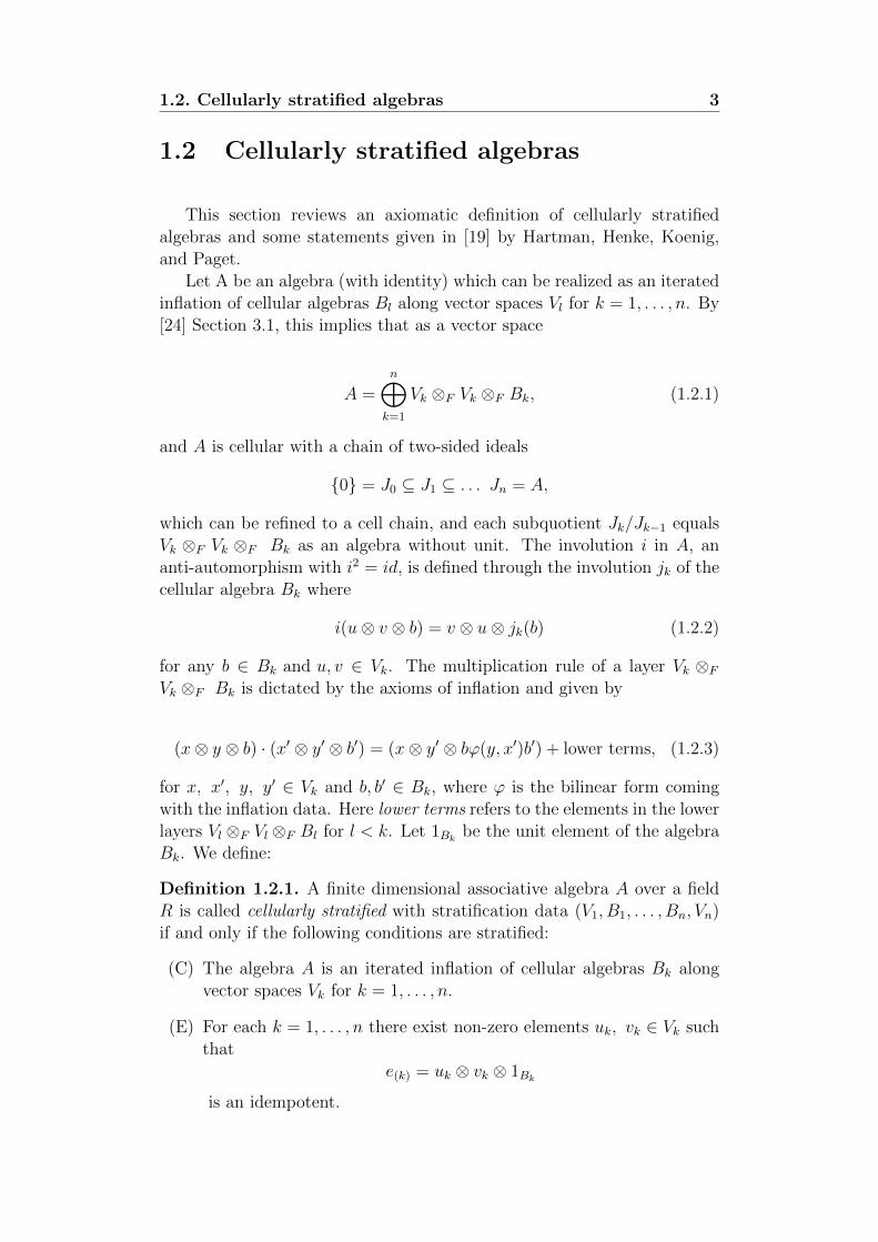
Let A be an algebra (with identity) which can be realized as an iteratedinflation of cellular algebras Bl along vector spaces Vl for k = 1, . . . , n. By[24] Section 3.1, this implies that as a vector space
A =n⊕k=1
Vk ⊗F Vk ⊗F Bk, (1.2.1)
and A is cellular with a chain of two-sided ideals
{0} = J0 ⊆ J1 ⊆ . . . Jn = A,
which can be refined to a cell chain, and each subquotient Jk/Jk−1 equalsVk ⊗F Vk ⊗F Bk as an algebra without unit. The involution i in A, ananti-automorphism with i2 = id, is defined through the involution jk of thecellular algebra Bk where
i(u⊗ v ⊗ b) = v ⊗ u⊗ jk(b) (1.2.2)
for any b ∈ Bk and u, v ∈ Vk. The multiplication rule of a layer Vk ⊗FVk ⊗F Bk is dictated by the axioms of inflation and given by
(x⊗ y ⊗ b) · (x′ ⊗ y′ ⊗ b′) = (x⊗ y′ ⊗ bϕ(y, x′)b′) + lower terms, (1.2.3)
for x, x′, y, y′ ∈ Vk and b, b′ ∈ Bk, where ϕ is the bilinear form comingwith the inflation data. Here lower terms refers to the elements in the lowerlayers Vl ⊗F Vl ⊗F Bl for l < k. Let 1Bk be the unit element of the algebraBk. We define:
Definition 1.2.1. A finite dimensional associative algebra A over a fieldR is called cellularly stratified with stratification data (V1, B1, . . . , Bn, Vn)if and only if the following conditions are stratified:
(C) The algebra A is an iterated inflation of cellular algebras Bk alongvector spaces Vk for k = 1, . . . , n.
(E) For each k = 1, . . . , n there exist non-zero elements uk, vk ∈ Vk suchthat
e(k) = uk ⊗ vk ⊗ 1Bk
is an idempotent.
4 Background
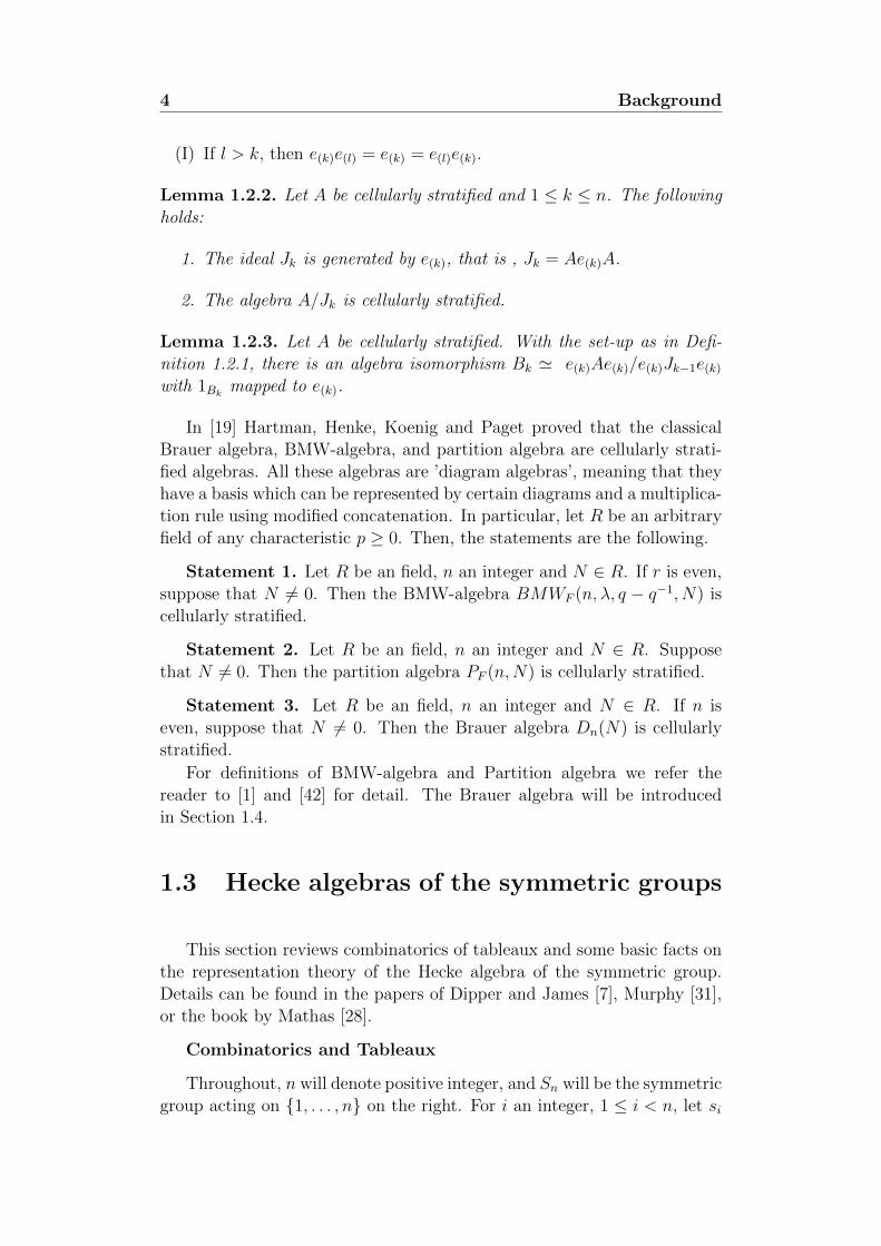
(I) If l > k, then e(k)e(l) = e(k) = e(l)e(k).
Lemma 1.2.2. Let A be cellularly stratified and 1 ≤ k ≤ n. The followingholds:
1. The ideal Jk is generated by e(k), that is , Jk = Ae(k)A.
2. The algebra A/Jk is cellularly stratified.
Lemma 1.2.3. Let A be cellularly stratified. With the set-up as in Defi-nition 1.2.1, there is an algebra isomorphism Bk ' e(k)Ae(k)/e(k)Jk−1e(k)
with 1Bk mapped to e(k).
In [19] Hartman, Henke, Koenig and Paget proved that the classicalBrauer algebra, BMW-algebra, and partition algebra are cellularly strati-fied algebras. All these algebras are ’diagram algebras’, meaning that theyhave a basis which can be represented by certain diagrams and a multiplica-tion rule using modified concatenation. In particular, let R be an arbitraryfield of any characteristic p ≥ 0. Then, the statements are the following.
Statement 1. Let R be an field, n an integer and N ∈ R. If r is even,suppose that N 6= 0. Then the BMW-algebra BMWF (n, λ, q − q−1, N) iscellularly stratified.
Statement 2. Let R be an field, n an integer and N ∈ R. Supposethat N 6= 0. Then the partition algebra PF (n,N) is cellularly stratified.
Statement 3. Let R be an field, n an integer and N ∈ R. If n iseven, suppose that N 6= 0. Then the Brauer algebra Dn(N) is cellularlystratified.
For definitions of BMW-algebra and Partition algebra we refer thereader to [1] and [42] for detail. The Brauer algebra will be introducedin Section 1.4.
1.3 Hecke algebras of the symmetric groups
This section reviews combinatorics of tableaux and some basic facts onthe representation theory of the Hecke algebra of the symmetric group.Details can be found in the papers of Dipper and James [7], Murphy [31],or the book by Mathas [28].
Combinatorics and Tableaux
Throughout, n will denote positive integer, and Sn will be the symmetricgroup acting on {1, . . . , n} on the right. For i an integer, 1 ≤ i < n, let si
1.3. Hecke algebras of the symmetric groups 5
denote the transposition (i, i+ 1). Then Sn is generated by s1, s2, . . . , sn−1,which satisfy the defining relations
s2i = 1 for 1 ≤ i < n;
sisi+1si = si+1sisi+1 for 1 ≤ i < n− 1;
sisj = sjsi for 2 ≤ |i− j|.
Let k be an integer, 0 ≤ k ≤ [n/2]. Denote S2k+1,n to be the subgroup ofSn generated by generators s2k+1, s2k+2, · · · , sn−1.
For i, j intergers, 1 ≤ i, j ≤ n, denote si,j := sisi+1 . . . sj if i ≤ j andsi,j := sisi−1 . . . sj if otherwise.
Definition 1.3.1. Let w be a permutation in Sn. An expression
w = si1si2 · · · simin which m is minimal is called a reduced expression for w, and `(w) = mis the length of w.
Definition 1.3.2. (1) Let e(q) be the least positive integer m such that[m]q = 1 + q+ q2 + ...+ qm−1 = 0 if that exists, and let e(q) =∞ otherwise.
(2) Similarly, let e(q2) be the least positive integer m such that[m]q2 = 1 + q2 + q4 + ... + q2(m−1) = 0 if it exists, and let e(q2) = ∞otherwise.
Definition 1.3.3. Let k be an integer, 0 ≤ k ≤ [n/2]. If n − 2k > 0, apartition of n− 2k is a sequence λ = (λ1, λ2, · · · ) of non-negative integerssuch that λi ≥ λi+1 for all i ≥ 1 and |λ| =
∑i=1 λi = n− 2k. The integers
λi, for i ≥ 1, are the parts of λ; if λi = 0 for i > m we identify λ with(λ1, λ2, · · · , λm) and denote λ ` n− 2k. If n− 2k = 0, write λ = ∅ for theempty partition.
Definition 1.3.4. A partition λ = (λ1, λ2, ..., λf ) of n − 2k is callede(q) − restricted if λi − λi+1 < e(q) for all i ≥ 1. The e(q2) − restrictedpartition is defined similarly.
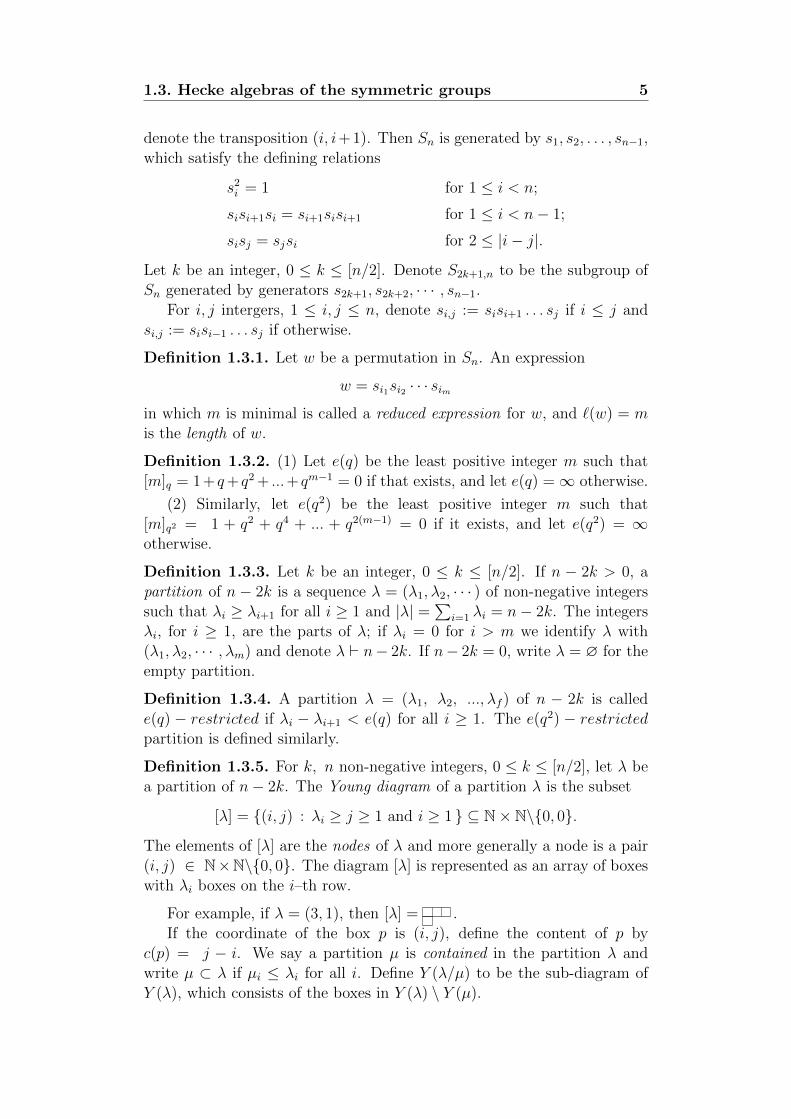
Definition 1.3.5. For k, n non-negative integers, 0 ≤ k ≤ [n/2], let λ bea partition of n− 2k. The Young diagram of a partition λ is the subset
[λ] = {(i, j) : λi ≥ j ≥ 1 and i ≥ 1 } ⊆ N× N\{0, 0}.
The elements of [λ] are the nodes of λ and more generally a node is a pair(i, j) ∈ N×N\{0, 0}. The diagram [λ] is represented as an array of boxeswith λi boxes on the i–th row.
For example, if λ = (3, 1), then [λ] = .If the coordinate of the box p is (i, j), define the content of p by
c(p) = j − i. We say a partition µ is contained in the partition λ andwrite µ ⊂ λ if µi ≤ λi for all i. Define Y (λ/µ) to be the sub-diagram ofY (λ), which consists of the boxes in Y (λ) \ Y (µ).
6 Background
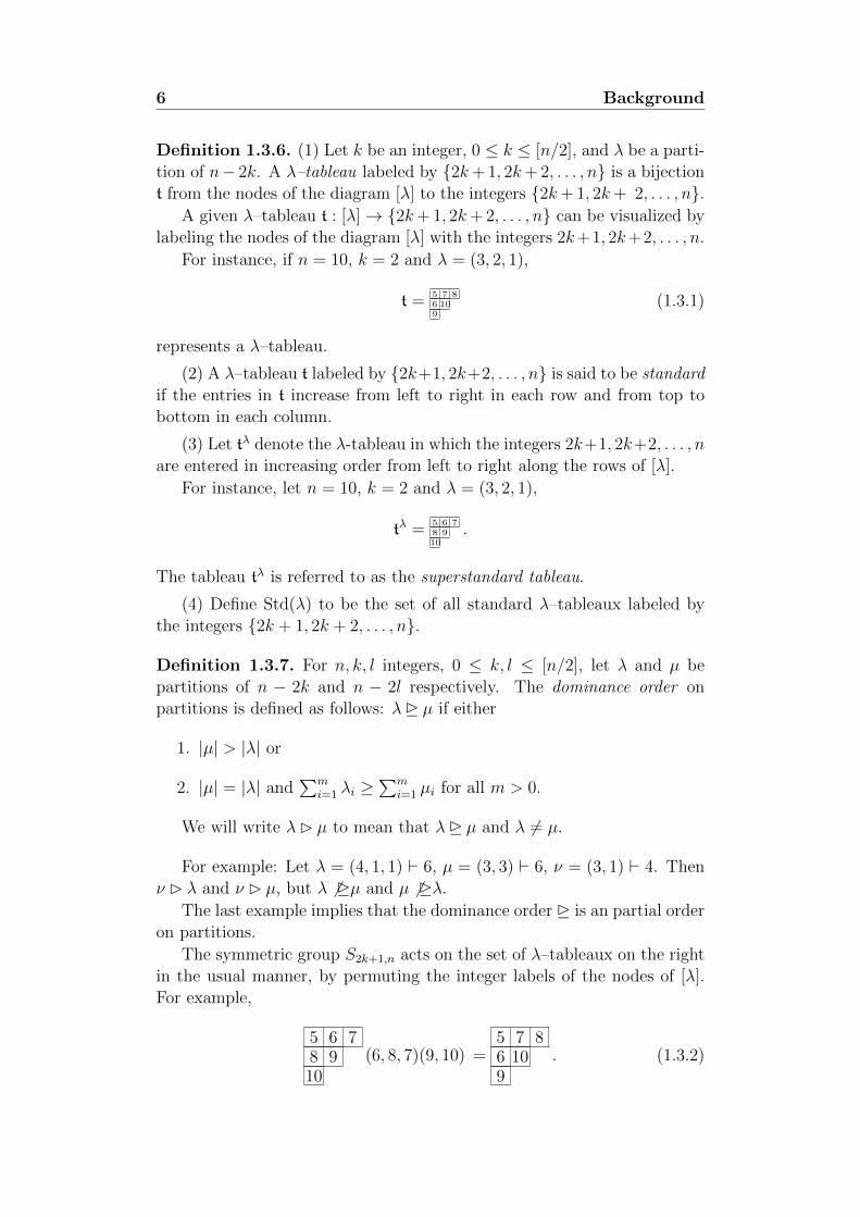
Definition 1.3.6. (1) Let k be an integer, 0 ≤ k ≤ [n/2], and λ be a parti-tion of n− 2k. A λ–tableau labeled by {2k+ 1, 2k+ 2, . . . , n} is a bijectiont from the nodes of the diagram [λ] to the integers {2k+ 1, 2k+ 2, . . . , n}.
A given λ–tableau t : [λ]→ {2k+ 1, 2k+ 2, . . . , n} can be visualized bylabeling the nodes of the diagram [λ] with the integers 2k+1, 2k+2, . . . , n.
For instance, if n = 10, k = 2 and λ = (3, 2, 1),
t =5 7 86 109
(1.3.1)
represents a λ–tableau.
(2) A λ–tableau t labeled by {2k+1, 2k+2, . . . , n} is said to be standardif the entries in t increase from left to right in each row and from top tobottom in each column.
(3) Let tλ denote the λ-tableau in which the integers 2k+1, 2k+2, . . . , nare entered in increasing order from left to right along the rows of [λ].
For instance, let n = 10, k = 2 and λ = (3, 2, 1),
tλ =5 6 78 910
.
The tableau tλ is referred to as the superstandard tableau.
(4) Define Std(λ) to be the set of all standard λ–tableaux labeled bythe integers {2k + 1, 2k + 2, . . . , n}.
Definition 1.3.7. For n, k, l integers, 0 ≤ k, l ≤ [n/2], let λ and µ bepartitions of n − 2k and n − 2l respectively. The dominance order onpartitions is defined as follows: λ� µ if either
1. |µ| > |λ| or
2. |µ| = |λ| and∑m
i=1 λi ≥∑m
i=1 µi for all m > 0.
We will write λ� µ to mean that λ� µ and λ 6= µ.
For example: Let λ = (4, 1, 1) ` 6, µ = (3, 3) ` 6, ν = (3, 1) ` 4. Thenν � λ and ν � µ, but λ 6 �µ and µ 6 �λ.
The last example implies that the dominance order � is an partial orderon partitions.
The symmetric group S2k+1,n acts on the set of λ–tableaux on the rightin the usual manner, by permuting the integer labels of the nodes of [λ].For example,
5 6 78 910
(6, 8, 7)(9, 10) =5 7 86 109
. (1.3.2)
1.3. Hecke algebras of the symmetric groups 7
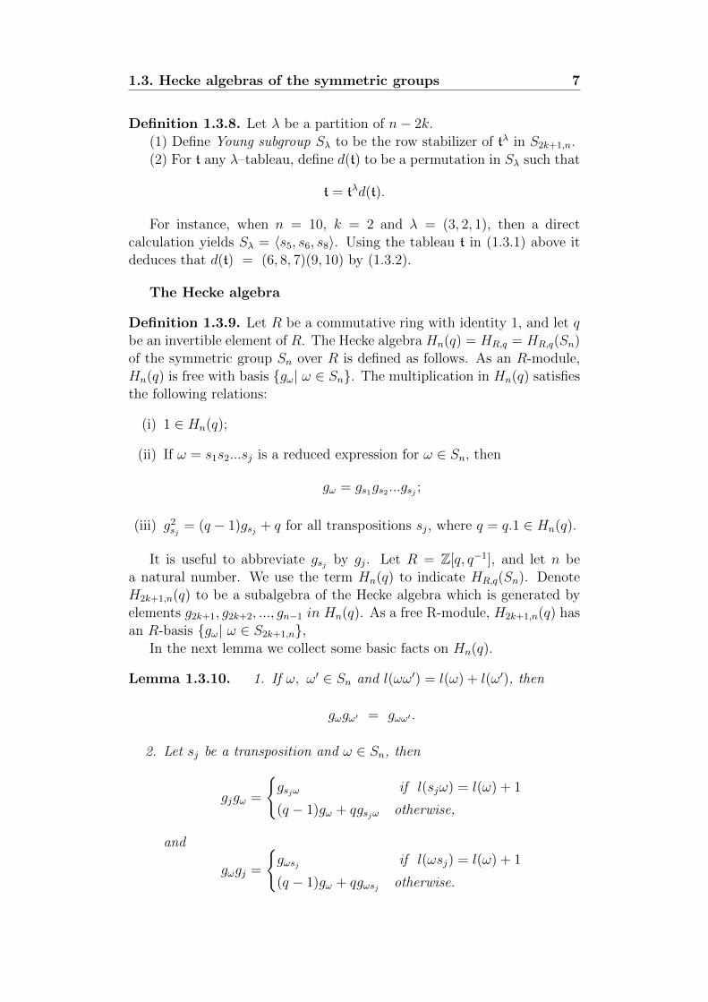
Definition 1.3.8. Let λ be a partition of n− 2k.
(1) Define Young subgroup Sλ to be the row stabilizer of tλ in S2k+1,n.
(2) For t any λ–tableau, define d(t) to be a permutation in Sλ such that
t = tλd(t).
For instance, when n = 10, k = 2 and λ = (3, 2, 1), then a directcalculation yields Sλ = 〈s5, s6, s8〉. Using the tableau t in (1.3.1) above itdeduces that d(t) = (6, 8, 7)(9, 10) by (1.3.2).
The Hecke algebra
Definition 1.3.9. Let R be a commutative ring with identity 1, and let qbe an invertible element of R. The Hecke algebra Hn(q) = HR,q = HR,q(Sn)of the symmetric group Sn over R is defined as follows. As an R-module,Hn(q) is free with basis {gω| ω ∈ Sn}. The multiplication in Hn(q) satisfiesthe following relations:
(i) 1 ∈ Hn(q);
(ii) If ω = s1s2...sj is a reduced expression for ω ∈ Sn, then
gω = gs1gs2 ...gsj ;
(iii) g2sj
= (q − 1)gsj + q for all transpositions sj, where q = q.1 ∈ Hn(q).
It is useful to abbreviate gsj by gj. Let R = Z[q, q−1], and let n bea natural number. We use the term Hn(q) to indicate HR,q(Sn). DenoteH2k+1,n(q) to be a subalgebra of the Hecke algebra which is generated byelements g2k+1, g2k+2, ..., gn−1 in Hn(q). As a free R-module, H2k+1,n(q) hasan R-basis {gω| ω ∈ S2k+1,n},
In the next lemma we collect some basic facts on Hn(q).
Lemma 1.3.10. 1. If ω, ω′ ∈ Sn and l(ωω′) = l(ω) + l(ω′), then
gωgω′ = gωω′ .
2. Let sj be a transposition and ω ∈ Sn, then
gjgω =
{gsjω if l(sjω) = l(ω) + 1
(q − 1)gω + qgsjω otherwise,
and
gωgj =
{gωsj if l(ωsj) = l(ω) + 1
(q − 1)gω + qgωsj otherwise.
8 Background
3. Let ω ∈ Sn. Then gω is invertible in Hn(q) with inverseg−1ω = g−1
j g−1j−1...g
−12 g−1
1 , where ω = s1s2...sj is a reduced expres-sion for ω, and
g−1j = q−1gj + (q−1 − 1), so gj = qg−1
j + (q − 1) for all sj.
In the literature, the Hecke algebras Hn(q) are equivalently defined bygenerators gi, 1 ≤ i < n and relations
(H1) gigi+1gi = gi+1gigi+1 for 1 ≤ i ≤ n− 1;
(H2) gigj = gjgi for |i− j| > 1.
The next statement is implicit in [7] (or see Lemma 2.3 of [31]).
Lemma 1.3.11. The R-linear map i: Hn(q) −→ Hn(q) determined byi(gω) = gω−1 for each ω ∈ Sn is an involution on Hn(q)
Theorem 1.3.12. (Graham and Lehrer [15]) Let R = Z[q, q−1]. ThenR-algebra Hn(q) is a cellular algebra.
Remark 1.3.13. All facts above hold true for another version of the Heckealgebra with parameter q2 and its subalgebra, say Hn(q2) and H2k+1,n(q2)respectively. In detail, the Hecke algebra Hn(q2) (resp. H2k+1,n(q2)) isdefined via the same generators and relations as forHn(q) (resp. H2k+1,n(q))respectively, but the parameter q is replaced by q2. These notions are goingto be used from the Chapter 2.
The Murphy basis
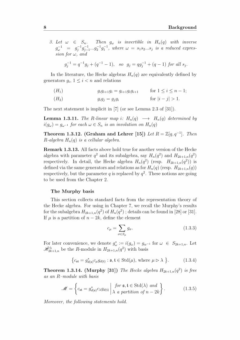
This section collects standard facts from the representation theory ofthe Hecke algebra. For using in Chapter 7, we recall the Murphy’s resultsfor the subalgebraH2k+1,n(q2) of Hn(q2) ; details can be found in [28] or [31].If µ is a partition of n− 2k, define the element
cµ =∑σ∈Sµ
gσ. (1.3.3)
For later convenience, we denote g∗ω := i(gω) = gw−1 for ω ∈ S2k+1,n. LetH λ
2k+1,n be the R-module in H2k+1,n(q2) with basis{cst = g∗d(s)cµgd(t) : s, t ∈ Std(µ), where µ� λ
}. (1.3.4)
Theorem 1.3.14. (Murphy [31]) The Hecke algebra H2k+1,n(q2) is freeas an R–module with basis
M =
{cst = g∗d(s)cλgd(t)
∣∣∣∣ for s, t ∈ Std(λ) and
λ a partition of n− 2k
}. (1.3.5)
Moreover, the following statements hold.
1.3. Hecke algebras of the symmetric groups 9
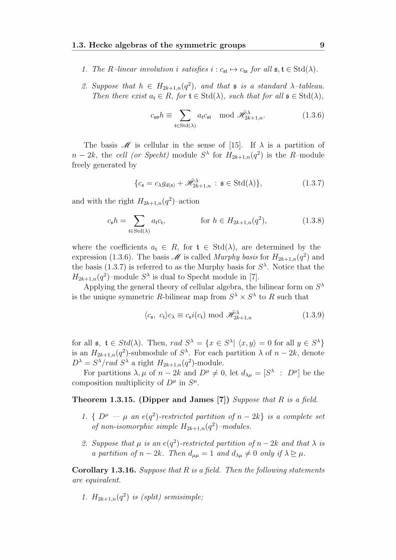
1. The R–linear involution i satisfies i : cst 7→ cts for all s, t ∈ Std(λ).
2. Suppose that h ∈ H2k+1,n(q2), and that s is a standard λ–tableau.Then there exist at ∈ R, for t ∈ Std(λ), such that for all s ∈ Std(λ),
csvh ≡∑
t∈Std(λ)
atcst mod H λ2k+1,n. (1.3.6)
The basis M is cellular in the sense of [15]. If λ is a partition ofn − 2k, the cell (or Specht) module Sλ for H2k+1,n(q2) is the R–modulefreely generated by
{cs = cλgd(s) + H λ2k+1,n : s ∈ Std(λ)}, (1.3.7)
and with the right H2k+1,n(q2)–action
csh =∑
t∈Std(λ)
atct, for h ∈ H2k+1,n(q2), (1.3.8)
where the coefficients at ∈ R, for t ∈ Std(λ), are determined by theexpression (1.3.6). The basis M is called Murphy basis for H2k+1,n(q2) andthe basis (1.3.7) is referred to as the Murphy basis for Sλ. Notice that theH2k+1,n(q2)–module Sλ is dual to Specht module in [7].
Applying the general theory of cellular algebra, the bilinear form on Sλ
is the unique symmetric R-bilinear map from Sλ × Sλ to R such that
〈cs, ct〉cλ ≡ csi(ct) mod H λ2k+1,n (1.3.9)
for all s, t ∈ Std(λ). Then, rad Sλ = {x ∈ Sλ| 〈x, y〉 = 0 for all y ∈ Sλ}is an H2k+1,n(q2)-submodule of Sλ. For each partition λ of n− 2k, denoteDλ = Sλ/rad Sλ a right H2k+1,n(q2)-module.
For partitions λ, µ of n − 2k and Dµ 6= 0, let dλµ = [Sλ : Dµ] be thecomposition multiplicity of Dµ in Sµ.
Theorem 1.3.15. (Dipper and James [7]) Suppose that R is a field.
1. { Dµ — µ an e(q2)-restricted partition of n − 2k} is a complete setof non-isomorphic simple H2k+1,n(q2)–modules.
2. Suppose that µ is an e(q2)-restricted partition of n− 2k and that λ isa partition of n− 2k. Then dµµ = 1 and dλµ 6= 0 only if λ� µ.
Corollary 1.3.16. Suppose that R is a field. Then the following statementsare equivalent.
1. H2k+1,n(q2) is (split) semisimple;
10 Background
2. Sλ = Dλ for all partitions λ of n− 2k;
3. e(q2) > n− 2k.
Lemma 1.3.17. (Hemmer and Nakano [20], Proposition 4.2.1).Let e(q) ≥ 4, and suppose that µ� λ. Then Ext1Hn(q)(S
µ, Sλ) = 0.
Lemma 1.3.18. (Hemmer and Nakano [20], Lemma 4.4.1).Let e(q) ≥ 3. Then
1. If µ 6 �λ, then HomHn(q)(Sλ, Sµ) = 0.
2. HomHn(q)(Sλ, Sλ) ≡ R.
1.4 Brauer algebra
Brauer algebras were introduced first by Richard Brauer [2] in order tostudy the nth tensor power of the defining representation of the orthogonalgroups and symplectic groups. Afterwards, they were studied in more detailby various mathematicians. We refer the reader to work of Brown [3, 4],Hanlon and Wales [16, 17, 10], Graham and Lehrer [15], Koenig and Xi[25, 26], Wenzl [36] for more information.
Definition
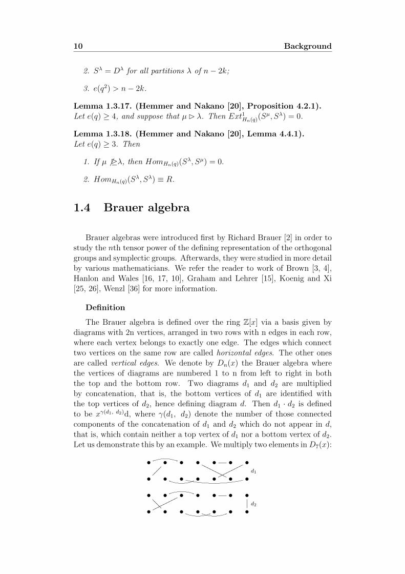
The Brauer algebra is defined over the ring Z[x] via a basis given bydiagrams with 2n vertices, arranged in two rows with n edges in each row,where each vertex belongs to exactly one edge. The edges which connecttwo vertices on the same row are called horizontal edges. The other onesare called vertical edges. We denote by Dn(x) the Brauer algebra wherethe vertices of diagrams are numbered 1 to n from left to right in boththe top and the bottom row. Two diagrams d1 and d2 are multipliedby concatenation, that is, the bottom vertices of d1 are identified withthe top vertices of d2, hence defining diagram d. Then d1 · d2 is definedto be xγ(d1, d2)d, where γ(d1, d2) denote the number of those connectedcomponents of the concatenation of d1 and d2 which do not appear in d,that is, which contain neither a top vertex of d1 nor a bottom vertex of d2.Let us demonstrate this by an example. We multiply two elements inD7(x):
• •��
��• •
OOOOOOOOO • • •ooooooooo
d1
• • • • • • •
•??
??• •
ooooooooo • • • •d2
• • • • • • •
1.4. Brauer algebra 11
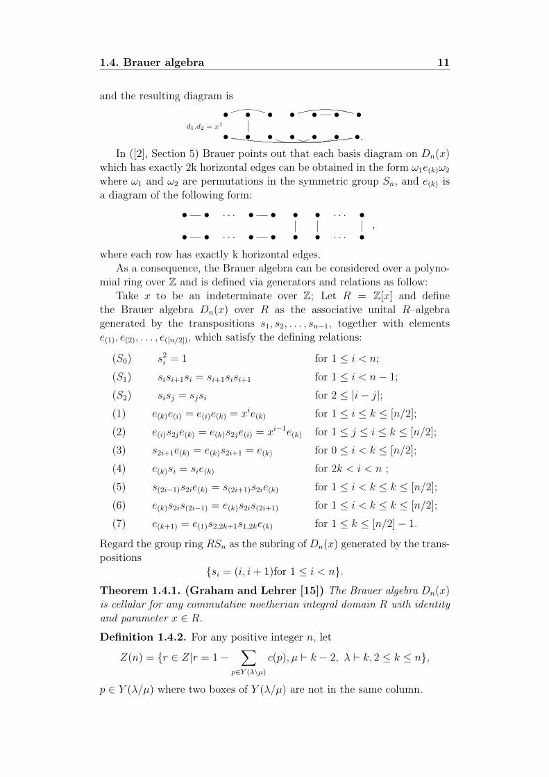
and the resulting diagram is
• • • • • • •
•d1.d2 = x1
• • • • • •.In ([2], Section 5) Brauer points out that each basis diagram on Dn(x)
which has exactly 2k horizontal edges can be obtained in the form ω1e(k)ω2
where ω1 and ω2 are permutations in the symmetric group Sn, and e(k) isa diagram of the following form:
• • . . . • • • • . . . •
• • . . . • • • • . . . •,
where each row has exactly k horizontal edges.As a consequence, the Brauer algebra can be considered over a polyno-
mial ring over Z and is defined via generators and relations as follow:Take x to be an indeterminate over Z; Let R = Z[x] and define
the Brauer algebra Dn(x) over R as the associative unital R–algebragenerated by the transpositions s1, s2, . . . , sn−1, together with elementse(1), e(2), . . . , e([n/2]), which satisfy the defining relations:
(S0) s2i = 1 for 1 ≤ i < n;
(S1) sisi+1si = si+1sisi+1 for 1 ≤ i < n− 1;
(S2) sisj = sjsi for 2 ≤ |i− j|;(1) e(k)e(i) = e(i)e(k) = xie(k) for 1 ≤ i ≤ k ≤ [n/2];
(2) e(i)s2je(k) = e(k)s2je(i) = xi−1e(k) for 1 ≤ j ≤ i ≤ k ≤ [n/2];
(3) s2i+1e(k) = e(k)s2i+1 = e(k) for 0 ≤ i < k ≤ [n/2];
(4) e(k)si = sie(k) for 2k < i < n ;
(5) s(2i−1)s2ie(k) = s(2i+1)s2ie(k) for 1 ≤ i < k ≤ k ≤ [n/2];
(6) e(k)s2is(2i−1) = e(k)s2is(2i+1) for 1 ≤ i < k ≤ k ≤ [n/2];
(7) e(k+1) = e(1)s2,2k+1s1,2ke(k) for 1 ≤ k ≤ [n/2]− 1.
Regard the group ring RSn as the subring of Dn(x) generated by the trans-positions
{si = (i, i+ 1)for 1 ≤ i < n}.
Theorem 1.4.1. (Graham and Lehrer [15]) The Brauer algebra Dn(x)is cellular for any commutative noetherian integral domain R with identityand parameter x ∈ R.
Definition 1.4.2. For any positive integer n, let
Z(n) = {r ∈ Z|r = 1−∑
p∈Y (λ\µ)
c(p), µ ` k − 2, λ ` k, 2 ≤ k ≤ n},
p ∈ Y (λ/µ) where two boxes of Y (λ/µ) are not in the same column.
12 Background
Theorem 1.4.3. (Rui [35]) Let D(N) be the complex Brauer algebra.
1. Suppose N 6= 0. Then D(N) is semisimple if and only if N /∈ Z(n).
2. Dn(0) is semisimple if and only if n ∈ {1, 3, 5}.
Theorem 1.4.4. (Rui [35])Let D(N) be the Brauer algebra over a fieldR with charR > 0.
1. Suppose N 6= 0. Then D(N) is semisimple if and only if N /∈ Z(n)and charR - n!.
2. Dn(0) is semisimple if and only if n ∈ {1, 3, 5} and charR - n!.
By Brown ([4], Section 3) the Brauer algebra has a decomposition asabelian groups
Dn(x) ∼=[n/2]⊕k=0
Z[x]Sne(k)Sn.
SetI(m) =
⊕k≥m
Z[x]Sne(k)Sn,
then I(m) is a two-sided ideal in Dn(x) for each m ≤ [n/2].
The modules V ∗k and Vk
In this subsection we recall particular modules of Brauer algebras.Dn(N) has a decomposition into direct some of vector spaces
Dn(N) ∼=[n/2]⊕k=0
(Z[N ]Sne(k)Sn + I(k+1))/I(k+1).
Using the same arguments as in Section 1 ([39]), each factor module
(Z[N ]Sne(k)ωj + I(k+1))/I(k+1)
is a left Dn(N)-module with a basis given by the basis diagrams ofZ[N ]Sne(k)ωj, where ωj ∈ Sn is a diagram such that e(k)ωj is a diagram inDn(N) with no intersection between any two vertical edges. In particular
I(k)/I(k+1) ∼=⊕
j∈P (n,k)
(Z[N ]Sne(k)ωj + I(k+1))/I(k+1), (1.4.1)
where P (n, k) is the set of all possibilities of ωj. As multiplication from theright by ωj commutes with the Dn(N)-action, each summand on the righthand side is isomorphic to the module
V ∗k = (Z[N ]Sne(k) + I(k+1))/I(k+1). (1.4.2)
1.4. Brauer algebra 13
Combinatorially, V ∗k is spanned by basis diagrams with exactly k edges inthe bottom row, where the i− th edge connects the vertices 2i− 1 and 2i.Observe that V ∗k is a free, finitely generated Z[N ] module with Z[N ]-rankn!/2kk!.Similarly, a right Dn(N)-module is defined
Vk = (Z[N ]e(k)Sn + I(k+1))/I(k+1), (1.4.3)
where basis diagrams are obtained from those in V ∗k by an involution, say*, of Dn(N) which rotates a diagram d ∈ V ∗k around its horizontal axisdownward. For convenience later in Chapter 4 we use the term V ∗k replacing
V(k)n . More details for setting up V ∗k can be found in Section 1 of [39].
Lemma 1.4.5. (Wenzl [39], Lemma 1.1(d)) The algebra Dn(N) is
faithfully represented on⊕[n/2]
k=0 V∗k (and also on
⊕[n/2]k=0 Vk).
Length function for Brauer algebras Dn(N)
Generalizing the length of elements in reflection groups, Wenzl [39] hasdefined a length function for a diagram of Dn(N) as follows:
For a diagram d ∈ Dn(N) with exactly 2k horizontal edges, thedefinition of the length `(d) is given by
`(d) = min{`(ω1) + `(ω2)| ω1e(k)ω2 = d, ω1, ω2 ∈ Sn}.
We will call the diagrams d of the form ωe(k) where l(ω) = l(d) and ω ∈ Snbasis diagrams of the module V ∗k .
Remark 1.4.6. 1. Recall that the length of a permutation ω ∈ Sn isdefined by `(ω) = the cardinality of set
{(i, j)|(j)ω < (i)ω| 1 ≤ i < j ≤ n},
where the symmetric group acts on {1, 2, ..., n} on the right.2. Given a diagram d, there can be more than one ω satisfying ωe(k) = d
and `(ω) = `(d). e.g. s2j−1s2je(k) = s2j+1s2je(k) for 2j+ 1 < k. This meansthat such an expression of d is not unique with respect to ω ∈ Sn.
For later use, if si = (i, i+ 1) is a transposition in symmetric goup Sn withi, j = 1, ..., k let
si,j =
{sisi+1...sj if i ≤ j,
sisi−1...sj if i > j.
A permutation ω ∈ Sn can be written uniquely in the formω = tn−1tn−2...t1, where tj = 1 or tj = sij ,j with 1 ≤ ij ≤ j and 1 ≤ j < n.This can be seen as follows: For given ω ∈ Sn, there exists a unique tn−1
14 Background
such that (n)tn−1 = (n)ω. Hence ω′ = (n)t−1n−1ω = n, and we can consider
ω′ as an element of Sn−1. Repeating this process on n implies the generalclaim. Set
B∗k = {tn−1tn−2...t2kt2k−2t2k−4...t2}. (1.4.4)
By the definition of tj given above, the number of possibilities of tj is j+1.A direct computation shows that B∗k has n!/2kk! elements. In fact, thenumber of elements in B∗k is equal to the number of diagrams d∗ in Dn(N)in which d∗ has k horizontal edges in each row and one of its rows is fixedlike that of e(k).
3. From now on, a permutation of a symmetric group is seen as adiagram with no horizontal edges, and the product ω1ω2 in Sn is seen as aconcatenation of two diagrams in Dn(N).
4. Given a basis diagram d∗ = ωe(k) with `(ω) = `(d∗) does not implythat ω ∈ B∗k, but there does exist ω′ ∈ B∗k such that d∗ = ω′e(k). The latterwill be shown in Lemma 1.4.8 to exist and to be unique for each basiselement of the module V ∗k . Wenzl even got `(d∗) = `(ω) = `(ω′), where`(ω′) is the number of factors for ω′ in B∗k.
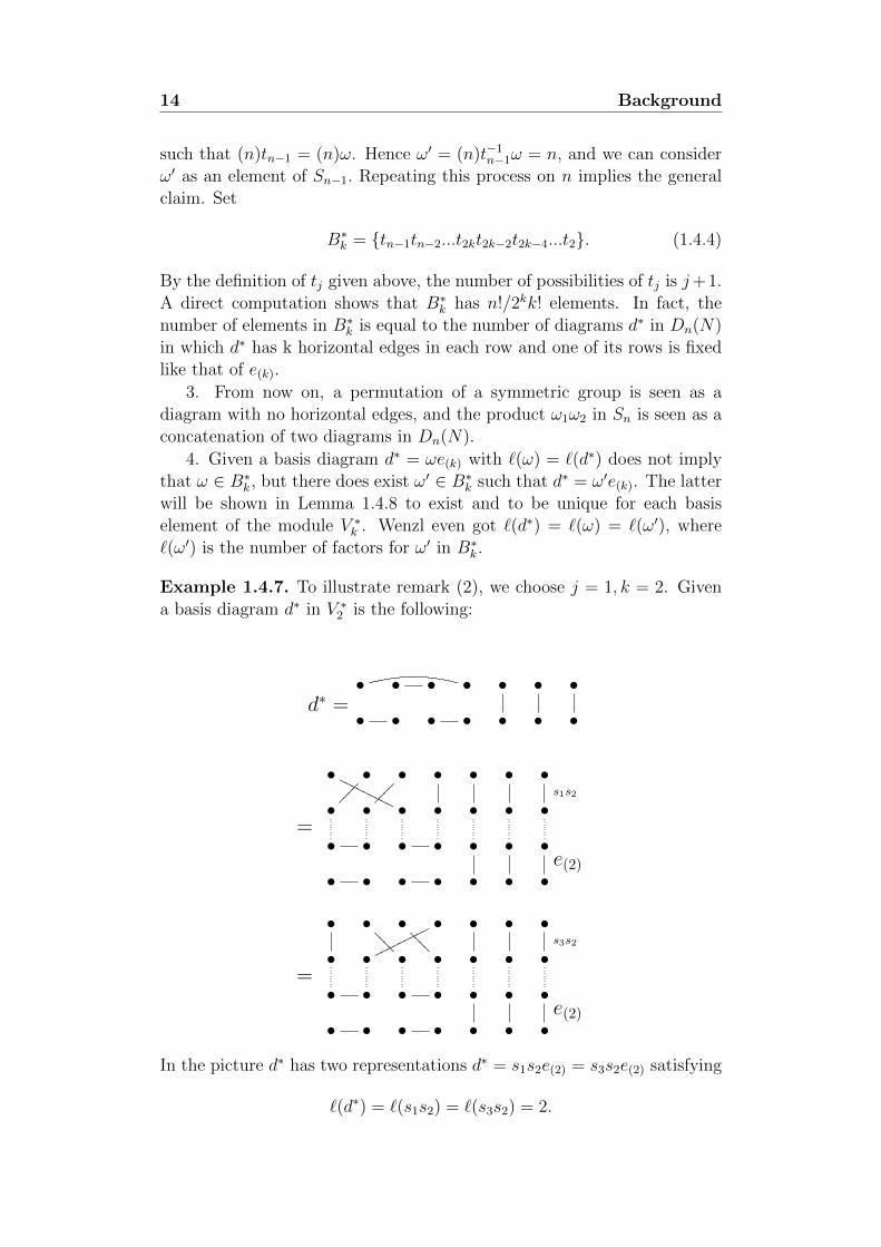
Example 1.4.7. To illustrate remark (2), we choose j = 1, k = 2. Givena basis diagram d∗ in V ∗2 is the following:
• • • • • • •
•d∗ =
• • • • • •
•OOOOOOOOO •
����
•��
��• • • •
s1s2
• • • • • • •
•=
• • • • • •e(2)
• • • • • • •
• •??
??•
????•
ooooooooo • • •s3s2
• • • • • • •
•=
• • • • • •e(2)
• • • • • • •
In the picture d∗ has two representations d∗ = s1s2e(2) = s3s2e(2) satisfying
`(d∗) = `(s1s2) = `(s3s2) = 2.
1.4. Brauer algebra 15
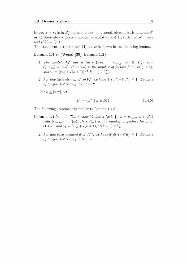
However, s1s2 is in B∗2 but s3s2 is not. In general, given a basis diagram d∗
in V ∗k there always exists a unique permutation ω ∈ B∗k such that d∗ = ωekand l(d∗) = l(ω).The statement in the remark (4) above is shown in the following lemma.
Lemma 1.4.8. (Wenzl [39], Lemma 1.2)
1. The module V ∗k has a basis {ωv1 = vωe(k) , ω ∈ B∗k} with`(ωe(k)) = `(ω). Here `(ω) is the number of factors for ω in (1.4.4),and v1 = (e(k) + I(k + 1))/I(k + 1) ∈ V ∗k .
2. For any basis element d∗ of V ∗k , we have |`(sid∗)−`(d∗)| ≤ 1. Equalityof lengths holds only if sid
∗ = d∗.
For k ≤ [n/2], let
Bk = {ω−1| ω ∈ B∗k}. (1.4.5)
The following statement is similar to Lemma 1.4.8.
Lemma 1.4.9. 1. The module Vk has a basis {v1ω = ve(k)ω, ω ∈ Bk}with `(e(k)ω) = `(ω). Here `(ω) is the number of factors for ω in(1.4.5), and v1 = (e(k) + I(k + 1))/I(k + 1) ∈ Vk.
2. For any basis element d of V(k)n , we have |`(dsi)− `(d)| ≤ 1. Equality
of lengths holds only if dsi = d.
Chapter 2
The q-Brauer algebras
In this Chapter we review basic and necessary facts about the q-Braueralgebra due to Wenzl [39]. Then, we introduce more general versions for theq-Brauer algebra that are necessary for our work in this thesis. Apart fromWenzl’s results, Definitions 2.1.4 - 2.1.7 and Lemmas 2.1.10, 2.2.2 are new.
2.1 Definitions
Definition 2.1.1. Fix N ∈ Z \ {0} and let [N ] =1− qN
1− q∈ Z[q, q−1]. The
q-Brauer algebra Brn(N) is defined over ring Z[q, q−1] via generators g1,g2, g3, ..., gn−1 and e and relations
(H)′ The elements g1, g2, g3, ..., gn−1 satisfy the relations of the Heckealgebra Hn(q);
(E1)′ e2 = [N ]e;
(E2)′ egi = gie for i > 2, eg1 = g1e = qe, eg2e = qNe and eg−12 e = q−1e;
(E3)′ e(2) = g2g3g−11 g−1
2 e(2) = e(2)g2g3g−11 g−1
2 , where e(2) = e(g2g3g−11 g−1
2 )e.
A second version of the q-Brauer algebra is the following.
Definition 2.1.2. The q-Brauer algebra, denoted Brn(r, q), is defined overthe ring Z[q±1, r±1, (r − 1)/(q − 1)] by generators g1, g2, g3, ..., gn−1 and e
and relations
(H) The elements g1, g2, g3, ..., gn−1 satisfy the relations of the Heckealgebra Hn(q);
(E1) e2 =r − 1
q − 1e;
16
2.1. Definitions 17
(E2) egi = gie for i > 2, eg1 = g1e = qe, eg2e = re and eg−12 e = q−1e;
(E3) e(2) = g2g3g−11 g−1
2 e(2) = e(2)g2g3g−11 g−1
2 , where e(2) = e(g2g3g−11 g−1
2 )e.
Remark 2.1.3. 1. A closely related algebra has appeared in Molev’s work.In 2003, Molev [29] introduced a new q-analogue of the Brauer algebra byconsidering the centralizer of the natural action in tensor spaces of a non-standard deformation of the universal enveloping algebra U(oN). He de-fined relations for these algebras and constructed representations of themon tensor spaces. However, in general the representations are not faithful,and little is known about these abstract algebras besides their representa-tions. The q-Brauer algebra, a closely related algebra with that of Molev,was introduced later by Wenzl [39] via generators and relations. In partic-ular, over the field Q[r, q] he proved that it is semisimple and isomorphic tothe Brauer algebra. It can be checked that the representations of Molev’salgebras in [29] are representations of q-Brauer algebras ([41], Section 2.2)and that the relations written down by Molev are satisfied by generators ofthe q-Brauer algebras; but potentially, Molev’s abstractly defined algebrascould be larger ([30]).
2. Obviously, by setting r = qN the version Brn(r, q) coincides withBrn(N). Over a ring allowing to form the limit q → 1, such as the realor complex field, the q-Brauer algebra (both versions for q → 1) recoversthe classical Brauer algebra Dn(N). In this case gi becomes the simplereflection si and the element e(k) can be identified with the diagram e(k).However, over any field of prime characteristic for which the limit q → 1does not exist, Wenzl’s definitions cause technical difficulties to work. Inparticular, over a field of prime characteristic we can not give a comparisonbetween the q-Brauer algebra and the classical Brauer algebra in the caseq = 1 or q → 1. Further, if the coefficients [N ] = 0 and (r− 1)/(q− 1) = 0,then we remark that the involution defined by Wenzl for the q-Braueralgebra (see [39], Remark 3.1.2) does not exist (a proof of this is in Lemma3.2.1(3)). For studying in detail the q-Brauer algebra we subsequently givethe modified versions for the q-Brauer algebra. So, the q-Brauer algebracan be considered over any field of characteristic p ≥ 0, as well as in thecase q = 1 or q → 1.
Definition 2.1.4. Fix N ∈ Z \ {0} and let [N ] = 1 + q1 + · · · + qN−1.The q-Brauer algebra, Brn(N), over the ring Z[q±1, [N ]±1] is defined bythe same generators and relations as in Definition 2.1.1.
Definition 2.1.5. Fix N ∈ Z \ {0}, let q and r be invertible elements.Moreover, assume that if q = 1 then r = qN . The q-Brauer algebraBrn(r, q) over the ring Z[q±1, r±1, ((r − 1)/(q − 1))±1] is defined by thesame generators and relations as in Definition 2.1.2.
18 The q-Brauer algebras
In Chapter 6 we need to use new versions of the q-Brauer algebra. Inthese versions the q-Brauer algebra contains the Hecke algebra Hn(q2) asa subalgebra. The definitions are the following.
Definition 2.1.6. Let r and q be invertible elements over the ringZ[q±1, r±1, ((r − r−1)/(q − q−1))±1]. Moreover, if q = 1 then assume thatr = qN with N ∈ Z \ {0}. The q-Brauer algebra Brn(r2, q2) over the ringZ[q±1, r±1, ((r− r−1)/(q− q−1))±1] is the algebra defined via generators g1,g2, g3, ..., gn−1 and e and relations
(H)′′ The elements g1, g2, g3, ..., gn−1 satisfy the relations of the Heckealgebra Hn(q2);
(E1)′′ e2 =r − r−1
q − q−1e;
(E2)′′ egi = gie for i > 2, eg1 = g1e = q2e, eg2e = rqe and eg−12 e = (rq)−1e;
(E3)′′ g2g3g−11 g−1
2 e(2) = e(2)g2g3g−11 g−1
2 , where e(2) = e(g2g3g−11 g−1
2 )e.
Definition 2.1.7. Fix N ∈ Z \ {0} and let [N2] = 1 + q2 + · · · + q2(N−1),where q is an invertible element in Z[q±1, r±1, ((r− r−1)/(q− q−1))±1]. Theq-Brauer algebra Brn(N2) over ring Z[q±1, r±1, ((r − r−1)/(q − q−1))±1] isdefined by generators g1, g2, . . . , gn−1 and e and relations (H), (E3) as inDefinition 2.1.6, and
(E ′1) e2 = [N2]e;
(E ′2) egi = gie for i > 2, eg1 = g1e = q2e, eg2e = qN+1e andeg−1
2 e = (q)−1−Ne.
Remark 2.1.8. 1. In the q-Brauer algebra, the version Brn(r2, q2) isisomorphic with the version Brn(r, q). In fact, the version Brn(r2, q2) canbe obtained by substituting in Brn(r, q) old q, r and e by q2, r2 and (q−1r)erespectively.
2. The new versions do not affect the properties of the q-Brauer algebra,which were studied in detail by Wenzl. This means that it is sufficient togive proofs of properties of the q-Brauer algebra for one version. Those ofthe other versions are the same.
3. In this thesis, we are going to work on Definitions 2.1.4 - 2.1.7 of theq-Brauer algebra replacing Wenzl’s. In particular, we start working withthe versions Brn(N) and Brn(r, q) from this Chapter, the other versionsare intensively used in Chapter 6.
4. It is clear that in the case q = 1 the q-Brauer algebra Brn(N) (resp.Brn(N2)) coincides with the classical Brauer algebra Dn(N). And over aring for which the limit q → 1 can be formed the q-Brauer algebra Brn(r, q)
2.1. Definitions 19
(resp. Brn(r2, q2)) recovers the classical Brauer algebra. Also note that alldefinitions above imply the equality
eg−11 = g−1
1 e = q−1e or eg−11 = g−1
1 e = q−2e. (2.1.1)
Let
g+l,m =
{glgl+1...gm if l ≤ m;
glgl−1...gm if l > m,
and
g−l,m =
{g−1l g−1
l+1...g−1m if l ≤ m;
g−1l g−1
l−1...g−1m if l > m,
for 1 ≤ l,m ≤ n.
Definition 2.1.9. Let k be an integer, 1 ≤ k ≤ [n/2]. The element e(k) ofthe q-Brauer algebra is defined inductively by e(1) = e and by
e(k+1) = eg+2,2k+1g
−1,2ke(k).
Notice that in this thesis we abuse notation by denoting e(k) both acertain diagram in the Brauer algebra Dn(N) and an element in theq-Brauer algebra Brn(r, q). Given a diagram d the geometric realizationimplies that diagrams e(k) and ω(d) commute on the Brauer algebra. Simi-larly, this also remains on the level of the q-Brauer algebra. The statementis the following.
Lemma 2.1.10. Let k be an integer, 1 ≤ k ≤ [n/2]. If gω ∈ H2k+1,n(q)(resp. H2k+1,n(q2)), then e(k)gω = gωe(k).
Proof. It is sufficient to show that e(k)gi = gie(k) with 2k + 1 ≤ i ≤ n− 1.This is shown by induction on k. Indeed, in the case k = 1, egi = gie for3 ≤ i ≤ n− 1 by (E2). Suppose that
e(k−1)gi = gie(k−1) for 2k − 1 ≤ i ≤ n− 1.
Then for 2k + 1 ≤ i ≤ n− 1
e(k)giDef2.1.9
= (eg+2,2k−1g
−1,2k−2e(k−1))gi
Induction= e(g+
2,2k−1g−1,2k−2)gie(k−1)
(H2)= gie(g
+2,2k−1g
−1,2k−2)e(k−1)
Def2.1.9= gie(k).
20 The q-Brauer algebras
2.2 Basic properties
Throughout this section, denote R to be a commutative ring containingground rings in Definitions 2.1.4 - 2.1.7.
The next lemmas indicate how the properties of the classical Braueralgebra extend to the q-Brauer algebra.
Lemma 2.2.1. Let Brn(N) be the q-Brauer algebra over R. Assume morethat [N ] and q are invertible elements in R. Then the following statementshold.
1. The elements e(k) are well-defined.
2. g+1,2le(k) = g+
2l+1,2e(k) and g−1,2le(k) = g−2l+1,2e(k) for l < k.
3. g2j−1g2je(k) = g2j+1g2je(k) and g−12j−1g
−12j e(k) = g−1
2j+1g−12j e(k)
for 1 ≤ j < k.
4. For any j ≤ k we have e(j)e(k) = e(k)e(j) = [N ]je(k).
5. [N ]j−1e(k+1) = e(j)g+2j,2k+1g
−2j−1,2ke(k) for 1 ≤ j < k.
6. e(j)g2je(k) = qN [N ]j−1e(k) for 1 ≤ j ≤ k.
Lemma 2.2.2. Let Brn(r, q) be the q-Brauer algebra over R. Assumemore that r, q, and (r − 1)/(q − 1) are invertible elements in R. Then thefollowing statements hold.
(1), (2), (3) as in Lemma 2.2.1.
4. For any j ≤ k we have e(j)e(k) = e(k)e(j) = (r − 1
q − 1)je(k).
5. (r − 1
q − 1)j−1e(k+1) = e(j)g
+2j,2k+1g
−2j−1,2ke(k) for 1 ≤ j < k.
6. e(j)g2je(k) = r(r − 1
q − 1)j−1e(k) for 1 ≤ j ≤ k.
Proof. The proof is the same as that of Lemma 2.2.1
Lemma 2.2.3. We have
e(j)Hn(q)e(k) ⊂ H2j+1,n(q)e(k) +∑
m≥k+1 Hn(q)e(m)Hn(q),
where j ≤ k. Moreover, if j1 ≥ 2k and j2 ≥ 2k + 1, we also have:
1. eg+2,j2g+
1,j1e(k) = e(k+1)g
+2k+1,j2
g−2k+1,j1, if j1 ≥ 2k and j2 ≥ 2k + 1.
2. eg+2,j2g+
1,j1is equal to
e(k+1)g+2k+2,j1
g+2k+1,j2
+qN+1(q−1)k∑l=1
q2l−2(g2l+1 +1)g+2l+2,j2
g+2l+1,j1
e(k).
2.3. The Brn(r, q)-modules V ∗k 21
Lemma 2.2.4. The algebra Brn(r, q) is spanned by∑[n/2]
k=0 Hn(q)e(k)Hn(q).In particular, its dimension is at most the one of the Brauer algebra.
Theorem 2.2.5. (restate a part of Theorem 5.3 in [39]) Let R be afield of characteristic zero. The algebra Brn(r, q) over R is semisimple ifr 6= qk for |k| ≤ n and if e(q) > n (for e(q) see Definition 1.3.2). In thiscase, it has the same decomposition into simple matrix rings as the genericBrauer algebra, and the trace tr is nondegenerate.
2.3 The Brn(r, q)-modules V ∗k
An action of generators of q-Brauer algebra on module V ∗k is defined asfollows:
gjvd =
qvd if sjd = d,
vsjd if l(sjd) > l(d),
(q − 1)vd + qvsjd if l(sjd) < l(d),
and
ehg+2,j2g−1,j1v1 =
qNhg+
3,j2v1 if g−1,j1 = 1,
q−1hg−j2+1,j1v1 if g−1,j1 = 1,
0 if j1 6= 2k and j2 6= 2k + 1,
where v1 is defined as in Lemma 1.4.8 and h ∈ H3,n.
Lemma 2.3.1. The action of the elements gj with 1 ≤ j < n and e on V ∗kas given above defines a representation of Brn(r, q).
Chapter 3
A basis and an involution for
the q-Brauer algebra
In this chapter, we construct an explicit basis and provide an involutionfor the q-Brauer algebra. The final section gives a comparison between thisbasis and another one due to Wenzl. These results are going to be used forproducing cellular structure for the q-Brauer algebra over the commutativering R in Chapter 4. Throughout, we prefer to work on the version Brn(r, q)of q-Brauer algebra. However, the other versions are still available.
3.1 A basis for q-Brauer algebra
By definition, the cellularity of an algebra depends on particular bases.That is, the cellular structure of an algebra can be only recognized onsuitable bases. Here we give such a basis for the q-Brauer algebra. Thisbasis is indexed by the set of all diagrams of the classical Brauer algebraDn(N), where the parameter N is an integer N ∈ Z \ {0}.
Construction
Given a diagram d ∈ Dn(N) with exactly 2k horizontal edges, it isconsidered as concatenation of three diagrams (d1, ω(d), d2) as follows:
1. d1 is a diagram in which the top row has the positions of horizontaledges as these in the first row of d, its bottom row is like a row of diagrame(k), and there is no crossing between any two vertical edges.
2. Similarly, d2 is a diagram where its bottom row is the same row ind, the other one is similar to that of e(k), and there is no crossing betweenany two vertical edges.
3. The diagram ω(d) is described as follows : We enumerate the freevertices, which belong to vertical edges, in both rows of d from left to rightby 2k+ 1, 2k+ 2, ..., n. We also enumerate the vertices in each of two rows
22
3.1. A basis for q-Brauer algebra 23
of ω(d) from left to right by 1, 2, ..., 2k + 1, 2k + 2, ..., n. Assume that eachvertical edge in d is connected by i − th vertex of the top row and j − thvertex of the other one with 2k+ 1 ≤ i, j ≤ n. Define ω(d) a diagram whichhas first vertical edges 2k joining m−th points in each of two rows togetherwith 1 ≤ m ≤ 2k, and its other vertical edges are obtained by maintainingthe vertical edges (i, j) of d.
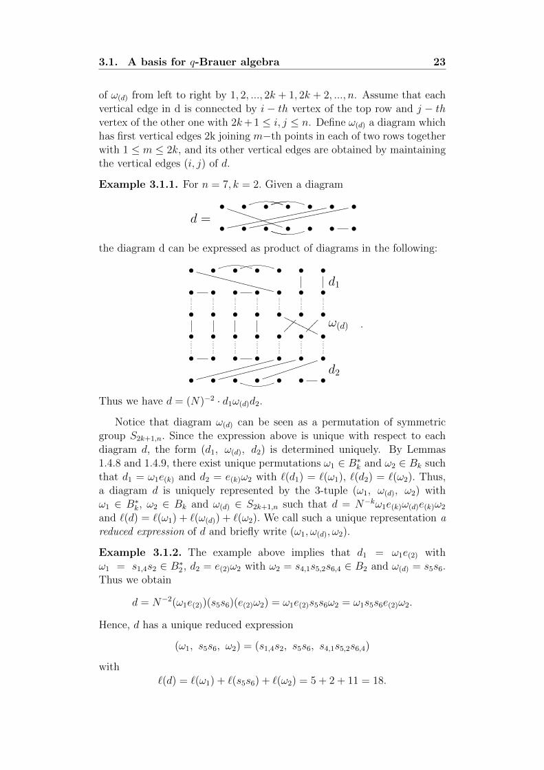
Example 3.1.1. For n = 7, k = 2. Given a diagram
•TTTTTTTTTTTTT • • • • •
eeeeeeeeeeeeeeeeeeeeeee •eeeeeeeeeeeeeeeeeeeeeee
•d =
• • • • • •
the diagram d can be expressed as product of diagrams in the following:
•WWWWWWWWWWWWWWWWWW • • • • • •
d1• • • • • • •
• • • • •OOOOOOOOO •
����
•��
�� ω(d)• • • • • • •
• • • • •gggggggggggggggggg •
gggggggggggggggggg •jjjjjjjjjjjjj
d2• • • • • • •
.
Thus we have d = (N)−2 · d1ω(d)d2.
Notice that diagram ω(d) can be seen as a permutation of symmetricgroup S2k+1,n. Since the expression above is unique with respect to eachdiagram d, the form (d1, ω(d), d2) is determined uniquely. By Lemmas1.4.8 and 1.4.9, there exist unique permutations ω1 ∈ B∗k and ω2 ∈ Bk suchthat d1 = ω1e(k) and d2 = e(k)ω2 with `(d1) = `(ω1), `(d2) = `(ω2). Thus,a diagram d is uniquely represented by the 3-tuple (ω1, ω(d), ω2) withω1 ∈ B∗k, ω2 ∈ Bk and ω(d) ∈ S2k+1,n such that d = N−kω1e(k)ω(d)e(k)ω2
and `(d) = `(ω1) + `(ω(d)) + `(ω2). We call such a unique representation areduced expression of d and briefly write (ω1, ω(d), ω2).
Example 3.1.2. The example above implies that d1 = ω1e(2) withω1 = s1,4s2 ∈ B∗2 , d2 = e(2)ω2 with ω2 = s4,1s5,2s6,4 ∈ B2 and ω(d) = s5s6.Thus we obtain
d = N−2(ω1e(2))(s5s6)(e(2)ω2) = ω1e(2)s5s6ω2 = ω1s5s6e(2)ω2.
Hence, d has a unique reduced expression
(ω1, s5s6, ω2) = (s1,4s2, s5s6, s4,1s5,2s6,4)
with`(d) = `(ω1) + `(s5s6) + `(ω2) = 5 + 2 + 11 = 18.
24 A basis and an involution for the q-Brauer algebra
Definition 3.1.3. For each diagram d of the Brauer algebra Dn(N), wedefine a corresponding element, say gd, in the q-Brauer algebra Brn(r, q) asfollows: If d has exactly 2k horizontal edges and (ω1, ω(d), ω2) is a reducedexpression of d, then define gd := gω1e(k)gω(d)
gω2 . If the diagram d has nohorizontal edge, then d is seen as a permutation ω(d) of the symmetric groupSn. In this case define gd = gω(d)
.
The main result of this section is stated below.
Theorem 3.1.4. The q-Brauer algebra Brn(r, q) over the ring R has abasis {gd |d ∈ Dn(N)} labeled by diagrams of the Brauer algebra.
Proof. A diagram d of Brauer algebra with exactly 2k horizontal edges hasa unique reduced expression with data (ω1, ω(d), ω2). By the uniquenessof reduced expression with respect to a diagram d in D(N), the elementsgd in Brn(r, q) are well-defined. Observe that these elements gd belong toHn(q)e(k)Hn(q) since gω1 , gω(d)
and gω2 are in Hn(q). Lemma 1.4.5 showsthat there is a faithful representation of the Brauer algebra Dn(N) on⊕[n/2]
k=0 V∗k . By Lemma 2.3.1, this is a specialization of the representation of
Brn(r, q) on the same direct sum of modules V ∗k , and hence, the dimensionof Brn(r, q) has to be at least the one of Dn(N). Now, the other dimensioninequality follows from using the result in Lemma 2.2.4. The theorem isproved.
3.2 An involution for the q-Brauer algebra
The following lemma provides more properties of the q-Brauer algebra.
Lemma 3.2.1. 1. g2j+1g+2,2k+1g
−1,2k = g+
2,2k+1g−1,2kg2j−1, and
g−2k,1g+2k+1,2g2j+1 = g2j−1g
−2k,1g
+2k+1,2 for 1 ≤ j ≤ k.
2. g2j+1e(k) = e(k)g2j+1 = qe(k), and g−12j+1e(k) = e(k)g
−12j+1 = q−1e(k)
for 0 ≤ j < k.
3. e(k+1) = e(k)g−2k,1g
+2k+1,2e.
Proof. 1. Let us to prove the first equality, the other one is similar.
g2j+1g+2,2k+1g
−1,2k
(H2)= g+
2,2j−1(g2j+1g2jg2j+1)g+2j+2,2k+1g
−1,2k
(H1)= g+
2,2j−1(g2jg2j+1g2j)g+2j+2,2k+1g
−1,2k
= g+2,2j+1g2jg
+2j+2,2k+1g
−1,2k
(H2)= g+
2,2k+1g2jg−1,2k
(H2)= g+
2,2k+1g−1,2j−2g2jg
−2j−1,2k
3.2. An involution for the q-Brauer algebra 25
Lem1.3.10(3)= g+
2,2k+1g−1,2j−2[(q − 1) + qg−1
2j ]g−2j−1,2k
= (q − 1)g+2,2k+1g
−1,2k + qg+
2,2k+1g−1,2j−2(g−1
2j g−12j−1g
−12j )g−2j+1,2k
(H1)= (q − 1)g+
2,2k+1g−1,2k + qg+
2,2k+1g−1,2j−2(g−1
2j−1g−12j g
−12j−1)g−2j+1,2k
= (q − 1)g+2,2k+1g
−1,2k + qg+
2,2k+1g−1,2jg
−12j−1g
−2j+1,2k
(H2)= (q − 1)g+
2,2k+1g−1,2k + qg+
2,2k+1g−1,2kg
−12j−1
Lem1.3.10(3)= (q − 1)g+
2,2k+1g−1,2k + qg+
2,2k+1g−1,2k[q
−1g2j−1 + (q−1 − 1)]
= g+2,2k+1g
−1,2kg2j−1.
Notice that when j = k then g+2j+2,2k+1 = g−2j+1,2k = 1, where 1 is the
identity element in Brn(r, q).2. To prove (2), we begin by showing the equality
g2j+1e(k) = qe(k) with 0 ≤ j < k. (3.2.1)
Then the equality
g−12j+1e(k) = q−1e(k) with 0 ≤ j < k (3.2.2)
comes as a consequence.The other equalities will be shown simultaneously with proving (3). The
equality (3.2.1) is shown by induction on k as follows:For k = 1, the claim follows from (E2). Now suppose that the equality
(3.2.1) holds for k − 1, that is,
g2j+1e(k−1) = qe(k−1) for j < k − 1.
Then with j < k
g2j+1e(k)(2.1.9)
= g2j+1eg+2,2k−1g
−1,2k−2e(k−1)
(a) for j<k= eg+
2,2k−1g−1,2k−2(g2j−1e(k−1))
(a)= qeg+
2,2k−1g−1,2k−2e(k−1)
(2.1.9)= qe(k)
by the induction assumption. The equality (3.2.2) is obtained immediatelyby multiplying the equality (3.2.1) by g−1
2j+1 on the left.The following equalities
e(k)g2j+1 = qe(k) (3.2.3)
and
e(k)g−12j+1 = q−1e(k) for 0 ≤ j < k, (3.2.4)
are proven by induction on k in a combination with (3) in the followingway: If (3) holds for k−1 then the equalities (3.2.3) and (3.2.4) are proven
26 A basis and an involution for the q-Brauer algebra
to hold for k. This result implies that (3) holds for k, and hence, theequalities (3.2.3) and (3.2.4), again, are true for k + 1. Proceeding in thisway, all relations (3), (3.2.3) and (3.2.4) are obtained. Indeed, when k = 1(3) follows from direct calculation:
e(2)(E3)= e(g2g3g
−11 g−1
2 )e (3.2.5)
Lem1.3.10(3)= e((q − 1) + qg−1
2 )g3g−11 (q−1g2 − q−1(q − 1))e
=q − 1
qeg3g
−11 g2e+ eg−1
2 g3g−11 g2e−
(q − 1)2
qeg3(g−1
1 e)− (q − 1)eg−12 g3(g−1
1 e)
(E2)= eg−1
2 g3g−11 g2e+
q − 1
qg3(eg−1
1 )g2e−(q − 1)2
qeg3(g−1
1 e)− (q − 1)eg−12 g3(g−1
1 e)
(2.1.1)= eg−1
2 g3g−11 g2e+
q − 1
q2g3(eg2e)−
(q − 1)2
q2eg3e−
q − 1
qeg−1
2 g3e
(E2)= eg−1
2 g3g−11 g2e+
(q − 1)r
qg3e−
(q − 1)2
q2e2g3 − q−1(q − 1)eg−1
2 eg3
(E1), (E2)= eg−1
2 g3g−11 g2e+
(q − 1)r
q2g3e−
(q − 1)(r − 1)
q2eg3 −
q − 1
q2eg3
= eg−12 g3g
−11 g2e
(H2)= eg−1
2 g−11 g3g2e.
The above equality implies (3.2.3) for k = 2 and j < 2 in the followingway:
e(2)g1(E3)= eg+
2,3g−1,2(eg1)
(E2),(E3)= qe(2);
e(2)g3(3.2.5)
= (eg−12 g−1
1 g3g2e)g3(E2)= e(g−1
2 g−11 g3g2)g3e
(1) for k=1= (eg1)g−1
2 g−11 g3g2e
(E2)= qeg−1
2 g−11 g3g2e
(3.2.5)= qe(2).
Therefore, in this case the equality (3.2.4) follows from multiplying theequality (3.2.3) with g−1
2j+1 on the right. As a consequence, (3) is shown tobe true for k = 2 by following calculation.
e(2)g−4,1g
+5,2e
(E3)= (eg+
2,3g−1,2e)g
−4,1g
+5,2e
(H2)= (eg+
2,3g−1,2e)(g
−4,3g
+5,4)g−2,1g
+3,2e
(E2)= eg+
2,3g−1,2(g−4,3g
+5,4)(eg−2,1g
+3,2e)
(H2),(E3)= eg+
2,3g−14 g5g
−11,3g4e(2)
Lem1.3.10(3)= eg+
2,3[q−1g4 + (q−1 − 1)]g5g−1,3[(q − 1) + qg−1
4 ]e(2)
=q − 1
qeg+
2,5g−1,3e(2) + eg+
2,5g−1,4e(2) −
q − 1
q2eg+
2,3g5g−1,3e(2) − (q − 1)eg+
2,3g5g−1,4e(2)
(2.1.9)=
q − 1
qeg+
2,5g−1,3e(2) + e(3) −
(q − 1)2
qeg+
2,3g5g−1,3e(2) − (q − 1)eg+
2,3g5g−1,4e(2).
Subsequently, it remains to prove that
q−1(q−1)eg+2,5g
−1,3e(2)−q−1(q−1)2eg+
2,3g5g−1,3e(2)−(q−1)eg+
2,3g5g−1,4e(2) = 0.
3.2. An involution for the q-Brauer algebra 27
To this end, considering separately each summand in the left hand sideof the last equality, it yields
q − 1
qeg+
2,5g−1,3e(2)
(H2)=
q − 1
qeg+
2,3g−1,2g
+4,5(g−1
3 e(2)) (3.2.6)
(3.2.2) for k=2=
q − 1
q2eg+
2,3g−1,2g
+4,5e(2)
Lem2.2.2(4)=
(q − 1)2
q2(r − 1)(eg+
2,3g−1,2)g+
4,5ee(2)
(E2)=
(q − 1)2
q2(r − 1)(eg+
2,3g−1,2e)g
+4,5e(2)
(E3)=
(q − 1)2
q2(r − 1)e(2)g
+4,5e(2)
(E2), (H2)=
(q − 1)2
q2(r − 1)e(2)g4e(2)g5
Lem2.2.2(6)=
r(q − 1)3
q2(r − 1)2e(2)g5.
(q − 1)2
qeg+
2,3g5g−1,3e(2)
(E2), (H2)=
(q − 1)2
qeg+
2,3g−1,2(g−1
3 e(2))g5 (3.2.7)
(3.2.1) for k=2=
(q − 1)2
q2eg+
2,3g−1,2e(2)g5
Lem2.2.2(4)=
(q − 1)3
q2(r − 1)(eg+
2,3g−1,2e)e(2)g5
=(q − 1)3
q2(r − 1)e(2)e(2)g5
Lem2.2.2(4)=
(q − 1)(r − 1)
q2e(2)g5.
(q − 1)eg+2,3g5g
−1,4e(2)
(E2), (H2)= (q − 1)g5eg
+2,3g
−1,2g
−3,4e(2) (3.2.8)
Lem2.2.2(4)=
(q − 1)2
r − 1g5(eg+
2,3g−1,2)g−3,4(ee(2))
(E2)=
(q − 1)2
r − 1g5(eg+
2,3g−1,2e)g
−3,4e(2)
(E3)=
(q − 1)2
r − 1g5(e(2)g
−13 )g−1
4 e(2)
(3.2.4)for k=2=
(q − 1)2
q(r − 1)g5e(2)g
−14 e(2)
Lem1.3.10(3)=
(q − 1)2
q(r − 1)g5e(2)[q
−1g4 + (q−1 − 1)]e(2)
28 A basis and an involution for the q-Brauer algebra
=(q − 1)2
q2(r − 1)g5e(2)g4e(2) −
(q − 1)3
q2(r − 1)g5e(2)e(2)
(E2),(H2),Lem2.2.2(4),(6)=
r(q − 1)3
q2(r − 1)2e(2)g5 −
(q − 1)(r − 1)
q2e(2)g5.
By (3.2.6), (3.2.7) and (3.2.8), it implies the equation (3) for k = 2. Nowsuppose that the relations (3.2.3) and (3.2.4) hold for k. We will show that(3) holds for k, and as a consequence both (3.2.3) and (3.2.4) hold withk + 1. Indeed, we have:
e(k)g−2k,1g
+2k+1,2e
(2.1.9)= (eg+
2,2k−1g−1,2k−2e(k−1))(g
−12k g
−12k−1g
−2k−2,1)(g2k+1g2kg
+2k−1,2e)
(H2)= (eg+
2,2k−1g−1,2k−2e(k−1))(g
−12k g2k+1)(g−1
2k−1g2k)g−2k−2,1g
+2k−1,2e
(E2), (H2)= eg+
2,2k−1g−1,2k−2(g−1
2k g2k+1)(g−12k−1g2k)e(k−1)g
−2k−2,1g
+2k−1,2e
(H2)= eg+
2,2k−1(g−12k g2k+1)g−1,2k−2(g−1
2k−1g2k)(e(k−1)g−2k−2,1g
+2k−1,2e).
By induction assumption, the last formula is equal to
eg+2,2k−1[q−1g2k + (q−1 − 1)]g2k+1g
−1,2k−1[(q − 1) + qg−1
2k ]e(k),
and direct calculation implies
eg+2,2k+1g
−1,2ke(k) + q−1(q − 1)eg+
2,2k+1g−1,2k−1e(k)
− q−1(q − 1)2eg+2,2k−1g2k+1g
−1,2k−1e(k) − (q − 1)eg+
2,2k−1g2k+1g−1,2ke(k)
(2.1.9)= e(k+1) + q−1(q − 1)eg+
2,2k+1g−1,2k−1e(k)
− q−1(q − 1)2eg+2,2k−1g2k+1g
−1,2k−1e(k) − (q − 1)eg+
2,2k−1g2k+1g−1,2ke(k).
Applying the same arguments as in the case k = 3, each separatesummand in the above formula can be computed as follows:
q − 1
qeg+
2,2k+1g−1,2k−1e(k) =
q − 1
qeg+
2,2k+1g−1,2k−1(g−1
2k−1e(k)) (3.2.9)
(3.2.2) for k=
q − 1
q2eg+
2,2k+1g−1,2k−2e(k)
(H2)=
q − 1
q2eg+
2,2k−1g−1,2k−2g
+2k,2k+1e(k)
Lem2.2.2(4)=
(q − 1)k
q2(r − 1)k−1(eg+
2,2k−1g−1,2k−2)g+
2k,2k+1(e(k−1)e(k))
(H2), (E2)=
(q − 1)k
q2(r − 1)k−1(eg+
2,2k−1g−1,2k−2e(k−1))g2ke(k)g2k+1
(2.1.9)=
(q − 1)k
q2(r − 1)k−1e(k)g2ke(k)g2k+1
Lem2.2.2(6)=
r(q − 1)2k−1
q2(r − 1)2k−2e(k)g2k+1.
3.2. An involution for the q-Brauer algebra 29
(q − 1)2
qeg+
2,2k−1g2k+1g−1,2k−1e(k)
(H2), (E2)=
(q − 1)2
qg2k+1eg
+2,2k−1g
−1,2k−2(g−1
2k−1e(k))
(3.2.10)
(3.2.1)=
(q − 1)2
q2g2k+1eg
+2,2k−1g
−1,2k−2e(k)
Lem2.2.2(4)=
(q − 1)k+1
q2(r − 1)k−1g2k+1(eg+
2,2k−1g−1,2k−2e(k−1))e(k)
(2.1.9)=
(q − 1)k+1
q2(r − 1)k−1g2k+1e(k)e(k)
Lem2.2.2(4), (E2)=
(q − 1)(r − 1)
q2e(k)g2k+1
(q − 1)eg+2,2k−1g2k+1g
−1,2ke(k)
(H2),(E2)= (q − 1)g2k+1(eg+
2,2k−1g−1,2k−2)g−2k−1,2ke(k)
(3.2.11)
Lem2.2.2(4)=
(q − 1)k
(r − 1)k−1g2k+1(eg+
2,2k−1g−1,2k−2)g−2k−1,2k(e(k−1)e(k))
(E2),(H2)=
(q − 1)k
(r − 1)k−1g2k+1(eg+
2,2k−1g−1,2k−2e(k−1))g
−2k−1,2ke(k)
(2.1.9)=
(q − 1)k
(r − 1)k−1g2k+1(e(k)g
−12k−1)g−1
2k e(k)
(3.2.4) for k=
(q − 1)k
q(r − 1)k−1g2k+1e(k)g
−12k e(k)
Lem1.3.10(3)=
(q − 1)k
q(r − 1)k−1g2k+1e(k)[q
−1g2k + (q−1 − 1)]e(k)
=(q − 1)k
q2(r − 1)k−1g2k+1e(k)g2ke(k) −
(q − 1)k+1
q2(r − 1)k−1g2k+1(e(k))
2
Lem2.2.2(4),(6)=
r(q − 1)2k−1
q2(r − 1)2k−2e(k)g2k+1 −
(q − 1)(r − 1)
q2e(k)g2k+1.
The above calculations imply that e(k)g−2k,1g
+2k+1,2e = e(k+1). Thus (3) holds
with value k. Using the relation (1), and the equalities (3.2.3) and (3) fork, it yields the equalities (3.2.3) and (3.2.4) for k + 1 as follows:
For j < (k + 1) then
e(k+1)g2j+1(3) for k
= (e(k)g−2k,1g
+2k+1,2e)g2j+1
(E2)= e(k)(g
−2k,1g
+2k+1,2g2j+1)e
(1)for k= (e(k)g2j−1)g−2k,1g
+2k+1,2e
(3.2.3) for k= q(e(k)g
−2k,1g
+2k+1,2e)
(3) for k= qe(k+1).
The relation (3.2.4) for k+1 is obtained by multiplying the relation (3.2.3)for k + 1 by g−1
2j+1 on the right.
30 A basis and an involution for the q-Brauer algebra
The next result provides an involution on the q-Brauer algebraBrn(r, q).
Proposition 3.2.2. Let i be the map from Brn(r, q) to itself defined by
i(gω) = gω−1 and i(e) = e
for each ω ∈ Sn, extended an anti-homomorphism. Then i is an involutionon the q-Brauer algebra Brn(r, q).
Proof. It is sufficient to show that i maps a basis element gd∗ to a basiselement i(gd∗) on the q-Brauer algebra Brn(r, q). If given a diagram d∗
with no horizontal edge, then d∗ is as a permutation in Sn, it implies thatobviously i(gd∗) = g(d∗)−1 = gd is a basis element of the q-Brauer algebra,where d is diagram which is obtained after rotating d∗ downward via anhorizontal axis. If the diagram d∗ = e(k), then by Definition 3.1.3 thecorresponding basis element in the q-Brauer algebra is gd∗ = e(k). Theequality i(gd∗) = i(e(k)) = e(k) is obtained by induction on k as follows:with k = 1 obviously i(e) = e by definition. Suppose i(e(k−1)) = e(k−1),then
i(e(k))(2.1.9)
= i(eg+2,2k−1g
−1,2k−2e(k−1))
= i(e(k−1))i(g+2,2k−1g
−1,2k−2)i(e)
= e(k−1)g−2k−2,1g
+2k−1,2e
Lem3.2.1(3)= e(k).
Now given a reduced expression (ω1, ω(d∗), ω2) of a diagram d∗, whereω1 ∈ B∗k, ω2 ∈ Bk and ω(d∗) ∈ S2k+1,n, the corresponding basis element onthe q-Brauer algebra Brn(r, q) is gd∗ = gω1gω(d∗)e(k)gω2 . This yields
i(gd∗) = i(gω1gω(d∗)e(k)gω2) = i(gω2)i(e(k))i(gω(d∗))i(gω1) (3.2.12)
= gω−12e(k)gω−1
(d∗)gω−1
1
Lem2.1.10= gω−1
2gω−1
(d∗)e(k)gω−1
1.
ω1 ∈ B∗k and ω2 ∈ Bk imply that ω−11 ∈ Bk and ω−1
2 ∈ B∗k. Therefore,by Lemmas 1.4.8 and 1.4.9, `(e(k)ω
−11 ) = `(ω−1
1 ) and `(ω−12 e(k)) = `(ω−1
2 ).This means that the 3-triple (ω−1
2 , ω−1(d∗), ω
−11 ) is a reduced expression of the
diagram d∗ = N−kω−12 e(k)ω
−1(d∗)e(k)ω
−11 . Thus i(gd∗) = gω−1
2gω−1
(d∗)e(k)gω−1
1is a
basis element in Brn(r, q) corresponding to the diagram d.
The next corollary is needed for Chapter 4.
Corollary 3.2.3. The statements hold for the q-Brauer algebra Brn(r, q).
1. g+2m−1,2je(k) = g+
2j+1,2me(k) and g−2m−1,2je(k) = g−2j+1,2me(k)
for 1 ≤ m ≤ j < k.
2. e(k)g+2l,1 = e(k)g
+2,2l+1 and e(k)g
−2l,1 = e(k)g
−2,2l+1 for l < k.
3.2. An involution for the q-Brauer algebra 31
3. e(k)g+2j,2i−1 = e(k)g
+2i,2j+1 and e(k)g
−2j,2i−1 = e(k)g
−2i,2j+1 for 1 ≤ i ≤
j < k.
4. (r − 1
q − 1)j−1e(k+1) = e(k)g
−2k,2j−1g
+2k+1,2je(j) for 1 ≤ j < k.
5. e(k)g2je(j) = r(r − 1
q − 1)j−1e(k) for 1 ≤ j ≤ k.
6. e(k)Hn(q)e(j) ⊂ e(k)H2j+1,n(q) +∑
m≥k+1 Hn(q)e(m)Hn(q), wherej ≤ k.
Proof. These results, without the relations (1) and (3), are directly deducedfrom Lemmas 2.2.2 and 2.2.3 using the property of the above involution.The statement (1) can be proven by induction on m as follow: With m = 1obviously (1) follows from Lemma 2.2.2(2) with j = l. Suppose that (1)holds for m− 1, that is,
g+2m−3,2(j−1)e(k) = g+
2(j−1)+1,2m−2e(k) and (3.2.13)
g−2m−3,2(j−1)e(k) = g−2(j−1)+1,2m−2e(k) for 1 ≤ m ≤ j < k. (3.2.14)
Then
g+2m−1,2je(k) = g−2m−2,2m−3(g+
2m−3,2j−2)g+2j−1,2je(k)
Lem2.2.2(3)= g−2m−2,2m−3(g+
2m−3,2j−2)g+2j+1,2je(k)
(H2)= g−2m−2,2m−3g
+2j+1,2j(g
+2m−3,2j−2)e(k)
(3.2.13)= g−2m−2,2m−3g
+2j+1,2j(g
+2j−1,2m−2)e(k)
= g−2m−2,2m−3g+2j+1,2m−2e(k)
(H2)= g+
2j+1,2mg−2m−2,2m−3g
+2m−1,2m−2e(k)
Lem2.2.2(3)= g+
2j+1,2mg−2m−2,2m−3g
+2m−3,2m−2e(k)
= g+2j+1,2me(k).
The other equality is proven similarly. The relation (3) is directly deducedfrom (1) by using the involution.
Notice that the equality (3) in Lemma 2.2.2 is the special case of theabove equality (1).
Remark 3.2.4. In the proof of Lemma 3.2.1, the properties (2) and (3) areshown by using assumption (r−1)/(q−1) invertible. So, over commutative
ring R that (r− 1)/(q− 1) is not invertible, such as R = Z[q±1, r±1,r − 1
q − 1]
in Definition 2.1.2, these properties do not hold true. This implies thatProposition 3.2.2 is wrong. Thus, the map i is not an involution on theq-Brauer algebra Brn(r, q) if (r − 1)/(q − 1) is not invertible.
32 A basis and an involution for the q-Brauer algebra
3.3 An algorithm producing basis elements
We introduce here an algorithm which produces basis elements gd for theq-Brauer algebra Brn(r, q) from a given diagram d in the classical Braueralgebra Dn(N). This algorithm’s construction is based on the proof ofLemma 1.4.8(1) (see [39], Lemma 1.2(a) for a complete proof). From theexpression of an arbitrary diagram d as concatenation of three partialdiagrams (d1, ω(d), d2) in Section 3.1 it is sufficient to consider diagrams d∗
as the form of d1. That is, d∗ has exactly k horizontal edges on each row,its bottom row is like a row of the diagram e(k), and there is no crossingbetween any two vertical edges. Let D∗k,n be the set of all diagrams d∗
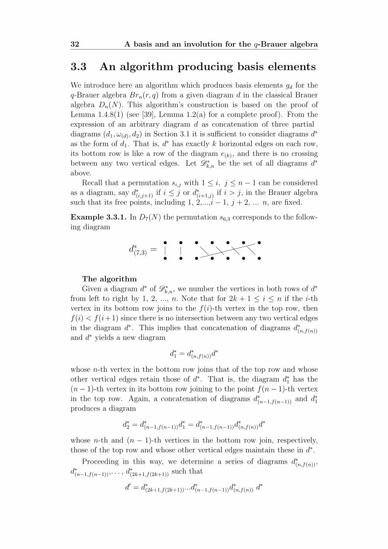
above.Recall that a permutation si,j with 1 ≤ i, j ≤ n− 1 can be considered
as a diagram, say d∗(i,j+1) if i ≤ j or d∗(i+1,j) if i > j, in the Brauer algebrasuch that its free points, including 1, 2,...,i− 1, j + 2, ... n, are fixed.
Example 3.3.1. In D7(N) the permutation s6,3 corresponds to the follow-ing diagram
• • •??
??•
????•
????•
????•
gggggggggggggggggg
•d∗(7,3) =
• • • • • •
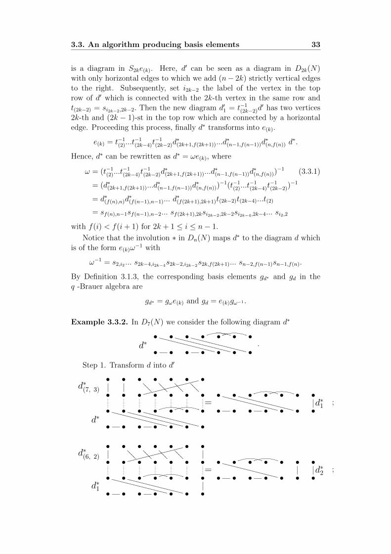
The algorithmGiven a diagram d∗ of D∗k,n, we number the vertices in both rows of d∗
from left to right by 1, 2, ..., n. Note that for 2k + 1 ≤ i ≤ n if the i-thvertex in its bottom row joins to the f(i)-th vertex in the top row, thenf(i) < f(i+1) since there is no intersection between any two vertical edgesin the diagram d∗. This implies that concatenation of diagrams d∗(n,f(n))
and d∗ yields a new diagram
d∗1 = d∗(n,f(n))d∗
whose n-th vertex in the bottom row joins that of the top row and whoseother vertical edges retain those of d∗. That is, the diagram d∗1 has the(n− 1)-th vertex in its bottom row joining to the point f(n− 1)-th vertexin the top row. Again, a concatenation of diagrams d∗(n−1,f(n−1)) and d∗1produces a diagram
d∗2 = d∗(n−1,f(n−1))d∗1 = d∗(n−1,f(n−1))d
∗(n,f(n))d
∗
whose n-th and (n − 1)-th vertices in the bottom row join, respectively,those of the top row and whose other vertical edges maintain these in d∗.
Proceeding in this way, we determine a series of diagrams d∗(n,f(n)),d∗(n−1,f(n−1)),. . . , d∗(2k+1,f(2k+1)) such that
d′ = d∗(2k+1,f(2k+1))...d∗(n−1,f(n−1))d
∗(n,f(n)) d
∗
3.3. An algorithm producing basis elements 33
is a diagram in S2ke(k). Here, d′ can be seen as a diagram in D2k(N)with only horizontal edges to which we add (n− 2k) strictly vertical edgesto the right. Subsequently, set i2k−2 the label of the vertex in the toprow of d′ which is connected with the 2k-th vertex in the same row andt(2k−2) = si2k−2,2k−2. Then the new diagram d′1 = t−1
(2k−2)d′ has two vertices
2k-th and (2k − 1)-st in the top row which are connected by a horizontaledge. Proceeding this process, finally d∗ transforms into e(k).
e(k) = t−1(2)...t
−1(2k−4)t
−1(2k−2)d
∗(2k+1,f(2k+1))...d
∗(n−1,f(n−1))d
∗(n,f(n)) d
∗.
Hence, d∗ can be rewritten as d∗ = ωe(k), where
ω = (t−1(2)...t
−1(2k−4)t
−1(2k−2)d
∗(2k+1,f(2k+1))...d
∗(n−1,f(n−1))d
∗(n,f(n)))
−1 (3.3.1)
= (d∗(2k+1,f(2k+1))...d∗(n−1,f(n−1))d
∗(n,f(n)))
−1(t−1(2)...t
−1(2k−4)t
−1(2k−2))
−1
= d∗(f(n),n)d∗(f(n−1),n−1)... d
∗(f(2k+1),2k+1)t(2k−2)t(2k−4)...t(2)
= sf(n),n−1sf(n−1),n−2... sf(2k+1),2ksi2k−2,2k−2si2k−4,2k−4... si2,2
with f(i) < f(i+ 1) for 2k + 1 ≤ i ≤ n− 1.
Notice that the involution ∗ in Dn(N) maps d∗ to the diagram d whichis of the form e(k)ω
−1 with
ω−1 = s2,i2 ... s2k−4,i2k−4s2k−2,i2k−2
s2k,f(2k+1)... sn−2,f(n−1)sn−1,f(n).
By Definition 3.1.3, the corresponding basis elements gd∗ and gd in theq -Brauer algebra are
gd∗ = gωe(k) and gd = e(k)gω−1 .
Example 3.3.2. In D7(N) we consider the following diagram d∗
•WWWWWWWWWWWWWWWWWW •
WWWWWWWWWWWWWWWWWW •WWWWWWWWWWWWWWWWWW • • • •
•d∗
• • • • • •.
Step 1. Transform d into d′
• • •??
??•
????•
????•
????•
gggggggggggggggggg
•d∗(7, 3)
• • • • • •=•
WWWWWWWWWWWWWWWWWW •WWWWWWWWWWWWWWWWWW • • • • •
d∗1•WWWWWWWWWWWWWWWWWW •
WWWWWWWWWWWWWWWWWW •WWWWWWWWWWWWWWWWWW • • • • • • • • • • •
•d∗
• • • • • •
;
• •??
??•
????•
????•
????•
gggggggggggggggggg •
•d∗(6, 2)
• • • • • •=•
WWWWWWWWWWWWWWWWWW • • • • • •d∗2•
WWWWWWWWWWWWWWWWWW •WWWWWWWWWWWWWWWWWW • • • • • • • • • • • •
•d∗1 • • • • • •
;
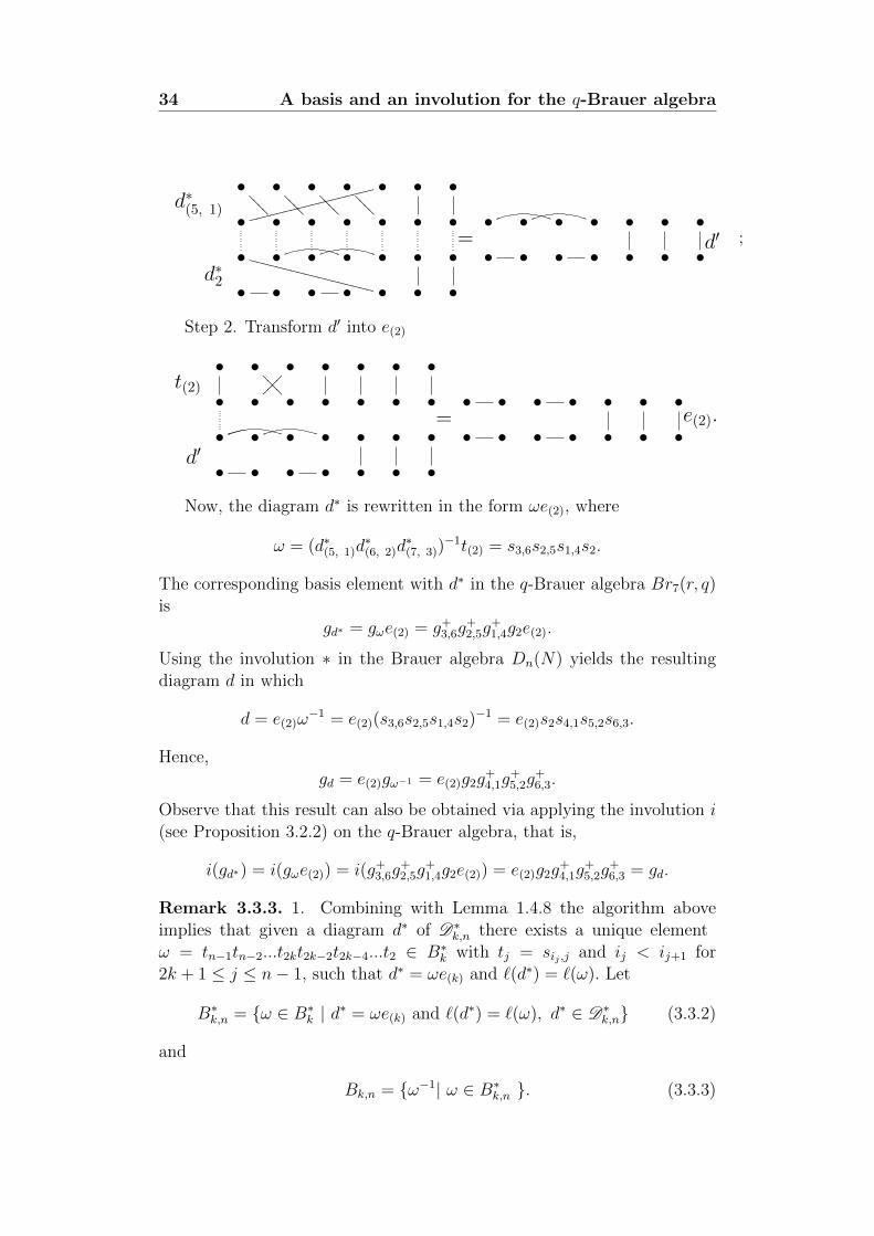
34 A basis and an involution for the q-Brauer algebra
•??
??•
????•
????•
????•
gggggggggggggggggg • •
•d∗(5, 1)
• • • • • •=• • • • • • •
d′•
WWWWWWWWWWWWWWWWWW • • • • • • • • • • • • •
•d∗2 • • • • • •
;
Step 2. Transform d′ into e(2)
• •??
??•
����
• • • •
•t(2)
• • • • • •=• • • • • • •
e(2).• • • • • • • • • • • • • •
•d′
• • • • • •
Now, the diagram d∗ is rewritten in the form ωe(2), where
ω = (d∗(5, 1)d∗(6, 2)d
∗(7, 3))
−1t(2) = s3,6s2,5s1,4s2.
The corresponding basis element with d∗ in the q-Brauer algebra Br7(r, q)is
gd∗ = gωe(2) = g+3,6g
+2,5g
+1,4g2e(2).
Using the involution ∗ in the Brauer algebra Dn(N) yields the resultingdiagram d in which
d = e(2)ω−1 = e(2)(s3,6s2,5s1,4s2)−1 = e(2)s2s4,1s5,2s6,3.
Hence,gd = e(2)gω−1 = e(2)g2g
+4,1g
+5,2g
+6,3.
Observe that this result can also be obtained via applying the involution i(see Proposition 3.2.2) on the q-Brauer algebra, that is,
i(gd∗) = i(gωe(2)) = i(g+3,6g
+2,5g
+1,4g2e(2)) = e(2)g2g
+4,1g
+5,2g
+6,3 = gd.
Remark 3.3.3. 1. Combining with Lemma 1.4.8 the algorithm aboveimplies that given a diagram d∗ of D∗k,n there exists a unique elementω = tn−1tn−2...t2kt2k−2t2k−4...t2 ∈ B∗k with tj = sij ,j and ij < ij+1 for2k + 1 ≤ j ≤ n− 1, such that d∗ = ωe(k) and `(d∗) = `(ω). Let
B∗k,n = {ω ∈ B∗k | d∗ = ωe(k) and `(d∗) = `(ω), d∗ ∈ D∗k,n} (3.3.2)
and
Bk,n = {ω−1| ω ∈ B∗k,n }. (3.3.3)
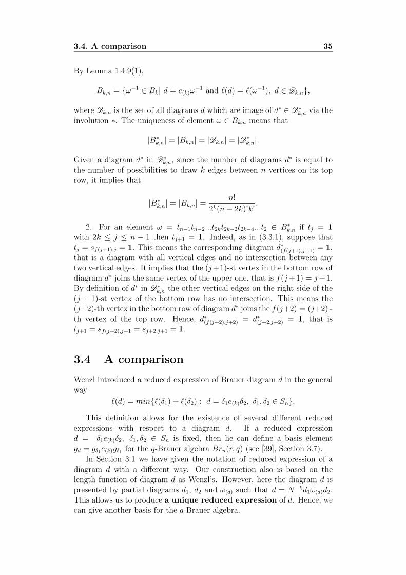
3.4. A comparison 35
By Lemma 1.4.9(1),
Bk,n = {ω−1 ∈ Bk| d = e(k)ω−1 and `(d) = `(ω−1), d ∈ Dk,n},
where Dk,n is the set of all diagrams d which are image of d∗ ∈ D∗k,n via theinvolution ∗. The uniqueness of element ω ∈ Bk,n means that
|B∗k,n| = |Bk,n| = |Dk,n| = |D∗k,n|.
Given a diagram d∗ in D∗k,n, since the number of diagrams d∗ is equal tothe number of possibilities to draw k edges between n vertices on its toprow, it implies that
|B∗k,n| = |Bk,n| =n!
2k(n− 2k)!k!.
2. For an element ω = tn−1tn−2...t2kt2k−2t2k−4...t2 ∈ B∗k,n if tj = 1with 2k ≤ j ≤ n − 1 then tj+1 = 1. Indeed, as in (3.3.1), suppose thattj = sf(j+1),j = 1. This means the corresponding diagram d∗(f(j+1),j+1) = 1,that is a diagram with all vertical edges and no intersection between anytwo vertical edges. It implies that the (j+1)-st vertex in the bottom row ofdiagram d∗ joins the same vertex of the upper one, that is f(j+ 1) = j+ 1.By definition of d∗ in D∗k,n the other vertical edges on the right side of the(j + 1)-st vertex of the bottom row has no intersection. This means the(j+2)-th vertex in the bottom row of diagram d∗ joins the f(j+2) = (j+2) -th vertex of the top row. Hence, d∗(f(j+2),j+2) = d∗(j+2,j+2) = 1, that istj+1 = sf(j+2),j+1 = sj+2,j+1 = 1.
3.4 A comparison
Wenzl introduced a reduced expression of Brauer diagram d in the generalway
`(d) = min{`(δ1) + `(δ2) : d = δ1e(k)δ2, δ1, δ2 ∈ Sn}.
This definition allows for the existence of several different reducedexpressions with respect to a diagram d. If a reduced expressiond = δ1e(k)δ2, δ1, δ2 ∈ Sn is fixed, then he can define a basis elementgd = gδ1e(k)gδ1 for the q-Brauer algebra Brn(r, q) (see [39], Section 3.7).
In Section 3.1 we have given the notation of reduced expression of adiagram d with a different way. Our construction also is based on thelength function of diagram d as Wenzl’s. However, here the diagram d ispresented by partial diagrams d1, d2 and ω(d) such that d = N−kd1ω(d)d2.This allows us to produce a unique reduced expression of d. Hence, wecan give another basis for the q-Brauer algebra.
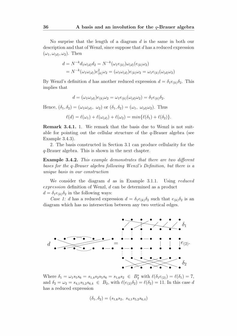
36 A basis and an involution for the q-Brauer algebra
No surprise that the length of a diagram d is the same in both ourdescription and that of Wenzl, since suppose that d has a reduced expression(ω1, ω(d), ω2). Then
d = N−kd1ω(d)d2 = N−k(ω1e(k))ω(d)(e(k)ω2)
= N−k(ω1ω(d))e2(k)ω2 = (ω1ω(d))e(k)ω2 = ω1e(k)(ω(d)ω2)
By Wenzl’s definition d has another reduced expression d = δ1e(k)δ2. Thisimplies that
d = (ω1ω(d))e(k)ω2 = ω1e(k)(ω(d)ω2) = δ1e(k)δ2.
Hence, (δ1, δ2) = (ω1ω(d), ω2) or (δ1, δ2) = (ω1, ω(d)ω2). Thus
`(d) = `(ω1) + `(ω(d)) + `(ω2) = min{`(δ1) + `(δ2)}.
Remark 3.4.1. 1. We remark that the basis due to Wenzl is not suit-able for pointing out the cellular structure of the q-Brauer algebra (seeExample 3.4.3).
2. The basis constructed in Section 3.1 can produce cellularity for theq-Brauer algebra. This is shown in the next chapter.
Example 3.4.2. This example demonstrates that there are two differentbases for the q-Brauer algebra following Wenzl’s Definition, but there is aunique basis in our construction
We consider the diagram d as in Example 3.1.1. Using reducedexpression definition of Wenzl, d can be determined as a productd = δ1e(k)δ2 in the following ways:
Case 1: d has a reduced expression d = δ1e(k)δ2 such that e(k)δ2 is andiagram which has no intersection between any two vertical edges.
•ZZZZZZZZZZZZZZZZZZZZZZZZZZZ •
����
• •ooooooooo •
����
•��
��•
���� δ1
• • • • • • •
•TTTTTTTTTTTTT • • • • •
eeeeeeeeeeeeeeeeeeeeeee •eeeeeeeeeeeeeeeeeeeeeee
=• • • • • • •
e(2).•
d• • • • • • • • • • • • •
•OOOOOOOO •
TTTTTTTTTTTTT •TTTTTTTTTTTTT •
TTTTTTTTTTTTT •gggggggggggggggggg •
gggggggggggggggggg •jjjjjjjjjjjjj
δ2• • • • • • •
Where δ1 = ω1s5s6 = s1,4s2s5s6 = s1,6s2 ∈ B∗2 with `(δ1e(2)) = `(δ1) = 7,and δ2 = ω2 = s4,1s5,2s6,4 ∈ B2, with `(e(2)δ2) = `(δ2) = 11. In this case dhas a reduced expression
(δ1, δ2) = (s1,6s2, s4,1s5,2s6,4)
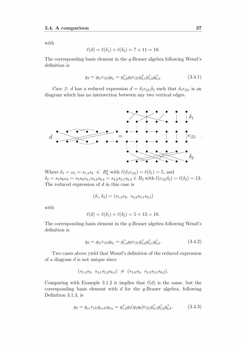
3.4. A comparison 37
with
`(d) = `(δ1) + `(δ2) = 7 + 11 = 18.
The corresponding basis element in the q-Brauer algebra following Wenzl’sdefinition is
gd = gδ1e(2)gδ2 = g+1,6g2e(2)g
+4,1g
+5,2g
+6,4. (3.4.1)
Case 2: d has a reduced expression d = δ1e(k)δ2 such that δ1e(k) is andiagram which has no intersection between any two vertical edges.
•WWWWWWWWWWWWWWWWWW •
����
• •ooooooooo •
����
• •δ1
• • • • • • •
•TTTTTTTTTTTTT • • • • •
eeeeeeeeeeeeeeeeeeeeeee •eeeeeeeeeeeeeeeeeeeeeee
=• • • • • • •
e(2)•
d• • • • • • • • • • • • •
•OOOOOOOO •
TTTTTTTTTTTTT •TTTTTTTTTTTTT •
TTTTTTTTTTTTT •��
��•
eeeeeeeeeeeeeeeeeeeeee •eeeeeeeeeeeeeeeeeeeeeee
δ2• • • • • • •
.
Where δ1 = ω1 = s1,4s2 ∈ B∗2 with `(δ1e(2)) = `(δ1) = 5, andδ2 = s5s6ω2 = s5s6s4,1s5,2s6,4 = s4,2s5,1s6,2 ∈ B2 with `(e(2)δ2) = `(δ2) = 13.The reduced expression of d in this case is
(δ1, δ2) = (s1,4s2, s4,2s5,1s6,2)
with
`(d) = `(δ1) + `(δ2) = 5 + 13 = 18.
The corresponding basis element in the q-Brauer algebra following Wenzl’sdefinition is
gd = gδ1e(2)gδ2 = g+1,4g2e(2)g
+4,2g
+5,1g
+6,2. (3.4.2)
Two cases above yield that Wenzl’s definition of the reduced expressionof a diagram d is not unique since
(s1,4s2, s4,1s5,2s6,4) 6= (s1,6s2, s4,2s5,1s6,2).
Comparing with Example 3.1.2 it implies that `(d) is the same, but thecorresponding basis element with d for the q-Brauer algebra, followingDefinition 3.1.3, is
gd = gω1e(2)gω(d)gω2 = g+1,4g2(g5g6)e(2)g
+4,1g
+5,2g
+6,4. (3.4.3)
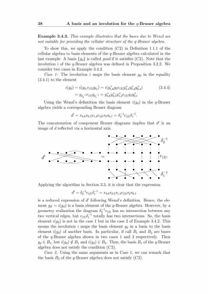
38 A basis and an involution for the q-Brauer algebra
Example 3.4.3. This example illustrates that the bases due to Wenzl arenot suitable for providing the cellular structure of the q-Brauer algebra.
To show this, we apply the condition (C2) in Definition 1.1.1 of thecellular algebra to basis elements of the q-Brauer algebra calculated in thelast example. A basis {gd} is called good if it satisfies (C2). Note that theinvolution i of the q-Brauer algebra was defined in Proposition 3.2.2. Weconsider two cases in Example 3.4.2.
Case 1: The involution i maps the basis element gd in the equality(3.4.1) to the element
i(gd) = i(gδ1e(2)gδ2) = i(g+1,6g2e(2)g
+4,1g
+5,2g
+6,4) (3.4.4)
= gδ−12e(2)gδ−1
1= g+
4,6g+2,5g
+1,4e(2)g2g
+6,1
Using the Wenzl’s defintition the basis element i(gd) in the q-Braueralgebra yields a corresponding Brauer diagram
d′ = s4,6s2,5s1,4e(2)s2s6,1 = δ−12 e(2)δ
−11 .
The concatenation of component Brauer diagrams implies that d′ is animage of d reflected via a horizontal axis.
•WWWWWWWWWWWWWWWWWW •
WWWWWWWWWWWWWWWWWW •oooooooo •
TTTTTTTTTTTTT •jjjjjjjjjjjjj •
jjjjjjjjjjjjj •jjjjjjjjjjjjj
δ−12• • • • • • •
•YYYYYYYYYYYYYYYYYYYYYYY •
YYYYYYYYYYYYYYYYYYYYYYY • •jjjjjjjjjjjjj • • •
=• • • • • • •
e(2).•
d′• • • • • • • • • • • • •
•??
??•
OOOOOOOOO • •??
??•
????•
????•
ddddddddddddddddddddddddddd
δ−11• • • • • • •Applying the algorithm in Section 3.3, it is clear that the expression
d′ = δ−12 e(2)δ
−11 = s4,6s2,5s1,4e(2)s2s6,1
is a reduced expression of d′ following Wenzl’s definition. Hence, the ele-ment gd′ = i(gd) is a basis element of the q-Brauer algebra. However, by ageometry realization the diagram δ−1
2 e(2) has no intersection between anytwo vertical edges, but e(2)δ
−11 totally has two intersections. So, the basis
element i(gd) is not in the case 1 but in the case 2 of Example 3.4.2. Thismeans the involution i maps the basis element gd in a basis to the basiselement i(gd) of another basis. In particular, if call B1 and B2 are basesof the q-Brauer algebra shown in two cases 1 and 2 respectively. Thengd ∈ B1, but i(gd) /∈ B1 and i(gd) ∈ B2. Thus, the basis B1 of the q-Braueralgebra does not satisfy the condition (C2).
Case 2. Using the same arguments as in Case 1, we can remark thatthe basis B2 of the q-Brauer algebra does not satisfy (C2).
Chapter 4
Cellular structure of the
q-Brauer algebra
This section is devoted to establish cellularity of the q-Brauer algebraon the version Brn(r, q). All results in this section hold true for the otherversions. In fact, to describe cellular structure of Brn(r, q) we need touse an explicit basis which has been introduced in the previous chapter.The first main result in this chapter is Theorem 4.2.2 that states: Theq-Brauer algebra over commutative ring is a cellular algebra with respectto the involution i. Further, it is an iterated inflation of Hecke algebras ofthe symmetric groups. More detail about the concept ”iterated inflation”is given in [24, 26]. The second main result is Theorem 4.2.7 which givesa complete set of indexes of simple modules, up to isomorphism, of theq-Brauer algebra.
4.1 An iterated inflation
The free finitely generated R-module V ∗k,n and Vk,n
As usual let k be an integer, 0 ≤ k ≤ [n/2], and denote Dn(N) theclassical Brauer algebra over commutative ring R with unity. Define V ∗k,nto be an R-vector space linearly spanned by D∗k,n. This implies V ∗k,n is anR-submodule of V ∗k . Hence, by Lemma 1.4.8(1) a given basis diagramd∗ in V ∗k,n has a unique reduced expression in the form d∗ = ωe(k) with`(d∗) = `(ω) and ω ∈ B∗k,n. Similarly, let Vk,n be an R-vector space linearlyspanned by Dk,n. That is, a basis diagram d in Vk,n has exactly 2khorizontal edges, its top row is the same as a row of e(k), and there is nointersection between any two vertical edges.
The following lemma is directly deduced from definitions.
39
40 Cellular structure of the q-Brauer algebra
Lemma 4.1.1. The R-module V ∗k,n has a basis {d∗ = ωe(k), ω ∈ B∗k,n}.Dually, the R-module Vk,n has a basis {d = e(k)ω, ω ∈ Bk,n}. Moreover,
dimRVk,n = dimRV∗k,n =
n!
2k(n− 2k)!k!.
Statements below in Lemmas 4.1.2, 4.1.4, 4.1.5 and Corollary 4.1.3 areneeded for later reference.
Lemma 4.1.2. Let d∗ be a basis diagram in V ∗k,n and π be a permutation inS2k+1,n. Then d∗π is a basis diagram in V ∗k satisfying `(d∗π) = `(d∗)+ `(π).
Proof. Since d∗ ∈ V ∗k,n, it implies that there exists a unique elementω ∈ B∗k,n such that d∗ = ωe(k). Consider π as a diagram in Dn(N) andalso observe that two diagrams e(k) and π commute. It follows from con-catenation of diagrams d∗ and π that the diagram d∗π is a basis diagramin V ∗k . This yields d∗π = ωe(k)π = ωπe(k). Since the basis diagram d∗ hasno intersection between any two vertical edges, the number of intersectionsof vertical edges in the resulting basis diagram d∗π is equal to that of thediagram π. In fact, the number of intersections of vertical edges in thediagram π is equal to its length. This produces `(d∗π) = `(d∗) + `(π).
Corollary 4.1.3. Let ω be a permutation in B∗k,n and π be a permutationin S2k+1,n. Then
`(ωπ) = `(ω) + `(π) and ωπ ∈ B∗k.
Proof. Set d∗ = ωe(k), then `(d∗) = `(ω) since ω ∈ B∗k,n. Lemma 4.1.2implies that `(d∗π) = `(d∗)+`(π) = `(ω)+`(π) and d∗π = ωπe(k) is a basisdiagram in V ∗k . The latter deduces that `(d∗π) = `(ωπe(k)) ≤ `(ωπ), thatis, `(d∗π) ≤ `(ωπ). Immediately, the first equality follows from applyingthe inequality `(ω) + `(π) ≥ `(ωπ).
Let d′ = d∗π ∈ V ∗k , then by Lemma 1.4.8 there uniquely exists anelement ω′ in B∗k such that d′ = ω′e(k) and `(d′) = `(ω′). This implies that
d′ = ωπe(k) = ω′e(k) (4.1.1)
and`(d′) = `(ωπ) = `(ω) + `(π) = `(ω′).
The equality (4.1.1) yields πe(k) = ω−1ω′e(k). Observe that the basisdiagram πe(k) is a combination of two separate parts where the first partincludes all horizontal edges on the left side and the second consists of allvertical edges on the other side. As π and e(k) commute, π correspondsone-to-one with the second part of the basis diagram πe(k). This impliesthat the basis diagram πe(k) is uniquely presented as a concatenation ofdiagrams ω ∈ S2k+1,n and e(k). Now, the equality πe(k) = ω−1ω′e(k) impliesthat π = ω−1ω′, that is, ωπ = ω′. So that ωπ ∈ B∗k.
4.1. An iterated inflation 41
Lemma 4.1.4. Let σ be a permutation in B∗k. Then there exists a uniquepair (ω′, π′), where ω′ ∈ B∗k,n and π′ ∈ S2k+1,n, such that σ = ω′π′.
Proof. Observe that σe(k) is a basis diagram in V ∗k in which `(σe(k)) = `(σ)by Lemma 1.4.8(1). Now suppose that there are two pairs (ω′, π′) and(ω, π) satisfying
σ = ω′π′ = ωπ, (4.1.2)
where ω, ω′ ∈ B∗k,n and π, π′ ∈ S2k+1,n. Suppose that ω 6= ω′ thenωe(k) 6= ω′e(k) by definition of B∗k,n. This implies that two diagrams ωe(k)
and ω′e(k) differ from position of horizontal edges in their top rows. Bydefinition of diagrams in D∗k,n, the position of horizontal edges in the toprow of the basis diagram ωe(k) (or ω′e(k)) is unchanged after concatenat-ing it with an arbitrary element of S2k+1,n on the right. This implies thatωe(k)π differs from ω′e(k)π
′, that is, ωπe(k) 6= ω′π′e(k). However, the equality(4.1.2) yields ωπe(k) = ω′π′e(k), a contradiction. Thus ω = ω′, and hence,π = π′ by multiplying (4.1.2) with ω−1 on the left.
Lemma 4.1.5. Let k, l be non-negative integers, 0 ≤ l, k ≤ [n/2]. Letω be a permutation in B∗l,n and π be a permutation in S2l+1,n. Then thereexist ω′ ∈ B∗k,n and π′ ∈ S2k+1,n such that
ωπe(k) = ω′π′e(k).
Proof. Observe that ωπe(k) is a basis diagram in V ∗k by concatenation ofdiagrams ω, π and e(k). By Lemma 1.4.8(1) there exists a unique elementσ ∈ B∗k such that ωπe(k) = σe(k) and `(ωπe(k)) = `(σ). Lemma 4.1.4implies that σ can be rewritten in the form σ = ω′π′, where ω′ and π′ areelements uniquely determined in B∗k,n and S2k+1,n, respectively. Therefore,σe(k) = ωπe(k) = ω′π′e(k).
Note that given ω ∈ B∗l,n and π ∈ S2l+1,n, Lemma 4.1.5 can be obtainedvia a direct calculation using the defining relations as follows:
By Corollary 4.1.3, ωπ is in the form
ωπ = tn−1tn−2...t2lt2l−2t2l−4...t2 ∈ B∗l ,
where tj = 1 or tj = sij ,j for 1 ≤ ij ≤ j ≤ n− 1. Concatenation of ωπ ande(k) will transform ωπe(k) into σe(k), where σ = t′n−1t
′n−2...t
′2kt′2k−2t
′2k−4...t
′2
is in B∗k with t′j = 1 or t′j = sij ,j for 1 ≤ ij ≤ j ≤ n − 1. This process isdone by using defining relations on the Brauer algebra Dn(N), including(S0), (S1), (S2), (3) and (5). In fact, two final relations yield the vanishingof some transpositions si in ωπe(k) and the three first imply an rearrangeωπe(k) into σe(k).
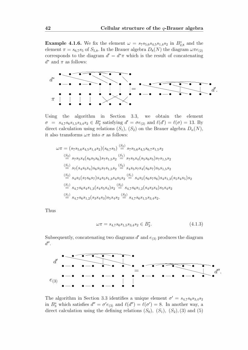
42 Cellular structure of the q-Brauer algebra
Example 4.1.6. We fix the element ω = s7s5,6s4,5s1,4s2 in B∗2,8 and theelement π = s6,7s5 of S5,8. In the Brauer algebra D8(N) the diagram ωπe(2)
corresponds to the diagram d′ = d∗π which is the result of concatenatingd∗ and π as follows:
•WWWWWWWWWWWWWWWWWW • • •
OOOOOOOOO •OOOOOOOOO • •
????•
•d∗
• • • • • • •=•
YYYYYYYYYYYYYYYYYYYYYYY • • •WWWWWWWWWWWWWWWWWW • • • •d′.
• • • • •??
??•
OOOOOOOOO •ooooooooo •
����
• • • • • • • •
•π
• • • • • • •
Using the algorithm in Section 3.3, we obtain the elementσ = s4,7s6s1,5s3,4s2 ∈ B∗2 satisfying d′ = σe(2) and `(d′) = `(σ) = 13. Bydirect calculation using relations (S1), (S2) on the Brauer algebra Dn(N),it also transforms ωπ into σ as follows:
ωπ = (s7s5,6s4,5s1,4s2)(s6,7s5)(S2)= s7s5,6s4,5s6,7s1,5s2
(S2)= s7s5s4(s6s5s6)s7s1,5s2
(S1)= s7s5s4(s5s6s5)s7s1,5s2
(S1)= s7(s4s5s4)s6s5s7s1,5s2
(S2)= s4s5s7s4(s6s7)s5s1,5s2
(S2)= s4s5(s7s6s7)s4s5s1,3s4s5s2
(S1)= s4s5(s6s7s6)s4s1,3(s5s4s5)s2
(S1)= s4,7s6s4s1,3(s4s5s4)s2
(S2)= s4,7s6s1,2(s4s3s4)s5s4s2
(S1)= s4,7s6s1,2(s3s4s3)s5s4s2
(S2)= s4,7s6s1,5s3,4s2.
Thus
ωπ = s4,7s6s1,5s3,4s2 ∈ B∗2 . (4.1.3)
Subsequently, concatenating two diagrams d′ and e(3) produces the diagramd′′.
•YYYYYYYYYYYYYYYYYYYYYYY • • •
WWWWWWWWWWWWWWWWWW • • • •
•d′
• • • • • • •=• • • •
WWWWWWWWWWWWWWWWWW • • • •d′′.
• • • • • • • • • • • • • • • •
•e(3)
• • • • • • •
The algorithm in Section 3.3 identifies a unique element σ′ = s4,7s6s3,4s2
in B∗3 which satisfies d′′ = σ′e(3) and `(d′′) = `(σ′) = 8. In another way, adirect calculation using the defining relations (S0), (S1), (S2), (3) and (5)
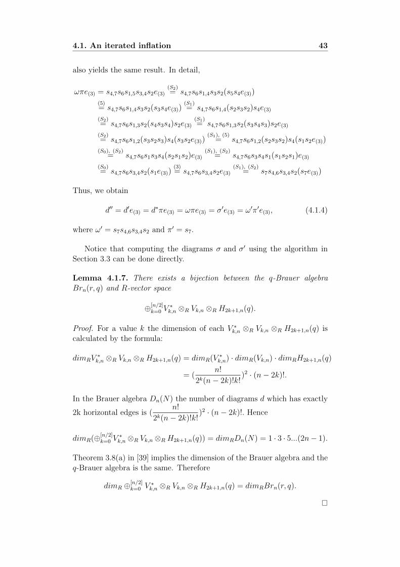
4.1. An iterated inflation 43
also yields the same result. In detail,
ωπe(3) = s4,7s6s1,5s3,4s2e(3)(S2)= s4,7s6s1,4s3s2(s5s4e(3))
(5)= s4,7s6s1,4s3s2(s3s4e(3))
(S1)= s4,7s6s1,4(s2s3s2)s4e(3)
(S2)= s4,7s6s1,3s2(s4s3s4)s2e(3)
(S1)= s4,7s6s1,3s2(s3s4s3)s2e(3)
(S2)= s4,7s6s1,2(s3s2s3)s4(s3s2e(3))
(S1), (5)= s4,7s6s1,2(s2s3s2)s4(s1s2e(3))
(S0), (S2)= s4,7s6s1s3s4(s2s1s2)e(3)
(S1), (S2)= s4,7s6s3s4s1(s1s2s1)e(3)
(S0)= s4,7s6s3,4s2(s1e(3))
(3)= s4,7s6s3,4s2e(3)
(S1), (S2)= s7s4,6s3,4s2(s7e(3))
Thus, we obtain
d′′ = d′e(3) = d∗πe(3) = ωπe(3) = σ′e(3) = ω′π′e(3), (4.1.4)
where ω′ = s7s4,6s3,4s2 and π′ = s7.
Notice that computing the diagrams σ and σ′ using the algorithm inSection 3.3 can be done directly.
Lemma 4.1.7. There exists a bijection between the q-Brauer algebraBrn(r, q) and R-vector space
⊕[n/2]k=0 V
∗k,n ⊗R Vk,n ⊗R H2k+1,n(q).
Proof. For a value k the dimension of each V ∗k,n ⊗R Vk,n ⊗R H2k+1,n(q) iscalculated by the formula:
dimRV∗k,n ⊗R Vk,n ⊗R H2k+1,n(q) = dimR(V ∗k,n) · dimR(Vk,n) · dimRH2k+1,n(q)
= (n!
2k(n− 2k)!k!)2 · (n− 2k)!.
In the Brauer algebra Dn(N) the number of diagrams d which has exactly
2k horizontal edges is (n!
2k(n− 2k)!k!)2 · (n− 2k)!. Hence
dimR(⊕[n/2]k=0 V
∗k,n ⊗R Vk,n ⊗RH2k+1,n(q)) = dimRDn(N) = 1 · 3 · 5...(2n− 1).
Theorem 3.8(a) in [39] implies the dimension of the Brauer algebra and theq-Brauer algebra is the same. Therefore
dimR ⊕[n/2]k=0 V ∗k,n ⊗R Vk,n ⊗R H2k+1,n(q) = dimRBrn(r, q).
44 Cellular structure of the q-Brauer algebra
Now an explicit bijection will be given. Suppose that d is a diagramwith a unique reduced expression (ω1, ω(d), ω2), where ω1 ∈ B∗k,n, ω2 ∈ Bk,n
and ω(d) ∈ S2k+1,n. As indicated in Section 3.1, the partial diagramsd1 = ω1e(k) and d2 = e(k)ω2 with `(d1) = `(ω1) and `(d2) = `(ω2) are basisdiagrams of V ∗k,n (Vk,n), respectively. Therefore, the diagram d correspondsone-to-one to a basis element
d1 ⊗ d2 ⊗ gω(d)= ω1e(k) ⊗ e(k)ω2 ⊗ gω(d)
of the R-vector space V ∗k,n ⊗R Vk,n ⊗RH2k+1,n(q). Now, the correspondencebetween an arbitrary diagram d in the Brauer algebra and a basis elementgd = gω1gω(d)
e(k)gω2 of the q-Brauer algebra shown in Theorem 3.1.4, implies
a bijection fromBrn(r, q) to⊕[n/2]k=0 V
∗k,n⊗RVk,n⊗RH2k+1,n(q) linearly spanned
by the rule
gd = gω1gω(d)e(k)gω2 7−→ ω1e(k) ⊗ e(k)ω2 ⊗ gω(d)
.
From now on, if no confusion can arise, we denote by gd both a basis ele-ment of the q-Brauer algebra Bn(r, q) and its corresponding representationin V ∗k,n ⊗R Vk,n ⊗R H2k+1,n(q).
The R-bilinear form for V ∗k,n ⊗R Vk,n ⊗R H2k+1,n(q)
Now we want to construct an R-bilinear form
ϕk : Vk,n ⊗R V ∗k,n −→ H2k+1,n(q)
for each 0 ≤ k ≤ [n/2].Given elements ω1, ω2 ∈ B∗k,n, by Lemma 4.1.7 we form the element
Xj := d∗j⊗dj⊗1 in V ∗k,n⊗RVk,n⊗RH2k+1,n(q) for j = 1, 2, where d∗j = ωje(k)
and dj = e(k)ω−1j . The corresponding basis element of Xj in the q-Brauer
algebra is Xj = gωje(k)gω−1j. Then
X1X2 = (gω1e(k)gω−11
)(gω2e(k)gω−12
). (4.1.5)
Using Lemma 2.2.3 for j = k implies
e(k)gω−11gω2e(k) ∈ H2k+1,n(q)e(k) +
∑m≥k+1
Hn(q)e(m)Hn(q).
Hence, e(k)gω−11gω2e(k) can be rewritten as an R-linear combination of the
forme(k)gω−1
1gω2e(k) =
∑j
ajgω(cj)e(k) + a′,
where aj ∈ R, gω(cj)∈ H2k+1,n(q), and a′ is a linear combination of basis
elements in∑
m≥k+1Hn(q)e(m)Hn(q). This implies that
X1X2 = gω1(∑j
ajgω(cj)e(k))gω−1
2+ gω1a
′gω−1
2=∑j
ajgω1gω(cj)e(k)gω−1
2+ a,
4.1. An iterated inflation 45
where a is an R-linear combination in∑
m≥k+1 Hn(q)e(m)Hn(q). ByDefinition 3.1.3, the elements gω1gω(cj)
e(k)gω−12
, denoted by gcj , are basiselements in the q-Brauer algebra, and hence, the product X1X2 can berewritten to be
∑j ajgcj + a. Using Lemma 4.1.7, gcj can be expressed in
the form
gcj = ω1e(k) ⊗ e(k)ω−12 ⊗ gω(cj)
.
Finally, X1X2 can be presented as
X1X2 =∑j
ω1e(k) ⊗ e(k)ω−12 ⊗ ajgω(cj)
+ a. (4.1.6)
Subsequently, ϕk : Vk,n⊗RV ∗k,n −→ H2k+1,n(q) is an R-bilinear form definedby
ϕk(d1, d∗2) =
∑j
ajgω(cj)∈ H2k+1,n(q). (4.1.7)
In a particular case
ϕk(e(k), e(k)) = (r − 1
q − 1)k ∈ H2k+1,n(q). (4.1.8)
Also note that, the equality (4.1.6) and Definition 4.1.7 yield the productX1X2 in the q-Brauer algebra Brn(r, q)
X1X2 = gω1ϕk(d1, d∗2)e(k)gω−1
2+ a = gω1e(k)ϕk(d1, d
∗2)gω−1
2+ a. (4.1.9)
Definition 4.1.8. Define Jk to be an R −module generated by the basiselements gd in the q-Brauer algebra Brn(r, q), where d is a diagram whosenumber of vertical edges, say ϑ(d), are less than or equal n− 2k.
It is clear that Jk+1 ⊂ Jk and Jk is an ideal in Brn(r, q). By Lemma
2.2.4, Jk =∑[n/2]
m=kHn(q)e(m)Hn(q).
Lemma 4.1.9. Let gc = c1 ⊗ c2 ⊗ gω(c)and gd = d1 ⊗ d2 ⊗ gω(d)
, wheregω(c)
, gω(d)∈ H2k+1,n(q), c1 = ω1e(k), c2 = e(k)ω2, d1 = δ1e(k), d2 = e(k)δ2
with ω1, δ1 ∈ B∗k,n and ω2, δ2 ∈ Bk,n. Then
gcgd = c1 ⊗ d2 ⊗ gω(c)ϕk(c2, d1)gω(d)
(mod Jk+1).
Proof. Note that the basis diagram c2 = e(k)ω2 ∈ Vk,n (similarlyd1 = δ1e(k) ∈ V ∗k,n) can be seen as elements
gc2 = e(k) ⊗ e(k)ω2 ⊗ 1 and gd1 = δ1e(k) ⊗ e(k) ⊗ 1
in V ∗k,n ⊗R Vk,n ⊗R H2k+1,n(q). Lemma 4.1.7 implies that gc2 = e(k)gω2 andgd1 = gδ1e(k) are corresponding basis elements in the q-Brauer algebra
46 Cellular structure of the q-Brauer algebra
Brn(r, q), respectively. Applying Lemma 2.2.3 for j = k, the product of gc2and gd1 is
gc2gd1 = e(k)gω2gδ1e(k) ∈ H2k+1,n(q)e(k) +∑
m≥k+1
Hn(q)e(m)Hn(q).
Therefore,
gω−12gc2gd1gδ−1
1= (gω−1
2e(k)gω2)(gδ1e(k)gδ−1
1)
(4.1.9)= gω−1
2ϕk(c2, d1)e(k)gδ−1
1+ a,
where a is a linear combination of basis elements in Jk+1 and ϕk(c2, d1) isthe R-bilinear form defined above. This means
gc2gd1 = ϕk(c2, d1)e(k) + a′ (4.1.10)
with a′ = (gω−12
)−1a(gδ−11
)−1 ∈ Jk+1. As a consequence, gcgd is formed as aproduct of basis elements:
gcgd = (gω1gω(c)e(k)gω2)(gδ1gω(d)
e(k)gδ2)
= gω1gω(c)(e(k)gω2gδ1e(k))gω(d)
gδ2
= gω1gω(c)(gc2gd1)gω(d)
gδ2(4.1.10)
= gω1gω(c)(ϕk(c2, d1)e(k) + a′)gω(d)
gδ2
= gω1gω(c)ϕk(c2, d1)e(k)gω(d)
gδ2 + a′′
with a′′ ∈ Jk+1. Thus, by Lemma 4.1.7, gcgd can be expressed as
gcgd ≡ c1 ⊗ d2 ⊗ gω(c)ϕk(c2, d1)gω(d)
(mod Jk+1).
Lemma 4.1.7 implies that Brn(r, q) has a decomposition as R-modules :
Brn(r, q) ∼= ⊕[n/2]k=0 V
∗k,n ⊗R Vk,n ⊗R H2k+1,n(q).
Lemma 4.1.10. Let ω be an arbitrary permutation in B∗k,n and π ∈ S2k+1,n.Then gωgπe(k) is a basis element in the q-Brauer algebra Brn(r, q).
Proof. Corollary 4.1.3 yields that the basis diagram d = ωπe(k) satisfies
`(d) = `(ωπ) = `(ω) + `(π).
This means the pair (ω, π) is a reduced expression of d. Therefore, byDefinition 3.1.3 we get the precise statement.
Lemma 4.1.11. Let k, l be non-negative integers, 0 ≤ l, k ≤ [n/2]. Let ωbe a permutation in B∗l,n and π a permutation in S2l+1,n. Then
gωgπe(k) =∑j
ajgω′jgπ′je(k),
where aj ∈ R, ω′j ∈ B∗k,n, and π′j ∈ S2k+1,n.
4.1. An iterated inflation 47
Proof. Corollary 4.1.3 implies `(ωπ) = `(ω) + `(π). As a consequence,gωgπ = gωπ by applying Lemma 1.3.10(1). The remainder of proof followsfrom the correspondence between the classical Brauer algebra Dn(N) andthe q-Brauer algebra Brn(r, q) in the following way:
Using the common properties of the Brauer algebra Dn(N) in Chapter1, Section 1.4 and of the q-Brauer algebra Brn(r, q) in Chapter 2, hence,the effect of the basis element gωπ on e(k) on the left(right) is similar to thisof diagram (permutation) ωπ with respect to diagram e(k), respectively, onthe left (right).
In fact, the operations used to move the diagram ωπe(k) into the diagramω′π′e(k) in Lemma 4.1.5 are (S0), (S1), (S2), (3) and (5) on the Braueralgebra Dn(N). In the same way, the product gωπe(k) transforms into theform
∑j ajgω′jgπ′je(k) via using corresponding relations g2
i = (q− 1)gi + q inDefinition 1.3.9(iii), (H1)and (H2) on the Hecke algebra of the symmetricgroup as well as two relations in Lemmas 3.2.1(2) and 2.2.2(3).
Example 4.1.12. Continue considering the same diagram as in Example4.1.6 with ω = s7s5,6s4,5s1,4s2 ∈ B∗2,8 and π = s6,7s5 ∈ S5,8. As in (4.1.3),the product of gω and gπ in the q-Brauer algebra Brn(r, q) is
gωgπLem1.3.10(1)
= gωπ(4.1.3)
= g+4,7g6g
+1,5g
+3,4g2.
Hence,
gωπe(3) = g+4,7g6g
+1,5g
+3,4g2e(3)
(H2)= g+
4,7g6g+1,4g3g2(g5g4e(3))
Lem1.3.10(3)= g+
4,7g6g+1,4g3g2(g3g4e(3))
(H1)= g+
4,7g6g+1,4(g2g3g2)g4e(3)
(H2)= g+
4,7g6g+1,3g2(g4g3g4)g2e(3)
(H1)= g+
4,7g6g1,3g2(g3g4g3)g2e(3)
(H2)= g+
4,7g6g+1,2(g3g2g3)g4(g3g2e(3))
(H1), Lem2.2.2(2)= g+
4,7g6g+1,2(g2g3g2)g4(g1g2e(3))
Def1.3.9(iii), (H2)= g+
4,7g6g1((q − 1)g2 + q)g3g4(g2g1g2)e(3)
(H1)= g+
4,7g6g1((q − 1)g2 + q)g3g4(g1g2g1)e(3)
Lem3.2.1(2)= qg+
4,7g6g1((q − 1)g2 + q)g3g4g1g2e(3)
= q(q − 1)g+4,7g6g1g2g3g4g1g2e(3) + q2g+
4,7g6g1g3g4g1g2e(3)
(H2)= q(q − 1)g+
4,7g6g+1,4g
+1,2e(3) + q2g+
4,7g6g+3,4g1g1g2e(3)
Def1.3.9(iii)= q(q − 1)g+
4,7g6g+1,4g
+1,2e(3) + q2g+
4,7g6g+3,4((q − 1)g1 + q)g2e(3)
= q(q − 1)g+4,7g6g
+1,4g
+1,2e(3) + q2(q − 1)g+
4,7g6g+3,4g
+1,2e(3) + q3g+
4,7g6g+3,4g2e(3)
Thus, in the q-Brauer algebra Brn(r, q) the element gωπe(3) is rewritten asan R- linear combination of elements gωje(3) (1 ≤ j ≤ 3), where ωj ∈ B∗3 .Now, using Lemmas 4.1.5 and 4.1.10, each element ωj of B∗3 can be uniquely
48 Cellular structure of the q-Brauer algebra
expressed in the form ωj = ω′jπ′j, where ω′j ∈ B∗3,8 and π′j ∈ S7,8, as follows:
gωπe(3) =3∑j=1
ajgω′jgπ′je(3) = q(q − 1)g7g+4,6g
+1,4g
+1,2(g7e(3)) (4.1.11)
+ q2(q − 1)g7g+4,6g
+3,4g
+1,2(g7e(3)) + q3g7g
+4,6g
+3,4g2(g7e(3)).
Note that if fix r = qN and q → 1, then Brn(r, q) ≡ Dn(N). In thiscase gi becomes the transposition si and the element e(k) can be identifiedwith the diagram e(k). Hence, the last Lemma coincides with Lemma 4.1.5.This means the equality (4.1.11) in the above example recovers the equality(4.1.4) in Example 4.1.6.
The next statement shows how to get an ideal in Brn(r, q) from an idealin Hecke algebras.
Proposition 4.1.13. Let I be an ideal in H2k+1,n(q). Then
Jk+1 + V ∗k,n ⊗R Vk,n ⊗ I
is an ideal in Brn(r, q).
Proof. Given two elements gc = c1 ⊗ c2 ⊗ gω(c)with c ∈ Dn(N) and
ϑ(c) = n− 2l, and gd = d1⊗d2⊗ gω(d) with d ∈ Dn(N) and ϑ(d) = n− 2k,we need to prove out that:
(c1 ⊗ c2 ⊗ gω(c))(d1 ⊗ d2 ⊗ gω(d)
) ≡ b⊗ d2 ⊗ agω(d)(mod Jk+1)
for some b ∈ V ∗k , and a is an element in H2k+1,n(q) which is independentof gω(d)
.
This property is shown via considering the multiplication of the basiselements of the q-Brauer algebra Brn((r, q) as in the proof of Lemma 4.1.7.Assume that
gc = gω1e(l)gω(c)gω2 and gd = gδ1e(k)gω(d)
gδ2
are basis elements on Brn(r, q), where ω(d) ∈ S2k+1,n; ω(c) ∈ S2l+1,n;ω1, ω
−12 ∈ B∗l,n and δ1, δ
−12 ∈ B∗k,n. Then, it implies
gcgd = gω1(e(l)gω(c)gω2gδ1e(k))gω(d)
gδ2 .
In the following we consider two separate cases of l and k.Case 1: If l > k, then Corollary 3.2.3(6) implies that
e(l)gω(c)gω2gδ1e(k) ∈ e(l)H2k+1,n(q) +
∑m≥l+1
Hn(q)e(m)Hn(q),
4.1. An iterated inflation 49
and hence
gcgd = gω1(e(l)gω(c)gω2gδ1e(k))gω(d)
gδ2
∈ gω1e(l)H2k+1,n(q)gω(d)gδ2 +
∑m≥l+1
Hn(q)e(m)Hn(q)
⊆ Hn(q)e(l)Hn(q) +∑m≥l+1
Hn(q)e(m)Hn(q)
=∑m≥l
Hn(q)e(m)Hn(q) = Jll>k
⊆ Jk+1.
Thus, in this case we obtain gcgd ≡ 0 (mod Jk+1).Case 2: If l ≤ k, then by Lemma 2.2.3,
e(l)gω(c)gω2gδ1e(k) ∈ H2l+1,ne(k) +
∑m≥k+1
Hn(q)e(m)Hn(q)
and
gcgd = gω1(e(l)gω(c)gω2gδ1e(k))gω(d)
gδ2
∈ gω1H2l+1,ne(k)gω(d)gδ2 +
∑m≥k+1
Hn(q)e(m)Hn(q).
Without loss of generality we may assume that
gcgd = gω1(∑i
bigω(ci)e(k))gω(d)
gδ2 + b′ =∑i
bi(gω1gω(ci)e(k))gω(d)
gδ2 + b′,
where bi ∈ R, gω(ci)∈ H2l+1,n, and b′ ∈
∑m≥k+1Hn(q)e(m)Hn(q).
Using Lemma 4.1.11 with respect to ω1 ∈ Bl and ω(ci) ∈ S2l+1,n, it impliesthat
gω1gω(ci)e(k) =
∑j
a(i,j)gω′(i,j)gπ′
(i,j)e(k),
where a(i,j) ∈ R, ω′
(i,j) ∈ B∗k,n, and π′
(i,j) ∈ S2k+1,n for l ≤ k.
Finally, gcgd can be rewritten as an R - linear combination of basiselements in the q-Brauer algebra Brn(r, q) as follows:
gcgd =∑i
bi(gω1gω(ci)e(k))gω(d)
gδ2 + b′
=∑i
bi(∑
j
a(i,j)gω′(i,j)gπ′
(i,j)e(k)
)gω(d)
gδ2 + b′
=∑i
∑j
bia(i,j)(gω′(i,j)gπ′
(i,j)e(k)gω(d)
gδ2) + b′
=∑i, j
bia(i,j)gω′(i,j)gπ′
(i,j)gω(d)
e(k)gδ2 + b′,
50 Cellular structure of the q-Brauer algebra
where π′(i,j) and ω(d) are in S2k+1,n; bia(i,j) ∈ R; ω′(i,j) ∈ B∗k,n and δ2 ∈ Bk,n.Lemma 4.1.7 implies that the corresponding element of the product gcgd inV ∗k,n ⊗R Vk,n ⊗R H2k+1,n(q) is
gcgd ≡∑i, j
bia(i,j)(ω′(i,j)e(k) ⊗ e(k)δ2 ⊗ gπ′
(i,j)gω(d)
) mod Jk+1
≡∑i, j
(ω′(i,j)e(k) ⊗ e(k)δ2 ⊗ (bia(i,j))gπ′(i,j)gω(d)
) mod Jk+1
≡ b⊗ d2 ⊗ agω(d)(mod Jk+1),
where b =∑
i, j ω′(i,j)e(k) ∈ V ∗k , a =
∑i, j bia(i,j)gπ′
(i,j)∈ H2k+1,n(q), and
d2 = e(k)δ2.
The following lemma describes the effect of the involution i of theq-Brauer algebra on V ∗k,n ⊗R Vk,n ⊗R H2k+1,n(q).
Lemma 4.1.14. 1. If gd = d1 ⊗ d2 ⊗ gω(d)with a reduced expression
d = (ω1, ω(d), ω2) in Dn(N). Then i(gd) = d−12 ⊗ d−1
1 ⊗ i(gω(d)) with
d−12 = ω−1
2 e(k) ∈ V ∗k,n and d−11 = e(k)ω
−12 ∈ Vk,n.
2. The involution i on H2k+1,n(q) and the R−bilinear form ϕk have thefollowing property:
iϕk(c, d) = ϕk(d−1, c−1)
for all c ∈ Vk,n and d ∈ V ∗k,n.
Proof. Part (1). The basis element corresponding to the reduced expressiond = (ω1, ω(d), ω2) is gd = gω1e(k)gπ(d)gω2 . As shown in the equality (3.2.12)of Proposition 3.2.2, the image of gd via involution i is
i(gd) = gω−12e(k)gω−1
(d)gω−1
1
with `(d−12 ) = `(ω−1
2 e(k)) = `(ω−12 ) and `(d−1
1 ) = `(e(k)ω−11 ) = `(ω−1
1 ).Definitions of V ∗k,n and Vk,n imply that d−1
1 ∈ Vk,n and d−12 ∈ V ∗k,n. Hence,
by Lemma 4.1.2 the element i(gd) can be rewritten as
i(gd) = d−12 ⊗ d−1
1 ⊗ i(gω(d)) ∈ V ∗k,n ⊗R Vk,n ⊗R H2k+1,n(q).
Part (2). Using the same argument as in the proof of Lemma 4.1.9, cand d can be expressed as basis elements of V ∗k,n⊗R Vk,n⊗RH2k+1,n(q) withgc = e(k) ⊗ c ⊗ 1 and gd = d ⊗ e(k) ⊗ 1, where 1 is identity in H2k+1,n(q).As a consequence,
gcgd = (e(k) ⊗ c⊗ 1)(d⊗ e(k) ⊗ 1)Lem4.1.9
= e(k) ⊗ e(k) ⊗ ϕk(c, d) (mod Jk+1).
4.2. Main results 51
This means the corresponding basis element in the q-Brauer algebra isgcgd = e(k)ϕk(c, d) + a with a ∈ Jk+1. And hence,
i(gcgd) = i(e(k)ϕk(c, d) + a) = i(ϕk(c, d))i(e(k)) + i(a)
Prop3.2.2= i(ϕk(c, d))e(k) + i(a)
Lem2.1.10= e(k)i(ϕk(c, d)) + i(a).
Thus, the corresponding element in V ∗k,n⊗RVk,n⊗RH2k+1,n(q) is of the form
i(gcgd) = i(e(k) ⊗ e(k) ⊗ ϕk(c, d)) = e(k) ⊗ e(k) ⊗ iϕk(c, d) (mod Jk+1)
(4.1.12)
since i(a) ∈ Jk+1.
In another way, the part (1) implies that i(gc) = c−1 ⊗ e(k) ⊗ 1 andi(gd) = e(k) ⊗ d−1 ⊗ 1. Therefore,
i(gd)i(gc) = (e(k) ⊗ d−1 ⊗ 1)(c−1 ⊗ e(k) ⊗ 1) (4.1.13)
Lem4.1.9= e(k) ⊗ e(k) ⊗ ϕk(d−1, c−1) (mod Jk+1).
Now the equality i(gcgd) = i(gd)i(gc) shows that
e(k) ⊗ e(k) ⊗ iϕk(c, d) = e(k) ⊗ e(k) ⊗ ϕk(d−1, c−1),
that is, iϕk(c, d) = ϕk(d−1, c−1).
The below statement gives an ′iterated inflation′ structure for theq-Brauer algebra Brn(r, q), and the proof of this comes from above results.
Proposition 4.1.15. Let R be a commutative ring. Assume more thatr, q and (r − 1)/(q − 1) are invertible in R. Then the q-Brauer algebraBrn(r, q) over R is an iterated inflation of Hecke algebras of the symmetricgroup algebras. More precisely: as a free R-module, Brn(r, q) is equal to
V ∗0,n⊗RV0,n⊗RHn(q)⊕V ∗1,n⊗RV1,n⊗RH3,n(q)⊕V ∗2,n⊗RV2,n⊗RH5,n(q)⊕ ...,
and the iterated inflation starts with Hn(q), inflates it along V ∗k,n ⊗R Vk,nand so on, ending with an inflation of R = Hn,n(q) or R = Hn+1,n(q) asbottom layer (depending on whether n is odd or even), where H2k+1,n(q) isHecke algebra with generators g2k+1, g2k+2... gn−1.
Corollary 4.1.16. The statement in Proposition 4.1.15 holds on Brn(N).
4.2 Main results
Before giving the main result we need the following lemma. This lemma isshown in [42] as a condition to ensure that an algebra has cellular structure.
52 Cellular structure of the q-Brauer algebra
Lemma 4.2.1. (Xi [42], Lemma 3.3) Let A be a Λ − algebra with aninvolution i. Suppose there is a decomposition
A = ⊕mj=1V(j) ⊗Λ V(j) ⊗Λ Bj (direct sum of Λ−modules)
where V(j) is a free Λ−modules of finite rank and Bj is a cellular Λ−algebrawith respect to an involution δj and a cell chain J j1 ⊂ J j2 ... ⊂ J jsj = Bj foreach j. Define Jt = ⊕tj=1V(j) ⊗Λ V(j) ⊗Λ Bj. Assume that the restrictionof i on ⊕tj=1V(j) ⊗Λ V(j) ⊗Λ Bj is given by w ⊗ v ⊗ b −→ v ⊗ w ⊗ δj(b).If for each j there is a bilinear from ϕj : V(j) ⊗Λ V(j) −→ Bj such thatδj(ϕj(w, v)) = ϕj(v, w) for all w, v ∈ V(j) and that the multiplication of twoelements in V(j) ⊗Λ V(j) ⊗Λ Bj is governed by φj modulo Jj−1; that is, forx, y, u, v ∈ V(j), and b, c ∈ Bj, we have
(x⊗ y ⊗ b)(u⊗ v ⊗ c) = x⊗ v ⊗ bϕj(y, u)c
modulo the ideal Jj−1, and if V(j) ⊗Λ V(j) ⊗Λ J jl + Jj−1 is an ideal in A forall l and j, then A is a cellular algebra.
Theorem 4.2.2. Suppose that Λ is a commutative noetherian ring whichcontains R as a subring with the same identity. If q, r and (r− 1)/(q− 1)are invertible in Λ, then the q-Brauer algebra Brn(r, q) over the ring Λ iscellular with respect to the involution i.
Proof. From the above construction, we know that V ∗k,n and Vk,n has thesame finite rank. Now apply Lemma 4.2.1 to the q-Brauer algebra Brn(r, q)with j = k. Set Bn−2k = H2k+1,n(q) with 0 ≤ k ≤ [n/2], then the q-Braueralgebra Brn(r, q) has a decomposition
Brn(r, q) = V ∗0,n⊗ΛV0,n⊗ΛHn(q)⊕V ∗1,n⊗ΛV1,n⊗ΛH3,n(q)⊕V ∗2,n⊗ΛV2,n⊗ΛH5,n(q)⊕
...⊕V ∗[n/2]−1,n⊗ΛV[n/2]−1,n⊗ΛH2[n/2]−1,n(q)⊕V ∗[n/2],n⊗ΛV[n/2],n⊗ΛH2[n/2]+1,n(q),
where Hn,n(q) = Hn+1,n(q) = Λ and V ∗0,n = V0,n = Λ. Lemmas 4.1.2,4.1.7, 4.1.9, 4.1.14, Proposition 4.1.13 and Theorem 1.3.12 show that theconditions of Lemma 4.2.1 applied for q-Brauer algebra are satisfied. Thus,the q-Brauer algebra Brn(r, q) is a cellular algebra.
Corollary 4.2.3. Suppose that Λ is a commutative noetherian ring whichcontains R as a subring with the same identity. If q, r and [N ] are invertiblein Λ, then the q-Brauer algebra Brn(N) over the ring Λ is cellular withrespect to the involution i.
Remark 4.2.4. By Remark 2.1.3(2), in the case q = 1 the statements inCorollaries 4.1.16 and 4.2.3 recover these for the Brauer algebra Dn(N) dueto Koenig and Xi ([26], Theorem 5.6).
4.2. Main results 53
As a consequence of Theorem 4.2.2, we have the following parametriza-tion of cell modules for q-Brauer algebra. Given a natural number n, denoteby I the set {(n− 2k, λ)| k ∈ N with 0 ≤ k ≤ [n/2], λ ` (n− 2k) with theshape (λ1, λ2, ..., λl)}.
Corollary 4.2.5. Let r, q and (r − 1)/(q − 1) be invertible elements overa commutative Noetherian ring R. The q-Brauer algebra Brn(r, q) over Rhas the set of cell modules
{∆k(λ) = V ∗k,n ⊗ dk ⊗∆(λ)|(n− 2k, λ) ∈ I}
where dk is non-zero elements in Vk,n and ∆(λ) are cell modules of theHecke algebra H2k+1,n(q) corresponding to the partition λ of (n− 2k).
Let us describe here what is the R-bilinear form, say Φ(k,λ), on cellularq-Brauer algebra Brn(r, q). A general definition of the R-bilinear forminduced by cellular algebras is defined in [15].
Definition 4.2.6. Keep the above notations. Define
Φ(k,λ) : ∆k(λ)×∆k(λ) −→ R
determined by
Φ(k,λ)(d∗k ⊗ b⊗ x, c⊗ dk ⊗ y) := φ(k,λ)(xϕk(b, c), y)
is an R-bilinear form, where (d∗k⊗ b⊗ x) and (c⊗ dk⊗ y) are in ∆k(λ) andφ(k,λ) is the symmetric R-bilinear form on the Hecke algebra H2k+1,n(q).
In the following we assume that R is a field which contains non-zeroelements q, r. Recall that e(q) to be the least positive integer m such that[m]q = 1+q+q2...+qm−1 = 0 if that exists, let e(q) =∞ otherwise. Noticethat, q can be also seen as an e(q)−th primitive root of unity and e(q) =∞if q is not an m− th root of unity for all m. A partition λ = (λ1, λ2, ..., λl)is called e(q)-restricted if λj − λj+1 < e(q), for all j.
Theorem 4.2.7. Let Brn(r, q) be the q-Brauer algebra over an arbitraryfield R of characteristic p ≥ 0. More assume that q, r and (r − 1)/(q − 1)are invertible in R. Then the non-isomorphic simple Brn(r, q)-modules areparametrized by the set {(n− 2k, λ) ∈ I| λ is an e(q)-restricted partition of(n - 2k)}.
Proof. By Theorem 4.2.2, the q-Brauer algebra Brn(r, q) is cellular. Then,it follows from Corollary 4.2.5 and ([15], Theorem 3.4) that the simpleBrn(r, q)-modules are parametrized by the set {(n−2k, λ) ∈ I | Φ(k,λ) 6= 0}.If n− 2k 6= 0, then given a pair of basis elements gc = e(k)⊗ e(k)⊗ gω(c)
and
54 Cellular structure of the q-Brauer algebra
gd = e(k)⊗ e(k)⊗ gω(d)in V ∗k,n⊗R Vk,n⊗RH2k+1,n(q) with gω(c)
, gω(d)∈ ∆(λ),
it follows from Definition 4.2.6 and Lemma 4.1.9 that
Φ(k,λ)(gc, gd) = Φ(k,λ)(e(k) ⊗ e(k) ⊗ gω(c), e(k) ⊗ e(k) ⊗ gω(d)
)
= φ(k,λ)(gω(c)ϕk(e(k), e(k)), gω(d)
)
(4.1.8)= (
r − 1
q − 1)kφ(k,λ)(gω(c)
, gω(d)).
The last formula implies that Φ(k,λ) 6= 0 if and only if the correspondinglinear form φ(k,λ) for the cellular algebra H2k+1,n(q) is not zero. By using aresult of Dipper and James ([7], Theorem 7.6) that states that φ(k,λ) 6= 0 ifand only if λ is an e(q)-restricted partition of (n− 2k), it yields Φ(k,λ) 6= 0if and only if the partition λ of n− 2k is e(q)-restricted. If n− 2k = 0 then
the last formula above implies Φ(k,λ) = (r − 1
q − 1)(n/2) 6= 0. Hence, we obtain
the precise statement.
Remark 4.2.8. The last theorem points out that all simple Brn(r, q)-modules are labeled by Young diagrams [λ] with n, n− 2, n− 4, ... boxes,where each Young diagram [λ] with e(q)-restricted partition λ of n − 2kindexes a simple module ∆(λ) of the Hecke algebra H2k+1,n(q)
The next consequence follows from applying Theorem 4.2.2 and a resultin [25], Proposition 3.2 on cellular algebras:
Corollary 4.2.9. Let Brn(r, q) be the q-Brauer algebra over a field R. As-sume more that r, q, and (r − 1)/(q − 1) are invertible elements. Thenthe determinant of the Cartan matrix C of the q-Brauer algebra is a pos-itive integer, where the entries of C are by definition the multiplicities ofcomposition factors in indecomposable projective modules.
As another consequence of Theorem 4.2.2 and [15], Theorem 3.8, weobtain the following corollary.
Corollary 4.2.10. Under the assumption of the Theorem 4.2.2, theq-Brauer algebra is semisimple if and only if the cell modules are simpleand pairwise non-isomorphic.
Chapter 5
Quasi-heredity of the q-Brauer
algebra over a field
Let R be a field and q, r are non-zero elements in R. Sometimes, acellular structure also provides a quasi-hereditary structure. For instance,Koenig and Xi [23, 25] and Xi [42, 43] showed that with suitable choices ofparameters Brauer algebras, Partition algebras, Temperley-Lieb algebras oftype A and BMW-algebras are quasi-hereditary. These results motivate toask for a quasi-hereditary structure of the q-Brauer algebra. The questionis that what conditions the q-Brauer algebra is quasi-hereditary? In thischapter we give the answer for the q-Brauer algebra Brn(r, q). We remarkthat this result holds true for the other versions. Let us first recall thedefinition of quasi-hereditary algebras introduced in [6] due to Cline,Parshall and Scott. Examples of quasi-hereditary algebras are givenin [33, 6].
Definition 5.0.11. Let A be a finite dimensional R-algebra. An ideal J inA is called a heredity ideal if J is idempotent, J(rad(A))J = 0 and J is aprojective left (or right) A-module. The algebra A is called quasi-hereditaryprovided there is a finite chain 0 = J0 ⊂ J1 ⊂ J0 ⊂ ... ⊂ Jn = A of idealsin A such that Ji+1/Ji is a hereditary ideal in A/Ji for all i. Such a chainis then called a heredity chain of the quasi-hereditary algebra A.
Subsequently, we state below when the q-Brauer algebra is quasihereditary. Recall that the Hecke algebra Hn(q) is semisimple if and onlyif e(q) > n (Dipper and James, [7] or [8] for more details).
Theorem 5.0.12. Let R be an arbitrary field of any characteristic. As-sume moreover that q, r, and (r− 1)/(q− 1) are invertible elements in R.Then the q-Brauer algebra Brn(r, q) is quasi-hereditary if and only if e(q)is strictly bigger than n.
Proof. Suppose that the q-Brauer algebra is quasi-hereditary. For anychoice of non-zero parameter, the q-Brauer algebra has a quotient which
55
56 Quasi-heredity of the q-Brauer algebra over a field
is isomorphic to the Hecke algebra Hn(q) of the symmetric group algebra.This quotient actually arises as Brn(r, q)/J1 for some ideal in the cell chain.Furthermore, we know by [25] that any cell chain is a hereditary chain andalso note that a self-injective algebra is quasi-heredity if and only if it issemisimple. Thus, as a consequence, the Hecke algebra Hn(q) is semisimple,that is e(q) > n.
Conversely, if e(q) is strictly bigger than n, then using Corollary1.3.16(3) the Hecke algebra H2k+1,n(q) is semisimple. To prove that underour assumption the algebra Brn(r, q) is quasi-hereditary, we need to showby [25] that the square (V ∗k,n ⊗R Vk,n ⊗R H2k+1,n(q))2 is not zero moduloJk+1 for all 0 ≤ k ≤ [n/2]. Proceed as in [25], let
{gλS,T | λ = (λ1, λ2, ..., λl) is a partition of n− 2k, and S, T ∈ Std(λ)}
be a cellular basis of the semisimple cellular algebra H2k+1,n(q). Then byTheorem 3.8 [15] there are two elements gλS,T and gλU,V such that gλS,Tg
λU,V
is not zero modulo the span of all gµS′ ,T ′
, where µ strictly smaller than λ
and S ′, T ′ are standard tableau of shape µ . Take the element e(k) in V ∗k,n(Vk,n) and consider the product of e(k) ⊗ e(k) ⊗ gλS,T and e(k) ⊗ e(k) ⊗ gλU,V .By Lemma 4.1.9, it implies
x := (e(k) ⊗ e(k) ⊗ gλS,T )(e(k) ⊗ e(k) ⊗ gλU,V )
≡ e(k) ⊗ e(k) ⊗ gλS,Tϕk(e(k), e(k))gλU,V
(4.1.8)≡ e(k) ⊗ e(k) ⊗ gλS,T (
r − 1
q − 1)kgλU,V
≡ e(k) ⊗ e(k) ⊗ (r − 1
q − 1)k(gλS,Tg
λU,V ) (mod Jk+1).
Sincer − 1
q − 16= 0, x is non-zero modulo Jk+1.
As a consequence of the last theorem and ([25], Theorem 3.1), we obtainthe following corollary.
Corollary 5.0.13. Let R be any field. Moreover, assume that q, r, and(r − 1)/(q − 1) are non-zero in R. If e(q) > n, then
1. Brn(r, q) has finite global dimension.
2. The Cartan determinant of Brn(r, q) is 1.
3. The simple Brn(r, q)−modules can be parametrized by the set of allpairs (n − 2k, λ) where 0 ≤ k ≤ [n/2] and λ is an e(q)-restrictedpartition of n− 2k of the form (λ1, λ2, ..., λl).
We obtain the similar results for the version Brn(N) as follows:
57
Corollary 5.0.14. Let R be any field. Assume more that q, r, and [N ]are non-zero in R. Then the q-Brauer algebra Brn(N) is quasi-hereditaryif and only if e(q) is strictly bigger than n.
Corollary 5.0.15. Let R be any field. Assume more that q, r, and [N ] arenon-zero in R. If e(q) > n, then
1. Brn(N) has finite global dimension.
2. The Cartan determinant of Brn(N) is 1.
3. The simple Brn(N) −modules can be parametrized by the set of allpairs (n − 2k, λ) with 0 ≤ k ≤ [n/2] and λ is an e(q)-restrictedpartition of n− 2k of the form (λ1, λ2, ..., λl).
Remark 5.0.16. Note that if q = 1 then
[m]q = 10 + 1 + 12...+ 1m−1 = m = 0
and hence e(q) is equal to the characteristic of R. As a consequence, theresult in Corollary 5.0.14 recovers this of the Brauer algebra Dn(N) withthe non-zero parameter due to Koenig and Xi ([25], Theorem 1.3).
Chapter 6
A Murphy basis
This chapter is devoted to answer the following two questions about theq-Brauer algebra.
Question 6.0.17. How to give a combinatorial and direct proof forparametrization of simple modules of the q-Brauer algebra shown inTheorem 4.2.7?
Question 6.0.18. In general, does there exist an algebra isomorphismbetween the q-Brauer algebra and the BMW-algebra?
Theorem 4.2.7 states that all non-isomorphic simple q-Brauer modulesare indexed by the e(q)-restricted partitions of n−2k where k is an integer,0 ≤ k ≤ [n/2]. Its proof needs to use the structure ”iterated inflation” ofthe q-Brauer algebra which is complicated. Here we give a simple answer forthe question 6.0.17 in Theorem 6.2.1 via using the combinatorial languagewhich does not relate at all to the structure of the q-Brauer algebra.
The question 6.0.18 arises from the similarity between the q-Braueralgebra and the BMW-algebra, such as having the same dimension, thesame cellular structure, and the same index set of simple modules, up toisomorphism. To answer this second question, we will first give a crite-rion for being semisimple of the q-Brauer algebra in the case n ∈ {2, 3}(Propositions 6.3.1, 6.3.2, 6.3.3). Then, Examples 6.3.5, 6.3.6, 6.3.7 yieldthe answer:
Claim 6.0.19. In general, there does not exist an algebra isomorphismbetween the q-Brauer algebra and the BMW- algebra.
To obtain the results above, we start by introducing a new basis for theq-Brauer algebra, called Murphy basis. This basis is a lift of the Mur-phy bases of the Hecke algebra of the symmetric groups ([28] or [31]).The main result stated in Theorem 6.1.10 is that: The q-Brauer algebraover a commutative ring has a basis consisting of elements that are in-dexed by two pairs, in each pair the first entry is a standard tableaux
58
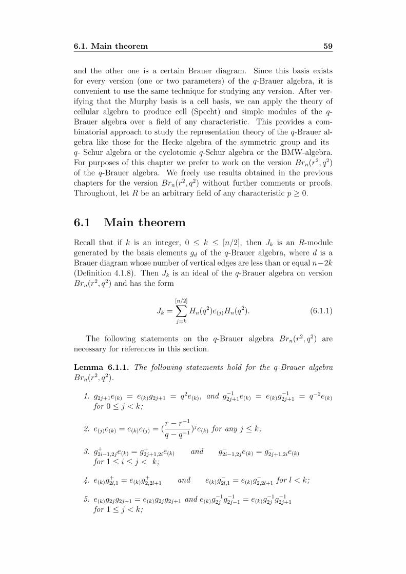
6.1. Main theorem 59
and the other one is a certain Brauer diagram. Since this basis existsfor every version (one or two parameters) of the q-Brauer algebra, it isconvenient to use the same technique for studying any version. After ver-ifying that the Murphy basis is a cell basis, we can apply the theory ofcellular algebra to produce cell (Specht) and simple modules of the q-Brauer algebra over a field of any characteristic. This provides a com-binatorial approach to study the representation theory of the q-Brauer al-gebra like those for the Hecke algebra of the symmetric group and itsq- Schur algebra or the cyclotomic q-Schur algebra or the BMW-algebra.For purposes of this chapter we prefer to work on the version Brn(r2, q2)of the q-Brauer algebra. We freely use results obtained in the previouschapters for the version Brn(r2, q2) without further comments or proofs.Throughout, let R be an arbitrary field of any characteristic p ≥ 0.
6.1 Main theorem
Recall that if k is an integer, 0 ≤ k ≤ [n/2], then Jk is an R-modulegenerated by the basis elements gd of the q-Brauer algebra, where d is aBrauer diagram whose number of vertical edges are less than or equal n−2k(Definition 4.1.8). Then Jk is an ideal of the q-Brauer algebra on versionBrn(r2, q2) and has the form
Jk =
[n/2]∑j=k
Hn(q2)e(j)Hn(q2). (6.1.1)
The following statements on the q-Brauer algebra Brn(r2, q2) arenecessary for references in this section.
Lemma 6.1.1. The following statements hold for the q-Brauer algebraBrn(r2, q2).
1. g2j+1e(k) = e(k)g2j+1 = q2e(k), and g−12j+1e(k) = e(k)g
−12j+1 = q−2e(k)
for 0 ≤ j < k;
2. e(j)e(k) = e(k)e(j) = (r − r−1
q − q−1)je(k) for any j ≤ k;
3. g+2i−1,2je(k) = g+
2j+1,2ie(k) and g−2i−1,2je(k) = g−2j+1,2ie(k)
for 1 ≤ i ≤ j < k;
4. e(k)g+2l,1 = e(k)g
+2,2l+1 and e(k)g
−2l,1 = e(k)g
−2,2l+1 for l < k;
5. e(k)g2jg2j−1 = e(k)g2jg2j+1 and e(k)g−12j g
−12j−1 = e(k)g
−12j g
−12j+1
for 1 ≤ j < k;
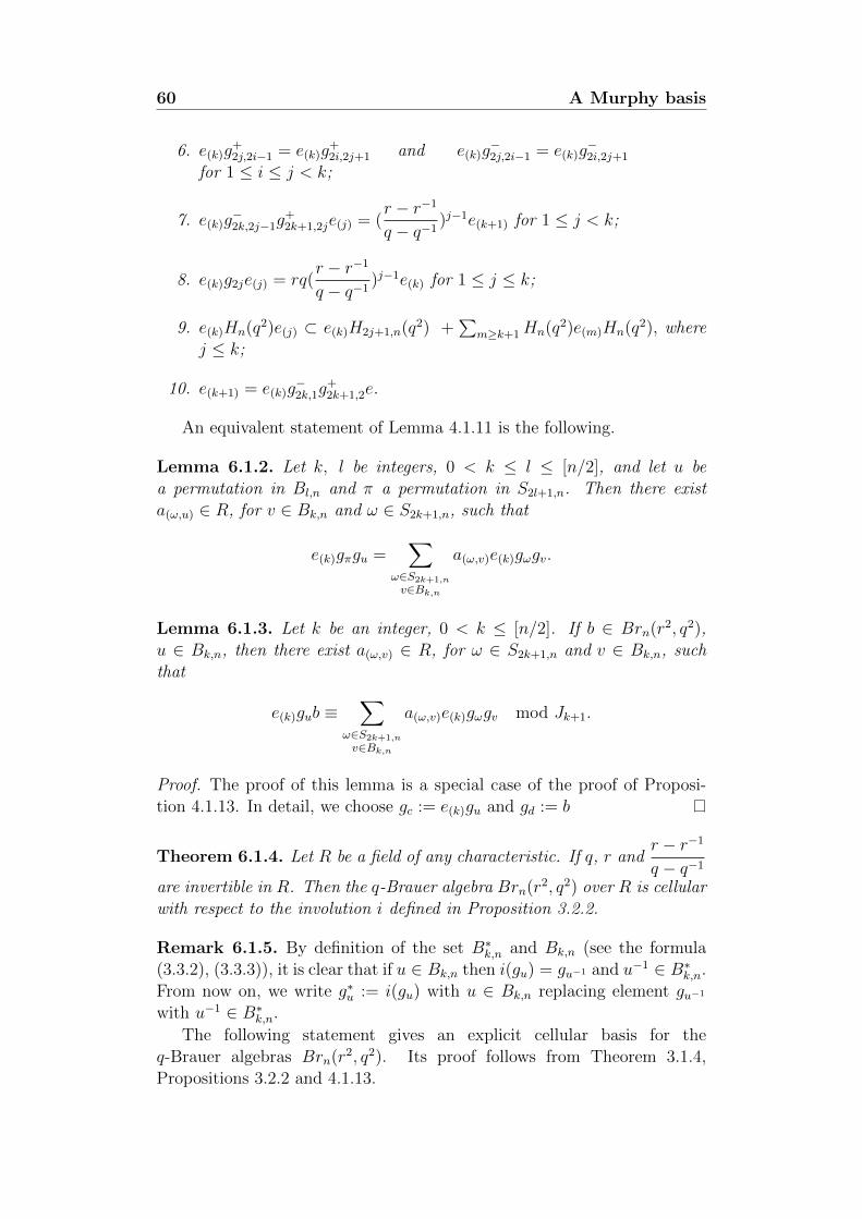
60 A Murphy basis
6. e(k)g+2j,2i−1 = e(k)g
+2i,2j+1 and e(k)g
−2j,2i−1 = e(k)g
−2i,2j+1
for 1 ≤ i ≤ j < k;
7. e(k)g−2k,2j−1g
+2k+1,2je(j) = (
r − r−1
q − q−1)j−1e(k+1) for 1 ≤ j < k;
8. e(k)g2je(j) = rq(r − r−1
q − q−1)j−1e(k) for 1 ≤ j ≤ k;
9. e(k)Hn(q2)e(j) ⊂ e(k)H2j+1,n(q2) +∑
m≥k+1Hn(q2)e(m)Hn(q2), wherej ≤ k;
10. e(k+1) = e(k)g−2k,1g
+2k+1,2e.
An equivalent statement of Lemma 4.1.11 is the following.
Lemma 6.1.2. Let k, l be integers, 0 < k ≤ l ≤ [n/2], and let u bea permutation in Bl,n and π a permutation in S2l+1,n. Then there exista(ω,u) ∈ R, for v ∈ Bk,n and ω ∈ S2k+1,n, such that
e(k)gπgu =∑
ω∈S2k+1,n
v∈Bk,n
a(ω,v)e(k)gωgv.
Lemma 6.1.3. Let k be an integer, 0 < k ≤ [n/2]. If b ∈ Brn(r2, q2),u ∈ Bk,n, then there exist a(ω,v) ∈ R, for ω ∈ S2k+1,n and v ∈ Bk,n, suchthat
e(k)gub ≡∑
ω∈S2k+1,n
v∈Bk,n
a(ω,v)e(k)gωgv mod Jk+1.
Proof. The proof of this lemma is a special case of the proof of Proposi-tion 4.1.13. In detail, we choose gc := e(k)gu and gd := b
Theorem 6.1.4. Let R be a field of any characteristic. If q, r andr − r−1
q − q−1
are invertible in R. Then the q-Brauer algebra Brn(r2, q2) over R is cellularwith respect to the involution i defined in Proposition 3.2.2.
Remark 6.1.5. By definition of the set B∗k,n and Bk,n (see the formula(3.3.2), (3.3.3)), it is clear that if u ∈ Bk,n then i(gu) = gu−1 and u−1 ∈ B∗k,n.From now on, we write g∗u := i(gu) with u ∈ Bk,n replacing element gu−1
with u−1 ∈ B∗k,n.
The following statement gives an explicit cellular basis for theq-Brauer algebras Brn(r2, q2). Its proof follows from Theorem 3.1.4,Propositions 3.2.2 and 4.1.13.
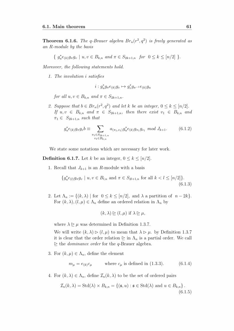
6.1. Main theorem 61
Theorem 6.1.6. The q-Brauer algebra Brn(r2, q2) is freely generated asan R-module by the basis
{ g∗ue(k)gπgv | u, v ∈ Bk,n and π ∈ S2k+1,n for 0 ≤ k ≤ [n/2] }.
Moreover, the following statements hold.
1. The involution i satisfies
i : g∗ugπe(k)gv 7→ g∗vgπ−1e(k)gu
for all u, v ∈ Bk,n and π ∈ S2k+1,n.
2. Suppose that b ∈ Brn(r2, q2) and let k be an integer, 0 ≤ k ≤ [n/2].If u, v ∈ Bk,n and π ∈ S2k+1,n, then there exist v1 ∈ Bk,n andπ1 ∈ S2k+1,n such that
g∗ue(k)gπgvb ≡∑
π1∈S2k+1,n
v1∈Bk,n
a(π1,v1)g∗ue(k)gπ1gv1 mod Jk+1. (6.1.2)
We state some notations which are necessary for later work.
Definition 6.1.7. Let k be an integer, 0 ≤ k ≤ [n/2].
1. Recall that Jk+1 is an R-module with a basis
{g∗ue(l)gπgv | u, v ∈ Bl,n and π ∈ S2l+1,n for all k < l ≤ [n/2]}.(6.1.3)
2. Let Λn := {(k, λ) | for 0 ≤ k ≤ [n/2], and λ a partition of n− 2k}.For (k, λ), (l, µ) ∈ Λn define an ordered relation in Λn by
(k, λ) � (l, µ) if λ� µ,
where λ� µ was determined in Definition 1.3.7.
We will write (k, λ) � (l, µ) to mean that λ � µ. by Definition 1.3.7it is clear that the order relation � in Λn is a partial order. We call� the dominance order for the q-Brauer algebra.
3. For (k, µ) ∈ Λn, define the element
mµ = e(k)cµ where cµ is defined in (1.3.3). (6.1.4)
4. For (k, λ) ∈ Λn, define In(k, λ) to be the set of ordered pairs
In(k, λ) = Std(λ)×Bk,n = {(s, u) : s ∈ Std(λ) and u ∈ Bk,n} .(6.1.5)
62 A Murphy basis
Example 6.1.8. Let n = 10 and µ = (3, 2, 1). The example in (1.3.2)yields the subgroup Sµ = 〈s5, s6, s8〉, and
mµ = e(2)
∑σ∈Sµ
gσ = e(2)(1 + g5)(1 + g6 + g6g5)(1 + g8).
Let Brλ
n be an R-module with spanning set{xµ(s,u)(t,v) := g∗ug
∗d(s)mµgd(t)gv
∣∣∣∣ (s, u), (t, v) ∈ In(l, µ)
µ� λ for (l, µ), (k, λ) ∈ Λn
}. (6.1.6)
Lemma 6.1.9. Suppose that (k, λ) ∈ Λn, then Jk+1 ⊆ Brλ
n and Brλ
n is anideal of the q-Brauer algebra Brn(r2, q2).
Proof. By (6.1.3) every basis element in Jk+1 is of the form g∗ue(l)gπgv whereu, v ∈ Bl,n and π ∈ S2l+1,n, k+1 ≤ l ≤ [n/2]. By the definition in Theorem1.3.14, the element gπ can be rewritten as gπ =
∑(s,t,µ) g
∗d(s)cµgd(t) with
(l, µ) ∈ Λn. Since n− 2l < n− 2k, Definition 1.3.7 of the dominance orderimplies that µ� λ. Thus,
g∗ue(l)gπgv =∑
(s,t,µ) g∗ug∗d(s)mµgd(t)gv =
∑(s,t,µ) x
µ(s,u)(t,v) ∈ Br
λ
n,
meaning Jk+1 ⊆ Brλ
n.To prove the second statement, it is sufficient to show that the product
xµ(s,u)(t,v) ·b is in Brλ
n, where xµ(s,u)(t,v) ∈ Brλ
n (with µ�λ) and b is an arbitrary
basis element of the q-Brauer algebra Brn(r2, q2). Lemma 6.1.3 implies
(e(l)gv)b ≡∑
π1∈S2l+1,n
v1∈Bl,n
a(π1,v1)e(l)gπ1gv1 mod Jl+1.
Notice that in the formula (1.3.5) of Theorem 1.3.14, we have c1t = 1cµgd(t).
We have the calculation:
xµ(s,u)(t,v) · b = (g∗ug∗d(s)mµgd(t)gv)b = (g∗ug
∗d(s)cµgd(t))(e(l)gvb)
=∑
π1∈S2l+1,n
v1∈Bl,n
a(π1,v1)g∗ug∗d(s)e(l)(1cµgd(t)gπ1)gv1 + Jl+1
(1.3.5)=
∑π1∈S2l+1,n
v1∈Bl,n
a(π1,v1)g∗ug∗d(s)e(l)(c1tgπ1)gv1 + Jl+1
(1.3.6)=
∑π1∈S2l+1,n
v1∈Bl,n
a(π1,v1)g∗ug∗d(s)e(l)(
∑t1∈Std(µ)
at1c1t1 + H µ2l+1,n)gv1 + Jl+1
(1.3.5)=
∑π1∈S2l+1,n
v1∈Bl,n
a(π1,v1)g∗ug∗d(s)e(l)(
∑t1∈Std(µ)
at1cµgd(t1) + H µ2l+1,n)gv1 + Jl+1
6.1. Main theorem 63
=∑
π1∈S2l+1,n
v1∈Bl,n
∑t1∈Std(µ)
at1a(π1,v1)(g∗ug∗d(s)e(l)cµgd(t1)gv1)
+∑
π1∈S2l+1,n
v1∈Bl,n
a(π1,v1)(g∗ug∗d(s)e(l)H
µ2l+1,ngv1) + Jl+1
(6.1.4),(1.3.4)=
∑π1∈S2l+1,n
v1∈Bl,n
∑t1∈Std(µ)
at1a(π1,v1)(g∗ug∗d(s)mµgd(t1)gv1)
+∑
π1∈S2l+1,n
v1∈Bl,n
∑µ2`n−2l, µ2�µs2,t2∈Std(µ2)
a(π1,v1)a(s2,t2)(g∗ug∗d(s2)mµ2gd(t2)gv1) + Jl+1
=∑
π1∈S2l+1,n
v1∈Bl,n
∑t1∈Std(µ)
at1a(π1,v1)(xµ(s,u)(t1,v1))
+∑
π1∈S2l+1,n
v1∈Bl,n
∑µ2`n−2l, µ2�µs2,t2∈Std(µ2)
a(π1,v1)a(s2,t2)(xµ2(s2,u)(t2,v1)) + Jl+1,
where a(π1,v1), at1 and as2,t2 are in R, and H µ2l+1,n is the ideal of H2l+1,n(q2)
defined in (1.3.4). By Lemma 6.1.9 and the assumption µ � λ (hence
l ≥ k), all elements occuring in the last formula are in Brλ
n, and hence, sois xµ(s,u)(t,v) · b.
The main result of this section is the following.
Theorem 6.1.10. The q-Brauer algebra Brn(r2, q2) is freely generated asan R–module by the collection{
xλ(s,u)(t,v) = g∗ug∗d(s)mλgd(t)gv
∣∣∣∣ (s, u), (t, v) ∈ In(k, λ), for (k, λ) ∈ Λn
}.
(6.1.7)
Moreover, the following statements hold.
1. The involution i sends xλ(s,u)(t,v) to i(xλ(s,u)(t,v)) = xλ(t,v)(s,u) for all(t, v), (s, u) ∈ In(k, λ).
2. Suppose that b ∈ Brn(r2, q2), (k, λ) ∈ Λn and (s, u), (t, v) ∈ In(k, λ).Then there exist a(t2,v2) ∈ R, (t2, v2) ∈ In(k, λ) such that
xλ(s,u)(t,v) · b ≡∑
(t2,v2)∈In(k,λ)
a(t2,v2)xλ(s,u)(t2,v2) mod Br
λ
n. (6.1.8)
64 A Murphy basis
Proof. Let b be an arbitrary element in the q-Brauer algebra Brn(r2, q2).Then by Theorem 6.1.6, b can be expressed as an R-linear combination ofbasis elements g∗ujgπje(kj)gvj ,
b =∑j
ajg∗ujgπje(kj)gvj , (6.1.9)
where (kj, λ) ∈ Λn, aj ∈ R, πj ∈ S2k+1,n, and uj, vj ∈ Bkj ,n. Using thedefinition in Theorem 1.3.14, the element gπj has an expression
gπj = g∗d(sj)cλjgd(tj)
with sj, tj ∈ Std(λj). Replace gπj in (6.1.9) by the last formula,
b =∑j
ajg∗ujg∗d(sj)
cλjgd(tj)e(kj)gvj =∑j
ajg∗ujg∗d(sj)
e(kj)cλjgd(tj)gvj
(6.1.4)=
∑j
ajg∗ujg∗d(sj)
mλjgd(tj)gvj =∑j
ajxλ(sj ,uj)(tj ,vj)
,
where (sj, uj), (tj, vj) ∈ In(kj, λj).Therefore, the set (6.1.7) linearly spans the q-Brauer algebra
Brn(r2, q2). The independence of (6.1.7) follows from the linear indepen-dences in Theorems 1.3.14 and 6.1.6.
The statement (1) is obtained by combining the involution i on theHecke algebra Hn(q2) and Lemma 6.1.1(10).
The statement (2) is shown as follows: Let (k, λ), (l, µ) ∈ Λn. As thesame arguments in the proof above, it suffices to consider the productxλ(s,u)(t,v) · b, where b = xµ(s1,u1)(t1,v1) with (s1, u1), (t1, v1) ∈ In(l, µ) is a basis
element in Brn(r2, q2). Subsequently, consider two cases with respect topartitions µ and λ.
The first case is µ B λ: Then Definition 1.3.7 of the dominance orderimplies that k ≤ l. So, by Lemma 2.2.3 we get
e(k)gvg∗u1e(l) ∈ H2k+1,n(q2)e(l) +
∑m≥l+1
Hne(m)Hn.
Hence,
(cλgd(t))(e(k)gvg∗u1e(l))(g
∗d(s1)cµ) ∈ cλgd(t)H2k+1,n(q2)e(l)g
∗d(s1)cµ +
∑m≥l+1
Hne(m)Hn
(6.1.4)
⊆ H2k+1,n(q2)g∗d(s1)mµ +∑m≥l+1
Hne(m)Hn
k≤l⊆ H2k+1,n(q2)g∗d(s1)mµ +
∑m≥k+1
Hne(m)Hn
(6.1.1)
⊆ H2k+1,n(q2)g∗d(s1)mµ + Jk+1 ⊆ Brλ
n.
6.1. Main theorem 65
Since (cλgd(t))(e(k)gvg∗u1e(l))(g
∗d(s1)cµ)
(6.1.4)= (mλgd(t)gv)(g
∗u1g∗d(s1)mµ), the last
inclusion yields
(xλ(s,u)(t,v))(xµ(s1,u1)(t1,v1)) = (g∗ug
∗d(s)mλgd(t)gv)(g
∗u1g∗d(s1)mµgd(t1)gv1)
∈ g∗ug∗d(s)Br
λ
ngd(t1)gv1 ⊆ Brλ
n.
Thus, xλ(s,u)(t,v))(xµ(s1,u1)(t1,v1)) ≡ 0 (mod Br
λ
n), namely,
xλ(s,u)(t,v) · b ≡ 0 (mod Brλ
n).
The second case is λ D µ, that is l ≤ k: Using Lemma 6.1.1(9), it yields
e(k)gvg∗u1e(l) ∈ e(k)H2l+1,n +
∑m≥k+1
Hne(m)Hn.
Applying Lemma 6.1.1(9) and the same arguments as in the previous caseimplies that
(cλgd(t))(e(k)gvg∗u1e(l))(g
∗d(s1)cµ) = (mλgd(t)gv)(g
∗u1g∗d(s1)mµ)
∈ cλgd(t)e(k)H2l+1,ng∗d(s1)cµ +
∑m≥k+1
Hne(m)Hn
(6.1.1),(6.1.4)
⊆ mλH2l+1,n + Jk+1 ⊆ mλH2l+1,n + Brλ
n (by Lemma 6.1.9).
Hence,
xλ(s,u)(t,v) · b = (g∗ug∗d(s)mλgd(t)gv)(g
∗u1g∗d(s1)mµgd(t1)gv1)
∈ g∗ug∗d(s)mλH2l+1,ngd(t1)gv1 + Brλ
n
⊆ g∗ug∗d(s)mλH2l+1,ngv1 + Br
λ
n.
It implies that xλ(s,u)(t,v) · b can be rewritten as an R-linear combination
xλ(s,u)(t,v) · b = g∗ug∗d(s)mλ
( ∑π1∈S2l+1,n
aπ1gπ1)gv1 + Br
λ
n
(6.1.4)= g∗ug
∗d(s)cλ
( ∑π1∈S2l+1,n
aπ1e(k)gπ1gv1)
+ Brλ
n
Lem6.1.2= g∗ug
∗d(s)cλ
( ∑π1∈S2l+1,n
aπ1(∑
ωπ1∈S2k+1,n
vπ1∈Bk,n
a(ωπ1 ,vπ1 )e(k)gωπ1gvπ1 ))
+ Brλ
n
=∑
π1∈S2l+1,n
aπ1(∑
ωπ1∈S2k+1,n
vπ1∈Bk,n
a(ωπ1 ,vπ1 )g∗ug∗d(s)e(k)(cλgωπ1 )gvπ1 ) + Br
λ
n
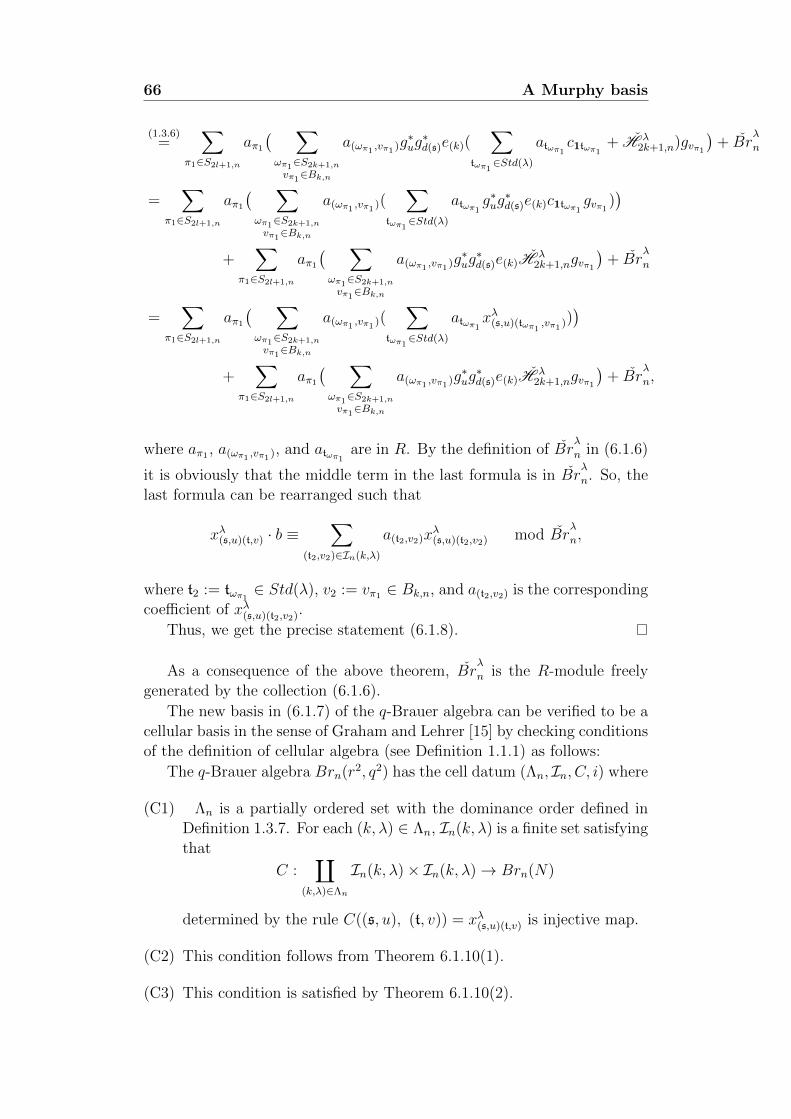
66 A Murphy basis
(1.3.6)=
∑π1∈S2l+1,n
aπ1( ∑ωπ1∈S2k+1,n
vπ1∈Bk,n
a(ωπ1 ,vπ1 )g∗ug∗d(s)e(k)(
∑tωπ1∈Std(λ)
atωπ1 c1tωπ1 + H λ2k+1,n)gvπ1
)+ Br
λ
n
=∑
π1∈S2l+1,n
aπ1( ∑ωπ1∈S2k+1,n
vπ1∈Bk,n
a(ωπ1 ,vπ1 )(∑
tωπ1∈Std(λ)
atωπ1 g∗ug∗d(s)e(k)c1tωπ1 gvπ1 )
)+
∑π1∈S2l+1,n
aπ1( ∑ωπ1∈S2k+1,n
vπ1∈Bk,n
a(ωπ1 ,vπ1 )g∗ug∗d(s)e(k)H
λ2k+1,ngvπ1
)+ Br
λ
n
=∑
π1∈S2l+1,n
aπ1( ∑ωπ1∈S2k+1,n
vπ1∈Bk,n
a(ωπ1 ,vπ1 )(∑
tωπ1∈Std(λ)
atωπ1xλ(s,u)(tωπ1 ,vπ1 ))
)+
∑π1∈S2l+1,n
aπ1( ∑ωπ1∈S2k+1,n
vπ1∈Bk,n
a(ωπ1 ,vπ1 )g∗ug∗d(s)e(k)H
λ2k+1,ngvπ1
)+ Br
λ
n,
where aπ1 , a(ωπ1 ,vπ1 ), and atωπ1 are in R. By the definition of Brλ
n in (6.1.6)
it is obviously that the middle term in the last formula is in Brλ
n. So, thelast formula can be rearranged such that
xλ(s,u)(t,v) · b ≡∑
(t2,v2)∈In(k,λ)
a(t2,v2)xλ(s,u)(t2,v2) mod Br
λ
n,
where t2 := tωπ1 ∈ Std(λ), v2 := vπ1 ∈ Bk,n, and a(t2,v2) is the correspondingcoefficient of xλ(s,u)(t2,v2).
Thus, we get the precise statement (6.1.8).
As a consequence of the above theorem, Brλ
n is the R-module freelygenerated by the collection (6.1.6).
The new basis in (6.1.7) of the q-Brauer algebra can be verified to be acellular basis in the sense of Graham and Lehrer [15] by checking conditionsof the definition of cellular algebra (see Definition 1.1.1) as follows:
The q-Brauer algebra Brn(r2, q2) has the cell datum (Λn, In, C, i) where
(C1) Λn is a partially ordered set with the dominance order defined inDefinition 1.3.7. For each (k, λ) ∈ Λn, In(k, λ) is a finite set satisfyingthat
C :∐
(k,λ)∈Λn
In(k, λ)× In(k, λ)→ Brn(N)
determined by the rule C((s, u), (t, v)) = xλ(s,u)(t,v) is injective map.
(C2) This condition follows from Theorem 6.1.10(1).
(C3) This condition is satisfied by Theorem 6.1.10(2).
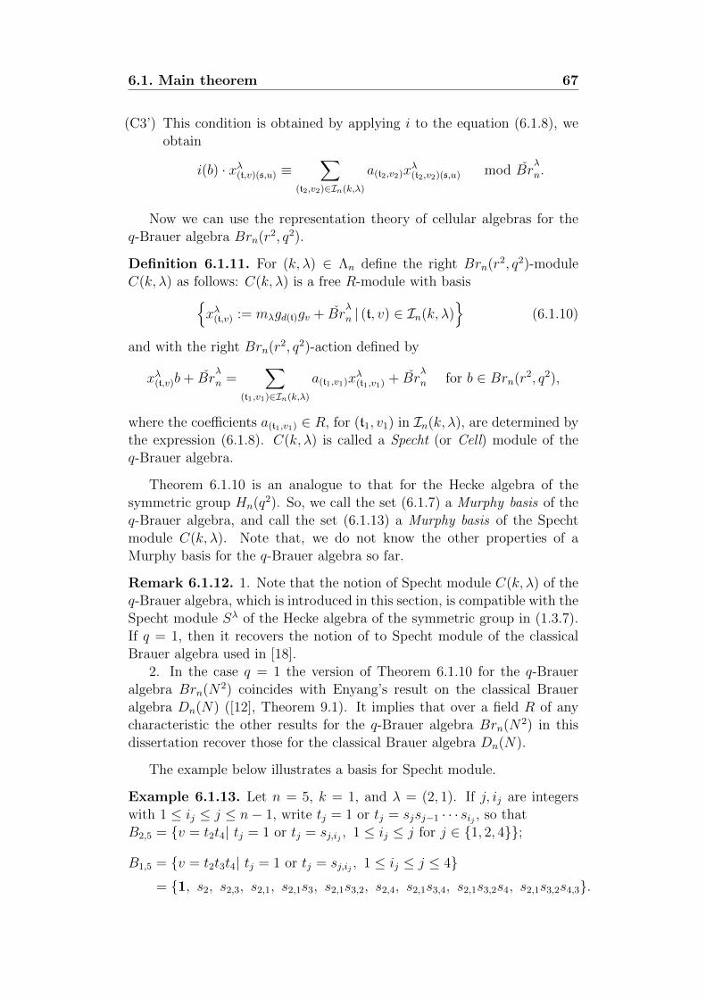
6.1. Main theorem 67
(C3’) This condition is obtained by applying i to the equation (6.1.8), weobtain
i(b) · xλ(t,v)(s,u) ≡∑
(t2,v2)∈In(k,λ)
a(t2,v2)xλ(t2,v2)(s,u) mod Br
λ
n.
Now we can use the representation theory of cellular algebras for theq-Brauer algebra Brn(r2, q2).
Definition 6.1.11. For (k, λ) ∈ Λn define the right Brn(r2, q2)-moduleC(k, λ) as follows: C(k, λ) is a free R-module with basis{
xλ(t,v) := mλgd(t)gv + Brλ
n | (t, v) ∈ In(k, λ)}
(6.1.10)
and with the right Brn(r2, q2)-action defined by
xλ(t,v)b+ Brλ
n =∑
(t1,v1)∈In(k,λ)
a(t1,v1)xλ(t1,v1) + Br
λ
n for b ∈ Brn(r2, q2),
where the coefficients a(t1,v1) ∈ R, for (t1, v1) in In(k, λ), are determined bythe expression (6.1.8). C(k, λ) is called a Specht (or Cell) module of theq-Brauer algebra.
Theorem 6.1.10 is an analogue to that for the Hecke algebra of thesymmetric group Hn(q2). So, we call the set (6.1.7) a Murphy basis of theq-Brauer algebra, and call the set (6.1.13) a Murphy basis of the Spechtmodule C(k, λ). Note that, we do not know the other properties of aMurphy basis for the q-Brauer algebra so far.
Remark 6.1.12. 1. Note that the notion of Specht module C(k, λ) of theq-Brauer algebra, which is introduced in this section, is compatible with theSpecht module Sλ of the Hecke algebra of the symmetric group in (1.3.7).If q = 1, then it recovers the notion of to Specht module of the classicalBrauer algebra used in [18].
2. In the case q = 1 the version of Theorem 6.1.10 for the q-Braueralgebra Brn(N2) coincides with Enyang’s result on the classical Braueralgebra Dn(N) ([12], Theorem 9.1). It implies that over a field R of anycharacteristic the other results for the q-Brauer algebra Brn(N2) in thisdissertation recover those for the classical Brauer algebra Dn(N).
The example below illustrates a basis for Specht module.
Example 6.1.13. Let n = 5, k = 1, and λ = (2, 1). If j, ij are integerswith 1 ≤ ij ≤ j ≤ n− 1, write tj = 1 or tj = sjsj−1 · · · sij , so thatB2,5 = {v = t2t4| tj = 1 or tj = sj,ij , 1 ≤ ij ≤ j for j ∈ {1, 2, 4}};
B1,5 = {v = t2t3t4| tj = 1 or tj = sj,ij , 1 ≤ ij ≤ j ≤ 4}= {1, s2, s2,3, s2,1, s2,1s3, s2,1s3,2, s2,4, s2,1s3,4, s2,1s3,2s4, s2,1s3,2s4,3}.
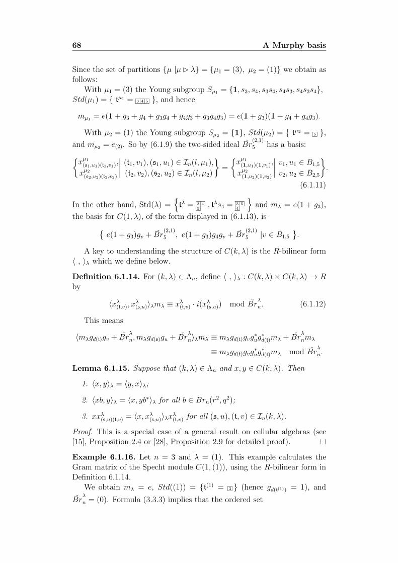
68 A Murphy basis
Since the set of partitions {µ |µ� λ} = {µ1 = (3), µ2 = (1)} we obtain asfollows:
With µ1 = (3) the Young subgroup Sµ1 = {1, s3, s4, s3s4, s4s3, s4s3s4},Std(µ1) = { tµ1 = 3 4 5 }, and hence
mµ1 = e(1 + g3 + g4 + g3g4 + g4g3 + g3g4g3) = e(1 + g3)(1 + g4 + g4g3).
With µ2 = (1) the Young subgroup Sµ2 = {1}, Std(µ2) = { tµ2 = 5 },and mµ2 = e(2). So by (6.1.9) the two-sided ideal Br
(2,1)
5 has a basis:{xµ1(s1,u1)(t1,v1),
xµ2(s2,u2)(t2,v2)
∣∣∣∣ (t1, v1), (s1, u1) ∈ In(l, µ1),
(t2, v2), (s2, u2) ∈ In(l, µ2)
}=
{xµ1(1,u1)(1,v1),
xµ2(1,u2)(1,v2)
∣∣∣∣ v1, u1 ∈ B1,5
v2, u2 ∈ B2,5
}.
(6.1.11)
In the other hand, Std(λ) ={tλ = 3 4
5, tλs4 = 3 5
4
}and mλ = e(1 + g3),
the basis for C(1, λ), of the form displayed in (6.1.13), is{e(1 + g3)gv + Br
(2,1)
5 , e(1 + g3)g4gv + Br(2,1)
5 |v ∈ B1,5
}.
A key to understanding the structure of C(k, λ) is the R-bilinear form〈 , 〉λ which we define below.
Definition 6.1.14. For (k, λ) ∈ Λn, define 〈 , 〉λ : C(k, λ) × C(k, λ) → Rby
〈xλ(t,v), xλ(s,u)〉λmλ ≡ xλ(t,v) · i(xλ(s,u)) mod Br
λ
n. (6.1.12)
This means
〈mλgd(t)gv + Brλ
n,mλgd(s)gu + Brλ
n〉λmλ ≡ mλgd(t)gvg∗ug∗d(t)mλ + Br
λ
nmλ
≡ mλgd(t)gvg∗ug∗d(t)mλ mod Br
λ
n.
Lemma 6.1.15. Suppose that (k, λ) ∈ Λn and x, y ∈ C(k, λ). Then
1. 〈x, y〉λ = 〈y, x〉λ;
2. 〈xb, y〉λ = 〈x, yb∗〉λ for all b ∈ Brn(r2, q2);
3. xxλ(s,u)(t,v) = 〈x, xλ(s,u)〉λxλ(t,v) for all (s, u), (t, v) ∈ In(k, λ).
Proof. This is a special case of a general result on cellular algebras (see[15], Proposition 2.4 or [28], Proposition 2.9 for detailed proof).
Example 6.1.16. Let n = 3 and λ = (1). This example calculates theGram matrix of the Specht module C(1, (1)), using the R-bilinear form inDefinition 6.1.14.
We obtain mλ = e, Std((1)) = {t(1) = 3 } (hence gd(t(1)) = 1), and
Brλ
n = (0). Formula (3.3.3) implies that the ordered set
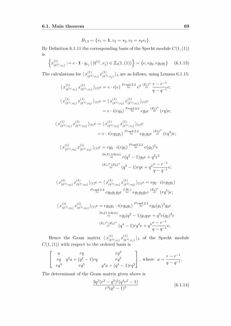
6.1. Main theorem 69
B1,3 = {v1 = 1, v2 = s2, v3 = s2s1}.
By Definition 6.1.11 the corresponding basis of the Specht module C(1, (1))is {
x(1)
(t(1),vj):= e · 1 · gvj | (t(1), vj) ∈ I3(1, (1))
}= {e, eg2, eg2g1} (6.1.13)
The calculations for 〈x(1)
(t(1),vi)x
(1)
(t(1),vj)〉λ are as follows, using Lemma 6.1.15:
〈x(1)
(t(1),v1)x
(1)
(t(1),v1)〉(1)e = e · i(e) Prop3.2.2
= e2 (E1)′′
=r − r−1
q − q−1e;
〈x(1)
(t(1),v1)x
(1)
(t(1),v2)〉(1)e = 〈x(1)
(t(1),v2)x
(1)
(t(1),v1)〉(1)e
= e · i(eg2)Prop3.2.2
= eg2e(E2)′′
= (rq)e;
〈x(1)
(t(1),v1)x
(1)
(t(1),v3)〉(1)e = 〈x(1)
(t(1),v3)x
(1)
(t(1),v1)〉(1)e
= e · i(eg2g1)Prop3.2.2
= eg1g2e(E2)′′
= (rq3)e;
〈x(1)
(t(1),v2)x
(1)
(t(1),v2)〉(1)e = eg2 · i(eg2)
Prop3.2.2= e(g2)2e
Def1.3.9(iii)= e(q2 − 1)g2e+ q2e2
(E1)′′,(E2)′′
= (q2 − 1)rqe+ q2 r − r−1
q − q−1e;
〈x(1)
(t(1),v2)x
(1)
(t(1),v3)〉(1)e = 〈x(1)
(t(1),v3)x
(1)
(t(1),v2)〉(1)e = eg2 · i(eg2g1)
Prop3.2.2= eg2g1g2e
((H1)= eg1g2g1e
(E2)′′
= (rq5)e;
〈x(1)
(t(1),v3)x
(1)
(t(1),v3)〉(1)e = eg2g1 · i(eg2g1)
Prop3.2.2= eg2(g1)2g2e
Def1.3.9(iii)= eg2(q2 − 1)g1g2e+ q2e(g2)2e
(E1)′′,(E2)′′
= (q4 − 1)rq3e+ q4 r − r−1
q − q−1e;
Hence the Gram matrix 〈x(1)
(t(1),vi)x
(1)
(t(1),vj)〉λ of the Specht module
C(1, (1)) with respect to the ordered basis is a rq rq3
rq q2a+ (q2 − 1)rq rq5
rq3 rq5 q4a+ (q4 − 1)rq3
, where a =r − r−1
q − q−1.
The determinant of the Gram matrix given above is
3q5(r2 − q2)2(q4r2 − 1)
r3(q2 − 1)3(6.1.14)
70 A Murphy basis
6.2 Representation theory over a field
Using a Murphy basis of Specht modules C(k, λ), we have defined the newR-bilinear form, 〈 , 〉λ, for the q-Brauer algebra. This bilinear form differsfrom the one given in Definition 4.2.6. In detail, instead of determining thebilinear form via the known bilinear forms, including two bilinear forms ofboth the Hecke algebra and the iterated inflation’s algebra, 〈 , 〉λ is directlydefined using a Murphy basis of Specht modules. This enables us to giveexplicit calculations in the proof of Theorem 6.2.1.
Using the general theory of cellular algebras we obtain some resultsabout the representation theory of q-Brauer algebras.
Denote rad(C(k, λ)) = {x ∈ C(k, λ)| 〈x, y〉λ = 0 for all y ∈ C(k, λ)}and D(k, λ) = C(k, λ)/rad(C(k, λ)).
The following are special cases of results in [15].Statement 1. For (k, λ) ∈ Λn, r, q and (r − r−1)/(q − q−1) invertible
elements in an arbitrary field R, let Brn(r2, q2) be the q-Brauer algebraover R. Then
1. rad(C(k, λ)) is a Brn(r2, q2)-submodule of C(k, λ);
2. If D(k, λ) 6= 0 then
(a) D(k, λ) is simple;
(b) rad(C(k, λ)) is the radical of the Brn(r2, q2)-module C(k, λ).
Statement 2. For (k, λ), (l, µ) ∈ Λn, let Brn(r2, q2) be a q-Braueralgebra over an arbitrary field R. Suppose M is a Brn(r2, q2)-submoduleof C(k, λ) and
ϕ : C(l, µ) −→ C(k, λ)/M
is a Brn(r2, q2)-module homomorphism, and 〈, 〉µ 6= 0. Then
1. ϕ 6= 0 only if λ� µ.
2. If λ = µ, then there are elements r0 6= 0 and r1 in R such that for allx ∈ C(l, µ), we have r0ϕ(x) = r1x+M .
For (k, λ), (l, µ) ∈ Λn and D(l, µ) 6= 0, let dλµ = [C(k, λ) : D(l, µ)] bethe composition multiplicity of D(l, µ) in C(k, λ).
The next statement gives a classification of the simple modules, up toisomorphism, of the q-Brauer algebra. This result is an analogue to thatfor the Hecke algebra due to Dipper and James (see [7], Theorem 7.6).
Theorem 6.2.1. For (k, λ) ∈ Λn, r, q and (r − r−1)/(q − q−1) invertibleelements in an arbitrary field R, let Brn(r2, q2) be a q-Brauer algebra overR. Then
6.2. Representation theory over a field 71
1. The set {D(l, µ)| (l, µ) ∈ Λn, µ is an e(q2)-restricted partition} is acomplete set of pairwise non-isomorphic simple Brn(r2, q2)-modules.
2. For (k, λ), (l, µ) ∈ Λn, suppose that µ is an e(q2)-restricted partition.Then dµµ = 1 and dλµ 6= 0 only if λ� µ.
Proof. (1). Since the q-Brauer algebra is a cellular algebra, it follows fromTheorem 3.4 in [15] that the set
{D(l, µ)| D(l, µ) 6= 0 for partition µ of n− 2l, 0 ≤ l ≤ [n/2]}
is a complete set of pairwise non-isomorphic simple Brn(r2, q2)-modules.The remainder of proof is to show that D(l, µ) 6= 0 if and only if µ ise(q2)-restricted partition of n− 2l.
Indeed, pick two non-zero elements xµ(s,u) = mµgd(s)gu + Brµ
n and
xµ(t,v) = mµgtgv+ Brµ
n in C(l, µ) with arbitrary pairs (s, u), (t, v) ∈ In(l, µ).This yields, using (6.1.12),
〈xµ(s,u), xµ(t,v)〉µmµ = 〈mµgd(s)gu + Br
µ
n, mµgd(t)gv + Brµ
n〉µmµ (6.2.1)
(6.1.12)≡ mµgd(s)gvg
∗ug∗d(t)mµ mod Br
µ
n
(6.1.4)≡ e(l)(cµgd(s))gvg
∗u(g∗d(t)cµ)e(l) mod Br
µ
n
(1.3.5)≡ e(l)(c1sgv)(g
∗uct1)e(l) mod Br
µ
n
(1.3.6)≡ e(l)(
∑s1∈Std(µ)
as1c1s1 + H µ2l+1,n)(
∑t1∈Std(µ)
at1ct11 + H µ2l+1,n)e(l) mod Br
µ
n
(1.3.7)≡ e(l)(
∑s1∈Std(µ)
as1cs1)(∑
t1∈Std(µ)
at1c∗t1
)e(l) mod Brµ
n
≡ e(l)
∑s1,t1∈Std(µ)
as1at1(cs1c∗t1
)e(l) mod Brµ
n
(1.3.9)≡ e(l)
∑s1,t1∈Std(µ)
as1at1(〈cs1 , ct1〉cµ + H µ2l+1,n)e(l) mod Br
µ
n
(6.1.4),Lem6.1.1(2)≡
∑s1,t1∈Std(µ)
(r − r−1
q − q−1
)las1at1〈cs1 , ct1〉mµ mod Br
µ
n
where as1 , at1 are coefficients in R.Then, using Theorem 1.3.15(1) if µ is an e(q2)-restricted partition of
n − 2l then Dµ 6= 0. The definition of Dµ implies that there exists, t ∈ Std(µ) such that 〈cs, ct〉 6= 0. Now fixing xµ(s,1) = mµgd(s) +Br
µ
n and
xµ(t,1) = mµgd(t) + Brµ
n the previous calculation yields
〈xµ(s,1), xµ(t,1)〉µmµ ≡
(r − r−1
q − q−1
)l〈cs, ct〉mµ mod Brµ
n.
72 A Murphy basis
It implies 〈x, y〉µ =(r − r−1
q − q−1
)l〈cs, ct〉 6= 0, that is D(l, µ) 6= 0.
Conversely, if µ is not e(q2)-restricted then by Theorem 1.3.15(1) the R-bilinear form 〈 , 〉 on the Specht module Sµ of the Hecke algebra H2k+1,n(q2)is zero. This means that 〈cs1 , ct1〉 = 0 for any cs1 , ct1 ∈ Sµ. By calculationin (6.2.1) it implies 〈xµ(s,u), x
µ(t,v)〉µ = 0 for all xµ(s,u), x
µ(t,v) ∈ C(l, µ), namely,
D(l, µ) = 0.
(2). The second statement follows by applying the general theory ofcellular algebra and Proposition 3.6 [15].
Corollary 6.2.2. For (k, λ) ∈ Λn, r, q and (r − r−1)/(q − q−1) invertibleelements in an arbitrary field R, let Brn(r2, q2) be a q-Brauer algebra overR. The following statements are equivalent.
1. Brn(r2, q2) is semisimple;
2. C(k, λ) = D(k, λ) for all (k, λ) ∈ Λn;
3. The R-bilinear form 〈 , 〉λ (cf. (6.1.12)) is non-degenerate for all(k, λ) ∈ Λn.
Remark 6.2.3. The same results as Theorem 6.2.1 and Corollary 6.2.2hold true for the version Brn(N2) of the q-Brauer algebra. Furthermore,when q = 1 then the result in Theorem 6.2.1 recovers that for the classicalBrauer algebra Dn(N) with non-zero parameter which was shown in [15],Theorem 4.17 by Graham and Lehrer. Also notice that in this case theSpecht module of the classical Brauer algebra in [15] is dual to the one inthis chapter.
6.3 Is the q-Brauer algebra generically iso-
morphic with the BMW-algebra?
This section starts by proving a semisimplicity criterion for the q-Braueralgebra in the case n = {2, 3}. The statements are the following.
Proposition 6.3.1. Let Brn(r2, q2) be the q-Brauer algebra over R with
invertible elements r, q andr − r−1
q − q−1∈ R. Then
1. Br2(r2, q2) is semisimple if and only if e(q2) > 2.
2. Br3(r2, q2) is semisimple if and only if e(q2) > 3 and
3q5(r2 − q2)2(q4r2 − 1)
r3(q2 − 1)36= 0.
6.3. Is the q-Brauer algebra generically isomorphic with theBMW-algebra? 73
Proof. If n = 2 and λ is a partition of 2, then the cell modules C(0, λ)coincide with the cell modules Sλ of the Hecke algebra H2, and it hence〈 , 〉 ≡ 〈 , 〉λ. Therefore, by Corollary 1.3.16, the R-bilinear form 〈 , 〉 is
non-degenerate if and only if e(q2) > 2. If λ = ∅, then Brλ
2 ≡ H λ2 = R
and mλ = e. As shown in (6.1.13), the cell module C(1, λ) has a basis
{ egv + Brλ
2 | v ∈ B1,2 = {1} } = {e}.
The Gram determinant with respect to this basis is
〈e , e〉λe = e2 (E1)′′
=r − r−1
q − q−1e, that is, 〈e , e〉λ =
r − r−1
q − q−1.
With n = 3 and λ a partition of 3, using the same argument as above yieldsthat the R-bilinear form 〈 , 〉λ is non-degenerate if and only if e(q2) > 3.Otherwise, if n = 3 and λ = (1), then applying Example (6.1.16) the Gramdeterminant on C(1, λ) is non-zero if and only if
3q5(r2 − q2)2(q4r2 − 1)
r3(q2 − 1)36= 0.
Hence, we get the statement (2) by using Corollary 6.2.2.
When replacing the version Brn(r2, q2) by Brn(N2) or Brn(r, q), thenthe statements are the following.
Proposition 6.3.2. Let Brn(r, q) be the q-Brauer algebra over R with
invertible elements r, q andr − 1
q − 1∈ R. Then
1. Br2(r, q) is semisimple if and only if e(q) > 2.
2. Br3(r, q) is semisimple if and only if e(q) > 3 and
3q(r − q)2(q2r − 1)
(q − 1)36= 0.
The proof is similar to the one above.
Proposition 6.3.3. Let N ∈ Z\{0}. Let Brn(N2) be the q-Brauer algebraover R with 0 6= q, [N2] ∈ R. Then
1. Br2(N) is semisimple if and only if e(q) > 2.
2. Br3(N) is semisimple if and only if e(q) > 3 and
3q4(qN − q[N ])([N ] + qN+1 + qN+3) 6= 0.
The proof uses the same arguments as in Proposition 6.3.1.
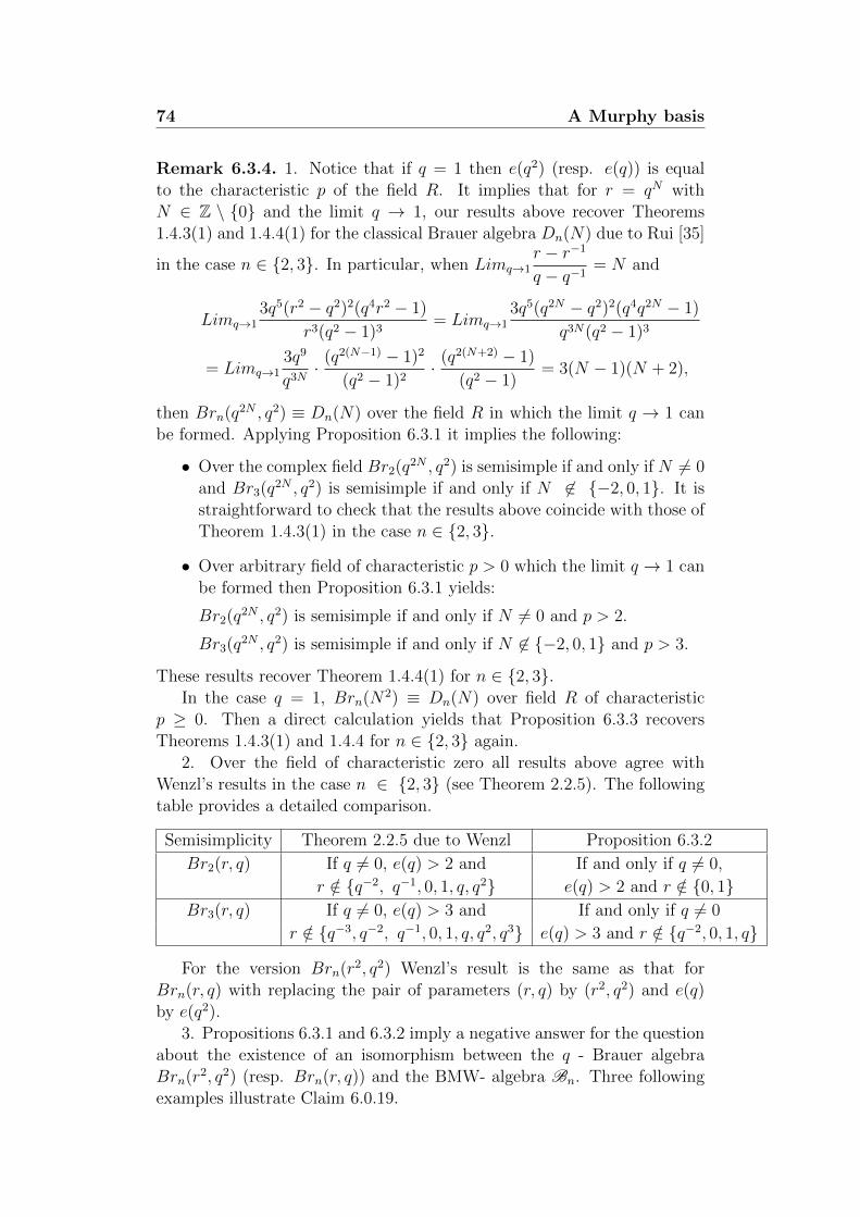
74 A Murphy basis
Remark 6.3.4. 1. Notice that if q = 1 then e(q2) (resp. e(q)) is equalto the characteristic p of the field R. It implies that for r = qN withN ∈ Z \ {0} and the limit q → 1, our results above recover Theorems1.4.3(1) and 1.4.4(1) for the classical Brauer algebra Dn(N) due to Rui [35]
in the case n ∈ {2, 3}. In particular, when Limq→1r − r−1
q − q−1= N and
Limq→13q5(r2 − q2)2(q4r2 − 1)
r3(q2 − 1)3= Limq→1
3q5(q2N − q2)2(q4q2N − 1)
q3N(q2 − 1)3
= Limq→13q9
q3N· (q2(N−1) − 1)2
(q2 − 1)2· (q2(N+2) − 1)
(q2 − 1)= 3(N − 1)(N + 2),
then Brn(q2N , q2) ≡ Dn(N) over the field R in which the limit q → 1 canbe formed. Applying Proposition 6.3.1 it implies the following:
• Over the complex field Br2(q2N , q2) is semisimple if and only if N 6= 0and Br3(q2N , q2) is semisimple if and only if N 6∈ {−2, 0, 1}. It isstraightforward to check that the results above coincide with those ofTheorem 1.4.3(1) in the case n ∈ {2, 3}.
• Over arbitrary field of characteristic p > 0 which the limit q → 1 canbe formed then Proposition 6.3.1 yields:
Br2(q2N , q2) is semisimple if and only if N 6= 0 and p > 2.
Br3(q2N , q2) is semisimple if and only if N 6∈ {−2, 0, 1} and p > 3.
These results recover Theorem 1.4.4(1) for n ∈ {2, 3}.In the case q = 1, Brn(N2) ≡ Dn(N) over field R of characteristic
p ≥ 0. Then a direct calculation yields that Proposition 6.3.3 recoversTheorems 1.4.3(1) and 1.4.4 for n ∈ {2, 3} again.
2. Over the field of characteristic zero all results above agree withWenzl’s results in the case n ∈ {2, 3} (see Theorem 2.2.5). The followingtable provides a detailed comparison.
Semisimplicity Theorem 2.2.5 due to Wenzl Proposition 6.3.2
Br2(r, q) If q 6= 0, e(q) > 2 and If and only if q 6= 0,
r /∈ {q−2, q−1, 0, 1, q, q2} e(q) > 2 and r /∈ {0, 1}Br3(r, q) If q 6= 0, e(q) > 3 and If and only if q 6= 0
r /∈ {q−3, q−2, q−1, 0, 1, q, q2, q3} e(q) > 3 and r /∈ {q−2, 0, 1, q}
For the version Brn(r2, q2) Wenzl’s result is the same as that forBrn(r, q) with replacing the pair of parameters (r, q) by (r2, q2) and e(q)by e(q2).
3. Propositions 6.3.1 and 6.3.2 imply a negative answer for the questionabout the existence of an isomorphism between the q - Brauer algebraBrn(r2, q2) (resp. Brn(r, q)) and the BMW- algebra Bn. Three followingexamples illustrate Claim 6.0.19.
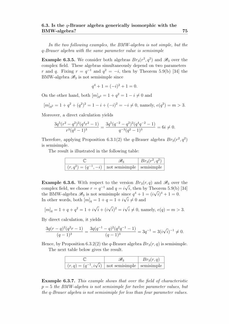
6.3. Is the q-Brauer algebra generically isomorphic with theBMW-algebra? 75
In the two following examples, the BMW-algebra is not simple, but theq-Brauer algebra with the same parameter value is semisimple
Example 6.3.5. We consider both algebras Br3(r2, q2) and B3 over thecomplex field. These algebras simultaneously depend on two parametersr and q. Fixing r = q−1 and q2 = −i, then by Theorem 5.9(b) [34] theBMW-algebra B3 is not semisimple since
q4 + 1 = (−i)2 + 1 = 0.
On the other hand, both [m]q2 = 1 + q2 = 1− i 6= 0 and
[m]q2 = 1 + q2 + (q2)2 = 1− i+ (−i)2 = −i 6= 0, namely, e(q2) = m > 3.
Moreover, a direct calculation yields
3q5(r2 − q2)2(q4r2 − 1)
r3(q2 − 1)3=
3q5(q−2 − q2)2(q4q−2 − 1)
q−3(q2 − 1)3= 6i 6= 0.
Therefore, applying Proposition 6.3.1(2) the q-Brauer algebra Br3(r2, q2)is semisimple.
The result is illustrated in the following table:
C B3 Br3(r2, q2)
(r, q2) = (q−1,−i) not semisimple semisimple
Example 6.3.6. With respect to the version Br3(r, q) and B3 over thecomplex field, we choose r = q−1 and q = i
√i, then by Theorem 5.9(b) [34]
the BMW-algebra B3 is not semisimple since q4 + 1 = (i√i)4 + 1 = 0.
In other words, both [m]q = 1 + q = 1 + i√i 6= 0 and
[m]q = 1 + q + q2 = 1 + i√i+ (i
√i)2 = i
√i 6= 0, namely, e(q) = m > 3.
By direct calculation, it yields
3q(r − q)2(q2r − 1)
(q − 1)3=
3q(q−1 − q)2(q2q−1 − 1)
(q − 1)3= 3q−1 = 3(i
√i)−1 6= 0.
Hence, by Proposition 6.3.2(2) the q-Brauer algebra Br3(r, q) is semisimple.The next table below gives the result.
C B3 Br3(r, q)
(r, q) = (q−1, i√i) not semisimple semisimple
Example 6.3.7. This example shows that over the field of characteristicp = 5 the BMW-algebra is not semisimple for twelve parameter values, butthe q-Brauer algebra is not semisimiple for less than four parameter values.
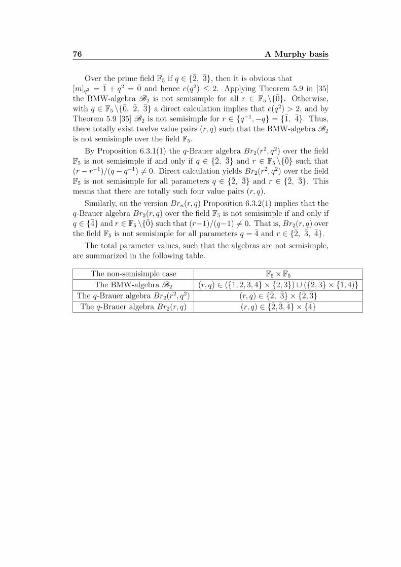
76 A Murphy basis
Over the prime field F5 if q ∈ {2, 3}, then it is obvious that[m]q2 = 1 + q2 = 0 and hence e(q2) ≤ 2. Applying Theorem 5.9 in [35]the BMW-algebra B2 is not semisimple for all r ∈ F5 \{0}. Otherwise,with q ∈ F5 \{0, 2, 3} a direct calculation implies that e(q2) > 2, and byTheorem 5.9 [35] B2 is not semisimple for r ∈ {q−1,−q} = {1, 4}. Thus,there totally exist twelve value pairs (r, q) such that the BMW-algebra B2
is not semisimple over the field F5.
By Proposition 6.3.1(1) the q-Brauer algebra Br2(r2, q2) over the fieldF5 is not semisimple if and only if q ∈ {2, 3} and r ∈ F5 \{0} such that(r− r−1)/(q − q−1) 6= 0. Direct calculation yields Br2(r2, q2) over the fieldF5 is not semisimple for all parameters q ∈ {2, 3} and r ∈ {2, 3}. Thismeans that there are totally such four value pairs (r, q).
Similarly, on the version Brn(r, q) Proposition 6.3.2(1) implies that theq-Brauer algebra Br2(r, q) over the field F5 is not semisimple if and only ifq ∈ {4} and r ∈ F5 \{0} such that (r−1)/(q−1) 6= 0. That is, Br2(r, q) overthe field F5 is not semisimple for all parameters q = 4 and r ∈ {2, 3, 4}.
The total parameter values, such that the algebras are not semisimple,are summarized in the following table.
The non-semisimple case F5×F5
The BMW-algebra B2 (r, q) ∈ ({1, 2, 3, 4} × {2, 3}) ∪ ({2, 3} × {1, 4)}The q-Brauer algebra Br2(r2, q2) (r, q) ∈ {2, 3} × {2, 3}The q-Brauer algebra Br2(r, q) (r, q) ∈ {2, 3, 4} × {4}
Chapter 7
The cellularly stratified
structure of the q-Brauer
algebra
We consider the version Brn(N) of q-Brauer algebra. Throughout, let Rbe an arbitrary field of any characteristic. Assume moreover that q and[N ] are invertible in R.
7.1 The main result
An iterated inflation
In this section we are going to construct another iterated inflation forthe q-Brauer algebra Brn(N). This new iterated inflation enables us toassert that the q-Brauer algebra is cellularly stratified. The main reasonfor this construction is that: In [19], the cellularly stratified structure justappears on ’diagram algebras’. These algebras have a basis which can berepresented by certain diagrams. In particular, diagram algebras in [19]which are shown to be cellularly stratified include Brauer algebras, BMW-algebras and Partition algebras. In their proofs the conditions (E) and (I)in Definition 1.2.1 are easily verified since multiplying two diagrams e(l)
and e(k) is essentially concatenation. In the case of the q-Brauer algebra,we do not know if the q- Brauer algebra is a diagram algebra. That is,it is not known if there exists a basis represented by certain diagrams forthe q-Brauer algebra. So, the iterated inflation for the q-Brauer algebrain Chapter 4, defined by certain diagrams, faces some technical difficultiesin proving the conditions (E) and (I). In construction of a new iteratedinflation of the q-Brauer algebra we define a general multiplication forelements on any two inflations (Definition 7.1.4). This multiplicationenables us to give a simple calculation for product of elements e(k) ande(l) in the proof of the main theorem (Theorem 7.1.8).
77
78 The cellularly stratified structure of the q-Brauer algebra
For k an integer, 0 ≤ k ≤ [n/2], denote e(k) :=1
[N ]ke(k). Notice that
e(k) is an element of the q-Brauer algebra Brn(N) in Definition 2.1.9.Define Uk to be an R-vector space spanned by the set
{ 1
[N ]kgd | d is a basis diagram in Vk,n}
and let U∗k := R{ 1
[N ]kgd−1| d−1 is a basis diagram in V ∗k,n}.
Lemma 7.1.1. The R-module Uk has a basis {gωe(k) | ω ∈ Bk,n}. Dually,the R-module U∗k has a basis {e(k)g
−1ω | ω ∈ Bk,n}. Moreover,
dimRUk = dimRU∗k =
n!
2k(n− 2k)!k!.
Proof. Observe that each basis diagram of Vk,n is a diagram of the Braueralgebra. For a basis diagram d ∈ Vk,n, by Lemma 4.1.1 and Definition3.1.3 gd is a basis element of the q-Brauer algebra and is of the formgd = gωe(k), where ω ∈ Bk,n. Theorem 3.1.4 implies that the elements
1
[N ]kgd (=
1
[N ]kgωe(k)) with ω ∈ Bk,n are independent. The proof is the
same for U∗k . Thus, we get the precise statement.
Proposition 7.1.2. Fix an index k and let B := Jk/Jk+1 be the R-algebra(possibly without identity). Then B is isomorphic (as R-algebra) to aninflation U∗k ⊗R Uk ⊗R H2k+1,n(q) of the Hecke algebra of symmetric groupH2k+1,n(q) along free R-modules Uk, U∗k . The R-bilinear form
φ : Uk ⊗R U∗k −→ H2k+1,n(q)
is determined by
φ(e(k)gv ⊗ gue(k))e(k) := e(k)gv · gue(k) mod Jk+1,
where u−1, v are in Bk,n.
Proof. Obviously, by (6.1.1), it implies that B = Jk/Jk+1∼= Hne(k)Hn as
R-vector spaces. Hence, dimRB = dimRHne(k)Hn. Using Theorem 3.8(b)in [39], dimRHne(k)Hn is equal to the number of all Brauer diagrams dwhich has exactly 2k horizontal edges. By direct calculation we obtain
dimRHne(k)Hn = dimRB = dimRU∗k⊗RUk⊗RH2k+1,n(q) =
(n!)2
4k(n− 2k)!(k!)2.
As a consequence, by Theorem 3.1.4 B is a vector space with R-basis
{gd : = gw1e(k)gωgw2| d a diagram with exactly 2k horizontal edges in Dn(N)}.
7.1. The main result 79
Denote fk : B −→ U∗k ⊗R Uk ⊗R H2k+1,n(q) to be a map determined by
gw1e(k)gωgw2 7→ [N ]k(gw1 e(k) ⊗ e(k)gw2 ⊗ gω),
where (w1, ω, w2) is a reduced expression of d.
This definition provides an isomorphism of R-modules. In order toshow fk is an algebra isomorphism, we need to define a multiplication onU∗k ⊗R Uk ⊗R H2k+1,n(q) using the R-bilinear form φ as follows:
For u−11 , u−1
2 , v1, v2 ∈ Bk,n and ω1, ω2 ∈ Σ2k+1,n, define
(gu1 e(k) ⊗ e(k)gv1 ⊗ gω1)·(gu2 e(k) ⊗ e(k)gv2 ⊗ gω2) (7.1.1)
:= (gu1 e(k) ⊗ e(k)gv2 ⊗ (gω1φ(e(k)gv1 , gu2 e(k))gω2).
By Theorem 3.1 in [24] the multiplication makes U∗k⊗RUk⊗RH2k+1,n(q) intoan associative algebra (possibly without identity). It is left to verify thatfk is a ring isomorphism. To this end, pick two arbitrary basis elementsgh1 , gh2 ∈ B up. Assume that gh1 = gu1e(k)gω1gv1 , gh2 = gu2e(k)gω2gv2 .Then, we obtain
gh1 · gh2 = (gu1e(k)gω1gv1)(gu2e(k)gω2gv2) (7.1.2)
L2.2.1(4)= (gu1e(k)gω1)(e(k)gv1gu2 e(k))(e(k)gω2gv2)
φ= (gu1e(k)gω1)(φ(e(k)gv1 ⊗ gu2 e(k))e(k))(e(k)gω2gv2)
L2.2.1(4)= (gu1e(k)gω1)(φ(e(k)gv1 ⊗ gu2 e(k)))(e(k)gω2gv2).
= (gu1e(k))(gω1φ(e(k)gv1 ⊗ gu2 e(k))gω2)(e(k)gv2).
Since gω1φ(e(k)gv1 ⊗ gu2 e(k))gω2 ∈ H2k+1,n(q), it can be represented as anR-linear combination of basis elements gw with w ∈ S2k+1,n. That is,
gω1φ(e(k)gv1 ⊗ gu2 e(k))gω2 =∑
w∈Σ2k+1,n
awgw, (7.1.3)
where aw are coefficients in R. Putting this formula into the equation(7.1.2), it yields
gh1 · gh2(7.1.3)
= (gu1e(k))(∑
w∈Σ2k+1,n
awgw)(e(k)gv2) (7.1.4)
=∑
w∈Σ2k+1,n
aw(gu1e(k)gwe(k)gv2).
80 The cellularly stratified structure of the q-Brauer algebra
Hence,
fk(gh1 · gh2)(7.1.4)
= fk(∑
w∈Σ2k+1,n
aw(gu1e(k)gwe(k)gv2))
=∑
w∈Σ2k+1,n
awfk(gu1e(k)gwe(k)gv2)
Lem2.2.1(4)=
∑w∈Σ2k+1,n
[N ]kawfk(gu1e(k)gwgv2)
fk=∑
w∈Σ2k+1,n
[N ]2kaw(gu1 e(k) ⊗ e(k)gv2 ⊗ gw).
In other words, we also have
fk(gh1) · fk(gh2)fk= [N ]k(gu1 e(k) ⊗ e(k)gv1 ⊗ gω1) · [N ]k(gu2 e(k) ⊗ e(k)gv2 ⊗ gω2)
(7.1.1)= [N ]2kgu1 e(k) ⊗ e(k)gv2 ⊗ gω1φ(e(k)gv1 , gu2 e(k))gω2
(7.1.3)= [N ]2k(gu1 e(k) ⊗ e(k)gv2 ⊗
∑w∈Σ2k+1,n
awgw)
=∑
w∈Σ2k+1,n
[N ]2kaw(gu1 e(k) ⊗ e(k)gv2 ⊗ gw).
Hence, fk(gh1 · gh2) = fk(gh1) · fk(gh2). Thus, fk is an algebra isomorphism.
The next statement can be verified directly.
Lemma 7.1.3. Under fk the involution i : B → B corresponds to theinvolution on U∗k ⊗R Uk ⊗R H2k+1,n(q) which sends gue(k) ⊗ e(k)gv ⊗ gω togv−1 e(k) ⊗ e(k)gu−1 ⊗ gω−1, where u−1, v ∈ Bk,n and ω ∈ Σ2k+1,n.
Recall that i is the involution determined in Proposition 3.2.2 byi(e(k)) = e(k) and i(gω) = g−1
ω with ω ∈ Sn.We next show that the layers fit together (which is more than just
having a filtration by two-sided ideals).
Definition 7.1.4. For k, l non-negative integers, 0 ≤ k, l ≤ [n/2], letx ∈ U∗k ⊗R Uk ⊗R H2k+1,n(q) and y ∈ U∗l ⊗R Ul ⊗R H2l+1,n(q). Define
x · y := fk(f−1k (x) · f−1
l (y) mod Jk+1),
where fj, 0 ≤ j ≤ [n/2], is the isomorphism defined in Proposition 7.1.2.
Note that the product in the right hand-side of definition is the usualmultiplication in the q-Brauer algebra. When k = l, the definition aboverecovers Definition (7.1.1). This claim is a consequence of the followinglemma.
7.1. The main result 81
Lemma 7.1.5. For k, l non-negative integers, 0 ≤ k, l ≤ [n/2], letgh1 := gu1e(k)gω1gv1 ∈ Jk \ Jk+1 and gh2 := gu2e(l)gω2gv2 ∈ Jl \ Jl+1 be twobasis elements in the q-Brauer algebra and let their respective f -images begu1 e(k) ⊗ e(k)gv1 ⊗ gω1 and gu2 e(l) ⊗ e(l)gv2 ⊗ gω2. Then the product gh1 · gh2either is an element of Jk+1 or is an element of Jk \ Jk+1, and in thelatter case it corresponds under f to a scalar multiple of an elementgu1 e(k) ⊗ b ⊗ gω1c where b is an element in Uk and c is an element inH2k+1,n(q)
Proof. We separately consider two cases of l and k.Case 1. If l > k, then Lemma 2.2.3 implies that
e(k)gv1 · gu2gω2e(l) ∈ H2k+1,n(q)e(l) +∑m≥l+1
Hne(m)Hn,
and hence
(gu1e(k)gω1gv1) · (gu2e(l)gω2gv2) = gu1gω1(e(k)gv1 · gu2gω2e(l))gv2
∈ gu1gω1H2k+1,n(q)e(l)gv2 +∑m≥l+1
Hne(m)Hn
⊆ Hne(l)Hn +∑m≥l+1
Hne(m)Hn
=∑m≥l
Hne(m)Hn(6.1.1)
= Jll>k
⊆ Jk+1.
Thus, gh1 · gh2 ≡ 0 (mod Jk+1), that is, gh1 · gh2 ∈ Jk.Case 2. If l ≤ k, then by Corollary 3.2.3(6), we obtain
e(k)gv1 · gu2e(l) ∈ e(k)H2l+1,n +∑
m≥k+1
Hne(m)Hn.
Hence,
e(k)gv1 · gu2e(l)gω2gv2 ∈ e(k)H2l+1,ngv2 +∑
m≥k+1
Hne(m)Hn.
Since v2 ∈ Bl,n, applying Lemma 6.1.2 the product e(k)gv1 ·gu2gω2e(l)gv2 canbe rewritten as an R-linear combination of elements of the form e(k)gω3gv3where v3 ∈ Bk,n and ω3 ∈ Σ2k+1,n. This means
e(k)gv1gu2gω2e(l)gv2 =∑
ω3∈Σ2k+1,n
v3∈Bk,n
a(ω3,v3)e(k)gω3gv3 + a, (7.1.5)
where a(ω3,v3) are coefficients in R and a is an R-linear combination in Jk+1.
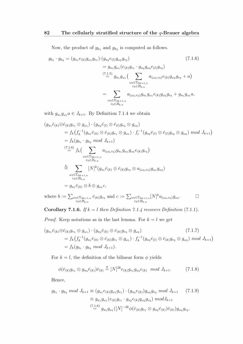
82 The cellularly stratified structure of the q-Brauer algebra
Now, the product of gh1 and gh2 is computed as follows.
gh1 · gh2 = (gu1e(k)gω1gv1)·(gu2e(l)gω2gv2) (7.1.6)
= gu1gω1(e(k)gv1 · gu2gω2e(l)gv2)
(7.1.5)= gu1gω1
( ∑ω3∈Σ2k+1,n
v3∈Bk,n
a(ω3,v3)e(k)gω3gv3 + a)
=∑
ω3∈Σ2k+1,n
v3∈Bk,n
a(ω3,v3)gu1gω1e(k)gω3gv3 + gu1gω1a,
with gu1gω1a ∈ Jk+1. By Definition 7.1.4 we obtain
(gu1 e(k)⊗e(k)gv1 ⊗ gω1) · (gu2 e(l) ⊗ e(l)gv2 ⊗ gω2)
= fk(f−1k (gu1 e(k) ⊗ e(k)gv1 ⊗ gω1) · f−1
l (gu2 e(l) ⊗ e(l)gv2 ⊗ gω2) mod Jk+1
)= fk(gh1 · gh2 mod Jk+1)
(7.1.6)= fk
( ∑ω3∈Σ2k+1,n
v3∈Bk,n
a(ω3,v3)gu1gω1gω3e(k)gv3)
fk=∑
ω3∈Σ2k+1,n
v3∈Bk,n
[N ]k(gu1 e(k) ⊗ e(k)gv3 ⊗ a(ω3,v3)gω1gω3)
= gu1 e(k) ⊗ b⊗ gω1c,
where b :=∑
ω3∈Σ2k+1,n
v3∈Bk,ne(k)gv3 and c :=
∑ω3∈Σ2k+1,n
v3∈Bk,n[N ]ka(ω3,v3)gω3 .
Corollary 7.1.6. If k = l then Definition 7.1.4 recovers Definition (7.1.1).
Proof. Keep notations as in the last lemma. For k = l we get
(gu1 e(k)⊗e(k)gv1 ⊗ gω1) · (gu2 e(k) ⊗ e(k)gv2 ⊗ gω2) (7.1.7)
= fk(f−1k (gu1 e(k) ⊗ e(k)gv1 ⊗ gω1) · f−1
k (gu2 e(l) ⊗ e(k)gv2 ⊗ gω2) mod Jk+1
)= fk(gh1 · gh2 mod Jk+1).
For k = l, the definition of the bilinear form φ yields
φ(e(k)gv1 ⊗ gu2 e(k))e(k)φ= [N ]2ke(k)gv1gu2e(k) mod Jk+1. (7.1.8)
Hence,
gh1 · gh2 mod Jk+1 ≡ (gu1e(k)gω1gv1) · (gu2e(k))gω2gv2 mod Jk+1 (7.1.9)
≡ gu1gω1(e(k)gv1 · gu2e(k)gω2gv2) modJk+1
(7.1.8)= gu1gω1([N ]−2kφ(e(k)gv1 ⊗ gu2 e(k))e(k))gω2gv2 .
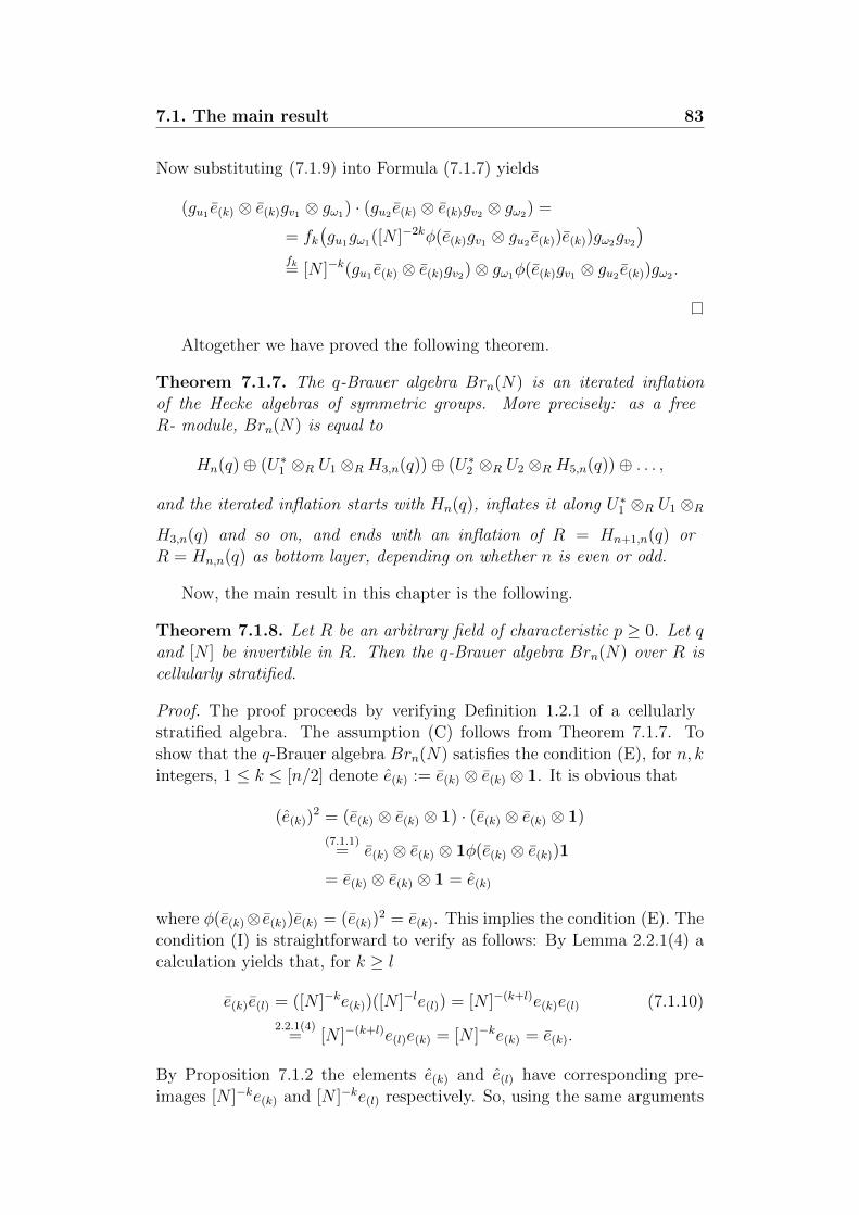
7.1. The main result 83
Now substituting (7.1.9) into Formula (7.1.7) yields
(gu1 e(k) ⊗ e(k)gv1 ⊗ gω1) · (gu2 e(k) ⊗ e(k)gv2 ⊗ gω2) =
= fk(gu1gω1([N ]−2kφ(e(k)gv1 ⊗ gu2 e(k))e(k))gω2gv2
)fk= [N ]−k(gu1 e(k) ⊗ e(k)gv2)⊗ gω1φ(e(k)gv1 ⊗ gu2 e(k))gω2 .
Altogether we have proved the following theorem.
Theorem 7.1.7. The q-Brauer algebra Brn(N) is an iterated inflationof the Hecke algebras of symmetric groups. More precisely: as a freeR- module, Brn(N) is equal to
Hn(q)⊕ (U∗1 ⊗R U1 ⊗R H3,n(q))⊕ (U∗2 ⊗R U2 ⊗R H5,n(q))⊕ . . . ,
and the iterated inflation starts with Hn(q), inflates it along U∗1 ⊗R U1 ⊗RH3,n(q) and so on, and ends with an inflation of R = Hn+1,n(q) orR = Hn,n(q) as bottom layer, depending on whether n is even or odd.
Now, the main result in this chapter is the following.
Theorem 7.1.8. Let R be an arbitrary field of characteristic p ≥ 0. Let qand [N ] be invertible in R. Then the q-Brauer algebra Brn(N) over R iscellularly stratified.
Proof. The proof proceeds by verifying Definition 1.2.1 of a cellularlystratified algebra. The assumption (C) follows from Theorem 7.1.7. Toshow that the q-Brauer algebra Brn(N) satisfies the condition (E), for n, kintegers, 1 ≤ k ≤ [n/2] denote e(k) := e(k) ⊗ e(k) ⊗ 1. It is obvious that
(e(k))2 = (e(k) ⊗ e(k) ⊗ 1) · (e(k) ⊗ e(k) ⊗ 1)
(7.1.1)= e(k) ⊗ e(k) ⊗ 1φ(e(k) ⊗ e(k))1
= e(k) ⊗ e(k) ⊗ 1 = e(k)
where φ(e(k)⊗ e(k))e(k) = (e(k))2 = e(k). This implies the condition (E). The
condition (I) is straightforward to verify as follows: By Lemma 2.2.1(4) acalculation yields that, for k ≥ l
e(k)e(l) = ([N ]−ke(k))([N ]−le(l)) = [N ]−(k+l)e(k)e(l) (7.1.10)
2.2.1(4)= [N ]−(k+l)e(l)e(k) = [N ]−ke(k) = e(k).
By Proposition 7.1.2 the elements e(k) and e(l) have corresponding pre-images [N ]−ke(k) and [N ]−ke(l) respectively. So, using the same arguments
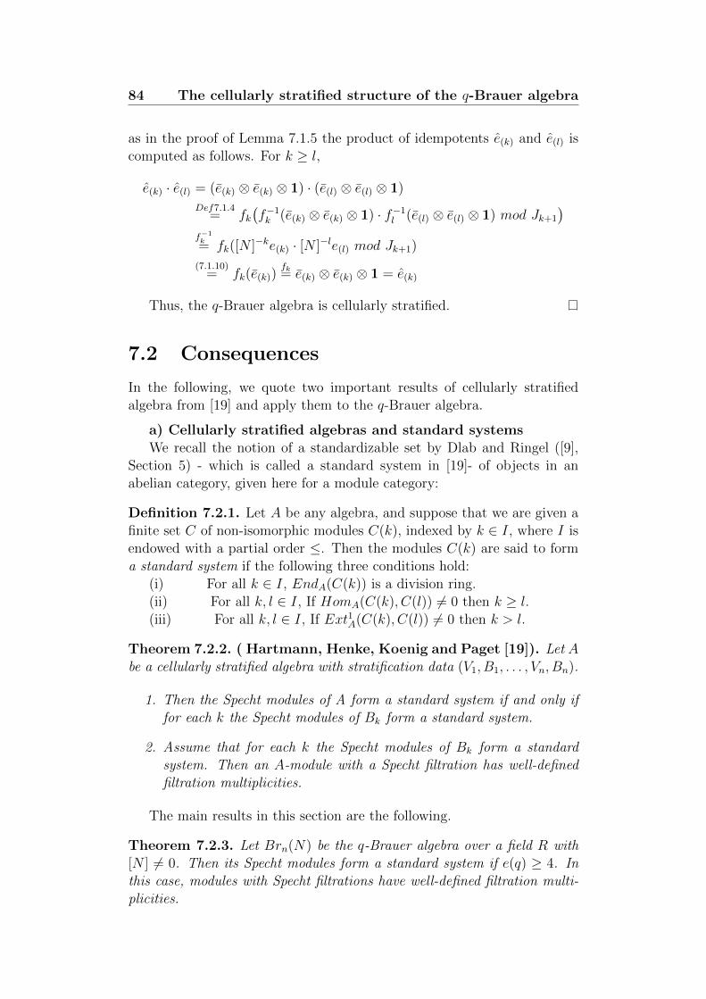
84 The cellularly stratified structure of the q-Brauer algebra
as in the proof of Lemma 7.1.5 the product of idempotents e(k) and e(l) iscomputed as follows. For k ≥ l,
e(k) · e(l) = (e(k) ⊗ e(k) ⊗ 1) · (e(l) ⊗ e(l) ⊗ 1)
Def7.1.4= fk
(f−1k (e(k) ⊗ e(k) ⊗ 1) · f−1
l (e(l) ⊗ e(l) ⊗ 1) mod Jk+1
)f−1k= fk([N ]−ke(k) · [N ]−le(l) mod Jk+1)
(7.1.10)= fk(e(k))
fk= e(k) ⊗ e(k) ⊗ 1 = e(k)
Thus, the q-Brauer algebra is cellularly stratified.
7.2 Consequences
In the following, we quote two important results of cellularly stratifiedalgebra from [19] and apply them to the q-Brauer algebra.
a) Cellularly stratified algebras and standard systemsWe recall the notion of a standardizable set by Dlab and Ringel ([9],
Section 5) - which is called a standard system in [19]- of objects in anabelian category, given here for a module category:
Definition 7.2.1. Let A be any algebra, and suppose that we are given afinite set C of non-isomorphic modules C(k), indexed by k ∈ I, where I isendowed with a partial order ≤. Then the modules C(k) are said to forma standard system if the following three conditions hold:
(i) For all k ∈ I, EndA(C(k)) is a division ring.(ii) For all k, l ∈ I, If HomA(C(k), C(l)) 6= 0 then k ≥ l.(iii) For all k, l ∈ I, If Ext1A(C(k), C(l)) 6= 0 then k > l.
Theorem 7.2.2. ( Hartmann, Henke, Koenig and Paget [19]). Let Abe a cellularly stratified algebra with stratification data (V1, B1, . . . , Vn, Bn).
1. Then the Specht modules of A form a standard system if and only iffor each k the Specht modules of Bk form a standard system.
2. Assume that for each k the Specht modules of Bk form a standardsystem. Then an A-module with a Specht filtration has well-definedfiltration multiplicities.
The main results in this section are the following.
Theorem 7.2.3. Let Brn(N) be the q-Brauer algebra over a field R with[N ] 6= 0. Then its Specht modules form a standard system if e(q) ≥ 4. Inthis case, modules with Specht filtrations have well-defined filtration multi-plicities.
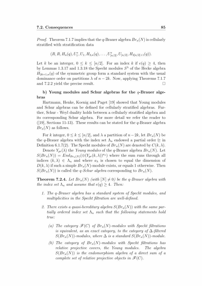
7.2. Consequences 85
Proof. Theorem 7.1.7 implies that the q-Brauer algebraBrn(N) is cellularlystratified with stratification data
(R,R,Hn(q), U∗1 , U1, H3,n(q), . . . , U∗[n/2], U[n/2], H2[n/2]+1(q)).
Let k be an interger, 0 ≤ k ≤ [n/2]. For an index k if e(q) ≥ 4, thenby Lemmas 1.3.17 and 1.3.18 the Specht modules Sλ of the Hecke algebraH2k+1,n(q) of the symmetric group form a standard system with the usualdominance order on partitions λ of n− 2k. Now, applying Theorems 7.1.7and 7.2.2 yield the precise result.
b) Young modules and Schur algebras for the q-Brauer alge-bras
Hartmann, Henke, Koenig and Paget [19] showed that Young modulesand Schur algebras can be defined for cellularly stratified algebras. Fur-ther, Schur - Weyl duality holds between a cellularly stratified algebra andits corresponding Schur algebra. For more detail we refer the reader to([19], Sections 11-13). These results can be stated for the q-Brauer algebraBrn(N) as follows.
For k integer, 0 ≤ k ≤ [n/2], and λ a partition of n−2k, let Brn(N) bethe q-Brauer algebra with the index set Λn endowed a partial order � inDefinition 6.1.7(2). The Specht modules of Brn(N) are denoted by C(k, λ).
Denote Ypr(λ) the Young modules of the q-Brauer algebra Brn(N). LetS(Brn(N)) = EndBrn(N)(⊕(Ypr(k, λ))aλ) where the sum runs through allindices (k, λ) ∈ Λn and where aλ is chosen to equal the dimension ofD(k, λ) if such a simple Brn(N)-module exists, or equals 1 otherwise. ThenS(Brn(N)) is called the q-Schur algebra corresponding to Brn(N).
Theorem 7.2.4. Let Brn(N) (with [N ] 6= 0) be the q-Brauer algebra withthe index set Λn and assume that e(q) ≥ 4. Then:
1. The q-Brauer algebra has a standard system of Specht modules, andmultiplicities in the Specht filtration are well-defined.
2. There exists a quasi-hereditary algebra S(Brn(N)) with the same par-tially ordered index set Λn such that the following statements holdtrue:
(a) The category F (C) of Brn(N)-modules with Specht filtrationsis equivalent, as an exact category, to the category of ∆-filteredS(Brn(N))-modules, where ∆ is a standard S(Brn(N))-module.
(b) The category of Brn(N)-modules with Specht filtrations hasrelative projective covers, the Young modules. The algebraS(Brn(N)) is the endomorphism algebra of a direct sum of acomplete set of relative projective objects in F (C).
86 The cellularly stratified structure of the q-Brauer algebra
(c) Schur-Weyl duality holds between Brn(N) and S(Brn(N)). Thefaithfully balanced bimodule affording the double centralizer prop-erty between Brn(N) and S(Brn(N)) is the direct sum of theYoung modules.
Proof. This theorem is a special case of Theorem 13.1 in [19].
Bibliography
[1] J. Birman, H. Wenzl, Braids, link polynomials and a new algebra,Trans. Amer. Math. Soc., 313(1) (1989), 249-273.
[2] R. Brauer, On algebras which are connected with the semisimple con-tinuous groups, Ann. of Math., 63 (1937), 854-872.
[3] W.P. Brown, An algebra related to the orthogonal group, MichiganMath. J., 3 (1955), 1-22.
[4] W.P. Brown, The semisimplicity of ωnf , Ann. of Math., 63(2) (1956),324 - 335.
[5] V. Chari, A. Pressley, A guide to quantum groups, Cambridge Univer-sity Press, 1994.
[6] E. Cline, B. Parshall, L. Scott, Finite dimensional algebras and highestweight categories, J. Reine Angew. Math., 391 (1988), 85-99.
[7] R. Dipper, G.D. James, Representations of Hecke algebras and generallinear groups, Proc.London Math. Soc., 52(3) (1986), 20-52.
[8] R. Dipper, G.D. James, Blocks and idempotents of Hecke algebras andgeneral linear groups, Proc. London Math. Soc., 54(3) (1987), 57 - 82.
[9] V. Dlab and C.M. Ringel, The module theoretic approach toquasi-hereditary algebras. In ”Representations of Algebras and RelatedTopics” (Kyoto, 1990). London Math. Soc. Lecture Note Ser., 168,200- 224. Cambridge University Press, 1992.
[10] W. Doran, D. Wales, P. Hanlon, On the semisimplicity of the Brauercentralizer algebras, J. Algebra, 211 (1999), 647 - 685.
[11] N.T. Dung, Cellular structure of q-Brauer algebras, arXiv:1208.6424,(2012).
[12] J. Enyang, Specht modules and semisimplicity criteria for Brauer andBirman-Murakami-Wenzl algebras, J. Comb. Theory, Ser. A 26 (2007),291-341.
88
[13] A.M. Gavrilik, A.U. Klimyk, q-Deformed orthogonal and pseudo-orthogonal algebras and their representations, Lett. Math. Phys. 21(3)(1991), 215-220.
[14] M. Geck, Hecke algebras of finite type are cellular, Invent. Math., 169(3) (2007), 501-517.
[15] J.J. Graham, G. I. Lehrer, Cellular algebras, Invent. Math., 123 (1)(1996), 1-34.
[16] P. Hanlon, D. Wales, On the decomposition of Brauer’s centralizeralgebras, J. Algebra, 121(2) (1989), 409 - 445.
[17] P. Hanlon, D. Wales, Computing the discriminants of Brauer’s cen-tralizer algebras, Math. Comp., 54 (1990), 771 - 796.
[18] R. Hartmann, R. Paget, Young modules and filtration multiplicitiesfor Brauer algebras, Math. Z., 254 (2006), 333-357.
[19] R. Hartmann, A. Henke, S. Koenig, R. Paget,Cohomological stratifi-cation of diagrams algebras, Math. Ann., 347 (2010), 765-804.
[20] D. Hemmer, D. Nakano, Specht filtration for Hecke algebras of type A,J. Lond. Math. Soc., 69(2) (2004), 623-638.
[21] G.D. James, The representation theory of the symmetric groups, SLN,682, Springer-Verlag, New York, 1978.
[22] M. Jimbo, A q-analog of U(gl (n+1)), Hecke Algebra and the Yang-Baxter Equation, Lett. Math. Phys., 11 (1986), 247-252.
[23] S. Koenig, C. C. Xi, On the structure of cellular algebras. In: Algebrasand modules II (Geiranger 1996), CMS Conf. Proc. 24, Amer. Math.Soc., (1998), 365-386.
[24] S. Koenig, C. C. Xi, Cellular algebras: Inflations and Morita equiva-lences, J. Lond. Math. Soc., 60(2) (1999), 700-722.
[25] S. Koenig, C. C. Xi,When is a cellular algebra quasi-heredity?, Mat.Ann., 315 (1999), 281-293.
[26] S. Koenig, C. C. Xi, A characteristic free approach to Brauer algebras,Trans. Amer. Math. Soc., 353(4) (2000), 1489-1505.
[27] R. Leduc, A. Ram, A Ribbon Hopf Algebra Approach to the IrreducibleRepresentations of Centralizer Algebras: The Brauer, Birman-Wenzl,and Type A Iwahori-Hecke Algebras, Adv. Math., 125(1) (1997), 1-94.
89
[28] A. Mathas, Iwahori-Hecke Algebras and Schur Algebras of theSymmetric Group, University Lecture Series. American Mathemati-cal Society, Providence, R.I., vol. 15, 1999.
[29] A.I. Molev, A new quantum analog of the Brauer algebra, CzechoslovakJ. Phys., 53 (2003), 1073-1078.
[30] A.I. Molev, private communication.
[31] E. Murphy, The representations of Hecke algebras of type An,J.Algebra, 173(1) (1995), 97-121.
[32] J. Murakami, The Kauffman polynomials of links and representationtheory, Osaka J. Math., 24(4) (1987), 745-758.
[33] B. Parshall, L. Scott, Derived categories, quasi-hereditary algebras andalgebraic groups, in “Proceeding of the Ottawa-Moosonee Workshop inAlgebra 1987”, Math. Lecture Note series, Carleton University, 1988.
[34] H. Rui, M. Si, Gram determinants and semisimplicity criteria forBirman-Wenzl Algebras, J. Reine Angew. Math., 631 (2009), 153-179.
[35] H. Rui, A criterion on the semisimple Brauer algebras, J. Comb. The-ory, Ser. A, 111 (2005), 78-88.
[36] H. Wenzl, On the structure of Brauer’s centralizer algebras, Ann. ofMath., 128 (1988), 173-193.
[37] H. Wenzl, Quantum groups and subfactors of type B, C, and D, Comm.Math. Phys., 133 (1990), 383-432.
[38] H. Wenzl, A q-Brauer algebra, arXiv:1102.3892v1.
[39] H. Wenzl, A q-Brauer algebra, J. Algebra, 358 (2012), 102-127.
[40] H. Wenzl, Quotients of representation rings, Represent. Theory, 15(2011), 385-406.
[41] H. Wenzl, Fusion symmetric spaces and subfactors, Pacific J. Math.,259(2) (2012), 483-510.
[42] C. C. Xi, Partition algebras are cellular, Compositio Math., 119(1)(1999), 99-109.
[43] C. C. Xi, On the quasi-heredity of Birman-Wenzl algebras, Adv. Math.,154 (2000), 280-298.
![Technische Universit at Ilmenau Institut fur Mathematik ... · [11] H. Weber: Einf uhrung in die Wahrscheinlichkeitsrechnung und Statistik f ur Ingenieure. 3. Au age, Teubner Stuttgart](https://img.pdfslide.org/doc/110x75/5f7017ac66484f573b29e60b/technische-universit-at-ilmenau-institut-fur-mathematik-11-h-weber-einf.jpg)