„Im Rahmen der hochschulweiten Open-Access-Strategie für die Zweitveröffentlichung identifiziert durch die Universitätsbibliothek Ilmenau.“

“Within the academic Open Access Strategy identified for deposition by Ilmenau University Library.”

„Dieser Beitrag ist mit Zustimmung des Rechteinhabers aufgrund einer (DFG-geförderten) Allianz- bzw. Nationallizenz frei zugänglich.“

„This publication is with permission of the rights owner freely accessible due to an Alliance licence and a national licence (funded by the DFG, German Research Foundation) respectively.”

Di Rienzo, Luca; Haueisen, Jens:

Numerical comparison of sensor arrays for magnetostatic linear inverse problems based on a projection method

URN: urn:nbn:de:gbv:ilm1-2014210127

Published OpenAccess: September 2014

Original published in: Compel : international journal of computation & mathematics in electrical & electronic engineering. - Bradford : Emerald (ISSN-p 0332-1649). - 26 (2007) 2, S. 356-367. DOI: 10.1108/03321640710727719 URL: http://dx.doi.org/10.1108/03321640710727719 [Visited: 2014-09-02]

COMPEL - The international journal for computation and mathematicsin electrical and electronic engineeringNumerical comparison of sensor arrays for magnetostatic linear inverse problems basedon a projection methodLuca Di Rienzo Jens Haueisen

Article information:To cite this document:Luca Di Rienzo Jens Haueisen, (2007),"Numerical comparison of sensor arrays for magnetostatic linearinverse problems based on a projection method", COMPEL - The international journal for computation andmathematics in electrical and electronic engineering, Vol. 26 Iss 2 pp. 356 - 367Permanent link to this document:http://dx.doi.org/10.1108/03321640710727719

Downloaded on: 02 September 2014, At: 07:54 (PT)References: this document contains references to 15 other documents.To copy this document: permissions@emeraldinsight.comThe fulltext of this document has been downloaded 161 times since 2007*

Users who downloaded this article also downloaded:Luca Di Rienzo, Jens Haueisen, Cesare Mario Arturi, (2005),"Three component magnetic field data:Impact on minimum norm solutions in a biomedical application", COMPEL - The international journal forcomputation and mathematics in electrical and electronic engineering, Vol. 24 Iss 3 pp. 869-881A. Yao, M. Soleimani, (2012),"A pressure mapping imaging device based on electrical impedancetomography of conductive fabrics", Sensor Review, Vol. 32 Iss 4 pp. 310-317O. Korostynska, A. Mason, A. Al-Shamma'a, (2014),"Microwave sensors for the non-invasive monitoringof industrial and medical applications", Sensor Review, Vol. 34 Iss 2 pp. 182-191 http://dx.doi.org/10.1108/SR-11-2012-725

Access to this document was granted through an Emerald subscription provided by 514728 []

For AuthorsIf you would like to write for this, or any other Emerald publication, then please use our Emerald forAuthors service information about how to choose which publication to write for and submission guidelinesare available for all. Please visit www.emeraldinsight.com/authors for more information.

About Emerald www.emeraldinsight.comEmerald is a global publisher linking research and practice to the benefit of society. The companymanages a portfolio of more than 290 journals and over 2,350 books and book series volumes, as well asproviding an extensive range of online products and additional customer resources and services.

Emerald is both COUNTER 4 and TRANSFER compliant. The organization is a partner of the Committeeon Publication Ethics (COPE) and also works with Portico and the LOCKSS initiative for digital archivepreservation.

*Related content and download information correct at time of download.

Dow

nloa

ded

by U

NIV

ERSI

TAET

SBIB

LIO

THEK

ILM

ENA

U A

t 07:

54 0

2 Se

ptem

ber 2

014

(PT)

Numerical comparison of sensorarrays for magnetostatic linearinverse problems based on a

projection methodLuca Di Rienzo

Politecnico di Milano, Dipartimento di Elettrotecnica, Milano, Italy, and

Jens HaueisenInstitute of Biomedical Engineering and Informatics,Technical University Ilmenau, Ilmenau, Germany

Abstract

Purpose – To define a methodology for comparing sensor arrays for solving magnetostatic linearinverse problems.

Design/methodology/approach – A singular value decomposition related projection method isused for comparing sensor arrays and we applied it to a biomagnetic inverse problem, as an example.Furthermore, a theoretical reference sensor system is introduced and used as a benchmark for theanalysed sensor arrays.

Findings – The method has turned out to be effective in comparing three different theoretical sensorarrays, showing the superiority of the two arrays constituted by three-axial sensors.

Research limitations/implications – The method has been applied only to the case ofover-determined problems. The underdetermined case will be considered in future work.

Practical implications – From the applicative point of view, the illustrated methodology is usefulwhen one has to choose between existing sensor arrays or in the design phase of a new sensor array.

Originality/value – A new methodology is proposed for comparing sensor arrays. The advantage ofthe methodology are to take into account the regularization in the solution of the inverse problem andto be general, not depending on a particular source configuration.

Keywords Sensors, Magnetic fields

Paper type Research paper

1. IntroductionThere are many applications in magneto fluid dynamics (Ziolkowski et al., 2006),superconductivity (Bruzzone et al., 2002; Bellina et al., 2002), non-destructive testing(Haueisen et al., 2002), magnetic fields characterization (Scorretti et al., 2004; Rouveet al., 2006), reconstruction of a magnetization distribution (Chadebec et al., 2002),biomagnetism (Arturi et al., 2004; Di Rienzo et al., 2005) that can be formulated asmagnetostatic linear inverse problems (IPs).

In their direct formulation this kind of problems are typically described by thefollowing equation:

B ¼ L ·ptrue þ 1 ð1Þwhere B is the column vector of m scalar magnetic field measurements, L [ Rm£n isthe kernel matrix, ptrue is the source distribution represented by a column vector of

The current issue and full text archive of this journal is available at

www.emeraldinsight.com/0332-1649.htm

COMPEL26,2

356

COMPEL: The International Journalfor Computation and Mathematics inElectrical and Electronic EngineeringVol. 26 No. 2, 2007pp. 356-367q Emerald Group Publishing Limited0332-1649DOI 10.1108/03321640710727719

length n and 1 is the column vector representing the noise. In IPs a relevant source ofuncertainty can be due to system inaccuracies (e.g. sensor alignments or sensorposition variations). Those inaccuracies affect the kernel matrix L and are not takeninto account in the error analysis proposed here. On the other hand, they can beneglected to some extent in biomagnetic applications like the one analyzed in our work.

When these problems are over-determined (i.e. the number of measurements m ishigher than the number of unknown parameters n) and ill-posed, the solution istypically obtained with the help of the truncated singular value decomposition (TSVD)as a regularization scheme (Vogel, 2002; Hansen, 1998; Golub and Van Loan, 1989;Shim and Cho, 1981; Nalbach and Dossel, 2002; Kemppainem and Ilmoniemi, 1989).

After computing the singular value decomposition (SVD) of L: L ¼ USV T; wherethe matrices U ¼ ðu1;u2; . . . ;unÞ [ R

m£m and V ¼ ðv1; v2; . . . ; vnÞ [ Rn£n are

with orthonormal columns and where S ¼ diagðs1;s2; . . . ;sgÞ; g ¼ rankðLÞ hasnon-negative diagonal elements (singular values), inverting the linear system (1) thefollowing solution is obtained:

L21B ¼ VS21U TB ¼

Xg

i¼1

uTi ·B

si

vi ¼ VS21U TLptrue þ VS

21U T1

¼ ptrue þXg

i¼1

uTi · 1

si

vi

ð2Þ

The small singular values at denominator in equation (2) cause instability. In order toavoid this instability, only the first r terms corresponding to the first r singular valuesare kept, obtaining the TSVD regularized solution:

pTSVD ¼Xr

i¼1

uTi ·B

si

vi ð3Þ

The proper choice of the order r of the TSVD depends on the noise level in the dataand can be performed according to different criteria (Vogel, 2002; Hansen, 1998;Shim and Cho, 1981).

The solution given by equation (3) is the minimum norm solution (MNS) of thelinear system:

B ¼ Lr ·p ð4Þ

where the matrix L is replaced by a truncated version L r of rank r given by thefollowing expansion:

Lr ¼Xr

i¼1

uisivTi ð5Þ

Often one has to choose between different geometries of magnetic sensor arrays.For this scope, it is important to introduce theoretical criteria to compare sensor arraysperformances.

A typical cost function used in sensor array optimization is given by thecondition number (CN) of the kernel matrix (Bruzzone et al., 2002; Bellina et al., 2002;Rouve et al., 2006; Arturi et al., 2004; Di Rienzo et al., 2005). The analysis based on the CN islimited by the fact that the solution of an ill-posed IP is obtained by a regularization

Numericalcomparison ofsensor arrays

357

Dow

nloa

ded

by U

NIV

ERSI

TAET

SBIB

LIO

THEK

ILM

ENA

U A

t 07:

54 0

2 Se

ptem

ber 2

014

(PT)

algorithm and the CN of the regularization algorithm is different from the CN of the kernelmatrix.

Furthermore, while the commonly applied CN analysis is based, by definition, only onthe first and the last singular values, the projection analysis used here is based on all theright singular vectors and hence is expected to give a more comprehensive insight.

The principle of the projection method used in our paper was introduced in Nalbachand Dossel (2002). We expand the basic principle to regularized TSVD problems.Furthermore, we introduce a theoretical measurement system which completelysamples the magnetic field and works as a gold standard reference. We then apply thecomparison method to kernel matrices representing theoretical sensor setups used inMagnetocardiography and described in Arturi et al. (2004) and in Di Rienzo et al. (2005).

2. Comparison criteria based on TSVD projectionsIn order to compare two different sensor arrays geometries, that can be madeof different numbers of sensors, let us consider the associated kernel matricesL1 [ R

m1£n and L2 [ Rm2£n: After applying TSVD with truncation order r1 to L1 and

with truncation order r2 to L2, the matrices L1 and L2 are replaced by their truncatedversions Lr1

1 and Lr22 ;, respectively. After computing SVD:

L1 ¼ U 1S1VT1 ; L2 ¼ U 2S2V

T2 ð6Þ

the following partitionings of V 1 and V 2 can be introduced (Golub and Van Loan,1989):

V 1 ¼ ½V 1r1;V 1n�; V 2 ¼ ½V 2r2

;V 2n� ð7Þ

V 1r1¼ ½v1

1; v12; . . . ; v

1r1�; V 2r2

¼ ½v21; v

22; . . . ; v

2r2� ð8Þ

V 1n ¼ ½v1r1þ1; v

1r1þ2; . . . ; v

1n� V 2n ¼ ½v2

r2þ1; v2r2þ2; . . . ; v

2n� ð9Þ

where the columns of V 1r1¼ ½v1

1; v12; . . . ; v

1r1� are an orthonormal basis of the row

space of Lr1

1 ; indicated with RðLrT

1

1 Þ; similarly the columns of V 2r2¼ ½v2

1; v22; . . . ; v

2r2�

are an orthonormal basis of the row space of Lr2

2 ; indicated with RðLrT

2

2 Þ: The columns ofthe other two matrices V 1n ¼ ½v1

r1þ1; v1r1þ2; . . . ; v

1n� and V 2n ¼ ½v2

r2þ1; v2r2þ2; . . . ; v

2n�

are, respectively, orthonormal bases of the null spaces N ðLr1

1 Þ of Lr1

1 and N ðLr2

2 Þ of Lr2

2 :The following projectors can be then defined (Golub and Van Loan, 1989):

P1r1¼ V 1r1

VT1r1

Projector onto RðLrT

1

1 Þ ð10aÞ

P2r2¼ V 2r2

VT2r2

Projector onto RðLrT

2

2 Þ ð10bÞ

Since, the MNS associated to the linear overdetermined system B ¼ Lr ·p lies onto the

row space of Lr; RðLrT

1

1 Þ; contains all the MNSs obtained using the sensor array No. 1

with kernel matrix L1 and TSVD of order r1 and RðLrT

2

2 Þ contains all the MNS obtainedusing the sensor array No. 2 with kernel matrix L2 and TSVD of order r2.

COMPEL26,2

358

Dow

nloa

ded

by U

NIV

ERSI

TAET

SBIB

LIO

THEK

ILM

ENA

U A

t 07:

54 0

2 Se

ptem

ber 2

014

(PT)

According to the comparison criterion described here, matrix V 2r2is orthogonally

projected onto RðLrT

1

1 Þ: The result is a n £ r2 matrix P2!1 ¼ P1r1

·V 2r2; whose jth

column is the projection of v2j onto RðL

rT1

1 Þ; given by the vector P1r1

· v2j : This projection

is the MNS of the linear system B ¼ L1r1

·p when the true solution is v2j : The norm of

this projection is generally less than one because v2j � RðL

rT1

1 Þ and the higher the valueof the norm the better v2

j is catched by Lr1

1 : On the other hand, by construction, the

source v2j is totally visible using Lr2

2 ; because v2j [ RðL

rT2

2 Þ and its norm is unitary.

Since any MNS of the system B ¼ Lr2

2 ·p can be expanded as a linear combination ofthe orthonormal base vectors {v2

1; v22; . . . ; v

2r2

}; the norms of the projected vectors{P1

r1· v2

1;P1r1

· v22; . . . ;P

1r1

· v2r2

}; that are the columns of the matrix P2!1; indicate howwell Lr1

1 is capable of recovering the sources that are perfectly reconstructed by Lr2

2 :The statement above obviously holds true for vice versa, so changing 1 with 2 anddefining matrix P1!2 ¼ P2

r2·V 1r1

:The first comparison criterion can then be stated as follows.Comparison criterion No. 1: if the columns of P2!1 have larger norms than the

columns of P1!2 then sensor array No. 1 is to be preferred to sensor array No. 2.A second comparison criterion can be defined projecting the null space base vectors

of one kernel matrix onto the row space of the other kernel matrix. More specifically,since the orthonormal vectors{v1

r1þ1; v1r1þ2; . . . ; v

1n} are a basis of the null space of Lr1

1 ;any linear combination of these vectors is a source that is invisible to Lr1

1 : If their

projections onto RðLrT

2

2 Þ are different from zero, they are partially visible to Lr2

2 : It is thenconvenient to define the matrix Q1!2 ¼ P2

r2·V 1n: The statement above obviously holds

true for the vice versa, so changing 1 with 2 and defining the matrix Q2!1 ¼ P1r1

·V 2n:The second comparison criterion can be stated as follows.Comparison criterion No. 2: if the columns of Q2!1 have larger norms than the

columns of Q1!2 then sensor array No. 1 is to be preferred to sensor array No. 2.

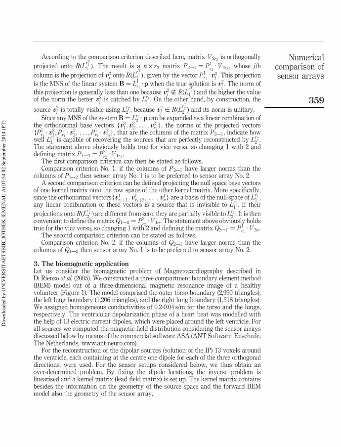
3. The biomagnetic applicationLet us consider the biomagnetic problem of Magnetocardiography described inDi Rienzo et al. (2005). We constructed a three compartment boundary element method(BEM) model out of a three-dimensional magnetic resonance image of a healthyvolunteer (Figure 1). The model comprised the outer torso boundary (2,990 triangles),the left lung boundary (1,206 triangles), and the right lung boundary (1,318 triangles).We assigned homogeneous conductivities of 0.2-0.04 s/m for the torso and the lungs,respectively. The ventricular depolarization phase of a heart beat was modelled withthe help of 13 electric current dipoles, which were placed around the left ventricle. Forall sources we computed the magnetic field distribution considering the sensor arraysdiscussed below by means of the commercial software ASA (ANT Software, Enschede,The Netherlands, www.ant-neuro.com).

For the reconstruction of the dipolar sources (solution of the IP) 13 voxels aroundthe ventricle, each containing at the centre one dipole for each of the three orthogonaldirections, were used. For the sensor setups considered below, we thus obtain anover-determined problem. By fixing the dipole locations, the inverse problem islinearised and a kernel matrix (lead field matrix) is set up. The kernel matrix containsbesides the information on the geometry of the source space and the forward BEMmodel also the geometry of the sensor array.

Numericalcomparison ofsensor arrays

359

Dow

nloa

ded

by U

NIV

ERSI

TAET

SBIB

LIO

THEK

ILM

ENA

U A

t 07:

54 0

2 Se

ptem

ber 2

014

(PT)

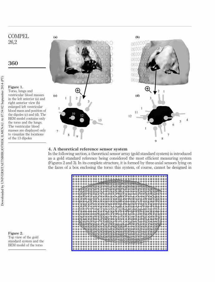
4. A theoretical reference sensor systemIn the following section, a theoretical sensor array (gold standard system) is introducedas a gold standard reference being considered the most efficient measuring system(Figures 2 and 3). In its complete structure, it is formed by three-axial sensors lying onthe faces of a box enclosing the torso: this system, of course, cannot be designed in

Figure 1.Torso, lungs andventricular blood massesin the left anterior (a) andright anterior view (b)enlarged left ventricularblood mass and position ofthe dipoles (c) and (d). TheBEM model contains onlythe torso and the lungs.The ventricular bloodmasses are displayed onlyto visualize the locationsof the 13 dipoles

(a)

(c)1 2

10 12

3

1312

111

3

2 1

1

98

7

65 4

987

1

(b)

(d)

Figure 2.Top view of the goldstandard system and theBEM model of the torso

COMPEL26,2

360

Dow

nloa

ded

by U

NIV

ERSI

TAET

SBIB

LIO

THEK

ILM

ENA

U A

t 07:

54 0

2 Se

ptem

ber 2

014

(PT)

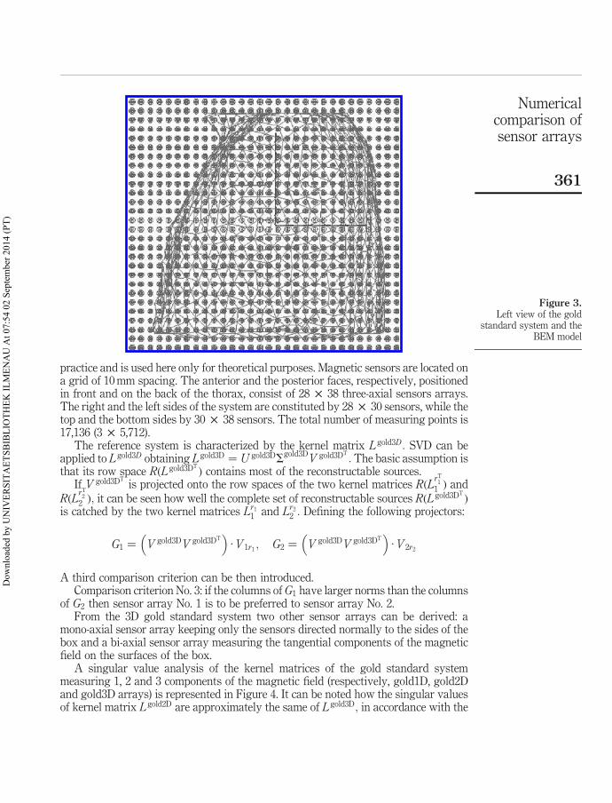
practice and is used here only for theoretical purposes. Magnetic sensors are located ona grid of 10 mm spacing. The anterior and the posterior faces, respectively, positionedin front and on the back of the thorax, consist of 28 £ 38 three-axial sensors arrays.The right and the left sides of the system are constituted by 28 £ 30 sensors, while thetop and the bottom sides by 30 £ 38 sensors. The total number of measuring points is17,136 (3 £ 5,712).

The reference system is characterized by the kernel matrix Lgold3D: SVD can beapplied to Lgold3D obtaining Lgold3D ¼ U gold3DS

gold3DV gold3DT

: The basic assumption isthat its row space RðLgold3DT

Þ contains most of the reconstructable sources.If V gold3DT

is projected onto the row spaces of the two kernel matrices RðLrT

1

1 Þ andRðL

rT2

2 Þ; it can be seen how well the complete set of reconstructable sources RðLgold3DTÞ

is catched by the two kernel matrices Lr1

1 and Lr2

2 : Defining the following projectors:

G1 ¼�V gold3DV gold3DT

�·V 1r1

; G2 ¼�V gold3DV gold3DT

�·V 2r2

A third comparison criterion can be then introduced.Comparison criterion No. 3: if the columns of G1 have larger norms than the columns

of G2 then sensor array No. 1 is to be preferred to sensor array No. 2.From the 3D gold standard system two other sensor arrays can be derived: a

mono-axial sensor array keeping only the sensors directed normally to the sides of thebox and a bi-axial sensor array measuring the tangential components of the magneticfield on the surfaces of the box.

A singular value analysis of the kernel matrices of the gold standard systemmeasuring 1, 2 and 3 components of the magnetic field (respectively, gold1D, gold2Dand gold3D arrays) is represented in Figure 4. It can be noted how the singular valuesof kernel matrix Lgold2D are approximately the same of Lgold3D; in accordance with the

Figure 3.Left view of the gold

standard system and theBEM model

Numericalcomparison ofsensor arrays

361

Dow

nloa

ded

by U

NIV

ERSI

TAET

SBIB

LIO

THEK

ILM

ENA

U A

t 07:

54 0

2 Se

ptem

ber 2

014

(PT)

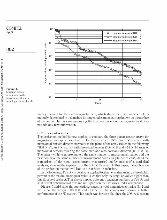
unicity theorem for the electromagnetic field, which states that the magnetic field isuniquely determined in a domain if its tangential components are known on the surfaceof the domain. In this case, measuring the third component of the magnetic field doesnot add any new information.

5. Numerical resultsThe projection method is now applied to compare the three planar sensor arrays formagnetocardiography described in Di Rienzo et al. (2005): an 8 £ 8 array withmono-axial sensors directed normally to the plane of the array (called in the following“1D8 £ 8”), an 8 £ 8 array with three-axial sensors (3D8 £ 8) and a 14 £ 14 array ofmono-axial sensors covering the same area and also normally directed (1D14 £ 14).The latter two have approximately the same number of measurement values and thefirst two have the same number of measurement points. In (Di Rienzo et al., 2005) thecomparison of the same sensor arrays was carried out by means of a statisticalanalysis, showing the superiority of the 3D8 £ 8 system. In this paper, the applicationof the projection method will lead to a consistent conclusion.

In the following, TSVD will be always applied to a kernel matrix using as threshold 1percent of the maximum singular value, such that only the singular values higher thanthis threshold are kept. This choice implies different truncation numbers in TSVDs andso different dimensions of row and null spaces in the two cases under comparison.

Figures 5 and 6 show the application, respectively, of comparison criterion No. 1 andNo. 2 to the arrays 1D8 £ 8 and 3D8 £ 8. The comparison shows a betterperformance of the 3D system. This result was foreseeable, since the 3D8 £ 8 system

Figure 4.Singular valuesnormalized to theirmaximum value in asemi-logarithmical scale

1 11 21 31 3910−5

10−4

10−3

10−2

10−1

100

Index

Singular values gold1DSingular values gold2DSingular values gold3D

Sing

ular

val

ues,

sem

i log

arith

mic

scal

e

COMPEL26,2

362

Dow

nloa

ded

by U

NIV

ERSI

TAET

SBIB

LIO

THEK

ILM

ENA

U A

t 07:

54 0

2 Se

ptem

ber 2

014

(PT)

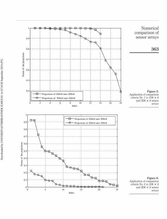
Figure 6.Application of comparison

criteria No. 2 to 1D8 £ 8and 3D8 £ 8 sensor

arrays

Figure 5.Application of comparison

criteria No. 1 to 1D8 £ 8and 3D8 £ 8 sensor

arrays

Numericalcomparison ofsensor arrays

363

Dow

nloa

ded

by U

NIV

ERSI

TAET

SBIB

LIO

THEK

ILM

ENA

U A

t 07:

54 0

2 Se

ptem

ber 2

014

(PT)

is characterized by three times the number of collected magnetic field data than the1D8 £ 8 array.

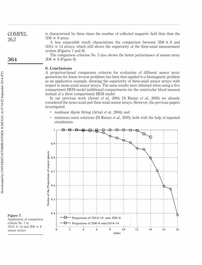
A less expectable result characterizes the comparison between 3D8 £ 8 and1D14 £ 14 arrays, which still shows the superiority of the three-axial measurementsystem (Figures 7 and 8).

The comparison criterion No. 3 also shows the better performance of sensor array3D8 £ 8 (Figure 9).

6. ConclusionsA projection-based comparison criterion for evaluation of different sensor arraygeometries for linear inverse problems has been then applied to a biomagnetic problemas an applicative example, showing the superiority of three-axial sensor arrays withrespect to mono-axial sensor arrays. The same results were obtained when using a fivecompartment BEM model (additional compartments for the ventricular blood masses)instead of a three compartment BEM model.

In our previous work (Arturi et al., 2004; Di Rienzo et al., 2005) we alreadyconsidered the mono-axial and three-axial sensor arrays. However, the previous papersinvestigated:

. nonlinear dipole fitting (Arturi et al., 2004); and

. minimum norm solutions (Di Rienzo et al., 2005), both with the help of repeatedsimulations.

Figure 7.Application of comparisoncriteria No. 1 to1D14 £ 14 and 3D8 £ 8sensor arrays 0 2 4 6 8 10 12 14 16 18

0.4

0.5

0.6

0.7

0.8

0.9

1

index

Nor

ms

of th

e Pr

ojec

tions

of s

ourc

e sp

aces

Projections of 1D14×14 onto 3D8×8

Projections of 3D8×8 onto1D14×14

COMPEL26,2

364

Dow

nloa

ded

by U

NIV

ERSI

TAET

SBIB

LIO

THEK

ILM

ENA

U A

t 07:

54 0

2 Se

ptem

ber 2

014

(PT)

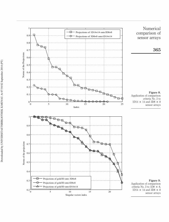
Figure 9.Application of comparisoncriteria No. 3 to 1D8 £ 8,1D14 £ 14 and 3D8 £ 8

sensor arrays

Figure 8.Application of comparison

criteria No. 2 to1D14 £ 14 and 3D8 £ 8

sensor arrays

Numericalcomparison ofsensor arrays

365

Dow

nloa

ded

by U

NIV

ERSI

TAET

SBIB

LIO

THEK

ILM

ENA

U A

t 07:

54 0

2 Se

ptem

ber 2

014

(PT)

In the current paper we compare the sensor arrays with the help of a projection methodin order to gain insight how one system can represent all the source configurationsvisible by the other system and vice versa. Furthermore, unlike the repeatedsimulations approach, the projection method is not influenced by the amount of noiseand thus gives a more theoretical and general view on the comparison of the differentsensor set-ups. Consistent over all methods we found that three-axial sensor systemperforms better than the mono-axial sensor systems.

The example presented here is an over-determined biomagnetic inverse problem,but the same approach would hold for other over-determined magnetostatic inverseproblems. The methodology can be also applied to under-determined magnetostaticinverse problems.

For the design of biomagnetic sensor systems we conclude that three-axial systemsare to be preferred.

References

Arturi, C.M., Di Rienzo, L. and Haueisen, J. (2004), “Information content in single-componentversus three-component cardiomagnetic fields”, IEEE Transactions on Magnetics, Vol. 40No. 2, pp. 631-4.

Bellina, F., Bettini, P. and Trevisan, F. (2002), “Optimization analysis of the magneticmeasurements on multistrand SC cables”, IEEE Transactions on AppliedSuperconductivity, Vol. 12 No. 1, pp. 1651-4.

Bruzzone, P., Formisano, A. and Martone, R. (2002), “Optimal magnetic probes location forcurrent reconstruction in multistrands superconducting cables”, IEEE Transactions onMagnetics, Vol. 38 No. 2, pp. 1057-60.

Chadebec, O., Coulomb, J., Cauffet, G., Bongiraud, J. and Le Thiec, P. (2002), “Recentimprovements for solving inverse magnetostatic problem applied to thin shells”, IEEETransactions on Magnetics, Vol. 38 No. 2, pp. 1005-8.

Di Rienzo, L., Haueisen, J. and Arturi, C.M. (2005), “Three component magnetic field data: impacton minimum norm solutions in a biomedical application”, COMPEL, The InternationalJournal for Computation and Mathematics in Electrical and Electronic Engineering, Vol. 24No. 3, pp. 869-81.

Golub, G.H. and Van Loan, C.F. (1989), Matrix Computations, The John Hopkins UniversityPress, Baltimore, MD.

Hansen, P.C. (1998), Rank-Deficient and Discrete Ill-posed Problems: Numerical Aspects of LinearInversion, SIAM, Philadelphia, PA.

Haueisen, J., Unger, R., Beuker, T. and Bellemann, M.E. (2002), “Evaluation of inverse algorithmsin the analysis of magnetic flux leakage data”, IEEE Transactions on Magnetics, Vol. 38No. 3, pp. 1481-8.

Kemppainen, P.K. and Ilmoniemi, R.J. (1989), “Channel capacity of multichannelmagnetometers”, in Williamson, S.J. et al. (Eds), Advances in Biomagnetism, PlenumPress, New York, NY, pp. 635-8.

Nalbach, M. and Dossel, O. (2002), “Comparison of sensor arrangements in MCG and ECG withrespect to information content”, Physica C, pp. 54-258.

Rouve, L., Schmerber, L., Chadebec, O. and Foggia, A. (2006), “Optimal magnetic sensor locationfor spherical harmonics identification applied to radiated electrical devices”, IEEETransactions on Magnetics, Vol. 42 No. 4, pp. 1167-70.

COMPEL26,2

366

Dow

nloa

ded

by U

NIV

ERSI

TAET

SBIB

LIO

THEK

ILM

ENA

U A

t 07:

54 0

2 Se

ptem

ber 2

014

(PT)

Scorretti, R., Takahashi, R., Nicolas, L. and Burais, N. (2004), “Optimal characterization of LFmagnetic field using multipoles”, COMPEL, The International Journal for Computationand Mathematics in Electrical and Electronic Engineering, Vol. 23 No. 4, pp. 1053-61.

Shim, Y.S. and Cho, Z.H. (1981), “SVD pseudoinversion image reconstruction”, IEEETransactions on Acoustics, Speech and Signal Processing, Vol. 29 No. 4.

Vogel, C.R. (2002), Computational Methods for Inverse Problems, SIAM, Philadelphia, PA.

Ziolkowski, M., Brauer, H. and Kuilekov, M. (2006), “Identification of dominant modes in theinterface between two conducting fluids”, IEEE Transactions on Magnetics, Vol. 42 No. 4,pp. 1083-6.

About the authorsLuca Di Rienzo was born in Foggia, Italy, in 1971. He received the Laurea degree and thePhD degree in electrical engineering from Politecnico di Milano, in 1996 in 2001, respectively.He is Assistant Professor with the Dipartimento di Elettrotecnica of Politecnico di Milano. Hisresearch interests are in computational electromagnetics. Luca Di Rienzo is the correspondingauthor and can be contacted at: luca.dirienzo@polimi.it

Jens Haueisen received a MS and a PhD in electrical engineering from the TechnicalUniversity Ilmenau, Germany, in 1992 and 1996, respectively. Since, 2005 he is Professor ofBiomedical Engineering and directs the Institute of Biomedical Engineering and Informatics atthe Technical University Ilmenau, Germany. His research interests are in bioelectromagnetism.E-mail: jens.haueisen@tu-ilmenau.de

Numericalcomparison ofsensor arrays

367

To purchase reprints of this article please e-mail: reprints@emeraldinsight.comOr visit our web site for further details: www.emeraldinsight.com/reprints

Dow

nloa

ded

by U

NIV

ERSI

TAET

SBIB

LIO

THEK

ILM

ENA

U A

t 07:

54 0

2 Se

ptem

ber 2

014

(PT)