Embed Size (px)
Citation preview
Towards Coherent Control of a
Single Cs Atom
in an Ultracold Rb Cloud
vonFarina Kindermann
Masterarbeit in Physik
angefertigt amInstitut fur Angewandte Physik
vorgelegt derMathematisch-Naturwissenschaftlichen Fakultat
der Rheinischen Friedrich-Wilhelms-Universitat Bonn
September 2011
1. Gutachter: Prof. Dr. Dieter Meschede2. Gutachter: Prof. Dr. Artur Widera

Contents
1 Introduction 2
2 Immersion of single Cs atoms into an ultracold Rb gas 42.1 General overview of the traps involved . . . . . . . . . . . . . . . . . . . 42.2 Magneto optical trap for single Cs atoms . . . . . . . . . . . . . . . . . . 52.3 Optical Lattice . . . . . . . . . . . . . . . . . . . . . . . . . . . . . . . . 7
2.3.1 Theoretical description . . . . . . . . . . . . . . . . . . . . . . . . 72.3.2 Experimental Setup . . . . . . . . . . . . . . . . . . . . . . . . . . 92.3.3 Transfer efficiency and lifetime measurement . . . . . . . . . . . . 102.3.4 Trap frequencies . . . . . . . . . . . . . . . . . . . . . . . . . . . 12
2.4 Temperature measurements in the lattice . . . . . . . . . . . . . . . . . . 132.4.1 Release recapture method . . . . . . . . . . . . . . . . . . . . . . 142.4.2 Experimental results . . . . . . . . . . . . . . . . . . . . . . . . . 15
2.5 Atoms in the running wave trap . . . . . . . . . . . . . . . . . . . . . . . 152.5.1 Experimental setup . . . . . . . . . . . . . . . . . . . . . . . . . . 162.5.2 Transfer and temperature measurement of single atoms in the run-
ning wave trap . . . . . . . . . . . . . . . . . . . . . . . . . . . . 17
3 Coherent control of the internal degree of freedom of a single Cs Atom 203.1 Optical Bloch equations . . . . . . . . . . . . . . . . . . . . . . . . . . . 21
3.1.1 Rabi oscillations and resonant pulses . . . . . . . . . . . . . . . . 233.2 Experimental methods . . . . . . . . . . . . . . . . . . . . . . . . . . . . 25
3.2.1 Laser and microwave setup . . . . . . . . . . . . . . . . . . . . . . 253.2.2 Experimental sequence . . . . . . . . . . . . . . . . . . . . . . . . 28
3.3 Microwave spectroscopy . . . . . . . . . . . . . . . . . . . . . . . . . . . 283.4 Rabi oscillations . . . . . . . . . . . . . . . . . . . . . . . . . . . . . . . . 313.5 Conclusion . . . . . . . . . . . . . . . . . . . . . . . . . . . . . . . . . . . 32
4 Measuring the coherence time of a single Cs atom 344.1 Classification of decoherence effects . . . . . . . . . . . . . . . . . . . . . 344.2 Measuring the population decay time . . . . . . . . . . . . . . . . . . . . 364.3 Ramsey spectroscopy . . . . . . . . . . . . . . . . . . . . . . . . . . . . . 37
4.3.1 Experiment . . . . . . . . . . . . . . . . . . . . . . . . . . . . . . 384.3.2 Inhomogeneous dephasing . . . . . . . . . . . . . . . . . . . . . . 40

4.4 Spin echo technique . . . . . . . . . . . . . . . . . . . . . . . . . . . . . . 454.4.1 Experiment . . . . . . . . . . . . . . . . . . . . . . . . . . . . . . 454.4.2 Homogeneous dephasing . . . . . . . . . . . . . . . . . . . . . . . 46
5 Conclusions and Outlook 52
1 Introduction
The development of the laser cooling technique [1] as well as the method of evaporativecooling [2] allows to investigate temperature regions where quantum mechanical effectsare dominant. Since then, preparation, manipulation and detection of a well definedquantum state have become easy to implement. In 1995 the groups of W. Ketterle, E.A.Cornell and C.E. Wieman realised the first experimental Bose-Einstein Condensates us-ing alkali metal atoms [3, 4]. This breakthrough motivated a tremendous increase ofexperiments in this field.
The experiments evolved from the interference of coherent matter waves [5] and the atomlaser [6] over observation of quantised vortices [7] as proof for the BECs superfluidity tothe point when condensates consisting of magnons[8] or photons[9] were realised. Fur-thermore, many phenomena in nature such as superfluidity [10] or formation of dimers[11] and trimers [12] rely on the interaction between particles. This is also the case forFeshbach resonances [13, 14], which allow to manipulate the interaction strength in acontrolled way. In the beginning the interest was mainly focussed on interactions be-tween atoms of the same element, but nowadays more experiments investigate mixturesof different atom species, so called heteronuclear mixtures. In 2002 a double condensateof 39K atoms and 87Rb atoms was realised in a magnetic trap [15] for the first time.
Not only many body systems but also single quantum systems have been an interestingand promising subject of research in quantum optics. Many experiments investigate thedetection and manipulation of few or single atoms. The development has improved insuch a way that it is nowadays possible to transport single atoms, which are stored ina dipole trap, like being on a conveyor belt [16] or to perform a quantum walk [17] of asingle atom.
Different proposals for a combination of a many body system with a single particleand for unbalanced mixtures have been made. For example a single atom being in asuperposition state may be cooled by a BEC and therefore gain a much longer coherencetime due to the suppression of heating effects [18, 19]. A combination of the two sys-tems allows to use the advantages of both. Single atoms are easy to manipulate but itis difficult to generate coherent interactions between them. In contrast many body sys-tems such as BECs are perfect to study interactions, but single atom resolution remainsa challenge. Only recently, single site resolution in optical lattices was demonstrated[20, 21].
1 Introduction
In this thesis an experiment using a strongly imbalanced mixture of two bosonic speciesnamely Caesium (133Cs) and Rubidium (87Rb) is investigated. A single Cs atom mayserve as a probe for the many particle system, consisting of Rb atoms, causing leastpossible perturbation. Hence it could be possible to determine phase fluctuations [22]or decoherence [23] of the BEC. First steps to combine the systems were the realisationof a single atom magneto optical trap (MOT) and the construction of a fluorescencedetection setup for single atoms [24]. While pervious work[25, 26] was devoted to in-vestigate molecular potentials, the focus is now laid on studies of coherent ground stateinteractions of a single atom with a many body system.
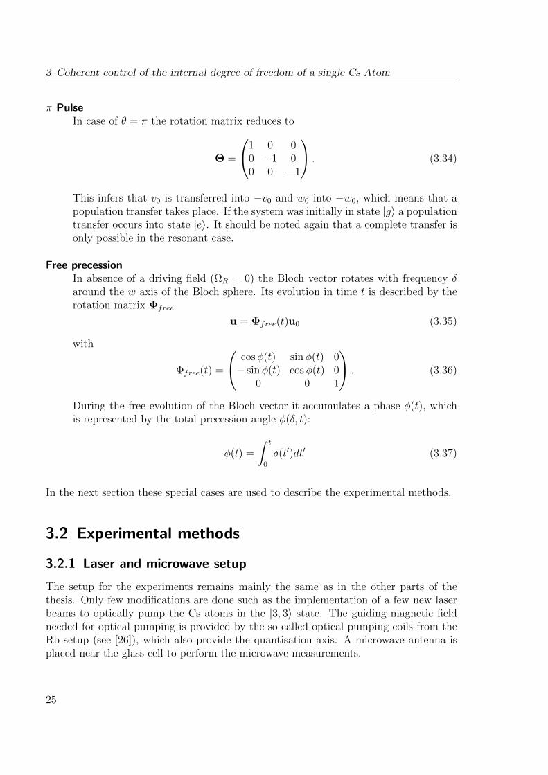
One of the interesting next aims is to investigate the coherence time of a single atomduring the interaction with an ultracold cloud. Therefore, three important requirementshave to be fulfilled. First, the single atom needs to be stored in the same optical trapas the ultracold cloud, so that both systems are combined. In a next step one needsto control the internal degree of freedom of the single atom in order to generate a su-perposition state and in a last step the coherence time of the single atom is studied byRamsey spectroscopy and spin echo measurements.
My thesis will present the experimental realisation and characterisation of all of theseprerequisites necessary for the investigation of the coherence dynamics of single atomsimmersed in a quantum gas: In the first chapter, the traps used to combine the singleCs atom with the ultracold Rb cloud are presented and characterised. Afterwards themethods used to control the internal degree of freedom of the Cs atom, e.g. microwavespectroscopy, are introduced. In the last chapter the coherence time of the generatedsuperposition states is measured.
3
2 Immersion of single Cs atoms intoan ultracold Rb gas
The aim of this thesis is to immerse the single Cs atom into the ultracold Rb cloudand to investigate the coherence properties of the single atom. In order to achieve themixture of both species three different traps are used: a magneto optical trap (MOT),a one dimensional optical lattice and a crossed dipole trap. In this chapter the theoryof these different optical traps is introduced. The reason to use three different traps isexplained and measurements of characteristic parameters are presented.
The description focusses on the involved traps and the preparation of the single atom,because the preparation of the ultracold cloud has already been discussed in great detailin [25] and [26].
2.1 General overview of the traps involved
All experiments are performed in a glass cell, which is part of an ultra high vacuumsystem (pressure inside the system 10−11 mbar), in order to avoid limitations due tobackground gas collisions. Figure 2.1 illustrates the three traps used. In the beginningthe single Cs atoms are stored in a dissipative magneto optical trap (MOT), whereasthe Rb is trapped in a conservative crossed optical dipole trap, from now on referred toas running wave (trap). In order to obtain a high number of Rb atoms in the ultracoldcloud, a large trap volume is desired for the running wave trap.
The single atoms trapped in the MOT have a temperature of a few 100 µK, depend-ing on the alignment of the laser beams. As the Rb is evaporatively cooled the runningwave trap is very shallow. It is therefore not possible to directly transfer the Cs atomsinto running wave trap. Hence, a one dimensional optical lattice, from now on referredto as lattice, is used in an intermediate step. The lattice parameters, e.g. beam waist,wavelength and power, are chosen such that on the one hand a trap depth that allowsto store even very hot atoms from the MOT is obtained and on the other hand Rbis only slightly affected by the lattice potential. After transferring the atoms into thelattice, they are further cooled by adiabatic lowering of the lattice potential down to atemperature suitable to store the atoms in the running wave trap. During that processthe potential of the running wave trap is still present and in a last step the atoms are
2 Immersion of single Cs atoms into an ultracold Rb gas
DT radial
Quadrupole coils
DT axial
Ioffe coil
Dichroic mirror
Lattice beam A
Lattice beam B
Glass cell
MOT cloud
z
y x
Figure 2.1: Schematic overview on the different traps (not true to scale). Few Cs atomsare trapped in the MOT, which is depicted in orange. The MOT is formed within aglass cell, which contains an ultra high vacuum (UHV). An optical lattice (depicted inyellow) is used in an intermediate step to transfer the Cs atoms into the running wavetrap, where the Rb cloud is stored. The lattice is therefore overlapped with the radialbeam of the running wave trap (DT radial). The axial beam (DT axial) is shined inperpendicular to the lattice axis. Additionally, quadrupole coils generating the magneticfield for the MOT and the Ioffe coil used to create a magnetic trap for the ultracold cloudare illustrated.
transferred into the running wave trap by lowering the lattice potential to a zero value.
2.2 Magneto optical trap for single Cs atoms
A magneto optical trap (MOT) uses the technique of laser cooling to cool single atoms[1, 27]. The atoms are cooled by six perpendicular and counter propagating laser beams.The laser beams are red detuned, which together with the Doppler effect causes the atomsto preferably absorb counterpropagating photons. In this process, the atom is given amomentum kick in direction of the photon before absorption. The atom is deexcited bythe spontaneous emission of a photon and because the direction of spontaneous emissionis isotropic, the atoms are cooled by the momentum exchange and pushed towards thecentre of the cooling region.
With this method the atoms are cooled but not trapped to the region of interest. There-fore quadrupole coils are used to generate a magnetic field, which increases with radialdistance to the cooling region. Because of Zeeman splitting, which is proportional tothe magnetic field, the atoms experience a position-depending force towards the coolingregion. The polarisation of the laser beams determines the direction in which the atom
5
2.2 Magneto optical trap for single Cs atoms
Figure 2.2: In the figure on the left, a loading curve of the MOT in high gradient phaseis shown. One can see that only one atom per second is loaded into the MOT. Theright picture illustrates a typical histogram recorded for the Cs MOT with fluorescenceimaging. The fluorescence count rate is related to the number of atoms in the trap. Eachgaussian distribution of fluorescence counts belongs to a specific atom number. Eachdistribution is well separated from its nearest neighbours, enabling a good resolutionwhen counting the number of atoms. In addition the histogram reveals that during theMOT loading phase only up to 5 atoms are trapped. [Pictures: N.Spethmann]
is pushed. Therefore laser beams with opposite handed circular polarisation are used(σ+ and σ− light).
In this experiment the hyperfine states |F = 4〉 and |F ′ = 5〉 of the Cs atom areused as the cooling cycling transition, which leads to a wavelength of 852 nm for thecooling laser. Due to a finite excitation probability into the |F ′ = 4〉 level, the atom maydecay into the |F = 3〉 state and hence no longer participates in the cooling cycle. Inorder to correct this another laser - the repumping laser - is used to transfer the atomsback into the |F ′ = 4〉 state.
There are some possibilities to tune the MOT to only trap single Cs atoms, whichis desired in our experiments. At the beginning of the loading phase, a low magneticfield gradient of 60 G/cm is used for 150 ms to load few atoms into the MOT. Then themagnetic field is increased to about 300 G/cm. With this method and with small MOTbeam diameters, the trapping region is held small and therefore a loading rate of about1 atom/s is achieved. In picture 2.2 a typical trace of the high gradient MOT phase isshown.
The atoms are detected by a sensitive fluorescence imaging system which was builtin a prior Diploma thesis [24]. It consists of an high numerical aperture objective and
6
2 Immersion of single Cs atoms into an ultracold Rb gas
a single photon counting module (SPCM). By illuminating the atoms in the MOT withnear resonant light, they send out fluorescence photons which are collected by the objec-tive an guided through a glass fibre onto the SPCM chip. The chip is sensitive to singlephotons and from the count rate of the chip it is possible to derive the atom number. Arecorded histogram, which is shown in figure 2.2(right), reveals the relation between thefluorescence count rate and the atom number. Typical values for one atom are about800-1000 counts/100 ms depending on the alignment of the MOT position with respectto the imaging system as well as on parameters of the laser beams.
2.3 Optical Lattice
Because of the high temperature of the atoms in the MOT and its dissipative character,it is not possible to directly transfer the atoms into the very shallow potential of therunning wave trap. Hence a one dimensional optical lattice is used to further cool theatoms and to transfer them into the running wave trap. Furthermore the lattice isalso used to recapture the atoms from the running wave trap and reload them into theMOT, where the atoms can be detected again. This is an important step because allour experiments rely on counting the atom number before and after manipulation of theatoms.
2.3.1 Theoretical description
The optical lattice is formed out of two linear polarised counter propagating gaussianlaser beams. Due to the interaction of the red detuned laser beams with the dipole mo-ment of the atom, a row of harmonic potential wells are formed. The distance betweenthese potentials is given by the periodicity of the standing wave (= λopt/2).
The optical lattice is a quantum mechanical effect but nevertheless it may be describedby a classical model. The lattice is comparable to the Lorentz model of a classicaldamped harmonic oscillator which is driven by an external electric field [28, 29]:
E(r, t) = (E0(r) exp(−iωt) + c.c.)/2 . (2.1)
In this model the dipole moment of the atom fulfils the classical equation of motion
d(r, t) + Γωd(r, t) + ω20d(r, t) =
e2
me
E(r, t) , (2.2)
with ω0 the resonance frequency of the oscillator and Γω the damping rate due to theclassical dipole radiation
Γω =e2ω2
6πε0mec3(2.3)
7
2.3 Optical Lattice
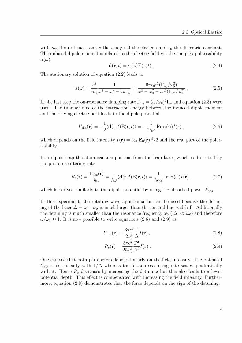
with me the rest mass and e the charge of the electron and ε0 the dielectric constant.The induced dipole moment is related to the electric field via the complex polarisabilityα(ω):
d(r, t) = α(ω)E(r, t) . (2.4)
The stationary solution of equation (2.2) leads to
α(ω) =e2
me
1
ω2 − ω20 − iωΓω
=6πε0c
3(Γω0/ω20)
ω2 − ω20 − iω3(Γω0/ω
20). (2.5)
In the last step the on-resonance damping rate Γω0 = (ω/ω0)2Γω and equation (2.3) wereused. The time average of the interaction energy between the induced dipole momentand the driving electric field leads to the dipole potential
Udip(r) = −1
2〈d(r, t)E(r, t)〉 = − 1
2ε0cReα(ω)I(r) , (2.6)
which depends on the field intensity I(r) = cε0|E0(r)|2/2 and the real part of the polar-isability.
In a dipole trap the atom scatters photons from the trap laser, which is described bythe photon scattering rate
Rs(r) =Pabs(r)
~ω=
1
~ω〈d(r, t)E(r, t)〉 =
1
~ε0cImα(ω)I(r) , (2.7)
which is derived similarly to the dipole potential by using the absorbed power Pabs.
In this experiment, the rotating wave approximation can be used because the detun-ing of the laser ∆ = ω − ω0 is much larger than the natural line width Γ. Additionallythe detuning is much smaller than the resonance frequency ω0 (|∆| ω0) and thereforeω/ω0 ≈ 1. It is now possible to write equations (2.6) and (2.9) as
Udip(r) =3πc2
2ω30
Γ
∆I(r) , (2.8)
Rs(r) =3πc2
2~ω30
Γ2
∆2I(r) . (2.9)
One can see that both parameters depend linearly on the field intensity. The potentialUdip scales linearly with 1/∆ whereas the photon scattering rate scales quadraticallywith it. Hence Rs decreases by increasing the detuning but this also leads to a lowerpotential depth. This effect is compensated with increasing the field intensity. Further-more, equation (2.8) demonstrates that the force depends on the sign of the detuning.
8
2 Immersion of single Cs atoms into an ultracold Rb gas
Ti:Sa System To
Experiment
(a)
Glass Cell (UHV)
(b)
Fibre Coupler
Lens Shutter QWP Mirror Dichroic Mirror
Pol. Optics 850 nm & 900 nm
PBS
HWP
AOM Optical Isolator
Figure 2.3: (Figure not true to scale.)(a) Schematic sketch of the optical setup for thelattice before the light is guided to the experimental table. The laser light is generatedby a Ti:Sa system. It passes first an optical isolator and is then splitted into twodifferent beams by use of a quarter wave plate (QWP) and a polarising beam splittercube (PBS). With an acousto-optic modulator (AOM) the power of each beam, whichis transmitted via single-mode-polarisation-maintaining-fibres to the main experimentaltable, is stabilised. A telescope is used to focus the beam in order to achieve a highcoupling efficiency into the fibre. (b) Setup for the lattice on the experimental table.The polarisation of the beams is increased by use of a half wave plate (HWP) and aPBS. With dichroic mirrors the beams are coupled into the glass cell and a lens focussesthe beams down to 31 µm at the position of the atoms.
The trap frequencies, which are the oscillation frequencies of the atom in the trap,in axial and radial direction are given by
ωrad =
(4U0
mw20
)1/2
(2.10)
ωax =
(2U0
mz20
)1/2
. (2.11)
Here w0 denotes the beam waist and z0 the Rayleigh length of the beam described inGaussian optics (details on Gaussian optics can be found in [30]).
2.3.2 Experimental Setup
In order to generate the lattice potential a commercially available Titanium:sapphire(Ti:Sa) laser (Model: Microlase MBR-110) was aligned during this thesis. It is pumpedby a frequency doubled Neodym:YAG laser (Spectra Physics MilleniaX) which deliversa power of 10 W at a wavelength of 532 nm. This leads to an output power of 700
9
2.3 Optical Lattice
mW for the Ti:Sa laser operating at a wavelength of 899.9 nm. The wavelength dif-fers by only 5.3 nm from the Cs D1 line [31] leading to a photon scattering rate of afew 100 Hz, which is the limiting factor for the longitudinal relaxation time T1 (see sec.4.2). However, the chosen wavelength provides the desired trap depth for the Cs atomsand at the same time does not disturb the Rb. For more details on this point see [24, 32].
A schematic view on the optical path, which was set up during the thesis is shownin figure 2.3. After passing an optical isolator (Newport) the laser beam is divided intotwo beams, each containing roughly half of the laser power. In using a setup consistingof a half wave plate (HP) and a polarising beam splitter cube (PBS) one is able tochange the power distribution of the beams. With acousto-optic modulators (AOM) thepower is actively stabilised and controlled by an electronical feedback loop. By meansof single-mode-polarisation-maintaining-fibres the light is guided to the vacuum setupand is coupled into the vacuum chamber via dichroic mirrors, which transmit light of860 nm and lower but are reflective for wavelengths greater than 860 nm. Afterwardsthe light passes a lens to focus the beam to a waist of w0 = 31 µm at the position ofthe atoms. After passing all optical components, a maximum laser power of 150 mW ineach beam is achieved.
To be sure that both beams perfectly overlap, one beam was coupled into the fibreoutput of the other beam. In this case a coupling efficiency of 65% from one fibre intothe other is achieved. The deviation from unity arises due to aberration caused by theoptical elements in the beam path (see fig. 2.3) which affects the coupling efficiency.
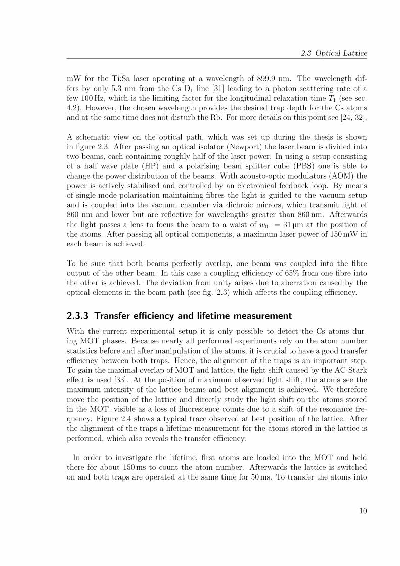
2.3.3 Transfer efficiency and lifetime measurement
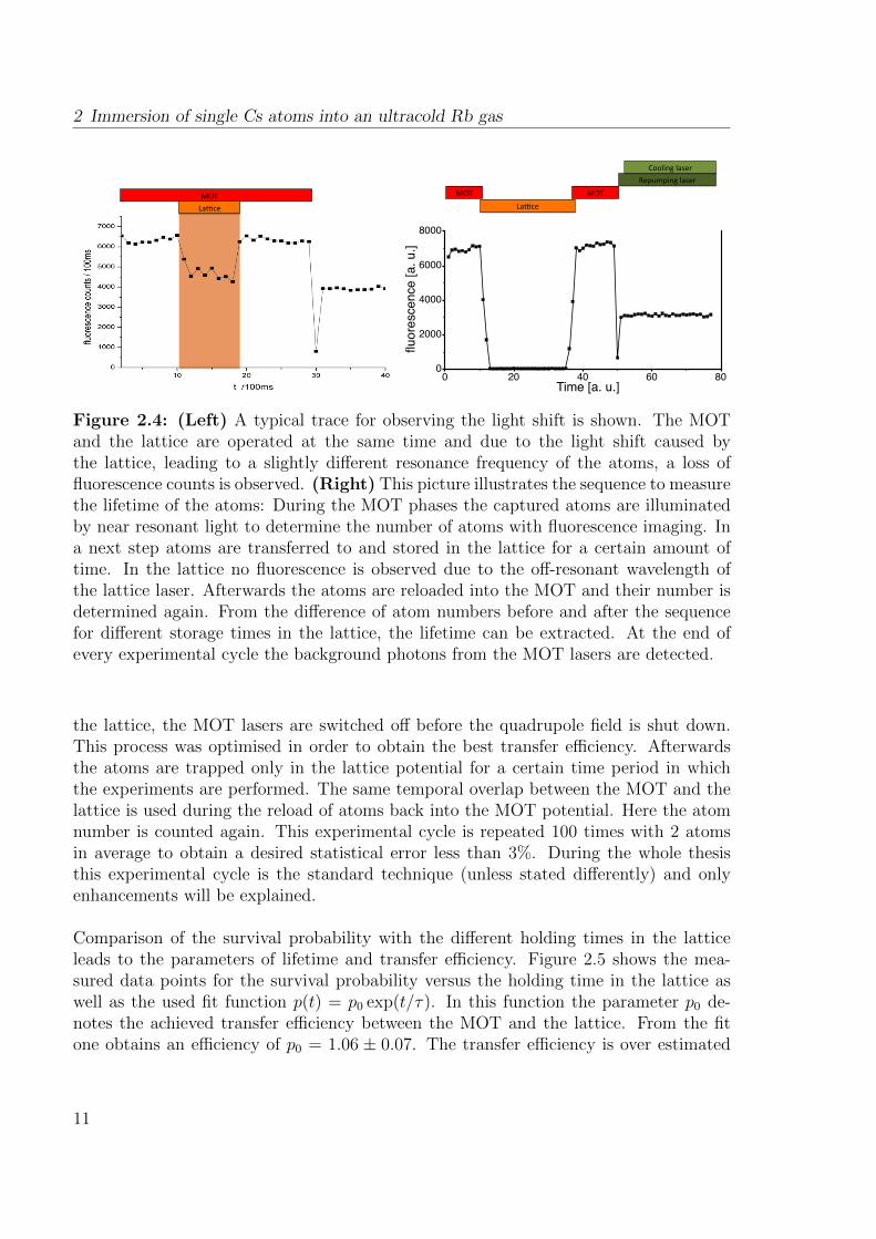
With the current experimental setup it is only possible to detect the Cs atoms dur-ing MOT phases. Because nearly all performed experiments rely on the atom numberstatistics before and after manipulation of the atoms, it is crucial to have a good transferefficiency between both traps. Hence, the alignment of the traps is an important step.To gain the maximal overlap of MOT and lattice, the light shift caused by the AC-Starkeffect is used [33]. At the position of maximum observed light shift, the atoms see themaximum intensity of the lattice beams and best alignment is achieved. We thereforemove the position of the lattice and directly study the light shift on the atoms storedin the MOT, visible as a loss of fluorescence counts due to a shift of the resonance fre-quency. Figure 2.4 shows a typical trace observed at best position of the lattice. Afterthe alignment of the traps a lifetime measurement for the atoms stored in the lattice isperformed, which also reveals the transfer efficiency.
In order to investigate the lifetime, first atoms are loaded into the MOT and heldthere for about 150 ms to count the atom number. Afterwards the lattice is switchedon and both traps are operated at the same time for 50 ms. To transfer the atoms into
10
2 Immersion of single Cs atoms into an ultracold Rb gas
MOT La'ce
MOT
La'ce
MOT Repumping laser
Cooling laser
0 20 40 60 800
2000
4000
6000
8000
Time [a. u.]
fl
uore
scen
ce [a
. u.]
Figure 2.4: (Left) A typical trace for observing the light shift is shown. The MOTand the lattice are operated at the same time and due to the light shift caused bythe lattice, leading to a slightly different resonance frequency of the atoms, a loss offluorescence counts is observed. (Right) This picture illustrates the sequence to measurethe lifetime of the atoms: During the MOT phases the captured atoms are illuminatedby near resonant light to determine the number of atoms with fluorescence imaging. Ina next step atoms are transferred to and stored in the lattice for a certain amount oftime. In the lattice no fluorescence is observed due to the off-resonant wavelength ofthe lattice laser. Afterwards the atoms are reloaded into the MOT and their number isdetermined again. From the difference of atom numbers before and after the sequencefor different storage times in the lattice, the lifetime can be extracted. At the end ofevery experimental cycle the background photons from the MOT lasers are detected.
the lattice, the MOT lasers are switched off before the quadrupole field is shut down.This process was optimised in order to obtain the best transfer efficiency. Afterwardsthe atoms are trapped only in the lattice potential for a certain time period in whichthe experiments are performed. The same temporal overlap between the MOT and thelattice is used during the reload of atoms back into the MOT potential. Here the atomnumber is counted again. This experimental cycle is repeated 100 times with 2 atomsin average to obtain a desired statistical error less than 3%. During the whole thesisthis experimental cycle is the standard technique (unless stated differently) and onlyenhancements will be explained.
Comparison of the survival probability with the different holding times in the latticeleads to the parameters of lifetime and transfer efficiency. Figure 2.5 shows the mea-sured data points for the survival probability versus the holding time in the lattice aswell as the used fit function p(t) = p0 exp(t/τ). In this function the parameter p0 de-notes the achieved transfer efficiency between the MOT and the lattice. From the fitone obtains an efficiency of p0 = 1.06 ± 0.07. The transfer efficiency is over estimated
11
2.3 Optical Lattice
0 1 2 3 4 5 6 7 8storage time [s]
0.0
0.2
0.4
0.6
0.8
1.0
1.2
surv
ival pro
babili
ty
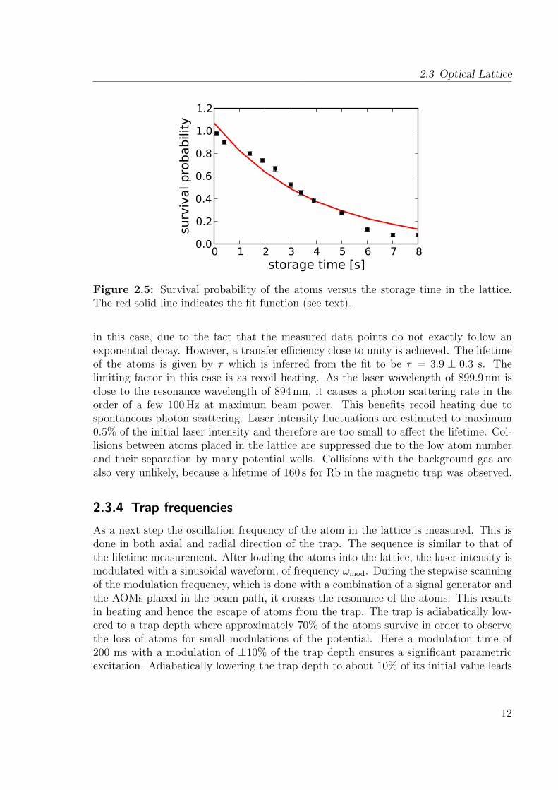
Figure 2.5: Survival probability of the atoms versus the storage time in the lattice.The red solid line indicates the fit function (see text).
in this case, due to the fact that the measured data points do not exactly follow anexponential decay. However, a transfer efficiency close to unity is achieved. The lifetimeof the atoms is given by τ which is inferred from the fit to be τ = 3.9 ± 0.3 s. Thelimiting factor in this case is as recoil heating. As the laser wavelength of 899.9 nm isclose to the resonance wavelength of 894 nm, it causes a photon scattering rate in theorder of a few 100 Hz at maximum beam power. This benefits recoil heating due tospontaneous photon scattering. Laser intensity fluctuations are estimated to maximum0.5% of the initial laser intensity and therefore are too small to affect the lifetime. Col-lisions between atoms placed in the lattice are suppressed due to the low atom numberand their separation by many potential wells. Collisions with the background gas arealso very unlikely, because a lifetime of 160 s for Rb in the magnetic trap was observed.
2.3.4 Trap frequencies
As a next step the oscillation frequency of the atom in the lattice is measured. This isdone in both axial and radial direction of the trap. The sequence is similar to that ofthe lifetime measurement. After loading the atoms into the lattice, the laser intensity ismodulated with a sinusoidal waveform, of frequency ωmod. During the stepwise scanningof the modulation frequency, which is done with a combination of a signal generator andthe AOMs placed in the beam path, it crosses the resonance of the atoms. This resultsin heating and hence the escape of atoms from the trap. The trap is adiabatically low-ered to a trap depth where approximately 70% of the atoms survive in order to observethe loss of atoms for small modulations of the potential. Here a modulation time of200 ms with a modulation of ±10% of the trap depth ensures a significant parametricexcitation. Adiabatically lowering the trap depth to about 10% of its initial value leads
12
2 Immersion of single Cs atoms into an ultracold Rb gas
260 280 300 320 340modulation frequency / kHz
0.2
0.3
0.4
0.5
0.6
0.7
surv
ival pro
babili
ty
1 2 3 4 5 6modulation frequency / kHz
0.1
0.2
0.3
0.4
0.5
surv
ival pro
babili
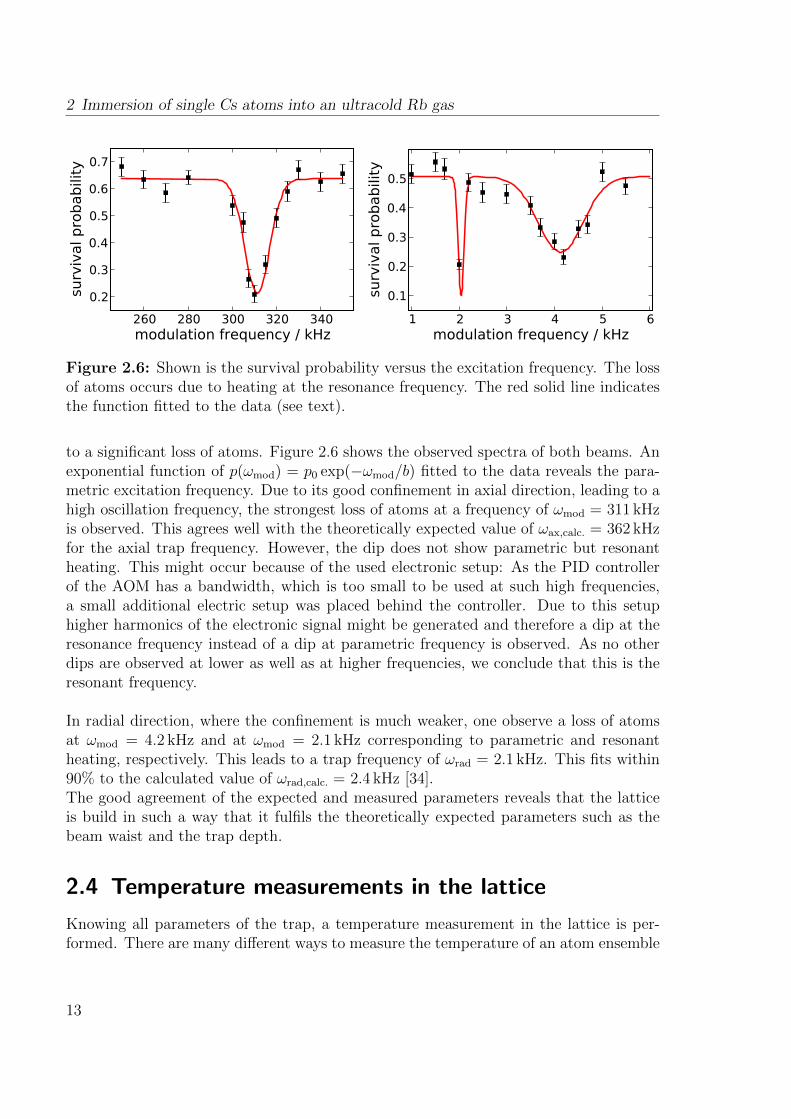
tyFigure 2.6: Shown is the survival probability versus the excitation frequency. The lossof atoms occurs due to heating at the resonance frequency. The red solid line indicatesthe function fitted to the data (see text).
to a significant loss of atoms. Figure 2.6 shows the observed spectra of both beams. Anexponential function of p(ωmod) = p0 exp(−ωmod/b) fitted to the data reveals the para-metric excitation frequency. Due to its good confinement in axial direction, leading to ahigh oscillation frequency, the strongest loss of atoms at a frequency of ωmod = 311 kHzis observed. This agrees well with the theoretically expected value of ωax,calc. = 362 kHzfor the axial trap frequency. However, the dip does not show parametric but resonantheating. This might occur because of the used electronic setup: As the PID controllerof the AOM has a bandwidth, which is too small to be used at such high frequencies,a small additional electric setup was placed behind the controller. Due to this setuphigher harmonics of the electronic signal might be generated and therefore a dip at theresonance frequency instead of a dip at parametric frequency is observed. As no otherdips are observed at lower as well as at higher frequencies, we conclude that this is theresonant frequency.
In radial direction, where the confinement is much weaker, one observe a loss of atomsat ωmod = 4.2 kHz and at ωmod = 2.1 kHz corresponding to parametric and resonantheating, respectively. This leads to a trap frequency of ωrad = 2.1 kHz. This fits within90% to the calculated value of ωrad,calc. = 2.4 kHz [34].The good agreement of the expected and measured parameters reveals that the latticeis build in such a way that it fulfils the theoretically expected parameters such as thebeam waist and the trap depth.
2.4 Temperature measurements in the lattice
Knowing all parameters of the trap, a temperature measurement in the lattice is per-formed. There are many different ways to measure the temperature of an atom ensemble
13
2.4 Temperature measurements in the lattice
0 20 40 60 800
2000
4000
6000
8000
Time [a. u.]
fl
uore
scen
ce [a
. u.]
MOT
La'ce
MOT Repumping laser
Cooling laser
La'ce
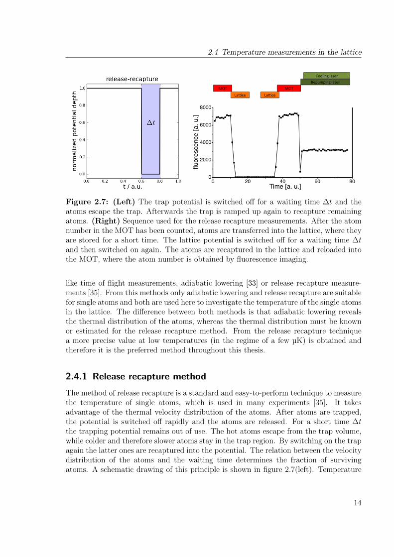
Figure 2.7: (Left) The trap potential is switched off for a waiting time ∆t and theatoms escape the trap. Afterwards the trap is ramped up again to recapture remainingatoms. (Right) Sequence used for the release recapture measurements. After the atomnumber in the MOT has been counted, atoms are transferred into the lattice, where theyare stored for a short time. The lattice potential is switched off for a waiting time ∆tand then switched on again. The atoms are recaptured in the lattice and reloaded intothe MOT, where the atom number is obtained by fluorescence imaging.
like time of flight measurements, adiabatic lowering [33] or release recapture measure-ments [35]. From this methods only adiabatic lowering and release recapture are suitablefor single atoms and both are used here to investigate the temperature of the single atomsin the lattice. The difference between both methods is that adiabatic lowering revealsthe thermal distribution of the atoms, whereas the thermal distribution must be knownor estimated for the release recapture method. From the release recapture techniquea more precise value at low temperatures (in the regime of a few µK) is obtained andtherefore it is the preferred method throughout this thesis.
2.4.1 Release recapture method
The method of release recapture is a standard and easy-to-perform technique to measurethe temperature of single atoms, which is used in many experiments [35]. It takesadvantage of the thermal velocity distribution of the atoms. After atoms are trapped,the potential is switched off rapidly and the atoms are released. For a short time ∆tthe trapping potential remains out of use. The hot atoms escape from the trap volume,while colder and therefore slower atoms stay in the trap region. By switching on the trapagain the latter ones are recaptured into the potential. The relation between the velocitydistribution of the atoms and the waiting time determines the fraction of survivingatoms. A schematic drawing of this principle is shown in figure 2.7(left). Temperature
14
2 Immersion of single Cs atoms into an ultracold Rb gas
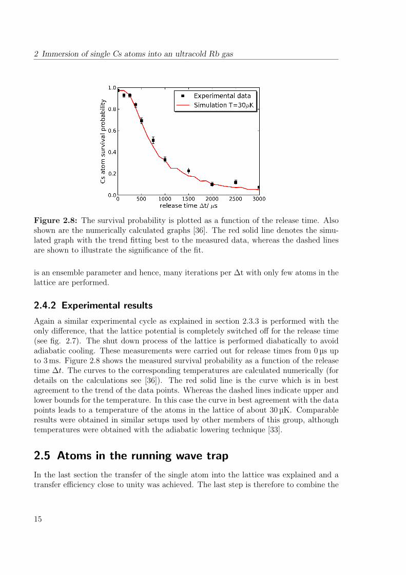
Figure 2.8: The survival probability is plotted as a function of the release time. Alsoshown are the numerically calculated graphs [36]. The red solid line denotes the simu-lated graph with the trend fitting best to the measured data, whereas the dashed linesare shown to illustrate the significance of the fit.
is an ensemble parameter and hence, many iterations per ∆t with only few atoms in thelattice are performed.
2.4.2 Experimental results
Again a similar experimental cycle as explained in section 2.3.3 is performed with theonly difference, that the lattice potential is completely switched off for the release time(see fig. 2.7). The shut down process of the lattice is performed diabatically to avoidadiabatic cooling. These measurements were carried out for release times from 0 µs upto 3 ms. Figure 2.8 shows the measured survival probability as a function of the releasetime ∆t. The curves to the corresponding temperatures are calculated numerically (fordetails on the calculations see [36]). The red solid line is the curve which is in bestagreement to the trend of the data points. Whereas the dashed lines indicate upper andlower bounds for the temperature. In this case the curve in best agreement with the datapoints leads to a temperature of the atoms in the lattice of about 30 µK. Comparableresults were obtained in similar setups used by other members of this group, althoughtemperatures were obtained with the adiabatic lowering technique [33].
2.5 Atoms in the running wave trap
In the last section the transfer of the single atom into the lattice was explained and atransfer efficiency close to unity was achieved. The last step is therefore to combine the
15
2.5 Atoms in the running wave trap
0 20 40 60 800
2000
4000
6000
8000
Time [a. u.]
fluo
resc
ence
[a. u
.]
MOT MOT Repumping laser
Cooling laser
Dipole trap
80 40 0 40 80z-position offset / µm
0.0
0.2
0.4
0.6
0.8
1.0
surv
ival pro
babili
ty
Figure 2.9: (Left) Sequence used to transfer the atom into the running wave trap. Theprocess remains the same for the MOT and the lattice, except that during the latticephase the running wave trap potential is already present. With adiabatic lowering ofthe lattice, which cools the atoms, the transfer into the running wave trap takes place.(Right) Survival probability of the Cs atoms loaded into the running wave trap versusthe position offset of the axial beam in z direction
single Cs atom and the ultracold cloud in the running wave trap.
2.5.1 Experimental setup
Two perpendicular aligned laser beams form the optical dipole trap, generated by a fibreamplifier system at 1064 nm. It consist of a seed laser (CrystaLaser) with a power ofa few 100 mW and a fibre amplifier (Nufern Laser) delivering a power of 10 W. With apolarising beam splitter cube and a half wave plate, allowing a variable power splitting,the power is divided into two beams. Both beams pass a shutter and an AOM, whichis used to control the beam power, before the beams are guided via a special glass fibrefor high light intensities (Liekki) to the experimental table (Details on this setup see[26]). One beam, called axial beam (see fig. 2.1, is focussed through the Ioffe coil, whichis part of the QUIC trap [37] to generate the ultracold cloud (see [25, 26]), and has abeam waist of 100 µm. Using a dichroic mirror the radial beam is coupled onto the sameaxis as the lattice and is focussed down to a beam waist of 48 µm. This ensures highspatial overlap of the beam with the lattice and thus a high transfer efficiency. In theexperiments we use a power of 2 W in the axial direction and a power of 0.6 W in radialdirection (unless stated differently). With the mentioned parameters we obtain a trapdepth of ≈ 100 µK for the Cs atoms in the dipole trap.
16
2 Immersion of single Cs atoms into an ultracold Rb gas
Figure 2.10: Survival probability versus release time in the running wave trap. Theblack squares are the measured data points and the red solid line indicates the simulatedgraph with the trend fitting best to the measured data.
2.5.2 Transfer and temperature measurement of single atoms inthe running wave trap
A crucial step during the sequence is to transfer the atoms from the lattice into therunning wave trap. Hence, a good spatial overlap of both traps is needed to avoid atomlosses. As already mentioned in the last section, the lattice and the radial beam ofthe dipole trap are operated on the same experimental axis, which allows to couple thedipole trap beam into the fibre of one lattice beam (see fig. 2.3 and fig. 2.1), whichresults in a good spatial overlap of both beams. Because the lattice is well alignedwith respect to the MOT, overlapping one beam of the running wave trap with the lat-tice simultaneously guarantees a well aligned overlap of the running wave with the MOT.
For the axial beam of the trap, a measurement was performed to find the best posi-tion, which is defined as the position where the maximal transfer efficiency for the Csatoms occurs. The transfer efficiency was measured at different voltages of a piezo elec-tric mirror, resulting in slightly different positions in z direction of the dipole trap (seefig. 2.9).
The experimental sequence is performed as follows (see also fig. 2.9):
1. A few atoms are stored in the lattice and at the same time the running wave trap isramped up to its full power.
2. Then the lattice is adiabatically lowered within a few ms leading to further cooling
17
2.5 Atoms in the running wave trap
of the atoms.
3. At a certain lattice depth, the Cs atoms leave the trap and are from now on storedin the crossed dipole trap.
At the point of best alignment a transfer efficiency of ≈ 93% is achieved. With thealready explained technique of a release recapture, one experimentally measures a tem-perature of 4.6 µK for the single atoms in the running wave trap (see fig 2.10). Thelower temperature occurs due to the adiabatic lowering of the lattice, which results incooling of the single atom. For more details on the transfer of Cs atoms, when Rb inthe running wave is present, see [34].
18

2 Immersion of single Cs atoms into an ultracold Rb gas
19
3 Coherent control of the internaldegree of freedom of a single CsAtom
In the previous chapter, the experimental procedure to store the single Cs atom in thesame trap as the ultracold Rb cloud was discussed. The next step is to investigate thecoherence time of the single atom. Therefore it is necessary to control its internal degreeof freedom. This is only possible in the lattice or the running wave trap, because of theirconservative and state preservative potential.
The desired state for the Cs atom is the |F = 3,mf = 3〉 state, which is the absoluteground state so that no decay channels for Cs-Rb collisions exist (Note that Cs-Rb-Rbcollisions are still possible). Optical pumping [38, 39] is used to prepare the atoms inthe desired state |3, 3〉.
In order to generate a superposition state, of which the coherence time is investigated,the transition between |3, 3〉 and |4, 2〉 is driven by a microwave pulse. The |4, 2〉 stateis chosen, because it provides the longest coherence time in combination with the |3, 3〉state. This is required if one wants to investigate the cooling of the superposition state,where the thermalisation time is in the order of 25 ms [36]. By the use of methods suchas microwave spectroscopy and driven Rabi oscillations, the control parameters for theinternal degree of freedom are studied.
The interaction between the single atom and the microwave radiation field and its dy-namical evolution is to good approximation described by the semiclassical Bloch vectormodel. In this model the classically treated radiation field interacts with a quantummechanical two level atom.
A variant of the Bloch equations [40], namely the optical Bloch equations are a sys-tem of three differential equations. They delineate the evolution of the Bloch vector onthe Bloch sphere, which is comparable to the dynamical evolution of a spin-1/2 systemin presence of a magnetic field. Here the dynamical evolution of a pseudo spin systemwith the atomic polarisation and the population difference as the components of thevector is used instead. In the next chapters the Bloch vector model is extensively used
3 Coherent control of the internal degree of freedom of a single Cs Atom
to describe the experimental processes.
3.1 Optical Bloch equations
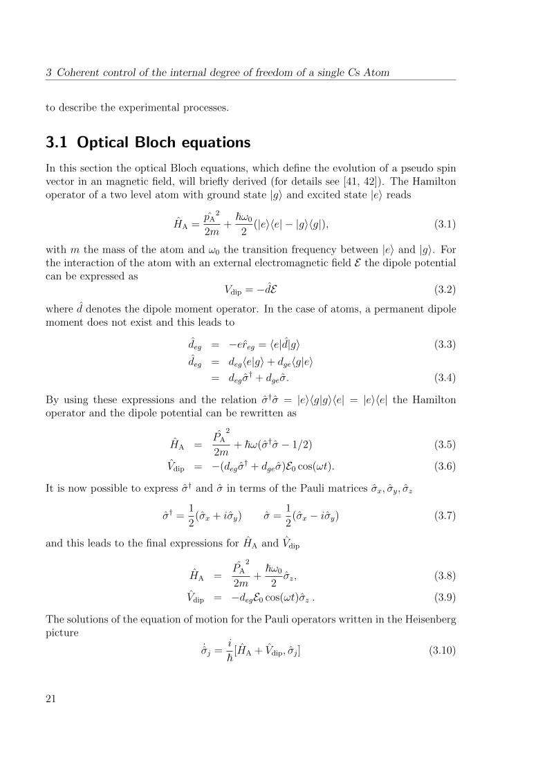
In this section the optical Bloch equations, which define the evolution of a pseudo spinvector in an magnetic field, will briefly derived (for details see [41, 42]). The Hamiltonoperator of a two level atom with ground state |g〉 and excited state |e〉 reads
HA =pA
2
2m+
~ω0
2(|e〉〈e| − |g〉〈g|), (3.1)
with m the mass of the atom and ω0 the transition frequency between |e〉 and |g〉. Forthe interaction of the atom with an external electromagnetic field E the dipole potentialcan be expressed as
Vdip = −dE (3.2)
where d denotes the dipole moment operator. In the case of atoms, a permanent dipolemoment does not exist and this leads to
deg = −ereg = 〈e|d|g〉 (3.3)
deg = deg〈e|g〉+ dge〈g|e〉= degσ
† + dgeσ. (3.4)
By using these expressions and the relation σ†σ = |e〉〈g|g〉〈e| = |e〉〈e| the Hamiltonoperator and the dipole potential can be rewritten as
HA =PA
2
2m+ ~ω(σ†σ − 1/2) (3.5)
Vdip = −(degσ† + dgeσ)E0 cos(ωt). (3.6)
It is now possible to express σ† and σ in terms of the Pauli matrices σx, σy, σz
σ† =1
2(σx + iσy) σ =
1
2(σx − iσy) (3.7)
and this leads to the final expressions for HA and Vdip
HA =PA
2
2m+
~ω0
2σz, (3.8)
Vdip = −degE0 cos(ωt)σz . (3.9)
The solutions of the equation of motion for the Pauli operators written in the Heisenbergpicture
˙σj =i
~[HA + Vdip, σj] (3.10)
21
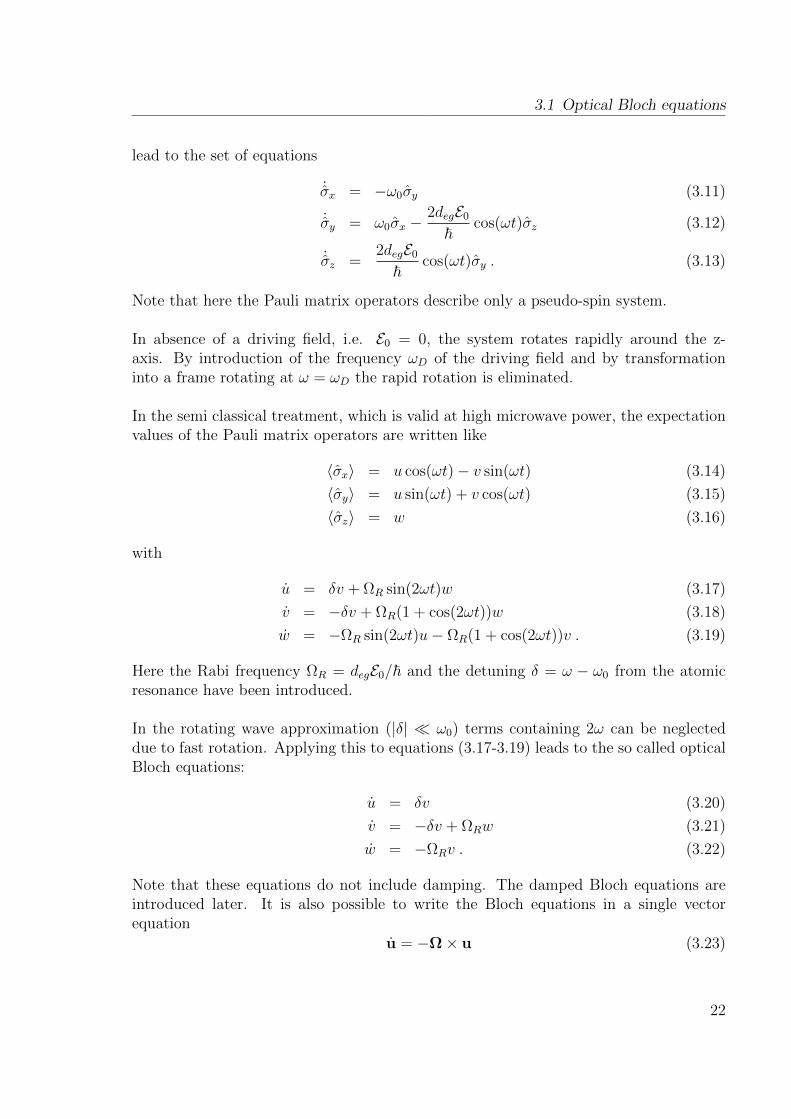
3.1 Optical Bloch equations
lead to the set of equations
˙σx = −ω0σy (3.11)
˙σy = ω0σx −2degE0
~cos(ωt)σz (3.12)
˙σz =2degE0
~cos(ωt)σy . (3.13)
Note that here the Pauli matrix operators describe only a pseudo-spin system.
In absence of a driving field, i.e. E0 = 0, the system rotates rapidly around the z-axis. By introduction of the frequency ωD of the driving field and by transformationinto a frame rotating at ω = ωD the rapid rotation is eliminated.
In the semi classical treatment, which is valid at high microwave power, the expectationvalues of the Pauli matrix operators are written like
〈σx〉 = u cos(ωt)− v sin(ωt) (3.14)
〈σy〉 = u sin(ωt) + v cos(ωt) (3.15)
〈σz〉 = w (3.16)
with
u = δv + ΩR sin(2ωt)w (3.17)
v = −δv + ΩR(1 + cos(2ωt))w (3.18)
w = −ΩR sin(2ωt)u− ΩR(1 + cos(2ωt))v . (3.19)
Here the Rabi frequency ΩR = degE0/~ and the detuning δ = ω − ω0 from the atomicresonance have been introduced.
In the rotating wave approximation (|δ| ω0) terms containing 2ω can be neglecteddue to fast rotation. Applying this to equations (3.17-3.19) leads to the so called opticalBloch equations:
u = δv (3.20)
v = −δv + ΩRw (3.21)
w = −ΩRv . (3.22)
Note that these equations do not include damping. The damped Bloch equations areintroduced later. It is also possible to write the Bloch equations in a single vectorequation
u = −Ω× u (3.23)
22
3 Coherent control of the internal degree of freedom of a single Cs Atom
with the torque vector Ω = (ΩR, 0, 0) and the so called Bloch vector u = (u, v, w). Incase of the undamped Bloch equations the Bloch vector has unit length and its evolutionlies on a unit sphere. A magnetic dipole transition is to good approximation described bythe Bloch equations. In this case the u and v components of the Bloch vector delineatethe components of the magnetic dipole moment which are in phase and in quadraturewith the driving field E , respectively. Furthermore equation (3.22) infers that u is thedispersive component of the dipole moment and v is the absorptive component. Thepopulation number difference of the two states is given by w and only one state is pop-ulated in case of w = ±1.
It is also possible two write the Bloch vector in other representations of the two levelatom. A very common one is the state vector representation. The derivation of thetransformation into the corresponding state vector is not shown here (see [42]) but thevery descriptive solution is presented:
u = sinϑ cosφ (3.24)
v = sinϑ sinφ (3.25)
w = cosϑ . (3.26)
Here ϑ describes the angle of the Bloch vector with the w-axis and φ describes its positionin the uv-plane.
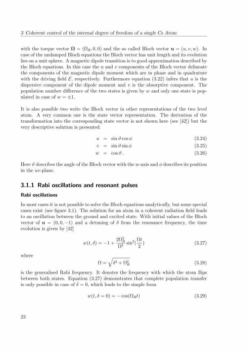
3.1.1 Rabi oscillations and resonant pulses
Rabi oscillations
In most cases it is not possible to solve the Bloch equations analytically, but some specialcases exist (see figure 3.1). The solution for an atom in a coherent radiation field leadsto an oscillation between the ground and excited state. With initial values of the Blochvector of u = (0, 0,−1) and a detuning of δ from the resonance frequency, the timeevolution is given by [42]
w(t, δ) = −1 +2Ω2
R
Ω2sin2(
Ωt
2) (3.27)
where
Ω =√δ2 + Ω2
R (3.28)
is the generalised Rabi frequency. It denotes the frequency with which the atom flipsbetween both states. Equation (3.27) demonstrates that complete population transferis only possible in case of δ = 0, which leads to the simple form
w(t, δ = 0) = − cos(ΩRt) (3.29)
23
3.1 Optical Bloch equations
w
v u
w
v u
w
v u
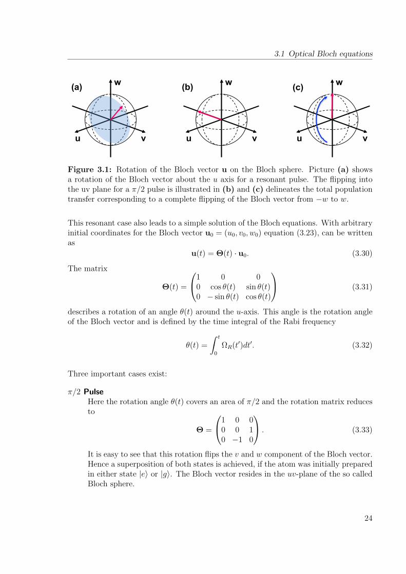
(a) (b) (c)
Figure 3.1: Rotation of the Bloch vector u on the Bloch sphere. Picture (a) showsa rotation of the Bloch vector about the u axis for a resonant pulse. The flipping intothe uv plane for a π/2 pulse is illustrated in (b) and (c) delineates the total populationtransfer corresponding to a complete flipping of the Bloch vector from −w to w.
This resonant case also leads to a simple solution of the Bloch equations. With arbitraryinitial coordinates for the Bloch vector u0 = (u0, v0, w0) equation (3.23), can be writtenas
u(t) = Θ(t) · u0. (3.30)
The matrix
Θ(t) =
1 0 00 cos θ(t) sin θ(t)0 − sin θ(t) cos θ(t)
(3.31)
describes a rotation of an angle θ(t) around the u-axis. This angle is the rotation angleof the Bloch vector and is defined by the time integral of the Rabi frequency
θ(t) =
∫ t
0
ΩR(t′)dt′. (3.32)
Three important cases exist:
π/2 PulseHere the rotation angle θ(t) covers an area of π/2 and the rotation matrix reducesto
Θ =
1 0 00 0 10 −1 0
. (3.33)
It is easy to see that this rotation flips the v and w component of the Bloch vector.Hence a superposition of both states is achieved, if the atom was initially preparedin either state |e〉 or |g〉. The Bloch vector resides in the uv-plane of the so calledBloch sphere.
24
3 Coherent control of the internal degree of freedom of a single Cs Atom
π PulseIn case of θ = π the rotation matrix reduces to
Θ =
1 0 00 −1 00 0 −1
. (3.34)
This infers that v0 is transferred into −v0 and w0 into −w0, which means that apopulation transfer takes place. If the system was initially in state |g〉 a populationtransfer occurs into state |e〉. It should be noted again that a complete transfer isonly possible in the resonant case.
Free precessionIn absence of a driving field (ΩR = 0) the Bloch vector rotates with frequency δaround the w axis of the Bloch sphere. Its evolution in time t is described by therotation matrix Φfree
u = Φfree(t)u0 (3.35)
with
Φfree(t) =
cosφ(t) sinφ(t) 0− sinφ(t) cosφ(t) 0
0 0 1
. (3.36)
During the free evolution of the Bloch vector it accumulates a phase φ(t), whichis represented by the total precession angle φ(δ, t):
φ(t) =
∫ t
0
δ(t′)dt′ (3.37)
In the next section these special cases are used to describe the experimental methods.
3.2 Experimental methods
3.2.1 Laser and microwave setup
The setup for the experiments remains mainly the same as in the other parts of thethesis. Only few modifications are done such as the implementation of a few new laserbeams to optically pump the Cs atoms in the |3, 3〉 state. The guiding magnetic fieldneeded for optical pumping is provided by the so called optical pumping coils from theRb setup (see [26]), which also provide the quantisation axis. A microwave antenna isplaced near the glass cell to perform the microwave measurements.
25
3.2 Experimental methods
Laser system
In addition to the MOT beams, the lattice and the running wave trap, optical pumpingbeams and a so called push out beam are implemented in the main setup.
MOT laser As in the previous chapters, the closed transition of F = 4 to F ′ = 5 isused as the cooling transition. The laser power is provided by a Tapered Amplifiersystem (Sacher Lasersystems), which is locked onto the F = 4 to F ′ = 3 transitionby polarisation spectroscopy. In order to obtain the desired transition the laserfrequency is shifted by an AOM, which is also used to control the atom numberand the fluorescence per atom during the experimental cycle. The repumping laserruns on the F = 3 to F ′ = 4 transition and pumps the lost atoms in F = 3 backinto the cooling cycle. It is overlapped with the cooling laser beam via a PBS andtransmitted to the experiment by the same fibre.
Optical pumping beam The optical pumping of Cs is performed with two differentbeams. For the first beam a diode laser, which is locked onto the F = 4 tocrossover F ′ = 4/5 transition, is used. With an AOM the frequency is shifted by125.5 MHz to the frequency of the F = 4 to F ′ = 4 transition. The beam is shinedin on the lattice axis using π-polarised light.The second beam is realised in diverting part of the light of the repumping laser,which is then frequency shifted to the F = 3 to F ′ = 3 transition. This laser isshined in along the axis of the radial dipole trap beam and consists of σ+-polarisedlight.
Push out beam For state selective detection it is important to remove the atoms whichare not in the state of interest. Therefore the so called push out laser which runson the F = 4 to F ′ = 5 transition is used. It removes all atoms in the F = 4state but leaves the atoms in F = 3 unaffected. The beam is provided by the samelaser which is used for the first optical pumping beam. In this case the frequencyis shifted with a double pass setup of the AOM. This beam is overlapped with thesecond beam of the optical pumping and is therefore shined in on the radial axisof the dipole trap.
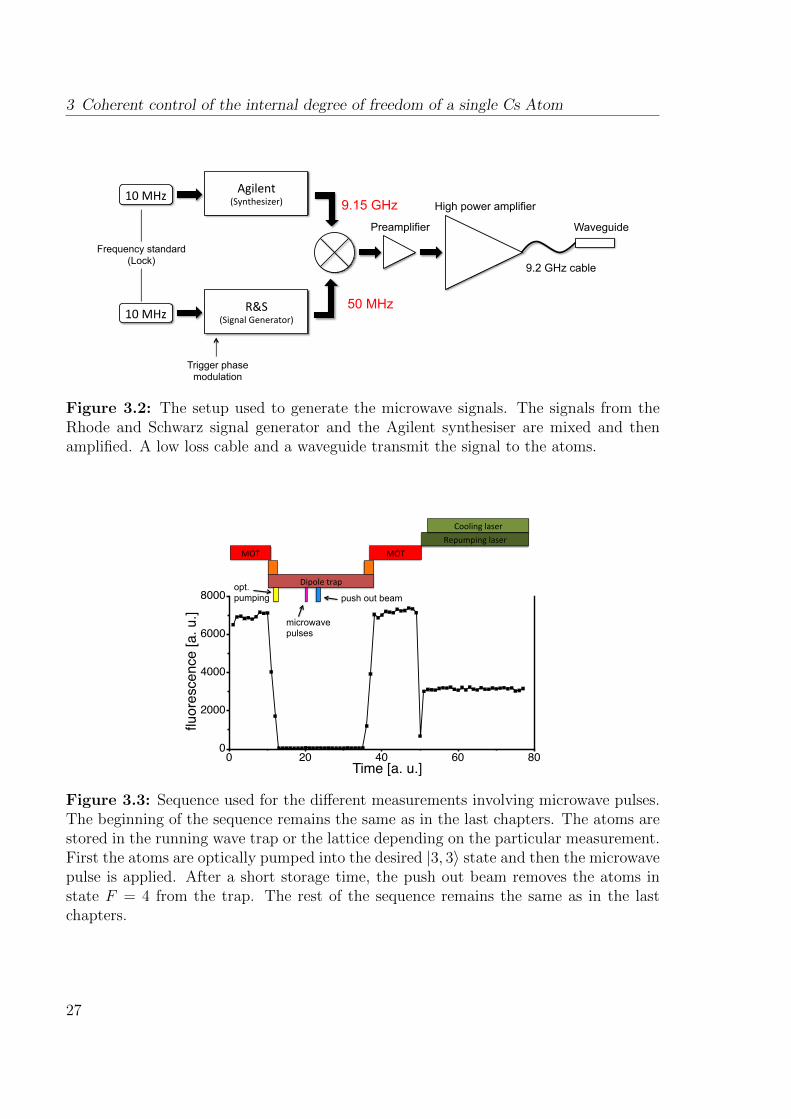
Microwave setup
The ground state hyperfine splitting between F = 3 and F = 4 of Cs is nearly 9.2 GHz[31]. In order to generate the microwave pulses a synthesiser (Agilent 83751A, 0.01-20GHz, from now on referred to as synthesiser) is used, which is connected to the LO-Inputof the mixer (Mixer model: Mini Circuits ZMX-10G+, 3700-10000 MHz) and the signalis then mixed with 50 MHz (IF-Input of the Mixer) from a Rhode and Schwarz signalgenerator (from now on referred to as signal generator). Both, the signal generator andthe synthesiser are locked onto the 10 MHz Rubidium frequency standard. For Ramsey
26
3 Coherent control of the internal degree of freedom of a single Cs Atom
10 MHz Agilent (Synthesizer)
10 MHz R&S (Signal Generator)
50 MHz
9.15 GHz Preamplifier
High power amplifier
Waveguide
9.2 GHz cable
Frequency standard (Lock)
Trigger phase modulation
Figure 3.2: The setup used to generate the microwave signals. The signals from theRhode and Schwarz signal generator and the Agilent synthesiser are mixed and thenamplified. A low loss cable and a waveguide transmit the signal to the atoms.
0 20 40 60 800
2000
4000
6000
8000
Time [a. u.]
fluo
resc
ence
[a. u
.]
MOT MOT Repumping laser
Cooling laser
Dipole trap
push out beam
microwave pulses
opt. pumping
Figure 3.3: Sequence used for the different measurements involving microwave pulses.The beginning of the sequence remains the same as in the last chapters. The atoms arestored in the running wave trap or the lattice depending on the particular measurement.First the atoms are optically pumped into the desired |3, 3〉 state and then the microwavepulse is applied. After a short storage time, the push out beam removes the atoms instate F = 4 from the trap. The rest of the sequence remains the same as in the lastchapters.
27
3.3 Microwave spectroscopy
spectroscopy it is in this case necessary to have access to phase modulation (see chapter4.3). It is decided to use mixing of the signals as this is the simplest way to obtain phasemodulation, which can only be provided by the signal generator.
Both devices are operated in the cw mode, but while the signal generator delivers acontinuous signal, the synthesiser resides in the trigger mode. It is remote-controlledby a computer and a signal is only generated if the synthesiser receives a trigger signal.The generated signal is then pre-amplified (Amplifier model: Kuhne Electronics, KULNA 922 A HEMT-220) and finally sent to a power amplifier (Industrial Electronics,AM53-9-9.4-33-35), which is connected to a waveguide ( see figure 3.2). In the end apower of 4 W is achieved for the microwave pulse. To avoid high losses, short cables,which are specified for microwave frequencies (Coax Multiflex 141, attenuation at 9.9GHz: 1.45 dB/m), are used. The high power amplifier is connected to the wave guidevia a -3.5 dB cable with a length of 0.5 m.
3.2.2 Experimental sequence
Again the previously introduced experimental cycle with the transfer processes into thelattice and the running wave trap is applied. It is however extended by the use of opticalpumping of the Cs atoms, application of microwave pulses and the push out beam. Themeasurements are performed in both traps, in the lowered lattice and in the runningwave trap, respectively. However, the experimental cycle in figure 3.3 is only shown forthe running wave but remains the same in the lattice (except of the transfer in the run-ning wave trap). Off-resonant Raman scattering destroys the Zeeman state preparation,hence optical pumping into the |3, 3〉 state of Cs takes place directly after lowering thelattice potential resulting in a lower photon scattering rate. Details about the Ramanscattering are given in section 4.2.
After optical pumping the atoms are stored in the lattice or the running wave trap,respectively. During the storage an external magnetic field is applied and microwavepulses are used to manipulate the atoms. The number of pulses as well as the durationof the pulses depend on the particular experiment. In order to know the exact hyperfinestate in which the atom resides, the push out beam is used as a means of state selectivedetection, leading to the removal of atoms in the F = 4 state. Note that the push outbeam only acts on the hyperfine state F and not to the particular Zeeman state mf ,which is only resolvable with microwave spectroscopy for single atoms.
3.3 Microwave spectroscopy
An essential point is to understand the influence of an external magnetic field on thelevel structure of an atom. In absence of an external magnetic field the hyperfine states
28
3 Coherent control of the internal degree of freedom of a single Cs Atom
are degenerated. If an external magnetic field is present, the degeneracy is removed andthe hyperfine states F split into 2F + 1 sub levels. In this case the interesting statesare the F = 3 and F = 4 states, which split into 7 and 9 sublevels respectively. Thesplitting depends directly on the strength of the applied external field. Only for smallmagnetic fields B < 20 G, where the energy shift is small compared to the hyperfinesplitting, F is still a good quantum number. The energy shift is given by the analyticBreit-Rabi formula [43]
∆EF,mF= − ∆Ehfs
2(2I + 2)− gIµBmFB ±
∆Ehfs
2
√1 +
4mF
2I + 1x+ x2 (3.38)
with the hyperfine splitting ∆Ehfs, m = mi ±mj and x given by
x =(gI − gJ)µBB
∆Ehfs
, (3.39)
where gJ and gI denote the Lande factors. Cs atoms have a nuclear spin of I = 7/2,the hyperfine splitting is ∆Ehfs = 9.2 GHz and the Lande factors are gJ = 2.0 andgI = −0.4× 10⁻³, respectively [31].
The shift of the transition from m3 to m4 due to the linear Zeeman effect is givenby [31]
∆ωm3→m4 = 2π × 3.51kHz
µT(m3 + m4) (3.40)
and corresponds to a shift of 2π × 17.55 kHzµT
for the |3, 3〉 to |4, 2〉 transition.
Measuring the microwave spectrum of the |3, 3〉 → |4, 2〉 transition
The atoms are prepared in the absolute ground state, i.e. |3, 3〉 and the measurementsare performed in the lattice as well as in the running wave trap, as explained in the pre-vious parts of this chapter. In the running wave trap the measurements are performedwith a power of Paxial = 2.0 W in axial direction and Pradial = 1.5 W in radial direction.In the lattice each beam has a power of Plattice = 100 mW.
In order to perform microwave spectroscopy the microwave frequency of the appliedpulse is stepwise scanned. The total span of the frequency is 90 kHz with a step size of 3kHz in the running wave and 1 kHz in the lattice. For the measurements in the lattice amore simple microwave setup was used, consisting only of the Agilent synthesiser with-out mixing of the 50 MHz signal. In the running wave trap, the previously explainedsetup (sec 3.2.1) was used and the frequency of the signal from the signal generator washeld stable at 50 MHz whereas the frequency of the synthesiser was varied.
Depending on the microwave frequency the pulse transfers the atoms into the |4, 2〉 state,
29
3.3 Microwave spectroscopy
60 40 20 0 20 40 60frequency / kHz
0.1
0.2
0.3
0.4
0.5
0.6
0.7
0.8su
rviv
al pro
babili
ty
40 30 20 10 0 10 20 30 40frequency / kHz
0.0
0.2
0.4
0.6
0.8
1.0
surv
ival pro
babili
ty
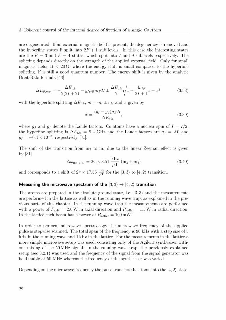
Figure 3.4: The graphs show the survival probability for atoms in the |3, 3〉 state versusthe microwave frequency relative to the resonance frequency. The left measurementbelongs to atoms in the lattice, whereas the right one is a measurement of the microwavespectrum in the running wave. Crossing the resonance frequency leads to the dip,because all atoms are transferred in the |4, 2〉 state and therefore removed from thetrap by the state selective detection. A sine squared curve is fitted to the data and isshown here as the red line (see text).
Parameter Notation Lattice Dipole Trap
total population transfer A 0.59 ± 0.04 0.83 ± 0.03Rabi frequency ΩR/2π (4947 ± 449) Hz (2359 ± 416) Hzpulse duration t/2 (58 ± 2) µs (100 ± 5) µsoffset B -0.26 ± 0.01 -0.07 ± 0.01
Table 3.1: Fit parameter for the microwave spectra of the lattice and the running wave,respectively.
leading to the spectra shown in figure 3.4. By fitting the following function resultingfrom the Rabi formula (eq.3.27) to the data points [42]
P3(ω) = 1− (A · Ω2R
Ω2sin2(
Ω2t
2)) +B with Ω2 = Ω2
R + (2π(δ − δs))2 (3.41)
one obtains the parameters summarised in table 3.1. The large offset in the latticearises due to imperfections of the optical pumping process resulting in the fact that afew atoms are lost and one therefore only reaches about 80% survival probability in thelattice. Optimisation of the process leads to the small offset in the running wave trap.Due to the slightly different microwave setups, a smaller coupling strength is achieved inthe running wave trap. Thus the Rabi oscillations are slower and the π-pulse durationis a bit longer compared to the values for the lattice. A pulse duration of 58 µs in thelattice and 100 µs in the dipole trap, respectively, leads to a Fourier limited spectrum in
30
3 Coherent control of the internal degree of freedom of a single Cs Atom
0 50 100 150 200 250 300 350 400pulse duration / µs
0.1
0.2
0.3
0.4
0.5
0.6
0.7
0.8
surv
ival pro
babili
ty
0 50 100 150 200 250 300 350 400 450pulse duration / µs
0.0
0.2
0.4
0.6
0.8
1.0
surv
ival pro
babili
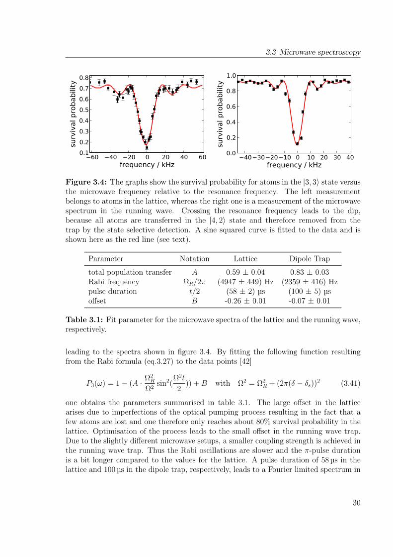
tyFigure 3.5: (Left) Rabi oscillations in the lattice. (Right) Rabi oscillations in therunning wave trap. Survival probability for atoms in the |3, 3〉 state versus the pulseduration of the microwave pulse. A fit of a cosine, indicated by the red line, to the datayields a Rabi frequency of 2π × (8.8 ± 0.03) kHz for atoms stored in the lattice and afrequency of 2π× (6.2±0.02) kHz for atoms stored in the running wave trap. This leadsto π pulse durations of approximately 56 µs and 80 µs, respectvely.
both traps.
With knowledge of the width of the Fourier limited spectrum, one can obtain a lowerbound for the resolution of the applied magnetic field. In the running wave trap, a pulsewith a duration of 100 µs was applied and hence a width of 10 kHz was measured. By useof the theoretical value of equation (3.40) and the width ∆ωrs of the measured spectra,the minimum resolution is inferred:
∆Bres =∆ωrs
2π ×∆ωm3→m4
=2π × 10 kHz
2π × 17.55 kHzµT
= 0.57 µT . (3.42)
3.4 Rabi oscillations
Since the exact resonance frequency of the transition is known, one can measure theRabi frequency in both traps. The trap parameters stay the same as in the last section.Again the transition |3, 3〉 → |4, 2〉 is driven by the microwave pulse, with the full powerof 4 W and the frequency of the signal is set to the measured resonance frequency. Thepulse duration is varied from 0 to 425 µs in steps of 25 µs. As in this case the resonancefrequency is used, the time evolution follows from equation (3.29), which is a solution ofthe Bloch equations. Hence, the population in F = 3 can be calculated with [42]
P3(t) =C
2cos(ΩRt) exp(−t) +B. (3.43)
31
3.5 Conclusion
Parameter Notation Lattice Dipole Trap
total population transfer C 0.58 ± 0.03 0.82 ± 0.03π pulse duration t/2 (56.5 ± 0.2) µs (80.5 ± 0.3) µsRabi oscillation ΩR/2π (8.8 ± 0.03) kHz (6.2 ± 0.02) kHzoffset B 0.4 ± 0.01 0.5 ± 0.01
Table 3.2: Fit parameter for the Rabi oscillations of the lattice and the running wavetrap, respectively.
The measured oscillations are shown in figure 3.5 and the obtained fit parameters aresummarised in table 3.2. Due to imperfections in the optical pumping process and thestate selective detection, respectively, a reduced contrast results. The damping of theRabi oscillations in the lattice arises due to an inhomogeneous decay time in the orderof a π-pulse duration and is discussed in the next chapter.
3.5 Conclusion
In this chapter, the experimental details to control the internal degree of freedom havebeen demonstrated. The Bloch vector model was introduced and served as a theoreticalmodel to describe the experimental techniques. By use of microwave radiation of ap-proximately 9.2 GHz the transition of |3, 3〉 → |4, 2〉 was driven and probed by means ofmicrowave spectroscopy. On this transition also Rabi oscillations were observed, whichallow to infer the duration of a π- and π/2- pulse. These are important prerequisites inorder to perform Ramsey spectroscopy and spin echo, as explained in the next chapter.
32

3 Coherent control of the internal degree of freedom of a single Cs Atom
33
4 Measuring the coherence time of asingle Cs atom
A closed quantum system without any interaction has a coherence time of infinity. How-ever, real quantum systems always couple to their environment and therefore the coher-ence decays. The different decay constants, which are discussed in this chapter, areimplemented in the optical Bloch equations as damping terms. This decay constants,directly corresponding to the so called coherence times, are investigated by use of Ram-sey spectroscopy and spin echo techniques as described in this chapter.
With the knowledge of the π-pulse duration and the transition frequency of the states|3, 3〉 → |4, 2〉 obtained in the last chapter, it is possible to control the internal degree offreedom of the single atom. The microwave setup is now used to create a superpositionbetween both states representing a quantum system.
4.1 Classification of decoherence effects
Data acquisition and analysis relies on the observation of an ensemble average of quan-tum states. In such systems decoherence manifests itself in the decay of the measuredmacroscopic polarisation or the dephasing of the relative phase. This is caused by var-ious effects, but it is however reasonable to classify these as either homogeneous orinhomogeneous dephasing. Homogeneous dephasing mechanisms affect each atom of theensemble in the same way. In contrast inhomogeneous dephasing only appears if everyatom in the ensemble possesses a slightly different resonance frequency. Practically themost important difference between both effects lies in the reversibility. While inhomoge-neous dephasing can be reversed using a spin echo technique, homogeneous dephasing isirreversible and also inevitable. This means that homogeneous dephasing is the limitingfactor for long coherence times.
Optical Bloch equations with damping
Because real quantum systems always couple to the environment, the initial state decayswith time. Hence the Bloch equations introduced in chapter 3.1 need to be extended todescribe a real quantum system. The decay rates are included as damping terms into
4 Measuring the coherence time of a single Cs atom
Name Symbol Dominant effects
population decay time (= longi-tudinal decay time), irreversible
T1 Mixing of hyperfine and Zeemanstates due to off resonant Ramanscattering
homogeneous dephasing time(=transverse decay time), irre-versible
T ′2 variations of differential light shift(caused by pointing instability ofthe trap laser or magnetic fieldfluctuations)
inhomogeneous dephasing time,reversible
T ∗2 distribution of differential lightshift
total transverse decay time T2 1/T2 = 1/T ∗2 + 1/T ′2
Table 4.1: Summary of the different decay constants and their main sources.
the Bloch equations for an atom ensemble average
〈u〉 = δ〈v〉 − 〈u〉T2
(4.1)
〈v〉 = −δ〈u〉+ ΩR〈w〉 −〈v〉T2
(4.2)
〈w〉 = −ΩR〈v〉 −〈w〉 − weq
T1
. (4.3)
Here 〈...〉 denotes the ensemble average. The homogenous longitudinal relaxation timeT1 and transversal decay time T2 have been introduced. T1 corresponds to the populationdecay to a stationary value weq and hence to a loss of “polarisation”. In contrast T2 onlyaffects the relative phase and preserves the population. T2 is made up of two differentcomponents, the inhomogeneous dephasing time T ∗2 and the homogenous dephasing timeT ′2. They are connected via the following relation
1
T2
=1
T ∗2+
1
T ′2. (4.4)
With knowledge about all three relaxation times, summarised in table 4.1, it is possi-ble to predict the whole evolution of an initially pure quantum system into a mixed state.
The dominant effect causing the longitudinal relaxation time T1 is in this case spon-taneous photon scattering from the light field of the lattice and the dipole trap laser.Due to Raman scattering the hyperfine and Zeeman states become distributed over allpossible states of an atom ensemble and the initially prepared polarised state is de-stroyed. The effect is indeed observable for experiments performed in the rather near
35
4.2 Measuring the population decay time
resonant lattice potential and was measured for different trap depths (see section 4.2),such that the T1 time can be estimated.
T ∗2 is the inhomogeneous and therefore reversible dephasing time. It is dominated bythe initial energy distribution of the atoms and results in a distribution of the lightshifts with respect to the initial temperature of the atom. This leads to slightly differentresonance frequencies for each atom and causes a phase decay.
The polarisation decay time, denoted by T ′2, is mostly affected by fluctuations of ex-perimental parameters during the experimental cycle. Such parameters are the laserintensity or the differential light shift, which are varying because of technical imperfec-tions like the pointing instability of the lattice and the running wave trap laser. Anotherpoint is the influence of fluctuating magnetic fields. Variations may arise from currentfluctuations in the coils, which create the magnetic traps or from magnetic stray fieldsproduced by electrical devices in the lab.A common way to measure the components of the T2 time is Ramsey spectroscopy andvariations of this method.
4.2 Measuring the population decay time
Scattering of photons from the trap laser results in population relaxation of the twoground states and is characterised by the decay time T1.In an optical dipole trap, such as the lattice or the running wave trap, photon scatteringis inevitable [42, 44, 45]. Whereas in most cases the photons are elastically scattered(namely Rayleigh scattering), which preserves the hyperfine state, a small fraction ofphotons are scattered inelastically. This process, so called off-resonant Raman scatter-ing, can result in a change of hyperfine or Zeeman level. In the present case the initialstate is the |3, 3〉 state and the possible final states are all Zeeman sublevels of the F =3 and F = 4 states.The photon scattering rate is anti-proportional to the detuning of the dipole laser withrespect to the D-lines of the Cs atom, which means that for small detunings a highscattering rate is obtained. Due to the detuning of only 5 nm of the lattice laser fromthe Cs D1-line [31], one expects a high scattering rate of a few 100 kHz and hence ashort T1 time.
To measure the population relaxation, atoms are either prepared in the F = 3 or inthe F = 4 state. The atoms are then stored in the trap for a certain time, before thestate selective detection reveals the number of remaining atoms in state F = 3. In thelattice one observes an exponential decay of the survival probability for atoms initiallyprepared in F = 3 and an exponential increase of the survival probability for atoms ini-tially prepared in F = 4. Figure 4.1 shows the measured survival probability for atoms
36
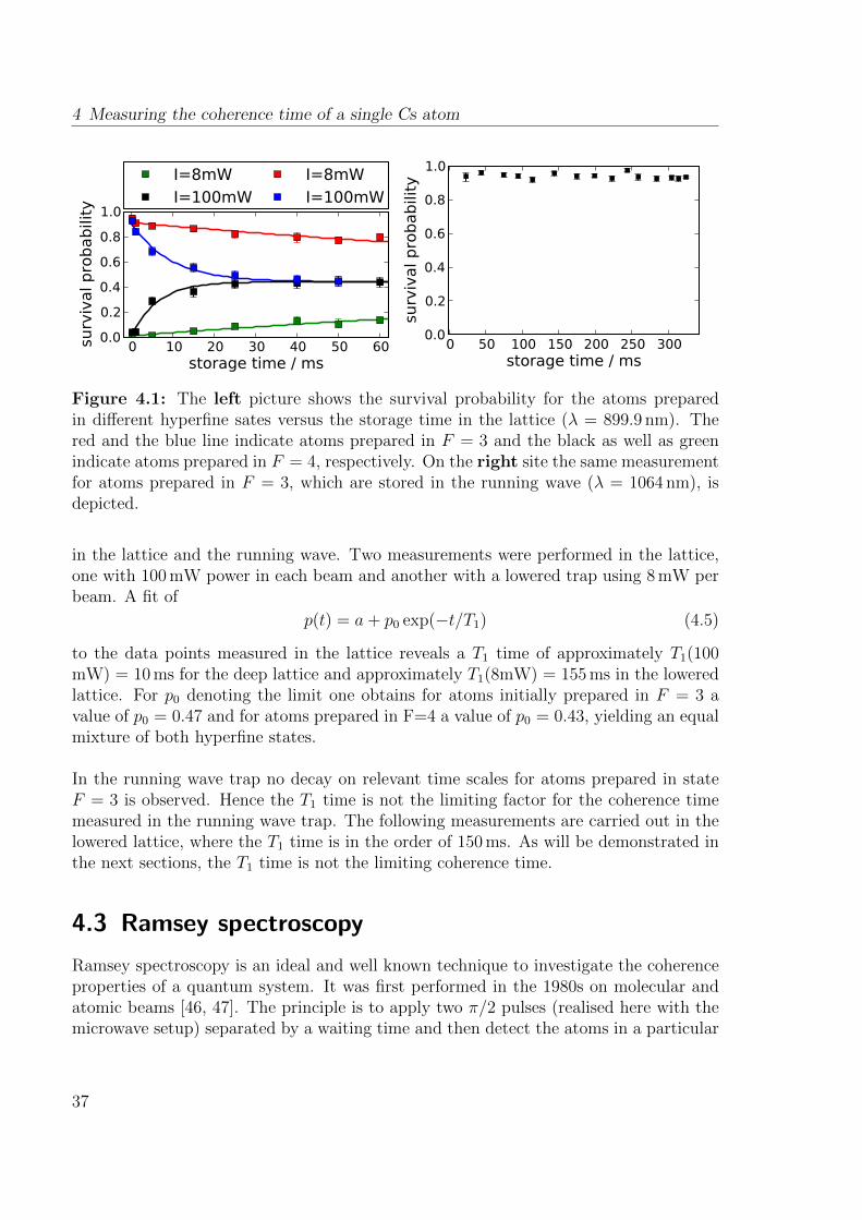
4 Measuring the coherence time of a single Cs atom
0 10 20 30 40 50 60storage time / ms
0.0
0.2
0.4
0.6
0.8
1.0
surv
ival pro
babili
ty
I=8mWI=100mW
I=8mWI=100mW
0 50 100 150 200 250 300storage time / ms
0.0
0.2
0.4
0.6
0.8
1.0
surv
ival pro
babili
tyFigure 4.1: The left picture shows the survival probability for the atoms preparedin different hyperfine sates versus the storage time in the lattice (λ = 899.9 nm). Thered and the blue line indicate atoms prepared in F = 3 and the black as well as greenindicate atoms prepared in F = 4, respectively. On the right site the same measurementfor atoms prepared in F = 3, which are stored in the running wave (λ = 1064 nm), isdepicted.
in the lattice and the running wave. Two measurements were performed in the lattice,one with 100 mW power in each beam and another with a lowered trap using 8 mW perbeam. A fit of
p(t) = a+ p0 exp(−t/T1) (4.5)
to the data points measured in the lattice reveals a T1 time of approximately T1(100mW) = 10 ms for the deep lattice and approximately T1(8mW) = 155 ms in the loweredlattice. For p0 denoting the limit one obtains for atoms initially prepared in F = 3 avalue of p0 = 0.47 and for atoms prepared in F=4 a value of p0 = 0.43, yielding an equalmixture of both hyperfine states.
In the running wave trap no decay on relevant time scales for atoms prepared in stateF = 3 is observed. Hence the T1 time is not the limiting factor for the coherence timemeasured in the running wave trap. The following measurements are carried out in thelowered lattice, where the T1 time is in the order of 150 ms. As will be demonstrated inthe next sections, the T1 time is not the limiting coherence time.
4.3 Ramsey spectroscopy
Ramsey spectroscopy is an ideal and well known technique to investigate the coherenceproperties of a quantum system. It was first performed in the 1980s on molecular andatomic beams [46, 47]. The principle is to apply two π/2 pulses (realised here with themicrowave setup) separated by a waiting time and then detect the atoms in a particular
37
4.3 Ramsey spectroscopy
w
v u
w
v u
w
v u
w
v u
π/2, φrf
State selective detection
π/2
t
τ
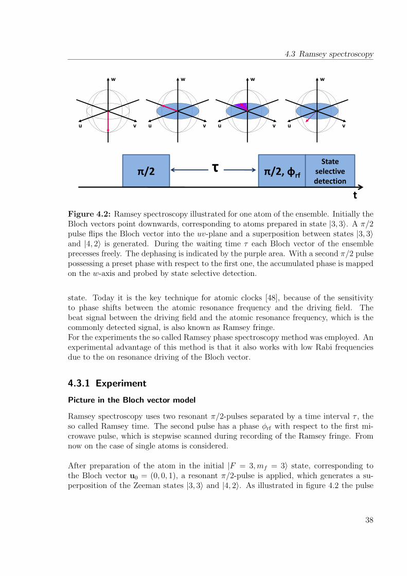
Figure 4.2: Ramsey spectroscopy illustrated for one atom of the ensemble. Initially theBloch vectors point downwards, corresponding to atoms prepared in state |3, 3〉. A π/2pulse flips the Bloch vector into the uv-plane and a superposition between states |3, 3〉and |4, 2〉 is generated. During the waiting time τ each Bloch vector of the ensembleprecesses freely. The dephasing is indicated by the purple area. With a second π/2 pulsepossessing a preset phase with respect to the first one, the accumulated phase is mappedon the w-axis and probed by state selective detection.
state. Today it is the key technique for atomic clocks [48], because of the sensitivityto phase shifts between the atomic resonance frequency and the driving field. Thebeat signal between the driving field and the atomic resonance frequency, which is thecommonly detected signal, is also known as Ramsey fringe.For the experiments the so called Ramsey phase spectroscopy method was employed. Anexperimental advantage of this method is that it also works with low Rabi frequenciesdue to the on resonance driving of the Bloch vector.
4.3.1 Experiment
Picture in the Bloch vector model
Ramsey spectroscopy uses two resonant π/2-pulses separated by a time interval τ , theso called Ramsey time. The second pulse has a phase φrf with respect to the first mi-crowave pulse, which is stepwise scanned during recording of the Ramsey fringe. Fromnow on the case of single atoms is considered.
After preparation of the atom in the initial |F = 3,mf = 3〉 state, corresponding tothe Bloch vector u0 = (0, 0, 1), a resonant π/2-pulse is applied, which generates a su-perposition of the Zeeman states |3, 3〉 and |4, 2〉. As illustrated in figure 4.2 the pulse
38
4 Measuring the coherence time of a single Cs atom
rotates the Bloch vector around the u-axis into the uv-plane of the Bloch sphere andthe final Bloch vector is given by u = (0, 1, 0). For the time interval τ the vector freelyprecesses in the uv-plane and accumulates a phase Φa(τ) = δ · τ , with δ the detuningbetween the microwave frequency and the resonance frequency of the atoms. The secondπ/2 pulse shifted by an initially set phase φrf with respect to the first pulse rotates theBloch vector around the u-axis once again. The population in F = 3 is probed by stateselective detection.
The matrix formalism introduced in section 3.1.1 can be used to describe the Ram-sey sequence,
uRamsey = Θπ/2 ·Φfree(t) ·Θπ/2 (4.6)
with Θπ/2 and Φfree(t) being known rotation matrices. The w-component depending onthe accumulated phase and the Ramsey time reads
wRamsey(φrf , τ) = C(τ) cos(φrf − Φa(τ)) (4.7)
with C(τ) the Ramsey fringe contrast. As one will see later, the last equations areused to derive the fit function for the Ramsey fringe contrast in order to obtain theinhomogeneous T ∗2 time.
Experimental parameters and observations
Ramsey spectroscopy was performed in both the lattice and the running wave trap. Forboth measurements, already introduced techniques of state preparation and state selec-tive detection as described previously in section 3.2.2 is used. The sequence remainsthe same as for microwave spectroscopy, but instead of one microwave pulse, two res-onant π/2 pulses are applied. For the phase modulation of the second π/2 pulse themodulation capability of the signal generator is used. The rest of the microwave setupremains the same as in the previous chapter. From the measured Rabi oscillations a π/2pulse duration of 30 µs in the lattice and 40 µs in the dipole trap is inferred. For themeasurement in the optical lattice, the lattice depth is adiabatically lowered to 8% of itsinitial value to avoid a high photon scattering rate, which may cause shorter coherencetimes and at the same time the adiabatic lowering of the lattice potential leads to furthercooling of the atoms.
To investigate the time evolution of the system and hence the T ∗2 time, Ramsey fringesfor varying Ramsey times are recorded. Figure 4.3 shows a sample of recorded Ramseyfringes from the lattice as well as from the dipole trap. A fit of equation (4.7) leads tothe Ramsey contrast C(τ), from which the T ∗2 time can be calculated.
39
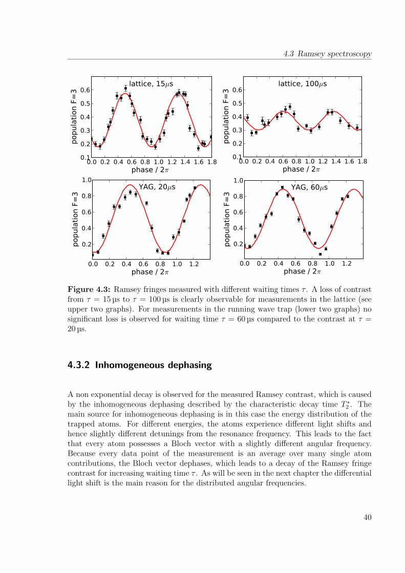
4.3 Ramsey spectroscopy
0.0 0.2 0.4 0.6 0.8 1.0 1.2 1.4 1.6 1.8phase / 2π
0.1
0.2
0.3
0.4
0.5
0.6
popula
tion F
=3
lattice, 15µs
0.0 0.2 0.4 0.6 0.8 1.0 1.2 1.4 1.6 1.8phase / 2π
0.1
0.2
0.3
0.4
0.5
0.6
popula
tion F
=3
lattice, 100µs
0.0 0.2 0.4 0.6 0.8 1.0 1.2phase / 2π
0.2
0.4
0.6
0.8
1.0
popula
tion F
=3
YAG, 20µs
0.0 0.2 0.4 0.6 0.8 1.0 1.2phase / 2π
0.2
0.4
0.6
0.8
1.0
popula
tion F
=3
YAG, 60µs
Figure 4.3: Ramsey fringes measured with different waiting times τ . A loss of contrastfrom τ = 15 µs to τ = 100 µs is clearly observable for measurements in the lattice (seeupper two graphs). For measurements in the running wave trap (lower two graphs) nosignificant loss is observed for waiting time τ = 60 µs compared to the contrast at τ =20 µs.
4.3.2 Inhomogeneous dephasing
A non exponential decay is observed for the measured Ramsey contrast, which is causedby the inhomogeneous dephasing described by the characteristic decay time T ∗2 . Themain source for inhomogeneous dephasing is in this case the energy distribution of thetrapped atoms. For different energies, the atoms experience different light shifts andhence slightly different detunings from the resonance frequency. This leads to the factthat every atom possesses a Bloch vector with a slightly different angular frequency.Because every data point of the measurement is an average over many single atomcontributions, the Bloch vector dephases, which leads to a decay of the Ramsey fringecontrast for increasing waiting time τ . As will be seen in the next chapter the differentiallight shift is the main reason for the distributed angular frequencies.
40
4 Measuring the coherence time of a single Cs atom
Differential light shift
Due to the light of the laser generating the trap (the Ti:Sa or the Nd:YAG, respectively)the atoms experience a light shift, which is given via the trapping potential [29, 42]
U0 =Γ~8
Imax
I0
Γ
∆(4.8)
with the natural line width of the transition Γ, the detuning ∆, the saturation intensityI0, which is 1.1 mW/cm2 for the Cs 6S→6P transition [31] and the maximum intensity
Imax =4P
πw20
(4.9)
with P the beam power and w0 the beam waist. For atoms in the hyperfine state F = 4the detuning from the D-line of the trap laser is 9.2 GHz less than for an atom inthe state F = 3 leading to a slightly stronger shift for atoms in F = 4 and a shift ofthe microwave frequency of the F = 3 → F = 4 transition towards smaller resonancefrequencies. The difference of the light shift for atoms in different hyperfine states iscalled differential light shift and it can be calculated with
~δls = U0(∆eff)− U0(∆eff + ∆hfs) . (4.10)
Here ∆eff denotes the effective detuning of the trap laser, which is given by [42]
1
∆eff
=1
3
(2
∆3/2
+1
∆1/2
)(4.11)
with ∆J = ωL − ωJ the detuning from the D-line transition. The hyperfine splitting isthe F = 3→ F = 4 transition frequency ∆hfs = 2π × 9.2 GHz = 1.2 Γ.For the lattice, lowered to 8% of its initial depth, with the parameters
λ = 899.9 nm (4.12)
Γ = 2π × 4.95 MHz (4.13)
∆eff = 522× 103 Γ (4.14)
one obtains a maximum differential light shift of δls = −2π × 30 kHz. The maximumdifferential light shift for atoms in the running wave trap is given by δls = −2π×1.1 kHzat a trap depth of ≈ 100 µK (for details see [42]). As the differential light shift is thedominant effect causing the T ∗2 time, these values are used to calculate a theoretical T ∗2time, which can be compared to the measured one.
Thermal distribution and T ∗2 time
Until now only atoms in the bottom of the trap with energy E = 0 were investigated,but one needs to take into account that the atoms have a thermal distribution. Due to
41
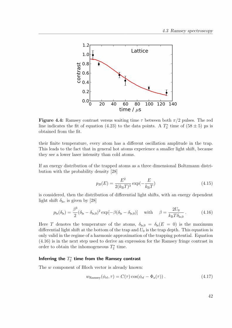
4.3 Ramsey spectroscopy
0 20 40 60 80 100 120 140time / µs
0.0
0.2
0.4
0.6
0.8
1.0
1.2
contr
ast
Lattice
Figure 4.4: Ramsey contrast versus waiting time τ between both π/2 pulses. The redline indicates the fit of equation (4.23) to the data points. A T ∗2 time of (58 ± 5) µs isobtained from the fit.
their finite temperature, every atom has a different oscillation amplitude in the trap.This leads to the fact that in general hot atoms experience a smaller light shift, becausethey see a lower laser intensity than cold atoms.
If an energy distribution of the trapped atoms as a three dimensional Boltzmann distri-bution with the probability density [28]
pB(E) =E2
2(kBT )3exp(− E
kBT) (4.15)
is considered, then the distribution of differential light shifts, with an energy dependentlight shift δls, is given by [28]
pls(δls) =β3
2(δls − δls,0)2 exp[−β(δls − δls,0)] with β =
2U0
kBTδls,0
. (4.16)
Here T denotes the temperature of the atoms, δls,0 = δls(E = 0) is the maximumdifferential light shift at the bottom of the trap and U0 is the trap depth. This equation isonly valid in the regime of a harmonic approximation of the trapping potential. Equation(4.16) is in the next step used to derive an expression for the Ramsey fringe contrast inorder to obtain the inhomogeneous T ∗2 time.
Inferring the T ∗2 time from the Ramsey contrast
The w component of Bloch vector is already known:
wRamsey(φrf , τ) = C(τ) cos(φrf − Φa(τ)) . (4.17)
42
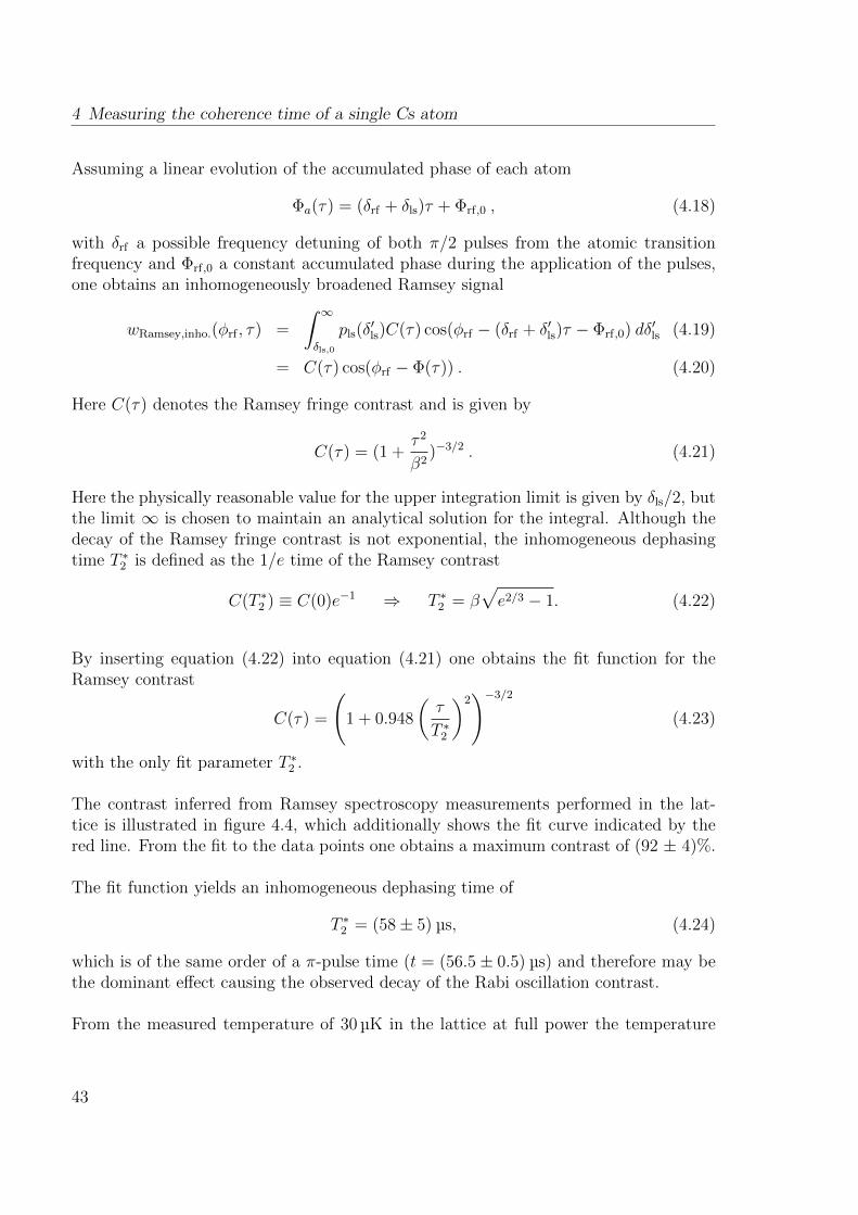
4 Measuring the coherence time of a single Cs atom
Assuming a linear evolution of the accumulated phase of each atom
Φa(τ) = (δrf + δls)τ + Φrf,0 , (4.18)
with δrf a possible frequency detuning of both π/2 pulses from the atomic transitionfrequency and Φrf,0 a constant accumulated phase during the application of the pulses,one obtains an inhomogeneously broadened Ramsey signal
wRamsey,inho.(φrf , τ) =
∫ ∞δls,0
pls(δ′ls)C(τ) cos(φrf − (δrf + δ′ls)τ − Φrf,0) dδ′ls (4.19)
= C(τ) cos(φrf − Φ(τ)) . (4.20)
Here C(τ) denotes the Ramsey fringe contrast and is given by
C(τ) = (1 +τ 2
β2)−3/2 . (4.21)
Here the physically reasonable value for the upper integration limit is given by δls/2, butthe limit ∞ is chosen to maintain an analytical solution for the integral. Although thedecay of the Ramsey fringe contrast is not exponential, the inhomogeneous dephasingtime T ∗2 is defined as the 1/e time of the Ramsey contrast
C(T ∗2 ) ≡ C(0)e−1 ⇒ T ∗2 = β√e2/3 − 1. (4.22)
By inserting equation (4.22) into equation (4.21) one obtains the fit function for theRamsey contrast
C(τ) =
(1 + 0.948
(τ
T ∗2
)2)−3/2
(4.23)
with the only fit parameter T ∗2 .
The contrast inferred from Ramsey spectroscopy measurements performed in the lat-tice is illustrated in figure 4.4, which additionally shows the fit curve indicated by thered line. From the fit to the data points one obtains a maximum contrast of (92 ± 4)%.
The fit function yields an inhomogeneous dephasing time of
T ∗2 = (58± 5) µs, (4.24)
which is of the same order of a π-pulse time (t = (56.5± 0.5) µs) and therefore may bethe dominant effect causing the observed decay of the Rabi oscillation contrast.
From the measured temperature of 30 µK in the lattice at full power the temperature
43
4.3 Ramsey spectroscopy
0 50 100 150 200time / µs
0.2
0.4
0.6
0.8
1.0
contr
ast
YAG
0
0,1
0,2
0,3
0,4
0,5
0,6
0,7
0,8
0,9
-‐0,2 0,3 0,8 1,3 1,8
survival proba
bility in F=3
Phase /2pi
360 260 560 760 260
Figure 4.5: (Left) Ramsey contrast versus the waiting time τ between the two π/2pulses. The data is obtained from measurements on atoms stored in the running wavetrap. (Right) Ramsey fringes for different waiting times measured on atoms stored inthe running wave trap. One can see that the survival probability fluctuates during themeasurements. A cosine could be estimated, but it was not possible to fit any reasonableequation to the data points.
in the adiabatically lowered trap is calculated. This is possible because in a harmonicpotential the fraction E/Ω, with E the sum of the potential and kinetic energy and Ωthe oscillation frequency, is invariant under adiabatic changes of the trapping potential.It results in the fact that, by using the relation Ω ∝
√U , one can directly infer the
temperature from the trap depth via T (U) = T ′√U/U ′.
With a theoretically expected value of δls = −2π×30 kHz and a temperature of approx-imately 9 µK in the adiabatically lowered trap of trap depth U0 = 58 µK an inhomoge-neous dephasing time of
T ∗2,theo = 66± 9 µs (4.25)
is calculated from equations (4.22) and (4.16). The error is calculated with propaga-tion of uncertainty by estimating a 10% error for the temperature as well as for the trapdepth. Within the error boundaries the measured value fits to the theoretically expectedtime. It is hence reasonable to assume that the T ∗2 time in the lattice is dominated bythe differential light shift.
Until now only the T ∗2 time in the lattice was examined, but Ramsey spectroscopy wasalso performed in the running wave trap. The contrast inferred from the Ramsey fringemeasured in the running wave trap, is shown in figure 4.5. Only three points are shownbecause for longer waiting times τ it was not possible to measure the contrast. Due tounknown effects the data points during recording of the Ramsey fringes fluctuated and
44
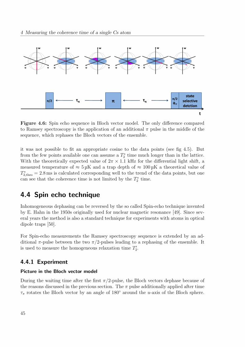
4 Measuring the coherence time of a single Cs atom
π state
selective detction
π/2 φrf
π/2
t
τπ τπ
w
v u
w
v u
w
v u
w
v u
w
v u
w
v u
Figure 4.6: Spin echo sequence in Bloch vector model. The only difference comparedto Ramsey spectroscopy is the application of an additional π pulse in the middle of thesequence, which rephases the Bloch vectors of the ensemble.
it was not possible to fit an appropriate cosine to the data points (see fig 4.5). Butfrom the few points available one can assume a T ∗2 time much longer than in the lattice.With the theoretically expected value of 2π × 1.1 kHz for the differential light shift, ameasured temperature of ≈ 5 µK and a trap depth of ≈ 100 µK a theoretical value ofT ∗2,theo = 2.8 ms is calculated corresponding well to the trend of the data points, but onecan see that the coherence time is not limited by the T ∗2 time.
4.4 Spin echo technique
Inhomogeneous dephasing can be reversed by the so called Spin-echo technique inventedby E. Hahn in the 1950s originally used for nuclear magnetic resonance [49]. Since sev-eral years the method is also a standard technique for experiments with atoms in opticaldipole traps [50].
For Spin-echo measurements the Ramsey spectroscopy sequence is extended by an ad-ditional π-pulse between the two π/2-pulses leading to a rephasing of the ensemble. Itis used to measure the homogeneous relaxation time T ′2.
4.4.1 Experiment
Picture in the Bloch vector model
During the waiting time after the first π/2-pulse, the Bloch vectors dephase because ofthe reasons discussed in the previous section. The π pulse additionally applied after timeτπ rotates the Bloch vector by an angle of 180 around the u-axis of the Bloch sphere.
45
4.4 Spin echo technique
0.0 0.2 0.4 0.6 0.8 1.0 1.2phase / 2π
0.2
0.4
0.6
0.8
1.0popula
tion F
=3
YAG, echo 1 pulse, 100µs
0.0 0.2 0.4 0.6 0.8 1.0 1.2phase / 2π
0.2
0.4
0.6
0.8
1.0
popula
tion F
=3
YAG, echo 1 pulse, 980µs
Figure 4.7: Two exemplary Ramsey fringes measured with the spin echo technique foratoms stored in the running wave trap. After a waiting time τπ of approximately 1 msan sufficient contrast is still observable.
This leads to a time reversal and hence the Bloch vectors are completely rephased instate u = (0, 1, 0) after time 2τπ, see figure 4.6.
Because Ramsey spectroscopy and the spin echo technique are similar methods, thematrix formalism derived in section 3.1.1 is used again to describe the spin echo se-quence. The evolution of the Bloch vector prepared in the initial state u0 = (0, 0,−1),yields
uecho(φrf , 2τπ) = Θπ/2 · Φfree,1(τπ) ·Θπ · Φfree,2(τπ) ·Θπ/2 · u0 (4.26)
with the known rotation matrices for Θπ/2, Θπ and Φfree (see section 3.1.1). For the wcomponent we obtain from equation (4.26):
wecho =1
2(1 + cos[φrf −∆Φ(τ) + π]) (4.27)
with ∆Φ = Φfree,1(τπ)−Φfree,2(τπ) the difference between the accumulated phases beforeand after the π pulse, respectively.
Experimental parameters and Observations
For the spin echo sequence the same experimental parameters as for Ramsey spectroscopyare employed due to similarities of the techniques. Again the transition |3, 3〉 → |4, 2〉is used. The pulse length of the π-pulse is 60 µs in the lattice and 80 µs in the runningwave trap, respectively. In figure 4.7 some Ramsey fringes recorded with the spin echotechnique are depicted.
4.4.2 Homogeneous dephasing
In the ideal case, meaning that during the experimental cycle the individual resonancefrequency of each atom stays the same, the spin echo method is able to fully reverse the
46
4 Measuring the coherence time of a single Cs atom
0 500 1000 1500 2000time / µs
0.0
0.1
0.2
0.3
0.4
0.5
0.6
0.7
contr
ast
Figure 4.8: Spin echo contrast versus waiting time τπ. The black squares indicate thedata points, whereas the red solid line represents a fit of equation (4.34) to the data. Ahomogeneous decay time T ′2 of (1.19± 0.06) ms is inferred from the fit.
dephasing which occurs during the time in which the Bloch vector precesses freely. Theresult would be a spin echo contrast of 100 %.
However, the experiments show that the spin echo contrast decays, which is due toirreversible dephasing mechanisms, denoted by the homogeneous dephasing time T ′2.Sources for such effects are fluctuations of the laser intensity or of magnetic fields duringthe performance of the sequence. These fluctuations lead to the fact that the accumu-lated phases before and after the π pulse are different. The effect is expressed by a timeaveraged detuning difference ∆δ in time τπ
∆Φa(τπ) = ∆δ · τπ. (4.28)
A Gaussian shape for the probability distribution of the average detuning difference isassumed [28]
p(∆δ, τπ) =1√
2πσ(τπ)exp
[− (∆δ)2
2σ2(τπ)
](4.29)
with mean ∆δ = 0 and variance σ2(τπ). Then the homogeneously broadened spin echosignal is given by [28]
wecho,homo.(φrf , 2τπ) =
∫ ∞−∞
p(∆δ), τπ)C(τ) cos[φrf −∆δτπ + π] d∆δ (4.30)
= C(2τπ) cos[φrf + π] (4.31)
with the spin echo contrast
C(2τπ) = exp[−1
2τ 2πσ
2(τπ)]. (4.32)
47
4.4 Spin echo technique
0 500 1000 1500 2000time / µs
0.00.10.20.30.40.50.60.70.80.9
contr
ast
0 500 1000 1500 2000time / µs
0.00.10.20.30.40.50.60.70.80.9
contr
ast
Figure 4.9: Spin echo contrast versus waiting time τπ. The data was obtained fromatoms stored in the running wave trap at a different trap depth as the first measurement.A power of Paxial = 3 W in axial direction and of Pradial = 0.6 W in radial direction wasused during this measurements.
Again the T ′2 time is defined as the 1/e time of the spin echo contrast signal
C(2τπ = T ′2) ≡ C(0)e−1 =⇒ T ′2 =
√2
σ(τπ). (4.33)
Combining the last equation with equation (4.32) and adding a fit parameter, which takesthe deviation from the maximal contrast into account, leads to the used fit function of
C(2τπ) = Cmax exp
[−(τ 2π
T ′2
)2], (4.34)
which directly reveals the inhomogeneous T ′2 time.
The measurements were performed in the running wave trap with a power of Paxial = 2 Win axial direction and Pradial = 1.5 W in radial direction. Figure 4.8 shows the evolutionof the contrast depending on the spin echo time τπ. A dephasing time of
C(2τπ) = (1186± 60) µs (4.35)
is inferred from the fit resulting in a variance of
σ(τπ) = (190± 10) Hz . (4.36)
Measurements (see fig. 4.9) with a different trap depth (Paxial = 3 W and Pradial = 0.6 W)yield nearly the same T ′2 times, which are T ′2 = (1300 ± 84) µs and T ′2 = (1129 ± 74) µs,respectively. Hence intensity fluctuations or pointing instability of the trap laser, causingchanges of the trap depth and therefore changes of the differential light shift, are assumednot to be the limiting factors.
48
4 Measuring the coherence time of a single Cs atom
Analysis of dephasing mechanisms
In the next step the variances resulting from different effects are calculated and thencompared to the measured one, following the methods of references [42, 28]. The devia-tions of the parameters are estimations in most cases.
Intensity fluctuations Fluctuations of the laser intensity of the trap laser directly affectthe trap depth and hence the differential light shift. Because we need to performthe spin echo measurement about a 100 times, every atom sees a trap depth slightlydifferent resulting in a dephasing of the Bloch vectors corresponding to each atom.Due to the fact that an electronic feed back loop is used to control the laser powerin each beam independently, one is only limited by its accuracy. Therefore thefluctuations are estimated to ε = 0.5% of the initial intensity.The variance caused by the fluctuations can be calculated via
σ(τ)
2π=√
2δlsε (4.37)
with ε the estimated variance of the parameter, rather than the Allen varianceused in [42]. For a maximum light shift of δls = 2π × 1.1 kHz one hence obtains
a variance of σ(τ)2π
= 7.8 Hz. This is one order of magnitude too small to be thelimiting effect. It corresponds well to the fact that neither the trap depth nor thedifferential light shift matter here.
Beam pointing instability Like intensity fluctuations the pointing instability of thelaser generating the trap causes fluctuations of the trap depth and hence of thedifferential light shift. Here the pointing instability is estimated to be small com-pared to the beam waist, as one would observe a lower transfer efficiency from thelattice into the running wave otherwise. A variance of σ(τ)
2π= 31 Hz is calculated
from equation (4.37) with ε = 2%. This is again too small to be the limiting factor.
Magnetic field fluctuations The current through the coils generating the magneticguiding field may be slightly unstable and hence results in fluctuations of themagnetic field. Due to the linear Zeeman shift, this is directly translated intoresonance frequency shifts of the relevant transition (|3, 3〉 → |4, 2〉). The shift isin this case calculated via
∆ω = 2B0∆ωm3→m4 (4.38)
with B0 = 1 mT the applied magnetic field strength and ∆ωm3→m4 = 2π ×3.51kHz
µT(m3 + m4) = 5 · 2π × 3.51kHz
µTthe splitting due to the linear Zeeman shift.
For the variance one obtains
σ(τ)
2π=√
2∆ωε = 208 Hz (4.39)
with ε = Irms/I0 = 3 × 10⁻⁶ given by the Toellner power supply. Although thevalue is larger than the measured one, it is in the expected variance range and it
49
4.4 Spin echo technique
makes sense that the magnetic field fluctuations are the limiting factor, due to thestrong dependency of the transition frequency for the outer Zeeman states on themagnetic field.
Summarising the effect limiting the inhomogeneous decay time are probably magneticfield fluctuations, because the transition frequency |3, 3〉 → |4, 2〉 strongly depends on themagnetic field. It was furthermore found the differential light shift not to be responsiblefor the limited coherence time in measurements for different trap depths. This statementwas supported by calculations for the beam pointing instability and the laser intensityfluctuations. Note that the magnetic field fluctuations arising from electrical devices inthe lab are not taken into account.
50

4 Measuring the coherence time of a single Cs atom
51
5 Conclusions and Outlook
During this thesis a species selective lattice was built and implemented in the currentsetup. A transfer efficiency from the single atom MOT into the lattice and back closeto unity has been achieved. this is an essential prerequisite for future experiments, be-cause all measurements rely on counting the atom number in the MOT before and aftermanipulation of the atom. It was verified that the measured lattice parameters agreewith the theoretically predicted values. Therefore it is now used as an intermediate stepfor combining a single Cs atom from a dissipative trap with a many particle system ofRb atoms, which are evaporatively cooled and stored in a conservative shallow dipoletrap, resulting in the demonstration of sympathetic cooling of the single atom by theRb cloud (see [36]).
After combination of both systems it was the intention to investigate the coherencebehaviour of a single superposition state during or after the interaction with the ultra-cold gas. The measurements being performed and introduced in this thesis are in factthe calibration of such measurements. To this end a microwave setup has been built andused to generate a superposition state of two Zeeman states in a single Cs atom.
From a Ramsey spectroscopy measurement performed in the lattice, the inhomogeneouscoherence time of nearly 60 µs has been inferred and the differential light shift has beenfound to be the limiting factor. This time is however too small compared to the ther-malisation time of 25 ms [36] to analyse a possible decay during the interaction of thesingle atom and the ultracold cloud. Besides the fact that the Rb cloud is stored in thedipole trap, the low differential light shift and hence a longer coherence time is anotherreason to use the dipole trap instead of the lattice.
Within the dipole trap we measured the homogeneous coherence time of approximately1200 µs using different trap depths, observing that the time stays the same in each mea-surement. We therefore conclude that inhomogeneous effects, such as the differentiallight shift, are not the limiting factors. In contrast homogeneous effects limit the co-herence time. The limiting processes are mainly ascribed to fluctuations of the currentflowing through the coils generating the magnetic guiding field. This is reasonable be-cause the used transition between the Zeeman states is very sensitive to magnetic fieldsdue to the linear Zeeman effect. Although we neither use the outer most transitions wecan compare our value to others measured in the group, where a time of 415 µs [28] for|3, 3〉 → |4, 4〉 transition have been observed. Referring to this measurements our coher-
5 Conclusions and Outlook
ence time is much longer and is a good candidate to investigate the coherence propertiesof a single atom during the interaction with an ultracold gas. The thermalisation timefor the Cs atom in the ultracold Rb cloud is in the order of 25 ms. Therefore on timescales of the coherence time (1 ms) it is possible to observe cooling of the superpositionstate. Unfortunately it was not possible to perform a combined measurement of a singleCs atom and an ultracold Rb cloud because of a major vacuum leak.
In the near future a new experimental setup will be build having an all optical BECallowing a much faster measurement cycle (up to 6 s per BEC compared to 1 minutein the old setup). With this setup, higher Rb densities may be gained resulting in afaster thermalisation process and hence it is then possible to analyse the coherence timeduring combination of both systems.
53
Bibliography
[1] T. W. Hansch, “Cooling of gases by laser radiation,” Optics Communications,vol. 13, no. I, pp. 68–69, 1975.
[2] H. F. Hess, “Evaporative cooling of magnetically trapped and compressed spin-polarized hydrogen,” Phys. Rev. B, vol. 34, pp. 3476–3479, 1986.
[3] M. H. Anderson, J. R. Ensher, M. R. Matthews, C. E. Wieman, and E. a. Cornell,“Observation of bose-einstein condensation in a dilute atomic vapor.” Science (NewYork, N.Y.), vol. 269, no. 5221, pp. 198–201, 1995.
[4] K. B. Davis, M. O. Mewes, M. R. Andrews, N. J. van Druten, D. S. Durfee, D. M.Kurn, and W. Ketterle, “Bose-einstein condensation in a gas of sodium atoms,”Phys. Rev. Lett., vol. 75, pp. 3969–3973, 1995.
[5] M. R. Andrews, C. G. Townsend, H.-J. Miesner, D. S. Durfee, D. M. Kurn, andW. Ketterle, “Observation of interference between two bose condensates,” Science,vol. 275, no. 5300, pp. 637–641, 1997.
[6] I. Bloch, T. W. Hansch, and T. Esslinger, “Atom laser with a cw output coupler,”Phys. Rev. Lett., vol. 82, pp. 3008–3011, 1999.
[7] K. W. Madison, F. Chevy, W. Wohlleben, and J. Dalibard, “Vortex formation in astirred bose-einstein condensate,” Phys. Rev. Lett., vol. 84, pp. 806–809, 2000.
[8] S. O. Demokritov, V. E. Demidov, O. Dzyapko, G. a. Melkov, a. a. Serga, B. Hille-brands, and a. N. Slavin, “Bose-Einstein condensation of quasi-equilibrium magnonsat room temperature under pumping.” Nature, vol. 443, no. 7110, pp. 430–3, 2006.
[9] J. Klaers, J. Schmitt, F. Vewinger, and M. Weitz, “Bose-Einstein condensation ofphotons in an optical microcavity.” Nature, vol. 468, no. 7323, pp. 545–8, 2010.
[10] M. Tinkham, Introduction to Superconductivity, 2nd ed. McGraw-Hill, 1996.
[11] R. Wynar, R. S. Freeland, D. J. Han, C. Ryu, and D. J. Heinzen, “Molecules in abose-einstein condensate,” Science, vol. 287, no. 5455, pp. 1016–1019, 2000.
[12] T. Kraemer, M. Mark, P. Waldburger, J. G. Danzl, C. Chin, B. Engeser, a. D.Lange, K. Pilch, a. Jaakkola, H.-C. Nagerl, and R. Grimm, “Evidence for Efimov
54
Bibliography
quantum states in an ultracold gas of caesium atoms.” Nature, vol. 440, no. 7082,pp. 315–8, 2006.
[13] F. K. Fatemi, K. M. Jones, and P. D. Lett, “Observation of optically inducedfeshbach resonances in collisions of cold atoms,” Phys. Rev. Lett., vol. 85, pp. 4462–4465, 2000.
[14] S. Inouye, M. R. Andrews, J. Stenger, H. Miesner, and W. Ketterle, “Observationof Feshbach resonances in a Bose -Einstein condensate,” Nature, pp. 8–11, 1998.
[15] G. Modugno, M. Modugno, F. Riboli, G. Roati, and M. Inguscio, “Two atomicspecies superfluid,” Phys. Rev. Lett., vol. 89, p. 190404, 2002.
[16] D. Schrader, S. Kuhr, W. Alt, M. Muller, V. Gomer, and D. Meschede, “An opticalconveyor belt for single neutral atoms,” Applied Physics B, vol. 73, pp. 819–824,2001.
[17] M. Karski, L. Forster, J.-M. Choi, A. Steffen, W. Alt, D. Meschede, and A. Widera,“Quantum walk in position space with single optically trapped atoms,” Science, vol.325, no. 5937, pp. 174–177, 2009.
[18] A. J. Daley, P. O. Fedichev, and P. Zoller, “Single-atom cooling by superfluid im-mersion: A nondestructive method for qubits,” Phys. Rev. A, vol. 69, p. 022306,2004.
[19] A. Griessner, A. J. Daley, S. R. Clark, D. Jaksch, and P. Zoller, “Dark-state coolingof atoms by superfluid immersion,” Phys. Rev. Lett., vol. 97, p. 220403, 2006.
[20] J. F. Sherson, C. Weitenberg, M. Endres, M. Cheneau, I. Bloch, and S. Kuhr,“Single-atom-resolved fluorescence imaging of an atomic Mott insulator,” Nature,vol. 467, no. 7311, pp. 68–72, 2010.
[21] T. Gericke, P. Wurtz, D. Reitz, T. Langen, and H. Ott, “High-resolution scanningelectron microscopy of an ultracold quantum gas,” Nature Physics, vol. 4, no. 12,pp. 949–953, 2008.
[22] M. Bruderer and D. Jaksch, “Probing bec phase fluctuations with atomic quantumdots,” New Journal of Physics, vol. 8, no. 6, p. 87, 2006.
[23] H. T. Ng and S. Bose, “Single-atom-aided probe of the decoherence of a bose-einsteincondensate,” Phys. Rev. A, vol. 78, p. 023610, 2008.
[24] T. Weikum, “Ein System zur Fluoreszenzdetektion einzelner Casiumatome in einemRubidium Bose-Einstein-Kondensat,” 2009, Diplomarbeit.
55
Bibliography
[25] C. Weber, “Controlled few-body interactions in ultracold bosonic mixtures,” Ph.D.dissertation, University of Bonn, 2009.
[26] S. John, “Towards Single atom aided probing of an ultracold quantum gas,” Ph.D.dissertation, University of Bonn, 2011.
[27] E. L. Raab, M. Prentiss, A. Cable, S. Chu, and D. E. Pritchard, “Trapping of neutralsodium atoms with radiation pressure,” Phys. Rev. Lett., vol. 59, pp. 2631–2634,1987.
[28] M. Karski, “State-selective transport of single neutral atoms,” Ph.D. dissertation,University of Bonn, 2010.
[29] R. Grimm, M. Weidemuller, and Y. B. Ovchinnikov, “Optical dipole traps for neu-tral atoms,” in Advances In Atomic, Molecular, and Optical Physics, 2000, vol. 42,pp. 95 – 170.
[30] D. Meschede, Optik, Licht und Laser, 2nd ed. Teubner, 2005.
[31] D. A. Steck, “Cesium D Line Data,” http://steck.us/alkalidata.
[32] O. Fetsch, “A species selective trap for single Cs atoms,” 2010, Diplomarbeit.
[33] W. Alt, “Optical control of single neutral atoms,” Ph.D. dissertation, University ofBonn, 2004.
[34] N. Spethmann, F. Kindermann, S. John, C. Weber, D. Meschede, and A. Widera,“Inserting single Cs atoms into an ultracold Rb gas,” arXiv:1109.1639v1, 2011.
[35] M. Mudrich, S. Kraft, K. Singer, R. Grimm, A. Mosk, and M. Weidemuller, “Sym-pathetic cooling with two atomic species in an optical trap,” Phys. Rev. Lett.,vol. 88, p. 253001, 2002.
[36] N. Spethmann, “Dissertation,” to be published.
[37] T. Esslinger, I. Bloch, and T. W. Hansch, “Bose-einstein condensation in aquadrupole-ioffe-configuration trap,” Phys. Rev. A, vol. 58, pp. R2664–R2667, 1998.
[38] A. Kastler, “Optical Methods of Atomic Orientation and of Magnetic Resonance,”JOSA, vol. 47, no. 6, pp. 460–465, 1957.
[39] T. R. Carver, “Optical Pumping.” Science (New York, N.Y.), vol. 141, no. 3581,pp. 599–608, 1963.
[40] F. Bloch, “Nuclear induction,” Phys. Rev., vol. 70, pp. 460–474, 1946.
56
Bibliography
[41] L. Allen and J. H. Eberly, Optical Resonance and Two-Level Atoms. Dover Pub-lications, 1987.
[42] S. Kuhr, “A controlled quantum system of individual neutral atoms,” Ph.D. disser-tation, University of Bonn, 2003.
[43] G. Breit and I. I. Rabi, “Measurement of nuclear spin,” Phys. Rev., vol. 38, pp.2082–2083, 1931.
[44] D. Frese, B. Ueberholz, S. Kuhr, W. Alt, D. Schrader, V. Gomer, and D. Meschede,“Single atoms in an optical dipole trap: Towards a deterministic source of coldatoms,” Physical Review Letters, vol. 85, no. 18, pp. 3777–3780, 2000.
[45] R. a. Cline, J. D. Miller, M. R. Matthews, and D. J. Heinzen, “Spin relaxation ofoptically trapped atoms by light scattering.” Optics letters, vol. 19, no. 3, p. 207,1994.
[46] N. F. Ramsey, “A molecular beam resonance method with separated oscillatingfields,” Phys. Rev., vol. 78, pp. 695–699, 1950.
[47] N. Ramsey, Molecular Beams. Oxford University Press, 1956.
[48] J. Vanier and C. Audoin, The Quantum Physics of Atomic Frequency Standards.Adam Hilger, 1989.
[49] E. L. Hahn, “Spin echoes,” Phys. Rev., vol. 80, pp. 580–594, 1950.
[50] M. F. Andersen, A. Kaplan, and N. Davidson, “Echo spectroscopy and quantumstability of trapped atoms,” Phys. Rev. Lett., vol. 90, p. 023001, 2003.
57
DanksagungAn dieser Stelle mochte ich mich bei allen bedanken, die mich wahrend meiner Master-arbeitszeit unterstutzt haben.
Zu aller erst danke ich Prof. Dr. Meschede fur die Moglichkeit meine Masterarbeitan diesem spannenden Experiment anfertigen zu durfen.
Prof. Dr. Artur Widera danke ich fur die grossartige Unterstutzung wahrend meinergesamten Masterarbeit, fur die Klarung meiner physikalischer Fragen, fur seine opti-mistische Art , fur das hilfreiche Korrekturlesen meiner Arbeit und nicht zuletzt fur dieUbernahme des Zweitgutachtens.
Nicolas Spethmann danke ich ebenfalls fur die grossartige Unterstutzung wahrend meinergesamten Masterarbeit, fur das hilfreiche Korrekturlesen dieser Arbeit, fur seine geduldigeArt und fur das beantworten samtlicher meiner Fragen.
Auch Claudia und Shincy, die zu Begin meiner Arbeit am Experiment mit gearbeitethaben, mochte ich ebenfalls fur ihre Unterstutzung danken.
Dem Rest der Arbeitsgruppe danke ich fur die angenehme Atmosphare und insbesondereWolfgang fur hilfreiche Tips wahrend der Teepausen.
Mein ganz besonderer Dank gilt meiner Mutter und meinem Freund Philip. Beide habenmich nicht nur wahrend meiner Masterarbeit, sondern wahrend meiner gesamten Stu-dienzeit und daruber hinaus ausserordentlich unterstutzt. Ohne sie ware diese Arbeitnicht moglich gewesen.


I herby certify that the work presented here was accomplished by myself and withoutthe use of illegitimate means or support, and that no sources and tools were used otherthan those cited.
Bonn,


![QUANTUM MEMORY: DESIGN AND OPTIMIZATION Xiaotong Ni · quantum key distribution [BB84] in the early phase, as well as quantum metrology [GLM06] and quantum machine learning [LMR13]](https://img.pdfslide.org/doc/110x75/5e1f5cc589c7e33bda676412/quantum-memory-design-and-optimization-xiaotong-ni-quantum-key-distribution-bb84.jpg)