Embed Size (px)
Citation preview

BrainXPloreDecision finding in Brain Biopsy Planning
DIPLOMARBEIT
zur Erlangung des akademischen Grades
Diplom-Ingenieur
im Rahmen des Studiums
Visual Computing
eingereicht von
Lukas PezenkaMatrikelnummer 0625948
an der Fakultät für Informatik
der Technischen Universität Wien
Betreuung: Ao.Univ.Prof. Univ.-Doz. Dipl.-Ing. Dr.techn. Eduard GröllerMitwirkung: Dipl.-Math. Dr. Katja Bühler
Assoc.Prof. Dr. Stefan Wolfsberger
Wien, 28. November 2017Lukas Pezenka Eduard Gröller
Technische Universität WienA-1040 Wien Karlsplatz 13 Tel. +43-1-58801-0 www.tuwien.ac.at


BrainXPloreDecision finding in Brain Biopsy Planning
DIPLOMA THESIS
submitted in partial fulfillment of the requirements for the degree of
Diplom-Ingenieur
in
Visual Computing
by
Lukas PezenkaRegistration Number 0625948
to the Faculty of Informatics
at the TU Wien
Advisor: Ao.Univ.Prof. Univ.-Doz. Dipl.-Ing. Dr.techn. Eduard GröllerAssistance: Dipl.-Math. Dr. Katja Bühler
Assoc.Prof. Dr. Stefan Wolfsberger
Vienna, 28th November, 2017Lukas Pezenka Eduard Gröller
Technische Universität WienA-1040 Wien Karlsplatz 13 Tel. +43-1-58801-0 www.tuwien.ac.at


Erklärung zur Verfassung derArbeit
Lukas PezenkaGerasdorfer Straße 61/2/6
Hiermit erkläre ich, dass ich diese Arbeit selbständig verfasst habe, dass ich die verwen-deten Quellen und Hilfsmittel vollständig angegeben habe und dass ich die Stellen derArbeit – einschließlich Tabellen, Karten und Abbildungen –, die anderen Werken oderdem Internet im Wortlaut oder dem Sinn nach entnommen sind, auf jeden Fall unterAngabe der Quelle als Entlehnung kenntlich gemacht habe.
Wien, 28. November 2017Lukas Pezenka
v


Acknowledgements
This work was enabled by the Competence Centre VRVis. VRVis is funded by BMVIT,BMWFW, Styria, SFG and Vienna Business Agency in the scope of COMET - Compe-tence Centers for Excellent Technologies (854174) which is managed by FFG.
I thank my partner, Sabine, for her patience and support. Further, I thank my parentsfor encouraging me to pursue an academic education. Finally, thank my friends andcolleagues, especially Chris and Nicolas, for providing feedback and offering advicewhenever I was stuck.
A big salute goes to my supervisors, Katja Bühler and Eduard Gröller for supervisionand proofreading of this thesis. Additional thanks go to Florian, Alexey and Gert fortheir advice and support.
vii

Kurzfassung
Neurochirurgen treffen Entscheidungen auf Basis ihres Expertenwissens. In diesem Prozesswerden Faktoren wie die Distanz zu gefährdeten Strukturen, Pfadlänge und -winkel, etc.berücksichtigt. Während manche Kriterien (wie etwa das Unterschreiten der minimalenDistanz zu Blutgefäßen) zum Ausschluß einer potentiellen Trajektorie führen, sindandere Kriterien (etwa die Pfadlänge) weniger rigide. Diese Faktoren können dannzur Reihung und Bewertung von potentiellen Trajektorien herangezogen werden. NachAnalyse tatsächlich erfolgter Eingriffe sowie Rücksprache mit Neurochirurgen haben wirwichtige Regeln zur Planung und Durchführung von Gehirnbiopsien identifiziert.
In dieser Arbeit präsentieren wir BrainXplore, ein in Zusammenarbeit mit der medizin-schen Universität Wien entwickeltes System zur Unterstützung von Neurochriurgen beider Planung von Gehirnbiopsien. BrainXplore ist ein erweiterbares Biopsieplanungs-rahmenwerk, das die erarbeiteten Regeln implementiert und dabei dem Benutzer volleFlexibilität hinsichtlich deren Definition und Erweiterung bietet. Das System berechnetautomatisch eine Menge an potentiellen Trajektorien. Durch die Definition und Verfei-nerung der Regeln kann diese Menge schrittweise verkleinert werden, bis eine geeigneteTrajektorie gefunden wurde. Durch den Einsatz eines räumlichen Indexes können beliebigviele anatomische Strukturen bei beliebiger Auflösung zur Berechnung der Trajektorienherangezogen werden. Somit wird der Einsatz hochauflösender multimodaler Datensätzemöglich, welcher bisher aufgrund von Speicherplatzlimiterungen der Graphikkarte unmög-lich war. Um den Neurochirurgen bei der Entscheidungsfindung zu unterstützen bietetBrainXPlore Methoden der Informationsvisualisierung, wie parallele Koordinatensystemeund Risikoprofildiagramme.
Wir haben BrainXPlore auf realen Daten einer tatsächlich erfolgten Biopsie getestetund akzeptable Resultate erzielt. Der partizipierende Neurochirurg gab uns das Feedback,dass der Einsatz von BrainXPlore zu einer Verringerung der Dauer von Gehirnbiopsienführen kann und sinnvoll zur Unterstützung weniger erfahrener Chirurgen eingesetztwerden kann.
ix

Abstract
Neurosurgeons make decisions based on expert knowledge that takes factors such assafety margins, the avoidance of risk structures, trajectory length and trajectory angleinto consideration. While some of those factors are mandatory, others can be optimizedin order to obtain the best possible trajectory under the given circumstances. Throughcomparison with the actually chosen trajectories from real biopsies and qualitativeinterviews with domain experts, we identified important rules for trajectory planning.
In this thesis, we present BrainXplore, an interactive visual analysis tool for aidingneurosurgeons in planning brain biopsies. BrainXplore is an extendable BiopsyPlanning framework that incorporates those rules while at the same time leaving fullflexibility for their customization and adding of new structures at risk. Automaticallycomputed candidate trajectories can be incrementally refined in an interactive manneruntil an optimal trajectory is found. We employ a spatial index server as part of oursystem that allows us to access distance information on an unlimited number of riskstructures at arbitrary resolution. Furthermore, we implemented InfoVis techniques suchas Parallel Coordinates and risk signature charts to drive the decision process. As a casestudy, BrainXPlore offers a variety of information visualization modalities to presentmultivariate data in different ways.
We evaluated BrainXPlore on a real dataset and accomplished acceptable results. Theparticipating neurosurgeon gave us the feedback that BrainXPlore can decrease thetime needed for biopsy planning and aid novice users in their decision making process.
xi

Contents
Kurzfassung ix
Abstract xi
Contents xiii
1 Introduction 1
2 Medical Background 52.1 Medical Imaging Methods . . . . . . . . . . . . . . . . . . . . . . . . . 52.2 Brain Anatomy Segmentation . . . . . . . . . . . . . . . . . . . . . . . 122.3 Planning Guidelines . . . . . . . . . . . . . . . . . . . . . . . . . . . . 15
3 Related Work 193.1 Biopsy Planning . . . . . . . . . . . . . . . . . . . . . . . . . . . . . . 193.2 Medical Information Visualization . . . . . . . . . . . . . . . . . . . . 30
4 Visual Computing Work-flow and System Design 354.1 Requirement Analysis . . . . . . . . . . . . . . . . . . . . . . . . . . . 354.2 System Overview . . . . . . . . . . . . . . . . . . . . . . . . . . . . . . . 414.3 Visual Computing Work-flow . . . . . . . . . . . . . . . . . . . . . . . 43
5 Methods and Data 455.1 Data Acquisition and Segmentation . . . . . . . . . . . . . . . . . . . . 455.2 Data Preprocessing . . . . . . . . . . . . . . . . . . . . . . . . . . . . . 465.3 Indexing . . . . . . . . . . . . . . . . . . . . . . . . . . . . . . . . . . . 465.4 Trajectory Generation and Preprocessing . . . . . . . . . . . . . . . . 475.5 Trajectory Filtering and Refinement . . . . . . . . . . . . . . . . . . . 48
6 Implementation 556.1 MeVisLab Work-Flow . . . . . . . . . . . . . . . . . . . . . . . . . . . 556.2 Data Preprocessing . . . . . . . . . . . . . . . . . . . . . . . . . . . . . 566.3 Indexing . . . . . . . . . . . . . . . . . . . . . . . . . . . . . . . . . . . 576.4 User Interface . . . . . . . . . . . . . . . . . . . . . . . . . . . . . . . . 57
xiii

6.5 Information Visualization . . . . . . . . . . . . . . . . . . . . . . . . . 67
7 Evaluation 717.1 Internal Evaluation . . . . . . . . . . . . . . . . . . . . . . . . . . . . . . 717.2 External Evaluation . . . . . . . . . . . . . . . . . . . . . . . . . . . . 86
8 Conclusion 918.1 Future Work . . . . . . . . . . . . . . . . . . . . . . . . . . . . . . . . 92
List of Figures 95
List of Tables 97
List of Algorithms 99
Bibliography 101

CHAPTER 1Introduction
More than 100 different tumor types with widely divergent biologies and clinical outcomesare known [SR06]. Different treatment options, such as surgery, radiation, and palliativecytotoxics exist and are well established in medicine. Before deciding between furthertreatment options, however, the tumor needs to be identified.
A brain tumor biopsy is the extraction of tissue from a tumor for the analysis of itsnature, i.e., whether it is benign or malignant. For the biopsy, a hole is drilled into thecranium, trough which a biopsy needle is inserted into the brain. In general, a needletrajectory is defined by an entry point in the skin and a target point on the tumor.
To prevent permanent damage to the patient, vital tissues have to be avoided by thetrajectory and hence, protected from damage caused by the needle. Certain rules haveto be fulfilled for a trajectory to be deemed acceptable. Amongst those rules are theavoidance of risk structures, minimization of trajectory length, etc.
Satisfying all those rules requires good knowledge of the particular brain’s anatomy.Due to the high risk, carrying out the biopsy also requires a high degree of precisionA stereotactic brain biopsy makes use of medical imaging data such as magneticresonance imaging (MRI) and computer tomography (CT) to precisely identify and targetany brain area in a 3D coordinate system. The biopsy needle can be positioned by arobotic arm after the patient was registered to the 3D coordinate system. Stereotacticbiopsies are well established and have a high success rate. Shoshan et al. [SPS+95]report a diagnostic success rate of 96% over a three-year period.
Deep Brain Stimulation (DBS) is a method of treating advanced Parkinson’s dis-ease [BSB04], movement disorders and other psychiatric and neurological disorders suchas epilepsy [LKG14]. The neurosurgeon places electrodes in the patient’s brain alongwell-defined neural pathways. These electrodes further serve to regulate the flow of neuralinformation, including pathological signals mediating seizure propagation. This mech-
1

1. Introduction
anism is known as neuro-modulation. Like brain biopsies, the placement of electrodesrequires careful and precise planning.
Despite the available technologies and tools, brain biopsy and DBS planning is still atime-intensive task that requires a high amount of expert knowledge. Different systemshave been proposed to plan and visualize needle trajectories. While some aspects ofthe planning process are (partially) solved by the proposed systems, others need to beimproved upon.
For one, most systems operate on a rigid set of rules to augment the planning process. Toour knowledge, no existing work allows the inclusion of an arbitrary number of distinctstructures (e.g., fiber bundles, anatomical atlas, etc) and the flexible definition of rulesfor trajectory filtering. This does not necessarily allow neurosurgeons, who ultimatelyare the domain experts, to use the tool in such a way as to optimally support their (ortheir hospital’s) preferred planning methods.
On the other hand, only a limited number of structures is taken into consideration byexisting solutions at this moment. As brain atlases become more sophisticated andwhite matter tracts are better understood, the number of structures that are consideredwhen planning a biopsy is likely to increase greatly in the near future. Orringer et al.[OGJ12] points out that advances in MRI imaging provide the possibility of incorporatingfunctional data into the neuronavigational datasets. Modern imaging data that mighthave not been considered for planning purposes in the past, such as fMRI, is gainingsignificance [BHWB07]. When designing planning tools, these developments have to beaccounted for and scalability must be guaranteed. Some of the existing systems limitthemselves by design, others are limited by their system architecture with regards tofuture scalability (e.g., by the reliance on video memory, which is limited in typicalconsumer hardware).
In this thesis we propose BrainXPlore, an interactive data exploration and filteringsystem to support the neurosurgeon in planning biopsies. BrainXPlore offers a setof filtering operations that allow the surgeon to incrementally refine a set of potentialtrajectories until an optimum has been found.
We solve the issue of scalability by including a spatial index server that has previouslysuccessfully been used in the research of fly brains [BŠG+09]. This component in ourwork-flow allows us, in contrast to existing solutions, to access a very high numberof structures at an arbitrary spatial resolution. Šoltészová [Šol10] has presented theefficiency of the index structure for large distance tables of 2GB.
Besides supporting the surgeon, we also aim at creating insight when it comes to thedecision process. To evaluate our system, we had a neurosurgeon use BrainXPlore togo through the planning process on a real-world data set of a past biopsy.
The remainder of this thesis is structured as follows: Chapter 1, provides informationof the methods used in medical image acquisition and data segmentation. An overviewover the planning guidelines as laid down by a domain expert at our partner hospital
2

is given. Finally, we present a real case study to illustrate the state of the art in brainbiopsy planning. Chapter 2 evaluates related work in the fields of biopsy planningand visualization of multivariate data. Chapter 4 offers an overview of the softwareand hardware we used for the implementation. Chapter 5 provides information on themethods we have employed when designing and implementing BrainXPlore. Imple-mentation details are outlined in Chapter 6. Chapter 7 evaluates our system basedon a real data set. Finally, Chapter 8 summarizes the contributions of this thesis andproposes future work.
3

CHAPTER 2Medical Background
Stereotactic brain biopsies are an efficient and safe [TFM+09] method of obtainingtissue samples of brain tumors for further histological evaluation. The planning processbuilds upon detailed knowledge of the human brain. Because no two brains are identical,medical images have to be obtained for every patient. Orringer et al. [OGJ12] state that"currently, all systems for stereotactic biopsy rely on navigation based on preoperativelyobtained images". To build a (semi)automated planning system, structures at risk needto be segmented from the obtained data. Blood vessels are arguably the most criticalof these structures. Another commonly considered example is the ventricular system,comprised of the lateral ventricles, third and fourth ventricle.
This Chapter is structured as follows. In Section 2.1, we describe the medical imagingmethods that are employed to acquire the data needed to plan a biopsy. Section 2.2describes the process of segmenting structures at risk from the obtained data. Finally,planning guidelines from related literature are presented in Section 2.3.
2.1 Medical Imaging Methods
Many anatomical structures can be considered in the process of planning a brain biopsy.In order to use data, it first needs to be acquired. The following sections describe thedata acquisition methods and explain the relevance of the different data modalities tothe planning process.
2.1.1 Computed tomography
As presented in Chapter 3, in brain biopsy planning, the skull is often used to automaticallycalculate candidate entry points. The best modality for skull image data acquisition iscomputed tomography (CT).
5
2. Medical Background
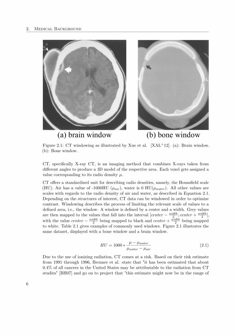
Figure 2.1: CT windowing as illustrated by Xue et al. [XAL+12]. (a): Brain window.(b): Bone window.
CT, specifically X-ray CT, is an imaging method that combines X-rays taken fromdifferent angles to produce a 3D model of the respective area. Each voxel gets assigned avalue corresponding to its radio density µ.
CT offers a standardized unit for describing radio densities, namely, the Hounsfield scale(HU). Air has a value of -1000HU (µair), water is 0 HU(µwater). All other values arescales with regards to the radio density of air and water, as described in Equation 2.1.Depending on the structures of interest, CT data can be windowed in order to optimizecontrast. Windowing describes the process of limiting the relevant scale of values to adefined area, i.e., the window. A window is defined by a center and a width. Grey valuesare then mapped to the values that fall into the interval [center − width
2 ; center + width2 ],
with the value center − width2 being mapped to black and center + width
2 being mappedto white. Table 2.1 gives examples of commonly used windows. Figure 2.1 illustrates thesame dataset, displayed with a bone window and a brain window.
HU = 1000 ∗ µ− µwaterµwater − µair
(2.1)
Due to the use of ionizing radiation, CT comes at a risk. Based on their risk estimatefrom 1991 through 1996, Brenner et al. state that "it has been estimated that about0.4% of all cancers in the United States may be attributable to the radiation from CTstudies" [BH07] and go on to project that "this estimate might now be in the range of
6

2.1. Medical Imaging Methods
Center WidthLung -650 1500Emphysema -800 800Soft tissue without contrast agent 40 400Liver without contrast agent 40 200Soft tissue with contrast agent 70 400Liver with contrast agent 60 - 100 300Neck with contrast agent 50 300CT Angiography 100 - 200 500Bones 500 2000Osteoporosis 300 1000 - 1500
Table 2.1: Commonly used CT windows, adapted from Prokop et al. [PGSP06]
1.5 to 2.0%" based on the current CT use. Hence, eliminating CT scans from the biopsyplanning process does not only make data fusion simpler and the whole process cheaper(by eliminating an additional study), but also potentially preserves patient health.
2.1.2 Magnetic Resonance Imaging
In biopsy planning, differentiating between different tissue types, e.g., in the brain, iscrucial. For soft tissues, Magnetic Resonance Imaging (MRI) is better suited thanCT, as it provides much more detail.
MRI is based on the relaxation of hydrogen atoms after excitation by a strong electromag-netic field. Schild [Sch12] describes the process quite simply: "1) the patient is placed ina magnet, 2) radio wave is sent in, 3) the radio wave is turned off, 4) the patient emits asignal, which is received and used for 5) reconstruction of the picture" [Sch12].
Atoms consist of a nucleus and a shell. Inside the nucleus, amongst other things, areprotons, i.e., positively charged particles. Protons spin around their axes and therebycreate an electrical current. While protons are normally aligned in a random fashion,exposure to a strong magnetic field aligns them either parallel or anti-parallel to theexternal magnetic field. Slightly more protons are aligned parallel than anti-parallel.Protons precess around the magnetic fields longitudinal axis. The precession frequency isdependent of the magnetic field strength and can be calculated as stated in Equation 2.2.ω0 specifies the precession frequency, γ is the gyro-magnetic ratio and B0 indicates themagnetic field strength.
ω0 = γB0 (2.2)
Parallelly and anti-parallelly aligned protons that point in opposite directions canceleach other out when it comes to the net electric current they create. Since thereare more parallelly than anti-parallelly aligned protons, however, not all current is
7

2. Medical Background
eliminated. When considering the reduced set of protons, i.e., only those with a parallelalignment, elimination occurs in the plane perpendicular to the magnetic field. Let Zbe the axis defined by the magnetic field. Then, currents in the XY plane that point toopposite directions cancel each other out. In contrast, all parallelly aligned positronsinduce magnetic vectors that point in the same direction along the Z axis and henceadd up. This magnetization is referred to as longitudinal magnetization. Because themagnetization is longitudinal to the external magnetic field, however, it can not directlybe measured.
To resolve this issue, a radio frequency (RF) pulse is applied to the magnetic field. Thefrequency is based on the Larmour Equation. By matching the radio frequency to theprotons precession frequency, resonance is created and energy transfer occurs. For one,this energy transfer flips the alignment of some protons, such that parallelly alignedprotons take an anti-parallel alignment and hence, the longitudinal magnetization isreduced. On the other hand, the RF pulse puts the protons in sync, i.e., they all pointto the same direction in the XY plane at the same time. The resulting magnetic vectoris referred to as transverse magnetization. Due to the precession of the positrons, themagnetic vector is constantly moving, thus inducing an electric current that also has theprecession frequency. This current is the MR signal. After turning off the RF pulse, theprotons whose alignment has been flipped from parallel to anti-parallel take their initialalignment again, thus increasing the longitudinal magnetization. This process is knownas longitudinal relaxation or spin-lattice relaxation (as the protons hand over energy totheir surroundings, the so-called lattice). The relaxation is described by a time constantT1. Conversely, the transverse relaxation (also called spin-spin relaxation), is describedby a time constant T2. Different tissues have different relaxation times. While water,for example, has a long T1 and long T2, fat has a short T1 and a shorter T2 than water[Sch12].
Various sequences can be used to weigh an MRI. The most common are T1-weighted,T2-weighted, T1-weighted with contrast, Diffusion and FLAIR. T1-weighted MRI isparticularly useful for assessing the cerebral cortex. T2-weighted MRI helps in detectingedema and inflammation and revealing white matter lesions. Diffusion weighted imaging(DWI) can be used to perform tractography and identify neural tracts.
While the Hounsfield scale used for CT offers a standardized scale, MRI images takenfor the same patient on the same scanner at different times may appear different fromeach other due to a variety of scanner-dependent variations [NUZ00]. This means thatabsolute intensity values have no fixed meaning and windowing has to be performed foreach image. More recently, variants of data standardization have been proposed, such asthe work performed by Nyul et al. [NUZ00].
Contrast agents can be used if necessary. Especially in the context of tumor detec-tion, they further enhance the image contrast for more accurate cancer detection anddiagnosis [ZL13]. Paramagnetic compounds such as gadolinium based agents are themost commonly used contrast agents in clinical MRI [ZL13]. They mainly reduce thelongitudinal (T1) relaxation property and result in a brighter signal [Sho13, ZL13]. Super-
8
2.1. Medical Imaging Methods
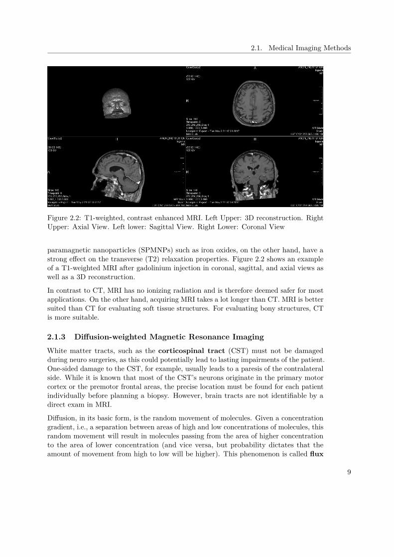
Figure 2.2: T1-weighted, contrast enhanced MRI. Left Upper: 3D reconstruction. RightUpper: Axial View. Left lower: Sagittal View. Right Lower: Coronal View
paramagnetic nanoparticles (SPMNPs) such as iron oxides, on the other hand, have astrong effect on the transverse (T2) relaxation properties. Figure 2.2 shows an exampleof a T1-weighted MRI after gadolinium injection in coronal, sagittal, and axial views aswell as a 3D reconstruction.
In contrast to CT, MRI has no ionizing radiation and is therefore deemed safer for mostapplications. On the other hand, acquiring MRI takes a lot longer than CT. MRI is bettersuited than CT for evaluating soft tissue structures. For evaluating bony structures, CTis more suitable.
2.1.3 Diffusion-weighted Magnetic Resonance Imaging
White matter tracts, such as the corticospinal tract (CST) must not be damagedduring neuro surgeries, as this could potentially lead to lasting impairments of the patient.One-sided damage to the CST, for example, usually leads to a paresis of the contralateralside. While it is known that most of the CST’s neurons originate in the primary motorcortex or the premotor frontal areas, the precise location must be found for each patientindividually before planning a biopsy. However, brain tracts are not identifiable by adirect exam in MRI.
Diffusion, in its basic form, is the random movement of molecules. Given a concentrationgradient, i.e., a separation between areas of high and low concentrations of molecules, thisrandom movement will result in molecules passing from the area of higher concentrationto the area of lower concentration (and vice versa, but probability dictates that theamount of movement from high to low will be higher). This phenomenon is called flux
9

2. Medical Background
(J) and is defined by Fick’s first law as presented in Equation 2.3. The diffusion coefficientD equates the flow vector and the concentration gradient c.
J = −D∇c (2.3)
Diffusion-weighted Magnetic Resonance Imaging (DWI) is an imaging methodthat builds on MRI and exploits the diffusion patterns of water molecules to revealmicroscopic details about tissues. DWI provides an estimate of the rate of waterdiffusion for each voxel. This information can be used to detect early stages of apathological change.
To acquire a DWI image, first an RF is applied to the subject as with standard MRI,to excite water molecules. Then, a positive, so-called dephasing gradient magneticfield is set up. This dephasing gradient will cause electrons in water atoms to spin atdifferent speeds with respect to their spatial location inside the gradient field (they arebrought out of phase, hence, dephasing gradient). Once the gradient is turned off (i.e., ahomogeneous magentic field is restored), rotation speed will be the same again for allmolecules. Applying a gradient inverse to the initial one will again cause rotation speedsto change with respect to the corresponding atoms location. If the same field strengthwas applied for the same duration, all molecules should rotate at the same speed andbe in phase again. Hence, this negative gradient is called the rephasing gradient. In astatic system, the rephasing would be perfect. However, if water atoms move due todiffusion, this process will be imperfect, i.e., after the rephasing gradient was applied,not all the molecules will be in phase. This imperfect refocusing will result in a signalloss, which can be used to measure the diffusion constant. However, only the diffusionalong the gradient direction can be measured. To obtain Fiber directions, multiple scansare necessary.
Diffusion Tensor Imaging (DTI) expands on DWI by considering not only the rate, butalso the average direction of diffusion. In areas that are made up of an internal fibrousstructure, water will diffuse faster in the direction parallel to the structure [HJM+06].Since a defining characteristic of neuronal tissue is its fibrillar structure, this considerationallows for the identification of brain tracts. As pointed out, this is not possible in T1-weighted or T2-weighted MRI. In contrast to DWI, DTI is usually built on six or moregradient directions, rather than three. Multiple gradient directions (mathematically, atleast six, although often more are used) are necessary to calculate a diffusion tensor.
In anisotropic media, the diffusion coefficient D depends on the direction. Therefore, inDTI, it is replaced by the diffusion tensor D. D is a 3 x 3 matrix that fully characterizesdiffusion in 3D space [HJM+06] and can be calculated with the help of the Stejskal-Tanner-Equation presented in Equation 2.4. g denotes the gradient direction. The b-valuespecifies the diffusion weighting and is proportional to the product of the square ofthe gradient strength q and the diffusion time interval ∆ [HJM+06] as illustrated inEquation 2.5. S0 is the signal intensity without the diffusion weighting, S is the signal
10
2.1. Medical Imaging Methods
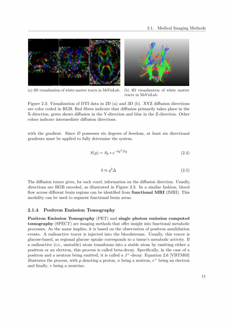
(a) 3D visualization of white matter tracts in MeVisLab. (b) 3D visualization of white mattertracts in MeVisLab.
Figure 2.3: Visualization of DTI data in 2D (a) and 3D (b). XYZ diffusion directionsare color coded in RGB. Red fibers indicate that diffusion primarily takes place in theX-direction, green shows diffusion in the Y-direction and blue in the Z-direction. Othercolors indicate intermediate diffusion directions.
with the gradient. Since D possesses six degrees of freedom, at least six directionalgradients must be applied to fully determine the system.
S(g) = S0 ∗ e−bgTDg (2.4)
b ≈ q2∆ (2.5)
The diffusion tensor gives, for each voxel, information on the diffusion direction. Usually,directions are RGB encoded, as illustrated in Figure 2.3. In a similar fashion, bloodflow across different brain regions can be identified from functional MRI (fMRI). Thismodality can be used to segment functional brain areas.
2.1.4 Positron Emission Tomography
Positron Emission Tomography (PET) and single photon emission computedtomography (SPECT) are imaging methods that offer insight into functional metabolicprocesses. As the name implies, it is based on the observation of positron annihilationevents. A radioactive tracer is injected into the bloodstream. Usually, this tracer isglucose-based, as regional glucose uptake corresponds to a tissue’s metabolic activity. Ifa radioactive (i.e., unstable) atom transforms into a stable atom by emitting either apositron or an electron, this process is called beta-decay. Specifically, in the case of apositron and a neutron being emitted, it is called a β+-decay. Equation 2.6 [VBTM03]illustrates the process, with p denoting a proton, n being a neutron, e+ being an electronand finally, v being a neutrino.
11

2. Medical Background
p→ n+ e+ + v (2.6)
As the tracer undergoes β+-decay, it emits a positron which, eventually, interacts with anelectron. Since the positron has the opposite charge of the electron, both are annihilatedduring the interaction. The annihilation results in a pair of annihilation photons, i.e.,γ-quanta, moving at an angle of 180 degree to each other. On their way, those quantainteract with their surrounding tissues and are attenuated. One they leave the body, thephotons are measured by means of a scintillator. Based on their location and attenuation,the physician can draw conclusions regarding the spatial distribution of the tracer. PETimages are functional rather than topological imaging techniques and hence results haveto be correlated to other data, e.g., CT scans. Modern CT devices are capable of acquiringboth image modalities in the same session.
In this context, the most important application of PET scans is the examination oftumors with regards to metastases. Since the cost of PET scans is fairly high, no suchdata has been considered in the case studies presented in this work.
2.2 Brain Anatomy Segmentation
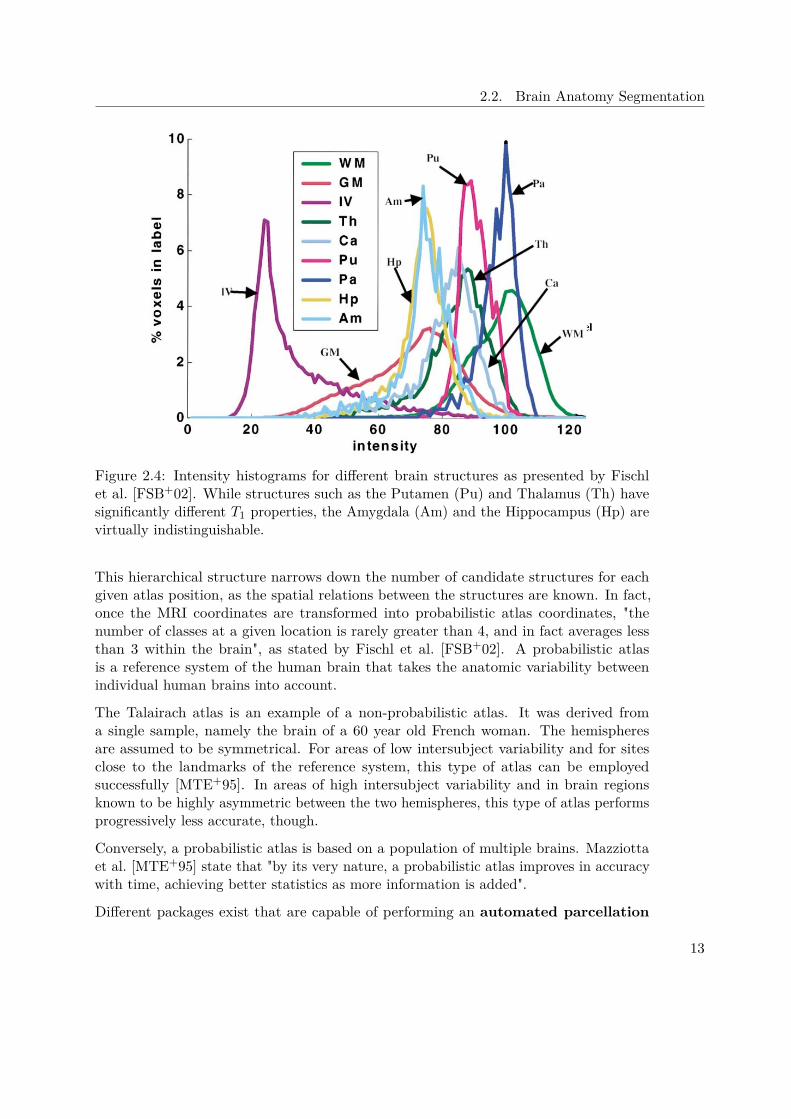
Segmenting the brain at a structural level is not trivial. Figure 2.4 shows intensityhistograms for different subcortical brain structures. Based on their intensity valuesalone, the Amygdala (Am) and the Hippocampus (Hp) are virtually indistinguishable.However, by including spatial information in the segmentation process (i.e., the Amygdalaresiding to the anterior and superior to the Hippocampus), the inherent ambiguity ofclass intensity distributions can be overcome. To incorporate this spatial information,brain segmentation is facilitated by the construction of a probabilistic atlas. In such anatlas, somewhat arbitrary raw image coordinates are transformed to a space in whichcoordinates have an anatomical meaning. Atlases can be based on single specimens, suchas the Talairach atlas, or can be constructed from a large population, as presented byMazziotta et al. [MTE+95].
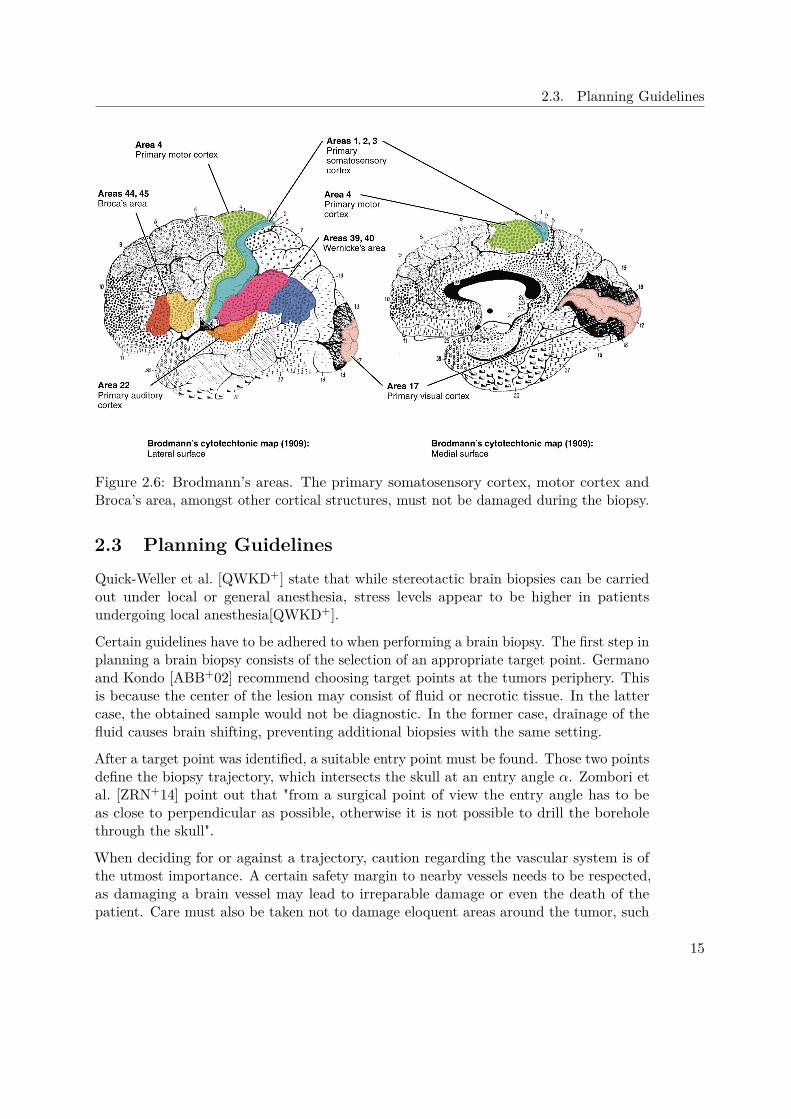
In the context of brain segmentation, different functional levels of increasing granularitycan be observed, as illustrated in Figure 2.5. At the topmost level is the hemisphere. TheHemisphere is important because crossing the mid-sagittal plane should be avoided inbrain biopsies. Beneath the Hemisphere Level lies the Lobe Level. Here, the four mainLobes (Frontal, Temporal, Parietal, and Occipital), the Limbic Lobe and a sub-lobarregion can be identified. Further down in the hierarchy is the Gyrus Level. In the GyrusLevel, anatomical classes (e.g., Caudate, Thalamus, Lentiform, etc.) are defined. Incontrast, the Tissue Level defines the type of tissue within a voxel (i.e., white matter,grey matter, cerebrospinal fluid). At the lowest level, the Cell Level, the brain canbe labeled by cell-type in the cortex using Brodmann’s scheme [Gar94], presented inFigure 2.6. This is important as certain cortical areas must not be damaged, as explainedin Section 4.1.1.
12
2.2. Brain Anatomy Segmentation
Figure 2.4: Intensity histograms for different brain structures as presented by Fischlet al. [FSB+02]. While structures such as the Putamen (Pu) and Thalamus (Th) havesignificantly different T1 properties, the Amygdala (Am) and the Hippocampus (Hp) arevirtually indistinguishable.
This hierarchical structure narrows down the number of candidate structures for eachgiven atlas position, as the spatial relations between the structures are known. In fact,once the MRI coordinates are transformed into probabilistic atlas coordinates, "thenumber of classes at a given location is rarely greater than 4, and in fact averages lessthan 3 within the brain", as stated by Fischl et al. [FSB+02]. A probabilistic atlasis a reference system of the human brain that takes the anatomic variability betweenindividual human brains into account.
The Talairach atlas is an example of a non-probabilistic atlas. It was derived froma single sample, namely the brain of a 60 year old French woman. The hemispheresare assumed to be symmetrical. For areas of low intersubject variability and for sitesclose to the landmarks of the reference system, this type of atlas can be employedsuccessfully [MTE+95]. In areas of high intersubject variability and in brain regionsknown to be highly asymmetric between the two hemispheres, this type of atlas performsprogressively less accurate, though.
Conversely, a probabilistic atlas is based on a population of multiple brains. Mazziottaet al. [MTE+95] state that "by its very nature, a probabilistic atlas improves in accuracywith time, achieving better statistics as more information is added".
Different packages exist that are capable of performing an automated parcellation
13

2. Medical Background
Figure 2.5: The five hierarchical levels in the Talairach Atlas as described by Lancasteret al. [LWP+00]: Hemisphere Level, Lobe Level, Gyrus Level, Tissue Level, Cell Level
of subcortical structures. Two commonly used packages are FreeSurfer [RSRF12] andFIRST [PSKJ11]. FIRST is a part of FMRIB’s Software Library (FSL) [SJW+04].Studies [MPX+09] have compared the performance of those packages.
Morey et al. [MPX+09] used both packages to automatically segment the Amygdalaand Hippocampus and compared the respective results to hand tracings performed by asingle expert rater with the experience of performing over 500 hippocampal tracings. Theauthors conclude that FSL and FreeSurfer are not equal when compared to manual tracingand further state that FreeSurfer is generally preferred to FIRST. Conversely, Perlakiet al. [PHN+17] find that FIRST is superior to FreeSurfer with regards to putaminalsegmentation.
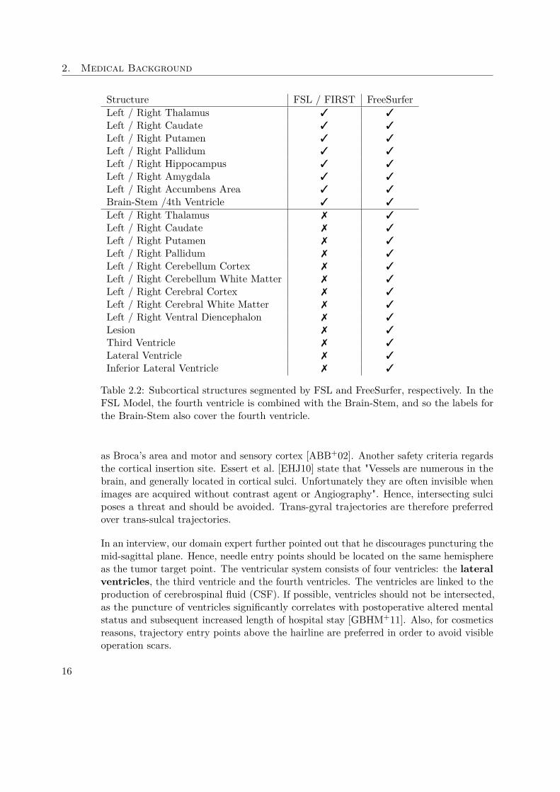
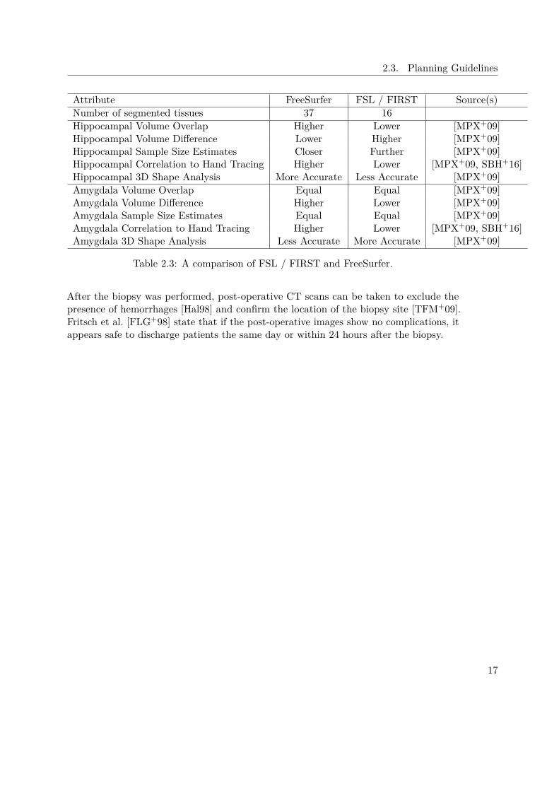
Table 2.3 gives an overview of each packages strengths and weaknesses. FreeSurfer iscapable of segmenting more structures than FSL. Table 2.2 gives an overview over eachpackages set of subcortical labels.
Cortical Parcellation is based on standard atlases, as described above. Both FreeSurferand FSL offer different atlases. For the cortical parcellation used in the data segmentationprocess of our case study (see Section 7), the Destrieux atlas [DFDH10] was used. Itwas built on a training set of twelve data sets and segments the cortex into 74 regions ofinterest per hemisphere.
14
2.3. Planning Guidelines
Figure 2.6: Brodmann’s areas. The primary somatosensory cortex, motor cortex andBroca’s area, amongst other cortical structures, must not be damaged during the biopsy.
2.3 Planning GuidelinesQuick-Weller et al. [QWKD+] state that while stereotactic brain biopsies can be carriedout under local or general anesthesia, stress levels appear to be higher in patientsundergoing local anesthesia[QWKD+].
Certain guidelines have to be adhered to when performing a brain biopsy. The first step inplanning a brain biopsy consists of the selection of an appropriate target point. Germanoand Kondo [ABB+02] recommend choosing target points at the tumors periphery. Thisis because the center of the lesion may consist of fluid or necrotic tissue. In the lattercase, the obtained sample would not be diagnostic. In the former case, drainage of thefluid causes brain shifting, preventing additional biopsies with the same setting.
After a target point was identified, a suitable entry point must be found. Those two pointsdefine the biopsy trajectory, which intersects the skull at an entry angle α. Zombori etal. [ZRN+14] point out that "from a surgical point of view the entry angle has to beas close to perpendicular as possible, otherwise it is not possible to drill the boreholethrough the skull".
When deciding for or against a trajectory, caution regarding the vascular system is ofthe utmost importance. A certain safety margin to nearby vessels needs to be respected,as damaging a brain vessel may lead to irreparable damage or even the death of thepatient. Care must also be taken not to damage eloquent areas around the tumor, such
15
2. Medical Background
Structure FSL / FIRST FreeSurferLeft / Right Thalamus 3 3
Left / Right Caudate 3 3
Left / Right Putamen 3 3
Left / Right Pallidum 3 3
Left / Right Hippocampus 3 3
Left / Right Amygdala 3 3
Left / Right Accumbens Area 3 3
Brain-Stem /4th Ventricle 3 3
Left / Right Thalamus 7 3
Left / Right Caudate 7 3
Left / Right Putamen 7 3
Left / Right Pallidum 7 3
Left / Right Cerebellum Cortex 7 3
Left / Right Cerebellum White Matter 7 3
Left / Right Cerebral Cortex 7 3
Left / Right Cerebral White Matter 7 3
Left / Right Ventral Diencephalon 7 3
Lesion 7 3
Third Ventricle 7 3
Lateral Ventricle 7 3
Inferior Lateral Ventricle 7 3
Table 2.2: Subcortical structures segmented by FSL and FreeSurfer, respectively. In theFSL Model, the fourth ventricle is combined with the Brain-Stem, and so the labels forthe Brain-Stem also cover the fourth ventricle.
as Broca’s area and motor and sensory cortex [ABB+02]. Another safety criteria regardsthe cortical insertion site. Essert et al. [EHJ10] state that "Vessels are numerous in thebrain, and generally located in cortical sulci. Unfortunately they are often invisible whenimages are acquired without contrast agent or Angiography". Hence, intersecting sulciposes a threat and should be avoided. Trans-gyral trajectories are therefore preferredover trans-sulcal trajectories.
In an interview, our domain expert further pointed out that he discourages puncturing themid-sagittal plane. Hence, needle entry points should be located on the same hemisphereas the tumor target point. The ventricular system consists of four ventricles: the lateralventricles, the third ventricle and the fourth ventricles. The ventricles are linked to theproduction of cerebrospinal fluid (CSF). If possible, ventricles should not be intersected,as the puncture of ventricles significantly correlates with postoperative altered mentalstatus and subsequent increased length of hospital stay [GBHM+11]. Also, for cosmeticsreasons, trajectory entry points above the hairline are preferred in order to avoid visibleoperation scars.
16
2.3. Planning Guidelines
Attribute FreeSurfer FSL / FIRST Source(s)Number of segmented tissues 37 16Hippocampal Volume Overlap Higher Lower [MPX+09]Hippocampal Volume Difference Lower Higher [MPX+09]Hippocampal Sample Size Estimates Closer Further [MPX+09]Hippocampal Correlation to Hand Tracing Higher Lower [MPX+09, SBH+16]Hippocampal 3D Shape Analysis More Accurate Less Accurate [MPX+09]Amygdala Volume Overlap Equal Equal [MPX+09]Amygdala Volume Difference Higher Lower [MPX+09]Amygdala Sample Size Estimates Equal Equal [MPX+09]Amygdala Correlation to Hand Tracing Higher Lower [MPX+09, SBH+16]Amygdala 3D Shape Analysis Less Accurate More Accurate [MPX+09]
Table 2.3: A comparison of FSL / FIRST and FreeSurfer.
After the biopsy was performed, post-operative CT scans can be taken to exclude thepresence of hemorrhages [Hal98] and confirm the location of the biopsy site [TFM+09].Fritsch et al. [FLG+98] state that if the post-operative images show no complications, itappears safe to discharge patients the same day or within 24 hours after the biopsy.
17

CHAPTER 3Related Work
In the previous chapter, the medical background of brain biopsies was presented andestablished planning guidelines were explained. The aim of a biopsy planning systemis to incorporate medical data and aid the neurosurgeon in finding a suitable needletrajectory. Such a system must provide overview of the medical data in a concise andunderstandable manner, as well as implement the planning guidelines which are appliedin the respective hospital. In this chapter, relevant state-of-the-art solutions in the fieldof brain biopsy planning on the one hand and medical information visualization on theother hand are summarized.
This Chapter is structured as follows. First, existing solutions for brain biopsy planningare presented in Section 3.1. Second, methods of medical information visualization areshown in Section 3.2.
3.1 Biopsy PlanningIn this section, we review the state-of-the art solutions for brain biopsy planning. In Sec-tion 3.1 will give an overview of current brain biopsy planning systems. Section 3.1.1 offersinformation on the different work-flows implemented in the existing systems. Dataacquisition and Segmentation is outlined in Section 3.1.2. The Rules and Guide-lines for planning trajectories are presented in Section 3.1.3. Visualization modalitiesfor calculated trajectories are shown in Section 3.1.4. Finally, in Section 3.1.5, theexisting solutions are summarized and their limitations, along with the improvementsintroduced by BrainXPlore, are discussed.
3.1.1 Work-Flow
Automatic and semi-automatic trajectory planning is a research topic that occurs mainlyin Brain Biopsy (BP) Planning [KKMS11, HMG11, HMP+12, GCH+14] and DBS plan-
19
3. Related Work
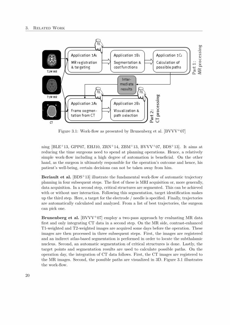
Figure 3.1: Work-flow as presented by Brunenberg et al. [BVVV+07]
ning [BLE+13, GPP07, EHJ10, ZRN+14, ZBM+13, BVVV+07, BDS+13]. It aims atreducing the time surgeons need to spend at planning operations. Hence, a relativelysimple work-flow including a high degree of automation is beneficial. On the otherhand, as the surgeon is ultimately responsible for the operation’s outcome and hence, hispatient’s well-being, certain decisions can not be taken away from him.
Beriault et al. [BDS+13] illustrate the fundamental work-flow of automatic trajectoryplanning in four subsequent steps. The first of these is MRI acquisition or, more generally,data acquisition. In a second step, critical structures are segmented. This can be achievedwith or without user interaction. Following this segmentation, target identification makesup the third step. Here, a target for the electrode / needle is specified. Finally, trajectoriesare automatically calculated and analyzed. From a list of best trajectories, the surgeoncan pick one.
Brunenberg et al. [BVVV+07] employ a two-pass approach by evaluating MR datafirst and only integrating CT data in a second step. On the MR side, contrast-enhancedT1-weighted and T2-weighted images are acquired some days before the operation. Theseimages are then processed in three subsequent steps. First, the images are registeredand an indirect atlas-based segmentation is performed in order to locate the subthalamicnucleus. Second, an automatic segmentation of critical structures is done. Lastly, thetarget points and segmentation results are used to calculate possible paths. On theoperation day, the integration of CT data follows. First, the CT images are registered tothe MR images. Second, the possible paths are visualized in 3D. Figure 3.1 illustratesthe work-flow.
20
3.1. Biopsy Planning
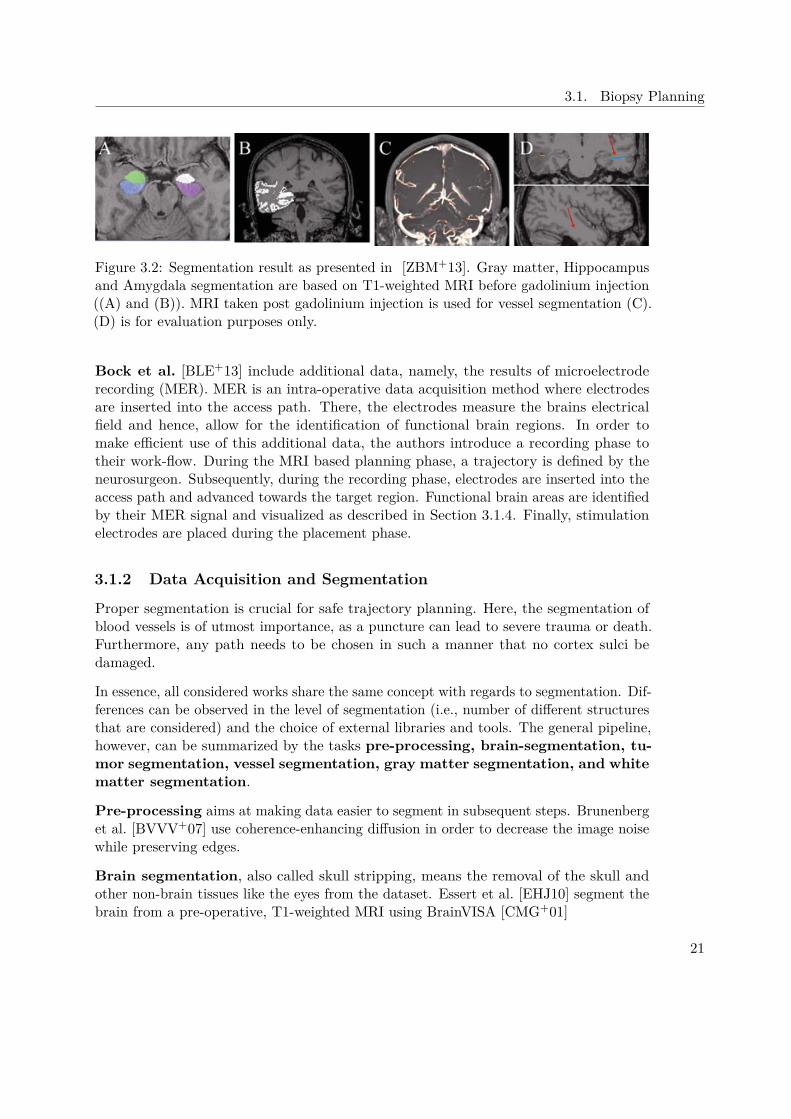
Figure 3.2: Segmentation result as presented in [ZBM+13]. Gray matter, Hippocampusand Amygdala segmentation are based on T1-weighted MRI before gadolinium injection((A) and (B)). MRI taken post gadolinium injection is used for vessel segmentation (C).(D) is for evaluation purposes only.
Bock et al. [BLE+13] include additional data, namely, the results of microelectroderecording (MER). MER is an intra-operative data acquisition method where electrodesare inserted into the access path. There, the electrodes measure the brains electricalfield and hence, allow for the identification of functional brain regions. In order tomake efficient use of this additional data, the authors introduce a recording phase totheir work-flow. During the MRI based planning phase, a trajectory is defined by theneurosurgeon. Subsequently, during the recording phase, electrodes are inserted into theaccess path and advanced towards the target region. Functional brain areas are identifiedby their MER signal and visualized as described in Section 3.1.4. Finally, stimulationelectrodes are placed during the placement phase.
3.1.2 Data Acquisition and Segmentation
Proper segmentation is crucial for safe trajectory planning. Here, the segmentation ofblood vessels is of utmost importance, as a puncture can lead to severe trauma or death.Furthermore, any path needs to be chosen in such a manner that no cortex sulci bedamaged.
In essence, all considered works share the same concept with regards to segmentation. Dif-ferences can be observed in the level of segmentation (i.e., number of different structuresthat are considered) and the choice of external libraries and tools. The general pipeline,however, can be summarized by the tasks pre-processing, brain-segmentation, tu-mor segmentation, vessel segmentation, gray matter segmentation, and whitematter segmentation.
Pre-processing aims at making data easier to segment in subsequent steps. Brunenberget al. [BVVV+07] use coherence-enhancing diffusion in order to decrease the image noisewhile preserving edges.
Brain segmentation, also called skull stripping, means the removal of the skull andother non-brain tissues like the eyes from the dataset. Essert et al. [EHJ10] segment thebrain from a pre-operative, T1-weighted MRI using BrainVISA [CMG+01]
21
3. Related Work
Tumor segmentation is necessary in order to define a target region. This can bedone automatically or manually. Herghelegiu et al. [HMG11] segment the tumor in aT1-weighted MRI sequence using the watershed algorithm, which is based on the variationof voxel gradients.
Vessel segmentation is crucial as hitting a vessel is arguably the highest risk onefaces when performing a biopsy. Proper segmentation is therefore of the utmost im-portance. Most authors make use of a vesselness-filter, which enhances voxels withintubular structures. Herghelegiu et al. [HMG11] obtain the blood vessel mask by manualsegmentation. Zelmann et al. [ZBM+13] process a post-gadolinium set of MRI witha vesselness-filter that returns a voxel likelihood of blood vessel presence in the [0;1]range. Figure 3.2(C) shows a corresponding MRI. Brunenberg et al. [BVVV+07] alsouse a vesselness measure, based on the work of Frangi et al. [FNVV98]. Beriault etal. [BDS+13] fully automatically extract arteries from time-of-flight (TOF) angiographyand veins from susceptibility-weighted imaging (SWI) venography. SWI data is processedwith a vesselness-filter. Zombori et al. [ZRN+14] extract the vasculature from computedtomography angiography (CTA), 3D Phase Contrast MRI and Time-of-flight (ToF) MRusing a custom tool.
Gray Matter Segmentation reveals structures at risk in the gray matter. Thoseinclude the ventricles, sulci, gyri and other subcortical structures. Different authorspropose different segmentation strategies:
Ventriclesmust not be punctured during the biopsy. Gemmar et al. [GGF+08] preprocessthe T1-weighted MRI with an nonlinear anisotropic diffusion (NLAD) filter and thenapply a modified 3D region growing algorithm to segment the 3rd ventricle. From the3rd ventricle’s symmetry plane, the mid-sagittal plane (MSP) is found. The anterior(AC) and posterior (PC) commissure of the 3rd ventricle is then identified at theanterior and posterior boundaries of the 3rd ventricle. Brunenberg et al. [BVVV+07]segment ventricles with a region-growing method based on the work of Schnack etal. [SPB+01] in combination with morphological methods presented by Géraud [Gér98].Essert et al. [EHJ10] segment ventricles semi-automatically using MITK (Medical ImagingInteraction ToolKit [MNMW09]). Beriault et al. [BDS+13] segment the ventricles fromthe T1-weighted MRI using ANIMAL [CZBE99].
Cortical Structures need to be segmented because trans-gyral trajectories are preferredover trans-sulcal trajectories. This is because small vessels in the sulci are usually notdetectable in MRI yet still pose a risk. Brunenberg et al. [BVVV+07] use morphologicaloperations (i.e., dilation and erosion) based on the methods of Géraud [Gér98] as well asmasking of T2- with results from T1-weighted MR and a connected component analysis incombination with the method of Lohman [Loh98] to segment the sulci and gyri. Essert etal. [EHJ10] automatically segment cortical sulci from the previously extracted brain usingan algorithm based on curvature information. Beriault et al. [BDS+13] and Zelmann etal. [ZBM+13] segment the sulci from the T1-weighted MRI using ANIMAL [CZBE99].
Subcortical Structures are at risk in the case of tumors which are situated deeper
22

3.1. Biopsy Planning
in the brain, i.e., further away from the cortex. Beriault et al. [BDS+13] segment theCaudate from the T1-weighted MRI using ANIMAL [CZBE99]. Zelmann et al. [ZBM+13]use ANIMAL, augmented with a template library and label fusion [CP10] to segment theAmygdala and Hippocampus from T1-weighted MRI. In Figure 3.2 (A) and (B), thosestructures are highlighted in the respective MRI.
White Matter Segmentation reveals structures at risk in the white matter, pri-marily white matter tracts (e.g. cortico-spinal tract, optic radiation tract). Zelmannet al. [ZBM+13] segment the white matter from the T1-weighted MRI using ANI-MAL [CZBE99]. Zombori et al. [ZRN+14] point out that they segment white mattertracts from DTI data.
3.1.3 Path Planning
After proper segmentation, the goal of most presented works is automatic or semi-automatic trajectory planning. Basically, the planning process is performed eitheron a mesh/geometry base (e.g., the work performed by Gao et al. [GCH+14]) or on anvolume base (e.g., the work performed by Shamir et al. [STD+10]). Regardless of thechosen approach, the general steps can be summarized as follows.
The first step is the selection of a target point or area. This choice is usually basedon a prior segmentation, e.g. with a watershed algorithm or manual intervention bythe surgeon. After a target point or area was chosen, potential entry points must beselected. This can be done either fully automatically or based on a user-specified entryregion. Usually, a skull mesh is used for sample point generation. Based on the targetpoint or area and an entry point or area, a list of potential trajectories is generated.The list of trajectory candidates is processed and each candidate is assessed for qualitybased on certain criteria. While different authors propose different evaluation criteria,the consensus is that the minimum distance between the trajectory and the closest vesselis of utmost importance. This trajectory evaluation yields the set of results. Thetrajectories that score best in the assessment are presented to the user in a subsequentstep.
Brunenberg et al. [BVVV+07], automatically generate a set of safe entry points. Thesepoints are chosen such that they begin in front of the motor cortex but behind the hairline.From each of these points, a straight path towards the target is calculated based on thesegmentation results. For each such path, two cost functions are stored. Those costsare based on the minimum distance to a vessel (function one) and the minimumdistance to a ventricle (function two). For faster search in the result set, safe paths(i.e., paths that do not cross a safe margin of 5 mm around vessels and/or ventricles)are stored in bins representing the respective distances. This way, good paths (i.e., suchpaths that exhibit higher distances than defined thresholds) can be proposed withoutfurther examination.
Gao et al. [GCH+14] present a prototype system for craniofacial surgery. and presentexperimental results for tumor surgery. In a first step, the authors form a spherical target
23
3. Related Work
area around the target point. Trajectories are evaluated based on visibility attributesof this target area. Five measures are used for quantification of a path’s quality: TheVital Distance (VD) essentially encompasses the same information as considered byBrunenberg et al. [BVVV+07]. The Insertion Depth gives a measure of the pathslength, with shorter paths being superior to longer ones. The Visible Size of theTarget Area (VSTA) from the entry point yields a safety margin. The target areais defined as a sphere centered around the target point. Higher visibility means lessocclusion and, as a consequence, higher distances to vital structures. Hence, paths witha larger visible size of the target area are preferable. The authors claim that if the VSTAis above a specified threshold, the safety of the path can be guaranteed. The AbsoluteVisible Size (AVS) accounts for the fact that tumors and similar structures are notnecessarily spherical in their appearance. Therefore, the AVS is defined as the visibility ofthe segmented target structure from the starting point, when considering the occlusionsthrough surrounding tissues. The Relative Visible Rate (RVR) of the target is theAVS divided by the whole area size (WAS) of the target. The WAS is the size ofthe tumor from the start point of the path when no surrounding tissues are considered.Like the AVS, the RVT gives a measure of occlusion and thus, risk of crossing a vitalstructure.
The scene is bounded by a sphere, which is sampled with approximately 18k samplepoints. Using each sample point as a camera position with the focal point set at the targetposition, the scene is rendered twice, once with surrounding tissues and once withoutthem. From these renderings, the AVS and RVR can be acquired. These two measures,together with the visible size of the target area, can be used to filter and dispose ofunsuitable paths before calculating the other markers for the remaining paths. Since thenumber of remaining paths can still be too large to allow for a feasible selection, all pathsare clustered using a mean shift algorithm as proposed by Cheng [Che95]. Clusteredpaths are further reduced to the safest one. Implicitly, a safety margin is given by theposition inside the cluster, as medial paths naturally offer a bigger margin than lateralones. Additionally, as outlined before, a shorter path is preferable over a longer one.Figure 3.3 illustrates the concept of the clustering approach.
Essert et al. [EHJ10] introduce additional rules for their DBS planning system. Here, aset of eight rules has been developed in cooperation with participating neurosurgeons.The first four of these rules are Boolean (i.e., they must be satisfied for a path to beacceptable). First, the target point needs to be placed at the target. Second, the entrypoint must be on the scalp. Third, path length is restricted to a maximum of 90 mm.This eliminates insertion points on the other side of the cranium. Finally, structures atrisk, i.e., vessels and ventricles, are avoided.
The remaining four rules are preferences (i.e., they need to be optimized based on a set ofweights). The first rule concerns theminimization of the path length, as longer pathsare inherently more damaging and dangerous than shorter ones. This is a low-weightrule and can be omitted. The second rule states that distances to structures at riskshould be maximized. Again, this is a preference rule, as the avoidance of risky structures
24

3.1. Biopsy Planning
already yields a safety margin. The third rule defines a relationship between the targetshape and the orientation of the electrode. The trajectory axis should be orientedas close as possible with target main axis. Finally, according to the fourth rule, the tipof the electrode should be placed as close as possible to the center of the target. Thispreference rule is more important for DBS than for biopsy planning, as the electroderemains in the brain with DBS.
While the first four of these rules are Boolean (i.e., they must be satisfied for a pathto be acceptable), the remaining four are preferences (i.e., they need to be optimizedbased on a set of weights). Rules one and two, regarding the position of insertion pointsand target points, are provided with the input data rather than being determined, hencereducing the model’s complexity.
The insertion mesh is evaluated on a triangle-by-triangle basis, with triangles that do notsatisfy the hard constraints being eliminated from the solution set. Triangles which onlypartially satisfy the constraints are further subdivided into four smaller triangles whichare then re-tested. From the remaining set of insertion points, some homogeneouslyspaced points are chosen and evaluated with regards to satisfying of the soft constraints.Around the best of these points, a connected components analysis is performed andNelder-Mead optimization is done from the best candidate. This way, local minima areavoided. Evaluated triangles are rendered with a transfer function that color codes theaggregative cost function for a trajectory. Good entry regions are presented in green, badentry regions are presented in red, and a range of progressive intermediate colors is usedfor the other areas. Figure 3.4 illustrates the color map, applied to the insertion mesh.
Herghelegiu et al. [HMG11] follow a slightly different approach. First, they segment thetumor using a watershed algorithm. Furthermore, they manually segment a blood-vesselmask. Then, they apply a distance transformation (DT) to the vessel-segmentationresults. This distance transform yields color-coded information about the proximity ofvessels for every pixel in a slice. For every entry point EP and every tumor point TP,a simple check is performed to determine whether the tumor point is reachable, i.e.,whether it lies on the tumor’s surface and allows for sufficiently deep entry to actuallytake a sample. Each point satisfying these requirements is added to a list of reachablepoints. Around each of those reachable tumor points, a disk D is created in the needlepathway’s (NP’s) normal plane as a proxy object for cost calculation. For each voxelV on the slice, a direction between the entry point EP and V is derived. If a point TPbelonging to the tumor is found along that direction, the corresponding NP is storedwith its cost being set to the nearest distance to a vessel. This distance can be acquiredfrom the previously calculated DT.
Zombori et al. [ZRN+14] point out that for reasons of robustness, the entry angle of thetrajectory should be as close to 90 degrees as possible. In their MITK based EpiNavsystem, a system for DBS planning, the authors consider much more information than allthe above presented implementations: White matter tracts derived from DTI data,lesions and eloquent cortex derived from fMRI, areas of ictal hyperperfusionderived from SPECT images, areas of hypometabolism derived from PET image, ictal
25

3. Related Work
or interictal EEG/MEG sources, blood vessels derived from CTA, 3D Phase ContrastMR imaging and in some cases ToF MR and, the skull surface derived from CT, CTAor pseudo CT synthesized from an MR scan.
Entry point candidates are automatically created from the vertices of the skull mesh. Ina first step, distance and entry angle for each trajectory are checked against user-definedthresholds. Trajectories that do not match the criteria are immediately discarded. Thisshrinks the search space in a computationally inexpensive way. The innovation thatis presented in EpiNav is the inclusion of a full distance profile along the trajectory,presenting distances to critical structures for 256 sample points per trajectory. Thetrajectory that exhibits the lowest overall risk is chosen and presented to the surgeon.
Zelmann et al. [ZBM+13] introduce novel scoring factors specific to deep brain stimulation.These factors revolve around the fact that deep electrodes need to cover a large volumefor recording purposes. For the purposes of biopsy planning, those factors are notrelevant. What is interesting, however, is that the authors chose to pick one thousand,pseudo-randomly chosen (i.e., they are uniformly spaced) trajectories for evaluation. Thisraises the question whether or not good paths get discarded by chance. Still, validationshows that results are significantly further away from blood vessels (p < 0.01) than themanually chosen paths.
3.1.4 Visualization
Although there are obvious differences in the visualization pipelines implemented bythe various authors, some shared principles exist. For example, 3D medical images aretraditionally displayed in an MPR view, i.e., a set of orthogonal cuts through thevolume. By selecting a voxel in one of the slices, the linked views displaying the otherplanes are automatically updated and the planes containing the voxel are presented.More context is offered in 3D views. Hence, these views are most practical for creatinga global understanding of the trajectory. A different use of the MPR view is the NeedlePath Slice View. To keep the decision transparent, information on the trajectory canbe encoded by choosing planes that are orthogonal to the needle path. This way, thevolume can be presented from the needle’s perspective. This is also called a Probe’s EyeView. Finally, any number of charts, plots and other well-known InfoVis techniques canbe employed to communicate certain qualitative or quantitative criteria of a trajectoryexplicitly. These Visual Analytics Views aim at creating insight into data that mightnot be revealed easily in more traditional views.
Essert et al. [EHJ10] present to the user a global color map which encodes the aggregatecost function for each path. Green pixels indicate the best insertion points whereas redpixels represent the worst points. Since the individual rules are evaluated in distinctcolor maps, the weighting parameters can be changed interactively, as only the costaggregation needs to be recalculated.
Gao et al. [GCH+14] provide the user with a 3D view illustrating vessels, tumors, and thesuggested path. Furthermore, a slice view is given where the path can easily by altered.
26
3.1. Biopsy Planning
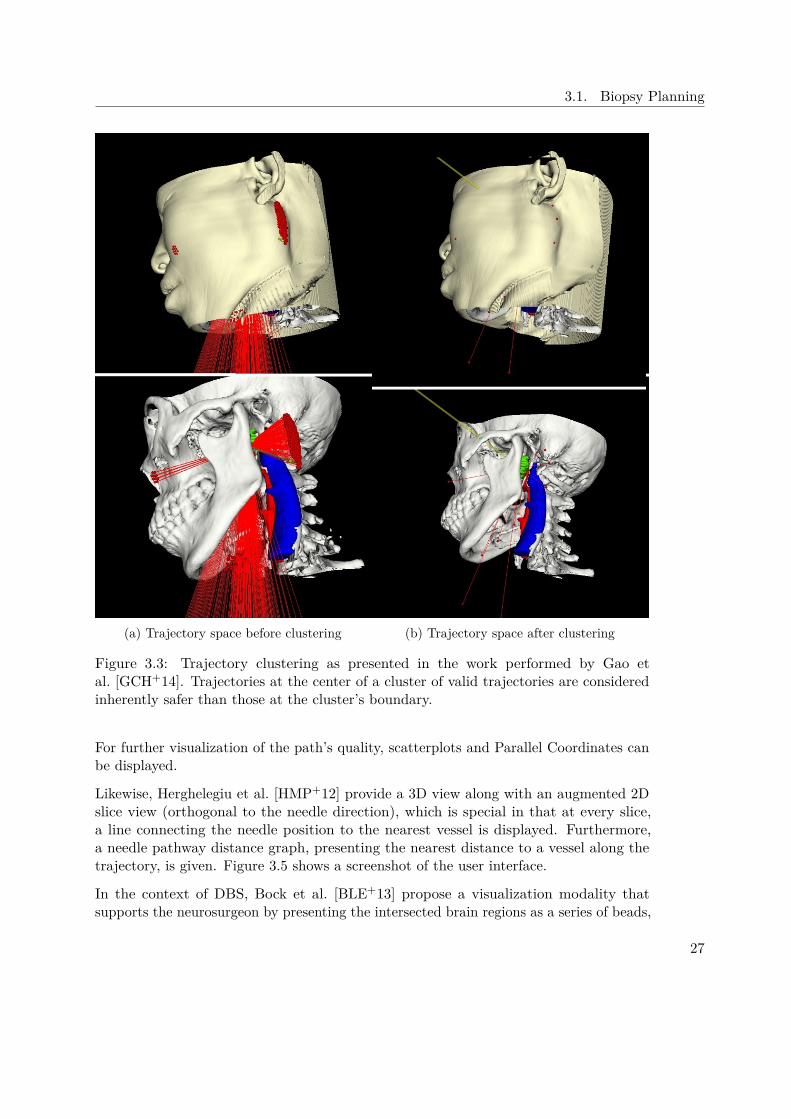
(a) Trajectory space before clustering (b) Trajectory space after clustering
Figure 3.3: Trajectory clustering as presented in the work performed by Gao etal. [GCH+14]. Trajectories at the center of a cluster of valid trajectories are consideredinherently safer than those at the cluster’s boundary.
For further visualization of the path’s quality, scatterplots and Parallel Coordinates canbe displayed.
Likewise, Herghelegiu et al. [HMP+12] provide a 3D view along with an augmented 2Dslice view (orthogonal to the needle direction), which is special in that at every slice,a line connecting the needle position to the nearest vessel is displayed. Furthermore,a needle pathway distance graph, presenting the nearest distance to a vessel along thetrajectory, is given. Figure 3.5 shows a screenshot of the user interface.
In the context of DBS, Bock et al. [BLE+13] propose a visualization modality thatsupports the neurosurgeon by presenting the intersected brain regions as a series of beads,
27
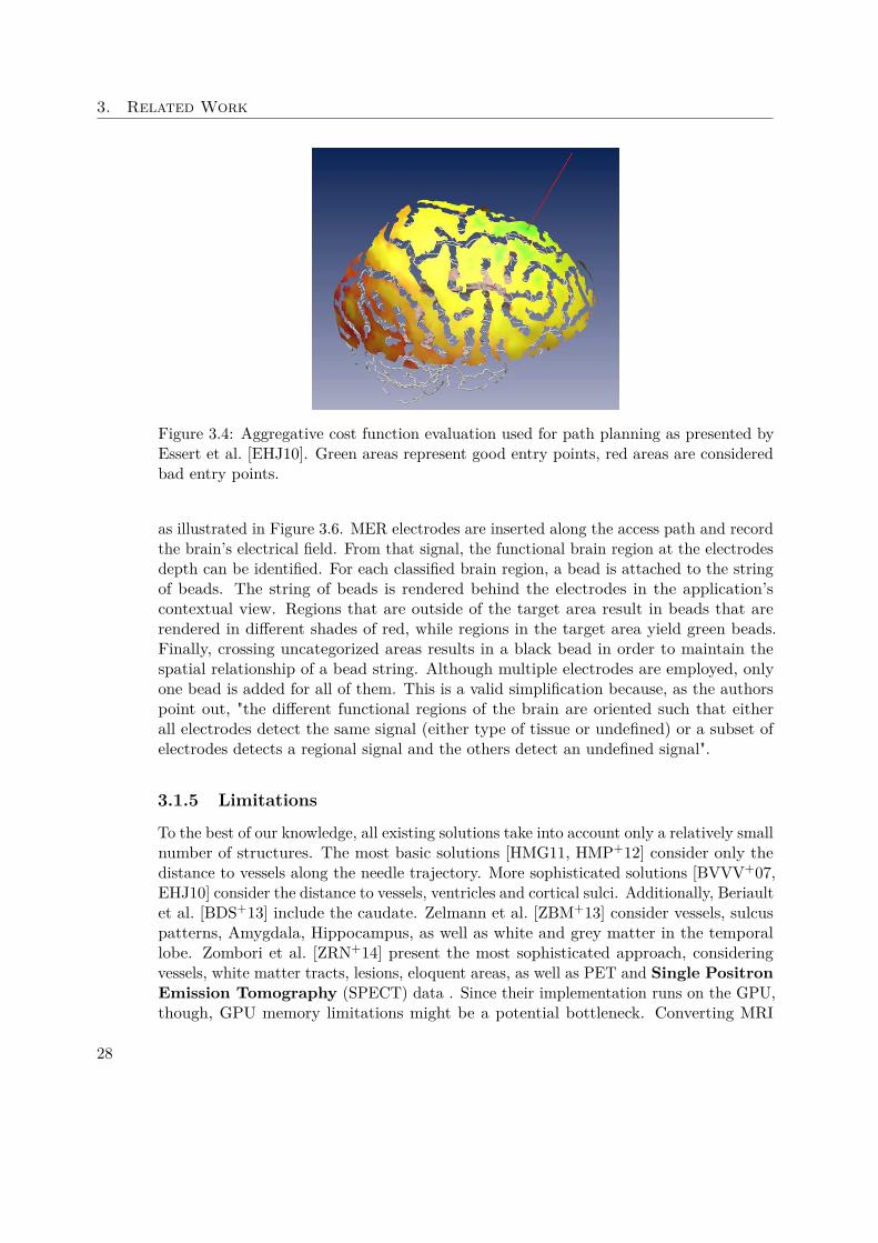
3. Related Work
Figure 3.4: Aggregative cost function evaluation used for path planning as presented byEssert et al. [EHJ10]. Green areas represent good entry points, red areas are consideredbad entry points.
as illustrated in Figure 3.6. MER electrodes are inserted along the access path and recordthe brain’s electrical field. From that signal, the functional brain region at the electrodesdepth can be identified. For each classified brain region, a bead is attached to the stringof beads. The string of beads is rendered behind the electrodes in the application’scontextual view. Regions that are outside of the target area result in beads that arerendered in different shades of red, while regions in the target area yield green beads.Finally, crossing uncategorized areas results in a black bead in order to maintain thespatial relationship of a bead string. Although multiple electrodes are employed, onlyone bead is added for all of them. This is a valid simplification because, as the authorspoint out, "the different functional regions of the brain are oriented such that eitherall electrodes detect the same signal (either type of tissue or undefined) or a subset ofelectrodes detects a regional signal and the others detect an undefined signal".
3.1.5 Limitations
To the best of our knowledge, all existing solutions take into account only a relatively smallnumber of structures. The most basic solutions [HMG11, HMP+12] consider only thedistance to vessels along the needle trajectory. More sophisticated solutions [BVVV+07,EHJ10] consider the distance to vessels, ventricles and cortical sulci. Additionally, Beriaultet al. [BDS+13] include the caudate. Zelmann et al. [ZBM+13] consider vessels, sulcuspatterns, Amygdala, Hippocampus, as well as white and grey matter in the temporallobe. Zombori et al. [ZRN+14] present the most sophisticated approach, consideringvessels, white matter tracts, lesions, eloquent areas, as well as PET and Single PositronEmission Tomography (SPECT) data . Since their implementation runs on the GPU,though, GPU memory limitations might be a potential bottleneck. Converting MRI
28

3.1. Biopsy Planning
Figure 3.5: Visualization of the Biopsy Planner presented by Herghelegiu et al. [HMP+12].Spatial information on the needle trajectory can be derived from the 3D and 2D views.Furthermore, the augmented slice view highlights vessels in the needle trajectoriesproximity. The needle pathway distance graph plots the needle’s distance to the nearestvessel along the trajectory. Finally, the entry points stability map presents the safetymargin for each potential entry point inside an ellipsoidal region of interest defined bythe user.
data, whose native format is voxel-based, to geometry meshes yields an additional lossof precision. If this loss of precision is to be avoided, a volume-based approach mustbe taken. In this case, video memory may be too small for a sufficiently high numberof structures at risk. A typical MRI resolution is 2563. When storing each segmentedstructure in a 3D texture for further use on the GPU, each texture has a size of 16 MB.At this time, typical consumer hardware offers 2GB of dedicated video memory. Thismeans that 125 distinct structures can be uploaded into the video memory. As brainatlases become more sophisticated, the number of structures at risk to be considered in abiopsy is likely to increase greatly.
We overcome this limitation and allow for an unlimited number of structures at arbitraryresolution by integrating a spatial index server [BŠG+09] into BrainXPlore that canbe queried for distance information in a very fast and efficient manner. The decision toresort to this spatial index instead of performing GPU-based distance computation wasmade considering that this approach is not limited by GPU memory, but rather offers aconvenient way of accessing out-of-core data.
Linked to the limited number of structures is the rigid definition of rules. Systems, whichare restricted to a defined number of structures at risk do not necessarily support customoperation guidelines that are unique to a particular hospital. For example, our domainexpert noted that in our partner hospital, as a rule, the mid-sagittal plane is not crossed
29

3. Related Work
Figure 3.6: Contextual view during the recording phase as proposed by Bock etal. [BLE+13] The beads behind the electrode indicate intersected functional brain regions,identified by their MER signal. Red beads are outside of the target area, green beadsindicate a region that is within the target area. Black beads represent areas that couldnot be classified.
during biopsies. To the best of our knowledge, no system in the established body of workallows for such constraints. We offer the neurosurgeon a set of geometric rules (e.g., needleinsertion angle at the skull, needle insertion angle at the tumor, trajectory length) aspresented in other works [GCH+14, EHJ10]. Additionally, we introduce a flexible spatialrule system that can consider any given structure (e.g., the afore-mentioned mid-sagittalplane) and discard trajectories based on their spatial relationship to that structure (e.g.,maximal overlap, minimal distance).
3.2 Medical Information Visualization
Information is processed or interpreted data that has a meaning for those who know howto read it. Presenting this information in a meaningful way is the aim of InformationVisualization (InfoVis). Card et al. define InfoVis as "the use of computer-supported,interactive, visual representation of abstract non-physically based data to amplify cogni-tion" [CMS99]. In the following sections, we review the state of the art of typical InfoVismethods and evaluate their relevance to the interaction techniques we implemented.
In Section 3.2.1, the use of Parallel Coordinates in existing brain biopsy planning systemsis presented. Information on different implementations of sparklines and line graphs isgiven in Section 3.2.2. Finally, in Section 3.2.3, methods for visualizing multivariate dataare investigated.
30

3.2. Medical Information Visualization
3.2.1 Parallel Coordinates
Parallel Coordinates [Ins85] are a well established InfoVis technique used for displayingmultivariate data. Data sets are displayed as lines passing through a set of vertical,parallel axes, where each axis represents a single data feature. By arranging the axes,correlations between data features can be identified.
In the context of brain biopsy planning, Parallel Coordinates have been employed byGao et al. [GCH+14]. The risk signature for each trajectory is represented in the ParallelCoordinate View and updated interactively when the path is adjusted.
Martin and Ward [MW95] evaluated the usefulness of brushing in Parallel Coordinatesand found it an "indispensable tool for visualizing and examining" multivariate data.To the best of our knowledge, no existing work in the context of brain biopsy planningimplements trajectory picking based on a Parallel Coordinate View.
3.2.2 Line Graphs and Spark Lines
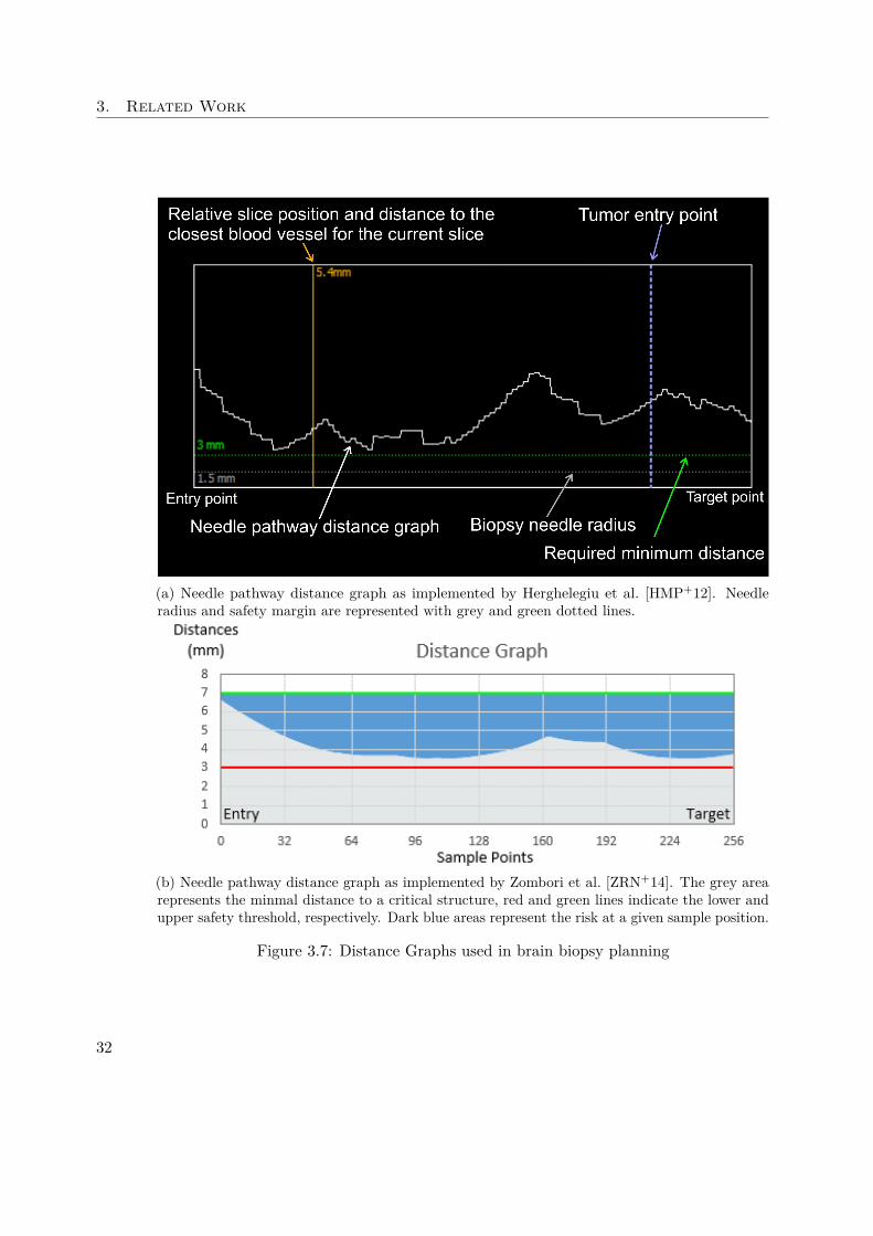
A line graph is a type of chart which, similar to a scatter plot, displays data based onpoint, so-called markers, on a 2-dimensional grid. Markers are connected by straight linesegments. Those graphs offer insight into data trends and help the viewer to understandthe relationship between the considered variables. A spark line is a special type of linegraph that indicates the change over time in some variable. Spark lines are commonlyused to illustrate the value of shares in the stock market. In the context of brain biopsyplanning, spark lines have been employed to qualitatively visualize the distance betweenthe trajectory and structures at risk.
Herghelegiu et al. [HMP+12] present a special form of line graph. A needle pathwaydistance graph shows the distance to the closest blood vessel for every point of theneedle pathway. Zombori et al. [ZRN+14] expand on this concept by introducing filledareas and annotations indicating the minimum distance to structures, risk thresholds,safety margins and the resulting risk at each sample position. Figure 3.7 illustrates bothviews.
3.2.3 Methods for Visualizing Multivariate Data
In the context of biopsy planning, the quality of a candidate trajectory depends on amultitude of factors. In some views (e.g., summary and filtering views ), multivariatedata must be displayed in such a manner so as to instantly reveal significant featuresto the user to drive the selection process. At the same time, dimensionality must bereduced to such a degree that visual cluttering is avoided.
Ropinski et al. [ROP11] discuss glyph-based visualization techniques for spatial mul-tivariate medical data. The authors differentiate between a pre-attentive and anattentive phase of stimulus processing. During the pre-attentive phase, impulses areperceived in parallel, while during the attentive phase, they are perceived sequentially.The authors identify the basic glyph shape, color, transparency, and texture as well as
31
3. Related Work
(a) Needle pathway distance graph as implemented by Herghelegiu et al. [HMP+12]. Needleradius and safety margin are represented with grey and green dotted lines.
(b) Needle pathway distance graph as implemented by Zombori et al. [ZRN+14]. The grey arearepresents the minmal distance to a critical structure, red and green lines indicate the lower andupper safety threshold, respectively. Dark blue areas represent the risk at a given sample position.
Figure 3.7: Distance Graphs used in brain biopsy planning
32
3.2. Medical Information Visualization
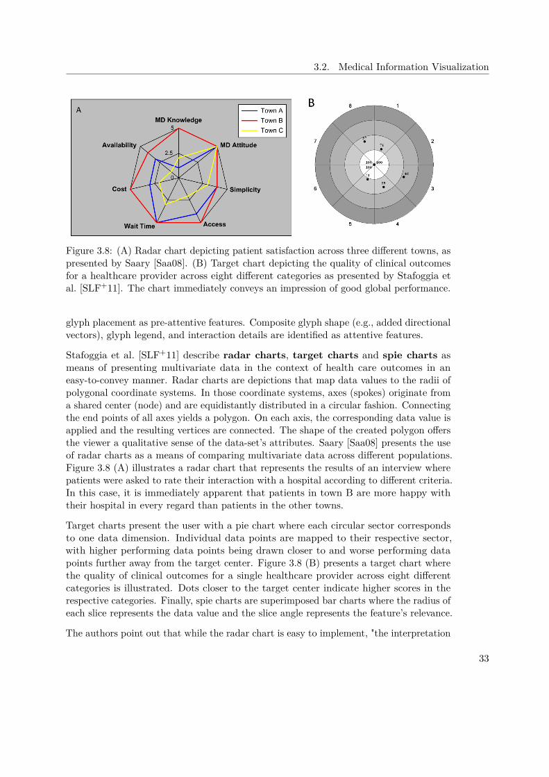
Figure 3.8: (A) Radar chart depicting patient satisfaction across three different towns, aspresented by Saary [Saa08]. (B) Target chart depicting the quality of clinical outcomesfor a healthcare provider across eight different categories as presented by Stafoggia etal. [SLF+11]. The chart immediately conveys an impression of good global performance.
glyph placement as pre-attentive features. Composite glyph shape (e.g., added directionalvectors), glyph legend, and interaction details are identified as attentive features.
Stafoggia et al. [SLF+11] describe radar charts, target charts and spie charts asmeans of presenting multivariate data in the context of health care outcomes in aneasy-to-convey manner. Radar charts are depictions that map data values to the radii ofpolygonal coordinate systems. In those coordinate systems, axes (spokes) originate froma shared center (node) and are equidistantly distributed in a circular fashion. Connectingthe end points of all axes yields a polygon. On each axis, the corresponding data value isapplied and the resulting vertices are connected. The shape of the created polygon offersthe viewer a qualitative sense of the data-set’s attributes. Saary [Saa08] presents the useof radar charts as a means of comparing multivariate data across different populations.Figure 3.8 (A) illustrates a radar chart that represents the results of an interview wherepatients were asked to rate their interaction with a hospital according to different criteria.In this case, it is immediately apparent that patients in town B are more happy withtheir hospital in every regard than patients in the other towns.
Target charts present the user with a pie chart where each circular sector correspondsto one data dimension. Individual data points are mapped to their respective sector,with higher performing data points being drawn closer to and worse performing datapoints further away from the target center. Figure 3.8 (B) presents a target chart wherethe quality of clinical outcomes for a single healthcare provider across eight differentcategories is illustrated. Dots closer to the target center indicate higher scores in therespective categories. Finally, spie charts are superimposed bar charts where the radius ofeach slice represents the data value and the slice angle represents the feature’s relevance.
The authors point out that while the radar chart is easy to implement, "the interpretation
33
3. Related Work
of the results strongly depends on the ordering of the indicators being displayed". Also,missing information introduces ambiguity (i.e., it is impossible to distinguish between amissing data feature and one whose value is zero). They continue to state that the targetchart does not perform well in situations where many data dimensions are displayed.Finally, they conclude that spie charts overcome the limitations of both radar charts andtarget charts and allow for the flexible definition of the different weights of displayed datadimensions. Finally, the authors conclude that out of the three presented techniques, "thespie chart is the best alternative for graphically presenting clinical outcome indicatorsfor comparative evaluations among health care providers or populations".
Chernoff [Che73] proposes Chernoff Faces, another form of iconic representation ofmultivariate data. In this visualization, data features are mapped to 18 distinct facialfeatures on cartoon faces. The author explains that this approach is based on a reverseimage recognition algorithm - instead of discriminating between human faces by reducingthem to numbers, numbers are discriminated by rendering faces and leaving interpretationto the expert user. Morris et al. [MER00] conclude that Chernoff facial feature perceptionis not pre-attentive and that hence "Chernoff faces may not have significant advantageover other multivariate iconic visualization techniques".
34
CHAPTER 4Visual Computing Work-flow and
System Design
After briefly discussing the state-of-the art in brain biopsy planning, in this Chapterwe present our prototype for a novel brain biopsy planning framework. It allows thedefinition of custom planning rules and interactive exploration of the resulting trajectories.Here we explain how the requirements were defined and how our system overcomes thechallenges presented by existing solutions.
In Section 4.1, we describe how we conducted the requirement analysis and the resultsit produced. Section 4.2 offers a global overview of our system and the participatingmodules. Finally, in Section 4.3, the work-flow from the user’s perspective is presented.
4.1 Requirement Analysis
To evaluate the requirements of our new system, we have conducted interviews withthe domain expert and asked about the biopsy planning work-flow as performed in thepartner hospital. Before deriving requirements, we will discuss the interview in thisSection.
Currently, our domain expert performs the biopsy planning with the help of the MedTronic(http://www.medtronic.com) StealthStation Surgical Navigation System. In an ortho-graphic coordinate system, MRI data is displayed in a sagittal, cranial and coronalview. Also, a supporting 3D view is presented to the surgeon. Various data (i.e., CT,MRA, etc) can be used as overlays to highlight structures such as vessels.
To plan the biopsy, as a first step, a target point or area on the tumor is defined. Thistarget point should be located inside living tissue, as necrotic tissue is not well suited forfurther histological examination. To define an entry point, the surgeon first defines the
35
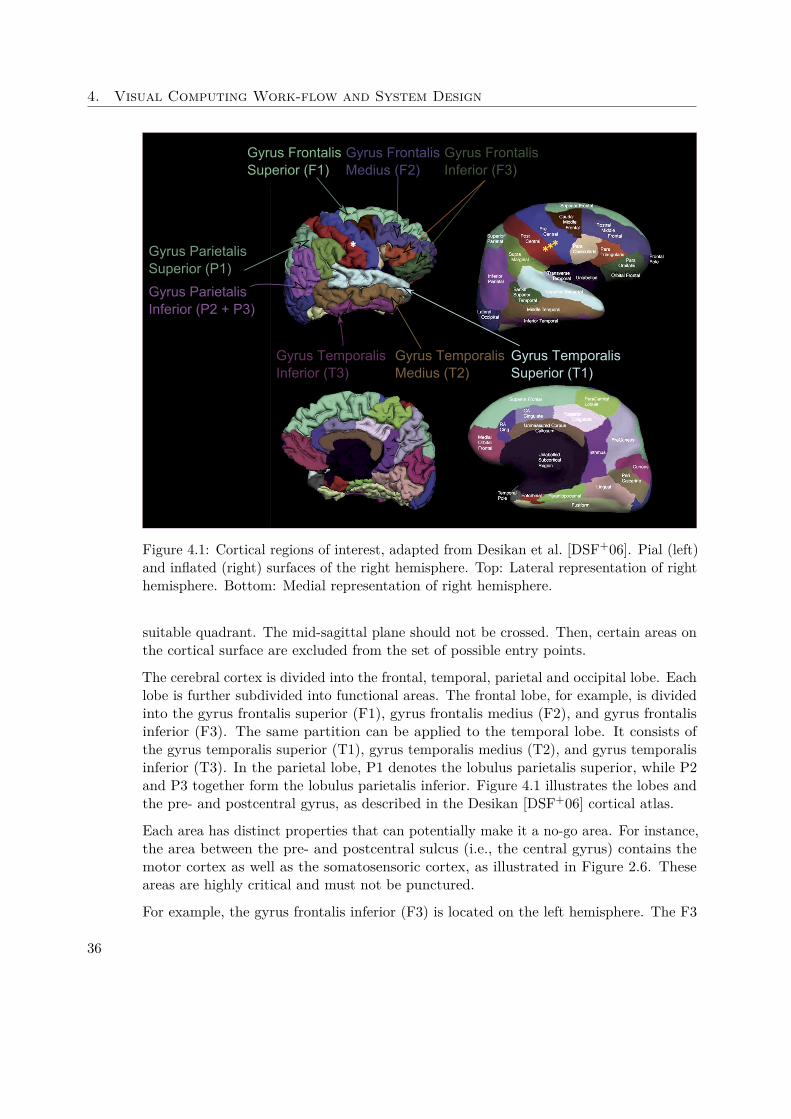
4. Visual Computing Work-flow and System Design
Gyrus Frontalis Superior (F1)
Gyrus Frontalis Medius (F2)
Gyrus Frontalis Inferior (F3)
Gyrus Temporalis Superior (T1)
Gyrus Temporalis Medius (T2)
Gyrus Temporalis Inferior (T3)
Gyrus Parietalis Superior (P1)
Gyrus Parietalis Inferior (P2 + P3)
Figure 4.1: Cortical regions of interest, adapted from Desikan et al. [DSF+06]. Pial (left)and inflated (right) surfaces of the right hemisphere. Top: Lateral representation of righthemisphere. Bottom: Medial representation of right hemisphere.
suitable quadrant. The mid-sagittal plane should not be crossed. Then, certain areas onthe cortical surface are excluded from the set of possible entry points.
The cerebral cortex is divided into the frontal, temporal, parietal and occipital lobe. Eachlobe is further subdivided into functional areas. The frontal lobe, for example, is dividedinto the gyrus frontalis superior (F1), gyrus frontalis medius (F2), and gyrus frontalisinferior (F3). The same partition can be applied to the temporal lobe. It consists ofthe gyrus temporalis superior (T1), gyrus temporalis medius (T2), and gyrus temporalisinferior (T3). In the parietal lobe, P1 denotes the lobulus parietalis superior, while P2and P3 together form the lobulus parietalis inferior. Figure 4.1 illustrates the lobes andthe pre- and postcentral gyrus, as described in the Desikan [DSF+06] cortical atlas.
Each area has distinct properties that can potentially make it a no-go area. For instance,the area between the pre- and postcentral sulcus (i.e., the central gyrus) contains themotor cortex as well as the somatosensoric cortex, as illustrated in Figure 2.6. Theseareas are highly critical and must not be punctured.
For example, the gyrus frontalis inferior (F3) is located on the left hemisphere. The F3
36
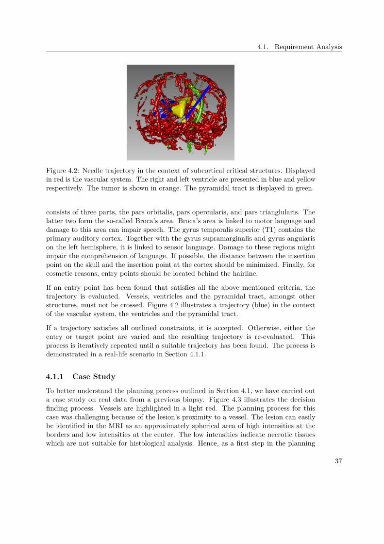
4.1. Requirement Analysis
Figure 4.2: Needle trajectory in the context of subcortical critical structures. Displayedin red is the vascular system. The right and left ventricle are presented in blue and yellowrespectively. The tumor is shown in orange. The pyramidal tract is displayed in green.
consists of three parts, the pars orbitalis, pars opercularis, and pars trianglularis. Thelatter two form the so-called Broca’s area. Broca’s area is linked to motor language anddamage to this area can impair speech. The gyrus temporalis superior (T1) contains theprimary auditory cortex. Together with the gyrus supramarginalis and gyrus angularison the left hemisphere, it is linked to sensor language. Damage to these regions mightimpair the comprehension of language. If possible, the distance between the insertionpoint on the skull and the insertion point at the cortex should be minimized. Finally, forcosmetic reasons, entry points should be located behind the hairline.
If an entry point has been found that satisfies all the above mentioned criteria, thetrajectory is evaluated. Vessels, ventricles and the pyramidal tract, amongst otherstructures, must not be crossed. Figure 4.2 illustrates a trajectory (blue) in the contextof the vascular system, the ventricles and the pyramidal tract.
If a trajectory satisfies all outlined constraints, it is accepted. Otherwise, either theentry or target point are varied and the resulting trajectory is re-evaluated. Thisprocess is iteratively repeated until a suitable trajectory has been found. The process isdemonstrated in a real-life scenario in Section 4.1.1.
4.1.1 Case Study
To better understand the planning process outlined in Section 4.1, we have carried outa case study on real data from a previous biopsy. Figure 4.3 illustrates the decisionfinding process. Vessels are highlighted in a light red. The planning process for thiscase was challenging because of the lesion’s proximity to a vessel. The lesion can easilybe identified in the MRI as an approximately spherical area of high intensities at theborders and low intensities at the center. The low intensities indicate necrotic tissueswhich are not suitable for histological analysis. Hence, as a first step in the planning
37

4. Visual Computing Work-flow and System Design
process, a target point near the lesion’s caudal border is defined where the tissue is aliveand metabolically active.
In a second step, an entry point is chosen, in accordance with the criteria defined inSection 2.3. Because the target point is located in the left hemisphere and the mid-sagittalplane must not be crossed, the entry point must be on the left side as well. Since thetarget is also located anterior to the mid-coronal plane, the parietal and occipital lobesare disqualified as entry regions. This leaves the frontal and temporal lobe as candidates.F3 and T1 are excluded due to their anatomical relevance, as explained in Section 2.3. Asuitable trajectory was found iteratively, as illustrated in Figures 4.3 and 4.4.
4.1.2 Core Requirements
Based on the state of the art case study presented in Section 4.1.1, we have derived thefollowing core requirements for our system:
• Automatic entry point generation
• Multiple target point optimization
• Avoidance of structures at risk
Given the relevant hemisphere, a set of potential entry points must be calculated au-tomatically. These entry points must be on the skull surface and must not be locatedon areas where trajectories are not feasible such as the eyes or ears. Trajectories mustbe evaluated for a set of target points rather than a single target. This, in conjunctionwith the automatic entry point generation, allows the system to evaluate a multitude ofcandidate trajectories. As presented in the case study, currently the surgeon manuallyevaluates a relatively small set of trajectories, piece by piece, until a suitable candidate isfound. Delegating this task to the system is the main driver for time savings. To ensurethe patient’s safety, structures at risk such as vessels, ventricles and sulci must not bedamaged by any resulting trajectory.
While this list satisfies all requirements that arise from the case study, we have decidedto expand it and make some fundamental improvements. First, rather than dictating theselection criteria for valid trajectories, we want our system to allow for a Flexible FilterRule Definition. The system must allow the neurosurgeon to flexibly define rules fortrajectory evaluation. Trajectories that violate those rules must are not considered forfurther evaluation. Furthermore, discriminates valid trajectories with regards to theirquality. It also offers the neurosurgeon a way of defining the rules for this TrajectoryQuality Evaluation.
From a interaction design point of view, the system should allow for interactive filteringof trajectories. Initially generated trajectories can be filtered based on attributes such aslength, structure to vital distances, etc. Filtering is interactive and provides immediate
38
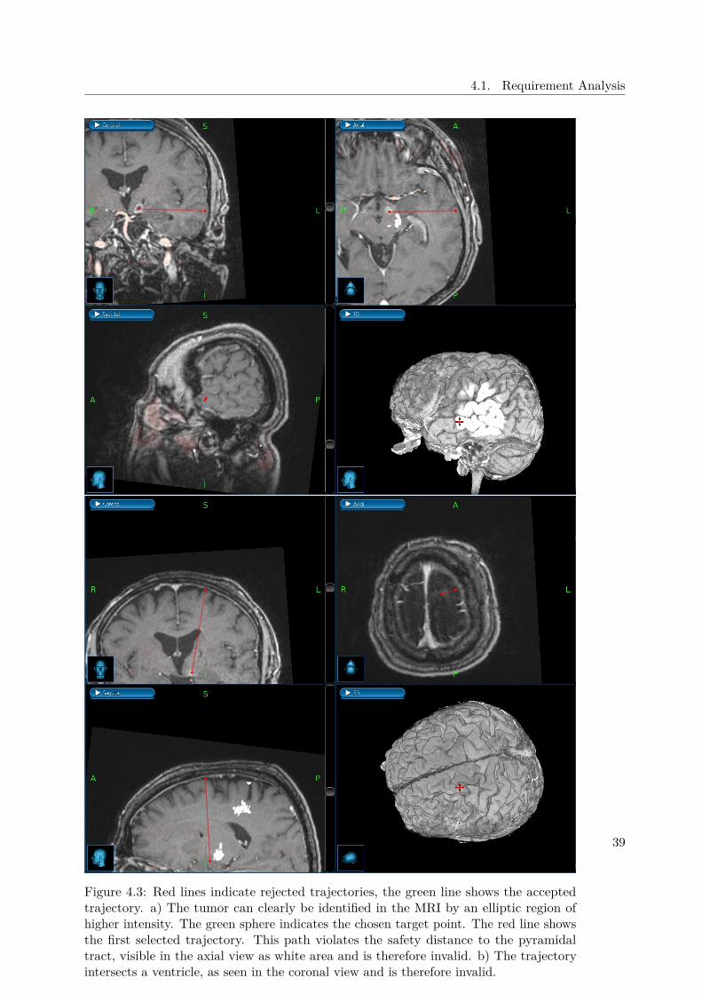
4.1. Requirement Analysis
Figure 4.3: Red lines indicate rejected trajectories, the green line shows the acceptedtrajectory. a) The tumor can clearly be identified in the MRI by an elliptic region ofhigher intensity. The green sphere indicates the chosen target point. The red line showsthe first selected trajectory. This path violates the safety distance to the pyramidaltract, visible in the axial view as white area and is therefore invalid. b) The trajectoryintersects a ventricle, as seen in the coronal view and is therefore invalid.
39
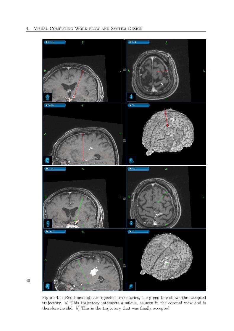
4. Visual Computing Work-flow and System Design
Figure 4.4: Red lines indicate rejected trajectories, the green line shows the acceptedtrajectory. a) This trajectory intersects a sulcus, as seen in the coronal view and istherefore invalid. b) This is the trajectory that was finally accepted.
40

4.2. System Overview
feedback. Since the neurosurgeon is the authority in his field and ultimately has theresponsibility for the biopsies outcome, the system should offer the possibility of manuallyrefining existing trajectories and evaluating the result. The interactive refinementand addition of trajectories must be accomplished at interactive framerates.
Because our system is designed to be a proof-of-concept prototype, we have decided toimplement different visualization techniques and evaluate them in the context of biopsyplanning.
4.1.3 Interaction Requirements
To define requirements for the user interface of BrainXPlore, we conducted multipledesign sessions with a domain expert. We discussed the challenges in his work-flowand utilized tools. Based on our consultation with the expert and previous work, weimplemented the following design guidelines for developing the interface:
Workflow-based user interaction: The work-flow, from the user’s perspective, isdescribed in Section 4.3. The user interface should be arranged so that it supportsthe work-flow rather than hinders it.
Interactivity: Data segmentation is non-trivial and error-prone. Hence, the finaldecision should always belong to the surgeon. The system should allow to changeboth endpoints of a suggested trajectory and provide interactive feedback. Also,rule refinement should provide immediate visual feedback.
Providing diverse data perspectives and views: 3D views offer good spatial con-text but also tend to exhibit a high degree of occlusion. 2D slice views, on theother hand, do not offer the same spatial context but are very good at conveyinginformation on a limited part of the data. In the context of brain biopsy planning,for example, when tracing the needle trajectory, a slice orthogonal to the trajectorycan be extracted from the MRI dataset at every point on the trajectory. This slicethen offers a direct view of the needle’s surroundings, i.e., a probe’s eye view. Info-Vis views such as Parallel Coordinates offer information that goes beyond spatialinformation, e.g., data distribution and correlation in multidimensional datasets.For example, histograms can offer an estimate of how a rule refinement may affectthe number of available trajectories. Parallel Coordinates offer a convenient pickingmethod that allows the user to select trajectories based on multiple features in oneview.
4.2 System OverviewBrainXPlore consists of four major components: a data preprocessing module, atrajectory preprocessing module, the index server, and an interactive visualizationmodule (i.e., the user interface). The interactive visualization module is implementedin the rapid prototyping software MeVisLab [Sol17]. Figure 4.5 illustrates our system
41

4. Visual Computing Work-flow and System Design
Figure 4.5: Overview of BrainXPlore system architecture. Data acquisition andsegmentation are not part of BrainXPlore and can be accomplished using variousapproaches. The data preprocessing module translates data into BrainXPlore’s internalformat. The index server stores distance information for all trajectories. The trajectorypreprocessing module samples the volume and generates initial trajectories. All userinteraction takes place in the user interface module, where rules are defined and refineduntil a suitable trajectory has been found.
42
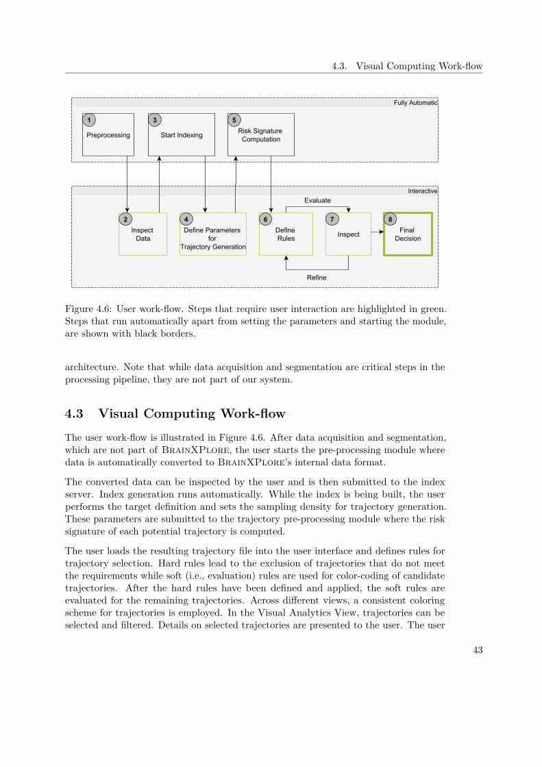
4.3. Visual Computing Work-flow
Figure 4.6: User work-flow. Steps that require user interaction are highlighted in green.Steps that run automatically apart from setting the parameters and starting the module,are shown with black borders.
architecture. Note that while data acquisition and segmentation are critical steps in theprocessing pipeline, they are not part of our system.
4.3 Visual Computing Work-flow
The user work-flow is illustrated in Figure 4.6. After data acquisition and segmentation,which are not part of BrainXPlore, the user starts the pre-processing module wheredata is automatically converted to BrainXPlore’s internal data format.
The converted data can be inspected by the user and is then submitted to the indexserver. Index generation runs automatically. While the index is being built, the userperforms the target definition and sets the sampling density for trajectory generation.These parameters are submitted to the trajectory pre-processing module where the risksignature of each potential trajectory is computed.
The user loads the resulting trajectory file into the user interface and defines rules fortrajectory selection. Hard rules lead to the exclusion of trajectories that do not meetthe requirements while soft (i.e., evaluation) rules are used for color-coding of candidatetrajectories. After the hard rules have been defined and applied, the soft rules areevaluated for the remaining trajectories. Across different views, a consistent coloringscheme for trajectories is employed. In the Visual Analytics View, trajectories can beselected and filtered. Details on selected trajectories are presented to the user. The user
43
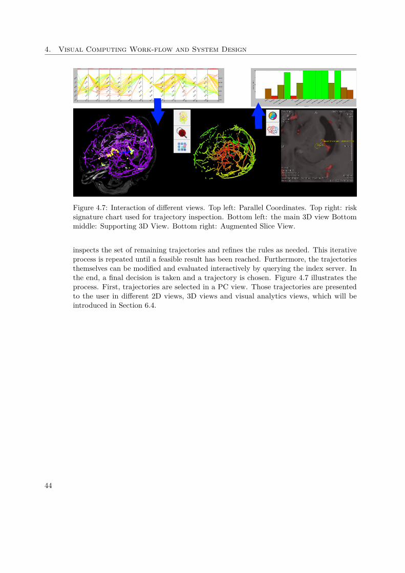
4. Visual Computing Work-flow and System Design
Figure 4.7: Interaction of different views. Top left: Parallel Coordinates. Top right: risksignature chart used for trajectory inspection. Bottom left: the main 3D view Bottommiddle: Supporting 3D View. Bottom right: Augmented Slice View.
inspects the set of remaining trajectories and refines the rules as needed. This iterativeprocess is repeated until a feasible result has been reached. Furthermore, the trajectoriesthemselves can be modified and evaluated interactively by querying the index server. Inthe end, a final decision is taken and a trajectory is chosen. Figure 4.7 illustrates theprocess. First, trajectories are selected in a PC view. Those trajectories are presentedto the user in different 2D views, 3D views and visual analytics views, which will beintroduced in Section 6.4.
44

CHAPTER 5Methods and Data
BrainXPlore is a system that consists of different modules which all fulfill specificroles. In the following sections we offer an overview of the methods we have employed ineach module. The interaction of the modules with each other is illustrated in Figure 4.5.
The methods we used for data acquisition and segmentation are presented in Section 5.1.In Section 5.2, we outline the steps we have undertaken to preprocess the segmenteddata. Indexing is discussed in Section 5.3. Our methods of trajectory generation arepresented in Section 5.4. Finally, in Section 5.5, filtering and refinement of generatedtrajectories is discussed.
5.1 Data Acquisition and SegmentationWe used a real dataset from a past biopsy to test and evaluate our system. The patientunderwent contrast enhanced CT, MR and MRA scans. Also, a MRI scan was takenpost-operatively to verify the site of the biopsy and exclude the existence of hemorrhage.All images exhibited different spatial resolutions. The image dimensions for each imagemodality is presented in Table 5.1.
Any segmentation software can be used to segment risk structures. In our case study, weused FreeSurfer for cortical and subcortical segmentation. Results for vessel segmentation
Data Width Height Depth (Slices)Pre-Op MRI 288 288 205Post-Op MRI 232 256 192MRA 528 528 125CT 512 512 164
Table 5.1: Spatial resolution of the considered input data.
45
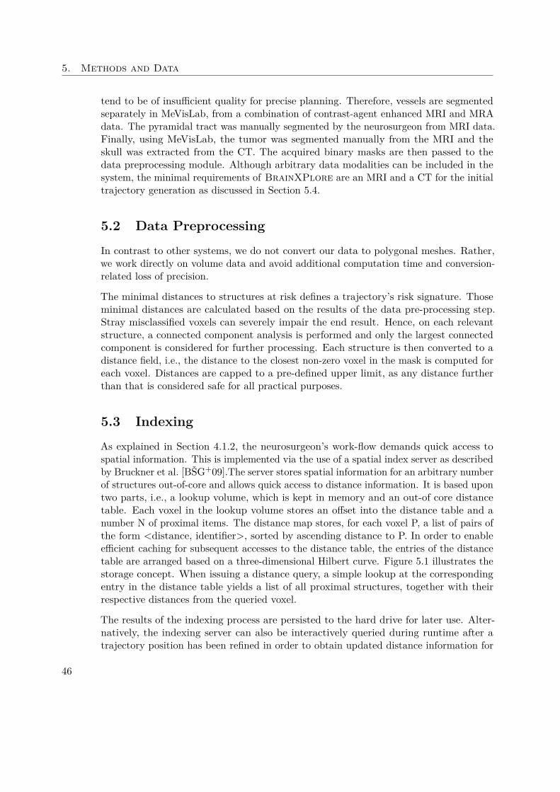
5. Methods and Data
tend to be of insufficient quality for precise planning. Therefore, vessels are segmentedseparately in MeVisLab, from a combination of contrast-agent enhanced MRI and MRAdata. The pyramidal tract was manually segmented by the neurosurgeon from MRI data.Finally, using MeVisLab, the tumor was segmented manually from the MRI and theskull was extracted from the CT. The acquired binary masks are then passed to thedata preprocessing module. Although arbitrary data modalities can be included in thesystem, the minimal requirements of BrainXPlore are an MRI and a CT for the initialtrajectory generation as discussed in Section 5.4.
5.2 Data Preprocessing
In contrast to other systems, we do not convert our data to polygonal meshes. Rather,we work directly on volume data and avoid additional computation time and conversion-related loss of precision.
The minimal distances to structures at risk defines a trajectory’s risk signature. Thoseminimal distances are calculated based on the results of the data pre-processing step.Stray misclassified voxels can severely impair the end result. Hence, on each relevantstructure, a connected component analysis is performed and only the largest connectedcomponent is considered for further processing. Each structure is then converted to adistance field, i.e., the distance to the closest non-zero voxel in the mask is computed foreach voxel. Distances are capped to a pre-defined upper limit, as any distance furtherthan that is considered safe for all practical purposes.
5.3 Indexing
As explained in Section 4.1.2, the neurosurgeon’s work-flow demands quick access tospatial information. This is implemented via the use of a spatial index server as describedby Bruckner et al. [BŠG+09].The server stores spatial information for an arbitrary numberof structures out-of-core and allows quick access to distance information. It is based upontwo parts, i.e., a lookup volume, which is kept in memory and an out-of core distancetable. Each voxel in the lookup volume stores an offset into the distance table and anumber N of proximal items. The distance map stores, for each voxel P, a list of pairs ofthe form <distance, identifier>, sorted by ascending distance to P. In order to enableefficient caching for subsequent accesses to the distance table, the entries of the distancetable are arranged based on a three-dimensional Hilbert curve. Figure 5.1 illustrates thestorage concept. When issuing a distance query, a simple lookup at the correspondingentry in the distance table yields a list of all proximal structures, together with theirrespective distances from the queried voxel.
The results of the indexing process are persisted to the hard drive for later use. Alter-natively, the indexing server can also be interactively queried during runtime after atrajectory position has been refined in order to obtain updated distance information for
46
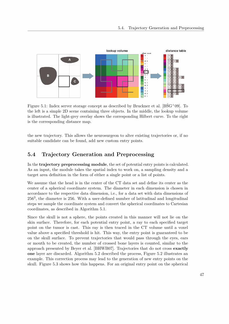
5.4. Trajectory Generation and Preprocessing
Figure 5.1: Index server storage concept as described by Bruckner et al. [BŠG+09]. Tothe left is a simple 2D scene containing three objects. In the middle, the lookup volumeis illustrated. The light-grey overlay shows the corresponding Hilbert curve. To the rightis the corresponding distance map.
the new trajectory. This allows the neurosurgeon to alter existing trajectories or, if nosuitable candidate can be found, add new custom entry points.
5.4 Trajectory Generation and Preprocessing
In the trajectory preprocessing module, the set of potential entry points is calculated.As an input, the module takes the spatial index to work on, a sampling density and atarget area definition in the form of either a single point or a list of points.
We assume that the head is in the center of the CT data set and define its center as thecenter of a spherical coordinate system. The diameter in each dimension is chosen inaccordance to the respective data dimension, i.e., for a data set with data dimensions of2563, the diameter is 256. With a user-defined number of latitudinal and longitudinalsteps we sample the coordinate system and convert the spherical coordinates to Cartesiancoordinates, as described in Algorithm 5.1.
Since the skull is not a sphere, the points created in this manner will not lie on theskin surface. Therefore, for each potential entry point, a ray to each specified targetpoint on the tumor is cast. This ray is then traced in the CT volume until a voxelvalue above a specified threshold is hit. This way, the entry point is guaranteed to beon the skull surface. To prevent trajectories that would pass through the eyes, earsor mouth to be created, the number of crossed bone layers is counted, similar to theapproach presented by Beyer et al. [BHWB07]. Trajectories that do not cross exactlyone layer are discarded. Algorithm 5.2 described the process, Figure 5.2 illustrates anexample. This correction process may lead to the generation of new entry points on theskull. Figure 5.3 shows how this happens. For an original entry point on the spherical
47

5. Methods and Data
coordinate system, three rays are cast to their respective tumor target point. Since eachpoint intersects the skull surface at a different voxel, three entry points are generated.This means that specifying multiple tumor target points may inherently lead to a denserskull sampling.
After the correction, for each calculated potential entry point, a ray is cast to eachspecified target point on the tumor and the minimal distances to each structure alongthat trajectory are queried. Good, noiseless distance fields (i.e., such where only relevantconnected components above a certain size threshold are stored) are of crucial importancehere. While not visually disruptive, noise in the form of misclassified voxels can lead tosignificantly altered minimal distances.
An initial list of candidate trajectories is created from every possible combination ofentry sample points and tumor target points. These candidate trajectories are saved to afile for further use in the visualization module.
The trajectory preprocessing module can also be interactively queried at runtime tocreate a list of new entry sample points at a higher sampling density around a promisingcandidate. This allows the neurosurgeon to assess promising regions where one or moresuitable entry points have already been found.
Algorithm 5.1: Creation of geographic coordinate system for sample generation.After the loop, each sample point can be identified with the tuple (latitude, longitude)Input: Volume Size sxyz in x/y/z, number of latitudinal steps latsteps, number of
longitudinal steps lonstepsOutput: List c of potential entry points on Sphere
1 for x← {stepsize ∗ n|n ∈ N, n ∈ {−180, 180}} do2 lat← x∗π
180 ;3 for y ← {stepsize ∗ n|n ∈ N, n ∈ {−180, 180}} do4 lon← y∗π
180 ;5 cx,y,0 ← (sx − 1) ∗ sin lon∗sin lat
2.0 + sx2.0 ;
6 cx,y,1 ← (sy − 1) ∗ sin lon cos lat2.0 + sy
2.0 ;7 cx,y,2 ← (sz − 1) ∗ cos lon
2.0 + sz2.0 ;
8 end9 end
5.5 Trajectory Filtering and Refinement
After the initial set of potential trajectories has been generated on the index server asdescribed in Section 5.4, is is subjected to optimization as well as incremental refinementand filtering. If more than one target point on the tumor is specified, optimization aimsat choosing, for each entry point, the best target point such that the resulting trajectorycandidate best satisfies the rules laid down by the neurosurgeon. The optimization process
48

5.5. Trajectory Filtering and Refinement
Algorithm 5.2: Correction of entry-points based on CT data. Given a set oftrajectories T described by all Bresenham points t along the trajectory, the algorithmfinds the first point on the skull and returns the corrected (i.e., cropped) trajectorythat now goes from the tumor target point to the skull surface.Input: List of potential trajectories T based on result of Algorithm5.1, CT image
data COutput: List c of potential entry points on Sphere
1 for t ∈ T do2 cnt← 0 bonecnt← 0;3 insidebone← 0;4 skullpoint← Nothing;5 goodidx← −1;6 for pt ∈ t, t is the set of Bresenham points in the current trajectory do7 if Cpt > 0 then8 if insidebone == 0 then9 insidebone← 1;
10 bonecnt← bonecnt+ 1;11 end12 else13 if insidebone == 1 then14 insidebone← 0;15 goodidx← cnt;16 end17 end18 cnt← cnt+ 119 end20 if bonecnt 6= 1 or goodidx < 0 then21 return Nothing;22 else23 return {ti | t ∈ T , i ≤ goodidx}24 end25 end
49

5. Methods and Data
Tumor
SkullOriginal Entry Point A
One Bone layer
Two Bone Layers
No Bone Layers
Translated Entry Point A'
Sampling Hemisphere
Original Entry Point B
Original Entry Point C
Figure 5.2: Example of entry Point Correction as described in Algorithm 5.2. Three entrypoint candidates (A, B, C) have been sampled on the geographic coordinate system’supper hemisphere. Between point A and the tumor (yellow), exactly one layer of bone ispassed. Hence, A is translated to the first intersection with the skull and stored as newentry point A′. Point B yields a trajectory that passes through two layers of bone. Thetrajectory between point C and the target point does not pass any bone layer. Hence,both entry points are discarded.
is described in Section 5.5.1. The resulting set of trajectory candidates is evaluatedagainst hard constraints and filtered accordingly. The idea and process of this step isexplained in Section 5.5.2.
5.5.1 Target Optimization
During the data loading process, the most suitable target point is selected for eachpotential entry point. In the GUI, up to three evaluation criteria can be specified for thisoptimization. Amongst these criteria are minimal distances to each structure, path length,insertion angles at the skull and tumor, etc. The criteria are processed hierarchically forpairs of trajectories. If two trajectories originate from the same entry point candidate onthe skull but reach different target points on the tumor, the first criterion is evaluatedfor both trajectories. The results are then compared and a choice is made dependingon a user-specified operation (i.e., <, =<, >=, >). If the trajectories are equal withregards to the first criterion, the second one is evaluated likewise. Finally, if both the
50
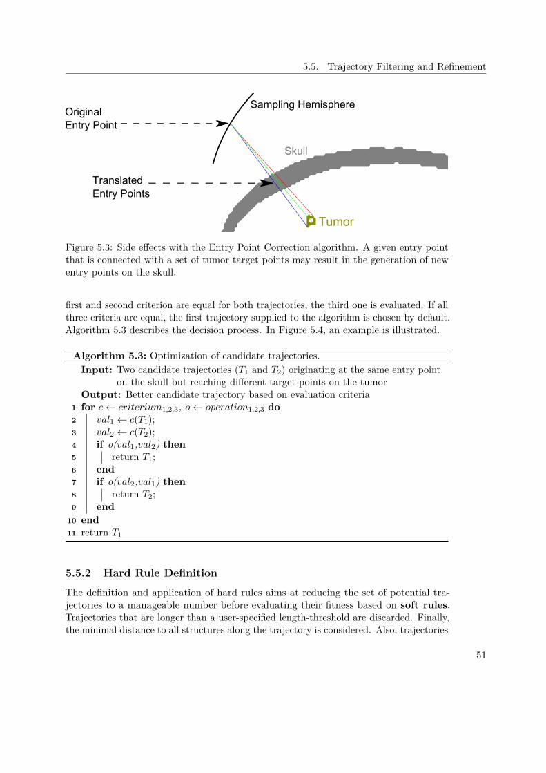
5.5. Trajectory Filtering and Refinement
Tumor
Original Entry Point
Translated Entry Points
Sampling Hemisphere
Skull
Figure 5.3: Side effects with the Entry Point Correction algorithm. A given entry pointthat is connected with a set of tumor target points may result in the generation of newentry points on the skull.
first and second criterion are equal for both trajectories, the third one is evaluated. If allthree criteria are equal, the first trajectory supplied to the algorithm is chosen by default.Algorithm 5.3 describes the decision process. In Figure 5.4, an example is illustrated.
Algorithm 5.3: Optimization of candidate trajectories.Input: Two candidate trajectories (T1 and T2) originating at the same entry point
on the skull but reaching different target points on the tumorOutput: Better candidate trajectory based on evaluation criteria
1 for c← criterium1,2,3, o← operation1,2,3 do2 val1 ← c(T1);3 val2 ← c(T2);4 if o(val1,val2) then5 return T1;6 end7 if o(val2,val1) then8 return T2;9 end
10 end11 return T1
5.5.2 Hard Rule Definition
The definition and application of hard rules aims at reducing the set of potential tra-jectories to a manageable number before evaluating their fitness based on soft rules.Trajectories that are longer than a user-specified length-threshold are discarded. Finally,the minimal distance to all structures along the trajectory is considered. Also, trajectories
51

5. Methods and Data
that do not satisfy the user-defined safety requirements are discarded. Since all data hasalready been preprocessed by the trajectory generation module, distance look-ups can beperformed in a very time-efficient manner. Algorithm 5.4 describes how the list of initialtrajectory candidates is processed.
Algorithm 5.4: Pre-Filtering of target points.Input: Unfiltered List ts of Trajectory Candidates, List of structures ss and
corresponding minimal distances mdOutput: Filtered List of Trajectory Candidates
1 for t← ts do2 for s← ss do3 if mindistance(s, t) < mds then4 discard t;5 end6 end7 end8 return filtered List of Trajectory Candidates
5.5.3 Soft Rule Definition and Evaluation
In contrast to hard rules, which aim at reducing the number of potential trajectories byimposing rigid exclusion criteria, a set of soft rules can be used to evaluate the remainingtrajectories and optimize the result. The quality Qt of a trajectory t is defined as shownin Equation 5.1.
Qt =n∑i=1
di ∗ wimaxi
(5.1)
di denotes the minimal distance to structure i along the trajectory, wi is the weightassigned to that structure and maxi is the maximal minimal distance found in allremaining trajectories. All weights need to sum up to 1.0. Each Qt is then divided bythe best encountered quality. This yields a relative measure, i.e., trajectory qualities aregiven with respect to the best currently found trajectory.
52

5.5. Trajectory Filtering and Refinement
Figure 5.4: Example of target point optimization as described in Algorithm 5.3. Threetrajectories originating from the same entry point but ending at different points on thetumor are sequentially compared. Optimization is set to distance maximization, withthe distance to the nearest vessel being the top priority, followed by the distance tothe nearest sulcus and finally, the distance to the ventricle. Sequentially evaluating thecandidate trajectories against these optimization criteria yields the selection of Trajectory3.
53

CHAPTER 6Implementation
To demonstrate the feasibility of our system, we have implemented a prototype. Allmodules were implemented and tested on a Windows 10 operated laptop PC with an IntelCore i7-3630QM processor, 12GB RAM and an NVidia GTX 660M graphics processorwith 2GB dedicated GPU memory.
In this Chapter the implementation details of our system are presented. Section 6.1briefly describes the MeVisLab work-flow. Specifics on data preprocessing are discussed inSection 6.2. Our implementation of the spatial index is presented in Section 6.3. The userinterface, including details on each step of the user-work-flow is discussed in Section 6.4.Information Visualization techniques can be found in Section 6.5.
6.1 MeVisLab Work-Flow
MeVisLab is a rapid prototyping system developed by the MeVis Medical SolutionsAG. It offers extensive data processing and visualization capabilities and is thereforean excellent choice for creating a prototype. The work-flow in MeVisLab is based oncreating networks from various modules. Each module has input and output fields aswell as parameters. Input and output fields can be image data, OpenInventor scenes, andbase objects (e.g., lists of markers, strings, etc). Modules are placed with drag-and-dropand input fields are joined to the corresponding output fields of modules at an earlierstage in the network. Data evaluation is performed on demand, i.e., modules may ormay not actually request data from their predecessors. Parameter fields communicate inthe form of string variables. Figure 6.1 shows an example network in MeVisLab. Newmodules can be created by joining existing ones into macro modules and extending theirfunctionality by adding Python [Ros95] or Java Script [Fla98] Code. Alternatively, newmodules can be written in C++.
55

6. Implementation
Figure 6.1: Example network in MeVisLab. Green nodes represent inventor modules,blue nodes are MevisLab modules and brown nodes are macro modules. Triangularconnectors represent image data, round connectors represent Open Inventor Scenes andsquare connectors are used for Base objects such as lists. [AG17]
6.2 Data Preprocessing
Data preprocessing was performed in MeVisLab. Structures that were segmented withFreeSurfer and stored as NIFTI files were imported and processed. Connected componentanalysis was performed with MeVisLab’s built in module ComputeConnectedComponents.From the resulting list, the largest component was filtered using the FilterConnected-Components module.
Each structure was stored as a set of files. On the one hand, a DICOM file was storedfor visualization purposes. On the other hand, a raw file in an 8 bit unsigned int formatwas stored for the corresponding distance field. Distance fields were calculated usingMeVisLab’s built in EuclideanDTF module. They were then capped to a maximumdistance of 20 mm, as higher distances are not relevant for our purposes. Distances werescaled to the to the range [0,255] in order to fit the 8 bit data format.
56
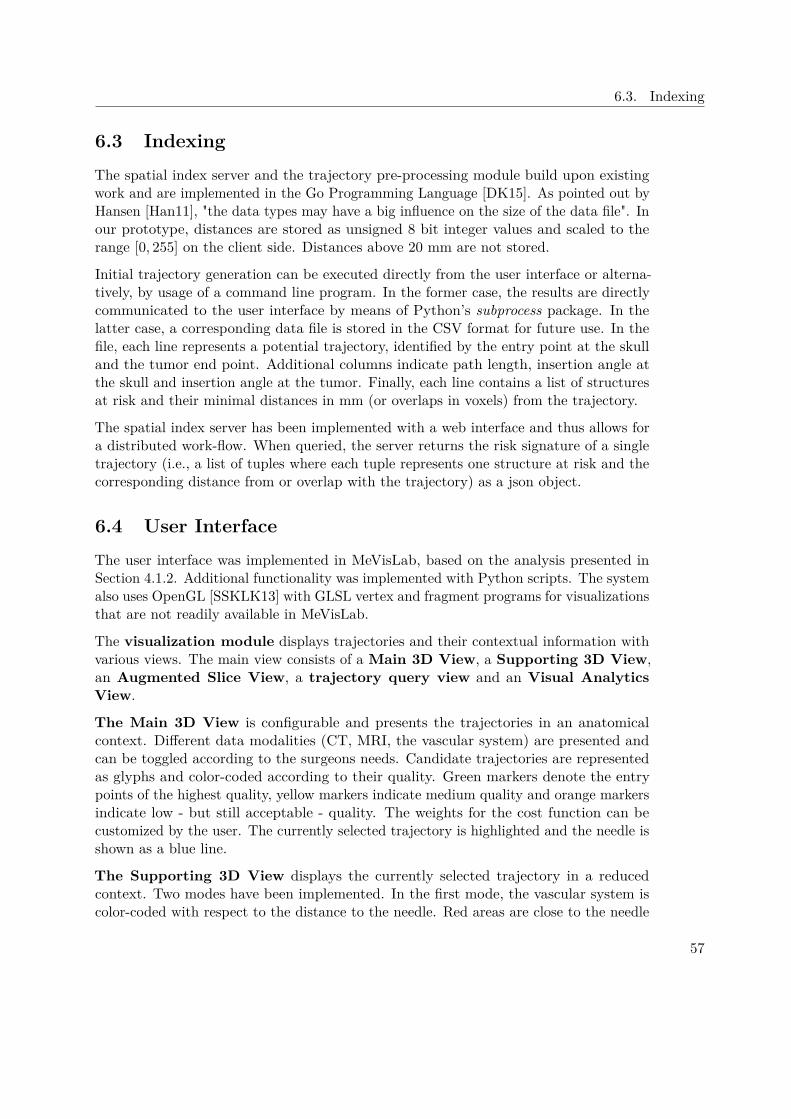
6.3. Indexing
6.3 IndexingThe spatial index server and the trajectory pre-processing module build upon existingwork and are implemented in the Go Programming Language [DK15]. As pointed out byHansen [Han11], "the data types may have a big influence on the size of the data file". Inour prototype, distances are stored as unsigned 8 bit integer values and scaled to therange [0, 255] on the client side. Distances above 20 mm are not stored.
Initial trajectory generation can be executed directly from the user interface or alterna-tively, by usage of a command line program. In the former case, the results are directlycommunicated to the user interface by means of Python’s subprocess package. In thelatter case, a corresponding data file is stored in the CSV format for future use. In thefile, each line represents a potential trajectory, identified by the entry point at the skulland the tumor end point. Additional columns indicate path length, insertion angle atthe skull and insertion angle at the tumor. Finally, each line contains a list of structuresat risk and their minimal distances in mm (or overlaps in voxels) from the trajectory.
The spatial index server has been implemented with a web interface and thus allows fora distributed work-flow. When queried, the server returns the risk signature of a singletrajectory (i.e., a list of tuples where each tuple represents one structure at risk and thecorresponding distance from or overlap with the trajectory) as a json object.
6.4 User InterfaceThe user interface was implemented in MeVisLab, based on the analysis presented inSection 4.1.2. Additional functionality was implemented with Python scripts. The systemalso uses OpenGL [SSKLK13] with GLSL vertex and fragment programs for visualizationsthat are not readily available in MeVisLab.
The visualization module displays trajectories and their contextual information withvarious views. The main view consists of a Main 3D View, a Supporting 3D View,an Augmented Slice View, a trajectory query view and an Visual AnalyticsView.
The Main 3D View is configurable and presents the trajectories in an anatomicalcontext. Different data modalities (CT, MRI, the vascular system) are presented andcan be toggled according to the surgeons needs. Candidate trajectories are representedas glyphs and color-coded according to their quality. Green markers denote the entrypoints of the highest quality, yellow markers indicate medium quality and orange markersindicate low - but still acceptable - quality. The weights for the cost function can becustomized by the user. The currently selected trajectory is highlighted and the needle isshown as a blue line.
The Supporting 3D View displays the currently selected trajectory in a reducedcontext. Two modes have been implemented. In the first mode, the vascular system iscolor-coded with respect to the distance to the needle. Red areas are close to the needle
57

6. Implementation
Figure 6.2: Visualization module user interface, with alternate supplemental views. Topleft: Main 3D View. Top middle: Supporting 3D View, set to critical region view mode.Vessels are red, the left lateral ventricle is yellow, the right lateral ventricle is blue, andthe pyramidal tract is green. Top right: Augmented Slice View, set to critical regionview. Coloring is consistent with the Supporting 3D View. Bottom: Parallel Coordinatesfor trajectory picking. Between the Main 3D View and the command buttons, in thewhite boy on the left, is the trajectory query Visual Analytics View that offers real-timeinformation on the minimal distances for trajectories that have not been generated inthe pre-processing step.
and therefore at risk, while green areas are further away and therefore safe. We useda MevisLab module for the distance calculation and visualization. In the second mode,selected structures at risk can be displayed. Each structure can be assigned a customcolor and opacity value. Figures 4.7 and 6.2 illustrate the supporting 3D views.
The Augmented Slice View always presents a needle-aligned slice stack with additionalannotations and highlights. In one mode, the augmented 2D view highlights vessels inthe current slice and annotates the distance to the needle center. This is similar to thework performed by Herghelegiu et al. [HMP+12]. In another mode, the augmented 2Dview highlights the structures at risk. Figures 6.2 and 4.7 illustrate the two modes of theaugmented 2D view.
The Trajectory Query View offers a tabular overview of the best trajectory at a givenpoint on the skull, similar to the work done by Bruckner et al. [BŠG+09]. Information isqueried online and can be obtained for arbitrary positions, even if no samples have beengenerated at this point during the initial sampling process. In Figure 6.2, the trajectoryquery view can be seen under the command buttons, in the white box on the left.
58
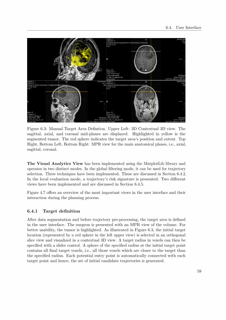
6.4. User Interface
Figure 6.3: Manual Target Area Defintion. Upper Left: 3D Contextual 3D view. Thesagittal, axial, and coronal mid-planes are displayed. Highlighted in yellow is thesegmented tumor. The red sphere indicates the target area’s position and extent. TopRight, Bottom Left, Bottom Right: MPR view for the main anatomical planes, i.e., axial,sagittal, coronal.
The Visual Analytics View has been implemented using the MatplotLib library andoperates in two distinct modes. In the global filtering mode, it can be used for trajectoryselection. Three techniques have been implemented. These are discussed in Section 6.4.2.In the local evaluation mode, a trajectory’s risk signature is presented. Two differentviews have been implemented and are discussed in Section 6.4.5.
Figure 4.7 offers an overview of the most important views in the user interface and theirinteraction during the planning process.
6.4.1 Target definition
After data segmentation and before trajectory pre-processing, the target area is definedin the user interface. The surgeon is presented with an MPR view of the volume. Forbetter usability, the tumor is highlighted. As illustrated in Figure 6.3, the initial targetlocation (represented by a red sphere in the left upper view) is selected in an orthogonalslice view and visualized in a contextual 3D view. A target radius in voxels can then bespecified with a slider control. A sphere of the specified radius at the initial target pointcontains all final target voxels, i.e., all those voxels which are closer to the target thanthe specified radius. Each potential entry point is automatically connected with eachtarget point and hence, the set of initial candidate trajectories is generated.
59
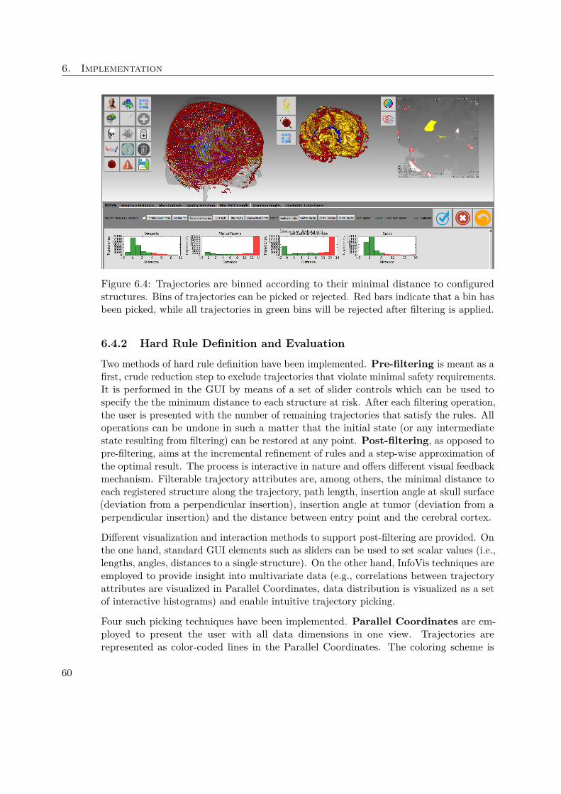
6. Implementation
Figure 6.4: Trajectories are binned according to their minimal distance to configuredstructures. Bins of trajectories can be picked or rejected. Red bars indicate that a bin hasbeen picked, while all trajectories in green bins will be rejected after filtering is applied.
6.4.2 Hard Rule Definition and Evaluation
Two methods of hard rule definition have been implemented. Pre-filtering is meant as afirst, crude reduction step to exclude trajectories that violate minimal safety requirements.It is performed in the GUI by means of a set of slider controls which can be used tospecify the the minimum distance to each structure at risk. After each filtering operation,the user is presented with the number of remaining trajectories that satisfy the rules. Alloperations can be undone in such a matter that the initial state (or any intermediatestate resulting from filtering) can be restored at any point. Post-filtering, as opposed topre-filtering, aims at the incremental refinement of rules and a step-wise approximation ofthe optimal result. The process is interactive in nature and offers different visual feedbackmechanism. Filterable trajectory attributes are, among others, the minimal distance toeach registered structure along the trajectory, path length, insertion angle at skull surface(deviation from a perpendicular insertion), insertion angle at tumor (deviation from aperpendicular insertion) and the distance between entry point and the cerebral cortex.
Different visualization and interaction methods to support post-filtering are provided. Onthe one hand, standard GUI elements such as sliders can be used to set scalar values (i.e.,lengths, angles, distances to a single structure). On the other hand, InfoVis techniques areemployed to provide insight into multivariate data (e.g., correlations between trajectoryattributes are visualized in Parallel Coordinates, data distribution is visualized as a setof interactive histograms) and enable intuitive trajectory picking.
Four such picking techniques have been implemented. Parallel Coordinates are em-ployed to present the user with all data dimensions in one view. Trajectories arerepresented as color-coded lines in the Parallel Coordinates. The coloring scheme is
60
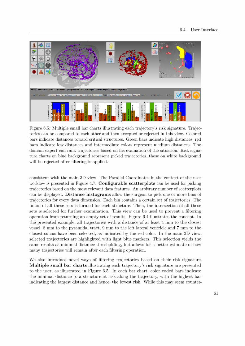
6.4. User Interface
Ves
sels
Mo
tor
Fib
ers
Lef
t L
at. V
entr
icle
Su
lci
Ves
sels
Mo
tor
Fib
ers
Lef
t L
at. V
entr
icle
Su
lci
Ves
sels
Mo
tor
Fib
ers
Lef
t L
at. V
entr
icle
Su
lci
Mo
tor
Fib
ers
Ves
sels
Lef
t L
at. V
entr
icle
Su
lci
Ves
sels
Mo
tor
Fib
ers
Lef
t L
at. V
entr
icle
Su
lci
Ves
sels
Mo
tor
Fib
ers
Lef
t L
at. V
entr
icle
Su
lci
Figure 6.5: Multiple small bar charts illustrating each trajectory’s risk signature. Trajec-tories can be compared to each other and then accepted or rejected in this view. Coloredbars indicate distances toward critical structures. Green bars indicate high distances, redbars indicate low distances and intermediate colors represent medium distances. Thedomain expert can rank trajectories based on his evaluation of the situation. Risk signa-ture charts on blue background represent picked trajectories, those on white backgroundwill be rejected after filtering is applied.
consistent with the main 3D view. The Parallel Coordinates in the context of the userworklow is presented in Figure 4.7. Configurable scatterplots can be used for pickingtrajectories based on the most relevant data features. An arbitrary number of scatterplotscan be displayed. Distance histograms allow the surgeon to pick one or more bins oftrajectories for every data dimension. Each bin contains a certain set of trajectories. Theunion of all these sets is formed for each structure. Then, the intersection of all thesesets is selected for further examination. This view can be used to prevent a filteringoperation from returning an empty set of results. Figure 6.4 illustrates the concept. Inthe presented example, all trajectories with a distance of at least 4 mm to the closestvessel, 8 mm to the pyramidal tract, 9 mm to the left lateral ventricle and 7 mm to theclosest sulcus have been selected, as indicated by the red color. In the main 3D view,selected trajectories are highlighted with light blue markers. This selection yields thesame results as minimal distance thresholding, but allows for a better estimate of howmany trajectories will remain after each filtering operation.
We also introduce novel ways of filtering trajectories based on their risk signature.Multiple small bar charts illustrating each trajectory’s risk signature are presentedto the user, as illustrated in Figure 6.5. In each bar chart, color coded bars indicatethe minimal distance to a structure at risk along the trajectory, with the highest barindicating the largest distance and hence, the lowest risk. While this may seem counter-
61
6. Implementation
intuitive at first, the reasoning was that the highest bar inherently draws the user’sattention. Representing higher risks with higher bars emphasizes the trajectories thatexhibit a greater risk. The goal, however, is to find the best suited trajectories forfurther evaluation, not identify those with the highest risk. Also, the color-coding, whichgoes from green for trajectories of low risk to red for those with a high risk furtheraids the selection process. Note that the charts are scaled with regards to the highestencountered distance and hence, scales may differ between individual charts. To illustratethe difference in scale, a white dashed line has been inserted at the 3 mm and 4 mmmark of the first and last trajectory.
Here, the color coding offers a more intuitive and concise measure than bar height alone.This becomes visible, for example, when comparing the second and fourth chart inFigure 6.5. The third bar, i.e., the distance to the left lateral ventricle, appears to be ofthe same height in both charts. Due to differences in scale, however, the distance in thesecond chart is 10 mm, while it is 14 mm in the fourth chart. This difference becomesevident when also considering the color coding, i.e., the bright green in the fourth chartas opposed to the olive green in the second chart. In Figure 6.5, the first trajectorymaximizes the distance to the vessels. In contrast, the last trajectory does not performas well with regards to vessels, but exhibits a higher safety margin towards the nearestsulcus.
An icon based view that maps trajectories to cartoon faces, as proposed by Cher-noff [Che73] has been implemented, as shown in Figure 6.6. Trajectory properties suchas length, distance to vessels, etc can be mapped to spatial features such as, e.g., theslant of the eyes or the length of the nose. Each of these views can be used to accept orreject trajectories based on their properties.
Potential trajectories are also visualized in a main 3D view. Figure 6.7 presents ParallelCoordinates used for selecting trajectories, along with the main 3D view. After eachoperation on the trajectory space, the set of options is refined accordingly and the numberof remaining candidates is presented to the user. As in the pre-filtering step, everyoperation can be undone at any point.
6.4.3 Soft Rule Defintion and Evaluation
After each filtering operation, all remaining trajectory candidates are evaluated for theirfitness as described in Section 5.5.3. Rules can be defined in a configuration file whereeach line represents a soft constraint that will be used for quality evaluation. For eachsoft constraint, the corresponding weight is supplied.
Those trajectory candidates, which are not excluded due to the violation of a hardconstraint are divided into six bins according to their quality. The best bin gets assignedthe color green, the worst bin is red. The potential entry points in the Main 3D Vieware colored accordingly. Lines in the Parallel Coordinates are given the same colors asthe entry points they represent. The coloring scheme can be seen in Figures 4.7 and 6.7.
62

6.4. User Interface
Figure 6.6: Chernoff faces map features of multivariate data to facial features on comicfaces. According to Chernoff, by presenting data in a very familiar fashion, namely,human faces, "an investigator can quickly comprehend relevant information and thenapply appropriate statistical analysis" [Che73]. Faces on blue background representpicked trajectories, those on white background will be rejected after filtering is applied.
6.4.4 Trajectory Addition and Removal
Trajectories can be added interactively at any time. This can be done in three ways:addition of new samples in the main 3D view, resampling around existing samples andfinally, refinement of existing trajectories.
In the main 3D view, trajectories can be added manually at any time. A GPU-basedrisk evaluation was implemented in order to aid the surgeon in the decision where toplace a new sample. Figure 6.8 presents the view. For each point on the skull surface,a ray is cast to the specified target point on the tumor. A distance field containingthe vessel system is supplied to the GPU as a 3D texture. The texture is sampled ateach point along the trajectory and the minimal distance to the closest vessel along thetrajectory is found. The corresponding value is then projected onto the skull surface.Safe entry points are displayed in green, while entry points that result in the intersectionof a vessel are displayed in red. This is an extension of the work done by Herghelegiuet al. [HMG11], who project the stability map of a given, user-defined ellipsoidal entryregion onto a sagittal plane.
In Figure 6.8 A, a trajectory in a green, i.e., safe entry zone is presented. Conversely,Figure 6.8 B shows a trajectory in a red, i.e., unsafe entry zone. As can be verified inthe supporting 3D view (top right) and Visual Analytics View (bottom), the minimaldistance to the nearest vessel is much higher for the trajectory presented in Figure 6.8 A,than for the one presented in Figure 6.8 B.
63
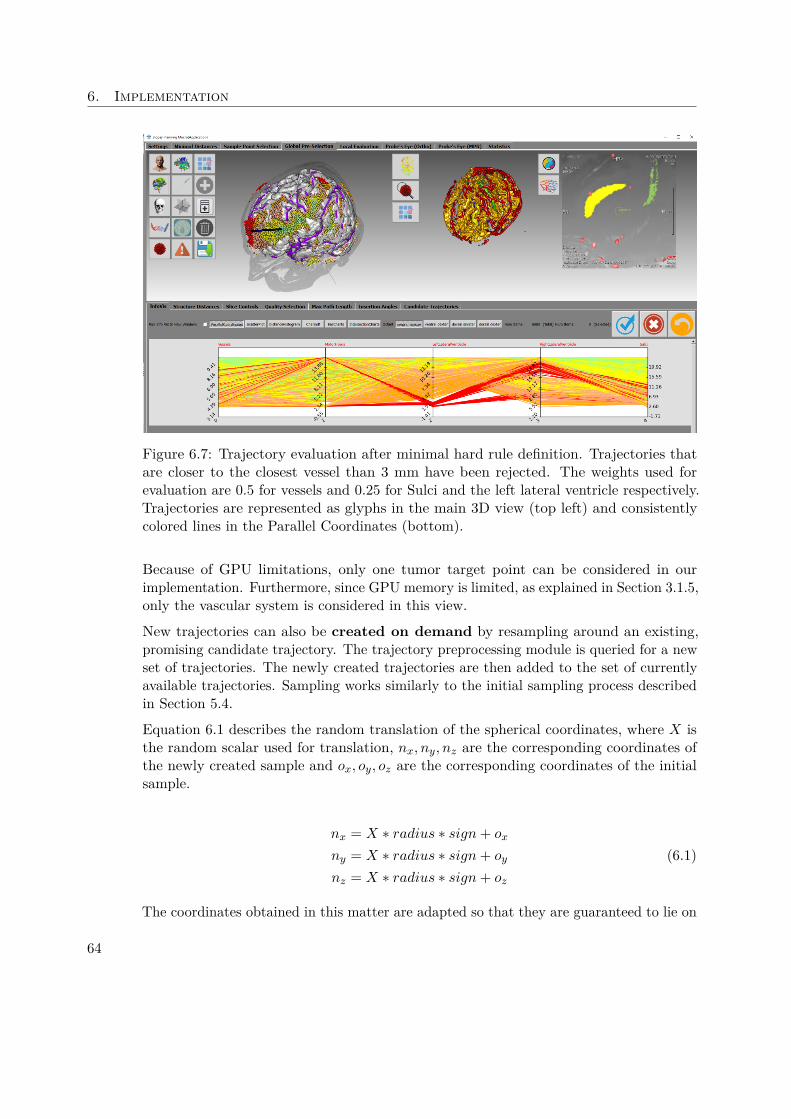
6. Implementation
Figure 6.7: Trajectory evaluation after minimal hard rule definition. Trajectories thatare closer to the closest vessel than 3 mm have been rejected. The weights used forevaluation are 0.5 for vessels and 0.25 for Sulci and the left lateral ventricle respectively.Trajectories are represented as glyphs in the main 3D view (top left) and consistentlycolored lines in the Parallel Coordinates (bottom).
Because of GPU limitations, only one tumor target point can be considered in ourimplementation. Furthermore, since GPU memory is limited, as explained in Section 3.1.5,only the vascular system is considered in this view.
New trajectories can also be created on demand by resampling around an existing,promising candidate trajectory. The trajectory preprocessing module is queried for a newset of trajectories. The newly created trajectories are then added to the set of currentlyavailable trajectories. Sampling works similarly to the initial sampling process describedin Section 5.4.
Equation 6.1 describes the random translation of the spherical coordinates, where X isthe random scalar used for translation, nx, ny, nz are the corresponding coordinates ofthe newly created sample and ox, oy, oz are the corresponding coordinates of the initialsample.
nx = X ∗ radius ∗ sign+ ox
ny = X ∗ radius ∗ sign+ oy
nz = X ∗ radius ∗ sign+ oz
(6.1)
The coordinates obtained in this matter are adapted so that they are guaranteed to lie on
64
6.4. User Interface
a bony surface as described in Algorithm 5.2 and converted into cartesian coordinates asshown in Algorithm 5.1. Figure 6.9 illustrates the process of adding new trajectories byresampling around an existing one. Steps that are performed in the visualization moduleare represented by black boxes, green boxes indicate a step is performed on the servermodule.
Finally, existing trajectories can also be refined in an MPR view. Both the entry pointand the tumor target point can be translated. The spatial index server is queried for therisk signature of the new trajectory. A risk signature chart as illustrated in Figure 6.5 ispresented to the user and the new trajectory is added to the set of currently availabletrajectories. This manual refinement function acknowledges the fact that, ultimately,the neurosurgeon is the domain expert and might make decisions based on criteria thatare hard to quantify.
Exclusion of trajectories is usually done by refining the rules and applying the filter. Alltrajectories that do not satisfy the rules are excluded from further examination. However,if a trajectory does satisfy all rules but is still deemed unsuitable by the neurosurgeon, itcan also be deleted manually.
6.4.5 Trajectory Inspection
During evaluation, the reduced set of trajectories is presented to the user. As in thepost-filtering stage, the user can navigate between different views. The Main andSupporting 3D Views offer spatial context, while the Visual Analytics View presentsdetail information. A trajectory’s risk signature is displayed in one of three ways in theVisual Analytics View.
The Visual Analytics View offers detail information on the trajectories risk signature.Figure 4.7, on the top right, illustrates the risk signature chart view. Bars are coloredaccording to their value with a simple linear interpolation in RGB space between green(for distances of 20 mm) and red (for distances of 0 mm). In case a trajectory doesintersect a structure, a negative bar representing the total overlap volume between theneedle and the structure is presented. These bars are displayed in red.
Alternatively, the distance profile from the needle to all structures at risk can be plottedas a set of colored functions in a shared coordinate system. The spatial index server canbe queried for all voxels that lie on the trajectory. Sample positions are calculated with amodified Bresenham’s line drawing algorithm. Figure 6.10 illustrates the needle pathwaydistance graph view. Although the most important measure regarding the distance toa structure along the trajectory is the minimum, considering the distance at multiplesample points might reveal additional insight into the trajectory’s quality. For example,although two trajectories might exhibit an identical minimal distance to a given structure,with everything else being equal, the trajectory with a higher average distance is betterthan the one with a lower average distance.
Finally, the radar chart view presents a trajectory’s risk signature as a geometric figure.Radar charts can be freely configured to include arbitrary structures such as to best
65

6. Implementation
suit the user’s needs. On each plot, the trajectory is presented as a pair of shapes.One shape, the distance polygon, reflects the minimal distances to structures. Thesecond shape, the overlap polygon, depicts the overlap with structures. Shapes arecreated by setting up a polygonal coordinate system where each data dimension isrepresented by an axis connecting the plot center with the respective polygon vertex.For example, a three-dimensional dataset can be represented in a triangular coordinatesystem, while a four-dimensional dataset requires a square or diamond-shaped coordinatesystem. Data points in each dimension are scaled such that each axis has the same length.In our implementation, the area under the distance polygon gives an estimate of thesafety margin. Hence, distance polygons with larger areas and overlap polygons withsmaller areas generally represent safer trajectories. In order to alleviate the radar chart’sshortcomings described by Staffogia et al. [SLF+11], namely, the inability of the radarchart to differentiate between the case when information on a data dimension is missingand the data dimension’s value is zero, we fill missing data dimensions with a value of 20.
A distance of zero or less indicates an intersection with, and hence, a violation of astructure at risk. Representing missing values as zero therefore leads to the potentialexclusion of trajectories. The only way a data dimension is missing, in our case, is if itis capped by the spatial index server. This happens if a structure is further away fromthe needle center than 20 mm. In that case, it is deemed not to be at risk, i.e., it is safe.Hence, while substituting 20 mm for the true value skews the data, this is of no clinicalrelevance.
Spatial information regarding the trajetories relation to structures at risk is also presentedto the user. In a Supporting 3D View, the vascular system can be color coded withregards to the vessel’s distance to the needle. Alternatively, the needle is presentedin the context of selected critical structures, as shown in Figure 6.2. An AugmentedSlice View presents the needle-aligned slice stack with highlighted vessels and distanceannotations. Alternatively, the surgeon can choose to display a selected set of criticalstructures highlighted in the needle-aligned slice stack, as presented in Figure 6.2.
Finally, the results can be viewed slice by slice in either the original coordinate systemor in a needle-aligned slice stack. These views are very similar to those offered by thesystem our domain expert currently uses. By creating familiar views, we aim at makingthe transition from one system to the other easy.
6.4.6 Trajectory refinement
Trajectories can be refined in two ways, either by resampling around an existing entrypoint or by manually altering the trajectory start- and endpoint. On the one hand, thetrajectory generation module can be queried for a set of trajectories sampled at a higherresolution around an existing entry point as described in Section 6.4.4. This approach ismeant to support the automatic addition of new trajectories in promising entry areas, atearlier stages of the planning process. Alternatively, the surgeon can interactively modifya trajectory in either the original coordinate system or in a needle-aligned slice stack
66

6.5. Information Visualization
and query the spatial index server for updated distance information. The new trajectoryis then added to the visualization module. This approach is meant to be used in laterstages of the planning process, when acceptable solution may have already been foundbut expert knowledge makes certain subtle changes preferable.
6.5 Information VisualizationAlthough Staffogia et al. [SLF+11] deem the spie chart the best representation formultivariate data for clinical outcome indicators, we have decided to rather implementthe radar chart to illustrate the quality of individual trajectories.
This is due to the nature of our data. Rather than clinical outcome data, which is limitedto a positive range, we have to display spatial information that can be either positiveor negative, as described in Section 6.4.5. Also, the ambiguity between missing datadimensions and those items whose value is zero is a non-issue in our case, as missinginformation can be interpreted and handled easily in our system. The details of our radarchart implementation are discussed in Section 6.4.5.
Needle pathway distance graphs are implemented such that each structure at risk isrepresented by an individual line. This allows for a more detailed qualitative analysis oftrajectories. Different structures may have different levels of risk associated with them,so displaying only a single line representing the nearest structure at risk for every samplepoint might take away important information. Figure 6.10 illustrates our implementation.
We have implemented Parallel Coordinates in which trajectories can be interactivelypicked and filtered. To the best of our knowledge, no existing solution in the context ofbrain biopsy planning implements this interaction technique.
Finally, Chernoff Faces seem to be a feasible visualization technique, as brain regions canbe mapped to facial features based on their function. For example, the distance to theoptic chiasm can be mapped to the size of the eyes, while Broca’s area, the motor centerfor speech, can be mapped to the slant of the mouth. While not pre-attentive, in thescenario of brain surgery, this view enables to user to directly map at least a few featuresto the cartoon face. Figure 6.6 shows our implementation.
67

6. Implementation
Figure 6.8: Presented in the Main 3D View (left) is the risk map. For each point on theskull surface, a ray is cast to the specified target point on the tumor and the minimaldistance to the nearest vessel along the trajectory is found. Safe entry points withregards to the vascular system are displayed in green, while entry points that resultin the intersection of a vessel are displayed in red. The Supporting 3D View (right)shows a color coded representation of the trajectory in the context of the vascular system.Blood vessels in red are closer to the trajectory, i.e., at risk. in the Visual AnalyticsView (bottom), the risk structure of the selected trajectory candidate is presented. A)Trajectory in a green, i.e., safe entry zone. B) Trajectory in a red, i.e., unsafe entry zone.
68

6.5. Information Visualization
Figure 6.9: Adding new trajectories by resampling around an existing one. Black boxes:steps in the visualization module. Green boxes: steps that are performed on the spatialindex server.
Figure 6.10: The needle pathway distance graph (bottom) represents the currentlyinspected trajectory (visible in the contextual 3D view in the top left and center) as aset of line graphs. Each structure at risk is represented by a colored line. The abscissarepresents the current insertion depth while the ordinate shows the minimal distance tothe respective structure at that position. This representation summarizes the informationthat could be gathered by slicing through the annotated volume in the augmented sliceview (top right).
69

CHAPTER 7Evaluation
We performed an internal evaluation of BrainXPlore, where we evaluated the systemfor performance, accuracy and result quality. The methods used for the evaluation aswell as the results are presented in Section 7.1. Furthermore, we performed an externalevaluation and compared BrainXPlore to existing solutions. Our findings are presentedin Section 7.2.
7.1 Internal Evaluation
We evaluated the usefulness of our application based on the dataset used for the case studyin Section 4.1.1. Because our input data came from independent scans, pre-processinghad to be performed. The CT and MRA scans were resampled in order to produce resultswith the same resolution as the FreeSurfer results (2563). The resampled results weremanually registered to the pre-operation MRI scan. Then, semi-automatic vessel andtumor segmentation was performed in MeVisLab.
Based on this data, different spatial index files were built. Candidate entry points weresampled on a spherical coordinate system at 255 latitudinal steps and 255 longitudinalsteps, as described in Section 5.4. For trajectory generation, we provided the system withdifferent tumor point configurations. The most basic configuration contained only onetarget point at the tumor’s periphery. To test the performance for multi-target scenarios,we added additional definitions for 3, 5, 10 and 15 target points.
With those spatial index files, entry points, and target points, we evaluated the per-formance of the individual components of our system. Then, in cooperation with ourdomain expert, we used BrainXPlore to produce a biopsy trajectory for the dataset inour case study and evaluated the quality of the result.
71

7. Evaluation
The rest of this Chapter is structured as follows: First, in Section 7.1.1, we present theperformance of our system under different conditions. Then, in Section 7.1.7, we showthe neurosurgical evaluation of our results.
7.1.1 Performance Evaluation
We examined the efficiency of each individual part of our solution. A laptop computerrunning on a Windows 10 Professional 64 bit operating system with an Intel Core i7-3630CPU was used for the evaluation. The machine has 12 GB of memory and an NVIDIAGeForce GTX 660M with 2 GB of video memory. In a real world scenario we expect thenumber of relevant trajectory candidates to be in the vicinity of 200-6000, as stated byZombori et al. [ZRN+14]. However, use cases of upwards of 10000 trajectory candidatesare possible. We have therefore decided to test our system with higher numbers oftrajectory candidates than usually encountered in real world examples.
7.1.2 Index Generation
Although it is not within the scope of this thesis, the spatial index is a crucial componentof our system. In order to assess the usefulness of our system, we have decided to includean evaluation for this component as well. To evaluate the performance of the spatialindex generation, we measured the average computation time for the creation of indicesof different sizes. Indices were built for 1, 5, 10, 50, 100, 150 and 178 structures at risk.The maximum number of 178 structures resulted from the extraction of cortical andsubcortical regions of interest from our data set. We used the Destrieux Atlas providedby FreeSurfer for cortical parcellation the atlas developed by Fischl et al. [FSB+02],which is also provided by FreeSurfer, for subcortical segmentation. All empty results, i.e.,those structures that could not be classified, were discarded. This process resulted in 175structures. In addition to those structures, we used our semi-automatically segmentedblood-vessels, a union of all sulci (except for the precentral and postcentral sulcus) aswell as the manually segmented pyramid tract.
Each configuration was built five times and the times were recorded using the Measure-Command function of Microsoft’s PowerShell. Table 7.1 provides details on the measure-ments, Figure 7.1 shows the average runtimes as a function of the number of structuresat risk. As can be seen, the time required to construct an index for a single structure isapproximately 13 seconds. This time is used for startup of the system and the allocationof memory.
7.1.3 Online Interactive Trajectory Query
To evaluate the performance of the spatial index query, we measured the average compu-tation time for sending queries to the index server and processing the results on the clientside. This excludes visualization. For the evaluation, different sets of tumor target pointshave been considered. We performed evaluations for 1, 3, 5, 10 and 15 distinct targetpoints on the tumor surface. Additionally, we performed all tests on different spatial
72
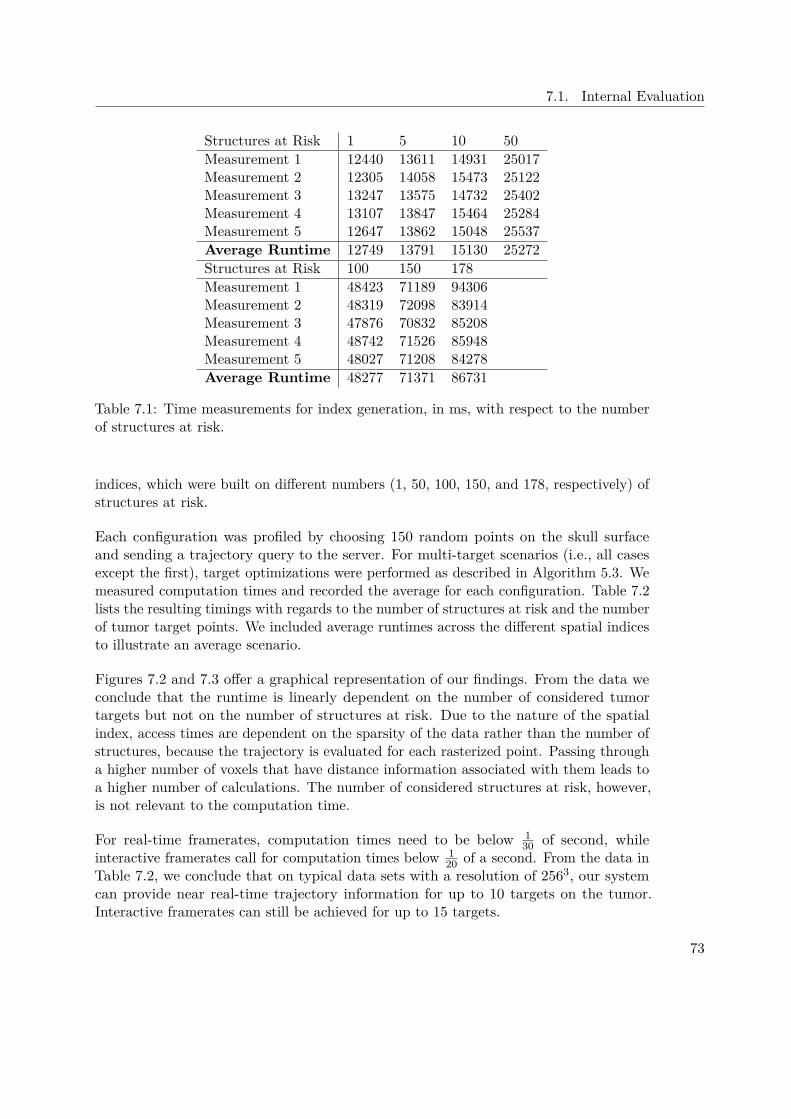
7.1. Internal Evaluation
Structures at Risk 1 5 10 50Measurement 1 12440 13611 14931 25017Measurement 2 12305 14058 15473 25122Measurement 3 13247 13575 14732 25402Measurement 4 13107 13847 15464 25284Measurement 5 12647 13862 15048 25537Average Runtime 12749 13791 15130 25272Structures at Risk 100 150 178Measurement 1 48423 71189 94306Measurement 2 48319 72098 83914Measurement 3 47876 70832 85208Measurement 4 48742 71526 85948Measurement 5 48027 71208 84278Average Runtime 48277 71371 86731
Table 7.1: Time measurements for index generation, in ms, with respect to the numberof structures at risk.
indices, which were built on different numbers (1, 50, 100, 150, and 178, respectively) ofstructures at risk.
Each configuration was profiled by choosing 150 random points on the skull surfaceand sending a trajectory query to the server. For multi-target scenarios (i.e., all casesexcept the first), target optimizations were performed as described in Algorithm 5.3. Wemeasured computation times and recorded the average for each configuration. Table 7.2lists the resulting timings with regards to the number of structures at risk and the numberof tumor target points. We included average runtimes across the different spatial indicesto illustrate an average scenario.
Figures 7.2 and 7.3 offer a graphical representation of our findings. From the data weconclude that the runtime is linearly dependent on the number of considered tumortargets but not on the number of structures at risk. Due to the nature of the spatialindex, access times are dependent on the sparsity of the data rather than the number ofstructures, because the trajectory is evaluated for each rasterized point. Passing througha higher number of voxels that have distance information associated with them leads toa higher number of calculations. The number of considered structures at risk, however,is not relevant to the computation time.
For real-time framerates, computation times need to be below 130 of second, while
interactive framerates call for computation times below 120 of a second. From the data in
Table 7.2, we conclude that on typical data sets with a resolution of 2563, our systemcan provide near real-time trajectory information for up to 10 targets on the tumor.Interactive framerates can still be achieved for up to 15 targets.
73

7. Evaluation
1 5 10 50 100 150 1780
10000
20000
30000
40000
50000
60000
70000
80000
90000
100000
Spatial Index Creation
Average Runtimes in ms
RuntimeLinear (Runtime)
Number of Structures at Risk
Run
time
in m
s
Figure 7.1: Average runtimes for the spatial index generation with respect to the numberof considered structures at risk
Targets / Structures at Risk 1 50 100 150 178 Average1 Target 4 4 5 5 5 53 Targets 7 8 8 8 8 85 Targets 12 12 12 12 13 1210 Targets 23 23 24 24 25 2415 Targets 33 34 36 35 36 35
Table 7.2: Average runtimes in ms for a trajectory query and subsequent optimizations.Also provided are the average runtimes across different numbers of structures.
7.1.4 Sample Point Generation
We also evaluated the performance of our system by profiling the sample generationprocess with different sets of tumor target points, as described in Section 7.1.3. We set upa spatial index consisting of 178 structures at risk. Then we generated a set of sampleson a spherical coordinate system consisting of 250 longitudinal and 250 latitudinal stepsas described in Algorithm 5.1. Each of created grid points was corrected as described inAlgorithm 5.2. From each corrected entry point, a trajectory to each specified tumor point
74

7.1. Internal Evaluation
1 Target 3 Targets 5 Targets 10 Targets 15 Targets0
10
20
30
40
50
60
Trajectory Query
average runtime in relation to the number of tumor target points(1500 Samples)
4 Structures at Risk
5 Structures at Risk
6 Structures at Risk
7 Structures at Risk
8 Structures at Risk
9 Structures at Risk
10 Structures at Risk
11 Structures at Risk
12 Structures at Risk
13 Structures at Risk
14 Structures at Risk
Average
Number of Target Points on Tumor
Co
mpu
tatio
n T
ime
in m
s
Figure 7.2: Average runtimes for querying a trajectory with respect to the number ofconsidered structures at risk and tumor target points. It can be seen that the runtimestrongly correlates with the number of tumor target points.
was calculated on the server. First, we created trajectories for a single target point onthe tumor. Then, we created sets of trajectories for 3, 5, 10 and 15 targets, as describedin Section 7.1.3. For reasons explained in Section 5.4, introducing additional targetpoints yields additional trajectories. Each target configuration was run 50 times and theaverage time was recorded. Table 7.3 offers an overview over the average computationtimes. Figure 7.4 illustrates the linear relationship between the computation time andthe number of target points on the tumor.
The resulting set of trajectories was then parsed on the client and in the multi-target case,trajectory optimizations were performed as described in Algorithm 5.3. Also, trajectorylength was calculated on the client. We evaluated the client with the same method asoutlined above. Table 7.4 offers an overview of the average computation times. Figure 7.5illustrates the results.
75
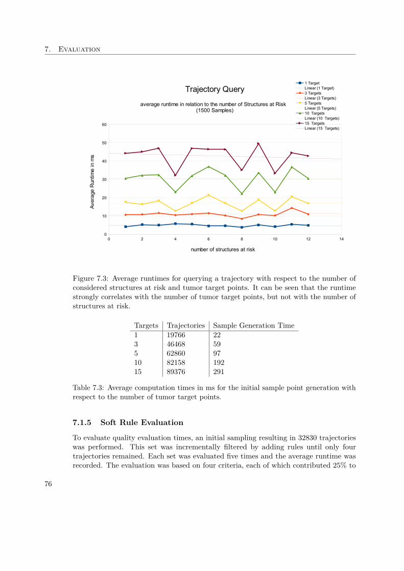
7. Evaluation
0 2 4 6 8 10 12 140
10
20
30
40
50
60
Trajectory Query
average runtime in relation to the number of Structures at Risk (1500 Samples)
1 TargetLinear (1 Target)3 TargetsLinear (3 Targets)5 TargetsLinear (5 Targets)10 TargetsLinear (10 Targets)15 TargetsLinear (15 Targets)
number of structures at risk
Ave
rage
Run
time
in m
s
Figure 7.3: Average runtimes for querying a trajectory with respect to the number ofconsidered structures at risk and tumor target points. It can be seen that the runtimestrongly correlates with the number of tumor target points, but not with the number ofstructures at risk.
Targets Trajectories Sample Generation Time1 19766 223 46468 595 62860 9710 82158 19215 89376 291
Table 7.3: Average computation times in ms for the initial sample point generation withrespect to the number of tumor target points.
7.1.5 Soft Rule Evaluation
To evaluate quality evaluation times, an initial sampling resulting in 32830 trajectorieswas performed. This set was incrementally filtered by adding rules until only fourtrajectories remained. Each set was evaluated five times and the average runtime wasrecorded. The evaluation was based on four criteria, each of which contributed 25% to
76
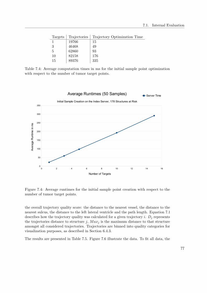
7.1. Internal Evaluation
Targets Trajectories Trajectory Optimization Time1 19766 153 46468 495 62860 9310 82158 17615 89376 335
Table 7.4: Average computation times in ms for the initial sample point optimizationwith respect to the number of tumor target points.
0 2 4 6 8 10 12 14 160
50
100
150
200
250
300
350
Average Runtimes (50 Samples)
Initial Sample Creation on the Index Server, 178 Structures at Risk
Server Time
Number of Targets
Ave
rage
Run
time
in m
s
Figure 7.4: Average runtimes for the initial sample point creation with respect to thenumber of tumor target points.
the overall trajectory quality score: the distance to the nearest vessel, the distance to thenearest sulcus, the distance to the left lateral ventricle and the path length. Equation 7.1describes how the trajectory quality was calculated for a given trajectory i. Dj representsthe trajectories distance to structure j, Maxj is the maximum distance to that structureamongst all considered trajectories. Trajectories are binned into quality categories forvisualization purposes, as described in Section 6.4.3.
The results are presented in Table 7.5. Figure 7.6 illustrate the data. To fit all data, the
77
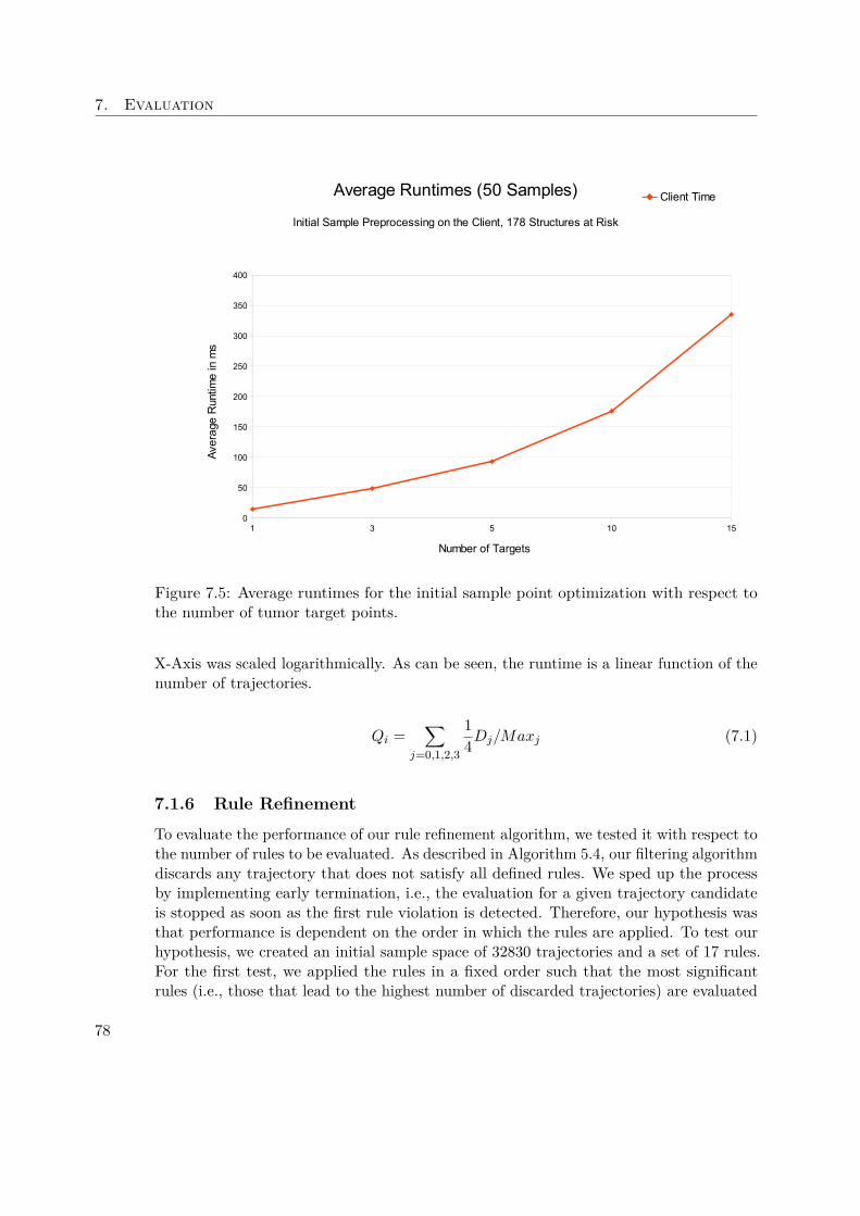
7. Evaluation
1 3 5 10 150
50
100
150
200
250
300
350
400
Average Runtimes (50 Samples)
Initial Sample Preprocessing on the Client, 178 Structures at Risk
Client Time
Number of Targets
Ave
rage
Run
time
in m
s
Figure 7.5: Average runtimes for the initial sample point optimization with respect tothe number of tumor target points.
X-Axis was scaled logarithmically. As can be seen, the runtime is a linear function of thenumber of trajectories.
Qi =∑
j=0,1,2,3
14Dj/Maxj (7.1)
7.1.6 Rule Refinement
To evaluate the performance of our rule refinement algorithm, we tested it with respect tothe number of rules to be evaluated. As described in Algorithm 5.4, our filtering algorithmdiscards any trajectory that does not satisfy all defined rules. We sped up the processby implementing early termination, i.e., the evaluation for a given trajectory candidateis stopped as soon as the first rule violation is detected. Therefore, our hypothesis wasthat performance is dependent on the order in which the rules are applied. To test ourhypothesis, we created an initial sample space of 32830 trajectories and a set of 17 rules.For the first test, we applied the rules in a fixed order such that the most significantrules (i.e., those that lead to the highest number of discarded trajectories) are evaluated
78

7.1. Internal Evaluation
Trajectories Measure 1 Measure 2 Measure 3 Measure 4 Measure 5 Avg. Runtime32830 1896 1890 1876 1873 1886 1884.217339 1173 1190 1180 1190 1167 11806081 582 586 586 587 588 585.83053 320 312 314 314 313 314.61812 200 202 199 203 199 200.6588 122 117 117 118 116 118106 30 25 25 26 26 26.41 3 3 3 3 3 3
Table 7.5: Average runtimes in ms for soft rule evaluation on a set of four rules. Eachevaluation was performed five times, Measures 1 through 5 show the respective timingsin ms.
1 10 100 1000 10000 1000000
200
400
600
800
1000
1200
1400
1600
1800
2000
Average Runtime in MS
Risk Evaluation (5 Sample Average)
Avg. Runtime
Linear (Avg. Runtime)
Total Number of Samples (Logarithmic Scale)
Run
time
in M
S
Figure 7.6: Average runtimes in ms for soft rule evaluation on logarithmic scale.
79
7. Evaluation
in the beginning. We filtered our initial sample space iteratively and added one rule ineach iteration, i.e., the same sample space was first filtered with a single rule, then withtwo rules and so on, until all rules were enabled. To test the stability of our approach,we ran the process five times and recorded runtimes for each individual test run as wellas average runtimes. Table 7.6 presents the resulting times.
In Figure 7.7 it can be seen that the runtimes appear to be a linear function of thenumber of evaluated rules, until rule six is evaluated, at which time they exhibit aconsiderable drop-off. At this point, the combination of three rules (namely, distance tovessels, distance to the sulci and distance to the left lateral ventricle) lead to an earlytermination of the evaluation for all but 20 samples. This supports our hypothesis thatthe order of rules significantly affects the performance.
We performed the same experiment again, on the same set of initial samples. The secondtime, however, the order of rule application was randomized, i.e., in each of the fivetest runs, the order of rule application was different. Table 7.7 presents the resultingruntimes. As can be seen in Figure 7.8, the same characteristic drop-off in computationtimes can be observer in all measurements, only at different times. This indicates that theintroduction of the respective rule led to a set of rules which result in the early rejectionof most trajectories. We conclude that while the computation time is a linear function ofthe number of rules to be evaluated, the order in which those rules are introduced can bevery significant.
7.1.7 Neurosurgical Evaluations
Our domain expert employs biopsy needles with a diameter of 3.5 mm and therefore aradius of 1.75 mm. We compute minimal distances from the needle center to structuresat risk. The safety margin then describes the distance between the needle’s edge and thestructure, i.e., we subtract the needle radius from the minimal distance.
Pre-filtering was applied with the minimal distances presented in Table 7.8. This yielded390 potential trajectories. Limiting path length to 80 mm reduced this set to 20 potentialtrajectories. Samples were further spatially limited to the left side, behind the hairline,by defining an appropriate ROI in the user interface. This reduced the set to 9 validcandidates. These were evaluated based on their minimal distance to the sulci.
From the set, the best trajectory (i.e., the one with the largest safety margin towardsthe sulci) is illustrated in Figures 7.10 and 7.11. Figure 7.10 presents the trajectoryin an orthogonal slice view in the original coordinate system. The solid yellow lineindicates the part of the trajectory behind the current needle tip position, dashed linesindicate the part of the trajectory that has not yet been crossed. As can be seen in thecoronal view, the trajectory does not originate at a sulcus (highlighted in orange). Thesagittal view reveals that the trajectory laterally passes the ventricle. Table 7.9 lists theminimal distances to structures at risk along the needle trajectory for those structuresthat are within the critical range of 20 mm. The associated risk signature is illustratedin Figure 7.9.
80
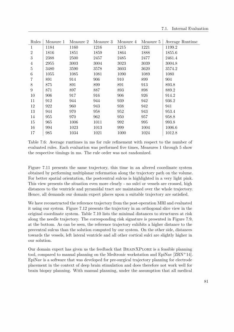
7.1. Internal Evaluation
Rules Measure 1 Measure 2 Measure 3 Measure 4 Measure 5 Average Runtime1 1184 1160 1216 1215 1221 1199.22 1816 1851 1859 1864 1888 1855.63 2388 2500 2457 2485 2477 2461.44 2955 3003 3004 3023 3039 3004.85 3480 3590 3578 3603 3620 3574.26 1055 1085 1081 1090 1089 10807 891 914 906 910 899 9048 875 891 899 891 913 893.89 871 897 887 893 898 889.210 906 917 916 906 926 914.211 912 944 944 939 942 936.212 922 960 943 938 942 94113 944 970 958 952 943 953.414 955 970 962 950 957 958.815 965 1006 1011 992 995 993.816 994 1023 1013 999 1004 1006.617 985 1034 1021 1000 1024 1012.8
Table 7.6: Average runtimes in ms for rule refinement with respect to the number ofevaluated rules. Each evaluation was performed five times, Measures 1 through 5 showthe respective timings in ms. The rule order was not randomized.
Figure 7.11 presents the same trajectory, this time in an altered coordinate systemobtained by performing multiplanar reformation along the trajectory path on the volume.For better spatial orientation, the postcentral sulcus is highlighted in a very light pink.This view presents the situation even more clearly - no sulci or vessels are crossed, highdistances to the ventricle and pyramidal tract are maintained over the whole trajectory.Hence, all demands our domain expert places upon a suitable trajectory are satisfied.
We have reconstructed the reference trajectory from the post-operation MRI and evaluatedit using our system. Figure 7.12 presents the trajectory in an orthogonal slice view in theoriginal coordinate system. Table 7.10 lists the minimal distances to structures at riskalong the needle trajectory. The corresponding risk signature is presented in Figure 7.9,at the bottom. As can be seen, the reference trajectory exhibits a higher distance to theprecentral sulcus than the solution computed by our system. On the other side, distancestowards the vessels, left lateral ventricle and all other cortical sulci are slightly higher inour solution.
Our domain expert has given us the feedback that BrainXPlore is a feasible planningtool, compared to manual planning on the Medtronic workstation and EpiNav [ZRN+14].EpiNav is a software that was developed for pre-surgical trajectory planning for electrodeplacement in the context of deep brain stimulation and does therefore not work well forbrain biopsy planning. With manual planning, under the assumption that all medical
81

7. Evaluation
Rules Measure 1 Measure 2 Measure 3 Measure 4 Measure 5 Average Runtime1 1172 799 1171 1181 1179 1100.42 1795 896 1803 1804 1798 1619.23 961 930 2409 2605 2002 1781.44 994 1022 3006 2654 2322 1999.65 950 1023 3532 2801 2828 2226.86 1022 1020 3742 2827 1051 1932.47 1032 1078 4381 3204 1102 2159.48 1101 1041 5077 3459 1129 2361.49 927 1091 2216 3739 1207 183610 922 1127 1967 1096 1283 127911 972 1141 2223 953 1279 1313.612 917 1145 2506 948 1355 1374.213 929 997 2585 995 1372 1375.614 941 986 2638 997 1268 136615 950 1011 2941 1006 1016 1384.816 944 1003 1046 1007 1009 1001.817 985 1024 1041 1016 1013 1015.8
Table 7.7: Average runtimes in ms for rule refinement with respect to the number ofevaluated rules. Each evaluation was performed five times, Measures 1 through 5 showthe respective timings in ms. The rule order was randomized.
Structure Minimal Distance Safety MarginVessels 4 2.25Pyramid Tract 4 2.25Left Lat Ventricle 4 2.25Right Lat Ventricle 4 2.25Sulci 3 1.25Gyrus sup. temp. 4 2.25Occipital Pole (LH) 4 2.25Pars Opercularis (LH) 4 2.25Pars Triangularis (LH) 3 1.25Gyrus Supramarginalis 4 2.25Postcentral Sulcus (LH) 4 2.25Precentral Sulcus (LH) 4 2.25
Table 7.8: Minimal distance in mm to each structure along the needle trajectory in thecase study. The safety margin is calculated by
82
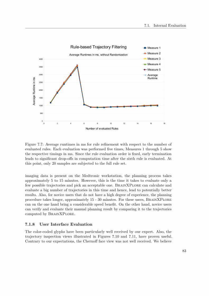
7.1. Internal Evaluation
0 2 4 6 8 10 12 14 16 180
500
1000
1500
2000
2500
3000
3500
4000
Rule-based Trajectory Filtering
Average Runtimes in ms, without Randomization
Measure 1
Measure 2
Measure 3
Measure 4
Measure 5
Average Runtime
Number of evaluated Rules
Ave
rage
Run
time
in m
s
Figure 7.7: Average runtimes in ms for rule refinement with respect to the number ofevaluated rules. Each evaluation was performed five times, Measures 1 through 5 showthe respective timings in ms. Since the rule evaluation order is fixed, early terminationleads to significant drop-offs in computation time after the sixth rule is evaluated. Atthis point, only 20 samples are subjected to the full rule set.
imaging data is present on the Medtronic workstation, the planning process takesapproximately 5 to 15 minutes. However, this is the time it takes to evaluate only afew possible trajectories and pick an acceptable one. BrainXPlore can calculate andevaluate a big number of trajectories in this time and hence, lead to potentially betterresults. Also, for novice users that do not have a high degree of experience, the planningprocedure takes longer, approximately 15 - 30 minutes. For these users, BrainXPlorecan on the one hand bring a considerable speed benefit. On the other hand, novice userscan verify and evaluate their manual planning result by comparing it to the trajectoriescomputed by BrainXPlore.
7.1.8 User Interface Evaluation
The color-coded glyphs have been particularly well received by our expert. Also, thetrajectory inspection views illustrated in Figures 7.10 and 7.11, have proven useful.Contrary to our expectations, the Chernoff face view was not well received. We believe
83

7. Evaluation
0 2 4 6 8 10 12 14 16 180
1000
2000
3000
4000
5000
6000
Rule-based Trajectory Filtering
Average Runtimes in ms, with Randomization
Measure 1
Measure 2
Measure 3
Measure 4
Measure 5
Average Runtime
Number of evaluated Rules
Ave
rage
Run
time
in m
s
Figure 7.8: Average runtimes in ms for rule refinement with respect to the number ofevaluated rules. Since the rule evaluation order is randomized, early termination leads tosignificant drop-offs in computation time at different points. After the most significantrules have been implemented, only 20 samples are subjected to the full rule set.
that this is due to a lack of apparent relevance concerning the given data. Still, we believethat further evaluation with more direct mappings, as described in Section 8, might leadto higher acceptance rates.
7.1.9 Precision
Segmentation and registration of different data modalities arguably introduce the mostsignificant source of error. These steps are not part of our system however. Hence,evaluating them lies outside of this thesis’ scope. In our system we could identifyone aspect that may adversely impact precision. Our implementation of the spatialindex operates on 8 bit integer precision. Distances that do not exceed the safetythreshold of 40 mm are scaled to the range [0,255]. In this step, a certain amount ofprecision is necessarily lost. To test the impact of this scaling operation, we built floating-point precision distance fields from the original segmentation results using MevisLab’sEuclideanDTF module. We consider these distance fields the ground truth.
84
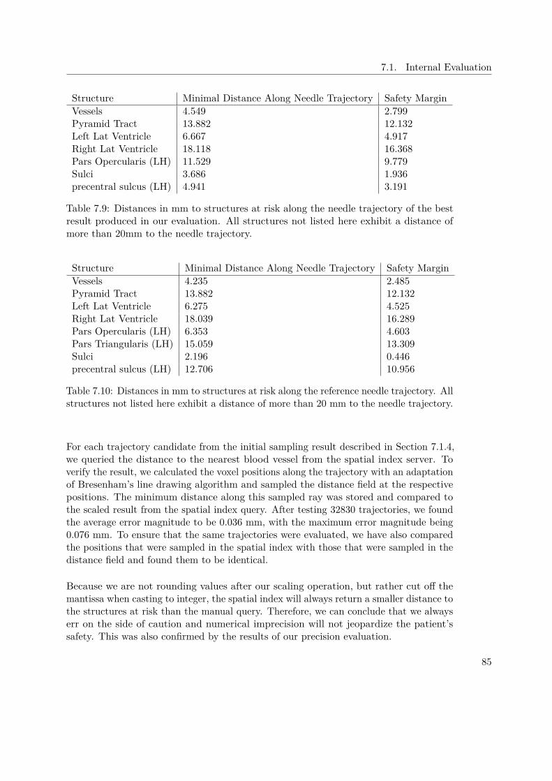
7.1. Internal Evaluation
Structure Minimal Distance Along Needle Trajectory Safety MarginVessels 4.549 2.799Pyramid Tract 13.882 12.132Left Lat Ventricle 6.667 4.917Right Lat Ventricle 18.118 16.368Pars Opercularis (LH) 11.529 9.779Sulci 3.686 1.936precentral sulcus (LH) 4.941 3.191
Table 7.9: Distances in mm to structures at risk along the needle trajectory of the bestresult produced in our evaluation. All structures not listed here exhibit a distance ofmore than 20mm to the needle trajectory.
Structure Minimal Distance Along Needle Trajectory Safety MarginVessels 4.235 2.485Pyramid Tract 13.882 12.132Left Lat Ventricle 6.275 4.525Right Lat Ventricle 18.039 16.289Pars Opercularis (LH) 6.353 4.603Pars Triangularis (LH) 15.059 13.309Sulci 2.196 0.446precentral sulcus (LH) 12.706 10.956
Table 7.10: Distances in mm to structures at risk along the reference needle trajectory. Allstructures not listed here exhibit a distance of more than 20 mm to the needle trajectory.
For each trajectory candidate from the initial sampling result described in Section 7.1.4,we queried the distance to the nearest blood vessel from the spatial index server. Toverify the result, we calculated the voxel positions along the trajectory with an adaptationof Bresenham’s line drawing algorithm and sampled the distance field at the respectivepositions. The minimum distance along this sampled ray was stored and compared tothe scaled result from the spatial index query. After testing 32830 trajectories, we foundthe average error magnitude to be 0.036 mm, with the maximum error magnitude being0.076 mm. To ensure that the same trajectories were evaluated, we have also comparedthe positions that were sampled in the spatial index with those that were sampled in thedistance field and found them to be identical.
Because we are not rounding values after our scaling operation, but rather cut off themantissa when casting to integer, the spatial index will always return a smaller distance tothe structures at risk than the manual query. Therefore, we can conclude that we alwayserr on the side of caution and numerical imprecision will not jeopardize the patient’ssafety. This was also confirmed by the results of our precision evaluation.
85
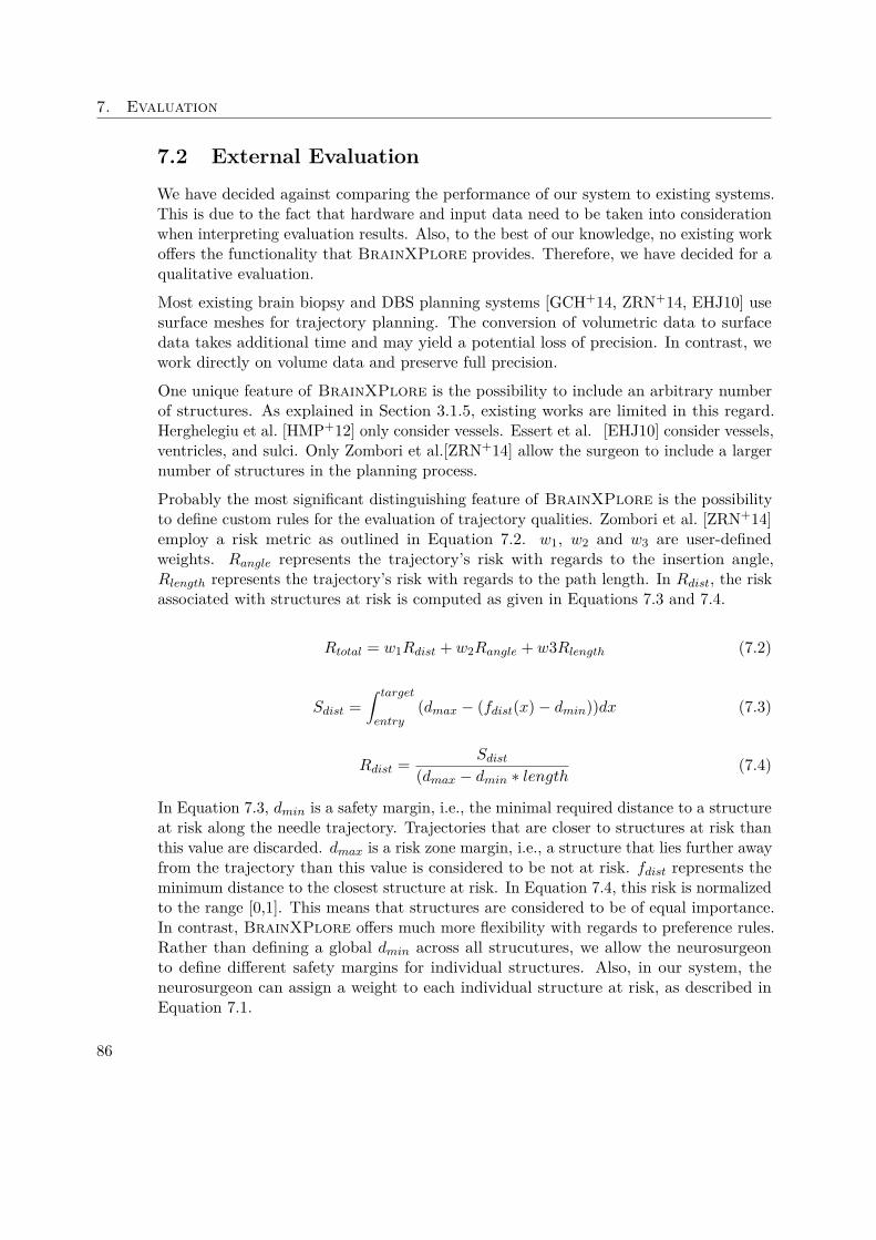
7. Evaluation
7.2 External EvaluationWe have decided against comparing the performance of our system to existing systems.This is due to the fact that hardware and input data need to be taken into considerationwhen interpreting evaluation results. Also, to the best of our knowledge, no existing workoffers the functionality that BrainXPlore provides. Therefore, we have decided for aqualitative evaluation.
Most existing brain biopsy and DBS planning systems [GCH+14, ZRN+14, EHJ10] usesurface meshes for trajectory planning. The conversion of volumetric data to surfacedata takes additional time and may yield a potential loss of precision. In contrast, wework directly on volume data and preserve full precision.
One unique feature of BrainXPlore is the possibility to include an arbitrary numberof structures. As explained in Section 3.1.5, existing works are limited in this regard.Herghelegiu et al. [HMP+12] only consider vessels. Essert et al. [EHJ10] consider vessels,ventricles, and sulci. Only Zombori et al.[ZRN+14] allow the surgeon to include a largernumber of structures in the planning process.
Probably the most significant distinguishing feature of BrainXPlore is the possibilityto define custom rules for the evaluation of trajectory qualities. Zombori et al. [ZRN+14]employ a risk metric as outlined in Equation 7.2. w1, w2 and w3 are user-definedweights. Rangle represents the trajectory’s risk with regards to the insertion angle,Rlength represents the trajectory’s risk with regards to the path length. In Rdist, the riskassociated with structures at risk is computed as given in Equations 7.3 and 7.4.
Rtotal = w1Rdist + w2Rangle + w3Rlength (7.2)
Sdist =∫ target
entry(dmax − (fdist(x)− dmin))dx (7.3)
Rdist = Sdist(dmax − dmin ∗ length
(7.4)
In Equation 7.3, dmin is a safety margin, i.e., the minimal required distance to a structureat risk along the needle trajectory. Trajectories that are closer to structures at risk thanthis value are discarded. dmax is a risk zone margin, i.e., a structure that lies further awayfrom the trajectory than this value is considered to be not at risk. fdist represents theminimum distance to the closest structure at risk. In Equation 7.4, this risk is normalizedto the range [0,1]. This means that structures are considered to be of equal importance.In contrast, BrainXPlore offers much more flexibility with regards to preference rules.Rather than defining a global dmin across all strucutures, we allow the neurosurgeonto define different safety margins for individual structures. Also, in our system, theneurosurgeon can assign a weight to each individual structure at risk, as described inEquation 7.1.
86

7.2. External Evaluation
Figure 7.9: Top: Risk Signature for resulting trajectory. Bottom: Risk Signature forreference trajectory All specified quality criteria have been met. Compared to thereference, our solution puts the precentral sulcus at a higher risk. However, our solutionalso exhibits higher safety margins to the other cortical sulci. Also, the pars opercularisof the gyris frontalis inferior is at a lower risk in our solution
87

7. Evaluation
Figure 7.10: Needle trajectory in original coordinate system (i.e., in the sagittal, axial,and coronal plane). Vessels are highlighted in red, sulci in orange, the left lateral ventriclein green, the pyramidal tract in cyan, and the tumor in yellow.
88

7.2. External Evaluation
Figure 7.11: Needle trajectory in a coordinate system obtained from performing multi-planar reformation along the needle path on the volume. Vessels are highlighted in red,sulci in orange, the left lateral ventricle in green, the pyramidal tract in cyan, and thetumor in yellow. Additionally, for better spatial orientation, the postcentral sulcus ishighlighted in a very light pink.
89
7. Evaluation
Figure 7.12: Reference needle trajectory in a coordinate system obtained by performingmultiplanar reformation along the needle path in the volume. Vessels are highlighted inred, sulci in orange, the left lateral ventricle in green, the pyramidal tract in cyan, andthe tumor in yellow. Additionally, for better spatial orientation, the postcentral sulcus ishighlighted in a very light pink.
90
CHAPTER 8Conclusion
In this thesis, a proof-of-concept of our BrainXPlore biopsy planning system was given.Based on interviews with an experienced neurosurgeon, we identified gaps in currentlyavailable brain biopsy planning tools. While sophisticated solutions to planning brainbiopsies exist, all existing systems are limited by the number of critical structures theycan consider. This is because GPU-based implementations, although fast and efficient,are limited by the amount of GPU memory. As brain atlases get more sophisticatedand more structures, e.g., due to fMRI and DTI, are included into the planning process,this bottleneck may limit the feasibility of such solutions, especially on consumer-gradehardware. Also, existing solutions operate on a fixed set of rules, which may not accuratelyreflect the specific planning guidelines of a particular neurosurgeon or hospital.
Based on these considerations, in collaboration with a domain expert from the MedicalUniversity of Vienna, we have implemented BrainXPlore, an interactive biopsy planningframework. We solve the problem of limited GPU memory by introducing a spatialindex server as described by Bruckner et al. [BŠG+09] into our system. This allowsfor fast and efficient access to an unlimited number of risk structures at an arbitraryresolution. To the best of our knowledge, this has not been achieved by other works thusfar. BrainXPlore also allows the user to define custom planning rules. These rules canconcern the minimal distance of a trajectory to a structure at risk or be geometricallyoriented and consider the trajectory’s length or angle.
A set of candidate trajectories is generated by the system and automatically evaluatedagainst those rules. Trajectories that do not satisfy hard constraints are discarded. Byinteractively refining rules the number of considered trajectories is iteratively decreaseduntil a suitable candidate has been found. To further support the user, custom rules fortrajectory quality evaluation can be defined. These soft rules do not lead to trajectoriesbeing discarded, but rather play a role in the visualization of the set of availabletrajectories. Trajectories are subjected to a consistent color-coding that reflects their
91

8. Conclusion
quality. This measure makes the decision process more intuitive. Trajectories caninteractively be added, removed and altered.
We also present novel ways of user interaction which have not been implemented beforein the context of biopsy planning. Our system combines 2D views, 3D views and InfoVistechniques such as Parallel Coordinates. These views present multivariate trajectorydata in an anatomical context and offer a high degree of overview.
We evaluated our system based on a real planning use case. The evaluation presented inSection 7.1.7 shows that our system finds trajectories that satisfy all demands imposedby our domain expert. However, there are also challenges that arise and have so far keptus from a clinical evaluation on a larger scale. Segmentation with FreeSurfer takes a longtime (>24 hours) on consumer-grade hardware. In the clinical practice, pre-operationMRI scans are sometimes performed on the day of the biopsy. In order to take fulladvantage of our system and consider a large number of structures, the schedule has tobe changed so as to plan enough time between the patient’s arrival at the hospital, thescans, and the biopsy.
8.1 Future WorkIn the future, we would like to improve on our system. Based on the feedback we havereceived from the surgeon during the evaluation, we have identified several points thatneed to be improved.
Initial Sampling Instead of globally sampling over a sphere, the system should limitsample generation to a user-defined lobe. While this requires an additional userinteraction, it allows for a higher sampling density without increasing preprocessingtimes.
Segmentation Our domain expert pointed out that in clinical practice, especially vesselsegmentation tends to be of insufficient quality and hence, visual path evaluationtools on the raw MRI images are critically important. Also, packages like FreeSurferdo not perform well for alterations in brain physiology that are due to lesions.Finally, the segmentation process takes a long time (upwards of 24 hours in our casestudy if performed on the hardware specified in Chapter 4). This somewhat limitsthe feasibility of automated systems that heavily rely on a thorough segmentationof medical imaging data.
Post-filtering In the future, we want trajectories to be sortable by user defined criteriain views such as the risk signature chart view.
Visualization The glyph-based Chernoff faces we have implemented have not been wellreceived. This may be due to the fact that the parameter mapping is not particularlyintuitive and few details are revealed on a pre-attentive level. Introducing a color-coding might alleviate this limitation. The coloring scheme can either be consistent
92
8.1. Future Work
with the one employed for the 3D glyphs and the Parallel Coordinates, or codeeach data dimension (represented in this case as eyes, ears, nose, etc) individually.Further user studies need to be carried out in order to find the most feasiblerepresentation or decide to drop the Chernoff view altogether.In order to introduce another distinguishing feature at the pre-attentive level, weplan on scaling the 3D glyphs according to the relation to their neighborhood. AsRopinski et al. [ROP11] point out, "when using a continuous color mapping, anabsolute quantification is difficult to achieve because differences in color are harderto perceive than for instance spatial distances". Hence, while the color-codingindicates a global quality measure as described in Section 6.4, glyph size may beused in order to better distinguish trajectories in relatively homogeneous potentialentry regions. Furthermore, we need to evaluate whether or not exchanging ourbasic glyphs with composite glyphs indicating the needle insertion angles at theskull and tumor surface impact the final decision.Although the glyph-based representation does offer benefits, as outlined above, highsampling densities lead to a high amount of geometry to be rendered and hence,increase computational cost, thereby potentially decreasing framerates. Hence,we plan on evaluating an alternative way of visualization. Instead of renderingglyphs over the skull, quality is then stored for each skull surface point in a 3Dtexture. Although this would lead to a rather significant increase in data volume,it could simplify the scene. User studies will show which method leads to a higheracceptance.
93


List of Figures
2.1 Computed Tomography . . . . . . . . . . . . . . . . . . . . . . . . . . . . 62.2 T1-weighted MRI after Gadolinium Injection . . . . . . . . . . . . . . . . 92.3 DTI . . . . . . . . . . . . . . . . . . . . . . . . . . . . . . . . . . . . . . . . 112.4 Intensity histograms for different brain structures . . . . . . . . . . . . . . 132.5 Talairach Atlas, Hierarchical Levels . . . . . . . . . . . . . . . . . . . . . . 142.6 Brodmann’s areas . . . . . . . . . . . . . . . . . . . . . . . . . . . . . . . 15
3.1 Work-flow in related work . . . . . . . . . . . . . . . . . . . . . . . . . . . 203.2 Subcortical Segmentation in related work . . . . . . . . . . . . . . . . . . . 213.3 Trajectory clustering . . . . . . . . . . . . . . . . . . . . . . . . . . . . . . 273.4 Aggregative cost function . . . . . . . . . . . . . . . . . . . . . . . . . . . 283.5 Visualization of the Biopsy Planner . . . . . . . . . . . . . . . . . . . . . 293.6 Bead-and-String representation . . . . . . . . . . . . . . . . . . . . . . . . 303.7 Distance Graphs . . . . . . . . . . . . . . . . . . . . . . . . . . . . . . . . 323.8 Radar Chart and Target Chart . . . . . . . . . . . . . . . . . . . . . . . . 33
4.1 Cortical regions of interest . . . . . . . . . . . . . . . . . . . . . . . . . . . 364.2 Structures at Risk, 3D Trajectory Context . . . . . . . . . . . . . . . . . . 374.3 Case Study, Trajectories 1 & 2 . . . . . . . . . . . . . . . . . . . . . . . . 394.4 Case Study, Trajectories 3 & 4 . . . . . . . . . . . . . . . . . . . . . . . . 404.5 System Overview . . . . . . . . . . . . . . . . . . . . . . . . . . . . . . . . 424.6 User work-flow . . . . . . . . . . . . . . . . . . . . . . . . . . . . . . . . . 434.7 Interaction of different views . . . . . . . . . . . . . . . . . . . . . . . . . 44
5.1 Index server storage concept . . . . . . . . . . . . . . . . . . . . . . . . . . 475.2 Entry Point Correction . . . . . . . . . . . . . . . . . . . . . . . . . . . . 505.3 Entry Point Correction Side Effects . . . . . . . . . . . . . . . . . . . . . . . 515.4 Target Point Optimization . . . . . . . . . . . . . . . . . . . . . . . . . . . 53
6.1 Example network in MeVisLab . . . . . . . . . . . . . . . . . . . . . . . . 566.2 Visualization Module . . . . . . . . . . . . . . . . . . . . . . . . . . . . . . 586.3 Manual Target Area Defintion . . . . . . . . . . . . . . . . . . . . . . . . . 596.4 Distance Histogram Post-Filtering . . . . . . . . . . . . . . . . . . . . . . 606.5 Risk Signature Chart Post-Filtering . . . . . . . . . . . . . . . . . . . . . . 61
95

6.6 Chernoff Faces Post-Filtering . . . . . . . . . . . . . . . . . . . . . . . . . 636.7 Trajectory Evaluation . . . . . . . . . . . . . . . . . . . . . . . . . . . . . 646.8 Risk Map . . . . . . . . . . . . . . . . . . . . . . . . . . . . . . . . . . . . 686.9 Trajectory addition . . . . . . . . . . . . . . . . . . . . . . . . . . . . . . . 696.10 Needle Pathway Graph . . . . . . . . . . . . . . . . . . . . . . . . . . . . . 69
7.1 Index Generation Runtimes . . . . . . . . . . . . . . . . . . . . . . . . . . 747.2 Trajectory Query Runtimes . . . . . . . . . . . . . . . . . . . . . . . . . . 757.3 Trajectory Query Runtimes . . . . . . . . . . . . . . . . . . . . . . . . . . 767.4 Initial Sampling Runtimes, Server Side . . . . . . . . . . . . . . . . . . . . 777.5 Initial Sampling Runtimes, Client Side . . . . . . . . . . . . . . . . . . . . 787.6 Trajectory Evaluation Runtimes . . . . . . . . . . . . . . . . . . . . . . . 797.7 Rule Refinement Runtimes without Rule order Randomization . . . . . . 837.8 Rule Refinement Runtimes with Rule order Randomization . . . . . . . . 847.9 Risk Signature for resulting trajectory and reference trajectory . . . . . . 877.10 Resulting Needle Trajectory . . . . . . . . . . . . . . . . . . . . . . . . . . 887.11 Resulting Needle Trajectory, Probe’s Eye . . . . . . . . . . . . . . . . . . 897.12 Reference Needle Trajectory . . . . . . . . . . . . . . . . . . . . . . . . . . 90
96

List of Tables
2.1 CT Windows . . . . . . . . . . . . . . . . . . . . . . . . . . . . . . . . . . 72.2 FSL VS FreeSurfer, Subcortical Segmentation . . . . . . . . . . . . . . . . 162.3 A comparison of FSL / FIRST and FreeSurfer. . . . . . . . . . . . . . . . 17
5.1 Input data image resolution . . . . . . . . . . . . . . . . . . . . . . . . . . 45
7.1 Index Generation Runtimes . . . . . . . . . . . . . . . . . . . . . . . . . . 737.2 Trajectory Query Runtimes . . . . . . . . . . . . . . . . . . . . . . . . . . 747.3 Initial Sampling Runtimes, Server Side . . . . . . . . . . . . . . . . . . . . 767.4 Initial Sampling Runtimes, Client Side . . . . . . . . . . . . . . . . . . . . 777.5 Trajectory Evaluation Runtimes . . . . . . . . . . . . . . . . . . . . . . . 797.6 Rule Refinement Runtimes without Rule order Randomization . . . . . . . 817.7 Rule Refinement Runtimes without Rule order Randomization . . . . . . 827.8 Case Study Rule Configuration . . . . . . . . . . . . . . . . . . . . . . . . 827.9 Distance to Structures at Risk in mm for resulting trajectory . . . . . . . 857.10 Distance to Structures at Risk in mm for reference trajectory . . . . . . . 85
97


List of Algorithms
5.1 Geographic Coordinate System Setup . . . . . . . . . . . . . . . . . . . 48
5.2 Entry Point Correction . . . . . . . . . . . . . . . . . . . . . . . . . . . 49
5.3 Target Point Optimization . . . . . . . . . . . . . . . . . . . . . . . . . . 51
5.4 Target Point Pre-Filtering . . . . . . . . . . . . . . . . . . . . . . . . . 52
99


Bibliography
[ABB+02] J. R. Adler, G. H. Barnett, C. J. Barry, J. B. Bederson, A. Benabid, M. S.Berger, W. E. Bingaman, R. Bucholz, S. D. Chang, G. Dandie, D. Dean,H. Deutsch, R. Fahlbusch, M. G. Fehlings, K. T. Foley, O. Ganslandt,I. M. Germano, I. C. Gibbs, P. L. Gildenberg, E. J. Hadar, P. Heilbrun,C. J. Hodge, P. Johnson, I. H. Kalfas, D. Karahalios, E. Keles, K. D. Kim,W. A. King, S. Kondo, E. L. Lapresto, M. A. Lefkowitz, J. Y. Lim, R. J.Maciunas, D. P. Martin, C. R. Mascott, C. R. Maurer, K. Mori, C. Nimsky,W. L. Nowinski, S. L. Ondra, S. M. Papadopulos, N. P. Patel, T. Rohlfing,D. Rueckert, T. C. Ryken, A. Y. Schwartz, R. Shahidi, A. H. Siddiqui,L. Tansey, W. D. Tobler, V. C. Traynelis, E. Watanabe, J. B. West, andA. S. Youkilis. Advanced Techniques in Image-Guided Brain and SpineSurgery. Georg Thieme Verlag, Stuttgart, New York, 2002 edition, 2002.DOI: 10.1055/b-002-46954.
[AG17] MeVis Medical Solutions AG. Mevislab software developmentkit (sdk). https://www.mevislab.de/mevislab/features/mevislab-sdk/, 2017. Accessed: November 26, 2017.
[BDS+13] S. Beriault, S. Drouin, A. F. Sadikot, Y. Xiao, D. L. Collins, and G. B.Pike. A prospective evaluation of computer-assisted deep brain stimulationtrajectory planning. In Clinical Image-Based Procedures. From Planning toIntervention, pages 42–49. Springer Berlin Heidelberg, 2013.
[BH07] D. J. Brenner and E. J. Hall. Computed tomography — an increasing sourceof radiation exposure. New England Journal of Medicine, 357(22):2277–2284,2007. PMID: 18046031.
[BHWB07] J. Beyer, M. Hadwiger, S. Wolfsberger, and K. Bühler. High-quality multi-modal volume rendering for preoperative planning of neurosurgical interven-tions. Transactions on Visualization and Computer Graphics (Proceedingsof IEEE Vis 2007), 13(6):1696–1703, 2007.
[BLE+13] A. Bock, N. Lang, G. Evangelista, R. Lehrke, and T. Ropinski. Guiding deepbrain stimulation interventions by fusing multimodal uncertainty regions.
101
In 2013 IEEE Pacific Visualization Symposium (PacificVis), pages 97–104,2013.
[BSB04] S. Breit, J. B. Schulz, and A. L. Benabid. Deep brain stimulation. Cell andTissue Research, 318(1):275–288, 2004.
[BŠG+09] S. Bruckner, V. Šoltészová, E. Gröller, J. Hladuvka, K. Bühler, J. Y. Yu, andB. J. Dickson. Braingazer - visual queries for neurobiology research. IEEETransactions on Visualization and Computer Graphics, 15(6):1497–1504,2009.
[BVVV+07] E. J. L. Brunenberg, A. Vilanova, V. Visser-Vandewalle, Y. Temel, L. Acker-mans, B. Platel, and B.M. ter Haar Romeny. Automatic trajectory planningfor deep brain stimulation : a feasibility study. In N. Ayache, S. Ouselin,and A. Maeder, editors, Proceedings of the 10th International Conference onMedical Image Computing and Computer-Assisted Intervention, Brisbane,Australia, volume 4791, pages 584–592, Berlin, Germany, 2007. Springer.
[Che73] H. Chernoff. The use of faces to represent points in k-dimensional spacegraphically. Journal of the American Statistical Association, 68(342):361–368, 1973.
[Che95] Y. Cheng. Mean shift, mode seeking, and clustering. IEEE Trans. PatternAnal. Mach. Intell., 17(8):790–799, 1995.
[CMG+01] Y. Cointepas, J. Mangin, L. Garnero, J. Poline, and H. Benali. Brainvisa:Software platform for visualization and analysis of multi-modality braindata. In Neuroimage, volume 13, page S98, 2001.
[CMS99] S. K. Card, J. D. Mackinlay, and B. Shneiderman, editors. Readings inInformation Visualization: Using Vision to Think. Morgan KaufmannPublishers Inc., San Francisco, CA, USA, 1999.
[CP10] D. L. Collins and J. C. Pruessner. Towards accurate, automatic segmentationof the hippocampus and amygdala from mri by augmenting animal with atemplate library and label fusion. NeuroImage, 52(4):1355 – 1366, 2010.
[CZBE99] D. L. Collins, A. P. Zijdenbos, W. F. C. Baaré, and A. C. Evans. ANI-MAL+INSECT: Improved Cortical Structure Segmentation, pages 210–223.Springer Berlin Heidelberg, Berlin, Heidelberg, 1999.
[DFDH10] C. Destrieux, B. Fischl, A. Dale, and E. Halgren. Automatic parcellationof human cortical gyri and sulci using standard anatomical nomenclature.NeuroImage, 53(1):1 – 15, 2010.
[DK15] A. A. A. Donovan and B. W. Kernighan. The Go Programming Language.Addison-Wesley Professional, 1st edition, 2015.
102

[DSF+06] R. S. Desikan, F. Ségonne, C. Fischl, B. T. Quinn, B. C. Dickerson,D. Blacker, R. L. Buckner, A. M. Dale, R. P. Maguire, B. T. Hyman,M. S. Albert, and R. J. Killiany. An automated labeling system for subdi-viding the human cerebral cortex on mri scans into gyral based regions ofinterest. NeuroImage, 31(3):968 – 980, 2006.
[EHJ10] C. Essert, C. Haegelen, and P. Jannin. Automatic computation of electrodestrajectory for deep brain stimulation. In Medical Imaging and AugmentedReality - 5th International Workshop, Beijing, China. Proceedings, pages149–158, 2010.
[Fla98] D. Flanagan. JavaScript: The Definitive Guide. O’Reilly & Associates,Inc., Sebastopol, CA, USA, 3rd edition, 1998.
[FLG+98] M. J. Fritsch, M. J. Leber, L. Gossett, B. A. Lulu, and A. J. Hamilton.Stereotactic biopsy of intracranial brain lesions: High diagnostic yieldwithout increased complications: 65 consecutive biopsies with early post-operative ct scans. Stereotactic and Functional Neurosurgery, 71(1):36–42,1998.
[FNVV98] A. F. Frangi, W.J. Niessen, K. L. Vincken, and M. A. Viergever. Multiscalevessel enhancement filtering, pages 130–137. Springer Berlin Heidelberg,1998.
[FSB+02] B. Fischl, D. H. Salat, E. Busa, M. Albert, M. Dieterich, C. Haselgrove,A. van der Kouwe, R. Killiany, D. Kennedy, S. Klaveness, A. Montillo,N. Makris, B. Rosen, and A. M. Dale. Whole brain segmentation: automatedlabeling of neuroanatomical structures in the human brain. Neuron, 33:341–355, 2002.
[Gar94] L. J. Garey. Brodmann’s ‘localisation in the cerebral cortex’. World Scientific,1994.
[GBHM+11] Y. Gologorsky, S. Ben-Haim, E. L. Moshier, J. Godbold, M. Tagliati,D. Weisz, and R. L. Alterman. Transgressing the ventricular wall duringsubthalamic deep brain stimulation surgery for parkinson disease increasesthe risk of adverse neurological sequelae. Neurosurgery, 69(2):294–300,2011.
[GCH+14] C. Gao, L. Chen, B. Hou, X. Liu, and C. Guo. Precise and semi-automaticpuncture trajectory planning in craniofacial surgery: A prototype study. In7th International Conference on Biomedical Engineering and Informatics,Dalian, China, pages 617–622, 2014.
[Gér98] T. Géraud. Segmentation des structures internes du cerveau en imageriepar résonance magnétique tridimensionnelle. PhD thesis, ENST, 1998.
103
[GGF+08] P. Gemmar, O. Gronz, K. Fisch, P. Mrosek, F. Hertel, and C. Decker.Automated target location and trajectory selection for stereotactic planningin deep brain stimulation. In Analysis of Biomedical Signals and Images,19th Biennial International Eurasip Conference Biosignal, 2008.
[GPP07] T. Guo, A. G. Parrent, and T. M. Peters. Automatic Target and TrajectoryIdentification for Deep Brain Stimulation (DBS) Procedures, pages 483–490.Springer Berlin Heidelberg, Berlin, Heidelberg, 2007.
[Hal98] W. A. Hall. The safety and efficacy of stereotactic biopsy for intracraniallesions. Cancer, 82(9):1749–1755, 1998.
[Han11] M. Hansen. A scalable and dynamic index structure for fast distance querieson rasterized spatial objects. Master’s thesis, Universität Koblenz Landau,Germany, 2011.
[HJM+06] P. Hagmann, L. Jonasson, P. Maeder, J. P. Thiran, V. J. Wedeen, andR. Meuli. Understanding diffusion mr imaging techniques: From scalardiffusion-weighted imaging to diffusion tensor imaging and beyond. Radio-Graphics, 26(suppl_1):S205–S223, 2006.
[HMG11] P. Herghelegiu, V. Manta, and E. Gröller. Needle-stability maps for brain-tumor biopsies. In Editura Universitaria Craiova (EUC), editor, Proceedingsof 15th International Conference on System Theory, Control and computing,pages 259–263, 2011.
[HMP+12] P. Herghelegiu, V. Manta, R. Perin, S. Bruckner, and E. Gröller. Biopsyplanner - visual analysis for needle pathway planning in deep seated braintumor biopsy. Computer Graphics Forum, 31(3):1085–1094, 2012. presentedat EuroVis 2012.
[Ins85] A. Inselberg. The plane with parallel coordinates. The Visual Computer,1(2):69–91, 1985.
[KKMS11] R. Khlebnikov, B. Kainz, J. Muehl, and D. Schmalstieg. Crepuscular raysfor tumor accessibility planning. IEEE Transactions on Visualization andComputer Graphics, 17(12):2163–2172, 2011.
[LKG14] N. G. Laxpati, W. S. Kasoff, and R. E. Gross. Deep brain stimulation forthe treatment of epilepsy: Circuits, targets, and trials. Neurotherapeutics,11(3):508–526, 2014.
[Loh98] G. Lohmann. Extracting line representations of sulcal and gyral patternsin mr images of the human brain. IEEE Transactions on Medical Imaging,17(6):1040–1048, 1998.
104
[LWP+00] J. L. Lancaster, M. G. Woldorff, L. M. Parsons, M. Liotti, C. S. Freitas,L. Rainey, P. V. Kochunov, D. Nickerson, S. A. Mikiten, and P. T. Fox.Automated talairach atlas labels for functional brain mapping. Humanbrain mapping, 10(3):120–131, 2000.
[MER00] C. J. Morris, D. S. Ebert, and P. L. Rheingans. Experimental analysis ofthe effectiveness of features in chernoff faces. Proc. SPIE, 3905:12–17, 2000.
[MNMW09] D. Maleike, M. Nolden, H.-P. Meinzer, and I. Wolf. Interactive segmentationframework of the medical imaging interaction toolkit. Computer Methodsand Programs in Biomedicine, 96(1):72 – 83, 2009.
[MPX+09] R. A. Morey, C. M. Petty, Y. Xu, J. P. Hayes, H. R. Wagner, D. V. Lewis,K. S. LaBar, M. Styner, and G. McCarthy. A comparison of automatedsegmentation and manual tracing for quantifying hippocampal and amygdalavolumes. NeuroImage, 45(3):855–866, 2009.
[MTE+95] J. C. Mazziotta, A. W. Toga, A. Evans, P. Fox, and J. Lancaster. A proba-bilistic atlas of the human brain: Theory and rationale for its development.NeuroImage, 2(2):89 – 101, 1995.
[MW95] A. R. Martin and M. O. Ward. High dimensional brushing for interactiveexploration of multivariate data. In Proceedings of the 6th Conference onVisualization’95, page 271. IEEE Computer Society, 1995.
[NUZ00] L. G. Nyul, J. K. Udupa, and X. Zhang. New variants of a method of mriscale standardization. IEEE Transactions on Medical Imaging, 19(2):143–150, 2000.
[OGJ12] D. A. Orringer, A. Golby, and F. Jolesz. Neuronavigation in the surgicalmanagement of brain tumors: current and future trends. Expert Review ofMedical Devices, 9(5):491–500, 2012.
[PGSP06] M. Prokop, M. Galanski, and C. Schaefer-Prokop. Ganzkörper-Computertomographie: Spiral- und Multislice-CT. Referenz-Reihe Radiolo-gie. Thieme, 2006.
[PHN+17] G. Perlaki, R. Horvath, S. A. Nagy, P. Bogner, T. Doczi, J. Janszky, andG. Orsi. Comparison of accuracy between FSL’s FIRST and Freesurfer forcaudate nucleus and putamen segmentation. Scientific Reports, 7(1):2418,2017.
[PSKJ11] B. Patenaude, S. M. Smith, D. N. Kennedy, and M. Jenkinson. A bayesianmodel of shape and appearance for subcortical brain segmentation. Neu-roImage, 56(3):907 – 922, 2011.
105
[QWKD+] J. Quick-Weller, J. Konczalla, S. Duetzmann, C. Franz-Jaeger, U. Strouhal,N. Brawanski, M. Setzer, S. Lescher, V. Seifert, G. Marquardt, and L. M.Weise. General anesthesia versus local anesthesia in stereotactic biopsiesof brain lesions: A prospective randomized study. World Neurosurgery,97:16–20.
[ROP11] T. Ropinski, S. Oeltze, and B. Preim. Survey of glyph-based visualizationtechniques for spatial multivariate medical data. Computers & Graphics,35(2):392–401, 2011.
[Ros95] G. Rossum. Python reference manual. Technical report, Amsterdam, TheNetherlands, The Netherlands, 1995.
[RSRF12] M. Reuter, N. J. Schmansky, H. D. Rosas, and B. Fischl. Within-subjecttemplate estimation for unbiased longitudinal image analysis. NeuroImage,61(4):1402–1418, 2012.
[Saa08] M. J. Saary. Radar plots: a useful way for presenting multivariate healthcare data. Journal of Clinical Epidemiology, 61(4):311 – 317, 2008.
[SBH+16] D. Schoemaker, C. Buss, K. Head, C. A. Sandman, E. P. Davis, M. M.Chakravarty, S. Gauthier, and J. C. Pruessner. Hippocampus and amygdalavolumes from magnetic resonance images in children: Assessing accuracy ofFreeSurfer and FSL against manual segmentation. NeuroImage, 129:1 – 14,2016.
[Sch12] H. H. Schild. MRI made easy: (...well almost). Bayer Medical AG, 2012.
[Sho13] H. Shokrollahi. Contrast agents for MRI. Materials Science and Engineering:C, 33(8):4485 – 4497, 2013.
[SJW+04] S. M. Smith, M. Jenkinson, M. W. Woolrich, C. F. Beckmann, T. E. J.Behrens, H. Johansen-Berg, P. R. Bannister, M. De Luca, I. Drobnjak, D. E.Flitney, R. K. Niazy, J. Saunders, J. Vickers, Y. Zhang, N. De Stefano, J. M.Brady, and P. M. Matthews. Advances in functional and structural MRimage analysis and implementation as FSL. NeuroImage, 23(Supplement1):S208 – S219, 2004. Mathematics in Brain Imaging.
[SLF+11] M. Stafoggia, A. Lallo, D. Fusco, A. P. Barone, M. D’Ovidio, C. Sorge,and C. A. Perucci. Spie charts, target plots, and radar plots for displayingcomparative outcomes of health care. Journal of Clinical Epidemiology,64(7):770 – 778, 2011.
[Šol10] V. Šoltészová. Visual queries in neuronal data exploration. Master’s thesis,Institute of Computer Graphics and Algorithms, Vienna University ofTechnology, Favoritenstrasse 9-11/186, A-1040 Vienna, Austria, 2010.
106
[Sol17] MeVis Medical Solutions. Mevislab reference manual. https://mevis.de/,2017.
[SPB+01] H. G. Schnack, H. E. Hulshoff Pol, W. F. C. Baaré, M.A. Viergever, andR. S. Kahn. Automatic segmentation of the ventricular system from mrimages of the human brain. NeuroImage, 14(1):95 – 104, 2001.
[SPS+95] Y. Shoshan, SH. Pomeranz, D. Sofer, E. Ashkenazi, Z. Israel, and F. Uman-sky. Stereotactic brain biopsy. Harefuah, 128(8):470–4, 1995.
[SR06] S. Sathornsumetee and J. N. Rich. New approaches to primary brain tumortreatment. Anti-cancer drugs, 17(9):1003–1016, 2006.
[SSKLK13] D. Shreiner, G. Sellers, J. M. Kessenich, and B. M. Licea-Kane. OpenGLProgramming Guide: The Official Guide to Learning OpenGL, Version 4.3.Addison-Wesley Professional, 8th edition, 2013.
[STD+10] R. R. Shamir, I. Tamir, E. Dabool, L. Joskowicz, and Y. Shoshan. Amethod for planning safe trajectories in image-guided keyhole neurosurgery.In Medical Image Computing and Computer-Assisted Intervention, 13thInternational Conference, Beijing, China, Proceedings, Part III, pages457–464, 2010.
[TFM+09] M. J. Teixeira, E. T. Fonoff, M. Mandel, H. L. Alves, and S. Rosemberg.Stereotactic biopsies of brain lesions. Arquivos de Neuro-Psiquiatria, 67:74– 77, 2009.
[VBTM03] P. E. Valk, D. L. Bailey, D. W. Townsend, and M. N. Maisey. Positronemission tomography: basic science and clinical practice. Springer London,2003.
[XAL+12] Z. Xue, S. Antani, L. R. Long, D. Demner-Fushman, and G. R. Thoma.Window classification of brain ct images in biomedical articles. In AmericanMedical Informatics Association Annual Symposium, Chicago, Illinois, USA.AMIA, 2012.
[ZBM+13] R. Zelmann, S. Bériault, K. Mok, C. Haegelen, J. Hall, G. B. Pike, A. Olivier,and D. L. Collins. Automatic optimization of depth electrode trajectoryplanning. CLIP, 99-107(2013), 2013.
[ZL13] Z. Zhou and Z. Lu. Gadolinium-based contrast agents for magnetic reso-nance cancer imaging. Wiley Interdisciplinary Reviews: Nanomedicine andNanobiotechnology, 5(1):1–18, 2013.
[ZRN+14] G. Zombori, R. Rodionov, M. Nowell, M. A. Zuluaga, M. J. Clarkson,C. Micallef, B. Diehl, T. Wehner, A. Miserochi, A. W. McEvoy, J. S. Duncan,and S. Ourselin. A computer assisted planning system for the placement of
107

seeg electrodes in the treatment of epilepsy. In Information Processing inComputer-Assisted Interventions - 5th International Conference, Fukuoka,Japan. Proceedings, pages 118–127, 2014.
108