Embed Size (px)
Citation preview
Doctoral Thesis
Probabilistic Data Reconciliationin Material Flow Analysis
submitted in satisfaction of the requirements for the degree ofDoctor of Science in Civil Engineering
of the TU Wien, Faculty of Civil Engineering
Dissertation
Probabilistischer Datenausgleichin der Materialflussanalyse
ausgeführt zum Zwecke der Erlangung des akademischen Grades einesDoktors der technischen Wissenschaft
eingereicht an der Technischen Universität Wien, Fakultät für Bauingenieurwesen
von
Dipl.-Ing. Oliver CencicMatr.Nr.: 09140006Petronell-C., Austria
Supervisor: Univ.-Prof. Dipl.-Ing. Dr.techn. Helmut RechbergerInstitute for Water Quality and Resource ManagementTechnische Universität Wien, Austria
Supervisor: Univ.-Doz. Dipl.-Ing. Dr. Rudolf FrühwirthInstitute of High Energy Physics (HEPHY)Austrian Academy of Sciences, Austria
Assessor: Associate Prof. Reinout HeijungsDepartment of Econometrics and Operations ResearchVrije Universiteit Amsterdam, The Netherlands
Assessor: Prof. Julian M. AllwoodDepartment of EngineeringUniversity of Cambridge, United Kingdom
Vienna, February 2018


Acknowledgement
First of all, I would like to express my deepest gratitude to Dr. Rudolf Frühwirthfor his patience and his unlimited support during the work on this theses. I learnedso much about statistics and programming in MATLAB through all the discussionwe had. It was motivating, inspiring, and a great honor to work with him. I alsowant to thank Prof. Helmut Rechberger for supervising my work and giving me thefreedom to work on mathematical methodologies deviating from the actual fieldof research at the department. I would also like to express my appreciation toProf. Reinout Heijungs and Prof. Julian Allwood for their evaluation of my thesis.Special thanks to my colleagues Nada Dzubur, Oliver Schwab, David Laner andManuel Hahn for giving me the chance to internally discuss uncertainty mattersafter many years of solitary work on this topic. Thanks also to Alfred Kovacs for hismarvelous work in programming the free software STAN. Finally, I want to thankmy parents, my friends and my family for all their encouragement and support.

Abstract
Material Flow Analysis (MFA) is a tool that helps to model and quantify the flowsand stocks of a system of interest. Due to unavoidable measurement or estimationerrors, the observed values of flows and stocks are in conflict with known constraintssuch as the law of mass conservation. The basic idea of data reconciliation is toresolve these contradictions by statistically adjusting the collected data based onthe assumption that their uncertainty is described by a probability density function(pdf).
Most solving techniques that have been developed over the last 60 years are basedon a weighted least-squares minimization of the measurement adjustments subjectto constraints involving observed variables, unknown variables and fixed quantities.The underlying main assumption of this approach is that of normally distributed(Gaussian) observation errors, with zero mean and known covariance matrix. InSTAN, a freely available software that supports MFA and allows to consider datauncertainties, this approach has been implemented. Paper 1 of this cumulativedoctoral thesis covers the mathematical foundation of the nonlinear data reconcili-ation algorithm incorporated in STAN and demonstrates its use on a hypotheticalexample from MFA.
In scientific models in general and in MFA models in particular, however, data isoften not normally distributed. Thus, a different approach to data reconciliation,based on Bayesian reasoning, was developed within the scope of this thesis thatcan deal with arbitrary continuous probability distributions. Its main idea is torestrict the joint prior probability distribution of the observed variables with modelconstraints to get a joint posterior probability distribution. Because in generalthe posterior probability density function cannot be calculated analytically, it isshown that it has decisive advantages to sample from the posterior distribution bya Markov chain Monte Carlo (MCMC) method. From the resulting sample, the joint
VI
pdf of observed and unobserved variables and its moments can be estimated, alongwith the marginal posterior densities, moments, quantiles, and other characteristics.Paper 2 covers the case of linear constraints while paper 3 deals with nonlinearconstraints. In both papers, the method is illustrated by examples from MFA andchemical engineering.
Finally, the summary of this thesis contains two additional topics for the Bayesianapproach, which haven’t been covered by the papers 2 and 3: it is shown how touse copulas to implement correlated observations, and how to use M-estimators toget a reconciliation procedure that is robust against outlying observations and doesnot require any prior assumptions on the distribution of the outliers.
Kurzfassung
Die Materialflussanalyse (MFA) ist ein Werkzeug, das dabei hilft, die Flüsse undLager eines zu untersuchenden Systems zu modellieren und zu quantifizieren. AufGrund unvermeidlicher Mess- und Schätzfehler sind die erhobenen Daten im Wi-derspruch mit bekannten Zwangsbedingungen wie zum Beispiel dem Massenerhal-tungsgesetz. Die grundlegende Idee des Datenausgleichs ist es, diese Widersprücheaufzulösen, indem die gesammelten Daten statistisch angepasst werden. Dabeiwird angenommen, dass deren Unsicherheit durch eine Wahrscheinlichkeitsdich-tefunktion beschrieben werden kann. Die meisten Lösungsverfahren, die in denletzten 60 Jahren entwickelt wurden, basieren auf einer Minimierung der gewich-teten Quadrate der notwendigen Beobachtungsanpassungen (Methode der klein-sten Fehlerquadrate), bei der die zu erfüllenden Zwangsbedingungen beobachteteVariablen, unbekannte Variablen und fixe Größen enthalten können. Die zugrun-deliegende Hauptannahme dieses Ansatzes ist, dass die Fehler der Beobachtungennormalverteilt sind, mit Mittelwert Null und bekannter Kovarianzmatrix. DieserAnsatz wurde auch in STAN verwendet, einer frei erhältlichen Software für MFA,die die Berücksichtigung von Datenunsicherheiten unterstützt. Artikel 1 dieserkumulativen Dissertation behandelt die mathematischen Grundlagen des nichtline-aren Ausgleichsalgorithmus, der in STAN implementiert wurde und demonstriertseine Anwendung an einem hypothetischen Beispiel aus der MFA.
In wissenschaftlichen Modellen im allgemeinen, und in MFA-Modellen im speziel-len, sind die verwendeten Daten jedoch oft nicht normalverteilt. Deshalb wurdeim Rahmen dieser Doktorarbeit ein alternativer Zugang zum Datenausgleich ent-wickelt, der auf bayesschen Schlussfolgerungen basiert und mit beliebigen steti-gen Wahrscheinlichkeitsverteilungen umgehen kann. Die Hauptidee diese Ansat-zes ist, die gemeinsame a-priori Wahrscheinlichkeitsverteilung der beobachtetenGrößen mit den Modellgleichungen einzuschränken, um die gemeinsame a-posteriori

VIII Kurzfassung
Wahrscheinlichkeitsverteilung zu erhalten. Da im allgemeinen die a-posteriori Ver-teilung nicht analytisch berechnet werden kann, wird gezeigt, dass es erhebliche Vor-teile bringt, die a-posteriori Verteilung mittels eines Markov-Ketten-Monte-Carlo-Verfahrens (MCMC) zu beproben. Aus der resultierende Stichprobe können die ge-meinsame Wahrscheinlichkeitsverteilung, sowie die a-posteriori Randverteilungen,Momente, Quantile und andere Charakteristika der beobachteten und unbekanntenVariablen berechnet werden. Artikel 2 deckt den Fall der linearen Randbedingun-gen ab, während sich Artikel 3 mit nicht linearen Zwangsbedingungen beschäftigt.In beiden Artikeln werden Beispiele aus der MFA und der chemischen Literaturverwendet, um die Anwendung der entwickelten Methode zu demonstrieren.
Zusätzlich enthält die Rahmenschrift dieser Doktorarbeit zwei Erweiterungen fürden bayesschen Ansatz, die in den Artikeln 2 und 3 nicht behandelt wurden: (1) dieVerwendung von Copulas für die Implementierung von korrelierten Beobachtungenund (2) die Verwendung von M-Schätzern, um eine Ausgleichsprozedur zu erhal-ten, die robust gegen Ausreißer ist und keine Annahmen über die Verteilung derAusreißer benötigt.
Published articles and author’s contribution
This thesis brings together the results of more than 10 years of research and buildsupon three journal articles (see appendix):
Paper 1Nonlinear data reconciliation in material flow analysis with softwareSTANOliver CencicSustainable Environment Research, 2016, 26 (6)DOI: 10.1016/j.serj.2016.06.00
Paper 2A general framework for data reconciliation - Part I: Linear constraintsOliver Cencic and Rudolf FrühwirthComputers and Chemical Engineering, 2015, 75DOI: 10.1016/j.compchemeng.2014.12.004
Paper 3Data reconciliation of nonnormal observations with nonlinear constraintsOliver Cencic and Rudolf FrühwirthJournal of Applied Statistics, 2018, in pressDOI: 10.1080/02664763.2017.1421916
Paper 1 was completely written by myself. In the papers 2 and 3, I primarilycontributed to the problem definition, development of the methodology, examplepreparation, interpretation of the results and implementation of the algorithms inMATLAB. The derivation of the mathematical/statistical proofs and the imple-mentation of the examples in MATLAB were done by Rudolf Frühwirth.

Contents
1 Introduction 1
2 Methodology 32.1 Error Model . . . . . . . . . . . . . . . . . . . . . . . . . . . . . . . 32.2 Weighted Least Squares Approach to DR . . . . . . . . . . . . . . . 3
2.2.1 Linear Constraints . . . . . . . . . . . . . . . . . . . . . . . 42.2.2 Nonlinear Constraints . . . . . . . . . . . . . . . . . . . . . 82.2.3 Correlated Observations . . . . . . . . . . . . . . . . . . . . 102.2.4 Gross Error Detection . . . . . . . . . . . . . . . . . . . . . 11
2.3 Bayesian Approach to DR . . . . . . . . . . . . . . . . . . . . . . . 112.3.1 Linear Constraints . . . . . . . . . . . . . . . . . . . . . . . 172.3.2 Nonlinear Constraints . . . . . . . . . . . . . . . . . . . . . 182.3.3 Correlated Observations . . . . . . . . . . . . . . . . . . . . 242.3.4 Robust Reconciliation and Gross Error Detection . . . . . . 27
3 Conclusions and Outlook 35
Bibliography 37
Notation 41
Abbreviations 47
Appendix 49

1 Introduction
Collecting data is an important part of each modeling procedure. Due to the factthat information often originates from different sources, collected data is unavoida-bly of varying quality. If only the point estimators of observations are considered,known constraints such as the conservation laws of mass and energy are frequentlyviolated. Considering also the uncertainties of these point estimators, data recon-ciliation (DR) can be applied to statistically adjust contradicting observations byusing redundant information.
Since the first publication on DR in the context of process optimization (Kuehnand Davidson, 1961), a variety of techniques has been developed to deal with theseproblems. For a comprehensive review see Narasimhan and Jordache (2000); Ro-magnoli and Sanchez (2000); Bagajewicz (2010). Most of the proposed methodsare based on a weighted least squares minimization of the measurement adjust-ments subject to constraints involving observed (measured or estimated) variables,unobserved variables and fixed quantities. This classical approach, based on the as-sumption that the observation errors are normally distributed with zero mean andknown variance, has also been implemented in STAN, a freely available softwarethat supports MFA and enables the consideration of uncertain data under nonlinearconstraints (Cencic and Rechberger, 2008). The calculation algorithm of STAN al-lows to make use of redundant information to reconcile uncertain “conflicting” data(with DR) and subsequently to compute unknown variables including their uncer-tainties (with error propagation) (Cencic, 2016). For more detailed informationabout the software, visit the website www.stan2web.net.
In scientific models in general and in MFA models in particular, however, data isoften known to be not normally distributed. If, for instance, a process model iscorrect (i.e. there are no model uncertainties), mass flows cannot take negativevalues, and mass fractions and transfer coefficients 1are restricted to the unit in-
2 1 Introduction
terval. Another example is provided by expert opinions that frequently have tobe relied on in MFA due to missing data. These opinions are often modeled byuniform, triangular or trapezoidal distributions, depending on the expert’s know-ledge about the quantity under consideration. And finally, if a sufficient number ofmeasurements of the quantity is available, either a parametric model can be fitted,or a nonparametric model such as the empirical distribution function or the kernelestimate can be used.
Therefore, an alternative approach to DR based on Bayesian reasoning was deve-loped that is able to perform DR with arbitrarily distributed input data (Cencicand Frühwirth, 2015, 2018). The goal of this work is to deliver a methodology tobe able to compare the results from the classical approach, using the assumptionof normally distributed data, to those of the Bayesian approach, using arbitrarypdfs.
Note that in this thesis pdfs are used to express the uncertainties of variables.Thus, probabilistic DR is covered only. For a possibilistic approach to DR, wherethe uncertainties of variables are expressed with membership functions (fuzzy sets)instead, see Dubois et al. (2014); Dzubur et al. (2017).
1A transfer coefficient describes the percentage of the input of a process that is transferred toa certain output flow.
2 Methodology
Remark: Because the notations used in the three papers of this doctoral thesis(Cencic, 2016; Cencic and Frühwirth, 2015, 2018) are slightly different (e.g. accentsof variables), it was necessary to unify them in this summary in order to be ableto give a consistent overview of the used methods and to show the connectionsbetween them.
2.1 Error Model
Observations are subject to observation errors that are of random or systematicnature. The respective error model can be written as
x = µx + ϵ+ δ, (2.1)
where x is the vector of observations, µx is the vector of true values of the observedvariables x, ϵ is the vector of random errors (with expectation E(ϵ) = 0) and δ isthe vector of measurement biases.
In the following, it is assumed that δ = 0, i.e. the observations are free of systematicerrors. How to deal with gross errors (δ = 0), see sections 2.2.4 and 2.3.4.
2.2 Weighted Least Squares Approach to DR
If the observation errors ϵ are assumed to be normally distributed with zero meanand known joint covariance matrix,
ϵ ∼ N (0,Qx), (2.2)
4 2 Methodology
the best estimates x of the true but unknown values µx of the observed variablesx can be found by minimizing the objective function
J(x) = (x− x)TQ−1x (x− x) (2.3)
with respect to x, subject to the constraints
G(y;x; z) = 0. (2.4)
x is the vector of observed variables, y is the vector of unobserved variables and z
is the vector of fixed (nonrandom) quantities.
2.2.1 Linear Constraints
If Eq. (2.4) is a set of linear constraints, the system of equations can be writtenas
G(y;x; z) = By +Ax+Cz = 0,
= By +Ax+ c = 0,(2.5)
where A, B and C are coefficient matrices, which, in the linear case, contain onlyfixed entries. c is a vector of aggregated fixed quantities.
If by transformation of the linear equality constraints at least one equation can befound that contains no unknown but at least one observed variable, DR can beperformed to improve the accuracy and precision of the observations.
To eliminate unobserved variables from the DR problem, Madron (1992) proposedto apply a Gauss-Jordan elimination to the coefficient matrix (B,A, c) 1 of thelinear constraints to get its canonical form (= reduced row echelon form, RREF).After reordering the columns of the resulting matrix and the corresponding rows of
1The comma (semicolon) denotes horizontal (vertical) concatenation of vectors and matrices(Matlab convention).
2 Methodology 5
the variable vector, the initial system of constraints
(B A c
)y
x
1
= 0 (2.6)
can be written as
I O O O E1 E2 e
O I F0 O F1 F2 fu
O O O I D1 O d
O O O O O O fz
O O O O O O O
yo
yu1
yu2
xr1
xr2
xn
1
= 0. (2.7)
The structure of the resulting matrix in Eq. (2.7) simplifies the reconciliation pro-cedure and provides useful information for variable classification.
Given that all elements of Eq. (2.7) exist
• yo are “observable” unknown variables that can be computed from the con-straints.
• yu1 and yu2 are “unobservable” unknown variables that cannot be computedfrom the constraints.
• xr1 and xr2 are “redundant” observed variables. Each of these variablescould be computed from the rest of the redundant observations if its valuewas missing. Thus, it would become an observable unknown variable.
• xn are “nonredundant” observed variables. None of these variables could becomputed from the rest of the observations if its value was missing. Thus, itwould become an unobservable unknown variable.
6 2 Methodology
• F0 is a matrix where each row contains at least one nonzero element. Zerocolumns in F0 indicate that the corresponding unobserved variables are notincluded in the constraints.
• D1 is a matrix where each column contains at least one nonzero element.
• E1, E2, F1 and F2 are matrices with arbitrary content. Zero columns inmatrix (E2;F2) indicate that the corresponding redundant observed variablesare not included in the constraints.
• e, fu and d are column vectors with arbitrary content.
• fz is a scalar that is either 0 or 1.
Zero rows at the bottom of the matrix exist if
• the given constraints included dependent equations that have been eliminatedduring the Gauss-Jordan elimination procedure,
• there are given/transformed constraints containing constant noncontradictinginput data only.
If the constant input data violate given/transformed constraints, fz = 1. In thiscase, the respective contradictions have to be resolved before being able to solvethe system of equations, resulting in a zero row with fz = 0.
In all cases, zero rows can be ignored because they have no influence on the solutionof the equation system.
The remaining equations can then be written as
yo +E1xr2 +E2xn + e = 0, (2.8)yu1 + F0yu2 + F1xr2 + F2xn + fu = 0, (2.9)
xr1 +D1xr2 + d = 0. (2.10)
Eq. (2.10) is a set of equations, containing observed variables and fixed quantitiesonly, which is normally not satisfied by the observations. However, it can be usedto adjust the observations by DR. Note that Eq. (2.10) is free of nonredundantobserved variables xn. That is the reason why xn is not adjusted during DR
2 Methodology 7
provided that the observations xr and xn are not correlated.
Eq. (2.9) represents a set of equations that cannot be solved because each involvedequation contains at least two unobservable variables, one from yu1 and least onefrom yu2 .
Eq. (2.8) is a set of equations that can be used to compute the observable variablesyo.
Note that yo is a function of xr2 and xn, and xr1 is a function of xr2 only. Thus,in section 2.3, (xr2 ;xn) is denoted as the vector of free observed variables w of theequation system, and xr1 as the vector of dependent observed variables u.
For the sake of simplicity, we assume in the following that y = (yo;yu1 ;yu2) andx = (xr1 ;xr2 ;xn) = (u;w), i.e. the entries of y and x are already in the rightorder to reach the structure of the matrix in Eq. (2.7) without having to reorderany columns after the Gauss-Jordan elimination. Additionally, the classification ofthe observed variables will be ignored even if it could be exploited to accelerate thecomputation.
By removing the unobservable variables yu1 and yu2 from the variable vector, anddeleting the corresponding rows and columns of the coefficient matrix in Eq. (2.7)(by deleting columns 2 and 3, and row 2), the constraints can be rewritten as
I E e
O D d
yo
x
1
= 0. (2.11)
with E = (O,E1,E2) and D = (I,D1,O).
Eq. (2.10) then becomes
Dx+ d = 0. (2.12)
The result of minimizing the objective function (Eq. (2.3)) subject to the nowreduced set of constraints (Eq. (2.12)) can be found by using the classical method
8 2 Methodology
of Lagrange multipliers (solved first in Kuehn and Davidson (1961)):
x = x−QxDT(DQxD
T)−1(Dx+ d) (2.13)
The best estimates of the observable unknown variables yo can then be calculatedfrom Eq. (2.8):
yo +Ex+ e = 0 (2.14)
The variance-covariance matrices Qx of the reconciled observations x, and Qyo ofthe best estimates yo of the observable unknown variables can be computed byerror propagation from Eqs. (2.13) and (2.14) leading to
Qx = (I −QxDT(DQxD
T)−1D)Qx, (2.15)Qyo = EQxE
T. (2.16)
The complete variance-covariance matrix of all estimated variables can be writtenas
Q =
Qyo −EQx
−QxET Qx
. (2.17)
Fully worked examples can be found in Brunner and Rechberger (2016, section 2.3).
2.2.2 Nonlinear Constraints
Nonlinear DR problems that contain only equality constraints can be solved usingiterative techniques based on successive linearization and analytical solution of thelinear reconciliation problem (Narasimhan and Jordache, 2000).
If Eq. (2.4) is a set of nonlinear constraints, a linear approximation can be obtainedfrom a first order Taylor series expansion:
G(y;x; z) ≈ Jy(y; x; z)(y − y) + Jx(y; x; z)(x− x) +G(y; x; z) = 0 (2.18)
2 Methodology 9
This can be written as
(B A c
)y − y
x− x
1
= 0, (2.19)
where A and B are the Jacobi matrices Jx = ∂G/∂x and Jy = ∂G/∂y, respecti-vely, and c is the vector of the residuals of the equality constraints G, all evaluatedat the expansion point (y; x; z).
The only differences to the linear case (Eq. (2.6)) are:
• the variable vector contains the differences to the expansion point instead ofthe variable values themselves,
• the entries of A, B and c may also contain functions of variables (evaluatedat the expansion point), in contrast to only constant entries in the case oflinear constraints.
Because of the latter, the solution must be found iteratively.
Applying the same procedure as described in section 2.2.1, the reduced constraintscan be written as
(yo − yo) +E(x− x) + e = 0, (2.20)D(x− x) + d = 0. (2.21)
The solution of minimizing the objective function (Eq. (2.3)) subject to the reducedset of constraints (Eq. (2.21)) can again be found by using the classical method ofLagrange multipliers:
xi+1 = x−QxDiT(DiQxDi
T)−1(Di(x− xi) + di) (2.22)
The best estimates of the observable unknown variables yo can be computed from
10 2 Methodology
Eq. (2.20):
yo,i+1 = yo,i −Ei(xi+1 − xi)− ei (2.23)
In the first iteration, the observations x are taken as initial estimates x1. If thereare also unobserved variables, an educated guess of the initial estimates yo,1 hasto be provided by the user. Alternatively, e.g. the constraint consensus met-hod (Chinneck, 2004) can be employed to find proper starting values for unobservedvariables.
If the new estimates xi+1 and yo,i+1 are significantly different from the previous es-timates xi and yo,i, respectively, another iteration is performed by re-expanding thenonlinear constraints at the updated expansion point (y; x; z) (see Eq. (2.18)). Notethat the new y also contains the initial estimates of the unobservable unknown vari-ables yu. As soon as convergence is reached, the procedure is stopped and the com-plete variance-covariance matrix is computed from Eqs. (2.15), (2.16) and (2.17),as in the linear case.
A fully worked example can be found in Cencic (2016).
2.2.3 Correlated Observations
In the case of normally distributed measurement errors, correlations between theobservations x can be easily introduced by modifying their joint covariance matrixQx.
If the correlation matrix R is given, the corresponding covariance matrix Qx canbe computed from
Qx = diag(σx)R diag(σx), (2.24)
where diag(σx) is a diagonal matrix constructed from the vector of standard devi-ations of the observations.
2 Methodology 11
2.2.4 Gross Error Detection
Beyond their statistical uncertainty, the observations may also be corrupted bygross errors δ such as biased observations or faulty readings. If these gross errorsare not detected and eliminated or at least down-weighted, the reconciled valueswill be biased.
If the observations follow normal distributions, there are various test statistics withknown distribution under the null hypothesis of no gross errors. These can be usedfor detecting or identifying corrupted observations. For instance, the mere presenceof gross errors can be detected by a test on the global chi-square statistic (Almasyand Sztano, 1975; Madron et al., 1977). In Tamhane and Mah (1985), two testswere discussed that identify the contaminated observation(s) so that they can beremoved from the reconciliation process, the nodal test and the measurement test(see also Madron (1992)). Instead of identifying and removing observations withgross errors, the approach taken by robust methods is to give them smaller weight orlarger variance during reconciliation. In Johnston and Kramer (1995), a maximumlikelihood rectification technique was proposed that is closely related to robustregression. The use of M-estimators in general and of redescending M-estimators inparticular has been discussed extensively in the literature, see e.g. Arora and Biegler(2001); Özyurt and Pike (2004); Hu and Shao (2006); Llanos et al. (2015). Finally,the methods proposed in Alhaj-Dibo et al. (2008); Yuan et al. (2015) describesimultaneous reconciliation and gross error detection based on prior informationabout the distribution of the gross errors.
For comprehensive reviews on gross error detection techniques with illustrativeexamples, see Narasimhan and Jordache (2000); Romagnoli and Sanchez (2000);Bagajewicz (2010).
2.3 Bayesian Approach to DR
In the context of MFA, in most cases, the precise but unknown true value of aquantity of interest is to be estimated (e.g. the mass of residual solid waste produ-ced in Austria in the year 2016). The respective uncertainty of this estimator is of
12 2 Methodology
epistemic nature (in contrast to aleatory variability) because it could be reducedif more information were available. Often, the assumption of normally distributedobservation errors is not justified (e.g. mass flows, for instance, cannot take nega-tive values, and mass fractions and transfer coefficients are restricted to the unitinterval). The more information about the quantity of interest is available, thebetter the shape of the pdf of the estimator can be modeled. If a sufficient numberof observations of the quantity is available, either a parametric model can be fitted,or a nonparametric model such as the empirical distribution function or the kernelestimate can be used.
If no observation is available, expert opinions are often used instead to restrict thepossible location of the true value of a quantity of interest. These opinions arefrequently modeled by uniform, triangular or trapezoidal distributions, dependingon the expert’s knowledge about the quantity under consideration.
As the objective function in Eq. (2.3) uses only the first two moments of the distri-butions, in all of the above mentioned cases, it is not possible to take into accountthe complete information contained in the joint pdf of the observations. Conse-quently, the reconciliation problem cannot be fully solved by minimizing an ob-jective function of this form. Only in the case of linear constraints, the constrainedleast-squares estimator is unbiased and a linear function of the observations, andtherefore gives the correct mean and covariance matrix of the reconciled values.Their distribution, however, is not known, and it is not possible to compute quan-tiles or higher moments such as the skewness.
This problem was solved in Cencic and Frühwirth (2015) by a Bayesian methodthat gives the joint (posterior) distribution of the reconciled variables under linearconstraints for arbitrary continuous (prior) distributions of the observations. InCencic and Frühwirth (2018), the method was extended to nonlinear constraints.
The main idea of this approach is to restrict the joint prior probability distribu-tion of the observed variables with model constraints to get their joint posteriorprobability distribution. Thus, the posterior distribution is the prior distributionconditional on the constraints, and not on observed data (which are already partof the prior distribution).
2 Methodology 13
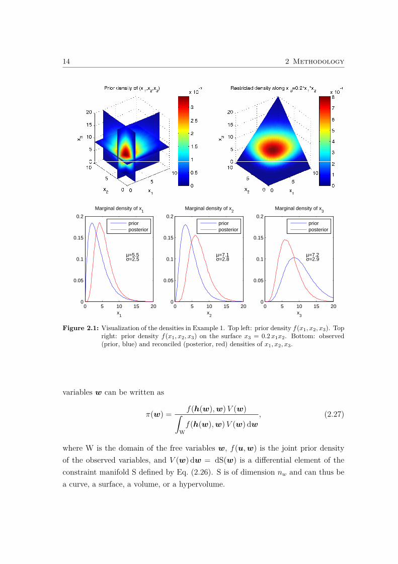
Example 1: Let us assume that there are three observed variables x1, x2 and x3
with the prior density f(x1, x2, x3) defined on R3. The constraint equation x3 =
0.2x1x2 defines a surface in R3. If the prior density is restricted to points in thissurface and normalized to 1, the joint posterior density of x1, x2, x3 is obtained. Bycomputing the marginal distributions of the posterior we get the posterior densitiesof x1, x2 and x3, respectively.
Figure 2.1 shows an instance of this problem, with x1, x2, x3 independent, f1(x1) =
γ(x1; 2, 2), f2(x2) = γ(x2; 3, 1.5) and f3(x3) = γ(x3; 6, 1.7), where γ(x; a, b) is thedensity of the gamma distribution with parameters a and b:
γ(x; a, b) =xa−1 e−x/b
ba Γ(a)
The values of f(x1, x2, x3) are shown color-coded. �
Notes: (1) The Bayesian approach also allows to consider inequality constraints byintroducing slack variables. For instance, the inequality constraint x1 ≤ f(x2, x3)
can be transformed into the equality constraint x1 + xS = f(x2, x3) with a slackvariable xS ≥ 0, which is assumed to have a proper or an improper prior enforcingpositivity. (2) If multiple observations (priors) of the same quantity are available,additional equality constraints have to be added stating that the posteriors of theobservations have to be identical. (3) While in the classical weighted least squaresapproach only the point estimators of true values are reconciled, in the Bayesianapproach the complete pdfs are taken into account.
As shown in section 2.2.1, the nx observed variables x can be split into nw freevariables w and nu dependent variables u. The nyo observable variables yo andthe dependent observed variables u can then be expressed as functions of the freevariables w:
yo = k(w) (2.25)u = h(w) (2.26)
In Cencic and Frühwirth (2018) it was shown that the posterior density of the free
14 2 Methodology
0 5 10 15 200
0.05
0.1
0.15
0.2
Marginal density of x1
x1
µ=5.5σ=2.5
priorposterior
0 5 10 15 200
0.05
0.1
0.15
0.2
Marginal density of x2
x2
µ=7.1σ=2.8
priorposterior
0 5 10 15 200
0.05
0.1
0.15
0.2
Marginal density of x3
x3
µ=7.2σ=2.9
priorposterior
Figure 2.1: Visualization of the densities in Example 1. Top left: prior density f(x1, x2, x3). Topright: prior density f(x1, x2, x3) on the surface x3 = 0.2x1x2. Bottom: observed(prior, blue) and reconciled (posterior, red) densities of x1, x2, x3.
variables w can be written as
π(w) =f(h(w),w)V (w)∫
W
f(h(w),w)V (w) dw, (2.27)
where W is the domain of the free variables w, f(u,w) is the joint prior densityof the observed variables, and V (w) dw = dS(w) is a differential element of theconstraint manifold S defined by Eq. (2.26). S is of dimension nw and can thus bea curve, a surface, a volume, or a hypervolume.
2 Methodology 15
V (w) can be computed from
V (w) =√
|I +HTH|, (2.28)
where H is the Jacobian of the function h,
H(w) =∂h(w)
∂w, (2.29)
and I +HTH is the metric tensor of the induced metric in S (O’Neill, 1983).
If the observed variables are independent, their joint prior density factorizes intothe marginal densities fu(u) and fw(w), and the posterior density of w is equalto
π(w) =fu(h(w)) fw(w)V (w)∫
W
fu(h(w)) fw(w)V (w) dw. (2.30)
The reason why it is not possible to state the posterior distribution π(x) of allobserved variables explicitly is demonstrated by the following example: Let us as-sume there are two measured variables x1 and x2, with given joint prior distributionf(x1, x2), which have to obey the constraint x2 = h(x1). The constraint can be vi-sualized as a 1-dimensional cut of the 2-dimensional density f(x1, x2). Taking thecut as a new 1-dimensional coordinate system, there exists a posterior density alongthis cut. But, because the cut has no area, there is no posterior density definedwith respect to the original 2-dimensional coordinate system, which is denoted assingular pdf. However, the 1-dimensional posterior density along the cut can betransformed into a corresponding pdf with respect to a different 1-dimensional re-ference system (the one of the so called free variable), which in our case could bethe x1-axis or the x2-axis of the originally given 2-dimensional reference system.Note that in this example it is completely arbitrary which variable to choose as thefree variable, provided the transformation is done correctly by taking into accountthe metric structure, i.e., the arc length of the curve as a function of x1 or x2.
The explicit calculation of the posterior density in Eqs. (2.27) and (2.30) can beavoided by generating a random sample from the posterior distribution by means
16 2 Methodology
of Markov chain Monte Carlo (MCMC) methods (Robert and Casella, 2004; Liu,2004; Brooks et al., 2011). This has two advantages: 1. the normalization constant(= denominator of Eqs. (2.27) and (2.30)) is irrelevant; 2. the corresponding sam-ple values of the dependent variables yo and u can be computed by Eqs. (2.25)and (2.26). It is therefore straightforward to estimate posterior marginals, expec-tations, variances and covariances of all variables from the full sample.
The first MCMC sampling algorithm was presented in Metropolis et al. (1953),which was generalized later in Hastings (1970). Its goal is to get a large representa-tive sample from a posterior distribution π(w) that cannot be sampled directly orwhose normalizing constant is not known. The requirements for this sampler are
• a function proportional to the posterior (in our case the numerator of Eqs. (2.27)and (2.30)), which can be evaluated at any point w,
• a proposal density p(wtarget|wsource) = p(wtarget −wsource) to suggest whereto go next, which can also be evaluated at any point w, and from whichrandom vectors can be generated.
The proposed position w (= wtarget), which depends on the current position wi (=
wsource) in the chain, is accepted with a certain probability α(wi, w), i.e. if a uniformrandom number drawn from the unit interval is smaller than or equal to
α(wi, w) = min
(1,
π(w) p(wi|w)
π(wi) p(w|wi)
). (2.31)
Otherwise, the current position wi is appended to the sample instead.
In Cencic and Frühwirth (2015) it was argued that the sampler best suited to thecontext of DR is the independence sampler (Chib and Greenberg, 1995; Liu, 1996;Brooks et al., 2011), in which the proposal values w are drawn from a proposaldensity p(w) independent of the current position . The acceptance probability ofthe sampler is given by
α(wi, w) = min
(1,
π(w) p(wi)
π(wi) p(w)
). (2.32)
2 Methodology 17
In the case of independent observations, this is equivalent to
α(wi, w) = min
(1,
fu(h(w)) fw(w)V (w) p(wi)
fu(h(wi)) fw(wi)V (wi) p(w)
). (2.33)
Note that the normalizing constant of π(w) cancels in Eqs. (2.31), (2.32) and (2.33),so there is no need to compute it. If the proposal density is chosen as p(w) = fw(w),Eq. (2.33) reduces to
α(wi, w) = min
(1,
fu(h(w))V (w)
fu(h(wi))V (wi)
). (2.34)
In the general case of correlated observations, the acceptance probability has to becomputed according to Eq. (2.32), with a suitable proposal density p(w).
2.3.1 Linear Constraints
Using w and u instead of x, Eq. (2.7) can be rewritten as
G(y;u;w) =
I O E e
O I D d
yo
u
w
1
= 0, (2.35)
with E = (E1,E2), D = (D1,O), u = xr1 and w = (xr2 ;xn).
Due to the Gauß-Jordan elimination, the observable unknown variables yo, whichare linear functions of w only, are eliminated from the DR problem, simplifying theconstraints to
u = h(w) = −Dw − d. (2.36)
The observable unknown variables can be computed from
yo = k(w) = −Ew − e. (2.37)
18 2 Methodology
Thus, for any given w the corresponding u and yo can be computed from Eqs. (2.36)and (2.37), which is prerequisite for the Bayesian approach.
In the case of linear constraints, V (w) is a constant and cancels in the posteriordensities defined in Eqs. (2.27) and (2.30).
Fully worked examples can be found in Cencic and Frühwirth (2015).
2.3.2 Nonlinear Constraints
If the explicit computation of the dependent variables yo and u as functions of thechosen free variables w (see Eqs. (2.25) and (2.26)) is not feasible, the solution hasto be computed by numerical methods. The algorithms that can be employed tothis purpose fall into two categories. Algorithms in the first category use gradientinformation, algorithms in the second category do not, i.e. are gradient-free. Atypical example of the first category is the Newton-Raphson algorithm.
Adapting Eq. (2.35) for nonlinear constraints yields
G(y;u;w) ≈
I O E e
O I D d
yo − yo
u− u
w − w
1
= 0. (2.38)
For given w, the corresponding yo and u are to be computed. With initial educatedguesses yo and u, and the choice w = w, Eq. (2.38) reduces to
(yo − yo) + e = 0, (2.39)(u− u) + d = 0, (2.40)
leading to the update equations
yo,i+1 = yo,i − ei, (2.41)ui+1 = ui − di. (2.42)
2 Methodology 19
If yo,i+1 and ui+1 are significantly different from yo,i and ui, respectively, anotheriteration is performed with re-expanding the nonlinear constraints at the updatedexpansion point (y; x; z) = (y; u; w; z) as described in section 2.2.2. Note that thenew y also contains the initial estimates of the unobservable unknown variables yu.Convergence is guaranteed only if the initial y1 and u1 are sufficiently close to thefinal solution.
Note that, in this context, the finally found y, u and w are not estimated parame-ters of distributions, as in chapter 2.2.1 and 2.2.2, but a set of numbers complyingwith the constraints. Thus, for any given w the corresponding u and y can becomputed by this iterative procedure, which is prerequisite for the Bayesian appro-ach.
If the Newton-Raphson iteration (or any other gradient-based method) fails toconverge, a gradient-free approach can be applied. For example, the objectivefunction
J(y;u) = ∥G(y;u;w)∥2 (2.43)
can be minimized for given w with respect to y and u by the simplex algo-rithm (Nelder and Mead, 1965).
Gradient-based methods need an initial expansion point, gradient-less methodsneed a starting point. For a dependent observed variable the natural choice is themode of the prior distribution of the variable. If there are unobserved variables,an educated guess of the starting point should be sufficient to find the correctsolution by the simplex algorithm. Alternative methods such as the constraintconsensus method (Chinneck, 2004) can also be employed to find starting valuesfor unobserved variables. The simplex algorithm is less sensitive to the startingpoint than gradient-based methods, as it is possible to leave a local minimum byrestarting the search with a sufficiently large initial simplex.
The application of the independence sampler additionally requires the compu-tation of H = ∂u/∂w to derive V (w), which is part of the posterior density
20 2 Methodology
(see Eqs. (2.27) and (2.30)). It follows from Eq. (2.38) that
H = −D. (2.44)
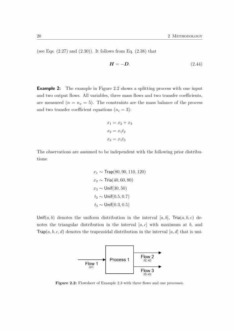
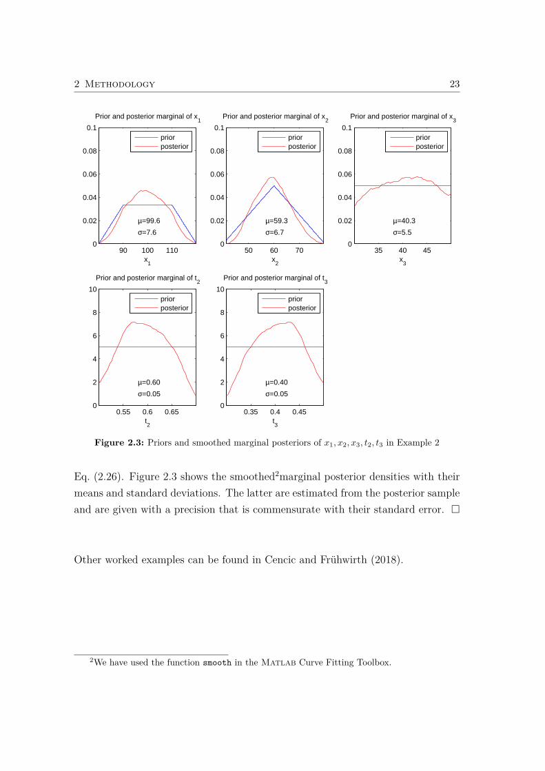
Example 2: The example in Figure 2.2 shows a splitting process with one inputand two output flows. All variables, three mass flows and two transfer coefficients,are measured (n = nx = 5). The constraints are the mass balance of the processand two transfer coefficient equations (nc = 3):
x1 = x2 + x3
x2 = x1t2
x3 = x1t3
The observations are assumed to be independent with the following prior distribu-tions:
x1 ∼ Trap(80, 90, 110, 120)x2 ∼ Tria(40, 60, 80)x3 ∼ Unif(30, 50)t2 ∼ Unif(0.5, 0.7)t3 ∼ Unif(0.3, 0.5)
Unif(a, b) denotes the uniform distribution in the interval [a, b], Tria(a, b, c) de-notes the triangular distribution in the interval [a, c] with maximum at b, andTrap(a, b, c, d) denotes the trapezoidal distribution in the interval [a, d] that is uni-
Figure 2.2: Flowsheet of Example 2.3 with three flows and one processes.
2 Methodology 21
form in [b, c].
For this simple example, u = h(w) can be written in closed form. If e.g. w =
(x3; t3) is selected as the nw = n− nc = 5− 3 = 2 free variables, u = (x1;x2; t2) =
h(w) becomes
u =
x1
x2
t2
=
x3/t3
x3/t3 − x3
1− t3
.
Note that not all choices of w lead to a feasible solution for the dependent variables:e.g. w = (t2; t3) leads to u = (x1;x2;x3) = (0; 0; 0).
V (w) can be derived from Eq. (2.28):
H(w) =∂h(w)
∂w=
∂x1
∂x3
∂x1
∂t3
∂x2
∂x3
∂x2
∂t3
∂t2∂x3
∂t2∂t3
=
1t3
− x3
t32
( 1t3− 1) − x3
t32
0 −1
V (w) =
√|I +HTH| =
√(3x3
2 + 4t34 − 4t3
3 + 4t32)/t3
4
Because the analytical computation of V (w) gets laborious pretty fast even forsmall models, the numerical solution is often to be preferred:
The Taylor series expansion of the original constraints leads to
1 −1 0 −1 0 x1− x2− x3
−t2 1 −x1 0 0 x2 − x1t2
−t3 0 0 1 −x1 x3 − x1t3
x1 − x1
x2 − x2
t2 − t2
x3 − x3
t3 − t3
1
=
0
0
0
.
22 2 Methodology
After the Gauss-Jordan elimination, these constraints can be written as
1 0 0 − 1
t3
x1
t3
x3−t3x1
t3
0 1 0 t3−1t3
x1
t3
t3x2−x3+t3x3
t3
0 0 1 t2+t3−1t3x1
− t2−1t3
x3(t2+t3−1)
t3x1
x1 − x1
x2 − x2
t2 − t2
x3 − x3
t3 − t3
1
=
0
0
0
,
(I D d
)u− u
w − w
1
= 0.
Note that normally the Gauss-Jordan elimination is performed numerically. Forcomparison reasons, here it was done analytically.
Using the Newton-Raphson algorithm, the corresponding u for given w are compu-ted iteratively via update equation Eq. (2.42). After convergence, the constraintscan be written as
1 0 0 − 1
t3
x3
t320
0 1 0 t3−1t3
x3
t320
0 0 1 0 1 0
x1 − x1
x2 − x2
t2 − t2
x3 − x3
t3 − t3
1
=
0
0
0
.
Comparing the result with the analytical derivation of H(w)), it can be seen thatH(w) = −D, as stated in Eq. (2.44).
By using the independence sampler, a sample W = (w1,w2, . . . ,wL) of size L isdrawn from the posterior distribution of the free variables w. The correspondingsample U = (u1,u2, . . . ,uL) of the dependent variables u is computed by using
2 Methodology 23
35 40 450
0.02
0.04
0.06
0.08
0.1
x3
Prior and posterior marginal of x3
µ=40.3
σ=5.5
priorposterior
0.35 0.4 0.450
2
4
6
8
10
t3
Prior and posterior marginal of t3
µ=0.40
σ=0.05
priorposterior
90 100 1100
0.02
0.04
0.06
0.08
0.1
x1
Prior and posterior marginal of x1
µ=99.6
σ=7.6
priorposterior
50 60 700
0.02
0.04
0.06
0.08
0.1
x2
Prior and posterior marginal of x2
µ=59.3
σ=6.7
priorposterior
0.55 0.6 0.650
2
4
6
8
10
t2
Prior and posterior marginal of t2
µ=0.60
σ=0.05
priorposterior
Figure 2.3: Priors and smoothed marginal posteriors of x1, x2, x3, t2, t3 in Example 2
Eq. (2.26). Figure 2.3 shows the smoothed2marginal posterior densities with theirmeans and standard deviations. The latter are estimated from the posterior sampleand are given with a precision that is commensurate with their standard error. �
Other worked examples can be found in Cencic and Frühwirth (2018).
2We have used the function smooth in the Matlab Curve Fitting Toolbox.
24 2 Methodology
2.3.3 Correlated Observations
In the case of normal observations, correlations between the observed variables canbe introduced by modifying their joint covariance matrix. In the nonnormal case,the standard way of imposing correlations on observations with given marginaldistributions is via a copula.
A function C : [0, 1]d → [0, 1] is called a d-dimensional copula if it is the jointcumulative distribution function (cdf) of a d-dimensional random vector on theunit hypercube [0, 1]d with uniform marginals (Nelsen, 2006). In the following, theGaussian copula CG(ξ;R) with ξ ∈ [0, 1]d and correlation matrix R is used. Itsdensity cG is given by
cG(ξ;R) =1√
detRexp
[−1
2Φ−1(ξ)T
(R−1 − I
)Φ−1(ξ)
], ξ ∈ [0, 1]d, (2.45)
where Φ−1 is the inverse distribution function of the d-dimensional standard normaldistribution.
In the general form of the posterior density (Eq. (2.27)), f(u;w) is the joint densityof all observed variables, which in the presence of correlations no longer factorizesinto the marginal densities of u and w (cf. Eq. (2.30)).
Let fk(xk) denote the prior marginal density of the (observed) variable xk andFk(xk) its cdf, where k = 1, . . . , nx. R is the assumed or estimated correlationmatrix of x. The following lemma shows how to compute the joint density functionof x and its correlation matrix.
Lemma. Assume that ξ is distributed according to the Gaussian copula CG(ξ;R)
and xk = F−1k (ξk), k = 1, . . . , nx. Then:
(a) The joint density of x is equal to
g(x) = cG(F1(x1), . . . , Fnx(xnx);R)nx∏k=1
fk(xk) (2.46)
and the marginal density of xk is equal to fk(xk).
2 Methodology 25
(b) The joint correlation matrix of x is equal to R in first-order Taylor approxi-mation.
Proof. Assertion (a) follows from the relations ξk = Fk(xk) and the transformationtheorem for densities:
g(x) = cG(ξ, . . . , ξnx ;R)
∣∣∣∣ ∂ξ∂x∣∣∣∣
= cG(F1(x1), . . . , Fnx(xnx);R)nx∏k=1
fk(xk)
Assertion (b) can be proved by noting that the linear error propagation from ξ tox has the following form:
Cov(x) = J Cov(ξ)JT, with J =∂x
∂ξ(2.47)
J is diagonal, which reduces the error propagation to a rescaling of the variables.As correlation matrices are invariant under such a transformation, the correlationmatrix of x is equal to R in first-order approximation.
The simplest proposal density p(w) is the product of the marginal densities of thefree variables:
p(w) =nw∏k=1
fw,k(wk) (2.48)
The sampling algorithm is summarized in the box Algorithm 1.
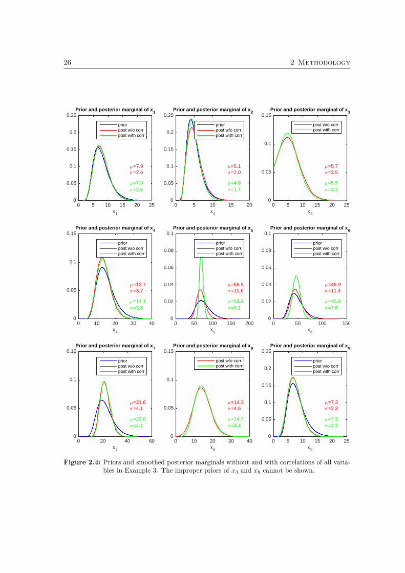
Example 3: The modified sampler is illustrated using the linear model in Cencicand Frühwirth (2015, Example 4.3) which has nine flows and four processes. Va-riables x3 and x8 are unobserved. The other variables are modeled by lognormalpriors. The effect of setting ρ24 = 0.7, ρ56 = −0.4, ρ57 = −0.3, ρ67 = −0.6 is shownin Figure 2.4. The posterior densities of x5 and x6 are significantly affected by thecorrelations, whereas the other variables hardly change. �
26 2 Methodology
x3
0 5 10 15 20 250
0.05
0.1
0.15
7=5.7<=3.5
7=5.5<=3.3
Prior and posterior marginal of x3
post w/o corrpost with corr
x8
0 10 20 30 400
0.05
0.1
0.15
7=14.3<=4.6
7=14.7<=4.4
Prior and posterior marginal of x8
post w/o corrpost with corr
x5
0 50 100 150 2000
0.02
0.04
0.06
0.08
0.1
7=68.5<=11.6
7=68.9<=5.1
Prior and posterior marginal of x5
priorpost w/o corrpost with corr
x7
0 20 40 600
0.05
0.1
0.15
7=21.6<=4.1
7=22.0<=4.1
Prior and posterior marginal of x7
priorpost w/o corrpost with corr
x6
0 50 100 1500
0.02
0.04
0.06
0.08
0.1
7=46.9<=11.4
7=46.9<=7.6
Prior and posterior marginal of x6
priorpost w/o corrpost with corr
x4
0 10 20 30 400
0.05
0.1
0.15
7=13.7<=3.7
7=14.1<=3.8
Prior and posterior marginal of x4
priorpost w/o corrpost with corr
x1
0 5 10 15 20 250
0.05
0.1
0.15
0.2
0.25
7=7.9<=2.6
7=7.9<=2.6
Prior and posterior marginal of x1
priorpost w/o corrpost with corr
x9
0 5 10 15 20 250
0.05
0.1
0.15
0.2
0.25
7=7.3<=2.3
7=7.3<=2.3
Prior and posterior marginal of x9
priorpost w/o corrpost with corr
x2
0 5 10 15 200
0.05
0.1
0.15
0.2
0.25
7=5.1<=2.0
7=4.8<=1.7
Prior and posterior marginal of x2
priorpost w/o corrpost with corr
Figure 2.4: Priors and smoothed posterior marginals without and with correlations of all varia-bles in Example 3. The improper priors of x3 and x8 cannot be shown.
2 Methodology 27
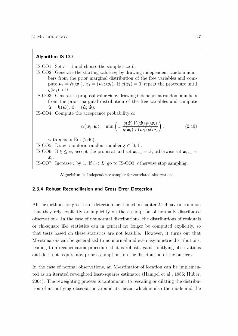
Algorithm IS-CO
IS-CO1. Set i = 1 and choose the sample size L.IS-CO2. Generate the starting value w1 by drawing independent random num-
bers from the prior marginal distribution of the free variables and com-pute u1 = h(w1), x1 = (u1;w1). If g(x1) = 0, repeat the procedure untilg(x1) > 0.
IS-CO3. Generate a proposal value w by drawing independent random numbersfrom the prior marginal distribution of the free variables and computeu = h(w), x = (u; w).
IS-CO4. Compute the acceptance probability α:
α(wi, w) = min
(1,
g(x)V (w) p(wi)
g(xi)V (wi) p(w)
), (2.49)
with g as in Eq. (2.46).IS-CO5. Draw a uniform random number ξ ∈ [0, 1].IS-CO6. If ξ ≤ α, accept the proposal and set xi+1 = x; otherwise set xi+1 =
xi.IS-CO7. Increase i by 1. If i < L, go to IS-CO3, otherwise stop sampling.
Algorithm 1: Independence sampler for correlated observations
2.3.4 Robust Reconciliation and Gross Error Detection
All the methods for gross error detection mentioned in chapter 2.2.4 have in commonthat they rely explicitly or implicitly on the assumption of normally distributedobservations. In the case of nonnormal distributions, the distributions of residualsor chi-square like statistics can in general no longer be computed explicitly, sothat tests based on these statistics are not feasible. However, it turns out thatM-estimators can be generalized to nonnormal and even asymmetric distributions,leading to a reconciliation procedure that is robust against outlying observationsand does not require any prior assumptions on the distribution of the outliers.
In the case of normal observations, an M-estimator of location can be implemen-ted as an iterated reweighted least-squares estimator (Hampel et al., 1986; Huber,2004). The reweighting process is tantamount to rescaling or dilating the distribu-tion of an outlying observation around its mean, which is also the mode and the
28 2 Methodology
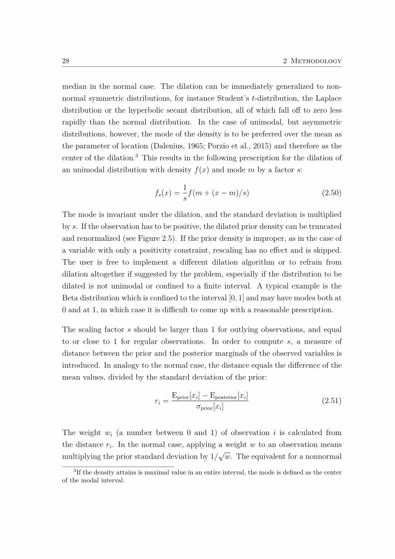
median in the normal case. The dilation can be immediately generalized to non-normal symmetric distributions, for instance Student’s t-distribution, the Laplacedistribution or the hyperbolic secant distribution, all of which fall off to zero lessrapidly than the normal distribution. In the case of unimodal, but asymmetricdistributions, however, the mode of the density is to be preferred over the mean asthe parameter of location (Dalenius, 1965; Porzio et al., 2015) and therefore as thecenter of the dilation.3 This results in the following prescription for the dilation ofan unimodal distribution with density f(x) and mode m by a factor s:
fs(x) =1
sf(m+ (x−m)/s) (2.50)
The mode is invariant under the dilation, and the standard deviation is multipliedby s. If the observation has to be positive, the dilated prior density can be truncatedand renormalized (see Figure 2.5). If the prior density is improper, as in the case ofa variable with only a positivity constraint, rescaling has no effect and is skipped.The user is free to implement a different dilation algorithm or to refrain fromdilation altogether if suggested by the problem, especially if the distribution to bedilated is not unimodal or confined to a finite interval. A typical example is theBeta distribution which is confined to the interval [0, 1] and may have modes both at0 and at 1, in which case it is difficult to come up with a reasonable prescription.
The scaling factor s should be larger than 1 for outlying observations, and equalto or close to 1 for regular observations. In order to compute s, a measure ofdistance between the prior and the posterior marginals of the observed variables isintroduced. In analogy to the normal case, the distance equals the difference of themean values, divided by the standard deviation of the prior:
ri =Eprior[xi]− Eposterior[xi]
σprior[xi](2.51)
The weight wi (a number between 0 and 1) of observation i is calculated fromthe distance ri. In the normal case, applying a weight w to an observation meansmultiplying the prior standard deviation by 1/
√w. The equivalent for a nonnormal
3If the density attains is maximal value in an entire interval, the mode is defined as the centerof the modal interval.
2 Methodology 29
−5 0 5 10 15 200
0.01
0.02
0.03
0.04
0.05
0.06
0.07
0.08
0.09
0.1
m x
(x−m)/s f(m+(x−m)/s) = s*fs(x)
x−m
fs(x)
originaldilated (nonnormalized)dilateddilated + truncated
Figure 2.5: Visualization of the dilation procedure: The original prior (blue line) is dilatedaround the mode by factor s. The resulting dilated prior (red line) needs to benormalized by dividing its density by s. The normalized dilated prior (green line) istruncated at zero and renormalized (black line).
observation is to dilate its prior density by the factor s = 1/√w around the mode.
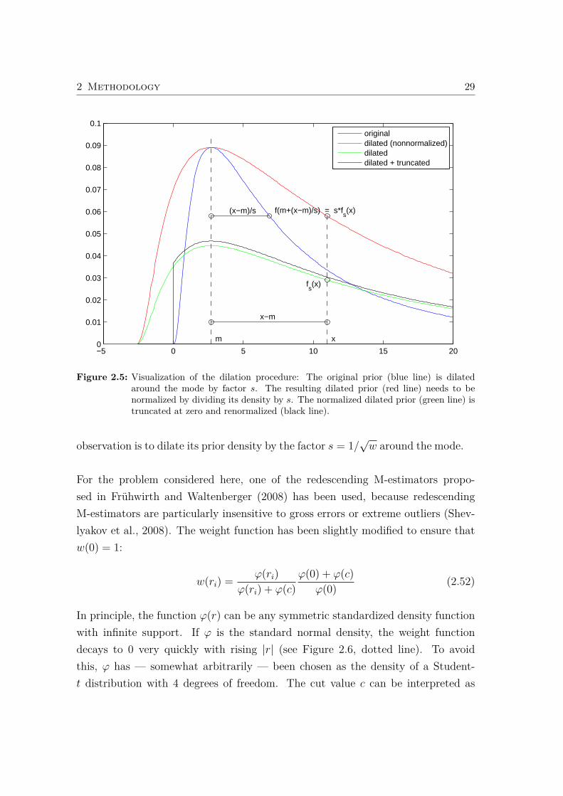
For the problem considered here, one of the redescending M-estimators propo-sed in Frühwirth and Waltenberger (2008) has been used, because redescendingM-estimators are particularly insensitive to gross errors or extreme outliers (Shev-lyakov et al., 2008). The weight function has been slightly modified to ensure thatw(0) = 1:
w(ri) =φ(ri)
φ(ri) + φ(c)
φ(0) + φ(c)
φ(0)(2.52)
In principle, the function φ(r) can be any symmetric standardized density functionwith infinite support. If φ is the standard normal density, the weight functiondecays to 0 very quickly with rising |r| (see Figure 2.6, dotted line). To avoidthis, φ has — somewhat arbitrarily — been chosen as the density of a Student-t distribution with 4 degrees of freedom. The cut value c can be interpreted as
30 2 Methodology
a (fuzzy) boundary which discriminates between “good” and “bad”, or “inlying”and “outlying” observations. The weight function w(|r|) with c = 2.5 is shown bythe full line in Figure 2.6. If necessary, the number of degrees of freedom can beadapted to the problem at hand, or a different family of densities can be chosen.
0 5 10 15 20
|r|
0
0.2
0.4
0.6
0.8
1
w(|
r|)
weight function (Student-t)weight function (std normal)cut value
0 5 10 15 20
|r|
10 -4
10 -3
10 -2
10 -1
100
w(|
r|)
Figure 2.6: The weight function of Eq. (2.52) (full line) on a linear scale (left) and a logarithmicscale (right). The weight function based on the standard normal density (dottedline) is shown for comparison.
The sampler can be run as usual, but has to be iterated. After each run of thesampler, the distances ri and the corresponding weights wi are recomputed, theprior distributions are dilated accordingly, and the sampler is run again, until con-vergence of the weights. Note that the distances (Eq. (2.51)) have to be computedusing the spread of the original, undilated prior.
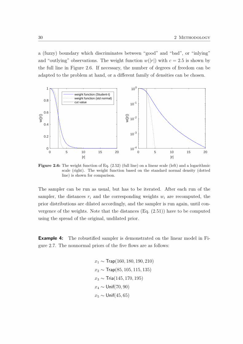
Example 4: The robustified sampler is demonstrated on the linear model in Fi-gure 2.7. The nonnormal priors of the five flows are as follows:
x1 ∼ Trap(160, 180, 190, 210)x2 ∼ Trap(85, 105, 115, 135)x3 ∼ Tria(145, 170, 195)x4 ∼ Unif(70, 90)x5 ∼ Unif(45, 65)
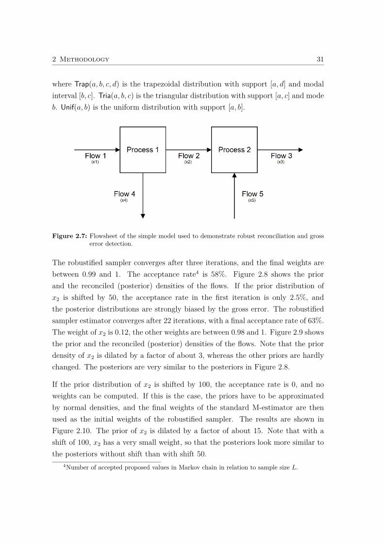
2 Methodology 31
where Trap(a, b, c, d) is the trapezoidal distribution with support [a, d] and modalinterval [b, c]. Tria(a, b, c) is the triangular distribution with support [a, c] and modeb. Unif(a, b) is the uniform distribution with support [a, b].
Figure 2.7: Flowsheet of the simple model used to demonstrate robust reconciliation and grosserror detection.
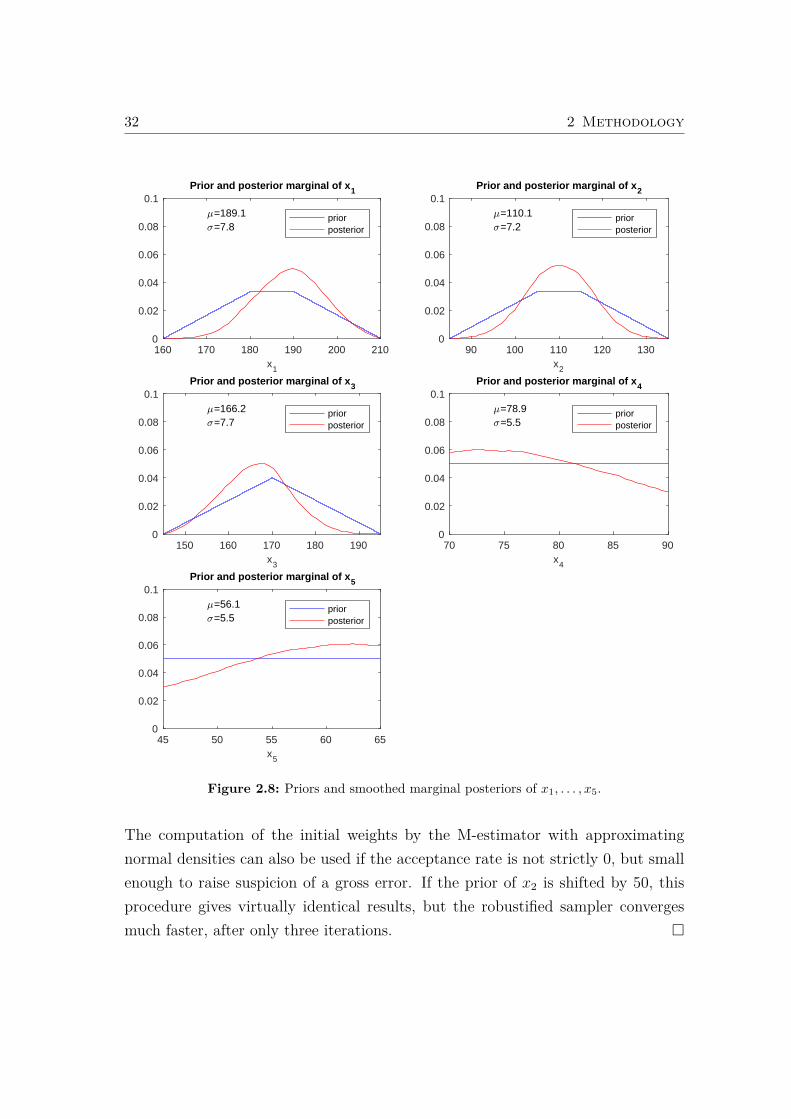
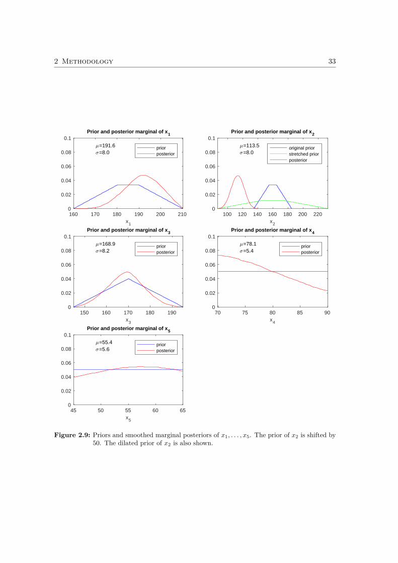
The robustified sampler converges after three iterations, and the final weights arebetween 0.99 and 1. The acceptance rate4 is 58%. Figure 2.8 shows the priorand the reconciled (posterior) densities of the flows. If the prior distribution ofx2 is shifted by 50, the acceptance rate in the first iteration is only 2.5%, andthe posterior distributions are strongly biased by the gross error. The robustifiedsampler estimator converges after 22 iterations, with a final acceptance rate of 63%.The weight of x2 is 0.12, the other weights are between 0.98 and 1. Figure 2.9 showsthe prior and the reconciled (posterior) densities of the flows. Note that the priordensity of x2 is dilated by a factor of about 3, whereas the other priors are hardlychanged. The posteriors are very similar to the posteriors in Figure 2.8.
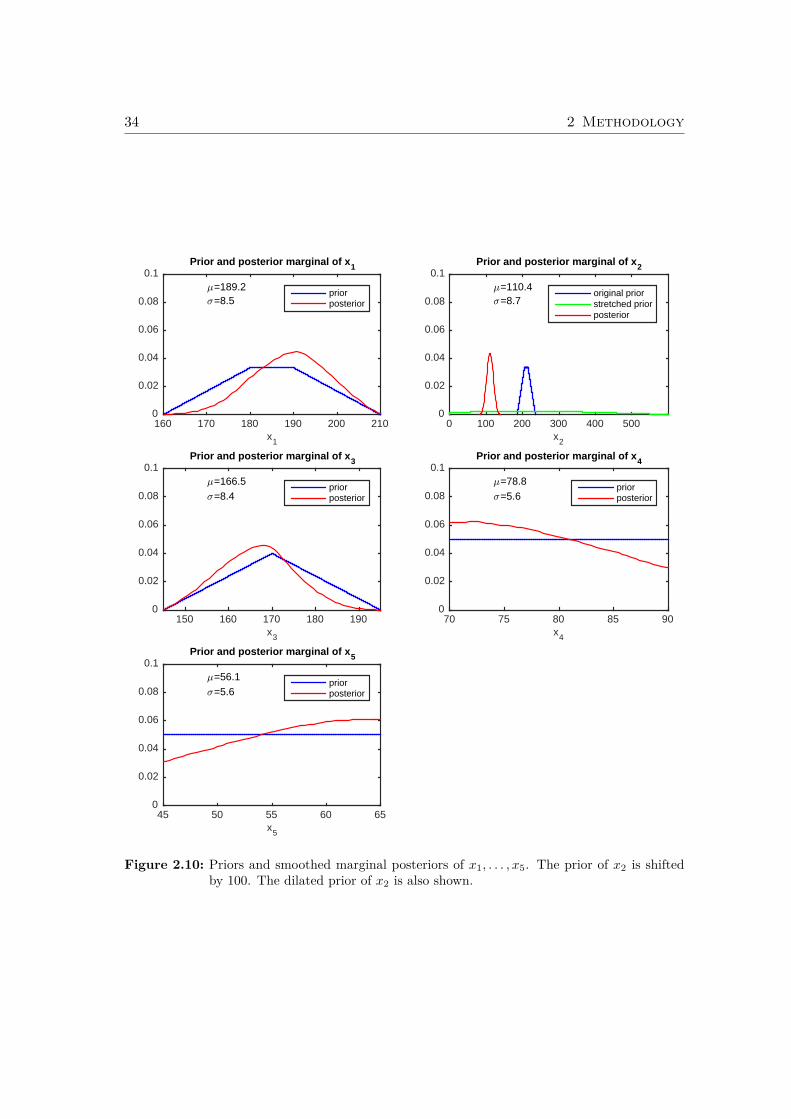
If the prior distribution of x2 is shifted by 100, the acceptance rate is 0, and noweights can be computed. If this is the case, the priors have to be approximatedby normal densities, and the final weights of the standard M-estimator are thenused as the initial weights of the robustified sampler. The results are shown inFigure 2.10. The prior of x2 is dilated by a factor of about 15. Note that with ashift of 100, x2 has a very small weight, so that the posteriors look more similar tothe posteriors without shift than with shift 50.
4Number of accepted proposed values in Markov chain in relation to sample size L.
32 2 Methodology
160 170 180 190 200 210x1
0
0.02
0.04
0.06
0.08
0.1Prior and posterior marginal of x1
7=189.1<=7.8
priorposterior
90 100 110 120 130x2
0
0.02
0.04
0.06
0.08
0.1Prior and posterior marginal of x2
7=110.1<=7.2
priorposterior
150 160 170 180 190x3
0
0.02
0.04
0.06
0.08
0.1Prior and posterior marginal of x3
7=166.2<=7.7
priorposterior
70 75 80 85 90x4
0
0.02
0.04
0.06
0.08
0.1Prior and posterior marginal of x4
7=78.9<=5.5
priorposterior
45 50 55 60 65x5
0
0.02
0.04
0.06
0.08
0.1Prior and posterior marginal of x5
7=56.1<=5.5
priorposterior
Figure 2.8: Priors and smoothed marginal posteriors of x1, . . . , x5.
The computation of the initial weights by the M-estimator with approximatingnormal densities can also be used if the acceptance rate is not strictly 0, but smallenough to raise suspicion of a gross error. If the prior of x2 is shifted by 50, thisprocedure gives virtually identical results, but the robustified sampler convergesmuch faster, after only three iterations. �
2 Methodology 33
160 170 180 190 200 210x1
0
0.02
0.04
0.06
0.08
0.1Prior and posterior marginal of x1
7=191.6<=8.0
priorposterior
100 120 140 160 180 200 220x2
0
0.02
0.04
0.06
0.08
0.1Prior and posterior marginal of x2
7=113.5<=8.0
original priorstretched priorposterior
150 160 170 180 190x3
0
0.02
0.04
0.06
0.08
0.1Prior and posterior marginal of x3
7=168.9<=8.2
priorposterior
70 75 80 85 90x4
0
0.02
0.04
0.06
0.08
0.1Prior and posterior marginal of x4
7=78.1<=5.4
priorposterior
45 50 55 60 65x5
0
0.02
0.04
0.06
0.08
0.1Prior and posterior marginal of x5
7=55.4<=5.6
priorposterior
Figure 2.9: Priors and smoothed marginal posteriors of x1, . . . , x5. The prior of x2 is shifted by50. The dilated prior of x2 is also shown.
34 2 Methodology
x1
160 170 180 190 200 2100
0.02
0.04
0.06
0.08
0.17=189.2<=8.5
Prior and posterior marginal of x1
priorposterior
x2
0 100 200 300 400 5000
0.02
0.04
0.06
0.08
0.17=110.4<=8.7
Prior and posterior marginal of x2
original priorstretched priorposterior
x3
150 160 170 180 1900
0.02
0.04
0.06
0.08
0.17=166.5<=8.4
Prior and posterior marginal of x3
priorposterior
x4
70 75 80 85 900
0.02
0.04
0.06
0.08
0.17=78.8<=5.6
Prior and posterior marginal of x4
priorposterior
x5
45 50 55 60 650
0.02
0.04
0.06
0.08
0.17=56.1<=5.6
Prior and posterior marginal of x5
priorposterior
Figure 2.10: Priors and smoothed marginal posteriors of x1, . . . , x5. The prior of x2 is shiftedby 100. The dilated prior of x2 is also shown.
3 Conclusions and Outlook
The classical weighted least squares approach to DR, which assumes normally dis-tributed observation errors, poses the problem that only in case of linear constraintsthe estimation errors of the adjusted observations are normally distributed again.In case of nonlinear constraints, however, the normally distributed results gainedfrom linearization can differ substantially from the precise solution, especially if theinvolved uncertainties are large. Additionally, in scientific models, the assumptionof normally distributed input data is often not justified.
Therefore, in Cencic and Frühwirth (2018), the Bayesian approach to DR for linearconstraints, presented in Cencic and Frühwirth (2015), was further developed andextended to nonlinear constraints.
The advantages of the Bayesian approach are: First, arbitrary continuous pdfs canbe used to describe the uncertainty of the observations. Second, even nonparametricestimators of the pdf are allowed, provided that it is possible to draw a randomsample from them. Third, not only means, variances and covariances of observedand unobserved variables can be computed a posteriori, but also various othercharacteristics of the marginal posteriors, such as the mode, skewness, quantiles,and HPD intervals.
The main idea of the method is to restrict the joint prior probability distributionof the observed variables with model constraints to get a joint posterior probabilitydistribution. The derived joint posterior of the free observed variables is sampledby a MCMC method using the independence sampler, and the dependent variables(observed and unobserved) are computed from this sample.
By construction, all individual elements of the Markov chain satisfy the constraints,but the sample mean in the nonlinear case in general does not. If a representativevalue of the posterior distribution satisfying the constraints is required, the element
36 3 Conclusions and Outlook
of the Markov chain with the smallest distance from the sample mean can beselected. Possible distance measures are, among others, the L1, the L2 and the L∞
distance.
It was shown that, for nonlinear constraints, it is essential to consider the metricof the constraint manifold. The posterior density derived in Cencic and Frühwirth(2018) contains the term V (w) (Eq. (2.28)), which in the linear case is constantand cancels. If V (w) is neglected in the nonlinear case, the posterior is no longerinvariant under the choice of the free variables.
For the Bayesian approach, in chapter 2.3.3 it was shown how to incorporate corre-lated observations, and in chapter 2.3.4 how to perform robust gross error detectionwith the help on redescending M-estimators. Note that both topics are not coveredin the three papers of this thesis.
In subsequent work, the Bayesian method will be applied to more extensive real lifeexamples in order to compare the results to alternative approaches such as classi-cal weighted least squares, fuzzy sets (possibilistic approach to DR), and anotherBayesian approach that was published recently in Lupton and Allwood (2018).
Bibliography
Alhaj-Dibo, M., Maquin, D., and Rago, J. Data reconciliation: A robust approachusing a contaminated distribution. Control Engineering Practice, 16:159–170,2008.
Almasy, G. and Sztano, T. Checking and Correction of Measurements on the Basisof Linear System Model. Problems of Control and Information Theory, 4:57–69,1975.
Arora, N. and Biegler, L. Redescending estimators for data reconciliation and pa-rameter estimation. Computers and Chemical Engineering, 25:1585–1599, 2001.
Bagajewicz, M. Smart Process Plants : Software and Hardware Solutions for Accu-rate Data and Profitable Operations. McGraw-Hill, New York, 2010.
Brooks, S., Gelman, A., Jones, G., and Meng, X.-L., editors. Handbook of MarkovChain Monte Carlo. Chapman & Hall, Boca Raton, 2011.
Brunner, P. and Rechberger, H. Handbook of Material Flow Analysis: For Envi-ronmental, Resource, and Waste Engineers, Second Edition. CRC Press, BocaRaton, Florida, 2016.
Cencic, O. Nonlinear data reconciliation in material flow analysis with softwareSTAN. Sustainable Environment Reserach, 26:291–298, 2016.
Cencic, O. and Frühwirth, R. A general framework for data reconciliation—Part I:Linear constraints. Computers and Chemical Engineering, 75:196–208, 2015.
Cencic, O. and Frühwirth, R. Data reconciliation of nonnormal observations withnonlinear constraints. Journal of Applied Statistics, 2018.
Cencic, O. and Rechberger, H. Material flow analysis with software STAN. Journalof Environmental Engineering and Management, 18(1):3–7, 2008.
38 Bibliography
Chib, S. and Greenberg, E. Understanding the Metropolis–Hastings Algorithm.The American Statistician, 49(4):327–335, 1995.
Chinneck, J. The Constraint Consensus Method for Finding Approximately Fea-sible Points in Nonlinear Programs. INFORMS Journal on Computing, 16(3):255–265, 2004.
Dalenius, T. The Mode—A Neglected Statistical Parameter. Journal of the RoyalStatistical Society A, 128(1):110–117, 1965.
Dubois, D., Fargier, H., Ababou, M., and Guyonnet, D. A fuzzy constraint-basedapproach to data reconciliation in material flow analysis. International Journalof General Systems, 43(8):787–809, 2014.
Dzubur, N., Sunanta, O., and Laner, D. A fuzzy set-based approach to datareconciliation in material flow modeling. Applied Mathematical Modelling, 43:464–480, 2017.
Frühwirth, R. and Waltenberger, W. Redescending M-estimators and DeterministicAnnealing. Austrian Journal of Statistics, 37(3&4):301–317, 2008.
Hampel, F., Ronchetti, E., Rousseeuw, P., and Stahel, W. Robust Statistics: TheApproach Based on Influence Functions. John Wiley & Sons, New York, 1986.
Hastings, W. Monte Carlo sampling methods using Markov chains and their appli-cations. Biometrika, 57:97–107, 1970.
Hu, M. and Shao, H. Theory Analysis of Nonlinear Data Reconciliation and Ap-plication to a Coking Plant. Industrial & Engineering Chemistry Research, 45:8973–8984, 2006.
Huber, P. Robust Statistics: Theory and Methods. John Wiley & Sons, New York,2004.
Johnston, L. and Kramer, M. Maximum Likelihood Data Rectification: Steady-State Systems. AIChE Journal, 24(11):2415–2426, 1995.
Kuehn, D. and Davidson, H. Computer control - II. Mathematics of control. Che-mical Engineering Progress, 57(6), 1961.
Bibliography 39
Liu, J. Metropolized independent sampling with comparisons to rejection samplingand importance sampling. Statistics and Computing, 6:113–119, 1996.
Liu, J. Monte Carlo Strategies in Scientific Computing. Springer, New York, 2004.
Llanos, C., Sanchéz, M., and Maronna, R. Robust Estimators for Data Reconcili-ation. Industrial & Engineering Chemistry Research, 54:5096–5105, 2015.
Lupton, R. C. and Allwood, J. M. Incremental Material Flow Analysis with Baye-sian Inference. Journal of Industrial Ecology, in press, 2018.
Madron, F. Process Plant Performance. Ellis Horwood, New York, 1992.
Madron, F., Veverka, V., and Venecek, V. Statistical Analysis of Material Balanceof a Chemical Reactor. AIChE Journal, 57(6):482–486, 1977.
Metropolis, N. et al. Equation of State Calculations by Fast Computing Machines.The Journal of Chemical Physics, 21:1087–1091, 1953.
Narasimhan, S. and Jordache, C. Data Reconciliation and Gross Error Detection.An Intelligent Use of Process Data. Gulf Publishing Company, Houston, 2000.
Nelder, J. and Mead, R. A Simplex Method for Function Minimization. ComputerJournal, 7:308–313, 1965.
Nelsen, R. An Introduction to Copulas. Springer, New York, 2006.
O’Neill, B. Semi-Riemannian Geometry. Academic Press, San Diego, 1983.
Özyurt, D. and Pike, R. Theory and practice of simultaneous data reconciliationand gross error detection for chemical processes. Computers and Chemical En-gineering, 28:381–402, 2004.
Porzio, G., Ragozini, G., Liebscher, S., and Kirschstein, T. Minimum volume pee-ling: A robust nonparametric estimator of the multivariate mode. ComputationalStatistics & Data Analysis, 93:456–468, 2015.
Robert, C. and Casella, C. Monte Carlo Statistical Methods. Springer, New York,2004.
40 Bibliography
Romagnoli, J. and Sanchez, M. Data Processing and Reconciliation for ChemicalProcess Operations. Academic Press, San Diego, 2000.
Shevlyakov, G., Morgenthaler, S., and Shurygin, A. Redescending M-estimators.Journal of Statistical Planning and Inference, 138(10):2906 – 2917, 2008.
Tamhane, A. and Mah, R. Data Reconciliation and Gross Error Detection inChemical Process Networks. Technometrics, 27(4):409–422, 1985.
Yuan, Y., Khatibisepehr, S., Huang, B., and Li, Z. Bayesian method for simul-taneous gross error detection and data reconciliation. AIChE Journal, 61(10):3232–3248, 2015.
Notation
a parameter of a distribution
A coefficient matrix of observed variables
b parameter of a distribution
B coefficient matrix of unobserved variables
c parameter of a distribution
c vector of aggregated constant quantities
C copula
C coefficient matrix of constant quantities
cG probability density function of the Gaussian copula
CG cumulative distribution function of the Gaussian copula
d parameter of a distribution
d vector, which is a submatrix of RREF(B,A, c)
D submatrix of RREF(B,A, c)
dS differential element of the constraint manifold S
D1 submatrix of RREF(B,A, c)
e vector, which is a submatrix of RREF(B,A, c)
E expectation
E submatrix of RREF(B,A, c)
E1 submatrix of RREF(B,A, c)
E2 submatrix of RREF(B,A, c)
f distribution function
F cumulative distribution function
fs dilated distribution function
42 Notation
fu joint prior density of dependent observed variables
fu vector, which is a submatrix of RREF(B,A, c)
fw joint prior density of free observed variables
fz scalar that is either 0 or 1
F0 submatrix of RREF(B,A, c)
F1 submatrix of RREF(B,A, c)
F2 submatrix of RREF(B,A, c)
g joint prior density of correlated observed variables
G vector of equality constraint equations
h vector of functions of free observed variables to compute dependentobserved variables
H partial derivatives of function h with respect to w
i counter of iterations
I identity matrix
J objective function to be minimized
J partial derivatives of x with respect to ξ
Jx partial derivatives of equality constraints G with respect to observedvariables x
Jy partial derivatives of equality constraints G with respect to unknownvariables y
k counter of observed variables
k vector of functions of free observed variables to compute observableunknown variables
L sample size
L1 Manhattan distance
L2 Euclidean distance
L∞ Chebyshev distance
m mode
m vector containing one element of the Markov chain
Notation 43
n number of variables
N normal distribution
nc number of independent equality constraint equations
nu number of dependent observed variables
nw number of free observed variables
nx number of observed variables
nyo number of observable unknown variables
O null matrix
p proposal density for MCMC algorithm
Q variance-covariance matrix of estimated observable unknown and re-conciled observed variables
Qx variance-covariance matrix of reconciled observed variables
Qx variance-covariance matrix of observations of observed variables
Qyo variance-covariance matrix of estimated observable unknown variables
r measure of distance between prior and posterior distribution
R correlation matrix
t transfer coefficient
s dilation factor
S constraint manifold; domain of the constraint manifold
u vector of dependent observed variables
V square root of the determinant of the metric tensor
w weight, a number in the interval [0, 1]
w vector of free observed variables
W domain of the free variables w
x observed variable
x vector of observed variables
xn vector of nonredundant observed variables
xr1 vector of dependent redundant observed variables
44 Notation
xr2 vector of free redundant observed variables
y vector of unknown variables
yo vector of observable unknown variables; subset of y
yu1 vector of ’dependent’ unobservable unknown variables; subset of y
yu2 vector of ’free’ unobservable unknown variables; subset of y
z vector of constant quantities
0 null vector
Greek symbols:
α probability of acceptance
γ gamma distribution
Γ complete gamma function
δ vector of measurement biases of observed variables
ϵ vector of random errors of observed variables
µ mean value
µx vector of true values of observed variables
σ standard deviation
σ vector of standard deviations
φ symmetric standardized density function with infinite support
Φ−1 inverse distribution function of the multi-dimensional standard normaldistribution
ξ uniform random numbers in the interval [0,1]
ξ vector of uniform random numbers in the interval [0,1]
π joint posterior distribution
ρ correlation coefficient
Notation 45
Superscripts:
~ measured/observed values
^ estimated values
· proposed values
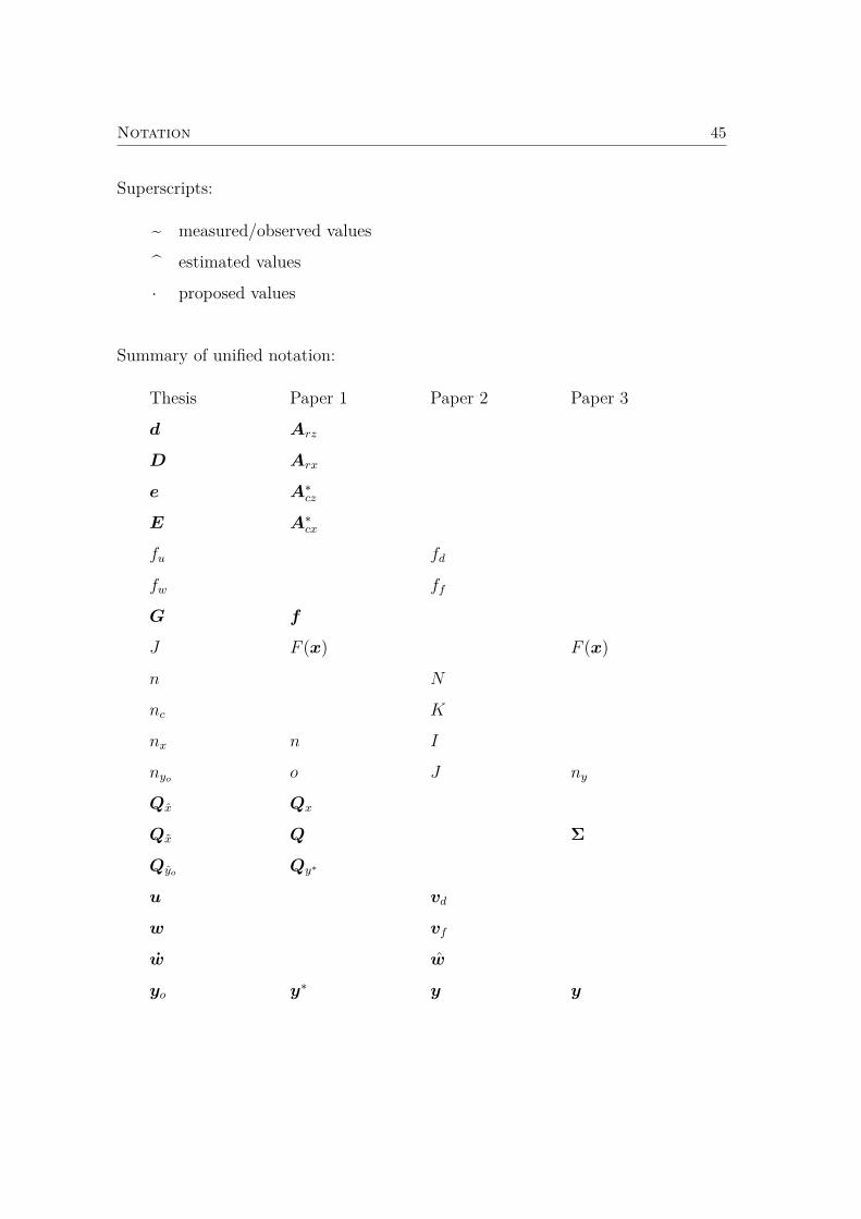
Summary of unified notation:
Thesis Paper 1 Paper 2 Paper 3
d Arz
D Arx
e A∗cz
E A∗cx
fu fd
fw ff
G f
J F (x) F (x)
n N
nc K
nx n I
nyo o J ny
Qx Qx
Qx Q Σ
Qyo Qy∗
u vd
w vf
w w
yo y∗ y y

Abbreviations
cdf cumulative distribution functionCov covarianceDR data reconciliatione.g. for examplei.e. that is; in other wordsIS-CO independence sampler - correlated observationsMCMC Markov chain Monte CarloMFA material flow analysispdf probability density functionRREF reduced row echelon formSTAN software for subSTance flow ANalysisTrap trapezoidal distribution functionTria triangular distribution functionUnif uniform distribution function

Appendix
Paper 1:
Nonlinear data reconciliation in material flow analysiswith software STANOliver CencicSustainable Environment Research 2016, 26 (6)DOI: 10.1016/j.serj.2016.06.00

Technical note
Nonlinear data reconciliation in material flow analysis with softwareSTAN
Oliver CencicInstitute for Water Quality, Resource and Waste Management, Vienna University of Technology, Vienna A-1040, Austria
a r t i c l e i n f o
Article history:Received 18 January 2016Received in revised form26 March 2016Accepted 19 April 2016Available online 16 June 2016
Keywords:Material flow analysisSTANNonlinear data reconciliationError propagation
a b s t r a c t
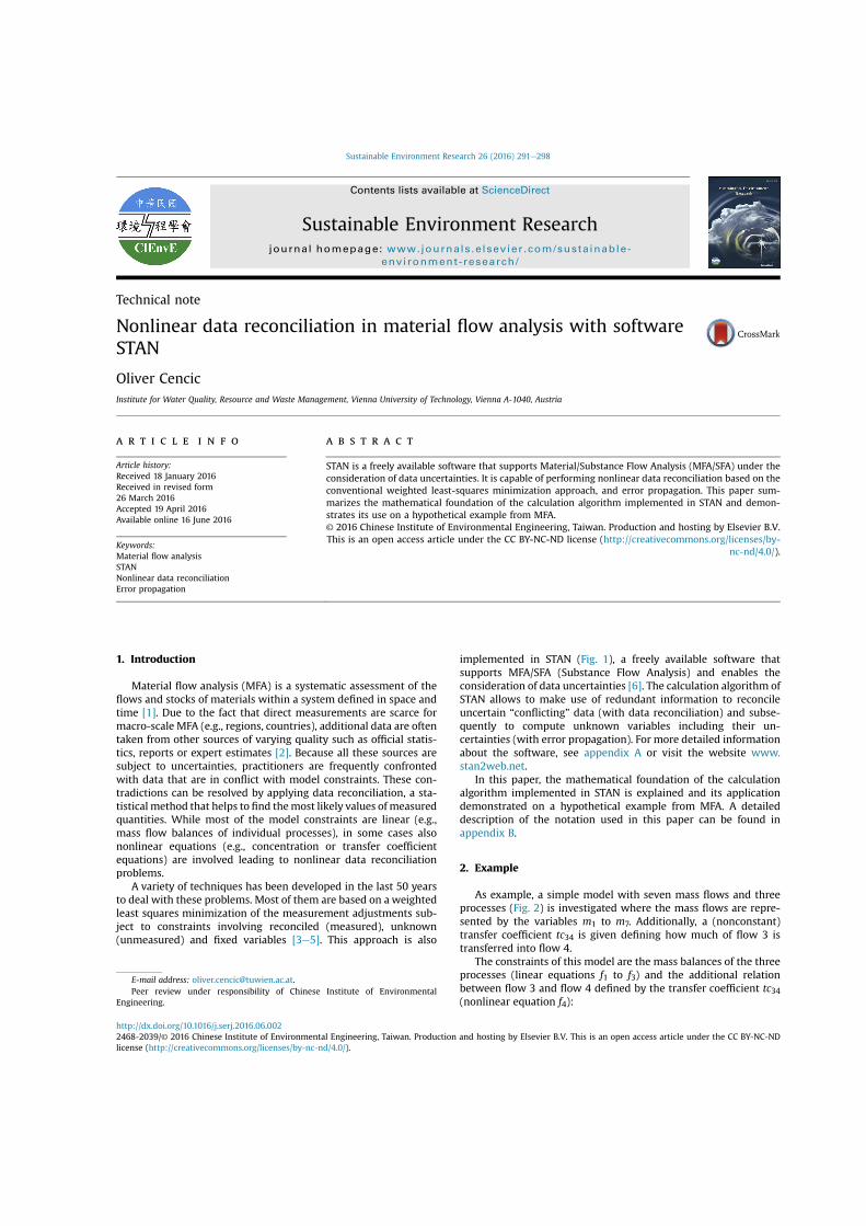
STAN is a freely available software that supports Material/Substance Flow Analysis (MFA/SFA) under theconsideration of data uncertainties. It is capable of performing nonlinear data reconciliation based on theconventional weighted least-squares minimization approach, and error propagation. This paper sum-marizes the mathematical foundation of the calculation algorithm implemented in STAN and demon-strates its use on a hypothetical example from MFA.© 2016 Chinese Institute of Environmental Engineering, Taiwan. Production and hosting by Elsevier B.V.This is an open access article under the CC BY-NC-ND license (http://creativecommons.org/licenses/by-
nc-nd/4.0/).
1. Introduction
Material flow analysis (MFA) is a systematic assessment of theflows and stocks of materials within a system defined in space andtime [1]. Due to the fact that direct measurements are scarce formacro-scale MFA (e.g., regions, countries), additional data are oftentaken from other sources of varying quality such as official statis-tics, reports or expert estimates [2]. Because all these sources aresubject to uncertainties, practitioners are frequently confrontedwith data that are in conflict with model constraints. These con-tradictions can be resolved by applying data reconciliation, a sta-tistical method that helps to find themost likely values of measuredquantities. While most of the model constraints are linear (e.g.,mass flow balances of individual processes), in some cases alsononlinear equations (e.g., concentration or transfer coefficientequations) are involved leading to nonlinear data reconciliationproblems.
A variety of techniques has been developed in the last 50 yearsto deal with these problems. Most of them are based on a weightedleast squares minimization of the measurement adjustments sub-ject to constraints involving reconciled (measured), unknown(unmeasured) and fixed variables [3e5]. This approach is also
implemented in STAN (Fig. 1), a freely available software thatsupports MFA/SFA (Substance Flow Analysis) and enables theconsideration of data uncertainties [6]. The calculation algorithm ofSTAN allows to make use of redundant information to reconcileuncertain “conflicting” data (with data reconciliation) and subse-quently to compute unknown variables including their un-certainties (with error propagation). For more detailed informationabout the software, see appendix A or visit the website www.stan2web.net.
In this paper, the mathematical foundation of the calculationalgorithm implemented in STAN is explained and its applicationdemonstrated on a hypothetical example from MFA. A detaileddescription of the notation used in this paper can be found inappendix B.
2. Example
As example, a simple model with seven mass flows and threeprocesses (Fig. 2) is investigated where the mass flows are repre-sented by the variables m1 to m7. Additionally, a (nonconstant)transfer coefficient tc34 is given defining how much of flow 3 istransferred into flow 4.
The constraints of this model are the mass balances of the threeprocesses (linear equations f1 to f3) and the additional relationbetween flow 3 and flow 4 defined by the transfer coefficient tc34(nonlinear equation f4):
E-mail address: [email protected] review under responsibility of Chinese Institute of Environmental
Engineering.
Contents lists available at ScienceDirect
Sustainable Environment Researchjournal homepage: www.journals .e lsevier .com/sustainable-
environment-research/
http://dx.doi.org/10.1016/j.serj.2016.06.0022468-2039/© 2016 Chinese Institute of Environmental Engineering, Taiwan. Production and hosting by Elsevier B.V. This is an open access article under the CC BY-NC-NDlicense (http://creativecommons.org/licenses/by-nc-nd/4.0/).
Sustainable Environment Research 26 (2016) 291e298
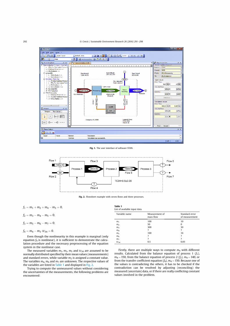
f1 ¼ m1 þm2 þm4 �m3 ¼ 0;
f2 ¼ m3 �m4 �m5 ¼ 0;
f3 ¼ m5 �m6 �m7 ¼ 0;
f4 ¼ m4 �m3$tc34 ¼ 0:
Even though the nonlinearity in this example is marginal (onlyequation f4 is nonlinear), it is sufficient to demonstrate the calcu-lation procedure and the necessary preprocessing of the equationsystem in the nonlinear case.
The measured variables m1, m3, m5 and tc34 are assumed to benormally distributed specified by theirmeanvalues (measurements)and standard errors, while variable m2 is assigned a constant value.The variables m4, m6 and m7 are unknown. The respective values ofthe variables are listed in Table 1 and displayed in Fig. 2.
Trying to compute the unmeasured values without consideringthe uncertainties of the measurements, the following problems areencountered:
Firstly, there are multiple ways to compute m4 with differentresults. Calculated from the balance equation of process 1 (f1),m4¼150, from the balance equation of process 2 (f2), m4¼140, orfrom the transfer coefficient equation (f4),m4¼150. Because one ofthe values is contradicting the others, it has to be checked if thecontradiction can be resolved by adjusting (reconciling) themeasured (uncertain) data, or if there are really conflicting constantvalues involved in the problem.
Fig. 1. The user interface of software STAN.
Fig. 2. Flowsheet example with seven flows and three processes.
Table 1List of available input data.
Variable name Measurement ofmass flow
Standard errorof measurement
m1 100 10m2 50 0m3 300 30m4 ? ?m5 160 16m6 ? ?m7 ? ?tc34 0.5 0.05
O. Cencic / Sustainable Environment Research 26 (2016) 291e298292
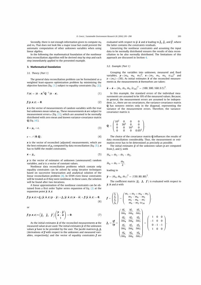
Secondly, there is not enough information given to compute m6and m7. That does not look like a major issue but could prevent theautomatic computation of other unknown variables when usinglinear algebra.
In the following the mathematical foundation of the nonlineardata reconciliation algorithmwill be derived step by step and eachstep immediately applied to the presented example.
3. Mathematical foundation
3.1. Theory (Part 1)
The general data reconciliation problem can be formulated as aweighted least-squares optimization problem by minimizing theobjective function (Eq. (1)) subject to equality constraints (Eq. (2)).
FðxÞ ¼ ð~x� xÞTQ�1ð~x� xÞ; (1)
f ðy; x; zÞ ¼ 0: (2)
~x is the vector of measurements of random variables with the truebut unknownmean values mx. These measurements ~x are subject tomeasurement errors ε (Eq. (3)), which are assumed to be normallydistributed with zero mean and known variance-covariance matrixQ (Eq. (4)).
~x ¼ mx þ ε; (3)
ε � N ð0;Q Þ: (4)
x is the vector of reconciled (adjusted) measurements, which arethe best estimates of mx computed by data reconciliation (Eq. (5)). xhas to fulfill the model constraints.
x ¼ bmx: (5)
y is the vector of estimates of unknown (unmeasured) randomvariables, and z is a vector of constant values.
Nonlinear data reconciliation problems which contain onlyequality constraints can be solved by using iterative techniquesbased on successive linearization and analytical solution of thelinear reconciliation problem [4]. In STAN even linear constraintswill be treated as if they were nonlinear. In these cases, the solutionwill be found after two iterations.
A linear approximation of the nonlinear constraints can be ob-tained from a first order Taylor series expansion of Eq. (2) at theexpansion point by; bx; z:f ðy; x; zÞzJyðby; bx; zÞðy � byÞ þ Jxðby; bx; zÞðx� bxÞ þ f ðby; bx; zÞ ¼ 0;
(6)
or
f ðy; x; zÞz�bJy bJ x bf �
0@ y � by
x� bx1
1A ¼ 0: (7)
As the initial estimates bx of the reconciled measurements x themeasured values ~x are used. The initial estimates by of the unknownvalues y have to be provided by the user. The Jacobi matrices Jy, Jx(derivations of f with respect to the unknown and measured vari-ables, respectively) and the vector of equality constraints f are
evaluated with respect to by; bx and z leading to bJy, bJ x and bf , wherethe latter contains the constraints residuals.
Linearizing the nonlinear constraints and assuming the inputdata to be normally distributed ensures the results of data recon-ciliation to be also normally distributed. The limitations of thisapproach are discussed in Section 4.
3.2. Example (Part 1)
Grouping the variables into unknown, measured and fixedvariables, y¼ (m4, m6, m7)T, x¼ (m1, m3, m5, tc34)T andz¼ (m2)¼ (50). As initial estimates bx of the reconciled measure-ments x, the measurements ~x themselves are taken:
bx ¼ ~x ¼ �~m1; ~m3; ~m5;~tc34
�T ¼ ð100;300;160;0:5ÞT:In this example, the standard errors of the individual mea-
surements are assumed to be 10% of the measured values. Because,in general, the measurement errors are assumed to be indepen-dent, i.e., there are no covariances, the variance-covariance matrixQ has nonzero entries only in the diagonal, representing thevariance of the measurement errors. Therefore, the variance-covariance matrix is
Q ¼
0BB@
102 0 0 00 302 0 00 0 162 00 0 0 0:052
1CCA:
The choice of the covariance matrix Q influences the results ofdata reconciliation considerably. Thus, the measurement or esti-mation error has to be determined as precisely as possible.
The initial estimates by of the unknown values y are computedfrom f1 and f3 with
bm4 ¼ ~m3 � ~m1 � ~m2;
bm6 ¼ ~m7 ¼ ~m5
2;
leading to
by ¼ ð bm4; bm6; bm7ÞT ¼ ð150;80;80ÞT:The coefficient matrix
�Jy Jx f
�is evaluated with respect toby; bx and z with
f ¼
0BB@
f1f2f3f4
1CCA ¼
0BB@
m1 þm2 þm4 �m3m3 �m4 �m5m5 �m6 �m7m4 �m3$tc34
1CCA;
Jy ¼ vfvy
¼
0BBBBBBBBBBBBB@
vf1vm4
vf1vm6
vf1vm7
vf2vm4
vf2vm6
vf2vm7
vf3vm4
vf3vm6
vf3vm7
vf4vm4
vf4vm6
vf4vm7
1CCCCCCCCCCCCCA
¼
0BBBB@
1 0 0
�1 0 0
0 �1 �1
1 0 0
1CCCCA;
O. Cencic / Sustainable Environment Research 26 (2016) 291e298 293
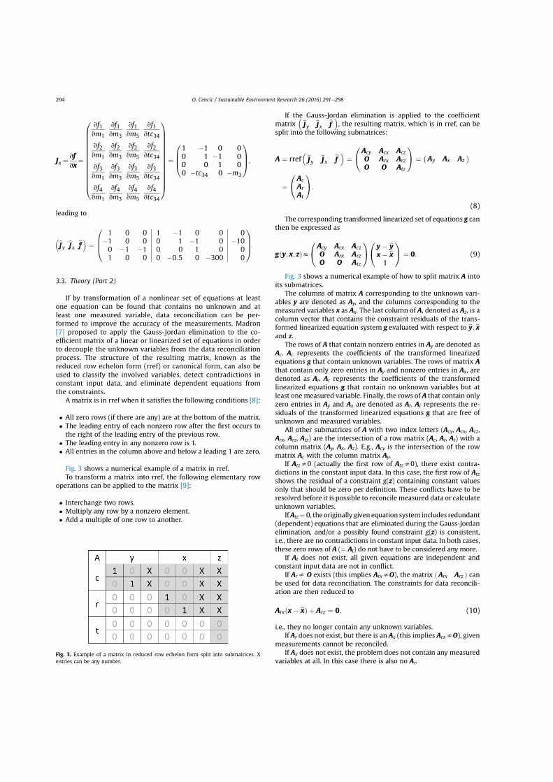
Jx ¼vfvx
¼
0BBBBBBBBBBBBB@
vf1vm1
vf1vm3
vf1vm5
vf1vtc34
vf2vm1
vf2vm3
vf2vm5
vf2vtc34
vf3vm1
vf3vm3
vf3vm5
vf3vtc34
vf4vm1
vf4vm3
vf4vm5
vf4vtc34
1CCCCCCCCCCCCCA
¼
0BB@1 �1 0 00 1 �1 00 0 1 00 �tc34 0 �m3
1CCA;
leading to
3.3. Theory (Part 2)
If by transformation of a nonlinear set of equations at leastone equation can be found that contains no unknown and atleast one measured variable, data reconciliation can be per-formed to improve the accuracy of the measurements. Madron[7] proposed to apply the Gauss-Jordan elimination to the co-efficient matrix of a linear or linearized set of equations in orderto decouple the unknown variables from the data reconciliationprocess. The structure of the resulting matrix, known as thereduced row echelon form (rref) or canonical form, can also beused to classify the involved variables, detect contradictions inconstant input data, and eliminate dependent equations fromthe constraints.
A matrix is in rref when it satisfies the following conditions [8]:
� All zero rows (if there are any) are at the bottom of the matrix.� The leading entry of each nonzero row after the first occurs tothe right of the leading entry of the previous row.
� The leading entry in any nonzero row is 1.� All entries in the column above and below a leading 1 are zero.
Fig. 3 shows a numerical example of a matrix in rref.To transform a matrix into rref, the following elementary row
operations can be applied to the matrix [9]:
� Interchange two rows.� Multiply any row by a nonzero element.� Add a multiple of one row to another.
If the Gauss-Jordan elimination is applied to the coefficientmatrix
�bJy bJ x bf �, the resulting matrix, which is in rref, can besplit into the following submatrices:
A ¼ rref�bJy bJx bf � ¼
0@Acy Acx Acz
O Arx ArzO O Atz
1A ¼ �
Ay Ax Az�
¼0@Ac
ArAt
1A:
(8)
The corresponding transformed linearized set of equations g canthen be expressed as
gðy; x; zÞz0@Acy Acx Acz
O Arx ArzO O Atz
1A0@ y � by
x� bx1
1A ¼ 0: (9)
Fig. 3 shows a numerical example of how to split matrix A intoits submatrices.
The columns of matrix A corresponding to the unknown vari-ables y are denoted as Ay, and the columns corresponding to themeasured variables x as Ax. The last column of A, denoted as Az, is acolumn vector that contains the constraint residuals of the trans-formed linearized equation system g evaluated with respect to by; bxand z.
The rows of A that contain nonzero entries in Ay are denoted asAc. Ac represents the coefficients of the transformed linearizedequations g that contain unknown variables. The rows of matrix Athat contain only zero entries in Ay and nonzero entries in Ax, aredenoted as Ar. Ar represents the coefficients of the transformedlinearized equations g that contain no unknown variables but atleast one measured variable. Finally, the rows of A that contain onlyzero entries in Ay and Ax are denoted as At. At represents the re-siduals of the transformed linearized equations g that are free ofunknown and measured variables.
All other submatrices of A with two index letters (Acy, Acx, Acz,Arx, Arz, Atz) are the intersection of a row matrix (Ac, Ar, At) with acolumn matrix (Ay, Ax, Az). E.g., Acy is the intersection of the rowmatrix Ac with the column matrix Ay.
If Atzs0 (actually the first row of Atzs0), there exist contra-dictions in the constant input data. In this case, the first row of Atz
shows the residual of a constraint g(z) containing constant valuesonly that should be zero per definition. These conflicts have to beresolved before it is possible to reconcile measured data or calculateunknown variables.
IfAtz¼ 0, the originallygiven equation system includes redundant(dependent) equations that are eliminated during the Gauss-Jordanelimination, and/or a possibly found constraint g(z) is consistent,i.e., there are no contradictions in constant input data. In both cases,these zero rows of A (¼ At) do not have to be considered any more.
If At does not exist, all given equations are independent andconstant input data are not in conflict.
If Ars O exists (this implies ArxsO), the matrix ðArx Arz Þ canbe used for data reconciliation. The constraints for data reconcili-ation are then reduced to
Arxðx� bxÞ þ Arz ¼ 0; (10)
i.e., they no longer contain any unknown variables.If Ar does not exist, but there is an Ax (this implies AcxsO), given
measurements cannot be reconciled.If Ax does not exist, the problem does not contain any measured
variables at all. In this case there is also no Ar.Fig. 3. Example of a matrix in reduced row echelon form split into submatrices. Xentries can be any number.
O. Cencic / Sustainable Environment Research 26 (2016) 291e298294
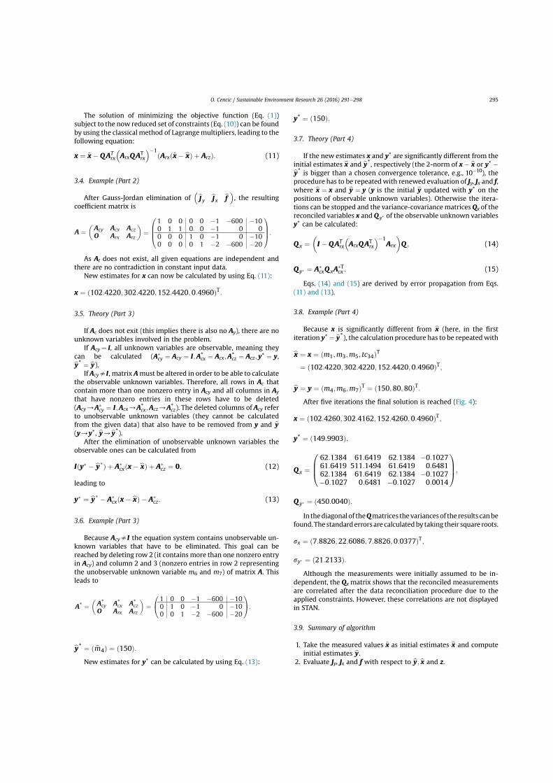
The solution of minimizing the objective function (Eq. (1))subject to the now reduced set of constraints (Eq. (10)) can be foundby using the classical method of Lagrangemultipliers, leading to thefollowing equation:
x ¼ ~x� QATrx
�ArxQAT
rx
��1ðArxð~x� bxÞ þ ArzÞ: (11)
3.4. Example (Part 2)
After Gauss-Jordan elimination of�bJy bJ x bf �, the resulting
coefficient matrix is
As At does not exist, all given equations are independent andthere are no contradiction in constant input data.
New estimates for x can now be calculated by using Eq. (11):
x ¼ ð102:4220;302:4220;152:4420;0:4960ÞT:
3.5. Theory (Part 3)
If Ac does not exit (this implies there is also no Ay), there are nounknown variables involved in the problem.
If Acy¼ I, all unknown variables are observable, meaning theycan be calculated (A�
cy ¼ Acy ¼ I;A*cx ¼ Acx;A*
cz ¼ Acz; y* ¼ y,by* ¼ by).If AcysI, matrix Amust be altered in order to be able to calculate
the observable unknown variables. Therefore, all rows in Ac thatcontain more than one nonzero entry in Acy and all columns in Ay
that have nonzero entries in these rows have to be deleted(Acy/A�
cy ¼ I;Acx/A*cx;Acz/A*
cz). The deleted columns of Acy referto unobservable unknown variables (they cannot be calculatedfrom the given data) that also have to be removed from y and by(y/y*, by/by*).
After the elimination of unobservable unknown variables theobservable ones can be calculated from
Iðy� � by�Þ þ A�cxðx� bxÞ þ A�
cz ¼ 0; (12)
leading to
y� ¼ by� � A�cxðx� bxÞ � A�
cz: (13)
3.6. Example (Part 3)
Because AcysI the equation system contains unobservable un-known variables that have to be eliminated. This goal can bereached by deleting row 2 (it contains more than one nonzero entryin Acy) and column 2 and 3 (nonzero entries in row 2 representingthe unobservable unknown variable m6 and m7) of matrix A. Thisleads to
by* ¼ ð bm4Þ ¼ ð150Þ:New estimates for y* can be calculated by using Eq. (13):
y* ¼ ð150Þ:
3.7. Theory (Part 4)
If the new estimates x and y* are significantly different from theinitial estimates bx and by*, respectively (the 2-norm of x� bx or y* �by* is bigger than a chosen convergence tolerance, e.g., 10�10), theprocedure has to be repeatedwith renewed evaluation of Jy, Jx and f,where bx ¼ x and by ¼ y (y is the initial by updated with y* on thepositions of observable unknown variables). Otherwise the itera-tions can be stopped and the variance-covariancematricesQx of thereconciled variables x and Q y* of the observable unknown variablesy* can be calculated:
Q x ¼�I � QAT
rx
�ArxQAT
rx
��1Arx
�Q ; (14)
Q y� ¼ A�cxQ xA
�Tcx : (15)
Eqs. (14) and (15) are derived by error propagation from Eqs.(11) and (13).
3.8. Example (Part 4)
Because x is significantly different from bx (here, in the firstiteration y* ¼ by*), the calculation procedure has to be repeatedwith
bx ¼ x ¼ ðm1;m3;m5; tc34ÞT
¼ ð102:4220;302:4220;152:4420;0:4960ÞT;
by ¼ y ¼ ðm4;m6;m7ÞT ¼ ð150;80;80ÞT:After five iterations the final solution is reached (Fig. 4):
x ¼ ð102:4260;302:4162;152:4260;0:4960ÞT;
y* ¼ ð149:9903Þ;
Q x ¼
0BB@
62:1384 61:6419 62:1384 �0:102761:6419 511:1494 61:6419 0:648162:1384 61:6419 62:1384 �0:1027�0:1027 0:6481 �0:1027 0:0014
1CCA;
Q y� ¼ ð450:0040Þ:In thediagonal of theQmatrices thevariancesof the results canbe
found.Thestandarderrorsare calculatedby taking their square roots.
sx ¼ ð7:8826;22:6086;7:8826;0:0377ÞT;
sy� ¼ ð21:2133Þ:Although the measurements were initially assumed to be in-
dependent, the Qx matrix shows that the reconciled measurementsare correlated after the data reconciliation procedure due to theapplied constraints. However, these correlations are not displayedin STAN.
3.9. Summary of algorithm
1. Take the measured values ~x as initial estimates bx and computeinitial estimates by .
2. Evaluate Jy, Jx and f with respect to by; bx and z.
O. Cencic / Sustainable Environment Research 26 (2016) 291e298 295
3. Compute rref�bJy bJ x bf �.
4. Eliminate unobservable unknown variables and redundantequations.
5. Compute new estimates x with Eq. (11).6. Compute new estimates y* with Eq. (13).7. If the new estimates x and y* are significantly different from bx
and by*, respectively, set bx ¼ x and by ¼ y and go to 2. Otherwisego to 8.
8. Compute the variance-covariance-matrices Qx with Eq. (14) andQ y* with Eq. (15).
4. Discussion and outlook
In this paper, the nonlinear data reconciliation algorithmimplemented in STAN was explained and its application demon-strated on a simple hypothetical example from MFA.
A restriction of the used weighted least squares minimizationapproach is the assumption of normally distributed measurementerrors. In scientific models in general and in MFA models inparticular, this assumption is often not valid: e.g., concentrationscannot take negative values, and transfer coefficients are restrictedto the unit interval. To overcome the limitation of normality, ageneral framework to reconcile data with arbitrarily distributedmeasurement errors was introduced [10]. This framework is limitedto linear constraints, but has been extended to nonlinear con-straints in Ref. [11].
It was shown [12] that it is also possible to use a possibilisticapproach for data reconciliation. There, the uncertainty of mea-surements is modelled with membership functions instead ofprobability density functions to account for the epistemic nature ofmeasurements errors (that is, error due to insufficient knowledge).While the paper covers linear constraints only, the approach hasbeen extended to nonlinear constraints in Ref. [13].
The problem of nonlinear data reconciliation can also be solvedwith nonlinear programming techniques, like sequential quadraticprogramming or reduced gradientmethods. These techniques allowfor a general objective function, not just one with weighted leastsquares, and they are able to handle inequality constraints andvariable bounds. For a short reviewof thesemethods see e.g. Ref. [5].
While all of these alternative approaches definitely have theiradvantages, their common disadvantage is the large amount ofcomputation time required compared to the conventional approachof weighted least squares.
In general, nonlinear data reconciliation of normally distributedinput data does not result in normally distributed output data. Thisis only the case for linear constraints or linearized nonlinear con-straints. The latter approximation, however, delivers sound resultsonly if the uncertainties of the input data are small. If the un-certainties are large, the results of linearization can differ sub-stantially from the precise solution.
In the weighted least squares minimization approach, the in-verse of the covariance matrix Q was chosen as the weight matrixbecause it delivers the best linear unbiased estimator of x in Eq.(11). A prove of the linear case can be found in Ref. [14].
The following list contains some limitations of STAN that shouldbe addressed/optimized in a future version:
1. While the variable classification using the Gauss-Jordan elimi-nation is easy to understand, it is not the best way in acomputational sense. Other equation-oriented approaches havebeen developed to reach the same goal more efficiently [5].
2. There is no equation parser implemented in STAN, thus, it isrestricted to a few types of equations only: mass balances,transfer coefficient equations, linear relations between similarentities (can be used to model, e.g., losses from stocks) andconcentration equations.
3. The default algorithm used in STAN (called “Cencic2012”) iscoded for dense matrices, thus, the speed of the calculation isreduced considerably when dealing with large models. Animplementation of sparse matrices would increase the calcula-tion speed substantially.
4. The only gross error detection test that has been yet imple-mented in STAN is the so called measurement test [4] that isbased on measurement adjustments. A more sophisticatedrobust gross error detection routine would be of advantage.
Since September 2012, an alternative commercial calculationalgorithm developed by J.D. Kelly is available in STAN. Originallycalled “Kelly2011”, it was later renamed into “IAL-IMPL2013”. Itapplies a regularization approach by assuming unknown variablesto be known with a sufficient large uncertainty. Details about thealgorithm can be found in Ref. [15].
Since the first version of STANwas released in 2006, a lot of MFAstudies have been conducted with its help. An updated list ofpublications can be found under www.stan2web.net/infos/publications. Unfortunately, still a lot of recent MFA studies donot consider data uncertainties, thus, ignoring valuable informationfor decision makers. The author would appreciate if STAN couldhelp to raise the awareness for the importance of uncertainties,thus, taking MFA to the next level.
Final remark: The presented nonlinear data reconciliation al-gorithm is of course not restricted to MFAmodels. It can be used forarbitrary reconciliation problems.
Acknowledgement
STAN was funded by Altstoff Recycling Austria (ARA), voes-talpine, the Austrian Federal Ministry of Agriculture, Forestry,Environment and Water Management, and the Federal States ofAustria. For more detailed information and to download the soft-ware visit www.stan2web.net.
Fig. 4. Results of flowsheet example rounded to one decimal place.
O. Cencic / Sustainable Environment Research 26 (2016) 291e298296
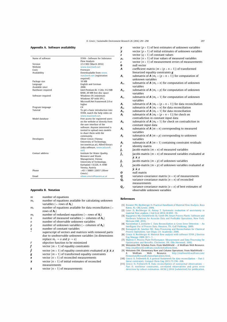
Appendix A. Software availability
Appendix B. Notation
m number of equationsmc number of equations available for calculating unknown
variables (¼ rows of Ac)mr number of equations available for data reconciliation (¼
rows of Ar)mt number of redundant equations (¼ rows of At)n number of measured variables (¼ columns of Ax)o number of observable unknown variablesp number of unknown variables (¼ columns of Ay)q number of constant variables* superscript of vectors and matrices with removed parts
due to unobservable unknown variables (in dimensionsreplace mc/ o and p/ o)
F objective function to be minimizedf vector (m� 1) of equality constraintsbf vector (m� 1) of equality constraints evaluated at by; bx; zg vector (m� 1) of transformed equality constraintsx vector (n� 1) of reconciled measurementsbx vector (n� 1) of initial estimates of reconciled
measurements~x vector (n� 1) of measurements
y vector (p� 1) of best estimates of unknown variablesby vector (p� 1) of initial estimates of unknown variablesz vector (q� 1) of constant valuesmx vector (n� 1) of true values of measured variablesε vector (n� 1) of measurement errors of measurements0 null vectorA coefficient matrix (m� (pþ nþ 1)) of transformed
linearized equality constraints gAc submatrix of A (mc� (pþ nþ 1)) for computation of
unknown variablesAcx submatrix of A (mc� n) for computation of unknown
variablesAcy submatrix of A (mc� p) for computation of unknown
variablesAcz submatrix of A (mc� 1) for computation of unknown
variablesAr submatrix of A (mr� (pþ nþ 1)) for data reconciliationArx submatrix of A (mr� n) for data reconciliationArz submatrix of A (mr� 1) for data reconciliationAt submatrix of A (mt� (pþ nþ 1)) for check on
contradiction in constant input dataAtz submatrix of A (mt� 1) for check on contradiction in
constant input dataAx submatrix of A (m� n) corresponding to measured
variablesAy submatrix of A (m� p) corresponding to unknown
variablesAz submatrix of A (m� 1) containing constraint residualsI identity matrixJx Jacobi-matrix (m� n) of measured variablesbJ x Jacobi-matrix (m� n) of measured variables evaluated atby; bx; zJy Jacobi-matrix (m� p) of unknown variablesbJy Jacobi-matrix (m� p) of unknown variables evaluated atby; bx; zO null matrixQ variance-covariance matrix (n� n) of measurementsQx variance-covariance matrix (n� n) of reconciled
measurementsQ y* variance-covariance matrix (o� o) of best estimates of
observable unknown variables
References
[1] Brunner PH, Rechberger H. Practical Handbook of Material Flow Analysis. BocaRaton, FL: CRC/Lewis; 2004.
[2] Laner D, Rechberger H, Astrup T. Systematic evaluation of uncertainty inmaterial flow analysis. J Ind Ecol 2014;18:859e70.
[3] Bagajewicz MJ, Chmielewski DJ, Tanth DN. Smart Process Plants: Software andHardware Solutions for Accurate Data and Profitable Operations. New York:McGraw-Hill; 2010.
[4] Narasimhan S, Jordache C. Data Reconciliation & Gross Error Detection e AnIntelligent Use of Process Data. Houston, TX: Gulf Publising; 2000.
[5] Romagnoli JA, S�anchez MC. Data Processing and Reconciliation for ChemicalProcess Operations. San Diego, CA: Academic; 2000.
[6] Cencic O, Rechberger H. Material flow analysis with software STAN. J EnvironEng Manage 2008;18:3e7.
[7] Madron F. Process Plant Performance: Measurement and Data Processing forOptimization and Retrofits. Chichester, UK: Ellis Horwood; 1992.
[8] Weisstein EW. Echelon Form. From MathWorld e A Wolfram Web Resource.http://mathworld.wolfram.com/EchelonForm.html.
[9] Weisstein EW. Elementary Row and Column Operations. From MathWorld eA Wolfram Web Resource. http://mathworld.wolfram.com/ElementaryRowandColumnOperations.html.
[10] Cencic O, Frühwirth R. A general framework for data reconciliation e Part I:linear constraints. Comput Chem Eng 2015;75:196e208.
[11] Cencic O, Frühwirth R. Data reconciliation of nonnormal observations ePart II: nonlinear constraints, correlated observations and gross errordetection by robust estimation. AIChE J 2016 [submitted] for publication.
Name of software STAN - Software for SubstanceFlow Analysis
Version 2.5.1302 (March 2016)Website www.stan2web.netCosts FreewareAvailability Downloadable from www.
stan2web.net (registrationrequired)
Package size 10 MBLanguage English and GermanAvailable since 2006Hardware required Intel Pentium III, 1 GHz, 512 MB
RAM, 20 MB free disc spaceSoftware required Windows OS (minimum
Windows XP with SP1),Microsoft.Net Framework 2.0 orhigher
Program language C#Tutorial To get a basic introduction into
STAN, watch the help video onwww.stan2web.net.
Model database Free access for registered userson the website or directly fromthe user interface of thesoftware. Anyone interested isinvited to upload own modelsto share them with thecommunity.
Developers Oliver Cencic (ViennaUniversity of Technology,iwr.tuwien.ac.at), Alfred Kovacs(inka software, www.inkasoft.net)
Contact address Institute for Water Quality,Resource and WasteManagement, ViennaUniversity of Technology,Karlsplatz 13/226, A-1040Vienna, Austria
Phone þ43 1 58801 22657 (OliverCencic)
Email [email protected]
O. Cencic / Sustainable Environment Research 26 (2016) 291e298 297
[12] Dubois D, Fargier H, Ababou M, Guyonnet D. A fuzzy constraint-basedapproach to data reconciliation in material flow analysis. Int J Gen Syst2014;43:787e809.
[13] Dzubur N, Sunata O, Laner D. A fuzzy set-based approach for data reconciliationin material flowmodeling. Appl Math Model 2016 [submitted] for publication.
[14] Kailath T, Sayed AH, Hassibi B. Linear Estimation. Upper Saddle River, NJ:Prentice Hall; 2000.
[15] Kelly JD. A regularization approach to the reconciliation of constrained datasets. Comput Chem Eng 1998;22:1771e88.
O. Cencic / Sustainable Environment Research 26 (2016) 291e298298
Paper 2:
A general framework for data reconciliation -Part I: Linear constraintsOliver Cencic and Rudolf FrühwirthComputers and Chemical Engineering 2015, 75DOI: 10.1016/j.compchemeng.2014.12.004

Computers and Chemical Engineering 75 (2015) 196–208
Contents lists available at ScienceDirect
Computers and Chemical Engineering
j our na l ho me pa g e: www.elsev ier .com/ locate /compchemeng
A general framework for data reconciliation—Part I: Linear constraints
Oliver Cencica,∗, Rudolf Frühwirthb
a Institute for Water Quality, Resource and Waste Management, Vienna University of Technology, Karlsplatz 13/226, A-1040 Wien, Austriab Institute of High Energy Physics (HEPHY), Austrian Academy of Sciences, Nikolsdorfer Gasse 18, A-1050 Wien, Austria
a r t i c l e i n f o
Article history:Received 21 April 2014Received in revised form 3 October 2014Accepted 2 December 2014Available online 12 December 2014
Keywords:Data reconciliationNonnormal distributionsLinear equality constraintsMarkov chain Monte Carlo (MCMC)Independence Metropolis–HastingssamplerMaterial flow analysis (MFA)
a b s t r a c t
This paper presents a new method, based on Bayesian reasoning, for the reconciliation of data fromarbitrary probability distributions. The main idea is to restrict the joint prior probability distribution ofthe involved variables with model constraints to get a joint posterior probability distribution. This papercovers the case of linearly constrained variables, with the focus on equality constraints. The procedureis demonstrated with the help of three simple graphical examples. Because in general the posteriorprobability density function cannot be calculated analytically, it is sampled with a Markov chain MonteCarlo (MCMC) method. From this sample the density and its moments can be estimated, along with themarginal densities, moments and quantiles. The method is tested on several artificial examples frommaterial flow analysis, using an independence Metropolis–Hastings sampler.
© 2014 Elsevier Ltd. All rights reserved.
1. Introduction
The goal of material flow analysis (MFA) is to model and quan-tify all flows and stocks of a system of interest. For this reason asmuch information about the system as possible is collected whichcomprises direct measurements when available, but more oftendata taken from official statistics, reports, publications, expert esti-mates and similar sources (Laner et al., 2014). Unfortunately thesedata are often in conflict with known conservation laws such asmass or energy balances, preventing the calculation of unknownquantities or parameters of the model that cannot be measureddirectly. The basic idea of data reconciliation (DR) is to resolve thesecontradictions by statistically adjusting the collected data based onthe assumption that their uncertainty is described by a probabilitydensity function.
DR has been widely used in chemical engineering for more than50 years to adjust plant measurements. Most solving techniquesthat have been developed in this period of time are based on aweighted least-squares minimization of the measurement adjust-ments subject to constraints involving reconciled, unmeasured andfixed variables (Narasimhan and Jordache, 2000; Romagnoli andSanchez, 2000; Bagajewicz, 2010). The underlying main assump-tion of this approach is that of normally distributed (Gaussian)
∗ Corresponding author. Tel.: +43 1 58801 22657; fax: +43 1 58801 9 22657.E-mail address: [email protected] (O. Cencic).
measurement errors with zero mean (Johnston and Kramer, 1995).However, in scientific models in general and in MFA models inparticular, data is often not normally distributed. If, for instance,a process model is correct, mass flows and concentrations cannottake negative values, and transfer coefficients are restricted to theunit interval.
Another example is provided by expert opinions that frequentlyhave to be relied on in MFA due to scarce or missing data. Theyare often modeled by uniform, triangular or trapezoidal distribu-tions. The more detailed the expert’s knowledge about the quantityunder consideration is, the more precisely the distribution can bemodeled. If a sufficient number of measurements of the quantityis available, one can either fit a parametric model to the measureddata or use a nonparametric model such as the empirical distri-bution function or the kernel estimate of the probability densityfunction. In the following we will denote a variable as “measured”if there is prior information on the variable of any kind, which isnot necessarily a proper measurement.
Although it was demonstrated in Crowe (1996) that theassumption of a normal distribution is acceptable for unknown dis-tributions having relative standard deviations smaller than 30%,it is questionable in the context of macro-scale MFA (e.g. region,country) where relative standard deviations larger than 30% arenot uncommon. In addition, the normal distribution is unsuitableto describe uncertainties with strong intrinsic asymmetry.
In the following we propose a numerical DR procedure thatis also able to deal with data that cannot be modeled by normal
http://dx.doi.org/10.1016/j.compchemeng.2014.12.0040098-1354/© 2014 Elsevier Ltd. All rights reserved.
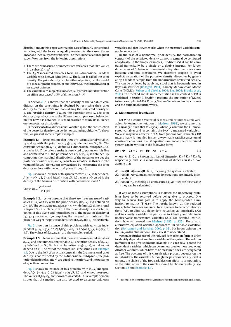
O. Cencic, R. Frühwirth / Computers and Chemical Engineering 75 (2015) 196–208 197
distributions. In this paper we treat the case of linearly constrainedvariables, with the focus on equality constraints; the cases of non-linear and inequality constraints will be the subject of a subsequentpaper. We start from the following assumptions:
1. There are N measured or unmeasured variables that take valuesin a subset D ⊆ R
N .2. The I ≤ N measured variables form an I-dimensional random
variable with known joint density. The latter is called the priordensity. The prior density can be either objective, i.e. the modelof a measurement process, or subjective, i.e. the formalization ofan expert opinion.
3. The variables are subject to linear equality constraints that definean affine subspace S ⊂ R
N of dimension P < N.
In Section 2 it is shown that the density of the variables con-ditional on the constraints is obtained by restricting their priordensity to the set D ∩ S and normalizing the restricted density to1. The resulting density is called the posterior density. The priordensity plays a key role in the DR mechanism proposed below. Nomatter how it is obtained, it is good practice to study its influenceon the posterior distribution.
In the case of a low-dimensional variable space, the constructionof the posterior density can be demonstrated graphically. To showthis, we present some simple examples.
Example 1.1. Let us assume that there are two measured variablesx1 and x2 with the prior density f(x1, x2) defined on D ⊆ R
2. Theconstraint equation x1 = x2 defines a 1-dimensional subspace S, i.e.a line in R
2. If the prior density is restricted to points on this lineand normalized to 1, the posterior density of x1, x2 is obtained. Bycomputing the marginal distributions of the posterior we get theposterior densities of x1 and x2, which are identical in this case. Thevalues of f(x1, x2) along S can be visualized by intersecting the priordensity surface with the vertical plane through S.
Fig. 1 shows an instance of this problem, with x1, x2 independent,f1(x1) = �(x1 ; 2, 2) and f2(x2) = �(x2 ; 3, 1.5), where �(x ; a, b) is thedensity of the Gamma distribution with parameters a and b:
�(x; a, b) = xa−1 e−x/b
ba �(a).
Example 1.2. Let us assume that there are three measured vari-ables x1, x2 and x3 with the prior density f(x1, x2, x3) defined onD ⊆ R
3. The constraint equation x3 = x1 + x2 defines a 2-dimensionalsubspace S, i.e. a plane in R
3. If the prior density is restricted topoints in this plane and normalized to 1, the posterior density ofx1, x2, x3 is obtained. By computing the marginal distributions of theposterior we get the posterior densities of x1, x2 and x3, respectively.
Fig. 2 shows an instance of this problem, with x1, x2, x3 inde-pendent, f1(x1) = �(x1 ; 2, 2), f2(x2) = �(x2 ; 3, 1.5) and f3(x3) = �(x3 ; 6,1.7). The values of f(x1, x2, x3) are shown color-coded.
Example 1.3. Let us assume that there are two measured variablesx1, x2 and one unmeasured variable x3. The prior density of x1, x2,x3 is defined on D ⊆ R
3, but can be written as f(x1, x2), as it does notdepend on x3. The rest of the procedure is the same as in Example1.2. Due to the lack of an actual constraint the 2-dimensional priordensity is not restricted by the 2-dimensional subspace S, the pos-terior densities of x1 and x2 are equal to the priors, and the posteriorof x3 is their convolution.
Fig. 3 shows an instance of this problem, with x1, x2 indepen-dent, f1(x1) = �(x1 ; 2, 2), f2(x2) = �(x2 ; 3, 1.5) and x3 not measured.The values of f(x1, x2) are shown color-coded. This example demon-strates that the method can also be used to calculate unknown
variables and that it even works when the measured variables can-not be reconciled.
In the case of a nonnormal prior density, the normalizationconstant of the restricted density cannot in general be computedanalytically. In the simple examples just discussed, it can be com-puted numerically by a single or a double integral. For largerdimensions of S, however, numerical integration becomes cum-bersome and time-consuming. We therefore propose to avoidexplicit calculation of the posterior density altogether by gener-ating a random sample from the unnormalized restricted density.This can be achieved by applying a tool that is frequently used inBayesian statistics (O’Hagan, 1994), namely Markov chain MonteCarlo (MCMC) (Robert and Casella, 2004; Liu, 2004; Brooks et al.,2011). The method and its implementation in the context of DR isexplained in Section 3. Section 4 presents the application of MCMCto four examples in MFA. Finally, Section 5 contains our conclusionsand the outlook on further work.
2. Mathematical foundation
Let v be a column vector of N measured or unmeasured vari-ables. Following the notation in Madron (1992), we assume thatv is arranged such that v = (y; x), where y contains the J unmea-sured variables and x contains the I = N − J measured variables.1
We also may have a vector z of M fixed (nonrandom) variables. DRmeans that v is modified in such a way that it satisfies a system ofconstraint equations. If all K equations are linear, the constrainedsystem can be written in the following form:
By + Ax + Cz = 0 or By + Ax + c = 0, (1)
where A, B, C are known matrices of dimension K × I, K × J, K × M,respectively, and c is a column vector of dimension K × 1. Weassume that
A1. rank(B, A) = rank(B, A, c), meaning the system is solvable;A2. rank(B, A) = K, meaning the model equations are linearly inde-
pendent;A3. rank(B) = J, meaning all unmeasured quantities are observable
(they can be calculated).
If any of these assumptions is violated the underlying prob-lems have to be resolved before being able to proceed. Oneway to achieve this goal is to apply the Gauss-Jordan elim-ination to matrix (B, A, c). The result, known as the reducedrow echelon form (or canonical form), serves to detect contradic-tions (A1), to eliminate dependent equations automatically (A2)and to classify variables, in particular to identify and eliminateunobservable unmeasured variables (A3). For detailed instruc-tions how to proceed see Madron (1992, p. 125). There existalternative equation-oriented approaches for variable classifica-tion (Romagnoli and Sanchez, 2000, p. 33), but in our opinion theGauss–Jordan elimination is the easiest to understand.
We make further use of the reduced row echelon form in orderto identify dependent and free variables of the system. The columnnumbers of the pivot elements (leading 1 in each row) denote thedependent variables, which can be unmeasured or measured ones.All other variables, which have to be measured ones, are designatedas free. The outcome of this classification process depends on theinitial order of the variables. Although the posterior density itself isunique, the choice of the free variables can affect its computation,so the initial order of the variables should be chosen carefully (seeSection 3.2 and Example 4.4).
1 The semicolon (comma) denotes vertical (horizontal) concatenation of matrices.
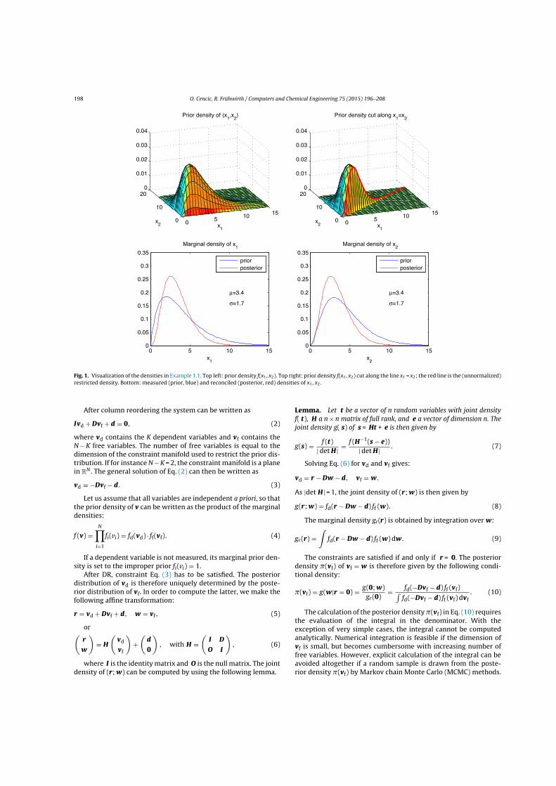
198 O. Cencic, R. Frühwirth / Computers and Chemical Engineering 75 (2015) 196–208
0 5 10 150
10
200
0.01
0.02
0.03
0.04
x1
Prior density of (x1,x 2
)
x2 0 5 10 15
0
10
200
0.01
0.02
0.03
0.04
x1
Prior density cut along x1=x 2
x2
0 5 10 150
0.05
0.1
0.15
0.2
0.25
0.3
0.35
μ=3.4
σ=1.7
x1
Marginal density of x1
priorposterior
0 5 10 150
0.05
0.1
0.15
0.2
0.25
0.3
0.35
μ=3.4
σ=1.7
x2
Marginal density of x2
priorposterior
Fig. 1. Visualization of the densities in Example 1.1. Top left: prior density f(x1, x2). Top right: prior density f(x1, x2) cut along the line x1 = x2; the red line is the (unnormalized)restricted density. Bottom: measured (prior, blue) and reconciled (posterior, red) densities of x1, x2.
After column reordering the system can be written as
Ivd + Dvf + d = 0, (2)
where vd contains the K dependent variables and vf contains theN − K free variables. The number of free variables is equal to thedimension of the constraint manifold used to restrict the prior dis-tribution. If for instance N − K = 2, the constraint manifold is a planein R
N . The general solution of Eq. (2) can then be written as
vd = −Dvf − d. (3)
Let us assume that all variables are independent a priori, so thatthe prior density of v can be written as the product of the marginaldensities:
f (v) =N∏
i=1
fi(vi) = fd(vd) · ff(vf). (4)
If a dependent variable is not measured, its marginal prior den-sity is set to the improper prior fi(vi) = 1.
After DR, constraint Eq. (3) has to be satisfied. The posteriordistribution of vd is therefore uniquely determined by the poste-rior distribution of vf. In order to compute the latter, we make thefollowing affine transformation:
r = vd + Dvf + d, w = vf, (5)
or(r
w
)= H
(vd
vf
)+
(d
0
), with H =
(I D
O I
), (6)
where I is the identity matrix and O is the null matrix. The jointdensity of (r; w) can be computed by using the following lemma.
Lemma. Let t be a vector of n random variables with joint densityf( t), H a n × n matrix of full rank, and e a vector of dimension n. Thejoint density g( s) of s = Ht + e is then given by
g(s) = f (t)| det H| = f (H−1(s − e))
| det H| . (7)
Solving Eq. (6) for vd and vf gives:
vd = r − Dw − d, vf = w.
As |det H| = 1, the joint density of (r; w) is then given by
g(r; w) = fd(r − Dw − d) ff (w). (8)
The marginal density gr(r) is obtained by integration over w:
gr(r) =∫
fd(r − Dw − d) ff (w) dw. (9)
The constraints are satisfied if and only if r = 0. The posteriordensity �(vf) of vf = w is therefore given by the following condi-tional density:
�(vf) = g(w|r = 0) = g(0; w)gr(0)
= fd(−Dvf − d) ff (vf)∫fd(−Dvf − d) ff (vf) dvf
. (10)
The calculation of the posterior density �(vf) in Eq. (10) requiresthe evaluation of the integral in the denominator. With theexception of very simple cases, the integral cannot be computedanalytically. Numerical integration is feasible if the dimension ofvf is small, but becomes cumbersome with increasing number offree variables. However, explicit calculation of the integral can beavoided altogether if a random sample is drawn from the poste-rior density �(vf) by Markov chain Monte Carlo (MCMC) methods.
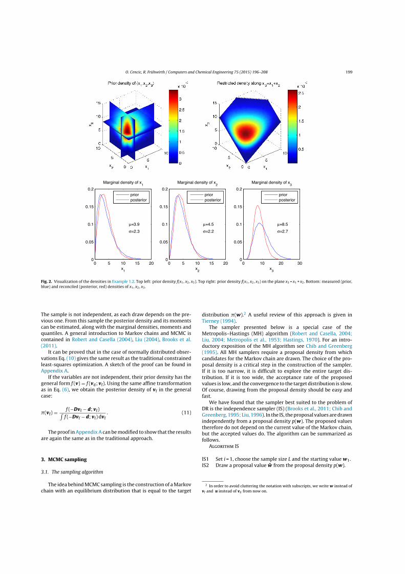
O. Cencic, R. Frühwirth / Computers and Chemical Engineering 75 (2015) 196–208 199
0 5 10 15 200
0.05
0.1
0.15
0.2
Marginal density of x1
x1
μ=3.9
σ=2.3
priorposterior
0 5 10 15 200
0.05
0.1
0.15
0.2
Marginal density of x2
x2
μ=4.5
σ=2.2
priorposterior
0 10 20 300
0.05
0.1
0.15
0.2
Marginal density of x3
x3
μ=8.5
σ=2.7
priorposterior
Fig. 2. Visualization of the densities in Example 1.2. Top left: prior density f(x1, x2, x3). Top right: prior density f(x1, x2, x3) on the plane x3 = x1 + x2. Bottom: measured (prior,blue) and reconciled (posterior, red) densities of x1, x2, x3.
The sample is not independent, as each draw depends on the pre-vious one. From this sample the posterior density and its momentscan be estimated, along with the marginal densities, moments andquantiles. A general introduction to Markov chains and MCMC iscontained in Robert and Casella (2004), Liu (2004), Brooks et al.(2011).
It can be proved that in the case of normally distributed obser-vations Eq. (10) gives the same result as the traditional constrainedleast-squares optimization. A sketch of the proof can be found inAppendix A.
If the variables are not independent, their prior density has thegeneral form f (v) = f (vd; vf). Using the same affine transformationas in Eq. (6), we obtain the posterior density of vf in the generalcase:
�(vf) = f (−Dvf − d; vf)∫f (−Dvf − d; vf) dvf
. (11)
The proof in Appendix A can be modified to show that the resultsare again the same as in the traditional approach.
3. MCMC sampling
3.1. The sampling algorithm
The idea behind MCMC sampling is the construction of a Markovchain with an equilibrium distribution that is equal to the target
distribution �(w).2 A useful review of this approach is given inTierney (1994).
The sampler presented below is a special case of theMetropolis–Hastings (MH) algorithm (Robert and Casella, 2004;Liu, 2004; Metropolis et al., 1953; Hastings, 1970). For an intro-ductory exposition of the MH algorithm see Chib and Greenberg(1995). All MH samplers require a proposal density from whichcandidates for the Markov chain are drawn. The choice of the pro-posal density is a critical step in the construction of the sampler.If it is too narrow, it is difficult to explore the entire target dis-tribution. If it is too wide, the acceptance rate of the proposedvalues is low, and the convergence to the target distribution is slow.Of course, drawing from the proposal density should be easy andfast.
We have found that the sampler best suited to the problem ofDR is the independence sampler (IS) (Brooks et al., 2011; Chib andGreenberg, 1995; Liu, 1996). In the IS, the proposal values are drawnindependently from a proposal density p(w). The proposed valuestherefore do not depend on the current value of the Markov chain,but the accepted values do. The algorithm can be summarized asfollows.Algorithm IS
IS1 Set i = 1, choose the sample size L and the starting value w1.IS2 Draw a proposal value w from the proposal density p(w).
2 In order to avoid cluttering the notation with subscripts, we write w instead ofvf and u instead of vd from now on.
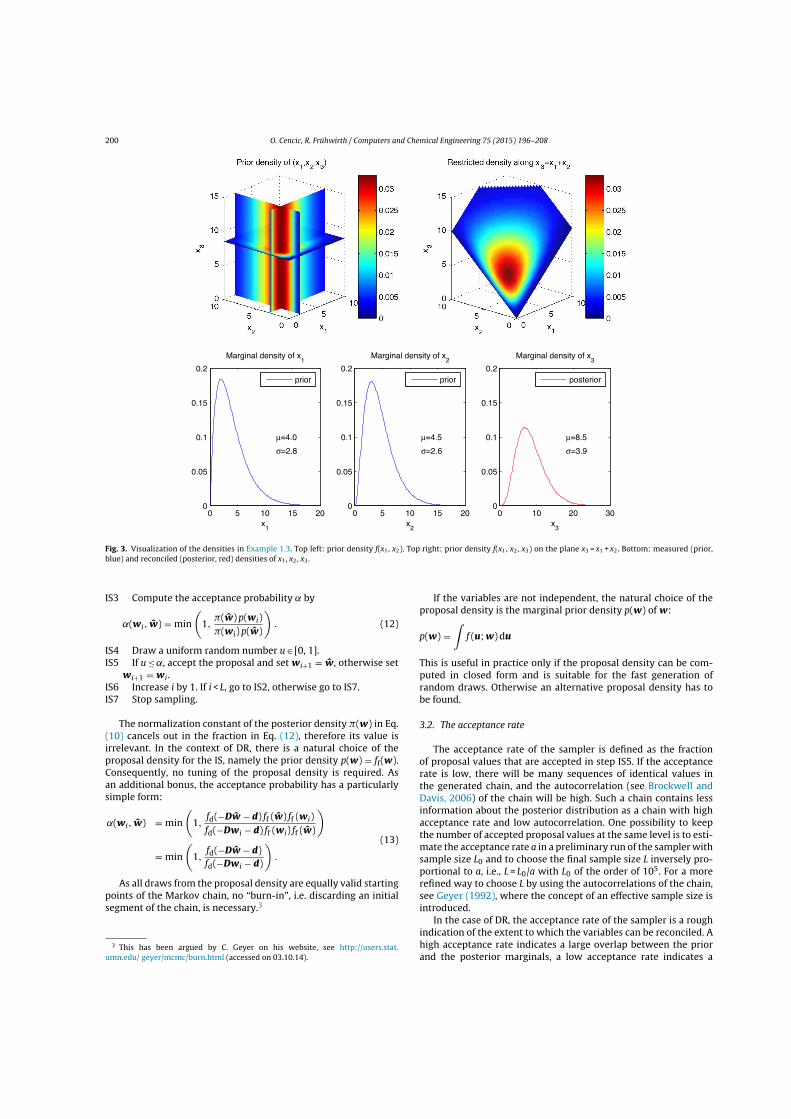
200 O. Cencic, R. Frühwirth / Computers and Chemical Engineering 75 (2015) 196–208
0 5 10 15 200
0.05
0.1
0.15
0.2
Marginal density of x1
x1
μ=4.0
σ=2.8
prior
0 5 10 15 200
0.05
0.1
0.15
0.2
Marginal density of x2
x2
μ=4.5
σ=2.6
prior
0 10 20 300
0.05
0.1
0.15
0.2
Marginal density of x3
x3
μ=8.5
σ=3.9
posterior
Fig. 3. Visualization of the densities in Example 1.3. Top left: prior density f(x1, x2). Top right: prior density f(x1, x2, x3) on the plane x3 = x1 + x2. Bottom: measured (prior,blue) and reconciled (posterior, red) densities of x1, x2, x3.
IS3 Compute the acceptance probability by
˛(wi, w) = min
(1,
�(w) p(wi)�(wi) p(w)
). (12)
IS4 Draw a uniform random number u ∈ [0, 1].IS5 If u ≤ ˛, accept the proposal and set wi+1 = w, otherwise set
wi+1 = wi.IS6 Increase i by 1. If i < L, go to IS2, otherwise go to IS7.IS7 Stop sampling.
The normalization constant of the posterior density �(w) in Eq.(10) cancels out in the fraction in Eq. (12), therefore its value isirrelevant. In the context of DR, there is a natural choice of theproposal density for the IS, namely the prior density p(w) = ff(w).Consequently, no tuning of the proposal density is required. Asan additional bonus, the acceptance probability has a particularlysimple form:
˛(wi, w) = min
(1,
fd(−Dw − d) ff (w) ff (wi)fd(−Dwi − d) ff (wi) ff (w)
)
= min
(1,
fd(−Dw − d)fd(−Dwi − d)
).
(13)
As all draws from the proposal density are equally valid startingpoints of the Markov chain, no “burn-in”, i.e. discarding an initialsegment of the chain, is necessary.3
3 This has been argued by C. Geyer on his website, see http://users.stat.umn.edu/ geyer/mcmc/burn.html (accessed on 03.10.14).
If the variables are not independent, the natural choice of theproposal density is the marginal prior density p(w) of w:
p(w) =∫
f (u; w) du
This is useful in practice only if the proposal density can be com-puted in closed form and is suitable for the fast generation ofrandom draws. Otherwise an alternative proposal density has tobe found.
3.2. The acceptance rate
The acceptance rate of the sampler is defined as the fractionof proposal values that are accepted in step IS5. If the acceptancerate is low, there will be many sequences of identical values inthe generated chain, and the autocorrelation (see Brockwell andDavis, 2006) of the chain will be high. Such a chain contains lessinformation about the posterior distribution as a chain with highacceptance rate and low autocorrelation. One possibility to keepthe number of accepted proposal values at the same level is to esti-mate the acceptance rate a in a preliminary run of the sampler withsample size L0 and to choose the final sample size L inversely pro-portional to a, i.e., L = L0/a with L0 of the order of 105. For a morerefined way to choose L by using the autocorrelations of the chain,see Geyer (1992), where the concept of an effective sample size isintroduced.
In the case of DR, the acceptance rate of the sampler is a roughindication of the extent to which the variables can be reconciled. Ahigh acceptance rate indicates a large overlap between the priorand the posterior marginals, a low acceptance rate indicates a
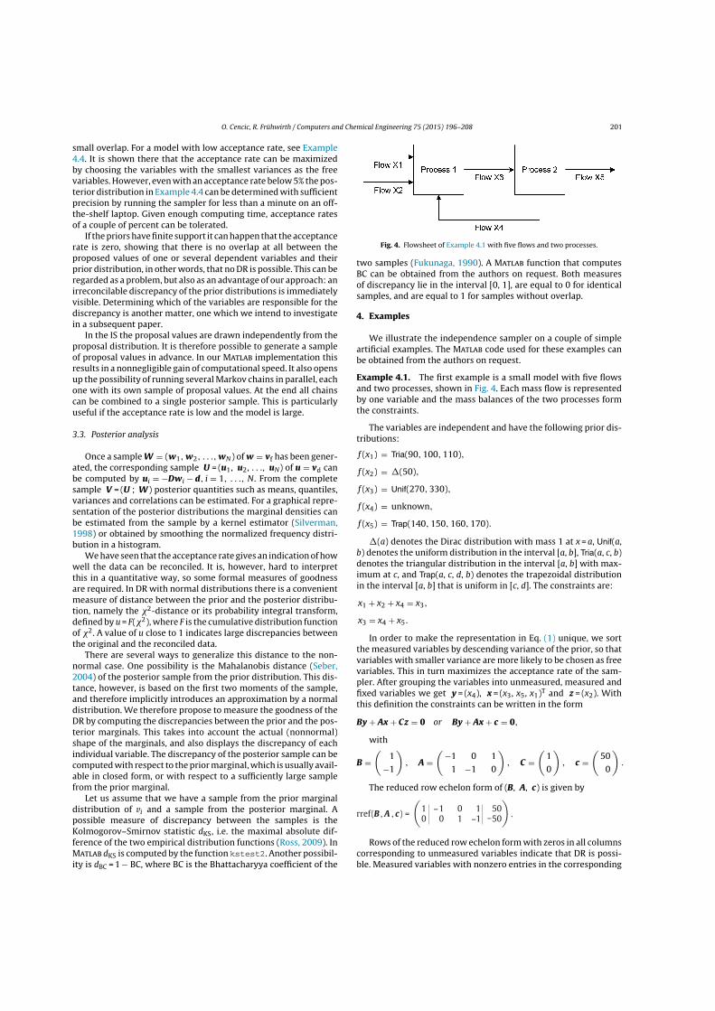
O. Cencic, R. Frühwirth / Computers and Chemical Engineering 75 (2015) 196–208 201
small overlap. For a model with low acceptance rate, see Example4.4. It is shown there that the acceptance rate can be maximizedby choosing the variables with the smallest variances as the freevariables. However, even with an acceptance rate below 5% the pos-terior distribution in Example 4.4 can be determined with sufficientprecision by running the sampler for less than a minute on an off-the-shelf laptop. Given enough computing time, acceptance ratesof a couple of percent can be tolerated.
If the priors have finite support it can happen that the acceptancerate is zero, showing that there is no overlap at all between theproposed values of one or several dependent variables and theirprior distribution, in other words, that no DR is possible. This can beregarded as a problem, but also as an advantage of our approach: anirreconcilable discrepancy of the prior distributions is immediatelyvisible. Determining which of the variables are responsible for thediscrepancy is another matter, one which we intend to investigatein a subsequent paper.
In the IS the proposal values are drawn independently from theproposal distribution. It is therefore possible to generate a sampleof proposal values in advance. In our Matlab implementation thisresults in a nonnegligible gain of computational speed. It also opensup the possibility of running several Markov chains in parallel, eachone with its own sample of proposal values. At the end all chainscan be combined to a single posterior sample. This is particularlyuseful if the acceptance rate is low and the model is large.
3.3. Posterior analysis
Once a sample W = (w1, w2, . . ., wN) of w = vf has been gener-ated, the corresponding sample U = (u1, u2, . . ., uN) of u = vd canbe computed by ui = −Dwi − d, i = 1, . . ., N. From the completesample V = (U ; W ) posterior quantities such as means, quantiles,variances and correlations can be estimated. For a graphical repre-sentation of the posterior distributions the marginal densities canbe estimated from the sample by a kernel estimator (Silverman,1998) or obtained by smoothing the normalized frequency distri-bution in a histogram.
We have seen that the acceptance rate gives an indication of howwell the data can be reconciled. It is, however, hard to interpretthis in a quantitative way, so some formal measures of goodnessare required. In DR with normal distributions there is a convenientmeasure of distance between the prior and the posterior distribu-tion, namely the �2-distance or its probability integral transform,defined by u = F(�2), where F is the cumulative distribution functionof �2. A value of u close to 1 indicates large discrepancies betweenthe original and the reconciled data.
There are several ways to generalize this distance to the non-normal case. One possibility is the Mahalanobis distance (Seber,2004) of the posterior sample from the prior distribution. This dis-tance, however, is based on the first two moments of the sample,and therefore implicitly introduces an approximation by a normaldistribution. We therefore propose to measure the goodness of theDR by computing the discrepancies between the prior and the pos-terior marginals. This takes into account the actual (nonnormal)shape of the marginals, and also displays the discrepancy of eachindividual variable. The discrepancy of the posterior sample can becomputed with respect to the prior marginal, which is usually avail-able in closed form, or with respect to a sufficiently large samplefrom the prior marginal.
Let us assume that we have a sample from the prior marginaldistribution of vi and a sample from the posterior marginal. Apossible measure of discrepancy between the samples is theKolmogorov–Smirnov statistic dKS, i.e. the maximal absolute dif-ference of the two empirical distribution functions (Ross, 2009). InMatlab dKS is computed by the function kstest2. Another possibil-ity is dBC = 1 − BC, where BC is the Bhattacharyya coefficient of the
Fig. 4. Flowsheet of Example 4.1 with five flows and two processes.
two samples (Fukunaga, 1990). A Matlab function that computesBC can be obtained from the authors on request. Both measuresof discrepancy lie in the interval [0, 1], are equal to 0 for identicalsamples, and are equal to 1 for samples without overlap.
4. Examples
We illustrate the independence sampler on a couple of simpleartificial examples. The Matlab code used for these examples canbe obtained from the authors on request.
Example 4.1. The first example is a small model with five flowsand two processes, shown in Fig. 4. Each mass flow is representedby one variable and the mass balances of the two processes formthe constraints.
The variables are independent and have the following prior dis-tributions:
f (x1) = Tria(90, 100, 110),
f (x2) = �(50),
f (x3) = Unif(270, 330),
f (x4) = unknown,
f (x5) = Trap(140, 150, 160, 170).
�(a) denotes the Dirac distribution with mass 1 at x = a, Unif(a,b) denotes the uniform distribution in the interval [a, b], Tria(a, c, b)denotes the triangular distribution in the interval [a, b] with max-imum at c, and Trap(a, c, d, b) denotes the trapezoidal distributionin the interval [a, b] that is uniform in [c, d]. The constraints are:
x1 + x2 + x4 = x3,
x3 = x4 + x5.
In order to make the representation in Eq. (1) unique, we sortthe measured variables by descending variance of the prior, so thatvariables with smaller variance are more likely to be chosen as freevariables. This in turn maximizes the acceptance rate of the sam-pler. After grouping the variables into unmeasured, measured andfixed variables we get y = (x4), x = (x3, x5, x1)T and z = (x2). Withthis definition the constraints can be written in the form
By + Ax + Cz = 0 or By + Ax + c = 0,
with
B =(
1
−1
), A =
(−1 0 1
1 −1 0
), C =
(1
0
), c =
(50
0
).
The reduced row echelon form of (B, A, c) is given by
rref(B , A , c) = 1 −1 0 1 500 0 1 −1 −5 0 .
Rows of the reduced row echelon form with zeros in all columnscorresponding to unmeasured variables indicate that DR is possi-ble. Measured variables with nonzero entries in the corresponding
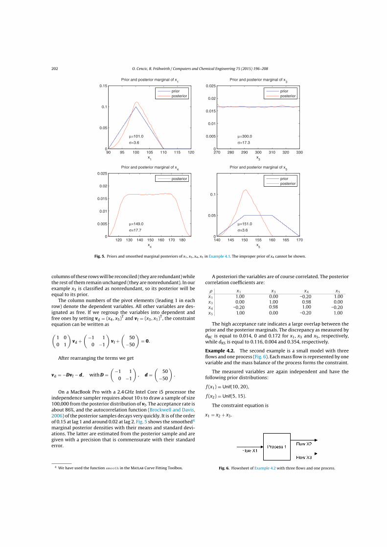
202 O. Cencic, R. Frühwirth / Computers and Chemical Engineering 75 (2015) 196–208
270 280 290 300 310 320 3300
0.005
0.01
0.015
0.02
0.025
x3
Prior and posterior marginal of x3
μ=300.0
σ=17.3
priorposterior
90 95 100 105 110 115 1200
0.05
0.1
0.15
x1
Prior and posterior marginal of x1
μ=101.0
σ=3.6
priorposterior
120 130 140 150 160 170 1800
0.005
0.01
0.015
0.02
0.025
x4
Prior and posterior marginal of x4
μ=149.0
σ=17.7
posterior
140 145 150 155 160 165 1700
0.05
0.1
x5
Prior and posterior marginal of x5
μ=151.0
σ=3.6
priorposterior
Fig. 5. Priors and smoothed marginal posteriors of x1, x3, x4, x5 in Example 4.1. The improper prior of x4 cannot be shown.
columns of these rows will be reconciled (they are redundant) whilethe rest of them remain unchanged (they are nonredundant). In ourexample x3 is classified as nonredundant, so its posterior will beequal to its prior.
The column numbers of the pivot elements (leading 1 in eachrow) denote the dependent variables. All other variables are des-ignated as free. If we regroup the variables into dependent andfree ones by setting vd = (x4, x5)T and vf = (x3, x1)T, the constraintequation can be written as
(1 0
0 1
)vd +
(−1 1
0 −1
)vf +
(50
−50
)= 0.
After rearranging the terms we get
vd = −Dvf − d, with D =(
−1 1
0 −1
), d =
(50
−50
).
On a MacBook Pro with a 2.4 GHz Intel Core i5 processor theindependence sampler requires about 10 s to draw a sample of size100,000 from the posterior distribution of vf. The acceptance rate isabout 86%, and the autocorrelation function (Brockwell and Davis,2006) of the posterior samples decays very quickly. It is of the orderof 0.15 at lag 1 and around 0.02 at lag 2. Fig. 5 shows the smoothed4
marginal posterior densities with their means and standard devi-ations. The latter are estimated from the posterior sample and aregiven with a precision that is commensurate with their standarderror.
4 We have used the function smooth in the Matlab Curve Fitting Toolbox.
A posteriori the variables are of course correlated. The posteriorcorrelation coefficients are:
x1 x3 x4 x5
x1 1.00 0.00 1.00x3 0.00 1.00 0.98 0.00
0.98 1.00x4 −0.20 −0.20x5 1.00 0.00 −0.20
−0.20
1.00
The high acceptance rate indicates a large overlap between theprior and the posterior marginals. The discrepancy as measured bydBC is equal to 0.014, 0 and 0.172 for x1, x3 and x5, respectively,while dKS is equal to 0.116, 0.004 and 0.354, respectively.
Example 4.2. The second example is a small model with threeflows and one process (Fig. 6). Each mass flow is represented by onevariable and the mass balance of the process forms the constraint.
The measured variables are again independent and have thefollowing prior distributions:
f (x1) = Unif(10, 20),
f (x2) = Unif(5, 15).
The constraint equation is
x1 = x2 + x3.
Fig. 6. Flowsheet of Example 4.2 with three flows and one process.
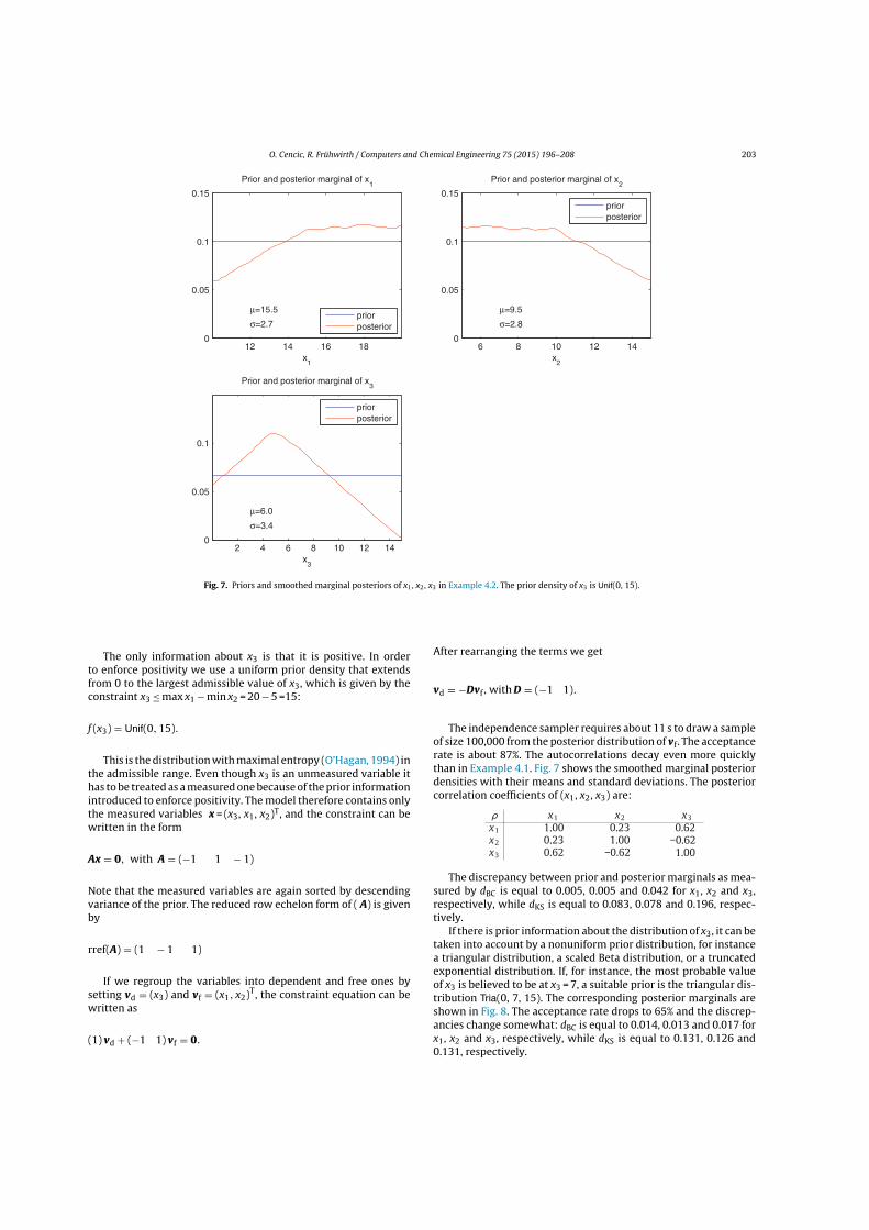
O. Cencic, R. Frühwirth / Computers and Chemical Engineering 75 (2015) 196–208 203
12 14 16 180
0.05
0.1
0.15
x1
Prior and posterior marginal of x1
μ=15.5
σ=2.7priorposterior
6 8 10 12 140
0.05
0.1
0.15
x2
Prior and posterior marginal of x2
μ=9.5
σ=2.8
priorposterior
2 4 6 8 10 12 140
0.05
0.1
x3
Prior and posterior marginal of x3
μ=6.0
σ=3.4
priorposterior
Fig. 7. Priors and smoothed marginal posteriors of x1, x2, x3 in Example 4.2. The prior density of x3 is Unif(0, 15).
The only information about x3 is that it is positive. In orderto enforce positivity we use a uniform prior density that extendsfrom 0 to the largest admissible value of x3, which is given by theconstraint x3 ≤ max x1 − min x2 = 20 − 5 =15:
f (x3) = Unif(0, 15).
This is the distribution with maximal entropy (O’Hagan, 1994) inthe admissible range. Even though x3 is an unmeasured variable ithas to be treated as a measured one because of the prior informationintroduced to enforce positivity. The model therefore contains onlythe measured variables x = (x3, x1, x2)T, and the constraint can bewritten in the form
Ax = 0, with A = (−1 1 − 1)
Note that the measured variables are again sorted by descendingvariance of the prior. The reduced row echelon form of ( A) is givenby
rref(A) = (1 − 1 1)
If we regroup the variables into dependent and free ones bysetting vd = (x3) and vf = (x1, x2)T, the constraint equation can bewritten as
(1) vd + (−1 1) vf = 0.
After rearranging the terms we get
vd = −Dvf, with D = (−1 1).
The independence sampler requires about 11 s to draw a sampleof size 100,000 from the posterior distribution of vf. The acceptancerate is about 87%. The autocorrelations decay even more quicklythan in Example 4.1. Fig. 7 shows the smoothed marginal posteriordensities with their means and standard deviations. The posteriorcorrelation coefficients of (x1, x2, x3) are:
x1 x2 x3
x1 1.00x2 0.23x3 0.62
0.231.00
−0.62
0.62
1.00−0.62
The discrepancy between prior and posterior marginals as mea-sured by dBC is equal to 0.005, 0.005 and 0.042 for x1, x2 and x3,respectively, while dKS is equal to 0.083, 0.078 and 0.196, respec-tively.
If there is prior information about the distribution of x3, it can betaken into account by a nonuniform prior distribution, for instancea triangular distribution, a scaled Beta distribution, or a truncatedexponential distribution. If, for instance, the most probable valueof x3 is believed to be at x3 = 7, a suitable prior is the triangular dis-tribution Tria(0, 7, 15). The corresponding posterior marginals areshown in Fig. 8. The acceptance rate drops to 65% and the discrep-ancies change somewhat: dBC is equal to 0.014, 0.013 and 0.017 forx1, x2 and x3, respectively, while dKS is equal to 0.131, 0.126 and0.131, respectively.
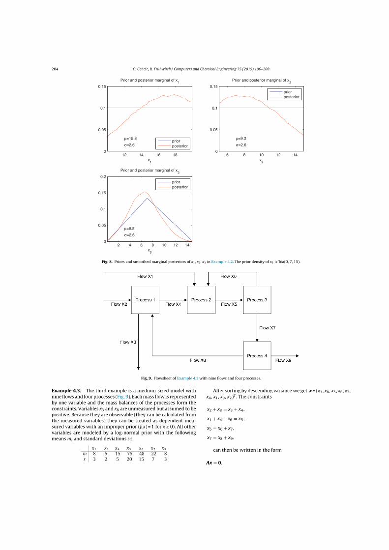
204 O. Cencic, R. Frühwirth / Computers and Chemical Engineering 75 (2015) 196–208
12 14 16 180
0.05
0.1
0.15
x1
Prior and posterior marginal of x1
μ=15.8
σ=2.6priorposterior
6 8 10 12 140
0.05
0.1
0.15
x2
Prior and posterior marginal of x2
μ=9.2
σ=2.6
priorposterior
2 4 6 8 10 12 140
0.05
0.1
0.15
0.2
x3
Prior and posterior marginal of x3
μ=6.5
σ=2.6
priorposterior
Fig. 8. Priors and smoothed marginal posteriors of x1, x2, x3 in Example 4.2. The prior density of x3 is Tria(0, 7, 15).
Fig. 9. Flowsheet of Example 4.3 with nine flows and four processes.
Example 4.3. The third example is a medium-sized model withnine flows and four processes (Fig. 9). Each mass flow is representedby one variable and the mass balances of the processes form theconstraints. Variables x3 and x8 are unmeasured but assumed to bepositive. Because they are observable (they can be calculated fromthe measured variables) they can be treated as dependent mea-sured variables with an improper prior (f(x) = 1 for x ≥ 0). All othervariables are modeled by a log-normal prior with the followingmeans mi and standard deviations si:
x1 x2 x4 x5 x6 x7 x9
m 8 5 15 75 48 22 8s 3 2 5 20 15 7 3
After sorting by descending variance we get x = (x3, x8, x5, x6, x7,x4, x1, x9, x2)T. The constraints
x2 + x8 = x3 + x4,
x1 + x4 + x6 = x5,
x5 = x6 + x7,
x7 = x8 + x9,
can then be written in the form
Ax = 0,
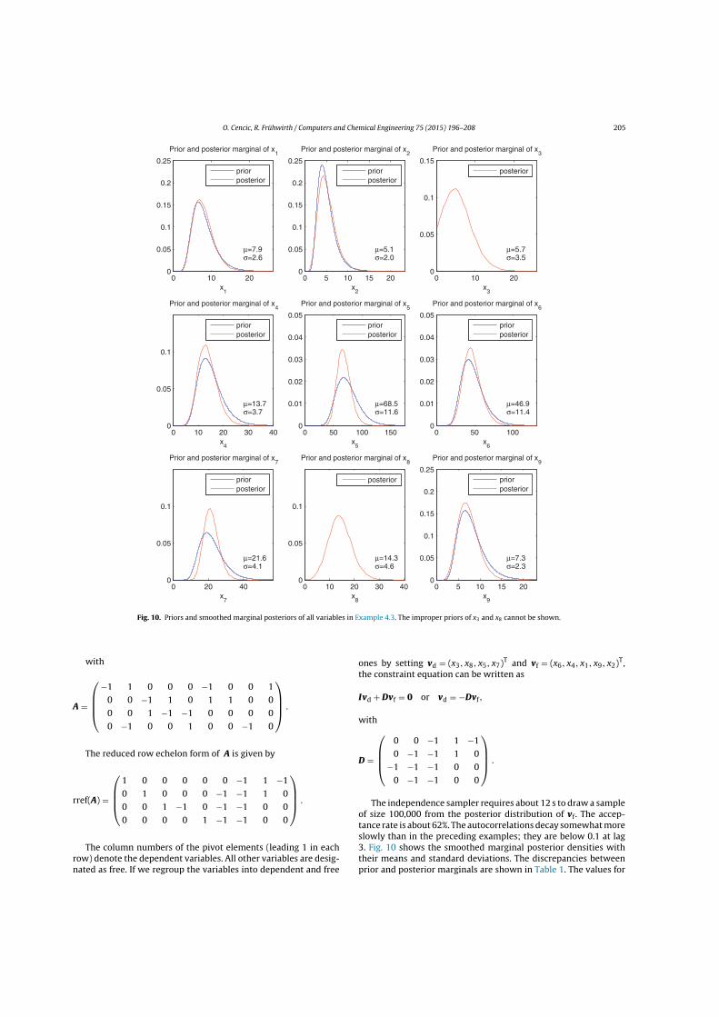
O. Cencic, R. Frühwirth / Computers and Chemical Engineering 75 (2015) 196–208 205
0 10 200
0.05
0.1
0.15
x3
Prior and posterior marginal of x3
μ=5.7σ=3.5
posterior
0 10 20 30 400
0.05
0.1
x8
Prior and posterior marginal of x8
μ=14.3σ=4.6
posterior
0 50 100 1500
0.01
0.02
0.03
0.04
0.05
x5
Prior and posterior marginal of x5
μ=68.5σ=11.6
priorposterior
0 20 400
0.05
0.1
x7
Prior and posterior marginal of x7
μ=21.6σ=4.1
priorposterior
0 50 1000
0.01
0.02
0.03
0.04
0.05
x6
Prior and posterior marginal of x6
μ=46.9σ=11.4
priorposterior
0 10 20 30 400
0.05
0.1
x4
Prior and posterior marginal of x4
μ=13.7σ=3.7
priorposterior
0 10 200
0.05
0.1
0.15
0.2
0.25
x1
Prior and posterior marginal of x1
μ=7.9σ=2.6
priorposterior
0 5 10 15 200
0.05
0.1
0.15
0.2
0.25
x9
Prior and posterior marginal of x9
μ=7.3σ=2.3
priorposterior
0 5 10 15 200
0.05
0.1
0.15
0.2
0.25
x2
Prior and posterior marginal of x2
μ=5.1σ=2.0
priorposterior
Fig. 10. Priors and smoothed marginal posteriors of all variables in Example 4.3. The improper priors of x3 and x8 cannot be shown.
with
A =
⎛⎜⎜⎝
−1 1 0 0 0 −1 0 0 1
0 0 −1 1 0 1 1 0 0
0 0 1 −1 −1 0 0 0 0
0 −1 0 0 1 0 0 −1 0
⎞⎟⎟⎠ .
The reduced row echelon form of A is given by
rref(A) =
⎛⎜⎜⎝
1 0 0 0 0 0 −1 1 −1
0 1 0 0 0 −1 −1 1 0
0 0 1 −1 0 −1 −1 0 0
0 0 0 0 1 −1 −1 0 0
⎞⎟⎟⎠ .
The column numbers of the pivot elements (leading 1 in eachrow) denote the dependent variables. All other variables are desig-nated as free. If we regroup the variables into dependent and free
ones by setting vd = (x3, x8, x5, x7)T and vf = (x6, x4, x1, x9, x2)T,the constraint equation can be written as
Ivd + Dvf = 0 or vd = −Dvf,
with
D =
⎛⎜⎜⎝
0 0 −1 1 −1
0 −1 −1 1 0
−1 −1 −1 0 0
0 −1 −1 0 0
⎞⎟⎟⎠ .
The independence sampler requires about 12 s to draw a sampleof size 100,000 from the posterior distribution of vf. The accep-tance rate is about 62%. The autocorrelations decay somewhat moreslowly than in the preceding examples; they are below 0.1 at lag3. Fig. 10 shows the smoothed marginal posterior densities withtheir means and standard deviations. The discrepancies betweenprior and posterior marginals are shown in Table 1. The values for
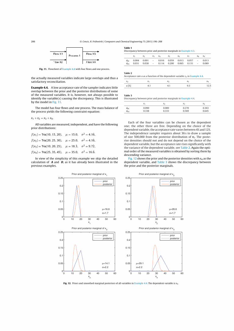
206 O. Cencic, R. Frühwirth / Computers and Chemical Engineering 75 (2015) 196–208
Fig. 11. Flowsheet of Example 4.4 with four flows and one process.
the actually measured variables indicate large overlaps and thus asatisfactory reconciliation.
Example 4.4. A low acceptance rate of the sampler indicates littleoverlap between the prior and the posterior distributions of someof the measured variables. It is, however, not always possible toidentify the variable(s) causing the discrepancy. This is illustratedby the model in Fig. 11.
The model has four flows and one process. The mass balance ofthe process yields the following constraint equation:
x1 + x2 = x3 + x4.
All variables are measured, independent, and have the followingprior distributions:
f (x1) = Tria(10, 15, 20), � = 15.0, �2 = 4.16,
f (x2) = Tria(20, 25, 30), � = 25.0, �2 = 4.16,
f (x3) = Tria(10, 20, 25), � = 18.3, �2 = 9.72,
f (x4) = Tria(25, 35, 45), � = 35.0, �2 = 16.6.
In view of the simplicity of this example we skip the detailedcalculation of A and D, as it has already been illustrated in theprevious examples.
Table 1Discrepancy between prior and posterior marginals in Example 4.3.
x1 x2 x3 x4 x5 x6 x7 x8 x9
dBC 0.004 0.001 – 0.016 0.059 0.013 0.057 – 0.013dKS 0.031 0.038 – 0.114 0.200 0.065 0.131 – 0.089
Table 2Acceptance rate a as a function of the dependent variable vd in Example 4.4.
vd x1 x2 x3 x4
a [%] 4.1 4.1 9.3 12.5
Table 3Discrepancy between prior and posterior marginals in Example 4.4.
x1 x2 x3 x4
dBC 0.090 0.089 0.270 0.363dKS 0.338 0.333 0.569 0.645
Each of the four variables can be chosen as the dependentone; the other three are free. Depending on the choice of thedependent variable, the acceptance rate varies between 4% and 12%.The independence sampler requires about 36 s to draw a sampleof size 500,000 from the posterior distribution of vf. The poste-rior densities should not and do not depend on the choice of thedependent variable, but the acceptance rate rises significantly withthe variance of the dependent variable, see Table 2. Again the opti-mal order of the measured variables is obtained by sorting them bydescending variance.
Fig. 12 shows the prior and the posterior densities with x4 as thedependent variable, and Table 3 shows the discrepancy betweenthe prior and the posterior marginals.
0 10 20 30 40 50 600
0.05
0.1
0.15
0.2
0.25
x1
Prior and posterior marginal of x1
μ=16.6
σ=1.7
priorposterior
0 10 20 30 40 50 600
0.05
0.1
0.15
0.2
0.25
x2
Prior and posterior marginal of x2
μ=26.6
σ=1.7
priorposterior
0 10 20 30 40 50 600
0.05
0.1
0.15
0.2
0.25
x3
Prior and posterior marginal of x3
μ=14.1
σ=2.2
priorposterior
0 10 20 30 40 50 600
0.05
0.1
0.15
0.2
0.25
x4
Prior and posterior marginal of x4
μ=29.1
σ=2.2
priorposterior
Fig. 12. Priors and smoothed marginal posteriors of all variables in Example 4.4. The dependent variable is x4.
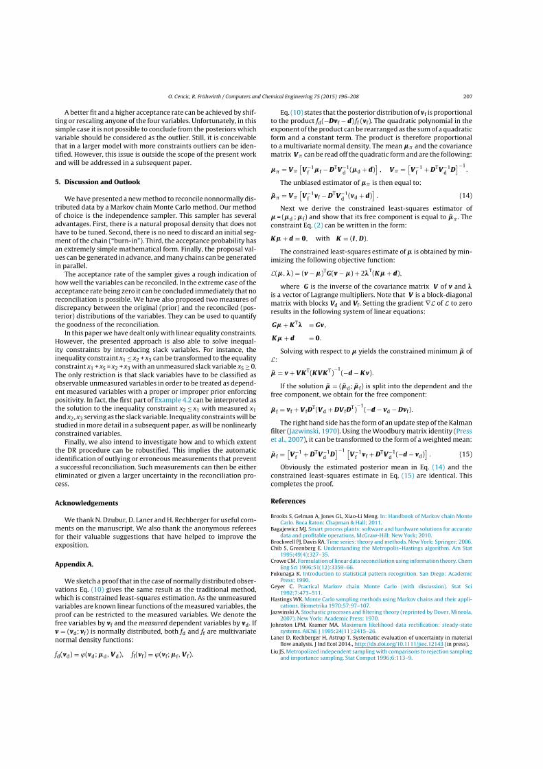
O. Cencic, R. Frühwirth / Computers and Chemical Engineering 75 (2015) 196–208 207
A better fit and a higher acceptance rate can be achieved by shif-ting or rescaling anyone of the four variables. Unfortunately, in thissimple case it is not possible to conclude from the posteriors whichvariable should be considered as the outlier. Still, it is conceivablethat in a larger model with more constraints outliers can be iden-tified. However, this issue is outside the scope of the present workand will be addressed in a subsequent paper.
5. Discussion and Outlook
We have presented a new method to reconcile nonnormally dis-tributed data by a Markov chain Monte Carlo method. Our methodof choice is the independence sampler. This sampler has severaladvantages. First, there is a natural proposal density that does nothave to be tuned. Second, there is no need to discard an initial seg-ment of the chain (“burn-in”). Third, the acceptance probability hasan extremely simple mathematical form. Finally, the proposal val-ues can be generated in advance, and many chains can be generatedin parallel.
The acceptance rate of the sampler gives a rough indication ofhow well the variables can be reconciled. In the extreme case of theacceptance rate being zero it can be concluded immediately that noreconciliation is possible. We have also proposed two measures ofdiscrepancy between the original (prior) and the reconciled (pos-terior) distributions of the variables. They can be used to quantifythe goodness of the reconciliation.
In this paper we have dealt only with linear equality constraints.However, the presented approach is also able to solve inequal-ity constraints by introducing slack variables. For instance, theinequality constraint x1 ≤ x2 + x3 can be transformed to the equalityconstraint x1 + xS = x2 + x3 with an unmeasured slack variable xS ≥ 0.The only restriction is that slack variables have to be classified asobservable unmeasured variables in order to be treated as depend-ent measured variables with a proper or improper prior enforcingpositivity. In fact, the first part of Example 4.2 can be interpreted asthe solution to the inequality constraint x2 ≤ x1 with measured x1and x2, x3 serving as the slack variable. Inequality constraints will bestudied in more detail in a subsequent paper, as will be nonlinearlyconstrained variables.
Finally, we also intend to investigate how and to which extentthe DR procedure can be robustified. This implies the automaticidentification of outlying or erroneous measurements that preventa successful reconciliation. Such measurements can then be eithereliminated or given a larger uncertainty in the reconciliation pro-cess.
Acknowledgements
We thank N. Dzubur, D. Laner and H. Rechberger for useful com-ments on the manuscript. We also thank the anonymous refereesfor their valuable suggestions that have helped to improve theexposition.
Appendix A.
We sketch a proof that in the case of normally distributed obser-vations Eq. (10) gives the same result as the traditional method,which is constrained least-squares estimation. As the unmeasuredvariables are known linear functions of the measured variables, theproof can be restricted to the measured variables. We denote thefree variables by vf and the measured dependent variables by vd. Ifv = (vd; vf) is normally distributed, both fd and ff are multivariatenormal density functions:
fd(vd) = ϕ(vd; �d, Vd), ff(vf) = ϕ(vf; �f, V f).
Eq. (10) states that the posterior distribution of vf is proportionalto the product fd(−Dvf − d) ff (vf). The quadratic polynomial in theexponent of the product can be rearranged as the sum of a quadraticform and a constant term. The product is therefore proportionalto a multivariate normal density. The mean �� and the covariancematrix V� can be read off the quadratic form and are the following:
�� = V�
[V−1
f �f − DTV−1d (�d + d)
], V� =
[V−1
f + DTV−1d D
]−1.
The unbiased estimator of �� is then equal to:
�� = V�
[V−1
f vf − DTV−1d (vd + d)
]. (14)
Next we derive the constrained least-squares estimator of� = (�d ; �f) and show that its free component is equal to �� . Theconstraint Eq. (2) can be written in the form:
K� + d = 0, with K = (I, D).
The constrained least-squares estimate of � is obtained by min-imizing the following objective function:
L(�, �) = (v − �)TG(v − �) + 2�T(K� + d),
where G is the inverse of the covariance matrix V of v and �is a vector of Lagrange multipliers. Note that V is a block-diagonalmatrix with blocks Vd and Vf. Setting the gradient ∇L of L to zeroresults in the following system of linear equations:
G� + KT� = Gv,
K� + d = 0.
Solving with respect to � yields the constrained minimum � ofL:
� = v + VKT(KVKT)−1
(−d − Kv).
If the solution � = (�d; �f) is split into the dependent and thefree component, we obtain for the free component:
�f = vf + V fDT(Vd + DV fD
T)−1
(−d − vd − Dvf).
The right hand side has the form of an update step of the Kalmanfilter (Jazwinski, 1970). Using the Woodbury matrix identity (Presset al., 2007), it can be transformed to the form of a weighted mean:
�f =[V−1
f + DTV−1d D
]−1 [V−1
f vf + DTV−1d (−d − vd)
]. (15)
Obviously the estimated posterior mean in Eq. (14) and theconstrained least-squares estimate in Eq. (15) are identical. Thiscompletes the proof.
References
Brooks S, Gelman A, Jones GL, Xiao-Li Meng. In: Handbook of Markov chain MonteCarlo. Boca Raton: Chapman & Hall; 2011.
Bagajewicz MJ. Smart process plants: software and hardware solutions for accuratedata and profitable operations. McGraw-Hill: New York; 2010.
Brockwell PJ, Davis RA. Time series: theory and methods. New York: Springer; 2006.Chib S, Greenberg E. Understanding the Metropolis–Hastings algorithm. Am Stat
1995;49(4):327–35.Crowe CM. Formulation of linear data reconciliation using information theory. Chem
Eng Sci 1996;51(12):3359–66.Fukunaga K. Introduction to statistical pattern recognition. San Diego: Academic
Press; 1990.Geyer C. Practical Markov chain Monte Carlo (with discussion). Stat Sci
1992;7:473–511.Hastings WK. Monte Carlo sampling methods using Markov chains and their appli-
cations. Biometrika 1970;57:97–107.Jazwinski A. Stochastic processes and filtering theory (reprinted by Dover, Mineola,
2007). New York: Academic Press; 1970.Johnston LPM, Kramer MA. Maximum likelihood data rectification: steady-state
systems. AIChE J 1995;24(11):2415–26.Laner D, Rechberger H, Astrup T. Systematic evaluation of uncertainty in material
flow analysis. J Ind Ecol 2014., http://dx.doi.org/10.1111/jiec.12143 (in press).Liu JS. Metropolized independent sampling with comparisons to rejection sampling
and importance sampling. Stat Comput 1996;6:113–9.
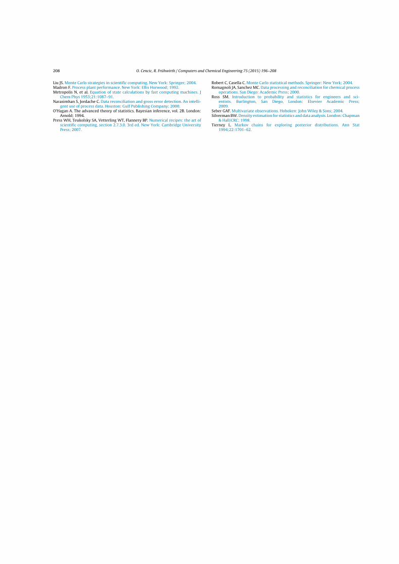
208 O. Cencic, R. Frühwirth / Computers and Chemical Engineering 75 (2015) 196–208
Liu JS. Monte Carlo strategies in scientific computing. New York: Springer; 2004.Madron F. Process plant performance. New York: Ellis Horwood; 1992.Metropolis N, et al. Equation of state calculations by fast computing machines. J
Chem Phys 1953;21:1087–91.Narasimhan S, Jordache C. Data reconciliation and gross error detection. An intelli-
gent use of process data. Houston: Gulf Publishing Company; 2000.O’Hagan A. The advanced theory of statistics. Bayesian inference, vol. 2B. London:
Arnold; 1994.Press WH, Teukolsky SA, Vetterling WT, Flannery BP. Numerical recipes: the art of
scientific computing, section 2.7.3.0. 3rd ed. New York: Cambridge UniversityPress; 2007.
Robert C, Casella C. Monte Carlo statistical methods. Springer: New York; 2004.Romagnoli JA, Sanchez MC. Data processing and reconciliation for chemical process
operations. San Diego: Academic Press; 2000.Ross SM. Introduction to probability and statistics for engineers and sci-
entists. Burlington, San Diego, London: Elsevier Academic Press;2009.
Seber GAF. Multivariate observations. Hoboken: John Wiley & Sons; 2004.Silverman BW. Density estimation for statistics and data analysis. London: Chapman
& Hall/CRC; 1998.Tierney L. Markov chains for exploring posterior distributions. Ann Stat
1994;22:1701–62.

Paper 3:
Data reconciliation of nonnormal observationswith nonlinear constraintsOliver Cencic and Rudolf FrühwirthJournal of Applied Statistics 2018, in pressDOI: 10.1080/02664763.2017.1421916

JOURNAL OF APPLIED STATISTICS, 2018https://doi.org/10.1080/02664763.2017.1421916
Data reconciliation of nonnormal observations with nonlinearconstraints
Oliver Cencica and Rudolf Frühwirthb,c
aInstitute for Water Quality, Resource and Waste Management, TU Wien, Wien, Austria; bInstitute of HighEnergy Physics (HEPHY), Austrian Academy of Sciences, Wien, Austria; cInstitute of Statistics andMathematical Methods in Economics, TU Wien, Wien, Austria
ABSTRACTThis paper presents a new method for the reconciliation of datadescribed by arbitrary continuous probability distributions, with thefocus on nonlinear constraints. The main idea, already applied tolinear constraints in apreviouspaper, is to restrict the joint prior prob-ability distribution of the observed variables with model constraintsto get a joint posterior probability distribution. Because in generalthe posterior probability density function cannot be calculated ana-lytically, it is shown that it has decisive advantages to sample fromthe posterior distribution by a Markov chain Monte Carlo (MCMC)method. From the resulting sample of observed and unobservedvariables various characteristics of the posterior distribution can beestimated, suchas themean, the full covariancematrix,marginal pos-terior densities, as well as marginal moments, quantiles, and HPDintervals. The procedure is illustrated by examples frommaterial flowanalysis and chemical engineering.
ARTICLE HISTORYReceived 23 June 2017Accepted 21 December 2017
KEYWORDSData reconciliation; Bayesianapproach; nonlinearconstraints; nonnormaldistributions; Markov chainMonte Carlo
1. Introduction
Data reconciliation (DR) is a statisticalmethod to adjust observed data that are, due tomea-surement or sampling errors, in conflict with known constraints such as the conservationlaws of mass and energy. By imposing the constraints on the observations external infor-mation is added, and consequently the reconciled values have smaller uncertainty than theoriginal observations. In addition, unobserved variables occurring in the constraints canbe estimated, as long as the assumptions in Section 2.2 are fulfilled.
Traditionally, DR is formulated as a minimization problem where the observations areadjusted so that they obey a set of constraint equations and, at the same time, minimizean objective function. An important example of such an objective function is the sum ofsquared differences (weighted or unweighted) between the adjusted and the original values,resulting in a least-squares reconciliation.
In the simplest case, the observations x are normally distributed with unknown meanvector x and known or estimated joint covariance matrix �. Furthermore, the vector x is
CONTACT Oliver Cencic [email protected] Institute for Water Quality, Resource and WasteManagement, TU Wien, Karlsplatz 13/226, A-1040 Wien, Austria
© 2018 The Author(s). Published by Informa UK Limited, trading as Taylor & Francis GroupThis is anOpenAccess article distributed under the terms of the Creative CommonsAttribution License (http://creativecommons.org/licenses/by/4.0/), which permits unrestricted use, distribution, and reproduction in any medium, provided the original work is properly cited.
2 O. CENCIC AND R. FRÜHWIRTH
known to obey a system of linear equality constraints:
Ax + By + c = 0, (1)
where y is a vector of unobserved variables, A and B are known coefficient matrices of xand y, respectively, and c is a vector of known constants. Under certain conditions (seeAppendix), a unique explicit solution can be found by constrained minimization withrespect to x of the following least-squares objective function:
F(x) = (x − x)T�−1(x − x), (2)
usually with the help of Lagrange multipliers [19]. The least-squares solution (y; x)1 fulfillsthe constraints, the reconciled vector x is an unbiased estimator of x, and the variances ofx are smaller than the variances of x. As the covariance matrix of x is rank deficient, itsdistribution is singular, i.e. concentrated on a set of Lebesgue measure zero, and does nothave a pdf (cf. Section 2.3). If x follows a normal distribution, so does the solution (y; x);otherwise it does not.
This basic problem of DR can be generalized in two directions: first, the constraintscan be extended to nonlinear and/or inequality constraints; second, the distribution ofthe observations x can be extended to arbitrary, but absolutely continuous, multivariatedistributions, characterized by a probability density function (pdf) f (x).
The first extension to nonlinear and/or inequality constraints is conceptually simple,but may pose technical difficulties. The solution can no longer be obtained in closed form,but has to be computed iteratively by suitable algorithms for the constrained minimizationof F(x), with the usual potential problems of convergence, local minima and saddle points.There is a large variety of methods that can be applied. Some examples in the engineer-ing literature are successive linearization [10], nonlinear programming [1], quasi-Newtonmethods [14] and genetic algorithms [23]. For textbooks on optimization with nonlinearconstraints, see, for instance, [5,6,22]. Note that with nonlinear constraints the reconciledvalues are not normally distributed, even if the observations x are.
The second extension to nonnormal observations can be achieved by an alternativeapproach to the problem of DR. As the objective function in Equation (2) uses only thefirst twomoments of the distribution, it is not able to take into account the full informationcontained in the joint pdf of the observations. Consequently, the reconciliation problemcannot be fully solved by minimizing an objective function of the form of Equation (2),even if the joint pdf of the observations belongs to a parametric family. In the case of linearconstraints, the constrained least-squares estimator is unbiased and a linear function of theobservations, and therefore gives the correct mean and covariancematrix of the reconciledvalues. Their distribution, however, is not known, and it is not possible to compute quan-tiles or highermoments such as the skewness. This problemwas solved in [3] by a Bayesianmethod that gives the joint (posterior) distribution of the reconciled variables under lin-ear constraints for arbitrary (prior) distributions of the observations. In the appendix, it isproved that this method delivers the same results as the least-squares approach in the caseof linear constraints and normal observations with arbitrary covariance matrix �.
This paper extends the method of Cencic and Frühwirth [3] to the case of nonlinearconstraints, which usually are present in all but the simplest models. In Section 2 the basicassumptions about nonnormal models with nonlinear constraints are spelled out, and the

JOURNAL OF APPLIED STATISTICS 3
posterior pdf of the free variables of themodel is derived. It is shown that the joint posteriordistribution of all variables, derived from the posterior distribution of the free variables,is invariant under the choice of the free variables. Section 3 presents the independencesampler that produces a Markov chain of all variables, observed and unobserved. FromtheMarkov chain, important characteristics of the posterior distribution can be estimated,among them the mean and the covariance matrix, marginal pdfs, marginal moments andmarginal quantiles. In Section 4 the sampler is applied to two examples, one from the fieldofmaterial flow analysis (MFA), the other from the chemical engineering literature. Finally,Section 5 presents conclusions and gives an outlook to further work.
2. Nonnormal models with nonlinear constraints
2.1. Motivation and specification of priors
As the objective function in Equation (2) uses only the first two moments of the joint dis-tribution of the observations, it is based on the implicit assumption of normally distributedobservation errors. This assumption guarantees normally distributed reconciled observa-tions in case of linear or linearized constraints, where in the latter case the results are onlyapproximations. Sometimes, these approximations are not sufficient and the precise pdfsof the results are desired instead.
Additionally, there might be variables involved in the problem where the normalassumption is not appropriate. First, variables can be bounded in some ways. A typicalexample is found in MFA, where it is crucial to close the mass balances of goods and sub-stances traversing different kinds of processes in order to get reliable data for subsequentevaluation. By definition, mass flows cannot take negative values, and transfer coefficients,which describe how much of the mass going into a process is transferred into specific out-put flows, as well as mass fractions of substances in goods are restricted to the unit interval,rendering the assumption of normality implausible. Second, modelling the uncertaintyof observations by normal distributions can be too restrictive. If a sufficient number ofobservations of a quantity is available and the observations fail a test on normality (see, forinstance [17]), one can fit a nonnormal parametricmodel to the observed data or constructa nonparametric model such as the empirical distribution function or the kernel estimateof the pdf. Third, if there are few or no observations of a quantity of interest, which isfrequently the case in MFA, expert opinions have to be relied on. The more detailed theexpert’s knowledge about the quantity under consideration is, the more precisely the dis-tribution can be modelled. Common choices in this context (with rising complexity) areuniform, triangular or trapezoidal distributions.
The data reconciliation method presented here is able to deal with arbitrary pdfsdescribing the uncertainty of an observation, regardless of the procedure by which it hasbeen derived. Thus, nonnormal models can be used as they are, without any need for nor-mal approximation. Before the constraints are imposed, the joint pdf of the observations,built from these nonnormal models, is called the ‘prior’ pdf. As in least-squares DR, thejoint distribution of the reconciled observations is singular; there is, however, a subsetof the variables (called the free variables in the following) with a nonsingular distribu-tion and a pdf, called the ‘posterior’ pdf. Although Bayes’ theorem is not invoked in thederivation of the posterior pdf, the terms ‘prior’ and ‘posterior’ can be justified by the fact
4 O. CENCIC AND R. FRÜHWIRTH
that the posterior pdf is a conditional density, namely the prior pdf conditioned on theconstraints.
2.2. Basic assumptions
Let m = (y; x) be a column vector of n variables that is arranged such that y contains theny unobserved variables and x contains the nx = n − ny observed variables. In addition,there is a system of nc independent constraint equations, where ny ≤ nc ≤ n:
G(y; x) = 0, G : Rn −→ Rnc . (3)
The functionG usually also depends on a vector z of known constants. In order to simplifythe notation, this dependence is not shown explicitly.
The derivation of the posterior pdf of the observed variables is based on the followingassumptions:
(1) The n observed or unobserved variables take values in a subset D ⊆ Rn.
(2) The observations of the nx ≤ n observed variables x form an nx-dimensional randomvariable with known joint pdf, called the prior pdf of the observed variables. As out-lined in Section 2.1, the prior pdf of an observed variable can result from an individualmeasurement, from a collection of measurements, or from capturing expert opinionin a pdf.
(3) Then variables are subject tonc independent nonlinear equality constraints that definea differentiable manifold S ⊂ R
n of dimension n − nc.(4) The nc nonlinear equality constraints can be uniquely solved for a set of nc depen-
dent variables (observed or unobserved) that are differentiable functions of n − ncfree variables (observed only), for each admissible value of the free variables.
There is no prior information on the unobserved variables y. Their posterior distribution iscomputed from the posterior distribution of the free variables using themodel constraints.
Assumption 4 implies that potentially involved unobservable variables have alreadybeen eliminated from the system of equations. Additional constraints such as positivity orboundedness can be incorporated directly in the prior distributions of the observed vari-ables and need not be enforced explicitly.2 Inequality constraints can be transformed intoequality constraints by introducing slack variables with uninformative priors restricted topositive values. For instance, the inequality constraint x1 ≤ x2 x3 can be transformed tox1 + xS = x2 x3 with xS ≥ 0 a priori.
2.3. The posterior pdf with nonlinear constraints
By assumption, the nonlinear constraints are solved by representing the ny unobservedvariables y and the nu = nc − ny dependent observed variables u as functions of the nw =n − nc chosen free observed variables w ∈ W, where W ⊆ R
nw is the domain of the freevariables:
y = k(w), (4)
JOURNAL OF APPLIED STATISTICS 5
u = h(w). (5)
It is assumed that the function h is differentiable everywhere in W, with the followingJacobian:
H(w) = ∂h(w)
∂w, w ∈ W. (6)
If the constraints are sufficiently simple, the functions k and h can be computed explicitly.In general, however, the nonlinear constraint equations have to be solved numerically for yand u. The linearization method combined with Newton–Raphson iteration is a commonchoice in this context. If this fails, gradient-freemethods such as the simplex algorithm [11]are viable alternatives to compute y and u for given w (see Example 4.2).
The joint prior pdf does not depend on the unobserved variables y and can be written asf (u;w). DR is tantamount to conditioning the prior distribution of the observed variableson the constraints in Equation (5) and to find the resulting posterior distribution. Becausethe unobserved variables y have thus been eliminated from the DR problem, the constraintmanifold S can now be considered as a nw-dimensional differentiable manifold inR
nx withthe following embedding:
ϕ(w) = (h(w);w), w ∈ W. (7)
The constraint manifold S has Lebesgue measure zero in Rnx , so the prior distribution
restricted to S is singular and has no pdf with respect to the Lebesgue measure. It can,however, be characterized by a pdf with respect to the measure dS on S that is induced bythemetric structure of S [15,16]. This pdf is then transformed to a pdf π(w) in terms of thefree variables w (with respect to the Lebesgue measure inW ⊆ R
nw), which is the sought-after reconciled or posterior pdf. It is uniquely determined by the prior pdf and the set ofconstraints. In perfect analogy to DR by least squares, where the covariance matrix of x isrank deficient, there is no joint posterior pdf of all variables. As the constraint manifoldS is embedded into R
nx by the mapping in Equation (7), the metric tensor of the inducedmetric in S is equal to T(w) = I + HTH, whereH is evaluated at w [13]. The metric T(w)
induces a differential volume element in the nw-dimensional tangent space at the point(h(w);w), and thus a measure on the manifold [15,16]. The differential volume elementdS(w) of S at w is then given by
dS(w) = V(w) dw, with V(w) =√
|I + HTH|. (8)
Depending on the dimension of S, dS(w) can actually be the differential element of a curve,a surface, a volume or a hypervolume. If S is a curve u = h1(w) in R
2 or a surface u =h2(w1,w2) inR
3, thewell-known respective expressions for the differential of the arc lengthand the differential of the area are recovered:
u = h1(w) =⇒ dS =√1 + (dh1/dw)2 dw, (9)
u = h2(w1,w2) =⇒ dS =√1 + (∂h2/∂w1)2 + (∂h2/∂w2)2 dw1 dw2. (10)
The prior pdf f (u;w), restricted to S and written as a function of w only, is equal tof (h(w);w), which in turn is proportional to the pdf fS(w) with respect to the measure dS
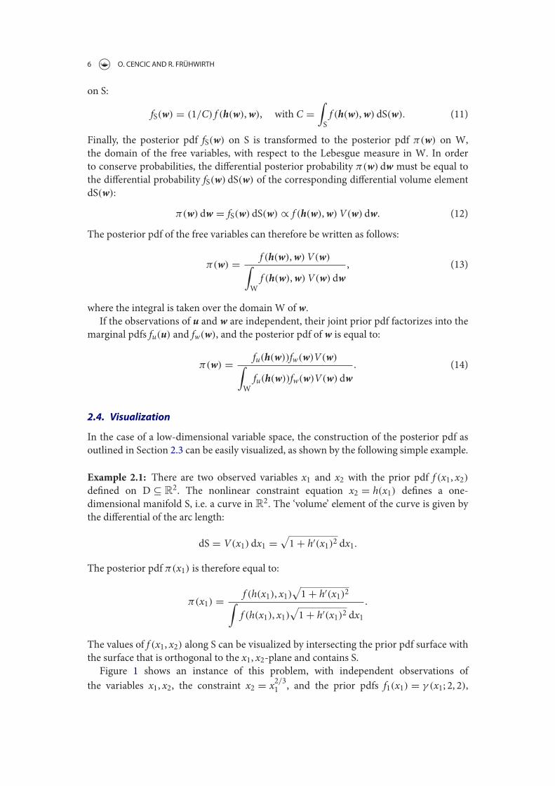
6 O. CENCIC AND R. FRÜHWIRTH
on S:
fS(w) = (1/C) f (h(w),w), with C =∫Sf (h(w),w) dS(w). (11)
Finally, the posterior pdf fS(w) on S is transformed to the posterior pdf π(w) on W,the domain of the free variables, with respect to the Lebesgue measure in W. In orderto conserve probabilities, the differential posterior probability π(w) dw must be equal tothe differential probability fS(w) dS(w) of the corresponding differential volume elementdS(w):
π(w) dw = fS(w) dS(w) ∝ f (h(w),w)V(w) dw. (12)
The posterior pdf of the free variables can therefore be written as follows:
π(w) = f (h(w),w)V(w)∫Wf (h(w),w)V(w) dw
, (13)
where the integral is taken over the domain W of w.If the observations of u and w are independent, their joint prior pdf factorizes into the
marginal pdfs fu(u) and fw(w), and the posterior pdf of w is equal to:
π(w) = fu(h(w))fw(w)V(w)∫Wfu(h(w))fw(w)V(w) dw
. (14)
2.4. Visualization
In the case of a low-dimensional variable space, the construction of the posterior pdf asoutlined in Section 2.3 can be easily visualized, as shown by the following simple example.
Example 2.1: There are two observed variables x1 and x2 with the prior pdf f (x1, x2)defined on D ⊆ R
2. The nonlinear constraint equation x2 = h(x1) defines a one-dimensional manifold S, i.e. a curve in R
2. The ‘volume’ element of the curve is given bythe differential of the arc length:
dS = V(x1) dx1 =√1 + h′(x1)2 dx1.
The posterior pdf π(x1) is therefore equal to:
π(x1) = f (h(x1), x1)√1 + h′(x1)2∫
f (h(x1), x1)√1 + h′(x1)2 dx1
.
The values of f (x1, x2) along S can be visualized by intersecting the prior pdf surface withthe surface that is orthogonal to the x1, x2-plane and contains S.
Figure 1 shows an instance of this problem, with independent observations ofthe variables x1, x2, the constraint x2 = x2/31 , and the prior pdfs f1(x1) = γ (x1; 2, 2),
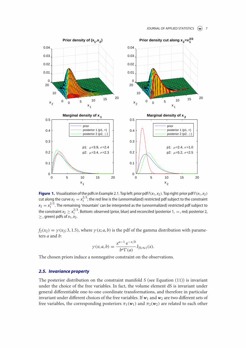
JOURNAL OF APPLIED STATISTICS 7
0
0.01
20
0.02
0.03
0.04
x2
10
Prior density of (x1,x2)
20
x1
15100 50
0
0.01
20
0.02
0.03
0.04
x2
10
Prior density cut along x2=x12/3
20
x1
15100 50
0 5 10 15 20
x1
0
0.1
0.2
0.3
0.4
0.5Marginal density of x 1
p1: =3.9, =2.4
p2: =3.4, =2.3
priorposterior 1 (p1, =)posterior 2 (p2, )
0 5 10 15 20
x2
0
0.1
0.2
0.3
0.4
0.5Marginal density of x 2
p1: =2.4, =1.0
p2: =5.2, =2.5
priorposterior 1 (p1, =)posterior 2 (p2, )
Figure 1. Visualizationof thepdfs in Example 2.1. Top left: prior pdf f (x1, x2). Top right: prior pdf f (x1, x2)cut along the curve x2 = x2/31 ; the red line is the (unnormalized) restricted pdf subject to the constraint
x2 = x2/31 . The remaining ‘mountain’ can be interpreted as the (unnormalized) restricted pdf subject to
the constraint x2 ≥ x2/31 . Bottom: observed (prior, blue) and reconciled (posterior 1, = , red; posterior 2,≥ , green) pdfs of x1, x2.
f2(x2) = γ (x2; 3, 1.5), where γ (x; a, b) is the pdf of the gamma distribution with parame-ters a and b:
γ (x; a, b) = xa−1 e−x/b
ba�(a)I[0,∞)(x).
The chosen priors induce a nonnegative constraint on the observations.
2.5. Invariance property
The posterior distribution on the constraint manifold S (see Equation (11)) is invariantunder the choice of the free variables. In fact, the volume element dS is invariant undergeneral differentiable one-to-one coordinate transformations, and therefore in particularinvariant under different choices of the free variables. If w1 and w2 are two different sets offree variables, the corresponding posteriors π1(w1) and π2(w2) are related to each other
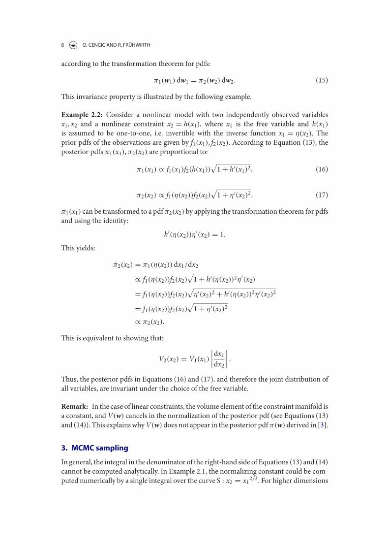
8 O. CENCIC AND R. FRÜHWIRTH
according to the transformation theorem for pdfs:
π1(w1) dw1 = π2(w2) dw2. (15)
This invariance property is illustrated by the following example.
Example 2.2: Consider a nonlinear model with two independently observed variablesx1, x2 and a nonlinear constraint x2 = h(x1), where x1 is the free variable and h(x1)is assumed to be one-to-one, i.e. invertible with the inverse function x1 = η(x2). Theprior pdfs of the observations are given by f1(x1), f2(x2). According to Equation (13), theposterior pdfs π1(x1),π2(x2) are proportional to:
π1(x1) ∝ f1(x1)f2(h(x1))√1 + h′(x1)2, (16)
π2(x2) ∝ f1(η(x2))f2(x2)√1 + η′(x2)2. (17)
π1(x1) can be transformed to a pdf π2(x2) by applying the transformation theorem for pdfsand using the identity:
h′(η(x2))η′(x2) = 1.
This yields:
π2(x2) = π1(η(x2)) dx1/dx2
∝ f1(η(x2))f2(x2)√1 + h′(η(x2))2η′(x2)
= f1(η(x2))f2(x2)√
η′(x2)2 + h′(η(x2))2η′(x2)2
= f1(η(x2))f2(x2)√1 + η′(x2)2
∝ π2(x2).
This is equivalent to showing that:
V2(x2) = V1(x1)∣∣∣∣dx1dx2
∣∣∣∣ .Thus, the posterior pdfs in Equations (16) and (17), and therefore the joint distribution ofall variables, are invariant under the choice of the free variable.
Remark: In the case of linear constraints, the volume element of the constraintmanifold isa constant, and V(w) cancels in the normalization of the posterior pdf (see Equations (13)and (14)). This explains whyV(w) does not appear in the posterior pdfπ(w) derived in [3].
3. MCMC sampling
In general, the integral in the denominator of the right-hand side of Equations (13) and (14)cannot be computed analytically. In Example 2.1, the normalizing constant could be com-puted numerically by a single integral over the curve S : x2 = x12/3. For higher dimensions
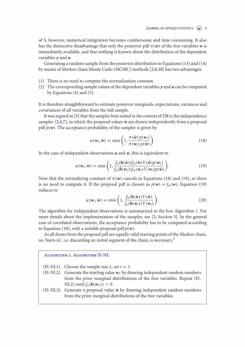
JOURNAL OF APPLIED STATISTICS 9
of S, however, numerical integration becomes cumbersome and time consuming. It alsohas the distinctive disadvantage that only the posterior pdf π(w) of the free variables w isimmediately available, and that nothing is known about the distribution of the dependentvariables y and u.
Generating a random sample from the posterior distribution in Equations (13) and (14)by means of Markov chainMonte Carlo (MCMC)methods [2,8,18] has two advantages:
(1) There is no need to compute the normalization constant.(2) The corresponding sample values of the dependent variables y and u can be computed
by Equations (4) and (5).
It is therefore straightforward to estimate posterior marginals, expectations, variances andcovariances of all variables from the full sample.
It was argued in [3] that the sampler best suited to the context of DR is the independencesampler [2,4,7], in which the proposal values w are drawn independently from a proposalpdf p(w). The acceptance probability of the sampler is given by
α(wi, w) = min(1,
π(w) p(wi)
π(wi) p(w)
). (18)
In the case of independent observations u and w, this is equivalent to
α(wi, w) = min(1,
fu(h(w))fw(w)V(w)p(wi)
fu(h(wi))fw(wi)V(wi)p(w)
). (19)
Note that the normalizing constant of π(w) cancels in Equations (18) and (19), so thereis no need to compute it. If the proposal pdf is chosen as p(w) = fw(w), Equation (19)reduces to
α(wi, w) = min(1,
fu(h(w))V(w)
fu(h(wi))V(wi)
). (20)
The algorithm for independent observations is summarized in the box Algorithm 1. Formore details about the implementation of the sampler, see [3, Section 3]. In the generalcase of correlated observations, the acceptance probability has to be computed accordingto Equation (18), with a suitable proposal pdf p(w).
As all draws from the proposal pdf are equally valid starting points of theMarkov chain,no ‘burn-in’, i.e. discarding an initial segment of the chain, is necessary.3
Algorithm 1. Algorithm IS-NL
(IS-NL1). Choose the sample size L, set i = 1.(IS-NL2). Generate the starting valuew1 by drawing independent random numbers
from the prior marginal distributions of the free variables. Repeat (IS-NL2) until fu(h(w1)) > 0.
(IS-NL3). Generate a proposal value w by drawing independent random numbersfrom the prior marginal distributions of the free variables.
10 O. CENCIC AND R. FRÜHWIRTH
(IS-NL4). Compute the acceptance probability α according to Eq. (20).(IS-NL5). Draw a uniform random number ξ ∈ [0, 1].(IS-NL6). If ξ ≤ α, accept the proposal and set wi+1 = w, otherwise set wi+1 = wi.(IS-NL7). Increase i by 1. If i < L, go to (IS-NL3), otherwise stop sampling.
Remark: If a large number of variables is involved, the numerator and/or the denominatorof Equation (20)may fall belowmachine precision. This can be circumvented by taking thelogarithms of both sides of the equations and accepting when log ξ ≤ logα.
The proposal values W = (w1, w2, . . . , wL) and the corresponding values of U =(u1, u2, . . . , uL) and Y = (y1, y2, . . . , yL) can be precomputed via ui = h(wi) and yi =k(wi), respectively, for i = 1, . . . , L (see Equations (4) and (5)). As the proposal valuesare independent, their computation can be easily parallelized. After the sampler has fin-ished, the final Markov chain (Y ;U ;W) can then be used to estimate posterior quantitiessuch as means, variances, quantiles and correlations of all variables, both observed andunobserved. For a graphical representation of the posterior distributions, the marginalpdfs can be estimated from the Markov chain by a kernel estimator [20] or obtained bysmoothing the normalized frequency distribution in a histogram. For more details aboutthe acceptance rate and the posterior analysis, see [3].
By construction, all individual elementsmi = (yi; ui;wi) of theMarkov chain satisfy thenonlinear constraints, but the sample mean in general does not. If a representative value ofthe posterior distribution satisfying the constraints is required, the element of the Markovchain with the smallest distance from the sample mean, the sample median or the sam-ple mode can be selected. The multivariate sample mode is, however, notoriously difficultto compute, and there are different ways to define a multivariate median [12]. Thus, theelement closest to the sample mean turns out to be virtually the only practical possibility.
4. Applications
The two examples in this section show the application of the independence sampler toMFAand chemical engineering. TheMATLAB code used for the examples can be obtained fromthe authors on request.
In both examples we assume that there is independent prior information for each of theobserved variables. The prior pdf displays the initial knowledge about the variable. Thisknowledge can be objective, being the model of a measurement process, or it can be sub-jective, being the expression of an expert opinion via a pdf. The mode of the prior pdfrepresents the most probable or most credible value of the variable before imposing theconstraints. Similarly, the mode of the posterior pdf represents the most probable or cred-ible value after imposing the constraints. Note that even if the observations are assumedto be independent a priori, all variables are correlated a posteriori. A comparison of theprior and the posterior marginal pdfs shows that the uncertainty of the observed vari-ables is reduced: standard deviations become smaller, HPD intervals become shorter. Bothexamples additionally contain unobserved variables. Although they have no prior pdfs,their posterior marginal pdfs are estimated from the Markov chain of the free variables.
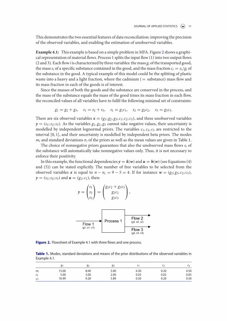
JOURNAL OF APPLIED STATISTICS 11
This demonstrates the two essential features of data reconciliation: improving the precisionof the observed variables, and enabling the estimation of unobserved variables.
Example 4.1: This example is based on a simple problem inMFA. Figure 2 shows a graphi-cal representation ofmaterial flows. Process 1 splits the input flow (1) into two output flows(2 and 3). Each flow i is characterized by three variables: themass gi of the transported good,themass si of a specific substance contained in the good, and themass fraction ci = si/gi ofthe substance in the good. A typical example of this model could be the splitting of plasticwaste into a heavy and a light fraction, where the cadmium (= substance) mass flow andits mass fraction in each of the goods is of interest.
Since the masses of both the goods and the substance are conserved in the process, andthe mass of the substance equals the mass of the good times its mass fraction in each flow,the reconciled values of all variables have to fulfil the following minimal set of constraints:
g1 = g2 + g3, s1 = s2 + s3, s1 = g1c1, s2 = g2c2, s3 = g3c3.
There are six observed variables x = (g1; g2, g3; c1; c2; c3), and three unobserved variablesy = (s1; s2; s3). As the variables g1, g2, g3 cannot take negative values, their uncertainty ismodelled by independent lognormal priors. The variables c1, c2, c3 are restricted to theinterval [0, 1], and their uncertainty is modelled by independent beta priors. The modesmi and standard deviations σi of the priors as well as the mean values are given in Table 1.
The choice of nonnegative priors guarantees that also the unobserved mass flows si ofthe substance will automatically take nonnegative values only. Thus, it is not necessary toenforce their positivity.
In this example, the functional dependencies y = k(w) and u = h(w) (see Equations (4)and (5)) can be stated explicitly. The number of free variables to be selected from theobserved variables x is equal to n − nc = 9 − 5 = 4. If for instance w = (g2; g3; c2; c3),y = (s1; s2; s3) and u = (g1; c1), then:
y =⎛⎝s1s2s3
⎞⎠ =
⎛⎝g2c2 + g3c3
g2c2g3c3
⎞⎠ ,
Figure 2. Flowsheet of Example 4.1 with three flows and one process.
Table 1. Modes, standard deviations and means of the prior distributions of the observed variables inExample 4.1.
g1 g2 g3 c1 c2 c3
mi 15.00 8.00 5.00 0.30 0.20 0.50σi 5.00 3.00 2.00 0.03 0.02 0.05μi 16.99 9.28 5.89 0.30 0.20 0.50
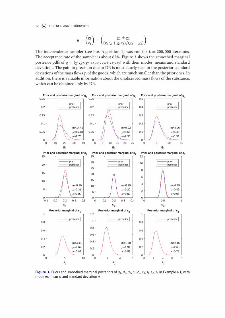
12 O. CENCIC AND R. FRÜHWIRTH
u =(g1c1
)=
(g2 + g3
(g2c2 + g3c3)/(g2 + g3)
).
The independence sampler (see box Algorithm 1) was run for L = 200, 000 iterations.The acceptance rate of the sampler is about 62%. Figure 3 shows the smoothed marginalposterior pdfs of q = (g1; g2; g3; c1; c2; c3; s1; s2; s3) with their modes, means and standarddeviations. The gain in precision due to DR is most clearly seen in the posterior standarddeviations of themass flows gi of the goods, which aremuch smaller than the prior ones. Inaddition, there is valuable information about the unobserved mass flows of the substance,which can be obtained only by DR.
0 10 20 30 40
g1
0
0.05
0.1
0.15
0.2
0.25Prior and posterior marginal of g1
m=14.43
=15.13
=2.76
priorposterior
0 5 10 15 20 25
g2
0
0.05
0.1
0.15
0.2
0.25Prior and posterior marginal of g2
m=9.02
=9.65
=2.30
priorposterior
0 5 10 15
g3
0
0.1
0.2
0.3
0.4
0.5Prior and posterior marginal of g3
m=4.96
=5.48
=1.51
priorposterior
0.1 0.2 0.3 0.4 0.5
c1
0
5
10
15
20
25Prior and posterior marginal of c1
m=0.30
=0.31
=0.02
priorposterior
0 0.1 0.2 0.3 0.4
c2
0
5
10
15
20
25
30
35Prior and posterior marginal of c2
m=0.20
=0.20
=0.02
priorposterior
0 0.5 1
c3
0
2
4
6
8
10
12Prior and posterior marginal of c3
m=0.49
=0.49
=0.05
priorposterior
0 5 10
s1
0
0.2
0.4
0.6
0.8
1Posterior marginal of s1
m=4.41
=4.62
=0.89
posterior
0 2 4 6
s2
0
0.2
0.4
0.6
0.8
1
1.2Posterior marginal of s2
m=1.78
=1.94
=0.53
posterior
0 2 4 6 8
s3
0
0.2
0.4
0.6
0.8
1Posterior marginal of s3
m=2.46
=2.68
=0.71
posterior
Figure 3. Priors and smoothed marginal posteriors of g1, g2, g3, c1, c2, c3, s1, s2, s3 in Example 4.1, withmodem, meanμ and standard deviation σ .
JOURNAL OF APPLIED STATISTICS 13
Table 2. Sample mean q and sample value qmin that is closest to the sample mean as measured by theL2 distance.
Variable g1 g2 g3 c1 c2 c3 s1 s2 s3
q 15.13 9.65 5.48 0.31 0.20 0.49 4.62 1.94 2.68qmin 15.12 9.65 5.46 0.31 0.20 0.50 4.67 1.94 2.73
The sample mean q and the sample value qmin that is closest to the sample mean, asmeasured by the L2 distance, are given in Table 2.
Example 4.2: The second example uses the system of nonlinear constraints analysedin [14], which is a commonly used benchmark example4 for nonlinear data reconciliationwith normally distributed observation errors:
G1(y; x) = 0.5x21 − 0.7x2 + x3y1 + x22y1y2 + 2x3y23 − 255.8 = 0,
G2(y; x) = x1 − 2x2 + 3x1x3 − 2x2y1 − x2y2y3 + 111.2 = 0,
G3(y; x) = x3y1 − x1 + 3x2 + x1y2 − x3y0.53 − 33.57 = 0,
G4(y; x) = x4 − x1 − x23 + y2 + 3y3 = 0,
G5(y; x) = x5 − 2x3y2y3 = 0,
G6(y; x) = 2x1 + x2x3y1 + y2 − y3 − 126.6 = 0.
The variables x = (x1; x2; x3; x4; x5) are observed with the following values:
x = (4.4; 5.5; 1.7; 1.6; 5)
and the covariance matrix � = I. Although the context of the model is not stated in [14],we assume that all variables have to be nonnegative. The prior of the observation xi isassumed to be the lognormal pdf with mean xi and standard deviation σi = 1, for i =1, . . . , 5. Assuming the observations to be independent, the joint prior is the product ofthe individual priors. The unobserved variables y = (y1; y2; y3) can be forced to be non-negative by assigning them an improper constant prior on [0,∞); however, this turns outto be unnecessary.
If the two free variables are chosen as w = (x1; x2), the three dependent observed vari-ables are equal to u = (x3; x4; x5). For given w, the functions u = h(w) and y = k(w)
(see Equations (4) and (5)) are computed by minimizing ‖G(y; u;w)‖2, using the simplexalgorithm [11] with restart. The starting point of the minimization is equal to (y; x), where
y = argminy
‖G(y; x)‖2.
The JacobianH(w) = ∂h(w)/∂w is computed by numerical differentiation.The independence sampler was run for L = 200,000 iterations, with an acceptance rate
of about 13%. The posterior pdfs are shown in Figure 4. Clear deviations from normalitycan be observed. The reconciled values of x and y given in [14] are very close to the pos-terior modes. The posterior standard deviations of the observed values are significantlysmaller than 1, showing again the gain in precision due to data reconciliation.
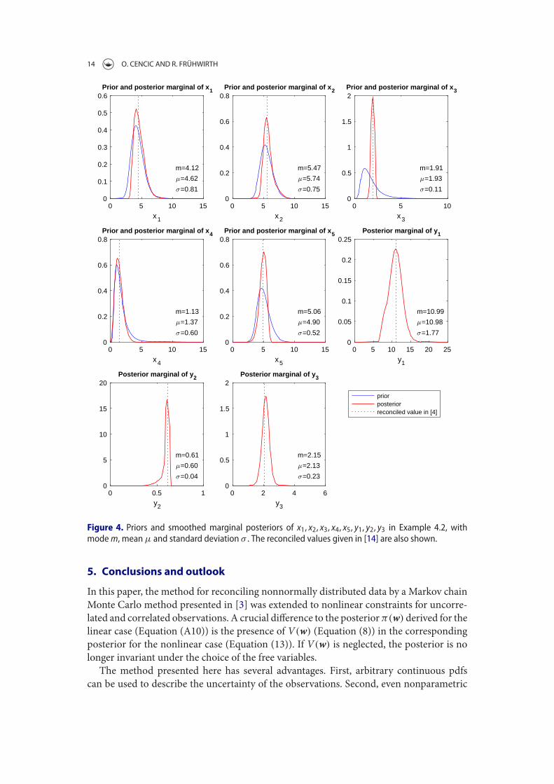
14 O. CENCIC AND R. FRÜHWIRTH
0 5 10 15
x1
0
0.1
0.2
0.3
0.4
0.5
0.6Prior and posterior marginal of x1
m=4.12
=4.62
=0.81
0 5 10 15
x2
0
0.2
0.4
0.6
0.8Prior and posterior marginal of x2
m=5.47
=5.74
=0.75
0 5 10
x3
0
0.5
1
1.5
2Prior and posterior marginal of x3
m=1.91
=1.93
=0.11
0 5 10 15
x4
0
0.2
0.4
0.6
0.8Prior and posterior marginal of x4
m=1.13
=1.37
=0.60
0 5 10 15
x5
0
0.2
0.4
0.6
0.8Prior and posterior marginal of x5
m=5.06
=4.90
=0.52
0 5 10 15 20 25
y1
0
0.05
0.1
0.15
0.2
0.25Posterior marginal of y1
m=10.99
=10.98
=1.77
0 0.5 1
y2
0
5
10
15
20Posterior marginal of y2
m=0.61
=0.60
=0.04
0 2 4 6
y3
0
0.5
1
1.5
2Posterior marginal of y3
m=2.15
=2.13
=0.23
priorposteriorreconciled value in [4]
Figure 4. Priors and smoothed marginal posteriors of x1, x2, x3, x4, x5, y1, y2, y3 in Example 4.2, withmodem, meanμ and standard deviation σ . The reconciled values given in [14] are also shown.
5. Conclusions and outlook
In this paper, the method for reconciling nonnormally distributed data by a Markov chainMonte Carlo method presented in [3] was extended to nonlinear constraints for uncorre-lated and correlated observations. A crucial difference to the posteriorπ(w) derived for thelinear case (Equation (A10)) is the presence of V(w) (Equation (8)) in the correspondingposterior for the nonlinear case (Equation (13)). If V(w) is neglected, the posterior is nolonger invariant under the choice of the free variables.
The method presented here has several advantages. First, arbitrary continuous pdfscan be used to describe the uncertainty of the observations. Second, even nonparametric
JOURNAL OF APPLIED STATISTICS 15
estimators of the pdf are allowed, provided that it is possible to draw a random sample fromthem. Third, not only means, variances and covariances of observed and unobserved vari-ables can be computed a posteriori, but also various other characteristics of the marginalposteriors, such as the mode, skewness, quantiles, and HPD intervals.
In some systems of nonlinear constraints not all choices of free variables lead to fea-sible solutions for the dependent variables. If this is the case, we propose to permute thepositions of the free variables randomly and repeat the calculations until a feasible solutionis reached. In large and complex models this may lead to an unacceptable combinatorialoverhead. A general procedure for finding a suitable set of free variables therefore remainsan important open question for further research.
The procedure developed in this paper for DR with nonlinear constraints can alsobe applied to linear constraints. Thus, it is not necessary to assume improper priors forunobserved variables, as was proposed in [3].
Beyond their statistical uncertainty, the observations may also be corrupted by grosserrors such as biased observations or faulty readings.Work is already in progress to developa robustification of the DR procedure by automatic identification of outlying or erroneousobservations that prevent a successful reconciliation.
In subsequent work, the method will be applied to a more extensive real-world examplein order to compare the results to alternative approaches such as classical weighted leastsquares and fuzzy sets.
Notes
1. The comma (semicolon) denotes horizontal (vertical) concatenation of vectors and matrices(Matlab convention).
2. See, however, the discussion of constraints versus priors in [21].3. This has been argued by C. Geyer on his website, see http://users.stat.umn.edu/ geyer/mcmc/
burn.html. Last accessed on January 2, 2018.4. See ‘Citing literature’ on http://onlinelibrary.wiley.com/doi/10.1002/aic.690340521/abstract.
Last accessed on January 2, 2018.
Acknowledgments
We thank Nada Dzubur, Manuel Hahn, David Laner and Oliver Schwab for their useful commentson the manuscript. We also thank the editor and the anonymous reviewers for their comments,suggestions and corrections, which have greatly improved themanuscript. The authors acknowledgethe TUWien University Library for financial support through its Open Access Funding Program.
Disclosure statement
No potential conflict of interest was reported by the authors.
References
[1] V.B. Barbosa Jr, M.R.M. Wolf, and R.M. Fo, Development of data reconciliation for dynamicnonlinear system: Application the polymerization reactor, Comput. Chem. Eng. 24 (2000), pp.501–506.
[2] S. Brooks, A. Gelman, G.L. Jones, and X.-L. Meng (eds.), Handbook of Markov Chain MonteCarlo, Chapman & Hall, Boca Raton, FL, 2011.
16 O. CENCIC AND R. FRÜHWIRTH
[3] O. Cencic and R. Frühwirth, A general framework for data reconciliation – Part I: Linearconstraints, Comput. Chem. Eng. 75 (2015), pp. 196–208.
[4] S. Chib and E. Greenberg, Understanding the metropolis–hastings algorithm, Am. Stat. 49(1995), pp. 327–335.
[5] L.R. Foulds, Optimization Techniques: An Introduction, Springer, New York, 1981.[6] P.E. Gill, W. Murray, andM.H.Wright, Practical Optimization, Academic Press, London, 2000.[7] J.S. Liu,Metropolized independent sampling with comparisons to rejection sampling and impor-
tance sampling, Stat. Comput. 6 (1996), pp. 113–119.[8] J.S. Liu,Monte Carlo Strategies in Scientific Computing, Springer, New York, 2004.[9] F. Madron, Process Plant Performance, Ellis Horwood, New York, 1992.[10] F. Madron, V. Veverka, and V. Venecek, Statistical analysis of material balance of a chemical
reactor, AIChE J. 23 (1977), pp. 482–486.[11] J.A. Nelder and R. Mead, A simplex method for function minimization, Comput. J. 7 (1965), pp.
308–313.[12] H. Oja, Multivariate median, in Robustness and Complex Data Structures, C. Becker, R. Fried,
and S. Kuhnt, eds., Springer, Berlin, 2013.[13] B. O’Neill, Semi-Riemannian Geometry, Academic Press, San Diego, CA, 1983.[14] C.C.D. Pai and G.D. Fisher, Application of Broyden’s method to reconciliation of nonlinearly
constrained data, AIChE J. 34 (1988), pp. 873–876.[15] X. Pennec, Probabilities and Statistics on Riemannian Manifolds: Basic Tools for Geomet-
ric Measurements, In Proceedings of the IEEE-EURASIP Workshop on Nonlinear Signaland Image Processing (NSIP ’99), Vol. 1. Bogaziçi University, Istanbul, Turkey, 1999, pp.194–198. Available at http://www-sop.inria.fr/asclepios/Publications/Xavier.Pennec/Pennec.NSIP99.pdf (last accessed on January 2, 2018).
[16] X. Pennec, Probabilities and statistics on Riemannian manifolds: A geometric approach, Tech.Rep. RR-5093, INRIA, January 2004. Available at https://hal.inria.fr/inria-00071490/document(last accessed on January 2, 2018).
[17] W.-D. Richter, L. Strelec, H. Ahmadinezhad, andM. Stehlik, Geometric aspects of robust testingfor normality and sphericity, Stoch. Anal. Appl. 35 (2017), pp. 511–532.
[18] C. Robert and C. Casella,Monte Carlo Statistical Methods, Springer, New York, 2004.[19] J.A. Romagnoli and M.C. Sanchez, Data Processing and Reconciliation for Chemical Process
Operations, Academic Press, San Diego, 2000.[20] B.W. Silverman, Density Estimation for Statistics and Data Analysis, Chapman & Hall/CRC,
London, 1998.[21] P.B. Stark, Constraints versus Priors, SIAM/ASA J Uncertain Quantif. 3 (2015), pp. 586–598.[22] P.Whittle,Optimization under Constraints: Theory andApplications of Nonlinear Programming,
Wiley-Interscience, London, 1971.[23] W.Wongrat, T. Srinophakun, and P. Srinophakun,Modified genetic algorithm for nonlinear data
reconciliation, Comput. Chem. Eng. 29 (2005), pp. 1059–1067.
Appendix. Proof of equivalence with linear constraints
For the case of normally distributed independent observations and linear constraints, it was provedin [3] that the unbiased estimate of the expectationμπ of π(w) is equal to the least-squares solutionw. Here, the proof is generalized to correlated observations.
Consider a system of nc linear constraint equations:
G(y; x) = By + Ax + c = 0, (A1)
where x is the vector of observed variables of dimension nx × 1, y is the vector of unobserved vari-ables of dimension ny × 1, c is a constant vector of dimension nc × 1, and A and B are knownmatrices of dimensionnc × nx andnc × ny, respectively. The system is assumed to have the followingproperties:
(A1) rank(B,A) = rank(B,A, c), meaning the system has at least one solution;
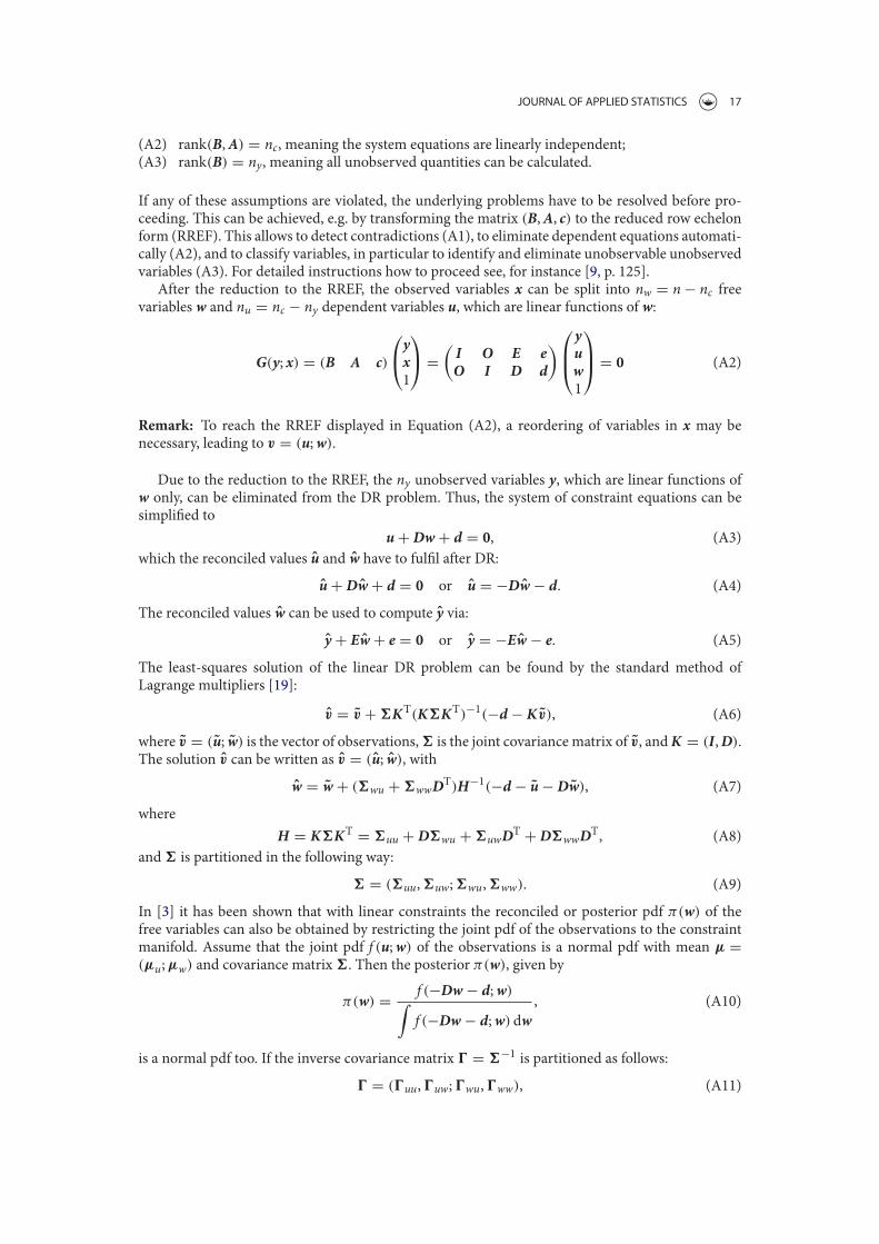
JOURNAL OF APPLIED STATISTICS 17
(A2) rank(B,A) = nc, meaning the system equations are linearly independent;(A3) rank(B) = ny, meaning all unobserved quantities can be calculated.
If any of these assumptions are violated, the underlying problems have to be resolved before pro-ceeding. This can be achieved, e.g. by transforming the matrix (B,A, c) to the reduced row echelonform (RREF). This allows to detect contradictions (A1), to eliminate dependent equations automati-cally (A2), and to classify variables, in particular to identify and eliminate unobservable unobservedvariables (A3). For detailed instructions how to proceed see, for instance [9, p. 125].
After the reduction to the RREF, the observed variables x can be split into nw = n − nc freevariables w and nu = nc − ny dependent variables u, which are linear functions of w:
G(y; x) = (B A c)
⎛⎝yx1
⎞⎠ =
(I O E eO I D d
) ⎛⎜⎝yuw1
⎞⎟⎠ = 0 (A2)
Remark: To reach the RREF displayed in Equation (A2), a reordering of variables in x may benecessary, leading to v = (u;w).
Due to the reduction to the RREF, the ny unobserved variables y, which are linear functions ofw only, can be eliminated from the DR problem. Thus, the system of constraint equations can besimplified to
u + Dw + d = 0, (A3)which the reconciled values u and w have to fulfil after DR:
u + Dw + d = 0 or u = −Dw − d. (A4)
The reconciled values w can be used to compute y via:
y + Ew + e = 0 or y = −Ew − e. (A5)
The least-squares solution of the linear DR problem can be found by the standard method ofLagrange multipliers [19]:
v = v + �KT(K�KT)−1(−d − Kv), (A6)
where v = (u; w) is the vector of observations,� is the joint covariance matrix of v, andK = (I,D).The solution v can be written as v = (u; w), with
w = w + (�wu + �wwDT)H−1(−d − u − Dw), (A7)
whereH = K�KT = �uu + D�wu + �uwDT + D�wwDT, (A8)
and � is partitioned in the following way:
� = (�uu,�uw;�wu,�ww). (A9)
In [3] it has been shown that with linear constraints the reconciled or posterior pdf π(w) of thefree variables can also be obtained by restricting the joint pdf of the observations to the constraintmanifold. Assume that the joint pdf f (u;w) of the observations is a normal pdf with mean μ =(μu;μw) and covariance matrix �. Then the posterior π(w), given by
π(w) = f (−Dw − d;w)∫f (−Dw − d;w) dw
, (A10)
is a normal pdf too. If the inverse covariance matrix � = �−1 is partitioned as follows:
� = (�uu,�uw;�wu,�ww), (A11)
18 O. CENCIC AND R. FRÜHWIRTH
the quadratic form Q(w) in the exponent of π(w):
Q(w) = [(−Dw − d;w) − (μu;μw)]T� [(−Dw − d;w) − (μu;μw)], (A12)
can be written in the following form:
Q(w) = wT(DT�uuD − DT�uw − �wuD + �ww)w
− 2wT[(�ww − DT�uw)μw + (�wu − DT�uu)(d + μu)] + const. (A13)
π(w) is therefore the pdf of the normal distribution with inverse covariance matrix C and mean μπ
given by
C = DT�uuD − DT�uw − �wuD + �ww, (A14)
μπ = C−1[(�ww − DT�uw)μw + (�wu − DT�uu)(d + μu)]. (A15)
μπ can be expanded and rearranged in the following form:
μπ = μw + C−1(�wu − DT�uu)(d + μu + Dμw). (A16)
Its unbiased estimator μπ is obtained by replacing μu and μw by the observations u and w,respectively:
μπ = w + C−1(�wu − DT�uu)(d + u + Dw). (A17)A comparison with w in Equation (A7) shows that
μπ = w ⇐⇒ C−1(�wu − DT�uu) = −(�wu + �wwDT)H−1
⇐⇒ (�wu − DT�uu)H + C(�wu + �wwDT) = O. (A18)
Expansion of the products while taking into account the symmetry of � and � along with therelations:
�uu�uu + �uw�wu = I,
�uu�uw + �uw�ww = O,
�wu�uu + �ww�wu = O,
�wu�uw + �ww�ww = I
(A19)
shows that indeed μπ = w.