Embed Size (px)
Citation preview
Journal of Machine Learning Research 22 (2021) 1-55 Submitted 11/17; Published 1/21
Domain Generalization by Marginal Transfer Learning
Gilles Blanchard [email protected] Paris-Saclay, CNRS, Inria, Laboratoire de mathematiques d’Orsay
Aniket Anand Deshmukh [email protected] AI & Research
Urun Dogan [email protected] AI & Research
Gyemin Lee [email protected]. Electronic and IT Media EngineeringSeoul National University of Science and Technology
Clayton Scott [email protected]
Electrical and Computer Engineering, Statistics
University of Michigan
Editor: Arthur Gretton
Abstract
In the problem of domain generalization (DG), there are labeled training data sets fromseveral related prediction problems, and the goal is to make accurate predictions on futureunlabeled data sets that are not known to the learner. This problem arises in several ap-plications where data distributions fluctuate because of environmental, technical, or othersources of variation. We introduce a formal framework for DG, and argue that it can beviewed as a kind of supervised learning problem by augmenting the original feature spacewith the marginal distribution of feature vectors. While our framework has several con-nections to conventional analysis of supervised learning algorithms, several unique aspectsof DG require new methods of analysis.
This work lays the learning theoretic foundations of domain generalization, building onour earlier conference paper where the problem of DG was introduced (Blanchard et al.,2011). We present two formal models of data generation, corresponding notions of risk, anddistribution-free generalization error analysis. By focusing our attention on kernel meth-ods, we also provide more quantitative results and a universally consistent algorithm. Anefficient implementation is provided for this algorithm, which is experimentally comparedto a pooling strategy on one synthetic and three real-world data sets.
Keywords: domain generalization, generalization error bounds, Rademacher complexity,kernel methods, universal consistency, kernel approximation
1. Introduction
Domain generalization (DG) is a machine learning problem where the learner has access tolabeled training data sets from several related prediction problems, and must generalize toa future prediction problem for which no labeled data are available. In more detail, thereare N labeled training data sets Si = (Xij , Yij)1≤j≤ni , i = 1, . . . , N , that describe similarbut possibly distinct prediction tasks. The objective is to learn a rule that takes as input
c©2021 Gilles Blanchard, Aniket Anand Deshmukh, Urun Dogan, Gyemin Lee and Clayton Scott.
License: CC-BY 4.0, see https://creativecommons.org/licenses/by/4.0/. Attribution requirements are providedat http://jmlr.org/papers/v22/17-679.html.
Blanchard, Deshmukh, Dogan, Lee and Scott
a previously unseen unlabeled test data set XT1 , . . . , X
TnT
, and accurately predicts outcomesfor these or possibly other unlabeled points drawn from the associated learning task.
DG arises in several applications. One prominent example is precision medicine, wherea common objective is to design a patient-specific classifier (e.g., of health status) basedon clinical measurements, such as an electrocardiogram or electroencephalogram. In suchmeasurements, patient-to-patient variation is common, arising from biological variationsbetween patients, or technical or environmental factors influencing data acquisition. Be-cause of patient-to-patient variation, a classifier that is trained on data from one patientmay not be well matched to another patient. In this context, domain generalization enablesthe transfer of knowledge from historical patients (for whom labeled data are available) to anew patient without the need to acquire training labels for that patient. A detailed examplein the context of flow cytometry is given below.
We view domain generalization as a conventional supervised learning problem wherethe original feature space is augmented to include the marginal distribution generating thefeatures. We refer to this reframing of DG as “marginal transfer learning,” because it reflectsthe fact that in DG, information about the test task must be drawn from that task’s marginalfeature distribution. Leveraging this perspective, we formulate two statistical frameworksfor analyzing DG. The first framework allows the observations within each data set tohave arbitrary dependency structure, and makes connections to the literature on Campbellmeasures and structured prediction. The second framework is a special case of the first,assuming the data points are drawn i.i.d. within each task, and allows for a more refinedrisk analysis.
We further develop a distribution-free kernel machine that employs a kernel on theaforementioned augmented feature space. Our methodology is shown to yield a universallyconsistent learning procedure under both statistical frameworks, meaning that the domaingeneralization risk tends to the best possible value as the relevant sample sizes tend infinity,with no assumptions on the data generating distributions. Although DG may be viewed asa conventional supervised learning problem on an augmented feature space, the analysis isnontrivial owing to unique aspects of the sampling plans and risks. We offer a computation-ally efficient and freely available implementation of our algorithm, and present a thoroughexperimental study validating the proposed approach on one synthetic and three real-worlddata sets, including comparisons to a simple pooling approach.1
To our knowledge, the problem of domain generalization was first proposed and studiedby our earlier conference publication (Blanchard et al., 2011) which this work extendsin several ways. It adds (1) a new statistical framework, the agnostic generative modeldescribed below; (2) generalization error and consistency results for the new statisticalmodel; (3) an extensive literature review; (4) an extension to the regression setting inboth theory and experiments; (5) a more general statistical analysis, in particular, we nolonger assume a bounded loss, and therefore accommodate common convex losses such asthe hinge and logistic losses; (6) extensive experiments (the conference paper considered asingle small data set); (7) a scalable implementation based on a novel extension of randomFourier features; and (8) error analysis for the random Fourier features approximation.
1. Code is available at https://github.com/aniketde/DomainGeneralizationMarginal.
2
Domain Generalization by Marginal Transfer Learning
2. Motivating Application: Automatic Gating of Flow Cytometry Data
Flow cytometry is a high-throughput measurement platform that is an important clinicaltool for the diagnosis of blood-related pathologies. This technology allows for quantitativeanalysis of individual cells from a given cell population, derived for example from a bloodsample from a patient. We may think of a flow cytometry data set as a set of d-dimensionalattribute vectors (Xj)1≤j≤n, where n is the number of cells analyzed, and d is the numberof attributes recorded per cell. These attributes pertain to various physical and chemicalproperties of the cell. Thus, a flow cytometry data set may be viewed as a random samplefrom a patient-specific distribution.
Now suppose a pathologist needs to analyze a new (test) patient with data (XTj )1≤j≤nT .
Before proceeding, the pathologist first needs the data set to be “purified” so that only cellsof a certain type are present. For example, lymphocytes are known to be relevant for thediagnosis of leukemia, whereas non-lymphocytes may potentially confound the analysis. Inother words, it is necessary to determine the label Y T
j ∈ −1, 1 associated to each cell,
where Y Tj = 1 indicates that the j-th cell is of the desired type.
In clinical practice this is accomplished through a manual process known as “gating.”The data are visualized through a sequence of two-dimensional scatter plots, where at eachstage a line segment or polygon is manually drawn to eliminate a portion of the unwantedcells. Because of the variability in flow cytometry data, this process is difficult to quantifyin terms of a small subset of simple rules. Instead, it requires domain-specific knowledgeand iterative refinement. Modern clinical laboratories routinely see dozens of cases per day,so it is desirable to automate this process.
Since clinical laboratories maintain historical databases, we can assume access to anumber (N) of historical (training) patients that have already been expert-gated. Because
of biological and technical variations in flow cytometry data, the distributions P(i)XY of
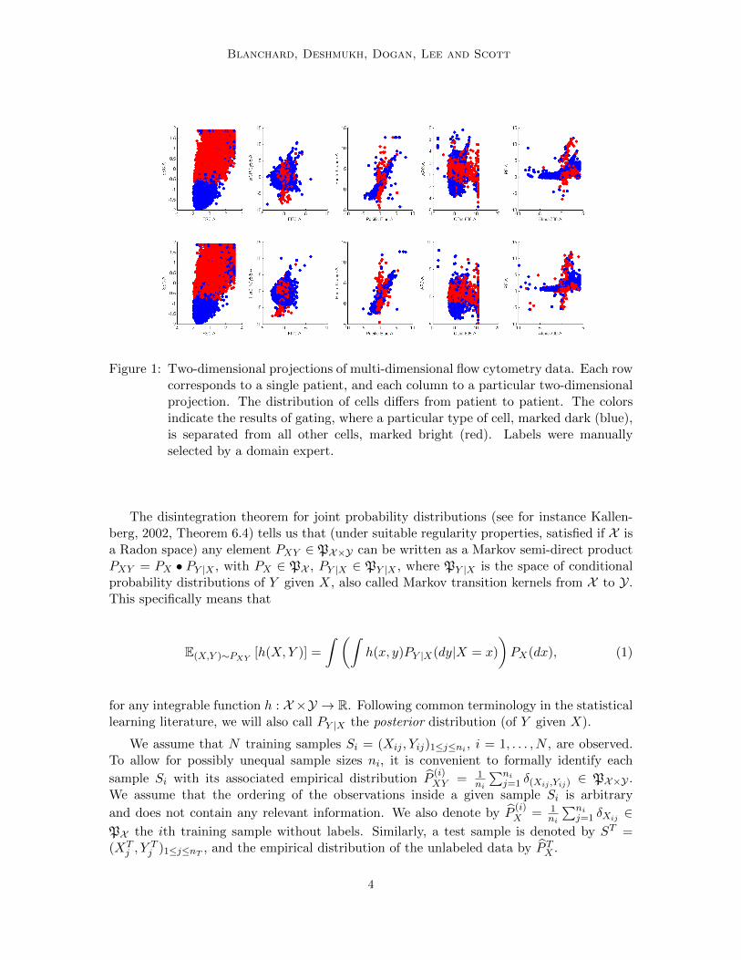
the historical patients will vary. To illustrate the flow cytometry gating problem, we usethe NDD data set from the FlowCap-I challenge.2 For example, Fig. 1 shows exemplarytwo-dimensional scatter plots for two different patients – see caption for details. Despitedifferences in the two distributions, there are also general trends that hold for all patients.Virtually every cell type of interest has a known tendency (e.g., high or low) for mostmeasured attributes. Therefore, it is reasonable to assume that there is an underlyingdistribution (on distributions) governing flow cytometry data sets, that produces roughlysimilar distributions thereby making possible the automation of the gating process.
3. Formal Setting and General Results
In this section we formally define domain generalization via two possible data generationmodels together with associated notions of risk. We also provide a basic generalization errorbound for the first of these data generation models.
Let X denote the observation space (assumed to be a Radon space) and Y ⊆ R theoutput space. Let PX and PX×Y denote the set of probability distributions on X andX × Y, respectively. The spaces PX and PX×Y are endowed with the topology of weakconvergence and the associated Borel σ-algebras.
2. We will revisit this data set in Section 8.5 where details are given.
3
Blanchard, Deshmukh, Dogan, Lee and Scott
Figure 1: Two-dimensional projections of multi-dimensional flow cytometry data. Each rowcorresponds to a single patient, and each column to a particular two-dimensionalprojection. The distribution of cells differs from patient to patient. The colorsindicate the results of gating, where a particular type of cell, marked dark (blue),is separated from all other cells, marked bright (red). Labels were manuallyselected by a domain expert.
The disintegration theorem for joint probability distributions (see for instance Kallen-berg, 2002, Theorem 6.4) tells us that (under suitable regularity properties, satisfied if X isa Radon space) any element PXY ∈ PX×Y can be written as a Markov semi-direct productPXY = PX • PY |X , with PX ∈ PX , PY |X ∈ PY |X , where PY |X is the space of conditionalprobability distributions of Y given X, also called Markov transition kernels from X to Y.This specifically means that
E(X,Y )∼PXY [h(X,Y )] =
∫ (∫h(x, y)PY |X(dy|X = x)
)PX(dx), (1)
for any integrable function h : X ×Y → R. Following common terminology in the statisticallearning literature, we will also call PY |X the posterior distribution (of Y given X).
We assume that N training samples Si = (Xij , Yij)1≤j≤ni , i = 1, . . . , N , are observed.To allow for possibly unequal sample sizes ni, it is convenient to formally identify each
sample Si with its associated empirical distribution P(i)XY = 1
ni
∑nij=1 δ(Xij ,Yij) ∈ PX×Y .
We assume that the ordering of the observations inside a given sample Si is arbitrary
and does not contain any relevant information. We also denote by P(i)X = 1
ni
∑nij=1 δXij ∈
PX the ith training sample without labels. Similarly, a test sample is denoted by ST =(XT
j , YTj )1≤j≤nT , and the empirical distribution of the unlabeled data by P TX .
4

Domain Generalization by Marginal Transfer Learning
3.1 Data Generation Models
We propose two data generation models. The first is more general, and includes the secondas a special case.
Assumption 1 (AGM) There exists a distribution PS on PX×Y such that S1, . . . , SN arei.i.d. realizations from PS.
We call this the agnostic generative model. This is a quite general model in which samples areassumed to be identically distributed and independent of each other, but nothing particularis assumed about the generation mechanism for observations inside a given sample, nor forthe (random) sample size.
We also introduce a more specific generative mechanism, where observations (Xij , Yij)
inside the sample Si are themselves i.i.d. from P(i)XY , a latent unobserved random distribu-
tion, as follows. The symbol ⊗ indicates a product measure.
Assumption 2 (2SGM) There exists a distribution µ on PX×Y and a distribution ν on
N, such that (P(1)XY , n1), . . . , (P
(N)XY , nN ) are i.i.d. realizations from µ⊗ ν, and conditional to
(P(i)XY , ni) the sample Si is made of ni i.i.d. realizations of (X,Y ) following the distribution
P(i)XY .
This model, called the 2-stage generative model, is a subcase of (AGM): since the
(P(i)XY , ni) are i.i.d., the samples Si also are. This model was the one studied in our conference
paper (Blanchard et al., 2011). It has been considered in the distinct but related context of“learning to learn” (Baxter, 2000; see also a more detailed discussion below, Section 4.2).Many of our results will hold for the agnostic generative model, but the two-stage generativemodel allows for additional developments.
Since in (2SGM) we assume that the latent random distribution of the points in thesample Si and its size ni are independent (which is not necessarily the case for (AGM)),in this model it becomes a formally well-defined question to ask how the learning problemevolves if we only change the size of the samples. In other words, we may study the settingwhere the generating distribution µ remains fixed, but their size distribution ν changes.In particular, this work examines the following different situations of interest in which thedistribution µ is fixed:
• The samples all have the same fixed size n, i.e. ν = δn;
• The training samples are subsampled (without replacement) to a fixed size n in orderto reduce computational complexity; this reduces to the first setting;
• Both the training samples N and their size grow. In this case the size distribution νNdepends on N (possibly νN = δn(N))
We note that when the distribution of the sample sizes ni is a Poisson or a mixture ofPoisson distributions, the (2SGM) is (a particular case of) what is known as a Cox modelor doubly stochastic Poisson process in the point process literature (see, e.g., Daley andVere-Jones, 2003, Section 6.2), which is a Poisson process with random (inhomogeneous)intensity.
5
Blanchard, Deshmukh, Dogan, Lee and Scott
3.2 Decision Functions and Augmented Feature Space
In domain generalization, the learner’s goal is to infer from the training data a generalrule that takes an arbitrary, previously unseen, unlabeled data set corresponding to a newprediction task, and produces a classifier for that prediction task that could be applied toany x (possibly outside the unlabeled data set). In other words, the learner should out-put a mapping g : PX → (X → R). Equivalently, the learner should output a functionf : PX × X → R, where the two notations are related via g(PX)(x) = f(PX , x). In thelatter viewpoint, f may be viewed as a standard decision function on the “augmented”or “extended” feature space PX × X , which facilitates connections to standard supervisedlearning. We refer to this view of DG as marginal transfer learning, because the informa-tion that facilitates generalization to a new task is conveyed entirely through the marginaldistribution. In the next two subsections, we present two definitions of the risk of a decisionfunction f , one associated to each of the two data generation models.
3.3 Risk and Generalization Error Bound under the Agnostic GenerativeModel
Consider a test sample ST = (XTj , Y
Tj )1≤j≤nT , whose labels are not observed. If ` : R×Y 7→
R+ is a loss function for a single prediction, and predictions of a fixed decision function fon the test sample are given by Y T
j = f(P TX , XTj ), then the empirical average loss incurred
on the test sample is
L(ST , f) :=1
nT
nT∑j=1
`(Y Tj , Y
Tj ) .
Thus, we define the risk of a decision function as the average of the above quantity whentest samples are drawn according to the same mechanism as the training samples:
E(f) := EST∼PS[L(ST , f)
]= EST∼PS
1
nT
nT∑j=1
`(f(P TX , XTj ), Y T
j )
.In a similar way, we define the empirical risk of a decision function as its average predictionerror over the training samples:
E(f,N) :=1
N
N∑i=1
L(Si, f) =1
N
N∑i=1
1
ni
ni∑j=1
`(f(P(i)X , Xij), Yij). (2)
Remark 3 It is possible to understand the above setting as a particular instance of a struc-tured output learning problem (Tsochantaridis et al., 2005; Bakır et al., 2007), in whichthe input variable X∗ is P TX , and the “structured output” Y ∗ is the collection of labels(Y Ti )1≤i≤nT (matched to their respective input points). As is generally the case for struc-
tured output learning, the nature of the problem and the “structure” of the outputs is verymuch encoded in the particular form of the loss function. In our setting the loss function isadditive over the labels forming the collection Y ∗, and we will exploit this particular formfor our method and analysis.
6
Domain Generalization by Marginal Transfer Learning
Remark 4 The risk E(f) defined above can be described in the following way: consider therandom variable ξ := (PXY ; (X,Y )) obtained by first drawing PXY according to PS, then,conditional to this, drawing (X,Y ) according to PXY . The risk is then the expectation of acertain function of ξ (namely Ff (ξ) = `(f(PX , X), Y )). In probability theory literature, thedistribution of the variable ξ is known as the Campbell measure associated to the distribu-tion PS over the measure space PX×Y ; this object is in particular of fundamental use inpoint process theory (see, e.g., Daley and Vere-Jones, 2008, Section 13.1). We will denoteit by C(PS) here. This intriguing connection suggests that more elaborate tools of pointprocess literature may find their use to analyze DG when various classical point processesare considered for the generating distribution. The Campbell measure will also appear inthe Rademacher analysis below.
The next result establishes an analogue of classical Rademacher analysis under theagnostic generative model.
Theorem 5 (Uniform estimation error control under (AGM)) Let F be a class ofdecision functions PX ×X → R. Assume the following boundedness condition holds:
supf∈F
supPX∈PX
sup(x,y)∈X×Y
`(f(PX , x), y) ≤ B`. (3)
Under (AGM), if S1, . . . , SN are i.i.d. realizations from PS, then with probability at least1− δ with respect to the draws of the training samples:
supf∈F
∣∣∣E(f,N)− E(f)∣∣∣
≤ 2
NE(P
(i)XY ;(Xi,Yi))∼C(PS)⊗N
E(εi)1≤i≤N
[supf∈F
∣∣∣∣∣N∑i=1
εi`(f(P(i)X , Xi), Yi)
∣∣∣∣∣]
+B`
√log(δ−1)
2N, (4)
where (εi)1≤i≤N are i.i.d. Rademacher variables, independent from (P(i)XY , (Xi, Yi))1≤i≤N ,
and C(PS) is the Campbell measure on PX×Y × (X × Y) associated to PS (see Remark 4).
Proof Since the (Si)1≤i≤N are i.i.d., supf∈F
∣∣∣E(f,N)− E(f)∣∣∣ takes the form of a uniform
deviation between average and expected loss over the function class F . We can thereforeapply standard analysis (Azuma-McDiarmid inequality followed by Rademacher complexityanalysis for a nonnegative bounded loss; see, e.g., Koltchinskii, 2001; Bartlett and Mendel-son, 2002, Theorem 8) to obtain that with probability at least 1 − δ with respect to thedraw of the training samples (Si)1≤i≤N :
supf∈F
∣∣∣E(f,N)− E(f)∣∣∣ ≤ 2
NE(Si)1≤i≤NE(εi)1≤i≤N
[supf∈F
∣∣∣∣∣N∑i=1
εiL(Si, f)
∣∣∣∣∣]
+B`
√log(δ−1)
2N,
where (εi)1≤i≤N are i.i.d. Rademacher variables, independent of (Si)1≤i≤N .We may write
L(Si, f) =1
ni
ni∑j=1
`(f(P(i)X , Xij), Yij) = E
(X,Y )∼P (i)XY
[`(f(P
(i)X , X), Y )
];
7
Blanchard, Deshmukh, Dogan, Lee and Scott
thus, we have
E(Si)1≤i≤NE(εi)1≤i≤N
[supf∈F
∣∣∣∣∣N∑i=1
εiL(Si, f)
∣∣∣∣∣]
= E(P
(i)XY )1≤i≤N
E(εi)1≤i≤N
[supf∈F
∣∣∣∣∣N∑i=1
εiE(Xi,Yi)∼P(i)XY
[`(f(P
(i)X , Xi), Yi)
]∣∣∣∣∣]
≤ E(P
(i)XY )1≤i≤N
E(X1,Y1)∼P (1)
XY ,...,(XN ,YN )∼P (N)XY
E(εi)1≤i≤N
[supf∈F
∣∣∣∣∣N∑i=1
εi`(f(P(i)X , Xi), Yi)
∣∣∣∣∣].
In the above inequality, the inner expectation on the (Xi, Yi) is pulled outwards by Jensen’sinequality and convexity of the supremum.
To obtain the announced estimate, notice that the above expectation is the same as theexpectation with respect to the N -fold Campbell measure C(PS).
Remark 6 The main term in the theorem is just the conventional Rademacher complexityfor the augmented feature space PX × X endowed with the Campbell measure C(PS). Itcould also be thought of as the Rademacher complexity for the meta-distribution PS.
3.4 Idealized Risk under the 2-stage Generative Model
The additional structure of (2SGM) allows us to define a different notion of risk under thismodel. Toward this end, let P TXY denote the testing data distribution, P TX the marginalX-distribution of P TXY , nT the test sample size, ST = (XT
i , YTi )1≤i≤nT the testing sample,
and P TX the empirical X-distribution. Parallel to the training data generating mechanismunder (2SGM), we assume that P TXY is drawn according to µ.
We first define the risk of any f : PX ×X → R, conditioned on a test sample of size nT ,to be
E(f |nT ) := EPTXY ∼µE(XTi ,Y
Ti )1≤i≤nT∼(P
TXY )⊗nT
[1
nT
nT∑i=1
`(f(P TX , XTi ), Y T
i )
]. (5)
In this definition, the test sample ST consist of nT iid draws from and random P TXY drawnfrom µ. This conditional risk may be viewed as the previously defined risk for (AGM)specialized to (2SGM), where ν = δnT .
We are particularly interested in the idealized situation where the test sample size nTgrows to infinity. By the law of large numbers, as nT grows, P TX converges to P TX (in thesense of weak convergence). This motivates the introduction of the following idealized riskwhich assumes access to an infinite test sample, and thus to the true marginal P TX :
E∞(f) := EPTXY ∼µE(XT ,Y T )∼PTXY
[`(f(P TX , X
T ), Y T )]. (6)
Note that both notions of risk in (5) and (6) depends on µ, but not on ν.The following proposition more precisely motivates viewing E∞(f) as a limiting case of
E(f |nT ).
8
Domain Generalization by Marginal Transfer Learning
Proposition 7 Assume ` is a bounded, L-Lipschitz loss function and f : PX × X → R isa fixed decision function which is continuous with respect to both its arguments (recallingPX is endowed with the weak convergence topology). Then it holds under (2SGM):
limnT→∞
E(f |nT ) = E∞(f).
Remark 8 This result provides one setting where the risk E∞ is clearly motivated as thegoal of asymptotic analysis when nT →∞. Although Proposition 7 is not used elsewhere inthis work, a more quantitative version of this result is stated below for kernels (see Theorem15), where convergence holds uniformly and the assumption of a bounded loss is dropped.
To gain more insight into the idealized risk E∞, recalling the standard decomposition (1)of PXY into the marginal PX and the posterior PY |X , we observe that we can apply thedisintegration theorem not only to any PXY , but also to µ, and thus decompose it into twoparts, µX which generates the marginal distribution PX , and µY |X which, conditioned onPX , generates the posterior PY |X . (More precise notation might be µPX instead of µX and
µPY |X |PX instead of µY |X , but this is rather cumbersome.) Denote X = (PX , X). We thenhave, using Fubini’s theorem,
E∞(f) = EPX∼µXEPY |X∼µY |XEX∼PXEY∼PY |X[`(f(X), Y )
]= EPX∼µXEX∼PXEPY |X∼µY |XEY∼PY |X
[`(f(X), Y )
]= E
(X,Y )∼Qµ
[`(f(X), Y )
].
Here Qµ is the distribution that generates X by first drawing PX according to µX , and thendrawing X according to PX ; similarly, Y is generated, conditioned on X, by first drawingPY |X according to µY |X , and then drawing Y from PY |X . (The distribution of X againtakes the form of a Campbell measure, see Remark 4.)
From the previous expression, we see that the risk E∞ is like a standard supervisedlearning risk based on (X, Y ) ∼ Qµ. Thus, we can deduce properties that are knownto hold for supervised learning risks. For example, in the binary classification setting, ifthe loss is the 0/1 loss, then f∗(X) = 2η(X) − 1 is an optimal predictor, where η(X) =EY∼Qµ
Y |X
[1Y=1
], and
E∞(f)− E∞(f∗) = EX∼Qµ
X
[1sign(f(X))6=sign(f∗(X))|2η(X)− 1|
].
Furthermore, consistency in the sense of E∞ with respect to a general loss ` (thought of asa surrogate) will imply consistency for the 0/1 loss, provided ` is classification calibrated(Bartlett et al., 2006).
For a given loss `, the optimal or Bayes E∞-risk in DG is in general larger than theexpected Bayes risk under the (random) test sample generating distribution P TXY , becauseit is typically not possible to fully determine the Bayes-optimal predictor from only themarginal P TX . There is, however, a condition where for µ-almost all test distributions P TXY ,the decision function f∗(P TX , .) (where f∗ is a global minimizer of Equation 6) coincides with
9
Blanchard, Deshmukh, Dogan, Lee and Scott
an optimal Bayes decision function for P TXY . This condition is simply that the posteriorPY |X is (µ-almost surely) a function of PX (in other words, with the notation introducedabove, µY |X(PX) is a Dirac measure for µ-almost all PX). Although we will not be assumingthis condition throughout the paper under (2SGM), observe that it is implicitly assumedin the motivating application presented in Section 2, where an expert labels the data pointsby just looking at their marginal distribution.
Lemma 9 For a fixed distribution PXY , and a decision function g : X → R, let us denoteR(g, PXY ) = E(X,Y )∼PXY [`(g(X), Y )] and
R∗(PXY ) := ming:X→R
R(g, PXY ) = ming:X→R
E(X,Y )∼PXY [`(g(X), Y )]
the corresponding optimal (Bayes) risk for the loss function ` under data distribution PXY .Then under (2SGM):
E∞(f∗) ≥ EPXY ∼µ [R∗(PXY )] ,
where f∗ : PX ×X → R is a minimizer of the idealized DG risk E∞ defined in (6).
Furthermore, if µ is a distribution on PX×Y such that µ-a.s. it holds PY |X = F (PX)for some deterministic mapping F , then for µ-almost all PXY :
R(f∗(PX , .), PXY ) = R∗(PXY )
and
E∞(f∗) = EPXY ∼µ [R∗(PXY )] .
Proof For any f : PX × X → R, one has for all PXY : R(f(PX , .), PXY ) ≥ R∗(PXY ).Taking expectation with respect to PXY establishes the first claim. Now for any fixedPX ∈ PX , consider PXY := PX •F (PX) and g∗(PX) a Bayes decision function for this jointdistribution. Pose f(PX , x) := g∗(PX)(x). Then f coincides for µ-almost all PXY with aBayes decision function for PXY , achieving equality in the above inequality. The secondequality follows by taking expectation over PXY ∼ µ.
Under (2SGM), we will establish that our proposed learning algorithm is E∞-consistent,provided the average sample size grows to infinity as well as the total number of samples.Thus, the above result provides a condition on µ under which it is possible to asymptoticallyattain the (classical, single-task) Bayes risk on any test distribution although no labels fromthis test distribution are observed.
More generally, and speaking informally, if µ is such that PY |X is close to being afunction of PX in some sense, we can expect the Bayes E∞-risk for domain generalizationto be close to the expected (classical single-task) Bayes risk for a random test distribution.We reiterate, however, that we make no assumptions on µ in this work so that the twoquantities may be far apart. In the worst case, the posterior may be independent of themarginal, in which case a method for domain generalization will do no better than thenaıve pooling strategy. For further discussion, see the comparison of domain adaptationand domain generalization in the next section.
10
Domain Generalization by Marginal Transfer Learning
4. Related Work
Since at least the 1990s, machine learning researchers have investigated the possibility ofsolving one learning problem by leveraging data from one or more related problems. In thissection, we provide an overview of such problems and their relation to domain generalization,while also reviewing prior work on DG.
Two critical terms are domain and task. Use of these terms is not consistent throughoutthe literature, but at a minimum, the domain of a learning problem describes the input(feature) space X and marginal distribution of X, while the task describes the output spaceY and the conditional distribution of Y given X (also called posterior). In many settings,however, the sets X and Y are the same for all learning problems, and the terms “domain”and “task” are used interchangeably to refer to a joint distribution PXY on X ×Y. This isthe perspective adopted in this work, as well as in much of the work on multi-task learning,domain adaptation (DA), and domain generalization.
Multi-task learning is similar to DG, except only the training tasks are of interest,and the goal is to leverage the similarity among distributions to improve the learning ofindividual predictors for each task (Caruana, 1997; Evgeniou et al., 2005; Yang et al., 2009).In contrast, in DG, we are concerned with generalization to a new task.
4.1 Domain Generalization vs. Domain Adaptation
Domain adaptation refers to the setting in which there is a specific target task and one ormore source tasks. The goal is to design a predictor for the target task, for which there aretypically few to no labeled training examples, by leveraging labeled training data from thesource task(s).
Formulations of domain adaptation may take several forms, depending on the numberof sources and whether there are any labeled examples from the target to supplementthe unlabeled examples. In multi-source, unsupervised domain adaptation, the learner ispresented with labeled training data from several source distributions, and unlabeled datafrom a target marginal distribution (see Zhang et al. (2015) and references therein). Thus,the available data are the same as in domain generalization, and algorithms for one of theseproblems may be applied to the other.
In all forms of DA, the goal is to attain optimal performance with respect to the jointdistribution of the target domain. For example, if the performance measure is a risk, the goalis to attain the Bayes risk for the target domain. To achieve this goal, it is necessary to makeassumptions about how the source and target distributions are related (Quionero-Candelaet al., 2009). For example, several works adopt the covariate shift assumption, whichrequires the source and target domains to have the same posterior, allowing the marginalsto differ arbitrarily (Zadrozny, 2004; Huang et al., 2007; Cortes et al., 2008; Sugiyamaet al., 2008; Bickel et al., 2009; Kanamori et al., 2009; Yu and Szepesvari, 2012; Ben-Davidand Urner, 2012). Another common assumption is target shift, which stipulates that thesource and target have the same class-conditional distributions, allowing the prior classprobability to change (Hall, 1981; Titterington, 1983; Latinne et al., 2001; Storkey, 2009;Du Plessis and Sugiyama, 2012; Sanderson and Scott, 2014; Azizzadenesheli et al., 2019).Mansour et al. (2009b); Zhang et al. (2015) assume that the target posterior is a weightedcombination of source posteriors, while Zhang et al. (2013); Gong et al. (2016) extend target
11
Blanchard, Deshmukh, Dogan, Lee and Scott
shift by also allowing the class-conditional distributions to undergo a location-scale shift,and Tasche (2017) assumes the ratio of class-conditional distributions is unchanged. Workon classification with label noise assumes the source data are obtained from the targetdistribution but the labels have been corrupted in either a label-dependent (Blanchardet al., 2016; Natarajan et al., 2018; van Rooyen and Williamson, 2018) or feature-dependent(Menon et al., 2018; Cannings et al., 2018; Scott, 2019) way. Finally, there are several worksthat assume the existence of a predictor that achieves good performance on both source andtarget domains (Ben-David et al., 2007, 2010; Blitzer et al., 2008; Mansour et al., 2009a;Cortes et al., 2015; Germain et al., 2016).
The key difference between DG and DA may be found in the performance measuresoptimized. In DG, the goal is to design a single predictor f(PX , x) that can apply to anyfuture task, and risk is assessed with respect to the draw of both a new task, and (under2SGM) a new data point from that task. This is in contrast to DA, where the targetdistribution is typically considered fixed, and the goal is to design a predictor f(x) where, inassessing the risk, the only randomness is in the draw of a new sample from the target task.This difference in performance measures for DG and DA has an interesting consequencefor analysis. As we will show, it is possible to attain optimal risk (asymptotically) in DGwithout making any distributional assumptions like those described above for DA. Of course,this optimal risk is typically larger than the Bayes risk for any particular target domain(see Lemma 9). An interesting question for future research is whether it is possible toclose or eliminate this gap (between DG and expected DA risks) by imposing distributionalassumptions like those for DA.
Another difference between DA and DG lies in whether the learning algorithm must bererun for each new test data set. Most unsupervised DA methods employ the unlabeledtarget data for training and thus, when a new unlabeled target data set is presented, thelearning algorithm must be rerun. In contrast, most existing DG methods do not assumeaccess to the unlabeled test data at learning time, and are capable of making predictionsas new unlabeled data sets arrive without any further training.
4.2 Domain Generalization vs. Learning to Learn
In the problem of learning to learn (LTL, Thrun, 1996), which has also been called biaslearning, meta-learning, and (typically in an online setting) lifelong learning, there arelabeled data sets for several tasks, as in DG. There is also a given family of learning algo-rithms, and the objective is to design a meta-learner that selects the learning algorithm thatwill perform best on future tasks. The learning theoretic study of LTL traces to the workof Baxter (2000), who was the first to propose a distribution on tasks, which he calls an“environment,” and which coincides with our µ. Given this setting, the performance of thelearning algorithm selected by a meta-learner is obtained by drawing a new task at random,drawing a labeled training data set from that task, running the selected algorithm, drawinga test point, and evaluating the expected loss, where the expectation is with respect to allsources of randomness (new task, training data from new task, test point from new task).
Baxter analyzes learning algorithms given by usual empirical risk minimization over ahypothesis (prediction function) class, and the goal of the meta-learner is then to select ahypothesis class from a family of such classes. He shows that it is possible to find a good
12
Domain Generalization by Marginal Transfer Learning
trade-off between the complexity of a hypothesis class and its approximation capabilitiesfor tasks sampled from µ, in an average sense. In particular, the information gained byfinding a well-adapted hypothesis class can lead to significantly improved sample efficiencywhen learning a new task. See Maurer (2009) for further discussion of the results of Baxter(2000).
Later work on LTL establishes similar results that quantify the ability of a meta-learnerto transfer knowledge to a new task. These meta-learners all optimize a particular structurethat defines a learning algorithm, such as a feature representation (Maurer, 2009; Maureret al., 2016; Denevi et al., 2018b), a prior on predictors in a PAC-Bayesian setting (Pentinaand Lampert, 2014), a dictionary (Maurer et al., 2013), the bias of a regularizer (Deneviet al., 2018a), and a pretrained neural network (Finn et al., 2017). It is also worth not-ing that some algorithms on multi-task learning extract structures that characterize anenvironment and can be applied to LTL.
Although DG and LTL both involve generalization to a new task, they are clearlydifferent problems because LTL assumes access to labeled data from the new task, whereasDG only sees unlabeled data and requires no additional learning. In LTL, the learner canachieve the Bayes risk for the new task, the only issue is the sample complexity. DG isthus a more challenging problem, but also potentially more useful since in many transferlearning settings, labeled data for the new task are unavailable.
4.3 Prior Work on Domain Generalization
To our knowledge, the first paper to consider domain generalization (as formulated in Sec-tion 3.2) was our earlier conference paper (Blanchard et al., 2011). The term “domaingeneralization” was coined by Muandet et al. (2013), who study the same setting and buildupon our work by extracting features that facilitate DG. Yang et al. (2013) study an ac-tive learning variant of DG in the realizable setting, and directly learn the task samplingdistribution.
Other methods for DG were studied by Khosla et al. (2012); Xu et al. (2014); Grubingeret al. (2015); Ghifary et al. (2015); Gan et al. (2016); Ghifary et al. (2017); Motiian et al.(2017); Li et al. (2017, 2018a,b,c,d); Balaji et al. (2018); Ding and Fu (2018); Shankaret al. (2018); Hu et al. (2019); Dou et al. (2019); Carlucci et al. (2019); Wang et al. (2019);Akuzawa et al. (2019). Many of these methods learn a common feature space for all tasks.Such methods are complementary to the method that we study. Indeed, our kernel-basedlearning algorithm may be applied after having learned a feature representation by anothermethod, as was done by Muandet et al. (2013). Since our interest is primarily theoretical,we restrict our experimental comparison to another algorithm that also operates directly onthe original input space, namely, a simple pooling algorithm that lumps all training tasksinto a single data set and trains a single support vector machine.
5. Learning Algorithm
In this section, we introduce a concrete algorithm to tackle the learning problem exposed inSection 3, using an approach based on kernels. The function k : Ω×Ω→ R is called a kernelon Ω if the matrix (k(xi, xj))1≤i,j≤n is symmetric and positive semi-definite for all positiveintegers n and all x1, . . . , xn ∈ Ω. It is well known that every kernel k on Ω is associated to
13
Blanchard, Deshmukh, Dogan, Lee and Scott
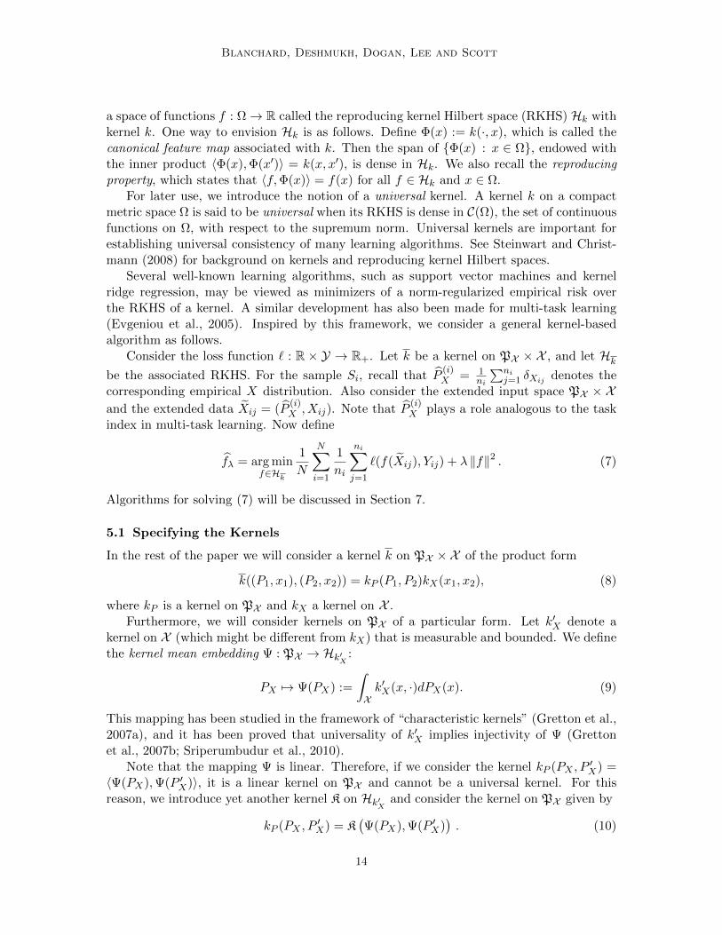
a space of functions f : Ω→ R called the reproducing kernel Hilbert space (RKHS) Hk withkernel k. One way to envision Hk is as follows. Define Φ(x) := k(·, x), which is called thecanonical feature map associated with k. Then the span of Φ(x) : x ∈ Ω, endowed withthe inner product 〈Φ(x),Φ(x′)〉 = k(x, x′), is dense in Hk. We also recall the reproducingproperty, which states that 〈f,Φ(x)〉 = f(x) for all f ∈ Hk and x ∈ Ω.
For later use, we introduce the notion of a universal kernel. A kernel k on a compactmetric space Ω is said to be universal when its RKHS is dense in C(Ω), the set of continuousfunctions on Ω, with respect to the supremum norm. Universal kernels are important forestablishing universal consistency of many learning algorithms. See Steinwart and Christ-mann (2008) for background on kernels and reproducing kernel Hilbert spaces.
Several well-known learning algorithms, such as support vector machines and kernelridge regression, may be viewed as minimizers of a norm-regularized empirical risk overthe RKHS of a kernel. A similar development has also been made for multi-task learning(Evgeniou et al., 2005). Inspired by this framework, we consider a general kernel-basedalgorithm as follows.
Consider the loss function ` : R × Y → R+. Let k be a kernel on PX × X , and let Hkbe the associated RKHS. For the sample Si, recall that P
(i)X = 1
ni
∑nij=1 δXij denotes the
corresponding empirical X distribution. Also consider the extended input space PX × Xand the extended data Xij = (P
(i)X , Xij). Note that P
(i)X plays a role analogous to the task
index in multi-task learning. Now define
fλ = arg minf∈Hk
1
N
N∑i=1
1
ni
ni∑j=1
`(f(Xij), Yij) + λ ‖f‖2 . (7)
Algorithms for solving (7) will be discussed in Section 7.
5.1 Specifying the Kernels
In the rest of the paper we will consider a kernel k on PX ×X of the product form
k((P1, x1), (P2, x2)) = kP (P1, P2)kX(x1, x2), (8)
where kP is a kernel on PX and kX a kernel on X .Furthermore, we will consider kernels on PX of a particular form. Let k′X denote a
kernel on X (which might be different from kX) that is measurable and bounded. We definethe kernel mean embedding Ψ : PX → Hk′X :
PX 7→ Ψ(PX) :=
∫Xk′X(x, ·)dPX(x). (9)
This mapping has been studied in the framework of “characteristic kernels” (Gretton et al.,2007a), and it has been proved that universality of k′X implies injectivity of Ψ (Grettonet al., 2007b; Sriperumbudur et al., 2010).
Note that the mapping Ψ is linear. Therefore, if we consider the kernel kP (PX , P′X) =
〈Ψ(PX),Ψ(P ′X)〉, it is a linear kernel on PX and cannot be a universal kernel. For thisreason, we introduce yet another kernel K on Hk′X and consider the kernel on PX given by
kP (PX , P′X) = K
(Ψ(PX),Ψ(P ′X)
). (10)
14
Domain Generalization by Marginal Transfer Learning
Note that particular kernels inspired by the finite dimensional case are of the form
K(v, v′) = F (∥∥v − v′∥∥), (11)
orK(v, v′) = G(
⟨v, v′
⟩), (12)
where F,G are real functions of a real variable such that they define a kernel. For exam-ple, F (t) = exp(−t2/(2σ2)) yields a Gaussian-like kernel, while G(t) = (1 + t)d yields apolynomial-like kernel. Kernels of the above form on the space of probability distributionsover a compact space X have been introduced and studied in Christmann and Steinwart(2010). Below we apply their results to deduce that k is a universal kernel for certain choicesof kX , k
′X , and K.
5.2 Relation to Other Kernel Methods
By choosing k differently, one can recover other existing kernel methods. In particular,consider the class of kernels of the same product form as above, but where
kP (PX , P′X) =
1 PX = P ′Xτ PX 6= P ′X
If τ = 0, the algorithm (7) corresponds to training N kernel machines f(P(i)X , ·) using kernel
kX (e.g., support vector machines in the case of the hinge loss) on each training data set,independently of the others (note that this does not offer any generalization ability to a newdata set). If τ = 1, we have a “pooling” strategy that, in the case of equal sample sizes ni,is equivalent to pooling all training data sets together in a single data set, and running aconventional supervised learning algorithm with kernel kX (i.e., this corresponds to tryingto find a single “one-fits-all” prediction function which does not depend on the marginal).In the intermediate case 0 < τ < 1, the resulting kernel is a “multi-task kernel,” and thealgorithm recovers a multitask learning algorithm like that of Evgeniou et al. (2005). Wecompare to the pooling strategy below in our experiments. We also examined the multi-task kernel with τ < 1, but found that, as far as generalization to a new unlabeled task isconcerned, it was always outperformed by pooling, and so those results are not reported.This fits the observation that the choice τ = 0 does not provide any generalization to anew task, while τ = 1 at least offers some form of generalization, if only by fitting the samepredictor to all data sets.
In the special case where all labels Yij are the same value for a given task, and kX istaken to be the constant kernel, the problem we consider reduces to “distributional” classi-fication or regression, which is essentially standard supervised learning where a distribution(observed through a sample) plays the role of the feature vector. Many of our analysistechniques specialize to this setting.
6. Learning Theoretic Study
This section presents generalization error and consistency analysis for the proposed kernelmethod under the agnostic and 2-stage generative models. Although the regularized esti-mation formula (7) defining fλ is standard, the generalization error analysis is not, owingto the particular sampling structures and risks under (AGM) and (2SGM).
15
Blanchard, Deshmukh, Dogan, Lee and Scott
6.1 Universal Consistency under the Agnostic Generative Model
We will consider the following assumptions on the loss function and kernels:
(LB) The loss function ` : R × Y → R+ is L`-Lipschitz in its first variable and satisfiesB0 := supy∈Y `(0, y) <∞.
(K-Bounded) The kernels kX , k′X and K are bounded respectively by constants B2
k, B2k′ ≥
1, and B2K .
The condition B0 < ∞ always holds for classification, as well as certain regressionsettings. The boundedness assumptions are clearly satisfied for Gaussian kernels, and canbe enforced by normalizing the kernel (discussed further below).
We begin with a generalization error bound that establishes uniform estimation errorcontrol over functions belonging to a ball of Hk . We then discuss universal kernels, andfinally deduce universal consistency of the algorithm.
Let Bk(r) denote the closed ball of radius r, centered at the origin, in the RKHS of thekernel k. We start with the following simple result allowing us to bound the loss on a RKHSball.
Lemma 10 Suppose k is a kernel on a set Ω, bounded by B2. Let ` : R×Y → [0,∞) be aloss satisfying (LB). Then for any R > 0 and f ∈ Bk(R), and any z ∈ Ω and y ∈ Y,∣∣`(f(z), y)
∣∣ ≤ B0 + L`RB (13)
Proof By the Lipschitz continuity of `, the reproducing property, and Cauchy-Schwarz,we have ∣∣`(f(z), y)
∣∣ ≤ `(0, y) +∣∣`(f(z), y)− `(0, y)
∣∣≤ B0 + L`|f(z)− 0|= B0 + L`
∣∣〈f, k(z, ·)〉∣∣
≤ B0 + L`‖f‖HkB≤ B0 + L`RB.
The expression in (13) serves to replace the boundedness assumption (3) in Theorem 5.We now state the following, which is a specialization of Theorem 5 to the kernel setting.
Theorem 11 (Uniform estimation error control over RKHS balls) Assume (LB)and (K-Bounded) hold, and data generation follows (AGM). Then for any R > 0, withprobability at least 1− δ (with respect to the draws of the samples Si, i = 1, . . . , N)
supf∈Bk(R)
∣∣∣E(f,N)− E(f)∣∣∣ ≤ (B0 + L`RBKBk)
(√
log δ−1 + 2)√N
. (14)
16
Domain Generalization by Marginal Transfer Learning
Proof This is a direct consequence of Theorem 5 and of Lemma 10, the kernel k onPX × X being bounded by B2
kB2K. As noted there, the main term in the upper bound (4)
is a standard Rademacher complexity on the augmented input space P×X , endowed withthe Campbell measure C(PS).
In the kernel learning context, we can bound the Rademacher complexity term usinga standard bound for the Rademacher complexity of a Lipschitz loss function on the ballof radius R of Hk (Koltchinskii, 2001; Bartlett and Mendelson, 2002, e.g., Theorems 8, 12and Lemma 22 there), using again the bound B2
kB2K on the kernel k, giving the conclusion.
Next, we turn our attention to universal kernels (see Section 5 for the definition). Arelevant notion for our purposes is that of a normalized kernel. If k is a kernel on Ω, then
k∗(x, x′) :=k(x, x′)√
k(x, x)k(x′, x′)
is the associated normalized kernel. If a kernel is universal, then so is its associated normal-ized kernel. For example, the exponential kernel k(x, x′) = exp(κ〈x, x′〉Rd), κ > 0, can beshown to be universal on Rd through a Taylor series argument. Consequently, the Gaussiankernel
kσ(x, x′) :=exp( 1
σ2 〈x, x′〉)exp( 1
2σ2 ‖x‖2) exp( 12σ2 ‖x′‖2)
is universal, being the normalized kernel associated with the exponential kernel with κ =1/σ2. See Steinwart and Christmann (2008) for additional details and discussion.
To establish that k is universal on PX ×X , the following lemma is useful.
Lemma 12 Let Ω,Ω′ be two compact spaces and k, k′ be kernels on Ω,Ω′, respectively. Ifk, k′ are both universal, then the product kernel
k((x, x′), (y, y′)) := k(x, y)k′(x′, y′)
is universal on Ω× Ω′.
Several examples of universal kernels are known on Euclidean space. For our purposes,we also need universal kernels on PX . Fortunately, this was studied by Christmann andSteinwart (2010). Some additional assumptions on the kernels and feature space are re-quired:
(K-Univ) kX , k′X , K, and X satisfy the following:
• X is a compact metric space
• kX is universal on X• k′X is continuous and universal on X• K is universal on any compact subset of Hk′X .
Adapting the results of Christmann and Steinwart (2010), we have the following.
17
Blanchard, Deshmukh, Dogan, Lee and Scott
Theorem 13 (Universal kernel) Assume condition (K-Univ) holds. Then, for kP de-fined as in (10), the product kernel k in (8) is universal on PX ×X .
Furthermore, the assumption on K is fulfilled if K is of the form (12), where G is ananalytical function with positive Taylor series coefficients, or if K is the normalized kernelassociated to such a kernel.
Proof By Lemma 12, it suffices to show PX is a compact metric space, and that kP (PX , P′X)
is universal on PX . The former statement follows from Theorem 6.4 of Parthasarathy(1967), where the metric is the Prohorov metric. We will deduce the latter statement fromTheorem 2.2 of Christmann and Steinwart (2010). The statement of Theorem 2.2 thereis apparently restricted to kernels of the form (12), but the proof actually only uses thatthe kernel K is universal on any compact set of Hk′X . To apply Theorem 2.2, it remainsto show that Hk′X is a separable Hilbert space, and that Ψ is injective and continuous.Injectivity of Ψ is equivalent to k′X being a characteristic kernel, and follows from theassumed universality of k′X (Sriperumbudur et al., 2010). The continuity of k′X impliesseparability of Hk′X (Steinwart and Christmann (2008), Lemma 4.33) as well as continuity ofΨ (Christmann and Steinwart (2010), Lemma 2.3 and preceding discussion). Now Theorem2.2 of Christmann and Steinwart (2010) may be applied, and the results follows.
The fact that kernels of the form (12), where G is analytic with positive Taylor coeffi-cients, are universal on any compact set of Hk′X was established in the proof of Theorem2.2 of the same work (Christmann and Steinwart, 2010).
As an example, suppose that X is a compact subset of Rd. Let kX and k′X be Gaussiankernels on X . Taking G(t) = exp(t), it follows that K(PX , P
′X) = exp(〈Ψ(PX),Ψ(P ′X)〉Hk′
X
)
is universal on PX . By similar reasoning as in the finite dimensional case, the Gaussian-likekernel K(PX , P
′X) = exp(− 1
2σ2 ‖Ψ(PX) − Ψ(P ′X)‖2Hk′X
) is also universal on PX . Thus the
product kernel is universal on PX ×X .From Theorems 11 and 13, we may deduce universal consistency of the learning algo-
rithm.
Corollary 14 (Universal consistency) Assume that conditions (LB), (K-Bounded)and (K-Univ) are satisfied. Let λ = λ(N) be a sequence such that as N →∞: λ(N)→ 0and λ(N)N/ logN →∞. Then
E(fλ(N))→ inff :PX×X→R
E(f) a.s., as N →∞.
The proof of the corollary relies on the bound established in Theorem 11, the universalityof k established in Theorem 13, and otherwise relatively standard arguments.
One notable feature of this result is that we have established consistency where only Nis required to diverge. In particular, the training sample sizes ni may remain bounded. Inthe next subsection, we consider the role of the ni under the 2-stage generative model.
6.2 Role of the Individual Sample Sizes under the 2-Stage Generative Model
In this section, we are concerned with the role of the individual sample sizes (ni)1≤i≤N , moreprecisely, of their distribution ν under (2SGM), see Section 3.1. A particular motivation
18
Domain Generalization by Marginal Transfer Learning
for investigating this point is that in some applications the number of training points pertask is large, which can give rise to a high computational burden at the learning stage (andalso for storing the learned model in computer memory). A practical way to alleviate thisissue is to reduce the number of training points per task by random subsampling, which ineffect modifies the sample size distribution ν while keeping the generating distribution µfor the tasks’ point distributions unchanged. Observe that under (AGM) the sample sizeand the sample point distribution may be dependent in general, and subsampling wouldthen affect that relationship in an unknown manner. This is why we assume (2SGM) inthe present section.
We will consider the following additional assumption.
(K-Holder) The canonical feature map ΦK : Hk′X → HK associated to K satisfies a Holdercondition of order α ∈ (0, 1] with constant LK, on Bk′X (Bk′) :
∀v, w ∈ Bk′X (Bk′) : ‖ΦK(v)− ΦK(w)‖ ≤ LK ‖v − w‖α . (15)
Sufficient conditions for (15) are described in Section A.4. As an example, the condition isshown to hold with α = 1 when K is the Gaussian-like kernel on Hk′X .
Since we are interested in the influence of the number of training points per task, itis helpful to introduce notations for the (2SGM) risks that are conditioned on a fixedtask PXY . Thus, we introduce the following notation, in analogy to (5)–(6) introduced inSection 3.4, for risk at sample size n, and risk at infinite sample size, conditional to PXY :
E(f |PXY , n) := EST∼(PXY )⊗n
[1
n
n∑i=1
`(f(PX , Xi), Yi)
]; (16)
E∞(f |PXY ) := E(X,Y )∼PXY [`(f(PX , X), Y )] . (17)
The following proposition gives an upper bound on the discrepancy between these risks.It can be seen as a quantitative version of Proposition 7 in the kernel setting, which isfurthermore uniform over an RKHS ball.
Theorem 15 Assume conditions (LB), (K-Bounded), and (K-Holder) hold. If thesample S = (Xj , Yj)1≤j≤n is made of n i.i.d. realizations from PXY , with PXY and n fixed,then for any R > 0, with probability at least 1− δ:
supf∈Bk(R)
|L(S, f)− E∞(f |PXY )| ≤ (B0 + 3L`RBk(Bαk′LK + BK))
(log(3δ−1)
n
)−α2
. (18)
Averaging over the draw of S, again with PXY and n fixed, it holds for any R > 0:
supf∈Bk(R)
|E(f |PXY , n)− E∞(f |PXY )| ≤ 2L`RBkLKBαk′n−α/2. (19)
As a consequence, for the unconditional risks when (PXY , n) is drawn from µ ⊗ ν under(2SGM), for any R > 0:
supf∈Bk(R)
|E(f)− E∞(f)| ≤ 2RL`BkLKBαk′Eν
[n−
α2
]. (20)
19
Blanchard, Deshmukh, Dogan, Lee and Scott
The above results are useful in a number of ways. First, under (2SGM), we can considerthe goal of asymptotically achieving the idealized optimal risk inff E∞(f), where we recallthat E∞(f) is the expected loss of a decision function f over a random test task P TXY in thecase where P TX would be perfectly observed (this can be thought of as observing an infinitesample from the marginal). Equation (20) bounds the risk under (2SGM) in terms of therisk under (AGM), for which we have already established consistency. Thus, consistencyto the idealized risk under (2SGM) will be possible if the number of examples ni pertraining task also grows together with the number of training tasks N . The following resultformalizes this intuition.
Corollary 16 Assume (LB), (K-Bounded), and (K-Holder), and assume (2SGM).Then for any R > 0, with probability at least 1− δ with respect to the draws of the trainingtasks and training samples
supf∈Bk(R)
∣∣∣∣∣ 1
N
N∑i=1
L(Si, f)− E∞(f)
∣∣∣∣∣≤ (B0 + L`RBKBk)
(√
log δ−1 + 2)√N
+ 2RL`BkLKBαk′Eν
[n−
α2
]. (21)
Consider an asymptotic setting under (2SGM) in which, as the number of training tasksN → ∞, the distribution µ remains fixed but the sample size distribution νN depends onN . Denote κ−1N := EνN
[n−α/2
]. Assuming (K-Univ) is satisfied, and the regularization
parameter λ(N) is such that λ(N)→ 0 and λ(N) min(N,κ2N )→∞, then
E(fλ(N))→ inff :PX×X→R
E∞(f) in probability, as N →∞.
Proof The setting is that of the (2SGM) model. This is a particular case of (AGM),so we can apply Theorem 11 and combine with (20) to get the announced bound. Theconsistency statement follows the same argument as in the proof of Corollary 14, with E(f)replaced by E∞(f), and ε(N) there replaced by the RHS in (21).
Remark 17 The bound (21) is non-asymptotic and can be used as such to assess the re-spective role of number of tasks N and of the sample size distribution ν when the objectiveis the idealized risk (see below). The result of consistency to that risk on the other hand, isformalized as a “triangular array” type of asymptotics where the distribution of the sizes niof the i.i.d. training samples Si changes with their number N .
Remark 18 Our conference paper (Blanchard et al., 2011) also established a generalizationerror bound and consistency for E∞ under (2SGM). That bound had a different form fortwo main reasons. First, it assumed the loss to be bounded, whereas the present analysisavoids that assumption via Lemma 10. Second, that analysis did not leverage a connectionto (AGM), which led to a logN in the second term. This required the two sample sizes tobe coupled asymptotically to achieve consistency. In the present analysis, the two samplesizes N and n may diverge at arbitrary rates.
20
Domain Generalization by Marginal Transfer Learning
Remark 19 It is possible to obtain a result similar to Corollary 16 when the trainingtask sample sizes (ni)1≤i≤N are fixed (considered as deterministic), unequal and possiblyarbitrary. In this case we would follow a slightly different argument, leveraging (18) foreach single training task together with a union bound, and applying Theorem 11 to theidealized situation with an infinite number of samples per training task. This way, the term
Eν[n−
α2
]is replaced by log(N)N−1
∑Ni=1 n
−α2
i , the additional logarithmic factor being the
price of the union bound. We eschew an exact statement for brevity.
We now come back to our initial motivation of possibly reducing computational burdenby subsampling and analyze to what extent this affects statistical error. Under (2SGM)the effect of subsampling (without replacement) is transparent: it amounts to changingthe original individual sample size distribution ν by ν ′ = δn′ , while keeping the generatingdistribution µ for the tasks’ point distributions fixed. Here n′ is the common fixed size ofthe training subsamples, and we must assume implicitly that the original sample sizes area.s. larger than n′, i.e. that their distribution ν has support [n′,∞). For simplicity, for therest of the discussion we only consider the case of equal, deterministic sizes of sample (n)and subsample (n′ < n). Using (21) we compare the two settings to a common reference,namely the idealized risk E∞. We see that the statistical risk bound in (21) is unchangedup to a small factor if n′ ≥ min(Nα, n). Assuming α = 1 to simplify, in the case where theoriginal sample sizes n are much larger than the number of training tasks N , this suggeststhat we can subsample to n′ ≈ N without taking a significant hit to performance. Thisapplies equally well to subsampling the tasks used for prediction or testing. The most precisestatement in this regard is (18), since it bounds the deviations of the observed predictionloss for a fixed task PXY and i.i.d. sample from that task.
The minimal subsampling size n′ can be interpreted as an optimal efficiency/accuracytradeoff, since it reduces computational complexity as much as possible without sacrificingstatistical accuracy. Similar considerations appear in the context of distribution regres-sion (Szabo et al., 2016, Remark 6). In that reference, a sharp analysis giving rise to fastconvergence rates is presented, resulting in a more involved optimal balance between N andn. In the present work, we have focused on slow rates based on a uniform control of theestimation error over RKHS balls; we leave for future work sharper convergence bounds (un-der additional regularity conditions), which would also give rise to more refined balancingconditions between n and N .
7. Implementation
Implementation of the algorithm in (7) relies on techniques that are similar to those usedfor other kernel methods, but with some variations.3 The first subsection illustrates how,for the case of hinge loss, the optimization problem corresponds to a certain cost-sensitivesupport vector machine. The second subsection focuses on more scalable implementationsbased on approximate feature mappings.
3. Code is available at https://github.com/aniketde/DomainGeneralizationMarginal
21
Blanchard, Deshmukh, Dogan, Lee and Scott
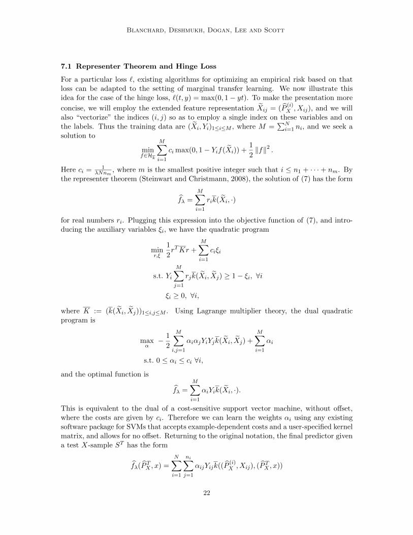
7.1 Representer Theorem and Hinge Loss
For a particular loss `, existing algorithms for optimizing an empirical risk based on thatloss can be adapted to the setting of marginal transfer learning. We now illustrate thisidea for the case of the hinge loss, `(t, y) = max(0, 1− yt). To make the presentation more
concise, we will employ the extended feature representation Xij = (P(i)X , Xij), and we will
also “vectorize” the indices (i, j) so as to employ a single index on these variables and onthe labels. Thus the training data are (Xi, Yi)1≤i≤M , where M =
∑Ni=1 ni, and we seek a
solution to
minf∈Hk
M∑i=1
ci max(0, 1− Yif(Xi)) +1
2‖f‖2 .
Here ci = 1λNnm
, where m is the smallest positive integer such that i ≤ n1 + · · ·+ nm. Bythe representer theorem (Steinwart and Christmann, 2008), the solution of (7) has the form
fλ =M∑i=1
rik(Xi, ·)
for real numbers ri. Plugging this expression into the objective function of (7), and intro-ducing the auxiliary variables ξi, we have the quadratic program
minr,ξ
1
2rTKr +
M∑i=1
ciξi
s.t. Yi
M∑j=1
rjk(Xi, Xj) ≥ 1− ξi, ∀i
ξi ≥ 0, ∀i,
where K := (k(Xi, Xj))1≤i,j≤M . Using Lagrange multiplier theory, the dual quadraticprogram is
maxα− 1
2
M∑i,j=1
αiαjYiYjk(Xi, Xj) +
M∑i=1
αi
s.t. 0 ≤ αi ≤ ci ∀i,
and the optimal function is
fλ =
M∑i=1
αiYik(Xi, ·).
This is equivalent to the dual of a cost-sensitive support vector machine, without offset,where the costs are given by ci. Therefore we can learn the weights αi using any existingsoftware package for SVMs that accepts example-dependent costs and a user-specified kernelmatrix, and allows for no offset. Returning to the original notation, the final predictor givena test X-sample ST has the form
fλ(P TX , x) =N∑i=1
ni∑j=1
αijYijk((P(i)X , Xij), (P
TX , x))
22
Domain Generalization by Marginal Transfer Learning
where the αij are nonnegative. Like the SVM, the solution is often sparse, meaning mostαij are zero.
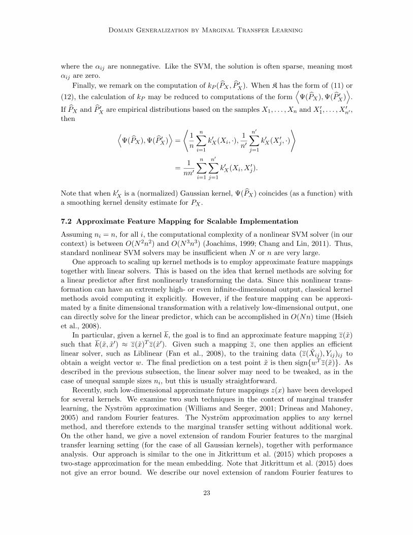
Finally, we remark on the computation of kP (PX , P′X). When K has the form of (11) or
(12), the calculation of kP may be reduced to computations of the form⟨
Ψ(PX),Ψ(P ′X)⟩
.
If PX and P ′X are empirical distributions based on the samples X1, . . . , Xn and X ′1, . . . , X′n′ ,
then ⟨Ψ(PX),Ψ(P ′X)
⟩=
⟨1
n
n∑i=1
k′X(Xi, ·),1
n′
n′∑j=1
k′X(X ′j , ·)
⟩
=1
nn′
n∑i=1
n′∑j=1
k′X(Xi, X′j).
Note that when k′X is a (normalized) Gaussian kernel, Ψ(PX) coincides (as a function) witha smoothing kernel density estimate for PX .
7.2 Approximate Feature Mapping for Scalable Implementation
Assuming ni = n, for all i, the computational complexity of a nonlinear SVM solver (in ourcontext) is between O(N2n2) and O(N3n3) (Joachims, 1999; Chang and Lin, 2011). Thus,standard nonlinear SVM solvers may be insufficient when N or n are very large.
One approach to scaling up kernel methods is to employ approximate feature mappingstogether with linear solvers. This is based on the idea that kernel methods are solving fora linear predictor after first nonlinearly transforming the data. Since this nonlinear trans-formation can have an extremely high- or even infinite-dimensional output, classical kernelmethods avoid computing it explicitly. However, if the feature mapping can be approxi-mated by a finite dimensional transformation with a relatively low-dimensional output, onecan directly solve for the linear predictor, which can be accomplished in O(Nn) time (Hsiehet al., 2008).
In particular, given a kernel k, the goal is to find an approximate feature mapping z(x)such that k(x, x′) ≈ z(x)T z(x′). Given such a mapping z, one then applies an efficientlinear solver, such as Liblinear (Fan et al., 2008), to the training data (z(Xij), Yij)ij toobtain a weight vector w. The final prediction on a test point x is then signwT z(x). Asdescribed in the previous subsection, the linear solver may need to be tweaked, as in thecase of unequal sample sizes ni, but this is usually straightforward.
Recently, such low-dimensional approximate future mappings z(x) have been developedfor several kernels. We examine two such techniques in the context of marginal transferlearning, the Nystrom approximation (Williams and Seeger, 2001; Drineas and Mahoney,2005) and random Fourier features. The Nystrom approximation applies to any kernelmethod, and therefore extends to the marginal transfer setting without additional work.On the other hand, we give a novel extension of random Fourier features to the marginaltransfer learning setting (for the case of all Gaussian kernels), together with performanceanalysis. Our approach is similar to the one in Jitkrittum et al. (2015) which proposes atwo-stage approximation for the mean embedding. Note that Jitkrittum et al. (2015) doesnot give an error bound. We describe our novel extension of random Fourier features to
23
Blanchard, Deshmukh, Dogan, Lee and Scott
the marginal transfer learning setting, with error bounds, in the appendix, where we alsoreview the Nystrom method.
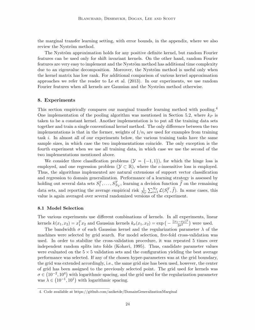
The Nystrom approximation holds for any positive definite kernel, but random Fourierfeatures can be used only for shift invariant kernels. On the other hand, random Fourierfeatures are very easy to implement and the Nystrom method has additional time complexitydue to an eigenvalue decomposition. Moreover, the Nystrom method is useful only whenthe kernel matrix has low rank. For additional comparison of various kernel approximationapproaches we refer the reader to Le et al. (2013). In our experiments, we use randomFourier features when all kernels are Gaussian and the Nystrom method otherwise.
8. Experiments
This section empirically compares our marginal transfer learning method with pooling.4
One implementation of the pooling algorithm was mentioned in Section 5.2, where kP istaken to be a constant kernel. Another implementation is to put all the training data setstogether and train a single conventional kernel method. The only difference between the twoimplementations is that in the former, weights of 1/ni are used for examples from trainingtask i. In almost all of our experiments below, the various training tasks have the samesample sizes, in which case the two implementations coincide. The only exception is thefourth experiment when we use all training data, in which case we use the second of thetwo implementations mentioned above.
We consider three classification problems (Y = −1, 1), for which the hinge loss isemployed, and one regression problem (Y ⊂ R), where the ε-insensitive loss is employed.Thus, the algorithms implemented are natural extensions of support vector classificationand regression to domain generalization. Performance of a learning strategy is assessed byholding out several data sets ST1 , . . . , S
TNT
, learning a decision function f on the remaining
data sets, and reporting the average empirical risk 1NT
∑NTi=1 L(STi , f). In some cases, this
value is again averaged over several randomized versions of the experiment.
8.1 Model Selection
The various experiments use different combinations of kernels. In all experiments, linear
kernels k(x1, x2) = xT1 x2 and Gaussian kernels kσ(x1, x2) = exp(− ||x1−x2||
2
2σ2
)were used.
The bandwidth σ of each Gaussian kernel and the regularization parameter λ of themachines were selected by grid search. For model selection, five-fold cross-validation wasused. In order to stabilize the cross-validation procedure, it was repeated 5 times overindependent random splits into folds (Kohavi, 1995). Thus, candidate parameter valueswere evaluated on the 5× 5 validation sets and the configuration yielding the best averageperformance was selected. If any of the chosen hyper-parameters was at the grid boundary,the grid was extended accordingly, i.e., the same grid size has been used, however, the centerof grid has been assigned to the previously selected point. The grid used for kernels wasσ ∈
(10−2, 104
)with logarithmic spacing, and the grid used for the regularization parameter
was λ ∈(10−1, 101
)with logarithmic spacing.
4. Code available at https://github.com/aniketde/DomainGeneralizationMarginal
24
Domain Generalization by Marginal Transfer Learning
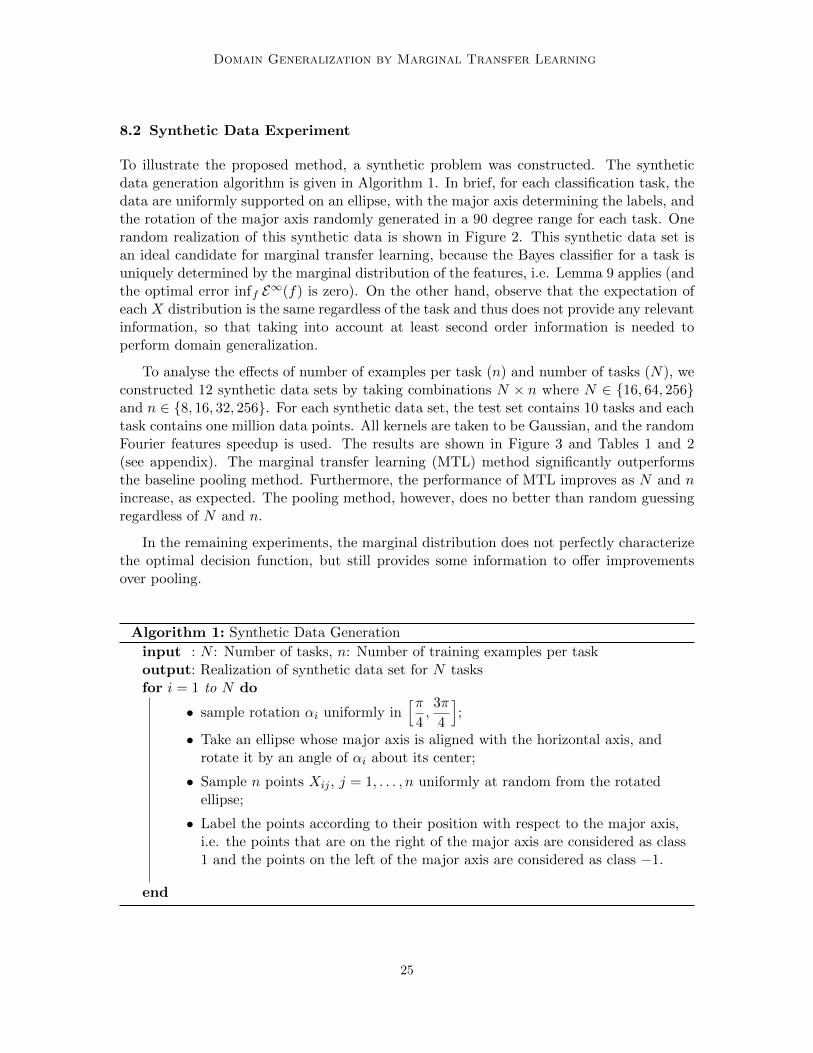
8.2 Synthetic Data Experiment
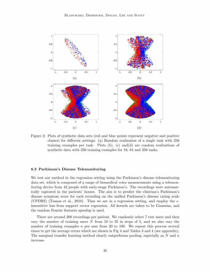
To illustrate the proposed method, a synthetic problem was constructed. The syntheticdata generation algorithm is given in Algorithm 1. In brief, for each classification task, thedata are uniformly supported on an ellipse, with the major axis determining the labels, andthe rotation of the major axis randomly generated in a 90 degree range for each task. Onerandom realization of this synthetic data is shown in Figure 2. This synthetic data set isan ideal candidate for marginal transfer learning, because the Bayes classifier for a task isuniquely determined by the marginal distribution of the features, i.e. Lemma 9 applies (andthe optimal error inff E∞(f) is zero). On the other hand, observe that the expectation ofeach X distribution is the same regardless of the task and thus does not provide any relevantinformation, so that taking into account at least second order information is needed toperform domain generalization.
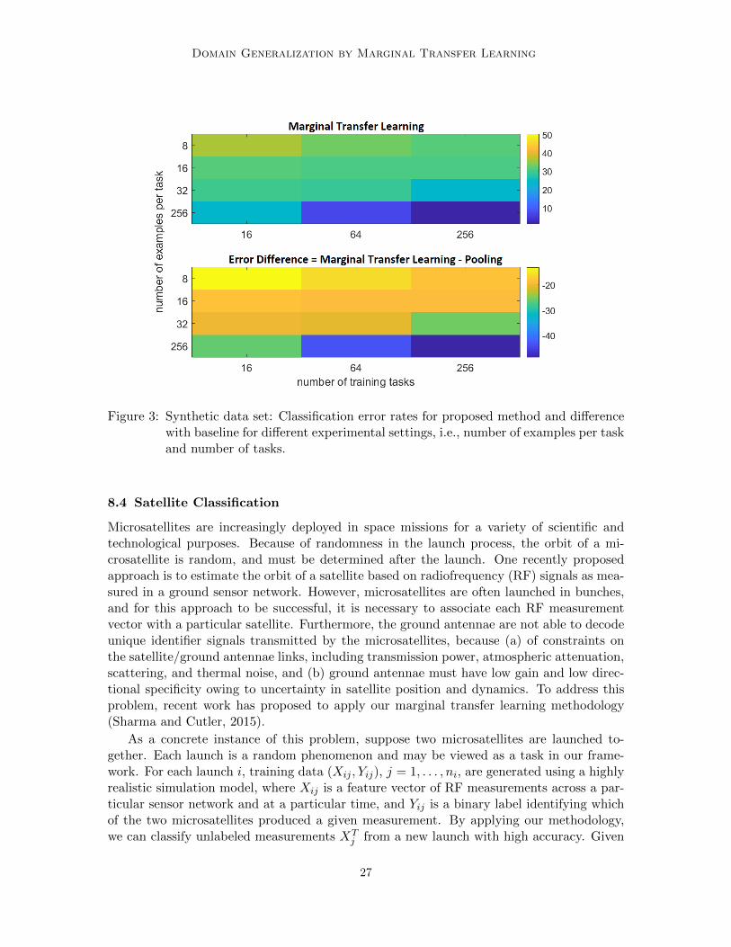
To analyse the effects of number of examples per task (n) and number of tasks (N), weconstructed 12 synthetic data sets by taking combinations N × n where N ∈ 16, 64, 256and n ∈ 8, 16, 32, 256. For each synthetic data set, the test set contains 10 tasks and eachtask contains one million data points. All kernels are taken to be Gaussian, and the randomFourier features speedup is used. The results are shown in Figure 3 and Tables 1 and 2(see appendix). The marginal transfer learning (MTL) method significantly outperformsthe baseline pooling method. Furthermore, the performance of MTL improves as N and nincrease, as expected. The pooling method, however, does no better than random guessingregardless of N and n.
In the remaining experiments, the marginal distribution does not perfectly characterizethe optimal decision function, but still provides some information to offer improvementsover pooling.
Algorithm 1: Synthetic Data Generation
input : N : Number of tasks, n: Number of training examples per taskoutput: Realization of synthetic data set for N tasksfor i = 1 to N do
• sample rotation αi uniformly in[π
4,3π
4
];
• Take an ellipse whose major axis is aligned with the horizontal axis, androtate it by an angle of αi about its center;
• Sample n points Xij , j = 1, . . . , n uniformly at random from the rotatedellipse;
• Label the points according to their position with respect to the major axis,i.e. the points that are on the right of the major axis are considered as class1 and the points on the left of the major axis are considered as class −1.
end
25
Blanchard, Deshmukh, Dogan, Lee and Scott
(a) (b)
(c) (d)
Figure 2: Plots of synthetic data sets (red and blue points represent negative and positiveclasses) for different settings: (a) Random realization of a single task with 256training examples per task. Plots (b), (c) and(d) are random realizations ofsynthetic data with 256 training examples for 16, 64 and 256 tasks.
8.3 Parkinson’s Disease Telemonitoring
We test our method in the regression setting using the Parkinson’s disease telemonitoringdata set, which is composed of a range of biomedical voice measurements using a telemon-itoring device from 42 people with early-stage Parkinson’s. The recordings were automat-ically captured in the patients’ homes. The aim is to predict the clinician’s Parkinson’sdisease symptom score for each recording on the unified Parkinson’s disease rating scale(UPDRS) (Tsanas et al., 2010). Thus we are in a regression setting, and employ the ε-insensitive loss from support vector regression. All kernels are taken to be Gaussian, andthe random Fourier features speedup is used.
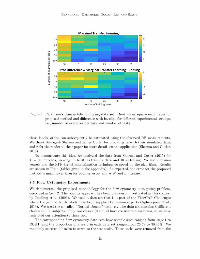
There are around 200 recordings per patient. We randomly select 7 test users and thenvary the number of training users N from 10 to 35 in steps of 5, and we also vary thenumber of training examples n per user from 20 to 100. We repeat this process severaltimes to get the average errors which are shown in Fig 4 and Tables 3 and 4 (see appendix).The marginal transfer learning method clearly outperforms pooling, especially as N and nincrease.
26
Domain Generalization by Marginal Transfer Learning
Figure 3: Synthetic data set: Classification error rates for proposed method and differencewith baseline for different experimental settings, i.e., number of examples per taskand number of tasks.
8.4 Satellite Classification
Microsatellites are increasingly deployed in space missions for a variety of scientific andtechnological purposes. Because of randomness in the launch process, the orbit of a mi-crosatellite is random, and must be determined after the launch. One recently proposedapproach is to estimate the orbit of a satellite based on radiofrequency (RF) signals as mea-sured in a ground sensor network. However, microsatellites are often launched in bunches,and for this approach to be successful, it is necessary to associate each RF measurementvector with a particular satellite. Furthermore, the ground antennae are not able to decodeunique identifier signals transmitted by the microsatellites, because (a) of constraints onthe satellite/ground antennae links, including transmission power, atmospheric attenuation,scattering, and thermal noise, and (b) ground antennae must have low gain and low direc-tional specificity owing to uncertainty in satellite position and dynamics. To address thisproblem, recent work has proposed to apply our marginal transfer learning methodology(Sharma and Cutler, 2015).
As a concrete instance of this problem, suppose two microsatellites are launched to-gether. Each launch is a random phenomenon and may be viewed as a task in our frame-work. For each launch i, training data (Xij , Yij), j = 1, . . . , ni, are generated using a highlyrealistic simulation model, where Xij is a feature vector of RF measurements across a par-ticular sensor network and at a particular time, and Yij is a binary label identifying whichof the two microsatellites produced a given measurement. By applying our methodology,we can classify unlabeled measurements XT
j from a new launch with high accuracy. Given
27
Blanchard, Deshmukh, Dogan, Lee and Scott
Figure 4: Parkinson’s disease telemonitoring data set: Root mean square error rates forproposed method and difference with baseline for different experimental settings,i.e., number of examples per task and number of tasks.
these labels, orbits can subsequently be estimated using the observed RF measurements.We thank Srinagesh Sharma and James Cutler for providing us with their simulated data,and refer the reader to their paper for more details on the application (Sharma and Cutler,2015).
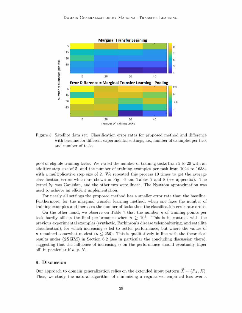
To demonstrate this idea, we analyzed the data from Sharma and Cutler (2015) forT = 50 launches, viewing up to 40 as training data and 10 as testing. We use Gaussiankernels and the RFF kernel approximation technique to speed up the algorithm. Resultsare shown in Fig 5 (tables given in the appendix). As expected, the error for the proposedmethod is much lower than for pooling, especially as N and n increase.
8.5 Flow Cytometry Experiments
We demonstrate the proposed methodology for the flow cytometry auto-gating problem,described in Sec. 2. The pooling approach has been previously investigated in this contextby Toedling et al. (2006). We used a data set that is a part of the FlowCAP Challengeswhere the ground truth labels have been supplied by human experts (Aghaeepour et al.,2013). We used the so-called “Normal Donors” data set. The data set contains 8 differentclasses and 30 subjects. Only two classes (0 and 2) have consistent class ratios, so we haverestricted our attention to these two.
The corresponding flow cytometry data sets have sample sizes ranging from 18,641 to59,411, and the proportion of class 0 in each data set ranges from 25.59 to 38.44%. Werandomly selected 10 tasks to serve as the test tasks. These tasks were removed from the
28
Domain Generalization by Marginal Transfer Learning
Figure 5: Satellite data set: Classification error rates for proposed method and differencewith baseline for different experimental settings, i.e., number of examples per taskand number of tasks.
pool of eligible training tasks. We varied the number of training tasks from 5 to 20 with anadditive step size of 5, and the number of training examples per task from 1024 to 16384with a multiplicative step size of 2. We repeated this process 10 times to get the averageclassification errors which are shown in Fig. 6 and Tables 7 and 8 (see appendix). Thekernel kP was Gaussian, and the other two were linear. The Nystrom approximation wasused to achieve an efficient implementation.
For nearly all settings the proposed method has a smaller error rate than the baseline.Furthermore, for the marginal transfer learning method, when one fixes the number oftraining examples and increases the number of tasks then the classification error rate drops.
On the other hand, we observe on Table 7 that the number n of training points pertask hardly affects the final performance when n ≥ 103. This is in contrast with theprevious experimental examples (synthetic, Parkinson’s disease telemonitoring, and satelliteclassification), for which increasing n led to better performance, but where the values ofn remained somewhat modest (n ≤ 256). This is qualitatively in line with the theoreticalresults under (2SGM) in Section 6.2 (see in particular the concluding discussion there),suggesting that the influence of increasing n on the performance should eventually taperoff, in particular if n N .
9. Discussion
Our approach to domain generalization relies on the extended input pattern X = (PX , X).Thus, we study the natural algorithm of minimizing a regularized empirical loss over a
29
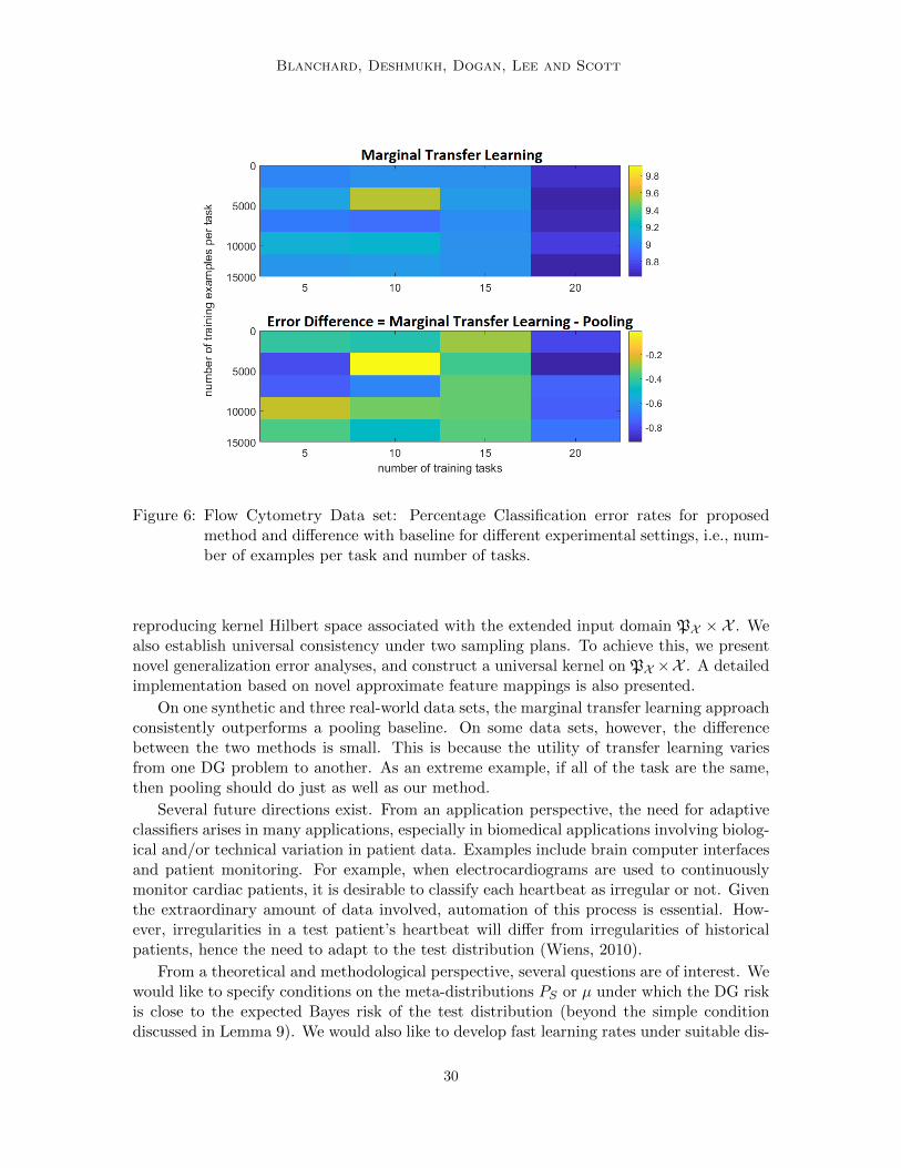
Blanchard, Deshmukh, Dogan, Lee and Scott
Figure 6: Flow Cytometry Data set: Percentage Classification error rates for proposedmethod and difference with baseline for different experimental settings, i.e., num-ber of examples per task and number of tasks.
reproducing kernel Hilbert space associated with the extended input domain PX × X . Wealso establish universal consistency under two sampling plans. To achieve this, we presentnovel generalization error analyses, and construct a universal kernel on PX ×X . A detailedimplementation based on novel approximate feature mappings is also presented.
On one synthetic and three real-world data sets, the marginal transfer learning approachconsistently outperforms a pooling baseline. On some data sets, however, the differencebetween the two methods is small. This is because the utility of transfer learning variesfrom one DG problem to another. As an extreme example, if all of the task are the same,then pooling should do just as well as our method.
Several future directions exist. From an application perspective, the need for adaptiveclassifiers arises in many applications, especially in biomedical applications involving biolog-ical and/or technical variation in patient data. Examples include brain computer interfacesand patient monitoring. For example, when electrocardiograms are used to continuouslymonitor cardiac patients, it is desirable to classify each heartbeat as irregular or not. Giventhe extraordinary amount of data involved, automation of this process is essential. How-ever, irregularities in a test patient’s heartbeat will differ from irregularities of historicalpatients, hence the need to adapt to the test distribution (Wiens, 2010).
From a theoretical and methodological perspective, several questions are of interest. Wewould like to specify conditions on the meta-distributions PS or µ under which the DG riskis close to the expected Bayes risk of the test distribution (beyond the simple conditiondiscussed in Lemma 9). We would also like to develop fast learning rates under suitable dis-
30
Domain Generalization by Marginal Transfer Learning
tributional assumptions. Furthermore, given the close connections with supervised learning,many common variants of supervised learning can also be investigated in the DG context,including multiclass classification, class probability estimation, and robustness to variousforms of noise.
We can also ask how the methodology and analysis can be extended to the contextwhere a small number of labels are available for the test distribution (additionally to alarger number of unlabeled data from the same distribution); this situation appears to becommon in practice, and can be seen as intermediary between the DG and learning to learn(LTL, see Section 4.2) settings (one could dub it “semi-supervised domain generalization”).In this setting, two approaches appear promising to take advantage of the labeled data. Thesimplest one is to use the same optimization problem (7), where we include additionallythe labeled examples of the test distribution. However, if several test samples are to betreated in succession, and we want to avoid a full, resource-consuming re-training usingall the training samples each time, an interesting alternative is the following: learn oncea function f0(PX , x) using the available training samples via (7); then, given a partiallylabeled test sample, learn a decision function on this sample only via the usual kernel (kX)norm regularized empirical loss minimization method, but replace the usual regularizer
term ‖f‖2H by∥∥∥f − f0(P TX , .)∥∥∥2H (note that f0(P
TX , .) ∈ HkX ). In this sense, the marginal-
adaptive decision function learned from the training samples would serve as a “prior” or“informed guess” for learning on the test data. This can be also interpreted as learningan adequate complexity penalty to improve learning on new samples, thus connecting tothe general principles of LTL (see Section 4.2). An interesting difference with underlyingexisting LTL approaches is that those tend to adapt the hypothesis class or the“shape” of theregularization penalty to the problem at hand, while the approach delineated above wouldmodify the “origin” of the penalty, using the marginal distribution information. These twoprinciples could also be combined.
Acknowledgments
C. Scott and A. Deshmukh were supported in part by NSF Grants No. 1422157, 1217880,1047871, 1838179, and 2008074. G. Blanchard was supported in part by the DeutscheForschungsgemeinschaft (DFG) via Research Unit FG1735/2 Structural Inference in Statis-tics, and via SFB1294/1 - 318763901DFG Data Assimilation; and by the Agence Nationalede la Recherche (ANR) via the IA Chair BiSCottE. G. Lee was supported by the NationalResearch Foundation of Korea (NRF-2014R1A1A1003458).
Appendix A. Proofs, Technical Details, and Experimental Details
This appendix contains the remaining proofs, as well as additional technical and experi-mental details.
31
Blanchard, Deshmukh, Dogan, Lee and Scott
A.1 Proof of Proposition 7
Let P TXY be a fixed probability distribution on X × R, and ε > 0 a fixed number. Since Xis a Radon space, by definition any Borel probability measure on it, in particular P TX (theX-marginal of P TXY ), is inner regular, so that there exists a compact set K ⊂ X such thatP TX(Kc) ≤ ε.
For all x ∈ K, by the assumed continuity of the decision function f at point (P TX , x) thereexists an open neighborhood Ux×Vx ⊂ PX×X of this point such that
∣∣f(u, v)− f(P TX , x)∣∣ ≤
ε for all (u, v) ∈ Ux × Vx. Since the family (Vx)x∈K is an open covering of the compactK, there exists a finite subfamily (Vxi)i∈I covering K. Denoting U0 :=
⋂i∈I Uxi which is
an open neighborhood of P TX in PX , it therefore holds for any P ∈ U0 and uniformly overx ∈ K that
∣∣f(P, x)− f(P TX , x)∣∣ ≤ |f(P, x)− f(P, xi0)|+
∣∣f(P TX , x)− f(P, xi0)∣∣ ≤ 2ε, where
i0 ∈ I is such that x ∈ Vxi0 .
Denote ST = (XTi , Y
Ti )1≤i≤nT a sample of size nT drawn i.i.d. from P TXY , and A the
eventP TX ∈ U0
. By the law of large numbers, P TX weakly converges to P TX in probability,
so that P [Ac] ≤ ε holds for nT large enough. We have (denoting B a bound on the lossfunction):
EST
[1
nT
nT∑i=1
`(f(P TX , XTi ), Y T
i )
]≤ Bε+ EST
[1
nT
nT∑i=1
`(f(P TX , XTi ), Y T
i )1XTi ∈K
]
≤ B(ε+ P [Ac]) + EST
[1PTX∈U0
1
nT
nT∑i=1
`(f(P TX , XTi ), Y T
i )1XTi ∈K
]
≤ 2Bε+ 2Lε+ EST
[1
nT
nT∑i=1
`(f(P TX , XTi ), Y T
i )
]≤ 2(B + L)ε+ E(XT ,Y T )∼PTXY
[`(f(P TX , X
T ), Y T )].
Conversely,
EST
[1
nT
nT∑i=1
`(f(P TX , XTi ), Y T
i )
]≥ EST
[1PTX∈U0
1
nT
nT∑i=1
`(f(P TX , XTi ), Y T
i )1XTi ∈K
]
≥ EST
[1
nT
nT∑i=1
`(f(P TX , XTi ), Y T
i )
]− 2Bε− 2Lε
≥ E(XT ,Y T )∼PTXY
[`(f(P TX , X
T ), Y T )]− 2(B + L)ε.
Since the above inequalities hold for any ε > 0 provided nT is large enough, this yields thatfor any fixed P TXY , we have
limnT→∞
EST∼(PTXY )⊗nT
[1
nT
nT∑i=1
`(f(P TX , XTi ), Y T
i )
]= E(XT ,Y T )∼PTXY
[`(f(P TX , X
T ), Y T )].
Finally, since the above right-hand side is bounded by B, applying dominated convergenceto integrate over P TXY ∼ µ yields the desired conclusion.
32
Domain Generalization by Marginal Transfer Learning
A.2 Proof of Corollary 14
Proof Denote E∗ = inff :PX×X→R E(f). Let ε > 0. Since k is a universal kernel on PX ×Xand ` is Lipschitz, there exists f0 ∈ Hk such that E(f0) ≤ E∗+ ε
2 (Steinwart and Christmann,2008).
By comparing the objective function in (7) at the minimizer fλ and at the null function,using assumption (LB) we deduce that we must have ‖fλ‖ ≤
√B0/λ. Applying Theorem 11
for R = Rλ =√B0/λ, and δ = 1/N2, gives that with probability at least 1− 1/N2,
supf∈Bk(R)
∣∣∣E(f,N)− E(f)∣∣∣ ≤ ε(N) := (B0 + L`BKBk
√B0/λ)
(√
logN + 2)√N
.
Let N be large enough so that ‖f0‖ ≤ Rλ. We can now deduce that with probability atleast 1− 1/N2,
E(fλ) ≤ E(fλ, N) + ε(N)
= E(fλ, N) + λ‖fλ‖2 − λ‖fλ‖2 + ε(N)
≤ E(f0, N) + λ‖f0‖2 − λ‖fλ‖2 + ε(N)
≤ E(f0, N) + λ‖f0‖2 + ε(N)
≤ E(f0) + λ‖f0‖2 + 2ε(N)
≤ E∗ +ε
2+ λ‖f0‖2 + 2ε(N).
The last two terms become less than ε2 for N sufficiently large by the assumptions on the
growth of λ = λ(N). This establishes that for any ε > 0, there exists N0 such that∑N≥N0
Pr(E(fλ) ≥ E∗ + ε) ≤∑N≥N0
1
N2<∞,
and so the result follows by the Borel-Cantelli lemma.
A.3 Proof of Theorem 15
We control the difference between the training loss and the conditional risk at infinite samplesize via the following decomposition:
supf∈Bk(R)
|L(S, f)− E∞(f |PXY )| = supf∈Bk(R)
∣∣∣∣∣ 1nn∑i=1
`(f(PX , Xi), Yi)− E∞(f |PXY )
∣∣∣∣∣≤ sup
f∈Bk(R)
∣∣∣∣∣ 1nn∑i=1
(`(f(PX , Xi), Yi)− `(f(PX , Xi), Yi)
)∣∣∣∣∣+ supf∈Bk(R)
∣∣∣∣∣ 1nn∑i=1
`(f(PX , Xi), Yi)− E∞(f |PXY )
∣∣∣∣∣=: (I) + (II). (22)
33
Blanchard, Deshmukh, Dogan, Lee and Scott
A.3.1 Control of Term (I)
Using the assumption that the loss ` is L`-Lipschitz in its first coordinate, we can boundthe first term as follows:
(I) ≤ L` supf∈Bk(R)
1
n
n∑i=1
∣∣∣f(PX , Xi)− f(PX , Xi)∣∣∣ ≤ L` sup
f∈Bk(R)
∥∥∥f(PX , ·)− f(PX , ·)∥∥∥∞. (23)
This can now be controlled using the first part of the following result:
Lemma 20 Assume (K-Bounded) holds. Let PX be an arbitrary distribution on X andPX denote an empirical distribution on X based on an iid sample of size n from PX . Thenwith probability at least 1− δ over the draw of this sample, it holds that
supf∈Bk(R)
∥∥∥f(PX , ·)− f(PX , ·)∥∥∥∞≤ 3RBkLKB
αk′
(log 2δ−1
n
)α2
. (24)
In expectation, it holds
E
[sup
f∈Bk(R)
∥∥∥f(PX , ·)− f(PX , ·)∥∥∥∞
]≤ 2RBkLKB
αk′n−α/2. (25)
Proof Let X1, . . . , Xn denote the n-sample from PX . Let us denote by Φ′X the canonicalfeature mapping x 7→ k′X(x, ·) from X into Hk′X . We have for all x ∈ X , ‖Φ′X(x)‖ ≤ Bk′ ,and so, as a consequence of Hoeffding’s inequality in a Hilbert space (see, e.g., Pinelis andSakhanenko, 1985), it holds with probability at least 1− δ:
∥∥∥Ψ(PX)−Ψ(PX)∥∥∥ =
∥∥∥∥∥ 1
n
n∑i=1
Φ′X(Xi)− EX∼PX[Φ′X(X)
]∥∥∥∥∥ ≤ 3Bk′
√log 2δ−1
n. (26)
Furthermore, using the reproducing property of the kernel k, we have for any x ∈ X andf ∈ Bk(R):
|f(PX , x)− f(PX , x)| =∣∣∣⟨k((PX , x), ·)− k((PX , x), ·), f
⟩∣∣∣≤ ‖f‖
∥∥∥k((PX , x), ·)− k((PX , x), ·)∥∥∥
≤ RkX(x, x)12
(K(Ψ(PX),Ψ(PX))
+ K(Ψ(PX),Ψ(PX))− 2K(Ψ(PX),Ψ(PX))) 1
2
≤ RBk∥∥∥ΦK(Ψ(PX))− ΦK(Ψ(PX))
∥∥∥≤ RBkLK
∥∥∥Ψ(PX)−Ψ(PX)∥∥∥α ,
where in the last step we have used property (K-Holder) together with the fact that forall P ∈ PX , ‖Ψ(P )‖ ≤
∫X ‖k
′X(x, ·)‖ dPX(x) ≤ Bk′ , so that Ψ(P ) ∈ Bk′X (Bk′). Combining
with (26) gives (24).
34
Domain Generalization by Marginal Transfer Learning
For the bound in expectation, we use the inequality above, and can bound further (usingJensen’s inequality, since α ≤ 1)
E[∥∥∥Ψ(PX)−Ψ(PX)
∥∥∥α] ≤ E[∥∥∥Ψ(PX)−Ψ(PX)
∥∥∥2]α/2
=
1
n2
n∑i,j=1
E[⟨
Φ′X(Xi)− E[Φ′X(X)
],Φ′X(Xj)− E
[Φ′X(X)
]⟩]α/2
=
(1
n2
n∑i=1
E[∥∥Φ′X(Xi)− E
[Φ′X(X)
]∥∥2])α/2
≤(
4B2k′
n
)α2
,
which yields (25) in combination with the above.
A.3.2 Control of Term (II)
Term (II) takes the form of a uniform deviation over a RKHS ball of an empirical lossfor the data (Xi, Yi), where Xi := (PX , Xi). Since PX is fixed (in contrast with term (I)where PX depended on the whole sample), these data are i.i.d. Similar to the proofs ofTheorems 5 and 11, we can therefore apply again standard Rademacher analysis, this timeat the level of one specific task (Azuma-McDiarmid inequality followed by Rademachercomplexity analysis for a Lipschitz, bounded loss over a RKHS ball; see Koltchinskii, 2001;Bartlett and Mendelson, 2002, Theorems 8, 12 and Lemma 22 there). The kernel k isbounded by B2
kB2K by assumption (K-Bounded); by Lemma 10 and assumption (LB), the
loss is bounded by B0 +L`RBkBK, and is L`-Lipschitz. Therefore, with probability at least1− δ we get
(II) ≤ (B0 + 3L`RBkBK) min
(√log(δ−1)
2n, 1
)
≤ (B0 + 3L`RBkBK) min
((log(δ−1)
2n
)α2
, 1
). (27)
Observe that we can cap the second factor at 1 since (II) is upper bounded by the boundon the loss in all cases; the second inequality then uses α ≤ 1. Combining with a unionbound the probabilistic controls (23), (24) of term (I) and (27) of (II) yields (18).
35
Blanchard, Deshmukh, Dogan, Lee and Scott
To establish the bound (19) we use a similar argument. We use the decomposition
supf∈Bk(R)
|E(f |PXY , n)− E∞(f |PXY )|
≤ supf∈Bk(R)
∣∣∣∣∣ESn∼(PXY )⊗n
[1
n
n∑i=1
(`(f(PX , X
Ti ), Yi)− `(f(PX , Xi), Yi)
)]∣∣∣∣∣+ supf∈Bk(R)
∣∣∣∣∣ES∼(PXY )⊗n
[1
n
n∑i=1
(`(f(PX , X
Ti ), Yi)
)]− E(X,Y )∼PXY [`(f(PX , X), Y )]
∣∣∣∣∣=: (I ′) + (II ′).
It is easily seen that the second term vanishes: for any fixed f ∈ Bk(R) and PXY , thedifference of the expectations is zero. For the first term, using Lipschitzness of the loss,then (25), we obtain
(I ′) ≤ L`E
[sup
f∈Bk(R)
∥∥∥f(PX , .)− f(PX , .)∥∥∥∞
]≤ 2L`RBkLKB
αk′n−α/2,
yielding (19). The bound (20) is obtained as a direct consequence by taking expectationover PXY ∼ µ and using Jensen’s inequality to pull out the absolute value.
A.4 Regularity Conditions for the Kernel on Distributions
We investigate sufficient conditions on the kernel K to ensure the regularity condition (K-Holder) (15). Roughly speaking, the regularity of the feature mapping of a reproducingkernel is “one half” of the regularity of the kernel in each of its variables. The next resultconsiders the situation where K is itself simply a Holder continuous function of its variables.
Lemma 21 Let α ∈ (0, 12 ]. Assume that the kernel K is Holder continuous of order 2α andconstant L2
K/2 in each of its two variables on Bk′X (Bk′). Then (K-Holder) is satisfied.
Proof For any v, w ∈ Bk′X (Bk′):
‖ΦK(v)− ΦK(w)‖ = (K(v, v) + K(w,w)− 2K(v, w))12 ≤ LK ‖v − w‖α .
The above type of regularity only leads to a Holder feature mapping of order at most 12
(when the kernel function is Lipschitz continuous in each variable). Since this order playsan important role in the rate of convergence of the upper bound in the main error controltheorem, it is desirable to study conditions ensuring more regularity, in particular a featuremapping which has at least Lipschitz continuity. For this, we consider the following strongercondition, namely that the kernel function is twice differentiable in a specific sense:
Lemma 22 Assume that, for any u, v ∈ Bk′X (Bk′) and unit norm vector e of Hk′X , the
function hu,v,e : (λ, µ) ∈ R2 7→ K(u+λe, v+µe) admits a mixed partial derivative ∂1∂2hu,v,eat the point (λ, µ) = (0, 0) which is bounded in absolute value by a constant C2
K independentof (u, v, e). Then (15) is satisfied with α = 1 and LK = CK, that is, the canonical featuremapping of K is Lipschitz continuous on Bk′X (Bk′).
36
Domain Generalization by Marginal Transfer Learning
Proof The argument is along the same lines as Steinwart and Christmann (2008), Lemma4.34. Observe that, since hu,v,e(λ + λ′, µ + µ′) = hu+λe,v+µe,e(λ
′, µ′), the function hu,v,eactually admits a uniformly bounded mixed partial derivative in any point (λ, µ) ∈ R2 suchthat (u+ λe, v+ µe) ∈ Bk′X (Bk′) . Let us denote ∆1hu,v,e(λ, µ) := hu,v,e(λ, µ)− hu,v,e(0, µ) .
For any u, v ∈ Bk′X (Bk′) , u 6= v , let us set λ := ‖v − u‖ and the unit vector e := λ−1(v−u);we have
‖ΦK(u)− ΦK(v)‖2 = K(u, u) + K(u+ λe, u+ λe)− K(u, u+ λe)− K(u+ λe, u)
= ∆1hu,v,e(λ, λ)−∆1hu,v,e(λ, 0)
= λ∂2∆1hu,v,e(λ, λ′) ,
where we have used the mean value theorem, yielding existence of λ′ ∈ [0, λ] such that thelast equality holds. Furthermore,
∂2∆1hu,v,e(λ, λ′) = ∂2hu,v,e(λ, λ
′)− ∂2hu,v,e(0, λ′)= λ∂1∂2hu,v,e(λ
′′, λ′) ,
using again the mean value theorem, yielding existence of λ′′ ∈ [0, λ] in the last equality.Finally, we get
‖ΦK(u)− ΦK(v)‖2 = λ2∂1∂2hu,v,e(λ′, λ′′) ≤ C2
K ‖v − u‖2 .
Lemma 23 Assume that the kernel K takes the form of either (a) K(u, v) = g(‖u− v‖2)or (b) K(u, v) = g(〈u, v〉) , where g is a twice differentiable real function of a real variabledefined on [0, 4B2
k′ ] in case (a), and on [−B2k′ , B
2k′ ] in case (b). Assume ‖g′‖∞ ≤ C1 and
‖g′′‖∞ ≤ C2. Then K satisfies the assumption of Lemma 22 with CK := 2C1 + 16C2B2k′ in
case (a), and CK := C1 + C2B2k′ for case (b).
Proof In case (a), we have hu,v,e(λ, µ) = g(‖u− v + (λ− µ)e‖2). It follows
|∂1∂2hu,v,e(0, 0)| =∣∣∣−2g′(‖u− v‖2) ‖e‖2 − 4g′′(‖u− v‖2) 〈u− v, e〉2
∣∣∣≤ 2C1 + 16C2B
2k′ .
In case (b), we have hu,v,e(λ, µ) = g(〈u+ λe, v + µe〉). It follows
|∂1∂2hu,v,e(0, 0)| =∣∣∣g′(〈u, v〉) ‖e‖2 + g′′(〈u, v〉) 〈u, e〉 〈v, e〉
∣∣∣≤ C1 + C2B
2k′ .
37
Blanchard, Deshmukh, Dogan, Lee and Scott
A.5 Proof of Lemma 12
Proof Let H,H′ the RKHS associated to k, k′ with the associated feature mappings Φ,Φ′.Then it can be checked that (x, x′) ∈ X × X ′ 7→ Φ(x) ⊗ Φ′(x′) is a feature mapping fork into the Hilbert space H ⊗ H′. Using (Steinwart and Christmann, 2008), Th. 4.21,we deduce that the RKHS H of k contains precisely all functions of the form (x, x′) ∈X × X ′ 7→ Fw(x, x′) = 〈w,Φ(x)⊗ Φ(x′)〉, where w ranges over H ⊗ H′. Taking w of theform w = g ⊗ g′, g ∈ H, g ∈ H′, we deduce that H contains in particular all functions ofthe form f(x, x′) = g(x)g(x′), and further
H := span
(x, x′) ∈ X × X ′ 7→ g(x)g(x′); g ∈ H, g′ ∈ H′⊂ H.
Denote C(X ), C(X ′), C(X ×X ′) the set of real-valued continuous functions on the respectivespaces. Let
C(X )⊗ C(X ′) := span
(x, x′) ∈ X × X ′ 7→ f(x)f ′(x′); f ∈ C(X ), f ′ ∈ C(X ′).
Let G(x, x′) be an arbitrary element of C(X ) ⊗ C(X ′), G(x, x′) =∑k
i=1 λigi(x)g′i(x′) with
gi ∈ C(X ), g′i ∈ C(X ′) for i = 1, . . . , k. For ε > 0, by universality of k and k′, thereexist fi ∈ H, f ′i ∈ H′ so that ‖fi − gi‖∞ ≤ ε, ‖f ′i − g′i‖∞ ≤ ε for i = 1, . . . , k. Let
F (x, x′) :=∑k
i=1 λifi(x)f ′i(x′) ∈ H. We have
∥∥F (x, x′)−G(x, x′)∥∥∞ ≤
∥∥∥∥∥k∑i=1
λi(gi(x)g′i(x)− fi(x)f ′i(x))
∥∥∥∥∥∞
=
∥∥∥∥∥k∑i=1
λi
[(fi(x)− gi(x))(g′i(x
′)− f ′i(x′))
+ gi(x)(g′i(x)− f ′i(x′)) + (gi(x)− fi(x))g′i(x′)]∥∥∥∥∥∞
≤ εk∑i=1
|λi| (ε+ ‖gi‖∞ +∥∥g′i∥∥∞) .
This establishes that H is dense in C(X )⊗ C(X ′) for the supremum norm. It can be easilychecked that C(X )⊗ C(X ′) is an algebra of functions which does not vanish and separatespoints on X ×X ′. By the Stone-Weierstrass theorem, it is therefore dense in C(X ×X ′) forthe supremum norm. We deduce that H (and thus also H) is dense in C(X × X ′), so thatk is universal.
A.6 Approximate Feature Mapping for Scalable Implementation
We first treat random Fourier features and then the Nystrom method.
A.6.1 Random Fourier Features
The approximation of Rahimi and Recht (2007) is based on Bochner’s theorem, whichcharacterizes shift invariant kernels.
38
Domain Generalization by Marginal Transfer Learning
Theorem 24 A continuous kernel k(x, y) = k(x− y) on Rd is positive definite iff k(x− y)is the Fourier transform of a finite positive measure p(w), i.e.,
k(x− y) =
∫Rdp(w)ejw
T (x−y)dw . (28)
If a shift invariant kernel k(x− y) is properly scaled then Theorem 24 guarantees thatp(w) in (28) is a proper probability distribution.
Random Fourier features (RFFs) approximate the integral in (28) using samples drawnfrom p(w). If w1, w2, ..., wL are i.i.d. draws from p(w),
k(x− y) =
∫Rdp(w)ejw
T (x−y)dw
=
∫Rdp(w) cos(wTx− wT y)dw
≈ 1
L
L∑i=1
cos(wTi x− wTi y)
=1
L
L∑i=1
cos(wTi x) cos(wTi y) + sin(wTi x) sin(wTi y)
=1
L
L∑i=1
[cos(wTi x), sin(wTi x)]T [cos(wTi y), sin(wTi y)]
= zw(x)T zw(y) , (29)
where zw(x) = 1√L
[cos(wT1 x), sin(wT1 x), ..., cos(wTLx), sin(wTLx)] ∈ R2L is an approximate
nonlinear feature mapping of dimensionality 2L. In the following, we extend the RFFmethodology to the kernel k on the extended feature space PX × X . Let X1, . . . , Xn1
and X ′1, . . . , X′n2
be i.i.d. realizations of PX and P ′X respectively, and let PX and P ′Xdenote the corresponding empirical distributions. Given x, x′ ∈ X , denote x = (PX , x)and x′ = (P ′X , x
′). The goal is to find an approximate feature mapping z(x) such thatk(x, x′) ≈ z(x)T z(x′). Recall that
k(x, x′) = kP (PX , P′X)kX(x, x′);
specifically, we consider kX and k′X to be Gaussian kernels and the kernel on distributionskP to have the Gaussian-like form
kP (PX , P′X) = exp
1
2σ2P‖Ψ(PX)−Ψ(P ′X)‖2Hk′
X
.
As noted earlier in this section, the calculation of kP (PX , P′X) reduces to the computation
of
〈Ψ(PX),Ψ(P ′X)〉 =1
n1n2
n1∑i=1
n2∑j=1
k′X(Xi, X′j). (30)
39
Blanchard, Deshmukh, Dogan, Lee and Scott
We use Theorem 24 to approximate k′X and thus 〈Ψ(PX),Ψ(P ′X)〉. Let w1, w2, ..., wL bei.i.d. draws from p′(w), the inverse Fourier transform of k′X . Then we have:
〈Ψ(PX),Ψ(P ′X)〉 =1
n1n2
n1∑i=1
n2∑j=1
k′X(Xi, X′j)
≈ 1
Ln1n2
L∑l=1
n1∑i=1
n2∑j=1
cos(wTl Xi − wTl X ′j)
=1
Ln1n2
L∑l=1
n1∑i=1
n2∑j=1
[cos(wTl Xi) cos(wTl X′j) + sin(wTl Xi) sin(wTl X
′j)]
=1
Ln1n2
L∑l=1
n1∑i=1
[cos(wTl Xi), sin(wTl Xi)]T
n2∑j=1
[cos(wTl X′j), sin(wTl X
′j)]
= ZP (PX)TZP (P ′X),
where
ZP (PX) =1
n1√L
n1∑i=1
[cos(wT1Xi), sin(wT1Xi), ..., cos(wTLXi), sin(wTLXi)
], (31)
and ZP (P ′X) is defined analogously with n1 replaced by n2. For the proof of Theorem 25,
let z′X denote the approximate feature map corresponding to k′X , which satisfies ZP (PX) =1n1
∑n1i=1 z
′X(Xi).
Note that the lengths of the vectors ZP (PX) and ZP (P ′X) are 2L. To approximate k wemay write
k(x, x′) ≈ exp−‖ZP (PX)− ZP (P ′X)‖2R2L
2σ2P· exp
−‖x− x′‖2Rd2σ2X
(32)
= exp−(σ2X‖ZP (PX)− ZP (P ′X)‖2R2L + σ2P ‖x− x′‖2Rd)
2σ2Pσ2X
= exp−(‖σXZP (PX)− σXZP (P ′X)‖2R2L + ‖σPx− σPx′‖2Rd)
2σ2Pσ2X
= exp−‖(σXZP (PX), σPx)− (σXZP (P ′X), σPx
′)‖2R2L+d
2σ2Pσ2X
.
This is also a Gaussian kernel, now on R2L+d. Again by applying Theorem 24, we have
k(PX , X), (P ′X , X′)) ≈
∫R2L+d
p(v)ejvT ((σXZP (PX),σPX)−(σXZP (P ′X),σPX
′))dv.
Let v1, v2, ..., vq be drawn i.i.d. from p(v), the inverse Fourier transform of the Gaussian
kernel with bandwidth σPσX . Let u = (σXZP (PX), σPx) and u′ = (σXZP (P ′X), σPx′).
40
Domain Generalization by Marginal Transfer Learning
Then
k(x, x′) ≈ 1
Q
Q∑q=1
cos(vTq (u− u′))
= z(x)T z(x′),
where
z(x) =1√Q
[cos(vT1 u), sin(vT1 u), ..., cos(vTQu), sin(vTQu)] ∈ R2Q (33)
and z(x′) is defined similarly.This completes the construction of the approximate feature map. The following result,
which uses Hoeffding’s inequality and generalizes a result of Rahimi and Recht (2007), saysthat the approximation achieves any desired approximation error with very high probabilityas L,Q→∞.
Theorem 25 Let L be the number of random features to approximate the kernel on distri-butions and Q be the number of features to approximate the final product kernel. For anyεl > 0, εq > 0, x = (PX , x), x′ = (P ′X , x
′),
P (|k(x, x′)− z(x)T z(x′)| ≥ εl + εq) ≤ 2 exp(−Qε2q
2
)+ 6n1n2 exp
(− Lε2
2
), (34)
where ε =σ2P2 log(1+ εl), σP is the bandwidth parameter of the Gaussian-like kernel kP , and
n1 and n2 are the sizes of the empirical distributions PX and P ′X , respectively.
Proof Observe:
k(x, x′) = exp
−1
2σ2P‖Ψ(PX)−Ψ(P ′X)‖2
exp
−1
2σ2X‖x− x′‖2
,
and denote:
k(x, x′) = exp
−1
2σ2P‖ZP (PX)− ZP (P ′X)‖2
exp
−1
2σ2X‖x− x′‖2
,
We omit the arguments of k, k for brevity. Let kq be the final approximation (kq =z(x)T z(x′)) and then we have
|k − kq| = |k − k + k − kq| ≤ |k − k|+ |k − kq|. (35)
From Eqn. (35) it follows that,
P (|k − kq| ≥ εl + εq) ≤ P (|k − k| ≥ εl) + P (|k − kq| ≥ εq). (36)
By a direct application of Hoeffding’s inequality,
P (|k − kq| ≥ εq) ≤ 2 exp(−Qε2q
2). (37)
41
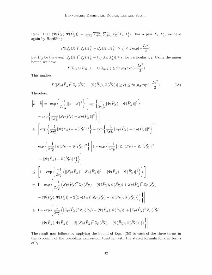
Blanchard, Deshmukh, Dogan, Lee and Scott
Recall that 〈Ψ(PX),Ψ(P ′X)〉 = 1n1n2
∑n1i=1
∑n2j=1 k
′X(Xi, X
′j). For a pair Xi, X
′j , we have
again by Hoeffding
P (|z′X(Xi)T z′X(X ′j)− k′X(Xi, X
′j)| ≥ ε) ≤ 2 exp(−Lε
2
2).
Let Ωij be the event |z′X(Xi)T z′X(X ′j)−k′X(Xi, X
′j)| ≥ ε, for particular i, j. Using the union
bound we have
P (Ω11 ∪ Ω12 ∪ . . . ∪ Ωn1n2) ≤ 2n1n2 exp(−Lε2
2)
This implies
P (|ZP (PX)TZP (P ′X)− 〈Ψ(PX),Ψ(P ′X)〉| ≥ ε) ≤ 2n1n2 exp(−Lε2
2). (38)
Therefore,∣∣∣k − k∣∣∣ =
∣∣∣∣∣ exp
−1
2σ2X‖x− x′‖2
[exp
−1
2σ2P‖Ψ(PX)−Ψ(P ′X)‖2
− exp
−1
2σ2P‖ZP (PX)− ZP (P ′X)‖2
]∣∣∣∣∣≤
∣∣∣∣∣[
exp
−1
2σ2P‖Ψ(PX)−Ψ(P ′X)‖2
− exp
−1
2σ2P‖ZP (PX)− ZP (P ′X)‖2
]∣∣∣∣∣=
∣∣∣∣∣ exp
−1
2σ2P‖Ψ(PX)−Ψ(P ′X)‖2
[1− exp
−1
2σ2P
(‖ZP (PX)− ZP (P ′X)‖2
− ‖Ψ(PX)−Ψ(P ′X)‖2)]∣∣∣∣∣
≤
∣∣∣∣∣[
1− exp
−1
2σ2P
(‖ZP (PX)− ZP (P ′X)‖2 − ‖Ψ(PX)−Ψ(P ′X)‖2
)]∣∣∣∣∣=
∣∣∣∣∣1− exp
−1
2σ2P
(ZP (PX)TZP (PX)− 〈Ψ(PX),Ψ(PX)〉+ ZP (P ′X)TZP (P ′X)
− 〈Ψ(P ′X),Ψ(P ′X)〉 − 2(ZP (PX)TZP (P ′X)− 〈Ψ(PX),Ψ(P ′X)〉
))∣∣∣∣∣≤
∣∣∣∣∣1− exp
1
2σ2P
(|ZP (PX)TZP (PX)− 〈Ψ(PX),Ψ(PX)〉|+ |ZP (P ′X)TZP (P ′X)
− 〈Ψ(P ′X),Ψ(P ′X)〉|+ 2|(ZP (PX)TZP (P ′X)− 〈Ψ(PX),Ψ(P ′X)〉
)|)∣∣∣∣∣
The result now follows by applying the bound of Eqn. (38) to each of the three terms inthe exponent of the preceding expression, together with the stated formula for ε in termsof ε`.
42
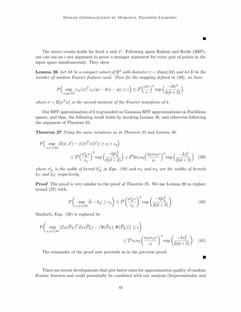
Domain Generalization by Marginal Transfer Learning
The above results holds for fixed x and x′. Following again Rahimi and Recht (2007),one can use an ε-net argument to prove a stronger statement for every pair of points in theinput space simultaneously. They show
Lemma 26 LetM be a compact subset of Rd with diameter r = diam(M) and let D be thenumber of random Fourier features used. Then for the mapping defined in (29), we have
P(
supx,y∈M
|zw(x)T zw(y)− k(x− y)| ≥ ε)≤ 28
(σrε
)2exp
( −Dε22(d+ 2)
),
where σ = E[wTw] is the second moment of the Fourier transform of k.
Our RFF approximation of k is grounded on Gaussian RFF approximations on Euclideanspaces, and thus, the following result holds by invoking Lemma 26, and otherwise followingthe argument of Theorem 25.
Theorem 27 Using the same notations as in Theorem 25 and Lemma 26,
P(
supx,x′∈M
|k(x, x′)− z(x)T z(x′)| ≥ εl + εq
)≤ 28
(σ′Xrεq
)2exp
( −Qε2q2(d+ 2)
)+ 293n1n2
(σPσXrεl
)2exp
( −Lε2l2(d+ 2)
)(39)
where σ′X is the width of kernel k′X in Eqn. (30) and σP and σX are the widths of kernelskP and kX respectively.
Proof The proof is very similar to the proof of Theorem 25. We use Lemma 26 to replacebound (37) with:
P
(sup
x,x′∈M|k − kq| ≥ εq
)≤ 28
(σ′Xr
εq
)2
exp
( −Qε2q2(d+ 2)
). (40)
Similarly, Eqn. (38) is replaced by
P
(sup
x,x′∈M
∣∣ZP (PX)TZP (P ′X)−⟨Ψ(PX),Ψ(P ′X)
⟩∣∣ ≥ ε)≤ 29n1n2
(σPσXr
εl
)2
exp
(−Lε2l
2(d+ 2)
). (41)
The remainder of the proof now proceeds as in the previous proof.
There are recent developments that give faster rates for approximation quality of randomFourier features and could potentially be combined with our analysis (Sriperumbudur and
43
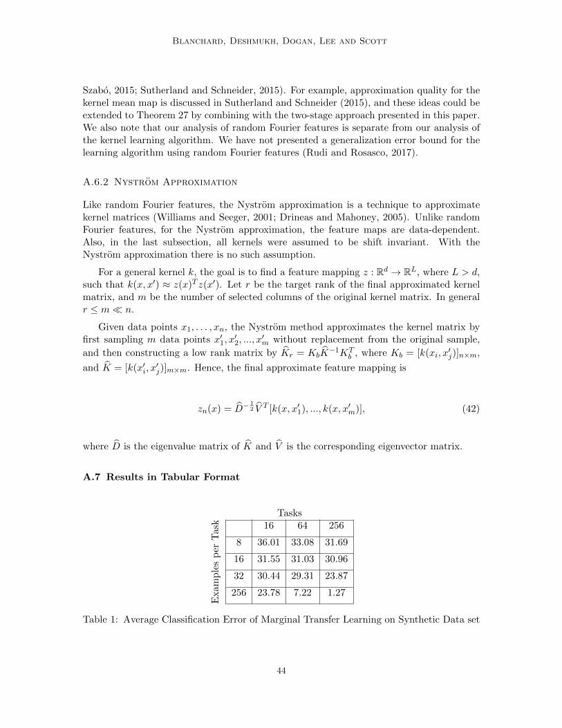
Blanchard, Deshmukh, Dogan, Lee and Scott
Szabo, 2015; Sutherland and Schneider, 2015). For example, approximation quality for thekernel mean map is discussed in Sutherland and Schneider (2015), and these ideas could beextended to Theorem 27 by combining with the two-stage approach presented in this paper.We also note that our analysis of random Fourier features is separate from our analysis ofthe kernel learning algorithm. We have not presented a generalization error bound for thelearning algorithm using random Fourier features (Rudi and Rosasco, 2017).
A.6.2 Nystrom Approximation
Like random Fourier features, the Nystrom approximation is a technique to approximatekernel matrices (Williams and Seeger, 2001; Drineas and Mahoney, 2005). Unlike randomFourier features, for the Nystrom approximation, the feature maps are data-dependent.Also, in the last subsection, all kernels were assumed to be shift invariant. With theNystrom approximation there is no such assumption.
For a general kernel k, the goal is to find a feature mapping z : Rd → RL, where L > d,such that k(x, x′) ≈ z(x)T z(x′). Let r be the target rank of the final approximated kernelmatrix, and m be the number of selected columns of the original kernel matrix. In generalr ≤ m n.
Given data points x1, . . . , xn, the Nystrom method approximates the kernel matrix byfirst sampling m data points x′1, x
′2, ..., x
′m without replacement from the original sample,
and then constructing a low rank matrix by Kr = KbK−1KT
b , where Kb = [k(xi, x′j)]n×m,
and K = [k(x′i, x′j)]m×m. Hence, the final approximate feature mapping is
zn(x) = D−12 V T [k(x, x′1), ..., k(x, x′m)], (42)
where D is the eigenvalue matrix of K and V is the corresponding eigenvector matrix.
A.7 Results in Tabular Format
Tasks
Exam
ple
sp
erT
ask 16 64 256
8 36.01 33.08 31.69
16 31.55 31.03 30.96
32 30.44 29.31 23.87
256 23.78 7.22 1.27
Table 1: Average Classification Error of Marginal Transfer Learning on Synthetic Data set
44
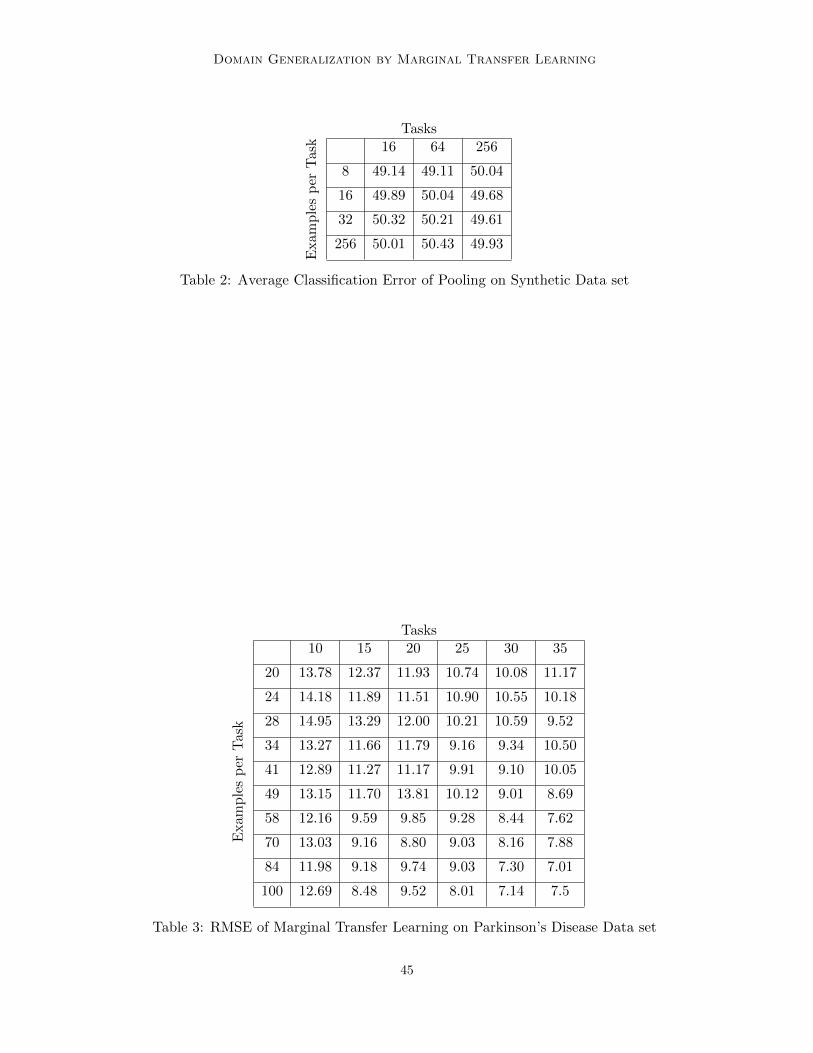
Domain Generalization by Marginal Transfer Learning
Tasks
Exam
ple
sp
erT
ask 16 64 256
8 49.14 49.11 50.04
16 49.89 50.04 49.68
32 50.32 50.21 49.61
256 50.01 50.43 49.93
Table 2: Average Classification Error of Pooling on Synthetic Data set
Tasks
Exam
ple
sp
erT
ask
10 15 20 25 30 35
20 13.78 12.37 11.93 10.74 10.08 11.17
24 14.18 11.89 11.51 10.90 10.55 10.18
28 14.95 13.29 12.00 10.21 10.59 9.52
34 13.27 11.66 11.79 9.16 9.34 10.50
41 12.89 11.27 11.17 9.91 9.10 10.05
49 13.15 11.70 13.81 10.12 9.01 8.69
58 12.16 9.59 9.85 9.28 8.44 7.62
70 13.03 9.16 8.80 9.03 8.16 7.88
84 11.98 9.18 9.74 9.03 7.30 7.01
100 12.69 8.48 9.52 8.01 7.14 7.5
Table 3: RMSE of Marginal Transfer Learning on Parkinson’s Disease Data set
45
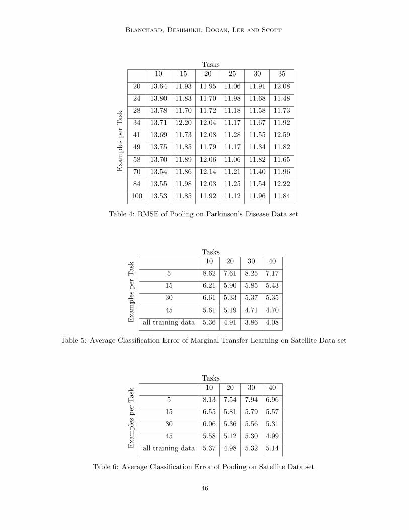
Blanchard, Deshmukh, Dogan, Lee and Scott
Tasks
Exam
ple
sp
erT
ask
10 15 20 25 30 35
20 13.64 11.93 11.95 11.06 11.91 12.08
24 13.80 11.83 11.70 11.98 11.68 11.48
28 13.78 11.70 11.72 11.18 11.58 11.73
34 13.71 12.20 12.04 11.17 11.67 11.92
41 13.69 11.73 12.08 11.28 11.55 12.59
49 13.75 11.85 11.79 11.17 11.34 11.82
58 13.70 11.89 12.06 11.06 11.82 11.65
70 13.54 11.86 12.14 11.21 11.40 11.96
84 13.55 11.98 12.03 11.25 11.54 12.22
100 13.53 11.85 11.92 11.12 11.96 11.84
Table 4: RMSE of Pooling on Parkinson’s Disease Data set
Tasks
Exam
ple
sp
erT
ask 10 20 30 40
5 8.62 7.61 8.25 7.17
15 6.21 5.90 5.85 5.43
30 6.61 5.33 5.37 5.35
45 5.61 5.19 4.71 4.70
all training data 5.36 4.91 3.86 4.08
Table 5: Average Classification Error of Marginal Transfer Learning on Satellite Data set
Tasks
Exam
ple
sp
erT
ask
10 20 30 40
5 8.13 7.54 7.94 6.96
15 6.55 5.81 5.79 5.57
30 6.06 5.36 5.56 5.31
45 5.58 5.12 5.30 4.99
all training data 5.37 4.98 5.32 5.14
Table 6: Average Classification Error of Pooling on Satellite Data set
46
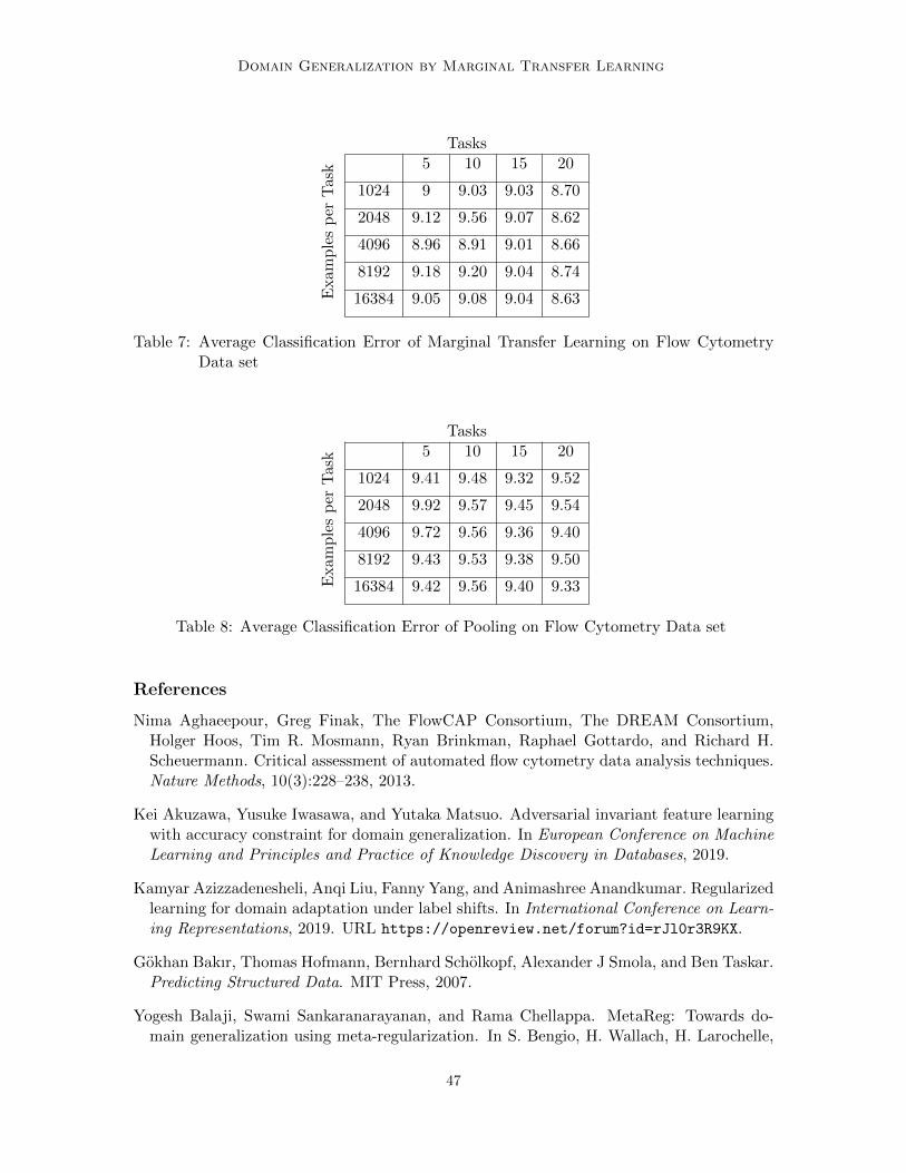
Domain Generalization by Marginal Transfer Learning
Tasks
Exam
ple
sp
erT
ask 5 10 15 20
1024 9 9.03 9.03 8.70
2048 9.12 9.56 9.07 8.62
4096 8.96 8.91 9.01 8.66
8192 9.18 9.20 9.04 8.74
16384 9.05 9.08 9.04 8.63
Table 7: Average Classification Error of Marginal Transfer Learning on Flow CytometryData set
Tasks
Exam
ple
sp
erT
ask 5 10 15 20
1024 9.41 9.48 9.32 9.52
2048 9.92 9.57 9.45 9.54
4096 9.72 9.56 9.36 9.40
8192 9.43 9.53 9.38 9.50
16384 9.42 9.56 9.40 9.33
Table 8: Average Classification Error of Pooling on Flow Cytometry Data set
References
Nima Aghaeepour, Greg Finak, The FlowCAP Consortium, The DREAM Consortium,Holger Hoos, Tim R. Mosmann, Ryan Brinkman, Raphael Gottardo, and Richard H.Scheuermann. Critical assessment of automated flow cytometry data analysis techniques.Nature Methods, 10(3):228–238, 2013.
Kei Akuzawa, Yusuke Iwasawa, and Yutaka Matsuo. Adversarial invariant feature learningwith accuracy constraint for domain generalization. In European Conference on MachineLearning and Principles and Practice of Knowledge Discovery in Databases, 2019.
Kamyar Azizzadenesheli, Anqi Liu, Fanny Yang, and Animashree Anandkumar. Regularizedlearning for domain adaptation under label shifts. In International Conference on Learn-ing Representations, 2019. URL https://openreview.net/forum?id=rJl0r3R9KX.
Gokhan Bakır, Thomas Hofmann, Bernhard Scholkopf, Alexander J Smola, and Ben Taskar.Predicting Structured Data. MIT Press, 2007.
Yogesh Balaji, Swami Sankaranarayanan, and Rama Chellappa. MetaReg: Towards do-main generalization using meta-regularization. In S. Bengio, H. Wallach, H. Larochelle,
47
Blanchard, Deshmukh, Dogan, Lee and Scott
K. Grauman, N. Cesa-Bianchi, and R. Garnett, editors, Advances in Neural InformationProcessing Systems 31, pages 998–1008. Curran Associates, Inc., 2018.
Peter Bartlett and Shahar Mendelson. Rademacher and Gaussian complexities: Risk boundsand structural results. Journal of Machine Learning Research, 3:463–482, 2002.
Peter Bartlett, Michael Jordan, and Jon McAuliffe. Convexity, classification, and riskbounds. Journal of the American Statistical Association, 101(473):138–156, 2006.
Jonathan Baxter. A model of inductive bias learning. Journal of Artificial IntelligenceResearch, 12:149–198, 2000.
Shai Ben-David and Ruth Urner. On the hardness of domain adaptation and the utilityof unlabeled target samples. In Nader H. Bshouty, Gilles Stoltz, Nicolas Vayatis, andThomas Zeugmann, editors, Algorithmic Learning Theory, pages 139–153, 2012.
Shai Ben-David, John Blitzer, Koby Crammer, and Fernando Pereira. Analysis of repre-sentations for domain adaptation. In B. Scholkopf, J. C. Platt, and T. Hoffman, editors,Advances in Neural Information Processing Systems 19, pages 137–144. 2007.
Shai Ben-David, John Blitzer, Koby Crammer, Alex Kulesza, Fernando Pereira, and Jen-nifer Wortman Vaughan. A theory of learning from different domains. Machine Learning,79:151–175, 2010.
Steffen Bickel, Michael Bruckner, and Tobias Scheffer. Discriminative learning under co-variate shift. Journal of Machine Learning Research, 10:2137–2155, 2009.
Gilles Blanchard, Gyemin Lee, and Clayton Scott. Generalizing from several related clas-sification tasks to a new unlabeled sample. In John Shawe-Taylor, Richard S. Zemel,Peter L. Bartlett, Fernando Pereira, and Kilian Q. Weinberger, editors, Advances inNeural Information Processing Systems 24, pages 2178–2186. 2011.
Gilles Blanchard, Marek Flaska, Gregory Handy, Sara Pozzi, and Clayton Scott. Classifica-tion with asymmetric label noise: Consistency and maximal denoising. Electronic Journalof Statistics, 10:2780–2824, 2016.
John Blitzer, Koby Crammer, Alex Kulesza, Fernando Pereira, and Jennifer Wortman.Learning bounds for domain adaptation. In J. C. Platt, D. Koller, Y. Singer, and S. T.Roweis, editors, Advances in Neural Information Processing Systems 20, pages 129–136.2008.
Timothy I. Cannings, Yingying Fan, and Richard J. Samworth. Classification with imperfecttraining labels. Technical Report arXiv:1805.11505, 2018.
Fabio Maria Carlucci, Antonio D’Innocente, Silvia Bucci, Barbara Caputo, and TatianaTommasi. Domain generalization by solving jigsaw puzzles. 2019 IEEE Conference onComputer Vision and Pattern Recognition (CVPR), pages 2224–2233, 2019.
Rich Caruana. Multitask learning. Machine Learning, 28:41–75, 1997.
48
Domain Generalization by Marginal Transfer Learning
Chih-Chung Chang and Chih-Jen Lin. LIBSVM: A library for support vector machines.ACM Transactions on Intelligent Systems and Technology, 2(3):27, 2011.
Andreas Christmann and Ingo Steinwart. Universal kernels on non-standard input spaces.In J. Lafferty, C. K. I. Williams, J. Shawe-Taylor, R. Zemel, and A. Culotta, editors,Advances in Neural Information Processing Systems 23, pages 406–414, 2010.
Corinna Cortes, Mehryar Mohri, Michael Riley, and Afshin Rostamizadeh. Sample selectionbias correction theory. In Algorithmic Learning Theory, pages 38–53, 2008.
Corinna Cortes, Mehryar Mohri, and Andres Munoz Medina. Adaptation algorithm andtheory based on generalized discrepancy. In Proceedings of the 21th ACM SIGKDDInternational Conference on Knowledge Discovery and Data Mining, KDD ’15, pages169–178, 2015.
Daryl J. Daley and David Vere-Jones. An Introduction to the Theory of Point Processes,volume I: Elementary Theory and Methods. Springer, 2003.
Daryl J. Daley and David Vere-Jones. An Introduction to the Theory of Point Processes,volume II: General Theory and Structure. Springer, 2008.
Giulia Denevi, Carlo Ciliberto, Dimitris Stamos, and Massimiliano Pontil. Learning tolearn around a common mean. In S. Bengio, H. Wallach, H. Larochelle, K. Grauman,N. Cesa-Bianchi, and R. Garnett, editors, Advances in Neural Information ProcessingSystems 31, pages 10169–10179. 2018a.
Giulia Denevi, Carlo Ciliberto, Dimitros Stamos, and Massimiliano Pontil. Incrementallearning-to-learn with statistical guarantees. In Proc. Uncertainty in Artificial Intelli-gence, 2018b.
Zhengming Ding and Yun Fu. Deep domain generalization with structured low-rank con-straint. IEEE Transactions on Image Processing, 27:304–313, 2018.
Qi Dou, Daniel Coelho de Castro, Konstantinos Kamnitsas, and Ben Glocker. Domain gen-eralization via model-agnostic learning of semantic features. In H. Wallach, H. Larochelle,A. Beygelzimer, F. d’ Alche-Buc, E. Fox, and R. Garnett, editors, Advances in NeuralInformation Processing Systems 32, pages 6450–6461. 2019.
Petros Drineas and Michael W. Mahoney. On the Nystrom method for approximatinga gram matrix for improved kernel-based learning. The Journal of Machine LearningResearch, 6:2153–2175, 2005.
Marthinus Christoffel Du Plessis and Masashi Sugiyama. Semi-supervised learning of classbalance under class-prior change by distribution matching. In J. Langford and J. Pineau,editors, Proc. 29th Int. Conf. on Machine Learning, pages 823–830, 2012.
Theodoros Evgeniou, Charles A. Michelli, and Massimiliano Pontil. Learning multiple taskswith kernel methods. Journal of Machine Learning Research, 6:615–637, 2005.
49
Blanchard, Deshmukh, Dogan, Lee and Scott
Rong-En Fan, Kai-Wei Chang, Cho-Jui Hsieh, Xiang-Rui Wang, and Chih-Jen Lin. LI-BLINEAR: A library for large linear classification. The Journal of Machine LearningResearch, 9:1871–1874, 2008.
Chelsea Finn, Pieter Abbeel, and Sergey Levine. Model-agnostic meta-learning for fastadaptation of deep networks. In Doina Precup and Yee Whye Teh, editors, Interna-tional Conference on Machine Learning, volume 70 of Proceedings of Machine LearningResearch, pages 1126–1135, 2017.
Chuang Gan, Tianbao Yang, and Boqing Gong. Learning attributes equals multi-sourcedomain generalization. In The IEEE Conference on Computer Vision and Pattern Recog-nition (CVPR), June 2016.
Pascal Germain, Amaury Habrard, Francois Laviolette, and Emilie Morvant. A new pac-bayesian perspective on domain adaptation. In Internation Conference on Machine Learn-ing, volume 48 of JMLR Workshop and Conference Proceedings, pages 859–868, 2016.
Muhammad Ghifary, W. Bastiaan Kleijn, Mengjie Zhang, and David Balduzzi. Domaingeneralization for object recognition with multi-task autoencoders. In IEEE InternationalConference on Computer Vision, page 2551–2559, 2015.
Muhammad Ghifary, David Balduzzi, W. Bastiaan Kleijn, and Mengjie Zhang. Scattercomponent analysis: A unified framework for domain adaptation and domain generaliza-tion. IEEE Transactions on Pattern Analysis and Machine Intelligence, 39(7):1411–1430,2017.
Mingming Gong, Kun Zhang, Tongliang Liu, Dacheng Tao, Clark Glymour, and BernhardScholkopf. Domain adaptation with conditional transferable components. In Internationalconference on machine learning, pages 2839–2848, 2016.
Arthur Gretton, Karsten Borgwardt, Malte Rasch, Bernhard Scholkopf, and AlexanderSmola. A kernel approach to comparing distributions. In R. Holte and A. Howe, editors,22nd AAAI Conference on Artificial Intelligence, pages 1637–1641, 2007a.
Arthur Gretton, Karsten Borgwardt, Malte Rasch, Bernhard Scholkopf, and AlexanderSmola. A kernel method for the two-sample-problem. In B. Scholkopf, J. Platt, andT. Hoffman, editors, Advances in Neural Information Processing Systems 19, pages 513–520, 2007b.
Thomas Grubinger, Adriana Birlutiu, Holger Schoner, Thomas Natschlager, and Tom Hes-kes. Domain generalization based on transfer component analysis. In I. Rojas, G. Joya,and A. Catala, editors, Advances in Computational Intelligence, International Work-Conference on Artificial Neural Networks, volume 9094 of Lecture Notes in ComputerScience, pages 325–334. Springer International Publishing, 2015.
Peter Hall. On the non-parametric estimation of mixture proportions. Journal of the RoyalStatistical Society, 43(2):147–156, 1981.
50
Domain Generalization by Marginal Transfer Learning
Cho-Jui Hsieh, Kai-Wei Chang, Chih-Jen Lin, S. Sathiya Keerthi, and S. Sundararajan. Adual coordinate descent method for large-scale linear SVM. In International Conferenceon Machine Learning, pages 408–415. ACM, 2008.
Shoubo Hu, Kun Zhang, Zhitang Chen, and Laiwan Chan. Domain generalization viamultidomain discriminant analysis. In Amir Globerson and Ricardo Silva, editors, Un-certainty in Artificial Intelligence, 2019.
Jiayuan Huang, Alexander J. Smola, Arthur Gretton, Karsten M. Borgwardt, and BernhardScholkopf. Correcting sample selection bias by unlabeled data. In Advances in NeuralInformation Processing Systems, pages 601–608, 2007.
Wittawat Jitkrittum, Arthur Gretton, Nicolas Heess, SM Eslami, Balaji Lakshminarayanan,Dino Sejdinovic, and Zoltan Szabo. Kernel-based just-in-time learning for passing expec-tation propagation messages. In Proceedings of the Thirty-First Conference on Uncer-tainty in Artificial Intelligence, pages 405–414. AUAI Press, 2015.
Thorsten Joachims. Making large-scale SVM learning practical. In B. Scholkopf, C. Burges,and A. Smola, editors, Advances in Kernel Methods - Support Vector Learning, chapter 11,pages 169–184. MIT Press, Cambridge, MA, 1999.
Olav Kallenberg. Foundations of Modern Probability. Springer, 2002.
Takafumi Kanamori, Shohei Hido, and Masashi Sugiyama. A least-squares approach todirect importance estimation. Journal of Machine Learning Research, 10:1391–1445, 2009.
Aditya Khosla, Tinghui Zhou, Tomasz Malisiewicz, Alexei A. Efros, and Antonio Torralba.Undoing the damage of dataset bias. In 12th European Conference on Computer Vision- Volume Part I, page 158–171, 2012.
Ron Kohavi. A study of cross-validation and bootstrap for accuracy estimation and modelselection. In International Joint Conference on Artificial Intelligence, volume 14, pages1137–1145, 1995.
Vladimir Koltchinskii. Rademacher penalties and structural risk minimization. IEEE Trans-actions on Information Theory, 47(5):1902 – 1914, 2001.
Patrice Latinne, Marco Saerens, and Christine Decaestecker. Adjusting the outputs of aclassifier to new a priori probabilities may significantly improve classification accuracy:Evidence from a multi-class problem in remote sensing. In C. Sammut and A. H. Hoff-mann, editors, International Conference on Machine Learning, pages 298–305, 2001.
Quoc Le, Tamas Sarlos, and Alex Smola. Fastfood: approximating kernel expansions inloglinear time. In International Conference on International Conference on MachineLearning-Volume 28, pages III–244, 2013.
Da Li, Yongxin Yang, Yi-Zhe Song, and Timothy M Hospedales. Deeper, broader andartier domain generalization. In Proceedings of the IEEE International Conference onComputer Vision, pages 5542–5550, 2017.
51
Blanchard, Deshmukh, Dogan, Lee and Scott
Da Li, Yongxin Yang, Yi-Zhe Song, and Timothy M Hospedales. Learning to generalize:Meta-learning for domain generalization. In AAAI Conference on Artificial Intelligence,2018a.
Haoliang Li, Sinno Jialin Pan, Shiqi Wang, and Alex C. Kot. Domain generalization withadversarial feature learning. In IEEE Conference on Computer Vision and Pattern Recog-nition, pages 5400–5409, 2018b.
Ya Li, Mingming Gong, Xinmei Tian, Tongliang Liu, and Dacheng Tao. Domain gen-eralization via conditional invariant representations. In AAAI Conference on ArtificialIntelligence, 2018c.
Ya Li, Xinmei Tian, Mingming Gong, Yajing Liu, Tongliang Liu, Kun Zhang, and DachengTao. Deep domain generalization via conditional invariant adversarial networks. In Pro-ceedings of the European Conference on Computer Vision (ECCV), pages 624–639, 2018d.
Yishay Mansour, Mehryar Mohri, and Afshin Rostamizadeh. Domain adaptation: Learningbounds and algorithms. In Conference on Learning Theory, 2009a.
Yishay Mansour, Mehryar Mohri, and Afshin Rostamizadeh. Domain adaptation withmultiple sources. In Advances in Neural Information Processing Systems, pages 1041–1048, 2009b.
Andreas Maurer. Transfer bounds for linear feature learning. Machine Learning, 75(3):327–350, 2009.
Andreas Maurer, Massimiliano Pontil, and Bernardino Romera-Paredes. Sparse codingfor multitask and transfer learning. In Sanjoy Dasgupta and David McAllester, editors,International Conference on Machine Learning, volume 28 of Proceedings of MachineLearning Research, pages 343–351, 2013.
Andreas Maurer, Massimiliano Pontil, and Bernardino Romera-Paredes. The benefit ofmultitask representation learning. Journal of Machine Learning Research, 17(1):2853–2884, 2016.
Aditya Krishna Menon, Brendan van Rooyen, and Nagarajan Natarajan. Learning frombinary labels with instance-dependent noise. Machine Learning, 107:1561–1595, 2018.
Saeid Motiian, Marco Piccirilli, Donald A. Adjeroh, and Gianfranco Doretto. Unified deepsupervised domain adaptation and generalization. In IEEE International Conference onComputer Vision, pages 5715–5725, 2017.
Krikamol Muandet, David Balduzzi, and Bernhard Scholkopf. Domain generalization viainvariant feature representation. In International Conference on Machine Learning, vol-ume 28 of Proceedings of Machine Learning Research, pages I–10–I–18, 2013.
Nagarajan Natarajan, Inderjit S. Dhillon, Pradeep Ravikumar, and Ambuj Tewari. Cost-sensitive learning with noisy labels. Journal of Machine Learning Research, 18(155):1–33,2018. URL http://jmlr.org/papers/v18/15-226.html.
52
Domain Generalization by Marginal Transfer Learning
Kalyanapuram Rangachari Parthasarathy. Probability Measures on Metric Spaces. Aca-demic Press, 1967.
Anastasia Pentina and Christoph Lampert. A PAC-Bayesian bound for lifelong learning. InEric P. Xing and Tony Jebara, editors, International Conference on Machine Learning,volume 32 of Proceedings of Machine Learning Research, pages 991–999, 2014.
Iosif F. Pinelis and Aleksandr Ivanovich Sakhanenko. Remarks on inequalities for probabil-ities of large deviations. Theory Probab. Appl., 30(1):143–148, 1985.
Joaquin Quionero-Candela, Masashi Sugiyama, Anton Schwaighofer, and Neil Lawrence.Dataset Shift in Machine Learning. The MIT Press, 2009.
Ali Rahimi and Ben Recht. Random features for large-scale kernel machines. In Advancesin Neural Information Processing Systems, pages 1177–1184, 2007.
Alessandro Rudi and Lorenzo Rosasco. Generalization properties of learning with randomfeatures. In Advances in Neural Information Processing Systems, pages 3215–3225, 2017.
Tyler Sanderson and Clayton Scott. Class proportion estimation with application to mul-ticlass anomaly rejection. In Conferencen on Artificial Intelligence and Statistics, 2014.
Clayton Scott. A generalized Neyman-Pearson criterion for optimal domain adaptation. InAurelien Garivier and Satyen Kale, editors, Algorithmic Learning Theory, volume 98 ofProceedings of Machine Learning Research, pages 738–761, 2019.
Shiv Shankar, Vihari Piratla, Soumen Chakrabarti, Siddhartha Chaudhuri, Preethi Jyothi,and Sunita Sarawagi. Generalizing across domains via cross-gradient training. In In-ternational Conference on Learning Representations, 2018. URL https://openreview.
net/forum?id=r1Dx7fbCW.
Srinagesh Sharma and James W. Cutler. Robust orbit determination and classification: Alearning theoretic approach. Interplanetary Network Progress Report, 203:1, 2015.
Bharath Sriperumbudur and Zoltan Szabo. Optimal rates for random Fourier features. InAdvances in Neural Information Processing Systems, pages 1144–1152, 2015.
Bharath Sriperumbudur, Arthur Gretton, Kenji Fukumizu, Bernhard Scholkopf, and GertLanckriet. Hilbert space embeddings and metrics on probability measures. Journal ofMachine Learning Research, 11:1517–1561, 2010.
Ingo Steinwart and Andreas Christmann. Support Vector Machines. Springer, 2008.
Amos J Storkey. When training and test sets are different: characterising learning transfer.In Dataset Shift in Machine Learning, pages 3–28. MIT Press, 2009.
Masashi Sugiyama, Taiji Suzuki, Shinichi Nakajima, Hisashi Kashima, Paul von Bunau, andMotoaki Kawanabe. Direct importance estimation for covariate shift adaptation. Annalsof the Institute of Statistical Mathematics, 60:699–746, 2008.
53
Blanchard, Deshmukh, Dogan, Lee and Scott
Danica J. Sutherland and Jeff Schneider. On the error of random Fourier features. InUncertainty in Artificial Intelligence, pages 862–871, 2015.
Zoltan Szabo, Bharath K Sriperumbudur, Barnabas Poczos, and Arthur Gretton. Learningtheory for distribution regression. The Journal of Machine Learning Research, 17(1):5272–5311, 2016.
Dirk Tasche. Fisher consistency for prior probability shift. Journal of Machine LearningResearch, 18:1–32, 2017.
Sebastian Thrun. Is learning the n-th thing any easier than learning the first? Advances inNeural Information Processing Systems, pages 640–646, 1996.
D. Michael Titterington. Minimum distance non-parametric estimation of mixture propor-tions. Journal of the Royal Statistical Society, 45(1):37–46, 1983.
Joern Toedling, Peter Rhein, Richard Ratei, Leonid Karawajew, and Rainer Spang. Auto-mated in-silico detection of cell populations in flow cytometry readouts and its applicationto leukemia disease monitoring. BMC Bioinformatics, 7:282, 2006.
Athanasios Tsanas, Max A. Little, Patrick E. McSharry, and Lorraine O. Ramig. Accuratetelemonitoring of Parkinson’s disease progression by noninvasive speech tests. IEEETransactions on Biomedical Engineering, 57(4):884–893, 2010.
Ioannis Tsochantaridis, Thorsten Joachims, Thomas Hofmann, and Yasemin Altun. Largemargin methods for structured and interdependent output variables. Journal of machinelearning research, 6(Sep):1453–1484, 2005.
Brendan van Rooyen and Robert C. Williamson. A theory of learning with corrupted labels.Journal of Machine Learning Research, 18(228):1–50, 2018.
Haohan Wang, Zexue He, Zachary C. Lipton, and Eric P. Xing. Learning robust represen-tations by projecting superficial statistics out. In International Conference on LearningRepresentations, 2019. URL https://openreview.net/forum?id=rJEjjoR9K7.
Jenna Wiens. Machine Learning for Patient-Adaptive Ectopic Beat Classication. Mas-ters Thesis, Department of Electrical Engineering and Computer Science, MassachusettsInstitute of Technology, 2010.
Christopher Williams and Matthias Seeger. Using the Nystrom method to speed up kernelmachines. In Advances in Neural Information Processing Systems, pages 682–688, 2001.
Zheng Xu, Wen Li, Li Niu, and Dong Xu. Exploiting low-rank structure from latent domainsfor domain generalization. In European Conference on Computer Vision, pages 628–643.Springer, 2014.
Liu Yang, Steve Hanneke, and Jamie Carbonell. A theory of transfer learning with appli-cations to active learning. Machine Learning, 90(2):161–189, 2013.
54
Domain Generalization by Marginal Transfer Learning
Xiaolin Yang, Seyoung Kim, and Eric P. Xing. Heterogeneous multitask learning withjoint sparsity constraints. In Advances in Neural Information Processing Systems, pages2151–2159, 2009.
Yao-Liang Yu and Csaba Szepesvari. Analysis of kernel mean matching under covariateshift. In International Conference on Machine Learning, pages 607–614, 2012.
Bianca Zadrozny. Learning and evaluating classifiers under sample selection bias. In Inter-national Conference on Machine Learning, 2004.
Kun Zhang, Bernhard Scholkopf, Krikamol Muandet, and Zhikun Wang. Domain adapta-tion under target and conditional shift. In International Conference on Machine Learning,pages 819–827, 2013.
Kun Zhang, Mingming Gong, and Bernhard Scholkopf. Multi-source domain adaptation:A causal view. In AAAI Conference on Artificial Intelligence, pages 3150–3157. AAAIPress, 2015.
55