Embed Size (px)
Citation preview
TECHNISCHE UNIVERSITAT MUNCHENLehrstuhl fur Datenverarbeitung
Efficient Binaural Sound
Localization for Humanoid
Robots and Telepresence
Applications
Fakheredine Keyrouz
Vollstandiger Abdruck der von der Fakultat fur Elektrotechnik und Informa-tionstechnik der Technischen Universitat Munchen zur Erlangung des akademischenGrades eines
Doktor–Ingenieurs
genehmigten Dissertation.
Vorsitzender: Univ.-Prof. Dr.-Ing. / Univ. Tokio M. Buss
Prufer der Dissertation: 1. Univ.-Prof. Dr.-Ing. K. Diepold
2. apl. Prof. Dr.-Ing., Dr.-Ing. habil. H. Fastl
Die Dissertation wurde am 21.02.2008 bei der Technischen Universitat Muncheneingereicht und durch die Fakultat fur Elektrotechnik und Informationstechnik am06.06.2008 angenommen.

II
Acknowledgments
I would like to thank professor Klaus Diepold for giving me the opportunity towork on my dissertation with him. His support, encouragement, questions, com-ments, and suggestions have influenced the contents of this work. Furthermore, Ithank Professor Patrick Dewilde (Delft University of Technology, Netherlands) forhis continuous interest in my research and for his insights and discussions.
In addition, I would like to thank the contribution of Bill Gardner and his colleaguesat the Media Laboratory at Massachusetts Institute of Technology for measuring theHRTFs and sharing the database as a courtesy. Besides, I would like to thank Dipl.-Ing. Walter Bamberger for his continuous help throughout my research time. I alsothank my colleagues at the data processing institute for the friendly and supportiveatmosphere.
Last but not least, I want to thank all my friends and comrades who encouragedme during my work on the thesis. A special and cordial thanks is due to MissNeunhoffer for the value of proofreading every single chapter of this book. I wouldalso like to thank my parents and family for their unconditioned support. Finally, Iwant to thank God, for being my constant help.
And when you have reached the mountain top, then you shall begin to climb. K. G.
III

IV
Contents
Acknowledgments III
List of Figures VII
List of Tables XII
Abstract XV
1 Introduction 11.1 Telepresence Framework . . . . . . . . . . . . . . . . . . . . . . . . . 1
1.1.1 Acoustic Telepresence . . . . . . . . . . . . . . . . . . . . . . 21.1.2 Teleoperator Sound Localization . . . . . . . . . . . . . . . . . 2
1.2 State-of-the-Art Sound Localization Techniques . . . . . . . . . . . . 41.2.1 Sound Localization in General . . . . . . . . . . . . . . . . . . 41.2.2 Sound Localization Using Two Microphones . . . . . . . . . . 61.2.3 Microphone Array Based Sound Localization . . . . . . . . . . 14
1.3 Main Contributions and Overview . . . . . . . . . . . . . . . . . . . . 161.3.1 Main Contributions . . . . . . . . . . . . . . . . . . . . . . . . 161.3.2 Overview and Organization of the Thesis . . . . . . . . . . . . 17
2 Binaural Techniques 212.1 The Head Related Transfer Function . . . . . . . . . . . . . . . . . . 212.2 HRTF Cues . . . . . . . . . . . . . . . . . . . . . . . . . . . . . . . . 222.3 HRTF Properties . . . . . . . . . . . . . . . . . . . . . . . . . . . . . 23
2.3.1 Time Domain Impulse Responses . . . . . . . . . . . . . . . . 242.3.2 Frequency Domain Transfer Functions . . . . . . . . . . . . . 26
2.4 HRTF Measurements . . . . . . . . . . . . . . . . . . . . . . . . . . . 282.5 First Binaural Localization Model . . . . . . . . . . . . . . . . . . . . 282.6 HRTFs and Sound Localization . . . . . . . . . . . . . . . . . . . . . 292.7 HRTFs Reduction Techniques . . . . . . . . . . . . . . . . . . . . . . 30
2.7.1 Diffuse-Field Equalization . . . . . . . . . . . . . . . . . . . . 302.7.2 Balanced Model Truncation . . . . . . . . . . . . . . . . . . . 32
V
VI Contents
2.7.3 Principal Component Analysis . . . . . . . . . . . . . . . . . . 32
3 Binaural Sound Source Localization Based on HRTFs 373.1 A Novel Approach To Sound Localization . . . . . . . . . . . . . . . . 373.2 Efficient State-Space HRTF Interpolation . . . . . . . . . . . . . . . . 39
3.2.1 Previous Interpolation Methods . . . . . . . . . . . . . . . . . 413.2.2 Formulation of the Rational Interpolation Problem . . . . . . 413.2.3 Experimental Setup . . . . . . . . . . . . . . . . . . . . . . . . 433.2.4 Discussion of Results . . . . . . . . . . . . . . . . . . . . . . . 453.2.5 Subjective Analysis . . . . . . . . . . . . . . . . . . . . . . . . 463.2.6 Performance Results . . . . . . . . . . . . . . . . . . . . . . . 47
3.3 Efficient State-Space HRTF Inversion . . . . . . . . . . . . . . . . . . 493.3.1 Problem Formulation . . . . . . . . . . . . . . . . . . . . . . . 503.3.2 Inner-Outer Factorization . . . . . . . . . . . . . . . . . . . . 51
4 Enhanced Sound Source Localization Techniques 534.1 Source Cancelation Algorithm . . . . . . . . . . . . . . . . . . . . . . 53
4.1.1 Kalman Filtering and ROI Extraction . . . . . . . . . . . . . . 554.1.2 Simulation Results . . . . . . . . . . . . . . . . . . . . . . . . 574.1.3 Experimental Results . . . . . . . . . . . . . . . . . . . . . . . 604.1.4 A Case Study . . . . . . . . . . . . . . . . . . . . . . . . . . . 614.1.5 Performance Comparison . . . . . . . . . . . . . . . . . . . . . 634.1.6 Region of Interest . . . . . . . . . . . . . . . . . . . . . . . . . 64
4.2 Cross Convolution Approach . . . . . . . . . . . . . . . . . . . . . . . 664.2.1 Extended Kalman Filtering . . . . . . . . . . . . . . . . . . . 684.2.2 Implementation . . . . . . . . . . . . . . . . . . . . . . . . . . 694.2.3 Performance Analysis . . . . . . . . . . . . . . . . . . . . . . . 70
5 Concurrent Sound Source Localization and Separation 735.1 Motivation . . . . . . . . . . . . . . . . . . . . . . . . . . . . . . . . . 745.2 Source Separation and Localization Using Adaptive MIMO-Filtering . 75
5.2.1 Source Separation . . . . . . . . . . . . . . . . . . . . . . . . . 755.2.2 System Identification . . . . . . . . . . . . . . . . . . . . . . . 79
5.3 Localization and Separation by Clustering in Time-Frequency Domain 805.3.1 Blind System Identification Framework . . . . . . . . . . . . . 805.3.2 Self-Splitting Competitive Learning . . . . . . . . . . . . . . . 835.3.3 Solving the Permutation Problem . . . . . . . . . . . . . . . . 855.3.4 HRTF Database Lookup . . . . . . . . . . . . . . . . . . . . . 87
5.4 Source Separation Process . . . . . . . . . . . . . . . . . . . . . . . . 885.4.1 Determined System . . . . . . . . . . . . . . . . . . . . . . . . 885.4.2 Underdetermined System . . . . . . . . . . . . . . . . . . . . . 88

Contents VII
5.5 Simulation Results . . . . . . . . . . . . . . . . . . . . . . . . . . . . 925.5.1 Localization With Adaptive MIMO Systems . . . . . . . . . . 925.5.2 Localization by Clustering in Time-Frequency Domain . . . . 935.5.3 Separation Performance . . . . . . . . . . . . . . . . . . . . . 955.5.4 Localization Performance . . . . . . . . . . . . . . . . . . . . . 96
6 Sound Localization in Highly Reverberant Environments 996.1 New Hardware Setup . . . . . . . . . . . . . . . . . . . . . . . . . . . 996.2 Monaural System . . . . . . . . . . . . . . . . . . . . . . . . . . . . . 1006.3 Combined System . . . . . . . . . . . . . . . . . . . . . . . . . . . . . 1016.4 Bayesian Information Fusion . . . . . . . . . . . . . . . . . . . . . . . 103
6.4.1 Feature Vectors Extraction . . . . . . . . . . . . . . . . . . . . 1036.4.2 Decision Making . . . . . . . . . . . . . . . . . . . . . . . . . 104
6.5 Discussion of Results . . . . . . . . . . . . . . . . . . . . . . . . . . . 1056.5.1 Simulation Results . . . . . . . . . . . . . . . . . . . . . . . . 1056.5.2 Experimental Results . . . . . . . . . . . . . . . . . . . . . . . 108
7 Conclusion 111
Appendices 113
A Inner-outer Factorization Theorem Proof 115
B The State-Space Loewner Matrix 119
C List of Frequently Used Acronyms 121
Bibliography 135

VIII Contents
List of Figures
1.1 A multi-modal telepresence system. . . . . . . . . . . . . . . . . . . . 2
1.2 Acoustic telepresence scenario. . . . . . . . . . . . . . . . . . . . . . . 3
1.3 Interaural Time/Intensity Difference (ITD/IID). . . . . . . . . . . . . 6
1.4 Generalized cross-correlation (GCC) process. . . . . . . . . . . . . . . 8
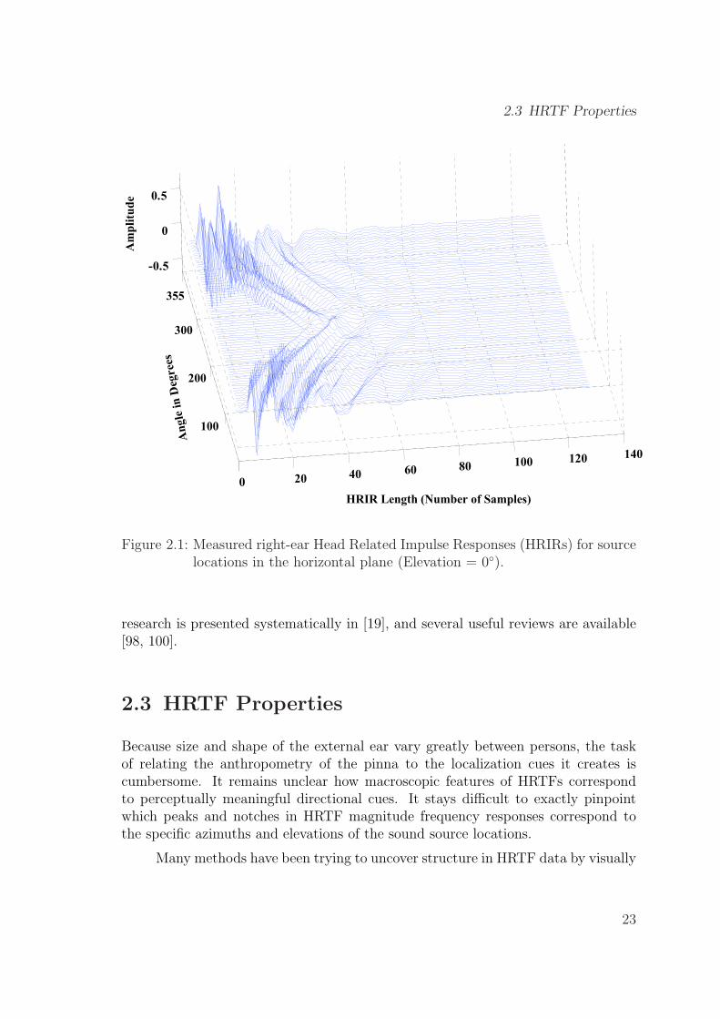
2.1 Measured right-ear Head Related Impulse Responses (HRIRs) forsource locations in the horizontal plane (Elevation = 0◦). . . . . . . . 23
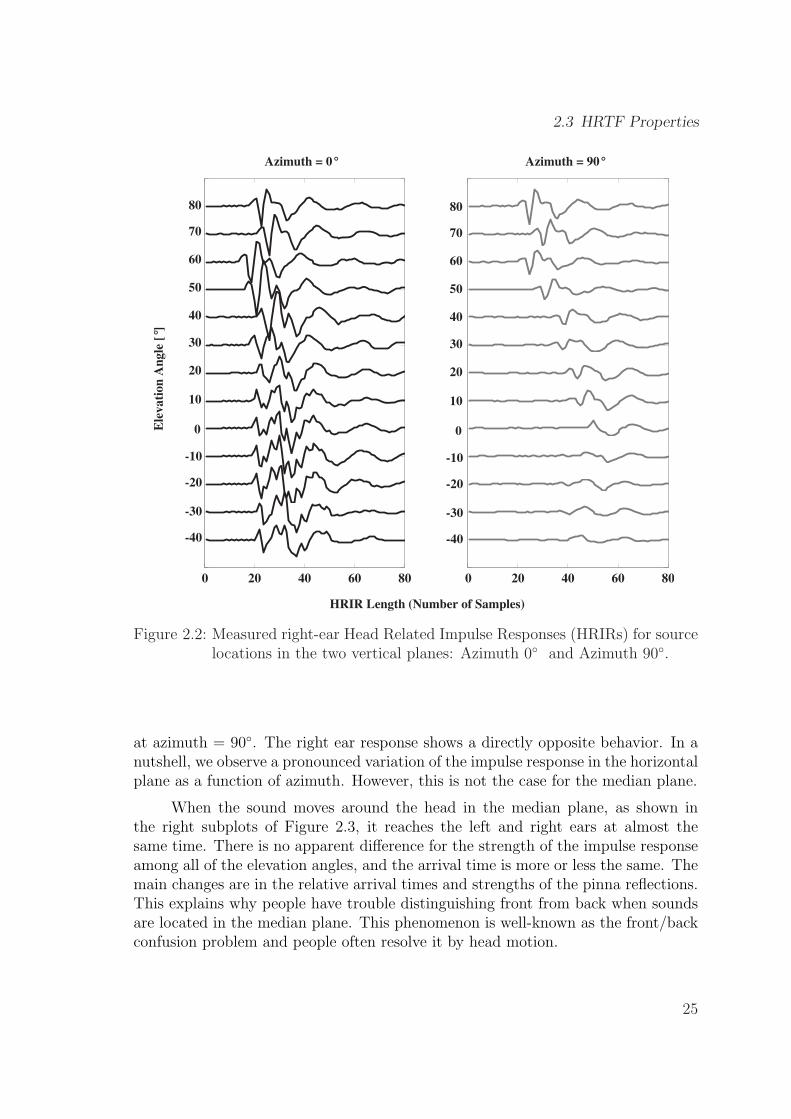
2.2 Measured right-ear Head Related Impulse Responses (HRIRs) forsource locations in the two vertical planes: Azimuth 0◦ and Azimuth90◦. . . . . . . . . . . . . . . . . . . . . . . . . . . . . . . . . . . . . . 25
2.3 Left two plots: HRIRs in the horizontal plane (elevation=0◦). Righttwo plots: HRIRs in the median plane (azimuth=0◦). . . . . . . . . . 26
2.4 Head-Related Transfer Functions (HRTFs). Left: variations in themedian plane (azimuth = 0◦ ). Right: variations in the horizontalplane (elevation = 0◦ ). . . . . . . . . . . . . . . . . . . . . . . . . . . 27
2.5 Magnitude response of the original 512-FIR (solid) and the reduced128-FIR (dashed) of an HRTF (left ear, 0◦ azimuth) . . . . . . . . . 31
2.6 Magnitude response of the 128-FIR (solid line) and the reduced 25-IIR (dashed line) of a HRTF (left ear, 0◦ azimuth). . . . . . . . . . . 33
2.7 Magnitude response of the 128-FIR (solid line) and the reduced 35-FIR (dashed line) of a HRTF (left ear, 5◦ azimuth). . . . . . . . . . 34
3.1 Flowchart of the sound localization algorithm. . . . . . . . . . . . . . 40
3.2 The interpolation process. . . . . . . . . . . . . . . . . . . . . . . . . 44
3.3 Interpolation accuracy. . . . . . . . . . . . . . . . . . . . . . . . . . . 45
3.4 Predicted localization accuracy averaged for 20 test subjects every30◦ from 0◦ to 330◦. . . . . . . . . . . . . . . . . . . . . . . . . . . . . 47
3.5 Listening test results averaged over 20 subjects: perceived angle ver-sus target angle. . . . . . . . . . . . . . . . . . . . . . . . . . . . . . . 48
4.1 Flow chart of the Source Cancelation Algorithm (SCA). . . . . . . . . 54
IX

X List of Figures
4.2 Flowchart of the Source Cancelation Algorithm using a Region ofInterest (ROI). . . . . . . . . . . . . . . . . . . . . . . . . . . . . . . 56
4.3 Percentage of correct localization using DFE, PCA and BMT reducedHRTFs. . . . . . . . . . . . . . . . . . . . . . . . . . . . . . . . . . . 57
4.4 Percentage of correct localization using SCA compared to the state-space inversion, and to the original method in [66]. . . . . . . . . . . 58
4.5 The falsely localized sound sources: average distance to their targetpositions, for every HRIR length. . . . . . . . . . . . . . . . . . . . . 59
4.6 The laboratory hardware setup. . . . . . . . . . . . . . . . . . . . . . 60
4.7 Case study: The SCA theoretical and experimental performance us-ing a artificial head with or without pinnae. . . . . . . . . . . . . . . 62
4.8 SCA processing time for different ROI intervals. . . . . . . . . . . . . 65
4.9 Flow chart of the convolution based algorithm. . . . . . . . . . . . . . 67
4.10 Comparison of cross convolution method and SCA in presence of re-flections and noise. . . . . . . . . . . . . . . . . . . . . . . . . . . . . 68
4.11 Block diagram of the HRTF-Kalman algorithm. . . . . . . . . . . . . 70
4.12 Localization performance averaged over different speech and broad-band sound signals moving clockwise around the head. . . . . . . . . 71
5.1 Differing transmission paths between sound sources and artificial headmicrophones modeled as a HRTF MIMO system. . . . . . . . . . . . 76
5.2 Demixing system with filters w11, w12, w21 and w22 which are adaptedby simultaneous diagonalization of short-time correlation matrices ofoutput signals y1(k) and y2(k) in order to separate the sound sources. 77
5.3 The combination of HRTF system and MIMO system for blind sourceseparation can be divided into four SIMO-MISO systems. . . . . . . . 80
5.4 Simultaneously running processes: BSS and HRTF lookup. TheHRTF lookup process takes the adapted filters w11, w12, w21 and w22
from the BSS process and finds the azimuth and elevation positionsof the first source (az1, elev1) and of the second source (az2, elev2). . 81
5.5 Samples from the two ear microphones after STFT. The two sub-plots depict the real part of X1 and the real part of X2 versus theimaginary part of X2, respectively. The data was gathered from 400time-frames at a frequency of 538 Hz and normalized according to(5.21) and (5.22). The clusters show that there are two speakerspresent. Furthermore, the prototypes determined by Self-SplittingCompetitive Learning are depicted in the cluster centers. . . . . . . . 82
List of Figures XI
5.6 Left: Learning process of the first prototype. Step 1 shows the initial-ization of the second component of ~P1 and the APV ~A1. Step 2 showstheir positions after 100 iterations. In step 3 the distance between ~P1
and ~A1 has fallen to 0.01 and learning stops.Right: Learning of prototype ~P2 created after ~P1 has settled in thecenter of the topmost cluster. It is initialized together with an APV~A2 at a certain distance from the first prototype (step 1), and is ledto the center of the cluster at the bottom after some 100 iterations(step 2). . . . . . . . . . . . . . . . . . . . . . . . . . . . . . . . . . . 83
5.7 Five prototypes at the end of the learning process with three concur-rent sound sources. This figure shows imaginary and real parts of thesecond component of the prototypes. In this frequency bin, only ~P1,~P2 and ~P3 represent the HRTFs which filtered the sound sources. ~P4
and ~P5 are discarded. . . . . . . . . . . . . . . . . . . . . . . . . . . . 86
5.8 In adjacent frequency bins the position of the clusters in the featurespace hardly changes. Hence, one searches for the prototype in theprevious frequency bin which has minimum distance to a prototype inthe current frequency bin. The arrows match two prototypes whichbelong to the same HRTF. . . . . . . . . . . . . . . . . . . . . . . . . 87
5.9 Estimated interaural HRTF (left) and corresponding interaural HRTFfrom database (right). In this case the sound source is placed at 30azimuth and 0 elevation. In each frequency bin the absolute differ-ence between the estimated ILD/IPD and the database ILD/IPD iscalculated. The HRTF from the database which yields minimum dif-ference in ILD and IPD is assumed to be the one that actually filteredthe source signal. . . . . . . . . . . . . . . . . . . . . . . . . . . . . . 89
5.10 After STFT of the ear-input signals, the self-splitting competitivelearning algorithm finds the prototypes that represent the HRTFs ineach frequency bin. By looking for the HRTFs that match best theestimated ones, the azimuth and elevation positions of the M sourcesare determined. With the aid of these database HRTFs the soundsources are separated. . . . . . . . . . . . . . . . . . . . . . . . . . . . 90
5.11 The shortest path from the origin O to the data point X is O-A-X. Hence, X decomposes as O-A along direction h1, as A-X alongdirection h2 and zero along direction h3. The vectors h1 and h2 encloseθ from above and from below. . . . . . . . . . . . . . . . . . . . . . . 91
5.12 Estimated azimuth (top) and elevation (bottom) angles obtained from50 simulation runs with two male speakers randomly positioned in thehorizontal plane and the whole 3D space. . . . . . . . . . . . . . . . . 92
XII List of Figures
5.13 Left: Estimated azimuth (top) and elevation (bottom) angles ob-tained from 100 simulation runs with randomly chosen two concurrentspeaker positions in the whole 3D space.Right: Estimated azimuth (top) and elevation (bottom) angles forthree concurrent speakers. . . . . . . . . . . . . . . . . . . . . . . . . 94
6.1 Proposed localization mechanism: After data acquisition, both innerand outer microphone signals are divided. . . . . . . . . . . . . . . . 101
6.2 Block diagram of the overall localization system. . . . . . . . . . . . . 1026.3 Proposed Bayesian network for the monaural and binaural informa-
tion fusion. . . . . . . . . . . . . . . . . . . . . . . . . . . . . . . . . 1036.4 A state of the Bayesian network: the connections between the nodes
simply emphasize that the corresponding observation nodes are in the”1” state. . . . . . . . . . . . . . . . . . . . . . . . . . . . . . . . . . 104
6.5 Percentage of correct localization for the combined system comparedto the cross convolution system. The audio data was simulated withthe image method for room acoustics. . . . . . . . . . . . . . . . . . . 106
6.6 Average distance of the falsely localized angle locations to their targetpositions, for every HRIR filter order. . . . . . . . . . . . . . . . . . . 107
6.7 The laboratory hardware setup. . . . . . . . . . . . . . . . . . . . . . 108
List of Tables
1.1 Various generalized cross correlation weighting functions. . . . . . . . 9
3.1 Initial Sound localization algorithm. . . . . . . . . . . . . . . . . . . . 383.2 Performance comparison in terms of million instructions per second
(MIPS). . . . . . . . . . . . . . . . . . . . . . . . . . . . . . . . . . . 49
4.1 Performance comparison with generalized cross correlation methods. . 644.2 Performance comparison with the arrival time difference method [49]. 72
5.1 Signal to Interference Ratio (SIR) for determined and underdeter-mined sound source separation. . . . . . . . . . . . . . . . . . . . . . 95
6.1 The number of instructions required for processing 350 msecs of audioinput using the combined system. . . . . . . . . . . . . . . . . . . . . 108
6.2 Localization mean angular error comparison. . . . . . . . . . . . . . . 110
XIII

XIV List of Tables
Abstract
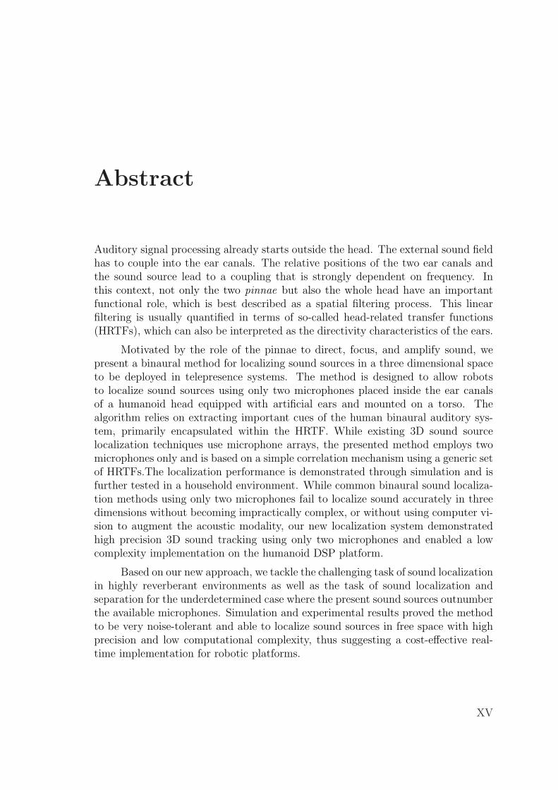
Auditory signal processing already starts outside the head. The external sound fieldhas to couple into the ear canals. The relative positions of the two ear canals andthe sound source lead to a coupling that is strongly dependent on frequency. Inthis context, not only the two pinnae but also the whole head have an importantfunctional role, which is best described as a spatial filtering process. This linearfiltering is usually quantified in terms of so-called head-related transfer functions(HRTFs), which can also be interpreted as the directivity characteristics of the ears.
Motivated by the role of the pinnae to direct, focus, and amplify sound, wepresent a binaural method for localizing sound sources in a three dimensional spaceto be deployed in telepresence systems. The method is designed to allow robotsto localize sound sources using only two microphones placed inside the ear canalsof a humanoid head equipped with artificial ears and mounted on a torso. Thealgorithm relies on extracting important cues of the human binaural auditory sys-tem, primarily encapsulated within the HRTF. While existing 3D sound sourcelocalization techniques use microphone arrays, the presented method employs twomicrophones only and is based on a simple correlation mechanism using a generic setof HRTFs.The localization performance is demonstrated through simulation and isfurther tested in a household environment. While common binaural sound localiza-tion methods using only two microphones fail to localize sound accurately in threedimensions without becoming impractically complex, or without using computer vi-sion to augment the acoustic modality, our new localization system demonstratedhigh precision 3D sound tracking using only two microphones and enabled a lowcomplexity implementation on the humanoid DSP platform.
Based on our new approach, we tackle the challenging task of sound localizationin highly reverberant environments as well as the task of sound localization andseparation for the underdetermined case where the present sound sources outnumberthe available microphones. Simulation and experimental results proved the methodto be very noise-tolerant and able to localize sound sources in free space with highprecision and low computational complexity, thus suggesting a cost-effective real-time implementation for robotic platforms.
XV

XVI List of Tables
Chapter 1
Introduction
1.1 Telepresence Framework
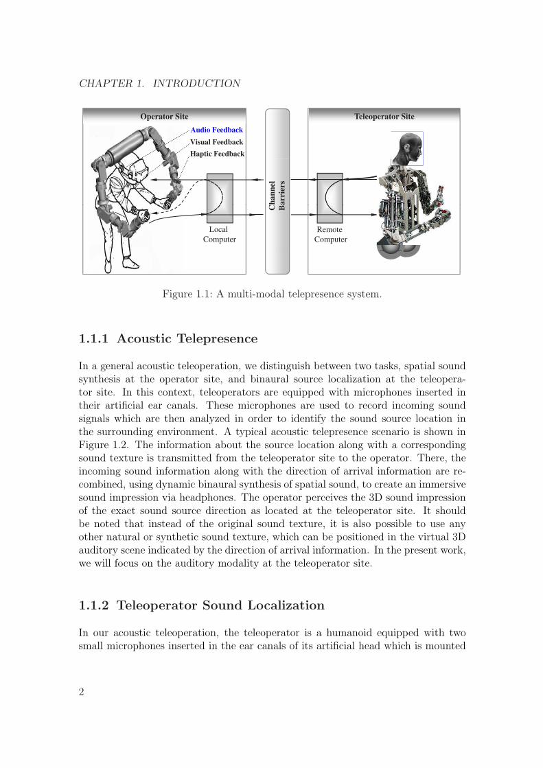
Telepresence systems aim at supplying the senses of a human operator with stimuliwhich are perceptually plausible to an extent that the operator develops a persis-tent experience of actually being somewhere else, a so-called sense of ”presence”.The most important stimuli are vision, audio, and haptics. The generic model oftelepresence and teleaction is depicted in Figure 1.1. The perceptual world thatthe operator is experiencing is built up of sensory data provided by a teleoperator,e.g. a tele-robot, located at a remote site. At the local operator site, a humanoperator is interacting with a multi-modal human-machine interface that rendersthe sensory data. The human operator manipulates the teleoperator through theinterface, which generates the corresponding control signals to be transmitted tothe remote site. The integration of audio with other modalities, like vision andhaptic not only enhances immersion, but also creates a sense of time-flow within thetelepresence operation. In a comparison of auditory and visual perception, Handel[42] arrived at the notion of vision as the generator of the concept of space andthe auditory system as a time-keeper. The integration of the auditory and hapticmodalities has the potential of mutually enforcing each other [11]. Furthermore, thefact that hearing is an undirected sense is of valuable importance, particularly incase of multiple teleoperators acting at the remote site, since it enables the operatorto receive warnings and cues of activities outside his field of view.
1
CHAPTER 1. INTRODUCTION
Teleoperator Site
Audio Feedback
Haptic Feedback
Visual Feedback
Operator Site
han
nel
arr
iers
C B
Local
Computer
Remote
Computer
Figure 1.1: A multi-modal telepresence system.
1.1.1 Acoustic Telepresence
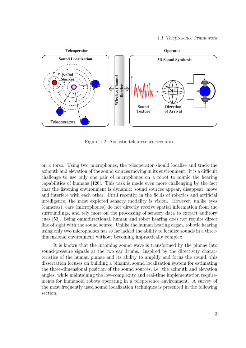
In a general acoustic teleoperation, we distinguish between two tasks, spatial soundsynthesis at the operator site, and binaural source localization at the teleopera-tor site. In this context, teleoperators are equipped with microphones inserted intheir artificial ear canals. These microphones are used to record incoming soundsignals which are then analyzed in order to identify the sound source location inthe surrounding environment. A typical acoustic telepresence scenario is shown inFigure 1.2. The information about the source location along with a correspondingsound texture is transmitted from the teleoperator site to the operator. There, theincoming sound information along with the direction of arrival information are re-combined, using dynamic binaural synthesis of spatial sound, to create an immersivesound impression via headphones. The operator perceives the 3D sound impressionof the exact sound source direction as located at the teleoperator site. It shouldbe noted that instead of the original sound texture, it is also possible to use anyother natural or synthetic sound texture, which can be positioned in the virtual 3Dauditory scene indicated by the direction of arrival information. In the present work,we will focus on the auditory modality at the teleoperator site.
1.1.2 Teleoperator Sound Localization
In our acoustic teleoperation, the teleoperator is a humanoid equipped with twosmall microphones inserted in the ear canals of its artificial head which is mounted
2
1.1 Telepresence Framework
Auditory Scene Analysis
Operator
SoundSources
Teleoperators
t
Teleoperator
3D Sound Synthesis
SoundTexture
Directionof Arrival
Wir
eles
s C
han
nel
Ba
rrie
rs
Sound Localization
Figure 1.2: Acoustic telepresence scenario.
on a torso. Using two microphones, the teleoperator should localize and track theazimuth and elevation of the sound sources moving in its environment. It is a difficultchallenge to use only one pair of microphones on a robot to mimic the hearingcapabilities of humans [126]. This task is made even more challenging by the factthat the listening environment is dynamic: sound sources appear, disappear, moveand interfere with each other. Until recently, in the fields of robotics and artificialintelligence, the most explored sensory modality is vision. However, unlike eyes(cameras), ears (microphones) do not directly receive spatial information from thesurroundings, and rely more on the processing of sensory data to extract auditorycues [53]. Being omnidirectional, human and robot hearing does not require directline of sight with the sound source. Unlike the human hearing organ, robotic hearingusing only two microphones has so far lacked the ability to localize sounds in a three-dimensional environment without becoming impractically complex.
It is known that the incoming sound wave is transformed by the pinnae intosound-pressure signals at the two ear drums. Inspired by the directivity charac-teristics of the human pinnae and its ability to amplify and focus the sound, thisdissertation focuses on building a binaural sound localization system for estimatingthe three-dimensional position of the sound sources, i.e. the azimuth and elevationangles, while maintaining the low-complexity and real-time implementation require-ments for humanoid robots operating in a telepresence environment. A survey ofthe most frequently used sound localization techniques is presented in the followingsection.
3
CHAPTER 1. INTRODUCTION
1.2 State-of-the-Art Sound Localization
Techniques
The interest in accurate sound localization has rapidly grown in the past few years,mainly due to the fastly increasing necessity of realistic solutions in numerous fieldsrelated to audio and acoustics, e.g. 3D sound synthesis, hearing-aid technology,and acoustically-based surveillance and navigation. A large number of localizationmodels have been proposed, most of them are based on microphone arrays, requiringexhaustive processing power in many situations. However, fewer work has dealtwith binaural localization where only two microphones are deployed to pinpoint thethree dimensional position of a sound, and to allow satisfying real-time localizationin acoustically adverse environments.
1.2.1 Sound Localization in General
In many everyday listening situations, human beings benefit from having two ears,naturally evolved to analyze concurrent sound sources in various listening environ-ments. For more than a century, research has been conducted to understand whichacoustic cues are resolved by the auditory system to localize and separate concur-rent sounds. The term binaural hearing refers to the mode of functioning of theauditory system of humans or animals using two ears. These ear organs serve asa preprocessor and signal conditioner, they segregate the acoustic cues to help thebrain solve tasks related to auditory localization, detection, or recognition.
In humans, the term cocktail-party effect denotes the fact that listeners withhealthy binaural hearing capabilities are able to concentrate on one talker in acrowd of concurrent talkers and discriminate the speech of this talker from the rest.Also, binaural hearing is able to suppress noise, reverberance, and sound colorationto a certain extent. One of the key features of the human auditory system is itsnearly constant omni-directional sensitivity, e.g., the system reacts to alerting signalscoming from a direction differing from the sight of focused visual attention. Inmany surveillance situations where vision completely fails as the human eyes, or thehumanoid cameras, have no direct line of sight with the sound sources, the ability toestimate the direction of the sources of danger relying on the acoustic informationbecomes of crucial importance.
The process the auditory system undergoes in combining the single cues of theimpinging sound waves at the ear drums to a single, or multiple auditory event is nottrivial. This holds true, in particular since many psycho-acoustical and neurophys-iological details are still unknown, e.g., how the single cues have to be weighted ingeneral. The question of what primitive mammals like bats experience and how they
4
1.2 State-of-the-Art Sound Localization Techniques
process sound with only two ears and a pea-sized brain remains a major mystery[46].
For the problem of localizing the spatial position of a sound source, a numberof models have already been proposed [44]. Most of them are based on using morethan two microphones to detect and track sound in a real environment. Mathemat-ical models of sound wave propagation were found to significantly depend on thespecific characteristics of the sources and the environment, and are therefore com-plex and hard to optimize [35]. Adaptive neural network structures have also beenproposed to self-adjust a sound localization model to particular environments [104].These structures disregard the head and pinnae, and create a sort of scanning orbeamforming system which can focus on the main source and attenuate reflectionsas well as other sources. While these networks have been intended to work in specif-ically controlled milieus, they become very complex in handling multiple sources inreverberant environments. Other methods are designed to mimic the human bio-logical sound localization mechanism by building models of the outer, middle andinner ear, using knowledge of how acoustic events are transduced and transformedby biological auditory systems [41]. Obviously, the difficulty with this approach isthat neurophysiologists do not completely understand how living organisms localizesounds.
The human hearing organ is a signal preprocessor stimulating the central ner-vous system, and providing outstanding signal processing capabilites. It consists ofmechanic, acoustic, hydroacoustic, and electric components, which, in total, realizea sensitive receiver and high-resolution spectral analyzer. Binaural hearing does notonly have the abilities to focus and discriminate between different sound sources ina host of concurrent sources, but is also able to suppress noise, reverberations, andsound colouration to a certain extent [19].
From a signal processing perspective, the underlying physical principles anda too-detailed description of a very complex system, like the ear organ of manyspecies, are of little interest and rather undesired, because computing times are dra-matically increased. Many specialized cells in the auditory pathway contribute tothe highly complex signal processing, which by far exceeds the performance of mod-ern computers. Hence, a minimal-complexity sound localization system is needed.Most of the available sound systems today deploy microphone arrays for efficientlocalization. Those systems which rely on using only two microphones for binauralsound localization are either limited to azimuthal localization only, or they requireextensive training sets becoming thus heavily complex and therefore unsuitable forreal-time implementation over a robotic platform.
5
CHAPTER 1. INTRODUCTION
1.2.2 Sound Localization Using Two Microphones
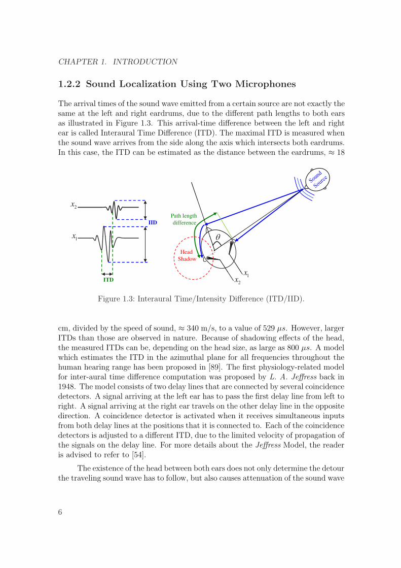
The arrival times of the sound wave emitted from a certain source are not exactly thesame at the left and right eardrums, due to the different path lengths to both earsas illustrated in Figure 1.3. This arrival-time difference between the left and rightear is called Interaural Time Difference (ITD). The maximal ITD is measured whenthe sound wave arrives from the side along the axis which intersects both eardrums.In this case, the ITD can be estimated as the distance between the eardrums, ≈ 18
Path length
differenceIID
x
2x
Head
Shadow
x
1x
ITD1x
2x
Figure 1.3: Interaural Time/Intensity Difference (ITD/IID).
cm, divided by the speed of sound, ≈ 340 m/s, to a value of 529 µs. However, largerITDs than those are observed in nature. Because of shadowing effects of the head,the measured ITDs can be, depending on the head size, as large as 800 µs. A modelwhich estimates the ITD in the azimuthal plane for all frequencies throughout thehuman hearing range has been proposed in [89]. The first physiology-related modelfor inter-aural time difference computation was proposed by L. A. Jeffress back in1948. The model consists of two delay lines that are connected by several coincidencedetectors. A signal arriving at the left ear has to pass the first delay line from left toright. A signal arriving at the right ear travels on the other delay line in the oppositedirection. A coincidence detector is activated when it receives simultaneous inputsfrom both delay lines at the positions that it is connected to. Each of the coincidencedetectors is adjusted to a different ITD, due to the limited velocity of propagation ofthe signals on the delay line. For more details about the Jeffress Model, the readeris advised to refer to [54].
The existence of the head between both ears does not only determine the detourthe traveling sound wave has to follow, but also causes attenuation of the sound wave
6
1.2 State-of-the-Art Sound Localization Techniques
at the contra-lateral eardrum, which leads to Interaural Intensity Differences (IIDs)which are frequently referred to as Interaural Level Differences (ILDs). In contrastto the ITDs, the IIDs are strongly frequency dependent. In the low-frequency range,the human head is small in comparison to the wave length and, therefore, diffractionhas only a minor effect on the sound wave. In the high-frequency range, however, thewave length is short as compared to the to the dimensions of the head, and muchlarger IIDs than in the low-frequency range can be observed. In this frequencyregion, the IIDs are not only determined by the shape of the head, but are alsogreatly influenced by the shape of the outer ears. Already in 1877, a geometricmodel was established to estimate IIDs for various sound-source positions [120].
The Interaural Phase Difference (IPD) refers to the difference in the phaseof a wave that reaches each ear, and is dependent on the frequency of the soundwave and on the ITD. For a 1000Hz tone that reaches the left ear 0.5ms beforethe right. As the wavelength reaches the right ear, it will be 180 degrees out ofphase with the wave at the left ear. IPDs are extremely useful as the human earhas the ability to detect differences as small as 3 degrees, and the combination ofIPD and ITD, not only aids the listener in determining where the sound stimulioriginated from, but also helps identify the frequency of the sound. Once the brainhas analyzed IID, ITD, and IID the location of a stationary sound source can bedetermined with relative accuracy. For fast moving sound sources, however, thehuman binaural system is slow and less accurate in localization. In this context,the minimum audible movement angle plays an important role in evaluating thelocalization capability of a given biological or electro-mechanical auditory system.This is defined as the angle through which a sound source has to move in order tobe distinguished from a stationary source. A number of investigators have studiedthis angle subjectively and have reported the maximum ability of humans to followchanges in the location of stimuli over time, i.e., to perceive movements of a soundsource [32, 17]. For low rates of movement (15◦/s), this angle is about 5◦, but asthe rate of movement increases, the angle increases progressively to about 21◦ for arate of 90◦/s [40]. Thus, the binaural system was found to be relatively insensitiveto movements at high rates.
One common method for determining the time delay D between the two mi-crophone signals x1 and x2 of Figure 1.3 is the standard cross-correlation function
Rx1x2(τ) = E[x1(t)x2(t− τ)] (1.1)
where E denotes expectation. The argument τ that maximizes (1.1) provides anestimate of delay. Because of the finite observation time, however, Rx1x2(τ) can onlybe estimated. For example, for ergodic processes, an estimate of the cross correlationis given by
Rx1x2(τ) =1
T − τ
∫ T
τ
x1(t)x2(t− τ)dt (1.2)
7
CHAPTER 1. INTRODUCTION
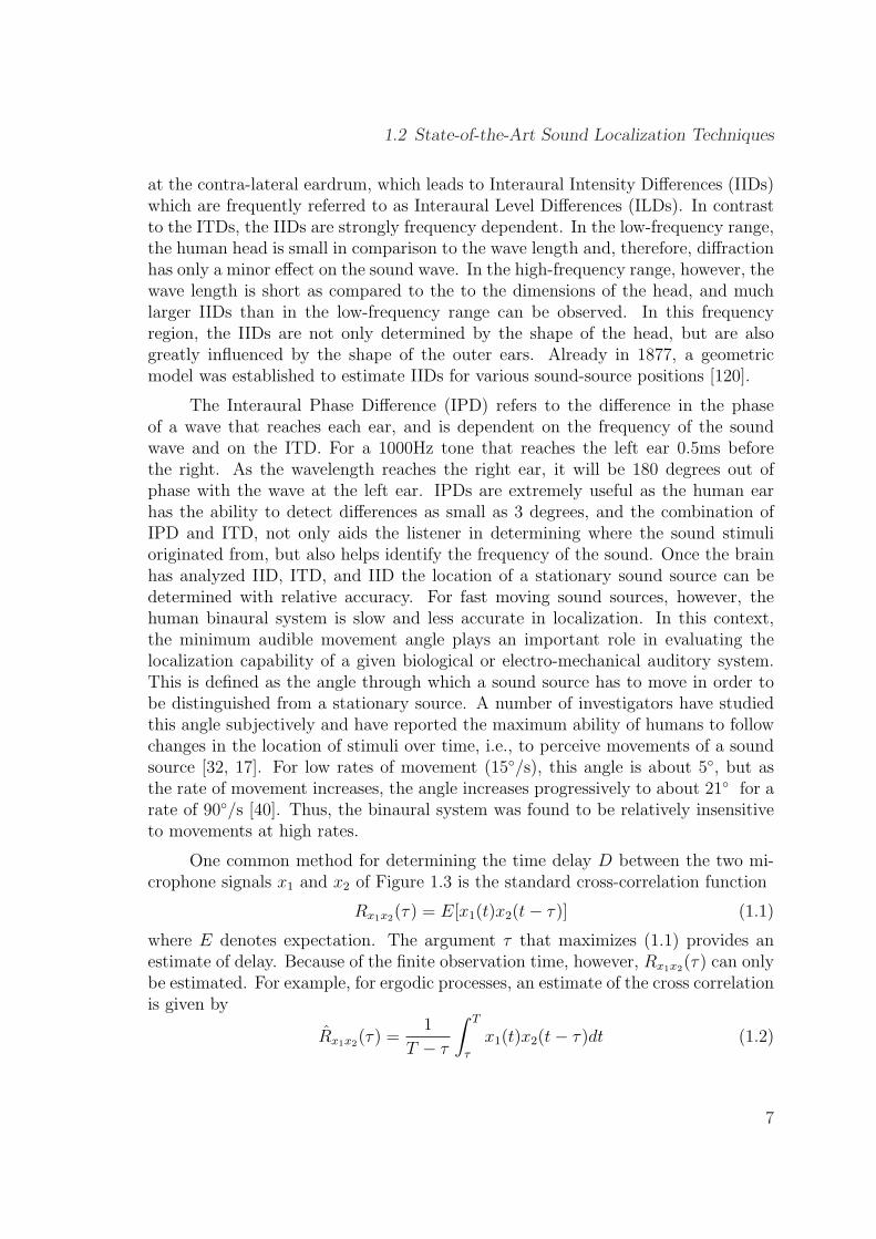
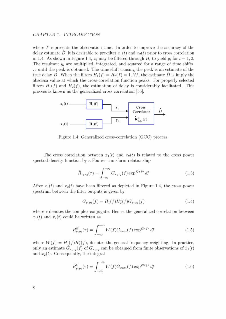
where T represents the observation time. In order to improve the accuracy of thedelay estimate D, it is desirable to pre-filter x1(t) and x2(t) prior to cross correlationin 1.4. As shown in Figure 1.4, xi may be filtered through Hi to yield yi for i = 1, 2.The resultant yi are multiplied, integrated, and squared for a range of time shifts,τ , until the peak is obtained. The time shift causing the peak is an estimate of thetrue delay D. When the filters H1(f) = H2(f) = 1, ∀f , the estimate D is imply theabscissa value at which the cross-correlation function peaks. For properly selectedfilters H1(f) and H2(f), the estimation of delay is considerably facilitated. Thisprocess is known as the generalized cross correlation [56].
1x (t)
1H (f )
Crossy
2x (t)
2H (f )
1 2
G
y yR ( )
Cross
Correlator D1
y
2y
Figure 1.4: Generalized cross-correlation (GCC) process.
The cross correlation between x1(t) and x2(t) is related to the cross powerspectral density function by a Fourier transform relationship
Rx1x2(τ) =
∫ +∞
−∞Gx1x2(f) expj2πfτ df (1.3)
After x1(t) and x2(t) have been filtered as depicted in Figure 1.4, the cross powerspectrum between the filter outputs is given by
Gy1y2(f) = H1(f)H∗2 (f)Gx1x2(f) (1.4)
where ∗ denotes the complex conjugate. Hence, the generalized correlation betweenx1(t) and x2(t) could be written as
RGy1y2
(τ) =
∫ +∞
−∞W (f)Gx1x2(f) expj2πfτ df (1.5)
where W (f) = H1(f)H∗2 (f), denotes the general frequency weighting. In practice,
only an estimate Gx1x2(f) of Gx1x2 can be obtained from finite observations of x1(t)and x2(t). Consequently, the integral
RGy1y2
(τ) =
∫ +∞
−∞W (f)Gx1x2(f) expj2πfτ df (1.6)
8
1.2 State-of-the-Art Sound Localization Techniques
is evaluated and used for estimating the time delay D,
D = arggmaxτ
(RG
y1y2(τ)
). (1.7)
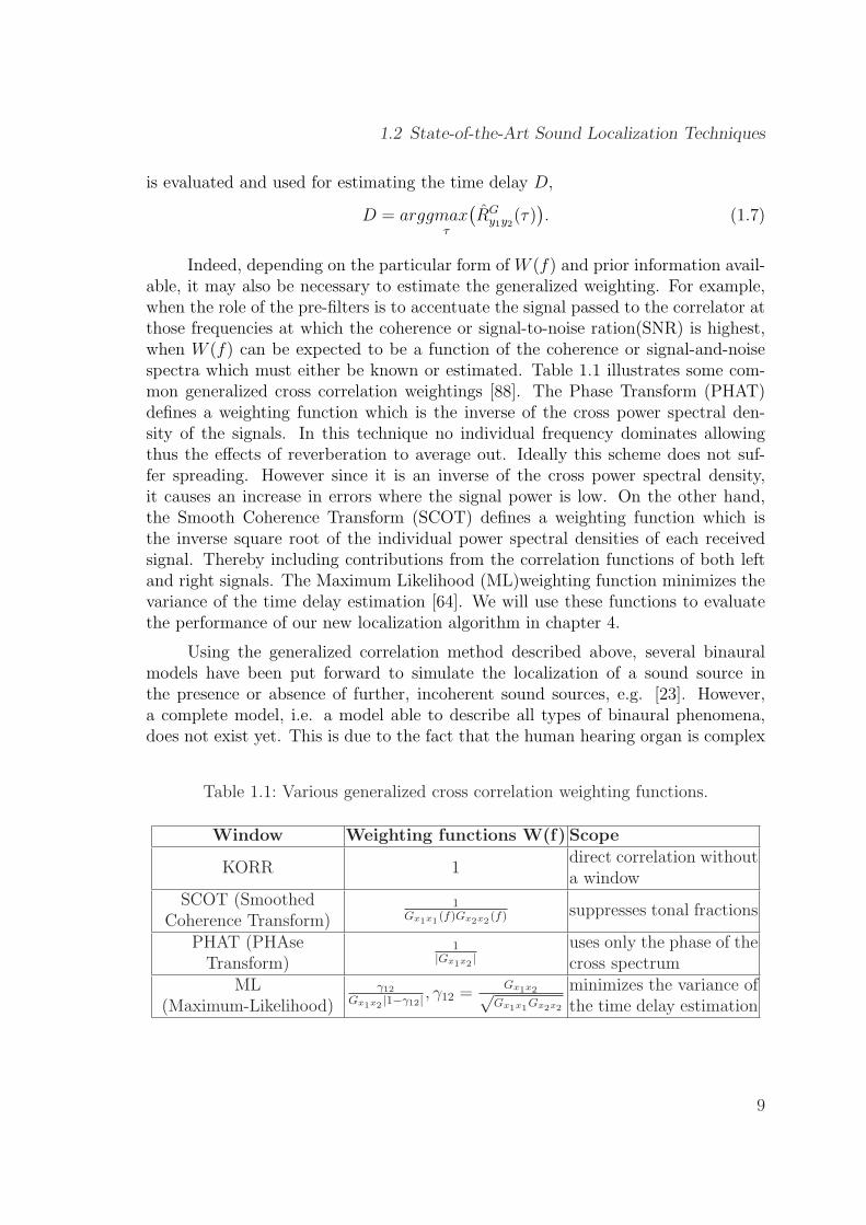
Indeed, depending on the particular form of W (f) and prior information avail-able, it may also be necessary to estimate the generalized weighting. For example,when the role of the pre-filters is to accentuate the signal passed to the correlator atthose frequencies at which the coherence or signal-to-noise ration(SNR) is highest,when W (f) can be expected to be a function of the coherence or signal-and-noisespectra which must either be known or estimated. Table 1.1 illustrates some com-mon generalized cross correlation weightings [88]. The Phase Transform (PHAT)defines a weighting function which is the inverse of the cross power spectral den-sity of the signals. In this technique no individual frequency dominates allowingthus the effects of reverberation to average out. Ideally this scheme does not suf-fer spreading. However since it is an inverse of the cross power spectral density,it causes an increase in errors where the signal power is low. On the other hand,the Smooth Coherence Transform (SCOT) defines a weighting function which isthe inverse square root of the individual power spectral densities of each receivedsignal. Thereby including contributions from the correlation functions of both leftand right signals. The Maximum Likelihood (ML)weighting function minimizes thevariance of the time delay estimation [64]. We will use these functions to evaluatethe performance of our new localization algorithm in chapter 4.
Using the generalized correlation method described above, several binauralmodels have been put forward to simulate the localization of a sound source inthe presence or absence of further, incoherent sound sources, e.g. [23]. However,a complete model, i.e. a model able to describe all types of binaural phenomena,does not exist yet. This is due to the fact that the human hearing organ is complex
Table 1.1: Various generalized cross correlation weighting functions.
Window Weighting functions W(f) Scope
KORR 1direct correlation withouta window
SCOT (SmoothedCoherence Transform)
1Gx1x1 (f)Gx2x2(f) suppresses tonal fractions
PHAT (PHAseTransform)
1|Gx1x2 |
uses only the phase of thecross spectrum
ML(Maximum-Likelihood)
γ12
Gx1x2 |1−γ12| , γ12 =Gx1x2√
Gx1x1Gx2x2
minimizes the variance ofthe time delay estimation
9
CHAPTER 1. INTRODUCTION
by nature. Sound source separation and localization using only two microphones,has so far lacked the ability to localize sounds in a three-dimensional environment.Methods based on measuring the binaural auditory cues, ITD and IID, resulted inhigh performance only in the azimuthal plane and except for a slight bias towardthe front for sources in the lateral positions. In such methods, the source is assumedto be far enough so that the impinging wavefront is planar. IID and ITD areregarded as frequency dependant; with ITD being more significant at low frequencieswhile IID is more significant at high frequencies. Reflectors can be placed aroundthe microphones to augment the usual time difference information with intensitydifference [90].
From another perspective, average binaural level (ABL), or single-ear spectralenergy could be added to the combination of ITD and IID information, to enhancethe localization performance [41]. With a pair of microphones, localization is lim-ited to two dimensions, and only up to a front-back ambiguity. Methods based onthe robots movement are able to resolve this ambiguity, with high angular acuity(±2◦) [9]. Such methods, however, still lack the ability to localize sound in 3D, andare impractical for sounds of short duration. It is worth noting that such a setupis also subject to mechanical failures due to movement of the robot. The existingalgorithms perform poorly in reverberant environments, and techniques trying tocompensate for the reverberation by learning a dereverberating filter showed to bevery sensitive to even small changes in the acoustic environment [111]. An encour-aging and practical method for improving audio source localization by making useof the precedence effect 1 was explored in [137], again adding to the complexity ofthe system.
Lately, a biologically-based binaural technique based on a probabilistic modelwas proposed [136]. The technique applies a probabilistic evaluation of a two-dimensional map containing frequency versus time-delay representation of binauralcues, also called activity map. However, the technique is limited to the frontal az-imuthal half-plane. As for sound localization based on monaural cues, little workhas been done on the subject, and few systems were able to localize sound in 3D,without becoming very complex [61]. The localization model in [29] is based ona neuromorphic microphone taking advantage of the biologically-based monauralspectral cues to localize sound sources in a plane. The microphone depends on aspecially shaped reflecting structure that allows echo-time processing to localize thesound source.
A biomimetic algorithm was recently proposed which determines the direction
1The precedence effect (PE) describes an illusion produced when two similar sounds are deliveredin quick succession (interclick delays of 2-8 msec) from sound sources at different locations so thatonly a single sound is perceived. The localization of the perceived sound is dominated by thelocation of the leading sound.
10
1.2 State-of-the-Art Sound Localization Techniques
of arrival of sound by devising two curves, the acoustical phase difference and theintensity level difference between two microphones as functions of the measured fre-quency. These curves are then weighted against a table of theoretically generatedcurves in order to determine the direction of arrival of the impinging sound waves.However, due to the symmetrical geometry of the front and back hemispheres, thealgorithm applies time-consuming routines to distinguish between the two hemi-spheres. The algorithm can localize sound source in the horizontal plane only andis limited to the bandwidth of the source and its performance deteriorates in thepresence of acoustic and electronic noise [44].
A binaural localization approach based on audio-visual integration was pro-posed in [107]. The localization method implemented hierarchical integration ofvisual and auditory processing with hypothetical reasoning on IPD and IID for eachsubband. In creating hypotheses, the reference data of IPD and IID is calculated bythe auditory epipolar geometry on demand. The resulting performance of auditorylocalization varies according to the relative sound source position. The resolutionof the center of the robot is much higher than that of peripherals, indicating simi-lar property of visual fovea (high resolution in the center of human eye). To makethe best use of this property, an active direction-pass filter (ADPF), that sepa-rates sounds originating from the specified direction by using a pair of microphones,controls the direction of a head by motor movement. In order to recognize soundstreams separated by the ADPF, a Hidden Markov Model (HMM) based automaticspeech recognition is built with multiple acoustic models trained by the output ofthe ADPF under different conditions. The method is able to localize sound only inthe azimuthal plane and is prone to front/back confusion.
Another method for estimating the location of a sound source using two earsand vision was suggested in [48]. The method is based on extracting localizationcues such as ITD, IID, and spectral notches. The authors used a spherical head,having a diameter of 14 cm, and two spiral formed ears of slightly different sizes andwith different inclinations to make the extraction of spectral notches possible. Thesesnotches are supposed to change position linearly as the elevation angle increases. Thespiral form of the ears provided a simplified mathematical derivation of the HRTFfor the spherical head. The robot was made to learn the HRTF either by supervisedlearning or by using vision. Audio-motor maps are used to associate sound featuresto the corresponding location of the sound source and to move the robot to thatlocation. Theses maps are learned using an online vision-based algorithm and areused to provide the appropriate pan and tilt angles for the robot camera. Thesuggested method has a good accuracy within the possible movements of the headused in the experiments, i.e. -20 to 20 degrees. We will use this method in chapter4 for comparison purposes with our binaural sound localization technique.
A binaural sound localization method for elevation estimation using a special
11
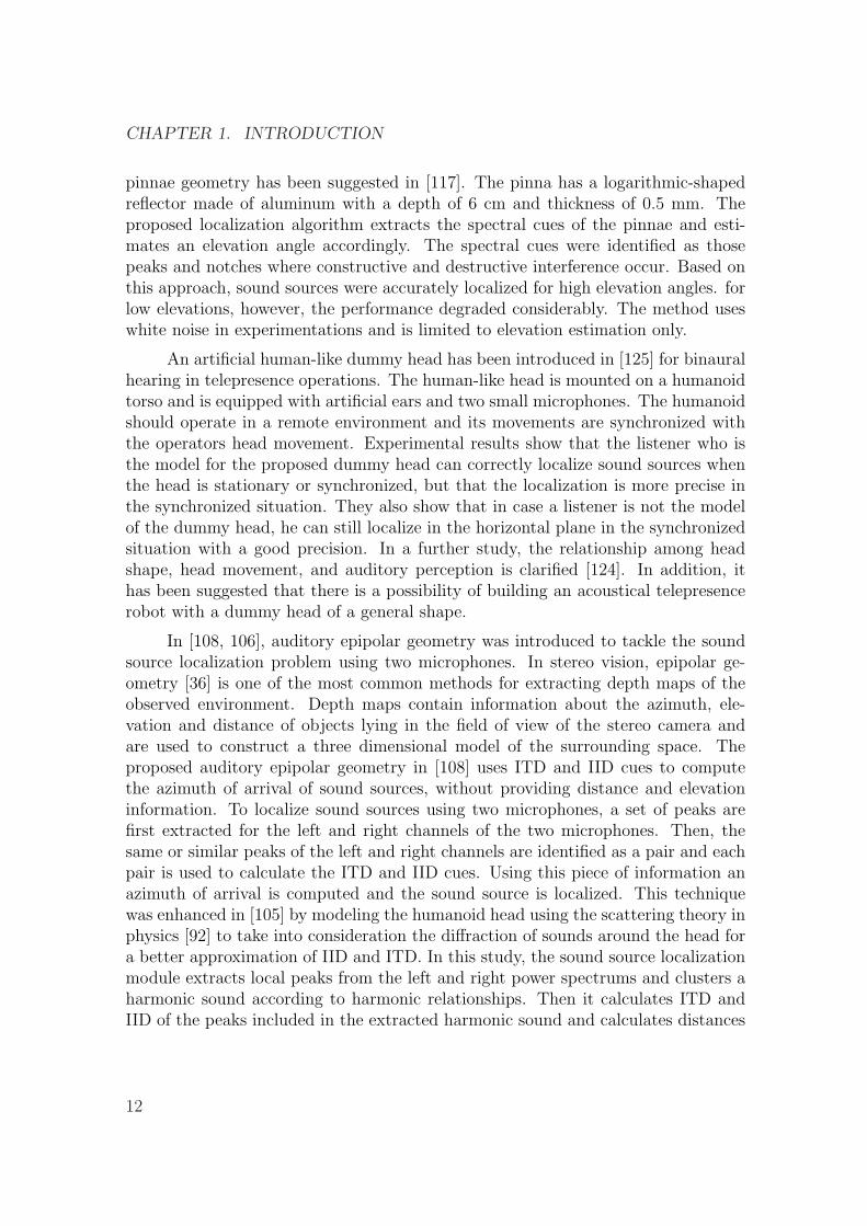
CHAPTER 1. INTRODUCTION
pinnae geometry has been suggested in [117]. The pinna has a logarithmic-shapedreflector made of aluminum with a depth of 6 cm and thickness of 0.5 mm. Theproposed localization algorithm extracts the spectral cues of the pinnae and esti-mates an elevation angle accordingly. The spectral cues were identified as thosepeaks and notches where constructive and destructive interference occur. Based onthis approach, sound sources were accurately localized for high elevation angles. forlow elevations, however, the performance degraded considerably. The method useswhite noise in experimentations and is limited to elevation estimation only.
An artificial human-like dummy head has been introduced in [125] for binauralhearing in telepresence operations. The human-like head is mounted on a humanoidtorso and is equipped with artificial ears and two small microphones. The humanoidshould operate in a remote environment and its movements are synchronized withthe operators head movement. Experimental results show that the listener who isthe model for the proposed dummy head can correctly localize sound sources whenthe head is stationary or synchronized, but that the localization is more precise inthe synchronized situation. They also show that in case a listener is not the modelof the dummy head, he can still localize in the horizontal plane in the synchronizedsituation with a good precision. In a further study, the relationship among headshape, head movement, and auditory perception is clarified [124]. In addition, ithas been suggested that there is a possibility of building an acoustical telepresencerobot with a dummy head of a general shape.
In [108, 106], auditory epipolar geometry was introduced to tackle the soundsource localization problem using two microphones. In stereo vision, epipolar ge-ometry [36] is one of the most common methods for extracting depth maps of theobserved environment. Depth maps contain information about the azimuth, ele-vation and distance of objects lying in the field of view of the stereo camera andare used to construct a three dimensional model of the surrounding space. Theproposed auditory epipolar geometry in [108] uses ITD and IID cues to computethe azimuth of arrival of sound sources, without providing distance and elevationinformation. To localize sound sources using two microphones, a set of peaks arefirst extracted for the left and right channels of the two microphones. Then, thesame or similar peaks of the left and right channels are identified as a pair and eachpair is used to calculate the ITD and IID cues. Using this piece of information anazimuth of arrival is computed and the sound source is localized. This techniquewas enhanced in [105] by modeling the humanoid head using the scattering theory inphysics [92] to take into consideration the diffraction of sounds around the head fora better approximation of IID and ITD. In this study, the sound source localizationmodule extracts local peaks from the left and right power spectrums and clusters aharmonic sound according to harmonic relationships. Then it calculates ITD andIID of the peaks included in the extracted harmonic sound and calculates distances
12
1.2 State-of-the-Art Sound Localization Techniques
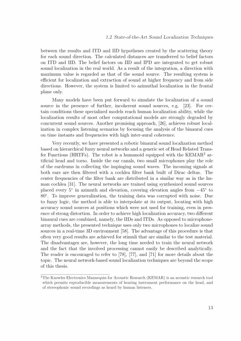
between the results and ITD and IID hypotheses created by the scattering theoryfor each sound direction. The calculated distances are transferred to belief factorson ITD and IID. The belief factors on IID and IPD are integrated to get robustsound localization in the real world. As a result of the integration, a direction withmaximum value is regarded as that of the sound source. The resulting system isefficient for localization and extraction of sound at higher frequency and from sidedirections. However, the system is limited to azimuthal localization in the frontalplane only.
Many models have been put forward to simulate the localization of a soundsource in the presence of further, incoherent sound sources, e.g. [23]. For cer-tain conditions these specialized models reach human localization ability, while thelocalization results of most other computational models are strongly degraded byconcurrent sound sources. Another promising approach, [26], achieves robust local-ization in complex listening scenarios by focusing the analysis of the binaural cueson time instants and frequencies with high inter-aural coherence.
Very recently, we have presented a robotic binaural sound localization methodbased on hierarchical fuzzy neural networks and a generic set of Head Related Trans-fer Functions (HRTFs). The robot is a humanoid equipped with the KEMAR2 ar-tificial head and torso. Inside the ear canals, two small microphones play the roleof the eardrums in collecting the impinging sound waves. The incoming signals atboth ears are then filtered with a cochlea filter bank built of Dirac deltas. Thecenter frequencies of the filter bank are distributed in a similar way as in the hu-man cochlea [31]. The neural networks are trained using synthesized sound sourcesplaced every 5◦ in azimuth and elevation, covering elevation angles from −45◦ to80◦. To improve generalization, the training data was corrupted with noise. Dueto fuzzy logic, the method is able to interpolate at its output, locating with highaccuracy sound sources at positions which were not used for training, even in pres-ence of strong distortion. In order to achieve high localization accuracy, two differentbinaural cues are combined, namely, the IIDs and ITDs. As opposed to microphone-array methods, the presented technique uses only two microphones to localize soundsources in a real-time 3D environment [58]. The advantage of this procedure is thatoften very good results are achieved for stimuli that are similar to the test material.The disadvantages are, however, the long time needed to train the neural networkand the fact that the involved processing cannot easily be described analytically.The reader is encouraged to refer to [78], [77], and [71] for more details about thetopic. The neural network-based sound localization techniques are beyond the scopeof this thesis.
2The Knowles Electronics Mannequin for Acoustic Research (KEMAR) is an acoustic research toolwhich permits reproducible measurements of hearing instrument performance on the head, andof stereophonic sound recordings as heard by human listeners.
13
CHAPTER 1. INTRODUCTION
1.2.3 Microphone Array Based Sound Localization
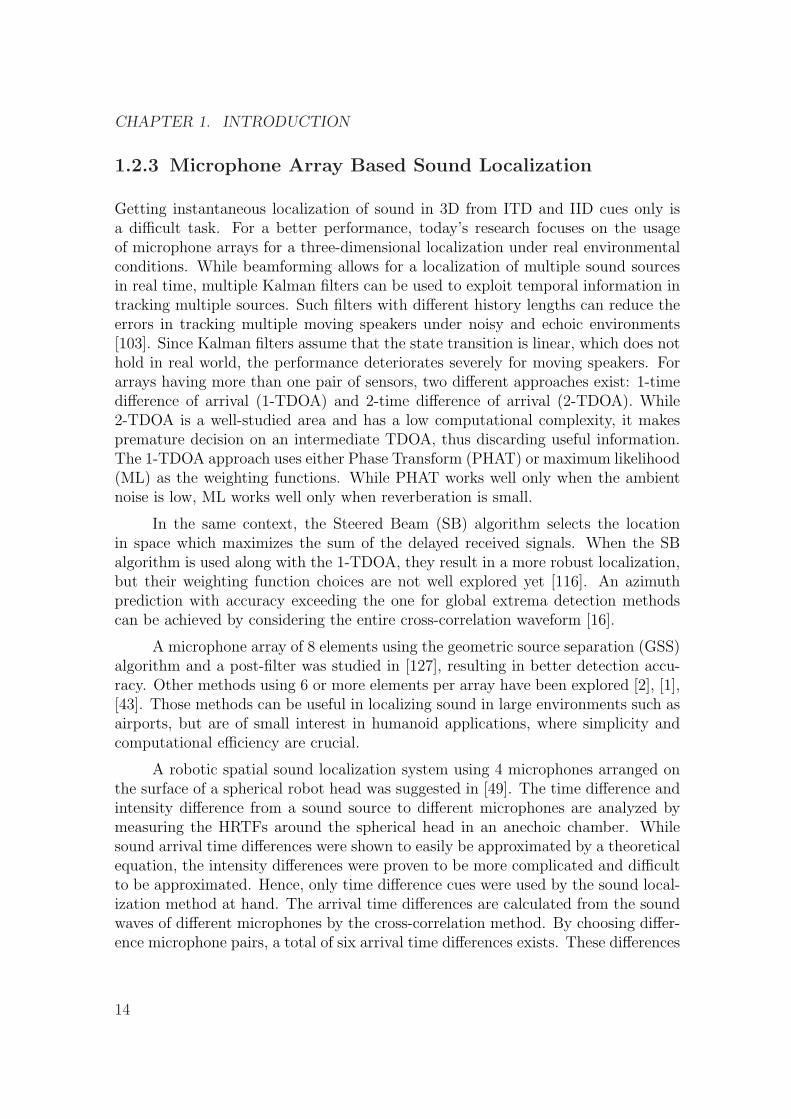
Getting instantaneous localization of sound in 3D from ITD and IID cues only isa difficult task. For a better performance, today’s research focuses on the usageof microphone arrays for a three-dimensional localization under real environmentalconditions. While beamforming allows for a localization of multiple sound sourcesin real time, multiple Kalman filters can be used to exploit temporal information intracking multiple sources. Such filters with different history lengths can reduce theerrors in tracking multiple moving speakers under noisy and echoic environments[103]. Since Kalman filters assume that the state transition is linear, which does nothold in real world, the performance deteriorates severely for moving speakers. Forarrays having more than one pair of sensors, two different approaches exist: 1-timedifference of arrival (1-TDOA) and 2-time difference of arrival (2-TDOA). While2-TDOA is a well-studied area and has a low computational complexity, it makespremature decision on an intermediate TDOA, thus discarding useful information.The 1-TDOA approach uses either Phase Transform (PHAT) or maximum likelihood(ML) as the weighting functions. While PHAT works well only when the ambientnoise is low, ML works well only when reverberation is small.
In the same context, the Steered Beam (SB) algorithm selects the locationin space which maximizes the sum of the delayed received signals. When the SBalgorithm is used along with the 1-TDOA, they result in a more robust localization,but their weighting function choices are not well explored yet [116]. An azimuthprediction with accuracy exceeding the one for global extrema detection methodscan be achieved by considering the entire cross-correlation waveform [16].
A microphone array of 8 elements using the geometric source separation (GSS)algorithm and a post-filter was studied in [127], resulting in better detection accu-racy. Other methods using 6 or more elements per array have been explored [2], [1],[43]. Those methods can be useful in localizing sound in large environments such asairports, but are of small interest in humanoid applications, where simplicity andcomputational efficiency are crucial.
A robotic spatial sound localization system using 4 microphones arranged onthe surface of a spherical robot head was suggested in [49]. The time difference andintensity difference from a sound source to different microphones are analyzed bymeasuring the HRTFs around the spherical head in an anechoic chamber. Whilesound arrival time differences were shown to easily be approximated by a theoreticalequation, the intensity differences were proven to be more complicated and difficultto be approximated. Hence, only time difference cues were used by the sound local-ization method at hand. The arrival time differences are calculated from the soundwaves of different microphones by the cross-correlation method. By choosing differ-ence microphone pairs, a total of six arrival time differences exists. These differences
14
1.2 State-of-the-Art Sound Localization Techniques
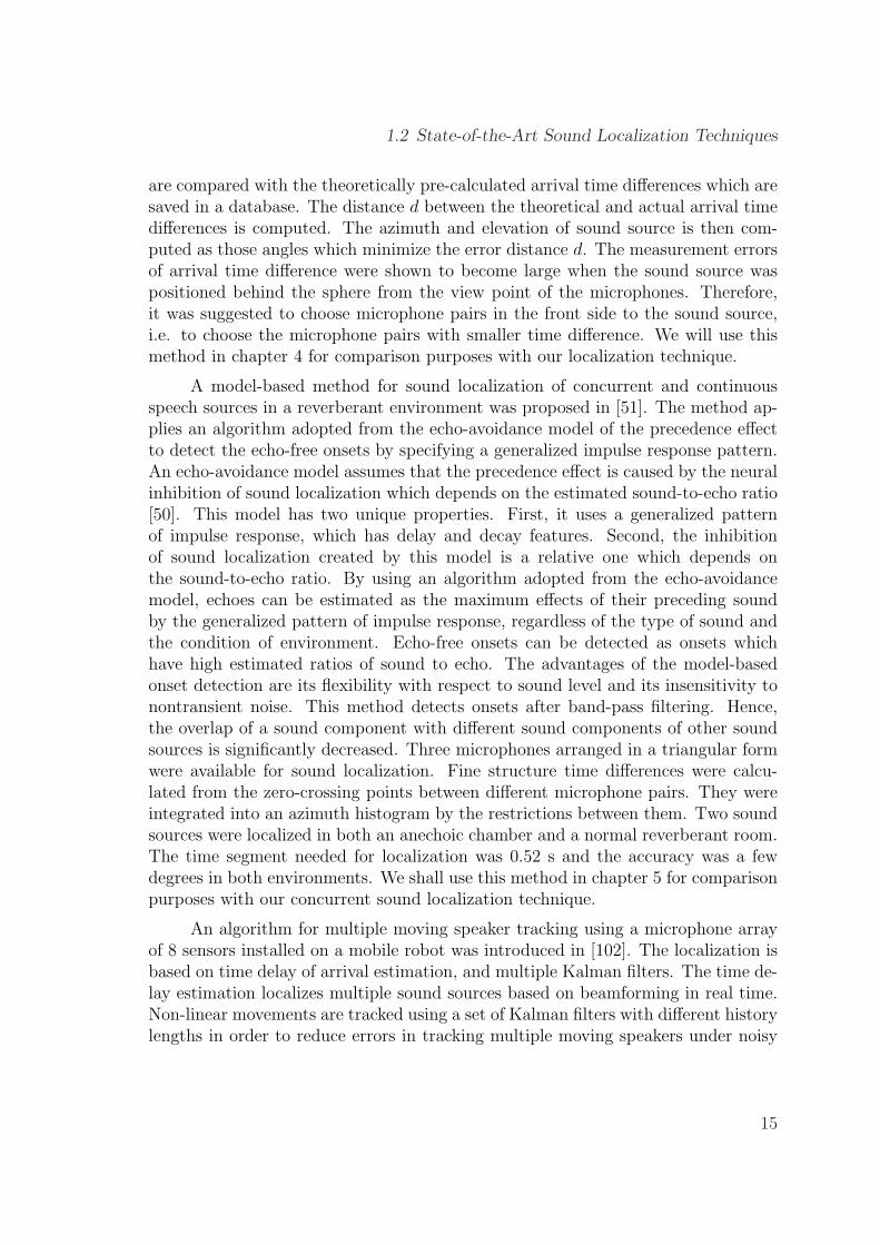
are compared with the theoretically pre-calculated arrival time differences which aresaved in a database. The distance d between the theoretical and actual arrival timedifferences is computed. The azimuth and elevation of sound source is then com-puted as those angles which minimize the error distance d. The measurement errorsof arrival time difference were shown to become large when the sound source waspositioned behind the sphere from the view point of the microphones. Therefore,it was suggested to choose microphone pairs in the front side to the sound source,i.e. to choose the microphone pairs with smaller time difference. We will use thismethod in chapter 4 for comparison purposes with our localization technique.
A model-based method for sound localization of concurrent and continuousspeech sources in a reverberant environment was proposed in [51]. The method ap-plies an algorithm adopted from the echo-avoidance model of the precedence effectto detect the echo-free onsets by specifying a generalized impulse response pattern.An echo-avoidance model assumes that the precedence effect is caused by the neuralinhibition of sound localization which depends on the estimated sound-to-echo ratio[50]. This model has two unique properties. First, it uses a generalized patternof impulse response, which has delay and decay features. Second, the inhibitionof sound localization created by this model is a relative one which depends onthe sound-to-echo ratio. By using an algorithm adopted from the echo-avoidancemodel, echoes can be estimated as the maximum effects of their preceding soundby the generalized pattern of impulse response, regardless of the type of sound andthe condition of environment. Echo-free onsets can be detected as onsets whichhave high estimated ratios of sound to echo. The advantages of the model-basedonset detection are its flexibility with respect to sound level and its insensitivity tonontransient noise. This method detects onsets after band-pass filtering. Hence,the overlap of a sound component with different sound components of other soundsources is significantly decreased. Three microphones arranged in a triangular formwere available for sound localization. Fine structure time differences were calcu-lated from the zero-crossing points between different microphone pairs. They wereintegrated into an azimuth histogram by the restrictions between them. Two soundsources were localized in both an anechoic chamber and a normal reverberant room.The time segment needed for localization was 0.52 s and the accuracy was a fewdegrees in both environments. We shall use this method in chapter 5 for comparisonpurposes with our concurrent sound localization technique.
An algorithm for multiple moving speaker tracking using a microphone arrayof 8 sensors installed on a mobile robot was introduced in [102]. The localization isbased on time delay of arrival estimation, and multiple Kalman filters. The time de-lay estimation localizes multiple sound sources based on beamforming in real time.Non-linear movements are tracked using a set of Kalman filters with different historylengths in order to reduce errors in tracking multiple moving speakers under noisy
15
CHAPTER 1. INTRODUCTION
and echoic environments. For quantitative evaluation of the tracking, motion refer-ences of sound sources and a mobile robot were measured accurately by ultrasonic3D tag sensors. The system tracked three simultaneous sound sources in a roomexhibiting large reverberation. We will use this method in chapter 5 for comparisonpurposes with our localization technique.
An accurate sound localization method using 8 microphones and applying thesimple TDOA algorithm to localize sound sources in three dimensions was introducedin [128]. Using cross-correlation, this method determines the delay between thesignals captured by the different microphones. A major limitation of this approachis that the correlation is strongly dependent on the statistical properties of the sourcesignal. Since most signals, including voice, are generally low-pass, the correlationbetween adjacent samples is high and generates cross-correlation peaks that can bevery wide. The problem of wide cross-correlation peaks is solved by whitening thespectrum of the signals prior to computing the cross-correlation. However, afterapplying the whitened cross-correlation method, each frequency bin of the spectrumis forced to contribute the same amount to the final correlation, even if the signal atthat frequency is dominated by noise. This makes the system less robust to noise,while making detection of voice (which has a narrow bandwidth) more difficult. Inorder to counter the problem, a weighting function of the spectrum was introducedwhich gives more weight to regions in the spectrum where the local signal-to-noiseratio (SNR) is the highest. The overall system is able to perform localization even onshort-duration sounds and does not require the use of any noise cancelation method.The precision of the localization is 3◦ over 3 meters. We will use this method inchapter 6 for comparison purposes with our localization technique.
As an alternative to microphone arrays, much psychoacoustic research hasbeen performed on human beings and animals to isolate the individual cues of soundlocalization [30]. One novel approach is sound localization based on HRTFs, whichare also called anatomical transfer functions (ATFs). These functions describe thefiltering of sound on its way to the inner ear. The HRTFs will be the main focus ofthe next chapter.
1.3 Main Contributions and Overview
1.3.1 Main Contributions
We have addressed the challenging task of binaural sound localization using a pairof microphones inserted in the ear canals of a humanoid head mounted on a torsoand operating in a general telepresence environment. This task is made even morechallenging by the fact that the listening environment is dynamic: sound sources
16
1.3 Main Contributions and Overview
appear, disappear, move and interfere with each other. The today existing soundlocalization models fail to localize sound in both azimuth and elevation using onlytwo microphones. Common binaural methods are limited to localizing sound sourcesin either azimuth or elevation. Those methods which try to achieve three dimensionallocalization, using only two sensors, become impractically complex by relying heavilyon training sets for every environment, or by using computer vision to augment theacoustic modality. Hence, successful sound localization techniques are based onmicrophone arrays to detect and track sound in a real environment. Microphonearrays require exhaustive processing powers and are therefore not suited for oursimple hardware setup deploying two artificial ears.
We have proposed a unifying framework for novel three-dimensional sound lo-calization methods to be implemented on a humanoid robot. The initial proposal isbased on dividing the ear signals with the left and right HRTFs and subsequentlytaking the maximum correlation coefficient as a pointer to the source location. thismethod is enhanced using proper state-space HRTF inversion. In addition, a newalgorithm called cross convolution was developed to further decrease the computa-tional requirements of the initial method. Nevertheless, with the help of a simpleproperly tuned Kalman filter, a ROI was introduced to account for fast movingsound sources. The efficiency of the new algorithm suggests a cost-effective imple-mentation for robot platforms and allows fast localization of moving sound sources.
Using the presented methods, we have addressed the challenging task of binau-ral concurrent sound source localization and separation in reverberant environments.We presented a new algorithm for binaural localization of concurrent sound sourcesin both azimuth and elevation. Compared to existing techniques using microphonearrays for the same purpose, our algorithm is less complex and very accurate. Besidelocalization, we have proposed a sound source separation algorithm which provedto be outperforming compared to other blind source separation methods solving thesame determined problem under the same conditions.
For highly reverberant environments, a new algorithm using four microphonesis presented. Bayesian information fusion is then used to increase the localizationresolution in a three-dimensional reverberant environment. Compared to existingtechniques, the method is able to localize sound sources in three dimensions, underhigh reverberation conditions, with fewer sensors and higher accuracy.
1.3.2 Overview and Organization of the Thesis
Chapter 2: Binaural Techniques
In chapter 2, we summarize all important aspects of HRTFs, ranging from theirmeasurement procedure, their time and frequency domain visualization, to their
17
CHAPTER 1. INTRODUCTION
recent deployment in our sound localization system. In section 2.7, we introducethree methods for HRTF order reduction, namely the Balanced Model Truncation(BMT), Diffuse-Field Equalization (DFE), and the Principal Component Analysis(PCA). These techniques are used in the following chapters to help reducing thelocalization processing time of a HRTF-based sound localization system. In contrastto conventional methods utilizing HRTFs to synthesize sound for virtual reality, weuse the HRTFs for real-life sound detection.
Chapter 3: Binaural Sound Source Localization Based on HRTFs
A novel sound localization technique based on HRTFs and matched filtering isproposed in section 3.1 of this chapter. As opposed to sound localization methodsbased on microphones arrays, the method localizes sound in azimuth and elevationby using only two small microphones placed inside the ear canal of a humanoid headmounted on a torso.
In section 3.2 two novel techniques for accurate HRTF interpolation and robustinversion are presented. In section 3.2.2, an accurate HRTF state-space interpolationtechnique is introduced to ensure the availability of sufficient HRTFs for higherprecision localization performance. In section 3.3, a stable inverse of the HRTFsis computed using state-space inversion based on inner-outer factorization. Thisinversion technique is deployed in chapter 4 to stabilize the localization of a novelhumanoid binaural sound system.
Chapter 4: Enhanced Sound Source Localization Techniques
In this chapter, we have considerably improved the initial matched filteringapproach to sound localization using the reduced and inverted HRTFs, as in chapters2 and 3. This set up proved to be able to localize sound sources up to a veryhigh precision in free space. In addition, a cross convolution algorithm for realtime localization and tracking is proposed. Applying HRTFs for sound localizationtogether with extended Kalman filtering, we are able to accurately track movingsound sources in real time in a highly reverberant environment. This algorithm usesonly two microphones and requires no prior knowledge of the sound signals.
Chapter 5: Concurrent Sound Source Localization and Separation
In chapter 5, we combine blind source separation and binaural localizationfor tracking concurrent sound sources using only two microphones. Section 5.2 de-scribes an algorithm for two sound sources that iteratively adapts the coefficientsof a Multiple Input Multiple Output (MIMO) system and provides the two statisti-cally independent source signals. This well-known separation method exploiting thenon-stationarity of the sources is used to retrieve two speakers from two convolutivemixtures in real-time. By using a simple relation between blind source separationand system identification, the HRTFs that filtered the sound sources can be de-
18
1.3 Main Contributions and Overview
termined under the condition of an anechoic environment. The second algorithm,presented in section 5.3, applies Short-Time Fourier Transform (STFT) to the earsignals and makes use of the sparseness of the sources in a time-frequency domain.As in each frequency band the normalized time-frequency patterns of speech sig-nals cluster around the HRTF values, the interaural HRTFs can be retrieved. Thepositions of the sources are finally determined by a database lookup. With the re-spective HRTFs of the database, the sources can be separated by inversion of theHRTF-system in case of two concurrent sound sources or by L1-norm minimizationin case of more than two sources.
Chapter 6: Sound Localization in Highly Reverberant Environments
In this chapter, a novel monaural 3D sound localization technique is presented.The proposed system, an upgrade of monaural-based localization techniques, usestwo microphones: one inserted within the ear canal of a humanoid head equippedwith an artificial ear, and the second held outside the ear. The outer microphone issmall enough to avoid reflections that might contribute to localization errors. Thesystem exploits the spectral information of the signals from the two microphonesin such a way that a simple correlation mechanism, using a generic set of HRTFs,is used to localize the sound sources. The main focus of this chapter is on thedetection of sound events under severe acoustic conditions, i.e. high reverberationand background noise. The location of the sound source obtained from monauraland binaural observation sensors is fused using a properly tuned Bayesian networkin order to increase the localization resolution in a three-dimensional reverberantenvironment.
19

CHAPTER 1. INTRODUCTION
20
Chapter 2
Binaural Techniques
2.1 The Head Related Transfer Function
Within the framework of human sound localization, it is generally accepted that thehead pinnae modify the spectra of incoming sounds in a way that depends on theangle of incidence of the sound relative to the head. The spectral changes producedby the head and pinna can be used to estimate the localization of a sound source.This has been confirmed by measurements in the ear canal of human observersand by measurements using realistic models of the human head [19], [133]. Thehead and pinnae together form a complex direction-dependent filter. The filteringaction is often characterized by measuring the spectrum of the sound source andthe spectrum of the sound reaching the eardrum. The ratio of these two is calledthe HRTF or equivalently, the head related impulse response (HRIR). The HRTFscapture the diffraction of sound waves by the human or humanoid torso, shoulders,head, and outer ears and hence vary in a complex way with azimuth, elevation andfrequency. In addition, the HRTFs depend on the morphology of the listener’s body,and therefore vary significantly from person to person. The HRTF for a particularindividual is called his or her individualized HRTF.
Binaural sound reproduction builds on the concept that our auditory perceptsare primarily formed on the basis of only two inputs, specifically the sound pressuresignals formed at our two eardrums. If these are recorded using small microphonesinserted inside the ears of listeners, and reproduced authentically when played back,then all acoustic cues and all spatial aspects are accessible to the listeners for pro-ducing authentic replicas of the original auditory percepts.
21
Chapter 2 Binaural Techniques
The main application area for HRTFs is the reproduction of binaural hearingfor virtual reality application. In this context, instead of being picked up inside theears of the listener, the signals to the two ears, called binaural signals, are generatedelectronically by the use of filters representing HRTFs. In this case the methodwill be denoted binaural synthesis. In binaural synthesis, a virtual sound source iscreated by simply convolving a sound signal with a pair of HRTFs [67]. The successof binaural synthesis strongly depends on details of the procedures applied for deter-mining and realizing HRTFs, such as physical aspects of the measurement situation,post-processing of data, and implementation as digital filters. If the full spatial in-formation is maintained in the resulting binaural signals, we say that the HRTFscontain all properties of the sound transmission and all descriptors of localizationcues.
2.2 HRTF Cues
The acoustic cues for sound localization have been studied for over a century [19].The most reliable cues used in the localization of sounds, some of them dependingupon a comparison of the signals reaching the two ears, could be generally dividedinto five main categories: 1) ITD, 2) IID/ILD, 3) monaural cues, 4) head rotationand 5) Interaural Coherence (IC). While ITDs and IIDs are the most commonlyused for modeling sound localization systems, monaural cues, resulting from thecomplex topographic shape of the pinnae, play a very important role in decoding theelevation information of the impinging sound sources. Head rotation is commonlyused to resolve front/back ambiguity as well as the cone of confusion problem1. TheIC cues are mainly used by acousticians to extract the auditory spatial propertiesof a certain environment [21]. The limits to the auditory system localization abilityare determined by the limits of detecting and analyzing the above mentioned cues.
The HRTF can be interpreted as the directivity characteristics of the two earsand shows a complex pattern of peaks and dips which varies systematically with thedirection of the sound source relative to the head and which is unique for each threedimensional direction. Recently, a method to robustly extract the frequencies of thepinna spectral notches from the measured HRIR, distinguishing them from otherconfounding features, has been properly devised [112]. Scientific study of HRTFshas focused on two questions: what acoustic cues do people use to localize soundsources, and what parts of the body are responsible for generating those cues. This
1For a given interaural spectrum, there exists a surface or a locus of points corresponding to soundsource locations for which ITDs and ILDs are identical. A cone (whose axis is a line drawn betweenthe ears and whose origin is the center of the head) is a fair approximation of this surface. Usingonly ITDs/ILDs there are no cues available to resolve positional ambiguity on such a cone.
22
2.3 HRTF Properties
0 20 40 60 80 100 120 140
-0.5
0
0.5
HRIR Length (Number of Samples)
100
200
300
355
Am
pli
tud
e
An
gle
inD
egre
es
Figure 2.1: Measured right-ear Head Related Impulse Responses (HRIRs) for sourcelocations in the horizontal plane (Elevation = 0◦).
research is presented systematically in [19], and several useful reviews are available[98, 100].
2.3 HRTF Properties
Because size and shape of the external ear vary greatly between persons, the taskof relating the anthropometry of the pinna to the localization cues it creates iscumbersome. It remains unclear how macroscopic features of HRTFs correspondto perceptually meaningful directional cues. It stays difficult to exactly pinpointwhich peaks and notches in HRTF magnitude frequency responses correspond tothe specific azimuths and elevations of the sound source locations.
Many methods have been trying to uncover structure in HRTF data by visually
23
Chapter 2 Binaural Techniques
comparing subsets of HRTFs sharing the same azimuth, elevation, and frequency inthe time or frequency domain. It was shown in [27] how the location of a spectralnotch near 7 kHz changes as a function of elevation. In [4], the authors show howdiffraction effects due to the head and shoulder can be seen as secondary echoes intime domain versions of HRTFs. Within this framework, it was suggested in [28] howpeaks in plots of spatial location vs. HRTF for a fixed frequency could correspond toperceptually preferred directions in space. The method in [5] shows that a compositemodel combining independent contributions of the pinna and of the head and torsoconsidered as a unit results in a good HRTF approximation. This model isolatesthe pinna by treating it as if it were mounted on an infinite plane, and leads to asignificant simplification in the pinna response, the so-called Pinna-Related TransferFunction (PRTF). In the following, we shall distinguish between two visualizationsof the HRTF, the time domain impulse response and the frequency domain transferfunction.
2.3.1 Time Domain Impulse Responses
The measurements shown in Figure 2.1 are taken for the KEMAR right ear and areplotted as a function of azimuth in the horizontal plane (elevation = 0◦). Lookingat this figure, one can observe the relatively large amplitude of the initial peaks inthe impulse responses corresponding to azimuth +90◦, i.e. to the location where thesource is directly facing the right ear. While the source is moving towards the leftear, the HRIR peaks fade down slowly due to increased head shadowing, and reacha minimum at the contralateral location where the source is directly facing the leftear.
Figure 2.2 shows measured HRIRs as a function of elevation in the medianplane (azimuth 0◦) and in the vertical plane corresponding to azimuth 90◦. One canalso see elevation-related effects as there is a slight difference in arrival times forpositive and negative elevations. From Figures 2.1 and 2.2, we can observe that, inaddition to the initial peak, the measured HRIRs contain many secondary peaks.This is caused by the numerous spatial cues as well as by the complex morphologicalstructure of the outer ear, although these effects could also be related to the inherentnoise in the measurement process.
Figure 2.3 is the image representation of the KEMAR’s HRIRs. The figureshows the responses of the left and right ear to an impulsive source in the horizontaland median plane. The strength of the response is represented using different levelsof brightness. Looking at the left ear data, we can see that when the sound sourceis moving in the horizontal plane, the strongest response is reached at an azimuthangle of 270◦ or equivalently -90◦, the weakest and mostly delayed response occurs
24
2.3 HRTF Properties
0 20 40 60 80 0 20 40 60 80
HRIR Length (Number of Samples)
-40
Azimuth = 0°E
lev
ati
on
An
gle
[°]
-30
-20
-10
0
10
20
30
40
50
60
70
80
Azimuth = 90°
-40
-30
-20
-10
0
10
20
30
40
50
60
70
80
Figure 2.2: Measured right-ear Head Related Impulse Responses (HRIRs) for sourcelocations in the two vertical planes: Azimuth 0◦ and Azimuth 90◦.
at azimuth = 90◦. The right ear response shows a directly opposite behavior. In anutshell, we observe a pronounced variation of the impulse response in the horizontalplane as a function of azimuth. However, this is not the case for the median plane.
When the sound moves around the head in the median plane, as shown inthe right subplots of Figure 2.3, it reaches the left and right ears at almost thesame time. There is no apparent difference for the strength of the impulse responseamong all of the elevation angles, and the arrival time is more or less the same. Themain changes are in the relative arrival times and strengths of the pinna reflections.This explains why people have trouble distinguishing front from back when soundsare located in the median plane. This phenomenon is well-known as the front/backconfusion problem and people often resolve it by head motion.
25
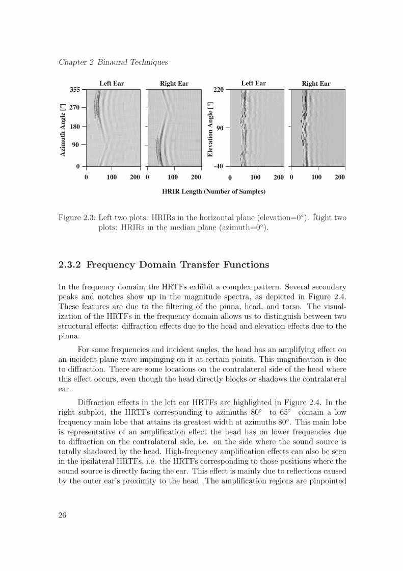
Chapter 2 Binaural Techniques
0 100 200 0 100 200 0 100 200 0 100 200
-40
220
90
0
180
90
270
355
HRIR Length (Number of Samples)
Left Ear
Azi
mu
th A
ngle
[°]
Ele
va
tion
An
gle
[°]
Right Ear Left Ear Right Ear
Figure 2.3: Left two plots: HRIRs in the horizontal plane (elevation=0◦). Right twoplots: HRIRs in the median plane (azimuth=0◦).
2.3.2 Frequency Domain Transfer Functions
In the frequency domain, the HRTFs exhibit a complex pattern. Several secondarypeaks and notches show up in the magnitude spectra, as depicted in Figure 2.4.These features are due to the filtering of the pinna, head, and torso. The visual-ization of the HRTFs in the frequency domain allows us to distinguish between twostructural effects: diffraction effects due to the head and elevation effects due to thepinna.
For some frequencies and incident angles, the head has an amplifying effect onan incident plane wave impinging on it at certain points. This magnification is dueto diffraction. There are some locations on the contralateral side of the head wherethis effect occurs, even though the head directly blocks or shadows the contralateralear.
Diffraction effects in the left ear HRTFs are highlighted in Figure 2.4. In theright subplot, the HRTFs corresponding to azimuths 80◦ to 65◦ contain a lowfrequency main lobe that attains its greatest width at azimuths 80◦. This main lobeis representative of an amplification effect the head has on lower frequencies dueto diffraction on the contralateral side, i.e. on the side where the sound source istotally shadowed by the head. High-frequency amplification effects can also be seenin the ipsilateral HRTFs, i.e. the HRTFs corresponding to those positions where thesound source is directly facing the ear. This effect is mainly due to reflections causedby the outer ear’s proximity to the head. The amplification regions are pinpointed
26
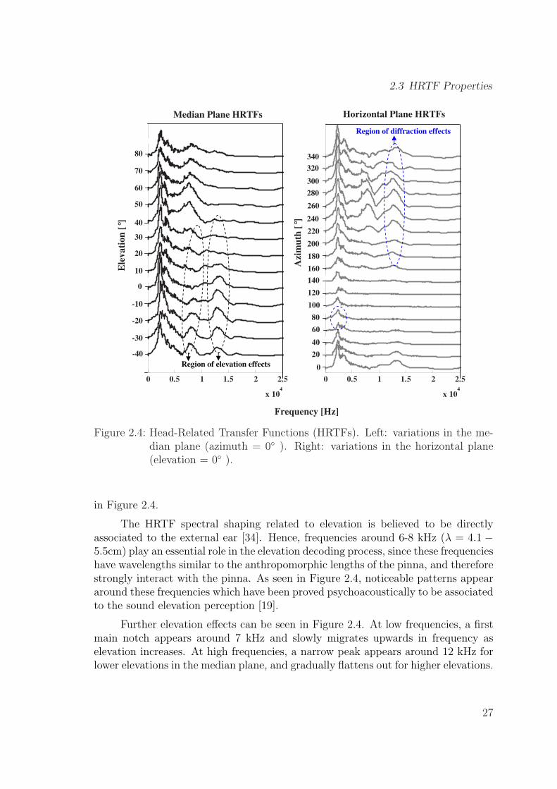
2.3 HRTF Properties
0 0.5 1 1.5 2 2.5
x 104
0 0.5 1 1.5 2 2.5
x 104
Frequency [Hz]
-40
Median Plane HRTFsE
lev
ati
on
[°]
-30
-20
-10
0
10
20
30
40
50
60
70
80
Azi
mu
th [
°]
Horizontal Plane HRTFs
0
40
60
80
100
120
140
160
180
200
220
240
260
280
20
300
320
340
Region of diffraction effects
Region of elevation effects
Figure 2.4: Head-Related Transfer Functions (HRTFs). Left: variations in the me-dian plane (azimuth = 0◦ ). Right: variations in the horizontal plane(elevation = 0◦ ).
in Figure 2.4.
The HRTF spectral shaping related to elevation is believed to be directlyassociated to the external ear [34]. Hence, frequencies around 6-8 kHz (λ = 4.1 −5.5cm) play an essential role in the elevation decoding process, since these frequencieshave wavelengths similar to the anthropomorphic lengths of the pinna, and thereforestrongly interact with the pinna. As seen in Figure 2.4, noticeable patterns appeararound these frequencies which have been proved psychoacoustically to be associatedto the sound elevation perception [19].
Further elevation effects can be seen in Figure 2.4. At low frequencies, a firstmain notch appears around 7 kHz and slowly migrates upwards in frequency aselevation increases. At high frequencies, a narrow peak appears around 12 kHz forlower elevations in the median plane, and gradually flattens out for higher elevations.
27
Chapter 2 Binaural Techniques
Several scientific studies have tried to disclose the relationship between peaks,notches and spectral shapes of certain HRTF databases, as well as their systemati-cal contribution to the perception of azimuth and elevation. Consequently, severalfrequency-domain based signal processing techniques attempted to parameterize orcompute HRTFs models. For example, frequency-domain HRTF interpolation, aswell as frequency based PCA and pole-zero modeling have been repeatedly studied[45].
2.4 HRTF Measurements
Until today, almost all available HRTF data has been obtained from direct acousticmeasurements [114, 47, 130, 134, 39]. A conventional HRTF measurement procedureconsists of placing an artificial humanoid head and torso on a motorized turntablewhich can be rotated accurately to any required azimuth. A speaker mounted on aboom stand enables accurate positioning of the speaker to any elevation with respectto the humanoid. Thus, the measurements can be made one elevation at a time, bysetting the speaker to the proper elevation and then rotating the humanoid to eachazimuth. Such a conventional HRTF measurement procedure is tedious and requireexpensive specialized equipment. Normally, only a sparse spatial grid of HRTFs ismeasured.
Several HRTF databases have been made publicly available [122, 93, 91, 6].In addition, commercial products are available for measuring individualized HRTFs[13]. Although various methods for speeding up the measurement process have beenproposed [141, 38], the acoustic measurement of accurate, high-resolution HRTFsremains a time-consuming process that requires special equipment that is not widelyavailable. This presents a serious obstacle to the widespread usage of HRTFs.Hence, as an alternative to the measurement process, numerous investigations ofsignal processing methods for approximating and modeling the HRTFs have beenconducted [118]. For example, physical HRTF modeling techniques allowed indi-vidualized HRTFs to be reproduced by adjusting the parameters of such models inorder to fit the anthropometry of the pinnae, head, and torso for a certain individual.
2.5 First Binaural Localization Model
The celebrated duplex theory proposed [113] is known to be the very first binauralhearing model. The theory is based on the idea that humans use the ITD at lowfrequencies and the ILD at high frequencies to judge the lateral (azimuthal) angle,the angle between a ray to the sound source and the median plane. These difference
28
2.6 HRTFs and Sound Localization
cues have the important property that they are independent of the source spectrum.Moreover, by approximating the head by a rigid sphere, Rayleigh gave a quantitativeexplanation of how the ITD and ILD are produced by diffraction and scattering ofthe incident waves by the listener’s head.
Although the spherical-head model is obviously only a first approximation toa real head, it continues to be a source of insight into HRTF behavior [4, 119, 135].Rayleigh understood that interaural difference cues vanish on the median plane, andthus cannot resolve front/back confusion. In general, the ITD and ILD constrainthe ray to the source to lie on a cone called the ”cone of confusion”. It is commonexperience that when we are not sure if a source is in front of us or in our back, weturn our heads, which works well unless the sounds are very brief. In a study of theeffects of head motion, it was speculated that to resolve front/back confusion forbrief sounds, the auditory system somehow uses the selective sound shadow of theouter ears or pinnae. For longer duration sounds, it was shown that head motioncues dominate other cues [131]. The role of the pinnae in resolving the front/backconfusion problem was subsequently confirmed by other researchers [37, 110]. Allculminated to the undisputed fact that the pinnae are perceptually important andhave a major effect on the HRTF.
2.6 HRTFs and Sound Localization
In our telepresence scenario, a robot placed at a remote site is supposed to detectthe location, in terms of azimuth and elevation, of the sound sources randomlypartitioned in a certain environment. This angle information along with the soundsignals are sent through the wireless channel to the remote human operator site,where sound synthesis using HRTFs takes place for 3D virtual reproduction of therobots auditory space.
To date, the usage of HRTFs basically revolved around binaural sound syn-thesis, e.g. surround sound by headphones, 3D auditory displays, binaural mixingconsoles. As opposed to virtual reality sound synthesis using HRTFs, the presentthesis aims at using the HRTFs for real-life robotic sound localization. Our tar-get is to build a robotic sound source localizer using the cues encapsulated withingeneric HRTF measurements, and then use these measurements and develop a low-complexity model for azimuth and elevation estimation. Towards this end, we inter-polate, truncate, and invert the HRTFs. Interpolation is used to avoid the complexand time-consuming measurement process. Truncation of the HRTF database isneeded for faster signal processing, and stable inversion ensures better sound local-ization results.
29
Chapter 2 Binaural Techniques
Experiments have shown that measured individualized HRTFs can undergoa great deal of distortion (i.e. smoothing, reduction, etc.) and still be relativelyeffective at generating spatialized sound [19]. This implies that the reduced HRTFstill contains all the necessary descriptors of localization cues and is able to uniquelyrepresent the transfer of sound from a particular point in the 3D space. We can takeadvantage of this fact to greatly simplify the task of sound source localization byusing approximations of an individual’s HRTFs, thus shortening the length of eachHRTF and consequently reducing the overall localization processing time.
The research group at MIT Media Lab has made extensive measurements usingKEMAR. They provide a data set consisting of 710 measurements taken over a broadrange of spatial locations, with each HRTF having a length of 512 samples. TheKEMAR HRTFs can be modeled as a set of linear time-invariant digital filters, beingrepresented either as Finite Impulse Response (FIR) filters or as Infinite ImpulseResponse (IIR) filters. Note that audio professionals consider the length of 512samples for the measured HRTFs as rather short. When it is necessary to use longerfilters the computational burden increases accordingly. Therefore, we investigatethree techniques for reducing the length of the HRTF, two FIR and one IIR, whichare applied to the KEMAR dataset, and which lead to a significant reduction inthe size of the measured HRTF dataset. The original HRTFs containing the 512coefficients of the FIR filter will be denoted as HFIR
512 . Using the reduced dataset,we present a novel approach in chapter 4 to localize sound sources using only twomicrophones in a real environment.
2.7 HRTFs Reduction Techniques
2.7.1 Diffuse-Field Equalization
In order to reduce the computational burden for convolution, we aim at shorteningthe length of the FIR filter representation of the originally measured HRTFs. Thisneeds to be done while preserving the main characteristics of the measured impulseresponses. We adopt the algorithm proposed by [101] for a Diffuse-Field Equalization(DFE). In DFE, a reference spectrum is derived by computing a power-average overall HRTFs for each ear and taking the square root of this average spectrum. Diffuse-field equalized HRTFs are obtained by de-convolving the original transfer functionby the diffuse-field reference HRTF of that ear. This leads to the result that thefactors that are not dependent on the incident-angle, such as the ear canal resonance,are removed. The DFE is achieved according to a four step procedure:
1. Remove the initial time delay from the beginning of the measured impulse
30
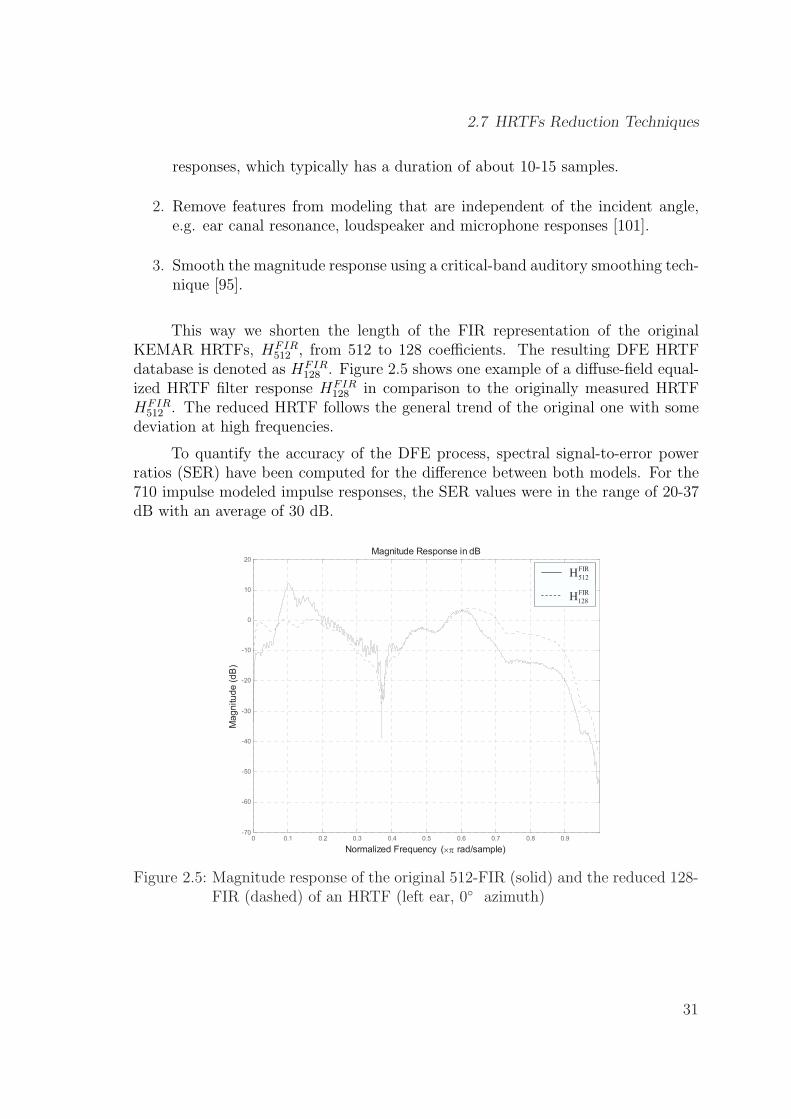
2.7 HRTFs Reduction Techniques
responses, which typically has a duration of about 10-15 samples.
2. Remove features from modeling that are independent of the incident angle,e.g. ear canal resonance, loudspeaker and microphone responses [101].
3. Smooth the magnitude response using a critical-band auditory smoothing tech-nique [95].
This way we shorten the length of the FIR representation of the originalKEMAR HRTFs, HFIR
512 , from 512 to 128 coefficients. The resulting DFE HRTFdatabase is denoted as HFIR
128 . Figure 2.5 shows one example of a diffuse-field equal-ized HRTF filter response HFIR
128 in comparison to the originally measured HRTFHFIR
512 . The reduced HRTF follows the general trend of the original one with somedeviation at high frequencies.
To quantify the accuracy of the DFE process, spectral signal-to-error powerratios (SER) have been computed for the difference between both models. For the710 impulse modeled impulse responses, the SER values were in the range of 20-37dB with an average of 30 dB.
0 0.1 0.2 0.3 0.4 0.5 0.6 0.7 0.8 0.9-70
-60
-50
-40
-30
-20
-10
0
10
20
Normalized Frequency ( rad/sample)
Mag
nitu
de
(d
B)
Magnitude Response in dB
FIR (512)
FIR (128)
FIR
512H
FIR
128H
Figure 2.5: Magnitude response of the original 512-FIR (solid) and the reduced 128-FIR (dashed) of an HRTF (left ear, 0◦ azimuth)
31
Chapter 2 Binaural Techniques
2.7.2 Balanced Model Truncation
In order to examine to which extent the HRTF can be reduced while still pre-serving the characteristic information making it unique, we reduce the previouslyderived diffused-field HRTF dataset further by adopting the balanced model trun-cation (BMT) technique to design a low-order IIR filter model of the HRTF from ahigh-order FIR filter response HFIR
128 . A detailed description of the BMT techniqueis given in [15]. However, a brief outline will be presented here. For applying BMT,we determine a linear time-invariant state-space system, which realizes the filter.We start using the 128-coefficient FIR filter HFIR
128 . The transfer function of thisfilter can be written as: F (z) = c0 + c1 · z + c2 · z2 + . . .+ cnzn, where n = 127. Notethat we follow the notation of positive exponents for the z-transform. This filter canbe represented as state-space difference equations:
x(k + 1) = A · x(k) + B · u(k) (2.1)
y(k) = C · x(k) + D · u(k)
Then, a transformation matrix T is found such that the controllability and observ-ability Grammians are equal and diagonal. This is the characteristic feature of abalanced system. The corresponding system states are ordered according to theircontribution to the system response. The order of the states is reflected in the Han-kel Singular Values (HSV) of the system. Thus, the balanced system can be dividedinto two sub-systems: the truncated system of order m < n, where the first m HSVsare used to model the filter, and the rejected system of order (n −m). Figure 2.6shows the BMT-reduced IIR filter representation (m = 25) in comparison to theFIR (n = 128) for one example of a HRTF. The transfer function of the IIR filterfollows the general trend of the FIR filter with small deviation at high frequencies.Quantitative SER ratios have been computed for the difference between the FIRand IIR models. For all the 710 impulse responses that we modeled, SERs were inthe range of 24-36 dB, with an average of 29 dB.
2.7.3 Principal Component Analysis
In order to examine to which extent the HRTF can be further reduced while stillpreserving the characteristic information which makes it unique, we reduce the pre-viously derived diffused-field HRTF data set, HFIR
128 , by applying a Principal Com-ponent Analysis (PCA).
PCA has already been applied to HRTFs [96, 99, 87]. All the applicationspointed out substantial data reduction, as this method allows the description of allHRTF data with merely 4-7 basic functions and their corresponding weights. The
32
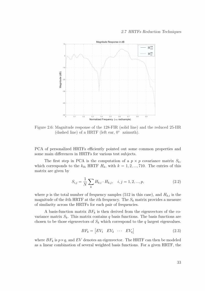
2.7 HRTFs Reduction Techniques
0 0.1 0.2 0.3 0.4 0.5 0.6 0.7 0.8 0.9-50
-40
-30
-20
-10
0
10
Normalized Frequency ( rad/sample)
Ma
gn
itu
de
(d
B)
Magnitude Response in dB
FIR (128)
BMT (25)
FIR
128H
IIR
25H
Figure 2.6: Magnitude response of the 128-FIR (solid line) and the reduced 25-IIR(dashed line) of a HRTF (left ear, 0◦ azimuth).
PCA of personalized HRTFs efficiently pointed out some common properties andsome main differences in HRTFs for various test subjects.
The first step in PCA is the computation of a p × p covariance matrix Sk,which corresponds to the kth HRTF Hk, with k = 1, 2, ..., 710. The entries of thismatrix are given by
Si,j =1
N
∑
k
Hk,i ·Hk,j, i, j = 1, 2, ..., p, (2.2)
where p is the total number of frequency samples (512 in this case), and Hk,i is themagnitude of the kth HRTF at the ith frequency. The Sk matrix provides a measureof similarity across the HRTFs for each pair of frequencies.
A basis-function matrix BFk is then derived from the eigenvectors of the co-variance matrix Sk. This matrix contains q basis functions. The basis functions arechosen to be those eigenvectors of Sk which correspond to the q largest eigenvalues.
BFk =[EV1 EV2 · · · EVq
](2.3)
where BFk is p×q, and EV denotes an eigenvector. The HRTF can then be modeledas a linear combination of several weighted basis functions. For a given HRTF, the
33
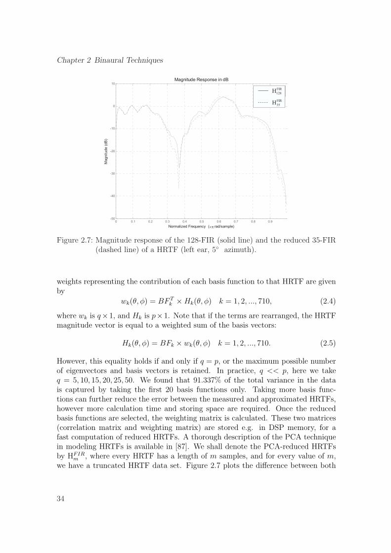
Chapter 2 Binaural Techniques
0 0.1 0.2 0.3 0.4 0.5 0.6 0.7 0.8 0.9-50
-40
-30
-20
-10
0
10
Normalized Frequency ( rad/sample)
Magnitude (
dB
)
Magnitude Response in dB
FIR (128)
PCA (35)FIR
128H
FIR
35H
Figure 2.7: Magnitude response of the 128-FIR (solid line) and the reduced 35-FIR(dashed line) of a HRTF (left ear, 5◦ azimuth).
weights representing the contribution of each basis function to that HRTF are givenby
wk(θ, φ) = BF Tk ×Hk(θ, φ) k = 1, 2, ..., 710, (2.4)
where wk is q× 1, and Hk is p× 1. Note that if the terms are rearranged, the HRTFmagnitude vector is equal to a weighted sum of the basis vectors:
Hk(θ, φ) = BFk × wk(θ, φ) k = 1, 2, ..., 710. (2.5)
However, this equality holds if and only if q = p, or the maximum possible numberof eigenvectors and basis vectors is retained. In practice, q << p, here we takeq = 5, 10, 15, 20, 25, 50. We found that 91.337% of the total variance in the datais captured by taking the first 20 basis functions only. Taking more basis func-tions can further reduce the error between the measured and approximated HRTFs,however more calculation time and storing space are required. Once the reducedbasis functions are selected, the weighting matrix is calculated. These two matrices(correlation matrix and weighting matrix) are stored e.g. in DSP memory, for afast computation of reduced HRTFs. A thorough description of the PCA techniquein modeling HRTFs is available in [87]. We shall denote the PCA-reduced HRTFsby HFIR
m , where every HRTF has a length of m samples, and for every value of m,we have a truncated HRTF data set. Figure 2.7 plots the difference between both
34

2.7 HRTFs Reduction Techniques
FIR models. The SER values were found to fall in the range of 23-37 dB, with anaverage of 30 dB.
In the following chapter, we will introduce two novel HRTF inversion and inter-polation techniques which help stabilizing and increasing the localization accuracyof our new sound localization system.
35

Chapter 2 Binaural Techniques
36
Chapter 3
Binaural Sound SourceLocalization Based on HRTFs
In this chapter, we propose a new binaural sound source localization technique basedon using only two small microphones placed inside the ear canal of a robot’s head.The head is equipped with artificial ears and is mounted on a torso. In contrast toexisting sound source localization methods, we employ a matched filtering approachusing the HRTFs applied to the signals collected by the two microphones. Thisset-up proves to be able to localize sound sources in free space with high precision.Note that, so far, HRTFs have mainly been used for synthesis of spatial sound, whilewe are using them here for sound source localization.
Furthermore, this chapter introduces two novel approaches for inverting andspatially interpolating the HRTFs to be used later in our sound localization algo-rithm. Using HRTF data, we create proper matrix transfer functions or equivalentlyappropriate state-space realizations. We base our method on the factorization of ablock Loewner matrix into a product of generalized observability and controllabilitymatrices. We recollect certain properties to be satisfied by the Loewner matrix,and use it to construct a minimal state-space realization of an interpolating matrixtransfer function.
3.1 A Novel Approach To Sound Localization
The new algorithm for binaural sound source localization relies on a simple corre-lation approach [82]. We assume that we receive a signal originating from a sound
37
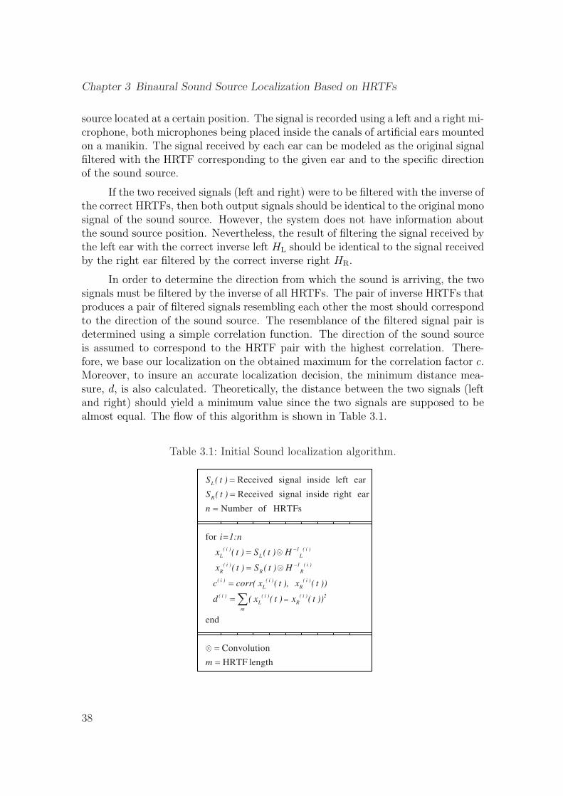
Chapter 3 Binaural Sound Source Localization Based on HRTFs
source located at a certain position. The signal is recorded using a left and a right mi-crophone, both microphones being placed inside the canals of artificial ears mountedon a manikin. The signal received by each ear can be modeled as the original signalfiltered with the HRTF corresponding to the given ear and to the specific directionof the sound source.
If the two received signals (left and right) were to be filtered with the inverse ofthe correct HRTFs, then both output signals should be identical to the original monosignal of the sound source. However, the system does not have information aboutthe sound source position. Nevertheless, the result of filtering the signal received bythe left ear with the correct inverse left HL should be identical to the signal receivedby the right ear filtered by the correct inverse right HR.
In order to determine the direction from which the sound is arriving, the twosignals must be filtered by the inverse of all HRTFs. The pair of inverse HRTFs thatproduces a pair of filtered signals resembling each other the most should correspondto the direction of the sound source. The resemblance of the filtered signal pair isdetermined using a simple correlation function. The direction of the sound sourceis assumed to correspond to the HRTF pair with the highest correlation. There-fore, we base our localization on the obtained maximum for the correlation factor c.Moreover, to insure an accurate localization decision, the minimum distance mea-sure, d, is also calculated. Theoretically, the distance between the two signals (leftand right) should yield a minimum value since the two signals are supposed to bealmost equal. The flow of this algorithm is shown in Table 3.1.
Table 3.1: Initial Sound localization algorithm.
Received signal inside left ear
Received signal inside right ear
Number of HRTFs
for
L
R
( i ) 1 ( i )
L L L
( i ) 1 ( i )
R R R
( i ) ( i ) ( i )
L R
( i ) ( i ) ( i )
L R
m
S ( t )
S ( t )
n
i=1:n
x ( t ) S ( t ) H
x ( t ) S ( t ) H
c corr( x ( t ), x ( t ))
d ( x ( t ) x
end
Convolution
HRTF length
2( t ))
m
38
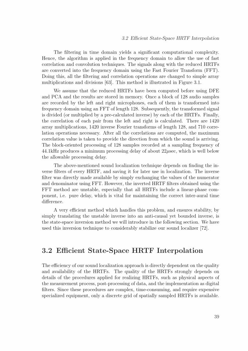
3.2 Efficient State-Space HRTF Interpolation
The filtering in time domain yields a significant computational complexity.Hence, the algorithm is applied in the frequency domain to allow the use of fastcorrelation and convolution techniques. The signals along with the reduced HRTFsare converted into the frequency domain using the Fast Fourier Transform (FFT).Doing this, all the filtering and correlation operations are changed to simple arraymultiplications and divisions [63]. This method is illustrated in Figure 3.1.
We assume that the reduced HRTFs have been computed before using DFEand PCA and the results are stored in memory. Once a block of 128 audio samplesare recorded by the left and right microphones, each of them is transformed intofrequency domain using an FFT of length 128. Subsequently, the transformed signalis divided (or multiplied by a pre-calculated inverse) by each of the HRTFs. Finally,the correlation of each pair from the left and right is calculated. There are 1420array multiplications, 1420 inverse Fourier transforms of length 128, and 710 corre-lation operations necessary. After all the correlations are computed, the maximumcorrelation value is taken to provide the direction from which the sound is arriving.The block-oriented processing of 128 samples recorded at a sampling frequency of44.1kHz produces a minimum processing delay of about 22µsec, which is well belowthe allowable processing delay.
The above-mentioned sound localization technique depends on finding the in-verse filters of every HRTF, and saving it for later use in localization. The inversefilter was directly made available by simply exchanging the values of the numeratorand denominator using FFT. However, the inverted HRTF filters obtained using theFFT method are unstable, especially that all HRTFs include a linear-phase com-ponent, i.e. pure delay, which is vital for maintaining the correct inter-aural timedifference.
A very efficient method which handles this problem, and ensures stability, bysimply translating the unstable inverse into an anti-causal yet bounded inverse, isthe state-space inversion method we will introduce in the following section. We haveused this inversion technique to considerably stabilize our sound localizer [72].
3.2 Efficient State-Space HRTF Interpolation
The efficiency of our sound localization approach is directly dependent on the qualityand availability of the HRTFs. The quality of the HRTFs strongly depends ondetails of the procedures applied for realizing HRTFs, such as physical aspects ofthe measurement process, post-processing of data, and the implementation as digitalfilters. Since these procedures are complex, time-consuming, and require expensivespecialized equipment, only a discrete grid of spatially sampled HRTFs is available.
39
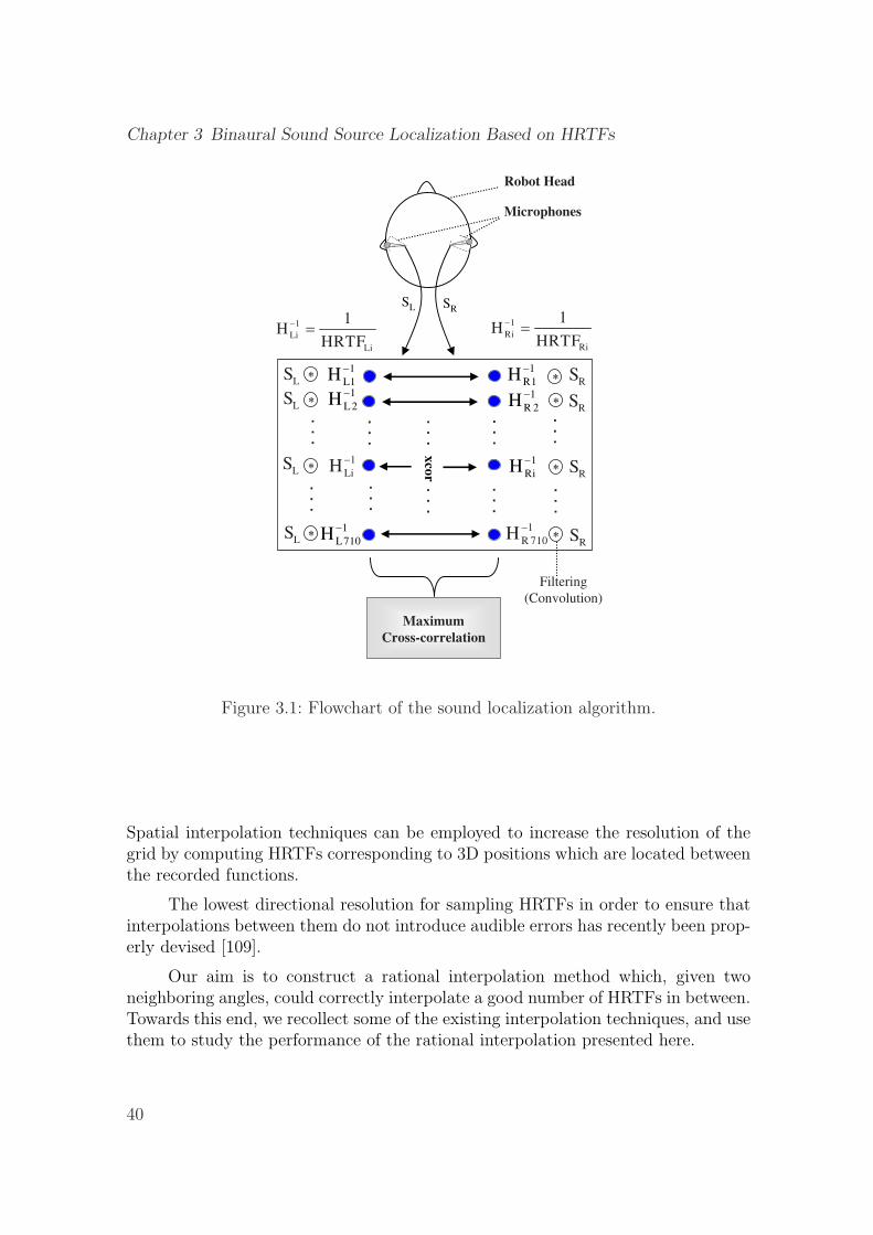
Chapter 3 Binaural Sound Source Localization Based on HRTFs
xco
r
1
L1H
1
L 2H
1
L710H
1
R1H1
R 2H
1
R 710H
1
RiH
1
LiH
1
Li
Li
1H
HRTF
Filtering
(Convolution)
LS
LS
LS
LS
RS
RS
RS
RS
Microphones
Robot Head
SL SR
Maximum
Cross-correlation
1
Ri
Ri
1H
HRTF
. . .
. . .
. . .
. . .
. . .
. . .
. . .
. . .
. . .
. . .
Figure 3.1: Flowchart of the sound localization algorithm.
Spatial interpolation techniques can be employed to increase the resolution of thegrid by computing HRTFs corresponding to 3D positions which are located betweenthe recorded functions.
The lowest directional resolution for sampling HRTFs in order to ensure thatinterpolations between them do not introduce audible errors has recently been prop-erly devised [109].
Our aim is to construct a rational interpolation method which, given twoneighboring angles, could correctly interpolate a good number of HRTFs in between.Towards this end, we recollect some of the existing interpolation techniques, and usethem to study the performance of the rational interpolation presented here.
40
3.2 Efficient State-Space HRTF Interpolation
3.2.1 Previous Interpolation Methods
The bilinear method [14] is a simple and direct way used to perform HRTF interpo-lation. It consists of computing the binaural response corresponding to a given pointon the horizontal circle as weighted mean of the measured binaural responses andassociated with the two adjacent points to the desired point. The discrete FourierTransform (DFT) [97] is used to interpolate binaural impulse responses in the timedomain. The method inserts all HRTFs column-wise in one common H matrix.It then computes the DFT of every row and appends it with zeros before apply-ing inverse DFT to obtain an oversampled matrix, where the oversampled columnscorrespond to the interpolated HRTFs. The plenacoustic function [121] and themathematical spline function [115] have also been used to interpolate HRTFs.
In [97], the authors investigated the effect of arrival time correction (initialtime-delay equalization) on the accuracy of the three interpolation methods, namely,bilinear interpolation, discrete Fourier transform and third-order spline function.The initial time-delay equalization was demonstrated to increase the accuracy ofall proposed interpolation techniques. In this chapter, we use the outcome of theirexperiments to compare and evaluate the performance of the rational HRTF inter-polation we are presenting. Before we present the framework in which we appliedrational interpolation, we will have a brief review of the scalar and matrix rationalinterpolation methods.
3.2.2 Formulation of the Rational Interpolation Problem
The rational interpolation problem was first solved for the scalar transfer functioncase [10]. Due to its frequent occurrences in linear system theory, a transfer-functionmatrix solution rather than the scalar representation was basically of more relevance,hence a state-space description of the problem was later devised in [8]. We willrecapitulate some of the key properties of the scalar rational interpolation problem,before tackling the state-space rational interpolation problem.
Scalar Rational Interpolation
Consider the array of points P := {(xi, yi), i = 1, . . . , N}, with xi 6= xj, and xi, yi ∈C. The fundamental rational interpolation problem [8] is to parameterize all rational
functions y(x) = b(x)a(x)
having minimal Smith-McMillan degree, which interpolate theabove points. If xi 6= xj for i 6= j, then the desired rational function must satisfyy(xi) = yi, for i = 1, . . . , n. For this purpose, the rational interpolating function
41
Chapter 3 Binaural Sound Source Localization Based on HRTFs
y(x) could be selected such that
n∑i=1
ciy(x)− yi
x− xi
= 0, ci 6= 0. (3.1)
The function y(x) is the desired interpolation function, for which we clearly havey(xi) = yi, if ci 6= 0. The goal is to minimize the degree of the adopted y. One wayto do this is to consider a summation as in (3.1) containing only q < n summands,for any set of non-zero coefficients ci, then the rational function y, of degree q − 1,interpolates the first q points. Making use of the freedom in selecting the ci, we thentry to interpolate the remaining n − q points. Let c := [c1 . . . cq]
T ; in order for theremaining n− q points to be interpolated, c must satisfy
q∑i=1
ciyq+j − yi
xq+j − xi
= 0, i = 1, 2, . . . , n− q. (3.2)
or in matrix formL · c = 0, (3.3)
where L is a Loewner or divided-differences matrix of dimensions (n−q)×q, derivedfrom the given pairs of points. This Loewner matrix is a major instrument for therational interpolation problem. The key property of this matrix is that its rankis directly related to the degree of the corresponding minimal-degree interpolatingfunction. More about the Loewner matrix characteristics is found in [8].
The interpolation problem now reduces to determining the c vector such that(3.3) is satisfied. Once c is obtained, we can compute the rational interpolation
function y(x, c) = b(x,c)a(x,c)
where
b(x, c) =n∑i
ciyi
∏
j 6=i
(x− xj), a(x, c) =n∑i
ci
∏
j 6=i
(x− xj). (3.4)
For the proof of (3.4) refer to [10]. After having reviewed what we need on Loewnermatrices associated with the interpolation of scalar transfer functions, we turn ourattention to the matrix transfer functions, and how their minimal state-space real-izations are computed.
State-Space Rational Interpolation
Let Y (x) be a matrix transfer-function with a minimal state-space realization {A,B, C,D}of the form
Y (x) = C∗(xI − A)−1B + D. (3.5)
42
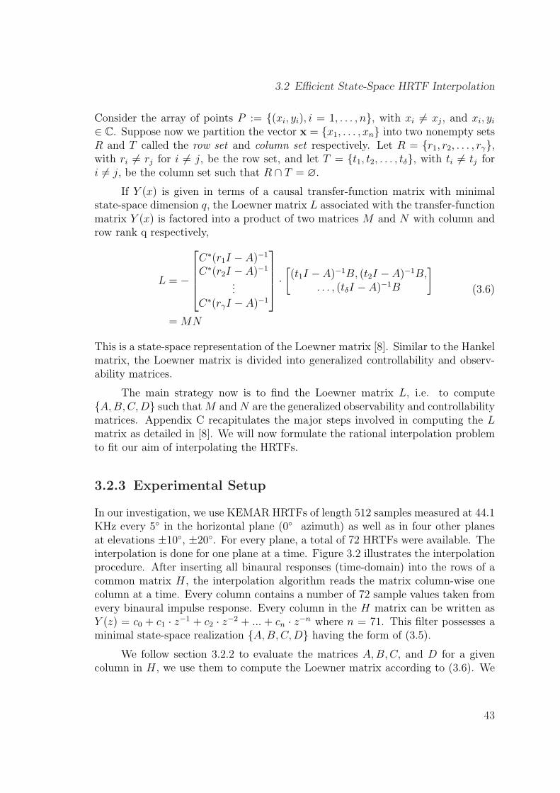
3.2 Efficient State-Space HRTF Interpolation
Consider the array of points P := {(xi, yi), i = 1, . . . , n}, with xi 6= xj, and xi, yi
∈ C. Suppose now we partition the vector x = {x1, . . . , xn} into two nonempty setsR and T called the row set and column set respectively. Let R = {r1, r2, . . . , rγ},with ri 6= rj for i 6= j, be the row set, and let T = {t1, t2, . . . , tδ}, with ti 6= tj fori 6= j, be the column set such that R ∩ T = ∅.
If Y (x) is given in terms of a causal transfer-function matrix with minimalstate-space dimension q, the Loewner matrix L associated with the transfer-functionmatrix Y (x) is factored into a product of two matrices M and N with column androw rank q respectively,
L = −
C∗(r1I − A)−1
C∗(r2I − A)−1
...C∗(rγI − A)−1
·
[(t1I − A)−1B, (t2I − A)−1B,
. . . , (tδI − A)−1B
]
= MN
(3.6)
This is a state-space representation of the Loewner matrix [8]. Similar to the Hankelmatrix, the Loewner matrix is divided into generalized controllability and observ-ability matrices.
The main strategy now is to find the Loewner matrix L, i.e. to compute{A, B, C, D} such that M and N are the generalized observability and controllabilitymatrices. Appendix C recapitulates the major steps involved in computing the Lmatrix as detailed in [8]. We will now formulate the rational interpolation problemto fit our aim of interpolating the HRTFs.
3.2.3 Experimental Setup
In our investigation, we use KEMAR HRTFs of length 512 samples measured at 44.1KHz every 5◦ in the horizontal plane (0◦ azimuth) as well as in four other planesat elevations ±10◦, ±20◦. For every plane, a total of 72 HRTFs were available. Theinterpolation is done for one plane at a time. Figure 3.2 illustrates the interpolationprocedure. After inserting all binaural responses (time-domain) into the rows of acommon matrix H, the interpolation algorithm reads the matrix column-wise onecolumn at a time. Every column contains a number of 72 sample values taken fromevery binaural impulse response. Every column in the H matrix can be written asY (z) = c0 + c1 · z−1 + c2 · z−2 + ... + cn · z−n where n = 71. This filter possesses aminimal state-space realization {A,B, C, D} having the form of (3.5).
We follow section 3.2.2 to evaluate the matrices A, B, C, and D for a givencolumn in H, we use them to compute the Loewner matrix according to (3.6). We
43
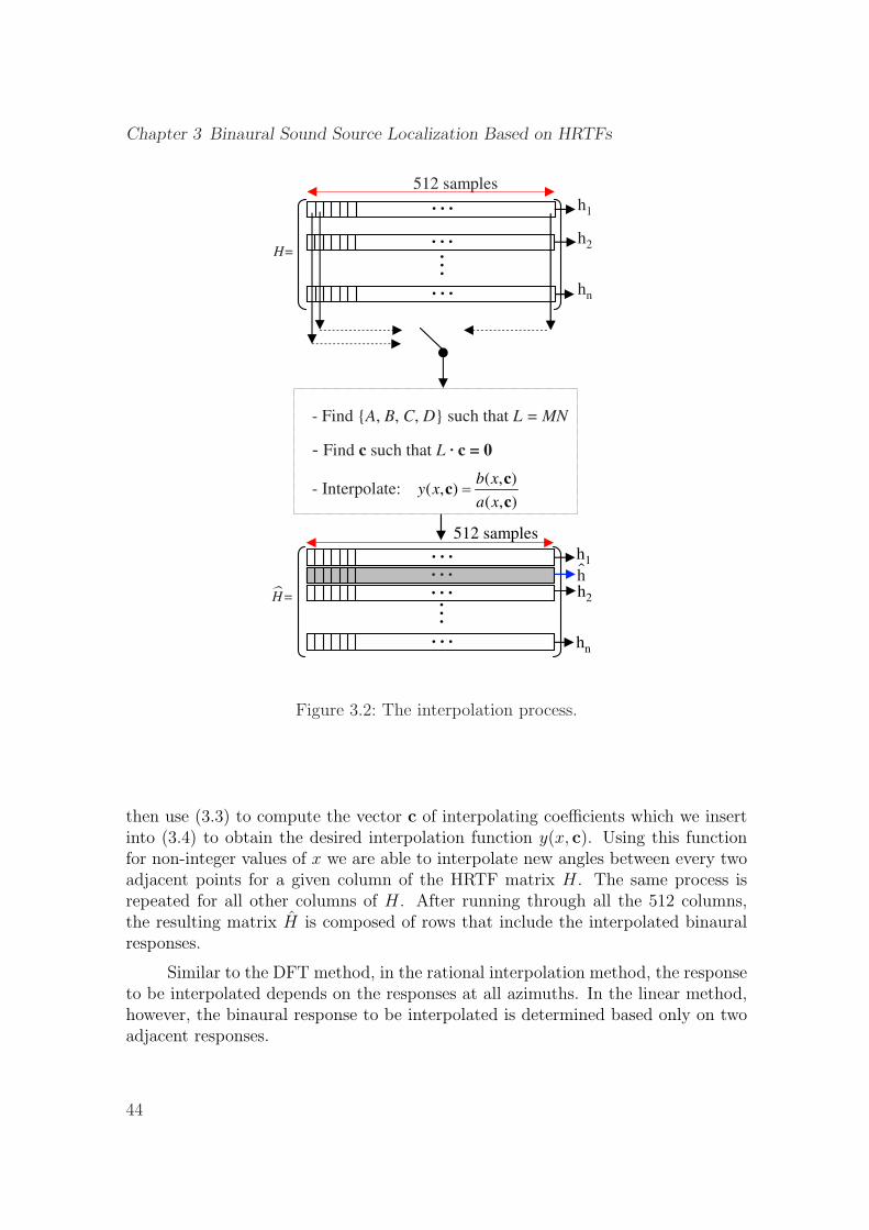
Chapter 3 Binaural Sound Source Localization Based on HRTFs
512 samples
h1
- Find {A, B, C, D} such that L = MN
- Find c such that L · c = 0
- Interpolate:( , )
( , )( , )
b xy x
a x
cc
c
h1
h2
hn
H=
H=h2
hn
. . .
. . .
. . .
. . .
. . .
. . .
. . .
. . .
. . .
512 samples
h
Figure 3.2: The interpolation process.
then use (3.3) to compute the vector c of interpolating coefficients which we insertinto (3.4) to obtain the desired interpolation function y(x, c). Using this functionfor non-integer values of x we are able to interpolate new angles between every twoadjacent points for a given column of the HRTF matrix H. The same process isrepeated for all other columns of H. After running through all the 512 columns,the resulting matrix H is composed of rows that include the interpolated binauralresponses.
Similar to the DFT method, in the rational interpolation method, the responseto be interpolated depends on the responses at all azimuths. In the linear method,however, the binaural response to be interpolated is determined based only on twoadjacent responses.
44
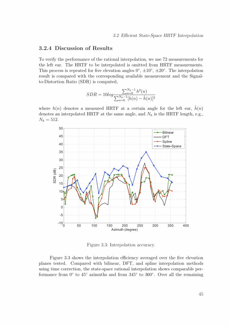
3.2 Efficient State-Space HRTF Interpolation
3.2.4 Discussion of Results
To verify the performance of the rational interpolation, we use 72 measurements forthe left ear. The HRTF to be interpolated is omitted from HRTF measurements.This process is repeated for five elevation angles 0◦, ±10◦, ±20◦. The interpolationresult is compared with the corresponding available measurement and the Signal-to-Distortion Ratio (SDR) is computed,
SDR = 10log
∑Nh−1n=0 h2(n)∑Nh−1
n=0 [h(n)− h(n)]2
where h(n) denotes a measured HRTF at a certain angle for the left ear, h(n)denotes an interpolated HRTF at the same angle, and Nh is the HRTF length, e.g.,Nh = 512.
0 50 100 150 200 250 300 350 400-10
-5
0
5
10
15
20
25
30
35
40
45
50
Azimuth (degree)
SD
R (
dB
)
Bilinear
DFT
Spline
State-Space
Figure 3.3: Interpolation accuracy.
Figure 3.3 shows the interpolation efficiency averaged over the five elevationplanes tested. Compared with bilinear, DFT, and spline interpolation methodsusing time correction, the state-space rational interpolation shows comparable per-formance from 0◦ to 45◦ azimuths and from 345◦ to 360◦. Over all the remaining
45
Chapter 3 Binaural Sound Source Localization Based on HRTFs
azimuth range the SDR for the rational method is higher than that for the otherthree methods. The mean SDR value for the state-space method is 28.3 dB com-pared to 12.07 dB, 9.46 dB and 10.44 dB for the bilinear, DFT, and spline methods,respectively.
Compared with existing interpolation techniques, the state-space method wehave introduced allowed very precise reconstruction of HRTFs and proved to havehigher performance for a wide range of azimuths [66], [59], [62]. Nevertheless, itshould be noted that more gain can be achieved if we use the time correction methodalong with the presented rational interpolation method. We will use this inter-polation method to increase the accuracy of a novel sound localization algorithmpresented in chapter 6.
3.2.5 Subjective Analysis
In order to verify the theoretical results, we carried out headphone listening exper-iments. The goal was to study the performance of the state-of-the-art interpolationtechniques as compared to our RSS method. A total of 20 male test subjects partici-pated in the listening experiment with ages ranging between 23 and 35. The hearingof all test subjects was tested using standard audiometry. None of the subjects hadreportable hearing loss that could effect the test results.
Test Methods
In the first test method, the subjects were asked to determine the angle of arrival ofthe synthesized test tones. In each trial the same test signal was repeated two timeswith 0.5s silence between each play. The HRTF used to synthesize the test toneswas randomly chosen from 12 Kemar HRTFs measured every 30◦ in the horizontalplane. This type of subjective tests, however, is prone to localization errors such asin-head localization and front back confusions, therefore, a second listening test wasimplemented.
In this test, an A/B paired comparison hidden reference paradigm was em-ployed. The subjects were asked to grade localization impairment against the hid-den reference on a continuous 1.0 to 5.0 scale (1- very different, 2- Slightly different,3- Slightly similar, 4- Relatively similar, 5- No difference). The hidden reference ineach case was randomly chosen from the 72 measured Kemar HRTFs of the hori-zontal plane. The other test signal was synthesized using interpolated HRTFs. Thefour above-mentioned interpolation methods were tested. In each trial two test se-quences were presented with 0.5s between each sequence, i.e. A/B - 0.5s - B/A. Twodifferent random orders of presentation were used to minimize bias. Listeners were
46
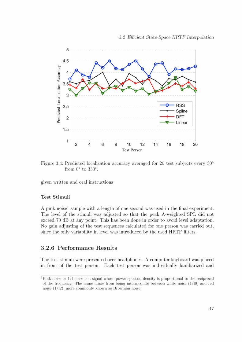
3.2 Efficient State-Space HRTF Interpolation
2 4 6 8 10 12 14 16 18 201
1.5
2
2.5
3
3.5
4
4.5
5
Test Person
Pre
dic
ted
Lo
cali
zati
on
Accu
racy
RSS
Spline
DFT
Linear
Figure 3.4: Predicted localization accuracy averaged for 20 test subjects every 30◦
from 0◦ to 330◦.
given written and oral instructions
Test Stimuli
A pink noise1 sample with a length of one second was used in the final experiment.The level of the stimuli was adjusted so that the peak A-weighted SPL did notexceed 70 dB at any point. This has been done in order to avoid level adaptation.No gain adjusting of the test sequences calculated for one person was carried out,since the only variability in level was introduced by the used HRTF filters.
3.2.6 Performance Results
The test stimuli were presented over headphones. A computer keyboard was placedin front of the test person. Each test person was individually familiarized and
1Pink noise or 1/f noise is a signal whose power spectral density is proportional to the reciprocalof the frequency. The name arises from being intermediate between white noise (1/f0) and rednoise (1/f2), more commonly known as Brownian noise.
47
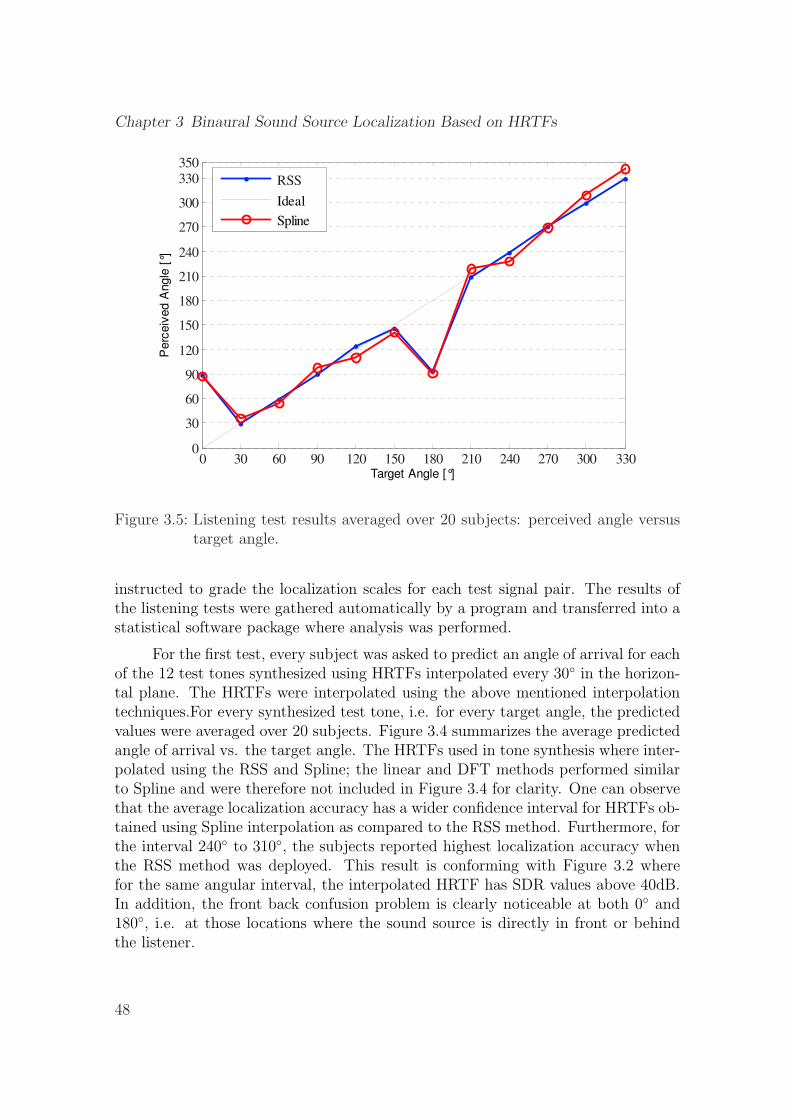
Chapter 3 Binaural Sound Source Localization Based on HRTFs
0 30 60 90 120 150 180 210 240 270 300 3300
30
60
90
120
150
180
210
240
270
300
330350
Target Angle [°]
Perc
eiv
ed A
ngle
[°]
RSS
Ideal
Spline
Figure 3.5: Listening test results averaged over 20 subjects: perceived angle versustarget angle.
instructed to grade the localization scales for each test signal pair. The results ofthe listening tests were gathered automatically by a program and transferred into astatistical software package where analysis was performed.
For the first test, every subject was asked to predict an angle of arrival for eachof the 12 test tones synthesized using HRTFs interpolated every 30◦ in the horizon-tal plane. The HRTFs were interpolated using the above mentioned interpolationtechniques.For every synthesized test tone, i.e. for every target angle, the predictedvalues were averaged over 20 subjects. Figure 3.4 summarizes the average predictedangle of arrival vs. the target angle. The HRTFs used in tone synthesis where inter-polated using the RSS and Spline; the linear and DFT methods performed similarto Spline and were therefore not included in Figure 3.4 for clarity. One can observethat the average localization accuracy has a wider confidence interval for HRTFs ob-tained using Spline interpolation as compared to the RSS method. Furthermore, forthe interval 240◦ to 310◦, the subjects reported highest localization accuracy whenthe RSS method was deployed. This result is conforming with Figure 3.2 wherefor the same angular interval, the interpolated HRTF has SDR values above 40dB.In addition, the front back confusion problem is clearly noticeable at both 0◦ and180◦, i.e. at those locations where the sound source is directly in front or behindthe listener.
48
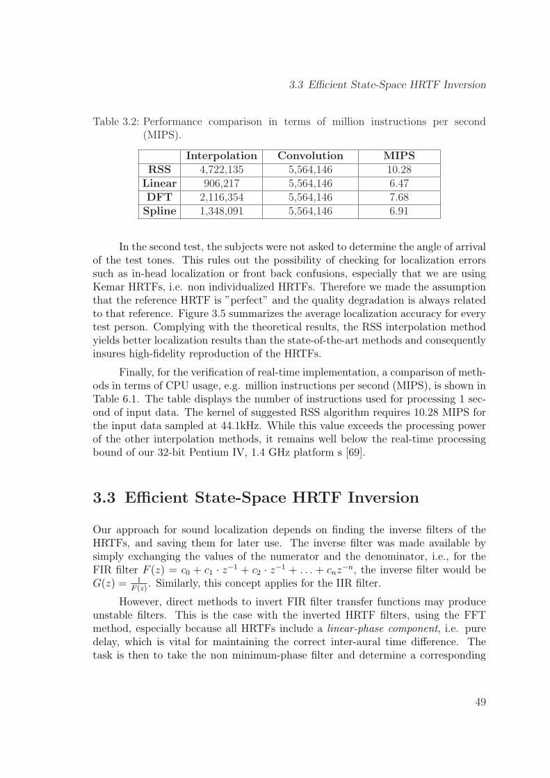
3.3 Efficient State-Space HRTF Inversion
Table 3.2: Performance comparison in terms of million instructions per second(MIPS).
Interpolation Convolution MIPSRSS 4,722,135 5,564,146 10.28
Linear 906,217 5,564,146 6.47DFT 2,116,354 5,564,146 7.68Spline 1,348,091 5,564,146 6.91
In the second test, the subjects were not asked to determine the angle of arrivalof the test tones. This rules out the possibility of checking for localization errorssuch as in-head localization or front back confusions, especially that we are usingKemar HRTFs, i.e. non individualized HRTFs. Therefore we made the assumptionthat the reference HRTF is ”perfect” and the quality degradation is always relatedto that reference. Figure 3.5 summarizes the average localization accuracy for everytest person. Complying with the theoretical results, the RSS interpolation methodyields better localization results than the state-of-the-art methods and consequentlyinsures high-fidelity reproduction of the HRTFs.
Finally, for the verification of real-time implementation, a comparison of meth-ods in terms of CPU usage, e.g. million instructions per second (MIPS), is shown inTable 6.1. The table displays the number of instructions used for processing 1 sec-ond of input data. The kernel of suggested RSS algorithm requires 10.28 MIPS forthe input data sampled at 44.1kHz. While this value exceeds the processing powerof the other interpolation methods, it remains well below the real-time processingbound of our 32-bit Pentium IV, 1.4 GHz platform s [69].
3.3 Efficient State-Space HRTF Inversion
Our approach for sound localization depends on finding the inverse filters of theHRTFs, and saving them for later use. The inverse filter was made available bysimply exchanging the values of the numerator and the denominator, i.e., for theFIR filter F (z) = c0 + c1 · z−1 + c2 · z−1 + . . . + cnz−n, the inverse filter would beG(z) = 1
F (z). Similarly, this concept applies for the IIR filter.
However, direct methods to invert FIR filter transfer functions may produceunstable filters. This is the case with the inverted HRTF filters, using the FFTmethod, especially because all HRTFs include a linear-phase component, i.e. puredelay, which is vital for maintaining the correct inter-aural time difference. Thetask is then to take the non minimum-phase filter and determine a corresponding
49
Chapter 3 Binaural Sound Source Localization Based on HRTFs
minimum-phase filter, which can then be safely inverted to produce a stable inversefilter. The resulting filter may be non-causal but serves as an approximation tothe original unstable filter. Non-causality is a small price to pay if magnitude andphase information are critical to performance, which is the case in our situation.The following section will provide details of the inversion process we have adoptedin this work using an inner-outer factorization approach.
One method which handles the previously mentioned inversion problem ensur-ing stability is to replace the unstable inverse by an anti-causal yet bounded inverse.This can be done efficiently using the state-space inversion method with inner-outerfactorization. According to this method, the inner factor captures the part of thetransfer function that causes the instability in the inverse, while the outer part canbe straightforwardly inverted.
3.3.1 Problem Formulation
There are a variety of reasons why a state-space representation of the HRTFs isbeneficial. While transfer functions only deal with input/output behavior or thesystem, state-space forms provide an easy access to the internal features and responseof the system. General system properties, for example, the system controllabilityor observability can be defined and determined. One of the main advantages ofthe state-space modeling is the possibility of ordering the system states based ontheir significance to the representation of the system characteristics. This is a veryimportant feature that allows model simplification, e.g. HRTF order reduction, bydirect truncation, i.e., by discarding its ”less important” states.
For rational time-invariant single-input single-output systems, the inner-outerfactorization is a factorization of an analytical (causal) transfer function H(z) intothe product of an inner and an outer transfer function according to
H(z) = Ho(z)V (z). (3.7)
The inner factor V (z) has its poles outside the unit disc and has modulus 1 on theunit circle, whereas the outer factor Ho(z) and its inverse are analytical in the openunit disc. Before deriving these inner and outer factors, we will review the stepsinvolved in inverting a given transfer function given a state-space representationthereof.
Let H(z) = D + Cz(I −Az)−1B be a minimal state-space representation of agiven HRTF, with D being square and non-singular. This transfer function can alsobe represented by the state-space equations,
xk+1 = Axk + Buk
yk = Cxk + Duk
(3.8)
50
3.3 Efficient State-Space HRTF Inversion
where x is the n-dimensional state vector, u is the scalar system input, y its output,with the matrix A, vectors B and C, and scalar D fully defining the system.
Starting with the transfer function of the general state-space model, H(z) =D+Cz(I−Az)−1B, we may first observe that the poles of H(z) are either the sameas or some subset of the poles of Hp(z) = z(I − Az)−1 (They are the same whenall modes are controllable and observable). By Cramer’s rule for matrix inversion,the denominator polynomial for Hp(z) is given by the determinant D(z) = |(Iz−1−A)−1|, where |.| denotes the determinant of a square matrix. In linear algebra,the polynomial D(z) = |(Iz−1 − A)−1| is called the characteristic polynomial forthe matrix A. The roots of the characteristic polynomial are the eigenvalues of A.Thus, the eigenvalues of the state transition matrix are the poles of the correspondinglinear time-invariant system. In particular, note that the poles of the system do notdepend on the matrices B, C, and D, although these matrices, by placing systemzeros, can cause pole-zero cancelations (unobservable or uncontrollable modes).
The direct way of inverting the transfer function H(z) results in an unstablesystem, knowing that H(z) represents a non minimum-phase transfer function. Thisunstable inverse could be, in state-space, directly derived. We first take the secondpart of (3.8) and solve for uk:
uk = D−1yk −D−1Cxk. (3.9)
Inserting this in the first part of (3.8)
xk+1 = Axk + B(D−1yk −D−1Cxk), (3.10)
leads to the inversion in the state-space, which can be written as
xk+1 = (A−BD−1C)xk + BD−1yk
uk = −D−1Cxk + D−1yk
(3.11)
We denote the quadruple {A, B, C, D}, where A = A − BD−1C, B = BD−1, C =−D−1C, and D = D−1, as the state-space realization of the unstable inverse transferfunction, H−1(z), corresponding to the inverse HRTF. The state-space realizationA has its poles outside the unit circle and, therefore, drives the system unstable. Toensure stability, we implement the inner-outer factorization theorem stated below.
3.3.2 Inner-Outer Factorization
Given a minimal state-space realization of the transfer function H(z), we would liketo find the factors V (z) and Ho(z), as in (3.7), where V (z) is unitary and Ho(z) is
51
Chapter 3 Binaural Sound Source Localization Based on HRTFs
an outer function, that is to say it is minimum phase, and hence H−1o (z) is bounded
but not causal.
Equation (3.7) can be expressed in a state-space form:
D + Cz(I − Az)−1B = (3.12)[Do + Coz(I − Az)−1B
] [Dv + Cvz(I − Avz)−1Bv
](3.13)
where {Av, Bv, Cv, Dv} is a realization for V (z), and {A,B, C0, D0} is a realizationfor Ho(z).
Expansion of the quadratic term in (3.12), and equating members leads to
[A BC D
] [Y 00 I
]=
[Y C0
0 D0
] [Av Bv
Cv Dv
](3.14)
where the diagonal matrix Y satisfies the Lyapunov-Stein equation
Y = BB?v + AY A?
v (3.15)
To get the inner and outer factors we are looking for, Eq. (3.15) must besolvable, and the kernel and maximality requirements on Y and Do must indeedproduce an outer factor Ho(z).
Theorem: Let W be a unitary matrix, and Y be a uniformly bounded matrixwhich satisfies the following equality,
[A BC D
] [Y 00 I
]=
[Y B0
0 D0
]W (3.16)
such that Y has a maximal dimension and ker(Y.) = 0. Let
W =
[Av Bv
Cv Dv
]. (3.17)
Then {Av, Bv, Cv, Dv} is an isometric realization for the sought inner factor V (z),and {A,B,C0, D0} is a realization for the outer factor Ho(z). The proof of the abovetheorem is detailed in [33]. In appendix A, we recapitulate the main steps of thistheorem.
We shall use the above-mentioned state-space inversion algorithm to consider-ably stabilize and enhance the performance of our new sound localization techniquespresented in the following chapter.
52
Chapter 4
Enhanced Sound SourceLocalization Techniques
In this chapter, we have considerably improved the initial matched filtering approachto sound localization in order to achieve low-complexity tracking of moving sound.the humanoid detects the current location of the sound source using a number ofcorrelation operations between the input signals at the microphones and a genericset of transfer functions. Using a properly tuned Kalman filter, a Region Of Interest(ROI) is automatically extracted within the HRTFs, leading to a faster detection,due to less correlation operations and low processing power requirements. Theproposed method is demonstrated through simulations and is further tested in ahousehold environment. In contrast to microphone-array methods, using only twomicrophones, the new system demonstrated high precision 3D sound tracking andenabled a low-complexity implementation on the humanoid DSP platform [66].
4.1 Source Cancelation Algorithm
In the previous algorithm, the main goal was to pass the received signal throughall possible inverse filters. The set of filters from the correct direction would resultin canceling the effects of the HRTF and extracting the original signal from bothsides [60]. However, a more direct approach can be taken to localize a sound source.Instead of attempting to retrieve it, discarding the original signal from the receivedinputs, so that only the HRTFs are left, may be possible. Such an approach isdenoted as the Source Cancelation Algorithm (SCA) and is illustrated in Figure
53
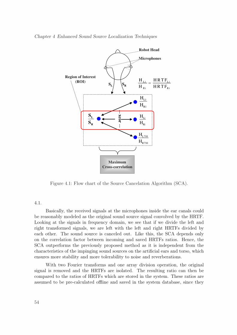
Chapter 4 Enhanced Sound Source Localization Techniques
Robot Head
Microphones
SLSR
L i L i
R i R i
H H R T F
H H R T F
Region of Interest
(ROI)
Maximum
Cross-correlation
xco
r
L1
R1
H
H
Li
Ri
H
H
L
R
S
S
L710
R710
H
H
……
Figure 4.1: Flow chart of the Source Cancelation Algorithm (SCA).
4.1.
Basically, the received signals at the microphones inside the ear canals couldbe reasonably modeled as the original sound source signal convolved by the HRTF.Looking at the signals in frequency domain, we see that if we divide the left andright transformed signals, we are left with the left and right HRTFs divided byeach other. The sound source is canceled out. Like this, the SCA depends onlyon the correlation factor between incoming and saved HRTFs ratios. Hence, theSCA outperforms the previously proposed method as it is independent from thecharacteristics of the impinging sound sources on the artificial ears and torso, whichensures more stability and more tolerability to noise and reverberations.
With two Fourier transforms and one array division operation, the originalsignal is removed and the HRTFs are isolated. The resulting ratio can then becompared to the ratios of HRTFs which are stored in the system. These ratios areassumed to be pre-calculated offline and saved in the system database, since they
54
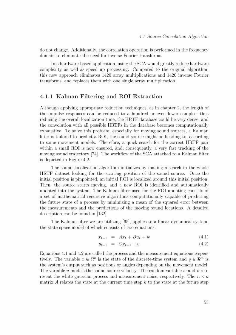
4.1 Source Cancelation Algorithm
do not change. Additionally, the correlation operation is performed in the frequencydomain to eliminate the need for inverse Fourier transforms.
In a hardware-based application, using the SCA would greatly reduce hardwarecomplexity as well as speed up processing. Compared to the original algorithm,this new approach eliminates 1420 array multiplications and 1420 inverse Fouriertransforms, and replaces them with one single array multiplication.
4.1.1 Kalman Filtering and ROI Extraction
Although applying appropriate reduction techniques, as in chapter 2, the length ofthe impulse responses can be reduced to a hundred or even fewer samples, thusreducing the overall localization time, the HRTF database could be very dense, andthe convolution with all possible HRTFs in the database becomes computationallyexhaustive. To solve this problem, especially for moving sound sources, a Kalmanfilter is tailored to predict a ROI, the sound source might be heading to, accordingto some movement models. Therefore, a quick search for the correct HRTF pairwithin a small ROI is now ensured, and, consequently, a very fast tracking of themoving sound trajectory [74]. The workflow of the SCA attached to a Kalman filteris depicted in Figure 4.2.
The sound localization algorithm initializes by making a search in the wholeHRTF dataset looking for the starting position of the sound source. Once theinitial position is pinpointed, an initial ROI is localized around this initial position.Then, the source starts moving, and a new ROI is identified and automaticallyupdated into the system. The Kalman filter used for the ROI updating consists ofa set of mathematical recursive algorithms computationally capable of predictingthe future state of a process by minimizing a mean of the squared error betweenthe measurements and the predictions of the moving sound locations. A detaileddescription can be found in [132].
The Kalman filter we are utilizing [65], applies to a linear dynamical system,the state space model of which consists of two equations:
xk+1 = Axk + Buk + w (4.1)
yk+1 = Cxk+1 + v (4.2)
Equations 4.1 and 4.2 are called the process and the measurement equations respec-tively. The variable x ∈ <n is the state of the discrete-time system and y ∈ <m isthe system’s output such as positions or angles depending on the movement model.The variable u models the sound source velocity. The random variable w and v rep-resent the white gaussian process and measurement noise, respectively. The n × nmatrix A relates the state at the current time step k to the state at the future step
55
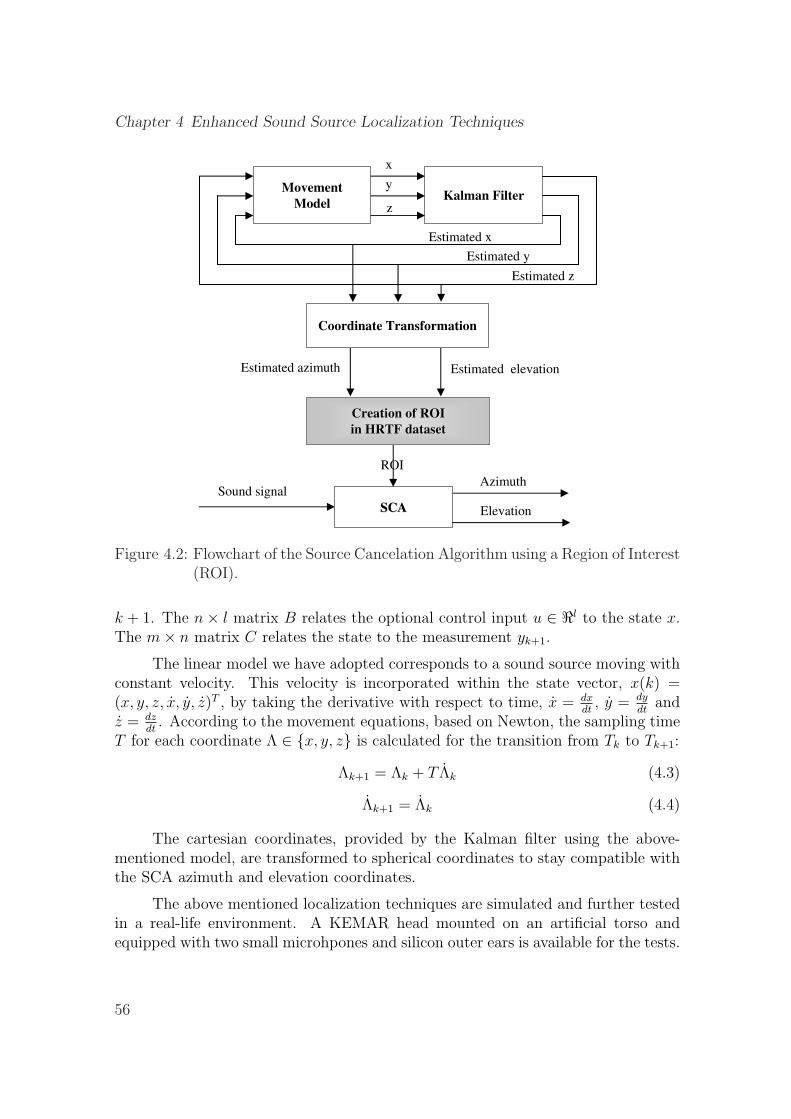
Chapter 4 Enhanced Sound Source Localization Techniques
Coordinate Transformation
SCASCA
Estimated azimuth Estimated elevation
ROI
Sound signalAzimuth
Elevation
Movement
ModelKalman Filter
y
x
z
Estimated x
Estimated y
Estimated z
Creation of ROICreation of ROI
in HRTF in HRTF datasetdataset
Figure 4.2: Flowchart of the Source Cancelation Algorithm using a Region of Interest(ROI).
k + 1. The n× l matrix B relates the optional control input u ∈ <l to the state x.The m× n matrix C relates the state to the measurement yk+1.
The linear model we have adopted corresponds to a sound source moving withconstant velocity. This velocity is incorporated within the state vector, x(k) =(x, y, z, x, y, z)T , by taking the derivative with respect to time, x = dx
dt, y = dy
dtand
z = dzdt
. According to the movement equations, based on Newton, the sampling timeT for each coordinate Λ ∈ {x, y, z} is calculated for the transition from Tk to Tk+1:
Λk+1 = Λk + T Λk (4.3)
Λk+1 = Λk (4.4)
The cartesian coordinates, provided by the Kalman filter using the above-mentioned model, are transformed to spherical coordinates to stay compatible withthe SCA azimuth and elevation coordinates.
The above mentioned localization techniques are simulated and further testedin a real-life environment. A KEMAR head mounted on an artificial torso andequipped with two small microhpones and silicon outer ears is available for the tests.
56
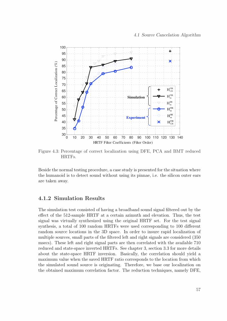
4.1 Source Cancelation Algorithm
0 10 20 30 40 50 60 70 80 90 100 110 120 130 14030
35
40
45
50
55
60
65
70
75
80
85
90
95
100
HRTF Filter Coefficients (Filter Order)
Per
centa
ge
of
Co
rrec
t L
oca
liza
tio
n (
%)
FIR
128H
FIR
mH
IIR
mH
Simulation
ExperimentFIR
128H
FIR
mH
IIR
mH
Figure 4.3: Percentage of correct localization using DFE, PCA and BMT reducedHRTFs.
Beside the normal testing procedure, a case study is presented for the situation wherethe humanoid is to detect sound without using its pinnae, i.e. the silicon outer earsare taken away.
4.1.2 Simulation Results
The simulation test consisted of having a broadband sound signal filtered out by theeffect of the 512-sample HRTF at a certain azimuth and elevation. Thus, the testsignal was virtually synthesized using the original HRTF set. For the test signalsynthesis, a total of 100 random HRTFs were used corresponding to 100 differentrandom source locations in the 3D space. In order to insure rapid localization ofmultiple sources, small parts of the filtered left and right signals are considered (350msecs). These left and right signal parts are then correlated with the available 710reduced and state-space inverted HRTFs. See chapter 3, section 3.3 for more detailsabout the state-space HRTF inversion. Basically, the correlation should yield amaximum value when the saved HRTF ratio corresponds to the location from whichthe simulated sound source is originating. Therefore, we base our localization onthe obtained maximum correlation factor. The reduction techniques, namely DFE,
57
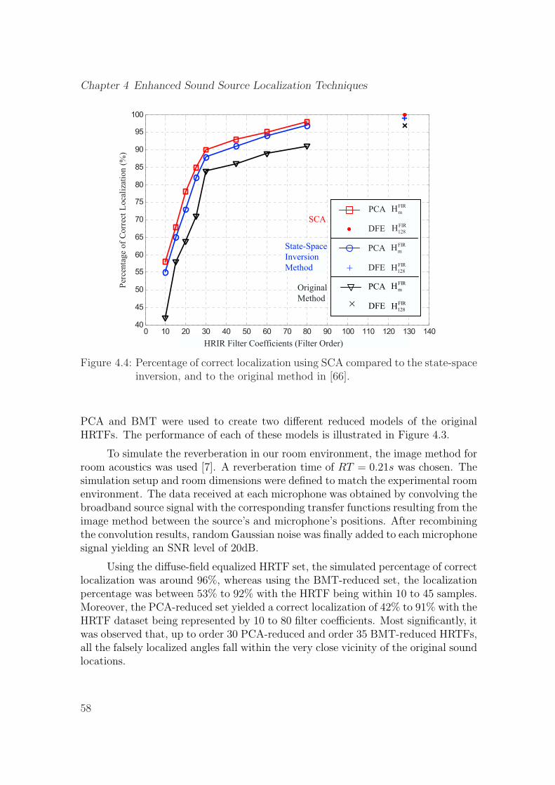
Chapter 4 Enhanced Sound Source Localization Techniques
0 10 20 30 40 50 60 70 80 90 100 110 120 130 14040
45
50
55
60
65
70
75
80
85
90
95
100
HRIR Filter Coefficients (Length in Samples)
Per
cen
tag
e o
f C
orr
ect
Lo
cali
zati
on
(%
)
DFE
PCA
PCA
DFE
FIR
mHPCA
DFEFIR
128H
FIR
mHPCA
DFE FIR
128H
State-Space
Inversion
Method
SCA
+
FIR
mHPCA
DFE FIR
128H
Original
Method
HRIR Filter Coefficients (Filter Order)
Figure 4.4: Percentage of correct localization using SCA compared to the state-spaceinversion, and to the original method in [66].
PCA and BMT were used to create two different reduced models of the originalHRTFs. The performance of each of these models is illustrated in Figure 4.3.
To simulate the reverberation in our room environment, the image method forroom acoustics was used [7]. A reverberation time of RT = 0.21s was chosen. Thesimulation setup and room dimensions were defined to match the experimental roomenvironment. The data received at each microphone was obtained by convolving thebroadband source signal with the corresponding transfer functions resulting from theimage method between the source’s and microphone’s positions. After recombiningthe convolution results, random Gaussian noise was finally added to each microphonesignal yielding an SNR level of 20dB.
Using the diffuse-field equalized HRTF set, the simulated percentage of correctlocalization was around 96%, whereas using the BMT-reduced set, the localizationpercentage was between 53% to 92% with the HRTF being within 10 to 45 samples.Moreover, the PCA-reduced set yielded a correct localization of 42% to 91% with theHRTF dataset being represented by 10 to 80 filter coefficients. Most significantly, itwas observed that, up to order 30 PCA-reduced and order 35 BMT-reduced HRTFs,all the falsely localized angles fall within the very close vicinity of the original soundlocations.
58
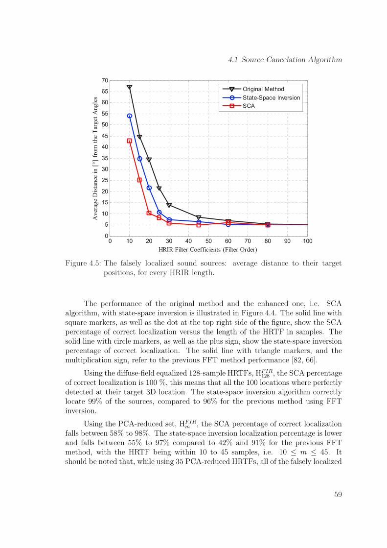
4.1 Source Cancelation Algorithm
0 10 20 30 40 50 60 70 80 90 1000
5
10
15
20
25
30
35
40
45
50
55
60
65
70
HRIR Filter Coefficients (Filter Order)
Aver
age
Dis
tance
in [
°] f
rom
th
e T
arg
et A
ng
les
Original Method
State-Space Inversion
SCA
Figure 4.5: The falsely localized sound sources: average distance to their targetpositions, for every HRIR length.
The performance of the original method and the enhanced one, i.e. SCAalgorithm, with state-space inversion is illustrated in Figure 4.4. The solid line withsquare markers, as well as the dot at the top right side of the figure, show the SCApercentage of correct localization versus the length of the HRTF in samples. Thesolid line with circle markers, as well as the plus sign, show the state-space inversionpercentage of correct localization. The solid line with triangle markers, and themultiplication sign, refer to the previous FFT method performance [82, 66].
Using the diffuse-field equalized 128-sample HRTFs, HFIR128 , the SCA percentage
of correct localization is 100 %, this means that all the 100 locations where perfectlydetected at their target 3D location. The state-space inversion algorithm correctlylocate 99% of the sources, compared to 96% for the previous method using FFTinversion.
Using the PCA-reduced set, HFIRm , the SCA percentage of correct localization
falls between 58% to 98%. The state-space inversion localization percentage is lowerand falls between 55% to 97% compared to 42% and 91% for the previous FFTmethod, with the HRTF being within 10 to 45 samples, i.e. 10 ≤ m ≤ 45. Itshould be noted that, while using 35 PCA-reduced HRTFs, all of the falsely localized
59
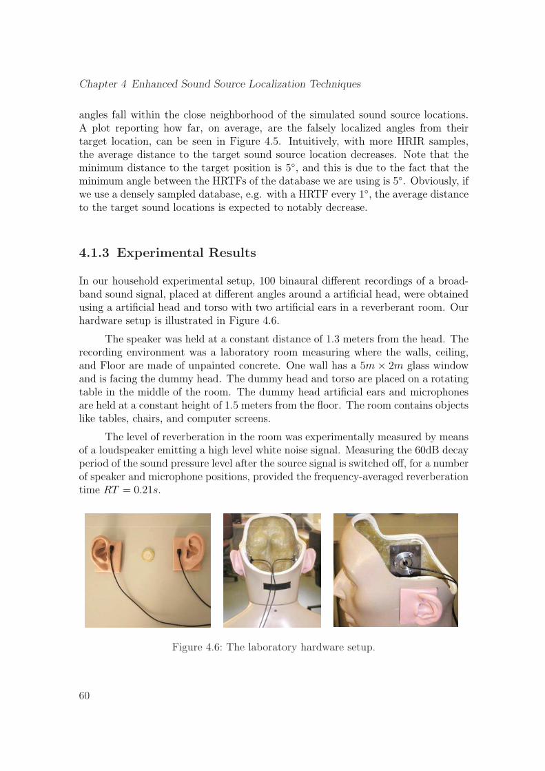
Chapter 4 Enhanced Sound Source Localization Techniques
angles fall within the close neighborhood of the simulated sound source locations.A plot reporting how far, on average, are the falsely localized angles from theirtarget location, can be seen in Figure 4.5. Intuitively, with more HRIR samples,the average distance to the target sound source location decreases. Note that theminimum distance to the target position is 5◦, and this is due to the fact that theminimum angle between the HRTFs of the database we are using is 5◦. Obviously, ifwe use a densely sampled database, e.g. with a HRTF every 1◦, the average distanceto the target sound locations is expected to notably decrease.
4.1.3 Experimental Results
In our household experimental setup, 100 binaural different recordings of a broad-band sound signal, placed at different angles around a artificial head, were obtainedusing a artificial head and torso with two artificial ears in a reverberant room. Ourhardware setup is illustrated in Figure 4.6.
The speaker was held at a constant distance of 1.3 meters from the head. Therecording environment was a laboratory room measuring where the walls, ceiling,and Floor are made of unpainted concrete. One wall has a 5m × 2m glass windowand is facing the dummy head. The dummy head and torso are placed on a rotatingtable in the middle of the room. The dummy head artificial ears and microphonesare held at a constant height of 1.5 meters from the floor. The room contains objectslike tables, chairs, and computer screens.
The level of reverberation in the room was experimentally measured by meansof a loudspeaker emitting a high level white noise signal. Measuring the 60dB decayperiod of the sound pressure level after the source signal is switched off, for a numberof speaker and microphone positions, provided the frequency-averaged reverberationtime RT = 0.21s.
Figure 4.6: The laboratory hardware setup.
60
4.1 Source Cancelation Algorithm
To keep a fair comparison with the simulation setup, each of the recordings was350 msecs long. The microphones were placed at a distance of 26 mm away from theear’s opening. The recorded sound signals, also containing external and electronicnoise, were used as inputs to the SCA, the state-space inversion algorithm, and theoriginal algorithm. A HRTF database reduced using the DFE method, HFIR
128 , wasavailable for the test.
Using the original method, 80% of the estimated angles are correctly localized,compared to 97% for the simulated case. This difference is mainly due to the externalreverberation, and internal equipment noise, and due to the differences between theartificial manikin model used in the experiment and the KEMAR model used toobtain the HRTF dataset. The 20% falsely localized sound sources are located atan average angular distance of 27.5◦ from the target angle.
Using state-space inversion, 88% of the estimated angles are found at the cor-rect location, compared with the 99% obtained from the theoretical simulation. The14% falsely localized sources are found at an average angular distance of 11.45◦ ofthe target sound source location. This is a remarkable improvement, compared tothe repartition of the falsely localized angles in the case of the original method usingthe FFT inversion.
Using the SCA, 94% of the estimated azimuth and elevation angles turned outto be exactly at the target location, compared to 100% obtained from the simulation.The other falsely localized 6% were identified at the near vicinity of the targetangles, with an average distance of 5.85◦. Again, this is a notable observation,and a considerable improvement compared to the original as well as the state-spaceinversion algorithms. As foreseen in our theoretical study, the SCA outperforms, insimulations as well as in real life, the previously proposed methods. This is due tothe fact that SCA is canceling the sound source signals, and thus the accompanyingnoise, making it, thus, less dependent on the characteristics of the sound sources,and consequently more stable and more tolerable to noise and reverberations.
4.1.4 A Case Study
Finally, a case study is performed to test the SCA algorithm in the special casewhere the two pinnae of the artificial head are taken away. The microphones areplaced at a distance of 26 mm away from the ear canal opening. The performancein this case is depicted in Figure 5.8. For comparison purposes, the SCA theoreticaland experimental performance for the artificial head deployed with two pinnae arealso shown. The line with circle markers represents the theoretical performance ofthe SCA using PCA-reduced HRTFs, and the plus sign represents the performanceusing 128-sample long DFE-reduced HRTFs. The line with circle markers, and
61
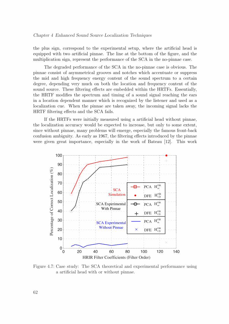
Chapter 4 Enhanced Sound Source Localization Techniques
the plus sign, correspond to the experimental setup, where the artificial head isequipped with two artificial pinnae. The line at the bottom of the figure, and themultiplication sign, represent the performance of the SCA in the no-pinnae case.
The degraded performance of the SCA in the no-pinnae case is obvious. Thepinnae consist of asymmetrical grooves and notches which accentuate or suppressthe mid and high frequency energy content of the sound spectrum to a certaindegree, depending very much on both the location and frequency content of thesound source. These filtering effects are embedded within the HRTFs. Essentially,the HRTF modifies the spectrum and timing of a sound signal reaching the earsin a location dependent manner which is recognized by the listener and used as alocalization cue. When the pinnae are taken away, the incoming signal lacks theHRTF filtering effects and the SCA fails.
If the HRTFs were initially measured using a artificial head without pinnae,the localization accuracy would be expected to increase, but only to some extent,since without pinnae, many problems will emerge, especially the famous front-backconfusion ambiguity. As early as 1967, the filtering effects introduced by the pinnaewere given great importance, especially in the work of Bateau [12]. This work
80
90
100
ion (
%)
on
(%
)
50
60
70
orr
ect
Localiz
ati
SCA
Simulation
FIR
mHPCA
DFEFIR
128H
FIR
mHPCASCA Experimental
orr
ect
Loca
liza
ti
20
30
40
erc
enta
ge o
f C
o
DFEFIR
128H+FIR
mHPCA
DFEFIR
128H
With Pinnae
SCA Experimental
Without Pinnae
erce
nta
ge
of
Co
0 20 40 60 80 100 120 1400
10
HRIR Filter Coefficients (Length in Samples)
Pe
HRIR Filter Coefficients (Filter Order)
P
Figure 4.7: Case study: The SCA theoretical and experimental performance usinga artificial head with or without pinnae.
62
4.1 Source Cancelation Algorithm
demonstrated that the duplex theory, which was prevailing at that time, and whichexplains the human hearing localization based solely on the two ITD and ILD cues,is insufficient in explaining the human spatial hearing, and in resolving ambiguoussituations such as the front-back confusion problem.
4.1.5 Performance Comparison
We evaluate the performance of our SCA algorithm in comparison to the well-knowngeneralized correlation method described in chapter 1. The method applies Fouriertransform to both microphone signals and uses weighting functions to accentuatethe signal passed to a correlator for those frequencies at which the coherence orsignal-to-noise ration(SNR) is highest. In our experimental setup, 100 binauraldifferent recordings of a broadband sound signal, placed at different angles around aartificial head, were obtained using KEMAR. Table 4.1 shows different correlation-based localization methods and their average deviation to the target sound sourcelocation.
The table shows that the localization error for the direct correlation methodwithout a weighting function is the highest. This is obvious in our reverberantenvironment. The localization error decreases when applying SCOT, PHAT, or MLand reaches a minimum with the SCA algorithm. It should be noted that the abovementioned correlation methods using only two microphones fail to detect sound inthree dimensions and suffer from the front/back confusion problem. Conversely,using two microphones, the SCA method is not restricted to azimuthal localization,it covers all the three dimensional space.
Moreover, it should be noted that the HRTF dataset is measured on the hori-zontal planes from 0◦ to 360◦ with a minimum of 5◦ increments and on the verticalplane from -40◦ to 90◦ with 10◦ increments. Therefore, the results indicate thatwe can localize the sound source with an accuracy of about 5◦. If we constructthe HRTF dataset with smaller increments, the resolution of estimation will beincreased.
Hence, we have applied the new HRTF interpolation method [66] proposed inchapter 3 to obtain a high-spatial-resolution HRTF database with one HRTF every1◦ azimuth, spanning an elevation range from -20◦ to 60◦. Using this database,we compare our method with the 3D robotic sound localization system proposed in[48].
This method uses a spherical robot head with spiral-formed ears of slightlydifferent sizes. The spiral form makes it easy to mathematically derive the IID, ITDand spectral cues used for localization. The robot was made to learn these cues bysupervised learning or by using vision. A total of 132 sound recordings were taken
63
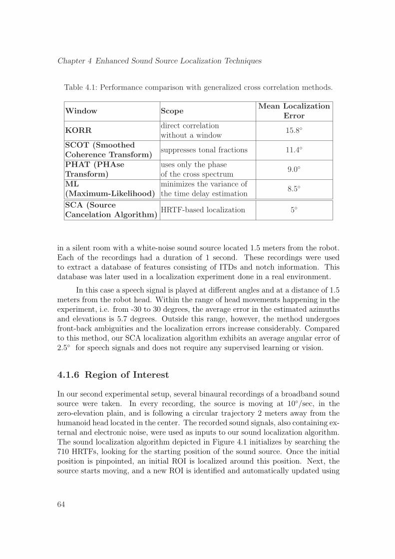
Chapter 4 Enhanced Sound Source Localization Techniques
Table 4.1: Performance comparison with generalized cross correlation methods.
Window ScopeMean Localization
Error
KORRdirect correlationwithout a window
15.8◦
SCOT (SmoothedCoherence Transform)
suppresses tonal fractions 11.4◦
PHAT (PHAseTransform)
uses only the phaseof the cross spectrum
9.0◦
ML(Maximum-Likelihood)
minimizes the variance ofthe time delay estimation
8.5◦
SCA (SourceCancelation Algorithm)
HRTF-based localization 5◦
in a silent room with a white-noise sound source located 1.5 meters from the robot.Each of the recordings had a duration of 1 second. These recordings were usedto extract a database of features consisting of ITDs and notch information. Thisdatabase was later used in a localization experiment done in a real environment.
In this case a speech signal is played at different angles and at a distance of 1.5meters from the robot head. Within the range of head movements happening in theexperiment, i.e. from -30 to 30 degrees, the average error in the estimated azimuthsand elevations is 5.7 degrees. Outside this range, however, the method undergoesfront-back ambiguities and the localization errors increase considerably. Comparedto this method, our SCA localization algorithm exhibits an average angular error of2.5◦ for speech signals and does not require any supervised learning or vision.
4.1.6 Region of Interest
In our second experimental setup, several binaural recordings of a broadband soundsource were taken. In every recording, the source is moving at 10◦/sec, in thezero-elevation plain, and is following a circular trajectory 2 meters away from thehumanoid head located in the center. The recorded sound signals, also containing ex-ternal and electronic noise, were used as inputs to our sound localization algorithm.The sound localization algorithm depicted in Figure 4.1 initializes by searching the710 HRTFs, looking for the starting position of the sound source. Once the initialposition is pinpointed, an initial ROI is localized around this position. Next, thesource starts moving, and a new ROI is identified and automatically updated using
64
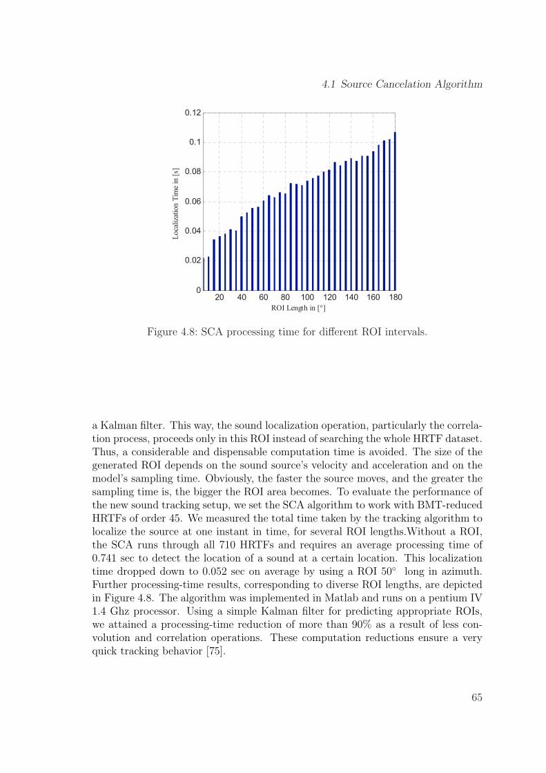
4.1 Source Cancelation Algorithm
20 40 60 80 100 120 140 160 1800
0.02
0.04
0.06
0.08
0.1
0.12
ROI Length in [°]
Loca
liza
tion
Tim
e in
[s]
Figure 4.8: SCA processing time for different ROI intervals.
a Kalman filter. This way, the sound localization operation, particularly the correla-tion process, proceeds only in this ROI instead of searching the whole HRTF dataset.Thus, a considerable and dispensable computation time is avoided. The size of thegenerated ROI depends on the sound source’s velocity and acceleration and on themodel’s sampling time. Obviously, the faster the source moves, and the greater thesampling time is, the bigger the ROI area becomes. To evaluate the performance ofthe new sound tracking setup, we set the SCA algorithm to work with BMT-reducedHRTFs of order 45. We measured the total time taken by the tracking algorithm tolocalize the source at one instant in time, for several ROI lengths.Without a ROI,the SCA runs through all 710 HRTFs and requires an average processing time of0.741 sec to detect the location of a sound at a certain location. This localizationtime dropped down to 0.052 sec on average by using a ROI 50◦ long in azimuth.Further processing-time results, corresponding to diverse ROI lengths, are depictedin Figure 4.8. The algorithm was implemented in Matlab and runs on a pentium IV1.4 Ghz processor. Using a simple Kalman filter for predicting appropriate ROIs,we attained a processing-time reduction of more than 90% as a result of less con-volution and correlation operations. These computation reductions ensure a veryquick tracking behavior [75].
65
Chapter 4 Enhanced Sound Source Localization Techniques
4.2 Cross Convolution Approach
The matched filtering approach and SCA algorithm require the availability of theinverse HRTFs. The problem arises when the inverted filter is an unstable one.This is the case with the inverted HRTF filters especially that all HRTFs include alinear-phase component, i.e. pure delay, which is vital for maintaining the correctinter-aural time difference. Furthermore, both SCA and matched filtering assumea non-reverberant environment. Hence, we propose an algorithm which is robustto environmental noise and reverberations and which do not involve calculation ofinverse HRTFs [85].
The flowchart for the convolution based HRTF algorithm is shown in Fig. 4.9.The ⊗ symbol in the figure indicates the convolution operator. The total numberof HRTF pairs are assumed to be N . The left and right received signals could bemodeled as the original signal convolved with the left and right HRTFs correspond-ing to the direction of the sound source. If we convolve the left and right receivedsignals with the right and left HRTFs corresponding to the source direction, theconvolution results should closely match. Mathematically,this can be expressed as:
SL ⊗HR = (S⊗HL)⊗HR (4.5)
SR ⊗HL = (S⊗HR)⊗HL (4.6)
where ⊗ indicates the convolution operator. The term S is the original signal comingfrom a specific direction, and SL and SR are the signals received at left and rightmicrophones respectively. The two terms HL and HR are the left and right HRTFsrespectively. Fast Fourier transform is used to reduce the computational complexityof convolution in time domain.
The convolution based algorithm operates as follows: In order to determinethe direction of arrival of sound, the left and right microphone signals, SL and SR
must be filtered by all N right and left HRTFs. The HRTFs that result in a pairof signals that closely resemble each other should correspond to the direction of thesound source. The direction of the sound source is assumed to be the HRTF pairwith the highest correlation [86].
In order to compare the performance of SCA and convolution based HRTFalgorithm in a reverberant simulated environments, a total of 100 KEMAR HRTFscorresponding to different locations in 3D space were randomly chosen and testsignals were synthesized by convolving a broadband speech signal with these HRTFs.For each test signal, we processed 512 samples of the speech signal and we performedtwo types of tests. In the first case, we considered the reflections of the source signalto be the major factor affecting the binaural signals. For this purpose, to simulate
66
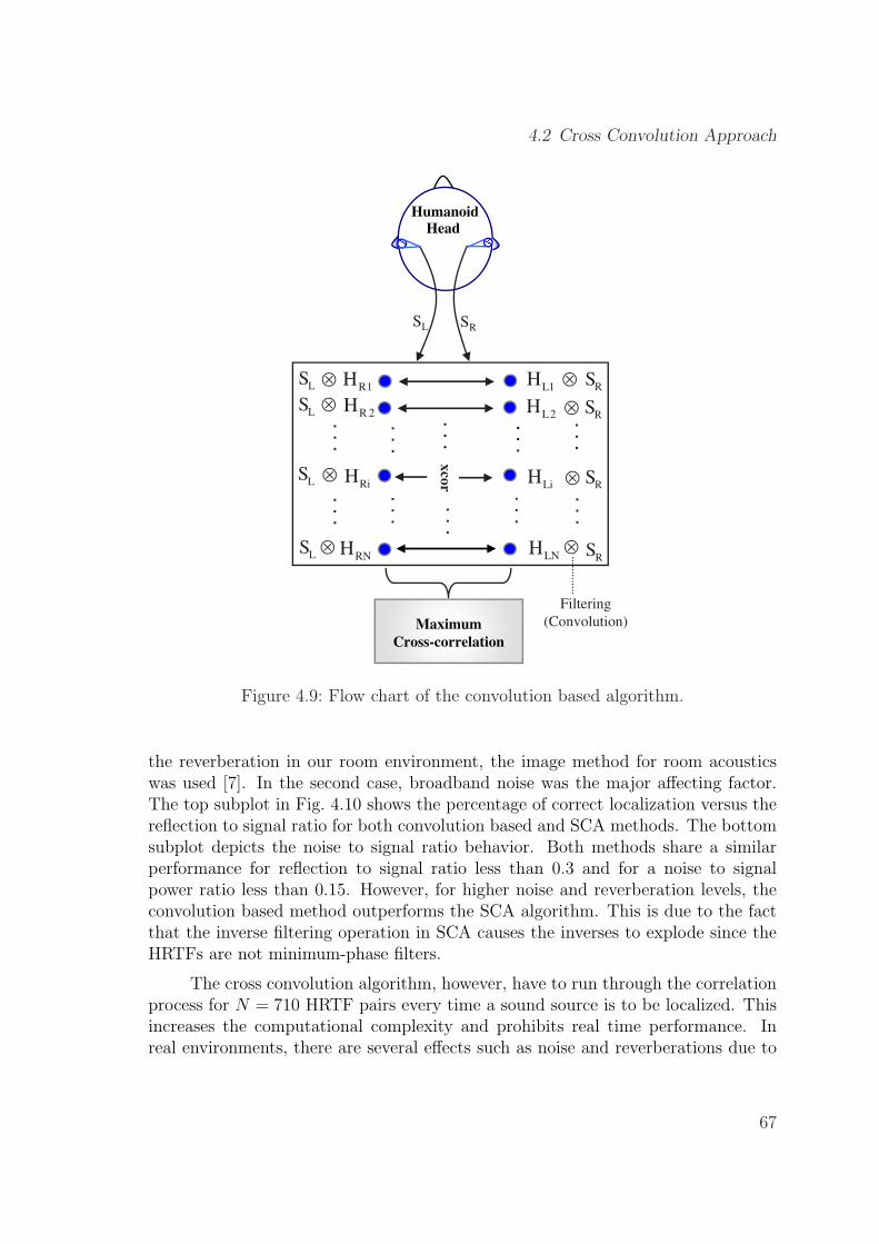
4.2 Cross Convolution Approach
Humanoid
Head
SL SR
R1H
R 2HL1
H
L2H
LS
LSR
S
RS
. . .
. . .
. . .
. . .
. . .
RNH LNH
LiHRiHL
S
LS
RS
RS
xco
r
il i
. . .
.. . .
. . .
.
. . .
. . .
Filtering
(Convolution)Maximum
Cross-correlation
Figure 4.9: Flow chart of the convolution based algorithm.
the reverberation in our room environment, the image method for room acousticswas used [7]. In the second case, broadband noise was the major affecting factor.The top subplot in Fig. 4.10 shows the percentage of correct localization versus thereflection to signal ratio for both convolution based and SCA methods. The bottomsubplot depicts the noise to signal ratio behavior. Both methods share a similarperformance for reflection to signal ratio less than 0.3 and for a noise to signalpower ratio less than 0.15. However, for higher noise and reverberation levels, theconvolution based method outperforms the SCA algorithm. This is due to the factthat the inverse filtering operation in SCA causes the inverses to explode since theHRTFs are not minimum-phase filters.
The cross convolution algorithm, however, have to run through the correlationprocess for N = 710 HRTF pairs every time a sound source is to be localized. Thisincreases the computational complexity and prohibits real time performance. Inreal environments, there are several effects such as noise and reverberations due to
67
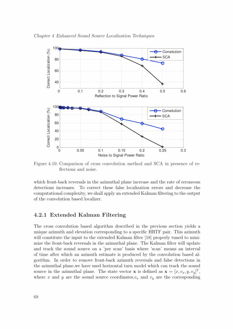
Chapter 4 Enhanced Sound Source Localization Techniques
0 0.1 0.2 0.3 0.4 0.5 0.6
40
60
80
100
Reflection to Signal Power Ratio
Corr
ect
Localiz
ation (
%)
0 0.05 0.1 0.15 0.2 0.25 0.30
20
40
60
80
100
Noise to Signal Power Ratio
Corr
ect
Localiz
ation (
%)
Convolution
SCA
Convolution
SCA
Figure 4.10: Comparison of cross convolution method and SCA in presence of re-flections and noise.
which front-back reversals in the azimuthal plane increase and the rate of erroneousdetections increases. To correct these false localization errors and decrease thecomputational complexity, we shall apply an extended Kalman filtering to the outputof the convolution based localizer.
4.2.1 Extended Kalman Filtering
The cross convolution based algorithm described in the previous section yields aunique azimuth and elevation corresponding to a specific HRTF pair. This azimuthwill constitute the input to the extended Kalman filter [18] properly tuned to mini-mize the front-back reversals in the azimuthal plane. The Kalman filter will updateand track the sound source on a ’per scan’ basis where ’scan’ means an intervalof time after which an azimuth estimate is produced by the convolution based al-gorithm. In order to remove front-back azimuth reversals and false detections inthe azimuthal plane,we have used horizontal turn model which can track the soundsource in the azimuthal plane. The state vector x is defined as x = [x, vx, y, vy]
T ,where x and y are the sound source coordinates,vx and vy are the corresponding
68
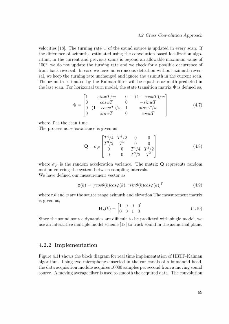
4.2 Cross Convolution Approach
velocities [18]. The turning rate w of the sound source is updated in every scan. Ifthe difference of azimuths, estimated using the convolution based localization algo-rithm, in the current and previous scans is beyond an allowable maximum value of100◦, we do not update the turning rate and we check for a possible occurrence offront-back reversal. In case we have an erroneous detection without azimuth rever-sal, we keep the turning rate unchanged and ignore the azimuth in the current scan.The azimuth estimated by the Kalman filter will be equal to azimuth predicted inthe last scan. For horizontal turn model, the state transition matrix Φ is defined as,
Φ =
1 sinwT/w 0 −(1− coswT )/w0 coswT 0 −sinwT0 (1− coswT )/w 1 sinwT/w0 sinwT 0 coswT
(4.7)
where T is the scan time.The process noise covariance is given as
Q = σq2
T 4/4 T 3/2 0 0T 3/2 T 2 0 0
0 0 T 4/4 T 3/20 0 T 3/2 T 2
(4.8)
where σq2 is the random acceleration variance. The matrix Q represents randommotion entering the system between sampling intervals.We have defined our measurement vector as
z(k) = [rcosθ(k)cosϕ(k), rsinθ(k)cosϕ(k)]T (4.9)
where r,θ and ϕ are the source range,azimuth and elevation.The measurement matrixis given as,
Hx(k) =
[1 0 0 00 0 1 0
](4.10)
Since the sound source dynamics are difficult to be predicted with single model, weuse an interactive multiple model scheme [18] to track sound in the azimuthal plane.
4.2.2 Implementation
Figure 4.11 shows the block diagram for real time implementation of HRTF-Kalmanalgorithm. Using two microphones inserted in the ear canals of a humanoid head,the data acquisition module acquires 10000 samples per second from a moving soundsource. A moving average filter is used to smooth the acquired data. The convolution
69
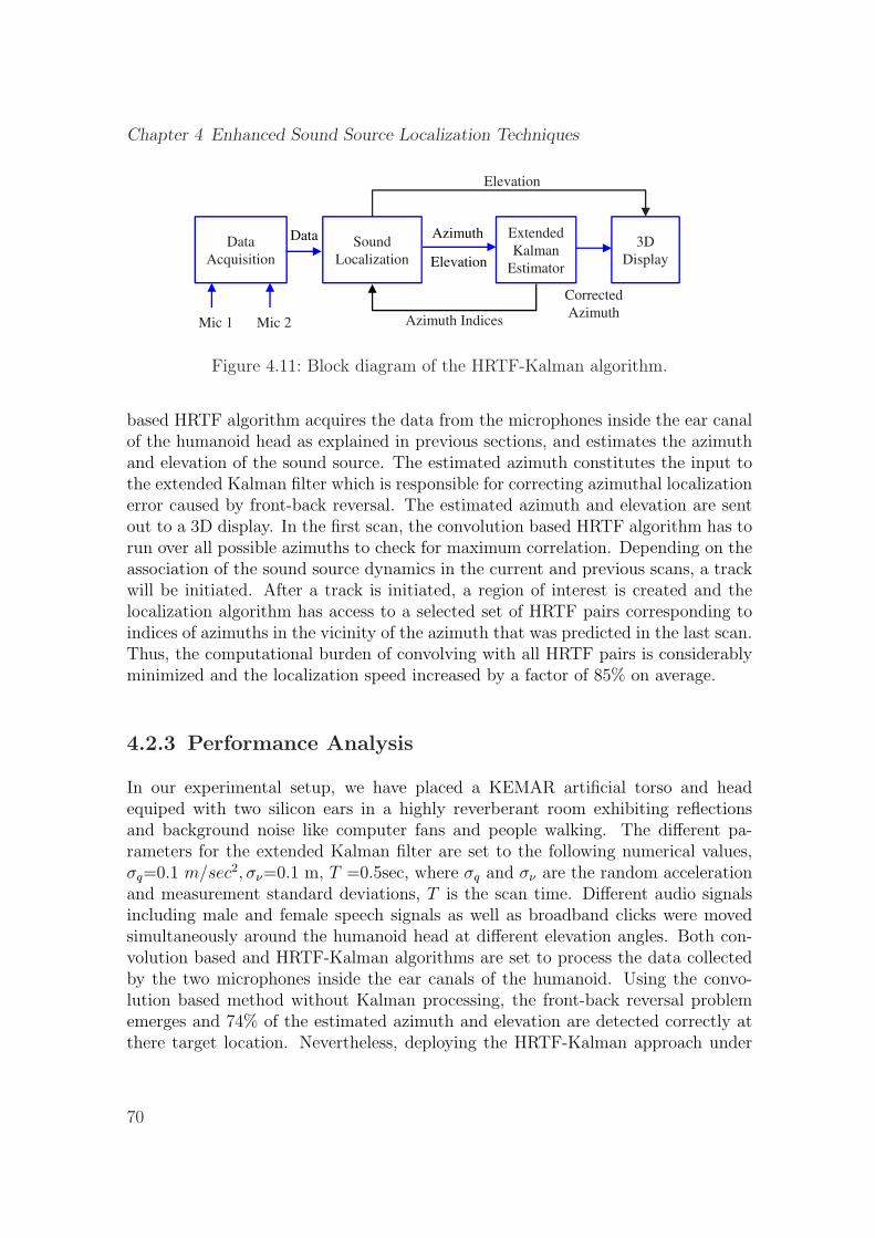
Chapter 4 Enhanced Sound Source Localization Techniques
Elevation
Data
Acquisition
Mic 1 Mic 2
Data Sound
Localization
Extended
Kalman
Estimator
Azimuth
Elevation
Azimuth Indices
3D
Display
Corrected
AzimuthMic 1 Mic 2 Azimuth Indices
Figure 4.11: Block diagram of the HRTF-Kalman algorithm.
based HRTF algorithm acquires the data from the microphones inside the ear canalof the humanoid head as explained in previous sections, and estimates the azimuthand elevation of the sound source. The estimated azimuth constitutes the input tothe extended Kalman filter which is responsible for correcting azimuthal localizationerror caused by front-back reversal. The estimated azimuth and elevation are sentout to a 3D display. In the first scan, the convolution based HRTF algorithm has torun over all possible azimuths to check for maximum correlation. Depending on theassociation of the sound source dynamics in the current and previous scans, a trackwill be initiated. After a track is initiated, a region of interest is created and thelocalization algorithm has access to a selected set of HRTF pairs corresponding toindices of azimuths in the vicinity of the azimuth that was predicted in the last scan.Thus, the computational burden of convolving with all HRTF pairs is considerablyminimized and the localization speed increased by a factor of 85% on average.
4.2.3 Performance Analysis
In our experimental setup, we have placed a KEMAR artificial torso and headequiped with two silicon ears in a highly reverberant room exhibiting reflectionsand background noise like computer fans and people walking. The different pa-rameters for the extended Kalman filter are set to the following numerical values,σq=0.1 m/sec2, σν=0.1 m, T =0.5sec, where σq and σν are the random accelerationand measurement standard deviations, T is the scan time. Different audio signalsincluding male and female speech signals as well as broadband clicks were movedsimultaneously around the humanoid head at different elevation angles. Both con-volution based and HRTF-Kalman algorithms are set to process the data collectedby the two microphones inside the ear canals of the humanoid. Using the convo-lution based method without Kalman processing, the front-back reversal problememerges and 74% of the estimated azimuth and elevation are detected correctly atthere target location. Nevertheless, deploying the HRTF-Kalman approach under
70
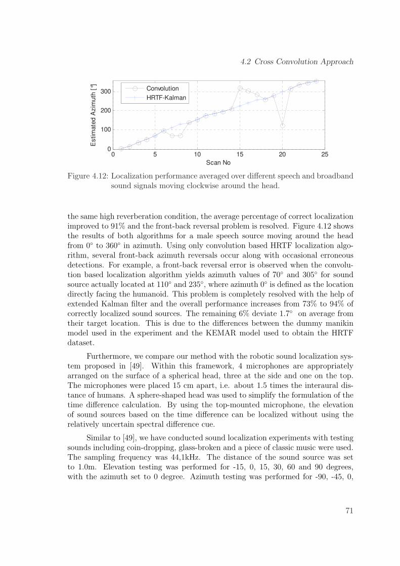
4.2 Cross Convolution Approach
0 5 10 15 20 250
100
200
300
Scan No
Estim
ate
d A
zim
uth
[°] Convolution
HRTF-Kalman
Figure 4.12: Localization performance averaged over different speech and broadbandsound signals moving clockwise around the head.
the same high reverberation condition, the average percentage of correct localizationimproved to 91% and the front-back reversal problem is resolved. Figure 4.12 showsthe results of both algorithms for a male speech source moving around the headfrom 0◦ to 360◦ in azimuth. Using only convolution based HRTF localization algo-rithm, several front-back azimuth reversals occur along with occasional erroneousdetections. For example, a front-back reversal error is observed when the convolu-tion based localization algorithm yields azimuth values of 70◦ and 305◦ for soundsource actually located at 110◦ and 235◦, where azimuth 0◦ is defined as the locationdirectly facing the humanoid. This problem is completely resolved with the help ofextended Kalman filter and the overall performance increases from 73% to 94% ofcorrectly localized sound sources. The remaining 6% deviate 1.7◦ on average fromtheir target location. This is due to the differences between the dummy manikinmodel used in the experiment and the KEMAR model used to obtain the HRTFdataset.
Furthermore, we compare our method with the robotic sound localization sys-tem proposed in [49]. Within this framework, 4 microphones are appropriatelyarranged on the surface of a spherical head, three at the side and one on the top.The microphones were placed 15 cm apart, i.e. about 1.5 times the interaural dis-tance of humans. A sphere-shaped head was used to simplify the formulation of thetime difference calculation. By using the top-mounted microphone, the elevationof sound sources based on the time difference can be localized without using therelatively uncertain spectral difference cue.
Similar to [49], we have conducted sound localization experiments with testingsounds including coin-dropping, glass-broken and a piece of classic music were used.The sampling frequency was 44,1kHz. The distance of the sound source was setto 1.0m. Elevation testing was performed for -15, 0, 15, 30, 60 and 90 degrees,with the azimuth set to 0 degree. Azimuth testing was performed for -90, -45, 0,
71
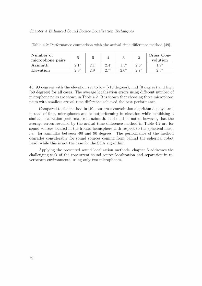
Chapter 4 Enhanced Sound Source Localization Techniques
Table 4.2: Performance comparison with the arrival time difference method [49].
Number ofmicrophone pairs
6 5 4 3 2Cross Con-volution
Azimuth 2.1◦ 2.1◦ 2.4◦ 1.5◦ 2.6◦ 1.9◦
Elevation 2.9◦ 2.9◦ 2.7◦ 2.6◦ 2.7◦ 2.3◦
45, 90 degrees with the elevation set to low (-15 degrees), mid (0 degree) and high(60 degrees) for all cases. The average localization errors using different number ofmicrophone pairs are shown in Table 4.2. It is shown that choosing three microphonepairs with smallest arrival time difference achieved the best performance.
Compared to the method in [49], our cross convolution algorithm deploys two,instead of four, microphones and is outperforming in elevation while exhibiting asimilar localization performance in azimuth. It should be noted, however, that theaverage errors revealed by the arrival time difference method in Table 4.2 are forsound sources located in the frontal hemisphere with respect to the spherical head,i.e. for azimuths between -90 and 90 degrees. The performance of the methoddegrades considerably for sound sources coming from behind the spherical robothead, while this is not the case for the SCA algorithm.
Applying the presented sound localization methods, chapter 5 addresses thechallenging task of the concurrent sound source localization and separation in re-verberant environments, using only two microphones.
72
Chapter 5
Concurrent Sound SourceLocalization and Separation
We combine binaural sound-source localization and separation techniques for aneffective deployment in telerobotics. Relying on the concept of binaural hearing,where the human auditory 3D percepts are predominantly formed on the basis ofthe sound-pressure signals at the two eardrums, our robotic 3D localization systemuses only two microphones placed inside the ear canals of a robot head equippedwith artificial ears and mounted on a torso. The challenging task of using only twomicrophones for 3D localization is made more intriguing by allowing more sourcesto coexist and randomly move within the robot’s environment. The proposed lo-calization algorithm exploits all the binaural cues encapsulated within the HRTFs.Taking advantage of the sparse representations of the ear input signals, the 3D posi-tions of three concurrent sound sources are extracted. The location of the sources isextracted after identifying which HRTFs they have been filtered with using a well-known self-splitting competitive learning clustering algorithm. Once the locationsof the sources are identified, they are separated using a generic HRTF dataset. Sim-ulation results demonstrated highly accurate 3D localization of the two concurrentsound sources, and a very high Signal-to-Interference Ratio (SIR) for the separatedsound signals.
73
Chapter 5 Concurrent Sound Source Localization and Separation
5.1 Motivation
One of the most challenging characteristics of human spatial hearing, is the cocktailparty phenomenon, where attention pertains to the ability of a listener to focuson one channel while ignoring other irrelevant channels. In robotics, on the otherhand, efficient and accurate binaural 3D localization of several sound sources isquite a challenging task. In recent years, a good number of algorithms have beenproposed to tackle this problem. Basically, most of the detection methods used relyon microphone arrays, where the number of microphones is more or equal to thenumber of sound sources to be localized concurrently in 3D [52]. Among them, someapproaches deal with simultaneous localization and separation of sound sources [123].However, a more intriguing, and naturally more demanding scenario, is localizationof sound sources that outnumber the available number of microphones. Very fewapproaches were able to estimate the position of the sound sources, while onlyproviding azimuth angles [94]. Humans and most mammals, however, are capableof detecting multiple concurrent sound sources with two ears by assessing monauralcues and binaural cues like ILD and ITD, in several frequency bands.
Recent investigations on the auditory space map of the barn owl, a predatorwith an astonishing ability to localize sound, revealed that the ILD/ITD cues clusteraround two positions in the auditory map when two uncorrelated sound sources aresimultaneously present. These clusters stem from time-frequency instances whenone source predominates the other, i.e. has a stronger intensity [57]. Using this factwe present two new approaches for separating and localizing two or more concurrentsound sources in 3D using only two small microphones placed inside the KEMARartificial ears.
Section 5.2 describes an algorithm for two sound sources that iteratively adaptsthe coefficients of a MIMO system and provides the two statistically independentsource signals. This well-known separation method which exploits the non-stationarityof the sources is used to retrieve two speakers from two convolutive mixtures. Byusing a simple relation between blind source separation and system identification,the HRTFs that filtered the sound sources can be determined under the conditionof an anechoic environment.
The second algorithm, presented in section 5.3, applies Short-Time FourierTransform (STFT) to the ear signals and makes use of the sparseness of the sourcesin time-frequency domain. If the concurrent signals are sparse, which is naturallythe case with speech signals, there must exist many instances when one sourcepredominates the other. In such cases, the ear signals cluster around the actualHRTF, corresponding to the correct source location, in the single frequency bands.The positions of the sources are finally determined by a database lookup. With the
74
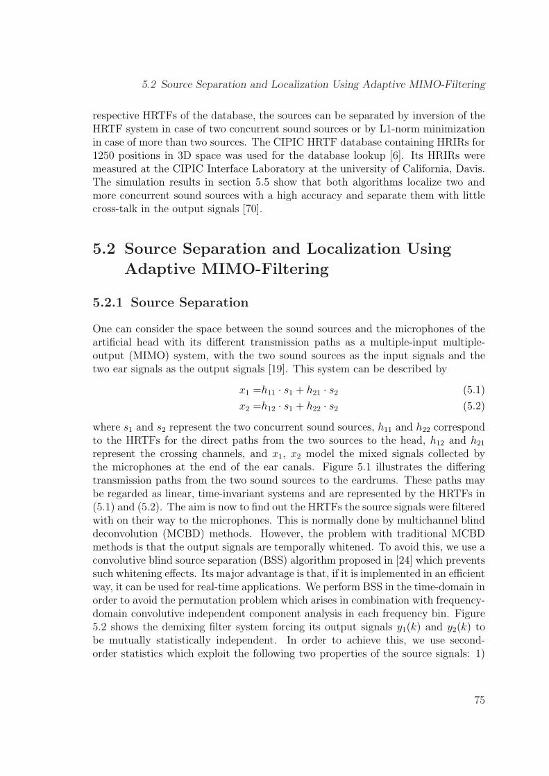
5.2 Source Separation and Localization Using Adaptive MIMO-Filtering
respective HRTFs of the database, the sources can be separated by inversion of theHRTF system in case of two concurrent sound sources or by L1-norm minimizationin case of more than two sources. The CIPIC HRTF database containing HRIRs for1250 positions in 3D space was used for the database lookup [6]. Its HRIRs weremeasured at the CIPIC Interface Laboratory at the university of California, Davis.The simulation results in section 5.5 show that both algorithms localize two andmore concurrent sound sources with a high accuracy and separate them with littlecross-talk in the output signals [70].
5.2 Source Separation and Localization Using
Adaptive MIMO-Filtering
5.2.1 Source Separation
One can consider the space between the sound sources and the microphones of theartificial head with its different transmission paths as a multiple-input multiple-output (MIMO) system, with the two sound sources as the input signals and thetwo ear signals as the output signals [19]. This system can be described by
x1 =h11 · s1 + h21 · s2 (5.1)
x2 =h12 · s1 + h22 · s2 (5.2)
where s1 and s2 represent the two concurrent sound sources, h11 and h22 correspondto the HRTFs for the direct paths from the two sources to the head, h12 and h21
represent the crossing channels, and x1, x2 model the mixed signals collected bythe microphones at the end of the ear canals. Figure 5.1 illustrates the differingtransmission paths from the two sound sources to the eardrums. These paths maybe regarded as linear, time-invariant systems and are represented by the HRTFs in(5.1) and (5.2). The aim is now to find out the HRTFs the source signals were filteredwith on their way to the microphones. This is normally done by multichannel blinddeconvolution (MCBD) methods. However, the problem with traditional MCBDmethods is that the output signals are temporally whitened. To avoid this, we use aconvolutive blind source separation (BSS) algorithm proposed in [24] which preventssuch whitening effects. Its major advantage is that, if it is implemented in an efficientway, it can be used for real-time applications. We perform BSS in the time-domain inorder to avoid the permutation problem which arises in combination with frequency-domain convolutive independent component analysis in each frequency bin. Figure5.2 shows the demixing filter system forcing its output signals y1(k) and y2(k) tobe mutually statistically independent. In order to achieve this, we use second-order statistics which exploit the following two properties of the source signals: 1)
75
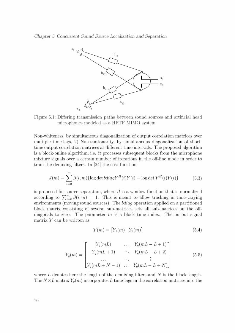
Chapter 5 Concurrent Sound Source Localization and Separation
s1
s2
x1
x2h21
h12
h22
h11
Figure 5.1: Differing transmission paths between sound sources and artificial headmicrophones modeled as a HRTF MIMO system.
Non-whiteness, by simultaneous diagonalization of output correlation matrices overmultiple time-lags, 2) Non-stationarity, by simultaneous diagonalization of short-time output correlation matrices at different time intervals. The proposed algorithmis a block-online algorithm, i.e. it processes subsequent blocks from the microphonemixture signals over a certain number of iterations in the off-line mode in order totrain the demixing filters. In [24] the cost function
J(m) =m∑
i=0
β(i,m){log det bdiagY H(i)Y (i)− log det Y H(i)Y (i)} (5.3)
is proposed for source separation, where β is a window function that is normalizedaccording to
∑mi=0 β(i,m) = 1. This is meant to allow tracking in time-varying
environments (moving sound sources). The bdiag operation applied on a partitionedblock matrix consisting of several sub-matrices sets all sub-matrices on the off-diagonals to zero. The parameter m is a block time index. The output signalmatrix Y can be written as
Y (m) =[Y1(m) Y2(m)
](5.4)
Yq(m) =
Yq(mL) . . . Yq(mL− L + 1)
Yq(mL + 1). . . Yq(mL− L + 2)
. . .. . .
...Yq(mL + N − 1) . . . Yq(mL− L + N)
(5.5)
where L denotes here the length of the demixing filters and N is the block length.The N×L matrix Yq(m) incorporates L time-lags in the correlation matrices into the
76
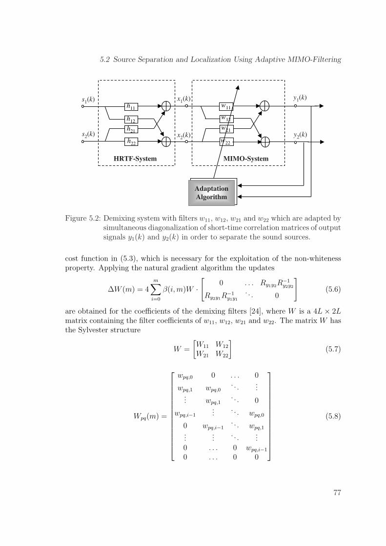
5.2 Source Separation and Localization Using Adaptive MIMO-Filtering
s1(k)
s2(k)
HRTF-System MIMO-System
x2(k)
x1(k)
y2(k)
y1(k)w11
w12
w21
w22
h11
h12
h21
h22
Adaptation
Algorithm
Figure 5.2: Demixing system with filters w11, w12, w21 and w22 which are adapted bysimultaneous diagonalization of short-time correlation matrices of outputsignals y1(k) and y2(k) in order to separate the sound sources.
cost function in (5.3), which is necessary for the exploitation of the non-whitenessproperty. Applying the natural gradient algorithm the updates
∆W (m) = 4m∑
i=0
β(i,m)W ·[
0 . . . Ry1y2R−1y2y2
Ry2y1R−1y1y1
. . . 0
](5.6)
are obtained for the coefficients of the demixing filters [24], where W is a 4L × 2Lmatrix containing the filter coefficients of w11, w12, w21 and w22. The matrix W hasthe Sylvester structure
W =
[W11 W12
W21 W22
](5.7)
Wpq(m) =
wpq,0 0 . . . 0
wpq,1 wpq,0. . .
...... wpq,1
. . . 0
wpq,i−1...
. . . wpq,0
0 wpq,i−1. . . wpq,1
......
. . ....
0 . . . 0 wpq,i−1
0 . . . 0 0
(5.8)
77
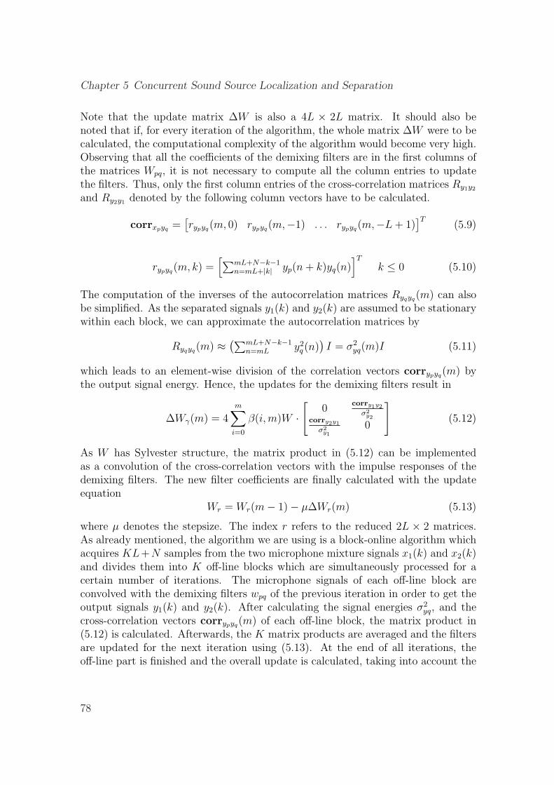
Chapter 5 Concurrent Sound Source Localization and Separation
Note that the update matrix ∆W is also a 4L × 2L matrix. It should also benoted that if, for every iteration of the algorithm, the whole matrix ∆W were to becalculated, the computational complexity of the algorithm would become very high.Observing that all the coefficients of the demixing filters are in the first columns ofthe matrices Wpq, it is not necessary to compute all the column entries to updatethe filters. Thus, only the first column entries of the cross-correlation matrices Ry1y2
and Ry2y1 denoted by the following column vectors have to be calculated.
corrxpyq =[rypyq(m, 0) rypyq(m,−1) . . . rypyq(m,−L + 1)
]T(5.9)
rypyq(m, k) =[∑mL+N−k−1
n=mL+|k| yp(n + k)yq(n)]T
k ≤ 0 (5.10)
The computation of the inverses of the autocorrelation matrices Ryqyq(m) can alsobe simplified. As the separated signals y1(k) and y2(k) are assumed to be stationarywithin each block, we can approximate the autocorrelation matrices by
Ryqyq(m) ≈ (∑mL+N−k−1n=mL y2
q (n))I = σ2
yq(m)I (5.11)
which leads to an element-wise division of the correlation vectors corrypyq(m) bythe output signal energy. Hence, the updates for the demixing filters result in
∆Wγ(m) = 4m∑
i=0
β(i,m)W ·[
0corry1y2
σ2y2corry2y1
σ2y1
0
](5.12)
As W has Sylvester structure, the matrix product in (5.12) can be implementedas a convolution of the cross-correlation vectors with the impulse responses of thedemixing filters. The new filter coefficients are finally calculated with the updateequation
Wr = Wr(m− 1)− µ∆Wr(m) (5.13)
where µ denotes the stepsize. The index r refers to the reduced 2L × 2 matrices.As already mentioned, the algorithm we are using is a block-online algorithm whichacquires KL+N samples from the two microphone mixture signals x1(k) and x2(k)and divides them into K off-line blocks which are simultaneously processed for acertain number of iterations. The microphone signals of each off-line block areconvolved with the demixing filters wpq of the previous iteration in order to get theoutput signals y1(k) and y2(k). After calculating the signal energies σ2
yq, and thecross-correlation vectors corrypyq(m) of each off-line block, the matrix product in(5.12) is calculated. Afterwards, the K matrix products are averaged and the filtersare updated for the next iteration using (5.13). At the end of all iterations, theoff-line part is finished and the overall update is calculated, taking into account the
78
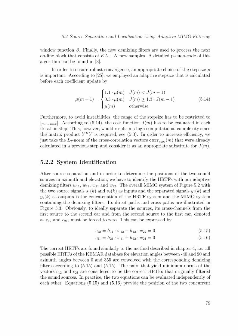
5.2 Source Separation and Localization Using Adaptive MIMO-Filtering
window function β. Finally, the new demixing filters are used to process the nexton-line block that consists of KL + N new samples. A detailed pseudo-code of thisalgorithm can be found in [3].
In order to ensure robust convergence, an appropriate choice of the stepsize µis important. According to [25], we employed an adaptive stepsize that is calculatedbefore each coefficient update by
µ(m + 1) =
1.1 · µ(m) J(m) < J(m− 1)
0.5 · µ(m) J(m) ≥ 1.3 · J(m− 1)
µ(m) otherwise
(5.14)
Furthermore, to avoid instabilities, the range of the stepsize has to be restricted to[min, max]. According to (5.14), the cost function J(m) has to be evaluated in eachiteration step. This, however, would result in a high computational complexity sincethe matrix product Y HY is required, see (5.3). In order to increase efficiency, wejust take the L2-norm of the cross-correlation vectors corrypyq(m) that were alreadycalculated in a previous step and consider it as an appropriate substitute for J(m).
5.2.2 System Identification
After source separation and in order to determine the positions of the two soundsources in azimuth and elevation, we have to identify the HRTFs with our adaptivedemixing filters w11, w12, w21 and w22. The overall MIMO system of Figure 5.2 withthe two source signals s1(k) and s2(k) as inputs and the separated signals y1(k) andy2(k) as outputs is the concatenation of the HRTF system and the MIMO systemcontaining the demixing filters. Its direct paths and cross paths are illustrated inFigure 5.3. Obviously, to ideally separate the sources, its cross-channels from thefirst source to the second ear and from the second source to the first ear, denotedas c12 and c21, must be forced to zero. This can be expressed by
c12 = h11 · w12 + h12 · w22 = 0 (5.15)
c21 = h21 · w11 + h22 · w21 = 0 (5.16)
The correct HRTFs are found similarly to the method described in chapter 4, i.e. allpossible HRTFs of the KEMAR database for elevation angles between -40 and 90 andazimuth angles between 0 and 355 are convolved with the corresponding demixingfilters according to (5.15) and (5.15). The pairs that yield minimum norms of thevectors c12 and c21 are considered to be the correct HRTFs that originally filteredthe sound sources. In practice, the two equations can be evaluated independently ofeach other. Equations (5.15) and (5.16) provide the position of the two concurrent
79
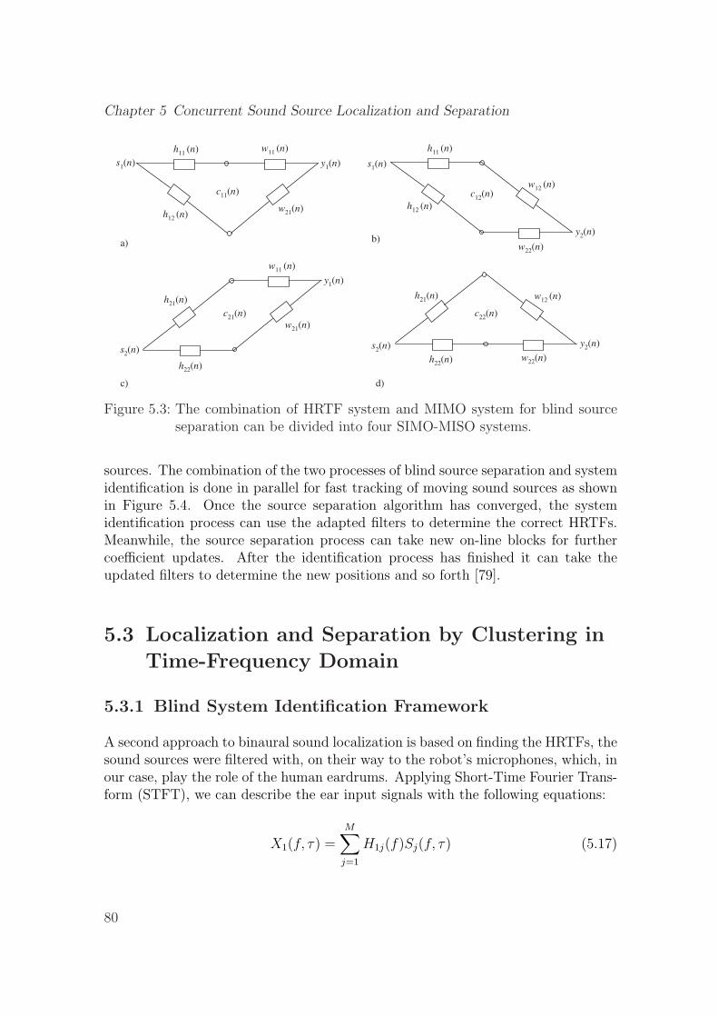
Chapter 5 Concurrent Sound Source Localization and Separation
h11 (n)
h12 (n)
s1(n)
w11 (n)
w21(n)
y1(n)
h22(n)
w11 (n)
h21(n)
s2(n)
w21(n)
y1(n)
w22(n)
s1(n)
h11 (n)
h12 (n)
w12 (n)
y2(n)
s2(n)
h21(n)
h22(n)
w12 (n)
w22(n)
y2(n)
c11(n) c12(n)
c21(n) c22(n)
a) b)
c) d)
Figure 5.3: The combination of HRTF system and MIMO system for blind sourceseparation can be divided into four SIMO-MISO systems.
sources. The combination of the two processes of blind source separation and systemidentification is done in parallel for fast tracking of moving sound sources as shownin Figure 5.4. Once the source separation algorithm has converged, the systemidentification process can use the adapted filters to determine the correct HRTFs.Meanwhile, the source separation process can take new on-line blocks for furthercoefficient updates. After the identification process has finished it can take theupdated filters to determine the new positions and so forth [79].
5.3 Localization and Separation by Clustering in
Time-Frequency Domain
5.3.1 Blind System Identification Framework
A second approach to binaural sound localization is based on finding the HRTFs, thesound sources were filtered with, on their way to the robot’s microphones, which, inour case, play the role of the human eardrums. Applying Short-Time Fourier Trans-form (STFT), we can describe the ear input signals with the following equations:
X1(f, τ) =M∑
j=1
H1j(f)Sj(f, τ) (5.17)
80
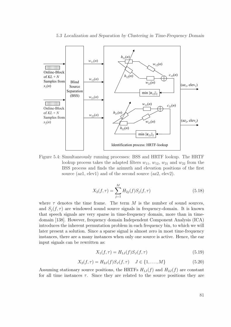
5.3 Localization and Separation by Clustering in Time-Frequency Domain
h11(n)
min ||c12||2
min ||c21||2
Identification process: HRTF-lookup
(az1, elev1)Blind
Source
Separation
(BSS)
h12(n)
w12(n)
w22(n)
c12(n)
h21(n)
h22(n)
w11(n)
w21(n)
c21(n)
(az2, elev2)
Online-Block
of KL + N
Samples from
x1(n)
Online-Block
of KL + N
Samples from
x2(n)
w11(n)
w12(n)
w21(n)
w22(n)
Figure 5.4: Simultaneously running processes: BSS and HRTF lookup. The HRTFlookup process takes the adapted filters w11, w12, w21 and w22 from theBSS process and finds the azimuth and elevation positions of the firstsource (az1, elev1) and of the second source (az2, elev2).
X2(f, τ) =M∑
j=1
H2j(f)Sj(f, τ) (5.18)
where τ denotes the time frame. The term M is the number of sound sources,and Sj(f, τ) are windowed sound source signals in frequency-domain. It is knownthat speech signals are very sparse in time-frequency domain, more than in time-domain [138]. However, frequency domain Independent Component Analysis (ICA)introduces the inherent permutation problem in each frequency bin, to which we willlater present a solution. Since a sparse signal is almost zero in most time-frequencyinstances, there are a many instances when only one source is active. Hence, the earinput signals can be rewritten as:
X1(f, τ) = H1J(f)SJ(f, τ) (5.19)
X2(f, τ) = H2J(f)SJ(f, τ) J ∈ {1, . . . , M} (5.20)
Assuming stationary source positions, the HRTFs H1J(f) and H2J(f) are constantfor all time instances τ . Since they are related to the source positions they are
81
Chapter 5 Concurrent Sound Source Localization and Separation
0 0.5 1-1
-0.5
0
0.5
1
real(X1)
imag(X2)
-1 0 1-1
-0.5
0
0.5
1
real(X2)
imag(X2)
P1,1
P2,1
P1,2
P2,2
Figure 5.5: Samples from the two ear microphones after STFT. The two subplotsdepict the real part of X1 and the real part of X2 versus the imaginarypart of X2, respectively. The data was gathered from 400 time-framesat a frequency of 538 Hz and normalized according to (5.21) and (5.22).The clusters show that there are two speakers present. Furthermore,the prototypes determined by Self-Splitting Competitive Learning aredepicted in the cluster centers.
different for each source. This means ideally, that the time-frequency samples of theear input signals, X1(f, τ) and X2(f, τ) , that originate from the J-th source, clusterat each frequency f around the corresponding complex HRTFs values. Additionally,the Fourier transforms of the ear input signals are phase and amplitude normalized:
X1(f, τ) ← X1(f, τ)√X2
1 (f, τ) + X22 (f, τ)
exp−ϕx1 (5.21)
X2(f, τ) ← X2(f, τ)√X2
1 (f, τ) + X22 (f, τ)
exp−ϕx1 (5.22)
where ϕx1 is the phase corresponding to the input signal of the left ear microphone,which is chosen as a reference sensor. Figure 5.5 illustrates the clustering of thenormalized data in the feature space.
82
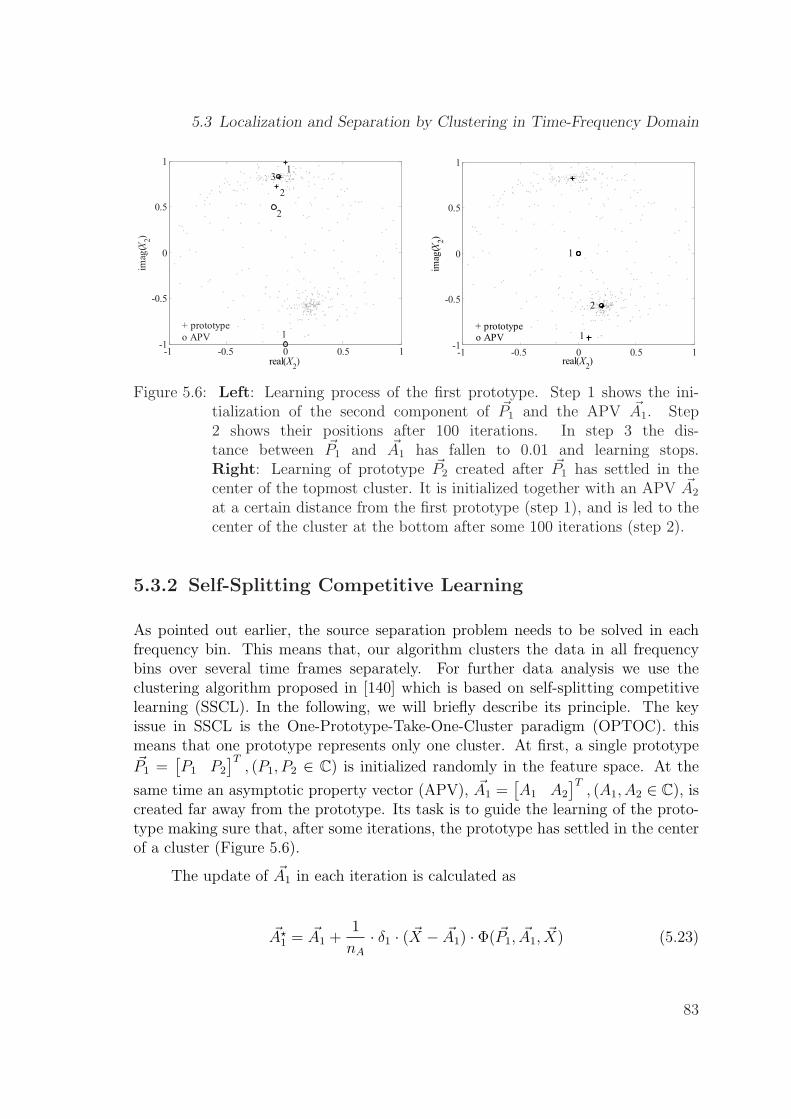
5.3 Localization and Separation by Clustering in Time-Frequency Domain
-1 -0.5 0 0.5 1-1
-0.5
0
0.5
1
real(X2)
imag
(X2)
1
1
2
3
2
+ prototype
o APV
-1 -0.5 0 0.5 1-1
-0.5
0
0.5
1
real(X2)
imag
(X2)
1
1
2
+ prototype o APV
Figure 5.6: Left: Learning process of the first prototype. Step 1 shows the ini-tialization of the second component of ~P1 and the APV ~A1. Step2 shows their positions after 100 iterations. In step 3 the dis-tance between ~P1 and ~A1 has fallen to 0.01 and learning stops.Right: Learning of prototype ~P2 created after ~P1 has settled in thecenter of the topmost cluster. It is initialized together with an APV ~A2
at a certain distance from the first prototype (step 1), and is led to thecenter of the cluster at the bottom after some 100 iterations (step 2).
5.3.2 Self-Splitting Competitive Learning
As pointed out earlier, the source separation problem needs to be solved in eachfrequency bin. This means that, our algorithm clusters the data in all frequencybins over several time frames separately. For further data analysis we use theclustering algorithm proposed in [140] which is based on self-splitting competitivelearning (SSCL). In the following, we will briefly describe its principle. The keyissue in SSCL is the One-Prototype-Take-One-Cluster paradigm (OPTOC). thismeans that one prototype represents only one cluster. At first, a single prototype~P1 =
[P1 P2
]T, (P1, P2 ∈ C) is initialized randomly in the feature space. At the
same time an asymptotic property vector (APV), ~A1 =[A1 A2
]T, (A1, A2 ∈ C), is
created far away from the prototype. Its task is to guide the learning of the proto-type making sure that, after some iterations, the prototype has settled in the centerof a cluster (Figure 5.6).
The update of ~A1 in each iteration is calculated as
~A?1 = ~A1 +
1
nA
· δ1 · ( ~X − ~A1) · Φ( ~P1, ~A1, ~X) (5.23)
83
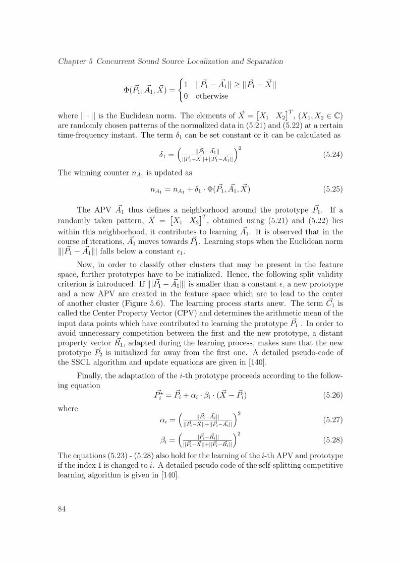
Chapter 5 Concurrent Sound Source Localization and Separation
Φ( ~P1, ~A1, ~X) =
{1 || ~P1 − ~A1|| ≥ || ~P1 − ~X||0 otherwise
where || · || is the Euclidean norm. The elements of ~X =[X1 X2
]T, (X1, X2 ∈ C)
are randomly chosen patterns of the normalized data in (5.21) and (5.22) at a certaintime-frequency instant. The term δ1 can be set constant or it can be calculated as
δ1 =(
|| ~P1− ~A1|||| ~P1− ~X||+|| ~P1− ~A1||
)2
(5.24)
The winning counter nA1 is updated as
nA1 = nA1 + δ1 · Φ( ~P1, ~A1, ~X) (5.25)
The APV ~A1 thus defines a neighborhood around the prototype ~P1. If a
randomly taken pattern, ~X =[X1 X2
]T, obtained using (5.21) and (5.22) lies
within this neighborhood, it contributes to learning ~A1. It is observed that in thecourse of iterations, ~A1 moves towards ~P1. Learning stops when the Euclidean norm‖| ~P1 − ~A1‖| falls below a constant ε1.
Now, in order to classify other clusters that may be present in the featurespace, further prototypes have to be initialized. Hence, the following split validitycriterion is introduced. If ‖| ~P1− ~A1‖| is smaller than a constant ε, a new prototypeand a new APV are created in the feature space which are to lead to the centerof another cluster (Figure 5.6). The learning process starts anew. The term ~C1 iscalled the Center Property Vector (CPV) and determines the arithmetic mean of the
input data points which have contributed to learning the prototype ~P1 . In order toavoid unnecessary competition between the first and the new prototype, a distantproperty vector ~R1, adapted during the learning process, makes sure that the newprototype ~P2 is initialized far away from the first one. A detailed pseudo-code ofthe SSCL algorithm and update equations are given in [140].
Finally, the adaptation of the i-th prototype proceeds according to the follow-ing equation
~P ?i = ~Pi + αi · βi · ( ~X − ~Pi) (5.26)
where
αi =(
|| ~Pi− ~Ai|||| ~Pi− ~X||+|| ~Pi− ~Ai||
)2
(5.27)
βi =(
|| ~Pi− ~Ri|||| ~Pi− ~X||+|| ~Pi− ~Ri||
)2
(5.28)
The equations (5.23) - (5.28) also hold for the learning of the i-th APV and prototypeif the index 1 is changed to i. A detailed pseudo code of the self-splitting competitivelearning algorithm is given in [140].
84
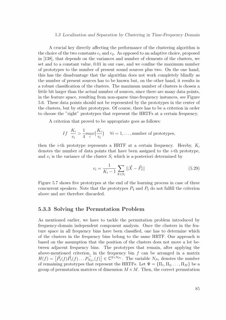
5.3 Localization and Separation by Clustering in Time-Frequency Domain
A crucial key directly affecting the performance of the clustering algorithm isthe choice of the two constants ε1 and ε2. As opposed to an adaptive choice, proposedin [138], that depends on the variances and number of elements of the clusters, weset and to a constant value, 0.01 in our case, and we confine the maximum numberof prototypes to the number of present sound sources plus two. On the one hand,this has the disadvantage that the algorithm does not work completely blindly asthe number of present sources has to be known but, on the other hand, it results ina robust classification of the clusters. The maximum number of clusters is chosen alittle bit larger than the actual number of sources, since there are many data points,in the feature space, resulting from non-sparse time-frequency instances, see Figure5.6. These data points should not be represented by the prototypes in the center ofthe clusters, but by other prototypes. Of course, there has to be a criterion in orderto choose the ”right” prototypes that represent the HRTFs at a certain frequency.
A criterion that proved to be appropriate goes as follows:
IfKi
vi
>1
4max
i
(Ki
vi
) ∀i = 1, . . . , number of prototypes,
then the i-th prototype represents a HRTF at a certain frequency. Hereby, Ki
denotes the number of data points that have been assigned to the i-th prototype,and vi is the variance of the cluster Si which is a-posteriori determined by
vi =1
Ki − 1
∑X∈Si
|| ~X − ~Pi|| (5.29)
Figure 5.7 shows five prototypes at the end of the learning process in case of threeconcurrent speakers. Note that the prototypes P4 and P5 do not fulfill the criterionabove and are therefore discarded.
5.3.3 Solving the Permutation Problem
As mentioned earlier, we have to tackle the permutation problem introduced byfrequency-domain independent component analysis. Once the clusters in the fea-ture space in all frequency bins have been classified, one has to determine whichof the clusters in the frequency bins belong to the same HRTF. Our approach isbased on the assumption that the position of the clusters does not move a lot be-tween adjacent frequency bins. The prototypes that remain, after applying theabove-mentioned criterion, in the frequency bin f can be arranged in a matrixH(f) =
[~P1(f) ~P1(f) . . . ~PNPr
(f)] ∈ C2×NPr . The variable NPr denotes the number
of remaining prototypes that represent the HRTFs. Let Ψ = {Π1, Π2, . . . , ΠM} be agroup of permutation matrices of dimension M×M . Then, the correct permutation
85
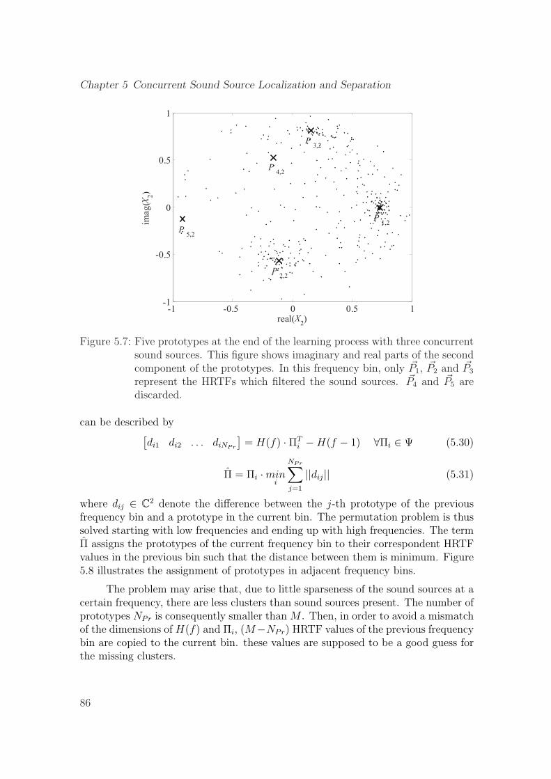
Chapter 5 Concurrent Sound Source Localization and Separation
-1 -0.5 0 0.5 1-1
-0.5
0
0.5
1
real(X2)
imag(X2)
P1,2
P3,2
P2,2
P4,2
P5,2
Figure 5.7: Five prototypes at the end of the learning process with three concurrentsound sources. This figure shows imaginary and real parts of the secondcomponent of the prototypes. In this frequency bin, only ~P1, ~P2 and ~P3
represent the HRTFs which filtered the sound sources. ~P4 and ~P5 arediscarded.
can be described by[di1 di2 . . . diNPr
]= H(f) · ΠT
i −H(f − 1) ∀Πi ∈ Ψ (5.30)
Π = Πi ·mini
NPr∑j=1
||dij|| (5.31)
where dij ∈ C2 denote the difference between the j-th prototype of the previousfrequency bin and a prototype in the current bin. The permutation problem is thussolved starting with low frequencies and ending up with high frequencies. The termΠ assigns the prototypes of the current frequency bin to their correspondent HRTFvalues in the previous bin such that the distance between them is minimum. Figure5.8 illustrates the assignment of prototypes in adjacent frequency bins.
The problem may arise that, due to little sparseness of the sound sources at acertain frequency, there are less clusters than sound sources present. The number ofprototypes NPr is consequently smaller than M . Then, in order to avoid a mismatchof the dimensions of H(f) and Πi, (M−NPr) HRTF values of the previous frequencybin are copied to the current bin. these values are supposed to be a good guess forthe missing clusters.
86
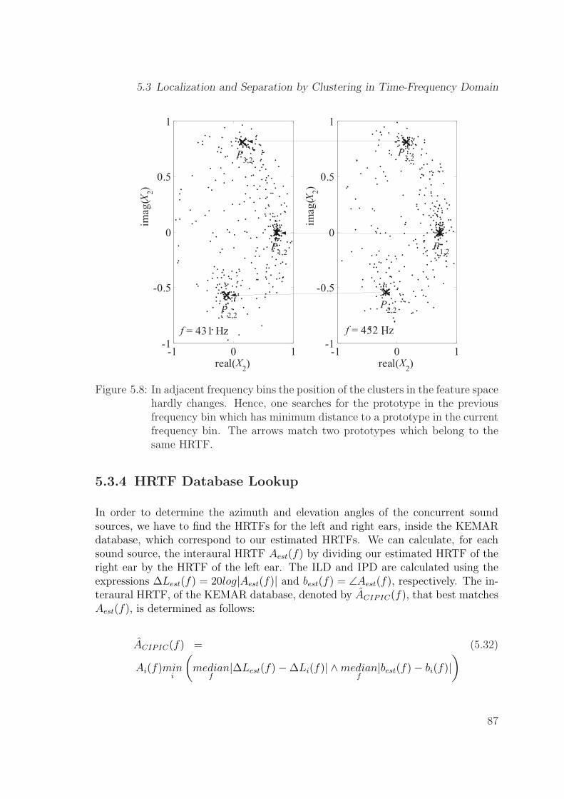
5.3 Localization and Separation by Clustering in Time-Frequency Domain
-1 0 1-1
-0.5
0
0.5
1
real(X2)
imag
(X2)
-1 0 1-1
-0.5
0
0.5
1
real(X2)
imag
(X2)
f = 431 Hz f = 452 Hz
P1,2
P1,2
P2,2
P2,2
P3,2
P3,2
Figure 5.8: In adjacent frequency bins the position of the clusters in the feature spacehardly changes. Hence, one searches for the prototype in the previousfrequency bin which has minimum distance to a prototype in the currentfrequency bin. The arrows match two prototypes which belong to thesame HRTF.
5.3.4 HRTF Database Lookup
In order to determine the azimuth and elevation angles of the concurrent soundsources, we have to find the HRTFs for the left and right ears, inside the KEMARdatabase, which correspond to our estimated HRTFs. We can calculate, for eachsound source, the interaural HRTF Aest(f) by dividing our estimated HRTF of theright ear by the HRTF of the left ear. The ILD and IPD are calculated using theexpressions ∆Lest(f) = 20log|Aest(f)| and best(f) = ∠Aest(f), respectively. The in-teraural HRTF, of the KEMAR database, denoted by ACIPIC(f), that best matchesAest(f), is determined as follows:
ACIPIC(f) = (5.32)
Ai(f)mini
(median
f|∆Lest(f)−∆Li(f)| ∧median
f|best(f)− bi(f)|
)
87
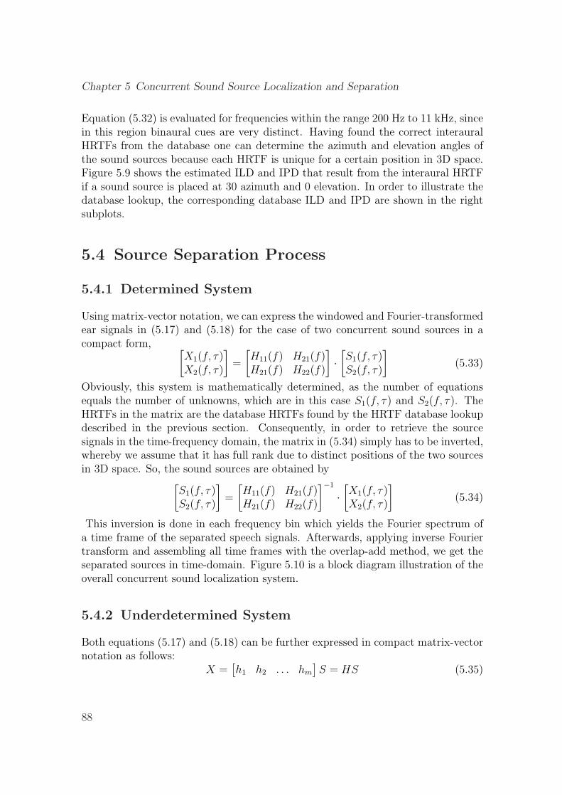
Chapter 5 Concurrent Sound Source Localization and Separation
Equation (5.32) is evaluated for frequencies within the range 200 Hz to 11 kHz, sincein this region binaural cues are very distinct. Having found the correct interauralHRTFs from the database one can determine the azimuth and elevation angles ofthe sound sources because each HRTF is unique for a certain position in 3D space.Figure 5.9 shows the estimated ILD and IPD that result from the interaural HRTFif a sound source is placed at 30 azimuth and 0 elevation. In order to illustrate thedatabase lookup, the corresponding database ILD and IPD are shown in the rightsubplots.
5.4 Source Separation Process
5.4.1 Determined System
Using matrix-vector notation, we can express the windowed and Fourier-transformedear signals in (5.17) and (5.18) for the case of two concurrent sound sources in acompact form, [
X1(f, τ)X2(f, τ)
]=
[H11(f) H21(f)H21(f) H22(f)
]·[S1(f, τ)S2(f, τ)
](5.33)
Obviously, this system is mathematically determined, as the number of equationsequals the number of unknowns, which are in this case S1(f, τ) and S2(f, τ). TheHRTFs in the matrix are the database HRTFs found by the HRTF database lookupdescribed in the previous section. Consequently, in order to retrieve the sourcesignals in the time-frequency domain, the matrix in (5.34) simply has to be inverted,whereby we assume that it has full rank due to distinct positions of the two sourcesin 3D space. So, the sound sources are obtained by
[S1(f, τ)S2(f, τ)
]=
[H11(f) H21(f)H21(f) H22(f)
]−1
·[X1(f, τ)X2(f, τ)
](5.34)
This inversion is done in each frequency bin which yields the Fourier spectrum ofa time frame of the separated speech signals. Afterwards, applying inverse Fouriertransform and assembling all time frames with the overlap-add method, we get theseparated sources in time-domain. Figure 5.10 is a block diagram illustration of theoverall concurrent sound localization system.
5.4.2 Underdetermined System
Both equations (5.17) and (5.18) can be further expressed in compact matrix-vectornotation as follows:
X =[h1 h2 . . . hm
]S = HS (5.35)
88
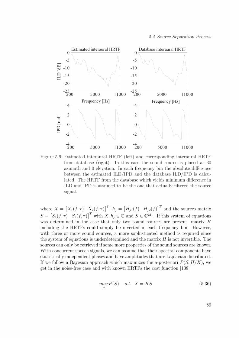
5.4 Source Separation Process
200 5000 11000-25
-20
-15
-10
-5
0
Frequency [Hz]
ILD
[d
B]
200 5000 11000-4
-2
0
2
4
IPD
[ra
d]
200 5000 11000-25
-20
-15
-10
-5
0
200 5000 11000-4
-2
0
2
4
Estimated interaural HRTF Database interaural HRTF
Frequency [Hz]
Figure 5.9: Estimated interaural HRTF (left) and corresponding interaural HRTFfrom database (right). In this case the sound source is placed at 30azimuth and 0 elevation. In each frequency bin the absolute differencebetween the estimated ILD/IPD and the database ILD/IPD is calcu-lated. The HRTF from the database which yields minimum difference inILD and IPD is assumed to be the one that actually filtered the sourcesignal.
where X =[X1(f, τ) X2(f, τ)
]T, hj =
[Hj1(f) Hj2(f)
]Tand the sources matrix
S =[S1(f, τ) S2(f, τ)
]Twith X, hj ∈ C and S ∈ CM . If this system of equations
was determined in the case that only two sound sources are present, matrix Hincluding the HRTFs could simply be inverted in each frequency bin. However,with three or more sound sources, a more sophisticated method is required sincethe system of equations is underdetermined and the matrix H is not invertible. Thesources can only be retrieved if some more properties of the sound sources are known.With concurrent speech signals, we can assume that their spectral components havestatistically independent phases and have amplitudes that are Laplacian distributed.If we follow a Bayesian approach which maximizes the a-posteriori P (S, H/X), weget in the noise-free case and with known HRTFs the cost function [138]
maxs
P (S) s.t. X = HS (5.36)
89
Chapter 5 Concurrent Sound Source Localization and Separation
Sound Source Separation:
HRTF Inversion
Frames Assembly
1( )x t
STFT .
.
.
fmax
Self-
Splitting
Competitive
Learning
HRTFM
.
.
.
(azM,
elevM)
. . . f = 1 fmax
.
.
.
Database
HRTFs
.
.
.
s1(t)
sM(t)
HRTF
database
lookup
f = 1 (az1,
elev1)
2( )x t
. . .
Figure 5.10: After STFT of the ear-input signals, the self-splitting competitive learn-ing algorithm finds the prototypes that represent the HRTFs in eachfrequency bin. By looking for the HRTFs that match best the esti-mated ones, the azimuth and elevation positions of the M sources aredetermined. With the aid of these database HRTFs the sound sourcesare separated.
With Laplacian distributed components Si, this cost function yields
mins
∑i
|Si|, i = 1, . . . , M s.t. X = HS (5.37)
for each time instance τ . In the case, using the L1-norm minimization of real-valuedproblems, we obtain the sound sources by shortest path decomposition as proposedin [22]. In our particular case with two microphones, the shortest path from theorigin to the data point X is obtained by choosing the two HRTF vectors h1 and h2
whose directions are the closest from below and from above to the direction θ. Inthe example of Figure 5.11 these HRTF vectors are illustrated. The solution Spath
is then obtained by:
Spath =
[[h1 h2
]−1X
0
](5.38)
However, the source signals and the HRTFs in frequency domain are in general notreal-valued, so that the shortest path decomposition does not necessarily yield theminimum L1-norm. Hence, we add a vector S ∈ CM to our solution Sspath that iselement of the nullspace of H and thus fulfills:
X = HSspath + HS = H(Sspath + S) (5.39)
90
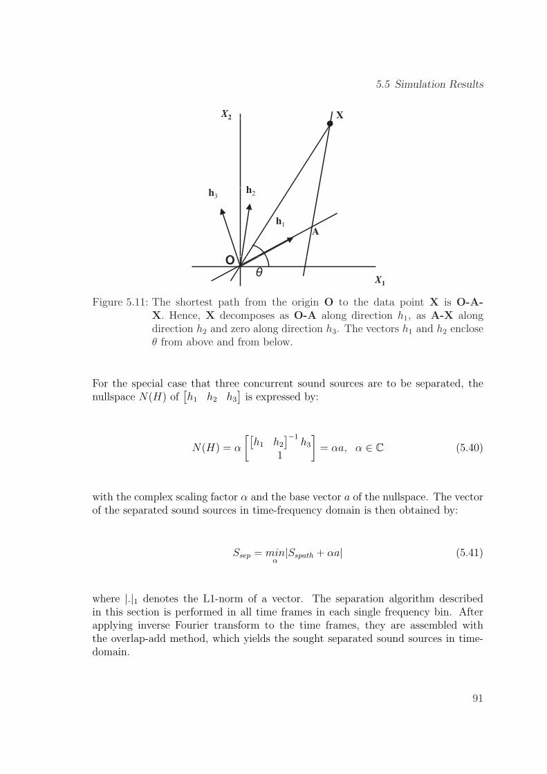
5.5 Simulation Results
X2 X2
h
X
h1
h3h2
O
A
X1
O
Figure 5.11: The shortest path from the origin O to the data point X is O-A-X. Hence, X decomposes as O-A along direction h1, as A-X alongdirection h2 and zero along direction h3. The vectors h1 and h2 encloseθ from above and from below.
For the special case that three concurrent sound sources are to be separated, thenullspace N(H) of
[h1 h2 h3
]is expressed by:
N(H) = α
[[h1 h2
]−1h3
1
]= αa, α ∈ C (5.40)
with the complex scaling factor α and the base vector a of the nullspace. The vectorof the separated sound sources in time-frequency domain is then obtained by:
Ssep = minα|Sspath + αa| (5.41)
where |.|1 denotes the L1-norm of a vector. The separation algorithm describedin this section is performed in all time frames in each single frequency bin. Afterapplying inverse Fourier transform to the time frames, they are assembled withthe overlap-add method, which yields the sought separated sound sources in time-domain.
91
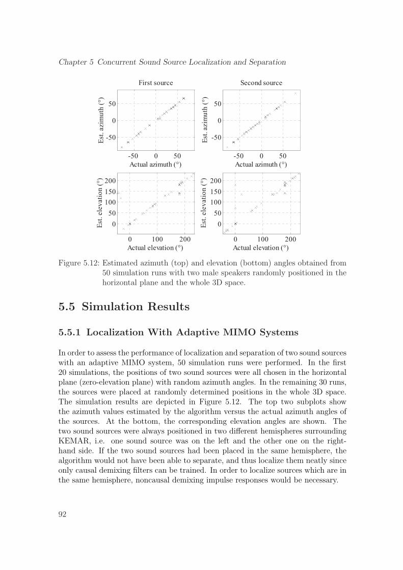
Chapter 5 Concurrent Sound Source Localization and Separation
-50 0 50
-50
0
50
Actual azimuth (°)
Est
. azim
uth
(°)
First source
0 100 200
0
50
100
150
200
Actual elevation (°)
-50 0 50
-50
0
50
Actual azimuth (°)
Est
. azim
uth
(°)
Second source
0 100 200
0
50
100
150
200
Actual elevation (°)
Est
. ele
vati
on
(°)
Est
. ele
vati
on
(°)
Figure 5.12: Estimated azimuth (top) and elevation (bottom) angles obtained from50 simulation runs with two male speakers randomly positioned in thehorizontal plane and the whole 3D space.
5.5 Simulation Results
5.5.1 Localization With Adaptive MIMO Systems
In order to assess the performance of localization and separation of two sound sourceswith an adaptive MIMO system, 50 simulation runs were performed. In the first20 simulations, the positions of two sound sources were all chosen in the horizontalplane (zero-elevation plane) with random azimuth angles. In the remaining 30 runs,the sources were placed at randomly determined positions in the whole 3D space.The simulation results are depicted in Figure 5.12. The top two subplots showthe azimuth values estimated by the algorithm versus the actual azimuth angles ofthe sources. At the bottom, the corresponding elevation angles are shown. Thetwo sound sources were always positioned in two different hemispheres surroundingKEMAR, i.e. one sound source was on the left and the other one on the right-hand side. If the two sound sources had been placed in the same hemisphere, thealgorithm would not have been able to separate, and thus localize them neatly sinceonly causal demixing filters can be trained. In order to localize sources which are inthe same hemisphere, noncausal demixing impulse responses would be necessary.
92
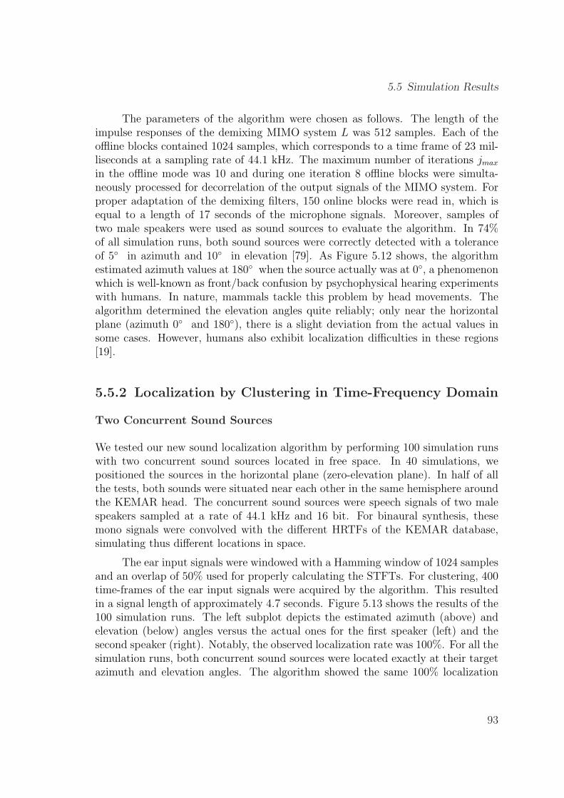
5.5 Simulation Results
The parameters of the algorithm were chosen as follows. The length of theimpulse responses of the demixing MIMO system L was 512 samples. Each of theoffline blocks contained 1024 samples, which corresponds to a time frame of 23 mil-liseconds at a sampling rate of 44.1 kHz. The maximum number of iterations jmax
in the offline mode was 10 and during one iteration 8 offline blocks were simulta-neously processed for decorrelation of the output signals of the MIMO system. Forproper adaptation of the demixing filters, 150 online blocks were read in, which isequal to a length of 17 seconds of the microphone signals. Moreover, samples oftwo male speakers were used as sound sources to evaluate the algorithm. In 74%of all simulation runs, both sound sources were correctly detected with a toleranceof 5◦ in azimuth and 10◦ in elevation [79]. As Figure 5.12 shows, the algorithmestimated azimuth values at 180◦ when the source actually was at 0◦, a phenomenonwhich is well-known as front/back confusion by psychophysical hearing experimentswith humans. In nature, mammals tackle this problem by head movements. Thealgorithm determined the elevation angles quite reliably; only near the horizontalplane (azimuth 0◦ and 180◦), there is a slight deviation from the actual values insome cases. However, humans also exhibit localization difficulties in these regions[19].
5.5.2 Localization by Clustering in Time-Frequency Domain
Two Concurrent Sound Sources
We tested our new sound localization algorithm by performing 100 simulation runswith two concurrent sound sources located in free space. In 40 simulations, wepositioned the sources in the horizontal plane (zero-elevation plane). In half of allthe tests, both sounds were situated near each other in the same hemisphere aroundthe KEMAR head. The concurrent sound sources were speech signals of two malespeakers sampled at a rate of 44.1 kHz and 16 bit. For binaural synthesis, thesemono signals were convolved with the different HRTFs of the KEMAR database,simulating thus different locations in space.
The ear input signals were windowed with a Hamming window of 1024 samplesand an overlap of 50% used for properly calculating the STFTs. For clustering, 400time-frames of the ear input signals were acquired by the algorithm. This resultedin a signal length of approximately 4.7 seconds. Figure 5.13 shows the results of the100 simulation runs. The left subplot depicts the estimated azimuth (above) andelevation (below) angles versus the actual ones for the first speaker (left) and thesecond speaker (right). Notably, the observed localization rate was 100%. For all thesimulation runs, both concurrent sound sources were located exactly at their targetazimuth and elevation angles. The algorithm showed the same 100% localization
93
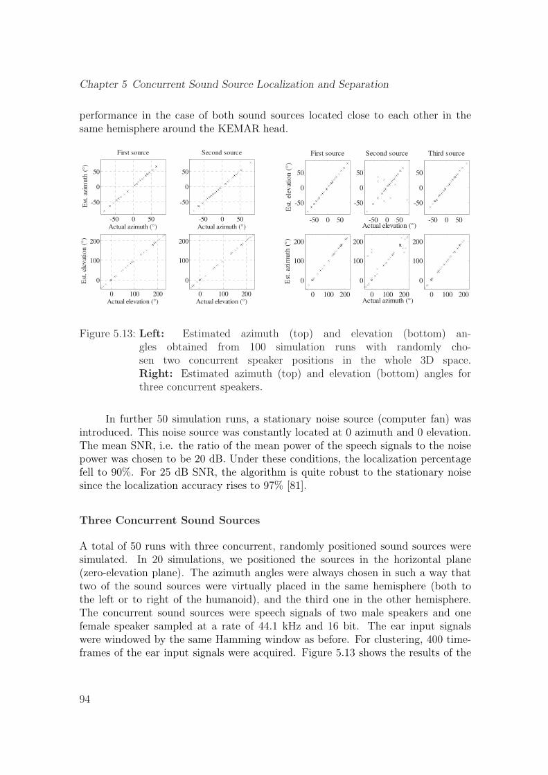
Chapter 5 Concurrent Sound Source Localization and Separation
performance in the case of both sound sources located close to each other in thesame hemisphere around the KEMAR head.
-50 0 50
-50
0
50
Actual elevation (°)
Est
. el
evat
ion
(°)
First source
0 100 200
0
100
200
Actual azimuth (°)
Est
. az
imu
th (
°)
-50 0 50
-50
0
50
Second source
0 100 200
0
100
200
-50 0 50
-50
0
50
Third source
0 100 200
0
100
200
-50 0 50
-50
0
50
Actual azimuth (°)
Est
. az
imu
th (
°)
First source
0 100 200
0
100
200
Actual elevation (°)
Est
. el
evat
ion
(°)
-50 0 50
-50
0
50
Actual azimuth (°)
Second source
0 100 200
0
100
200
Actual elevation (°)
Figure 5.13: Left: Estimated azimuth (top) and elevation (bottom) an-gles obtained from 100 simulation runs with randomly cho-sen two concurrent speaker positions in the whole 3D space.Right: Estimated azimuth (top) and elevation (bottom) angles forthree concurrent speakers.
In further 50 simulation runs, a stationary noise source (computer fan) wasintroduced. This noise source was constantly located at 0 azimuth and 0 elevation.The mean SNR, i.e. the ratio of the mean power of the speech signals to the noisepower was chosen to be 20 dB. Under these conditions, the localization percentagefell to 90%. For 25 dB SNR, the algorithm is quite robust to the stationary noisesince the localization accuracy rises to 97% [81].
Three Concurrent Sound Sources
A total of 50 runs with three concurrent, randomly positioned sound sources weresimulated. In 20 simulations, we positioned the sources in the horizontal plane(zero-elevation plane). The azimuth angles were always chosen in such a way thattwo of the sound sources were virtually placed in the same hemisphere (both tothe left or to right of the humanoid), and the third one in the other hemisphere.The concurrent sound sources were speech signals of two male speakers and onefemale speaker sampled at a rate of 44.1 kHz and 16 bit. The ear input signalswere windowed by the same Hamming window as before. For clustering, 400 time-frames of the ear input signals were acquired. Figure 5.13 shows the results of the
94
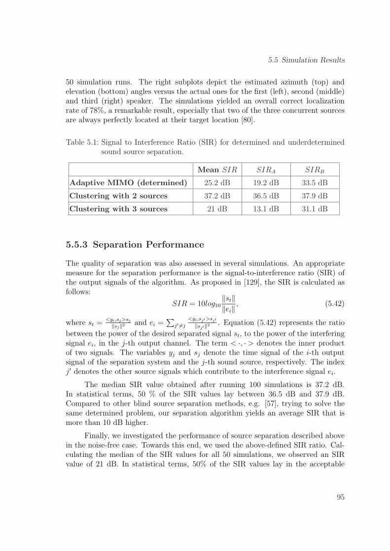
5.5 Simulation Results
50 simulation runs. The right subplots depict the estimated azimuth (top) andelevation (bottom) angles versus the actual ones for the first (left), second (middle)and third (right) speaker. The simulations yielded an overall correct localizationrate of 78%, a remarkable result, especially that two of the three concurrent sourcesare always perfectly located at their target location [80].
Table 5.1: Signal to Interference Ratio (SIR) for determined and underdeterminedsound source separation.
Mean SIR SIRA SIRB
Adaptive MIMO (determined) 25.2 dB 19.2 dB 33.5 dB
Clustering with 2 sources 37.2 dB 36.5 dB 37.9 dB
Clustering with 3 sources 21 dB 13.1 dB 31.1 dB
5.5.3 Separation Performance
The quality of separation was also assessed in several simulations. An appropriatemeasure for the separation performance is the signal-to-interference ratio (SIR) ofthe output signals of the algorithm. As proposed in [129], the SIR is calculated asfollows:
SIR = 10log10‖st‖‖ei‖ , (5.42)
where st =<yi,sj>sj
‖sj‖2 and ei =∑
j′ 6=j
<yi,sj′>sj′‖sj′‖2 . Equation (5.42) represents the ratio
between the power of the desired separated signal st, to the power of the interferingsignal ei, in the j-th output channel. The term < ·, · > denotes the inner productof two signals. The variables yj and sj denote the time signal of the i-th outputsignal of the separation system and the j-th sound source, respectively. The indexj′ denotes the other source signals which contribute to the interference signal ei.
The median SIR value obtained after running 100 simulations is 37.2 dB.In statistical terms, 50 % of the SIR values lay between 36.5 dB and 37.9 dB.Compared to other blind source separation methods, e.g. [57], trying to solve thesame determined problem, our separation algorithm yields an average SIR that ismore than 10 dB higher.
Finally, we investigated the performance of source separation described abovein the noise-free case. Towards this end, we used the above-defined SIR ratio. Cal-culating the median of the SIR values for all 50 simulations, we observed an SIRvalue of 21 dB. In statistical terms, 50% of the SIR values lay in the acceptable
95
Chapter 5 Concurrent Sound Source Localization and Separation
interval of 13.1 dB to 31.2 dB. These values are notably higher than SIR valuesprovided by other underdetermined separation algorithms, trying to solve the prob-lem of more sources than observations under the same conditions [25]. The soundsource separation performance bounds for the determined and underdeterined casesare summarized in Table 5.1
The interval between SIRA and SIRB encloses 50% of the SIR values aroundthe median value. In case of three sound sources, the obtained values are higherthan SIR values provided by other underdetermined separation algorithms, tryingto solve the problem of more sources than observations, e.g. [20], since the measureddatabase HRTFs and not the estimated HRTFs are used for source separation [70].
5.5.4 Localization Performance
We have compared our method with the concurrent detection method based on theecho-avoidance model [51] introduced in chapter 1. Sound localization experimentswere conducted in an anechoic chamber and a normal room. Three microphonesarranged in a triangular form were available for sound recording. Two sound sourceswere played concurrently. The sources were set in two fixed positions each distanced1 meter from the wall. The azimuth of the first sound source was 0 degree facingdirection one of the three microphones and the second sound source was about 38degrees to that microphone. The distance from the sound sources to the center ofthe microphone set was about 2.9 m and the distance between sound sources wasabout 1.9 m. Sound data were recorded by a multi-channel analog data recorderwith a sampling frequency of 9600 Hz.
The azimuth histograms for the anechoic chamber and the normal room werecomputed. The contribution of each sound/echo was added to the sum azimuthhistogram. The histogram peaks are pronounced around 0 and 38 degrees over alltime segments in the histograms of the anechoic chamber. These two rows of peakscorrespond to the first and the second sound source, respectively. The positions ofmajor peaks are in the regions of [0, 4] and [35, 39] degrees, i.e., the first sound sourcewas localized in 2(±2) degrees and the second sound source in 37(±2) degrees. Themaximum absolute error is 4 degrees. The histograms of the normal room, however,show more disorder comparing to the anechoic chamber. The scores are smallerand the size of the peaks is not consistent. After smoothing the histograms by atwo-dimension Gaussian function, the time resolution decreased to about 2 s, butthe peak positions became more consistent. The positions of major peaks are in theregions of [-2, 2] and [33, 37] degrees, i.e., the first sound source was localized in0(±2) degrees and the second sound source was localized in 35(±2) degrees. Themaximum absolute errors is 5 degrees. All the results are similar to the results
96
5.5 Simulation Results
obtained in the anechoic chamber except that 2 seconds are now needed to obtainan accurate localization, compared with 0.5 second for the anechoic room. Usingour SSCL-based localization method in the anechoic room, the first sound sourcelocated at 0 degree was detected in the region [0, 5] degrees. The second sourcelocated at 38 degrees was detected in the region [35, 40] degrees. The maximumabsolute error is 5 degrees and the overall processing time is 4.7s. In the normalroom, the first sound source located at 0 degree was detected in the region [-5, 0]degrees, and the second source located at 38 degrees was detected in the region [30,35] degrees. The maximum absolute error is 5 degrees for and overall processing timeof 11.5s. It should be noted that, on the expense of increased computational power,the 5-degree absolute error could be reduced to 1 degree if we use a HRTF databasesampled every one degree in the azimuthal plane. In addition, the SSCL-basedmethod is not limited to azimuthal localization and uses only two microphones.
Furthermore, we compare our method with the beamforming technique [102]introduced in chapter 1. This method utilizes a microphone array of 8 sensors anddeploys time delay of arrival estimation, and multiple Kalman filters for concurrentsound source tracking in azimuth. A steered beamformer was used for the soundsource localization. The basic idea of this method is to direct a beamformer inall possible directions and look for maximal output. The beamformer searches aspherical space around the microphone array which is divided into 5,120 trianglegrids with 2,562 vertices. The beamformer energy is computed for each vertex byincremental refinements from a large triangle to smaller ones. The direction of asound source is estimated as that of the region with the maximal energy. Thismethod localized sound source accurately for stationary and moving sound sources.Although the method provided directional information at each time frame, a tempo-ral grouping of the same sound source was not attained. Therefore, it was difficultto track multiple moving sound sources. This ambiguity was clarified by feedingthe temporal information to a multiple Kalman filter with different history lengths.Multiple Kalman filters with different history length predict next states in parallel,and provides a set of estimates. The current estimate is obtained by the filter whichpredicted the state with the minimal error in the previous frame. The continuity oflocalization for each speaker is forced by using acoustic features of separated speechsignals. For this purpose, the power spectrum was computed in each frame, in orderto reduce the ambiguities in tracking moving speakers. The observed value whosepower spectrum is similar to the past one of a speaker is selected as the observedvalue of the speaker. The power spectrum of a separated sound is calculated byusing a delay-and-sum beamformer, which uses a localization angle as a clue. If theseparated speech of each moving speaker is available, the fundamental frequency ofthe speech is used for the accurate selection of the observed value.
The algorithm processes loudspeaker signals using 8 channel sound recorded
97
Chapter 5 Concurrent Sound Source Localization and Separation
with a sampling rate of 48kHz. The accuracy of the multiple Kalman filter method,for two concurrent sound sources placed at 0 and 30 degrees in front of the robot,yielded a mean square angular error of 26, compared to a mean square error of 20 forour SSCL-based technique. For three concurrent sound sources located at 0, 80 and110 degrees, the multiple Kalman filter method undergoes a mean square angularerror of 28, compared to a mean square error of 25 for the SSCL-based technique.The increased accuracy of the SSCL-based technique comes at the expense of a 4.7sprocessing time compared to 2.4s for the multiple filter method. While the multipleKalman filter method covers only azimuthal localization, our SSCL-based methodcovers the whole 3D space surrounding the robot head, and deploys two instead of8 microphones.
Summing up, we have used only two microphones in combination with a genericHRTF database to localize and separate two concurrent moving sources in a 3Dspace. The simplicity of the proposed sound source separation and localization al-gorithm suggests a cost-effective implementation for robot platforms. While thedetection of sound in elevation was similar to the human ability, our results demon-strated very precise localization of the sound sources in the azimuth angles. Sincethe HRTF dataset used was measured on the horizontal plane from 0◦ to 360◦ with5◦ increment and on the vertical plane from -40◦ to 90◦ with 10◦ increment, wecan localize the sound source with an accuracy of about 5◦ to 10◦. Obviously, anHRTF dataset with smaller increments increases the resolution of estimation. Inthe following chapter, the HRTF interpolation method presented in chapter 3 willbe used to enhance the accuracy of a localizer operating in a highly-reverberantenvironment.
98
Chapter 6
Sound Localization in HighlyReverberant Environments
In this chapter, we introduce a robust sound localization algorithm, which usesBayesian information fusion to increase the localization resolution in a three-dimensionalreverberant environment. The main focus is the detection of sound events under se-vere acoustic conditions, i.e. high reverberation and background noise. The locationof the sound source obtained from a number of observation sensors is fused using aproperly tuned Bayesian network so that an accurate three-dimensional direction ofarrival estimation, in terms of both azimuth and elevation, is guaranteed.
6.1 New Hardware Setup
The new sound localization setup takes two sound signals as input: 1) the spatialsound signal measured inside the ear canal of KEMAR humanoid’s artificial ear,and 2) the sound signal measured outside the artificial ear, placed 5 cm away fromthe inner microphone. This hardware configuration is illustrated in Figure 6.2.
After data acquisition, both inner and outer signals are divided, in the spectraldomain, in an attempt to exclude the incoming sound signal and, thus, isolate theeffect of the pinna, head, and torso. Consequently, the appropriate HRTF whichhas shaped the incoming sound signal is extracted. Using simple correlation, theextracted HRTF is then compared with a database of HRTFs, [6], and the maximumcorrelation coefficient is taken to be corresponding to the 3D sound source location.The HRTFs were measured every 5◦ in elevation and azimuth. An accurate, recently
99
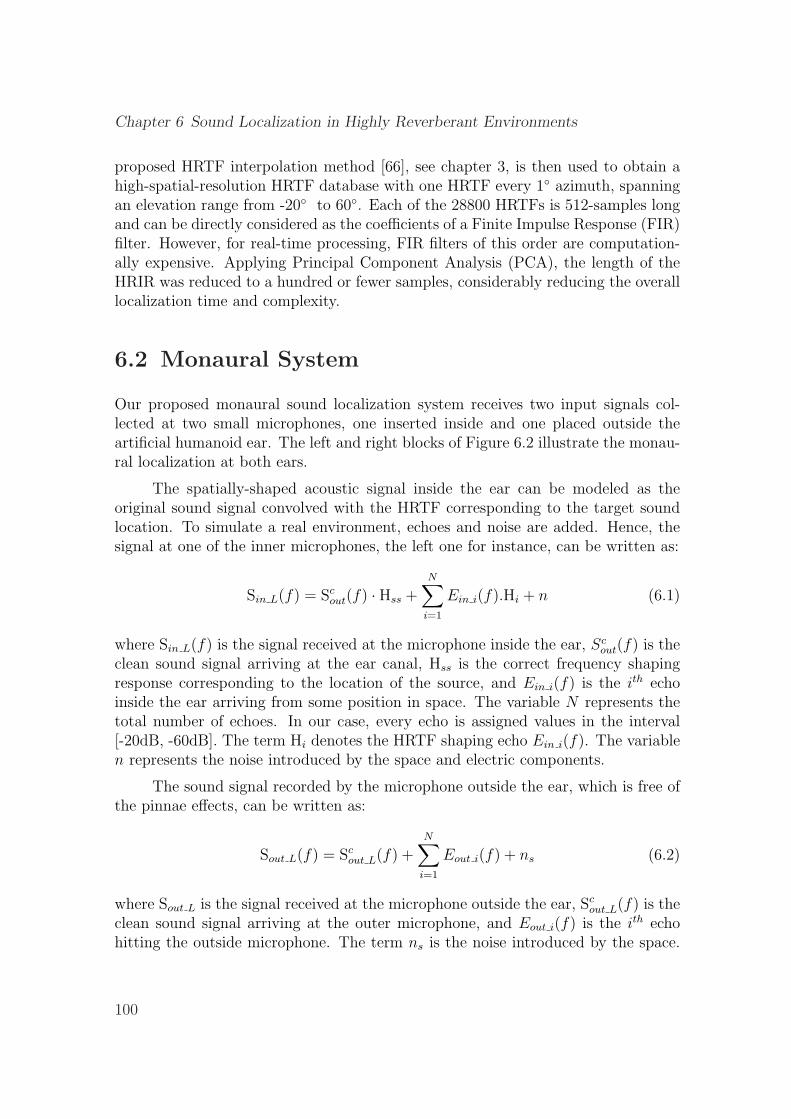
Chapter 6 Sound Localization in Highly Reverberant Environments
proposed HRTF interpolation method [66], see chapter 3, is then used to obtain ahigh-spatial-resolution HRTF database with one HRTF every 1◦ azimuth, spanningan elevation range from -20◦ to 60◦. Each of the 28800 HRTFs is 512-samples longand can be directly considered as the coefficients of a Finite Impulse Response (FIR)filter. However, for real-time processing, FIR filters of this order are computation-ally expensive. Applying Principal Component Analysis (PCA), the length of theHRIR was reduced to a hundred or fewer samples, considerably reducing the overalllocalization time and complexity.
6.2 Monaural System
Our proposed monaural sound localization system receives two input signals col-lected at two small microphones, one inserted inside and one placed outside theartificial humanoid ear. The left and right blocks of Figure 6.2 illustrate the monau-ral localization at both ears.
The spatially-shaped acoustic signal inside the ear can be modeled as theoriginal sound signal convolved with the HRTF corresponding to the target soundlocation. To simulate a real environment, echoes and noise are added. Hence, thesignal at one of the inner microphones, the left one for instance, can be written as:
Sin L(f) = Scout(f) · Hss +
N∑i=1
Ein i(f).Hi + n (6.1)
where Sin L(f) is the signal received at the microphone inside the ear, Scout(f) is the
clean sound signal arriving at the ear canal, Hss is the correct frequency shapingresponse corresponding to the location of the source, and Ein i(f) is the ith echoinside the ear arriving from some position in space. The variable N represents thetotal number of echoes. In our case, every echo is assigned values in the interval[-20dB, -60dB]. The term Hi denotes the HRTF shaping echo Ein i(f). The variablen represents the noise introduced by the space and electric components.
The sound signal recorded by the microphone outside the ear, which is free ofthe pinnae effects, can be written as:
Sout L(f) = Scout L(f) +
N∑i=1
Eout i(f) + ns (6.2)
where Sout L is the signal received at the microphone outside the ear, Scout L(f) is the
clean sound signal arriving at the outer microphone, and Eout i(f) is the ith echohitting the outside microphone. The term ns is the noise introduced by the space.
100
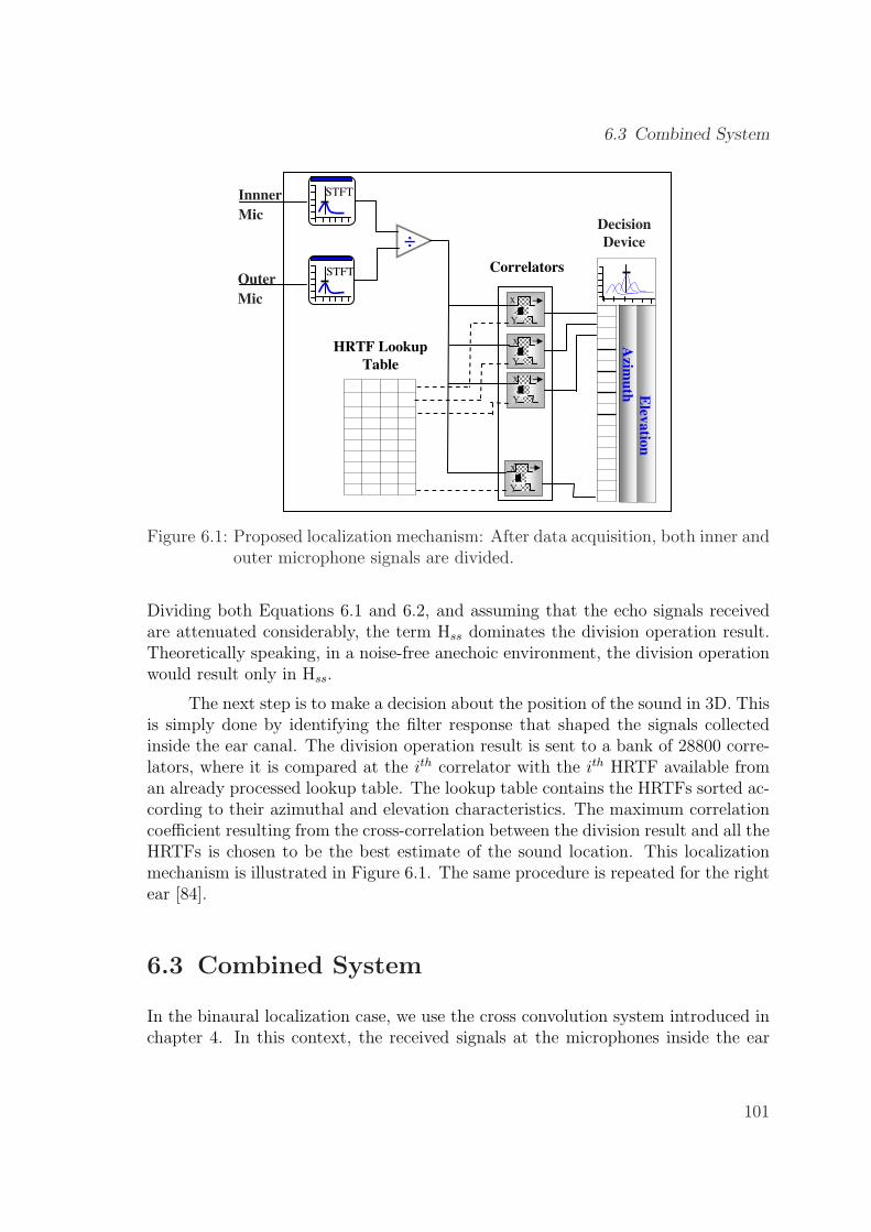
6.3 Combined System
Innner
Mic
Outer
Mic
STFT
STFT
1
HRTF Lookup
Table
x
Y
x
Y
x
Y
x
Y
Correlators
Decision
DeviceA
zimu
th Elev
atio
n÷
Figure 6.1: Proposed localization mechanism: After data acquisition, both inner andouter microphone signals are divided.
Dividing both Equations 6.1 and 6.2, and assuming that the echo signals receivedare attenuated considerably, the term Hss dominates the division operation result.Theoretically speaking, in a noise-free anechoic environment, the division operationwould result only in Hss.
The next step is to make a decision about the position of the sound in 3D. Thisis simply done by identifying the filter response that shaped the signals collectedinside the ear canal. The division operation result is sent to a bank of 28800 corre-lators, where it is compared at the ith correlator with the ith HRTF available froman already processed lookup table. The lookup table contains the HRTFs sorted ac-cording to their azimuthal and elevation characteristics. The maximum correlationcoefficient resulting from the cross-correlation between the division result and all theHRTFs is chosen to be the best estimate of the sound location. This localizationmechanism is illustrated in Figure 6.1. The same procedure is repeated for the rightear [84].
6.3 Combined System
In the binaural localization case, we use the cross convolution system introduced inchapter 4. In this context, the received signals at the microphones inside the ear
101
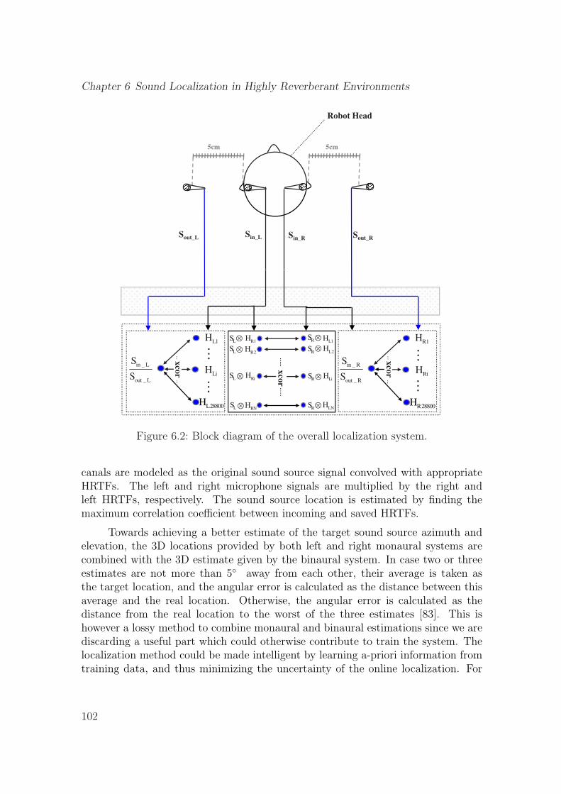
Chapter 6 Sound Localization in Highly Reverberant Environments
5cm5cm
Robot Head
Sin_L Sin_RSout_L Sout_R
L1H
…
R1H
…
…
LS
LS
RS
RS
L1H
L2H
R1H
R2H
xco
r LiH
in _ L
out _ L
S
S
L28800H
……
xco
r RiH
in _ R
out _ R
S
S
R28800H
……
……
……
xco
rLS
LS
RS
RS
LNH
LiH
RNH
RiH
Figure 6.2: Block diagram of the overall localization system.
canals are modeled as the original sound source signal convolved with appropriateHRTFs. The left and right microphone signals are multiplied by the right andleft HRTFs, respectively. The sound source location is estimated by finding themaximum correlation coefficient between incoming and saved HRTFs.
Towards achieving a better estimate of the target sound source azimuth andelevation, the 3D locations provided by both left and right monaural systems arecombined with the 3D estimate given by the binaural system. In case two or threeestimates are not more than 5◦ away from each other, their average is taken asthe target location, and the angular error is calculated as the distance between thisaverage and the real location. Otherwise, the angular error is calculated as thedistance from the real location to the worst of the three estimates [83]. This ishowever a lossy method to combine monaural and binaural estimations since we arediscarding a useful part which could otherwise contribute to train the system. Thelocalization method could be made intelligent by learning a-priori information fromtraining data, and thus minimizing the uncertainty of the online localization. For
102
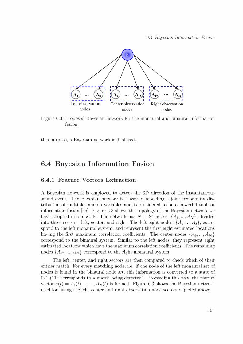
6.4 Bayesian Information Fusion
S
Left observation
nodes
Center observation
nodes
Right observation
nodes
A1 A8 A9 A16 A17 A24… ……
Figure 6.3: Proposed Bayesian network for the monaural and binaural informationfusion.
this purpose, a Bayesian network is deployed.
6.4 Bayesian Information Fusion
6.4.1 Feature Vectors Extraction
A Bayesian network is employed to detect the 3D direction of the instantaneoussound event. The Bayesian network is a way of modeling a joint probability dis-tribution of multiple random variables and is considered to be a powerful tool forinformation fusion [55]. Figure 6.3 shows the topology of the Bayesian network wehave adopted in our work. The network has N = 24 nodes, {A1, ..., AN}, dividedinto three sectors: left, center, and right. The left eight nodes, {A1, ..., A8}, corre-spond to the left monaural system, and represent the first eight estimated locationshaving the first maximum correlation coefficients. The center nodes {A9, ..., A16}correspond to the binaural system. Similar to the left nodes, they represent eightestimated locations which have the maximum correlation coefficients. The remainingnodes {A17, ..., A24} correspond to the right monaural system.
The left, center, and right sectors are then compared to check which of theirentries match. For every matching node, i.e. if one node of the left monaural set ofnodes is found in the binaural node set, this information is converted to a state of0/1 (”1” corresponds to a match being detected). Proceeding this way, the featurevector a(t) = A1(t), ..., ..., AN(t) is formed. Figure 6.3 shows the Bayesian networkused for fusing the left, center and right observation node sectors depicted above.
103
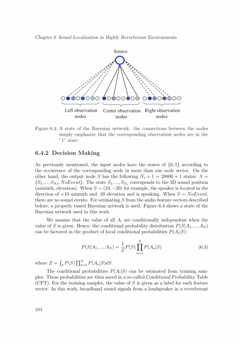
Chapter 6 Sound Localization in Highly Reverberant Environments
Left observation
nodes Center observation
nodes
Right observation
nodes
Source
Figure 6.4: A state of the Bayesian network: the connections between the nodessimply emphasize that the corresponding observation nodes are in the”1” state.
6.4.2 Decision Making
As previously mentioned, the input nodes have the states of {0, 1} according tothe occurrence of the corresponding node in more than one node sector. On theother hand, the output node S has the following Ns + 1 = 28800 + 1 states: S ={S1, ..., SNs, NoEvent}. The state S1, ..., SNs corresponds to the 3D sound position(azimuth, elevation). When S = (10,−20) for example, the speaker is located in thedirection of +10 azimuth and -20 elevation and is speaking. When S = NoEvent,there are no sound events. For estimating S from the audio feature vectors describedbefore, a properly tuned Bayesian network is used. Figure 6.4 shows a state of theBayesian network used in this work.
We assume that the value of all Ai are conditionally independent when thevalue of S is given. Hence, the conditional probability distribution P (S|A1, ..., AN)can be factored in the product of local conditional probabilities P (Ai|S):
P (S|A1, ..., AN) =1
ZP (S)
N∏n=1
P (An|S) (6.3)
where Z =∫
SP (S)
∏Nn=1 P (An|S)dS.
The conditional probabilities P (Ai|S) can be estimated from training sam-ples. These probabilities are then saved in a so-called Conditional Probability Table(CPT). For the training samples, the value of S is given as a label for each featurevector. In this work, broadband sound signals from a loudspeaker in a reverberant
104
6.5 Discussion of Results
laboratory room were used as training samples. The location of the loudspeaker wasvaried between −40 and +60 every 5◦in azimuth and elevation. Each sample was 30seconds long. There were no significant noise sources in the laboratory room, therewas however high background noise such as that from a PC fan. These samples wereused as a supervisor for training the CPT.
In the operation phase, the feature vectors are obtained as evidence at everytime block. Using the evidence and the CPTs obtained above, the conditionalprobability (6.3) is calculated and the most probable state of S is obtained, i.e. themost probable sound source location.
6.5 Discussion of Results
6.5.1 Simulation Results
The simulation test consisted of having a 100 broadband sound signals filtered by512-samples long HRIR at different azimuths and elevations corresponding to 100different random source locations in the 3D space. White Gaussian noise and highreverberations, i.e. echoes 20dB below the signal level, were added to the simulatedsound sources. In order to insure rapid localization of multiple sources, small partsof the filtered left and right signals are considered (350 msecs). These left and rightsignal parts are then correlated with the available 28800 reduced HRIRs. Basically,the correlation should yield a maximum value when the saved HRTF ratio, for thebinaural system, corresponds to the location from which the simulated sound sourceis originating. Similarly, for the monaural system, when the saved HRTF ratiocorresponds to the location from which the simulated sound source is coming, thecorrelation should yield a maximum value. Therefore, we base our localization onthe obtained maximum correlation factor. The PCA reduction technique was usedto create a truncated model of the original HRTFs.
To simulate the reverberation in our room environment, the image method forroom acoustics was used [7]. The simulation setup and room dimensions were de-fined to match the experimental room environment. A room size of 9.5m×7m×4mwas considered. The simulation setup and room dimensions were defined to matchthe experimental room environment. The data received at each microphone wasobtained by convolving the broadband source signal with the corresponding transferfunctions resulting from the image method between the source’s and microphone’spositions. After recombining the convolution results, random Gaussian noise wasfinally added to each microphone signal yielding an SNR level of 20dB. Figure 6.5shows the sound localization performance for the cross convolution technique, com-pared to the combined system operating with Bayesian information fusion. The
105
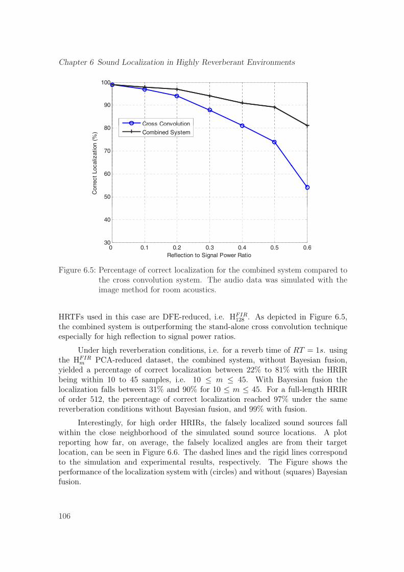
Chapter 6 Sound Localization in Highly Reverberant Environments
100
90
Cross Convolution
70
80
caliz
ation (
%)
Cross Convolution
Combined System
50
60
Corr
ect
Loc
0 0 1 0 2 0 3 0 4 0 5 0 630
40
0 0.1 0.2 0.3 0.4 0.5 0.6
Reflection to Signal Power Ratio
Figure 6.5: Percentage of correct localization for the combined system compared tothe cross convolution system. The audio data was simulated with theimage method for room acoustics.
HRTFs used in this case are DFE-reduced, i.e. HFIR128 . As depicted in Figure 6.5,
the combined system is outperforming the stand-alone cross convolution techniqueespecially for high reflection to signal power ratios.
Under high reverberation conditions, i.e. for a reverb time of RT = 1s. usingthe HFIR
m PCA-reduced dataset, the combined system, without Bayesian fusion,yielded a percentage of correct localization between 22% to 81% with the HRIRbeing within 10 to 45 samples, i.e. 10 ≤ m ≤ 45. With Bayesian fusion thelocalization falls between 31% and 90% for 10 ≤ m ≤ 45. For a full-length HRIRof order 512, the percentage of correct localization reached 97% under the samereverberation conditions without Bayesian fusion, and 99% with fusion.
Interestingly, for high order HRIRs, the falsely localized sound sources fallwithin the close neighborhood of the simulated sound source locations. A plotreporting how far, on average, the falsely localized angles are from their targetlocation, can be seen in Figure 6.6. The dashed lines and the rigid lines correspondto the simulation and experimental results, respectively. The Figure shows theperformance of the localization system with (circles) and without (squares) Bayesianfusion.
106
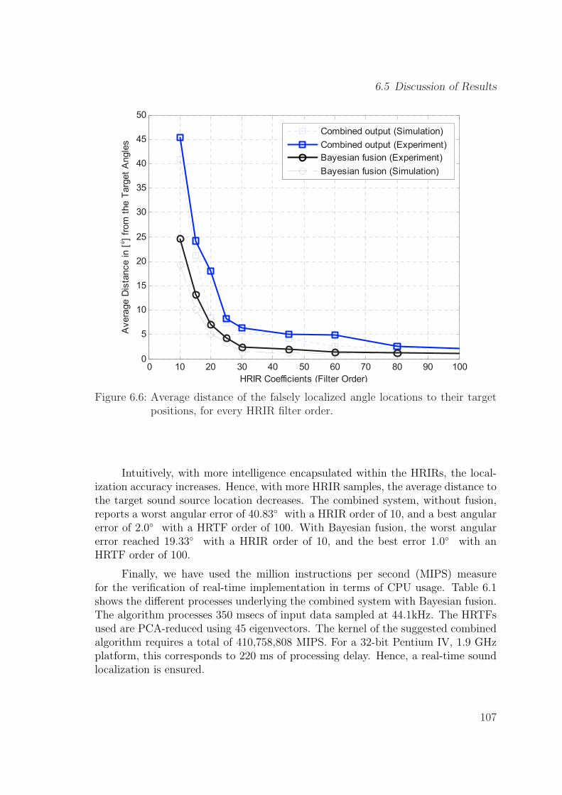
6.5 Discussion of Results
0 10 20 30 40 50 60 70 80 90 1000
5
10
15
20
25
30
35
40
45
50
HRIR Coefficients (Filter Order)
Avera
ge D
ista
nce in [
°] f
rom
the T
arg
et
Angle
sCombined output (Simulation)
Combined output (Experiment)
Bayesian fusion (Experiment)
Bayesian fusion (Simulation)
Figure 6.6: Average distance of the falsely localized angle locations to their targetpositions, for every HRIR filter order.
Intuitively, with more intelligence encapsulated within the HRIRs, the local-ization accuracy increases. Hence, with more HRIR samples, the average distance tothe target sound source location decreases. The combined system, without fusion,reports a worst angular error of 40.83◦ with a HRIR order of 10, and a best angularerror of 2.0◦ with a HRTF order of 100. With Bayesian fusion, the worst angularerror reached 19.33◦ with a HRIR order of 10, and the best error 1.0◦ with anHRTF order of 100.
Finally, we have used the million instructions per second (MIPS) measurefor the verification of real-time implementation in terms of CPU usage. Table 6.1shows the different processes underlying the combined system with Bayesian fusion.The algorithm processes 350 msecs of input data sampled at 44.1kHz. The HRTFsused are PCA-reduced using 45 eigenvectors. The kernel of the suggested combinedalgorithm requires a total of 410,758,808 MIPS. For a 32-bit Pentium IV, 1.9 GHzplatform, this corresponds to 220 ms of processing delay. Hence, a real-time soundlocalization is ensured.
107
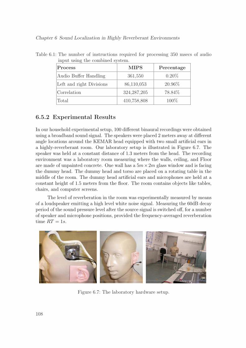
Chapter 6 Sound Localization in Highly Reverberant Environments
Table 6.1: The number of instructions required for processing 350 msecs of audioinput using the combined system.
Process MIPS Percentage
Audio Buffer Handling 361,550 0.20%
Left and right Divisions 86,110,053 20.96%
Correlation 324,287,205 78.84%
Total 410,758,808 100%
6.5.2 Experimental Results
In our household experimental setup, 100 different binaural recordings were obtainedusing a broadband sound signal. The speakers were placed 2 meters away at differentangle locations around the KEMAR head equipped with two small artificial ears ina highly-reverberant room. Our laboratory setup is illustrated in Figure 6.7. Thespeaker was held at a constant distance of 1.3 meters from the head. The recordingenvironment was a laboratory room measuring where the walls, ceiling, and Floorare made of unpainted concrete. One wall has a 5m×2m glass window and is facingthe dummy head. The dummy head and torso are placed on a rotating table in themiddle of the room. The dummy head artificial ears and microphones are held at aconstant height of 1.5 meters from the floor. The room contains objects like tables,chairs, and computer screens.
The level of reverberation in the room was experimentally measured by meansof a loudspeaker emitting a high level white noise signal. Measuring the 60dB decayperiod of the sound pressure level after the source signal is switched off, for a numberof speaker and microphone positions, provided the frequency-averaged reverberationtime RT = 1s.
Figure 6.7: The laboratory hardware setup.
108
6.5 Discussion of Results
To keep a fair comparison with the simulation setup, each of the recordingswas 350 msecs long, and the noise was kept around 20dB below the signal level.The microphones were placed inside the ears at a distance of 26 mm away from theear’s opening. The outside microphones are placed 5 cm away from the inside ones.The recorded sound signals, also containing external and electronic noise, were usedas inputs to the system. A HRIR database reduced using the PCA method, HFIR
m ,was available for the test.
The combined system, without Bayesian fusion, yielded a percentage of correctlocalization between 6% to 74% with the HRIR being within 10 to 45-samples long,i.e. 10 ≤ m ≤ 45. For a full-length HRIR, i.e. 512-samples long, the percentageof correct localization reached 81% under the same reverberation conditions. WithBayesian fusion the localization falls between 19% and 85% for 10 ≤ m ≤ 45. Fora full-length HRIR of order 512, the percentage of correct localization reached 89%under the same reverberation conditions.
Similar to the simulation results, for high order HRIRs, the falsely localizedangles fall in the vicinity of the target sound source. Figure 6.6 illustrates theaverage distance to the target angles. The combined system yielded a worst angularerror of 45.33◦ with a HRIR order of 10, and a best angular of 1.6◦ with a HRIRorder of 128. With Bayesian fusion, the worst angular error reached 24.57◦ with aHRIR order of 10, and the best error 1.2◦ with HRTF order of 100.
It is worth mentioning that common robotic sound localization methods whichuse only 4 microphones fail to localize sound accurately in three dimensions withoutbecoming impractically complex, or without using computer vision to augment theacoustic modality [56]. We have thus compared our experimental results to themethod in [128], (also see chapter 1). This method uses 8 microphones and appliesthe simple TDOA algorithm to localize sound sources in three dimensions. Like in[128], the sounds we have used have a large bandwidth, e.g. fingers snapping andpercussive noises.
The system was tested with sound sources placed at different locations in theenvironment. In each case, the distance and elevation are fixed and recordings aretaken for different horizontal angles. The mean angular error for every arrangementis computed. Table 6.2 shows the performance of our system as compared to thesystem in [128]. Using only 4 microphones, our system performed more accuratelywhen localizing the sound sources placed at the same distance, azimuth and elevationangles as in [128]. It should be noted that part of this error, mainly at shortdistances, is due to the difficulty of precisely placing the source and due to the factthat the speaker employed is not a point source. Other sources of error come fromreverberation on the floor especially for those locations where the source is high.The angular error is almost the same for sources located in the horizontal plane and
109
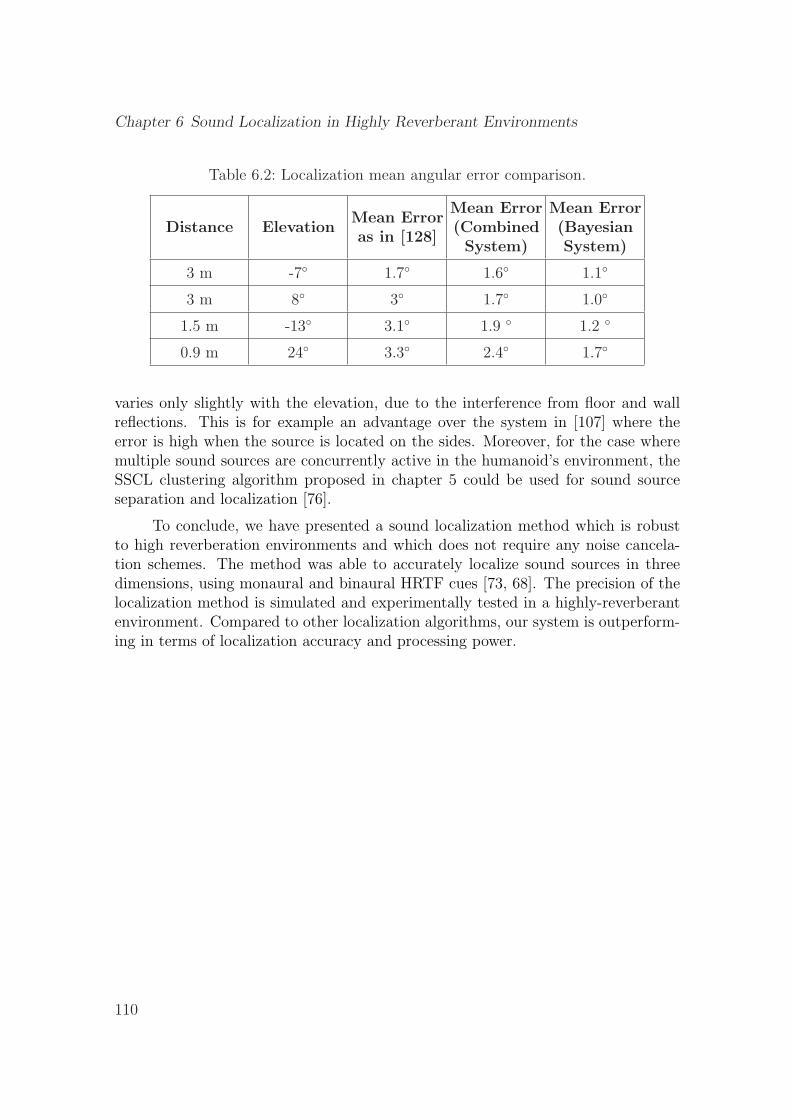
Chapter 6 Sound Localization in Highly Reverberant Environments
Table 6.2: Localization mean angular error comparison.
Distance ElevationMean Erroras in [128]
Mean Error(CombinedSystem)
Mean Error(BayesianSystem)
3 m -7◦ 1.7◦ 1.6◦ 1.1◦
3 m 8◦ 3◦ 1.7◦ 1.0◦
1.5 m -13◦ 3.1◦ 1.9 ◦ 1.2 ◦
0.9 m 24◦ 3.3◦ 2.4◦ 1.7◦
varies only slightly with the elevation, due to the interference from floor and wallreflections. This is for example an advantage over the system in [107] where theerror is high when the source is located on the sides. Moreover, for the case wheremultiple sound sources are concurrently active in the humanoid’s environment, theSSCL clustering algorithm proposed in chapter 5 could be used for sound sourceseparation and localization [76].
To conclude, we have presented a sound localization method which is robustto high reverberation environments and which does not require any noise cancela-tion schemes. The method was able to accurately localize sound sources in threedimensions, using monaural and binaural HRTF cues [73, 68]. The precision of thelocalization method is simulated and experimentally tested in a highly-reverberantenvironment. Compared to other localization algorithms, our system is outperform-ing in terms of localization accuracy and processing power.
110
Chapter 7
Conclusion
It is a difficult challenge to use only one pair of microphones on a robot to mimicthe hearing capabilities of humans. This task is made even more challenging by thefact that the listening environment is dynamic: sound sources appear, disappear,move and interfere with each other. Most of the proposed localization models todayare based on using more than two microphones to detect and track sound in a realenvironment. Mathematical models of sound wave propagation were found to sig-nificantly depend on the specific characteristics of the sources and the environment,and are therefore complex and hard to optimize. Adaptive neural network struc-tures have also been proposed to self-adjust a sound localization model to particularenvironments. While these networks have been intended to work in specificallycontrolled milieus, they become very complex in handling multiple sources in rever-berant environments. Other methods are designed to mimic the human biologicalsound localization mechanism by building models of the outer, middle and inner ear,using knowledge of how acoustic events are transduced and transformed by biolog-ical auditory systems. The difficulty with this approach is that neurophysiologistsdo not completely understand how living organisms localize sounds. For instance, Itremains unclear whether the ITD and ILD cues are combined, in the central nervoussystem, before or after they are spatially mapped. Moreover, the question of whatprimitive mammals like bats experience and how they process sound with only twoears and a pea-sized brain remains a major mystery.
We have proposed a unifying framework for three-dimensional sound localiza-tion methods to be deployed on a humanoid robot operating in a general telepresenceenvironment. Motivated by the important role of the human pinnae to focus andamplify sound, and knowing that the HRTFs can also be interpreted as the di-
111
Chapter 7 Conclusion
rectivity characteristics of the two pinnae, only two microphones in combinationwith a generic HRTF database were required to localize sound sources in a threedimensional space. Common binaural sound localization methods using only twomicrophones fail to localize sound accurately in three dimensions without becomingimpractically complex, or without using computer vision to augment the acousticmodality.
For faster localization performance, the HRTFs are reduced using three dif-ferent model truncation techniques, namely Diffuse-Field Equalization, BalancedModel Truncation, and Principle Component Analysis. Furthermore, for a robustand more accurate localization mechanism, which demonstrates precise azimuth andelevation estimation, we have introduced a novel state-space solution to the HRTFinversion and interpolation problems. Beside its application in our sound localiza-tion system, the stable inversion of transfer functions is of valuable importance forsound synthesis and channel equalization, not only to compensate from deficienciesof the transduction chain (amplifiers, loudspeakers, headphones), but also to repro-duce a spatially coherent sound field. On the other hand, the HRTF interpolationtechnique we have introduced for sound localization purposes can also be used in theimmense field of binaural sound synthesis for high-fidelity reconstruction of HRTFsespecially in cases where fast and immersive synthesis of moving sound sources isneeded.
The initially proposed sound localization method is based on dividing theear signals with the left and right HRTFs and subsequently taking the maximumcorrelation coefficient as a pointer to the source location. This method is enhancedusing proper state-space HRTF inversion. Nevertheless, a new algorithm called crossconvolution was developed to further decrease the computational requirements of theinitial method. In comparison to the previous methods, the cross convolution is ableto achieve remarkable reduction in the processing requirements while increasing theaccuracy of the sound localization. Furthermore, with the help of a simple properlytuned Kalman filter, a ROI was introduced to account for fast moving sound sources.Simulation and experimental results showed a real-time tracking performance and ahigher noise-tolerance capacity. The efficiency of the new algorithm suggests a cost-effective implementation for robot platforms and allows fast localization of movingsound sources.
Using the presented methods, we have addressed the challenging task of bin-aural concurrent sound source localization and separation in reverberant environ-ments. Relying on the concept of binaural hearing, where the human auditory 3Dpercepts are predominantly formed on the basis of the sound-pressure signals atthe two eardrums, our robotic localization system uses only two microphones. Wepresented a new algorithm for binaural localization of concurrent sound sources inboth azimuth and elevation. By exploiting the ILD and IPD binaural cues that
112
are encapsulated within the HRTFs, binaural 3D concurrent sound localization wasmade possible using only two microphones placed inside the artificial ears of theKEMAR head. Compared to existing techniques using microphone arrays for thesame purpose, our algorithm is less complex and very accurate. It was shown thattwo concurrent sound sources could be perfectly localized at their intended 3D lo-cations even in the anti-causal case where both sources share the same hemispherearound the humanoid’s head. This is a remarkable improvement compared to theinitially proposed adaptive MIMO approach.
The self-splitting competitive learning technique, mainly deployed in imageprocessing, turned out to be very reliable for acoustical signal processing. It provedto be an intelligent tool to retrieve the exact cluster centers inside the feature spaceof the impinging sound signals, and consequently, to extract the 3D locations of theconcurrent sound sources. After localization, the proposed sound source separationalgorithm proved to be outperforming compared to other blind source separationmethods solving the same determined problem under the same conditions.
For highly reverberant environments, a new algorithm using four microphonesis presented. Bayesian information fusion is then used to increase the localiza-tion resolution in a three-dimensional reverberant environment. The algorithm wastested in simulations as well as in a household environment. Compared to existingtechniques, the method is able to localize sound sources in three dimensions, underhigh reverberation conditions, with fewer sensors and higher accuracy.
Based on the simplicity of the presented new approach for sound source local-ization, the integration of audio with other modalities like haptic and vision becomespromising. This kind of integration will allow the multi-sensory telepresence systemto improve the perceived degree of immersion for the human operator. Inspiredby the human binaural hearing, this development is adding to the solution andattractiveness of the humanoid hearing technology, as humanoids share many char-acteristics with the human being, which is, after all, the most interesting object ofscientific research.
113

Chapter 7 Conclusion
114
Appendix A
Inner-outer Factorization TheoremProof
Theorem: Let W be a unitary matrix, and Y be a uniformly bounded matrix whichsatisfies the following equality,
[A B
C D
][Y 0
0 I
]=
[Y B0
0 D0
]W (A.1)
such that Y has a maximal dimension and ker(Y.) = 0. Let
W =
[Av Bv
Cv Dv
]. (A.2)
Then {Av, Bv, Cv, Dv} is an isometric realization for the sought inner factor V (z),and {A,B,C0, D0} is a realization for the outer factor Ho(z). The proof of the abovetheorem is detailed in [33].
Proof: Since the Y sought is such that kern(Y.) = 0, using RQ-factorization orSVD, we can always express it as
Y = V
[σ
0
], (A.3)
in which σ is square non-singular and V is unitary.
115
Appendix A Inner-outer Factorization Theorem Proof
We now let ∆ be a block Schur eingenspace decomposition for the term A −BD−1C,
∆ = A−BD−1C = V ?
[δ11 δ12
δ21 δ22
]V, (A.4)
where δ11 collects the eigenvalues of ∆ which are strictly outside the unit circle,thus, causing instability.
Given the state-space realization {A,B, C, D}, and assuming that D is squareinvertible, we can write down the following schur factorization
[A B
C D
]=
[I BD−1
0 I
][∆ 0
0 D
] [I 0
D−1C I
], (A.5)
where ∆ = A−BD−1C is the Schur complement of D. We can now write (A.1) as
[∆ 0
C D
][Y 0
0 I
]W ? =
[I BD−1
0 I
][Y B0
0 D0
]. (A.6)
Looking at the second block column of this equation, we find
[∆ 0
C D
][Y 0
0 I
][W ?
21
W ?22
]=
[Y
0
], (A.7)
where W ?21 = A?
v and W ?22 = B?
v .
From the last equation we can write, ∆Y = Y W−?21 , or W−?
21 = Y +∆Y , where
Y + =[σ−1 0
]V ?, (A.8)
thus
W−?21 =
[σ−1 0
]V ?∆V
[σ
0
](A.9)
= σ−1δ11σ. (A.10)
It is important, at this point, to observe that since W21 = Av = σ?δ−?11 σ−?, the
matrix, δ−?11 , must have its eigenvalues strictly inside the unit disc, achieving thus
the sought system stability.
116
Multiplying (A.7) with Y + we get
[σ−1δ11σ 0
CY D
][W ?
21
W ?22
]=
[I
0
]. (A.11)
Introducing
β = D−1CV
[δ−111
0
],
we find[W ?
21
W ?22
]=
[σ−1δ−1
11 σ 0
−βσ D−1
][I
0
]. (A.12)
Finally, setting M = σ−?σ−1, we obtain the Lyapunov-Stein equation
M = β?β + δ−?11 Mδ−1
11 . (A.13)
Knowing that δ−111 has its eigenvalues strictly inside the unit disc of the complex
plane, (A.13) must have a unique solution, and both W21 = Av and W22 = Bv havealso unique solutions,
[W ?
21 W ?22
]=
[σ?δ−?
11 σ−? −σ?β?]. (A.14)
Once we find both Av and Bv realizations corresponding to the inner-factorV (z), we can proceed to compute Y in (A.3) and use it in (A.1) to solve a systemof four equations for the remaining inner-factor realizations Cv and Dv as well asthe outer-factor, Ho(z), realizations C0 and D0. Finally, the sought stable inverse,H−1(z) = Ho(z)−1V ?(z), is calculated, in which Ho(z)−1 is singular and causal, andV ?(z) is anticausal and stable.
It should be noted that the outer-inner factorization computed using theLyapunov-Stein equation, ensures a linear solution adequate for a fast real-timeimplementation, compared with other methods [139] which solve the same outer-inner factorization problem quadratically using the celebrated Riccati equation, andneedlessly condition a problem which is already well-conditioned.
117

Appendix A Inner-outer Factorization Theorem Proof
118
Appendix B
The State-Space Loewner Matrix
We will recapitulate the major steps involved in computing the L matrix as detailedin [8]. To begin with, the generalized controllability matrix N is first partitioned as
N =[N1 N2
]where N1 = (t1I − A)−1B. Define the term
N = N2 −[N1 N1 . . . N1
]= NJ, (B.1)
where
J =
−I −I . . . −I
I 0 . . . 0
0 I . . . 0
0 0 . . . I
(B.2)
Define next
N = N2 diag[t2I, t3I, . . . , tδI]− t1
[N1, N1, . . . , N1
]
= NJt,(B.3)
where
Jt =
−t1I −t1I . . . −t1I
t2I 0 . . . 0
0 t3I . . . 0
0 0 . . . tδI
(B.4)
119
Appendix B The State-Space Loewner Matrix
Now that N and N are defined, the state-space realizations {A,B,C, D} whichensures a minimum degree for the interpolation transfer-function matrix Y (x) canbe computed according to the following equations,
A = NN ′(NN ′)−1 (B.5)
B = (t1I − A)N
I
0...
0
(B.6)
C =[I 0 . . . 0
]M(r1I − A) (B.7)
D = Y (r1)− C(r1I − A)−1B (B.8)
Note that N should have a full row rank for the inverse in (B.5) to exist. This{A,B, C, D} realization ensures that the transfer-function Y (x) interpolates thedata and has least degree among interpolating transfer-function matrices [8].
120

Appendix C
List of Frequently Used Acronyms
Acronym Description
ADPF Active Direction-Pass Filter
APV Asymptotic Property Vector
BSS Blind Source Separationt
CIPIC Center for Image Processing and Integrated Computing
CPT Conditional Probability Table
CPV Center Property Vector
DLOS Direct Line Of Sight
DOA Direction of Arrival
DFT Discrete Fourier Transform
DPV Distant Property Vector
FFT Fast Fourier Transform
FIR Finite Impulse Response
HRIR Head-Related Impulse Response
HRTF Head-Related Transfer Function
121

Appendix C List of Frequently Used Acronyms
Acronym Description
ICA Independent Component Analysis
IID Interaural Intensity Difference
ILD Interaural Level Difference
IPD Interaural Phase Difference
ITD Interaural Time Difference
ICA Independent Component Analysis
KEMAR Knowles Electronics Mannequin for Acoustic Research
MAMA Minimum Audible Movement Angle
MIMO Multiple-Input Multiple-Output
MISO Multiple-Input Multiple-Output
MIT Massachusetts Institute of Technology
OPTMC One-Prototype-Take-Multiclusters
OPTOC One-Prototype-Take-One-Cluster
SCA Source Cancelation Algorithm
PRTF Pinna-Related Transfer Function
SIMO Single-Input Multiple-Output
SDR Signal-to-Distortion Ratio
SIR Signal-to-Interference Ratio
SNR Signal-to-Noise Ratio
STFT Short-Time Fourier Transform
3D Three-Dimensional
122
Bibliography
[1] P. Aarabi. The fusion of distributed microphone arrays for sound localization.J. Acoust. Soc. Am., (4):338–347, 2003.
[2] P. Aarabi and B. Mungamuru. Scene reconstruction using distributed micro-phone arrays. In Proc. International Conference on Multimedia and Expo,pages 53–56, 2003.
[3] R. Aichner, H. Buchner, F. Yan, and W. Kellermann. Real-time convolutiveblind source separation based on a broadband approach. In Proc. Int. Symp.ICA, pages 833–840, Granada, Spain, 2004.
[4] V. Algazi, R. Duda, R. Duraiswami, N. Gumerov, and Z. Tang. Approximatingthe head-related transfer function using simple geometric models of head andtorso. J. Acoust. Soc. Am., 112(5):2053–2064, 2002.
[5] V. Algazi, R. Duda, D. Thompson, and C. Avendano. Structural compositionand decomposition of hrtfs. In Proc. IEEE Workshop on Appl. of Sig. Proc.to Aud. and Acc., pages 103–106, New Paltz, NY, 2001.
[6] V. R. Algazi, R. O. Duda, D. M. Thompson, and C. Avendano. The cipichrtf database. In Proc. 2001 IEEE Work. on Appl. of Sig. Proc. to Audioand Electroacoustics, pages 21–24, New Paltz, NY, 2001. HRTF data sets areavailable at http://interface.cipic.ucdavis.edu/.
[7] J.B. Allen and D.A. Berkley. Image method for efficiently simulating small-room acoustics. J. Acoust. Soc. Am., 65(4):943–950, 1979.
[8] B.D.O. Anderson and A.C. Antoulas. Rational interpolation and state-variablerealizations. Linear Algebra and its Applications, 137:479 – 509, 1990.
[9] S. Andersson, A. Handzel, V. Shah, and P. Krishnaprasad. Robot phono-taxis with dynamic sound-source localization. In Proc. IEEE InternationalConference on Robotics and Automation, pages 4833–4838, 2004.
123
Bibliography
[10] A.C. Antoulas and B.D.Q. Anderson. On the scalar rational interpolationproblem. IMA J.Math. Control and Inorm., 3:61–81, 1986.
[11] F. Avanzini, D. Rocchesso, and S. Serafin. Friction sounds for sensory substi-tution. In Proc. Int. Conf. on Auditory Display, volume 4, pages 1–8, 2004.
[12] D. W. Bateau. Listening with the naked ear. S. J. Freedman, editor, Neuropsy-chology of Spatially Oriented Behavior. Dorsey Press, Homewood, IL. USA,1968.
[13] D. Begault, M. Godfroy, J. Miller, A. Roginska, M. Anderson, and E. Wen-zel. Design and verification of headzap, a semi-automated hrir mea-surement system. In Proc. 120th Convention of the Audio Engineer-ing Society, Paris, France, 2006. Product information can be found athttp://ausim3d.com/products.
[14] D.R. Begault. 3-d sound for virtual reality and multimedia. Academic Press,1994.
[15] B. Beliczynski, I. Kale, and G.D. Cain. Low-order modeling of head-relatedtransfer functions using balanced model truncation. IEEE Trans. Signal Pro-cessing, 40(3):532–542, 1997.
[16] E. Ben-Reuven and Y. Singer. Discriminative binaural sound localization. InProc. Neural Information Processing Systems (NIPS), pages 1229–1236, 2002.
[17] L. Bernstein, C. Trahiotis, M. Akeroyd, and K. Hartung. Sensitivity to briefchanges of interaural time and interaural intensity. J. Acoust. Soc. Am.,109:1604–1615, 2001.
[18] S. Blackman and R. Popoli. Design and analysis of modern tracking sys-tems(Book). Norwood, MA: Artech House, 1999.
[19] J. Blauert. An introduction to binaural technology. In Binaural and SpatialHearing, pages 593–609, R. Gilkey, T. Anderson, Eds., Lawrence Erlbaum,USA-Hilldale NJ, 1997.
[20] A. Blin, S. Araki, and S. Makino. A sparseness mixing matrix estimation(smme) solving the underdetermined bss for convolutive mixtures. In Proc.IEEE Int. Conference on Acoustics, Speech and Signal Processing, volume 4,pages 85–88, Genua, Italy, 2004.
[21] S. E. Boehnke, S. E. Hall, and T. Merquadt. Detection of static and dynamicchanges in interaural correlation. J. Acoust. Soc. Am., 112:1617–1626, 2002.
124
Bibliography
[22] P. Bofill and M. Zibulevsky. Blind separation of more sources than mixturesusing sparsity of their short-time fourier transform. In Proc. Int. WorkshopIndependent Component Anal. Blind Signal Separation, page 8792, Helsinki,Finland, June 2000.
[23] J. Braasch. Localization in the presence of a distracter and reverberation inthe frontal horizontal plane. ACUSTICA/acta acustica, 88:956–969, 2002.
[24] H. Buchner, R. Aichner, and W. Kellermann. A generalization of blind sourceseparation algorithms for convolutive mixtures based on second-order statis-tics. IEEE Transactions on Speech and Audio Processing, 13(1):120–134, 2005.
[25] H. Buchner, R. Aichner, and W. Kellermann. A real-time blind source sepa-ration scheme and its application to reverberant and noisy acoustic environ-ments. Signal Processing, 86:1260–1277, 2006.
[26] J. Merimaa C. Faller. Source localization in complex listening situations:selection of binaural cues based on interaural coherence. J. Acoust. Soc. Amer.,116:3075–3089, 2004.
[27] S. Carlile and D. Pralong. The location-dependent nature of perceptuallysalient features of the human head-related transfer functions. J. Acoust. Soc.Am., 95(6):3445–3459, 1994.
[28] C. Cheng and G. Wakefield. Spatial frequency response surfaces (sfrs’s): Analternative visualization and interpolation technique for head-related transferfunctions (hrtf’s). In Proc. of the 16th Audio Eng. Soc. (AES) Int. Conf. onSpatial Sound Reproduction, pages 961–964, Rovaniemi, Finland, 1999.
[29] P. Chiang-Jung, J. Harris, and J. Principe. A neuromorphic microphone forsound localization. In Proc. IEEE/RSJ Intl. Conf. on Intell. Rob. and Sys.,pages 1147–1152, USA, 2003.
[30] Y. Cohen and E. Knudsen. Representation of binaural spatial cues in field lof the barn owl forebrain. J. Neurophysiol, 79:879–890, 1998.
[31] H. Colburn and J. Latimer. Theory of binaural interaction based on auditory-nerve data, iii. joint dependence on inter-aural time and amplitude differencesin discrimination and detection. J. Acoust. Soc. Am., 64:95–106, 1978.
[32] J. Culling and H. Colburn. Binaural sluggishness in the perception of tonesequences and speech in noise. J. Acoust. Soc. Am., 79:1939–1949, 1986.
125
Bibliography
[33] P. Dewilde and A. J. van der Veen. Inner-outer factorization and the inversionof locally finite systems of equations. Linear Algebra and Its Applications,313:53–100, 2000.
[34] R. Duda and W. Martens. Range depend-ence of the response of a sphericalhead model. J. Acoust. Soc. Am., 104(5):3048–3058, 1998.
[35] R. Duraiswami, L. Zhiyun, D. Zotkin, E. Grassi, and N. Gumerov. Plane-wavedecomposition analysis for spherical microphone arrays. In Proc. IEEE Wrok.on Appl. of Sig. Proc. to Audio and Acoustics (WASPAA), pages 150–153,2005.
[36] O. Faugeras, editor. Three Dimensional Computer Vision: A Geometric View-point. MA: MIT Press, Cambridge, 1993.
[37] H. Fisher and S. Freedman. The role of the pinna in auditory localization. J.Audit. Res., 8:15–26, 1968.
[38] K. Fukudome, Y. Tashiro, K. Takenouchi, T. Samejima, and N. Ono. De-velopment of the fast measurement system for the listener’s own head-relatedimpulse responses. J. Acoust. Soc. Am., 120(5):3094(A), 2006.
[39] W. G. Gardner and K. D. Marting. Hrtf measurements of a kemar. J. Acoust.Soc. Amer., 97(6):3907–3908, 1995.
[40] D. Grantham. Detection and discrimination of simulated motion of auditorytargets in the horizontal plane. J. Acoust. Soc. Am., 107:517–527, 2000.
[41] E. Grassi and S. Shamma. A biologically inspired, learning, sound localizationalgorithm. In Proc. Conference on Information Sciences and Systems, pages344–348, 2001.
[42] S. Handel. Space is to time as vision is to audition: seductive but misleading.Journal of Experimental Psychology: Human Perception and Performance,(14):315–317, 1988.
[43] A. Handzel. Planar spherical diffraction-arrays: Linear sound localization al-gorithms. In Proc. Fourth IEEE Workshop on Sensor Array and MultichannelProcessing, pages 655–658, 2006.
[44] A. Handzel and P. Krishnaprasad. Biomimetic sound-source localization. In-formation Fusion (Special Issue on Robust Speech Processing), 5(2):131–140,2004.
126
Bibliography
[45] K. Hartung, J. Braasch, and S. Sterbing. Comparison of different methods forthe interpolation of head-related transfer functions. In proc. of 6th Aud. Eng.Soc. (AES) Int. Conf. on Spatial Sound Reprod., pages 19–28, Rovaniemi,Finland., 1999.
[46] T. Horiuchi. ”seeing” in the dark: neuromorphic vlsi modeling of bat echolo-cation. IEEE Signal Processing Magazine, pages 134–139, 2005.
[47] S. Hosoe, T. Nishino, K. Itou, and K. Takeda. Measurement of head-relatedtransfer functions in the proximal region. In Proc. Forum Acusticum, pages2539–2542, Budapest, Hungary, 2005.
[48] J. Hrnstein, M. Lopes, J. Santos-Victor, and F. Lacerda. Sound localizationfor humanoid robots - building audio-motor maps based on the hrtf. In Proc.IEEE/RSJ Int. Conf. on Intelligent Robots and Systems (IROS), pages 1170–1176, Beijing, China, October 2006.
[49] J. Huang, K. Kume, A. Saji, M. Nishihashi, T. Watanabe, and W. Martens.Robotic spatial sound localization and its 3-d sound human interface. InProc. of the IEEE First Int. Symp. on Cyber Worlds (CW.02), pages 191–197, Tokyo, Japan, November 2002.
[50] J. Huang, N. Ohnishi, X. Guo, and N. Sugie. A computational model of theprecedence effect based on echo-avoidance. In Proc. ASA/ASJ Third JointMeeting, page 635640, Dec. 1996.
[51] J. Huang, N. Ohnishi, and N. Sugie. Sound localization in reverberant envi-ronment based on the model ofthe precedence effect. IEEE Transactions onInstrumentation and Measurement, 1997.
[52] J. Huang, N. Ohnishi, and N. Sugie. Spatial localization of sound sources:Azimuth and elevation estimation. In Proc. IEEE Instrumentation and Mea-surement Conference, pages 330–333, USA, May 1998.
[53] R. E. Irie. Robust sound localization: an application of an auditory perceptionsystem for a humanoid robot. Master’s thesis, Massachussets Institute ofTechnology, June 1995.
[54] L. Jeffress. A place theory of sound localization. J. Comp. Phsiol. Psychol.,41:35–39, 1948.
[55] F. V. Jensen. An Introduction to Bayesian Networks. Springer Verlag, NewYork, 1996.
127
Bibliography
[56] P. Julian, A. Andreou, L. Riddle, S. Shamma, D. Goldberg, and G. Cauwen-berghs. A comparative study of sound localization algorithms for energy awaresensor network nodes. IEEE Transactions on Circuits and Systems I: Funda-mental Theory and Applications, 51(4):640 – 648, 2004.
[57] C.H. Keller and T.T. Takahashi. Localization and identification of con-current sounds in the owl’s auditory space map. Journal of Neuroscience,25(45):10446–10461, 2005.
[58] F. Keyrouz and K. Diepold. Artificial neural network based sound localiza-tion. Technical Report LDV-TR-M4-02, TU Munchen, Lehrstuhl fur Daten-verarbeitung (LDV), 2006.
[59] F. Keyrouz and K. Diepold. Efficient state-space rational interpolation ofhrtfs. In Proc. Audio Eng. Soc. (AES) 28th Intl. Conf., pages 185–189, Pitea,Sweden, 2006.
[60] F. Keyrouz and K. Diepold. An enhanced binaural 3d sound localizationalgorithm. In proceedings of IEEE Int. Symposium on Signal Processing andInf. Technology (ISSPIT), pages 663–665, Vancouver, Canada, 2006.
[61] F. Keyrouz and K. Diepold. Monaurale lokalisierung. Technical Report LDV-TR-M4-07, TU Munchen, Lehrstuhl fur Datenverarbeitung (LDV), 2006.
[62] F. Keyrouz and K. Diepold. A rational hrtf interpolation approach for fastrendering of moving sound. In Proc. IEEE Digital Signal Processing (DSP)Workshop, pages 222–226, Yellowstone, Whyoming, USA, 2006.
[63] F. Keyrouz and K. Diepold. Robotic sound detection: A novel human-basedapproach. In Proc. Of the 2nd Int. Workshop on Human-Centered RoboticSystems (HCRS’06), pages 25–31, Munich, Germany, 2006.
[64] F. Keyrouz and K. Diepold. Sound localization techniques: Implementationand comparison. Technical Report LDV-TR-M4-01, TU Munchen, Lehrstuhlfur Datenverarbeitung (LDV), 2006.
[65] F. Keyrouz and K. Diepold. Tracking of fast moving sources using kalmanfilters. Technical Report LDV-TR-M4-03, TU Munchen, Lehrstuhl fur Daten-verarbeitung (LDV), 2006.
[66] F. Keyrouz and K. Diepold. Binaural source localization and spatial audioreproduction for telepresence applications. Presence: Teleoperators and Vir-tual Environments, Special Issue on High Fidelity Telepresence II, MIT Press,15(2):509–522, 2007.
128
Bibliography
[67] F. Keyrouz and K. Diepold. Implementation of a real-time 3d sound render-ing system. Technical Report LDV-TR-M4-06, TU Munchen, Lehrstuhl furDatenverarbeitung (LDV), 2007.
[68] F. Keyrouz and K. Diepold. Robotic binaural and monaural information fusionusing bayesian networks type of communication. In Proc. 5th IEEE Int. Symp.on Intelligent Signal Processing, pages 79–83, Madrid, Spain, October 2007.(Excellent top 10 paper).
[69] F. Keyrouz and K. Diepold. A new hrtf interpolation approach for fast synthe-sis of dynamic environmental interaction. Audio Engineering Society (AES)Journal, January 2008.
[70] F. Keyrouz and K. Diepold. Self-splitting competitive learning for binauralsound localization and separation in telerobotics. International Journal of In-formation Technology and Intelligent Computing (ITIC), IEEE ComputationalIntelligence Society, 1, 2008. (Accepted for publication).
[71] F. Keyrouz and K. Diepold. A novel biologically-inspired neural network so-lution for robotic 3d sound source sensing. Soft Computing Journal, Springer,February 2008. (Accepted for publication).
[72] F. Keyrouz, K. Diepold, and P. Dewilde. Robust 3d robotic sound localizationusing state-space hrtf inversion. In proceedings of IEEE Int. Conf. on Roboticsand Biomimetics (ROBIO), pages 245–250, Kunming, China, 2006. (BestPaper Award Nomination).
[73] F. Keyrouz, K. Diepold, and S. Keyrouz. High performance 3d sound lo-calization for surveillance applications. In Proc. of IEEE Int. Conference onAdvanced Video and Signal Based Surveillance (AVSS), London, UK, 2007.
[74] F. Keyrouz, K. Diepold, and S. Keyrouz. Humanoid binaural sound trackingusing kalman filtering and hrtfs. Book of Robot Motion and Control: Lec-ture Notes in Control and Information Sciences (LNCIS), Springer Verlag,London, pages 329–340, 2007.
[75] F. Keyrouz, K. Diepold, and S. Keyrouz. Kalman filtering for three dimen-sional sound tracking. In Proc. 6th IEEE Int. Workshop on Robot Motion andControl, pages 114–118, Poland, June 2007.
[76] F. Keyrouz and S. Keyrouz. Humanoid monaural sound localization usingusupervised clustering. In Proc. IEEE Int. Conference on Signal Processingand Communication (ICSPC07), Dubai, November 2007. (Accepted for pub-lication).
129
Bibliography
[77] F. Keyrouz, F. Lazarno-blasco, and K. Diepold. Hierarchical fuzzy neuralnetworks for robotic 3d sound source sensing. Lecture Notes in ComputerScience (LNCS), Springer Verlag, 2007. (Accepted for publication).
[78] F. Keyrouz, F. Lazaro-blasco, and K. Diepold. Robotic sound detection basedon hierarchical neural networks. In Proc. IEEE intl. Symp. on Neural Networks(ISNN), China, 2007.
[79] F. Keyrouz, W. Maier, and K. Diepold. A novel humanoid binaural 3d soundlocalization and separation algorithm. In Proc. IEEE-RAS International Con-ference on Humanoid Robots (Humanoids06), page 296301, Genua, Italy, De-cember 2006.
[80] F. Keyrouz, W. Maier, and K. Diepold. Robotic binaural localization andseparation of more than two concurrent sound sources. In Proc. IEEE Int.Symposium on Signal Processing and its Applications (ISSPA), United ArabEmirates, 2007. 225-230.
[81] F. Keyrouz, W. Maier, and K. Diepold. Robotic localization and separationof concurrent sound sources using self-splitting competitive learning. In Proc.of the First IEEE Symposium on Computational Intelligence in Image andSignal Processing (CIISP), Hawaii, 2007. 340-345.
[82] F. Keyrouz, Y. Naous, and K. Diepold. A new method for binaural 3d local-ization based on hrtfs. In proceedings of IEEE Int. Conf. on Acoustics, Speech,and Signal Processing (ICASSP), pages 341–344, Toulouse, France, May 2006.
[83] F. Keyrouz, A. Abou Saleh, and K. Diepold. Intelligent sound localizationbased on head-related transfer functions extraction. In Proc. IEEE 3rd Int.Conf. on Intelligent Computer Comm. and Proc.(ICCP), pages 42–46, Roma-nia, 2007.
[84] F. Keyrouz, A. Bou Saleh, and K. Diepold. A novel approach to monauralsound localization. In Proc. 122nd Audio Engineering Society (AES) Conven-tion, Vienna, Austria, May 2007.
[85] F. Keyrouz, M. Usman, and K. Diepold. Real time 3d humanoid soundsource localization in actual environments. In IEEE 21st Canadian Confer-ence on Electrical and Computer Engineering (CCECE08), Ontario, Canada,May 2008. (Accepted for publictation).
[86] F. Keyrouz, M. Usman, and K. Diepold. Real time humanoid sound source lo-calization and tracking in a highly reverberant environment. In Proc. 4th IEEEInt. Coll. on Signal Processing and its Applications (CSPA), Kuala Lumpur,Malaysia, March 2008. (Accepted for publictation).
130
Bibliography
[87] D.J. Kistler and F.L. Wightman. A model of head-related transfer functionsbased on principal components analysis and minimum-phase reconstruction.J. Acoust. Soc. Amer., 91(3):1637–1647, 1992.
[88] C. Knapp and G. Carter. The generalized correlation method for estimationof time delay. IEEE Transactions on Acoustics, Speech, and Signal Processing,24(4):320–327, 1976.
[89] G. Kuhn. Model for the inter-aural time differences in the azimuthal plane.J. Acoust. Soc. Am., 62:157–167, 1977.
[90] G. Metta L. Natale and G. Sandini. Development of auditory-evoked reflexes:Visuo-acoustic cues integration in a binocular head. Robotics and AutonomousSystems, 39(2):87–106, 2002.
[91] Itakura Laboratory. Database of head related transfer functions, 1999.http://www.itakura.nuee.nagoya-u.ac.jp/.
[92] P. Lax and R. Phillips, editors. Scarrering Theory. Academic Press, NY, 1989.
[93] Paris France 2002 Listen HRTF Database, IRCAM. HRTF data sets areavailable at http://recherche.ircam.fr/equipes/salles/listen.
[94] C. Liu and B. Wheeler et al. Localization of multiple sound sources with twomicrophones. Journal of the Acoustical Society of America, 108(4):1888–1905,2000.
[95] J. Mackenzie, J. Huopaniemi, V. Vlimki, and I. Kale. Low-order modeling ofhead-related transfer functions using balanced model truncation. IEEE SignalProcessing Letters, 4(2):39–41, 1997.
[96] W. Martens. Principal components analysis and resynthesis of spectral cuesto perceived direction. In Proc. of the Int. Computer Music Conference, pages274–281, 1987.
[97] M. Matsumoto, S. Yamanaka, and M. Tohyama. Effect of arrival time correc-tion on the accuracy of binaural impulse response interpolation. Journal ofthe Audio Engineering Society, 52:56–61, 2004.
[98] J. Middlebrooks. Narrow-band sound localization related to external ear acous-tics. J. Acoust. Soc. Am., 92(5):2607–2624, 1992.
[99] J. Middlebrooks and D. Green. Observations on a principal components anal-ysis of head-related transfer functions. J. Acoust. Soc. Amer., 92(1):597–599,1992.
131
Bibliography
[100] W. Mills. Auditory localization. Foundations of modern auditory theory,II:303–348 (New York, NY, Academic Press), 1972.
[101] H. Moeller. Fundamentals of binaural technology. Appl. Acoust., 36(3-4):171–218, 1992.
[102] M. Murase, S. Yamamoto, and J. Valin et al. Multiple moving speaker trackingby microphone array on mobile robot. In Proc. European Conf. on Speech Com-munication and Technology (Interspeech), pages 249–252, September 2005.
[103] M. Murase, S. Yamamoto, J. Valin, and et al. Multiple moving speaker track-ing by microphone array on mobile robot. In Proc. European Conference onSpeech Communication and Technology (Interspeech), volume 1, pages 143–145, 2005.
[104] J. Murray, H. Erwin, and S. Wermter. Recurrent neural network for sound-source motion tracking and prediction. In Proc. IEEE Int. Joint Conf. onNeural Network (IJCNN), volume 4, pages 2232–2236, 2005.
[105] K. Nakadai, D. Matsuura, H. Okuno, and H. Kitano. Applying scattering the-ory to robot audition system. In Proceedings of IEEE/RSJ International Con-ference on Intelligent Robots and Systems (IROS), pages 1147–1152, Japan,September 2004.
[106] K. Nakadai, H. Okuno, and H. Kitano. Auditory fovea based speech separationand its application to dialog system. In Proceedings of IEEE/RSJ Interna-tional Conference on Intelligent Robots and Systems (IROS), pages 1320–1325,Geneva, October 2002.
[107] K. Nakadai, H. G. Okuno, and H. Kitano. Realtime sound source localiza-tion and separation for robot audition. In Proc. IEEE Int. Conf. on SpokenLanguage Processing, pages 193–196, 2002.
[108] H. Okuno, K. Nakadai, K. Hidai, H. Mizoguchi, and H. Kitano. Human-robotinteraction through real-time auditory and visual multiple-talker tracking. InProceedings of IEEE/RSJ International Conference on Intelligent Robots andSystems (IROS), pages 1402–1409, Hawaii, October 2001.
[109] J. Plogsties P. Minaar and F. Christensen. Directional resolution of head-related transfer functions required in binaural synthesis. Journal of the AudioEngineering Society, 53(10):919–929, 2005.
[110] S. Perrett and W. Noble. The effect of head rotations on vertical plane soundlocalization. J. Audit. Res., 102(4):2325–2332, 1997.
132
Bibliography
[111] B. Radlovic, R. Williamson, and R. Kennedy. Equalization in an acousticreverberant environment: Robustness result. In Proc. IEEE Transactions onSpeech and Audio Processing, volume 8, page 311319, 2000.
[112] V. C. Raykara and R. Duraiswami. Extracting the frequencies of the pinnaspectral notches in measured head related impulse responses. J. Acoust. Soc.Am., 118(1):364–374, 2005.
[113] J. Strutt (Lord Rayleigh). On our perception of sound direction. PhilosophicalMagazine, 13:214–232, 1907.
[114] K. Riederer. HRTF analysis: Objective and subjective evaluation of measuredhead-related transfer functions. Phd dissertation, Laboratory of Acoustics andAudio Signal Processing, Helsinki University of Technology, Espoo, Finland,2005.
[115] S.M. Robeson. Spherical methods for spatial interpolation: review and evalu-ation. Cartography and Geographic Information Systems, 24(1):3–20, 1997.
[116] Y. Rui and D. Florencio. New direct approaches to robust sound source local-ization. In Proc. of IEEE International Conf. on Multimedia Expo (ICME),pages 6–9, 2003.
[117] T. Shimoda, T. Nakashima, M. Kumon, R. Kohzawa, I. Mizumoto, andZ. Iwai. Spectral cues for robust sound localization with pinnae. In Proceed-ings of IEEE/RSJ International Conference on Intelligent Robots and Systems(IROS), pages 386–391, China, October 2006.
[118] B. Shinn-Cunningham and A. Kulkarni. Recent developments in virtual au-ditory space. Simon Carlile, Ed., Virtual Auditory space: Generation andApplications, pages 185–243, (Austin, TX: R. G. Landes Company), 1996.
[119] B. Shinn-Cunningham, S. Santarelli, and N. Kopco. Tori of confusion: Binau-ral cues for sources within reach of a listener. J. Acoust. Soc. Am., 107(3):1627–1636, 1999.
[120] A. Steinhauser. The theory of binaural audition. Phil. Mag., 7:261–274, 1877.
[121] L. Sbaiz T. Ajdler and M. Vetterli. The plenacoustic function on the circlewith application to hrtf interpolation. In proceedings of IEEE ICASSP, 2005.
[122] S. Takane, D. Arai, T. Miyajima, K. Watanabe, Y. Suzuki, and T. Sone.A database of head-related transfer functions in whole directions on upperhemisphere. Acoustical Science and Technology, 23(2):160–162, 2002. HRTFdata sets are available at the Suzuki Laboratory, Tohoku University, Japan,http://www.ais.riec.tohoku.ac.jp.
133
Bibliography
[123] Y. Tamai, Y. Sasaki, S. Kagami, and H. Mizoguchi. Three ring microphonearray for 3d sound localization and separation for mobile robot audition. InProc. IEEE International Conference on Intelligent Robots and Systems, pages4172–4177, USA, 2005.
[124] I. Toshima and S. Aoki. The effect of head movement on sound localizationin an acoustical telepresence robot: TeleHead. In Proceedings of IEEE/RSJInternational Conference on Intelligent Robots and Systems (IROS), pages872–877, China, October 2006.
[125] I. Toshima, S. Aoki, and T. Hirahara. An acoustical tele-presence robot: Tele-Head II. In Proceedings of IEEE/RSJ International Conference on IntelligentRobots and Systems (IROS), pages 2105–2110, Japan, September 2004.
[126] J. Valin, F. Michaud, J. Rouat, and D. Ltourneau. Robust sound sourcelocalization using a microphone array on a mobile robot. In Proc. IEEE/RSJInt. Conf. on Intelligent Robots and Systems (IROS), pages 1228– 1233, Oct.2003.
[127] J. Valin, J. Rouat, and F. Michaud. Enhanced robot audition based on mi-crophone array source separation with post-filter. In Proc. IEEE/RSJ Inter-national Conference on Intelligent Robots and Systems (IROS)), pages 1033–1038, 2004.
[128] J. M. Valin, F. Michaud, J. Rouat, and D. Ltourneau. Robust sound sourcelocalization using a microphone array on a mobile robot. In Proc. IEEE Intl.Conf. on Intelligent Robots and Systems, pages 1228–1233, Saitama, Japan,2003.
[129] E. Vincent, R. Gribonval, and C. Fevotte. Performance measurement in blindaudio source separation. IEEE Transactions on Audio, Speech and LanguageProcessing, 14(4):1462–1469, 2006.
[130] A. Vljame, P. Larsson, D. Vstfjll, and M. Kleiner. Auditory presence, indi-vidualized head-related transfer functions, and illusory ego-motion in virtualenvironments. In Proc. Presence, pages 141–147, Valencia, Spain, Oct. 2004.
[131] H. Wallach. On sound localization. J. Acoust. Soc. Am., 10(4):270–274, 1939.
[132] G. Welch and G. Bishop. An intoduction to the kalman filter. Tr95-041 tech.rep., Univ. of North Carolina, Department of Computer Science, 1995.
[133] E. Wenzel, M. Arruda, D. Kistler, and F. Wightman. Localization using nonin-dividualized head-related transfer functions. J. Acoust. Soc. Am., 94:111–123,1993.
134
Bibliography
[134] F. Wightman and D. Kistler. Headphone simulation of free-field listening:Stimulus synthesis. J. Acoust. Soc. Am., 1989.
[135] F. Wightman and D. Kistler. The dominant role of low-frequency interauraltime differences in sound localization. J. Acoust. Soc. Am., 91(3):1648–1661,1992.
[136] V. Willert, J. Eggert, J. Adamy, R. Stahl, and E. Krner. A probabilisticmodel for binaural sound localization. IEEE Transactions on Systems, Man,and Cybernetics, 36(65):982–994, 2006.
[137] K. Wilson and T. Darrel. Improving audio source localization by learningthe precedence effect. In Proc. IEEE International Conference on Acoustics,Speech, and Signal Processing, volume 4, pages 1125–1128, 2005.
[138] S. Winter, W. Kellermann, H. Sawada, and S. Makino. Map based underde-termined blind source separation of convolutive mixtures by hierarchical clus-tering and l1-norm minimization. EURASIP Journal on Advances in SignalProcessing, page Article ID 24717, 2007.
[139] K. Yamada and K. Watanabe. Inner-outer factorization for the discrete-timestrictly proper systems. In proceedings of IEEE 35th Conf. on Decison andControl, pages 1491–1492, 1996.
[140] Y.-J. Zhang and Z.-Q. Liu. Self-splitting competitive learning: A new on-lineclustering paradigm. IEEE Transactions on Neural Networks, 13(2):369–380,2002.
[141] D. Zotkin, R. Duraiswami, E. Grassi, and N. Gumerov. Fast head re-lated transfer function measurement via reciprocity. J. Acoust. Soc. Am.,120(4):2202–2215, 2006.
135