Embed Size (px)
Citation preview
Dynamics of Localization Phenomena for
Hardcore Bosons in Optical Lattices
Diplomarbeit
an der Physikalisch-Astronomischen Fakultatder Friedrich-Schiller Universitat Jena,
durchgefuhrtam Max-Planck-Institut fur Quantenoptik in Garching
Birger Horstmann (Matrikelnummer 55625)Enzianstraße 7
85748 Garching, [email protected]
Betreuer:Prof. Dr. J. Ignacio Cirac (Dr. Tommaso Roscilde)
Theory Devision MPQ Garching
Garching, Marz 2007
ABSTRACT
Quantum particles propagating in static disorder can become localized in a finiteregion of space, even for energies for which classical motion is not bounded,a phenomenon known as Anderson localization. There have been proposalsand experimental attempts to observe Anderson localization in systems of coldatoms. In these experiments, where a disordered potential was introduced byusing laser speckles or incommensurate lattices, non-classical localization bycoherent backscattering could not be achieved due to the long length scale ofthe disordered potential or strong interactions between the atoms.
We analyse a system of cold atoms in an optical lattice in presence of disordercreated by the interaction with a different immobile/frozen species of atoms.Two distinguishable species of particles in optical lattices can be realized bypreparing a mono-atomic gas into two different internal states of the atoms.The atoms are prepared in a Tonks-Girardeau gas, i.e. a one-dimensional systemof hard-core bosons, that has been realized in experiments and can be solvedexactly by numerical diagonalization.
For this kind of disorder we find that initially confined particles remainlocalized during time evolution for any value of the interaction strength betweenthe two species and that the quasi-condensation, present in a Tonks-Girardeaugas without disorder, disappears in the presence of disorder.
CONTENTS
1. Introduction . . . . . . . . . . . . . . . . . . . . . . . . . . . . . . . . . 5
2. Disordered Systems . . . . . . . . . . . . . . . . . . . . . . . . . . . . . 92.1 Localization in One-Dimensional Disorder Potentials . . . . . . . 92.2 Participation Ratio . . . . . . . . . . . . . . . . . . . . . . . . . . 102.3 Random Dimer Model . . . . . . . . . . . . . . . . . . . . . . . . 11
3. System and Method . . . . . . . . . . . . . . . . . . . . . . . . . . . . 133.1 Hamiltonian Dynamics . . . . . . . . . . . . . . . . . . . . . . . . 133.2 Jordan-Wigner Transformation and Implementation . . . . . . . 16
3.2.1 Jordan-Wigner Transformation . . . . . . . . . . . . . . . 163.2.2 One-Particle Density Matrix . . . . . . . . . . . . . . . . 173.2.3 Time Evolution . . . . . . . . . . . . . . . . . . . . . . . . 213.2.4 Real Space Properties . . . . . . . . . . . . . . . . . . . . 233.2.5 Coherence and Condensation . . . . . . . . . . . . . . . . 24
3.3 Disorder Averaging . . . . . . . . . . . . . . . . . . . . . . . . . . 263.3.1 Disorder Weights . . . . . . . . . . . . . . . . . . . . . . . 263.3.2 Ground State of Frozen Bosons . . . . . . . . . . . . . . . 273.3.3 Random Disorder . . . . . . . . . . . . . . . . . . . . . . . 313.3.4 Monte Carlo Sampling . . . . . . . . . . . . . . . . . . . . 32
3.4 Characteristics of Disorder . . . . . . . . . . . . . . . . . . . . . . 363.4.1 Statistics of Clusters . . . . . . . . . . . . . . . . . . . . . 363.4.2 Correlation Function . . . . . . . . . . . . . . . . . . . . . 38
4. Ground State Properties . . . . . . . . . . . . . . . . . . . . . . . . . . 414.1 Localization . . . . . . . . . . . . . . . . . . . . . . . . . . . . . . 414.2 Quasi-Condensation . . . . . . . . . . . . . . . . . . . . . . . . . 42
5. Dynamical Properties in a Trap . . . . . . . . . . . . . . . . . . . . . . 465.1 Localization . . . . . . . . . . . . . . . . . . . . . . . . . . . . . . 46
5.1.1 Rabi Oscillations . . . . . . . . . . . . . . . . . . . . . . . 465.1.2 Time Averaged Participation Ratio . . . . . . . . . . . . . 495.1.3 Disorder Strengths, Initial Conditions, and Number of
Particles . . . . . . . . . . . . . . . . . . . . . . . . . . . . 515.2 Quasi-Condensation . . . . . . . . . . . . . . . . . . . . . . . . . 545.3 Harmonic Confinement . . . . . . . . . . . . . . . . . . . . . . . . 57
Contents 4
6. Transport Properties . . . . . . . . . . . . . . . . . . . . . . . . . . . . 616.1 Localization . . . . . . . . . . . . . . . . . . . . . . . . . . . . . . 61
6.1.1 Disorder without Long-Range Correlations . . . . . . . . 616.1.2 Disorder with Long-Range Correlations . . . . . . . . . . 66
6.2 Quasi-Condensation . . . . . . . . . . . . . . . . . . . . . . . . . 726.2.1 Time Evolution Starting from Mott Insulator . . . . . . . 726.2.2 Time Evolution Starting from Superfluid . . . . . . . . . 80
7. Experimental Realization . . . . . . . . . . . . . . . . . . . . . . . . . 867.1 Interaction between Light and Matter . . . . . . . . . . . . . . . 867.2 Optical Lattice . . . . . . . . . . . . . . . . . . . . . . . . . . . . 897.3 Bose-Hubbard Model . . . . . . . . . . . . . . . . . . . . . . . . . 907.4 State Dependent Lattices . . . . . . . . . . . . . . . . . . . . . . 927.5 Measurement of Localization Effects . . . . . . . . . . . . . . . . 94
8. Conclusion . . . . . . . . . . . . . . . . . . . . . . . . . . . . . . . . . 96
9. Acknowledgements . . . . . . . . . . . . . . . . . . . . . . . . . . . . . 97
Appendix 98
A. Markov Processes and Stochastic Matrices . . . . . . . . . . . . . . . . 99
B. Statistical Error of Monte Carlo Sampling . . . . . . . . . . . . . . . . 102
1. INTRODUCTION
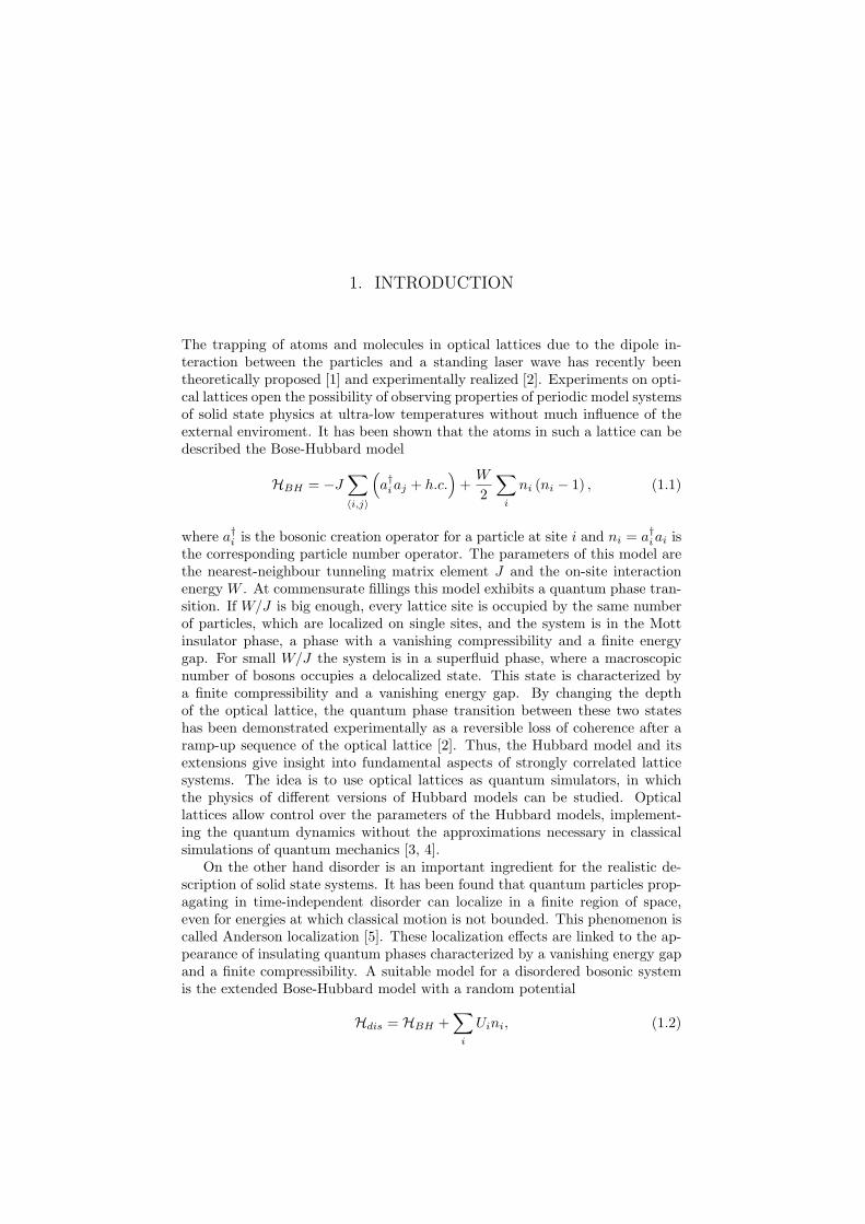
The trapping of atoms and molecules in optical lattices due to the dipole in-teraction between the particles and a standing laser wave has recently beentheoretically proposed [1] and experimentally realized [2]. Experiments on opti-cal lattices open the possibility of observing properties of periodic model systemsof solid state physics at ultra-low temperatures without much influence of theexternal enviroment. It has been shown that the atoms in such a lattice can bedescribed the Bose-Hubbard model
HBH = −J∑
〈i,j〉
(a†iaj + h.c.
)+
W
2
∑
i
ni (ni − 1) , (1.1)
where a†i is the bosonic creation operator for a particle at site i and ni = a†iai isthe corresponding particle number operator. The parameters of this model arethe nearest-neighbour tunneling matrix element J and the on-site interactionenergy W . At commensurate fillings this model exhibits a quantum phase tran-sition. If W/J is big enough, every lattice site is occupied by the same numberof particles, which are localized on single sites, and the system is in the Mottinsulator phase, a phase with a vanishing compressibility and a finite energygap. For small W/J the system is in a superfluid phase, where a macroscopicnumber of bosons occupies a delocalized state. This state is characterized bya finite compressibility and a vanishing energy gap. By changing the depthof the optical lattice, the quantum phase transition between these two stateshas been demonstrated experimentally as a reversible loss of coherence after aramp-up sequence of the optical lattice [2]. Thus, the Hubbard model and itsextensions give insight into fundamental aspects of strongly correlated latticesystems. The idea is to use optical lattices as quantum simulators, in whichthe physics of different versions of Hubbard models can be studied. Opticallattices allow control over the parameters of the Hubbard models, implement-ing the quantum dynamics without the approximations necessary in classicalsimulations of quantum mechanics [3, 4].
On the other hand disorder is an important ingredient for the realistic de-scription of solid state systems. It has been found that quantum particles prop-agating in time-independent disorder can localize in a finite region of space,even for energies at which classical motion is not bounded. This phenomenon iscalled Anderson localization [5]. These localization effects are linked to the ap-pearance of insulating quantum phases characterized by a vanishing energy gapand a finite compressibility. A suitable model for a disordered bosonic systemis the extended Bose-Hubbard model with a random potential
Hdis = HBH +∑
i
Uini, (1.2)
1. Introduction 6
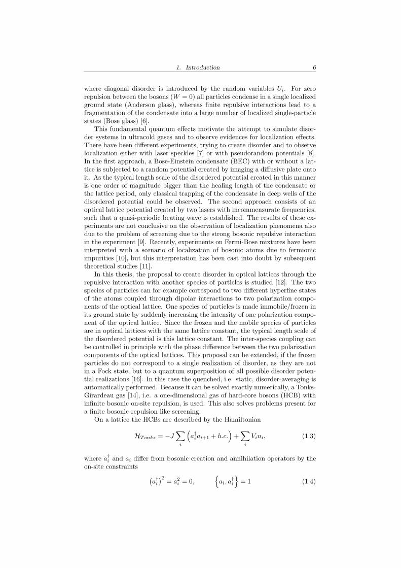
where diagonal disorder is introduced by the random variables Ui. For zerorepulsion between the bosons (W = 0) all particles condense in a single localizedground state (Anderson glass), whereas finite repulsive interactions lead to afragmentation of the condensate into a large number of localized single-particlestates (Bose glass) [6].
This fundamental quantum effects motivate the attempt to simulate disor-der systems in ultracold gases and to observe evidences for localization effects.There have been different experiments, trying to create disorder and to observelocalization either with laser speckles [7] or with pseudorandom potentials [8].In the first approach, a Bose-Einstein condensate (BEC) with or without a lat-tice is subjected to a random potential created by imaging a diffusive plate ontoit. As the typical length scale of the disordered potential created in this manneris one order of magnitude bigger than the healing length of the condensate orthe lattice period, only classical trapping of the condensate in deep wells of thedisordered potential could be observed. The second approach consists of anoptical lattice potential created by two lasers with incommensurate frequencies,such that a quasi-periodic beating wave is established. The results of these ex-periments are not conclusive on the observation of localization phenomena alsodue to the problem of screening due to the strong bosonic repulsive interactionin the experiment [9]. Recently, experiments on Fermi-Bose mixtures have beeninterpreted with a scenario of localization of bosonic atoms due to fermionicimpurities [10], but this interpretation has been cast into doubt by subsequenttheoretical studies [11].
In this thesis, the proposal to create disorder in optical lattices through therepulsive interaction with another species of particles is studied [12]. The twospecies of particles can for example correspond to two different hyperfine statesof the atoms coupled through dipolar interactions to two polarization compo-nents of the optical lattice. One species of particles is made immobile/frozen inits ground state by suddenly increasing the intensity of one polarization compo-nent of the optical lattice. Since the frozen and the mobile species of particlesare in optical lattices with the same lattice constant, the typical length scale ofthe disordered potential is this lattice constant. The inter-species coupling canbe controlled in principle with the phase difference between the two polarizationcomponents of the optical lattices. This proposal can be extended, if the frozenparticles do not correspond to a single realization of disorder, as they are notin a Fock state, but to a quantum superposition of all possible disorder poten-tial realizations [16]. In this case the quenched, i.e. static, disorder-averaging isautomatically performed. Because it can be solved exactly numerically, a Tonks-Girardeau gas [14], i.e. a one-dimensional gas of hard-core bosons (HCB) withinfinite bosonic on-site repulsion, is used. This also solves problems present fora finite bosonic repulsion like screening.
On a lattice the HCBs are described by the Hamiltonian
HTonks = −J∑
i
(a†iai+1 + h.c.
)+
∑
i
Vini, (1.3)
where a†i and ai differ from bosonic creation and annihilation operators by theon-site constraints
(a†i
)2 = a2i = 0,
ai, a
†i
= 1 (1.4)
1. Introduction 7
and Vi is an external trapping potential. It is assumed that the number ofparticles is lower than the number of lattices sites. The operator constraintsensure that at most one particle can be on a single lattice site. This system canbe mapped onto noninteracting spinless fermions through the Jordan-Wignertransformation [15], which gives the many-particle ground state in the first-quantized real-space picture as the modulus of the fermionic Slater determinant.Therefore, the HCBs in one dimension have the same real-space behaviour asfree fermions, i.e. no true many-body effects appear here.
A Tonks-Girardeau gas has already been realized in an optical lattice [13].The dynamics of the gas is restricted to one dimension by tightly confining theatoms in two orthogonal directions with a very deep optical lattice potential. Inthe remaining dimension a weaker optical lattice is formed, allowing tunnelingbetween its minima. As the lattice increases the effective mass of the atoms,the ratio between the mean interaction energy and the mean kinetic energy perparticle increases, such that the Tonks-Girardeau gas regime is reached. Themomentum profiles measured in the experiment are in very good agreementwith the theoretical predictions for a Tonks-Girardeau gas.
It has been shown analytically with Bethe Ansatz that the one-particledensity matrix (OPDM) ρij = 〈a†iaj〉 in the ground state of the HCBs in aone-dimensional homogeneous system (Vi = 0) with periodic boundary condi-tions decays algebraically in the thermodynamic limit as ρij ∼ |i− j|−α, whereα = 0.5 [17]. Because the OPDM decays to zero, there is no long-range order,however the decay is less than exponential, making it quasi-long-range order.This demonstrates the nontrivial off-diagonal many-body physics of the HCBs.The Bose-Hubbard model for 0 < W <∞ exhibits quasi-long-range order witha different exponent α, whereas the non-interacting system W = 0 exhibits truelong-range order. The eigenvectors of the OPDM, the natural orbitals (NO),are interpreted as effective single-particle wave functions and the correspond-ing eigenvalues as their occupations. The system exhibits condensation, if thegreatest of these eigenvalues increases linearly with the number of particles [18].In the case at hand of a translationally invariant system, the momentum statesare the eigenfunctions of the OPDM, so that the occupations of the NOs andthe momentum distribution function (MDF) coincide. The number of particlesin the zero momentum state is the integral of the OPDM, i.e. nk=0 ∼
√N for
HCBs. Therefore, the fraction of particles in every single state decays to zero inthe thermodynamic limit, but algebraically, such that this behaviour is calledquasi-condensation.
The exact diagonalization of HCBs in one dimensions, based on the Jordan-Wigner transformation, allows to study the ground state properties for ar-bitrary shapes of an additional external potential and the time evolution inthese systems for up to 10000 lattice sites [19]. Based on this approach, ithas been demonstrated that the quasi-long-range order and the related quasi-condensation is a very robust feature for one-dimensional HCBs. It persists forthe ground states of HCBs in confining traps of the form Vi ∝ ia for any valueof the characteristic density, where due to the inhomogeneity of the system theNOs and their occupations have to be considered to suggest quasi-condensation.The free expansion without an external potential of HCBs, initially confined ina trap, does not destroy the quasi-condensation and the quasi-long-range order[20]. Furthermore, during free expansion starting from a Mott insulator state,which is localized in the system centre, two degenerate quasi-condensates at
1. Introduction 8
momenta k = ±π/2 with the characteristic√
N scaling appear, moving to theleft and to the right [21].
In this thesis the exact-diagonalization approach is applied to one-dimen-sional HCBs in a disordered potential created by a frozen species of HCBs. Thechapter 2 reviews general results of the localization theory and the crucial roleof correlations in the disordered potential. A general scaling argument predictsthat localization should always be present in one and two dimensions, whereasthree-dimensional systems exhibit localization only above a critical strength ofthe disorder [25]. As an example that correlations in the disordered potentialcan make localization effects disappear, the random dimer model can be men-tioned [26], where a non-macroscopic number of extended eigenstates leads todynamical delocalization.
In the following chapter 3 the system of frozen and mobile bosons is intro-duced, and the numerical algorithm of this work, based on the exact diagonal-ization of the HCBs and the Monte Carlo sampling of the disorder, is explainedin detail. Furthermore, the different kinds of disorder discussed in this work arecompared.
The effect of disorder on the ground state of HCBs in a periodic potential isexamined in chapter 4, focusing on the spatial extend of the wave function andthe quasi-condensation properties of HCBs. It is shown that quasi-condensationis absent in the disorder-averaged ground state and all eigenstates seem to belocalized.
In chapter 5 the dynamical properties of HCBs in disordered potentials areexamined. The mobile and the frozen HCBs are initialized in the ground stateof a translationally invariant system or in a system with harmonic confine-ment and subsequently time evolved in the same system, interacting with thedisordered potential. Localization effects in real-space and the destruction ofquasi-condensation in the initial state during the evolution is analysed.
Finally, the expansion of initially confined HCBs in a disordered potentialis discussed in chapter 6. It can be observed that the system reaches a steadystate, which is localized for any value of the disorder strength. Additionally,ad hoc correlations are added to the disordered potential created by the frozenHCBs, initialising them in a superlattice. But the localization of the mobilebosons persists in this case as well. The many-particle dynamics of HCBs arestudied with the same setup in the second part of chapter 6, by observing thedisappearance or non-creation of quasi-condensation during time evolution. Inthis case, different initial conditions are examined.
Chapter 7 discusses, how the system presented in this thesis can be realizedin an experiment and how signatures of disorder-induced localization can bemeasured.
In this thesis, except for chapters 2 and 7, the dimensions of the variablesare chosen such that Planck’s constant devided by 2π and the lattice constantare unity, i.e. ~ = 1 and a = 1.
2. DISORDERED SYSTEMS
In this introductory chapter, general results for the appearance of localizationin disordered systems are presented, focussing on one-dimensional systems. Insection 2.1 the localization of the eigenstates in a one-dimensional lattice systemis discussed. The participation ratio as a measure for the localization of wavefunctions is defined in section 2.2. Section 2.3 is devoted to a particular system,the random-dimer model, in which dynamical delocalization is found in spite ofthe presence of a disordered potential.
2.1 Localization in One-Dimensional Disorder Potentials
The single-particle eigenstates of the Hamiltonian
H1D = −J∑
i
(a†nan+1 + h.c.
)+
∑n
Unnn, (2.1)
describing a lattice model with nearest-neighbour tunneling and a random po-tential Vn, can be examined in one dimension by a transfer matrix approach.The operator a†n denotes a single-particle creation operator and ni is the cor-responding density operator. If the eigenstate
∣∣Φ〉 with energy eigenvalue E isdecomposed as
∣∣Φ〉 =∑
n cna†n∣∣0〉, the eigenvalue equation for site n becomes
Ecn = Uncn − Jcn−1 − Jcn+1. (2.2)
On a semi-infinite chain with site indices n = 1, 2, . . . the coefficients cn for afixed energy eigenvalue E are recursively determined by the initial coefficientsc0 and c1 (c2
0 + c21 6= 0) [23]. This recursive formula can be expressed as
(cn+1
cn
)= TnTn−1 · · ·T1
(c1
c0
), (2.3)
where the transfer matrices Ti are given by
Tn =(
(Un − E) /J −11 0
). (2.4)
In a homogeneous system without a disordered potential, i.e. with Vn = 0,this recursive expression can be evaluated. For energies |E| < 2, for whichsingle-particle eigenstates of the Hamiltonian H1D exists, it holds
limn→∞
1n
log(a2
n + a2n+1
)= 0, (2.5)
and for |E| > 2, for which no single-particle eigenstates exist,
limn→∞
1n
log(a2
n + a2n+1
)=
2λ for c1
c06= ±e−λ
−2λ for c1c0
= ±e−λ, (2.6)
2. Disordered Systems 10
where λ = cosh−1 |E|/2. For the system with a disordered potential Vn, inwhich the disorder site energies Vn are independent and identically distributedwith at least to allowed values of the site energy Vn, the infinite product of therandomly distributed matrices Tn can be analysed by Furstenberg’s theorem, alimit theorem for noncommuting random products [24]. For the case discussedin this section it assumes the form
limn→∞
1n
log∥∥∥∥Tn · · ·T1 ·
(c1
c0
)∥∥∥∥ = limn→∞
log(c2n + c2
n+1
)= 2
1ξ
> 0. (2.7)
As for large n cn and cn+1 are of the same order of magnitude, i.e. c2n ≈ c2
n+1,the coefficients cn of the wavefunction
∣∣Φ〉 can be estimated for large n as
cn ∼ en/ξ, (2.8)
where ξ is called localization length. It can further be argued that these ex-ponentially increasing solutions for the semi-infinite lattice chain correspond toexponentially localized energy eigenstates for the infinite lattice with two openends [23]. For this argument, the transfer matrix approach is applied to bothends of a finite system with sites n = 1, 2, . . . , L, since exponentially localizedstates are only weakly effected by the boundary conditions for large enough sys-tems (LÀ ξ). Therefore, it is expected that all eigenstates of a one-dimensionallattice with nearest-neighbour tunneling and an uncorrelated random potentialare exponentially localized. This result can be extended by a similar line ofargument to different one-dimensional models [23]. Furthermore, the scalingtheory of localization [25] predicts that no localization-delocalization transitionexists in less than three dimensions.
2.2 Participation Ratio
A disordered potential leads to exponentially localized states as shown in theprevious section 2.1. The localization can be quantified with the decay lengthof the wave function, the localization length ξ. In order to be able to describemore complicatedly shaped density profiles of the HCBs the participation ratio(PR) is used in this thesis
PR(∣∣Φ〉) =
(∑Li=1〈ni〉
)2
∑Li=1〈ni〉2
=N2
∑Li=1〈ni〉2
, (2.9)
where 〈ni〉 = 〈Φ∣∣a†iai
∣∣Φ〉 is the average density of HCBs on site i and N is thenumber of particles.
The interpretation of this quantity can be justified by calculating the par-ticipation ratio for a rectangular profile
〈ni〉 =
1 for i ≤ l0 for i ≥ l + 1 =⇒ PR = l, (2.10)
where the participation ratio gives the support of the profile, and for a Gaussianand an exponentially decaying profile on an infinite and continuous lattice
〈n (x)〉 ∝ e−x2
2σ2 =⇒ PR ∝ σ (2.11)
〈n (x)〉 ∝ e−|x|ξ =⇒ PR ∝ ξ, (2.12)
2. Disordered Systems 11
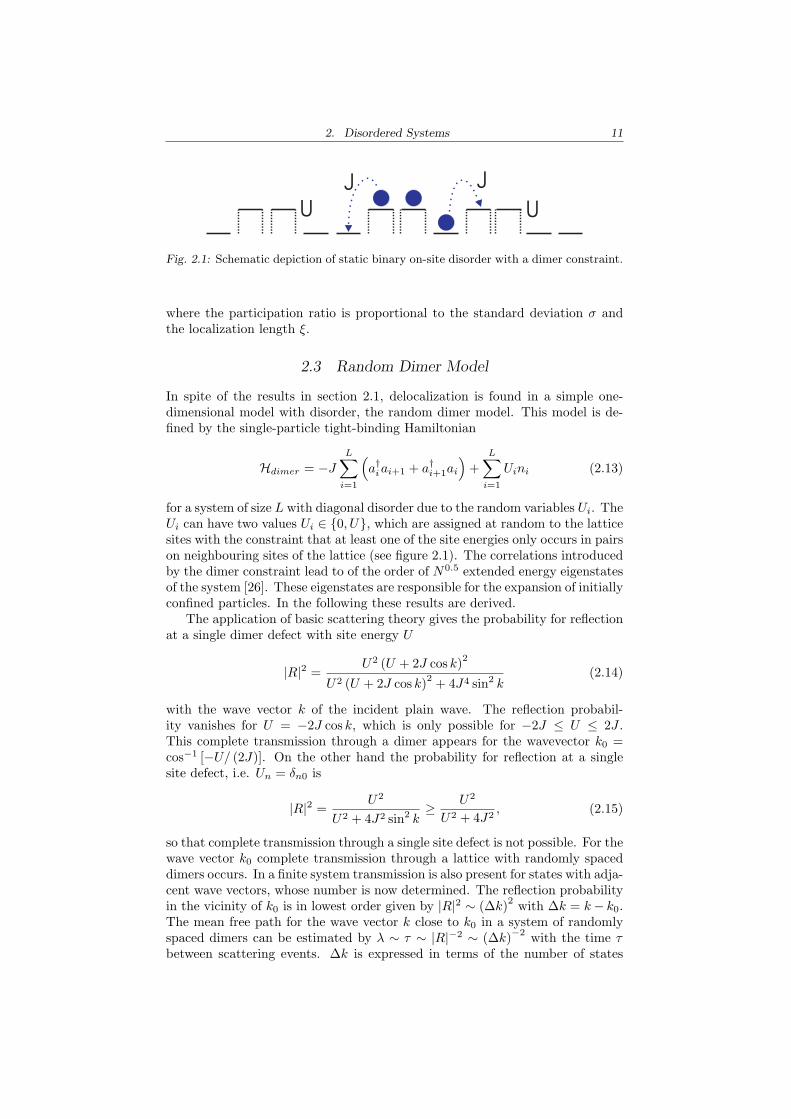
J J
U U
Fig. 2.1: Schematic depiction of static binary on-site disorder with a dimer constraint.
where the participation ratio is proportional to the standard deviation σ andthe localization length ξ.
2.3 Random Dimer Model
In spite of the results in section 2.1, delocalization is found in a simple one-dimensional model with disorder, the random dimer model. This model is de-fined by the single-particle tight-binding Hamiltonian
Hdimer = −J
L∑
i=1
(a†iai+1 + a†i+1ai
)+
L∑
i=1
Uini (2.13)
for a system of size L with diagonal disorder due to the random variables Ui. TheUi can have two values Ui ∈ 0, U, which are assigned at random to the latticesites with the constraint that at least one of the site energies only occurs in pairson neighbouring sites of the lattice (see figure 2.1). The correlations introducedby the dimer constraint lead to of the order of N0.5 extended energy eigenstatesof the system [26]. These eigenstates are responsible for the expansion of initiallyconfined particles. In the following these results are derived.
The application of basic scattering theory gives the probability for reflectionat a single dimer defect with site energy U
|R|2 =U2 (U + 2J cos k)2
U2 (U + 2J cos k)2 + 4J4 sin2 k(2.14)
with the wave vector k of the incident plain wave. The reflection probabil-ity vanishes for U = −2J cos k, which is only possible for −2J ≤ U ≤ 2J .This complete transmission through a dimer appears for the wavevector k0 =cos−1 [−U/ (2J)]. On the other hand the probability for reflection at a singlesite defect, i.e. Un = δn0 is
|R|2 =U2
U2 + 4J2 sin2 k≥ U2
U2 + 4J2, (2.15)
so that complete transmission through a single site defect is not possible. For thewave vector k0 complete transmission through a lattice with randomly spaceddimers occurs. In a finite system transmission is also present for states with adja-cent wave vectors, whose number is now determined. The reflection probabilityin the vicinity of k0 is in lowest order given by |R|2 ∼ (∆k)2 with ∆k = k− k0.The mean free path for the wave vector k close to k0 in a system of randomlyspaced dimers can be estimated by λ ∼ τ ∼ |R|−2 ∼ (∆k)−2 with the time τbetween scattering events. ∆k is expressed in terms of the number of states
2. Disordered Systems 12
∆L with momentum |k − k0| ≤ ∆k as ∆k = (2π∆L) /L. As the localizationlength is approximately equal to the mean free path, equating the latter withthe system size yields the scaling ∆L ∼ √L for the number of extended states∆L in a hypercube with side L.
The dynamical properties of the system are described by the diffusion con-stant D0, which is determined by the integration of v (k) λ (k) over the states,which participate in the transport, i.e. the
√L extended states. The group
velocity v (k) is constant and non-vanishing for k states, which are not at theband edges, i.e. cos2 k > 1. As the fraction ∆k ∼ 1/
√L of states are extended
and λ (k) ∼ L, the diffusion coefficient becomes D0 ∼√
L within the band, i.e.for −2J < U < 2J . Substituting the system size L with the time t becauseof the constant group velocity yields D0 ∼ t0.5. At the band edges, i.e. forU = ±2J , the group velocity vanishes like v (k) ∼ k and the diffusion constantbecomes D0 ∼ 1.
Applying the relation between the spatial extend of the diffusion PR andthe associated time L ∝ √D0t, the width PR of the density profile of an initiallyconfined particle can be estimated. For −2J < U < 2J the transport is superdif-fusive, but subballistic PR ∼ t0.75 and for U = ±2J it is diffusive PR ∼ t0.5.The density profile stays localized for stronger values of the site energy U . Thesetransport properties have been confirmed by numerical simulations [26].
Therefore, a non-macroscopic number of extended eigenstates causes dynam-ical delocalization. This paradox can be clarified further by examining the timeevolution of an initially confined particle
∣∣Ψ(t)〉 = e−iHt~
∣∣Ψ(0)〉 = e−iHt~ a†0
∣∣0〉 (2.16)
in the energy eigenvector basis∣∣ϕk〉 =
∑
i
ϕki a†i
∣∣0〉 (2.17)
with the corresponding energy eigenvalues Ek. The amplitudes of the wavefunction are
〈0∣∣ai
∣∣Ψ(0)〉 =∑
k
e−iEkt
~ · 〈0∣∣ai
∣∣ϕk〉〈ϕk∣∣a0
∣∣0〉
=∑
k
e−iEkt
~ ϕki ϕk
0
∗.
(2.18)
If i corresponds to the end of the system i = L/2, only the Lα extended statescontribute to the sum. For big system sizes it can further be assumed ϕk′
j ∼√
Lfor the extended states with index k′. The space density at the system edge canthus be estimated as
〈nL/2〉 ∼∣∣∣∣∣∑
k′e−i
Ekt
~1L
∣∣∣∣∣
2
≤ L2(α−1) (2.19)
In the case of the random dimer model, α = 0.5 holds and the estimate 2.19gives 〈nL/2〉 . L−1, such that it even allows for ballistic expansion. Even for afinite number of extended eigenstates (α = 0) it seems possible to have a statewhich is not exponentially localized, but only polynomially localized after aninfinitely long time evolution.
3. SYSTEM AND METHOD
In this chapter the numerical procedure used in this thesis, and some resultsabout different kinds of disorder are presented. The Hamiltonian of the mobileand frozen hard-core bosons (HCB) is introduced in section 3.1, where it isexplained how the frozen bosons can be regarded as static disorder and howthe unitary evolution of both species of particles realizes quenched disorder-averaging. After this, the Jordan-Wigner transformation and its implementationis presented in section 3.2, making it possible to study the one-particle densitymatrix (OPDM) of time evolved HCBs. The presentation of the algorithm isconcluded in section 3.3 with the description of the Monte-Carlo sampling ofthe disorder distribution. Finally, in section 3.4 the statistics of the disordercreated by frozen bosons is investigated and compared with the statistics ofuncorrelated random disorder.
3.1 Hamiltonian Dynamics
The full system is described by the Hamiltonian
H = H0 +Hf +Hint, (3.1)
where the Hamiltonian of the moving HCBs, which can be prepared in a parabo-lic trap with strength k, is
H0 = −J
L∑
i=1
(a†iai+1 + h.c.
)+ k
L∑
i=1
(i− i0)2ni, (3.2)
the one for the frozen particles, which can be prepared in a superlattice withstrength V , is
Hf = −JfL∑
i=1
(af†
i afi+1 + h.c
)+ V
L∑
i=1
(−1)inf
i (3.3)
and the interaction Hamiltonian is
Hint = U
L∑
i=1
ninfi , (3.4)
where L is the number of sites of the system. Here a†i and ai are boson creationand annihilation operators and ni = a†iai is the number operator for site i withthe hard-core constraint 〈ni〉 ∈ [0, 1], assured by the on-site anti-commutationrelations
a†i2
= ai2 = 0,
ai, a
†i
= 1, (3.5)
3. System and Method 14
that complement the bosonic off-site commutation relations[a†i , aj
]=
[ai, aj
]=
[a†i , a
†j
]= 0, for i 6= j. (3.6)
Symbols with the superscript f are the corresponding operators for the frozenbosons that create the disordered potential. Periodic boundary conditions areenforced by aL+1 = a1, whereas open boundary conditions can be introducedby neglecting terms with aL+1 or a†L+1 in the Hamiltonians.
At t = 0 the two species of HCBs are prepared independently (U=0) inthe factorized ground state
∣∣Ψ〉 =∣∣Φ〉 ⊗
∣∣Φ〉f of the Hamiltonian H with fixednumbers of particles N and Nf . The ground state
∣∣Φ〉f of the frozen particlesis decomposed in the basis of Fock states
∣∣Φf 〉 =∑
nfi :nf
i ∈0,1,Pi nfi =Nf
c(
nfi
) ∣∣
nfi
〉, (3.7)
where the sum extends over all Fock states
nf
i
=
nf
1 , nf2 , . . . , nf
L :L∑
i=1
nfi = Nf , nf
i ∈ 0, 1
. (3.8)
For V > 0 the frozen bosons are prepared in a superlattice with a wavelength oftwo lattice spacings. This superlattice is used to create additional correlationsin the disordered potential (see section 3.4). Its effect on the mobile HCBs isdiscussed in section 6.1.2 only.
For k > 0 the mobile bosons are prepared in a harmonic trap, where k =∞corresponds to a Mott insulator region around i0, i.e. a region with constantand maximal density ni = 0. Dimenional considerations allow the definition ofa typical particle density in the trap [22]. Equating the typical kinetic energiesof the HCBs J , which serves as the unit of energy in this thesis, with thetypical trapping energy kl2 for a particle at the fringes of a density profile ofsize 2l, results in the typical length scale of the particles in the trap l =
√J/k.
Therefore, the particle density in the trap is characterized by
ρ = N
√k
J, (3.9)
where N is the number of particles in the trap. For ρ→ 0 the continuum limitis recovered, whereas for a value of ρ > ρc ≈ 2.6 a Mott insulator region appearsin the trap centre [22]. Except for section 5.3, the frozen particles are preparedwith periodic boundary conditions, and are not effected by the trapping of themobile particles.
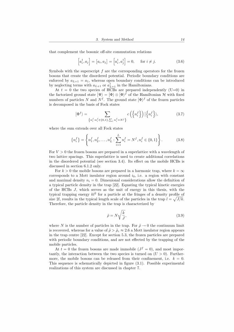
At t = 0 the frozen bosons are made immobile (Jf = 0), and most impor-tantly, the interaction between the two species is turned on (U > 0). Further-more, the mobile bosons can be released from their confinement, i.e. k = 0.This sequence is schematically depicted in figure (3.1). Possible experimentalrealizations of this system are discussed in chapter 7.
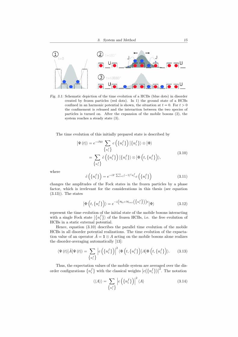
3. System and Method 15
Fig. 3.1: Schematic depiction of the time evolution of a HCBs (blue dots) in disordercreated by frozen particles (red dots). In 1) the ground state of a HCBsconfined in an harmonic potential is shown, the situation at t = 0. For t > 0the confinement is released and the interaction between the two species ofparticles is turned on. After the expansion of the mobile bosons (2), thesystem reaches a steady state (3).
The time evolution of this initially prepared state is described by∣∣Ψ(t)〉 = e−iHt
∑
nfi
c(
nfi
) ∣∣nfi
〉 ⊗∣∣Φ〉
=∑
nf
i
c(
nfi
) ∣∣nfi
〉 ⊗∣∣Φ
(t,
nf
i
)〉,
(3.10)
wherec(
nfi
)= e−iV
PLi=1(−1)inf
i c(
nfi
)(3.11)
changes the amplitudes of the Fock states in the frozen particles by a phasefactor, which is irrelevant for the considerations in this thesis (see equation(3.13)). The states
∣∣Φ(t,
nf
i
)〉 = e
−i“H0+Hint
“nf
i
””t∣∣Φ〉 (3.12)
represent the time evolution of the initial state of the mobile bosons interactingwith a single Fock state
∣∣nfi
〉 of the frozen HCBs, i.e. the free evolution ofHCBs in a static external potential.
Hence, equation (3.10) describes the parallel time evolution of the mobileHCBs in all disorder potential realizations. The time evolution of the expacta-tion value of an operator A = 1⊗A acting on the mobile bosons alone realizesthe disorder-averaging automatically [13]:
〈Ψ(t)∣∣A
∣∣Ψ(t)〉 =∑
nf
i
∣∣∣c
(nf
i
)∣∣∣2
〈Φ(t,
nf
i
)∣∣A∣∣Φ
(t,
nf
i
)〉. (3.13)
Thus, the expectation values of the mobile system are averaged over the dis-order configurations
nf
i
with the classical weights
∣∣c(nfi
)∣∣2. The notation
〈〈A〉〉 =∑
nf
i
∣∣∣c
(nf
i
)∣∣∣2
〈A〉 (3.14)
3. System and Method 16
is used in this work for explicitly specifying disorder-averaged quantities.The numerical calculations described the following sections has been per-
formed with the Intel Fortran Compiler 9.1, the Message Passing Interface forcommunication between processors on the AMD opteron cluster of the theorydivision of the Max-Planck-Institut fur Quantenoptik, and the Intel Math Ker-nel Library 9.0 for linear algebra routines.
3.2 Jordan-Wigner Transformation and Implementation
As derived in the previous section, an important step towards calculating ex-pectation values as in equation (3.13) is to calculate the time evolution of HCBsin a static external potential Vi, i.e. under a Hamiltonian of the form
HHCB = −J
L∑
i=1
(a†iai+1 + h.c.
)+
L∑
i=1
Vini, (3.15)
where the creation and annihilation operators a†i and ai obey the (anti-)commu-tation relations of equations (3.5) and (3.6).
3.2.1 Jordan-Wigner Transformation
The system of equation (3.15) can be solved with the Jordan-Wigner transfor-mation (JWT) [15],
a†i = f†i
i−1∏
k=1
e−iπf†kfk , ai =i−1∏
k=1
eiπf†kfkfi, (3.16)
which maps the HCBs onto spinless fermions
fi, f†j
= δij , fi, fj =
f†i , f†j
= 0. (3.17)
The Hamiltonian is invariant under the Jordan-Wigner transformation
HF = −J
L∑
i=1
(f†i fi+1 + h.c.
)+
L∑
i=1
Vif†i fi, (3.18)
so that it maps the HCBs to noninteracting fermions.Some technical remarks about the JWT are appropriate at this point to
clarify the invariance of the Hamiltonian. Since the site occupations do notchange under the JWT a†iai = f†i fi, the fermionic creation and annihilationoperators in the exponents of the transformation in (3.16) can be replaced bythe corresponding operators for the HCBs. This replacement easily leads to theinversion of the JWT.
Because of(f†i fi
)2 = f†i fi, one obtains
e−iπf†i fi = 1 +(e−iπ − 1
)f†i fi = 1− 2f†i fi. (3.19)
Therefore, the typical tunneling term in the Hamiltonian can be written fori 6= L
a†iai+1 = f†i eiπf†i fifi+1 = f†i fi+1. (3.20)
3. System and Method 17
If periodic boundary conditions aL+1 = ±a1 are imposed, the following identityholds, projected onto the space of a fixed number of particles N
a†La1 = f†L
L−1∏
k=1
eiπf†kfkf1 = f†Lf1
L−1∏
k=2
eiπf†kfk
= f†Lf1 (−1)N−1,
(3.21)
where equation 3.19 is used in the first step. The second step relies on the factthat the matrix components of this operator are nonvanishing only between Fockstates in which either the first or the last site is occupied. Therefore, for odd Nthe fermionic system obeys periodic boundary conditions, whereas for N evenit obeys anti-periodic boundary conditions. If the HCBs obey open boundaryconditions instead, the fermions obey open boundary conditions as well.
The invariance of the Hamiltonian under the JWT means that the HCBshave the same spectrum as the fermionic system.
3.2.2 One-Particle Density Matrix
A fundamental observable is represented by the one-particle density matrix(OPDM)
ρij = 〈a†iaj〉, (3.22)
which is related to the two-point Green’s function
Gij = 〈aia†j〉 (3.23)
throughρij = Gij + δij (1− 2Gii) . (3.24)
The OPDM can be understood as the density matrix of the many-bodystate after the space of N − 1 particles is traced out [18], which leads to theinterpretations in the context of natural orbitals (see section 3.2.5).
The two-point Green’s function of the HCBs (see equation (3.23)) can nowbe written [19]
Gij = 〈Φ∣∣aia
†j
∣∣Φ〉
= 〈ΦF
∣∣i−1∏
k=1
eiπf†kfkfif†j
j−1∏
l=1
e−iπf†l fl∣∣ΦF 〉
Gij = 〈ΦiF
∣∣ΦjF 〉,
(3.25)
where∣∣Φ〉 is a state of the HCBs and
∣∣ΦF 〉 is the corresponding fermionic state.The modified fermionic states
∣∣ΦkF 〉 are defined through
∣∣ΦjF 〉 = f†j
j−1∏
l=1
e−iπf†l fl∣∣ΦF 〉. (3.26)
The fermionic states are represented in the form
∣∣ΦF 〉 =N∏
m=1
L∑n=1
Pnmf†n∣∣0〉,
∣∣ΦkF 〉 =
N+1∏m=1
L∑n=1
Pnmf†n∣∣0〉, (3.27)
3. System and Method 18
where the matrix Pk ∈ CL×(N+1) is determined from the matrix P = (Pij) ∈CL×N . The columns of these matrices are the wave functions for the N fermions,i.e. the columns of the matrix for the fermionic ground state are the eigenfunc-tions to the lowest N eigenvalues of HF . For the algorithm in this work it iscrucial that the columns of these matrices are orthonormal to each other.
The action ofj−1∏
l=1
e−iπf†l fl =j−1∏
l=1
(1− 2f†l fl
)(3.28)
(see equation (3.19)) on the fermionic state∣∣ΦF 〉 is determined by the anti-
commutation and commutation relations
1− 2f†l fl, f†l
= 0,
[1− 2f†l fl, f
†n
]= 0 for n 6= l, (3.29)
i.e. it changes the signs of the first j − 1 rows of the matrix P. The furthercreation operator f†j leads to the addition of an extra column to P, such thatPj
n(N+1) = δnj . In fact, the creation operator gives the precursion of an extra
column, but because this is done for Pi and Pj in equation 3.25, the additionis also correct. In summary, Pk is given by
Pj =
−P11 −P12 . . . −P1N 0. . . . . . .
−P(j−1)1 −P(j−1)2 . . . −P(j−1)N 0Pj1 Pj2 . . . PjN 1
P(j+1)1 P(j+1)2 . . . P(j+1)N 0. . . . . . .
PL1 PL2 . . . PLN 0
. (3.30)
It remains to calculate the scalar product 〈ΦiF
∣∣ΦjF 〉.
Gij = 〈0∣∣
1∏
k=N
L∑
l=1
P i∗lk fn
N∏m=1
L∑n=1
P jnmf†n
∣∣0〉
=L∑
n1,...,nN ,m1,...,mN
=1
P i∗nN N
· · · P i∗n11P
jm11· · · P j
mN N〈0
∣∣fnN. . . fn1f
†m1
. . . f†mN
∣∣0〉
=∑
n1,...,nNnr 6=ns
∑
Psign (P) P i∗
nN N· · · P i∗
n11PjnP11 · · · P j
nPN
N
=∑
P
∑n1,...,nN
sign (P) P i∗nN N
· · · P i∗n11P
jn1P1
· · · P jnNPN
=∑
π
sign (P)(Pi†Pj
)1P1
· · ·(Pi†Pj
)NPN
Gij = det(Pi†Pj
),
(3.31)
where N = N + 1 and P denotes a permutation of the numbers 1, . . . , N . Thecondition nr 6= ns, which ensures the Pauli principle for the fermionic operators
3. System and Method 19
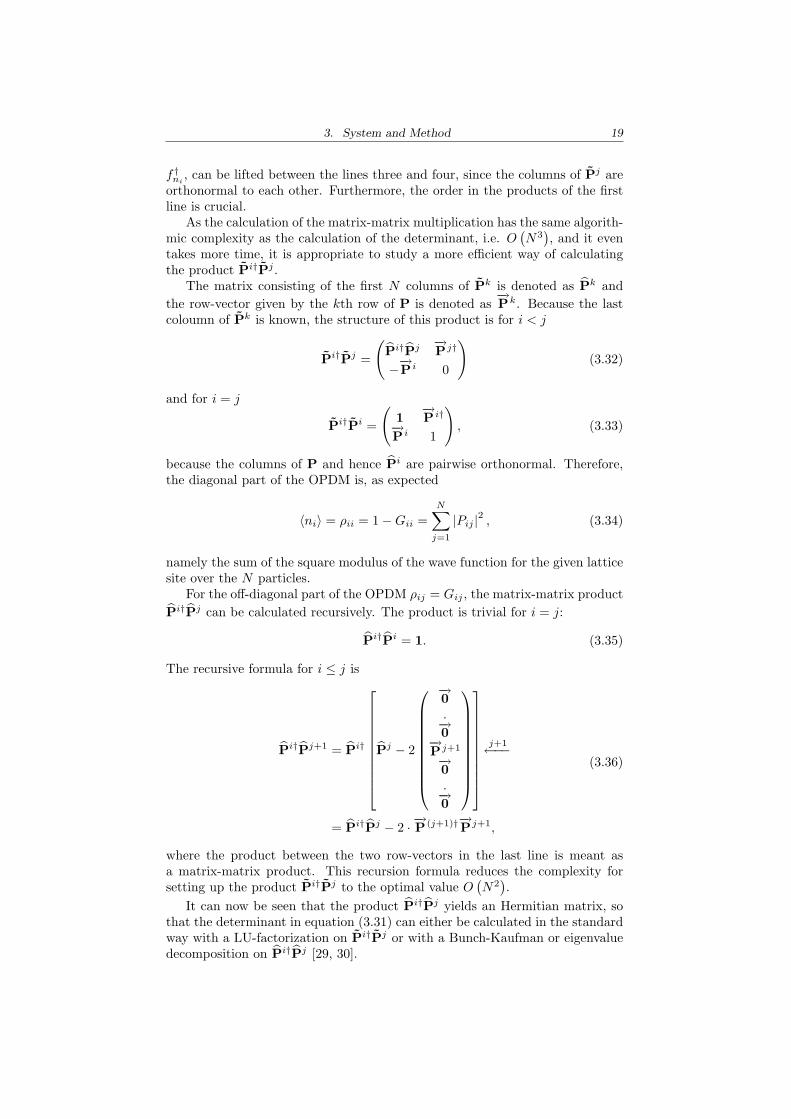
f†ni, can be lifted between the lines three and four, since the columns of Pj are
orthonormal to each other. Furthermore, the order in the products of the firstline is crucial.
As the calculation of the matrix-matrix multiplication has the same algorith-mic complexity as the calculation of the determinant, i.e. O
(N3
), and it even
takes more time, it is appropriate to study a more efficient way of calculatingthe product Pi†Pj .
The matrix consisting of the first N columns of Pk is denoted as Pk andthe row-vector given by the kth row of P is denoted as
−→Pk. Because the last
coloumn of Pk is known, the structure of this product is for i < j
Pi†Pj =
(Pi†Pj −→
P j†
−−→P i 0
)(3.32)
and for i = j
Pi†Pi =
(1−→P i†
−→P i 1
), (3.33)
because the columns of P and hence Pi are pairwise orthonormal. Therefore,the diagonal part of the OPDM is, as expected
〈ni〉 = ρii = 1−Gii =N∑
j=1
|Pij |2 , (3.34)
namely the sum of the square modulus of the wave function for the given latticesite over the N particles.
For the off-diagonal part of the OPDM ρij = Gij , the matrix-matrix productPi†Pj can be calculated recursively. The product is trivial for i = j:
Pi†Pi = 1. (3.35)
The recursive formula for i ≤ j is
Pi†Pj+1 = Pi†
Pj − 2
−→0.−→0−→
P j+1
−→0.−→0
j+1←−−
= Pi†Pj − 2 · −→P (j+1)†−→P j+1,
(3.36)
where the product between the two row-vectors in the last line is meant asa matrix-matrix product. This recursion formula reduces the complexity forsetting up the product Pi†Pj to the optimal value O
(N2
).
It can now be seen that the product Pi†Pj yields an Hermitian matrix, sothat the determinant in equation (3.31) can either be calculated in the standardway with a LU-factorization on Pi†Pj or with a Bunch-Kaufman or eigenvaluedecomposition on Pi†Pj [29, 30].
3. System and Method 20
If the number of HCBs is of the same order of magnitude as the numberof lattice sites, a further speed up of the algorithm is possible. For each rowi in the OPDM ρij , a Gram-Schmidt decomposition, implemented with a nu-merically stable equivalent, as e.g. the Householder transformation [31], withcomputational complexity O
((N − i)2 (3L−N)
)is performed on the matrix
(Pmn) = LQ, (3.37)
where the rows k ≥ i (, only which have to be calculated,) of L ∈ CN×L form alower triangular matrix and Q ∈ CL×L is a unitary matrix. This decompositionis used to factorize the product (i ≤ j)
Pi†Pj =
(Q†Li†LjQ
−→P j†
(2δij − 1)−→P i δij
)
=(Q† 00 1
) (Li†Lj Q
−→P j†
(2δij − 1)−→P iQ† δij
) (Q 00 1
),
(3.38)
where the matrix Li is L with the signs of the first i rows changed. As Q isunitary, the result (3.31) can now be written
ρij = det
(Li†Lj −→
L j†
−−→L i 0
), (3.39)
where the row-vector−→L i denotes the ith row of L. Since Li†Li = 1, the
recursive algorithm described above can still be used with P replaced by L.The speed gain of this version of the algorithm relies on the fact that only thefirst min (j − i + 1, L) components of the vectors
−→L j are nonzero, which reduces
the effective size of the matrix in the argument of the determinant.These results for the OPDM of HCBs can be compared with the OPDM of
fermions. This can be derived in the matrix formalism. The two-point Green’sfunction for fermions with state matrix P is given by
Gij = det(Pi†Pj
)
= det
(P†P
−→P j†
(2δij − 1)−→P i δij
)
Gij = det
(1
−→P j†
(2δij − 1)−→P i δij
),
(3.40)
where the matrices Pj do not have the minus signs, which are present for HCBs.The OPDM for fermions thus becomes
ρij = det
(1
−→P j†
(2δij − 1)−→P i δij
)=−→P i−→P j†. (3.41)
This demonstrates that the off-diagonal properties of fermions and HCBs aredifferent, whereas the real-space densities coincide (see equation (3.34)).
3. System and Method 21
3.2.3 Time Evolution
The time evolution of a state of HCBs∣∣Φ(t)〉 = e−iHt
∣∣Φ〉 (3.42)
can be performed on the fermionic state∣∣ΦF 〉 related to it through the JWT,
using the state representation of equation (3.27). The non-interacting fermionicHamiltonian, as a special case of bilinear operator, is diagonalized
HF =L∑
i,j=1
f†i Hijfj =L∑
k=1
Ekg†kgk (3.43)
based onH = UDU†, (3.44)
where U ∈ CL×L is unitary and D ∈ RL×L is diagonal with elements Ei. Thefermionic annihilation operators gk are defined through
gi =L∑
j=1
U†ijfj . (3.45)
The time evolution of the fermionic state is now given by [32]
∣∣ΦF (t)〉 = e−iHF t∣∣ΦF 〉 = e−iHF t
N∏m=1
L∑n=1
Pnmf†n∣∣0〉
= e−itP
f†i Hijfj
L∑
i1,...,iN=1
N∏
k=1
Pikkf†ik
∣∣0〉
= e−itP
Ekg†kgk
L∑
j1,...,jN=1
N∏
k=1
(U†P
)jkk
g†jk
∣∣0〉
=L∑
j1,···jN=1
N∏
k=1
e−iEjkt(U†P
)jkk
g†jk
∣∣0〉
=L∑
i1,···iLN=1
N∏
k=1
(Ue−iDtU†P
)ikk
f†ik
∣∣0〉
=N∏
m=1
L∑n=1
(e−iHtP
)nm
f†n∣∣0〉
∣∣ΦF (t)〉 =N∏
m=1
L∑n=1
Pnm (t) f†n∣∣0〉,
(3.46)
where the new state matrix P(t) is computed by the matrix-matrix multiplica-tion
P (t) = e−iHtP (3.47)
of the initial state matrix P with the single-particle time evolution operatordefined by (
e−iHt)ij
= 〈0∣∣fie
−iHF tf†j∣∣0〉. (3.48)
3. System and Method 22
This shows explicitly, that the action of exponentials of operators, which arebilinear in the fermionic creation and annihilation operators, on states givenby state matrices (see equation (3.27)) generates new state matrices. The Nnon-interacting fermions, i.e. the columns of the state matrix P, thus evolveindependently in time. After the fermionic state matrix P (t) is determined, theOPDM can be calculated from it as described in section 3.2.2.
The time evolution (3.47) can be implemented numerically exact by con-structing the matrix exponential of the Hamiltionian, e.g. with the spectraldecomposition (3.44), and using matrix-matrix multiplications. This algorithmhas the computational time complexity O
(L2N
)because of the multiplications
and the memory complexity O(L2
)from the storage of the single-particle time
evolution operator.The single-particle Hamiltonian H (from equation (3.15)) is sparse. For
sparse matrices, where matrix-vector products can be implemented efficiently,several approximate time evolution algorithms with a better performance exist[33]. These algorithms iteratively approximate the time evolution in small timesteps ∆t.
Basic methods are nth order Taylor expansions of the exponential of theHamiltonian
∣∣Ψ(t + ∆t)〉 =n∑
j=1
(−iH∆t)j
j!
∣∣Ψ(t)〉+ O((∆t)n+1
), (3.49)
where the fourth order method is equivalent to a Runge-Kutta method [33]. TheDirac notation is used for single-particle wave vectors here, i.e. for the columnsof state matrices P.
In contrast to Taylor expansions, Pade approximations of the Hamiltonian,like the Crank-Nicholson method [33]
∣∣Ψ(t + ∆t)〉 ≈ 1− iH∆t/21− iH∆t/2
∣∣Ψ (t)〉, (3.50)
conserve unity.The Lanczos-method [34] is an iterative eigensolver, calculating the lowest
eigenvalues and the corresponding eigenstates of sparse matrices efficiently, butcan also be used to approximately calculate time evolutions. This method alsoconserves unity.
In this procedure, the Hamiltonian is projected onto the Krylov-space, whichis spanned by the vectors
∣∣u0〉,H∣∣u0〉,H2
∣∣u0〉, . . . ,Hn∣∣u0〉. (3.51)
These vectors are orthogonalized in a recursive Gram-Schmidt process∣∣un+1〉 = H
∣∣un〉 − an
∣∣un〉 − b2n
∣∣un−1〉, (3.52)
where
an =〈un
∣∣H∣∣un〉
〈un
∣∣un〉and b2
n =〈un
∣∣un〉〈un−1
∣∣un−1〉(3.53)
with b0 = 0 and∣∣u−1〉 = 0 to get the Krylov basis. The recursive othogonaliza-
tion is truncated after subtraction of two states due to the special form of thevectors 3.51.

3. System and Method 23
The Hamiltonian projected onto the Krylov-space is represented in the nor-malized Krylov-basis as the tridiagonal matrix
Tn =
a0 b1
b1 a1 b2 0
b2 a2. . .
0. . . . . . bn
bn an
∈ Rn×n, (3.54)
which can be diagonalized efficiently.The time evolution operator (3.48) for a small time interval ∆t is projected
onto the Krylov space for∣∣u0〉 =
∣∣Ψ(t)〉 to calculate one iteration of the timeevolution ∣∣Ψ(t + ∆t)〉approx = Vne−iTn∆tV†
n (t)∣∣Ψ(t)〉, (3.55)
where Vn ∈ CL×n, which contains the normalized Lanczos vectors∣∣ui〉 in its
columns, maps the Krylov-space into the full Hilbert space. The matrix expo-nential of Tn is calculated through diagonalization.
Since the time evolution is exact in the Krylov-space, the approximation ofthe Lanczos process with n vectors is at least as good as an nth order Taylorexpansion (3.49). An exact bound for the error in the approximation can begiven [35]
εn =∥∥∣∣Ψ (t + ∆t)〉 − ∣∣Ψ(t + ∆t)〉approx
∥∥ ≤ 12e−(ρ∆t)2
16n
(eρ∆t
4n
)n
, (3.56)
if n ≥ ρ∆t/2, where ρ is the width of the spectrum of the Hamiltonian. Inthe case of the moving HCBs with Hamiltonians (3.2) and (3.4) and a shallowharmonic trap during time evolution, ρ . 4J + U holds. For the simulationsin this work n = 20 or even n = 10 and ∆t = 0.5J−1 is sufficient to reachan accuracy that exceeds the one of the disorder-averaging by several orders ofmagnitude.
In the case of N HCBs time-evolved as N non-interacting fermions, a Krylovspace is constructed for each time step and each fermion. Therefore, the timecomplexity of the Lanczos method for each time step is O (nNL) and the mem-ory complexity is O ((n + N)L).
3.2.4 Real Space Properties
The real-space properties of HCBs are crucial for the description of localizationeffects expected in a disordered potential. Furthermore, the real-space densitiesof the frozen particles represent the disordered potential. It should be empha-sized again that HCBs do not differ from fermions in these diagonal properties.
The correlations of the frozen bosons∣∣Φf 〉 in a spatially invariant system
can be characterized by the normalized density-density correlation function
Cr
(∣∣Φf 〉) =1L
∑Li=1〈
(nf
i − nf)(
nfi+r − nf
)〉
1L
∑Li=1〈
(nf
i − nf)2
〉
=1L
∑Li=1〈nf
i nfi+r〉 −
(nf
)2
1L
∑Li=1〈
(nf
i
)2
〉 − (nf
)2,
(3.57)
3. System and Method 24
where
nf =1L
L∑
i=1
〈nfi 〉 =
Nf
L(3.58)
is the average particle density.The denominator in equation (3.57), the variance of the density, can be
evaluated with the identity n2i = ni for HCBs and fermions to give
1L
L∑
i=1
〈(nf
i − nf)2
〉 =Nf
L
(1− Nf
L
). (3.59)
The significant term in the nominator of equation (3.57) is 〈nfi nf
j 〉, which istreated by the JWT (3.16)
nfi nf
j = a†iaia†jaj = f†i fif
†j fj
= nfi + (1− δij)
(fjfif
†i f†j + nf
j − 1)
.(3.60)
The expression 〈fjfif†i f†j 〉 is evaluated in the matrix representation (3.27).
The matrix P ∈ CL×Nf
of the fermionic state∣∣Φ〉F leads to the state
∣∣ΦF 〉 with
representation P ∈ CL×(Nf+2),
Pmn =
Pmn for n ≤ Nf
δmi for n = Nf + 1δmj for n = Nf + 2
, (3.61)
where two columns are added to P. This representation gives for i 6= j with(3.31)
〈ΦF
∣∣fjfif†i f†j
∣∣ΦF 〉 = 〈ΦF
∣∣ΦF 〉
= det
1−→P i† −→
P j†−→P i 1 0−→P j 0 1
(3.62)
and with (3.60) it finally follows
〈ninj〉 =
|−→P i|2|−→P j |2 −
∣∣∣−→P i · −→P j†∣∣∣2
for i 6= j
|−→P i|2 for i = j, (3.63)
where the row-vectors−→Pk are the rows of P.
3.2.5 Coherence and Condensation
The momentum distribution function (MDF) of particles in an optical latticecan be measured as absorption images of the atomic cloud after release from theoptical lattice (see chapter 7). It is defined as the density in momentum space
〈nk〉 =1L
L∑m,n=1
e−ik(m−n)〈a†man〉
=1N
L∑m,n=1
e−ik(m−n)ρmn,
(3.64)
3. System and Method 25
where ρij is the OPDM.The particle-hole symmetry of the Hamiltonian (3.1) for the mixture of two
species of HCBs, present in the homogeneous case without a superlattice andan external trapping potential, is relevant for the calculation of the MDF. Thissymmetry is given by the transformation
a†i = ai, af†i = af
i (3.65)
to another two-component mixture of HCBs, under which the Hamiltonian (3.1)in the subspace of fixed particle numbers N and Nf is transformed into aHamiltonian with particle numbers N = L−N and Nf = L− N , which has thesame form except for a constant. Therefore, the HCBs with N and Nf particleshave the same spectrum as the holes with N and Nf particles. This impliesthat the OPDM of the two systems, i.e. the ones averaged over the disorderdistribution are related through
ρij
(N , Nf
)= ρji
(N, Nf
)+ δij
(1− 2ρii
(N,Nf
)). (3.66)
This particle-hole symmetry leads to the following identity for the MDF
nk
(N, Nf
)=
1L
L∑
i,j=1
e−ik(i−j)〈〈a†iaj〉〉
=1L
L∑
i,j=1
e−ik(i−j)[〈〈a†j ai〉〉+ δij
(1− 2〈〈a†i ai〉〉
)]
nk
(N, Nf
)= n−k
(N , Nf
)+ 1− 2N
L.
(3.67)
The dependence on the density in this expression is not present in the fermioniccase [22]. The same identity holds for the case of uncorrelated and homogeneousrandom disorder, where the ”particle-hole” symmetry is obvious.
The natural orbitals (NO) φηi and their occupations λη are relevant for the
definition of condensation effects. The NOs are the eigenvectors of the OPDM
L∑
j=1
ρijφηj = ληφη
i , (3.68)
so that they can be interpreted as effective single-particle wave functions. TheNOs and their occupations λ0, λ1, . . . , λL−1 are ordered starting from the great-est occupation.
The criterion for condensation, introduced by Penrose and Onsager [18], isλ0/N 9 0 in the thermodynamic limit given by L→∞ and N/L = const, i.e.condensation is present if a quantum state is macroscopically occupied.
Under the assumption that ρij has the asymptotic form ΨiΨ∗j for large |i−j|,it can be shown that this criterion for condensation is equivalent to Ψi 9 0 inthe thermodynamic limit [18]. This means that condensation is equivalent tooff-diagonal long-range order.
In a spatially uniform system (Vi = 0 in the Hamiltonian (3.15)) with pe-riodic boundary conditions, the OPDM only depends on the distance betweensites ρij = ρ (|i− j|). In this case, the OPDM is a Toeplitz matrix, which can
3. System and Method 26
be diagonalized by a Fourier transform. Therefore, the momentum states arethe eigenstates of the OPDM and the occupations λη and the MDF coincide.
The interactions of HCBs and the strong quantum fluctuations in one dimen-sion destroy the Bose-Einstein condensation, which occurs in higher dimensionsfor interacting of bosons. Nevertheless, the ground-state of a one-dimensionalHCBs shows quasi-condensation, defined through λ0 ∼ Lα in the thermody-namic limit, with the exponent α = 0.5. The number of particles in a quasi-condensate is not extensive, but it is still diverging in the thermodynamic limit.This can be shown analytically through Bethe Ansatz [17].
Quasi-condensation is related to off-diagonal quasi-long-range order ρij ∼|i − j|−α. For a spatially uniform system with periodic boundary conditions,this relation follows from a simple integration
λ0 = 〈nk=0〉 =1L
L∑
i,j=1
ρij ≈∫ L
a
dx1xα∼ L1−α. (3.69)
3.3 Disorder Averaging
The expectation values for HCBs in a single ralization of disorder have to beaveraged over the disorder distribution to describe the full system of two speciesof HCBs (see Hamiltonian (3.1)).
3.3.1 Disorder Weights
According to equation (3.13), the weights of the disorder configurations are∣∣c(nfi
)∣∣2, defined in equation (3.7) as
c(
nfi
)= 〈nf
i
∣∣Φf 〉. (3.70)
This scalar product is evaluated with the JWT (3.16) using the matrix repre-sentation (see equation (3.27)) Pf for the fermionic ground state
∣∣ΦfF 〉 of the
Hamiltonian (3.3). The HCB Fock state∣∣nf
i
〉 = a†i1a†i2
. . . a†iNf
∣∣0〉 (3.71)
corresponds to a fermionic Fock state with a matrix given by Qmn = δmin ,where the order of the creation operators and the overall sign of Q does notchange the disorder weights and can be neglected here. With equation (3.31)the coefficients (3.70) become
c(
nfi
)= det
(Q†Pf
)= detR, (3.72)
where R ∈ CNf×Nf
consists of the rows of Pf belonging to the Fock state, i.e.
Rmn = P fimn. (3.73)
3. System and Method 27
3.3.2 Ground State of Frozen Bosons
The numerical calculation of the disorder weights by calculating the determi-nants (3.72) has the time complexity O
(N3
). To obtain a large sample of the
disorder distribution it is important to be able to calculate the weights effi-ciently. This can be done by analytically finding the ground state matrix P forthe frozen particles.
The Hamiltonian (3.3) for the frozen particles after the JWT is
HfF = −J
L−1∑
i=0
(f†i fi+1 + f†i+1fi
)+ V
L∑
i=0
(−1)ini (3.74)
with the fermion creation and annihilation operators f†i and fi, periodic bound-ary conditions fL = f0 and an even system size L. A Bogoliubov transformationis applied to this Hamiltonian [36].
Fermionic operators associated to the two sublattices defined by the stag-gering potential are introduced
f+i = f2i, f−i = f2i+1 (3.75)
and transformed to momentum space
f+k =
1√L/2
L/2−1∑
j=0
ei 4πL kjf+
j (3.76)
f−k =1√L/2
L/2−1∑
j=0
ei 4πL k(j+ 1
2 )f−j , (3.77)
so that the Hamiltonian becomes
HfF =
L/2−1∑
k=0
ω0k
(f+†
k f−k + f−†k f+k
)+ V
L/2−1∑
k=0
(f+†
k f+k − f−†k f−k
)(3.78)
with the dispersion relation for the homogeneous case ω0k = −2J cos
(2πL k
). The
Hamiltonian is diagonalized by the actual Bogoliubov transformation
f+k = αk cos
θk
2− βk sin
θk
2,
f−k = αk sinθk
2+ βk cos
θk
2, (3.79)
where
tan θk =ω0
k
V, (3.80)
such that
HfF =
L/2−1∑
k=0
[ω−k α†kαk + ω+
k β†kβk
](3.81)
with the dispersion relation for the staggered potential
ω±k = ±√(−2J cos
(2π
Lk
))2
+ V 2. (3.82)
3. System and Method 28
A gap of size ω = 2V is present at half-filling Nf = L/2. The ground state ofthe frozen particles for this commensurate filling is
∣∣ΦfF 〉 =
L/2−1∏
k=0
f−†k
∣∣0〉
=L/2−1∏
k=0
(f+†
k cosθk
2+ f−†k sin
θk
2
) ∣∣0〉
∣∣ΦfF 〉 =
√2L
L/2−1∏
k=0
L−1∑
j=0
σjke−i 2π
L kjf†j∣∣0〉,
(3.83)
where the factor
σjk =
1 + (−1)j
2cos
θk
2+
1− (−1)j
2sin
θk
2(3.84)
weights even sites with cos (θk/2) and odd sites with sin (θk/2). The matrixrepresentation (3.27) of this state is given by
P fmn =
√2L
σmn e−i 2π
L mn. (3.85)
This representation allows to calculate the weights of the disorder configurationswith equations (3.72) and (3.73). However, the analytical evaluation of thedeterminant (3.72) seems only possible for the limiting cases V = 0 and V =∞.
For the trivial case V =∞ at half-filling, the system of frozen particles is inthe Fock state ∣∣Φf 〉 = f†1f†3 · · · f†2L−1
∣∣0〉. (3.86)
Therefore, there is no disorder in this situation and the frozen particles repre-sent a single external superlattice potential for the mobile HCBs Vi = V nf
i =(−1)i
V .The interesting case without a superlattice V = 0 can be simplified for
arbitrary fillings. The fermionic state of the frozen particles is given by
P fmn =
1√L
e−i 2πL mn. (3.87)
This leads to the matrix R, defined in equation (3.73), for each Fock state∣∣nfi
〉 (equation (3.71)) with
Rmn =1√L
e−i 2πL imn. (3.88)
The indices i1, i2, . . . , ifN specify the position of the frozen particles in the Fock
state. This is a Vandermonde matrix with some prefactors
R =1
LNf /2
Nf∏n=1
xn
1 x1 x21 . . . xNf−1
1
1 x2 x22 . . . xNf−1
2
1 x3 x23 . . . xNf−1
3
. . . . . . .
1 xNf x2Nf . . . xNf−1
Nf
(3.89)
3. System and Method 29
with xn = e−i 2πL in . It can be added that R†R is even a Toeplitz matrix. The
determinant of this matrix is known to be
c(
nfi
)= detR =
1LNf /2
Nf∏n=1
xn
∏
1≤i<j≤Nf
(xj − xi) , (3.90)
so that the disorder weights become
∣∣c(
nfi
)∣∣2 =1
LNf
∏
1≤n<m≤Nf
sin2[π
L(in − im)
]. (3.91)
In a Monte Carlo simulation with local updates the ratios of the disorder weightsfor two disorder configurations differing in a single site have to be calculated.If without loss of generality the two configurations are given by the indices inand jn of occupied sites with in = jn for n = 2, . . . , Nf , the ratio between thecorresponding weights is
∣∣c(
nfi
)∣∣2∣∣c
(nf
j
)∣∣2 =Nf∏n=2
sin2[
πL (i1 − in)
]
sin2[
πL (j1 − jn)
] . (3.92)
This formula allows to compute the ratio of the disorder weights with the timecomplexity O
(Nf
).
For later use in characterizing and comparing with fully uncorrelated randomdisorder, real-space densities and density-density correlation functions of thefrozen particles are also computed at this point.
The real-space densities for half-filling can be calculated with equation (3.34)from the matrix representation of the frozen particles (3.85) to
〈nf2i〉 =
2L
L/2−1∑
k=0
cos2θk
2, 〈nf
2i+1〉 =2L
L/2−1∑
k=0
sin2 θk
2. (3.93)
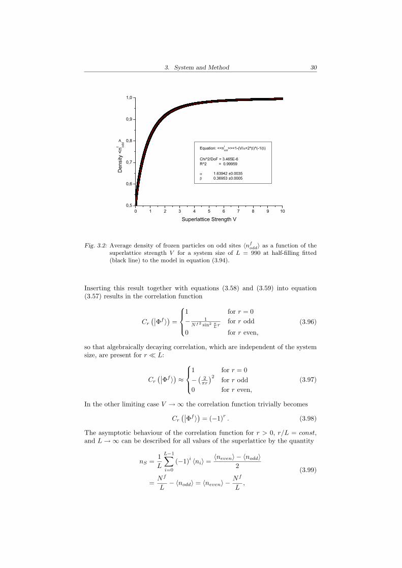
The average density on odd sites 〈nfodd〉 is evaluated numerically in figure 3.2.
For L ≥ 50 no significant dependence of this average density on the system sizeis found. The numerical data is fitted with the model
V = α
[(1
1− p
)β
−(
12
)β]
(3.94)
for later comparison with random staggered disorder.The density-density correlation function for arbitrary fillings and no super-
lattice V = 0 given in equation (3.63) becomes
〈nfi nf
i+r〉 =
Nf
L for r = 0(Nf
L
)2[1− 1
Nf 2 sin2( πL r)
]for r odd
(Nf
L
)2
for r even.
(3.95)
3. System and Method 30
0 1 2 3 4 5 6 7 8 9 100,5
0,6
0,7
0,8
0,9
1,0
Equation: <<nfodd>>=1-(V/ +2^ )^(-1/ )
Chi^2/DoF = 3.465E-6R^2 = 0.99959
1.63942 ±0.00350.36953 ±0.0005
Den
sity
<nf od
d>
Superlattice Strength V
Fig. 3.2: Average density of frozen particles on odd sites 〈nfodd〉 as a function of the
superlattice strength V for a system size of L = 990 at half-filling fitted(black line) to the model in equation (3.94).
Inserting this result together with equations (3.58) and (3.59) into equation(3.57) results in the correlation function
Cr
(∣∣Φf 〉) =
1 for r = 0− 1
Nf 2 sin2 πL r
for r odd
0 for r even,
(3.96)
so that algebraically decaying correlation, which are independent of the systemsize, are present for r ¿ L:
Cr
(∣∣Φf 〉) ≈
1 for r = 0− (
2πr
)2 for r odd0 for r even,
(3.97)
In the other limiting case V →∞ the correlation function trivially becomes
Cr
(∣∣Φf 〉) = (−1)r. (3.98)
The asymptotic behaviour of the correlation function for r > 0, r/L = const,and L→∞ can be described for all values of the superlattice by the quantity
nS =1L
L−1∑
i=0
(−1)i 〈ni〉 =〈neven〉 − 〈nodd〉
2
=Nf
L− 〈nodd〉 = 〈neven〉 − Nf
L,
(3.99)
3. System and Method 31
where 2Nf/L = 〈neven〉+ 〈nodd〉 is used, which gives
〈ni − n〉 = (−1)inS (3.100)
with n = Nf/L. Since it is expected that in the thermodynamic limit the sitedensities for different sites are independent of each other, i.e.
〈(ni − n) (ni+r − n)〉 → 〈(ni − n)〉〈(ni+r − n)〉 (3.101)
for r > 0, the correlation function can be studied in this limit for arbitraryfillings and any value of the superlattice potential depths
Cr
(∣∣Φf 〉)→ (−1)rn2
S
Nf
L
(1− Nf
L
) , (3.102)
and especially at half-filling with equation (3.99)
Cr
(∣∣Φf 〉)→ (−1)r (2 · 〈nodd〉 − 1)2 . (3.103)
The correlation function thus oscillates between a positive and a negative valuefor big r, which is given by 〈nodd〉 (see also figure 3.2).
3.3.3 Random Disorder
The disorder created by frozen particles has to be compared to fully uncorrelatedrandom disorder. To this end, a model of disorder with two site energies Vi ∈0, V and a fixed number Nf of sites with the nonzero site energy V on alattice of even size L is considered. A disorder configuration is denoted by
nf
i
in analogy to the frozen bosons, where Vi = V nfi .
In order to simulate the staggered superlattice potential, the parameter p ∈[0.5, 1] is introduced. The ratio of the weights for two disorder configurationsdiffering on a single site i1, j1 only is
∣∣c(
nfi
)∣∣2∣∣c
(nf
j
)∣∣2 =
1 for i1 − j1 evenp2
(1−p)2for j1 even, i1 odd
(1−p)2
p2 for i1 even, j1 odd,
(3.104)
where the notation from equation (3.92) is used.The average site energy and the correlations between sites can be evaluated
in this model at half-filling by releasing the constraint of fixed filling. In thiscase, the subsystem of the odd sites and the subsystem of the even sites areBernoulli systems with probabilities p and 1−p, where the number of sites withenergy V is binomially distributed in each subsystem
P(Nf
odd = k)
= B (k|p, L/2) , (3.105)
P(Nf
even = k)
= B (k|1− p, L/2) , (3.106)
where
B (k, p, L) =(
Lk
)pk (1− p)L−k
. (3.107)
3. System and Method 32
These distributions have the expectation values⟨Nf
odd
⟩= L/2 · p,
⟨Nf
even
⟩= L/2 · (1− p) (3.108)
and the variances
σ2(Nf
odd
)= σ2
(Nf
even
)= L/2 · p (1− p) . (3.109)
Thus, the average filling is Nf = Nfodd + Nf
even = L/2. Since the relativevariance is vanishing in the thermodynamic limit for both subsystems, e.g. forthe odd sites it holds
σ(Nf
odd
)
⟨Nf
odd
⟩ =√
2L
1− p
p
L→∞−−−−→ 0, (3.110)
the properties of this unrestricted system coincide with those of the system withthe fixed filling Nf = L/2.
This argument leads to the average densities
〈nfodd〉 = p, 〈nf
even〉 = 1− p, (3.111)
which can be equated with the densities (3.93) of the frozen particles in a su-perlattice to compare the results for the different types of disorder. It can benoted that within this comparison, the random staggered disorder correspondsto a two-site mean-field ansatz for the frozen HCBs projected on a fixed numberof particles. For the system sizes used in this work, no significant deviations ofthe average densities from this values were found.
The correlation function Cr in the thermodynamic limit at half-filling is
Cr
(p,Nf =
L
2
)=
1 for r = 0(−1)r (2p− 1)2 for r ≥ 1,
(3.112)
so that there are no correlations beyond the ones introduced by the symme-try breaking, manifesting itself in the alternation of the correlation function(compare equation (3.103)).
There are two limiting cases in this model: The trivial case p = 1 describesa situation, in which only the maximally ordered configuration has a nonzeroweight. The case p = 0.5 refers to a situation without symmetry breaking,i.e. it it is comparable to the disorder created by frozen particles without asuperlattice. In this case, the real-space density is constant and the correlationfunction in the thermodynamic limit becomes Cr = δr0 for arbitrary fillings.
3.3.4 Monte Carlo Sampling
It is practically impossible to evaluate the sum over the disorder configurationsin equation (3.13) for systems greater than L ≈ 30, as the number of configura-tions is (
LNf
). (3.113)
This problem is due to the high dimensionality L of the disorder configurationspace. Such sums can be evaluated with Monte Carlo algorithms, where a
3. System and Method 33
random walk through the configuration space is performed, reproducing theprobability distribution given by the weights
∣∣nfi
∣∣2 in the limit of an infinitenumber of steps. The sum (3.13) over the disorder is finally estimated as theaverage over the Monte Carlo steps
〈〈A〉〉 ≈ 〈〈A〉〉MC =1
Nsteps
Nsteps∑
i=1
〈A〉i. (3.114)
In appendix A the conditions are described, which guarantee the conver-gence of a Markovian random walk to a given probability distribution. Therandom walk is described by stochastic matrices Wµν giving the probability ofa transition from a configuration denoted by µ to a configuration denoted by ν.A probability distribution is given by a stochastic vector −→qµ.
A Markovian process converges to the unique fix point of the stochasticmatrix if the stochastic matrix, is attractive. The fix point condition
−→q eq = −→q eq ·W (3.115)
is satisfied, if the detailed balance condition
−→qνeqWνµ = −→qµ
eqWµν (3.116)
is imposed. The second condition which is imposed on the Markovian process isergodicity. A process is ergodic, if the probability to reach any state from anyother state in a finite number of steps is finite. This ensures that the stochasticmatrix for the process is attractive.
The detailed balance condition (3.116) does not fully determine the transi-tion probabilities. These are written as the product of a selection probabilityTµν and an acceptance probability Aµν
Wµν = TµνAµν . (3.117)
The selection probability Tµν is the probability to propose a move from thestate µ to the state ν, whereas the acceptance probability Aµν is the probabilityof actually accepting the move. The selection probabilities should be chosen insuch a way that the acceptance rate is not too small.
For this work a Monte Carlo Metropolis algorithm has been implemented.In each state only a small constant number of moves Ns is proposed with equalprobabilities
Tµν =
1/Ns if µ→ ν allowed0 otherwise.
(3.118)
The selection probabilities are taken to be symmetric Tµν = Tνµ in this work.The acceptance probability from a state µ to a different state ν 6= µ is chosento be
Aµν = min(
Pν
Pµ, 1
). (3.119)
The transition probability Wµµ, which is not restricted by the detailed balancecondition (3.116), is chosen, such that W is a stochastic matrix (A.5).
We implemented a Monte Carlo Metropolis algorithm with local moves, en-suring that the acceptance rate is not too small. A state
nf
i
is represented
3. System and Method 34
by the indices of the sites occupied by frozen particles i = (i1, i2, . . . , iN ). Thealgorithm is performed with the following series of steps. Let the initial stateof the Markovian walk be the disorder configuration
nf
i
and the site index
which is updated be ik.
1. A statenf
j
is chosen randomly with a uniform distribution under all
states reachable fromnf
i
. One condition on the new state is il = jl iff
l 6= k, because only the index ik is treated in this step. Local moves areimplemented by setting jk to one of the Ns nearest unoccupied sites to theleft of ik in the configuration
nf
i
or to one of the Ns nearest unoccupied
sites to the right of ik in the configurationnf
i
.
2. A random number r ∈ [0, 1] with a uniform distribution is generated. If
r ≤ min
∣∣c(
nfj
)∣∣2∣∣c
(nf
i
)∣∣2 , 1
, (3.120)
the configurationnf
i
is changed to
nf
j
. Otherwise, the configuration
is not changed.
3. The interesting quantities are calculated in the new configurationnf
i
.
The algorithm continues at step 1 for the index k → k + 1.
Considering only unoccupied sites in the first step ensures that reachableconfigurations exist for each configuration. In this procedure, periodic boundaryconditions are applied.
Since the sum over the Markovian random walk is equal to the sum over theconfiguration space only for an infinite number of Monte Carlo steps, the firstMonte Carlo steps are discarded. When the variations in quantities measuredduring the Markovian process do not become smaller any more, the process isclose to the equilibrium distribution and the actual calculation can start. Itis therefore advantageous to start with a highly probable configuration. In thecase of a staggered superlattice, we started from a staggered configuration of thefrozen particles, otherwise we started from a random configuration. We usedbetween 100 and 10000 Monte Carlo steps before the calculation of the sumbegan.
The error of the Monte Carlo simulation due to the finite number of MonteCarlo steps can be estimated by the variance of the mean (see equation (3.114))σ(〈〈A〉〉MC
), which is given by variance of the single random variable accord-
ing to the central limit theorem. The variance of the single measurements isestimated by the variance over the Markovian process
σ2A =
⟨⟨(〈A〉 − 〈〈A⟩⟩MC
)2〉〉MC (3.121)
The statistical error of the Monte Carlo simulation is finally estimated as [38]
∆A =
√σ2
A
Nsteps. (3.122)
However, this estimate of the error requires that the individual Monte Carlomeasurements are independent of each other.
3. System and Method 35
The correlations between the individual measurements, which are naturallypresent in a random walk through configuration space, can be described by theautocorrelation function for the quantity 〈A〉
CAA (i) =1
(Nstep − i)σ2A
Nstep−i∑
j=1
(〈A〉i − 〈〈A〉〉MC) (〈A〉i+j − 〈〈A〉〉MC) .
(3.123)If the correlations are exponentially decaying CAA (i) ∼ exp (−i/τexp
A ), the char-acteristic (Monte Carlo) time τexp
A can be assigned to the correlations in a ran-dom walk. This characteristic time can be generalized for an arbitrary decayshape of CAA to the integrated autocorrelation time
τ intA =
Nstep−1∑
i=1
CAA (i) . (3.124)
Therefore, the series of Nstep Monte Carlo steps can be decomposed into bins ofsize 2τA, which are uncorrelated between each other. This leads to the correctstatistical error of a Monte Carlo simulation
∆A =
√2τA
σ2A
Nsteps. (3.125)
The relevance of the integrated autocorrelation time for this estimate can bemade more rigorous through its closer examination with respect to the blockingmethod [38].
It should also be stated how the error of non-linear functions of statisticalaverages Y = Y (〈〈X1〉〉MC , 〈〈X2〉〉MC , . . .), e.g. the participation ratio as afunction of the real-space densities and the occupation of the natural orbitals as afunction of the OPDM, is estimated. The series of measurements is decomposedinto bins of size τ À max
(τ intX1
, τ intX2
, . . .). In this way, each bin represents an
independent Monte Carlo simulation. The function Y is calculated for eachbin and the distribution of these results over all bins allows an estimate of thestatistical error.
Let Y be the result of the Monte Carlo simulation for Y and let 〈Y 〉 denotethe average over the bins of the estimate of Y in each bin. The error of theMonte Carlo simulation can be estimated with the variance
σ2Y =
⟨(Y − Y
)2⟩
=⟨Y 2
⟩− 〈Y 〉2 +(〈Y 〉 − Y
)2(3.126)
with equation (3.122).Strategies have bin implemented to reduce the typical autocorrelation time
to get effectively uncorrelated Monte carlo steps. These strategies are discussedfor different kinds of disorder in appendix B. In this appendix the size of thebins for the estimation of the statistical error of non-linear functions of statisticalaverages is also analysed.
Nevertheless, for system sizes L ≈ 30 there are at maximum, i.e. for Nf =L/2 (
LL/2
)=
(3015
)≈ 1.5 · 108 (3.127)
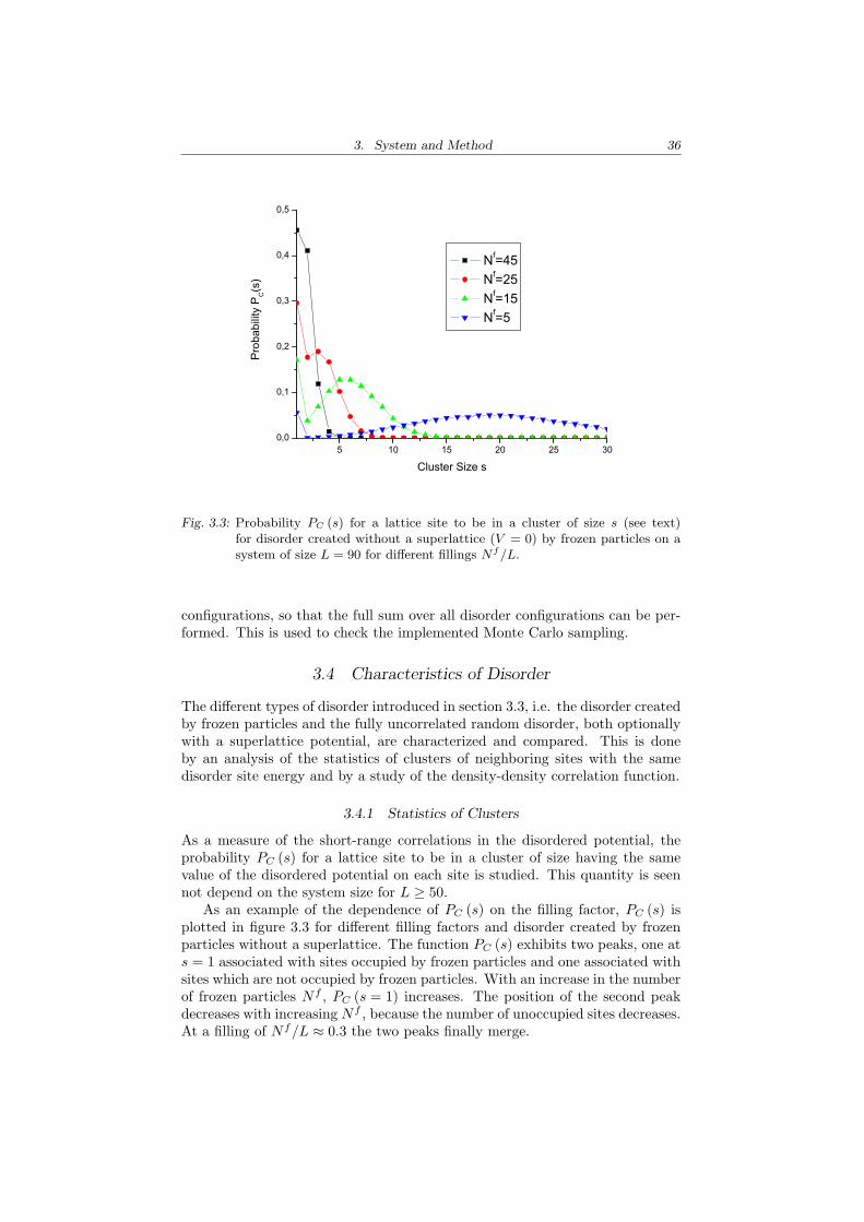
3. System and Method 36
5 10 15 20 25 300,0
0,1
0,2
0,3
0,4
0,5
Prob
abilit
y P C
(s)
Cluster Size s
Nf=45 Nf=25 Nf=15 Nf=5
Fig. 3.3: Probability PC (s) for a lattice site to be in a cluster of size s (see text)for disorder created without a superlattice (V = 0) by frozen particles on asystem of size L = 90 for different fillings Nf/L.
configurations, so that the full sum over all disorder configurations can be per-formed. This is used to check the implemented Monte Carlo sampling.
3.4 Characteristics of Disorder
The different types of disorder introduced in section 3.3, i.e. the disorder createdby frozen particles and the fully uncorrelated random disorder, both optionallywith a superlattice potential, are characterized and compared. This is doneby an analysis of the statistics of clusters of neighboring sites with the samedisorder site energy and by a study of the density-density correlation function.
3.4.1 Statistics of Clusters
As a measure of the short-range correlations in the disordered potential, theprobability PC (s) for a lattice site to be in a cluster of size having the samevalue of the disordered potential on each site is studied. This quantity is seennot depend on the system size for L ≥ 50.
As an example of the dependence of PC (s) on the filling factor, PC (s) isplotted in figure 3.3 for different filling factors and disorder created by frozenparticles without a superlattice. The function PC (s) exhibits two peaks, one ats = 1 associated with sites occupied by frozen particles and one associated withsites which are not occupied by frozen particles. With an increase in the numberof frozen particles Nf , PC (s = 1) increases. The position of the second peakdecreases with increasing Nf , because the number of unoccupied sites decreases.At a filling of Nf/L ≈ 0.3 the two peaks finally merge.
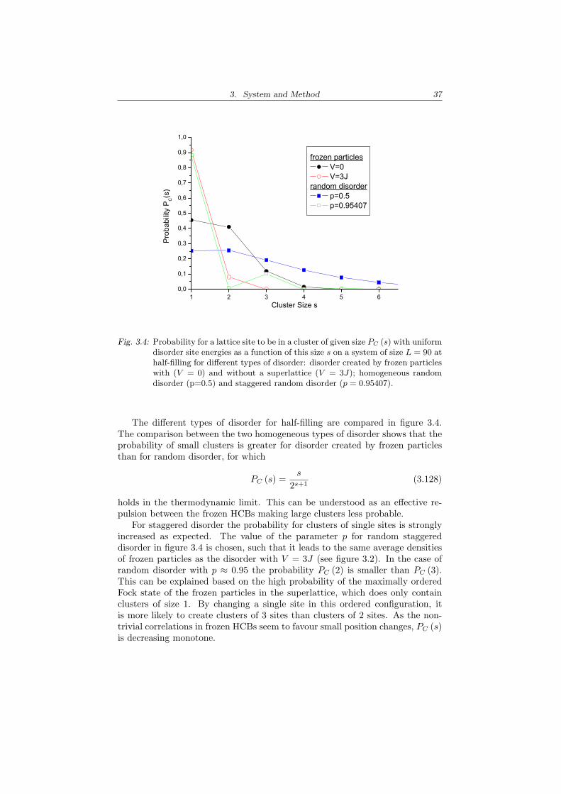
3. System and Method 37
1 2 3 4 5 60,0
0,1
0,2
0,3
0,4
0,5
0,6
0,7
0,8
0,9
1,0
frozen particles V=0 V=3J
random disorder p=0.5 p=0.95407
Prob
abilit
y P C
(s)
Cluster Size s
Fig. 3.4: Probability for a lattice site to be in a cluster of given size PC (s) with uniformdisorder site energies as a function of this size s on a system of size L = 90 athalf-filling for different types of disorder: disorder created by frozen particleswith (V = 0) and without a superlattice (V = 3J); homogeneous randomdisorder (p=0.5) and staggered random disorder (p = 0.95407).
The different types of disorder for half-filling are compared in figure 3.4.The comparison between the two homogeneous types of disorder shows that theprobability of small clusters is greater for disorder created by frozen particlesthan for random disorder, for which
PC (s) =s
2s+1(3.128)
holds in the thermodynamic limit. This can be understood as an effective re-pulsion between the frozen HCBs making large clusters less probable.
For staggered disorder the probability for clusters of single sites is stronglyincreased as expected. The value of the parameter p for random staggereddisorder in figure 3.4 is chosen, such that it leads to the same average densitiesof frozen particles as the disorder with V = 3J (see figure 3.2). In the case ofrandom disorder with p ≈ 0.95 the probability PC (2) is smaller than PC (3).This can be explained based on the high probability of the maximally orderedFock state of the frozen particles in the superlattice, which does only containclusters of size 1. By changing a single site in this ordered configuration, itis more likely to create clusters of 3 sites than clusters of 2 sites. As the non-trivial correlations in frozen HCBs seem to favour small position changes, PC (s)is decreasing monotone.
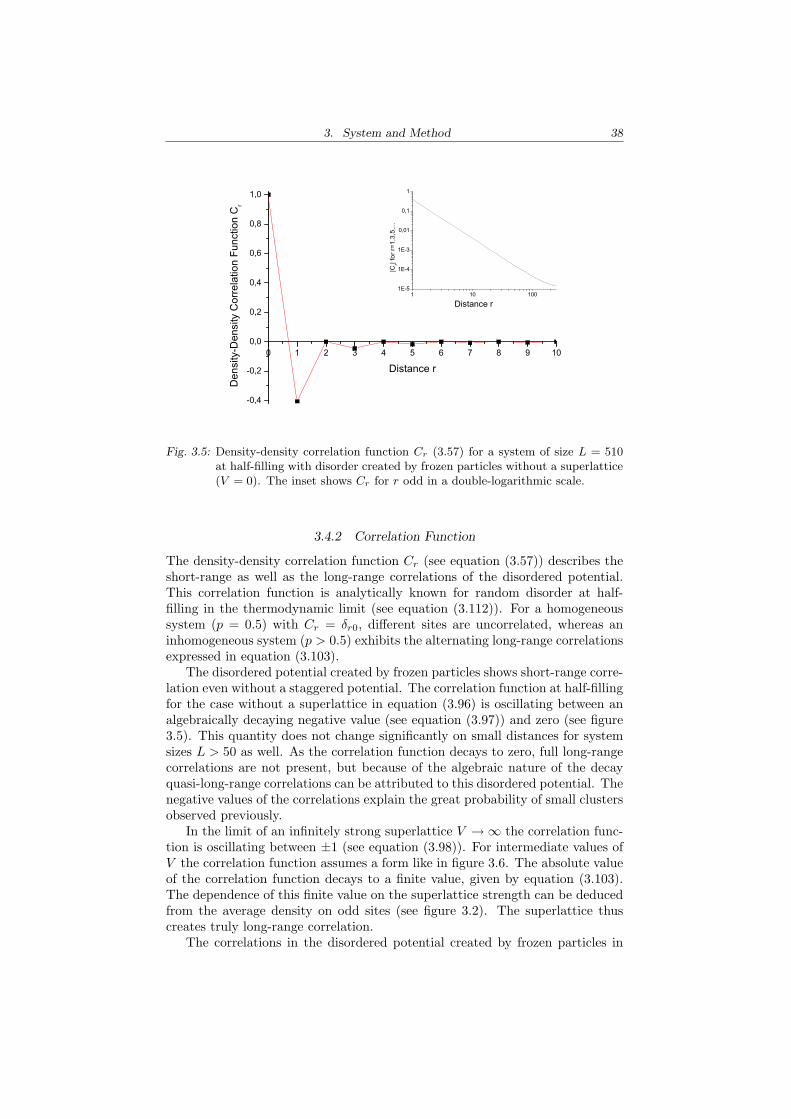
3. System and Method 38
0 1 2 3 4 5 6 7 8 9 10
-0,4
-0,2
0,0
0,2
0,4
0,6
0,8
1,0
1 10 1001E-5
1E-4
1E-3
0,01
0,1
1
Den
sity
-Den
sity
Cor
rela
tion
Func
tion
Cr
Distance r
Distance r
|Cr| f
or r=
1,3,
5,...
Fig. 3.5: Density-density correlation function Cr (3.57) for a system of size L = 510at half-filling with disorder created by frozen particles without a superlattice(V = 0). The inset shows Cr for r odd in a double-logarithmic scale.
3.4.2 Correlation Function
The density-density correlation function Cr (see equation (3.57)) describes theshort-range as well as the long-range correlations of the disordered potential.This correlation function is analytically known for random disorder at half-filling in the thermodynamic limit (see equation (3.112)). For a homogeneoussystem (p = 0.5) with Cr = δr0, different sites are uncorrelated, whereas aninhomogeneous system (p > 0.5) exhibits the alternating long-range correlationsexpressed in equation (3.103).
The disordered potential created by frozen particles shows short-range corre-lation even without a staggered potential. The correlation function at half-fillingfor the case without a superlattice in equation (3.96) is oscillating between analgebraically decaying negative value (see equation (3.97)) and zero (see figure3.5). This quantity does not change significantly on small distances for systemsizes L > 50 as well. As the correlation function decays to zero, full long-rangecorrelations are not present, but because of the algebraic nature of the decayquasi-long-range correlations can be attributed to this disordered potential. Thenegative values of the correlations explain the great probability of small clustersobserved previously.
In the limit of an infinitely strong superlattice V →∞ the correlation func-tion is oscillating between ±1 (see equation (3.98)). For intermediate values ofV the correlation function assumes a form like in figure 3.6. The absolute valueof the correlation function decays to a finite value, given by equation (3.103).The dependence of this finite value on the superlattice strength can be deducedfrom the average density on odd sites (see figure 3.2). The superlattice thuscreates truly long-range correlation.
The correlations in the disordered potential created by frozen particles in
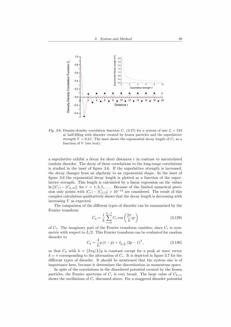
3. System and Method 39
0 2 4 6 8 10 12 14 16 18 20
-0,4
-0,2
0,0
0,2
0,4
0,6
0,8
1,0
0 2 4 6 8 100,0
0,4
0,8
1,2
1,6
2,0
2,4
2,8
Expo
nent
ial D
ecay
Len
gth
of C
r
Superlattice Strength V
Den
sity
-Den
sity
Cor
rela
tion
Func
tion
Cr
Distance r
Fig. 3.6: Density-density correlation function Cr (3.57) for a system of size L = 510at half-filling with disorder created by frozen particles and the superlatticestrength V = 0.3J . The inset shows the exponential decay length of Cr as afunction of V (see text).
a superlattice exhibit a decay for short distances r in contrast to uncorrelatedrandom disorder. The decay of these correlations to the long-range correlationsis studied in the inset of figure 3.6. If the superlattice strength is increased,the decay changes from an algebraic to an exponential shape. In the inset offigure 3.6 the exponential decay length is plotted as a function of the super-lattice strength. This length is calculated by a linear regression on the valuesln
(|Cr| − |CL/2|)
for r = 1, 3, 5, . . . . Because of the limited numerical preci-sion only points with |Cr| − |CL/2| > 10−14 are considered. The result of thiscomplex calculation qualitatively shows that the decay length is decreasing withincreasing V as expected.
The comparison of the different types of disorder can be summarized by theFourier transform
Cq =1L
L−1∑r=0
Cr cos(
2π
Lqr
)(3.129)
of Cr. The imaginary part of the Fourier transform vanishes, since Cr is sym-metric with respect to L/2. This Fourier transform can be evaluated for randomdisorder to
Cq =4L
p (1− p) + δq, L2
(2p− 1)2 , (3.130)
so that Ck with k =(2πq/L
)q is constant except for a peak at wave vector
k = π corresponding to the alternation of Cr. It is depicted in figure 3.7 for thedifferent types of disorder. It should be mentioned that the system size is ofimportance here, because it determines the discretization in momentum space.
In spite of the correlations in the disordered potential created by the frozenparticles, the Fourier spectrum of Cr is very broad. The large value of Ck=π
shows the oscillations of Cr discussed above. For a staggered disorder potential
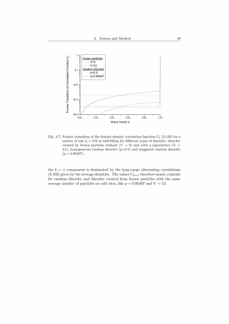
3. System and Method 40
0,0 0,2 0,4 0,6 0,8 1,01E-4
1E-3
0,01
0,1
1
Four
ier T
rans
form
of C
orre
latio
n Fu
nctio
n C
k
Wave Vector k
frozen particles V=0 V=3J
random disorder p=0.5 p=0.95407
Fig. 3.7: Fourier transform of the density-density correlation function Ck (3.129) for asystem of size L = 510 at half-filling for different types of disorder: disordercreated by frozen particles without (V = 0) and with a superlattice (V =3J); homogeneous random disorder (p=0.5) and staggered random disorder(p = 0.95407).
the k = π component is dominated by the long-range alternating correlations(3.103) given by the average densities. The values Ck=π therefore nearly coincidefor random disorder and disorder created from frozen particles with the sameaverage number of particles on odd sites, like p = 0.95407 and V = 3J .
4. GROUND STATE PROPERTIES
In this chapter the properties of the eigenstates of the Hamiltonian H0 +Hint
(see equations (3.2) and (3.4)) for the mobile bosons are investigated. Theanalysis begins with the localization properties of the eigenstates in real-space(see section 4.1) and continues with the off-diagonal many-body physics of HCBsin a disordered potential (see section 4.2).
4.1 Localization
It is analysed in this section whether some or all of the eigenstates of the Hamil-tonian H0 (see equation (3.2)) with periodic boundary conditions are localized.Within a disorder configuration, the participation ratios of the eigenstates ofH0 + Hint are calculated. The eigenstates are distributed into bins of eigen-states with the same energy eigenvalue and its participation ratios are added.The sums of the participation ratios in the bins are disorder-averaged with theweights
∣∣c(nfi
)∣∣2 given by the frozen HCBs. Finally, the disorder-averagedcumulated participation ratio for each bin is divided by the disorder averagednumber of eigenstates in the corresponding bin, i.e. the density of states (DOS),to get the average participation ratio of an eigenstate as a function of the en-ergy. This analysis is repeated for different system sizes with the same filling offrozen HCBs, in order to determine how the average extent of each eigenstateincreases with the system size.
The results of this analysis are plotted in the upper part of figure 4.1. Theaverage participation ratio of an eigenstate as a function of the energy is domi-nated by the average DOS depicted in the lower part of figure 4.1. The positiveenergy part of the band structure is shifted by the interaction energy U andthe new lower and upper bands are compressed. Additionally four peaks corre-sponding to very strongly localized states appear near the band edges.
In the average participation ratio of an eigenstate the peaks close to theband edges disappear, because the corresponding states are highly localized.The participation ratios in the lower and upper band are increasing with thesystem size, but sublinear. This residual increase can be attributed to thefinite system sizes, which are not sufficiently larger than the localization length.Therefore, if extended states exist, their number is not extensive.
Nevertheless, a non-extensive number of extended eigenstates is sufficient tosuppress localization in transport experiments, as shown in the random-dimermodel (see section 2.3), and even a finite number of extended states can lead topolynomial localization. Therefore, the results of this section are not conclusivefor the presence of exponential localization in disorder created by frozen HCBs.
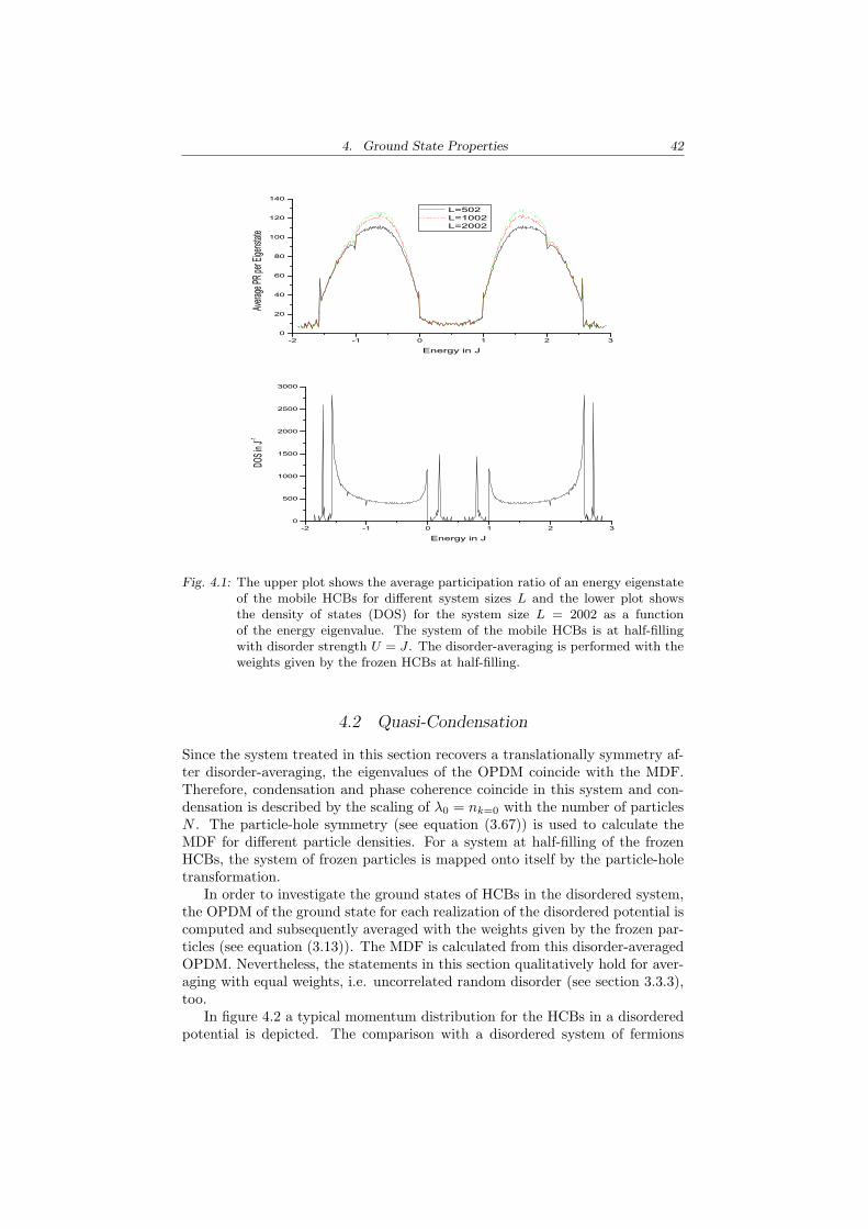
4. Ground State Properties 42
-2 -1 0 1 2 30
20
40
60
80
100
120
140
Averag
e PR p
er Eige
nstate
Energy in J
L=502 L=1002 L=2002
-2 -1 0 1 2 30
500
1000
1500
2000
2500
3000
DOS i
n J-1
Energy in J
Fig. 4.1: The upper plot shows the average participation ratio of an energy eigenstateof the mobile HCBs for different system sizes L and the lower plot showsthe density of states (DOS) for the system size L = 2002 as a functionof the energy eigenvalue. The system of the mobile HCBs is at half-fillingwith disorder strength U = J . The disorder-averaging is performed with theweights given by the frozen HCBs at half-filling.
4.2 Quasi-Condensation
Since the system treated in this section recovers a translationally symmetry af-ter disorder-averaging, the eigenvalues of the OPDM coincide with the MDF.Therefore, condensation and phase coherence coincide in this system and con-densation is described by the scaling of λ0 = nk=0 with the number of particlesN . The particle-hole symmetry (see equation (3.67)) is used to calculate theMDF for different particle densities. For a system at half-filling of the frozenHCBs, the system of frozen particles is mapped onto itself by the particle-holetransformation.
In order to investigate the ground states of HCBs in the disordered system,the OPDM of the ground state for each realization of the disordered potential iscomputed and subsequently averaged with the weights given by the frozen par-ticles (see equation (3.13)). The MDF is calculated from this disorder-averagedOPDM. Nevertheless, the statements in this section qualitatively hold for aver-aging with equal weights, i.e. uncorrelated random disorder (see section 3.3.3),too.
In figure 4.2 a typical momentum distribution for the HCBs in a disorderedpotential is depicted. The comparison with a disordered system of fermions
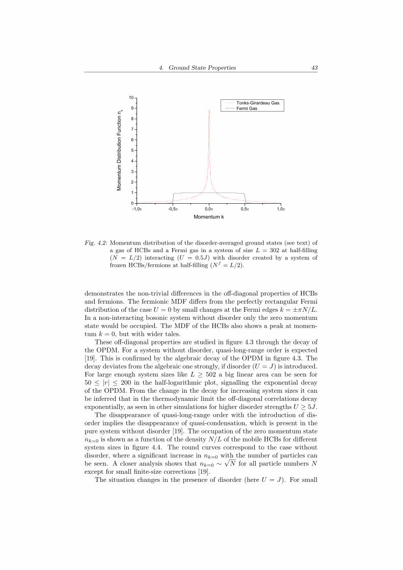
4. Ground State Properties 43
-1,0 -0,5 0,0 0,5 1,00
1
2
3
4
5
6
7
8
9
10 Tonks-Girardeau Gas Fermi Gas
Mom
entu
m D
istri
butio
n Fu
nctio
n n k
Momentum k
Fig. 4.2: Momentum distribution of the disorder-averaged ground states (see text) ofa gas of HCBs and a Fermi gas in a system of size L = 302 at half-filling(N = L/2) interacting (U = 0.5J) with disorder created by a system offrozen HCBs/fermions at half-filling (Nf = L/2).
demonstrates the non-trivial differences in the off-diagonal properties of HCBsand fermions. The fermionic MDF differs from the perfectly rectangular Fermidistribution of the case U = 0 by small changes at the Fermi edges k = ±πN/L.In a non-interacting bosonic system without disorder only the zero momentumstate would be occupied. The MDF of the HCBs also shows a peak at momen-tum k = 0, but with wider tales.
These off-diagonal properties are studied in figure 4.3 through the decay ofthe OPDM. For a system without disorder, quasi-long-range order is expected[19]. This is confirmed by the algebraic decay of the OPDM in figure 4.3. Thedecay deviates from the algebraic one strongly, if disorder (U = J) is introduced.For large enough system sizes like L ≥ 502 a big linear area can be seen for50 ≤ |r| ≤ 200 in the half-logarithmic plot, signalling the exponential decayof the OPDM. From the change in the decay for increasing system sizes it canbe inferred that in the thermodynamic limit the off-diagonal correlations decayexponentially, as seen in other simulations for higher disorder strengths U ≥ 5J .
The disappearance of quasi-long-range order with the introduction of dis-order implies the disappearance of quasi-condensation, which is present in thepure system without disorder [19]. The occupation of the zero momentum statenk=0 is shown as a function of the density N/L of the mobile HCBs for differentsystem sizes in figure 4.4. The round curves correspond to the case withoutdisorder, where a significant increase in nk=0 with the number of particles canbe seen. A closer analysis shows that nk=0 ∼
√N for all particle numbers N
except for small finite-size corrections [19].The situation changes in the presence of disorder (here U = J). For small
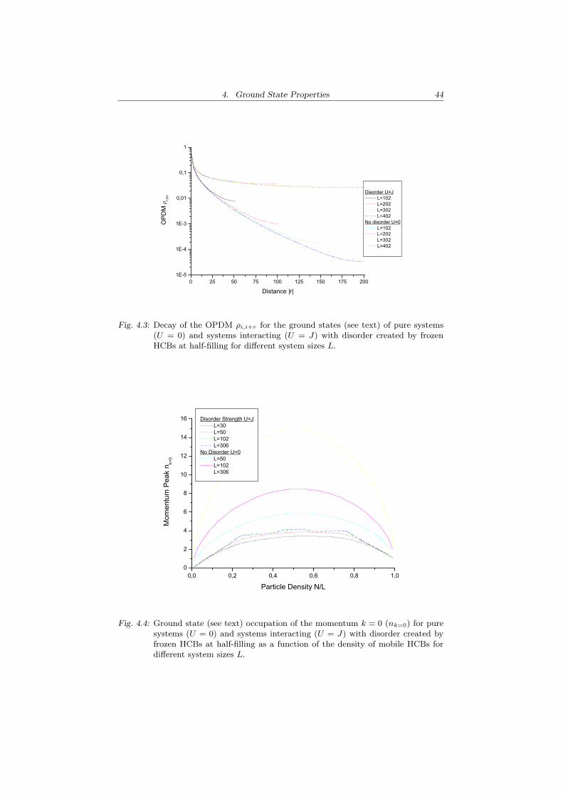
4. Ground State Properties 44
0 25 50 75 100 125 150 175 2001E-5
1E-4
1E-3
0,01
0,1
1
OPD
M
i,i+r
Distance |r|
Disorder U=J L=102 L=202 L=302 L=402
No disorder U=0 L=102 L=202 L=302 L=402
Fig. 4.3: Decay of the OPDM ρi,i+r for the ground states (see text) of pure systems(U = 0) and systems interacting (U = J) with disorder created by frozenHCBs at half-filling for different system sizes L.
0,0 0,2 0,4 0,6 0,8 1,00
2
4
6
8
10
12
14
16 Disorder Strength U=J L=30 L=50 L=102 L=306
No Disorder U=0 L=50 L=102 L=306
Mom
entu
m P
eak
n k=0
Particle Density N/L
Fig. 4.4: Ground state (see text) occupation of the momentum k = 0 (nk=0) for puresystems (U = 0) and systems interacting (U = J) with disorder created byfrozen HCBs at half-filling as a function of the density of mobile HCBs fordifferent system sizes L.
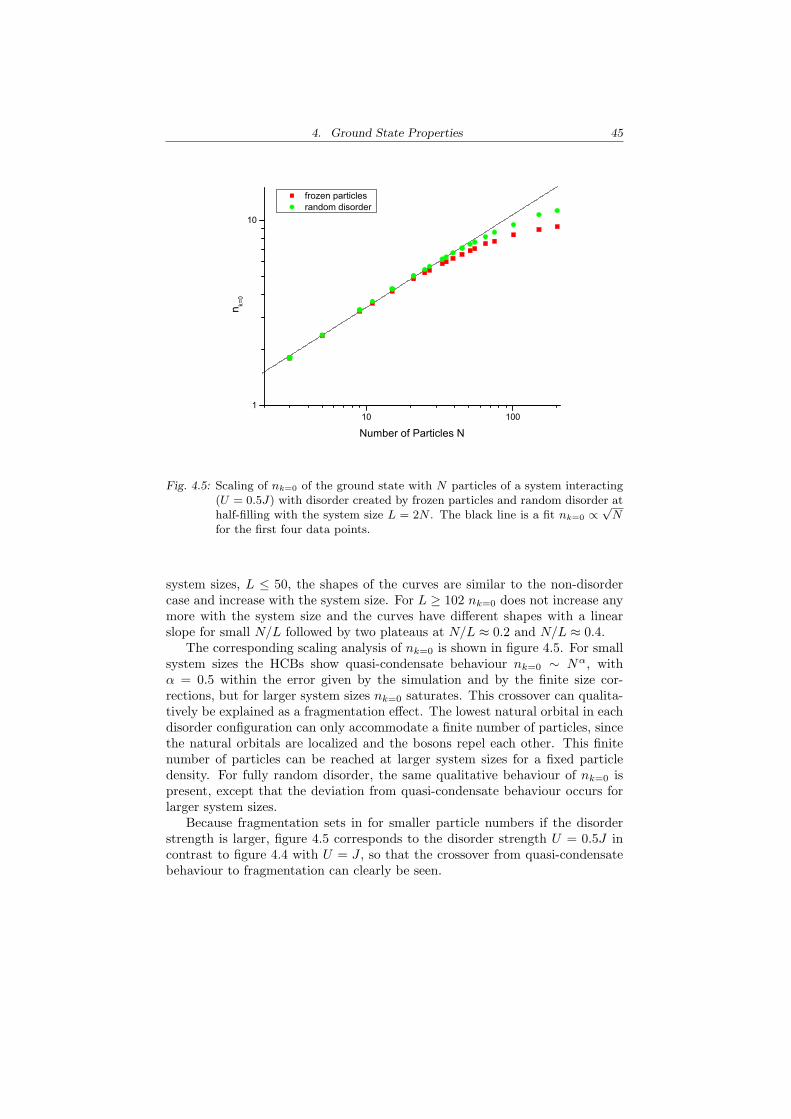
4. Ground State Properties 45
10 1001
10
frozen particles random disorder
n k=0
Number of Particles N
Fig. 4.5: Scaling of nk=0 of the ground state with N particles of a system interacting(U = 0.5J) with disorder created by frozen particles and random disorder athalf-filling with the system size L = 2N . The black line is a fit nk=0 ∝
√N
for the first four data points.
system sizes, L ≤ 50, the shapes of the curves are similar to the non-disordercase and increase with the system size. For L ≥ 102 nk=0 does not increase anymore with the system size and the curves have different shapes with a linearslope for small N/L followed by two plateaus at N/L ≈ 0.2 and N/L ≈ 0.4.
The corresponding scaling analysis of nk=0 is shown in figure 4.5. For smallsystem sizes the HCBs show quasi-condensate behaviour nk=0 ∼ Nα, withα = 0.5 within the error given by the simulation and by the finite size cor-rections, but for larger system sizes nk=0 saturates. This crossover can qualita-tively be explained as a fragmentation effect. The lowest natural orbital in eachdisorder configuration can only accommodate a finite number of particles, sincethe natural orbitals are localized and the bosons repel each other. This finitenumber of particles can be reached at larger system sizes for a fixed particledensity. For fully random disorder, the same qualitative behaviour of nk=0 ispresent, except that the deviation from quasi-condensate behaviour occurs forlarger system sizes.
Because fragmentation sets in for smaller particle numbers if the disorderstrength is larger, figure 4.5 corresponds to the disorder strength U = 0.5J incontrast to figure 4.4 with U = J , so that the crossover from quasi-condensatebehaviour to fragmentation can clearly be seen.
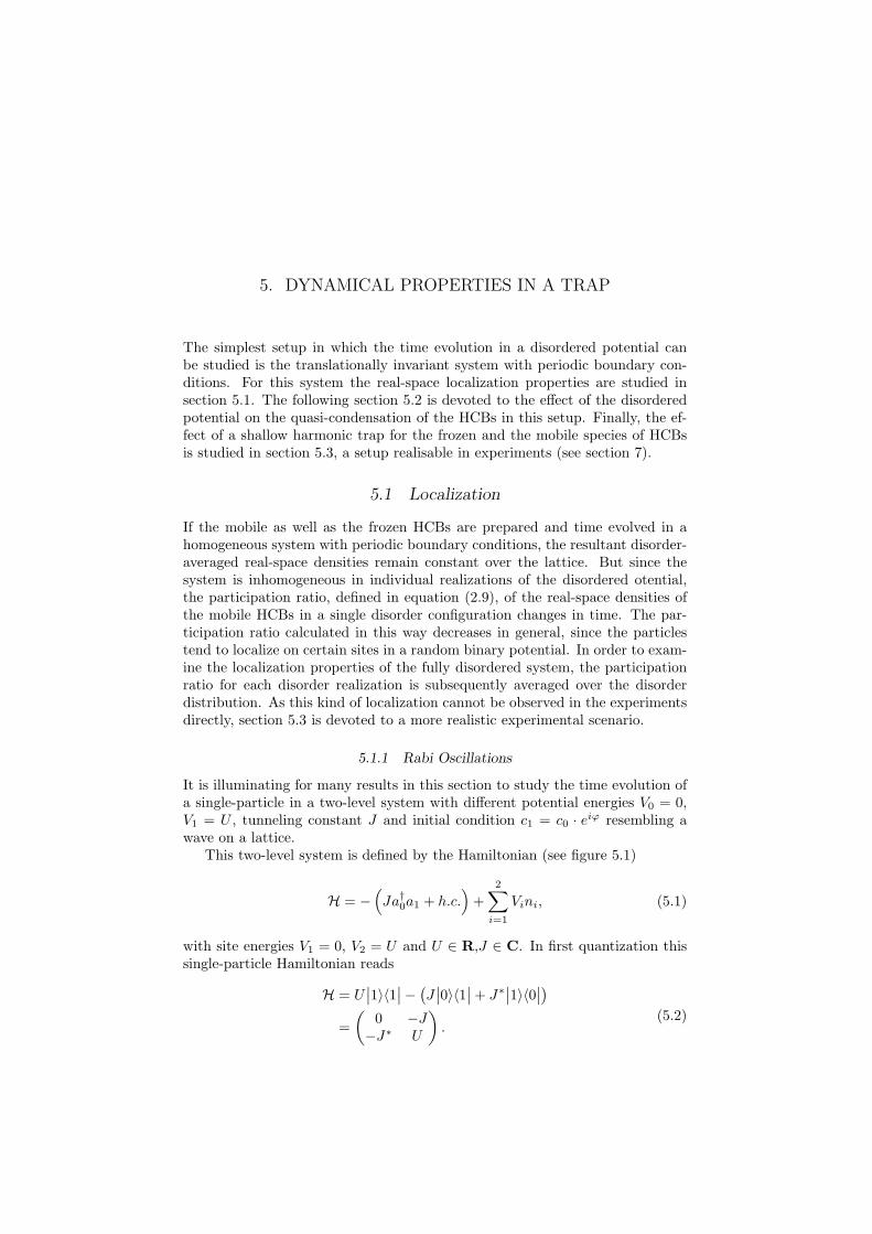
5. DYNAMICAL PROPERTIES IN A TRAP
The simplest setup in which the time evolution in a disordered potential canbe studied is the translationally invariant system with periodic boundary con-ditions. For this system the real-space localization properties are studied insection 5.1. The following section 5.2 is devoted to the effect of the disorderedpotential on the quasi-condensation of the HCBs in this setup. Finally, the ef-fect of a shallow harmonic trap for the frozen and the mobile species of HCBsis studied in section 5.3, a setup realisable in experiments (see section 7).
5.1 Localization
If the mobile as well as the frozen HCBs are prepared and time evolved in ahomogeneous system with periodic boundary conditions, the resultant disorder-averaged real-space densities remain constant over the lattice. But since thesystem is inhomogeneous in individual realizations of the disordered otential,the participation ratio, defined in equation (2.9), of the real-space densities ofthe mobile HCBs in a single disorder configuration changes in time. The par-ticipation ratio calculated in this way decreases in general, since the particlestend to localize on certain sites in a random binary potential. In order to exam-ine the localization properties of the fully disordered system, the participationratio for each disorder realization is subsequently averaged over the disorderdistribution. As this kind of localization cannot be observed in the experimentsdirectly, section 5.3 is devoted to a more realistic experimental scenario.
5.1.1 Rabi Oscillations
It is illuminating for many results in this section to study the time evolution ofa single-particle in a two-level system with different potential energies V0 = 0,V1 = U , tunneling constant J and initial condition c1 = c0 · eiϕ resembling awave on a lattice.
This two-level system is defined by the Hamiltonian (see figure 5.1)
H = −(Ja†0a1 + h.c.
)+
2∑
i=1
Vini, (5.1)
with site energies V1 = 0, V2 = U and U ∈ R,J ∈ C. In first quantization thissingle-particle Hamiltonian reads
H = U∣∣1〉〈1∣∣− (
J∣∣0〉〈1∣∣ + J∗
∣∣1〉〈0∣∣)
=(
0 −J−J∗ U
).
(5.2)
5. Dynamical Properties in a Trap 47
U
0
1-J
Fig. 5.1: Schematic depiction of a two-level system.
In the interaction picture, i.e. with the Ansatz∣∣Φ(t)〉 = c0 (t)
∣∣0〉+ c1 (t) e−iUt∣∣1〉 (5.3)
the time dependent Schrodinger equation i∂t
∣∣Φ(t)〉 = H∣∣Φ(t)〉 becomes
i∂tc0 (t) = −Jc1 (t) e−iUt (5.4)
i∂tc1 (t) = −J∗c0 (t) eiUt. (5.5)
Inserting c1 from equation (5.4) into equation (5.5), one gets a linear differentialequation of second order, which can be solved. With the initial conditionsc0 (0) = c0 and c1 (0) = c1 the exact solution for this two-level system is
c0 (t) = e−i U2 t
(c0 cosωt + i
U
2ωc0 sin ωt + i
J
ωc1 sin ωt
)(5.6)
c1 (t) = ei U2 t
(c1 cos ωt− i
U
2ωc1 sin ωt + i
J∗
ωc0 sinωt
), (5.7)
where the energy
ω =√
(U/2)2 + |J |2 (5.8)
describes the frequency of the occupation oscillation between the two levels. Forsimplicity J ∈ R is chosen in the following.
The real-space density n0 = |c0 (t) |2 thus becomes
n0 = |c0|2 cos2 ωt +(
U
2ω
)2
|c0|2 sin2 ωt +(
J
ω
)2
|c1|2 sin2 ωt
+J
ω
i
2sin 2ωt (c∗0c1 − c0c
∗1)−
UJ
2ω2sin2 ωt (c∗0c1 + c0c
∗1) . (5.9)
With the initial conditions c1 = c0eiϕ, which allows the comparision with a
wave as initial condition on a lattice, this density becomes
n0 (t) =12− J
2ωsin 2ωt sinϕ +
UJ
2ω2sin2 ωt cosϕ. (5.10)
Therefore, the occupation performs a periodic oscillation between the two levels.In order to compare these Rabi oscillations with the disordered lattice system,the density n0 is time-averaged over one period of the oscillation, i.e. t ∈[0, π/ω]. The result
〈n0 (t)〉t =12
+UJ
4ω2cos ϕ (5.11)
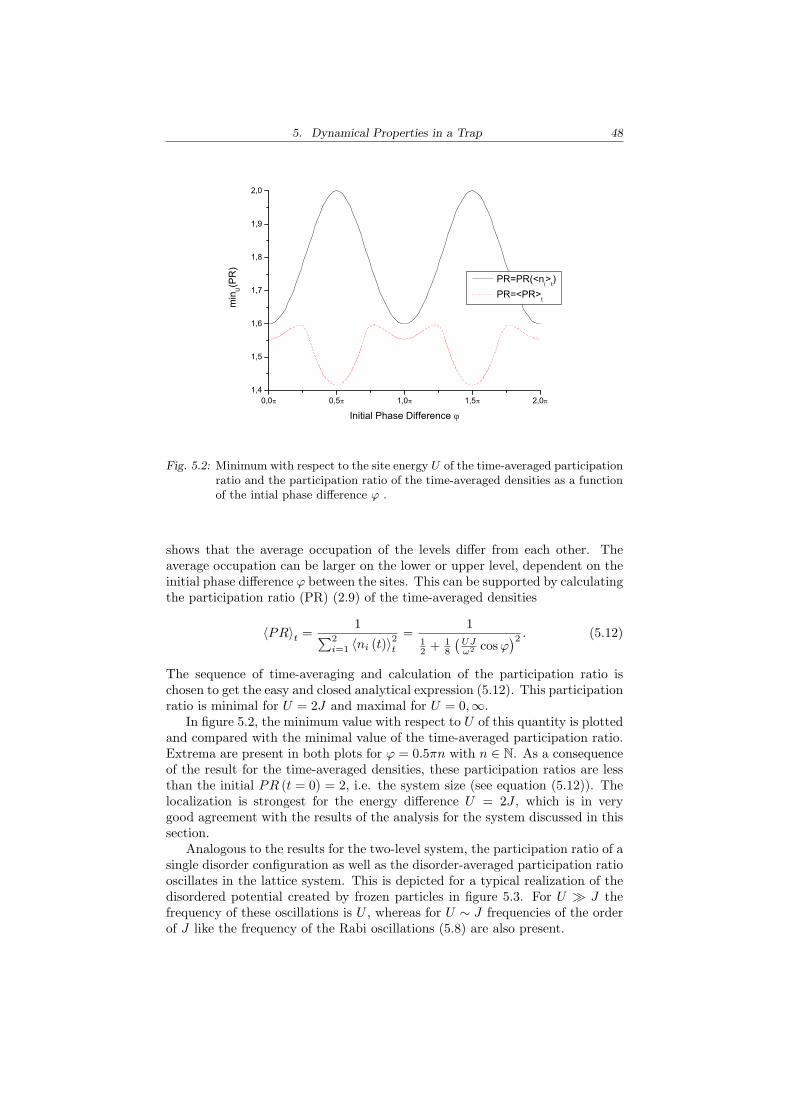
5. Dynamical Properties in a Trap 48
0,0 0,5 1,0 1,5 2,01,4
1,5
1,6
1,7
1,8
1,9
2,0
min
U(P
R)
Initial Phase Difference
PR=PR(<ni>t) PR=<PR>t
Fig. 5.2: Minimum with respect to the site energy U of the time-averaged participationratio and the participation ratio of the time-averaged densities as a functionof the intial phase difference ϕ .
shows that the average occupation of the levels differ from each other. Theaverage occupation can be larger on the lower or upper level, dependent on theinitial phase difference ϕ between the sites. This can be supported by calculatingthe participation ratio (PR) (2.9) of the time-averaged densities
〈PR〉t =1∑2
i=1 〈ni (t)〉2t=
112 + 1
8
(UJω2 cosϕ
)2 . (5.12)
The sequence of time-averaging and calculation of the participation ratio ischosen to get the easy and closed analytical expression (5.12). This participationratio is minimal for U = 2J and maximal for U = 0,∞.
In figure 5.2, the minimum value with respect to U of this quantity is plottedand compared with the minimal value of the time-averaged participation ratio.Extrema are present in both plots for ϕ = 0.5πn with n ∈ N. As a consequenceof the result for the time-averaged densities, these participation ratios are lessthan the initial PR (t = 0) = 2, i.e. the system size (see equation (5.12)). Thelocalization is strongest for the energy difference U = 2J , which is in verygood agreement with the results of the analysis for the system discussed in thissection.
Analogous to the results for the two-level system, the participation ratio of asingle disorder configuration as well as the disorder-averaged participation ratiooscillates in the lattice system. This is depicted for a typical realization of thedisordered potential created by frozen particles in figure 5.3. For U À J thefrequency of these oscillations is U , whereas for U ∼ J frequencies of the orderof J like the frequency of the Rabi oscillations (5.8) are also present.
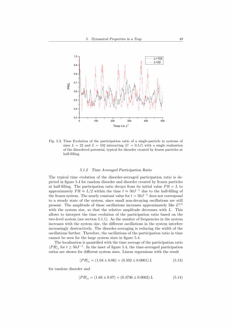
5. Dynamical Properties in a Trap 49
0 100 200 300 400 5000,3
0,4
0,5
0,6
0,7
0,8
0,9
1,0 L=102 L=22
PR/L
Time t in J-1
Fig. 5.3: Time Evolution of the participation ratio of a single-particle in systems ofsizes L = 22 and L = 102 interacting (U = 0.5J) with a single realizationof the disordered potential, typical for disorder created by frozen particles athalf-filling.
5.1.2 Time Averaged Participation Ratio
The typical time evolution of the disorder-averaged participation ratio is de-picted in figure 5.4 for random disorder and disorder created by frozen particlesat half-filling. The participation ratio decays from its initial value PR = L toapproximately PR ≈ L/2 within the time t ≈ 50J−1 due to the half-filling ofthe frozen system. The nearly constant value for t > 50J−1 does not correspondto a steady state of the system, since small non-decaying oscillations are stillpresent. The amplitude of these oscillations increases approximately like L0.5
with the system size, so that the relative amplitude decreases with L. Thisallows to interpret the time evolution of the participation ratio based on thetwo-level system (see section 5.1.1). As the number of frequencies in the systemincreases with the system size, the different oscillations in the system interfereincreasingly destructively. The disorder-averaging is reducing the width of theoscillations further. Therefore, the oscillations of the participation ratio in timecannot be seen for the large system sizes in figure 5.4.
The localization is quantified with the time average of the participation ratio〈PR〉t for t ≥ 50J−1. In the inset of figure 5.4, the time-averaged participationratios are shown for different system sizes. Linear regressions with the result
〈PR〉t = (1.04± 0.06) + (0.502± 0.0001)L (5.13)
for random disorder and
〈PR〉t = (1.68± 0.07) + (0.4736± 0.0002)L (5.14)
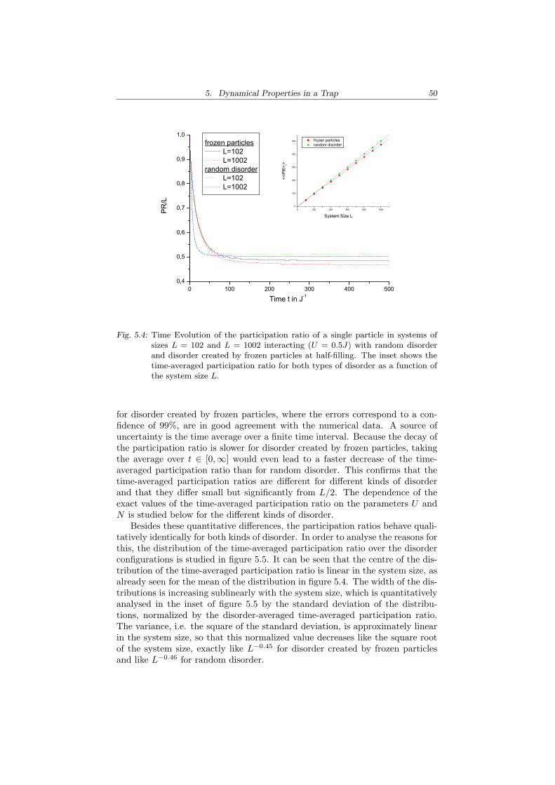
5. Dynamical Properties in a Trap 50
0 100 200 300 400 5000,4
0,5
0,6
0,7
0,8
0,9
1,0
0 200 400 600 800 10000
100
200
300
400
500
PR/L
frozen particles L=102 L=1002
random disorder L=102 L=1002
Time t in J-1
System Size L
<<P
R> t>
frozen particles random disorder
Fig. 5.4: Time Evolution of the participation ratio of a single particle in systems ofsizes L = 102 and L = 1002 interacting (U = 0.5J) with random disorderand disorder created by frozen particles at half-filling. The inset shows thetime-averaged participation ratio for both types of disorder as a function ofthe system size L.
for disorder created by frozen particles, where the errors correspond to a con-fidence of 99%, are in good agreement with the numerical data. A source ofuncertainty is the time average over a finite time interval. Because the decay ofthe participation ratio is slower for disorder created by frozen particles, takingthe average over t ∈ [0,∞] would even lead to a faster decrease of the time-averaged participation ratio than for random disorder. This confirms that thetime-averaged participation ratios are different for different kinds of disorderand that they differ small but significantly from L/2. The dependence of theexact values of the time-averaged participation ratio on the parameters U andN is studied below for the different kinds of disorder.
Besides these quantitative differences, the participation ratios behave quali-tatively identically for both kinds of disorder. In order to analyse the reasons forthis, the distribution of the time-averaged participation ratio over the disorderconfigurations is studied in figure 5.5. It can be seen that the centre of the dis-tribution of the time-averaged participation ratio is linear in the system size, asalready seen for the mean of the distribution in figure 5.4. The width of the dis-tributions is increasing sublinearly with the system size, which is quantitativelyanalysed in the inset of figure 5.5 by the standard deviation of the distribu-tions, normalized by the disorder-averaged time-averaged participation ratio.The variance, i.e. the square of the standard deviation, is approximately linearin the system size, so that this normalized value decreases like the square rootof the system size, exactly like L−0.45 for disorder created by frozen particlesand like L−0.46 for random disorder.
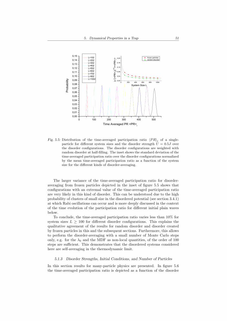
5. Dynamical Properties in a Trap 51
0 100 200 300 400 5000,000,010,020,030,040,050,060,070,080,090,100,110,120,130,140,15
0 200 400 600 800 10000,00
0,04
0,08
0,12
0,16
0,20
Prob
abilit
y
Time Averaged PR <PR>t
L=102 L=202 L=302 L=402 L=502 L=602 L=702 L=902 L=1002
System Size L
((<
PR> t))1/
2 /<<P
R> t> frozen particles
random disorder
Fig. 5.5: Distribution of the time-averaged participation ratio 〈PR〉t of a single-particle for different system sizes and the disorder strength U = 0.5J overthe disorder configurations. The disorder configurations are weighted withrandom disorder at half-filling. The inset shows the standard deviation of thetime-averaged participation ratio over the disorder configurations normalizedby the mean time-averaged participation ratio as a function of the systemsize for the different kinds of disorder-averaging.
The larger variance of the time-averaged participation ratio for disorder-averaging from frozen particles depicted in the inset of figure 5.5 shows thatconfigurations with an extremal value of the time-averaged participation ratioare very likely in this kind of disorder. This can be understood due to the highprobability of clusters of small size in the disordered potential (see section 3.4.1)at which Rabi oscillations can occur and is more deeply discussed in the contextof the time evolution of the participation ratio for different initial plain wavesbelow.
To conclude, the time-averaged participation ratio varies less than 10% forsystem sizes L ≥ 100 for different disorder configurations. This explains thequalitative agreement of the results for random disorder and disorder createdby frozen particles in this and the subsequent sections. Furthermore, this allowsto perform the disorder-averaging with a small number of Monte Carlo stepsonly, e.g. for the λ0 and the MDF as non-local quantities, of the order of 100steps are sufficient. This demonstrates that the disordered systems consideredhere are self-averaging in the thermodynamic limit.
5.1.3 Disorder Strengths, Initial Conditions, and Number of Particles
In this section results for many-particle physics are presented. In figure 5.6the time-averaged participation ratio is depicted as a function of the disorder
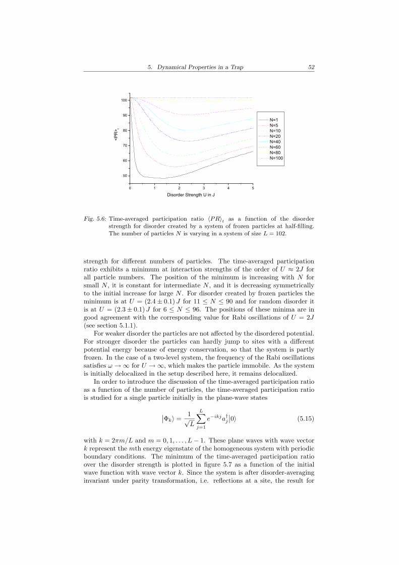
5. Dynamical Properties in a Trap 52
0 1 2 3 4 5
50
60
70
80
90
100
<PR
> t
Disorder Strength U in J
N=1 N=5 N=10 N=20 N=40 N=60 N=80 N=100
Fig. 5.6: Time-averaged participation ratio 〈PR〉t as a function of the disorderstrength for disorder created by a system of frozen particles at half-filling.The number of particles N is varying in a system of size L = 102.
strength for different numbers of particles. The time-averaged participationratio exhibits a minimum at interaction strengths of the order of U ≈ 2J forall particle numbers. The position of the minimum is increasing with N forsmall N , it is constant for intermediate N , and it is decreasing symmetricallyto the initial increase for large N . For disorder created by frozen particles theminimum is at U = (2.4± 0.1)J for 11 ≤ N ≤ 90 and for random disorder itis at U = (2.3± 0.1)J for 6 ≤ N ≤ 96. The positions of these minima are ingood agreement with the corresponding value for Rabi oscillations of U = 2J(see section 5.1.1).
For weaker disorder the particles are not affected by the disordered potential.For stronger disorder the particles can hardly jump to sites with a differentpotential energy because of energy conservation, so that the system is partlyfrozen. In the case of a two-level system, the frequency of the Rabi oscillationssatisfies ω →∞ for U →∞, which makes the particle immobile. As the systemis initially delocalized in the setup described here, it remains delocalized.
In order to introduce the discussion of the time-averaged participation ratioas a function of the number of particles, the time-averaged participation ratiois studied for a single particle initially in the plane-wave states
∣∣Φk〉 =1√L
L∑
j=1
e−ikja†j∣∣0〉 (5.15)
with k = 2πm/L and m = 0, 1, . . . , L− 1. These plane waves with wave vectork represent the mth energy eigenstate of the homogeneous system with periodicboundary conditions. The minimum of the time-averaged participation ratioover the disorder strength is plotted in figure 5.7 as a function of the initialwave function with wave vector k. Since the system is after disorder-averaginginvariant under parity transformation, i.e. reflections at a site, the result for
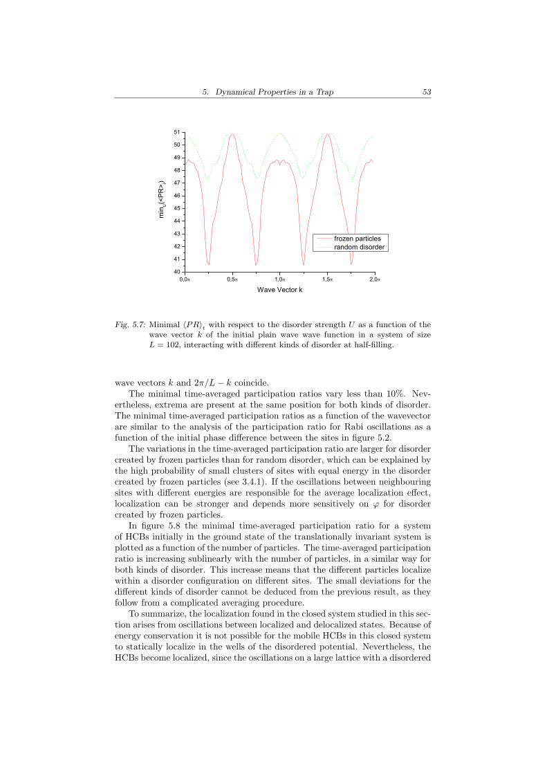
5. Dynamical Properties in a Trap 53
0,0 0,5 1,0 1,5 2,040
41
42
43
44
45
46
47
48
49
50
51
min
U(<
PR> t)
Wave Vector k
frozen particles random disorder
Fig. 5.7: Minimal 〈PR〉t with respect to the disorder strength U as a function of thewave vector k of the initial plain wave wave function in a system of sizeL = 102, interacting with different kinds of disorder at half-filling.
wave vectors k and 2π/L− k coincide.The minimal time-averaged participation ratios vary less than 10%. Nev-
ertheless, extrema are present at the same position for both kinds of disorder.The minimal time-averaged participation ratios as a function of the wavevectorare similar to the analysis of the participation ratio for Rabi oscillations as afunction of the initial phase difference between the sites in figure 5.2.
The variations in the time-averaged participation ratio are larger for disordercreated by frozen particles than for random disorder, which can be explained bythe high probability of small clusters of sites with equal energy in the disordercreated by frozen particles (see 3.4.1). If the oscillations between neighbouringsites with different energies are responsible for the average localization effect,localization can be stronger and depends more sensitively on ϕ for disordercreated by frozen particles.
In figure 5.8 the minimal time-averaged participation ratio for a systemof HCBs initially in the ground state of the translationally invariant system isplotted as a function of the number of particles. The time-averaged participationratio is increasing sublinearly with the number of particles, in a similar way forboth kinds of disorder. This increase means that the different particles localizewithin a disorder configuration on different sites. The small deviations for thedifferent kinds of disorder cannot be deduced from the previous result, as theyfollow from a complicated averaging procedure.
To summarize, the localization found in the closed system studied in this sec-tion arises from oscillations between localized and delocalized states. Because ofenergy conservation it is not possible for the mobile HCBs in this closed systemto statically localize in the wells of the disordered potential. Nevertheless, theHCBs become localized, since the oscillations on a large lattice with a disordered
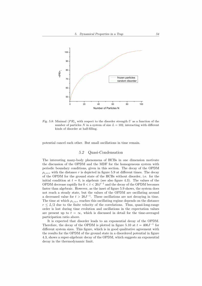
5. Dynamical Properties in a Trap 54
0 20 40 60 80 100
50
60
70
80
90
100
<PR
> t
Number of Particles N
frozen particles random disorder
Fig. 5.8: Minimal 〈PR〉t with respect to the disorder strength U as a function of thenumber of particles N in a system of size L = 102, interacting with differentkinds of disorder at half-filling.
potential cancel each other. But small oscillations in time remain.
5.2 Quasi-Condensation
The interesting many-body phenomena of HCBs in one dimension motivatethe discussion of the OPDM and the MDF for the homogeneous system withperiodic boundary conditions, given in this section. The decay of the OPDMρi,i+r with the distance r is depicted in figure 5.9 at different times. The decayof the OPDM for the ground state of the HCBs without disorder, i.e. for theinitial condition at t = 0, is algebraic (see also figure 4.3). The values of theOPDM decrease rapidly for 0 < t < 20J−1 and the decay of the OPDM becomesfaster than algebraic. However, as the inset of figure 5.9 shows, the system doesnot reach a steady state, but the values of the OPDM are oscillating arounda decreased value for t > 20J−1. These oscillations are not decaying in time.The time at which ρi,i+r reaches this oscillating regime depends on the distancer ≤ L/2 due to the finite velocity of the correlations. Thus, quasi-long-rangeorder is lost during time evolution and oscillations in the expectation valuesare present up to t = ∞, which is discussed in detail for the time-averagedparticipation ratio above.
It is expected that disorder leads to an exponential decay of the OPDM.Therefore, the decay of the OPDM is plotted in figure 5.10 at t = 400J−1 fordifferent system sizes. This figure, which is in good qualitative agreement withthe results for the OPDM of the ground state in a disordered potential in figure4.3, shows a super-algebraic decay of the OPDM, which suggests an exponentialdecay in the thermodynamic limit.
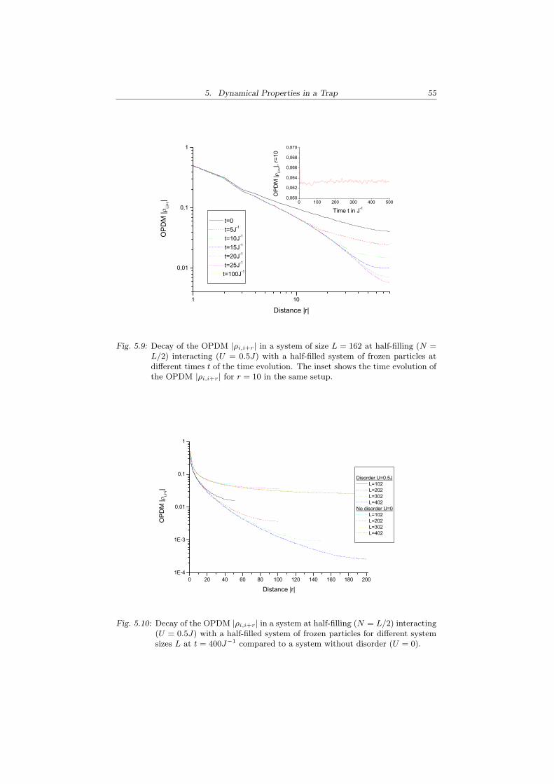
5. Dynamical Properties in a Trap 55
1 10
0,01
0,1
1
0 100 200 300 400 5000,060
0,062
0,064
0,066
0,068
0,070
t=0 t=5J-1
t=10J-1
t=15J-1
t=20J-1
t=25J-1
t=100J-1
OPD
M |
i,i+r|
Distance |r|
Time t in J-1
OPD
M |
i,i+r|,
r=10
Fig. 5.9: Decay of the OPDM |ρi,i+r| in a system of size L = 162 at half-filling (N =L/2) interacting (U = 0.5J) with a half-filled system of frozen particles atdifferent times t of the time evolution. The inset shows the time evolution ofthe OPDM |ρi,i+r| for r = 10 in the same setup.
0 20 40 60 80 100 120 140 160 180 2001E-4
1E-3
0,01
0,1
1
Disorder U=0.5J L=102 L=202 L=302 L=402
No disorder U=0 L=102 L=202 L=302 L=402
OPD
M |
i,i+r|
Distance |r|
Fig. 5.10: Decay of the OPDM |ρi,i+r| in a system at half-filling (N = L/2) interacting(U = 0.5J) with a half-filled system of frozen particles for different systemsizes L at t = 400J−1 compared to a system without disorder (U = 0).
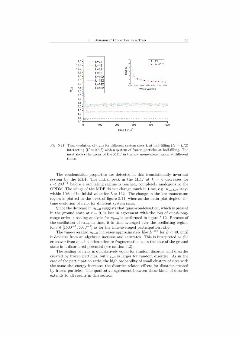
5. Dynamical Properties in a Trap 56
0 100 200 300 400 5003,03,54,04,55,05,56,06,57,07,58,08,59,09,5
10,010,511,0
0,00 0,02 0,04 0,06 0,08 0,10 0,120
2
4
6
8
10
12
n k=0
Time t in J-1
L=22 L=42 L=62 L=82 L=102 L=122 L=142 L=162 Wave Vector k
MD
F n k
t=0 t=100J-1
Fig. 5.11: Time evolution of nk=0 for different system sizes L at half-filling (N = L/2)interacting (U = 0.5J) with a system of frozen particles at half-filling. Theinset shows the decay of the MDF in the low momentum region at differenttimes.
The condensation properties are detected in this translationally invariantsystem by the MDF. The initial peak in the MDF at k = 0 decreases fort < 20J−1 before a oscillating regime is reached, completely analogous to theOPDM. The wings of the MDF do not change much in time, e.g. nk=L/2 stayswithin 10% of its initial value for L = 162. The change in the low momentumregion is plotted in the inset of figure 5.11, whereas the main plot depicts thetime evolution of nk=0 for different system sizes.
Since the decrease in nk=0 suggests that quasi-condensation, which is presentin the ground state at t = 0, is lost in agreement with the loss of quasi-long-range order, a scaling analysis for nk=0 is performed in figure 5.12. Because ofthe oscillation of nk=0 in time, it is time-averaged over the oscillating regimefor t ∈ [150J−1, 500J−1] as for the time-averaged participation ratio.
The time-averaged nk=0 increases approximately like L−0.5 for L < 40, untilit deviates from an algebraic increase and saturates. This is interpreted as thecrossover from quasi-condensation to fragmentation as in the case of the groundstate in a disordered potential (see section 4.2).
The scaling of nk=0 is qualitatively equal for random disorder and disordercreated by frozen particles, but nk=0 is larger for random disorder. As in thecase of the participation ratio, the high probability of small clusters of sites withthe same site energy increases the disorder related effects for disorder createdby frozen particles. The qualitative agreement between these kinds of disorderextends to all results in this section.
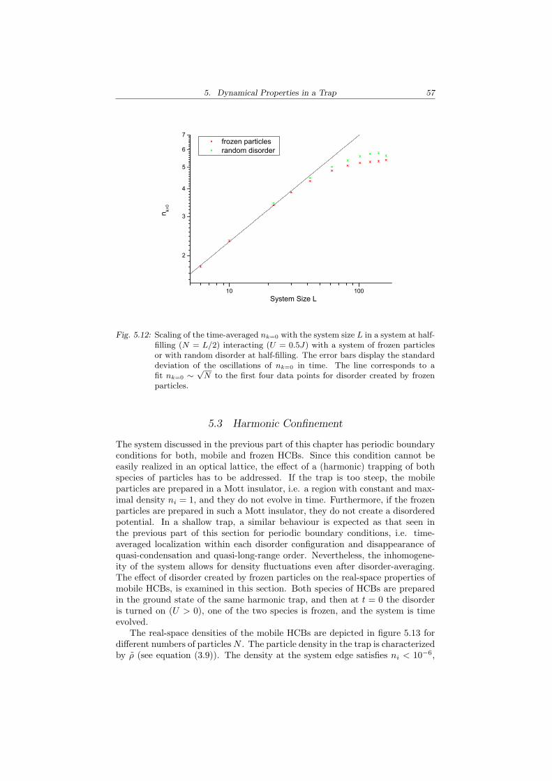
5. Dynamical Properties in a Trap 57
10 100
2
3
4
5
6
7 frozen particles random disorder
n k=0
System Size L
Fig. 5.12: Scaling of the time-averaged nk=0 with the system size L in a system at half-filling (N = L/2) interacting (U = 0.5J) with a system of frozen particlesor with random disorder at half-filling. The error bars display the standarddeviation of the oscillations of nk=0 in time. The line corresponds to afit nk=0 ∼
√N to the first four data points for disorder created by frozen
particles.
5.3 Harmonic Confinement
The system discussed in the previous part of this chapter has periodic boundaryconditions for both, mobile and frozen HCBs. Since this condition cannot beeasily realized in an optical lattice, the effect of a (harmonic) trapping of bothspecies of particles has to be addressed. If the trap is too steep, the mobileparticles are prepared in a Mott insulator, i.e. a region with constant and max-imal density ni = 1, and they do not evolve in time. Furthermore, if the frozenparticles are prepared in such a Mott insulator, they do not create a disorderedpotential. In a shallow trap, a similar behaviour is expected as that seen inthe previous part of this section for periodic boundary conditions, i.e. time-averaged localization within each disorder configuration and disappearance ofquasi-condensation and quasi-long-range order. Nevertheless, the inhomogene-ity of the system allows for density fluctuations even after disorder-averaging.The effect of disorder created by frozen particles on the real-space properties ofmobile HCBs, is examined in this section. Both species of HCBs are preparedin the ground state of the same harmonic trap, and then at t = 0 the disorderis turned on (U > 0), one of the two species is frozen, and the system is timeevolved.
The real-space densities of the mobile HCBs are depicted in figure 5.13 fordifferent numbers of particles N . The particle density in the trap is characterizedby ρ (see equation (3.9)). The density at the system edge satisfies ni < 10−6,
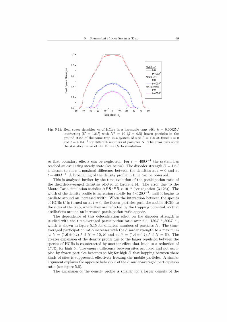
5. Dynamical Properties in a Trap 58
-50 -40 -30 -20 -10 0 10 20 30 40 500,0
0,2
0,4
0,6
0,8
1,0
N=60, t=0 t=400J-1
N=20, =1 t=0 t=400J-1
N=10, =0.5 t=0 t=400J-1R
eal S
pace
Den
sity
ni
Site Index i-i0
Fig. 5.13: Real space densities ni of HCBs in a harmonic trap with k = 0.00025Jinteracting (U = 1.6J) with Nf = 10 (ρ = 0.5) frozen particles in theground state of the same trap in a system of size L = 120 at times t = 0and t = 400J−1 for different numbers of particles N . The error bars showthe statistical error of the Monte Carlo simulation.
so that boundary effects can be neglected. For t = 400J−1 the system hasreached an oscillating steady state (see below). The disorder strength U = 1.6Jis chosen to show a maximal difference between the densities at t = 0 and att = 400J−1. A broadening of the density profile in time can be observed.
This is analysed further by the time evolution of the participation ratio ofthe disorder-averaged densities plotted in figure 5.14. The error due to theMonte Carlo simulation satisfies ∆PR/PR < 10−5 (see equation (3.126)). Thewidth of the density profile is increasing rapidly for t < 20J−1, until it begins tooscillate around an increased width. When the interaction between the speciesof HCBs U is turned on at t = 0, the frozen particles push the mobile HCBs tothe sides of the trap, where they are reflected by the trapping potential, so thatoscillations around an increased participation ratio appear.
The dependence of this delocalization effect on the disorder strength isstudied with the time-averaged participation ratio over t ∈ [150J−1, 500J−1],which is shown in figure 5.15 for different numbers of particles N . The time-averaged participation ratio increases with the disorder strength to a maximumat U = (1.6± 0.2)J if N = 10, 20 and at U = (1.4± 0.2)J if N = 60. Thegreater expansion of the density profile due to the larger repulsion between thespecies of HCBs is counteracted by another effect that leads to a reduction of〈PR〉t for high U . The energy difference between sites occupied and not occu-pied by frozen particles becomes so big for high U that hopping between thesekinds of sites is suppressed, effectively freezing the mobile particles. A similarargument explains the opposite behaviour of the disorder-averaged participationratio (see figure 5.6).
The expansion of the density profile is smaller for a larger density of the
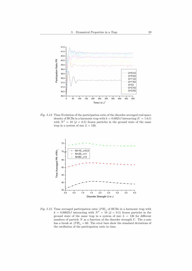
5. Dynamical Properties in a Trap 59
0 50 100 150 200 250 300 350 400 450 50036,0
36,5
37,0
37,5
38,0
38,5
39,0
39,5
40,0
40,5
41,0
41,5
Parti
cipa
tion
Rat
io P
R
Time t in J-1
U=0.4J U=0.8J U=1.2J U=1.6J U=2J U=2.4J U=2.8J
Fig. 5.14: Time Evolution of the participation ratio of the disorder-averaged real-spacedensity of HCBs in a harmonic trap with k = 0.0025J interacting (U = 1.6J)with Nf = 10 (ρ = 0.5) frozen particles in the ground state of the sametrap in a system of size L = 120.
0,0 0,5 1,0 1,5 2,0 2,5 3,0 3,5 4,035
40
45
50
55
70
75
Tim
e Av
erag
ed P
R <
PR> t
Disorder Strength U in J
N=10, =0.5 N=20, =1 N=60, =3
Fig. 5.15: Time averaged participation ratio 〈PR〉t of HCBs in a harmonic trap withk = 0.00025J interacting with Nf = 10 (ρ = 0.5) frozen particles in theground state of the same trap in a system of size L = 120 for differentnumbers of particle N as a function of the disorder strength U . The y-axishas a break at 〈PR〉t = 60. The error bars show the standard deviations ofthe oscillation of the participation ratio in time.
5. Dynamical Properties in a Trap 60
mobile particles. This is due to the fact that if more mobile than frozen particlesare present, the mobile HCBs at the edge of the many-body wave function donot interact with the frozen particles, which are localized close to the centre ofthe trap, while the mobility of the mobile HCBs in the trap centre is restrictedby the high density of mobile HCBs in the trap centre. Furthermore, the energyneeded for a particle to hop to a neighbouring site away from the trap centreincreases linearly with the distance from the trap centre.
Therefore, the effect of disorder on the disorder-averaged real-space densities,which is accessible to experiment (see section 7), is delocalization rather thanlocalization.
6. TRANSPORT PROPERTIES
In the previous chapter, the effect of disorder on the time evolution of theinitially extended ground state of HCBs is discussed. In this case, disorderintroduces oscillations in the time evolution, leading to an average localizationeffect. This average localization has the peculiar property that the measure forlocalization is not monotone in the disorder strength.
Localization can be seen more clearly in the time evolution of an initiallyconfined wave function in an infinite system discussed in this chapter. Sincethe wave function spreads forever without disorder, the halt of the expansion inpresence of disorder explicitly shows localization.
Section 6.1 deals with the expansion of an initially confined wave functionin the presence of different kinds of disorder including staggered disorder, whilesection 6.2 studies the appearance and disappearance of quasi-condensation andthe decay of the OPDM for different initial conditions.
6.1 Localization
In this section the real-space properties of initially confined mobile HCBs (k =0.01) interacting with a disordered potential created by frozen particles is anal-ysed. The frozen particles are prepared in a system with periodic boundaryconditions. In section 6.1.2 the frozen particles are prepared in a superlattice,in section 6.1.1 no superlattice is present.
6.1.1 Disorder without Long-Range Correlations
A typical time evolution of a single-particle wave function interacting with dis-order is depicted in figure 6.1. The size of the system is chosen, such that atthe system ends ni (t) . 10−5 holds for the longest evolution times considered,in order to limit finite size effects. The main plot shows, how the peak in thedensities is reduced and the support of the wave function increases during timeevolution, asymptotically reaching a steady state. It is fundamental to stressthat this steady state does not correspond to the ground state of the system.The time-evolved state
∣∣Φ(t)〉 of the mobile HCBs is determined by the initial
state∣∣Φ〉 =
∑i ci
∣∣i〉 through
∣∣Φ(t)〉 =∑
i
e−iEitci
∣∣i〉 (6.1)
with the energy eigenstates Ei and eigenvectors∣∣i〉 of the final Hamiltonian.
The modulus of the overlap∣∣〈i
∣∣Φ(t)〉∣∣ = |ci| between the time-evolved state
and the energy eigenstates of the final Hamiltonian does not change during
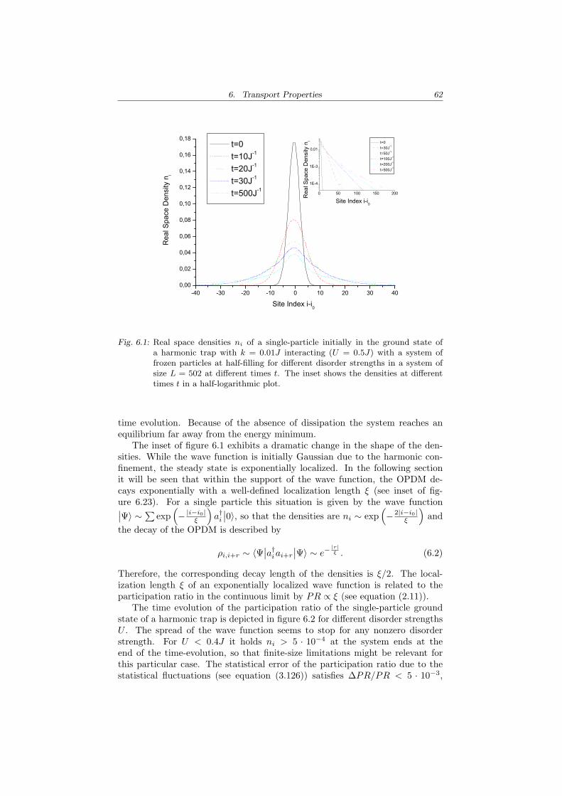
6. Transport Properties 62
-40 -30 -20 -10 0 10 20 30 400,00
0,02
0,04
0,06
0,08
0,10
0,12
0,14
0,16
0,18
0 50 100 150 200
1E-4
1E-3
0,01
Rea
l Spa
ce D
ensi
ty n
i
Site Index i-i0
t=0 t=10J-1
t=20J-1
t=30J-1
t=500J-1
Site Index i-i0
Rea
l Spa
ce D
ensi
ty n
i t=0 t=30J-1
t=50J-1
t=100J-1
t=200J-1
t=500J-1
Fig. 6.1: Real space densities ni of a single-particle initially in the ground state ofa harmonic trap with k = 0.01J interacting (U = 0.5J) with a system offrozen particles at half-filling for different disorder strengths in a system ofsize L = 502 at different times t. The inset shows the densities at differenttimes t in a half-logarithmic plot.
time evolution. Because of the absence of dissipation the system reaches anequilibrium far away from the energy minimum.
The inset of figure 6.1 exhibits a dramatic change in the shape of the den-sities. While the wave function is initially Gaussian due to the harmonic con-finement, the steady state is exponentially localized. In the following sectionit will be seen that within the support of the wave function, the OPDM de-cays exponentially with a well-defined localization length ξ (see inset of fig-ure 6.23). For a single particle this situation is given by the wave function∣∣Ψ〉 ∼∑
exp(− |i−i0|
ξ
)a†i
∣∣0〉, so that the densities are ni ∼ exp(− 2|i−i0|
ξ
)and
the decay of the OPDM is described by
ρi,i+r ∼ 〈Ψ∣∣a†iai+r
∣∣Ψ〉 ∼ e−|r|ξ . (6.2)
Therefore, the corresponding decay length of the densities is ξ/2. The local-ization length ξ of an exponentially localized wave function is related to theparticipation ratio in the continuous limit by PR ∝ ξ (see equation (2.11)).
The time evolution of the participation ratio of the single-particle groundstate of a harmonic trap is depicted in figure 6.2 for different disorder strengthsU . The spread of the wave function seems to stop for any nonzero disorderstrength. For U < 0.4J it holds ni > 5 · 10−4 at the system ends at theend of the time-evolution, so that finite-size limitations might be relevant forthis particular case. The statistical error of the participation ratio due to thestatistical fluctuations (see equation (3.126)) satisfies ∆PR/PR < 5 · 10−3,
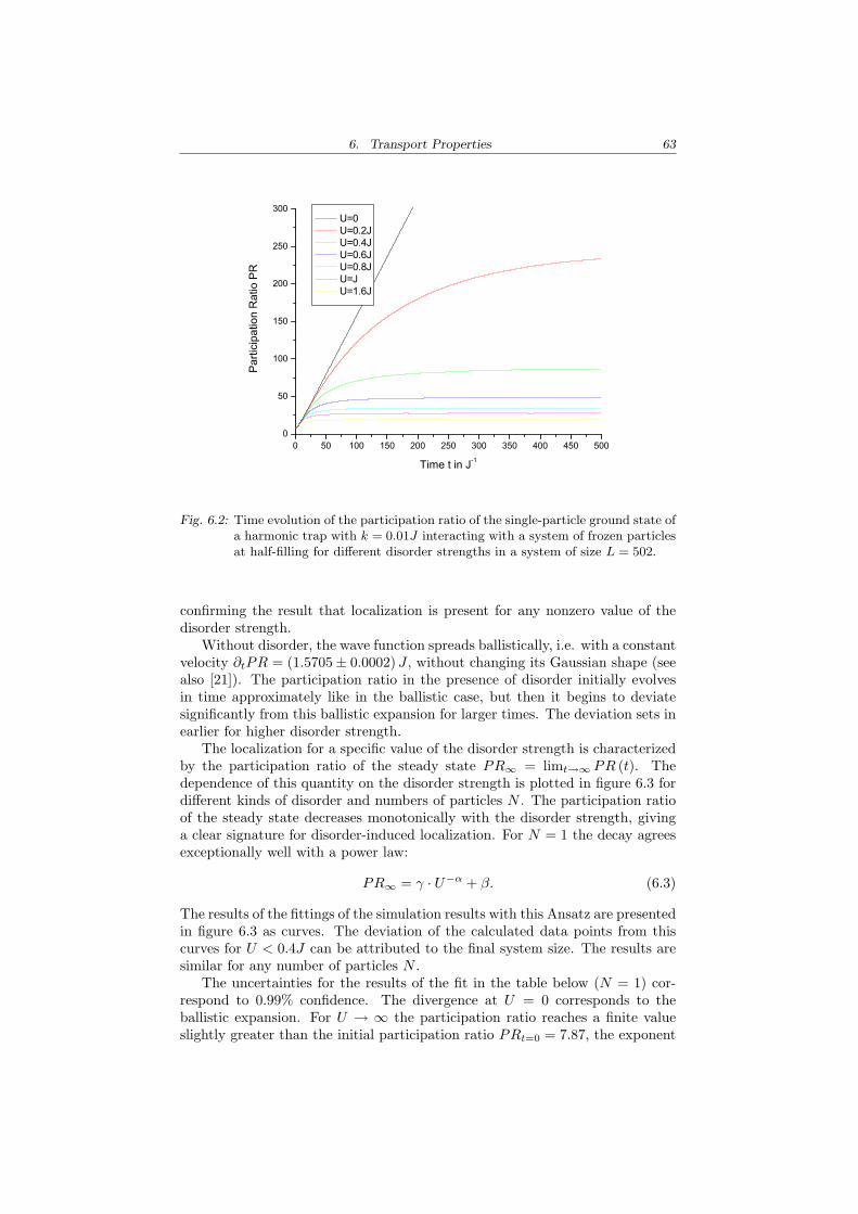
6. Transport Properties 63
0 50 100 150 200 250 300 350 400 450 5000
50
100
150
200
250
300
Parti
cipa
tion
Rat
io P
R
Time t in J-1
U=0 U=0.2J U=0.4J U=0.6J U=0.8J U=J U=1.6J
Fig. 6.2: Time evolution of the participation ratio of the single-particle ground state ofa harmonic trap with k = 0.01J interacting with a system of frozen particlesat half-filling for different disorder strengths in a system of size L = 502.
confirming the result that localization is present for any nonzero value of thedisorder strength.
Without disorder, the wave function spreads ballistically, i.e. with a constantvelocity ∂tPR = (1.5705± 0.0002)J , without changing its Gaussian shape (seealso [21]). The participation ratio in the presence of disorder initially evolvesin time approximately like in the ballistic case, but then it begins to deviatesignificantly from this ballistic expansion for larger times. The deviation sets inearlier for higher disorder strength.
The localization for a specific value of the disorder strength is characterizedby the participation ratio of the steady state PR∞ = limt→∞ PR (t). Thedependence of this quantity on the disorder strength is plotted in figure 6.3 fordifferent kinds of disorder and numbers of particles N . The participation ratioof the steady state decreases monotonically with the disorder strength, givinga clear signature for disorder-induced localization. For N = 1 the decay agreesexceptionally well with a power law:
PR∞ = γ · U−α + β. (6.3)
The results of the fittings of the simulation results with this Ansatz are presentedin figure 6.3 as curves. The deviation of the calculated data points from thiscurves for U < 0.4J can be attributed to the final system size. The results aresimilar for any number of particles N .
The uncertainties for the results of the fit in the table below (N = 1) cor-respond to 0.99% confidence. The divergence at U = 0 corresponds to theballistic expansion. For U → ∞ the participation ratio reaches a finite valueslightly greater than the initial participation ratio PRt=0 = 7.87, the exponent
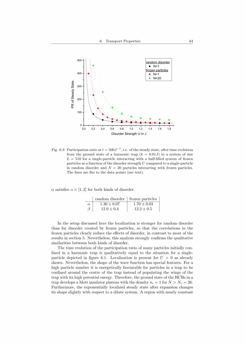
6. Transport Properties 64
0,0 0,2 0,4 0,6 0,8 1,0 1,2 1,4 1,6 1,80
100
200
300
400
500
PR o
f Ste
ady
Stat
e
Disorder Strength U in J
random disorderN=1
frozen particlesN=1N=20
Fig. 6.3: Participation ratio at t = 500J−1, i.e. of the steady state, after time evolutionfrom the ground state of a harmonic trap (k = 0.01J) in a system of sizeL = 510 for a single-particle interacting with a half-filled system of frozenparticles as a function of the disorder strength U compared to a single-particlein random disorder and N = 20 particles interacting with frozen particles.The lines are fits to the data points (see text).
α satisfies α ∈ [1, 2] for both kinds of disorder.
random disorder frozen particlesα 1.30± 0.07 1.70± 0.03β 12.0± 0.4 12.2± 0.5
In the setup discussed here the localization is stronger for random disorderthan for disorder created by frozen particles, so that the correlations in thefrozen particles clearly reduce the effects of disorder, in contrast to most of theresults in section 5. Nevertheless, this analysis strongly confirms the qualitativesimilarities between both kinds of disorder.
The time evolution of the participation ratio of many particles initially con-fined in a harmonic trap is qualitatively equal to the situation for a single-particle depicted in figure 6.1. Localization is present for U > 0 as alreadyshown. Nevertheless, the shape of the wave function has special features. For ahigh particle number it is energetically favourable for particles in a trap to beconfined around the centre of the trap instead of populating the wings of thetrap with its high potential energy. Therefore, the ground state of the HCBs in atrap develops a Mott insulator plateau with the density ni = 1 for N > Nc = 26.Furthermore, the exponentially localized steady state after expansion changesits shape slightly with respect to a dilute system. A region with nearly constant
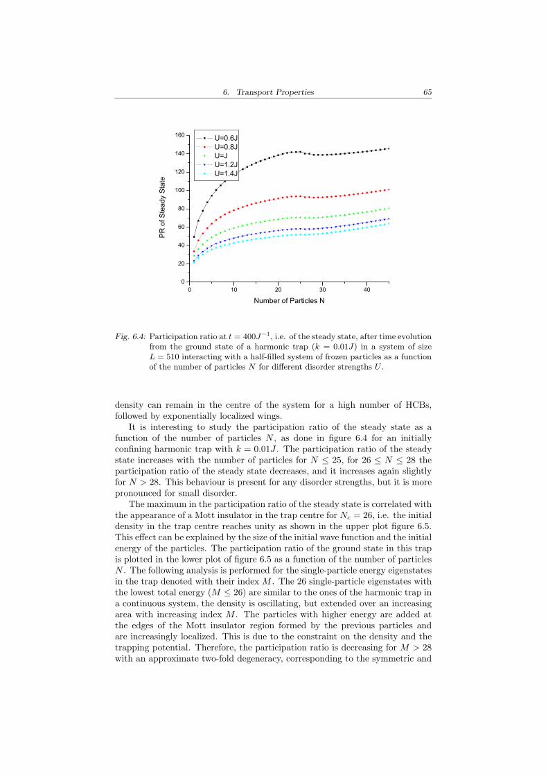
6. Transport Properties 65
0 10 20 30 400
20
40
60
80
100
120
140
160
PR o
f Ste
ady
Stat
e
Number of Particles N
U=0.6J U=0.8J U=J U=1.2J U=1.4J
Fig. 6.4: Participation ratio at t = 400J−1, i.e. of the steady state, after time evolutionfrom the ground state of a harmonic trap (k = 0.01J) in a system of sizeL = 510 interacting with a half-filled system of frozen particles as a functionof the number of particles N for different disorder strengths U .
density can remain in the centre of the system for a high number of HCBs,followed by exponentially localized wings.
It is interesting to study the participation ratio of the steady state as afunction of the number of particles N , as done in figure 6.4 for an initiallyconfining harmonic trap with k = 0.01J . The participation ratio of the steadystate increases with the number of particles for N ≤ 25, for 26 ≤ N ≤ 28 theparticipation ratio of the steady state decreases, and it increases again slightlyfor N > 28. This behaviour is present for any disorder strengths, but it is morepronounced for small disorder.
The maximum in the participation ratio of the steady state is correlated withthe appearance of a Mott insulator in the trap centre for Nc = 26, i.e. the initialdensity in the trap centre reaches unity as shown in the upper plot figure 6.5.This effect can be explained by the size of the initial wave function and the initialenergy of the particles. The participation ratio of the ground state in this trapis plotted in the lower plot of figure 6.5 as a function of the number of particlesN . The following analysis is performed for the single-particle energy eigenstatesin the trap denoted with their index M . The 26 single-particle eigenstates withthe lowest total energy (M ≤ 26) are similar to the ones of the harmonic trap ina continuous system, the density is oscillating, but extended over an increasingarea with increasing index M . The particles with higher energy are added atthe edges of the Mott insulator region formed by the previous particles andare increasingly localized. This is due to the constraint on the density and thetrapping potential. Therefore, the participation ratio is decreasing for M > 28with an approximate two-fold degeneracy, corresponding to the symmetric and
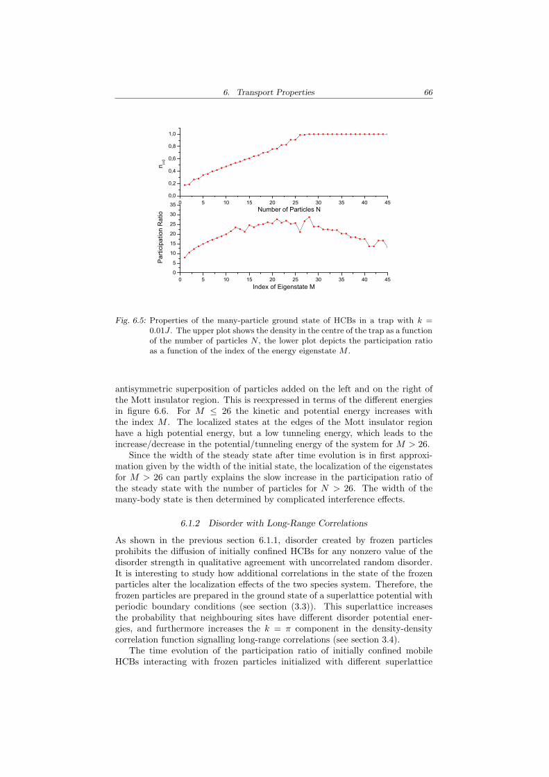
6. Transport Properties 66
0 5 10 15 20 25 30 35 40 450
5
10
15
20
25
30
35
Parti
cipa
tion
Rat
io
Index of Eigenstate M
Number of Particles N0 5 10 15 20 25 30 35 40 45
0,0
0,2
0,4
0,6
0,8
1,0
n i=0
Fig. 6.5: Properties of the many-particle ground state of HCBs in a trap with k =0.01J . The upper plot shows the density in the centre of the trap as a functionof the number of particles N , the lower plot depicts the participation ratioas a function of the index of the energy eigenstate M .
antisymmetric superposition of particles added on the left and on the right ofthe Mott insulator region. This is reexpressed in terms of the different energiesin figure 6.6. For M ≤ 26 the kinetic and potential energy increases withthe index M . The localized states at the edges of the Mott insulator regionhave a high potential energy, but a low tunneling energy, which leads to theincrease/decrease in the potential/tunneling energy of the system for M > 26.
Since the width of the steady state after time evolution is in first approxi-mation given by the width of the initial state, the localization of the eigenstatesfor M > 26 can partly explains the slow increase in the participation ratio ofthe steady state with the number of particles for N > 26. The width of themany-body state is then determined by complicated interference effects.
6.1.2 Disorder with Long-Range Correlations
As shown in the previous section 6.1.1, disorder created by frozen particlesprohibits the diffusion of initially confined HCBs for any nonzero value of thedisorder strength in qualitative agreement with uncorrelated random disorder.It is interesting to study how additional correlations in the state of the frozenparticles alter the localization effects of the two species system. Therefore, thefrozen particles are prepared in the ground state of a superlattice potential withperiodic boundary conditions (see section (3.3)). This superlattice increasesthe probability that neighbouring sites have different disorder potential ener-gies, and furthermore increases the k = π component in the density-densitycorrelation function signalling long-range correlations (see section 3.4).
The time evolution of the participation ratio of initially confined mobileHCBs interacting with frozen particles initialized with different superlattice
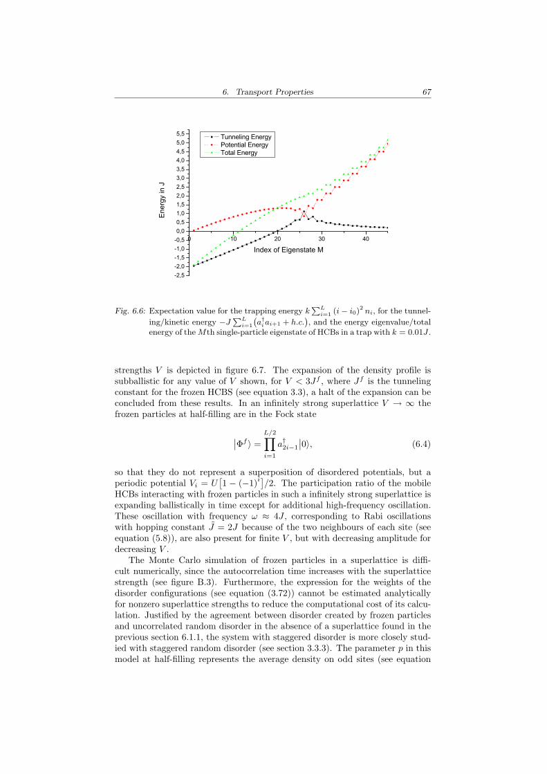
6. Transport Properties 67
0 10 20 30 40
-2,5-2,0-1,5-1,0-0,50,00,51,01,52,02,53,03,54,04,55,05,5 Tunneling Energy
Potential Energy Total Energy
Ener
gy in
J
Index of Eigenstate M
Fig. 6.6: Expectation value for the trapping energy kPL
i=1 (i− i0)2 ni, for the tunnel-
ing/kinetic energy −JPL
i=1
`a†i ai+1 + h.c.
´, and the energy eigenvalue/total
energy of the Mth single-particle eigenstate of HCBs in a trap with k = 0.01J .
strengths V is depicted in figure 6.7. The expansion of the density profile issubballistic for any value of V shown, for V < 3Jf , where Jf is the tunnelingconstant for the frozen HCBS (see equation 3.3), a halt of the expansion can beconcluded from these results. In an infinitely strong superlattice V → ∞ thefrozen particles at half-filling are in the Fock state
∣∣Φf 〉 =L/2∏
i=1
a†2i−1
∣∣0〉, (6.4)
so that they do not represent a superposition of disordered potentials, but aperiodic potential Vi = U
[1 − (−1)i]
/2. The participation ratio of the mobileHCBs interacting with frozen particles in such a infinitely strong superlattice isexpanding ballistically in time except for additional high-frequency oscillation.These oscillation with frequency ω ≈ 4J , corresponding to Rabi oscillationswith hopping constant J = 2J because of the two neighbours of each site (seeequation (5.8)), are also present for finite V , but with decreasing amplitude fordecreasing V .
The Monte Carlo simulation of frozen particles in a superlattice is diffi-cult numerically, since the autocorrelation time increases with the superlatticestrength (see figure B.3). Furthermore, the expression for the weights of thedisorder configurations (see equation (3.72)) cannot be estimated analyticallyfor nonzero superlattice strengths to reduce the computational cost of its calcu-lation. Justified by the agreement between disorder created by frozen particlesand uncorrelated random disorder in the absence of a superlattice found in theprevious section 6.1.1, the system with staggered disorder is more closely stud-ied with staggered random disorder (see section 3.3.3). The parameter p in thismodel at half-filling represents the average density on odd sites (see equation
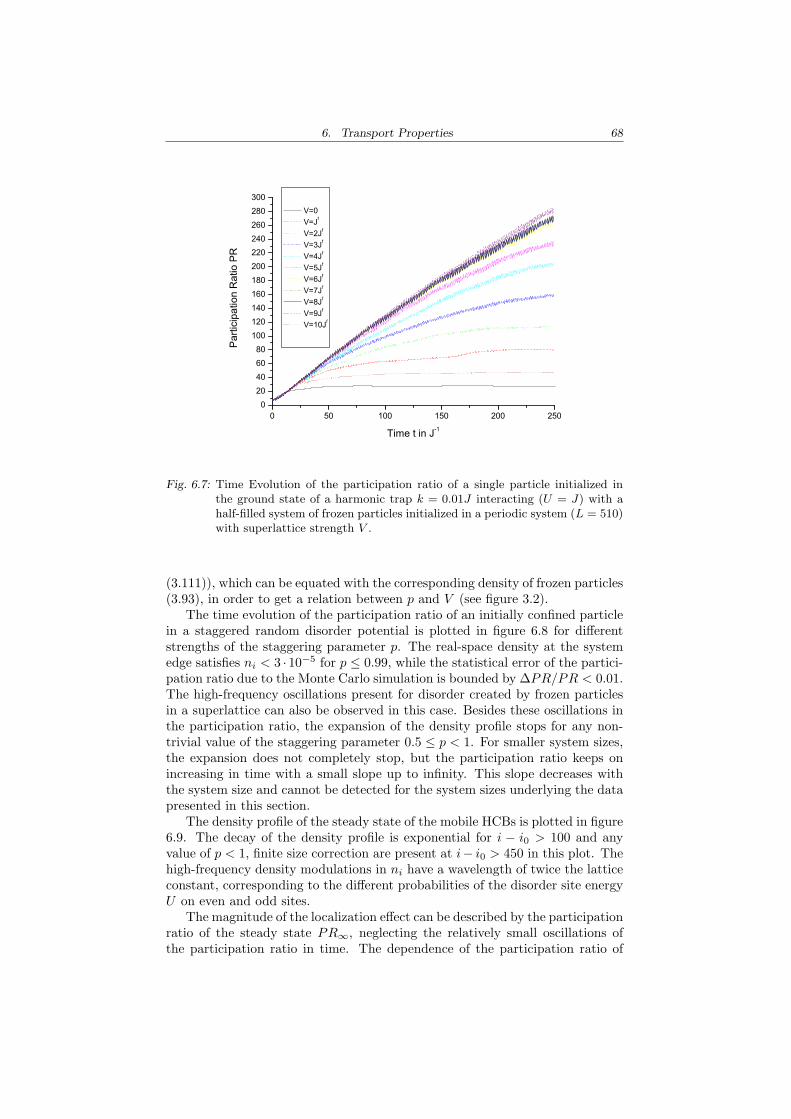
6. Transport Properties 68
0 50 100 150 200 250020406080100120140160180200220240260280300
V=0 V=Jf
V=2Jf
V=3Jf
V=4Jf
V=5Jf
V=6Jf
V=7Jf
V=8Jf
V=9Jf
V=10Jf
Parti
cipa
tion
Rat
io P
R
Time t in J-1
Fig. 6.7: Time Evolution of the participation ratio of a single particle initialized inthe ground state of a harmonic trap k = 0.01J interacting (U = J) with ahalf-filled system of frozen particles initialized in a periodic system (L = 510)with superlattice strength V .
(3.111)), which can be equated with the corresponding density of frozen particles(3.93), in order to get a relation between p and V (see figure 3.2).
The time evolution of the participation ratio of an initially confined particlein a staggered random disorder potential is plotted in figure 6.8 for differentstrengths of the staggering parameter p. The real-space density at the systemedge satisfies ni < 3 · 10−5 for p ≤ 0.99, while the statistical error of the partici-pation ratio due to the Monte Carlo simulation is bounded by ∆PR/PR < 0.01.The high-frequency oscillations present for disorder created by frozen particlesin a superlattice can also be observed in this case. Besides these oscillations inthe participation ratio, the expansion of the density profile stops for any non-trivial value of the staggering parameter 0.5 ≤ p < 1. For smaller system sizes,the expansion does not completely stop, but the participation ratio keeps onincreasing in time with a small slope up to infinity. This slope decreases withthe system size and cannot be detected for the system sizes underlying the datapresented in this section.
The density profile of the steady state of the mobile HCBs is plotted in figure6.9. The decay of the density profile is exponential for i − i0 > 100 and anyvalue of p < 1, finite size correction are present at i− i0 > 450 in this plot. Thehigh-frequency density modulations in ni have a wavelength of twice the latticeconstant, corresponding to the different probabilities of the disorder site energyU on even and odd sites.
The magnitude of the localization effect can be described by the participationratio of the steady state PR∞, neglecting the relatively small oscillations ofthe participation ratio in time. The dependence of the participation ratio of
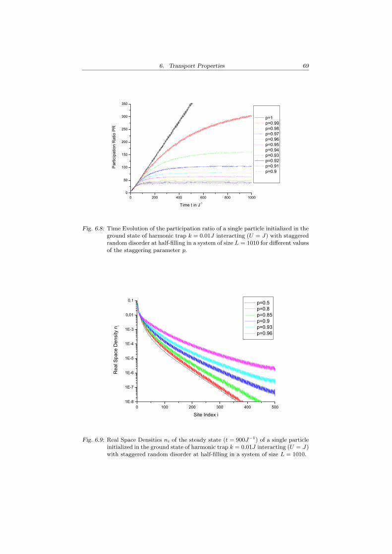
6. Transport Properties 69
0 200 400 600 800 10000
50
100
150
200
250
300
350
Parti
cipa
tion
Rat
io P
R
Time t in J-1
p=1 p=0.99 p=0.98 p=0.97 p=0.96 p=0.95 p=0.94 p=0.93 p=0.92 p=0.91 p=0.9
Fig. 6.8: Time Evolution of the participation ratio of a single particle initialized in theground state of harmonic trap k = 0.01J interacting (U = J) with staggeredrandom disorder at half-filling in a system of size L = 1010 for different valuesof the staggering parameter p.
0 100 200 300 400 5001E-8
1E-7
1E-6
1E-5
1E-4
1E-3
0,01
0,1
Rea
l Spa
ce D
ensi
ty n
i
Site Index i
p=0.5 p=0.8 p=0.85 p=0.9 p=0.93 p=0.96
Fig. 6.9: Real Space Densities ni of the steady state (t = 900J−1) of a single particleinitialized in the ground state of harmonic trap k = 0.01J interacting (U = J)with staggered random disorder at half-filling in a system of size L = 1010.
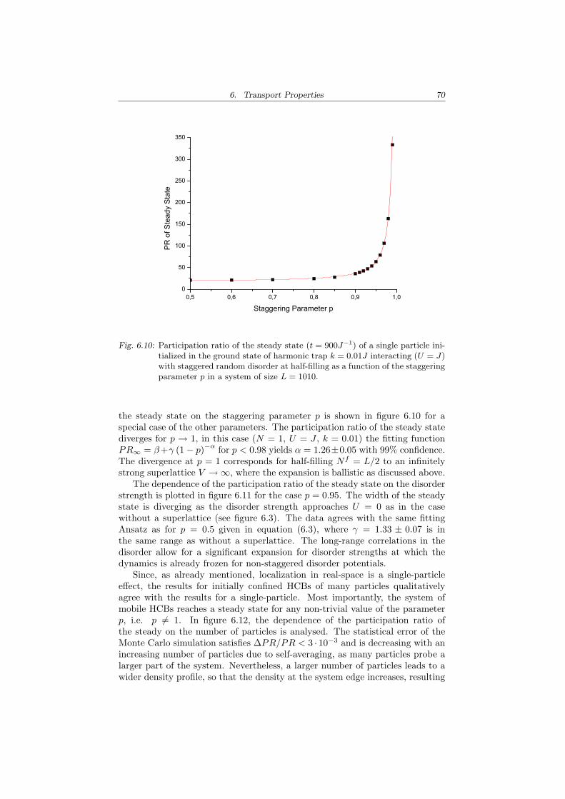
6. Transport Properties 70
0,5 0,6 0,7 0,8 0,9 1,00
50
100
150
200
250
300
350
PR o
f Ste
ady
Stat
e
Staggering Parameter p
Fig. 6.10: Participation ratio of the steady state (t = 900J−1) of a single particle ini-tialized in the ground state of harmonic trap k = 0.01J interacting (U = J)with staggered random disorder at half-filling as a function of the staggeringparameter p in a system of size L = 1010.
the steady state on the staggering parameter p is shown in figure 6.10 for aspecial case of the other parameters. The participation ratio of the steady statediverges for p → 1, in this case (N = 1, U = J , k = 0.01) the fitting functionPR∞ = β+γ (1− p)−α for p < 0.98 yields α = 1.26±0.05 with 99% confidence.The divergence at p = 1 corresponds for half-filling Nf = L/2 to an infinitelystrong superlattice V →∞, where the expansion is ballistic as discussed above.
The dependence of the participation ratio of the steady state on the disorderstrength is plotted in figure 6.11 for the case p = 0.95. The width of the steadystate is diverging as the disorder strength approaches U = 0 as in the casewithout a superlattice (see figure 6.3). The data agrees with the same fittingAnsatz as for p = 0.5 given in equation (6.3), where γ = 1.33 ± 0.07 is inthe same range as without a superlattice. The long-range correlations in thedisorder allow for a significant expansion for disorder strengths at which thedynamics is already frozen for non-staggered disorder potentials.
Since, as already mentioned, localization in real-space is a single-particleeffect, the results for initially confined HCBs of many particles qualitativelyagree with the results for a single-particle. Most importantly, the system ofmobile HCBs reaches a steady state for any non-trivial value of the parameterp, i.e. p 6= 1. In figure 6.12, the dependence of the participation ratio ofthe steady on the number of particles is analysed. The statistical error of theMonte Carlo simulation satisfies ∆PR/PR < 3 · 10−3 and is decreasing with anincreasing number of particles due to self-averaging, as many particles probe alarger part of the system. Nevertheless, a larger number of particles leads to awider density profile, so that the density at the system edge increases, resulting
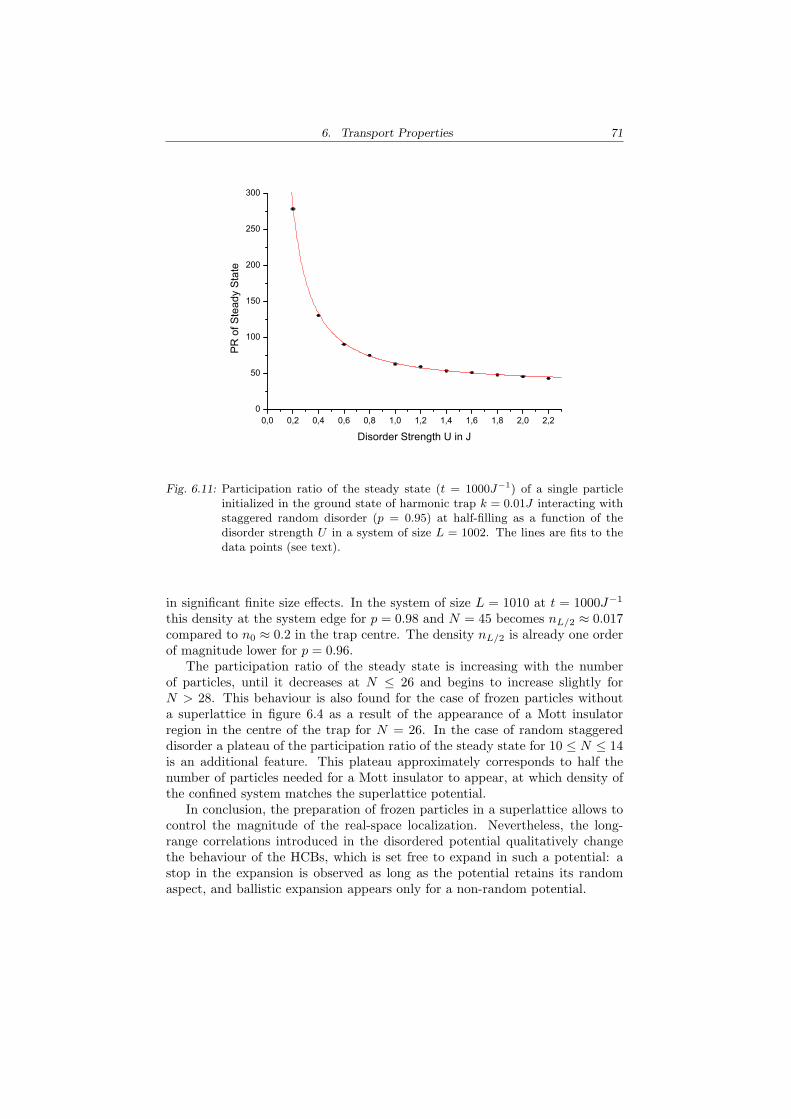
6. Transport Properties 71
0,0 0,2 0,4 0,6 0,8 1,0 1,2 1,4 1,6 1,8 2,0 2,20
50
100
150
200
250
300
PR o
f Ste
ady
Stat
e
Disorder Strength U in J
Fig. 6.11: Participation ratio of the steady state (t = 1000J−1) of a single particleinitialized in the ground state of harmonic trap k = 0.01J interacting withstaggered random disorder (p = 0.95) at half-filling as a function of thedisorder strength U in a system of size L = 1002. The lines are fits to thedata points (see text).
in significant finite size effects. In the system of size L = 1010 at t = 1000J−1
this density at the system edge for p = 0.98 and N = 45 becomes nL/2 ≈ 0.017compared to n0 ≈ 0.2 in the trap centre. The density nL/2 is already one orderof magnitude lower for p = 0.96.
The participation ratio of the steady state is increasing with the numberof particles, until it decreases at N ≤ 26 and begins to increase slightly forN > 28. This behaviour is also found for the case of frozen particles withouta superlattice in figure 6.4 as a result of the appearance of a Mott insulatorregion in the centre of the trap for N = 26. In the case of random staggereddisorder a plateau of the participation ratio of the steady state for 10 ≤ N ≤ 14is an additional feature. This plateau approximately corresponds to half thenumber of particles needed for a Mott insulator to appear, at which density ofthe confined system matches the superlattice potential.
In conclusion, the preparation of frozen particles in a superlattice allows tocontrol the magnitude of the real-space localization. Nevertheless, the long-range correlations introduced in the disordered potential qualitatively changethe behaviour of the HCBs, which is set free to expand in such a potential: astop in the expansion is observed as long as the potential retains its randomaspect, and ballistic expansion appears only for a non-random potential.
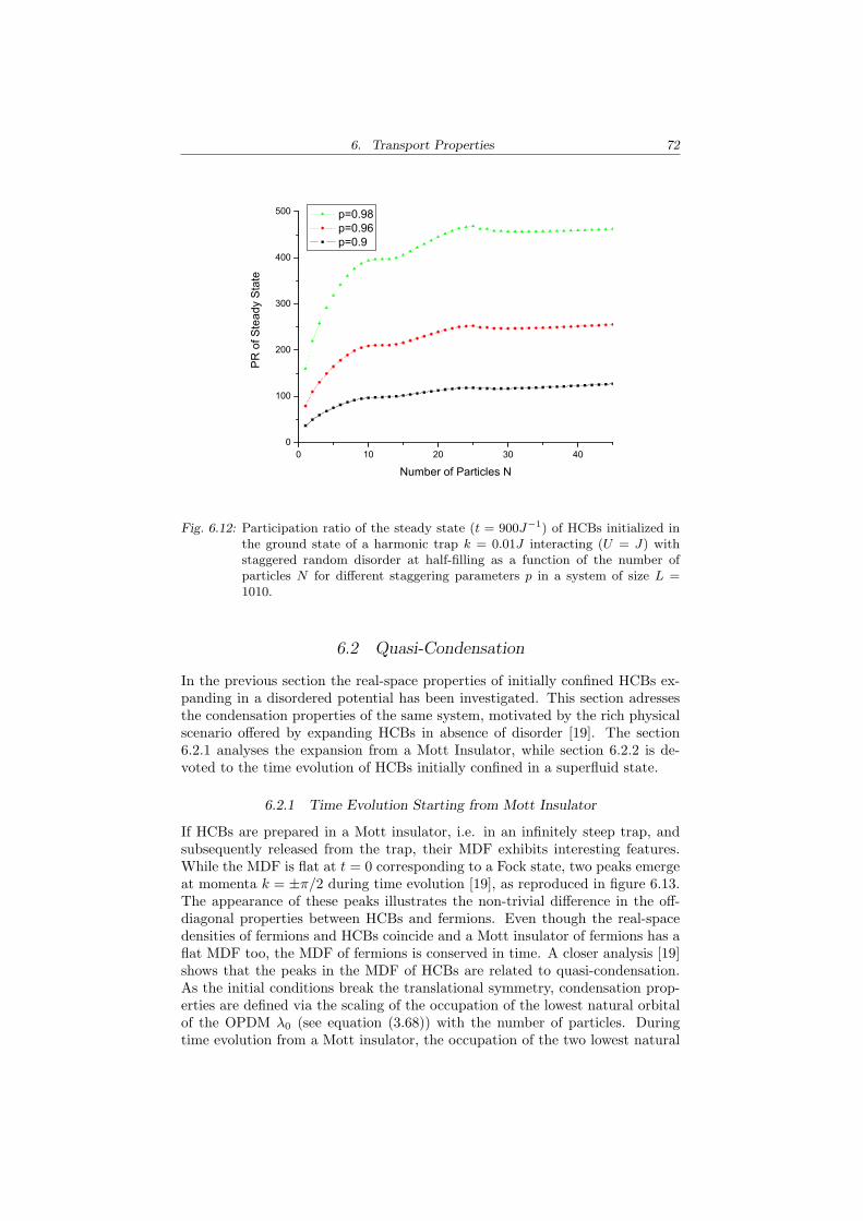
6. Transport Properties 72
0 10 20 30 400
100
200
300
400
500
PR o
f Ste
ady
Stat
e
Number of Particles N
p=0.98 p=0.96 p=0.9
Fig. 6.12: Participation ratio of the steady state (t = 900J−1) of HCBs initialized inthe ground state of a harmonic trap k = 0.01J interacting (U = J) withstaggered random disorder at half-filling as a function of the number ofparticles N for different staggering parameters p in a system of size L =1010.
6.2 Quasi-Condensation
In the previous section the real-space properties of initially confined HCBs ex-panding in a disordered potential has been investigated. This section adressesthe condensation properties of the same system, motivated by the rich physicalscenario offered by expanding HCBs in absence of disorder [19]. The section6.2.1 analyses the expansion from a Mott Insulator, while section 6.2.2 is de-voted to the time evolution of HCBs initially confined in a superfluid state.
6.2.1 Time Evolution Starting from Mott Insulator
If HCBs are prepared in a Mott insulator, i.e. in an infinitely steep trap, andsubsequently released from the trap, their MDF exhibits interesting features.While the MDF is flat at t = 0 corresponding to a Fock state, two peaks emergeat momenta k = ±π/2 during time evolution [19], as reproduced in figure 6.13.The appearance of these peaks illustrates the non-trivial difference in the off-diagonal properties between HCBs and fermions. Even though the real-spacedensities of fermions and HCBs coincide and a Mott insulator of fermions has aflat MDF too, the MDF of fermions is conserved in time. A closer analysis [19]shows that the peaks in the MDF of HCBs are related to quasi-condensation.As the initial conditions break the translational symmetry, condensation prop-erties are defined via the scaling of the occupation of the lowest natural orbitalof the OPDM λ0 (see equation (3.68)) with the number of particles. Duringtime evolution from a Mott insulator, the occupation of the two lowest natural
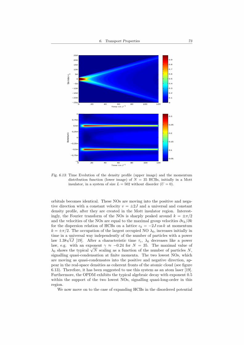
6. Transport Properties 73
Time t in J−1
Site
Index
i−i 0
0 20 40 60 80 100 120−250
−200
−150
−100
−50
0
50
100
150
200
250
0
0.1
0.2
0.3
0.4
0.5
0.6
0.7
0.8
0.9
Time t in J−1
Mome
ntum
k
0 20 40 60 80 100 120−π
−0,75π
−0,5π
−0,25π
0
0,25π
0,5π
0,75π
π
0.05
0.1
0.15
0.2
0.25
0.3
Fig. 6.13: Time Evolution of the density profile (upper image) and the momentumdistribution function (lower image) of N = 35 HCBs, initially in a Mottinsulator, in a system of size L = 502 without disorder (U = 0).
orbitals becomes identical. These NOs are moving into the positive and nega-tive direction with a constant velocity v = ±2J and a universal and constantdensity profile, after they are created in the Mott insulator region. Interest-ingly, the Fourier transform of the NOs is sharply peaked around k = ±π/2and the velocities of the NOs are equal to the maximal group velocities ∂εk/∂kfor the dispersion relation of HCBs on a lattice εk = −2J cos k at momentumk = ±π/2. The occupation of the largest occupied NO λ0, increases initially intime in a universal way independently of the number of particles with a powerlaw 1.38
√tJ [19]. After a characteristic time τc, λ0 decreases like a power
law, e.g. with an exponent γ ≈ −0.24 for N = 35. The maximal value ofλ0 shows the typical
√N scaling as a function of the number of particles N ,
signalling quasi-condensation at finite momenta. The two lowest NOs, whichare moving as quasi-condensates into the positive and negative direction, ap-pear in the real-space densities as coherent fronts of the atomic cloud (see figure6.13). Therefore, it has been suggested to use this system as an atom laser [19].Furthermore, the OPDM exhibits the typical algebraic decay with exponent 0.5within the support of the two lowest NOs, signalling quasi-long-order in thisregion.
We now move on to the case of expanding HCBs in the disordered potential
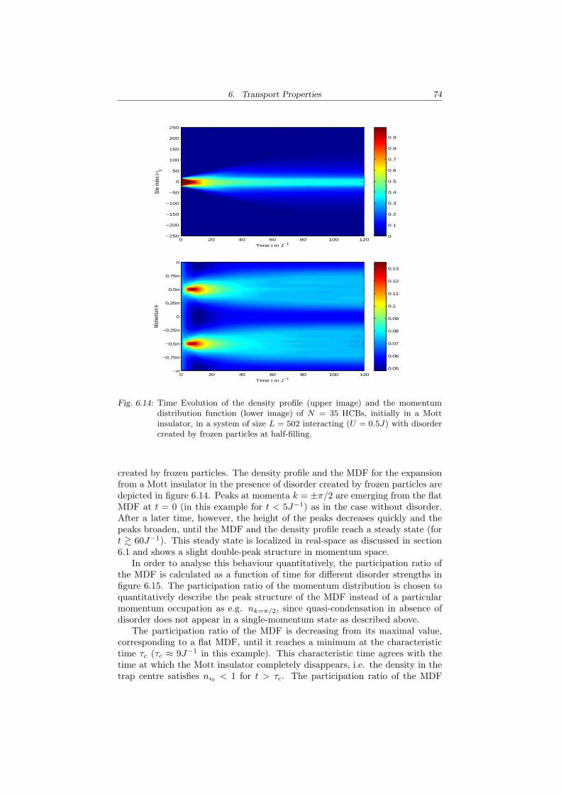
6. Transport Properties 74
Time t in J−1
Site
Index
i−i 0
0 20 40 60 80 100 120−250
−200
−150
−100
−50
0
50
100
150
200
250
0
0.1
0.2
0.3
0.4
0.5
0.6
0.7
0.8
0.9
Time t in J−1
Mome
ntum
k
0 20 40 60 80 100 120−π
−0,75π
−0,5π
−0,25π
0
0,25π
0,5π
0,75π
π
0.05
0.06
0.07
0.08
0.09
0.1
0.11
0.12
0.13
Fig. 6.14: Time Evolution of the density profile (upper image) and the momentumdistribution function (lower image) of N = 35 HCBs, initially in a Mottinsulator, in a system of size L = 502 interacting (U = 0.5J) with disordercreated by frozen particles at half-filling.
created by frozen particles. The density profile and the MDF for the expansionfrom a Mott insulator in the presence of disorder created by frozen particles aredepicted in figure 6.14. Peaks at momenta k = ±π/2 are emerging from the flatMDF at t = 0 (in this example for t < 5J−1) as in the case without disorder.After a later time, however, the height of the peaks decreases quickly and thepeaks broaden, until the MDF and the density profile reach a steady state (fort & 60J−1). This steady state is localized in real-space as discussed in section6.1 and shows a slight double-peak structure in momentum space.
In order to analyse this behaviour quantitatively, the participation ratio ofthe MDF is calculated as a function of time for different disorder strengths infigure 6.15. The participation ratio of the momentum distribution is chosen toquantitatively describe the peak structure of the MDF instead of a particularmomentum occupation as e.g. nk=π/2, since quasi-condensation in absence ofdisorder does not appear in a single-momentum state as described above.
The participation ratio of the MDF is decreasing from its maximal value,corresponding to a flat MDF, until it reaches a minimum at the characteristictime τc (τc ≈ 9J−1 in this example). This characteristic time agrees with thetime at which the Mott insulator completely disappears, i.e. the density in thetrap centre satisfies ni0 < 1 for t > τc. The participation ratio of the MDF
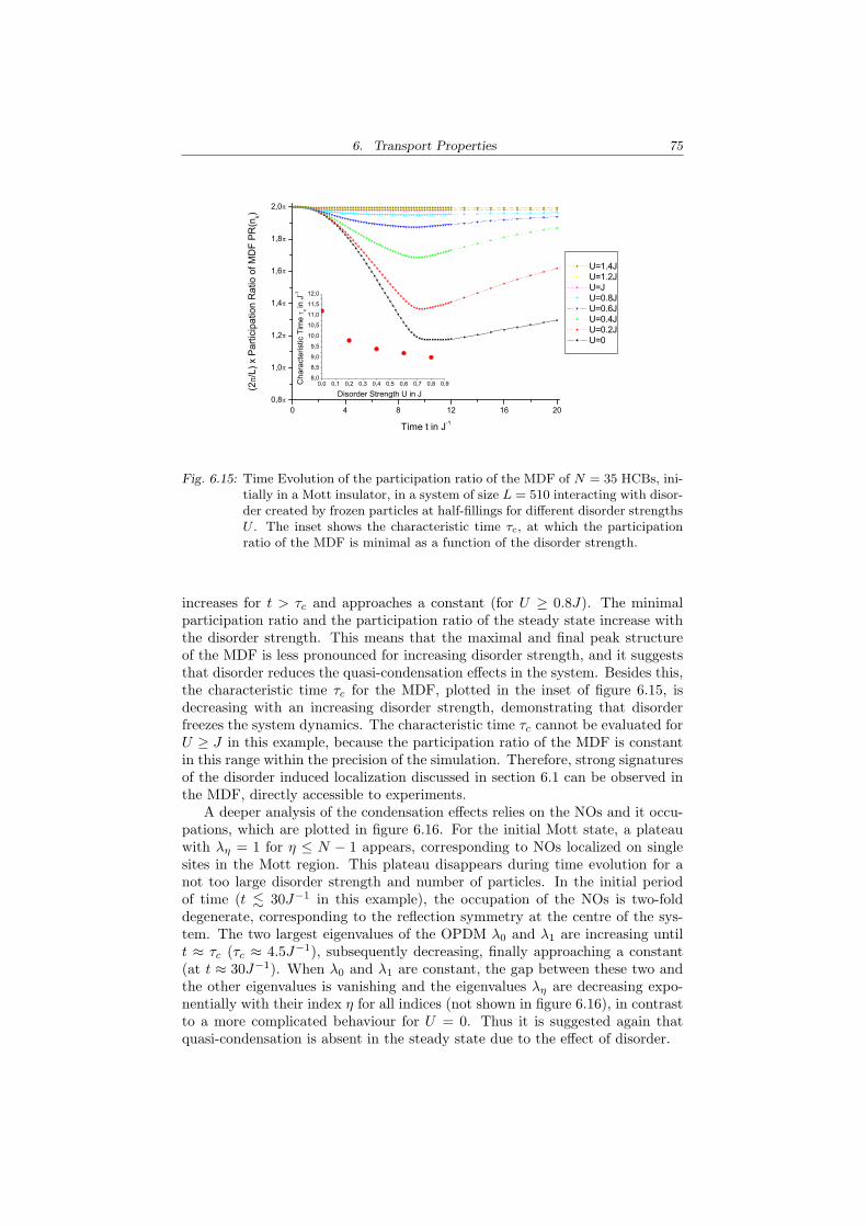
6. Transport Properties 75
0 4 8 12 16 200,8
1,0
1,2
1,4
1,6
1,8
2,0
0,0 0,1 0,2 0,3 0,4 0,5 0,6 0,7 0,8 0,98,0
8,5
9,0
9,5
10,0
10,5
11,0
11,5
12,0
U=1.4J U=1.2J U=J U=0.8J U=0.6J U=0.4J U=0.2J U=0
(2/L
) x P
artic
ipat
ion
Rat
io o
f MD
F PR
(nk)
Time t in J-1
Disorder Strength U in J
Cha
ract
eris
tic T
ime
c in
J-1
Fig. 6.15: Time Evolution of the participation ratio of the MDF of N = 35 HCBs, ini-tially in a Mott insulator, in a system of size L = 510 interacting with disor-der created by frozen particles at half-fillings for different disorder strengthsU . The inset shows the characteristic time τc, at which the participationratio of the MDF is minimal as a function of the disorder strength.
increases for t > τc and approaches a constant (for U ≥ 0.8J). The minimalparticipation ratio and the participation ratio of the steady state increase withthe disorder strength. This means that the maximal and final peak structureof the MDF is less pronounced for increasing disorder strength, and it suggeststhat disorder reduces the quasi-condensation effects in the system. Besides this,the characteristic time τc for the MDF, plotted in the inset of figure 6.15, isdecreasing with an increasing disorder strength, demonstrating that disorderfreezes the system dynamics. The characteristic time τc cannot be evaluated forU ≥ J in this example, because the participation ratio of the MDF is constantin this range within the precision of the simulation. Therefore, strong signaturesof the disorder induced localization discussed in section 6.1 can be observed inthe MDF, directly accessible to experiments.
A deeper analysis of the condensation effects relies on the NOs and it occu-pations, which are plotted in figure 6.16. For the initial Mott state, a plateauwith λη = 1 for η ≤ N − 1 appears, corresponding to NOs localized on singlesites in the Mott region. This plateau disappears during time evolution for anot too large disorder strength and number of particles. In the initial periodof time (t . 30J−1 in this example), the occupation of the NOs is two-folddegenerate, corresponding to the reflection symmetry at the centre of the sys-tem. The two largest eigenvalues of the OPDM λ0 and λ1 are increasing untilt ≈ τc (τc ≈ 4.5J−1), subsequently decreasing, finally approaching a constant(at t ≈ 30J−1). When λ0 and λ1 are constant, the gap between these two andthe other eigenvalues is vanishing and the eigenvalues λη are decreasing expo-nentially with their index η for all indices (not shown in figure 6.16), in contrastto a more complicated behaviour for U = 0. Thus it is suggested again thatquasi-condensation is absent in the steady state due to the effect of disorder.
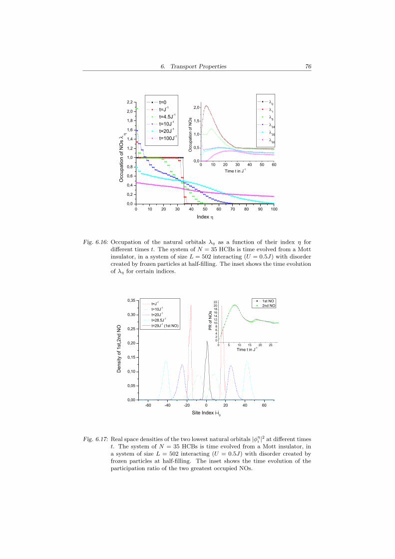
6. Transport Properties 76
0 10 20 30 40 50 60 70 80 90 1000,0
0,2
0,4
0,6
0,8
1,0
1,2
1,4
1,6
1,8
2,0
2,2
0 10 20 30 40 50 600,0
0,5
1,0
1,5
2,0 0
1
5
34
35
50
t=0 t=J-1
t=4.5J-1
t=10J-1
t=20J-1
t=100J-1
Occ
upat
ion
of N
Os
Index
Time t in J-1
Occ
upat
ion
of N
Os
Fig. 6.16: Occupation of the natural orbitals λη as a function of their index η fordifferent times t. The system of N = 35 HCBs is time evolved from a Mottinsulator, in a system of size L = 502 interacting (U = 0.5J) with disordercreated by frozen particles at half-filling. The inset shows the time evolutionof λη for certain indices.
-60 -40 -20 0 20 40 600,00
0,05
0,10
0,15
0,20
0,25
0,30
0,35
0 5 10 15 20 2502468
10121416182022
Den
sity
of 1
st,2
nd N
O
Site Index i-i0
t=J-1
t=10J-1
t=20J-1
t=28.5J-1
t=29J-1 (1st NO)
Time t in J-1
PR o
f NO
s
1st NO 2nd NO
Fig. 6.17: Real space densities of the two lowest natural orbitals |φηi |2 at different times
t. The system of N = 35 HCBs is time evolved from a Mott insulator, ina system of size L = 502 interacting (U = 0.5J) with disorder created byfrozen particles at half-filling. The inset shows the time evolution of theparticipation ratio of the two greatest occupied NOs.
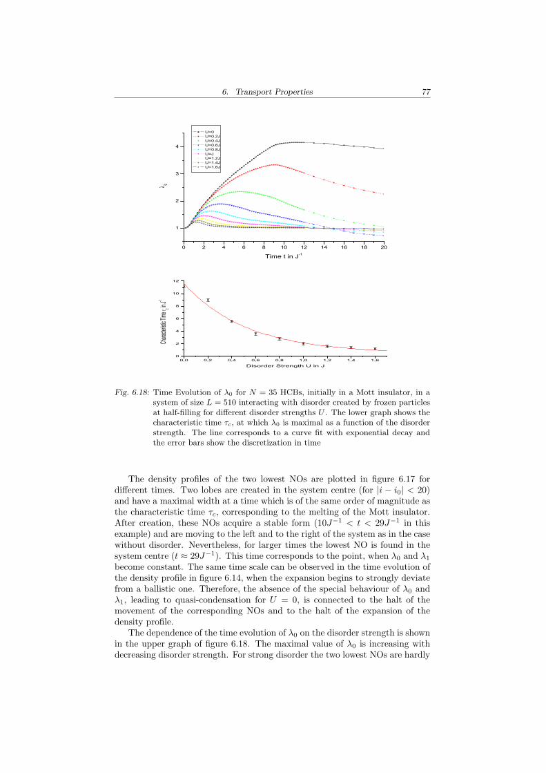
6. Transport Properties 77
0 2 4 6 8 10 12 14 16 18 20
1
2
3
4
0
Time t in J-1
U=0 U=0.2J U=0.4J U=0.6J U=0.8J U=J U=1.2J U=1.4J U=1.6J
0,0 0,2 0,4 0,6 0,8 1,0 1,2 1,4 1,60
2
4
6
8
10
12
Charac
teristic
Time c in J
-1
Disorder Strength U in J
Fig. 6.18: Time Evolution of λ0 for N = 35 HCBs, initially in a Mott insulator, in asystem of size L = 510 interacting with disorder created by frozen particlesat half-filling for different disorder strengths U . The lower graph shows thecharacteristic time τc, at which λ0 is maximal as a function of the disorderstrength. The line corresponds to a curve fit with exponential decay andthe error bars show the discretization in time
The density profiles of the two lowest NOs are plotted in figure 6.17 fordifferent times. Two lobes are created in the system centre (for |i − i0| < 20)and have a maximal width at a time which is of the same order of magnitude asthe characteristic time τc, corresponding to the melting of the Mott insulator.After creation, these NOs acquire a stable form (10J−1 < t < 29J−1 in thisexample) and are moving to the left and to the right of the system as in the casewithout disorder. Nevertheless, for larger times the lowest NO is found in thesystem centre (t ≈ 29J−1). This time corresponds to the point, when λ0 and λ1
become constant. The same time scale can be observed in the time evolution ofthe density profile in figure 6.14, when the expansion begins to strongly deviatefrom a ballistic one. Therefore, the absence of the special behaviour of λ0 andλ1, leading to quasi-condensation for U = 0, is connected to the halt of themovement of the corresponding NOs and to the halt of the expansion of thedensity profile.
The dependence of the time evolution of λ0 on the disorder strength is shownin the upper graph of figure 6.18. The maximal value of λ0 is increasing withdecreasing disorder strength. For strong disorder the two lowest NOs are hardly
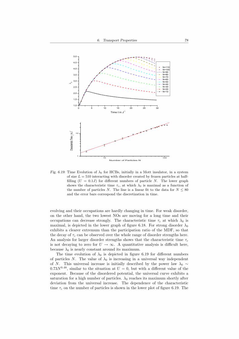
6. Transport Properties 78
0 5 10 15 20 25 301,0
1,5
2,0
2,5
3,0
3,5
4,0
4,5
5,0
o
Time t in J-1
N=110 N=100 N=90 N=80 N=70 N=60 N=50 N=40 N=30 N=20 N=10
10 1001
10
Charac
teristic
Time c in
J-1
Number of Particles N
Fig. 6.19: Time Evolution of λ0 for HCBs, initially in a Mott insulator, in a systemof size L = 510 interacting with disorder created by frozen particles at half-filling (U = 0.1J) for different numbers of particle N . The lower graphshows the characteristic time τc, at which λ0 is maximal as a function ofthe number of particles N . The line is a linear fit to the data for N ≤ 80and the error bars correspond the discretization in time.
evolving and their occupations are hardly changing in time. For weak disorder,on the other hand, the two lowest NOs are moving for a long time and theiroccupations can decrease strongly. The characteristic time τc at which λ0 ismaximal, is depicted in the lower graph of figure 6.18. For strong disorder λ0
exhibits a clearer extremum than the participation ratio of the MDF, so thatthe decay of τc can be observed over the whole range of disorder strengths here.An analysis for larger disorder strengths shows that the characteristic time τc
is not decaying to zero for U → ∞. A quantitative analysis is difficult here,because λ0 is nearly constant around its maximum.
The time evolution of λ0 is depicted in figure 6.19 for different numbersof particles N . The value of λ0 is increasing in a universal way independentof N . This universal increase is initially described by the power law λ0 ∼0.73N0.48, similar to the situation at U = 0, but with a different value of theexponent. Because of the disordered potential, the universal curve exhibits asaturation for a high number of particles. λ0 reaches its maximum shortly afterdeviation from the universal increase. The dependence of the characteristictime τc on the number of particles is shown in the lower plot of figure 6.19. The
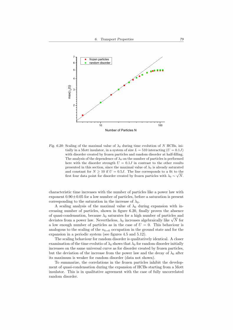
6. Transport Properties 79
10 100
2
3
4
5
6
7 frozen particles random disorder
max
(0(t)
)
Number of Particles N
Fig. 6.20: Scaling of the maximal value of λ0 during time evolution of N HCBs, ini-tially in a Mott insulator, in a system of size L = 510 interacting (U = 0.1J)with disorder created by frozen particles and random disorder at half-filling.The analysis of the dependence of λ0 on the number of particles is performedhere with the disorder strength U = 0.1J in contrast to the other resultspresented in this section, since the maximal value of λ0 is already saturatedand constant for N ≥ 10 if U = 0.5J . The line corresponds to a fit to thefirst four data point for disorder created by frozen particles with λ0 ∼
√N .
characteristic time increases with the number of particles like a power law withexponent 0.90±0.05 for a low number of particles, before a saturation is presentcorresponding to the saturation in the increase of λ0.
A scaling analysis of the maximal value of λ0 during expansion with in-creasing number of particles, shown in figure 6.20, finally proves the absenceof quasi-condensation, because λ0 saturates for a high number of particles anddeviates from a power law. Nevertheless, λ0 increases algebraically like
√N for
a low enough number of particles as in the case of U = 0. This behaviour isanalogous to the scaling of the nk=0 occupation in the ground state and for theexpansion in a periodic system (see figures 4.5 and 5.12).
The scaling behaviour for random disorder is qualitatively identical. A closerexamination of the time evolutio of λ0 shows that λ0 for random disorder initiallyincreases on the same universal curve as for disorder created by frozen particles,but the deviation of the increase from the power law and the decay of λ0 afterits maximum is weaker for random disorder (data not shown).
To summarize, the correlations in the frozen particles inhibit the develop-ment of quasi-condensation during the expansion of HCBs starting from a Mottinsulator. This is in qualitative agreement with the case of fully uncorrelatedrandom disorder.
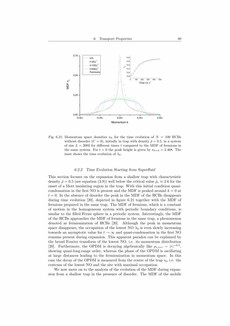
6. Transport Properties 80
-0,50 -0,25 0,00 0,25 0,500,00
0,25
0,50
0,75
0 100 200 300 400 500
12,8
13,0
13,2
13,4
13,6
13,8
MD
F n k
Momentum k
t=0 t=25J-1
t=100J-1
t=500J-1
Fermions
Time t in J-1
0
Fig. 6.21: Momentum space densities nk for the time evolution of N = 100 HCBswithout disorder (U = 0), initially in trap with density ρ = 0.5, in a systemof size L = 2002 for different times t compared to the MDF of fermions inthe same system. For t = 0 the peak height is given by nk=0 = 2.468. Theinset shows the time evolution of λ0.
6.2.2 Time Evolution Starting from Superfluid
This section focuses on the expansion from a shallow trap with characteristicdensity ρ = 0.5 (see equation (3.9)) well below the critical value ρc ≈ 2.6 for theonset of a Mott insulating region in the trap. With this initial condition quasi-condensation in the first NO is present and the MDF is peaked around k = 0 att = 0. In the absence of disorder the peak in the MDF of the HCBs disappearsduring time evolution [20], depicted in figure 6.21 together with the MDF offermions prepared in the same trap. The MDF of fermions, which is a constantof motion in the homogeneous system with periodic boundary conditions, issimilar to the filled Fermi sphere in a periodic system. Interestingly, the MDFof the HCBs approaches the MDF of fermions in the same trap, a phenomenondenoted as fermionization of HCBs [20]. Although the peak in momentumspace disappears, the occupation of the lowest NO λ0 is even slowly increasingtowards an asymptotic value for t→∞ and quasi-condensation in the first NOremains present during expansion. This apparent paradox can be explained bythe broad Fourier transform of the lowest NO, i.e. its momentum distribution[20]. Furthermore, the OPDM is decaying algebraically like ρi,i+r ∼ |r|−0.5,showing quasi-long-range order, whereas the phase of the OPDM is oscillatingat large distances leading to the fermionization in momentum space. In thiscase the decay of the OPDM is measured from the centre of the trap i0, i.e. thecentrum of the lowest NO and the site with maximal occupation.
We now move on to the analysis of the evolution of the MDF during expan-sion from a shallow trap in the presence of disorder. The MDF of the mobile
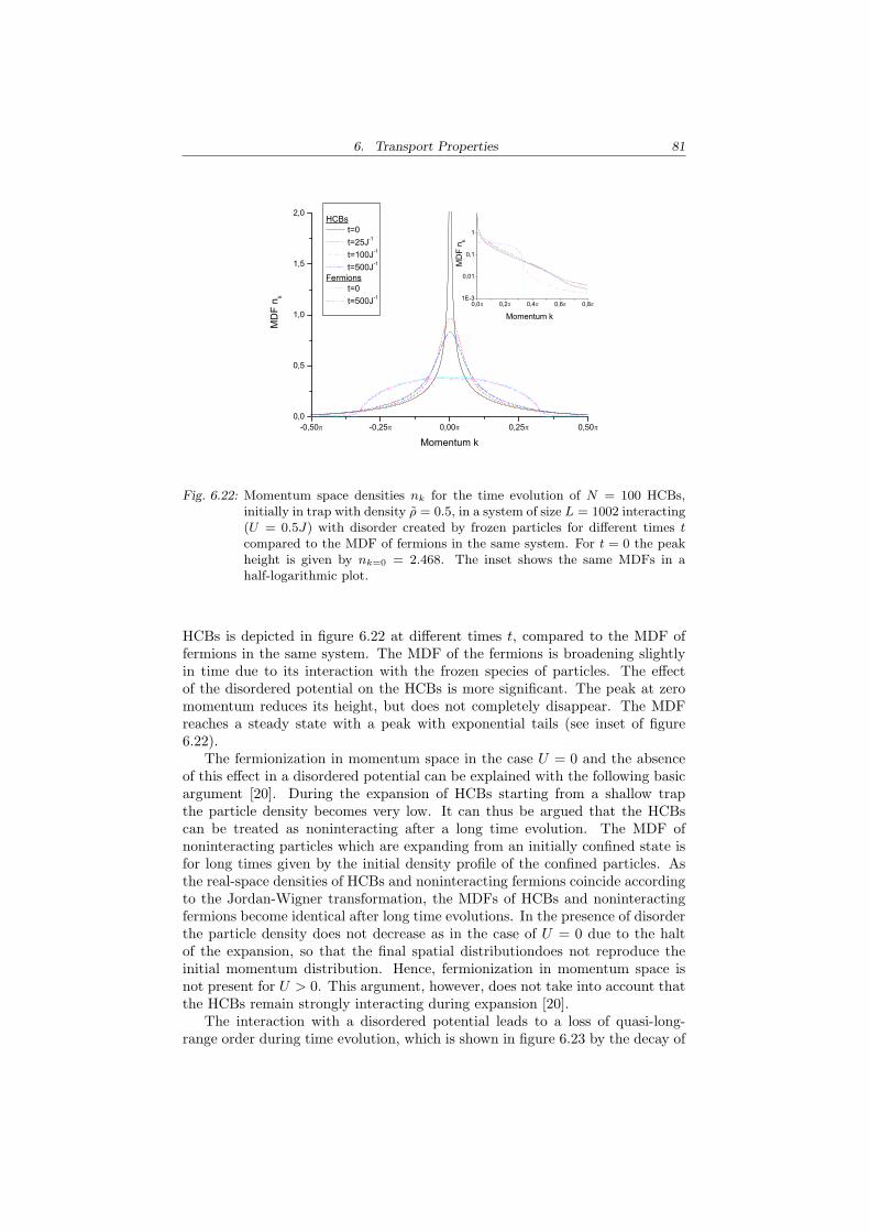
6. Transport Properties 81
-0,50 -0,25 0,00 0,25 0,500,0
0,5
1,0
1,5
2,0
0,0 0,2 0,4 0,6 0,81E-3
0,01
0,1
1
MD
F n k
Momentum k
HCBs t=0 t=25J-1
t=100J-1
t=500J-1
Fermions t=0 t=500J-1
Momentum k
MD
F n k
Fig. 6.22: Momentum space densities nk for the time evolution of N = 100 HCBs,initially in trap with density ρ = 0.5, in a system of size L = 1002 interacting(U = 0.5J) with disorder created by frozen particles for different times tcompared to the MDF of fermions in the same system. For t = 0 the peakheight is given by nk=0 = 2.468. The inset shows the same MDFs in ahalf-logarithmic plot.
HCBs is depicted in figure 6.22 at different times t, compared to the MDF offermions in the same system. The MDF of the fermions is broadening slightlyin time due to its interaction with the frozen species of particles. The effectof the disordered potential on the HCBs is more significant. The peak at zeromomentum reduces its height, but does not completely disappear. The MDFreaches a steady state with a peak with exponential tails (see inset of figure6.22).
The fermionization in momentum space in the case U = 0 and the absenceof this effect in a disordered potential can be explained with the following basicargument [20]. During the expansion of HCBs starting from a shallow trapthe particle density becomes very low. It can thus be argued that the HCBscan be treated as noninteracting after a long time evolution. The MDF ofnoninteracting particles which are expanding from an initially confined state isfor long times given by the initial density profile of the confined particles. Asthe real-space densities of HCBs and noninteracting fermions coincide accordingto the Jordan-Wigner transformation, the MDFs of HCBs and noninteractingfermions become identical after long time evolutions. In the presence of disorderthe particle density does not decrease as in the case of U = 0 due to the haltof the expansion, so that the final spatial distributiondoes not reproduce theinitial momentum distribution. Hence, fermionization in momentum space isnot present for U > 0. This argument, however, does not take into account thatthe HCBs remain strongly interacting during expansion [20].
The interaction with a disordered potential leads to a loss of quasi-long-range order during time evolution, which is shown in figure 6.23 by the decay of
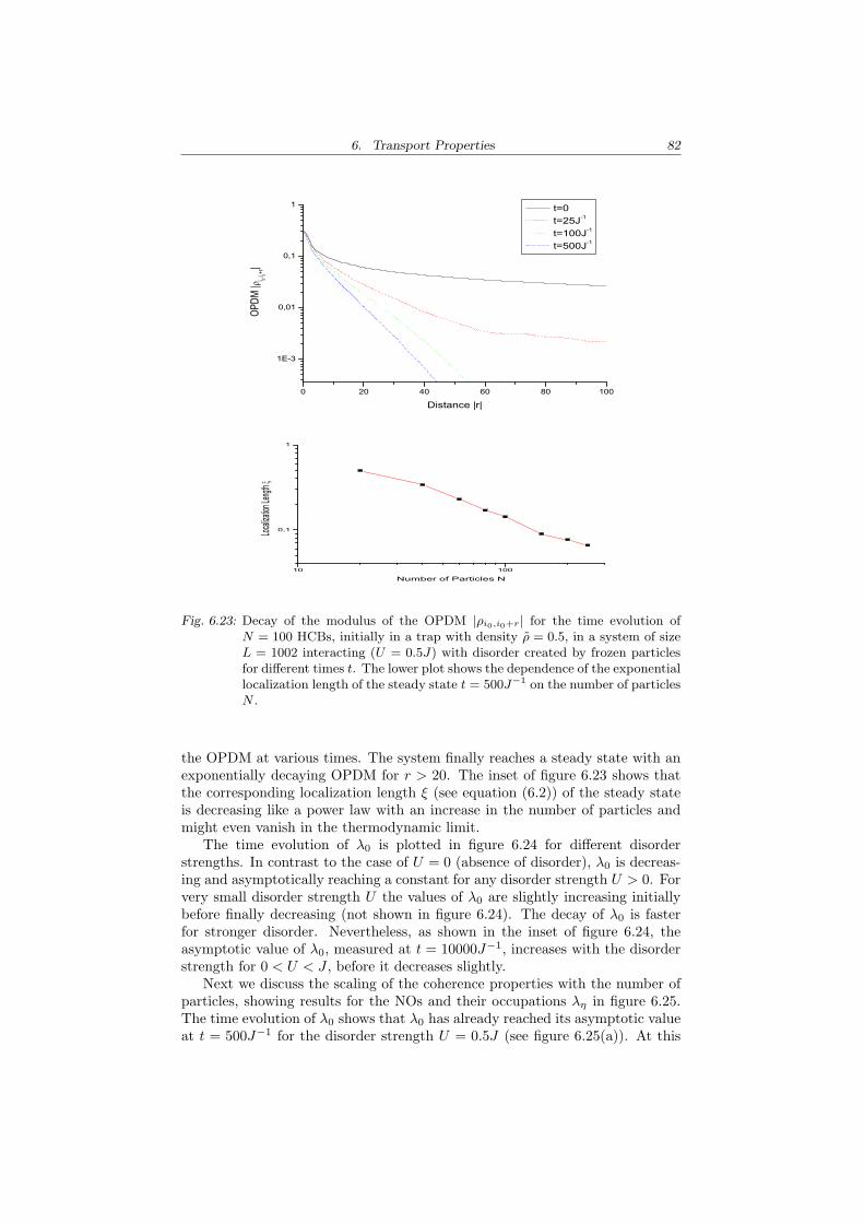
6. Transport Properties 82
0 20 40 60 80 100
1E-3
0,01
0,1
1
OPDM
|i 0,i 0+r
|
Distance |r|
t=0 t=25J-1
t=100J-1
t=500J-1
10 100
0,1
1
Localiz
ation L
ength
Number of Particles N
Fig. 6.23: Decay of the modulus of the OPDM |ρi0,i0+r| for the time evolution ofN = 100 HCBs, initially in a trap with density ρ = 0.5, in a system of sizeL = 1002 interacting (U = 0.5J) with disorder created by frozen particlesfor different times t. The lower plot shows the dependence of the exponentiallocalization length of the steady state t = 500J−1 on the number of particlesN .
the OPDM at various times. The system finally reaches a steady state with anexponentially decaying OPDM for r > 20. The inset of figure 6.23 shows thatthe corresponding localization length ξ (see equation (6.2)) of the steady stateis decreasing like a power law with an increase in the number of particles andmight even vanish in the thermodynamic limit.
The time evolution of λ0 is plotted in figure 6.24 for different disorderstrengths. In contrast to the case of U = 0 (absence of disorder), λ0 is decreas-ing and asymptotically reaching a constant for any disorder strength U > 0. Forvery small disorder strength U the values of λ0 are slightly increasing initiallybefore finally decreasing (not shown in figure 6.24). The decay of λ0 is fasterfor stronger disorder. Nevertheless, as shown in the inset of figure 6.24, theasymptotic value of λ0, measured at t = 10000J−1, increases with the disorderstrength for 0 < U < J , before it decreases slightly.
Next we discuss the scaling of the coherence properties with the number ofparticles, showing results for the NOs and their occupations λη in figure 6.25.The time evolution of λ0 shows that λ0 has already reached its asymptotic valueat t = 500J−1 for the disorder strength U = 0.5J (see figure 6.25(a)). At this

6. Transport Properties 83
0 100 200 300 400 5000
1
2
3
4
5
6
7
8
0,0 0,2 0,4 0,6 0,8 1,0 1,2 1,4 1,6 1,8 2,00
2
4
6
80
Time in J-1
U=0 U=0.1J U=0.4J U=1.2J U=2J
Disorder Strength U in J
0
Fig. 6.24: Time evolution of λ0 for different disorder strengths U for N = 35 initiallyconfined HCBs with density ρ = 0.5, in a system of size L = 1002 (L = 2002for U = 0) with disorder created by frozen particles. The inset shows λ0
at t = 10000J−1 for U > 0 and t = 500J−1 for U = 0 as a function of thedisorder strength U .
0 100 200 300 400 5000123456789
1011121314
0 200 400 600 800 1000
1E-7
1E-6
1E-5
1E-4
1E-3
0,01
0,1
1
-60 -40 -20 0 20 40 600,00
0,01
0,02
0,03
0,04
0,05
-200 -100 0 100 2000,000
0,004
0,008
0,012
0,016
0,020 (c)
N=100 N=80 N=60 N=40 N=20
Site Index i-i0
Index
Site Index i-i0
Con
dens
ate
Frac
tion
0
Occ
upat
ion
of N
Os
(b) N=100 N=80 N=60 N=40 N=20
Time t in J-1
(d) N=100 N=80 N=60 N=40 N=20
Den
sity
Pro
file
of 1
st N
O
Den
sity
Pro
file
of 1
st N
O
(a)
t=500J-1
t=100J-1
t=25J-1
t=0
Fig. 6.25: Results for the NOs and its occupation during time evolution of N initiallyharmonically confined HCBs with density ρ = 0.5, in a system of size L =1002 interacting (U = 0.5J) with disorder created by frozen particles. (a)Time evolution of λ0, (b) occupation of the NOs λη as a function of theindex η for t = 500J−1, (c) |φ0
i |2 for N = 100 at different times, (d) densityprofile of the first NO |φ0
i |2 at t = 500J−1 for different N .
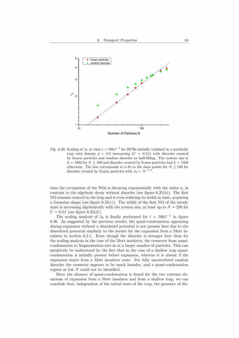
6. Transport Properties 84
10 1001
2
3
4
5 frozen particlesrandom disorder
0
Number of Particles N
Fig. 6.26: Scaling of λ0 at time t = 500J−1 for HCBs initially confined in a parabolictrap with density ρ = 0.5 interacting (U = 0.5J) with disorder createdby frozen particles and random disorder at half-filling. The system size isL = 1002 for N ≤ 100 and disorder created by frozen particles and L = 1502otherwise. The line corresponds to a fit to the data points for N ≤ 100 fordisorder created by frozen particles with λ0 ∼ N−0.5.
time the occupation of the NOs is decaying exponentially with the index η, incontrast to the algebraic decay without disorder (see figure 6.25(b)). The firstNO remains centred in the trap and is even reducing its width in time, acquiringa Gaussian shape (see figure 6.25(c)). The width of the first NO of the steadystate is increasing algebraically with the system size, at least up to N = 250 forU = 0.5J (see figure 6.25(d)).
The scaling analysis of λ0 is finally performed for t = 500J−1 in figure6.26. As suggested by the previous results, the quasi-condensation appearingduring expansion without a disordered potential is not present here due to thedisordered potential similarly to the results for the expansion from a Mott in-sulator in section 6.2.1. Even though the disorder is stronger here than forthe scaling analysis in the case of the Mott insulator, the crossover from quasi-condensation to fragmentation sets in at a larger number of particles. This canintuitively be understood by the fact that in the case of a shallow trap quasi-condensation is initially present before expansion, whereas it is absent if theexpansion starts from a Mott insulator state. For fully uncorrelated randomdisorder the crossover appears to be much broader, and a quasi-condensationregime at low N could not be identified.
Since the absence of quasi-condensation is found for the two extreme sit-uations of expansion from a Mott insulator and from a shallow trap, we canconclude that, independent of the initial state of the trap, the presence of dis-

6. Transport Properties 85
order leads to the absence of quasi-condensation and to real-space localizationin the steady state of the system.
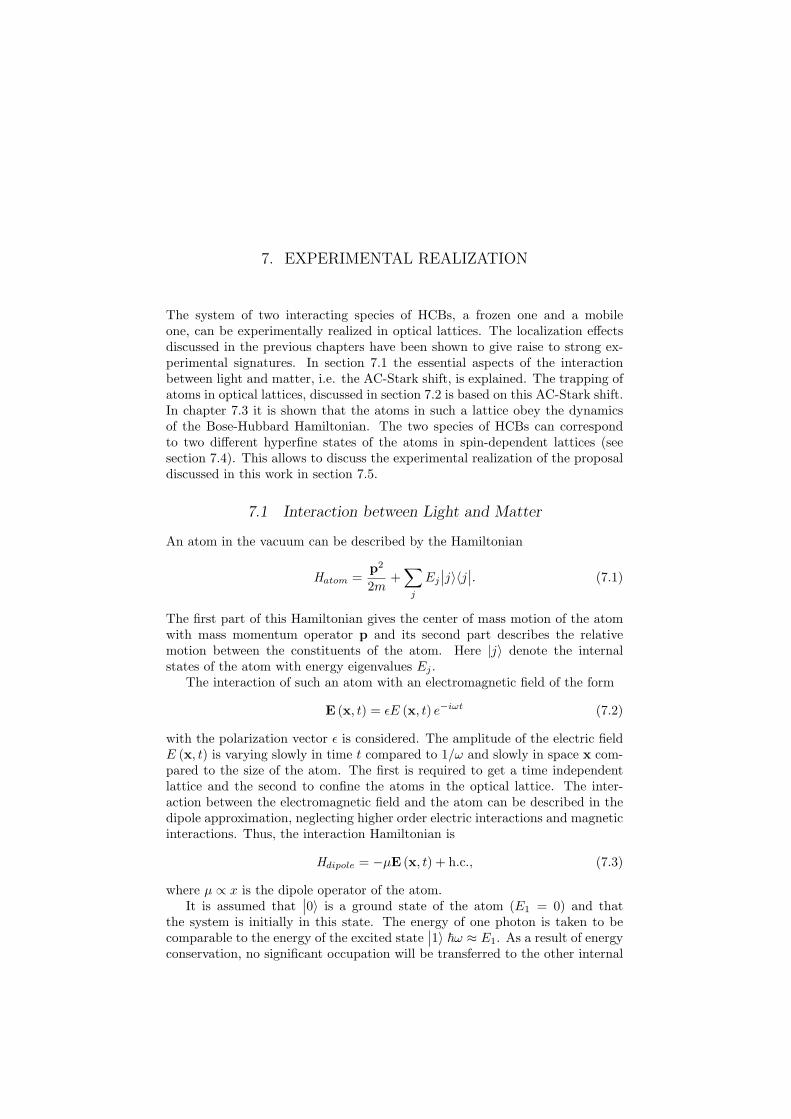
7. EXPERIMENTAL REALIZATION
The system of two interacting species of HCBs, a frozen one and a mobileone, can be experimentally realized in optical lattices. The localization effectsdiscussed in the previous chapters have been shown to give raise to strong ex-perimental signatures. In section 7.1 the essential aspects of the interactionbetween light and matter, i.e. the AC-Stark shift, is explained. The trapping ofatoms in optical lattices, discussed in section 7.2 is based on this AC-Stark shift.In chapter 7.3 it is shown that the atoms in such a lattice obey the dynamicsof the Bose-Hubbard Hamiltonian. The two species of HCBs can correspondto two different hyperfine states of the atoms in spin-dependent lattices (seesection 7.4). This allows to discuss the experimental realization of the proposaldiscussed in this work in section 7.5.
7.1 Interaction between Light and Matter
An atom in the vacuum can be described by the Hamiltonian
Hatom =p2
2m+
∑
j
Ej
∣∣j〉〈j∣∣. (7.1)
The first part of this Hamiltonian gives the center of mass motion of the atomwith mass momentum operator p and its second part describes the relativemotion between the constituents of the atom. Here |j〉 denote the internalstates of the atom with energy eigenvalues Ej .
The interaction of such an atom with an electromagnetic field of the form
E (x, t) = εE (x, t) e−iωt (7.2)
with the polarization vector ε is considered. The amplitude of the electric fieldE (x, t) is varying slowly in time t compared to 1/ω and slowly in space x com-pared to the size of the atom. The first is required to get a time independentlattice and the second to confine the atoms in the optical lattice. The inter-action between the electromagnetic field and the atom can be described in thedipole approximation, neglecting higher order electric interactions and magneticinteractions. Thus, the interaction Hamiltonian is
Hdipole = −µE (x, t) + h.c., (7.3)
where µ ∝ x is the dipole operator of the atom.It is assumed that
∣∣0〉 is a ground state of the atom (E1 = 0) and thatthe system is initially in this state. The energy of one photon is taken to becomparable to the energy of the excited state
∣∣1〉 ~ω ≈ E1. As a result of energyconservation, no significant occupation will be transferred to the other internal
7. Experimental Realization 87
D
E1
hwW
0
1
w
Fig. 7.1: Two-level system with transition energy E1 interacting with an electric fieldat frequency ω, detuned from the transition by ∆ = E1 − ~ω. The singleground state
˛0〉 is coupled to the excited state
˛1〉 by the Rabi frequency Ω.
states during time evolution, so that the calculations can be restricted to aneffective two-level system (see figure 7.1). As Hatom commutes with parity andµ ∝ x has odd parity, 〈j∣∣µε
∣∣j〉 = 0 holds. Restricting the Hilbert space to theground state
∣∣0〉 and the excited state∣∣1〉, the interaction Hamiltonian takes
the form
Hdipole = −E (x, t) e−iωt〈0∣∣µε
∣∣1〉∣∣0〉〈1∣∣ + 〈1∣∣µε∣∣0〉∣∣1〉〈0∣∣ + h.c.. (7.4)
It is now changed to the reference frame rotating with the frequency of theelectric field, by applying the transformation Γ = exp
(−iωt∣∣1〉〈1
∣∣) to vectors∣∣Ψ〉′ = Γ∣∣Ψ〉. It follows from the time dependent Schrodinger equation that the
Hamiltonian has to be changed by
H ′ = ΓHΓ−1 − ~ω∣∣1〉〈1
∣∣. (7.5)
The subtraction of ~ω is due to the time dependence of the unitary transforma-tion Γ.
With this transformation the atomic Hamiltonian in the rotating frame (’will be omitted) becomes
Hatom =p2
2m+ ∆
∣∣1〉〈1∣∣, (7.6)
where ∆ = E1−~ω is the detuning of the electric field frequency from the atomictransition between
∣∣0〉 and∣∣1〉. The resulting Hamiltonian for the interaction
is.
Hdipole = −E (x, t) 〈0∣∣µε
∣∣1〉∣∣0〉〈1
∣∣− E∗ (x, t) 〈1∣∣µ†ε
∣∣0〉∣∣1〉〈0
∣∣− E (x, t) e−2iωt〈0
∣∣µε∣∣1〉
∣∣0〉〈1∣∣− E∗ (x, t) e2iωt〈1
∣∣µ†ε∣∣0〉
∣∣1〉〈0∣∣ (7.7)
In the rotating wave approximation, the two quickly oscillating terms withexp (±2iωt) are neglected, as they are averaged out over times tÀ 1/ω.
7. Experimental Realization 88
Hence, the Hamiltonian for the internal states in the rotating frame afterapplying the rotating wave approximation is
Hinternal = ∆∣∣1〉〈1
∣∣ +Ω2
∣∣0〉〈1∣∣ +
Ω∗
2
∣∣1〉〈0∣∣
=(
0 Ω/2Ω∗/2 ∆
),
(7.8)
where Ω = −2E (x, t) 〈0∣∣µε
∣∣1〉 is the Rabi frequency of the transition. Thedynamics of such a two-level system is solved in section 5.1.1 with the notationchange Ω→ −2J , ∆→ U . The Ansatz 5.3 leads to the dynamics 5.6, which forthe initial conditions c1
(t = 0
)= 0 and c0
(t = 0
)= c0 become
c0 (t) = c0e−i ∆
2 t
(cos
(λt
~
)+ i
∆2λ
c0 sin(
λt
~
))
c1 (t) = c0ei ∆
2 t Ω∗
2iλsin
(λt
~
),
(7.9)
where the energy λ =√
∆2 + Ω2/2 describes the frequency of the occupationoscillation between the two levels. For a large detuning of the electric fieldfrequency |∆| À Ω from the atomic transition, no significant occupation istransferred to the excited level
∣∣1〉 and the dynamics of the system can berestricted to the ground state
∣∣0〉. This is referred to as adiabatic elimination.These results can be shown by expanding c0 (t) and c1 (t) in terms of Ω/∆.Expanding c1 (t) yields
c1 (t) = c0ei~
∆2 t Ω
i∆
(1 + O
(Ω2
∆2
))sin
(λt
~
). (7.10)
To first order in Ω/∆ the occupation of the excited level remains zero |c1 (t)|2 ≡ 0and the ground state only acquires a phase
c0 (t) = c0 exp− i
~
(∆2− λ
)t
+ O
(Ω2
∆2
)
= c0 exp
i
~
(Ω2
4∆+ O
(Ω4
∆5
))t
+ O
(Ω2
∆2
)
c0 (t) ≈ c0 exp(
i
~Ω2
4∆t
).
(7.11)
The physical process behind the adiabatic elimination can be interpreted in-tuitively. The energy needed for stimulated transitions between the relevantatomic energy levels is only partly from the electromagnetic field, which is pos-sible for small time scales due to the uncertainty principle ∆E ·∆t . ~. Sincethe detuning of the electromagnetic field is very large, the borrowed energy isquite large, so that the excited state decays immediately. Thus, there is a re-sulting effect to the atomic ground states without population transfer to theexcited state.
The total Hamiltonian of the system can now be written as
H =p2
2m+ V (x, t) (7.12)
7. Experimental Realization 89
with the potential
V (x, t) = −|Ω(x, t) |24∆
, (7.13)
where the atom always stays in its internal ground state.This energy shift of the atomic ground state, expressed as a potential due
to the electric dipole interaction with a time dependent electromagnetic field, isreferred to as AC-Stark shift.
7.2 Optical Lattice
A pair of beams, counter-propagating along the x-axis, can be described byan electric field of the form 7.2 with amplitude E (x, t) = α/2 exp (ikx) +α/2 exp (−ikx) = α cos (kx), where the wavenumber k = 2π/λ is given bythe wavelength λ. So the potential 7.13 becomes V (x, t) ∝ cos2 (kx). Thisrepresents a one-dimensional optical lattice with spatial period λ/2. Three per-pendicular pairs of laser beams, where each pair couples the same ground stateto different excited states, create the potential
V (x, t) = V0x cos2 (kxx) + V0y cos2 (kyy) + V0z cos2 (kzz) , (7.14)
realizing a simple cubic three-dimensional periodic trapping potential, the op-tical lattice. If the three pairs of laser beams have slightly different frequencies,though coupling the ground state to the same excited state, the potential 7.14with kx = ky = kz is effectively realized, as any residual interference betweenthe different pairs is time-averaged to zero. The depth of this lattice in eachdirection is proportional to the square of the amplitude of the correspondingpair of laser beams, which is easily controlled in experiments.
The single-particle Hamiltonian for an one-dimensional optical lattice is
H = −~2∂2
x
2m+ V0 cos2 (kx) + VT (x) , (7.15)
where VT (x) is a slowly varying trapping potential, needed to prevent the atomfrom escaping the optical lattice. Since the optical lattice potential is periodicin space, the eigenstates of this Hamiltonian can be written as Bloch waves
Φ(n)q (x) = eiqxu(n)
q (x) , (7.16)
where u(n)q (x) are periodic u
(n)q (x + a) = u
(n)q (x) and q ∈ [−π/a, π/a]. The
index n refers to the Bloch band.In figure 7.2 the band structure for this Hamiltonian is shown. The energy
is given in units of the recoil energy ER = ~2k2/2m. For energies much smallerthen the potential depth the gap between the Bloch bands is much greater thantheir width, corresponding to states localized on single sites.
The Wannier functions
wn (x− xj) ∝∑
q
e−iqxj u(n)q (x) . (7.17)
are related to the Bloch waves by a Fourier transform, and they represent an-other complete set of orthogonal functions within one Bloch band. The maximaof these functions are centered at xj . For sufficiently large potential depths,these Wannier functions become localized within a single potential well and canbe interpreted as localized single-site states.
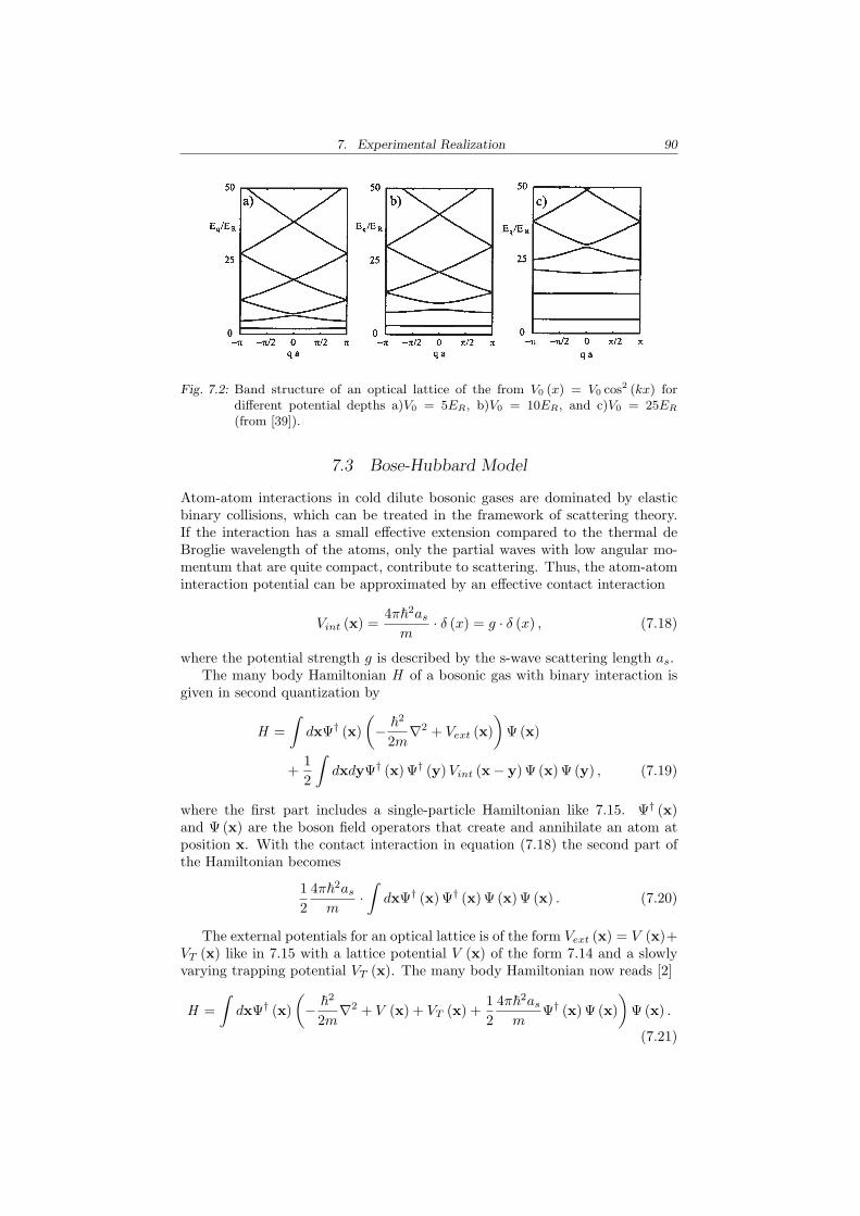
7. Experimental Realization 90
Fig. 7.2: Band structure of an optical lattice of the from V0 (x) = V0 cos2 (kx) fordifferent potential depths a)V0 = 5ER, b)V0 = 10ER, and c)V0 = 25ER
(from [39]).
7.3 Bose-Hubbard Model
Atom-atom interactions in cold dilute bosonic gases are dominated by elasticbinary collisions, which can be treated in the framework of scattering theory.If the interaction has a small effective extension compared to the thermal deBroglie wavelength of the atoms, only the partial waves with low angular mo-mentum that are quite compact, contribute to scattering. Thus, the atom-atominteraction potential can be approximated by an effective contact interaction
Vint (x) =4π~2as
m· δ (x) = g · δ (x) , (7.18)
where the potential strength g is described by the s-wave scattering length as.The many body Hamiltonian H of a bosonic gas with binary interaction is
given in second quantization by
H =∫
dxΨ† (x)(− ~
2
2m∇2 + Vext (x)
)Ψ(x)
+12
∫dxdyΨ† (x)Ψ† (y) Vint (x− y)Ψ (x)Ψ (y) , (7.19)
where the first part includes a single-particle Hamiltonian like 7.15. Ψ† (x)and Ψ (x) are the boson field operators that create and annihilate an atom atposition x. With the contact interaction in equation (7.18) the second part ofthe Hamiltonian becomes
12
4π~2as
m·∫
dxΨ† (x) Ψ† (x)Ψ (x)Ψ (x) . (7.20)
The external potentials for an optical lattice is of the form Vext (x) = V (x)+VT (x) like in 7.15 with a lattice potential V (x) of the form 7.14 and a slowlyvarying trapping potential VT (x). The many body Hamiltonian now reads [2]
H =∫
dxΨ† (x)(− ~
2
2m∇2 + V (x) + VT (x) +
12
4π~2as
mΨ† (x) Ψ (x)
)Ψ(x) .
(7.21)
7. Experimental Realization 91
Because the atom-atom interactions are local, the field operator is expandedin the basis of the localized Wannier functions ωn (x− xj), defined in equation7.17. If neither the thermal energy nor the interaction energy is sufficient toinduce a transition from the lowest Bloch band to a higher one, the field operatorcan be approximated in the tight binding approximation
Ψ (x) =∑
j
ajw0 (x− xj) , (7.22)
where aj annihilates a particle in the Wannier state w0 (x− xj), localized atlattice site xj , and obeys bosonic commutation relations. The Hamiltonian nowbecomes [39]
Hfull = −∑
i,j
Jija†iaj +
∑
i,j
Vija†iaj +
12
∑
i,j,k,l
Wijkla†ia†jakal, (7.23)
where the tunneling matrix element Jij is
Jij = −∫
dxw∗0 (x− xi)(
p2
2m+ V (x)
)w0 (x− xj) , (7.24)
the offset matrix element εij is
Vij = −∫
dxw∗0 (x− xi)VT (x)w0 (x− xj) , (7.25)
and the interaction matrix element Wijkl is
Wijkl =4πas~2
m
∫dxw∗0 (x− xi)w∗0 (x− xj) w0 (x− xk)w0 (x− xl) . (7.26)
In the limit of sufficiently large potential depths and localized Wannier func-tions, the interaction matrix elements, centered at different lattice sites, becomenegligibly small against the on site matrix element
W = Wiiii =4πas~2
m
∫dx|w0 (x− x0) |4. (7.27)
Since VT (x) is slowly varying, only the offset at a single lattice site Vi = Vii ≈V (xi) is of importance, and because of the localization of the Wannier func-tions only nearest neighbour tunneling remains. Therefore, for reasonably deeplattices V0x,0y,0z & 5ER [39], the system is described by the Bose-HubbardHamiltonian
HBH = −J∑
〈i,j〉
(a†iaj + h.c.
)+
W
2
∑
j
nj (nj − 1) +∑
j
Vjnj , (7.28)
where nj = a†jaj is the particle number operator for the lattice site xj and 〈i, j〉refers to nearest neighbours.
The limit, in which the Bose-Hubbard Hamiltonian is valid, can be sum-marized by the inequalities as ¿ a0x,0y,0z ¿ a and U ¿ ~ω [1]. Here as isthe s-wave scattering length, a0 describes the width of the Wannier functions,
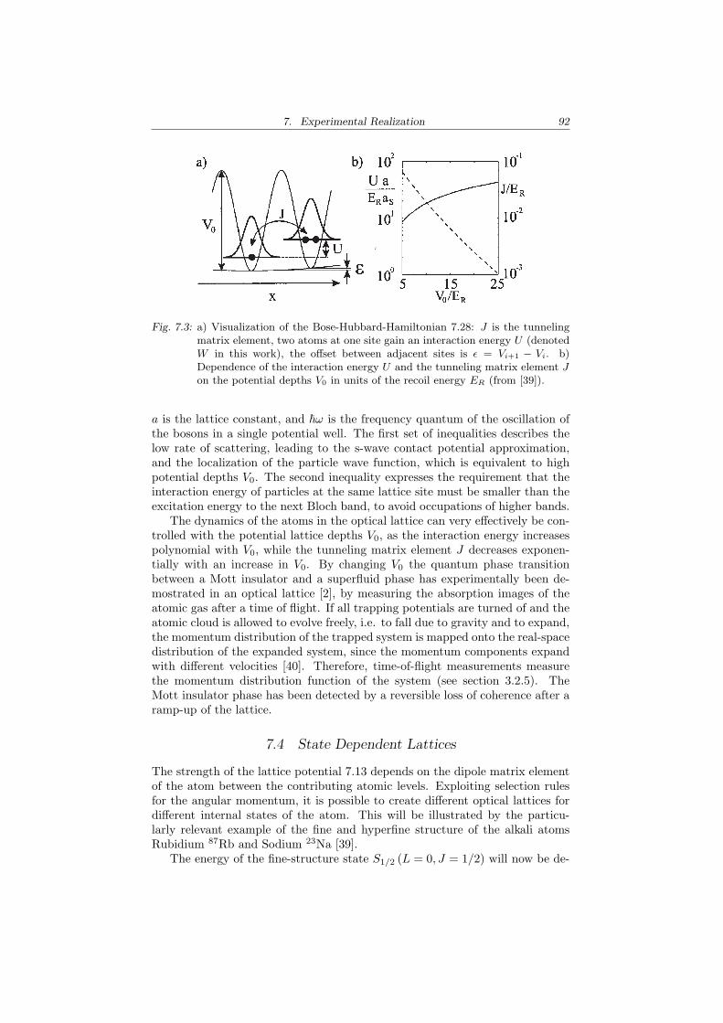
7. Experimental Realization 92
Fig. 7.3: a) Visualization of the Bose-Hubbard-Hamiltonian 7.28: J is the tunnelingmatrix element, two atoms at one site gain an interaction energy U (denotedW in this work), the offset between adjacent sites is ε = Vi+1 − Vi. b)Dependence of the interaction energy U and the tunneling matrix element Jon the potential depths V0 in units of the recoil energy ER (from [39]).
a is the lattice constant, and ~ω is the frequency quantum of the oscillation ofthe bosons in a single potential well. The first set of inequalities describes thelow rate of scattering, leading to the s-wave contact potential approximation,and the localization of the particle wave function, which is equivalent to highpotential depths V0. The second inequality expresses the requirement that theinteraction energy of particles at the same lattice site must be smaller than theexcitation energy to the next Bloch band, to avoid occupations of higher bands.
The dynamics of the atoms in the optical lattice can very effectively be con-trolled with the potential lattice depths V0, as the interaction energy increasespolynomial with V0, while the tunneling matrix element J decreases exponen-tially with an increase in V0. By changing V0 the quantum phase transitionbetween a Mott insulator and a superfluid phase has experimentally been de-mostrated in an optical lattice [2], by measuring the absorption images of theatomic gas after a time of flight. If all trapping potentials are turned of and theatomic cloud is allowed to evolve freely, i.e. to fall due to gravity and to expand,the momentum distribution of the trapped system is mapped onto the real-spacedistribution of the expanded system, since the momentum components expandwith different velocities [40]. Therefore, time-of-flight measurements measurethe momentum distribution function of the system (see section 3.2.5). TheMott insulator phase has been detected by a reversible loss of coherence after aramp-up of the lattice.
7.4 State Dependent Lattices
The strength of the lattice potential 7.13 depends on the dipole matrix elementof the atom between the contributing atomic levels. Exploiting selection rulesfor the angular momentum, it is possible to create different optical lattices fordifferent internal states of the atom. This will be illustrated by the particu-larly relevant example of the fine and hyperfine structure of the alkali atomsRubidium 87Rb and Sodium 23Na [39].
The energy of the fine-structure state S1/2 (L = 0, J = 1/2) will now be de-
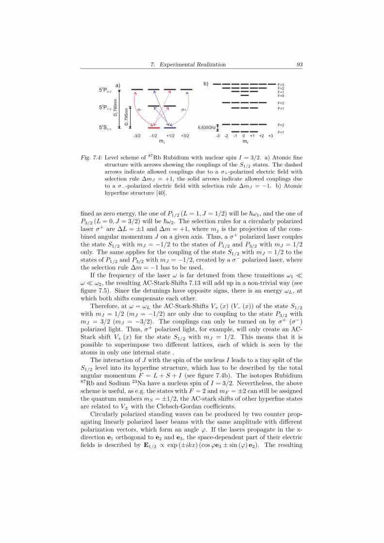
7. Experimental Realization 93
0 +1+1/2 +2 +3+3/2 -3-3/2 -1-1/2 -2
mFmJ
D7
95
nm
1
D7
80
nm
2
5 S2
1/ 2
5 P2
1/ 2
5 P2
3/ 2
F=1
F=2
F=1
F=2
F=0F=1F=2F=3
6,835Ghz
a) b)
s+s-
Fig. 7.4: Level scheme of 87Rb Rubidium with nuclear spin I = 3/2. a) Atomic finestructure with arrows showing the couplings of the S1/2 states. The dashedarrows indicate allowed couplings due to a σ+-polarized electric field withselection rule ∆mJ = +1, the solid arrows indicate allowed couplings dueto a σ−-polarized electric field with selection rule ∆mJ = −1. b) Atomichyperfine structure [40].
fined as zero energy, the one of P1/2 (L = 1, J = 1/2) will be ~ω1, and the one ofP3/2 (L = 0, J = 3/2) will be ~ω2. The selection rules for a circularly polarizedlaser σ+ are ∆L = ±1 and ∆m = +1, where mj is the projection of the com-bined angular momentum J on a given axis. Thus, a σ+ polarized laser couplesthe state S1/2 with mJ = −1/2 to the states of P1/2 and P3/2 with mJ = 1/2only. The same applies for the coupling of the state S1/2 with mJ = 1/2 to thestates of P1/2 and P3/2 with mJ = −1/2, created by a σ− polarized laser, wherethe selection rule ∆m = −1 has to be used.
If the frequency of the laser ω is far detuned from these transitions ω1 ¿ω ¿ ω2, the resulting AC-Stark-Shifts 7.13 will add up in a non-trivial way (seefigure 7.5). Since the detunings have opposite signs, there is an energy ωL, atwhich both shifts compensate each other.
Therefore, at ω = ωL the AC-Stark-Shifts V+ (x) (V− (x)) of the state S1/2
with mJ = 1/2 (mJ = −1/2) are only due to coupling to the state P3/2 withmJ = 3/2 (mJ = −3/2). The couplings can only be turned on by σ+ (σ−)polarized light. Thus, σ+ polarized light, for example, will only create an AC-Stark shift V+ (x) for the state S1/2 with mJ = 1/2. This means that it ispossible to superimpose two different lattices, each of which is seen by theatoms in only one internal state .
The interaction of J with the spin of the nucleus I leads to a tiny split of theS1/2 level into its hyperfine structure, which has to be described by the totalangular momentum F = L + S + I (see figure 7.4b). The isotopes Rubidium87Rb and Sodium 23Na have a nucleus spin of I = 3/2. Nevertheless, the abovescheme is useful, as e.g. the states with F = 2 and mF = ±2 can still be assignedthe quantum numbers mS = ±1/2, the AC-stark shifts of other hyperfine statesare related to V± with the Clebsch-Gordan coefficients.
Circularly polarized standing waves can be produced by two counter prop-agating linearly polarized laser beams with the same amplitude with differentpolarization vectors, which form an angle ϕ. If the lasers propagate in the x-direction e1 orthogonal to e2 and e3, the space-dependent part of their electricfields is described by E1/2 ∝ exp (±ikx) (cos ϕe3 ± sin (ϕ) e2). The resulting
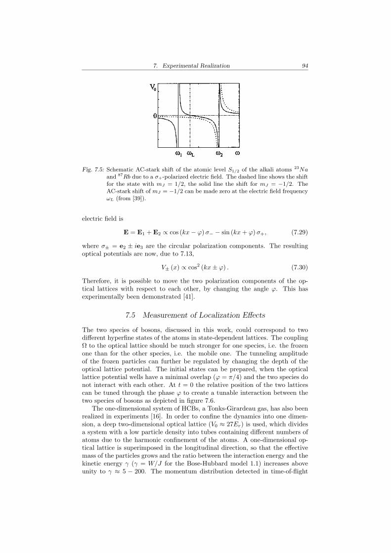
7. Experimental Realization 94
Fig. 7.5: Schematic AC-stark shift of the atomic level S1/2 of the alkali atoms 23Naand 87Rb due to a σ+-polarized electric field. The dashed line shows the shiftfor the state with mJ = 1/2, the solid line the shift for mJ = −1/2. TheAC-stark shift of mJ = −1/2 can be made zero at the electric field frequencyωL (from [39]).
electric field is
E = E1 + E2 ∝ cos (kx− ϕ)σ− − sin (kx + ϕ)σ+, (7.29)
where σ± = e2 ± ie3 are the circular polarization components. The resultingoptical potentials are now, due to 7.13,
V± (x) ∝ cos2 (kx± ϕ) . (7.30)
Therefore, it is possible to move the two polarization components of the op-tical lattices with respect to each other, by changing the angle ϕ. This hasexperimentally been demonstrated [41].
7.5 Measurement of Localization Effects
The two species of bosons, discussed in this work, could correspond to twodifferent hyperfine states of the atoms in state-dependent lattices. The couplingΩ to the optical lattice should be much stronger for one species, i.e. the frozenone than for the other species, i.e. the mobile one. The tunneling amplitudeof the frozen particles can further be regulated by changing the depth of theoptical lattice potential. The initial states can be prepared, when the opticallattice potential wells have a minimal overlap (ϕ = π/4) and the two species donot interact with each other. At t = 0 the relative position of the two latticescan be tuned through the phase ϕ to create a tunable interaction between thetwo species of bosons as depicted in figure 7.6.
The one-dimensional system of HCBs, a Tonks-Girardeau gas, has also beenrealized in experiments [16]. In order to confine the dynamics into one dimen-sion, a deep two-dimensional optical lattice (V0 ≈ 27Er) is used, which dividesa system with a low particle density into tubes containing different numbers ofatoms due to the harmonic confinement of the atoms. A one-dimensional op-tical lattice is superimposed in the longitudinal direction, so that the effectivemass of the particles grows and the ratio between the interaction energy and thekinetic energy γ (γ = W/J for the Bose-Hubbard model 1.1) increases aboveunity to γ ≈ 5 − 200. The momentum distribution detected in time-of-flight
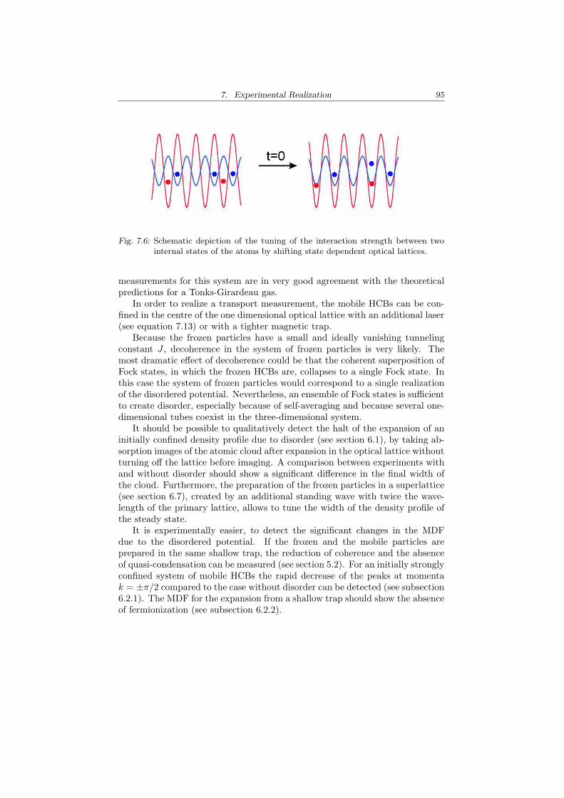
7. Experimental Realization 95
Fig. 7.6: Schematic depiction of the tuning of the interaction strength between twointernal states of the atoms by shifting state dependent optical lattices.
measurements for this system are in very good agreement with the theoreticalpredictions for a Tonks-Girardeau gas.
In order to realize a transport measurement, the mobile HCBs can be con-fined in the centre of the one dimensional optical lattice with an additional laser(see equation 7.13) or with a tighter magnetic trap.
Because the frozen particles have a small and ideally vanishing tunnelingconstant J , decoherence in the system of frozen particles is very likely. Themost dramatic effect of decoherence could be that the coherent superposition ofFock states, in which the frozen HCBs are, collapses to a single Fock state. Inthis case the system of frozen particles would correspond to a single realizationof the disordered potential. Nevertheless, an ensemble of Fock states is sufficientto create disorder, especially because of self-averaging and because several one-dimensional tubes coexist in the three-dimensional system.
It should be possible to qualitatively detect the halt of the expansion of aninitially confined density profile due to disorder (see section 6.1), by taking ab-sorption images of the atomic cloud after expansion in the optical lattice withoutturning off the lattice before imaging. A comparison between experiments withand without disorder should show a significant difference in the final width ofthe cloud. Furthermore, the preparation of the frozen particles in a superlattice(see section 6.7), created by an additional standing wave with twice the wave-length of the primary lattice, allows to tune the width of the density profile ofthe steady state.
It is experimentally easier, to detect the significant changes in the MDFdue to the disordered potential. If the frozen and the mobile particles areprepared in the same shallow trap, the reduction of coherence and the absenceof quasi-condensation can be measured (see section 5.2). For an initially stronglyconfined system of mobile HCBs the rapid decrease of the peaks at momentak = ±π/2 compared to the case without disorder can be detected (see subsection6.2.1). The MDF for the expansion from a shallow trap should show the absenceof fermionization (see subsection 6.2.2).
8. CONCLUSION
In this thesis, the proposal to create a disordered potential through a systemof frozen particles, interacting with another species of mobile bosons has beenanalysed for hard-core bosons on a one-dimensional lattice. Although the dis-order distribution generated by frozen particles exhibits significant correlations,throughout this thesis we observe a qualitative agreement with the effect ofa fully uncorrelated random disorder potential for static and dynamic proper-ties. The single-particle eigenstates in a disordered potential created by frozenparticles turn out to be localized.
At first, we have studied the dynamics of mobile and frozen hard-core bosonsinitially prepared in a one-dimensional periodic system (see chapter 5). The caseof a system with periodic boundary conditions does not lead to a measurablespatial localization after disorder-averaging, but localization in single disorderconfigurations is observed. In the experimentally realisable inhomogeneous sys-tem, where both particles are confined in a harmonic trap, disorder leads to anincrease in the width of the density profile due to demixing of the two species.
The effect of disorder in real-space can very clearly be seen through the ab-sence of dynamical delocalization (see chapter 6). Disorder causes the halt ofthe expansion of initially confined mobile particles. The density profile reachesan exponentially localized steady state for any nonvanishing value of the disor-der strength. Long-range correlations in the disordered potential, realized bypreparing the frozen particles in a superlattice, can change the width of the finalstate, but do not result in a localization-delocalization transition.
For any setup discussed in this work, we observe the absence of quasi-condensation and quasi-long-range order due to the disordered potential. Thestructure of the momentum distribution function is changed dramatically dueto disorder. In the periodic system the reduction of the peak at zero momen-tum and the change in its scaling with the number of particles corresponds tothe absence of quasi-condensation. During the expansion from a Mott insulatorstate two emerging peaks at finite momenta, which reveal quasi-condensation inthe absence of disorder, are suppressed in its presence. In contrast to the casewithout disorder, there is no fermionization in the momentum spectrum afterexpansion from a shallow trap.
Hence disorder created by a species of frozen hard-core bosons represents arealistic way to experimentally implement strongly fluctuating random poten-tials in optical lattices (see chapter 7). It is possible to observe the effects ofdisorder in the momentum distribution commonly measured in current experi-ments.
9. ACKNOWLEDGEMENTS
I would like to thank Dr. Tommaso Roscilde for his supervision - his explana-tions and the very fruitful discussions. I am glad that his door has always beenopen. Also many thanks to Prof. Dr. Ignacio Cirac, who has admitted me tohis group at the Max-Planck Institut fur Quantenoptik. Our discussions havebeen very important for my thesis.
Many thanks to Valentin Murg for his help with the Linux Opteron Clusterand the Intel Math Kernel Library, and to Dr. Juan Jose Garcıa-Ripoll for hisintroduction to the efficient calculation of single-particle time evolutions.
I would also like to express my thanks to my roommates Toby Cubitt, MariaEckholt-Perotti, and Christine Muschik, and the whole theory group for thefriendly atmosphere.
Most importantly, my deepest thanks go to my family, my parents and mysister Birte, who have given me a lot of assistance through my life and for myeducation.
APPENDIX
A. MARKOV PROCESSES AND STOCHASTIC MATRICES
In this appendix, a Markov process, which is a stepwise process, where a newstate depends on the previous state only, is described in a finite configurationspace. It is shown that such a process converge to its unique fix point undercertain conditions [37].
Theorem 1. Let W be an attractive stochastic matrix and −→q be a stochasticvector. Then W has a unique fix point −→q eq and it applies
limn→∞
−→q Wn = −→q eq. (A.1)
Definition 1. A stochastic vector is a vector −→qµ ∈ RN , which is nonnegative
−→qµ ≥ 0 (A.2)
and normalized ∑µ
−→qµ = 1. (A.3)
This implies that the space of stochastic vectors is compact.
Definition 2. A stochastic matrix is a quadratic matrix W ∈ RN×N , which isnonnegative
Wµν ≥ 0 (A.4)
and normalized ∑ν
Wµν = 1. (A.5)
Therefore, the application of a stochastic matrix on a stochastic vector yieldsa new stochastic vector −→q ′ = −→q ·W. (A.6)
Lemma 2. Every stochastic matrix W has at least one fixed point
−→q eq ·W = −→q eq. (A.7)
Proof. The sequence
−→q n =1n
n−1∑
i=0
−→q Wi (A.8)
of stochastic vectors is by definition (1) compact, so that a convergent subse-quence −→qnk
exists1nk
nk−1∑
i=0
−→q Wi k→∞−−−−→ −→q eq. (A.9)
A. Markov Processes and Stochastic Matrices 100
Multiplying this equation with W from the right
1nk
nk∑
i=1
−→q Wi k→∞−−−−→ −→q eqW (A.10)
and subtracting both limits leads to
−→q eq −−→q eqW = limk→∞
1nk
(−→q −−→q Wnk) = 0. (A.11)
This means that the vector −→q eq is a fixed point of W.
Definition 3. A stochastic matrix is called attractive, iff it contains at leastone column ν, whose entries are lower bounded by a positive number δ ∈ (0, 1]
Wµν ≥ δ ∀µ. (A.12)
An attractive matrix has a nonzero probability for the transition from anystate to a certain one.
Lemma 3. An attractive stochastic matrix W is contractive on vectors with∑Nν=0 qν = 0
‖−→q W‖1 ≤ (1− δ) ‖−→q ‖1 , (A.13)
where δ ∈ (0, 1] and ‖−→q ‖1 =∑N
mu=0 |qµ|.Proof. Because the statement (A.13) is linear in −→q , it must w.l.o.g. be provenfor ‖−→q ‖1 = 2 only. Because p, q ∈ R obey
|p− q| = p + q − 2min (p, q) , (A.14)
stochastic vectors obey
‖−→p −−→q ‖ = 2− 2N∑
µ=0
min (pµ, qµ) . (A.15)
Let −→e i be the unit vectors−→eiµ = δiµ, such that
−→eiµW is the ith row of W. The
identity (A.15) for the rows of the attractive matrix W is∥∥−→e iW −−→e jW
∥∥ = (1− δ)∥∥−→e i −−→e j
∥∥ (A.16)
with δ ∈ (0, 1].Let −→q be a vector with ‖−→q ‖ = 2 and
∑Nµ=0−→qµ = 0. It can w.l.o.g. be
assumed that
−→qµ ≥ 0 for 1 ≤ µ ≤ k (A.17)−→qµ < 0 for k < µ ≤ N. (A.18)
The right side of equation (A.13) is evaluated in this case with
‖−→q ‖ = 2 = −2k∑
µ=1
−→qν
N∑
ν=k+1
−→qν
= −k∑
µ=1
N∑
ν=k+1
−→qµ−→qν ‖−→e µ −−→e ν‖
(A.19)
A. Markov Processes and Stochastic Matrices 101
and the left side becomes
‖−→q W‖ =∥∥∥
k∑µ=1
−→qµ−→e µW
N∑
µ=k+1
−→qµ−→e νW
∥∥∥
=∥∥∥−
k∑µ=1
N∑
ν=k+1
−→qµ−→qν (−→e µ −−→e ν)W
∥∥∥
≤ −k∑
µ=1
N∑
ν=k+1
−→qµ−→qν ‖(−→e µ −−→e ν)W‖
= −k∑
µ=1
N∑
ν=k+1
−→qµ−→qν ‖−→e µ −−→e ν‖ (1− δ) ,
(A.20)
where∑k
µ=1−→qµ = 1,
∑Nµ=k+1
−→qµ = −1, and equation (A.16) has been used. Thelemma immediately follows from the last two equations.
Proof of theorem. The stochastic matrix W has at least one fixed point −→q eq
according to lemma 2. Because W is attractive, it holds for any stochasticvector −→q
limn→∞
‖−→q Wn −−→q eq‖ = limn→∞
‖(−→q −−→q eq)Wn‖≤ ‖−→q −−→q eq‖ lim
n→∞(1− δ)n
= 0,
(A.21)
where lemma 3 with δ > 0 has been applied to the difference of two stochasticvectors. This proves equation (A.1).
Let −→p eq be a second fix point of W, i.e.
−→p eq ·Wn = −→p eq. (A.22)
By applying equation (A.1) to −→p eq the identity −→p eq = −→q eq follows. This showsthat the fixed point is unique.
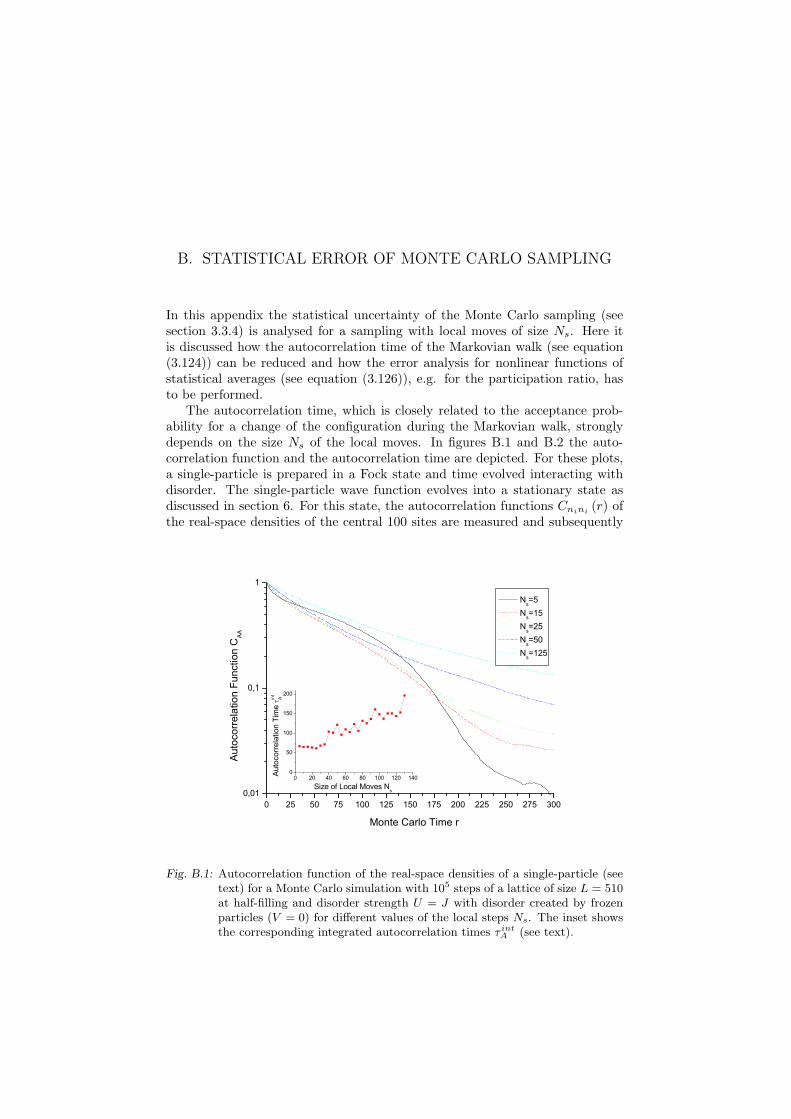
B. STATISTICAL ERROR OF MONTE CARLO SAMPLING
In this appendix the statistical uncertainty of the Monte Carlo sampling (seesection 3.3.4) is analysed for a sampling with local moves of size Ns. Here itis discussed how the autocorrelation time of the Markovian walk (see equation(3.124)) can be reduced and how the error analysis for nonlinear functions ofstatistical averages (see equation (3.126)), e.g. for the participation ratio, hasto be performed.
The autocorrelation time, which is closely related to the acceptance prob-ability for a change of the configuration during the Markovian walk, stronglydepends on the size Ns of the local moves. In figures B.1 and B.2 the auto-correlation function and the autocorrelation time are depicted. For these plots,a single-particle is prepared in a Fock state and time evolved interacting withdisorder. The single-particle wave function evolves into a stationary state asdiscussed in section 6. For this state, the autocorrelation functions Cnini (r) ofthe real-space densities of the central 100 sites are measured and subsequently
0 25 50 75 100 125 150 175 200 225 250 275 3000,01
0,1
1
0 20 40 60 80 100 120 1400
50
100
150
200
Auto
corre
latio
n Ti
me
int
A
Size of Local Moves Ns
Auto
corre
latio
n Fu
nctio
n C
AA
Monte Carlo Time r
Ns=5 Ns=15 Ns=25 Ns=50 Ns=125
Fig. B.1: Autocorrelation function of the real-space densities of a single-particle (seetext) for a Monte Carlo simulation with 105 steps of a lattice of size L = 510at half-filling and disorder strength U = J with disorder created by frozenparticles (V = 0) for different values of the local steps Ns. The inset showsthe corresponding integrated autocorrelation times τ int
A (see text).
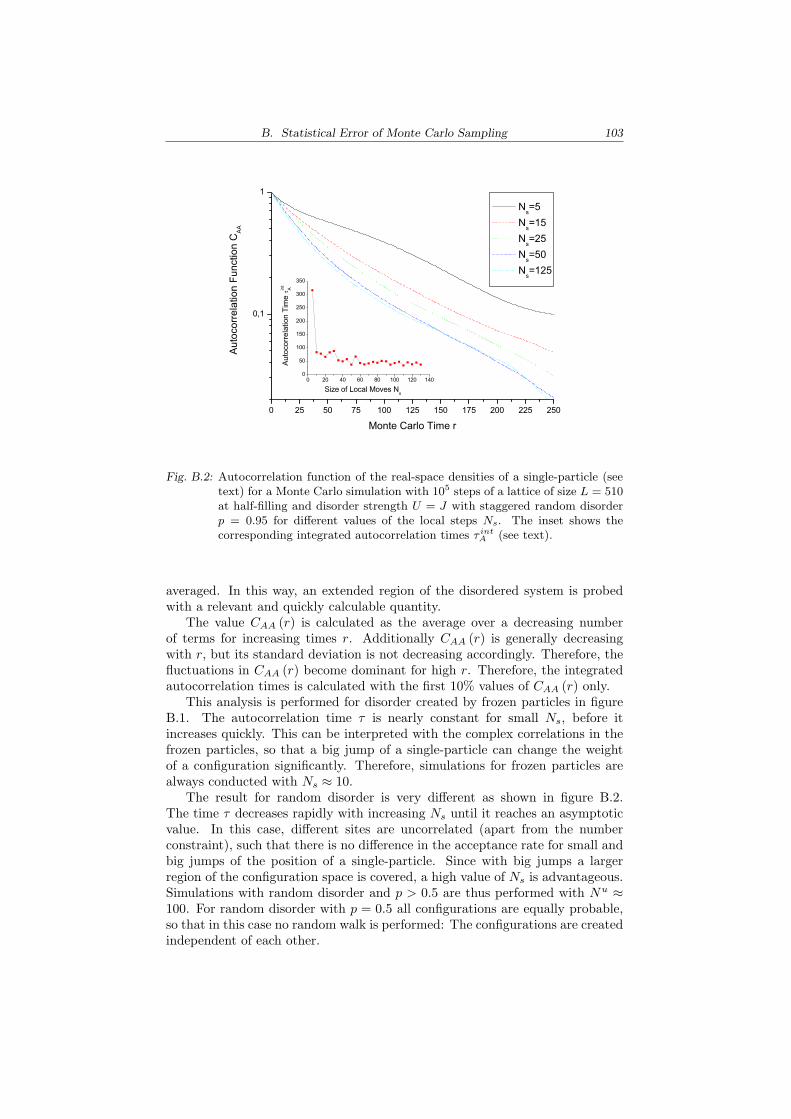
B. Statistical Error of Monte Carlo Sampling 103
0 25 50 75 100 125 150 175 200 225 250
0,1
1
0 20 40 60 80 100 120 1400
50
100
150
200
250
300
350Au
toco
rrela
tion
Tim
e in
tA
Size of Local Moves Ns
Auto
corre
latio
n Fu
nctio
n C
AA
Monte Carlo Time r
Ns=5 Ns=15 Ns=25 Ns=50 Ns=125
Fig. B.2: Autocorrelation function of the real-space densities of a single-particle (seetext) for a Monte Carlo simulation with 105 steps of a lattice of size L = 510at half-filling and disorder strength U = J with staggered random disorderp = 0.95 for different values of the local steps Ns. The inset shows thecorresponding integrated autocorrelation times τ int
A (see text).
averaged. In this way, an extended region of the disordered system is probedwith a relevant and quickly calculable quantity.
The value CAA (r) is calculated as the average over a decreasing numberof terms for increasing times r. Additionally CAA (r) is generally decreasingwith r, but its standard deviation is not decreasing accordingly. Therefore, thefluctuations in CAA (r) become dominant for high r. Therefore, the integratedautocorrelation times is calculated with the first 10% values of CAA (r) only.
This analysis is performed for disorder created by frozen particles in figureB.1. The autocorrelation time τ is nearly constant for small Ns, before itincreases quickly. This can be interpreted with the complex correlations in thefrozen particles, so that a big jump of a single-particle can change the weightof a configuration significantly. Therefore, simulations for frozen particles arealways conducted with Ns ≈ 10.
The result for random disorder is very different as shown in figure B.2.The time τ decreases rapidly with increasing Ns until it reaches an asymptoticvalue. In this case, different sites are uncorrelated (apart from the numberconstraint), such that there is no difference in the acceptance rate for small andbig jumps of the position of a single-particle. Since with big jumps a largerregion of the configuration space is covered, a high value of Ns is advantageous.Simulations with random disorder and p > 0.5 are thus performed with Nu ≈100. For random disorder with p = 0.5 all configurations are equally probable,so that in this case no random walk is performed: The configurations are createdindependent of each other.
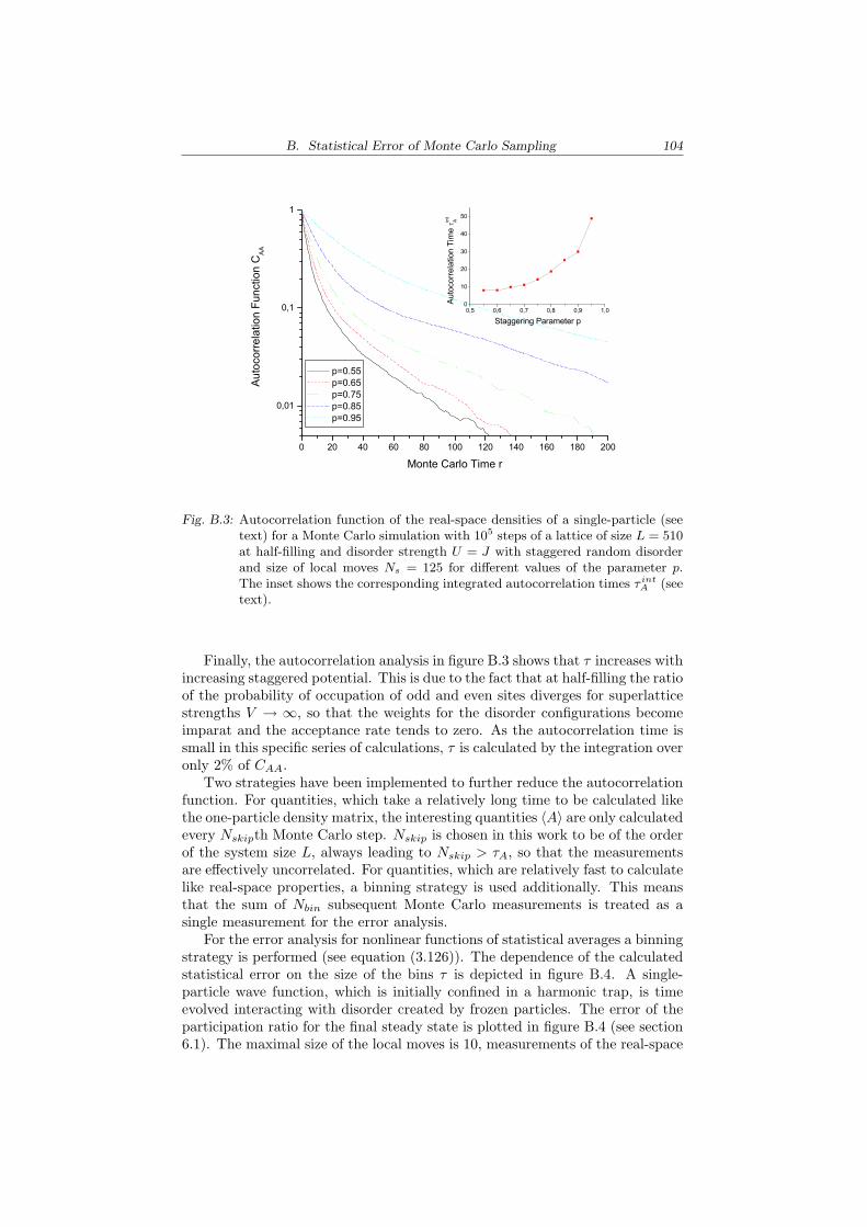
B. Statistical Error of Monte Carlo Sampling 104
0 20 40 60 80 100 120 140 160 180 200
0,01
0,1
1
0,5 0,6 0,7 0,8 0,9 1,00
10
20
30
40
50
Auto
corre
latio
n Ti
me
int
A
Staggering Parameter p
Auto
corre
latio
n Fu
nctio
n C
AA
Monte Carlo Time r
p=0.55 p=0.65 p=0.75 p=0.85 p=0.95
Fig. B.3: Autocorrelation function of the real-space densities of a single-particle (seetext) for a Monte Carlo simulation with 105 steps of a lattice of size L = 510at half-filling and disorder strength U = J with staggered random disorderand size of local moves Ns = 125 for different values of the parameter p.The inset shows the corresponding integrated autocorrelation times τ int
A (seetext).
Finally, the autocorrelation analysis in figure B.3 shows that τ increases withincreasing staggered potential. This is due to the fact that at half-filling the ratioof the probability of occupation of odd and even sites diverges for superlatticestrengths V → ∞, so that the weights for the disorder configurations becomeimparat and the acceptance rate tends to zero. As the autocorrelation time issmall in this specific series of calculations, τ is calculated by the integration overonly 2% of CAA.
Two strategies have been implemented to further reduce the autocorrelationfunction. For quantities, which take a relatively long time to be calculated likethe one-particle density matrix, the interesting quantities 〈A〉 are only calculatedevery Nskipth Monte Carlo step. Nskip is chosen in this work to be of the orderof the system size L, always leading to Nskip > τA, so that the measurementsare effectively uncorrelated. For quantities, which are relatively fast to calculatelike real-space properties, a binning strategy is used additionally. This meansthat the sum of Nbin subsequent Monte Carlo measurements is treated as asingle measurement for the error analysis.
For the error analysis for nonlinear functions of statistical averages a binningstrategy is performed (see equation (3.126)). The dependence of the calculatedstatistical error on the size of the bins τ is depicted in figure B.4. A single-particle wave function, which is initially confined in a harmonic trap, is timeevolved interacting with disorder created by frozen particles. The error of theparticipation ratio for the final steady state is plotted in figure B.4 (see section6.1). The maximal size of the local moves is 10, measurements of the real-space
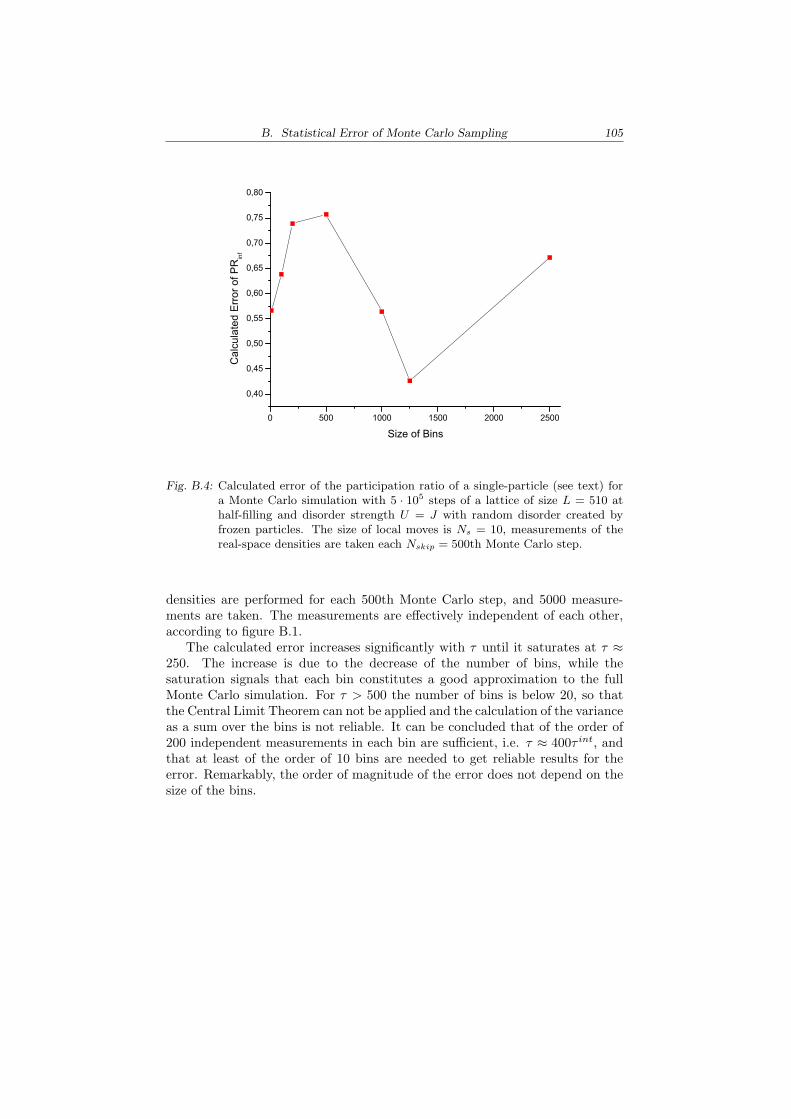
B. Statistical Error of Monte Carlo Sampling 105
0 500 1000 1500 2000 2500
0,40
0,45
0,50
0,55
0,60
0,65
0,70
0,75
0,80
Cal
cula
ted
Erro
r of P
Rin
f
Size of Bins
Fig. B.4: Calculated error of the participation ratio of a single-particle (see text) fora Monte Carlo simulation with 5 · 105 steps of a lattice of size L = 510 athalf-filling and disorder strength U = J with random disorder created byfrozen particles. The size of local moves is Ns = 10, measurements of thereal-space densities are taken each Nskip = 500th Monte Carlo step.
densities are performed for each 500th Monte Carlo step, and 5000 measure-ments are taken. The measurements are effectively independent of each other,according to figure B.1.
The calculated error increases significantly with τ until it saturates at τ ≈250. The increase is due to the decrease of the number of bins, while thesaturation signals that each bin constitutes a good approximation to the fullMonte Carlo simulation. For τ > 500 the number of bins is below 20, so thatthe Central Limit Theorem can not be applied and the calculation of the varianceas a sum over the bins is not reliable. It can be concluded that of the order of200 independent measurements in each bin are sufficient, i.e. τ ≈ 400τ int, andthat at least of the order of 10 bins are needed to get reliable results for theerror. Remarkably, the order of magnitude of the error does not depend on thesize of the bins.
BIBLIOGRAPHY
[1] D. Jaksch, C. Bruder, I.J. Cirac, C.W. Gardiner, and C. Zoller, Phys. Rev.Lett. 81, 3108 (1998).
[2] M. Greiner, O. Mandel, T. Esslinger, T.W. Hansch, and I. Bloch, Nature(London) 415, 39 (2002).
[3] R.P. Feynman, Opt. News 11, 11 (1985).
[4] E. Jane, G. Vidal, W. Dur, P. Zoller, and J.I. Cirac, Quant. Inform. Com-put. 3, 15 (2003).
[5] P.W. Anderson, Phys. Rev. Lett. 109, 1492 (1958).
[6] M.P.A. Fisher, P.B. Weichmann, P. Grinstein, and D.S. Fisher, Phys. Rev.B 40, 546 (1989).
[7] J. Lye, L. Fallani, M. Modugno, D.S. Wiersma, C. Fort, and M. Inguscio,Phys. Rev. Lett. 95, 070401 (2005); D. Clement, A.F. Varn, M. Hugbart,J.A. Retter, P. Bouyer, L. Sanchez-Palencia, D.M. Gangardt, G.V. Shlyap-nikov, and A. Aspect, Phys. Rev. Lett. 95, 170409 (2005); C. Fort, L.Fallani, V. Guarrera, J.E. Lye, M. Modugno, D.S. Wiersma, and M. In-guscio, Phys. Rev. Lett. 95, 170410 (2005); T. Schulte, S. Drenkelforth, J.Kruse, W. Ertmer, J. Arlt, K. Sacha, J. Zakrzewski, and M. Lewenstein,Phys. Rev. Lett. 95, 170411 (2005).
[8] L. Fallani, J. E. Lye, V. Guarrera, C. Fort, and M. Inguscio, cond-mat/0603655 (2006).
[9] T. Schulte, S. Drenkelforth, J. Kruse1, R. Tiemeyer, K. Sacha, J. Za-krzewski, M. Lewenstein, W. Ertmer, and J.J. Arlt, New J. Phys. 8, 230(2006).
[10] S. Ospelkaus, C. Ospelkaus, O. Wille, M. Succo, P. Ernst, K. Sengstock,and K. Bongs, Phys. Rev. Lett. 96, 180403 (2006); K. Gunter, T. Stoferle,H. Moritz, M. Kohl, and T. Esslinger, Phys. Rev. Lett. 96, 180402 (2006).
[11] L. Pollet, C. Kollath, U. Schollwock, and M. Troyer, cond-mat/0609604(2006).
[12] U. Gavish, and Y. Castin, Phys. Rev. Lett. 95, 020401 (2005).
[13] B. Paredes, F. Verstraete, and J.I. Cirac, Phys. Rev. Lett. 95, 140501(2005).
[14] M. Girardeau, J. Math. Phys. 1, 516 (1960).
Bibliography 107
[15] E. Lieb, Ann. Phys (NY) 16, 406 (1961).
[16] B. Paredes, A. Widera, V. Murg, O. Mandel, S. Folling, I.J. Cirac, G.V.Shlyapnikov, T.W. Hansch, I. Bloch, Nature 429, 277 (2004).
[17] V.E. Korepin, A.G. Izergin, and N.M. Bogoliubov, Quantum Inverse Scat-tering Method and Correlation Functions, Cambridge University Press(1993).
[18] O. Penrose, and L. Onsager, Phys Rev. 104, 576 (1956).
[19] M. Rigol and A. Muramatsu, Phys. Rev. Lett. 93, 230404 (2004).
[20] M. Rigol and A. Muramatsu, Phys. Rev. Lett. 94, 240403 (2005).
[21] M. Rigol and A. Muramatsu, Phys. Rev. A 70, 031603 (2004)
[22] M. Rigol, PhD dissertation, University of Stuttgart (2004).
[23] K. Ishii, Suppl. Progr. Theor. Phys. 53, 77 (1972).
[24] H. Furstenberg, Trans. Amer. Math. Soc 108, 377 (1963).
[25] E. Abrahams, P.W. Abrahams, D.C. Licciardello, T.V. Ramakrishnan,Phys. Rev. Lett. 42, 673 (1979).
[26] D.H. Dunlap, H.-L. Wu, P. Phillips, Phys. Rev. Lett. 65, 88 (1990).
[27] P. Phillips, Advanced Solid State Physics, Westview Press (2003).
[28] D.J. Thouless, Phys. Rep. 13C, 93 (1974).
[29] W.H. Press, S.A. Teukolsky, W.T. Vetterling, B.P. Flannery, NumericalRecipes in Fotran 77: The Art of Scientific Computing, 2nd edition, Cam-bridge University Press (1992).
[30] J. R. Bunch, L. Kaufmann, and B. N. Parlett, Numer. Math., 27, 95 (1976).
[31] A.S. Householder, Journal ACM 5, 339 (1958).
[32] F.F. Assad, Quantum Simulations of Complex Many-Body Systems: FromTheory to Algorithms, edited by J. Grotendorst, D. Marx, and A. Mura-matsu, Vol. 10, pp. 99, John von Neumann Institute for Computing, Julich(2002).
[33] J.J. Garcıa-Ripoll, cond-mat/0602305 (2006).
[34] K. Lanczos, J. Res. Natl. Bur. Stand 45, 225 (1950).
[35] M. Hochbruck, and C. Lubich, SIAM J. Numerical Anal. 34, 1911 (1997).
[36] I. Titvinidze, and G.I. Japaridze, Eur. Phys. J. B 32, 383 (2003)
[37] A. Wipf, Lecture Notes: Path Integrals, http://www.personal.uni-jena.de/˜p5anwi/lecturenotes.html, University of Jena (2001).
[38] K. Binder and D.P. London, A Guide to Monte Carlo Simulations in Sta-tistical Physics, Cambridge University Press (2000).
Bibliography 108
[39] D. Jaksch, and P. Zoller, Annals of Physics 315, 1 (2004).
[40] M. Greiner, PhD Dissertation, LMU University of Munich (2003).
[41] O. Mandel, M. Greiner, A. Widera, T. Rom, T.W. Hansch, and I. Bloch,Nature 425, 937 (2003).