EFFECTIVE HAMILTONIANS FOR LINEARENVIRONMENTS

bachelor’s thesis

presented by

Jakob Stubenrauch

under the supervision of

Prof. Dr. Fabian Hasslerand

Prof. Dr. David DiVincenzo

Institute for Quantum Information

August 14th, 2018

ii

Zentrales Prüfungsamt/Central Examination Office

Eidesstattliche Versicherung Statutory Declaration in Lieu of an Oath

___________________________ ___________________________

Name, Vorname/Last Name, First Name Matrikelnummer (freiwillige Angabe) Matriculation No. (optional)

Ich versichere hiermit an Eides Statt, dass ich die vorliegende Arbeit/Bachelorarbeit/

Masterarbeit* mit dem Titel I hereby declare in lieu of an oath that I have completed the present paper/Bachelor thesis/Master thesis* entitled

__________________________________________________________________________

__________________________________________________________________________

__________________________________________________________________________

selbstständig und ohne unzulässige fremde Hilfe (insbes. akademisches Ghostwriting)

erbracht habe. Ich habe keine anderen als die angegebenen Quellen und Hilfsmittel benutzt.

Für den Fall, dass die Arbeit zusätzlich auf einem Datenträger eingereicht wird, erkläre ich,

dass die schriftliche und die elektronische Form vollständig übereinstimmen. Die Arbeit hat in

gleicher oder ähnlicher Form noch keiner Prüfungsbehörde vorgelegen. independently and without illegitimate assistance from third parties (such as academic ghostwriters). I have used no other than

the specified sources and aids. In case that the thesis is additionally submitted in an electronic format, I declare that the written

and electronic versions are fully identical. The thesis has not been submitted to any examination body in this, or similar, form.

___________________________ ___________________________

Ort, Datum/City, Date Unterschrift/Signature

*Nichtzutreffendes bitte streichen

*Please delete as appropriate

Belehrung: Official Notification:

§ 156 StGB: Falsche Versicherung an Eides Statt

Wer vor einer zur Abnahme einer Versicherung an Eides Statt zuständigen Behörde eine solche Versicherung

falsch abgibt oder unter Berufung auf eine solche Versicherung falsch aussagt, wird mit Freiheitsstrafe bis zu drei

Jahren oder mit Geldstrafe bestraft.

Para. 156 StGB (German Criminal Code): False Statutory Declarations

Whoever before a public authority competent to administer statutory declarations falsely makes such a declaration or falsely

testifies while referring to such a declaration shall be liable to imprisonment not exceeding three years or a fine. § 161 StGB: Fahrlässiger Falscheid; fahrlässige falsche Versicherung an Eides Statt

(1) Wenn eine der in den §§ 154 bis 156 bezeichneten Handlungen aus Fahrlässigkeit begangen worden ist, so

tritt Freiheitsstrafe bis zu einem Jahr oder Geldstrafe ein.

(2) Straflosigkeit tritt ein, wenn der Täter die falsche Angabe rechtzeitig berichtigt. Die Vorschriften des § 158

Abs. 2 und 3 gelten entsprechend.

Para. 161 StGB (German Criminal Code): False Statutory Declarations Due to Negligence

(1) If a person commits one of the offences listed in sections 154 through 156 negligently the penalty shall be imprisonment not exceeding one year or a fine. (2) The offender shall be exempt from liability if he or she corrects their false testimony in time. The provisions of section 158 (2) and (3) shall apply accordingly.

Die vorstehende Belehrung habe ich zur Kenntnis genommen: I have read and understood the above official notification:

___________________________ ___________________________

Ort, Datum/City, Date Unterschrift/Signature

iv

ABSTRACT

Understanding the role of an object is not possible if it is only observed in isolation.The effect caused on a degree of freedom through a surrounding multi-mode cavity ishighly complex and its calculation often requires numerics or heavy approximations.The attempt of this thesis is to investigate these effects analytically through the exam-ple of a qubit represented by an LC-oscillator that is weakly coupled to a transmissionline. Especially the dispersive and the resonant case are characterized with the em-phasis on accurately understanding the limits of their validity. We find that in thedispersive regime the transmission line acts like a single-mode resonator. However,we also discuss a correction due to the other modes which displays an asymmetry withrespect to the detuning. Additionally, we discuss a Caldeira-Leggett Hamiltonian foran arbitrary impedance and present an expansion for two-port networks.

v

vi

CONTENTS

1 Introduction 1

2 Description of the environment 32.1 Two-port impedance of a transmission line . . . . . . . . . . . . . . . . . . . . . . . 32.2 Validity of the continuum limit . . . . . . . . . . . . . . . . . . . . . . . . . . . . . 52.3 The transmission line as a resonator . . . . . . . . . . . . . . . . . . . . . . . . . . 5

3 Principle mode coupling 93.1 Rotating wave approximation . . . . . . . . . . . . . . . . . . . . . . . . . . . . . . 103.2 Hamiltonian representation . . . . . . . . . . . . . . . . . . . . . . . . . . . . . . . 113.3 Determination of frequency shifts and decay rates . . . . . . . . . . . . . . . . . . . 12

4 Constant admittance approach 154.1 General admittances and conditions . . . . . . . . . . . . . . . . . . . . . . . . . . 154.2 The transmission line as a constant admittance . . . . . . . . . . . . . . . . . . . . 164.3 Influence of the other modes . . . . . . . . . . . . . . . . . . . . . . . . . . . . . . . 174.4 Coupling across a two port network . . . . . . . . . . . . . . . . . . . . . . . . . . . 18

5 The full system 215.1 Cotangent expansion/ equivalent circuit . . . . . . . . . . . . . . . . . . . . . . . . 215.2 Lagrangian and equations of motion . . . . . . . . . . . . . . . . . . . . . . . . . . 225.3 The respective Hamiltonian . . . . . . . . . . . . . . . . . . . . . . . . . . . . . . . 25

6 Dissipative systems 276.1 The Caldeira-Leggett Hamiltonian . . . . . . . . . . . . . . . . . . . . . . . . . . . 276.2 Expansion for two port devices . . . . . . . . . . . . . . . . . . . . . . . . . . . . . 29

7 Conclusion 31

Bibliography 33

vii

viii CONTENTS

CHAPTER 1: INTRODUCTION

One of the first approximations physicists often make when trying to describe a system is neglectall environmental influences. Sometimes, this sort of reductionism is a good approach to under-standing the characteristics of that specific system. But both in experimental situations and intechnological exploitation, this approach is sensitive and leads to false predictions, at least if thetime scales observed are long enough. Environmental influences are a major cause of error, espe-cially in quantum information technology, where effects at extremely low energy scale are beingutilized.

The concept of linear environments is based on linear response theory. A time-dependent causec(t) and effect e(t) have to be linked like

e(t) =

∫ t

−∞[χ(t− t′)c(t′) + ...)] dt′, (1.1)

where the three dots stand for higher orders of the cause c(t) and are being neglected in theapproach of linear response theory. Here, χ is called the response function. There are numerousexamples in many physical fields where a linear response describes nature very well. Dependingon the choice of the material, the linear magnetic susceptibility can quite well describe the mag-netization response to an applied magnetizing field [1]. The force towards equilibrium is a linearresponse from the displacement in the context of friction [2]. In circuit electrodynamics Ohm’s lawdescribes the voltage across an element responding to the current in terms of an element-specificlinear response function — the impedance and now look how far it has gotten us!

A specific subject in quantum information theory that remains challenging is to understandthe interaction of a qubit with the surrounding wires. The wires act like a multi-mode cavityand can strongly restrict the relaxation time T1 of a qubit [3]. Previous research shows that for asingle-mode cavity the corresponding decay rate is given by the Purcell rate γP = κ(g/∆)2, whereg is the coupling from the qubit to the cavity mode, ∆ is the detuning, and κ is the cavity mode’sdecay [3,4]. Additionally, the corresponding frequency shift of the qubit was determined to be theLamb shift [4–7]. Among other things we reproduce these quantities and precisely determine theirlimits of validity.

The calculations presented in this thesis are of a classical nature. This is mainly for two reasons.First, calculations become much easier in the classical regime. Quantum mechanical approachesto achieve similar results are more difficult and rely heavily on numerics. Second, quantizing thefinal Hamiltonians presented in this work is very simple and well documented due to the Secondquantization-like notation we use [8].

Since two-state systems do not exist in classical physics, we are instead investigating theinfluence on an LC-oscillator through its surrounding wires. The harmonic oscillator is the leadingapproximation for many stable and metastable systems. Even two-state systems can be describedby a modified quantum mechanical harmonic oscillator and the treatment of qubit as LC-oscillatorin the circuit model is common [3]. The wires surrounding our LC-oscillator are modelled bytransmission lines (TM-lines), see Fig. 1.1. We find that the wires act like finite waveguides.Therefore, one could call the setup in a more abstract manner a harmonic oscillator coupled to amulti-mode cavity. An analogous situation to our circuit is therefore a membrane mounted on aHooke’s spring in a tube, see Fig. 1.2. Although we use the language of circuit electrodynamicsthroughout this thesis, the techniques and results presented here are highly transferable to other

1

2 CHAPTER 1. INTRODUCTION

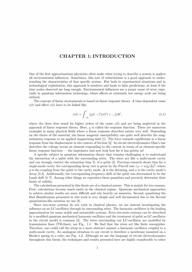
Figure 1.1: LC-oscillator connected to two symmetric wires of length W modelled by transmission lines(TM-lines). The TM-lines consist of identical inductances L and capacitances C. They are loadedby the ohmic resistance Rl and capacitance Cl. The LC-oscillator and the TM-lines are coupled viathe capacitance CC . The TM-lines interact with the LC-oscillator like a multi-mode cavity. Theemphasis of this thesis is to understand and describe those interactions as well as the interactionsof the modes among each other.

Figure 1.2: A membrane mounted on a Hooke’s spring in a tube. The tube has acoustical eigenmodesdue to its acoustical waveguide properties. In vacuum, the membrane on the spring is a harmonicoscillator. If filled with gas, this is another example of a harmonic oscillator being influenced by amulti-mode cavity.

physical fields.A Hamiltonian formulation is indispensable for quantum mechanical treatment. In this context,

there are two major difficulties in Hamiltonian mechanics and thus also in quantum mechanics.Getting results from a system coupled to a multi-mode cavity without cutoff is difficult becausean infinite number of modes have to be integrated out. Therefore, matrices of infinite dimensionhave to be diagonalized and inverted [7]. We study the system in terms of circuit electrodynamicsin Chs. 3 and 4 and present effective Hamiltonians that should also result from a complete andfully diagonalized Hamiltonian. In other words, we determine the frequency shift δ relative to thefrequency ω0 of the isolated harmonic oscillator so that for boson modes b, b∗ the Hamiltonian hasthe form

Heff = (ω0 + δ)b∗b, (1.2)

were the decay rates that we also determine are set to zero.In Ch. 5, we find a link to Lagrangians and Hamiltonians describing the complete system to

see how our circuit electrodynamics calculus relates to these formalisms.The other difficulty in Hamiltonian mechanics is that due to its energy conserving nature, dis-

sipation cannot straightforwardly be described. When it comes to writing an effective Hamiltonianin Chs. 3 and 4, dissipative properties of the TM-line are neglected. We will therefore present amethod for dealing with this difficulty, namely Caldeira-Leggett-model [9] and in the attempt tomake the environment description upscalable we extent this method for two-port networks in Ch.6.

CHAPTER 2: DESCRIPTION OF THE ENVIRONMENT

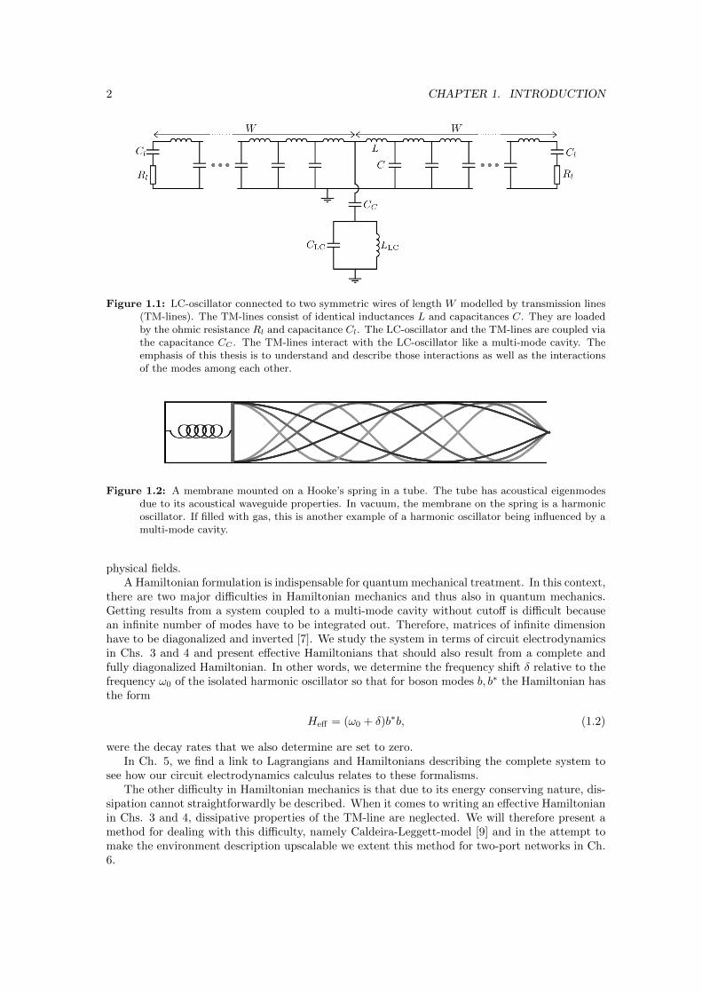
As mentioned in the introduction, we model the wires around the LC-oscillator through a trans-mission line, see Fig. 2.1. We want to express this TM-line by its linear response between voltageand current. Therefore we find and characterize its impedance.

2.1 Two-port impedance of a transmission line

In order to express the admittance/ impedance of the environment shown in Fig. 1.1, we calculatethe impedance of the bare TM-line model shown in Fig. 2.1. All calculations in this section arebeing done in frequency space, if not explicitly noted otherwise in form of dependency on t.Kirchhoff’s rules for each node k > 0 are

Uk(YC + 2YL) = Uk−1YL + Uk+1YL, (2.1)

Jk = (Uk − Uk+1)YL, (2.2)

where YC = −iωC and YL = i/ωL are the admittances of the capacitors and inductors.We introduce the lengthscale a as the spacial distance between two units of the TM-line, see Fig.2.1. Instead of the indexed Uk, we can thereby write the voltage U(x) = U(ka) ≡ Uk, defined forx ∈ 0, a, 2a, .... In the limit a → 0, U(x) will become a dense space-dependent function. Weexpand the voltages next to the node k

Uk+1 = U(x) + aU ′(x) +a2

2U ′′(x) +O(a3), (2.3)

Uk−1 = U(x)− aU ′(x) +a2

2U ′′(x) +O(a3). (2.4)

Figure 2.1: A pair of wires modelled by a transmission line. Its two port impedance is calculated in thecontinuum limit, where the spacial distances a→ 0 and the number of units N →∞ such that thelength W = Na is constant. The TM-line consist of identical inductances L and capacitances C.The voltages at the nodes that are labelled Uk are oscillating quantities. Because of their couplingthe TM-line is a waveguide.

3

4 CHAPTER 2. DESCRIPTION OF THE ENVIRONMENT

Equations (2.1) and (2.2) then become

U(x) = a2 YLYC

U ′′(x), (2.5)

J(x) = −aYLU ′(x). (2.6)

The continuum limit (a→ 0, N →∞ with number of nodesN) is achieved by defining capacitance-and inductance densities l = L/a and c = C/a. This way the RHS’s in Eqs. (2.5) and (2.6) arefinite and we find the wave equation and according current relation

U ′′(x) + k2U(x) = 0, (2.7)

J(x) = − i

ωlU ′(x), (2.8)

with the wave number k = ω/v and the speed of wave propagation v = 1/√lc.

The general solution of Eq. (2.7) is

U(x) = U+eikx + U−e

−ikx. (2.9)

We call I1 ≡ J(0) the current entering at port 1, and I2 ≡ −J(W ) the current entering atport 2. Mind the sign of I2 due to the direction of currents established in Eq. (2.2). The generalsolution, given in Eq. (2.9) is then specified by boundary conditions resulting from Eq. (2.8)

Z0I1 = U+ − U−, Z0I2 = −(U+e

ikW − U−e−ikW), (2.10)

where we introduced the characteristic impedance Z0 =√l/c =

√L/C. A typical value of the

characteristic impedance in applications is 50Ω.

The frequency-dependent two-port-impedance matrix Z(ω) describing the TM-line as a blackbox is defined by (

V1

V2

)= Z(ω)

(I1I2

)(2.11)

Its components can be calculated by applying open boundary conditions, i.e. I1 = 0 to determine

Z12 =V1

I2

∣∣∣∣I1=0

, Z22 =V2

I2

∣∣∣∣I1=0

, (2.12)

following the definition. Respectively

Z11 =V1

I1

∣∣∣∣I2=0

, Z21 =V2

I1

∣∣∣∣I2=0

. (2.13)

With the solution and boundary conditions (2.9) and (2.10), one finds

Z(ω) = iZ0

[cot(ξ) csc(ξ)csc(ξ) cot(ξ)

], where ξ = kW =

W

vω. (2.14)

As cotangent and cosecant are odd functions, Z(ω) fulfils the condition Z(ω) = Z∗(−ω). Forany pair of currents fulfilling that same symmetry I(ω) = I∗(−ω), the time dependent voltagesV(t) = F−1 [Z(ω)I(ω)] 1 are therefore real functions.

1F−1() denotes the inverse Fourier transform. Throughout this work we use the physicists convention for Fouriertransforms that is f(ω) = F [f(t)](ω) =

∫∞−∞ exp(iωt)f(t)dt and f(t) = F−1[f(ω)](t) =

∫∞−∞ exp(−iωt)f(ω)dω/2π.

2.2. VALIDITY OF THE CONTINUUM LIMIT 5

2.2 Validity of the continuum limit

We need to analyse how the continuum limit calculation differs from a discrete treatment of Eqs.(2.1) and (2.2). For the case that the width W is infinitely long, one can set U− = 0, i.e. theincoming wave at port 1 is never reflected. The impedance at port 1 Z1 = U(0)/I(0) = Z0 thenbecomes the characteristic impedance in the continuum limit model.

Z1 can also be determined in the discrete model, i.e. without using the continuum limit. Theresulting impedance Zdiscr

1 (ω) = −iωL/2 +√L/C − ω2L2/4 corresponds to the continuum limit

result for frequencies

ω2 1

LC. (2.15)

This condition marks the regime in which the continuum limit calculations agree with the TM-line model in Fig. 2.1. However, if that model describes a real cable which is the purpose, thelengthscale a must be very small. Therefore and with 1/LC = 1/a2lc, even large frequencies areallowed by the condition in Eq. (2.15). This condition can easily be found as equivalent to theintuitive non-aliasing condition λ a, where λ = 2π/k denotes the wavelength.

2.3 The transmission line as a resonator

In this section we express the admittance2 for one port of the TM-line with open boundaryconditions and that of the TM-line with a load. We determine the resonance frequencies of theTM-line, initially without load. Then we investigate how adding a load changes the resonancefrequencies. We also characterize a load for which these changes are small.

Lets take an electric component with the admittance Y (ω). With the voltage across thatcomponent V (ω) and the current through that component I(ω), Ohm’s Law is V (ω) = I(ω)/Y (ω).If Y (ω) has a root at the frequency ωr, the voltage amplitude diverges for ω → ωr as longas I(ωr) 6= 0. Therefore, we define the resonance frequencies of a non-dissipative3 electricalcomponent as the roots of its admittance.

For the case of open boundary conditions at port 2 of the TM-line in Fig. 2.1, i.e. I2 = 0, port1 has the admittance

Y obcr (ω) = 1/Z11(ω) = −iY0 tan(ξ), (2.16)

where Y0 = 1/Z0 denotes the characteristic admittance. According to our definition of resonancefrequencies for non-dissipative components, we find its equidistant resonance frequencies

ωn = nπv

W= nω1. (2.17)

These frequencies can also be understood because of the TM-lines waveguide properties. TheTM-line with open boundary condition is a cavity with open ends, therefore standing waves, alsocalled modes, with wavelength λ = 2W/n can arise, n ∈ N. Each mode corresponds to a frequencyωn = 2πv/λn = nπv/W , conform with those, found in Eq. (2.17). This description is closer tothe acoustic analogy mentioned in the introduction in Fig. 1.2.

We notice that ξ = ωW/v = πω/ω1 can be expressed in terms of ω1.In practice, physical systems are often dissipative. We can express dissipation by adding a

load at the end of the TM-lines, as shown in Fig. 1.1. This load consists of an ohmic resistanceRl, where dissipation arises from, and of a capacitance Cl to target realistic and more generalscenarios. Each TM-line then acts as the admittance

Y loadedr (ω) = Y0

Yl(ω)− iY0 tan(ξ)

Y0 − iYl(ω) tan(ξ). (2.18)

2The inverse of an impedance Y (ω) = Z(ω)−1. We use admittances from here on, because the expansions,approximations and other calculations in the following Chs. are easier that way.

3The admittances and impedances of such devices are purely imaginary

6 CHAPTER 2. DESCRIPTION OF THE ENVIRONMENT

as follows from Kirchhoff’s rules and Eq. (2.14). Yl(ω) = (Rl + i/ωCl)−1 is the load admittance.

Due to the dissipative ohmic resistance Rl, Yloadedr (ω) has a non-zero, positive, real part.

Therefore, the roots of the admittance are complex numbers λ. Having in mind how a complexnumber replacing the frequency in an oscillating function affects its behaviour

e−iλt = e−iRe(λ)teIm(λ)t, (2.19)

we define the resonance frequency as the real part of the root and the decay rate4 as minus theimaginary part of that root.

If the decay rate is at the order of a resonance frequency ωr, any voltage decays within timescales∼ 1/ωr so that frequency shifting and other phenomena can hardly be observed, and the TM-line acts comparable to a pure ohmic resistor. In quantum information technologies, phenomenalike this highly restrict the fidelity of the system, e.g. the relaxation time of a qubit T1 [3].Therefore, we are especially interested in loads that leave the decay small compared to resonancefrequencies.

To achieve that, we choose the load resistance large compared to the characteristic impedance

Rl Z0 (2.20)

and the discharging time of the capacitor long compared to the oscillation periods of the resonatormodes.

τ = RlCl 1

ω1≥ 1

ωn, (2.21)

with the resonance frequencies ωn of the TM-line with open boundary conditions. The admittanceof the load can be expanded

Yl(ω) =1

Rl− iClωτ2

+O[(1/ωτ)

3]. (2.22)

and the admittance in Eq. (2.18) can then be approximated by

Y loadedr (ω) = 1/Rl − iCl/ωτ2 − iY0 tan(ξ). (2.23)

We assume for the shift δn of the n’th resonance frequency relative to the unloaded case and forthe decay rate of the n’th mode κn

|δn| ω1 and κn ω1, (2.24)

which is an assumption that has to be confirmed later. With this we can determine the n’th rootof Y loaded

r (ω). With tan(πn+ x) = tan(x) = x+O(x3) we only have to solve

1

Rl− iClωnτ2

− iπY0δn − iκnω1

= 0 (2.25)

and find

δn = −ClZ0

πnτ2and κn ≡ κ =

ω1Z0

πRl, (2.26)

where we introduced the number-of-mode-independent decay rate κ.Equations (2.20) and (2.21) imply

(ωnτ)2 ωnτ ω1ClZ0 −→ClZ0

nτ2 ωn. (2.27)

4Necessarily positive

2.3. THE TRANSMISSION LINE AS A RESONATOR 7

With this and with κ = O(Z0/Rl) we can see that by the choices for the load in Eqs. (2.20)and (2.21) the assumption in Eq. (2.24) is fulfilled and δn and κ are determined selfconsistently.Because δn is of order κ2 we neglect it. We write Y loaded

r (ω) in terms of κ

Y loadedr (ω) = −iY0 tan[π(ω + iκ)/ω1] (2.28)

and expanded around one of its resonance frequencies

Y loadedr (ω) = Y loaded

r (ωn + ε) = Cr(−iε+ κ) +O(ε3), (2.29)

with Cr = πY0/ω1. This expansion will be referred to as single-mode approximation, when ordersε3 are neglected.

8 CHAPTER 2. DESCRIPTION OF THE ENVIRONMENT

CHAPTER 3: PRINCIPLE MODE COUPLING

In this Ch., the effect of a single mode cavity on the LC-oscillator is determined by solving coupleddifferential equations for the LC-oscillator and the principle resonator mode. Based on the resultsfrom Ch. 2, namely the TM-line admittance found in Eq.(2.29) we treat the circuit shown in Fig.1.1 like that shown in Fig. 3.1. Kirchhoff’s rules for the voltages VLC and Vr are in frequencyspace

VLC(YLC + YCC) = VrYCC

, (3.1)

Vr(Yr + YCC) = VLCYCC

. (3.2)

The admittance of the coupling capacitance is YCC= −iωCC and that of the LC-oscillator is

YLC =CLC

−iω

(1

LLCCLC− ω2

). (3.3)

We denote the frequency of the LC-oscillator, shifted by the presence of the capacitance CC , asω0 = 1/

√LLC(CLC + CC) and these of the TM-line as ωk = kω1 for k ∈ N. Of course, CC also

shifts the resonance frequency of Yr(ω). We see this shift in Eq. (3.12) and neglect it because itis weak and not very interesting. It could easily be taken into account anyway by adding it to thedetuning. For a more complete treatment see Sec 4.4.

Let n be an arbitrary but fix integer such that ω0 is closer to ωn than to any other mode.∆k denotes the detuning of the LC-oscillator frequency to the k’th TM-line frequency, i.e. ∆k =ωk − ω0.

We define the frequency variables ε = ω − ωn and η = ω − ω0 for convenience. That way wealso find ∆n = η − ε.

As mentioned in the beginning of this chapter, we approximate the environment to be a singlemode resonator at ωn which we therefore call the principle mode. That leads to the admittance

Y smr (ω) = 2Cr(−iε+ κ), (3.4)

whereby the factor 2 results from the fact that parallel admittances can be summed up directly.1

As one can see from Eq. (2.29) this is a good approximation if the voltage spectrum Vr(ω) ismainly distributed close to ωn such that Vr(ωn + ε) is non-zero2, only for

|ε| ω1. (3.5)

By also choosing the LC-oscillator parameters such that

|∆n| ω1, (3.6)

the assumption in Eq. (3.5) is equivalent to the assumption

|η| ω0, (3.7)

for all η, where VLC(ω0 + η) is non-zero. We specify this assumption later and confirm it in theend.

1Parallel admittances can be summarized by summing them up directly, admittances in series have to be summedup inversely. You can proof that easily by using Ohms law across two admittances in series or parallel respectively.

2The distributions we found are non-zero everywhere. We will use this term, having in mind that even thenon-dissipative admittances we discuss here that show divergences are not truly divergent in physical nature andwill therefore be suppressed by the tininess of the distributions far from the ”non-zero” peak.

9

10 CHAPTER 3. PRINCIPLE MODE COUPLING

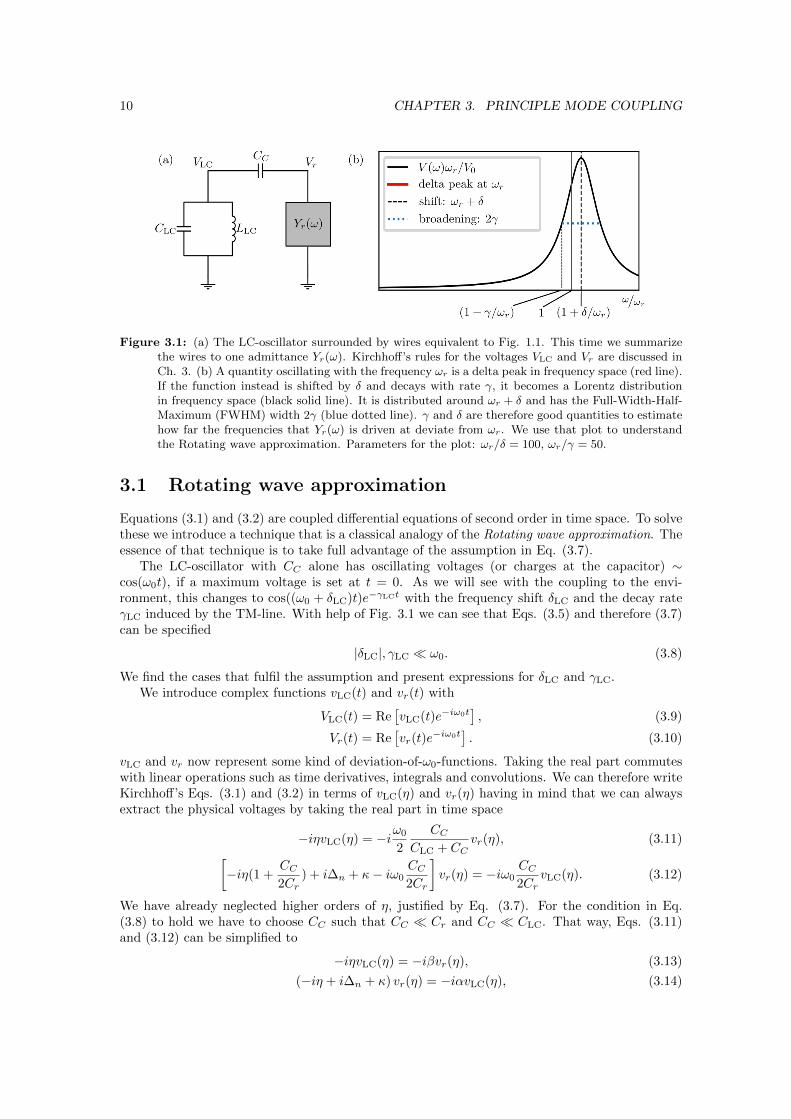
Figure 3.1: (a) The LC-oscillator surrounded by wires equivalent to Fig. 1.1. This time we summarizethe wires to one admittance Yr(ω). Kirchhoff’s rules for the voltages VLC and Vr are discussed inCh. 3. (b) A quantity oscillating with the frequency ωr is a delta peak in frequency space (red line).If the function instead is shifted by δ and decays with rate γ, it becomes a Lorentz distributionin frequency space (black solid line). It is distributed around ωr + δ and has the Full-Width-Half-Maximum (FWHM) width 2γ (blue dotted line). γ and δ are therefore good quantities to estimatehow far the frequencies that Yr(ω) is driven at deviate from ωr. We use that plot to understandthe Rotating wave approximation. Parameters for the plot: ωr/δ = 100, ωr/γ = 50.

3.1 Rotating wave approximation

Equations (3.1) and (3.2) are coupled differential equations of second order in time space. To solvethese we introduce a technique that is a classical analogy of the Rotating wave approximation. Theessence of that technique is to take full advantage of the assumption in Eq. (3.7).

The LC-oscillator with CC alone has oscillating voltages (or charges at the capacitor) ∼cos(ω0t), if a maximum voltage is set at t = 0. As we will see with the coupling to the envi-ronment, this changes to cos((ω0 + δLC)t)e−γLCt with the frequency shift δLC and the decay rateγLC induced by the TM-line. With help of Fig. 3.1 we can see that Eqs. (3.5) and therefore (3.7)can be specified

|δLC|, γLC ω0. (3.8)

We find the cases that fulfil the assumption and present expressions for δLC and γLC.We introduce complex functions vLC(t) and vr(t) with

VLC(t) = Re[vLC(t)e−iω0t

], (3.9)

Vr(t) = Re[vr(t)e

−iω0t]. (3.10)

vLC and vr now represent some kind of deviation-of-ω0-functions. Taking the real part commuteswith linear operations such as time derivatives, integrals and convolutions. We can therefore writeKirchhoff’s Eqs. (3.1) and (3.2) in terms of vLC(η) and vr(η) having in mind that we can alwaysextract the physical voltages by taking the real part in time space

−iηvLC(η) = −iω0

2

CCCLC + CC

vr(η), (3.11)[−iη(1 +

CC2Cr

) + i∆n + κ− iω0CC2Cr

]vr(η) = −iω0

CC2Cr

vLC(η). (3.12)

We have already neglected higher orders of η, justified by Eq. (3.7). For the condition in Eq.(3.8) to hold we have to choose CC such that CC Cr and CC CLC. That way, Eqs. (3.11)and (3.12) can be simplified to

−iηvLC(η) = −iβvr(η), (3.13)

(−iη + i∆n + κ) vr(η) = −iαvLC(η), (3.14)

3.2. HAMILTONIAN REPRESENTATION 11

where

α =ω0

2

CCCr

and β =ω0

2

CCCLC

. (3.15)

In time space, Eqs. (3.13) and (3.14) are3

vLC(t) = −iβvr(t), (3.16)

vr(t) + i∆nvr(t) + κvr(t) = −iαvLC(t) (3.17)

Imagine CC = 0. From Eq. (3.16) follows that vLC(t) would be constant and therefore VLC

exactly oscillating with frequency ω0. Respectively, from Eq. (3.17) one can see that the resonatormode would be oscillating at a frequency by ∆n detuned from ω0 and it would decay with rate κ.

3.2 Hamiltonian representation

We define the principle mode coupling

g =√αβ =

ω0

2

CC√CrCLC

. (3.18)

We also write bLC(t) = NLCvLC(t) and br(t) = Nrvr(t). We do not have to fix the Ni absolutely,but claim that NLC/Nr =

√α/β. We define the functions

bi(t) = e−iω0tbi(t), implying that b∗i (t) = eiω0tb∗i (t) (3.19)

for i = LC, r as classical counterparts to boson operators so we can write a Second Quantization-like Hamiltonian that is easy to quantize. With qi = (bi + b∗i )/

√2 and pi = i(b∗i − bi)/

√2 as

canonical variables, the Poisson brackets of the boson functions fulfil the relation

bi, b∗j = −iδi,j (3.20)

with the Kronecker delta δi,j . The canonical variables qi(t) and pi(t) are real as a direct result fromthe definition. They are proportional to the voltages Vi(t) and conjugate momenta respectively(dimensionally currents). To see this note also how besides a factor Eq. (3.19) undoes Eqs. (3.9)and (3.10). Having this we can write the Hamiltonian

H(qLC, qr, pLC, pr) = ω0b∗LCbLC + ωnb

∗rbr + g(b∗LC + bLC)(b∗r + br), (3.21)

and show that it produces the right equations of motion. That expression justifies the nameprinciple mode coupling for g, defined in Eq. (3.18). We obtain the equations of motion by using

f [qi(t), pi(t)] = f,H[qi(t), pi(t)] (3.22)

and the relation in Eq. (3.20). With the linearity of Poisson brackets we get

bLC(t) = −iω0bLC(t)− ig[b∗r(t) + br(t)], (3.23)

br(t) = −iωnbr(t)− ig[b∗LC(t) + bLC(t)]. (3.24)

We change back to the rotating wave functions, i.e. to the bk(t) functions and find in frequencyspace

−iηbLC(η) = −ig[b∗r(2ω0 + η) + br(η)

], (3.25)

−iηbr(η) = −i∆nbr(η)− ig[b∗LC(2ω0 + η) + bLC(η)

]. (3.26)

3As one can see from the definition of the Fourier transform and with integration by parts, F−1[−iωf(ω)](t) =(d/dt)F−1[f(ω)](t). We use this identity frequently and from now on without mentioning it.

12 CHAPTER 3. PRINCIPLE MODE COUPLING

As discussed before, vi(η) is mainly distributed around frequencies |η| ω0. This is also valid forb∗i (η). Therefore, b∗i (2ω0 + η) is much smaller than br(η) at relevant (small) frequencies η and canbe neglected. Another way of seeing this is to say that b∗k(t) rotates at much higher frequenciesthan bk(t), see Eq. (3.19), and influences average out at relevant time scales ∼ 1/|η| 1/(2ω0+η).This is another use of the Rotating wave approximation technique.

With this and when transforming back into time space we find that the Hamiltonian in Eq.(3.21) leads to the equations of motion in Eqs. (3.16) and (3.17) in a symmetrical form. Themodes do not decay, κ = 0, in the Hamiltonian description. To find Hamiltonians that can alsodescribe the decay, see Ch. 6.

3.3 Determination of frequency shifts and decay rates

We keep the symmetry but allow κ 6= 0 again to use what also could have been derived directlyfrom Eqs. (3.13) and (3.14)

−iηbLC(η) = −igbr(η), (3.27)

(−iη + i∆n + κ) br(η) = −igbLC(η). (3.28)

Integrating out the resonator mode br is easy in frequency space. We get an equation for bLC only

−iηbLC(η) = − g2

−iη + i∆n + κbLC(η). (3.29)

In Eq. (3.7) we assumed |η| ω0 for vLC(η) non-zero. We go further and show that even

|η| max(|∆n|, κ) for all η where bLC(η) 6= 0 (3.30)

is consistent with the results, even though |∆n|, κ ω0. Under this assumption Eq. (3.29) canbe simplified to

˙bLC(t) = − g2

i∆n + κbLC (3.31)

in time space. With vLC(t) ∼ bLC(t), we find the shift of the LC-oscillators frequency

δLC = − ∆ng2

∆2n + κ2

(3.32)

and the decay rate of the LC-oscillator

γLC =κg2

∆2n + κ2

. (3.33)

The assumption in Eq. (3.30) can be confirmed for |δLC|, |γLC| max(|∆n|, κ), see again Fig.3.1. This is given for two cases:

• Dispersive case, i.e. |∆n| κ. Note that calling this case off resonant would not becorrect, as it is still limited by |∆n| ω1. The shift becomes the lamb shift [4–6], the decaybecomes the Purcell rate [3, 4]

δLC = − g2

∆nand γLC = κ

g2

∆2n

. (3.34)

By choosing CC such that g |∆n|, the assumption in Eq. (3.30) is fulfilled and thereforealso the earlier assumption |η| ω0. Large shifts and fast decays are prevented by the

3.3. DETERMINATION OF FREQUENCY SHIFTS AND DECAY RATES 13

detuning in the dispersive regime. For κ = 0 the Hamiltonian in Eq. (3.21) can be reducedto the effective Hamiltonian for the LC-oscillator

H(qLC, pLC) =

(ω0 −

g2

∆n

)b∗LCbLC (3.35)

that we mentioned in the introduction in Eq. (1.2).

• Resonant case, i.e. |∆n| κ. The frequencies of both modes now agree within thebroadening caused by κ. The shift and the decay rate become

δLC = −∆ng2

κ2and γLC =

g2

κ. (3.36)

In this case, the assumption in Eq. (3.30) holds for choices of CC such that g κ. Largeshifts and fast decays in the resonant regime can be prevented by a relatively fast decay ofthe resonator mode. Setting κ to zero would lead to divergences. It is therefore difficult toachieve that result quantum mechanically. An effective Hamiltonian could only be formulatedwith help of another model such as the Caldeira-Legett model described in Ch. 6.

We also see how the resonator mode changes due to the coupling by calculating the respectivefrequency shift δr and decay rate γr. The calculation is the same as for the LC-oscillator, startingfrom Eqs. (3.27) and (3.28). By changing from the rotating wave at frequency ω0 to a rotatingwave at frequency ωn, an assumption equivalent to that in Eq. (3.30) can be made leading to

˙br = −κ∆n + ig2

∆n + iκbr. (3.37)

Thereby δr and γr can be determined

δr =κ(∆2n + g2

)∆2n + κ2

and γr =∆n

(g2 − κ2

)∆2n + κ2

. (3.38)

Both cases mentioned above agree with the assumption:

• Dispersive case, |∆n| κ and g |∆n|. The shift and decay rate become

δr =g2

∆n− κ2

∆n= 0 +O

(g2

∆n

)+O

(κ2

∆n

)(3.39)

and γr = κ

(1 +

g2

∆2n

)= κ+O

(g2

∆n

), (3.40)

which means that, as intuitively expected, the resonators behaviour hardly changes in thedispersive case.

• Resonant case, |∆n| κ and g κ. The shift and decay rate become

δr = ∆n

(1− g2

κ2

)= −∆n +O

(g2

κ2

)(3.41)

and γr =∆2n

κ+g2

κ= 0 +O

(g2

κ

)+O

(∆2n

κ

). (3.42)

The decay is smaller than in the uncoupled case and the resonator mode gets shifted to theLC-oscillator frequency nearly completely.

In Eq. (3.34) we found the decay rate to be the purcell rate. It is important to note at thispoint that we made the assumption |∆n| ω1 in Eq. (3.6). Only the principle mode of theTM-line effects this decay rate. Generalizations of the form

γP =∑n

κn(gn/∆n)2, (3.43)

trying to take into account all the other modes are therefore no valid conclusion of our results. Ifstill using this form, gn has to be redefined, insuring that the sum does not diverge.

14 CHAPTER 3. PRINCIPLE MODE COUPLING

CHAPTER 4: CONSTANT ADMITTANCE APPROACH

The calculations in Ch. 3 have already been relatively easy and still lead to the purcell rate andlamb shift. It would also be easy to find higher order corrections to those quantities. However, wecan find these results with even less effort. By summing up (inversely) the coupling capacitanceCC and the TM-line to the total admittance YT (ω), the circuit in Fig. 4.1 can be evaluated,leading to one single Kirchhoff’s rule

V (ω)[YLC(ω) + YT (ω)] = 0. (4.1)

4.1 General admittances and conditions

We investigate the case of a constant admittance YT (ω) ≡ YG = const and find the condition forYG that fulfils

|δLC|, γLC ω1, (4.2)

We again use

YLC =CLC

−iω

(1

LLCCLC− ω2

)(4.3)

and also 1/LLCCLC − ω20 = ω0CC/CLC. In terms of rotating wave functions, i.e. V (t) =

Re[v(t)e−iω0t

], explained in Ch. 3, Eq. (4.1) becomes

v(η)

[−iη

(1 + i

YG + iω0CC2ω0CLC

)+YG + iω0CC

2CLC

]= 0 (4.4)

where terms of order η/ω0 have been neglected, while terms ∼ ηCLC/ω0CC have been kept, as wechoose weak coupling CC CLC again. We will see that the condition in Eq. (4.2) is fulfilled, forYG such that

|ReYG|, | ImYG| Y charLC =

√CLC

LLC, (4.5)

introducing the characteristic admittance of the LC-oscillator Y charLC . With this we omit higher

orders in Eq. (4.4) and find in time space

v(t) + v(t)YG + iω0CC

2CLC= 0, (4.6)

and therefore the frequency shift and the decay rate of the LC-oscillator are

δLC = Im

(YG + iω0CC

2CLC

)and γLC = Re

(YG + iω0CC

2CLC

). (4.7)

Note that with CC CLC and the condition in Eq. (4.5) those expressions fulfil the condition inEq. (4.2) and are therefore valid.

15

16 CHAPTER 4. CONSTANT ADMITTANCE APPROACH

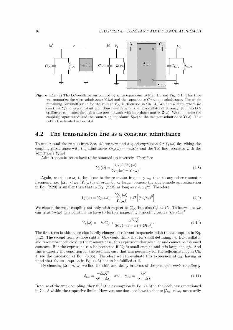
Figure 4.1: (a) The LC-oscillator surrounded by wires equivalent to Fig. 1.1 and Fig. 3.1. This timewe summarize the wires admittance Yr(ω) and the capacitance CC to one admittance. The singleremaining Kirchhoff’s rule for the voltage VLC is discussed in Ch. 4. We find a limit, where wecan treat YT (ω) as a constant admittance evaluated at the LC-oscillators frequency. (b) Two LC-oscillators connected through a two port network with impedance matrix Z(ω). We summarize thecoupling capacitances and the connecting impedance Z(ω) to the two port admittance Y(ω). Thisnetwork is treated in Sec. 4.4.

4.2 The transmission line as a constant admittance

To understand the results from Sec. 4.1 we now find a good expression for YT (ω) describing thecoupling capacitance with the admittance YCC

(ω) = −iωCC and the TM-line resonator with theadmittance Yr(ω).

Admittances in series have to be summed up inversely. Therefore

YT (ω) =YCC

(ω)Yr(ω)

YCC(ω) + Yr(ω)

. (4.8)

Again, we choose ω0 to be closer to the resonator frequency ωn than to any other resonatorfrequency, i.e. |∆n| < ω1. Yr(ω) is of order Cr or larger because the single-mode approximationin Eq. (2.29) is smaller than that in Eq. (2.28) as long as ε < ω1/2. Therefore

YT (ω) = YCC(ω)−

Y 2CC

(ω)

Yr(ω)+O

[(CC/Cr)

3]

(4.9)

We choose the weak coupling not only with respect to CLC but also CC Cr. To know how wecan treat YT (ω) as a constant we have to further inspect it, neglecting orders (CC/Cr)

3

YT (ω) = −iωCC +ω2C2

C

2Cr(−iε+ κ) +O(ε3). (4.10)

The first term in this expression hardly changes at relevant frequencies with the assumption in Eq.(4.2). The second term is more subtle. One could think that for small detuning, i.e. LC-oscillatorand resonator mode close to the resonant case, this expression changes a lot and cannot be assumedconstant. But the expression can be protected if CC is small enough and κ is large enough. Andthis is exactly the condition for the resonant case that was necessary for the selfconsistency in Ch.3, see the discussion of Eq. (3.36). Therefore we can evaluate this expression at ω0, having inmind that the assumption in Eq. (4.5) has to be fulfilled still.

By choosing |∆n| ω1 we find the shift and decay in terms of the principle mode coupling g

δLC =−∆ng

2

κ2 + ∆2n

and γLC =κg2

κ2 + ∆2n

. (4.11)

Because of the weak coupling, they fulfil the assumption in Eq. (4.5) in the both cases mentionedin Ch. 3 within the respective limits. However, one does not have to choose |∆n| ω1 necessarily

4.3. INFLUENCE OF THE OTHER MODES 17

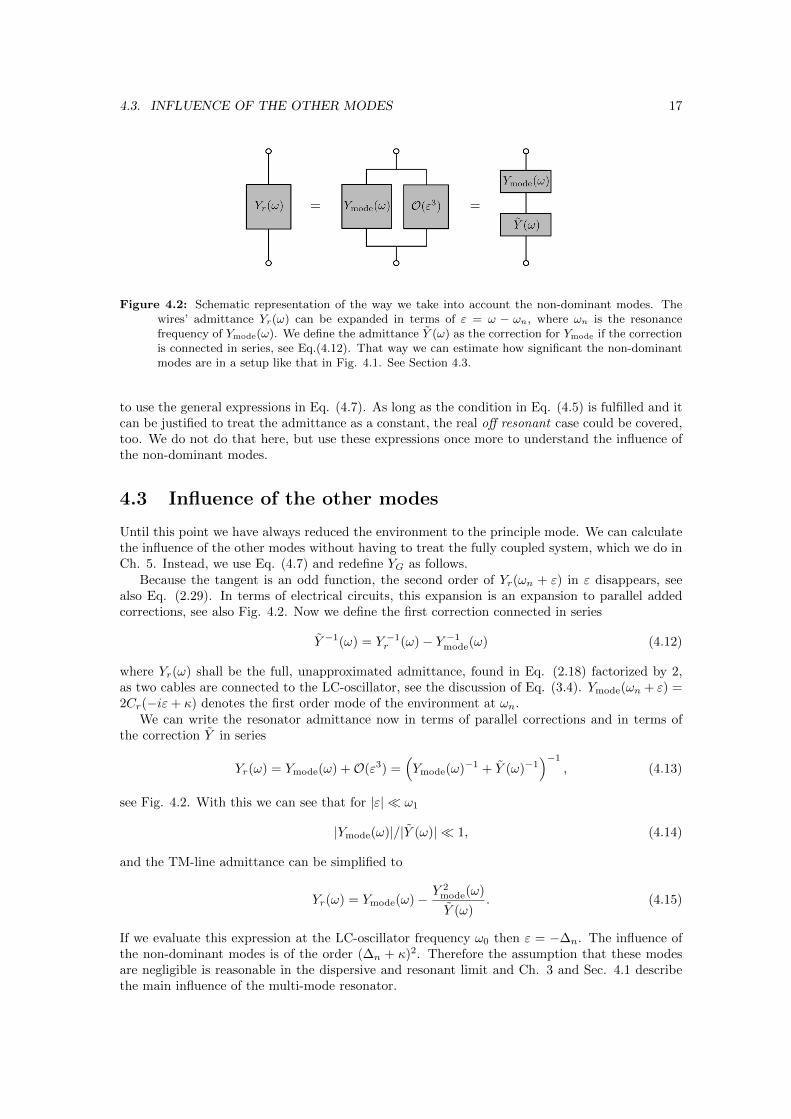
Figure 4.2: Schematic representation of the way we take into account the non-dominant modes. Thewires’ admittance Yr(ω) can be expanded in terms of ε = ω − ωn, where ωn is the resonancefrequency of Ymode(ω). We define the admittance Y (ω) as the correction for Ymode if the correctionis connected in series, see Eq.(4.12). That way we can estimate how significant the non-dominantmodes are in a setup like that in Fig. 4.1. See Section 4.3.

to use the general expressions in Eq. (4.7). As long as the condition in Eq. (4.5) is fulfilled and itcan be justified to treat the admittance as a constant, the real off resonant case could be covered,too. We do not do that here, but use these expressions once more to understand the influence ofthe non-dominant modes.

4.3 Influence of the other modes

Until this point we have always reduced the environment to the principle mode. We can calculatethe influence of the other modes without having to treat the fully coupled system, which we do inCh. 5. Instead, we use Eq. (4.7) and redefine YG as follows.

Because the tangent is an odd function, the second order of Yr(ωn + ε) in ε disappears, seealso Eq. (2.29). In terms of electrical circuits, this expansion is an expansion to parallel addedcorrections, see also Fig. 4.2. Now we define the first correction connected in series

Y −1(ω) = Y −1r (ω)− Y −1

mode(ω) (4.12)

where Yr(ω) shall be the full, unapproximated admittance, found in Eq. (2.18) factorized by 2,as two cables are connected to the LC-oscillator, see the discussion of Eq. (3.4). Ymode(ωn + ε) =2Cr(−iε+ κ) denotes the first order mode of the environment at ωn.

We can write the resonator admittance now in terms of parallel corrections and in terms ofthe correction Y in series

Yr(ω) = Ymode(ω) +O(ε3) =(Ymode(ω)−1 + Y (ω)−1

)−1

, (4.13)

see Fig. 4.2. With this we can see that for |ε| ω1

|Ymode(ω)|/|Y (ω)| 1, (4.14)

and the TM-line admittance can be simplified to

Yr(ω) = Ymode(ω)− Y 2mode(ω)

Y (ω). (4.15)

If we evaluate this expression at the LC-oscillator frequency ω0 then ε = −∆n. The influence ofthe non-dominant modes is of the order (∆n + κ)2. Therefore the assumption that these modesare negligible is reasonable in the dispersive and resonant limit and Ch. 3 and Sec. 4.1 describethe main influence of the multi-mode resonator.

18 CHAPTER 4. CONSTANT ADMITTANCE APPROACH

We won’t neglect them at this point to demonstrate their influence on δLC and γLC. With Eqs.(4.7) and (4.9) neglecting the terms of order (CC/Cr)

3 we find

δLC = Im(λ), γLC = Re(λ), λ =g2

κ+ i∆n − 2Cr(κ+ i∆n)2/Y (ω0), (4.16)

where g is again the principle mode coupling defined in Eq. (3.18).For an undamped resonator κ = 0, which corresponds to open boundary conditions, instead of

a finite load resistance Rl, Y has no real part and

δLC = − g2

∆n − 2Cr∆2n/ Im(Y (ω0))

. (4.17)

This expression is based on |ε| ω1 and on |η| ω1 according to the assumption in Eq. (4.2)and that leading to Eq. (4.14), which also means that it is based on |∆n| ω1 and we did notleave the dispersive regime here. However, an important property can be seen that should alsobe valid for the off resonant regime, namely that the shift δLC is asymmetric with respect to thedetuning ∆n. The fact that the direction of the detuning matters was suggested by Ref. [3].

4.4 Coupling across a two port network

An advantage of understanding that we can treat the environment as a constant impedance isthe ability to calculate the frequency shifts and decay rates of two LC-oscillators connected by anarbitrary two port impedance, see Fig. 4.1, with just as much effort as the calculations in Ch. 3have been. We treat the case described in Fig. 4.1 in this Section in a universal way. This helpsalso to understand the calculations in Ch. 3 better. By choosing the coupling capacitance CC andby restricting the validity for ω not to be too huge

ωCC Z−1ij (4.18)

with the impedance parameters of the inner two port network Zij , we can characterize the admit-tance parameters for the network including the capacitances

Y(ω) =

[−iωCC +O(C2

C) Z12ω2C2

C +O(C3C)

Z21ω2C2

C +O(C3C) −iωCC +O(C2

C)

], (4.19)

which we could simplify to the dominant orders as we are choosing weak coupling again. Butbesides using the structure of its expansion we treat the admittance generally. Kirchhoff’s rulesare

V1(ω)[YLC1(ω)− Y11(ω)] = V2(ω)Y12(ω), (4.20)

V2(ω)[YLC2(ω)− Y22(ω)] = V1(ω)Y21(ω). (4.21)

with the LC-oscillator admittances

YLCi(ω) =CLCi

−iω(ω2

LCi − ω2), ωLCi =1√

CLCiLLCi

, i = 1, 2. (4.22)

We choose the LC-oscillator parameters such that for the detuning ∆ = ωLC2 − ωLC1

|∆| ωLC1. (4.23)

We want to determine the frequency shifts and decay rates of both LC-oscillators, δLCi, γLCi.As in earlier calculations we claim that

|δLCi|, γLCi ωLC1, (4.24)

4.4. COUPLING ACROSS A TWO PORT NETWORK 19

which has to be confirmed in the end. With that assumption we evaluate our expression for Y(ω)at the LC-oscillator frequencies, as you can see from its expanded structure in Eq. (4.19). Sofrom now on we denote Yij ≡ Yij(ωLCi). We write both voltages in the rotating wave functionsaround ωLC1, i.e. Vi(t) = Re [vi(t) exp(−iωLC1t)], as explained in Sec. 3.1. We write η = ω−ωLC1.Because of Eqs. (4.23) and (4.24), both functions vi(η) are mainly distributed around zero, seeagain the technique in Sec. 3.1. With this we write the simplified Kirchhoff’s rules in time space

v1(t)− Y11

2CLC1v1(t) =

Y12

2CLC1v2(t) (4.25)

v2(t)− Y22

2CLC2v2(t) + i∆v2(t) =

Y21

2CLC2v1(t) (4.26)

The terms ∼ Yii which are dominated by YCCmainly shift the frequencies of the LC-oscillators

independently. In Ch. 3 we avoided one of these shifts by defining ω0 already shifted, see thebeginning of that Ch. In Eq. (3.12) we found the shift of the resonator mode and neglected it asit is of little interest and small in the case of weak coupling. Its dependency on ω0 was only dueto evaluating the resonator admittance at ω0. In this case, these terms primarily describe a tinyshift, too. In higher orders though Yii could also contain a real part. We use

b1 = N1v1 and b2 = N2v2,N1

N2=

√CLC1Y21

CLC2Y12, (4.27)

to symmetrize Eqs. (4.25) and (4.26)

˙b1(t)− Y11

2CLC1b1(t) = −igTPb2(t) (4.28)

˙b2(t)− Y22

2CLC2b2(t) + i∆b2(t) = −igTPb1(t) (4.29)

with the generally complex two port coupling

gTP =1

2

√−Y12Y21

CLC1CLC2, (4.30)

which is real in first order CC . It has the expected similarity to the principle mode coupling inEq. (3.18).

The resulting shifts and decays are

δ1 = Imλ1, γ1 = Reλ1, λ1 = − Y11

2CLC1+

g2TP

i∆− Y22/2CLC2, (4.31)

δ2 = Imλ2, γ2 = Reλ2, λ2 = − Y22

2CLC2+

g2TP

−i∆− Y11/2CLC1. (4.32)

They are valid for a generalized dispersive case, where

|Yii/CLCi| |∆|, i = 1, 2 and |gTP| |∆| (4.33)

and for a resonant case, where

|∆| |Yii/CLCi| ω1, i = 1, 2 and |gTP| |Yii/CLCi|, i = 1, 2. (4.34)

This last resonant case is interesting because it can describe two harmonic oscillators having thesame resonance frequency (∆ = 0) but they do not diverge because the connection shifts them offresonance. Divergence is reached only if a non-dissipative environment exactly balances out thedetuning.

If all admittances Yij are purely imaginary we can write an effective Hamiltonian with bi(t) =

e−iωLC1tbi

H = (ωLC1 − ImY11/2CLC1)b∗1b1 + (ωLC2 − ImY22/2CLC2)b∗2b2 + gTP(b∗1 + b1)(b∗2 + b2). (4.35)

20 CHAPTER 4. CONSTANT ADMITTANCE APPROACH

The coupling gTP is real in this case. The Hamiltonian leads to the equations of motion in Eqs.(4.28) and (4.29) if proceeding like in Sec. 3.2.

With the determination of the frequency shifts following Eqs. (4.31) and (4.32), one couldeasily write effective Hamiltonians for each of the oscillators alone like that in the introduction inEq. (1.2).

The method in this section can easily be used for the important case of to LC-oscillatorsconnected via a transmission line. From the TM-line impedance-matrix in Eq. (2.14) we cancompute the coupling constant

gTM−lineTP =

ωLC1

2

C2C

Cr√CLC1CLC2

. (4.36)

Compare this with the principle mode coupling constant defined in Eq. (3.18). The couplingcapacitance CC is squared in this two-port coupling. This is due to the fact that in this caseboth modes are coupled via CC . Therefore the effect on a qubit in a circuit through anotherparticipating qubit is smaller than that of the cable itself especially if it has loaded ends.

CHAPTER 5: THE FULL SYSTEM

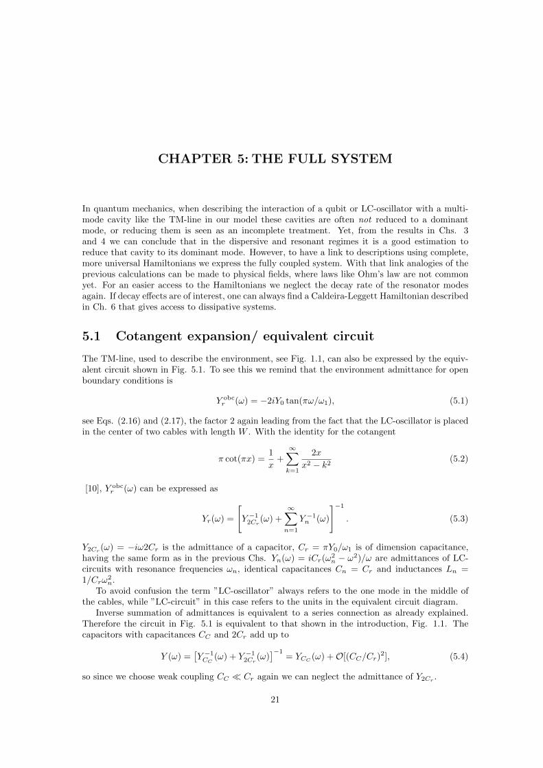
In quantum mechanics, when describing the interaction of a qubit or LC-oscillator with a multi-mode cavity like the TM-line in our model these cavities are often not reduced to a dominantmode, or reducing them is seen as an incomplete treatment. Yet, from the results in Chs. 3and 4 we can conclude that in the dispersive and resonant regimes it is a good estimation toreduce that cavity to its dominant mode. However, to have a link to descriptions using complete,more universal Hamiltonians we express the fully coupled system. With that link analogies of theprevious calculations can be made to physical fields, where laws like Ohm’s law are not commonyet. For an easier access to the Hamiltonians we neglect the decay rate of the resonator modesagain. If decay effects are of interest, one can always find a Caldeira-Leggett Hamiltonian describedin Ch. 6 that gives access to dissipative systems.

5.1 Cotangent expansion/ equivalent circuit

The TM-line, used to describe the environment, see Fig. 1.1, can also be expressed by the equiv-alent circuit shown in Fig. 5.1. To see this we remind that the environment admittance for openboundary conditions is

Y obcr (ω) = −2iY0 tan(πω/ω1), (5.1)

see Eqs. (2.16) and (2.17), the factor 2 again leading from the fact that the LC-oscillator is placedin the center of two cables with length W . With the identity for the cotangent

π cot(πx) =1

x+

∞∑k=1

2x

x2 − k2(5.2)

[10], Y obcr (ω) can be expressed as

Yr(ω) =

[Y −1

2Cr(ω) +

∞∑n=1

Y −1n (ω)

]−1

. (5.3)

Y2Cr(ω) = −iω2Cr is the admittance of a capacitor, Cr = πY0/ω1 is of dimension capacitance,

having the same form as in the previous Chs. Yn(ω) = iCr(ω2n − ω2)/ω are admittances of LC-

circuits with resonance frequencies ωn, identical capacitances Cn = Cr and inductances Ln =1/Crω

2n.

To avoid confusion the term ”LC-oscillator” always refers to the one mode in the middle ofthe cables, while ”LC-circuit” in this case refers to the units in the equivalent circuit diagram.

Inverse summation of admittances is equivalent to a series connection as already explained.Therefore the circuit in Fig. 5.1 is equivalent to that shown in the introduction, Fig. 1.1. Thecapacitors with capacitances CC and 2Cr add up to

Y (ω) =[Y −1CC

(ω) + Y −12Cr

(ω)]−1

= YCC(ω) +O[(CC/Cr)

2], (5.4)

so since we choose weak coupling CC Cr again we can neglect the admittance of Y2Cr.

21

22 CHAPTER 5. THE FULL SYSTEM

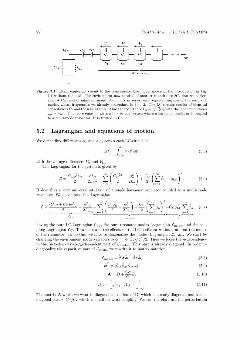
Figure 5.1: Exact equivalent circuit to the transmission line model shown in the introduction in Fig.1.1 without the load. The environment now consists of another capacitance 2Cr that we neglectagainst CC , and of infinitely many LC-circuits in series, each representing one of the resonatormodes, whose frequencies we already determined in Ch. 2. The LC-circuits consist of identicalcapacitances Cr and the n’th LC-circuit has the inductance Ln = 1/ω2

nCr with the mode frequenciesωn = nω1. This representation gives a link to any system where a harmonic oscillator is coupledto a multi-mode resonator. It is treated in Ch. 5.

5.2 Lagrangian and equations of motion

We define flux-differences φn and φLC across each LC-circuit as

φ(t) =

∫ t

−∞V (t′)dt′, (5.5)

with the voltage-differences Vn and VLC.The Lagrangian for the system is given by

L =CLCφ

2LC

2− φ2

LC

2LLC+

∞∑n=1

(Cnφ

2n

2− φ2

n

2Ln

)+CC2

( ∞∑n=1

φn − φLC

)2

. (5.6)

It describes a very universal situation of a single harmonic oscillator coupled to a multi-moderesonator. We decompose this Lagrangian

L =(CLC + CC)φ2

LC

2− φ2

LC

2LLC︸ ︷︷ ︸LLC

+

∞∑n=1

(Cnφ

2n

2− φ2

n

2Ln

)+CC2

( ∞∑n=1

φn

)2

︸ ︷︷ ︸Lmodes

−CC φLC

∞∑n=1

φn︸ ︷︷ ︸LC

, (5.7)

having the pure LC-Lagrangian LLC, the pure resonator modes Lagrangian Lmodes and the cou-pling Lagrangian LC . To understand the effects on the LC-oscillator we integrate out the modesof the resonator. To do this, we have to diagonalize the modes’ Lagrangian Lmodes. We start bychanging the environment mode variables to φn = φnωn

√Cr/2. Thus we loose the n-dependency

in the (non-derivative)-φn-dependent part of Lmodes. This part is already diagonal. In order todiagonalize the capacitive part of Lmodes we rewrite it to matrix notation

Lmodes =˙φA

˙φ− φ1φ, (5.8)

φT

= [φ1, φ2, φ3, ...], (5.9)

A = D +CCCr

Ω, (5.10)

Dij =1

ω2i

δi,j Ωij =1

ωiωj. (5.11)

The matrix A which we want to diagonalize consists of D, which is already diagonal, and a non-diagonal part ∼ CC/Cr which is small for weak coupling. We can therefore use the perturbation

5.2. LAGRANGIAN AND EQUATIONS OF MOTION 23

theory often used in quantum mechanics when having a slightly disturbed Hamiltonian H = H0 +εV with a well-known and dominant diagonal part H0. According to this theory the eigenvaluesand eigenvectors of A, fulfilling

Avn = λnvn (5.12)

can be determined in orders of ν ≡ CC/Cr

λn = λ0n + ν〈v0

n | Ω | v0n〉+ ν2

∑m 6=n

|〈v0m | Ω | v0

n|2

λ0n − λ0

m

+O(ν3), (5.13)

vn = v0n + ν

∑m 6=n

〈v0m | Ω | v0

n〉λ0m − λ0

n

v0m +O

(ν2). (5.14)

Here, λ0n = 1/ω2

n and v0n = en are the eigenvalues and corresponding eigenvectors of D, en being

the unit vectors corresponding to φ and A as defined in Eqs. (5.9) and (5.10). Consider that theeigenvalues of A are non-degenerate which is apparent from the dominant part D. Since we areinterested in weak couplings ν 1, we neglect the higher orders in Eqs. (5.13) and (5.14) andspecify the eigenvalues and -vectors for our system

λn =1

ω2n

(1 + ν) +ν2

ω21

∞∑m=1,m6=n

1

m2 − n2, (5.15)

vn = en + ν

∞∑m=1,m 6=n

nm

m2 − n2em. (5.16)

The sum in Eq. (5.15) converges [11] such that

λn =1

ω2n

(1 + ν +

3

4ν2

). (5.17)

We find the unitary matrix

S =

| | |v1 v2 v3 . . .| | |

→ Snm = δn,m + νnm

n2 −m2(1− δn,m) (5.18)

that according to basic algebra diagonalizes A, i.e. Λ = S−1AS is diagonal with the elementsΛnn = λn. We change the coordinates of the resonator modes again ϕ = S−1φ, where S−1 = ST

due to its unitarity. Then the Lagrangian describing the modes becomes diagonal

Lmodes = ϕΛϕ−ϕ1ϕ (5.19)

Considering the two transformations we made on the resonator mode coordinates we can alsorewrite the coupling Lagrangian in terms of ϕn

LC = −φLC

∞∑n=1

knϕn, kn = CC

√2

Cr

∞∑m=1

Smnωm

(5.20)

Again, the sum in kn converges such that

kn =

√2Crωn

(ν +

3

4ν2

). (5.21)

The full Lagrangian is now given by

L =(CLC + CC)φ2

LC

2− φ2

LC

2LLC+ ϕΛϕ−ϕ1ϕ− φLC

∞∑n=1

knϕn, (5.22)

24 CHAPTER 5. THE FULL SYSTEM

and it leads to the Euler-Lagrange equations of motion

(CLC + CC)φLC + φLC/LLC =

∞∑n=1

knϕn (5.23)

and ∀n ∈ N : 2λnϕn + 2ϕn = knφLC. (5.24)

These can be written in Fourier space such that the infinitely many Eqs. (5.24) can be put intoEq. (5.23), leading to

φLC(ω)

(−iωCLC +

i

ωLLC− iωCC +

ω2

2i

∞∑n=1

ωk2n

1− ω2λn

)= 0, (5.25)

where we denoted φLC(ω), meaning F [φLC(t)](ω). This way we have a good link to the voltage,see Eq. (5.5). The first three terms in Eq. (5.25) can be identified with the admittances of theLC-oscillator YLC(ω) = −iωCLC + i/ωLLC and the coupling capacitance YCC

= −iωCC . WithEqs. (5.17) and (5.21) we rewrite Eq. (5.25)

φLC(ω)

(YLC + YCC

+ ω2C2C

∞∑n=1

Y −1n

), (5.26)

where the admittances Yn describe LC-circuits

Yn = iCrω

(ω2n − ω2

), Cr =

2C2Cλ1

k21

, ωn =n√λ1

. (5.27)

We simplify Eq. (5.26) to the second order in CC/Cr, as we are interested in weak coupling. Sincethe factor in front of the sum in Eq. (5.26) is already ∼ C2

C , we must approximate Yn to zerothorder. We find that

Yn = Yn +O(ν) (5.28)

agrees with the LC-circuit admittances, found in Eq. (5.3) in zeroth order. Using that formula inEq. (5.3) and consistently neglecting Y2Cr (ω) compared to YCC

(ω), see Eq. (5.4), we rewrite Eq.(5.26)

φLC(ω)[YLC(ω) + YCC

(ω)− Y 2CC

(ω)/Yr(ω) +O(ν3)]

= 0. (5.29)

Comparing this expression with the inverse summation in Eq. (4.8) and the expansion of this inEq. (4.9), we find the bare Kirchhoff’s rule describing the circuit in Fig. 4.1 and therefore thestarting point of Ch. 4

VLC(ω)[YLC(ω) + YT (ω)] = 0. (5.30)

The link hereby found between the Lagrangian in Eq. (5.6) and Kirchhoff’s rules is a linkbetween circuit electrodynamics and other linear response theories.

5.3. THE RESPECTIVE HAMILTONIAN 25

5.3 The respective Hamiltonian

In this section we present two Hamiltonians. The first one describes the fully coupled system andthe second is diagonal with respect to the resonator modes.

To proceed, we first have to cut off the modes at the N ’th mode, N being big enough so thatωN ω0 applies. The limit N → ∞ has to be taken at the end. The Lagrangian in Eq. (5.6)describes the fully coupled system. For the Legendre transform it is useful to express its capacitivepart in matrix notation

L =1

2φCφ− φ2

LC

2LLC−

N∑n=1

φ2n

2Ln(5.31)

φ = [φLC, φ1, φ2, φ3, ..., φN ] (5.32)

C =

CLC + CC −CC −CC −CC . . . −CC−CC Cr + CC CC CC . . . CC−CC CC Cr + CC CC . . . CC−CC CC CC Cr + CC

......

.... . .

−CC CC CC Cr + CC

(5.33)

Proceeding like Ref. [7] we find the charges

QLC =∂L∂φLC

= CLCφLC + CC

(φLC −

N∑n=1

φn

), (5.34)

Qn =∂L∂φn

= Cnφn − CC

(φLC −

N∑m=1

φm

), (5.35)

as the conjugate momenta

φi, Qj = δi,j . (5.36)

The Legendre transform is then given by

H =1

2QC−1Q +

φ2LC

2LLC+

N∑n=1

φ2n

2Ln. (5.37)

We invert the capacitance matrix to the first order of CC , using that C can be decomposed intoa dominant, diagonal part and a weak part containing off diagonal elements

C = C0 + CCCC. (5.38)

The identity

C−1 = C0−1 − CCC0

−1CCC0−1 +O(C2

C) (5.39)

can be checked in a very general way by verifying that C−1C = CC−1 = 1 +O(C2C). Thus,

C−1 =

1

CLC− CC

C2LC

CC

CLCCr

CC

CLCCr. . .

CC

CLCCr

1Cr− CC

C2r

−CC

C2r

CC

CLCCr−CC

C2r

1Cr− CC

C2r

.... . .

+O(C2C

)(5.40)

26 CHAPTER 5. THE FULL SYSTEM

and we receive the Hamiltonian, describing the full system for weak coupling

H =Q2

LC

2

1

CLC

(1− CC

CLC

)+

φ2LC

2LLC︸ ︷︷ ︸HLC

+CC

CLCCrQLC

N∑n=1

Qn︸ ︷︷ ︸HC

+

N∑n=1

(Q2n

2

1

Cr

(1− CC

Cr

)+

φ2n

2Ln

)−

N∑n,m=1;n 6=m

QnQm2

CCC2r︸ ︷︷ ︸

Hmodes

. (5.41)

We expand the corrections to the capacitances (1−CC/Ci)/Ci = 1/[Ci+CC+O(C2C)] and neglect

second order CC corrections. We define the classical counterparts of boson operators

bi = 4

√Ci + CC

4Liφi + i 4

√Li

4(Ci + CC)Qi, bi, b∗j = −iδi,j , (5.42)

in order that the Hamiltonian is in the Second Quantization form

H = ω0b∗LCbLC︸ ︷︷ ︸HLC

−N∑n=1

gLCn(b∗LC − bLC)(b∗n − bn)︸ ︷︷ ︸HC

+

N∑n=1

ωnb∗nbn +

N∑n,m=1;n 6=m

gnm(b∗n − bn)(b∗m − bm)︸ ︷︷ ︸Hmodes

,

(5.43)

where the coupling constants

gLCn =1

2

√ω0ωn

CC√CrCLC

, gnm =1

2

√ωnωm

CCCr

(5.44)

have about the form of the light-matter coupling [4]. Hereby, ωn are the environment frequencies,containing a correction from the coupling capacitance that arose already in Eqs. (3.12) and (4.26).The coupling constant g for the LC-oscillator, coupling only to the principle mode ωn = ω0 + ∆n,|∆n| ω1 that was defined in Eq. (3.18) has the same form as gLCn for ∆n = 0.

We can also find an effective Hamiltonian in terms of diagonal environment modes that do nolonger couple with each other. We can do this by either diagonalizing the respective modes inthe Hamiltonian in Eq. (5.43) or by Legendre transforming the Lagrangian in Eq. (5.22), wherethe environment modes are already diagonal. By again expanding to the first order of ν, bothmethods lead to

H =Q2

LC

2(CLC + CC)+

φ2LC

2LLC+

N∑n=1

[ω2n

4(1− ν)q2

n + ϕ2n

]+QLC

N∑n=1

gnqn, (5.45)

with

gn =CCωn

CLC

√8Cr

. (5.46)

The momenta, conjugate to ϕn

qn =∂L∂ϕ

= 21 + ν

ω2n

ϕn − φLC

N∑n=1

kn (5.47)

do not converge in the limit N →∞. That is why we had to choose a cutoff, why the limit has tobe taken in the end of determining a physical quantity, and that is why it is difficult to calculatethe influence of the multi-mode cavity in Hamiltonian mechanics.

CHAPTER 6: DISSIPATIVE SYSTEMS

As already mentioned several times in this thesis, dissipation cannot be described straightforwardlyin Hamiltonian mechanics, due to its in-build Energy conservation property. A method to treatthis difficulty was found by Caldeira and Leggett [9].

6.1 The Caldeira-Leggett Hamiltonian

The idea is that energy conservation is kept if a virtual bath of infinitely many harmonic oscillators,representing the environmental degrees of freedom φn, Qn is given. The system of interest iscoupled to every bath mode, whereby the coupling describes the way in which energy is lost, i.e.transferred to the bath. Before starting it should be mentioned that it is highly unobvious andonly due to the infinite number of bath degrees that a bath consisting only of non-dissipativecomponents never returns this energy back to the system. A similar miracle happens with theTM-line which consists of non-dissipative components and becomes dissipative at infinite lengthW , see Ch. 2.

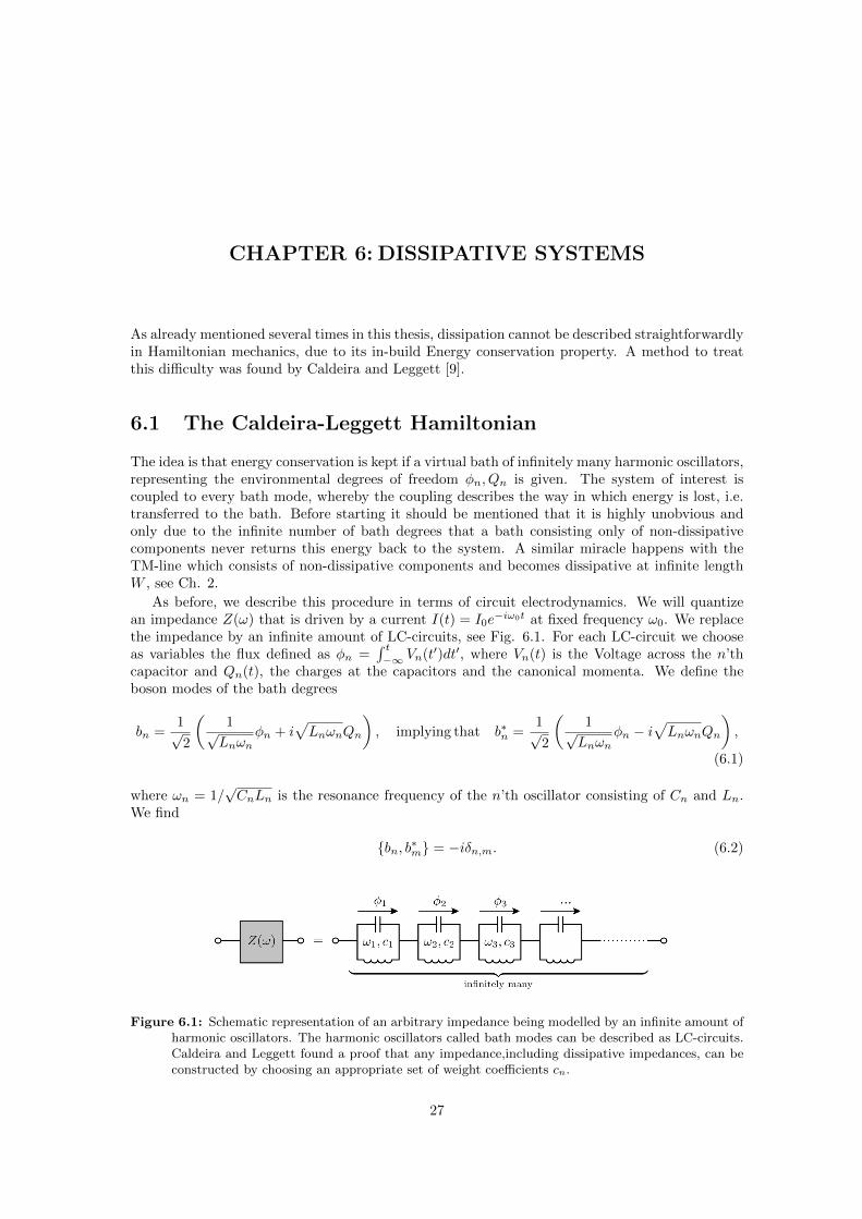
As before, we describe this procedure in terms of circuit electrodynamics. We will quantizean impedance Z(ω) that is driven by a current I(t) = I0e

−iω0t at fixed frequency ω0. We replacethe impedance by an infinite amount of LC-circuits, see Fig. 6.1. For each LC-circuit we chooseas variables the flux defined as φn =

∫ t−∞ Vn(t′)dt′, where Vn(t) is the Voltage across the n’th

capacitor and Qn(t), the charges at the capacitors and the canonical momenta. We define theboson modes of the bath degrees

bn =1√2

(1√Lnωn

φn + i√LnωnQn

), implying that b∗n =

1√2

(1√Lnωn

φn − i√LnωnQn

),

(6.1)

where ωn = 1/√CnLn is the resonance frequency of the n’th oscillator consisting of Cn and Ln.

We find

bn, b∗m = −iδn,m. (6.2)

Figure 6.1: Schematic representation of an arbitrary impedance being modelled by an infinite amount ofharmonic oscillators. The harmonic oscillators called bath modes can be described as LC-circuits.Caldeira and Leggett found a proof that any impedance,including dissipative impedances, can beconstructed by choosing an appropriate set of weight coefficients cn.

27

28 CHAPTER 6. DISSIPATIVE SYSTEMS

The flux across the whole impedance is the sum of the partial fluxes across all bath oscillators

Φ(t) =

∫ t

−∞V (t′)dt′ =

∑n

φn(t) =∑n

√ωnLn

2[b∗n(t) + bn(t)]. (6.3)

where V (t) is the voltage across the impedance. Now the good thing is that we can choose ωnand Ln independently for every mode, because there is always a capacitance Cn that ensures thatω2n = 1/LnCn. Therefore, we call

cn =√ωnLn/2 (6.4)

the n’th weight coefficient that can be chosen independently of ωn.We suppose that the bath is coupled to the system via the current and write the Hamiltonian

for the impedance

H =∑n

ωnb∗nbn − I(t)Φ (6.5)

We obtain the equations of motion by using

f [φi(t), Qi(t)] = f,H[φi(t), Qi(t)] (6.6)

and can thereby write for the flux in frequency space

Φ(ω) = χ(ω)I(ω), χ(ω) =

N→∞∑n

|cn|2(

1

ωn − ω+

1

ωn + ω

), (6.7)

where we defined the response function χ(ω) that we have to say a few things about. The inverseFourier transform of χ(ω) is

χ(t) =

∫ ∞−∞

dω

2πe−iωtχ(ω). (6.8)

For t < 0 this integral could be solved by adding the vanishing semicircle contour in the upperhalf plane. By Cauchy’s residue theorem the integral is non-zero if χ(ω) has a pole in the upperhalf-plane. If χ(t) is non-zero, the present current would have influenced1 the past flux, which canbe seen in the convolution integral that you get when transforming Eq. (6.7) to time space. Thatmeans that for causality χ(ω) must be analytic in the upper half-plane, which is established byadding an infinitely small imaginary part to the frequency, thus

χ(ω) = limε→0

N→∞∑n

|cn|2(

1

ωn − ω − iε+

1

ωn + ω + iε

), (6.9)

We denoted the upper border of the sum in Eqs. (6.7) and (6.9) not only ∞ because this limitrequires some more attention. W.l.o.g. we claim that the ωn are sorted according to size. Alsowe claim that they are equidistant with distance dω. That way, we express the limit N → ∞,dω → 0 in Eq. (6.9) with help of the mode density

G(ω) =

∞∑n=1

|cn|2δ(ωn − ω), (6.10)

with the Dirac-distribution δ(x) such that

χ(ω) = limε→0

∫ ∞0

(1

ω − ω − iε+

1

ω + ω + iε

)G(ω)dω. (6.11)

1It is hard to decide, which tense to use here...

6.2. EXPANSION FOR TWO PORT DEVICES 29

Here, G(ω)dω is the weight of the modes with frequencies between ω and ω + dω. The integrandis a dense function now.

The Sokhotski-Plemlj-Therom2 says that in the sense of distributions34

limε→0

1

x− iε= P

(1

x

)+ iπδ(x). (6.12)

Equation (6.7) can be rewritten with the definition of the flux in Eq. (6.3), leading to Ohm’slaw

V (ω) = −iωχ(ω)I(ω). (6.13)

With that we find the impedance

Z(ω) = −iωχ(ω) = −iωiπ[G(ω) +G(−ω)] + P

∫ ∞0

(1

ωn − ω+

1

ωn + ω

)G(ω)dω

. (6.14)

And especially for its real part at positive frequencies we find

ReZ(ω) = G(ω) =∑n

πω|cn|2δ(ωn − ω). (6.15)

According to Kramers-Kronig relations, every physical impedance is fully determined by its real orimaginary part [12]. Therefore every physical impedance including dissipative impedances can beconstructed by choosing a set of the infinitely many weight coefficients cn that fulfils Eq. (6.15)5.That way we can use the Hamiltonian in Eq. (6.5) as an effective Hamiltonian for the impedance.

6.2 Expansion for two port devices

Just like the Hamiltonian for a one-port impedance Z(ω) we can also write an effective Hamiltonianthat leads to equations of motion for an arbitrary two-port impedance matrix Z(ω).

We adopt the bath of Section 6.1 that is we use the same bath variables. But instead of findingthe weight coefficients by defining how the bath oscillators are connected to the network ports weleave that open and choose abstractly two sets of complex coupling constants ck and dk to defineboth fluxes at port 1 and port 2

Φ1(t) =∑n

cnb∗n(t) + c∗nbn(t), Φ2(t) =

∑n

dnb∗n(t) + d∗nbn(t). (6.16)

Again, we write the coupling via the current. In this case via the two currents entering at port 1and port 2 respectively so that the Hamiltonian becomes

H =∑n

ωnb∗nbn − I1(t)Φ1 − I2(t)Φ2. (6.17)

With the equations of motion we can again find the flux response to the current, this time as amatrix [

Φ1

Φ2

]= limε→0

∑n

[|cn|2

ωn−ω−iε + |cn|2ωn+ω+iε

cnd∗n

ωn−ω−iε +c∗ndn

ωn+ω+iεdnc

∗n

ωn−ω−iε +d∗ncn

ωn+ω+iε|dn|2

ωn−ω−iε + |dn|2ωn+ω+iε

] [I1I2

], (6.18)

2Sometimes referred to as Dirac identity3That means that a statement is meant to be true for the integrand of a Cauchy Principle Value Integral.4P

∫dx denotes the Cauchy Principle Value Integral. P[f(x)] denotes an expression that the Cauchy Principle

Value has to be taken of.5One could say, the fact that a bath of infinitely many non-dissipative components can be dissipative relies on

causality

30 CHAPTER 6. DISSIPATIVE SYSTEMS

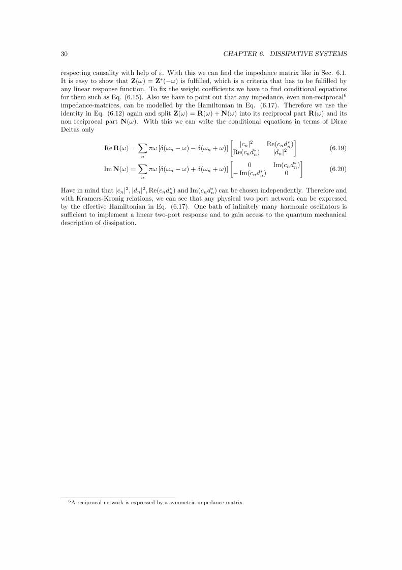
respecting causality with help of ε. With this we can find the impedance matrix like in Sec. 6.1.It is easy to show that Z(ω) = Z∗(−ω) is fulfilled, which is a criteria that has to be fulfilled byany linear response function. To fix the weight coefficients we have to find conditional equationsfor them such as Eq. (6.15). Also we have to point out that any impedance, even non-reciprocal6

impedance-matrices, can be modelled by the Hamiltonian in Eq. (6.17). Therefore we use theidentity in Eq. (6.12) again and split Z(ω) = R(ω) + N(ω) into its reciprocal part R(ω) and itsnon-reciprocal part N(ω). With this we can write the conditional equations in terms of DiracDeltas only

Re R(ω) =∑n

πω [δ(ωn − ω)− δ(ωn + ω)]

[|cn|2 Re(cnd

∗n)

Re(cnd∗n) |dn|2

](6.19)

Im N(ω) =∑n

πω [δ(ωn − ω) + δ(ωn + ω)]

[0 Im(cnd

∗n)

− Im(cnd∗n) 0

](6.20)

Have in mind that |cn|2, |dn|2,Re(cnd∗n) and Im(cnd

∗n) can be chosen independently. Therefore and

with Kramers-Kronig relations, we can see that any physical two port network can be expressedby the effective Hamiltonian in Eq. (6.17). One bath of infinitely many harmonic oscillators issufficient to implement a linear two-port response and to gain access to the quantum mechanicaldescription of dissipation.

6A reciprocal network is expressed by a symmetric impedance matrix.

CHAPTER 7: CONCLUSION

We have investigated the influence of wires connected to an LC-oscillator on its properties bymodelling the wires as transmission lines. In Ch. 2, we confirmed that the TM-line behaves likea waveguide. We found both its two-port impedance and the impedance of a loaded TM-line.Both expression show that the wires act like multi-mode resonators The principle effect of theenvironment on the oscillator has turned out to be a shift of resonance frequency and a decayrate representing dissipation. We found these quantities for the dispersive and the resonant caseby solving coupled differential equations for the LC-oscillator and the principle resonator mode inCh. 3. They agree with the results of previous research [3–6]. We were also able to calculate forwhat type of load these effects are low.

We found an even easier way to determine the Purcell rate and the Lamb shift in Ch. 4 byevaluating the environment at a fixed frequency. Our results provide easy access to understandingthese effects, even without quantum mechanics. In this way we could calculate the influence ofthe non-principle modes to the lowest order and understand how insignificant their contributionis. However, the contribution includes an asymmetric behaviour predicted for off resonant casesin circuit models and measured in experiments in Ref. [3]. In addition, we were able to find theinteraction effects of two LC-oscillators coupled via a linear, off-resonant two-port network.

In Ch. 5, we were able to derive Kirchhof’s laws from a much more general Lagrangian thatfully describes the system with all modes. We also presented the according Hamiltonian for weakcoupling. This allowed us to understand why it is so delicate to diagonalize the Hamiltonian.

As presented in Eq. (3.35), this problem can be avoided if the frequency shift δ induced by theenvironment is determined in the circuit model. This quantity is sufficient to write a decoupled,effective Hamiltonian for the boson modes b, b∗ of the form

Heff = (ω0 + δ)b∗b. (7.1)

Therefore, if it comes to larger, upscaled networks, the technique used in Ch. 4 is a greatcandidate for analytically estimating environmental influences. Further research on this topicshould definitely find a way to formalize these calculations for larger circuits. Experiments stillneed to be done to confirm that the presented shifts and decays are correct within the respectivelimits and in particular with the load parameters for weak decay proposed in Eqs. (2.20) and(2.21).

By further developing the circuit model presented in this study, current architectures for devicesbased on circuit quantum electrodynamics could be improved. Excitation energies can be matchedbetter and relaxation times of qubits can be increased.

31

32 CHAPTER 7. CONCLUSION

BIBLIOGRAPHY

[1] T. Fließbach. Elektrodynamik: Lehrbuch zur Theoretischen Physik II. Spektrum AkademischerVerlag, 2012.

[2] Peter Eastman. Introduction to statistical mechanics. https://peastman.github.io/

statmech/friction.html#linear-response-theory.

[3] A. A. Houck, J. A. Schreier, B. R. Johnson, J. M. Chow, Jens Koch, J. M. Gambetta, D. I.Schuster, L. Frunzio, M. H. Devoret, S. M. Girvin, and R. J. Schoelkopf. Controlling thespontaneous emission of a superconducting transmon qubit. Phys. Rev. Lett., 101:080502,Aug 2008.

[4] Moein Malekakhlagh, Alexandru Petrescu, and Hakan E. Tureci. Cutoff-free circuit quantumelectrodynamics. https://link.aps.org/doi/10.1103/PhysRevLett.119.073601, Aug2017.

[5] Alexandre Blais, Ren-Shou Huang, Andreas Wallraff, S. M. Girvin, and R. J. Schoelkopf.Cavity quantum electrodynamics for superconducting electrical circuits: An architecture forquantum computation. Phys. Rev. A, 69:062320, Jun 2004.

[6] Sal Bosman, Mario Gely, V Singh, Alessandro Bruno, Daniel Bothner, and Gary Steele.Multi-mode ultra-strong coupling in circuit quantum electrodynamics. 3, 04 2017.

[7] Mario F. Gely, Adrian Parra-Rodriguez, Daniel Bothner, Ya. M. Blanter, Sal J. Bosman,Enrique Solano, and Gary A. Steele. Convergence of the multimode quantum rabi model ofcircuit quantum electrodynamics. Phys. Rev. B, 95:245115, Jun 2017.

[8] Yuli V. Nazarov and Yaroslav M. Blanter. Quantum Transport: Introduction to Nanoscience.Cambridge University Press, 2009.

[9] A. O. Caldeira and A. J. Leggett. Influence of dissipation on quantum tunneling in macro-scopic systems. Phys. Rev. Lett., 46:211–214, Jan 1981.

[10] E.R. Hansen. A table of series and products. Prentice-Hall series in automatic computation.Prentice-Hall, 1975.

[11] Izrail S. Gradstejn. Table of integrals, series and products. Elsevier, 7 edition, 2007.

[12] R. de L. Kronig. On the theory of dispersion of x-rays. J. Opt. Soc. Am., 12(6):547–557, Jun1926.

33

34 BIBLIOGRAPHY

ACKNOLEDGEMENTS

I am very grateful to Prof. Dr. Fabian Hassler for his time and patience. He needs nocheating because brilliance results from deep understanding.

35