Embed Size (px)
Citation preview
econstor www.econstor.eu
Der Open-Access-Publikationsserver der ZBW – Leibniz-Informationszentrum WirtschaftThe Open Access Publication Server of the ZBW – Leibniz Information Centre for Economics
Standard-Nutzungsbedingungen:
Die Dokumente auf EconStor dürfen zu eigenen wissenschaftlichenZwecken und zum Privatgebrauch gespeichert und kopiert werden.
Sie dürfen die Dokumente nicht für öffentliche oder kommerzielleZwecke vervielfältigen, öffentlich ausstellen, öffentlich zugänglichmachen, vertreiben oder anderweitig nutzen.
Sofern die Verfasser die Dokumente unter Open-Content-Lizenzen(insbesondere CC-Lizenzen) zur Verfügung gestellt haben sollten,gelten abweichend von diesen Nutzungsbedingungen die in der dortgenannten Lizenz gewährten Nutzungsrechte.
Terms of use:
Documents in EconStor may be saved and copied for yourpersonal and scholarly purposes.
You are not to copy documents for public or commercialpurposes, to exhibit the documents publicly, to make thempublicly available on the internet, or to distribute or otherwiseuse the documents in public.
If the documents have been made available under an OpenContent Licence (especially Creative Commons Licences), youmay exercise further usage rights as specified in the indicatedlicence.
zbw Leibniz-Informationszentrum WirtschaftLeibniz Information Centre for Economics
Boeri, Tito; Garibaldi, Pietro; Moen, Espen R.
Working Paper
The labor market consequences of adverse financialshocks
Discussion Paper series, Forschungsinstitut zur Zukunft der Arbeit, No. 6826
Provided in Cooperation with:Institute for the Study of Labor (IZA)
Suggested Citation: Boeri, Tito; Garibaldi, Pietro; Moen, Espen R. (2012) : The labor marketconsequences of adverse financial shocks, Discussion Paper series, Forschungsinstitut zurZukunft der Arbeit, No. 6826
This Version is available at:http://hdl.handle.net/10419/62353
DI
SC
US
SI
ON
P
AP
ER
S
ER
IE
S
Forschungsinstitut zur Zukunft der ArbeitInstitute for the Study of Labor
The Labor Market Consequences ofAdverse Financial Shocks
IZA DP No. 6826
August 2012
Tito BoeriPietro GaribaldiEspen R. Moen
The Labor Market Consequences of
Adverse Financial Shocks
Tito Boeri Bocconi University,
fRDB and IZA
Pietro Garibaldi University of Torino,
Collegio Carlo Alberto and IZA
Espen R. Moen Norwegian School of Management
Discussion Paper No. 6826 August 2012
IZA
P.O. Box 7240 53072 Bonn
Germany
Phone: +49-228-3894-0 Fax: +49-228-3894-180
E-mail: [email protected]
Any opinions expressed here are those of the author(s) and not those of IZA. Research published in this series may include views on policy, but the institute itself takes no institutional policy positions. The Institute for the Study of Labor (IZA) in Bonn is a local and virtual international research center and a place of communication between science, politics and business. IZA is an independent nonprofit organization supported by Deutsche Post Foundation. The center is associated with the University of Bonn and offers a stimulating research environment through its international network, workshops and conferences, data service, project support, research visits and doctoral program. IZA engages in (i) original and internationally competitive research in all fields of labor economics, (ii) development of policy concepts, and (iii) dissemination of research results and concepts to the interested public. IZA Discussion Papers often represent preliminary work and are circulated to encourage discussion. Citation of such a paper should account for its provisional character. A revised version may be available directly from the author.
IZA Discussion Paper No. 6826 August 2012
ABSTRACT
The Labor Market Consequences of Adverse Financial Shocks The recent financial crises, alongside a dramatic rise in unemployment on both sides of the Atlantic, suggest that financial shocks do translate into the labor markets. In this paper we first document that financial recessions amplify labor market volatility and Okun’s elasticity over the business cycle. Second, we highlight a key mechanism linking financial shocks to job destruction, presenting and solving a simple model of labor market search and endogenous finance. While finance increases job creation and net output in normal times, it also augments their aggregate response in the aftermath of a financial shock. Third, we present evidence coherent with the idea that more leveraged sectors experience larger employment volatility during financial recessions. Theoretically, the job destruction effect of finance works as follows. Leveraged firms may find themselves in a position in which their liquidity is suddenly called back by the lender. This has direct consequences on a firm ability to run and manage existing jobs. As a result, firms may be obliged to shut down part of their operations and destroy existing jobs. We argue that with well-developed capital markets, firms will have an incentive to rely more on liquidity, and in normal times deep capital markets lead to tight labor markets. After an adverse liquidity shock, firms that rely much on liquidity are hit disproportionally hard. This may explain why the unemployment rate in the US during the Great Recession increased more than in European countries experiencing larger output losses. Empirically, the paper uses a variety of datasets to test the implications of the model. At first we identify crises that, just like in the model, caused a sudden reduction of liquidity to firms. Next we draw on sector-level data on employment and leverage in a number of OECD countries at quarterly frequencies to assess whether highly leveraged equilibria originate more employment adjustment under financial recessions. We find that highly leveraged sectors and periods are associated with higher employment- to-output elasticities during banking crises and this effect explains the observation of higher Okun’s elasticities during financial recessions. We also argue that the effect of leverage on employment adjustment can be interpreted as a causal effect, if our identification assumptions are considered plausible. All this amounts essentially for a test of the labor demand channel of adjustment. JEL Classification: G1, J2, J6 Keywords: financial shocks, matching, Okun’s elasticities Corresponding author: Tito Boeri Department of Economics Università Bocconi via Roentgen 1 20136 Milano Italy E-mail: [email protected]
1 Introduction
In the aftermath of the financial crisis, unemployment in the U.S almost doubled from peak to trough,within a few quarters. Its short-run dynamics displayed remarkably larger Okun’s elasticity than in previousrecessions. US unemployment is now declining at a very low pace, denoting more persistence than inprevious recoveries, including the jobless recoveries of the last two decades. Unemployment in Europe hasbeen consistently lower than in the US throughout the Great Recession (Figure 1), although the aggregate EUfigures conceal large cross-country heterogeneity in the responsiveness of unemployment to output changes.
Some of these differences in response across the two sides of the Atlantic are arguably linked to thedifferent labor market institutions. According to an institutional approach and economic analysis fashionablein the mid nineties, one could argue that strict employment protection legislation (EPL) in Europe is thesmoking gun. High costs of dismissals, according to this perspective, are associated with lower labor marketvolatility. However, the countries with the strictest EPL, like Spain, this time experienced the largest increasein unemployment. The fact of the matter is that European labor markets are today much more flexible onaverage than a couple of decades ago, and are characterized by a dual structure. Such a dual structure,with a flexible temporary fringe alongside a rigid stock of regular contracts, increased labor market responseto adverse business conditions precisely in those countries displaying the strictest employment protectionprovisions for regular contracts.
One should therefore go beyond labor market institutions to understand these asymmetric and largelyunprecedented developments. A key factor behind the response of the labor market to the current recession islikely to be in the nature of the shocks that led to the Great Recession. In particular, one should look at thefinancial markets where the crisis developed and became global in the aftermath of the Lehman bankruptcyin the Fall of 2008. Financial markets and the banking sector experienced a credit crunch well into the 2009.Such a credit crunch has been documented by several authors and took place in both Europe and the U.S.This global credit crunch is likely to have been playing a key role in labor market adjustment during thedownturn and in the recovery.
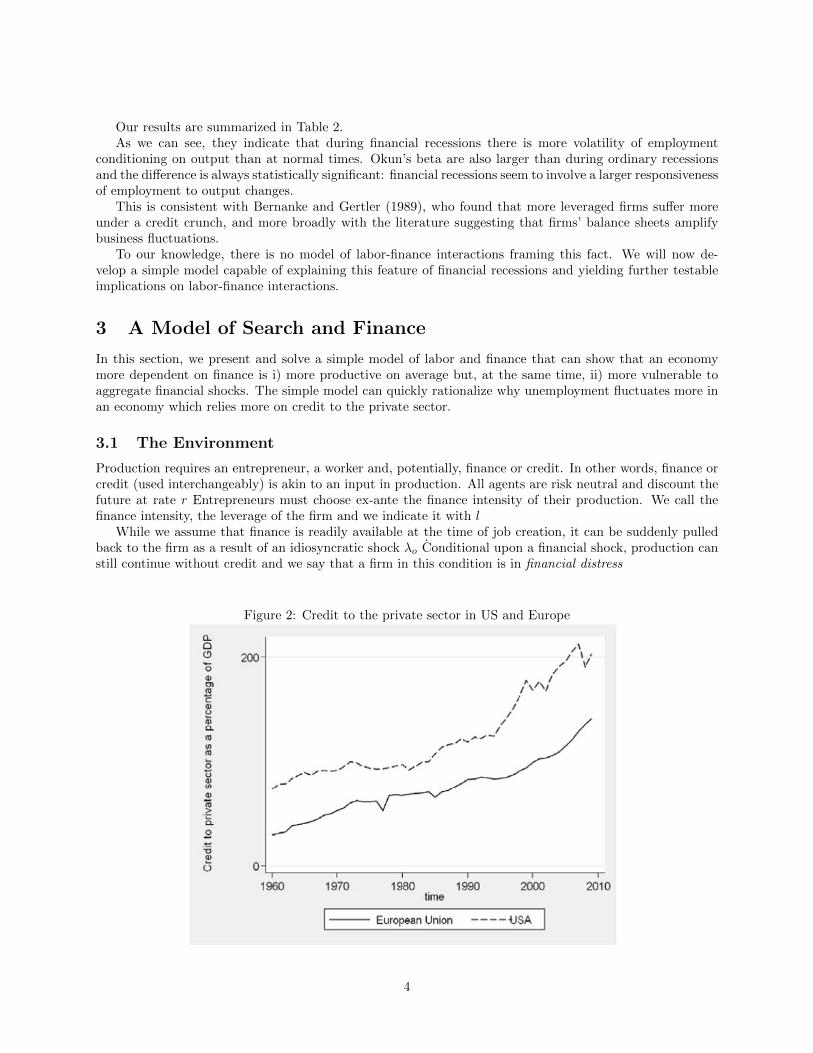
With respect to the financial sector, one of the key differences between the two sides of the Atlantic isthe degree of financial deepening. A simple empirical measure to account for this difference is the stockmarket capitalization over GDP. While the size of the financial shocks, measured in terms of losses of stockmarket capitalization, appear very similar in terms of timing and size, what is striking is the fact that thelevel of financial deepening is indeed very different: credit to the private sector as a share of GDP has beenconsistently larger in the US than in Europe in the last 50 years and the gap across the two sides of theAtlatic actually increased over time (Figure 2). Similarly, in the US stock market capitalization is largerthan in the EU: at the outset of the Great Recession it was some 100 percent of GDP, while the same ratioin Europe was about 75 percent (Figure 3).
We study theoretically and empirically the basic links and transmission mechanisms between the shocksto the financial markets and the labor market. The questions of this line of research are the following.How does a credit crunch translate into job destruction and larger unemployment? Is financial deepening– larger as we have seen in the U.S. than in Europe – responsible for the acceleration and increase of theunemployment to output response in the U.S. to the financial shocks of 2008 and 2009? How does thisexplanation cope with the sluggish dynamics of US unemployment during the recovery? And how aboutdifferences in Okun’s elasticities across sectors?
The paper focuses on the job destruction effect of finance. Leveraged firms may find themselves in aposition in which their liquidity is suddenly called back by the lender. Such a sudden call back in liquidityhas direct consequences on a firm ability to run and manage existing jobs. As a result, firms may be obligedto shut down part of their operations and destroy existing jobs. In this sense, the job destruction effect ofthe credit crunch is essentially a labor demand driven channel of adjustment.
We argue that with deep capital markets, firms will have an incentive to rely more on liquidity, and innormal times deep capital markets lead to tight labor markets. After an adverse liquidity shock, firms thatrely much on liquidity, are hit disproportionally hard. This may explain why the unemployment rate in theUS has increased relatively more compared with many European countries in the aftermath of the GreatRecession.
2
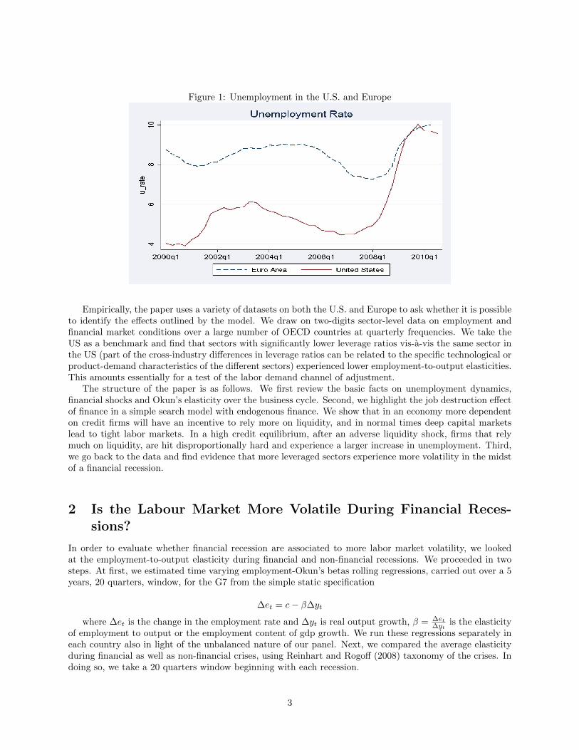
Figure 1: Unemployment in the U.S. and Europe
Empirically, the paper uses a variety of datasets on both the U.S. and Europe to ask whether it is possibleto identify the effects outlined by the model. We draw on two-digits sector-level data on employment andfinancial market conditions over a large number of OECD countries at quarterly frequencies. We take theUS as a benchmark and find that sectors with significantly lower leverage ratios vis-a-vis the same sector inthe US (part of the cross-industry differences in leverage ratios can be related to the specific technological orproduct-demand characteristics of the different sectors) experienced lower employment-to-output elasticities.This amounts essentially for a test of the labor demand channel of adjustment.
The structure of the paper is as follows. We first review the basic facts on unemployment dynamics,financial shocks and Okun’s elasticity over the business cycle. Second, we highlight the job destruction effectof finance in a simple search model with endogenous finance. We show that in an economy more dependenton credit firms will have an incentive to rely more on liquidity, and in normal times deep capital marketslead to tight labor markets. In a high credit equilibrium, after an adverse liquidity shock, firms that relymuch on liquidity, are hit disproportionally hard and experience a larger increase in unemployment. Third,we go back to the data and find evidence that more leveraged sectors experience more volatility in the midstof a financial recession.
2 Is the Labour Market More Volatile During Financial Reces-sions?
In order to evaluate whether financial recession are associated to more labor market volatility, we lookedat the employment-to-output elasticity during financial and non-financial recessions. We proceeded in twosteps. At first, we estimated time varying employment-Okun’s betas rolling regressions, carried out over a 5years, 20 quarters, window, for the G7 from the simple static specification
∆et = c− β∆yt
where ∆et is the change in the employment rate and ∆yt is real output growth, β = ∆et∆yt
is the elasticityof employment to output or the employment content of gdp growth. We run these regressions separately ineach country also in light of the unbalanced nature of our panel. Next, we compared the average elasticityduring financial as well as non-financial crises, using Reinhart and Rogoff (2008) taxonomy of the crises. Indoing so, we take a 20 quarters window beginning with each recession.
3
Our results are summarized in Table 2.As we can see, they indicate that during financial recessions there is more volatility of employment
conditioning on output than at normal times. Okun’s beta are also larger than during ordinary recessionsand the difference is always statistically significant: financial recessions seem to involve a larger responsivenessof employment to output changes.
This is consistent with Bernanke and Gertler (1989), who found that more leveraged firms suffer moreunder a credit crunch, and more broadly with the literature suggesting that firms’ balance sheets amplifybusiness fluctuations.
To our knowledge, there is no model of labor-finance interactions framing this fact. We will now de-velop a simple model capable of explaining this feature of financial recessions and yielding further testableimplications on labor-finance interactions.
3 A Model of Search and Finance
In this section, we present and solve a simple model of labor and finance that can show that an economymore dependent on finance is i) more productive on average but, at the same time, ii) more vulnerable toaggregate financial shocks. The simple model can quickly rationalize why unemployment fluctuates more inan economy which relies more on credit to the private sector.
3.1 The Environment
Production requires an entrepreneur, a worker and, potentially, finance or credit. In other words, finance orcredit (used interchangeably) is akin to an input in production. All agents are risk neutral and discount thefuture at rate r Entrepreneurs must choose ex-ante the finance intensity of their production. We call thefinance intensity, the leverage of the firm and we indicate it with l
While we assume that finance is readily available at the time of job creation, it can be suddenly pulledback to the firm as a result of an idiosyncratic shock λo Conditional upon a financial shock, production canstill continue without credit and we say that a firm in this condition is in financial distress
Figure 2: Credit to the private sector in US and Europe
4
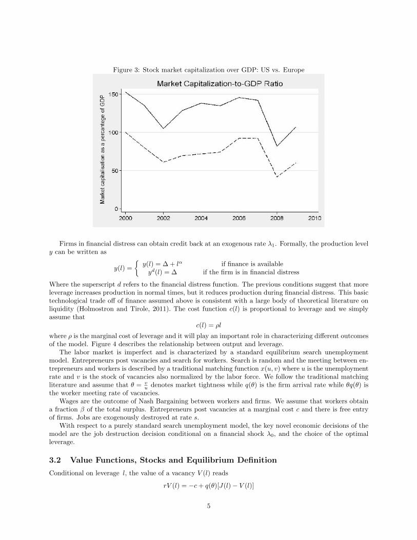
Figure 3: Stock market capitalization over GDP: US vs. Europe
Firms in financial distress can obtain credit back at an exogenous rate λ1. Formally, the production levely can be written as
y(l) =
{y(l) = ∆ + lα if finance is availableyd(l) = ∆ if the firm is in financial distress
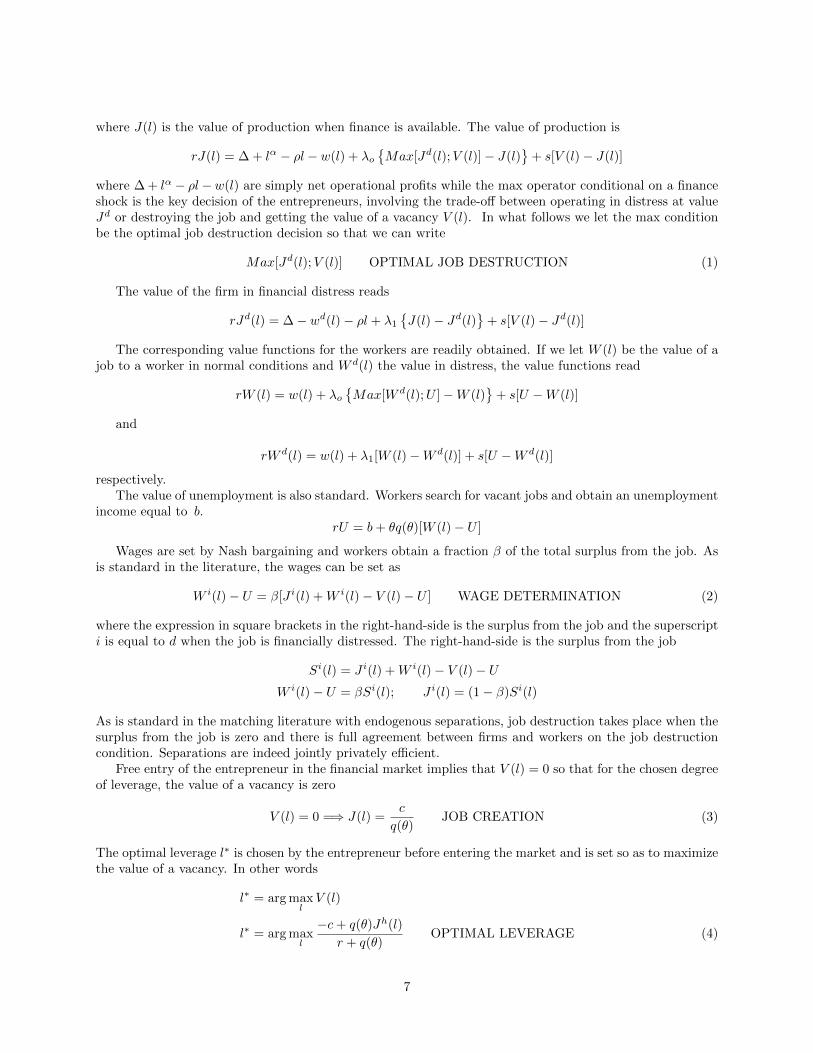
Where the superscript d refers to the financial distress function. The previous conditions suggest that moreleverage increases production in normal times, but it reduces production during financial distress. This basictechnological trade off of finance assumed above is consistent with a large body of theoretical literature onliquidity (Holmostron and Tirole, 2011). The cost function c(l) is proportional to leverage and we simplyassume that
c(l) = ρl
where ρ is the marginal cost of leverage and it will play an important role in characterizing different outcomesof the model. Figure 4 describes the relationship between output and leverage.
The labor market is imperfect and is characterized by a standard equilibrium search unemploymentmodel. Entrepreneurs post vacancies and search for workers. Search is random and the meeting between en-trepreneurs and workers is described by a traditional matching function x(u, v) where u is the unemploymentrate and v is the stock of vacancies also normalized by the labor force. We follow the traditional matchingliterature and assume that θ = v
u denotes market tightness while q(θ) is the firm arrival rate while θq(θ) isthe worker meeting rate of vacancies.
Wages are the outcome of Nash Bargaining between workers and firms. We assume that workers obtaina fraction β of the total surplus. Entrepreneurs post vacancies at a marginal cost c and there is free entryof firms. Jobs are exogenously destroyed at rate s.
With respect to a purely standard search unemployment model, the key novel economic decisions of themodel are the job destruction decision conditional on a financial shock λ0, and the choice of the optimalleverage.
3.2 Value Functions, Stocks and Equilibrium Definition
Conditional on leverage l, the value of a vacancy V (l) reads
rV (l) = −c+ q(θ)[J(l)− V (l)]
5
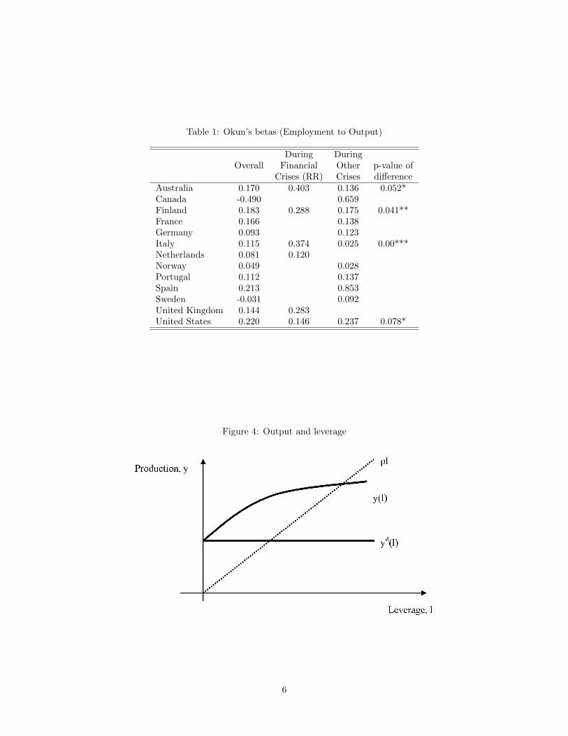
Table 1: Okun’s betas (Employment to Output)
During DuringOverall Financial Other p-value of
Crises (RR) Crises differenceAustralia 0.170 0.403 0.136 0.052*Canada -0.490 0.659Finland 0.183 0.288 0.175 0.041**France 0.166 0.138Germany 0.093 0.123Italy 0.115 0.374 0.025 0.00***Netherlands 0.081 0.120Norway 0.049 0.028Portugal 0.112 0.137Spain 0.213 0.853Sweden -0.031 0.092United Kingdom 0.144 0.283United States 0.220 0.146 0.237 0.078*
Figure 4: Output and leverage
6
where J(l) is the value of production when finance is available. The value of production is
rJ(l) = ∆ + lα − ρl − w(l) + λo{Max[Jd(l);V (l)]− J(l)
}+ s[V (l)− J(l)]
where ∆ + lα − ρl−w(l) are simply net operational profits while the max operator conditional on a financeshock is the key decision of the entrepreneurs, involving the trade-off between operating in distress at valueJd or destroying the job and getting the value of a vacancy V (l). In what follows we let the max conditionbe the optimal job destruction decision so that we can write
Max[Jd(l);V (l)] OPTIMAL JOB DESTRUCTION (1)
The value of the firm in financial distress reads
rJd(l) = ∆− wd(l)− ρl + λ1
{J(l)− Jd(l)
}+ s[V (l)− Jd(l)]
The corresponding value functions for the workers are readily obtained. If we let W (l) be the value of ajob to a worker in normal conditions and W d(l) the value in distress, the value functions read
rW (l) = w(l) + λo{Max[W d(l);U ]−W (l)
}+ s[U −W (l)]
and
rW d(l) = w(l) + λ1[W (l)−W d(l)] + s[U −W d(l)]
respectively.The value of unemployment is also standard. Workers search for vacant jobs and obtain an unemployment
income equal to b.rU = b+ θq(θ)[W (l)− U ]
Wages are set by Nash bargaining and workers obtain a fraction β of the total surplus from the job. Asis standard in the literature, the wages can be set as
W i(l)− U = β[J i(l) +W i(l)− V (l)− U ] WAGE DETERMINATION (2)
where the expression in square brackets in the right-hand-side is the surplus from the job and the superscripti is equal to d when the job is financially distressed. The right-hand-side is the surplus from the job
Si(l) = J i(l) +W i(l)− V (l)− UW i(l)− U = βSi(l); J i(l) = (1− β)Si(l)
As is standard in the matching literature with endogenous separations, job destruction takes place when thesurplus from the job is zero and there is full agreement between firms and workers on the job destructioncondition. Separations are indeed jointly privately efficient.
Free entry of the entrepreneur in the financial market implies that V (l) = 0 so that for the chosen degreeof leverage, the value of a vacancy is zero
V (l) = 0 =⇒ J(l) =c
q(θ)JOB CREATION (3)
The optimal leverage l∗ is chosen by the entrepreneur before entering the market and is set so as to maximizethe value of a vacancy. In other words
l∗ = arg maxlV (l)
l∗ = arg maxl
−c+ q(θ)Jh(l)
r + q(θ)OPTIMAL LEVERAGE (4)
7

In steady state, unemployment inflows are equal to unemployment outflows. Job creation is given by θq(θ)uwhile job destruction is exogenously given by the separation rate plus the financial shock λo conditional onthe optimal job destruction condition of (1). This suggests that the balance flow condition is
θq(θ)u = [s+ Φλ0]u
where Φ is an indicator function that takes the value 1 when Jd(l) < 0. The equilibrium unemploymentrate is then
u =s+ Φλ0
s+ Φλ0 + θq(θ)EQUILIBRIUM UNEMPLOYMENT (5)
Definition 1 The equilibrium is a set of value functions [J(l), Jd(l), V (l),W (l),W d(l), U .], unemploymentstock [u], market tightness θ and leverage l satisfying i) Optimal Job Destruction (equation 1, ii) Job Cre-ation (equation 3) iii) Wage determination (equation 2)iv) Optimal Leverage (equation 4) v) EquilibriumUnemployment (equation 5)
3.3 Solving the Model
To solve the model we need to obtain the value functions in terms of the surplus S(l). Since V (l) = 0 at theoptimal leverage, adding the value functions for firms and workers and subtracting rU, after using the wagedetermination rule one obtains
(r + λo + s)S(l) = ∆ + lα − b− ρl + λo[Max(Sd(l); 0)]− θq(θ)βS(l)
(r + λ1 + s)Sd(l) = ∆− b− ρl + λ1[S(l)− Sd(l)]− θq(θ)βS(l)
The value of leverage, reads
l∗ = arg max−c+ q(θ)(1− β)S(l)
r + q(θ)
while job creation is simplyc
q(θ)= (1− β)S(l)
The solution of the model crucially depends on the optimal job destruction threshold, conditional on anadverse financial shock λo. We define two types of equiibria depending on whether the firm operates or notin financial distress. In particular we let
Sd(l) = Max[0;Sd(l)] Low credit equilibrium
0 = Max[0;Sd(l)] High credit equilibrium
and the characterization of the two equilibria will be determined in terms of ρ, the cost of credit. The keyparameter for discriminating between the two equilibria will be the marginal cost of credit.
3.4 High Credit Equilibrium
In the high credit equilibrium, firms destroy jobs in financial distress. The value of the surplus in normalcondition determines immediately the optimal leverage l∗ equating the marginal benefits of an additionalunit of leverage to its marginal cost so that
ρ = αlα−1
as
l∗ =
(α
ρ
) 11−α
Proposition 2 In a high credit market equilibrium, optimal leverage is independent of the arrival rate offinancial shocks and it depends only on its marginal cost and its marginal impact on productivity.
8

The optimal job creation is
c
q(θ)= (1− β)S(l)
c
q(θ)= (1− β)
[∆ + lα − ρl − b
r + λo + s+ βθq(θ)
]c(r + λo + s)
q(θ)+ cθβ = (1− β)[∆ + lα − ρl − b]
where in the last condition we substituted for the free entry condition in the surplus condition.
Proposition 3 A higher cost of credit and a higher arrival rate of financial shocks reduce market tightnessand job creation
Proof: ∂θ∂ρ < 0; ∂θ
∂λ0< 0
The unemployment rate is
u =s+ λo
s+ λo + θq(θ)
Proposition 4 In the high credit equilibrium an increase in λ0 has an adverse direct impact on unemploy-ment (through an increase in job destruction ) and an adverse indirect impact through job creation (thereduction in market tightness)
To characterize a high credit equilibrium, the key condition is
Jd(l) < 0
Using the definition of surplus and wage determination, the surplus in distress reads
(r + λ1 + s)Sd(l) = ∆− b− ρl + (λ1 − θq(θ)β)S(l)
(r + λ1 + s)Sd(l) = ∆− b− ρl + (λ1 − θq(θ)β)
[∆ + lα − ρl − b
r + λo + s+ βθq(θ)
]so that the condition is
∆− b− ρl + (λ1 − θq(θ)β)
[∆ + lα − ρl − b
r + λo + s+ βθq(θ)
]< 0
(∆− b)(r + λo + s+ λ1) < (r + λo + s+ λ1)ρ−α
1−αα1
1−α − (λ1 − θq(θ)β)ρ−α
1−ααα
1−α
where we substituted l = l∗hc. The previous condition suggests that we have a high credit equilibrium aslong as
ρ ≤ ρhc =
[(r + λo + s+ λ1)ρ−
α1−αα
11−α − (λ1 − θq(θ)β)α
α1−α
(∆− b)(r + λo + s+ λ1)
] 1−αα
3.5 Low Credit Equilibrium
In the low credit equilibrium firms operate in financial distress,
Jd(l) = Max[Jd(l); 0]
The surplus in the two states reads
(r + s)S(l) = ∆ + lα − b− ρl + λo[Sd(l)− S(l)]− α(θ)βS(l)
(r + s)Sd(l) = ∆− b− ρl + λ1[S(l)− Sd(l)]− α(θ)βS(l)
9

From which it immediately follows that the net difference between two two surplus is proportional to leverage
S(l)− Sd(l) =lα
r + s+ λo + λ1
Making use of the previous expression, the optimal leverage in the low credit equilibrium is
l∗ =
(αφ
ρ
) 11−α
where φ = r+s+λ1
r+s+λo+λ1. Two simple propositions immediately follow.
Proposition 5 For a given set of parameters, leverage in the low credit equilibrium is lower than in thehigh credit equilibrium.
Proposition 6 Financial parameters affect optimal leverage in the low credit equilibrium. In particular, ahigher arrival rate of financial shocks reduces leverage ( ∂l
∗
∂λo≤ 0) while a shorter duration of distress increases
leverage ∂l∗
∂λ1≥ 0
The condition for optimal job creation is
c
q(θ)= (1− β)
[∆ + lα − ρl − λolα
r + s+ βθq(θ)
]c(r + s)
q(θ)+ βcθ = (1− β)[∆ + lα − ρl − λolα]
where λ0 = λor+s+λ1+λo
Proposition 7 In a low credit equilibrium, a larger financial shock and a shorter financial distress reducejob creation: ∂θ
∂λo< 0; and ∂θ
∂λ1> 0
Unemployment in the low credit equilibrium is given by
u =s
s+ θq(θ)
This has two important implications.
Proposition 8 An increase in the intensity of the financial crisis λo has no direct impact on unemploymentin the low credit equilibrium, since it only operates through job creation.
Proposition 9 In the low credit equilibrium, financial market variables operate only through job creationand have no direct impact on job destruction.
The condition for the low credit market equilibrium is
(r + s+ α(θ)β)Sd(l) = ∆− b− ρl +(λ1 − α(θ)β)lα
r + s+ λo + λ1> 0
(∆− b)(r + s+ λ0 + λ1) ≥ ρ−α
1−αα1
1−αφ1
1−α + (α(θ)β − λ1)αα
1−αφα
1−α
where we used the optimal leverage l∗ =(αφρ
) 11−α
. The formal condition on the cost of credit is
ρ ≥ ρlc =
[(r + λo + s+ λ1)α
11−αφ
11−α − (λ1 − θq(θ)β)α
α1−αφ
11−α
(∆− b)(r + λo + s+ λ1)
] 1−αα
10
3.6 Multiple Equilibria
Before considering the issue of multiple equilibria, we need to establish a simple and basic result related tothe two regimes, namely the fact that in the high credit market equilibrium θhc > θlc.
Proposition 10 In the high credit market equilibrium job creation is higher and the labor market is tighter.
To prove the proposition consider the two job creation conditions
(r + s+ λ0)c
q(θhc)+ θhcβc = (1− β)[∆ + lhcα − ρlhc − b]
(r + s)c
q(θlc)+ θlcβc = (1− β)[∆ + (1− λo)llcα − ρllc − b]
So that subtracting each side we obtain
(r + s)c[1
q(θhc)− 1
q(θlc)] +
λ0c
q(θhc)+ βc[θhc − θlc] = (1− β)[lhcα − ρlhc − ((1− λo)llcα − ρllc)]
Substituting for (1−λo) = φ , lhc = ρ−1
1−αα1
1−α ; lcc = ρ−1
1−αα1
1−αφ1
1−α , and noting that φllcα = ρ−α
1−ααα
1−αφ1
1−α
one has that
(1− β)[lhcα − ρlhc − ((1− λo)llcα − ρllc)] = [1− φ1
1−α ]ρ−α
1−α [αα
1−α − α1
1−α ] > 0
so that the right-hand-side is positive and implies that θhc > θlc for the left-hand-side to be positive.Let us now turn to the multiple equilibria issue. While a cost of credit ρ large enough ensures a low
credit equilibrium, a cost of credit low enough supports a high credit equilibrium. A sufficient condition forthe existence of multiple equilibria is that ρhc > ρlc. Comparing the two cutoff costs ρlc and ρhc, one canshow that θhc = θlc = θ
ρhc > ρlc if
[Rα1
1−α + βθq(θ)αα
1−α − λ1αα
1−α ] > [Rα1
1−αφ1
1−α + βθq(θ)αα
1−αφα
1−α − λ1αα
1−αφα
1−α ]
Rα1
1−α (1− φ1
1−α ) + (βθq(θ)− λ1)αα
1−α (1− φ1
1−α ) > 0
if βθq(θ) > λ1
Since θhc ≥ θlc the previous inequality is reinforced.
3.7 An Increase in Financial Shock in the Two Regimes
While the model is static in nature, we can use an increase in the shock arrival rate as a way to study aggregatedynamics. An increase in λo is akin to an aggregate financial shock. The idea is that in the aftermath of anincrease in λo the high credit market equilibrium features a larger response in unemployment. The result iseasily established by the following proposition.
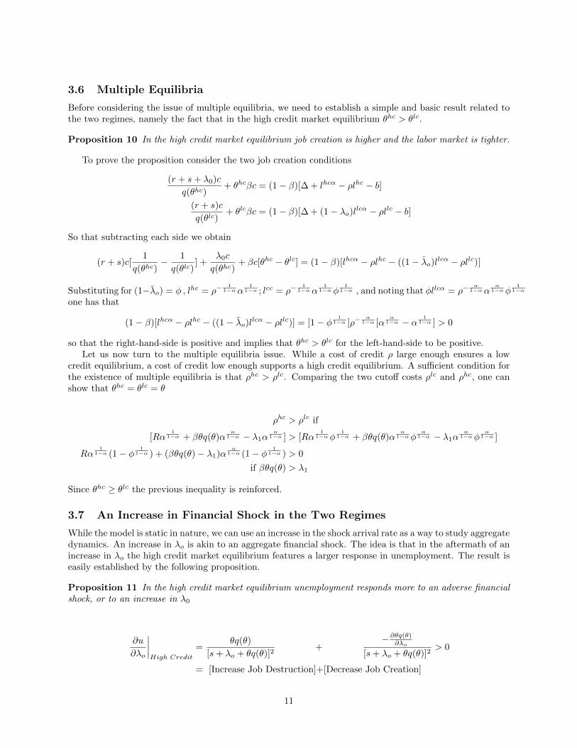
Proposition 11 In the high credit market equilibrium unemployment responds more to an adverse financialshock, or to an increase in λ0
∂u
∂λo
∣∣∣∣High Credit
=θq(θ)
[s+ λo + θq(θ)]2+
−∂θq(θ)∂λo
[s+ λo + θq(θ)]2> 0
= [Increase Job Destruction]+[Decrease Job Creation]
11
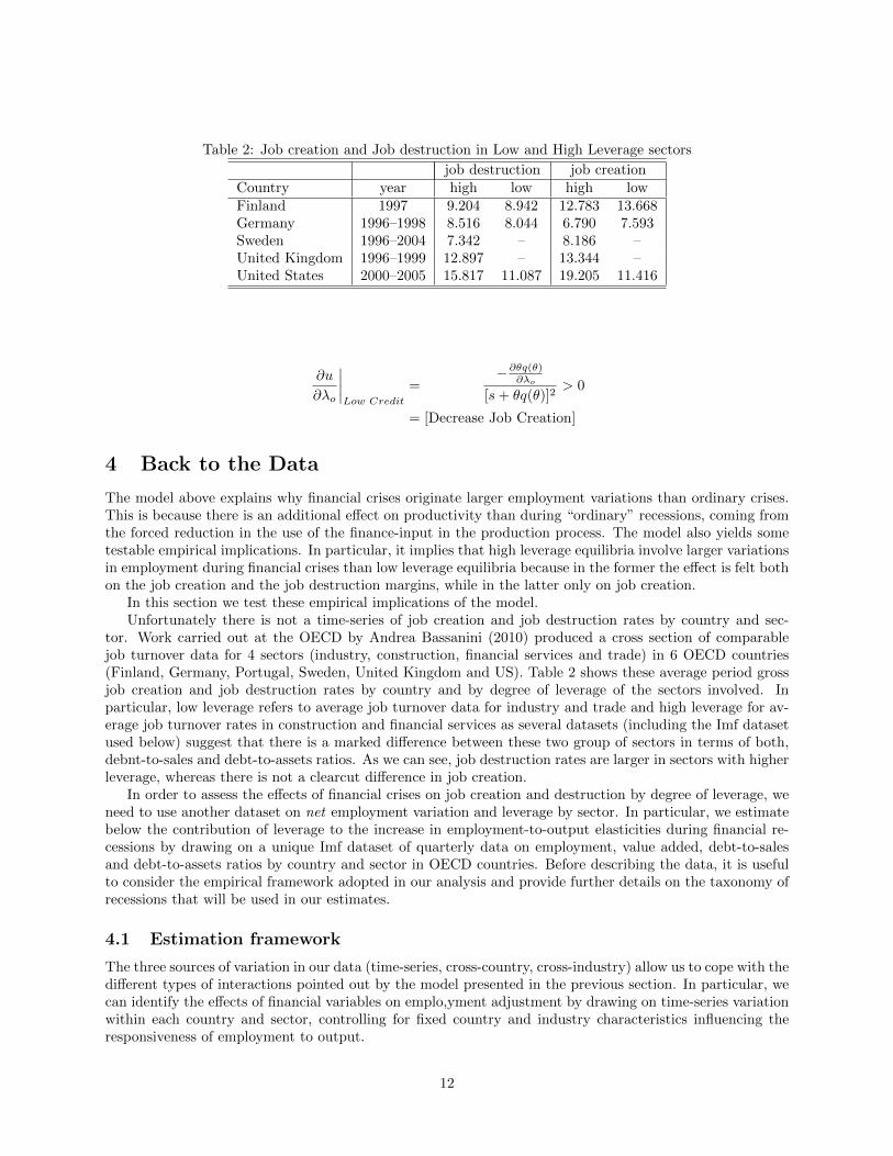
Table 2: Job creation and Job destruction in Low and High Leverage sectors
job destruction job creationCountry year high low high lowFinland 1997 9.204 8.942 12.783 13.668Germany 1996–1998 8.516 8.044 6.790 7.593Sweden 1996–2004 7.342 – 8.186 –United Kingdom 1996–1999 12.897 – 13.344 –United States 2000–2005 15.817 11.087 19.205 11.416
∂u
∂λo
∣∣∣∣Low Credit
=−∂θq(θ)∂λo
[s+ θq(θ)]2> 0
= [Decrease Job Creation]
4 Back to the Data
The model above explains why financial crises originate larger employment variations than ordinary crises.This is because there is an additional effect on productivity than during “ordinary” recessions, coming fromthe forced reduction in the use of the finance-input in the production process. The model also yields sometestable empirical implications. In particular, it implies that high leverage equilibria involve larger variationsin employment during financial crises than low leverage equilibria because in the former the effect is felt bothon the job creation and the job destruction margins, while in the latter only on job creation.
In this section we test these empirical implications of the model.Unfortunately there is not a time-series of job creation and job destruction rates by country and sec-
tor. Work carried out at the OECD by Andrea Bassanini (2010) produced a cross section of comparablejob turnover data for 4 sectors (industry, construction, financial services and trade) in 6 OECD countries(Finland, Germany, Portugal, Sweden, United Kingdom and US). Table 2 shows these average period grossjob creation and job destruction rates by country and by degree of leverage of the sectors involved. Inparticular, low leverage refers to average job turnover data for industry and trade and high leverage for av-erage job turnover rates in construction and financial services as several datasets (including the Imf datasetused below) suggest that there is a marked difference between these two group of sectors in terms of both,debnt-to-sales and debt-to-assets ratios. As we can see, job destruction rates are larger in sectors with higherleverage, whereas there is not a clearcut difference in job creation.
In order to assess the effects of financial crises on job creation and destruction by degree of leverage, weneed to use another dataset on net employment variation and leverage by sector. In particular, we estimatebelow the contribution of leverage to the increase in employment-to-output elasticities during financial re-cessions by drawing on a unique Imf dataset of quarterly data on employment, value added, debt-to-salesand debt-to-assets ratios by country and sector in OECD countries. Before describing the data, it is usefulto consider the empirical framework adopted in our analysis and provide further details on the taxonomy ofrecessions that will be used in our estimates.
4.1 Estimation framework
The three sources of variation in our data (time-series, cross-country, cross-industry) allow us to cope with thedifferent types of interactions pointed out by the model presented in the previous section. In particular, wecan identify the effects of financial variables on emplo,yment adjustment by drawing on time-series variationwithin each country and sector, controlling for fixed country and industry characteristics influencing theresponsiveness of employment to output.
12
Our estimation framework is akin an augmented Okun’s law for employment. In particular, our depen-dent variable is the log variation in employment while, on the right-hand-side we control for fixed countryand sector effects affecting the intercept (hence the minimum level of output growth inducing employmentgrowth), output growth by itself as well as interacted with indicators of financial recessions, leverage ra-tios and time varying institutions potentially affecting the employment responsiveness to output changes.Formally, the model that we estimate is as follows:
∆eijt = αj + αi + β∆yijt[1 + γ1Levijt + γ2FCit + γ3 ∗ FCit ∗ Levijt+δXijt] + εijt
where ∆eijt is log employment variation in country i, sector j at time t, αj and αi denote the coefficients ofsectoral and country dummies respectively, ∆y is the log variation in output, Lev is the leverage ratio (eitherdebt-to-assets or debt-to-sales), FC denotes financial recessions,and X a set of time-varying institutionalvariables potentially affecting the responsiveness of employment to output change. As the literature points toa large number of institutions which may affect labor-finance interactions depending on the degree of leverageof different industries, we also include country–sector dummies. This amounts essentially for identifying theeffect of financial variables on employment adjustment via time-series variation. In some specifications, wealso cluster observations by sector, year and country.
Our key parameter of interest is γ3 denoting the effects of leverage on the Okun’s elasticity during financialrecessions.
A problem with this framework is that the presence of leverage on the righ-hand-side of the estimatedequation poses a potential problem of endogeneity. Firms’ hiring policies are indeed likely to affect the degreeof leverage of firms and this could bias our estimates. We tackle this issue in two ways. In our first empiricalstrategy we parametrize leverage by operating on the distribution of debt-to-assets and debt-to-sales ratiosover the entire period. The alternative strategy is to use current values for the leverage ratios but imposean exclusion restriction, defining variables that are correlated with leverage but not with εijt.
Before turning to our estimates, we need to explain how we identify the recessions considered in ourmodel and provide further details on the data at hand.
4.2 Identifying Credit Shocks
The model has implications related to credit shocks, involving an unexpected reduction in credit flows tofirms. There are two taxonomies of financial crises, we can draw upon in our empirical analysis.
The first taxonomy was also introduced in Section 2 and was developed by Reinhart and Rogoff (2008)(RR henceforth). It captures a relatively large set of recessions involving the financial sector, includinghousing booms-bust sequences. The second taxonomy was developed by Atkinson and Morelli (2011) (AMhenceforth) and is focused only on banking crises, it looks precisely at those shocks that affect access byfirms to liquid assets. Atkinson and Morelli identified 8 banking crisis episodes in some 13 countries in theyears 1965 to 2009. A banking crisis is, according to this definition, one where any of the following threeconditions is met:
1. there are bank runs that lead to the closure, merging, or takeover by the public sector of one or morefinancial institutions;
2. there are no bank runs, but the closure, merging, takeover, or large-scale government assistance of animportant financial institution (or group of institutions), that marks the start of a string of similaroutcomes for other financial institutions;
3. a country’s corporate and financial sectors experience a large number of defaults, and financial insti-tutions and corporations face great difficulties repaying contracts on time.
The first two criteria correspond to those used by Reinhart and Rogoff (2008) (RR henceforth) in theirtaxonomy of crises, while the third one was proposed by Laeven and Valencia (2008).
13
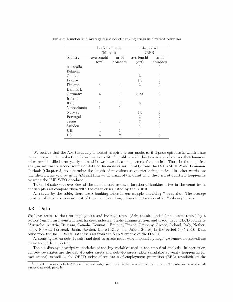
Table 3: Number and average duration of banking crises in different countries
banking crises other crises(Morelli) NBER
country avg lenght nr of avg lenght nr of(qrt) episodes (qrt) episodes
Australia 1 1BelgiumCanada 3 1France 3.5 2Finland 4 1 3 3DenmarkGermany 4 1 3.33 3IrelandItaly 4 1 5 3Netherlands 1 1Norway 3.5 2Portugal 2 2Spain 4 1 2 2Sweden 4 1UK 4 1US 4 2 7 3
We believe that the AM taxonomy is closest in spirit to our model as it signals episodes in which firmsexperience a sudden reduction the access to credit. A problem with this taxonomy is however that financialcrises are identified over yearly data while we have data at quarterly frequencies. Thus, in the empiricalanalysis we used a second source of data on financial crises, notably from the IMF’s 2010 World EconomicOutlook (Chapter 3) to determine the length of recessions at quarterly frequencies. In other words, weidentified a crisis year by using AM and then we determined the duration of the crisis at quarterly frequenciesby using the IMF-WEO database.1.
Table 3 displays an overview of the number and average duration of banking crises in the countries inour sample and compare them with the other crises listed by the NBER.
As shown by the table, there are 8 banking crises in our sample, involving 7 countries. The averageduration of these crises is in most of these countries longer than the duration of an “ordinary” crisis.
4.3 Data
We have access to data on employment and leverage ratios (debt-to-sales and debt-to-assets ratios) by 6sectors (agriculture, construction, finance, industry, public administration, and trade) in 11 OECD countries(Australia, Austria, Belgium, Canada, Denmark, Finland, France, Germany, Greece, Ireland, Italy, Nether-lands, Norway, Portugal, Spain, Sweden, United Kingdom, United States) in the period 1985-2008. Datacome from the IMF—WDI Database and from the STAN archive of the OECD.
As some figures on debt-to-sales and debt-to-assets ratios were implausibly large, we removed observationsabove the 96th percentile.
Table 4 displays descriptive statistics of the key variables used in the empirical analysis. In particular,our key covariates are the debt-to-sales assets and debt-to-assets ratios (available at yearly frequencies foreach sector) as well as the OECD index of strictness of employment protection (EPL) (available at the
1In the few cases in which AM identified a country–year of crisis that was not recorded in the IMF data, we considered allquarters as crisis periods.
14
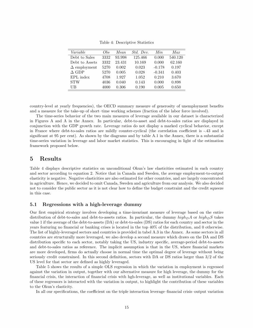
Table 4: Descriptive Statistics
Variable Obs Mean Std. Dev. Min MaxDebt to Sales 3332 93.998 125.466 0.000 540.120Debt to Assets 3332 23.431 10.169 0.000 62.160∆ employment 5270 0.002 0.023 -0.178 0.197∆ GDP 5270 0.005 0.028 -0.341 0.403EPL index 4708 1.927 1.052 0.210 3.670STW 4036 0.040 0.143 0.000 0.898UB 4000 0.306 0.190 0.005 0.650
country-level at yearly frequencies), the OECD summary measure of generosity of unemployment benefitsand a measure for the take-up of short–time working schemes (fraction of the labor force involved).
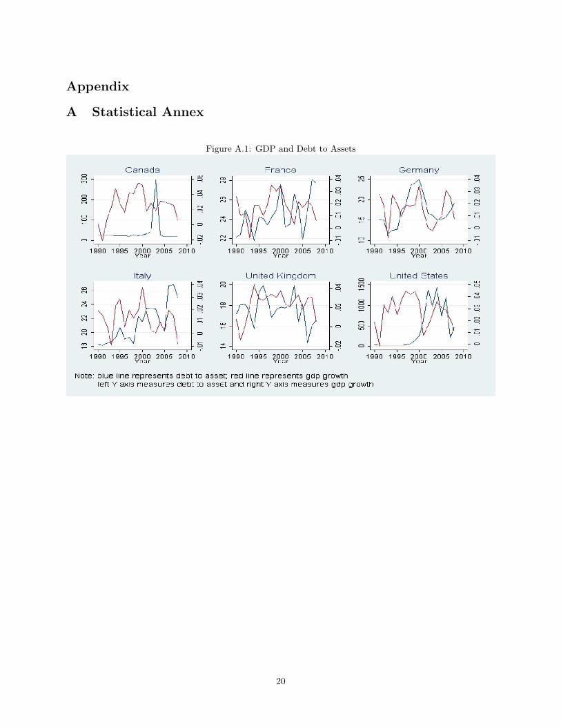
The time-series behavior of the two main measures of leverage available in our dataset is characterizedin Figures A and A in the Annex. In particular, debt-to-asset and debt-to-sales ratios are displayed inconjunction with the GDP growth rate. Leverage ratios do not display a marked cyclical behavior, exceptin France where debt-to-sales ratios are mildly counter-cyclical (the correlation coefficient is -.43 and issignificant at 95 per cent). As shown by the diagrams and by table A.1 in the Annex, there is a substantialtime-series variation in leverage and labor market statistics. This is encouraging in light of the estimationframework proposed below.
5 Results
Table 4 displays descriptive statistics on unconditional Okun’s law elasticities estimated in each countryand sector according to equation 2. Notice that in Canada and Sweden, the average employment-to-outputelasticity is negative. Negative elasticities are also estimated for other countries, and are largely concentratedin agriculture. Hence, we decided to omit Canada, Sweden and agriculture from our analysis. We also decidednot to consider the public sector as it is not clear how to define the budget constraint and the credit squeezein this case.
5.1 Regressions with a high-leverage dummy
Our first empirical strategy involves developing a time-invariant measure of leverage based on the entiredistribution of debt-to-sales and debt-to-assets ratios. In particular, the dummy highDA or highDS takesvalue 1 if the average of the debt-to-assets (DA) or debt-to-sales (DS) ratios for each country and sector in theyears featuring no financial or banking crises is located in the top 40% of the distribution, and 0 otherwise.The list of highly-leveraged sectors and countries is provided in tabel A.3 in the Annex. As some sectors in allcountries are structurally more leveraged, we also develop a second measure which draws on the DA and DSdistribution specific to each sector, notably taking the US, industry specific, average-period debt-to-assetsand debt-to-sales ratios as reference. The implicit assumption is that in the US, where financial marketsare more developed, firms do actually choose in normal time the optimal degree of leverage without beingseriously credit constrained. In this second definition, sectors with DA or DS ratios larger than 3/2 of theUS level for that sector are defined as highly leveraged.
Table 5 shows the results of a simple OLS regression in which the variation in employment is regressedagainst the variation in output, together with our alternative measure for high leverage, the dummy for thefinancial crisis, the interaction of financial crisis with hgh-leverage, as well as institutional variables. Eachof these regressors is interacted with the variation in output, to highlight the contribution of these variablesto the Okun’s elasticity.
In all our specifications, the coefficient on the triple interaction leverage–financial crisis–output variation
15
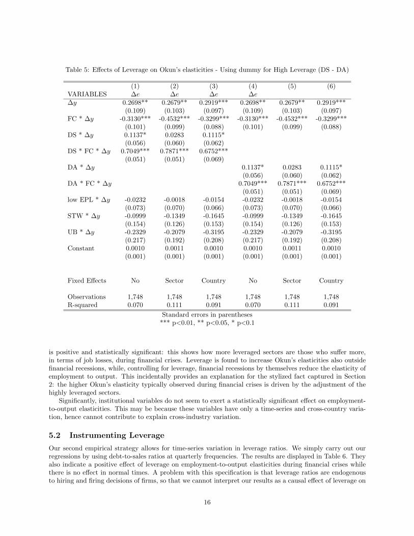
Table 5: Effects of Leverage on Okun’s elasticities - Using dummy for High Leverage (DS - DA)
(1) (2) (3) (4) (5) (6)VARIABLES ∆e ∆e ∆e ∆e∆y 0.2698** 0.2679** 0.2919*** 0.2698** 0.2679** 0.2919***
(0.109) (0.103) (0.097) (0.109) (0.103) (0.097)FC * ∆y -0.3130*** -0.4532*** -0.3299*** -0.3130*** -0.4532*** -0.3299***
(0.101) (0.099) (0.088) (0.101) (0.099) (0.088)DS * ∆y 0.1137* 0.0283 0.1115*
(0.056) (0.060) (0.062)DS * FC * ∆y 0.7049*** 0.7871*** 0.6752***
(0.051) (0.051) (0.069)DA * ∆y 0.1137* 0.0283 0.1115*
(0.056) (0.060) (0.062)DA * FC * ∆y 0.7049*** 0.7871*** 0.6752***
(0.051) (0.051) (0.069)low EPL * ∆y -0.0232 -0.0018 -0.0154 -0.0232 -0.0018 -0.0154
(0.073) (0.070) (0.066) (0.073) (0.070) (0.066)STW * ∆y -0.0999 -0.1349 -0.1645 -0.0999 -0.1349 -0.1645
(0.154) (0.126) (0.153) (0.154) (0.126) (0.153)UB * ∆y -0.2329 -0.2079 -0.3195 -0.2329 -0.2079 -0.3195
(0.217) (0.192) (0.208) (0.217) (0.192) (0.208)Constant 0.0010 0.0011 0.0010 0.0010 0.0011 0.0010
(0.001) (0.001) (0.001) (0.001) (0.001) (0.001)
Fixed Effects No Sector Country No Sector Country
Observations 1,748 1,748 1,748 1,748 1,748 1,748R-squared 0.070 0.111 0.091 0.070 0.111 0.091
Standard errors in parentheses*** p<0.01, ** p<0.05, * p<0.1
is positive and statistically significant: this shows how more leveraged sectors are those who suffer more,in terms of job losses, during financial crises. Leverage is found to increase Okun’s elasticities also outsidefinancial recessions, while, controlling for leverage, financial recessions by themselves reduce the elasticity ofemployment to output. This incidentally provides an explanation for the stylized fact captured in Section2: the higher Okun’s elasticity typically observed during financial crises is driven by the adjustment of thehighly leveraged sectors.
Significantly, institutional variables do not seem to exert a statistically significant effect on employment-to-output elasticities. This may be because these variables have only a time-series and cross-country varia-tion, hence cannot contribute to explain cross-industry variation.
5.2 Instrumenting Leverage
Our second empirical strategy allows for time-series variation in leverage ratios. We simply carry out ourregressions by using debt-to-sales ratios at quarterly frequencies. The results are displayed in Table 6. Theyalso indicate a positive effect of leverage on employment-to-output elasticities during financial crises whilethere is no effect in normal times. A problem with this specification is that leverage ratios are endogenousto hiring and firing decisions of firms, so that we cannot interpret our results as a causal effect of leverage on
16
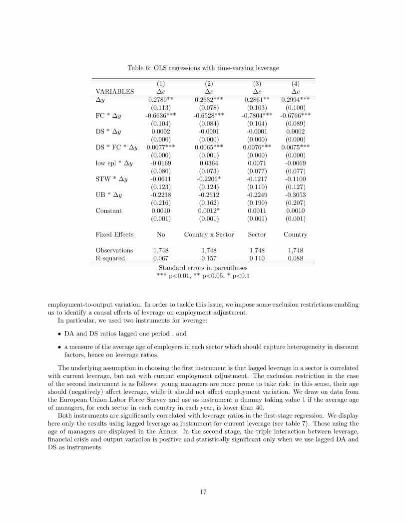
Table 6: OLS regressions with time-varying leverage
(1) (2) (3) (4)VARIABLES ∆e ∆e ∆e ∆e∆y 0.2789** 0.2682*** 0.2861** 0.2994***
(0.113) (0.078) (0.103) (0.100)FC * ∆y -0.6636*** -0.6528*** -0.7804*** -0.6766***
(0.104) (0.084) (0.104) (0.089)DS * ∆y 0.0002 -0.0001 -0.0001 0.0002
(0.000) (0.000) (0.000) (0.000)DS * FC * ∆y 0.0077*** 0.0065*** 0.0076*** 0.0075***
(0.000) (0.001) (0.000) (0.000)low epl * ∆y -0.0169 0.0364 0.0071 -0.0069
(0.080) (0.073) (0.077) (0.077)STW * ∆y -0.0611 -0.2206* -0.1217 -0.1100
(0.123) (0.124) (0.110) (0.127)UB * ∆y -0.2218 -0.2612 -0.2249 -0.3053
(0.216) (0.162) (0.190) (0.207)Constant 0.0010 0.0012* 0.0011 0.0010
(0.001) (0.001) (0.001) (0.001)
Fixed Effects No Country x Sector Sector Country
Observations 1,748 1,748 1,748 1,748R-squared 0.067 0.157 0.110 0.088
Standard errors in parentheses*** p<0.01, ** p<0.05, * p<0.1
employment-to-output variation. In order to tackle this issue, we impose some exclusion restrictions enablingus to identify a causal effects of leverage on employment adjustment.
In particular, we used two instruments for leverage:
• DA and DS ratios lagged one period , and
• a measure of the average age of employers in each sector which should capture heterogeneity in discountfactors, hence on leverage ratios.
The underlying assumption in choosing the first instrument is that lagged leverage in a sector is correlatedwith current leverage, but not with current employment adjustment. The exclusion restriction in the caseof the second instrument is as follows: young managers are more prone to take risk: in this sense, their ageshould (negatively) affect leverage, while it should not affect employment variation. We draw on data fromthe European Union Labor Force Survey and use as instrument a dummy taking value 1 if the average ageof managers, for each sector in each country in each year, is lower than 40.
Both instruments are significantly correlated with leverage ratios in the first-stage regression. We displayhere only the results using lagged leverage as instrument for current leverage (see table 7). Those using theage of managers are displayed in the Annex. In the second stage, the triple interaction between leverage,financial crisis and output variation is positive and statistically significant only when we use lagged DA andDS as instruments.
17
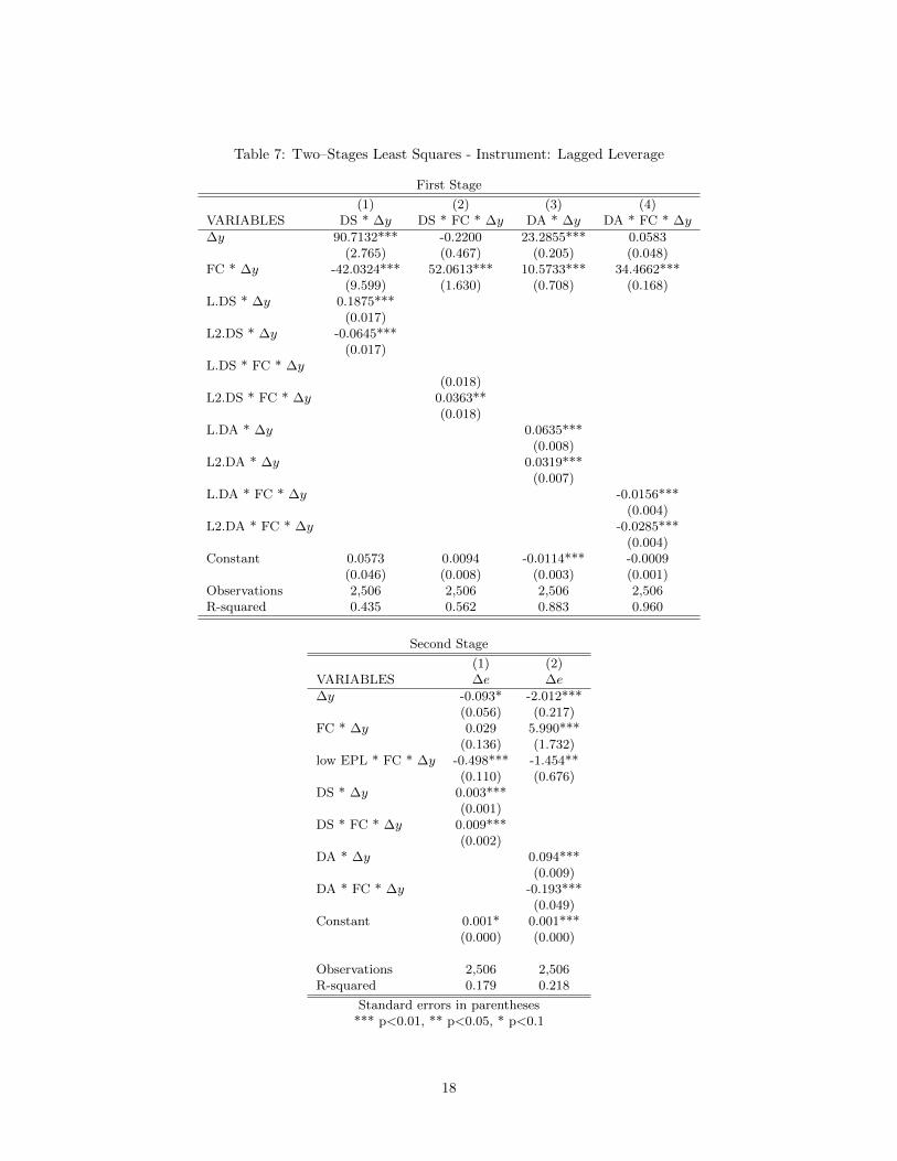
Table 7: Two–Stages Least Squares - Instrument: Lagged Leverage
First Stage
(1) (2) (3) (4)VARIABLES DS * ∆y DS * FC * ∆y DA * ∆y DA * FC * ∆y
∆y 90.7132*** -0.2200 23.2855*** 0.0583(2.765) (0.467) (0.205) (0.048)
FC * ∆y -42.0324*** 52.0613*** 10.5733*** 34.4662***(9.599) (1.630) (0.708) (0.168)
L.DS * ∆y 0.1875***(0.017)
L2.DS * ∆y -0.0645***(0.017)
L.DS * FC * ∆y(0.018)
L2.DS * FC * ∆y 0.0363**(0.018)
L.DA * ∆y 0.0635***(0.008)
L2.DA * ∆y 0.0319***(0.007)
L.DA * FC * ∆y -0.0156***(0.004)
L2.DA * FC * ∆y -0.0285***(0.004)
Constant 0.0573 0.0094 -0.0114*** -0.0009(0.046) (0.008) (0.003) (0.001)
Observations 2,506 2,506 2,506 2,506R-squared 0.435 0.562 0.883 0.960
Second Stage
(1) (2)VARIABLES ∆e ∆e
∆y -0.093* -2.012***(0.056) (0.217)
FC * ∆y 0.029 5.990***(0.136) (1.732)
low EPL * FC * ∆y -0.498*** -1.454**(0.110) (0.676)
DS * ∆y 0.003***(0.001)
DS * FC * ∆y 0.009***(0.002)
DA * ∆y 0.094***(0.009)
DA * FC * ∆y -0.193***(0.049)
Constant 0.001* 0.001***(0.000) (0.000)
Observations 2,506 2,506R-squared 0.179 0.218
Standard errors in parentheses*** p<0.01, ** p<0.05, * p<0.1
18
6 Final Remarks
Empirical evidence suggests that financial shocks have important implications on labor market adjustment.This paper develops a simple model indicating that in highly leveraged equilibria there is not only a negativeeffect of recessions on job creation, but also an additional effect of financial shocks on the job destructionmargin. We use a variety of datasets to test the implications of the model. We find that highly leveragedsectors are characterised by higher job destruction rates than low-leveraged sectors and that higher debt-to-sales or debt-to-assets ratios are associated with higher employment-to-output elasticities during bankingcrises. If our identification assumptions are considered plausible, the relationship between leverage andemployment adjustment can be interpreted as a causal effect.
References
[1] Ansgar, Belke, and Rainer Fehn, 2001, “Institutions and Structural Unemployment: Do Capital-MarketImperfections Matter?,” Vienna Economics Papers 0106, University of Vienna, Department of Economics.
[2] Bernanke, Ben, and Mark Gertler, 1989, “Agency Costs, Net Worth and Business Fluctuations,” Amer-ican Economic Review, Vol. 79 (March), pp. 14–31.
[3] Bertola, Giuseppe, and Richard Rogerson, 1997 “Institutions and labor reallocation,”European EconomicReview, 41(6): 1147-1171.
[4] Reinhart, Carmen, and Kenneth Rogoff, 2008, “Is the 2007 U.S. Sub-Prime Crisis So Different? An Inter-national Historical Comparison,” NBER Working Paper No.13761 (Cambridge, Massachusetts: NationalBureau of Economic Research).
[5] Gatti, Donatella, Rault, Christophe, and Anne–Gael Vaubourg, 2009, “Unemployment and Finance: Howdo Financial and Labour Market Factors Interact?,“CESifo Working Paper Series 2901, CESifo GroupMunich.
[6] Koskela, Erkki, and Rune Stenbacka, 2001, “Equilibrium Unemployment with Credit and Labour MarketImperfections, ”Bank of Finland Discussion Paper n. 5.
[7] Monacelli,Tommaso, Quadrini, Vincenzo, and Antonella Trigari, 2011, “Financial Markets and Unem-ployment,”NBER Working Papers 17389, National Bureau of Economic Research, Inc.
[8] Rendon, Sılvio, 2006, “Job Search And Asset Accumulation Under Borrowing Constraints, ” InternationalEconomic Review (Institute of Social and Economic Research Association), vol. 47(1): 233-263.
[9] Wasmer, Etienne, and Philippe Weil, 2004, “The Macroeconomics of Labor and Credit Market Imper-fections,” American Economic Review (American Economic Association), 94(4): 944–963.
19
Appendix
A Statistical Annex
Figure A.1: GDP and Debt to Assets
20
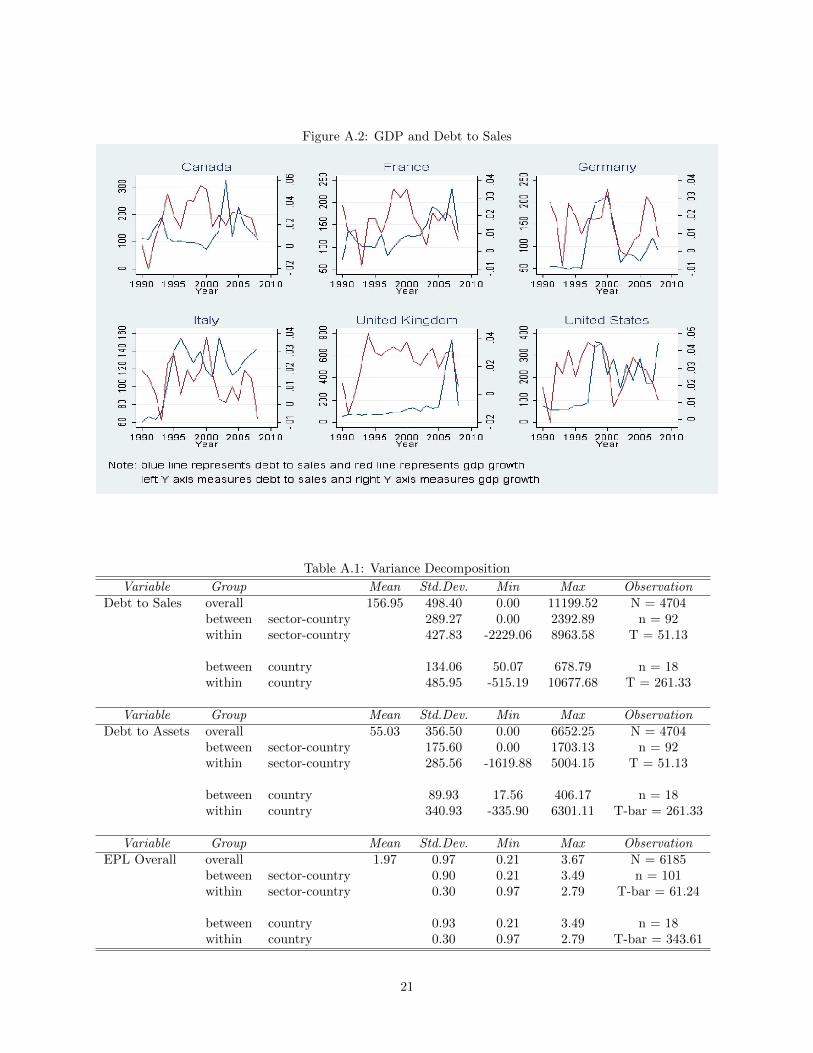
Figure A.2: GDP and Debt to Sales
Table A.1: Variance Decomposition
Variable Group Mean Std.Dev. Min Max ObservationDebt to Sales overall 156.95 498.40 0.00 11199.52 N = 4704
between sector-country 289.27 0.00 2392.89 n = 92within sector-country 427.83 -2229.06 8963.58 T = 51.13
between country 134.06 50.07 678.79 n = 18within country 485.95 -515.19 10677.68 T = 261.33
Variable Group Mean Std.Dev. Min Max ObservationDebt to Assets overall 55.03 356.50 0.00 6652.25 N = 4704
between sector-country 175.60 0.00 1703.13 n = 92within sector-country 285.56 -1619.88 5004.15 T = 51.13
between country 89.93 17.56 406.17 n = 18within country 340.93 -335.90 6301.11 T-bar = 261.33
Variable Group Mean Std.Dev. Min Max ObservationEPL Overall overall 1.97 0.97 0.21 3.67 N = 6185
between sector-country 0.90 0.21 3.49 n = 101within sector-country 0.30 0.97 2.79 T-bar = 61.24
between country 0.93 0.21 3.49 n = 18within country 0.30 0.97 2.79 T-bar = 343.61
21
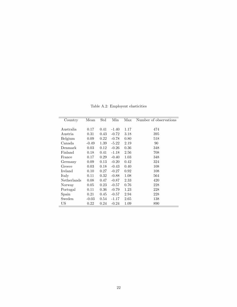
Table A.2: Employent elasticities
Country Mean Std Min Max Number of observations
Australia 0.17 0.41 -1.40 1.17 474Austria 0.31 0.43 -0.72 3.18 395Belgium 0.09 0.22 -0.78 0.80 518Canada -0.49 1.39 -5.22 2.19 90Denmark 0.03 0.12 -0.26 0.36 348Finland 0.18 0.41 -1.18 2.56 708France 0.17 0.29 -0.40 1.03 348Germany 0.09 0.13 -0.20 0.42 324Greece 0.03 0.18 -0.43 0.40 108Ireland 0.10 0.27 -0.27 0.92 108Italy 0.11 0.32 -0.88 1.08 564Netherlands 0.08 0.47 -0.87 2.33 420Norway 0.05 0.23 -0.57 0.76 228Portugal 0.11 0.36 -0.79 1.23 228Spain 0.21 0.45 -0.57 2.94 228Sweden -0.03 0.54 -1.17 2.65 138US 0.22 0.24 -0.24 1.09 890
22
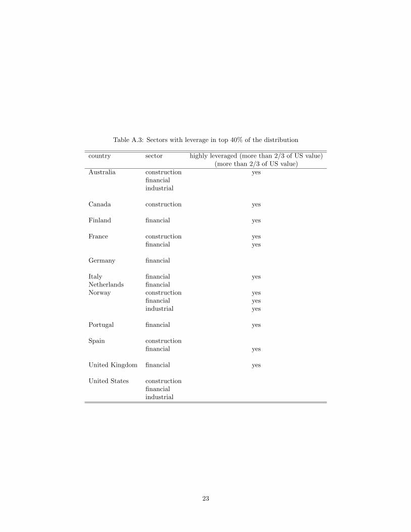
Table A.3: Sectors with leverage in top 40% of the distribution
country sector highly leveraged (more than 2/3 of US value)(more than 2/3 of US value)
Australia construction yesfinancialindustrial
Canada construction yes
Finland financial yes
France construction yesfinancial yes
Germany financial
Italy financial yesNetherlands financialNorway construction yes
financial yesindustrial yes
Portugal financial yes
Spain constructionfinancial yes
United Kingdom financial yes
United States constructionfinancialindustrial
23
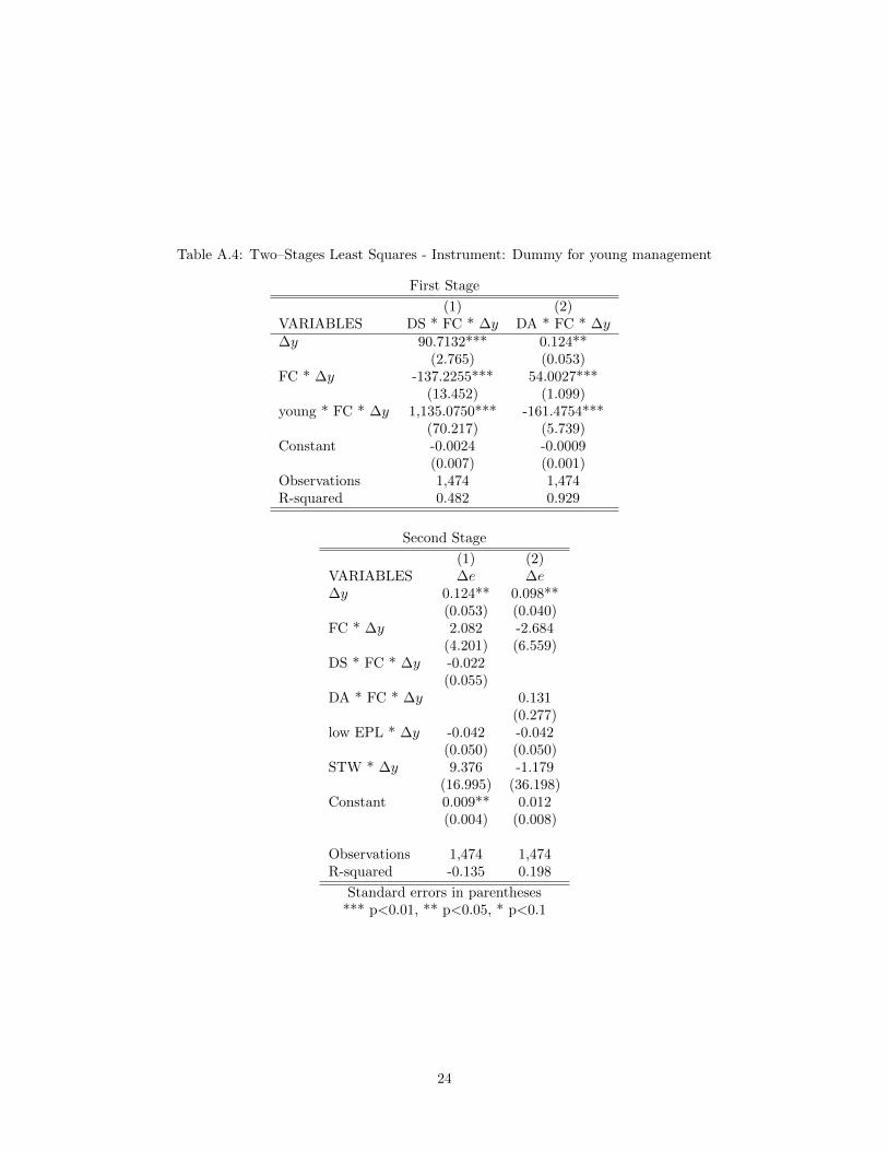
Table A.4: Two–Stages Least Squares - Instrument: Dummy for young management
First Stage
(1) (2)VARIABLES DS * FC * ∆y DA * FC * ∆y∆y 90.7132*** 0.124**
(2.765) (0.053)FC * ∆y -137.2255*** 54.0027***
(13.452) (1.099)young * FC * ∆y 1,135.0750*** -161.4754***
(70.217) (5.739)Constant -0.0024 -0.0009
(0.007) (0.001)Observations 1,474 1,474R-squared 0.482 0.929
Second Stage
(1) (2)VARIABLES ∆e ∆e∆y 0.124** 0.098**
(0.053) (0.040)FC * ∆y 2.082 -2.684
(4.201) (6.559)DS * FC * ∆y -0.022
(0.055)DA * FC * ∆y 0.131
(0.277)low EPL * ∆y -0.042 -0.042
(0.050) (0.050)STW * ∆y 9.376 -1.179
(16.995) (36.198)Constant 0.009** 0.012
(0.004) (0.008)
Observations 1,474 1,474R-squared -0.135 0.198
Standard errors in parentheses*** p<0.01, ** p<0.05, * p<0.1
24