Geometric Complexity Theoryand Orbit Closures of Homogeneous Forms

vorgelegt von

Diplom-Mathematiker

Jesko Hüttenhain

aus Siegen

Von der Fakultät II - Mathematik und Naturwissenschaftender Technischen Universität Berlin

zur Erlangung des akademischen GradesDoktor der Naturwissenschaften

Dr. rer. nat.

genehmigte Dissertation

Promotionsausschuss

Vorsitzender : Prof. Dr. Jörg LiesenGutachter : Prof. Dr. Peter BürgisserGutachter : Prof. Dr. Giorgio Ottaviani

Tag der wissenschaftlichen Aussprache: 3. Juli 2017

Berlin 2017

Niemals aufgeben, niemals kapitulieren.— Peter Quincy Taggart

Deutsche Einleitung

Das P-NP-Problem gehört zu den fundamentalsten und faszinierensten Problemen derheutigen Mathematik. Es hat umfangreiche Bedeutung für praktische Anwendungenund ist gleichermaßen eine grundsätzliche Frage über die Natur der Mathematik ansich. Wäre unerwartet P = NP, so könnte etwa ein Computer effizient bestimmen,ob eine mathematische Aussage wahr oder falsch ist. Seit die Frage 1971 von Cook[Coo71] gestellt wurde, scheinen wir einer Antwort jedoch nicht nennenswert nähergekommen zu sein. Der größte Fortschritt ist das ernüchternde Resultat von Razborovund Rudich [RR97], dass es keine „natürlichen“ Beweise für P = NP geben kann, siehederen Arbeit für eine Definition und Details.

Peter Bürgisser hat gezeigt [Bü00], dass unter der verallgemeinerten Riemann-Hypothese die nicht-uniforme Version von P = NP eine Vermutung von Valiant im-pliziert, welche weithin als ein algebraisches Analogon betrachtet wird. Diese Vermu-tung ist ein ebenso offenes Problem wie das ursprüngliche, doch es gibt die Hoffnung,dass die zusätzliche algebraische Struktur mehr Ansatzpunkte liefert. Wir geben einenkurzen Überblick über die zugrundeliegende Theorie in Kapitel 1: Die besagte Ver-mutung von Valiant (Vermutung 1.4.5) ist die zentrale Motivation für die hier vorge-stellten Forschungsergebnisse.

In Kapitel 2 verschärfen wir ein Resultat von Valiant indem wir zeigen, dass sichjedes ganzzahlige Polynom stets als Determinante einer Matrix schreiben lässt, de-ren Einträge nur Variablen, Nullen und Einsen sind. The Größe der kleinsten solchenMatrix ist ein sinnvolles Komplexitätsmaß, welches sich rein kombinatorisch untersu-chen lässt. Als Anwendung beweisen wir untere Schranken in kleinen Fällen durchComputerberechnung.

Von hier an widmen wir uns einem Ansatz zum Beweis von Valiant’s Vermutung,welcher 2001 von Mulmuley und Sohoni vorgestellt wurde und den Titel „GeometricComplexity Theory“ trägt, oder auch kurz GCT. Valiants Ergebnisse werden hier inAussagen der Algebraischen Geometrie und Darstellungstheorie übersetzt, um da-durch die Probleme vorheriger Ansätze zu vermeiden [For09]. Eine Zusammenfas-sung dieses interessanten Übersetzungsprozesses ist in Kapitel 3 zu finden.

iii

Um Komplexitätsklassen voneinander zu trennen, muss bewiesen werden, dasskein effizienter Algorithmus für ein mutmaßlich schweres Problem existiert. GCT lie-fert ein Kriterium, wonach die Existenz gewisser ganzzahliger Vektoren schon dieseTrennung impliziert. Solche Vektoren nennen wir auch Obstruktionen. Die Hoffnungvon Mulmuley und Sohoni war, dass man sich für den Beweis von Valiants Vermu-tung auf eine bestimmte Art von Obstruktionen beschränken kann, doch wir konn-ten bereits 2015 bemerken, dass es starke Anzeichen dagegen gibt. Wir stellen dieseErgebnisse in Kapitel 4 vor. Erst kürzlich haben Bürgisser, Ikenmeyer und Panovaschlussendlich gezeigt, dass diese sogenannten occurrence obstructions nicht ausrei-chen, um Valiants Vermutung zu beweisen.

Im zweiten Teil der Arbeit beschäftigen wir uns näher und in größerer Allgemein-heit mit einem der zentralen Konzepte von GCT: Wir betrachten die Wirkung der GLn

auf dem Raum der homogenen, n-variaten Polynome vom Grad d durch Verkettungvon rechts und beobachten, dass alle Elemente einer Bahn imWesentlichen die gleicheBerechnungskomplexität haben. Man ordnet einem Polynom P das kleinste d zu, sodass P im Bahnabschluss des d× d – Determinantenpolynoms liegt. Diese Kennzahlist dann äquivalent zu Valiants ursprünglichem Komplexitätsmaß für Polynome, so-fern auch Approximationen zugelassen werden. Die Geometrie des Bahnabschlussesder Determinante ist wenig verstanden, sogar für kleine Werte von d. Wir können al-lerdings die im Rand auftretenden Komponenten für d = 3 vollständig klassifizieren.

Die benötigten algebraischen und geometrischen Werkzeuge werden im einfüh-renden Kapitel 5 vorgestellt. Bahnabschlüsse von homogenen Formen sind stets al-gebraische Varietäten mit der oben genannten GLn-Wirkung und werden klassischin der geometrischen Invariantentheorie studiert. Neben der Determinante beschäfti-gen wir uns in den darauffolgenden Kapiteln auch mit den Bahnabschlüssen andererhomogener Formen.

In Kapitel 6 behandeln wir das allgemeine Monom x1 · · · xd, dessen Relevanz fürGCT daher stammt, dass es auch als Einschränkung des Determinantenpolynoms aufDiagonalmatrizen verstanden werden kann. Das Studium seines Bahnabschlusses istbeispielsweise das zentrale Hilfsmittel in Kapitel 4. Wir bemerken in diesem Kapitel,dass das Monom die seltene Eigenschaft hat, dass jedes Polynom in seinem Bahnab-schluss lediglich das Ergebnis einer Variablensubstitution ist. Eine Klassifikation allerPolynome mit dieser Eigenschaft bleibt offen, obwohl wir einige Fragen im Hinblickdarauf beantworten können.

Wir stellen für die beiden abschließenden Kapitel noch weitere Techniken in Kapi-tel 7 vor. Maßgeblich ist eine obere Schranke für die Anzahl irreduzibler Komponen-ten des Randes eines Bahnabschlusses. Die erste Anwendung dieser Aussage lieferteine Beschreibung des Randes für det3 in Kapitel 8. Wir bestimmen hier auch denStabilisator der Determinante einer allgemeinen, spurlosen Matrix und können so

iv

schlussfolgern, dass der Bahnabschluss dieses Polynoms stets eine Komponente imRand des Bahnabschlusses der Determinante ist.

Das letzte Kapitel enthält bisher unveröffentlichte Ergebnisse über das allgemeineBinom x1 · · · xd + y1 · · · yd. Wie auch das Monom ist das Binom im Bahnabschlussvon detd enthalten. Ein solides Verständnis dieser Familie homogener Formen solltedaher Voraussetzung dafür sein, den Bahnabschluss des Determinantenpolynoms imAllgemeinen zu studieren. Die hier aufkommenden geometrischen Fragen sind bereitsdeutlich komplexer als im Fall des Monoms: Wir können zwei Komponenten desRandes im Detail beschreiben, müssen jedoch eine subtile Frage offen lassen. Soferndiese sich positiv beantworten lässt, erhalten wir jedoch so bereits eine vollständigeBeschreibung des Randes.

v

Contents

Acknowledgements 1

Introduction 3

I Geometric Complexity Theory 7

1 Algebraic Complexity Theory 91.1 Arithmetic Circuits . . . . . . . . . . . . . . . . . . . . . . . . . . . . . . . 91.2 The Classes VP and P . . . . . . . . . . . . . . . . . . . . . . . . . . . . . 121.3 Reduction and Completeness . . . . . . . . . . . . . . . . . . . . . . . . . 131.4 The Classes VNP and NP . . . . . . . . . . . . . . . . . . . . . . . . . . . 141.5 Determinant Versus Permanent . . . . . . . . . . . . . . . . . . . . . . . . 16

2 Binary Determinantal Complexity 212.1 The Cost of Computing Integers . . . . . . . . . . . . . . . . . . . . . . . 222.2 Lower Bounds . . . . . . . . . . . . . . . . . . . . . . . . . . . . . . . . . . 262.3 Uniqueness of Grenet’s construction in the 7× 7 case . . . . . . . . . . . 292.4 Algebraic Complexity Classes . . . . . . . . . . . . . . . . . . . . . . . . . 302.5 Graph Constructions for Polynomials . . . . . . . . . . . . . . . . . . . . 31

3 Geometric Complexity Theory 353.1 Orbit and Orbit Closure as Complexity Measure . . . . . . . . . . . . . . 353.2 Border Complexity . . . . . . . . . . . . . . . . . . . . . . . . . . . . . . . 373.3 The Flip via Obstructions . . . . . . . . . . . . . . . . . . . . . . . . . . . 393.4 Orbit and Orbit Closure . . . . . . . . . . . . . . . . . . . . . . . . . . . . 41

4 Occurrence Obstructions 454.1 Weight Semigroups . . . . . . . . . . . . . . . . . . . . . . . . . . . . . . . 454.2 Saturations of Weight Semigroups of Varieties . . . . . . . . . . . . . . . 474.3 Proof of Main Results . . . . . . . . . . . . . . . . . . . . . . . . . . . . . 49

vii

II Orbit Closures of Homogeneous Forms 55

5 Preliminaries 575.1 Conciseness . . . . . . . . . . . . . . . . . . . . . . . . . . . . . . . . . . . 585.2 Grading of Coordinate Rings and Projectivization . . . . . . . . . . . . . 605.3 Rational Orbit Map . . . . . . . . . . . . . . . . . . . . . . . . . . . . . . . 61

6 Closed Forms 656.1 A Sufficient Criterion . . . . . . . . . . . . . . . . . . . . . . . . . . . . . . 656.2 Normalizations of Orbit Closures . . . . . . . . . . . . . . . . . . . . . . . 676.3 Proof of Main Theorem . . . . . . . . . . . . . . . . . . . . . . . . . . . . 71

7 Techniques for Boundary Classification 777.1 Approximating Degenerations . . . . . . . . . . . . . . . . . . . . . . . . 777.2 The Lie Algebra Action . . . . . . . . . . . . . . . . . . . . . . . . . . . . . 807.3 Resolving the Rational Orbit Map . . . . . . . . . . . . . . . . . . . . . . 82

8 The 3 by 3 Determinant Polynomial 898.1 Construction of Two Components of the Boundary . . . . . . . . . . . . 908.2 There Are Only Two Components . . . . . . . . . . . . . . . . . . . . . . 918.3 The Traceless Determinant . . . . . . . . . . . . . . . . . . . . . . . . . . . 968.4 The Boundary of the 4× 4 Determinant . . . . . . . . . . . . . . . . . . . 102

9 The Binomial 1079.1 Stabilizer and Maximal Linear Subspaces . . . . . . . . . . . . . . . . . . 1089.2 The First Boundary Component . . . . . . . . . . . . . . . . . . . . . . . 1109.3 The Second Boundary Component . . . . . . . . . . . . . . . . . . . . . . 1169.4 The Indeterminacy Locus . . . . . . . . . . . . . . . . . . . . . . . . . . . 118

III Appendix 123

A Algebraic Groups and Representation Theory 125A.1 Algebraic Semigroups and Groups . . . . . . . . . . . . . . . . . . . . . . 125A.2 Representation Theory of Reductive Groups . . . . . . . . . . . . . . . . 130A.3 Polynomial Representations . . . . . . . . . . . . . . . . . . . . . . . . . . 139

Bibliography 141

List of Symbols 149

Index 153

viii

Acknowledgements

I had the immense privilege to work in the most comfortable scientific environmentimaginable, having both the freedom to pursue my interests and the support of myadvisor, Peter Bürgisser. I want to thank him heartily for providing this and alsofor the many things that I learned from him. Researching under these great con-ditions was also made possible by the grants BU 1371/2-2 and BU 1371/3-2 of theDeutsche Forschungsgemeinschaft. Their support is highly appreciated. In late 2014 Iparticipated in the program on Algorithms and Complexity in Algebraic Geometry at theSimons Institute with great benefit. I am very grateful for this opportunity and extendmy thanks to the organizers Peter Bürgisser, Joseph Landsberg, Ketan Mulmuley andBernd Sturmfels.

I also had the pleasure to enjoy the company of extraordinary colleagues, two ofwhich are also my coauthors. I thank Christian Ikenmeyer and Pierre Lairez for theconfusion we shared, the time we spent pondering and the insights we could claimtogether.

My parents have given me more than words could ever say, and my gratitude forall their love and support is eternal.

Ever since a memorable chess game in late 2004, I am part of a friendship thatparticularly sustained me throughout the years. I want to thank Nikolai Nowaczykfor sharing it with me – across time, space, and the fall of empires.

1

Introduction

The P vs. NP problem is among the deepest and most intriguing questions of math-ematics today. While having a multitude of implications for practical applications, italso carries fundamental questions in its wake, about the nature of mathematics itself.If for example P = NP would hold unexpectedly, then we could program a machineto efficiently determine the truth of mathematical statements. Introduced in 1971 byCook [Coo71], the problem is already 46 years old and we seem as far from the so-lution as ever. The most notable progress so far is the sobering result by Razborovand Rudich [RR97] that no “natural” proof for P = NP exists, see their work for adefinition and details.

Peter Bürgisser has shown [Bü00] that the nonuniform version of P = NP im-plies, under the generalized Riemann hypothesis, a conjecture by Valiant which iswidely considered an algebraic analogue. It remains as unresolved as the former,even though the additional algebraic structure involved is believed to provide betterpoints of vantage. We give a brief review of the underlying theory in Chapter 1 – Itis the said conjecture by Valiant (Conjecture 1.4.5) that serves as motivation for theresearch presented herein.

In Chapter 2, we slightly strengthen a result by Valiant: The core observation isthat integer polynomials can always be written as the determinant of a matrix whoseentries are variables, zeros and ones. The size of the smallest such matrix then gives areasonable complexity measure which at the same time is accessible to combinatorics.As an application, we can provide lower bounds in small cases by computationalmethods.

From there on, we are concerned with a recent approach to Valiant’s Conjectureknown as Geometric Complexity Theory, or GCT for short. Introduced in 2001 byMulmuley and Sohoni, it avoids the difficulties of many previous attempts [For09] bytranslating Valiant’s results to statements in algebraic geometry and representationtheory. An outline of this enticing transition is given in Chapter 3.

Where complexity theory is clasically concerned with proving the nonexistence ofgood algorithms for supposedly hard problems, GCT provides a criterion whereby the

3

existence of certain integer vectors implies a separation of complexity classes. We referto the vectors in question simply as obstructions. It was the hope of Mulmuley andSohoni that the search could be further restricted to a particular kind of obstructions,but we already observed in 2015 that this appears unlikely – we present these resultsin Chapter 4. Quite recently in 2016 it was shown by Bürgisser, Ikenmeyer, andPanova that indeed these so-called occurrence obstructions do not suffice to proveValiant’s Conjecture, representing a bitter setback for the programme.

For the second part of the thesis, we treat a central topic of GCT in more detail andgenerality: One can measure the approximate complexity of polynomials by studyingthe closure of their orbit under the action of a general linear group by precomposi-tion. The smallest d for which a polynomial appears in the orbit closure of the d× ddeterminant polynomial is equivalent to Valiant’s original measure for its complexity,if approximations are permitted. The geometry of the determinant orbit closure islittle understood even for small values of d, but we can give a classification of thecomponents that appear in the boundary for d = 3.

The required toolbox of geometric and algebraic techniques is introduced in thepreliminary Chapter 5. Quite generally, the orbit closure of a homogeneous form is analgebraic variety with a GLn-action which is both intuitive and yet incredibly intrigu-ing, and is an object of study to the beautiful fields of classical geometric invarianttheory and birational geometry. In the subsequent chapters we study this problem forother homogeneous forms than the determinant.

Chapter 6 deals with a polynomial that has appeared in the context of GCT before,namely the universal monomial x1 · · · xd. Its orbit closure is contained in the orbitclosure of detd and was instrumental in proving the results of Chapter 4, for example.It also has the remarkable and rare property that every polynomial in its orbit closureis the result of a variable substitution. A classification of all polynomials with thisproperty remains open, but we both answer and pose several questions to advance it.

In Chapter 7, we introduce additional techniques used in the two subsequent chap-ters: We bound the number of irreducible components of the orbit closure boundaryby the number of smooth blowups required to resolve the indeterminacy of a relatedrational map.

The first application of this technique yields a classification of the boundary of det3in Chapter 8. Here, we also describe the stabilizer group of the determinant of ageneric traceless matrix and conclude that the orbit closure of this polynomial isalways a codimension one component of the boundary of the orbit closure of thedeterminant.

The final chapter contains unpublished work on the universal sum of two mono-mials, the binomial x1 · · · xd + y1 · · · yd. Like the monomial, the binomial is containedin the orbit closure of detd. A firm understanding of this polynomial should therefore

4

precede the study of general determinantal expressions. The binomial already givesrise to a significantly more involved geometry than the monomial. We can describetwo components of the boundary in detail, but must leave a subtle question open. Ifsaid question could be answered affirmatively however, these two components con-stitute the entire boundary of the orbit closure of the binomial.

5

Part I

Geometric Complexity Theory

7

Chapter 1Algebraic Complexity Theory

The following is only the briefest of summaries: Complexity theory analyzes thecomplexity of solving problems. Problems have instances of different sizes which canbe solved by algorithms. Denoting by t(m) the minimum number of steps performedby any algorithm that solves all instances of size m, the complexity of a problem isthe function t : N → N. The definitions of “problem”, “algorithm” and related notionsis encompassed by a model of computation. The classical model of computation isthe Turing machine, which mimics our present-day computers. Liberally quoting thefamous Church-Turing thesis, any problem that we consider computationally solvableis solvable by a Turing machine. This generality comes at a price, however: The Turingmodel provides very little mathematical structure to be exploited.

In this chapter, we explore the algebraic model, where a problem is given as afamily of polynomial functions and the goal is quite simply to evaluate them.

1.1 Arithmetic Circuits

×

+

x y

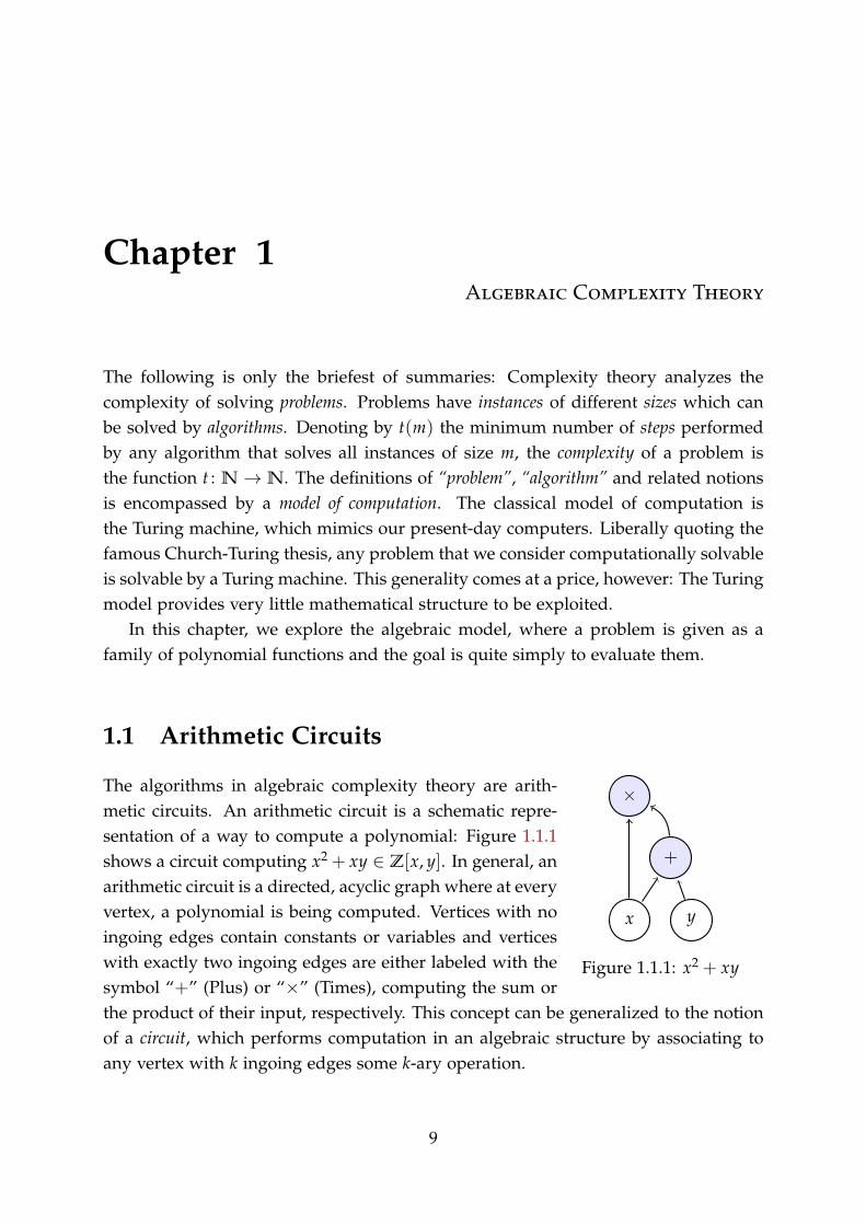
Figure 1.1.1: x2 + xy

The algorithms in algebraic complexity theory are arith-metic circuits. An arithmetic circuit is a schematic repre-sentation of a way to compute a polynomial: Figure 1.1.1shows a circuit computing x2 + xy ∈ Z[x, y]. In general, anarithmetic circuit is a directed, acyclic graph where at everyvertex, a polynomial is being computed. Vertices with noingoing edges contain constants or variables and verticeswith exactly two ingoing edges are either labeled with thesymbol “+” (Plus) or “×” (Times), computing the sum orthe product of their input, respectively. This concept can be generalized to the notionof a circuit, which performs computation in an algebraic structure by associating toany vertex with k ingoing edges some k-ary operation.

9

1.1.1 Definition. Let R be a commutative ring and R[x] the polynomial ring over Rin a countably infinite set of variables x. An arithmetic circuit over R is a directedacyclic graph C with vertex labels, subject to the following conditions:

(1) The vertices with no incoming edges are labelled with elements of R ∪ x. Anysuch vertex is called an input gate.

(2) Since C is acyclic, every vertex of C has a well-defined depth, which is the lengthof a longest path from an input gate to it. Any vertex of positive depth has exactlytwo incoming edges and is labelled with an element of +,×. Any such vertexis also called a computation gate.

We define P(v) ∈ R[x] for every vertex v recursively by depth, as follows: If v is aninput gate, P(v) is defined to be the label of v. Otherwise, let ∗v ∈+,× be the labelof v and denote by u and w the source vertices of the two incoming edges of v. Then,we can define P(v) := P(u) ∗v P(w).

The circuit C computes an element P ∈ R[x] if there is a vertex v with P = P(v).The size of C is the number of computation gates, denoted by |C|.

1.1.2 Example. In Figure 1.1.2, we give an example of an arithmetic circuit over C

which computes the equation of an affine elliptic curve in the variablesx, y.

+

+

×

+

×

××

−1 x y

Figure 1.1.2: An arithmetic circuit computing y2 + xy− x3 − 1.

1.1.3 Definition. Let R be a commutative ring. The (circuit) complexity of a poly-nomial P with coefficients in R is the minimum size of an arithmetic circuit over Rwhich computes P. We denote this number by ccR(P).

10

It should be emphasized that complexity theory does not study the complexity ofsingle polynomials. Instead, the object of study are families of polynomials. This isthe main reason why it is convenient to work with infinitely many variables.

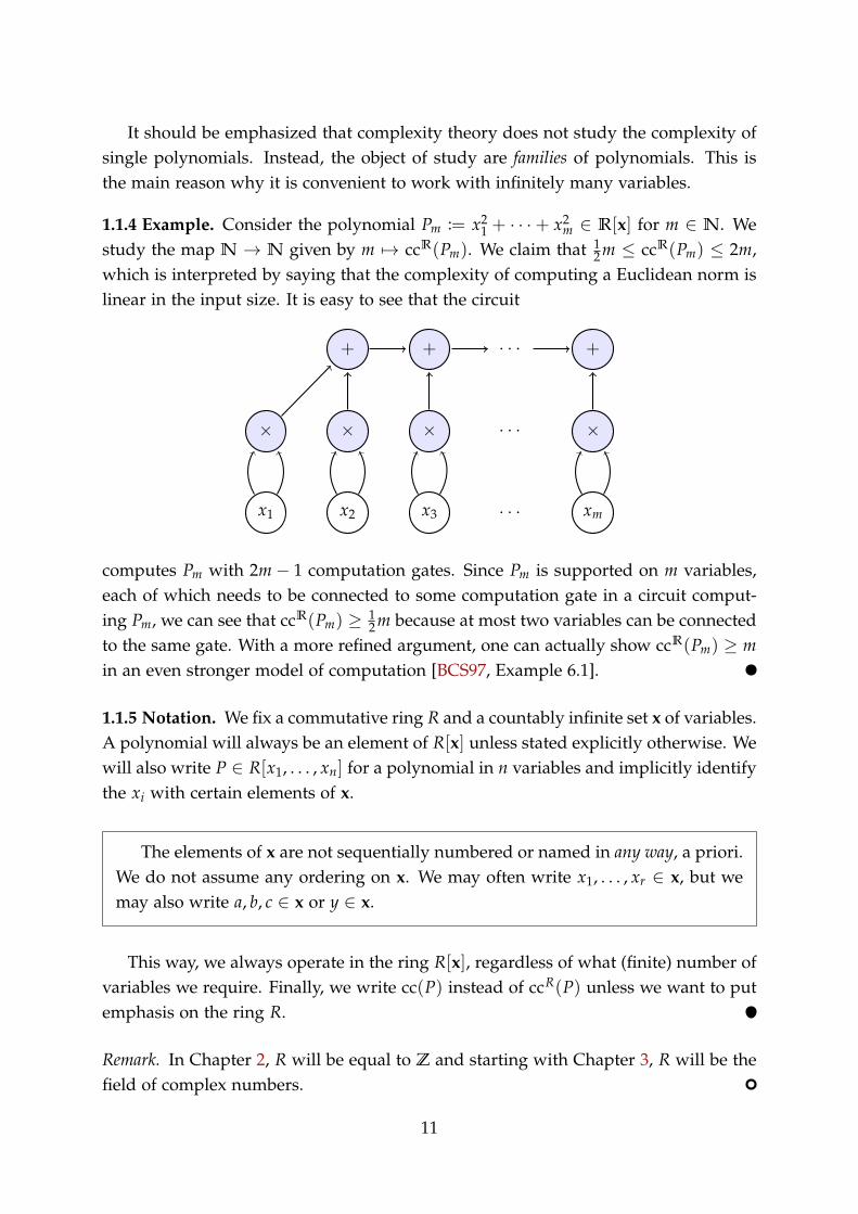
1.1.4 Example. Consider the polynomial Pm := x21 + · · ·+ x2m ∈ R[x] for m ∈ N. Westudy the map N → N given by m ↦→ ccR(Pm). We claim that 1

2m ≤ ccR(Pm) ≤ 2m,which is interpreted by saying that the complexity of computing a Euclidean norm islinear in the input size. It is easy to see that the circuit

+· · ·++

× × × · · · ×

x1 x2 x3 · · · xm

computes Pm with 2m− 1 computation gates. Since Pm is supported on m variables,each of which needs to be connected to some computation gate in a circuit comput-ing Pm, we can see that ccR(Pm) ≥ 1

2m because at most two variables can be connectedto the same gate. With a more refined argument, one can actually show ccR(Pm) ≥ min an even stronger model of computation [BCS97, Example 6.1].

1.1.5 Notation. We fix a commutative ring R and a countably infinite set x of variables.A polynomial will always be an element of R[x] unless stated explicitly otherwise. Wewill also write P ∈ R[x1, . . . , xn] for a polynomial in n variables and implicitly identifythe xi with certain elements of x.

The elements of x are not sequentially numbered or named in any way, a priori.We do not assume any ordering on x. We may often write x1, . . . , xr ∈ x, but wemay also write a, b, c ∈ x or y ∈ x.

This way, we always operate in the ring R[x], regardless of what (finite) number ofvariables we require. Finally, we write cc(P) instead of ccR(P) unless we want to putemphasis on the ring R.

Remark. In Chapter 2, R will be equal to Z and starting with Chapter 3, R will be thefield of complex numbers.

11

1.2 The Classes VP and P

Only for very few and rather simple families (Pm)m∈N of polynomials, we can deter-mine the function m ↦→ cc(Pm) “explicitly”. As is often the case in complexity theory,we restrict instead to the classification of such functions by their asymptotic rate ofgrowth. Even this task turns out to be quite challenging.

1.2.1 Definition. A function t : N → N is called polynomially bounded if there is apolynomial p ∈ Z[x] and m0 ∈ N such that ∀m ≥ m0 : t(m) ≤ p(m). We define polyas the set of all polynomially bounded functions N → N.

Remark. We will often write t(m) ∈ poly(m) instead of t ∈ poly, for example wewould write m3 ∈ poly(m) instead of giving the function m ↦→ m3 a name. If anumeric quantity t(m) ∈ N is associated to each element of a family P = (Pm)m∈N,we say that P has (or admits) polynomially many of said quantity to express thatt ∈ poly.

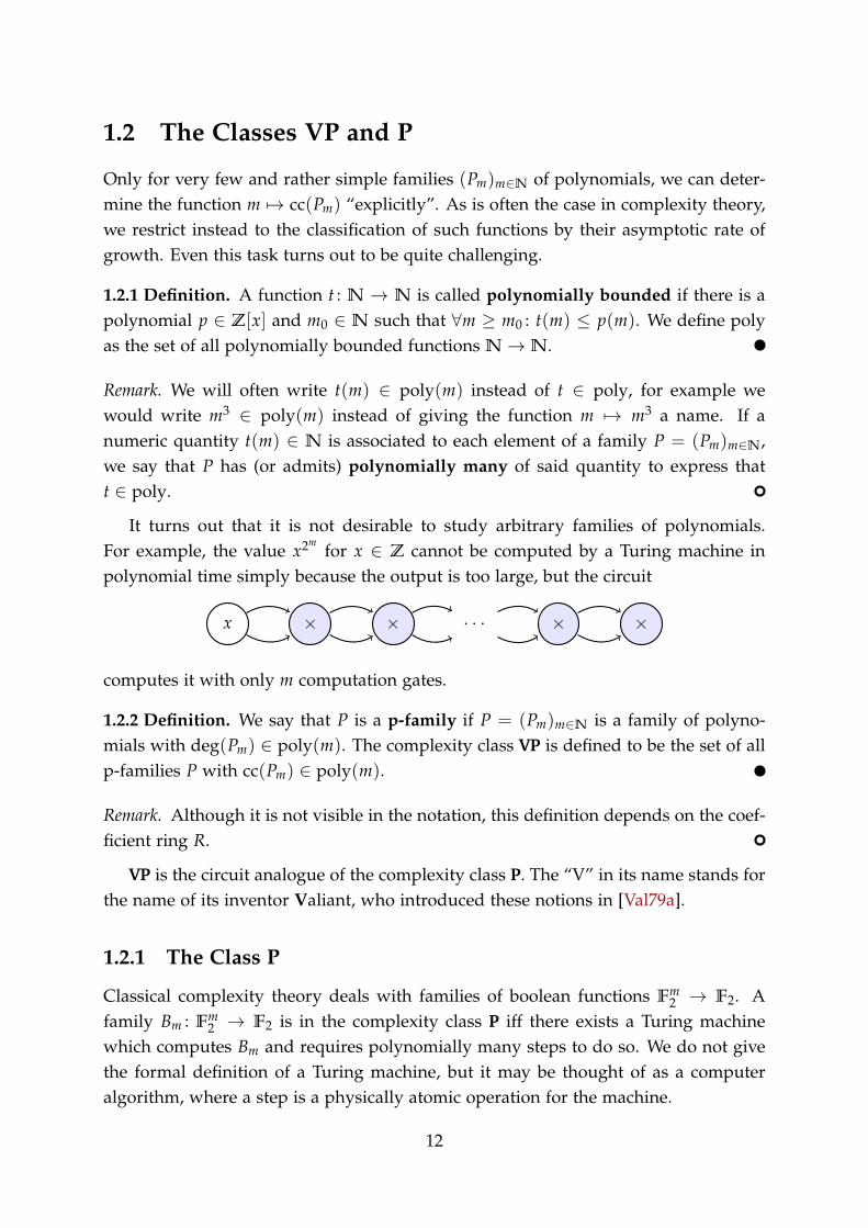
It turns out that it is not desirable to study arbitrary families of polynomials.For example, the value x2

mfor x ∈ Z cannot be computed by a Turing machine in

polynomial time simply because the output is too large, but the circuit

××· · ·××x

computes it with only m computation gates.

1.2.2 Definition. We say that P is a p-family if P = (Pm)m∈N is a family of polyno-mials with deg(Pm) ∈ poly(m). The complexity class VP is defined to be the set of allp-families P with cc(Pm) ∈ poly(m).

Remark. Although it is not visible in the notation, this definition depends on the coef-ficient ring R.

VP is the circuit analogue of the complexity class P. The “V” in its name stands forthe name of its inventor Valiant, who introduced these notions in [Val79a].

1.2.1 The Class P

Classical complexity theory deals with families of boolean functions Fm2 → F2. A

family Bm : Fm2 → F2 is in the complexity class P iff there exists a Turing machine

which computes Bm and requires polynomially many steps to do so. We do not givethe formal definition of a Turing machine, but it may be thought of as a computeralgorithm, where a step is a physically atomic operation for the machine.

12

The class P has the nonuniform analogue P/poly which has a description in termsof circuits: Nonuniformity means that we are not asking for a single algorithm towork on all input sizes, but we allow different algorithms for different input sizes. Inthe language of circuits, a family Bm : Fm

2 → F2 of boolean functions is in P/poly ifand only if ccF2(Bm) ∈ poly(m). Note that by polynomial interpolation, any functionFm2 → F2 is given by some polynomial in F2[x1, . . . , xm] ⊆ F2[x].

1.3 Reduction and Completeness

An important concept in boolean as well as algebraic complexity theory is reduction.Informally put, a problem Q can be reduced to a problem P if one can produce analgorithm for Q from an algorithm for P without measurably increasing the runtime.This is only a vague description, of course. We will give the precise definition for thealgebraic model after introducing some notation.

1.3.1 Definition. Denote by N(x) the x-indexed sequences α = (αx)x∈x of naturalnumbers with αx = 0 for only finitely many x ∈ x. By definition, a polynomialP ∈ R[x] is a map P : N(x) → R which we denote α ↦→ Pα and require Pα = 0 for onlyfinitely many α ∈ N(x). One then writes

P = ∑α∈N(x)

Pα · ∏x∈x

xαx .

We define the support of P to be the set of variables that occur in this expression, i.e.

supp(P) :=x ∈ x

∃α ∈ N(x) : αx = 0∧ Pα = 0.

Note that supp(P) is always a finite set. For P ∈ R[x] with supp(P) = x1, . . . , xn,the expression for P becomes the familiar P = ∑α∈Nn Pα · ∏n

i=1 xαii .

1.3.2 Example. Let x, y, z ∈ x. For Q = x2y+ z3, we have supp(Q) = x, y, z. Thepolynomial P = x2y+ y3 can also be viewed as an element of C[x, y, z] but we havesupp(P) =x, y because z does not occur in P.

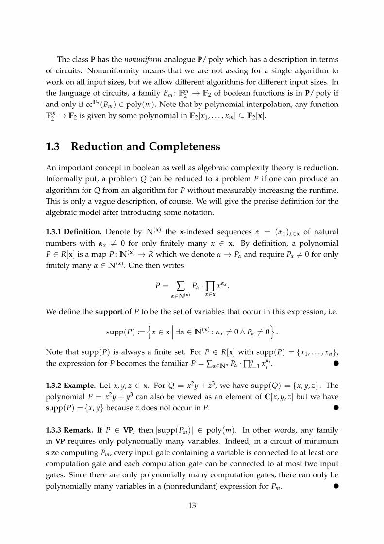
1.3.3 Remark. If P ∈ VP, then |supp(Pm)| ∈ poly(m). In other words, any familyin VP requires only polynomially many variables. Indeed, in a circuit of minimumsize computing Pm, every input gate containing a variable is connected to at least onecomputation gate and each computation gate can be connected to at most two inputgates. Since there are only polynomially many computation gates, there can only bepolynomially many variables in a (nonredundant) expression for Pm.

13

We next define a partial order “≤” on R[x] where P ≤ Q holds if P can be ob-tained from Q by variable substitution. For example, P ≤ Q holds in Example 1.3.2because P arises from Q by substituting z for y. This is formalized in the followingDefinition 1.3.4:

1.3.4 Definition. For S ⊆ x and a map σ : S → R[x], we extend σ to a map x → R[x]by the identity. We then denote by Pσ the image of P under the unique R-algebrahomomorphism R[x] → R[x] which maps x ↦→ σ(x) for all x ∈ x.

A polynomial P is called a projection of another polynomial Q if there is someS ⊆ supp(Q) and a map σ : S → x ∪ R such that P = Qσ. We denote this by P ≤R Q.The definition extends to families as follows: A p-family P is a p-projection of anotherp-family Q, in symbols P ≤R Q, if there is some t ∈ poly such that Pm ≤ Qt(m) for allm ∈ N. We will write P ≤ Q in both cases if there is no ambiguity concerning R.

1.3.5 Example. Let x, y, z ∈ x and Q := y2z+ xyz− x3 − z3. Let σ : x → R[x] be theidentity everywhere except for σ(z) = 1. Then, one obtains Qσ = y2 + xy− x3 − 1.

1.3.6 Example. Let ai ∈ x and xi ∈ x be distinct variables for all i ∈ N. For d ∈ N, weconsider the family Q = (Qd)d∈N given by

Qd := a0 + a1x1 + . . .+ adxd

with supp(Qd) =a0, . . . , ad, x1, . . . , xd. Any p-family P ∈ VP of affine linear polyno-mials satisfies P ≤ Q. Indeed, this follows because t(m) := |supp(Pm)| is polynomiallybounded by Remark 1.3.3.

1.4 The Classes VNP and NP

Valiant introduced the class VNP as an analogue of the class NP, but we will give adefinition of the class VNP first because our focus is on the algebraic model. We willthen discuss the relation to NP.

1.4.1 Definition. Let P be a p-family. Then P ∈ VNP if and only if there exists a familyQ ∈ VP and a sequence (Cm)m∈N with Cm ⊆ supp(Qm) such that P is a projection ofthe family Q = (Qm)m∈N, which is defined as

Qm := ∑σ : Cm→0,1

Qσm · ∏

x∈Cmσ(x)=1

x.

Remark. We use here the original definition from [Val79a, p. 252] because we can latermake the analogy to classical complexity classes more clear. In subsequent literature,the definition appears in seemingly weaker, but equivalent form [Bü00, p. 5].

14

Remark. It follows from the definition that VP ⊆ VNP: For P ∈ VP, choose Q = P andCm := ∅ for all m ∈ N. By Definition 1.3.1, the empty map σ : ∅ → 0, 1 satisfiesPσm = Pm for all m ∈ N.

Remark. Note that for P ∈ VNP, we again have |supp(Pm)| ∈ poly(m). Indeed, inDefinition 1.4.1 we know that |supp(Qm)| ∈ poly(m) by Remark 1.3.3. Furthermore,supp(Qm) ⊆ supp(Qm) and and since Pm ≤ Qm, we have

|supp(Pm)| ≤supp(Qm)

≤|supp(Qm)| ∈ poly(m).

1.4.1 The Class NP

We will now explain and motivate this definition by comparing Valiant’s class withthe classical one. A family Bm : Fm

2 → F2 is in NP if and only if there are functionstm ∈ poly(m) and Cm : Fm

2 × Ftm2 → F2 such that

• the family (Cm)m∈N is in P and

• ∀m ∈ N : ∀σ ∈ Fm2 : (Bm(σ) = 1) ⇔ (∃c ∈ F

tm2 : Cm(σ, c) = 1).

In other words, it might not be easy to decide whether Bm(σ) = 1, but it is easy toconfirm that Bm(σ) = 1 if given a valid certificate c ∈ F

tm2 .

Again, there is a relevant related complexity class known as #P. It contains familiesof maps Fm

2 → N. Such a family Pm : Fm2 → N is in #P if and only if there exists a

family (Bm)m∈N ∈ NP which has a certificate function (Qm)m∈N ∈ P such that Pmcounts the number of certificates, i.e.,

Pm(σ) =c ∈ F

tm2

Qm(σ, c) = 1 .

Note that Bm(σ) = 1 if and only if Pm(σ) > 0.If we interpret Qm ∈ F2[x, y] where x =x1, . . . , xm and y =y1, . . . , ytm, then

Qm := ∑σ : y→0,1

Qσm ·

tm

∏k=1

σ(yk)=1

yk

is an element of VNP over F2 by Definition 1.4.1 and for any σ ∈ Fm2 = Fx

2, i.e.,viewing σ as a map σ : x →0, 1 = F2, we have Qσ

m = 0 if and only if Bm(σ) = 0.More precisely, Qσ

m has exactly Pm(σ) monomials and the monomial

∏tmk=1ck=1

yk

occurs in Qσm if and only if c ∈ F

tm2 is a certificate with Qm(σ, c) = 1.

15

1.4.2 Completeness of the Permanent

1.4.2 Definition. Let C be some class of p-families, like VP or VNP. A p-family P iscalled C-complete if P ∈ C and ∀Q ∈ C : Q ≤ P.

Two completeness results by Valiant make the connection between #P and VNPeven more tangible. They both concern the permanent polynomial family. The per-manent of an m×m matrix (xij)1≤i,j≤m is defined as

perm := ∑π∈Sm

m

∏i=1

xi,π(i), (1)

where Sm denotes the symmetric group on m symbols, i.e., the group of all set auto-morphisms of [m] := 1, . . . ,m. We will consider per = (perm)m∈N as a family ofpolynomials in the variables xij.

1.4.3 Theorem ([Val79b]). The problem of computing the permanent of a binary ma-trix (one where every entry is either 0 or 1) is #P-complete.

1.4.4 Theorem ([Val79a]). The permanent family is VNP-complete over any field ofcharacteristic different from 2.

By a formula of Ryser [Rys63], we know that perm can be computed by a circuitof size m · 2m, but no significant improvement over this is known. This leads to thefollowing conjecture:

1.4.5 Conjecture (Valiant’s Hypothesis). The inclusion VP ⊆ VNP is strict.

Given any VP-complete family P, one could prove VP = VNP by showing that thepermanent is not a p-projection of P.

1.5 Determinant Versus Permanent

The definition of the permanent (1) is quite similar to the familiar definition of thedeterminant family

detd := ∑π∈Sd

sgn(π) ·d

∏i=1

xi,π(i).

It is known [MV97] that detd can be computed by a circuit of size O(d6) – this is notimmediately obvious because the classical procedure of Gaussian elimination per-forms divisions: Arithmetic circuits only allow for multiplication and addition.

Unfortunately, the determinant is not known to be VP-complete, nor is it thoughtto be. However, it is complete for a subclass of VP which we will study next.

16

1.5.1 Classes for the Determinant

The class of polynomials for which the determinant family is complete can be definedin several different ways. We will not go into detail and instead refer to [MP08; Tod92].However, we give one definition:

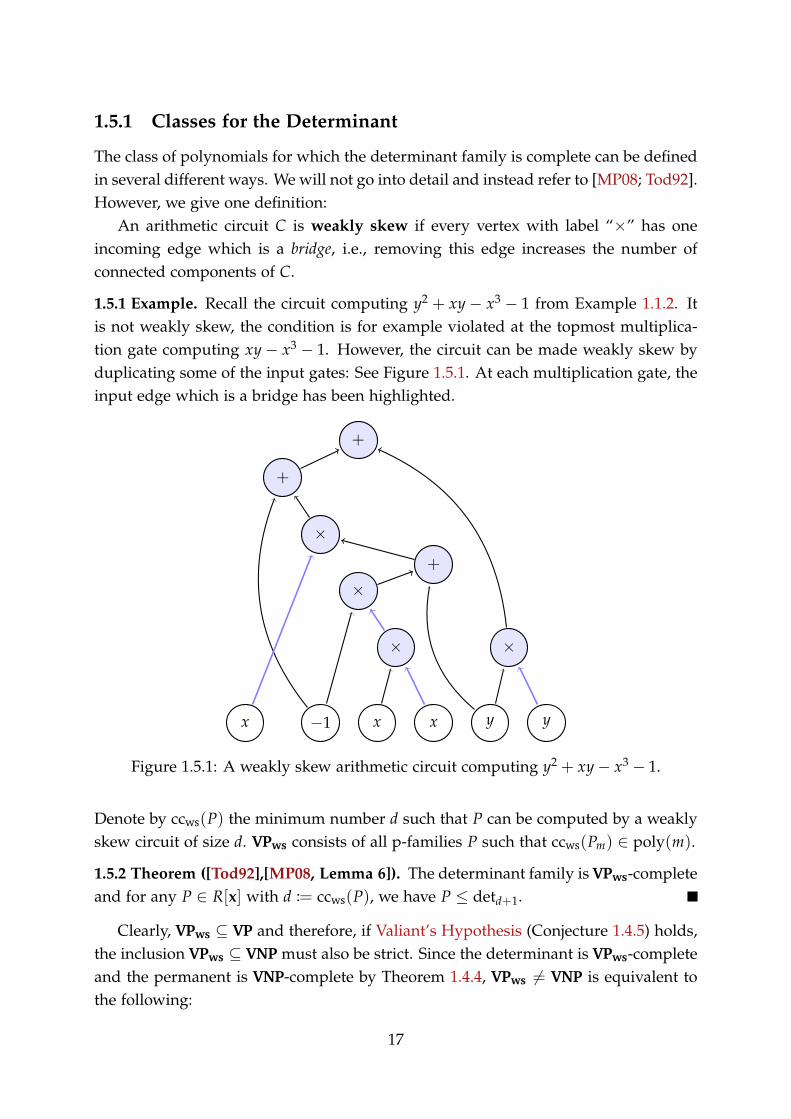
An arithmetic circuit C is weakly skew if every vertex with label “×” has oneincoming edge which is a bridge, i.e., removing this edge increases the number ofconnected components of C.

1.5.1 Example. Recall the circuit computing y2 + xy− x3 − 1 from Example 1.1.2. Itis not weakly skew, the condition is for example violated at the topmost multiplica-tion gate computing xy− x3 − 1. However, the circuit can be made weakly skew byduplicating some of the input gates: See Figure 1.5.1. At each multiplication gate, theinput edge which is a bridge has been highlighted.

+

+

×

+

×

××

−1x x x y y

Figure 1.5.1: A weakly skew arithmetic circuit computing y2 + xy− x3 − 1.

Denote by ccws(P) the minimum number d such that P can be computed by a weaklyskew circuit of size d. VPws consists of all p-families P such that ccws(Pm) ∈ poly(m).

1.5.2 Theorem ([Tod92],[MP08, Lemma 6]). The determinant family is VPws-completeand for any P ∈ R[x] with d := ccws(P), we have P ≤ detd+1.

Clearly, VPws ⊆ VP and therefore, if Valiant’s Hypothesis (Conjecture 1.4.5) holds,the inclusion VPws ⊆ VNP must also be strict. Since the determinant is VPws-completeand the permanent is VNP-complete by Theorem 1.4.4, VPws = VNP is equivalent tothe following:

17

1.5.3 Conjecture (Permanent vs. Determinant). The permanent polynomial family isnot a p-projection of the determinant polynomial family.

1.5.2 Determinantal Complexity

In order to approach Permanent versus Determinant (Conjecture 1.5.3), we need tostudy p-projections of the determinant. We will show that the determinant is uni-versal, meaning that every polynomial is a projection of detd for some d ∈ N. Thisimportant insight gives rise to the definition of determinantal complexity: For a poly-nomial P we define

dc(P) := mind ∈ N | P ≤ detd .

This allows us to reformulate Conjecture 1.5.3 simply as dc(perm) /∈ poly(m). Thebenefit of this reformulation is the fact that there are no more circuits involved in itand methods from algebra directly apply.

1.5.4 Theorem ([Val79a, §2]). Let R be a commutative ring and P ∈ R[x1, . . . , xn] apolynomial. Then, there is a natural number d ∈ N such that P is a projection of detd.

Remark. This highlights the importance of the determinant in a very fundamentalway. Quoting Valiant himself, “for the problem of finding a subexponential formula for apolynomial when one exists, linear algebra is essentially the only technique in the sense that itis always applicable.”

Proof. The proof is based on a graph construction which we will sketch here: Givena matrix a = (aij)1≤i,j≤m we can consider the labelled directed graph Ga on the setof vertices 1, . . . ,m where the edge (i, j) has label aij. We treat edges with label 0as nonexistent. For a directed graph with labels in R[x1, . . . , xn], we can reverse thisprocess and obtain a matrix from G which we will refer to as its adjacency matrix. Acycle cover of Ga is a partition of Ga into vertex disjoint cycles. The permutations on theset1, . . . ,m are in bijection with the cycle covers of Ga. To each cycle we associate asign, which is −1 if the cycle has even length and 1 otherwise. To each cycle we thenassociate a weight, which is its sign times the product of its edge labels. The weightof a cycle cover is the product of the weights of its cycles. The determinant of a isthen, by definition, the sum of the weights of all cycle covers of Ga.

Given a polynomial P ∈ R[x1, . . . , xn], let k := deg(P) be its (total) degree. Aproduct of k + 1 constants and variables can produce any monomial that occurs inP, so we can write P = ∑r

i=1 ∏kj=0 Pij for some r ∈ N and Pij ∈ R ∪x1, . . . , xn. For

example, consider the polynomial

P = x3 + 1− y2 − xy = (x · x · x) + (1 · 1 · 1) + (−1 · y · y) + (−1 · x · y).

18

For this example, we used only 3 factors in each summand as opposed to the 4 factorsthat the construction would yield for a general cubic polynomial.

t

x

1

y

y

x

1

y

x

s

x

1

−1

−1

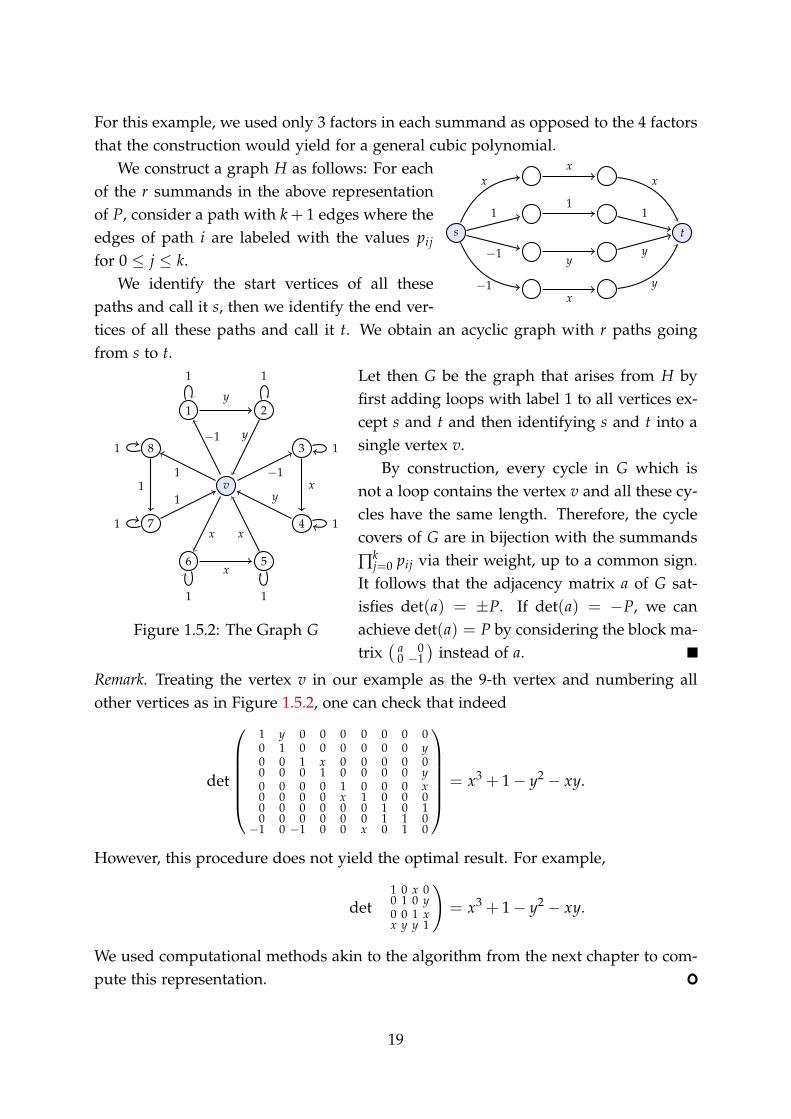
We construct a graph H as follows: For eachof the r summands in the above representationof P, consider a path with k+ 1 edges where theedges of path i are labeled with the values pijfor 0 ≤ j ≤ k.

We identify the start vertices of all thesepaths and call it s, then we identify the end ver-tices of all these paths and call it t. We obtain an acyclic graph with r paths goingfrom s to t.

v

2

1

y

1y

1

−1

4 1

y

3

x

1

−1

5

1

x

6x

1

x71

1

8

1

1

1

Figure 1.5.2: The Graph G

Let then G be the graph that arises from H byfirst adding loops with label 1 to all vertices ex-cept s and t and then identifying s and t into asingle vertex v.

By construction, every cycle in G which isnot a loop contains the vertex v and all these cy-cles have the same length. Therefore, the cyclecovers of G are in bijection with the summands∏k

j=0 pij via their weight, up to a common sign.It follows that the adjacency matrix a of G sat-isfies det(a) = ±P. If det(a) = −P, we canachieve det(a) = P by considering the block ma-trix

( a 00 −1

)instead of a.

Remark. Treating the vertex v in our example as the 9-th vertex and numbering allother vertices as in Figure 1.5.2, one can check that indeed

det

⎛⎜⎜⎜⎜⎜⎝1 y 0 0 0 0 0 0 00 1 0 0 0 0 0 0 y0 0 1 x 0 0 0 0 00 0 0 1 0 0 0 0 y0 0 0 0 1 0 0 0 x0 0 0 0 x 1 0 0 00 0 0 0 0 0 1 0 10 0 0 0 0 0 1 1 0

−1 0 −1 0 0 x 0 1 0

⎞⎟⎟⎟⎟⎟⎠ = x3 + 1− y2 − xy.

However, this procedure does not yield the optimal result. For example,

det

(1 0 x 00 1 0 y0 0 1 xx y y 1

)= x3 + 1− y2 − xy.

We used computational methods akin to the algorithm from the next chapter to com-pute this representation.

19

Chapter 2Binary Determinantal Complexity

This chapter contains the contents of the previously published work [HI16]. We onlyconsider polynomials with integer coefficients here, i.e., we assume R = Z.

Proving Valiant’s Hypothesis (Conjecture 1.4.5) amounts to bounding the growthof dc(perm) superpolynomially from below. Lower bounds are a notoriously difficultproblem in complexity theory. On the other hand, finding upper bounds admits thestraightforward approach of constructing algorithms: In our case, an algorithm canbe described as a sequence of matrices Am ∈ (x ∪ Z)tm×tm such that det(Am) = perm.Here, the numbers tm ≥ dc(perm) achieve equality if and only if the algorithm isoptimal. To get a better idea of how dc(perm) grows, it is therefore reasonable toattempt the construction of good algorithms. The best one known so far is a graphconstruction by Grenet [Gre11], see Section 2.5, with the following consequence:

2.0.1 Theorem. For every natural number m there exists a matrix A of size 2m − 1such that perm = det(A). Moreover, A can be chosen such that the entries in A areonly variables, zeros, and ones, but no other constants.

Theorem 2.0.1 gives rise to the following definition: We call a matrix whose entriesare only zeros, ones, or variables, a binary variable matrix. We will prove in Corol-lary 2.1.3 that every polynomial P with integer coefficients can be written as the de-terminant of a binary variable matrix and that the size is almost equal to dc(P), seeProposition 2.1.2 for a precise statement. We then denote by bdc(P) the smallest dsuch that P can be written as a determinant of an d× d binary variable matrix. It iscalled the binary determinantal complexity of P.

The complexity class of families (Pm)m∈N with polynomially bounded binary de-terminantal complexity bdc(Pm) is exactly VP0ws, the constant free version of VPws, seeSection 2.4 for definitions and proofs.

Theorem 2.0.1 shows that bdc(perm) ≤ 2m − 1. This upper bound is clearly sharpfor m = 1 and for m = 2, and we can also verify that it is sharp for m = 3:

2.0.2 Theorem. bdc(per3) = 7.

21

We use a computer aided proof and enumeration of bipartite graphs in our study.The binary determinantal complexity of perm is now known to be exactly 2m − 1 form ∈1, 2, 3. Unfortunately, determining bdc(per4) is currently out of reach with ourmethods.

The best known general lower bound is bdc(perm) ≥ dc(perm) ≥ m2

2 due to[MR04] in a stronger model of computation, see also [LMR13] for the same boundin an even stronger model of computation. After the proof of Theorem 2.0.2 waspublished, Alper, Bogart, and Velasco proved in [ABV15] that dc(per3) = 7, but un-fortunately per4 remains out of reach even with their methods.

2.1 The Cost of Computing Integers

The main purpose of this section is to prove that even though we only allow theconstants 0 and 1, all polynomials with integer coefficients can be obtained as thedeterminant of a binary variable matrix, see Corollary 2.1.3. Moreover, the size ofthe matrices is not much larger than had we allowed integer constants, see Propo-sition 2.1.2. We use standard techniques from algebraic complexity theory, heavilybased on [Val79a], but a certain attention to the signs has to be taken.

In what follows, a digraph is always a finite directed graph which may possiblyhave loops, but which has no parallel edges. We label the edges of a digraph bypolynomials. We will almost exclusively be concerned with digraphs whose labelsare only variables or the constant 1. Note that we consider only labeled digraphs.

A cycle cover of a digraph G is a set of cycles in G such that each vertex of Gis contained in exactly one of these cycles. If a cycle in G has i edges with labelse1, . . . , ei, then its weight is defined as (−1)i−1 · e1 · · · ei. The weight of a cycle cover isthe product of the weights of its cycles. The value of G is the polynomial that arises asthe sum over the weights of all cycle covers in G. We then define the directed adjacencymatrix A of a digraph G as the matrix whose entry Aij is the label of the edge (i, j) or0 if that edge does not exist.

In what follows, we will often construct matrices as the directed adjacency matricesof digraphs. The reason is the well-known observation that the value of a digraph Gequals the determinant of its directed adjacency matrix – see for example [Val79a].

As an intermediate step, we will often construct a binary algebraic branching pro-gram: This is an acyclic digraph Γ = (Γ, s, t) where every edge is labeled by either 1 ora variable. The digraph Γ has two distinguished vertices, the source s and the target t,where s has no incoming and t has no outgoing edges. If an s-t-path in Γ has i edgeswith labels e1, . . . , ei, then its path weight is defined as the value (−1)i−1 · e1 · · · ei.The path value of Γ is the polynomial that arises as the sum over the path weights of

22

all s-t-paths in Γ. We remark that this notion of weight differs from the literature by asign.

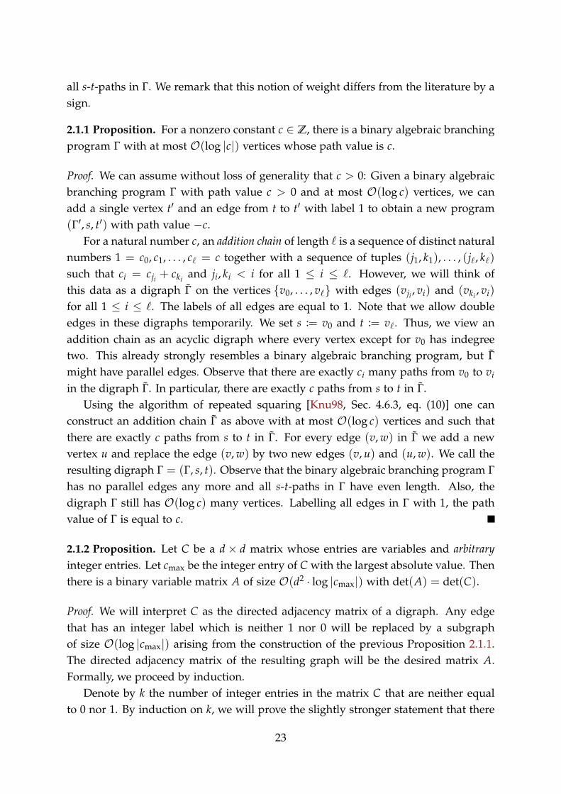
2.1.1 Proposition. For a nonzero constant c ∈ Z, there is a binary algebraic branchingprogram Γ with at most O(log |c|) vertices whose path value is c.

Proof. We can assume without loss of generality that c > 0: Given a binary algebraicbranching program Γ with path value c > 0 and at most O(log c) vertices, we canadd a single vertex t′ and an edge from t to t′ with label 1 to obtain a new program(Γ′, s, t′) with path value −c.

For a natural number c, an addition chain of length ℓ is a sequence of distinct naturalnumbers 1 = c0, c1, . . . , cℓ = c together with a sequence of tuples (j1, k1), . . . , (jℓ, kℓ)such that ci = cji + cki and ji, ki < i for all 1 ≤ i ≤ ℓ. However, we will think ofthis data as a digraph Γ on the vertices v0, . . . , vℓ with edges (vji , vi) and (vki , vi)for all 1 ≤ i ≤ ℓ. The labels of all edges are equal to 1. Note that we allow doubleedges in these digraphs temporarily. We set s := v0 and t := vℓ. Thus, we view anaddition chain as an acyclic digraph where every vertex except for v0 has indegreetwo. This already strongly resembles a binary algebraic branching program, but Γmight have parallel edges. Observe that there are exactly ci many paths from v0 to viin the digraph Γ. In particular, there are exactly c paths from s to t in Γ.

Using the algorithm of repeated squaring [Knu98, Sec. 4.6.3, eq. (10)] one canconstruct an addition chain Γ as above with at most O(log c) vertices and such thatthere are exactly c paths from s to t in Γ. For every edge (v,w) in Γ we add a newvertex u and replace the edge (v,w) by two new edges (v, u) and (u,w). We call theresulting digraph Γ = (Γ, s, t). Observe that the binary algebraic branching program Γhas no parallel edges any more and all s-t-paths in Γ have even length. Also, thedigraph Γ still has O(log c) many vertices. Labelling all edges in Γ with 1, the pathvalue of Γ is equal to c.

2.1.2 Proposition. Let C be a d × d matrix whose entries are variables and arbitraryinteger entries. Let cmax be the integer entry of C with the largest absolute value. Thenthere is a binary variable matrix A of size O(d2 · log |cmax|) with det(A) = det(C).

Proof. We will interpret C as the directed adjacency matrix of a digraph. Any edgethat has an integer label which is neither 1 nor 0 will be replaced by a subgraphof size O(log |cmax|) arising from the construction of the previous Proposition 2.1.1.The directed adjacency matrix of the resulting graph will be the desired matrix A.Formally, we proceed by induction.

Denote by k the number of integer entries in the matrix C that are neither equalto 0 nor 1. By induction on k, we will prove the slightly stronger statement that there

23

x 3 y

2

x

x 3 y

2

x

x 3 yx

x 3 yx

x 3 yx

C =

⎛⎜⎝3 0 20 x 0x 0 y

⎞⎟⎠det(C) = 3xy− 2x2

Figure 2.1.1: Given a matrix C we construct a digraph H with directed adjacency matrix C (left handside) and the digraph G (right hand side) by replacing the edge with label 2 in H by a binary algebraicbranching program. We omit the labels for edges that have label 1. The right hand side depicts thecycle covers K of G and the left hand side shows the corresponding cycle covers KH of H.

is a binary variable matrix A of size d+ k · O(log |cmax|) with det(A) = det(C). Sincek ≤ d2, this implies the statement. Note that the case k = 0 is trivial, so we assumek ≥ 1 and perform the induction step.

Let H be the digraph whose directed adjacency matrix is C. Recall that this meansthe following: H is a digraph on the vertices 1, . . . , d and there is an edge (i, j) withlabel Cij if Cij = 0 and otherwise no such edge exists. Let e = (i, j) be the edgecorresponding to an integer entry c = Cij which is neither 0 nor 1. Let Γ = (Γ, s, t) bea binary algebraic branching program with path value c and O(log |c|) many vertices,which exists by Proposition 2.1.1.

We will now replace the edge (i, j) by Γ (see Figure 2.1.1): Let G be the digraph thatarises from H ∪ Γ by removing the edge (i, j), adding edges (i, s) and (t, j) with label1 and adding loops with label 1 to all vertices of Γ. The directed adjacency matrix ofG has size d+O(log |c|) ≤ d+O(log |cmax|) and contains k− 1 integer entries whichare neither 0 nor 1. By applying the induction hypothesis to the directed adjacencymatrix of G, we obtain a matrix A of size

d+O(log |cmax|) + (k− 1) · O(log |cmax|) = d+ k · O(log |cmax|)

24

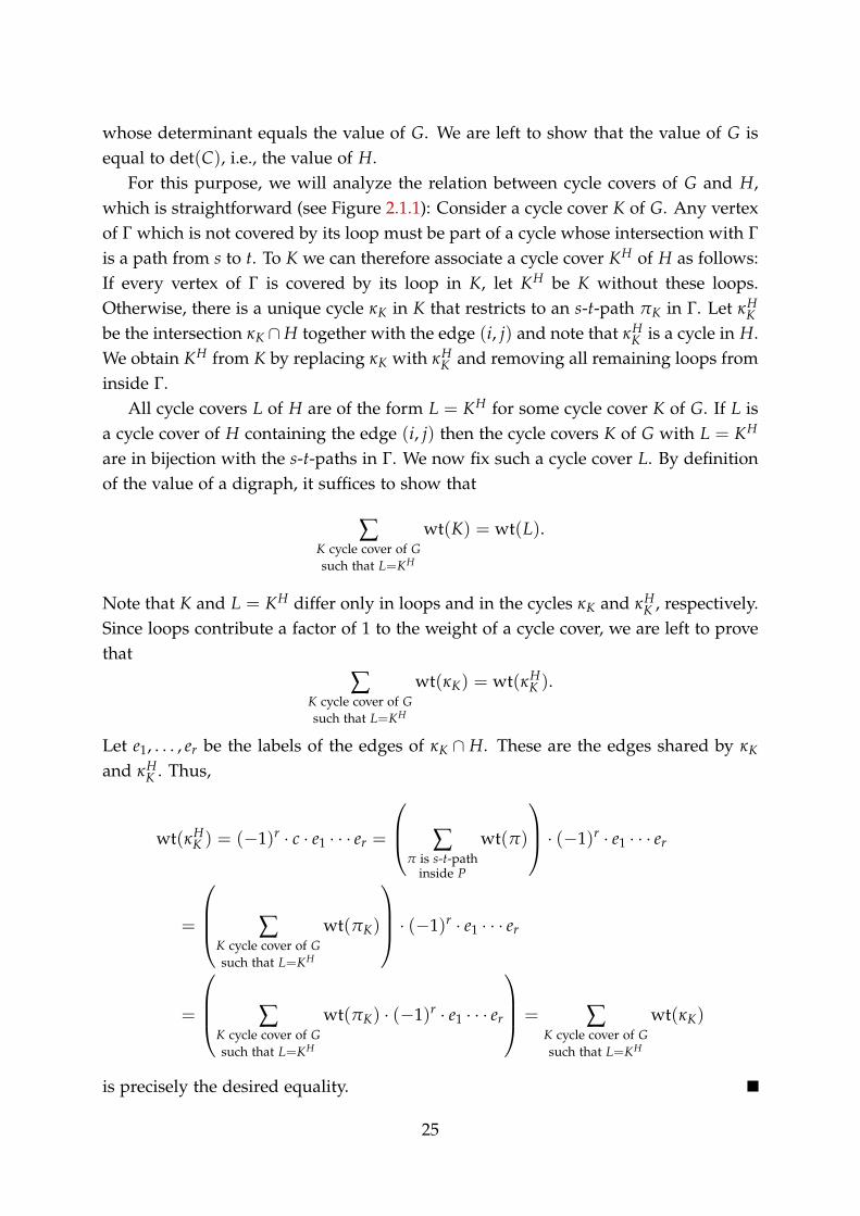
whose determinant equals the value of G. We are left to show that the value of G isequal to det(C), i.e., the value of H.

For this purpose, we will analyze the relation between cycle covers of G and H,which is straightforward (see Figure 2.1.1): Consider a cycle cover K of G. Any vertexof Γ which is not covered by its loop must be part of a cycle whose intersection with Γis a path from s to t. To K we can therefore associate a cycle cover KH of H as follows:If every vertex of Γ is covered by its loop in K, let KH be K without these loops.Otherwise, there is a unique cycle κK in K that restricts to an s-t-path πK in Γ. Let κH

Kbe the intersection κK ∩H together with the edge (i, j) and note that κH

K is a cycle in H.We obtain KH from K by replacing κK with κH

K and removing all remaining loops frominside Γ.

All cycle covers L of H are of the form L = KH for some cycle cover K of G. If L isa cycle cover of H containing the edge (i, j) then the cycle covers K of G with L = KH

are in bijection with the s-t-paths in Γ. We now fix such a cycle cover L. By definitionof the value of a digraph, it suffices to show that

∑K cycle cover of Gsuch that L=KH

wt(K) = wt(L).

Note that K and L = KH differ only in loops and in the cycles κK and κHK , respectively.

Since loops contribute a factor of 1 to the weight of a cycle cover, we are left to provethat

∑K cycle cover of Gsuch that L=KH

wt(κK) = wt(κHK ).

Let e1, . . . , er be the labels of the edges of κK ∩ H. These are the edges shared by κK

and κHK . Thus,

wt(κHK ) = (−1)r · c · e1 · · · er =

⎛⎜⎝ ∑π is s-t-pathinside P

wt(π)

⎞⎟⎠ · (−1)r · e1 · · · er

=

⎛⎜⎜⎝ ∑K cycle cover of Gsuch that L=KH

wt(πK)

⎞⎟⎟⎠ · (−1)r · e1 · · · er

=

⎛⎜⎜⎝ ∑K cycle cover of Gsuch that L=KH

wt(πK) · (−1)r · e1 · · · er

⎞⎟⎟⎠ = ∑K cycle cover of Gsuch that L=KH

wt(κK)

is precisely the desired equality.

25

2.1.3 Corollary. For every polynomial P ∈ Z[x] there exists a binary variable matrixwhose determinant is P.

Proof. Combine Theorem 1.5.4 and Proposition 2.1.2.

2.2 Lower Bounds

This section is dedicated to the proof of Theorem 2.0.2. Let B := 0, 1. A sequentialnumbering makes the proof much easier to read, so we think of the variables asarranged in a 3× 3 matrix

x =

⎛⎜⎝x1 x2 x3x4 x5 x6x7 x8 x9

⎞⎟⎠ .

In this section, we will understand per3 = per(x) as a polynomial in the variablesx1, . . . , x9 instead of the variables xij with 1 ≤ i, j ≤ 3.

2.2.1 Proof Outline

Let d ∈ N and A an d× d binary variable matrix. The binary matrix B(A) ∈ Bd×d

is defined as the matrix arising from A by setting all variables to 1. We call B(A) thesupport matrix of A. If we set all variables to 1 in per3, we obtain the value 6, so ifper3 = det(A), then substituting 1 for all variables on both sides of the equation, weobtain the condition

6 = det(B(A)). (1)

In [EZ62; Slo11], the maximal values of determinants of binary matrices are computedfor small values of d. Since

∀B ∈ B5×5 : det(B) ≤ 5, (2)

we immediately obtain the lower bound bdc(per3) ≥ 6.Unfortunately, there are several matrices B ∈ B6×6 that satisfy det(B) = 6. We

proceed in two steps to verify that nevertheless, none of these matrices B is the supportmatrix B(A) of a candidate matrix A with per3 = det(A). A rough outline is thefollowing:

(a) Enumerate all matrices B ∈ B6×6 with det(B) = 6 up to symmetries.

(b) For all those matrices B prove that B is not the support matrix B(A) of a binaryvariable matrix A with det(A) = per3. We describe this process in the nextsubsection.

26

2.2.2 Stepwise Reconstruction

Let us make (b) precise. In the hope of failing, we attempt to reconstruct a binaryvariable matrix A that has support B and which also satisfies det(A) = per3. Duringthe reconstruction process, we successively replace 1’s in B by the next variable. Theprocess is as follows:

Given a binary matrix B ∈ B6×6, let

S :=(i, j)

Bij = 1

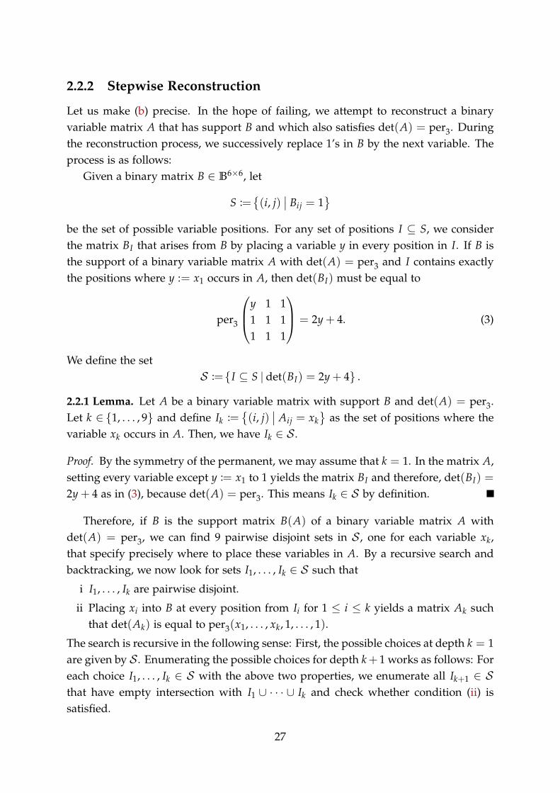
be the set of possible variable positions. For any set of positions I ⊆ S, we considerthe matrix BI that arises from B by placing a variable y in every position in I. If B isthe support of a binary variable matrix A with det(A) = per3 and I contains exactlythe positions where y := x1 occurs in A, then det(BI) must be equal to

per3

⎛⎜⎝y 1 11 1 11 1 1

⎞⎟⎠ = 2y+ 4. (3)

We define the setS :=I ⊆ S | det(BI) = 2y+ 4 .

2.2.1 Lemma. Let A be a binary variable matrix with support B and det(A) = per3.Let k ∈ 1, . . . , 9 and define Ik :=

(i, j)

Aij = xkas the set of positions where the

variable xk occurs in A. Then, we have Ik ∈ S .

Proof. By the symmetry of the permanent, we may assume that k = 1. In the matrix A,setting every variable except y := x1 to 1 yields the matrix BI and therefore, det(BI) =

2y+ 4 as in (3), because det(A) = per3. This means Ik ∈ S by definition.

Therefore, if B is the support matrix B(A) of a binary variable matrix A withdet(A) = per3, we can find 9 pairwise disjoint sets in S , one for each variable xk,that specify precisely where to place these variables in A. By a recursive search andbacktracking, we now look for sets I1, . . . , Ik ∈ S such that

i I1, . . . , Ik are pairwise disjoint.

ii Placing xi into B at every position from Ii for 1 ≤ i ≤ k yields a matrix Ak suchthat det(Ak) is equal to per3(x1, . . . , xk, 1, . . . , 1).

The search is recursive in the following sense: First, the possible choices at depth k = 1are given by S . Enumerating the possible choices for depth k+ 1 works as follows: Foreach choice I1, . . . , Ik ∈ S with the above two properties, we enumerate all Ik+1 ∈ Sthat have empty intersection with I1 ∪ · · · ∪ Ik and check whether condition (ii) issatisfied.

27

If the recursive search never reaches k = 9 or fails there, then B is not the supportof a binary variable matrix A with det(A) = per3. If we reach level 9 however and donot fail there, we have found such an A.

In practice, the evaluation of det(A) is sped up significantly by working over alarge finite field Fp and choosing random elements x1, . . . , x9 ∈ Fp \0, 1.

2.2.3 Exploiting Symmetries in Enumeration

Let us call two matrices equivalent if they arise from each other by transposition and/orpermutation of rows and/or columns. A key observation is that equivalent matriceshave the same determinant up to sign. Therefore we do not have to list all binarymatrices B ∈ B6×6 with det(B) = 6, but it suffices to list one representative matrixB with det(B) = ±6 for each equivalence class. It happens to be the case that theequivalence classes of 6× 6 binary matrices are in bijection to graph isomorphy classesof undirected bipartite graphs G = (V ∪W, E) with |V| = |W| = 6, V ∩W = ∅ asfollows: For V = v1, . . . , v6 and W = w1, . . . ,w6, the bipartite adjacency matrixB(G) ∈ B6×6 of G is defined via B(G)i,j = 1 if and only if

vi,wj

∈ E. Row and

column permutations in B(G) are reflected by renaming vertices in G. Transpositionof B(G) amounts to switching V and W in G.

The computer software nauty [MP13] can enumerate all 251 610 of these bipar-tite graphs, which is already a significant improvement over the 236 = 68 719 476 736elements of B6×6. To further limit the number of bipartite graphs that have to beconsidered, we make the following observations:

• We need not consider binary matrices B containing a row i with only a single entryBij equal to 1. Indeed, Laplace expansion over the i-th row yields that det(B) isequal to the determinant of a 5× 5 binary matrix, which can at most be 5, see (2).Translating to bipartite graphs, we only need to consider those bipartite graphswhere all vertices have at least two neighbours.

• If two distinct vertices in G have the same neighbourhood, then the bipartite adja-cency matrix B(G) has two identical rows (or columns) which would implydet(B(G)) = 0. Hence, we only need to enumerate bipartite graphs where all ver-tices have distinct neighbourhoods. Unfortunately nauty can impose this restrictiononly on rows and not on columns.

With these restrictions, the nauty command

genbg -d2:2 -z 6 6

generates 44 384 bipartite graphs, only 263 of which have a bipartite adjacency matrixwith determinant equal to ±6. We then preprocess this list by swapping the first tworows of any matrix with negative determinant.

28

Finally, the stepwise reconstruction (Subsection 2.2.2) fails for all of these 263 ma-trices, proving that bdc(per3) ≥ 7. The algorithm takes 28 seconds on an Intel Core™i7-4500U CPU (2.4 GHz) to finish.

Unfortunately, bdc(per4) can currently not be determined in this fashion becausethe enumeration of all apropriate bipartite graphs, already on 9+ 9 vertices, is infea-sible.

2.3 Uniqueness of Grenet’s construction in the 7× 7 case

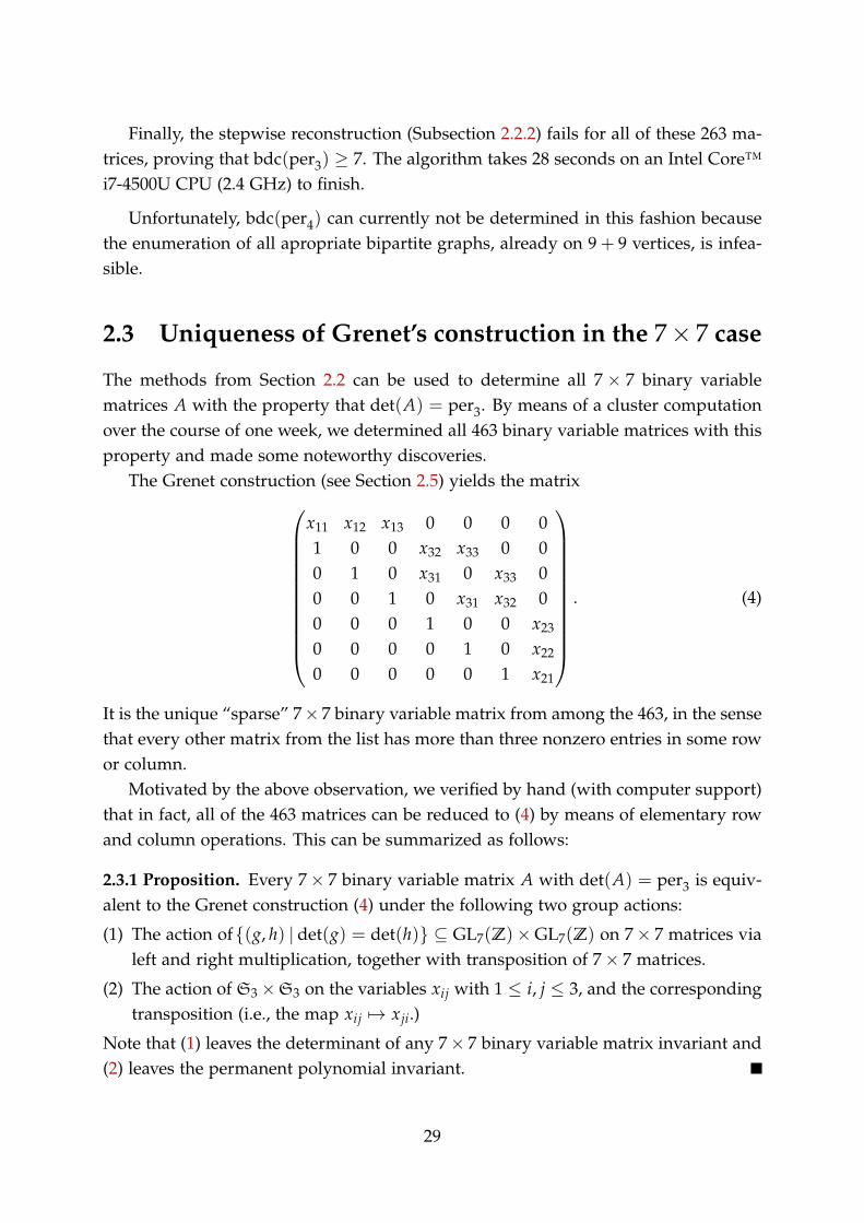
The methods from Section 2.2 can be used to determine all 7 × 7 binary variablematrices A with the property that det(A) = per3. By means of a cluster computationover the course of one week, we determined all 463 binary variable matrices with thisproperty and made some noteworthy discoveries.

The Grenet construction (see Section 2.5) yields the matrix⎛⎜⎜⎜⎜⎜⎜⎜⎜⎜⎜⎜⎝

x11 x12 x13 0 0 0 01 0 0 x32 x33 0 00 1 0 x31 0 x33 00 0 1 0 x31 x32 00 0 0 1 0 0 x230 0 0 0 1 0 x220 0 0 0 0 1 x21

⎞⎟⎟⎟⎟⎟⎟⎟⎟⎟⎟⎟⎠. (4)

It is the unique “sparse” 7× 7 binary variable matrix from among the 463, in the sensethat every other matrix from the list has more than three nonzero entries in some rowor column.

Motivated by the above observation, we verified by hand (with computer support)that in fact, all of the 463 matrices can be reduced to (4) by means of elementary rowand column operations. This can be summarized as follows:

2.3.1 Proposition. Every 7× 7 binary variable matrix A with det(A) = per3 is equiv-alent to the Grenet construction (4) under the following two group actions:

(1) The action of(g, h) | det(g) = det(h) ⊆ GL7(Z)×GL7(Z) on 7× 7 matrices vialeft and right multiplication, together with transposition of 7× 7 matrices.

(2) The action of S3 ×S3 on the variables xij with 1 ≤ i, j ≤ 3, and the correspondingtransposition (i.e., the map xij ↦→ xji.)

Note that (1) leaves the determinant of any 7× 7 binary variable matrix invariant and(2) leaves the permanent polynomial invariant.

29

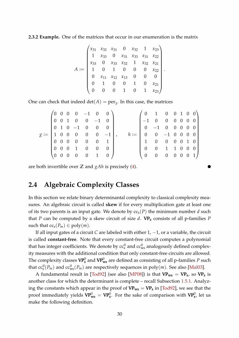
2.3.2 Example. One of the matrices that occur in our enumeration is the matrix

A :=

⎛⎜⎜⎜⎜⎜⎜⎜⎜⎜⎜⎜⎝

x31 x32 x31 0 x32 1 x231 x33 0 x31 x33 x31 x22x33 0 x33 x32 1 x32 x211 0 1 0 0 0 x220 x11 x12 x13 0 0 00 1 0 0 1 0 x210 0 0 1 0 1 x23

⎞⎟⎟⎟⎟⎟⎟⎟⎟⎟⎟⎟⎠.

One can check that indeed det(A) = per3. In this case, the matrices

g :=

⎛⎜⎜⎜⎜⎜⎜⎜⎜⎜⎜⎜⎝

0 0 0 0 −1 0 00 0 1 0 0 −1 00 1 0 −1 0 0 01 0 0 0 0 0 −10 0 0 0 0 0 10 0 0 1 0 0 00 0 0 0 0 1 0

⎞⎟⎟⎟⎟⎟⎟⎟⎟⎟⎟⎟⎠, h :=

⎛⎜⎜⎜⎜⎜⎜⎜⎜⎜⎜⎜⎝

0 1 0 0 1 0 0−1 0 0 0 0 0 00 −1 0 0 0 0 00 0 −1 0 0 0 01 0 0 0 0 1 00 0 1 1 0 0 00 0 0 0 0 0 1

⎞⎟⎟⎟⎟⎟⎟⎟⎟⎟⎟⎟⎠are both invertible over Z and gAh is precisely (4).

2.4 Algebraic Complexity Classes

In this section we relate binary determinantal complexity to classical complexity mea-sures. An algebraic circuit is called skew if for every multiplication gate at least oneof its two parents is an input gate. We denote by ccs(P) the minimum number d suchthat P can be computed by a skew circuit of size d. VPs consists of all p-families Psuch that ccs(Pm) ∈ poly(m).

If all input gates of a circuit C are labeled with either 1, −1, or a variable, the circuitis called constant-free. Note that every constant-free circuit computes a polynomialthat has integer coefficients. We denote by cc0s and cc0ws analogously defined complex-ity measures with the additional condition that only constant-free circuits are allowed.The complexity classes VP0s and VP0ws are defined as consisting of all p-families P suchthat cc0s (Pm) and cc0ws(Pm) are respectively sequences in poly(m). See also [Mal03].

A fundamental result in [Tod92] (see also [MP08]) is that VPws = VPs, so VPs isanother class for which the determinant is complete – recall Subsection 1.5.1. Analyz-ing the constants which appear in the proof of VPws = VPs in [Tod92], we see that theproof immediately yields VP0ws = VP0s . For the sake of comparison with VP0s , let usmake the following definition.

30

2.4.1 Definition. The complexity class DETP0 consists of all sequences of polynomialsthat have polynomially bounded binary determinantal complexity bdc.

The main purpose of this section is to show the following statement.

2.4.2 Proposition. VP0ws = VP0s = DETP0.

Proof. The proof of [Tod92, Lemma 3.4] immediately shows that DETP0 ⊆ VP0s . Toshow that VP0s ⊆ DETP0 we adapt the proof of [Tod92, Lemma 3.5 or Theorem 4.3],but a subtlety arises: The proof shows that from a weakly skew or skew circuit C wecan construct a matrix A′ of size polynomially bounded in the number of vertices in Csuch that det(A′) is the polynomial computed by C with the drawback that A′ is nota binary variable matrix, but A′ has as entries variables and constants 0, 1, and −1.Fortunately Proposition 2.1.2 establishes DETP0 = VP0s = VP0ws.

2.4.3 Remark. In the past, other models of computation with bounded coefficientshave already given way to stronger lower bounds than their corresponding unre-stricted models: [Mor73] on the Fast Fourier Transform, [Raz03] on matrix multipli-cation, and [BL04] on arithmetic operations on polynomials.

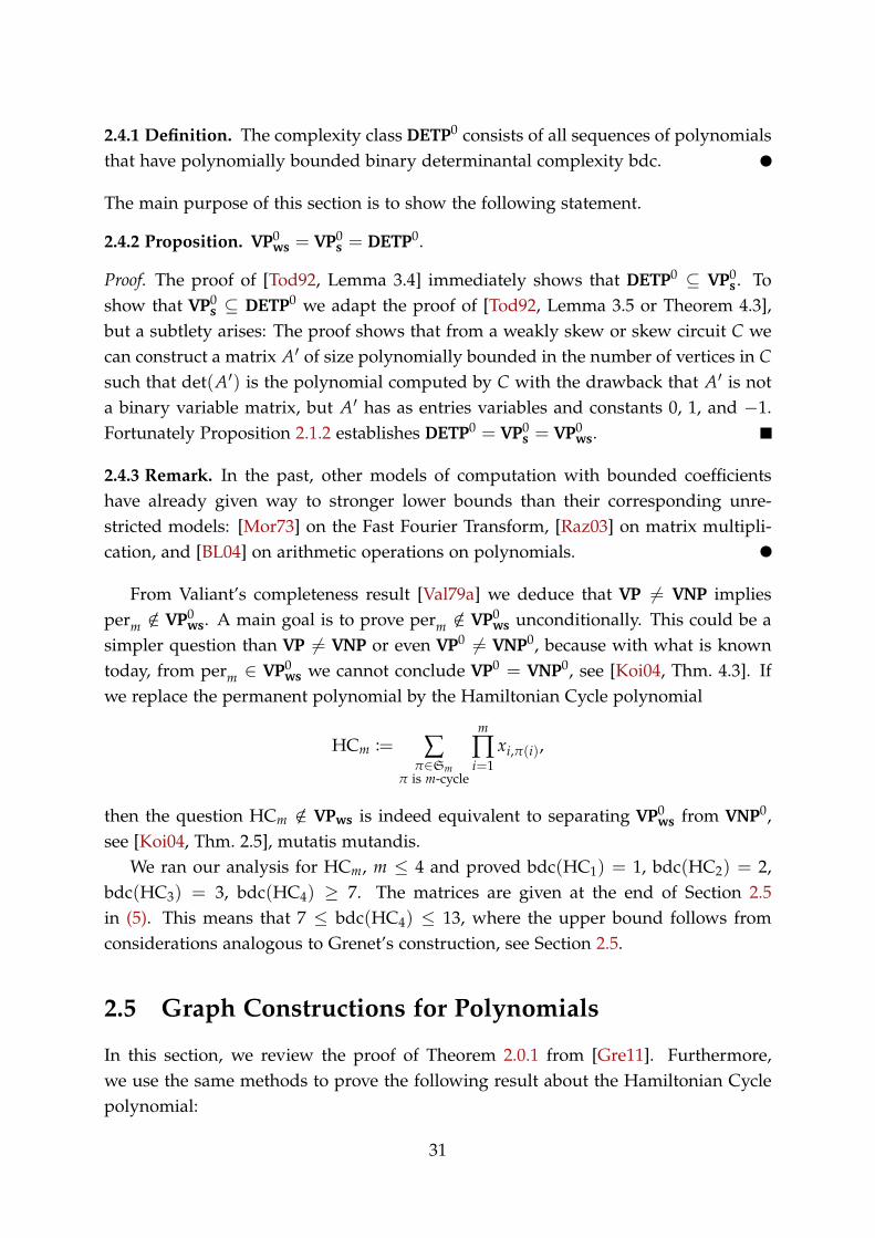
From Valiant’s completeness result [Val79a] we deduce that VP = VNP impliesperm /∈ VP0ws. A main goal is to prove perm /∈ VP0ws unconditionally. This could be asimpler question than VP = VNP or even VP0 = VNP0, because with what is knowntoday, from perm ∈ VP0ws we cannot conclude VP0 = VNP0, see [Koi04, Thm. 4.3]. Ifwe replace the permanent polynomial by the Hamiltonian Cycle polynomial

HCm := ∑π∈Sm

π is m-cycle

m

∏i=1

xi,π(i),

then the question HCm /∈ VPws is indeed equivalent to separating VP0ws from VNP0,see [Koi04, Thm. 2.5], mutatis mutandis.

We ran our analysis for HCm, m ≤ 4 and proved bdc(HC1) = 1, bdc(HC2) = 2,bdc(HC3) = 3, bdc(HC4) ≥ 7. The matrices are given at the end of Section 2.5in (5). This means that 7 ≤ bdc(HC4) ≤ 13, where the upper bound follows fromconsiderations analogous to Grenet’s construction, see Section 2.5.

2.5 Graph Constructions for Polynomials

In this section, we review the proof of Theorem 2.0.1 from [Gre11]. Furthermore,we use the same methods to prove the following result about the Hamiltonian Cyclepolynomial:

31

2.5.1 Theorem. We have bdc(HCm+1) ≤ m · 2m−1 + 1 for all m ∈ N.

Recall that we denote by [m] :=1, . . . ,m the set of numbers between 1 and m.

2.5.1 Grenet’s Construction for the Permanent

We prove Theorem 2.0.1. The construction of Grenet is a digraph Γ whose verticesV := vI | I ⊆ [m] are indexed by the subsets of [m]. Hence, d := |V| = 2m. Wepartition V = V0 ∪ · · · ∪ Vm such that Vi contains the vertices belonging to subsetsof size i. We set s := v∅ and t := v[m], so V0 = s and Vm = t. Edges will goexclusively from Vi−1 to Vi for i ∈ [m]. In fact, we insert an edge from vI to vJ ifand only if there is some j ∈ [m] with J = I ∪j. This edge is then labeled with thevariable xij, where i = |J|. For example, there are m edges going from V0 to V1, onefor each variable x1j with 1 ≤ j ≤ m. It is clear that for each permutation π ∈ Sm,there is precisely one s-t-path in Γ whose path weight is (−1)m−1 · x1,π(1) · · · xm,π(m).Consequently, the path value of the algebraic branching program Γ = (Γ, s, t) is equalto (−1)m−1 · perm. Theorem 2.0.1 then follows from the following lemma:

2.5.2 Lemma. Let Γ = (Γ, s, t) be a binary algebraic branching program on d ≥ 3vertices with path value ±P. Then, there is a binary variable matrix of size d − 1whose determinant is equal to P.

Remark. The proof of this lemma is essentially identical to the proof of Theorem 1.5.4,but it seems convenient to present it anyway.

Proof. We first construct a graph G from Γ by identifying the two vertices s and tand adding loops with label 1 to every other vertex. The s-t-paths in Γ are then inone-to-one correspondence with the cycle covers of G: Indeed, any cycle cover in Gmust cover the vertex s = t and this cycle corresponds to an s-t-path in Γ. Everyother vertex can only be covered by its loop because Γ is acyclic. The graph G nowhas the value ±P by definition and its directed adjacency matrix A has size d − 1.Since d − 1 ≥ 2, we can exchange the first two rows of A to change the sign of itsdeterminant.

2.5.2 Hamiltonian Cycle Polynomial

In this subsection, we prove Theorem 2.5.1 using Lemma 2.5.2. In order to constructa binary algebraic branching program Γ = (Γ, s, t) with path value HCm+1, we pro-ceed similar to Grenet’s construction for the permanent. We will refer to cyclic per-mutations in Sm+1 of order m + 1 simply as cycles because no cyclic permutationsof lower order will be considered. Observe that the cycles in Sm+1 are in bijection

32

with the permutations in Sm. This can be seen by associating to π ∈ Sm the cy-cle σ = (π(1), . . . ,π(m),m + 1) ∈ Sm+1. In other words, σ maps m + 1 to π(1), itmaps π(1) to π(2) and so on.

In addition to two vertices s and t, our binary algebraic branching program willhave a vertex v(I,i) for every nonempty subset I ⊆ [m] and i ∈ I. By our aboveLemma 2.5.2, the resulting binary variable matrix will have a size of

1+m

∑i=1

(mi

)· i = m · 2m−1 + 1.

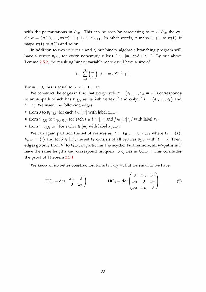
For m = 3, this is equal to 3 · 22 + 1 = 13.We construct the edges in Γ so that every cycle σ = (a1, . . . , am,m+ 1) corresponds

to an s-t-path which has v(I,i) as its k-th vertex if and only if I = a1, . . . , ak andi = ak. We insert the following edges:

• from s to v(i,i) for each i ∈ [m] with label xm+1,i

• from v(I,i) to v(I∪j,j) for each i ∈ I ⊆ [m] and j ∈ [m] \ I with label xi,j• from v([m],i) to t for each i ∈ [m] with label xi,m+1.

We can again partition the set of vertices as V = V0 ∪ . . . ∪ Vm+1 where V0 = s,Vm+1 = t and for k ∈ [m], the set Vk consists of all vertices v(I,i) with |I| = k. Then,edges go only from Vk to Vk+1, in particular Γ is acyclic. Furthermore, all s-t-paths in Γhave the same lengths and correspond uniquely to cycles in Sm+1 . This concludesthe proof of Theorem 2.5.1.

We know of no better construction for arbitrary m, but for small m we have

HC2 = det

(x12 00 x21

)HC3 = det

⎛⎜⎝ 0 x12 x13x21 0 x23x31 x32 0

⎞⎟⎠ . (5)

33

Chapter 3Geometric Complexity Theory

Recall Definition 1.3.4 for the notation P ≤R Q when P,Q ∈ R[x] are polynomialsover a commutative ring R. We call two polynomials P and Q equivalent if P ≤R Qand Q ≤R P. We write P ≃R Q in this case and P ≃ Q if there is no ambiguityconcerning the ring R. This notion has been used for p-families already [Bü00, p. 8]but we require it here for single polynomials only.

It follows directly from the definition that circuit complexity and (binary) deter-minantal complexity are examples for complexity measures in the following sense:

3.0.1 Definition. Let R be a commutative ring. An arithmetic complexity measureover R is a function c : R[x] → N such that P ≤R Q implies c(P) ≤ c(Q).

Remark. For every complexity measure c, equivalent polynomials clearly have thesame complexity with respect to c. Observe also that equivalent polynomials areidentical up to renaming the variables, which follows easily from the definition. It isstraightforward to check that “≃” is an equivalence relation.

Notation. If P and Q are two sets of polynomials, we write P ≃ Q to indicate that(P/≃ ) =(Q/≃ ), i.e., the equivalence classes of polynomials represented by P and Qare the same.

We will work exclusively over the field R = C of complex numbers from here onin, mainly because it simplifies the representation theory and algebraic geometry thatenters the picture later.

3.1 Orbit and Orbit Closure as Complexity Measure

We will now introduce a new complexity measure which is the first step towards a ge-ometric interpretation of Conjecture 1.5.3. LetWd := Cd×d be the space of d× d squarematrices. It is a complex vector space and End(Wd) denotes the set of all endomor-phisms a : Wd → Wd. The determinant is a map detd : Wd → C, so for a ∈ End(Wd),

35

we can consider the composition detd a, which is again a polynomial function: Thisis just linear substitution of variables. We then define the determinantal orbit com-plexity of P as

doc(P) := mind ∈ N | ∃a ∈ End(Wd) : P ≤ detd a , (1)

which is well-defined because doc(P) ≤ dc(P) for all polynomials P. Our main goalwill be to show that the two measures are actually equivalent in the following sense:

3.1.1 Definition. Let X be a set and c1, c2 : X → N two functions. We say that c1 andc2 are polynomially equivalent if there exist t1, t2 ∈ poly such that c1(x) ≤ t2(c2(x))and c2(x) ≤ t1(c1(x)) for all x ∈ X. We denote this by c1 ≡ c2.

3.1.2 Proposition. We have dc ≡ doc.

Proof. The inequality doc ≤ dc is clear. The following Lemma 3.1.3 states that there isa function t ∈ poly such that dc(detd a) ≤ t(d) for every a ∈ End(Cd×d). Since anypolynomial P with d := doc(P) admits a linear transformation a ∈ End(Cd×d) withP ≤ detd a, we have dc(P) ≤ dc(detd a) ≤ t(d) = t(doc(P)).

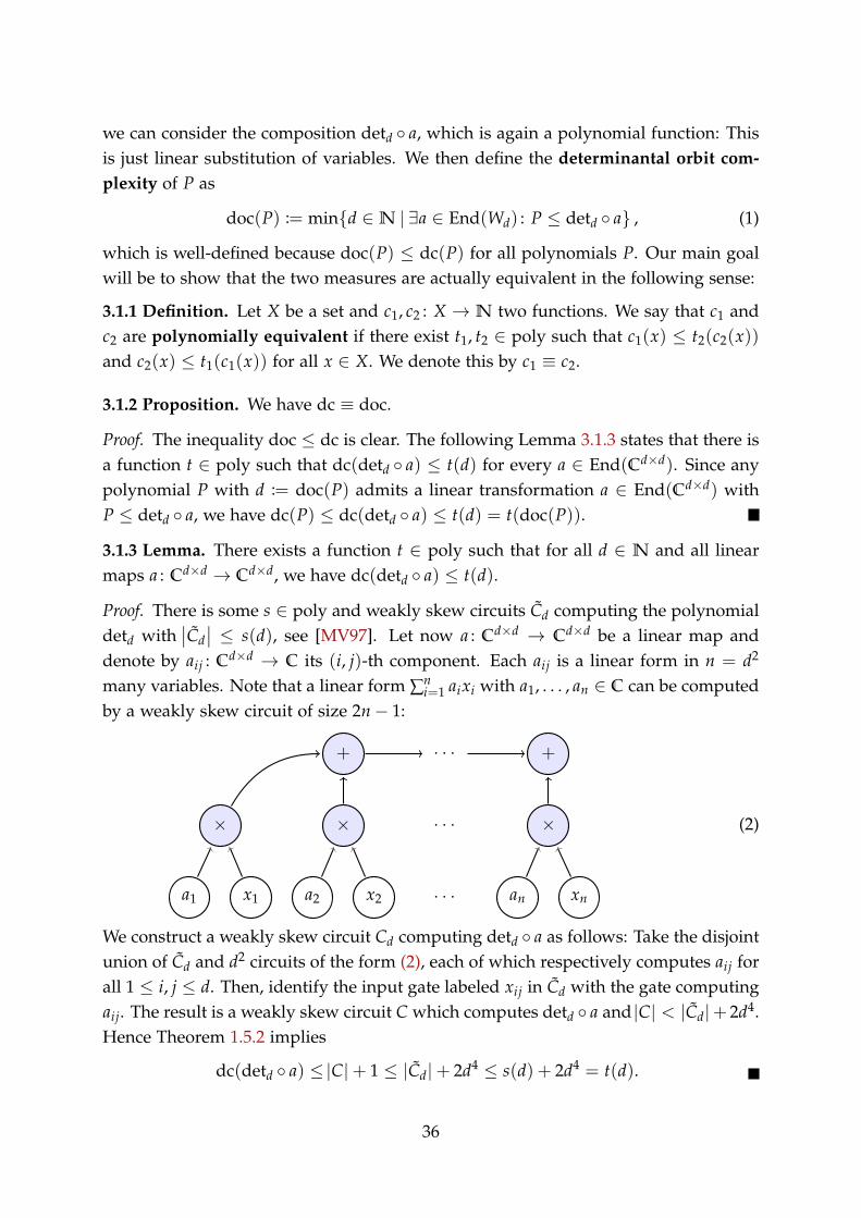
3.1.3 Lemma. There exists a function t ∈ poly such that for all d ∈ N and all linearmaps a : Cd×d → Cd×d, we have dc(detd a) ≤ t(d).

Proof. There is some s ∈ poly and weakly skew circuits Cd computing the polynomialdetd with

Cd ≤ s(d), see [MV97]. Let now a : Cd×d → Cd×d be a linear map and

denote by aij : Cd×d → C its (i, j)-th component. Each aij is a linear form in n = d2

many variables. Note that a linear form ∑ni=1 aixi with a1, . . . , an ∈ C can be computed

by a weakly skew circuit of size 2n− 1:

+· · ·+

× × · · · ×

a1 x1 a2 x2 · · · an xn

(2)

We construct a weakly skew circuit Cd computing detd a as follows: Take the disjointunion of Cd and d2 circuits of the form (2), each of which respectively computes aij forall 1 ≤ i, j ≤ d. Then, identify the input gate labeled xij in Cd with the gate computingaij. The result is a weakly skew circuit C which computes detd a and |C| < |Cd|+ 2d4.Hence Theorem 1.5.2 implies

dc(detd a) ≤|C|+ 1 ≤ |Cd|+ 2d4 ≤ s(d) + 2d4 = t(d).

36

3.2 Border Complexity

Let Wd := Cd×d be the space of d× d square matrices. By Proposition 3.1.2, Conjec-ture 1.5.3 can be expressed in terms of the values d,m ∈ N where perm is a projectionof some polynomial in detd End(Wd).

3.2.1 Remark. Unfortunately, detd End(Wd) is unattractive from a geometric pointof view because it is neither a closed nor an open set for the Euclidean or the Zariskitopology in general. We will now replace this set by its closure, which correspondsto allowing arbitrary approximation in our computational model. This is arguablynatural from both a computational and a geometric point of view, but the implicationsfor the computational model are not completely understood yet.

For y = y1, . . . , yn ⊆ x and d ∈ N, the space C[y]≤d = P ∈ C[y] | deg(P) ≤ d isa finite-dimensional vector space which we endow with the Euclidean topology andwe consider on C[y] the final topology with respect to the inclusions C[y]≤d ⊆ C[y].Lastly, the topology on C[x] that we use is the final topology with respect to theinclusions C[y] ⊆ C[x] for all finite subsets y ⊆ x.

For any complexity measure c : C[x] → N, we define the corresponding bordercomplexity function as

c(P) := mind ∈ N

P ∈ c−1([d]),

where we use the notation [d] := 1, . . . , d and hence, c−1([d]) = P | c(P) ≤ d. If cmeasures complexity, then c measures approximate complexity: c(P) ≤ d means thatany neighbourhood of P contains a polynomial of complexity at most d. Clearly,c(P) ≤ c(P) always holds.

This defines the determinantal orbit border complexity doc : C[x] → N and thedeterminantal border complexity dc : C[x] → N. We note that dc and doc are poly-nomially equivalent by general principle:

3.2.2 Proposition. For two complexity measures c1 and c2, c1 ≡ c2 implies c1 ≡ c2.

Proof. There is a t ∈ poly such that c1(P) ≤ t(c2(P)) for all P ∈ C[x]. In otherwords, we have c−1

2 ([d]) ⊆ c−11 ([t(d)]). If P ∈ C[x] satisfies d := c2(P), then it follows

from an elementary topological argument that P ∈ c−12 ([d]) ⊆ c−1

1 ([t(d)]), hencec1(P) ≤ t(d) = t(c2(P)). The statement follows by symmetry.

With Proposition 3.1.2 we obtain:

3.2.3 Corollary. doc ≡ dc.

The precise statement of the conjecture by Mulmuley and Sohoni is the following:

37

3.2.4 Conjecture ([MS01, 4.3]). doc(perm) is not polynomially bounded in m.

While the converse is not known, Conjecture 3.2.4 implies Conjecture 1.5.3 be-cause we have doc(perm) ≤ doc(perm): If doc(perm) /∈ poly(m), then we also havedoc(perm) /∈ poly(m). For homogeneous polynomials such as the permanent, we cangive a more concrete description of doc. We denote by GL(Wd) ⊆ End(Wd) the set ofinvertible endomorphisms, the general linear group on Wd.

3.2.5 Proposition. For a homogeneous polynomial P ∈ C[x]m and any x ∈ x withx /∈ supp(P), we have

doc(P) = mind ∈ N

∃Q ∈ detd GL(Wd) : xd−mP ≃ Q.

For the proof, we require the following observations:

3.2.6 Lemma. We have detd End(Wd) = detd GL(Wd).

Proof. We only have to show the inclusion “⊆”. Since the right hand side is closed, itis in fact sufficient to show that it contains detd End(Wd). Consider the map

ω : End(Wd) −→ C[x]

a ↦−→ detd a

It is continuous because the coefficients of detd a are polynomials in the entries of (amatrix representation of) a. Since GL(Wd) is dense in End(Wd), we have

detd End(Wd) = ω(End(Wd)) = ω(GL(Wd)) ⊆ ω(GL(Wd)) = detd GL(Wd).

3.2.7 Lemma. For two sets P ,Q ⊆ C[x] of polynomials, P ≃ Q implies P ≃ Q.

Proof. Since “≃” is an equivalence relation, we can give C[x]/≃ the quotient topology

and we claim that the quotient map π : C[x] → C[x]/≃ closed. Let y ⊆ x be a finite

subset. We denote by Sy the group of all set automorphisms of y. For P,Q ∈ C[y],we then have P ≃ Q if and only if there is some π ∈ Sy with P = Qπ, in the senseof Definition 1.3.4. Hence, the equivalence class of any P ∈ C[y] is finite, from whichit follows easily that the quotient map C[y] → C[y]

/≃ is closed. Since C[x]

/≃ has

the final topology with respect to π and C[x] has the final topology with respect tothe inclusions C[y] ⊆ C[x] for any finite y ⊆ x, it follows that π is closed. Therefore,π(P) = π(Q) implies π(P) = π(P) = π(Q) = π(Q).

Proof of Proposition 3.2.5. Let x ∈ x and x := x \x. Note that every polynomial isequivalent to a polynomial in C[x]. The map hd : C[x]m → C[x]d given by P ↦→ xd−mPis linear, in particular it is continuous.

38

Claim. If doc(P) ≤ d, then there is some a ∈ End(Wd) with hd(P) ≃ detd a.

We will prove this claim later and show first that it implies the statement. Let docmbe the restriction of doc to C[x]m and observe

doc−1m ([d]) =P ∈ C[x]m | doc(P) ≤ d

=P ∈ C[x]m | ∃a ∈ End(Wd) : P ≤ detd a (by the claim)

≃P ∈ C[x]m | ∃a ∈ End(Wd) : hd(P) = detd a (by Lemma 3.2.7)

= h−1d (detd End(Wd)) (by definition)

= h−1d (detd End(Wd)) (hd is continuous)

= h−1d (detd GL(Wd)). (by Lemma 3.2.6)

We are left to prove our claim. Assume that doc(P) ≤ d, so there is an a ∈ End(Wd)

with P ≤ detd a. Potentially replacing P by an equivalent polynomial, we mayassume that supp(P) ⊆ supp(detd). Let S ⊆ supp(detd) and σ : S → S∪C be the mapwith P = (detd a)σ. After composing a with an appropriate linear transformation,we can assume that σ : S → C×, since mapping a variable to another variable or tozero is a linear operation on the parameter space. Since scaling the variables by anonzero complex number is also a linear operation, we achieve that σ : S → 1. IfS = ∅, then P = detd a and in particular m = deg(P) = d so we are done. Otherwise,we can compose a with a linear projection mapping all variables in S to one x ∈ S andconsequently replace S byx. Since P and detd a are both homogeneous, it followsthat xd−mP = detd a.

3.3 The Flip via Obstructions

In this section, we freely use concepts and results from representation theory andgeometric invariant theory, see Chapter A. We also expect the reader to be familiarwith elementary topology.

In light of Proposition 3.2.5 and Conjecture 3.2.4, for m ≤ d, we define the paddedpermanent ppd,m := xd−m

d,d · perm which is a degree d form on the space W = Cd×d.

3.3.1 Remark. The padding arises naturally from a computational perspective, but itcauses significant problems from a geometric point of view. We will point out theseproblems when they occur and conclude the discussion in Chapter 4.

3.3.2 Definition. For P ∈ C[W]d, we define Ω(P) := P GL(W) the orbit of P. Wedenote by Ω(P) the Euclidean closure of Ω(P). We also write ΩP and ΩP insteadof Ω(P) and Ω(P), depending on which is more readable.

39

Let W be a finite-dimensional complex vector space and P,Q ∈ C[W]d two homo-geneous forms of degree d onW. In the context of Conjecture 3.2.4, they play the rolesof Q = ppd,m and P = detd on W = Cd×d, for certain values of d,m ∈ N.

By Proposition 3.2.5, we are interested in a way to prove that Q /∈ ΩP. By The-orem A.1.9.(1), the set ΩP is locally closed and the following classical result impliesthat ΩP is also Zariski closed, hence an affine variety.

3.3.3 Theorem ([Kra85, AI.7.2]). Let X be a complex variety. For a constructible setU ⊆ X, the closure of U in the Euclidean and in the Zariski topology coincide.

It is the goal to show that Q /∈ ΩP. Assuming the converse, we get

Q ∈ P GL(W) ⇐⇒ Q GL(W) ⊆ P GL(W) ⇐⇒ Q GL(W) ⊆ P GL(W).

This would imply that there is a surjection π : C[ΩP] C[ΩQ] of the correspondingcoordinate rings. Via the induced action of GL(W) on these rings (see Remark A.1.5),π is also a morphism of GL(W)-modules. Choose a basis W ∼= Cn and by Para-graph A.2.8, we can write

C[ΩP] =⨁

λ∈Λ+n

V(λ)ocP(λ).

We call ocP(λ) the orbit closure coefficient of P at λ. Since π is a GLn-equivariantmorphism, Schur’s Lemma (Lemma A.2.2) implies that ocQ(λ) ≤ ocP(λ) for all λ ∈Λ+

d . Hence:

3.3.4 Proposition (The Flip). Let P,Q ∈ C[x1, . . . , xn]d. If there exists a λ ∈ Λ+n with

ocQ(λ) > ocP(λ), then Q /∈ ΩP.

This observation is called the “flip” because it allows us to prove the non-existenceof efficient algorithms by proving the existence of certain objects.

3.3.5 Remark. It is quite unlikely that Proposition 3.3.4 is sufficient to separate Qfrom ΩP for general P and Q: The GLn-module structure of the coordinate ring of anaffine variety does not define the variety uniquely, see Example 3.3.6 below. It waskindly communicated to the author by Michel Brion and further related developmentscan be found in [Bri11].

3.3.6 Example. Consider G = SL2 acting on the space V = C[x, y]2 of quadratic formsin two variables by precomposition. Let C[V] = C[a, b, c] where we write a quadraticform as a · x2+ b · 2xy+ c · y2. The discriminant of quadratic forms gives a G-invariantregular function ∆ := b2 − ac ∈ C[V]. For any t ∈ C, the polynomial ∆t := ∆ − t isalso G-invariant and the fibers Vt := Q ∈ V | ∆(Q) = t = Z(∆t) ⊆ V are closed

40

G-orbits in V, see [Kra85, II.3.3, Beispiel 1, p. 102]. The variety Vt is singular if andonly if t = 0, so for example V1 is not isomorphic to V0. However, we claim that theG-module structure of the coordinate ring does not depend on t. Indeed, let I ⊆ C[V]

be the ideal generated by ∆t. Since ∆t is G-invariant of degree 2, we have C[V]d−2∼= Id

as G-modules for all d ∈ Z, where the isomorphism is given by P ↦→ P · ∆t. Hence,the G-module structure of I does not depend on the choice of t and in particular, theresulting module structure of C[Vt] = C[V]/I is independent of t.

3.4 Orbit and Orbit Closure

For this chapter, let W be a C-vector space of finite dimension with some choice of abasis W ∼= Cn. Usually, n = d2 and W is a space of d× d matrices. We write GL(W)

when coordinates are not required and GLn otherwise.We study the variety ΩP = P GL(W) for some homogeneous form P ∈ C[W]d.

This is the natural first step towards understanding its closure. By Theorem A.1.9,we are interested in the stabilizer group GP := g ∈ GL(W) | P g = P of P. Thefollowing two results justify that for the rest of this section, we assume GP to bereductive and consequently, ΩP is an affine variety with coordinate ring C[GL(W)]GP .For a matrix A ∈ Cd×d, we denote by At its transpose.

3.4.1 Theorem ([Fro97]). Let W = Cd×d and let detd ∈ C[W]d be the determinant. Thestabilizer group Gdetd is reductive of dimension 2(d2 − 1). Moreover,

(1) The identity component of the stabilizer of detd is the group

Gdetd

=a ∈ GL(W) | ∃S, T ∈ SLd : ∀B ∈ W : a(B) = SBT .

(2) Denoting by t ∈ GL(W) the map t(B) := Bt, the group Gdetd consists of the twoconnected components G

detdand t G

detd.

3.4.2 Theorem ([Bot67; MM62]). Let W = Cm×m with m ≥ 3 and let perm ∈ C[W]mbe the permanent. The stabilizer group Gperm is reductive of dimension 2(m − 1).Moreover,

(1) Denoting by ∆m ⊆ SLm the subgroup of diagonal matrices where the product ofall entries on the diagonal equals 1,

Gperm

=a ∈ GL(W) | ∃S, T ∈ ∆m : ∀B ∈ W : a(B) = SBT .

(2) We embed Sm ⊆ GLm as the subgroup of permutation matrices. For σ, τ ∈ Sm,let cτ

σ ∈ GL(W) be the map cτσ(B) = σ B τ and let Gσ,τ

perm := cτσ G

perm.

Denoting by t ∈ GL(W) the map t(B) := Bt, the group Gperm consists of the 2m!2

connected components tk Gσ,τperm for k ∈0, 1 and σ, τ ∈ Sm.

41

C[ΩP] is also a G-module and the orbit coefficients ocP(λ) are defined by

C[ΩP] =⨁

λ∈Λ+n

V(λ)ocP(λ).

Since ΩP is an open, affine, GLn-invariant subset of ΩP, the restriction morphismC[ΩP] → C[ΩP] is an injective morphism of GLn-modules. By Schur’s Lemma(Lemma A.2.2), we therefore have ocP(λ) ≤ ocP(λ) for all λ ∈ Λ+

n . While the or-bit closure coefficients are quite elusive, the orbit coefficients admit a nice descriptionwhen GP is reductive:

3.4.3 Proposition. For P ∈ C[x1, . . . , xn] with reductive stabilizer GP and λ ∈ Λ+n , we

have ocP(λ) = dim(V(λ)GP).

Proof. Recall from Theorems A.1.9 and A.2.7 that

C[ΩP] = C[GLn]GP =

⨁λ∈Λ+

n

V(λ)∗ ⊗ V(λ)GP .

By Proposition A.2.10 and because λ ↦→ λ∗ defines an involution on Λ+n , we get

C[ΩP] =⨁

λ∈Λ+n

V(λ)⊗ (V(λ)∗)GP .

The statement follows by applying Proposition A.2.12 to the representation V(λ)∗ ofthe reductive group GP.

The orbit coefficients of the determinant and the padded permanent have beenanalyzed in [Bür+11].

3.4.1 Characterization by the Stabilizer

It is crucial to determine whether determinant and padded permanent suffer from theproblem raised in Remark 3.3.5. The following special case of a result due to Larsenand Pink is interesting in this context. We implicitly use Proposition 3.4.3.

3.4.4 Theorem ([LP90]). Let P ∈ C[x1, . . . , xn]d be such that GP is semisimple andconnected. If ϱ : GP → GLn is an irreducible GP-representation, then GP and ϱ areuniquely determined by the orbit coefficients ocP : Λ+

n → N, up to an isomorphism ofgroups and representations, respectively.

The theorem is interesting because it implies that for certain polynomials orbitcoefficients are sufficient to separate orbits. Mulmuley and Sohoni have shown thatthe determinant and the permanent are characterized by their stabilizer [MS01] in thefollowing sense:

42

3.4.5 Definition. Let G be an algebraic group acting linearly on a C-vector space W.A point P ∈ W is said to be characterized by its stabilizer if WGP = C · P.

With this notion, we have:

3.4.6 Corollary. Assume that P and Q satisfy the assumptions of Theorem 3.4.4, wehave Q /∈ ΩP and P is characterized by its stabilizer. Then, there exists a λ ∈ Λ+

n withocQ(λ) = ocP(λ).

Proof. We assume that P and Q have the same orbit coefficients and deduce Q ∈ ΩP.By Theorem 3.4.4, GP = g−1 · GQ · g = GQ g for some g ∈ GLn, this is the definitionof the two representations being isomorphic. Hence, Q g ∈ C[x1, . . . , xn]

GPd = C · P

because P is characterized by its stabilizer. In other words, Q ∈ ΩP.

Unfortunately, the stabilizer groups of determinant and permanent are both dis-connected, and only G

detdis semisimple, G

perm∼= G

2(m−1)m is a torus, therefore only

reductive. It has been established in [AYY13, Thm. 1.5] that the semisimplicity hy-pothesis in the general theorem by Larsen and Pink [LP90] cannot be dropped.

In the literature, the map λ ↦→ ocP(λ) is referred to as the dimension datum of GP.One can study the much more general case that G is an algebraic group and H ⊆ Gis a closed subgroup. The dimension datum of this inclusion is the map Irr(G) → N

given by V ↦→ dim(VH). Proposition 3.4.3 states that this is equivalent to the mapocP : Λ+

n → N in our situation. The question of how much information about theinclusion H ⊆ G is encoded in the dimension datum is an active and recent area ofresearch, for some advances see [Yu16].

It seems that there is no version of Theorem 3.4.4 which is taylored to the situa-tion we consider here, yet. We note however that the stabilizers of determinant andpermanent act irreducibly on W = Cd×d.

3.4.7 Proposition. The space W = Cd×d is an irreducible Gdetd

-representation and inparticular, an irreducible Gdetd-representation.

Proof. Since W ∼= Cd ⊗ Cd, it is an irreducible (SLd × SLd)-representation [FH04, Ex-ercise 2.36]. This is precisely the action of G

detd.

3.4.8 Proposition. The space W = Cm×m is an irreducible Gperm-representation.

Proof. Note first that W = ∑mi=1 ∑m

j=1 C · Eij where Eij is the matrix with entry 1 inposition (i, j) and 0 everywhere else. Using notation from Theorem 3.4.2, the group∆m × ∆m ∼= Gm−1

m ×Gm−1m is a torus and C · Eij is a weight space for the corresponding

action by simultaneous left and right multiplication. This is the action of Gperm

. Letnow U ⊆ W be some nonzero, Gperm-stable subspace of W. Then, U is in particular

43

stable under Gperm

and must therefore be a direct sum of certain weight spaces. Hence,there are indices i and j with Eij ∈ U. By Theorem 3.4.2, arbitrary row and columnpermutations are in Gperm , so Eij ∈ U for all 1 ≤ i, j ≤ m. Hence, W = U.

Remark. While this sounds good, closer inspection reveals that the padded perma-nent fails to retain the desired property. This is related to the padding variable, asannounced in Remark 3.3.1.

Let m < d be natural numbers and Q := ppd,m the padded permanent. Then,the space W = Cd×d is certainly not an irreducible GQ-representation: The one-dimensional space of matrices with zeros everywhere except in position (d, d) is in-variant under GQ due to the description of GQ in [Bür+11, 5.6].

Remark. Note that W = Cm×m is not an irreducible Gperm

-representation.

Even if we ignore all these problems for now, it remains an open question whetherthe orbit closure and its embedding are uniquely defined by the orbit closure coeffi-cients. This is the important question of whether or not Proposition 3.3.4 is sufficient:

3.4.9 Question. Let P,Q ∈ C[x1, . . . , xn]d have reductive stabilizer and Q /∈ ΩP. As-sume that P is irreducible, characterized by its stabilizer, and Cn is irreducible asa GP-module.

(1) Does there exist a λ ∈ Λ+n with ocQ(λ) > ocP(λ)?

(2) The same question, but under the additional assumption that Q = xd−mQ is theproduct an irreducible polynomial Q ∈ C[x1, . . . , xn]m of degree m < d with apower of a linear form x, such that Q is characterized by its stabilizer and Cn isirreducible as a GQ-module.

(3) The same question, but even more specifically with P = detd and Q = ppd,m.

44

Chapter 4Occurrence Obstructions

The Flip (Proposition 3.3.4) offers a way to prove noncontainment of orbit closures.For the polynomials P = detd and Q = ppd,m it is proposed in [MS01; MS08] to exhibitweights λ which satisfy ocP(λ) = 0 and ocQ(λ) = 0. This implies ocQ(λ) > ocP(λ)and therefore Q /∈ ΩP by Proposition 3.3.4. Such weights λ are called occurrenceobstructions.

We present in this chapter the results of the previously published [BIH17]. Thepaper features a result (Theorem 4.1.2) about the nature of occurrence obstructionswhich suggests that they are quite rare. In the subsequent works [IP16; BIP16],Bürgisser, Ikenmeyer, and Panova strengthened this result considerably, eventuallyproving that occurrence obstructions cannot be used to prove Conjecture 3.2.4. Theirmethod relies only on the fact that we consider a padded polynomial, see also Re-mark 3.3.1. This is by far the biggest clue to date that the padding variable, whilecomputationally harmless, causes severe problems for the geometry.

The auxiliary Propositions 4.3.5 and 4.3.8 remain of independent interest: Theyprovide an unconditional version of a related statement by Kumar, even though thebounds are not particularly impressive.

In what follows, we will denote by Dd := Ω(detd) and Pd,m := Ω(ppd,m) the orbitclosures of determinant and padded permanent. Let also n := d2. Both Dd and Pd,m

are closed subvarieties of the N-dimensional affine space AN = C[xij | 1 ≤ i, j ≤ d]dof degree d homogeneous forms on Cd×d, where we define N := (n+d−1

d ). The groupGLn ∼= GL(Cd×d) acts on AN by precomposition.

4.1 Weight Semigroups

We use notation from Section A.3 in this section. Let Z ⊆ AN be any GLn-invariantclosed subvariety. The group GLn acts on the coordinate ring C[Z] of Z via precom-position. We are interested in the set of irreducible GLn-representations occurringin C[Z] and define

Λ+(Z) :=

λ ∈ Λ+nV(λ)∗ ⊆ C[Z]

. (1)

45

It is known that Λ+(Z) is a finitely generated submonoid of Λ+n , cf. [Bri87]. We are

mainly interested in the case where Z = ΩP is an orbit closure, in this case it is easyto see that |λ| := λ1 + · · ·+ λn ∈ dZ for any λ ∈ Λ+(Z). We furthermore denote byℓ(λ) := mink | λk = 0 the length of λ. If P depends on ℓ variables only, then it isknown that ℓ(λ) ≤ ℓ for all λ ∈ Λ+(Z), cf. [Bür+11, §6.3].

An occurrence obstruction is some λ ∈ Λ+(Pd,m) \Λ+(Dd). If we want to prove atleast dc(perm) > m2 + 1 by exhibting an occurrence obstruction, then we may assumethat d ≥ m2 + 1. Since any λ in Λ+(Pd,m) satisfies |λ| ∈ dZ and ℓ(λ) ≤ m2 + 1 ≤ d,we have to look for such partitions λ outside of Λ+(Dd).

Before stating our main result, we need to introduce the concept of saturation,whose relevance for geometric complexity was already pointed out in [Mul07], seealso [BOR09].

For the following compare [MS05, §7.3]. Let S be a submonoid of a free abeliangroup F and ⟨S⟩ the group generated by S. We call S saturated if

∀λ ∈⟨S⟩ : ∀k ∈ N : kλ ∈ S ⇒ λ ∈ S.

The saturation Sat(S) of S is defined as the smallest saturated submonoid of F con-taining S. It can also be characterized as the intersection of ⟨S⟩ with the rational conegenerated by S. An element in Sat(S) \ S is called a gap of S. The reason for thisnaming becomes apparent from a simple example:

4.1.1 Example. Consider S = N2 \(0, 1), (1, 0), which has N2 as its saturation. Re-placing S by Sat(S) means filling up the gaps (0, 1), (1, 0). Generally, understandingmonoids is difficult due to the presence of gaps.

We can now state the main theorem of this chapter:

4.1.2 Theorem. The saturation of Λ+(Dd) contains the setλ ∈ Λ+

n ℓ(λ) ≤ d, |λ| ∈ dZ

,

provided that d > 2. Hence, occurrence obstructions must be gaps of Λ+(Dd).

4.1.1 Related Work

Our work is closely related to a result by Shrawan Kumar [Kum15]. A latin square ofsize d is an d× d matrix with entries from 1, . . . , d such that in each row and in eachcolumn each number occurs exactly once. The sign of a latin square is defined as theproduct of the signs of all the row and column permutations. Depending on the sign,we can speak about even and odd latin squares. The Alon-Tarsi conjecture [AT92]states that the number of even latin squares of size d is different from the number of

46

odd latin squares of size d, provided d is even. The Alon-Tarsi conjecture is known tobe true if d = p± 1 where p is a prime [Dri98; Gly10].

4.1.3 Theorem (Kumar). Let d be even. If the Alon-Tarsi conjecture for d × d latinsquares holds, then dλ ∈ Λ+(Dd) for all partitions λ such that ℓ(λ) ≤ d.

The above two theorems complement each other. Theorem 4.1.2 is unconditionaland also provides information about the group generated by Λ+(Dd). Theorem 4.1.3is conditional, but gives a very tight bound on the stretching factor, which is d if theAlon-Tarsi conjecture holds. The proofs of both theorems focus on the the d-th Chowvariety (see Section 4.3 for details), but otherwise proceed differently. Our proof alsogives information on the stretching factor in terms of certain degrees related to thenormalization the Chow variety, but we were so far unable to bound it in a reasonableway, see Proposition 4.3.5.

4.2 Saturations of Weight Semigroups of Varieties

We consider the following situation. G := GLn(C) is the complex general linear groupand U denotes its subgroup consisting of the upper triangular matrices. V is a finitedimensional C-vector space and a rational G-module such that scalar multiples ofthe unit matrix In ∈ G act on V by nontrivial homotheties, i.e., there is a nonzerod ∈ Z such that P tIn = tdP for t ∈ C× and P ∈ V. Further, Z denotes a G-invariant, irreducible, locally closed nonempty subset of V. Then Z is closed undermultiplication with scalars in C× by our assumption on the G-action.

We consider the induced action of G on the coordinate ring C[Z] of Z definedas in Remark A.1.5. We will denote this induced action from the left and by a dot,i.e., (g. f )(P) = f (P g−1) for P ∈ Z, f ∈ C[Z] and g ∈ G. As in (1) we definethe monoid Λ+(Z) of representations of the G-variety Z. We shall interpret Λ+(G)as a subset of Zn and denote by Λ(Z) := ⟨Λ+(Z)⟩ the group generated by Λ+(Z).Moreover, we denote by coneQ(Λ+(Z)) the rational cone generated by Λ+(Z), that is,

coneQ(Λ+(Z)) :=k−1λ

k ∈ N,λ ∈ Λ+(Z)⊆ Qn.

It is easy to check that the saturation of Λ+(Z) is obtained as

Sat(Λ+(Z)) = Λ(Z) ∩ coneQ(Λ+(Z)). (2)

We denote by Frac(R) the field of fractions of an integral ring R. We have an inducedG-action on the field of fractions C(Z) := Frac(C[Z]) and denote by C(Z)U its subfieldof U-invariants. Recall that a highest weight vector is a U-invariant weight vector. Thefollowing lemma is well known, but we include its proof for completeness.

47

4.2.1 Lemma. We have Frac(C[Z]U) = C(Z)U. Moreover, for a highest weight vectorf ∈ C(Z)U, there exist highest weight vectors p, q ∈ C[Z]U such that f = p/q.

Proof. The inclusion Frac(C[Z]U) ⊆ C(Z)U is obvious. Now let f ∈ C(Z)U andconsider the ideal J := q ∈ C[Z] | q f ∈ C[Z] of C[Z]. Since J = 0 we have JU = 0,cf. [Hum98, §17.5]. Choose a nonzero q ∈ JU. Then p := q f ∈ C[Z]U and f = p/q,hence f ∈ Frac(C[Z]U).

If f ∈ C(Z)U is a weight vector, we can argue as before, choosing q ∈ JU as ahighest weight vector. Then p := q f is a highest weight vector in C[Z]. The assertionfollows.

4.2.2 Remark. If Y = ∅ is a G-invariant open subset of Z, then Λ+(Z) ⊆ Λ+(Y) andΛ(Z) = Λ(Y). This follows immediately from Lemma 4.2.1.

Suppose now that Z is a closed subset of V, hence an affine variety. Then we havean induced G-action on the normalization N(Z) and the canonical map π : N(Z) → Zis G-invariant. Indeed, the integral closure R of C[Z] in C(Z) is G-invariant and π

corresponds to the inclusion C[Z] → R. By construction, we can identify C(N(Z))with C(Z). Note that Λ+(Z) ⊆ Λ+(N(Z)) since π is surjective.

4.2.3 Proposition. We have Λ(N(Z)) = Λ(Z) and Sat(Λ+(N(Z))) = Sat(Λ+(Z)).More precisely, assume that C[N(Z)] is generated as a C[Z]-module by r elements.Then for all λ ∈ Λ+(N(Z)), there is some k < r such that (r− k) · λ ∈ Λ+(Z).

Proof. Let λ ∈ Λ+(N(Z)) and f ∈ C[N(Z)]U be a highest weight vector of weight λ.Then f ∈ C(Z)U and Lemma 4.2.1 shows the existence of highest weight vectorsp, q ∈ C[Z]U, say with the weights µ, ν ∈ Λ+(Z), respectively, such that f = p/q.Therefore λ = µ − ν ∈ Λ(Z). This shows the equality for the groups.

Due to (2), it suffices to prove that coneQ(Λ+(Z)) = coneQ(Λ+(N(Z))). Supposef ∈ C[N(Z)] is a highest weight vector of weight λ. Since f is integral over C[Z],there are e ∈ N and a0, . . . , ae−1 ∈ C[Z] such that such that

f e +e−1

∑i=0

ai f i = 0. (3)

We assume that the degree e is the smallest possible.Note that e is at most the size of a generating set of C[N(Z)] as an C[Z]-module,

as follows from the classical theory of integral extensions, see [AM69, Prop. 5.1 andthe proof of Prop. 2.4].

Consider the weight decomposition ai = ∑µ ai,µ of ai, where ai,µ has the weight µ.Then ai,µ f i has the weight µ+ iλ. Moreover, f e has the weight eλ. Since the componentof weight eλ in (3) must vanish, we have

f e +e−1

∑i=0

ai,(e−i)λ · f i = 0.

48

As the degree e is the smallest possible, the above is the minimal polynomial of f . Ap-plying any element u ∈ U to the above equation and using u. f = f , we get the identityf e + ∑e−1

i=0 (u.ai,(e−i)λ) f i = 0. The uniqueness of the minimal polynomial implies thatu.ai,(e−i)λ = ai,(e−i)λ for all i. Hence ai,(e−i)λ is a highest weight vector, provided it isnonzero. Since there exists i < e with ai,(e−i)λ = 0, we see that (e− i)λ ∈ Λ+(C[Z])for this particular i. We conclude that λ ∈ coneQ(C[Z]).

4.2.4 Example. If we consider instead the torus G = (C×)d we can identify Λ+G

with Zd. Let S ⊆ Zd be a finitely generated submonoid and consider the finitely gen-erated subalgebra C[S] :=

⨁s∈S(C · xs11 · · · xsdd ) of C[x±1

1 , . . . , x±1d ]. If we interpret C[S]

as the coordinate ring of an affine variety Z, then we have a G-action on Z and Λ+(Z)can be identified with S (Z is called a toric variety). It is known that C[Sat(S)] equalsthe integral closure of C[S] in Frac(C[S]), cf. [MS05, Prop. 7.25, p. 140]. Thus theaffine variety corresponding to Sat(S) equals the normalization of Z. This illustratesProposition 4.2.3 in the special case of toric varieties.

4.3 Proof of Main Results

Write W := Cn, G := GL(W) and consider the symmetric power V := SymnW∗ withis natural G-action. Using the chosen coordinates on W, we obtain an isomorphismW → W∗ that we denote by a ↦→ a∗. We can interpret V as the space C[W]n ofdegree n forms. Note that C[V]k ∼= Symk SymnW as G-modules. Let x1, . . . , xn ∈ W∗

be a basis and consider the universal monomial

mnn := x1 · · · xn ∈ V.

Clearly, Ωmnn consists of all symmetric products a1 · · · an of n linearly independentlinear forms ai. We define the n-th Chow variety

C n := mnn End(W) =a1 · · · an | a1, . . . , an ∈ W∗ ⊆ V.

The name comes from the fact that C n is a special case of a Chow variety, see [GKZ94].

4.3.1 Lemma. We have C n = Ωmnn .

Proof. The inclusion C n ⊆ Ωmnn follows since GL(W) is dense in End(W). For theconverse inclusion, let Q ∈ Ωmnn be nonzero. By Theorem 3.3.3, it is the limit of asequence (tk · a1k · · · ank)k∈N, where tk ∈ C× and aik ∈ W∗ are linearly independentwith ∥aik∥ = 1. By compactness of the unit sphere in W∗ we may assume that afterpassing to a subsequence, (aik)k∈N is convergent for all 1 ≤ i ≤ n. Let bi := limk→∞ aik.Then, (∏n

i=1 aik)k∈N converges to b1 · · · bn = 0. It follows easily that (tk)k∈N convergesto some t ∈ C× and consequently, Q = t · b1 · · · bn ∈ C n.

49

When we identify xi with the variable xii, the Chow variety C n is contained in Dn

by mapping xij to 0 for i = j, c.f. [Lan15]. The basic strategy, as in Kumar [Kum15], isto replace Dn by the considerably simpler C n and to exhibit elements in the monoid ofrepresentations of the latter. More specifically, we have Λ+(C n) ⊆ Λ+(Dn) and henceSat(Λ+(C n)) ⊆ Sat(Λ+(Dn)). Our main Theorem 4.1.2 is an immediate consequenceof the following result.

4.3.2 Theorem. We have Sat(Λ+(C n)) =λ ∈ Λ+n : |λ| ∈ nZ, provided n > 2.

According to Proposition 4.2.3, for proving this we may replace C n by its normal-ization. It is crucial that the latter has an explicit description.

For the following arguments compare [Bri93] and [Lan15]. We will revisit them inSection 6.2. The symmetric group Sn operates on the group

Tn :=(t1, . . . , tn) ∈ Cn | t1 · · · tn = 1

by permutation. The corresponding semidirect product Hn := Tn oSn acts on thespaceWn = W× . . .×W by scaling and permutation. Note that this action commuteswith the G-action. Consider the product map

ω : Wn = W × . . .×W −→ C n

(a1, . . . , an) ↦−→ a∗1 · · · a∗n,

which is surjective and G-equivariant. Clearly, ω is invariant on H-orbits. Moreover,the fiber of a nonzero Q ∈ C n is an Hn-orbit. This easily follows from the uniquenessof polynomial factorization.

The group G contains the subgroup t · idW | t ∈ C× ∼= C× and this C×-actioninduces a natural grading on the coordinate rings C[Wn] and C[C n]. Since ω is G-equivariant, the corresponding comorphism ω♯ : C[C n] → C[Wn] is in particular ahomomorphism of graded C-algebras. However, the C×-action on C[C n] is not thecanonical one because t ∈ C× acts by multiplication with the scalar tn. A homoge-neous element of degree kn in C[C n] is the restriction of a k-form on V.

The categorical quotient Wn//Hn is defined as the affine variety that has as itscoordinate ring the ring of Hn-invariants C[Wn]Hn , which is finitely generated andgraded since Hn is reductive, cf. [Kra85]. The inclusion C[Wn]Hn → C[Wn] definesa G-equivariant, surjective morphism π : Wn → Wn//Hn. Since Wn is normal, thequotient Wn//Hn is normal as well, see [Dol03, p. 45] for the easy proof. The map ω

factors through a G-equivariant morphism

φ : Wn//Hn → C n, (4)

due to the universal property of categorical quotients. Moreover, by construction, thefibers of φ over a nonzero Q ∈ C n consist of just one element. The action of Hn

50

on C[Wn] is linear, therefore it respects the grading. It follows that the comorphismφ♯ : C[C n] → C[Wn]Hn is again a homomorphism of graded C-algebras.

The following is shown in [Bri93, Prop., p. 351] and we give a proof in slightlydifferent language in Section 6.3.

4.3.3 Lemma. The morphism φ : Wn//Hn → C n is the normalization of C n.

Furthermore,

4.3.4 Lemma. We have

Λ+(Wn//Hn) =

λ ∈ Λ+n

∃k : |λ| = kn and VG(λ) ⊆ Symn Symk Cn.

Proof. We shall decompose the coordinate ring C[Wn//Hn] with respect to the G-action. We have C[W] =

⨁k∈N SymkW∗ and therefore

C[Wn] = C[W]⊗n =⨁

(k1,...,kn)∈Nn

Symk1 W∗ · · · ⊗ Symkn W∗.

Taking Tn-invariants yields

C[Wn]Tn =⨁k∈N

SymkW∗ ⊗ . . .⊗ SymkW∗.

Taking Sn-invariants gives

C[Wn//Hn] ∼= C[Wn]TnoSn =⨁k∈N

Symn SymkW∗, (5)

and the assertion follows.

Recalling Theorem 4.1.3, we expect the stretching factor to be n. Without relyingon the Alon-Tarsi conjecture however, the following exponential bound is the best wecan currently provide.

4.3.5 Proposition. Λ+(C n) generates the rational cone q ∈ Qn | q1 ≥ · · · ≥ qn ≥ 0.More precisely: Assume n > 2. For each partition λ with ℓ(λ) ≤ n and |λ| ∈ nZ,

there is some number k < nn2−2n such that we have 2k · λ ∈ Λ+(C n).

Proof. For the first statement, it is sufficient to show that coneQ(Λ+(C n)) containsany partition λ with |λ| = nk and ℓ(λ) ≤ n. According to Proposition 4.2.3, thesemigroups Λ+(C n) and Λ+(Wn//Hn) generate the same rational cone. So we needto show that λ lies in coneQ(Λ+(Wn//Hn)).

In [BCI11] (see [Ike12] for a simpler proof) it was shown that VG(2λ) occurs inSymn Sym2k(Cn). Thus Lemma 4.3.4 with Proposition 4.2.3 imply that λ lies in therational cone generated by Λ+(Wn//Hn).

51

We will now make the above reference to Proposition 4.2.3 precise. Recall that thecomorphism of φ from (4) is an integral extension φ♯ : C[C n] → C[Wn]Hn of graded C-algebras. Note that the grading induced by G on these two rings is such that onlydegrees which are multiples of n contain nonzero elements. We therefore changethe grading such that degree n · k becomes degree k. This means that the directsum (5) is the grading of C[Wn]Hn and the grading of C[C n] is the grading inducedby the canonical grading induced by the polynomial ring C[V]. Therefore, C[C n] isgenerated by elements of degree one.

By [DK02, Lemma 2.4.7], there is a system of parameters y0, . . . , yr ∈ C[C n]1 fromamong sufficiently generic linear forms. This means that R := C[y0, . . . , yr] is a poly-nomial ring in the yi and C[C n] is a finite R-module. It follows that C[Wn]Hn is integralover R and y0, . . . , yr is also a homogeneous system of parameters for C[Wn]Hn .

We note that r + 1 = dim(Wn//Hn) = dim(Wn) − dim(Hn) = n2 − n + 1, sor = n2 − n. Furthermore, C[Wn]Hn is Cohen-Macaulay [DK02, Thm. 2.5.5] and by[DK02, Prop. 2.5.3], it follows that C[Wn]Hn is free as an R-module, i.e., C[Wn]Hn ∼= RD

for some D ∈ N. Since D is the number of generators of C[Wn]Hn as an R-module,D is a (possibly rough) upper bound for the number of generators of C[Wn]Hn as anC[C n]-module. The second assertion follows from Proposition 4.2.3 as soon as wehave verified that D < nn

2−2n.The Hilbert polynomial of RD is a polynomial of degree r whose leading coefficient

is equal to Dr! . Since (5) gives the grading of C[Wn]Hn , the Hilbert polynomial of

C[Wn]Hn is given, for sufficiently large k, by the map

k ↦→((k+n−1

n−1 ) + n− 1n

),

whose leading coefficient is 1n!(n−1)!n . Since r = n2 − n, we have D = (n2−n)!

n!(n−1)!n . Weapply Stirling’s approximation:

∀n > 0 : 1 ≤ n!√2π · e−n · nn+ 1

2≤ e

112n

to the fraction D and obtain

D =(n2 − n)!n!(n− 1)!n

≤√2π · e 1

12n · (n2 − n)n2−n+ 1

2 · en−n2

√2π · nn+ 1

2 · e−n ·√2π

n · (n− 1)(n−12 )n · e−(n−1)n

=

(e√2π

)n· e 1

12n · nn2−n+ 1

2 · (n− 1)n2−n+ 1

2

nn+12 · (n− 1)n2−

n2

=

((e√2π

)n· e 1

12n · (n− 1)1−n2

)

R(n)

· nn2−2n.

52

It is easy to see that R(n) is monotonically decreasing for n ≥ 2 and takes a valuesmaller than 1 for n = 3. Hence, for n > 2 we have D < nn

2−2n.

We shall now determine Λ(C n). Since Wn//Hn is the normalization of C n, Propo-sition 4.2.3 tells us that Λ(C n) = ⟨Λ+(Wn//Hn)⟩. The latter is described in terms ofplethysms in Lemma 4.3.4.

Recall W = Cn and G = GL(W). We say that λ occurs in Symn SymkW if VG(λ)

occurs as a submodule in the latter. We will also make use of the convenient notationk× d := (d, . . . , d, 0, . . . , 0) ∈ Zn for a rectangular partition with k rows of length d.

4.3.6 Lemma. Let ℓ ∈ N. If λ occurs in Symn SymkW, then (1× ℓk) + λ occurs inSymℓ+n SymkW.

Proof. Let WU = Cw, i.e., w is a highest weight vector of W with weight 1× 1. Thenw⊗ℓk ∈ Symℓ SymkW is a highest weight vector of weight (1× ℓk).

Let f ∈ Symn SymkW be a highest weight vector of weight λ. Then the productw⊗ℓk f ∈ Symℓ+n SymkW is a highest weight vector of weight (1× ℓk) + λ.

4.3.7 Lemma. Let n ≥ k ≥ 2, d := k(k− 1)/2, and the partition µ of size k2 be obtainedby appending to 2× d a column of length k. Further, let λ denote the partition of sizenk obtained by appending to µ a row of length (n− k)k. Then the partition λ occursin Symn SymkW.

Proof. The GL2-module Λk Symk−1 C2 is one-dimensional, since Symk−1 C2 is of di-mension k. Hence it contains a nonzero SL2-invariant. In other words, 2× d occursin Λk Symk−1 C2. The “inheritance principle” states that 2× d occurs in Λk Symk−1 Cn

(compare for instance [Ike12, Lemma 4.3.2]).Cor. 6.4 in [MM15] implies that µ occurs in Symk SymkW. Finally, Lemma 4.3.6

implies the assertion.

4.3.8 Proposition. Λ+(C n) generates the groupλ ∈ Zn : |λ| ∈ nZ if n > 2.

Proof. Using the software [BKT12], we checked that the partition (2, 2, 0, . . . , 0) occursin Sym2 Sym2W and (6, 3, 0, . . . , 0) occurs in Sym3 Sym3W. Using Lemma 4.3.6, wecan conclude that (2n− 2, 2, 0, . . . , 0) occurs in Symn Sym2W, and (3n− 3, 3, 0, . . . , 0)occurs in Symn Sym3W if n ≥ 3. (We note that (3, 3, 0, . . . , 0) does not occur inSym2 Sym3W; this is the reason for the assumption n > 2.) From Lemma 4.3.4 weconclude that

λ(2) := (n− 1, 1, 0, . . . , 0) = (3n− 3, 3, 0, . . . , 0)− (2n− 2, 2, 0, . . . , 0)

lies in the group Λ generated by Λ+(Wn//Hn). Clearly, λ(1) := (n, 0, . . . , 0) ∈ Λ.

53

For 3 ≤ k ≤ n let λ(k) ∈ Λ denote the partition from Lemma 4.3.7. Then we haveℓ(λ(k)) = k and λ

(k)k = 1. This easily implies that λ(1), . . . ,λ(n) generate the group

Λ :=λ ∈ Zn : |λ| ∈ nZ. Since Λ ⊆ Λ is obvious, we conclude that Λ = Λ.

Proof of Theorem 4.3.2. Use (2) with Propositions 4.3.5 and 4.3.8.

4.3.9 Remark. The assumption n > 2 in Theorem 4.3.2 is necessary. Indeed, we haveC 2 = Sym2 C2, and one can show that Λ+(Sym2 C2) generates the group (2Z)2, com-pare [FH04, §11.2].

54

Part II

Orbit Closures of Homogeneous Forms

55

Chapter 5Preliminaries

Throughout Part II, we will consider the following situation. We work over the field C

of complex numbers and W ∼= Cn is a C-vector space of dimension n, for whichwe sometimes assume some choice of coordinates C[W] = C[x1, . . . , xn], to iden-tify GL(W) with GLn = GLn(C). The group GL(W) acts on the space C[W]d =

SymdW∗ of homogeneous forms of degree d > 0 on W by precomposition from theright:

C[W]d ×GL(W) −→ C[W]d

(P, g) ↦−→ P g

We view V := C[W]d ∼= AN as an affine space of dimension N = (n+d+1d ). Note

that C[V] is simply a polynomial ring in the coefficients of all homogeneous degree dpolynomials in n variables. We will study subvarieties of this space in the languageof algebraic geometry, therefore we usually assume the Zariski topology on V.

This scenario is motivated by the GCT approach that we outlined in Chapter 3. Inthat context, one is interested only in special cases, primarily W = Cd×d and the pointP = detd. We put this into a slightly more general context here, one reason beingthat we have very little understanding of the determinant orbit closure, even for smallvalues of d. For what little we know, see Chapter 8. To gain a better understanding ofthe phenomena that occur, we believe that easier examples should be studied first.

Another reason is also that the generality we present here offers an interesting andlittle explored mathematical problem: Classical geometric invariant theory offers thetools to study the entire orbit structure of V, but a classification seems out of reachfor n > 3 and d > 4. We on the other hand pick specific forms P ∈ V and study onlythe orbit structure of ΩP, or even just the orbits that are of maximal dimension in acomponent of ∂ΩP. In this chapter, we make some general observations and elaborateon methods that we will apply in the chapters to come.

Unless explicitly stated otherwise, we only consider points P ∈ V whose stabilizerGP = g ∈ GL(W) | P g = P is reductive, mostly because it simplifies the theory

57

considerably and the condition is satisfied in our cases of primary interest, recallTheorems 3.4.1 and 3.4.2.

We write ΩP := P GL(W) ⊆ V for the orbit of P and denote by ΩP ⊆ V its closureas in Definition 3.3.2. Recall also that by Theorem 3.3.3, ΩP is both the Euclidean andthe Zariski closure of ΩP. An element of ∂ΩP is called a degeneration of P.

5.1 Conciseness

Let us call a form P ∈ V = C[W]d concise if it is not stabilized by any noninvertibleendomorphism, i.e.

∀a ∈ End(W) : (P a = P) ⇒ (a ∈ GL(W)).

We will give other characterizations of this property here, for example it means thatthere is no choice of coordinates C[W] = C[x1, . . . , xn] such that P ∈ C[x1, . . . , xn−1].Informally, this may be expressed as “P uses all variables”. We will also see that beingconcise is an open condition in Proposition 5.1.2.

5.1.1 Definition. Let x ∈ W∗ = C[W]1 and w ∈ W. We define the partial derivative ofxd ∈ C[W]d in direction w to be the form ∂wxd := d · x(w) · xd−1, c.f. [Lan12, eq. (2.6.6)].By linear extension, this defines ∂wP for any P ∈ C[W]d because C[W]d = SymdW∗

is spanned by powers of linear forms as a vector space [Mar73, Theorem 1.7]. If wehave chosen coordinates C[W] = C[x1, . . . , xn], we set ∂iP := ∂eiP for 1 ≤ i ≤ n, whereei ∈ W is the dual basis vector of xi ∈ W∗.

5.1.2 Proposition. Let W be a vector space of finite dimension. A form P ∈ C[W]d isconcise if and only if the linear map W → C[W], w ↦→ ∂wP is injective.

Proof. The case d = 0 is trivial, a constant form P is stabilized by any endomorphism,hence it is concise if and only if GL(W) = End(W), which is equivalent to W = 0.The case d ≥ 1 follows from Lemma 5.1.6 below for the identity map a = idW .

5.1.3 Remark. In particular, not being concise is a polynomial condition on the coeffi-cients of P ∈ C[W]d: It is given by the vanishing of all maximal minors of the linearmap W → C[W]d−1, w ↦→ ∂wP. Hence, the set of all concise forms is a Zariski opensubset of C[W]d.

5.1.4 Corollary. Let P ∈ C[x1, . . . , xn]d. Then, P is concise if and only if the partialderivatives ∂1P, . . . , ∂nP are linearly independent.

58

5.1.5 Remark. After choosing coordinates, a polynomial P ∈ C[x1, . . . , xn] satisfiesxi ∈ supp(P) if and only if ∂iP = 0. Hence, P is not concise if and only if there isa choice of coordinates such that one of the variables does not appear in the supportof P at all.

For a ∈ End(W), we denote by rk(a) := dim(a(W)) its rank.

5.1.6 Lemma. Let P ∈ C[W]d with d ≥ 1. For a ∈ End(W), we consider the linearmap δa : W → C[W], w ↦→ ∂w(P a). The following conditions are equivalent:

(1) rk(a) ≤ rk(δa).

(2) For any b ∈ End(W) with P a = P b, we have rk(a) ≤ rk(b).

Proof. We choose coordinates C[W] = C[x1, . . . , xn] and set Q := P a. Denote by

∇(Q) := (∂1Q, . . . , ∂nQ) ∈ C[x1, . . . , xn]1×nd−1

the (row) vector of partial derivatives of Q. Let v1, . . . , vk ∈ Cn be a basis of the vectorspace v ∈ Cn | ∇(Q) · v = 0, so r := n − k is the dimension of the C-vector spacespanned by the ∂iQ, i.e., r = rk(δa).

Assume that (2) holds. We have to show that rk(a) ≤ r. Let g ∈ GL(W) be aninvertible linear transformation that maps the i-th standard basis vector ei ∈ Cn to vifor 1 ≤ i ≤ k. Denoting by a dot the product of matrices, the chain rule yields

∂i(Q g) = ∇(Q g) · ei = (∇(Q) · vi) g = 0 for 1 ≤ i ≤ k.

This implies that Q g ∈ C[xk+1, . . . , xn]. We consider the linear map c ∈ End(W)

which maps xi c = 0 for 1 ≤ i ≤ k and xj c = xj for j > k. Then, Q g c = Q g,therefore P agcg−1 = Q = P a. It follows that r = rk(c) ≥ rk(agcg−1) ≥ rk(a) byour assumption.

Conversely, assume that (1) holds, so we have rk(a) ≤ r. Let b ∈ End(W) be suchthat P a = P b. For any v ∈ ker(b), the chain rule yields

∇(P a) · v = ∇(P b) · v = (∇(P) b) · b · v = 0,

so any v ∈ ker(b) is a linear relation among the partial derivatives of P a. In otherwords, k = dim(ker(δa)) ≥ dim(ker(b)). Therefore,

rk(a) ≤ r = n− k ≤ n− dim(ker(b)) = rk(b).

59

5.2 Grading of Coordinate Rings and Projectivization

The next observation is that ΩP and ΩP are both affine cones in the following sense:

5.2.1 Definition. A subset C ⊆ V is called an affine cone if ∀P ∈ C : C · P ⊆ C.

Note that GL(W) contains a central copy of Gm(C) = C× in the form of scalarmaps C× · idW , where idW denotes the identity map. Given Q ∈ ΩP ⊆ C[W]d andany t ∈ C, let ζ ∈ C be some d-th root of t. Then, tQ = ζdQ = Q ζ idW ∈ ΩQ = ΩP.Since scalar multiplication is continuous, we have the following general principle.

5.2.2 Lemma. If C ⊆ V is an affine cone, then C is also an affine cone.

Proof. The reductive group Gm = (C×, ·) acts algebraically on V by scalar multiplica-tion. Denote by α : Gm × V → V the action morphism. Since Gm × C = Gm × C, wehave α(Gm × C) ⊆ α(Gm × C) = C. Hence, C is Gm-invariant.

This means that ΩP is an affine cone. In particular, the coordinate ring C[ΩP]

inherits a N-grading from C[V]. On the other hand, C[GLn] has a natural Z-gradingthat is the result of localizing at the SLn-invariant polynomial detn. The coordinatering C[ΩP] = C[GLn]GP inherits this grading. By Proposition A.2.9,

C[ΩP]d =⨁

λ∈Λ+n

|λ|=d

V(λ)∗ ⊗ V(λ)GP .

We will now see that under reasonable assumptions, C[ΩP] is also the localizationof C[ΩP] at some SL(W)-invariant and the grading of C[ΩP] is the same as the naturalone induced by this localization. We call a form P ∈ C[W]d polystable if P SL(W)

is Zariski closed in C[W]d. Both the permanent and the determinant are polystable[BI15, 2.9]. Furthermore, Bürgisser and Ikenmeyer proved:

5.2.3 Theorem ([BI15, 3.9]). If P ∈ V = C[W]d is polystable, then there exists a homo-geneous invariant f ∈ C[ΩP]

SL(W) such that C[ΩP] = C[ΩP][ f−1]. In particular,

ΩP =Q ∈ ΩP

f (Q) = 0.

Furthermore, if f is homogeneous of minimal degree with this property, then f isunique up to scalar.

Remark. Bürgisser and Ikenmeyer also study the minimal degree and other numericalquantities related to these invariants, for the determinant and several other interestingfamilies of polynomials.

60

Studying the geometry of ΩP is equivalent to studying its projectivization P(ΩP),which is a projective variety. Furthermore, we know that P(ΩP) is a smooth, opensubset of P(ΩP) which we understand well. While this is quite promising, it turnsout [BI15, 3.10,3.17,3.29] that ΩP is not a normal variety in most cases and in partic-ular, when P is detn or pern with n ≥ 3. It follows that in all these cases, ΩP hassingularities. Since ΩP is smooth, these singularities will be part of the boundary∂ΩP := ΩP \ ΩP, which is therefore a subvariety that needs to be analyzed further.We note first that it is a hypersurface in our cases of interest:

5.2.4 Lemma. If GP is reductive, then ∂ΩP is pure of codimension one in ΩP.

Proof. The complement of an affine variety is always pure of codimension one [Gro67,Corollaire 21.12.7]. The statement follows because for reductive GP, the orbit ΩP isaffine by Theorem A.1.9.

5.3 Rational Orbit Map

The orbit map ωP : End(W) → ΩP given by a ↦→ P a is line-preserving, therefore itcan be viewed as a rational map

ϖP : P End(W) −→ PΩP (1)

[a] ↦−→ [P a]

Since it can happen that P a = 0 for a = 0, the map ϖP is not defined everywhere.If it was defined everywhere, it would be a dominant, projective morphism, thereforesurjective [Sha94, I.5.2]. We will transform ϖP into a projective morphism by twosteps, the first of which is explained in this section. In Chapter 6 we study the specialcase where we obtain a morphism after the first step already. The second step ispostponed until Section 7.3 and we will see how to combine both steps in the finaltwo chapters.

5.3.1 Definition. For a form P ∈ C[W]d, we define

AP :=a ∈ End(W) | P a = 0 (2)

and call it the annihilator of P. It is an affine cone in End(W) whose projectivizationis precisely the set of points where ϖP : P End(W) 99K PΩP is not defined.

5.3.2 Remark. Another way to see the annihilator is as

AP =a ∈ End(W) | a(W) ⊆ Z(P) ,

61

the set of all endomorphisms whose image is a linear subspace of the hypersurfaceZ(P) ⊆ W. We will call a linear subspace L ⊆ Z(P) maximal if there is no other linearsubspace of Z(P) which properly contains L. With this notion, AP is the set of alla ∈ End(W) whose image is contained in some maximal linear subspace of Z(P).

The stabilizer GP =g ∈ GL(W) | P g = P acts by left multiplication on End(W)

and ωP is GP-invariant with respect to this action, since ωP(g a) = P g a = P afor all g ∈ GP. This action induces an action on P End(W) and consequently, therational map ϖP from (1) is invariant with respect to this induced action. We stressagain that GP is assumed reductive unless explicitly stated otherwise.

Consider now a map a ∈ End(W) with 0 ∈ GP a, i.e., there is a sequence (gn)n∈N

with gn ∈ GP such that limn→∞ gn a = 0. Such points a ∈ End(W) are calledunstable with respect to the action of GP in the sense of geometric invariant theory[MFK94], see also [New78; Kra85; Dol03].

5.3.3 Definition. Let P be a homogeneous form. The set of unstable endomorphismswith respect to the action of GP is called the nullcone of P and we denote it by

N P :=a ∈ End(W)

0 ∈ GP a. (3)

See Subsection A.1.2 for other, equivalent definitions of the nullcone.

A central observation is the following:

5.3.4 Proposition. We have N P ⊆ AP. In other words, if a ∈ End(W) is unstable withrespect to the left action of GP, then P a = 0. This statement holds regardless ofwhether or not GP is reductive.

Proof. Let a ∈ N P, meaning 0 ∈ GP a. Since ω−1P (P a) is a closed subset of End(W)

containing GP a, it also contains its closure. Thus, 0 ∈ GP a ⊆ ω−1P (P a), which

means P a = P 0 = 0.

We will now explain that the points in N P induce “harmless” indeterminaciesof ϖP. We require the results from Subsection A.1.2, in particular the notion ofsemistability. In our situation,

End(W)ss := End(W) \ N P =a ∈ End(W)

0 /∈ GP a

is the set of semistable endomorphisms and P End(W)ss ⊆ P End(W) is an opensubvariety of P End(W) which admits a categorical quotient, see Proposition A.1.11.An important property of this quotient is the fact that

P End(W)ss//GP = Proj(C[End(W)]GP)

62

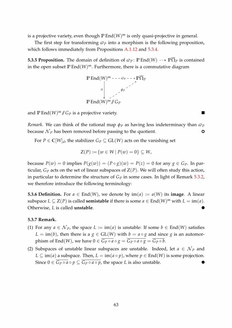
is a projective variety, even though P End(W)ss is only quasi-projective in general.The first step for transforming ϖP into a morphism is the following proposition,

which follows immediately from Propositions A.1.12 and 5.3.4.

5.3.5 Proposition. The domain of definition of ϖP : P End(W) 99K PΩP is containedin the open subset P End(W)ss. Furthermore, there is a commutative diagram

P End(W)ss

π

↓↓↓↓

ϖP →→ PΩP

P End(W)ss//GP

φP

and P End(W)ss//GP is a projective variety.

Remark. We can think of the rational map φP as having less indeterminacy than ϖP

because N P has been removed before passing to the quotient.

For P ∈ C[W]d, the stabilizer GP ⊆ GL(W) acts on the vanishing set

Z(P) :=w ∈ W | P(w) = 0 ⊆ W,

because P(w) = 0 implies P(g(w)) = (P g)(w) = P(z) = 0 for any g ∈ GP. In par-ticular, GP acts on the set of linear subspaces of Z(P). We will often study this action,in particular to determine the structure of GP in some cases. In light of Remark 5.3.2,we therefore introduce the following terminology:

5.3.6 Definition. For a ∈ End(W), we denote by im(a) := a(W) its image. A linearsubspace L ⊆ Z(P) is called semistable if there is some a ∈ End(W)ss with L = im(a).Otherwise, L is called unstable.

5.3.7 Remark.

(1) For any a ∈ N P, the space L := im(a) is unstable: If some b ∈ End(W) satisfiesL = im(b), then there is a g ∈ GL(W) with b = a g and since g is an automor-phism of End(W), we have 0 ∈ GP a g = GP a g = GP b.

(2) Subspaces of unstable linear subspaces are unstable. Indeed, let a ∈ N P andL ⊆ im(a) a subspace. Then, L = im(a p), where p ∈ End(W) is some projection.Since 0 ∈ GP a p ⊆ GP a p, the space L is also unstable.

63

Chapter 6Closed Forms

If P ∈ C[W]d satisfies ΩP = P End(W), we call it closed. This is equivalent to thefact that ωP has closed image.

6.0.1 Remark. If P is closed, then ∂ΩP is always irreducible: It is the image underωP : End(W) → ΩP of the irreducible hypersurface S ⊆ End(W) of noninvertibleendomorphisms.

6.0.2 Example. Every quadratic form is closed. In fact, if there is some symmetricmatrix b ∈ Cn×n such that P(x) = xtbx, then for any endomorphism a, the form P ais given by the matrix atba. We may assume that P is concise, i.e. b is invertible.

It follows thatatba

a ∈ Cn×n =ata a ∈ Cn×n is the space of symmetric ma-

trices, hence P End(Cn) = C[x1, . . . , xn]2. In particular, this is equal to ΩP and P isclosed.

6.1 A Sufficient Criterion

We know only very few examples of closed forms of higher degree. A classificationremains an interesting open problem, we can only give some partial results and poseseveral questions. Recall the definitions ofAP andN P from Definitions 5.3.1 and 5.3.3.A sufficient criterion for being closed is the following:

6.1.1 Proposition. Let P ∈ C[W]d be a form with reductive stabilizer GP ⊆ GL(W). Ifwe have AP = N P, then P is closed.

Proof. Recall the definition of ϖP from (1) and Proposition 5.3.5. The assumptionmeans that ϖP is defined everywhere on P End(W)ss and so the induced rationalmap φP : P End(W)ss//GP → PΩP is in fact a morphism. Since it is dominant andprojective, its image is equal to PΩP. The statement follows because ϖP has the sameimage as φP.

6.1.2 Corollary. If the hypersurface Z(P) has no semistable linear subspaces, then Pis closed.

65

In Proposition 5.3.4, we saw N P ⊆ AP. Proposition 6.1.1 states that P is closed ifthis inclusion is an equality. Having no counterexample but also no wide selection ofexamples in general, we ask the following question:

6.1.3 Question. Does N P = AP hold for every closed form P?

We know of no counterexample for Question 6.1.3, but for two examples of closedforms that are already well-known, we illustrate that N P = AP.

6.1.4 Example. We know from Example 6.0.2 that concise quadratic forms are closed.We claim that N P = AP for any such P ∈ V = C[x1, . . . , xn]2. We may assumewithout loss of generality that P = x21 + · · ·+ x2n because any concise quadratic formis an element of ΩP. On the one hand, we observe that

AP =a ∈ Cn×n P a = 0

= a ∈ Cn×n | ata = 0.

The stabilizer of P is the orthogonal group On =a ∈ GLn

at = a−1. As before,we consider the operation of On on Cn×n by left multiplication. By the First Fun-damental Theorem for the Orthogonal Group [Pro06, 11.2, Theorem on p. 390], theOn-invariant functions on Cn×n are generated by the entries of the map a ↦→ ata, andby Lemma A.1.10 we therefore also have N P =

a ∈ Cn×n

ata = 0.

6.1.5 Example. Consider P := z(y2 + xz) ∈ C[x, y, z]3. The classification of ternarycubic forms [KM02] implies that P is closed. We will show that AP = N P. ByExample 2 in said reference, the stabilizer GP ⊆ GL3 is generated by the matrices

uα :=

⎛⎜⎝1 −2α −α2

0 1 α

0 0 1

⎞⎟⎠ and tε :=

⎛⎜⎝ε4 0 00 ε 00 0 ε−2

⎞⎟⎠ .

Note that U := uα | α ∈ C ∼= (C,+) is a normal unipotent subgroup of GP whilethe group T := tε | ε ∈ C× ∼= (C×, ·) is reductive. More precisely, tεuαtε−1 = uε3α.We have GP = T nU, the unipotent radical of GP is equal to U and in particular GP

is not reductive and we cannot appeal to Proposition 6.1.1 to show that it is closed.However, the definitions of N P and AP do not require P to have reductive stabilizer.

Observe that Z(P) = Z(z)∪Z(y2 + xz). The maximal linear subspaces of Z(P) aretherefore the plane Z(z) and any line in Z(y2 + xz). We first note that Z(z) is unstablebecause for any w ∈ Z(z), we have tε(w) → 0 as ε → 0. Therefore, we are left to showthat any w ∈ Z(y2 + xz) \ Z(z) spans an unstable line. After applying an appropriatescaling matrix tε, we can assume that w = (−y2, y, 1). Consider

gε := tε−1 uε3−y =1ε4

·

⎛⎜⎝1 −2(ε3 − y) −(ε3 − y)2

0 ε3 ε3(ε3 − y)0 0 ε6

⎞⎟⎠ .

A straightforward computation shows that gε(w) = (−ε2, ε2, ε2) → 0 as ε → 0.

66

6.2 Normalizations of Orbit Closures

For almost every family of homogeneous forms studied in the context of GCT, the or-bit closures are not normal varieties [Kum15; BI11]. In Section 4.3, we saw a prominentexample of an orbit closure whose normalization has a nice representation-theoreticdescription: For this section, we choose coordinates C[W] = C[x1, . . . , xn] and con-sider the n-form mnn := x1 · · · xn, the universal monomial. It is also the top symmet-ric form. The variety C n = Ω(mnn) is called the n-th Chow variety. In Chapter 4 wealso used the notation Dn = Ω(detn), and we recall that C n ⊆ Dn because mnn is therestriction of detn to diagonal matrices.

By Lemma 4.3.1, the universal monomial is closed. Again, we observe that itactually satisfies the condition we discussed in the previous section:

6.2.1 Proposition. We have Nmnn = Amnn for all n ≥ 2.

Proof. We fix n ≥ 2 and let P := mnn. We show that any a ∈ End(W) with P a = 0satisfies 0 ∈ GP a. The group GP contains all diagonal matrices t = diag(t1, . . . , tn)with 1 = t1 · · · tn. Assume that a ∈ Cn×n ∼= End(W) satisfies P a = 0 and letai := xi a = ∑n

j=1 aijxj, then we have 0 = P a = a1 · · · an. Since C[W] is an integraldomain, it follows that there must be some iwith ai = 0. Without loss of generality, wemay assume that a1 = 0, i.e., the first row of a contains only zeros. The diagonal matrixtε := diag(ε1−n, ε, . . . , ε) stabilizes P and tε a = ε · a. We can view tε as a regular mapt : C → End(W) mapping ε ↦→ tε. Since t(C×) ⊆ GP, we have t(C×) a ⊆ GP a.Passing to the closure, we get 0 = t0 a ∈ GP a.

The following theorem is well-known. It is implied by the proof of Lemma 4.3.3,but we will also obtain it as a corollary of the upcoming Theorem 6.2.3 – we onlyquote it here to provide context. Refer to Section A.3 for the notion of the polynomialpart V⊒0 of a GL(W)-module V.

6.2.2 Theorem. Let ν : N(C n) → C n be the normalization of the Chow variety. Themorphism ν corresponds to the inclusion C[N(C n)] = C[C n]⊒0 ⊆ C[C n].

Arguably, Theorem 6.2.2 and Remark 6.0.1 motivated Landsberg [Lan15] to askthe following question: Is it true that whenever a GL(W)-orbit closure with reductivestabilizer has an irreducible boundary, the coordinate ring of the normalization of theorbit closure equals the polynomial part of the coordinate ring of the orbit?

The answer is negative, as we recently showed [Hü17]. We will instead prove thatC[N(ΩP)] = C[ΩP]⊒0 is equivalent to AP = N P. Furthermore, we illustrate thatthese equivalent conditions can be violated in cases where ∂ΩP is irreducible. Themain theorem of this chapter is the following, its proof is postponed to Section 6.3.

67

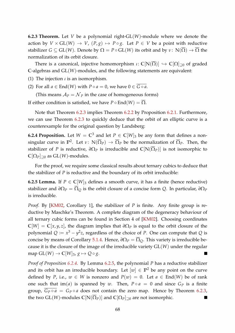
6.2.3 Theorem. Let V be a polynomial right-GL(W)-module where we denote theaction by V × GL(W) → V, (P, g) ↦→ P g. Let P ∈ V be a point with reductivestabilizer G ⊆ GL(W). Denote by Ω = P GL(W) its orbit and by ν : N(Ω) → Ω thenormalization of its orbit closure.

There is a canonical, injective homomorphism ι : C[N(Ω)] → C[Ω]⊒0 of gradedC-algebras and GL(W)-modules, and the following statements are equivalent:

(1) The injection ι is an isomorphism.

(2) For all a ∈ End(W) with P a = 0, we have 0 ∈ G a.(This means AP = N P in the case of homogeneous forms)

If either condition is satisfied, we have P End(W) = Ω.

Note that Theorem 6.2.3 implies Theorem 6.2.2 by Proposition 6.2.1. Furthermore,we can use Theorem 6.2.3 to quickly deduce that the orbit of an elliptic curve is acounterexample for the original question by Landsberg:

6.2.4 Proposition. Let W = C3 and let P ∈ C[W]3 be any form that defines a non-singular curve in P2. Let ν : N(ΩP) → ΩP be the normalization of ΩP. Then, thestabilizer of P is reductive, ∂ΩP is irreducible and C[N(ΩP)] is not isomorphic toC[ΩP]⊒0 as GL(W)-modules.

For the proof, we require some classical results about ternary cubics to deduce thatthe stabilizer of P is reductive and the boundary of its orbit irreducible:

6.2.5 Lemma. If P ∈ C[W]3 defines a smooth curve, it has a finite (hence reductive)stabilizer and ∂ΩP = ΩQ is the orbit closure of a concise form Q. In particular, ∂ΩP

is irreducible.

Proof. By [KM02, Corollary 1], the stabilizer of P is finite. Any finite group is re-ductive by Maschke’s Theorem. A complete diagram of the degeneracy behaviour ofall ternary cubic forms can be found in Section 4 of [KM02]. Choosing coordinatesC[W] = C[x, y, z], the diagram implies that ∂ΩP is equal to the orbit closure of thepolynomial Q := x3 − y2z, regardless of the choice of P. One can compute that Q isconcise by means of Corollary 5.1.4. Hence, ∂ΩP = ΩQ. This variety is irreducible be-cause it is the closure of the image of the irreducible variety GL(W) under the regularmap GL(W) → C[W]3, g ↦→ Q g.

Proof of Proposition 6.2.4. By Lemma 6.2.5, the polynomial P has a reductive stabilizerand its orbit has an irreducible boundary. Let [w] ∈ P2 be any point on the curvedefined by P, i.e., w ∈ W is nonzero and P(w) = 0. Let a ∈ End(W) be of rankone such that im(a) is spanned by w. Then, P a = 0 and since GP is a finitegroup, GP a = GP a does not contain the zero map. Hence by Theorem 6.2.3,the two GL(W)-modules C[N(ΩP)] and C[ΩP]⊒0 are not isomorphic.

68

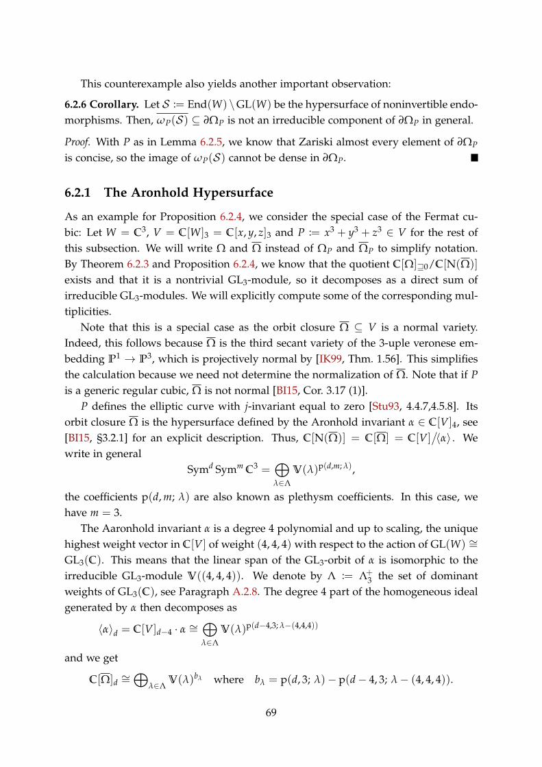
This counterexample also yields another important observation:

6.2.6 Corollary. Let S := End(W) \GL(W) be the hypersurface of noninvertible endo-morphisms. Then, ωP(S) ⊆ ∂ΩP is not an irreducible component of ∂ΩP in general.

Proof. With P as in Lemma 6.2.5, we know that Zariski almost every element of ∂ΩP

is concise, so the image of ωP(S) cannot be dense in ∂ΩP.

6.2.1 The Aronhold Hypersurface

As an example for Proposition 6.2.4, we consider the special case of the Fermat cu-bic: Let W = C3, V = C[W]3 = C[x, y, z]3 and P := x3 + y3 + z3 ∈ V for the rest ofthis subsection. We will write Ω and Ω instead of ΩP and ΩP to simplify notation.By Theorem 6.2.3 and Proposition 6.2.4, we know that the quotient C[Ω]⊒0/C[N(Ω)]

exists and that it is a nontrivial GL3-module, so it decomposes as a direct sum ofirreducible GL3-modules. We will explicitly compute some of the corresponding mul-tiplicities.

Note that this is a special case as the orbit closure Ω ⊆ V is a normal variety.Indeed, this follows because Ω is the third secant variety of the 3-uple veronese em-bedding P1 → P3, which is projectively normal by [IK99, Thm. 1.56]. This simplifiesthe calculation because we need not determine the normalization of Ω. Note that if Pis a generic regular cubic, Ω is not normal [BI15, Cor. 3.17 (1)].

P defines the elliptic curve with j-invariant equal to zero [Stu93, 4.4.7,4.5.8]. Itsorbit closure Ω is the hypersurface defined by the Aronhold invariant α ∈ C[V]4, see[BI15, §3.2.1] for an explicit description. Thus, C[N(Ω)] = C[Ω] = C[V]

/⟨α⟩ . We

write in generalSymd Symm C3 =

⨁λ∈Λ

V(λ)p(d,m;λ),

the coefficients p(d,m; λ) are also known as plethysm coefficients. In this case, wehave m = 3.

The Aaronhold invariant α is a degree 4 polynomial and up to scaling, the uniquehighest weight vector in C[V] of weight (4, 4, 4) with respect to the action of GL(W) ∼=GL3(C). This means that the linear span of the GL3-orbit of α is isomorphic to theirreducible GL3-module V((4, 4, 4)). We denote by Λ := Λ+

3 the set of dominantweights of GL3(C), see Paragraph A.2.8. The degree 4 part of the homogeneous idealgenerated by α then decomposes as

⟨α⟩d = C[V]d−4 · α ∼=⨁λ∈Λ

V(λ)p(d−4,3;λ−(4,4,4))

and we get

C[Ω]d ∼=⨁

λ∈ΛV(λ)bλ where bλ = p(d, 3; λ)− p(d− 4, 3; λ − (4, 4, 4)).

69

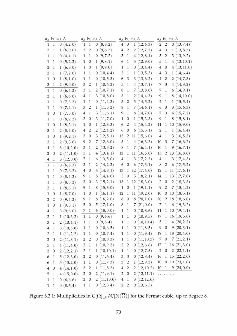
aλ bλ mλ λ

1 1 0 (4, 2, 0)2 1 1 (6, 0, 0)1 1 0 (4, 4, 1)1 1 0 (5, 2, 2)2 1 1 (6, 3, 0)2 1 1 (7, 2, 0)1 0 1 (8, 1, 0)3 1 2 (9, 0, 0)1 1 0 (6, 4, 2)2 1 1 (6, 6, 0)1 1 0 (7, 3, 2)1 1 0 (7, 4, 1)1 0 1 (7, 5, 0)1 1 0 (8, 2, 2)1 0 1 (8, 3, 1)3 1 2 (8, 4, 0)1 0 1 (9, 2, 1)3 1 2 (9, 3, 0)4 1 3 (10, 2, 0)2 0 2 (11, 1, 0)4 1 3 (12, 0, 0)1 1 0 (6, 6, 3)1 1 0 (7, 6, 2)1 1 0 (8, 4, 3)1 1 0 (8, 5, 2)2 1 1 (8, 6, 1)1 0 1 (8, 7, 0)2 2 0 (9, 4, 2)1 0 1 (9, 5, 1)4 1 3 (9, 6, 0)2 1 1 (10, 3, 2)3 1 2 (10, 4, 1)4 1 3 (10, 5, 0)2 1 1 (11, 2, 2)2 0 2 (11, 3, 1)5 1 4 (11, 4, 0)2 0 2 (12, 2, 1)6 1 5 (12, 3, 0)6 1 5 (13, 2, 0)4 0 4 (14, 1, 0)5 1 4 (15, 0, 0)1 1 0 (6, 6, 6)1 1 0 (8, 6, 4)

aλ bλ mλ λ

1 1 0 (8, 8, 2)2 2 0 (9, 6, 3)1 1 0 (9, 7, 2)1 0 1 (9, 8, 1)1 0 1 (9, 9, 0)1 1 0 (10, 4, 4)1 1 0 (10, 5, 3)3 2 1 (10, 6, 2)3 1 2 (10, 7, 1)4 1 3 (10, 8, 0)1 1 0 (11, 4, 3)3 2 1 (11, 5, 2)4 1 3 (11, 6, 1)3 0 3 (11, 7, 0)1 0 1 (12, 3, 3)4 2 2 (12, 4, 2)3 0 3 (12, 5, 1)9 2 7 (12, 6, 0)3 1 2 (13, 3, 2)5 1 4 (13, 4, 1)7 1 6 (13, 5, 0)3 1 2 (14, 2, 2)4 0 4 (14, 3, 1)9 1 8 (14, 4, 0)3 0 3 (15, 2, 1)9 1 8 (15, 3, 0)1 0 1 (16, 1, 1)9 1 8 (16, 2, 0)5 0 5 (17, 1, 0)7 1 6 (18, 0, 0)1 1 0 (9, 6, 6)1 1 0 (9, 8, 4)1 1 0 (10, 6, 5)1 1 0 (10, 7, 4)2 2 0 (10, 8, 3)2 1 1 (10, 9, 2)2 1 1 (10, 10, 1)2 2 0 (11, 6, 4)1 1 0 (11, 7, 3)3 2 1 (11, 8, 2)2 0 2 (11, 9, 1)2 0 2 (11, 10, 0)1 1 0 (12, 5, 4)

aλ bλ mλ λ

4 3 1 (12, 6, 3)4 2 2 (12, 7, 2)5 1 4 (12, 8, 1)6 1 5 (12, 9, 0)1 1 0 (13, 4, 4)2 1 1 (13, 5, 3)6 3 3 (13, 6, 2)5 1 4 (13, 7, 1)8 1 7 (13, 8, 0)3 1 2 (14, 4, 3)5 2 3 (14, 5, 2)8 1 7 (14, 6, 1)9 1 8 (14, 7, 0)1 0 1 (15, 3, 3)6 2 4 (15, 4, 2)6 0 6 (15, 5, 1)13 2 11 (15, 6, 0)5 1 4 (16, 3, 2)8 1 7 (16, 4, 1)12 1 11 (16, 5, 0)4 1 3 (17, 2, 2)6 0 6 (17, 3, 1)13 1 12 (17, 4, 0)5 0 5 (18, 2, 1)13 1 12 (18, 3, 0)1 0 1 (19, 1, 1)12 1 11 (19, 2, 0)8 0 8 (20, 1, 0)8 1 7 (21, 0, 0)1 1 0 (10, 8, 6)1 1 0 (10, 9, 5)1 1 0 (10, 10, 4)1 1 0 (11, 8, 5)1 1 0 (11, 9, 4)1 1 0 (11, 10, 3)2 2 0 (12, 6, 6)1 1 0 (12, 7, 5)3 3 0 (12, 8, 4)3 2 1 (12, 9, 3)4 2 2 (12, 10, 2)2 0 2 (12, 11, 1)4 1 3 (12, 12, 0)2 2 0 (13, 6, 5)

aλ bλ mλ λ

2 2 0 (13, 7, 4)4 3 1 (13, 8, 3)5 2 3 (13, 9, 2)5 1 4 (13, 10, 1)4 0 4 (13, 11, 0)4 3 1 (14, 6, 4)4 2 2 (14, 7, 3)7 3 4 (14, 8, 2)7 1 6 (14, 9, 1)9 1 8 (14, 10, 0)2 1 1 (15, 5, 4)6 3 3 (15, 6, 3)7 3 4 (15, 7, 2)9 1 8 (15, 8, 1)11 1 10 (15, 9, 0)2 1 1 (16, 4, 4)4 1 3 (16, 5, 3)10 3 7 (16, 6, 2)10 1 9 (16, 7, 1)15 2 13 (16, 8, 0)4 1 3 (17, 4, 3)8 2 6 (17, 5, 2)12 1 11 (17, 6, 1)14 1 13 (17, 7, 0)2 0 2 (18, 3, 3)9 2 7 (18, 4, 2)10 0 10 (18, 5, 1)20 2 18 (18, 6, 0)7 1 6 (19, 3, 2)11 1 10 (19, 4, 1)17 1 16 (19, 5, 0)5 1 4 (20, 2, 2)9 0 9 (20, 3, 1)19 1 18 (20, 4, 0)7 0 7 (21, 2, 1)17 1 16 (21, 3, 0)2 0 2 (22, 1, 1)16 1 15 (22, 2, 0)10 0 10 (23, 1, 0)10 1 9 (24, 0, 0). . . . . . . . .

Figure 6.2.1: Multiplicities in C[Ω]⊒0/C[N(Ω)] for the Fermat cubic, up to degree 8.

70

Note that bλ can be computed with the software package [BKT12].Denoting by aλ the coefficients such that C[Ω]⊒0 =

⨁λ∈Λ V(λ)aλ , we are inter-

ested in the numbers mλ := aλ − bλ, because:

C[Ω]⊒0/C[Ω] =⨁

λ∈ΛV(λ)aλ−bλ .

It follows from the Peter-Weyl Theorem (Theorem A.2.7) that aλ = dim(V(λ)G),where G ⊆ GL3 is the stabilizer of P. It is well-known [BI15, Prop. 2.4] that G consistsof permutation matrices and diagonal matrices whose diagonal entries are third rootsof unity. A matrix representation of the canonical projection V(λ) V(λ)G withrespect to the basis of semistandard Young tableaux (SSYT) is obtained by symmetriz-ing each SSYT with respect to G and straightening it [Ful97, § 7.4]. The quantity aλ

arises as the rank of this matrix. Using this method, we have computed the values ofthe mλ := aλ − bλ up to degree 8, see Figure 6.2.1 on page 70.

6.2.7 Remark. A formula for aλ is more involved than the one for bλ. Advancingmethods used in [BI11, Section 4.2] (see also [Ike12, Section 5.2]), Ikenmeyer [Ike16]determined such a formula: For λ ∈ Λ, denote by |λ| := λ1 + λ2 + λ3 the sum of itsentries. We have aλ = 0 unless |λ| = 3d for some d ∈ N. In this case,

aλ = ∑µ∈Λ|µ|=d

∑ν1,...,νd∈Λ,|νk|=3·k·µkfor all k

cλν1,...,νd ·

d

∏k=1

p(µk, 3k; νk), (1)

where cλν1,...,νd denotes the multi-Littlewood-Richardson coefficient and µk denotes the

number of times that k appears as an entry of µ.

6.3 Proof of Main Theorem

This section contains the proof of Theorem 6.2.3. We require results from Section A.3and Subsection A.1.1.

Note that the stabilizer G acts on the variety End(W) by multiplication fromthe left. Since V is a polynomial GL(W)-module, there is a well-defined morphismω : End(W) → Ω, a ↦→ P a. For h ∈ G and a ∈ End(W),

ω(ha) = P (ha) = P h a = P a = ω(a).

Therefore, ω is an G-invariant morphism. Since G is a reductive algebraic group,there is an affine quotient variety End(W)//G together with a surjective morphism

71

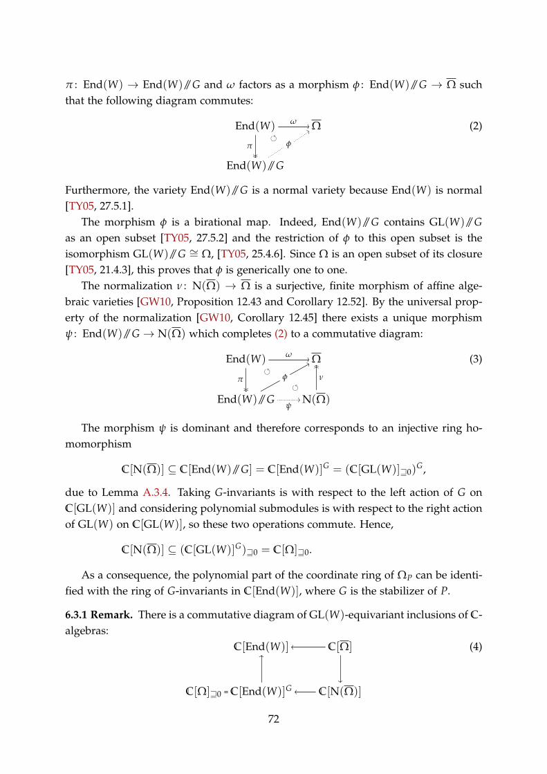
π : End(W) → End(W)//G and ω factors as a morphism φ : End(W)//G → Ω suchthat the following diagram commutes:

End(W)

π↓↓↓↓

ω→→ Ω

End(W)//G

φ

(2)

Furthermore, the variety End(W)//G is a normal variety because End(W) is normal[TY05, 27.5.1].

The morphism φ is a birational map. Indeed, End(W)//G contains GL(W)//Gas an open subset [TY05, 27.5.2] and the restriction of φ to this open subset is theisomorphism GL(W)//G ∼= Ω, [TY05, 25.4.6]. Since Ω is an open subset of its closure[TY05, 21.4.3], this proves that φ is generically one to one.

The normalization ν : N(Ω) → Ω is a surjective, finite morphism of affine alge-braic varieties [GW10, Proposition 12.43 and Corollary 12.52]. By the universal prop-erty of the normalization [GW10, Corollary 12.45] there exists a unique morphismψ : End(W)//G → N(Ω) which completes (2) to a commutative diagram:

End(W)

π↓↓↓↓

ω→→ Ω

End(W)//G

φ

ψ→→ N(Ω)

ν

↑↑↑↑

(3)

The morphism ψ is dominant and therefore corresponds to an injective ring ho-momorphism

C[N(Ω)] ⊆ C[End(W)//G] = C[End(W)]G = (C[GL(W)]⊒0)G,

due to Lemma A.3.4. Taking G-invariants is with respect to the left action of G onC[GL(W)] and considering polynomial submodules is with respect to the right actionof GL(W) on C[GL(W)], so these two operations commute. Hence,

C[N(Ω)] ⊆ (C[GL(W)]G)⊒0 = C[Ω]⊒0.

As a consequence, the polynomial part of the coordinate ring of ΩP can be identi-fied with the ring of G-invariants in C[End(W)], where G is the stabilizer of P.

6.3.1 Remark. There is a commutative diagram of GL(W)-equivariant inclusions of C-algebras:

C[End(W)] C[Ω]←←

↓↓

C[Ω]⊒0 C[End(W)]G

↑↑

C[N(Ω)]←←

(4)

72

Here, C[Ω] and C[End(W)]G have the same quotient field K. The inclusion

C[N(Ω)] ⊆ C[End(W)]G = C[Ω]⊒0

is an inclusion of integrally closed subrings of K. (By definition, C[N(Ω)] is theintegral closure of C[Ω] in K.)

We now show that (1) of Theorem 6.2.3 implies P End(W) = Ω. Recall (3). Thecondition C[N(Ω)] = C[Ω]⊒0 holds if and only if the morphism ψ is an isomorphism.In this case it follows that φ is the normalization of Ω. Thus, (1) implies in particularthat φ is surjective and therefore ω is surjective, which means P End(W) = Ω.

We now ask when the inclusion C[N(Ω)] ⊆ C[Ω]⊒0 becomes an equality. Wewill require an auxiliary lemma for the proof. The algebraic group C× = GL1 actspolynomially on a variety X if the action morphism C× × X → X lifts to a morphismC × X → X. We will denote this map by a dot, i.e., (t, x) ↦→ t.x.

6.3.2 Lemma. Let X and Y be affine varieties, each of them equipped with polynomialC×-actions admitting unique fixed points 0X ∈ X and 0Y ∈ Y, respectively. Letφ : X → Y be a C×-equivariant morphism. Then, φ−1(0Y) = 0X if and only if φ isfinite.

Proof. The “only if” part is [Lan15, Lemma 7.6.3]. For the converse, assume that φ isfinite. Let x ∈ X be such that φ(x) = 0Y. Then, φ(t.x) = t.φ(x) = t.0Y = 0Y for allt ∈ C× and hence, C×.x ⊆ φ−1(0Y). But φ−1(0Y) is a finite set, therefore C×.x is finiteand irreducible, i.e., a point. This implies C×.x =x, so x is a fixpoint for the actionof C×. It follows that x = 0X by uniqueness of the fixpoint.

Lemma 6.3.2 will be applied to the morphism φ : End(W)//G → Ω. We thereforestudy the action of the scalar matrices C× ⊆ GL(W) on End(W)//G and Ω. Observethat the morphism φ is equivariant with respect to this action. We need to make surethat both varieties have a unique fixpoint in order to make use of Lemma 6.3.2.

We first reduce to the case where V has a unique fixpoint under the action of allscalar matrices. For this purpose, fix some basis of W, so GL(W) ∼= GLn and letV =

⨁λ∈Nn V(λ) be the decomposition of V into isotypical components, i.e., V(λ) is

a direct sum of irreducible modules of type λ. Note that the only weights λ thatappear are in Nn because V is a polynomial GLn-module. Let P = ∑λ∈Nn Pλ be thecorresponding decomposition of P, i.e., Pλ ∈ V(λ). Observe that the point P := P− P0has the same stabilizer as P, because any element of V0 is GL(W)-invariant. LetV :=

⨁λ =0V(λ) be the complement of V0 in V. Then, Ω ∼= P0 × ΩP ⊆ V0 × V ∼= V

and consequently, ΩP =P0×ΩP∼= ΩP. This shows that we may henceforth assume

V = V and P = P. In this situation, the origin 0V ∈ V is the only fixpoint under theaction of the scalar matrices. Consequently, it is also the only C×-fixpoint in Ω.

73

On the other hand, End(W) also has a unique fixpoint with respect to the leftaction by scalar matrices, namely the zero map which we will denote by 0. At thispoint, we require the following lemma to deduce that End(W)//G also has a uniquefixpoint:

6.3.3 Lemma. Let E be an affine variety on which C× acts polynomially with a uniquefixpoint 0. Assume that a reductive group G acts on E from the left such that theactions of G and C× commute. Then, the quotient E//G also has a unique fixpointunder the induced action of C×.

The proof of this lemma is slightly technical and will be given afterwards. Usingit, we conclude that π(0) is the unique fixpoint in X := End(W)//G and 0V is theunique fixpoint in Y := Ω. The morphism φ : X → Y now satisfies the conditions ofLemma 6.3.2: We proceed to prove the equivalence of (1) and (2).

We first show (1) ⇒ (2). If (1) holds, ψ is an isomorphism and φ is a normalizationof Ω. Therefore, φ is a finite morphism. By one direction of Lemma 6.3.2, this impliesthat φ−1(0V) = π(0). In other words, φ(π(a)) = 0V implies π(a) = π(0). Wehave P a = ω(a) = φ(π(a)), so P a = 0V implies π(a) = π(0), which is the sameas saying that the zero map 0 is contained in the closure of the G-orbit of a. This isprecisely (2).

For the converse implication, we assume (2). For any a ∈ End(W), the condition0V = φ(π(a)) = ω(a) implies 0 ∈ G a by (2). By construction of the GIT quo-tient, this implies π(a) = π(0) and hence, φ−1(0V) = π(0). The other directionof Lemma 6.3.2 now states that φ is a finite morphism. Any finite morphism is inte-gral [GW10, Remark 12.10], so φ is an integral birational map from a normal varietyEnd(W)//G to Ω. By [GW10, Proposition 12.44], it follows that it is the normalizationof Ω, so ψ is an isomorphism.

Proof of Lemma 6.3.3. We first note that 0 is a fixpoint for the action of G as well. In-deed, for any h ∈ G and any t ∈ C×, we have t.h.0 = h.t.0 = h.0 because the actionscommute, so h.0 is a fixpoint for the action of C×. By uniqueness, this implies h.0 = 0.As h ∈ G was arbitrary, 0 is a fixpoint for the action of G.

We will denote by π : E → E//G the quotient morphism. Assume that x = π(a) isany fixpoint of the action of C×. Observe that

x = C×.x = C×.π(a) = π(C×.a),

so C×.a ⊆ π−1(x). Since the action of C× is polynomial, the orbit map lifts to aC×-equivariant morphism γ : C → E with γ(t) = t.a for t ∈ C×. Since

t.γ(0) = γ(t · 0) = γ(0)

74

for all t ∈ C×, it follows that γ(0) is a C×-fixpoint in E, so γ(0) = 0. This implies that0 ∈ C×.a. Because 0 is a fixpoint for the action of G, the set0 ⊆ E is a closed G-orbit.By the nature of the GIT-quotient, points of E that share a closed G-orbit are mappedto the same point in the quotient. In this case, a and 0 share the closed orbit 0 andit follows that x = π(a) = π(0). Thus, π(0) is the only fixpoint of the action of C×

on E//G.

75

Chapter 7Techniques for Boundary Classification

We now turn to the more general case that P ∈ C[W]d is not closed, so there existforms in ∂ΩP that are not of the form P a for any a ∈ End(W). Even so, anydegeneration of P can be obtained by approximation, as we will explain in Section 7.1.

In several examples, some components of ∂ΩP are orbit closures of degenerationsof P. In some cases, like the 3× 3 determinant, every component of the boundarycontains a dense orbit – see Chapter 8. In fact, we have seen one such examplein Lemma 6.2.5. If a degeneration Q of P is given, we can check whether ΩQ is acomponent of ∂ΩP by testing whether dim(GQ) = dim(GP) + 1. The latter impliesthat ΩQ is a proper, GP-invariant, codimension one subvariety of ΩP, hence disjointfrom ΩP and consequently a component of ∂ΩP. In Section 7.2, we describe a way tocompute the dimension of GQ by means of linear algebra.

We can classify the components of ∂ΩP in some cases by constructing all of themin this way. One way to ensure that all components have been found is to give a sharpupper bound on the number of components of ∂ΩP. The upper bound we will use isdevelopped in Section 7.3.

7.1 Approximating Degenerations

Let C[t] be the polynomial ring over C. For an element q ∈ End(W)⊗ C[t], we writeq = ∑K

k=1 qktk with qk ∈ End(W), i.e., qk is the k-th coefficient of q. On the other hand,

one can also think of q as an endomorphism of the free C[t]-module W ⊗ C[t]. Anyform P ∈ C[W] can also be viewed as a polynomial with coefficients in C[t], givingmeaning to the notation P q.

7.1.1 Proposition. Let P ∈ C[W]d. There exists a natural number K ∈ N such that forevery Q ∈ C[W]d, we have Q ∈ ΩP if and only if there exists a q ∈ End(W)⊗ C[t]such that P q ≡ tK ·Q (mod tK+1).

Proof. We denote by CJtK the ring of formal power series with complex coefficients.Furthermore, we denote by C((t)) its fraction field, which consists of power series with

77

finitely many terms of negative degree. Both rings contain C[t] in a natural way. By[LL89, Proposition 1 and the corollary on p. 11], there is a number M ∈ N with thefollowing property: For every Q ∈ ΩP, there exists q ∈ End(W)⊗ C((t)) such that wehave P q ≡ Q (mod t) and tMq ∈ CJtK. We define K := dM and claim that it has thedesired properties.

For the “⇐” direction, assume that ω(q) = P q = tKQ + ∑k>K Qktk with cer-tain polynomials Qk ∈ C[W]d. Let (ti)i∈N be a sequence of complex numbers thatconverges to zero. For every i ∈ N, pick a d-th root ζi of ti and define the endo-morphism ai := ζ−K

i q(ti) ∈ End(W). Since P is homogeneous of degree d, we haveP ζ−K

i idW = ζ−dKi P = t−K

i P and we may conclude that

Pi := P ai = t−Ki · (P q(ti)) = t−K

i

(tKi Q+ ∑

k>KQktki

)= Q+ ∑k≥1 Qk+Ktki

zero sequence

.

Hence, (Pi)i∈N is a sequence of elements in ΩP which converges to Q. Theorem 3.3.3implies that Q ∈ ΩP.

For the other direction, fix some Q ∈ C[W]d and let q = ∑∞k=−M qktk be such that

P q ≡ Q (mod t). We then define q := ∑Kk=0 qk−Mtk and note that it is sufficient to

showP q ≡ tK ·Q (mod tK+1). (1)

Recall that V = C[W]d and let E := End(W). The orbit map ω : E → V given byω(q) = P q is homogeneous of degree d, hence ω ∈ C[E]d ⊗ V. We can thereforewrite ω = ∑r

i=1 ωi ⊗Qi with certain ωi ∈ C[E]d and Qi ∈ V.Let p ∈ CJtK be such that tM · q = q+ tK+1p. Then,

ω(q) = ω(t−M

(q+ tK+1p

))= t−K · ω

(q+ tK+1p

)=

r

∑i=1

t−K · ωi

(q+ tK+1p

)·Qi

≡r

∑i=1

t−K · ωi(q) ·Qi = t−K · ω(q) (mod t).

Hence, Q ≡ P q = ω(q) ≡ t−K · ω(q) = t−K · (P q) (mod t). Multiplying thisequation by tK yields (1).

7.1.2 Remark. Note that for a particular Q, it can happen that the q from Proposi-tion 7.1.1 is divisible by t, say q = trp. Then, we have

tKQ ≡ P q = P (trp) = tdr · (P p) (mod tK+1)

so with k := K− dr < K, we have tkQ ≡ P p (mod tk+1).

78

7.1.3 Definition. Let P,Q ∈ C[W]d. A power series q ∈ End(W)⊗C[t] which satisfiesP q ≡ tk ·Q (mod tk+1) is called an approximation path from P to Q and the num-ber k is called its order. The minimum order of all approximation paths from P to Qis called the approximation order of Q with respect to P.

The order of approximation of ΩP is defined to be smalles number K that can bechosen in Proposition 7.1.1. It is also the maximum, taken over all Q ∈ ΩP, of theapproximation order of Q with respect to P.

7.1.4 Example. We give an example from the well-known study of ternary cubicforms, see [Kra85, I.7] for a complete classification. Compare also Lemma 6.2.5. Weconsider the homogeneous form P = zx2 − y3 − z3 ∈ C[x, y, z]3. It defines an irre-ducible, nonsingular cubic curve and it is known that dim(GP) = 0. Let

q :=( 1 0 0

0 0 00 0 0

)+( 0 0 0

0 1 00 0 0

)· t+

( 0 0 00 0 00 0 1

)· t3 = diag(1, t, t3) ∈ End(C3)⊗ C[t] .

Then, we have k = 3 and

P q = (t3z)x2 − (ty)3 − (t3z)3 = t3 · (zx2 − y3)− t9 · z3

Note that Q := zx2 − y3 is the equation of a cusp, which is singular. In particular wehave Q /∈ ΩP and one can compute dim(GQ) = 1 with the methods of Section 7.2. Itfollows that ΩQ is an irreducible component of ∂ΩP.

Since the set End(W)⊗ C[t] is entirely too large to choose from, we need more in-formation on how to choose approximation paths. There are only two straightforwardobservations we can make.

7.1.5 Remark. Let P ∈ C[W]d. An element Q ∈ ΩP has approximation order zerowith respect to P if and only if Q ∈ P End(W). In particular, P is closed if and onlyif ΩP has order of approximation zero.

7.1.6 Remark. Let Q ∈ ΩP have approximation order k ≥ 1 and let q = ∑Ki=0 qit

i bean approximation path from P to Q of order k. Then, P q0 = 0, because it is thecoefficient of t in P q. In other words, q0 ∈ AP.

We also ask the following question:

7.1.7 Question. Is the order of approximation of ΩP related to the degree of theunique SL(W)-invariant from Theorem 5.2.3?

If P ∈ C[W]d and Q ∈ ∂ΩP, we say that Q is a linear degeneration of P if there isa linear approximation path from P to Q, i.e., one of the form b+ at with b ∈ AP. Formany cases we consider, only linear degenerations occur.

79

7.2 The Lie Algebra Action

The Lie algebra of an algebraic group G is defined as the tangent space of G at theidentity element 1 ∈ G. We denote it by Lie(G) := T1(G). It carries the structure of aLie algebra, but this will not be of major importance for our considerations.

There is a strong relationship between the identity component G of an algebraicgroup and its Lie algebra, c.f. [Hum98, 9] and [TY05, 23]. Moreover, there is the notionof a Lie algebra action on a vector space, and the action of an algebraic group inducesan action of its Lie algebra as follows: The action of G on a space V is a morphismϱ : G → GL(V) of algebraic groups. Taking the derivative of this morphism at theidentity yields a linear map Dϱ : Lie(G) → Lie(GL(V)) ∼= End(V). The action ofan element a ∈ Lie(G) on v ∈ V returns the vector Dϱ(a)(v) ∈ V. We also use thecommon shorthands gl(V) := Lie(GL(V)) and gln := Lie(GLn).

By Proposition A.1.3 G is smooth, so we know that the dimension of Lie(G) as avector space is equal to the dimension of G as a variety. We will describe the vectorspace Lie(GP) explicitly in Corollary 7.2.3. Together with Theorem A.1.9, this alsoprovides a way to compute the dimension of ΩP.

Recall the partial derivative ∂wP of P ∈ C[W]d in direction w ∈ W from Defini-tion 5.1.1.

7.2.1 Proposition. Let V = C[W]d and let GL(W) act on V by precomposition. Then,the induced action of gl(W) = Lie(GL(W)) = End(W) = W∗ ⊗W on V is given by:

V × gl(W) −→ V

(P, a) ↦−→ P ∗ a

where P ∗ (y⊗ w) = y · ∂wP for rank one tensors.

Proof. Let ϱ : GL(W) → GL(V) be the morphism of algebraic groups correspondingto the action of GL(W) on V. We have to compute the differential Dϱ : gl(W) → gl(V).Define g(t) := idW + (ty⊗ w), it satisfies g(0) = idW and g′(0) = y⊗ w. Consider asymmetric power xd ∈ SymdW∗ = V with x ∈ W∗ and observe

ϱ(g(t))(xd) = xd g(t) = xd (idW + (ty⊗ w)) = (x+ t · x(w) · y)d.

The coefficient of t in this expression is Dϱ(y ⊗ w)(xd). Expanding the right handside, we can see that the coefficient of t is equal to d · y · x(w) · xd−1 = y · ∂wxd. Sincesymmetric powers span V, the result follows.

80

7.2.2 Corollary. If we choose coordinates C[W] = C[x1, . . . , xn], this gives an action ofGLn on V. The corresponding action of gln = Lie(GLn) in coordinates is given by

V × gln −→ V

(P, a) ↦−→n

∑i=1

n

∑j=1

aij · xj · ∂iP

where ∂iP denotes the partial derivative of P with respect to xi.

Proof. After choosing coordinates, a matrix a = (aij) ∈ Cn×n ∼= gln corresponds to thetensor a = ∑n

i=1 ∑nj=1 aij · (xj ⊗ ei), where ei ∈ W is the dual basis vector of xi ∈ W∗.

The result follows from Proposition 7.2.1.

7.2.3 Corollary. Let V = C[x1, . . . , xn]d and let GLn act on V by precomposition. ForP ∈ V, we have

Lie(GP) ∼=a ∈ Cn×n

n

∑j=1

n

∑i=1

(aij · xj · ∂iP

)= 0

Proof. This follows from Corollary 7.2.2 and the fact that Lie(GP) is the set of alla ∈ gl(W) that send P to zero, see [TY05, 25.1.3].

7.2.4 Example. Let W := Cd×d, so detd ∈ C[W]d. Let H := Gdetd

be the identitycomponent of the stabilizer of detd. We want to study Lie(H). For a square matrixA ∈ W, we denote by tr(A) := ∑d

r=1 Arr its trace.There is a bilinear map W ×W → End(W) defined by (A, B) ↦→ A ⊗ B, where

A⊗ B denotes the map C ↦→ ACBt. It is straightforward to check that this induces anisomorphism W ⊗W ∼= End(W). Let Eij ∈ W be the matrix that has the entry 1 inposition (i, j) and zeros elsewhere. These matrices form a basis of W and the matrixrepresentation of A⊗ B with respect to this basis is the Kronecker product

(A⊗ B)(ij),(rs) = (A⊗ B)(Ers)ij = (A · Ers · Bt)ij = AirBtsj = AirBjs.

Let xij ∈ W∗ be the dual vector of Eij ∈ W, so that C[W] is a polynomial ringin the variables xij. Then detd = det(x) where x = (xij) is the matrix containing allthe variables. We denote by x♯ the adjugate of the matrix x, i.e., the transpose of thecofactor matrix of x. By definition, x♯sr = ∂rs detd. By Corollary 7.2.2, the action ofA⊗ B ∈ End(W) = gl(W) on the form detd is given by

∑i,j

∑r,s(A⊗ B)(ij),(rs) · xij · x

♯sr = ∑

i,j,r,sAtrixijBjsx

♯sr = tr(AtxBx♯).

81

In summary, we have A ⊗ B ∈ Lie(H) if and only if tr(AtxBx♯) = 0 for all x ∈ W.Since GLd ⊆ W is dense and S♯ = det(S) · S−1 for all S ∈ GLd, we conclude:

A⊗ B ∈ Lie(H) ⇐⇒ ∀S ∈ GLd : tr(AtSBS−1) = 0. (2)

Theorem 3.4.1 states that there is a surjective homomorphism of algebraic groups

SLd × SLd H, which induces sld × sld Lie(H)

(A, B) ↦→ A⊗ B (A, B) ↦→ (A⊗ I) + (I ⊗ B).

Note that sld := Lie(SLd) is equal to the vector space of d× d matrices whose tracevanishes [TY05, 19.1]. Clearly, (A⊗ I) + (I ⊗ B) satisfies (2) when A and B are trace-less, but it is not immediately obvious that any sum ∑r

i=1 Ai ⊗ Bi satisfying (2) mustbe of the form (A⊗ I) + (I ⊗ B) with A and B traceless.

7.3 Resolving the Rational Orbit Map

Recall the rational map ϖP from (1) in Section 5.3. We denote by dom(ϖP) its domain,i.e., the maximal open subset of P End(W) on which ϖ is defined. There is a well-known classical way to resolve the indeterminacies of a rational map: One considersthe graph

Γ := Γ(ϖP) =(

a,ϖP(a)) a ∈ dom(ϖ)

⊆ P End(W)× PΩP

which has two natural morphisms β : Γ → P End(W) and γ : Γ → PΩP induced bythe projections. By definition, Γ is a projective variety. Since γ is a dominant projectivemorphism, it is surjective. With a good understanding of Γ, we could deduce a lot ofinformation about PΩP.

Unfortunately, while P End(W) is just a projective space, the variety Γ and themorphism β are not well-understood in general. A priori, we only know that β is ablowup [Har06, II.7.17.3]. This is not very informative because any birational projec-tive morphism is a blowup, see [Har06, II.7.17].

We want to give a minimal treatment here, even though one can define the blowupof any scheme in a closed subscheme, see [GW10, pp. 406] and [Har06, pp. 160]. Fora classical treatment in the language of varieties, see [Har95, pp. 80]. We do require ahint of scheme language but want to avoid the technical overhead: Hence, we restrictto the affine case and heavily rely on the fact that blowups are local: See [GW10,Prop. 13.91(2)] and use that open immersions are flat [GW10, Prop. 14.3(4)].

82

7.3.1 Definition. Let X be an affine complex variety and I ⊆ C[X] an ideal. It cor-responds uniquely to a subscheme A := Spec(C[X]/I) of X. Choose generatorsI = ⟨φ0, . . . , φr⟩ and consider the rational map

φ : X −→ Pr

x ↦−→ [φ0(x) : . . . : φr(x)]

We denote by Γ := Γ(φ) the closure of (x, φ(x)) | x ∈ dom(φ) ⊆ X × Pr, it is calledthe graph of φ. The projection β : Γ → X is called the blowup of X with center A. Upto an automorphism of Γ, this does not depend on the choice of the generators of I,see [Hü12, Prop. 1.19].

Remark. We will usually denote by A ⊆ X the subvariety of X corresponding to theradical ideal

√I, i.e., A is the support of A.

7.3.2 Definition. In line with the above definition, we denote by AP ⊆ End(W) theclosed subscheme of End(W) which corresponds to the ideal generated by the coef-ficients of P a. Furthermore, we denote by Ass

P the closed subscheme of the varietyEnd(W)ss which is defined locally by the same equations as AP.

Note that AP is supported on AP = a ∈ End(W) | P a = 0. The graph of ϖP isthe projectivization of the blowup of End(W) with center AP.

7.3.3 Example. In general, we do not have AP = AP, i.e., the scheme AP is notreduced. Consider W = C3 and let P ∈ C[W]3 be any regular cubic. The affinecone Z(P) ⊆ W is an irreducible surface of degree 3, therefore it cannot contain anylinear space of dimension two. It follows that the maximal linear subspaces of Z(P)are the lines contained in this cone and any nonzero a ∈ AP is a rank one linear mapwhose image is spanned by a point w ∈ Z(P). Hence, under the canonical isomor-phism E := End(W) = W ⊗W∗, we have a = w⊗ x for some x ∈ W∗. The projectiveclass of a is a point in the segre embedding

P2 × P2 ∼= PW × PW∗ ⊆ P(W ⊗W∗) = PE

whose first coordinate is a point on the projective smooth curve defined by P, i.e., wehave PAP = P Z(P)× P2. In particular, PAP is a smooth variety.

However, AP is not even a variety: On the one hand, the coefficients of P a arehomogeneous polynomials of degree 3, so the ideal I ⊆ C[End(W)] generated bythem cannot contain any degree two polynomial. On the other hand, let µ ∈ C[E]2be any 2× 2 minor, then µ vanishes on AP = Z(I) and therefore µ ∈

√I. Since I

contains no element of degree 2, we also have µ /∈ I. Hence, I =√I, so AP = AP.

Note also that passing to semistable points does not change this fact: In this par-ticular example, the stabilizer of P is a finite group by Lemma 6.2.5 and so every pointis semistable. Thus, Ass

P = AssP .

83

7.3.4 Remark. Example 7.3.3 generalizes as follows: Let n := dim(W) and P ∈ C[W]d.The hypersurface Z(P) cannot contain a linear subspace of dimension n− 1, so anyendomorphism a ∈ AP satisfies rk(a) < n − 1. Therefore, the ideal of AP containssome power of the (n− 1)× (n− 1) minors, which are polynomials of degree n− 1.The coefficients of P a are homogeneous polynomials of degree d in the entries of a,so the ideal generated by them is not radical when d ≥ n.

If P is generic, then Z(P) is smooth. Assuming d > 1, it can be shown [Sha94,Exercise II.1.13] that every linear subspace of Z(P) has dimension at most n

2 , so AP isnonreduced already when d ≥ n

2 .

7.3.5. For the rest of this section, we set E := P End(W) and G := P GL(W) for brevity.A modest invariant of the boundary ∂ΩP is its number of irreducible components.We are specifically interested in giving an upper bound on this number. We have thefollowing commutative diagram:

E ϖP →→ PΩP

Γ

β

γ

Define U := β−1(G) = γ−1(PΩP) and let Z := Γ \U be its complement.

Claim. The number of irreducible components of Z is an upper bound on the numberof irreducible components of ∂ΩP.

Proof of Claim. By commutativity, U = β−1(G) = γ−1(PΩP) and the restriction of γ

to U is an isomorphism onto PΩP. Since γ is also surjective, it follows that

γ(Z) = γ(Γ \U) = γ(Γ \ γ−1(PΩP)) = PΩP \ PΩP = P∂ΩP. (3)

Since P∂ΩP has the same number of irreducible components as ∂ΩP, the statementfollows.

Unfortunately, this number does not seem easier to estimate than the number ofcomponents of ∂ΩP itself. We will see later that passing to semistable points helpstremendously, which is what we will discuss next.

We give V := End(W)⊗ C[W]d a GP-module structure by acting trivially on theright tensor factor. The graph Γ of ϖP admits the canonical embedding

Γ :=([a], [P a]) | a /∈ AP ⊆ P End(W)× PΩP ⊆ P(V) (4)

via the Segre map, see [Lan12, Def. 4.3.4.1] and the following discussion.

7.3.6 Lemma. The embedding (4) realizes Γ as a GP-invariant subvariety of P(V).With the language of Subsection A.1.2, it turns Γ into a linearized GP-variety.

Furthermore, Γss is the graph of the restriction of ϖP to P End(W)ss.

84

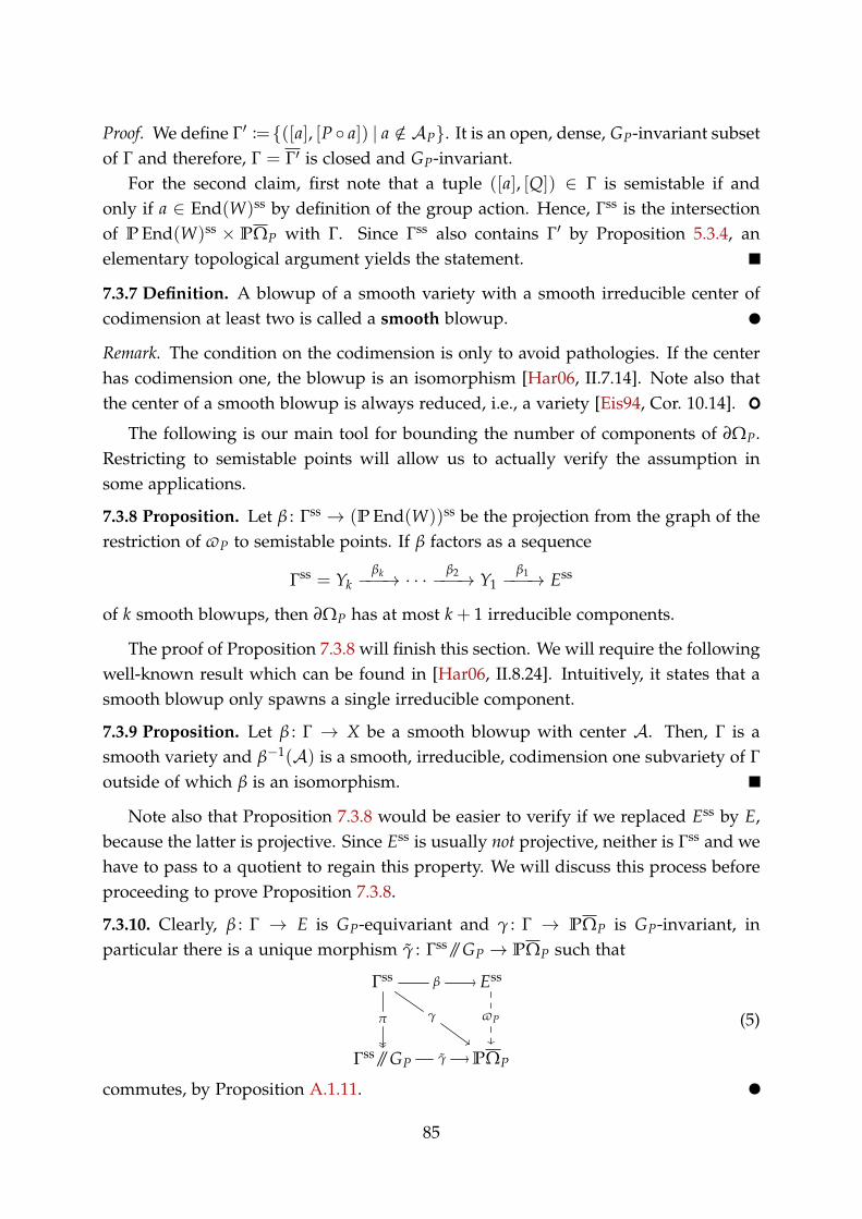
Proof. We define Γ′ :=([a], [P a]) | a /∈ AP. It is an open, dense, GP-invariant subsetof Γ and therefore, Γ = Γ′ is closed and GP-invariant.

For the second claim, first note that a tuple ([a], [Q]) ∈ Γ is semistable if andonly if a ∈ End(W)ss by definition of the group action. Hence, Γss is the intersectionof P End(W)ss × PΩP with Γ. Since Γss also contains Γ′ by Proposition 5.3.4, anelementary topological argument yields the statement.

7.3.7 Definition. A blowup of a smooth variety with a smooth irreducible center ofcodimension at least two is called a smooth blowup.

Remark. The condition on the codimension is only to avoid pathologies. If the centerhas codimension one, the blowup is an isomorphism [Har06, II.7.14]. Note also thatthe center of a smooth blowup is always reduced, i.e., a variety [Eis94, Cor. 10.14].

The following is our main tool for bounding the number of components of ∂ΩP.Restricting to semistable points will allow us to actually verify the assumption insome applications.

7.3.8 Proposition. Let β : Γss → (P End(W))ss be the projection from the graph of therestriction of ϖP to semistable points. If β factors as a sequence

Γss = Ykβk−−−→ · · · β2−−−→ Y1

β1−−−→ Ess

of k smooth blowups, then ∂ΩP has at most k+ 1 irreducible components.

The proof of Proposition 7.3.8 will finish this section. We will require the followingwell-known result which can be found in [Har06, II.8.24]. Intuitively, it states that asmooth blowup only spawns a single irreducible component.

7.3.9 Proposition. Let β : Γ → X be a smooth blowup with center A. Then, Γ is asmooth variety and β−1(A) is a smooth, irreducible, codimension one subvariety of Γoutside of which β is an isomorphism.

Note also that Proposition 7.3.8 would be easier to verify if we replaced Ess by E,because the latter is projective. Since Ess is usually not projective, neither is Γss and wehave to pass to a quotient to regain this property. We will discuss this process beforeproceeding to prove Proposition 7.3.8.

7.3.10. Clearly, β : Γ → E is GP-equivariant and γ : Γ → PΩP is GP-invariant, inparticular there is a unique morphism γ : Γss//GP → PΩP such that

Γss

γ

β →→

π

↓↓↓↓

Ess

ϖP

↓↓

Γss//GP γ →→ PΩP

(5)

commutes, by Proposition A.1.11.

85

7.3.11 Lemma. The morphism γ in (5) is a birational, surjective morphism and itsrestriction to U := γ−1(PΩP) is an isomorphism U ∼= PΩP.

Proof. Since ϖP and β are dominant, so is γ. The variety Γss//GP is projective, there-fore γ has closed image, so it is surjective. The orbit map ϖP restricts to a surjectivemorphism P GL(W) → PΩP, and its graph is the open subset

U =([g], [P g]) | g ∈ GL(W) ⊆ Γss.

Hence, β restricts to am isomorphism U ∼= P GL(W) of GP-varieties. We note herethat U = π(U) and γ(U) = γ(U) = PΩP, so γ : U → PΩP is a well-defined surjecivemorphism. As PΩP is smooth, γ is an isomorphism if and only if it is injective, byZariski’s Main Theorem [TY05, 17.4.6]. Let [Q] ∈ PΩP, then we are left to show thatthe fiber γ−1([Q]) contains exactly one element. To see this, let g ∈ GL(W) be suchthat Q = P g. Then,

γ−1([Q]) = π(β−1(ϖ−1([Q]))) = π(β−1(GP [g])).

Since β is an equivariant isomorphism, β−1(GP [g]) is an orbit. Since π is constanton orbits, we are done.

Proof of Proposition 7.3.8. We define Γ := Γss//GP and consider the diagram (5). Werecall that G = P GL(W) ⊆ P End(W) = E and U = γ−1(PΩP) = β−1(G).

Set Z := Γss \ U. By Lemma 7.3.11, the morphism γ : Γ → PΩP is birational,surjective, and restricts to an isomorphism on U = γ−1(PΩP) = π(U). We alsodefine the set Z := π(Z).

Claim. We have γ(Z) = P∂ΩP.

Proof of Claim. As every GP-orbit in U ∼= G is closed, Property (G4) of the good quo-tient π implies that U and Z are disjoint. Since π is surjective, Z is the complementof U in Γ. The claim follows as in (3) because γ is surjective by Lemma 7.3.11.

As P∂ΩP = γ(Z) = (γ π)(Z) isthe image of Z under a morphism, we are left toverify that Z has at most k+ 1 irreducible components.

Recall that β is a composition

Γss = Ykβk−−−→ · · · β2−−−→ Y1

β1−−−→ Y0 = Ess

of k smooth blowups. We set βi := β1 . . . βi for all 1 ≤ i ≤ k. Furthermore, denoteby Z0 := Ess \ G the set of projective classes of semistable endomorphisms that arenoninvertible. Since Ess is open in E, it follows that Z0 is an irreducible hypersurfacein Ess. Let Zi := β−1

i (Z0) for 1 ≤ i ≤ k. Since the complement of Zk ⊆ Yk = Γss isequal to U = β−1(G), we have Z = Zk. We prove by induction on i that Zi has at most

86

i + 1 irreducible components, which is tautological for i = 0 and proves our initialclaim for i = k. For the induction step, we assume 1 ≤ i ≤ k and that Zi−1 has atmost i irreducible components.

Claim. We have Ai ⊆ Zi−1 ⊆ Yi−1, where Ai is the center of βi : Yi → Yi−1.

Proof of Claim. Assume for contradiction that Ai intersects β−1i−1(G). Since Ai is of

codimension two and β−1i (Ai) is of codimension one by Proposition 7.3.9, the Fiber

Dimension Theorem [TY05, 15.5.4] implies that there is a point g ∈ G such that β−1i (g)

has positive dimension. As all βj are surjective, this would mean that β−1(g) haspositive dimension, which is a contradiction.

Since Ai ⊆ Zi−1, we get that

Zi = β−1i (Zi−1) = β−1

i (Zi−1 \ Ai) ∪ β−1i (Ai).

By Proposition 7.3.9, β−1i (Ai) is irreducible and β−1

i (Zi−1 \ Ai) ∼= Zi−1 \ Ai has atmost i irreducible components. Therefore, Zi has at most i + 1 irreducible compo-nents.

7.3.12 Remark. One can prove an even more refined statement than Proposition 7.3.8.Under the assumptions of the proposition, Z := Γss \ β−1(G) is a GP-invariant closedsubset of Γss. The action of GP on Γss therefore permutes the finite set of irreduciblecomponents of Z. Denoting by ℓ the number of orbits of this action, it follows fromthe proof of Proposition 7.3.8 that the number of irreducible components of ∂ΩP is atmost ℓ+ 1.

87

Chapter 8The 3 by 3 Determinant Polynomial

As outlined in Chapter 3, the orbit closure and boundary of the determinant poly-nomial is of particular interest for GCT. Yet, very few explicit results describing thegeometry are known in low dimension. In this chapter we give a description of theboundary of the orbit of the 3× 3 determinant. These results have been previouslypublished in [HL16].

We view det3 as the polynomial

det3 := det( x1 x2 x3

x4 x5 x6x7 x8 x9

)∈ C[x1, . . . , x9]3,

a homogeneous polynomial of degree 3 on the spaceW := C3×3. As before, we denoteby V := C[W]3 the space of all homogeneous forms of degree 3 on W.

Our main result is a description of ∂Ω(det3) that answers a question of Landsberg[Lan15, Problem 5.4]: The two known components are the only ones. In Section 8.1 weexplain the construction of the two components. Our contribution lies in Section 8.2where we show that there is no other component.

8.0.1 Theorem. The boundary ∂Ω(det3) has exactly two irreducible components:

• The orbit closure of the determinant of the generic traceless matrix, namely

Q1 := det

⎛⎜⎝ x1 x2 x3x4 x5 x6x7 x8 −x1 − x5

⎞⎟⎠ ;

• The orbit closure of the universal homogeneous polynomial of degree two in threevariables, namely

Q2 := x4 · x21 + x5 · x22 + x6 · x23 + x7 · x1x2 + x8 · x2x3 + x9 · x1x3.

Remark. The two components are different in nature: Ω(Q1) ⊆ det3 End(W) is theorbit closure of a polynomial in only eight variables; the second component is moresubtle and is not contained in det3 End(W). This component has analogues in higherdimension and some results are known about them [LMR13].

89

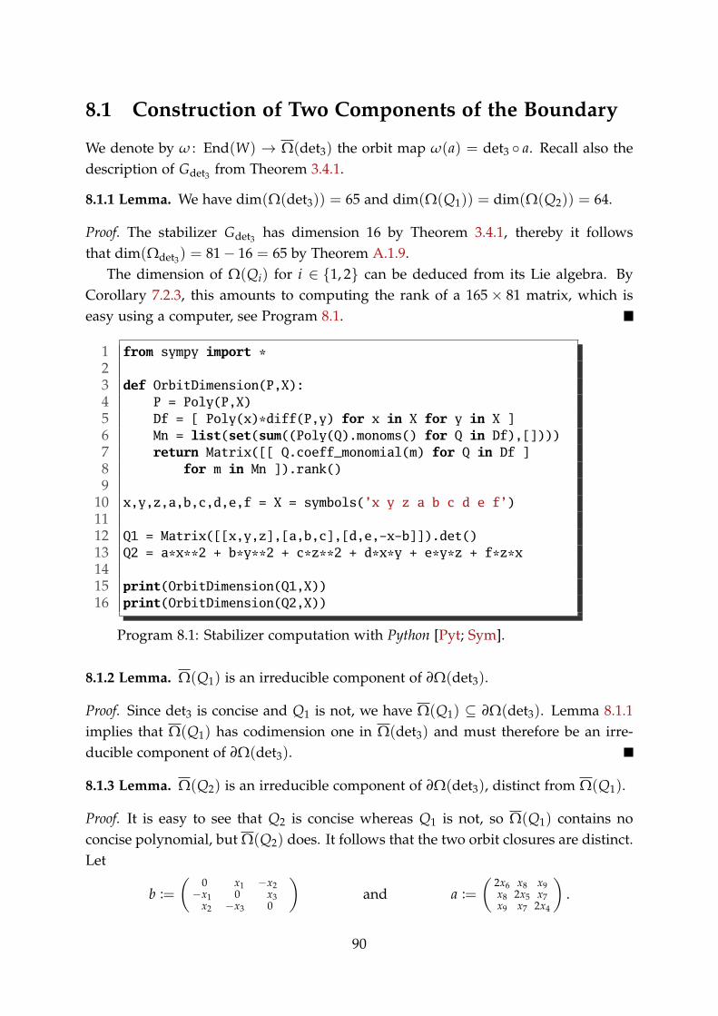
8.1 Construction of Two Components of the Boundary

We denote by ω : End(W) → Ω(det3) the orbit map ω(a) = det3 a. Recall also thedescription of Gdet3 from Theorem 3.4.1.

8.1.1 Lemma. We have dim(Ω(det3)) = 65 and dim(Ω(Q1)) = dim(Ω(Q2)) = 64.

Proof. The stabilizer Gdet3 has dimension 16 by Theorem 3.4.1, thereby it followsthat dim(Ωdet3) = 81− 16 = 65 by Theorem A.1.9.

The dimension of Ω(Qi) for i ∈ 1, 2 can be deduced from its Lie algebra. ByCorollary 7.2.3, this amounts to computing the rank of a 165× 81 matrix, which iseasy using a computer, see Program 8.1.

1 from sympy import * 2 3 def OrbitDimension(P,X): 4 P = Poly(P,X) 5 Df = [ Poly(x)*diff(P,y) for x in X for y in X ] 6 Mn = list(set(sum((Poly(Q).monoms() for Q in Df),[]))) 7 return Matrix([[ Q.coeff_monomial(m) for Q in Df ] 8 for m in Mn ]).rank() 9

10 x,y,z,a,b,c,d,e,f = X = symbols(’x y z a b c d e f’) 11 12 Q1 = Matrix([[x,y,z],[a,b,c],[d,e,-x-b]]).det() 13 Q2 = a*x**2 + b*y**2 + c*z**2 + d*x*y + e*y*z + f*z*x 14 15 print(OrbitDimension(Q1,X)) 16 print(OrbitDimension(Q2,X))

Program 8.1: Stabilizer computation with Python [Pyt; Sym].

8.1.2 Lemma. Ω(Q1) is an irreducible component of ∂Ω(det3).

Proof. Since det3 is concise and Q1 is not, we have Ω(Q1) ⊆ ∂Ω(det3). Lemma 8.1.1implies that Ω(Q1) has codimension one in Ω(det3) and must therefore be an irre-ducible component of ∂Ω(det3).

8.1.3 Lemma. Ω(Q2) is an irreducible component of ∂Ω(det3), distinct from Ω(Q1).

Proof. It is easy to see that Q2 is concise whereas Q1 is not, so Ω(Q1) contains noconcise polynomial, but Ω(Q2) does. It follows that the two orbit closures are distinct.Let

b :=(

0 x1 −x2−x1 0 x3x2 −x3 0

)and a :=

(2x6 x8 x9x8 2x5 x7x9 x7 2x4

).

90

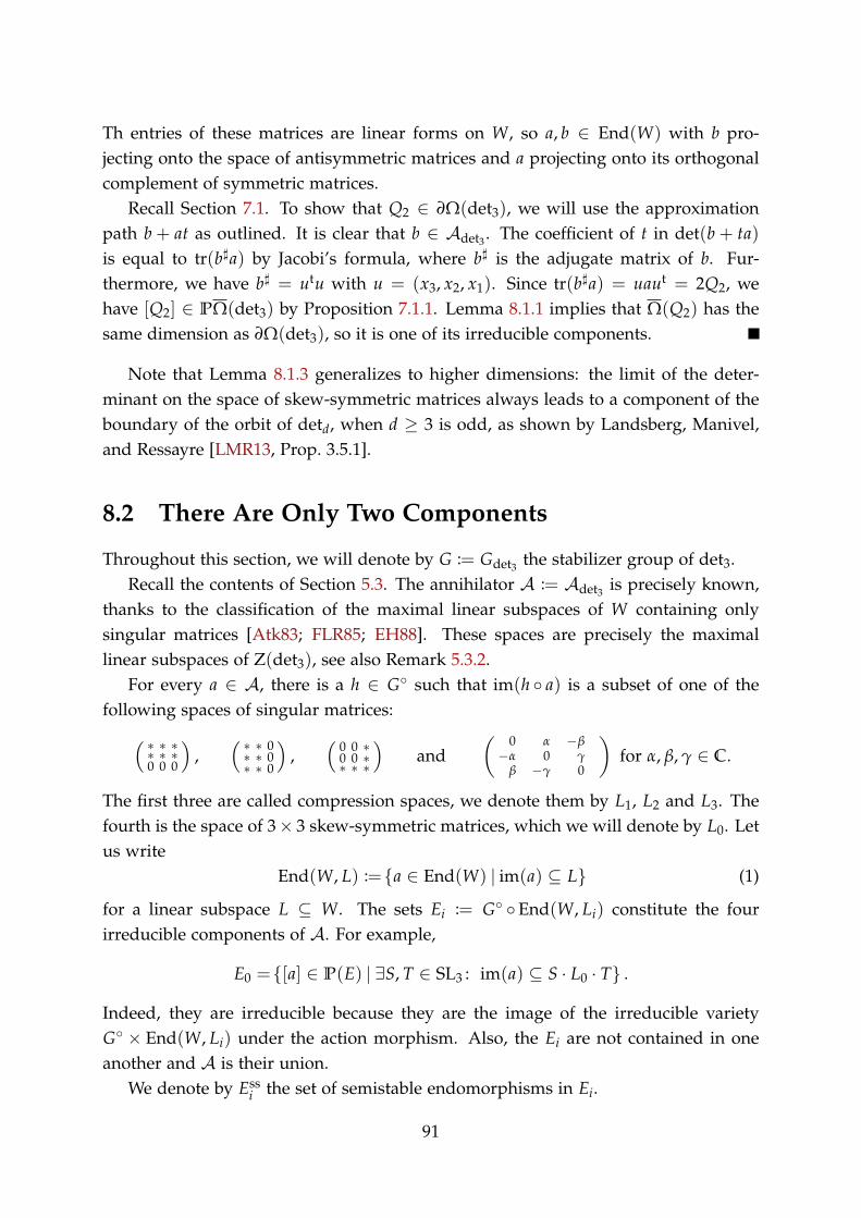
Th entries of these matrices are linear forms on W, so a, b ∈ End(W) with b pro-jecting onto the space of antisymmetric matrices and a projecting onto its orthogonalcomplement of symmetric matrices.

Recall Section 7.1. To show that Q2 ∈ ∂Ω(det3), we will use the approximationpath b+ at as outlined. It is clear that b ∈ Adet3 . The coefficient of t in det(b+ ta)is equal to tr(b♯a) by Jacobi’s formula, where b♯ is the adjugate matrix of b. Fur-thermore, we have b♯ = utu with u = (x3, x2, x1). Since tr(b♯a) = uaut = 2Q2, wehave [Q2] ∈ PΩ(det3) by Proposition 7.1.1. Lemma 8.1.1 implies that Ω(Q2) has thesame dimension as ∂Ω(det3), so it is one of its irreducible components.

Note that Lemma 8.1.3 generalizes to higher dimensions: the limit of the deter-minant on the space of skew-symmetric matrices always leads to a component of theboundary of the orbit of detd, when d ≥ 3 is odd, as shown by Landsberg, Manivel,and Ressayre [LMR13, Prop. 3.5.1].

8.2 There Are Only Two Components

Throughout this section, we will denote by G := Gdet3 the stabilizer group of det3.Recall the contents of Section 5.3. The annihilator A := Adet3 is precisely known,

thanks to the classification of the maximal linear subspaces of W containing onlysingular matrices [Atk83; FLR85; EH88]. These spaces are precisely the maximallinear subspaces of Z(det3), see also Remark 5.3.2.

For every a ∈ A, there is a h ∈ G such that im(h a) is a subset of one of thefollowing spaces of singular matrices:( ∗ ∗ ∗

∗ ∗ ∗0 0 0

),

( ∗ ∗ 0∗ ∗ 0∗ ∗ 0

),

(0 0 ∗0 0 ∗∗ ∗ ∗

)and

(0 α −β

−α 0 γβ −γ 0

)for α, β,γ ∈ C.

The first three are called compression spaces, we denote them by L1, L2 and L3. Thefourth is the space of 3× 3 skew-symmetric matrices, which we will denote by L0. Letus write

End(W, L) :=a ∈ End(W) | im(a) ⊆ L (1)

for a linear subspace L ⊆ W. The sets Ei := G End(W, Li) constitute the fourirreducible components of A. For example,

E0 =[a] ∈ P(E) | ∃S, T ∈ SL3 : im(a) ⊆ S · L0 · T .

Indeed, they are irreducible because they are the image of the irreducible varietyG × End(W, Li) under the action morphism. Also, the Ei are not contained in oneanother and A is their union.

We denote by Essi the set of semistable endomorphisms in Ei.

91

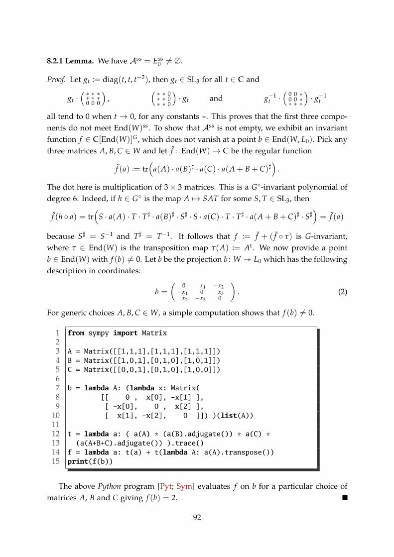
8.2.1 Lemma. We have Ass = Ess0 = ∅.

Proof. Let gt := diag(t, t, t−2), then gt ∈ SL3 for all t ∈ C and

gt ·( ∗ ∗ ∗

∗ ∗ ∗0 0 0

),

( ∗ ∗ 0∗ ∗ 0∗ ∗ 0

)· gt and g−1

t ·(

0 0 ∗0 0 ∗∗ ∗ ∗

)· g−1

t

all tend to 0 when t → 0, for any constants ∗. This proves that the first three compo-nents do not meet End(W)ss. To show that Ass is not empty, we exhibit an invariantfunction f ∈ C[End(W)]G, which does not vanish at a point b ∈ End(W, L0). Pick anythree matrices A, B,C ∈ W and let f : End(W) → C be the regular function

f (a) := tr(a(A) · a(B)♯ · a(C) · a(A+ B+ C)♯

).

The dot here is multiplication of 3× 3 matrices. This is a G-invariant polynomial ofdegree 6. Indeed, if h ∈ G is the map A ↦→ SAT for some S, T ∈ SL3, then

f (h a) = tr(S · a(A) · T · T♯ · a(B)♯ · S♯ · S · a(C) · T · T♯ · a(A+ B+ C)♯ · S♯

)= f (a)

because S♯ = S−1 and T♯ = T−1. It follows that f := f + ( f τ) is G-invariant,where τ ∈ End(W) is the transposition map τ(A) := At. We now provide a pointb ∈ End(W) with f (b) = 0. Let b be the projection b : W L0 which has the followingdescription in coordinates:

b =(

0 x1 −x2−x1 0 x3x2 −x3 0

). (2)

For generic choices A, B,C ∈ W, a simple computation shows that f (b) = 0.

1 from sympy import Matrix 2 3 A = Matrix([[1,1,1],[1,1,1],[1,1,1]]) 4 B = Matrix([[1,0,1],[0,1,0],[1,0,1]]) 5 C = Matrix([[0,0,1],[0,1,0],[1,0,0]]) 6 7 b = lambda A: (lambda x: Matrix( 8 [[ 0 , x[0], -x[1] ], 9 [ -x[0], 0 , x[2] ],

10 [ x[1], -x[2], 0 ]]) )(list(A)) 11 12 t = lambda a: ( a(A) * (a(B).adjugate()) * a(C) * 13 (a(A+B+C).adjugate()) ).trace() 14 f = lambda a: t(a) + t(lambda A: a(A).transpose()) 15 print(f(b))

The above Python program [Pyt; Sym] evaluates f on b for a particular choice ofmatrices A, B and C giving f (b) = 2.

92

8.2.2 Lemma. An endomorphism a ∈ Ass satisfies rk(a) ≥ 3.

Proof. In [BD06, Thm. 2 and discussion above it], Bürgin and Draisma show thatany 2-dimensional subspace of E containing only singular matrices is contained in acompression space. Therefore, if the image of a had dimension 2 or less, then a wouldlie in the nullcone, which is contrary to the choice of a.

Recall Section 7.3, in particular Definition 7.3.1. We set Ass := Assdet3

, so PAss

are the indeterminacies of ϖ : P End(W) → PΩ(det3). The following proposition inconjuction with Proposition 7.3.8 implies that ∂Ω(det3) has at most two irreduciblecomponents, both of which we have described in Section 8.1. This finishes the proofof Theorem 8.0.1.

8.2.3 Proposition. The subscheme PAss ⊆ P End(W) is a smooth subvariety. In par-ticular, the projection β : Γss → P End(W)ss is a smooth blowup, where Γss denotesthe graph of ϖ restricted to P End(W)ss.

Proof. We set E := End(W) to shorten notation. By Definition 7.3.1 and Lemma 7.3.6,Γss is the blowup of PEss along PAss. Therefore, we have to check that PAss isirreducible and smooth, the latter also implies that it is reduced, i.e., Ass = Ass.

Since scalar matrices stabilize any point in P(V), the stabilizer of [det3] ∈ P(V) isthe group H := G C idW ⊆ GL(W).

Claim. Let b ∈ Ass be the point defined in (2). We claim Ass = H b GL(W), theorbit of b under the action of H ×GL(W) by multiplication from left and right.

Proof of Claim. For “⊇”, note that the left hand side is invariant under both actionsand contains b. Conversely, let a ∈ Ass. By Lemma 8.2.1 and because L0 is invariantunder transposition, we may assume that the image of a is included in L0, up toreplacing a by another point in its orbit H a. By Lemma 8.2.2, we also know thatrk(a) ≥ 3, so a surjects onto L0. This implies that there is some g ∈ GL(W) suchthat a = b g, and thus a ∈ H b GL(W).

In particular, Ass is irreducible, and smooth by Theorem A.1.9.(1). We will nowshow that Ass is also smooth. Since Ass is invariant under the actions of both Hand GL(W) and its support Ass is an orbit under the same action, it suffices to verifythat Ass is smooth at one single point, say b. This amounts to checking that thedimension of the tangent space Tb Ass equals the dimension of Ass.

Recall that A is the scheme given by the coefficients of det3 a = 0, as polynomialsin the entries of a. By the Jacobian criterion [EH00, §V.3], we obtain the description

Tb Ass ∼=c ∈ E

t2 divides det3 (b+ tc),

93

where t is a formal variable. The dimension of Tb Ass can be determined by means ofProgram 8.2: It is equal to 35.

To calculate the dimension of Ass, we use the fact that it is an orbit under theaction of H ×GL(W). More precisely, we consider the derivative of the orbit map

H ×GL(W) −→ Ass

(a, c) ↦−→ a b c

at the neutral element, yielding a surjective linear map

Lie(H)× gl(W) −→ Tb Ass

(a, c) ↦−→ ab+ bc

We have gl(W) ∼= E. Recall the Lie algebra of G from Example 7.2.4. Similar to thatexample, we can check that the Lie algebra of H is given by the maps (S⊗ I)+ (I⊗T)for S, T ∈ W – i.e., there is no condition on S and T to be traceless because H containsscalar matrices. We can therefore express the tangent space as

Tb Ass =ab+ bc | a ∈ Lie(H), c ∈ gl(W) ⊂ Tb E ∼= E

=(S⊗ I) b+ (I ⊗ T) b+ b c | S, T ∈ W, c ∈ E .

In other words, Tb Ass consists of all maps of the form

W −→ W

C ↦−→ S · b(C) + b(C) · T + b(c(C))

for certain c ∈ E and S, T ∈ W. Program 8.2 also verifies that this space has dimen-sion 35, which terminates the proof.

94

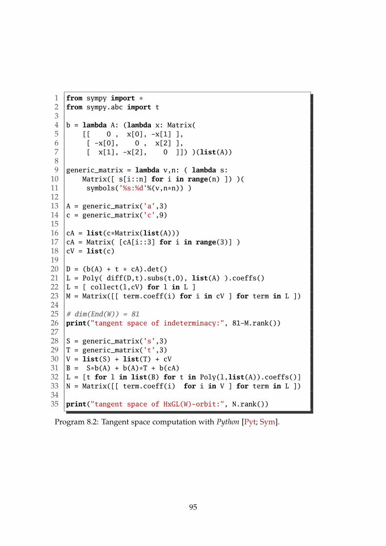
1 from sympy import * 2 from sympy.abc import t 3 4 b = lambda A: (lambda x: Matrix( 5 [[ 0 , x[0], -x[1] ], 6 [ -x[0], 0 , x[2] ], 7 [ x[1], -x[2], 0 ]]) )(list(A)) 8 9 generic_matrix = lambda v,n: ( lambda s:

10 Matrix([ s[i::n] for i in range(n) ]) )( 11 symbols(’%s:%d’%(v,n*n)) ) 12 13 A = generic_matrix(’a’,3) 14 c = generic_matrix(’c’,9) 15 16 cA = list(c*Matrix(list(A))) 17 cA = Matrix( [cA[i::3] for i in range(3)] ) 18 cV = list(c) 19 20 D = (b(A) + t * cA).det() 21 L = Poly( diff(D,t).subs(t,0), list(A) ).coeffs() 22 L = [ collect(l,cV) for l in L ] 23 M = Matrix([[ term.coeff(i) for i in cV ] for term in L ]) 24 25 # dim(End(W)) = 81 26 print("tangent space of indeterminacy:", 81-M.rank()) 27 28 S = generic_matrix(’s’,3) 29 T = generic_matrix(’t’,3) 30 V = list(S) + list(T) + cV 31 B = S*b(A) + b(A)*T + b(cA) 32 L = [t for l in list(B) for t in Poly(l,list(A)).coeffs()] 33 N = Matrix([[ term.coeff(i) for i in V ] for term in L ]) 34 35 print("tangent space of HxGL(W)-orbit:", N.rank())

Program 8.2: Tangent space computation with Python [Pyt; Sym].

95

8.3 The Traceless Determinant

A computation as in Lemma 8.1.2 shows that for d ∈3, 4, 5, the orbit closure of thetraceless d× d determinant is a component of ∂Ω(detd). We will show in this sectionthat it is true for all d ≥ 3. The main work in proving this claim is the followingdescription of the stabilizer of the traceless determinant. In fact, its dimension isthe only information required, but a complete description is certainly of independentinterest.

8.3.1 Theorem. Let W =A ∈ Cd×d

tr(A) = 0with d ≥ 3 and let P ∈ C[W]d be

the restriction of detd to W. The stabilizer group GP is reductive of dimension d2 − 1.Moreover,

(1) The identity component of the stabilizer of P is the group

GP =

g ∈ GL(W)

∃S ∈ SLd : ∀A ∈ W : g(A) = SAS−1.

(2) Let ∆ ⊆ GL(W) be the group generated by

• the transposition map t : W → W, t(A) = At

• and all ζ · idW where ζ ∈ C is a d-th root of unity.

Then, GP = ∆ · GP and GP has |∆| = 2d connected components.

The proof is postponed briefly in order to first draw the announced conclusion.

8.3.2 Corollary. The orbit closure of the traceless determinant is an irreducible com-ponent of ∂Ω(detd), for all d ≥ 3.

For the proof of this corollary, we also require the following technical lemma,which we will prove in direct succession.

8.3.3 Lemma. Let M ∼= Cn, D ∈ C[M]d a concise form and W ⊆ M a linear subspaceof codimension k. Let a ∈ End(M,W) be any projection onto W, let Q := D a anddenote by P ∈ C[W]d the restriction of Q to W. Then, dim(GQ) = dim(GP) + kn.

Proof of Corollary 8.3.2. We set M := Cd×d, D := detd ∈ C[M]d and W := ker(tr). Weuse the notation in Lemma 8.3.3, where k = 1 and n = d2. By Theorem 8.3.1 we havedim(GP) = n − 1 and Lemma 8.3.3 states that dim(GQ) = n − 1+ n = 2n − 1. ByTheorems A.1.9 and 3.4.1 this implies dim(ΩQ) = dim(Ωdetd)− 1.

Proof of Lemma 8.3.3. We can choose coordinates C[M] = C[x1, . . . , xn] such that the xiwith i ≤ n − k are coordinates on W. Then, Q is simply the polynomial that arisesfrom D by setting xi to zero for i > n− k, in the chosen coordinates. By Corollary 7.2.3,

Lie(GQ) =

a ∈ Cn×n

n

∑i=1

n

∑j=1

aijxj∂iQ = 0

=

a ∈ Cn×n

n−k

∑i=1

n

∑j=1

aijxj∂iQ = 0

96

because ∂iQ = 0 for i > n− k. It suffices to show that dim(Lie(GQ)) = dim(GP) + kn.We have

dim

(a ∈ Cn×n

n−k

∑i=1

n−k

∑j=1

aijxj∂iQ = 0

)(3)

= dim

(a ∈ C(n−k)×(n−k)

n−1

∑i=1

n−1

∑j=1

aijxj∂iP = 0

)+ (n2 − (n− k)2)

= dim(Lie(GP)) + 2kn− k2

Wewill show that⟨xj∂iQ

1 ≤ i ≤ n− k < j ≤ n,⟩

Chas dimension k(n− k) and trivial

intersection with ⟨xj∂iQ | 1 ≤ i, j ≤ n− k⟩C. This implies that Lie(GQ) arises from (3)by imposing k(n− k) = kn− k2 additional linearly independent conditions, droppingthe dimension from dim(GP) + 2kn− k2 to dim(GP) + kn as claimed.

The spaces intersect trivially because all monomials of polynomials in the secondspace are divisibly by some xj with j ≤ n− k and none of the monomials of polyno-mials in the first space are.

As a is the identity on W, we have ∂iQ = ∂iD for i ≤ n− k and the ∂iD are linearlyindependent by Proposition 5.1.2 because D is concise. It follows that the xj∂iQ with1 ≤ i ≤ n− k and n− k < j ≤ n are all linearly independent.

8.3.1 Proof of Theorem 8.3.1

The thesis of Reichenbach [Rei16] contains a very detailed proof of Theorem 3.4.1, thedescription of the stabilizer of detd. It can be adapted to verify Theorem 8.3.1, andsome parts of the proof require only slight modification or none at all. We thereforerefer to Reichenbach [Rei16] frequently and also make use of partial results therein.

We will denote by M := Cd×d the space of square matrices and recall thatW ⊆ M isthe subspace of traceless matrices. We will denote by Eij ∈ M the matrix with entry 1in position (i, j) and zeros elsewhere. We begin with the important observation thatwe only have to show GP ⊆ Gdetd :

8.3.4 Lemma. Let g ∈ GP. If there are S, T ∈ GLd such that g(A) = S · A · T for allA ∈ W, then there is a d-th root of unity ζ ∈ C such that T = ζ · S−1.

Proof. Set I := TS. Since g ∈ GL(W), we have SAT ∈ W for any A ∈ W. Hence,

∀A ∈ W : 0 = tr(SAT) = tr(ATS) = tr(AI).

Let Eij be the d × d matrix with entry 1 in position (i, j) and zeros elsewhere. Fordistinct indices i = j, we have 0 = tr(Eij I) = Iij and therefore I is a diagonal matrix.

97

Furthermore, from 0 = tr((Eii − Ejj)I) = Iii − Ijj it follows that all diagonal entriesof I are equal to some ζ := I11. Finally, pick some A ∈ W with det(A) = 0. From

det(A) = det(g(A)) = det(SAT) = det(S) · det(A) · det(T) = det(TS) · det(A),

it follows that 1 = det(TS) = det(I) = ζd.

Recall that a singular subspace of M is a linear space L ⊆ M such that det(A) = 0for all A ∈ L. We denote by L the set of all maximal left ideals of M as a ring. By[Rei16, Satz 2.24], there is a bijection Pd−1 ∼= L given by v ↦→ L(v), where

L(v) :=A ∈ M | v ⊆ ker(A) .

Here, v denotes a line in Cd. In particular, every element of L is a singular subspaceof M. For L ∈ L, we set Lt :=

At A ∈ L

, the image of L under transposition. The

set Lt =Lt L ∈ L

is the set of all maximal right ideals of M, see [Rei16, §2.3] for

the complete classification. Every left ideal is the intersection of maximal left ideals,and analogously for right ideals.

By [Rei16, Thm. 2.38], the set I := L ∪ Lt is the set of all singular subspaces of Mof maximal dimension. We will write LW :=L ∩W | L ∈ L and IW := LW ∪ Lt

W .An important preliminary observation is the following proposition, which allows

us to argue essentially as in [Rei16]:

8.3.5 Proposition. The map I → IW , L ↦→ L ∩W is a bijection. Furthermore, IW isthe set of all singular subspaces of W of maximal dimension.

We require a sequence of lemmata which will be useful throughout the proof.

8.3.6 Lemma. Let L ⊆ M be a linear space and assume that S ∈ M satisfies S · L ⊆ W.If Eij ∈ L, then Sji = 0.

Proof. Let I :=(i, j)

Eij ∈ L

and C[M] = C[xij 1 ≤ i, j ≤ d

]. We consider the

matrix A := ∑(i,j)∈I xijEij ∈ C[M]d×d. Then, 0 = tr(SA) = ∑di,j=1 SjiAij = ∑(i,j)∈I Sjixij

as a polynomial in C[M]. Hence, we have Sji = 0 for all (i, j) ∈ I by comparingcoefficients.

8.3.7 Lemma. Let L1, L2 ∈ L. Then, W does not contain L1 ∩ Lt2.

Proof. Assume for contradiction that I := L1 ∩ Lt2 ⊆ W. By [Rei16, Korollar 2.28], thereare S, T ∈ GLd such that L1 · T = L2 · St are both equal to the space of all matriceswith vanishing first column. Since L1 is a left ideal and Lt2 a right ideal,

L := S · I · T = S · (L1 ∩ Lt2) · T = (S · L1 · T) ∩ (S · Lt2 · T)

= (L1 · T) ∩ (S · Lt2) = (L1 · T) ∩ (L2 · St)t

98

is equal to the space of matrices where the first row and the first column vanish. Inparticular, Eij ∈ L for all i > 1 and j > 1. Since conjugation leaves the trace invariant,(ST)−1 · L = T−1 IT ⊆ W. By Lemma 8.3.6, this implies that (ST)−1 has zero entrieseverywhere except for the first row and column. Hence, rk((ST)−1) ≤ 2 < 3 ≤ d, acontradiction because (ST)−1 ∈ GLd.

8.3.8 Lemma. W does not contain any nonzero left or right ideal of M.

Proof. Since W is invariant under transposition, it suffices to show that W does notcontain any left ideal of M. For contradiction, assume that L ∈ L satisfies L ⊆ W andlet r be the maximum rank among elements of L, then r > 0 because L is nonzero. By[Rei16, Satz 2.24], we have dim(L) = dr and by [FLR85, Theorem 2], a singular spacewith this property admits matrices S, T ∈ GLd such that L′ := S · L · T is the spaceof all matrices whose first d− r columns vanish. Because r > 0, we have Eid ∈ L forall i. Since (ST)−1 · L′ = T−1LT ⊆ W, Lemma 8.3.6 implies that the last row of (ST)−1

vanishes, a contradiction.

Proof of Proposition 8.3.5. By definition, the map I → IW , L ↦→ L ∩W is surjective. Tosee that it is injective, assume for contradiction that there are I1, I2 ∈ I with I1 = I2and

J := I1 ∩W = I2 ∩W.

By Lemma 8.3.8, we have dim(J) = d2 − d − 1. Furthermore, [Rei16, Lemma 2.29]implies dim(I1 ∩ I2) ≤ d2 − 2d+ 1. Lemmata 8.3.7 and 8.3.8 yield that I1 ∩ I2 is notcontained in W, providing the last inequality in

d2 − d− 1 = dim(J) = dim(I1 ∩ I2 ∩W) ≤ d2 − 2d.

This means d ≤ 1, which is the contradiction we sought.Let K ⊆ W be a singular subspace of maximal dimension. To finish the proof, we

have to show that K ∈ IW .

Claim. There is some L ∈ L with K ⊆ L.

Proof of Claim. Note that dim(K) ≥ d2− d− 1 because K is of maximal dimension andfor example, the singular spaces in IW have dimension d2− d− 1. There are two casesto consider:Case 1 (d > 3). In this case, dim(K) > d2 − 2d + 2. By [FLR85, Theorem 3], anysingular space K ⊆ M with this property is contained in a left or right ideal of M.

Case 2 (d = 3). In this case, we have dim(K) ≥ 9− 3− 1 = 5. Assume for contradic-tion that K is not contained in any maximal left or right ideal of M. As K is singular,

99

it is contained in some maximal singular subspace of M, which we recall from Sec-tion 8.2. Since dim(K) > 3 and K is not contained in any left or right ideal, K iscontained in a space that is equivalent to

L :=(

0 0 ∗0 0 ∗∗ ∗ ∗

).

Since dim(L) = 5 ≤ dim(K), in fact K must be equivalent to L. By definition, thereare matrices S, T ∈ GLd with L = S · K · T. It follows that (ST)−1 · L = T−1KT ⊆ Wand Lemma 8.3.6 implies that the last row and column of the invertible matrix (ST)−1

vanish – a contradiction.

It follows from the claim that K ⊆ L ∩W, the latter is a singular subspace of W.Therefore, K = L ∩W because K is maximal, hence K ∈ IW .

With this at hand, we can mimic the six steps of the proof [Rei16, Thm. 4.2]. Recallthat we denote by t ∈ End(W) the transposition operator t(A) := At. The first step isthe following:

8.3.9 Proposition. Let g ∈ GP. After possibly replacing g by g t, the following holds:For any K ∈ LW , we have g(K) ∈ LW .

Proof. We first note that for any K ∈ IW , we have g(K) ∈ IW because g maps thesingular subspaces of W to singular subspaces, and preserves the dimension.

Let K1,K2 ∈ LW and L1, L2 ∈ L with Li ∩W = Ki. After possibly composing gwith t, we may assume that g(K1) ∈ LW . Furthermore,

dim(g(K1) ∩ g(K2)) = dim(g(K1 ∩ K2)) (g is injective)

= dim(K1 ∩ K2) (g is injective)

= dim(L1 ∩ L2 ∩W) (by definition)

= dim(L1 ∩ L2)− 1 (Lemma 8.3.8)

= d2 − 2d− 1. [Rei16, Lemma 2.29]

If we had g(K2) ∈ LtW , then Lemma 8.3.7 and [Rei16, Lemma 2.29] would imply that

dim(g(K1) ∩ g(K2)) = d2 − 2d. Hence, we have g(K2) ∈ LW as well. Since K2 wasarbitrary, the statement follows.

For the rest of the proof, fix some g ∈ GP. We now construct two bijective mapsφ,ψ : Pd−1 → Pd−1 as follows: Note that g maps any L(v) ∩W to some L(w) ∩W byProposition 8.3.9. Since LW

∼= L ∼= Pd−1, we can define φ and ψ via

g(L(v) ∩W) = L(φ(v)) ∩W, g(L(v)t ∩W) = L(ψ(v))t ∩W.

100

As g is a bijection, so are φ and ψ. Moreover, φ and ψ are induced by semilinearmaps T : Cd → Cd and S : Cd → Cd, respectively. This follows from the upcomingLemma 8.3.10 and the fundamental theorem of projective geometry [Rei16, Theo-rem 3.13].

8.3.10 Lemma. Both φ and ψ map projective lines to projective lines.

Proof. Assume that u, v,w ∈ Pd−1 are three pairwise different lines contained inone plane, i.e., these projective points lie on the same projective line. Let L :=L(u) ∩ L(v) ∩ L(w). Then, dim(L) = d2 − 2d by [Rei16, Satz 2.24, Korollar 2.27].By Lemma 8.3.8, we have dim(L ∩W) = d2 − d− 1. Thus,

d2 − 2d− 1 = dim(g(L ∩W)) = dim(a(L(v) ∩W) ∩ g(L(u) ∩W) ∩ g(L(w) ∩W)

)= dim(L(φ(u)) ∩ L(φ(v)) ∩ L(φ(w)) ∩W).

Again by Lemma 8.3.8, we get that

d2 − 2d = dim(L(φ(u)) ∩ L(φ(v)) ∩ L(φ(w)))

and [Rei16, Satz 2.24] implies that the lines φ(u), φ(v) and φ(w) span a plane. Theargument for ψ is completely analogous.

We have shown that g(L(v)∩W) = L(Tv)∩W and g(L(v)t ∩W) = L(Sv)t ∩W forall v. The third step is to show that S and T are linear maps, so we have S, T ∈ GLd.The proof is word for word the same as in [Rei16, Thm 4.2,Proof Step 3], except thatthe matrix E11 has to be replaced with E13, which is traceless. This is possible becausewe assumed d ≥ 3.

Let E := E11 + · · ·+ Edd be the identity matrix, so M = W ⊕ (C · E). We extend gto a map g ∈ GL(M) by declaring g(E) := E and g|W := g. We then define the map

u : M −→ M

A ↦−→ St · g(A) · T

Note that u ∈ GL(M) as well. For A ∈ L(v) ∩W, we know g(A) · Tv = 0, so inparticular we have u(A)v = St · g(A) · Tv = 0, so u(L(v) ∩W) ⊆ L(v). Equivalently,one has u(L(v)t ∩W) ⊆ L(v)t. We define

Dk := (E11 + Ek1)− (E1k + Ekk)

for k > 1, thenD2, . . . ,Dd ∪ Eij | i = j is a basis of W. Certainly, CEij for i = j canbe expressed as an intersection of maximal left and right ideals of M. We observe thatfor k > 2, we can also write

CDk =

⎛⎝L(e1 + ek) ∩⋂

i/∈1,kL(ei)

⎞⎠ ∩

⎛⎝L(e1 − ek)t ∩

⋂i/∈1,k

L(ei)t

⎞⎠ .

101

It follows that u(CDk) = CDk and u(CEij) = CEij for i = j and k > 2. Hence, thereare certain µk, µij ∈ C× with u(Dk) = µkDk and u(Eij) = µijEij. We will show that allthese coefficients are identical:

8.3.11 Lemma. There is a µ ∈ C× such that µ = µk and µ = µij for all i = j and k > 2.

Proof. For three distinct indices i, j, k (note that we require d ≥ 3 here), the linespanned by Eij + Ekj is contained in W and can be expressed as the intersection ofmaximal left and right ideals. Hence, there is some µijk ∈ C× with

µijEij + µkjEkj = u(Eij + Ekj) = µijk · (Eij + Ekj) = µijkEij + µijkEjk,

showing that µij = µijk = µkj. Similarly, one can show that µij = µik. It follows thatthere is a µ ∈ C× with µ = µij for all i = j. We are left to show that µk = µ holdsfor all k > 2. For this purpose, let j /∈1, k be a third index and observe that the linespanned by Dk + Ej1 − Ejk is contained in W and can be expressed as the intersectionof maximal left and right ideals. Indeed, it is equal to⎛⎝L(e1 + ek) ∩

⋂i/∈1,k

L(ei)

⎞⎠ ∩

⎛⎝L(e1 − ek)t ∩ L(e1 − ej) ∩

⋂i/∈1,j,k

L(ei)t

⎞⎠ .

From this, we get certain νjk ∈ C× with

µkDk + µEj1 − µEjk = u(Dk + Ej1 − Ejk) = νjk · (Dk + Ej1 − Ejk)

= νjkDk + νjkEj1 − νjkEjk

and therefore, µk = νjk = µ.

We conclude that u = µ · idM. We can replace S by µ−1S and achieve that u is theidentity. Consequently, we are done by Lemma 8.3.4.

8.4 The Boundary of the 4× 4 Determinant

The next logical step would be to study det4 and det5 to accumulate a more solidfoundation of examples. The maximal linear subspaces of Z(det4) up to action of thestabilizer are known [EH88, Cor. 1.3], [FLR85], they are as follows:

C0 =

( 0 ∗ ∗ ∗0 ∗ ∗ ∗0 ∗ ∗ ∗0 ∗ ∗ ∗

)and

C1 =

( ∗ ∗ ∗ ∗0 0 ∗ ∗0 0 ∗ ∗0 0 ∗ ∗

)

102

are compression spaces. The semistable spaces are the following:

L1 =

( 0 α −β ∗−α 0 γ ∗

β −γ 0 ∗0 0 0 ∗

) α, β,γ ∈ C

,

L2 =

( γ δ 0 00 0 γ δ

−α 0 −β 00 −α 0 −β

) α, β,γ, δ ∈ C

,

L3 =

( −β −δ 0 0α 0 −γ −δ

−δ 0 β 0γ α 0 β

) α, β,γ, δ ∈ C

.

By the computation given in Program 8.3, one can obtain the following result:

8.4.1 Proposition. For A, B ∈ W we let⟨A, B⟩ := tr(AtB). With respect to this bilinearform, we choose orthogonal complements W = Li ⊕ Ki for i ∈1, 2.

There are surjective linear maps ai ∈ End(W, Li) and bi ∈ End(W,Ki) such thatai + bi · t is an approximation path from det4 to a polynomial Qi ∈ ∂Ω(det4) andΩ(Qi) is a component of ∂Ω(det4) for i ∈1, 2.

Remark. The polynomial Q1 is equal to

Q1 = tr

⎛⎝( 0 x1 −x2 z3−x1 0 x3 z2x2 −x3 0 z10 0 0 t

)♯

·( c e f 0

e b d 0f d a 0y3 y2 y1 0

)⎞⎠= t · (a · x21 + b · x22 + c · x23 + d · x1x2 + e · x2x3 + f · x1x3)

− (y1x1 + y2x2 + y3x3)(z1x1 + z2x2 + z3x3),

as a polynomial in C[t, a, b, c, d, e, f , x1, x2, x3, y1, y2, y3, z1, z2, z3]. Note that the firstpolynomial from Theorem 8.0.1 appears with the factor t as the first summand here.The polynomial Q2 is equal to

Q2 = tr

⎛⎝( x1 x2 0 00 0 x1 x2x3 0 x4 00 x3 0 x4

)♯

·( y1 y2 b1 b2

b3 b4 −y1 −y2y3 a1 y4 a2a3 −y3 a4 −y4

)⎞⎠= x21(x3a2 − x4a1) + x22(x3a4 − x4a3) + x23(b1x2 − b2x1) + x24(b4x1 − b3x2)

− (y1x2x3x4 − x1y2x3x4 + x1x2y3x4 − x1x2x3y4),

as a polynomial in C[x1, x2, x3, x4, y1, y2, y3, y4, a1, a2, a3, a4, b1, b2, b3, b4].

Remark. As mentioned in [Lan15], these components were first observed by J. Brown,N. Bushek, L. Oeding, D. Torrance and Y. Qi.

Remark. We used several approximation paths a + bt for det4 with a ∈ End(W, L3).Every such path gave a degeneration Q of det4 whose orbit closure ΩQ had codimen-sion one in ∂Ω(det4), i.e., ΩQ was not a component of the boundary.

103

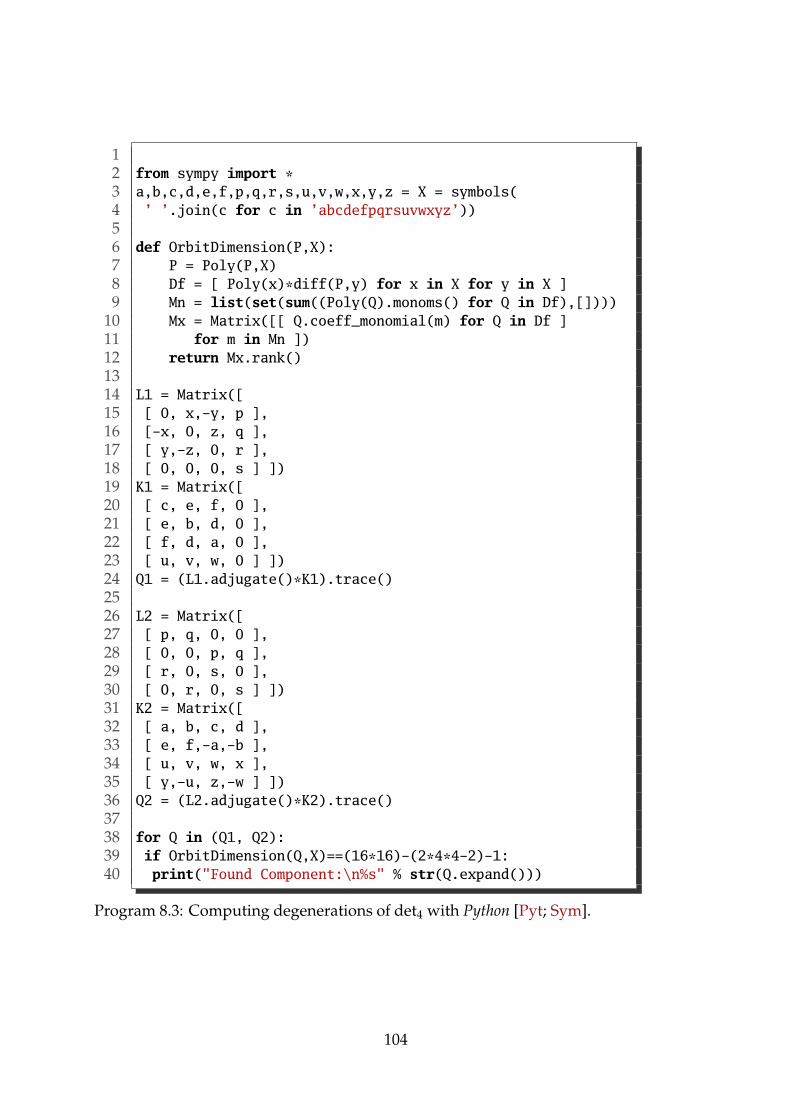
1 2 from sympy import * 3 a,b,c,d,e,f,p,q,r,s,u,v,w,x,y,z = X = symbols( 4 ’ ’.join(c for c in ’abcdefpqrsuvwxyz’)) 5 6 def OrbitDimension(P,X): 7 P = Poly(P,X) 8 Df = [ Poly(x)*diff(P,y) for x in X for y in X ] 9 Mn = list(set(sum((Poly(Q).monoms() for Q in Df),[])))

10 Mx = Matrix([[ Q.coeff_monomial(m) for Q in Df ] 11 for m in Mn ]) 12 return Mx.rank() 13 14 L1 = Matrix([ 15 [ 0, x,-y, p ], 16 [-x, 0, z, q ], 17 [ y,-z, 0, r ], 18 [ 0, 0, 0, s ] ]) 19 K1 = Matrix([ 20 [ c, e, f, 0 ], 21 [ e, b, d, 0 ], 22 [ f, d, a, 0 ], 23 [ u, v, w, 0 ] ]) 24 Q1 = (L1.adjugate()*K1).trace() 25 26 L2 = Matrix([ 27 [ p, q, 0, 0 ], 28 [ 0, 0, p, q ], 29 [ r, 0, s, 0 ], 30 [ 0, r, 0, s ] ]) 31 K2 = Matrix([ 32 [ a, b, c, d ], 33 [ e, f,-a,-b ], 34 [ u, v, w, x ], 35 [ y,-u, z,-w ] ]) 36 Q2 = (L2.adjugate()*K2).trace() 37 38 for Q in (Q1, Q2): 39 if OrbitDimension(Q,X)==(16*16)-(2*4*4-2)-1: 40 print("Found Component:\n%s" % str(Q.expand()))

Program 8.3: Computing degenerations of det4 with Python [Pyt; Sym].

104

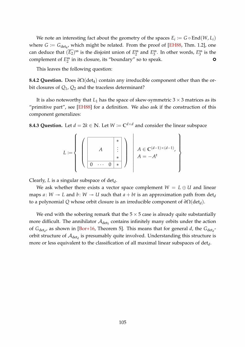
We note an interesting fact about the geometry of the spaces Ei := G End(W, Li)where G := Gdet4 , which might be related. From the proof of [EH88, Thm. 1.2], onecan deduce that (E2)

ss is the disjoint union of Ess2 and Ess

3 . In other words, Ess3 is the

complement of Ess2 in its closure, its “boundary” so to speak.

This leaves the following question:

8.4.2 Question. Does ∂Ω(det4) contain any irreducible component other than the or-bit closures of Q1, Q2 and the traceless determinant?

It is also noteworthy that L1 has the space of skew-symmetric 3× 3 matrices as its“primitive part”, see [EH88] for a definition. We also ask if the construction of thiscomponent generalizes:

8.4.3 Question. Let d = 2k ∈ N. Let W := Cd×d and consider the linear subspace

L :=

⎧⎪⎪⎪⎪⎪⎪⎪⎨⎪⎪⎪⎪⎪⎪⎪⎩

⎛⎜⎜⎜⎜⎝⎞⎟⎟⎟⎟⎠A

∗...∗

0 · · · 0 ∗

A ∈ C(d−1)×(d−1),A = −At

⎫⎪⎪⎪⎪⎪⎪⎪⎬⎪⎪⎪⎪⎪⎪⎪⎭Clearly, L is a singular subspace of detd.

We ask whether there exists a vector space complement W = L ⊕ U and linearmaps a : W L and b : W U such that a+ bt is an approximation path from detdto a polynomial Q whose orbit closure is an irreducible component of ∂Ω(detd).

We end with the sobering remark that the 5× 5 case is already quite substantiallymore difficult. The annihilator Adet5 contains infinitely many orbits under the actionof Gdetd , as shown in [Bor+16, Theorem 5]. This means that for general d, the Gdetd-orbit structure of Adetd is presumably quite involved. Understanding this structure ismore or less equivalent to the classification of all maximal linear subspaces of detd.

105

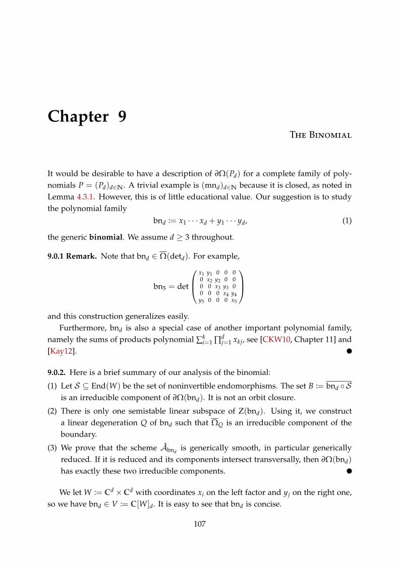
Chapter 9The Binomial

It would be desirable to have a description of ∂Ω(Pd) for a complete family of poly-nomials P = (Pd)d∈N. A trivial example is (mnd)d∈N because it is closed, as noted inLemma 4.3.1. However, this is of little educational value. Our suggestion is to studythe polynomial family

bnd := x1 · · · xd + y1 · · · yd, (1)

the generic binomial. We assume d ≥ 3 throughout.

9.0.1 Remark. Note that bnd ∈ Ω(detd). For example,

bn5 = det

⎛⎜⎝x1 y1 0 0 00 x2 y2 0 00 0 x3 y3 00 0 0 x4 y4y5 0 0 0 x5

⎞⎟⎠and this construction generalizes easily.

Furthermore, bnd is also a special case of another important polynomial family,namely the sums of products polynomial ∑k

i=1 ∏dj=1 xkj, see [CKW10, Chapter 11] and

[Kay12].

9.0.2. Here is a brief summary of our analysis of the binomial:

(1) Let S ⊆ End(W) be the set of noninvertible endomorphisms. The set B := bnd Sis an irreducible component of ∂Ω(bnd). It is not an orbit closure.

(2) There is only one semistable linear subspace of Z(bnd). Using it, we constructa linear degeneration Q of bnd such that ΩQ is an irreducible component of theboundary.

(3) We prove that the scheme Abnd is generically smooth, in particular genericallyreduced. If it is reduced and its components intersect transversally, then ∂Ω(bnd)has exactly these two irreducible components.

We let W := Cd × Cd with coordinates xi on the left factor and yj on the right one,so we have bnd ∈ V := C[W]d. It is easy to see that bnd is concise.

107

9.1 Stabilizer and Maximal Linear Subspaces

We will denote by Hd := Gbnd the stabilizer group of the binomial. The main goal ofthis section is to prove the following result:

9.1.1 Theorem. Let W := Cd × Cd with d ≥ 3. The stabilizer group Hd ⊆ GL(W) isreductive of dimension 2d− 2. Moreover,

(1) The identity component of the stabilizer of P is the group

Hd =

diag(s1, . . . , sd, t1, . . . , td)

∏di=1 si = ∏d

i=1 ti = 1.

(2) Let K ⊆ GL(W) be the group generated by

• the map t : W → W, (v,w) ↦→ (w, v), and

• the group Sd ×Sd ⊆ GLd ×GLd ⊆ GL(W) of permutation matrices that per-mute the first and last d coordinates among themselves, respectively.

Then, K ∼= Sd ≀ Z2 and Hd = K · Hd has |K| = 2 · d! · d! connected components.

9.1.2 Corollary. By Theorem A.1.9, dim(Ω(bnd)) = 4d2 − 2d+ 2.

One can prove Theorem 9.1.1 by means of the explicit description of Lie(Hd) fromCorollary 7.2.3, but another method is to study the action of Hd on linear subspacesof the vanishing locus Z(bnd) ⊆ W = Cd × Cd. It is straightforward to provide linearsubspaces of Z(bnd): The most canonical choice are the spaces Lij := Z(xi, yj) for1 ≤ i, j ≤ d. Furthermore, there is the space

L0 :=(w1, . . . ,wd, ζw1, . . . , ζwd) | w1, . . . ,wd ∈ C ⊆ W,

where ζ ∈ C will always denote a fixed d-th root of −1, i.e., we have ζd = −1. For theproof of Theorem 9.1.1, we will prove the following proposition as an auxiliary result.

9.1.3 Proposition. The maximal linear subspaces of Z(bnd) consist of the Lij and thespaces h(L0) for h ∈ Hd. Furthermore, the Lij are unstable.

Proof of Theorem 9.1.1. It is easy to see that the elements of Hd and K stabilize bnd.

We are left to show that Hd ⊆ K · Hd . The elements of Hd act on the set of linear

subspaces of Z(bnd) of any fixed dimension, so by Proposition 9.1.3 they permutethe Lij. Dually, the action of Hd on W∗ permutes the spaces L∗ij := ⟨xi, yj⟩ ⊆ W∗ for all1 ≤ i, j ≤ d in the sense that for all h ∈ Hd, there are 1 ≤ r, s ≤ d such that

L∗ij h := ⟨xi h, yj h⟩ = ⟨xr, ys⟩ = L∗rs.

108

Let h ∈ Hd and 1 ≤ k ≤ d. We claim that there is an index 1 ≤ i ≤ d such that thelinear form xk h is either a scalar multiple of xi or yi. To this end, let 1 ≤ i, j, r, s ≤ dbe such that L∗k1 h = L∗ij and L∗k2 h = L∗rs, then

⟨xk h⟩ = ⟨xk⟩ h = (L∗k1 ∩ L∗k2) h = L∗ij ∩ L∗rs.

Hence, the two planes L∗ij and L∗rs intersect in the line spanned by (xk h), in particularthis intersection is nontrivial. It follows that i = r or j = s because for i = r and j = s,we have L∗ij ∩ L∗rs =0. Therefore, either ⟨xk h⟩ = ⟨xi⟩ or ⟨xk h⟩ = ⟨yj⟩ as claimed.

In the same manner, we can show that yk h is some scalar multiple of a coordinatefunction. This means that h is the product of a permutation and a diagonal matrix.The result is a straightforward corollary.

We are left to show Proposition 9.1.3. The proof has been split up into the followingthree lemmata:

9.1.4 Lemma. A maximal linear subspace L ⊆ Z(bnd) which is contained in a coordi-nate hyperplane is equal to Lij for some choice of i and j.

Proof. Assume L ⊆ Z(xi). It follows that any (v1, . . . , vd,w1, . . . ,wd) ∈ L must satisfyw1 · · ·wd = 0. Consequently, L ⊆ Li1 ∪ · · · ∪ Lid. It follows that L = Lij for some j.

9.1.5 Lemma. The spaces Lij are unstable.

Proof. It is sufficient to show that L1d is unstable since Lij = h(L1d) for an appropriatepermutation h ∈ Hd. To see that L1d is unstable, let a : W → L1d be any linear mapand consider

hε := diag(ε1−d, ε, . . . , ε, ε1−d) ∈ Hd,

where ε1−d is in the first and last position. Note that the representing matrix of a hasvanishing first and last row. Therefore, hε a → 0 as ε → 0.

9.1.6 Lemma. Let L ⊆ Z(bnd) be a maximal linear subspace which is not containedin any coordinate hyperplane. Then, there is an h ∈ Hd such that h(L) = L0.

Proof. Since L is not contained in any of the coordinate hyperplanes, there is a point(u1, . . . , ud, v1, . . . , vd) ∈ L such that ui = 0 and vi = 0 for all 1 ≤ i ≤ d. Let u ∈ C besuch that ud = u1 · · · ud. We apply the scaling matrix

diag(

uu1

, . . . ,uud

,v2 · · · vdζd−1ud−1 ,

ζuv2

, . . . ,ζuvd

)∈ H

d

to the space L and thereby achieve that (u, . . . , u, ζu, . . . , ζu) ∈ L. By scaling, weget that p := (1, . . . , 1, ζ, . . . , ζ) ∈ L. We denote by K the discrete part of Hd, i.e.,

109

the finite group of permutations that stabilize bnd. We now claim that L ⊆ K.L0,so L is contained in a finite union of translates of L0. This will imply the state-ment because L has to be equal to one of the translates of L0. For the proof, letq = (u1, . . . , ud, v1, . . . , vd) ∈ L be any point different from p. Since the entire linecontaining p and q must be a subset of L and subsequently a subset of Z(bnd), thismeans that bnd vanishes at Tp− q for any T ∈ C. In other words,

0 =d

∏i=1

(T − ui) +d

∏i=1

(ζT − vi) =d

∏i=1

(T − ui)−d

∏i=1

(T − ζ−1vi)

as an identity of polynomials in C[T]. Hence, ui = ζ−1vi up to a permutation whichstabilizes bnd.

For future reference we consider the matrix

b :=(

I 0ζI 0

), (2)

then End(W, L0) = b GL(W) is the set of all endomorphisms that map into L0. FromProposition 9.1.3, we obtain:

Assbnd

=h a | a ∈ End(W, L0)ss = Hd End(W, L0)ss = Hd b GL(W)ss. (3)

9.2 The First Boundary Component

There are certain natural degenerations of bnd which we will study here. We introducethe notation P ∼ Q :⇔ P ∈ ΩQ and say that P is linearly equivalent to Q in this case.

9.2.1 Remark. An important property of linear equivalence is the fact that P ∼ Qimplies GP

∼= GQ, indeed if Q = P g then it is easy to see that GQ = g−1 GP g.

For the rest of this section, we also set

S :=a ∈ End(W) | rk(a) < 2d ,

so S is the hypersurface of noninvertible endomorphisms on W = C2d. Our mainresult of this section is the following:

9.2.2 Proposition. Let B ⊆ Ω(bnd) be the closure of bnd S . Then, B has codimensionone in Ω(bnd) and it is an irreducible component of ∂Ω(bnd).

For the proof, we define the polynomials

Qr,s = x1 · · · xd + y1 · · · yd−1 ·(

r

∑k=1

xk +s

∑k=1

yk

)for r ≤ d and s < d. Note that Qr,s ∈ bnd S . We defer the proof of the followingauxiliary result:

110

9.2.3 Lemma. The polynomials Qd−1,d−1 and Qd,d−1 are elements of bnd S whoseorbits are disjoint. Furthermore, both orbits are of codimension 2 in Ω(bnd).

Proof of Proposition 9.2.2. By definition, B is an irreducible closed subset of Ω(bnd),because it is the closure of the image of the irreducible variety S under the orbit map.Let us check that it is contained in ∂Ω(bnd): The elements of bnd S are not concise.Since that is a closed condition by Remark 5.1.3, no element of B is concise. As allelements of Ω(bnd) are concise, we know that B must lie in the complement.

We are left to determine the dimension of B. By Lemma 9.2.3, B has codimension atmost 2. Assume for contradiction that the codimension of B in ∂Ω(bnd) is equal to 2.The orbit closure Ω(Qd,d−1) is an irreducible closed subset of B and it has the samedimension as B by Lemma 9.2.3 and our assumption. This implies that Ω(Qd,d−1) = B.We have Qd−1,d−1 ∈ B = Ω(Qd,d−1), but Qd−1,d−1 /∈ Ω(Qd,d−1) by Lemma 9.2.3. Thismeans Qd−1,d−1 ∈ ∂Ω(Qd,d−1). However, the orbit of Qd−1,d−1 has the same dimensionas the orbit of Qd,d−1, which is a contradiction to Theorem A.1.9.(3).

It follows that the codimension of B is at most 1, and since it is completely con-tained in the boundary, this implies that it is a component.

Proof of Lemma 9.2.3. Let r ∈ d− 1, d and Q := Qr,d−1. We define the linear formℓ := x1 + · · ·+ xr + y1 + · · ·+ yd−1, so Q = x1 · · · xd + y1 · · · yd−1 · ℓ. Furthermore, wedenote by a ∈ S the endomorphism that satisfies yd a = ℓ and a is the identity on allother coordinates, so that Q = bnd a. We will compute the dimension of GQ and thenumber of its connected components. We will see that the former does not dependon r, whereas the latter does – this will imply the lemma by Remark 9.2.1. To obtaina description of GQ, we study its action on the set of linear subspaces of Z(Q).

Claim. If L ⊆ Z(Q) is a linear subspace with dim(L) = 2d− 2, then there are indices1 ≤ i, j ≤ d such that L = Z(xi, yj a).

For j < d, this means L = Lij = Z(xi, yj) and otherwise L = Z(xi, ℓ).

Proof of Claim. Since Q = bnd a, we know that a(L) is a linear subspace of Z(bnd), sothe space a(L) is contained in one of the spaces from Proposition 9.1.3. We first showthat there are 1 ≤ i, j ≤ d with a(L) ⊆ Lij.

The form yd − ℓ vanishes on im(a), but it is straightforward to verify that it doesnot vanish on h(L0) for any h ∈ Hd. Therefore, a(L) = L0, but it might be properlycontained in it. We show that this is not possible: Since d ≥ 3, we have

dim(a(L)) ≥ dim(L)− 1 = 2d− 3 ≥ d = dim(L0).

Hence, we have a(L) ⊆ Lij. In particular, the linear forms xi = xi a and yj aboth vanish on L. The latter is equal to yj for j < d and otherwise it is equal to ℓ. Ineither case however, the two forms are linearly independent and therefore cut out thespace L.

111

The action of GQ permutes these linear spaces. Dually, its action on W∗ per-mutes the spaces ⟨xi, yj a⟩ ⊆ W∗. Reminiscent of the proof of Theorem 9.1.1, wecan conclude in the same fashion that the action of GQ maps every element of the setM :=x1, . . . , xd, y1, . . . , yd−1, ℓ to a scalar multiple of an element of M. Of course, itcan map yd to any linear form which is linearly independent from the other coordi-nates. Hence, there is a group K ⊆ GL2d−1 such that GQ admits a matrix representa-tion

GQ =

⎧⎪⎪⎪⎪⎪⎪⎪⎨⎪⎪⎪⎪⎪⎪⎪⎩

⎛⎜⎜⎜⎜⎜⎜⎜⎝0

h...0

∗ · · · ∗ α

⎞⎟⎟⎟⎟⎟⎟⎟⎠

h ∈ K,α ∈ C×

⎫⎪⎪⎪⎪⎪⎪⎪⎬⎪⎪⎪⎪⎪⎪⎪⎭∼= K× C2d−1 × C×. (4)

Claim. K is a finite group of order |K| = r! · d2 · (d− 1)!.

This claim implies the lemma as follows: We have dim(GQ) = 2d = dim(Hd) + 2,the latter by Theorem 9.1.1. From Theorem A.1.9, we conclude that ΩQ has codimen-sion two in Ω(bnd). If Qd−1,d−1 and Qd,d−1 were in the same orbit, then their stabi-lizers would be conjugate and in particular, they would both have the same numberof connected components. However, the number of connected components of GQ isequal to |K|, which depends on r.

We are therefore left to verify our claim. We first study the subgroup

Π :=

π ∈ K ℓ π ∈ C×ℓ

of K and observe that its order depends on r:

Claim. We have Π ∼= Zd o (Sr ×Sd−1), where Zd corresponds to scaling all variableswith a d-th root of unity simultaneously and Sr ×Sd−1 permutes the x-variables andthe y-variables that occur in ℓ among themselves.

Proof of Claim. We first check that every π ∈ Π is a product of a diagonal and apermutation matrix. Let M := Cx1, . . . ,Cxd,Cy1, . . . ,Cyd−1,Cℓ be the set of linesspanned by elements of M. We know that π induces a permtutation of M whichhas Cℓ as a fixpoint. In particular, π induces a permutation of the lines spanned bythe first 2d− 1 coordinates. This is precisely what we claimed.

Next, we show that all diagonal matrices in Π are scalar and correspond to mul-tiplication with a d-th root of unity. Let π ∈ Π be a diagonal matrix and let ξ ∈ C×

be such that ℓ π = ξℓ. It is straightforward to see that this implies xi π = ξxi andyj π = ξyj for all 1 ≤ i, j ≤ d− 1. As π stabilizes

Q = x1 · · · xd + y1 · · · yd−1 ·(x1 + · · ·+ xr + y1 + · · ·+ yd−1) ,

112

it must, for instance, stabilize the monomial y21 · y2 · · · yd, whence ξd = 1. Let ϑ ∈ C×

be such that xd π = ϑxd. As π also stabilizes the monomial x1 · · · xd, we also getϑξd−1 = 1, hence ϑ = ξ.

We now assume that π ∈ Π is a permutation and show that π does not mapany x-variable to a y-variable. Observe that any monomial of Q that is divisible bya y-variable is divisible by d − 1 of the y-variables. Assume for contradiction thatsome x-variable is mapped to a y-variable. Then, since (x1 · · · xd) π = ∏d

i=1(xi π)

is a monomial of Q, we conclude that d− 1 of the d x-variables must be mapped toy-variables. In turn, all y-variables must be mapped to x-variables. As Q contains themonomial y21 · y2 · · · yd−1, this implies the contradiction that Q = Q π also containsthe monomial x21 · x2 · · · xd−1.

We are left to verify that for r = d− 1, every permutation π ∈ Π leaves xd invariant.Assume for contradiction that there is some i ≤ d− 1 such that xi π = xd. Then, Q =

Q π contains the monomial (y1 · · · yd−1 · xi) π = y1 · · · yd−1 · xd, a contradiction.

As |Π| = r! · d · (d− 1)!, we are left to verify that K/Π contains d residue classes,by Lagrange’s Theorem. For any 1 ≤ j < d, denote by gj ∈ K the map that satis-fies yj gj = −ℓ and is the identity on all other variables. Hence, ℓ gj = −yj and itis easy to check that gj stabilizes Q. We will show that

K/Π =Π, g1Π, . . . , gd−1Π . (5)

To this end, let g ∈ K be such that ℓ g is not a scalar multiple of ℓ. Then, there issome β ∈ C× with ℓ g = β · z, where z is a variable. Furthermore, there is an η ∈ C×

such that g maps a variable z ∈ M to η · ℓ. By applying an element of the subgroup Π,we may assume that z = z, i.e., we have z g = η · ℓ. We may furthermore assumethat g maps all variables other than z to scalar multiples of themselves. By studyingthe monomials of Q, it is straightforward to check that z = yj for some 1 ≤ j < d.There are certain scalars αi and βk such that

β · yj = ℓ g =(∑r

i=1 xi + ∑d−1k=1 yk

) g =

(∑r

i=1 αixi)+(∑k =j βkyk

)+ η · ℓ.

With β j := −β, we obtain that −η · ℓ = ∑ri=1 αixi +∑d−1

k=1 βkyk, so αi = −η and βk = −η

for all i and k. In particular, η = β. It is now again easy to check that −η is a d-th rootof unity, so we have achieved g ∈ gjK and proved (5).

It is natural to ask what a generic elements of B := bnd S looks like. It turns outthat B is not an orbit closure. Instead, for the one-parameter family of polynomials

Qt := t · x1 · · · xd + y1 · · · yd−1 ·(

d

∑k=1

xk +d−1

∑k=1

yk

), (t ∈ C×)

we prove the following result.

113

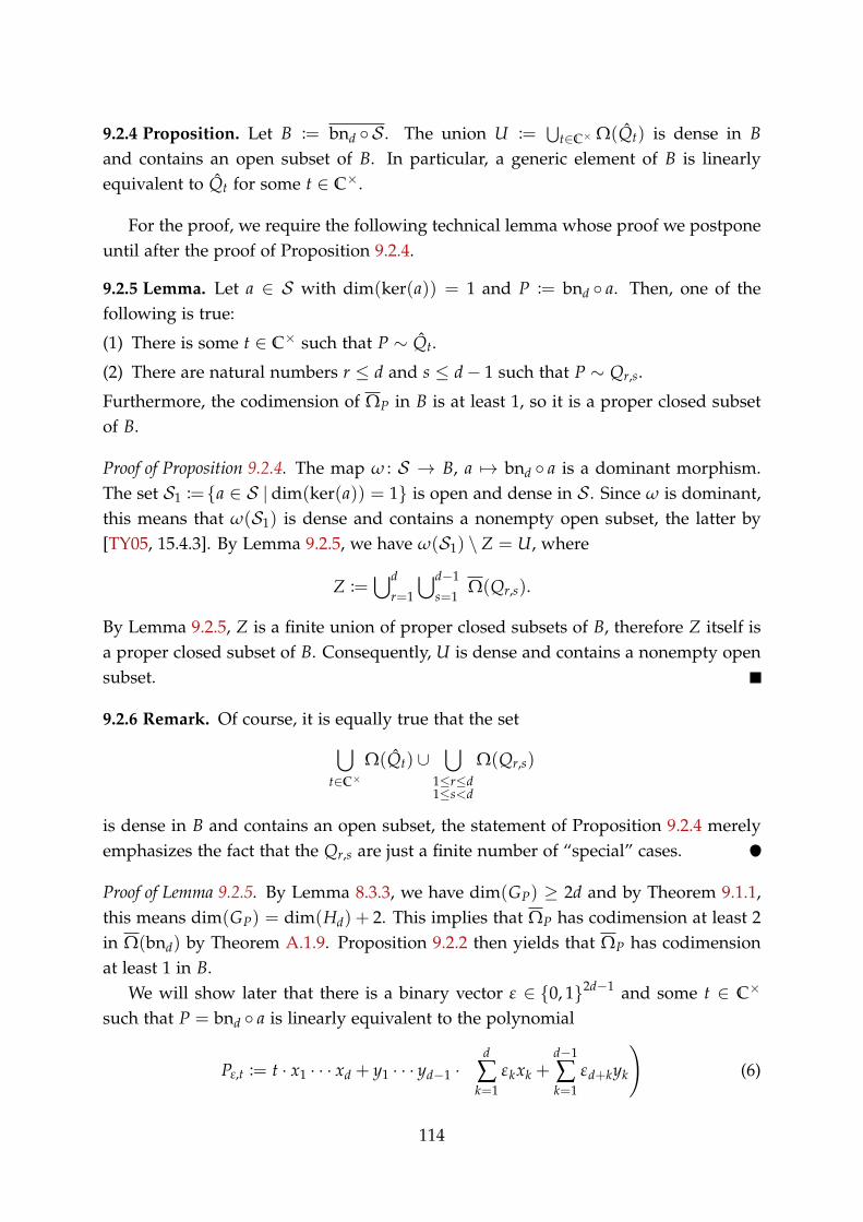
9.2.4 Proposition. Let B := bnd S . The union U :=⋃

t∈C× Ω(Qt) is dense in Band contains an open subset of B. In particular, a generic element of B is linearlyequivalent to Qt for some t ∈ C×.

For the proof, we require the following technical lemma whose proof we postponeuntil after the proof of Proposition 9.2.4.

9.2.5 Lemma. Let a ∈ S with dim(ker(a)) = 1 and P := bnd a. Then, one of thefollowing is true:

(1) There is some t ∈ C× such that P ∼ Qt.

(2) There are natural numbers r ≤ d and s ≤ d− 1 such that P ∼ Qr,s.

Furthermore, the codimension of ΩP in B is at least 1, so it is a proper closed subsetof B.

Proof of Proposition 9.2.4. The map ω : S → B, a ↦→ bnd a is a dominant morphism.The set S1 :=a ∈ S | dim(ker(a)) = 1 is open and dense in S . Since ω is dominant,this means that ω(S1) is dense and contains a nonempty open subset, the latter by[TY05, 15.4.3]. By Lemma 9.2.5, we have ω(S1) \ Z = U, where

Z :=⋃d

r=1

⋃d−1

s=1Ω(Qr,s).

By Lemma 9.2.5, Z is a finite union of proper closed subsets of B, therefore Z itself isa proper closed subset of B. Consequently, U is dense and contains a nonempty opensubset.

9.2.6 Remark. Of course, it is equally true that the set⋃t∈C×

Ω(Qt) ∪⋃

1≤r≤d1≤s<d

Ω(Qr,s)

is dense in B and contains an open subset, the statement of Proposition 9.2.4 merelyemphasizes the fact that the Qr,s are just a finite number of “special” cases.

Proof of Lemma 9.2.5. By Lemma 8.3.3, we have dim(GP) ≥ 2d and by Theorem 9.1.1,this means dim(GP) = dim(Hd) + 2. This implies that ΩP has codimension at least 2in Ω(bnd) by Theorem A.1.9. Proposition 9.2.2 then yields that ΩP has codimensionat least 1 in B.

We will show later that there is a binary vector ε ∈ 0, 12d−1 and some t ∈ C×

such that P = bnd a is linearly equivalent to the polynomial

Pε,t := t · x1 · · · xd + y1 · · · yd−1 ·(

d

∑k=1

εkxk +d−1

∑k=1

εd+kyk

)(6)

114

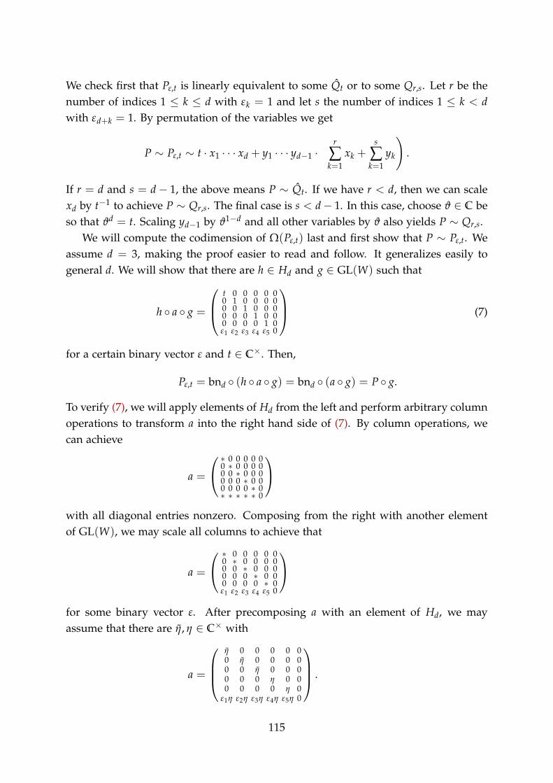
We check first that Pε,t is linearly equivalent to some Qt or to some Qr,s. Let r be thenumber of indices 1 ≤ k ≤ d with εk = 1 and let s the number of indices 1 ≤ k < dwith εd+k = 1. By permutation of the variables we get

P ∼ Pε,t ∼ t · x1 · · · xd + y1 · · · yd−1 ·(

r

∑k=1

xk +s

∑k=1

yk

).

If r = d and s = d− 1, the above means P ∼ Qt. If we have r < d, then we can scalexd by t−1 to achieve P ∼ Qr,s. The final case is s < d− 1. In this case, choose ϑ ∈ C beso that ϑd = t. Scaling yd−1 by ϑ1−d and all other variables by ϑ also yields P ∼ Qr,s.

We will compute the codimension of Ω(Pε,t) last and first show that P ∼ Pε,t. Weassume d = 3, making the proof easier to read and follow. It generalizes easily togeneral d. We will show that there are h ∈ Hd and g ∈ GL(W) such that

h a g =

⎛⎜⎝ t 0 0 0 0 00 1 0 0 0 00 0 1 0 0 00 0 0 1 0 00 0 0 0 1 0ε1 ε2 ε3 ε4 ε5 0

⎞⎟⎠ (7)

for a certain binary vector ε and t ∈ C×. Then,

Pε,t = bnd (h a g) = bnd (a g) = P g.

To verify (7), we will apply elements of Hd from the left and perform arbitrary columnoperations to transform a into the right hand side of (7). By column operations, wecan achieve

a =

⎛⎝ ∗ 0 0 0 0 00 ∗ 0 0 0 00 0 ∗ 0 0 00 0 0 ∗ 0 00 0 0 0 ∗ 0∗ ∗ ∗ ∗ ∗ 0

⎞⎠with all diagonal entries nonzero. Composing from the right with another elementof GL(W), we may scale all columns to achieve that

a =

⎛⎝ ∗ 0 0 0 0 00 ∗ 0 0 0 00 0 ∗ 0 0 00 0 0 ∗ 0 00 0 0 0 ∗ 0ε1 ε2 ε3 ε4 ε5 0

⎞⎠for some binary vector ε. After precomposing a with an element of Hd, we mayassume that there are η, η ∈ C× with

a =

⎛⎜⎜⎝η 0 0 0 0 00 η 0 0 0 00 0 η 0 0 00 0 0 η 0 00 0 0 0 η 0

ε1η ε2η ε3η ε4η ε5η 0

⎞⎟⎟⎠ .

115

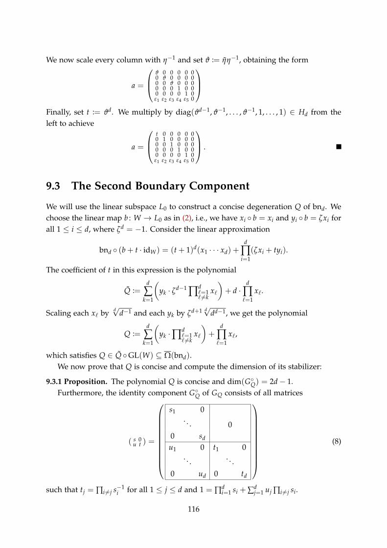
We now scale every column with η−1 and set ϑ := ηη−1, obtaining the form

a =

⎛⎜⎝ ϑ 0 0 0 0 00 ϑ 0 0 0 00 0 ϑ 0 0 00 0 0 1 0 00 0 0 0 1 0ε1 ε2 ε3 ε4 ε5 0

⎞⎟⎠Finally, set t := ϑd. We multiply by diag(ϑd−1, ϑ−1, . . . , ϑ−1, 1, . . . , 1) ∈ Hd from theleft to achieve

a =

⎛⎜⎝ t 0 0 0 0 00 1 0 0 0 00 0 1 0 0 00 0 0 1 0 00 0 0 0 1 0ε1 ε2 ε3 ε4 ε5 0

⎞⎟⎠ .

9.3 The Second Boundary Component

We will use the linear subspace L0 to construct a concise degeneration Q of bnd. Wechoose the linear map b : W → L0 as in (2), i.e., we have xi b = xi and yi b = ζxi forall 1 ≤ i ≤ d, where ζd = −1. Consider the linear approximation

bnd (b+ t · idW) = (t+ 1)d(x1 · · · xd) +d

∏i=1

(ζxi + tyi).

The coefficient of t in this expression is the polynomial

Q :=d

∑k=1

(yk · ζd−1 ∏d

ℓ=1ℓ =k

xℓ

)+ d ·

d

∏ℓ=1

xℓ.

Scaling each xℓ byd√d−1 and each yk by ζd+1 d√dd−1, we get the polynomial

Q :=d

∑k=1

(yk · ∏d

ℓ=1ℓ =k

xℓ

)+

d

∏ℓ=1

xℓ,

which satisfies Q ∈ Q GL(W) ⊆ Ω(bnd).We now prove that Q is concise and compute the dimension of its stabilizer:

9.3.1 Proposition. The polynomial Q is concise and dim(GQ) = 2d− 1.

Furthermore, the identity component GQ of GQ consists of all matrices

( s 0u t ) =

⎛⎜⎜⎜⎜⎜⎜⎜⎜⎜⎜⎝

s1 0. . . 0

0 sdu1 0 t1 0

. . . . . .

0 ud 0 td

⎞⎟⎟⎟⎟⎟⎟⎟⎟⎟⎟⎠(8)

such that tj = ∏i =j s−1i for all 1 ≤ j ≤ d and 1 = ∏d

i=1 si + ∑dj=1 uj ∏i =j si.

116

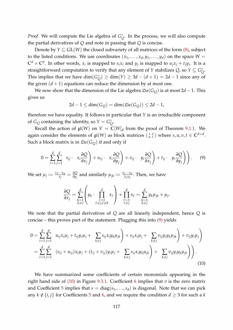
Proof. We will compute the Lie algebra of GQ. In the process, we will also compute

the partial derivatives of Q and note in passing that Q is concise.Denote by Y ⊆ GL(W) the closed subvariety of all matrices of the form (8), subject

to the listed conditions. We use coordinates (x1, . . . , xd, y1, . . . , yd) on the space W =

Cd × Cd. In other words, xi is mapped to sixi and yj is mapped to ujxj + tjyj. It is astraightforward computation to verify that any element of Y stabilizes Q, so Y ⊆ G

Q.This implies that we have dim(G

Q) ≥ dim(Y) ≥ 3d− (d+ 1) = 2d− 1 since any ofthe given (d+ 1) equations can reduce the dimension by at most one.

We now show that the dimension of the Lie algebra Lie(GQ) is at most 2d− 1. Thisgives us

2d− 1 ≤ dim(GQ) = dim(Lie(GQ)) ≤ 2d− 1,

therefore we have equality. It follows in particular that Y is an irreducible componentof GQ containing the identity, so Y = G

Q.Recall the action of gl(W) on V = C[W]d from the proof of Theorem 9.1.1. We

again consider the elements of gl(W) as block matrices ( s vu t ) where s, u, v, t ∈ Cd×d.

Such a block matrix is in Lie(GQ) if and only if

0 =d

∑i=1

d

∑j=1

(sij ·(xi

∂Q∂xj

)+ uij ·

(xi

∂Q∂yj

)+ vij ·

(yi

∂Q∂xj

)+ tij ·

(yi

∂Q∂yj

)). (9)

We set µj :=x1···xd

xj= ∂Q

∂yjand similarly µjk :=

x1···xdxjxk

. Then, we have

∂Q∂xj

=d

∑k=1k =j

⎛⎜⎝yk ·d

∏ℓ=1

ℓ =j,ℓ =k

xℓ

⎞⎟⎠+d

∏ℓ=1ℓ =j

xℓ =d

∑k=1k =j

ykµjk + µj.

We note that the partial derivatives of Q are all linearly independent, hence Q isconcise – this proves part of the statement. Plugging this into (9) yields

0 =d

∑i=1

d

∑j=1

(uijxiµj + tijyiµj +

(∑k =j

sijxiykµjk

)+ sijxiµj +

(∑k =j

vijyiykµjk

)+ vijyiµj

)

=d

∑i=1

d

∑j=1

((sij + uij)xiµj + (tij + vij)yiµj +

(∑k =j

sijxiykµjk

)+

(∑k =j

vijyiykµjk

)).

(10)

We have summarized some coefficients of certain monomials appearing in theright hand side of (10) in Figure 9.3.1. Coefficient 6 implies that v is the zero matrixand Coefficient 5 implies that s = diag(s1, . . . , sd) is diagonal. Note that we can pickany k /∈i, j for Coefficients 5 and 6, and we require the condition d ≥ 3 for such a k

117

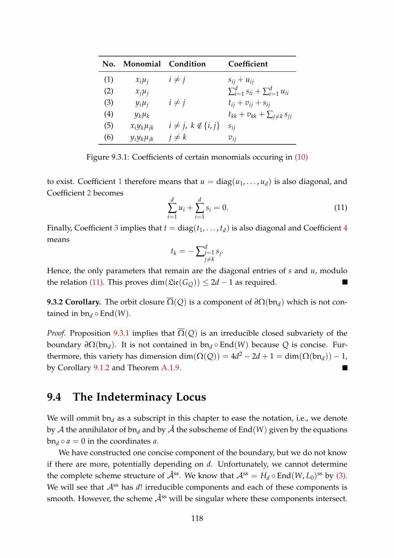
No. Monomial Condition Coefficient

(1) xiµj i = j sij + uij(2) xjµj ∑d

i=1 sii + ∑di=1 uii

(3) yiµj i = j tij + vij + sij(4) ykµk tkk + vkk + ∑j =k sjj(5) xiykµjk i = j, k /∈i, j sij(6) yiykµjk j = k vij

Figure 9.3.1: Coefficients of certain monomials occuring in (10)

to exist. Coefficient 1 therefore means that u = diag(u1, . . . , ud) is also diagonal, andCoefficient 2 becomes

d

∑i=1

ui +d

∑i=1

si = 0. (11)

Finally, Coefficient 3 implies that t = diag(t1, . . . , td) is also diagonal and Coefficient 4means

tk = −∑dj=1j =k

sj.

Hence, the only parameters that remain are the diagonal entries of s and u, modulothe relation (11). This proves dim(Lie(GQ)) ≤ 2d− 1 as required.

9.3.2 Corollary. The orbit closure Ω(Q) is a component of ∂Ω(bnd) which is not con-tained in bnd End(W).

Proof. Proposition 9.3.1 implies that Ω(Q) is an irreducible closed subvariety of theboundary ∂Ω(bnd). It is not contained in bnd End(W) because Q is concise. Fur-thermore, this variety has dimension dim(Ω(Q)) = 4d2 − 2d+ 1 = dim(Ω(bnd))− 1,by Corollary 9.1.2 and Theorem A.1.9.

9.4 The Indeterminacy Locus

We will ommit bnd as a subscript in this chapter to ease the notation, i.e., we denotebyA the annihilator of bnd and by A the subscheme of End(W) given by the equationsbnd a = 0 in the coordinates a.

We have constructed one concise component of the boundary, but we do not knowif there are more, potentially depending on d. Unfortunately, we cannot determinethe complete scheme structure of Ass. We know that Ass = Hd End(W, L0)ss by (3).We will see that Ass has d! irreducible components and each of these components issmooth. However, the scheme Ass will be singular where these components intersect.

118

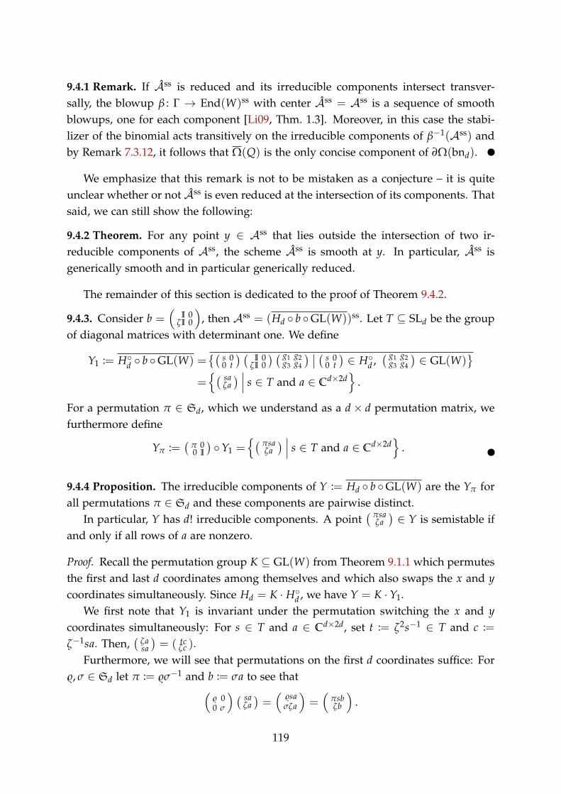
9.4.1 Remark. If Ass is reduced and its irreducible components intersect transver-sally, the blowup β : Γ → End(W)ss with center Ass = Ass is a sequence of smoothblowups, one for each component [Li09, Thm. 1.3]. Moreover, in this case the stabi-lizer of the binomial acts transitively on the irreducible components of β−1(Ass) andby Remark 7.3.12, it follows that Ω(Q) is the only concise component of ∂Ω(bnd).

We emphasize that this remark is not to be mistaken as a conjecture – it is quiteunclear whether or not Ass is even reduced at the intersection of its components. Thatsaid, we can still show the following:

9.4.2 Theorem. For any point y ∈ Ass that lies outside the intersection of two ir-reducible components of Ass, the scheme Ass is smooth at y. In particular, Ass isgenerically smooth and in particular generically reduced.

The remainder of this section is dedicated to the proof of Theorem 9.4.2.

9.4.3. Consider b =(

I 0ζI 0

), then Ass = (Hd b GL(W))ss. Let T ⊆ SLd be the group

of diagonal matrices with determinant one. We define

Y1 := Hd b GL(W) =

(s 00 t) (

I 0ζI 0) ( g1 g2

g3 g4) ( s 0

0 t)∈ H

d ,( g1 g2g3 g4

)∈ GL(W)

=( sa

ζa) s ∈ T and a ∈ Cd×2d

.

For a permutation π ∈ Sd, which we understand as a d× d permutation matrix, wefurthermore define

Yπ :=(

π 00 I

)Y1 =

( πsaζa) s ∈ T and a ∈ Cd×2d

.

9.4.4 Proposition. The irreducible components of Y := Hd b GL(W) are the Yπ forall permutations π ∈ Sd and these components are pairwise distinct.

In particular, Y has d! irreducible components. A point( πsa

ζa)∈ Y is semistable if

and only if all rows of a are nonzero.

Proof. Recall the permutation group K ⊆ GL(W) from Theorem 9.1.1 which permutesthe first and last d coordinates among themselves and which also swaps the x and ycoordinates simultaneously. Since Hd = K · H

d , we have Y = K ·Y1.We first note that Y1 is invariant under the permutation switching the x and y

coordinates simultaneously: For s ∈ T and a ∈ Cd×2d, set t := ζ2s−1 ∈ T and c :=ζ−1sa. Then,

(ζasa)= ( tc

ζc ).Furthermore, we will see that permutations on the first d coordinates suffice: For

ϱ, σ ∈ Sd let π := ϱσ−1 and b := σa to see that(ϱ 00 σ

) ( saζa)=(

ϱsaσζa

)=(

πsbζb

).

119

Assume now that Yπ = Yσ for two permutations π and σ. We have( π

ζI

)∈ Yπ = Yσ

and hence, there are a ∈ Cd×2d and an s ∈ T with( π

ζI

)=( σsa

ζa). This implies that we

have a = I and hence, σs = π, so s = σ−1π. However since s is diagonal, this meansit must be the identity and therefore σ = π. This proves that the Yπ are the pairwisedistinct irreducible components of Y.

The semistability condition follows immediately from the description of the maxi-mal linear subspaces in Section 9.1.

9.4.5 Corollary. A point( πsa

ζa)∈ Yπ lies in the intersection of Yπ with another com-

ponent Yσ of Y if and only if there are two rows of a ∈ Cd×2d that are scalar multiplesof one another.

Proof. If the i-th and j-th row of a are scalar multiples of one another, let σ be thecomposition of π with the transposition τ := (i, j). By assumption, there is a t ∈ Twith tτa = sa, so we have πsa = πτtτa = σtτa = σsa. Hence, a ∈ Yπ ∩Yσ.

Conversely, assume that there is a permutation σ = π with( πsa

ζa)=(

σtcζc

)for

some t ∈ T and c ∈ Cd×2d. It follows immediately that c = a, hence πsa = σta.Denoting by ai the i-th row of a, this means sπ(i)aπ(i) = tσ(i)aσ(i) for all 1 ≤ i ≤ d. Asπ = σ, there is an index i with k := π(i) = σ(i) =: j, so we have skak = tjaj, thereforeak = s−1

k tjaj.

The proof of Theorem 9.4.2 is now completed by the following proposition.

9.4.6 Proposition. Let a ∈ Cd×2d be such that no row of a is a scalar multiple ofanother. Let also π ∈ Sd and u ∈ T. Then, y :=

( πuaζa)is a smooth point of Ass.

Proof. We first note that dim(Y) = dim(Y1) = 2d2+ d− 1, hence we have to show thatthe tangent space Ty Ass has the same dimension.

As Hd ×GL(W) and Sd act by automorphisms on Ass, the tangent space at y isisomorphic to the tangent space of any element in the Hd ×GL(W) orbit of y. Hence,we may assume y =

( aζa).

Note that each row of a is nonzero. After applying some column operationfrom GL(W) we may assume that ai1 = 0 and the last d columns of a are zero.Scaling the first column by the inverse of a11 · · · ad1 with another column operation,we achieve that a11 · · · ad1 = 1. We then apply a row scaling operation from Hd toachieve ai1 = 1 for all 1 ≤ i ≤ d. We set ai := xi a = x1 + ∑d

j=2 aijxj. Since the ai arenot scalar multiples of one another, we achieve ai = x1+ cix2+ ai with further columnoperations, where the ci are all distinct and the ai are linear forms in x3, . . . , xd.

120

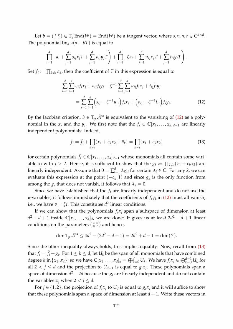
Let b = ( s vu t ) ∈ Ty End(W) = End(W) be a tangent vector, where s, v, u, t ∈ Cd×d.

The polynomial bnd (a+ bT) is equal to

d

∏i=1

(ai +

d

∑j=1

sijxjT +d

∑j=1

vijyjT

)+

d

∏i=1

(ζai +

d

∑j=1

uijxjT +d

∑j=1

tijyjT

).

Set fi := ∏k =i ak, then the coefficient of T in this expression is equal to

d

∑i=1

d

∑j=1

sij fixj + vij fiyj − ζ−1d

∑i=1

d

∑j=1

uij fixj + tij fiyj

=d

∑i=1

d

∑j=1

(sij − ζ−1uij

)fixj +

(vij − ζ−1tij

)fiyj. (12)

By the Jacobian criterion, b ∈ Ty Ass is equivalent to the vanishing of (12) as a poly-nomial in the xj and the yj. We first note that the fi ∈ C[x1, . . . , xd]d−1 are linearlyindependent polynomials: Indeed,

fi = fi + ∏k =i

(x1 + ckx2 + ak) = ∏k =i

(x1 + ckx2) (13)

for certain polynomials fi ∈ C[x1, . . . , xd]d−1 whose monomials all contain some vari-able xj with j > 2. Hence, it is sufficient to show that the gi := ∏k =i(x1 + ckx2) arelinearly independent. Assume that 0 = ∑d

i=1 λigi for certain λi ∈ C. For any k, we canevaluate this expression at the point (−ck, 1) and since gk is the only function fromamong the gi that does not vanish, it follows that λk = 0.

Since we have established that the fi are linearly independent and do not use they-variables, it follows immediately that the coefficients of fiyj in (12) must all vanish,i.e., we have v = ζt. This constitutes d2 linear conditions.

If we can show that the polynomials fixj span a subspace of dimension at leastd2 − d + 1 inside C[x1, . . . , xd]d, we are done: It gives us at least 2d2 − d + 1 linearconditions on the parameters ( s v

u t ) and hence,

dimTy Ass ≤ 4d2 − (2d2 − d+ 1) = 2d2 + d− 1 = dim(Y).

Since the other inequality always holds, this implies equality. Now, recall from (13)that fi = fi+ gi. For 1 ≤ k ≤ d, letUk be the span of all monomials that have combineddegree k inx1, x2, so we have C[x1, . . . , xd]d =

⨁dk=0Uk. We have fixj ∈

⨁d−1k=0 Uk for

all 2 < j ≤ d and the projection to Ud−1 is equal to gixj. These polynomials span aspace of dimension d2− 2d because the gi are linearly independent and do not containthe variables xj when 2 < j ≤ d.

For j ∈1, 2, the projection of fixj to Ud is equal to gixj and it will suffice to showthat these polynomials span a space of dimension at least d+ 1. Write these vectors in

121

coordinates with respect to the basis (x01xd2, x

11x

d−12 , x21x

d−22 , . . . , xd1x

02), then they form

the columns of a (d+ 1)× (2d) matrix

M :=

g1x1 · · · gdx1 g1x2 · · · gdx2⎛⎜⎜⎜⎝⎞⎟⎟⎟⎠

0 · · · 0g

g0 · · · 0

with g ∈ GLd because the gi are linearly independent. We have

M ·(g−1 00 g−1

)=

⎛⎜⎜⎜⎜⎝⎞⎟⎟⎟⎟⎠

∗ · · · ∗ 1

1. . .

. . . 11 ∗ · · · ∗

which is easily seen to have full rank.

As explained in Remark 9.4.1, it would be interesting to know whether Ass isreduced everywhere:

9.4.7 Question.

(1) Is the scheme Assbnd

Cohen-Macaulay?

(2) Is the scheme Assbnd

reduced?

Remark. Note that (1) implies (2) by Theorem 9.4.2 and the fact that Cohen-Macaulayschemes have no embedded components [GW10, Prop. 14.124].

122

Part III

Appendix

123

Appendix AAlgebraic Groups and Representation Theory

Throughout this chapter, we fix an algebraically closed field C of characteristic zero.We assume knowledge of classical algebraic geometry, see [Har06; Har95] and also[Kra85, Anhang]. We denote the coordinate ring of an affine C-variety X by C[X]. Wealso use the notation [n] :=1, . . . , n.

A.1 Algebraic Semigroups and Groups

If E is a semigroup acting on a set X, we usually denote this action by a dot, sothe action of g ∈ E on x ∈ X is denoted g.x. The set Ex := g ∈ E | g.x = x is thestabilizer of x ∈ X. The orbit of x under the action of E is the set E.x :=g.x | g ∈ E.If E.x = x, we say that x is E-invariant. If S ⊆ E is any subset, we denote byXS := x ∈ X | ∀s ∈ S : s.x = x the set of all S-invariant elements of X. A subsetY ⊆ X is E-stable if E.Y ⊆ Y. If E is a monoid, we write 1 or 1E for the unique neutralelement of E.

A.1.1 Definition. An algebraic semigroup is a semigroup (E, ) which is also a C-variety such that the composition map

µE : E× E −→ E

(g, h) ↦−→ g h

is a morphism of varieties. A morphism of algebraic semigroups is a morphismφ : E → E′ of varieties between two algebraic semigroups which is also a morphismof semigroups. An left-E-variety is a variety X together with a morphism

αX : E× X −→ X

which defines a left E-action on the set X. Similarly, the notion of a right-E-variety isdefined. An E-variety is defined to be a left-E-variety. A morphism of E-varieties isa map φ : X → Y which is a morphism of varieties such that φ(g.x) = g.φ(x) for allg ∈ E and x ∈ X.

125

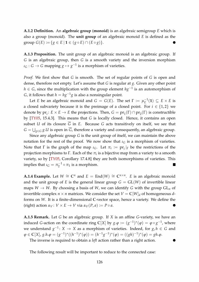
A.1.2 Definition. An algebraic group (monoid) is an algebraic semigroup E which isalso a group (monoid). The unit group of an algebraic monoid E is defined as thegroup G(E) :=g ∈ E | 1 ∈ (g E) ∩ (E g).

A.1.3 Proposition. The unit group of an algebraic monoid is an algebraic group. IfG is an algebraic group, then G is a smooth variety and the inversion morphismιG : G → G mapping g ↦→ g−1 is a morphism of varieties.

Proof. We first show that G is smooth. The set of regular points of G is open anddense, therefore not empty. Let’s assume that G is regular at g. Given any other pointh ∈ G, since the multiplication with the group element hg−1 is an automorphism ofG, it follows that h = hg−1g is also a nonsingular point.

Let E be an algebraic monoid and G = G(E). The set Γ := µ−1E (1) ⊆ E × E is

a closed subvariety because it is the preimage of a closed point. For i ∈ 1, 2 wedenote by pri : E× E → E the projections. Then, G = pr1(Γ) ∩ pr2(Γ) is constructibleby [TY05, 15.4.3]. This means that G is locally closed. Hence, it contains an opensubset U of its closure G in E. Because G acts transitively on itself, we see thatG =

⋃g∈G g.U is open in G, therefore a variety and consequently, an algebraic group.

Since any algebraic group G is the unit group of itself, we can maintain the abovenotation for the rest of the proof. We now show that ιG is a morphism of varieties.Note that Γ is the graph of the map ιG. Let πi := pri |Γ be the restrictions of theprojection morphisms to Γ. Each of the πi is a bijective map from a variety to a smoothvariety, so by [TY05, Corollary 17.4.8] they are both isomorphisms of varieties. Thisimplies that ιG = π−1

2 π1 is a morphism.

A.1.4 Example. Let W ∼= Cn and E = End(W) ∼= Cn×n. E is an algebraic monoidand the unit group of E is the general linear group G = GL(W) of invertible linearmaps W → W. By choosing a basis of W, we can identify G with the group GLn ofinvertible complex n× n matrices. We consider the set V = C[W]d of homogeneous d-forms on W. It is a finite-dimensional C-vector space, hence a variety. We define the(right) action αV : V × E → V via αV(P, a) := P a.

A.1.5 Remark. Let G be an algebraic group. If X is an affine G-variety, we have aninduced G-action on the coordinate ring C[X] by g.ϕ := (g−1)∗(ϕ) = ϕ g−1, wherewe understand g−1 : X → X as a morphism of varieties. Indeed, for g, h ∈ G andϕ ∈ C[X], g.h.ϕ = (g−1)∗((h−1)∗(ϕ)) = (h−1g−1)∗(ϕ) = ((gh)−1)∗(ϕ) = gh.ϕ.

The inverse is required to obtain a left action rather than a right action.

The following result will be important to reduce to the connected case:

126

A.1.6 Proposition. Let G be an algebraic monoid. There is a unique irreducible com-ponent G ⊆ G containing 1. G is a closed submonoid of G.

If G is an algebraic group, then G is a normal subgroup and the irreduciblecomponents of G are the cosets hG for h ∈ G. In particular, the quotient group G/G

is finite.

Proof. Let G be a connected component of G containing 1 and let X be any irreduciblecomponent of G. Then XG is the image of the restriction of µG to X×G. This meansthat XG is the image of an irreducible variety under a regular map, therefore XG isan irreducible, closed subvariety of G. Since 1 ∈ G, we have X ⊆ XG ⊆ XG. X isirreducible, so X = XG. This implies X = XG and similarly, we obtain X = GX.In particular, G = GG, so G is a closed submonoid. If 1 was also contained in X,then we could similarly conclude that GX = XG = G, so we have X = G.

Assume now that G is a group. If X is an irreducible component, then for anyh ∈ X, we know that h−1X is the image of an irreducible set under the automorphismh, so it is an irreducible component. Since 1 ∈ h−1X, we know that h−1X = G, henceX = hG. For any h ∈ G, similarly observe that hGh−1 is a component containing 1,so hGh−1 = G. This proves that G is a normal subgroup. Since its cosets are the(finitely many) irreducible components of X, this proves the statement.

A.1.1 Quotients by Algebraic Groups

Let X be a variety on which an algebraic group G acts. Then, a categorical quotientis a morphism π : X → Y such that

(C1) π is constant on G-orbits.

(C2) If ψ : X → Z is any morphism of varieties which is constant on G-orbits, thenthere exists a unique ψ : Y → Z with ψ π = ψ.

If a categorical quotient exists, it is unique up to unique isomorphism and wedenote it by Y = X//G.

However, categorical quotients can lack many properties one would expect fromthe quotient by a group action. For example, there are cases when the projectionmorphism is not surjective. A much stronger notion is the one of a good quotient,defined to be a morphism π : X → Y with the following properties:

(G1) The morphism π is G-invariant and surjective.

(G2) The comorphism of π induces an isomorphism OY∼= (π∗OX)

G.

(G3) For a closed and G-invariant subset Z ⊆ X, the image π(Z) is closed in Y.

(G4) Two closed, G-invariant subsets Z1,Z2 ⊆ X are disjoint if and only if π(Z1)

and π(Z2) are disjoint.

127

A good quotient is called a geometric quotient if the fibers of π are precisely theG-orbits of X.

A.1.7 Remark. See [TY05, 25.2] for some remarks on Property (G2). The gist is thatfor any open subset U ⊆ Y, the ring (π∗OX)(U) = OX(π

−1(U)) carries a G-modulestructure, so we can consider the corresponding subring of G-invariant functionsOX(π

−1(U))G. This defines a subsheaf of rings (π∗OX)G ⊆ (π∗OX).

By [New78, §4, Prop. 3.11], any good quotient is also a categorical quotient. If thequotient is geometric, we denote it by X/G .

A.1.8 Theorem. Let G be an affine, reductive algebraic group acting on an affine vari-ety X. The ring C[X]G is a finitely generated C-algebra and Y = Spec(C[X]G) togetherwith the surjective morphism π : X → Y induced by C[X]G ⊆ C[X] defines a goodquotient of X by G. Furthermore:

(1) If G is finite and X irreducible, then this quotient is geometric.

(2) For all x ∈ X, the fiber π−1(π(x)) contains a unique closed G-orbit Ω. Further-more, we have π−1(π(x)) =

y ∈ X

Ω ⊆ G.y.

Proof. See [TY05, 27.5] and [TY05, 25.5.2].

If a group G acts on a set X, one can identify the orbit G.x of any element x ∈ Xwith the set of cosets G/Gx where Gx = g ∈ G | g.x = x is the stabilizer of x. Itturns out that under certain assumptions, this remains valid and compatible when Xis a G-variety.

A.1.9 Theorem ([TY05, 21.4]). Let G be an affine algebraic group and X a G-variety.For every point x ∈ X, we have:

(1) The orbit G.x is a smooth subvariety of X which is open in its closure G.x.

(2) The stabilizer Gx is a closed subgroup of G and every component of G.x hasdimension dim(G)− dim(Gx).

(3) G.x is the union of G.x and orbits of strictly smaller dimension.

(4) If X is affine and Gx is reductive, the right action of Gx on G by multiplicationadmits the good quotient G.x ∼= G//Gx and in particular G.x is an affine varietywith coordinate ring C[G.x] ∼= C[G]Gx .

A.1.2 Nullcone and Projective Quotients

If an algebraic group G acts on a vector space V, the set N :=v ∈ V

0 ∈ G.v

is called the nullcone of this action. Especially when G is reductive, the geometry

128

of N carries a lot of information about the quotient, see [Kra85]. We will require thefollowing observations:

A.1.10 Lemma. Let G be a reductive affine algebraic group acting on a complex vectorspace V. Let π : V V//G be the quotient and N ⊆ V the nullcone. Then,

• N = π−1(π(0)), in particular N is a closed subset of V.

• N =v ∈ V

0 ∈ G.vwhere G is the connected identity component of G.

• N is the vanishing set of all homogeneous, G-invariant functions in C[V].

Proof. Since the origin 0 is a closed G-orbit, we have 0 ∈ G.v if and only if π(v) = π(0)according to Theorem A.1.8.

For the second item, note that G = H · G where H is a finite set, according toProposition A.1.6. Since G.v = H.G.v = H.G.v, we can see that 0 ∈ G.v if and onlyif 0 ∈ G.v.

Finally, the defining ideal of π(0) in C[V]G is equal to the maximal ideal generatedby all homogeneous elements of positive degree, and since π corresponds to the in-clusion C[V]G ⊆ C[V], the set N is the vanishing set of the same elements, consideredas functions on V.

If V is a G-module, the projective space P(V) is a G-variety in a natural way. Alinearized projective G-variety is a projective variety X with a fixed embedding asa closed, G-invariant subset X ⊆ P(V) for some G-module V. We write X ⊆ Vfor the affine cone over X, i.e., X is an affine variety which is closed under scalarmultiplication and X = P(X).

If X is a linearized projective G-invariant closed cone, then C[X] is a graded alge-bra. It is the projective coordinate ring of X. The invariant algebra C[X]G inherits thisgrading and in particular, one can consider the projective variety Y := Proj(C[X]G)and the induced rational map π : X 99K Y. If we denote by [x] ∈ X the projectiveclass of a point x ∈ X, then π([x]) = [π(x)] where π : X X//G is the affine quo-tient from Theorem A.1.8. This rational map is undefined when π(x) = 0, which byLemma A.1.10 means that PN is the indeterminacy locus of π. Hence, Xss := X \PNis the open set where π is defined. It is called the set of semistable points of X, withrespect to the (induced) action of G on X. One also calls Xss := X \ N the set ofsemistable points of X. Since N is a cone, we have Xss = (PX)ss = P(Xss) and wesometimes omit the brackets. The restriction π : Xss → Y is a morphism.

A.1.11 Proposition. Let X be a linearized projective G-variety and S its projectivecoordinate ring. The projective variety Y := Proj(SG) together with the morphismπ : Xss → Y induced by SG ⊆ S defines a good quotient Y = Xss//G.

129

Using Theorem A.1.8, the proof is straightforward. We omit it for brevity and referto [Dol03, Thm. 8.1, Prop. 8.1] for a modern treatment and [New78, §4, Thm. 3.14] fora more classical version. We note the following amplification of Property (C2):

A.1.12 Proposition. Let X be a linearized projective G-variety and let ϖ : X 99K Y bea G-invariant rational map between projective varieties. Then, there exists a rationalmap φ : Xss//G 99K Z such that the following diagram commutes:

Xss

π

ϖ →→ Y

Xss//G

φ

Here, π is the quotient morphism.

Proof. Fix some embedding of Y in a projective space. Let S and R be the projectivecoordinate rings of X and Y, respectively. The rational map ϖ corresponds to a homo-morphism ϖ♯ : R → S of graded C-algebras and the assumption that ϖ is G-invariantmeans that the image of ϖ♯ is contained in the invariant ring SG. Since SG is theprojective coordinate ring of Xss//G, this homomorphism R → SG induces a rationalmap φ : Xss//G 99K Y. The inclusion SG → S of graded rings corresponds to therational map π : X 99K Xss//G which restricts to π, so we have φ π = ϖ as rationalmaps. Restricting to Xss yields the result.

A.2 Representation Theory of Reductive Groups

Let G be an affine algebraic group throughout this section. A Borel subgroup of G isa maximal connected solvable subgroup B of G. It follows from the definition that aBorel subgroup of G is closed, because if H ⊆ G is connected and solvable, then so isits closure. By [Hum98, 21.3], G/B is a projective variety and all Borel subgroups ofG are conjugate. We fix one Borel B of G.

The only connected, algebraic C-groups of dimension one are the multiplicativegroup Gm := Gm(C) := (C×, ·) and the additive group Ga := Ga(C) := (C,+), see[TY05, 22.6.2]. A product of multiplicative groups Gr

m is called a torus.G contains a unique largest normal solvable subgroup [TY05, 27.1.1], which is au-

tomatically closed. Its identity component is then the largest connected normal solv-able subgroup of G and is called the radical of G, denoted R(G). By [TY05, 27.1.2],the set of unipotent elements of R(G) is the largest connected normal unipotent sub-group of G. It is denoted by Ru(G) and we call it the unipotent radical of G. Anaffine algebraic group G is called semisimple (resp. reductive) if R(G) (resp. Ru(G))is trivial. Note that we follow [TY05, 27.2] here and do not require G to be connected.

130

However, an algebraic group G has a unique, connected, normal subgroup G con-taining the neutral element [TY05, 21.1.5 & 21.1.6] and by definition, G is semisimple(resp. reductive) if and only G has this property.

For example, each torus is reductive. Furthermore, GLn is reductive, but notsemisimple. However, the subgroup SLn ⊆ GLn of matrices with determinant 1 issemisimple.

By [Hum98, 21.3], the maximal tori and the maximal unipotent subgroups of Gare those of the Borel subgroups of G, and all of them are also conjugate. We fix amaximal torus T ⊆ B and denote by U = Ru(B) the unipotent radical of B. We haveB = U o T by [Hum98, 19.3].

A.2.1 Example. The affine space Cn×n of all n× n matrices with entries in C has thecoordinate ring C

[xij i, j ∈ [n]

]. The group G := GLn of invertible n× n matrices is

the set of matrices where detn does not vanish and therefore a Zariski-open subsetof Cn×n. Hence, G is an affine algebraic group with coordinate ring C[xij, det

−1n ].

Denote by S := SLn the set of matrices with determinant 1, i.e., the vanishing set ofdetn −1. It is a closed, affine algebraic subgroup of G.

Denote by In be the unit matrix, then it is well-known that the center of G = GLn

is equal to Z := C× · In. By [Lan02, Part 3, Chapter XIII, 8 & 9], the projective lineargroup PGLn = G/Z = S

/(S ∩ Z) is simple. Thus, if R E G is solvable, then R/Z

is also solvable and can only be trivial or equal to PGLn. However, PGLn is notsolvable because S is perfect (i.e., [S, S] = S) and therefore not solvable. Thus, R/Z istrivial, which means R ⊆ Z. Since Z is connected, normal and solvable, we must haveR(G) = Z. The only unipotent central matrix is the unit matrix, so Ru(G) is trivialand we have verified that G is reductive.

A maximal Borel subgroup B of G is given by the upper triangular matrices ofnonvanishing determinant and its unipotent radical U is the subgroup of those ele-ments where all diagonal entries are equal to 1. The maximal torus T correspondingto this choice are the invertible diagonal matrices.

A.2.1 Representations

Let G be an algebraic group. A representation of G is a homomorphism of algebraicgroups ϱ : G → GL(V(ϱ)), where V(ϱ) is some finite-dimensional C-vector space. Thespace V(ϱ) becomes a G-variety via the induced action. We also write VG(ϱ) insteadof V(ϱ) if we want to put emphasis on the group. The degree of ϱ is defined to bedim(V(ϱ)).

Conversely, if V is some C-vector space which is also a G-variety, we say that V isa G-module. We remark that the G-modules are in bijection with the representations

131

of G by associating to a representation ϱ : G → GL(V) the action α : G×V → V whereα(g, v) := ϱ(g)(v).

A homomorphism of G-representations is a C-linear map φ : VG(ϱ1) → VG(ϱ2)

such that ϱ2(g) φ = φ ϱ1(g) for all g ∈ G. Equivalently, a homomorphism of G-modules is a C-linear map φ : V1 → V2 where φ(g.x) = g.φ(x) for all g ∈ G.

We say that ϱ1 is a subrepresentation of ϱ2 if there is an injective homomorphismof G-representations VG(ϱ1) → VG(ϱ2). Equivalently, a submodule of a G-moduleV1 is a linear subspace V1 ⊆ V2 such that V1 is stable under the action of G. Arepresentation ϱ is irreducible if ϱ has no nontrivial subrepresentations. Equivalentlya G-module V is irreducible if it has no G-invariant linear subspaces other than Vand 0. Denote by Rep(G) the set of all equivalence classes of G-representationsand by Irr(G) ⊆ Rep(G) the subset of all irreducible representations. If H ⊆ G is asubgroup, we have a canonical restriction map Rep(G) → Rep(H), ϱ ↦→ ϱ|H.

The arguably most important lemma of representation theory is the following:

A.2.2 Lemma (Schur’s Lemma). Let G be an algebraic group and ϱ1, ϱ2 ∈ Irr(G). Ev-ery nonzero homomorphism φ : V(ϱ1) → V(ϱ2) of G-representations is an isomor-phism.

Proof. Note that for v ∈ ker(φ), we have φ(g.v) = g.φ(v) = g.0 = 0, hence ker(φ) is aG-invariant subspace of V(ϱ1). Since φ is nonzero, we must have ker(φ) =0.

For two representations ϱ1, ϱ2 ∈ Rep(G) with Vi := V(ϱi), we define the repre-sentation ϱ1 ⊕ ϱ2 : G → GL(V1 ⊕ V2) via g ↦→ ϱ1(g) ⊕ ϱ2(g). For ϱ ∈ Rep(G), letϱ∗ : G → GL(VG(ϱ)

∗) be the representation defined by ϱ∗(g) := (ϱ(g)∗)−1, i.e., thegroup homomorphism corresponding to the action

G× VG(ϱ)∗ −→ VG(ϱ)

∗ (1)

(g, ϕ) ↦−→ ϕ ϱ(g)−1

A.2.2 Characters, Roots, Weights

Assume henceforth that G is reductive, we have chosen a Borel B ⊆ G and a maximaltorus Gr

m∼= T ⊆ B.

A multiplicative (resp. additive) character of an algebraic group H is a homomor-phism of algebraic groups H → Gm (resp. H → Ga). Conversely, a multiplicative(resp. additive) one-parameter-subgroup (also called 1-psg for short) is a homomor-phism of algebraic groups Gm → H (resp. Ga → H). When we say character or1-psg, we refer to the multiplicative version. The set of characters X(H) and the set

132

of 1-psgs X(H) become abelian groups under pointwise multiplication. There arecanonical isomorphisms

Zr −→ X(Grm) Zr −→ X(Gr

m) (2)

λ ↦−→ χλ γ ↦−→ χγ

where χλ and χγ are defined as

χλ : Grm −→ Gm χγ : Gm −→ Gr

m

t ↦−→ tλ := tλ11 · · · tλr

r x ↦−→ tγ := (tγ1 , . . . , tγr).

For (γ,λ) ∈ X(H)× X(H) we define ⟨γ,λ⟩ ∈ Z to be the integer corresponding toλ γ ∈ X(Gm) ∼= Z. In other words, g⟨γ,λ⟩ = (gγ)λ for all t ∈ C×. It is well-known[TY05, 22.5.2] that X(T) ∼= Irr(T) in the sense that any ϱ ∈ Rep(T) decomposes as adirect sum of weight spaces

V(ϱ)α =v ∈ V(ϱ) | ∀t ∈ T : t.v = tαv .

If ϱ ∈ Rep(G), we can also regard V(ϱ) as a T-module and denote by V(ϱ)α thecorresponding weight space. We call Λ(G) := X(T) the weight lattice of G.

To avoid an introduction to the theory of Lie algebras ([Hum98, Chapter III] or[TY05, 23]), we deviate from [Hum98] in defining α ∈ Λ(G) to be a root of G withrespect to T to be a if there exists an additive 1-psg εα : Ga → G such that

∀t ∈ T : ∀x ∈ C : t · εα(x) · t−1 = εα(tαx).

This definition of root is equivalent to the one given in [Hum98, 16.4]: Indeed, onedirection of this equivalence is stated in [Hum98, 26.3] and the proof actually verifiesthe other direction as well.

Denote by Φ := Φ(G, T) ⊆ Λ(G) the set of roots of G with respect to T. See[Hum98, 27] for a proof that Φ is a so-called abstract root system and [Hum80, III.9.2] or[TY05, 18] for general facts about abstract root systems. For α ∈ Φ, set Uα := εα(Ga).We call Φ+ :=α ∈ Φ |Uα ⊆ B the positive roots of G with respect to B.

A.2.3 Example. We continue Example A.2.1 and keep the notations already estab-lished. We identify Λ(G) = X(T) with Zn in the above way. For i, j ∈ [n] and i = j,denote by αij ∈ Zn the vector with the value 1 in position i, the value −1 in position jand 0 elsewhere. We claim that these weights are the roots of G with respect to T.

For i, j ∈ [n], we define Eij ∈ Cn×n to be the matrix with:

xrs(Eij) =

1 ; (r, s) = (i, j)0 ; (r, s) = (i, j)

133

With these notations, we define the map

εij : Ga = C −→ G

x ↦−→ In + x · Eij

It is elementary to check that this is a morphism of algebraic groups and furthermore,for any x ∈ C and any diagonal matrix t = (t1, . . . , tn) ∈ T,

t · εij(x) · t−1 = t · (In + x · Eij) · t−1 = tInt−1 + x · tEijt−1

= In + x · titj· Eij = εij(tαijx).

We therefore know that the αij are certainly roots. With more prelude and the the-ory of Lie algebras, one can see rather directly that these are, in fact, all the roots.See [Kra85, Bemerkung 4, III.1.4] or [GW09, Theorem 2.4.1] for a quite elementarytreatment.

The group Uij := Uαij is now the image of εij and from the definition we can seethat Uij =

In + t · Eij

t ∈ Cconsists of matrices with 1 on the main diagonal and

zeros everywhere else except at position (i, j). Since we chose B to be the group ofupper triangular matrices, we can see that αij ∈ Φ+ if and only if i < j.

It can be shown that there exists a (unique) subset ∆ ⊆ Φ of linearly independentweights with the property that for all α ∈ Φ+, there are nonnegative integers cδ suchthat α = ∑δ∈∆ cδδ. See [Hum80, III.10.1] or [TY05, 18.7.4] for a proof of this result. Aroot belonging to ∆ is called a simple root and |∆| is called the rank of G.

For every root α ∈ Λ(G) = X(T), there is a unique dual root α ∈ X(T) satisfyingthe two conditions

• ⟨α, α⟩ = 2 and

• ∀β ∈ Φ : β −⟨α, β⟩ · α ∈ Φ.

This is part of the root system axioms, see [Hum80, III.9.2] or [TY05, 18.2.1]. Notethat the map β ↦→ β −⟨α, β⟩ · α is referred to as σα in [Hum80], as sα,α in [TY05] andas τα In [Hum98]. It is called the reflection relative to α. It maps α to −α and leaves acertain hyperplane Hα invariant. We then call

Λ+(G) :=

λ ∈ Λ(G) ∀α ∈ Φ+ : ⟨α,λ⟩ ≥ 0

the dominant weights of G, the notation being justified in that they lie on the side ofHα which we have marked as “positive” by our choice of Φ+, which in turn is basedon the choice of B. See [TY05, 18.11.7] for a proof that Λ+(G) is a finitely generatedsemigroup.

134

A.2.4 Example. We continue Example A.2.3. For the set ∆, we choose in this case theroots αi := αi,(i+1) for i ∈ [n − 1]. There are n − 1 of these roots, they are linearlyindependent and for i < j, we have

αij = αi + αi+1 + · · ·+ αj−1.

The rank of GLn is therefore n− 1.Given any root α ∈ Zn ∼= X(T), we define its dual to be the 1-psg corresponding to

the same tuple via (2). With this definition, ⟨α, α⟩ corresponds simply to the ordinaryscalar product Zn × Zn → Z given by (α, β) ↦→ αtβ. We identify α and α. Clearly,⟨

αij, αij⟩= αij

tαij = 2.Let λ ∈ Zn. For i < j, we have λi ≥ λj if and only if

⟨αij,λ

⟩= λi − λj ≥ 0. Hence,

the dominant weights of GLn are precisely the weakly descending vectors of integernumbers – such a vector is called a generalized partition.

We remark that in this case, it is easy to see that the semigroup Λ+(GLn) is finitelygenerated: The vectors

ω1 := (1, 0, 0, . . . , 0),

ω2 := (1, 1, 0, . . . , 0),...

ωn := (1, 1, 1, . . . , 1)

(3)

form a generating set together with −ωn.

We denote by Λr(G) the N-span of Φ+. The group Λr(G) generated by Λr(G) isequal to the Z-span of all roots and is sometimes called the root lattice of G.

For two characters λ, µ ∈ X(T) we write λ D µ if λ − µ ∈ Λr(G).

A.2.5 Example. Still continuing Example A.2.4, we remark finally that the root latticeof G = GLn consists of all λ ∈ Zn with the property that the sum of all entriesvanishes, i.e., |λ| := λ1 + · · ·+ λn = 0. Furthermore,

Λr(G) =λ ∈ Zn | ∀k ∈ [n] : λ1 + · · ·+ λk ≥ 0,|λ| = 0 .

Indeed, if λ = ∑n−1k=1 ckαk is a sum of simple roots with ck ∈ Z, then λk = ck − ck−1.

Hence, ck ∈ N for all k ∈ N if and only if

λ1 + · · ·+ λk = c1 + (c2 − c1) + · · ·+ (ck − ck−1) = ck ≥ 0.

For dominant weights λ, µ ∈ Λ+(G), the dominance order is in agreement withthe following combinatorial definition of dominance order for integer partitions: Twointeger partitions λ = (λ1, . . . ,λn) and µ = (µ1, . . . , µn) satisfy λ D µ if and only if|λ| = |µ| and for all k ≤ n, we have λ1 + · · ·+ λk ≥ µ1 + · · ·+ µk.

135

Finally, we sum up the characterization of the irreducible representations of G inthe following theorem:

A.2.6 Theorem. Let ϱ ∈ Irr(G) and V := V(ϱ). There exists a unique dominantweight λ ∈ Λ+(G) such that:

(1) As a T-module, V =⨁

µEλ Vµ.

(2) dim(Vλ) = 1. Elements of Vλ are called highest weight vectors.

(3) U acts trivially on Vµ if and only if µ = λ.

(4) For α ∈ Φ and µ ∈ Λ(G), we have Uα.Vµ ⊆ ⨁d∈N Vµ+dα.

This defines a bijection Irr(G) ∼= Λ+(G). We henceforth identify the two.

Proof. The main statement as well as (1) to (3) can be found in [Hum98, Theorem 31.3]together with the statement [Hum98, 31.4] which proves that each dominant weighthas a corresponding irreducible representation. Part (4) is [Hum98, 27.2].

For ϱ ∈ Rep(G), the module V := V(ϱ) decomposes as

V =⨁

λ∈Λ+(G)

V(λ)

where V(λ)∼= V(λ)⊕nλ for certain nλ ∈ N. We call V(λ) the isotypical component of

weight λ of V. When f ∈ V(λ), we call wt( f ) := λ the weight of f .

A.2.3 The Coordinate Ring of an Algebraic Group

We recite a famous, general result about the weights that appear in the coordinatering of a reductive, affine, algebraic group:

A.2.7 Theorem (Algebraic Peter-Weyl Theorem). Let G be a reductive, affine, alge-braic group. The group G× G acts on G from the left via (g, h).x = gxh−1. Consider

ψ :⨁

λ∈Irr(G)V(λ)∗ ⊗ V(λ) −→ C[G]

f ⊗ v ↦−→ f ωv

where ωv : G → V(λ) is the morphism g ↦→ g.v.Then, ψ is an isomorphism of G × G – modules, where the action of the left and

right factor of G× G is on the left and right tensor factor, respectively.

Proof. See [TY05, 27.3.9]. We give a quick remark about the action. Recall from (1)that g ∈ G acts on f ∈ V(λ)∗ by g. f = f g−1 and recall from Remark A.1.5 that theinduced action on the coordinate ring of G is such that for ϕ ∈ C[G] and g, h, x ∈ G

136

we have ((g, h).ϕ)(x) = ϕ(g−1xh). Let λ ∈ Irr(G), f ∈ V(λ)∗, v ∈ V(λ) and g, h ∈ G.Then, the following holds for all x ∈ G:

((g, h).ψ( f ⊗ v))(x) = ((g, h).( f ωv))(x) = f (ωv(g−1xh)) = f (g−1xh.v)

= ( f g−1)(x.(h.v)) = (( f g−1) αh.v)(x) = ψ((g. f )⊗ (h.v))(x).

Hence, (g, h).ψ( f ⊗ v) = ψ((g. f )⊗ (h.v)) as claimed.

A.2.8. We summarize Examples A.2.1 and A.2.3 to A.2.5 as follows: The dominantweights for the reductive group GLn are the generalized partitions

Λ+n :=λ ∈ Zn | λ1 ≥ · · · ≥ λn .

We denote by V(λ) the irreducible GLn-module corresponding to the highest weightλ ∈ Λ+

n . Every GLn-module V decomposes as V =⨁

λ∈Λ+n

V(λ)nλ for certain nλ ∈N.

A.2.9 Proposition. The coordinate ring of GLn ⊆ Cn×n has a natural Z-grading be-cause it is the localization of a polynomial ring at the homogeneous polynomial detn.For d ∈ Z, the isomorphism from Theorem A.2.7 restricts to

C[GLn]d ∼=⨁

λ∈Λ+n

|λ|=dV(λ)∗ ⊗ V(λ).

Proof. Let λ ∈ Λ+n , d := |λ| and f ⊗ v ∈ V(λ)∗ ⊗ V(λ). By Theorem A.2.7 we only

have to show that f ωv is homogeneous of degree d. Given t ∈ C×, Theorem A.2.6implies that δt := diag(t, . . . , t) acts on a vector v ∈ V(λ) as δt.v = td · v because forall µ E λ, we have |µ| = |λ| = d (Example A.2.5). Hence,

f (ωv(t · g)) = f (ωv(gδt)) = f (g.δt.v) = f (g.(td · v)) = f (td · (g.v))= td · f (g.v) = td · f (ωv(g)).

Note that the fourth and fifth equality are due to the fact that v ↦→ g.v and f are bothlinear maps.

The module V(λ)∗ is also an irreducible module. More precisely, for any dominantweight λ = (λ1, . . . ,λn) ∈ Λ+

n we define λ∗ := (−λn, . . . ,−λ1) ∈ Λ+n . Then,

A.2.10 Proposition. Let λ ∈ Λ+n . Then, V(λ)∗ = V(λ∗) is an irreducible module.

Proof. This follows from Theorem A.2.6 and (1).

137

A.2.11. Proposition A.2.10 is a special case of a general principle. We denote by B theset of all Borel subgroups of G. By [Hum98, Proposition A in 24.1], the NormalizerN := NG(T) of T permutes the elements of B transitively. For G = GLn and Tthe subgroup of diagonal invertible matrices, note that N is the semidirect productSn n T, where the permutation group Sn is embedded in GLn as the subgroup ofpermutation matrices.

The induced action of the Weyl group S := N/T is free, so S parametrizes exactlythe possible choices of a base for the root system with respect to the torus T. Theaction of S on B is given by B ↦→ Bq := q−1Bq for q ∈ N.

Let τ ∈ N be such that B∩ Bτ = T. Note that in the case of G = GLn, this is simplythe permutation that maps (1, . . . , n) to the reverse vector (n, . . . , 1), because B is theset of upper triangular matrices and B ∩ Bτ = T if and only if Bτ is the set of lowertriangular matrices.

The image of τ in S is called the longest Weyl element. In the literature, it is oftendenoted by w0. With the terminology from [Spr08], w−1

0 has the same length as w0 andby [Spr08, Corollary 8.3.11], an element with this property is unique, hence w0 = w−1

0 .It follows that τ = τ−1.

The Weyl group acts on the weights X(T) as follows: For any χ ∈ X(T) and q ∈ N,we define the character q.λ via the rule (q.λ)(t) := λ(qtq−1). Then, the longest Weylelement maps highest weights to highest weights [Hum98, 31.6]. More precisely, wehave V(λ)∗ = V(−τ.λ). In the case of G = GLn, we have −τ.λ = λ∗.

In particular:

A.2.12 Proposition. Let V be a G-module. Then, VG ∼= (V∗)G.

Proof. By Theorem A.2.6, V =⨁

λ∈Λ+(G) V(λ), so VG = V(0). By the above Para-graph A.2.11, V∗ =

⨁λ∈Λ+(G) V(−τ.λ) where τ denotes the longest Weyl element.

Since −τ.λ = 0 is equivalent to λ = 0, we have (V∗)G ∼= VG.

We end by proving a Lemma that we will require in the next section and which isof independent interest:

A.2.13 Lemma. Let V be a G-module (or more generally, a factorial G-variety) andf ∈ C[V]. Assume that f = f k11 · · · f krr is the decomposition of f into irreduciblefactors. Then, f is a highest weight vector of weight λ if and only if the fi are highestweight vectors of weight λi with λ = k1λ1 + · · ·+ krλr.

Proof. If the fi are weight vectors, then f is still U-invariant and it is easy to see thatthe weight of f must be equal to k1λ1 + · · ·+ krλr.

For the converse, assume that f is a highest weight vector of weight λ and denoteby Z := Z( f ) ⊆ V the vanishing set of f . Note that Z is B-invariant, so we have

138

an action α : B × Z → Z induced by the action of B on V. Let Zi := Z( fi), thenZ = Z1 ∪ . . . ∪ Zr is the decomposition of Z into its irreducible components. Letαi : B× Zi → Z be the restriction of α to Zi. Since B is connected, B× Zi is irreducibleand Zi is contained in the image of αi – therefore, B.Zi = αi(B × Zi) = Zi. Hence,the Zi are invariant under B. It follows that B. fi ⊆ C · fi so B acts by a character on fi.This means that fi is a highest weight vector of some weight λi. Consequently, wemust have λ = k1λ1 + · · ·+ krλr.

A.3 Polynomial Representations

Let W ∼= Cn be a complex vector space with a chosen basis. The action of GLn on amodule V ∼= CN is a morphism ϱ : GLn → GLN of algebraic groups. Hence, it canbe described by N2 regular functions on GLn. In many cases we are interested in,these functions are polynomials in the entries of an n× n matrix, i.e., ϱ extends to amorphism Endn → EndN of affine spaces. In other words, the action of GLn extendsto an action V × Endn → V. We call such a representation a polynomial one.

A.3.1 Definition. There is a partial ordering ⊑ on Λ+n , called the inclusion, defined

as follows: We have µ ⊑ λ if and only if µi ≤ λi for all 1 ≤ i ≤ n.

Note that µ ⊑ λ implies µ E λ, but not the converse. We have

Λ+n :=

λ ∈ Λ+

n λ ⊒ 0

=λ ∈ Zn | λ1 ≥ . . . ≥ λn ≥ 0 ⊆ Nn,

the set of partitions of the number n. We will show:

A.3.2 Proposition. Let λ ∈ Λ+n , then V(λ) is polynomial if and only if λ ∈ Λ+

n .

When V is any GL(W)-module, we can decompose it as V ∼=⨁

λ∈Λ V(λ)⊕nλ forcertain nλ ∈ N. We then write

V⊒0 :=⨁

λ∈Λ+n

λ⊒0

V(λ)⊕nλ ⊆ V.

We call V⊒0 the polynomial part of V. It then follows:

A.3.3 Corollary. A GLn-module V is polynomial if and only if V = V⊒0.

We require an auxiliary lemma for the proof of Proposition A.3.2.

A.3.4 Lemma. The inclusion GLn ⊆ Endn is an open, GLn-equivariant immersion ofvarieties under the operation of GLn acting by multiplication from the left on bothaffine varieties. It induces an inclusion of their respective coordinate rings whichsatisfies C[Endn] = C[GLn]⊒0 =

⨁λ∈Λ+

nV(λ)⊗ V(λ)∗.

139

Proof. By [Lan12, Formula (6.5.1)], we get the last equality in

C[End(W)]d ∼= C[W ⊗W∗]d ∼= Symd(W ⊗W∗) ∼=⨁

0⊑λ∈Λ+n

λ1+···+λn=d

V(λ)⊗ V(λ)∗.

By summing over d and applying Theorem A.2.7, we obtain

C[End(W)] ∼=⨁

λ∈Λ+n

V(λ)⊗ V(λ)∗ = C[GL(W)]⊒0

by the definition of the polynomial part.

Proof of Proposition A.3.2. By Theorem A.2.7, the module C[GLn] contains a uniquehighest weight vector of weight µ for every µ ∈ Λ+

n , up to a scalar. Let f be thehighest weight vector of weight λ = (λ1, . . . ,λn). By Lemma A.3.4, we have λ ∈ Λ+

n

if and only if f extends to a regular function on Endn, i.e., it is a polynomial. Letf = q · detkn with k ∈ Z and q ∈ C[Endn] not divisible by detn. We have to show thatk ≥ 0 is equivalent to λn ≥ 0. In fact, we show that k = λn.

Denote by δ := (1, . . . , 1) ∈ Λ+n , then wt(detn) = δ. We claim that µ := wt(q)

satisfies µn = 0. Indeed, otherwise we’dhave µ − δ ∈ Λ+n and Lemma A.2.13 would

imply that q is divisible by the (unique) weight vector of weight δ, which is detn.Consequently, λn = µn + k = k.

140

Bibliography

[ABV15] Jarod Alper, Tristram Bogart, and Mauricio Velasco. “A Lower Bound forthe Determinantal Complexity of a Hypersurface”. In: Foundations of Com-putational Mathematics (2015), pp. 1–8.

[AM69] Michael Francis Atiyah and Ian Grant Macdonald. Introduction to Commu-tative Algebra. Addison-Wesley, 1969.

[AT92] Noga Alon and Michael Tarsi. “Colorings and orientations of graphs”. In:Combinatorica 12.2 (1992), pp. 125–134.

[Atk83] M. D. Atkinson. “Primitive spaces of matrices of bounded rank. II”. In: J.Austral. Math. Soc. Ser. A 34.3 (1983), pp. 306–315.

[AYY13] Jinpeng An, Jiu-Kang Yu, and Jun Yu. “On the dimension datum of asubgroup and its application to isospectral manifolds”. In: J. DifferentialGeom. 94.1 (2013), pp. 59–85. url: http://projecteuclid.org/euclid.jdg/1361889061.

[BCI11] Peter Bürgisser, Matthias Christandl, and Christian Ikenmeyer. “Even par-titions in plethysms”. In: J. Algebra 328 (2011), pp. 322–329.

[BCS97] Peter Bürgisser, Michael Clausen, and M. Amin Shokrollahi. Algebraic com-plexity theory. Vol. 315. Grundlehren der Mathematischen Wissenschaften[Fundamental Principles of Mathematical Sciences]. With the collaborationof Thomas Lickteig. Springer-Verlag, Berlin, 1997, pp. xxiv+618.

[BD06] Matthias Bürgin and Jan Draisma. “The Hilbert null-cone on tuples ofmatrices and bilinear forms”. In: Math. Z. 254.4 (2006), pp. 785–809.

[BI11] Peter Bürgisser and Christian Ikenmeyer. “Geometric complexity theoryand tensor rank”. In: STOC’11—Proceedings of the 43rd ACM Symposium onTheory of Computing. extended abstract. ACM, New York, 2011, pp. 509–518.

141

[BI15] Peter Bürgisser and Christian Ikenmeyer. “Fundamental invariants of orbitclosures”. To appear in J. Algebra. 2015. url: http://arxiv.org/abs/1511.02927.

[BIH17] Peter Bürgisser, Christian Ikenmeyer, and Jesko Hüttenhain. “PermanentVersus Determinant: Not Via Saturations”. In: Proc. AMS 145 (July 2017),pp. 1247–1258.

[BIP16] Peter Bürgisser, Christian Ikenmeyer, and Greta Panova. “No Occur-rence Obstructions in Geometric Complexity Theory”. arχiv:1604.06431,accepted for Publication in FOCS 2016. 2016.

[BKT12] Franck Butelle, Ronald King, and Fréric Toumazet. SCHUR. Version 6.07.Mar. 31, 2012. url: http://sourceforge.net/projects/schur/.

[BL04] Peter Bürgisser and Martin Lotz. “Lower bounds on the bounded coeffi-cient complexity of bilinear maps”. In: J. ACM 51.3 (2004), 464–482 (elec-tronic).

[Bor+16] A. Boralevi et al. “Uniform determinantal representations”. 2016. url:https://arxiv.org/abs/1607.04873.

[BOR09] Emmanuel Briand, Rosa Orellana, and Mercedes Rosas. “Reduced Kro-necker coefficients and counter-examples to Mulmuley’s saturation con-jecture SH”. In: Computational Complexity 18.4 (2009), pp. 577–600.

[Bot67] Peter Botta. “Linear transformations that preserve the permanent”. In:Proc. Amer. Math. Soc. 18 (1967), pp. 566–569.

[Bri11] Michel Brion. “Invariant Hilbert schemes”. 2011. url: https://arxiv.org/abs/1102.0198.

[Bri87] Michel Brion. “Sur l’image de l’application moment”. In: Séminaired’algèbre Paul Dubreil et Marie-Paule Malliavin (Paris, 1986). Vol. 1296.Lecture Notes in Math. Springer, Berlin, 1987, pp. 177–192.

[Bri93] Michel Brion. “Stable properties of plethysm: on two conjectures ofFoulkes”. In: Manuscripta Math. 80.4 (1993), pp. 347–371.

[Bür+11] Peter Bürgisser et al. “An overview of mathematical issues arising in thegeometric complexity theory approach to VP = VNP”. In: SIAM J. Comput.40.4 (2011), pp. 1179–1209.

[Bü00] Peter Bürgisser. Completeness and reduction in algebraic complexity theory.Vol. 7. Algorithms and Computation in Mathematics. Springer-Verlag,Berlin, 2000, pp. xii+168.

142

[CKW10] Xi Chen, Neeraj Kayal, and Avi Wigderson. “Partial derivatives in arith-metic complexity and beyond”. In: Found. Trends Theor. Comput. Sci. 6.1-2(2010), front matter, 1–138 (2011).

[Coo71] Stephen A. Cook. “The Complexity of Theorem-proving Procedures”. In:Proceedings of the Third Annual ACM Symposium on Theory of Computing.STOC ’71. New York, NY, USA: ACM, 1971, pp. 151–158.

[DK02] Harm Derksen and Gregor Kemper. Computational invariant theory. Invari-ant Theory and Algebraic Transformation Groups, I. Encyclopaedia ofMathematical Sciences, 130. Springer-Verlag, Berlin, 2002, pp. x+268.

[Dol03] Igor Dolgachev. Lectures on Invariant Theory. Cambridge University Press,2003.

[Dri98] Arthur Arnold Drisko. “Proof of the Alon-Tarsi conjecture for n = 2rp”.In: Electron. J. Combin. 5 (1998), Research paper 28, 5 pp. (electronic). url:http://www.combinatorics.org/Volume_5/Abstracts/v5i1r28.html.

[EH00] David Eisenbud and Joe Harris. The geometry of schemes. Vol. 197. GraduateTexts in Mathematics. Springer-Verlag, New York, 2000, pp. x+294.

[EH88] David Eisenbud and Joe Harris. “Vector spaces of matrices of low rank”.In: Adv. in Math. 70.2 (1988), pp. 135–155.

[Eis94] David Eisenbud. Commutative Algebra with a View Toward Algebraic Geome-try. New York: Springer, 1994.

[EZ62] H. Ehlich and K. Zeller. “Binäre Matrizen”. In: Zeitschrift für AngewandteMathematik und Mechanik 42.S1 (1962), T20–T21.

[FH04] William Fulton and Joe Harris. Representation Theory – A First Course. fifth.Springer, 2004.

[FLR85] P. Fillmore, C. Laurie, and H. Radjavi. “On matrix spaces with zero deter-minant”. In: Linear and Multilinear Algebra 18.3 (1985), pp. 255–266.

[For09] Lance Fortnow. “The Status of the P Versus NP Problem”. In: Commun.ACM 52.9 (Sept. 2009), pp. 78–86.

[Fro97] Ferdinand Georg Frobenius. “Über die Darstellung der endlichen Gruppedurch lineare Substitutionen”. In: Sitzungsberichte der Königlich PreussischenAkademie Der Wissenschaften zu Berlin (1897).

[Ful97] William Fulton. Young tableaux. Vol. 35. London Mathematical Society Stu-dent Texts. With applications to representation theory and geometry. Cam-bridge University Press, Cambridge, 1997, pp. x+260.

143

[GKZ94] Israïl Moyseyovich Gel’fand, Mikhail M. Kapranov, and Andrei Vladlen-ovich Zelevinsky. Discriminants, resultants, and multidimensional deter-minants. Mathematics: Theory & Applications. Birkhäuser Boston Inc.,Boston MA, 1994, pp. x+523.

[Gly10] David Gerald Glynn. “The conjectures of Alon-Tarsi and Rota in dimen-sion prime minus one”. In: SIAM J. Discrete Math. 24.2 (2010), pp. 394–399.

[Gre11] B. Grenet. “An upper bound for the permanent versus determinant prob-lem”. In: (2011). manuscript.

[Gro67] A. Grothendieck. “Éléments de géométrie algébrique. IV. Étude locale desschémas et des morphismes de schémas IV”. In: Inst. Hautes Études Sci.Publ. Math. 32 (1967), p. 361.

[GW09] Roe Goodman and Nolan Russell Wallach. Symmetry, Representations, andInvariants. Springer, 2009.

[GW10] Ulrich Görtz and Torsten Wedhorn. Algebraic Geometry I. Wiesbaden:Vieweg + Teubner, 2010.

[Har06] Robin Hartshorne. Algebraic Geometry. New York: Springer, 2006.

[Har95] Joe Harris. Algebraic Geometry – A First Course. Springer, 1995.

[HI16] J. Hüttenhain and C. Ikenmeyer. “Binary Determinantal Complexity”. In:Linear Algebra and its Applications 504 (2016), pp. 559 –573.

[HL16] J. Hüttenhain and P. Lairez. “The Boundary of the Orbit of the 3-by-3 De-terminant Polynomial”. In: Comptes rendus Mathematique 354.9 (Sept. 2016),pp. 931–935.

[Hum80] James Edward Humphreys. Introduction to Lie Algebras and RepresentationTheory. 3rd. Springer, 1980.

[Hum98] James Edward Humphreys. Linear Algebraic Groups. Springer, 1998.

[Hü12] J. Hüttenhain. “From Sylvester-Gallai Configurations to Branched Cover-ings”. Diplomarbeit. Universität Bonn, 2012.

[Hü17] Jesko Hüttenhain. “A Note on Normalizations of Orbit Closures”. In: Com-munications in Algebra 45.9 (Nov. 2017), pp. 3716–3723.

[IK99] Anthony Iarrobino and Vassil Kanev. Power sums, Gorenstein algebras, anddeterminantal loci. Vol. 1721. Lecture Notes in Mathematics. AppendixC by Iarrobino and Steven L. Kleiman. Springer-Verlag, Berlin, 1999,pp. xxxii+345.

144

[Ike12] Christian Ikenmeyer. “Geometric Complexity Theory, Tensor Rank, andLittlewood-Richardson Coefficients”. PhD thesis. Germany: UniversitätPaderborn, 2012.

[Ike16] Christian Ikenmeyer. Private communication. 2016.

[IP16] Christian Ikenmeyer and Greta Panova. “Rectangular Kronecker Coef-ficients and Plethysms in Geometric Complexity”. arχiv:1512.03798, ac-cepted for Publication in FOCS 2016. 2016.

[Kay12] Neeraj Kayal. “Affine projections of polynomials [extended abstract]”. In:STOC’12—Proceedings of the 2012 ACM Symposium on Theory of Computing.ACM, New York, 2012, pp. 643–661.

[KM02] Irina A. Kogan and Marc Moreno Maza. “Computation of canonical formsfor ternary cubics”. In: Proceedings of the 2002 International Symposium onSymbolic and Algebraic Computation. ACM, New York, 2002, 151–160 (elec-tronic).

[Knu98] Donald Ervin Knuth. The art of computer programming. Vol. 2. Seminu-merical algorithms, Third edition. Addison-Wesley, Reading, MA, 1998,pp. xiv+762.

[Koi04] Pascal Koiran. “Valiant’s model and the cost of computing integers”. In:Comput. Complexity 13.3-4 (2004), pp. 131–146.

[Kra85] Hanspeter Kraft. Geometrische Methoden in der Invariantentheorie. 2nd.Vieweg & Sohn Verlagsgesellschaft, 1985.

[Kum15] Shrawan Kumar. “A study of the representations supported by the or-bit closure of the determinant”. In: Compositio Mathematica 151.2 (2015),pp. 292–312.

[Lan02] Serge Lang. Algebra (Third Edition). Springer, 2002.

[Lan12] Joseph M. Landsberg. Tensors: geometry and applications. Vol. 128. GraduateStudies in Mathematics. Providence, RI: American Mathematical Society,2012.

[Lan15] Joseph Montague Landsberg. “Geometric complexity theory: an introduc-tion for geometers”. In: Ann. Univ. Ferrara. Sez. VII Sci. Mat. 61.1 (2015),pp. 65–117.

[Li09] Li Li. “Wonderful compactification of an arrangement of subvarieties”. In:Michigan Math. J. 58.2 (2009), pp. 535–563.

[LL89] Thomas Lehmkuhl and Thomas Lickteig. “On the order of approximationin approximative triadic decompositions of tensors”. In: Theoretical Com-puter Science 66.1 (1989), pp. 1–14.

145

[LMR13] Joseph Montague Landsberg, Laurent Manivel, and Nicolas Ressayre.“Hypersurfaces with degenerate duals and the geometric complexitytheory program”. In: Comment. Math. Helv. 88.2 (2013), pp. 469–484.

[LP90] M. Larsen and R. Pink. “Determining representations from invariant di-mensions”. In: Invent. Math. 102.2 (1990), pp. 377–398.

[Mal03] Guillaume Malod. “Polynômes et coefficients”. PhD thesis. L’UniversitéClaude Bernard Lyon 1, 2003.

[Mar73] Marvin Marcus. Finite dimensional multilinear algebra. Part 1. Pure andApplied Mathematics, Vol. 23. Marcel Dekker, Inc., New York, 1973,pp. x+292.

[MFK94] David Mumford, J. Fogarty, and F. Kirwan. Geometric invariant theory.3rd ed. Vol. 34. Ergebnisse der Mathematik und ihrer Grenzgebiete (2).Springer-Verlag, Berlin, 1994.

[MM15] Laurent Manivel and Mateusz Michałek. “Secants of minuscule and comi-nuscule minimal orbits”. In: Linear Algebra Appl. 481 (2015), pp. 288–312.

[MM62] Marvin Marcus and F. C. May. “The permanent function”. In: Canad. J.Math. 14 (1962), pp. 177–189.

[Mor73] Jacques Morgenstern. “Note on a lower bound of the linear complexity ofthe fast Fourier transform”. In: J. Assoc. Comput. Mach. 20 (1973), pp. 305–306.

[MP08] Guillaume Malod and Natacha Portier. “Characterizing Valiant’s algebraiccomplexity classes”. In: J. Complexity 24.1 (2008), pp. 16–38.

[MP13] B. D. McKay and A. Piperno. “Practical Graph Isomorphism, II”. In: J.Symbolic Computation 60 (2013), pp. 94–112.

[MR04] Thierry Mignon and Nicolas Ressayre. “A quadratic bound for the de-terminant and permanent problem”. In: Int. Math. Res. Not. 79 (2004),pp. 4241–4253.

[MS01] Ketan D. Mulmuley and Milind Sohoni. “Geometric complexity theory. I.An approach to the P vs. NP and related problems”. In: SIAM J. Comput.31.2 (2001), pp. 496–526.

[MS05] Erza Miller and Bernd Sturmfels. Combinatorial Commutative Algebra.Springer, 2005.

[MS08] Ketan D. Mulmuley and Milind Sohoni. “Geometric complexity theory. II.Towards explicit obstructions for embeddings among class varieties”. In:SIAM J. Comput. 38.3 (2008), pp. 1175–1206.

146

[Mul07] Ketan D. Mulmuley. Geometric complexity theory VI: the flip via saturated andpositive integer programming in representation theory and algebraic geometry.Tech. rep. TR–2007–04. Computer Science Department, The University ofChicago, May 2007.

[MV97] Meena Mahajan and V. Vinay. “Determinant: combinatorics, algorithms,and complexity”. In: Chicago J. Theoret. Comput. Sci. (1997), Article 5, 26 pp.(electronic).

[New78] P. E. Newstead. Introduction to moduli problems and orbit spaces. Vol. 51. TataInstitute of Fundamental Research Lectures on Mathematics and Physics.Tata Institute of Fundamental Research, Bombay; by the Narosa PublishingHouse, New Delhi, 1978, pp. vi+183.

[Pro06] Claudio Procesi. Lie Groups – An Approach through Invariants and Represen-tations. Springer, 2006.

[Pyt] Python. Version 3.5.2. Programming Language. Python Software Founda-tion, July 5, 2016. url: http://www.python.org/.

[Raz03] Ran Raz. “On the complexity of matrix product”. In: SIAM J. Comput. 32.5(2003), 1356–1369 (electronic).

[Rei16] Philipp Reichenbach. “Stabilisator der Determinante und maximal lineareTeilräume”. Bachelor Thesis. Germany: TU Berlin, 2016.

[RR97] Alexander A. Razborov and Steven Rudich. “Natural proofs”. In: J. Com-put. System Sci. 55.1, part 1 (1997). 26th Annual ACM Symposium on theTheory of Computing (STOC’94) (Montreal, PQ, 1994), pp. 24–35.

[Rys63] Herbert John Ryser. Combinatorial mathematics. The Carus MathematicalMonographs, No. 14. Distributed by John Wiley and Sons, Inc., New York.Mathematical Association of America, 1963, pp. xiv+154.

[Sha94] Igor Shafarevich. Basic Algebraic Geometry 1. 2nd. Berlin: Springer, 1994.

[Slo11] N. Sloane. The On-Line Encyclopedia of Integer Sequences, Sequence A003432.2011. url: http://oeis.org/A003432.

[Spr08] Tonny Albert Springer. Linear Algebraic Groups. Springer, 2008.

[Stu93] Bernd Sturmfels. Algorithms in invariant theory. Texts and Monographs inSymbolic Computation. Springer-Verlag, Vienna, 1993, pp. vi+197.

[Sym] SymPy. Version 1.0. Software Library. SymPy Development Team, Mar. 10,2016. url: http://www.sympy.org/.

147

[Tod92] Seinosuke Toda. “Classes of Arithmetic Circuits Capturing the Complex-ity of the Determinant”. In: IEICE TRANS. INF. & SYST. E75-D.1 (1992),pp. 116–124.

[TY05] Patrice Tauvel and Rupert W. T. Yu. Lie Algebras and Algebraic Groups.Springer, 2005.

[Val79a] Leslie G. Valiant. “Completeness Classes in Algebra”. In: Proceedings of the11h Annual ACM Symposium on Theory of Computing, April 30 - May 2, 1979,Atlanta, Georgia, USA. 1979, pp. 249–261.

[Val79b] Leslie G. Valiant. “The Complexity of Computing the Permanent”. In:Theor. Comput. Sci. 8 (1979), pp. 189–201.

[Yu16] Jun Yu. On the dimension datum of a subgroup. Duke Math. J., Advance Pub-lication, 1st July. 2016.

148

List of Symbols

⊑ Inclusion order on generalized partitions (page 137).

≡ Equivalence of complexity measures (page 36).

∇(P) Row vector of partial derivatives of P (page 59).

[m] The set of natural numbers from 1 to m (page 16).

X//G Quotient of a G-variety X by G (page 125).

P ∼ Q The form P is in the GL-orbit of the form Q. (page 108).

αX action morphism of a variety with semigroup action (page 123).

A♯ Adjugate of A, transpose of the cofactor matrix (page 80).

AP Annihilator scheme (page 82).

AssP Semistable part of AP (page 82).

At Transpose of the matrix A (page 41).

AP Annihilator of a form P (page 61).

bdc(P) Binary determinantal complexity of a polynomial P (page 21).

bnd The generic binomial (page 105).

cc(P) Circuit complexity of a polynomial P with coefficients in a fixed ring(usually a field). (page 10).

ccR(P) Circuit complexity of a polynomial P with coefficients in R (page 10).

C d d-th Chow variety, orbit closure of mnd = x1x . . . xd (page 49).

coneQ(S) Rational cone generated by a subset S ⊆ Zn (page 47).

CJtK The ring of formal power series with complex coefficients (page 77).

C[X] Coordinate ring of an affine variety X (page 123).

Dd The orbit closure of detd (page 45).

Dϱ Differential of a morphism ϱ between varieties (page 79).

149

∂iP The i-th partial derivative of a polynomial P (page 58).

∂wP Partial derivative of a form P in direction w (page 58).

Pd,m The orbit closure of ppd,m (page 45).

dc(P) Determinantal complexity of a polynomial P (page 18).

dc(P) Determinantal border complexity of a polynomial P (page 37).

detd The determinant polynomial of a generic d× d matrix (page 16).

doc(P) Determinantal orbit complexity of a polynomial P (page 36).

doc(P) Determinantal orbit border complexity of a polynomial P (page 37).

dom(ϖ) Domain of the rational map ϖ (page 81).

End(W) The linear endomorphisms of a vector space W (page 35).

End(W, L) Endomorphisms on W that map into the subspace L ⊆ W (page 89).

G Identity component of an algebraic group G (page 125).

Γ(φ) Graph of a rational map φ (page 81).

GP Stabilizer of a homogeneous polynomial P (page 41).

Ga The additive group (page 128).

GL(W) The general linear group of invertible endomorphisms of W (page 124).

GLn The group of invertible, complex n× n matrices (page 124).

gln Lie algebra of GLn (page 79).

gl(V) Lie algebra of GL(V) (page 79).

Gm The multiplicaive group (page 128).

HCm Hamilton Cycle polynomial (page 31).

In The n× n identity matrix (page 47).

idW The identity map on W (page 59).

im(a) Image of an endomorphism a (page 63).

Irr(G) All equivalence classes of irreducible G-representations (page 130).

|λ| Sum of all entries of an integer vector λ ∈ Zn (page 46).

ℓ(λ) Length of a partition λ (page 46).

L Usually a linear subspace of W, often a linear subspace of some hyper-surface Z(P) ⊆ W (page 61).

λ∗ Negative reverse of a parttion λ (page 135).

Λ+(G) Dominant weights of an affine algebraic group G (page 132).

150

Λ+(Z) Dominant weights in the coordinate ring of a GLn-variety Z (page 46).

Λ(G) Weight lattice of an affine algebraic group G (page 131).

Lie(G) Lie algebra of an algebraic group G (page 79).

Λ+n Generalized partitions, the dominant weights of GLn (page 135).

Λ+n Dominant weights of GLn that yield polynomial representations, parti-

tions of n (page 137).

Λ(Z) Group generated by Λ+(Z) (page 47).

mnd The universal monomial mnd = x1 · · · xd (page 49).

N P Nullcone of the action of the stabilizer group on the space of Endomor-phisms (page 62).

N(Z) Normalization of a variety Z (page 48).

ΩP, Ω(P) Orbit of a homogeneous polynomial (page 39).

ocP(λ) Orbit coefficient of P at λ (page 42).

ΩP, Ω(P) Orbit closure of a homogeneous polynomial (page 39).

ocP(λ) Orbit closure coefficient of P at λ (page 40).

∂ΩP Boundary of the orbit of a homogeneous form (page 60).

P Usually a set of polynomials (page 35).

Φ Usually a root system (page 131).

perm The permanent polynomial of a generic m×m matrix (page 16).

P ≤ Q P is a projection of Q over a fixed ring (page 14).

P ≃ Q The two polynomials P and Q are equivalent over a fixed ring (page 35).

P ≤R Q P is a projection of Q over the ring R (page 14).

P ≃R Q The two polynomials P and Q are equivalent over the ring R (page 35).

poly The set of polynomially bounded functions N → N. (page 12).

poly(n) Expressions that are polynomially bounded in n ∈ N. (page 12).

ppd,m Padded permanent polynomial (page 39).

Pσ The polynomial that arises from P by the substitution σ (page 14).

Q Usually a set of polynomials (page 35).

Rep(G) All equivalence classes of G-representations (page 130).

R(G) Radical of an algebraic group G (page 128).

rk(a) Rank of an endomorphism a (page 59).

151

Ru(G) Unipotent radical of an algebraic group G (page 128).

R[x] The polynomial ring in a countably infinite set x of variables (page 10).

⟨S⟩ Free abelian group generated by S (page 46).

Sm The symmetric group on m symbols (page 16).

Sat(S) Saturation of a semigroup S (page 46).

SLn Group of complex n× n matrices with determinant 1, the special lineargroup (page 129).

sln Lie algebra of SLn (page 81).

supp(P) Support of a polynomial P (page 13).

SymkW The k-th symmetric power of the vector space W (page 49).

tr(A) The trace of a square matrix A (page 80).

V A complex vector space, usually V = C[W]d (page 57).

V⊒0 Polynomial part of a GLn-module V (page 137).

V(ϱ) Vector space of a representation ϱ (page 129).

VG(ϱ) Vector space of a G-representation ϱ (page 129).

ωP Orbit map of a point/polynomial P (page 61).

ϖP Rational projective orbit map of a point/polynomial P (page 61).

W A complex vector space of dimension n (page 57).

x A countably infinite set of formal variables (page 10).

X(G) Character group of G (page 130).

X(G) One-paramter-subgrups of G (page 131).

Z(P) Affine vanishing set of a homogeneous form P (page 63).

152

Index

#P (complexity class): 151-psg: 132

additive group: 130adjugate: 81, 91affine cone: 60algebraic group: 126

Lie algebra: 80algebraic monoid: 126algebraic semigroup: 125

morphism: 125Alon-Tarsi conjecture: 46annihilator: 61, 91, 118approximation order: 79approximation path: 79

linear: 79order: 79

arithmetic circuit: 10arithmetic complexity measure: 35

binary determinantal complexity: 21binary variable matrix: 21binomial: 107blowup: 83, 85

smooth: 85border complexity: 37Borel subgroup: 130boundary: see also orbit

categorical quotient: 127center: 83

character: 132characterized by its stabilizer: 43Chow variety: 47, 49, 67circuit: 10

complexity: 10computes: 10constant-free: 30size: 10skew: 30weakly skew: 17

closed: 65closure: see also orbitcomplete: 16complexity: see also circuitcomplexity measure: 35compression space: 91computation gate: see also gatecomputes: see also circuitconcise: 58, 90, 107constant-free: see also circuit

degeneration: 58linear: 79

degree: 131depth: 10determinant: 16determinantal border complexity: 37determinantal complexity: 18determinantal orbit border

complexity: 37

153

determinantal orbit complexity: 36digraph: 22

value: 22weight: 22

dimension datum: 43domain: 82dominant weights: 134

endomorphismimage: 63rank: 59

equivalent: see also polynomial

G-variety: 125morphism: 125

gap: see also semigroupgate

computation gate: 10input gate: 10

general linear group: 38, 126generalized partition: 135, 137

inclusion: 139geometric quotient: 128good quotient: 127graph: 83

highest weight vectors: 136homomorphism: 132

image: see also endomorphisminclusion: see also generalized partitioninput gate: see also gateinvariant: 125irreducible: see also representationisotypical component: 136

Kronecker product: 81

latin square: 46length: see also partitionLie algebra: see also algebraic group

linear: see also approximation path, seealso degeneration

linear subspacemaximal: 62semistable: 63unstable: 63

linearized: 129linearly equivalent: see also polynomial

maximal: see also linear subspacemodule: 131morphism: see also algebraic semigroupmultiplicative group: 130

nonuniform: 13NP (complexity class): 15nullcone: 62, 128

occurrence obstructions: 45one-parameter-subgroup: 132orbit: 39, 125

boundary: 61closure: 39

orbit closure coefficient: 40orbit coefficients: 42order: see also approximation pathorder of approximation: 79

P (complexity class): 12p-family: 12p-projection: 14padded permanent: 39partial derivative: 58, 80partition: 139

length: 46path value: 22path weight: 22permanent: 16plethysm: 69polynomial: 139

equivalent: 35

154

linearly equivalent: 110polynomial part: 67, 139polynomially bounded: 12polynomially equivalent: 36polynomially many: 12polystable: 60positive: see also rootpower series: 77projection: 14

radical: 130rank: see also endomorphism, see also

reductive groupreductive: 57, 130reductive group

rank: 134reflection: 134representation: 131

irreducible: 132root: 133

positive: 133simple: 134

root lattice: 135

saturated: 46saturation: 46semigroup

gap: 46semisimple: 130semistable: 62, see also linear subspace,

84, 129simple: see also root

singular subspace: 98size: see also circuitskew: see also circuitsmooth: see also blowupstabilizer: 125stable: 125subrepresentation: 132support: 13support matrix: 26symmetric power: 49

toric variety: 49torus: 130trace: 81transpose: 41

uniform: 13unipotent radical: 130unit group: 126universal: 18universal monomial: 49, 67unstable: 62, see also linear subspace

value: see also digraphVNP (complexity class): 14VP (complexity class): 12

weakly skew: see also circuitweight: see also digraph, 136weight lattice: 133weight spaces: 133Weyl group: 138

155