Sonderforschungsbereich/Transregio 15 · www.sfbtr15.de Universität Mannheim · Freie Universität Berlin · Humboldt-Universität zu Berlin · Ludwig-Maximilians-Universität München

Rheinische Friedrich-Wilhelms-Universität Bonn · Zentrum für Europäische Wirtschaftsforschung Mannheim

Speaker: Prof. Dr. Klaus M. Schmidt · Department of Economics · University of Munich · D-80539 Munich, Phone: +49(89)2180 2250 · Fax: +49(89)2180 3510

* University of Mannheim

May 2013

Financial support from the Deutsche Forschungsgemeinschaft through SFB/TR 15 is gratefully acknowledged.

Discussion Paper No. 409

Identification and Estimation of

Intra-Firm and Industry Competition via Ownership

Change

Christian Michel *

Identification and Estimation of Intra-Firm and

Industry Competition via Ownership Change∗

Christian Michel†

University of Mannheim

May 26, 2013

Abstract

This paper proposes and empirically implements a framework for analyzing industry

competition and the degree of joint profit maximization of merging firms in differenti-

ated product industries. Using pre- and post-merger industry data, I am able to separate

merging firms’ intra-organizational pricing considerations from industry pricing consid-

erations. The insights of the paper shed light on a long-standing debate in the theoretical

literature about the consequences of organizational integration. Moreover, I propose a

novel approach to directly estimate industry conduct that relies on ownership changes

and input price variation. I apply my framework using data from the ready-to-eat ce-

real industry, covering the 1993 Post-Nabisco merger. My results show an increasing

degree of joint profit maximization of the merged entities over the first two years af-

ter the merger, eventually leading to almost full maximization of joint profits. I find

that between 14.3 and 25.6 percent of industry markups can be attributed to coopera-

tive industry behavior, while the remaining markup is due to product differentiation of

multi-product firms.

Keywords: Identification of Market Structure, Post-merger Internalization of Profits,Conduct Estimation, Ex-post Merger Evaluation, Estimation of Synergies

∗For the latest version, see http://sites.google.com/site/christianfelixmichel/.I would like to thank my advisors Volker Nocke, Philipp Schmidt-Dengler, and Yuya Takahashi for their guidance andsupport. I also benefited from conversations with Steve Berry, Pierre Dubois, Georg Duernecker, David Genesove,Alex Shcherbakov, Andre Stenzel, Andrew Sweeting, Naoki Wakamori, and Stefan Weiergraeber, and received helpfulcomments from seminar participants at Mannheim, Toulouse, Tilburg, Bocconi, Vienna, Compass Lexecon Europe,Copenhagen Business School, Autonoma Barcelona, Pompeu Fabra, ESSEC, the 2012 CEPR Applied IO SummerSchool, and the EARIE 2012 in Rome.†Department of Economics, University of Mannheim, L7, 3-5, 68161 Mannheim, Germany.

Email: christian.felix.michel@gmail.com.

1

1 Introduction

In this paper, I propose a framework to address two open questions in industrial organiza-

tion and organizational economics, and apply it to a merger from the ready-to-eat cereal

industry. First, I examine to what degree merging firms jointly maximize their profits after a

horizontal merger. This bridges a gap between empirical industrial organization models and

organizational economics models. Second, I provide a way to directly identify and estimate

industry conduct in differentiated product models, which has for a long time been a problem

in the industrial organization literature.

Existing empirical merger models make several simplifying assumptions with respect to

both industry and within firm behavior. On an organizational level, these models assume

that merging firms fully internalize their profits immediately after a merger. On an indus-

try level, the form of supply side competition is either assumed to be known, or is chosen

from a discrete set of non-nested forms of competition using some selection criterion. These

assumptions are usually used together with pre-merger data to predict post-merger indus-

try prices. My framework makes use of both observable pre- and post-merger data. This

allows me to relax either the assumption of full profit internalization or the assumption of

known industry conduct while keeping the other. I recover pre-merger marginal costs using

first-order conditions between merging firms and predict post-merger marginal costs using a

cost function estimation. Different forms of industry conduct or post-merger profit internal-

ization of merging firms, respectively, will lead to different markups charged by firms. My

identification strategy searches for the form of supply side competition that best predicts

post-merger industry prices. I can show that the difference between predicted and observed

post-merger prices amounts to a structural cost function error term, which helps to identify

the supply-side parameters of interest given proper instruments. Thus, my approach can be

seen as a supply side analogue to common demand side models that use structural error terms

to identify demand side and cost function parameters, see for example Berry, Levinsohn, and

Pakes (1995).

I apply the developed techniques to data from the ready-to-eat cereal industry covering the

1993 Post-Nabisco merger. In January 1993, Philipp Morris corporation’s owned Kraft foods

with its Post cereal line purchased the Nabisco ready-to-eat cereal branch from RJR Nabisco.

The results indicate an increasing degree of joint profit maximization among merging firms

after the merger. This suggest the existence of informational or contractual frictions among

merging firms shortly after the merger. With respect to industry competitiveness, I find that

between 14.3 and 25.6 percent of industry markups can be attributed to cooperative industry

behavior, while the remaining markup is due to product differentiation of multi-product firms.

The paper extends the existing literature along several dimensions. To my knowledge,

2

this is the first paper to focus on estimating the degree of joint profit maximization of a

merged entity. This links the empirical industrial organization literature to the theoretical

organizational economics literature on intra-firm coordination and horizontal integration by

allowing for frictions between different divisions of a firm. Conceptually, the approach also

differs from existing empirical organizational economics models in that its focus is on behav-

ior within a single (post-merger) organization rather than on correlations across firms and

industries. Moreover, I show that using proper supply side variation, it is indeed possible

to estimate industry conduct directly in differentiated product industries. Using demand

side variation, this can typically not be achieved due to a lack of sufficiently many demand

rotators, see for example Nevo (1998).

Following the seminal paper by Berry, Levinsohn, and Pakes (1995), identification of de-

mand and cost parameters relies on orthogonality conditions between structural error terms

and appropriate instruments. Unlike the existing literature, I also identify the model’s under-

lying supply side parameters, i.e. the degree of profit internalization and industry conduct,

respectively. I show that the difference between observed and predicted post-merger prices

represents a structural cost error term. I set up moment conditions that rely on orthogonal-

ity conditions between this error term and cost-side instruments to identify the supply side

parameters.

Modern empirical industrial organization models assume that a merged entity maximizes

the joint profits of all its products, thus abstracting from agency problems within the firm.

From an organizational viewpoint, several theories predict that full internalization of joint

profits cannot be achieved after a merger. Incentive structures that give managers bonuses

based on the performance of their own division rather than the performance of the firm as

a whole can cause different horizontal divisions to compete with each other. Fauli-Oller and

Giralt (1995) analyze a headquarter’s choice of the optimal incentive scheme for division

managers. Whenever products of different divisions are substitutes to each other, managers

bonuses will be partly based on their own division’s performance. There is also a growing

literature in organizational economics that focuses on the trade-offs between coordination of

decision-making through a headquarter and strategic communication of division managers.1

Other reasons for no full maximization of joint profits immediately after a merger are delays

in post-merger harmonization of firm strategies due to old contractual agreements, or a lack

of information concerning revenue potential right after a merger.

I focus on a single merger to assess its consequences on joint maximization of profits.

This differs from conventional empirical organizational economics frameworks that focus on

correlations between observable firm characteristics across different firms and industries.2

1Alonso, Dessein, and Matouschek (2008) study the optimal degree of centralization when managers communicatestrategically. They show that while centralization can improve horizontal outcomes, it will lead to adverse vertical ef-fects. Dessein, Garicano, and Gertner (2011) show the existence of endogenous incentive conflicts between headquartermanagers and division managers within multi-divisional firms.

2There is a large empirical literature in organizational economics focusing on the determinants for specific orga-

3

When estimating industry conduct, I maintain the assumption that merging firms in-

ternalize the profits after the merger. Given marginal cost estimates and price-elasticities

obtained from demand side-estimation, I can predict the effects of an ownership change on

prices ex-post. By varying the form of supply side competition (i.e. industry conduct), and

accounting for input price changes on the cost side, I look for the form of competition that

most accurately predicts the effects of the merger-induced ownership change on prices. I

estimate the predicted post-merger prices and compare them with the observed post-merger

prices. The differences of observed prices and predicted prices is used to form moments in

order to obtain the model’s underlying conduct parameters using a Generalized Methods of

Moments estimator.

Previous attempts to estimate both marginal costs and industry conduct have mostly

been made using demand side variation. Bresnahan (1982) and Lau (1982) provide iden-

tification results for estimating conduct in the homogeneous good case. In differentiated

product industries, these approaches usually face two kinds of problems. The first problem

is the difficulty to find a sufficient number of demand rotators. Without such rotators, these

approaches are not able to identify industry conduct.3 The second problem relates to the

estimation techniques, which only estimate the economic parameters of interest accurately in

special cases. Corts (1999) critically discusses the identification of conduct parameters. He

argues that the estimated parameters usually differ from the “as-if conduct parameters” and

therefore do not reflect the economic parameters of interest. The static conduct estimation

models are furthermore not able to detect all dynamic forms of collusion. While I cannot

account for the latter point due to the static character of my framework, my estimation

technique can overcome the former.

There is a small literature related to the estimation of industry conduct using supply side

variation. Ciliberto and Williams (2010) develop an approach that relies on multi-market

contact for estimating conduct in the airline industry. Their model includes conduct pa-

rameters that can have three different values, accounting for different degrees of cooperation

among profit-maximizing firms. Oliveira (2011) uses marginal profit ratios in a dynamic

model to distinguish between market competition and efficient “stick-and-carrot” collusion

in the airline market. Brito, Pereira, and Ramalho (2012) explore the effects of three Por-

tuguese insurance mergers on coordinated effects and efficiency. They find no indication for

an increase in coordinated effects after the mergers.

The remainder of the paper is organized as follows. Section 2 gives an overview over the

nizational structures across firms and industries, see for example Lafontaine and Slade (2012), and Bloom, Genakos,Sadun, and Van Reenen (2012) for an overview over the literature. McElheran (2010) finds a positive correlationbetween delegation of IT system adoption in multi-divisional firms and local information advantages, but a negativecorrelation between delegation of system adoption and firm size. Thomas (2011) argues that a reduction in the brandportfolios of firms in the laundry detergent industry across different countries would lead to an increase in their profits.

3Nevo (1998) discusses advantages and disadvantages of a direct conduct estimation compared to a non-nestedmenu approach. He argues that in practice estimating conduct directly will be impossible due to a lack of sufficientlymany distinct demand shifters.

4

industry and the merger. Section 3 introduces the baseline model and discusses the conduct

estimation strategy in detail. Section 4 provides identification results for both estimating

the degree of joint profit maximization of merging firms and estimating industry conduct,

respectively. Section 5 presents estimation results for both techniques. Section 6 introduces

several extensions to the baseline model as outlined above. Section 7 concludes with a

discussion of the results.

2 Industry Overview and the 1993 Post-Nabisco Merger

2.1 The ready-to-eat cereal industry

There are several factors that make the ready-to-eat (RTE) cereal industry an excellent

starting point for oligopoly analysis.4 Economies of scale in packaging different cereals,

as well as in the distribution of products, cause barriers to entry for new firms. There is

a frequent introduction of new products by existing firms, which goes in line with large

advertising campaigns in the beginning of a product’s lifecycle.5 The cereals differ with

respect to their product characteristics, such as sugar content or package design, and target

different consumer types. At the start of the period I analyze, the industry consists of 6

main nationwide manufacturers: Kellogg’s, General Mills, Post, Nabisco, Quaker Oats, and

Ralston Purina. Figure 1 shows the market shares of the different products. It is common

to classify the cereals into different groups, such as adult, family, and kids cereals, see also

Nevo (2001). Table 1 shows the classification of the different cereal brands in my dataset into

different segments. Kellogg’s as the firm with the biggest market share has a strong presence

in all segments. General Mills is mainly present in the family and kids segments, whereas

Post and Nabisco have their main strengths in the adult segments.

On a retail level, cereals are primarily distributed via supermarkets. Supermarket promo-

tions via price reductions or quantity discounts are a further tool used to increase quantities

sold for a period of time. Many retailers also own private labels that compete in their stores

with the nationwide manufacturers. I use scanner data from the first quarter of 1991 until

the fourth quarter of 1995 from the Dominick’s Finer Food database. My main dataset for

the conduct estimation includes 28 brands from the 6 different nationwide firms. The scanner

data involves 35 stores from the Chicago Metropolitan area, see Figure 2 for a geographic

map of the stores. In particular, the dataset includes data on product prices, quantities

sold, data on promotions, as well as 1990 census data yielding demographic variables for

the different store locations. I use additional input price data from the Thomson Reuters

Datastream database. Even though I also observe data on Dominick’s private label cereal, I

do not include it in my conduct estimation. There are two reasons for this. First, I want to

4This industry has already been studied extensively, see for example Schmalensee (1978), Nevo (2000), and Corts(1995). Although Corts presents a detailed industry description, to my knowledge the dynamic aspects on the supplyside have not been investigated in detail.

5See for example Hitsch (2006) for a study of the determinants of successful brand introductions.

5

focus on the degree of competition between firms that are operating nationwide. Because a

private label is only present for one retailer, and in my case a locally operating retailer, it will

have different underlying objectives than the nationwide operating manufacturers. Second,

a private label firm belongs to its retailer, thus leading to a joint maximization of profits up-

stream and downstream. This would require additional assumptions to be compatible with

estimating “upstream” industry conduct.

In my data, I also observe the retailer’s average acquisition costs for each product at a

given time. This variable reflects the inventory-weighted average of the fraction of the retail

price that was paid to the producer. From this variable I can compute a proxy for the average

retail margin for a given period.6 Figure 3 shows the development of the retail margin proxy

over time for the different firms in the dataset. There are several interesting features. The

retail margin varies significantly across the different firms. On average retail margins are

highest for Ralston, the firm with the smallest market share, followed by Kellogg’s, the firm

with the highest market share. Thus, there is no clear relationship between retail margin

and firm size, suggesting that there is no higher bargaining power for Kellogg’s.7 Another

interesting fact is that the retail margin drops significantly around the time of the merger,

from over 15% to single digit figures for several firms, including the merging firms. It is not

clear whether this drop is due to the merger, which would imply some form of renegotiation

between manufacturers and retailer in the period, or whether it is instead a pure coincidence.

2.2 The 1993 Post-Nabisco merger

Between 1990 and 1992, prices steadily increased in the industry, see Figure 4 for the price

development per firm. On November 12, 1992, Kraft Foods made an offer to purchase RJR

Nabisco’s ready-to-eat cereal line. The acquisition was cleared by the FTC on January 4,

1993. On February 10th, 1993, the New York State attorney however sued for a divestiture of

the Nabisco assets, which was finally turned down 3 weeks later.8 Figure 5 shows the merging

firms’ price development over all stores. Table 2 shows the price development per product

for the first four quarters after the merger. Average prices for the merging firms increase

over time, which is in line with a unilateral effects merger model. The price development

of other firms is more heterogeneous. Kellogg’s decreases part of its brands prices while

increasing some of its other prices. Prices for Ralston also go up. Prices for most of General

Mills products slightly decrease. This can be attributed to both a change in General Mills

high management in 1993, in which the company responded to soaring market shares, and

to the fact that General Mills was mostly present in the kids and family segment that was

not affected as much by the merger. Overall industry behavior remained stable. Between

1993 and March 1995, industry-wide prices for branded RTE cereal increased moderately.

6Dominick’s uses the following formula for the average acquisition costs (AAC): AAC(t+1) = (Inventory boughtin t) Price paid(t) + (Inventory, end of t-l-sales(t)) AAC(t).

7Another potential source for bargaining power not modeled here is bargaining power in form of leading to morepremium shelf spaces.

8See Rubinfeld (2000) for a detailed description.

6

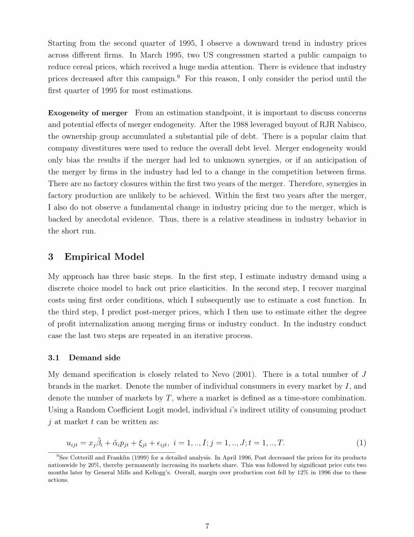
Starting from the second quarter of 1995, I observe a downward trend in industry prices

across different firms. In March 1995, two US congressmen started a public campaign to

reduce cereal prices, which received a huge media attention. There is evidence that industry

prices decreased after this campaign.9 For this reason, I only consider the period until the

first quarter of 1995 for most estimations.

Exogeneity of merger From an estimation standpoint, it is important to discuss concerns

and potential effects of merger endogeneity. After the 1988 leveraged buyout of RJR Nabisco,

the ownership group accumulated a substantial pile of debt. There is a popular claim that

company divestitures were used to reduce the overall debt level. Merger endogeneity would

only bias the results if the merger had led to unknown synergies, or if an anticipation of

the merger by firms in the industry had led to a change in the competition between firms.

There are no factory closures within the first two years of the merger. Therefore, synergies in

factory production are unlikely to be achieved. Within the first two years after the merger,

I also do not observe a fundamental change in industry pricing due to the merger, which is

backed by anecdotal evidence. Thus, there is a relative steadiness in industry behavior in

the short run.

3 Empirical Model

My approach has three basic steps. In the first step, I estimate industry demand using a

discrete choice model to back out price elasticities. In the second step, I recover marginal

costs using first order conditions, which I subsequently use to estimate a cost function. In

the third step, I predict post-merger prices, which I then use to estimate either the degree

of profit internalization among merging firms or industry conduct. In the industry conduct

case the last two steps are repeated in an iterative process.

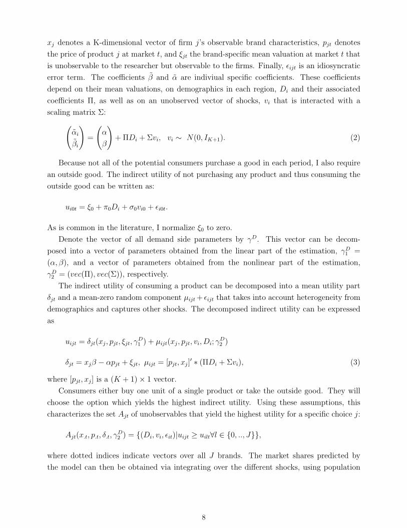
3.1 Demand side

My demand specification is closely related to Nevo (2001). There is a total number of J

brands in the market. Denote the number of individual consumers in every market by I, and

denote the number of markets by T , where a market is defined as a time-store combination.

Using a Random Coefficient Logit model, individual i’s indirect utility of consuming product

j at market t can be written as:

uijt = xjβi + αipjt + ξjt + εijt, i = 1, .., I; j = 1, .., J ; t = 1, .., T. (1)

9See Cotterill and Franklin (1999) for a detailed analysis. In April 1996, Post decreased the prices for its productsnationwide by 20%, thereby permanently increasing its markets share. This was followed by significant price cuts twomonths later by General Mills and Kellogg’s. Overall, margin over production cost fell by 12% in 1996 due to theseactions.

7

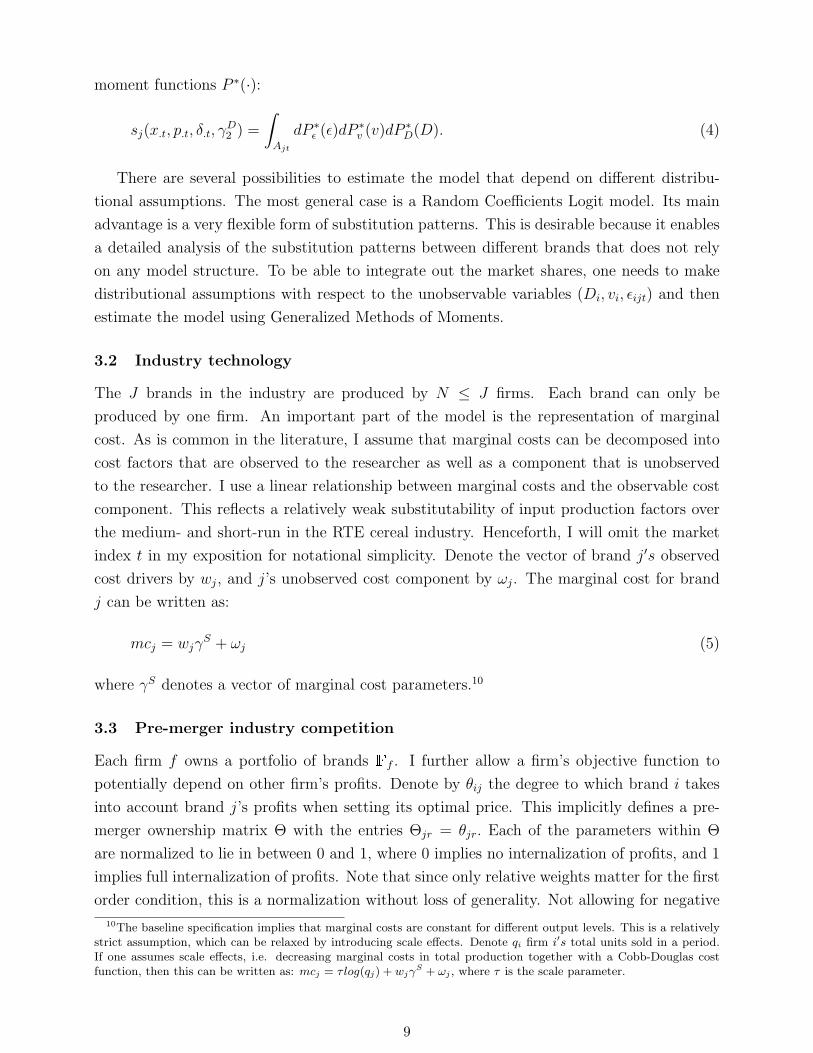
xj denotes a K-dimensional vector of firm j’s observable brand characteristics, pjt denotes

the price of product j at market t, and ξjt the brand-specific mean valuation at market t that

is unobservable to the researcher but observable to the firms. Finally, εijt is an idiosyncratic

error term. The coefficients β and α are indiviual specific coefficients. These coefficients

depend on their mean valuations, on demographics in each region, Di and their associated

coefficients Π, as well as on an unobserved vector of shocks, vi that is interacted with a

scaling matrix Σ:(αi

βi

)=

(α

β

)+ ΠDi + Σvi, vi ∼ N(0, IK+1). (2)

Because not all of the potential consumers purchase a good in each period, I also require

an outside good. The indirect utility of not purchasing any product and thus consuming the

outside good can be written as:

ui0t = ξ0 + π0Di + σ0vi0 + εi0t.

As is common in the literature, I normalize ξ0 to zero.

Denote the vector of all demand side parameters by γD. This vector can be decom-

posed into a vector of parameters obtained from the linear part of the estimation, γD1 =

(α, β), and a vector of parameters obtained from the nonlinear part of the estimation,

γD2 = (vec(Π), vec(Σ)), respectively.

The indirect utility of consuming a product can be decomposed into a mean utility part

δjt and a mean-zero random component µijt + εijt that takes into account heterogeneity from

demographics and captures other shocks. The decomposed indirect utility can be expressed

as

uijt = δjt(xj, pjt, ξjt, γD1 ) + µijt(xj, pjt, vi, Di; γ

D2 )

δjt = xjβ − αpjt + ξjt, µijt = [pjt, xj]′ ∗ (ΠDi + Σvi), (3)

where [pjt, xj] is a (K + 1)× 1 vector.

Consumers either buy one unit of a single product or take the outside good. They will

choose the option which yields the highest indirect utility. Using these assumptions, this

characterizes the set Ajt of unobservables that yield the highest utility for a specific choice j:

Ajt(x.t, p.t, δ.t, γD2 ) = (Di, vi, εit)|uijt ≥ uilt∀l ∈ 0, .., J,

where dotted indices indicate vectors over all J brands. The market shares predicted by

the model can then be obtained via integrating over the different shocks, using population

8

moment functions P ∗(·):

sj(x.t, p.t, δ.t, γD2 ) =

∫Ajt

dP ∗ε (ε)dP ∗v (v)dP ∗D(D). (4)

There are several possibilities to estimate the model that depend on different distribu-

tional assumptions. The most general case is a Random Coefficients Logit model. Its main

advantage is a very flexible form of substitution patterns. This is desirable because it enables

a detailed analysis of the substitution patterns between different brands that does not rely

on any model structure. To be able to integrate out the market shares, one needs to make

distributional assumptions with respect to the unobservable variables (Di, vi, εijt) and then

estimate the model using Generalized Methods of Moments.

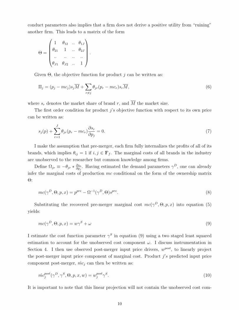
3.2 Industry technology

The J brands in the industry are produced by N ≤ J firms. Each brand can only be

produced by one firm. An important part of the model is the representation of marginal

cost. As is common in the literature, I assume that marginal costs can be decomposed into

cost factors that are observed to the researcher as well as a component that is unobserved

to the researcher. I use a linear relationship between marginal costs and the observable cost

component. This reflects a relatively weak substitutability of input production factors over

the medium- and short-run in the RTE cereal industry. Henceforth, I will omit the market

index t in my exposition for notational simplicity. Denote the vector of brand j′s observed

cost drivers by wj, and j’s unobserved cost component by ωj. The marginal cost for brand

j can be written as:

mcj = wjγS + ωj (5)

where γS denotes a vector of marginal cost parameters.10

3.3 Pre-merger industry competition

Each firm f owns a portfolio of brands Ff . I further allow a firm’s objective function to

potentially depend on other firm’s profits. Denote by θij the degree to which brand i takes

into account brand j’s profits when setting its optimal price. This implicitly defines a pre-

merger ownership matrix Θ with the entries Θjr = θjr. Each of the parameters within Θ

are normalized to lie in between 0 and 1, where 0 implies no internalization of profits, and 1

implies full internalization of profits. Note that since only relative weights matter for the first

order condition, this is a normalization without loss of generality. Not allowing for negative

10The baseline specification implies that marginal costs are constant for different output levels. This is a relativelystrict assumption, which can be relaxed by introducing scale effects. Denote qi firm i′s total units sold in a period.If one assumes scale effects, i.e. decreasing marginal costs in total production together with a Cobb-Douglas costfunction, then this can be written as: mcj = τ log(qj) + wjγ

S + ωj , where τ is the scale parameter.

9

conduct parameters also implies that a firm does not derive a positive utility from “ruining”

another firm. This leads to a matrix of the form

Θ =

1 θ12 .. θ1J

θ21 1 .. θ2J

.. .. .. ..

θJ1 θJ2 .. 1

.

Given Θ, the objective function for product j can be written as:

Πj = (pj −mcj)sjM +∑r 6=j

θjr(pr −mcr)srM, (6)

where sr denotes the market share of brand r, and M the market size.

The first order condition for product j’s objective function with respect to its own price

can be written as:

sj(p) +J∑r=1

θjr(pr −mcr)∂sr∂pj

= 0. (7)

I make the assumption that pre-merger, each firm fully internalizes the profits of all of its

brands, which implies θij = 1 if i, j ∈ Ff . The marginal costs of all brands in the industry

are unobserved to the researcher but common knowledge among firms.

Define Ωjr ≡ −θjr ∗ ∂sr

∂pj. Having estimated the demand parameters γD, one can already

infer the marginal costs of production mc conditional on the form of the ownership matrix

Θ:

mc(γD,Θ, p, x) = ppre − Ω−1(γD,Θ)spre. (8)

Substituting the recovered pre-merger marginal cost mc(γD,Θ, p, x) into equation (5)

yields:

mc(γD,Θ, p, x) = wγS + ω (9)

I estimate the cost function parameter γS in equation (9) using a two staged least squared

estimation to account for the unobserved cost component ω. I discuss instrumentation in

Section 4. I then use observed post-merger input price drivers, wpost, to linearly project

the post-merger input price component of marginal cost. Product j′s predicted input price

component post-merger, mcj can then be written as:

mcpostj (γD, γS,Θ, p, x, w) = wpostj γS. (10)

It is important to note that this linear projection will not contain the unobserved cost com-

10

ponent ωj. Henceforth, for notational simplicity I will drop the observable factors w, x, and

p when referring to marginal costs.

The key differences between estimating the degree of profit internalization of merging

firms and estimating industry conduct between firms lies in the treatment of the pre-merger

ownership matrix Θ and on the assumptions with respect to the merging firms’ post-merger

profit internalizations.

3.4 Post-merger prices when estimating the degree of profit internalization be-

tween merging firms

When estimating the degree of profit internalization post-merger, I assume that the form

of pre-merger industry competition, Θ, is known to the researcher. I assume that a merger

will involve a change in the pricing strategies of the merged entity. Denote by θ the degree

of joint profit maximization between the merging firms, which I assume to be unobserved

to the researcher, but common knowledge among firms in the industry. I assume that non-

merging firms will not change their competitive behavior after a merger, but will adapt to

the change in the merging firms’ pricing. Under these assumptions, given the degree of joint

profit maximization θ, the model’s post-merger prices given the parameters γD and γS can

be written as11:

ppost(γD, γS,Θ, θ) = mcpost(γD, γS,Θ) + Ω−1(γD,Θ, θ)spost + ωpostθ

. (11)

Here, ωpostθ

reflects the unobserved cost component in the cost function post-merger. Thus,

the unobserved error will not be accounted for in the linear projection of the post-merger

marginal cost in equation (10), but remains a separate term in the post merger equation.

3.5 Post-merger prices when estimating industry conduct

When estimating industry conduct, I assume that neither the form of pre-merger conduct, Θ,

nor post-merger industry conduct are known to the researcher. A key identifying assumption

is that even though the researcher does not know the underlying form of conduct, he knows

exactly how the merger will affect industry conduct. There are two channels for this, namely

post-merger profit internalization of merging firms, and how competitors consider the merged

entity post-merger. I assume that merging firms will fully internalize their profits after

a merger. Non-merging firms compete with each other in the same fashion. The change

between merging and non-merging firms after the merger is also known to the researcher,

which is summed up in the following assumption.

Assumption 1 (Conduct between merging and non-merging firms). Let f, g be two distinct

merging firms, and h a non-merging firm. Let θpreik and θpostik denote the pre- and post-merger

11Even if the degree of joint profit maximization, θ, is part of a post-merger industry conduct matrix, I will explicitlystate it in the model. This is to clearly distinguish the case of estimating the joint profit-maximization parametersfrom the case when estimating the industry conduct matrix Θ.

11

conduct parameters between firm i and k, respectively. Then, ∀i ∈ Ff , ∀j ∈ Fg, ∀k ∈ Fh, one

of the following three cases holds regarding the conduct between a merging and a non-merging

firm:

a. θpostik = θpreik ; θpostjk = θprejk (no change in conduct);

b. θpostik = θpreik ; θpostjk = θpreik (acquiring firm standard).

c. θpostik = θprejk ; θpostjk = θprejk (target firm standard);

Under Assumption 1a, the merger does not change how competitors consider the two

merging firms after the merger. In this case, the merging firms will fully internalize the

profits after the merger. Under Assumption 1b, the fully merged entity is considered and

behaves as the acquirer did pre-merger. Assumption 1c implies the reverse, i.e. that the

merged entity behaves as the target. I do not have to pre-specify the values of the conduct

parameters, but just the way in which the parameters change. Other change patterns can also

be accounted for, as long as the change in conduct between merging and non-merging firms is

known post-merger. Let the underlying form of pre-merger conduct, Θ, be element of the set

B. The post-merger conduct can then be expressed via a transition function b : B → B which

maps the pre-merger conduct matrix Θ into the post-merger conduct matrix Θpost = b(Θ).

This is because all merger-induced ownership transformations are known to the researcher.

Under these assumptions, for a specific form of pre-merger industry conduct Θ and transition

function b, the predicted post-merger prices given the estimated parameters γD and γS can

be written as:

ppost(γD, γS,Θ,Ωpost, b(Θ)) = mc(γD, γS,Θ) + Ω−1(γD, b(Θ))spost + ωpostΘ . (12)

As for the case of estimating the degree of post-merger profit internalization, the unobserved

cost component ωpostΘ is not accounted for in the marginal cost term mc, but is rather a distinct

component in the pricing equation. Appendix A illustrates different cases of pre- and post

merger industry conduct. It is worth mentioning the key difference to conjectural variation

models. I treat the conduct parameters Θ as part of the firms’ underlying objective functions

rather than as behavioral responses with respect to the competitors’ price setting behaviors.

I then form moment conditions to recover the underlying “level” conduct parameters using

a Generalized Method of Moments estimator.

4 Identification

In this section, I will present identification results for the different stages of the model, and

in particular the two supply side estimation approaches. Section 1 discusses identification

restrictions for the demand and cost function estimation. Section 4.2 discusses the identifi-

cation restrictions when estimating merging firms’ profit internalization parameters. Section

4.3 focuses on identification restrictions when estimating industry conduct.

12

My estimation method requires identification of three sets of parameters: demand-side

parameters, γD, cost parameters γS, and the supply side parameters, which amount either to

the degree of profit internalization θ, or to the industry conduct Θ. The correlation between

price and both unobserved brand and cost characteristics requires instrumentation for each

brand in the demand and pricing equations, respectively.

4.1 Model identification of demand and cost parameters

4.1.1 Identification of demand parameters

Denote by ξ(γD, x, p) the structural error term vector that consists of the market-specific

unobservable brand valuations for all brands. Regarding the demand side, I assume that

when being assessed at the true demand parameter values γD0 , this error term is uncorrelated

with respect to a Mξ-dimensional set of exogenous demand side instruments, Zξ. This leads

to the identification restriction:

E[Z ′ξξ(γD0 , x, p)] = 0. (13)

Note that I implicitly assume that the demand can be estimated independently of the

marginal cost and supply side parameters, respectively. The orthogonality conditions would

be violated if industry conduct or a change in production costs, not prices, would influence

consumer choice through the unobserved brand-specific component.12 I assume that the ob-

servable product characteristics of the different goods are exogenous, and therefore do not

respond to changes in industry pricing. Also accounting for potential brand replacement

or additional brand introductions would make traction of the full model nearly impossible.

Because of the inherent endogeneity between price and unobserved brand characteristics, I

need to find adequate instruments for the demand estimation. I use two different sets of

instruments to do so.

My first set of instruments relies on production cost shifters. The economic assumption

is that input cost variation should be correlated with variation in prices, but not with con-

sumers’ preferences for unobservable product characteristics. I use both cost factors that

affect all products in similar fashion, such as labor costs, packaging, and transportation,

as well as factors that differ among products, such as interactions between product charac-

teristics and input prices for wheat, sugar, and corn. My second set of instruments is the

ownership change itself. As argued above, a merger should cause a change in industry prices.

Similar to a cost shift, one can assume that the merger affects prices, but not the demand

characteristics. This assumption would be violated if the merger caused a change in brand

value which would affect the ξ’s of the merging firms. Because the actual brand names of

the cereals involved did not change after the merger, such an effect seems unlikely.

12This assumption would be violated if the merger caused a change in the perceived “brand values” of the mergedentities, which would affect the ξ components in the demand equation.

13

4.1.2 Identification of cost parameters

Conditional on a specific form of pre-merger industry conduct Θ, I can back out the marginal

cost via a first order condition and then regress them on observable product characteristics

combined with input prices.13 This allows me to predict the input cost component mc of the

post merger marginal costs using post-merger input price data and the estimated parameters.

I make the implicit assumption that firms cannot substitute between different input goods.

The recipes and production processes for a specific product in the ready-to-eat cereal industry

remain constant over time, such that this assumption is likely to hold in the medium and

short term. My identifying assumption concerning the marginal cost component pre-merger

is that the structural error term vector representing unobserved cost characteristics ωpre is

uncorrelated to a Mω-dimensional set of exogenous instruments Zωpre :

E[Z ′ωpreωprej (γD, γS0 ,Θ)] = 0, (14)

where γS0 reflects the true parameter value for γS. Together with the change in ownership,

the marginal cost estimates will influence the predicted post-merger prices in the market.

Berry, Levinsohn, and Pakes (1995) argue that the computation of the optimal set of

instruments when only conditional moment conditions are available is very difficult and

numerically complex. As a less computationally demanding approximation, they use poly-

nomials resulting from first order basis functions of the product characteristics. The validity

of these basis functions as instruments relies on exchangeability assumptions of firms’ own

characteristics with respect to permutations in the order of competitors’ product characteris-

tics. Because I allow for the possibilty of collusion among firms, this changes the structure of

potential Nash equilibria. The brand specific unobservable marginal cost component ω may

be correlated with unobservable product characteristics. Therefore it is essential to look for

instruments that are correlated with marginal costs, but not with the structural cost error.

To account for the effects of unobserved cost drivers on prices, I use first order basis functions

of the own brand characteristics, own firm characteristics, and competitors’ characteristics.

4.2 Model identification of post-merger profit internalization parameter

Setting equation (11) equal to the observed post-merger prices ppost, and solving for the

unobserved post-merger cost-component vector ωpostθ

(γD, γS,Θ, θ), yields:

ωpostθ

(γD, γS,Θ, θ) = ppost − mcpost(γD, γS,Θ)− Ω−1(γD,Θ, θ)spost. (15)

As an identification restriction for the degree of joint profit maximization, I use orthogonality

conditions between the residual of observed and predicted post-merger prices, which results

in the structural error ωpostθ,j

(γD, γS,Θ, θ) for a product j, and a Mθ-dimensional matrix of

13Explicitly using input prices to estimate a cost function is a difference to previous studies in the ready-to-eatcereal industry.

14

instruments Zθ.

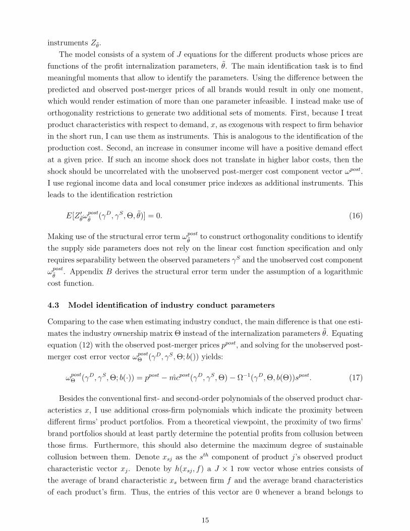
The model consists of a system of J equations for the different products whose prices are

functions of the profit internalization parameters, θ. The main identification task is to find

meaningful moments that allow to identify the parameters. Using the difference between the

predicted and observed post-merger prices of all brands would result in only one moment,

which would render estimation of more than one parameter infeasible. I instead make use of

orthogonality restrictions to generate two additional sets of moments. First, because I treat

product characteristics with respect to demand, x, as exogenous with respect to firm behavior

in the short run, I can use them as instruments. This is analogous to the identification of the

production cost. Second, an increase in consumer income will have a positive demand effect

at a given price. If such an income shock does not translate in higher labor costs, then the

shock should be uncorrelated with the unobserved post-merger cost component vector ωpost.

I use regional income data and local consumer price indexes as additional instruments. This

leads to the identification restriction

E[Z ′θωpostθ

(γD, γS,Θ, θ)] = 0. (16)

Making use of the structural error term ωpostθ

to construct orthogonality conditions to identify

the supply side parameters does not rely on the linear cost function specification and only

requires separability between the observed parameters γS and the unobserved cost component

ωpostθ

. Appendix B derives the structural error term under the assumption of a logarithmic

cost function.

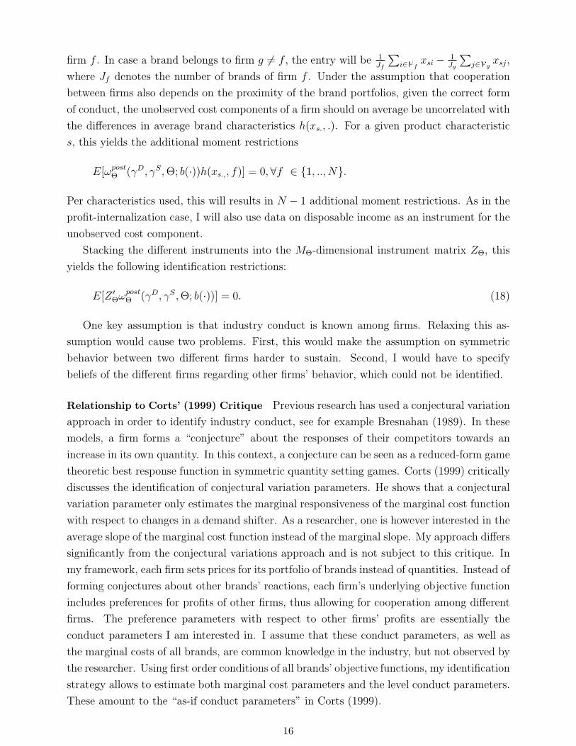
4.3 Model identification of industry conduct parameters

Comparing to the case when estimating industry conduct, the main difference is that one esti-

mates the industry ownership matrix Θ instead of the internalization parameters θ. Equating

equation (12) with the observed post-merger prices ppost, and solving for the unobserved post-

merger cost error vector ωpostΘ (γD, γS,Θ; b()) yields:

ωpostΘ (γD, γS,Θ; b(·)) = ppost − mcpost(γD, γS,Θ)− Ω−1(γD,Θ, b(Θ))spost. (17)

Besides the conventional first- and second-order polynomials of the observed product char-

acteristics x, I use additional cross-firm polynomials which indicate the proximity between

different firms’ product portfolios. From a theoretical viewpoint, the proximity of two firms’

brand portfolios should at least partly determine the potential profits from collusion between

those firms. Furthermore, this should also determine the maximum degree of sustainable

collusion between them. Denote xsj as the sth component of product j’s observed product

characteristic vector xj. Denote by h(xsj, f) a J × 1 row vector whose entries consists of

the average of brand characteristic xs between firm f and the average brand characteristics

of each product’s firm. Thus, the entries of this vector are 0 whenever a brand belongs to

15

firm f . In case a brand belongs to firm g 6= f , the entry will be 1Jf

∑i∈Ff

xsi − 1Jg

∑j∈Fg

xsj,

where Jf denotes the number of brands of firm f . Under the assumption that cooperation

between firms also depends on the proximity of the brand portfolios, given the correct form

of conduct, the unobserved cost components of a firm should on average be uncorrelated with

the differences in average brand characteristics h(xs., .). For a given product characteristic

s, this yields the additional moment restrictions

E[ωpostΘ (γD, γS,Θ; b(·))h(xs.,, f)] = 0,∀f ∈ 1, .., N.

Per characteristics used, this will results in N − 1 additional moment restrictions. As in the

profit-internalization case, I will also use data on disposable income as an instrument for the

unobserved cost component.

Stacking the different instruments into the MΘ-dimensional instrument matrix ZΘ, this

yields the following identification restrictions:

E[Z ′ΘωpostΘ (γD, γS,Θ; b(·))] = 0. (18)

One key assumption is that industry conduct is known among firms. Relaxing this as-

sumption would cause two problems. First, this would make the assumption on symmetric

behavior between two different firms harder to sustain. Second, I would have to specify

beliefs of the different firms regarding other firms’ behavior, which could not be identified.

Relationship to Corts’ (1999) Critique Previous research has used a conjectural variation

approach in order to identify industry conduct, see for example Bresnahan (1989). In these

models, a firm forms a “conjecture” about the responses of their competitors towards an

increase in its own quantity. In this context, a conjecture can be seen as a reduced-form game

theoretic best response function in symmetric quantity setting games. Corts (1999) critically

discusses the identification of conjectural variation parameters. He shows that a conjectural

variation parameter only estimates the marginal responsiveness of the marginal cost function

with respect to changes in a demand shifter. As a researcher, one is however interested in the

average slope of the marginal cost function instead of the marginal slope. My approach differs

significantly from the conjectural variations approach and is not subject to this critique. In

my framework, each firm sets prices for its portfolio of brands instead of quantities. Instead of

forming conjectures about other brands’ reactions, each firm’s underlying objective function

includes preferences for profits of other firms, thus allowing for cooperation among different

firms. The preference parameters with respect to other firms’ profits are essentially the

conduct parameters I am interested in. I assume that these conduct parameters, as well as

the marginal costs of all brands, are common knowledge in the industry, but not observed by

the researcher. Using first order conditions of all brands’ objective functions, my identification

strategy allows to estimate both marginal cost parameters and the level conduct parameters.

These amount to the “as-if conduct parameters” in Corts (1999).

16

Corts’ also criticizes the static game character of conventional conduct estimation models.

My approach is not fully exempt from this critique. I partially account for industry dynamics

by modeling the merger-induced industry change. Nonetheless, my static approach may not

detect certain dynamic collusion patterns. One big advantage of a static approach is a higher

degree of tractability. Modeling repeated games makes identification of conduct even more

difficult due to a larger set of potential dynamic equilibrium strategies. With my approach,

I am also able to identify patterns of full collusion as well as patterns of collusion between

only a subset of firms.

4.3.1 Rank conditions for industry conduct

This section provides identification results for different specifications when estimating con-

tinuous conduct parameters “directly”. This is opposed to the menu approach, which selects

among different non-nested models without estimating conduct parameters.

Recall the assumptions made on firms’ own-profit maximization. As in standard unilateral

merger models, I also assume that a merger does not change the behavior between non-

merging firms. There are furthermore some global assumptions that reduce the parameter

space which I will discuss in detail.

I only consider cases in which a firm treats all brands of a specific competitor’s firm in

the same way. This excludes the possibility that single brands of different firms collude while

others play against each other competitively. From a pure rank condition perspective the

number of parameters I would have to estimate when accounting for brand-specific collusion

between firms would easily exceed the number brands in the market. This makes it impossible

to identify the parameters.

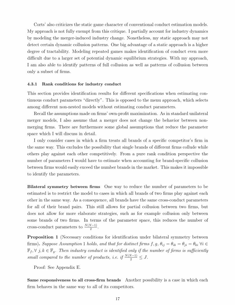
Bilateral symmetry between firms One way to reduce the number of parameters to be

estimated is to restrict the model to cases in which all brands of two firms play against each

other in the same way. As a consequence, all brands have the same cross-conduct parameters

for all of their brand pairs. This still allows for partial collusion between two firms, but

does not allow for more elaborate strategies, such as for example collusion only between

some brands of two firms. In terms of the parameter space, this reduces the number of

cross-conduct parameters to N(N−1)2

.

Proposition 1 (Necessary conditions for identification under bilateral symmetry between

firms). Suppose Assumption 1 holds, and that for distinct firms f, g, θij = θik = θji = θki ∀i ∈Ff ,∀ j, k ∈ Fg. Then industry conduct is identified only if the number of firms is sufficiently

small compared to the number of products, i.e. if N(N−1)2≤ J .

Proof: See Appendix E.

Same responsiveness to all cross-firm brands Another possibility is a case in which each

firm behaves in the same way to all of its competitors.

17

The advantage of this specification is that it reduces the number of parameters to only

N different cross-conduct parameters. However, there are also several problems associated

with the assumption. First, it is again no longer possible to detect partial collusion between

a subset of firms in the industry. Second, there is a consistency problem with respect to

a mutual responsiveness: Under this assumption, it can be possible that firm 1 is acting

collusively with firm 2, and firm 2 on the other hand acts competitively towards firm 1,

something which is hard to justify from an economic perspective.

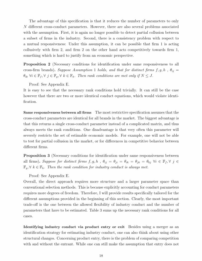
Proposition 2 (Necessary conditions for identification under same responsiveness to all

cross-firm brands). Suppose Assumption 1 holds, and that for distinct firms f, g, h , θij =

θik ∀i ∈ Ff ,∀ j ∈ Fg,∀ k ∈ Fh. Then rank conditions are met only if N ≤ J .

Proof: See Appendix E.

It is easy to see that the necessary rank conditions hold trivially. It can still be the case

however that there are two or more identical conduct equations, which would violate identi-

fication.

Same responsiveness between all firms The most restrictive specification assumes that the

cross-conduct parameters are identical for all brands in the market. The biggest advantage is

that this returns a single cross-conduct parameter instead of a complicated matrix, and thus

always meets the rank conditions. One disadvantage is that very often this parameter will

severely restricts the set of estimable economic models. For example, one will not be able

to test for partial collusion in the market, or for differences in competitive behavior between

different firms.

Proposition 3 (Necessary conditions for identification under same responsiveness between

all firms). Suppose for distinct firms f, g, h , θij = θji = θik = θjk = θkj ∀i ∈ Ff , ∀ j ∈Fg,∀ k ∈ Fh. Then the rank condition for industry conduct is always met.

Proof: See Appendix E.

Overall, the direct approach requires more structure and a larger parameter space than

conventional selection methods. This is because explicitly accounting for conduct parameters

requires more degrees of freedom. Therefore, I will provide results specifically tailored for the

different assumptions provided in the beginning of this section. Clearly, the most important

trade-off is the one between the allowed flexibility of industry conduct and the number of

parameters that have to be estimated. Table 3 sums up the necessary rank conditions for all

cases.

Identifying industry conduct via product entry or exit Besides using a merger as an

identification strategy for estimating industry conduct, one can also think about using other

structural changes. Concerning product entry, there is the problem of comparing competition

with and without the entrant. While one can still make the assumption that entry does not

18

change how existing brands compete with each other, one has to define how a new product

will interact with the existing products.

Unlike product entry, using product exit as an identification strategy is still feasible.

However, one has to ask why a product will exit. One reason can be that it is just not

profitable, which will then probably imply that its impact on the market is relatively low.

Therefore, a reduction of the brand space would not result in a big shift for firms strategies.

Another possibility would be that a brand is profitable on its own, but it would be more

profitable for a multi-brand firm to exit the product out of the market. This would result in

an endogeneity problem when estimating conduct using product exit.

5 Estimation

5.1 Demand estimation

I use the technique of Nevo (2001) to recover the structural demand side parameters γD and

the unobservable error term ξ(γD, x, p). Using Nevo’s estimation strategy on the demand

side allows me to estimate all the demand side parameters independently of the supply side.

I solve for the mean utility level across all brands at market t, δ.t, as to match the empirical

market shares sjt(x.t, p.t, ξ.t, γD) from equation (13) with the actual market shares sjt observed

in the data. Following equation (13) the objective is to find:

γD = arg minγD

ξ(γD, x, p)′ZξA−1ξ Z ′ξξ(γ

D, x, p); (19)

where A−1ξ is an estimate of the asymptotically efficient covariance

E[Z ′ξξ(γD, x, p)ξ(γD, x, p)′Zξ], given demand parameters γD obtained from the first-stage

GMM estimation.

Defining the market size is an important assumption, for it has implications on the dif-

ferent market shares and also on the differences between markets. I assume that the market

size is correlated with store specific characteristics. I compute the market size of a specific

store as a function of the average total sales of all supermarket products sold in this store.14

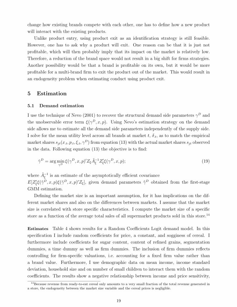
Estimates Table 4 shows results for a Random Coefficients Logit demand model. In this

specification I include random coefficients for price, a constant, and sogginess of cereal. I

furthermore include coefficients for sugar content, content of refined grains, segmentation

dummies, a time dummy as well as firm dummies. The inclusion of firm dummies reflects

controlling for firm-specific valuations, i.e. accounting for a fixed firm value rather than

a brand value. Furthermore, I use demographic data on mean income, income standard

deviation, household size and on number of small children to interact them with the random

coefficients. The results show a negative relationship between income and price sensitivity,

14Because revenue from ready-to-eat cereal only amounts to a very small fraction of the total revenue generated ina store, the endogeneity between the market size variable and the cereal prices is negligible.

19

which is consistent with higher markups in high income neighborhoods. Price sensitivity

also interacts negatively with the number of small children, which might account for their

responsiveness to advertising. However, both demographic interaction coefficients are not

statistically significant. Appendix C shows details about the estimation routine and other

computational issues.

As a robustness check, I also estimate different variants of a multinomial Logit model.

Table 5 shows demand side estimation results for several specifications of the multinomial

Logit model. I use input prices and prices of other zones together with the ownership change

as instruments for the sales price. When also including firm dummies yields a more elastic

demand curve than specification (6) without instruments, however, the price coefficients are

relatively close to each other. A bigger difference occurs between specifications that include

and do not include firm dummies. This can be seen by comparing specifications (1) and (2)

to (3) and (4). Overall, all of the price coefficients are lower in absolute magnitude than the

mean coefficient of a Random Coefficient Logit estimation. This suggest that the random

coefficient model is able to capture some of the consumer heterogeneity through interacting

demographic variables which increases the price coefficient in absolute terms.

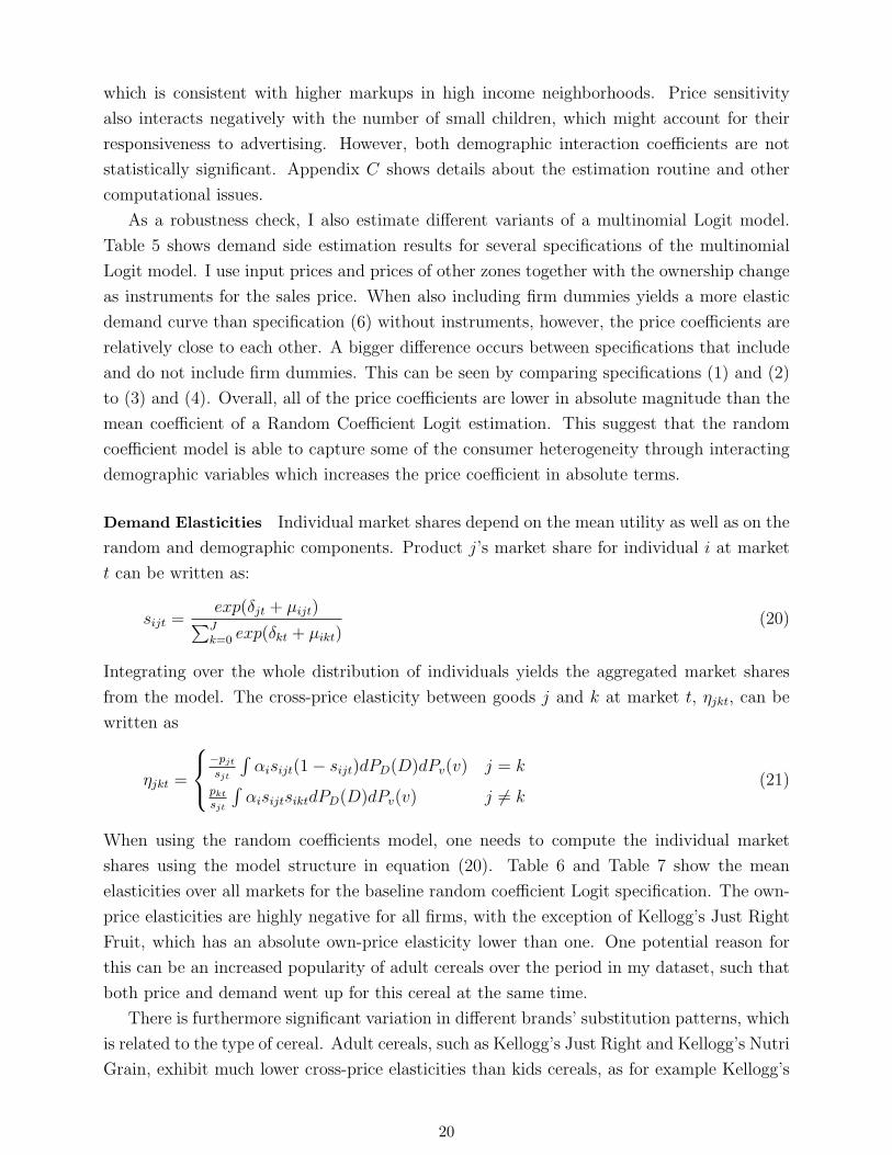
Demand Elasticities Individual market shares depend on the mean utility as well as on the

random and demographic components. Product j’s market share for individual i at market

t can be written as:

sijt =exp(δjt + µijt)∑Jk=0 exp(δkt + µikt)

(20)

Integrating over the whole distribution of individuals yields the aggregated market shares

from the model. The cross-price elasticity between goods j and k at market t, ηjkt, can be

written as

ηjkt =

−pjt

sjt

∫αisijt(1− sijt)dPD(D)dPv(v) j = k

pkt

sjt

∫αisijtsiktdPD(D)dPv(v) j 6= k

(21)

When using the random coefficients model, one needs to compute the individual market

shares using the model structure in equation (20). Table 6 and Table 7 show the mean

elasticities over all markets for the baseline random coefficient Logit specification. The own-

price elasticities are highly negative for all firms, with the exception of Kellogg’s Just Right

Fruit, which has an absolute own-price elasticity lower than one. One potential reason for

this can be an increased popularity of adult cereals over the period in my dataset, such that

both price and demand went up for this cereal at the same time.

There is furthermore significant variation in different brands’ substitution patterns, which

is related to the type of cereal. Adult cereals, such as Kellogg’s Just Right and Kellogg’s Nutri

Grain, exhibit much lower cross-price elasticities than kids cereals, as for example Kellogg’s

20

Fruit Loops or General Mills Honey Nut Cheerios with coefficients higher than .1. Overall,

the substitution patterns are relatively close to previous industry estimates, see for example

Nevo (2001).

5.2 Post-merger profit internalization

I first outline each step of the estimation algorithm when estimating the degree of joint profit

maximization.

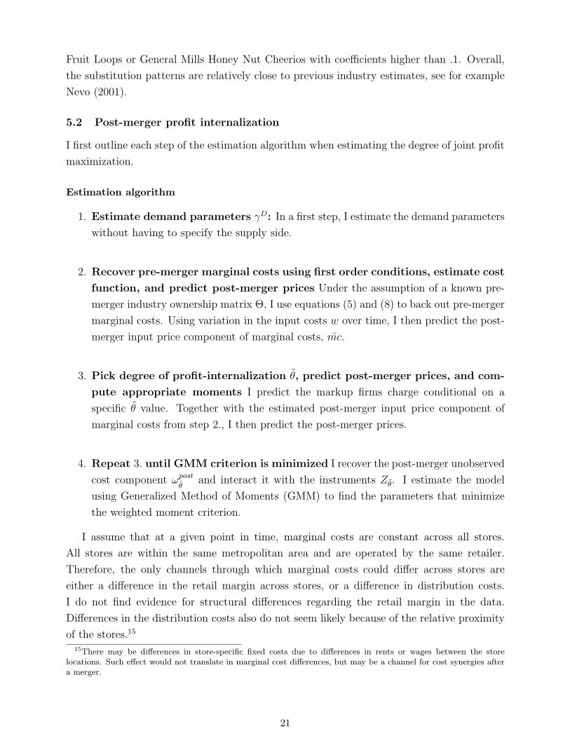
Estimation algorithm

1. Estimate demand parameters γD: In a first step, I estimate the demand parameters

without having to specify the supply side.

2. Recover pre-merger marginal costs using first order conditions, estimate cost

function, and predict post-merger prices Under the assumption of a known pre-

merger industry ownership matrix Θ, I use equations (5) and (8) to back out pre-merger

marginal costs. Using variation in the input costs w over time, I then predict the post-

merger input price component of marginal costs, mc.

3. Pick degree of profit-internalization θ, predict post-merger prices, and com-

pute appropriate moments I predict the markup firms charge conditional on a

specific θ value. Together with the estimated post-merger input price component of

marginal costs from step 2., I then predict the post-merger prices.

4. Repeat 3. until GMM criterion is minimized I recover the post-merger unobserved

cost component ωpostθ

and interact it with the instruments Zθ. I estimate the model

using Generalized Method of Moments (GMM) to find the parameters that minimize

the weighted moment criterion.

I assume that at a given point in time, marginal costs are constant across all stores.

All stores are within the same metropolitan area and are operated by the same retailer.

Therefore, the only channels through which marginal costs could differ across stores are

either a difference in the retail margin across stores, or a difference in distribution costs.

I do not find evidence for structural differences regarding the retail margin in the data.

Differences in the distribution costs also do not seem likely because of the relative proximity

of the stores.15

15There may be differences in store-specific fixed costs due to differences in rents or wages between the storelocations. Such effect would not translate in marginal cost differences, but may be a channel for cost synergies aftera merger.

21

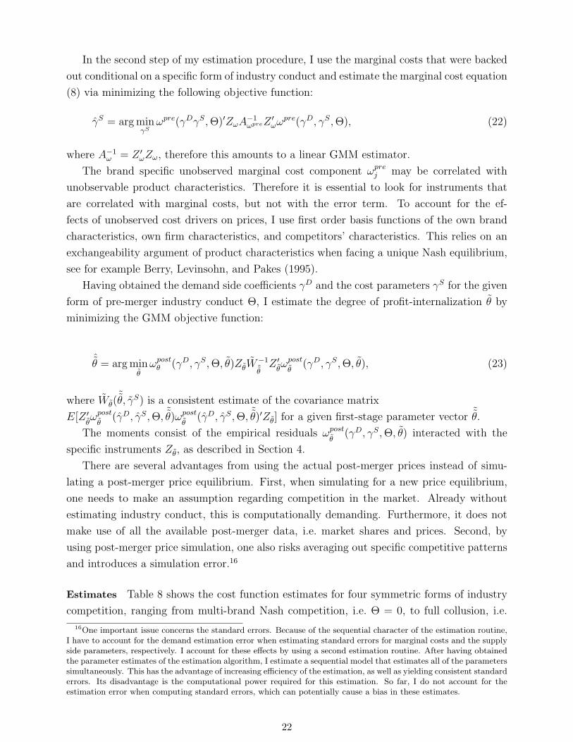
In the second step of my estimation procedure, I use the marginal costs that were backed

out conditional on a specific form of industry conduct and estimate the marginal cost equation

(8) via minimizing the following objective function:

γS = arg minγS

ωpre(γDγS,Θ)′ZωA−1ωpreZ ′ωω

pre(γD, γS,Θ), (22)

where A−1ω = Z ′ωZω, therefore this amounts to a linear GMM estimator.

The brand specific unobserved marginal cost component ωprej may be correlated with

unobservable product characteristics. Therefore it is essential to look for instruments that

are correlated with marginal costs, but not with the error term. To account for the ef-

fects of unobserved cost drivers on prices, I use first order basis functions of the own brand

characteristics, own firm characteristics, and competitors’ characteristics. This relies on an

exchangeability argument of product characteristics when facing a unique Nash equilibrium,

see for example Berry, Levinsohn, and Pakes (1995).

Having obtained the demand side coefficients γD and the cost parameters γS for the given

form of pre-merger industry conduct Θ, I estimate the degree of profit-internalization θ by

minimizing the GMM objective function:

ˆθ = arg minθωpostθ (γD, γS,Θ, θ)ZθW

−1˜θZ ′θωpostθ

(γD, γS,Θ, θ), (23)

where Wθ(˜θ, γS) is a consistent estimate of the covariance matrix

E[Z ′θωpostθ

(γD, γS,Θ, ˜θ)ωpostθ

(γD, γS,Θ, ˜θ)′Zθ] for a given first-stage parameter vector ˜θ.

The moments consist of the empirical residuals ωpostθ

(γD, γS,Θ, θ) interacted with the

specific instruments Zθ, as described in Section 4.

There are several advantages from using the actual post-merger prices instead of simu-

lating a post-merger price equilibrium. First, when simulating for a new price equilibrium,

one needs to make an assumption regarding competition in the market. Already without

estimating industry conduct, this is computationally demanding. Furthermore, it does not

make use of all the available post-merger data, i.e. market shares and prices. Second, by

using post-merger price simulation, one also risks averaging out specific competitive patterns

and introduces a simulation error.16

Estimates Table 8 shows the cost function estimates for four symmetric forms of industry

competition, ranging from multi-brand Nash competition, i.e. Θ = 0, to full collusion, i.e.

16One important issue concerns the standard errors. Because of the sequential character of the estimation routine,I have to account for the demand estimation error when estimating standard errors for marginal costs and the supplyside parameters, respectively. I account for these effects by using a second estimation routine. After having obtainedthe parameter estimates of the estimation algorithm, I estimate a sequential model that estimates all of the parameterssimultaneously. This has the advantage of increasing efficiency of the estimation, as well as yielding consistent standarderrors. Its disadvantage is the computational power required for this estimation. So far, I do not account for theestimation error when computing standard errors, which can potentially cause a bias in these estimates.

22

Θ = 1. The median marginal costs implied by the model lie between $.114 per serving for

multi-product Nash pricing and $.072 for full collusion, implying median markups between

40.8 and 63.1 percent. The cost function estimations show that especially the influence of

wheat on overall marginal costs is decreasing in the degree of industry competition, Θ. Figure

6 shows the development of profit internalization parameters over time for four different forms

of industry competition, ranging from multi-brand Nash competition to partial collusion,

i.e. Θ = .5, between all firms pre-merger. The results indicate an increasing degree of

profit internalization over the first six quarters for all three industry specifications. The

parameter values are the highest for the Nash specification and are decreasing in the degree

of industry cooperation. In the last two quarters of 1994, there is a sharp drop in the

profit internalization, which is followed by a sharp increase over the last year. However,

the parameter estimates are not statistically significant under this specification. Figure 7

accounts for heterogeneity across the merging’ entities with respect to the degree of profit

internalization for multi-product Nash pricing, i.e. Θ = 0. One can see that Post’s profit

internalization drops in the last two quarters of 1994 and subsequently increases. Overall,

except for the drop in joint profit internalization in 1994, the results for the whole post-merger

entity are consistent with a weak increase in profit internalization over time.

5.3 Industry conduct estimation

When estimating industry conduct, I have to iterate the processes of recovering pre-merger

marginal costs, predicting post-merger marginal cost using a cost function estimation, and

computing the industry conduct moments. This is because my object of interest, i.e. the pre-

merger conduct matrix Θ, influences the implied marginal cost in the industry. Overall, the

above steps can be decomposed into two parts. I use a nested two-step routine on the supply

side. In the first step, I back out marginal cost conditional on a specific form of conduct

as the outer loop. In the second step, I recover the supply side parameters by regressing

the backed out marginal costs on the observable cost characteristics while controlling for

unobserved brand characteristics. First, I will outline the conduct estimation routine.

1. Estimate demand parameters Using the instruments discussed above, I estimate

the demand parameters, without having to specify supply-side competition.

2. Pick Θ given the identification restrictions

3. Infer marginal costs and predict post-merger prices for given choice of Θ, and

compute appropriate moments Having estimated the demand side parameters, I can

infer the marginal costs of production conditional on the form of conduct Θ using proper

instruments. Using post-merger input cost data and the estimated cost-parameters, I

can predict post-merger marginal costs. Given the conduct matrix Θ and the estimated

demand parameters γD, I can then predict post-merger prices given Θ.

23

4. Repeat steps 2-3 until GMM criterion is minimized I recover the post-merger

unobserved cost component ωpostΘ and interact it with the instruments ZΘ. I estimate the

model using Generalized Method of Moments (GMM) to find the conduct parameters

that minimize the weighted moment criterion.

In the second step of my estimation procedure, I use the marginal costs that were backed

out conditional on a specific form of industry conduct and estimate the cost function from

equation (8) via minimizing the following GMM objective function:

γS = arg minγS

ωpre(γD, γS,Θ)′ZωA−1ωpreZ ′ωω

pre(γD, γS,Θ). (24)

A−1ω is a consistent estimate of the covariance E[Z ′ωω

pre(γD, γS,Θ)ωpre(γD, γS,Θ)′Zω] for a

given first-stage parameter vector γS.

Having obtained the demand side coefficients γD and the cost parameters γS for any form

of industry conduct, I estimate the conduct parameters Θ by minimizing the GMM objective

function. The moments consist of the empirical residuals ωpostΘ (γD, γS,Θ; b(·)) interacted with

the specific instruments ZΘ, as described in section 3.

Then the GMM objective in can be written as:

Θ = arg minΘωpostΘ (γD, γS,Θ; b(·))Z ′ΘW−1

Θ Z ′ΘωpostΘ (γD, γS,Θ; b(·)), (25)

where W (Θ, γS) is a consistent estimate of the covariance

E[Z ′ΘωpostΘ (γD, γS, Θ; b(·))ωpostΘ (γD, γS, Θ; b(·))′ZΘ] for a given first stage conduct matrix Θ.

Here, γS denotes the cost estimates from the second step that are conditional on a specific

form of conduct.

Estimates Table 10 shows estimation results when estimating a single industry conduct

parameter. The obtained parameter value is 0.708. It is interesting to compare the implied

price cost-margins to those from a multi-product Nash pricing supply side model. Under

multi-product Nash pricing, all of the markup can be attributed to product differentiation,

and not to cooperative effects. When estimating a single conduct parameter, 25.6 percent of

the price-cost margin is attributable to cooperative behavior between firms.

Table 11 shows the results when imposing symmetry in a firm’s behavior towards all of its

rivals. One can see that the two biggest players, General Mills and Kellogg’s, act in the most

cooperative behavior, while smaller companies act more competitively. According to this

specification, General Mills acts fully cooperatively, with a parameter value of 0.98. Under

this specification, 17.4 percent of the markups are attributable to cooperative behavior.

To account for even more heterogeneity with respect to behavior across firms, Table

12 shows the conduct estimation results under the assumption of bilateral brand symmetry.

The parameter estimates show a lot of heterogeneity in the parameter values, however, under

this specification, none of the parameters are statistically significant. The implied median

24

price-cost margins from the estimation are 14.3 percent higher than the median multi-brand

Nash price cost margins. This is lower than under a single conduct parameter specification,

reflecting the heterogeneity across different firm pairs.

6 Extensions

In this section I present extensions to my basic framework that address several merger related

issues.

6.1 Supply side selection methods

The menu approach selects the best fit among a discrete set (“menu”) of supply side models,

for example multi-brand Bertrand-Nash competition or full collusion among all firms. This

approach does not include any explicit conduct parameters, but rather fully pre-imposes the

form of competition, which often relaxes identification problems. In practice, there are two

popular ways to select among different non-nested industry specifications. However, both

have significant weaknesses.

The first method compares the marginal cost estimates of the different supply side spec-

ifications with cost estimates from other sources, such as accounting data, see for example

Nevo (2001). At first sight this seems to be an intuitive way to select the most appropriate

specification from the data. This approach, however, has several disadvantages. First, out-

side cost estimates are not always available, or do not have a reliable economic interpretation.

Second, such data is often only available on a very aggregate level, which makes a detailed

industry introspective nearly impossible.17 Third, if different specifications yield similar cost

estimates, it is not clear how one can use these results for a reliable model selection.

The second method uses forms of non-nested selection test in combination with pre-merger

data to look for the supply specification that is closest to the true data generating process,

see for example Vuong (1989) or Rivers and Vuong (2002). In vertical relations frameworks,

such tests are relatively successful for selecting among different non-nested models, see for

example Bonnet and Dubois (2010) for a detailed exposition. When using only pre-merger

data in a horizontal framework, however, in practice there is the problem that such tests

have relatively low predictive power, due to only very limited variation between the different

pre-merger model specifications.

I exploit changes in ownership as well as variation in the input cost data to select among

different non-nested horizontal models.Using pre-and post merger data in combination with

non-nested supply side models provides a tractable in-sample test. Testing can be done

using a J-Test or using a variant of the Rivers and Vuong (2002) test. Appendix D shows

the estimation details for applying the Rivers and Vuong (2002) approach.

Table 13 shows the results of using the Rivers and Vuong (2002) approach for testing

different non-nested hypotheses against each other. I use five non-nested specifications in17Nevo (2001) states that his data is not sufficiently detailed to test for collusion among a subset of firms.

25

which each firm play symmetrically against each other, with values 0, .25, .5, .75, and 1. The

results show that the non-nested test clearly rejects hypotheses of low industry cooperation

against the hypotheses of high cooperation among firms. Overall, this approach would select

a fully collusive model.

6.2 Direct estimation of synergies

From an antitrust viewpoint, the magnitude of synergies plays a key role for the welfare and

consumer welfare effects of horizontal mergers, see for example Farrell and Shapiro (1990)

and Nocke and Whinston (2010).18 To my knowledge there is no approach that uses a

differentiated goods framework to estimate the magnitude of merger related marginal cost

synergies directly. I propose the following estimation method. Assume that industry conduct

is known in an industry pre-merger and post-merger, and merging firms fully internalize their

profits. When accounting for the change in price elasticities and the change in conduct after

the merger, I can back out marginal costs both pre-merger and post merger via the vector of

first-order conditions. When conduct and demand is known, the only systematic change can

occur with respect to marginal costs. I will use information on the timing of the merger to

assess the impact of the merger on marginal costs of the merging firms, which in economic

terms reflects cost synergies.

Denote Θpre and Θpost the known pre- and post-merger industry conduct, respectively.

Then, using equation 8, I can back out the pre-merger and post-merger marginal cost from

the model:

mcpre = ppre − Ω−1(Θpre)spre

mcpost = ppost − Ω−1(Θpost)spost

Define mcall as the marginal cost vector both pre- and post-merger: mcall ≡ [mcpre;mcpost].

I will now propose three different specifications one can use to estimate for synergies

between merging firms given pre- and post-merger data.

1. Synergies in observable cost characteristics If one assumes that synergies affect all

observable brand characteristics in the same way, but do not affect unobserved brand char-

acteristics, then one can estimate the following equation:

mcjt = (1 + κ1merge,j)(γSwj) + ωj + εjt, (26)

where κ represents the change in the observable brand characteristics on input prices, and

1merge is an indicator function equal to one if the brand belongs to one of the merging firms

in the post-merger periods.

18One example for an industry with significant synergies is the beer industry. After the 2005 Coors-Molson merger,the company stated that it made $ 66 million worth merger related synergies in its first year as joined entity.

26

2. Synergies in unobservable cost characteristics If one assumes that synergies will affect

only the unobserved brand specific component, then one can estimate the following equation:

mcjt = γSwj + 1preωprej + (1− 1pre)ωpostj + εjt, (27)

where 1pre is an indicator function equal to one in pre-merger periods.

3. Synergies in output A third possibility to account for synergies is to test for returns

to scale in total firm output. This can account for increasing returns to scale in distribution

cost or advertising. In this case, the marginal cost for brand j of firm f can be written as

mcjt = τ∑i∈Ff

log(qi) + γSwj + ωj + εjt, (28)

where qi denotes the total quantity sold of brand i. Since I only observe output in one

metropolitan area and brand, I have to assume that my data is representative for the average

output over all retailers in the industry.

7 Conclusion

This paper proposes a framework to estimate the degree of joint profit maximization between

merging firms and the form of industry conduct in the ready-to-eat cereal industry. The

merger-induced ownership change serves as an important variation to identify firm behavior

in the industry.

The availability of pre- and post-merger industry data allows me to estimate the degree

of joint profit maximization rather than to assume it. The results shed light on the question

of cooperation within a firm after a merger. The empirical descriptive findings show a partial

pricing adjustment by the merging firms immediately after the merger. Furthermore, the

structural estimation suggest an overall increase in the joint profit maximization over the

first 10 quarters. The results are in line with informational and contractual frictions in a

post-merger integration period.

The merged firm’s pricing potential also crucially depends on the form of industry conduct.

The biggest difference of my conduct estimation approach compared to other approaches lies

in exploiting supply-side shifts using both pre- and post-merger industry data and thereby

inferring the underlying degree of competitiveness. I do not have to rely on aggregate out-

side data or on relatively weak selection methods to determine the industry conduct. The

estimation results suggest that markups in the industry are above those predicted under

multi-product Nash pricing. I find that between 14.3 and 25.6 percent of the estimated

markups can be attributed to cooperative industry behavior.

The proposed methods require sufficient variation in the price movement across different

products or a variation in input prices. This might not be achieved in all horizontal merger

27

cases. However, in the growing literature on ex-post merger evaluations there are already

examples with seemingly sufficient variation, for example painkillers (Bjoernerstedt and Ver-

boven 2012), motor oil and syrup (Weinberg and Hosken 2012), and cars (Yoshimoto 2011).

Up until now, this literature mainly compares the predictions of different demand models

under the assumption of multi-product Nash competition. Both methods can be applied to

all of these mergers. Besides additional information about competition and merging firms’

behavior within these industries, using such data would also give interesting information

about behavior across industries. From an organizational perspective, this can yield insights

about the effects of different managerial firm structures on post-merger behavior, and about

differences in the potential to maximize joint profits. From an industry perspective, this

can also provide information about the relationship between competition and market power

across different industries.

References

Alonso, R., W. Dessein, and N. Matouschek (2008): “When Does Coordination Re-

quire Centralization?,” The American Economic Review, 98(1), 145–179.

Appel, M., R. Labarre, and D. Radulovic (2004): “On accelerated random search,”

SIAM Journal on Optimization, 14(3), 708–731.

Berry, S., J. Levinsohn, and A. Pakes (1995): “Automobile prices in market equilib-

rium,” Econometrica, 63(4), 841–890.

Bjoernerstedt, J., and F. Verboven (2012): “Does Merger Simulation Work? A ”Nat-

ural Experiment” in the Swedish Analgesics Market,” mimeo.

Bloom, N., C. Genakos, R. Sadun, and J. Van Reenen (2012): “Management prac-

tices across firms and countries,” The Academy of Management Perspectives, 26(1), 12–33.

Bonnet, C., and P. Dubois (2010): “Inference on vertical contracts between manufacturers

and retailers allowing for nonlinear pricing and resale price maintenance,” The RAND

Journal of Economics, 41(1), 139–164.

Bresnahan, T. (1982): “The oligopoly solution concept is identified,” Economics Letters,

10(1-2), 87–92.

(1989): “Empirical studies of industries with market power,” Handbook of industrial

organization, 2, 1011–1057.

Brito, D., P. Pereira, and J. Ramalho (2012): “Mergers, Coordinated Effects and

Efficiency in the Portuguese Non-Life Insurance Industry,” mimeo.

Ciliberto, F., and J. Williams (2010): “Does Multimarket Contact Facilitate Tacit

Collusion? Inference on Conjectural Parameters in the Airline Industry,” mimeo.

28

Corts, K. (1995): The ready-to-eat breakfast cereal industry in 1994 (A). Harvard Business

School.

(1999): “Conduct parameters and the measurement of market power,” Journal of

Econometrics, 88(2), 227–250.

Cotterill, R., and A. Franklin (1999): “An estimation of consumer benefits from the

public campaign to lower cereal prices,” Agribusiness, 15(2), 273–287.

Dessein, W., L. Garicano, and R. Gertner (2011): “Organizing for Synergies,” Amer-

ican Economic Journal: Microeconomics, 2(4), 77–114.

Farrell, J., and C. Shapiro (1990): “Horizontal mergers: An equilibrium analysis,” The

American Economic Review, 80(1), 107–126.

Fauli-Oller, R., and M. Giralt (1995): “Competition and cooperation within a multi-

divisional firm,” The Journal of Industrial Economics, 43(1), 77–99.

Hitsch, G. (2006): “An empirical model of optimal dynamic product launch and exit under

demand uncertainty,” Marketing Science, 25(1), 25–50.

Knittel, C., and K. Metaxoglou (2011): “In Search of the Truth: Merger Simulations

using Random Coefficient Logit Models,” UC Davis Department of Economics working

paper.

Lafontaine, F., and M. Slade (2012): “Inter-Firm Contracts: Evidence,” in The Hand-

book of Organizational Economics, ed. by R. Gibbons, and J. Roberts. Princeton University

Press.

Lau, L. (1982): “On identifying the degree of competitiveness from industry price and

output data,” Economics Letters, 10(1-2), 93–99.

McElheran, K. (2010): “Delegation in Multi-Establishment Firms: The Organizational

Structure of IT Purchasing Authority,” US Census Bureau Center for Economic Studies

Paper No. CES-WP-10-35.

Nevo, A. (1998): “Identification of the oligopoly solution concept in a differentiated-

products industry,” Economics Letters, 59(3), 391–395.

(2000): “Mergers with differentiated products: The case of the ready-to-eat cereal

industry,” The RAND Journal of Economics, 31(3), 395–421.

(2001): “Measuring Market Power in the Ready-to-Eat Cereal Industry,” Econo-

metrica, 69(2), 307–342.

Nocke, V., and M. Whinston (2010): “Dynamic Merger Review,” Journal of Political

Economy, 118(6), 1201–1251.

29

Oliveira, A. (2011): “Estimating Market Power with a Generalized Supply Relation: Ap-

plication to an Airline Antitrust Case,” mimeo.

Rivers, D., and Q. Vuong (2002): “Model selection tests for nonlinear dynamic models,”

The Econometrics Journal, 5(1), 1–39.

Rubinfeld, D. (2000): “Market definition with differentiated products: the Post / Nabisco

cereal Merger,” Antitrust Law Journal, 68, 163–185.

Schmalensee, R. (1978): “Entry deterrence in the ready-to-eat breakfast cereal industry,”

The Bell Journal of Economics, 9(2), 305–327.

Thomas, C. (2011): “Too Many Products: Decentralized Decision Making in Multinational

Firms,” American Economic Journal: Microeconomics, 3(1), 280–306.

Weinberg, M. C., and D. Hosken (2012): “Evidence on the Accuracy of Merger Simu-

lations,” Review of Economics and Statistics, forthcoming.

Yoshimoto, H. (2011): “Reliability Examination in Horizontal-Merger Price Simulations:

An Ex-Post Evaluation of the Gap between Predicted and Observed Prices in the 1998

Hyundai–Kia Merger,” mimeo.

30

8 Rank conditions examples

In this section I present further examples that highlight the effects of the assumptions made

above. The main question will be under which circumstances marginal costs and industry

conduct will be jointly identified in a model.

3 firms, brands 1 and 2 belong to same firm Consider an industry that consists of 4

brands, where brands 1 and 2 belong to the same firm. For simplicity, assume in this example

that marginal costs are constant for each firm. Furthermore, denote by pi,mci, si the price,

marginal costs and market share of firm i, respectively. θij describes the degree to which

brand i takes into account the profits of brand j when making its decision. In the example,

the maximization problem of brand 1 thus yields

maxp1

(p1 −mc1)s1(p) + (p2 −mc2)s2(p) + θ13(p3 −mc3)s3(p) + θ14(p4 −mc4)s4(p)

The first-order condition for brand 1 with respect to its price then yields

(p1 −mc1)∂s1

∂p1

+ s1 + (p2 −mc2)∂s2

∂p1

+ θ13(p3 −mc3)∂s3

∂p1

+ θ14(p4 −mc4)∂s4

∂p1

= 0

There is a change in the ownership matrix pre- and post-merger if firms 2 and 3 merge. When

making the additional assumption that each firm maximizes the profits of all of its brands,

and merging firms fully internalize their profits, the associated pre- and post-merger conduct

matrices can be written as

Θ =

1 1 θ13 θ14

1 1 θ23 θ24

θ31 θ32 1 θ34

θ41 θ42 θ43 1

; Θpost = b(Θ) =

1 1 θ13 θ14

1 1 θ23 θ24

θ31 θ32 1 1

θ41 θ42 1 1

From firm 1’s first order condition, conditional on the form of industry conduct, firms will

adapt their prices after an ownership change. In the above example, without symmetry, there

are 10 parameters to estimate, with only 4 equations, such that the rank conditions are never

met for identification. I introduce different assumption on firm supply to reduce the number

of parameters to be estimated.

Bilateral symmetry between firms Instead of bilateral brand symmetry, a stricter as-

sumption is that for all brands of two distinct firms, each brand will take the other firms’

brands into account in the same fashion when making its pricing decision. Pre-merger and

post-merger conduct can be written as

31

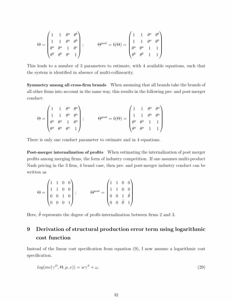
Θ =

1 1 θa θb

1 1 θa θb

θa θa 1 θc

θb θb θc 1

; Θpost = b(Θ) =

1 1 θa θb

1 1 θa θb

θa θa 1 1

θb θb 1 1

This leads to a number of 3 parameters to estimate, with 4 available equations, such that

the system is identified in absence of multi-collinearity.

Symmetry among all cross-firm brands When assuming that all brands take the brands of

all other firms into account in the same way, this results in the following pre- and post-merger

conduct:

Θ =

1 1 θa θa

1 1 θa θa

θa θa 1 θa

θa θa θa 1

; Θpost = b(Θ) =

1 1 θa θa

1 1 θa θa

θa θa 1 1

θa θa 1 1

There is only one conduct parameter to estimate and in 4 equations.

Post-merger internalization of profits When estimating the internalization of post merger

profits among merging firms, the form of industry competition. If one assumes multi-product

Nash pricing in the 3 firm, 4 brand case, then pre- and post-merger industry conduct can be

written as

Θ =

1 1 0 0

1 1 0 0

0 0 1 0

0 0 0 1

; Θpost =

1 1 0 0

1 1 0 0

0 0 1 θ

0 0 θ 1

Here, θ represents the degree of profit-internalization between firms 2 and 3.

9 Derivation of structural production error term using logarithmic

cost function

Instead of the linear cost specification from equation (9), I now assume a logarithmic cost

specification.

log(mc(γD,Θ, p, x)) = wγS + ω. (29)

32

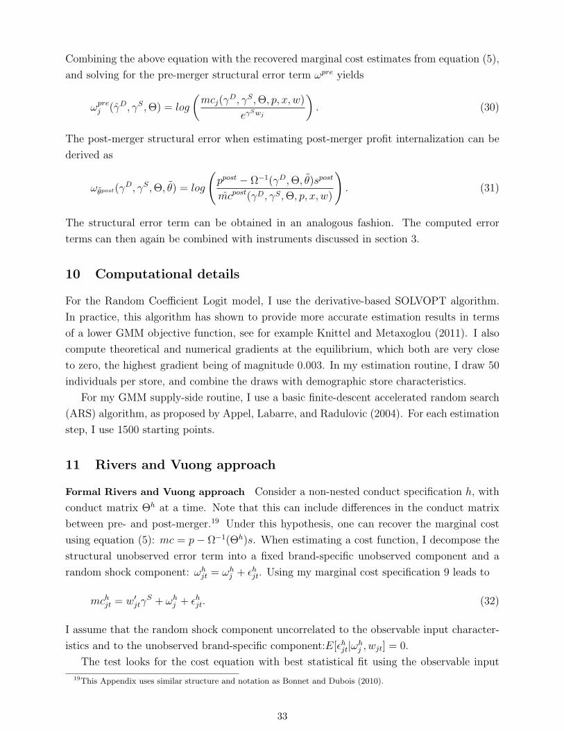
Combining the above equation with the recovered marginal cost estimates from equation (5),

and solving for the pre-merger structural error term ωpre yields

ωprej (γD, γS,Θ) = log

(mcj(γ

D, γS,Θ, p, x, w)

eγSwj

). (30)

The post-merger structural error when estimating post-merger profit internalization can be

derived as

ωθpost(γD, γS,Θ, θ) = log

(ppost − Ω−1(γD,Θ, θ)spost

mcpost(γD, γS,Θ, p, x, w)

). (31)

The structural error term can be obtained in an analogous fashion. The computed error

terms can then again be combined with instruments discussed in section 3.

10 Computational details

For the Random Coefficient Logit model, I use the derivative-based SOLVOPT algorithm.

In practice, this algorithm has shown to provide more accurate estimation results in terms

of a lower GMM objective function, see for example Knittel and Metaxoglou (2011). I also

compute theoretical and numerical gradients at the equilibrium, which both are very close

to zero, the highest gradient being of magnitude 0.003. In my estimation routine, I draw 50

individuals per store, and combine the draws with demographic store characteristics.

For my GMM supply-side routine, I use a basic finite-descent accelerated random search

(ARS) algorithm, as proposed by Appel, Labarre, and Radulovic (2004). For each estimation

step, I use 1500 starting points.

11 Rivers and Vuong approach

Formal Rivers and Vuong approach Consider a non-nested conduct specification h, with

conduct matrix Θh at a time. Note that this can include differences in the conduct matrix

between pre- and post-merger.19 Under this hypothesis, one can recover the marginal cost

using equation (5): mc = p− Ω−1(Θh)s. When estimating a cost function, I decompose the

structural unobserved error term into a fixed brand-specific unobserved component and a

random shock component: ωhjt = ωhj + εhjt. Using my marginal cost specification 9 leads to

mchjt = w′jtγS + ωhj + εhjt. (32)

I assume that the random shock component uncorrelated to the observable input character-

istics and to the unobserved brand-specific component:E[εhjt|ωhj , wjt] = 0.

The test looks for the cost equation with best statistical fit using the observable input

19This Appendix uses similar structure and notation as Bonnet and Dubois (2010).

33

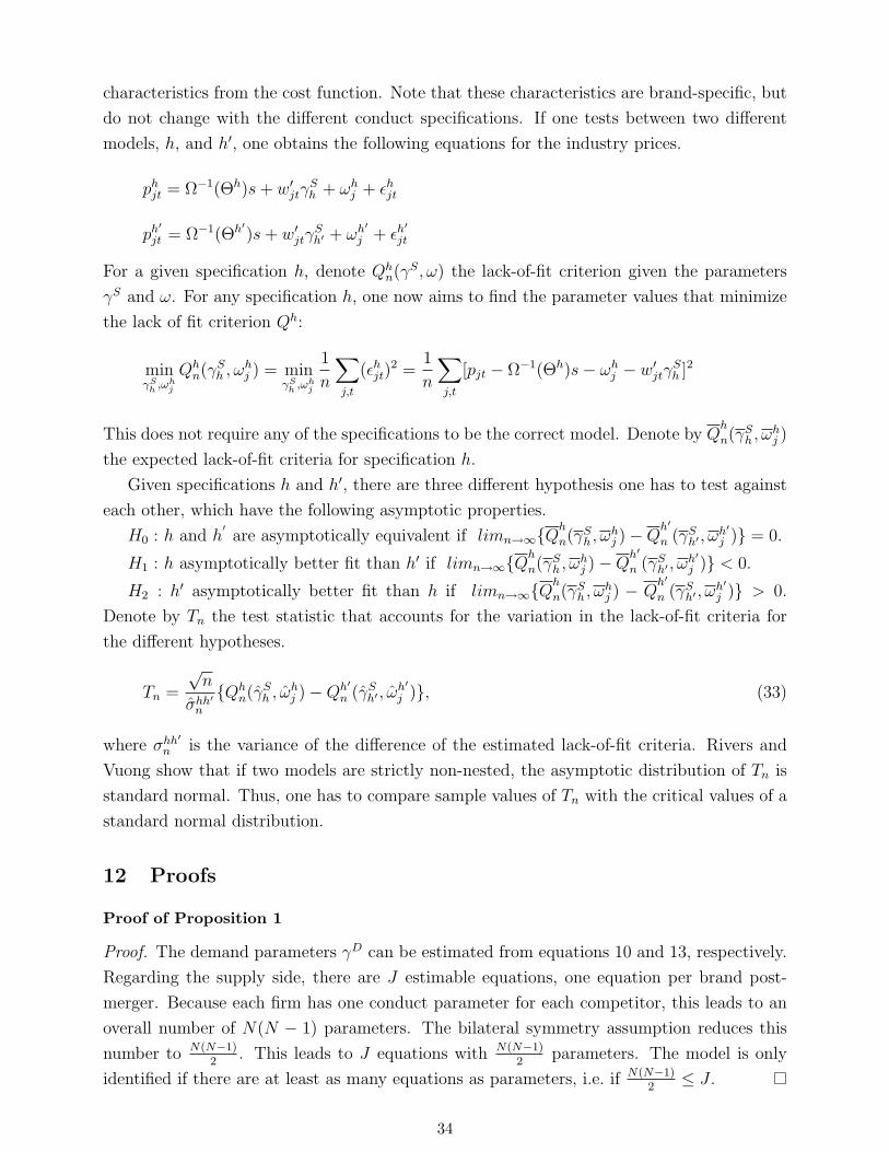
characteristics from the cost function. Note that these characteristics are brand-specific, but

do not change with the different conduct specifications. If one tests between two different

models, h, and h′, one obtains the following equations for the industry prices.

phjt = Ω−1(Θh)s+ w′jtγSh + ωhj + εhjt

ph′

jt = Ω−1(Θh′)s+ w′jtγSh′ + ωh

′

j + εh′

jt

For a given specification h, denote Qhn(γS, ω) the lack-of-fit criterion given the parameters

γS and ω. For any specification h, one now aims to find the parameter values that minimize

the lack of fit criterion Qh:

minγS

h ,ωhj

Qhn(γSh , ω

hj ) = min

γSh ,ω

hj

1

n

∑j,t

(εhjt)2 =

1

n

∑j,t

[pjt − Ω−1(Θh)s− ωhj − w′jtγSh ]2

This does not require any of the specifications to be the correct model. Denote by Qh

n(γSh , ωhj )

the expected lack-of-fit criteria for specification h.

Given specifications h and h′, there are three different hypothesis one has to test against

each other, which have the following asymptotic properties.

H0 : h and h′

are asymptotically equivalent if limn→∞Qh

n(γSh , ωhj )−Q

h′

n (γSh′ , ωh′j ) = 0.

H1 : h asymptotically better fit than h′ if limn→∞Qh

n(γSh , ωhj )−Q

h′

n (γSh′ , ωh′j ) < 0.

H2 : h′ asymptotically better fit than h if limn→∞Qh

n(γSh , ωhj ) − Q

h′

n (γSh′ , ωh′j ) > 0.

Denote by Tn the test statistic that accounts for the variation in the lack-of-fit criteria for

the different hypotheses.

Tn =

√n

σhh′n

Qhn(γSh , ω

hj )−Qh′

n (γSh′ , ωh′

j ), (33)

where σhh′

n is the variance of the difference of the estimated lack-of-fit criteria. Rivers and

Vuong show that if two models are strictly non-nested, the asymptotic distribution of Tn is

standard normal. Thus, one has to compare sample values of Tn with the critical values of a

standard normal distribution.

12 Proofs

Proof of Proposition 1

Proof. The demand parameters γD can be estimated from equations 10 and 13, respectively.

Regarding the supply side, there are J estimable equations, one equation per brand post-

merger. Because each firm has one conduct parameter for each competitor, this leads to an

overall number of N(N − 1) parameters. The bilateral symmetry assumption reduces this

number to N(N−1)2

. This leads to J equations with N(N−1)2

parameters. The model is only

identified if there are at least as many equations as parameters, i.e. if N(N−1)2≤ J .

34

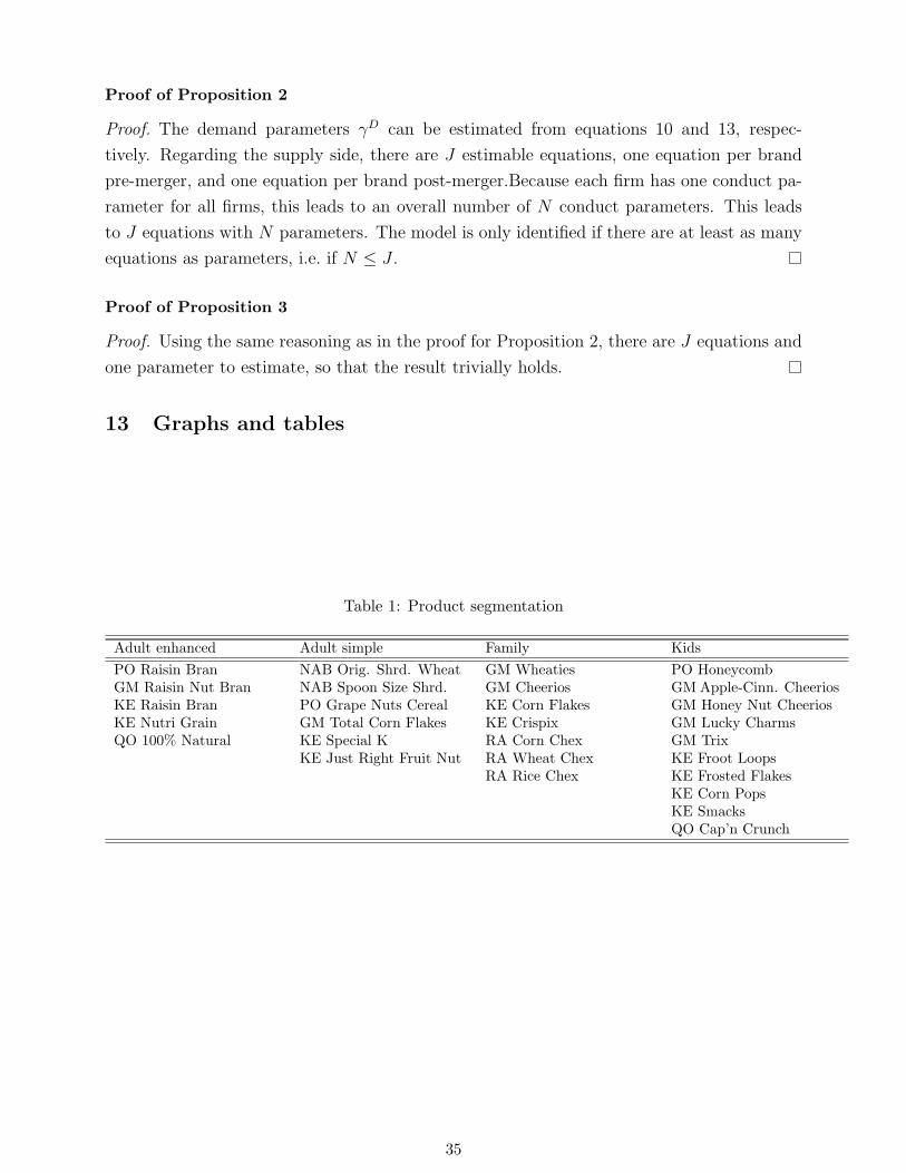
Proof of Proposition 2

Proof. The demand parameters γD can be estimated from equations 10 and 13, respec-

tively. Regarding the supply side, there are J estimable equations, one equation per brand

pre-merger, and one equation per brand post-merger.Because each firm has one conduct pa-

rameter for all firms, this leads to an overall number of N conduct parameters. This leads

to J equations with N parameters. The model is only identified if there are at least as many

equations as parameters, i.e. if N ≤ J .

Proof of Proposition 3

Proof. Using the same reasoning as in the proof for Proposition 2, there are J equations and

one parameter to estimate, so that the result trivially holds.

13 Graphs and tables

Table 1: Product segmentation

Adult enhanced Adult simple Family KidsPO Raisin Bran NAB Orig. Shrd. Wheat GM Wheaties PO HoneycombGM Raisin Nut Bran NAB Spoon Size Shrd. GM Cheerios GM Apple-Cinn. CheeriosKE Raisin Bran PO Grape Nuts Cereal KE Corn Flakes GM Honey Nut CheeriosKE Nutri Grain GM Total Corn Flakes KE Crispix GM Lucky CharmsQO 100% Natural KE Special K RA Corn Chex GM Trix

KE Just Right Fruit Nut RA Wheat Chex KE Froot LoopsRA Rice Chex KE Frosted Flakes

KE Corn PopsKE SmacksQO Cap’n Crunch

35

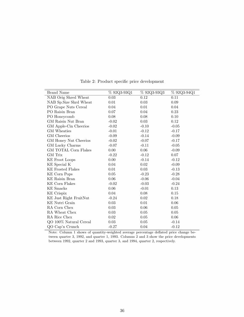
Table 2: Product specific price development

Brand Name % 92Q3-93Q1 % 92Q3-93Q3 % 92Q3-94Q1NAB Orig Shred Wheat 0.03 0.12 0.11NAB Sp.Size Shrd Wheat 0.01 0.03 0.09PO Grape Nuts Cereal 0.04 0.01 0.04PO Raisin Bran 0.07 0.04 0.23PO Honeycomb 0.08 0.08 0.10GM Raisin Nut Bran -0.02 0.03 0.12GM Apple-Cin Cheerios -0.02 -0.10 -0.05GM Wheaties -0.01 -0.12 -0.17GM Cheerios -0.09 -0.14 -0.09GM Honey Nut Cheerios -0.02 -0.07 -0.17GM Lucky Charms -0.07 -0.11 -0.05GM TOTAL Corn Flakes 0.00 0.06 -0.09GM Trix -0.22 -0.12 0.07KE Froot Loops 0.00 -0.14 -0.12KE Special K 0.04 0.02 -0.09KE Frosted Flakes 0.01 0.03 -0.13KE Corn Pops 0.05 -0.23 -0.28KE Raisin Bran 0.06 -0.06 -0.04KE Corn Flakes -0.02 -0.03 -0.24KE Smacks 0.06 -0.01 0.13KE Crispix 0.04 0.08 0.15KE Just Right FruitNut -0.24 0.02 0.18KE Nutri Grain 0.03 0.01 0.06RA Corn Chex 0.03 0.06 0.05RA Wheat Chex 0.03 0.05 0.05RA Rice Chex 0.02 0.05 0.06QO 100% Natural Cereal 0.03 0.05 -0.14QO Cap’n Crunch -0.27 0.04 -0.12Note: Column 1 shows of quantity-weighted average percentage deflated price change be-tween quarter 3, 1992, and quarter 1, 1993. Columns 2 and 3 show the price developmentsbetween 1992, quarter 2 and 1993, quarter 3, and 1994, quarter 2, respectively.

36

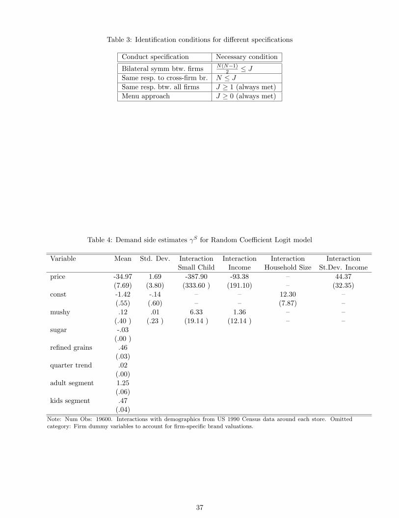
Table 3: Identification conditions for different specifications

Conduct specification Necessary condition

Bilateral symm btw. firms N(N−1)2 ≤ J

Same resp. to cross-firm br. N ≤ JSame resp. btw. all firms J ≥ 1 (always met)Menu approach J ≥ 0 (always met)

Table 4: Demand side estimates γS for Random Coefficient Logit model

Variable Mean Std. Dev. Interaction Interaction Interaction InteractionSmall Child Income Household Size St.Dev. Income

price -34.97 1.69 -387.90 -93.38 – 44.37(7.69) (3.80) (333.60 ) (191.10) – (32.35)

const -1.42 -.14 – – 12.30 –(.55) (.60) – – (7.87) –

mushy .12 .01 6.33 1.36 – –(.40 ) (.23 ) (19.14 ) (12.14 ) – –

sugar -.03(.00 )

refined grains .46(.03)

quarter trend .02(.00)

adult segment 1.25(.06)

kids segment .47(.04)

Note: Num Obs: 19600. Interactions with demographics from US 1990 Census data around each store. Omittedcategory: Firm dummy variables to account for firm-specific brand valuations.

37

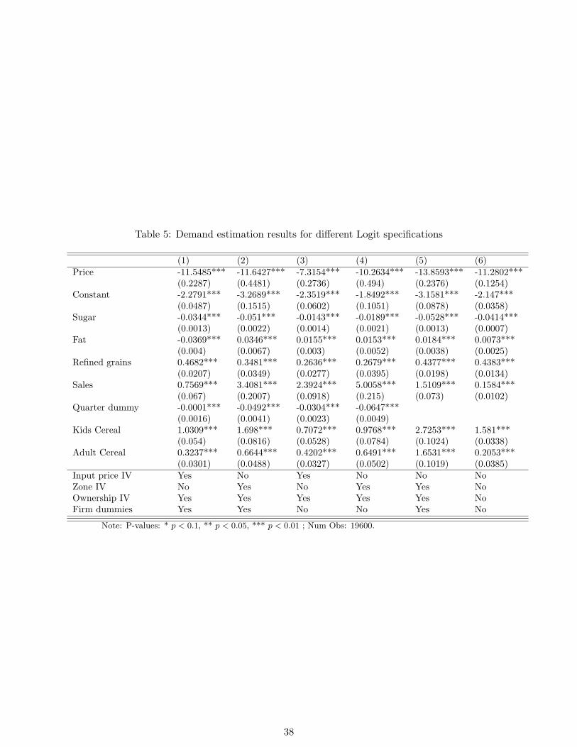
Table 5: Demand estimation results for different Logit specifications

(1) (2) (3) (4) (5) (6)Price -11.5485*** -11.6427*** -7.3154*** -10.2634*** -13.8593*** -11.2802***

(0.2287) (0.4481) (0.2736) (0.494) (0.2376) (0.1254)Constant -2.2791*** -3.2689*** -2.3519*** -1.8492*** -3.1581*** -2.147***

(0.0487) (0.1515) (0.0602) (0.1051) (0.0878) (0.0358)Sugar -0.0344*** -0.051*** -0.0143*** -0.0189*** -0.0528*** -0.0414***

(0.0013) (0.0022) (0.0014) (0.0021) (0.0013) (0.0007)Fat -0.0369*** 0.0346*** 0.0155*** 0.0153*** 0.0184*** 0.0073***

(0.004) (0.0067) (0.003) (0.0052) (0.0038) (0.0025)Refined grains 0.4682*** 0.3481*** 0.2636*** 0.2679*** 0.4377*** 0.4383***

(0.0207) (0.0349) (0.0277) (0.0395) (0.0198) (0.0134)Sales 0.7569*** 3.4081*** 2.3924*** 5.0058*** 1.5109*** 0.1584***

(0.067) (0.2007) (0.0918) (0.215) (0.073) (0.0102)Quarter dummy -0.0001*** -0.0492*** -0.0304*** -0.0647***

(0.0016) (0.0041) (0.0023) (0.0049)Kids Cereal 1.0309*** 1.698*** 0.7072*** 0.9768*** 2.7253*** 1.581***

(0.054) (0.0816) (0.0528) (0.0784) (0.1024) (0.0338)Adult Cereal 0.3237*** 0.6644*** 0.4202*** 0.6491*** 1.6531*** 0.2053***

(0.0301) (0.0488) (0.0327) (0.0502) (0.1019) (0.0385)Input price IV Yes No Yes No No NoZone IV No Yes No Yes Yes NoOwnership IV Yes Yes Yes Yes Yes NoFirm dummies Yes Yes No No Yes No

Note: P-values: * p < 0.1, ** p < 0.05, *** p < 0.01 ; Num Obs: 19600.

38

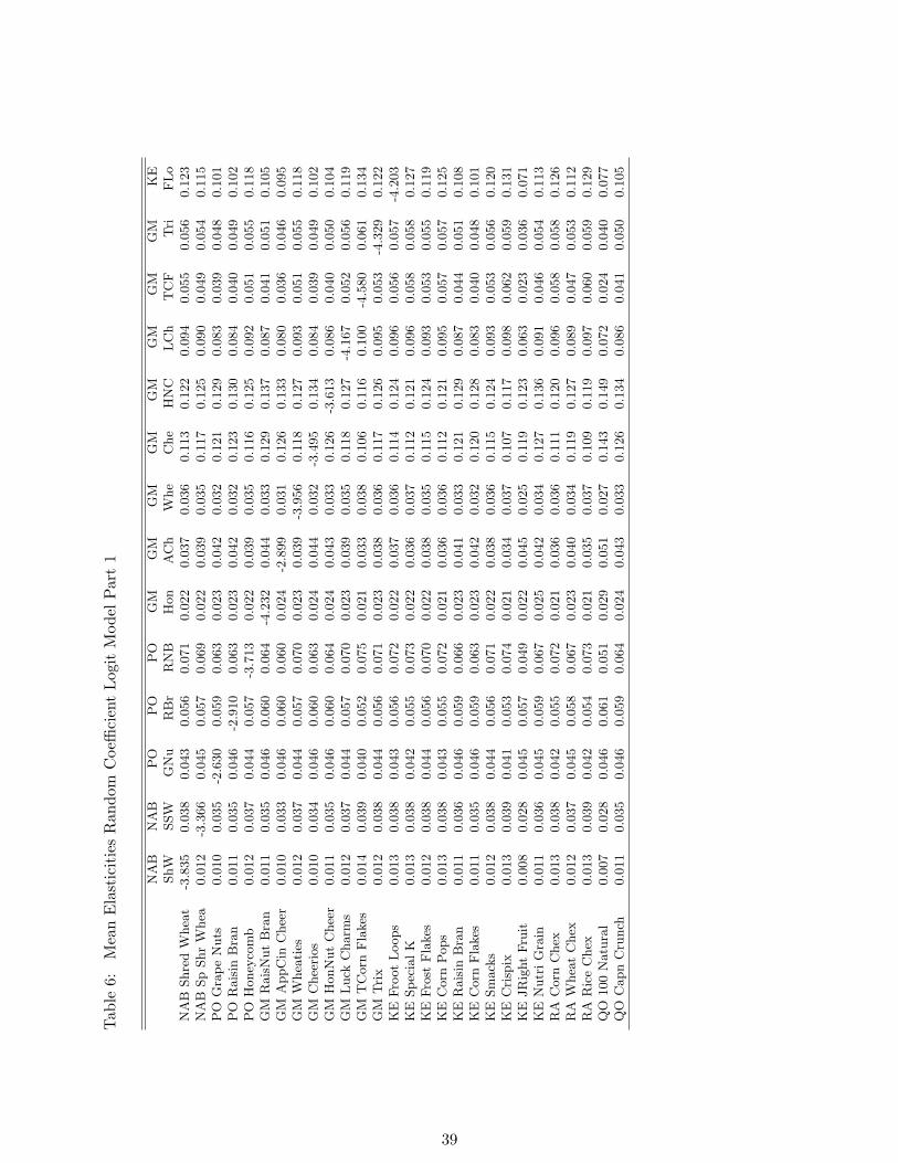
Tab

le6:

Mea

nE

last

icit

ies

Ran

dom

Coe

ffici

ent

Log

itM

odel

Par

t1

NA

BN

AB

PO

PO

PO

GM

GM

GM

GM

GM

GM

GM

GM

KE

ShW

SSW

GN

uR

Br

RN

BH

on

AC

hW

he

Che

HN

CL

Ch

TC

FT

riF

Lo

NA

BShre

dW

hea

t-3

.835

0.0

38

0.0

43

0.0

56

0.0

71

0.0

22

0.0

37

0.0

36

0.1

13

0.1

22

0.0

94

0.0

55

0.0

56

0.1

23

NA

BSp

Shr

Whea

0.0

12

-3.3

66

0.0

45

0.0

57

0.0

69

0.0

22

0.0

39

0.0

35

0.1

17

0.1

25

0.0

90

0.0

49

0.0

54

0.1

15

PO

Gra

pe

Nuts

0.0

10

0.0

35

-2.6

30

0.0

59

0.0

63

0.0

23

0.0

42

0.0

32

0.1

21

0.1

29

0.0

83

0.0

39

0.0

48

0.1

01

PO

Rais

inB

ran

0.0

11

0.0

35

0.0

46

-2.9

10

0.0

63

0.0

23

0.0

42

0.0

32

0.1

23

0.1

30

0.0

84

0.0

40

0.0

49

0.1

02

PO

Honey

com

b0.0

12

0.0

37

0.0

44

0.0

57

-3.7

13

0.0

22

0.0

39

0.0

35

0.1

16

0.1

25

0.0

92

0.0

51

0.0

55

0.1

18

GM

Rais

Nut

Bra

n0.0

11

0.0

35

0.0

46

0.0

60

0.0

64

-4.2

32

0.0

44

0.0

33

0.1

29

0.1

37

0.0

87

0.0

41

0.0

51

0.1

05

GM

AppC

inC

hee

r0.0

10

0.0

33

0.0

46

0.0

60

0.0

60

0.0

24

-2.8

99

0.0

31

0.1

26

0.1

33

0.0

80

0.0

36

0.0

46

0.0

95

GM

Whea

ties

0.0

12

0.0

37

0.0

44

0.0

57

0.0

70

0.0

23

0.0

39

-3.9

56

0.1

18

0.1

27

0.0

93

0.0

51

0.0

55

0.1

18

GM

Chee

rios

0.0

10

0.0

34

0.0

46

0.0

60

0.0

63

0.0

24

0.0

44

0.0

32

-3.4

95

0.1

34

0.0

84

0.0

39

0.0

49

0.1

02

GM

HonN

ut

Chee

r0.0

11

0.0

35

0.0

46

0.0

60

0.0

64

0.0

24

0.0

43

0.0

33

0.1

26

-3.6

13

0.0

86

0.0

40

0.0

50

0.1

04

GM

Luck

Charm

s0.0

12

0.0

37

0.0

44

0.0

57

0.0

70

0.0

23

0.0

39

0.0

35

0.1

18

0.1

27

-4.1

67

0.0

52

0.0

56

0.1

19

GM

TC

orn

Fla

kes

0.0

14

0.0

39

0.0

40

0.0

52

0.0

75

0.0

21

0.0

33

0.0

38

0.1

06

0.1

16

0.1

00

-4.5

80

0.0

61

0.1

34

GM

Tri

x0.0

12

0.0

38

0.0

44

0.0

56

0.0

71

0.0

23

0.0

38

0.0

36

0.1

17

0.1

26

0.0

95

0.0

53

-4.3

29

0.1

22

KE

Fro

ot

Loops

0.0

13

0.0

38

0.0

43

0.0

56

0.0

72

0.0

22

0.0

37

0.0

36

0.1

14

0.1

24

0.0

96

0.0

56

0.0

57

-4.2

03

KE

Sp

ecia

lK

0.0

13

0.0

38

0.0

42

0.0

55

0.0

73

0.0

22

0.0

36

0.0

37

0.1

12

0.1

21

0.0

96

0.0

58

0.0

58

0.1

27

KE

Fro

stF

lakes

0.0

12

0.0

38

0.0

44

0.0

56

0.0

70

0.0

22

0.0

38

0.0

35

0.1

15

0.1

24

0.0

93

0.0

53

0.0

55

0.1

19

KE

Corn

Pops

0.0

13

0.0

38

0.0

43

0.0

55

0.0

72

0.0

21

0.0

36

0.0

36

0.1

12

0.1

21

0.0

95

0.0

57

0.0

57

0.1

25

KE

Rais

inB

ran

0.0

11

0.0

36

0.0

46

0.0

59

0.0

66

0.0

23

0.0

41

0.0

33

0.1

21

0.1

29

0.0

87

0.0

44

0.0

51

0.1

08

KE

Corn

Fla

kes

0.0

11

0.0

35

0.0

46

0.0

59

0.0

63

0.0

23

0.0

42

0.0

32

0.1

20

0.1

28

0.0

83

0.0

40

0.0

48

0.1

01

KE

Sm

ack

s0.0

12

0.0

38

0.0

44

0.0

56

0.0

71

0.0

22

0.0

38

0.0

36

0.1

15

0.1

24

0.0

93

0.0

53

0.0

56

0.1

20

KE

Cri

spix

0.0

13

0.0

39

0.0

41

0.0

53

0.0

74

0.0

21

0.0

34

0.0

37

0.1

07

0.1

17

0.0

98

0.0

62

0.0

59

0.1

31

KE

JR

ight

Fru

it0.0

08

0.0

28

0.0

45

0.0

57

0.0

49

0.0

22

0.0

45

0.0

25

0.1

19

0.1

23

0.0

63

0.0

23

0.0

36

0.0

71

KE

Nutr

iG

rain

0.0

11

0.0

36

0.0

45

0.0

59

0.0

67

0.0

25

0.0

42

0.0

34

0.1

27

0.1

36

0.0

91

0.0

46

0.0

54

0.1

13

RA

Corn

Chex

0.0

13

0.0

38

0.0

42

0.0

55

0.0

72

0.0

21

0.0

36

0.0

36

0.1

11

0.1

20

0.0

96

0.0

58

0.0

58

0.1

26

RA

Whea

tC

hex

0.0

12

0.0

37

0.0

45

0.0

58

0.0

67

0.0

23

0.0

40

0.0

34

0.1

19

0.1

27

0.0

89

0.0

47

0.0

53

0.1

12

RA

Ric

eC

hex

0.0

13

0.0

39

0.0

42

0.0

54

0.0

73

0.0

21

0.0

35

0.0

37

0.1

09

0.1

19

0.0

97

0.0

60

0.0

59

0.1

29

QO

100

Natu

ral

0.0

07

0.0

28

0.0

46

0.0

61

0.0

51

0.0

29

0.0

51

0.0

27

0.1

43

0.1

49

0.0

72

0.0

24

0.0

40

0.0

77

QO

Capn

Cru

nch

0.0

11

0.0

35

0.0

46

0.0

59

0.0

64

0.0

24

0.0

43

0.0

33

0.1

26

0.1

34

0.0

86

0.0

41

0.0

50

0.1

05

39

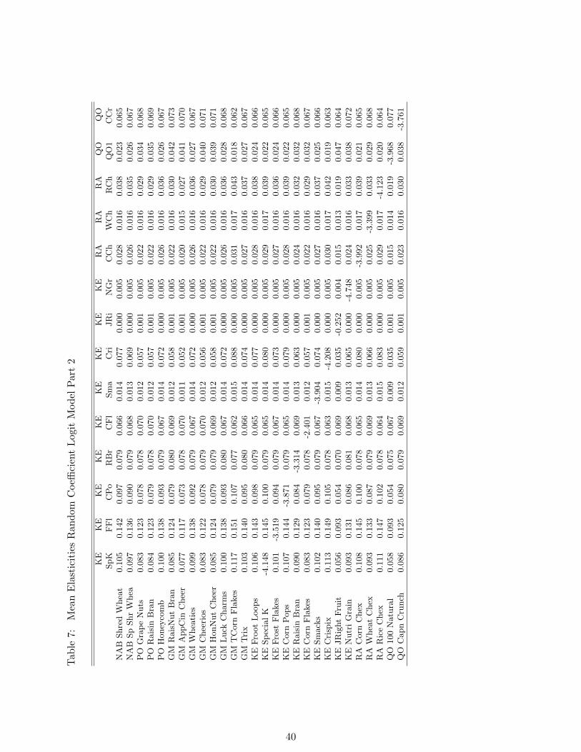
Tab

le7:

Mea

nE

last

icit

ies

Ran

dom

Coe

ffici

ent

Log

itM

odel

Par

t2

KE

KE

KE

KE

KE

KE

KE

KE

KE

RA

RA

RA

QO

QO

SpK

FF

lC

Po

RB

rC

Fl

Sm

aC

riJR

iN

Gr

CC

hW

Ch

RC

hQ

O1

CC

rN

AB

Shre

dW

hea

t0.1

05

0.1

42

0.0

97

0.0

79

0.0

66

0.0

14

0.0

77

0.0

00

0.0

05

0.0

28

0.0

16

0.0

38

0.0

23

0.0

65

NA

BSp

Shr

Whea

0.0

97

0.1

36

0.0

90

0.0

79

0.0

68

0.0

13

0.0

69

0.0

00

0.0

05

0.0

26

0.0

16

0.0

35

0.0

26

0.0

67

PO

Gra

pe

Nuts

0.0

83

0.1

23

0.0

78

0.0

78

0.0

70

0.0

12

0.0

57

0.0

01

0.0

05

0.0

22

0.0

16

0.0

29

0.0

34

0.0

68

PO

Rais

inB

ran

0.0

84

0.1

23

0.0

79

0.0

78

0.0

70

0.0

12

0.0

57

0.0

01

0.0

05

0.0

22

0.0

16

0.0

29

0.0

35

0.0

69

PO

Honey

com

b0.1

00

0.1

38

0.0

93

0.0

79

0.0

67

0.0

14

0.0

72

0.0

00

0.0

05

0.0

26

0.0

16

0.0

36

0.0

26

0.0

67

GM

Rais

Nut

Bra

n0.0

85

0.1

24

0.0

79

0.0

80

0.0

69

0.0

12

0.0

58

0.0

01

0.0

05

0.0

22

0.0

16

0.0

30

0.0

42

0.0

73

GM

AppC

inC

hee

r0.0

77

0.1

17

0.0

73

0.0

78

0.0

70

0.0

11

0.0

52

0.0

01

0.0

05

0.0

20

0.0

15

0.0

27

0.0

41

0.0

70

GM

Whea

ties

0.0

99

0.1

38

0.0

92

0.0

79

0.0

67

0.0

14

0.0

72

0.0

00

0.0

05

0.0

26

0.0

16

0.0

36

0.0

27

0.0

67

GM

Chee

rios

0.0

83

0.1

22

0.0

78

0.0

79

0.0

70

0.0

12

0.0

56

0.0

01

0.0

05

0.0

22

0.0

16

0.0

29

0.0

40

0.0

71

GM

HonN

ut

Chee

r0.0

85

0.1

24

0.0

79

0.0

79

0.0

69

0.0

12

0.0

58

0.0

01

0.0

05

0.0

22

0.0

16

0.0

30

0.0

39

0.0

71

GM

Luck

Charm

s0.1

00

0.1

38

0.0

93

0.0

80

0.0

67

0.0

14

0.0

72

0.0

00

0.0

05

0.0

26

0.0

16

0.0

36

0.0

28

0.0

68

GM

TC

orn

Fla

kes

0.1

17

0.1

51

0.1

07

0.0

77

0.0

62

0.0

15

0.0

88

0.0

00

0.0

05

0.0

31

0.0

17

0.0

43

0.0

18

0.0

62

GM

Tri

x0.1

03

0.1

40

0.0

95

0.0

80

0.0

66

0.0

14

0.0

74

0.0

00

0.0

05

0.0

27

0.0

16

0.0

37

0.0

27

0.0

67

KE

Fro

ot

Loops

0.1

06

0.1

43

0.0

98

0.0

79

0.0

65

0.0

14

0.0

77

0.0

00

0.0

05

0.0

28

0.0

16

0.0

38

0.0

24

0.0

66

KE

Sp

ecia

lK

-4.1

48

0.1

45

0.1

00

0.0

79

0.0

65

0.0

14

0.0

80

0.0

00

0.0

05

0.0

29

0.0

17

0.0

39

0.0

22

0.0

65

KE

Fro

stF

lakes

0.1

01

-3.5

19

0.0

94

0.0

79

0.0

67

0.0

14

0.0

73

0.0

00

0.0

05

0.0

27

0.0

16

0.0

36

0.0

24

0.0

66

KE

Corn

Pops

0.1

07

0.1

44

-3.8

71

0.0

79

0.0

65

0.0

14

0.0

79

0.0

00

0.0

05

0.0

28

0.0

16

0.0

39

0.0

22

0.0

65

KE

Rais

inB

ran

0.0

90

0.1

29

0.0

84

-3.3

14

0.0

69

0.0

13

0.0

63

0.0

00

0.0

05

0.0

24

0.0

16

0.0

32

0.0

32

0.0

68

KE

Corn

Fla

kes

0.0

83

0.1

23

0.0

79

0.0

78

-2.4

01

0.0

12

0.0

57

0.0

01

0.0

05

0.0

22

0.0

16

0.0

29

0.0

32

0.0

67

KE

Sm

ack

s0.1

02

0.1

40

0.0

95

0.0

79

0.0

67

-3.9

04

0.0

74

0.0

00

0.0

05

0.0

27

0.0

16

0.0

37

0.0

25

0.0

66

KE

Cri

spix

0.1

13

0.1

49

0.1

05

0.0

78

0.0

63

0.0

15

-4.2

08

0.0

00

0.0

05

0.0

30

0.0

17

0.0

42

0.0

19

0.0

63

KE

JR

ight

Fru

it0.0

56

0.0

93

0.0

54

0.0

70

0.0

69

0.0

09

0.0

35

-0.2

52

0.0

04

0.0

15

0.0

13

0.0

19

0.0

47

0.0

64

KE

Nutr

iG

rain

0.0

93

0.1

31

0.0

86

0.0

81

0.0

68

0.0

13

0.0

65

0.0

00

-4.7

48

0.0

24

0.0

16

0.0

33

0.0

38

0.0

72

RA

Corn

Chex

0.1

08

0.1

45

0.1

00

0.0

78

0.0

65

0.0

14

0.0

80

0.0

00

0.0

05

-3.9

92

0.0

17

0.0

39

0.0

21

0.0

65

RA

Whea

tC

hex

0.0

93

0.1

33

0.0

87

0.0

79

0.0

69

0.0

13

0.0

66

0.0

00

0.0

05

0.0

25

-3.3

99

0.0

33

0.0

29

0.0

68

RA

Ric

eC

hex

0.1

11

0.1

47

0.1

02

0.0

78

0.0

64

0.0

15

0.0

83

0.0

00

0.0

05

0.0

29

0.0

17

-4.1

23

0.0

20

0.0

64

QO

100

Natu

ral

0.0

58

0.0

93

0.0

54

0.0

75

0.0

67

0.0

09

0.0

35

0.0

01

0.0

05

0.0

15

0.0

14

0.0

19

-3.9

68

0.0

77

QO

Capn

Cru

nch

0.0

86

0.1

25

0.0

80

0.0

79

0.0

69

0.0

12

0.0

59

0.0

01

0.0

05

0.0

23

0.0

16

0.0

30

0.0

38

-3.7

61

40

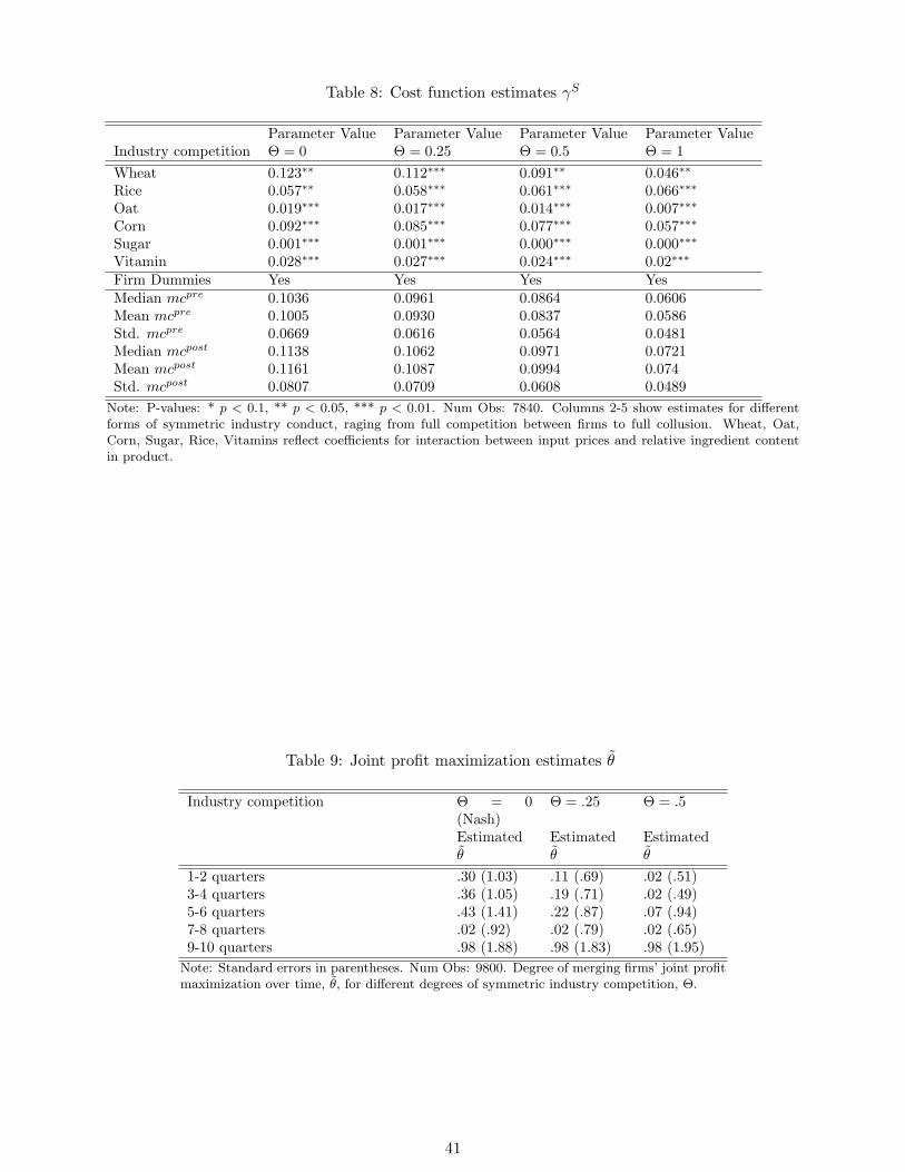
Table 8: Cost function estimates γS

Parameter Value Parameter Value Parameter Value Parameter ValueIndustry competition Θ = 0 Θ = 0.25 Θ = 0.5 Θ = 1Wheat 0.123∗∗ 0.112∗∗∗ 0.091∗∗ 0.046∗∗

Rice 0.057∗∗ 0.058∗∗∗ 0.061∗∗∗ 0.066∗∗∗

Oat 0.019∗∗∗ 0.017∗∗∗ 0.014∗∗∗ 0.007∗∗∗

Corn 0.092∗∗∗ 0.085∗∗∗ 0.077∗∗∗ 0.057∗∗∗

Sugar 0.001∗∗∗ 0.001∗∗∗ 0.000∗∗∗ 0.000∗∗∗

Vitamin 0.028∗∗∗ 0.027∗∗∗ 0.024∗∗∗ 0.02∗∗∗

Firm Dummies Yes Yes Yes YesMedian mcpre 0.1036 0.0961 0.0864 0.0606Mean mcpre 0.1005 0.0930 0.0837 0.0586Std. mcpre 0.0669 0.0616 0.0564 0.0481Median mcpost 0.1138 0.1062 0.0971 0.0721Mean mcpost 0.1161 0.1087 0.0994 0.074Std. mcpost 0.0807 0.0709 0.0608 0.0489

Note: P-values: * p < 0.1, ** p < 0.05, *** p < 0.01. Num Obs: 7840. Columns 2-5 show estimates for differentforms of symmetric industry conduct, raging from full competition between firms to full collusion. Wheat, Oat,Corn, Sugar, Rice, Vitamins reflect coefficients for interaction between input prices and relative ingredient contentin product.

Table 9: Joint profit maximization estimates θ

Industry competition Θ = 0(Nash)

Θ = .25 Θ = .5

Estimatedθ

Estimatedθ

Estimatedθ

1-2 quarters .30 (1.03) .11 (.69) .02 (.51)3-4 quarters .36 (1.05) .19 (.71) .02 (.49)5-6 quarters .43 (1.41) .22 (.87) .07 (.94)7-8 quarters .02 (.92) .02 (.79) .02 (.65)9-10 quarters .98 (1.88) .98 (1.83) .98 (1.95)

Note: Standard errors in parentheses. Num Obs: 9800. Degree of merging firms’ joint profitmaximization over time, θ, for different degrees of symmetric industry competition, Θ.

41

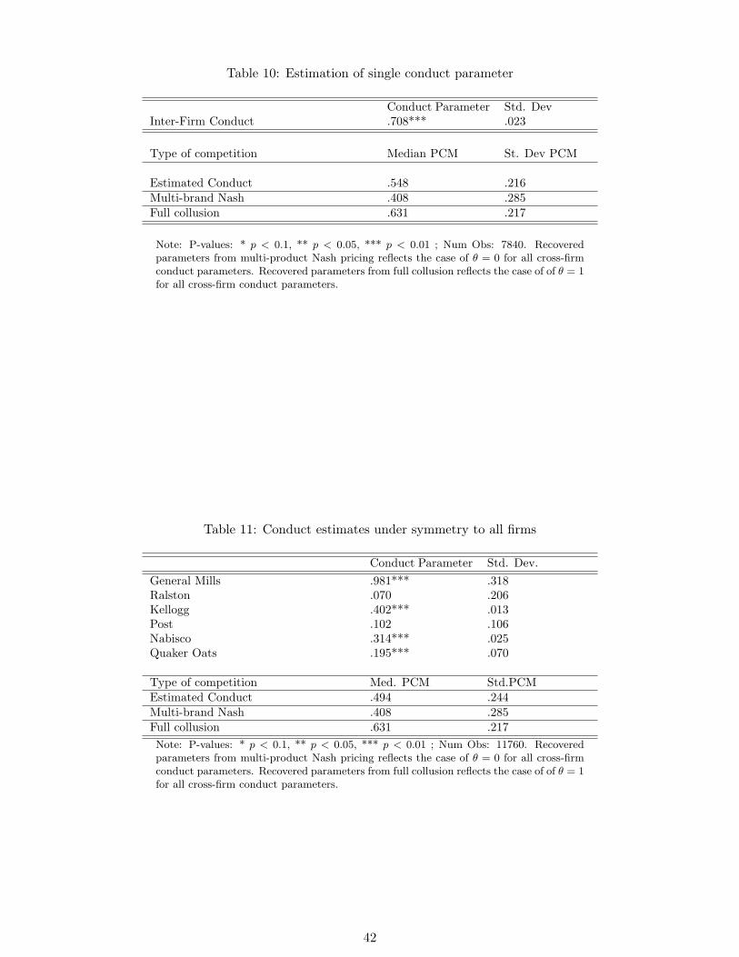
Table 10: Estimation of single conduct parameter

Conduct Parameter Std. DevInter-Firm Conduct .708*** .023

Type of competition Median PCM St. Dev PCM

Estimated Conduct .548 .216Multi-brand Nash .408 .285Full collusion .631 .217

Note: P-values: * p < 0.1, ** p < 0.05, *** p < 0.01 ; Num Obs: 7840. Recoveredparameters from multi-product Nash pricing reflects the case of θ = 0 for all cross-firmconduct parameters. Recovered parameters from full collusion reflects the case of of θ = 1for all cross-firm conduct parameters.

Table 11: Conduct estimates under symmetry to all firms

Conduct Parameter Std. Dev.General Mills .981*** .318Ralston .070 .206Kellogg .402*** .013Post .102 .106Nabisco .314*** .025Quaker Oats .195*** .070

Type of competition Med. PCM Std.PCMEstimated Conduct .494 .244Multi-brand Nash .408 .285Full collusion .631 .217Note: P-values: * p < 0.1, ** p < 0.05, *** p < 0.01 ; Num Obs: 11760. Recoveredparameters from multi-product Nash pricing reflects the case of θ = 0 for all cross-firmconduct parameters. Recovered parameters from full collusion reflects the case of of θ = 1for all cross-firm conduct parameters.

42

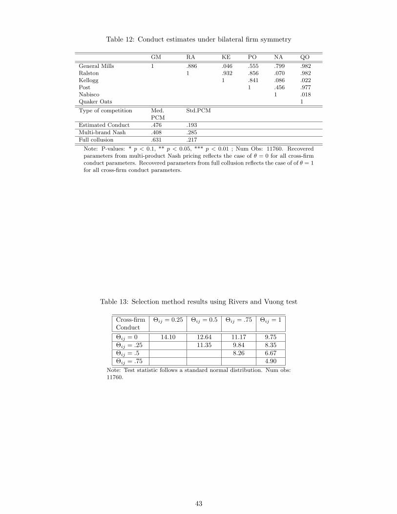
Table 12: Conduct estimates under bilateral firm symmetry

GM RA KE PO NA QO

General Mills 1 .886 .046 .555 .799 .982Ralston 1 .932 .856 .070 .982Kellogg 1 .841 .086 .022Post 1 .456 .977Nabisco 1 .018Quaker Oats 1

Type of competition Med.PCM

Std.PCM

Estimated Conduct .476 .193

Multi-brand Nash .408 .285

Full collusion .631 .217

Note: P-values: * p < 0.1, ** p < 0.05, *** p < 0.01 ; Num Obs: 11760. Recoveredparameters from multi-product Nash pricing reflects the case of θ = 0 for all cross-firmconduct parameters. Recovered parameters from full collusion reflects the case of of θ = 1for all cross-firm conduct parameters.

Table 13: Selection method results using Rivers and Vuong test

Cross-firm Θij = 0.25 Θij = 0.5 Θij = .75 Θij = 1ConductΘij = 0 14.10 12.64 11.17 9.75Θij = .25 11.35 9.84 8.35Θij = .5 8.26 6.67Θij = .75 4.90

Note: Test statistic follows a standard normal distribution. Num obs:11760.

43

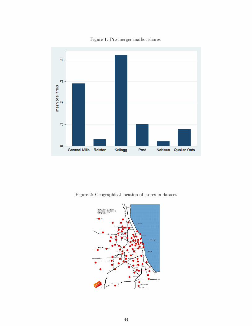
Figure 1: Pre-merger market shares

Figure 2: Geographical location of stores in dataset

44

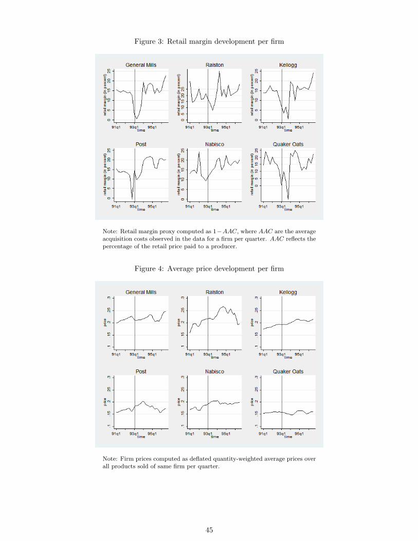
Figure 3: Retail margin development per firm

Note: Retail margin proxy computed as 1−AAC, where AAC are the averageacquisition costs observed in the data for a firm per quarter. AAC reflects thepercentage of the retail price paid to a producer.

Figure 4: Average price development per firm

Note: Firm prices computed as deflated quantity-weighted average prices overall products sold of same firm per quarter.

45

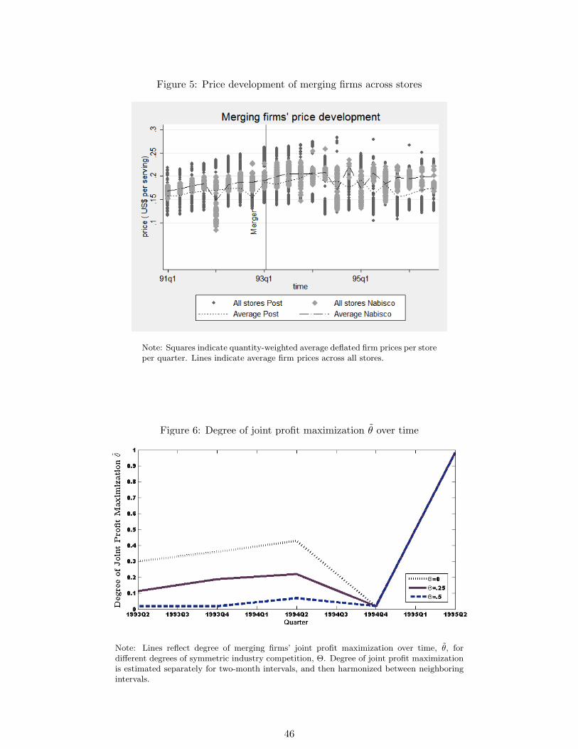
Figure 5: Price development of merging firms across stores

Note: Squares indicate quantity-weighted average deflated firm prices per storeper quarter. Lines indicate average firm prices across all stores.

Figure 6: Degree of joint profit maximization θ over time

Note: Lines reflect degree of merging firms’ joint profit maximization over time, θ, fordifferent degrees of symmetric industry competition, Θ. Degree of joint profit maximizationis estimated separately for two-month intervals, and then harmonized between neighboringintervals.

46

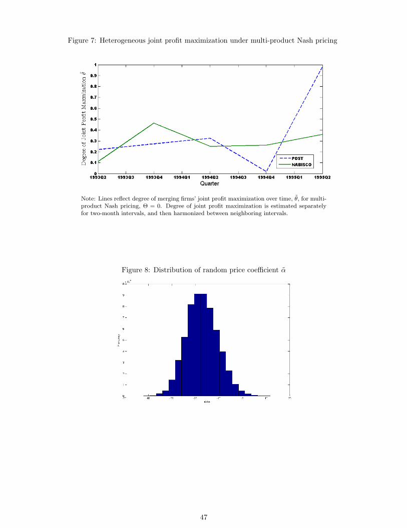
Figure 7: Heterogeneous joint profit maximization under multi-product Nash pricing

Note: Lines reflect degree of merging firms’ joint profit maximization over time, θ, for multi-product Nash pricing, Θ = 0. Degree of joint profit maximization is estimated separatelyfor two-month intervals, and then harmonized between neighboring intervals.

Figure 8: Distribution of random price coefficient α

47