Embed Size (px)
Citation preview
econstor www.econstor.eu
Der Open-Access-Publikationsserver der ZBW – Leibniz-Informationszentrum WirtschaftThe Open Access Publication Server of the ZBW – Leibniz Information Centre for Economics
Standard-Nutzungsbedingungen:
Die Dokumente auf EconStor dürfen zu eigenen wissenschaftlichenZwecken und zum Privatgebrauch gespeichert und kopiert werden.
Sie dürfen die Dokumente nicht für öffentliche oder kommerzielleZwecke vervielfältigen, öffentlich ausstellen, öffentlich zugänglichmachen, vertreiben oder anderweitig nutzen.
Sofern die Verfasser die Dokumente unter Open-Content-Lizenzen(insbesondere CC-Lizenzen) zur Verfügung gestellt haben sollten,gelten abweichend von diesen Nutzungsbedingungen die in der dortgenannten Lizenz gewährten Nutzungsrechte.
Terms of use:
Documents in EconStor may be saved and copied for yourpersonal and scholarly purposes.
You are not to copy documents for public or commercialpurposes, to exhibit the documents publicly, to make thempublicly available on the internet, or to distribute or otherwiseuse the documents in public.
If the documents have been made available under an OpenContent Licence (especially Creative Commons Licences), youmay exercise further usage rights as specified in the indicatedlicence.
zbw Leibniz-Informationszentrum WirtschaftLeibniz Information Centre for Economics
Chor, Davin; Lai, Edwin L.-C.
Working Paper
Cumulative Innovation, Growth and Welfare-Improving Patent Policy
CESifo Working Paper, No. 4407
Provided in Cooperation with:Ifo Institute – Leibniz Institute for Economic Research at the University ofMunich
Suggested Citation: Chor, Davin; Lai, Edwin L.-C. (2013) : Cumulative Innovation, Growth andWelfare-Improving Patent Policy, CESifo Working Paper, No. 4407
This Version is available at:http://hdl.handle.net/10419/84143
Cumulative Innovation, Growth and Welfare-Improving Patent Policy
Davin Chor Edwin L.-C. Lai
CESIFO WORKING PAPER NO. 4407 CATEGORY 6: FISCAL POLICY, MACROECONOMICS AND GROWTH
SEPTEMBER 2013
An electronic version of the paper may be downloaded • from the SSRN website: www.SSRN.com • from the RePEc website: www.RePEc.org
• from the CESifo website: Twww.CESifo-group.org/wp T
CESifo Working Paper No. 4407
Cumulative Innovation, Growth and Welfare-Improving Patent Policy
Abstract We construct a tractable general equilibrium model of cumulative innovation and growth, in which new ideas strictly improve upon frontier technologies, and productivity improvements are drawn in a stochastic manner. The presence of positive knowledge spillovers implies that the decentralized equilibrium features an allocation of labor to R&D activity that is strictly lower than the social planner’s benchmark, which suggests a role for patent policy. We focus on a “non-infringing inventive step” requirement, which stipulates the minimum improvement to the best patented technology that a new idea needs to make for it to be patentable and non-infringing. We establish that there exists a finite required inventive step that maximizes the rate of innovation, as well as a separate optimal required inventive step that maximizes welfare, with the former being strictly greater than the latter. These conclusions are robust to allowing for the availability of an additional instrument in the form of patent length policy.
JEL-Code: O310, O340, O400.
Keywords: innovation, growth, patent policy.
Davin Chor Department of Economics
National University of Singapore 1 Arts Link, AS2 #06-02
Singapore 117570 [email protected]
Edwin L.-C. Lai* Department of Economics
School of Business and Management Hong Kong University of Science and
Technology, Clear Water Bay Kowloon / Hong Kong
*corresponding author This draft: September 2013 We thank Costas Arkolakis, Angus Chu, Jonathan Eaton, Gino Gancia, Gene Grossman, Erzo G.J. Luttmer, Kalina Manova, Marc Melitz, Giacomo Ponzetto, Stephen Redding, Esteban Rossi-Hansberg, and Jonathan Vogel for helpful comments, as well as audiences at Penn State, the Philadelphia Fed, Princeton, UC San Diego, Stanford, the Barcelona GSE Summer Forum, the SED meetings (Seoul), and the Asian Meeting of the Econometric Society (Singapore). The work in this paper has been partially supported by the Hong Kong Research Grants Council (General Research Funds Project No. 642210). Davin thanks the International Economics Section at Princeton for their hospitality. All errors are our own.
1 Introduction
The economic analysis of intellectual property rights (IPR) protection has focused on the efficacy of
patents as an instrument for promoting research, growth and welfare. The bulk of this literature has
arguably focused on patent length – the duration of a patent’s validity – as the key policy of interest.
There is now a well-developed argument for the existence of an optimal patent length in a broad class of
models where innovation expands upon the set of products (e.g., Nordhaus 1969; Tirole 1988; Grossman
and Lai 2004): An increase in the patent length induces a higher rate of innovation by extending the
duration of the innovator’s monopoly power (the dynamic gains), and this is traded off at the margin
against the consumer surplus that is conceded (the static losses).1
In practice, however, patent protection is accorded in more ways than through the patent length.
Innovation often also takes the form of productivity improvements, where new technologies continually
build upon old ones in a cumulative fashion, rather than engineer a radically new product. To serve
its purpose of encouraging innovation, it is therefore imperative for the IPR regime to protect patent-
holders from incremental ideas that would compete away their profits too easily. Toward this end, patent
laws typically include clauses that disqualify an innovator from obtaining a new patent on the basis of
minor changes or trivial improvements. For example, the US patent code contains a “non-obviousness”
requirement. Similarly, Article 56 of the European Patent Convention (EPC) provides that “an invention
shall be considered as involving an inventive step if, having regard to the state of the art, it is not
obvious to a person skilled in the art.” In this paper, we develop a model of endogenous growth with
ongoing productivity improvements, and apply it to investigate the effects of instituting an inventive step
requirement to protect intellectual property in the above spirit.
In Section 2, we first construct a general equilibrium model of growth driven by cumulative innovation,
without yet introducing a binding inventive step requirement. We draw on the industry structure and
Poisson arrival process for ideas from Kortum (1997) and Eaton and Kortum (2001), but adapt their
setup to a specification where: (i) new ideas strictly improve upon existing frontier technologies (as
in the quality ladder models of Grossman and Helpman 1991, and Aghion and Howitt 1992); and (ii)
the size of the productivity improvement that each new idea makes is an independent draw from an
underlying Pareto distribution. We focus on a steady state in which a constant share of labor is engaged
in innovation, with the remaining workers allocated to production activity. (This steady state is one to
which the economy immediately jumps following any shock.) Of note, the steady state sustains a positive
rate of innovation and hence growth, even with a constant workforce size. The decentralized equilibrium
moreover features a strictly smaller allocation of labor to R&D than that which a social planner would
1Boldrin and Levine (2008) have argued that the patent system as currently conceived and implemented, cedes too muchpower to incumbent patent-holders to the extent that it has discouraged innovation effort instead.
1
optimally choose. We argue that this wedge arises solely from the fact that individual researchers do not
internalize the positive knowledge spillovers of their R&D effort on future innovators when ideas build
cumulatively on each other.
The above result – that the decentralized equilibrium features under-investment in R&D – suggests
that there may be room for policies to improve upon welfare outcomes. Given the innovation process
in our model, a natural policy to consider is an inventive step requirement, that stipulates how much
of an improvement a new idea needs to make over the existing best patented technology to be deemed
sufficiently non-obvious to qualify for a new patent. Specifically, if z is the productivity associated with
the current best patent for a given product, a new idea would need to deliver a productivity of at least
Bz for it to be patentable, where B ≥ 1 is a policy parameter set by the patent authority. For simplicity,
we will further assume that all ideas that are patentable will also be deemed to be non-infringing on
the scope of all other existing patents (and vice versa), so that goods made using the new idea can
be marketed without fear of legal action from incumbent patent-holders.2 We will therefore refer more
precisely to this policy instrument, B, as a “non-infringing inventive step” (NIS) requirement.3
We build this patent instrument into our growth model in Section 3 and unpack its various effects.
First, a higher B raises the profits of patent-holders as it allows them to exercise their monopoly power
for a longer expected duration, by protecting them against future innovations that are too incremental
(“profit” effect). At the same time, a more stringent NIS requirement raises the bar that ideas have to
clear to qualify for a new patent (“hurdle” effect), this being the key additional complication relative
to analyses of patent length policy. These two effects clearly exert forces in opposite directions on the
incentives to undertake research. We find that as long as the capacity of the economy to generate ideas
is sufficiently large, the profit effect will dominate when B is small, so that research incentives improve
when the NIS requirement is initially raised above 1. However, the hurdle effect necessarily dominates
when B is large, as an excessively high bar would instead discourage research. The relationship between
equilibrium R&D effort and the inventive step parameter thus takes on an inverted U-shape, and there
is a unique value of B (denoted by Bv) that maximizes the innovation rate.
We then turn to the implications of this NIS requirement for the representative consumer. From a
welfare perspective, the marginal social cost of setting a higher B is that it hurts consumer surplus by
conferring more monopoly power to patent-holders, this being the familiar static loss arising from patent
2In the patenting literature, this is otherwise known as the “leading breadth”, namely the extent to which a new innovationneeds to improve upon an existing patent to be considered non-infringing on the latter’s patent rights. If the new inventionis deemed to be infringing, the innovator would need to pay a royalty to the incumbent patent-holder in order to legallymarket the new product. The concepts of the “patentability requirement” (to qualify for a new patent) and the “leadingbreadth” (to avoid infringement) are closely related but distinct. See O’Donoghue (1998) and Scotchmer (2004), Chapter3, for a review of these issues.
3In the context of this paper, the terms “NIS requirement”, “inventive step requirement”, “patentability requirement”,and “leading breadth” can therefore be used interchangeably.
2
protection. Nevertheless, a higher NIS requirement raises innovation when B is sufficiently small, which
translates into faster reductions in prices for consumers (the dynamic gain). Our key result establishes
that there is indeed a unique welfare-maximizing inventive step requirement (denoted by Bw), which
is in general binding (i.e., strictly bigger than 1). This optimal tradeoff between dynamic gains and
static losses occurs at a value of B where research effort is still increasing in B, implying that the NIS
requirement that maximizes the innovation rate is necessarily larger than that which maximizes welfare
(Bw < Bv).
We extend our model in Section 4 to incorporate patent length policy, given its common use in
practice. When both patent length and NIS instruments are available to the patent authority, we find
that the welfare-maximizing policy entails setting an infinite patent length in tandem with a finite required
inventive step of B = Bw, this being the same Bw derived earlier in Section 3. This infinite patent length
result arises because there are no diminishing returns to innovation effort in our model – the Poisson
arrival rate of ideas is proportional to the aggregate number of research workers at each date – which
provides strong incentives to raise the patent length to promote innovation. These dynamic gains from
extending the patent length are always larger than the static consumer surplus losses, so long as the
parameters that govern the innovative capacity of the economy are large enough to begin with to ensure
a positive amount of R&D activity in the steady state. In contrast, the effect of the NIS requirement on
the rate of innovation is dampened by the hurdle effect, which gets stronger as B increases, hence ensuring
that Bw is finite. We provide further discussion in this section of how the optimal NIS requirement would
respond to the patent length, if the latter were nevertheless set at a finite value for exogenous reasons.
In terms of its structure, our framework falls within the class of endogenous growth models in which
innovation occurs along quality (or productivity) ladders (Grossman and Helpman 1991; Aghion and
Howitt 1992). Firms compete by investing in R&D and successful innovation allows them to climb onto
the next rung of the ladder, a process resembling the patent race in Reinganum (1985). We however
augment our model with features drawn from Kortum (1997) and Eaton and Kortum (2001), so that
the size of each innovation step is stochastic rather than deterministic. Relative to Kortum (1997),
our approach specifies productivity improvements, rather than productivity levels, to be the stochastic
outcomes of R&D effort, so that each new idea builds on its predecessor in a strictly cumulative fashion
and steady-state growth emerges endogenously.4 Our motivation for modeling this truly cumulative
innovation process stems in turn from our interest in exploring the scope for patent policy intervention
in the presence of knowledge spillovers, which are absent in the baseline model of Kortum (1997).
We should moreover stress that the model we develop is very tractable for analyzing the research
4This differs from the approach in several recent contributions where steady state growth arises instead through thelearning or diffusion of ideas from high to low productivity firms; see for example, Alvarez et al. (2008), Lucas and Moll(2012), Luttmer (2007), Perla and Tonetti (2012).
3
questions at hand. When each productivity improvement is independently drawn from an underlying
Pareto distribution, we show that the log productivity level of the best idea inherits a Gamma distribution,
an observation that facilitates explicit expressions for welfare and the growth rate. Conveniently, all
steady-state outcomes in the model end up depending only on three deep parameters, namely the rate
of time preference, the Pareto dispersion parameter, and what we shall term the innovative capacity of
the economy. This parsimony and tractability allows us to perform a clear decomposition of the effects
of patent policy on the innovation rate and welfare in a general equilibrium setting. While several other
papers have also worked with this specification of Pareto productivity improvements in an endogenous
growth setting (Koleda 2004; Minniti et al. 2011), our approach differs from this prior work in the extent
of the closed-form analytics that we pursue.
On a separate note, our paper is naturally connected to work in industrial organization studying
the effects of instruments related to the non-obviousness criterion in the patent code. In particular,
O’Donoghue (1998) concludes that a “patentability requirement” can lead to an improvement in social
welfare, while Hunt (2004) finds an inverted-U shape relationship between the rate of innovation and the
strength of this requirement.5 While these echo several of our findings, most of the results in this prior
work are derived in a partial equilibrium setting. An exception to this is O’Donoghue and Zweimuller
(2004), who embed such patentability considerations into a quality-ladder endogenous growth model and
derive conditions under which such policies can raise innovation, although their approach does not appear
to deliver a clean welfare analysis.6 The question of the optimal combination of patent length and patent
breadth policies has also been explored in this literature (see for example, Gilbert and Shapiro 1990,
Klemperer 1990, Gallini 1992, Denicolo 1996), although as we shall make clear in Section 4, the concept
of the patent breadth differs from the NIS instrument that we consider.
The non-monotonic relationship that we find between the strength of the NIS requirement and in-
novation outcomes bears parallels with several papers (including Hunt (2004), mentioned above). It has
been observed that increased patent protection does not necessarily translate into a faster rate of inno-
vation; see for example Sakakibara and Branstetter (2001) on Japan, Bessen and Maskin (2009) on the
US software industry, and the extensive review in Boldrin and Levine (2008, Chapter 8). These patterns
can be rationalized within our model if the NIS requirement has been set too high, namely at a level of
B above Bv. In this range, the hurdle effect dominates and lowers the ex-ante chance of an idea being
patentable, leading to less innovation when B is raised. On this note, Bessen and Maskin (2009) provide
5Green and Scotchmer (1995) tackle a similar problem, but focus on the leading breadth (the minimum required inventivestep to avoid infringement of existing patents), as opposed to the patentability requirement, as their policy instrument ofinterest. O’Donoghue et al. (1998) consider both leading and lagging breadth policies, where the latter serves to protectpatent-holders against imitators.
6On a related note, Li (2001) analyzes the effect of lagging patent breadth (protection against imitators) in a quality-ladder growth setting. Kwan and Lai (2003) incorporate patent length considerations into an endogenous growth model inthe vein of Romer (1990).
4
a related but distinct explanation, namely that the rate of innovation can decline in the strength of
patent protection when innovations are sequential and different lines of research effort complement each
other. More broadly, the above body of work speaks to the issue of the appropriate level of protection
new entrants should receive against an incumbent’s anti-competitive behavior in order to induce faster
innovation and/or raise welfare. Segal and Whinston (2007) provide a recent contribution here in the
context of antitrust policy; of note, they recognize that the level of antitrust protection can have both
positive and negative effects on the rate of innovation, when the latter is ongoing and cumulative.
The rest of the paper proceeds as follows. Section 2 develops our baseline model of cumulative
innovation and analyzes the welfare properties of the decentralized equilibrium. We incorporate a binding
NIS requirement in Section 3 and derive our key results on the scope for this patent instrument to raise
innovation and welfare. We extend the model to an analysis of patent length policy in Section 4. Section
5 concludes. Detailed proofs are presented in the Appendix.
2 Baseline Model with No Inventive Step Requirement
We first build and solve our baseline model of cumulative innovation and growth, in order to familiarize
readers with the key features of the setup. Accordingly, in this section, innovators will not face a binding
inventive step requirement for their ideas to be both patentable and marketable (non-infringing). For
now, we shall also assume that patents do not expire, namely that the patent length is infinite, so that
incumbent patent-holders lose their monopoly power only when superseded by a new innovation. This
will place the focus on the innovation process in our model, which we proceed to describe next. We will
then close the model in general equilibrium and discuss its properties.
2.1 Model setup: The innovation process
Consider an economy composed of one industry, in which a continuum of differentiated varieties indexed
by j ∈ [0, 1] is produced.7 The economy is endowed with L units of labor, which is the only factor of
production. All of this labor is inelastically supplied at the wage, wτ , where τ indexes time. Firms in
the economy are small, in the sense that each firm produces only one variety, while taking the prevailing
wage as given. (In the aggregate, however, wτ will be an outcome of the general equilibrium of the model,
as we will see below.)
Each unit of labor (or simply “worker”) can be engaged in one of two activities, namely either in the
production of differentiated varieties or in R&D activity. With regard to the former, production takes
place under a constant returns-to-scale technology. Let Zτ (j) denote the labor productivity associated
7It is straightforward to extend the model to include a non-innovating outside sector, whose output can then play therole of the numeraire.
5
with the best available idea for producing variety j at time τ ; 1/Zτ (j) units of labor are thus required
to produce each unit of this variety. Then, the unit cost faced by the firm that produces this variety is
simply: wτ/Zτ (j).
On the other hand, the objective of R&D activity is to generate ideas to improve upon existing
technologies. Each idea spells out a technology (equivalently, a labor productivity level) for a specific
differentiated variety. We model the generation of these ideas as a Poisson process with a constant arrival
rate of λ for each R&D worker.8 Following Kortum (1997) and Klette and Kortum (2004), conditional
on receiving a new idea, the identity of the variety to which the idea applies is determined by a random
draw from a uniform distribution on the unit interval.9
We specify a setting in which the innovation process is strictly cumulative. In particular, knowledge
about production technologies diffuses immediately as soon as the good in question is marketed, so that
the underlying knowhow becomes available to all agents in the economy. For example, this could be
because it is easy to reverse-engineer the technology after observing a physical sample of the good. As
the current best technology for producing each marketed good is widely-known, subsequent innovation
effort strictly builds upon this knowledge to generate productivity improvements. In equilibrium, the
best patented technology for each differentiated variety will indeed be used in production, with the good
being marketed, and hence each subsequent arriving idea will always improve upon the frontier patented
technology for the variety to which it applies.10
In the absence of IPR protection, the diffuse nature of knowledge would provide little incentive for
private agents to undertake R&D. We therefore require that an IPR regime be in place that allows any
new idea to be patented at negligible cost. By patenting a new idea, the firm in possession of that idea
gains exclusive rights to produce and market the variety (say, variety j) with the new technology, and
will indeed have the entire market for j to itself as it is now the most productive manufacturer of j. This
monopoly power only expires when the next idea that improves upon the technology for j arrives.11 Ideas
that are not patented but which are marketed can immediately be legally imitated by other firms, which
would compete away the profits accruing to the original innovator. It follows that firms will immediately
patent any new ideas that they receive, so that no goods will be marketed without first being patented.
Having spelt out the arrival process for ideas, we now describe what governs the productivity levels
associated with these ideas. To initialize the innovation process, we assume that at the start of time
8In other words, the probability that an individual worker will receive a new idea during a small time interval ∆τ isgiven by λ∆τ . Moreover, each R&D worker can receive only one idea at any instant in time.
9As in these preceding papers, this rules out the possibility that innovation effort can be directed toward the productionof specific varieties.
10Alternatively, the innovation process can be set up as one entailing improvements along a quality dimension, where eacharriving idea yields a higher utility to consumers with no change in the good’s production cost (and hence market price).
11Given the continuous measure of varieties, there is a zero probability that the same agent will consecutively receive twoideas for producing the same variety.
6
(τ = 0), there is a baseline technology for each variety that is freely available to all firms. We normalize
the productivity of this baseline technology to be 1 for all varieties, namely: Z0(j) = 1 for all j ∈ [0, 1].
Now, define Z(k)(j) to be the productivity associated with the k-th idea to arrive (after time 0) for
variety j, where k is a non-negative integer. Thus, Z(0)(j), Z(1)(j), Z(2)(j), . . . form a sequence of the
successive best technologies for producing this variety. To describe how this frontier technology evolves,
define ζ(k+1)(j) ≡ Z(k+1)(j)/Z(k)(j) to be the productivity improvement associated with the next idea
to arrive. We specify ζ(k+1)(j) to be a random variable that is an independent draw from the following
standardized Pareto distribution with shape parameter θ > 1:
Pr(ζ(k+1)(j) < z
)= 1− z−θ, where z ∈ [1,∞), for all k ≥ 0. (1)
Note that a lower θ implies a more fat-tailed distribution which places greater weight on drawing relatively
large productivity improvements. For simplicity, the distribution in (1) does not depend on j, so that the
underlying innovation process is symmetric across varieties. Moving forward, we will thus write Z(k)(j)
simply as Z(k), since the distribution of the productivity level of the k-th idea to arrive will be identical
for all varieties.12
Observe first that (1) embodies the notion of cumulative innovation, since the lower bound of the
support of the distribution of productivity improvements is 1. In effect, after the k-th idea has arrived,
the productivity Z(k) associated with that idea becomes the new knowledge frontier which the (k + 1)-
th idea will improve upon. This is consistent with our setting in which knowledge of a marketed idea
immediately diffuses through the whole economy, and all subsequent innovation effort then builds upon
it. Note also that we have assumed that the distribution in (1) does not depend on how many ideas have
already arrived (k) or on the productivity level of the last drawn idea (Z(k)). In sum, this means that
conditional on the realized value of Z(k), the next arriving idea Z(k+1) can be viewed as a draw from a
Pareto distribution with the same shape parameter but with a lower bound of Z(k).13
At this juncture, it is useful to discuss the relationship between the innovation process that we have
just described and that advanced in Kortum (1997) and Eaton and Kortum (2001). In the notation
that we have adopted, the analogue of their specification for the (stationary) distribution that governs
innovation is:
Pr(Z(k+1) < z) = 1− z−θ, where z ∈ [1,∞), for all k ≥ 0. (2)
Thus, in this earlier work, ideas that arrive may or may not surpass the current state-of-the-art technology,
Z(k); those ideas that fall short of the frontier are not competitive enough to survive in the market. As
12This Pareto specification for each productivity improvement is also adopted by Koleda (2004), Minniti et al. (2011),and Desmet and Rossi-Hansberg (2012). In particular, Minniti et al. (2011) provide descriptive evidence of: (i) substantialcross-firm heterogeneity in the usefulness of innovations (as captured by patent citations), and (ii) the Pareto providing areasonable fit to the distribution of the value of patents especially in its right-tail.
13Recall that if a Pareto distribution is truncated from the left, the resulting distribution remains Pareto with the sameshape parameter, but with the left truncation value serving as the new lower bound of its support.
7
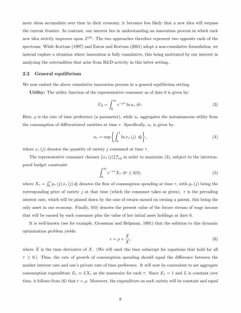
more ideas accumulate over time in their economy, it becomes less likely that a new idea will surpass
the current frontier. In contrast, our interest lies in understanding an innovation process in which each
new idea strictly improves upon Z(k). The two approaches therefore represent two opposite ends of the
spectrum: While Kortum (1997) and Eaton and Kortum (2001) adopt a non-cumulative formulation, we
instead explore a situation where innovation is fully cumulative, this being motivated by our interest in
analyzing the externalities that arise from R&D activity in this latter setting.
2.2 General equilibrium
We now embed the above cumulative innovation process in a general equilibrium setting.
Utility: The utility function of the representative consumer as of date 0 is given by:
U0 =
∫ ∞0
e−ρτ lnuτ dτ . (3)
Here, ρ is the rate of time preference (a parameter), while uτ aggregates the instantaneous utility from
the consumption of differentiated varieties at time τ . Specifically, uτ is given by:
uτ = exp
∫ 1
0lnxτ (j) dj
, (4)
where xτ (j) denotes the quantity of variety j consumed at time τ .
The representative consumer chooses xτ (j)∞τ=0 in order to maximize (3), subject to the intertem-
poral budget constraint: ∫ ∞0
e−rτXτ dτ ≤ b(0), (5)
where Xτ =∫ 1
0 pτ (j)xτ (j) dj denotes the flow of consumption spending at time τ , with pτ (j) being the
corresponding price of variety j at that time (which the consumer takes as given). r is the prevailing
interest rate, which will be pinned down by the rate of return earned on owning a patent, this being the
only asset in our economy. Finally, b(0) denotes the present value of the future stream of wage income
that will be earned by each consumer plus the value of her initial asset holdings at date 0.
It is well-known (see for example, Grossman and Helpman, 1991) that the solution to this dynamic
optimization problem yields:
r = ρ+X
X, (6)
where X is the time derivative of X. (We will omit the time subscript for equations that hold for all
τ ≥ 0.) Thus, the rate of growth of consumption spending should equal the difference between the
market interest rate and one’s private rate of time preference. It will now be convenient to set aggregate
consumption expenditure Eτ ≡ LXτ as the numeraire for each τ . Since Eτ = 1 and L is constant over
time, it follows from (6) that r = ρ. Moreover, the expenditure on each variety will be constant and equal
8
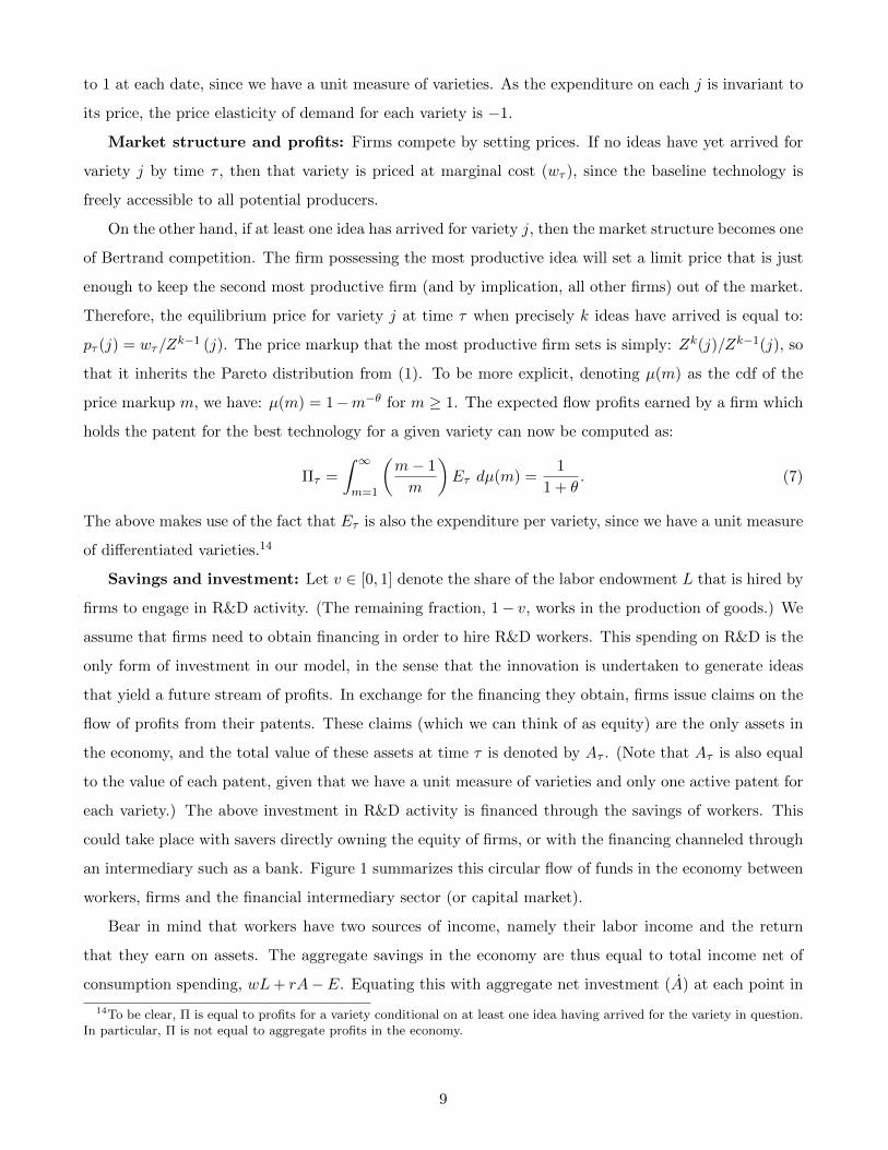
to 1 at each date, since we have a unit measure of varieties. As the expenditure on each j is invariant to
its price, the price elasticity of demand for each variety is −1.
Market structure and profits: Firms compete by setting prices. If no ideas have yet arrived for
variety j by time τ , then that variety is priced at marginal cost (wτ ), since the baseline technology is
freely accessible to all potential producers.
On the other hand, if at least one idea has arrived for variety j, then the market structure becomes one
of Bertrand competition. The firm possessing the most productive idea will set a limit price that is just
enough to keep the second most productive firm (and by implication, all other firms) out of the market.
Therefore, the equilibrium price for variety j at time τ when precisely k ideas have arrived is equal to:
pτ (j) = wτ/Zk−1 (j). The price markup that the most productive firm sets is simply: Zk(j)/Zk−1(j), so
that it inherits the Pareto distribution from (1). To be more explicit, denoting µ(m) as the cdf of the
price markup m, we have: µ(m) = 1−m−θ for m ≥ 1. The expected flow profits earned by a firm which
holds the patent for the best technology for a given variety can now be computed as:
Πτ =
∫ ∞m=1
(m− 1
m
)Eτ dµ(m) =
1
1 + θ. (7)
The above makes use of the fact that Eτ is also the expenditure per variety, since we have a unit measure
of differentiated varieties.14
Savings and investment: Let v ∈ [0, 1] denote the share of the labor endowment L that is hired by
firms to engage in R&D activity. (The remaining fraction, 1− v, works in the production of goods.) We
assume that firms need to obtain financing in order to hire R&D workers. This spending on R&D is the
only form of investment in our model, in the sense that the innovation is undertaken to generate ideas
that yield a future stream of profits. In exchange for the financing they obtain, firms issue claims on the
flow of profits from their patents. These claims (which we can think of as equity) are the only assets in
the economy, and the total value of these assets at time τ is denoted by Aτ . (Note that Aτ is also equal
to the value of each patent, given that we have a unit measure of varieties and only one active patent for
each variety.) The above investment in R&D activity is financed through the savings of workers. This
could take place with savers directly owning the equity of firms, or with the financing channeled through
an intermediary such as a bank. Figure 1 summarizes this circular flow of funds in the economy between
workers, firms and the financial intermediary sector (or capital market).
Bear in mind that workers have two sources of income, namely their labor income and the return
that they earn on assets. The aggregate savings in the economy are thus equal to total income net of
consumption spending, wL+ rA−E. Equating this with aggregate net investment (A) at each point in
14To be clear, Π is equal to profits for a variety conditional on at least one idea having arrived for the variety in question.In particular, Π is not equal to aggregate profits in the economy.
9
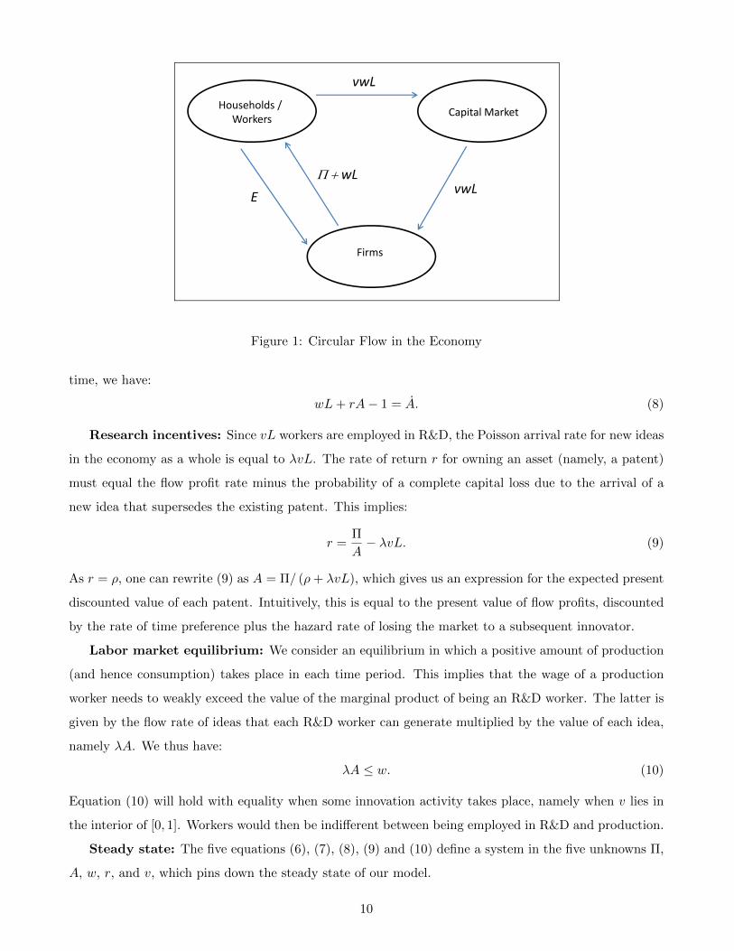
Households / Workers Capital Market
Firms
EwL
vwL
vwL
Figure 1: Circular Flow in the Economy
time, we have:
wL+ rA− 1 = A. (8)
Research incentives: Since vL workers are employed in R&D, the Poisson arrival rate for new ideas
in the economy as a whole is equal to λvL. The rate of return r for owning an asset (namely, a patent)
must equal the flow profit rate minus the probability of a complete capital loss due to the arrival of a
new idea that supersedes the existing patent. This implies:
r =Π
A− λvL. (9)
As r = ρ, one can rewrite (9) as A = Π/ (ρ+ λvL), which gives us an expression for the expected present
discounted value of each patent. Intuitively, this is equal to the present value of flow profits, discounted
by the rate of time preference plus the hazard rate of losing the market to a subsequent innovator.
Labor market equilibrium: We consider an equilibrium in which a positive amount of production
(and hence consumption) takes place in each time period. This implies that the wage of a production
worker needs to weakly exceed the value of the marginal product of being an R&D worker. The latter is
given by the flow rate of ideas that each R&D worker can generate multiplied by the value of each idea,
namely λA. We thus have:
λA ≤ w. (10)
Equation (10) will hold with equality when some innovation activity takes place, namely when v lies in
the interior of [0, 1]. Workers would then be indifferent between being employed in R&D and production.
Steady state: The five equations (6), (7), (8), (9) and (10) define a system in the five unknowns Π,
A, w, r, and v, which pins down the steady state of our model.
10
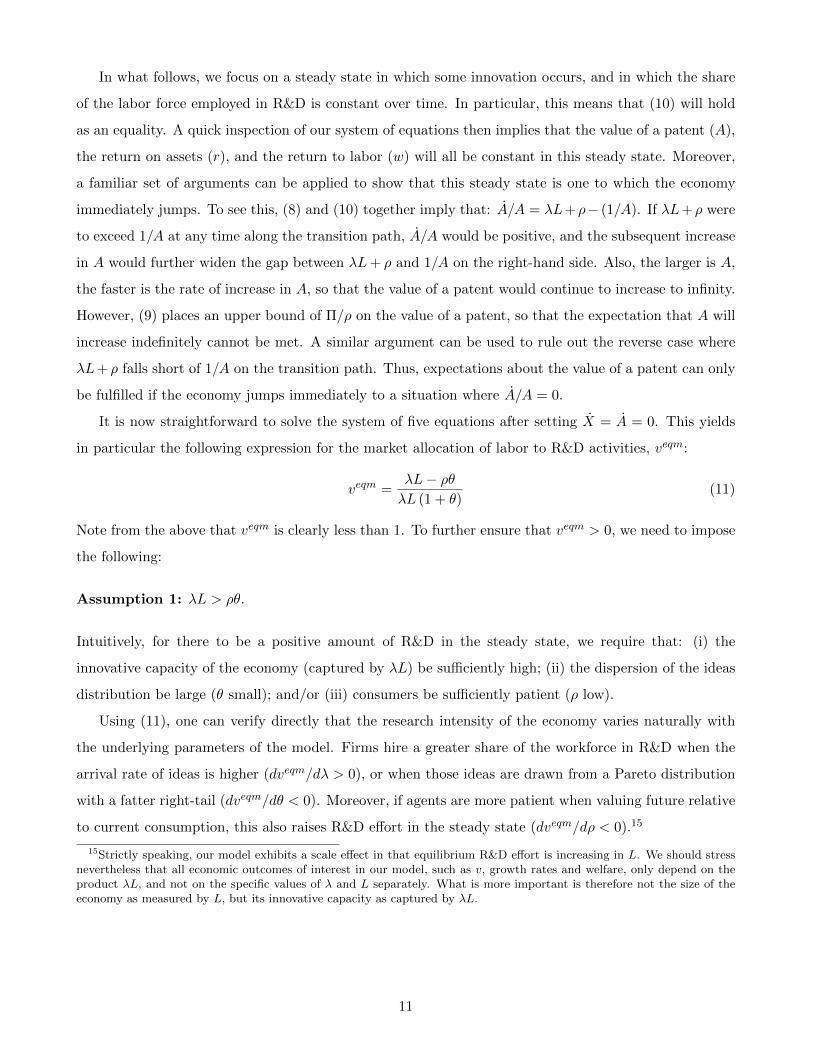
In what follows, we focus on a steady state in which some innovation occurs, and in which the share
of the labor force employed in R&D is constant over time. In particular, this means that (10) will hold
as an equality. A quick inspection of our system of equations then implies that the value of a patent (A),
the return on assets (r), and the return to labor (w) will all be constant in this steady state. Moreover,
a familiar set of arguments can be applied to show that this steady state is one to which the economy
immediately jumps. To see this, (8) and (10) together imply that: A/A = λL+ρ− (1/A). If λL+ρ were
to exceed 1/A at any time along the transition path, A/A would be positive, and the subsequent increase
in A would further widen the gap between λL+ ρ and 1/A on the right-hand side. Also, the larger is A,
the faster is the rate of increase in A, so that the value of a patent would continue to increase to infinity.
However, (9) places an upper bound of Π/ρ on the value of a patent, so that the expectation that A will
increase indefinitely cannot be met. A similar argument can be used to rule out the reverse case where
λL+ ρ falls short of 1/A on the transition path. Thus, expectations about the value of a patent can only
be fulfilled if the economy jumps immediately to a situation where A/A = 0.
It is now straightforward to solve the system of five equations after setting X = A = 0. This yields
in particular the following expression for the market allocation of labor to R&D activities, veqm:
veqm =λL− ρθλL (1 + θ)
(11)
Note from the above that veqm is clearly less than 1. To further ensure that veqm > 0, we need to impose
the following:
Assumption 1: λL > ρθ.
Intuitively, for there to be a positive amount of R&D in the steady state, we require that: (i) the
innovative capacity of the economy (captured by λL) be sufficiently high; (ii) the dispersion of the ideas
distribution be large (θ small); and/or (iii) consumers be sufficiently patient (ρ low).
Using (11), one can verify directly that the research intensity of the economy varies naturally with
the underlying parameters of the model. Firms hire a greater share of the workforce in R&D when the
arrival rate of ideas is higher (dveqm/dλ > 0), or when those ideas are drawn from a Pareto distribution
with a fatter right-tail (dveqm/dθ < 0). Moreover, if agents are more patient when valuing future relative
to current consumption, this also raises R&D effort in the steady state (dveqm/dρ < 0).15
15Strictly speaking, our model exhibits a scale effect in that equilibrium R&D effort is increasing in L. We should stressnevertheless that all economic outcomes of interest in our model, such as v, growth rates and welfare, only depend on theproduct λL, and not on the specific values of λ and L separately. What is more important is therefore not the size of theeconomy as measured by L, but its innovative capacity as captured by λL.
11
2.3 Welfare
We turn next to the task of evaluating country welfare, in order to facilitate our later analysis of the
efficacy of patent policy. The utility specification in (3) and (4) implies that welfare depends on the real
wage in each period, as: uτ = wτ/ exp∫ 1
0 ln pτ (j)dj
. (Recall in particular that the economy jumps
immediately to its steady state.) Since all varieties are ex ante symmetric and we have a unit measure
of these varieties, the law of large numbers implies that the ideal price index in the denominator is equal
to: exp E[lnPτ ], where Pτ is a random variable whose realization is the price of a variety at time τ ;
the expectation operator is taken over this price distribution.
We therefore need to understand how prices evolve over time. Due to the Poisson nature of the
innovation process, the probability that exactly k ideas have arrived by time τ when vL units of labor
are engaged in R&D at each date is: (λvLτ)k
k! e−λvLτ , where k is a non-negative integer. Recall that when
k = 0, the variety in question will be priced at wτ (its marginal cost). On the other hand, when k ≥ 1,
under the limit-pricing rule, the price of a variety will instead be a random variable that inherits the
distribution of wτ/Z(k−1). The expected log price of a variety at time τ is thus:
E [lnPτ ] =(λvLτ)0
0!e−λvLτ lnwτ +
∞∑k=1
(λvLτ)k
k!e−λvLτ
(lnwτ − E[lnZ(k−1)]
). (12)
Note that the first term and each term in the summation in (12) is equal to the probability that k ideas
have arrived between times 0 and τ , multiplied by the log price at time τ when there have indeed been
exactly k ideas (where k = 0, 1, 2, ...,∞).
We show in the Appendix how to evaluate (12) explicitly. The key to this is to recognize that in the
underlying innovation process, the random variable Z(k−1) = Z(k−1)/Z(0) is the product of k−1 indepen-
dent realizations from the standardized Pareto distribution given earlier in (1). (Recall that Z(0) = 1.)
Building off this observation, one can show that lnZ(k−1) is a random variable from a Gamma distribu-
tion with mean E[lnZ(k−1)] = (k−1)/θ (see the Appendix).16 The expected log productivity of the k-th
idea to arrive thus increases linearly in k, while increasing also in the thickness of the right-tail of the
Pareto distribution from which the productivity improvements are drawn. Substituting this expression
for E[lnZ(k−1)] into (12) and simplifying, one then obtains: E [lnPτ ] = lnwτ + 1θ
(1− λvLτ − e−λvLτ
).17
It follows that per-period utility (the real wage) is given by: uτ = exp−1θ
(1− λvLτ − e−λvLτ
).18
16To be absolutely precise, this statement about the distribution of lnZ(k−1) holds only for k ≥ 2. Nevertheless, whenk = 1, we have that E[lnZ(0)] = 0, so that the formula E[lnZ(k−1)] = (k − 1)/θ is also valid for k = 1.
17Much work has been done documenting the fit of the Pareto distribution for firm size distributions (e.g., Axtell 2001;Luttmer 2007; Arkolakis 2011). Interestingly, the Gamma distribution also features a thick right-tail, although it matchesthe empirical distribution of US firms less well for the largest firm sizes (Luttmer 2007).
18The nominal wage can also be solved for explicitly from the system of five equations that pin down the steady state.This is given by: wτ = λ/(ρ+ λL).
12
Defining the growth rate of the real wage to be gτ ≡ d ln (uτ ) /dτ , we have:
gτ =λvL
θ
(1− e−λvLτ
), (13)
which is clearly positive when v > 0. Although the economy jumps immediately to a steady state in
which A, Π, and w (the nominal wage) are constant, the real wage nevertheless rises over time as varieties
are on average becoming cheaper when there is a positive amount of R&D. In other words, Assumption 1
which guarantees that veqm > 0 also ensures that gτ > 0 for all τ ≥ 0. Substituting in the expression for
veqm from (11), one can further verify that: dgτ/dλ > 0 and dgτ/dθ < 0. Thus, a higher arrival rate of
ideas (higher λ) and a larger average productivity improvement (smaller θ) both raise the growth rate of
the real wage at each date τ . From (13), one can moreover see that the growth rate of the real wage rises
over time (dgτ/dτ > 0): From an initial value of gτ = 0, this asymptotes toward a maximum growth rate
of λvL/θ. This property derives from the fact that as time progresses, the baseline technology is shed
from use for a greater and greater share of varieties. As the first idea arrives for successive varieties, the
innovation process gets jump-started for a greater measure of varieties in the unit interval, hence causing
the overall growth rate to rise over time. However, this effect peters out, as the first idea eventually
arrives in expectation for all varieties.
It is instructive here to compare the above against the properties of the models in Kortum (1997)
and Eaton and Kortum (2001), which also focus on a steady state in which the share of the workforce
employed in R&D is constant. In these preceding papers, innovation is not cumulative in nature, and
perpetual growth in real wages is sustained instead by a growing R&D workforce (vL), which grows
at the same exogenous rate as the labor force (L). Thus, more ideas are drawn in each period by the
ever-growing number of R&D workers, overcoming the fact that it gets harder and harder for each idea
drawn from the stationary distribution in (2) to surpass the technological frontier. In contrast, the model
which we have just presented generates steady-state growth in real wages through the cumulative nature
of innovation – new ideas always strictly improve on the technological frontier – without requiring that
the labor force grow over time.
Finally, the expected welfare of the representative consumer is obtained by substituting the expression
for uτ into (3) and evaluating the associated integral. After some algebraic simplification, this yields:
U0 =(λvL)2
ρ2θ(ρ+ λvL)=
(λL− ρθ)2
ρ2θ(1 + θ)(ρ+ λL), (14)
where the last equality follows from replacing v by the expression for veqm from (11). One can show via
straightforward differentiation that so long as Assumption 1 holds, (14) is increasing in λ and decreasing
in θ. Welfare therefore rises either as innovations arrive more frequently or as the average productivity
improvement increases.
13
2.4 Contrast with the social optimum
To understand the efficiency properties of the steady state which we have just solved for, it is instructive
to compare the above market equilibrium with the outcomes under a benign social planner. Conceptually,
this social planner’s problem can be formulated as a labor allocation decision over the share of labor to
employ in R&D, as well as the value of Lpτ (j) for each j ∈ [0, 1], namely the amount of labor assigned to
the production of variety j at each point in time. Formally, the social planner sets out to solve:
maxv,Lpτ (j)1j=0
U0
s.t.
∫ 1
0Lpτ (j) dj = L(1− v) for all τ ≥ 0, (15)
and Lxτ (j) = Lpτ (j)Zτ (j) for all j ∈ [0, 1] and τ ≥ 0. (16)
The first constraint (15) is a labor market-clearing condition that states that all labor not engaged in
R&D must be employed in production. On the other hand, the second constraint (16) sets the quantity
demanded of variety j equal to the quantity produced at each period in time.
As we show in the Appendix, the solution to this social planner’s problem features an equal allocation
of labor to the production of each variety. In other words, given the choice of v, we have: Lpτ (j) =
L(1−v). Using this property, the planner’s problem can then be simplified to the following unconstrained
maximization problem over v:
maxv
U0 =ln(1− v)
ρ+λvL
ρ2θ.
The above maximand is a concave function in v and thus yields a unique optimal allocation of labor
between research and production activities. This social planner’s allocation, denoted by vSP , is given by:
vSP =λL− ρθλL
. (17)
This lies strictly in the interior of [0, 1] if λL > ρθ, namely if Assumption 1 holds. Moreover, comparing
this with the allocation that would emerge in the market equilibrium from (11), one immediately has the
following result:
Proposition 1 The share of labor that a social planner would allocate to research is strictly larger than
that which is observed in the market equilibrium, namely vSP > veqm.
The decentralized equilibrium in our model therefore unambiguously yields less investment in R&D
effort relative to the socially-optimal level. One can moreover see that the relative extent to which
veqm falls short of vSP , namely (vSP − veqm)/vSP is increasing in θ. Intuitively, the less fat-tailed is
the Pareto distribution of productivity improvement draws, the less attractive are the potential private
14
returns (profits) from R&D, and hence the greater the extent of under-investment in R&D in the market
equilibrium relative to the social optimum.
The literature on endogenous growth in the presence of knowledge spillovers has highlighted several
externalities that drive a wedge between the market and social-planner outcomes (e.g., Grossman and
Helpman, 1991; Aghion and Howitt, 1992), and these forces are present too in our model. First, there
is an “intertemporal spillover” effect arising from the cumulative nature of innovation: Firms apply a
higher effective discount rate when evaluating the value of a patent because they do not internalize the
positive knowledge spillovers from their innovation on future productivity improvements. Second, there
is an “appropriability” effect, in that the private profits which firms earn are in general smaller than
the full gains to consumer surplus that each innovation generates. Third, a “business-stealing” effect is
at play, since innovation effort erodes the profits of preceding innovators in a way that a social-planner
would want to fully internalize. The first two of these effects tend to decrease R&D in the market
equilibrium relative to the planner’s problem, while the last effect pushes firms toward over-investing in
R&D. Proposition 1 implies that in our model, the former two effects must dominate the latter “business-
stealing” mechanism.19
We can in fact make a more precise statement concerning the relative importance of these three
externalities. By rearranging (11), observe that the market allocation of labor to research activity is
determined as the solution to: λ(1−v)L(ρ+λvL)θ = 1. On the other hand, the first-order condition of the social
planner’s problem implies that vSP solves: λ(1−v)Lρθ = 1. Thus, the only wedge between the two solutions
arises from the different discount rates that are respectively applied: In the market equilibrium, firms use
a higher discount rate of ρ+ λvL, which takes into account the flow probability of suffering a complete
profit loss to a new innovation, on top of the social discount rate. The only externality that is relevant in
our model is thus the intertemporal spillover effect; evidently, the appropriability and business-stealing
effects must offset each other exactly.
3 Inventive Step Policy
The under-investment in R&D activity which our baseline model features gives rise to the possibility
of welfare-improving policy interventions. We turn next to analyze a policy instrument that can po-
tentially achieve this, namely a minimum inventive step requirement for an idea to be patentable and
non-infringing. As argued in the Introduction, this captures a key dimension of the non-obviousness
criterion commonly stipulated in patent codes. In order to focus attention on this NIS requirement, we
19Note that the presence of monopoly-pricing power per se does not distort labor allocations in our model. The reason isthat all firms charge the same markup in expectation (drawn from the standardized Pareto distribution, µ(m)), so that theallocation of production labor across varieties cannot be improved upon ex ante. See the related discussion in Grossmanand Helpman (1991), p.70.
15
maintain the assumption that patents do not expire; we shall return to incorporate considerations related
to a finite patent length later in Section 4.
3.1 Policy setup: The patenting environment
We retain the cumulative innovation process described in Section 2.1, where each successive productivity
improvement is an independent draw from the standardized Pareto distribution. Even though patenting
was necessary in the baseline model to confer a successful innovator with short-term monopoly power, the
patent authority there played a relatively passive role as all arriving ideas would automatically improve
upon the frontier technology and hence qualify for a patent.
Suppose now that the government announces at date τ = 0 that there will be a “non-infringing
inventive step” (NIS) requirement equal to B ≥ 1 with immediate effect: A new patent will be granted
if and only if the k-th idea to arrive for a given variety improves upon the productivity of the (k− 1)-th
idea by at least B. More formally, this k-th idea is not eligible for a patent if Z(k) ∈ [Z(k−1), BZ(k−1)),
an event that occurs with probability 1−B−θ, based on the Pareto distribution in (1). In this situation,
the firm in possession of this new idea would have no incentive to produce the good even though it
embodies an incrementally better technology, given that it would have no legal right to market the good.
Consequently, non-patentable ideas, which also infringe, are not marketed; the underlying knowledge
does not spread to the rest of society and hence cannot be built upon by subsequent innovators. This
serves to capture the idea that the public disclosure of technical knowhow that each patent application
requires is a crucial platform for facilitating knowledge diffusion.
We make explicit two remarks on this treatment of non-patentable ideas. First, note that the owner
of a non-patentable idea would herself be unable to build cumulatively on it, since future research effort
cannot be directed toward a particular variety in this setup. Second, we rule out the possibility of this
owner selling the non-patentable idea to the incumbent patent-holder of the variety. Any such attempted
sale would require the owner of the idea to first share information about it with the patent-holder (for
example, to show proof of concept). However, upon disclosure, the incumbent patent-holder would then
be able to appropriate the knowledge without compensating the owner of the idea, and further use it for
market production with no fear of legal action since the idea could not be patented in the first place.
The owner of the idea would thus have no incentive to attempt such a transaction.
On the other hand, if the k-th idea to arrive were to satisfy Z(k) ∈ [BZ(k−1),∞), an event that occurs
with probability B−θ, the firm in possession of this idea would indeed patent it in order to subsequently
enjoy the profits from marketing the good. Since what is important now is whether an idea is patentable
or not, we let Z(k) denote the random variable associated with the productivity level of the k-th patentable
idea to arrive after time τ = 0. Moreover, let ζ(k) = Z(k)/Z(k−1) denote the productivity improvement
16
that is associated with this k-th patentable idea. The distribution of ζ(k) is then governed by the following
conditional probability:
Pr(ζ(k) < z
)= Pr
(ζ(k) < z|ζ(k) > B
)=
Pr(B < ζ(k) < z
)Pr(ζ(k) > B)
= 1−( zB
)−θ, z ≥ B, (18)
where the above derivation makes use of the fact that ζ(k) is from the Pareto distribution given in (1).
The productivity improvement with each successive patentable innovation is thus also drawn from a
Pareto distribution with the same shape parameter θ, but with the lower bound of its support truncated
at B ≥ 1. Note too that the distribution of ζ(k) does not depend on k, the number of patentable ideas
that have already arrived.
3.2 Inventive step policy and equilibrium research effort
With the above formulation of the patenting process, we can readily embed our model in a general
equilibrium setting following the approach in Section 2.2. As explained above, we consider a situation
in which the NIS requirement, B, is introduced at date 0 and held constant subsequently. We highlight
below how this policy intervention alters profits and research incentives relative to the baseline model.
We describe first the prices that will be observed. For a given variety j, if no patentable ideas have
arrived by time τ , firms will produce this variety using the publicly-available baseline technology and
price the good at marginal cost, wτ . On the other hand, if k ≥ 1 patentable ideas have arrived for variety
j by time τ , Bertrand competition then implies that the firm with the best patentable idea will set a
limit-price equal to: wτ/Z(k−1) (j). Once patentable ideas have started arriving, the firm with the best
patented idea will price at a markup given by: Z(k)(j)/Z(k−1)(j), which from (18) is a random variable
with cdf: µ(m) = 1 − (m/B)−θ, where m ∈ [B,∞) is the markup. The flow of profits accruing to this
patent-holding firm can now be evaluated as:
Πτ =
∫ ∞m=B
(m− 1
m
)Eτ dµ(m) =
B(1 + θ)− θB(1 + θ)
. (19)
(Recall that Eτ = 1 by our choice of numeraire.) The above profit expression coincides with equation (7)
from the baseline model when B is equal to 1. From (19), one can see that profits will take up a larger
share of consumer expenditures when B is higher because patentable ideas embody a larger productivity
improvement on average. As before, a smaller θ is also associated with higher profits, as a more fat-tailed
Pareto distribution means that firms can on average expect to charge a higher markup.
The patenting requirement that is now in place will affect research incentives. As before, the value of
assets in the economy is equal to the aggregate value of patents. The rate of return r to owning a unit
of these assets must once again be equal to the profit rate net of the flow probability of experiencing a
complete capital loss. On the latter, even though the Poisson arrival rate of ideas remains λvL, each new
17
idea will only be patentable with probability B−θ. In particular, a binding inventive step requirement
(B > 1) would strictly lower the likelihood that an incumbent patent-holder gets superseded by a newly-
arrived idea, which effectively extends the duration of the incumbent’s monopoly power. At each point
in time, we thus have:
r =Π
A− λvLB−θ. (20)
It follows from (20) that the expected present discounted value of each patent, A, is now equal to
Π/(ρ+ λvLB−θ
).
Since the probability that a given idea will be patentable now depends on the required inventive step,
the labor market equilibrium condition must also be modified accordingly. The value of the marginal
product of an R&D worker is now λB−θA, as the flow probability of receiving an idea that clears the NIS
requirement is λB−θ. A more stringent requirement (a higher B) will thus reduce the expected returns
to working in R&D. For some production to occur in each time period, we require that:
λB−θA ≤ w, (21)
namely that the wages from being a production worker weakly exceed the value of the marginal product
of an R&D worker. In the steady state which we will consider, in which a positive and constant share of
the workforce is allocated to research, the above must hold as an equality.
To close out the model, observe that the intertemporal welfare maximization and circular flow condi-
tions from (6) and (8) remain unchanged. The equilibrium is therefore determined by these two equations
in combination with (19), (20) and (21). The five unknowns of this system are once again Π, A, w, r,
and v. As before, we focus our attention on a steady state in which v is (weakly) positive and constant.
A set of arguments analogous to that in the baseline model can be applied to show that A, w and r will
all be constant in this steady state. It will also be the case that the economy jumps instantaneously to
this steady state upon the introduction of the inventive step requirement, B.
Equilibrium research effort: Setting A = X = 0 and solving out for this steady state, one obtains
(after some algebraic simplification) the following expression for the R&D labor share:
v(B) = max
1− θ
B(1 + θ)− ρθBθ
λLB(1 + θ), 0
. (22)
We write v explicitly as a function of B to emphasize the scope that patent policy now has to affect
equilibrium research effort. Note from (22) that v(B) is strictly less than 1 for B ≥ 1, so the steady
state will never feature complete specialization in R&D. It is possible however for the steady state to
feature no R&D, as v(B) = 0 when B →∞ (since Bθ−1 would tend to ∞, as θ > 1). To be precise, we
have v(B) > 0 if and only if λL > ρθBθ
B(1+θ)−θ . When B = 1, this condition reduces back to Assumption
1 (which we will continue to adopt), and v(B) coincides exactly with the expression for veqm from (11);
18
in particular, this means that v(1) > 0. Straightforward differentiation further reveals that the function
Bθ
B(1+θ)−θ is decreasing when B ∈ [1, θ2/(θ2 − 1)), and increasing when B ∈ (θ2/(θ2 − 1),∞), with the
value of Bθ
B(1+θ)−θ tending to infinity as B gets arbitrarily large. This implies that there is a unique
value of B, which we denote as B0, below which λL > ρθBθ
B(1+θ)−θ , but above which the inequality will be
violated. Thus, v(B) > 0 if and only if B ∈ [1, B0).
Holding B constant, various comparative static properties of v(B) carry over from the baseline model.
Specifically, research effort will be (weakly) higher if agents are more patient (ρ low), the average produc-
tivity improvement is larger (θ low), or the arrival rate of ideas is higher (λ large). More interestingly,
we can characterize how patenting standards now affect R&D outcomes. From (22), the share of labor
in research clearly varies non-monotonically with B. This is consistent with the observation that a more
stringent inventive step requirement will have conflicting effects. On the one hand, a higher B lowers
the hazard rate that an incumbent patent-holder faces of losing its market to a new innovation, which
ex ante would raise incentives for firms to hire more R&D workers (a “profit” effect). However, a higher
required inventive step also lowers one’s probability of successfully obtaining a patentable idea in the
first place, which is often termed the “hurdle” effect in the patenting literature.
To analyze the net effect of these two forces, let us define: v(B) = 1− θB(1+θ) −
ρθBθ
λLB(1+θ) . We have:
dv
dB=
(θ
1 + θ
)1
B2
[1− ρ(θ − 1)
λLBθ
]. (23)
Denote the value of B for which dv/dB = 0 by Bv, given explicitly by: Bv =[
λLρ(θ−1)
] 1θ. Since dv/dB < 0
for all values of B lower than Bv, while dv/dB > 0 for all B above Bv, Bv is the unique turning point of
v(B). In addition, we have Bv > 1 so long as λL > ρ(θ−1), which is automatically satisfied if Assumption
1 holds. Using these properties, we can now characterize the behavior of v(B) = maxv(B), 0. As
illustrated in Figure 2, the equilibrium allocation of labor is positive at B = 1 and first rises as B is
raised above 1. It then reaches its maximum value when B = Bv, before declining toward 0 and meeting
the horizontal axis at B = B0; we then have v(B) = 0 for all B ≥ B0.
Defining the rate of innovation as the Poisson arrival rate of ideas, λvL, we now have:
Proposition 2 Suppose that λL > ρθ (Assumption 1 holds). Then: (i) dvdB > 0 when B ∈ [1, Bv), (ii)
dvdB < 0 when B ∈ (Bv, B0), and (iii) v(B) = 0 for all B ∈ [B0,∞), so that Bv is the unique value of
the NIS requirement that maximizes the equilibrium allocation of labor to R&D. In particular, raising B
slightly from B = 1 will induce a higher rate of innovation. However, raising B when the NIS parameter
is already above Bv will lower the rate of innovation.
Intuitively, when the inventive step requirement is smaller than Bv, the profit effect dominates the
hurdle effect, so that a more stringent patent standard raises the incentive to employ labor in R&D.
19
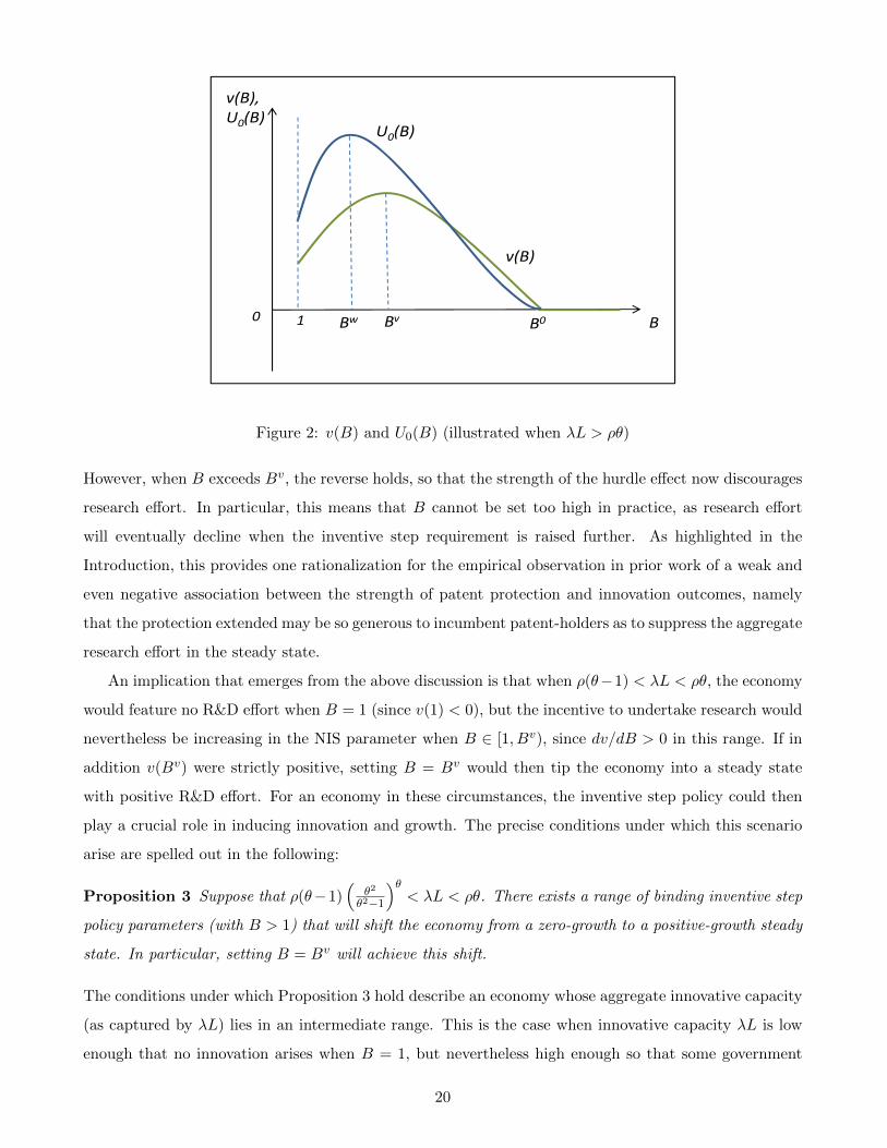
B1
v(B), U0(B) U0(B)
v(B)
Bw Bv B00
Figure 2: v(B) and U0(B) (illustrated when λL > ρθ)
However, when B exceeds Bv, the reverse holds, so that the strength of the hurdle effect now discourages
research effort. In particular, this means that B cannot be set too high in practice, as research effort
will eventually decline when the inventive step requirement is raised further. As highlighted in the
Introduction, this provides one rationalization for the empirical observation in prior work of a weak and
even negative association between the strength of patent protection and innovation outcomes, namely
that the protection extended may be so generous to incumbent patent-holders as to suppress the aggregate
research effort in the steady state.
An implication that emerges from the above discussion is that when ρ(θ−1) < λL < ρθ, the economy
would feature no R&D effort when B = 1 (since v(1) < 0), but the incentive to undertake research would
nevertheless be increasing in the NIS parameter when B ∈ [1, Bv), since dv/dB > 0 in this range. If in
addition v(Bv) were strictly positive, setting B = Bv would then tip the economy into a steady state
with positive R&D effort. For an economy in these circumstances, the inventive step policy could then
play a crucial role in inducing innovation and growth. The precise conditions under which this scenario
arise are spelled out in the following:
Proposition 3 Suppose that ρ(θ−1)(
θ2
θ2−1
)θ< λL < ρθ. There exists a range of binding inventive step
policy parameters (with B > 1) that will shift the economy from a zero-growth to a positive-growth steady
state. In particular, setting B = Bv will achieve this shift.
The conditions under which Proposition 3 hold describe an economy whose aggregate innovative capacity
(as captured by λL) lies in an intermediate range. This is the case when innovative capacity λL is low
enough that no innovation arises when B = 1, but nevertheless high enough so that some government
20
intervention can help to create research incentives. (The proof of this proposition is in the Appendix;
we also show there that (θ − 1)(
θ2
θ2−1
)θ< θ is satisfied for all θ > 1, so that the conditions for the
proposition to hold can indeed be met.)
3.3 Inventive step policy and welfare
We turn now to evaluate the consequences for welfare. As in our baseline model, this will require that
we evaluate the ideal price index that consumers face, in order to compute their real wage. Note that
the expected log price is now given by:
E [lnPτ (j)] =
(λvLB−θτ
)00!
e−λvLB−θτ lnwτ +
∞∑k=1
(λvLB−θτ
)kk!
e−λvLB−θτ(
lnwτ − E[ln Z(k−1)])
. (24)
The first term above is the expected log price for a variety when there are no patentable ideas, while
the remaining terms in the summation are the corresponding expressions that apply when exactly k ≥
1 patentable ideas have arrived. There are two modifications in (24) relative to equation (12) from
Section 1.3. First, the Poisson arrival rate is now λvLB−θ, with the additional B−θ term capturing the
productivity hurdle that new ideas must cross; this tends to lower the arrival probability of patentable
ideas. Second, when k ≥ 1, firms now set their limit price at the marginal cost implied by the previous
patentable idea, namely wτ/Z(k−1). Recall in particular that the productivity improvement between
consecutive patentable ideas (Z(k)/Z(k−1)) is drawn from the Pareto distribution in (18) with the lower
bound of its support equal to B.
Our analysis is once again tractable because the above price index can be worked out explicitly. We
show in the Appendix that ln Z(k−1) takes on the same Gamma distribution from the baseline model,
but with a linear shift. Specifically, we find that: E[ln(Zk−1)] = (k−1)(
1θ + lnB
)for all k ≥ 1, with the
additional (k− 1) lnB term reflecting the effect that the inventive step policy has in raising the expected
productivity level of the (k − 1)-th innovation. Substituting this property into (24), one can then show
that: E [lnPτ (j)] = lnwτ +(
1θ + lnB
) (1− λvLB−θτ − e−λvLB−θτ
).
It follows that the real wage at time τ , which is also equal to the period flow utility uτ , is given by:
wτ/E [lnPτ (j)] = exp−(
1θ + lnB
) (1− λvLB−θτ − e−λvLB−θτ
). At time τ , the real wage therefore
grows at the following positive rate:
gτ ≡d lnuτdτ
=
(1
θ+ lnB
)λvLB−θ
(1− e−λvLB−θτ
). (25)
Given B, and hence v(B), the growth rate of the real wage rises and asymptotes over time to a maximum
of(
1θ + lnB
)λvLB−θ, for much the same reasons as were discussed in the baseline model.
The welfare of the representative consumer is then given by plugging in the above expression for uτ
21
into (3) and evaluating the integral for the present discounted value of the flow of real wages. This yields:
U0(B) =
(1
θ+ lnB
) (λvLB−θ
)2ρ2 (ρ+ λvLB−θ)
. (26)
Further replacing v in the above by the expression for v(B) from (22), one then obtains a welfare formula
that depends only on the primitive parameters of the model (ρ, θ, and λL) and the required inventive
step, B.
We can now assess the tradeoffs that arise from the use of this NIS requirement. Note from (26) that
U0(B) = 0 for all B ≥ B0, as v(B) = 0 in this range of values of B. We thus restrict our attention
to study how welfare behaves when B ∈ [1, B0), where both U0(B) and v(B) take on positive values.
Differentiating the welfare expression in (26) with respect to B, one obtains:
dU0
dB∝(
1
θ+ lnB
)Bdv
dB− θv lnB − ρv
2ρ+ λvLB−θ, (27)
where ‘∝’ indicates equality up to a positive multiplicative term. The first-order necessary condition for
a local welfare maximum thus entails setting the right-hand side of (27) equal to 0.
Is the welfare-maximizing inventive step requirement binding (i.e., strictly greater than 1)? And does
the welfare function in (26) indeed exhibit a unique maximum turning point? The former issue can be
addressed by examining the behavior of dU0/dB in the neighborhood of B = 1. One can verify through
direct substitution that dU0/dB > 0 at B = 1, as long as Assumption 1 holds, so that there is in fact a
net gain from increasing the inventive step parameter slightly above 1. On the latter issue, even though
U0(B) is in general not concave for all B ∈ [1, B0), we nevertheless can prove that the right-hand side of
(27) is strictly decreasing in B in the smaller interval B ∈ [1, Bv). (See the Appendix for details.) Observe
too that for B > Bv, we have dv/dB ≤ 0; from (27), this implies that dU0/dB < 0 for B > Bv. Taken
together, we find that dU0/dB is first positive at B = 1, is strictly negative at B = Bv, and exhibits at
most one root in the interval [1, Bv). This allows us to conclude that there is a unique Bw that satisfies
dU0/dB = 0. Figure 2 illustrates these properties of the welfare function U0(B), in conjunction with the
behavior of v(B).
This leads us to our main result characterizing the optimal NIS requirement from a welfare perspective:
Proposition 4 Suppose that λL > ρθ (Assumption 1 holds). Then the welfare-maximizing inventive
step requirement is unique with 1 < Bw.
There is thus scope to improve welfare by setting an inventive step requirement strictly larger than 1,
so long as λL is sufficiently large. The role of Assumption 1 here is intuitive: The innovative capacity
of the economy needs to be high enough to ensure that the increased rate of innovation will more than
exceed the social cost of ceding more monopoly power to patent-holders.
22
It is helpful at this juncture to examine (27) closely in order to get more intuition on the economic
tradeoffs involved in the setting of the NIS requirement. The net effect of stronger patent protection is in
principle ambiguous, but the underlying effects can be decomposed systematically. Note first that welfare
can be written more explicitly as: U0 = U0(B, v (B)), with its corresponding total derivative given by:
dU0dB = ∂U0
∂vdvdB + ∂U0
∂B . The first term on the right-hand side of (27), namely(
1θ + lnB
)B dvdB , corresponds
precisely to the ∂U0∂v
dvdB term in this total derivative. The key force captured here is commonly referred
to in the IPR literature as the “dynamic” effect of patent protection in raising innovation rates (see for
example, Nordhaus 1969; Tirole 1988; Grossman and Lai 2004). In the context of our model, we have
already seen that when B is sufficiently small, specifically when B ∈ [1, Bv), an increase in the required
inventive step raises the steady-state allocation of labor to research ( dvdB > 0), thus raising the equilibrium
rate of innovation. Ceteris paribus, this has a positive effect on welfare as ∂U0∂v > 0, a fact which can be
verified by straightforward differentiation of (26). Therefore, this dynamic effect term, ∂U0∂v
dvdB , is indeed
positive when B ∈ [1, Bv).
This potential benefit from raising the NIS requirement needs to be weighed against a countervailing
force, namely the static loss suffered in each period by consumers arising from the longer duration of each
patent-holder’s monopoly power. This latter effect is reflected by the second and third terms in (27),
−θv lnB− ρv2ρ+λvLB−θ
, which are clearly negative when v > 0. Note that these terms indeed map precisely
to the ∂U0∂B term in the preceding total derivative. The welfare-maximizing inventive step requirement
therefore needs to trade off the dynamic gains from a greater degree of patent protection against the
static consumer surplus losses that are incurred.20 When B < Bw, the dynamic effect dominates the
static effect, and so dU0/dB > 0 in this range of values of B; conversely, when B > Bw, the static effect
dominates and dU0/dB < 0.
Inspecting dU0dB = ∂U0
∂vdvdB + ∂U0
∂B further, we have: dU0/dB < 0 for all B ∈ [Bv, B0). This holds because
dv/dB ≤ 0 when B ∈ [Bv, B0), and also because it is always true that ∂U0∂B < 0 and ∂U0
∂v > 0. Welfare is
therefore strictly decreasing in the interval [Bv, B0). Since the inventive step parameter that maximizes
welfare is unique, Bw must lie in the interval B ∈ [1, Bv) where dv/dB > 0, so that there is some benefit
from introducing an inventive step policy through the increased research effort it induces. We sum up
this argument as:
Proposition 5 The value of the required inventive step B that maximizes welfare is strictly less than
that which maximizes the rate of innovation. In other words, Bw < Bv.
This result is actually very intuitive, as the value of B that maximizes the research intensity of the
20A similar tradeoff is encountered if one considers instead the problem of choosing B to maximize the steady-state growthrate in (25). As discussed in section 3.2, the marginal benefit to innovators from raising B (profit effect) needs to be weighedagainst the marginal cost (hurdle effect).
23
economy requires consumers to give up too much current consumption to invest in R&D. When it is
welfare instead that is the policy-maker’s objective, an additional cost associated with raising B must
be taken into account, namely the loss to consumer surplus. This insight is in fact a relatively general
one: Horowitz and Lai (1996) also obtained an analogous result in a different setting where the policy
instrument instead takes the form of a specified patent length, namely that the patent duration that
maximizes the rate of innovation is longer than that which maximizes welfare.
3.4 Properties of the optimal inventive step requirement
Having established the existence of a unique welfare-maximizing NIS requirement, we turn next to explore
how Bw is influenced by the deep parameters of our model. As we do not have a closed-form expression for
Bw, we pursue a numerical approach to illustrate the behavior of this optimal inventive step requirement.
A convenient feature of our model is that the equilibrium is in fact characterized by a parsimonious
set of three parameters. These are the discount rate (ρ), the shape parameter of the Pareto distribution
(θ), and the innovative capacity of the economy (λL). In particular, all steady-state outcomes depend
only on the product λL, and not on the separate values taken on by λ and L. We proceed by adopting a
set of baseline values for these three parameters, from which we illustrate the effects of varying each key
parameter in turn. We should stress that the purpose here is not to offer a strict calibration, but rather
to explore how Bw (and Bv) behave around a sensible choice of parameters.
We first choose ρ = 0.07. This follows Kortum (1997), who matches this to the real return observed
on stock markets, which arguably provides a relevant reference point for the returns to innovation. That
said, we will explore a wide range of values for ρ ranging between 0.02 and 0.12. For θ, we set this
equal to 4; based on (7), this corresponds to expected profits making up a 25% share of expenditures
per variety in the absence of a binding inventive step policy (as 1/(1 + θ) = 0.25). We allow θ to vary
between 2 and 6 in our numerical exercises, which translates into an expected profit share ranging from
14% to 33%. Last but not least, we pick λL = 1, which implies a relatively modest average arrival rate
of one new idea per variety in a given year. Note that this set of baseline parameters satisfies λL > ρθ,
which is required for our propositions to hold. They moreover imply a baseline welfare-maximizing NIS
requirement of Bw = 1.14, with the steady-state share of labor allocated to R&D being v(Bw) = 0.22.21
The left-hand column of Figure 3 shows how the optimal inventive step requirement responds to the
underlying primitives of the model. Observe first that a higher discount rate is associated with a lower
Bw. Intuitively, as agents place a higher weight on current relative to future consumption, the marginal
social benefit of promoting innovation is lower, and so the welfare-maximizing patent policy responds by
placing less emphasis on promoting research. Not surprisingly, Bw is also lower if the idea distribution
21From (25), these parameter values also imply a maximum growth rate of the real wage of 4.8%, which is achievedasymptotically as τ −→∞.
24
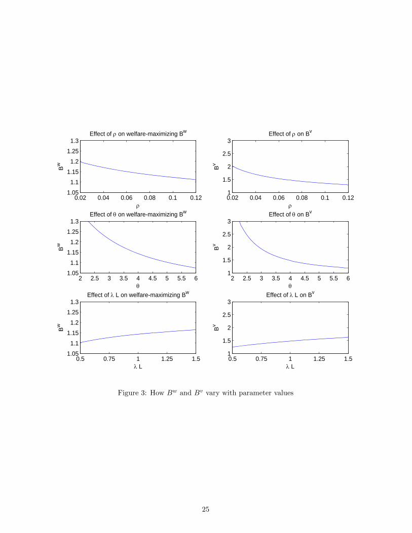
0.02 0.04 0.06 0.08 0.1 0.121.05
1.1
1.15
1.2
1.25
1.3
Bw
Effect of on welfare-maximizing Bw
0.02 0.04 0.06 0.08 0.1 0.121
1.5
2
2.5
3
Bv
Effect of on Bv
2 2.5 3 3.5 4 4.5 5 5.5 61.05
1.1
1.15
1.2
1.25
1.3
Bw
Effect of on welfare-maximizing Bw
2 2.5 3 3.5 4 4.5 5 5.5 61
1.5
2
2.5
3
Bv
Effect of on Bv
0.5 0.75 1 1.25 1.51.05
1.1
1.15
1.2
1.25
1.3
L
Bw
Effect of L on welfare-maximizing Bw
0.5 0.75 1 1.25 1.51
1.5
2
2.5
3
L
Bv
Effect of L on Bv
Figure 3: How Bw and Bv vary with parameter values
25
exhibits a thinner right-tail (higher θ), due to the smaller marginal benefit that can be gained from raising
B when the productivity improvement draws are on average smaller. A similar logic explains why one
should expect to see a higher optimal inventive step requirement in economies with a larger innovative
capacity (λL). Interestingly, among these three parameters, Bw appears most sensitive to changes in θ.
The plots in the right-hand column of Figure 3 moreover confirm that Bv (the inventive step requirement
that maximizes the allocation of labor to research) exhibits similar comparative statics. Note from the
figures that Bv is always less than Bw, consistent with Proposition 5.
4 Inventive Step Policy with Finite Patent Length
We turn now to incorporate considerations related to patent length. This is of independent interest,
given that much of the literature on IPR protection has arguably focused on patent length as the key
statutory instrument for promoting research. Our framework also raises questions related to how the
choice of patent length might interact with the NIS requirement when both instruments are available to
and jointly set by a welfare-maximizing government. It turns out that such issues can be tackled in our
model of cumulative innovation.
Suppose that the patent authority introduces a policy at time τ = 0, specifying that each patent will
expire after a fixed duration, Ω, has elapsed from the date the patent was first granted. Upon expiration,
all other firms in the economy are free to make use of the underlying technology to produce the variety
in question, which will immediately drive down the monopoly profits of the incumbent patent-holder to
zero. However, if a sufficiently good idea were to arrive before Ω has elapsed, namely one that clears
the required inventive step (and thus satisfies the non-obviousness criterion), then a new patent will
be granted to this innovation. In this latter situation, the incumbent will lose her market by virtue of
being superseded by a better idea, even though her patent has not yet expired. Our treatment in the
previous sections thus corresponds to Ω −→∞, namely where patents do not expire, so incumbents can
only be displaced by a newly-arrived idea that embodies a sufficiently large improvement. In practice,
however, patent boards do not grant patents of indefinite length. Under TRIPS, for example, Ω has been
harmonized to 20 years across all members of the World Trade Organization.
The key change that this makes in our equilibrium system of equations lies in its effect on research
incentives. While investors continue to apply an effective discount rate of ρ+ λvLB−θ when evaluating
the returns from a successful innovation, they now also have to contend with the finite expiry date of
each patent. With this modification, the flow value of an asset is:
A =
∫ Ω
0e−(ρ+λvLB−θ)τ Π dτ =
Π
ρ+ λvLB−θ
[1− e−(ρ+λvLB−θ)Ω
]. (28)
26
Note that the upper limit of the integral (previously ∞) has been replaced by Ω, to reflect the fact that
each patent will cease to yield a return after the patent length has been reached.22 The final expression
for A on the right-hand side of (28) thus equals the value of a patent if it had an infinite life span,
multiplied by the fraction of that value that accrues during the first Ω years after the patent is awarded.
The equilibrium is now obtained by solving (28) together with the previous four steady-state equations
(6), (8), (19), and (21). After substituting Π, A, w, and r out of this system, we are left with the following
equation that pins down v implicitly as a function of B, Ω and other model parameters:
ρ+ λvLB−θ
ρ+ λLB−θ=B(1 + θ)− θB(1 + θ)
[1− e−(ρ+λvLB−θ)Ω
]. (29)
Although we no longer can solve for the share of labor in R&D in closed-form, we can nevertheless use
(29) to establish the following lemma (see the Appendix for the proof):
Lemma 1: There exists a unique solution for v from equation (29) which lies in the interior of [0, 1] if
and only if λL > ρBθ[
B(1+θ)B(1+θ)−θ
(1
1−e−ρΩ
)− 1].
The algebraic condition in Lemma 1 is the analogue of Assumption 1 from our baseline model. (In
particular, setting B = 1 and Ω −→ ∞, the condition reduces to λL > ρθ.) Once again, the intuition
here is that the innovative capacity of the economy needs to be sufficiently large to ensure that the
equilibrium will feature a strictly positive amount of research effort. Note also that the longer is the
duration of patent protection, Ω, the easier it is for this condition to be satisfied. Moving forward, we
will assume that the above condition in Lemma 1 is met to guarantee the existence and uniqueness of v.
What implications does the patent length bear for research effort and welfare in our model? First,
one can verify via log differentiation of (29) that:
Lemma 2: dvdΩ > 0.
(See the Appendix for the proof.) In contrast to the NIS requirement, the allocation of labor to research
increases monotonically in the strength of protection accorded by the patent length. In other words,
granting a longer (expected) duration of monopoly power to each patent-holder strictly raises the incen-
tives to undertake R&D. A quick implication is that the equilibrium allocation of labor to research when
a finite patent length is set is strictly less than the v which would be observed under non-expiring patents
(as in our Section 3 model). This is because the patent length sets a finite upper bound on how long a
patent-holder can exercise her monopoly power, which clearly weakens research incentives relative to our
baseline model with a de facto infinite patent length. (The above holds regardless of the NIS requirement
22This assumes that investors can hold a diverse portfolio of assets each with the expected value given in (28), so that theactual timing of the expiration of an individual patent does not matter to investors.
27
that is chosen, so long as B is taken as given.) Put differently, while there is a “profit” effect, there does
not exist a “hurdle” effect in the case of patent length.
Turning to the issue of welfare, Lemma 2 implies that there will always be a dynamic gain to the
economy from raising the patent length, as research effort is increasing in Ω. This however needs to
be balanced against the static loss that consumers must bear, owing to the longer expected duration of
each incumbent’s monopoly power. In the Appendix, we carefully show how to compute the new price
index and welfare expression when Ω is finite, given the underlying idea arrival process in our model. To
summarize the arguments there, three cases need to be considered separately. First, when 0 < τ < Ω,
no patents would have expired yet during this early time frame, so that the patent length is irrelevant
for calculating the price index. Second, when τ > Ω and the time since the last idea arrived exceeds Ω,
then the patent on this last idea would have expired and the variety is priced at marginal cost. Third,
when τ > Ω, but the time since the last idea arrived is shorter than Ω, then the incumbent patent-holder
adopts a limit price. With these considerations in mind, and evaluating the welfare integral over all
τ > 0, we derive the following welfare expression:
U l0 =
(1
θ+ lnB
) (λvLB−θ
)2ρ2 (ρ+ λvLB−θ)
[1 +
ρ
λvLB−θe−(ρ+λvLB−θ)Ω
]. (30)
As one would expect, (30) converges to (26) from Section 3 when Ω −→ ∞. Holding v constant, the
welfare expression in the presence of a finite patent length is strictly greater than that when Ω −→ ∞,
the reason being that prices are on average lower under a finite patent length: Each patent-holder’s
monopoly pricing power definitively gets curtailed after a duration of Ω if it has not yet been leapfrogged
by a better idea.
We can now explicitly analyze the welfare consequences of patent length policy. Differentiating (30),
one can in fact show that dU l0/dΩ > 0 whenever Ω is finite. This leads to the following:
Proposition 6 When both patent length and inventive step policy instruments are available, the optimal
policy entails using an infinite patent length policy if welfare is the objective to be maximized.
The proof proceeds by considering (30) explicitly as a function of its arguments: U l0 = U l0 (B,Ω, v (B,Ω)).
Evaluating the total derivative with respect to Ω, we have:dU l0dΩ =
∂U l0∂v
dvdΩ +
∂U l0∂Ω . We show in the Appendix
that∂U l0∂Ω < 0, namely that there are indeed static consumer surplus losses from granting patent-holders
with a longer monopoly. Nevertheless, it turns out that the positive dynamic gains from raising R&D
(∂U l0∂v
dvdΩ , where
∂U l0∂v > 0 and dv
dΩ > 0 always) strictly dominate these static losses, regardless of the required
inventive step B that might be chosen. It follows from the above that the welfare-maximizing policy calls
for setting Ω −→∞ and adopting the optimal NIS requirement, Bw, characterized in Section 3.
What intuition can we offer for the above result? Note first that extending the patent length strictly
raises R&D effort, in contrast to the non-monotonic relationship seen in Section 3 between the NIS
28
parameter and v that arises from the hurdle effect. There is thus always a positive dynamic gain to be
had from raising Ω, which counteracts the static loss from extending monopoly power. This opens the
door to the possibility that the optimal patent length could be infinite. More importantly, there are
no diminishing returns to innovation effort in our model, as the Poisson arrival rate of ideas is simply
proportional to the aggregate amount of research labor vL at each date, and each arriving idea delivers
a productivity improvement drawn from the same underlying Pareto distribution. The intuition here
is best communicated in the case where the subjective discount rate is zero. The marginal static loss
of extending the patent length incrementally would then equal the additional consumer surplus ceded
at each date, which is a constant (independent of Ω) in our model. On the other hand, the marginal
dynamic gain – the benefit from more induced innovation – does not diminish even as Ω increases. Thus,
so long as the initial innovative capacity of the economy is large enough so that a positive amount of
R&D can be sustained (namely, the condition in Lemma 1 is met), there is always a net welfare gain
from raising Ω, implying an infinite optimal patent length.
It is interesting to compare our findings here with previous results from the industrial organization
literature on the optimal combination of patent instruments. Klemperer (1990) finds that the optimal
mix of patent length and patent breadth policies can call for either long and narrow patents, or short
and broad ones, depending on conditions related to the degree of substitutability across products. The
concept of the patent breadth adopted here nevertheless focuses more on the horizontal differentiation
of products, and applies less to our setting where innovation delivers ongoing improvements on existing
products. In contrast, Gilbert and Shapiro (1990) argue that an infinite patent length, plus a patent
breadth adjusted to provide a fixed profit to the innovator is, under reasonably general conditions, the
welfare-maximizing policy, where the notion of breadth is captured by the size of the flow profits that
are ceded to successful innovators.23
Notwithstanding the sharp result in Proposition 6, it is commonly observed that patent boards
around the world do set finite patent lengths in practice. While this would be inconsistent with welfare-
maximization in the context of our model, the patent authority may nevertheless seek to limit the duration
of IPR protection in pursuit of other objectives. For example, ethical or public health considerations
might prompt governments to curtail the monopoly power of pharmaceutical firms, in order to provide
cheaper access to drugs. Our final result asks how the welfare-maximizing inventive step requirement
would respond to Ω, when the latter is set by considerations that are outside of our model.
Proposition 7 Suppose that a finite patent length Ω is set by the patent board for exogenous reasons.
Then, the welfare-maximizing NIS requirement, Bw, is increasing in the choice of Ω by the patent board.
23Gallini (1992) finds that an infinite patent breadth could nevertheless be optimal if the threat of imitation by competitorsis explicitly modeled.
29
The NIS requirement and the patent length are thus policy complements, in the sense that increases
in Ω will lead to a welfare-maximizing choice of the required inventive step that grants more protection
to patent-holders (dBw/dΩ > 0). The underlying reason for this is that our model is rich enough that
the dynamic gains from inventive step policy can either increase or decrease in Ω (in other words, d2vdBdΩ
can be positive or negative). In a neighborhood around Bw, it turns out that d2vdBdΩ > 0, to the extent
that the benefit from the induced innovation strictly outweighs the static losses.
That said, from a quantitative perspective, setting a finite patent length at durations commonly
observed in patent codes delivers outcomes that are very similar to those in the infinite patent length
benchmark. With Ω = 20, the optimal NIS requirement that is implied by our baseline parameter values
from Section 3.4 (ρ = 0.07, θ = 4, λL = 1) implies a Bw of 1.13, and an equilibrium share of R&D
workers of v(Bw) = 0.21. This is only slightly lower than the corresponding outcomes when Ω −→ ∞,
which were reported earlier (Bw = 1.14 and v(Bw) = 0.22).
5 Conclusion
In this paper, we developed a general equilibrium model in which growth is sustained endogenously by
the cumulative nature of innovation. R&D activity generates new ideas that strictly build upon the
existing frontier, with the size of each productivity improvement given by an independent draw from a
Pareto distribution. We characterized the decentralized steady state of this economy, and confirmed that
it features a lower level of research effort than that which a social planner would optimally choose.
The model is particularly amenable to introducing considerations related to patent policy. We showed
how to incorporate a “non-infringing inventive step” requirement, and decomposed the effects of this
patent instrument on innovation and welfare. In particular, the model accommodates the possibility that
R&D may actually decline when patent protection is increased. The model also features a unique welfare-
maximizing NIS requirement that optimally trades off the potential innovation gains from a stronger
patent protection against the consumer surplus losses incurred. These results are robust even when the
patent authority has access to patent length policy, as the optimal choice of this latter instrument calls
for setting it to infinity.
While we have focused on patenting and the scope for welfare-improving policy in this paper, the
framework here nevertheless offers several promising avenues for future research. It would be natural to
generalize the model to a setting where knowledge is partially rather than fully cumulative, to relax the
strong structure that the latter specification imposes on the innovation process. The tractability of the
model moreover suggests that there is potential to take it to a multi-country setting, to study issues such
as the cross-border spillover effects of patent policy. These are lines of research that we hope to pursue.
30
6 References
Aghion, Philippe, and Peter Howitt, (1992), “A Model of Growth through Creative Destruction,” Econo-
metrica 60(2): 323-351.
Alvarez, Fernando E., Francisco J. Buera, and Robert E. Lucas Jr., (2008), “Models of Idea Flows,”
NBER Working Paper No. 14135.
Arkolakis, Costas, (2011), “A Unified Theory of Firm Selection and Growth,” NBER Working Paper
No. 17553.
Axtell, Robert L., (2001), “Zipf Distribution of U.S. Firm Sizes,” Science 293(5536): 1818-1820.
Bessen, James, and Eric Maskin, (2009), “Sequential Innovation, Patents, and Imitation,” RAND
Journal of Economics 40(4): 611-635.
Boldrin, Michele, and David K. Levine, (2008), Against Intellectual Monopoly, Cambridge University
Press.
Denicolo, Vincenzo, (1996), “Patent Races and Optimal Patent Breadth and Length,” Journal of
Industrial Economics 44(3): 249-265.
Desmet, Klaus, and Esteben Rossi-Hansberg, (2012), “Spatial Development,” mimeo.
Eaton, Jonathan, and Samuel S. Kortum, (2001), “Technology, Trade, and Growth: A Unified Frame-
work,” European Economic Review 45(4-6): 742-755.
Gallini, Nancy T., (1992), “Patent Policy and Costly Imitation,” RAND Journal of Economics 23(1):
52-63.
Gilbert, Richard, and Carl Shapiro, (1990), “Optimal Patent Length and Breadth,” RAND Journal
of Economics 21(1): 106-112.
Green, Jerry R., and Suzanne Scotchmer, (1995), “On the Division of Profit in Sequential Innovation,”
RAND Journal of Economics 26(1): 20-33.
Grossman, Gene M., and Elhanan Helpman, (1991), Innovation and Growth in the Global Economy,
MIT press.
Grossman, Gene M., and Edwin L.-C. Lai, (2004), “International Protection of Intellectual Property,”
American Economic Review 94(5): 1635-1653.
Gut, Allan, (2009), An Intermediate Course in Probability Theory, second edition, Springer.
Horowitz, Andrew W., and Edwin L.-C. Lai, (1996), “Patent Length and the Rate of Innovation,”
International Economic Review 37(4): 785-801.
Hunt, Robert M. (2004) “Patentability, Industry Structure, and Innovation.” Journal of Industrial
Economics, 52(3), September, pp. 401–425.
Klemperer, Paul, (1990), “How Broad should the Scope of Patent Protection Be?” RAND Journal
of Economics 21(1): 113-130.
Klette, Tor Jakob, and Samuel S. Kortum, (2004), “Innovating Firms and Aggregate Innovation,”
Journal of Political Economy 112(5): 986-1018.
Koleda, Gilles, (2004), “Patents’ Novelty Requirement and Endogenous Growth,” Revue d’economie
politique 114(2): 201-221.
Kortum, Samuel S., (1997), “Research, Patenting, and Technological Change,” Econometrica 65(6):
1389-1419.
Kwan, Yum K., and Edwin L.-C. Lai, (2003), “Intellectual Property Rights Protection and Endoge-
nous Economic Growth,” Journal of Economic Dynamics and Control 27(5): 853-873.
31
Li, Chol-Won, (2001), “On the Policy Implications of Endogenous Technological Progress,” Economic
Journal 111(471): C164-C179.
Lucas, Robert E., Jr., and Benjamin Moll, (2012), “Knowledge Growth and the Allocation of Time,”
mimeo.
Luttmer, Erzo G.J., (2007), “Selection, Growth, and the Size Distribution of Firms,” Quarterly
Journal of Economics 122(3): 1103-1144.
Minniti, Antonio, Carmelo P. Parello, and Paul S. Segerstrom, (2011), “A Schumpeterian Growth
Model with Random Quality Improvements,” Economic Theory, forthcoming.
Nordhaus, William, (1969), Invention, Growth and Welfare: A Theoretical Treatment of Technological
Change, Cambridge, MA: MIT Press.
O’Donoghue, Ted, (1998), “A Patentability Requirement for Sequential Innovation,” RAND Journal
of Economics 29(4): 654-679.
O’Donoghue, Ted, Suzanne Scotchmer, and Jacques-Fran¸cois Thisse, (1998), “Patent Breadth,
Patent Life, and the Pace of Technological Progress,” Journal of Economics and Management Strat-
egy 7(1): 1-32.
O’Donoghue, Ted, Josef Zweimuller, (2004), “Patents in a Model of Endogenous Growth,” Journal
of Economic Growth 9(1): 81-123.
Perla, Jesse, and Christopher Tonetti, (2012), “Equilibrium Imitation and Growth,” NYU mimeo.
Reinganum, Jennifer F., (1985), “Innovation and Industry Evolution,” Quarterly Journal of Eco-
nomics 100(1): 81-99.
Romer, Paul M., (1990), “Endogenous Technological Change,” Journal of Political Economy 98(5):
S71-102.
Sakakibara, M., and Lee Branstetter, (2001), “Do Stronger Patents Induce More Innovation? Evi-
dence from the 1998 Japanese Patent Law Reforms,” Rand Journal of Economics 32(1): 77-100.
Scotchmer, Suzanne, (2004), Innovation and Incentives, MIT press.
Segal, Ilya, and Michael D. Whinston, (2007), “Antitrust in Innovative Industries,” American Eco-
nomic Review 97(5): 1703-1730.
Tirole, Jean, (1988), The Theory of Industrial Organization, Cambridge, MA: MIT Press.
32
Appendix (Details of proofs)
Computing the price index (baseline model)
We derive the closed-form expression for the price index in the baseline model with no binding inventive
step requirement. This requires that we evaluate the expected log price in (12).
First, observe that if ζ is a random variable from a standardized Pareto distribution, then ln ζ inherits
an exponential distribution. Specifically, if Pr(ζ < z) = 1 − z−θ for all z ∈ [1,∞), then Pr(ln ζ <
ln z) = 1 − z−θ. Performing the change of variables y = ln z, we have: Pr(ln ζ < y) = 1 − exp−θy,which is the cdf of an exponential distribution with scale parameter 1/θ and support y ∈ [0,∞). Since
Z(k−1) = Πk−1l=1 Z
(l)/Z(l−1) is the product of (k − 1) independent draws from the standardized Pareto
distribution, it follows that lnZ(k−1) is the sum of (k−1) independent draws from the above exponential
distribution with cdf Pr(ln ζ < y) = 1− exp−θy.We now show that lnZ(k−1) inherits a Gamma distribution. In general, the Gamma distribution is a
two-parameter distribution with support z > 0 and pdf:
f(z) =1
Γ(p)zp−1a−pe−z/a,
where p is termed the shape parameter, and a is the scale parameter; Γ(p) =∫∞
0 e−ttp−1dt is a constant
of proportionality also known as the Gamma function evaluated at p. The mean of this distribution is
given by pa. (The cdf of the Gamma distribution does not take on a simple form.)
It turns out that the sum of (k − 1) independent draws from the exponential distribution with
cdf 1 − exp−θz inherits a Gamma distribution with shape parameter (k − 1) and scale parameter
1/θ. This is most easily seen by invoking properties of the characteristic function, specifically that the
characteristic function of the sum of two independent random variables is equal to the product of their
respective characteristic functions. For our purposes, note that the characteristic function of the above
exponential distribution is 1/(1− (1/θ)it), while that of the Gamma distribution with shape parameter
(k − 1) and scale parameter 1/θ is 1/(1 − (1/θ)it)k−1. It follows that E[lnZ(k−1)] is the mean of this
Gamma distribution, which is simply (k − 1)/θ. See, in particular, Gut (2009) for a reference for these
properties of the Gamma distribution.
The expected log price in (12) can now be evaluated as follows:
E [lnPτ ] =(λvLτ)0
0!e−λvLτ lnwτ +
∞∑k=1
(λvLτ)k
k!e−λvLτ
(lnwτ −
k − 1
θ
)
= (lnwτ )
∞∑k=0
(λvLτ)k
k!e−λvLτ +
1
θ
∞∑k=1
(λvLτ)k
k!e−λvLτ − 1
θ
∞∑k=1
(λvLτ)k
k!e−λvLτk.
Note that (λvLτ)k
k! e−λvLτ is the probability that exactly k events occur from a Poisson distribution with
mean λvLτ . For this distribution, we make use of the following properties: (i)∑∞
k=0(λvLτ)k
k! e−λvLτ = 1;
(ii)∑∞
k=1(λvLτ)k
k! e−λvLτ = 1 − e−λvLτ ; and (iii)∑∞
k=1(λvLτ)k
k! e−λvLτk =∑∞
k=0(λvLτ)k
k! e−λvLτk = λvLτ .
Substituting these into the above then yields: E [lnPτ ] = lnwτ + 1θ
(1− λvLτ − e−λvLτ
).
33
Solving the social planner’s problem
Observe from (16) that the quantity of each variety is given by:
lnxτ (j) = lnLpτ (j) + lnZτ (j)− lnL.
Substituting this expression for lnxτ (j) into the utility function (3), one can rewrite the maximand
of the social planner’s problem as:
U0 =
∫ ∞0
e−ρτ[∫ 1
0lnLpτ (j) dj +
∫ 1
0lnZτ (j) dj − lnL
]dτ . (31)
First, note that the expected log productivity of a variety at time τ can be evaluated as follows:∫ 1
0lnZτ (j) dj = E [lnZτ ] =
∞∑k=0
(λvLτ)k
k!e−λvLτE[lnZ(k)],
where recall that Z(k) denotes the productivity level if exactly k ideas have arrived between times 0
and τ . The argument that we applied in deriving the price index implies that lnZ(k) inherits a Gamma
distribution with mean k/θ. Replacing E[lnZ(k)] by k/θ and simplifying, we have:∫ 1
0 lnZτ (j) dj =1θ
∑∞k=0
(λvLτ)k
k! e−λvLτk = λvLτ/θ.
Next, conditional on her choice of v, the social planner would need to solve the following problem for
allocating production labor to each variety in order to maximize the expression for U0 in (31):
maxLpτ (j)1j=0
∫ 1
0lnLpτ (j) dj
s.t.
∫ 1
0Lpτ (j) dj = L(1− v) for all τ ≥ 0.
It is straightforward to see that the solution to the above is to have Lpτ (j) set constant and equal to
L(1 − v) for all varieties j and all τ ≥ 0. This arises from the fact that lnLpτ (j) is concave in Lpτ (j), so
that the integral will be maximized by spreading production labor evenly across each variety.
Substituting these expressions for∫ 1
0 lnZτ (j) dj and lnLpτ (j) into (31), we have:
U0 =
∫ ∞0
e−ρτ[ln [L(1− v)] +
λvLτ
θ− lnL
]dτ
=ln(1− v)
ρ+λvL
ρ2θ.
The problem of maximizing U0 is then solved by setting the first-order condition with respect to v equal
to zero:dU0
dv=
1
ρ
(− 1
1− v+λL
ρθ
)= 0,
which yields: vSP = λL−ρθλL , as claimed in Section 2.4. It can readily be seen that the second-order
condition is satisfied.
34
Proof of Proposition 3
Suppose that ρ(θ − 1)(
θ2
θ2−1
)θ< λL < ρθ. As discussed in the main text, when λL < ρθ, we know that
v(1) < 0. Also, since θ > 1, λL > ρ(θ − 1)(
θ2
θ2−1
)θ> ρ(θ − 1), which implies that Proposition 2 applies.
In particular, this means that dvdB > 0 for all B ∈ [1, Bv).
Bear in mind that v(B) is continuous for all B ≥ 1, and is moreover strictly increasing when B ∈[1, Bv). Thus, if v(Bv) were to be strictly positive, the intermediate value theorem can then be applied
to show that there exists a unique Br ∈ [1, Bv), such that setting a required inventive step B ∈ (Br, Bv]
will yield a strictly positive value of v and hence shift the economy into a positive-growth steady state.
Note that this argument implies that v(Bv) > 0 is a necessary and sufficient condition for the existence
of this Br. To simplify this condition, we substitute the closed-form expression for Bv from the main
text into equation (22). After some simplification, the requirement that v(Bv) > 0 is equivalent to
λL > ρ(θ−1)(
θ2
θ2−1
)θ, which is precisely the lower bound for λL stipulated as a condition for Proposition
3 to hold.
For completeness, we need to show that there exist values of θ that satisfy the conditions for
Proposition 3. Specifically, we need: θ > (θ − 1)(
θ2
θ2−1
)θ. After some rearrangement, this boils
down to:(θ−1θ
)θ−1>(
θθ+1
)θ. Consider then the function f(y) =
(yy+1
)y, for y > 0. It suffices
to show that d log f(y)/dy < 0 in order to establish that(θ−1θ
)θ−1>(
θθ+1
)θfor all θ > 1. Now:
d log f(y)/dy = log(
1− 1y+1
)+ 1
y+1 . Using the Taylor series expansion: log(1− x) = −∑∞
i=1 xi/i for all
|x| ≤ 1, and replacing x by 1y+1 , it is straightforward to see that d log f(y)/dy < 0 as desired.
Computing the price index (with required inventive step B ≥ 1)
Observe that Z(k−1) is the product of (k−1) independent draws from the Pareto distribution in (18) with
shape parameter θ and support [B,∞). (This uses the fact that Z(0) = 1, by our choice of normalization.)
If ζ is a draw from this Pareto distribution, then Pr(ln ζ < ln z) = 1−(z/B)−θ. Performing the change of
variables y = ln z, we have Pr(ln ζ < y) = 1− exp−θ(y − lnB) for y ∈ [lnB,∞). This is the cdf of an
exponential distribution with scale parameter 1/θ, but whose support has been linearly translated to the
right by lnB. Thus, the random variable ln(Z(k)/Z(k−1)
)− lnB takes on an exponential distribution
with cdf 1− exp−θy, where y ∈ [0,∞).
It follows that ln Z(k−1)−(k−1) lnB is the sum of (k−1) independent draws from this last exponential
distribution with support y ∈ [0,∞). As we have seen in the baseline model, this means that ln Z(k−1)−(k− 1) lnB has a Gamma distribution with shape parameter (k− 1) and scale parameter 1/θ, which we
have seen has mean (k − 1)/θ. We thus have: E[ln Z(k−1)] = (k − 1)/θ + (k − 1) lnB.
The log of the ideal price index from (24) can now be re-written as:
E [lnPτ (j)] = (lnwτ )
∞∑k=0
(λvLB−θτ
)kk!
e−λvLB−θτ −
(1
θ+ lnB
) ∞∑k=1
(λvLB−θτ
)kk!
e−λvLB−θτ (k − 1).
We now substitute in the following properties which come from the Poisson distribution with mean
λvLB−θτ : (i)∑∞
k=0(λvLB−θτ)
k
k! e−λvLB−θτ = 1; (ii)
∑∞k=1
(λvLB−θτ)k
k! e−λvLB−θτ = 1 − e−λvLB
−θτ ; and
35
(iii)∑∞
k=1(λvLB−θτ)
k
k! e−λvLB−θτk = λvLB−θτ . After some algebra, one then obtains: E [lnPτ (j)] =
lnwτ +(
1θ + lnB
) (1− λvLB−θτ − e−λvLB−θτ
).
Proof of Proposition 5: Existence and uniqueness of Bw
From Section 3.3, recall that U0(B) = 0 for all B ≥ B0, while U0(B) is clearly positive whenever v is
positive, namely when B ∈ [1, B0). We moreover established that dU0dB < 0 for all B ∈ [Bv, B0), where
Bv is the value of B that maximizes v(B). This led to the conclusion that the value of B that maximizes
U0(B) needs to satisfy Bw ∈ [1, Bv), as stated in Proposition 4.
To show that this welfare-maximizing Bw is unique, we therefore focus on the behavior of dU0dB in the
interval [1, Bv). From (27), we know that the sign of this derivative is given by the sign of:
h(B) =
(1
θ+ lnB
)Bdv
dB− θv lnB − ρv
2ρ+ λvLB−θ.
We now claim that: (i) h′(B) < 0 for all B ∈ [1, Bv); (ii) h(B) > 0 at B = 1; and (iii) h(B) < 0
at B = Bv. Given these properties, the intermediate value theorem will then imply that there is a
unique B ∈ [1, Bv) satisfying h′(B) = 0. This B will be precisely our desired unique welfare-maximizing
inventive step requirement.
To establish property (i), differentiate h(B) with respect to B. After some simplification, we have:
h′(B) =dv
dB− θv
B+
(1
θ+ lnB
)(dv
dB+B
d2v
dB2
)− (θ lnB)
dv
dB− ρ
2ρ+ λvLB−θ
(1− λvLB−θ
2ρ+ λvLB−θ
)dv
dB− ρλvLB−θ
(2ρ+ λvLB−θ)2
θv
B.
Looking first at the terms on the second line of the above expression, bear in mind that dvdB > 0 and
v(B) > 0 for all B ∈ [1, Bv). Observe that λvLB−θ
2ρ+λvLB−θ< 1, and also θ lnB ≥ 0 (since B ≥ 1). It
follows that all the terms on this second line are strictly negative in the interval [1, Bv), with the possible
exception of − (θ lnB) dvdB which is (at worse) weakly negative. The sum of these terms on the second
line is thus strictly negative.
Next, observe that: B d2vdB2 = −2 dv
dB −θ
1+θ1B2
ρ(θ−1)θλL Bθ. (This can be verified by direct differentiation
of (22).) From this, we can deduce that: lnB(dvdB +B d2v
dB2
)≤ 0 when B ∈ [1, Bv). We thus have that:
h′(B) <dv
dB− θv
B+
1
θ
(dv
dB+B
d2v
dB2
).
Now, substitute in the expressions for v from (22), for dvdB from (23), and for B d2v
dB2 from above into
the right-hand side of this inequality. Simplifying, this yields:
h′(B) <θ
1 + θ
1
B2
[(1−B)(1 + θ)− 1
θ− ρ
λLBθ
((θ − 1)2
θ− 1
)].
If (θ−1)2
θ − 1 ≥ 0, the right-hand side of the above would clearly be negative for all B ≥ 1. It follows
that h′(B) < 0 in the interval [1, Bv). Conversely, if (θ−1)2
θ − 1 < 0, a more careful argument is needed.
From (23), the condition that dvdB > 0 provides us with the following bound: ρ
λLBθ < 1
θ−1 . We thus have:
36
−1θ −
ρλLB
θ(
(θ−1)2
θ − 1)< −1
θ + 1θ−1
(1− (θ−1)2
θ
)< 0 when θ > 1. This leads us to the same conclusion
that h′(B) < 0 for all B ∈ [1, Bv). This completes the proof of property (i).
Property (ii) can be established by substituting in: v(1) = λL−ρθλL(1+θ) and dv
dB |B=1 = θ1+θ
λL−ρθ+ρλL into
the expression for h(B). After some algebra, one finds that h(1) is equal up to a positive multiplicative
constant to: (λL− ρθ)(λL+ 2ρ) + 2ρ2(1 + θ), so that h(1) > 0 under Assumption 1.
Last but not least, property (iii) follows the fact that dvdB = 0 and v > 0 at B = Bv. Substituting this
into the expression for h(B), one immediately sees that h(Bv) < 0.
Extension with patent length
Proof of Lemma 1: Taking the patent policy parameters (B and Ω) as given, we first rearrange (29)
in order to define the following function in v:
g(v) ≡ B(1 + θ)− θB(1 + θ)
[1− e−(ρ+λvLB−θ)Ω
]− ρ+ λvLB−θ
ρ+ λLB−θ
Our task boils down to establishing under what conditions there exists a v ∈ (0, 1) that satisfies g(v) = 0,
as well as whether this v is unique.
First, when v = 1, g(1) = B(1+θ)−θB(1+θ)
(1− e−(ρ+λLB−θ)Ω
)− 1 ≤ 0. This follows from the fact that: (i)
B(1+θ)−θB(1+θ) ∈ (0, 1] when B ∈ [1,∞); and (ii) 1− e−(ρ+λLB−θ)Ω ∈ (0, 1] when Ω > 0. Moreover, one can see
that g(1) < 0 (the inequality is strict) when B is finite. Next, straightforward differentiation shows that
g′′(v) < 0 when Ω > 0, so that g is concave.
It follows that if g(0) > 0, then the intermediate value theorem will imply the existence of at least one
solution for g(v) = 0 in the interior of [0, 1]. This solution will moreover be unique due to the concavity of
g: If g′(0) > 0, then g increases to its unique turning point and then decreases monotonically thereafter,
cutting the horizontal axis at a unique point. On the other hand, if g′(0) ≤ 0, it means that g decreases
monotonically to its negative value at g(1), hence ensuring the root is unique once again. The condition
that g(0) > 0 simplifies to: λL > ρBθ[
B(1+θ)B(1+θ)−θ
(1
1−e−ρΩ
)− 1], which is precisely the condition stated
in Lemma 1.
On the other hand, if g(0) ≤ 0, we show that g′(v) < 0 for all v > 0, so that there does not exist a v
in the interior of [0, 1] that solves g(v) = 0. If g(0) ≤ 0, we have that: B(1+θ)−θB(1+θ) ≤
ρρ+λLB−θ
(1
1−e−ρΩ
). It
follows that:
g′(v) =B(1 + θ)− θB(1 + θ)
λLB−θΩe−(ρ+λvLB−θ)Ω − λLB−θ
ρ+ λLB−θ
≤ ρ
ρ+ λLB−θλLB−θΩ
e−(ρ+λvLB−θ)Ω
1− e−ρΩ− λLB−θ
ρ+ λLB−θ
<λLB−θ
ρ+ λLB−θ
(ρΩe−ρΩ
1− e−ρΩ− 1
).
In the above, we use g(0) ≤ 0 to obtain the first inequality. For the second inequality, we use the fact
that: e−(ρ+λvLB−θ)Ω < e−ρΩ when v,Ω > 0. Consider now the function: f(x) ≡ xe−x + e−x− 1. Observe
that f(0) = 0 and that f ′(x) = −xe−x < 0 for all x > 0. Thus, f(x) < 0 for all x > 0. Replacing x by
ρΩ and rearranging, this implies: ρΩe−ρΩ
1−e−ρΩ − 1 < 0 when Ω > 0. It follows that g′(v) < 0 for all v > 0.
This establishes our claim that g(v) = 0 has no solution in the interior of [0, 1] when g(0) ≤ 0.
37
Thus, λL > ρBθ[
B(1+θ)B(1+θ)−θ
(1
1−e−ρΩ
)− 1]
is a necessary and sufficient condition for the existence and
uniqueness of a v ∈ (0, 1) that solves our equilibrium system of equations.
Proof of Lemma 2: Log differentiating (29), we have:
λLB−θ
ρ+ λvLB−θ
[1− (ρ+ λvLB−θ)Ωe−(ρ+λvLB−θ)Ω
1− e−(ρ+λvLB−θ)Ω
]dv =
(ρ+ λvLB−θ)e−(ρ+λvLB−θ)Ω
1− e−(ρ+λvLB−θ)ΩdΩ,
which implies:
dv
dΩ=
(ρ+ λvLB−θ)2
λLB−θ· e−(ρ+λvLB−θ)Ω
1− e−(ρ+λvLB−θ)Ω − (ρ+ λvLB−θ)Ωe−(ρ+λvLB−θ)Ω. (32)
In the proof of Lemma 1, we established properties of the function f(x) ≡ xe−x + e−x − 1, in particular
that f(x) < 0 for all x > 0. We now replace x by (ρ + λvLB−θ)Ω, from which it follows that: 1 −e−(ρ+λvLB−θ)Ω − (ρ+ λvLB−θ)Ωe−(ρ+λvLB−θ)Ω > 0. Thus, dv
dΩ > 0.
Deriving the welfare formula: As a first step, we need to re-compute the expression for the price
index, namely E[lnPτ (j)] for all τ ≥ 0, in the presence of a finite patent length, Ω.
When 0 ≤ τ < Ω, new patents can be granted on the basis of the inventive step requirement
being cleared, but no patents would yet have expired. During this early time period then, the patent
length is irrelevant and the price index is given by that in our Section 3 model, namely: E [lnPτ (j)] =
lnwτ +(
1θ + lnB
) (1− λvLB−θτ − e−λvLB−θτ
)when 0 ≤ τ < Ω.
When τ ≥ Ω, we need to consider sub-cases. First, if no patentable ideas have yet arrived for variety
j, the market price for this variety will equal its marginal cost, wτ . This event occurs with probability(λvLB−θτ)
0
0! e−λvLB−θτ .
Suppose then that exactly k ≥ 1 patentable ideas have arrived by time τ for the variety in question.
If all k of these ideas arrived between times 0 and τ −Ω, then the patent on the k-th idea would already
have expired. Producers can freely use the technology embodied by this k-th idea in production, so that
the expected log price of the variety would be equal to: lnwτ − E(
ln Z(k))
. This event occurs with
probability:[λvLB−θ (τ − Ω)
]kk!
e−λvLB−θ(τ−Ω) × e−λvLB
−θΩ
0!=
(λvLB−θτ
)kk!
e−λvLB−θτ
(τ − Ω
τ
)k.
Incidentally, the above discussion implies that conditional on having k ideas arrive between time 0 and
τ , the probability that the waiting time between the arrival of the k-th idea and time τ being greater
than Ω is equal to(τ−Ωτ
)k.
On the other hand, suppose that the k-th patentable idea actually did arrive between time τ −Ω and
τ . Since the patent on the k-th idea would not yet have expired, the expected log price of the variety
would be equal to: lnwτ − E(
ln Z(k−1))
, as the owner of the k-th idea would set this limit price. This
event occurs with complementary probability:(λvLB−θτ
)kk!
e−λvLB−θτ
[1−
(τ − Ω
τ
)k].
Combining these sub-cases, we thus have that when τ > Ω:
38
E [lnPτ (j)] =
(λvLB−θτ
)00!
e−λvLB−θτ lnwτ +
∞∑k=1
(λvLB−θτ
)kk!
e−λvLB−θτ
×
(τ − Ω
τ
)k [lnwτ − E
(ln Z(k)
)]+
(1−
(τ − Ω
τ
)k)[lnwτ − E
(ln Z(k−1)
)]
= lnwτ −∞∑k=1
(λvLB−θτ
)kk!
e−λvLB−θτ ×
(τ − Ω
τ
)kE(
ln Z(k))
+
(1−
(τ − Ω
τ
)k)E(
ln Z(k−1))
.
In Section 3.3, we saw that E[ln Z(k−1)] =(
1θ + lnB
)(k − 1) for all k ≥ 1. Using this property in the
above price index, we have:
E [lnPτ (j)] = lnwτ −(
1
θ+ lnB
) ∞∑k=1
(λvLB−θτ
)kk!
e−λvLB−θτ ×
k − 1 +
(τ − Ω
τ
)kTo simplify the above, we apply the following properties which are associated with the Poisson distribu-
tion: (i)∑∞
k=1(λvLB−θτ)
k
k! e−λvLB−θτ = 1− e−λvLB−θτ ; and (ii)
∑∞k=1
(λvLB−θτ)k
k! e−λvLB−θτk = λvLB−θτ .
Observe also that:
∞∑k=1
(λvLB−θ(τ − Ω)
)kk!
e−λvLB−θτ = e−λvLB
−θΩ∞∑k=1
(λvLB−θ(τ − Ω)
)kk!
e−λvLB−θ(τ−Ω)
= e−λvLB−θΩ − e−λvLB
−θτ .
Substituting these properties in and simplifying, we obtain the following expression for the price index
when τ ≥ Ω: E [lnPτ (j)] = lnwτ +(
1θ + lnB
) (1− λvLB−θτ − e−λvLB−θΩ
).
Welfare in the presence of patent length policy (denoted by U l0) is therefore given by:
U l0 =
∫ ∞0
e−ρτ ln
(wτ
E [lnPτ (j)]
)dτ
= −(
1
θ+ lnB
)[∫ Ω
0
e−ρτ(
1− λvLB−θτ − e−λvLB−θτ)dτ +
∫ ∞Ω
e−ρτ(
1− λvLB−θτ − e−λvLB−θΩ)dτ
]
=
(1
θ+ lnB
) (λvLB−θ
)2ρ2 (ρ+ λvLB−θ)
[1 +
ρ
λvLB−θe−(ρ+λvLB−θ)Ω
].
Proof of Proposition 6: To determine what the welfare-maximizing choice of patent length is, we first
derive an expression fordU l0dΩ . It will be useful here to perform this differentiation via:
dU l0dΩ =
∂U l0∂v
dvdΩ +
∂U l0∂Ω ,
since this provides us with a decomposition between the dynamic gains (∂U l0dv
dvdΩ) and static losses (
∂U l0∂Ω )
that arise from a small increase in the patent length. In particular, note that we already have an
expression for dvdΩ from (32), which was shown to be positive in Lemma 1.
The welfare expression from (30) delivers the following partial derivatives:
∂U l0∂v
=
(1
θ+ lnB
)λLB−θ
ρ2 (ρ+ λvLB−θ)2 ×
[(2ρ+ λvLB−θ)λvLB−θ
+ρ2e−(ρ+λvLB−θ)Ω − ρλvLB−θ(ρ+ λvLB−θ)Ωe−(ρ+λvLB−θ)Ω]
, and
∂U l0∂Ω
= −(
1
θ+ lnB
)λvLB−θ
ρe−(ρ+λvLB−θ)Ω.
39
Clearly,∂U l0∂Ω < 0, consistent with this term reflecting the static losses that result from conferring
patent-holders with a longer expected duration of monopoly power.
We can further show that∂U l0∂v > 0. To see this, recall that in the proof of dv
dΩ > 0, we showed that:
1 − e−(ρ+λvLB−θ)Ω > (ρ + λvLB−θ)Ωe−(ρ+λvLB−θ)Ω. We use this fact now, focusing specifically on the
terms in the square brackets in the expression for∂U l0∂v :
(2ρ+ λvLB−θ)λvLB−θ + ρ2e−(ρ+λvLB−θ)Ω − ρλvLB−θ(ρ+ λvLB−θ)Ωe−(ρ+λvLB−θ)Ω
> (2ρ+ λvLB−θ)λvLB−θ + ρ2e−(ρ+λvLB−θ)Ω + ρλvLB−θ(e−(ρ+λvLB−θ)Ω − 1
)> 0.
This verifies that the dynamic gains from raising Ω that work through the increase in research effort in
the economy are indeed positive. (In other words,∂U l0dv
dvdΩ > 0.)
We now use the above partial derivatives and the expression for dvdΩ from (32). After some algebraic
simplification, this gives:
dU l0dΩ
=
(1
θ+ lnB
)λLB−θ
ρ2(ρ+ λvLB−θ)
[λvLB−θ + ρe−(ρ+λvLB−θ)Ω
] dvdΩ
,
which is clearly positive. There is therefore always a marginal welfare gain from raising Ω, regardless of
the value of B. The welfare-maximizing choice is to set Ω −→ ∞, which corresponds to infinite patent
length policy.
Proof of Proposition 7: Suppose that Ω is exogenously set. Since Bw solvesdU l0dB = 0, we apply the
implicit function theorem to understand how Bw varies with Ω:
dBw
dΩ= − d2U l0
dBdΩ/d2U l0dB2
.
Since welfare is maximized at Bw, we haved2U l0dB2 < 0 when evaluated at B = Bw. Thus, dBw
dΩ will inherit
the sign ofd2U l0dBdΩ . (The above argument assumes that Bw exists and is not a corner solution, but as we
shall see below, this is indeed the case.)
To pin down the sign ofd2U l0dBdΩ , note from the proof of Proposition 6 that
dU l0dΩ can be re-written (after
some algebraic substitutions) as:dU l0dΩ
= U l01
v
dv
dΩ.
The desired cross-derivative can therefore be evaluated as:
d2U l0dBdΩ
=dU l0dB
1
v
dv
dΩ+ U l0
d
dB
(1
v
dv
dΩ
).
SincedU l0dB = 0 at B = Bw, only the second term in the sum on the right-hand side is relevant. The
derivative in this second term is in turn given by:
d
dB
1
v
dv
dΩ=
1
v
dv
dΩ
(dv
dB− θv
B
)×
[− ρ
v(ρ+ λvLB−θ)+
λLB−θ
ρ+ λvLB−θ
(1− e−(ρ+λvLB−θ)Ω − (ρ+ λvLB−θ)Ω
1− e−(ρ+λvLB−θ)Ω − (ρ+ λvLB−θ)Ωe−(ρ+λvLB−θ)Ω
)].
Note that the function 1− x− e−x assumes the value of 0 at x = 0, and moreover is decreasing in x (its
derivative is strictly negative for x > 0). We thus have: 1− e−(ρ+λvLB−θ)Ω− (ρ+ λvLB−θ)Ω < 0. Recall
40
also from the proof of Lemma 2 that: 1− e−(ρ+λvLB−θ)Ω− (ρ+λvLB−θ)Ωe−(ρ+λvLB−θ)Ω > 0. From this,
we deduce that the sign of the term in the square brackets above is strictly negative.
It remains to pin down the sign of dvdB −
θvB at B = Bw. To do so, we first differentiate U l0 with respect
to B, in order to write down the first-order necessary condition that Bw must satisfy, taking Ω as given.
Some algebraic work leads to the following:
dU l0dB
∝(
1
θ+ lnB
)Bdv
dB− θv lnB − ρv
ρ+ Ξ, (33)
where ‘∝’ denotes equality up to a positive multiplicative constant, and Ξ is defined as:
Ξ ≡ ρ+ λvLB−θ
λvLB−θλvLB−θ + ρe−(ρ+λvLB−θ)Ω
1− e−(ρ+λvLB−θ)Ω − (ρ+ λvLB−θ)Ωe−(ρ+λvLB−θ)Ω.
Note that Ξ > 0. Equation (33) is the analogue of equation (27) in Section 3.3 where no patent length
considerations were involved. At Bw, we must have:(
1θ + lnB
)B dvdB = θv lnB + ρv
ρ+Ξ , so that:(1
θ+ lnB
)B
(dv
dB− θv
B
)= v
(−1 +
ρ
ρ+ Ξ
)< 0.
Summing up the above argument, since 1vdvdΩ > 0 and dv
dB−θvB < 0, it follows that:
d2U l0dBdΩ = U l0
ddB
1vdvdΩ >
0, so that: dBw
dΩ > 0.
Two details remain to be checked, namely that maxima of the welfare function U l0 with respect to B
exist, and that Bw 6= 1 (the corner solution). We show first thatdU l0dB is strictly positive at B = 1, so that
the corner solution cannot be the welfare-maximizing inventive step requirement. Observe that (33) can
be re-written as:
dU l0dB
∝ v
(1− ρ
ρ+ Ξ
)+
(1
θ+ lnB
)B
(dv
dB− θv
B
).
Notice that if dvdB −
θvB > 0 at B = 1, then
dU l0dB will be strictly positive at B = 1. To evaluate the sign of
dvdB −
θvB , we totally differentiate equation (29) to obtain an expression for dv
dB , and then subtract θvB to
obtain:
dv
dB− θv
B=
θv
B
(1
B(1 + θ)− θ− λLB−θ
ρ+ λLB−θ
)1− e−(ρ+λvLB−θ)Ω
λvLB−θ + ρe−(ρ+λvLB−θ)ΩΞ.
AtB = 1, we have: 1B(1+θ)−θ−
λLB−θ
ρ+λLB−θ= ρ
ρ+λL > 0, so that dvdB−
θvB > 0 and hence
dU l0dB > 0. This rules out
the possibility of the corner solution being the welfare-maximizing inventive step requirement. Moreover,
it implies that small increases in B in the neighborhood of B = 1 generate welfare improvements.
To further show that a maxima exists, we argue that it cannot be the case thatdU l0dB > 0 for all B > 1,
by showing that there is at least one finite value of B for whichdU l0dB < 0. The continuity of
dU l0dB would
then imply the existence of at least one value of B (call it Bw) for whichdU l0dB < 0 in a small neighborhood
to the left of Bw,dU l0dB = 0 when evaluated at Bw, and
dU l0dB > 0 in a small neighborhood to the left of Bw.
It suffices for us to show that there exists at least one finite value of B for which dvdB = 0; from (33),
dU l0dB
would then be negative. To see this, observe first that dvdB −
θvB > 0 implies that dv
dB > 0 at B = 1. Now,
as we increase B toward ∞, the condition λL > ρBθ(
B(1+θ)B(1+θ)−θ
11−e−ρΩ − 1
)for an value of v interior to
[0, 1] to exist would eventually be violated for B sufficiently large, as the right-hand side of the inequality
would tend to ∞. When this occurs, the innovative capacity of the economy is not sufficiently large to
support research, so that v = 0. So we have v > 0 and dvdB > 0 at B = 1, and v eventually being 0 for B
sufficiently large. It follows that there exists a finite value of B at which dvdB = 0.
41