Embed Size (px)
Citation preview
Implementing a ReversibleDebugger for Python
DIPLOMARBEIT
zur Erlangung des akademischen Grades
Diplom-Ingenieur/in
im Rahmen des Studiums
Software Engineering & Internet Computing
eingereicht von
Patrick SabinMatrikelnummer 0425253
an derFakultät für Informatik der Technischen Universität Wien
BetreuungBetreuer: Univ.-Ass. Dr. M. Anton Ertl
Wien, 8.11.2010(Unterschrift Verfasser) (Unterschrift Betreuer)
Technische Universität WienA-1040 Wien � Karlsplatz 13 � Tel. +43-1-58801-0 � www.tuwien.ac.at


i
Hiermit erkläre ich, dass ich diese Arbeit selbständig verfasst habe, dass ich die ver-wendeten Quellen und Hilfsmittel vollständig angegeben habe und dass ich die Stellender Arbeit – einschließlich Tabellen, Karten und Abbildungen –, die anderen Werkenoder dem Internet im Wortlaut oder dem Sinn nach entnommen sind, auf jeden Fallunter Angabe der Quelle als Entlehnung kenntlich gemacht habe.
ii
Abstract
The programmer usually initiates a debugging process because of a failureandhis goal is to find the defect. The defect is always executed before the failure oc-curs, so it is natural to start at the failure and move backwards in a program to findthe defect. However this procedure is usually not supported by actual debuggers.
There are two different methods of implementing a reversible debugger, i.e.,adebugger which can run the program forwards and backwards. Thefirst one is thelogging-based approach, which records the state of the program afterevery instruc-tion and allows inspection after the program has finished running. The second oneis the replay-based approach, where the debugger runs the debuggee interactively.For this purpose it makes periodic snapshots. The debugger runs the debuggeebackwards by restoring a previous snapshot and then running the program forwarduntil it reaches the desired position.
In this thesis, I show that it is possible to implement a reversible debugger bycontinuous snapshotting of the program state. There are indeed some challengeswith using such a feature. For example, there are non-deterministic instructions,which execute differently each instance the interpreter executes them, e.g.,a func-tion, which returns the system time. Another example of this is when instructionschange some external state like a file on the hard drive, which the debugger doesnot save when it makes a snapshot. Another problem is that some instructions dosomething different each time the debugger executes them.
Therefore I present some methods of treating these problems. Accompanyingthis thesis, I have developed a proof-of-concept implementation of a reversibledebugger called epdb for the Python programming language, which solvesmost ofthe problems of reversible debugging.
In order to support reversible debugging of programs which have non-deter-ministic instructions in it, I introduce the new concept of timelines. With timelines,the user can decide which execution path he wants to take. I also introduce statefulresource management to support the management of the external state. This allowsthe user to investigate the environment corresponding to the actual position insidethe program, when he executes the program backwards.
iii
Zusammenfassung
Programmierer beginnen mit der Fehlersuche, weil sie ein falsches Verhaltendes Programmes feststellen. Das Ziel der Fehlersuche ist festzustellen woim Pro-gramm der Defekt ist, also der Teil des Programmes, welcher für das falsche Ver-halten verantwortlich ist. Der Defekt wird jedoch ausgeführt bevor ein falschesVerhalten sichtbar ist. Daher wäre es sinnvoll in einem Debugger das Programmam Ort, wo der Fehler sichtbar ist, zu beginnen und von dort weg das Programmschrittweise rückwärts auszuführen bis man zum Defekt gelangt. DiesesrückwärtsAusführen wird jedoch von vielen gängigen Debuggern nicht unterstützt.
Es gibt zwei grundsätzliche Strategien um einen rückwärtsausführenden De-bugger zu implementieren, das heißt einen Debugger der das Vorwärts- und Rück-wärtsausführen unterstützt. Die erste Variante ist die des Log-basierenden Debug-gers. Ein Log-basierender Debugger speichert den Programm State nach jeder aus-geführten Instruktion. Nachdem das Programm fertig ausgeführt worden ist kannder Anwender das Programm anhand des Logdatei erneut abspielen und den Statezu jedem beliebigen Zeitpunkt im Programm abspielen. Die zweite Variante ist dieSnapshot & Replay Strategie. Hierbei erlaubt der Debugger interaktive Steuerungdes Programmes. Beim Vorwärtsausführen werden hierbei regelmäßig Snapshotsvom State gemacht. Um das Programm rückwärts auszuführen wird ein vorherigerSnapshot aktiviert und das Programm solange erneut ausgeführt bis die gewünsch-te Position erreicht ist.
In dieser Diplomarbeit möchte ich zeigen, dass es möglich ist einen rückwärts-ausführenden Debugger zu schreiben, welcher regelmäßig Snapshots macht unddiese nutzt um Rückwärtsausführen zu ermöglichen. Es gibt einige Probleme diebeim Rückwärtsausführen auftreten. Zum Beispiel gibt es nichtdeterministische In-struktionen, welche der Interpreter jedes Mal anders ausführt, beispielsweise eineFunktion, die die Systemzeit zurück gibt. Ein weiteres Problem sind Instruktionenmit Seiteneffekten. Diese ändern einen Teil States vom Programm, welcher nichtmittels Snapshots gespeichert wird, wie zum Beispiel eine Funktion die auf dieFestplatte schreibt.
Daher möchte ich in dieser Arbeit Methoden vorstellen, die mit diesen Pro-blemen umgehen können. Außerdem habe ich zum Nachweis der Machbarkeiteinen Rückwärtsausführenden Debuggers für die Programmiersprache Python ent-wickelt, welcher die meisten Probleme der Rückwärtsausführung löst.
Um die Rückwärtsausführung von Programmen mit nichtdeterministischen In-struktionen zu ermöglichen, habe ich das neue Konzept der Zeitlinien eingeführt.Mit Zeitlinien kann der Benutzer entscheiden, welchen Ausführungspfad er wäh-len möchte, wenn er auf nichtdeterministische Instruktionen trifft. Außerdemhabeich das Konzept des zustandsorientierten Ressourcen Managements entwickelt, da-mit der Debugger auch den externen Zustand verwalten kann. Der Benutzer kannsomit auch die der aktuellen Position entsprechende Umgebung des Programmesansehen, wenn er das Programm rückwärts ausführt.

Contents
Abstract ii
Zusammenfassung iii
Contents v
List of Figures vii
List of Tables vii
1 Introduction 11.1 Motivation for Better Debugging Tools . . . . . . . . . . . . . . . .. . 11.2 Family of Bugs and Related Terms . . . . . . . . . . . . . . . . . . . . 21.3 Methods of Debugging . . . . . . . . . . . . . . . . . . . . . . . . . . 31.4 Epdb . . . . . . . . . . . . . . . . . . . . . . . . . . . . . . . . . . . . 51.5 Gepdb . . . . . . . . . . . . . . . . . . . . . . . . . . . . . . . . . . . 71.6 Challenges of Reversible Debugging . . . . . . . . . . . . . . . . . . .81.7 Contribution . . . . . . . . . . . . . . . . . . . . . . . . . . . . . . . . 10
2 Prerequisites 132.1 Python Versions . . . . . . . . . . . . . . . . . . . . . . . . . . . . . . 132.2 Types of Debuggers . . . . . . . . . . . . . . . . . . . . . . . . . . . . 142.3 Python and Debugging . . . . . . . . . . . . . . . . . . . . . . . . . . 17
3 Reverse Execution 213.1 Execution Modes . . . . . . . . . . . . . . . . . . . . . . . . . . . . . 213.2 Snapshots . . . . . . . . . . . . . . . . . . . . . . . . . . . . . . . . . 243.3 Instruction Counting . . . . . . . . . . . . . . . . . . . . . . . . . . . 273.4 Timelines . . . . . . . . . . . . . . . . . . . . . . . . . . . . . . . . . 283.5 Dealing with Non-Determinism . . . . . . . . . . . . . . . . . . . . . .313.6 Dealing with Side Effects . . . . . . . . . . . . . . . . . . . . . . . . . 323.7 Resources . . . . . . . . . . . . . . . . . . . . . . . . . . . . . . . . . 33
v
3.8 Instruction Patching . . . . . . . . . . . . . . . . . . . . . . . . . . . . 363.9 Atomicity . . . . . . . . . . . . . . . . . . . . . . . . . . . . . . . . . 37
4 Epdb Internals 394.1 Snapshot Processes . . . . . . . . . . . . . . . . . . . . . . . . . . . . 394.2 Bookkeeping in Epdb . . . . . . . . . . . . . . . . . . . . . . . . . . . 444.3 Shared Memory . . . . . . . . . . . . . . . . . . . . . . . . . . . . . . 454.4 Breakpoints . . . . . . . . . . . . . . . . . . . . . . . . . . . . . . . . 474.5 Implementation of Debugging Commands . . . . . . . . . . . . . . . .484.6 Example Patch Modules . . . . . . . . . . . . . . . . . . . . . . . . . . 504.7 Modules of the Standard Python Library . . . . . . . . . . . . . . .. . 57
5 Performance 595.1 Instruction Counting . . . . . . . . . . . . . . . . . . . . . . . . . . . 605.2 Snapshot Performance . . . . . . . . . . . . . . . . . . . . . . . . . . . 615.3 Epdb Performance . . . . . . . . . . . . . . . . . . . . . . . . . . . . . 63
6 Applications 676.1 Web Applications . . . . . . . . . . . . . . . . . . . . . . . . . . . . . 676.2 Smart Phone Development . . . . . . . . . . . . . . . . . . . . . . . . 686.3 Visualization of Algorithms . . . . . . . . . . . . . . . . . . . . . . .. 696.4 Design and Architecture . . . . . . . . . . . . . . . . . . . . . . . . . . 69
7 Related Work 717.1 Other Reversible Debuggers . . . . . . . . . . . . . . . . . . . . . . . 72
8 Further Work 758.1 Smart Snapshot Making . . . . . . . . . . . . . . . . . . . . . . . . . . 758.2 Reversible Debuggable Libraries and Other Tools . . . . . . .. . . . . 768.3 Native Instruction Counting and Bookkeeping . . . . . . . . . . .. . . 76
9 Conclusion 77
Bibliography 79
vi
List of Figures
1.1 Timeline example . . . . . . . . . . . . . . . . . . . . . . . . . . . . . . . 51.2 gepdb . . . . . . . . . . . . . . . . . . . . . . . . . . . . . . . . . . . . . 7
3.1 Redo and replay modes . . . . . . . . . . . . . . . . . . . . . . . . . . . . 223.2 Local snapshot fails activating a snapshot . . . . . . . . . . .. . . . . . . 253.3 New timeline . . . . . . . . . . . . . . . . . . . . . . . . . . . . . . . . . 293.4 A process and its resources . . . . . . . . . . . . . . . . . . . . . . . . .. 33
4.1 Star topology . . . . . . . . . . . . . . . . . . . . . . . . . . . . . . . . . 404.2 Frame count activation example . . . . . . . . . . . . . . . . . . . . .. . 434.3 Continue activation example . . . . . . . . . . . . . . . . . . . . . . . .. 444.4 Organization of shared data . . . . . . . . . . . . . . . . . . . . . . . .. . 474.5 Module math . . . . . . . . . . . . . . . . . . . . . . . . . . . . . . . . . 574.6 Module random . . . . . . . . . . . . . . . . . . . . . . . . . . . . . . . . 574.7 Module os . . . . . . . . . . . . . . . . . . . . . . . . . . . . . . . . . . . 57
5.1 Average time used relation between with and without instruction counting . 615.2 process creation . . . . . . . . . . . . . . . . . . . . . . . . . . . . . . . . 645.3 fork() overhead . . . . . . . . . . . . . . . . . . . . . . . . . . . . . . . . 65
7.1 Omniscient Debugger (odb) . . . . . . . . . . . . . . . . . . . . . . . . .. 72
List of Tables
5.1 Benchmarks for epdb . . . . . . . . . . . . . . . . . . . . . . . . . . . . . 66
vii

CHAPTER 1Introduction
Most debuggers out there are traditional debuggers, i.e., debuggers that can only run theprogram forward. Reversible debuggers, i.e., debuggers that can run the program back-wards too, can make debugging easier. Most users of debuggers have experienced thesituation, where they overshot the position in the program,where they wanted to exam-ine the value of some variables. With a traditional debuggerthey would have to restartthe program and go through the tedious initialization step.With a reversible debugger,they could accomplish this much faster by running the program backwards. Reversibledebuggers have certainly advantages over traditional ones. However, most debuggersare traditional ones because reverse execution requires some kind of simulation, be-cause machine instructions are usually not reversibly executable. Sometimes reverseexecution is straight forward, but it can be ambiguous, e.g., when sending a message toanother computer.
So alongside this thesis, I have developed the reversible debuggerepdb for thePython programming language. I have chosen a dynamic programming language, be-cause it is easier to direct[Sos95], i.e., to monitor and control the execution, than in astatically typed programming language. Epdb does not only allow reverse execution,but is also able to deal with ambiguous situations by providing a framework to work in,while allowing the user to control the forward and reverse execution in such situations.
1.1 Motivation for Better Debugging Tools
Debugging can cost a lot of time and money. For example Hailpern states:
"In a typical commercial development organization, the costof providingthis assurance via appropriate debugging, verification andtesting activitiescan easily range from 50% to 75% of the total development cost." [HS02]
1
2 CHAPTER 1. INTRODUCTION
This includes verification and testing activities, but it shows that debugging is an im-portant part of the software development process, that costs lots of time. Many of theproblems that occur during debugging are because of inadequate debugging tools. TheNational Institute of Standards and Technology[Tas03] estimated that based on inter-views, that software engineers spent 35 percent of their time on debugging and correct-ing errors.
The computer science community has largely ignored the debugging problem andso debugging is still more an art than a technique. Thereforethis thesis proposes anew debugger called epdb. Epdb extends a traditional debugger with reverse executioncapabilities. So it is possible to step through or run a program not only forwards but alsobackwards. Using this technique I hope to make debugging easier and more straightforward. Eisenstadt[Eis97] shows that many bugs are difficult to trap, because of thecause/effect chasm, i.e., bugs that materialize far away from where they were spawned.Debugging such bugs using a reversible debugger is easier, because the programmerdoesn’t have to restart the program every he they skipped over the defect.
1.2 Family of Bugs and Related Terms
Book writers and researchers in the area of fault-tolerant systems and dependabilityoften use the terms error, defect, failure, fault, etc. and give each of them a distinctivemeaning. However, if you look in different papers you often see different meaning foreach of these terms. For example, Laprie[Lap92] defines failure as "deviation of thedelivered service from compliance with the specification", but Chillarege[Chi96] notesthat in the world of software there aren’t well-defined specifications for most products.
For the area of debugging, a smaller subset of these terms is sufficient. In this paper Iwill stick to the terminology given by Zeller[Zel09]. He distinguishes between defects,infections and failures. Adefect is an incorrect piece of code. Aninfection is anincorrect programming state and afailure is an observable incorrect program behavior.He also uses the termflaw to mean defects which cannot be tracked down to a specificlocation. Abug can be an incorrect program code, state or program execution.
To illustrate the meaning of the terms I will give an example.In a typical error-fixingscenario a user reports a bug, because of a failure, i.e. an observable incorrect programbehavior. To fix the bug, the programmer tries to locate the defect in the program codeto provide a patch. He may use a debugger to locate the defect,or in case it is flawedhe may use it to understand what is wrong with the program in order to create a newarchitecture for the revised version of the program. To locate the bug, he first tries to findthe state of the program that is infected. The infection is found after the execution of thedefect. With a traditional debugger he will start at some non-infected part of the programand navigate forward in the program until he reaches an infected one. When its stateswitches from non-infected to infected he has found the defect. However, an infection
1.3. METHODS OF DEBUGGING 3
is usually not easily observable and it is likely that the programmer will step too far.In this case he has to restart the program. With a reversible debugger the programmercan start at a point where the program shows an observable wrong behavior. This stateis obviously infected and the programmer can start from there to run backwards untilhe finds a non-infected state. If he runs too far he can then runforward again. With areversible debugger he could use some binary search algorithm to quickly track downthe bug. This is especially helpful if there is a big cause/effect-chasm, i.e., the start ofthe infection is far away from the point of failure, in terms of instructions executed.
1.3 Methods of Debugging
There are quite a few debugging methods programmers use. Thesimplest isprint &peruse[Eis97]. Using print & peruse, the programmer typically inserts someprint()-functions. It doesn’t have to be justprint()-functions, but it can also be some moresophisticated logger. This approach has the advantage thatit is almost always availableand can be used, even with no additional software installed.This is very useful, if yourarchitecture doesn’t support debugging, for instance, in embedded systems. It is alsoeasy to understand and the technique is usable in any other programming environmentor programming language. Therefore, programmers don’t need to learn a new tool.
Of course there are some disadvantages to debugging by inserting print() functioncalls. For example, the users have to modify the code and after that, they have to undothe changes. By using a more sophisticated logger, which can turn the output off, thisavoids the need to undo the changes. However, with a logger the developers have tomaintain the logging statements. Too many lines of debugging output would makeperusing the information confusing, while with too few lines, the programmer may misssome important hint to a bug. Multiple log levels may improvethe situation, but mayalso raise the maintenance costs. The print or log statements are tightly coupled tothe rest of the program and therefore it is not clean softwareengineering practice. Abigger problem of print & peruse is, that the programmer has to guess where to inserttheprint() functions. If he guesses wrong, he has to restart the whole program. This canbe annoying, if the program has to run for quite a long time until it reaches the defect.Guessing good locations for theprint() functions also requires experience, which cannotbe easily taught. For example, someone posted the piece of code shown in Listing 1.1into the comp.lang.python mailing list, because he couldn’t find the bug. This piece ofprogram computes the greatest common divisor. After running it one will see that theprint() functions give exactly the output one would expect. However, one will also geta ZeroDivisonError at the end. Theprint() functions were not much help here, at leastif you arrange them like in the example.
Using atraditional debugger would help in the previous situation. I started pdb,the Python debugger that comes with most Python distributions and stepped through the
4 CHAPTER 1. INTRODUCTION
Listing 1.1: gcd.pya = 12345b = 54321m = 1whi le m != 0 :
i f b > a :n = b / am = b % ap r i n t b , " : " , a , " = " , n , " \ t m i s " , m
i f a < b : # use e l i f he ren = a / bm = a % bp r i n t a , " : " , b , " = " , ma = m
program. I discovered in the first run, that the body of both ifstatements were executedin one iteration, which obviously shouldn’t be. A debugger has the advantage here, thatthe user doesn’t need to guess the location of the defect before he starts the program, buthe can just start stepping through the program. If he finds something suspicious, he canset a breakpoint there. In contrast toprint() functions, the debugger is independent ofthe code, because there is no need to change it. However, there is still some dependence,because using a traditional debugger for longer running programs usually means usingbreakpoints, which refer to a line of code. Therefore if the program code changes,the breakpoints are lost. Depending on your debugger and debugger configuration, thebreakpoints can be even lost after a restart of the program. There is another problemwith a traditional debugger. If you have stepped too far and forgot to peruse some partof the program state, you have to restart your application and run forward again. Inlarger programs, it is often not appropriate to step throughthe whole program and so itis best to use breakpoints. However, here one needs to carefully guess where to set one’sbreakpoint. If one guesses wrong, it may be necessary to restart the program again.
A reversible debuggersolves some of the shortcomings of a traditional debugger.It eliminates the need to restart the program as it is always possible to go backwards.The users don’t need to guess breakpoint locations, becauseit is usually obvious wherethe program should break: at the position where it gets the first uncaught exception. Areversible debugger achieves more independence by not using breakpoints. Instead thedebugger breaks at an exception, which is runtime information, and therefore does notrely on information of the source code. Therefore using a reversible debugger can makethings easier.
1.4. EPDB 5
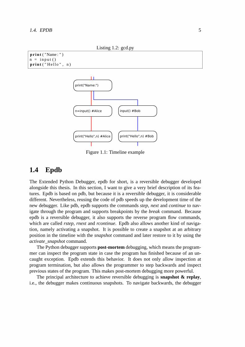
Listing 1.2: gcd.pyp r i n t ( "Name : " )n = i n p u t ( )p r i n t ( " He l l o " , n )
n=input() #Alice input() #Bob
print("Name:")
print("Hello",n) #Alice print("Hello",n) #Bob
Figure 1.1: Timeline example
1.4 Epdb
The Extended Python Debugger, epdb for short, is a reversible debugger developedalongside this thesis. In this section, I want to give a very brief description of its fea-tures. Epdb is based on pdb, but because it is a reversible debugger, it is considerabledifferent. Nevertheless, reusing the code of pdb speeds up the development time of thenew debugger. Like pdb, epdb supports the commandsstep, nextandcontinueto nav-igate through the program and supports breakpoints by thebreakcommand. Becauseepdb is a reversible debugger, it also supports the reverse program flow commands,which are calledrstep, rnext andrcontinue. Epdb also allows another kind of naviga-tion, namely activating a snapshot. It is possible to createa snapshot at an arbitraryposition in the timeline with thesnapshotcommand and later restore to it by using theactivate_snapshotcommand.
The Python debugger supportspost-mortemdebugging, which means the program-mer can inspect the program state in case the program has finished because of an un-caught exception. Epdb extends this behavior. It does not only allow inspection atprogram termination, but also allows the programmer to stepbackwards and inspectprevious states of the program. This makes post-mortem debugging more powerful.
The principal architecture to achieve reversible debugging is snapshot & replay,i.e., the debugger makes continuous snapshots. To navigatebackwards, the debugger
6 CHAPTER 1. INTRODUCTION
activates a previous snapshot and runs the program forward again. To create a snapshot,epdb uses the system callfork(), which makes a copy of the current process.
Timelines
Going back and forth in the program can lead to ambiguous situations. For example,Listing 1.2 shows a program that can have a different output every time the user executesit. Assuming the user has executed the program until the end and has typed the name‘Alice’ when the program asked him for a name. If the user now goes backwards tothe position where the program asked him for a name and runs forward from there, thedebugger has two possibilities to deal with this situation.It could either assume that theuser has entered the name ‘Alice’ and therefore the program could greet ‘Alice’ again,or it could ask the user for a new name and greet the user with the new name.
To resolve this ambiguous situations, epdb introduces timelines. A timeline is apossible execution path through the program. By default, epdb would execute thein-put()-function the same way as in the first run, i.e., in the previous example the programwould greet ‘Alice’ again. However, if the user wants to enter a new name, he couldcreate a new timeline and then enter a new name in this timeline, e.g. ‘Bob’. In thiscase, these two timelines would coexist and the user can switch between them. Figure1.1 shows the two timelines for the described scenario.
In order to implement timelines the debugger uses differentexecution modes. Itneeds them to distinguish, whether the program has already executed the instruction inthe current timeline or not. In case it has executed it, the debugger would simulate theprevious execution behavior of this instruction. Otherwise, it can execute it as usual.
Another point to consider with timelines is that simulatingprevious instruction be-havior requires the debugger to change the behavior of instructions. Therefore, epdbintroducesinstruction patching in order to change the behavior of instructions. Theinstruction patching mechanism of epdb is extensible, so that programmers can add newpatched instructions. These patched instructions work differently in each mode and cantherefore simulate the previous execution behavior of an instruction.
Resource Management
Epdb usesfork() to create snapshots and to save the program state. However,fork()does not save the whole state of the program, e.g., it does notsave files on the disk.Therefore, the debugger needs to manage the state, which is not saved byfork(), insome other way. Epdb usesresource managersto control the external state, i.e., thestate whichfork() does not copy. For epdb there exists a resource manager classforfiles, but it would also be possible to implement resource manager for other resourceslike databases. It allows the users to extend the debugger with newresource managersto provide resource management for their own resources. Theresource manager work
1.5. GEPDB 7
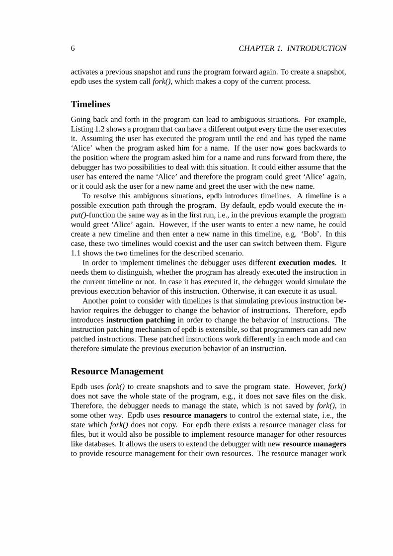
Figure 1.2: gepdb
in conjunction with instruction patching. When an instruction changes some externalstate, the patched instruction would call the resource manager in order to save the state.
1.5 Gepdb
Epdb is a command line debugger like pdb. However debugging is often easier in agraphical user interface. Therefore I developed gepdb. Gepdb is a graphical front endfor epdb. Gepdb has the advantage that it always shows the information a programmerusually needs like the source code, the actual variables, and actual timelines.
Figure 1.2 shows a screenshot of the graphical frontend for the debugger. Gepdblists all timelines that the program has in this debugging session and allows the userto create new timelines. Each timeline has its own resourcesand snapshots which thescreenshot shows at the right side. In the resource window, gepdb lists each resourcealong with its history, i.e., it shows at which instruction count a change to the state of theresource occurred. At the bottom right side, the user interface lists the snapshots of thecurrent timeline with theirid and theirinstruction count. At the left side, the user hasthe ability to monitor variables, which the user interfacesupdates, when the programstate changes, e.g., by stepping forward. At the bottom window, the debugger shows theoutput of the program which typically goes to the console, and it has an entry to do userinput, which gets only activated when the program expects some input. The tool bar atthe top allows one to navigate forwards and backwards. The source code is highlightedand when the user right clicks right beside the line number, apop-up menu shows upand allows the user to set a breakpoint. The status bar at the bottom shows the currentinstruction count and the current mode.
8 CHAPTER 1. INTRODUCTION
1.6 Challenges of Reversible Debugging
Reversible debugging has not been widely accepted yet. I believe that reverse debugginghas some intrinsic problems, which were not challenged by most actual reverse debug-gers. It is easy to simulate reverse execution for a program,which actually only doessome computation and some control structures such as ‘if’ and ‘while’. However, real-world programs are usually much more complex than that. Theyinteract with the op-erating system using system calls. Consequently they can execute in a non-predictableway, i.e., one can’t determine the state of the program at a position by just looking atthe source code, because the wholeenvironment, in which the program executes, in-fluences the program execution. So we can define two differentkind of program states.The internal state is the state of the program without looking at the environment, i.e.,the internal state typically consists of the process memoryand registers. Theexternalstate is the state of the part of the environment, which affects theprogram execution, ata given time in the program.
As Python is an interpreted language, the system calls are not directly visible. In-stead, a program consists of functions which may be implemented as a native codemodule. If functions are implemented in native code, they are able to execute systemcalls, either directly or by using another library. However, with a Python debugger youcan’t step into such functions, i.e., they areatomic in respect of debugging. In case offunctions which are not atomic, I am referring to these functions ascompositefunc-tions.
Determinism
If we look at atomic instructions, we have to distinguish between deterministic andnon-deterministic instructions. In this paper, a functionis said to bedeterministic ifthe outcome of the function is determined by the internal state only. So for example,a function that increments a variable is deterministic, because there is no influence ofthe environment. Look for example at an atomic function thatreturns the system time.The program cannot calculate the system time by running an algorithm. Therefore thereis a system clock built in the computer and the operating system provides some meansto access the clock. The system clock is part of the environment and therefore, theexecution of the function is influenced by the external state. Therefore, the functionwhich returns the system time is anon-deterministic function.
A deterministic atomic function is easy to handle for a reversible debugger, becauseit just has to keep track of the internal state, but for a non-deterministic function, trackingthe internal state is not sufficient, because the external state also affects the program andmay change when the debugger replays a function execution. In fact, it is even morecomplicated than that. When the user replays a non-deterministic function, he can haveeither of one two reasonable expectations. He could expect to have the same execution
1.6. CHALLENGES OF REVERSIBLE DEBUGGING 9
as in the first run or he could expect to run with the new environment. Both views makesense and an interactive reversible debugger should consider both of them.
Side effects
While the execution of non-deterministic functions is influenced by the environment,functions with side effects change their environment. A function which writes some-thing to the hard-drive is such a function, because it changes the information on the disk,which is not part of the internal state, but of the environment.
If someone debugs a program, and makes heavy usage of the environment, he isusually not only interested in the internal state, but also in the environment. Take for ex-ample an external sorting algorithm. If one wants to find a bug, he is not only interestedin the variables during program execution, but also in the state of the file, which containsthe data the program should sort. Therefore a reversible debugger should provide someway to manage the external state.
Bookkeeping
A reversible debugger must be able to recover previous states. Therefore it has to savetheexecution path historyand thedata change history[CFC01]. Epdb however doesnot save this history directly. It saves the data change history by making continuoussnapshots, but it also keeps a history of the execution path.Thus, epdb needs to calculatethe target position in the program when it replays an execution. For a snapshot & replaydebugger, which uses multiple processes, it has to exchangethis recorded informationwith the other snapshot processes.
Breakpoints
As a traditional debugger, a reversible debugger should support breakpoints and theyshould also work when the program runs backwards. The challenge here is especiallyfor a snapshot & replay debugger, because a snapshot & replaydebugger has multipleprocesses. When the user makes a breakpoint in one process, heshould see them inother processes too.
Deterministic and Non-deterministic execution
Since the user can navigate through the program backwards and forwards, the debuggercan execute instructions for the first time or it can execute instructions which it hasexecuted before. If the debugger executes instructions it has executed before, I amreferring to this execution as execution inredo mode.
10 CHAPTER 1. INTRODUCTION
When the debugger is in redo mode, it has two possibilities to execute non-de-terministic instructions. It could either execute them like in the first execution, or itcould execute them independently from the first execution. In other words, the debug-ger could choose to use the environment from the first execution1 or it could use theactual environment. I am referring to the execution of instructions with an old envi-ronment asdeterministic execution, because executing an instruction deterministicallywould change the internal state the same way as in a previous run. In the case of ex-ecuting instructions with the actual environment, I am referring this execution asnon-deterministic execution, because the internal state, which results from the execution ofthis non-deterministic instruction, is usually not the same as any other previous state.
Non-deterministic and deterministic execution is a challenge for reversible debug-gers because they have to decide which type of execution theychoose. Most reversibledebuggers usually support only one mode of execution, whichis usually deterministicexecution. However, epdb supports both types of execution by using timelines.
Extensibility
In a real world program, the program execution can be influenced by almost everythingwhich exists in the real world. For example, if the program controls a device, whichmeasures the temperature, the actual temperature becomes an important part of the en-vironment of the program. There are almost infinitely many possibilities to influence theprogram execution, and thus the programmers of a reversibledebugger can’t imagine ev-ery case which may become important for the users of a reversible debugger. Thereforea sophisticated reversible debugger should allow the user to extend the debugger so thathe is able to debug all the devices, which he uses for his application.
1.7 Contribution
Although there already exist a few reversible debuggers, none of them tackle the prob-lem that some instructions can execute differently each time the debugger executes themat the same position. Therefore, the program could execute in multiple different ways.Another problem is that the program may also change the external state, which can bean important source of information for the user, when he debugs the program.
The main contributions of this thesis to solve these problems are timelines and re-source management. With timelines users have the choice to replay code either de-terministically or non-deterministically. Consequently,users can decide if they wantto reproduce the state in which they have been before, or if they want to execute the
1In the case an instruction has been executed multiple times,it could also execute the instruction withthe environment of the second, third, any later execution
1.7. CONTRIBUTION 11
program in a possibly new way. Therefore, users have more control over the programexecution.
With resource management, the debugger provides a new way todeal with side ef-fects. A traditional debugger doesn’t need resource management, because the programwill change external resources when the execution proceeds. A reversible debuggerdoes not change the external state when it runs backwards. Therefore, without resourcemanagement the external state of the program would not be in sync with the internalstate. Epdb allows to manage the different states of each resource while debugging theprogram. For this purpose it uses resource managers. A resource manager tracks thedifferent states of some part of the external state, and it isable to restore a previousstate of the resource. The debugger interrelates the state of the resource with the corre-sponding instruction count. This system allows to manage the external state, it is easilyextensible, and it also has good performance, because the debugger only has to reset theresources when it actually stops the execution.

CHAPTER 2Prerequisites
Writing a debugger is quite different from writing other applications. In this section, Iwant to provide some information on how debuggers generallywork. Python alreadyships with a traditional debugger pdb, which epdb depends on. Pdb makes use of theinfrastructure Python provides to implement tools like debuggers, profilers, coveragetools and the like. Therefore I want to explain this infrastructure here too.
2.1 Python Versions
At the time of this writing, there are multiple different versions of Python around, whichalso work a little differently. For the prototype version ofthe debugger developed along-side this paper, I had to choose one to work with. First, thereare different types ofimplementation, which target different architectures, e.g., Jython, IronPython, PyPy orCPython. Although many of them are in use, the most important is CPython. The otherimplementations should work the same as CPython, but may lackone or another fea-ture. A more important distinction is between Python 2.x andPython 3.x. At the time ofthis writing, Python 2.x is the most used, while Python 3.x isthe newer one. Python 3.xhas some major changes to the syntax, most visible is the change from theprint state-ment to a function. It is difficult to develop a program which works with both versions,and therefore I decided to go for Python 3.x only. Dealing with functions instead ofstatements, has the advantage that they are easier to patch,a feature which epdb uses tosupport reversible debugging.
13
14 CHAPTER 2. PREREQUISITES
2.2 Types of Debuggers
There exists a whole bunch of different kinds of debuggers, each with their own differentpurpose. The kind of problem, programming language, programming environment orsystem affects the requirements to a debugger. I want to givean overview of some typesof debuggers in order to position epdb in the world of debuggers.
Machine Level Debuggers
Machine or low-level debuggers operate on machine code. People use them for pro-grams written in assembler, or to debug the code a compiler has generated, or to reverseengineer a program where the source is not available.
One of the main properties of a debugger is the ability to haltthe process. Thedebugger does this halting when it reaches a breakpoint. To achieve halting there aretwo principle options for the developers. Either they couldexecute it on a virtual ma-chine which allows directing the program, or they make use ofthe operating system orhardware support. So a machine level debugger uses the option of hardware or operat-ing system support. For the x86-architecture[Sei09], there is support for two kinds ofbreakpoints —soft breakpointsandhardware breakpoints.
Soft breakpoints are machine code which the debugger injects into the program codeat run time. For the x86 architecture, this is the machine code for the interrupt number3, or INT 3 for short. In fact, the debugger does not inject in the sense of adding newcode, but by changing a byte of the opcode. This works, because the opcode ofINT 3is very short, i.e., only one byte long. When the CPU hits theINT 3 instruction, it stopsthe execution and triggers an interrupt, which the debuggerhandles. Before continuingthe execution, the debugger has to restore the old instruction, that it overwrote beforewith theINT 3opcode.
As you can see, soft breakpoints change the program code, which the program loaderhas loaded into the memory. This has some implications when the user tries to use adebugger to look for malware, because malware often checks the CRC sum of the codeand will kill itself, if it changes. Consequently, malware developers can hinder the useof soft breakpoints to debug their malicious code.
Hardware breakpoints solve this problem by offering debug registers. These regis-ters hold the address where the program should be halted. Additionally, there are someflags, which allow creating breakpoints for three conditions: break when the particularaddress is executed, break when the particular address is written, break when the partic-ular address is read or written. Before an instruction is executed, the CPU first checksif a hardware breakpoint is set. Consequently, it is possibleto debug a native programwithout modifying it, but it is difficult to get around the limited number of registers forgeneral purpose debuggers.
2.2. TYPES OF DEBUGGERS 15
Source Level Debugger
A source level or symbolic debugger maps the source code directly to the application’smachine code. A compiler transforms source code into machine code that executes onthe hardware platform. The source level debugger’s job is tomap the machine instruc-tions back to the original source code. This is usually not trivial, because the transfor-mation done by the debugger doesn’t need to be bijective, injective or surjective, andtherefore the reverse transformation may not be unambiguous. However debuggers typ-ically solve this by compiling some additional informationabout the mapping into thecompiled version. This is the reason, why users should use the “-g” switch for gcc ifthey intend to debug their program afterwards.
Usually, the users of a high-level programming language prefer a source level de-bugger, because they usually “think” in their programming language instead of thinkingin machine code. However, sometimes the source to code mapping is not available, e.g.,when the software vendor only ships a binary version, and in this case, the programmerhas to fall back on a machine level debugger.
Interactive vs. Logging Debugger
Program execution is usually much faster than humans can perceive and understand thechanges to the state the program has performed. Therefore a debugger should havesome means to make them understandable to the user. Aninteractive debuggerdoesthis by allowing the user to stop the program and continue theexecution from thereon. Stopping here means, that the debugger shows the user some kind of prompt orwaits for some other action from the user. It usually supports breakpoints and typicallythe running commandsstep, nextandcontinue. The user can inspect variables or thestack at any point of the program and they may even modify the program execution byinserting some instructions or modifying variables.
A logging debuggeron the other hand executes the program without halting. It doeshowever log important information from the execution, but there is no user interaction.After the execution has finished, the user can inspect the logfile. On top of the logfile, the debugger could present a user interface, which would allow the user to navigatethrough the different states of the program. Therefore, it could almost feel like theprogram is running, while it is in fact, only replayed from the log. As the debugger hasto do some logging, the program is still somewhat slower thanin normal execution.
There are three ways to achieve logging of the programming state while running.The program could run on a virtual machine (see 2.2) which does the logging, or itcould have some support from the interpreter of the programming language (see 2.2),or it could use program instrumentation. With program instrumentation the debuggerwould actually change the code when the program loads. For native code, the debuggerwould have to change the machine code, but for object-oriented code which executes on
16 CHAPTER 2. PREREQUISITES
virtual machine like the Java Virtual Machine, the debuggercould overwrite the classloading mechanism[LB98].
Debugger for Interpreted Languages
Interpreted languages don’t compile to machine code and therefore a machine leveldebugger would only debug the interpreter itself and not theprogram written in theinterpreted language. Most interpreted languages providehowever some means to im-plement a debugger. For example, the interpreter could callsome debugging routinebefore executing some line of code. The developers of a debugger for an interpretedlanguage have the advantage, that they only need to use one programming language anddon’t need to understand machine code at all.
Virtual Machine Based Debuggers
One problem of using program directing using the mechanism built-in the hardware oroperating system is that they have to change the code. Becausethey usually operate inuser mode, they may also have problems to access code, which they don’t have accessto, for example code, in the kernel of the operating system[KNM06].
One way to implement a debugger instead of using soft or hardware breakpoints fordirecting is to execute the program on a virtual machine. Thevirtual machine can emitevents to the debugging process, which gathers the information to present it to the user.One can also implement a virtual machine[DF04] [KTD05], so that it stops executingfurther instructions on special events. This would represent a break in a program similarto a software or hardware breakpoint, but without modifyingany registers or code in thememory.
Reversible Debugger
A reversible debugger is a debugger that allows the user to navigate through the programin reverse. There are multiple ways to achieve this. The debugger could be a loggingdebugger, which logs the program execution and allows to examine every state of theprogram after it ends. Using this way, it is however not possible to inject some pieceof code into the program flow. Another strategy would be to record the changes ofevery instruction and when running backwards, undo the changes using the recordedinformation. A further one is to make continuous snapshots in the program and whengoing backwards the debugger could recover a previous snapshot and replay the programfrom there until it reaches the desired position in the program.
Epdb is an interactive reversible debugger. It actually executes instructions and haltsthe process to give the user live interaction. To simulate reverse execution it uses thesnapshot & replay mechanism.
2.3. PYTHON AND DEBUGGING 17
2.3 Python and Debugging
Python comes with a debugger calledpdb. Pdb makes use of another module calledbdb.The purpose ofbdb is to provide a basis for other debuggers. It uses thesys.settrace()function to intercept the program execution. Although it issufficient to have a hook-ing function likesys.settrace()to implement a full featured debugger, lots of organizingwork has to be done, e.g., keeping track of breakpoints, resetting the trace function andso on.Bdbbuilds some framework aroundsys.settraceand provides a higher level inter-face to develop a debugger. Thepdbmodule, which usesbdbas a basis, adds function-ality such as a user interface and higher level debugging features. The whole debuggeris written in pure Python, while only thesys.settrace()function is implemented in C.It doesn’t seem useful to reimplement all those features thedebugger already supports.The prototype accompanying this thesis is based on pdb and extends it with all reversibledebugging capabilities. This is feasible because all the code is open source.
Python Low-Level Dispatching
The sysmodule, which is part of the Python standard library, provides the functionsys.settrace(). This function takes one argument — the trace function. When the pro-gram sets the trace function, the interpreter calls it whenever one of the following eventshappen:
call The interpreter calls a function.
line The interpreter executes a line of code.
return A function is about to return.
exception A function throws an exception.
c_call Similar to call, but used when a C function is called.
c_return Similar to return except that it works for C function.
c_exception A C function throws an exception.
Thetracefunction takes three arguments: The stack frame, event and arg. The stackframe is the top stack frame of the code that raises the trace event. The arg dependson the event type. At the ‘return’ event it is the return value; at the ‘exception’ eventit is the tuple (exception, value, traceback); at the ‘c_call’ event it is the function to becalled. The other events have the argNone.
When the trace function finishes, the interpreter uses the return value to reset thetrace function. This means that the function should return itself to keep the trace func-tion active or otherwise when it returnsNone, the trace function gets deactivated.
18 CHAPTER 2. PREREQUISITES
Bdb
The main part of thebdb module is theBdb class. This class provides four func-tions — user_line(), user_call(), user_return(), anduser_exception(). These are tem-plate methods[GHJV94] which pdb implements. Bdb calls them when the trace func-tion trace_dispatch()receives an event of the type ’line’, ’call’ or ’return’. Bdb callsthese methods not directly in thetrace_dispatch()function. Instead, the trace func-tion calls one of the methodsdispatch_line(), dispatch_call(), dispatch_return()or dis-patch_exception()first. These methods do some breakpoint checking before actuallycalling theuser_*()methods. Thetrace_dispatch()function anddispatch_*()take careof resetting the trace function. Bdb only resets the trace function if there is a breakpointin the code of the current stack frame or some other reason to stop inside the function.Using these optimizations Bdb reduces the number of calls to the trace function.
user_line()
If the trace dispatch function is set,user_line()gets called every time before the inter-preter executes a line of code. Bdb usually calls this template method when there is atrace-dispatch event of type ‘line’, but does some additional work. It checks for break-points or other stop information and only callsuser_line()if a reason to stop exists. SoBdb doesn’t guarantee to calluser_line(), but epdb needs to stop at every atomic in-struction to implement instruction counting. In order to achieve this, epdb always setssome stop information to make bdb calluser_line()on every atomic instruction.
user_call()
Every time before the interpreter executes a function call,it sends a ’call’-event to thetrace function, if it is set. Bdb does some preprocessing before it calls the templatemethoduser_call(). It checks if there is some possibility to stop in this function eitherby a breakpoint or another reason, as if the user has used the step command. For epdb,theuser_call()method gets always called for composite functions, becauseeach of thenavigation commands work internally like a repeatedstepcommand to allow instructioncounting. The epdb implementation ofuser_call()increments the actual frame count,as every function call also increases the number of stack frames by one.
user_return()
The methoddispatch_return()calls the template methoduser_return()when there iseither a step over the return of a function or the user used thereturn command. Epdbdoesn’t support thereturncommand yet, but as it simulates every command as repeatedstep, user_return()always gets called when the function returns. Epdb also decrementsthe actual frame count.
2.3. PYTHON AND DEBUGGING 19
user_exception()
Similar to the previous methods,user_exception()gets called if there is the possibilityto break at the exception, either because of a breakpoint or because of a step command.However epdb uses repeatedstep, and souser_exception()gets called at every thrownexception in a composite function.
Pdb
The Pdb class inherits from Bdb and Cmd. Bdb provides the basis for debugging theprogram while the Cmd class handles the user interaction likeshowing a prompt orparsing user input.Pdbalso overwrites theuser_*-methods ofBdb. Epdb reimplementsthese methods. However, pdb implements some other methods which are important inconjunction with epdb.
interaction()
The interaction method shows a prompt and shows the user input. This is a methodwhich epdb calls when it stops the program flow, e.g., by reaching breakpoint.
do_*()
The do_*-methods are part of the command dispatch pattern[Boo03] of the base classCmd. These methods are called when the user enters some input, e.g., when the userentersstep, the methoddo_stepgets called. Epdb overwrites some of the commands,especiallystep, nextandcontinue, and it also adds some new ones, notablyrnext, rstepandrcontinue.

CHAPTER 3Reverse Execution
Epdb does reverse execution by restoring a previous snapshot and executing as manyinstructions as needed to reach the current instruction minus one. If all executed instruc-tions are deterministic, the process will exactly stop one instruction before the currentinstruction. The debugger has then to count the instructions, which it does by using thetrace function, but one has to be careful that pdb has some optimization, which turns thetrace function off, if there are no breakpoints. So this optimization has to be switchedoff.
3.1 Execution Modes
Epdb distinguishes three different execution modes. It uses normal mode when the pro-grammer asks to run or step forward over instructions the first time. To simulate back-ward running, it activates a previous snapshot and runs the program in replay mode.As it is possible to navigate back and forth, it is possible torun an instruction in thesame environment more than once. To allow implementation ofdeterministic execu-tion behavior, the debugger uses redo mode to execute non-deterministic instructionsdeterministically. The debugger uses different executionmodes to allow controllinginstructions differently, depending on its current state.
Normal Mode
Normal execution doesn’t differ much from a traditional debugger. One difference isthat epdb needs to count the instructions, which pdb doesn’tdo. For non-deterministicinstructions, it also has to record the external state whichaffects the execution behavior.For instructions with side effects it has to record the external state before the instructionchanges it, in order to restore it when the user runs the program backwards, later on.
21
22 CHAPTER 3. REVERSE EXECUTION
replay redo
current position max. positionSnapshot
Instruction
Figure 3.1: Redo and replay modes
Replay Mode
After restoring to an earlier snapshot, the debugger tries to recover a future state fromthat point on. It does this recovery in replay mode. In the simplest case, it executesthe statements as in forward execution. This works for deterministic statements withoutside effects, e.g., the line:
i = i + 1
is such a statement. It neither changes the external state, nor does it depend on it. How-ever, there are statements which are dependent on some external state, i.e., they have sideeffects. Let’s look at the example of writing something to disk, usingwrite(). When thedebugger executes thewrite() instruction in replay mode, the instruction would writesomething to the disk again. This behavior is usually not wanted. Therefore the debug-ger has to use a patched version of thewrite() instruction, which actually doesn’t writeanything to disk in replay mode.
In the write()-example, there is another problem to consider, because thewrite()function call returns the number of bytes written. Therefore it has not only side effects,but it is also non-deterministic. So replaying thewrite() call should return the numberof bytes written in the original run. So the debugger has to record the return value innormal mode and reuse it in replay mode.
Redo Mode
Redo mode is similar to replay mode. Like replay mode, epdb uses redo mode whenthe instruction counter is at a position in the program, which was already executedbefore in the actual timeline1. Epdb uses replay mode when it simulates backwardrunning. The part of the code executed in replay mode is always code which the userwould not expect to get executed at all. In redo mode, the debugger actually executescode which the user would expect to get executed, but which also has been executed
1You may want to read about timelines in section 3.4 before continuing
3.1. EXECUTION MODES 23
before. Replay mode is usually not visible to the user becausewhen the debugger hasfinished replaying instructions, it switches into redo or normal mode before it interactswith the user. So when the user sends the debugger a command torun the programbackwards, the debugger executes code in replay mode, but when he sends a commandto run forward, the debugger executes the code in redo or normal mode.
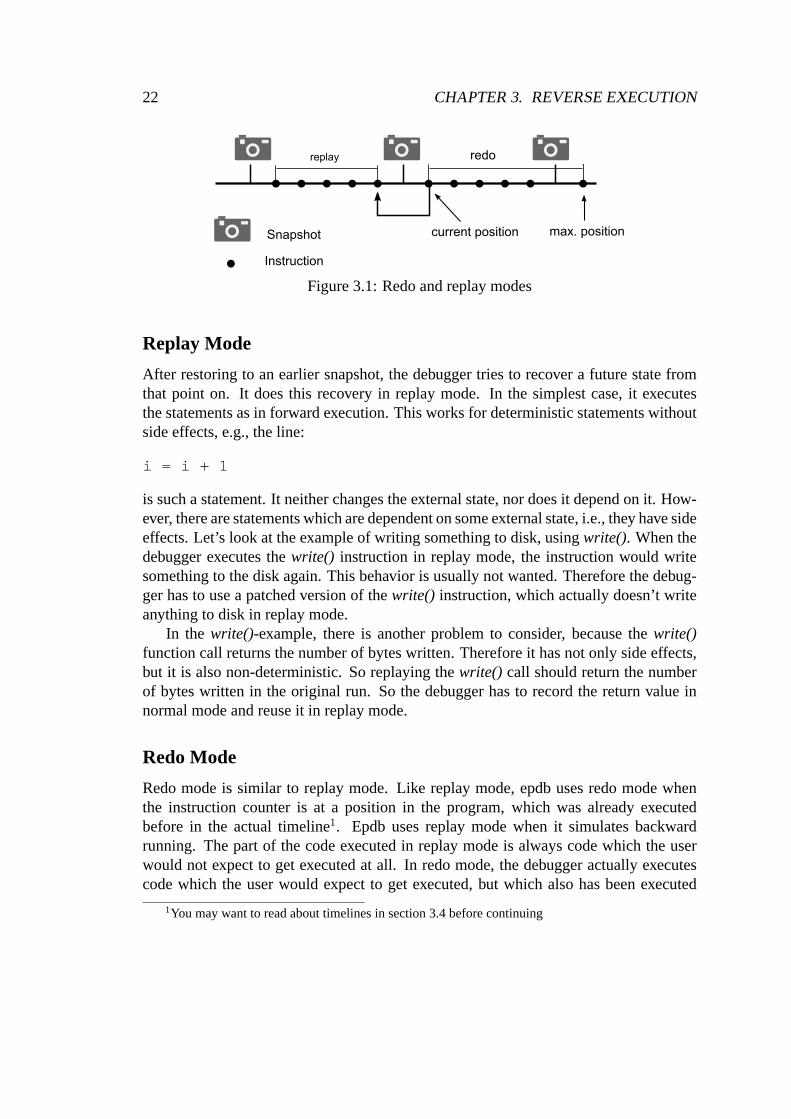
Figure 3.1 shows the difference between redo and replay modein the view of theactual timeline. Each timeline has a current and maximum instruction count. Epdb exe-cutes everything after the maximum instruction count in normal mode, but also sets thenew maximum instruction count after executing something innormal mode. Everythingafter the current instruction count until the maximum instruction gets executed in redomode. To step some instructions back, the debugger activates a previous snapshot andruns forward until it reaches the desired position. While it runs forward to the desiredposition the debugger sets itself to replay mode. After it reaches the target position, itswitches either to redo or normal mode, depending on whetherthe current instruction ison the maximum position of the timeline or not. Instruction execution in redo mode andreplay mode is usually very similar and most of the time patched instructions executethe same way in redo and replay mode.
Undo Mode
Undo mode was the first model to implement side effect management, however it is nowreplaced by the resources concept. I will describe the undo mode here, because I alsowant to document the the reasons for the decisions I made, while developing epdb forthe sake of completeness. If you want to know how epdb does side effect managementnow, read Section 3.7.
Undo mode was not really a mode, but in the case of running instructions with sideeffects backwards, the debugger should undo those side effects. The design was that thedebugger keeps a list of all instructions that were executedand which have side effects,together with their instruction count and some additional information for undoing them,which it gathered in normal mode. When the debugger runs backwards, it would lookup the list to find the instructions that it has to undo and runsthem in a special undomode.
As it turned out the undo mode approach wasn’t very practical, especially becauseepdb supports timeline switching. With timeline switching, it would be very complex tofind which instructions to run in undo mode and after that, which to run in redo mode. Itwould also not be very efficient if the resource would supportrestoring previous statesas some databases do.
24 CHAPTER 3. REVERSE EXECUTION
3.2 Snapshots
Snapshotting can be a very convenient feature, even withoutbeing able to run a programbackwards. For example, take a program, which has a long initialization phase, thatrequires the user to enter a lot of input from the keyboard. Ifthe defect in the program isat the end, every time the user restarts the application, he has to go through the tediousinitialization step. With snapshots, he could have set one snapshot after the initializationand instead of restarting, he could have restored the snapshot then.
Snapshotting was the first feature implemented to achieve the goal of reversible de-bugging. The technique I have chosen for implementing snapshots was using the systemcall fork(). Fork() creates a new process by duplicating the calling process. The deci-sion to usefork() has some implications. One of the most important is that the operatingsystem must support this system call, which is the case for Unix-like operating systems,but for example, not for Microsoft Windows. The advantage ofthis approach is that itis simple and independent of the programming language used and so, the implementa-tion approach could be easily applied to a debugger for another programming languageas well. Creating a process withfork() is very efficient, because it uses copy-on-write.With copy-on-write the operating system doesn’t copy the memory of the process, butinstead sets a bit for each memory page that the newly createdshares with the oldprocess[Bac86]. If one of the processes writes to a shared page the operating systemthen copies the page. Therefore, creating a snapshot usingfork() is extremely fast.
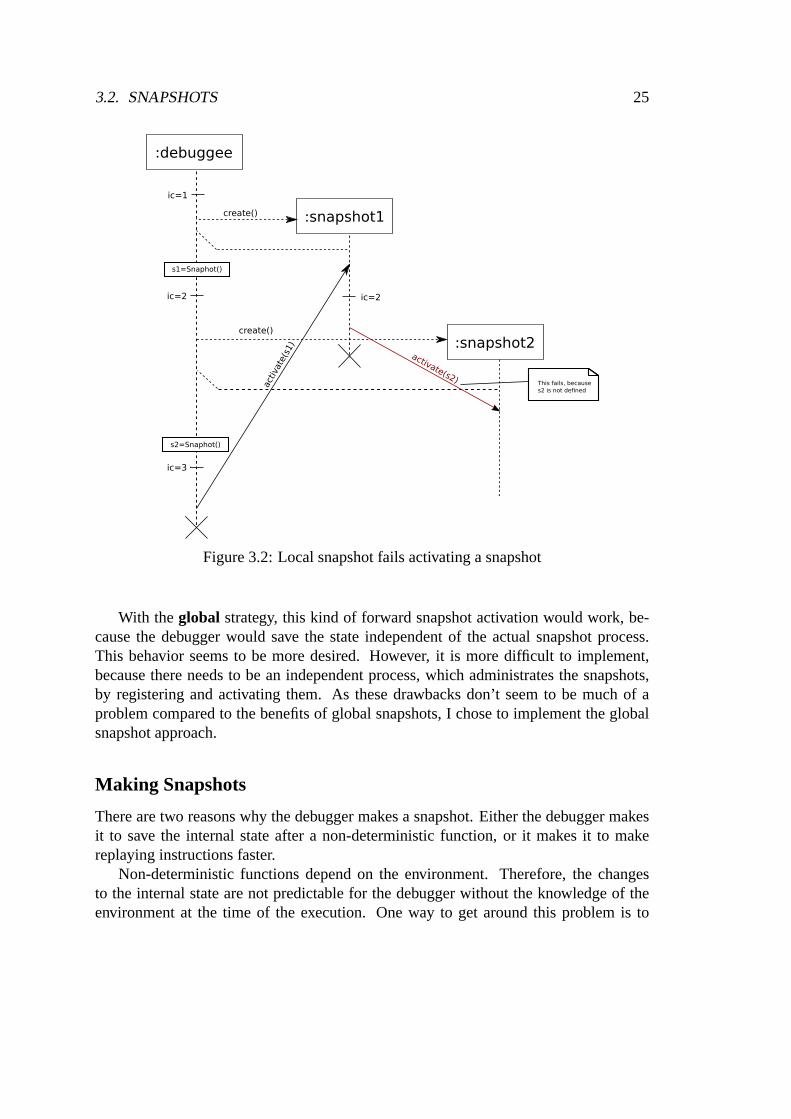
There are two different strategies to create snapshots; I call them local and globalsnapshot creation.Local means that the current executing process knows only about theinherited snapshots, and therefore cannot activate later snapshots, i.e., snapshots whichare taken at a higher instruction count. Let’s take the example in Figure 3.2, whichillustrates an example where local snapshots fail. The typeof diagram is an adaptedUML sequence diagram. The adaption concerns especially thetime of lifelines, whichin this diagram, is not time measured in seconds, but instead, measured as the number ofinstructions executed, i.e., the time in the lifeline is measured in the current instructioncount (ic). Therefore the processes can send messages backwards, because the processescan have different instruction counts at the same real time.The diagram indicates thisbackward sending by giving theactivate()messages an additional upward or downwarddirection. It also models the history of a snapshot, which result from thefork(), bybranching the lifelines. This should mean that the snapshothas copied the creatingprocess along with all its variables. In this diagram, a process makes two snapshots,one after the first and another after the second instruction.After the third instruction,it activates the first snapshot. This snapshot wants to activate the second snapshot, butthis fails because there was never an assignment to the variables2 in the diagram. Keepin mind that the diagram is very much simplified, in order to keep it neat. In fact, asnapshot wouldn’t start running, but instead would create another process usingfork(),which then runs as the new activated snapshot.
3.2. SNAPSHOTS 25
:debuggee
:snapshot1
:snapshot2
ic=1
s1=Snaphot()
ic=2
ic=3
s2=Snaphot()
act
ivate
(s1)
ic=2
activate(s2)This fails, because
s2 is not defined
create()
create()
Figure 3.2: Local snapshot fails activating a snapshot
With theglobal strategy, this kind of forward snapshot activation would work, be-cause the debugger would save the state independent of the actual snapshot process.This behavior seems to be more desired. However, it is more difficult to implement,because there needs to be an independent process, which administrates the snapshots,by registering and activating them. As these drawbacks don’t seem to be much of aproblem compared to the benefits of global snapshots, I choseto implement the globalsnapshot approach.
Making Snapshots
There are two reasons why the debugger makes a snapshot. Either the debugger makesit to save the internal state after a non-deterministic function, or it makes it to makereplaying instructions faster.
Non-deterministic functions depend on the environment. Therefore, the changesto the internal state are not predictable for the debugger without the knowledge of theenvironment at the time of the execution. One way to get around this problem is to
26 CHAPTER 3. REVERSE EXECUTION
Listing 3.1: sleep() example.pyimport t ime
t ime . s l e e p ( 3 )
p r i n t ( " S l e e p i n g done " )
make a snapshot after the non-deterministic instruction. When the debugger encountersthe instruction again in redo mode, it then can activate the next snapshot, instead ofexecuting the instruction. As a result of this, the debuggerrestores the internal state,not by executing instructions, but by restoring a snapshot.This makes it easy to handlenon-deterministic instructions correctly, even without knowing the details of how theywork.
If the user debugs a longer running program, the replaying ofcode could take a lot oftime, because the debugger has to recover from a snapshot from long ago. The debuggercan reduce the time it needs to replay instructions, by making continuous snapshotswhen debugging forward. Then it can use a snapshot in the morerecent past and startreplaying from there. Epdb has a timer variable, which the debugger increases with thetime it needs to execute each instruction. When this variableexceeds the time of onesecond, the debugger makes a snapshot of this position and resets the timer variable.Consequently, replaying will always take less than one second, assuming the executionspeed of the program is the same as in the first run. This is because the debugger wouldnever execute the last instruction, because it uses forwardactivation of snapshots (seeSection 3.4).
In the example in Listing 3.1, thetime.sleep()function waits for 3 seconds. When thedebugger replays this instruction, it would actually wait for 3 seconds again. However,epdb makes a snapshot after thetime.sleep(3), because the timer variable would exceedthe one second limit (in fact it would reach a value of slightly above 3 seconds). There-fore the debugger wouldn’t replay this instruction, but would use the snapshot after thetime.sleep()instead. When the user however steps in redo mode over thetime.sleep(),the debugger would use forward activation and restore the next snapshot, which is im-mediately after thetime.sleep(). Therefore, in redo mode the simulation of the executionof thetime.sleep()function would be much faster than in normal mode.
Reasons for Using fork()-Snapshots
Using fork() for making snapshots has some drawbacks, most notably the operatingsystem has to manage a lot more processes, which may affect the overall performance.Therefore, one can think of implementing snapshots withoutusingfork(). The Pythonprogramming language stores all its global variables in a publicly accessible dictionary
3.3. INSTRUCTION COUNTING 27
calledglobals, and the local variables in a publicly accessible dictionary calledlocals.One might try to make a deep copy of these dictionaries, save them and use them to re-store them later on. However, this doesn’t always work, because some information isn’teasily accessible within the Python interpreter, especially if a function is implementedin C instead of Python, which is quite common. Let’s look at the standard implemen-tation for file access. The standard library makes use of the standard C implementationof file access. This makes the interpreter portable among allplatforms that support C.This implementation allows one to write to a buffer, which isusually not written imme-diately, but rather when the program callsflush()or close()on the file descriptor. ThePython interpreter however, has no access to the buffer and therefore can’t change it,which is necessary in case of going backwards. Usingfork() allows the debugger tocreate a complete copy of the process, including the buffer for I/O.
Another advantage of usingfork() in conjunction with files is that the operatingsystem makes a copy of the file descriptor. Therefore, the filedescriptor in the processis open regardless if another process closes it later on. If one tries to implement a processcopy on the user side, he would need to take care of that. He would also have to takecare of the correct initialization of the registers of the CPU.
An additional advantage offork() is that the operating system uses copy-on-write,which makes creating a copy of a process extremely fast as discussed in Section 5.2.
3.3 Instruction Counting
In order to step an arbitrary number of instructions backwards, it is necessary to countthe instructions. In order for the user to step one instruction backwards, the debuggerwould restore the last snapshot, and then would run the number of instructions to itsoriginal location, minus one. Therefore the debugger has tocount the number of exe-cuted atomic instructions. Epdb doesn’t work on bytecode, but uses the trace functionto implement a debugger, which Python provides. With this approach, the length of oneinstruction is usually one line of code. One exception to this are function calls. In caseof function calls, the debugger also executes the lines of code inside this function beforefinishing the line of code where the function call occurred.
The easiest way to implement instruction counting is to set the trace function forevery instruction and then to increment an instruction counting variable every time aninstruction is executed. Compared to a traditional debugger, this may results in someperformance loss. The reason is that in traditional debugging the debugger can set thetrace function only for execution frames that contain at least one breakpoint or in oneof its succeeding frames. This approach allows optimization in many cases, becauseusually only very few breakpoints are used compared to the size of the code.
28 CHAPTER 3. REVERSE EXECUTION
Listing 3.2: rnd.pyimport random
random . seed ( )r = random . r a n d i n t ( 0 , 1 0 )p r i n t ( r )
3.4 Timelines
If the user runs a program backwards and later decides to go forward again, the debuggerhas two reasonable ways to execute the instructions. First,it could execute them asthey are (non-deterministic execution), or it could make them work the same way asthey worked in the first run (deterministic execution). The difference of the two waysemerges when we look at non-deterministic instructions which may change the internalstate of the program in a different way each time they get executed. Take for examplea program which generates a true random number as you see in Listing 3.2. Let’s saythe user has debugged towards the end of the program and the itprints the number4. Then the user decides to step backwards to theseed()instruction and after that hegoes forward using the step command twice. Now the debugger could either generate acompletely new random number or it could show the old one, which is 4.
Both ways to go forward again make sense and can be useful sometimes. Take fora example a program which makes Monte Carlo experiments, and for some reason theprogram provides a wrong result. If the programmer wants to examine the programin order to understand whats happening, he would most likelyuse the deterministicversion to execute the program. If however he wants to modifythe configuration ofsome variables and sees if the algorithm still returns a wrong result, he would preferthe non-deterministic version. Thus, a reversible debugger should support deterministicand non-deterministic running. Note that logging debuggers like odb1 only support thedeterministic version. However, simply adding two commands to step forward, calledfor example dstep (deterministic step) and nstep (non-deterministic step), introducesanother problem. If the user debugs in reverse, then steps forward using nstep, and thendebugs in reverse again and then uses dstep, there would be two ways to go forwardagain. Either the program can show the output of the first run or of the second run.
To solve these issues, epdb introduces timelines. A timeline is a deterministic waythrough the program, which can also go only through a part of the program. For thispurpose, each timeline has a current and a maximum instruction count. Thecurrentinstruction count is the position inside the timeline where the next instruction, whichthe debugger should execute, is located. Themaximum instruction count is the latest
1see Section 7.1
3.4. TIMELINES 29
1 2 3 4 5
current ic max. ic
1 2 3
1 2 31 2 3
current and
max. ic
new timeline
Figure 3.3: New timeline
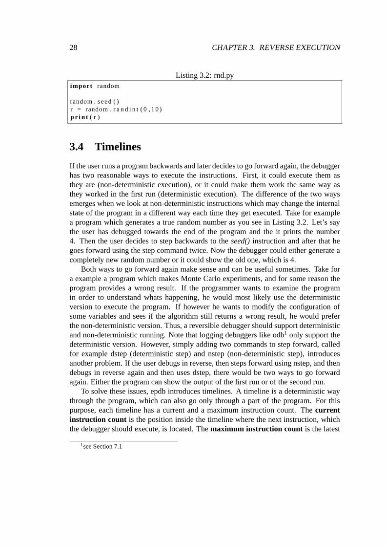
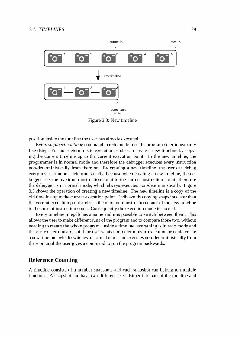
position inside the timeline the user has already executed.Everystep/next/continuecommand in redo mode runs the program deterministically
like dstep. For non-deterministic execution, epdb can create a new timeline by copy-ing the current timeline up to the current execution point. In the new timeline, theprogrammer is in normal mode and therefore the debugger executes every instructionnon-deterministically from there on. By creating a new timeline, the user can debugevery instruction non-deterministically, because when creating a new timeline, the de-bugger sets the maximum instruction count to the current instruction count. thereforethe debugger is in normal mode, which always executes non-deterministically. Figure3.3 shows the operation of creating a new timeline. The new timeline is a copy of theold timeline up to the current execution point. Epdb avoids copying snapshots later thanthe current execution point and sets the maximum instruction count of the new timelineto the current instruction count. Consequently the execution mode is normal.
Every timeline in epdb has a name and it is possible to switch between them. Thisallows the user to make different runs of the program and to compare those two, withoutneeding to restart the whole program. Inside a timeline, everything is in redo mode andtherefore deterministic, but if the user wants non-deterministic execution he could createa new timeline, which switches to normal mode and executes non-deterministically fromthere on until the user gives a command to run the program backwards.
Reference Counting
A timeline consists of a number snapshots and each snapshot can belong to multipletimelines. A snapshot can have two different uses. Either itis part of the timeline and
30 CHAPTER 3. REVERSE EXECUTION
therefore epdb uses it for snapshot & replay, or the user can use it to set the programto an earlier state by manually restoring a previous snapshot. Having many snapshotsmay have an impact on the performance, because each snapshothas its own process.Therefore, the debugger wants to keep the number of snapshots to a minimum, butsome snapshots are needed because they are part of the timeline. Making a timeline withfew or even no snapshots may also have an impact on the performance, because everyreverse navigation command would need to reset a very old snapshot or even restart theprogram. However, it would be advantageous to delete unneeded snapshots. A timelinedoes not need a snapshot, if the snapshot is not part of this timeline. However, it doesneed it, if it is part of the timeline. Epdb uses reference counting on snapshots. For eachsnapshot, there is a count to how many timelines it belongs. The users can only removesnapshots, which don’t belong to any timeline. If they want to remove a snapshot thatstill belongs to a timeline, they have to delete the timelines the snapshot belongs tofirst. Every time epdb creates a new timeline, it increments the reference count on everysnapshot that belongs to the new timeline by one, and every time epdb deletes a timeline,the reference count on every snapshot of this timeline gets decremented. Epdb doesn’tsupport removing snapshots from timelines (except by deletion), because snapshots canbe used to replay non-deterministic behavior.
Forward Activation
Let’s consider an example in redo mode where the actual position is one instructionbefore a snapshot and the user steps forward. The debugger has two ways to react.Either it can activate the new snapshot or it can execute the next instruction. Both waysshould usually result in the same internal state in case of a deterministic instruction,and because of the resource management, external resourcesshould be in the samedesired state in both cases. Consequently the debugger should provide some means tosimulate deterministic execution for non-deterministic instructions. One way to achievea correct replay of a non-deterministic function is to make asnapshot immediately afterthe instruction. Then, when the debugger runs the program forwards in redo mode, itactivates the new snapshot instead of executing the instruction. I call this activationof snapshots, while running forward,forward activation . The advantage of forwardactivation is that it makes it easier to patch non-deterministic instructions. The patchedinstruction can request the debugger to make a snapshot after its execution in normalmode. When the debugger executes the instruction later on, itdoesn’t execute it, butinstead recovers the snapshot and thus recovers the correctinternal state. Therefore,the only code a patched version of a non-deterministic function without contains is anadditional request in normal mode for the debugger to make a snapshot.
Forward activation also has the advantage that it restores the correct internal state,even if an earlier patched instruction was defective and ledto the wrong program state.Another advantage is that the deterministic execution can be a lot faster, because the
3.5. DEALING WITH NON-DETERMINISM 31
debugger doesn’t need to execute every instruction, but instead activates a later snapshotand runs the program just from there. Epdb therefore always uses forward activationand guarantees this to the user, so that he can rely on this property to write his ownpatched versions for his instructions. There is, however, the small disadvantage thatthere is no guarantee to the user that all instructions will get executed in redo mode whenthe user runs the program forward, which can make a difference when the user wantsto do something special in the patched instruction, such as doing some visualization.However, I think this shouldn’t be much of a problem most of the time, because thestate of the program is usually more important than the execution of instructions, andepdb emphasizes the importance of the program state even more by introducing statefulresource management1.
3.5 Dealing with Non-Determinism
As stated in Section 3.4, there are two ways to execute a non-deterministic instruction.Executing an instruction non-deterministically is usually simple, because the debuggerjust has to execute it without further directing. However, for deterministic executionthough, it has to do additional work. It has to use the information which it recordedfrom the previous run to simulate the running behavior of theprevious run. As epdbdoes non-deterministic execution with the use of timelines, I want to concentrate ondeterministic execution here.
To execute instructions deterministically, epdb has to logthe effects of atomic non-deterministic instructions. Epdb considers all functionsof the standard library as atomicfunctions. If one treats the effects of all atomic non-deterministic functions correctly,one implicitly treats all composite non-deterministic functions, because the non-deter-minism always results from some external state, which can only be accessed by func-tions that escape the interpreter in some way. These functions have to be atomic fora source level debugger. Composite functions may have non-deterministic behaviorbecause they depend on some non-deterministic functions either directly or indirectly(i.e., by calling other functions in between), but there areno other sources of non-determinism. So if one fixes all atomic non-deterministic functions by simulating adeterministic behavior, all composite non-deterministicfunctions will be simulated cor-rectly too.
To simulate deterministic behavior, the debugger therefore needs to record the non-deterministic behavior when the function is executed in thefirst debugging run, i.e.,when it executes in normal mode. There are two different approaches for recordingnon-deterministic behavior. The debugger could make a snapshot after the instructionin normal mode and then rely on the forward activation property as described in Section3.4. The other approach is to save the data from the environment which changes the
1see Section 3.7
32 CHAPTER 3. REVERSE EXECUTION
internal state. When the function is replayed in replay or redo mode, it is not executed,but the recorded behavior is looked up and simulated. Typically, a non-deterministicfunction manifests by having a non-deterministic return value. In this case, the debuggerwould store the return value with the corresponding instruction count where the functionwas called. Epdb stores this key/value pair in a shared dictionary callednde (non-deterministic effects). When the debugger replays the function, it would look up thebehavior and simulate it.
I want to illustrate this with an example. Assuming the debugger executes the func-tion time(), which returns the actual time. Then the patched function would save theactual time in thendedictionary at the current instruction count, before it returns. Thedebugger later executes it in redo mode, e.g., because the user stepped back and thenstepped forth. Then the the patched function would return the value of the dictionaryndeat the position of the current instruction count. Since the instruction count is the sameas it was when the debugger has executed the instruction in normal mode, it wouldtherefore return the same value as in the first run.
There is a caveat with multiple processes and their synchronization. The processwhich runs the function first is different one than the one which replays it, and thefork()of the processes is done before they are executed. Thereforethe record of the behaviorshould be done in some data structure, which is independent of the process, e.g., ashared memory as described in Section 4.3.
3.6 Dealing with Side Effects
Atomic functions with side effects may change the external state of the program. Whenredoing or replaying some piece of code, the debugger shouldrestore the external stateof the program. A function which has side effects can be either deterministic or non-deterministic. A deterministic function with side effectsdoes change the external state,but the internal state is not affected from the environment.Therefore the debugger canignore the effects of the environment to the execution in this case. If the function ishowever non-deterministic, the debugger can use the same approach as mentioned inSection 3.5.
Side effects don’t affect the internal state, and if the programmer is only interestedin the internal state, the debugger can even ignore them. However, ignoring them maycompletely mess up the environment, so that when the debugger switches to normalmode, either by creating a new timeline or by running over themaximum instructioncount of the timeline, the state of the environment may be inconsistent. Therefore, itmakes sense that the debugger also manages the external state, i.e., it should log changesto the environment and restore the state when it executes instructions in replay or redomode, or switches to another timeline. The debugger, however, can reduce the amountof external state recoveries by using the fact that side effects don’t change the internal
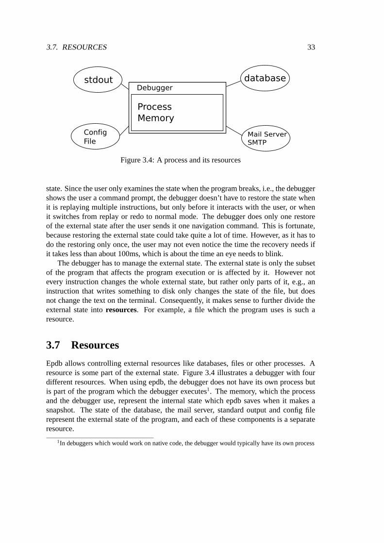
3.7. RESOURCES 33
Debugger
Process
Memory
stdout
Config
File
database
Mail Server
SMTP
Figure 3.4: A process and its resources
state. Since the user only examines the state when the program breaks, i.e., the debuggershows the user a command prompt, the debugger doesn’t have torestore the state whenit is replaying multiple instructions, but only before it interacts with the user, or whenit switches from replay or redo to normal mode. The debugger does only one restoreof the external state after the user sends it one navigation command. This is fortunate,because restoring the external state could take quite a lot of time. However, as it has todo the restoring only once, the user may not even notice the time the recovery needs ifit takes less than about 100ms, which is about the time an eye needs to blink.
The debugger has to manage the external state. The external state is only the subsetof the program that affects the program execution or is affected by it. However notevery instruction changes the whole external state, but rather only parts of it, e.g., aninstruction that writes something to disk only changes the state of the file, but doesnot change the text on the terminal. Consequently, it makes sense to further divide theexternal state intoresources. For example, a file which the program uses is such aresource.
3.7 Resources
Epdb allows controlling external resources like databases, files or other processes. Aresource is some part of the external state. Figure 3.4 illustrates a debugger with fourdifferent resources. When using epdb, the debugger does not have its own process butis part of the program which the debugger executes1. The memory, which the processand the debugger use, represent the internal state which epdb saves when it makes asnapshot. The state of the database, the mail server, standard output and config filerepresent the external state of the program, and each of these components is a separateresource.
1In debuggers which would work on native code, the debugger would typically have its own process
34 CHAPTER 3. REVERSE EXECUTION
Some operations on resources do not allow reversible debugging. For example, oneusually can’t undo the deletion of a file. However, if the debugger saves the content of afile before it deletes it, the debugger can undo the deletion.To restore the content, epdbdoesn’t try to undo the deletion, but instead it saves the state of the file before it getsdeleted. Then, when running to the instruction count beforethe file deletion, it restoresthe file.
Epdb supports an abstraction to implement such additional actions like saving andrestoring state of resources to make operations reversible. For every kind of resource theprogram uses, epdb needs aresource manager. There exists, for example, a resourcemanager to deal with files and another for databases. Every resource has a state, whichthe resource manager labels with an identifier. The identifier should be unique andtherefore a UUID[LMS05] offers some reasonable implementation. When an instruc-tion changes a resource, the patched version of this instruction calls thesave()methodof the corresponding resource manager after it has changed the resource. The resourcemanager then returns the identifier of its state, which epdb manages. The resource man-ager also has arestore()method, which epdb uses to restore to some previously savedstate of the resource. As the resource managers should persist switching snapshots andtherefore switching processes, it is necessary to make themdistributed, and thereforepickleable[Bea09], in order to serialize the object. A resource manager should also im-plement the magic__reduce__()method. Listing 3.3 shows the skeleton of a resourcemanager.
This design of resources isn’t arbitrary, but inspired by how some modern databasesdeal with their data. For example, the Oracle database supports a technology calledflashback[MAA+10]. With flashback, the user is able to restore the database to any pre-vious state. Every state of the database gets an ID, which theuser can use to identifya state. Some NoSQL databases provide similar version control of data. For exam-ple, CouchDB[ALS10] keeps the history of each piece of data andprovides a uniqueidentifier for each version. Making a resource manager for such a database shouldbe straightforward. For files, it should be possible to implement a file system whichallows restoring old versions of the files by never deleting them. Using such a file sys-tem would allow the debugger to transparently implement reversible debuggable files.NILFS[Lay09], for example, has many such properties required for a file system forreversible debugging.
Managing Resources
The resource managers offer a simple interface to save and restore the external state.However, they just assign the different states some identifier and thus there is no re-lation between the identifier for the state and the instruction count to which the statebelongs. This relation is necessary for the debugger, because it has to restore the ex-ternal state for a given instruction count. For example, if the debugger stops in redo
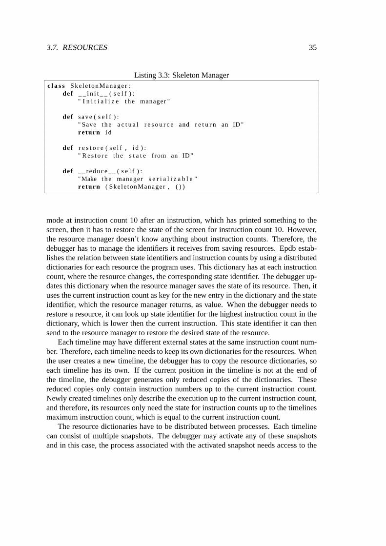
3.7. RESOURCES 35
Listing 3.3: Skeleton Managerc l a s s Ske le tonManager :
def _ _ i n i t _ _ ( s e l f ) :" I n i t i a l i z e t h e manager "
def save ( s e l f ) :" Save t h e a c t u a l r e s o u r c e and r e t u r n an ID "re turn i d
def r e s t o r e ( s e l f , i d ) :" R e s t o r e t h e s t a t e from an ID "
def __reduce__ ( s e l f ) :"Make t h e manager s e r i a l i z a b l e "re turn ( Ske le tonManager , ( ) )
mode at instruction count 10 after an instruction, which hasprinted something to thescreen, then it has to restore the state of the screen for instruction count 10. However,the resource manager doesn’t know anything about instruction counts. Therefore, thedebugger has to manage the identifiers it receives from saving resources. Epdb estab-lishes the relation between state identifiers and instruction counts by using a distributeddictionaries for each resource the program uses. This dictionary has at each instructioncount, where the resource changes, the corresponding stateidentifier. The debugger up-dates this dictionary when the resource manager saves the state of its resource. Then, ituses the current instruction count as key for the new entry inthe dictionary and the stateidentifier, which the resource manager returns, as value. When the debugger needs torestore a resource, it can look up state identifier for the highest instruction count in thedictionary, which is lower then the current instruction. This state identifier it can thensend to the resource manager to restore the desired state of the resource.
Each timeline may have different external states at the sameinstruction count num-ber. Therefore, each timeline needs to keep its own dictionaries for the resources. Whenthe user creates a new timeline, the debugger has to copy the resource dictionaries, soeach timeline has its own. If the current position in the timeline is not at the end ofthe timeline, the debugger generates only reduced copies ofthe dictionaries. Thesereduced copies only contain instruction numbers up to the current instruction count.Newly created timelines only describe the execution up to the current instruction count,and therefore, its resources only need the state for instruction counts up to the timelinesmaximum instruction count, which is equal to the current instruction count.
The resource dictionaries have to be distributed between processes. Each timelinecan consist of multiple snapshots. The debugger may activate any of these snapshotsand in this case, the process associated with the activated snapshot needs access to the
36 CHAPTER 3. REVERSE EXECUTION
resource dictionaries.
3.8 Instruction Patching
Epdb has three modes of execution: normal, replay and redo. While replay and redoalmost always work the same, there is very often a differencebetween normal and re-play/redo mode. Take for example thewrite() function, which writes some bytes todisk. In normal mode, it should actually write something to disk, but in replay mode,it wouldn’t be advisable, because the bytes would already have been written to disk bythe first execution in normal mode, and writing to disk again would change the file tosome wrong state. In replay and redo mode, the file shouldn’t be changed at all, becausemanaging the state of the file is the job of the resource manager. In fact,write() shoulddo nothing, except returning the number of bytes written in the first run.
The debugger knows how many bytes were written in the first runby using a mod-ified version ofwrite(), which actually stores the number of bytes written in some de-bugger internal variable. Epdb supports the shared dictionary nde, which thewrite()-function of a patch module can use to store information the function needs to implementdeterministic execution behavior.
As we see, a reversible debugger requires a different implementation of a functionin replay/redo than in normal mode. Consequently, it needs a way to patch the func-tion, but this patching shouldn’t change the execution while the program runs without adebugger. The patching has to be done at runtime or when the program loads. For dy-namic languages, patching the function at runtime seems to be the cleaner way. Patchinga function at runtime is often calledmonkey patching[Zia08]. Monkey patching is of-ten used in conjunction with software testing. There, it is used to inject a fake or mockobject into the the runtime environment, instead of the object itself. It may also be usedto fix a bug in a running server, which shouldn’t reboot to fix the bug. As I believe thatpatching of instructions has nothing to do with primates, I want to use the more genericterm instruction patching in this paper. It is more generic, because it does not nec-essarily mean that the patching is done at runtime. It may also be done using programinstrumentation at class loading for a statically typed language like Java. If I empha-size that the patching takes place at runtime, I will use the termdynamic instructionpatching. The name instruction patching also has the advantage that it emphasizes thatthe debugger replaces atomic instructions which also have some time context.
With dynamic instruction patching, the function or object is simply replaced atruntime with another one. As functions, objects, and classes are first-class objects inPython, the patching can be done using simple assignments. Using instruction patch-ing, the debugger can use a different version of a function, which distinguishes betweennormal, redo and replay mode.
Epdb uses instruction patching to implement patched versions of functions and ob-
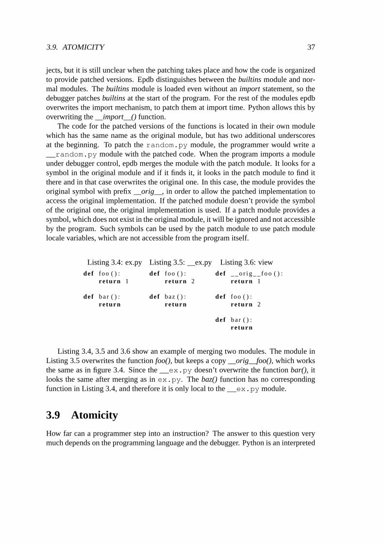
3.9. ATOMICITY 37
jects, but it is still unclear when the patching takes place and how the code is organizedto provide patched versions. Epdb distinguishes between the builtins module and nor-mal modules. Thebuiltins module is loaded even without animport statement, so thedebugger patchesbuiltins at the start of the program. For the rest of the modules epdboverwrites the import mechanism, to patch them at import time. Python allows this byoverwriting the__import__()function.
The code for the patched versions of the functions is locatedin their own modulewhich has the same name as the original module, but has two additional underscoresat the beginning. To patch therandom.py module, the programmer would write a__random.py module with the patched code. When the program imports a moduleunder debugger control, epdb merges the module with the patch module. It looks for asymbol in the original module and if it finds it, it looks in thepatch module to find itthere and in that case overwrites the original one. In this case, the module provides theoriginal symbol with prefix__orig__, in order to allow the patched implementation toaccess the original implementation. If the patched module doesn’t provide the symbolof the original one, the original implementation is used. Ifa patch module provides asymbol, which does not exist in the original module, it will be ignored and not accessibleby the program. Such symbols can be used by the patch module touse patch modulelocale variables, which are not accessible from the programitself.
Listing 3.4: ex.py
def foo ( ) :re turn 1
def bar ( ) :re turn
Listing 3.5: __ex.py
def foo ( ) :re turn 2
def baz ( ) :re turn
Listing 3.6: view
def __o r i g__ foo ( ) :re turn 1
def foo ( ) :re turn 2
def bar ( ) :re turn
Listing 3.4, 3.5 and 3.6 show an example of merging two modules. The module inListing 3.5 overwrites the functionfoo(), but keeps a copy__orig__foo(), which worksthe same as in figure 3.4. Since the__ex.py doesn’t overwrite the functionbar(), itlooks the same after merging as inex.py. Thebaz() function has no correspondingfunction in Listing 3.4, and therefore it is only local to the__ex.py module.
3.9 Atomicity
How far can a programmer step into an instruction? The answerto this question verymuch depends on the programming language and the debugger. Python is an interpreted
38 CHAPTER 3. REVERSE EXECUTION
language and it doesn’t seem to make sense to debug the interpreter itself using a Pythondebugger. The CPython interpreter isn’t even written in Python itself, but in C. If auser wants to debug the interpreter, he better chooses a debugger for C code such asgdb. Even if we ignore the interpreter itself, we may still encounter C code, becausea module for Python can be written in C. The Python debugger pdbstops here andignores stepping into functions in modules written in C, however, it allows stepping intomodules of the standard library. This is helpful for people who develop the standardlibrary, but is usually annoying for programmers who don’t.Many of the standardlibrary modules do some wrapping, before actually calling some module written in C.Therefore, most of the time a user doesn’t get a lot of insightjust by stepping into astandard library module. If they jump into such a module by accident, they often tryto come out as fast as possible. If the debugger allows stepping into a standard libraryfunction, jumping into the standard library code is sometimes unavoidable by the persondoing the debugging. For example, if a function call, which the user is interested todebug, is on the same line as a call to a standard library function, but the debuggerwould execute the standard library function first, then a step at this line would accessthe standard library function before the user defined function.
Epdb avoids stepping into standard library functions. One reason is that it is of-ten more annoying than useful. Another is that it makes it easier to count instructionscorrectly, because the library function might have non-deterministic parts in it. If epdbwould step into the standard library function, the implementer of reverse debugging ca-pabilities would need to make those function calls inside the standard library work inreverse. Those are often very poorly documented, if some documentation even exists.The standard library itself however has very good documentation, and therefore it isusually easier to implement reverse debugging for a standard library call.
One could argue that implementing reversible debugging forprimitive functions ispreferable to implementing reversible debugging for more complex ones, because thecomplex ones consist of primitive functions, and programmers would only have to im-plement a few primitive ones. However, it is often not possible to implement reverse de-bugging for primitive operations, while it is possible to undo more complex ones. Let’stake for example a program which sends a message to another process which shows themessage on the screen. A primitive operation would be, in this case, the sending of themessage. There is no way a program can undo that. When the message is sent, it gets onthe wire, the other process receives it, and does its actionsand then the debugger has noinformation what the other process has done. However, if we look at the more complexfunction “send a message to the other process to write something on the screen”, thedebugger has suddenly much more knowledge of what is happening. For example, toundo this action, it could send a message “undo the effects ofthe last message I sentyou” and the other process could restore the previous state.Of course, designers of sucha system need to pay close attention to such requirements.
CHAPTER 4Epdb Internals
Up to now, I have presented the overall architecture for a reversible debugger. Epdb isa fully working prototype and therefore I had to do many more specific decisions anddetailed design. I want to present them in this section.
4.1 Snapshot Processes
Epdb has three kinds of snapshot processes. There is onecontroller process, onede-buggeeprocess, but multiplesnapshotprocesses, i.e., as many as there are snapshots.
Epdb uses the controller process to manage the communication between the snap-shots. If there wouldn’t be a controller process, every process would need to know aboutevery other process, because every process may activate anyother snapshot and thissnapshot may activate any other snapshot again. The decision would be between a fullmesh or a star topology, but a full mesh topology would require a lot of work to keep theconnections alive and a lot of connections between the processes, i.e.,n(n−1)/2, wheren is the number of snapshots. A star topology requires onlyn connections. However, itrequires one additional process, the controller process. Epdb uses a star topology like inFigure 4.1. This communication topology always routes messages between a snapshotand the debuggee process through the controller process.
Beside the snapshot and the controller process, there is alsothe debuggee process.The debuggee process is the one that does the debugging at themoment, by interactingwith the user. It is the process which actually does work, while the others are just waitingmost of the time. There is only one debuggee process, becauseotherwise the two ormore processes would confuse each other. When the debuggee activates a snapshot, thissnapshot initiates a new debuggee and the previous debuggeeprocess terminates, so thatthere is only one debuggee at any time.
39
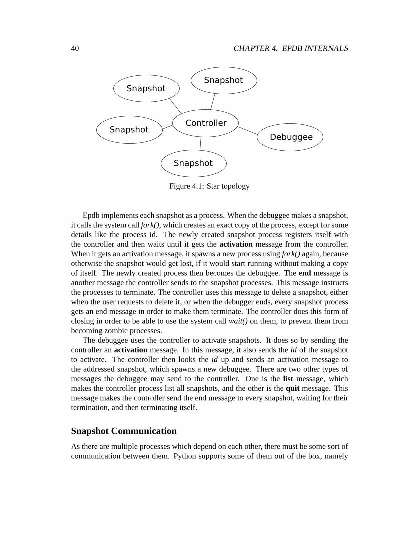
40 CHAPTER 4. EPDB INTERNALS
Controller
SnapshotSnapshot
Snapshot
Snapshot
Debuggee
Figure 4.1: Star topology
Epdb implements each snapshot as a process. When the debuggeemakes a snapshot,it calls the system callfork(), which creates an exact copy of the process, except for somedetails like the process id. The newly created snapshot process registers itself withthe controller and then waits until it gets theactivation message from the controller.When it gets an activation message, it spawns a new process using fork() again, becauseotherwise the snapshot would get lost, if it would start running without making a copyof itself. The newly created process then becomes the debuggee. Theend message isanother message the controller sends to the snapshot processes. This message instructsthe processes to terminate. The controller uses this message to delete a snapshot, eitherwhen the user requests to delete it, or when the debugger ends, every snapshot processgets an end message in order to make them terminate. The controller does this form ofclosing in order to be able to use the system callwait() on them, to prevent them frombecoming zombie processes.
The debuggee uses the controller to activate snapshots. It does so by sending thecontroller anactivation message. In this message, it also sends theid of the snapshotto activate. The controller then looks theid up and sends an activation message tothe addressed snapshot, which spawns a new debuggee. There are two other types ofmessages the debuggee may send to the controller. One is thelist message, whichmakes the controller process list all snapshots, and the other is thequit message. Thismessage makes the controller send the end message to every snapshot, waiting for theirtermination, and then terminating itself.
Snapshot Communication
As there are multiple processes which depend on each other, there must be some sort ofcommunication between them. Python supports some of them out of the box, namely
4.1. SNAPSHOT PROCESSES 41
signals, queue, shared memory and sockets. There are also third party modules for inter-process communication, for example, POSIX or System V queues. The requirementsfor the communication system don’t seem very high. There arenot so many messagesgoing around, but it is necessary that two process, which arenot in a parent/child re-lationship, can easily establish a connection. I tried quite a few forms of interprocesscommunication solutions, before I decided to go for sockets.
Signals
Signals are a very simple form of communication. The Python standard library has sup-port for them. Useful for implementing them is thesignal.pause()function. This makesthe process stop until it receives a signal. Signals seem to be an adequate solution, ifyou have only local snapshots. For global snapshots, there is much more communica-tion between the processes and signals, so there don’t seem to be a sufficient solution toit. Signals also suffer from portability issues.
Queue/Pipes
Python comes with amultiprocessingmodule. This module contains the classesQueueandPipe. Although they are used differently, they share almost the same advantagesand disadvantages. One big advantage is that they are not only bundled with Python,but also implemented portably and work on almost every platform. However, they havea problem: it is not easy to create a Pipe or Queue between two process, which do notknow about each other (i.e. for example in a parent-child relationship). This makes itvery difficult to establish communication, especially for global snapshots.
Shared Memory
There is support for shared memory in Python. Python supports a Managerobject.This object is a separate subprocess. Using shared memory this way wouldn’t saveany processes. It would be possible to save the data related to snapshots in the sharedobjects. Consequently, every process would have access to all snapshot data, but sharedmemory doesn’t solve the synchronization problems. These could be resolved usinglocks, but this would be more complicated than necessary.
POSIX/System V Queues/Pipes
As the Python Queue/Pipes had some shortcomings with respect to establishing com-munication, I looked at POSIX and System V queues and pipes. These are not part ofthe standard Python distribution, but there are third partymodules supporting them. Asit turned out, the problem of establishing a connection between two foreign processesisn’t well supported.
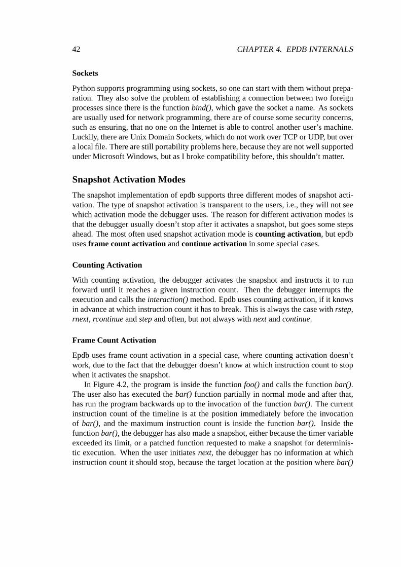
42 CHAPTER 4. EPDB INTERNALS
Sockets
Python supports programming using sockets, so one can startwith them without prepa-ration. They also solve the problem of establishing a connection between two foreignprocesses since there is the functionbind(), which gave the socket a name. As socketsare usually used for network programming, there are of course some security concerns,such as ensuring, that no one on the Internet is able to control another user’s machine.Luckily, there are Unix Domain Sockets, which do not work over TCP or UDP, but overa local file. There are still portability problems here, because they are not well supportedunder Microsoft Windows, but as I broke compatibility before, this shouldn’t matter.
Snapshot Activation Modes
The snapshot implementation of epdb supports three different modes of snapshot acti-vation. The type of snapshot activation is transparent to the users, i.e., they will not seewhich activation mode the debugger uses. The reason for different activation modes isthat the debugger usually doesn’t stop after it activates a snapshot, but goes some stepsahead. The most often used snapshot activation mode iscounting activation, but epdbusesframe count activation andcontinue activation in some special cases.
Counting Activation
With counting activation, the debugger activates the snapshot and instructs it to runforward until it reaches a given instruction count. Then thedebugger interrupts theexecution and calls theinteraction()method. Epdb uses counting activation, if it knowsin advance at which instruction count it has to break. This isalways the case withrstep,rnext, rcontinueandstepand often, but not always withnextandcontinue.
Frame Count Activation
Epdb uses frame count activation in a special case, where counting activation doesn’twork, due to the fact that the debugger doesn’t know at which instruction count to stopwhen it activates the snapshot.
In Figure 4.2, the program is inside the functionfoo() and calls the functionbar().The user also has executed thebar() function partially in normal mode and after that,has run the program backwards up to the invocation of the function bar(). The currentinstruction count of the timeline is at the position immediately before the invocationof bar(), and the maximum instruction count is inside the functionbar(). Inside thefunctionbar(), the debugger has also made a snapshot, either because the timer variableexceeded its limit, or a patched function requested to make asnapshot for determinis-tic execution. When the user initiatesnext, the debugger has no information at whichinstruction count it should stop, because the target location at the position wherebar()
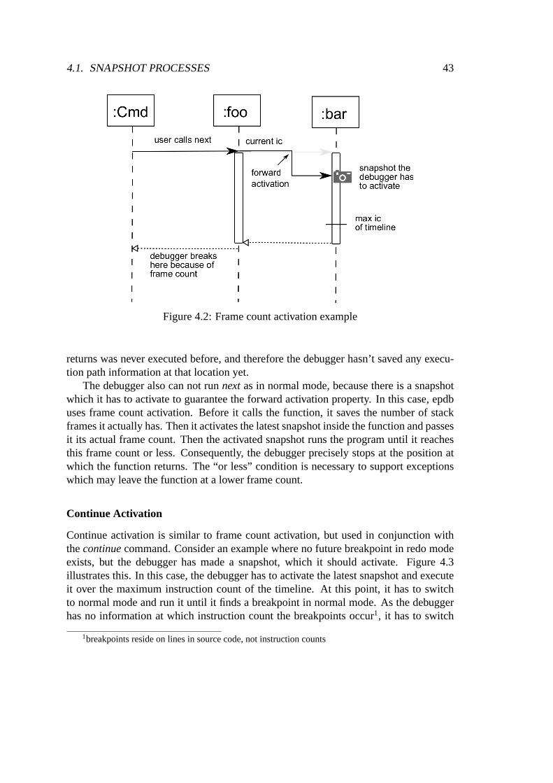
4.1. SNAPSHOT PROCESSES 43
:foo :bar
user calls next
snapshot thedebugger hasto activate
max icof timeline
debugger breakshere because offrame count
:Cmd
forward
activation
current ic
Figure 4.2: Frame count activation example
returns was never executed before, and therefore the debugger hasn’t saved any execu-tion path information at that location yet.
The debugger also can not runnextas in normal mode, because there is a snapshotwhich it has to activate to guarantee the forward activationproperty. In this case, epdbuses frame count activation. Before it calls the function, itsaves the number of stackframes it actually has. Then it activates the latest snapshot inside the function and passesit its actual frame count. Then the activated snapshot runs the program until it reachesthis frame count or less. Consequently, the debugger precisely stops at the position atwhich the function returns. The “or less” condition is necessary to support exceptionswhich may leave the function at a lower frame count.
Continue Activation
Continue activation is similar to frame count activation, but used in conjunction withthecontinuecommand. Consider an example where no future breakpoint in redo modeexists, but the debugger has made a snapshot, which it shouldactivate. Figure 4.3illustrates this. In this case, the debugger has to activatethe latest snapshot and executeit over the maximum instruction count of the timeline. At this point, it has to switchto normal mode and run it until it finds a breakpoint in normal mode. As the debuggerhas no information at which instruction count the breakpoints occur1, it has to switch
1breakpoints reside on lines in source code, not instructioncounts
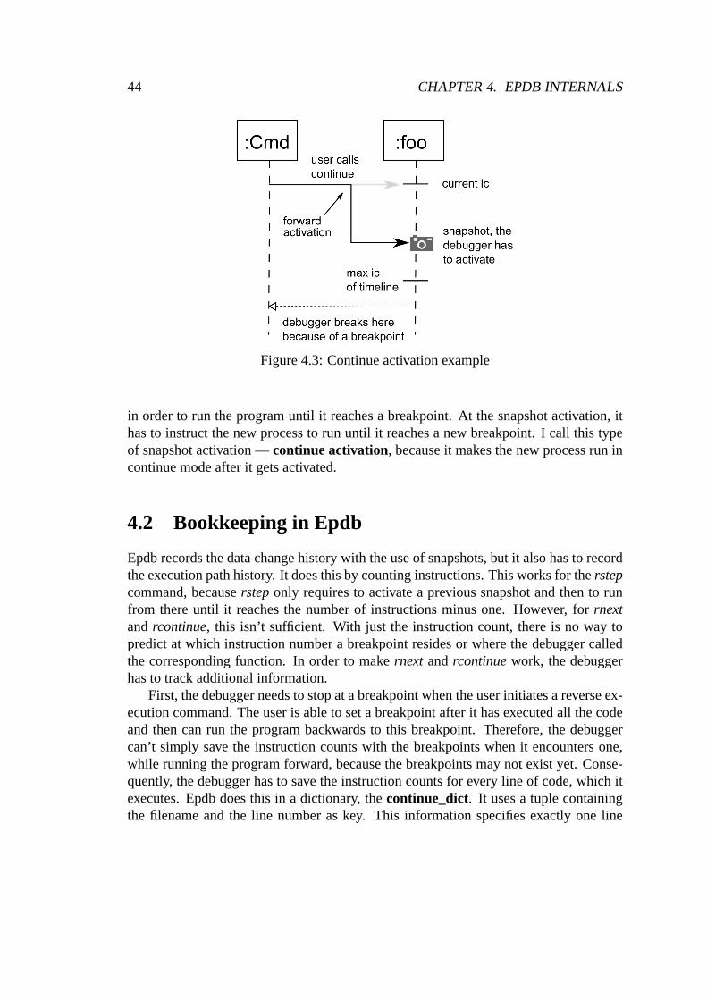
44 CHAPTER 4. EPDB INTERNALS
:foouser calls
continue
snapshot, the
debugger has
to activate
max ic
of timeline
debugger breaks here
because of a breakpoint
:Cmd
Figure 4.3: Continue activation example
in order to run the program until it reaches a breakpoint. At the snapshot activation, ithas to instruct the new process to run until it reaches a new breakpoint. I call this typeof snapshot activation —continue activation, because it makes the new process run incontinue mode after it gets activated.
4.2 Bookkeeping in Epdb
Epdb records the data change history with the use of snapshots, but it also has to recordthe execution path history. It does this by counting instructions. This works for therstepcommand, becausersteponly requires to activate a previous snapshot and then to runfrom there until it reaches the number of instructions minusone. However, forrnextandrcontinue, this isn’t sufficient. With just the instruction count, there is no way topredict at which instruction number a breakpoint resides orwhere the debugger calledthe corresponding function. In order to makernext andrcontinuework, the debuggerhas to track additional information.
First, the debugger needs to stop at a breakpoint when the user initiates a reverse ex-ecution command. The user is able to set a breakpoint after ithas executed all the codeand then can run the program backwards to this breakpoint. Therefore, the debuggercan’t simply save the instruction counts with the breakpoints when it encounters one,while running the program forward, because the breakpointsmay not exist yet. Conse-quently, the debugger has to save the instruction counts forevery line of code, which itexecutes. Epdb does this in a dictionary, thecontinue_dict. It uses a tuple containingthe filename and the line number as key. This information specifies exactly one line
4.3. SHARED MEMORY 45
of code. As a value it uses a list of instruction counts, whichare executed on this lineof code. Using this dictionary, it is possible to calculate the position of the breakpointwhen running multiple instructions backwards or when running forwards in redo mode.
For rnext to work, the information saved in thecontinue_dictis not enough, be-cause the debugger needs to know on which instruction countsthe functions have re-turned. It keeps another dictionary, thernext_dict. Every time the debugger encountersa user_return(), it adds an entry to the dictionary with the current instruction count asthe key and the instruction count of the correspondinguser_return()as the value. Con-sequently, it is possible to calculate the position in the program where arnext shouldstop the program execution.
There is another situation where the debugger needs additional information and thatis in case of anextcommand, when the debugger is in redo mode. There are maybesnapshots inside the function and therefore epdb must activate the latest snapshot insidethe function, because of the forward activation property. Epdb keeps another dictionary,the next_dict, which is the reverse form of thernext_dict, i.e., it has the instructioncount from the correspondinguser_call()as the key and the instruction count at theuser_return()as the value. Using this dictionary, the debugger can calculate the nearestsnapshot to the target position and therefore is able to guarantee forward activation.
With next_dictandcontinue_dict, there is the problem that the information the de-bugger saves may be used by a snapshot made earlier. As this earlier snapshot hasn’trecorded the information ofnext_dictand continue_dictfor later instruction counts,it wouldn’t have this information. Therefore epdb must use ashared dictionary fornext_dictandcontinue_dictto make this information available to all snapshot processes.This shared dictionary should belong to a timeline, i.e., each timeline should have itsown version ofcontinue_dictandnext_dict.
With rnext_dict, the situation is a little different. It is only needed for informationin the past. Therefore, the debugger doesn’t need to share the dictionary with otherprocesses, because each process can track the information it needs.
4.3 Shared Memory
As described in 3.5, the debugger has to record the behavior of non-deterministic func-tions and exchange the recorded data with other processes. Section 3.7 showed thatepdb makes use of resource managers, which must be synchronized among all pro-cesses. Section 4.4 shows that breakpoints need to be distributed. Epdb also has to keeptrack of the execution path history which should be available to all snapshots, and last,but not least, it has to keep information of timelines synchronized over all processes.
To synchronize all the data, epdb uses its own server process, which it starts at itsown startup. Most of the data can be handled in a shared dictionary, but the breakpoint
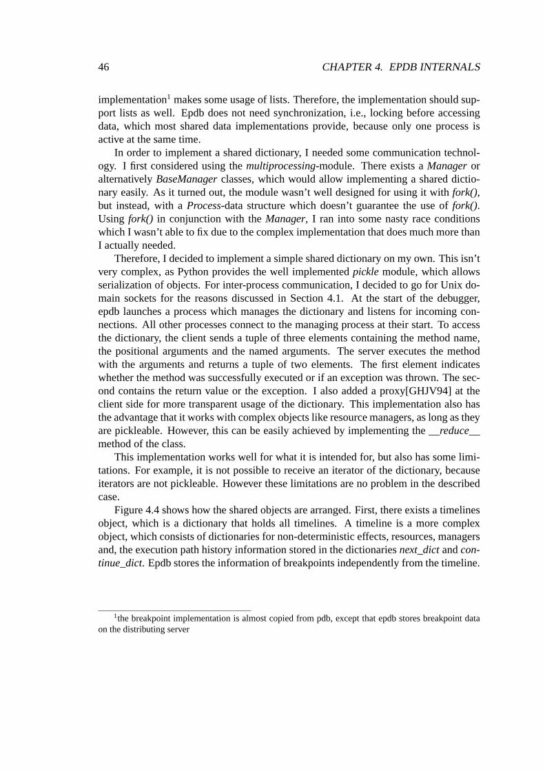
46 CHAPTER 4. EPDB INTERNALS
implementation1 makes some usage of lists. Therefore, the implementation should sup-port lists as well. Epdb does not need synchronization, i.e., locking before accessingdata, which most shared data implementations provide, because only one process isactive at the same time.
In order to implement a shared dictionary, I needed some communication technol-ogy. I first considered using themultiprocessing-module. There exists aManageroralternativelyBaseManagerclasses, which would allow implementing a shared dictio-nary easily. As it turned out, the module wasn’t well designed for using it withfork(),but instead, with aProcess-data structure which doesn’t guarantee the use offork().Using fork() in conjunction with theManager, I ran into some nasty race conditionswhich I wasn’t able to fix due to the complex implementation that does much more thanI actually needed.
Therefore, I decided to implement a simple shared dictionary on my own. This isn’tvery complex, as Python provides the well implementedpickle module, which allowsserialization of objects. For inter-process communication, I decided to go for Unix do-main sockets for the reasons discussed in Section 4.1. At thestart of the debugger,epdb launches a process which manages the dictionary and listens for incoming con-nections. All other processes connect to the managing process at their start. To accessthe dictionary, the client sends a tuple of three elements containing the method name,the positional arguments and the named arguments. The server executes the methodwith the arguments and returns a tuple of two elements. The first element indicateswhether the method was successfully executed or if an exception was thrown. The sec-ond contains the return value or the exception. I also added aproxy[GHJV94] at theclient side for more transparent usage of the dictionary. This implementation also hasthe advantage that it works with complex objects like resource managers, as long as theyare pickleable. However, this can be easily achieved by implementing the__reduce__method of the class.
This implementation works well for what it is intended for, but also has some limi-tations. For example, it is not possible to receive an iterator of the dictionary, becauseiterators are not pickleable. However these limitations are no problem in the describedcase.
Figure 4.4 shows how the shared objects are arranged. First,there exists a timelinesobject, which is a dictionary that holds all timelines. A timeline is a more complexobject, which consists of dictionaries for non-deterministic effects, resources, managersand, the execution path history information stored in the dictionariesnext_dictandcon-tinue_dict. Epdb stores the information of breakpoints independentlyfrom the timeline.
1the breakpoint implementation is almost copied from pdb, except that epdb stores breakpoint dataon the distributing server
4.4. BREAKPOINTS 47
Timelines
Timelinende
Next Continue
Resources
Managers
Breakpoints
Figure 4.4: Organization of shared data
4.4 Breakpoints
There are different processes communicating with the user.Therefore breakpointsshould appear to the user in the same way regardless which process is currently the de-buggee. Without changing the bdb implementation, every process would handle break-points separately. This means that after restoring a snapshot, the user would probablysee fewer or different breakpoints. Therefore, I decided toimplement a distributedversion using the shared memory approach. As it turned out, Icould reuse the imple-mentation of breakpoints from bdb and pdb, but I had to replace the data structures,which store the breakpoint information, with shared data structures, i.e., remote prox-ies, which forward the function calls to the shared memory server. For the breakpointimplementation, I needed a shared dictionary and a shared list, because bdb uses thosedata structures to index the breakpoints in different ways.
For the implementation of shared breakpoints, there are tworeasonable ways toimplement them. They could either belong to a timeline, or they could be global. If theybelong to a timeline, the users would see different breakpoints for each timeline. In theglobal approach, the users would see the same breakpoints when they switch to anothertimeline. I decided to go for the global approach, because breakpoints belong to someline in the source code. As the source code doesn’t change when the timeline changes,this seemed more reasonable to me. However, the timeline approach has advantagestoo. For example, the user may want to search for a different bug in two differenttimelines and therefore would need different breakpoints in each timeline. Therefore, afull-featured implementation of a reversible debugger might implement both.
48 CHAPTER 4. EPDB INTERNALS
4.5 Implementation of Debugging Commands
Although pdb provides an implementation for the standard debugging commandsstep,nextandcontinue, their implementation doesn’t combine well with instruction counting.The reason is that pdb doesn’t call a trace function on every instruction executed, butonly on those, which are located in frames, that have a breakpoint in it. This optimiza-tion makes debugging faster, but doesn’t allow applying instruction counting. Therefore,it is necessary to rewrite those functions.
Step
The stepcommand in epdb works similarly to the one in pdb, as it only steps one in-struction forward. Therefore, it doesn’t interfere with instruction counting, becauseinstruction counting requires the debugger to stop after each atomic instruction. Stepgoes exactly one atomic instruction ahead, and stops exactly where the instruction countmechanism increments its instruction count. Therefore thestop mechanism is the sameas in pdb in normal mode, but epdb also supports the redo mode.In redo mode, epdbfirst checks if there is a snapshot at the next instruction forthe current timeline. If it isthe case, it activates the snapshot instead of stepping one instruction forward, to guar-antee the forward activation property of the debugger. After a successful step in redomode, epdb has to restore all resources to their state for theactual instruction count.
Next
Nextworks similar tostep, except when the current line contains at least one functioncall. Then theuser_call()method is called beforeuser_line(). In the pdb implemen-tation, the_stop_frameis set to the current frame. This means that the debugger onlystops when it returns from the function call to the current frame. It also means that theinstruction count would only be increased by one, because the trace function would onlybe called once. This is undesirable because epdb would confuse the instruction countsin replay mode, because there, it would step into the function.
To fix this issue, epdb implementsnextsimilar tostepin that it calls the trace func-tion on every call, but doesn’t always calls theinteraction()method. If the debugger runsover a function call, it calls theuser_call()method beforehand and theuser_return()method afterwards. Before callingnextthe debugger stores the number of stack frameswhich the debuggee currently has. When it steps into the function, the function call setsup a new stack frame and increases the number of frames. When itleaves the function,it deletes a stack frame and decrements the number of frames.The debuggee may createadditional frames by calling other functions, but when it equals the number of frames itstored previously, it has returned from the function. If it is less than this number, thenit has left the function via an exception, and therefore has reached the position where
4.5. IMPLEMENTATION OF DEBUGGING COMMANDS 49
the next command should present the user a command prompt. Furthermore, the nextcommand should also consider breakpoints. A breakpoint check in user_line()solvesthis.
Like step, nexthas to treat normal and redo modes differently. In redo mode,epdbtries to find an appropriate snapshot, and then activates it.In contrast tostep, nextrequires two different activation modes. First, a snapshotactivation, combined withgoing a number of steps forward (see counting activation in Section 4.1), and second,a snapshot activation until the stack depth reaches a given number (see frame countactivation in Section 4.1). Asstep, nexthas to restore the resources before the debuggershows the command prompt.
Continue
Continuesuffers from the same problem asnext, in conjunction with instruction count-ing. The epdb version ofcontinuecalls the trace function on every line of code. In theuser_line()method, it checks if the actual line is a breakpoint, and in this case, providesa command prompt. In redo mode,continuecalculates the halting position using thecontinue_dictand tries to find the best positioned snapshot to reach it. However, if thenext breakpoint is after the maximum instruction count of the timeline or doesn’t ex-ist (in this case it is the end of the program), epdb uses the snapshot with the highestinstruction count from the timeline and activates it until it finds a breakpoint, or the pro-gram ends. This type of activation is called continue activation as described in Section4.1
Rstep
There is is no implementation for all the reverse debugging commands in pdb. There-fore, I had to implement them in epdb from scratch. For reverse execution, epdb ignoresthe external state at first and does replaying by activating aprevious snapshot. Then,it does counting activation until it reaches the current instruction count minus one. Itreplays some instructions in replay mode, and before it shows the command promptto signal that reverse stepping has finished, it switches to redo mode, and thus sets theresources to their state at this instruction count in the actual timeline. Consequently, thedebugger doesn’t need to reset the state after every replayed instruction, but only onceper initiated user command.
Rnext
A rnext means to avoid stepping into a function that returned to the actual position inthe program. In epdb,rnextdoes the opposite of a precedingnext. If the user has senta next, and afterwards arnext command, then he is at the same position in the source
50 CHAPTER 4. EPDB INTERNALS
code as before. The only thing that may change is the mode, i.e., if the debugger waspreviously in normal mode, it is after arnextalways in redo mode.
However, without additional tracked information, the debugger doesn’t know whichfunction to step in and which to skip while it is replaying. Arnext can mean to steponly one instruction backwards, or it can mean to step multiple instructions backwardsdepending on if the last instruction was a function call or not. To solve this problem,I decided to track every instruction count at a function callwith the correspondent in-struction count at the return of the function. Epdb stores this information in a dictionaryrnext_dict1, with the return instruction count as the key. Then, the debugger can lookup the corresponding call instruction count. If it does not exist, it can simply step onestep backwards. If it exists, it can step back until it reaches the call instruction count.Both of these types of stepping backwards only require counting activation.
Like rstep, rnextsets the resources to their appropriate state only before itshows acommand prompt.Rstepalways ends in redo mode.
Rcontinue
Similar tornext, for rcontinueto work, the debugger has to track additional information.Without this information, the debugger wouldn’t know at which breakpoint to stop. Itcould be that it has to stop at the first line with a breakpoint it encounters, or at thesecond or any following.
Epdb keeps a dictionarycontinue_dictwith a tuple, that contains the filename andline number as the key, and a list of instruction counts as thevalue. If the programmernavigates backwards, epdb can iterate through every breakpoint and check if there is aninstruction count in the dictionary. Then, it takes the highest instruction count and usesit to calculate the steps to run forward. When it reaches its goal, it sets the resources andthen switches to redo mode asrnextandrstepalways do.
In principle, it is possible to implement this dictionary locally for each process,because the program can reproduce it while running forward and it is usually not usedto jump forward. However, since epdb allows timeline switching, the correspondingcontinue dictionary is not available if the user is in a different timeline, and thereforecan’t switch to another timeline. Thus I made thecontinue_dictshared, because I feel itis the cleanest solution.
4.6 Example Patch Modules
I implemented a simple patch module set, which illustrates the principle of dealing withnon-determinism and side effects. For non-determinism, I chose thetime()-function of
1see Section 4.2
4.6. EXAMPLE PATCH MODULES 51
the time module. For functions which also have side effects, I chose the built-in fileediting functionsopen(), read(), write(), close().
Time
The time.time()function is a typical example of a non-deterministic function. It returnsthe actual time as a floating point number. This number represents the numbers ofseconds passed since January 1st 1970, at 0:00. Thetime.time()function does not haveside effects, because it doesn’t actively change the time.
There are two ways to implementtime.time(). The patched function could eitherstore the return value in a stored dictionary or it could instruct the debugger to make asnapshot after the instruction.
Implementation with a Shared Dictionary
In order to create an patched version of thetimemodule, the debugger needs a__timemodule. If this module exists, the debugger then merges these two modules. Listing 4.1shows an implementation for the__timemodule.
One tricky aspect in the implementation of thetimemodule is that the module nameis the same as the function name. Since the function needs to access the original module,it needs to import the originaltimemodule. However, this module has the same name asthe function and therefore every reference totimewould reference the function insteadof the module. Thus, the module should import thetimemodule as a different name. Inthe example, thetimemodule is imported astimemod.
The implementation of thetimefunction distinguishes between normal and redo/re-play mode. In normal mode it first uses the original implementation to get the systemtime. It then saves the time in the shared dictionary at the actual instruction count andafter that it returns the time value. In redo and replay mode it looks up the value in thedictionary and returns it. By this means the function always returns the same time valuein redo mode as it returned it in normal mode, when the debugger executed it the firsttime.
Implementation with Snapshots
The alternative implementation of__time instructs the debugger to make a snapshotafter the instruction. Listing 4.2 shows an implementationof time using the snapshotapproach. The dbg module provides the objectsnapshottingcontrolwith a method,which allows to do exactly this. In normal mode, the implementation calls this methodand then returns the system time using the original function. There is no implementationfor redo or replay mode, because the debugger never executesthe function in redo orreplay mode, but instead activates the snapshot after the instruction.
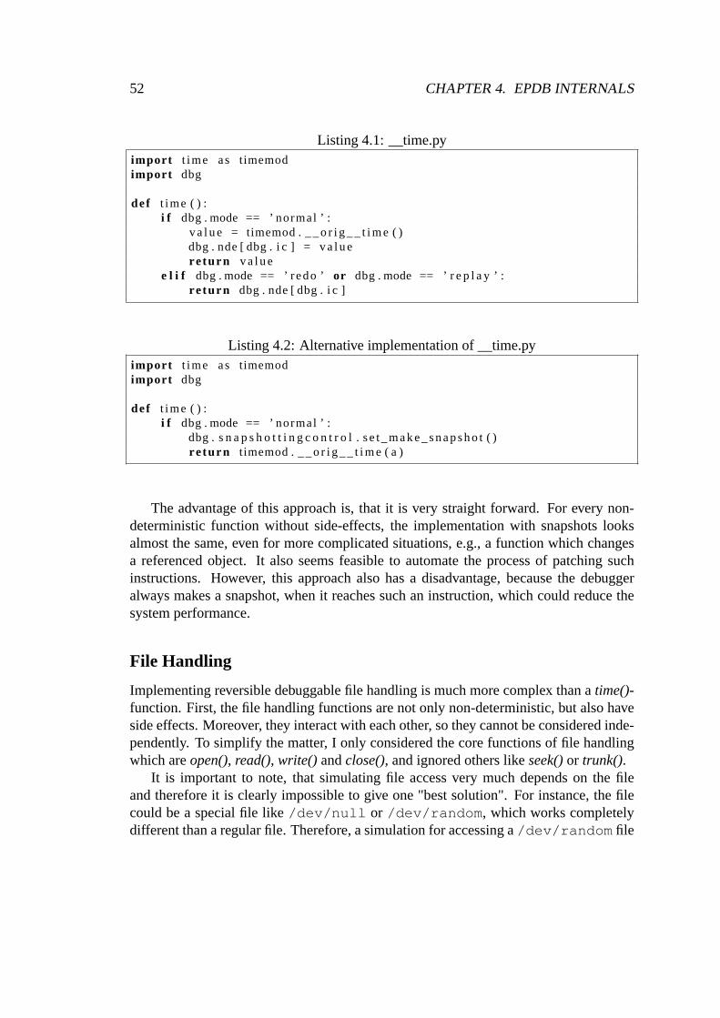
52 CHAPTER 4. EPDB INTERNALS
Listing 4.1: __time.pyimport t ime as timemodimport dbg
def t ime ( ) :i f dbg . mode == ’ normal ’ :
va l ue = timemod . __o r i g__ t i m e ( )dbg . nde [ dbg . i c ] = va l uere turn va l ue
e l i f dbg . mode == ’ redo ’ or dbg . mode == ’ r e p l a y ’ :re turn dbg . nde [ dbg . i c ]
Listing 4.2: Alternative implementation of __time.pyimport t ime as timemodimport dbg
def t ime ( ) :i f dbg . mode == ’ normal ’ :
dbg . s n a p s h o t t i n g c o n t r o l . se t_make_snapsho t ( )re turn t imemod . __o r i g__ t i m e ( a )
The advantage of this approach is, that it is very straight forward. For every non-deterministic function without side-effects, the implementation with snapshots looksalmost the same, even for more complicated situations, e.g., a function which changesa referenced object. It also seems feasible to automate the process of patching suchinstructions. However, this approach also has a disadvantage, because the debuggeralways makes a snapshot, when it reaches such an instruction, which could reduce thesystem performance.
File Handling
Implementing reversible debuggable file handling is much more complex than atime()-function. First, the file handling functions are not only non-deterministic, but also haveside effects. Moreover, they interact with each other, so they cannot be considered inde-pendently. To simplify the matter, I only considered the core functions of file handlingwhich areopen(), read(), write() andclose(), and ignored others likeseek()or trunk().
It is important to note, that simulating file access very muchdepends on the fileand therefore it is clearly impossible to give one "best solution". For instance, the filecould be a special file like/dev/null or /dev/random, which works completelydifferent than a regular file. Therefore, a simulation for accessing a/dev/random file
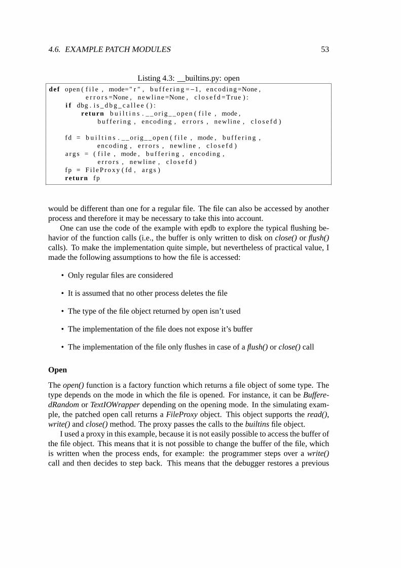
4.6. EXAMPLE PATCH MODULES 53
Listing 4.3: __builtins.py: opendef open ( f i l e , mode=" r " , b u f f e r i n g =−1 , encod ing =None ,
e r r o r s =None , new l ine =None , c l o s e f d =True ) :i f dbg . i s _ d b g _ c a l l e e ( ) :
re turn b u i l t i n s . __or ig__open ( f i l e , mode ,b u f f e r i n g , encoding , e r r o r s , newl ine , c l o s e f d )
fd = b u i l t i n s . __or ig__open ( f i l e , mode , b u f f e r i n g ,encoding , e r r o r s , newl ine , c l o s e f d )
a r g s = ( f i l e , mode , b u f f e r i n g , encoding ,e r r o r s , newl ine , c l o s e f d )
fp = F i l e P r o x y ( fd , a r g s )re turn fp
would be different than one for a regular file. The file can alsobe accessed by anotherprocess and therefore it may be necessary to take this into account.
One can use the code of the example with epdb to explore the typical flushing be-havior of the function calls (i.e., the buffer is only written to disk onclose()or flush()calls). To make the implementation quite simple, but nevertheless of practical value, Imade the following assumptions to how the file is accessed:
• Only regular files are considered
• It is assumed that no other process deletes the file
• The type of the file object returned by open isn’t used
• The implementation of the file does not expose it’s buffer
• The implementation of the file only flushes in case of aflush()or close()call
Open
Theopen()function is a factory function which returns a file object of some type. Thetype depends on the mode in which the file is opened. For instance, it can beBuffere-dRandomor TextIOWrapperdepending on the opening mode. In the simulating exam-ple, the patched open call returns aFileProxy object. This object supports theread(),write() andclose()method. The proxy passes the calls to thebuiltins file object.
I used a proxy in this example, because it is not easily possible to access the buffer ofthe file object. This means that it is not possible to change the buffer of the file, whichis written when the process ends, for example: the programmer steps over awrite()call and then decides to step back. This means that the debugger restores a previous
54 CHAPTER 4. EPDB INTERNALS
Listing 4.4: __builtins.py: FileProxyc l a s s F i l e P r o x y :
def _ _ i n i t _ _ ( s e l f , f i l e , a r g s ) :s e l f . _ _ f i l e _ _ = f i l es e l f . _a r gs = a r g ss e l f . fn = fn = a r g s [ 0 ]r e s o u r c e = dbg . c u r r e n t _ t i m e l i n e . \
new_resource ( ’ f i l e ’ , fn )rm = r e s o u r c e s . F i l eResourceManager ( s e l f . fn )s e l f . _ f i l e r e s o u r c e m a n a g e r = dbg . c u r r e n t _ t i m e l i n e . \
c rea te_manage r ( ( ’ f i l e ’ , fn ) , rm )i d = s e l f . _ f i l e r e s o u r c e m a n a g e r . save ( )i f not dbg . i c i n r e s o u r c e :
r e s o u r c e [ dbg . i c ] = i d
def w r i t e ( s e l f , b ) : " . . . "def r ead ( s e l f , n =−1): " . . . "def c l o s e ( s e l f ) : " . . . "
snapshot and terminates the previous debuggee. This means that all changes to thebuffer are flushed out, which should be considered by the activated process.
Another problem with open file descriptors is their behaviorin conjunction withfork(). Let’s consider a program which opens a file and writes to it. After that, it forksanother process and then both processes close the file. This would actually mean thatthe stream would be written twice, which is probably not intended. Epdb solves thisproblem by using resources, which have a state. If the debugger closes a process, e.g.,because the user deletes a snapshot, it can recover the external state by resetting the fileresource to its actual state.
The implementation of theopen()function can be seen in Listing 4.3. The first thingthis implementation checks is if the callee is some debuggerrelated module, becausethe debugger usesopen()as well. In this case, the debugger does not use the patchedversion ofopen(), but the original one. The implementation ofopen()works the samein redo, replay or normal mode, becauseopen()is a deterministic1 function with sideeffects. Instead of returning aFile object, the patched version ofopen()returns a proxyto it, i.e., theFileProxy. This proxy provides its own implementation ofread(), write()andclose()methods.
4.6. EXAMPLE PATCH MODULES 55
Listing 4.5: __builtins.py: read()def r ead ( s e l f , n =−1):
i f dbg . mode == ’ normal ’ :dbg . s n a p s h o t t i n g c o n t r o l . se t_make_snapsho t ( )va l ue = s e l f . _ _ f i l e _ _ . read ( n )re turn va l ue
FileProxy
As shown in Listing 4.4, theFileProxydoes not only provide patched versions ofread(),write() and close(), but also manages the file resource manager. It generates a newresource and a resource manager. Then it saves the actual state and stores theid in theshared resources dictionary. Keep in mind, that the currenttimeline can change betweenthe FileProxy initialization and its method calls (e.g., by creating a newtimeline) andtherefore, the resource dictionary should not be stored as amember variable for using itin other method calls.
Read
The read() method is a non-deterministic function without side effects. It is non-deterministic, because the debugger doesn’t know what the method is going to return.The read()-method relies on an external state, the file. However, it doesn’t change theexternal state and so it has no side effects. These considerations allow one to implementthe read()method using snapshots. The implementation shown in Listing 4.5 achievesthis by calling theset_make_snapshot()method of thesnapshotcontrolin normal mode.There is no implementation ofread() in replay or redo mode. This is because epdbwould never callread() in replay or redo mode, but would instead activate the nextsnapshot, because of forward activation. This snapshot hasthe correct internal stateafter theread()call in normal mode.
Write
Thewrite() method is a non-deterministic function with side effects. The side effects areobvious, because it changes an external state, the file. It isalso non-deterministic, be-cause thewrite() method also returns the number of bytes written and this number doesnot have to be the same as the number of characters in the argument. A possible im-plementation ofwrite() may look similar to Listing 4.6. Aswrite() is non-deterministic,it is easiest to just let the debugger do all the work and then to tell it to make a new
1at least if we consider the internals ofopen()such as the integer descriptor, as being of no particularinterest
56 CHAPTER 4. EPDB INTERNALS
Listing 4.6: __builtins.py: write()def w r i t e ( s e l f , b ) :
va l ue = s e l f . _ _ f i l e _ _ . w r i t e ( b )i d = s e l f . _ f i l e r e s o u r c e m a n a g e r . save ( )dbg . c u r r e n t _ t i m e l i n e . \
g e t _ r e s o u r c e ( ’ f i l e ’ , s e l f . fn ) [ dbg . i c +1] = i ddbg . s n a p s h o t t i n g c o n t r o l . se t_make_snapsho t ( )re turn va l ue
snapshot after the write call, as was done in theread()example. However,write() alsochanges the external state and therefore it should also tellthe resource manager to savethe state and to put the state identifier into the resource dictionary, so that the debuggercan restore the state of the file later on. Similar toread() the implementation ofwrite()doesn’t need an implementation for replay or redo mode because epdb uses forwardactivation.
Close
The close()method is an example of a deterministic function with side effects. Animplementation may look similar to the code in Listing 4.7. As it is deterministic, it isnot necessary to make a snapshot after this function call. However, it is necessary tosave the state of the file resource afterclose(), becauseclose()flushes the buffer. Asthe patchedclose()method does not instruct the debugger to make a snapshot after itsreturn, it is possible that the debugger calls theclose()function in redo or replay mode.The implementation also proxies theclose()method in these modes as opposed to thenon-deterministicread()andwrite() methods.
I do not consider this implementation of file handling a pretty one, but more of ahack. However, I think this example shows the power of the framework, that it can beused to simulate even such complex operations like file handling quite easily. A bettersolution to this problem, in my opinion, would be to use a special file system for the filesthe application uses. This file system should not delete or change files, but instead savea new version of the old file and it should allow the restoration of old versions of thefiles. This is similar to the way some databases with Multi Version Concurrency Control(MVCC) save their data. The file system in user space (FUSE) technology allows toimplement such a file system entirely in user space. Using a special file system wouldalso allow a way to deal with some special files like/dev/random. The file systemcould store old versions of the number generator. However, implementing such a filesystem is out of the scope of this thesis.
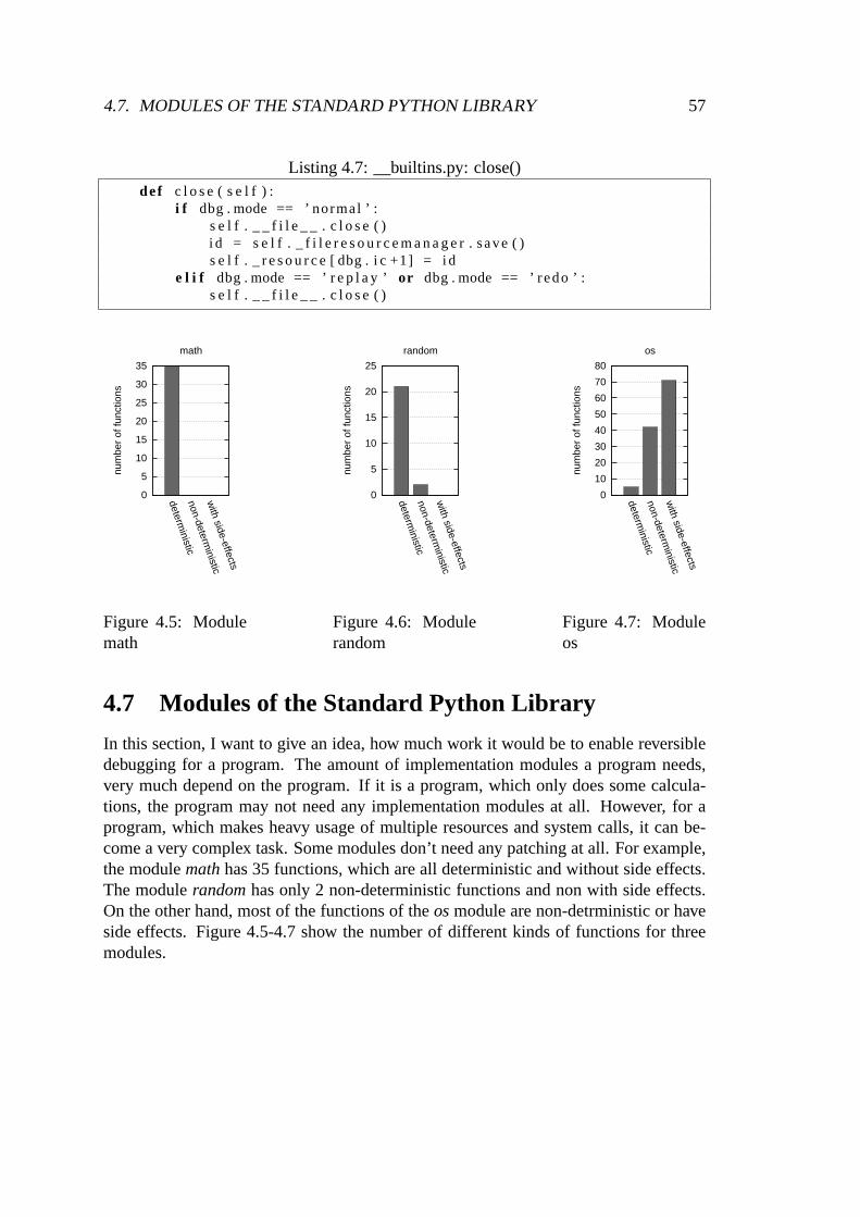
4.7. MODULES OF THE STANDARD PYTHON LIBRARY 57
Listing 4.7: __builtins.py: close()def c l o s e ( s e l f ) :
i f dbg . mode == ’ normal ’ :s e l f . _ _ f i l e _ _ . c l o s e ( )i d = s e l f . _ f i l e r e s o u r c e m a n a g e r . save ( )s e l f . _ r e s o u r c e [ dbg . i c +1] = i d
e l i f dbg . mode == ’ r e p l a y ’ or dbg . mode == ’ redo ’ :s e l f . _ _ f i l e _ _ . c l o s e ( )
0
5
10
15
20
25
30
35
deterministic
non-deterministic
with side-effects
num
ber
of fu
nctio
ns
math
Figure 4.5: Modulemath
0
5
10
15
20
25
deterministic
non-deterministic
with side-effects
num
ber
of fu
nctio
nsrandom
Figure 4.6: Modulerandom
0
10
20
30
40
50
60
70
80
deterministic
non-deterministic
with side-effects
num
ber
of fu
nctio
ns
os
Figure 4.7: Moduleos
4.7 Modules of the Standard Python Library
In this section, I want to give an idea, how much work it would be to enable reversibledebugging for a program. The amount of implementation modules a program needs,very much depend on the program. If it is a program, which onlydoes some calcula-tions, the program may not need any implementation modules at all. However, for aprogram, which makes heavy usage of multiple resources and system calls, it can be-come a very complex task. Some modules don’t need any patching at all. For example,the modulemathhas 35 functions, which are all deterministic and without side effects.The modulerandomhas only 2 non-deterministic functions and non with side effects.On the other hand, most of the functions of theosmodule are non-detrministic or haveside effects. Figure 4.5-4.7 show the number of different kinds of functions for threemodules.

CHAPTER 5Performance
Lienhard[LGN08] notes that the snapshot & replay approach is slow, because the debug-ger has to re-execute the program partly. I don’t agree, because replaying can be evenfaster than in logging-based debuggers, e.g., when the userwants to recover a positionwhere the debugger has made a snapshot. In this case, it has toclose its actual processand create a new process from the snapshot, which becomes thedebuggee. Creating anew processes with copy-on-write is so fast, that it takes usually less than 1ms. On theother hand, the seek time of a hard drive takes typically a fewmilliseconds for spinninghard drives or about 0.1ms for SSDs. The replaying time in thebest case is much lowerthan most users are able to perceive, which is about 100-200ms.
In the worst case, the performance of an execution command should end after acertain amount of time and therefore, the debugger should give some upper bound on theexecution time of the command. If this time is less than the user is able to perceive, thenthere is at least no performance reason to avoid using a reversible debugger. The purposeof this section is to show that it is in principle possible to achieve this performance goal.However, I don’t want to give benchmarks on epdb, because thereal execution timedepends so much on the hardware and epdb isn’t performance optimized yet.
Epdb distinguishes two modes, which are visible to the user,the normal and theredo mode. So we have to look at the performance of the debugger in each mode. Innormal mode, the debugger has a lot of overhead. Most important is the additional workit needs to count the number of instructions, since epdb implements this in pure Python.This slows down the execution. Then, there is some overhead to save non-deterministiceffects and to make snapshots and to track the execution pathhistory. A reversibledebugger is slower in this respect. However, the execution is slowed down by someconstant1 extra time per instruction.
1I haven’t added the time for the resource management here, because this time is very applicationdependent
59
60 CHAPTER 5. PERFORMANCE
In the situation in redo mode, assuming the timeline has beenexecuted until theprogram has finished and every instruction is executed in redo mode, the debugger onlyhas to restore a snapshot and run some instructions forward.Therefore, the activationtime of the new process takes some constant amount of time, but running forward an ar-bitrary number of instructions in redo mode takes constant time too! This is because thedebugger makes a snapshot every time the execution time counter passes one second.The debugger never executes the last instruction which exceeds the one second limit inredo mode, but instead activates the next snapshot. The execution time in redo modeis always below one second plus the time needed to activate the snapshot. Of coursethere is some additional overhead to recover the external state, but in the special case ofa program, which doesn’t make use of external resources, theexecution time of everynavigation command in redo mode is constant or in other wordsO(1). The executiontime of a program in redo mode can be even faster than the program execution of a pro-gram without a debugger. The constant execution time in redomode assumes however,that there is no overhead by having multiple snapshots, which is unfortunately not thecase. However, it is in principle possible to limit the number of processes by saving thesnapshots to disk and restoring them from there, but epdb does not implement snapshotslike that.
5.1 Instruction Counting
Python does not count the instructions by default. To do this, I implemented instruc-tion counting using the trace function. Every time an instruction is executed, the tracefunction is called, which increments the instruction counter by one. Consequently, itis possible to add instruction counting without changing the source code of the Pythoninterpreter. However, it has significant influence on the execution time. To estimatethe performance impact of instruction counting, I implemented a program that doesnothing else than executing a Python script with instruction counting with the abovedescribed approach. Then, I ran the microbenchmark programpybench, that comeswith the Python interpreter, with and without instruction counting. The tests were runon a AMD Athlon(tm) 7550 Dual-Core 64bit - Processor with 2.5 GHz. The Pythoninterpreter used was 3.1.1+ on an Ubuntu Karmic Koala.
The tests inpybenchwere repeated multiple times. Figure 5.1 shows the relationbetween the average execution time with instruction counting and without instructioncounting. As you can see from the diagram, with instruction counting the tests run mostof the time about 15 times slower. For one extreme example it runs even 110 timesslower.
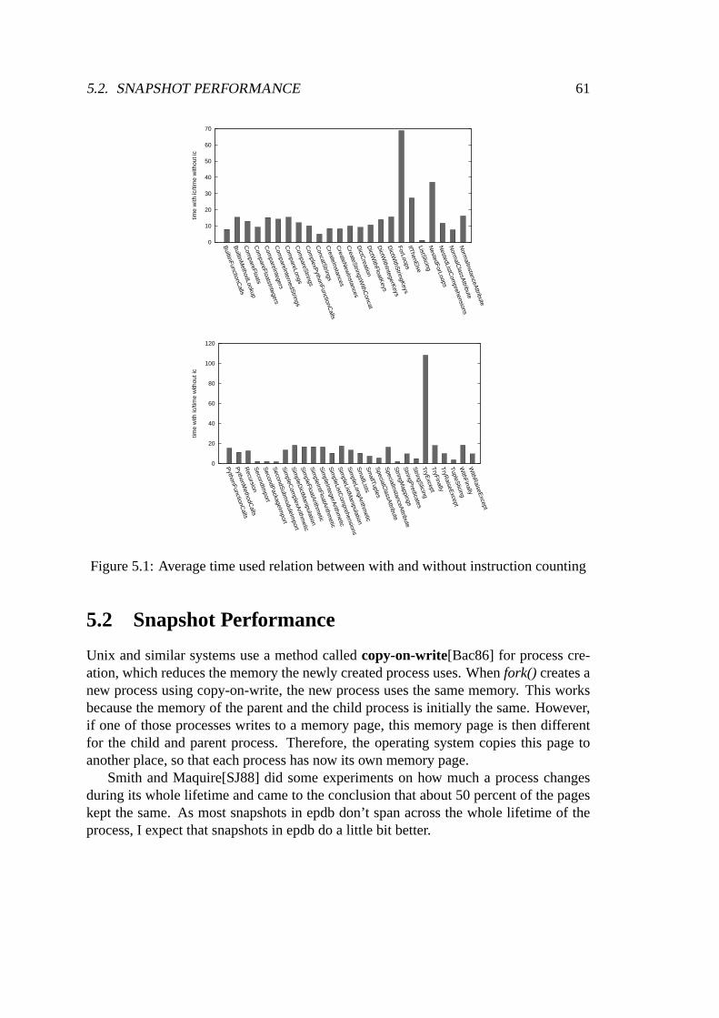
5.2. SNAPSHOT PERFORMANCE 61
0
10
20
30
40
50
60
70
BuiltinFunctionC
allsB
uiltinMethodLookup
Com
pareFloatsC
ompareFloatsIntegers
Com
pareIntegersC
ompareInternedS
trings
Com
pareLongsC
ompareS
tringsC
omplexP
ythonFunctionCalls
ConcatS
tringsC
reateInstancesC
reateNew
InstancesC
reateStringsW
ithConcat
DictC
reationD
ictWithFloatK
eysD
ictWithIntegerK
eysD
ictWithS
tringKeys
ForLoopsIfThenE
lseListS
licingN
estedForLoopsN
estedListCom
prehensions
Norm
alClassA
ttributeN
ormalInstanceA
ttribute
time
with
ic/ti
me
with
out i
c
0
20
40
60
80
100
120
PythonFunctionC
allsP
ythonMethodC
allsR
ecursionS
econdImport
SecondP
ackageImport
SecondS
ubmoduleIm
port
Sim
pleCom
plexArithm
etic
Sim
pleDictM
anipulation
Sim
pleFloatArithm
etic
Sim
pleIntFloatArithm
etic
Sim
pleIntegerArithm
etic
Sim
pleListCom
prehensions
Sim
pleListManipulation
Sim
pleLongArithm
etic
Sm
allListsS
mallTuples
SpecialC
lassAttribute
SpecialInstanceA
ttribute
StringM
appingsS
tringPredicates
StringS
licingTryE
xceptTryFinallyTryR
aiseExcept
TupleSlicing
WithFinally
WithR
aiseExcept
time
with
ic/ti
me
with
out i
c
Figure 5.1: Average time used relation between with and without instruction counting
5.2 Snapshot Performance
Unix and similar systems use a method calledcopy-on-write[Bac86] for process cre-ation, which reduces the memory the newly created process uses. Whenfork() creates anew process using copy-on-write, the new process uses the same memory. This worksbecause the memory of the parent and the child process is initially the same. However,if one of those processes writes to a memory page, this memorypage is then differentfor the child and parent process. Therefore, the operating system copies this page toanother place, so that each process has now its own memory page.
Smith and Maquire[SJ88] did some experiments on how much a process changesduring its whole lifetime and came to the conclusion that about 50 percent of the pageskept the same. As most snapshots in epdb don’t span across thewhole lifetime of theprocess, I expect that snapshots in epdb do a little bit better.
62 CHAPTER 5. PERFORMANCE
Copy-on-write process creation is really fast and typicallytakes less than 1 ms.Waiting for a process to finish takes a bit longer, but is usually done in less than 10 ms.
More interesting than the speed of the execution offork() is the amount of processesthe system can handle simultaneously. It is well-known thata fork bomb, like in Listing5.1, will make a system completely unresponsive. I tried to estimate how many simulta-neously processes the operating system could handle with the program shown in Listing5.2. This program measures how much time per created processit takes if the programcreates a bunch of processes. Figure 5.2 shows the result of this measurement. As onecan see, the number of processes the program creates hardly affects the process creationtime of a process, at least at these numbers of simultaneous created child processes.
The program also measures how much extra time it takes to not only create the pro-cesses, but also to wait for them afterwards. In order to do this, each process keeps itselflong enough alive so that the parent process has time to create all processes, before thesubprocesses finish. The child processes accomplish this waiting by usingtime.sleep(5)to stop the process for 5 seconds. After the parent process has created all child pro-cesses, it then waits for all of them to finish and measure the time up to this point. Aseach process waits 5 seconds, it therefore subtracts this amount of time to get the ad-ditional time the process needs to create all processes and to wait for their termination.Figure 5.3 visualizes the result of this measurement. The experiment was executed onan AMD Athlon(tm) 7550 Dual-Core Processor with 2.5 GHz and 4 GB of RAM and anUbuntu Lucid Lynx Linux Distribution. As one can see from thediagram, the overheadexplodes at some number of processes. This is where the machine typically becomescompletely unresponsive and the only way to recover it, is toreboot the computer. Fromthe diagram we, can extract an estimate of how many snapshotsthe debugger can han-dle. I tried to debug a program with epdb which made about 1000snapshots and wasstill able to work and debug reasonably well on my computer. As the program makesabout one snapshot per second1, it is possible to debug programs which require about16 minutes of execution time. This is enough for many applications, e.g., a programwhich handles a page request of a web server should typicallyrespond in a second oreven less. However some longer running programs such as server programs, may need amuch longer execution time. There is still some work required to handle bigger numbersof snapshots. One approach would be to swap the processes to disk, and then afterwardsto terminate them, and then only reactivate the process whenit gets activated. The op-erating system does swapping, but it doesn’t kill the process, which means that it has tocontinuously swap in and swap out, and this takes a lot of time.
1this is at least the case if the debugger does not make snapshots to handle non-determinism
5.3. EPDB PERFORMANCE 63
Listing 5.1: forkbomb.pyimport os
whi le True :os . f o r k ( )
Listing 5.2: maxfork.pyf o r maxnoproc i n range ( 1 0 0 , 1 0 0 0 , 1 0 0 ) :
s t a r t t i m e = t ime . t ime ( )f o r i i n range ( maxnoproc ) :
i d = os . f o r k ( )i f i d == 0 :
t ime . s l e e p ( 5 )break
e l s e:f i n i s h t i m e = t ime . t ime ( )c r e a t e t i m e = ( f i n i s h t i m e− s t a r t t i m e ) / maxnoproc )f o r i i n range ( maxnoproc ) :
os . wa i t ( )w a i t f i n i s h t i m e = t ime . t ime ( )overhead = ( w a i t f i n i s h t i m e− s t a r t t i m e−5) / maxnoprocp r i n t ( " C r e a t e t ime : " , c r e a t e t i m e )p r i n t ( " Overhead : " , overhead )con t inue
break
5.3 Epdb Performance
The performance of epdb is dependant on many factors. I compared execution time andmemory usage, when the program is run inside the debugger andwhen it is executedwithout the debugger. I chose two benchmarks –fankuch.pyandnbody.py– from thecomputer language benchmark game[CLB11]. The benchmarkgcd.pycalculates thegreatest common divisor for two very large integers using Euclidean algorithm. Thesethree tests should measure typical programs.
The benchmarkcall_snap.pyillustrates the case, when a program repeatedly calls anon-deterministic function. The program calls a patched function in a for-loop for 500times, which instructs the debugger to make a snapshot. Therefore, running the programwithout a debugger has not much overhead. However, when running it with epdb, thedebugger has to make a snapshot every time it encounters the function call.
The programcreate_array.pycreates a very large list of integers. It is an examplewhere debugger execution almost performs as well as native execution. To show, that it
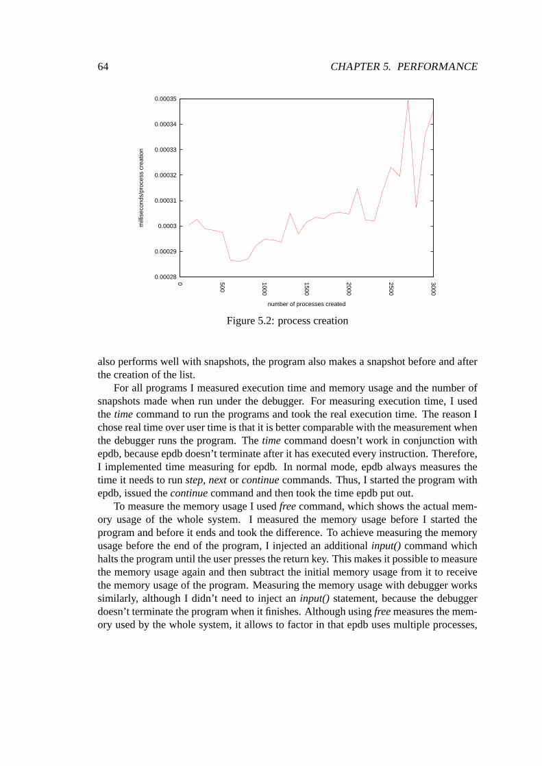
64 CHAPTER 5. PERFORMANCE
0.00028
0.00029
0.0003
0.00031
0.00032
0.00033
0.00034
0.00035
0 500
1000
1500
2000
2500
3000
mill
isec
onds
/pro
cess
cre
atio
n
number of processes created
Figure 5.2: process creation
also performs well with snapshots, the program also makes a snapshot before and afterthe creation of the list.
For all programs I measured execution time and memory usage and the number ofsnapshots made when run under the debugger. For measuring execution time, I usedthe timecommand to run the programs and took the real execution time.The reason Ichose real time over user time is that it is better comparablewith the measurement whenthe debugger runs the program. Thetime command doesn’t work in conjunction withepdb, because epdb doesn’t terminate after it has executed every instruction. Therefore,I implemented time measuring for epdb. In normal mode, epdb always measures thetime it needs to runstep, nextor continuecommands. Thus, I started the program withepdb, issued thecontinuecommand and then took the time epdb put out.
To measure the memory usage I usedfreecommand, which shows the actual mem-ory usage of the whole system. I measured the memory usage before I started theprogram and before it ends and took the difference. To achieve measuring the memoryusage before the end of the program, I injected an additionalinput() command whichhalts the program until the user presses the return key. Thismakes it possible to measurethe memory usage again and then subtract the initial memory usage from it to receivethe memory usage of the program. Measuring the memory usage with debugger workssimilarly, although I didn’t need to inject aninput() statement, because the debuggerdoesn’t terminate the program when it finishes. Although using freemeasures the mem-ory used by the whole system, it allows to factor in that epdb uses multiple processes,
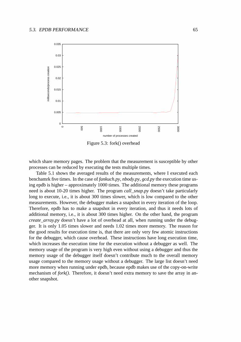
5.3. EPDB PERFORMANCE 65
0
0.005
0.01
0.015
0.02
0.025
0.03
0.035
0 500
1000
1500
2000
2500
3000
mill
isec
onds
/pro
cess
cre
atio
n
number of processes created
Figure 5.3: fork() overhead
which share memory pages. The problem that the measurement is susceptible by otherprocesses can be reduced by executing the tests multiple times.
Table 5.1 shows the averaged results of the measurements, where I executed eachbenchamrk five times. In the case offankuch.py, nbody.py, gcd.pythe execution time us-ing epdb is higher – approximately 1000 times. The additional memory these programsneed is about 10-20 times higher. The programcall_snap.pydoesn’t take particularlylong to execute, i.e., it is about 300 times slower, which is low compared to the othermeasurements. However, the debugger makes a snapshot in every iteration of the loop.Therefore, epdb has to make a snapshot in every iteration, and thus it needs lots ofadditional memory, i.e., it is about 300 times higher. On theother hand, the programcreate_array.pydoesn’t have a lot of overhead at all, when running under the debug-ger. It is only 1.05 times slower and needs 1.02 times more memory. The reason forthe good results for execution time is, that there are only very few atomic instructionsfor the debugger, which cause overhead. These instructionshave long execution time,which increases the execution time for the execution without a debugger as well. Thememory usage of the program is very high even without using a debugger and thus thememory usage of the debugger itself doesn’t contribute muchto the overall memoryusage compared to the memory usage without a debugger. The large list doesn’t needmore memory when running under epdb, because epdb makes use of the copy-on-writemechanism offork(). Therefore, it doesn’t need extra memory to save the array inan-other snapshot.
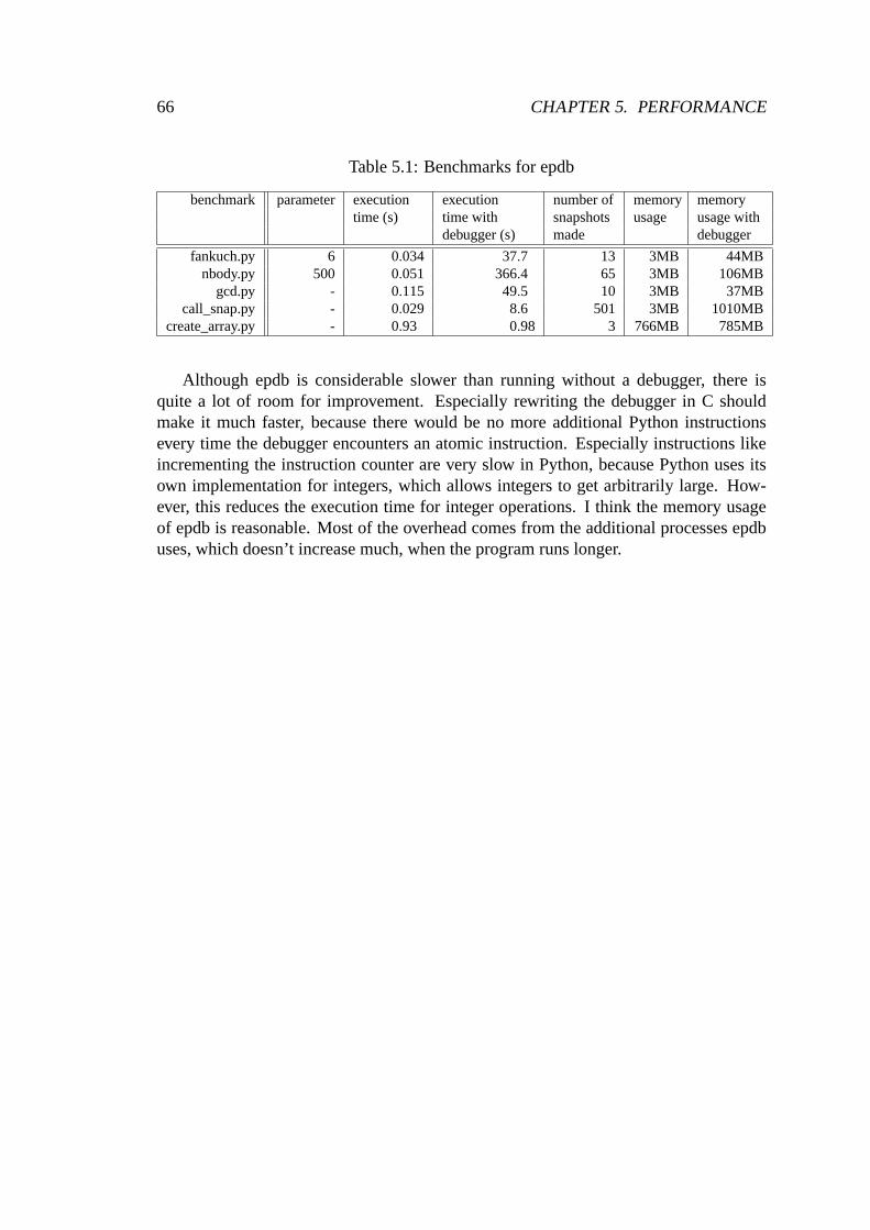
66 CHAPTER 5. PERFORMANCE
Table 5.1: Benchmarks for epdb
benchmark parameter executiontime (s)
executiontime withdebugger (s)
number ofsnapshotsmade
memoryusage
memoryusage withdebugger
fankuch.py 6 0.034 37.7 13 3MB 44MBnbody.py 500 0.051 366.4 65 3MB 106MB
gcd.py - 0.115 49.5 10 3MB 37MBcall_snap.py - 0.029 8.6 501 3MB 1010MB
create_array.py - 0.93 0.98 3 766MB 785MB
Although epdb is considerable slower than running without adebugger, there isquite a lot of room for improvement. Especially rewriting the debugger in C shouldmake it much faster, because there would be no more additional Python instructionsevery time the debugger encounters an atomic instruction. Especially instructions likeincrementing the instruction counter are very slow in Python, because Python uses itsown implementation for integers, which allows integers to get arbitrarily large. How-ever, this reduces the execution time for integer operations. I think the memory usageof epdb is reasonable. Most of the overhead comes from the additional processes epdbuses, which doesn’t increase much, when the program runs longer.
CHAPTER 6Applications
People, who have developed reversible debuggers have complained that nobody usestheir decent debugging tools, e.g., Lewis writes on the homepage [Lew07] of odb:
The ODB is as close to a silver bullet as you can get. Why don’t people useit?
I don’t get it. :-(
Lieberman, a developer of ZStep, has written some text[Lie97] about people not usinggood debugging tools.
I don’t want to join their complaints. Instead, I want to giveexamples of how a usermight want to use epdb. In this section, I want to risk lookingin the future, which meansthat I will write about features and additional tools which are not available yet.
6.1 Web Applications
Web application development is an important branch of software engineering. Thereare many tools and frameworks available for Python to ease the development of webapplications, e.g., Django, Pylons, Turbogears. Typically, these web frameworks pro-vide their own debugging mode, where they show some debugging information whenthe program fails, but usually don’t allow to control the program execution.
I think using epdb to debug web applications can work very well. Web applicationshave usually a short running time, because the user expects aweb page to load fast.Therefore the limited amount of snapshots of epdb doesn’t play a big role. They alsouse a limited amount of resources; often a database and files are the only resources theyuse. Some databases like Oracle or CouchDB already support accessing old versionsof the data records. If the database doesn’t allow this, it ismaybe possible to write
67
68 CHAPTER 6. APPLICATIONS
an object relational mapper which accomplishes this. Object relational mappers arevery common in web applications too. File access could be implemented by using aspecial file system, or the framework could add some implementation for file access toaccomplish reversible debuggable file access. Running the program with its resources inepdb should work without any bigger problems. What remains left is the interaction withthe user, preferably with a graphical user interface. Here the framework could presentthe user the interface via the browser and the use of AJAX. Whenthe user requests apage, the web server would start the Python program under debugging control. If it runssuccessfully, the web server sends the webpage to the browser to render it. Otherwise, itsends a webpage to the browser, which contains a graphical user interface to debug theprogram. This user interface would of course also allow the user to debug the programin reverse and it would be possible to run the program either deterministically or non-deterministically by making use of timelines. Of course, debugging a web applicationusing this approach should only be enabled in debug mode.
Another problem which debuggers of web applications face isthat web applicationstypically use some sort of template language. Often there isa bug in a template insteadof the code itself. Therender()method of the template typically raises an exception, butthis doesn’t give the programmer much insight into what wentwrong in the program.Thus it should be possible to inject a debugger inside the debugger, which works for thetemplate language. Using the patching mechanism of epdb, this should be possible toimplement.
6.2 Smart Phone Development
There are lots of small applications, which are often calledapps, for smart phones. Mostof these apps are written higher level programming framework. Developers usually testtheir software on a virtual machine, before deploying it to the phone. The host machineis usually much more powerful in terms of disk space, main memory and CPU speed.Therefore, it is reasonably to use a virtual machine, which does some additional workand allows reversible debugging of applications.
The developer of most apps usually use a higher programming framework, whichalso allows a limited amount of API calls to access resources. Therefore it seems fea-sible to develop reversible debuggable versions of these calls for the execution on thevirtual machine. On the virtual machine are already only simulated devices, and thismakes developing reversible debuggable resources even easier. Having a good debug-ging framework for smart phone development may attract manydevelopers, which de-velop lots of applications. A smart phone operating system with lots of application ismore likely to be a business success.
6.3. VISUALIZATION OF ALGORITHMS 69
6.3 Visualization of Algorithms
I believe using a debugger is a great way to get a better understanding of how a pro-gram works and a reversible debugger makes this process evenmore enjoyable. Oftenspeakers want to present some algorithm and illustrate how it works. It would be niceto visualize the data as the user steps through the program. ZStep1 focuses on visual-ization, but epdb can visualize data too. Using its mechanism to patch instructions, it ispossible to visualize an algorithm without changing its code.
6.4 Design and Architecture
In my opinion a well-designed program is one which is easy to test and easy to debug.Even if one doesn’t want to use a debugger, e.g., because one prefers to use test drivendevelopment, the basic understanding of the debugging architecture of epdb helps theprogrammer to design better programs. This is because epdb emphasizes the reproduc-tion of certain states. This is important in design because abug, which is not repro-ducible, is very difficult to fix. Therefore, the first step in fixing a bug is to reproduceit. The remaining part is straight forward at least for an experienced programmer whoknows the code.
1see Section 7.1

CHAPTER 7Related Work
Although reversible debugging has certainly various benefits, some authors have arguedagainst it. For example, Rosenberg [Ros96] argued against reversible debugging bycalling reverse execution a much-requested but dubious feature. He also believes thatthis feature is so much work and still fraught with so much error that it is not worththe engineering investment. He also gives some basic algorithm to implement reverseexecution. However, he does not mention copy-on-write optimizations
There is still a controversy between logging-based debuggers and replay-based de-buggers. Lienhard[LGN08] argues that the disadvantage of replay-based debuggers isthat moving backwards in time can be very slow. However, I can’t confirm this, becauseby using continuous snapshotting every second, the debugger can bound the amount oftime it needs to run backwards.
Feldman and Brown[FB88] give an alternative implementation of efficient snap-shots without usingfork(). Mellor-Crummey and LeBlanc[MCL89] discuss a softwareinstruction counter, which usually does not have more than 10% overhead.
Pan and Linton[PL88] describe how to usefork() to create new checkpoints (i.e.snapshots). They also describe the use of an event log, whichthe debugger uses duringreplay when accessing the shared memory or when it replays system calls.
Kessler[Kes90] gives an approach to implement fast breakpoints using self-modi-fying code. Netzer and Weaver[NW94] show an efficient adaptive tracing strategy forlogging-based debuggers. Demetrescu and Finocchi[DF04] describe the Leonardo vir-tual machine which allows directing and checkpointing, which is useful for reversibledebugging. Nitin[KNM06] shows how the virtual machine Xen could be used to imple-ment kernel debugging.
71
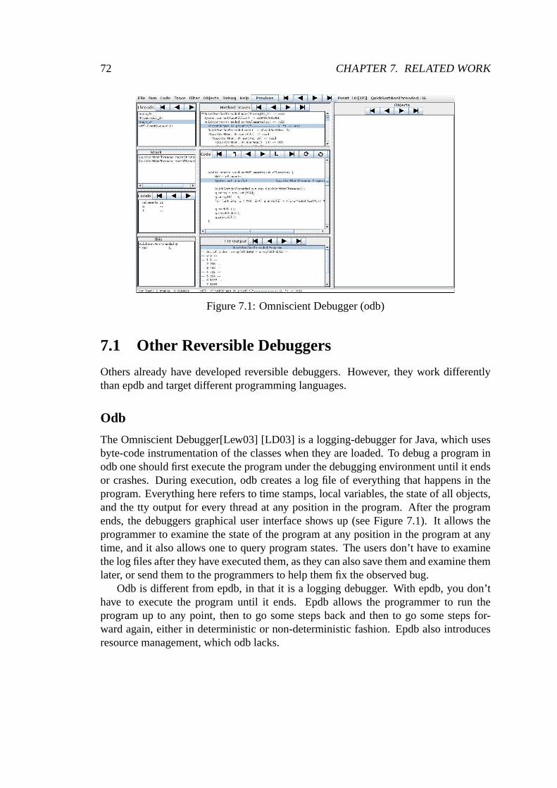
72 CHAPTER 7. RELATED WORK
Figure 7.1: Omniscient Debugger (odb)
7.1 Other Reversible Debuggers
Others already have developed reversible debuggers. However, they work differentlythan epdb and target different programming languages.
Odb
The Omniscient Debugger[Lew03] [LD03] is a logging-debugger for Java, which usesbyte-code instrumentation of the classes when they are loaded. To debug a program inodb one should first execute the program under the debugging environment until it endsor crashes. During execution, odb creates a log file of everything that happens in theprogram. Everything here refers to time stamps, local variables, the state of all objects,and the tty output for every thread at any position in the program. After the programends, the debuggers graphical user interface shows up (see Figure 7.1). It allows theprogrammer to examine the state of the program at any position in the program at anytime, and it also allows one to query program states. The users don’t have to examinethe log files after they have executed them, as they can also save them and examine themlater, or send them to the programmers to help them fix the observed bug.
Odb is different from epdb, in that it is a logging debugger. With epdb, you don’thave to execute the program until it ends. Epdb allows the programmer to run theprogram up to any point, then to go some steps back and then to go some steps for-ward again, either in deterministic or non-deterministic fashion. Epdb also introducesresource management, which odb lacks.
7.1. OTHER REVERSIBLE DEBUGGERS 73
Gdb
Gdb uses a technique to implement reversible debugging, which its developer nameprocess record & replay. As gdb is a native debugger, it has a parent process, thedebugger, and a child process which executes the program andgets directed by theparent process. With process record & replay, the parent process logs the execution ofeach machine instruction in the child process, together with each change in memory andregisters. With this execution log, the debugger can execute the program in reverse bysuccessively undoing each change of each logged instruction. To go forward again, italso uses the execution log to replay the state and so it then uses deterministic forwardexecution.
As odb, gdb has no resource management yet. However, it is more similar to epdb,in that it is an interactive debugger. A problem with gdb’s approach is that runningbackwards a huge amount of instructions takes a very long time, because each machineinstruction has to be undone. With epdb’s, approach the debugger activates a snapshotwhich is near to the target location in the program and startsfrom there, which can savereplaying time. In gdb, there is also no concept which distinguishes between determin-istic and non-deterministic instruction execution.
ZStep
ZStep is an interactive reversible debugger visualizationtool for Lisp, which allowsreverse execution of code. In contrast to epdb, ZStep does not work on source line level,but on expression level, which allows the user to step over smaller pieces of code. ZStepis also a visualization tool, which allows graphical representation of the data structuresor program execution, while the user steps through the program. However, ZStep hasno concept of non-deterministic functions and does not havean answer to side effects.The visualization of code is something epdb supports in principle too by allowing theuser to patch instructions.
EXDAMS
The oldest reversible debugger I know of is the EXtendable Debugging and MonitoringSystem, or EXDAMS[Bal69] for short. It was a debugger for the ancient Multics op-erating system. In fact, the authors didn’t call it a reversible debugger, but debug-timehistory playback. EXDAMS is a logging debugger. The debugging system augmentedthe source code with additional logging statements and allowed one to view the state ofthe program at any position in the program.
74 CHAPTER 7. RELATED WORK
IGOR
Igor [FB88] is a prototype reversible debugger for the DUNE distributed operating. Ituses a snapshot & replay approach. The authors refer to the snapshots as checkpoints.To implement checkpoints they make a special system callpagemod, which returns thepages that where written since the last call. With this system call the debugger can saveonly those pages, which have changed since the last checkpoint. Igor also has same verybasic form of resource management, i.e., it has aprestart routine which the debuggerbefore executing of the program. This routine sets the stateof user supplied files beforeexecuting the program. Although there are similarities with epdb resource management,IGOR does not track the different states of the files while executing. It also does notsupport timelines or a similar concept.
Bdb
Bdb [Boo00] is a prototype reversible debugger for C/C++ runningon Digital/CompaqAlpha based Unix workstations. Bdb uses a snapshot & replay approach similar to epdb.Like epdb, it uses the system callfork() to create snasphots. Bdb uses a technique calledexponential checkpoint thinning to reduce the number of checkpoints. With this tech-nique the debugger only keeps snapshots at exponential intervals and thus the numberof snapshots grows only logarithmically. While the program execution progresses, thedebugger thins out the number of snapshots. Although it reduces the number of snap-shots, it has the disadvantage that re-execution takes longer for code at the beginning ofthe program. In contrast to epdb, Bdb does not allow multiple timelines and it does notmanage the external state.
CHAPTER 8Further Work
In this section, I want to present interesting work which mayalso be useful for a re-versible debugger like epdb. I also want to give a short summary of other reversibledebuggers and their differences to epdb, as well as to give some ideas for additionalresearch which would help reversible debugging.
8.1 Smart Snapshot Making
Usually the user is only interested in a small part of the program and therefore somesnapshots are never activated. Such snapshots would be harmful, as they consume sys-tem resources without any need. Therefore a smart debugger could use a strategy toavoid making such snapshots in advance, but rather only whenthe user initiates a re-verse execution command. In this case, the debugger could make a snapshot of theprocess and insert it into the timeline. When the user does a reverse execution com-mand again, the reverse execution would be much faster because the debugger coulduse a more recent snapshot. A sophisticated strategy to makesnapshots would rely oninformation about how users use a reversible debugger. Therefore, one could log thebehavior of the users when they debug a program and then find a snapshot making strat-egy which would reduce the average time the user would need towait. This approachwould be even more powerful if it is combined with persistentsnapshots, i.e., snapshotswhich store the memory to disk. Therefore these snapshots don’t use a process whichreduces the system performance, but on the other hand the debugger would need moretime to create and to activate them than it needs to create andactivate snapshots, whichwere created by usingfork().
75
76 CHAPTER 8. FURTHER WORK
8.2 Reversible Debuggable Libraries and Other Tools
The resource management approach of epdb works well if it is easy to save and restorethe current state of the resource. Some databases already allow this, but other resourcessuch as files, network communication libraries, and graphical tools usually don’t supportstate saving. Therefore, it would be interesting if it is practical to implement this statesaving feature into these tools and libraries. As most computers today usually have hugeamounts of free disk space, it seems that marking data as deleted instead of actuallydeleting the data shouldn’t decrease the overall performance too much. I guess theperformance should be at least good enough for the debuggingmode.
8.3 Native Instruction Counting and Bookkeeping
Epdb uses the trace function to implement instruction counting and to do some book-keeping. This has the advantage that the whole debugger is written in Python, but onthe other hand, it has less performance as a result. This is because the interpreter callsa Python function for each line of code. Pdb can use a lot of optimizations, becauseit doesn’t rely on instruction counting. Therefore pdb can only trace functions, whichhave a breakpoint in their code. However it should be possible to put the instructioncounting and bookkeeping code into the interpreter itself.Consequently, this part of thecode would have to be written in C. Using this optimization, I would expect that epdbwould be much faster in its execution, especially in normal mode.
CHAPTER 9Conclusion
In this thesis, I have shown that it is possible to develop an interactive reversible de-bugger using the snapshot & replay approach with reasonableperformance. I have alsoshown that it is possible to get around the problems of non-deterministic instructionsand instructions with side effects, by using instruction patching, timelines and resourcemanagement. During this thesis, I have not only developed epdb, but also documentedthe design for a sophisticated reversible interactive snapshot & replay debugger, whichothers may use to implement reversible debuggers for their favorite programming lan-guage.
Reversible debugging, although a very old idea, is not very widely used yet. Never-theless, I hope that I have made reversible debugging easierto understand with the con-cepts I have developed in this thesis, i.e., that a function can affect the program environ-ment, or the execution of a function can be affected by the environment, as well. There-fore, any programming instruction can have side effects or can be non-deterministic. Afunction with side-effects changes the environment of the program, while the executionof a non-deterministic function depends on it. When the user replays a non-deterministicfunction, he can have either one of two different expectations. He could expect to havethe same result of the execution as in the first run (deterministic execution), or he couldexpect to run the function with the new environment (non-deterministic execution).
The implementation of epdb shows that this view of reversible debugging is actuallyuseful. Epdb introduces timelines and therefore allows unambigous reversible debug-ging, because it is now up to the user to decide which type of execution, deterministic ornon-deterministic, he wants to use. Epdb also introduces a new stateful resource man-agement concept. With resource management, the user can inspect the environment ofthe program which, because of resource management, always corresponds to the actualposition inside the program. The implementation of two resource managers for epdb,one for stdoutand one for file access, shows that the resource management concept
77
78 CHAPTER 9. CONCLUSION
is actually applicable for complex resources and it is possibly useful for many otherresources as well.
Bibliography
[ALS10] J. Chris Anderson, Jan Lehnardt, and Noah Slater.CouchDB: The DefinitiveGuide: Time to Relax (Animal Guide). O’Reilly Media, 1 edition, 1 2010.
[Bac86] Maurice J. Bach.The Design of the UNIX Operating System. Prentice-Hall,1986.
[Bal69] R. M. Balzer. Exdams: extendable debugging and monitoring system. InAFIPS ’69 (Spring): Proceedings of the May 14-16, 1969, spring jointcomputer conference, pages 567–580, New York, NY, USA, 1969. ACM.
[Bea09] David M. Beazley.Python Essential Reference. Addison-Wesley, fourthedition, 2009.
[Boo00] Bob Boothe. Efficient algorithms for bidirectional debugging. InPLDI,pages 299–310, 2000.
[Boo03] Duncan Booth. Patterns in Python.http://www.suttoncourtenay.org.uk/duncan/accu/pythonpatterns.html, March 2003.
[CFC01] Shyh-Kwei Chen, W. Kent Fuchs, and Jen-Yao Chung. Reversible de-bugging using program instrumentation.IEEE Trans. Software Eng.,27(8):715–727, 2001.
[Chi96] Ram Chillarege. What is software failure.IEEE Trans. Reliability, 45:354–355, Sep 1996.
[CJ03] Ron Crocker and Guy L. Steele Jr., editors.Companion of the 18th An-nual ACM SIGPLAN Conference on Object-Oriented Programming,Sys-tems, Languages, and Applications, OOPSLA 2003, October 26-30, 2003,Anaheim, CA, USA. ACM, 2003.
[CLB11] The Computer Language Benchmark Game.http://shootout.alioth.debian.org/, January 2011.
79
80 BIBLIOGRAPHY
[DF04] Camil Demetrescu and Irene Finocchi. A portable virtual machine forprogram debugging and directing. In Hisham Haddad, Andrea Omicini,Roger L. Wainwright, and Lorie M. Liebrock, editors,SAC, pages 1524–1530. ACM, 2004.
[Eis97] Marc Eisenstadt. My hairiest bug war stories.Commun. ACM, 40(4):30–37,1997.
[FB88] Stuart I. Feldman and Channing B. Brown. Igor: A system forprogram de-bugging via reversible execution. InWorkshop on Parallel and DistributedDebugging, pages 112–123, 1988.
[GHJV94] Erich Gamma, Richard Helm, Ralph Johnson, and John M.Vlissides.De-sign Patterns: Elements of Reusable Object-Oriented Software. Addison-Wesley Professional, 1 edition, 1994.
[HS02] Brent Hailpern and Padmanabhan Santhanam. Software debugging, testing,and verification.IBM Systems Journal, 41(1):4–12, 2002.
[Kes90] Peter B. Kessler. Fast breakpoints: Design and implementation. InPLDI,pages 78–84, 1990.
[KNM06] Nitin A. Kamble, Jun Nakajima, and Asit K. Mallick. Evolution in kerneldebugging using hardware virtualization with Xen.2006 Linux Symposium,Volume Two, 2006.
[KTD05] Toshihiko Koju, Shingo Takada, and Norihisa Doi. Anefficient and genericreversible debugger using the virtual machine based approach. In MichaelHind and Jan Vitek, editors,VEE, pages 79–88. ACM, 2005.
[Lap92] J. C. Laprie.Dependability : basic concepts and terminology in English,French, German, Italian and Japanese. Springer, 1992.
[Lay09] Jeffrey B. Layton. NILFS: A file system to make SSDs scream. LinuxMagazine, 6 2009.
[LB98] Sheng Liang and Gilad Bracha. Dynamic class loading in the Java VirtualMachine. InOOPSLA, pages 36–44, 1998.
[LD03] Bil Lewis and Mireille Ducassé. Using events to debug Java programsbackwards in time. In Crocker and Jr. [CJ03], pages 96–97.
[Lew03] Bil Lewis. Debugging backwards in time. In Michiel Ronsse and Koen DeBosschere, editors,AADEBUG, 2003.
BIBLIOGRAPHY 81
[Lew07] Bil Lewis. Omniscient debugging.http://www.lambdacs.com/debugger/, Feb 2007.
[LGN08] Adrian Lienhard, Tudor Gîrba, and Oscar Nierstrasz. Practical object-oriented back-in-time debugging. In Jan Vitek, editor,ECOOP, volume5142 of Lecture Notes in Computer Science, pages 592–615. Springer,2008.
[Lie97] Henry Lieberman. The debugging scandal and what to do about it (intro-duction to the special section).Commun. ACM, 40(4):26–29, 1997.
[LMS05] P. Leach, M. Mealling, and R. Salz. A Universally Unique IDentifier(UUID) URN Namespace. RFC 4122 (Proposed Standard), July 2005.
[MAA +10] Sheila Moore, D. Adams, L. Ashdown, M. Cowan, J. Melnick, R.Moran,E. Paapanen, J. Russell, R. Strohm, and R. Ward. Oracle ® database ad-vanced application developer’s guide 11g release 2 (11.2),2010.
[MCL89] John M. Mellor-Crummey and Thomas J. LeBlanc. A software instructioncounter. InASPLOS, pages 78–86, 1989.
[NW94] Robert H. B. Netzer and Mark H. Weaver. Optimal tracing and incrementalreexecution for debugging long-running programs. InPLDI, pages 313–325, 1994.
[PL88] Douglas Z. Pan and Mark A. Linton. Supporting reverseexecution of par-allel programs. InWorkshop on Parallel and Distributed Debugging, pages124–129, 1988.
[Ros96] Jonathan B. Rosenberg.How Debuggers Work: Algorithms, Data Struc-tures, and Architecture. Wiley, 1 edition, 9 1996.
[Sei09] Justin Seitz.Gray Hat Python: Python Programming for Hackers and Re-verse Engineers. No Starch Press, San Francisco, CA, USA, 2009.
[SJ88] Jonathan M. Smith and Gerald Q. Maguire Jr. Effects ofcopy-on-writememory management on the response time of UNIX fork operations.Com-puting Systems, 1(3):255–278, 1988.
[Sos95] Rok Sosic. The Dynascope directing server: Design and implementation.Computing Systems, 8(2):107–134, 1995.
[Tas03] Gregory Tassey, editor.The Economic Impacts of Inadequate Infrastructurefor Software Testing: Final Report. Diane Pub Co, 9 2003.
82 BIBLIOGRAPHY
[Zel09] Andreas Zeller.Why Programs Fail, Second Edition: A Guide to SystematicDebugging. Morgan Kaufmann, second edition, 6 2009.
[Zia08] Tarek Ziade.Expert Python Programming. Packt Publishing, 2008.