Embed Size (px)
Citation preview
Institut für Hydrologie
Albert � Ludwigs Universität Freiburg im Breisgau
Verweilzeitmodellierung mit 18O
auf der Grundlage eines konzeptuellen
Niederschlags-Ab�uss Modells
Transit time modelling with 18O
based on a conceptual
precipitation-runo� model
René Capell
Diplomarbeit unter der Leitung von Prof. Dr. Christian
Leibundgut
Freiburg im Breisgau, Februar 2007

Institut für Hydrologie
Albert � Ludwigs Universität Freiburg im Breisgau
Verweilzeitmodellierung mit 18O
auf der Grundlage eines konzeptuellen
Niederschlags-Ab�uss Modells
Transit time modelling with 18O
based on a conceptual
precipitation-runo� model
Autor: René Capell
Referent: Prof. Dr. Ch. LeibundgutKoreferent: Dr. J. Lange
Diplomarbeit unter der Leitung von Prof. Dr. Christian Leibundgut
Freiburg im Breisgau, Februar 2007

Contents i
Contents
Contents i
List of Figures iii
List of Tables v
Summary ix
Zusammenfassung xi
1 Introduction 11.1 General introduction . . . . . . . . . . . . . . . . . . . . . . . . 11.2 Objective . . . . . . . . . . . . . . . . . . . . . . . . . . . . . . 11.3 Transit time modelling approaches . . . . . . . . . . . . . . . . 2
1.3.1 Stable isotopes in transit time modelling . . . . . . . . . 21.3.2 Transit time distributions and modelling approaches . . . 3
1.4 Conclusions . . . . . . . . . . . . . . . . . . . . . . . . . . . . . 3
2 Area and investigation period 52.1 The Brugga and Zastlerbach Catchment . . . . . . . . . . . . . 5
2.1.1 Location and morphology . . . . . . . . . . . . . . . . . 52.1.2 Geology and soils . . . . . . . . . . . . . . . . . . . . . . 52.1.3 Climatic conditions and hydrology . . . . . . . . . . . . 6
2.2 Data . . . . . . . . . . . . . . . . . . . . . . . . . . . . . . . . . 112.2.1 Data sampling . . . . . . . . . . . . . . . . . . . . . . . . 112.2.2 Data processing and transformation . . . . . . . . . . . . 11
2.3 Conclusions . . . . . . . . . . . . . . . . . . . . . . . . . . . . . 16
3 Introduction to the HBV model 173.1 General description . . . . . . . . . . . . . . . . . . . . . . . . . 173.2 Model version . . . . . . . . . . . . . . . . . . . . . . . . . . . . 18
3.2.1 Modules . . . . . . . . . . . . . . . . . . . . . . . . . . . 183.2.2 Data requirements . . . . . . . . . . . . . . . . . . . . . 193.2.3 Model evaluation: objective functions . . . . . . . . . . . 19
3.3 Conclusions . . . . . . . . . . . . . . . . . . . . . . . . . . . . . 20
4 The conceptual transit time model 214.1 The single linear storage . . . . . . . . . . . . . . . . . . . . . . 214.2 Modi�cations for the integrated 18O transport model . . . . . . 22
ii Contents
4.2.1 Descriptive introduction . . . . . . . . . . . . . . . . . . 224.2.2 Derivation of the distribution model . . . . . . . . . . . . 234.2.3 R-coded example . . . . . . . . . . . . . . . . . . . . . . 27
4.3 The �nal HBV-18O model . . . . . . . . . . . . . . . . . . . . . 294.3.1 Modi�cations and additional parameters . . . . . . . . . 294.3.2 Model behaviour: arti�cial datasets . . . . . . . . . . . . 31
4.3.2.1 Impulse response . . . . . . . . . . . . . . . . . 314.3.2.2 Sine-wave response . . . . . . . . . . . . . . . . 33
4.4 Conclusions . . . . . . . . . . . . . . . . . . . . . . . . . . . . . 35
5 HBV-18O: Results & discussion 375.1 Brugga . . . . . . . . . . . . . . . . . . . . . . . . . . . . . . . . 37
5.1.1 Time series description and runo� simulation . . . . . . . 375.1.2 Input- and steady state issues, parameter variations . . . 395.1.3 HBV-18O model �t and transit time development . . . . 425.1.4 Conclusions . . . . . . . . . . . . . . . . . . . . . . . . . 46
5.2 Zastlerbach . . . . . . . . . . . . . . . . . . . . . . . . . . . . . 475.2.1 HBV-18O model �t and transit time development . . . . 475.2.2 Conclusions . . . . . . . . . . . . . . . . . . . . . . . . . 49
6 Sine-wave approach 516.1 Introduction . . . . . . . . . . . . . . . . . . . . . . . . . . . . . 516.2 Method . . . . . . . . . . . . . . . . . . . . . . . . . . . . . . . 516.3 Results . . . . . . . . . . . . . . . . . . . . . . . . . . . . . . . . 526.4 Conclusions . . . . . . . . . . . . . . . . . . . . . . . . . . . . . 57
7 Concluding discussion 597.1 Model applications . . . . . . . . . . . . . . . . . . . . . . . . . 597.2 Limitations and issues . . . . . . . . . . . . . . . . . . . . . . . 597.3 Final remarks . . . . . . . . . . . . . . . . . . . . . . . . . . . . 59
A Appendix 61
Bibliography 63
67
List of Figures iii
List of Figures
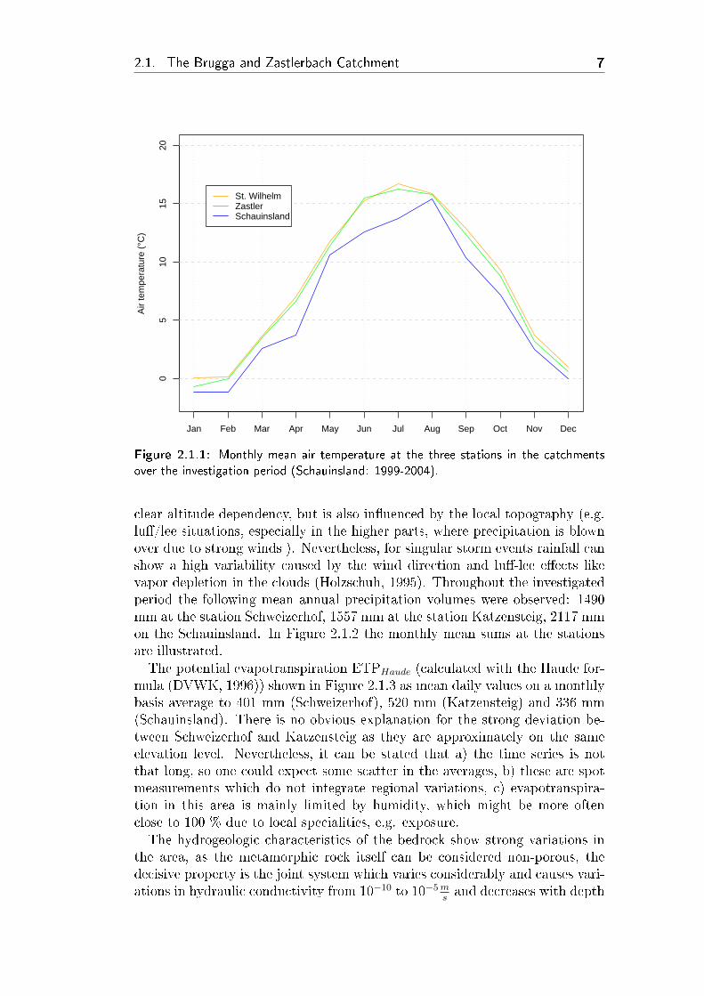
2.1.1 Monthly mean air temperature at the three stations in the catch-ments over the investigation period (Schauinsland: 1999-2004). . 7
2.1.2 Monthly mean precipitation sums at the three stations in thecatchments over the investigation period (Schauinsland: 1999-2004). . . . . . . . . . . . . . . . . . . . . . . . . . . . . . . . . 8
2.1.3 Daily potential evapotranspiration (after Haude), averaged bymonth at the three stations over the investigation period (Schauins-land: 1999-2004). . . . . . . . . . . . . . . . . . . . . . . . . . . 9
2.1.4 Runo� regime at the outlets of Brugga and Zastler, calculatedfrom investigation period data. . . . . . . . . . . . . . . . . . . 10
2.2.1 Precipitation gradient regression between Schauinsland and Schweiz-erhof. . . . . . . . . . . . . . . . . . . . . . . . . . . . . . . . . . 13
2.2.2 Precipitation gradient regression between Schauinsland and Katzen-steig. . . . . . . . . . . . . . . . . . . . . . . . . . . . . . . . . . 13
2.2.3 Temperature gradient regression between Schauinsland and Schweiz-erhof. . . . . . . . . . . . . . . . . . . . . . . . . . . . . . . . . . 14
2.2.4 Temperature gradient regression between Schauinsland and Katzen-steig. . . . . . . . . . . . . . . . . . . . . . . . . . . . . . . . . . 14
2.2.5 Precipitation δ18O in the Brugga catchment, corrected and un-corrected. . . . . . . . . . . . . . . . . . . . . . . . . . . . . . . 16
4.2.1 The SLS' native behaviour on runo� generation. . . . . . . . . . 23
4.2.2 Flowpaths and modelled storage. . . . . . . . . . . . . . . . . . 24
4.2.3 The distribution function for several β, green: κ = 1, red: κ = 0.6. 26
4.2.4 Modelstructure: Overview of the computations in one time step.Only the volume routine is pictured. . . . . . . . . . . . . . . . 27
4.3.1 The modi�ed HBV-18O model, structural overview. . . . . . . . 29
4.3.2 Variation of "Store" parameters, "ExpParam" parameters �x at0.01. Further explanations see text. . . . . . . . . . . . . . . . . 32
4.3.3 Variation of "ExpParam" parameters, "Store" parameters �x at300 mm. Further explanations see text. . . . . . . . . . . . . . . 33
4.3.4 Variation of "Store" parameters, "ExpParam" parameters �x at0.01. Further explanations see text. . . . . . . . . . . . . . . . . 34
4.3.5 Variation of "ExpParam" parameters, "Store" parameters �x300 mm. Further explanations see text. . . . . . . . . . . . . . . 34
iv List of Figures
5.1.1 Brugga catchment, time series of speci�c runo� (mm), δ18O con-centrations in precipitation and runo�. The size of precipita-tion concentration points depends on a volume ranking (volumeclasses in the legend). . . . . . . . . . . . . . . . . . . . . . . . . 38
5.1.2 Precipitation, observed and simulated runo� in the Brugga catch-ment. . . . . . . . . . . . . . . . . . . . . . . . . . . . . . . . . . 38
5.1.3 Exemplary model run with corrected and station-measured δ18Oinput in the Brugga catchment. . . . . . . . . . . . . . . . . . . 39
5.1.4 Model run with one year warm-up period, observed and simu-lated runo� di�er due to the un�lled storages, Brugga catchment. 40
5.1.5 Variation of parameter ExpParam in the Brugga catchment. . . 415.1.6 Variation of parameter Store in the Brugga catchment. . . . . . 415.1.7 Variation of parameter O�set in the Brugga catchment. . . . . . 425.1.8 Final transit time �t with transit time development (runo� age),
measured and modelled δ18O in runo� as well as measured spe-ci�c runo�, Brugga catchment. . . . . . . . . . . . . . . . . . . . 43
5.1.9 Transit time development during the dry spring/summer in 2003,Brugga catchment. . . . . . . . . . . . . . . . . . . . . . . . . . 44
5.1.10Transit time in the investigated period: probability mass func-tion (PMF) and cumulative distribution function (CDF), Bruggacatchment. . . . . . . . . . . . . . . . . . . . . . . . . . . . . . . 45
5.1.11Comparison of the transit time development in relation to pa-rameter variation, Brugga catchment. . . . . . . . . . . . . . . . 45
5.2.1 Precipitation, air temperature, and observed and simulated runo�in the Zastlerbach catchment. . . . . . . . . . . . . . . . . . . . 47
5.2.2 Final transit time �t with transit time development (runo� age),measured and modelled δ18O in runo� as well as measured spe-ci�c runo�, Zastlerbach catchment. . . . . . . . . . . . . . . . . 48
5.2.3 Transit time development during the dry spring/summer in 2003,Zastlerbach catchment. . . . . . . . . . . . . . . . . . . . . . . . 49
5.2.4 Transit time in the investigated period: probability mass func-tion (PMF) and cumulative distribution function (CDF), Za-stlerbach catchment. . . . . . . . . . . . . . . . . . . . . . . . . 50
6.3.1 Zastler catchment, δ18O variation in bulk precipitation samplesand �tted sine-wave model, further explanations see text. . . . . 55
6.3.2 Zastler catchment, δ18O variation in stream �ow samples and�tted sine-wave model, further explanations see text. . . . . . . 55
6.3.3 Brugga catchment, δ18O variation in bulk precipitation samplesand �tted sine-wave model, further explanations see text. . . . . 56
6.3.4 Brugga catchment, δ18O variation in stream �ow samples and�tted sine-wave model, further explanations see text. . . . . . . 56
A.1 The HBV - 18O parameter interface. . . . . . . . . . . . . . . . 61
List of Tables v
List of Tables
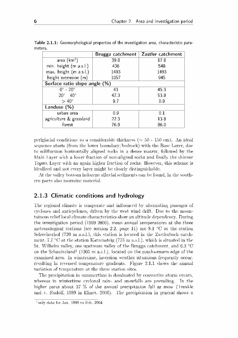
2.1.1 Geomorphological properties of the investigation area, charac-teristic parameters. . . . . . . . . . . . . . . . . . . . . . . . . . 6
2.1.2 Runo� characteristics at the gauging stations, runo� (*Q) inm3
s, speci�c runo� (*q) in l·km2
s(LfU, 2000 in Wissmeier, 2005). 9
2.2.1 Haude factors . . . . . . . . . . . . . . . . . . . . . . . . . . . . 122.2.2 Regression results and gradients, "�nal" rows contain the gra-
dients (per 100 m) used later on. Further explanation see text. . 15
4.3.1 Distribution model parameters and model behaviour, overview. . 30
5.1.1 Modeled transit time results (age, in years) and δ18O time seriesmeans (volume weighted), Brugga catchment . . . . . . . . . . . 43
5.2.1 Modelled transit time results (age, in years) and δ18O time seriesmeans (volume weighted), Zastlerbach catchment . . . . . . . . 48
6.3.1 Results of the sine-wave regressions, with the mean year "Mean",the respective 21day running average "21day" and period 2000to 2005 regression values "All". . . . . . . . . . . . . . . . . . . 53
6.3.2 EM and EPM model results, η = 1.2 (see text). With the meanyear "Mean", the respective 21day running average "21day" andperiod 2000 to 2005 results "All". . . . . . . . . . . . . . . . . . 57
A.1 Parameter sets used for the simulations in both catchments. . . 62A.2 Elevation and vegetation zoning for both catchments. . . . . . . 62

vi
vii
Danksagungen
Herrn Prof. Dr. Ch. Leibundgut danke ich für die Vergabe der Diplomar-beit und die Ermöglichung des Aufenthalts in Schweden im Rahmen dieserDiplomarbeit.Ein herzlicher Dank geht an Herrn Dr. J. Lange für die sehr gute Betreuung
und die vielen Diskussionen.Ausserdem danke ich Herrn Dr. J. Seibert für das zur Verfügung stellen
des HBV Codes, die Aufnahme und sehr gute Betreuung der Arbeit währendmeines Aufenthaltes in Stockholm, und ich möchte Herrn Dr. Ch. Küllsdanken für die vielen wertvollen Diskussionsbeiträge vor allem zu Beginn derDiplomarbeit.Des weiteren danke ich summarisch meinen Mitdiplomanden und Büroteil-
ern für die unzähligen hilfreichen Gespräche und allen Korrekturlesern fürsKorrekturlesen: Inga Capell, Timo Ehnes, Ingo Heidbüchel, Bredo Leipprand,Thorben Römer, Tobias Schütz, Stephan Tillmanns, Christian Wiesendanger,Julia Zábori.Ein besonderer Dank noch mal an Stephan für die ganz hervorragende Zeit
in Schweden!Zu guter Letzt danke ich meinen Eltern, die mir dieses Studium letztendlich
ermöglicht haben und meinen Schwestern für die generelle Unterstützung.

viii
ix
Summary
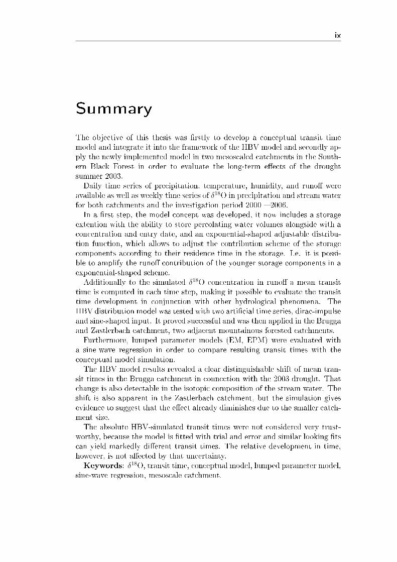
The objective of this thesis was �rstly to develop a conceptual transit timemodel and integrate it into the framework of the HBV model and secondly ap-ply the newly implemented model in two mesoscaled catchments in the South-ern Black Forest in order to evaluate the long-term e�ects of the droughtsummer 2003.Daily time series of precipitation, temperature, humidity, and runo� were
available as well as weekly time series of δ18O in precipitation and stream waterfor both catchments and the investigation period 2000 � 2006.In a �rst step, the model concept was developed, it now includes a storage
extention with the ability to store percolating water volumes alongside with aconcentration and entry date, and an exponential-shaped adjustable distribu-tion function, which allows to adjust the contribution scheme of the storagecomponents according to their residence time in the storage. I.e. it is possi-ble to amplify the runo� contribution of the younger storage components in aexponential-shaped scheme.Additionally to the simulated δ18O concentration in runo� a mean transit
time is computed in each time step, making it possible to evaluate the transittime development in conjunction with other hydrological phenomena. TheHBV distribution model was tested with two arti�cial time series, dirac-impulseand sine-shaped input. It proved successful and was then applied in the Bruggaand Zastlerbach catchment, two adjacent mountainous forested catchments.Furthermore, lumped parameter models (EM, EPM) were evaluated with
a sine-wave regression in order to compare resulting transit times with theconceptual model simulation.The HBV model results revealed a clear distinguishable shift of mean tran-
sit times in the Brugga catchment in connection with the 2003 drought. Thatchange is also detectable in the isotopic composition of the stream water. Theshift is also apparent in the Zastlerbach catchment, but the simulation givesevidence to suggest that the e�ect already diminishes due to the smaller catch-ment size.The absolute HBV-simulated transit times were not considered very trust-
worthy, because the model is �tted with trial and error and similar looking �tscan yield markedly di�erent transit times. The relative development in time,however, is not a�ected by that uncertainty.Keywords: δ18O, transit time, conceptual model, lumped parameter model,
sine-wave regression, mesoscale catchment.

x
xi
Zusammenfassung
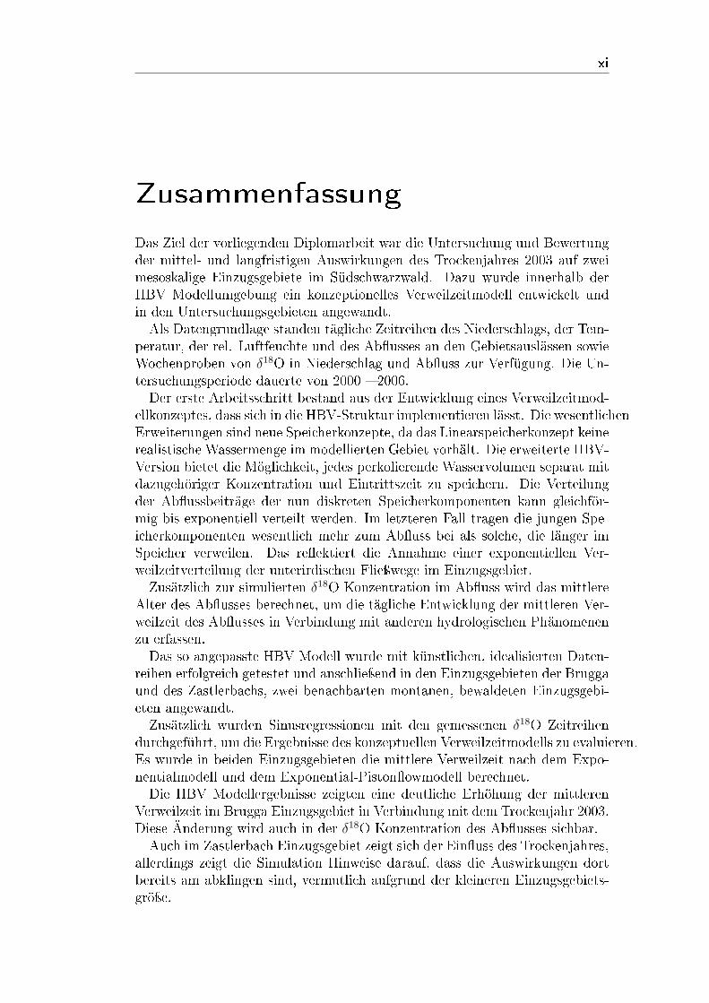
Das Ziel der vorliegenden Diplomarbeit war die Untersuchung und Bewertungder mittel- und langfristigen Auswirkungen des Trockenjahres 2003 auf zweimesoskalige Einzugsgebiete im Südschwarzwald. Dazu wurde innerhalb derHBV Modellumgebung ein konzeptionelles Verweilzeitmodell entwickelt undin den Untersuchungsgebieten angewandt.Als Datengrundlage standen tägliche Zeitreihen des Niederschlags, der Tem-
peratur, der rel. Luftfeuchte und des Ab�usses an den Gebietsauslässen sowieWochenproben von δ18O in Niederschlag und Ab�uss zur Verfügung. Die Un-tersuchungsperiode dauerte von 2000 � 2006.Der erste Arbeitsschritt bestand aus der Entwicklung eines Verweilzeitmod-
ellkonzeptes, dass sich in die HBV-Struktur implementieren lässt. Die wesentlichenErweiterungen sind neue Speicherkonzepte, da das Linearspeicherkonzept keinerealistische Wassermenge im modellierten Gebiet vorhält. Die erweiterte HBV-Version bietet die Möglichkeit, jedes perkolierende Wasservolumen separat mitdazugehöriger Konzentration und Eintrittszeit zu speichern. Die Verteilungder Ab�ussbeiträge der nun diskreten Speicherkomponenten kann gleichför-mig bis exponentiell verteilt werden. Im letzteren Fall tragen die jungen Spe-icherkomponenten wesentlich mehr zum Ab�uss bei als solche, die länger imSpeicher verweilen. Das re�ektiert die Annahme einer exponentiellen Ver-weilzeitverteilung der unterirdischen Flieÿwege im Einzugsgebiet.Zusätzlich zur simulierten δ18O Konzentration im Ab�uss wird das mittlere
Alter des Ab�usses berechnet, um die tägliche Entwicklung der mittleren Ver-weilzeit des Ab�usses in Verbindung mit anderen hydrologischen Phänomenenzu erfassen.Das so angepasste HBV Modell wurde mit künstlichen, idealisierten Daten-
reihen erfolgreich getestet und anschlieÿend in den Einzugsgebieten der Bruggaund des Zastlerbachs, zwei benachbarten montanen, bewaldeten Einzugsgebi-eten angewandt.Zusätzlich wurden Sinusregressionen mit den gemessenen δ18O Zeitreihen
durchgeführt, um die Ergebnisse des konzeptuellen Verweilzeitmodells zu evaluieren.Es wurde in beiden Einzugsgebieten die mittlere Verweilzeit nach dem Expo-nentialmodell und dem Exponential-Piston�owmodell berechnet.Die HBV Modellergebnisse zeigten eine deutliche Erhöhung der mittleren
Verweilzeit im Brugga Einzugsgebiet in Verbindung mit dem Trockenjahr 2003.Diese Änderung wird auch in der δ18O Konzentration des Ab�usses sichbar.Auch im Zastlerbach Einzugsgebiet zeigt sich der Ein�uss des Trockenjahres,
allerdings zeigt die Simulation Hinweise darauf, dass die Auswirkungen dortbereits am abklingen sind, vermutlich aufgrund der kleineren Einzugsgebiets-gröÿe.

xii
Die absoluten HBV-simulierten Verweilzeiten werden nicht als besonders ver-trauenswürdig eingestuft, da die Zeitreihen rein optisch angepasst wurden undsich ähnlich passende Modellanpassungen �nden lassen, die aber ein anderesmittleres Verweilzeitniveau erzeugen. Die relative zeitliche Entwicklung bleibtdavon aber unberührt.
1
1 Introduction
1.1 General introduction
Transit time modelling has been and is still an important research �eld in catch-ment hydrology. Transit time, the time a water volume spends in a hydrologicsystem, is an important catchment descriptor because it comprises informa-tion about �owpaths and helps understanding various catchment properties.Applications may be solute transport (contamination), recharge and aquifercapacity or more derivately water quality management.Environmental tracers are commonly used to asses transit times, especially
isotopes of the water itself (18O, 2H and 3H), continuously applied to the catch-ment with precipitation. Di�erent approaches exist to model the transit time.Generally, transit time modelling is limited by the precision of in- and output
data, the choice of a correct distribution model and assumptions on recharge,that have to be taken into account. In order to avoid at least some of theseissues and to get an estimation not only of longterm mean transit times but alsotransit time development during di�erent �ow conditions, especially low�ow,the thesis' approach was chosen.
1.2 Objective
The major aim of this thesis is the development of a transit time modellingmodule which �ts into the framework of a working quantitative model (HBVmodel) and the subsequent application on a mesoscale catchment. The closerobjective is to design a tool that reveals information on the development oftransit times in stream water during drought conditions and the mid- to long-term in�uence of droughts on the subsurface watersystem.The underlying motivation for this approach is to test the possibility to ben-
e�t from the conceptual structure of the quantitative model which describesimportant hydrological processes and catchment components (e.g. gradientsof temperature and precipitation, evapotranspiration dependent on season andclimatic condition, runo� contribution from soils, aquifer properties) and pro-duce time series of runo� ages along with the modelled runo�. This is primarilyaccomplished by the integration of a �ttable distribution of runo� componentsfrom the model's storages.Additionally, with a sine-wave regession a lumped parameter model is �tted
to estimate mean transit time in order to evaluate the results of the conceptualapproach.
2 Chapter 1. Introduction
1.3 Transit time modelling approaches
1.3.1 Stable isotopes in transit time modelling
Generally, the use of stable isotopes, i.e. δ 18O and 2H (D) in catchment hydrol-ogy can provide valuable information about origin, �ow pathways and storageconditions of stream�ow components and thus also for transit time estimations.Common approaches are based on lumped parameter modelling (Maloszewskiand Zuber, 1982), where mathematical transit time distribution (TTD) modelsare used to translate an input function (precipitation concentration) into anoutput (stream�ow concentration).The applicability of the water's stable isotopes is based upon concentration
changes in time. Fractionation processes occur due to the di�erent atomicmasses of 18O and D compared to the "normal", most abundant isotopes 16Oand 1H during phase transitions. They result in a depletion of 18O and D inevaporated and sublimated waters and enrichment during condensation andresublimation. These processes can, from a hydrological point of view, besummarized to several fractionation e�ects which in�uence the isotopic com-position of precipitation. Those are:
• Continental e�ect
• Elevation e�ect
• Latitude e�ect
• Amount e�ect
• Temperature e�ect
• Season e�ect
The most important e�ect relating to longtime mesoscaled observations intemperate climates is the elevation e�ect unless for single storm events thepattern of 18O can di�er extensively up to inversion of the common gradient.(Moser and Rauert, 1980; Kendall and McDonnell, 1998).In conjunction with transit time modelling another important e�ect besides
fractionation is the selection. It describes a "pseudo-fractionating" selectivebehaviour of components in the hydrological cycle due to other reasons than thedi�erence between the isotopes. An example is the saison-dependent transpi-ration and its in�uence on recharge volumes compared to precipitation, whichcan result in an o�set mean isotope composition of groundwater recharge com-pared to precipitation.The isotopes of the water molecule are ideal environmental tracers as they
consist of water themselves. This and their conservative behaviour in aquifersas well as soils and streams make them reliable tracers for transit time studiesthat cover all structural catchment parts in most cases. Other environmentalisotopes like noble gas isotopes which are applicable in aquifer studies cannot
1.4. Conclusions 3
be used here due to their interactions with the atmosphere (McGuire andMcDonnell, 2006).The 18O values in this thesis are presented in the δ notation, the normed
di�erence in sample concentration compared to a standard (V-SMOW).
1.3.2 Transit time distributions and modelling approaches
The transit time distribution (TTD) of a catchment is a hypothetical responsefunction that incorporates all catchment factors which in�uence a water vol-ume on its way through the re�ected system. While theoretically transit timedistributions might be time-variant, generally a time-invariance is supposed fortransit time estimations and a TTD model is �tted to observed data in orderto determine the transit times.Four common TTD model types exist: piston �ow, exponential, exponential-
piston �ow, and dispersion models. Piston �ow models describe no furtherdistribution but an time o�set (one parameter). Exponential models describea exponential pathway distribution, starting without time lag, i.e. a fractionpasses the system instantly with the rest following exponentially decreasing(one parameter). Exponential-piston �ow models combine these approaches,they are lagged exponential models (two parameters). Dispersion models �-nally describe a left-skewed distribution implying an advective-dispersive sys-tem (three parameters).Three approaches exist to �t the lumped models, these are: (a) integrating
the tracer input function with the TTD, the convolution integral which is solvednumerically in the time domain, (b) solving the convolution by transformationof in- and output to the frequency domain, and (c) estimating mean transittimes with a sine-wave regression. A sine-wave regression is applied in chapter6. For a comprehensive overview see McGuire and McDonnell (2006).Lumped TTD models are undependent of hydro- or meteorological data,
which is an advantage compared to conceptual approaches. But they haveseveral limitations, which are easily violated in catchment modeling. Theseare e.g. input function determination (spatial homogeneity and recharge) ortime variance of catchment properties. (Maloszewski and Zuber, 1982; Soulsbyet al., 2000; McGuire et al., 2002; Rodgers et al., 2005; McGuire and McDon-nell, 2006).
1.4 Conclusions
Several approaches are known to estimate transit times, most of them arebased on the assumption of a system-characteristic transit time distribution,to which tracer data can be �tted. For the application of lumped parametermodels no further catchment information is needed, but they have limitationsthat restrict their potential in catchment transit time modelling. Conceptualapproaches on the other hand have a high demand of hydrological data.

4 Chapter 1. Introduction
The objective of the thesis is to estimate mean transit time and transit timedevelopment under drought conditions in two mountainous catchments in theSouthern Black Forest. Two methods are used to estimate transit times, aconceptual approach based on the HBV model and the assumption of exp-nential pathway distribution, and additionally a lumped parameter sine-waveregression.
5
2 Area and investigation period
2.1 The Brugga and Zastlerbach Catchment
2.1.1 Location and morphology
Both Brugga and Zastlerbach are streams within the Dreisam catchment south-east of Freiburg (Br.) in the southern Black Forest. Whereas the surroundingDreisam catchment shows a distinct morphological division in the mountain-ous Black Forest parts, mostly forested with meadowy valley bottoms and theZarten basin, a large plain-shaped valley �lled with glacial sediments, mostlyagricultural land, the Brugga as well as the neighboured Zastlerbach catchmentare situated completely in the Black Forest.As this particular area has been under investigation by the Institute of
Hydrology over the last two decades, with enduring climatological and hy-drological routine measurements as well as numerous singular studies, lotsof publications and diploma theses have been released with descriptions ofthe area. Information presented in this section is mainly based on the worksby Holocher (1997), Lindenlaub (1998), Uhlenbrook (1999a), Didszun (2000),Wissmeier (2005) and Ehnes (2006). Table 2.1.1 gives some basic geographicalinformations about the catchments.Characteristical for the investigated area are deep valleys with steep, fores-
ted slopes. The forests' dominating species are Norway spruce and beech.Furthermore, in exceptionally steep parts and below rock outcrops screes andtalus �elds occur. The geomorphology was shaped by two major in�uences: thesouthern parts of both catchments where the highest point is located (Feldberg,1493 m a.s.l.) were temporarily glaciated during the Würm ice age (∼ 10000B.P.) and show results of glacial erosion like U-shaped valleys and morraines.The northern parts up to the opening into the Zarten basin never experiencedglaciation but were formed under periglacial circumstances (V-shaped valleysand gullying).
2.1.2 Geology and soils
The southern black forest consists mainly of metamorphic bedrocks (e.g. gneiss),which can be considerably jointed, especially in areas of intense tectonicalmovement. These bedrocks can crop out at the surface, but they are mostlycovered with a typical sequence ("`Periglaziale Deckschichten"') of Quarternary-developed layers constituting of rock debris, scree and �ne material. Thesedeveloped due to intense weathering and soli�uction on the steep slopes under
6 Chapter 2. Area and investigation period
Table 2.1.1: Geomorphological properties of the investigation area, characteristic para-meters.
Brugga catchment Zastler catchmentarea (km2) 39.8 17.8
min. height (m a.s.l.) 436 548max. height (m a.s.l.) 1493 1493height extension (m) 1057 945Surface ratio slope angle (%)
0◦ - 20◦ 43 45.320◦ - 40◦ 47.3 53.8> 40◦ 9.7 0.9
Landuse (%)urban area 0.9 0.1
agriculture & grassland 22.3 13.8forest 76.9 86.0
periglacial conditions to a considerable thickness (∼ 50 - 150 cm). An idealsequence starts (from the lower boundary/bedrock) with the Base Layer, dueto soli�uction horizontally aligned rocks in a dense matrix, followed by theMain Layer with a lower fraction of non-aligned rocks and �nally the thinnerTopset Layer with an again higher fraction of rocks. However, this scheme isidealized and not every layer might be clearly distinguishable.At the valley bottom holozene alluvial sediments can be found, in the south-
ern parts also morraine material.
2.1.3 Climatic conditions and hydrology
The regional climate is temperate and in�uenced by alternating passages ofcyclones and anticyclones, driven by the west wind drift. Due to the moun-tainous relief local climate characteristics show an altitude dependency. Duringthe investigation period (1999-2006), mean annual temperatures at the threemeteorological stations (see section 2.2, page 11) are 8.1 ◦C at the stationSchweizerhof (720 m a.s.l.), this station is located in the Zastlerbach catch-ment, 7.7 ◦C at the station Katzensteig (775 m a.s.l.), which is situated in theSt. Wilhelm valley, one upstream valley of the Brugga catchment, and 6.3 ◦Con the Schauinsland1 (1205 m a.s.l.), located on the southwestern edge of theexamined area. In wintertime, inversion weather situations frequently occur,resulting in reversed temperature gradients. Figure 2.1.1 shows the annualvariation of temperature at the three station sites.The precipitation in summertime is dominated by convective storm events,
whereas in wintertime cyclonal rain- and snowfalls are prevailing. In thehigher parts about 37 % of the annual precipitation fall as snow (Trenkleand v. Rudolf, 1989 in Ehnes, 2006). The precipitation in general shows a
1only data for Jan. 1999 to Feb. 2004
2.1. The Brugga and Zastlerbach Catchment 7
05
1015
20
Air
tem
pera
ture
(°C
)
Jan Feb Mar Apr May Jun Jul Aug Sep Oct Nov Dec
St. WilhelmZastlerSchauinsland
Figure 2.1.1: Monthly mean air temperature at the three stations in the catchmentsover the investigation period (Schauinsland: 1999-2004).
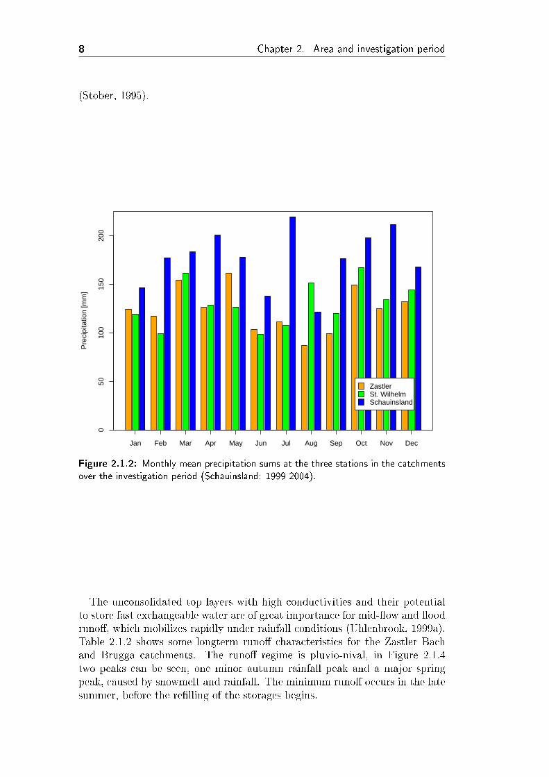
clear altitude dependency, but is also in�uenced by the local topography (e.g.lu�/lee situations, especially in the higher parts, where precipitation is blownover due to strong winds ). Nevertheless, for singular storm events rainfall canshow a high variability caused by the wind direction and lu�-lee e�ects likevapor depletion in the clouds (Holzschuh, 1995). Throughout the investigatedperiod the following mean annual precipitation volumes were observed: 1490mm at the station Schweizerhof, 1557 mm at the station Katzensteig, 2117 mmon the Schauinsland. In Figure 2.1.2 the monthly mean sums at the stationsare illustrated.The potential evapotranspiration ETPHaude (calculated with the Haude for-
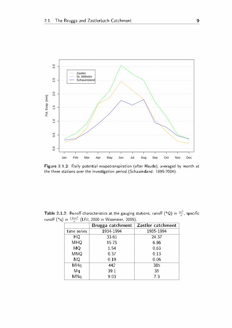
mula (DVWK, 1996)) shown in Figure 2.1.3 as mean daily values on a monthlybasis average to 401 mm (Schweizerhof), 520 mm (Katzensteig) and 336 mm(Schauinsland). There is no obvious explanation for the strong deviation be-tween Schweizerhof and Katzensteig as they are approximately on the sameelevation level. Nevertheless, it can be stated that a) the time series is notthat long, so one could expect some scatter in the averages, b) these are spotmeasurements which do not integrate regional variations, c) evapotranspira-tion in this area is mainly limited by humidity, which might be more oftenclose to 100 % due to local specialities, e.g. exposure.The hydrogeologic characteristics of the bedrock show strong variations in
the area, as the metamorphic rock itself can be considered non-porous, thedecisive property is the joint system which varies considerably and causes vari-ations in hydraulic conductivity from 10−10 to 10−5 m
sand decreases with depth
8 Chapter 2. Area and investigation period
(Stober, 1995).P
reci
pita
tion
[mm
]
050
100
150
200
Jan Feb Mar Apr May Jun Jul Aug Sep Oct Nov Dec
ZastlerSt. WilhelmSchauinsland
Figure 2.1.2: Monthly mean precipitation sums at the three stations in the catchmentsover the investigation period (Schauinsland: 1999-2004).
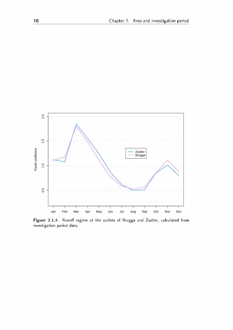
The unconsolidated top layers with high conductivities and their potentialto store fast exchangeable water are of great importance for mid-�ow and �oodruno�, which mobilizes rapidly under rainfall conditions (Uhlenbrook, 1999a).Table 2.1.2 shows some longterm runo� characteristics for the Zastler Bachand Brugga catchments. The runo� regime is pluvio-nival, in Figure 2.1.4two peaks can be seen, one minor autumn rainfall peak and a major springpeak, caused by snowmelt and rainfall. The minimum runo� occurs in the latesummer, before the re�lling of the storages begins.
2.1. The Brugga and Zastlerbach Catchment 9
0.0
0.5
1.0
1.5
2.0
2.5
3.0
Pot
. Eva
p. [m
m]
Jan Feb Mar Apr May Jun Jul Aug Sep Oct Nov Dec
ZastlerSt. WilhelmSchauinsland
Figure 2.1.3: Daily potential evapotranspiration (after Haude), averaged by month atthe three stations over the investigation period (Schauinsland: 1999-2004).
Table 2.1.2: Runo� characteristics at the gauging stations, runo� (*Q) in m3
s , speci�c
runo� (*q) in l·km2
s (LfU, 2000 in Wissmeier, 2005).
Brugga catchment Zastler catchmenttime series 1934-1994 1955-1994
HQ 33.61 24.37MHQ 15.75 6.86MQ 1.54 0.63MNQ 0.37 0.13NQ 0.19 0.06MHq 442 385Mq 39.1 35MNq 9.03 7.3
10 Chapter 2. Area and investigation period
0.5
1.0
1.5
2.0
Par
dé c
oeffi
cien
t
Jan Feb Mar Apr May Jun Jul Aug Sep Oct Nov Dec
ZastlerBrugga
Figure 2.1.4: Runo� regime at the outlets of Brugga and Zastler, calculated frominvestigation period data.
2.2. Data 11
2.2 Data
2.2.1 Data sampling
The investigation period which was �nally modelled with the modi�ed HBVmodel lasts from January 2000 to October 2006. Data series taken for gradientor runo� regimes partly covered longer periods which were then accepted forcalculations where possible.Isotope ratios and most meteorological data presented and interpreted in
this thesis (including δ 18O samples) originate from longterm routine measure-ments of the Institute of Hydrology carried out in the catchment of the nearbyDreisam and its contributing substreams respectively. Two climate observationstations, valley bottom located (see also section 2.1.3), provided temperatureand precipitation volumes in form of daily means and sums respectively. Fur-thermore, 2:00 p.m. humidity values from the stations were introduced forpotential evapotranspiration calculation.For the calculation of temperature and precipitation gradients, time series
from the DWD climate station Schauinsland were available, they lasted fromJanuary 1999 to January 2004.Runo� time series at the catchment outlets were measured by the Lan-
desanstalt für Umweltschutz (LfU) as gauge heights and converted to dischargewith spot-measurement based gage-runo� relations also provided by the LfU.
δ 18O sampling was taken out approximately weekly over the study period.The precipitation concentrations were measured from bulk samples collectedin a Hellmann precipitation collector and thus represent a mean value overthe space of time since the beforehand sampletaking, whereas the stream�owvalues are to be understood as snapshots as they were measured from samplevolumes taken directly out of the stream on the respective day.
δ 18O snow samples from the work of Ehnes (2006) were utilized for the dis-cussion of the model results. A gradient of δ 18O in precipitation was calculatedfrom event measurements taken out in the area by Holzschuh (1995).
2.2.2 Data processing and transformation
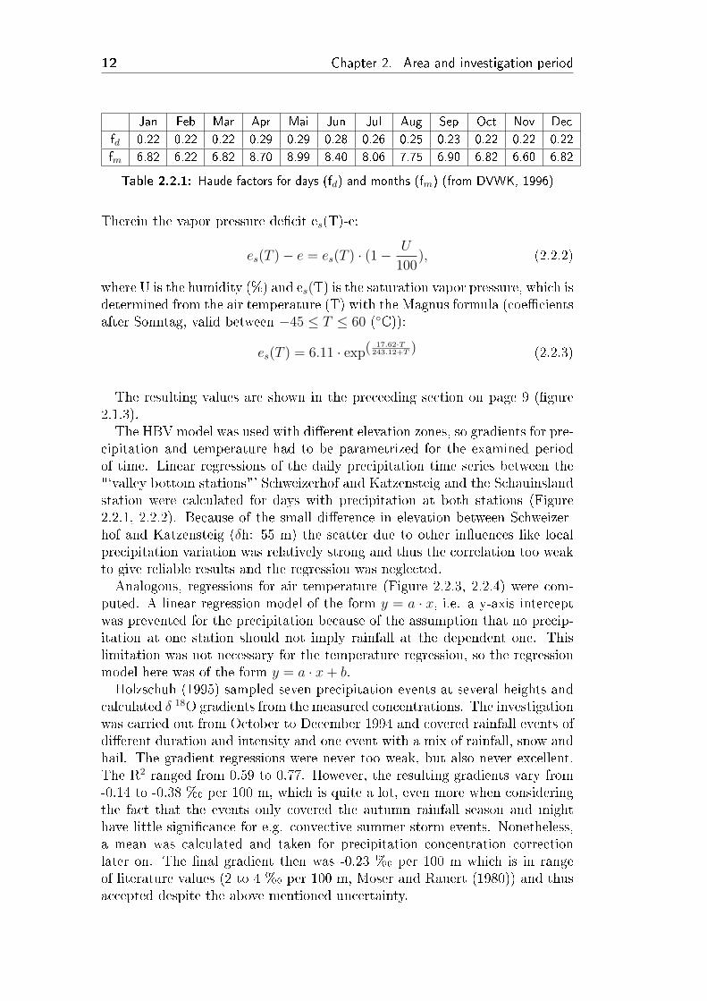
Potential evapotranspiration (ETP) was needed as input for the HBV modeland calculated as a monthly day-mean with the Haude formula (2.2.1) (Haudefactors see table 2.2.1). Because radiation measurements were not availablefrom the station Schweizerhof, the computation of more complex ETP modelswas impossible. But since the values were mainly calculated as input for theHBV model, which e�ects a generation of uncertainty anyway (e.g. transferspot measurement to area), this was considered admissible.The ETPHaude is calculated with 2:00 p.m. measurements and is an empirical
function of the vapor pressure de�cit:
ETPHaude = f · (es(T )− e)14 ≤ 7mm
d(2.2.1)
12 Chapter 2. Area and investigation period
Jan Feb Mar Apr Mai Jun Jul Aug Sep Oct Nov Dec
fd 0.22 0.22 0.22 0.29 0.29 0.28 0.26 0.25 0.23 0.22 0.22 0.22
fm 6.82 6.22 6.82 8.70 8.99 8.40 8.06 7.75 6.90 6.82 6.60 6.82
Table 2.2.1: Haude factors for days (fd) and months (fm) (from DVWK, 1996)
Therein the vapor pressure de�cit es(T)-e:
es(T )− e = es(T ) · (1− U
100), (2.2.2)
where U is the humidity (%) and es(T) is the saturation vapor pressure, which isdetermined from the air temperature (T) with the Magnus formula (coe�cientsafter Sonntag, valid between −45 ≤ T ≤ 60 (◦C)):
es(T ) = 6.11 · exp( 17.62·T243.12+T ) (2.2.3)
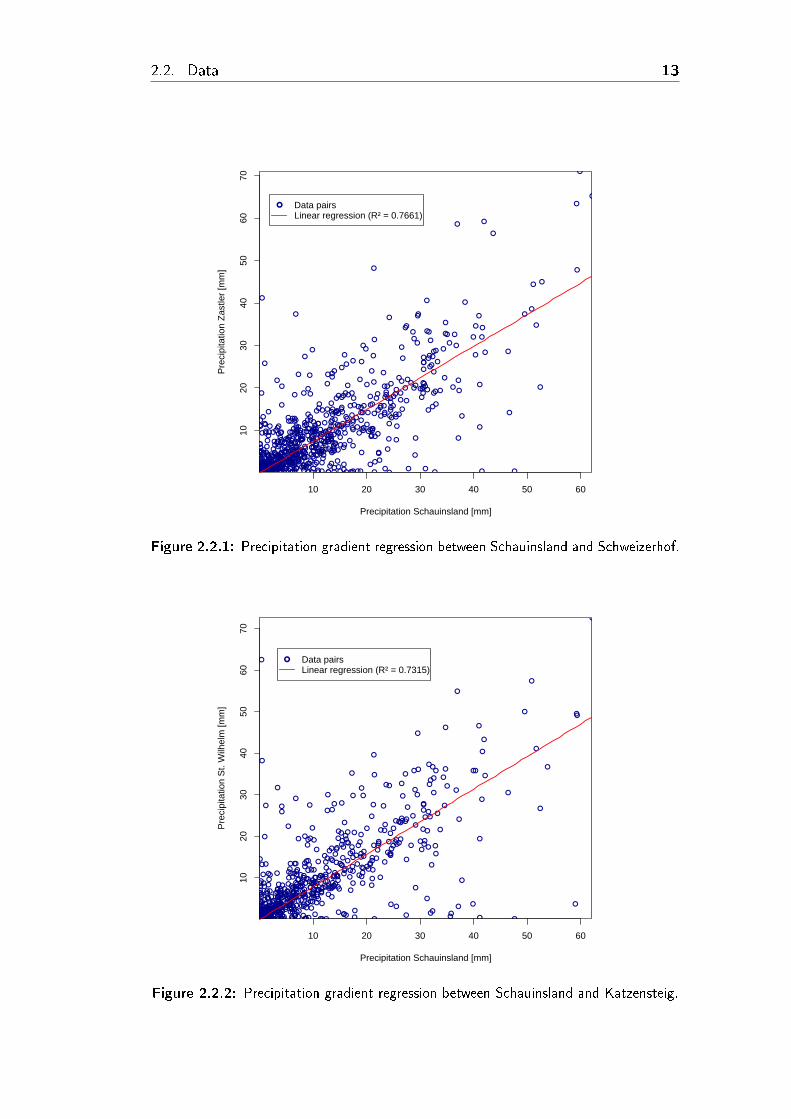
The resulting values are shown in the preceeding section on page 9 (�gure2.1.3).The HBV model was used with di�erent elevation zones, so gradients for pre-
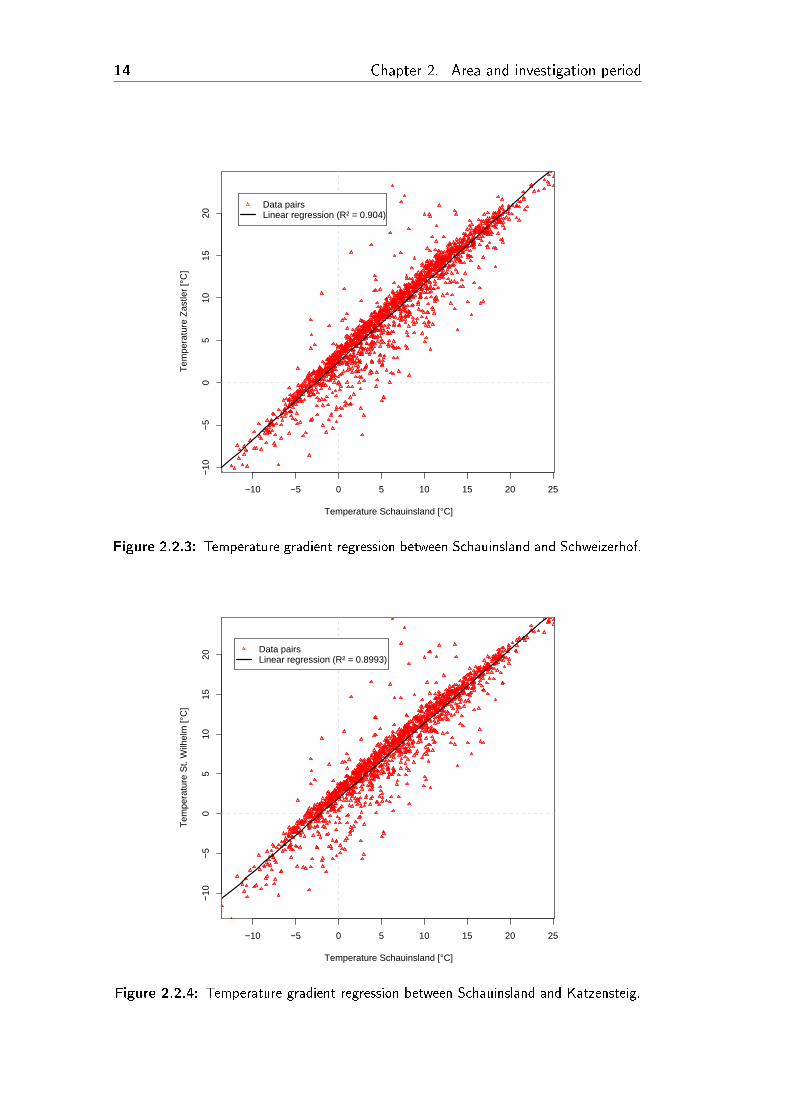
cipitation and temperature had to be parametrized for the examined periodof time. Linear regressions of the daily precipitation time series between the"`valley bottom stations"' Schweizerhof and Katzensteig and the Schauinslandstation were calculated for days with precipitation at both stations (Figure2.2.1, 2.2.2). Because of the small di�erence in elevation between Schweizer-hof and Katzensteig (δh: 55 m) the scatter due to other in�uences like localprecipitation variation was relatively strong and thus the correlation too weakto give reliable results and the regression was neglected.Analogous, regressions for air temperature (Figure 2.2.3, 2.2.4) were com-
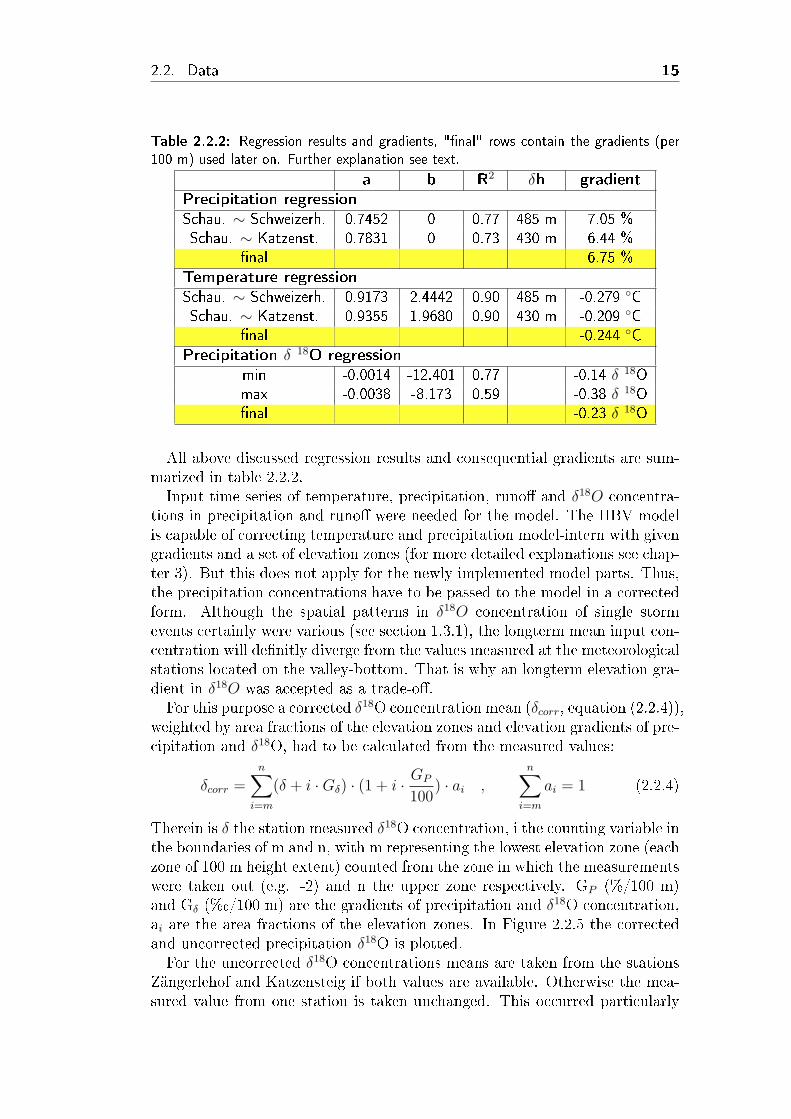
puted. A linear regression model of the form y = a · x, i.e. a y-axis interceptwas prevented for the precipitation because of the assumption that no precip-itation at one station should not imply rainfall at the dependent one. Thislimitation was not necessary for the temperature regression, so the regressionmodel here was of the form y = a · x + b.Holzschuh (1995) sampled seven precipitation events at several heights and
calculated δ 18O gradients from the measured concentrations. The investigationwas carried out from October to December 1994 and covered rainfall events ofdi�erent duration and intensity and one event with a mix of rainfall, snow andhail. The gradient regressions were never too weak, but also never excellent.The R2 ranged from 0.59 to 0.77. However, the resulting gradients vary from-0.14 to -0.38 %� per 100 m, which is quite a lot, even more when consideringthe fact that the events only covered the autumn rainfall season and mighthave little signi�cance for e.g. convective summer storm events. Nonetheless,a mean was calculated and taken for precipitation concentration correctionlater on. The �nal gradient then was -0.23 %� per 100 m which is in rangeof literature values (2 to 4 %� per 100 m, Moser and Rauert (1980)) and thusaccepted despite the above mentioned uncertainty.
2.2. Data 13
●
●
●●
●
●●
●
●●
●
●
●●
● ●
●
●
●●
●
●
●
●
●
●●
●
●
●
●
●
●
●●
●
●
● ●
●
●
●
●
●
●
●
●
●
●
●
●●
●●
●
●
●
●●
●●●
●
● ●
●
●●
●●
●
●
●
●
●
●
●
●
●
●
●
●
●
●
●
● ●
●●
●●
●
●
●
●
●
●●●●
●
●
●
●
●
●
●
●
●
●
●
●●
●
●
●●●●
●
●
●
●
●●●●
●●
●
●
●
●
●
●
●
●
●●●●●
●
●
●
●
●●
●
●
●
●
●
●●
●
●
●●●●●●
●
●
●●
●
●●
●
●
●
●
●
●
●
●
●
●
●
●
●
●
●
●
●●
●●
●●
●
●●●●●
● ●
●
●
●
●
●●
●
●
●
●
●
●
●
●
●
●
● ●
●
●
●
●
●
●
●
●
●
●
●●
●
●
●
●
●
●
●
●●●
●
●
●
●●
●
●
●
●●
●●
●●● ●
●
●●●
●
●●
●
●
●
●●●
●
●
●●●
●
●
●●
●
●
●
●●
●● ●●
●
●
●
●
●
●
●●
●
●
●●
●
●●
●●
●
● ●
●●
●●
●
●
●●
●●
●●
●●
●
●
●
●
●
●●●
●
●
●
●●
●
●●
●
●
●
●
● ●
● ●●
●
●
●
●
●●
●
● ●
●
●
●
●●●●
●
●
●
●
●
● ●
●
●
●
●
●●●
●
●
●
●
●●
●
●
●
●●
●
●
●●
●
●
●
●
● ●
●●
●
●
●
●
●
●●
●●
●
●
●
●
●
●
●
●
●
●●
●
●
●
●
●
●
●●
●
●
●
●
●
●
●
●
●
●
●
●
●
●
●
●
●
●
●
●
●
●●
● ●
●● ●
●
● ●
●
●
●
●●
●
●
●
●
●
●
●
●
●●
●
●
●
●
●
●
●
●
●
●●●
●
●
●
●
●
●
●
● ●● ●●
●
●
●
●●
●●●
●●
●
●
●
●
●
●●
●●
●
●
●
●
●
●
●
●
●
●
●●
●●
●
● ●
●
●
●●
●
●
●
●
●
●
●
●
●
●
●
●
●●
●●●
●
●●
●●
●
●
●
●
●
●
●
●
●
●
●
●
●
●●
●
●
●
●
●
●●
●
●
●
●● ●
●●
●
●
●
●
●
●
●
●
●
●
●
●
●●
●
●
●
●●
●
●
●
●
●
●
●
●●●
●
●
●
●
●
●
●
●
●
●
●
●
●
●●
●●●
●
●
●
●
●
●
●
●
●
●
●●
●
●
●
●●●
●
●
●
●
●
●
●
●
●
●
●
●
●
●●
●
●
●
●
●
●
●
●
●
●
●
●
●
●●
●
●
●
●
●
●●
●
●
●
●●
●
●
●
●
●
●
●
●
●
●●
●
●
●
●
●
●●
●
●
●
●
●
●
●●
●
●●
●
●
●
●
●
●
●
●
●
●
●
●
●
●
● ●●
●●
●
●
●
●
●
●●
●●
●
●
●
●
●
●
●
● ●
●
●
●
●
●
● ●●
●●●
●
●
●
●
●
●
●
●
●
●
●
●
●
●
●
●
●●
●
●
●
●
●
●
●
●
●●
●
●
●
●
●
●
●
●
●●
●
●●
●
●●
●
●
●
●
●
●
●
●
●
● ●●●
● ●
●
●●
●
●
●
●
●
●●●
●●●
●
●
●
●
●
●
●
●
●
●
●
●
●
●
●
●
●●
●
10 20 30 40 50 60
1020
3040
5060
70
Precipitation Schauinsland [mm]
Pre
cipi
tatio
n Z
astle
r [m
m]
● Data pairsLinear regression (R² = 0.7661)
Figure 2.2.1: Precipitation gradient regression between Schauinsland and Schweizerhof.
●
●
●
●
● ●●●●●●●
●
●
●
●
●
●
●
●
●
●
●●
●
●
●●●●●
●
●
●
●
●
●
●●
●
●
●
●
●
●
●
●
●
●
●
●
●
●
●
●
●
●
●
●
●●
●
●●
●
●
●
●
●
●
●
●
●
●
●
●
●
●
●●●
●
●
●
●
●
●
●
●
●
●●
●●
●
●●
●
●
●
●
●
●●
●
●
●●●
●●
●
●● ●
●
●●
●
●●
●
●
●● ●● ●
●●
●●●● ●
●●●
●
●●
●
●
●
●
●
●
●
● ●
●
●●
●
●
●
●●
●●
●
●
●●
●
●●
●
●
●
●
● ●
●●
●
●
●
●
●
●●
●
●●
●
●
●
●●●
●
●
●
●
●
●
● ●
●
●
●●
●●
●
●
●
●
●
●
●
●●
●●
●
●
●
●
●
●
●
●
●
●
●
●
●
●
●
●
●●
●
●
● ●
●
●
●
●●
●
●
●
●
●
●●
●
●
●●
●
●
● ●
●
●●
●
●
●
●
●
●
●
●
●
●
●
●
●●
●
●
●●
●
●
●
●
●●●
●
●●
●
●
●
●
●
●
●
●
●●
●
●
●
●
●
●●
●
●
●
●
●
●
●
●●
●
●
●
●
●
●
●
●
●●● ●
●
●
●
●●●
●
●●
●
●
●
●
●
●
●
●
●
●
●
●
●
●
●
●
●
●
●
●●
●
●
●●●
●
● ●
●
●
●●
●
●
●●
●
●●
●
●
●
●●
●
●●
●●
●● ●
●
●
●
●
●
●●
●
●
●
●
●
●● ●
●
●
●
●
●
●
●
●
●
●●
●
●
●
●
●
●
●●
●
●
●
●
●
●
●
●
●
●
●
●
● ●
●
●
●●
●
●
●
●
●
●
●
●
●
●
●
●
●
●
●
●
●●●
●
●
●
●
●
●
●
●
● ●
●●●
●
●
●
●●
●
●
●
●
●
●
●
●
●
●
●
●
●
●●
●
●
●
●
●
●
●
●●
●
●
●
●
●●
●
●
●
●
●
●●
●
●
●
●●
●
●
●
●
●
●
●
●
●●
●●
●
●
●
●
● ●●●
●
●
●●
●
●
●
●
●
●
●
●
●●
●
●●
●
●
●
●
●
●
●
●
●
●
●●
●
●
●
●
●
●
●
●
●
●●
●
●
●
●
●
●●●
●
●
●
●
●●
●
●
●
●
●●
●
●
●●
●
●
●
●●●
●
●
●
●
●
●
●●
●
●
●
●
●
●
●
●
●
●
●
●
●
●
●
●
●●
●
●
●
●
● ●
●
● ●
●
●
●
●
●
●
●
● ●●●
●
●
●
●
●
●
●
●
●
●●
●
●
●
●
●
●
●
●
●
●
●●
●
●
●
10 20 30 40 50 60
1020
3040
5060
70
Precipitation Schauinsland [mm]
Pre
cipi
tatio
n S
t. W
ilhel
m [m
m]
● Data pairsLinear regression (R² = 0.7315)
Figure 2.2.2: Precipitation gradient regression between Schauinsland and Katzensteig.
14 Chapter 2. Area and investigation period
−10 −5 0 5 10 15 20 25
−10
−5
05
1015
20
Temperature Schauinsland [°C]
Tem
pera
ture
Zas
tler
[°C
]
Data pairsLinear regression (R² = 0.904)
Figure 2.2.3: Temperature gradient regression between Schauinsland and Schweizerhof.
−10 −5 0 5 10 15 20 25
−10
−5
05
1015
20
Temperature Schauinsland [°C]
Tem
pera
ture
St.
Wilh
elm
[°C
]
Data pairsLinear regression (R² = 0.8993)
Figure 2.2.4: Temperature gradient regression between Schauinsland and Katzensteig.
2.2. Data 15
Table 2.2.2: Regression results and gradients, "�nal" rows contain the gradients (per100 m) used later on. Further explanation see text.
a b R2 δh gradientPrecipitation regressionSchau. ∼ Schweizerh. 0.7452 0 0.77 485 m 7.05 %Schau. ∼ Katzenst. 0.7831 0 0.73 430 m 6.44 %
�nal 6.75 %Temperature regressionSchau. ∼ Schweizerh. 0.9173 2.4442 0.90 485 m -0.279 ◦CSchau. ∼ Katzenst. 0.9355 1.9680 0.90 430 m -0.209 ◦C
�nal -0.244 ◦CPrecipitation δ 18O regression
min -0.0014 -12.401 0.77 -0.14 δ 18Omax -0.0038 -8.173 0.59 -0.38 δ 18O�nal -0.23 δ 18O
All above discussed regression results and consequential gradients are sum-marized in table 2.2.2.Input time series of temperature, precipitation, runo� and δ18O concentra-
tions in precipitation and runo� were needed for the model. The HBV modelis capable of correcting temperature and precipitation model-intern with givengradients and a set of elevation zones (for more detailed explanations see chap-ter 3). But this does not apply for the newly implemented model parts. Thus,the precipitation concentrations have to be passed to the model in a correctedform. Although the spatial patterns in δ18O concentration of single stormevents certainly were various (see section 1.3.1), the longterm mean input con-centration will de�nitly diverge from the values measured at the meteorologicalstations located on the valley-bottom. That is why an longterm elevation gra-dient in δ18O was accepted as a trade-o�.For this purpose a corrected δ18O concentration mean (δcorr, equation (2.2.4)),
weighted by area fractions of the elevation zones and elevation gradients of pre-cipitation and δ18O, had to be calculated from the measured values:
δcorr =n∑
i=m
(δ + i ·Gδ) · (1 + i · GP
100) · ai ,
n∑i=m
ai = 1 (2.2.4)
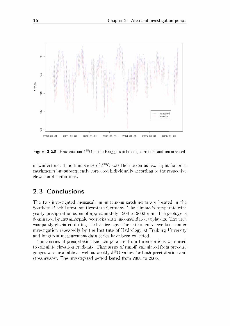
Therein is δ the station measured δ18O concentration, i the counting variable inthe boundaries of m and n, with m representing the lowest elevation zone (eachzone of 100 m height extent) counted from the zone in which the measurementswere taken out (e.g. -2) and n the upper zone respectively. GP (%/100 m)and Gδ (%�/100 m) are the gradients of precipitation and δ18O concentration,ai are the area fractions of the elevation zones. In Figure 2.2.5 the correctedand uncorrected precipitation δ18O is plotted.For the uncorrected δ18O concentrations means are taken from the stations
Zängerlehof and Katzensteig if both values are available. Otherwise the mea-sured value from one station is taken unchanged. This occurred particularly
16 Chapter 2. Area and investigation period
δδ 18
O ‰
2000−01−01 2001−01−01 2002−01−01 2003−01−01 2004−01−01 2005−01−01 2006−01−01
−25
−20
−15
−10
−5
measuredcorrected
Figure 2.2.5: Precipitation δ18O in the Brugga catchment, corrected and uncorrected.
in wintertime. This time series of δ18O was then taken as raw input for bothcatchments but subsequently corrected individually according to the respectiveelevation distributions.
2.3 Conclusions
The two investigated mesoscale mountainous catchments are located in theSouthern Black Forest, southwestern Germany. The climate is temperate withyearly precipitation sums of approximately 1500 to 2000 mm. The geology isdominated by metamorphic bedrocks with unconsolidated toplayers. The areawas partly glaciated during the last ice age. The catchments have been underinvestigation repeatedly by the Institute of Hydrology at Freiburg Unversityand longterm measurement data series have been collected.Time series of precipitation and temperature from three stations were used
to calculate elevation gradients. Time series of runo�, calculated from pressuregauges were available as well as weekly δ18O values for both precipitation andstreamwater. The investigated period lasted from 2000 to 2006.
17
3 Introduction to the HBV
model
3.1 General description
The HBV model was originally developed at the Swedish Meteorological andHydrological Institute, SMHI in the early 1970s. It has been widely appliedfor runo� simulations all over the world, but particulary in catchments withtemperate/cold-temperate climatic conditions with at least partly forested ar-eas. Also, it has in�uenced a number of succeeding models which incorporatede.g. di�erent snow routines. Known applications of the model cover a catch-ment size of less than one up to 40 000 m2. This wide adaptability is owedto the relative simplicity of the model structure, making the model general(Bergström, 1995). Holocher (1997) applied the HBV model in the Bruggaand a nested subcatchment (St. Wilhelmer Talbach) and stated good adapt-ability of the model (Reff ∼ 0.85) for this area.
Generally, the model simulates catchment properties with a lumped ap-proach, the used version o�ers at least partly distributed simulations, in termsof landcover- and elevation zones (see Section 3.2). Discharge is computedfrom time series of precipitation and potential evapotranspiration (ETP) in asequence of modules, which are (in order from the entering of a precipitationvolume): a day-degree snow routine, a soil moisture routine, a response func-tion (based on the single linear store, SLS) and �nally a routing routine inform of a weighted distribution function.
The version used in this thesis is the �HBV light�, a GUI front-end programwritten in Visual Basic 6 by Jan Seibert. It o�ers several alternative modelstructures (e.g. di�erent lumped/distributed choices, one/two/three ground-water boxes) as well as additional input possibilities like long-term daily meantemperature values for ETP correction or gradient series of precipitation andtemperature instead of constant values. Additionally, an optimation algorithmis integrated to the model.
The following section gives a short overview over the model's properties andparameters as well as the required data. For a more comprehensive descriptionrefer to Seibert (2002), where the following section is excerpted from.
18 Chapter 3. Introduction to the HBV model
3.2 Model version
3.2.1 Modules
In the following a short description of each model routine (only for the versionwhich was altered then for transit time computations) is given, including therelated parameters. An illustrating �gure can be found in chapter 4.3, page29. Although it shows the modi�cations for the transit time calculations thebasic model structure is obvious.
Snow routine: Precipitation is classi�ed as snow below a certain thresholdtemperature TT , then volume corrected by multiplication with a correc-tion factor SFCF and accumulates in a separate box. During meltingconditions (temperature above TT ), the melting volume is calculated bya simple degree day method via a degree-day-factor CFMAX , which is re-tained in the snow up to a certain amount (CWH , in % of the snow pack'swater equivalent) and �nally enters the next routine. When returningto freezing conditions from a melting phase, the retained water partlyrefreezes, controlled by a refreezing factor CFR. These calculations willbe carried out separately for possible set elevation and landuse zones.
Soil routine: The most important remark on the HBV's soil routine with re-spect to the implementation of the transit time modelling routine is thatit behaves like a dead end street for the percolating precipitation (resp.snowmelt) and serves only as a reservoir for evaporable and transpirablewater (both simplifying and limiting). The soil-contributed discharge isthus integrated in the next routine. The soil's maximum capacity is de-�ned by the maximum soil moisture storage FC (no indicator for real-life�eld capacities of the soils in the catchment). The percolating water isdivided into one part �lling the soil storage and another entering therunno� routine. Depending on the soil storage charge the relative con-tribution is determined by a power function with the parameter β in theexponent. Evapotranspiration is determined by a soil moisture value LP(relative charge compared to FC). It ranges from potential evapotranspi-ration ( charge
FC≥ LP ) to zero, reduced by a linear function if charge
FC≤ LP .
This routine can be computed separately for landuse and elevation zonesas well.
Runo� routine/response function: DHere, only the properties of the chosenmodel version are described (several exist, see section 3.1). The responsefunction consists of two storage components of which the upper one re-ceives all recharging water and then transfers a �xed amount PERC intothe lower one. In the next step, runo� is generated. While the lowerstorage SLZ is a basic single linear storage (SLS) with runo� propor-tional to the storage volume: Q2 = K2 · SLZ (K2: runo� coe�cient),the upper storage's runo� grows disproportional with increasing storagevolume, triggered by a second parameter α: Q1 = K1 · SUZα. This
3.2. Model version 19
results in a relatively higher runo� contribution from the upper storageon higher storage volumes. The upper storage has no volume limitationand in modeling practice generates the quick runo� reaction on a stormevent. The lower storage often has an about one decimal power smallerruno� coe�cient and is mainly responsible for longterm base�ow runo�.Calculations in this routine are always performed in a lumped way.
Routing routine : The runo� generated in one timestep is not directly passedto the outlet, but distributed onto the next days, given by parameterMAXBAS, and then weighted by an equilateral triangular function overthis number of days.
In total there are 13 parameters to �t a lumped model: �ve for the snow rou-tine (TT ), CFMAX , SFCF, CWH , CFR), three for the soil (FC, LP, β), four forthe runo� routine (PERC, α, K1, K2) and one for the routing (MAXBAS). Ifmodelling semidistributed, the parameter sets for snow and soil can be cho-sen up to three times, one for each landuse zone and they are supplied withdi�erent input for each elevation zone (up to 20). Additionally, gradients forprecipitation PCALT and TCALT have to be chosen, usually regression slopesover the modelled time series or other longterm means. This sums up to atotal of 31 parameters for the semidistributed model.The model does not need initial values to start a model run. Instead, a
"warm-up" phase, typically one year or longer, is used to �ll the modules withsu�cient volumes. The objective functions skip this phase for evaluation.
3.2.2 Data requirements
First of all, time series of precipitation and temperature are needed, also runo�measurements at the outlet in order to �t and evaluate the model. All cal-culations are carried out in a regionalized form, so information about (sub-)catchment sizes are mandatory. Unlike precipitation which is typically loggedin (mm), runo� measurements often have to be transformed from (m3
s) to spe-
ci�c runo� (mm).Furthermore, values of potential evapotranspiration, either twelve monthly
values or 365 daily values have to be passed to the model. Additionally, alongterm mean temperature value can be read into the model, likewise ina monthly or daily form, by which deviations between measured and meantemperature are determined and used to correct the actual evapotranspiration.When modelling semidistributed, gradients of precipitation and temperature
are mandatory, either as constant values or one value per day.
3.2.3 Model evaluation: objective functions
Even though the value of an "optical �t" should not be underestimated, espe-cially when there are reasons to distrust some measurements (e.g. snow precip-itation, frosted gauges etc.), and de�nitly represents the ultimate decision-aid
20 Chapter 3. Introduction to the HBV model
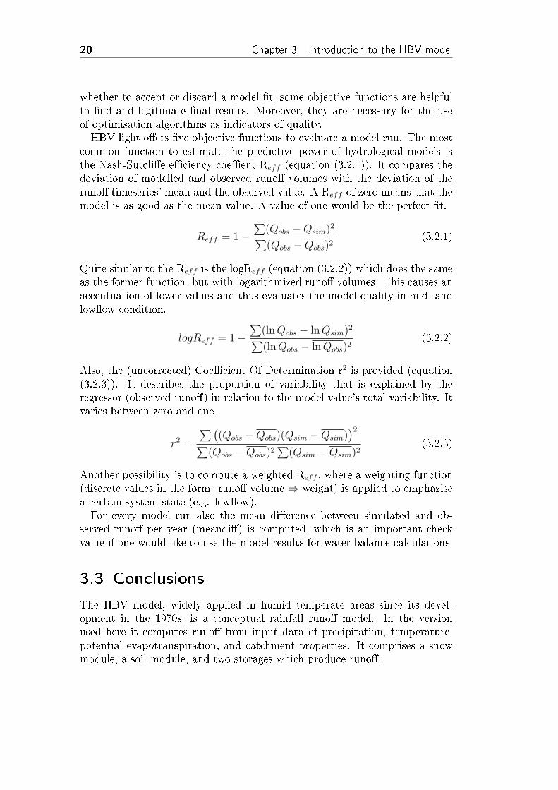
whether to accept or discard a model �t, some objective functions are helpfulto �nd and legitimate �nal results. Moreover, they are necessary for the useof optimisation algorithms as indicators of quality.HBV light o�ers �ve objective functions to evaluate a model run. The most
common function to estimate the predictive power of hydrological models isthe Nash-Sutcli�e e�ciency coe�ent Reff (equation (3.2.1)). It compares thedeviation of modelled and observed runo� volumes with the deviation of theruno� timeseries' mean and the observed value. A Reff of zero means that themodel is as good as the mean value. A value of one would be the perfect �t.
Reff = 1−∑
(Qobs −Qsim)2∑(Qobs −Qobs)2
(3.2.1)
Quite similar to the Reff is the logReff (equation (3.2.2)) which does the sameas the former function, but with logarithmized runo� volumes. This causes anaccentuation of lower values and thus evaluates the model quality in mid- andlow�ow condition.
logReff = 1−∑
(ln Qobs − ln Qsim)2∑(ln Qobs − ln Qobs)2
(3.2.2)
Also, the (uncorrected) Coe�cient Of Determination r2 is provided (equation(3.2.3)). It describes the proportion of variability that is explained by theregressor (observed runo�) in relation to the model value's total variability. Itvaries between zero and one.
r2 =
∑((Qobs −Qobs)(Qsim −Qsim)
)2∑(Qobs −Qobs)2
∑(Qsim −Qsim)2
(3.2.3)
Another possibility is to compute a weighted Reff , where a weighting function(discrete values in the form: runo� volume ⇒ weight) is applied to emphazisea certain system state (e.g. low�ow).For every model run also the mean di�erence between simulated and ob-
served runo� per year (meandi�) is computed, which is an important checkvalue if one would like to use the model results for water balance calculations.
3.3 Conclusions
The HBV model, widely applied in humid temperate areas since its devel-opment in the 1970s, is a conceptual rainfall runo� model. In the versionused here it computes runo� from input data of precipitation, temperature,potential evapotranspiration, and catchment properties. It comprises a snowmodule, a soil module, and two storages which produce runo�.
21
4 The conceptual transit time
model
4.1 The single linear storage
As described in the preceding chapter the runo� formation in the HBV ismodeled by a combination of single linear storages (SLS). The SLS is a keyconcept in hydrological modeling and describes a runo� Q which is directlyproportional to the stored volume S:
Q =S
k(4.1.1)
with the storage's runo� coe�cient k. The mass balance equation for the SLSis then
p · dt + Q · dt + dS = 0
⇒ dS
dt= p−Q (4.1.2)
where p is the input to the storage volume. The rate of change of storage intime (dS/dt) equals the di�erence of in- and out�ow (p-Q). In the following,p will be assumed to be an instantanious input at the beginning of a regardedperiod of time.The following equation is obtained by inserting Equation (4.1.1) in Equation
(4.1.2):dQ
dt=
p−Q
k, α =
1
k(4.1.3)
For the initial �lling the input function p behaves like a constant. Thus,Equation (4.1.3) is a di�erential equation of the type u′ = l + ku, constant kand u, with the analytical solution:
Q(t) =p
k· e−
tk (4.1.4)
And as p in this particular case is the storage at t = 0, S0, the �rst factor canbe replaced by Q0:
Q(t) = Q0 · e−tk (4.1.5)
For the discharge at the storage's mean residence time QT1/2applies:
QT1/2
Q0
=1
2(4.1.6)
22 Chapter 4. The conceptual transit time model
With this, Equation (4.1.5) can be changed to obtain the mean residence timeT1/2:
1
2= e−
T1/2k
⇔ T1/2 = ln 2 · k (4.1.7)
(Modi�ed after Dyck and Peschke (1995), Courant and Robbins (2000), Beven(2001).) In the HBV model the SLS is computed with a discrete recursivefunction (4.1.8), following the timesteps of the input series.
Qi = αM · Si , Si = Si−1 −Qi−1 + Ni (4.1.8)
Therein, Ni is the input to the storage (at the beginning of each timestep) andαM the model runo� coe�cient.
4.2 Modi�cations for the integrated 18O
transport model
4.2.1 Descriptive introduction
When analyzing the two storages in the HBV model regarding their behaviourin a transport model, one can quickly see that they behave like good mixingreservoirs. The storage volumes in the model are single variables, from whichthe in- and outputs are added and substracted. Thus, a concentration carriedalong with an input amount in the original model would have to be mixedout into the storage instantly, altering the overall storage concentration bythat. As this behaviour does not match the ideas of transit time distributionsstated in section 1.3.2, modi�cations had to be made in order to integrate adistribution model into the storages.A major issue with the usage of the HBV's SLS concept for solute transport
is that the stored volume which the runo� is composed of is far to small re-garding the amount stored in soils and aquifers in the modelled catchments.In the Brugga catchment for instance, mean volumes of the two storages in theHBV's runo� routine were ∼ 6 mm and ∼ 34 mm respectively for the modelledperiod. With a mean runo� of ∼ 1 and ∼ 2.5 mm this corresponds to a meanturnover time of approximately 11.5 days. Of course this is only a very roughapproximation, because there are phases with higher storage �llings, but theproblem is su�ciantly illustrated: the turnover time of the SLS concept is farto show to match reality � a general design problem of the SLS. It does nothelp to make the runo� coe�cient smaller even though it would enlarge thestored volumes, because that also prevents the model from producing fast andstrong runo� reactions to storm events as the relative input amount woulddecrease proportionally under that condition.Because of this problem a second modi�cation in the runo� routine was
made. Below the storage volume which is the base of the calculation of the
4.2. Modi�cations for the integrated 18O transport model 23
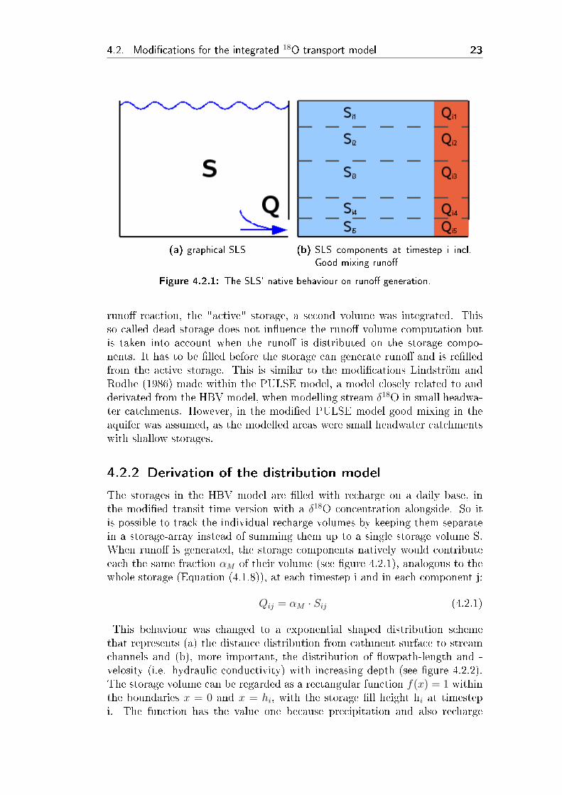
(a) graphical SLS (b) SLS components at timestep i incl.Good mixing runo�
Figure 4.2.1: The SLS' native behaviour on runo� generation.
runo� reaction, the "active" storage, a second volume was integrated. Thisso called dead storage does not in�uence the runo� volume computation butis taken into account when the runo� is distributed on the storage compo-nents. It has to be �lled before the storage can generate runo� and is re�lledfrom the active storage. This is similar to the modi�cations Lindström andRodhe (1986) made within the PULSE model, a model closely related to andderivated from the HBV model, when modelling stream δ18O in small headwa-ter catchments. However, in the modi�ed PULSE model good mixing in theaquifer was assumed, as the modelled areas were small headwater catchmentswith shallow storages.
4.2.2 Derivation of the distribution model
The storages in the HBV model are �lled with recharge on a daily base, inthe modi�ed transit time version with a δ18O concentration alongside. So itis possible to track the individual recharge volumes by keeping them separatein a storage-array instead of summing them up to a single storage volume S.When runo� is generated, the storage components natively would contributeeach the same fraction αM of their volume (see �gure 4.2.1), analogous to thewhole storage (Equation (4.1.8)), at each timestep i and in each component j:
Qij = αM · Sij (4.2.1)
This behaviour was changed to a exponential shaped distribution schemethat represents (a) the distance distribution from cathment surface to streamchannels and (b), more important, the distribution of �owpath-length and -velosity (i.e. hydraulic conductivity) with increasing depth (see �gure 4.2.2).The storage volume can be regarded as a rectangular function f(x) = 1 withinthe boundaries x = 0 and x = hi, with the storage �ll height hi at timestepi. The function has the value one because precipitation and also recharge
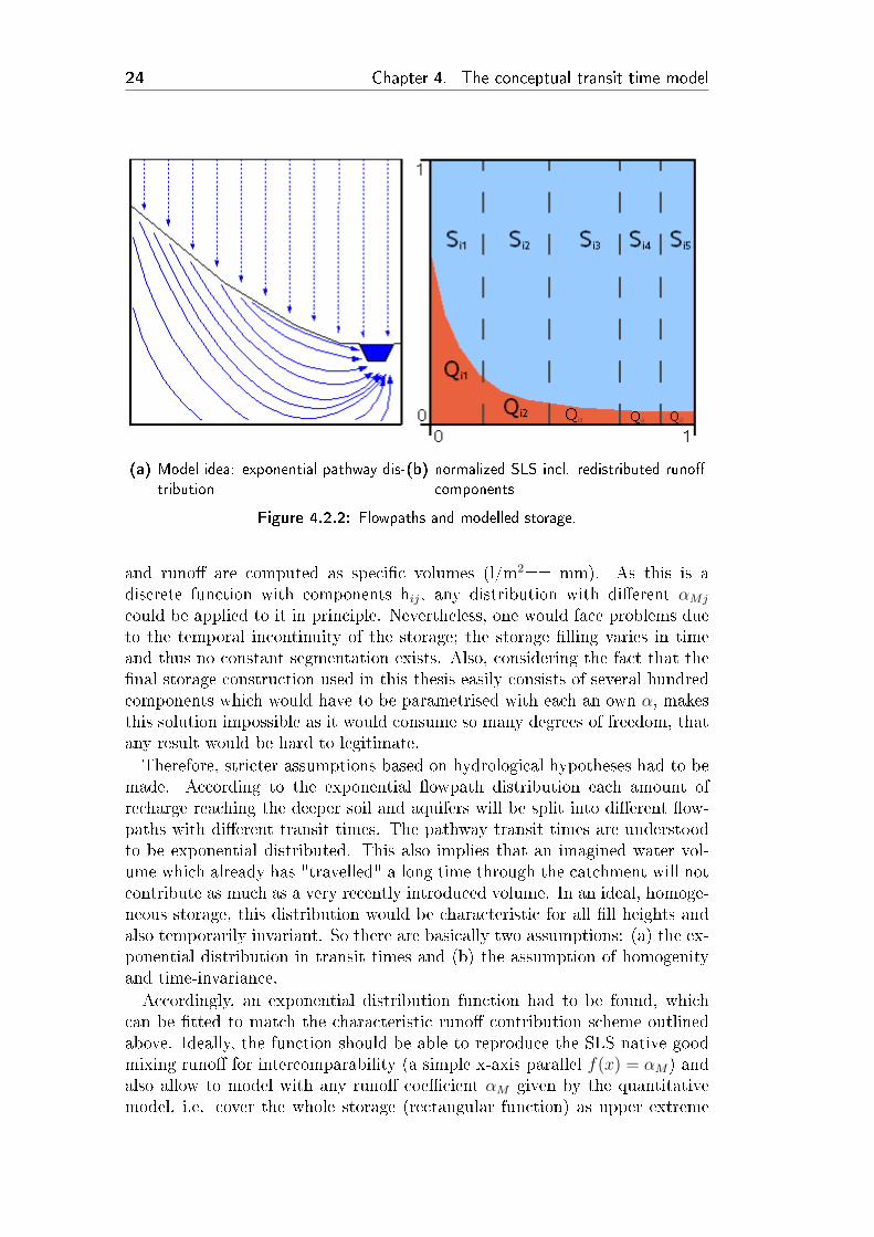
24 Chapter 4. The conceptual transit time model
(a) Model idea: exponential pathway dis-tribution
(b) normalized SLS incl. redistributed runo�components
Figure 4.2.2: Flowpaths and modelled storage.
and runo� are computed as speci�c volumes (l/m2== mm). As this is adiscrete function with components hij, any distribution with di�erent αMj
could be applied to it in principle. Nevertheless, one would face problems dueto the temporal incontinuity of the storage; the storage �lling varies in timeand thus no constant segmentation exists. Also, considering the fact that the�nal storage construction used in this thesis easily consists of several hundredcomponents which would have to be parametrised with each an own α, makesthis solution impossible as it would consume so many degrees of freedom, thatany result would be hard to legitimate.Therefore, stricter assumptions based on hydrological hypotheses had to be
made. According to the exponential �owpath distribution each amount ofrecharge reaching the deeper soil and aquifers will be split into di�erent �ow-paths with di�erent transit times. The pathway transit times are understoodto be exponential distributed. This also implies that an imagined water vol-ume which already has "travelled" a long time through the catchment will notcontribute as much as a very recently introduced volume. In an ideal, homoge-neous storage, this distribution would be characteristic for all �ll heights andalso temporarily invariant. So there are basically two assumptions: (a) the ex-ponential distribution in transit times and (b) the assumption of homogenityand time-invariance.Accordingly, an exponential distribution function had to be found, which
can be �tted to match the characteristic runo� contribution scheme outlinedabove. Ideally, the function should be able to reproduce the SLS native goodmixing runo� for intercomparability (a simple x-axis parallel f(x) = αM) andalso allow to model with any runo� coe�cient αM given by the quantitativemodel, i.e. cover the whole storage (rectangular function) as upper extreme
4.2. Modi�cations for the integrated 18O transport model 25
value(f(x) = SNORMi). This objective was achieved by normalizing the storage
volume S to a total volume of one at each time step i, by that creating arectangular function SNORM :
f(x) = SNORMi=
0 for x ≤ 01 for 0 < x ≤ 10 for x > 1
(4.2.2)
Now a function has to be found that integrates the runo� Q within the stor-age and is �ttable to di�erent distribution loadings with an emphasis on theyounger storage parts. This is indicated in Figure 4.2.2(b). With a standardexponential function:
f(x) = κ · e−βx (4.2.3)
where κ is the y-axis intercept, αM < κ ≤ 1, and β controls the curvature ofthe function, a variable and thus �ttable runo� integral can be spanned overthe normalized storage "surface". In order to do this the function has to beintegrated within the limits 0 and 1.
1∫0
κ · e−βxdx = −κ
β
[e−βx
]1
0(4.2.4)
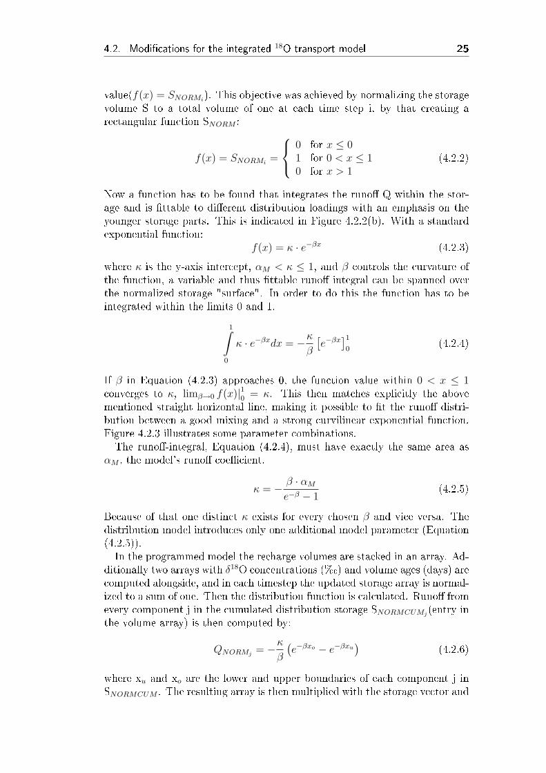
If β in Equation (4.2.3) approaches 0, the function value within 0 < x ≤ 1converges to κ, limβ→0 f(x)|10 = κ. This then matches explicitly the abovementioned straight horizontal line, making it possible to �t the runo� distri-bution between a good mixing and a strong curvilinear exponential function.Figure 4.2.3 illustrates some parameter combinations.The runo�-integral, Equation (4.2.4), must have exactly the same area as
αM , the model's runo� coe�cient.
κ = − β · αM
e−β − 1(4.2.5)
Because of that one distinct κ exists for every chosen β and vice versa. Thedistribution model introduces only one additional model parameter (Equation(4.2.5)).In the programmed model the recharge volumes are stacked in an array. Ad-
ditionally two arrays with δ18O concentrations (%�) and volume ages (days) arecomputed alongside, and in each timestep the updated storage array is normal-ized to a sum of one. Then the distribution function is calculated. Runo� fromevery component j in the cumulated distribution storage SNORMCUMj
(entry inthe volume array) is then computed by:
QNORMj= −κ
β
(e−βxo − e−βxu
)(4.2.6)
where xu and xo are the lower and upper boundaries of each component j inSNORMCUM . The resulting array is then multiplied with the storage vector and
26 Chapter 4. The conceptual transit time model
Figure 4.2.3: The distribution function for several β, green: κ = 1, red: κ = 0.6.
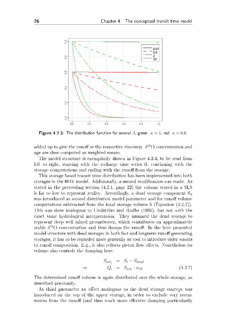
added up to give the runo� at the respective timestep. δ18O concentration andage are then computed as weighted means.The model structure is exemplarily shown in Figure 4.2.4, to be read from
left to right, starting with the recharge time series R, continuing with thestorage computations and ending with the runo� from the storage.This storage based transit time distribution has been implemented into both
storages in the HBV model. Additionally, a second modi�cation was made. Asstated in the preceeding section (4.2.1, page 22) the volume stored in a SLSis far to low to represent reality. Accordingly, a dead storage component Sd
was introduced as second distribution model parameter and for runo� volumecomputations subtracted from the total storage volume S (Equation (4.2.7)).This was done analogous to Lindström and Rodhe (1986), but not with theexact same hydrological interpretation. They assumed the dead storage torepresent deep well mixed groundwater, which contributes an approximatelystable δ18O concentration and thus damps the runo�. In the here presentedmodel structure with dead storages in both fast and longterm runo� generatingstorages, it has to be regarded more generally as tool to introduce older watersto runo� composition. E.g., it also re�ects piston �ow e�ects. Nonetheless itsvolume also controls the damping here.
Sacti = Si − Sdead
⇒ Qi = Sacti · αM (4.2.7)
The determined runo� volume is again distributed over the whole storage, asdescribed previously.As third parameter an o�set analogous to the dead storage concept was
introduced on the top of the upper storage, in order to exclude very recentwaters from the runo� (and thus reach more e�ective damping particularily
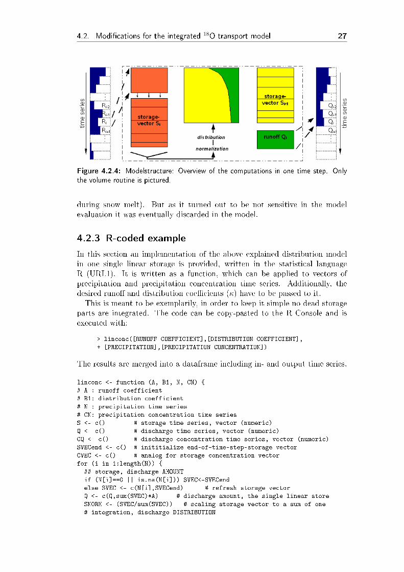
4.2. Modi�cations for the integrated 18O transport model 27
Figure 4.2.4: Modelstructure: Overview of the computations in one time step. Onlythe volume routine is pictured.
during snow melt). But as it turned out to be not sensitive in the modelevaluation it was eventually discarded in the model.
4.2.3 R-coded example
In this section an implementation of the above explained distribution modelin one single linear storage is provided, written in the statistical languageR (URL1). It is written as a function, which can be applied to vectors ofprecipitation and precipitation concentration time series. Additionally, thedesired runo� and distribution coe�cients (κ) have to be passed to it.This is meant to be exemplarily, in order to keep it simple no dead storage
parts are integrated. The code can be copy-pasted to the R Console and isexecuted with:
> linconc([RUNOFF COEFFICIENT],[DISTRIBUTION COEFFICIENT],
+ [PRECIPITATION],[PRECIPITATION CONCENTRATION])
The results are merged into a dataframe including in- and output time series.
linconc <- function (A, B1, N, CN) {
# A : runoff coefficient
# B1: distribution coefficient
# N : precipitation time series
# CN: precipitation concentration time series
S <- c() # storage time series, vector (numeric)
Q <- c() # discharge time series, vector (numeric)
CQ <- c() # discharge concentration time series, vector (numeric)
SVECend <- c() # inititialize end-of-time-step-storage vector
CVEC <- c() # analog for storage concentration vector
for (i in 1:length(N)) {
## storage, discharge AMOUNT
if (N[i]==0 || is.na(N[i])) SVEC<-SVECend
else SVEC <- c(N[i],SVECend) # refresh storage vector
Q <- c(Q,sum(SVEC)*A) # discharge amount, the single linear store
SNORM <- (SVEC/sum(SVEC)) # scaling storage vector to a sum of one
# integration, discharge DISTRIBUTION
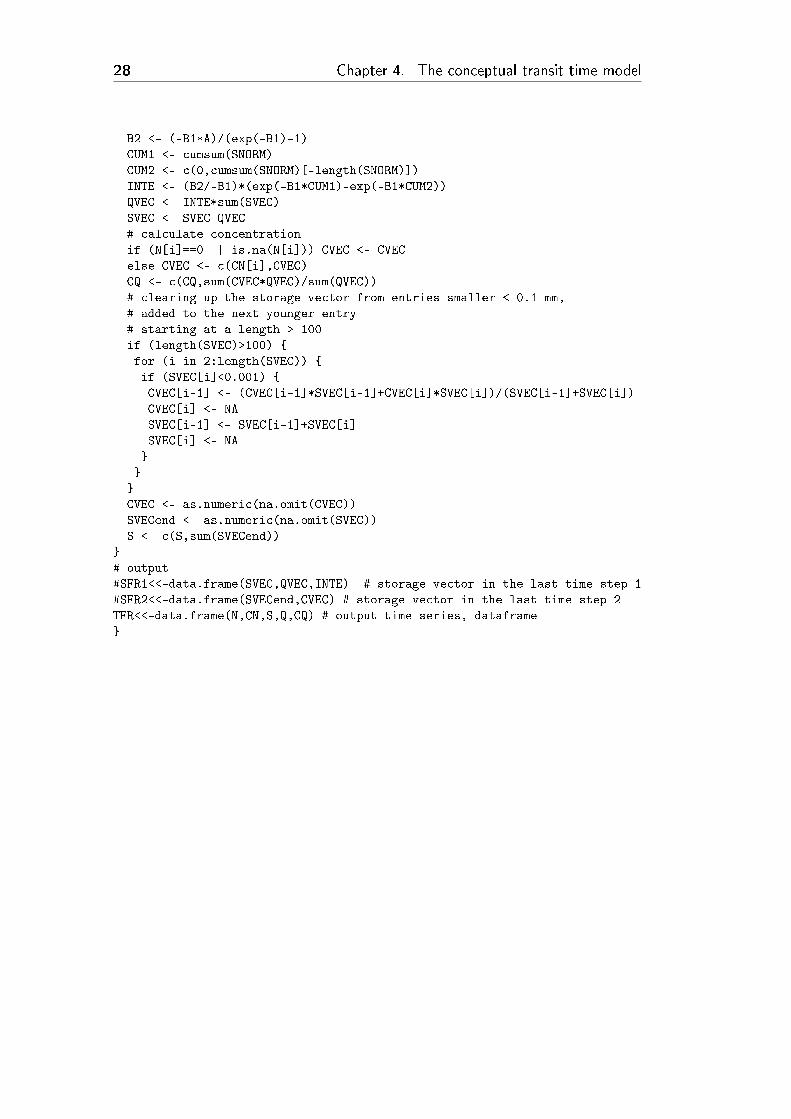
28 Chapter 4. The conceptual transit time model
B2 <- (-B1*A)/(exp(-B1)-1)
CUM1 <- cumsum(SNORM)
CUM2 <- c(0,cumsum(SNORM)[-length(SNORM)])
INTE <- (B2/-B1)*(exp(-B1*CUM1)-exp(-B1*CUM2))
QVEC <- INTE*sum(SVEC)
SVEC <- SVEC-QVEC
# calculate concentration
if (N[i]==0 || is.na(N[i])) CVEC <- CVEC
else CVEC <- c(CN[i],CVEC)
CQ <- c(CQ,sum(CVEC*QVEC)/sum(QVEC))
# clearing up the storage vector from entries smaller < 0.1 mm,
# added to the next younger entry
# starting at a length > 100
if (length(SVEC)>100) {
for (i in 2:length(SVEC)) {
if (SVEC[i]<0.001) {
CVEC[i-1] <- (CVEC[i-1]*SVEC[i-1]+CVEC[i]*SVEC[i])/(SVEC[i-1]+SVEC[i])
CVEC[i] <- NA
SVEC[i-1] <- SVEC[i-1]+SVEC[i]
SVEC[i] <- NA
}
}
}
CVEC <- as.numeric(na.omit(CVEC))
SVECend <- as.numeric(na.omit(SVEC))
S <- c(S,sum(SVECend))
}
# output
#SFR1<<-data.frame(SVEC,QVEC,INTE) # storage vector in the last time step 1
#SFR2<<-data.frame(SVECend,CVEC) # storage vector in the last time step 2
TFR<<-data.frame(N,CN,S,Q,CQ) # output time series, dataframe
}
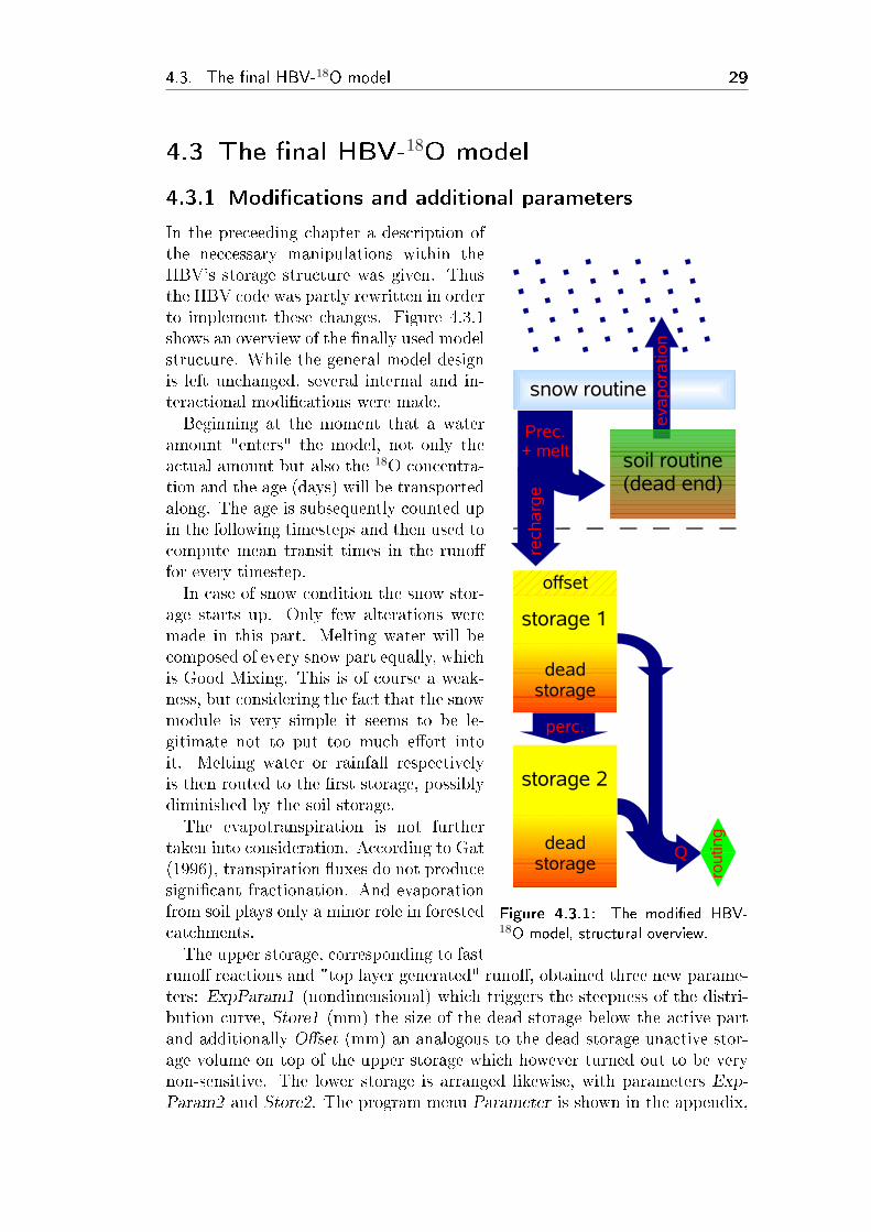
4.3. The �nal HBV-18O model 29
4.3 The �nal HBV-18O model
4.3.1 Modi�cations and additional parameters
snow routine
soil routine(dead end)
evap
orat
ion
Prec.+ melt
rech
arge
storage 1
storage 2
dead storage
dead storage
offset
perc.
Q
rout
ing
Figure 4.3.1: The modi�ed HBV-18O model, structural overview.
In the preceeding chapter a description ofthe neccessary manipulations within theHBV's storage structure was given. Thusthe HBV code was partly rewritten in orderto implement these changes. Figure 4.3.1shows an overview of the �nally used modelstructure. While the general model designis left unchanged, several internal and in-teractional modi�cations were made.Beginning at the moment that a water
amount "enters" the model, not only theactual amount but also the 18O concentra-tion and the age (days) will be transportedalong. The age is subsequently counted upin the following timesteps and then used tocompute mean transit times in the runo�for every timestep.In case of snow condition the snow stor-
age starts up. Only few alterations weremade in this part. Melting water will becomposed of every snow part equally, whichis Good Mixing. This is of course a weak-ness, but considering the fact that the snowmodule is very simple it seems to be le-gitimate not to put too much e�ort intoit. Melting water or rainfall respectivelyis then routed to the �rst storage, possiblydiminished by the soil storage.The evapotranspiration is not further
taken into consideration. According to Gat(1996), transpiration �uxes do not producesigni�cant fractionation. And evaporationfrom soil plays only a minor role in forestedcatchments.The upper storage, corresponding to fast
runo� reactions and "top layer generated" runo�, obtained three new parame-ters: ExpParam1 (nondimensional) which triggers the steepness of the distri-bution curve, Store1 (mm) the size of the dead storage below the active partand additionally O�set (mm) an analogous to the dead storage unactive stor-age volume on top of the upper storage which however turned out to be verynon-sensitive. The lower storage is arranged likewise, with parameters Exp-Param2 and Store2. The program menu Parameter is shown in the appendix,
30 Chapter 4. The conceptual transit time model
Table 4.3.1: Distribution model parameters and model behaviour, overview.
ExpParam Store
small Good Mixing runo�fast turnover, hardly any sea-sonal damping, small aquifer
largestrong exponential distribu-tion, preferably young runo�
long input memory, strong18O variation damping, bigaquifer
page 61.The percolation from the upper to the lower storage (controlled by param-
eter PERC, see section 3.1) in the form of Good Mixing percolation from allcomponents of the upper storage (dead and active) only takes place in periodswhen the upper storage contributes to runo�.The valid parameter ranges and subsequent storage behaviours are displayed
in table 4.3.1. The Store parameters range from > 0 to∞ (actually 1.8E+308,the 'double �oat' number range). It is important that they have to be non-zero,otherwise the program will crash with a runtime error. Large Store values willraise the mean age and are indicated in areas with extensive aquifers. TheExpParam parameters have the same lower limit (> 0). Their ranges arecapped upwards by the active runo� coe�cients K1 and K2. According toequation (4.2.5) in section 4.2.2 the parameters are validated and a warning"ExpParam out of range" is prompted to the user if the validation fails. WithHBV parameter names the validation formula is:
1 ≥ − ExpParam
e−ExpParam−1(4.3.1)
The closer the ExpParam values get to zero, the more the storages' runo�will resemble a Good Mixing runo�. Vice versa if ExpParam is large, thedistribution curve will be steep and preferentially young water will contributeto runo�.The timeseries input �le ptq.dat now contains two further columns cP and
cQ, that represent 18O concentrations of precipitation and runo� respectively.Precipitation concentrations currently have to be corrected as described insection 2.2.2 on page 15.Note that there must be a (interpolated) concentration available for every
precipitation volume, but not for the runo�. Empty �elds are represented by-999. The new input �le looks like this example:
Brugga Date,P,T,Q,cP,cQ
000101,8.9,0.760447836,5.455356784,-11.395,-999
000102,2.4,-0.439349054,5.175316583,-11.395,-999
000103,0,-2.088809189,4.615236181,-11.395,-999
000104,21.6,2.730869231,4.615236181,-11.395,-999
000105,4.8,2.650467103,6.013266332,-11.395,-999
4.3. The �nal HBV-18O model 31
· · ·
The simulated 18O time series is currently not plotted in the model's plotinterface. This may be updated in future versions. Instead they can be foundin the results �le resuxxx.dat as the new column cQsim.Additionally the mean transit times of runo� water is computed from the
contributing storage components. These can be found in the results �le as wellas column ageQsim.The HBV program slows down drastically with the modi�cations made, be-
cause a lot more information is transported through it (storage heights in formof �oating point values have been replaced by storage arrays with several hun-dred elements on which calculations in each timesteps are performed). Theadvised order to �t a catchment is to do the quantitative �t in the originalHBV model and subsequently take the resulting parameter set and �t thetransit time model in the modi�ed version. The distribution model has to�tted by trial and error. Note that the Warm up period, in which the modelapproaches steady state conditions can prolong drastically, depending on thevolume of the dead storages.
4.3.2 Model behaviour: arti�cial datasets
The modi�ed HBV model �nally incorporates the possibility to store reason-able amounts of water inside the model catchment and to pass storage compo-nents in an exponential-shaped distribution onto the runo� while the quanti-tative HBV routine is kept una�ected.In order to illustrate the behaviour of the model and the reaction in runo�
δ18O concentration on di�erent parametersets two arti�cial datasets were cre-ated. One showing a constant precipitation input with also constant δ18O con-centrations and one a quantitative and qualitative Dirac impulse, the secondwith constant precipitation and idealized sine-wave shaped δ18O concentrationchanges along the seasons, as found in the investigated catchment.All other input variables such as potential evapotranspiration and tempera-
ture were assumed to be homogenous, in order to focus on the behaviour of thestorages. Further model result time series on parameter variations can be foundin the following chapter 5 where model reactions on more complex catchmentsituations (the actual catchment data) are illustrated. The following sectionswill just demonstrate the general behaviour of the model.
4.3.2.1 Impulse response
In Figure 4.3.2 and 4.3.3 the model's reaction on a quantitative and qualitativeimpulse input is displayed. The upper shows variations of the Store parametersand their in�uence on the concentration in the runo� and the lower shows thein�uence of ExpParam variations respectively.Store1 and Store2 remained equally-sized with the variation in Figure 4.3.2,
but the more important part here is the lower storage as it contributes con-stantly to runo� whereas the upper only is �lled periodically. While Store was
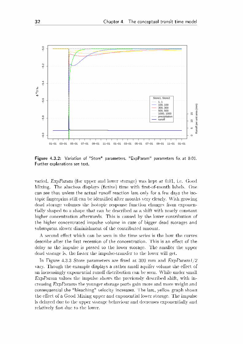
32 Chapter 4. The conceptual transit time model
δδ 18
O ‰
01−01 03−01 05−01 07−01 09−01 11−01 01−01 03−01 05−01 07−01 09−01 11−01 01−01
−6.
0−
5.8
−5.
6−
5.4
−5.
2−
5.0
05
1015
Run
off p
er u
nit a
rea
(mm
)
Store1, Store2
1, 1100, 100300, 300500, 5001000, 1000precipitationrunoff
Figure 4.3.2: Variation of "Store" parameters, "ExpParam" parameters �x at 0.01.Further explanations see text.
varied, ExpParam (for upper and lower storage) was kept at 0.01, i.e. GoodMixing. The abscissa displays (�ctive) time with �rst-of-month labels. Onecan see that unless the actual runo� reaction last only for a few days the iso-topic �ngerprint still can be identi�ed after months very clearly. With growingdead storage volumes the isotopic response function changes from exponen-tially shaped to a shape that can be described as a shift with nearly constanthigher concentration afterwards. This is caused by the lower contribution ofthe higher concentrated impulse volume in case of bigger dead storages andsubsequent slower diminishment of the contributed amount.
A second e�ect which can be seen in the time series is the bow the curvesdescribe after the �rst recession of the concentration. This is an e�ect of thedelay as the impulse is passed to the lower storage. The smaller the upperdead storage is, the faster the impulse-transfer to the lower will get.
In Figure 4.3.3 Store parameters are �xed at 300 mm and ExpParam1/2vary. Though the example displays a rather small aquifer volume the e�ect ofan increasingly exponential runo� distribution can be seen. While under smallExpParam values the impulse shows the previously described shift, with in-creasing ExpParams the younger storage parts gain more and more weight andconsequential the "bleaching" velocity increases. The last, yellow graph showsthe e�ect of a Good Mixing upper and exponential lower storage. The impulseis delayed due to the upper storage behaviour and decreases exponentially andrelatively fast due to the lower.

4.3. The �nal HBV-18O model 33
δδ 18
O ‰
01−01 03−01 05−01 07−01 09−01 11−01 01−01 03−01 05−01 07−01 09−01 11−01 01−01
−6.
0−
5.8
−5.
6−
5.4
−5.
2−
5.0
05
1015
Run
off p
er u
nit a
rea
(mm
)
ExpParam1, ExpParam2
0.01, 0.011, 15, 510, 100.01, 10precipitationrunoff
Figure 4.3.3: Variation of "ExpParam" parameters, "Store" parameters �x at 300 mm.Further explanations see text.
4.3.2.2 Sine-wave response
As an example of the model's reaction to a more realistic input time series asine-wave shaped arti�cial δ18O concentration time series was passed to themodel. The precipitation volumes however were kept constant (5 mm/day).Figure 4.3.4 and 4.3.5 show the e�ects of parameter variation analogouslyto the previous two �gures. Apparently the model is capable to reproducethe most obvious e�ect of input tranformation; the response function showsdistinct damping compared to the input function.
The increasing dead storages (with Good Mixing distribution) in Figure 4.3.4evoke an increasing damping and phase lag in the response time series.
When the distribution function is changed towards a more exponential shape(increasing ExpParam, see Figure 4.3.5), the damping is partially reversed.Additionally though, and this is not visible in the example due to the uniformsinus function, older volumes in the storage will remain longer in the storagethan with Good Mixing distributed runo� and thus in times of low runo� themodel is more likely to return a longterm mean of input concentrations (incase the overall size of the storage is su�ciently big, of course). I.e. a 2-yearsinusoidal input time series with two di�erent amplitudes will result in a morehomogenous response series amplitude when the ExpParam values are high.
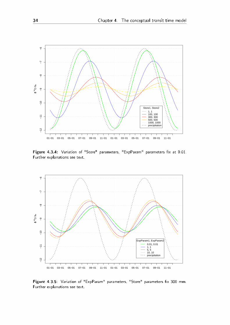
34 Chapter 4. The conceptual transit time model
δδ 18
O ‰
01−01 03−01 05−01 07−01 09−01 11−01 01−01 03−01 05−01 07−01 09−01 11−01
−12
−11
−10
−9
−8
−7
−6
Store1, Store2
1, 1100, 100300, 300500, 5001000, 1000precipitation
Figure 4.3.4: Variation of "Store" parameters, "ExpParam" parameters �x at 0.01.Further explanations see text.
δδ 18
O ‰
01−01 03−01 05−01 07−01 09−01 11−01 01−01 03−01 05−01 07−01 09−01 11−01
−12
−11
−10
−9
−8
−7
−6
ExpParam1, ExpParam2
0.01, 0.011, 15, 510, 10precipitation
Figure 4.3.5: Variation of "ExpParam" parameters, "Store" parameters �x 300 mm.Further explanations see text.
4.4. Conclusions 35
4.4 Conclusions
The HBV model had to be altered in order to be capable of computing δ18Otransport in a catchment scale. A conceptual approach to integrate a distribu-tion model into the existing model's single linear storage structure had to beformulated. This was done under consideration of pathway distribution whichwould lead to the assumption of an exponential transit time distribution inthe investigated mountainous catchments. A versatile, Good Mixing to expo-nential shaped adjustable and low parametrized (two additional parametersper storage) distribution approach was then successfully implemented into theHBV model.Other, probably important, e�ects such as snow fractionation had to be
neglected though.

36 Chapter 4. The conceptual transit time model
37
5 HBV-18O: Results &
discussion
5.1 Brugga
The Brugga section comprises the major part of this Chapter. It includes, be-sides the results of the model application in the catchment, a couple of �gureswith parameter variations in order to show the model behaviour and parametersensitivity under realistic conditions as well as a description of necessary inputtime series preparations. Speci�c attention will then be paid to the develop-ment of stream water transit times, especially during drought conditions andan interpretation of the underlying hydrological processes.
5.1.1 Time series description and runo� simulation
Figure 5.1.1 gives an overview over the input time series of δ18O concentrationin precipition and runo� as well as speci�c runo� and precipitation amounts(indicated by point sizes of precipitation-δ18O). The runo� responds fast andvolatile to precipitation events, as well in winter- and springtime with generallyhigher runo� as during mid�ow conditions. The δ18O concentration in precipi-tation shows a strong seasonal variation with an approximate mean amplitudeof 15 %�.Despite the runo�'s volatility and the strong variability in δ18O input, the
δ18O concentration in runo� varies little, especially not signi�cantly duringstorm runo� when a high contribution of event water would be expected. Itrather seems to be constant compared to precipitation. However although theδ18O response is strongly damped and also lagged it still shows a signi�cantseasonal variation with a nonetheless a lot smaller amplitude than δ18O inprecipitation (see also the �gures in chapter 6).The heaviest precipitation in the investigated period was measured during
the extraordinarily hot and dry summer saison 2003. Remarkably, this is alsoa period with a distinct trend in runo� δ18O (towards a higher concentration).The �rst modelling step was to �t the quantitative model in order to create
the transit time model "environment" as described in the previous chapter.The simulated runo�, along with measured precipitation and runo�, can beseen in Figure 5.1.2. The appendant Reff is 0.81. Overall, the simulatedvalues �t the measured ones quite well, although not every runo� peak iscovered perfectly and especially in phases when runo� declines the simulatedvalues seem to overestimate runo� a little bit. But under consideration of e.g.
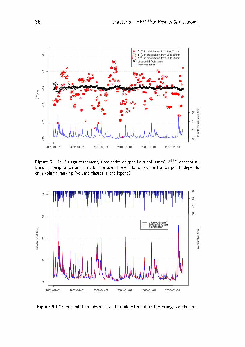
38 Chapter 5. HBV-18O: Results & discussion
●
●●
●
●
●
●●
●
●●●●
●●●●●●●●●
●●●●●●
●●●●●●
●
●●●●●●●
●●●●●●
●●●●●●●●
●●●●●●●●●●●●●●
●●●
●●●●●●●●
●●●●●●●●●●●
●●●●●●
●●●●●●●●●●●●●●
●●●●
●●●●●●●
●●●●●●●●●●●●●●
●●●●
●●●●●●
●●●●●
●●●●●●●●●●
●●●●●●
●●●●●●●●●
●●
●
●●●●
●
●●●●●●●●●●
●
●●●●●●●●
●●●●●
●●●●●●●●●●
●●●●●●●●●●
●●●●
●
●
●●●●●●●●●●
●●●●●●●
●●●●●●●●●●●●●●●●●●●
●●●●●●●
●●●●
δδ 18
O ‰
●●●●
●●●●●●●●●●●●●●●●
●●●●
●●●●●●●●●●●●●
●●●●●●
●●●●●
●●●●
●●●●
●●●●●
●●●●●●●
●●●●
●●●●●●●
●●●
●●●●●●
●●●●●
●●●●●●●
●●●●●●●
●●●
●●●
●●●●
●●●●●●●●●●●●●●●●●●●●●●●●●
●●●●●
●●
●●●●
●●●●●
●●●●●●
●●●●●
●●●●●●●●●
●●●●●●●●
●●●●●●●●●●●●●●●●
●●●●
●●●●●●●
●●●●●
●●●●●●●●●●●●●●●●●●●●●●●●●●●●●●●●●●●●●●●●●●●●●
●●●●●●●●●●●●●
●●●●●
●●●●
●●●●●●●
●●●●●●●●●●●●●●●●●●●●●
●●●●●●●●●●●●●●●●●●
●●●●●
●●●●
●●●●
●●●●●●●●
●
●●●●●●
●●●●
●●●●●●
●●
●●●●●●
●●●●●●●●●●●●●●●
●●●●●●
●●●●
●●●
●●●●●●●●●
●●●●●●●●●●●●●●●●●●●
●●●
●●●●●●●●●●●●●●
●●●●●
●●●●
●●●
●●●●●●●
●●●
●●●●●●●
●●●●●●●
●●●
●●●
●●●●●●●●●●●●
●●●●
●●●●
●●●●●●●●●●●●●●●●●●●●●●●●●
●●●
●●●●●●●●●●
●●●●●●●●●●●
●●●●●●●●●●
●●●●●
●●●●●●●●●●
●●●●●●●●●●
●●●●
●●●●●
●●●●●●●●●●●●
●●●●●
●●
●●●●●●●●●●●●●●●●●●●
●●●●●●
●●●●●●●●
●●●●●●●
●●●●●●●●●●
●●●●●●●●●●●●●●●●●●
●●●●●●
●●●●●●●
●●●●●●
●●●●●●
●●●●●●●
●
●●●●●●
●●●●●●●●●●●●●
●●●
●●●●●●●
●●●●●●●
●●●●●
●●●●
●●●●●●
●●●
●
●●●●
●●●●●●●●●●●
●●●●●
●●
●●●●●●
●●●●●●●●●●
●●●●●●
●●●●●●●
●●●●
●●●●●●●●
●
●●●●●●●●
●●●●●
●●●●●
●
●●●●●●●●●●●
●●●●●●
●●●●●●
●●●●●●●
●●●●●●●●
●●●●●
●●●●●●
●●
●●●●●●
●●●●●●
●●●●●●●●●●●●●●●●●●●●●●●●●●●●●●●
●●●●●●
●●●●●●●●●●●●●●●●●
●●●●●●●●●●●●●●●●●●●●●●●●●●●●●●●
●●●●●●●●●●●●
●●●●●●●●●
●
●●●●
●●●●
●●●●
●●●●●
●●●●●●
●●●●●●
●●●●●●●
●●●●●●●●●
●●●
●●●●●●●
●●●●●
●●●●●●●●●●●●●●
●●●●
●●●
●●●●●●●
●●●●●●●●●●●●●●●●
●●●●●●●●●●●●●●●●●●●●●●●●●●●●●●●●●●●●●●●●
●
●●●●●
●●●●●●●●●●●●●●●●●●●●●●●●●●●●●●●●●●●●●●●●●●●●●●●●●●●●●●●●●●●●●●●●●●●●●●●●●●●●●●●●●
●●●●
●●●●●
●●●●●
●●●
●●●●●●●
●●●●●●
●●●●
●●●●
●●●
●●
●
●●
●
●
●
●●
●
●●●●
●●●●●●●●●
●●●●●●
●●●●●●
●
●●●●●●●
●●●●●●
●●●●●●●●
●●●●●●●●●●●●●●
●●●
●●●●●●●●
●●●●●●●●●●●
●●●●●●
●●●●●●●●●●●●●●
●●●●
●●●●●●●
●●●●●●●●●●●●●●
●●●●
●●●●●●
●●●●●
●●●●●●●●●●
●●●●●●
●●●●●●●●●
●●
●
●●●●
●
●●●●●●●●●●
●
●●●●●●●●
●●●●●
●●●●●●●●●●
●●●●●●●●●●
●●●●
●
●
●●●●●●●●●●
●●●●●●●
●●●●●●●●●●●●●●●●●●●
●●●●●●●
●●●●
2001−01−01 2002−01−01 2003−01−01 2004−01−01 2005−01−01 2006−01−01
−25
−20
−15
−10
−5
0
010
2030
Run
off p
er u
nit a
rea
(mm
)
●
●●
●
δδ 18O in precipitation, from 1 to 25 mmδδ 18O in precipitation, from 26 to 50 mmδδ 18O in precipitation, from 51 to 75 mm
observed δδ 18Oin runoff observed runoff
Figure 5.1.1: Brugga catchment, time series of speci�c runo� (mm), δ18O concentra-tions in precipitation and runo�. The size of precipitation concentration points dependson a volume ranking (volume classes in the legend).
spec
ific
runo
ff (m
m)
2001−01−01 2002−01−01 2003−01−01 2004−01−01 2005−01−01 2006−01−01
010
2030
40
6040
200
prec
ipita
tion
(mm
)
observed runoffsimulated runoffprecipitation
Figure 5.1.2: Precipitation, observed and simulated runo� in the Brugga catchment.
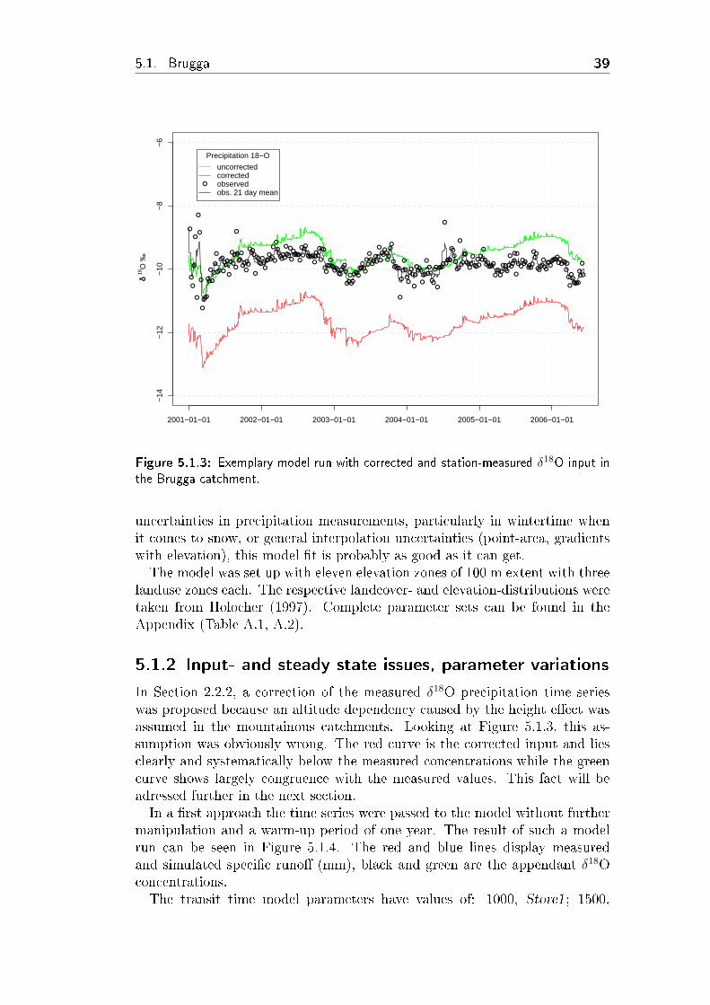
5.1. Brugga 39
δδ 18
O ‰
●
●
●
●
●
●
●
●
●
●
●●●
●●
●
●
●
●
●
●●
●●
●
●●●
●
●
●
●
●
●
●
●
●●
●
●●
●
●●
●●●●
●
●●●●
●●●
●●●●●
●
●
●
●●●●
●●
●
●●
●
●
●●●●●
●
●
●
●●
●●●●●
●●●●
●
●
●●
●●
●●
●
●●●●●
●●●●●
●
●●
●
●●
●●●●
●●●●●
●●
●
●●●●●●
●
●
●●●●
●●
●●
●●●●●
●
●
●
●
●
●●
●●●
●
●
●●●●
●
●●
●
●
●
●
●●
●●
●
●●●●
●
●●●●
●●●
●
●●
●
●●
●●
●●●●
●
●●
●●
●●
●
●●●●●●
●
●●●
●●
●●●●
●
●
●●●
●
●
●
●●
●●●
●●●●
●●●
●●●●
●
●●
●●●●●●●
●●●●●●
●
●
●
●
●●●●●●
●●
●
●
2001−01−01 2002−01−01 2003−01−01 2004−01−01 2005−01−01 2006−01−01
−14
−12
−10
−8
−6
●
Precipitation 18−O
uncorrectedcorrectedobservedobs. 21 day mean
Figure 5.1.3: Exemplary model run with corrected and station-measured δ18O input inthe Brugga catchment.
uncertainties in precipitation measurements, particularly in wintertime whenit comes to snow, or general interpolation uncertainties (point-area, gradientswith elevation), this model �t is probably as good as it can get.The model was set up with eleven elevation zones of 100 m extent with three
landuse zones each. The respective landcover- and elevation-distributions weretaken from Holocher (1997). Complete parameter sets can be found in theAppendix (Table A.1, A.2).
5.1.2 Input- and steady state issues, parameter variations
In Section 2.2.2, a correction of the measured δ18O precipitation time serieswas proposed because an altitude dependency caused by the height e�ect wasassumed in the mountainous catchments. Looking at Figure 5.1.3, this as-sumption was obviously wrong. The red curve is the corrected input and liesclearly and systematically below the measured concentrations while the greencurve shows largely congruence with the measured values. This fact will beadressed further in the next section.In a �rst approach the time series were passed to the model without further
manipulation and a warm-up period of one year. The result of such a modelrun can be seen in Figure 5.1.4. The red and blue lines display measuredand simulated speci�c runo� (mm), black and green are the appendant δ18Oconcentrations.The transit time model parameters have values of: 1000, Store1; 1500,
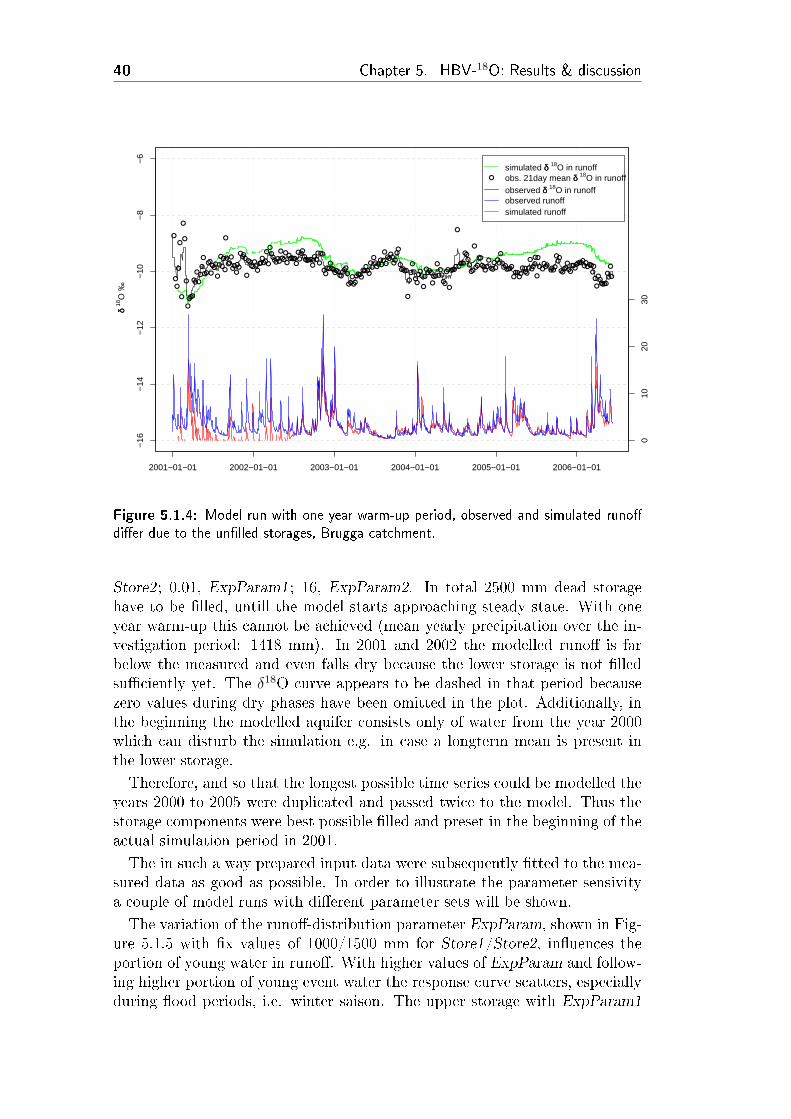
40 Chapter 5. HBV-18O: Results & discussion
δδ 18
O ‰
●
●
●
●
●
●
●
●
●
●
●●●
●●
●
●
●
●
●
●●
●●
●
●●●
●
●
●
●
●
●
●
●●●●
●●
●
●●
●●●●
●
●●●●
●●●
●●●●●
●
●
●●●●●
●●
●
●●
●
●
●●●●●
●
●
●●●
●●●●●
●●●●
●
●
●●
●●●●
●●●
●●●●●●●
●●
●●●
●●
●●●●
●●●●●
●●
●●●●
●●●
●
●
●●●●●●
●●
●●●●●
●
●
●
●
●
●●
●●●
●
●
●●●●
●
●●
●
●●●
●●
●●
●
●●●●
●
●●●●
●●●●
●●
●
●●
●●
●●●●
●
●●
●●
●●
●
●●●●●●●
●●●
●●●●
●●●
●
●●●
●
●
●
●●●●●
●●●●
●●●
●●●●
●●●
●●●●●●●
●●●●●●
●●
●
●
●●●●●●
●●
●
●
2001−01−01 2002−01−01 2003−01−01 2004−01−01 2005−01−01 2006−01−01
−16
−14
−12
−10
−8
−6
010
2030
●
simulated δδ 18O in runoffobs. 21day mean δδ 18O in runoffobserved δδ 18O in runoffobserved runoffsimulated runoff
Figure 5.1.4: Model run with one year warm-up period, observed and simulated runo�di�er due to the un�lled storages, Brugga catchment.
Store2; 0.01, ExpParam1; 16, ExpParam2. In total 2500 mm dead storagehave to be �lled, untill the model starts approaching steady state. With oneyear warm-up this cannot be achieved (mean yearly precipitation over the in-vestigation period: 1418 mm). In 2001 and 2002 the modelled runo� is farbelow the measured and even falls dry because the lower storage is not �lledsu�ciently yet. The δ18O curve appears to be dashed in that period becausezero values during dry phases have been omitted in the plot. Additionally, inthe beginning the modelled aquifer consists only of water from the year 2000which can disturb the simulation e.g. in case a longterm mean is present inthe lower storage.
Therefore, and so that the longest possible time series could be modelled theyears 2000 to 2005 were duplicated and passed twice to the model. Thus thestorage components were best possible �lled and preset in the beginning of theactual simulation period in 2001.
The in such a way prepared input data were subsequently �tted to the mea-sured data as good as possible. In order to illustrate the parameter sensivitya couple of model runs with di�erent parameter sets will be shown.
The variation of the runo�-distribution parameter ExpParam, shown in Fig-ure 5.1.5 with �x values of 1000/1500 mm for Store1/Store2, in�uences theportion of young water in runo�. With higher values of ExpParam and follow-ing higher portion of young event water the response curve scatters, especiallyduring �ood periods, i.e. winter saison. The upper storage with ExpParam1
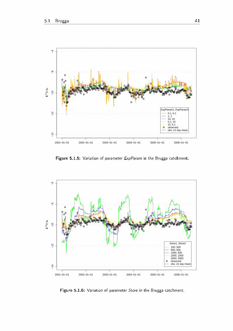
5.1. Brugga 41
δδ 18
O ‰
●
●
●
●
●
●
●
●
●
●
●●●
●●
●
●
●
●
●
●●
●●
●
●●●
●
●
●
●
●
●
●
●
●●
●
●●
●
●●
●●●●
●
●●●●
●●●
●●●●●
●
●
●
●●●●
●●
●
●●
●
●
●●●●●
●
●
●
●●
●●●●●
●●●●
●
●
●●
●●
●●
●
●●●●●
●●●●●
●
●●
●
●●
●●●●
●●●●●
●●
●
●●●●●●
●
●
●●●●
●●
●●
●●●●●
●
●
●
●
●
●●
●●●
●
●
●●●●
●
●●
●
●
●
●
●●
●●
●
●●●●
●
●●●●
●●●
●
●●
●
●●
●●
●●●●
●
●●
●●
●●
●
●●●●●●
●
●●●
●●
●●●●
●
●
●●●
●
●
●
●●
●●●
●●●●
●●●
●●●●
●
●●
●●●●●●●
●●●●●●
●
●
●
●
●●●●●●
●●
●
●
2001−01−01 2002−01−01 2003−01−01 2004−01−01 2005−01−01 2006−01−01
−14
−12
−10
−8
−6
●
ExpParam1, ExpParam2
0.1, 0.11, 110, 100.1, 1010, 0.1observedobs. 21 day mean
Figure 5.1.5: Variation of parameter ExpParam in the Brugga catchment.
δδ 18
O ‰
●
●
●
●
●
●
●
●
●
●
●●●
●●
●
●
●
●
●
●●
●●
●
●●●
●
●
●
●
●
●
●
●
●●
●
●●
●
●●
●●●●
●
●●●●
●●●
●●●●●
●
●
●
●●●●
●●
●
●●
●
●
●●●●●
●
●
●
●●
●●●●●
●●●●
●
●
●●
●●
●●
●
●●●●●
●●●●●
●
●●
●
●●
●●●●
●●●●●
●●
●
●●●●●●
●
●
●●●●
●●
●●
●●●●●
●
●
●
●
●
●●
●●●
●
●
●●●●
●
●●
●
●
●
●
●●
●●
●
●●●●
●
●●●●
●●●
●
●●
●
●●
●●
●●●●
●
●●
●●
●●
●
●●●●●●
●
●●●
●●
●●●●
●
●
●●●
●
●
●
●●
●●●
●●●●
●●●
●●●●
●
●●
●●●●●●●
●●●●●●
●
●
●
●
●●●●●●
●●
●
●
2001−01−01 2002−01−01 2003−01−01 2004−01−01 2005−01−01 2006−01−01
−14
−12
−10
−8
−6
●
Store1, Store2
100, 500500, 5001000, 5001000, 15002000, 3000observedobs. 21 day mean
Figure 5.1.6: Variation of parameter Store in the Brugga catchment.
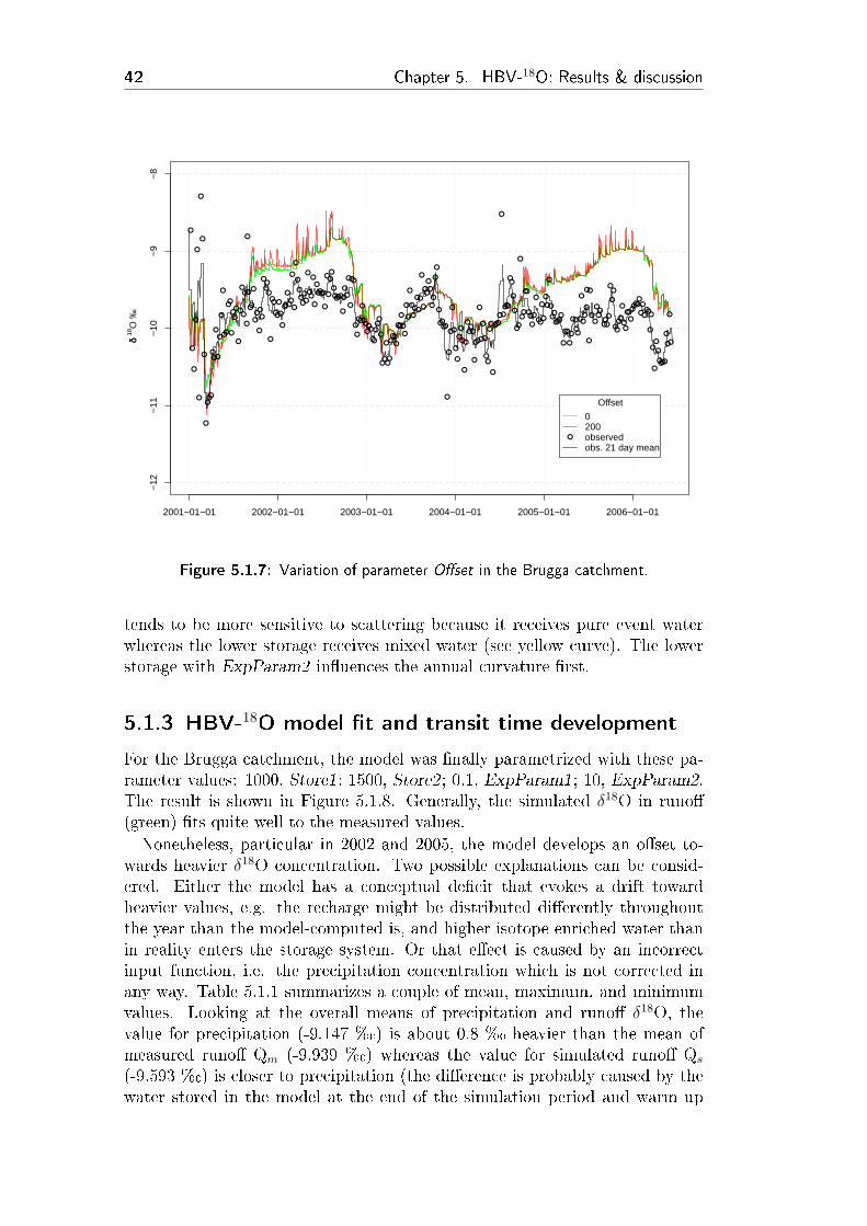
42 Chapter 5. HBV-18O: Results & discussion
δδ 18
O ‰
●
●
●
●
●
●
●
●
●
●
●●●
●●
●
●
●
●
●
●●
●●
●
●●
●
●
●
●
●
●
●
●
●
●●
●
●●
●
●●
●
●●
●
●
●●
●●
●
●
●
●●
●
●●
●
●
●
●
●
●●
●●
●
●●
●
●
●
●●●●
●
●
●
●●
●
●●●●
●
●
●●
●
●
●●
●
●
●●
●
●●
●●●
●●
●●●
●
●●
●
●●
●●●
●
●●
●
●
●
●
●
●
●
●●
●
●
●
●
●
●●
●
●
●
●
●
●
●
●●●●
●
●
●
●
●
●
●
●
●
●
●
●
●
●●●
●
●●
●
●
●
●
●●
●●
●
●●●
●
●
●
●●●
●●
●
●
●●
●
●●
●●
●●
●
●
●
●●
●
●
●
●
●
●
●●
●●●●
●
●●
●
●
●●
●●
●
●
●●
●
●
●
●
●●
●
●●
●●●
●
●
●
●
●●
●●
●
●●
●●●
●●●●
●
●
●
●●●
●
●
●
●
●
●
●●●●
●
●
●
●
2001−01−01 2002−01−01 2003−01−01 2004−01−01 2005−01−01 2006−01−01
−12
−11
−10
−9
−8
●
Offset
0200observedobs. 21 day mean
Figure 5.1.7: Variation of parameter O�set in the Brugga catchment.
tends to be more sensitive to scattering because it receives pure event waterwhereas the lower storage receives mixed water (see yellow curve). The lowerstorage with ExpParam2 in�uences the annual curvature �rst.
5.1.3 HBV-18O model �t and transit time development
For the Brugga catchment, the model was �nally parametrized with these pa-rameter values: 1000, Store1; 1500, Store2; 0.1, ExpParam1; 10, ExpParam2.The result is shown in Figure 5.1.8. Generally, the simulated δ18O in runo�(green) �ts quite well to the measured values.Nonetheless, particular in 2002 and 2005, the model develops an o�set to-
wards heavier δ18O concentration. Two possible explanations can be consid-ered. Either the model has a conceptual de�cit that evokes a drift towardheavier values, e.g. the recharge might be distributed di�erently throughoutthe year than the model-computed is, and higher isotope enriched water thanin reality enters the storage system. Or that e�ect is caused by an incorrectinput function, i.e. the precipitation concentration which is not corrected inany way. Table 5.1.1 summarizes a couple of mean, maximum, and minimumvalues. Looking at the overall means of precipitation and runo� δ18O, thevalue for precipitation (-9.147 %�) is about 0.8 %� heavier than the mean ofmeasured runo� Qm (-9.939 %�) whereas the value for simulated runo� Qs
(-9.593 %�) is closer to precipitation (the di�erence is probably caused by thewater stored in the model at the end of the simulation period and warm up
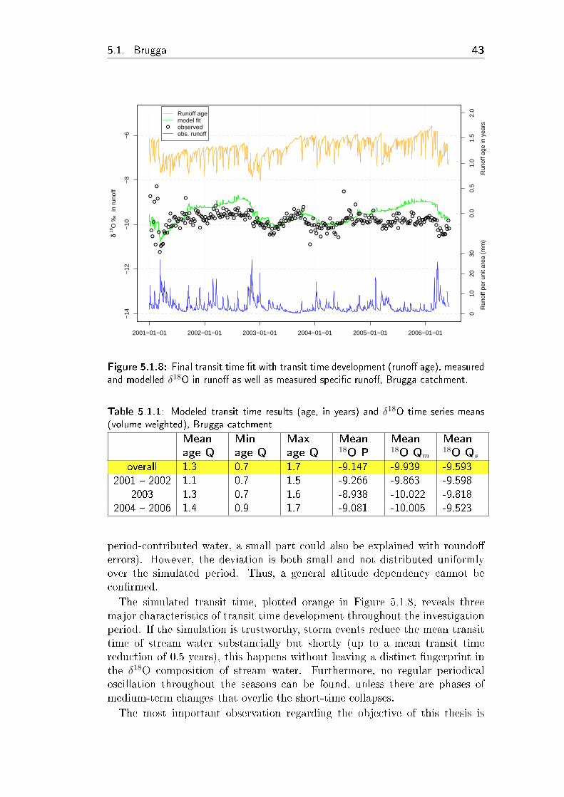
5.1. Brugga 43
δδ 18
O ‰
in
run
off
●
●
●
●
●
●
●
●
●
●
●●●
●●
●
●
●
●
●
●●
●●
●
●●●
●
●
●
●
●
●
●
●●●
●
●●
●
●●
●●●●
●
●●●●
●●●
●●●●●
●
●
●
●●●●●●
●
●●
●
●
●●●●●
●
●
●●●
●●●●●
●●●●
●
●
●●
●●●●
●●●●●●
●●●●●●
●●
●
●●
●●●●
●●●●●
●●
●●●●●●●
●
●
●●●●
●●
●●
●●●●●
●
●
●
●
●
●●
●●●
●
●
●●●●
●
●●
●
●●●
●●
●●
●
●●●●
●
●●●●
●●●●
●●
●
●●
●●
●●●●
●
●●
●●
●●
●
●●●●●●
●
●●●
●●●●
●●●
●
●●●
●
●
●
●●●●●
●●●●
●●●
●●●●●
●●
●●●●●●●
●●●●●●
●●
●
●
●●●●●●
●●
●
●
2001−01−01 2002−01−01 2003−01−01 2004−01−01 2005−01−01 2006−01−01
−14
−12
−10
−8
−6
0.0
0.5
1.0
1.5
2.0
Run
off a
ge in
yea
rs
010
2030
Run
off p
er u
nit a
rea
(mm
)
●
Runoff agemodel fitobserved obs. runoff
Figure 5.1.8: Final transit time �t with transit time development (runo� age), measuredand modelled δ18O in runo� as well as measured speci�c runo�, Brugga catchment.
Table 5.1.1: Modeled transit time results (age, in years) and δ18O time series means(volume weighted), Brugga catchment
Meanage Q
Minage Q
Maxage Q
Mean18O P
Mean18O Qm
Mean18O Qs
overall 1.3 0.7 1.7 -9.147 -9.939 -9.5932001 � 2002 1.1 0.7 1.5 -9.266 -9.863 -9.598
2003 1.3 0.7 1.6 -8.938 -10.022 -9.8182004 � 2006 1.4 0.9 1.7 -9.081 -10.005 -9.523
period-contributed water, a small part could also be explained with roundo�errors). However, the deviation is both small and not distributed uniformlyover the simulated period. Thus, a general altitude dependency cannot becon�rmed.The simulated transit time, plotted orange in Figure 5.1.8, reveals three
major characteristics of transit time development throughout the investigationperiod. If the simulation is trustworthy, storm events reduce the mean transittime of stream water substancially but shortly (up to a mean transit timereduction of 0.5 years), this happens without leaving a distinct �ngerprint inthe δ18O composition of stream water. Furthermore, no regular periodicaloscillation throughout the seasons can be found, unless there are phases ofmedium-term changes that overlie the short-time collapses.The most important observation regarding the objective of this thesis is
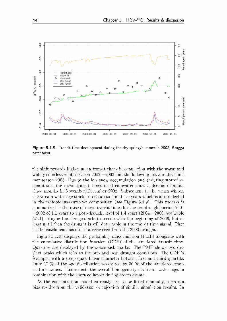
44 Chapter 5. HBV-18O: Results & discussion
δδ 18
O ‰
in
run
off
●
● ●
●
●
●
●
●
●
●
●
●
●
●
●
●
●
●●
●
●
●
●
●
●
●
●
2003−05−01 2003−06−01 2003−07−01 2003−08−01 2003−09−01 2003−10−01 2003−11−01
−11
.0−
10.5
−10
.0−
9.5
−9.
0−
8.5
−8.
0
0.0
0.5
1.0
1.5
2.0
Run
off a
ge in
yea
rs
05
10
Run
off p
er u
nit a
rea
(mm
)
●
Runoff agemodel fitobserved obs. runoffsim. runoff
Figure 5.1.9: Transit time development during the dry spring/summer in 2003, Bruggacatchment.
the shift towards higher mean transit times in connection with the warm andwidely snowless winter season 2002 � 2003 and the following hot and dry sum-mer season 2003. Due to the low snow accumulation and enduring storm�owconditions, the mean transit times in streamwater show a decline of aboutthree months in November/December 2002. Subsequent to the warm winter,the stream water age starts to rise up to about 1.5 years which is also re�ectedin the isotopic streamwater composition (see Figure 5.1.9). This process issummarized in the raise of mean transit times for the pre-drought period 2001� 2002 of 1.1 years to a post-drought level of 1.4 years (2004 � 2006, see Table5.1.1). Maybe the change starts to recede with the beginning of 2006, but atleast until then the drought is still detectable in the transit time signal. Thatis, the catchment has still not recovered from the 2003 drought.
Figure 5.1.10 displays the probability mass function (PMF) alongside withthe cumulative distribution function (CDF) of the simulated transit time.Quartiles are displayed by the x-axis tick marks. The PMF shows two dis-tinct peaks which refer to the pre- and post drought conditions. The CDF isS-shaped with a steep quasi-linear character between �rst and third quartile.Only 17 % of the age distribution is covered by 50 % of the simulated tran-sit time values. This re�ects the overall homogeneity of stream water ages incombination with the short collapses during storm events.
As the concentration model currently has to be �tted manually, a certainbias results from the validation or rejection of similar simulation results. In
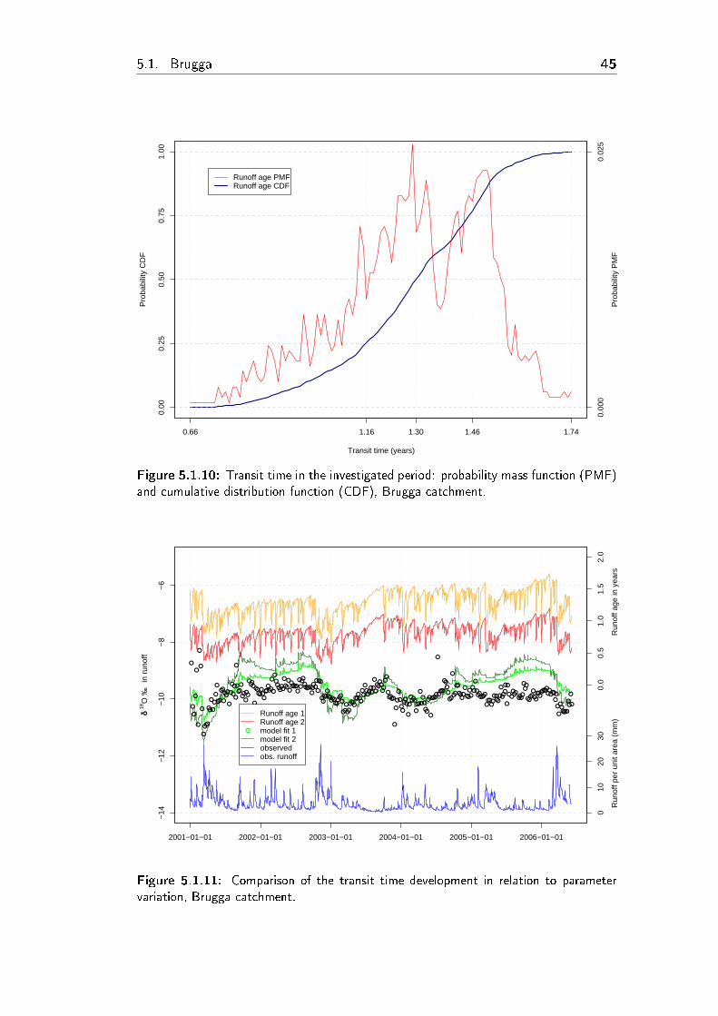
5.1. Brugga 45
Transit time (years)
Pro
babi
lity
CD
F
0.66 1.16 1.30 1.46 1.74
0.00
0.25
0.50
0.75
1.00
0.00
00.
025
Pro
babi
lity
PM
F
Runoff age PMFRunoff age CDF
Figure 5.1.10: Transit time in the investigated period: probability mass function (PMF)and cumulative distribution function (CDF), Brugga catchment.
δδ 18
O ‰
in
run
off
●
●
●
●
●
●
●
●
●
●
●●●
●●
●
●
●
●
●
●●
●●
●
●●●
●
●
●
●
●
●
●
●●●
●
●●
●
●●
●●●●
●
●●●●
●●●
●●●●●
●
●
●
●●●●●●
●
●●
●
●
●●●●●
●
●
●●●
●●●●●
●●●●
●
●
●●
●●●●
●●●●●●
●●●●●●
●●
●
●●
●●●●
●●●●●
●●
●●●●●●●
●
●
●●●●
●●
●●
●●●●●
●
●
●
●
●
●●
●●●
●
●
●●●●
●
●●
●
●●●
●●
●●
●
●●●●
●
●●●●
●●●●
●●
●
●●
●●
●●●●
●
●●
●●
●●
●
●●●●●●
●
●●●
●●●●
●●●
●
●●●
●
●
●
●●●●●
●●●●
●●●
●●●●●
●●
●●●●●●●
●●●●●●
●●
●
●
●●●●●●
●●
●
●
2001−01−01 2002−01−01 2003−01−01 2004−01−01 2005−01−01 2006−01−01
−14
−12
−10
−8
−6
0.0
0.5
1.0
1.5
2.0
Run
off a
ge in
yea
rs
010
2030
Run
off p
er u
nit a
rea
(mm
)
●
Runoff age 1Runoff age 2model fit 1model fit 2observed obs. runoff
Figure 5.1.11: Comparison of the transit time development in relation to parametervariation, Brugga catchment.
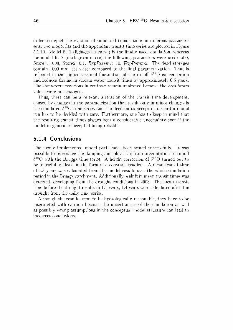
46 Chapter 5. HBV-18O: Results & discussion
order to depict the reaction of simulated transit time on di�erent parametersets, two model �ts and the appendant transit time series are plotted in Figure5.1.10. Model �t 1 (light-green curve) is the �nally used simulation, whereasfor model �t 2 (dark-green curve) the following parameters were used: 500,Store1; 1000, Store2; 0.1, ExpParam1; 10, ExpParam2. The dead storagescontain 1000 mm less water compared to the �nal parametrization. That isre�ected in the higher seasonal �uctuation of the runo� δ18O concentrationand reduces the mean stream water transit times by approximately 0.5 years.The short-term reactions in contrast remain unaltered because the ExpParamvalues were not changed.Thus, there can be a relevant alteration of the transit time development,
caused by changes in the parametrization that result only in minor changes isthe simulated δ18O time series and the decision to accept or discard a modelrun has to be decided with care. Furthermore, one has to keep in mind thatthe resulting transit times always bear a considerable uncertainty even if themodel in general is accepted being reliable.
5.1.4 Conclusions
The newly implemented model parts have been tested successfully. It waspossible to reproduce the damping and phase lag from precipitation to runo�δ18O with the Brugga time series. A height correction of δ18O turned out tobe unuseful, at least in the form of a constant gradient. A mean transit timeof 1.3 years was calculated from the model results over the whole simulationperiod in the Brugga catchment. Additionally, a shift in mean transit times wasdetected, developing from the drought conditions in 2003. The mean transittime before the drought results in 1.1 years, 1.4 years were calculated after thedrought from the daily time series.Although the results seem to be hydrologically reasonable, they have to be
interpreted with caution because the uncertainties of the simulation as wellas possibly wrong assumptions in the conceptual model structure can lead toincorrect conclusions.
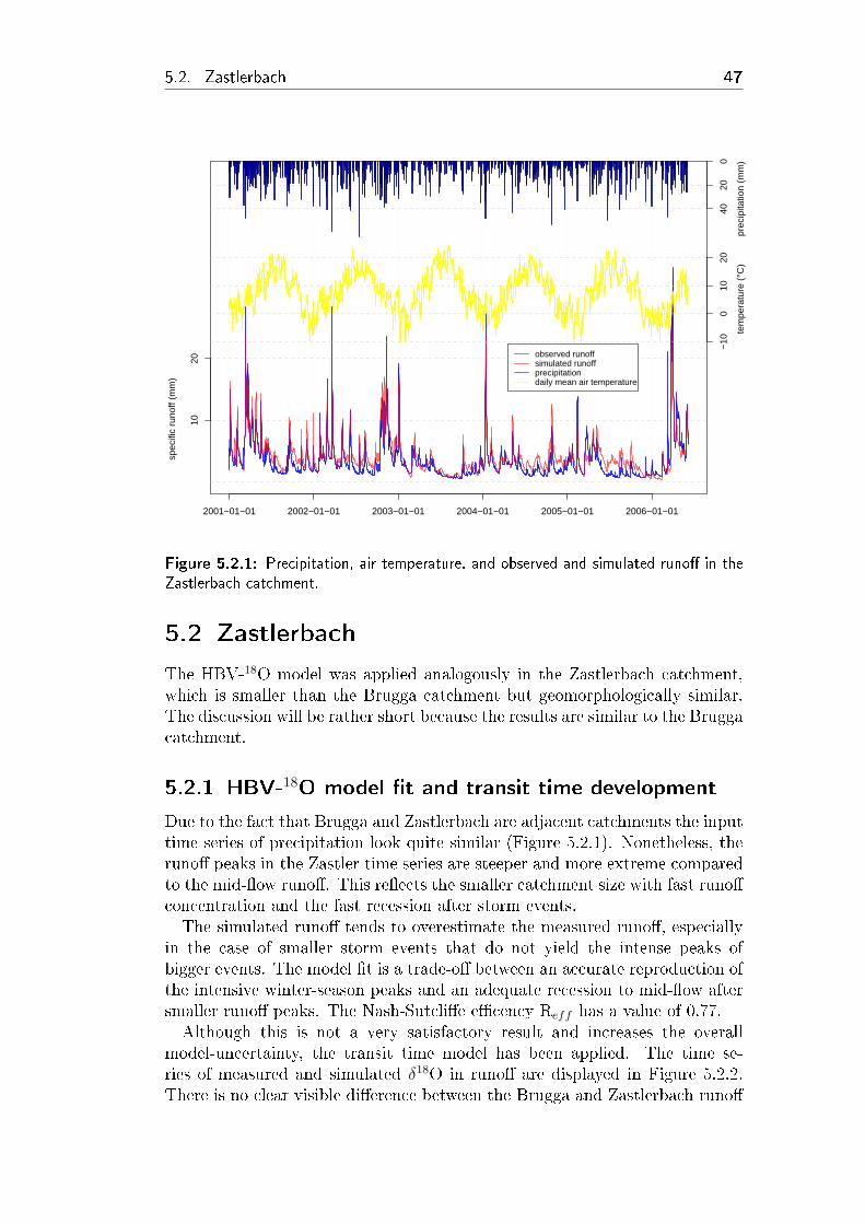
5.2. Zastlerbach 47
spe
cific
run
off (
mm
)
2001−01−01 2002−01−01 2003−01−01 2004−01−01 2005−01−01 2006−01−01
1020
4020
0
prec
ipita
tion
(mm
)
−10
010
20
te
mpe
ratu
re (
°C)
observed runoffsimulated runoffprecipitationdaily mean air temperature
Figure 5.2.1: Precipitation, air temperature, and observed and simulated runo� in theZastlerbach catchment.
5.2 Zastlerbach
The HBV-18O model was applied analogously in the Zastlerbach catchment,which is smaller than the Brugga catchment but geomorphologically similar.The discussion will be rather short because the results are similar to the Bruggacatchment.
5.2.1 HBV-18O model �t and transit time development
Due to the fact that Brugga and Zastlerbach are adjacent catchments the inputtime series of precipitation look quite similar (Figure 5.2.1). Nonetheless, theruno� peaks in the Zastler time series are steeper and more extreme comparedto the mid-�ow runo�. This re�ects the smaller catchment size with fast runo�concentration and the fast recession after storm events.The simulated runo� tends to overestimate the measured runo�, especially
in the case of smaller storm events that do not yield the intense peaks ofbigger events. The model �t is a trade-o� between an accurate reproduction ofthe intensive winter-season peaks and an adequate recession to mid-�ow aftersmaller runo� peaks. The Nash-Sutcli�e e�cency Reff has a value of 0.77.Although this is not a very satisfactory result and increases the overall
model-uncertainty, the transit time model has been applied. The time se-ries of measured and simulated δ18O in runo� are displayed in Figure 5.2.2.There is no clear visible di�erence between the Brugga and Zastlerbach runo�
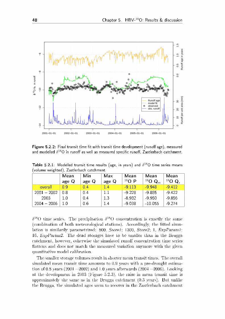
48 Chapter 5. HBV-18O: Results & discussion
δδ 18
O ‰
in
run
off
●
●●
●
●
●
●
●
●
●
●●●●●●
●●
●●
●●●●●●
●●●●●●●●●
●●
●●●●
●
●●●●●
●●●
●●
●●
●●●●●
●
●●
●
●●●●●
●
●
●
●●●●●●●●
●
●
●●
●●
●
●●●●●●
●
●●●
●
●●●
●
●●●●●
●
●●●●●
●●●
●●●
●●●
●●●
●●●●
●●●●●●●
●
●●●●●●●
●
●●
●
●●
●
●
●●●
●●●●
●
●
●
●●●●●
●●
●●●●●●●●●
●
●●
●
●
●
●
●
●●
●
●
●
●
●
●
●
●●●●●●●●●●●●●
●
●●
●●
●
●●●●
●●●●●
●●●●●●●
●
●
●
●●●
●●●●●●●●●
●
●●
●
●●●
●●●●●●●●
●●●
●●●●
●●●
●
●●●●●●
●●
●●
2001−01−01 2002−01−01 2003−01−01 2004−01−01 2005−01−01 2006−01−01
−14
−12
−10
−8
−6
0.0
0.5
1.0
1.5
Run
off a
ge in
yea
rs
010
2030
Run
off p
er u
nit a
rea
(mm
)
●
Runoff agemodel fitobserved obs. runoff
Figure 5.2.2: Final transit time �t with transit time development (runo� age), measuredand modelled δ18O in runo� as well as measured speci�c runo�, Zastlerbach catchment.
Table 5.2.1: Modelled transit time results (age, in years) and δ18O time series means(volume weighted), Zastlerbach catchment
Meanage Q
Minage Q
Maxage Q
Mean18O P
Mean18O Qm
Mean18O Qs
overall 0.9 0.4 1.4 -9.113 -9.948 -9.4122001 � 2002 0.8 0.4 1.1 -9.228 -9.855 -9.422
2003 1.0 0.4 1.3 -8.932 -9.950 -9.8562004 � 2006 1.0 0.6 1.4 -9.038 -10.055 -9.274
δ18O time series. The precipitation δ18O concentration is exactly the same(combination of both meteorological stations). Accordingly, the �tted simu-lation is similarily parametrized: 800, Store1; 1300, Store2; 1, ExpParam1;16, ExpParam2. The dead storages have to be smaller than in the Bruggacatchment, however, otherwise the simulated runo� concentration time series�attens and does not match the measured variation anymore with the givenquantitative model calibration.The smaller storage volumes result in shorter mean transit times. The overall
simulated mean transit time amounts to 0.9 years with a pre-drought estima-tion of 0.8 years (2001 � 2002) and 1.0 years afterwards (2004 � 2006). Lookingat the development in 2003 (Figure 5.2.3), the raise in mean transit time isapproximately the same as in the Brugga catchment (0.3 years). But unlikethe Brugga, the simulated ages seem to recover in the Zastlerbach catchment
5.2. Zastlerbach 49
δδ 18
O ‰
in
run
off
●
●
● ●
●
●
●●
●
●
●
●
●●
●
●
●●
●
●●
●
●
●
● ●
●
2003−05−01 2003−06−01 2003−07−01 2003−08−01 2003−09−01 2003−10−01 2003−11−01
−11
.0−
10.5
−10
.0−
9.5
−9.
0−
8.5
−8.
0
0.0
0.5
1.0
1.5
2.0
Run
off a
ge in
yea
rs
05
10
Run
off p
er u
nit a
rea
(mm
)
●
Runoff agemodel fitobserved obs. runoffsim. runoff
Figure 5.2.3: Transit time development during the dry spring/summer in 2003, Zastler-bach catchment.
from 2003 to 2005.The probability mass function in Figure 5.2.4 consequently does not show
the two peaks as distinct as in the Brugga catchment, the drought e�ect isalready receding.
5.2.2 Conclusions
The simulated mean transit time over the investigated period in the Zastler-bach catchment is 0.9 years. The simulation bears strong resemblance withthe adjacent Brugga catchment but in a somewhat alleviated form. I.e., themodelled drought in�uence is not as long-lasting as in the Brugga catchmentand the general catchment behaviour (e.g. runo� reaction) reveals the scaledi�erence between both catchments.
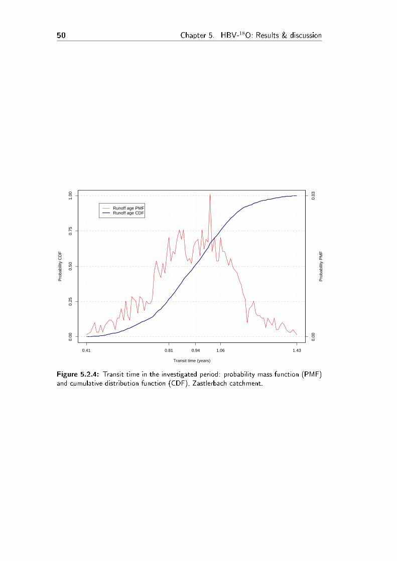
50 Chapter 5. HBV-18O: Results & discussion
Transit time (years)
Pro
babi
lity
CD
F
0.41 0.81 0.94 1.06 1.43
0.00
0.25
0.50
0.75
1.00
0.00
0.03
Pro
babi
lity
PM
F
Runoff age PMFRunoff age CDF
Figure 5.2.4: Transit time in the investigated period: probability mass function (PMF)and cumulative distribution function (CDF), Zastlerbach catchment.
51
6 Sine-wave approach
6.1 Introduction
For evaluation reasons and in order to get a comparable result with a com-monly adapted method, mean transit time estimations were determined bya sine-wave function, representing periodical oscillations in precipitation in-put and stream�ow output concentrations. The application of this method isrestricted to areas, where the precipitation shows a reasonable sinusoidal dis-tribution throughout the year (McGuire and McDonnell, 2006). The methodis comparatively simple and does not re�ect seasonal variations in recharge inthe version applied here. Nonetheless, it has been reported to provide reason-able estimations of mean residence times (e.g. DeWalle et al. 1997, Soulsbyet al. 2000, Rodgers et al. 2005, McGuire and McDonnell 2006) especially interms of a potential maximum value for catchment mean transit time, and thusitcan be used for validation of the results presented above. Moreover, since themethodology has been widely applied in residence time investigations, it alsoprovides the possiblity to compare the Brugga and Zastlerbach catchment withother studied sites.
6.2 Method
The sine-wave analysis is a regression statistically evaluating the in- and outputtime series of δ18O concentrations (here: precipitation and stream water). Dueto fractionation and selection e�ects (see section 1.3.1, page 2), the δ18O con-centrations often show a signi�cant seasonal variation, which can be expressedwith a sine-wave function. Bliss (1970) (in McGuire and McDonnell, 2006)provided a multiple linear regression model to evaluate a sine wave functionstatistically. Analytical solutions for the mean transit time of the exponentialmodel (EM) and also for the exponential-piston �ow model (EPM) exist. Ofcourse, this is limited to locations where precipitation shows a reasonable pe-riodical variation, and damping throughout the �ow system does not level thesignal completely (which would result in a constant concentration, the meanvalue of the input function).The sine-wave function that approximates δ18O concentrations (δ) through-
out the year has the form:
δ = β0 + A · (cos (ct− φ)) (6.2.1)
with the mean annual stable isotope concentration β0 (%�), the amplitude A(%�), the phase lag φ (rad) and the angular frequency constant c (2π/365,
52 Chapter 6. Sine-wave approach
where t are days) in (rad/d). The parameters in equation (6.2.1) are thenevaluated with the regression model.
δ = β0 + βcos · cos (ct) + βsin · sin (ct) (6.2.2)
The parameters A and φ from equation (6.2.1) are determined with the re-gression coe�cients βcos and βsin: A =
√β2
cos + β2sin and tan φ = βsin/βcos.
1
The mean transit time τm is then calculated by the damping from in- tooutput:
τm =
√f−2 − 1
c, f =
Aout
Ain
(EM) (6.2.3)
τm =η ·
√f−2 − 1
c(EPM) (6.2.4)
with Aout and Ain, the amplitudes of in- and output and η, the portion ofpiston �ow: η = 1 ⇒ EPM = EM, η → ∞ ⇒ EPM = PM. Values for η haveto be assumed and are taken from literature values in this thesis. (Equations(6.2.1) to (6.2.4) cited from McGuire and McDonnell (2006).)Looking at the isotope time series (e.g. Figure 5.1.1 on page 38) one can
see distinct seasonal changes in most of the investigated years. However, thesechanges show di�ering amplitudes and are not equally large throughout theyears. This is also the case for the respective stream water isotope time series.To estimate mean transit time in this thesis, the weekly time series of in-
and output (2000-2006) have been merged to a "mean year" series, with allsamples accumulated and averaged where required (two or more samples onone day). The regression model was applied to the resulting one year timeseries. For the Zastlerbach catchment, additionally regressions were computedfor every year and also over the complete regression period. The results werein agreement with the mean year computations. However, the mean yearcomputations improved the coe�cient of determination R2. Here, no �ux-weighting has been done. According to McGuire et al. (2002) this might leadto an over-estimation of mean transit time. Yet, at least the above mentionedmaximum value estimation can be seen. Also, the uncorrected precipitationconcentrations have been used, but since the mean transit time estimationdepends on amplitude damping, and the precipitation concentration amplitudeis not varied noteworthy by the height correction, this is considered acceptable.
6.3 Results
In the Zastlerbach catchment sine-wave regressions were computed for thewhole time series, yearwise and for the mean year over the investigation period.Because the mean year calculations in the Zastlerbach catchment �t well to
1When using the arctan function be aware of the quadrant: if βcos and/or βsin are negative,one or two π have to be added.
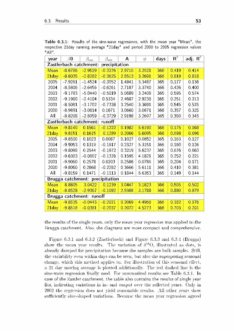
6.3. Results 53
Table 6.3.1: Results of the sine-wave regressions, with the mean year "Mean", therespective 21day running average "21day" and period 2000 to 2005 regression values"All".
year β0 βcos βsin A φ days R2
adj. R2
Zastlerbach catchment: precipitationMean -8.6786 -2.9529 -0.3276 2.9710 3.2521 366 0.419 0.41421day -8.6035 -2.8282 -0.3625 2.8513 3.2691 366 0.819 0.8182005 -7.9261 -1.4524 -0.3052 1.4841 3.3487 365 0.177 0.1362004 -8.5806 -2.6456 -0.6261 2.7187 3.3740 366 0.426 0.4002003 -9.1783 -5.0440 -0.5019 5.0689 3.2408 365 0.595 0.5742002 -9.1980 -2.4104 0.5334 2.4687 2.9238 365 0.251 0.2132001 -8.5081 -3.1702 -0.7338 3.2540 3.3691 365 0.545 0.5252000 -8.9891 -3.0614 0.1671 3.0660 3.0871 366 0.357 0.325All -8.8208 -2.8959 -0.3729 2.9198 3.2697 365 0.350 0.345
Zastlerbach catchment: runo�Mean -9.8140 0.1561 -0.1222 0.1982 5.6190 366 0.175 0.16821day -9.8151 0.1615 -0.1289 0.2066 5.6095 366 0.698 0.6962005 -9.8500 0.1023 0.0087 0.1027 0.0852 365 0.163 0.1272004 -9.9053 0.1319 -0.1917 0.2327 5.3151 366 0.160 0.1262003 -9.8098 0.2544 -0.1972 0.3219 5.6237 365 0.676 0.6632002 -9.6303 -0.0807 -0.1376 0.1595 4.1821 365 0.252 0.2212001 -9.9060 0.2578 0.0203 0.2586 0.0786 365 0.204 0.1712000 -9.8060 0.2868 -0.2282 0.3666 5.6111 366 0.410 0.381All -9.8159 0.1471 -0.1113 0.1844 5.6353 365 0.149 0.144
Brugga catchment: precipitationMean -8.8805 -3.0422 -0.1239 3.0447 3.1823 366 0.505 0.50221day -8.8528 -2.9367 -0.1092 2.9388 3.1788 366 0.880 0.879Brugga catchment: runo�Mean -9.8535 -0.0443 -0.2021 0.2069 4.4968 366 0.182 0.17621day -9.8518 -0.0381 -0.2037 0.2072 4.5273 366 0.703 0.701
the results of the single years, only the mean year regression was applied to theBrugga catchment. Also, the diagrams are more compact and comprehensive.
Figure 6.3.1 and 6.3.2 (Zastlerbach) and Figure 6.3.3 and 6.3.4 (Brugga)show the mean year results. The variation of δ18O, illustrated as dots, isalready damped for precipitation because the samples are bulk samples. Still,the variability even within days can be seen, but also the superposing seasonalchange, which this method applies to. For illustration of this seasonal e�ect,a 21 day moving average is plotted additionally. The red dashed line is thesine-wave regression �nally used. For summarized results see Table 6.3.1. Incase of the Zastler catchment, the table also contains the results of single year�ts, indicating variations in in- and output over the re�ected years. Only in2002 the regression does not yield reasonable results. All other years showsu�ciently sine-shaped variations. Because the mean year regression agreed
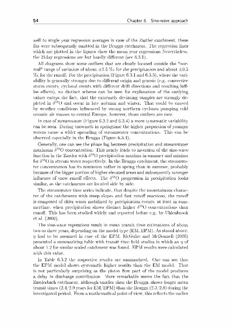
54 Chapter 6. Sine-wave approach
well to single year regression averages in case of the Zastler catchment, these�ts were subsequently omitted in the Brugga catchment. The regression lineswhich are plotted in the �gures show the mean year regressions Nevertheless,the 21day regressions are but hardly di�erent (see 6.3.1).
All diagrams show some outliers that are clearly located outside the "nor-mal" range of variation of about ±2.5 %� for the precipitation and about ±0.5%� for the runo�. For the precipitation (Figure 6.3.1 and 6.3.3), where the vari-ability is generally stronger due to di�erent origin and genesis (e.g. convectivestorm events, cyclonal events with di�erent drift directions and resulting lu�-lee e�ects), no distinct scheme can be seen for explanation of the outlyingvalues except the fact, that the extremely deviating samples are strongly de-pleted in δ18O and occur in late autumn and winter. That could be causedby weather conditions in�uenced by strong northern cyclones pumping coldoceanic air masses to central Europe. however, those outliers are rare.
In case of streamwater (Figure 6.3.2 and 6.3.4) a more systematic variabilitycan be seen. During snowmelt in springtime the higher proportion of youngerwaters cause a wider spreading of streamwater concentrations. This can beobserved especially in the Brugga (Figure 6.3.4).
Generally, one can see the phase lag between precipitation and streamwatermaximum δ18O concentration. This nearly leads to inversion of the sine-wavefunction in the Zastler with δ18O precipitation maxima in summer and minimafor δ18O in stream water respectively. In the Brugga catchment, the streamwa-ter concentration has its minimum rather in spring than in summer, probablybecause of the bigger portion of higher elevated areas and subsequently strongerin�uence of snow runo� e�ects. The δ18O progression in precipitation lookssimilar, as the catchments are located side by side.
The streamwater time series indicate, that despite the mountainous charac-ter of the catchments with steep slopes and fast runo� reactions, the runo�is composed of older water mobilized by precipitation events, at least in sum-mertime, when precipitation shows distinct higher δ18O concentrations thanruno�. This has been studied widely and reported before e.g. by Uhlenbrooket al. (2002).
The sine-wave regressions result in mean transit time estimations of abouttwo to three years, depending on the model type (EM, EPM). As stated above,η had to be assumed in case of the EPM. McGuire and McDonnell (2006)presented a summarizing table with transit time �eld studies in which an η ofabout 1.2 for similar scaled catchment was found. EPM results were calculatedwith this value.
In Table 6.3.2 the respective results are summarized. One can see thatthe EPM model shows systematic higher results than the EM model. Thatis not particularly surprising as the piston �ow part of the model producesa delay in discharge contribution. More remarkable seems the fact that theZastlerbach catchment, although smaller than the Brugga, shows longer meantransit times (2.4/2.9 years for EM/EPM) than the Brugga (2.3/2.8) during theinvestigated period. From a mathematical point of view, this re�ects the earlier
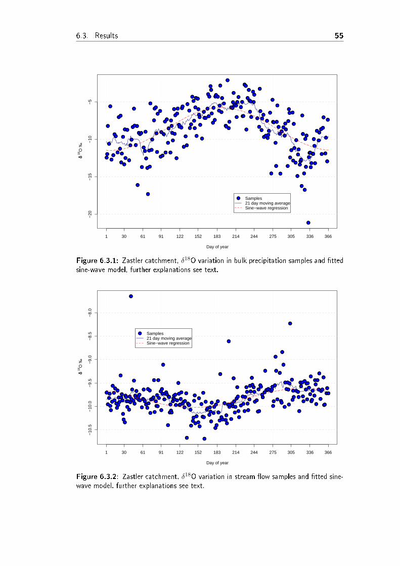
6.3. Results 55
●●
●
●
●
●●
●●
●
●
●
●
●
●
●
●
●
●
●
●
●
●
●
●
●
●
●
●
●●●
●
●●
●
●
●
●
●
●
●
●
●
●
●●
●
●
●●
●
●
●
●
●
●
●
●
●
●
●
●
●
●
●
●
●
●
●
●
●●●
●●
●
●
●
●
●
●●
●●
●
●
●
●
●
●
●
●●
●
●
●
●●
●
●
●
●
●●
●
●
●
●
●●●
●
●
●
●
●
●
●●
●
●
●
●●
●
●
●●●
●
●
●
●
●
●●
●●
●
●
●
●
●
●
●
●
●
●
●
●
●
●
●
●●
●●
●
●●●
●
●
●
●●
●
●
●
●
●
●
●
●●
●
●
●
●
●
●●
●
●
●
●
●
●
●
●
●
●
●
●●●
●
●
●
●
●
●
●
●
●
●●●
●●
●●
●
●
●
●
●
●●
●
●
●
●
●
●
●
−20
−15
−10
−5
Day of year
δδ 18
O ‰
1 30 61 91 122 152 183 214 244 275 305 336 366
●●
●
●
●
●●
●●
●
●
●
●
●
●
●
●
●
●
●
●
●
●
●
●
●
●
●
●
●●●
●
●●
●
●
●
●
●
●
●
●
●
●
●●
●
●
●●
●
●
●
●
●
●
●
●
●
●
●
●
●
●
●
●
●
●
●
●
●●●
●●
●
●
●
●
●
●●
●●
●
●
●
●
●
●
●
●●
●
●
●
●●
●
●
●
●
●●
●
●
●
●
●●●
●
●
●
●
●
●
●●
●
●
●
●●
●
●
●●●
●
●
●
●
●
●●
●●
●
●
●
●
●
●
●
●
●
●
●
●
●
●
●
●●
●●
●
●●●
●
●
●
●●
●
●
●
●
●
●
●
●●
●
●
●
●
●
●●
●
●
●
●
●
●
●
●
●
●
●
●●●
●
●
●
●
●
●
●
●
●
●●●
●●
●●
●
●
●
●
●
●●
●
●
●
●
●
●
●
● Samples21 day moving averageSine−wave regression
Figure 6.3.1: Zastler catchment, δ18O variation in bulk precipitation samples and �ttedsine-wave model, further explanations see text.
●
●
●●
●●
●
●
●
●
●
●●
●
●
●●
●
●●
●
●
●●
●●●
●
●
●
●
●
●
●
●
●
●
●
●●
●
●●●
●
●
●
●
●
●●●●
●
●
●
●
●●●●
●
●
●●
●
●
●
●
●
●
●●
●
●
●●●
●
●●
●
●
●●
●●●●●
●●
●
●
●●
●
●
●●
●
●
●
●
●●●●
●●●
●
●
●
●
●
●
●
●
●
●
●
●
●
●●
●
●●
●
●
●
●
●
●
●
●
●
●
●
●●
●
●●
●
●
●
●●
●
●●
●
●
●
●
●
●
●
●
●
●
●
●
●
●
●●
●
●
●
●
●
●
●●●
●●
●
●
●
●●
●●
●
●
●●●●●●●
●●
●
●
●
●
●
●●
●
●
●
●
●
●
●
●
●
●
●
●
●
●
●●
●
●
●●●
●
●
●
●
●
●
●●
●
●
●●
●
●
●●
●
●
●
●
●
●●
●
●●
●
●
●
−10
.5−
10.0
−9.
5−
9.0
−8.
5−
8.0
Day of year
δδ 18
O ‰
1 30 61 91 122 152 183 214 244 275 305 336 366
●
●
●●
●●
●
●
●
●
●
●●
●
●
●●
●
●●
●
●
●●
●●●
●
●
●
●
●
●
●
●
●
●
●
●●
●
●●●
●
●
●
●
●
●●●●
●
●
●
●
●●●●
●
●
●●
●
●
●
●
●
●
●●
●
●
●●●
●
●●
●
●
●●
●●●●●
●●
●
●
●●
●
●
●●
●
●
●
●
●●●●
●●●
●
●
●
●
●
●
●
●
●
●
●
●
●
●●
●
●●
●
●
●
●
●
●
●
●
●
●
●
●●
●
●●
●
●
●
●●
●
●●
●
●
●
●
●
●
●
●
●
●
●
●
●
●
●●
●
●
●
●
●
●
●●●
●●
●
●
●
●●
●●
●
●
●●●●●●●
●●
●
●
●
●
●
●●
●
●
●
●
●
●
●
●
●
●
●
●
●
●
●●
●
●
●●●
●
●
●
●
●
●
●●
●
●
●●
●
●
●●
●
●
●
●
●
●●
●
●●
●
●
●
● Samples21 day moving averageSine−wave regression
Figure 6.3.2: Zastler catchment, δ18O variation in stream �ow samples and �tted sine-wave model, further explanations see text.
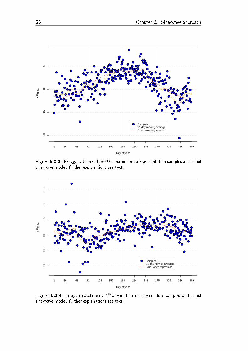
56 Chapter 6. Sine-wave approach
●
●
●
●
●
●
●
●●
●
●●
●
●
●●
●
●
●
●
●
●
●
●
●
●
●
●
●
●
●
●
●●●
●
●
●
●
●
●
●
●
●
●
●
●
●
●
●
●
●
●
●
●
●
●
●●
●
●
●●
●
●
●
●
●
●
●
●
●
●
●
●
●
●●
●
●
●●
●●●
●
●
●●
●
●●●
●
●
●
●
●●
●●
●
●
●
●
●
●●
●
●●
●●
●
●●●●
●●
●
●
●
●
●●
●●
●
●
●●
●
●
●●
●
●
●
●●●
●●
●
●
●
●●
●
●
●
●
●
●
●●●
●
●●●●
●
●
●
●
●●
●●●
●●
●
●
●
●
●
●
●
●
●●
●
●
●
●
●
●
●
●
●
●
●
●
●
●
●●
●
●
●
●
●●
●●
●
●
●●
●
●
●
●
●
●
●
●
●
●
●
●
●
●
●
●
●
●●
●
●
●
●
●
●
●
●●
●
●
●
●●
●
●
●
●●
●
●
●
●
●●
●
●
●
●
●
●
●
●
●●
●●
●●
●
●
●
●
●
●
●
●
●
●
●
●
●●
●
●
−20
−15
−10
−5
Day of year
δδ 18
O ‰
1 30 61 91 122 152 183 214 244 275 305 336 366
●
●
●
●
●
●
●
●●
●
●●
●
●
●●
●
●
●
●
●
●
●
●
●
●
●
●
●
●
●
●
●●●
●
●
●
●
●
●
●
●
●
●
●
●
●
●
●
●
●
●
●
●
●
●
●●
●
●
●●
●
●
●
●
●
●
●
●
●
●
●
●
●
●●
●
●
●●
●●●
●
●
●●
●
●●●
●
●
●
●
●●
●●
●
●
●
●
●
●●
●
●●
●●
●
●●●●
●●
●
●
●
●
●●
●●
●
●
●●
●
●
●●
●
●
●
●●●
●●
●
●
●
●●
●
●
●
●
●
●
●●●
●
●●●●
●
●
●
●
●●
●●●
●●
●
●
●
●
●
●
●
●
●●
●
●
●
●
●
●
●
●
●
●
●
●
●
●
●●
●
●
●
●
●●
●●
●
●
●●
●
●
●
●
●
●
●
●
●
●
●
●
●
●
●
●
●
●●
●
●
●
●
●
●
●
●●
●
●
●
●●
●
●
●
●●
●
●
●
●
●●
●
●
●
●
●
●
●
●
●●
●●
●●
●
●
●
●
●
●
●
●
●
●
●
●
●●
●
●
● Samples21 day moving averageSine−wave regression
Figure 6.3.3: Brugga catchment, δ18O variation in bulk precipitation samples and �ttedsine-wave model, further explanations see text.
●
●
●
●
●
●
●
●
●
●
●●●
●
●
●
●
●
●
●●●
●
●
●
●
●
●
●
●
●
●
●
●
●
●
●●●
●
●
●
●●
●
●
●●●
●
●
●
●●
●
●
●●
●
●●
●
●
●●
●
●
●
●
●
●
●
●
●
●
●
●
●●
●●
●
●
●●
●
●
●
●
●
●
●
●
●
●
●
●
●
●
●
●●
●
●●
●
●
●●●●
●
●●●●
●
●
●
●
●
●
●
●
●
●
●
●
●
●
●●●
●●●●
●
●
●
●
●
●
●●
●●
●●●
●
●
●●
●●
●
●
●
●●
●
●●
●
●
●
●
●●
●
●
●
●
●●
●
●
●
●
●
●●●●
●
●
●
●●●
●
●●●
●
●●●●
●
●
●
●●
●
●
●
●●
●
●
●
●
●
●
●
●
●
●
●
●
●
●
●●●●
●
●
●
●
●●
●
●●
●●●
●
●
●
●●
●
●
●
●
●
●●●
●
●
●●
●
●
●
●
●●
●
●
●
●
●
●●
●
●
●●
●●
●
●
−11
.0−
10.5
−10
.0−
9.5
−9.
0−
8.5
Day of year
δδ 18
O ‰
1 30 61 91 122 152 183 214 244 275 305 336 366
●
●
●
●
●
●
●
●
●
●
●●●
●
●
●
●
●
●
●●●
●
●
●
●
●
●
●
●
●
●
●
●
●
●
●●●
●
●
●
●●
●
●
●●●
●
●
●
●●
●
●
●●
●
●●
●
●
●●
●
●
●
●
●
●
●
●
●
●
●
●
●●
●●
●
●
●●
●
●
●
●
●
●
●
●
●
●
●
●
●
●
●
●●
●
●●
●
●
●●●●
●
●●●●
●
●
●
●
●
●
●
●
●
●
●
●
●
●
●●●
●●●●
●
●
●
●
●
●
●●
●●
●●●
●
●
●●
●●
●
●
●
●●
●
●●
●
●
●
●
●●
●
●
●
●
●●
●
●
●
●
●
●●●●
●
●
●
●●●
●
●●●
●
●●●●
●
●
●
●●
●
●
●
●●
●
●
●
●
●
●
●
●
●
●
●
●
●
●
●●●●
●
●
●
●
●●
●
●●
●●●
●
●
●
●●
●
●
●
●
●
●●●
●
●
●●
●
●
●
●
●●
●
●
●
●
●
●●
●
●
●●
●●
●
●
● Samples21 day moving averageSine−wave regression
Figure 6.3.4: Brugga catchment, δ18O variation in stream �ow samples and �ttedsine-wave model, further explanations see text.
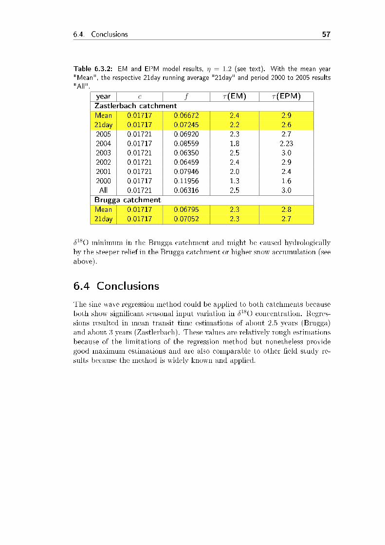
6.4. Conclusions 57
Table 6.3.2: EM and EPM model results, η = 1.2 (see text). With the mean year"Mean", the respective 21day running average "21day" and period 2000 to 2005 results"All".
year c f τ(EM) τ(EPM)Zastlerbach catchmentMean 0.01717 0.06672 2.4 2.921day 0.01717 0.07245 2.2 2.62005 0.01721 0.06920 2.3 2.72004 0.01717 0.08559 1.8 2.232003 0.01721 0.06350 2.5 3.02002 0.01721 0.06459 2.4 2.92001 0.01721 0.07946 2.0 2.42000 0.01717 0.11956 1.3 1.6All 0.01721 0.06316 2.5 3.0
Brugga catchmentMean 0.01717 0.06795 2.3 2.821day 0.01717 0.07052 2.3 2.7
δ18O minimum in the Brugga catchment and might be caused hydrologicallyby the steeper relief in the Brugga catchment or higher snow accumulation (seeabove).
6.4 Conclusions
The sine wave regression method could be applied to both catchments becauseboth show signi�cant seasonal input variation in δ18O concentration. Regres-sions resulted in mean transit time estimations of about 2.5 years (Brugga)and about 3 years (Zastlerbach). These values are relatively rough estimationsbecause of the limitations of the regression method but nonetheless providegood maximum estimations and are also comparable to other �eld study re-sults because the method is widely known and applied.

58 Chapter 6. Sine-wave approach
59
7 Concluding discussion
7.1 Model applications
Considering the absolute values, the sine-wave regression yielded substanciallylonger mean transit times than the conceptual approach. Depending on thedistribution model mean transit times of 2.5 to 3 years were computed. Theconceptual approach results in mean transit times of 1 to 1.4 years. As citedin the sine-wave chapter, this was also experienced in other studies.But, the main bene�t of the conceptual transit time model is certainly not an
improved estimation of mean transit times over longterm periods, but more thepossibility to assess the development during hydrological interesting phases likeextreme situations. I.e., the modelled results illustrate that event water cancontribute noteworthy to the runo� reaction but does not distinctly alteratethe isotopic concentration in runo�.
7.2 Limitations and issues
A conceptual approach bears always the risk that important processes have notbeen understood correctly and thus are implemented wrongly or even neglectedcompletely in a model scheme. Additionally, the higher the parametrisationof a conceptual model, the higher is also the risk that model de�ciencies arecovered by the plenty of degrees of freedom being available for the responsefunction.In the case of this thesis a, for its purpose well working, precipitation-runo�
model was modi�ed in order to �t the requirements of a transport model.The structure of the HBV model, e.g. the dead end soil storage with the FCparameter, comprises several trade-o�s between a functional reproduction ofcatchment behaviour and actual catchment processes and is certainly not likelyto depict catchment reality above a certain degree. If this structure is adoptedto model a di�erent process like the transit time development, it is probablyappropriate to be cautious with the results.
7.3 Final remarks
The results of the applied methods are in principle pleasant. The hypothesisof mean transit time overestimation by the sine-wave method proved true andthe simulated transit time development in connection with the dry summer2003 makes sense from a hydrological point of view.

60 Chapter 7. Concluding discussion
Nevertheless, it is di�cult to determine the validity of the model results.A validation with additional data, e.g. aquifer δ18O sampling, would give thepossiblity to consolitate (or discard, of course) the modelled results.
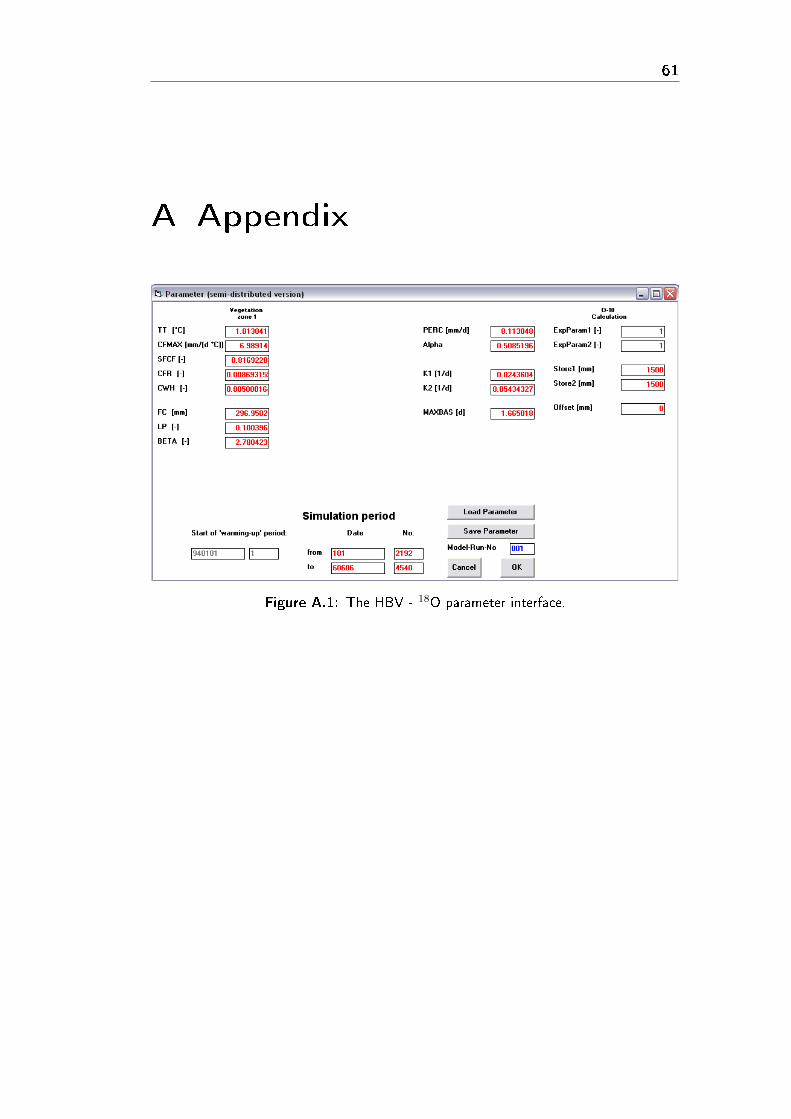
61
A Appendix
Figure A.1: The HBV - 18O parameter interface.
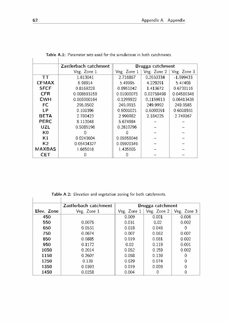
62 Appendix A. Appendix
Table A.1: Parameter sets used for the simulations in both catchments.
Zastlerbach catchment Brugga catchmentVeg. Zone 1 Veg. Zone 1 Veg. Zone 2 Veg. Zone 3
TT 1.813041 2.716867 0.2633334 -1.999433CFMAX 6.98914 5.49995 4.229291 5.47408SFCF 0.8169228 0.8951042 1.413672 0.6730116CFR 0.008693159 0.01000075 0.02758498 0.04580348CWH 0.005000164 0.1299922 0.1159813 0.06413436FC 296.9502 249.9915 249.9992 249.9585LP 0.100396 0.6000021 0.6000291 0.6001931
BETA 2.780423 2.999982 2.184225 2.749167PERC 8.113048 5.674984 � �UZL 0.5085196 0.2810796 � �K0 0 0 � �K1 0.0243604 0.05558046 � �K2 0.05434327 0.05920349 � �
MAXBAS 1.665018 1.435005 � �CET 0 0 � �
Table A.2: Elevation and vegetation zoning for both catchments.
Zastlerbach catchment Brugga catchmentElev. Zone Veg. Zone 1 Veg. Zone 1 Veg. Zone 2 Veg. Zone 3
450 - 0.009 0.001 0.008550 0.0076 0.031 0.02 0.002650 0.0531 0.018 0.048 0750 0.0674 0.007 0.062 0.007850 0.0885 0.019 0.081 0.002950 0.1172 0.02 0.119 0.0011050 0.2014 0.052 0.159 0.0021150 0.2607 0.058 0.139 01250 0.139 0.029 0.074 01350 0.0393 0.019 0.009 01450 0.0258 0.004 0 0
Bibliography 63
Bibliography
S. Bergström. Principles and con�dence in hydrological modelling. Nordic
Hydrology, 22:123�136, 1991.
S. Bergström. Computer Models of Watershed Hydrology, chapter 13. WaterResources Publications, 1995. ISBN 0-918334-91-8.
K. J. Beven. Rainfall-runo� modelling : the primer. John Wiley & Sons, 1stedition, 2001. ISBN 0-471-98553-8.
C. I. Bliss. Periodic Regression Statistics in Biology, pages 219�287. McGraw-Hill Book Co., New York, 1970.
R. Courant and H. Robbins. Was ist Mathematik? Springer, 2000. ISBN3-540-63777-X.
D. R. DeWalle, P. J. Edwards, B. R. Swistock, R. Aravena, and R. J. Drim-mie. Seasonal isotope hydrology of three appalachian forest catchments.Hydrological Processes, 11:1895�1906, 1997.
J. Didszun. Ab�ussbildung an Hängen. Diplomarbeit, Albert-Ludwigs-Universität Freiburg i. Br., Institut für Hydrologie, 2000.
DVWK. Ermittlung der Verdunstung von Land- und Wasser�ächen. Number238 in DVWK-Merkblätter zur Wasserwirtschaft. Deutscher Verband fürWasserwirtschaft und Kulturbau e.V. - Wirtschafts- und Verl.-Ges. Gas undWasser, Bonn, 1996. ISBN 3-89554-034-X.
S. Dyck and G. Peschke. Grundlagen der Hydrologie. Verl. für Bauwesen,Berlin, 3rd edition, 1995. ISBN 3-345-00586-7.
T. Ehnes. Der Ein�uss der Schneeschmelze auf die Ab�ussbildung und
die Grundwasserneubildung im Einzugsgebiet der Dreisam. Diplomarbeit,Albert-Ludwigs-Universität Freiburg i. Br., Institut für Hydrologie, 2006.
J. R. Gat. Oxygen and hydrogen isotopes in the hydrologic cycle. Annu. Rev.Earth Planet. Sci., 24:225�262, 1996.
M. Holocher. Anwendung des Niederschlags-Ab�uss-Modells HBV an der
Dreisam und verschieden skalierten Teileinzugsgebieten. Diplomarbeit,Albert-Ludwigs-Universität Freiburg i. Br., Institut für Hydrologie, 1997.
64 Bibliography
R. Holzschuh. Planung und Einrichtung eines Messnetzes zur Erfassung der re-
gionalen Isotopenverteilung im Niederschlag. Diplomarbeit, Albert-Ludwigs-Universität Freiburg i. Br., Institut für Hydrologie, 1995.
C. Kendall and J. J. McDonnell, editors. Isotope tracers in catchment hydrol-
ogy. Elsevier, Amsterdam, 1st edition, 1998. ISBN 0-444-81546-5.
LfU. Landesamt für umweltschutz: Pegelstatistik und hydrologischehauptzahlen der pegel brugga, dreisam, st. wilhelmer talbach, zastlerbachund wagensteigbach. unpublished, 2000.
M. Lindenlaub. Ab�uÿkomponenten und Herkunfträume im Einzugsgebiet
der Brugga : Aspekte zeitlicher und räumlicher Skalierung. Diplomarbeit,Albert-Ludwigs-Universität Freiburg i. Br., Institut für Hydrologie, 1998.
G. Lindström and A. Rodhe. Modelling water exchange and transit times intill basins using oxygen-18. Nordic Hydrology, 17:325�334, 1986.
P. Maloszewski and A. Zuber. Determining the turnover time of groundwatersystems with the aid of environmental tracers. Journal of Hydrology, 57:207�231, 1982.
K. J. McGuire and J. J. McDonnell. A review and evaluation of catchmenttransit time modeling. Journal of Hydrology, 2006. article in press.
K. J. McGuire, D. R. DeWalle, andW. J. Gburek. Evaluation of mean residencetime in subsurface waters using oxygen-18 �uctuations during drought con-ditions in the mid-appalachians. Journal of Hydrology, 261:132�149, 2002.
H. Moser and W. Rauert, editors. Isotopenmethoden in der Hydrologie.Number 8 in Lehrbuch der Hydrogeologie. Gebrüder Bornträger, Berlin -Stuttgart, 1980. ISBN 3-443-01012-1.
P. Rodgers, C. Soulsby, S. Waldron, and D. Tetzla�. Using stable isotopetracers to assess hydrological �ow paths, residence times and landscape in-�uences in a nested mesoscale catchment. Hydrology and Earth System Sci-
ences, 9:139�155, 2005.
J. Seibert. Hbv light version 2 user's manual. unpublished, 2002.
J. Seibert, A. Rodhe, and K. Bishop. Simulating interactions between satu-rated and unsaturated storage in a conceptual runo� model. Hydrological
Processes, 17:379�390, 2003.
C. Soulsby, R. Malcolm, R. Helliwell, R. C. Ferrier, and A. Jenkins. Isotopehydrology of the allt a' mharcaidh catchment, cairngorms, scotland: implica-tions for hydrological pathways and residence times. Hydrological Processes,14:747�762, 2000.
Bibliography 65
I. Stober. Die Wasserführung des kristallinen Grundgebirges : 16 Tabellen.Enke, Stuttgart, 1st edition, 1995. ISBN 3-432-26771-1.
H. Trenkle and H. v. Rudolf. Das klima im schwarzwald. In E. Liehl and W. D.Sick, editors, Der Schwarzwald - Beiträge zur Landeskunde, pages 59�100.Konkordia, Bühl/Baden, 1989. ISBN 3-7826-0047-9.
S. Uhlenbrook. Untersuchung und Modellierung der Ab�ussbildung in einem
mesoskaligen Einzugsgebiet. Number 10 in Freiburger HydrologischeSchriften. Institut für Hydrologie der Universität Freiburg, 1999a.
S. Uhlenbrook, J. Seibert, C. Leibundgut, and A. Rodhe. Prediction uncer-tainty of conceptual rainfall-runo� models caused by problems in identifyingmodel parameters and structure. Hydrological Sciences Journal, 44(5):779�797, 1999b.
S. Uhlenbrook, M. Frey, C. Leibundgut, and P. Maloszewski. Hydrograph sep-arations in a mesoscale mountainous basin at event and seasonal timescales.Water Resources Research, 38(6), 2002.
URL1. http://www.r-project.org/.
L. Wissmeier. Implementation of distributed solute transport into the catchmentmodel TACd and event based simulations using oxygen-18. Diplomarbeit,Albert-Ludwigs-Universität Freiburg i. Br., Institut für Hydrologie, 2005.

66 Bibliography
67
Ehrenwörtliche Erklärung:
Hiermit erkläre ich, dass die Arbeit selbständig und nur unter Verwendung derangegebenen Hilfsmittel angefertigt wurde.
Ort, Datum Unterschrift


![VO101 04 Zeitreihenanalyse.ppt [Kompatibilitätsmodus]¤sentationen/VO101... · 13.11.2010 1 Zeitreihenanalyse H.P. Nachtnebel Institut für Wasserwirtschaft, Hydrologie und konstruktiver](https://img.pdfslide.org/doc/110x75/5ba0719a09d3f2fb538c97d5/vo101-04-kompatibilitaetsmodus-sentationenvo101-13112010-1-zeitreihenanalyse.jpg)