NBER WORKING PAPER SERIES

INVESTMENT-LESS GROWTH:AN EMPIRICAL INVESTIGATION

Germán GutiérrezThomas Philippon

Working Paper 22897http://www.nber.org/papers/w22897

NATIONAL BUREAU OF ECONOMIC RESEARCH1050 Massachusetts Avenue

Cambridge, MA 02138December 2016

We are grateful to Janice Eberly, Olivier Blanchard, Toni Whited, René Stulz, Martin Schmalz, Boyan Jovanovic, Tano Santos, Charles Calomiris, Glenn Hubbard, Holger Mueller, Alexis Savov, Philipp Schnabl, Ralph Koijen, Ricardo Caballero, Emmanuel Farhi, Viral Acharya, and seminar participants at Columbia University and New York University for stimulating discussions. The views expressed herein are those of the authors and do not necessarily reflect the views of the National Bureau of Economic Research.

NBER working papers are circulated for discussion and comment purposes. They have not been peer-reviewed or been subject to the review by the NBER Board of Directors that accompanies official NBER publications.

© 2016 by Germán Gutiérrez and Thomas Philippon. All rights reserved. Short sections of text, not to exceed two paragraphs, may be quoted without explicit permission provided that full credit, including © notice, is given to the source.

Investment-less Growth: An Empirical Investigation Germán Gutiérrez and Thomas PhilipponNBER Working Paper No. 22897December 2016, Revised January 2016JEL No. E22,G3

ABSTRACT

We analyze private fixed investment in the U.S. over the past 30 years. We show that investment is weak relative to measures of profitability and valuation – particularly Tobin’s Q, and that this weakness starts in the early 2000’s. There are two broad categories of explanations: theories that predict low investment because of low Q, and theories that predict low investment despite high Q. We argue that the data does not support the first category, and we focus on the second one. We use industry-level and firm-level data to test whether under-investment relative to Q is driven by (i) financial frictions,(ii) measurement error (due to the rise of intangibles, globalization, etc), (iii)decreased competition (due to technology, regulation or common ownership), or (iv) tightenedgovernance and/or increased short-termism. We do not find support for theories based on riskpremia, financial constraints, or safe asset scarcity, and only weak support for regulatoryconstraints. Globalization and intangibles explain some of the trends at the industry level, buttheir explanatory power is quantitatively limited. On the other hand, we find fairly strong supportfor the competition and short-termism/governance hypotheses. Industries with moreconcentration and more common ownership invest less, even after controlling for current marketconditions. Within each industry-year, the investment gap is driven by firms that are owned byquasi-indexers and located in industries with more concentration and more common ownership.These firms spend a disproportionate amount of free cash flows buying back their shares.

Germán GutiérrezNYU Stern School of Business44 West 4th StreetKMC 9-190New York, NY 10012ggutierr@stern.nyu.edu

Thomas PhilipponNew York UniversityStern School of Business44 West 4th Street, Suite 9-190New York, NY 10012-1126and NBERtphilipp@stern.nyu.edu

In his March 2016 letter to the executives of S&P 500 firms, BlackRock’s CEO Laurence Fink

argues that, “in the wake of the financial crisis, many companies have shied away from investing

in the future growth of their companies. Too many companies have cut capital expenditure and

even increased debt to boost dividends and increase share buybacks.” The decline in investment has

been discussed in policy papers [Furman, 2015], especially in the context of a perceived decrease in

competition in the goods market [CEA, 2016]. There is little systematic evidence, however, on the

extent of the investment puzzle and on the potential explanations.

This paper tries to (at least partially) fill that gap. We clarify some of the theory and the

empirical evidence; and test whether alternate theories of under-investment are supported by the

data. The main contributions of the paper are to show that: (i) the lack of investment represents

a reluctance to invest despite high Tobin’s Q; and (ii) this investment wedge appears to be linked

to decreased competition and changes in governance that encourage shares buyback instead of

investment. We address the issues of causality of competition and governance in a companion paper

Gutiérrez and Philippon [2017].

It is useful, as a starting point, to distinguish two broad categories of explanations for low

investment rates: theories that predict low investment because they predict low Tobin’s Q and

theories that predict low investment despite high Tobin’s Q. The first category includes explanations

based on increasing risk aversion or decreasing expected growth. The standard Q-equation holds

in these theories, so the only way they can explain low investment is by predicting low values of Q.

The second category ranges from credit constraints to oligopolistic competition, and predicts a gap

between Q and investment due to differences between average and marginal Q (e.g., market power,

growth options) and/or differences between firm value and the manager’s objective function (e.g.,

governance, short-termism).

We find that private fixed investment is weak relative to measures of profitability and valuation

– particularly Tobin’s Q. Time effects from industry- and firm-level panel regressions on Q suggest

that this weakness starts around 2000. This is true controlling for firm age, size, and profitability;

focusing on subsets of industries; and even considering tangible and intangible investment separately.

Given these results, we discard theories that predict low investment because they predict low Q;

and focus on theories that predict a gap between Q and investment. This still leaves us with a large

set of potential explanations.

We consider the following eight potential explanations, grouped into four broad categories. See

Section 2 for a detailed discussion of these hypotheses.

• Financial frictions

1. External finance

2. Bank dependence

3. Safe asset scarcity

• Measurement Error

2

4. Intangibles

5. Globalization

• Lack of Competition

6. Regulation

7. Concentration due to other factors

• Tighter Governance

8. Ownership and Shareholder Activism

We emphasize that these hypotheses are not mutually exclusive. For instance, there is a large and

growing literature that focuses precisely on the interaction between governance and competition

(see, for example, Giroud and Mueller [2010, 2011]). Thus, our tests do not map one-to-one into

hypotheses (1) to (8); some tests overlap two or more hypotheses (e.g., measures of firm ownership

affect both governance and competition). We report the results of our tests and discuss their

implications for the above hypotheses in Section 4.

Testing these hypotheses requires a lot of data, at different levels of aggregation. Some are

industry-level theories (e.g., competition), some firm-level theories (e.g., ownership), and some the-

ories that can be tested at the industry level and/or at the firm level. Unfortunately, firm- and

industry-data are not readily comparable, because they differ in their definitions of investment and

capital, and in their coverage. As a result, we must spend a fair amount of time simply reconciling

the various data sources. Much of the work is explained in Section 3 and in the Appendix.

We gather industry investment data from the BEA and firm investment data from Compustat;

as well as additional data needed to test each of the eight hypotheses. For instance, for Concentra-

tion, we obtain measures of firm entry, firm exit, price-cost margins, and concentration (including

‘traditional’ and common ownership-adjusted Herfindahls1, as well as concentration ratios defined

as the share of sales and market value of the Top 4, 8, 20 and 50 firms in each industry). For gover-

nance and short-termism, we use measures of institutional ownership, including different ownership

types following Brian Bushee’s institutional investor classification.2

Competition and Governance We then analyze investment patterns at the industry- and firm-

level. At the industry level, we find that industries with more quasi-indexer institutional ownership

and less competition (as measured by higher ‘traditional’ and common ownership-adjusted Herfind-

ahls, as well as higher price-cost margins) invest less. These results are robust to controlling for

firm demographics (age and size) as well as Q.

1We follow Salop and O’Brien [2000] and Azar et al. [2016b] to compute the common ownership-adjusted Herfind-ahl, which accounts for anti-competitive incentives due to common ownership. See Section 2 for additional details

2The classification – described in Bushee [2001] – identifies Quasi-indexer, Transient and Dedicated institutionalinvestors based on the turnover and diversification of their holdings. Dedicated institutions have large, long-termholdings in a small number of firms. Quasi-indexers have diversified holdings and low portfolio turnover – consistentwith a passive, buy-and-hold strategy of investing portfolio funds in a broad set of firms. Transient owners have highdiversification and high portfolio turnover. See Section 3 for additional details.

3

The decrease in competition is supported by a growing literature3, though the empirical implica-

tions for investment have not been recently studied (to our knowledge). Similarly, the mechanisms

through which quasi-indexer institutional ownership impacts investment remain to be fully un-

derstood: while such ownership may improve governance (e.g., Appel et al. [2016a]), it may also

increase short-termism (e.g., Asker et al. [2014], Bushee [1998]) – both of which could lead to higher

buybacks and less investment. Firm-level results are consistent with industry-level results. They

suggest that within each industry-year and controlling for Q, firms with higher quasi-indexer in-

stitutional ownership invest less; and firms in industries with less competition also invest less. To

better understand the implications of safe asset scarcity and the rise of intangibles, we discuss these

hypotheses in greater detail.

Safe Assets According to the safe asset scarcity hypothesis, the value of being able to issue

safe assets increases after the Great Recession. This should increase the value of very sage (AAA)

firms, but, to the extent that safety cannot be readily scaled up, it would not increase their physical

investment to the same extent that it increases their value. This might then account for relatively low

investment despite high Q Note that, a some broad abstract level, this is a example of (potentially

sharp) decreasing returns to (physical) scale. The problem with this theory is that it predicts that

the valuation (and investment, to a lesser extent) of highly rated firms should increase relative to

that of other firms. We regress the 2014 firm value on the 2006 value and an indicator for being

initially AA to AAA rated firms and find no support for the hypothesis. We also fail to observe

higher investment for these firms in the cross-section. The safety premium seems present in the

data, but only in 2009 and 2010, not in later years. Therefore it cannot account for the persistence

of weak investment.

Intangibles The rise of intangibles can affect investment in several ways. Intangible investment

is difficult to measure. Under-estimation of I would lead to under-estimation of K, and therefore

over-estimation of Q. This could translate to an ‘observed’ under-investment at industries with a

higher share of intangibles. Alternatively, intangible assets might be more difficult to accumulate.

A rise in the relative importance of intangibles could then lead to a higher equilibrium value of Q

even if intangibles are correctly measured. Fortunately, the relationship between Q and intangi-

ble investment has been thoroughly studied by Peters and Taylor [2016]. Building on their work,

and using the Erickson et al. [2014] cumulant estimator, we find some support for these hypotheses

(industries with a higher share of intangibles exhibit lower investment) but we show that the ag-

gregate impact does not seem to be quantitatively very large. It is also important to emphasize, as

Peters and Taylor [2016] do, that Q explains intangible investment relatively well, and works even

better when both tangible and intangible investments are combined, exactly as the theory would

predict. Moreover, intangible investment exhibits roughly the same weakness as tangible invest-

3For instance, the Council of Economic Advisers issued a 2016 issue brief that “reviews three sets of trends that

are broadly suggestive of a decline in competition: increasing industry concentration, increasing rents accruing to a

few firms, and lower levels of firm entry and labor market mobility.” (see also Decker et al. [2015]).

4

ment. Properly accounting for intangible investment is clearly a first order empirical issue, but, as

far as we can tell, it does not lessen the puzzle that we document.

Other theories We find some evidence that firms in industries with more regulation invest less,

but the impact does not appear to affect industry-level investment. Industries with higher foreign

profits invest less in the US, as expected, but firm level investment does not depend on the share of

foreign profits. None of the other theories appear to be supported by the data. They often exhibit

the ‘wrong’ and/or inconsistent signs; or are not statistically significant.

Other Papers Overall, our results are aligned with Lee et al. [2016] who find that industries that

receive more funds have a higher industry Q until the mid-1990s, but not since then. The change

in the allocation of capital is explained by a decrease in capital expenditures and an increase in

stock repurchases by firms in high Q industries since the mid-1990s. Our results are also related

to Alexander and Eberly [2016] who study the implications of the rise of intangibles on investment.

Last, our results somewhat contrast with Bena et al. [2016], who study the relationship between

foreign institutional ownership (proxied by additions to the MSCI World Index), investment and

innovation across 30 countries. They find that foreign institutional ownership can increase long-term

investment in fixed capital, innovation, and human capital. It will therefore be interesting, in future

work, to understand if our results are specific to the United States. Finally, the above conclusions

are based on simple regressions and therefore cannot establish causality between competition, gov-

ernance and investment. In follow-up work Gutiérrez and Philippon [2017] we use a combination of

instrumental variables and natural experiments to test the causality of our two main explanations,

lack of competition and tight or short-termist governance.

From a macro-perspective, our paper is related to Jones and Philippon [2016] who explore the

macro-economic consequences of decreased competition in a DSGE model with time-varying pa-

rameters and an occasionally binding zero lower bound. They show that the trend decrease in

competition can explain the joint evolution of investment, Q, and the nominal interest rate. Absent

the decrease in competition, they find that the U.S. economy would have escaped the ZLB by the

end of 2010 and that the nominal rate today would be close to 2%.

The remainder of this paper is organized as follows. Section 1 presents five important facts

about aggregate private fixed investment in recent years. Section 2 discusses the theories that may

explain under-investment relative to Q and reviews the related literature. Section 3 describes the

data used to test our eight hypotheses. Section 4 discusses the methodology and results of our

analyses; and section 5 concludes.

1 Five Facts about US Non Financial Sector Investment

We present five important facts related to investment by the US non financial sector in recent years.

We focus on the non financial sector for three main reasons. First, this sector is the main source of

nonresidential investment. Second, we can roughly reconcile aggregate data from the Flow of Funds

5

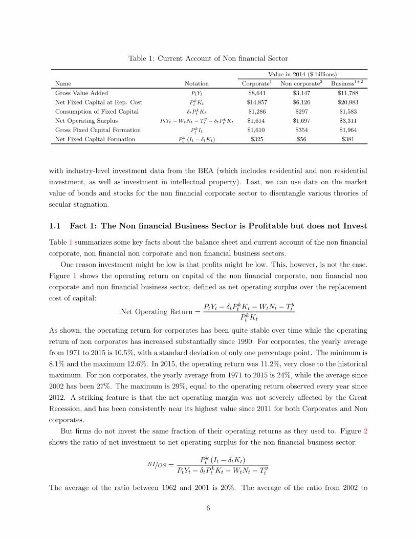
Table 1: Current Account of Non financial Sector

Value in 2014 ($ billions)

Name Notation Corporate1 Non corporate2 Business1+2

Gross Value Added PtYt $8,641 $3,147 $11,788

Net Fixed Capital at Rep. Cost P kt Kt $14,857 $6,126 $20,983

Consumption of Fixed Capital δtP kt Kt $1,286 $297 $1,583

Net Operating Surplus PtYt −WtNt − Tyt − δtP k

t Kt $1,614 $1,697 $3,311

Gross Fixed Capital Formation P kt It $1,610 $354 $1,964

Net Fixed Capital Formation P kt (It − δtKt) $325 $56 $381

with industry-level investment data from the BEA (which includes residential and non residential

investment, as well as investment in intellectual property). Last, we can use data on the market

value of bonds and stocks for the non financial corporate sector to disentangle various theories of

secular stagnation.

1.1 Fact 1: The Non financial Business Sector is Profitable but does not Invest

Table 1 summarizes some key facts about the balance sheet and current account of the non financial

corporate, non financial non corporate and non financial business sectors.

One reason investment might be low is that profits might be low. This, however, is not the case.

Figure 1 shows the operating return on capital of the non financial corporate, non financial non

corporate and non financial business sector, defined as net operating surplus over the replacement

cost of capital:

Net Operating Return =PtYt − δtP k

t Kt −WtNt − T yt

P kt Kt

As shown, the operating return for corporates has been quite stable over time while the operating

return of non corporates has increased substantially since 1990. For corporates, the yearly average

from 1971 to 2015 is 10.5%, with a standard deviation of only one percentage point. The minimum is

8.1% and the maximum 12.6%. In 2015, the operating return was 11.2%, very close to the historical

maximum. For non corporates, the yearly average from 1971 to 2015 is 24%, while the average since

2002 has been 27%. The maximum is 29%, equal to the operating return observed every year since

2012. A striking feature is that the net operating margin was not severely affected by the Great

Recession, and has been consistently near its highest value since 2011 for both Corporates and Non

corporates.

But firms do not invest the same fraction of their operating returns as they used to. Figure 2

shows the ratio of net investment to net operating surplus for the non financial business sector:

NI/OS =P kt (It − δtKt)

PtYt − δtP kt Kt −WtNt − T y

t

The average of the ratio between 1962 and 2001 is 20%. The average of the ratio from 2002 to

6

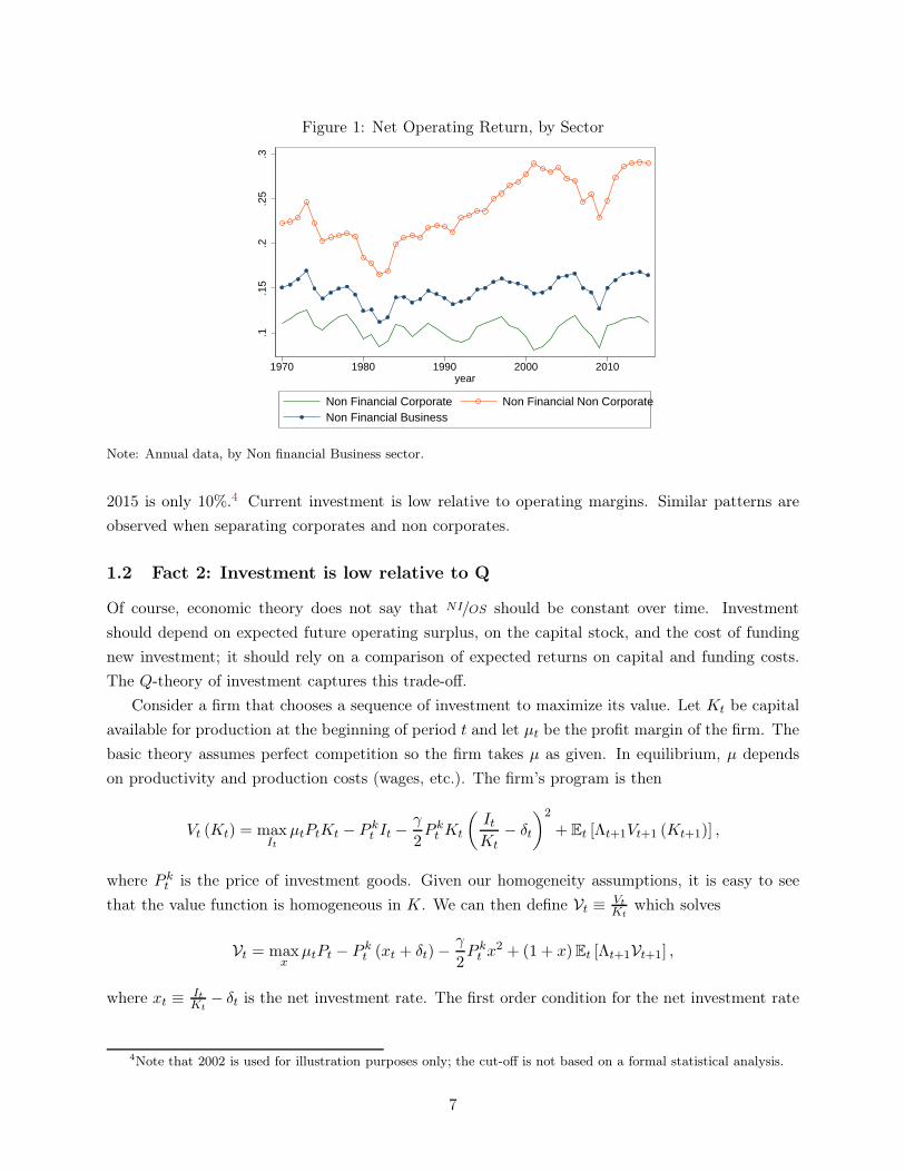
Figure 1: Net Operating Return, by Sector

.1.1

5.2

.25

.3

1970 1980 1990 2000 2010year

Non Financial Corporate Non Financial Non CorporateNon Financial Business

Note: Annual data, by Non financial Business sector.

2015 is only 10%.4 Current investment is low relative to operating margins. Similar patterns are

observed when separating corporates and non corporates.

1.2 Fact 2: Investment is low relative to Q

Of course, economic theory does not say that NI/OS should be constant over time. Investment

should depend on expected future operating surplus, on the capital stock, and the cost of funding

new investment; it should rely on a comparison of expected returns on capital and funding costs.

The Q-theory of investment captures this trade-off.

Consider a firm that chooses a sequence of investment to maximize its value. Let Kt be capital

available for production at the beginning of period t and let µt be the profit margin of the firm. The

basic theory assumes perfect competition so the firm takes µ as given. In equilibrium, µ depends

on productivity and production costs (wages, etc.). The firm’s program is then

Vt (Kt) = maxIt

µtPtKt − P kt It −

γ

2P kt Kt

(

ItKt

− δt

)2

+ Et [Λt+1Vt+1 (Kt+1)] ,

where P kt is the price of investment goods. Given our homogeneity assumptions, it is easy to see

that the value function is homogeneous in K. We can then define Vt ≡Vt

Ktwhich solves

Vt = maxx

µtPt − P kt (xt + δt)−

γ

2P kt x

2 + (1 + x)Et [Λt+1Vt+1] ,

where xt ≡ItKt

− δt is the net investment rate. The first order condition for the net investment rate

4Note that 2002 is used for illustration purposes only; the cut-off is not based on a formal statistical analysis.

7

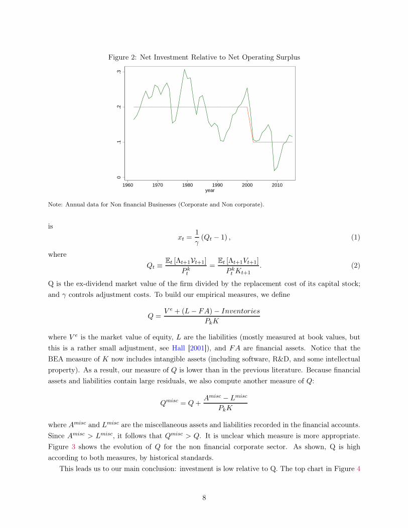
Figure 2: Net Investment Relative to Net Operating Surplus

0.1

.2.3

1960 1970 1980 1990 2000 2010year

Note: Annual data for Non financial Businesses (Corporate and Non corporate).

is

xt =1

γ(Qt − 1) , (1)

where

Qt ≡Et [Λt+1Vt+1]

P kt

=Et [Λt+1Vt+1]

P kt Kt+1

. (2)

Q is the ex-dividend market value of the firm divided by the replacement cost of its capital stock;

and γ controls adjustment costs. To build our empirical measures, we define

Q =V e + (L− FA)− Inventories

PkK

where V e is the market value of equity, L are the liabilities (mostly measured at book values, but

this is a rather small adjustment, see Hall [2001]), and FA are financial assets. Notice that the

BEA measure of K now includes intangible assets (including software, R&D, and some intellectual

property). As a result, our measure of Q is lower than in the previous literature. Because financial

assets and liabilities contain large residuals, we also compute another measure of Q:

Qmisc = Q+Amisc − Lmisc

PkK

where Amisc and Lmisc are the miscellaneous assets and liabilities recorded in the financial accounts.

Since Amisc > Lmisc, it follows that Qmisc > Q. It is unclear which measure is more appropriate.

Figure 3 shows the evolution of Q for the non financial corporate sector. As shown, Q is high

according to both measures, by historical standards.

This leads us to our main conclusion: investment is low relative to Q. The top chart in Figure 4

8

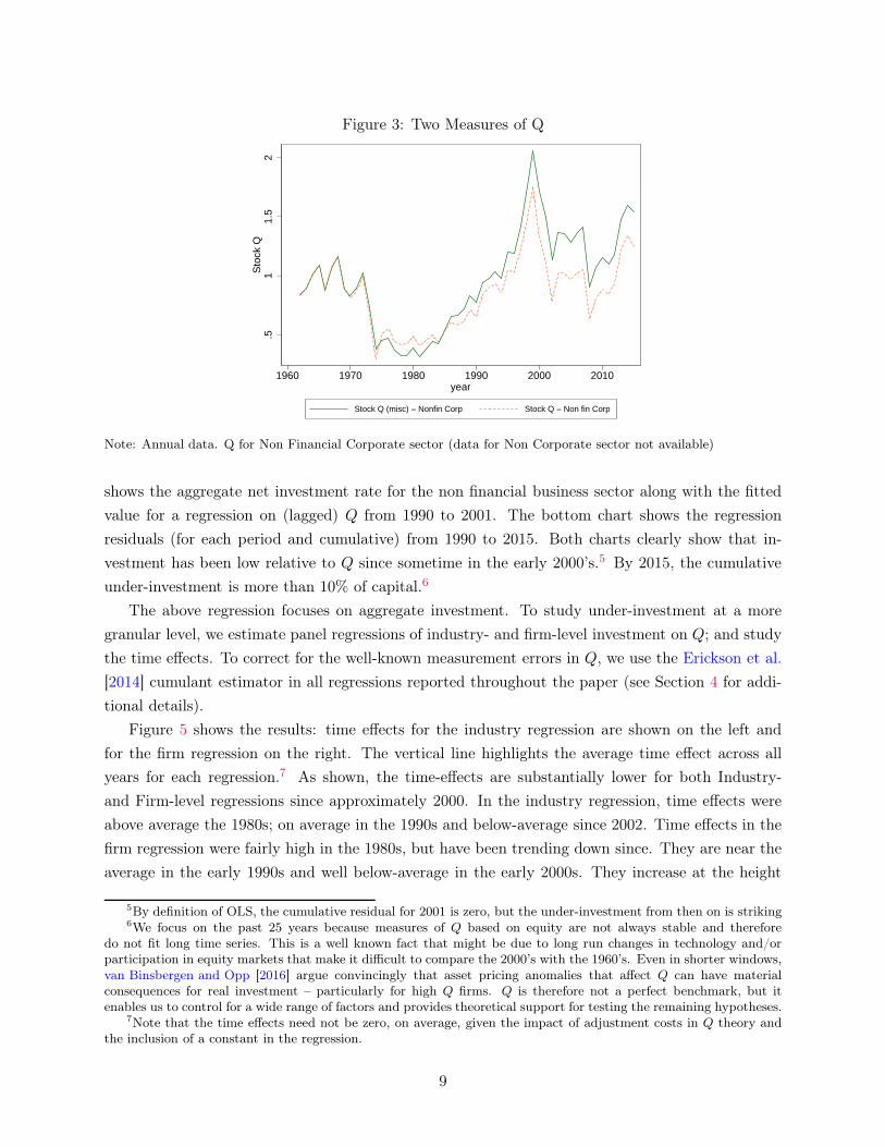
Figure 3: Two Measures of Q

.51

1.5

2St

ock

Q

1960 1970 1980 1990 2000 2010year

Stock Q (misc) − Nonfin Corp Stock Q − Non fin Corp

Note: Annual data. Q for Non Financial Corporate sector (data for Non Corporate sector not available)

shows the aggregate net investment rate for the non financial business sector along with the fitted

value for a regression on (lagged) Q from 1990 to 2001. The bottom chart shows the regression

residuals (for each period and cumulative) from 1990 to 2015. Both charts clearly show that in-

vestment has been low relative to Q since sometime in the early 2000’s.5 By 2015, the cumulative

under-investment is more than 10% of capital.6

The above regression focuses on aggregate investment. To study under-investment at a more

granular level, we estimate panel regressions of industry- and firm-level investment on Q; and study

the time effects. To correct for the well-known measurement errors in Q, we use the Erickson et al.

[2014] cumulant estimator in all regressions reported throughout the paper (see Section 4 for addi-

tional details).

Figure 5 shows the results: time effects for the industry regression are shown on the left and

for the firm regression on the right. The vertical line highlights the average time effect across all

years for each regression.7 As shown, the time-effects are substantially lower for both Industry-

and Firm-level regressions since approximately 2000. In the industry regression, time effects were

above average the 1980s; on average in the 1990s and below-average since 2002. Time effects in the

firm regression were fairly high in the 1980s, but have been trending down since. They are near the

average in the early 1990s and well below-average in the early 2000s. They increase at the height

5By definition of OLS, the cumulative residual for 2001 is zero, but the under-investment from then on is striking6We focus on the past 25 years because measures of Q based on equity are not always stable and therefore

do not fit long time series. This is a well known fact that might be due to long run changes in technology and/orparticipation in equity markets that make it difficult to compare the 2000’s with the 1960’s. Even in shorter windows,van Binsbergen and Opp [2016] argue convincingly that asset pricing anomalies that affect Q can have materialconsequences for real investment – particularly for high Q firms. Q is therefore not a perfect benchmark, but itenables us to control for a wide range of factors and provides theoretical support for testing the remaining hypotheses.

7Note that the time effects need not be zero, on average, given the impact of adjustment costs in Q theory andthe inclusion of a constant in the regression.

9

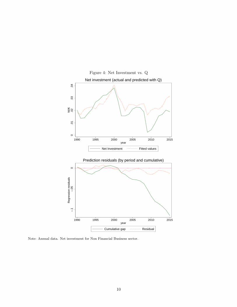
Figure 4: Net Investment vs. Q0

.01

.02

.03

.04

NI/K

1990 1995 2000 2005 2010 2015year

Net Investment Fitted values

Net investment (actual and predicted with Q)

−.1

−.05

0R

egre

ssio

n re

sidu

als

1990 1995 2000 2005 2010 2015year

Cumulative gap Residual

Prediction residuals (by period and cumulative)

Note: Annual data. Net investment for Non Financial Business sector.

10

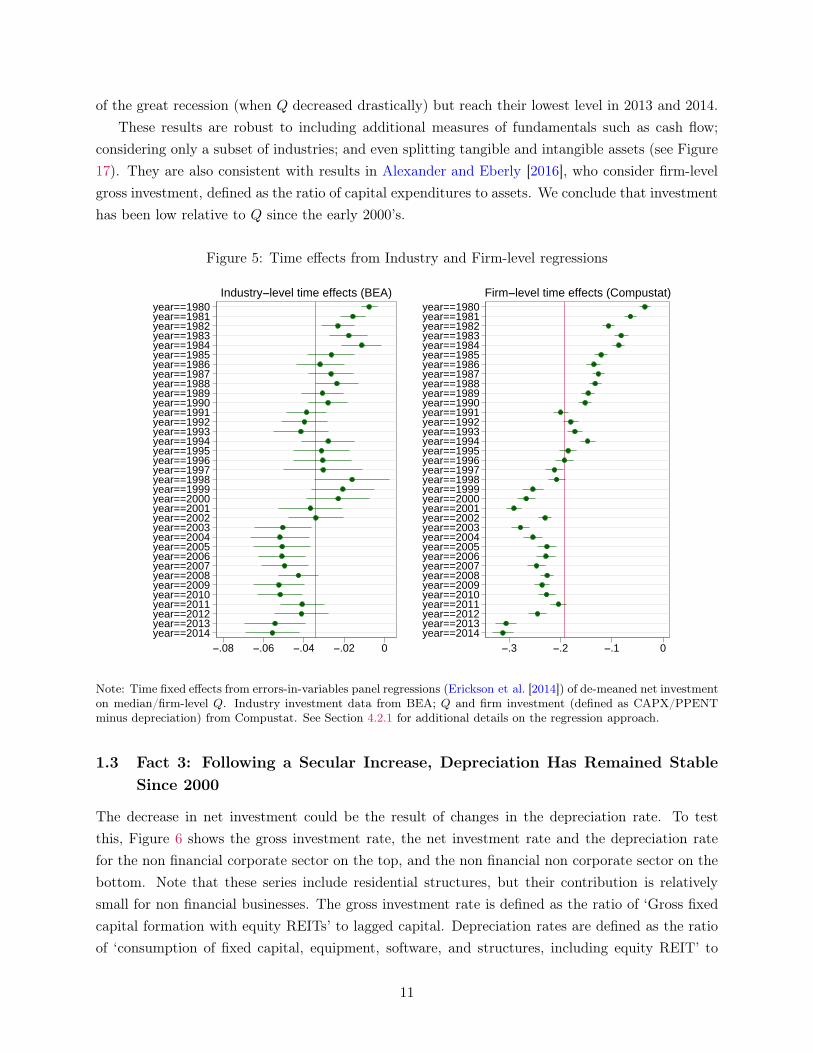
of the great recession (when Q decreased drastically) but reach their lowest level in 2013 and 2014.

These results are robust to including additional measures of fundamentals such as cash flow;

considering only a subset of industries; and even splitting tangible and intangible assets (see Figure

17). They are also consistent with results in Alexander and Eberly [2016], who consider firm-level

gross investment, defined as the ratio of capital expenditures to assets. We conclude that investment

has been low relative to Q since the early 2000’s.

Figure 5: Time effects from Industry and Firm-level regressions

year==1980year==1981year==1982year==1983year==1984year==1985year==1986year==1987year==1988year==1989year==1990year==1991year==1992year==1993year==1994year==1995year==1996year==1997year==1998year==1999year==2000year==2001year==2002year==2003year==2004year==2005year==2006year==2007year==2008year==2009year==2010year==2011year==2012year==2013year==2014

−.08 −.06 −.04 −.02 0

Industry−level time effects (BEA)year==1980year==1981year==1982year==1983year==1984year==1985year==1986year==1987year==1988year==1989year==1990year==1991year==1992year==1993year==1994year==1995year==1996year==1997year==1998year==1999year==2000year==2001year==2002year==2003year==2004year==2005year==2006year==2007year==2008year==2009year==2010year==2011year==2012year==2013year==2014

−.3 −.2 −.1 0

Firm−level time effects (Compustat)

Note: Time fixed effects from errors-in-variables panel regressions (Erickson et al. [2014]) of de-meaned net investmenton median/firm-level Q. Industry investment data from BEA; Q and firm investment (defined as CAPX/PPENTminus depreciation) from Compustat. See Section 4.2.1 for additional details on the regression approach.

1.3 Fact 3: Following a Secular Increase, Depreciation Has Remained Stable

Since 2000

The decrease in net investment could be the result of changes in the depreciation rate. To test

this, Figure 6 shows the gross investment rate, the net investment rate and the depreciation rate

for the non financial corporate sector on the top, and the non financial non corporate sector on the

bottom. Note that these series include residential structures, but their contribution is relatively

small for non financial businesses. The gross investment rate is defined as the ratio of ‘Gross fixed

capital formation with equity REITs’ to lagged capital. Depreciation rates are defined as the ratio

of ‘consumption of fixed capital, equipment, software, and structures, including equity REIT’ to

11

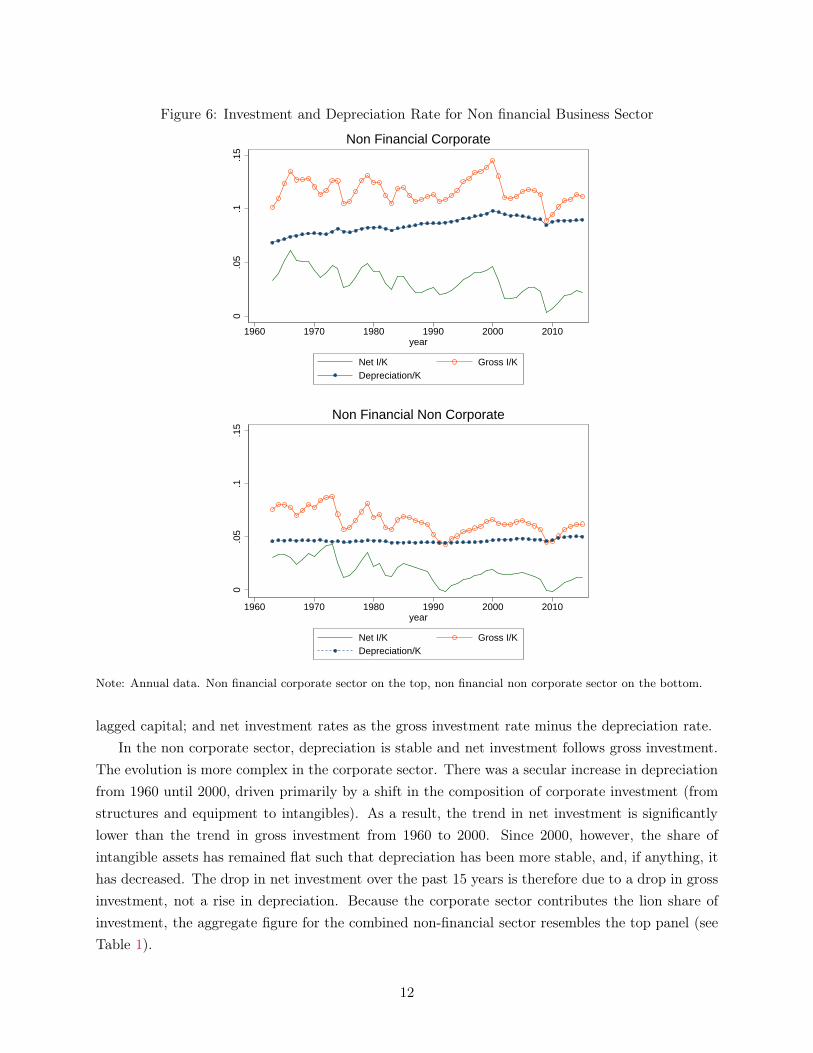
Figure 6: Investment and Depreciation Rate for Non financial Business Sector

0.0

5.1

.15

1960 1970 1980 1990 2000 2010year

Net I/K Gross I/KDepreciation/K

Non Financial Corporate

0.0

5.1

.15

1960 1970 1980 1990 2000 2010year

Net I/K Gross I/KDepreciation/K

Non Financial Non Corporate

Note: Annual data. Non financial corporate sector on the top, non financial non corporate sector on the bottom.

lagged capital; and net investment rates as the gross investment rate minus the depreciation rate.

In the non corporate sector, depreciation is stable and net investment follows gross investment.

The evolution is more complex in the corporate sector. There was a secular increase in depreciation

from 1960 until 2000, driven primarily by a shift in the composition of corporate investment (from

structures and equipment to intangibles). As a result, the trend in net investment is significantly

lower than the trend in gross investment from 1960 to 2000. Since 2000, however, the share of

intangible assets has remained flat such that depreciation has been more stable, and, if anything, it

has decreased. The drop in net investment over the past 15 years is therefore due to a drop in gross

investment, not a rise in depreciation. Because the corporate sector contributes the lion share of

investment, the aggregate figure for the combined non-financial sector resembles the top panel (see

Table 1).

12

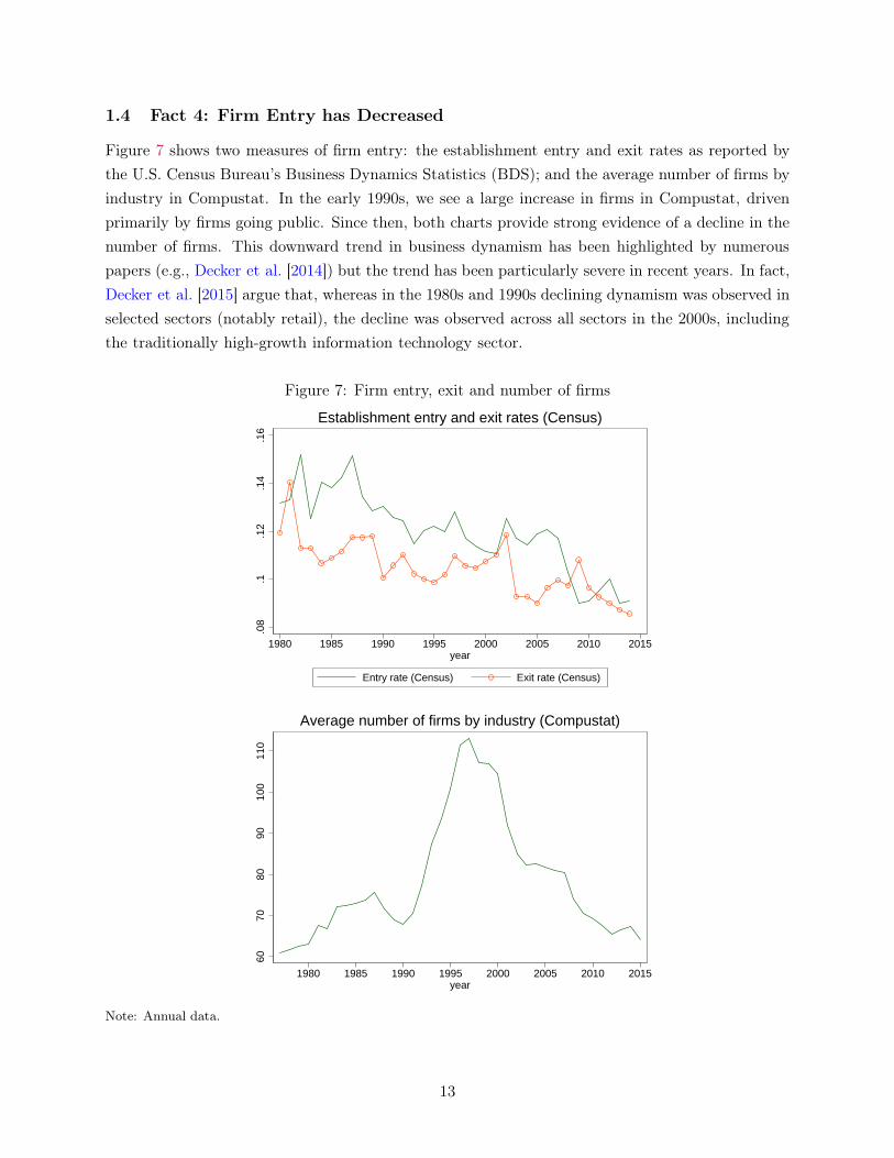
1.4 Fact 4: Firm Entry has Decreased

Figure 7 shows two measures of firm entry: the establishment entry and exit rates as reported by

the U.S. Census Bureau’s Business Dynamics Statistics (BDS); and the average number of firms by

industry in Compustat. In the early 1990s, we see a large increase in firms in Compustat, driven

primarily by firms going public. Since then, both charts provide strong evidence of a decline in the

number of firms. This downward trend in business dynamism has been highlighted by numerous

papers (e.g., Decker et al. [2014]) but the trend has been particularly severe in recent years. In fact,

Decker et al. [2015] argue that, whereas in the 1980s and 1990s declining dynamism was observed in

selected sectors (notably retail), the decline was observed across all sectors in the 2000s, including

the traditionally high-growth information technology sector.

Figure 7: Firm entry, exit and number of firms

.08

.1.1

2.1

4.1

6

1980 1985 1990 1995 2000 2005 2010 2015year

Entry rate (Census) Exit rate (Census)

Establishment entry and exit rates (Census)

6070

8090

100

110

1980 1985 1990 1995 2000 2005 2010 2015year

Average number of firms by industry (Compustat)

Note: Annual data.

13

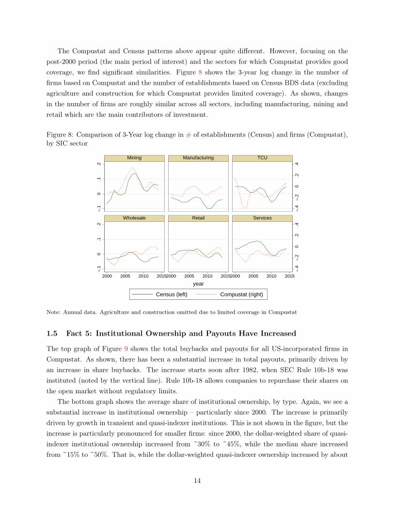
The Compustat and Census patterns above appear quite different. However, focusing on the

post-2000 period (the main period of interest) and the sectors for which Compustat provides good

coverage, we find significant similarities. Figure 8 shows the 3-year log change in the number of

firms based on Compustat and the number of establishments based on Census BDS data (excluding

agriculture and construction for which Compustat provides limited coverage). As shown, changes

in the number of firms are roughly similar across all sectors, including manufacturing, mining and

retail which are the main contributors of investment.

Figure 8: Comparison of 3-Year log change in # of establishments (Census) and firms (Compustat),by SIC sector

−.4

−.2

0.2

.4−.

4−.

20

.2.4

−.1

0.1

.2−.

10

.1.2

2000 2005 2010 20152000 2005 2010 20152000 2005 2010 2015

Mining Manufacturing TCU

Wholesale Retail Services

Census (left) Compustat (right)

year

Note: Annual data. Agriculture and construction omitted due to limited coverage in Compustat

1.5 Fact 5: Institutional Ownership and Payouts Have Increased

The top graph of Figure 9 shows the total buybacks and payouts for all US-incorporated firms in

Compustat. As shown, there has been a substantial increase in total payouts, primarily driven by

an increase in share buybacks. The increase starts soon after 1982, when SEC Rule 10b-18 was

instituted (noted by the vertical line). Rule 10b-18 allows companies to repurchase their shares on

the open market without regulatory limits.

The bottom graph shows the average share of institutional ownership, by type. Again, we see a

substantial increase in institutional ownership – particularly since 2000. The increase is primarily

driven by growth in transient and quasi-indexer institutions. This is not shown in the figure, but the

increase is particularly pronounced for smaller firms: since 2000, the dollar-weighted share of quasi-

indexer institutional ownership increased from ~30% to ~45%, while the median share increased

from ~15% to ~50%. That is, while the dollar-weighted quasi-indexer ownership increased by about

14

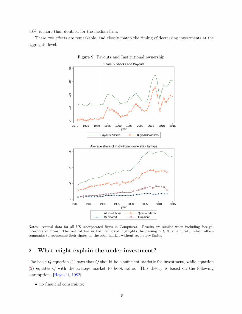
50%, it more than doubled for the median firm.

These two effects are remarkable, and closely match the timing of decreasing investments at the

aggregate level.

Figure 9: Payouts and Institutional ownership

0.0

2.0

4.0

6.0

8

1970 1975 1980 1985 1990 1995 2000 2005 2010 2015year

Payouts/Assets Buybacks/Assets

Share Buybacks and Payouts0

.2.4

.6

1980 1985 1990 1995 2000 2005 2010 2015year

All institutions Quasi−IndexerDedicated Transient

Average share of institutional ownership, by type

Notes: Annual data for all US incorporated firms in Compustat. Results are similar when including foreign-incorporated firms. The vertical line in the first graph highlights the passing of SEC rule 10b-18, which allowscompanies to repurchase their shares on the open market without regulatory limits.

2 What might explain the under-investment?

The basic Q-equation (1) says that Q should be a sufficient statistic for investment, while equation

(2) equates Q with the average market to book value. This theory is based on the following

assumptions [Hayashi, 1982]:

• no financial constraints;

15

• shareholder value maximization;

• constant returns to scale and perfect competition;

Low investment despite high levels of Q might be explained by a variety of theories – we consider

the following eight (grouped into four broad categories)8:

• Financial frictions

1. External finance constraints: A large literature has argued that frictions in finan-

cial markets can constrain investment decisions and force firms to rely on internal funds.

See Fazzari et al. [1987], Gomes [2001], Moyen [2004], and Hennessy and Whited [2007].9

Similarly, Rajan and Zingales [1998] show that industrial sectors that are relatively more

in need of external financing develop disproportionately faster in countries with more

developed financial markets. Thus, if certain sectors depend on external finance to in-

vest and are unable to obtain the required funds, they may under-invest relative to Q.

Relatedly, Acharya and Plantin [2016] study optimal monetary policy in the presence of

financial stability concerns. They show that monetary easing subsidizes inefficient ma-

turity transformation by financial intermediaries, which crowds out real investment (by

re-allocating savings away from real investment into carry trades).

2. Bank dependence: Financial constraints may differ between bank-dependent firms

and firms with access to the capital markets. As a result, we also test whether bank

dependent firms are responsible for the under-investment (see, for instance, Alfaro et al.

[2015]). This hypothesis is supported by recent papers such as Chen et al. [2016], which

shows that reductions in small business lending has affected investment by smaller firms.10

3. Safe asset scarcity: Safe asset scarcity and/or changes in the composition of assets

may affect corporations’ capital costs (see Caballero and Farhi [2014], for example). In

their simple form, such variations would impact Q. They would not cause a gap between

Q and investment. However, a gap may appear if safe firms are unable or unwilling to

take full advantage of low funding cost (due to, for example, product market rents). See

section 4.2.5 for additional discussion and results relevant to this hypothesis.

• Measurement Error8We also considered changes in R&D expenses as a proxy for lack of ideas (i.e., differences between average and

marginal Q). Firms increasing R&D expenses are likely to have better ideas and therefore a higher marginal Q. Sowe test whether under-investing industries (and firms) exhibit a parallel decrease in R&D expense. We do not findsupport for this hypothesis, but this is inconclusive: under some theories, a rise in R&D may actually imply lowermarginal Q (e.g., if ideas are harder to identify). We were unable to find a better measure for (lack of) ideas, so wecannot rule out this hypothesis.

9There is considerable controversy about the implications of financial frictions, of course, but this does not matterfor our analysis because we are not interested in estimating elasticities. While financial frictions make internal fundsrelevant, it is not at all clear that they increase the sensitivity of investment to cash flows. Kaplan and Zingales[1997] and Gomes [2001] show that financial frictions might not decrease the fit of the Q equation much.

10We should say from the outset that our ability to test this hypothesis is rather limited. Our industry dataincludes all firms, but investment is skewed and tends to be dominated by relatively large firms. Our firm-level datadoes not cover small firms.

16

4. Intangibles: The rise of intangibles may affect investment in several ways: first, in-

tangible investment is difficult to measure and is therefore prone to measurement error.

Under-estimation of I would lead to under-estimation of K, and therefore over-estimation

of Q; and would translate to an ‘observed’ under-investment at industries with a higher

share of intangibles. Alternatively, intangible assets might be more difficult to accu-

mulate. A rise in the relative importance of intangibles could then lead to a higher

equilibrium value of Q even if intangibles are correctly measured.

Both of these effects are analyzed in Peters and Taylor [2016]. They propose a new proxy

of Q that explicitly accounts for intangible capital, thereby correcting for measurement

error. This new proxy (referred to as ‘total Q’) is shown to be a better proxy of both

tangible and intangible investment.11 They also show that intangible capital adjusts

more slowly to changes in investment opportunities than tangible capital; which reflects

higher adjustment costs. 12

5. Globalization: official GDP statistics on private investment aim to capture investment

that occurs physically in the US, regardless of where the firm making the investment is

incorporated. For example, the investment series would include a manufacturing plant in

Michigan built by a German company and exclude investment in China by a US Retail

company. Thus, we may observe lower US private investment if US firms with foreign

activities are investing more abroad, or foreign firms are investing less in the US. This

would be pure measurement error: consolidated investment at the firm-level would still

follow Q, but would not be included in US Financial Accounts.

• Competition

6. Regulations & uncertainty: Regulation and regulatory uncertainty may affect invest-

ment in two ways. First, increased regulation may stifle competition by raising barriers

to entry. Second, per the theory of investment under uncertainty, irreversible investment

in an industry may decline if economic agents are uncertain about future payoffs (see,

for example, Bernanke [1983]). Thus, increased regulation and the associated regulatory

uncertainty may restrain investment.13

7. Concentration: A large literature has studied the link between competition, invest-

ment, and innovation (see Aghion et al. [2014] for a discussion). From a theoretical

11Our results are robust to using ‘total Q’ instead of the traditional measure of Q described in the data section,although the significance of QIX ownership decreases slightly at the industry-level.

12Intangibles can also interact with information technology and competition. For instance, Amazon does not needto open new stores to serve new customers; it simply needs to expand its distribution network. This may lead to alower equilibrium level of tangible capital (e.g., structures and equipment), thus a lower investment level on tangibleassets. But this would still be consistent with Q theory since the Q of the incumbent would fall. On the other hand,Amazon should increase its investments in intangible assets. Whether the Q of Amazon remains large then dependsmostly on competition. Finally, intangible assets can be used as a barrier to entry. For all these reasons, we thinkthat it is important to consider intangible investment together with competition.

13Increases in firm-specific uncertainty may also lead to lower investment levels due to manager risk-aversionPanousi and Papanikolauo [2012] and/or irreversible investment [Pindyck, 1988, Dixit and Pindyck, 1994]. We testthis hypothesis using stock market return and sales volatility; and find some, albeit limited support.

17

perspective, we know that the relationship is non-monotonic because of a trade-off be-

tween average and marginal profits. For a large set of parameters, however, we can expect

competition to increase innovation and investment. Firms in concentrated industries, ag-

ing industries and/or incumbents that do not face the threat of entry might have weak

incentives to invest.14

This hypothesis is supported by a growing literature that argues that competition may

be decreasing in several economic sectors (see for example CEA [2016], Decker et al.

[2015]) and is prevalent even at the product market level (e.g., Mongey [2016]). Simi-

larly, Jovanovic and Rousseau [2014] highlight differences in the sensitivity of investment

to Q between incumbents and new entrants. Blonigen and Pierce [2016] studies the im-

pact of mergers and acquisitions (M&As) on productivity and market power, and finds

that M&As are associated with increases in average markups. Given the rise in M&A

over the past decades, this suggests a potential rise in market power.

In addition, the rapid increase in institutional ownership (see Figure 9), and the increased

concentration in the asset management industry may have introduced substantial anti-

competitive effects of common ownership.15 Such anti-competitive effects are the subject

of a long theoretical literature in industrial organization, which argues that common

ownership of natural competitors may reduce incentives to compete (see, for example,

Salop and O’Brien [2000]). Azar et al. [2016a] and Azar et al. [2016b] show that this

effect is empirically important using the U.S. Airline and the U.S. Banking industries as

test cases.16

• Governance

8. Ownership and Shareholder Activism: beyond the anti-competitive effects of com-

mon ownership discussed above, ownership can affect management incentives through

short-termism (i.e., investment horizon) and governance. Regarding short-termism, some

have argued that equity markets can put excessive emphasis on quarterly earnings, and

that higher stock-based compensation incentivizes managers to focus on short term share

prices rather than long term profits (see Martin [2015], Lazonick [2014], for example).

In particular, Almeida et al. [2016] show that the probability of share repurchases is

sharply higher for firms that would have just missed the EPS forecast in the absence of

a repurchase; and Jolls [1998] shows that firms which rely heavily on stock-option-based

14We do not take a stand on the drivers of increased concentration; simply that it appears in the data.15For instance, Fichtner et al. [2016] show that the “Big Three” asset managers (BlackRock, Vanguard and State

Street) together constitute the largest shareholder in 88 percent of the S&P500 firms, which account for 82% ofmarket capitalization.

16It is worth noting that the exact mechanisms through which common ownership reduces competition remain tobe identified; but they need not be explicit directions from shareholders. They may result from lower incentives forowners to push firms to compete aggressively if they hold diversified positions in natural competitors; or from theability of board members elected by and representing the largest shareholders to minimize breakdowns of cooperativearrangements and undesirable price wars between their commonly owned firms. See Salop and O’Brien [2000] andAzar et al. [2016b] for additional details.

18

compensation are significantly more likely to repurchase their stock than firms which

rely less heavily on stock options to compensate their top executives. Given the rise of

institutional ownership, an increase in market-induced short-termism may lead firms to

increase buybacks and cut long term investment.

On the other hand, ownership may improve governance. A large literature following

Jensen [1986] argues that conflicts of interest between managers and shareholders can

lead firms to invest in ways that do not maximize shareholder value. 17 Harford et al.

[2008] and Richardson [2006] find evidence that poor governance associates with greater

industry-adjusted investment. Thus, improvements in governance driven by changes in

ownership may lead to lower investment levels.

The implications of shareholder activism and institutional ownership on governance and

payouts are studied in several papers. Appel et al. [2016a] find that passive owners influ-

ence firms’ governance choices (they lead to more independent directors, lower takeover

defenses, and more equal voting rights; as well as more votes against management).

Appel et al. [2016b] find that larger ownership stakes of passive institutional investors

make firms more susceptible to activist investors (increasing the ambitiousness of ac-

tivist objectives as well as the rate of success); and Crane et al. [2016] show that higher

(total and quasi-indexer) institutional ownership causes firms to increase their payouts.

But the evidence is not clear-cut: Schmidt and Fahlenbrach [2016] find opposite effects

for some governance measures (including the likelihood of CEO becoming chairman and

appointment of new independent directors), and an increase in value-destructing M&A

linked to higher institutional ownership.

In the end, it is unclear whether the higher payouts and the increased susceptibil-

ity to activist investors are evidence of tighter governance or increased short-termism.

Some papers provide qualitative support for governance (e.g., Crane et al. [2016] refer

to Chang et al. [2014] which argues that increasing passive institutional ownership leads

to share price increases), but it is inconclusive. And other studies such as Asker et al.

[2014] show that public firms invest substantially less and are less responsive to changes

in investment opportunities than private firms. In the end, we are unable to differen-

tiate between these two hypotheses empirically.18 Improvements in governance reduce

managerial entrenchment and require managers to continuously demonstrate strong per-

formance, just as increased short-termism would. We simply test whether increases in

(passive) institutional ownership lead to higher payouts and lower investment.

17This does not necessarily imply that managers invest too much; they might invest in the wrong projects instead.The general view, however, is that managers are reluctant to return cash to shareholders, and that they mightover-invest.

18This is true despite the very different mechanisms through which they impact investment: improved governancealigns the (manager’s) maximization problem with that of the shareholder’s, thereby increasing the focus on longterm value. Increased short-termism shifts the objective function of the maximization towards short-term value.

19

Table 2: Data sources

Data fields Source Granularity

Primary

datasets

Aggregate investment and Q Flow of Funds USIndustry-level investment andoperating surplus

BEA ~NAICS L3

Firm-level financials Compustat Firm

Additional

datasets

Sales and Market ValueConcentration

Census NAICS L3

Entry/Exit; firm demographics Census SIC L2Occupational Licensing PDII Survey NAICS L3Regulation index Mercatus NAICS L3Industry-level spreads Egon Zakrajsek NAICS L3Institutional ownership Thomson Reuters 13F FirmBushee’s institutional investorclassification

Brian Bushee’s website InstitutionalInvestor

3 Data

Testing the above theories requires the use of micro data. We gather and analyze a wide range

of aggregate-, industry- and firm-level data. The data fields and data sources are summarized in

Table 2. Sections 3.1 and 3.2 discuss the aggregate and industry datasets, respectively. Section

3.3 discusses the firm-level investment and Q datasets; and 3.4 discusses all other data sources,

including the explanatory variables used to test each theory. We discuss data reconciliation and

data validation results where appropriate.

3.1 Aggregate data

Aggregate data on funding costs, profitability, investment and market value for the US Economy

and the non financial sector is gathered from the US Flow of Funds accounts through FRED. These

data are used in the aggregate analyses discussed in Section 1; in the construction of aggregate Q;

and to reconcile and ensure the accuracy of more granular data. In addition, data on aggregate firm

entry and exit is gathered from the Census BDS; and used in aggregate regressions similar to those

reported in Section 4.

3.2 Industry investment data

3.2.1 Dataset

Industry-level investment and profitability data – including measures of private fixed assets (current-

cost and chained values for the net stock of capital, depreciation and investment) and value added

(gross operating surplus, compensation and taxes) – are gathered from the Bureau of Economic

Analysis (BEA).

20

Fixed assets data is available in three categories: structures, equipment and intellectual property

(which includes includes software, R&D and expenditures for entertainment, literary, and artistic

originals, among others). This breakdown allows us to (i) study investment patterns for intellectual

property separate from the more ‘traditional’ definitions of K (structures and equipment); and (ii)

better capture total investment in aggregate regressions, as opposed to only capital expenditures.

Investment and profitability data are available at the sector (19 groups) and detailed industry

(63 groups) level, in a similar categorization as the 2007 NAICS Level 3. We start with the 63

detailed industries and group them into 47 industry groupings to ensure investment, entry and

concentration measures are stable over time. In particular, we group detailed industries to ensure

each group has at least ~10 firms, on average, from 1990 - 2015 and it contributes a material share

of investment (see Appendix I: Industry Investment Data for details on the investment dataset).

We exclude Financials and Real Estate; and also exclude Utilities given the influence of government

actions in their investment and their unique experience after the crisis (e.g., they exhibit decreasing

operating surplus since 2000). Last, we exclude Management because there are no companies in

Compustat that map to this category. This leaves 43 industry groupings for our analyses, whose

total net investment since 2000 is summarized in Table 14 in the appendix. All other datasets are

mapped into these 43 industry groupings using the NAICS Level 3 mapping provided by the BEA.

We define industry-level gross investment rates as the ratio of ‘Investment in Private Fixed

Assets’ to lagged ‘Current-Cost Net Stock of Private Fixed Assets’; depreciation rates as the ratio

of ‘Current-Cost Depreciation of Private Fixed Assets’ to lagged ‘Current-Cost Net Stock of Private

Fixed Assets’; and net investment rates as the gross investment rate minus the depreciation rate.

Investment rates are computed across all asset types, as well as separating intellectual property

from structures and equipment.

The Gross Operating Surplus is provided by the BEA, while the Net Operating Surplus is

computed as the ‘Gross Operating Surplus’ minus ‘Current-Cost Depreciation of Private Fixed

Assets’. OS/K is defined as the ‘Net Operating Surplus’ over the lagged ‘Current-Cost Net Stock

of Private Fixed Assets’.

3.2.2 Data validation

In order to ensure industry-level figures are consistent with aggregate data, we reconcile the two

datasets. We first note that industry-level figures include all forms of organization (financials and

non financials, as well as corporates, non corporates and non businesses). A breakdown between

financials and non financials or corporates and non corporates by industry is not available. Thus,

a full reconciliation can only be achieved at the aggregate level or considering pre-aggregated BEA

series (such as non financial corporates). But these do not provide an industry breakdown. Instead,

we note that aggregating capital, depreciation and operating surplus across all industries except

Financials and Real Estate yields very similar series as the aggregated non financial business series

from the Flow of Funds (see Figure 10). The remaining differences appear to be explained by

non-businesses (households and non profit organizations) but cannot be reconciled due to data

21

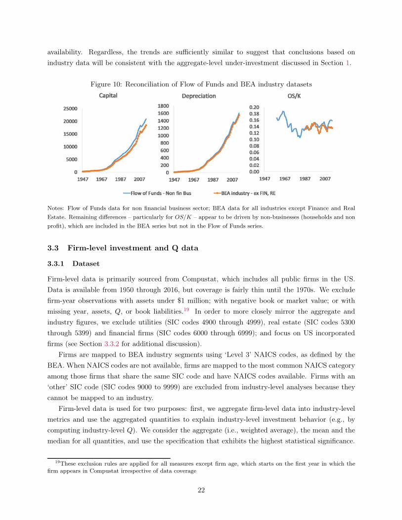
availability. Regardless, the trends are sufficiently similar to suggest that conclusions based on

industry data will be consistent with the aggregate-level under-investment discussed in Section 1.

Figure 10: Reconciliation of Flow of Funds and BEA industry datasets

Notes: Flow of Funds data for non financial business sector; BEA data for all industries except Finance and Real

Estate. Remaining differences – particularly for OS/K – appear to be driven by non-businesses (households and non

profit), which are included in the BEA series but not in the Flow of Funds series.

3.3 Firm-level investment and Q data

3.3.1 Dataset

Firm-level data is primarily sourced from Compustat, which includes all public firms in the US.

Data is available from 1950 through 2016, but coverage is fairly thin until the 1970s. We exclude

firm-year observations with assets under $1 million; with negative book or market value; or with

missing year, assets, Q, or book liabilities.19 In order to more closely mirror the aggregate and

industry figures, we exclude utilities (SIC codes 4900 through 4999), real estate (SIC codes 5300

through 5399) and financial firms (SIC codes 6000 through 6999); and focus on US incorporated

firms (see Section 3.3.2 for additional discussion).

Firms are mapped to BEA industry segments using ‘Level 3’ NAICS codes, as defined by the

BEA. When NAICS codes are not available, firms are mapped to the most common NAICS category

among those firms that share the same SIC code and have NAICS codes available. Firms with an

‘other’ SIC code (SIC codes 9000 to 9999) are excluded from industry-level analyses because they

cannot be mapped to an industry.

Firm-level data is used for two purposes: first, we aggregate firm-level data into industry-level

metrics and use the aggregated quantities to explain industry-level investment behavior (e.g., by

computing industry-level Q). We consider the aggregate (i.e., weighted average), the mean and the

median for all quantities, and use the specification that exhibits the highest statistical significance.

19These exclusion rules are applied for all measures except firm age, which starts on the first year in which thefirm appears in Compustat irrespective of data coverage

22

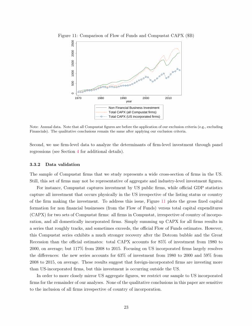
Figure 11: Comparison of Flow of Funds and Compustat CAPX ($B)

050

010

0015

0020

0025

00

1970 1980 1990 2000 2010year

Non Financial Business InvestmentTotal CAPX (all Compustat firms)Total CAPX (US incorporated firms)

Note: Annual data. Note that all Compustat figures are before the application of our exclusion criteria (e.g., excludingFinancials). The qualitative conclusions remain the same after applying our exclusion criteria.

Second, we use firm-level data to analyze the determinants of firm-level investment through panel

regressions (see Section 4 for additional details).

3.3.2 Data validation

The sample of Compustat firms that we study represents a wide cross-section of firms in the US.

Still, this set of firms may not be representative of aggregate and industry-level investment figures.

For instance, Compustat captures investment by US public firms, while official GDP statistics

capture all investment that occurs physically in the US irrespective of the listing status or country

of the firm making the investment. To address this issue, Figure 11 plots the gross fixed capital

formation for non financial businesses (from the Flow of Funds) versus total capital expenditures

(CAPX) for two sets of Compustat firms: all firms in Compustat, irrespective of country of incorpo-

ration, and all domestically incorporated firms. Simply summing up CAPX for all firms results in

a series that roughly tracks, and sometimes exceeds, the official Flow of Funds estimates. However,

this Compustat series exhibits a much stronger recovery after the Dotcom bubble and the Great

Recession than the official estimates: total CAPX accounts for 85% of investment from 1980 to

2000, on average; but 117% from 2008 to 2015. Focusing on US incorporated firms largely resolves

the differences: the new series accounts for 63% of investment from 1980 to 2000 and 59% from

2008 to 2015, on average. These results suggest that foreign-incorporated firms are investing more

than US-incorporated firms, but this investment is occurring outside the US.

In order to more closely mirror US aggregate figures, we restrict our sample to US incorporated

firms for the remainder of our analyses. None of the qualitative conclusions in this paper are sensitive

to the inclusion of all firms irrespective of country of incorporation.

23

We are interested in using Compustat firm-level data to reach conclusions about industry-level

investment. Thus, we need to understand whether Compustat firms in a given industry provide a

good representation of the industry as a whole. We define the following two measures of ‘coverage’:

the ratio of Compustat total CAPX to BEA Investment by industry, and the ratio of Compustat

total PP&E to BEA Capital. Table 14 in the Appendix shows the coverage for the 43 industries

under consideration. As shown, our Compustat sample provides good coverage for the majority of

material industries. In particular, Compustat provides at least 10% coverage across both metrics for

19 industries, which account for 55% of total net investment from 2000 to 2015. The most material

sectors for which Compustat does not provide good coverage are Health Care, Professional Services

and Wholesale Trade.

Low coverage levels increase the noise in Compustat estimates, but are not expected to bias

the results. We therefore include all industries in our analyses, and confirm that qualitative results

remain stable when including only industries with >10% coverage across both metrics.

3.3.3 Investment definition

We consider two investment definitions. First, the ‘traditional’ gross investment rate is defined

as in Rajan and Zingales [1998] (among others): capital expenditures (Compustat item CAPX) at

time t scaled by net Property, Plant and Equipment (item PPENT) at time t− 1. Net investment

rate is calculated by imputing the industry-level depreciation rate from BEA figures. In particular,

note that the depreciation figures available in Compustat include only the portion of depreciation

that affects the income statement, and therefore exclude depreciation included as part of Cost of

Goods Sold. For consistency, and because we are interested in aggregate quantities, we assume all

firms in a given industry have the same depreciation rate, and compute the net investment rate as

the gross investment rate minus the BEA-implied depreciation rate for structures and equipment

in each industry. Second, we estimate investment in intangibles as the ratio of R&D expenses to

assets (Compustat XRD / AT)20. We consider only the gross investment rate (i.e., do not subtract

depreciation) because a good proxy for R&D depreciation is not available.21

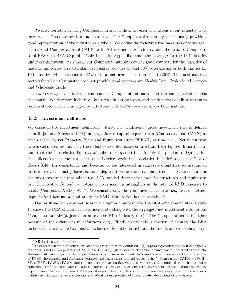
The resulting firm-level net investment figures closely mirror the BEA official estimates. Figure

11 shows the BEA official net investment rate along with the aggregate net investment rate for our

Compustat sample (adjusted to mirror the BEA industry mix). The Compustat series is higher

because of the differences in definitions (e.g., PP&E covers only a portion of capital; the BEA

includes all firms while Compustat includes only public firms), but the trends are very similar from

20XRD set to zero if missing21In order to ensure robustness, we also test three alternate definitions: (i) capital expenditures plus R&D expense

over total assets (Compustat (CAPX + XRD) / AT); (ii) a broader definition of investment constructed from thestatement of cash flows (capital expenditures plus increase in investments minus sale of investments over the sumof PP&E, Investment and Advances (equity) and Investment and Advances (other) (Compustat (CAPX + IVCH -SIV)/(PPE+IVAEQ+IVAO); and (iii) investment over market value, in which case Q is omitted from the regressionequations. Definitions (i) and (ii) aim to capture a broader set of long term investment activities than just capitalexpenditures. We use the total BEA-implied depreciation rate to compute net investment under all three alternatedefinitions. All qualitative conclusions are robust to using either of these broader definitions of investment.

24

Figure 12: Comparison of Compustat and BEA net investment rates

.08

.1.1

2.1

4.1

6.1

8C

ompu

stat

NI/K

0.0

1.0

2.0

3.0

4.0

5BE

A N

I/K

1970 1980 1990 2000 2010year

BEA NI/K Compustat NI/K

Note: Annual data. BEA and Compustat NI/K for selected sample.

each other.

3.3.4 Q definition

Firm-level stock Q is defined as the book value of total assets (AT) plus the market value of equity

(ME) minus the book value of equity scaled by the book value of total assets (AT). The market

value of equity (ME) is defined as the total number of common shares outstanding (item CSHO)

times the closing stock price at the end of the fiscal year (item PRCC_F). Book value of equity is

computed as AT - LT - PSTK.

Figure 13 shows the aggregate, mean and median Q across all firms in our Compustat sample,

along with the measure of Q constructed for non financial corporates using Flow of Funds data. As

shown, the aggregate and mean Q from Compustat closely mirror the Flow of Funds series. The

median Q is substantially lower in the early 2000s, because the corresponding increase in average

Q was driven by a few firms concentrated in particular industries. For some tests, we supplement

this traditional measure of Q with the ‘total Q’ of Peters and Taylor [2016], which aims to control

for intangible capital.

3.4 Explanatory Variables

Last, a wide range of additional variables are gathered and/or computed to test our eight theories

of under-investment.

3.4.1 Financial Frictions

External finance constraints. For external finance constraints, we are interested in the amount

of investment that cannot be financed through internal sources, i.e., the cash flow generated by the

25

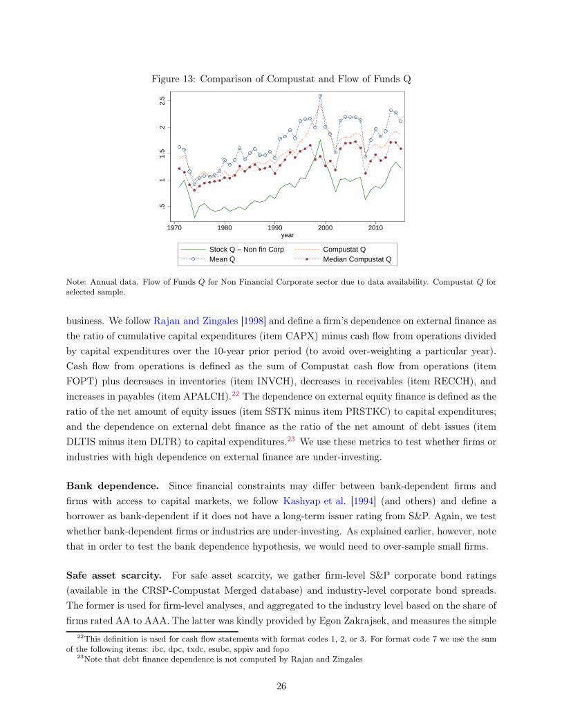
Figure 13: Comparison of Compustat and Flow of Funds Q

.51

1.5

22.

5

1970 1980 1990 2000 2010year

Stock Q − Non fin Corp Compustat QMean Q Median Compustat Q

Note: Annual data. Flow of Funds Q for Non Financial Corporate sector due to data availability. Compustat Q forselected sample.

business. We follow Rajan and Zingales [1998] and define a firm’s dependence on external finance as

the ratio of cumulative capital expenditures (item CAPX) minus cash flow from operations divided

by capital expenditures over the 10-year prior period (to avoid over-weighting a particular year).

Cash flow from operations is defined as the sum of Compustat cash flow from operations (item

FOPT) plus decreases in inventories (item INVCH), decreases in receivables (item RECCH), and

increases in payables (item APALCH).22 The dependence on external equity finance is defined as the

ratio of the net amount of equity issues (item SSTK minus item PRSTKC) to capital expenditures;

and the dependence on external debt finance as the ratio of the net amount of debt issues (item

DLTIS minus item DLTR) to capital expenditures.23 We use these metrics to test whether firms or

industries with high dependence on external finance are under-investing.

Bank dependence. Since financial constraints may differ between bank-dependent firms and

firms with access to capital markets, we follow Kashyap et al. [1994] (and others) and define a

borrower as bank-dependent if it does not have a long-term issuer rating from S&P. Again, we test

whether bank-dependent firms or industries are under-investing. As explained earlier, however, note

that in order to test the bank dependence hypothesis, we would need to over-sample small firms.

Safe asset scarcity. For safe asset scarcity, we gather firm-level S&P corporate bond ratings

(available in the CRSP-Compustat Merged database) and industry-level corporate bond spreads.

The former is used for firm-level analyses, and aggregated to the industry level based on the share of

firms rated AA to AAA. The latter was kindly provided by Egon Zakrajsek, and measures the simple

22This definition is used for cash flow statements with format codes 1, 2, or 3. For format code 7 we use the sumof the following items: ibc, dpc, txdc, esubc, sppiv and fopo

23Note that debt finance dependence is not computed by Rajan and Zingales

26

average corporate bond spread across all bonds in a given NAICS Level 3 code. This dataset was

used in Gilchrist and Zakrajsek [2011]. Not all industries are covered by the bond spread dataset.

3.4.2 Measurement Error

Intangibles. For Intangibles, we compute two types of metrics. First, we compute the investment

rate for tangible and intangible assets separately (as described above) and use these to (i) test

for under-investment in intangible assets and (ii) test whether the hypotheses supported for total

investment also hold for intangible assets. Second, we compute the ratio of intangibles excluding

goodwill to assets (Compustat (INTAN-GDWL)/AT); and use this ratio to test for measurement

error in intangibles. See Section 4.2.6 for additional details. Goodwill is excluded because it

primarily measures M&A activity, not formation of intangible capital.24

Globalization. For Globalization, we use Compustat item PRETAX INCOME - FOREIGN to

identify industries and firms with substantial foreign activities. This field contains the income of

a company’s foreign operations before taxes. It is reported only by some firms25, yet there are no

other indicators of the extent of a firm’s foreign operations available in Compustat (Foley et al.

[2007]). For industry-level analyses, we compute the industry share of foreign income as the ratio of

total PRETAX INCOME - FOREIGN to total PRETAX INCOME (i.e., across all firms in a given

industry and year). For firm-level analyses, we consider three transformations of foreign activities

given the potential for missing data: one omitting all firms with missing PRETAX INCOME -

FOREIGN; one setting missing PRETAX INCOME - FOREIGN equal to zero; and one with an

indicator for populated PRETAX INCOME - FOREIGN. We use these measures to test whether

industries with substantial foreign activities are over-investing relative to Q.

3.4.3 Competition

Regulation and Uncertainty For regulation and uncertainty, we consider two measures.

As a measure of the amount and change in regulations affecting a particular industry, we gather

the Regulation index published by the Mercatus Center at George Mason University. The index

relies on text analysis to count the number of relevant restrictions for each NAICS Level 3 in-

dustry from 1970 to 2014. Note that most, but not all industries are covered by the index. See

Al-Ubaydli and McLaughlin [2015] for additional details. Second, as a proxy for barriers to entry,

we gather the share of workers requiring Occupational Licensing in each NAICS Level 3 industry

from the 2008 PDII.26

24We also tested the ratio of intangibles to assets, but excluding goodwill is more appropriate and exhibits astronger link to investment

25Security and Exchange Commission regulations stipulate that firms should report foreign activities separatelyin each year that foreign assets, revenues or income exceed 10% of total activities

26The 2008 PDII was conducted by Westat, and analyzed in Kleiner and Krueger [2013]. It is based on a surveyof individual workers from across the nation.

27

Concentration and demographics. For concentration and firm demographics we use three

different sources: Compustat, the US Census Bureau and Thomson-Reuters’ Institutional Holdings

(13F) Database.

From Compustat, we compute four measures of concentration (i) the log-change in the number

of firms in a given industry as a measure of entry and exit; (ii) sales Herfindahls27, (iii) the share

of sales and market value held by the top 4, 8 and 20 firms in each industry, and (iv) the price-

cost ratio (also known as the Lerner index). We use Compustat item SALE for measures of sales

concentration and market value as defined in the computation of Q above for measures of market

value concentration. To compute the Lerner index, we follow Datta et al. [2013] and calculate the

ratio of operating profit (Compustat SALE - COGS - XSGA) to sales. We also compute (iv) age

(from entrance into Compustat) and (v) size (log of total assets) as measures of firm demographics.

The Lerner index differs from the Herfindahl and Concentration ratios because it does not rely on

precise definitions of geographic and product markets; rather it aims to measure a firm’s ability to

extract rents from the market.

From the U.S. Census Bureau, we gather industry-level establishment entry/exit rates and de-

mographics (age and size); and industry-level measures of sales and market value concentration The

former are available in the Business Dynamics Statistics (BDS) for 9 broad sectors (SIC Level 2)

since 1977. The latter are sourced from the Economic Census, and include the share of sales/market

value held by the top 4, 8, 20 and 50 firms in each industry; and are available for a subset of NAICS

Level 3 industries for 1997, 2002, 2007 and 2012. We aggregate concentration ratios to our 43

industry groupings by taking the average across industries.

The main benefit of the census data is that it covers all US firms (public and private). But

the limited granularity/coverage poses significant limitations for its use in regression analyses. We

mapped the 9 SIC sectors for which census entry/exit data are available to the BEA investment

categories and analyzed industry-level investment patterns. However, limited conclusions could be

reached given the very broad segmentation: Q exhibited significant measurement error, leading to

unintuitive coefficients. So we use these data only to validate the representativeness of relevant

Compustat series. For instance, Figure 8 above shows that from 2000 onward, changes in the

number firms in Compustat closely resemble those of the US as a whole.

Similarly, the census concentration data is available at a more granular level, but only for a subset

of years and industries. We use these metrics to test whether more concentrated industries exhibit

lower investment; and to compare nationwide concentration measures with those computed from

Compustat. Census and Compustat measures of concentration are found to be fairly correlated,

and both are significant predictors of industry-wide (under-)investment. We use Compustat as the

basis of our analyses because the corresponding measures are available for all industries and all

years; but we also report some regression results using Census-based concentration measures.

Last, to account for anti-competitive effects of common ownership, we compute the modified

Herfindahl. We use Compustat as well as Thomson-Reuters’ Institutional Holdings (see the next sub-

27Market value Herfindahl also considered, but Sales Herfindahl performs better and is therefore reported.

28

section). The Modified Herfindahl – described in Salop and O’Brien [2000] and Azar et al. [2016b]

– is defined as

MHHI = HHI +∑

j

∑

k ̸̸=j

sjsk

∑

i γijβik∑

i γijβij

= HHI +HHIadj

where sj and sk denote the share of sales for firms j, k in a given industry. γij and βik denote

the control share and the ownership share of investor i in firm j, respectively. The first term is

the traditional Herfindahl, while the second term is a measure of the anti-competitive incentives

due to common ownership. Theoretical justification for this measure can be derived using the

modified Herfindahl-Hirschman Index (MHHI) in a Cournot setting. See Salop and O’Brien [2000]

and Azar et al. [2016b] for additional details. We consider the combined MHHI in most of our

tests; but also separate HHI and HHIadj to assess their impact independently in some cases.

We make two assumptions to compute this measure empirically: first, because ownership data

is only available for institutional investors, we compute γij and βik as the control and ownership

share of investor i in firm j relative to total institutional ownership reported in the 13F database,

not total ownership. This is not expected to substantially influence the results because ownership

by non-institutional investors is likely limited and restricted to a single firm, which does not induce

common ownership links. Second, because data on the total number of voting shares per company is

not readily available, we assume γij = βik (i.e., we consider total ownership rather than voting and

non-voting shares separately).28 Last, following Azar et al. [2016b], we restrict the data to holdings

of at least 0.5% of shares outstanding.

3.4.4 Governance

For governance, we gather data on institutional ownership from Thomson-Reuters’ Institutional

Holdings (13F) Database. This data set includes investments in all US publicly traded stocks by

institutional investors managing more than $100 million.

We define the share of institutional ownership as the ratio of shares owned by fund managers filing

13Fs on a given firm over total shares outstanding.29 We also add Brian Bushee’s permanent clas-

sification of institutional owners (transient, quasi-indexer, and dedicated), available on his website.

This classification is based on the turnover and diversification of institutional investor’s holdings.

Dedicated institutions have large, long-term holdings in a small number of firms. Quasi-indexers

have diversified holdings and low portfolio turnover – consistent with a passive, buy-and-hold strat-

egy of investing portfolio funds in a broad set of firms. Transient owners have high diversification

and high portfolio turnover. Quasi-indexers are the largest category, and account for ~60% of total

28We also measured γij based on the (sole and shared) voting shares held by institutional investors only, but thisexhibits lower statistical significance.

29We use CRSP’s total shares outstanding instead of Thomson Reuter’s since the latter are available only inmillions for some periods.

29

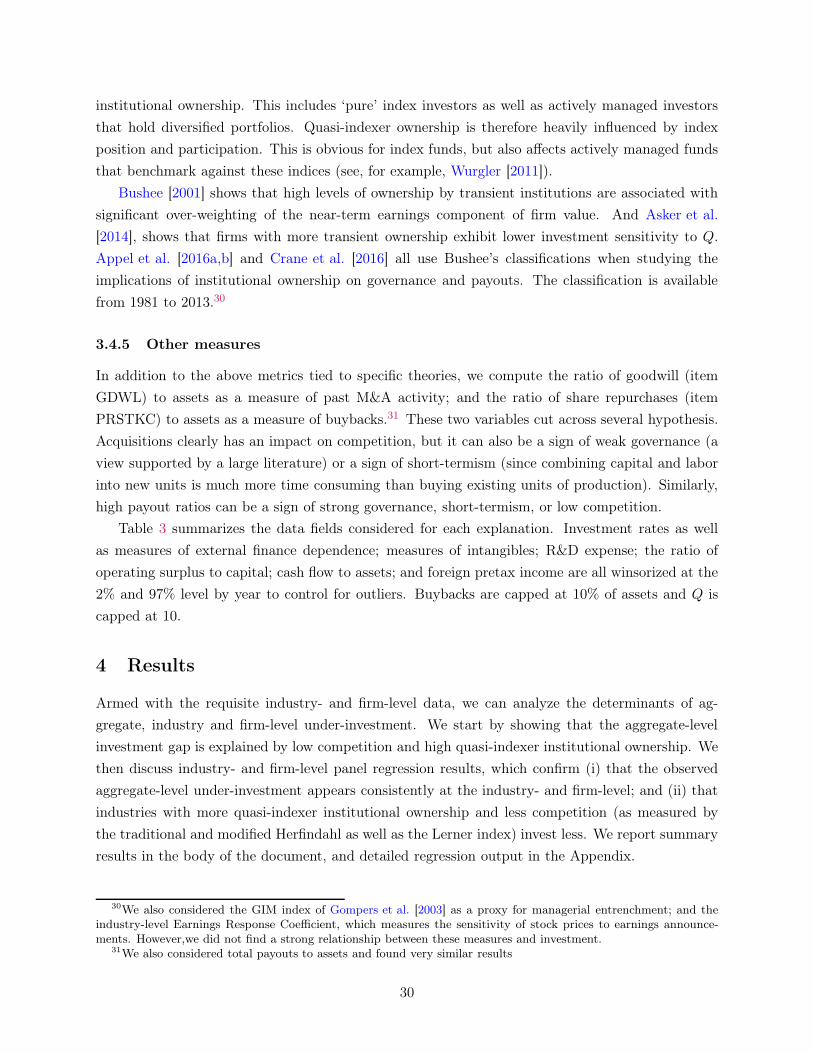
institutional ownership. This includes ‘pure’ index investors as well as actively managed investors

that hold diversified portfolios. Quasi-indexer ownership is therefore heavily influenced by index

position and participation. This is obvious for index funds, but also affects actively managed funds

that benchmark against these indices (see, for example, Wurgler [2011]).

Bushee [2001] shows that high levels of ownership by transient institutions are associated with

significant over-weighting of the near-term earnings component of firm value. And Asker et al.

[2014], shows that firms with more transient ownership exhibit lower investment sensitivity to Q.

Appel et al. [2016a,b] and Crane et al. [2016] all use Bushee’s classifications when studying the

implications of institutional ownership on governance and payouts. The classification is available

from 1981 to 2013.30

3.4.5 Other measures

In addition to the above metrics tied to specific theories, we compute the ratio of goodwill (item

GDWL) to assets as a measure of past M&A activity; and the ratio of share repurchases (item

PRSTKC) to assets as a measure of buybacks.31 These two variables cut across several hypothesis.

Acquisitions clearly has an impact on competition, but it can also be a sign of weak governance (a

view supported by a large literature) or a sign of short-termism (since combining capital and labor

into new units is much more time consuming than buying existing units of production). Similarly,

high payout ratios can be a sign of strong governance, short-termism, or low competition.

Table 3 summarizes the data fields considered for each explanation. Investment rates as well

as measures of external finance dependence; measures of intangibles; R&D expense; the ratio of

operating surplus to capital; cash flow to assets; and foreign pretax income are all winsorized at the

2% and 97% level by year to control for outliers. Buybacks are capped at 10% of assets and Q is

capped at 10.

4 Results

Armed with the requisite industry- and firm-level data, we can analyze the determinants of ag-

gregate, industry and firm-level under-investment. We start by showing that the aggregate-level

investment gap is explained by low competition and high quasi-indexer institutional ownership. We

then discuss industry- and firm-level panel regression results, which confirm (i) that the observed

aggregate-level under-investment appears consistently at the industry- and firm-level; and (ii) that

industries with more quasi-indexer institutional ownership and less competition (as measured by

the traditional and modified Herfindahl as well as the Lerner index) invest less. We report summary

results in the body of the document, and detailed regression output in the Appendix.

30We also considered the GIM index of Gompers et al. [2003] as a proxy for managerial entrenchment; and theindustry-level Earnings Response Coefficient, which measures the sensitivity of stock prices to earnings announce-ments. However,we did not find a strong relationship between these measures and investment.

31We also considered total payouts to assets and found very similar results

30

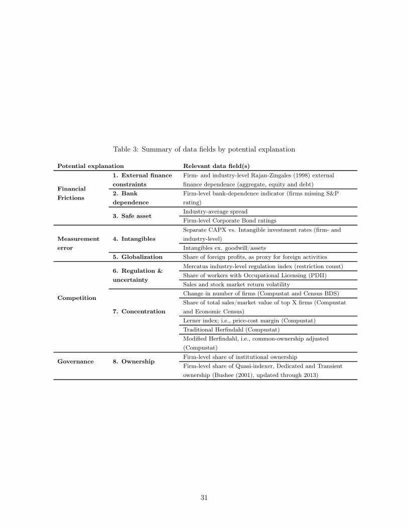
Table 3: Summary of data fields by potential explanation

Potential explanation Relevant data field(s)

Financial

Frictions

1. External finance

constraints

Firm- and industry-level Rajan-Zingales (1998) external

finance dependence (aggregate, equity and debt)

2. Bank

dependence

Firm-level bank-dependence indicator (firms missing S&P

rating)

3. Safe assetIndustry-average spread

Firm-level Corporate Bond ratings

Measurement

error

4. Intangibles

Separate CAPX vs. Intangible investment rates (firm- and

industry-level)

Intangibles ex. goodwill/assets

5. Globalization Share of foreign profits, as proxy for foreign activities

Competition

6. Regulation &

uncertainty

Mercatus industry-level regulation index (restriction count)

Share of workers with Occupational Licensing (PDII)

Sales and stock market return volatility

7. Concentration

Change in number of firms (Compustat and Census BDS)

Share of total sales/market value of top X firms (Compustat

and Economic Census)

Lerner index; i.e., price-cost margin (Compustat)

Traditional Herfindahl (Compustat)

Modified Herfindahl, i.e., common-ownership adjusted

(Compustat)

Governance 8. OwnershipFirm-level share of institutional ownership

Firm-level share of Quasi-indexer, Dedicated and Transient

ownership (Bushee (2001), updated through 2013)

31

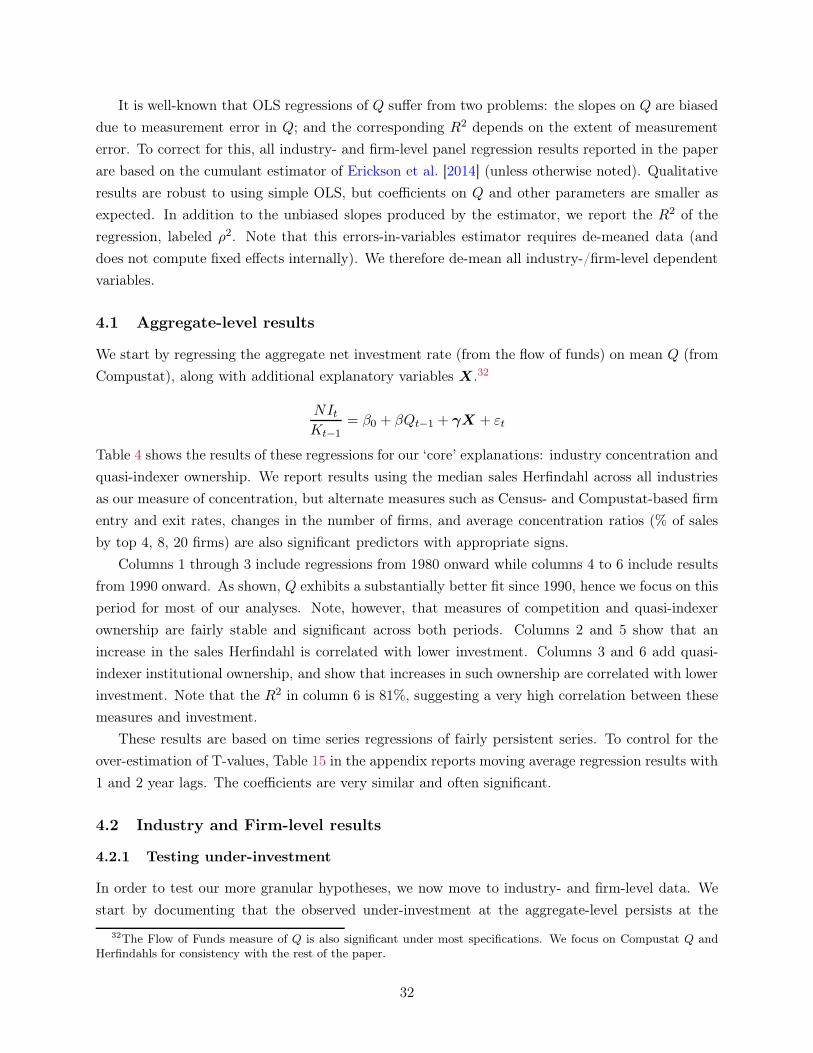
It is well-known that OLS regressions of Q suffer from two problems: the slopes on Q are biased

due to measurement error in Q; and the corresponding R2 depends on the extent of measurement

error. To correct for this, all industry- and firm-level panel regression results reported in the paper

are based on the cumulant estimator of Erickson et al. [2014] (unless otherwise noted). Qualitative

results are robust to using simple OLS, but coefficients on Q and other parameters are smaller as

expected. In addition to the unbiased slopes produced by the estimator, we report the R2 of the

regression, labeled ρ2. Note that this errors-in-variables estimator requires de-meaned data (and

does not compute fixed effects internally). We therefore de-mean all industry-/firm-level dependent

variables.

4.1 Aggregate-level results

We start by regressing the aggregate net investment rate (from the flow of funds) on mean Q (from

Compustat), along with additional explanatory variables X.32

NItKt−1

= β0 + βQt−1 + γX + εt

Table 4 shows the results of these regressions for our ‘core’ explanations: industry concentration and

quasi-indexer ownership. We report results using the median sales Herfindahl across all industries

as our measure of concentration, but alternate measures such as Census- and Compustat-based firm

entry and exit rates, changes in the number of firms, and average concentration ratios (% of sales

by top 4, 8, 20 firms) are also significant predictors with appropriate signs.

Columns 1 through 3 include regressions from 1980 onward while columns 4 to 6 include results

from 1990 onward. As shown, Q exhibits a substantially better fit since 1990, hence we focus on this

period for most of our analyses. Note, however, that measures of competition and quasi-indexer

ownership are fairly stable and significant across both periods. Columns 2 and 5 show that an

increase in the sales Herfindahl is correlated with lower investment. Columns 3 and 6 add quasi-

indexer institutional ownership, and show that increases in such ownership are correlated with lower

investment. Note that the R2 in column 6 is 81%, suggesting a very high correlation between these

measures and investment.

These results are based on time series regressions of fairly persistent series. To control for the

over-estimation of T-values, Table 15 in the appendix reports moving average regression results with

1 and 2 year lags. The coefficients are very similar and often significant.

4.2 Industry and Firm-level results

4.2.1 Testing under-investment

In order to test our more granular hypotheses, we now move to industry- and firm-level data. We

start by documenting that the observed under-investment at the aggregate-level persists at the

32The Flow of Funds measure of Q is also significant under most specifications. We focus on Compustat Q andHerfindahls for consistency with the rest of the paper.

32

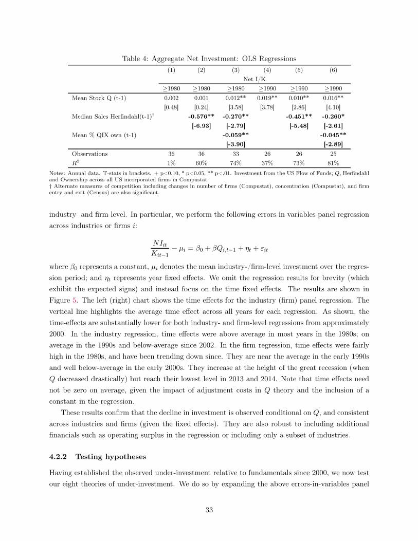
Table 4: Aggregate Net Investment: OLS Regressions

(1) (2) (3) (4) (5) (6)

Net I/K

≥1980 ≥1980 ≥1980 ≥1990 ≥1990 ≥1990

Mean Stock Q (t-1) 0.002 0.001 0.012** 0.019** 0.010** 0.016**

[0.48] [0.24] [3.58] [3.78] [2.86] [4.10]

Median Sales Herfindahl(t-1)† -0.576** -0.270** -0.451** -0.260*

[-6.93] [-2.79] [-5.48] [-2.61]

Mean % QIX own (t-1) -0.059** -0.045**

[-3.90] [-2.89]

Observations 36 36 33 26 26 25

R2 1% 60% 74% 37% 73% 81%

Notes: Annual data. T-stats in brackets. + p<0.10, * p<0.05, ** p<.01. Investment from the US Flow of Funds; Q, Herfindahland Ownership across all US incorporated firms in Compustat.† Alternate measures of competition including changes in number of firms (Compustat), concentration (Compustat), and firmentry and exit (Census) are also significant.

industry- and firm-level. In particular, we perform the following errors-in-variables panel regression

across industries or firms i:

NIitKit−1

− µi = β0 + βQi,t−1 + ηt + εit

where β0 represents a constant, µi denotes the mean industry-/firm-level investment over the regres-

sion period; and ηt represents year fixed effects. We omit the regression results for brevity (which

exhibit the expected signs) and instead focus on the time fixed effects. The results are shown in

Figure 5. The left (right) chart shows the time effects for the industry (firm) panel regression. The

vertical line highlights the average time effect across all years for each regression. As shown, the

time-effects are substantially lower for both industry- and firm-level regressions from approximately

2000. In the industry regression, time effects were above average in most years in the 1980s; on

average in the 1990s and below-average since 2002. In the firm regression, time effects were fairly

high in the 1980s, and have been trending down since. They are near the average in the early 1990s

and well below-average in the early 2000s. They increase at the height of the great recession (when

Q decreased drastically) but reach their lowest level in 2013 and 2014. Note that time effects need

not be zero on average, given the impact of adjustment costs in Q theory and the inclusion of a

constant in the regression.

These results confirm that the decline in investment is observed conditional on Q, and consistent

across industries and firms (given the fixed effects). They are also robust to including additional

financials such as operating surplus in the regression or including only a subset of industries.

4.2.2 Testing hypotheses

Having established the observed under-investment relative to fundamentals since 2000, we now test

our eight theories of under-investment. We do so by expanding the above errors-in-variables panel

33

regression to include additional measures for each theory:

NIitKit−1

− µi = β0 + βQi,t−1 + γXit−1 +α Yit−1 + ηt + εit

where, again, β0 and ηt represent a constant and year fixed effects, respectively. µi denotes the mean

industry-/firm-level investment over the regression period. Xit−1 denotes our ‘core’ explanations,

which are included in all regressions. These include the modified Herfindahl and the share of quasi-

indexer institutional ownership; as well as controls for age and size . We use the modified Herfindahl

as our base measure of competition because it exhibits the highest statistical significance, and

because it controls for anti-competitive effects of common ownership as well as traditional measures

of concentration. Yit−1 denotes the additional measures for each hypotheses, including measures

of financial constraints, globalization, etc. These measures are first included individually and then

simultaneously (if significant) to assess their correlation with cross-sectional investment levels.

Note that including year fixed effects implies that we no longer see under-investment relative

to Q. Instead, these regressions identify cross-sectional differences in investment, including which

variables explain under-/over-investing relative to Q. For industry-level regressions, the dependent

variable is the BEA net investment rate, and Q is the median Q across all Compustat firms in

a given industry.33 For firm-level regressions, the dependent variable is firm-level net investment

(based on CAPX/PPENT) and Q is the corresponding a firm-level value. Results for intangible

investment (using Intellectual Property investment at the industry level, and R&D expenses at the

firm-level) are reported and discussed in Section 4.2.6.

Table 5 summarizes industry- and firm-level error-corrected regression results across all hypothe-

ses. Tick-marks ( ) identify those variables that are significant and exhibit the ‘right’ coefficient.

Crosses ( ) identify variables that are not significant or exhibit the ‘wrong’ coefficient. A minus

sign after a tick-mark ( -) highlights that the variable is significant but not robust across peri-

ods, against the inclusion of other predictor variables or against changes in the specification (e.g.,

census-based concentration ratios are significant, but Compustat-based ratios are not; coefficients

on Dedicated and Transient ownership flip signs or are not significant under some robustness tests).

Detailed regression results underlying this summary table are included in Tables 16 to 19 in the

appendix. Specifically, Table 16 includes industry-level results for all variables except measures of

competition, which are included in Table 17. Table 18 shows firm-level errors-in-variables results for

all explanations except governance and short-termism, which are shown in Table 19. Last, Tables

20 to 23 show the same results as Tables 16 to 19 but from 2000 onward, to demonstrate that results

remain generally stable and robust over the more recent period (although coefficients are not always

significant given the short fitting period).

Note that, for brevity, we include only the most significant variables/transformations for each

type of measure in our reported regression results (e.g, we exclude the less significant transforma-

tions of foreign profits for Globalization, and the industry-average spread for safe asset scarcity).

Qualitative results are robust to using the alternate definitions of firm-level investment; including

33We also considered the weighted average and mean Q but median Q exhibits higher T-stats

34

Table 5: Summary of Firm- and Industry-level results

Significance

Potential explanation Relevant data field(s) Industry Firm

Financial

constraints

1. External

financeRZ external finance dependence (’99)

2. Bank

dependenceMissing S&P rating (’99)

3. Safe assetIndustry spread (’99)

Firm-level ratings (’99)

Measurement

error

4. Intangibles Intangibles ex. goodwill/assets

5. Globalization % foreign profits

Competition

6. Regulation &

uncertainty

Regulation index

Occupational Licensing

7. Concentration

∆Log #of firms

% sales/market value of top X firms -

Lerner index (Compustat)

Herfindahl (Compustat)

Modified Herfindahl (Compustat)

Governance 8. Ownership

Share of Institutional ownership

Share of QIX ownership

Share of DED ownership - -

Share of TRA ownership - -

Notes: Table summarizes industry- and firm-level errors-in-variables regression results across all potential explana-tions. Tick-marks ( ) identify those variables that are significant and exhibit the ‘right’ coefficient. Crosses ( )

identify variables that are not significant or exhibit the ‘wrong’ coefficient. A minus sign after a tick mark ( -)highlights that the variable is significant but not robust to inclusion of additional variables, sensitive to treatment ofmeasurement error or to alternate regression periods. See Appendix for detailed regression results and the text forcaveats and discussions of the limitations of our results (e.g., in the case of bank dependence).

only industries with good Compustat coverage; and (almost always) allowing for measurement error

in MHHI and Lerner index in addition to Q.

As shown, we find strong support for measures of competition and ownership; some support

for intangibles and globalization (at the industry-level) and regulation (at the firm-level); and no

support for the remaining hypotheses. Several measures of competition appear to be significant at

the industry- and firm-level – particularly the modified Herfindahl (and both of its components)

and the Lerner index.

Similarly, all four measures of ownership appear to be strongly correlated with industry- and

firm-level under-investment (see Table 19). We emphasize quasi-indexer ownership throughout the

paper because it exhibits high levels of significance across all specifications and robustness tests;

and because of its rapid growth since 2000. But the significance of all ownership measures in our

base specification suggests that the under-investment may in fact be linked to the financialization

of the economies broadly, rather than the growth of a particular type of ownership.

Among the remaining hypotheses, we find some support for intangibles, globalization and regula-

35

tion. Industries with a higher share of intangibles excluding goodwill tend to invest less, supporting

the measurement error and adjustment cost hypotheses. Industries with higher foreign profits also

exhibit lower US investment. This is expected, given their larger foreign operations. However,

since this result is not significant at the firm-level (where we include all investment irrespective of

the location), the under-investment in the US does not appear to be driven by US firms investing

disproportionately more abroad, but rather by all firms investing less. Last, firms in industries

with more regulations also appear to invest less; though this result is substantially less robust than

measures of competition and quasi-indexer ownership; and does not appear at the industry-level.

We highlight that these results cannot discard the theories for all subsets of firms. For instance,

other papers have documented that reductions in bank lending affect investment by smaller firms

(e.g.,Chen et al. [2016]). We do not observe such an effect in our sample, using the lack of corporate

bond ratings as a proxy for bank dependence. Still, our results are not inconsistent with the

existing literature. Industry-level investment tends to be dominated by relatively large firms (which

are rarely bank-dependent); and our firm-level data does not cover small firms. What our results

suggest is that under-investment by small firms is unlikely to account quantitatively for the bulk

of the aggregate investment gap. Finally, another caveat is that bank lending matters for business

formation [Alfaro et al., 2015]. A decrease in bank lending can then, over time, lead to an increase

in concentration.

The remainder of this section discusses the results in more detail. Section 4.2.3 and 4.2.4 discuss

the primary industry and firm-level regression results. Section 4.2.5 provides additional analysis

and support for discarding the safe asset scarcity hypothesis; while Section 4.2.6 discusses the

implications of rising intangibles on investment. Detailed results are included in the Appendix.

4.2.3 Industry Results

Table 6 shows the results of error-corrected industry regressions for our ‘core’ explanations. We

include the modified Herfindahl in columns 1 and 2, and separate the traditional and common own-

ership components in columns 3 and 4. As shown, all measures of concentration are significant from

1980 and 1990 onward. The differences in the magnitude of coefficients relative to the Aggregate

results of Table 4 are driven by a larger coefficient on Q due to measurement error correction. It

is worth noting that the coefficient on the common ownership adjustment is substantially larger

than the coefficient on the traditional Herfindahl. Measures of quasi-indexer ownership are also

significant.

4.2.4 Firm Results

Table 7 shows firm-level regression results including the modified Herfindahl and quasi-indexer

ownership. Columns 1 to 3 regress net investment (defined as CAPX/PPE), and columns 4 to 6

regress the ratio of buybacks to assets.

Columns 1 and 2 include year fixed effects; and the investment rate is de-meaned within each

industry and firm, respectively. As shown, quasi-indexer institutional ownership and concentration

36

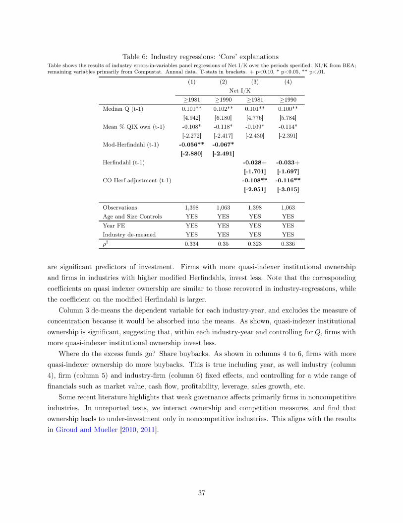
Table 6: Industry regressions: ‘Core’ explanationsTable shows the results of industry errors-in-variables panel regressions of Net I/K over the periods specified. NI/K from BEA;remaining variables primarily from Compustat. Annual data. T-stats in brackets. + p<0.10, * p<0.05, ** p<.01.

(1) (2) (3) (4)

Net I/K

≥1981 ≥1990 ≥1981 ≥1990

Median Q (t-1) 0.101** 0.102** 0.101** 0.100**

[4.942] [6.180] [4.776] [5.784]

Mean % QIX own (t-1) -0.108* -0.118* -0.109* -0.114*

[-2.272] [-2.417] [-2.430] [-2.391]

Mod-Herfindahl (t-1) -0.056** -0.067*

[-2.880] [-2.491]

Herfindahl (t-1) -0.028+ -0.033+

[-1.701] [-1.697]

CO Herf adjustment (t-1) -0.108** -0.116**

[-2.951] [-3.015]

Observations 1,398 1,063 1,398 1,063

Age and Size Controls YES YES YES YES

Year FE YES YES YES YES

Industry de-meaned YES YES YES YES

ρ2 0.334 0.35 0.323 0.336

are significant predictors of investment. Firms with more quasi-indexer institutional ownership

and firms in industries with higher modified Herfindahls, invest less. Note that the corresponding

coefficients on quasi indexer ownership are similar to those recovered in industry-regressions, while

the coefficient on the modified Herfindahl is larger.

Column 3 de-means the dependent variable for each industry-year, and excludes the measure of

concentration because it would be absorbed into the means. As shown, quasi-indexer institutional

ownership is significant, suggesting that, within each industry-year and controlling for Q, firms with

more quasi-indexer institutional ownership invest less.

Where do the excess funds go? Share buybacks. As shown in columns 4 to 6, firms with more

quasi-indexer ownership do more buybacks. This is true including year, as well industry (column

4), firm (column 5) and industry-firm (column 6) fixed effects, and controlling for a wide range of

financials such as market value, cash flow, profitability, leverage, sales growth, etc.

Some recent literature highlights that weak governance affects primarily firms in noncompetitive

industries. In unreported tests, we interact ownership and competition measures, and find that

ownership leads to under-investment only in noncompetitive industries. This aligns with the results

in Giroud and Mueller [2010, 2011].

37

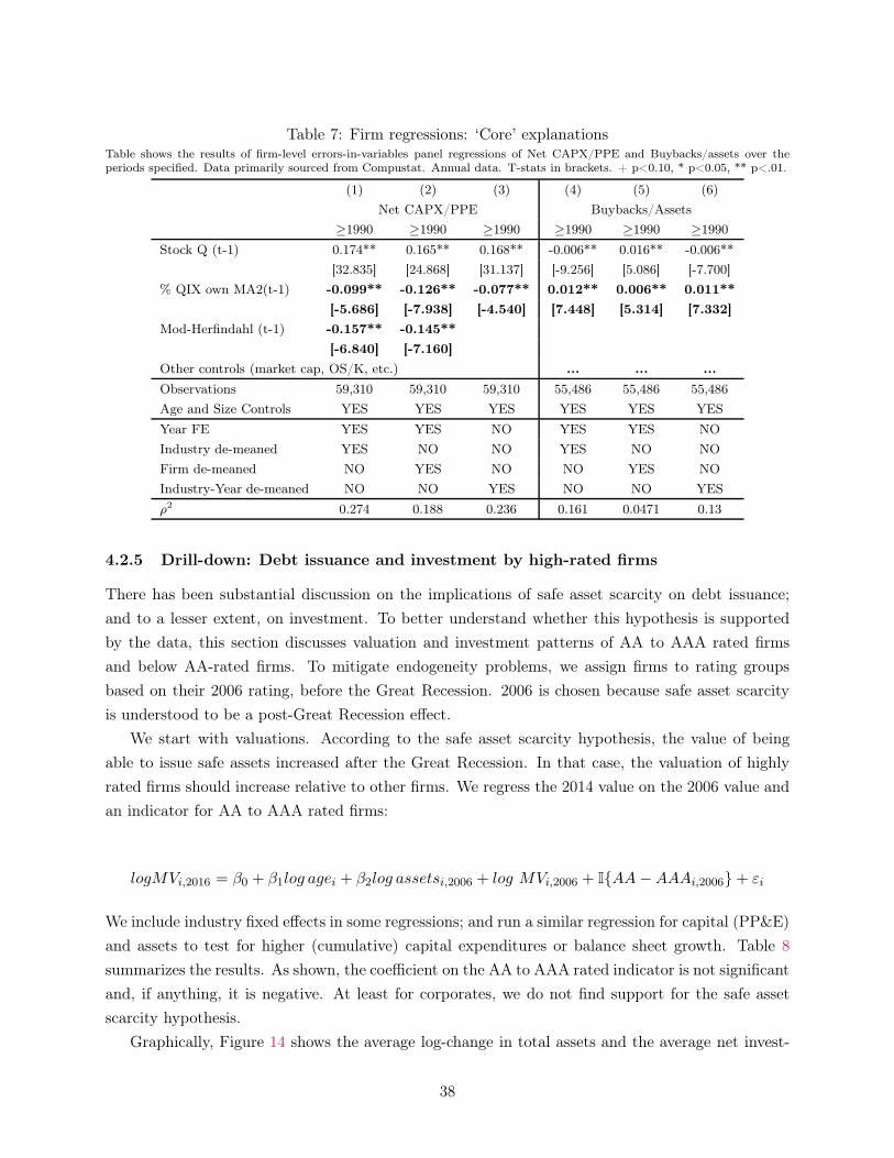
Table 7: Firm regressions: ‘Core’ explanationsTable shows the results of firm-level errors-in-variables panel regressions of Net CAPX/PPE and Buybacks/assets over theperiods specified. Data primarily sourced from Compustat. Annual data. T-stats in brackets. + p<0.10, * p<0.05, ** p<.01.

(1) (2) (3) (4) (5) (6)

Net CAPX/PPE Buybacks/Assets

≥1990 ≥1990 ≥1990 ≥1990 ≥1990 ≥1990

Stock Q (t-1) 0.174** 0.165** 0.168** -0.006** 0.016** -0.006**

[32.835] [24.868] [31.137] [-9.256] [5.086] [-7.700]

% QIX own MA2(t-1) -0.099** -0.126** -0.077** 0.012** 0.006** 0.011**

[-5.686] [-7.938] [-4.540] [7.448] [5.314] [7.332]

Mod-Herfindahl (t-1) -0.157** -0.145**

[-6.840] [-7.160]

Other controls (market cap, OS/K, etc.) ... ... ...

Observations 59,310 59,310 59,310 55,486 55,486 55,486

Age and Size Controls YES YES YES YES YES YES

Year FE YES YES NO YES YES NO

Industry de-meaned YES NO NO YES NO NO

Firm de-meaned NO YES NO NO YES NO

Industry-Year de-meaned NO NO YES NO NO YES

ρ2 0.274 0.188 0.236 0.161 0.0471 0.13

4.2.5 Drill-down: Debt issuance and investment by high-rated firms

There has been substantial discussion on the implications of safe asset scarcity on debt issuance;

and to a lesser extent, on investment. To better understand whether this hypothesis is supported

by the data, this section discusses valuation and investment patterns of AA to AAA rated firms

and below AA-rated firms. To mitigate endogeneity problems, we assign firms to rating groups

based on their 2006 rating, before the Great Recession. 2006 is chosen because safe asset scarcity

is understood to be a post-Great Recession effect.

We start with valuations. According to the safe asset scarcity hypothesis, the value of being

able to issue safe assets increased after the Great Recession. In that case, the valuation of highly

rated firms should increase relative to other firms. We regress the 2014 value on the 2006 value and

an indicator for AA to AAA rated firms:

logMVi,2016 = β0 + β1log agei + β2log assetsi,2006 + log MVi,2006 + I{AA−AAAi,2006}+ εi

We include industry fixed effects in some regressions; and run a similar regression for capital (PP&E)

and assets to test for higher (cumulative) capital expenditures or balance sheet growth. Table 8

summarizes the results. As shown, the coefficient on the AA to AAA rated indicator is not significant

and, if anything, it is negative. At least for corporates, we do not find support for the safe asset

scarcity hypothesis.

Graphically, Figure 14 shows the average log-change in total assets and the average net invest-

38

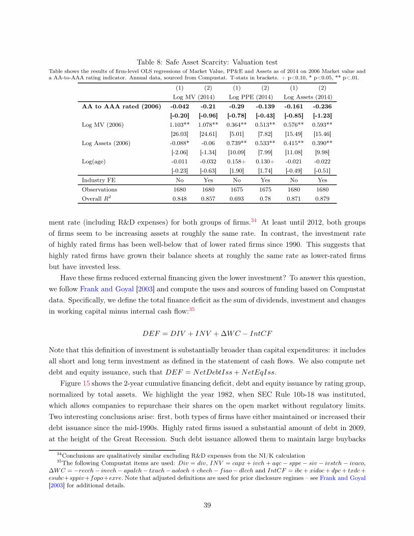
Table 8: Safe Asset Scarcity: Valuation testTable shows the results of firm-level OLS regressions of Market Value, PP&E and Assets as of 2014 on 2006 Market value anda AA-to-AAA rating indicator. Annual data, sourced from Compustat. T-stats in brackets. + p<0.10, * p<0.05, ** p<.01.

(1) (2) (1) (2) (1) (2)

Log MV (2014) Log PPE (2014) Log Assets (2014)

AA to AAA rated (2006) -0.042 -0.21 -0.29 -0.139 -0.161 -0.236

[-0.20] [-0.96] [-0.78] [-0.43] [-0.85] [-1.23]

Log MV (2006) 1.103** 1.078** 0.364** 0.513** 0.576** 0.593**

[26.03] [24.61] [5.01] [7.82] [15.49] [15.46]

Log Assets (2006) -0.088* -0.06 0.739** 0.533** 0.415** 0.390**

[-2.06] [-1.34] [10.09] [7.99] [11.08] [9.98]

Log(age) -0.011 -0.032 0.158+ 0.130+ -0.021 -0.022

[-0.23] [-0.63] [1.90] [1.74] [-0.49] [-0.51]

Industry FE No Yes No Yes No Yes

Observations 1680 1680 1675 1675 1680 1680

Overall R2 0.848 0.857 0.693 0.78 0.871 0.879

ment rate (including R&D expenses) for both groups of firms.34 At least until 2012, both groups

of firms seem to be increasing assets at roughly the same rate. In contrast, the investment rate

of highly rated firms has been well-below that of lower rated firms since 1990. This suggests that

highly rated firms have grown their balance sheets at roughly the same rate as lower-rated firms

but have invested less.

Have these firms reduced external financing given the lower investment? To answer this question,

we follow Frank and Goyal [2003] and compute the uses and sources of funding based on Compustat

data. Specifically, we define the total finance deficit as the sum of dividends, investment and changes

in working capital minus internal cash flow:35

DEF = DIV + INV +∆WC − IntCF

Note that this definition of investment is substantially broader than capital expenditures: it includes

all short and long term investment as defined in the statement of cash flows. We also compute net

debt and equity issuance, such that DEF = NetDebtIss+NetEqIss.

Figure 15 shows the 2-year cumulative financing deficit, debt and equity issuance by rating group,

normalized by total assets. We highlight the year 1982, when SEC Rule 10b-18 was instituted,

which allows companies to repurchase their shares on the open market without regulatory limits.

Two interesting conclusions arise: first, both types of firms have either maintained or increased their

debt issuance since the mid-1990s. Highly rated firms issued a substantial amount of debt in 2009,

at the height of the Great Recession. Such debt issuance allowed them to maintain large buybacks

34Conclusions are qualitatively similar excluding R&D expenses from the NI/K calculation35The following Compustat items are used: Div = div, INV = capx+ ivch + aqc− sppe− siv − ivstch − ivaco,

∆WC = −recch− invch− apalch− txach− aoloch+ chech− fiao− dlcch and IntCF = ibc+ xidoc+ dpc+ txdc+esubc+sppiv+fopo+exre. Note that adjusted definitions are used for prior disclosure regimes – see Frank and Goyal[2003] for additional details.

39

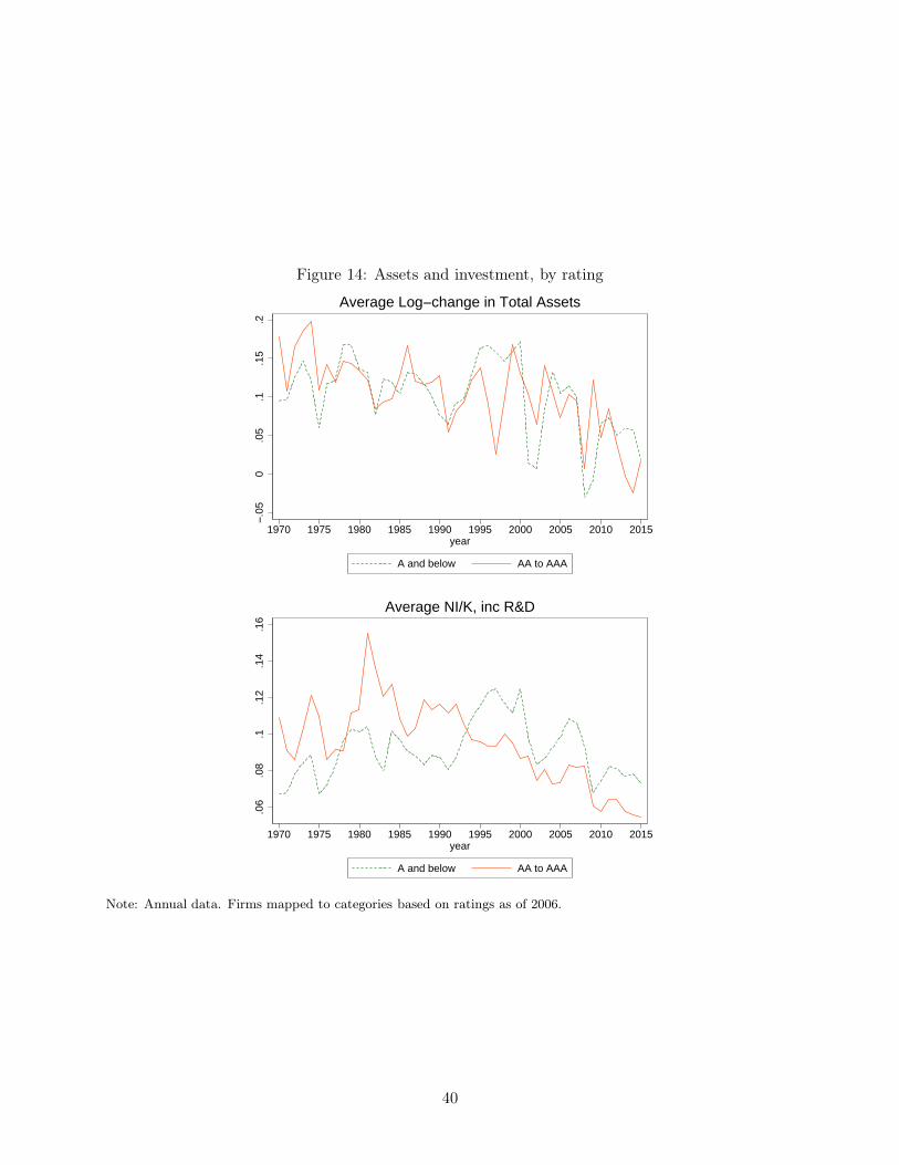
Figure 14: Assets and investment, by rating−.

050

.05

.1.1

5.2

1970 1975 1980 1985 1990 1995 2000 2005 2010 2015year

A and below AA to AAA

Average Log−change in Total Assets

.06

.08

.1.1

2.1

4.1

6

1970 1975 1980 1985 1990 1995 2000 2005 2010 2015year

A and below AA to AAA

Average NI/K, inc R&D

Note: Annual data. Firms mapped to categories based on ratings as of 2006.

40

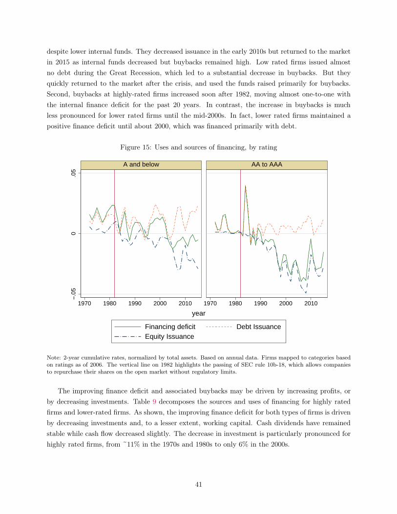
despite lower internal funds. They decreased issuance in the early 2010s but returned to the market

in 2015 as internal funds decreased but buybacks remained high. Low rated firms issued almost

no debt during the Great Recession, which led to a substantial decrease in buybacks. But they

quickly returned to the market after the crisis, and used the funds raised primarily for buybacks.

Second, buybacks at highly-rated firms increased soon after 1982, moving almost one-to-one with

the internal finance deficit for the past 20 years. In contrast, the increase in buybacks is much

less pronounced for lower rated firms until the mid-2000s. In fact, lower rated firms maintained a

positive finance deficit until about 2000, which was financed primarily with debt.

Figure 15: Uses and sources of financing, by rating

−.05

0.0

5

1970 1980 1990 2000 2010 1970 1980 1990 2000 2010

A and below AA to AAA

Financing deficit Debt IssuanceEquity Issuance

year

Note: 2-year cumulative rates, normalized by total assets. Based on annual data. Firms mapped to categories basedon ratings as of 2006. The vertical line on 1982 highlights the passing of SEC rule 10b-18, which allows companiesto repurchase their shares on the open market without regulatory limits.

The improving finance deficit and associated buybacks may be driven by increasing profits, or

by decreasing investments. Table 9 decomposes the sources and uses of financing for highly rated

firms and lower-rated firms. As shown, the improving finance deficit for both types of firms is driven

by decreasing investments and, to a lesser extent, working capital. Cash dividends have remained

stable while cash flow decreased slightly. The decrease in investment is particularly pronounced for

highly rated firms, from ~11% in the 1970s and 1980s to only 6% in the 2000s.

41

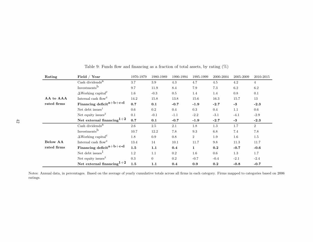
Table 9: Funds flow and financing as a fraction of total assets, by rating (%)

Rating Field / Year 1970-1979 1980-1989 1990-1994 1995-1999 2000-2004 2005-2009 2010-2015

AA to AAA

rated firms

Cash dividendsa 3.7 3.9 4.3 4.7 4.5 4.2 4

Investmentsb 9.7 11.9 8.4 7.9 7.3 6.2 6.2

∆Working capitalc 1.6 -0.3 0.5 1.4 1.4 0.8 0.1

Internal cash flowd 14.2 15.8 13.8 15.6 16.3 15.7 13

Financing deficita+b+c-d 0.7 0.1 -0.7 -1.9 -2.7 -3 -2.3

Net debt issues1 0.6 0.2 0.4 0.3 0.4 1.1 0.6

Net equity issues2 0.1 -0.1 -1.1 -2.2 -3.1 -4.1 -2.9

Net external financing1+2 0.7 0.1 -0.7 -1.9 -2.7 -3 -2.3

Below AA

rated firms

Cash dividendsa 2.6 2.5 2.1 1.8 1.3 1.7 2

Investmentsb 10.7 12.2 7.8 9.3 6.8 7.4 7.8

∆Working capitalc 1.8 0.9 0.8 2 1.9 1.6 1.5

Internal cash flowd 13.4 14 10.1 11.7 9.8 11.3 11.7

Financing deficita+b+c-d 1.5 1.1 0.4 1 0.2 -0.7 -0.6

Net debt issues1 1.2 1.1 0.2 1.6 0.6 1.3 1.7

Net equity issues2 0.3 0 0.2 -0.7 -0.4 -2.1 -2.4

Net external financing1+2 1.5 1.1 0.4 0.9 0.2 -0.8 -0.7

Notes: Annual data, in percentages. Based on the average of yearly cumulative totals across all firms in each category. Firms mapped to categories based on 2006ratings.

42

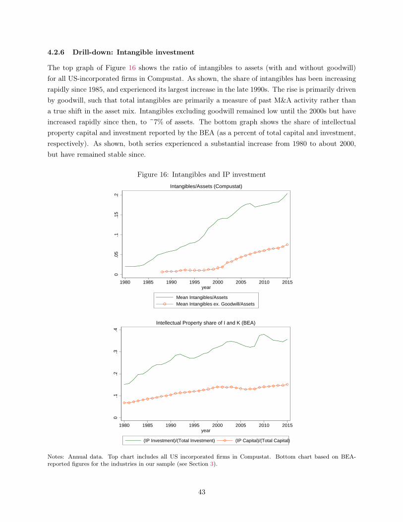
4.2.6 Drill-down: Intangible investment

The top graph of Figure 16 shows the ratio of intangibles to assets (with and without goodwill)

for all US-incorporated firms in Compustat. As shown, the share of intangibles has been increasing

rapidly since 1985, and experienced its largest increase in the late 1990s. The rise is primarily driven

by goodwill, such that total intangibles are primarily a measure of past M&A activity rather than

a true shift in the asset mix. Intangibles excluding goodwill remained low until the 2000s but have

increased rapidly since then, to ~7% of assets. The bottom graph shows the share of intellectual

property capital and investment reported by the BEA (as a percent of total capital and investment,

respectively). As shown, both series experienced a substantial increase from 1980 to about 2000,

but have remained stable since.

Figure 16: Intangibles and IP investment

0.0

5.1

.15

.2

1980 1985 1990 1995 2000 2005 2010 2015year

Mean Intangibles/AssetsMean Intangibles ex. Goodwill/Assets

Intangibles/Assets (Compustat)

0.1

.2.3

.4

1980 1985 1990 1995 2000 2005 2010 2015year

(IP Investment)/(Total Investment) (IP Capital)/(Total Capital)

Intellectual Property share of I and K (BEA)

Notes: Annual data. Top chart includes all US incorporated firms in Compustat. Bottom chart based on BEA-reported figures for the industries in our sample (see Section 3).

43

The rise of intangibles may affect investment in two ways: first, intangible investment is difficult

to measure and is therefore prone to measurement error. This can be seen, for instance, in the

very different trends between the share of intangibles in BEA data and the intangibles excluding

goodwill in Compustat. If intangible investment is under-estimated, K would be under-estimated,

and therefore Q would be over-estimated. Second, intangible assets might be more difficult to

accumulate. A rise in the relative importance of intangibles could lead to a higher equilibrium value

of Q even if intangibles are correctly measured. We test each of these hypothesis separately. We

find some support for them but their impact seems to be quantitatively limited.

Measurement error. Denote net investments in tangible and intangible assets by NIT and NII ,

such that total investments are NI = NIT + NII . Assume that tangible capital is perfectly

measured but intangible capital is under-estimated by a factor α – that is, assume that intangible

investment is consistently under-estimated across all industries. This is a simplifying assumption,

but it highlights the main reason for concern.

Under this assumptions, measured investment is given by

N̂I ≡ N̂IT+ N̂I

I

= NIT + αNII

The under-estimation of investment leads to under-estimation of capital K̂ and, since Q̂ is the ratio

of market value to replacement cost of capital, it leads to over-estimation of Q. Thus, a regression

of the form

ˆNIitˆKit−1

= βQ̂i,t−1 + γK̂I

ATi,t−1+ µi + ηt + εit

would yield a negative and significant coefficient γ. More complex measurement errors would yield

different structures, but broadly the negative coefficient should remain. Industries with higher

dependence on intangibles would appear to be under-investing due to an over-estimation of Q and

an under-estimation of investment.

We test this in two ways. First, we run measurement-error corrected regressions at the industry

level, using BEA measures of investment (which includes intellectual property investment) and the

traditional Compustat Q. The results are shown in columns 1 and 2 of Table 10. As shown, the

coefficient on intangibles is significant and negative, suggesting that industry-years with a larger

share of intangibles exhibit more under-investment relative to the traditional Q.

Second, we replace the Compustat Q with the ‘total Q’ of Peters and Taylor [2016]. Total Q aims

to correct for measurement error in intangibles by recognizing R&D and part of SG&A expenses

as investments. This procedure reduces the measurement error in Q due to intangibles, and should

therefore reduce the explanatory power of K̂I

ATi,t−1. The results are shown in column 3. Intangibles

remain significant but the corresponding coefficient is 30% smaller than using the Compustat Q, as

44

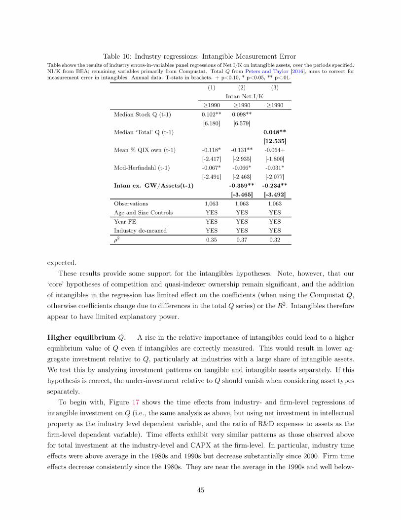
Table 10: Industry regressions: Intangible Measurement ErrorTable shows the results of industry errors-in-variables panel regressions of Net I/K on intangible assets, over the periods specified.NI/K from BEA; remaining variables primarily from Compustat. Total Q from Peters and Taylor [2016], aims to correct formeasurement error in intangibles. Annual data. T-stats in brackets. + p<0.10, * p<0.05, ** p<.01.

(1) (2) (3)

Intan Net I/K

≥1990 ≥1990 ≥1990

Median Stock Q (t-1) 0.102** 0.098**

[6.180] [6.579]

Median ‘Total’ Q (t-1) 0.048**

[12.535]

Mean % QIX own (t-1) -0.118* -0.131** -0.064+

[-2.417] [-2.935] [-1.800]

Mod-Herfindahl (t-1) -0.067* -0.066* -0.031*

[-2.491] [-2.463] [-2.077]

Intan ex. GW/Assets(t-1) -0.359** -0.234**

[-3.465] [-3.492]

Observations 1,063 1,063 1,063

Age and Size Controls YES YES YES

Year FE YES YES YES

Industry de-meaned YES YES YES

ρ2 0.35 0.37 0.32

expected.

These results provide some support for the intangibles hypotheses. Note, however, that our

‘core’ hypotheses of competition and quasi-indexer ownership remain significant, and the addition

of intangibles in the regression has limited effect on the coefficients (when using the Compustat Q,

otherwise coefficients change due to differences in the total Q series) or the R2. Intangibles therefore

appear to have limited explanatory power.

Higher equilibrium Q. A rise in the relative importance of intangibles could lead to a higher

equilibrium value of Q even if intangibles are correctly measured. This would result in lower ag-

gregate investment relative to Q, particularly at industries with a large share of intangible assets.

We test this by analyzing investment patterns on tangible and intangible assets separately. If this

hypothesis is correct, the under-investment relative to Q should vanish when considering asset types

separately.

To begin with, Figure 17 shows the time effects from industry- and firm-level regressions of

intangible investment on Q (i.e., the same analysis as above, but using net investment in intellectual

property as the industry level dependent variable, and the ratio of R&D expenses to assets as the

firm-level dependent variable). Time effects exhibit very similar patterns as those observed above

for total investment at the industry-level and CAPX at the firm-level. In particular, industry time

effects were above average in the 1980s and 1990s but decrease substantially since 2000. Firm time

effects decrease consistently since the 1980s. They are near the average in the 1990s and well below-

45

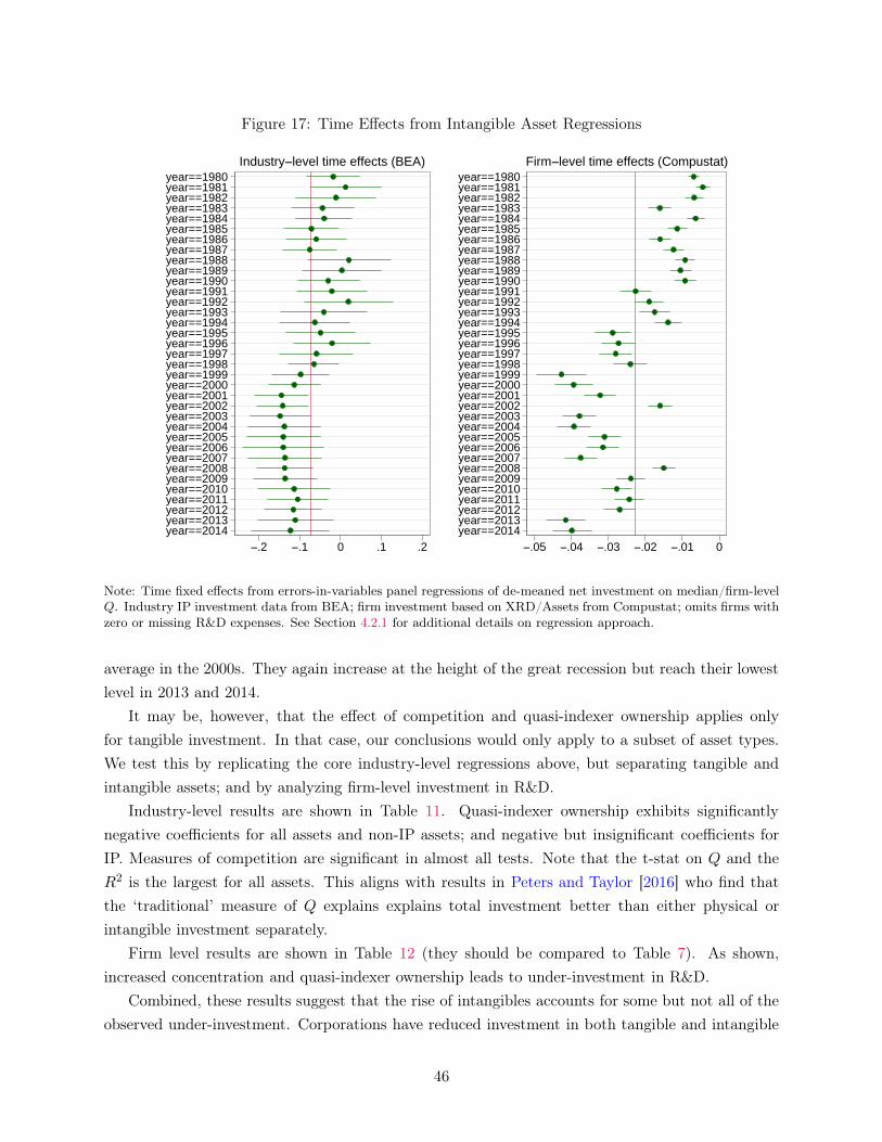
Figure 17: Time Effects from Intangible Asset Regressions

year==1980year==1981year==1982year==1983year==1984year==1985year==1986year==1987year==1988year==1989year==1990year==1991year==1992year==1993year==1994year==1995year==1996year==1997year==1998year==1999year==2000year==2001year==2002year==2003year==2004year==2005year==2006year==2007year==2008year==2009year==2010year==2011year==2012year==2013year==2014

−.2 −.1 0 .1 .2

Industry−level time effects (BEA)year==1980year==1981year==1982year==1983year==1984year==1985year==1986year==1987year==1988year==1989year==1990year==1991year==1992year==1993year==1994year==1995year==1996year==1997year==1998year==1999year==2000year==2001year==2002year==2003year==2004year==2005year==2006year==2007year==2008year==2009year==2010year==2011year==2012year==2013year==2014

−.05 −.04 −.03 −.02 −.01 0

Firm−level time effects (Compustat)

Note: Time fixed effects from errors-in-variables panel regressions of de-meaned net investment on median/firm-levelQ. Industry IP investment data from BEA; firm investment based on XRD/Assets from Compustat; omits firms withzero or missing R&D expenses. See Section 4.2.1 for additional details on regression approach.

average in the 2000s. They again increase at the height of the great recession but reach their lowest

level in 2013 and 2014.

It may be, however, that the effect of competition and quasi-indexer ownership applies only

for tangible investment. In that case, our conclusions would only apply to a subset of asset types.

We test this by replicating the core industry-level regressions above, but separating tangible and

intangible assets; and by analyzing firm-level investment in R&D.

Industry-level results are shown in Table 11. Quasi-indexer ownership exhibits significantly

negative coefficients for all assets and non-IP assets; and negative but insignificant coefficients for

IP. Measures of competition are significant in almost all tests. Note that the t-stat on Q and the

R2 is the largest for all assets. This aligns with results in Peters and Taylor [2016] who find that

the ‘traditional’ measure of Q explains explains total investment better than either physical or

intangible investment separately.

Firm level results are shown in Table 12 (they should be compared to Table 7). As shown,

increased concentration and quasi-indexer ownership leads to under-investment in R&D.

Combined, these results suggest that the rise of intangibles accounts for some but not all of the

observed under-investment. Corporations have reduced investment in both tangible and intangible

46

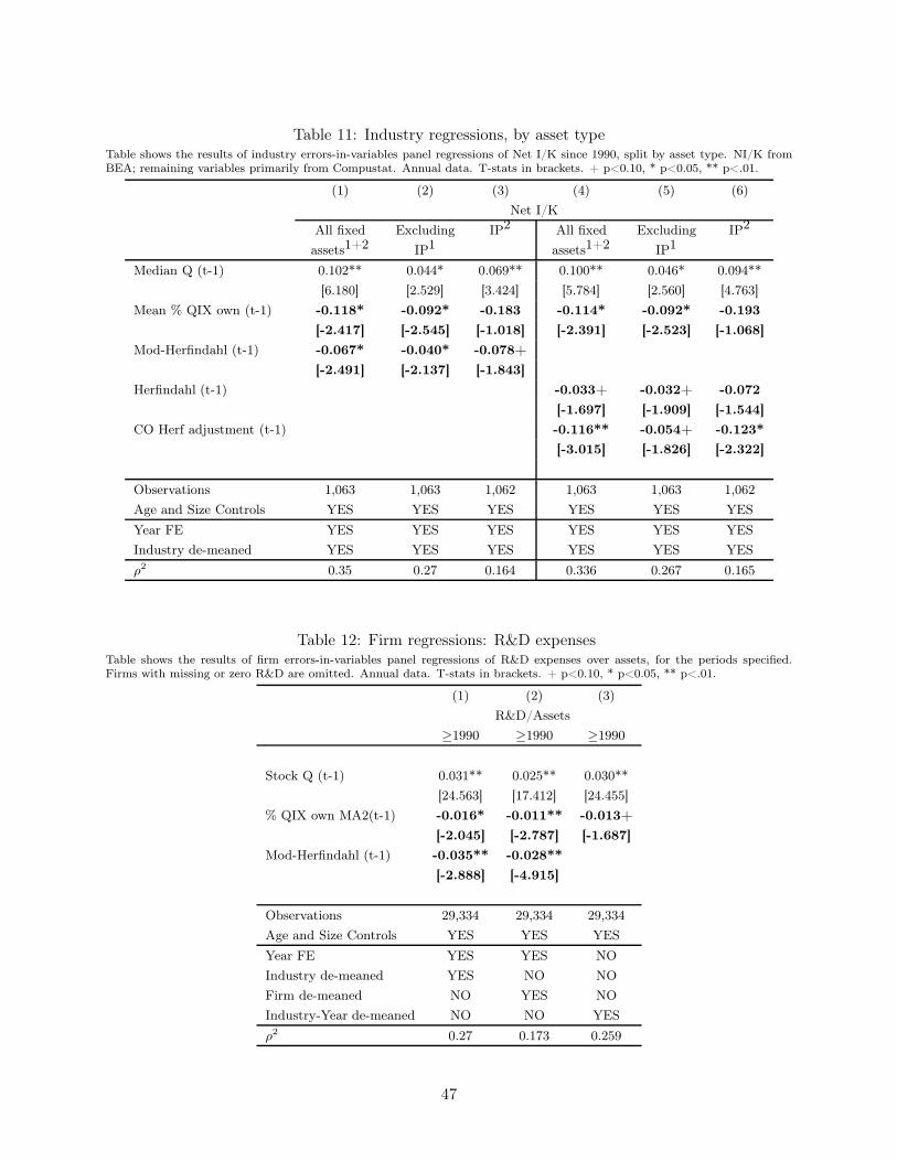
Table 11: Industry regressions, by asset typeTable shows the results of industry errors-in-variables panel regressions of Net I/K since 1990, split by asset type. NI/K fromBEA; remaining variables primarily from Compustat. Annual data. T-stats in brackets. + p<0.10, * p<0.05, ** p<.01.

(1) (2) (3) (4) (5) (6)

Net I/K

All fixed

assets1+2Excluding

IP1IP2 All fixed

assets1+2Excluding

IP1IP2

Median Q (t-1) 0.102** 0.044* 0.069** 0.100** 0.046* 0.094**

[6.180] [2.529] [3.424] [5.784] [2.560] [4.763]

Mean % QIX own (t-1) -0.118* -0.092* -0.183 -0.114* -0.092* -0.193

[-2.417] [-2.545] [-1.018] [-2.391] [-2.523] [-1.068]

Mod-Herfindahl (t-1) -0.067* -0.040* -0.078+

[-2.491] [-2.137] [-1.843]

Herfindahl (t-1) -0.033+ -0.032+ -0.072

[-1.697] [-1.909] [-1.544]

CO Herf adjustment (t-1) -0.116** -0.054+ -0.123*

[-3.015] [-1.826] [-2.322]

Observations 1,063 1,063 1,062 1,063 1,063 1,062

Age and Size Controls YES YES YES YES YES YES

Year FE YES YES YES YES YES YES

Industry de-meaned YES YES YES YES YES YES

ρ2 0.35 0.27 0.164 0.336 0.267 0.165

Table 12: Firm regressions: R&D expensesTable shows the results of firm errors-in-variables panel regressions of R&D expenses over assets, for the periods specified.Firms with missing or zero R&D are omitted. Annual data. T-stats in brackets. + p<0.10, * p<0.05, ** p<.01.

(1) (2) (3)

R&D/Assets

≥1990 ≥1990 ≥1990

Stock Q (t-1) 0.031** 0.025** 0.030**

[24.563] [17.412] [24.455]

% QIX own MA2(t-1) -0.016* -0.011** -0.013+

[-2.045] [-2.787] [-1.687]

Mod-Herfindahl (t-1) -0.035** -0.028**

[-2.888] [-4.915]

Observations 29,334 29,334 29,334

Age and Size Controls YES YES YES

Year FE YES YES NO

Industry de-meaned YES NO NO

Firm de-meaned NO YES NO

Industry-Year de-meaned NO NO YES

ρ2 0.27 0.173 0.259

47

assets since 2000, suggesting that other factors are in play.

5 Conclusion

Private fixed investment in the United States has been lower than expected since the early 2000’s.

The trend started before 2008, but the Great Recession made it more striking. Investment in the

is low despite high levels of profitability and Tobin’s Q. This simple observation rules out a whole

class of theories that would explain low investment by low values of Tobin’s Q. We test 8 alternative

theories that can explain the investment gap, i.e., low investment despite high Q. Among these,

the only ones that find consistent support in our industry and firm level datasets are decreased

competition, tightened governance and, potentially, increased short-termist pressures. Combined,

the competition and governance measures explain about 80% of the aggregate under-investment

relative to Q. The rise of intangibles explains some of the remaining investment gap, and it does

not diminish the explanatory power of competition and governance.

The above conclusions are based on simple regressions and therefore cannot establish causality

between competition, governance and investment. In follow-up work Gutiérrez and Philippon [2017]

we use a combination of instrumental variables and natural experiments to test the causality of our

two main explanations: lack of competition and tight or short-termist governance.

References

Viral Acharya and Guillaume Plantin. Monetary easing and financial instability. 2016.

Philippe Aghion, Stefan Bechtold, Lea Cassar, and Holger Herz. The causal effects of competition

on innovation: Experimental evidence. Working Paper, 2014.

Omar Al-Ubaydli and Patrick A. McLaughlin. Regdata: A numerical database on industry-specific

regulations for all united states industries and federal regulations, 1997 to 2012. Regulation &

Governance, 2015.

Lewis Alexander and Janice Eberly. Investment hollowing out. Working Paper, 2016.

Laura Alfaro, Thorsten Beck, and Charles Calomiris. Foreign bank entry and entrepreneurship.

Working Paper, 2015.

Heitor Almeida, Vyacheslav Fos, and Mathias Kronlund. The real effects of share repurchases.

Journal of Financial Economics, 119(1):168–185, jan 2016.

Ian R. Appel, Todd A. Gormley, and Donald B. Keim. Passive investors, not passive owners. Journal

of Financial Economics, 121(1):111 – 141, 2016a.

Ian R. Appel, Todd A. Gormley, and Donald B. Keim. Standing on the shoulders of giants: The

effect of passive investors on activism. September 2016b.

48

John Asker, Joan Farre-Mensa, and Alexander Ljungqvist. Corporate investment and stock market

listing: A puzzle? Review of Financial Studies, 2014.

Jose Azar, Sahil Raina, and Martin C. Schmalz. Ultimate ownership and bank competition. 2016a.

Jose Azar, Martin C. Schmalz, and Isabel Tecu. Anti-competitive effects of common ownership.

2016b.

Jan Bena, Miguel A. Ferreira, Pedro P. Matos, and Pedro Pires. Are foreign investors locusts?

the long-term effects of foreign institutional ownership. European Corporate Governance Institute

(ECGI) - Finance Working Paper No. 468/2016, 2016.

Ben S. Bernanke. Irreversibility, uncertainty, and cyclical investment. The Quarterly Journal of

Economics, 98(1):85–106, 1983.

Bruce A. Blonigen and Justin R. Pierce. Evidence for the effects of mergers on market power and

efficiency. October 2016.

Brian J. Bushee. The influence of institutional investors on myopic r&d investment behavior. The

Accounting Review, 73(3):305–333, 1998.

Brian J. Bushee. Do institutional investors prefer near-term earnings over long-run value? Con-

temporary Accounting Research, 18(2):207–246, 2001.

Ricardo J. Caballero and Emmanuel Farhi. The safety trap. February 2014.

CEA. Benefits of competition and indicators of market power. Issue Brief, April 2016.

Yen-Cheng Chang, Harrison Hong, and Inessa Liskovich. Regression discontinuity and the price

effects of stock market indexing*. Review of Financial Studies, 2014.

Brian Chen, Samuel G. Hanson, and Jeremy C. Stein. The decline in big-bank lending to small

businesses: Causes and consequences. Working paper, 2016.

Alan D. Crane, Sebastien Michenaud, and James P. Weston. The effect of institutional ownership

on payout policy: Evidence from index thresholds. Review of Financial Studies, 2016.

Sudip Datta, Mai Iskandar-Datta, and Vivek Singh. Product market power, industry structure, and

corporate earnings management. Journal of Banking & Finance, 37(8):3273 – 3285, 2013.

Ryan Decker, John Haltiwanger, Ron Jarmin, and Javier Miranda. The role of entrepreneurship in

us job creation and economic dynamism. Journal of Economic Perspectives, 28(3):3–24, August

2014.

Ryan A. Decker, John Haltiwanger, Ron S. Jarmin, and Javier Miranda. Where has all the skewness

gone? the decline in high-growth (young) firms in the u.s. November 2015.

49

Avinash K. Dixit and Robert S. Pindyck. Investment under Uncertainty. Princeton University

Press, 1994.

Timothy Erickson, Colin Huan Jiang, and Toni Whited. Minimum distance estimation of the errors-

in-variables model using linear cumulant equations. Journal of Econometrics, 183(2):211–221,

2014.

Steven Fazzari, R. Glenn Hubbard, and Bruce C. Petersen. Financing constraints and corporate

investment. September 1987.

Jan Fichtner, Eelke M. Heemskerk, and Javier Garcia-Bernardo. Hidden power of the big three?

passive index funds, re-concentration of corporate ownership, and new financial risk. 2016.

C. Fritz Foley, Jay C. Hartzell, Sheridan Titman, and Garry Twite. Why do firms hold so much

cash? a tax-based explanation. Journal of Financial Economics, 86(3):579–607, dec 2007.

Murray Z. Frank and Vidhan K. Goyal. Testing the pecking order theory of capital structure.

Journal of Financial Economics, 2003.

Jason Furman. Business investment in the united states: Facts, explanations, puzzles, and policies.

2015.

Simon Gilchrist and Egon Zakrajsek. Credit spreads and business cycle fluctuations. forthcoming

in American Economic Review, 2011.

Xavier Giroud and Holger M. Mueller. Does corporate governance matter in competitive industries?

Journal of Financial Economics, 95(3):312 – 331, 2010.

Xavier Giroud and Holger M. Mueller. Corporate governance, product market competition, and

equity prices. The Journal of Finance, 66(2):563–600, 2011.

Joao F. Gomes. Financing investment. American Economic Review, 91(5):1263–1285, December

2001.

Paul Gompers, Joy Ishii, and Andrew Metrick. Corporate governance and equity prices. The

Quarterly Journal of Economics, 118(1):107–156, 2003.

Germán Gutiérrez and Thomas Philippon. Competition, governance and investment. mimeo NYU,

2017.

Robert E. Hall. The stock market and capital accumulation. American Economic Review, 91(5):

1185–1202, December 2001.

Jarrad Harford, Sattar A. Mansi, and William F. Maxwell. Corporate governance and firm cash

holdings in the us. Journal of Financial Economics, 87(3):535 – 555, 2008.

50

Fumio Hayashi. Tobin’s marginal q and average q: A neoclassical interpretation. Econometrica, 50

(1):213–224, 1982.

Christopher A. Hennessy and Toni M. Whited. How costly is external financing? evidence from a

structural estimation. The Journal of Finance, 62(4):1705–1745, 2007.

Michael Jensen. Agency costs of free cash flow, corporate finance, and takeovers. American Economic

Review, 76(2):323–29, 1986.

Christine Jolls. Stock repurchases and incentive compensation. Mar 1998.

Callum Jones and Thomas Philippon. The secular stagnation of investment? 2016.

Boyan Jovanovic and Peter L. Rousseau. Extensive and intensive investment over the business cycle.

Journal of Political Economy, 122(4):863–908, aug 2014.

Steven N. Kaplan and Luigi Zingales. Do investment-cash flow sensitivities provide useful measures

of financing constraints? The Quarterly Journal of Economics, 112(1):169–215, 1997.

Anil K Kashyap, Owen A. Lamont, and Jeremy C. Stein. Credit conditions and the cyclical behavior

of inventories. The Quarterly Journal of Economics, 109(3):565–592, 1994.

Morris M. Kleiner and Alan B. Krueger. Analyzing the Extent and Influence of Occupational

Licensing on the Labor Market. Journal of Labor Economics, 31(S1):S173 – S202, 2013.

William Lazonick. Profits without prosperity. Harvard Business Review, September 2014.

Dong Wook Lee, Hyun-Han Shin, and Rene M. Stulz. Why does capital no longer flow more to the

industries with the best growth opportunities? Fisher College of Business Working Paper, 2016

(15), September 2016.

Roger Martin. Yes, short-termism really is a problem. Harvard Business Review, October 2015.

Simon Mongey. Market structure and monetary non-neutrality. Working paper, 2016.

Nathalie Moyen. Investment cash flow sensitivities: Constrained versus unconstrained firms. The

Journal of Finance, 59(5):2061–2092, 2004.

Vasia Panousi and Dimitris Papanikolauo. Investment, idiosyncratic risk, and ownership. The

Journal of Finance, 67(3):1113–1148, 2012.

Ryan H. Peters and Lucian A. Taylor. Intangible capital and the investment-q relation. Journal of

Financial Economics, 2016. ISSN 0304-405X.

Robert S. Pindyck. Irreversible investment, capacity choice, and the value of the firm. The American

Economic Review, 78(5):969–985, 1988.

51

Raghuram G. Rajan and Luigi Zingales. Financial dependence and growth. American Economic

Review, 88:559–586, 1998.

Scott A. Richardson. Over-investment of free cash flow. Review of Accounting Studies, 11(2-3):

159–189, jun 2006.

Steven C. Salop and Daniel P. O’Brien. Competitive effects of partial ownership: Financial interest

and corporate control. Antitrust Law Journal, 2000.

Cornelius Schmidt and Rudiger Fahlenbrach. Do exogenous changes in passive institutional owner-

ship affect corporate governance and firm value? Journal of Financial Economics, Forthcoming,

2016.

Jules H. van Binsbergen and Christian C. Opp. Real anomalies. Working paper, 2016.

Jeffrey Wurgler. On the economic consequences of index-linked investing. Challenges to Business

in the Twenty-First Century, 2011.

52

Appendix I: Industry Investment Data

As noted above, investment is available for 63 granular industry groupings from the BEA. These are

grouped into 47 categories (3 of which are omitted) to ensure all groupings have material investment

and better Compustat coverage. Industries are grouped to ensure measures of investment and

concentration are stable over time. In particular, we group industries to ensure each group has at

least ~10 firms, on average, from 1990 - 2015 and it contributes a material share of investment.

The groupings are summarized in Table 13, including the BEA industry code, the granular industry

name and the mapped industry group. We also include the dollar value and % of total capital as

of 2014. Table 14 shows the total (nominal) investment from 2000 to 2015 by grouping, along with

the Compustat coverage ratios defined as described in the text.

53

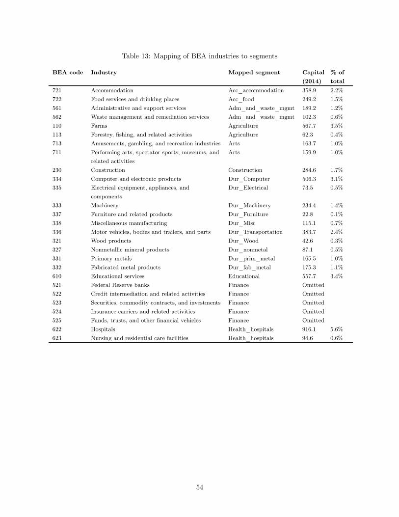
Table 13: Mapping of BEA industries to segments

BEA code Industry Mapped segment Capital

(2014)

% of

total

721 Accommodation Acc_accommodation 358.9 2.2%

722 Food services and drinking places Acc_food 249.2 1.5%

561 Administrative and support services Adm_and_waste_mgmt 189.2 1.2%

562 Waste management and remediation services Adm_and_waste_mgmt 102.3 0.6%

110 Farms Agriculture 567.7 3.5%

113 Forestry, fishing, and related activities Agriculture 62.3 0.4%

713 Amusements, gambling, and recreation industries Arts 163.7 1.0%

711 Performing arts, spectator sports, museums, and

related activities

Arts 159.9 1.0%

230 Construction Construction 284.6 1.7%

334 Computer and electronic products Dur_Computer 506.3 3.1%

335 Electrical equipment, appliances, and

components

Dur_Electrical 73.5 0.5%

333 Machinery Dur_Machinery 234.4 1.4%

337 Furniture and related products Dur_Furniture 22.8 0.1%

338 Miscellaneous manufacturing Dur_Misc 115.1 0.7%

336 Motor vehicles, bodies and trailers, and parts Dur_Transportation 383.7 2.4%

321 Wood products Dur_Wood 42.6 0.3%

327 Nonmetallic mineral products Dur_nonmetal 87.1 0.5%

331 Primary metals Dur_prim_metal 165.5 1.0%

332 Fabricated metal products Dur_fab_metal 175.3 1.1%

610 Educational services Educational 557.7 3.4%

521 Federal Reserve banks Finance Omitted

522 Credit intermediation and related activities Finance Omitted

523 Securities, commodity contracts, and investments Finance Omitted

524 Insurance carriers and related activities Finance Omitted

525 Funds, trusts, and other financial vehicles Finance Omitted

622 Hospitals Health_hospitals 916.1 5.6%

623 Nursing and residential care facilities Health_hospitals 94.6 0.6%

54

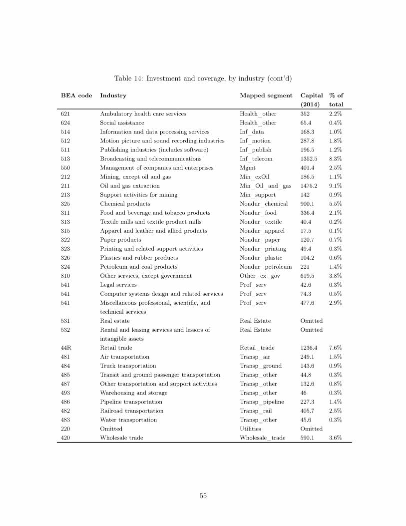
Table 14: Investment and coverage, by industry (cont’d)

BEA code Industry Mapped segment Capital

(2014)

% of

total

621 Ambulatory health care services Health_other 352 2.2%

624 Social assistance Health_other 65.4 0.4%

514 Information and data processing services Inf_data 168.3 1.0%

512 Motion picture and sound recording industries Inf_motion 287.8 1.8%

511 Publishing industries (includes software) Inf_publish 196.5 1.2%

513 Broadcasting and telecommunications Inf_telecom 1352.5 8.3%

550 Management of companies and enterprises Mgmt 401.4 2.5%

212 Mining, except oil and gas Min_exOil 186.5 1.1%

211 Oil and gas extraction Min_Oil_and_gas 1475.2 9.1%

213 Support activities for mining Min_support 142 0.9%

325 Chemical products Nondur_chemical 900.1 5.5%

311 Food and beverage and tobacco products Nondur_food 336.4 2.1%

313 Textile mills and textile product mills Nondur_textile 40.4 0.2%

315 Apparel and leather and allied products Nondur_apparel 17.5 0.1%

322 Paper products Nondur_paper 120.7 0.7%

323 Printing and related support activities Nondur_printing 49.4 0.3%

326 Plastics and rubber products Nondur_plastic 104.2 0.6%

324 Petroleum and coal products Nondur_petroleum 221 1.4%

810 Other services, except government Other_ex_gov 619.5 3.8%

541 Legal services Prof_serv 42.6 0.3%

541 Computer systems design and related services Prof_serv 74.3 0.5%

541 Miscellaneous professional, scientific, and

technical services

Prof_serv 477.6 2.9%

531 Real estate Real Estate Omitted

532 Rental and leasing services and lessors of

intangible assets

Real Estate Omitted

44R Retail trade Retail_trade 1236.4 7.6%

481 Air transportation Transp_air 249.1 1.5%

484 Truck transportation Transp_ground 143.6 0.9%

485 Transit and ground passenger transportation Transp_other 44.8 0.3%

487 Other transportation and support activities Transp_other 132.6 0.8%

493 Warehousing and storage Transp_other 46 0.3%

486 Pipeline transportation Transp_pipeline 227.3 1.4%

482 Railroad transportation Transp_rail 405.7 2.5%

483 Water transportation Transp_other 45.6 0.3%

220 Omitted Utilities Omitted

420 Wholesale trade Wholesale_trade 590.1 3.6%

55

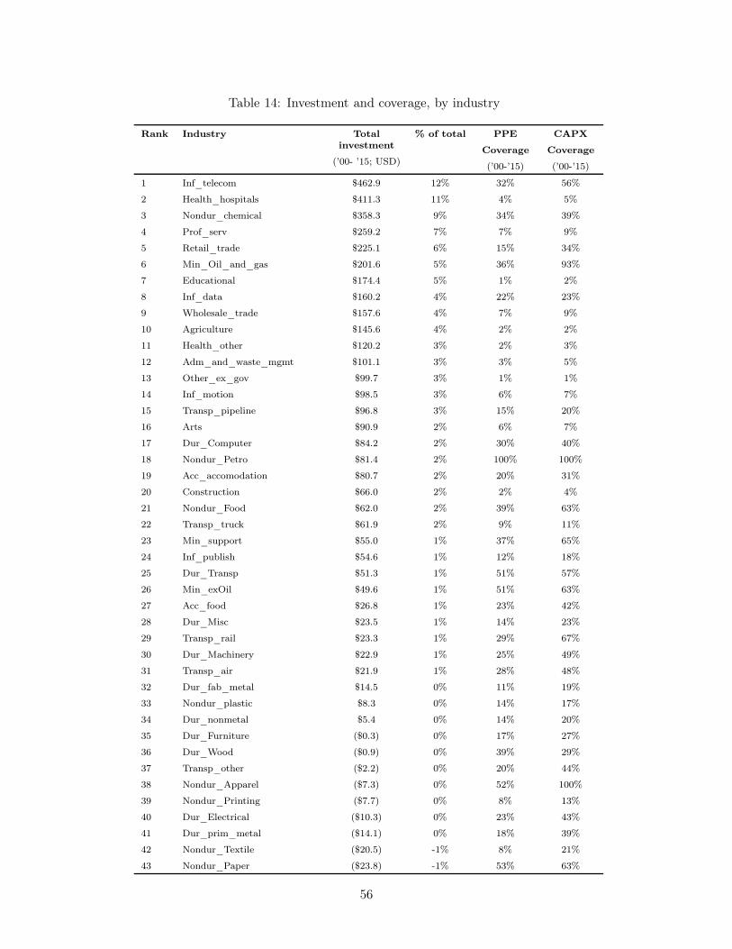
Table 14: Investment and coverage, by industry

Rank Industry Totalinvestment

(’00- ’15; USD)

% of total PPE

Coverage

(’00-’15)

CAPX

Coverage

(’00-’15)

1 Inf_telecom $462.9 12% 32% 56%

2 Health_hospitals $411.3 11% 4% 5%

3 Nondur_chemical $358.3 9% 34% 39%

4 Prof_serv $259.2 7% 7% 9%

5 Retail_trade $225.1 6% 15% 34%

6 Min_Oil_and_gas $201.6 5% 36% 93%

7 Educational $174.4 5% 1% 2%

8 Inf_data $160.2 4% 22% 23%

9 Wholesale_trade $157.6 4% 7% 9%

10 Agriculture $145.6 4% 2% 2%

11 Health_other $120.2 3% 2% 3%

12 Adm_and_waste_mgmt $101.1 3% 3% 5%

13 Other_ex_gov $99.7 3% 1% 1%

14 Inf_motion $98.5 3% 6% 7%

15 Transp_pipeline $96.8 3% 15% 20%

16 Arts $90.9 2% 6% 7%

17 Dur_Computer $84.2 2% 30% 40%

18 Nondur_Petro $81.4 2% 100% 100%

19 Acc_accomodation $80.7 2% 20% 31%

20 Construction $66.0 2% 2% 4%

21 Nondur_Food $62.0 2% 39% 63%

22 Transp_truck $61.9 2% 9% 11%

23 Min_support $55.0 1% 37% 65%

24 Inf_publish $54.6 1% 12% 18%

25 Dur_Transp $51.3 1% 51% 57%

26 Min_exOil $49.6 1% 51% 63%

27 Acc_food $26.8 1% 23% 42%

28 Dur_Misc $23.5 1% 14% 23%

29 Transp_rail $23.3 1% 29% 67%

30 Dur_Machinery $22.9 1% 25% 49%

31 Transp_air $21.9 1% 28% 48%

32 Dur_fab_metal $14.5 0% 11% 19%

33 Nondur_plastic $8.3 0% 14% 17%

34 Dur_nonmetal $5.4 0% 14% 20%

35 Dur_Furniture ($0.3) 0% 17% 27%

36 Dur_Wood ($0.9) 0% 39% 29%

37 Transp_other ($2.2) 0% 20% 44%

38 Nondur_Apparel ($7.3) 0% 52% 100%

39 Nondur_Printing ($7.7) 0% 8% 13%

40 Dur_Electrical ($10.3) 0% 23% 43%

41 Dur_prim_metal ($14.1) 0% 18% 39%

42 Nondur_Textile ($20.5) -1% 8% 21%

43 Nondur_Paper ($23.8) -1% 53% 63%

56

Appendix II: Detailed Regression Results

This appendix contains detailed regression results. In particular, it includes the following Tables:

1. Detailed regression results

(a) Table 15: Aggregate Moving Average Regressions

(b) Table 16: Industry regressions: all explanations except competition

(c) Table 17: Industry regressions: competition

(d) Table 18: Firm regressions: all explanations except governance and short-termism

(e) Table 19: Firm regressions: governance and short-termism

2. Post-2000 regression results

(a) Table 20: Post-2000 Industry regressions: all explanations except competition

(b) Table 21: Post-2000 Industry regressions: competition

(c) Table 22: Post-2000 Firm regressions: all explanations except governance and short-termism

(d) Table 23: Post-2000 Firm regressions: governance and short-termism

57

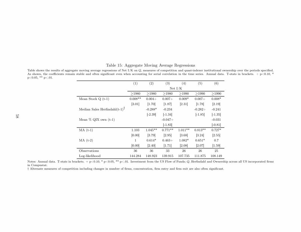
Table 15: Aggregate Moving Average RegressionsTable shows the results of aggregate moving average regressions of Net I/K on Q, measures of competition and quasi-indexer institutional ownership over the periods specified.As shown, the coefficients remain stable and often significant even when accounting for serial correlation in the time series. Annual data. T-stats in brackets. + p<0.10, *p<0.05, ** p<.01.

(1) (2) (3) (4) (5) (6)

Net I/K

≥1980 ≥1980 ≥1980 ≥1990 ≥1990 ≥1990

Mean Stock Q (t-1) 0.008** 0.004+ 0.007+ 0.009* 0.007+ 0.008*

[3.01] [1.70] [1.87] [2.31] [1.78] [2.19]

Median Sales Herfindahl(t-1)† -0.288* -0.234 -0.282+ -0.241

[-2.39] [-1.34] [-1.85] [-1.35]

Mean % QIX own (t-1) -0.047+ -0.031

[-1.83] [-0.81]

MA (t-1) 1.103 1.045** 0.771** 1.011** 0.813** 0.727*

[0.00] [3.79] [2.95] [3.68] [3.24] [2.55]

MA (t-2) 1 0.614* 0.463+ 1.082* 0.651* 0.7

[0.00] [2.40] [1.71] [2.08] [2.07] [1.59]

Observations 36 36 33 26 26 25

Log-likelihood 144.284 148.923 139.915 107.735 111.875 108.149

Notes: Annual data. T-stats in brackets. + p<0.10, * p<0.05, ** p<.01. Investment from the US Flow of Funds; Q, Herfindahl and Ownership across all US incorporated firmsin Compustat.† Alternate measures of competition including changes in number of firms, concentration, firm entry and firm exit are also often significant.

58

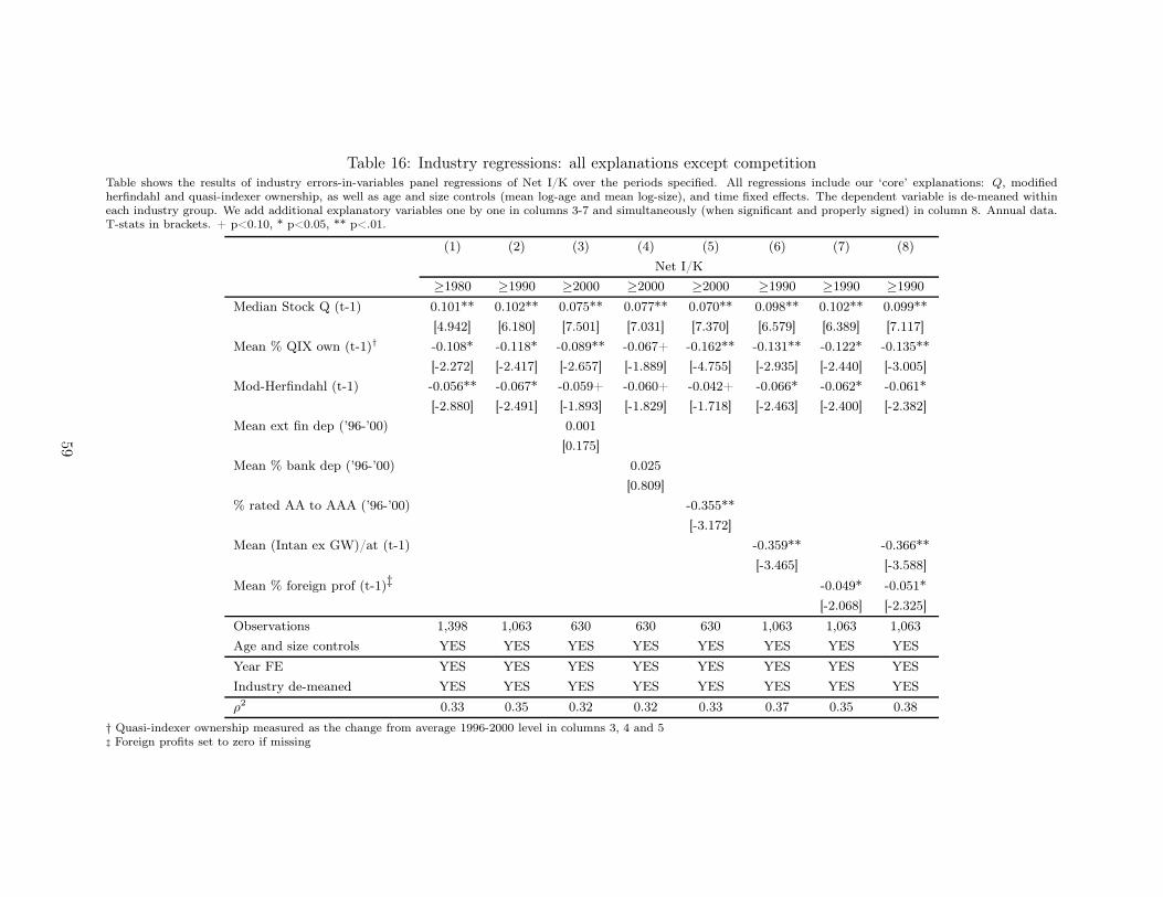
Table 16: Industry regressions: all explanations except competitionTable shows the results of industry errors-in-variables panel regressions of Net I/K over the periods specified. All regressions include our ‘core’ explanations: Q, modifiedherfindahl and quasi-indexer ownership, as well as age and size controls (mean log-age and mean log-size), and time fixed effects. The dependent variable is de-meaned withineach industry group. We add additional explanatory variables one by one in columns 3-7 and simultaneously (when significant and properly signed) in column 8. Annual data.T-stats in brackets. + p<0.10, * p<0.05, ** p<.01.

(1) (2) (3) (4) (5) (6) (7) (8)

Net I/K

≥1980 ≥1990 ≥2000 ≥2000 ≥2000 ≥1990 ≥1990 ≥1990

Median Stock Q (t-1) 0.101** 0.102** 0.075** 0.077** 0.070** 0.098** 0.102** 0.099**

[4.942] [6.180] [7.501] [7.031] [7.370] [6.579] [6.389] [7.117]

Mean % QIX own (t-1)† -0.108* -0.118* -0.089** -0.067+ -0.162** -0.131** -0.122* -0.135**

[-2.272] [-2.417] [-2.657] [-1.889] [-4.755] [-2.935] [-2.440] [-3.005]

Mod-Herfindahl (t-1) -0.056** -0.067* -0.059+ -0.060+ -0.042+ -0.066* -0.062* -0.061*

[-2.880] [-2.491] [-1.893] [-1.829] [-1.718] [-2.463] [-2.400] [-2.382]

Mean ext fin dep (’96-’00) 0.001

[0.175]

Mean % bank dep (’96-’00) 0.025

[0.809]

% rated AA to AAA (’96-’00) -0.355**

[-3.172]

Mean (Intan ex GW)/at (t-1) -0.359** -0.366**

[-3.465] [-3.588]

Mean % foreign prof (t-1)‡ -0.049* -0.051*

[-2.068] [-2.325]

Observations 1,398 1,063 630 630 630 1,063 1,063 1,063

Age and size controls YES YES YES YES YES YES YES YES

Year FE YES YES YES YES YES YES YES YES

Industry de-meaned YES YES YES YES YES YES YES YES

ρ2 0.33 0.35 0.32 0.32 0.33 0.37 0.35 0.38

† Quasi-indexer ownership measured as the change from average 1996-2000 level in columns 3, 4 and 5‡ Foreign profits set to zero if missing

59

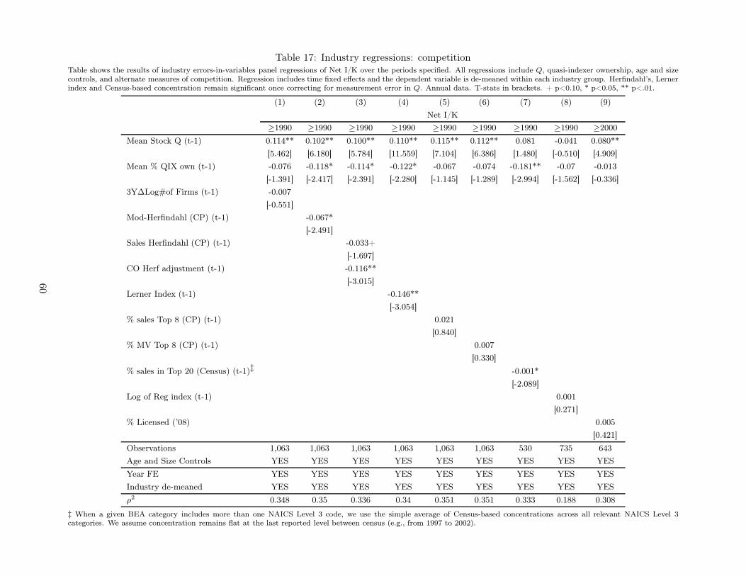
Table 17: Industry regressions: competitionTable shows the results of industry errors-in-variables panel regressions of Net I/K over the periods specified. All regressions include Q, quasi-indexer ownership, age and sizecontrols, and alternate measures of competition. Regression includes time fixed effects and the dependent variable is de-meaned within each industry group. Herfindahl’s, Lernerindex and Census-based concentration remain significant once correcting for measurement error in Q. Annual data. T-stats in brackets. + p<0.10, * p<0.05, ** p<.01.

(1) (2) (3) (4) (5) (6) (7) (8) (9)

Net I/K

≥1990 ≥1990 ≥1990 ≥1990 ≥1990 ≥1990 ≥1990 ≥1990 ≥2000

Mean Stock Q (t-1) 0.114** 0.102** 0.100** 0.110** 0.115** 0.112** 0.081 -0.041 0.080**

[5.462] [6.180] [5.784] [11.559] [7.104] [6.386] [1.480] [-0.510] [4.909]

Mean % QIX own (t-1) -0.076 -0.118* -0.114* -0.122* -0.067 -0.074 -0.181** -0.07 -0.013

[-1.391] [-2.417] [-2.391] [-2.280] [-1.145] [-1.289] [-2.994] [-1.562] [-0.336]

3Y∆Log#of Firms (t-1) -0.007

[-0.551]

Mod-Herfindahl (CP) (t-1) -0.067*

[-2.491]

Sales Herfindahl (CP) (t-1) -0.033+

[-1.697]

CO Herf adjustment (t-1) -0.116**

[-3.015]

Lerner Index (t-1) -0.146**

[-3.054]

% sales Top 8 (CP) (t-1) 0.021

[0.840]

% MV Top 8 (CP) (t-1) 0.007

[0.330]

% sales in Top 20 (Census) (t-1)‡ -0.001*

[-2.089]

Log of Reg index (t-1) 0.001

[0.271]

% Licensed (’08) 0.005

[0.421]

Observations 1,063 1,063 1,063 1,063 1,063 1,063 530 735 643

Age and Size Controls YES YES YES YES YES YES YES YES YES

Year FE YES YES YES YES YES YES YES YES YES

Industry de-meaned YES YES YES YES YES YES YES YES YES

ρ2 0.348 0.35 0.336 0.34 0.351 0.351 0.333 0.188 0.308

‡ When a given BEA category includes more than one NAICS Level 3 code, we use the simple average of Census-based concentrations across all relevant NAICS Level 3categories. We assume concentration remains flat at the last reported level between census (e.g., from 1997 to 2002).

60

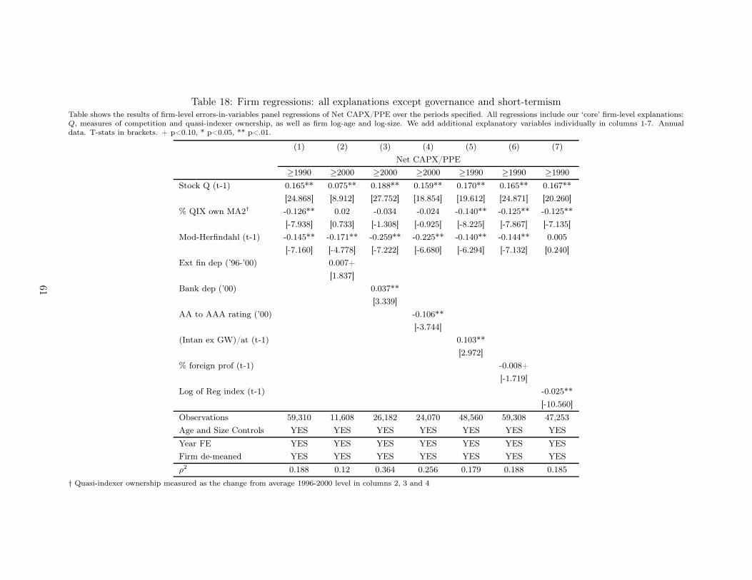
Table 18: Firm regressions: all explanations except governance and short-termismTable shows the results of firm-level errors-in-variables panel regressions of Net CAPX/PPE over the periods specified. All regressions include our ‘core’ firm-level explanations:Q, measures of competition and quasi-indexer ownership, as well as firm log-age and log-size. We add additional explanatory variables individually in columns 1-7. Annualdata. T-stats in brackets. + p<0.10, * p<0.05, ** p<.01.

(1) (2) (3) (4) (5) (6) (7)

Net CAPX/PPE

≥1990 ≥2000 ≥2000 ≥2000 ≥1990 ≥1990 ≥1990

Stock Q (t-1) 0.165** 0.075** 0.188** 0.159** 0.170** 0.165** 0.167**

[24.868] [8.912] [27.752] [18.854] [19.612] [24.871] [20.260]

% QIX own MA2† -0.126** 0.02 -0.034 -0.024 -0.140** -0.125** -0.125**

[-7.938] [0.733] [-1.308] [-0.925] [-8.225] [-7.867] [-7.135]

Mod-Herfindahl (t-1) -0.145** -0.171** -0.259** -0.225** -0.140** -0.144** 0.005

[-7.160] [-4.778] [-7.222] [-6.680] [-6.294] [-7.132] [0.240]

Ext fin dep (’96-’00) 0.007+

[1.837]

Bank dep (’00) 0.037**

[3.339]

AA to AAA rating (’00) -0.106**

[-3.744]

(Intan ex GW)/at (t-1) 0.103**

[2.972]

% foreign prof (t-1) -0.008+

[-1.719]

Log of Reg index (t-1) -0.025**

[-10.560]

Observations 59,310 11,608 26,182 24,070 48,560 59,308 47,253

Age and Size Controls YES YES YES YES YES YES YES

Year FE YES YES YES YES YES YES YES

Firm de-meaned YES YES YES YES YES YES YES

ρ2 0.188 0.12 0.364 0.256 0.179 0.188 0.185

† Quasi-indexer ownership measured as the change from average 1996-2000 level in columns 2, 3 and 4

61

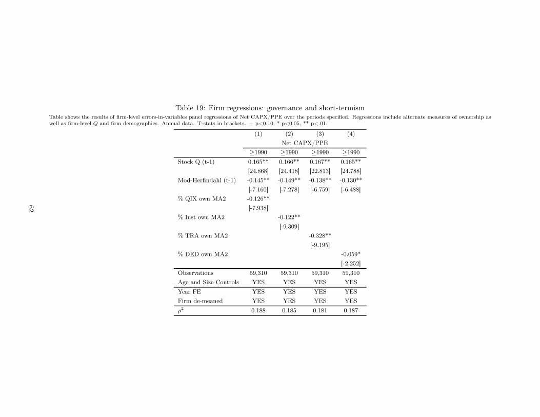
Table 19: Firm regressions: governance and short-termismTable shows the results of firm-level errors-in-variables panel regressions of Net CAPX/PPE over the periods specified. Regressions include alternate measures of ownership aswell as firm-level Q and firm demographics. Annual data. T-stats in brackets. + p<0.10, * p<0.05, ** p<.01.

(1) (2) (3) (4)

Net CAPX/PPE

≥1990 ≥1990 ≥1990 ≥1990

Stock Q (t-1) 0.165** 0.166** 0.167** 0.165**

[24.868] [24.418] [22.813] [24.788]

Mod-Herfindahl (t-1) -0.145** -0.149** -0.138** -0.130**

[-7.160] [-7.278] [-6.759] [-6.488]

% QIX own MA2 -0.126**

[-7.938]

% Inst own MA2 -0.122**

[-9.309]

% TRA own MA2 -0.328**

[-9.195]

% DED own MA2 -0.059*

[-2.252]

Observations 59,310 59,310 59,310 59,310

Age and Size Controls YES YES YES YES

Year FE YES YES YES YES

Firm de-meaned YES YES YES YES

ρ2 0.188 0.185 0.181 0.187

62

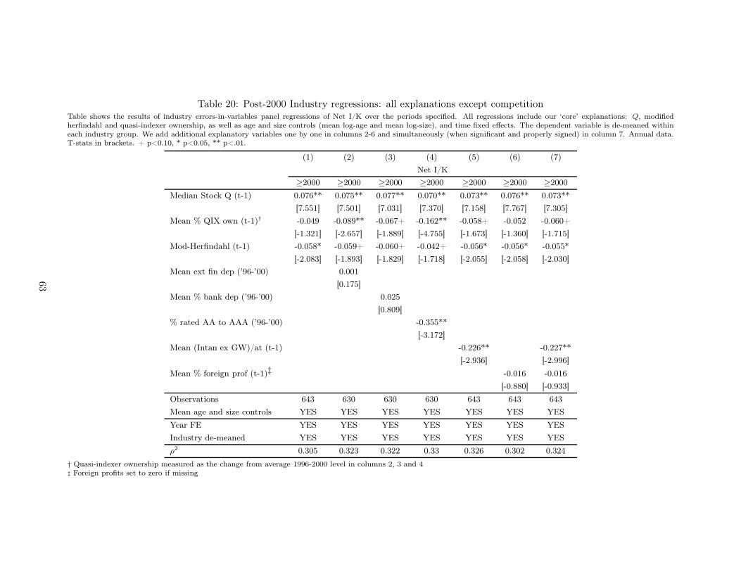
Table 20: Post-2000 Industry regressions: all explanations except competitionTable shows the results of industry errors-in-variables panel regressions of Net I/K over the periods specified. All regressions include our ‘core’ explanations: Q, modifiedherfindahl and quasi-indexer ownership, as well as age and size controls (mean log-age and mean log-size), and time fixed effects. The dependent variable is de-meaned withineach industry group. We add additional explanatory variables one by one in columns 2-6 and simultaneously (when significant and properly signed) in column 7. Annual data.T-stats in brackets. + p<0.10, * p<0.05, ** p<.01.

(1) (2) (3) (4) (5) (6) (7)

Net I/K

≥2000 ≥2000 ≥2000 ≥2000 ≥2000 ≥2000 ≥2000

Median Stock Q (t-1) 0.076** 0.075** 0.077** 0.070** 0.073** 0.076** 0.073**

[7.551] [7.501] [7.031] [7.370] [7.158] [7.767] [7.305]

Mean % QIX own (t-1)† -0.049 -0.089** -0.067+ -0.162** -0.058+ -0.052 -0.060+

[-1.321] [-2.657] [-1.889] [-4.755] [-1.673] [-1.360] [-1.715]

Mod-Herfindahl (t-1) -0.058* -0.059+ -0.060+ -0.042+ -0.056* -0.056* -0.055*

[-2.083] [-1.893] [-1.829] [-1.718] [-2.055] [-2.058] [-2.030]

Mean ext fin dep (’96-’00) 0.001

[0.175]

Mean % bank dep (’96-’00) 0.025

[0.809]

% rated AA to AAA (’96-’00) -0.355**

[-3.172]

Mean (Intan ex GW)/at (t-1) -0.226** -0.227**

[-2.936] [-2.996]

Mean % foreign prof (t-1)‡ -0.016 -0.016

[-0.880] [-0.933]

Observations 643 630 630 630 643 643 643

Mean age and size controls YES YES YES YES YES YES YES

Year FE YES YES YES YES YES YES YES

Industry de-meaned YES YES YES YES YES YES YES

ρ2 0.305 0.323 0.322 0.33 0.326 0.302 0.324

† Quasi-indexer ownership measured as the change from average 1996-2000 level in columns 2, 3 and 4‡ Foreign profits set to zero if missing

63

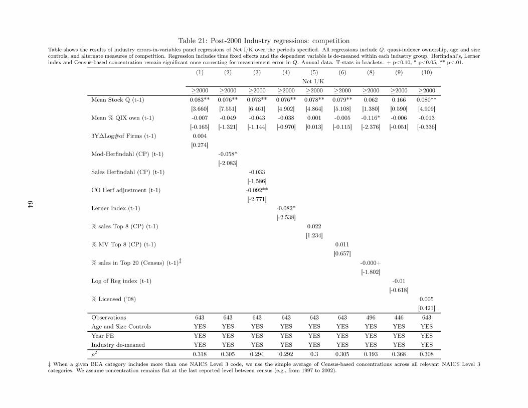
Table 21: Post-2000 Industry regressions: competitionTable shows the results of industry errors-in-variables panel regressions of Net I/K over the periods specified. All regressions include Q, quasi-indexer ownership, age and sizecontrols, and alternate measures of competition. Regression includes time fixed effects and the dependent variable is de-meaned within each industry group. Herfindahl’s, Lernerindex and Census-based concentration remain significant once correcting for measurement error in Q. Annual data. T-stats in brackets. + p<0.10, * p<0.05, ** p<.01.

(1) (2) (3) (4) (5) (6) (8) (9) (10)

Net I/K

≥2000 ≥2000 ≥2000 ≥2000 ≥2000 ≥2000 ≥2000 ≥2000 ≥2000

Mean Stock Q (t-1) 0.083** 0.076** 0.073** 0.076** 0.078** 0.079** 0.062 0.166 0.080**

[3.660] [7.551] [6.461] [4.902] [4.864] [5.108] [1.380] [0.590] [4.909]

Mean % QIX own (t-1) -0.007 -0.049 -0.043 -0.038 0.001 -0.005 -0.116* -0.006 -0.013

[-0.165] [-1.321] [-1.144] [-0.970] [0.013] [-0.115] [-2.376] [-0.051] [-0.336]

3Y∆Log#of Firms (t-1) 0.004

[0.274]

Mod-Herfindahl (CP) (t-1) -0.058*

[-2.083]

Sales Herfindahl (CP) (t-1) -0.033

[-1.586]

CO Herf adjustment (t-1) -0.092**

[-2.771]

Lerner Index (t-1) -0.082*

[-2.538]

% sales Top 8 (CP) (t-1) 0.022

[1.234]

% MV Top 8 (CP) (t-1) 0.011

[0.657]

% sales in Top 20 (Census) (t-1)‡ -0.000+

[-1.802]

Log of Reg index (t-1) -0.01

[-0.618]

% Licensed (’08) 0.005

[0.421]

Observations 643 643 643 643 643 643 496 446 643

Age and Size Controls YES YES YES YES YES YES YES YES YES

Year FE YES YES YES YES YES YES YES YES YES

Industry de-meaned YES YES YES YES YES YES YES YES YES

ρ2 0.318 0.305 0.294 0.292 0.3 0.305 0.193 0.368 0.308

‡ When a given BEA category includes more than one NAICS Level 3 code, we use the simple average of Census-based concentrations across all relevant NAICS Level 3categories. We assume concentration remains flat at the last reported level between census (e.g., from 1997 to 2002).

64

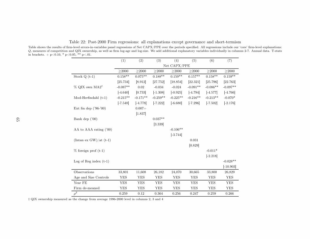
Table 22: Post-2000 Firm regressions: all explanations except governance and short-termismTable shows the results of firm-level errors-in-variables panel regressions of Net CAPX/PPE over the periods specified. All regressions include our ‘core’ firm-level explanations:Q, measures of competition and QIX ownership, as well as firm log-age and log-size. We add additional explanatory variables individually in columns 2-7. Annual data. T-statsin brackets. + p<0.10, * p<0.05, ** p<.01.

(1) (2) (3) (4) (5) (6) (7)

Net CAPX/PPE

≥2000 ≥2000 ≥2000 ≥2000 ≥2000 ≥2000 ≥2000

Stock Q (t-1) 0.158** 0.075** 0.188** 0.159** 0.157** 0.158** 0.159**

[25.734] [8.912] [27.752] [18.854] [22.321] [25.796] [22.763]

% QIX own MA2† -0.087** 0.02 -0.034 -0.024 -0.091** -0.086** -0.097**

[-4.640] [0.733] [-1.308] [-0.925] [-4.794] [-4.577] [-4.766]

Mod-Herfindahl (t-1) -0.215** -0.171** -0.259** -0.225** -0.216** -0.213** -0.070*

[-7.548] [-4.778] [-7.222] [-6.680] [-7.296] [-7.502] [-2.176]

Ext fin dep (’96-’00) 0.007+

[1.837]

Bank dep (’00) 0.037**

[3.339]

AA to AAA rating (’00) -0.106**

[-3.744]

(Intan ex GW)/at (t-1) 0.031

[0.829]

% foreign prof (t-1) -0.011*

[-2.218]

Log of Reg index (t-1) -0.028**

[-10.903]

Observations 33,801 11,608 26,182 24,070 30,665 33,800 26,829

Age and Size Controls YES YES YES YES YES YES YES

Year FE YES YES YES YES YES YES YES

Firm de-meaned YES YES YES YES YES YES YES

ρ2 0.259 0.12 0.364 0.256 0.247 0.259 0.266

† QIX ownership measured as the change from average 1996-2000 level in columns 2, 3 and 4

65

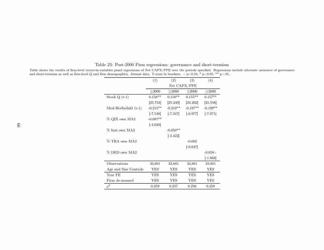
Table 23: Post-2000 Firm regressions: governance and short-termismTable shows the results of firm-level errors-in-variables panel regressions of Net CAPX/PPE over the periods specified. Regressions include alternate measures of governanceand short-termism as well as firm-level Q and firm demographics. Annual data. T-stats in brackets. + p<0.10, * p<0.05, ** p<.01.

(1) (2) (3) (4)

Net CAPX/PPE

≥2000 ≥2000 ≥2000 ≥2000

Stock Q (t-1) 0.158** 0.158** 0.155** 0.157**

[25.734] [25.249] [24.262] [25.556]

Mod-Herfindahl (t-1) -0.215** -0.210** -0.197** -0.199**

[-7.548] [-7.347] [-6.977] [-7.071]

% QIX own MA2 -0.087**

[-4.640]

% Inst own MA2 -0.050**

[-3.422]

% TRA own MA2 -0.002

[-0.047]

% DED own MA2 -0.058+

[-1.868]

Observations 33,801 33,801 33,801 33,801

Age and Size Controls YES YES YES YES

Year FE YES YES YES YES

Firm de-meaned YES YES YES YES

ρ2 0.259 0.257 0.256 0.258

66