Quantum simulation of the spin-boson model with a microwave circuit

Juha Leppakangas,1, 2 Jochen Braumuller,2 Melanie Hauck,1 Jan-Michael Reiner,1 Iris Schwenk,1

Sebastian Zanker,1 Lukas Fritz,1 Alexey V. Ustinov,2, 3 Martin Weides,2, 4 and Michael Marthaler1, 5, 6

1Institut fur Theoretische Festkorperphysik, Karlsruhe Institute of Technology, 76131 Karlsruhe, Germany2Physikalisches Institut, Karlsruhe Institute of Technology, 76131 Karlsruhe, Germany

3Russian Quantum Center, National University of Science and Technology MISIS, 119049 Moscow, Russia4Physikalisches Institut, Johannes Gutenberg University Mainz, 55128 Mainz, Germany

5Institut fur Theorie der Kondensierten Materie,Karlsruhe Institute of Technology, 76131 Karlsruhe, Germany

6 Theoretische Physik, Universitat des Saarlandes, 66123 Saarbrucken, Germany

We consider superconducting circuits for the purpose of simulating the spin-boson model. Thespin-boson model consists of a single two-level system coupled to bosonic modes. In most cases, themodel is considered in a limit where the bosonic modes are sufficiently dense to form a continuousspectral bath. A very well known case is the ohmic bath, where the density of states grows linearlywith the frequency. In the limit of weak coupling or large temperature, this problem can be solvednumerically. If the coupling is strong, the bosonic modes can become sufficiently excited to make aclassical simulation impossible. Here, we discuss how a quantum simulation of this problem can beperformed by coupling a superconducting qubit to a set of microwave resonators. We demonstratea possible implementation of a continuous spectral bath with individual bath resonators couplingstrongly to the qubit. Applying a microwave drive scheme potentially allows us to access the strong-coupling regime of the spin-boson model. We discuss how the resulting spin relaxation dynamicswith different initialization conditions can be probed by standard qubit-readout techniques fromcircuit quantum electrodynamics.

I. INTRODUCTION

The spin-boson model studies dynamics of a two-levelsystem interacting with a bosonic environment [1, 2]. Itis a generic model of quantum decoherence of two-levelsystems [3] and is of particular interest for the studiesof quantum phase transitions [4]. It assumes a linearcoupling between a two-level system (spin operator) anda collective coordinate of the bosonic bath. Despite ofits very simple form, the spin-boson model is not exactlysolvable by any known theoretical method [2].

Certain limits of the spin-boson problem are howeverwell understood. In the limit of weak system-bath cou-pling, perturbative methods such as the Born-Markovmaster equation [1, 2] can be applied, describing weaklydamped coherent oscillations. In the limit of high tem-perature, adequate perturbation theory may be possiblein the polaron basis [1, 2, 5], describing incoherent hop-ping of dressed states. In such situations, the correspond-ing spin-boson model can be solved in a good approxi-mation, analytically or numerically. On the other hand,when interaction strengths are of the order of involvedfrequencies, the problem becomes increasingly difficult,or even impossible, to solve in a desired accuracy. Thisregime covers many interesting problems of many-bodyphysics, such as the Kondo effect [1, 6, 7] and localization-delocalization transitions of spin dynamics in differentenvironments [1, 4, 8].

A commonly used strategy of obtaining new insightinto many quantum models, or to test previous theo-retical predictions, is the approach of quantum simula-tion [9–13]. The Hamiltonian of the problem is mappedto a well-controlled artificial quantum system and its dy-

namics is probed experimentally. Superconducting mi-crowave circuits have proven to be a particularly at-tractive experimental platform for engineering variousinteresting Hamiltonians [14–21] due to its good con-trollability and feasibility of realizing exotic parameterregimes [22–26].

The computational complexity of model Hamiltoni-ans is connected to the mutual coupling strengths ofthe individual elements relative to the subsystem ener-gies. Reaching the strong-coupling regime between aqubit and a resonator in a superconducting microwavecircuit, described by the Jaynes-Cummings model, hasenabled the reproduction of many fundamental phenom-ena from cavity quantum electrodynamics (QED) andhas led to the development of novel quantum systems andapplications [22–25, 27–29]. Here, the coupling strengthbetween the qubit and the bosonic mode is larger thanthe decay rates of the two coupled systems. If the cou-pling strength becomes comparable to the sub-systemenergies, the counter-rotating terms of the general quan-tum Rabi model cannot be neglected. This ultra-strongcoupling regime [30–32] has been experimentally demon-strated with superconducting circuits [33–39] and in vari-ous other platforms [40–42]. Interesting phenomena thatemerge include ground-state squeezing [43], single-modephase transitions [44], and non-classical state genera-tion [45–47].

The spin-boson model is a generalization of the single-mode quantum Rabi model to a continuous-mode envi-ronment. Near the coupling regime that exhibits Kondophysics and localization-delocalization transitions [1, 4,8], the energy decay rate Γ of the two-level system andits free evolution frequency ∆ are comparable, Γ .

arX

iv:1

711.

0746

3v3

[qu

ant-

ph]

24

May

201

8

2

∆ [48, 49]. A quantum simulation of this region withsuperconducting microwave circuits can be done by con-necting a superconducting qubit to an open transmis-sion line [6, 7, 48, 49]. Very strong couplings (combinedwith high qubit anharmonicities) are possible by design-ing system characteristic impedances comparable to theresistance quantum RQ = h/(2e)2 [6, 7, 48, 49]. Thesingle Cooper-pair charge 2e appears since the anhar-monicity of the system is ultimately based on Cooper-pair tunneling across a Josephson junction. For the two-level approximation to hold even under strong dissipa-tion, Cooper-pair tunneling must remain the dominantmechanism. In other words, the coupling strength mustbe smaller than the qubit anharmonicity, such that onlyvery non-linear qubits such as flux-based qubits are com-patible with reaching the ultra-strong coupling regime inthe laboratory frame.

Besides increasing the coupling strength via sampledesign, it also can be effectively increased by creat-ing a Hamiltonian in the rotating frame, based on theapplication of Rabi drives [18, 50]. In the effectiveframe, the sub-system energies of the original problemare down-converted to lower frequencies, while the cou-pling strength is preserved up to a factor of two. Ap-plying this approach, an effective ultra-strong couplingbetween a microwave resonator and a superconductingqubit has been demonstrated recently also experimen-tally [20, 51]. Here, the original qubit-resonator systemin the lab frame needs to be only in the strong-couplingregime. In this work, we study an extension of this ap-proach to a continuous-mode environment, yielding thespin-boson model. Recently, related approaches to effec-tively achieve ultra-strong coupling have been proposedbased on parametric driving [52, 53].

In this article, we study theoretically a realization ofthe spin-boson model with strong system-environmentcouplings using a superconducting qubit coupled to anengineered environment of bosonic modes. In analogy tothe approach described in Refs. [18, 20], we propose toconstruct an effective spin-boson Hamiltonian in the ro-tating frame. The bosonic environment is realized via aset of individual microwave resonators that reside in arestricted frequency range. We discuss in detail how themicrowave circuit maps onto the spin-boson model dis-cussed in literature. While in principle any bosonic en-vironment can be engineered with the proposed method,we consider the construction of an environment with anohmic spectral function that allows for probing localiza-tion dynamics of the spin-boson model. We find that thelocalization regime appears at strong coupling betweenthe qubit and individual bosonic modes, which is exper-imentally feasible to achieve.

We also discuss how the resulting spin dynamics canbe probed by standard readout techniques from circuitQED. In particular, the down-conversion of system fre-quencies allows for tracking the spin-relaxation dynamicsin real time. We also discuss an experimental implemen-tation, where the bosonic environment and the qubit are

fabricated on two separate chips in a modular approach.This setup allows for probing the system more rigorously,by characterizing both the qubit and the environmentalproperties in separate experiments.

The article is organized as follows: In Sec. II, we intro-duce the spin-boson problem in the notation widely usedin literature, and how it maps to the notation and meth-ods used in this article. We briefly go through centralresults and predictions of the spin-boson model. In par-ticular, in Sec. II C, we show how the effective spin-bosoncoupling strength can be tailored by two-tone driving.In Sec. III, we introduce an implementation of the spin-boson model by a superconducting transmon qubit cou-pled to a microwave circuit. We show how the impedanceof the environment is related to the spectral densityin the spin-boson model and discuss in detail how theimpedance affects to transmon. In Sec. IV, we analyzehow a set of microwave resonators can be used to tai-lor an ohmic spectral density in the rotating frame withKondo parameter α ∼ 1. In Sec. V, we provide a descrip-tion of an experimental realization based on a modularflip-chip approach and introduce measurement pulse se-quences that can be used to probe spin dynamics withdifferent initial conditions. Conclusions and discussionare given in Sec. VI.

II. SPIN-BOSON MODEL

We start our analysis by introducing the Hamiltonianand the spectral function of the spin-boson problem.After this, in Sec. II B, we go through central resultsand predictions of spin-boson problem obtained in litera-ture [1] and discuss what are the corresponding quantitiesto be measured in our realization. In Sec. II C, by ap-plying the method described in Refs. [18, 20], we derivean effective spin-boson Hamiltonian in the rotating framewith decreased sub-system energies. Finally, in Sec. II D,we analyze the limits of validity of the given derivation.

A. Spin-boson Hamiltonian and the spectraldensity

Here, we introduce the spin-boson Hamiltonian in thenotation as widely used in earlier literature. After this wediscuss how it maps to the notation used in this article.The notation and methods used throughout the remain-der of this article matches to the standard one used insuperconducting microwave circuits and therefore moredirectly allows us to relate properties of the spin-bosonmodel to proposed experimental realization.

3

1. Notation in literature

In earlier literature, the spin-boson model is often in-troduced by starting from the Hamiltonian [1, 2]

HSB = −~∆

2σx +

ε

2σz +

q0

2σz∑i

cixi + Hbath (1)

Hbath =∑i

[1

2miω

2i x

2i +

1

2mip2i

]. (2)

The two-level system, described by the Pauli matricesσi, may be regarded as two trapped positions of a virtualparticle in a certain potential landscape. The variableq0 denotes a trapping distance, ∆ a hopping rate, andε characterizes the energy difference. The environmentperceives the location of the particle and thereby couplesto σz. The free evolution of the environmental coordi-nate operators xi is defined by the quadratic harmonicoscillator Hamiltonian Hbath.

A central function of the theory is the spectral densityof the environment, defined formally as

J(ω) =π

2

∑i

c2imiωi

δ(ω − ωi) . (3)

The spectral function S(ω) of the collective bath opera-tor,

X =∑i

cix , (4)

is a function of temperature T and J(ω), and reads

S(ω) =⟨X(t)X(0)

⟩ω

=2~J(ω)

1− exp(− ~ωkBT

) . (5)

Together with the parameter q0, see Eq. (1), the spectralfunction includes all relevant information of the effect ofthe environment on the two-level system. The fundamen-tal reason is that the environmental fluctuations satisfyGaussian statistics. Accordingly, the Wick’s theorem isvalid and the time evolution of the reduced density ma-trix of the two-level system is fully described by two-timecorrelation functions of the environmental coupling oper-ator.

2. Notation in this article

When superconducting qubits are capacitively or in-ductively coupled to microwave cavities, their dipole mo-ment couples to the electric or magnetic field of the cav-ity. Since the dipole coupling is considered transversal,it is intuitive to write the coupling term proportionalto a σx operator. Therefore, even though circuit QEDsystems consisting of a superconducting qubit coupledto a set of microwave resonators are described by the

spin-boson Hamiltonian in Eq. (1), their Hamiltonian isusually written down in a notation where the definitionof σx and σz are interchanged, most typically in the con-text of the Jaynes-Cummings model [28]. In the case of atransmon qubit [54], the two energy levels correspond totwo eigenstates of a virtual particle in the same potentialminimum.

To keep the notation comparable with Sec. II A 1, wedefine the system parameters analogously as above. Wethen consider establishing the spin-boson Hamiltonianusing a superconducting qubit with energy splitting ~∆,coupled to a set of microwave resonators, described bythe total Hamiltonian

H =~∆

2σz +

q0

2σx∑i

gi

(bi + b†i

)+∑i

~ωib†i bi . (6)

This corresponds to the case ε = 0, which is the regimethat shows the physically most relevant and non-trivialbehavior [1]. This Hamiltonian is well implemented by aquantum circuit based on the transmon qubit [54]. Thespectral density, defined in Eq. (3), becomes

J(ω) =π

~∑i

g2i δ(ω − ωi) . (7)

We note that the coupling parameter q0 could also beincorporated in the definition of the coupling strengthsgi. Our separation is meaningful only when the variables

cixi = gi

(bi + b†i

)correspond to certain physical quan-

tities. In this article, we fix the bath coordinates xi tocorrespond to voltage fluctuations across the two capac-itors of the qubit,

X(t) ≡ V (t) . (8)

Therefore, q0 has the dimension of charge. It describesan effective charge shift of the artificial atom between itstwo states as seen by the environment. The variable q0

then absorbs all the information of the qubit and how itcouples to the voltage fluctuations: the following resultsare thereby valid, in principle, for arbitrary supercon-ducting qubits with appropriate adaptations of couplingparameter q0. Within this identification we then write,⟨

V (t)V (0)⟩ω

=2~J(ω)

1− exp(− ~ωkBT

) (9)

following from Eq. (5) and the identification made inEq. (8).

B. Different bath spectral functions andpredictions for the relaxation dynamics of the

spin-boson model

In the following, we briefly go through some centralpredictions made for the spin dynamics when interacting

4

0 time t (a.u.) 1

0

1

-1

P(t

)localization

damped oscillationsincoherent relaxation

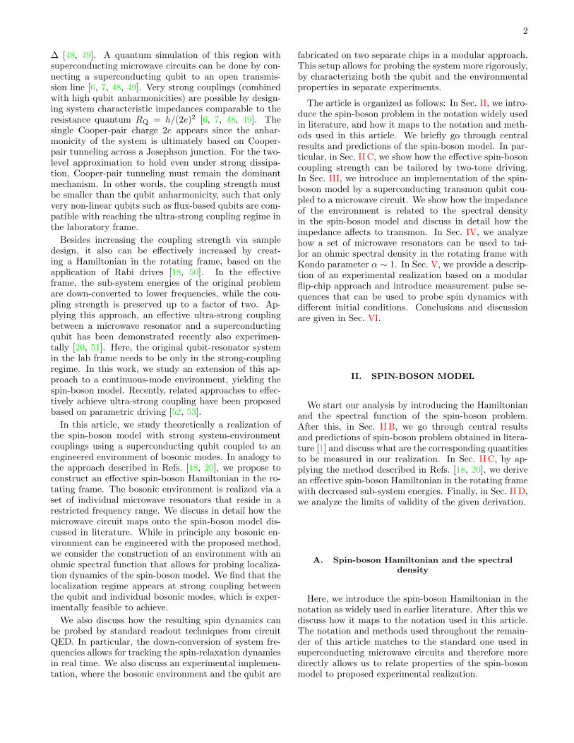
FIG. 1: Qualitative behavior of spin dynamics in the threemain regimes of the spin-boson model with an ohmic envi-ronment (s = 1). The probability P (t) corresponds in theproposed system to the expectation value P (t) = 〈σx(t)〉,when initialized to the +1 eigenstate of σx at t = 0. Forα < 0.5, (damped) oscillations prevail when ~∆rn & αkBT ,but change to incoherent relaxation when ~∆rn . αkBT (ex-ponential decay to zero). Localization effect leads to a decayof P (t) towards a finite value and occurs for α ≥ 1 and T = 0.In other regimes, the system exhibits incoherent relaxationwith subtle forms of the decay rate [1].

with bosonic environments of different spectral functions.We explain how these predictions correspond to dynam-ics in the considered circuit QED system. A more de-tailed explanation of an experimental realization is givenin Sec. V. Central predictions for an ohmic environmentare summarized qualitatively in Fig. 1.

1. Measured quantities

In the spin-boson model, a widely studied effect is thehopping dynamics between the two trapped positions ofthe fictitious particle (connected by the hopping ampli-tude ∆) under a perturbation caused by coupling to theenvironment. Here, we are not interested in the environ-ment itself, but in the short and intermediate time-scaleevolution of the system when subjected to a certain ini-tial condition. The long-time behavior is also interestingto study but can be much more challenging to observein experiment. The theoretical restrictions to small andintermediate time scales practically correspond to the ex-perimental restrictions due to the finite initialization timeand finite decoherence time of the superconducting qubit,correspondingly.

We consider now the notation introduced in Sec. II A 2and follow the discussion given in Ref. [1]. If inserted ini-tially in the left-hand side well, the probability the par-ticle to be found from this well again at some later timedepends on the hopping amplitude and interaction withthe environment. (For a rigorous mathematical defini-tion of the problem, particularly the initialization of thesystem, see Ref. [1].) Such population dynamics corre-sponds in our notation to the initialization of the systemat t = 0 to an eigenstate of operator σx and measuring

the value of σx at certain later time t > 0,

P (t) = 〈σx(t)〉 . (10)

Ideally, in the absence of interaction, we get (defining theleft-hand side as +1 eigenstate of σx)

P (t) = cos ∆t . (11)

When interacting with the environment, the hopping canbecome damped, over-damped, or even totally forbidden(localization).

We note that in our realization, we are naturally notrestricted to the theoretical scenarios in the literature:one can probe both σz and σx with different initializa-tion conditions, for the two-level system as well as for thebath (see Sec. V). The exact initialization of the bath af-fects the results essentially in the case of strong couplings,while it is not a requirement for the observation of thefollowing effects (in particular the localization).

2. Relaxation dynamics for different environments

A central example of the spin-boson model is the ohmicenvironment, which is described by a linear spectral den-sity

J(ω) = ηωFc(ω) . (12)

Here we have introduced a cut-off function Fc(ω). For in-stance, this can be an exponential drop Fc(ω) = e−ω/ωc

or a sharp cut-off Fc(ω) = Θ(ωc − ω), with cut-off fre-quency ωc, respectively. An important parameter de-scribing the coupling between the system and the envi-ronment in the ohmic case is the Kondo parameter

α = ηq20

2π~. (13)

It can be qualitatively interpreted as an environment-induced decay rate Γ normalized by the internal pre-cession frequency ∆, α ∼ Γ/∆: In the limit α 1,it directly corresponds to an inverse quality factor ofthe weakly perturbed two-level system, as derived inSec. III D, and a similar result can also hold for the quan-tum two-level system with α ∼ 1 [48, 49], even thoughhere a separation between the system and environmentdynamics is not necessary that clearly defined.

It has been understood that we have practically two in-dependent variables that define the solution of the prob-lem: the interaction strength α and the (bath renormal-ized) two-level system energy ∆rn [1]. Under the in-fluence of the environment, many qualitatively differentbehaviors of the well-hopping dynamics can occur. Forα < 1/2 we can have damped oscillations (∆rn & kBTα)changing to incoherent relaxation (∆rn . kBTα). Forα > 1/2, all dynamics are expected to be incoherent. Inthe regime α ≥ 1 and T = 0, one expects a total sup-

5

pression of hopping, whereas for T & 0 very slow thermalrelaxation should occur [1]. In the simple ohmic case witha linear increase of J(ω), we therefore expect very differ-ent types of behavior in various parameter regimes. Theregimes are summarized in Fig. 1.

It can be helpful to mention that the localizationmechanism in the spin-boson model is closely relatedto Coulomb blockade effect in superconducting tunneljunctions, i.e., Cooper-pair tunneling across a Joseph-son junction that is voltage-biased in series with anelectromagnetic environment. When the environmental(zero-frequency or characteristic resonator) impedance iscomparable with the resistance quantum RQ = h/4e2,the system enters the Coulomb blockade regime, wherecharge tunneling is strongly suppressed or even com-pletely prohibited [55–58].

The model for general power-law behavior of J(ω) isconveniently written in the form

J(ω) = Asωsω1−s

c Fc(ω) . (14)

Here, the case s < 1 is called the sub-ohmic regime ands > 1 is referred to as the super-ohmic regime. In par-ticular, s = 0 with T > 0 has been used as a model for1/f noise [3, 5]. The super-ohmic case appears in theelectron tunneling in solids with coupling to a (three-dimensional) phononic bath. The extra scaling factorω1−s

c has been introduced so that we can define a dimen-sionless variable A = Asq

20/2π~, in analogy to the Kondo

parameter α. However, it has less physical meaning hereas in the ohmic case. It also always appears togetherwith the introduced scaling by the cut-off, Aω1−s

c [1].In a rough overall picture, the super-ohmic case showsmostly damped oscillations and does not exhibit local-ization, whereas the sub-ohmic case is less trivial: it islocalized for weak tunneling amplitudes ∆ (depending onA) but even there, in non-equilibrium, can show coherentoscillations [8]. Also as opposed to the ohmic case, hereexists more than one relevant energy scale of coherentdynamics.

C. Simulation in the rotating frame

Here, we show how to establish an effective spin-boson Hamiltonian in the rotating frame by additionalmicrowave driving. We take use of modified interac-tion during driven evolution of the two-level system [59].An important detail of the following derivation is thateven though rotating-wave approximations (RWA) canbe taken in various places of the derivation, it cannot betaken for the final effective Hamiltonian, where the effectof counter-rotating terms can be essential.

1. Two-tone driving

Following Refs. [18, 20], we consider driving this sys-tem with two Rabi tones, both with transverse couplingto the qubit. A Hamiltonian that describes such a drivensystem has the form

H + Hd , (15)

where the drive is accounted for by the term

Hd = ~Ω1σx cosω1t+ ~Ω2σx cosω2t . (16)

Here Ωi is the amplitude and ωi the frequency of thedrive i. To obtain an immediate feeling of the drive fre-quencies and amplitudes we use, we note that in the fol-lowing scheme we consider a situation where ω1 & ω2

and Ω1 Ω2. During the derivation, also the conditionω1 − ω2 = Ω1 is taken to obtain the desired form of theHamiltonian (see below), and we will have ωi Ωi. Thedrive frequency can be assumed to be the qubit frequencyin the lab frame, ω1 = ∆.

We enter now a rotating frame with respect to thestronger transverse drive by performing a unitary trans-formation according to

U = exp

[iω1t

(∑i

b†i bi +1

2σz

)]. (17)

This is a combined rotating frame of the two-level systemand of all the bosonic modes. The Hamiltonian becomesnow

H1

~=

1

~

(UHU† − iU

˙U†)

=∆− ω1

2σz +

Ω1

2σx (18)

+∑i

(ωi − ω1)b†i bi +q0

2~∑i

gi

(biσ+ + b†i σ−

)+

Ω2

2

(ei(ω1−ω2)tσ+ + e−i(ω1−ω2)tσ−

).

We have neglected the contributions

O1 =q0

2~∑i

giσ+b†ie

2iω1t +Ω1

2σ+e

2iω1t (19)

+Ω2

2σ+e

i(ω1+ω2)t + H.c. .

This can be done if oscillations with the frequencies 2ω1

and ω1 +ω2 are much faster than frequencies Ω1 and Ω2.In addition, coupling to modes in the bosonic bath, withcouplings q0gi/~, is negligible if the bath will include onlymodes in a small frequency range ωc 2ωi.

In Hamiltonian of Eq. (18), the dominant term will bethe contribution proportional to Ω1. It is then favorableto move to the interaction picture defined by this term.This means performing another unitary transformation,

6

this time according to

U = exp

[iΩ1

2σxt

]. (20)

We also choose Ω1 = ω1 − ω2, which leads to

H2

~= (21)

Ω2

4σz +

q0

2~∑i

gi2σx(b†i + bi) +

∑i

(ωi − ω1)b†i bi .

We have again neglected fast oscillating terms,

O2 =Ω2

2σz

(sin2 Ω1t+

1

2

)(22)

− Ω2

2(σ1 sin Ω1t− σy sin 2Ω1t))

+ (∆− ω1)(σz cos Ω1t+ σy sin Ω1t)

+q0

4~∑i

gi

[(iσy cos Ω1t+ iσz ˆsinΩ1t

)b†i + H.c.

),

The first three terms on the right-hand side can be easilydropped with similar assumptions as above. The implica-tions due to dropping the fourth term need to be analyzedmore carefully, done below in Sec. II D.

2. Effective Hamiltonian and spectral density

We note that the Hamiltonian of Eq. (21) has the same(non-RWA) interaction term as in Eq. (6), with modifiedparameters. We then have the effective Hamiltonian

Heff =~∆eff

2σz (23)

+q0

2σx∑i

geffi

(bi + b†i

)+∑i

~ωeffi b†i bi ,

where the new parameters have the form

∆eff =Ω2

2(24)

ωeffi = ωi − ω1 (25)

geffi =

gi2. (26)

We see that the two-level system and bosonic energiesare tunable by the external drives. Since the couplinghas kept its form (up to a factor of 2), this allows fortailoring essentially stronger relative couplings betweenthe system and the environment [18, 20].

We also have a new coordinate operator of the envi-ronment. To determine its properties we first write down

the solution in the rotating frame

Veff(t) =1

2

∑i

gi

[bie−i(ωi−ω1)t + b†ie

i(ωi−ω1)t].(27)

Here the energies ωi−ω1 are the effective energies in therotating basis, which can be negative. The population ofthese modes can be determined from the thermal popula-tion in the laboratory frame. Using the spectral densityin the original frame, J(ω), we get for the thermal aver-age of the correlation function⟨

Veff(t)Veff(0)⟩ω

=~2

J(ω + ω1)

1− exp(−~(ω+ω1)

kBT

) . (28)

The temperature T is the real temperature of the bath.In the following, it is safe to assume that the real bathis at the zero temperature since practically ω1 kBT/~.We have then⟨

Veff(t)Veff(0)⟩ω

=~2J(ω + ω1) . (29)

In order to have an exact connection between the ef-fective system in the rotating frame and the spin-bosonmodel, the created correlation function in the rotatingframe has to simulate a finite temperature bath. To con-struct a specific spectral function in the rotating framewith an effective temperature Teff , the spectral density inthe laboratory frame is required to have a contribution(δω > 0) below the frequency of the rotating frame,

J(ω1 − δω) = J(ω1 + δω)1− exp

[− ~δωkBTeff

]exp

[~δωkBTeff

]− 1

. (30)

If this is satisfied for certain Teff , we have⟨[Veff(t), Veff(0)

]+

⟩ω

= 2~Jeff(δω) coth~δω

2kBTeff,(31)

where we have defined the effective spectral density inthe rotating frame

Jeff(δω) =1

4J(ω1 + δω)

1− exp

[− ~δωkBTeff

]. (32)

For Teff = 0 we have simply

Jeff(δω) =1

4J(ω1 + δω) . (33)

We note that even though the connection betweenthese two systems might seem trivial, just a frequencyshift due to the external drive, it is quite remarkable sinceit connects two completely different many-body physicsproblems: one problem including emission and absorp-tion of photons with same bosonic modes, and anotherproblem which includes only dissipation to two different

7

set of bosonic modes. The only property that needs tobe satisfied to connect these two problems is the effectivedetailed balance, Eq. (30).

D. Error estimation

Here, we sum up the restrictions and the size oferrors in the quantum simulation that appear due tothe taken approximations when deriving the effectiverotating-frame Hamiltonian. Errors occur from droppingthe terms in Eqs. (19) and (22). Furthermore, errors alsooccur due to a finite anharmonicity of the two-level sys-tem, which can lead to a finite population of the thirdlevel of the superconducting qubit.

Most terms in Eqs. (19) and (22) can be droppedwithin the assumptions Ωi/ωi 1 and (ω1−∆)/Ω1 1,as well as Ω2/Ω1 1. These conditions are easily real-ized in an experiment [20]. However, the most importantcontribution we neglected was the term

O =q0

4

∑i

gi

[(iσy cos Ω1t+ iσz sin Ω1t) b

†i + H.c.

).(34)

This sets a limit to the spectral width and the cut-off ofthe bath. This is since the term probes the bath in acompletely similar way as the central term

q0

4

∑i

giσx(b†i + bi) , (35)

in the effective Hamiltonian of Eq. (23), but with energiesΩ1 ± Ω2/2 ≈ Ω1.

To be more quantitative, let us assume that we have aresidue bath density at frequencies close to Ω1, which wenow write in the form

Jeff(Ω1) ≈ 2π~q20

αΩ2

2. (36)

The dimensionless variable α then compares the effectivequbit frequency Ω2/2 to the spectral density at frequencyΩ1. This gives a bath-induced decoherence rate

Γ ≈ παΩ2

2. (37)

In order to have a negligible contribution within the timescale of the effective two-level system oscillations, 1/Ω2,we demand α 1. Similarly, also a finite internal life-time of the two-level system, due to internal decay mech-anisms, limits the simulation length. Let us denote thisrate by Γinternal. Ideally, we would then like to engineer abath which does not limit the decay and dephasing timesof the qubit itself, i.e., we would like to be in the regimeΓ < Γinternal Ω2/2.

The second important restriction to the parameterregime is the finite anharmonicity of the qubit. The an-harmonicity is defined as the difference between the first

and second energy-level splittings,

~∆an = |(E2 − E1)− (E3 − E2)| . (38)

Too strong drive can induce transitions to the third stateof the artificial atom. The probability for the artifi-cial atom contributing through the third excited stateis roughly

Perror ∼(

Ω1

∆an

)2

. (39)

Therefore, a large anharmonicity qubit is favorable inorder to avoid a strong additional upper bound in Ω1.The qubit anharmonicity depends on the experimentalrealization. Flux-based qubits can easily reach anhar-monicities higher than the lowest energy-level splitting∆an > ∆. In this article, we consider a realization basedon a transmon qubit with ∆an ∆ for its simple oper-ation without the necessity of biasing [54], the feasibilityof a straightforward capacitive coupling, and its superiorcoherence properties. For a qubit with ∆ = 2π × 7 GHzand anharmonicity ∆an = 2π × 350 MHz, a drive withΩ1 = 2π × 80 MHz leads to a reasonable low errorPerror ∼ 0.05. Combining this with the above analy-sis, this would also mean that the bath spectral widthhas to be smaller than 80 MHz, in order to avoid un-wanted transitions due to the term in Eq. (34). Wewould then desire a bath that has a rather sharp cut-off at ωc < Ω1 = 2π × 80 MHz, Fc(ω) ∼ Θ(ωc − ω).Later, in Sec. IV, we show how to build such a bath froma set of microwave resonators.

III. IMPLEMENTATION OF THE SPIN-BOSONMODEL WITH A MICROWAVE CIRCUIT

In this section, we study how a superconducting qubitconnected to a dissipative microwave-circuit element canbe used to realize the spin-boson Hamiltonian. We con-sider explicitly the case of a transmon qubit. Our maingoal is to determine how the parameters of the spin-bosonmodel, the spectral density S(ω), the coupling q0, andthe qubit energy ∆, depend on the properties of the mi-crowave circuit. Section III A briefly sums up the centralresults. In Sec. III B, we describe how to determine theeffect of capacitance renormalization in circuits consid-ered in this article. In Sec. III C, we detail the derivationof the spin-boson parameters q0 and ∆, and in Sec. III D,we show the derivation of the Kondo parameter α. Theapproach we use is based on a linear circuit analysis, butthe results can also be derived by an exact Lagrangianquantization [60–65]. In addition, we provide also a con-sistency check based on the Born-Markov approach, inSec. III B. Even though we explicitly consider a transmonqubit, our formalism is generic and can be extended, inprinciple, to all superconducting qubit architectures.

8

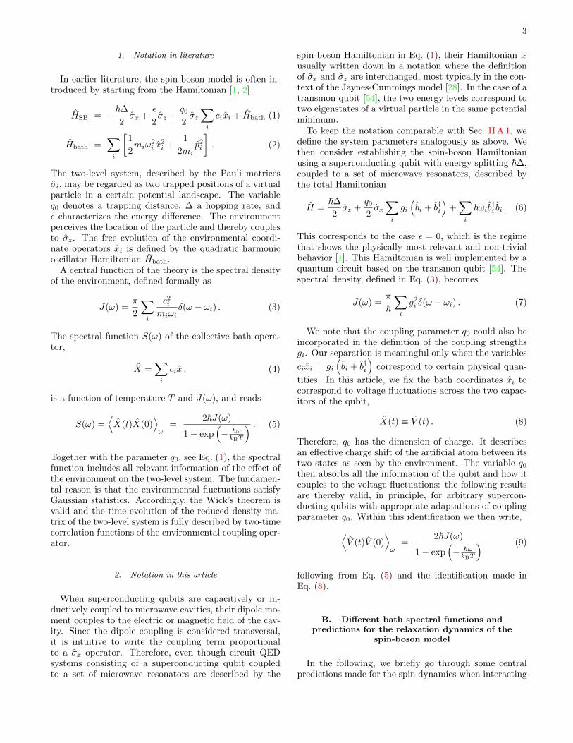
FIG. 2: (a) A model of a transmon qubit connected to animpedance Z(ω). The charge Q on the island between theJosephson junction (crossed box) and the ground capacitorCg is a conjugated variable to the phase across the Josephsonjunction, providing anharmonic energy levels and an effectivetwo-level system. The impedance Z induces voltage fluctu-ations (V ) and dissipation. (b) The circuit that defines thespectral density, Eqs. (41-43)

A. Spectral density and the system-bathinteraction

Our superconducting qubit couples to environmentalvoltage fluctuations V (t), that causes dissipation. Thequantity that describes its effect is the spectral den-

sity S(ω) =⟨V (t)V (0)

⟩ω

. There are several equivalent

ways of determining this quantity for microwave circuits,which basically all seek for the eigenmodes of the rele-vant (non-interacting) linear system. In this article, weassume that we know the impedance Z(ω) of the linearcircuit connected to the superconducting qubit, an exam-ple being the circuit we consider in Sec. IV. Guidelines fora determination of the spectral density in open circuitsis given in Appendix A as well as in other Refs. [60–65]

Voltage fluctuations across the impedance are de-scribed by the operator V . The exact circuit diagramof the considered setup is shown in Fig. 2(a). Generally,voltage fluctuations in a linear (free-evolution) electriccircuit satisfy the quantum fluctuation-dissipation theo-rem [56], ⟨

V (t)V (0)⟩ω

=2~ωRe[Zeff(ω)]

1− e−β~ω. (40)

In this free evolution solution, where the transmon islandcharge is set to zero (see below), the impedance Z(ω) seesa parallel capacitance Cint, which is the effective qubitcapacitance [56, 66, 67],

Cint =(C−1

J + C−1g

)−1. (41)

CJ and Cg denote the capacitances of the Josephson junc-tion and the capacitance to ground, respectively. Theeffective impedance of the environment, to be used in

Eq. (40), assumes the form

Z−1eff (ω) = iωCint + Z−1(ω) . (42)

The equivalent circuit is shown in Fig. 2(b). Note thatthe inductance of the Josephson junction, which deter-mines the qubit dynamics, does not enter the calculationof Z−1

eff (ω), but only the effective qubit capacitance Cint

that shunts the effective bath impedance.

We also note that the scenario where a bath cir-cuit is used to tailor a dissipative qubit environment isfundamentally different from the case where a certainimpedance is used to filter microwave transmission. Thereason is a different boundary condition at the qubit: Inthe case of the tailored bosonic environment, radiationreflects at the capacitor Cint, whereas in the case of amicrowave filter, we would have an impedance-matchedload and no reflection.

A direct comparison of Eqs. (9), (40) yields the relationbetween the spectral density of the spin-boson model andthe effective impedance,

J(ω) = ωRe[Zeff(ω)] . (43)

This equation is central for experimentally tailoring abosonic environment, relating the effective impedance tothe resulting spectral density J(ω). It has also beenshown recently that the parallel contribution Cint in thespectral density is indeed an essential quantity for aconsistent description of such systems in all parameterregimes [64, 65].

In the considered circuit, the transmon interacts withthe environmental voltage fluctuations through the oper-ator [66, 67]

Hint = βQV ≡ QintV (44)

β =Cg

CJ + Cg. (45)

Here Q is the charge operator of the transmon island.The interaction charge, Qint, accounts for an internaltransmon-qubit capacitive shunting through parameterβ, reducing the coupling to the island charge Q [54].The parameter β is not affected by renormalization ef-fects. However, for determination of the resulting spin-boson Hamiltonian parameter q0, one generally needs toconsider also the possible qubit-capacitance renormaliza-tion due to coupling to the impedance, as analyzed inSec. III B. The final result reads

q0 = 2eβ

√RQ

πZJ. (46)

Here, the characteristic impedance of the transmon is de-fined as ZJ = RQ

√2EC/π2EJ, where EJ is the Joseph-

son coupling energy, EC = e2/2(CJ + C0g ) the charging

energy, and the effective ground capacitance C0g depends

on the realization (see Sec. III B). In the simplest case

9

C0g = Cg. Finally, the normalized two-level system en-

ergy ∆ for typical transmon parameters becomes [54]

∆ ≈ 1

~√

8EJEC . (47)

In the following section, we show how to determine ECand demonstrate that the given identifications are con-sistent with the alternative approach of including the in-teraction term of Eq. (44) using a Born-Markov approx-imation. It is also consistent with the exact derivationwhen using an open-circuit, given in Appendix A.

B. Capacitance renormalization

The impedance Z(ω) can affect to the Hamiltonian ofthe transmon. The effect is generally twofold: it renor-malizes (i) the effective transmon capacitance and (ii) theJosephson coupling energy EJ. The effect (i) is analo-gous to mass renormalization in the spin-boson model [1]and can be here significant. The effect (ii) is analo-gous to tunneling-amplitude renormalization in the spin-boson model, before going into the spin-boson represen-tation [1], and stays here small due to considered smallenvironmental impedances, Z RQ, and low qubit en-ergies in comparison to the superconducting energy gap.

1. Hamiltonian of an isolated transmon

The Hamiltonian of a superconducting artificial atomcan be derived by applying a Lagrangian formalism toelectric circuits [68]. The Hamiltonian of an isolatedtransmon is of the form [54]

H isolatedtr = −EJ cos ϕ+

Q2

2(CJ + Cg), (48)

The first term on the right-hand side describes Cooper-pair tunneling across the superconducting junction as afunction of the superconducting phase difference ϕ acrossthe Josephson junction. The second term describes thecapacitive (Coulomb) energy related to the island chargeQ. In this isolated circuit, the effective island capacitanceis the sum of CJ and Cg. The phase and the charge areconjugated variables,[

Q

2e, eiϕ

]= eiϕ . (49)

The commutation relation is presented in this (periodic)form since the island charge takes only values that aremultiples of 2e, or equivalently, the phase distribution ishere by definition 2π-periodic.

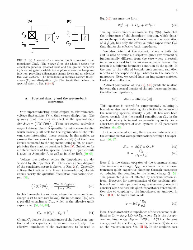
FIG. 3: Two environmental impedances Z(ω), whose capaci-tance renormalization is considered explicitly in this section.

2. Accounting for the counter-term

Finding the capacitance renormalization is analogousto identifying the ’counter-term’ in general system-reservoir models [1, 2]. In this analysis, we study twoequivalent forms of the total Hamiltonian,

Htotal = Htr + Hbath + Hint (50)

Htotal = H0tr + Hbath +

[Hint + Hct

], (51)

where then

H0tr = Htr − Hct . (52)

In addition to the qubit, bath, and interaction Hamil-tonians, we have introduced a term Hct, counteractingto the qubit Hamiltonian renormalization (coherent em-bedding of the environment) coming from the interaction

term Hint. It is here the interaction-normalized Hamilto-nian H0

tr that should be used when theoretically reducingthe transmon to a two-level system and whose dynamicsis observed in the experiment.

Strictly speaking, the renormalization is determinedtheoretically by first evaluating Hamiltonian of Eq. (50),for example, by using a Lagrangian approach (AppendixA), and then estimating the embedding due to the in-

teraction term Hint = QintV . However, we find that incircuits we consider the contributions Hct, Htr and H0

tr

can be deduced more straightforwardly from the follow-ing coherent solutions:

• The solution when the resistivity is put to zero,giving H0

tr.

• The solution when the resistive part is disentangledfrom the circuit, for example, with an additionalcapacitor Cdis → 0 in series with the resistor, givingHtr.

To illustrate the mathematics of this approach, letus consider the simple case of a bare ohmic impedanceZ(ω) = R. We then first identify the Hamiltonian of thecircuit when resistivity is set to zero. This fully coherent

10

system corresponds to the one in Eq. (48),

H0tr = H isolated

tr (53)

In the second stage, we identify the transmon Hamilto-nian when disconnected from the resistor lead, which hasthe form (Appendix A)

Htr = −EJ cos ϕ+Q2

2CJ. (54)

Using this we then find for the difference

Hct = Htr − H0tr

=Q2

2CJ− Q2

2(CJ + Cg)=

Q2int

2Cint. (55)

Let us then consider the circuit shown in Fig. 3(b),which is analogous to our proposal presented in Sec. IV.When the resistance is put to zero, an environmentalcapacitive remains with contribution C + Cc, leading to

H0tr = −EJ cos ϕ+

Q2

2(CJ + C0g ), (56)

where

C0g =

(C−1g + (C + Cc)−1

)−1. (57)

In the second stage, we get for the Hamiltonian corre-sponding to the disconnected resistor

Htr = −EJ cos ϕ+Q2

2(CJ + Cg′), (58)

where we have defined an effective gate capacitance

Cg′ =(C−1g + C−1

)−1. (59)

This is since C appears in series connection with Cg. Toevaluate the counter-term, let us consider explicitly thecase C → 0. (The analysis of this section also holds alsofor C 6= 0.) We get for the difference

Hct = Htr − H0tr

=Q2

2(CJ + Cg′)− Q2

2(CJ + C0g )

=Cc

Cc + Cint

1

2CintQ2

int . (60)

To show that the above results are sound, we canestimate the embedding due to the interaction termHint = QintV by an alternative method, using a Born-Markov master equation. Such an approach assumes thatthe effect of the environment (beyond the counter-term)is weak, but its result is valid also more generally sincethe embedding of the environment is the same for all R.Here we start from the Hamiltonian Htr, where the re-

sistor lead is decoupled from the transmon, and estimatethe renormalization explicitly. Considering the circuit ofFig. 3(a), we then use the property that for an ohmicenvironment with resistance R and cut-off defined by theparallel capacitor, (RCint)

−1 = ωc, we have transitionrates and energy-level renormalization terms

lims→0

∫ ∞0

dtei(ω+is)t⟨V (t)V (0)

⟩=

~ω1− e−β~ω

Re[Z(ω)]

− i~ωc

2Re[Z(ω)] + i

~ω2π

Re[Z(ω)]Ψ(ω) , (61)

where Re[Z(ω)] = R/[1 + (ω/ωc)2], and Ψ(ω) is definedby a digamma function [67]. The last (imaginary) con-tribution is for practical systems, with finite tempera-tures, of the same size as the real part: It stays smallfor environments inducing weak transition rates for thelab-frame qubit, which we assume to be true in this ar-ticle. In more details, this extra contribution is assumedto be small compared to the anharmonicity of the qubit.The other (and possibly large) imaginary term is inde-pendent of the resistance at usual frequencies which arewell below ωc and produces a constant −i/2Cint. As thisenters to a master equation through the matrix elementsof Qint, one obtains finally a coherent renormalizationterm Q2

int/2Cint, as obtained also in Eq. (55). This is thedesired result. In the same way, such consistency of thecapacitance renormalization between the two approachescan also be shown to hold for the circuit of Fig. 3(b) withcounter-term as in Eq. (60). The analysis of this sectionalso holds exactly for C > 0.

C. Parameters ∆ and q0 for a transmon qubit

After theoretically indentifying the capacitance renor-malization caused by the environment to the super-conducting artificial atom, we do the reduction of thetransmon to a two-level system using Hamiltonian H0

tr,Eq. (52). We can now make a connection between theparameters of the transmon qubit and the spin-bosonparameter q0.

For typical transmon parameters, the energy-level dif-ference between the ground and the first excited stateis

∆ ≈ 1

~√

8EJEC . (62)

Here, for example, for Hamiltonian of Eq. (56) the charg-ing energy EC = e2/2(CJ +C0

g ). The transmon is practi-cally a non-linear resonator, which reduces to a two-levelsystem when maximally only two lowest energy levels arepopulated. The relevant quantity describing this reduc-tion is the anharmonicity (difference between the firstand the second energy-level differences),

~∆an = E2 − E1 − (E3 − E2) ≈ EC . (63)

11

This variable will play an important role in a practicalrealization, since the drive amplitudes Ωi of Eq. (16) needto be smaller than the non-linearity of the qubit, as dis-cussed in Sec. II D

The transverse matrix element of the operator Q is onthe other hand

|〈↓ |Q| ↑〉|2 = e2

√EJ

2EC= e2 RQ

πZJ. (64)

Applying the result of Eq. (64), and comparing to theform of the spin-boson Hamiltonian of Eq. (6), we getthe connection

Qint = βQ = βe

√RQ

πZJσx

≡ q0

2σx , (65)

where now

q0 = 2eβ

√RQ

πZJ. (66)

Here again β = Cg/(CJ +Cg), where the ground capaci-tance is the unnormalized (original) one, Cg, whereas inthe definition of the charging energy and system energylevels the effective ground capacitance C0

g appears.

D. Parameter α for a transmon qubit (ohmicspectral density)

A central situation in the spin-boson theory is thecase of an ohmic environment. Assuming an ohmicimpedance, Re[Zeff ] = R, we have J(ω) = Rω ≡ ηω.This yields a Kondo parameter

α =1

πβ2 R

ZJ(67)

The coupling α scales linearly with R and is reducedby the capacitive shunting by the ground capacitance(β < 1). The relevant quantity to compare R is the char-acteristic impedance of the Josephson junction, ZJ. Thesize of α when realized in the rotating frame is studiedin Sec. IV.

Moreover, for a transmon qubit and for α 1 (weak-coupling limit) there is a direct connection between α andthe quality factor of the qubit. A golden rule calculationgives here for the decay rate [3] (inverse quality factor)

Γ↓∆

= β2 R

ZJ= πα . (68)

The limit β = 1 (no shunting of voltage fluctuations) isthe result for a dissipative classical resonator. This directconnection appears since we have treated the transmonas a harmonic oscillator, with weak non-linearity, whichis a good approximation since EJ EC . The relation

between the energy decay rate Γ↓ and the spin-bosonparameter α has been studied recently in Ref. [49] in thecase of a high-anharmonicity flux qubit coupled to anopen transmission line.

We note that if we would consider the Cooper-pair boxqubit, working in the limit EJ EC , we would haveq0 = 2e, leading to α = R/RQ. There, a resistanceR = RQ is then needed to reach α = 1.

IV. TAILORING AN OHMIC BATH IN THEROTATING FRAME

In this section, we consider constructing an ohmic bathin the rotating frame from multiple microwave resonatorswith broadening. Each such resonator can be, for exam-ple, a superconducting lumped element LC resonator in-tegrated with a resistive element R, or a superconductingcoplanar resonator with a leakage to an open transmis-sion line. After a qualitatively analysis of the achiev-able Kondo parameter α, Sec. IV A, we introduce ourmethod and show a numerical example of the bath con-struction, Sec. IV B. Analytical relations for bath prop-erties are derived in Sec. IV C and robustness againstparasitic coupling between neighboring resonators is an-alyzed in Sec. IV D.

A. Ohmic spectral density in the rotating frame

Let us first apply the idea presented in Sec. II C torealize an effective ohmic environment in the rotatingframe. We first note that in our effective system

ωc ω1 , (69)

where ω1 is the dominant Rabi frequency, which is tunedto the energy of the superconducting qubit, ∆ ∼ 2π ×7 GHz, and the cut-off frequency ωc . 2π × 100 MHz.This means that we practically need a linearly increasingimpedance to create a linearly increasing Jeff(ω), sincehere J(ω) = ωRe[Z(ω)] ≈ ω1Re[Z(ω)].

Let us now assume that a parameter R = η in someohmic environment of the original system describes alsothe maximum value of the spectral density in the con-structed effective system. Practically, such a parame-ter corresponds to a characteristic impedance of the mi-crowave transmission line or resonator. In this discus-sion, for simplicity, we neglect the factor 4 difference be-tween the laboratory-frame and the rotating-frame spec-tral densities. Let us denote ωq as the frequency wherethe maximal impedance is reached in the effective systemand the two impedances meet, so we have J(ωq) = Rωq,as depicted in Fig. 4. This gives for the coupling param-eter in the rotating frame

ηeff = Rωq

ωq − ω1= R

(1 +

ω1

ωc

). (70)

12

FIG. 4: Qualitative forms of the impedance Re[Z(ω)] andspectral density J(ω) of two different environments, one be-ing ohmic in the laboratory frame (blue lines) and one beingohmic in the rotating frame (red lines). For the same value ofimpedance at certain frequency ωq & ω1, Re[Z(ωq)] = R, thecoupling parameter η = ∂J(ω)/∂ω can be essentially largerin the rotating frame.

We see that establishing a linear increase of J(ω) in therotating frame, we can realize an essentially larger ηeff ,with the same maximal impedance R. It can also be in-terpreted that the impedance of the environment is effec-tively increased, without a change in the material design.

By applying this idea for a system with a transmonqubit we then get for the effective coupling in the rotatingframe (accounting for the factor 4)

αeff =β2

4π

ηeff

ZJ=β2

4π

R

ZJ

(1 +

ω1

ωc

). (71)

The individual multiplied contributions play an impor-tant role in determining the magnitude of αeff . The termβ2/4π reduces the coupling at least by an order of mag-nitude. Also the (maximal) resistivity needs to be rel-atively small, R/ZJ < 1. If we assume that these twocontributions reduce the coupling by two-to-three ordersof magnitude, then (in this example) it is the role of theterm 1 + ω1/ωc ≈ ω1/ωc to counteract this contribution.For example, we would need ω1/ωc ≈ 102 in order toreach very strong couplings αeff ∼ 0.1 − 1. This cor-responds to a relatively narrow-bandwidth environment,ωc . 2π × 100 MHz. This qualitative demand should beconsidered together with the restriction to drive strengthsΩ1 that are much weaker than the transmon qubit an-harmonicity, ∆an . 2π × 350 MHz, and that the Rabifrequency has to be above the cut-off of the effective en-vironment, Ω1 > ωc, see Sec. II D.

B. Bath engineering with multiple resonators

In this work, we consider constructing the environmen-tal impedance by using a set of LCR resonators, each ofthem coupled through a coupling capacitor Cci, as shownin Fig. 5. We desire a method that is based on a feasiblemanipulation of resonator parameters. Possible methodsfor tailoring the spectral density are varying the individ-ual couplings of the resonators to the qubit and varying

FIG. 5: We consider constructing the bosonic environmentfrom multiple LCR resonators coupled capacitively to a su-perconducting qubit. Each resonator can be a superconduct-ing lumped element LC resonator integrated with a resistiveelement R or, for example, a superconducting coplanar res-onator with leakage to an open transmission line. The qubititself contributes to the effective impedance through the in-teraction capacitance Cint, Eq. (41). The resonators are alsoassumed to be in parallel with an extra capacitor C, describ-ing the coupling of the qubit antenna to ground.

the spacings between the resonance frequencies. A gen-eral recipe that can be implemented in an experiment isthe following:

• Realize all resonators with slightly different fre-quencies, by varying their inductances Li and/orcapacitances Ci.

• Shape the spectral function by changing individ-ual coupling capacitances Cci and/or resonance-frequency spacing.

The resonator broadenings, defined by variables Ri, canbe used to shape the spectral function of the bath aswell, but more importantly, it is closely connected to theachievable Kondo parameter α, as shown below.

A practical example of bath shaping using our ap-proach is shown in Fig. 6, where an effective ohmicimpedance is constructed from N = 20 resonatorsby varying inductances Li and coupling capacitancesCci. A straightforward method for calculating the totalimpedance (and thereby the spectral function) of similarcircuits is given in Appendix C.

C. Analytical relations

More fundamental connections between the chosen pa-rameters and the achievable spectral density exists. Be-low, we first show analytically how the broadening andcoupling of individual modes relate to α. After this weconsider explicit formulas for the the size of the individ-ual couplings and study how the size of the constructed(smooth) impedance depends on resonator properties and

13

FIG. 6: Effective ohmic spectral density with three differentKondo parameters α in the rotating frame at ω1/2π = 7 GHz.The impedance is constructed from N = 20 dissipative res-onators with internal Q ≈ 2.2 × 103. A linear decreasein bath impedance Re[Z(ω)] is obtained here by reducingthe coupling capacitance from 0.5 fF quadratically to zero(∼ 1− (i− 1)2/N2, where i is the number of the resonator),while increasing the inductance linearly (with i). Differentcouplings α correspond to different parallel capacitors C, suchthat C + Cint takes the values 70 fF (α = 1),

√2 × 70 fF

(α = 1/2), and 2 × 70 fF (α = 1/4). The used trans-mon parameters are ZJ = 200 Ω, β = 1/

√2 and resonator

ZLC ≈ 113 Ω

the resonance-frequency density. We also estimate thesize of the transmon-capacitance renormalization.

1. Kondo parameter α

Let us first analyze how the linear increase of spectraldensity relates to the coupling to individual broadenedresonators. It is reasonable to assume that the steepnessof the spectral density at low effective frequencies (see forexample Fig. 6) is similar to, or limited by, the spectralsteepness related to the individual broadened resonators.The following discussion is made for a laboratory-framesystem, but the qualitative result is independent of thechosen frame.

We then evaluate the decay rate of the qubit due tosingle environmental broadened resonator. According tothe golden rule, the decay rate is

Γ =γ

γ2 + 4ω2g2 , (72)

where γ is the width (decay rate) of the resonator, ω thefrequency with respect to the resonance frequency, andg ≡ q0gi/~ the total coupling. The result for the decayrate is strictly valid for small couplings g γ, but this

formula indeed provides a general connection between anindividual resonator spectral density and a coupling tothe qubit. The derivative of the golden rule decay rate is

∂Γ

∂ω= −8

(g

γ

)2 ωγ[

1 + 4(ωγ

)2]2 . (73)

This has a maximal value & (g/γ)2. Assuming that wesynthesize a linear increase of the spectral density whichqualitatively follows this steepness, we can relate this di-rectly to the parameter α,

∂Γ

∂ω= πα ∼

(g

γ

)2

. (74)

We then find that for couplings α ∼ 1 at least some of theresonators are in the strong-coupling regime (g ∼ γ). Itis, however, not needed that individual resonators are inthe ultra-strong coupling regime. This seemingly funda-mental result states that the onset of the single-resonatorstrong-coupling regime, which comes together with non-Markovian system-environment interaction, is closely re-lated to the strong-coupling in the spin-boson model(α ∼ 1), when the environment is constructed from mul-tiple resonators.

2. Coupling to individual resonators

Let us consider now how the coupling to an individualresonator, g, relates to the system parameters. A Hamil-tonian for the qubit coupled to a single (non-dissipative)resonator with inductance L1 and capacitance C1 is hereof the form

H ≈ ~∆

2σz + ~ω1b

†b (75)

− 1

2β

Cc

C + Cint

√CT

C1~√

∆ω1

(b† − b

)(σ+ − σ−) ,

where ~∆ =√

8EJEC , EC = e2/2CT, CT = CJ +

CCg/(C + Cg), ω1 = 1/√L(C1 + Cc), and we have as-

sumed that Cc CJ, C1, Cg. For equal system frequen-cies, ∆ = ω1, we get

g = βCc

C + Cint

√CT

C1∆ . (76)

A practical example is β = 1/√

2, Cc = 0.1 fF, C+Cint =70 fF, C1 = 2CT = 200 fF, and ∆/2π = 7 GHz, whichgives g/2π = 5 MHz. In the rotating frame the couplingis halved to 2.5 MHz

When constructing the spectral density using multipleresonators with internal losses, the coupling to individ-ual resonators is reduced. This is due to the collective

14

capacitance due to all other resonators

Ctotalc ≡

N∑i=1

Cci . (77)

We assume here N 1 so that the considered resonatorcan be included in the sum with negligible error. Theeffect to coupling to a single resonator is the same asincreasing the extra capacitance to ground as C → C +Ctotal

c . The coupling to qubit is then approximately

g = βCc

C + Cint + Ctotalc

√CT

C1∆ . (78)

Here also ~∆ =√

8EJEC , EC = e2/2CT, but now withCT = CJ + (C + Ctotal

c )Cg/(C + Ctotalc + Cg).

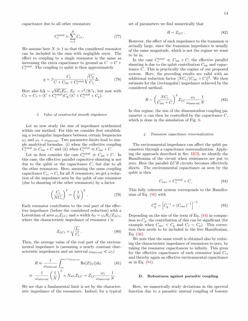
3. Value of constructed smooth impedance

Let us now study the size of impedance synthesizedwithin our method. For this we consider first establish-ing a rectangular impedance between certain frequenciesω1 and ω1 + ωinterval. Two parameter-limits lead to sim-ple analytical formulas: (i) when the collective couplingCtotal

c Cint + C and (ii) when Ctotalc Cint + C.

Let us first consider the case Ctotalc Cint + C. In

this case, the effective parallel capacitive shunting is notdue to the qubit or the capacitance C, but due to allthe other resonators. Here, assuming the same couplingcapacitance Cci = Cc for allN resonators, we get a reduc-tion of the impedance seen by the qubit of one resonator(due to shunting of the other resonators) by a factor(

Cc

NCc

)2

=

(1

N

)2

. (79)

Each resonator contributes to the real part of the effec-tive impedance (before the considered reduction) with aLorentzian of area ωiZLCi and a width δω = ωiRi/ZLCi,where the characteristic impedance of resonator i is

ZLCi =

√LiCi

. (80)

Then, the average value of the real part of the environ-mental impedance is (assuming a nearly constant char-acteristic impedances and an interval ωinterval ω1)

R ≈ 1

ωinterval

∫ ω1+ωinterval

ω1

Re[Z(ω)]dω (81)

≈ 1

ωinterval

(1

N

)2

×Nω1ZLC = ZLCω1

ωinterval

1

N.

We see that a fundamental limit is set by the character-istic impedance of the resonators. Indeed, for a typical

set of parameters we find numerically that

R ∼ ZLC . (82)

However, the effect of such impedance to the transmon isactually large, since the transmon impedance is usuallyof the same magnitude, which is not the regime we wantto be in.

In the case Ctotalc Cint + C, the effective parallel

shunting is due to the qubit contribution Cint and capac-itance C. This is practically the regime of our proposedsystem. Here, the preceding results are valid with anadditional reduction factor [NCc/(Cint + C)]2. We thenestimate for the (rectangular) impedance achieved by theconsidered method,

R ∼(

NCc

Cint + C

)2

ZLCω1

ωinterval

1

N. (83)

In this regime, the size of the dimensionless coupling pa-rameter α can then be controlled by the capacitance C,which is done in the simulation of Fig. 6.

4. Transmon capacitance renormalization

The environmental impedance can affect the qubit pa-rameters through a capacitance renormalization. Apply-ing the approach described in Sec. III B, we identify theHamiltonian of the circuit when resistances are put tozero. Here the parallel LCR circuits becomes effectivelyshorts. The environmental capacitance as seen by thequbit is then

Cenv = Ctotalc + C . (84)

This fully coherent system corresponds to the Hamilto-nian of Eq. (56) with

C0g =

[C−1

g + (Cenv)−1]−1

. (85)

Depending on the size of the term of Eq. (84) in compar-ison to Cg, the contribution of this can be significant (forexample when Cenv < Cg and CJ ∼ Cg). This correc-tion then needs to be included in the free Hamiltonian,Eq. (56).

We note that the same result is obtained also by reduc-ing the characteristic impedance of resonators to zero, bytaking the resonator capacitances to infinity. This givesfor the effective capacitance of each resonator lead Cci

and thereby again an effective environmental capacitanceas in Eq. (84).

D. Robustness against parasitic coupling

Here, we numerically study deviations in the spectralfunction due to a parasitic mutual coupling of bosonic

15

FIG. 7: The effect of parasitic resonator-resonator couplingto the impedance of system in Fig. 6. Here p = Cp/C

maxi

corresponds to the relative strength of the parasitic coupling,where Cp is the nearest-neighbor parasitic capacitance andCmax

i = 0.5 fF is the maximal coupling between a resonatorand qubit. The other parameters are as in Fig. 6 for α = 1.The curves have been separated by 0.04 GHz and the dashedlines correspond to the spectral densities with α = 1. We findthat the low-frequency part of the impedance is practicallyunchanged when parasitic coupling is of the same magnitudeor less than the (maximal) qubit-resonator coupling.

bath resonators. As described in Appendix C, we as-sume a capacitive nearest-neighbor coupling between res-onators, with cyclic boundary conditions. Unwanted sub-structure that is introduced by this mutual coupling issuppressed when resonators nearby in frequency are ar-ranged also spatially adjacent (except at the boundaryfrom the largest to the smallest). A numerical simulationof the effect of parasitic coupling is provided in Fig. 7.We generally find that the resonator-resonator couplingshould be of the same order or less than the coupling ofindividual resonators, so that our construction methodworks. In the opposite limit, the individual peaks arepushed away from each other and become visible. Wecan then summarize two important findings for tailor-ing the impedance for Kondo couplings α ∼ 1 using thepresented method:

• Coupling between the qubit and at least some of theresonators has to be in the strong-coupling limit,g ∼ γ.

• Parasitic coupling between resonators should bemaximally of the same order as the maximal cou-pling to the qubit, g.

V. EXPERIMENTAL REALIZATION

In this section, we provide a brief description of anexperimental realization of a spin-boson quantum simu-lator based on a modular flip-chip approach. In addi-tion, we discuss experimental protocols that allow oneto access interesting quantities of the two-level systemin the spin-boson simulator. They include the bath ini-tialization, qubit-state preparation, and the qubit-statemeasurement.

A. Flip-chip approach

In our preliminary experimental realization of the spin-boson model, we place the two-level system and thebosonic bath on two physically different chips. Both sam-ples are mounted in a specifically designed sample box ontop of each other in a flip-chip fashion [69, 70]. The qubitsample at the bottom is mounted on the ground levelof the sample box, which allows for the required bondconnections to the coaxial control lines, while the up-per sample containing the bosonic bath is flipped upsidedown and therefore facing the qubit chip. The capacitivecoupling between the qubit and bosonic bath is mediatedvia electric fields in the volume between the two samples.

We implement a bosonic bath formed by N = 20lumped-element resonators that individually couple tothe qubit via coupling antennas. The resonators areequipped with resistive elements that allow us to tai-lor their internal dissipation such that they overlap ina restricted frequency band and form a bosonic bath ofa smooth spectral function. A shaping of the bosonicbath impedance Z(ω) is achieved by adjusting the indi-vidual coupling strengths between qubit and the bosonicresonator modes, as described in Sec. IV. The two-levelsystem is formed by a concentric transmon qubit [71],which allows for an approximately equal coupling in anydirection in its plane due to its rotational symmetry.

In a preliminary experiment, we have demonstratedthat the qubit decay rate can be dominated by the engi-neered bosonic bath in a spectral range of ∼ 500 MHz.The bath-induced qubit decay rate at different frequen-cies corresponded here directly to the noise at differentfrequencies in the spin-boson model (α 1), and therebyshows that quantum simulation using the flip-chip ap-proach is possible. A more detailed description of thisexperiment is provided in Ref. [70].

B. Measurement protocols

In order to experimentally observe specific dynamicsof the spin-boson model, we propose two possible pulsesequences that allow us to access the expectation val-ues of σx [well population function P (t)] as well as ofσz (energy decay) with different bath initializations. A

16

(a)

qubitcontrol

freq.

readout

time

rotationexc.

(b)

t=0

(c)

t=0

A(t)time

i

S

readout

timeti

FIG. 8: Measurement protocols for the spin-boson simula-tor. (a) Pulse sequence for preparing an eigenstate of σz orσx, with the qubit out of resonance with the bosonic bath,followed by interaction with the bath during time τ and read-out. The qubit is tuned into the presence of the bosonic bathwith a fast detuning pulse. Prior to dispersive qubit readout,we can rotate the qubit state in order to measure 〈σz〉 or 〈σx〉.(b) Schematic location of the drive frequencies ω1, ω2. Thespectral location of the bosonic bath with individual modefrequencies ωi is schematically depicted in blue, indicating itsspectral function S(ω). (c) Proposed pulse sequence for mea-suring P (t) including a bath initialization scheme. The qubitis initially prepared in an eigenstate of σx via a π/2 rotation.At ti < t < 0, we initialize the bosonic bath via a strong bathdrive of amplitude ΩR and frequency ω1. For t > 0, we setΩR = 0.

brief description for the expected behavior of the well-population dynamics, function P (t), is given in Sec. II B 2and in Fig. 1.

1. Qubit initialization and measurement of 〈σz〉 and 〈σx〉

Observing the time evolution of the expectation values〈σz〉 or 〈σx〉 can be performed with an extension of themeasurement protocol applied in Ref. [20], see Fig. 8(a-b). The qubit in the laboratory frame is initially biasedto a frequency outside the spectral location of the bosonicbath. In the frequency space shown in Fig. 8(b), this isdenoted as ’qubit control’. The qubit is excited to theequatorial plane of the Bloch sphere by applying a π/2 ro-tation, see Fig. 8(a). By controlling the relative phase ofthe successive Rabi drives [20], we can prepare the qubitin an eigenstate of σx. This allows us to also initialize theeffective qubit state, because at t = 0 eigenstates remainunchanged during the transformation into the rotatingframe. Alternatively, the qubit can stay in its ground

state or be prepared in its excited state by applying aπ rotation prior to the start of the simulation sequenceat t = 0. With a fast frequency tuning pulse, the qubitis brought into resonance with the bosonic bath duringthe simulation time τ , where we apply the drive toneswith frequencies ω1, ω2 (see Sec. II C). As can be seenin the depicted pulse sequence in Fig. 8(b), the labora-tory frame qubit frequency is tuned to the lower cut-offfrequency ω0 of the bosonic bath. This also correspondsto zero frequency in the effective frame, given by the ro-tating frame frequency ω1 = ω0. After the simulation oftime τ , we apply an optional π/2 rotation prior to qubitreadout. This allows us to measure 〈σx〉 of the qubitstate. If no rotation is applied, we measure the qubitstate along its quantization axis, 〈σz〉.

2. Bath initialization

Within the above formalism we are able to probe therelaxation of qubit excitations for both 〈σz〉 and 〈σx〉.For a direct comparison with the spin-boson theory, forexample presented in Ref. [1], the environment has tobe properly initialized in addition. On the other hand,a comparison between the results obtained using differ-ent initialization methods allows for experimentally ex-ploring the effect of bath initialization in the spin-bosonmodel.

In order to observe the well population function P (t) asdiscussed in Ref. [1], the qubit in the spin-boson systemis initially required to be in an eigenstate of σx for t < 0,with the bath being relaxed in thermal equilibrium withinthis condition. This can be achieved experimentally byapplying a Rabi drive at the rotating frame frequencyω1 of enhanced amplitude ΩR = Ω1 + A(t). After thetransformation in the interaction picture, this leaves anadditional term in the effective spin-boson Hamiltonian

Heff +A(t)σx, (86)

with Heff given in Eq. (23). Initialization is applied atan effective amplitude A(t) = ΩR − Ω1 g, where g isthe typical coupling strength between qubit and individ-ual bosonic mode. Figure 8(c) shows a schematic of theproposed pulse sequence. Bath initialization takes placeduring ti < t < 0 with ti defined by the inverse spec-tral width of the bosonic bath. The simulation startsat t = 0, where the initialization drive is switched off,A(t) = 0, and the Rabi drives of the simulation schemeare switched on. To recover the well population func-tion P (t), we π/2 rotate the qubit state before readoutin order to measure 〈σx〉.

C. Bath heating

Dissipation of the bosonic bath can be implementedby adding an ancillary transmission line, providing a loss

17

channel for bath excitations [72]. In our approach, dis-sipation takes place by ohmic dissipation on-chip andtherefore involves Joule heating. The effect gives rise toa small modification of the bath spectral function. Themain source of on-chip dissipation can be assumed tobe the Rabi drive with amplitude Ω1 and frequency ω1,which in a realistic experiment also couples directly tothe bath.

If we assume that the coupling between the driveand the bath is mediated by the qubit, the effectivedrive of the environment is of an approximate amplitude(Cci/Cint)Ω1 per resonator i. Each resonator will cou-ple to the drive with separate coupling. In the systemconsidered in Sec. IV, each resonator has an approxi-mative width γi . 2π × 5 MHz. Considering explicitlythe highest-energy resonator, with the off-resonance driveωi−ω1 ∼ 2π×50 MHz, we get an average photon numberin this resonator

〈ni〉 ≈(Cci

Cint

)2(Ω1

ωi − ω1

)2

. 10−2 . (87)

This leads to photon dissipation rate Γdis = γi〈ni〉 .1 MHz. Due to the specific form of the designedimpedance, the result is approximately the same for allindividual resonators. The length of the one measure-ment process is roughly 1 µs, which implies that duringone measurement each on-chip resistor absorbs on aver-age less than 1 photon. The effect of this to the tem-perature of each resistor is small, but can set a minimal(cooling) time interval between two successive measure-ment protocols. Specific pulsing schemes that relax theenvironmental resonators to their ground states just be-fore the quantum simulation can also be used [73–75].

VI. CONCLUSIONS AND DISCUSSION

In conclusion, we have shown that a quantum sim-ulation of the spin-boson model can be performed in awide parameter range using a superconducting qubit con-nected to a microwave circuit. In order to probe numer-ically difficult parameter regimes, we considered an ex-tension of the driving scheme proposed in Ref. [18]. Thiseffectively down-converts the system dynamics from thegigahertz to the megahertz regime, while preserving theorder of the coupling strength between the two-level sys-tem and the environment. The approach allows for theobservation of a quantum phase transition in a regime ofa large effective Kondo parameter α ∼ 1, also withoutthe use of a high-anharmonicity superconducting qubit.We find that this requires strong coupling between thequbit and microwave resonators in the laboratory frame.The phase transition region in the spin-boson model cor-

responds to a regime with an energy decay rate of thetwo-level system that is comparable to its effective tran-sition frequency.

We discussed how to experimentally probe the wellpopulation dynamics P (t) under different initializationconditions of the bosonic bath. For this purpose, we pro-vided concrete measurement pulse sequences, based onwell-established control and detection schemes from cir-cuit QED. In the considered system, probing the wellpopulation dynamics corresponds to measuring the ex-pectation value of the σx(t) operator. It is also straight-forward to study other two-level system correlation func-tions, such as of the σz(t) operator, as well as the effectof bath initialization.

The proposed approach allows for engineering a ratherarbitrary spectral function in a restricted frequencyrange. We estimated that for a realization with a trans-mon qubit the spectral width of the environment mustbe in the range of 100 MHz. By controlling the driveand qubit frequencies, we can adjust the zero-frequencycondition of the tailored bosonic bath, which allows us tochoose the effective system temperature Teff . By control-ling the amplitude of the weaker Rabi drive, Ω2, we cantune the effective two-level system energy relative to thetemperature and the cut-off frequency ωc, which is of cen-tral importance in the spin-boson theory. In particular,Kondo physics can be observed for an effective tempera-ture below the Kondo temperature TK. At the Toulousepoint (α = 1/2) one can estimate [7] kBTK ∼ ~Ω2

2/ωc,which can be adjusted by Ω2. Hence, our system canaccess a large parameter space of the spin-boson modelvia experimental drive control. The proposed experimen-tal approach, based on the flip-chip technique, also fea-tures a modularity that allows to probe various fabricatedbosonic environments with the same qubit in successiveexperiments.

Acknowledgments

This work was supported by the European ResearchCouncil (ERC) within consolidator Grant No. 648011and Helmholtz IVF grant ’Scalable solid state quantumcomputing’. This work was also partially supported bythe Ministry of Education and Science of Russian Fed-eration in the framework of Increase CompetitivenessProgram of the NUST MISIS (contracts no. K2-2014-025, K2-2016-051, and K2-2016-063). J.B. acknowledgesfinancial support by the Landesgraduiertenforderung(LGF) of the federal state Baden-Wurttemberg and bythe Helmholtz International Research School for Tera-tronics (HIRST).

[1] A. Leggett, S. Chakravarty, A. Dorsey, M. Fisher,A. Garg, and W. Zwerger, Rev. Mod. Phys. 59, 1 (1987),

URL http://dx.doi.org/10.1103/RevModPhys.59.1.

18

[2] U. Weiss, Quantum Dissipative Systems, vol. 3rd ed.(World Scientific, Singapore, 2008).

[3] A. Shnirman, Y. Makhlin, and G. Schon, Phys.Scr. T102, 147 (2002), URL http://stacks.iop.org/

1402-4896/2002/i=T102/a=024.[4] P. P. Orth, A. Imambekov, and K. Le Hur, Phys. Rev. B

87, 014305 (2013), URL http://dx.doi.org/10.1103/

PhysRevB.87.014305.[5] M. Marthaler and J. Leppakangas, Phys. Rev. B 94,

144301 (2016).[6] K. Le Hur, Phys. Rev. B 85, 140506 (2012), URL https:

//link.aps.org/doi/10.1103/PhysRevB.85.140506.[7] M. Goldstein, M. H. Devoret, M. Houzet, and L. I.

Glazman, Phys. Rev. Lett. 110, 017002 (2013), URLhttps://link.aps.org/doi/10.1103/PhysRevLett.

110.017002.[8] F. B. Anders, R. Bulla, and M. Vojta, Phys. Rev. Lett.

98, 210402 (2007), URL https://link.aps.org/doi/

10.1103/PhysRevLett.98.210402.[9] I. Georgescu, S. Ashhab, and F. Nori, Rev. Mod.

Phys. 86, 153 (2014), URL https://doi.org/10.1103/

RevModPhys.86.153.[10] E. Manousakis, J. Low Temp. Phys. 126, 1501 (2002),

URL https://doi.org/10.1023/A:1014295416763.[11] D. Porras, F. Marquardt, J. von Delft, and J. I. Cirac,

Phys. Rev. A. 78, 010101(R) (2008), URL https://doi.

org/10.1103/PhysRevA.78.010101.[12] C. Schneider, D. Porras, and T. Schaetz, Rep. Prog.

Phys. 75, 024401 (2012), URL https://doi.org/10.

1088/0034-4885/75/2/024401.[13] A. Lemmer, C. Cormick, D. Tamascelli, T. Schaetz, S. F.

Huelga, and M. B. Plenio, arXiv:1704.00629 (2017), URLhttps://arxiv.org/abs/1704.00629.

[14] S. Mostame, P. Rebentrost, A. Eisfeld, A. J. Ker-man, D. I. Tsomokos, and A. Aspuru-Guzik, New J.Phys. 14, 105013 (2012), URL http://stacks.iop.org/

1367-2630/14/i=10/a=105013.[15] F. Mei, V. M. Stojanovic, I. Siddiqi, and L. Tian, Phys.

Rev. B 88, 224502 (2013), URL https://link.aps.org/

doi/10.1103/PhysRevB.88.224502.[16] J.-M. Reiner, M. Marthaler, J. Braumuller, M. Weides,

and G. Schon, Phys. Rev. A 94, 032338 (2016), URLhttp://dx.doi.org/10.1103/PhysRevA.94.032338.

[17] L. Garcıa-Alvarez, J. Casanova, A. Mezzacapo, I. L.Egusquiza, L. Lamata, G. Romero, and E. Solano, Phys.Rev. Lett. 114, 070502 (2015), URL https://link.aps.

org/doi/10.1103/PhysRevLett.114.070502.[18] D. Ballester, G. Romero, J. J. Garcıa-Ripoll, F. Deppe,

and E. Solano, Phys. Rev. X 2, 021007 (2012), URLhttp://dx.doi.org/10.1103/PhysRevX.2.021007.

[19] J. Li, M. Silveri, K. Kumar, J.-M. Pirkkalainen,A. Vepsalainen, W. Chien, J. Tuorila, M. Sillanpaa,P. Hakonen, E. Thuneberg, et al., Nat. Commun. 4, 1420(2013), URL http://dx.doi.org/10.1038/ncomms2383.

[20] J. Braumuller, M. Marthaler, A. Schneider, A. Stehli,H. Rotzinger, M. Weides, and A. V. Ustinov, Nat. Com-mun. 8, 779 (2017), URL https://doi.org/10.1038/

s41467-017-00894-w.[21] M. Haeberlein, F. Deppe, A. Kurcz, J. Goetz, A. Baust,

P. Eder, K. Fedorov, M. Fischer, E. P. Menzel, M. J.Schwarz, et al., Spin-boson model with an engineeredreservoir in circuit quantum electrodynamics (2017),URL https://arxiv.org/abs/arXiv1506.09114.

[22] J. Clarke and F. K. Wilhelm, Nature 453 (2008).[23] R. J. Schoelkopf and S. M. Girvin, Nature 451, 664

(2008).[24] M. H. Devoret and R. J. Schoelkopf, Science 339, 1169

(2013).[25] J. Q. You and F. Nori, Nature 474, 589 (2011), URL

https://doi.org/10.1038/nature10122.[26] X. Gu, A. F. Kockum, A. Miranowicz, Y. X. Liu, and

F. Nori, Phys. Rep. 718-719, 1 (2017), URL https://

doi.org/10.1016/j.physrep.2017.10.002.[27] A. Blais, R.-S. Huang, A. Wallraff, S. M. Girvin, and

R. J. Schoelkopf, Phys. Rev. A 69, 062320 (2004), URLhttps://doi.org/10.1103/PhysRevA.69.062320.

[28] J. M. Fink, M. Goppl, M. Baur, R. Bianchetti, P. J. Leek,A. Blais, and A. Wallraff, Nature 454, 315 (2008), URLhttp://dx.doi.org/10.1038/nature07112.

[29] M. Hofheinz, H. Wang, M. Ansmann, R. C. Bialczak,E. Lucero, M. Neeley, A. D. O’Connell, D. Sank, J. Wen-ner, J. M. Martinis, et al., Nature 459, 546 (2009), URLhttp://dx.doi.org/10.1038/nature08005.

[30] G. Gunter, A. A. Anappara, J. Hees, A. Sell, G. Bia-siol, L. Sorba, S. De Liberato, C. Ciuti, A. Tredicucci,A. Leitenstorfer, et al., Nature 458, 178 (2009), URLhttps://doi.org/10.1038/nature07838.

[31] A. A. Anappara, S. De Liberato, A. Tredicucci, C. Ciuti,G. Biasiol, L. Sorba, , and F. Beltram, Phys. Rev. B79, 201303(R) (2009), URL https://doi.org/10.1103/

PhysRevB.79.201303.[32] J. Casanova, G. Romero, I. Lizuain, J. J. Garcıa-Ripoll,

and E. Solano, Phys. Rev. Lett. 105, 263603 (2010),URL http://dx.doi.org/10.1103/PhysRevLett.105.

263603.[33] P. Forn-Dıaz, J. Lisenfeld, D. Marcos, J. J. Garcıa-Ripoll,

E. Solano, C. J. P. M. Harmans, and J. E. Mooij, Phys.Rev. Lett. 105, 237001 (2010), URL https://link.aps.

org/doi/10.1103/PhysRevLett.105.237001.[34] T. Niemczyk, F. Deppe, H. Huebl, E. P. Menzel,

F. Hocke, M. J. Schwarz, J. J. Garcia-Ripoll, D. Zueco,T. Hummer, E. Solano, et al., Nat. Phys. 6, 772 (2010),URL http://dx.doi.org/10.1038/nphys1730.

[35] A. Baust, E. Hoffmann, M. Haeberlein, M. J.Schwarz, P. Eder, J. Goetz, F. Wulschner, E. Xie,L. Zhong, F. Quijandrıa, et al., Phys. Rev. B 93,214501 (2016), URL https://link.aps.org/doi/10.

1103/PhysRevB.93.214501.[36] F. Yoshihara, T. Fuse, S. Ashhab, K. Kakuyanagi,

S. Saito, and K. Semba, Nat. Phys. 13, 44 (2016), URLhttp://dx.doi.org/10.1038/nphys3906.

[37] Z. Chen, Y. Wang, T. Li, L. Tian, Y. Qiu, K. Inomata,F. Yoshihara, S. Han, F. Nori, J. S. Tsai, et al., Phys.Rev. A 96, 012325 (2017), URL https://link.aps.org/

doi/10.1103/PhysRevA.96.012325.[38] S. J. Bosman, M. F. Gely, V. Singh, A. Bruno, D. Both-

ner, and G. A. Steele, npj Quantum Information 3,46 (2017), ISSN 2056-6387, URL https://doi.org/10.

1038/s41534-017-0046-y.[39] J. Puertas Martınez, S. Leger, N. Gheereart, R. Dasson-

neville, L. Planat, F. Foroughi, Y. Krupko, O. Buisson,C. Naud, W. Guichard, et al., arXiv:1802.00633 (2018),URL https://arxiv.org/abs/1802.00633.

[40] R. Gerritsma, G. Kirchmair, F. Zahringer, E. Solano,R. Blatt, and C. F. Roos, Nature 463, 68 (2010),ISSN 1476-4687, URL http://dx.doi.org/10.1038/

nature08688.

19

[41] M. Geiser, F. Castellano, G. Scalari, M. Beck,L. Nevou, and J. Faist, Phys. Rev. Lett. 108,106402 (2012), URL https://link.aps.org/doi/10.

1103/PhysRevLett.108.106402.[42] C. Maissen, G. Scalari, F. Valmorra, M. Beck,

J. Faist, S. Cibella, R. Leoni, C. Reichl, C. Char-pentier, and W. Wegscheider, Phys. Rev. B 90,205309 (2014), URL https://link.aps.org/doi/10.

1103/PhysRevB.90.205309.[43] C. Ciuti, G. Bastard, and I. Carusotto, Phys. Rev.

B 72, 115303 (2005), URL https://doi.org/10.1103/

PhysRevB.72.115303.[44] M.-J. Hwang, R. Puebla, and M. B. Plenio, Phys. Rev.

Lett. 115, 180404 (2015), URL https://doi.org/10.

1103/PhysRevLett.115.180404.[45] S. Ashhab and F. Nori, Phys. Rev. A 81, 042311 (2010),

URL https://doi.org/10.1103/PhysRevA.81.042311.[46] J. Leppakangas, M. Marthaler, D. Hazra, S. Jebari,

R. Albert, F. Blanchet, G. Johansson, and M. Hofheinz,Phys. Rev. A 97, 013855 (2018), URL https://doi.org/

10.1103/PhysRevA.97.013855.[47] A. F. Kockum, V. Macrı, L. Garziano, S. Savasta, and

F. Nori, Sci. Rep. 7, 5313 (2017), URL https://doi.

org/10.1038/s41598-017-04225-3.[48] P. Forn-Dıaz, J. Garcıa-Ripoll, B. Peropadre, J.-L. Or-

giazzi, M. Yurtalan, R. Belyansky, C. Wilson, and A. Lu-pascu, Nat. Phys. 13, 39 (2016), URL http://dx.doi.

org/10.1038/nphys3905.[49] L. Magazzu, P. Forn-Dıaz, R. Belyansky, J.-L. Orgiazzi,

M. A. Yurtalan, M. R. Otto, A. Lupascu, C. M. Wil-son, and M. Grifoni, Nat. Commun. 9, 1403 (2018), URLhttp://dx.doi.org/10.1038/s41467-018-03626-w.

[50] A. Mezzacapo, U. Las Heras, J. S. Pedernales, L. Di-Carlo, E. Solano, and L. Lamata, Scientific Re-ports 4, 7482 (2017), URL https://doi.org/10.1038/

srep07482.[51] N. K. Langford, R. Sagastizabal, M. Kounalakis,

C. Dickel, A. Bruno, F. Luthi, D. J. Thoen, A. Endo,and L. DiCarlo, Nat. Commun. 8, 1715 (2017), URLhttps://doi.org/10.1038/s41467-017-01061-x.

[52] W. Qin, A. Miranowicz, P.-B. Li, X.-Y. Lu,J. Q. You, and F. Nori, Phys. Rev. Lett. 120,093601 (2018), URL https://link.aps.org/doi/10.

1103/PhysRevLett.120.093601.[53] C. Leroux, L. C. G. Govia, and A. A. Clerk, Phys. Rev.

Lett. 120, 093602 (2018), URL https://link.aps.org/

doi/10.1103/PhysRevLett.120.093602.[54] J. Koch, T. M. Yu, J. Gambetta, A. A. Houck,

D. I. Schuster, J. Majer, A. Blais, M. H. Devoret,S. M. Girvin, and R. J. Schoelkopf, Phys. Rev. A76, 042319 (2007), URL http://link.aps.org/doi/10.

1103/PhysRevA.76.042319.[55] G. Schon and A. D. Zaikin, Phys. Rep. 198, 237

(1990), URL https://doi.org/10.1016/0370-1573(90)

90156-V.[56] G.-L. Ingold and Y. V. Nazarov, Single Charge Tunnel-

ing: Coulomb Blockade Phenomena in Nanostructures(Plenum, New York, 1992).

[57] S. Dambach, B. Kubala, V. Gramich, and J. Ankerhold,Phys. Rev. B 92, 054508 (2015), URL https://doi.org/

10.1103/PhysRevB.92.054508.[58] J. Leppakangas, M. Fogelstrom, M. Marthaler, and

G. Johansson, Phys. Rev. B 93, 014506 (2016),URL https://link.aps.org/doi/10.1103/PhysRevB.

93.014506.[59] G. Ithier, E. Collin, P. Joyez, P. J. Meeson, D. Vion,

D. Esteve, F. Chiarello, A. Shnirman, Y. Makhlin,J. Schriefl, et al., Phys. Rev. B 72, 134519 (2005), URLhttps://doi.org/10.1103/PhysRevB.72.134519.

[60] B. Yurke and J. S. Denker, Phys. Rev. A 29, 1419 (1984),URL https://doi.org/10.1103/PhysRevA.29.1419.

[61] D. M. Pozar, Microwave Engineering , 2nd ed. (Wiley,New York, 1998).

[62] M. Wallquist, V. S. Shumeiko, and G. Wendin, Phys.Rev. B 74, 224506 (2006), URL https://doi.org/10.

1103/PhysRevB.74.224506.[63] R. Loudon, The Quantum Theory of Light (Oxford Uni-

versity Press, New York, 2010).[64] M. Malekakhlagh and H. E. Tureci, Phys. Rev. A

93, 012120 (2016), URL https://doi.org/10.1103/

PhysRevA.93.012120.[65] A. Parra-Rodriguez, E. Rico, E. Solano, and I. L.

Egusquiza, Quantum Sci. Technol. 3, 024012 (2018),URL http://iopscience.iop.org/article/10.1088/

2058-9565/aab1ba/meta.[66] A. Shnirman and Y. Makhlin, Journal of Experimental

and Theoretical Physics Letters 78, 447 (2003), URLhttps://doi.org/10.1134/1.1633315.

[67] J. Leppakangas and E. Thuneberg, Phys. Rev. B 78,144518 (2008), URL https://link.aps.org/doi/10.

1103/PhysRevB.78.144518.[68] M. H. Devoret, in Quantum fluctuations in electrical cir-

cuits, edited by S. Reynaud, E. Giacobino, and J. Zinn-Justin (Elsevier, Amsterdam, 1995).

[69] Z. K. Minev, K. Serniak, I. M. Pop, Z. Legh-tas, K. Sliwa, M. Hatridge, L. Frunzio, R. J.Schoelkopf, and M. H. Devoret, Phys. Rev. Applied5, 044021 (2016), URL https://link.aps.org/doi/10.

1103/PhysRevApplied.5.044021.[70] J. Braumuller, Ph.D. thesis, Physikalisches Institut,

Karlsruhe Institute of Technology (2018).[71] J. Braumuller, M. Sandberg, M. R. Vissers, A. Schneider,

S. Schlor, L. Grunhaupt, H. Rotzinger, M. Marthaler,A. Lukashenko, A. Dieter, et al., Appl. Phys. Lett.108, 032601 (2016), URL http://dx.doi.org/10.1063/

1.4940230.[72] G. Rastelli and I. M. Pop, Phys. Rev. B 97, 205429

(2018), URL https://doi.org/10.1103/PhysRevB.97.

205429.[73] C. C. Bultink, M. A. Rol, T. E. OBrien, X. Fu, B. C. S.

Dikken, C. Dickel, R. F. L. Vermeulen, J. C. de Sterke,A. Bruno, R. N. Schouten, et al., Phys. Rev. Applied6, 034008 (2016), URL https://link.aps.org/doi/10.

1103/PhysRevApplied.6.034008.[74] D. T. McClure, H. Paik, L. S. Bishop, M. Steffen,

J. M. Chow, and J. M. Gambetta, Phys. Rev. Applied5, 011001 (2016), URL https://link.aps.org/doi/10.

1103/PhysRevApplied.5.011001.[75] S. Boutin, C. K. Andersen, J. Venkatraman, A. J. Fer-

ris, and A. Blais, Phys. Rev. A 96, 042315 (2017),URL https://link.aps.org/doi/10.1103/PhysRevA.

96.042315.

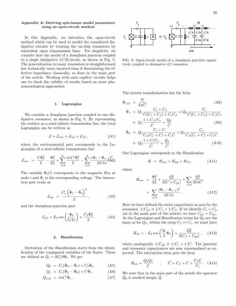
20

Appendix A: Deriving spin-boson model parametersusing an open-circuit method

In this Appendix, we introduce the open-circuitmethod which can be used to model the considered dis-sipative circuits by treating the on-chip resonators byequivalent open transmission lines. For simplicity, weconsider here the model of a Josephson junction coupledto a single dissipative LCR-circuit, as shown in Fig. 9.The generalization to many resonators is straightforwardbut technically more involved than if determining the ef-fective impedance classically, as done in the main partof the article. Working with such explicit circuits helpsone to check the validity of results based on more phe-nomenological approaches.

1. Lagrangian

We consider a Josephson junction coupled to one dis-sipative resonator, as shown in Fig. 9. By representingthe resistor as a semi-infinite transmission line, the totalLagrangian can be written as

L = Lenv + Lint + LJJ , (A1)

where the environmental part corresponds to the La-grangian of a semi-infinite transmission line

Lenv =CΦ2

1

2− Φ2

1

2L+

∞∑i≥2

δxC ′Φ2i

2−∞∑i≥2

(Φi − Φi−1)2

2L′δx.(A2)

The variable Φi(t) corresponds to the magnetic flux at

node i and Φi is the corresponding voltage. The interac-tion part reads as

Lint =Cc

(Φ1 − Φ0

)2

2, (A3)

and the Josephson-junction part

LJJ = EJ cos

(Φ0

~/2e

)+CJΦ2

0

2. (A4)

2. Hamiltonian

Derivation of the Hamiltonian starts from the identi-fication of the conjugated variables of the fluxes. Theseare defined as Qi = ∂L/∂Φi. We get

Q0 = Cc(Φ0 − Φ1) + CJΦ0 (A5)

Q1 = Cc(Φ1 − Φ0) + CΦ1 (A6)

Qi≥2 = δxC ′Φi . (A7)

FIG. 9: Open-circuit model of a Josephson junction capaci-tively coupled to dissipative LC-resonator.

The inverse transformation has the form

Φi≥2 =PiδxC ′

(A8)

Φ1 = Q1Cc + CJ

C(Cc + CJ) + CcCJ+Q0

CcC(Cc + CJ) + CcCJ

≡ Q11 + CJ/Cc

C+Q0

C(A9)

Φ0 = Q0Cc + C

CJ(Cc + C) + CcC+Q1

CcCJ(Cc + C) + CcC

≡ Q01 + C/Cc

C+Q1

C. (A10)

Our Lagrangian corresponds to the Hamiltonian

H = Henv +Hint +HJJ , (A11)

where

Henv =Φ2

1

2L+

Q21

2(C + Cp1)+∑i≥2

Q2i

2δxC ′

+∑i≥2

(Φi − Φi−1)2

2L′δx. (A12)

Here we have defined the series capacitance as seen by theresonator, 1/Cp1 ≡ 1/Cc + 1/CJ. If we identify Cc = Cg

(as in the main part of the article) we have Cp1 = Cint.As the Lagrangian and Hamiltonian terms for Q0 are thesame as for Q1, within the swap CJ ↔ C1, we must have

HJJ = −EJ cos

(2e

~Φ0

)+

Q20

2(CJ + Cp0), (A13)

where analogously 1/Cp0 ≡ 1/Cc + 1/C. The junctionand resonator capacitances are now renormalized as ex-pected. The interaction term gets the form

Hint =Q0Q1

C, C = CJ + C +

CJC

Cc. (A14)

We note that in the main part of the article the operatorQ0 is marked simply Q.

21

3. Solution

We have now determined the form of the Hamiltoniancorresponding to the circuit of Fig. 9. The next step is toestablish the solution when the interaction term is turnedoff. In the transmission line one obtains a wave equationwhose solution can be written in the form

Φ(x > 0, t) =

√~R4π

∫ ∞0

dω√ω

(A15)

×[bin(ω)ei(−kωx−ωt) + bout(ω)ei(kωx−ωt) + H.c.

],

Here the characteristic impedance R =√L′/C ′ and the

wave number kω = ω√L′C ′. The bosonic terms b†in(ω)

and bin(ω) correspond to incoming photon-field creationand annihilation operators. They (as well as the out-field

operators) satisfy[bin(ω), b†in(ω′)

]= δ(ω − ω′) .

The Heisenberg equations of motion at i = 1 read

ˆΦ1(t) =Q1

C + Cp1+ 0× Q0

C(A16)

ˆQ1(t) = − Φ1

L+

Φ2 − Φ1

δxL′

→ − Φ1

L+

1

L′∂Φ(x = 0, t)

∂x. (A17)

In the first equation, we have set the interaction term(boldface) to zero. The junction is now decoupled fromthe dissipative resonator. These equations lead to rela-tion

(C + Cp1) ˆΦ(x = 0, t) =

− Φ(x = 0, t)

L+

1

L′∂Φ(x = 0, t)

∂x. (A18)

This is a boundary condition between the incoming andoutgoing fields. The solution is obtained by Fouriertransforming, which gives

ω2(C + Cp1)[bin(ω) + bout(ω)

](A19)

=1

L

[bin(ω) + bout(ω)

]+ i

ω

R

[bin(ω)− bout(ω)

].

The solution is

bout(ω) = −1 + i Lω/R

1−(ω/ω1)2

1− i Lω/R1−(ω/ω1)2

bin(ω) . (A20)

We find that at zero as well as at infinite frequency, theboundary condition gives aout + ain = 0. Similarly, we

find

bin(ω) + bout(ω) = −2iLω/R

1− (ω/ω1)2 − iLω/Rbin(ω)

≡ A(ω)bin(ω) . (A21)

This is proportional to the impedance of parallel LCR-circuit:

Zeff(ω) =1

1R + 1

iωL + iω(C + Cp1)=R

2A∗(ω)(A22)

Re[Zeff(ω)] =R

4|A(ω)|2 . (A23)

The solution for the interaction voltage has the form

Vint(t) ≡Q1(t)

C= −i

CcCc + CJ

√~R4π

×∫ ∞

0

dω√ωA(ω)bin(ω)e−iωt + H.c. (A24)

〈Vint(t)Vint(0)〉T=0 =

(Cc

Cc + CJ

)2 ~π

×∫ ∞

0

dωωRe[Zeff(ω)]e−iωt . (A25)

This agrees with the results given in the main part of thearticle.

Appendix B: Single-mode versus continuous-modetreatment of a microwave resonator

In this appendix, we study the connection betweensingle- and continuous-mode treatments of a microwaveresonator. In the preceding appendix, we already de-rived an example of the connection between single- andmulti-mode treatments, by deriving an exact form of theamplitude function gi ∝ A(ω) in the case of a transmoncoupled to a single dissipative LCR resonator, Eqs. (A22-A25). In this appendix, we consider relations betweenthe single- and continuous-mode treatments by using the

representation in (numerable) bosonic operators bi.

For simplicity, we consider here the case q0 =2e (Cooper-pair box), generalization to other cases isstraightforward. In the single-mode analysis, the rela-tive coupling strength between the qubit and a mode offrequency ωr (divided by the mode frequency) is given(in the absence of coupling capacitor) by

g =

√πZLCRQ

, (B1)

where ZLC is the characteristic impedance of a microwaveresonator. On the other hand, for the continuous modedescription of the same broadened mode, it is the area of

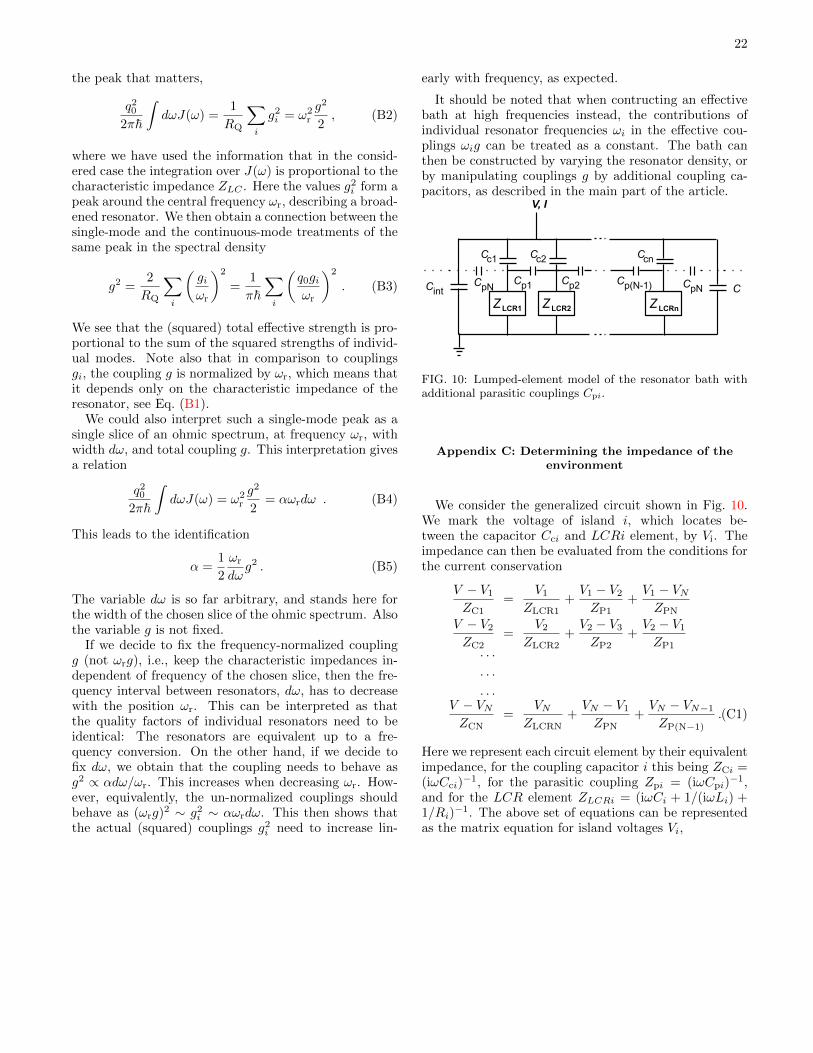
22

the peak that matters,

q20

2π~

∫dωJ(ω) =

1

RQ

∑i

g2i = ω2

r

g2

2, (B2)

where we have used the information that in the consid-ered case the integration over J(ω) is proportional to thecharacteristic impedance ZLC . Here the values g2

i form apeak around the central frequency ωr, describing a broad-ened resonator. We then obtain a connection between thesingle-mode and the continuous-mode treatments of thesame peak in the spectral density

g2 =2

RQ

∑i

(giωr

)2

=1

π~∑i

(q0giωr

)2

. (B3)

We see that the (squared) total effective strength is pro-portional to the sum of the squared strengths of individ-ual modes. Note also that in comparison to couplingsgi, the coupling g is normalized by ωr, which means thatit depends only on the characteristic impedance of theresonator, see Eq. (B1).

We could also interpret such a single-mode peak as asingle slice of an ohmic spectrum, at frequency ωr, withwidth dω, and total coupling g. This interpretation givesa relation

q20

2π~

∫dωJ(ω) = ω2

r

g2

2= αωrdω . (B4)

This leads to the identification

α =1

2

ωr

dωg2 . (B5)

The variable dω is so far arbitrary, and stands here forthe width of the chosen slice of the ohmic spectrum. Alsothe variable g is not fixed.

If we decide to fix the frequency-normalized couplingg (not ωrg), i.e., keep the characteristic impedances in-dependent of frequency of the chosen slice, then the fre-quency interval between resonators, dω, has to decreasewith the position ωr. This can be interpreted as thatthe quality factors of individual resonators need to beidentical: The resonators are equivalent up to a fre-quency conversion. On the other hand, if we decide tofix dω, we obtain that the coupling needs to behave asg2 ∝ αdω/ωr. This increases when decreasing ωr. How-ever, equivalently, the un-normalized couplings shouldbehave as (ωrg)2 ∼ g2

i ∼ αωrdω. This then shows thatthe actual (squared) couplings g2

i need to increase lin-

early with frequency, as expected.

It should be noted that when contructing an effectivebath at high frequencies instead, the contributions ofindividual resonator frequencies ωi in the effective cou-plings ωig can be treated as a constant. The bath canthen be constructed by varying the resonator density, orby manipulating couplings g by additional coupling ca-pacitors, as described in the main part of the article.

FIG. 10: Lumped-element model of the resonator bath withadditional parasitic couplings Cpi.

Appendix C: Determining the impedance of theenvironment

We consider the generalized circuit shown in Fig. 10.We mark the voltage of island i, which locates be-tween the capacitor Cci and LCRi element, by Vi. Theimpedance can then be evaluated from the conditions forthe current conservation

V − V1

ZC1=

V1

ZLCR1+V1 − V2

ZP1+V1 − VNZPN

V − V2

ZC2=

V2

ZLCR2+V2 − V3

ZP2+V2 − V1

ZP1. . .

. . .

. . .V − VNZCN

=VN

ZLCRN+VN − V1

ZPN+VN − VN−1

ZP(N−1).(C1)

Here we represent each circuit element by their equivalentimpedance, for the coupling capacitor i this being ZCi =(iωCci)

−1, for the parasitic coupling Zpi = (iωCpi)−1,

and for the LCR element ZLCRi = (iωCi + 1/(iωLi) +1/Ri)

−1. The above set of equations can be representedas the matrix equation for island voltages Vi,

23

V/ZC1

V/ZC2

. . .V/ZCN

=

1ZC1

+ 1ZLCR1

+ 1ZP1

+ 1ZPN

− 1ZP1

. . . − 1ZPN

− 1ZP1

1ZC2

+ 1ZLCR2

+ 1ZP2

+ 1ZP1

− 1ZP2

. . .. . . . . . . . . . . .− 1ZPN

. . . − 1ZP(N−1)

1ZCN

+ 1ZLCRN

+ 1ZPN

+ 1ZP(N−1)

V1

V2

. . .VN

.

(C2)

The relative voltages Vi/V can then be solved straight-forwardly numerically using matrix inversion. Theimpedance Z is solved using the relation

I =∑i

V − ViZCi

, (C3)

which then leads to equation for impedance Z,

1

Z≡ I

V=∑i

[1

ZCi− 1

V

ViZCi

]. (C4)

As discussed in the main text, the total effectiveimpedance includes also capacitors C and Cint. The an-swer for the total effective impedance is then

Zeff =(iωC + iωCint + Z−1

)−1. (C5)