Embed Size (px)
Citation preview
Isotopenfraktionierung als Indikator für den biotischen
und abiotischen Abbau von Xenobiotika in
Grundwasserleitern
Dissertation
zur Erlangung des Doktorgrades
der Naturwissenschaften im Fachbereich
Geowissenschaften
der Universität Hamburg
vorgelegt von
Alfred Steinbach
aus
Trier
Hamburg, 2003

Als Dissertation angenommen vom Fachbereich Geowissenschaften der Universität Hamburg
auf Grund der Gutachten von Prof. Dr. Walter Michaelis
und Dr. Richard Seifert.
Hamburg, den 25. November 2003
Prof. Dr. H. Schleicher
Dekan
des Fachbereichs Geowissenschaften
I
Inhaltsverzeichnis Vorwort ................................................................................................................................. IV Danksagung .........................................................................................................................VII Abkürzungsverzeichnis.....................................................................................................VIII 1 Einleitung........................................................................................................................1
1.1 Zielsetzung ..................................................................................................................4 2 Theoretische Grundlagen..............................................................................................6
2.1 Isotope und Isotopenfraktionierung.........................................................................6 2.2 Grundwasserkontaminationen ...............................................................................10 2.3 Schadstofffahnen im Grundwasser ........................................................................11 2.4 Immissionspumpversuche .......................................................................................14 2.5 Sanierungsstrategien................................................................................................16
2.5.1 Ex-situ-Sanierung...............................................................................................16 2.5.2 In-situ-Sanierung ................................................................................................16
2.5.2.1 In-situ-Bioremediation (Natural Attenuation).............................................16 2.5.2.2 Reaktive Wände ..........................................................................................21
2.6 Nachweis des biologischen Abbaus ........................................................................23 2.6.1 Drei Beweisniveaus (Lines of evidence) ............................................................23 2.6.2 Nachweis des biologischen Abbaus im Feld mittels Isotopenfraktionierung
und Immissionspumpversuchen .........................................................................24 3 Material und Methoden...............................................................................................26
3.1 Probennahme............................................................................................................26 3.1.1 Punktbeprobung Feld..........................................................................................26 3.1.2 Immissionspumpversuche ..................................................................................27 3.1.3 Säulenversuche ...................................................................................................27
3.2 Methodenentwicklung .............................................................................................27 3.2.1 Flüssig-Flüssig-Extraktion (LLE).......................................................................28 3.2.2 Festphasenmikroextraktion (SPME) ..................................................................34
3.3 Geräte und Chemikalien .........................................................................................46 4 Untersuchungsgebiete..................................................................................................51
4.1 Testfeld Süd ..............................................................................................................51 4.1.1 Lage und historische Erkundung ........................................................................51 4.1.2 Geologie und Hydrogeologie..............................................................................52
4.2 Feldstandort Rheine.................................................................................................53 5 Combined �13C and �2H monitoring of in situ biodegradation of aromatic
hydrocarbons in a contaminated aquifer...................................................................55 5.1 Introduction..............................................................................................................56 5.2 Method ......................................................................................................................57
5.2.1 Test site...............................................................................................................57 5.2.2 Sampling methods ..............................................................................................58 5.2.3 Compound specific isotope analysis...................................................................59
5.3 Results .......................................................................................................................60 5.3.1 Carbon isotopes ..................................................................................................60 5.3.2 Hydrogen isotopes ..............................................................................................63
5.4 Discussion..................................................................................................................63 5.5 Conclusions...............................................................................................................65 5.6 Acknowledgements ..................................................................................................65
II
6 Hydrogen and carbon isotope fractionation during anaerobic biodegradation of aromatic hydrocarbons - a field study...................................................................66
6.1 Abstract.....................................................................................................................67 6.2 Introduction..............................................................................................................67 6.3 Materials and methods ............................................................................................69
6.3.1 Field site .............................................................................................................69 6.3.2 Chemicals ...........................................................................................................70 6.3.3 Groundwater sampling and extraction................................................................71 6.3.4 Gas chromatography (GC) and GC-mass spectrometry (GC-MS) .....................71 6.3.5 Compound specific isotope analysis...................................................................72 6.3.6 Rayleigh calculations..........................................................................................73
6.4 Results .......................................................................................................................74 6.4.1 Carbon isotopes ..................................................................................................76 6.4.2 Hydrogen isotopes ..............................................................................................78
6.5 Discussion..................................................................................................................80 6.5.1 Isotopic fractionation..........................................................................................80 6.5.2 Biodegradation, dilution and dissolution processes in the Rayleigh model .......81 6.5.3 Implications ........................................................................................................86
6.6 Acknowledgements ..................................................................................................86 7 Assessing microbial degradation of o-xylene at field-scale from the reduction
in mass flow rate combined with compound-specific isotope analyses ...................87 7.1 Abstract.....................................................................................................................88 7.2 Introduction..............................................................................................................88 7.3 Site description .........................................................................................................92 7.4 Methods.....................................................................................................................94
7.4.1 Integral Groundwater Investigation method .......................................................94 7.4.2 Compound specific isotope analysis (CSIA)......................................................97 7.4.3 Combination of Integral Groundwater Investigation method with CSIA
(ICSIA) ...............................................................................................................99 7.5 Results and discussion ...........................................................................................104
7.5.1 Integral Goundwater Investigation method ......................................................104 7.5.2 Point scale application of the CSIA..................................................................110 7.5.3 Integral scale compound specific isotope analysis (ICSIA) .............................111
7.6 Method comparison and conclusions ...................................................................113 7.7 Acknowledgements ................................................................................................115
8 Stable carbon isotope fractionation during the reductive dehalogenation of tetrachloroethene (PCE) by zero valent iron: a tool to map the efficiency of iron treatment walls...................................................................................................116
8.1 Abstract...................................................................................................................117 8.2 Introduction............................................................................................................117 8.3 Materials and methods ..........................................................................................119
8.3.1 Experimental set up ..........................................................................................119 8.3.2 Groundwater sampling .....................................................................................121 8.3.3 Concentration analysis......................................................................................121 8.3.4 Compound specific isotope analysis.................................................................122
8.4 Results .....................................................................................................................124 8.4.1 Column experiments.........................................................................................124 8.4.2 Monitoring results ............................................................................................127
8.5 Interpretation of the monitoring results ..............................................................130 8.6 Discussion................................................................................................................134

III
8.6.1 Laboratory studies ............................................................................................134 8.6.2 Field monitoring ...............................................................................................135
8.7 Conclusions.............................................................................................................137 8.8 Acknowledgements ................................................................................................137
9 Zusammenfassung .....................................................................................................138 10 Literatur .....................................................................................................................143 Anhang .................................................................................................................................160
IV
Vorwort Die vorliegende Dissertationsschrift basiert zum großen Teil auf den Ergebnissen, die im
Teilprojekt „Schadstoffmobilität durch Bindung an natürliche makromolekulare organische
Stoffe im Sicker- und Grundwasser“ im Rahmen des DFG-Schwerpunktprogramms
„Geochemische Prozesse mit Langzeitfolgen im anthropogen beeinflussten Grund- und
Sickerwasser“ erarbeitet wurden. Mit dem Ziel, den im Untergrund eines ehemaligen
Gaswerks (Testfeld Süd) ablaufenden mikrobiologischen Schadstoffabbau quantitativ zu
erfassen, erfolgte nach der Entwicklung einer hinreichend empfindlichen und exakten
Anreicherungstechnik eine flächendeckende Charakterisierung von Isotopen in der
identifizierten Schadstofffahne. Auf der Grundlage dieser Ergebnisse wurden in einer
gemeinsam mit der Geowissenschaftlichen Fakultät der Universität Tübingen (A. Peter,
G. Teutsch) durchgeführten Probennahmekampagne erstmals Isotopenuntersuchungen an
integral bepumpten Brunnen durchgeführt.
Der zweite Teil dieser Arbeit beinhaltet die Resultate der Isotopenmessungen der vom
Geowissenschaftlichen Institut der Universität Kiel (E. Ebert, A. Dahmke) im Rahmen des
Forschungsverbundprojekts „RUBIN“ (Reaktionswände und -barrieren im Netzwerkverbund)
im Labor durchgeführten Säulenabbauversuche. Darauf basierend wurde am Standort Rheine
erstmalig versucht, mittels Isotopenmessungen Aussagen über die Langzeitstabilität einer im
Feld installierten Eisen-Reaktionswand zu treffen.
Der Ergebnisteil dieser Dissertation (Kapitel 5–8) besteht, wie nachfolgend aufgelistet, aus
bereits veröffentlichten oder zur Veröffentlichung in internationalen Fachzeitschriften
eingereichten Manuskripten und ist daher in englischer Sprache verfasst:
Kapitel 5: Combined �13C and �2H monitoring of in situ biodegradation of aromatic
hydrocarbons in a contaminated aquifer
Steinbach A. and Michaelis W. (2003) Combined �13C and �2H monitoring of in situ
biodegradation of aromatic hydrocarbons in a contaminated aquifer. In Geochemical
Processes in Soil and Groundwater, Measurement - Modelling - Upscaling (eds. H. D. Schulz
and A. Hadeler), Wiley-VCH, Weinheim, pp. 169-181.
V
Kapitel 6: Hydrogen and carbon isotope fractionation during anaerobic
biodegradation of aromatic hydrocarbons - a field study
Steinbach A., Seifert R., Annweiler E., and Michaelis W. (2004) Hydrogen and carbon isotope
fractionation during anaerobic biodegradation of aromatic hydrocarbons - a field study.
Environ. Sci. Technol. in press.
Kapitel 7: Assessing microbial degradation of o-xylene at field-scale from the
reduction in mass flow rate combined with compound-specific isotope
analyses
Peter A., Steinbach A., Liedl R., Ptak T., Michaelis W., and Teutsch G. (2003) Assessing
microbial degradation of o-xylene from the reduction in mass flow rate combined with
compound specific isotope analyses. J. Contam. Hydrol. in press.
Kapitel 8: Stable carbon isotope fractionation during the reductive dehalogenation of
tetrachloroethene (PCE) by zero valent iron: a tool to map the efficiency of
iron treatment walls
Ebert M., Steinbach A., Michaelis W., and Dahmke A. Stable carbon isotope fractionation
during the reductive dehalogenation of tetrachloroethene (PCE) by zero valent iron: a tool to
map the efficiency of iron treatment walls. Chemosphere submitted.
Ferner wurden Teilergebnisse in folgenden Tagungsbänden vorab veröffentlicht:
Annweiler E., Steinbach A., and Michaelis W. (2001) Compound specific stable isotope
fractionation to assess intrinsic biodegradation in tar oil contaminated aquifers. In
Proceedings of the 20th International Meeting on Organic Geochemistry. Abstracts Volume 1,
Nancy, France, pp. 222-223.
Steinbach A., Annweiler E., Meckenstock R. U., Richnow H. H. und Michaelis W. (2000)
Stabile Isotopen organischer Schadstoffe – Indikatoren für Natural Attenuation. In Resümee
und Beiträge zum 2. Symposium Natural Attenuation: Neue Erkenntnisse, Konflikte und
Anwendungen, 07. bis 08. Dezember 2000 (Ed. G. Kreysa, T. Track, J. Michels und
J. Wiesner), DECHEMA Gesellschaft für chemische Technik und Biotechnologie e.V.,
Frankfurt am Main, pp. 255-256.
VI
Steinbach A. and Michaelis W. (2002) Carbon and hydrogen isotope fractionation of organic
pollutants in aquifers. Geochim. Cosmochim. Acta 66, A739.
Steinbach A. und Michaelis W. (2002) Isotopenfraktionierung als Indikator für den
mikrobiellen Abbau von aromatischen Verbindungen in Grundwasserleitern – eine
Feldstudie. In Kurzfassungen zur Jahrestagung der Wasserchemischen Gesellschaft –
Fachgruppe in der Gesellschaft deutscher Chemiker, Eichstätt/Altmühltal, pp. 103-106.
Steinbach A., Schellig F., and Michaelis W. (2003) Isotope fractionation of organic
groundwater pollutants during biotic and abiotic degradation processes. In Proceedings of
the 21th International Meeting on Organic Geochemistry. Book of Abstracts Part I,
Kraków, Poland, pp. 142-143.
VII
Danksagung An aller erster Stelle möchte ich mich bei Herrn Prof. Dr. Walter Michaelis für die
Themenstellung, die ständige Diskussionsbereitschaft und die zahlreichen wertvollen
Anregungen sowie die mir gewährte Freiheit bei der wissenschaftlichen Bearbeitung danken.
Ein ganz herzliches Dankeschön für die Einarbeitung in die biogeochemische Thematik gilt
meiner Vorgängerin Dr. Eva Annweiler. Herrn Dr. Martin Blumenberg danke ich besonders
für die Einführung in die „Geheimnisse“ der Isotopenmassenspektrometrie und die vielen
fruchtbaren Diskussionen. Ebenso sei Dr. Siegmund Ertl für die vielen analytischen
Anregungen gedankt. Dr. Richard Seifert danke ich für seine ständige Diskussionsbereitschaft
und für seine zahlreichen fachlichen Ratschläge.
Herrn Frank Schellig danke ich ganz besonders für den Spaß und die Hilfe bei den zahlreichen
Probennahmen. Meinen Kolleginnen und Kollegen des Instituts für Biogeochemie und
Meereschemie, Sabine Beckmann, Dr. Sabine Brasse, Dr. Oliver Christof, Dr. Nikolaj
Delling, Michael Holzwarth, Thomas Pape, Oliver Schmale, Ariane Seraphin, Claudia Sill,
Peggy Widder sowie allen namentlich nicht erwähnten Mitarbeitern danke ich besonders für
die außerordentlich angenehme Arbeitsatmosphäre und die stete Hilfsbereitschaft. Ganz
besonders danke ich auch Frau Gabriele Thal für die kritische Durchsicht des Dokuments.
Der Deutschen Forschungsgemeinschaft danke ich für die Bereitstellung der Mittel zur
Durchführung dieser Arbeit (Mi 157/11).
Besonderen Spaß machte mir die Arbeit mit meinen Kooperationspartnern, welche die
vorliegende Arbeit in dieser Form erst ermöglichten. Besonderer Dank gilt Frau Dr. Anita
Peter (Universität Tübingen) für die gemeinsame Durchführung der Integralen Pumpversuche,
für die Bereitstellung von diversen Probennahmeutensilien und für die vielen
hydrogeologischen Ratschläge. Dr. Markus Ebert (Univerität Kiel) danke ich für die äußerst
angenehme Zusammenarbeit und für die ständige Diskussionsbereitschaft.
Nicht versäumen will ich es, mich bei den Mitarbeitern der TWS Gaisburg, insbesondere bei
Herrn Dettenmeyer und Dr. Schwarz für die Benutzung des Labors während der Probennahme
zu bedanken.
Mein letzter Dank gilt jenen, denen ich am meisten zu verdanken habe und ohne die die
vorliegende Arbeit nie entstanden wäre, meinen Eltern und meinem Bruder Rudolf sowie
meiner Lebensgefährtin Adriana.
VIII
Abkürzungsverzeichnis
Allgemein BN Beweisniveau Ct, C0 Konzentration zur Zeit t bzw. zur Zeit 0 (Rayleigh-Gleichung) Cx Konzentration einer Komponente in der Phase x
(Verteilungsgleichgewichte) Ci Konzentration der Komponente i (Quantifizierung) (95%) CI 95% Confidence Interval DNAPL Dense Nonaqeous Phase Liquid DVWK Deutscher Verband für Wasserwirtschaft und Kulturbau e.V. ECD Electron Capture Detector EPA Environmental Protection Agency ESF Frischer Eisenschwamm ESV Eisenschwamm aus dem Anstrombereich der Reaktionswand GGV Graugussgranulat aus dem Anstrombereich der Reaktionswand FID Flammenionisationsdetektor (bei der Gaschromatographie) GBS Geschwindigkeitsbestimmender Schritt IS Interner Standard KFG Faser-Gas-Verteilungskoeffizient KFW Faser-Wasser-Verteilungskoeffizient Kfr Freundlich-Koeffizient in L kg-1 KGW Gas-Wasser-Verteilungskoeffizient KH Henry-Koeffizient in atm m3 mol-1 KOW Oktanol-Wasser-Verteilungskoeffizient log KOW Dekadischer Logarithmus des Oktanol-Wasser-Verteilungs-
koeffizienten LNAPL Low Nonaqueous Phase Liquid N Neutronenzahl NAPL Nonaqueous Phase Liquid NRC National Research Council 1/nfr Freundlich-Exponent PFx Peakfläche der Komponente x in Vs PDMS Polydimethylsiloxan PV Pore Volume VPDB Vienna Pee Dee Belemnite VSMOW Vienna Standard Mean Ocean Water Z Protonen- bzw. Ordnungszahl
Immissionspumpversuche und Integral scale compound specific isotope analysis (Kapitel 7) B Aquifermächtigkeit in m b1, b2 Abstand der Grenzen der Schadstofffahne vom Pumpbrunnen in
m C12C, C13C Konzentration der 12C- bzw. 13C-Isotope in �g L-1 CC Kohlenstoffkonzentration in �g L-1 Cwell(t) Die zum Zeitpunkt t in einem abstromigen Brunnen gemessene
Konzentration in �g L-1 Cplume Konzentration einer idealisierten Fahne
IX
C Nach Anwendung des Inversionsalgorithmus räumlich gemittelte Konzentrationen in �g L-1
C 12C, C 13C Mittlere Konzentration der 12C- bzw. 13C-Isotope in �g L-1
iC Mittlere Schadstoffkonzentration an der Kontrollebene in �g L-1
C(r, �) Räumliche Konzentrationsverteilung in Zylinderkoordinaten k Hydraulische Leitfähigkeit in m s-1 M Massenflussrate in g d-1 n Zahl der Konzentrationsmessungen an einem bestimmten
Brunnen ne Effektive Porosität eines Grundwasserleiters Qi Natürlicher Grundwasserabfluss in m3 min-1 Qp Pumprate in m3 min-1
R Mittleres Isotopenverhältnis des selteneren zum häufigsten Isotop an einer Kontrollebene
r Radius der Isochrone in m t Pumpdauer in min ttot Gesamte Pumpdauer in min
h� Hydraulischer Gradient
Reaktive Wände (Kapitel 8) CF Gesamtkonzentration einer Mischung CM1, CM2 Konzentration der Lösung 1 bzw. 2 x Molenbruch der Lösung M1 y Molenbruch der Lösung M2
Kontaminanten BTEX Benzol, Toluol, Ethylbenzol, Xylole CE Chlorierte Ethene CHC Chlorinated Hydrocarbons cis-DCE cis-Dichlorethen trans-DCE trans-Dichlorethen 1,1-DCE 1,1-Dichlorethen CKW Chlorierte Kohlenwasserstoffe i-PB iso-Propylbenzol MKW Mineralölkohlenwasserstoffe MTBE Methyltertiärbutylether N Naphthalin n-BB n-Butylbenzol PAK, (PAH) Polyzyklische aromatische Kohlenwasserstoffe, (Polycyclic
Aromatic Hydrocarbons) PCE Perchlorethen bzw. Tetrachlorethen ST Styrol TCE Trichlorethen TMB Trimethylbenzol
Methoden AAS Atomic Absorption Spectroscopy CSIA Compound Specific Isotope Analysis
X
DI-IRMS Dual Inlet-Isotope Ratio Monitoring Gaschromatography d-SPME Direct-Solid-Phase Microextraction ENA Enhanced Natural Attenuation EA-P-IRMS Elemental Analyses-Pyrolysis-Isotope Ratio Mass Spectrometry GC Gaschromatographie GC-MS Gaschromatographie-Massenspektrometrie GC-C-IRMS Gaschromatography-Combustion-Isotope Ratio Mass
Spectrometry GC-TC-IRMS Gaschromatography-Temperature Conversion- Isotope Ratio Mass Spectrometry HPLC High Performance Liquid Chromatography h-SPME Headspace-Solid-Phase Microextraction IC Ion Chromatography ICSIA Integral Scale Compound Specific Isotope Analysis LLE Flüssig-Flüssig-Extraktion MNA Monitored Natural Attenuation NA Natural Attenuation PRB Permeable Reaktive Barrier SPME Solid-Phase Microextraction
Mathematische Variablen b Achsenabschnitt (lineare Geradengleichung) H Heaviside-Funktion, H(x) = 1 für x � 0 und H(x) = 0 für x � 0 m Steigung (lineare Geradengleichung)
Physikalische und chemische Größen a Beschleunigung in m2 s-2
D Direktionskonstante oder Kraftkonstante in N m-1 ds Feststoffdichte in kg L-1 F Kraft in N f Residuale, noch nicht abgebaute Fraktion (= Ct C0
-1) Gr° Freie Reaktionsenthalpie in kJ mol-1 h Planck’sche Konstante (6,626176�10-34 Js) k Geschwindigkeitskonstante in s-1 oder d-1 m Masse in kg n Stoffmenge n Rx Isotopenverhältnis des selteneren zum häufigsten Isotop t Zeit in s V Potenzielle Energie in J Vx Volumen der Phase x in cm3 v Schwingungsquantenzahl x Auslenkung in m
Griechische Variablen �� Isotopischer Fraktionierungsfaktor�� Kohlenstoffanteil in einer organischen Verbindung δ 13C mittlerer aus C 12C bzw. C 13C berechneter Isotopenwert in ‰ �
13CF der aus einer Mischung resultierende Isotopenwert in ‰�
�yX Delta-Notation in ‰, y ist die Masse des schwereren Isotops

XI
Isotopischer Anreicherungsfaktor in ‰ p Porosität � Tortuosität � Frequenz in s-1
e Neutrino � Variable (zur Lösung der Schwingungsgleichung)

1 Einleitung
1
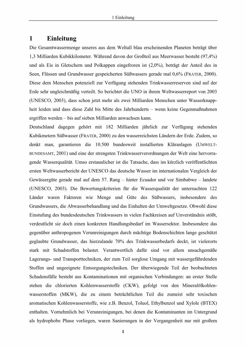
1 Einleitung Die Gesamtwassermenge unseres aus dem Weltall blau erscheinenden Planeten beträgt über
1,3 Milliarden Kubikkilometer. Während davon der Großteil aus Meerwasser besteht (97,4%)
und als Eis in Gletschern und Polkappen eingefroren ist (2,0%), beträgt der Anteil des in
Seen, Flüssen und Grundwasser gespeicherten Süßwassers gerade mal 0,6% (FRATER, 2000).
Diese dem Menschen potenziell zur Verfügung stehenden Trinkwasserreserven sind auf der
Erde sehr ungleichmäßig verteilt. So berichtet die UNO in ihrem Weltwasserreport von 2003
(UNESCO, 2003), dass schon jetzt mehr als zwei Milliarden Menschen unter Wasserknapp-
heit leiden und dass diese Zahl bis Mitte des Jahrhunderts – wenn keine Gegenmaßnahmen
ergriffen werden – bis auf sieben Milliarden anwachsen kann.
Deutschland dagegen gehört mit 182 Milliarden jährlich zur Verfügung stehenden
Kubikmetern Süßwasser (FRATER, 2000) zu den wasserreichsten Ländern der Erde. Zudem, so
denkt man, garantieren die 10.500 bundesweit installierten Kläranlagen (UMWELT-
BUNDESAMT, 2001) und eine der strengsten Trinkwasserverordnungen der Welt eine hervorra-
gende Wasserqualität. Umso erstaunlicher ist die Tatsache, dass im kürzlich veröffentlichten
ersten Weltwasserbericht der UNESCO das deutsche Wasser im internationalen Vergleich der
Gewässergüte gerade mal auf dem 57. Rang – hinter Ecuador und vor Simbabwe – landete
(UNESCO, 2003). Die Bewertungskriterien für die Wasserqualität der untersuchten 122
Länder waren Faktoren wie Menge und Güte des Süßwassers, insbesondere des
Grundwassers, die Abwasserbehandlung und das Einhalten der Umweltgesetze. Obwohl diese
Einstufung des bundesdeutschen Trinkwassers in vielen Fachkreisen auf Unverständnis stößt,
verdeutlicht sie doch einen konkreten Handlungsbedarf im Wassersektor. Insbesondere das
gegenüber anthropogenen Verunreinigungen durch mächtige Bodenschichten lange geschützt
geglaubte Grundwasser, das hierzulande 70% des Trinkwasserbedarfs deckt, ist vielerorts
stark mit Schadstoffen belastet. Verantwortlich dafür sind vor allem unsachgemäße
Lagerungs- und Transporttechniken, der zum Teil sorglose Umgang mit wassergefährdenden
Stoffen und ungeeignete Entsorgungstechniken. Der überwiegende Teil der beobachteten
Schadensfälle besteht aus Kontaminationen mit organischen Verbindungen: an erster Stelle
stehen die chlorierten Kohlenwasserstoffe (CKW), gefolgt von den Mineralölkohlen-
wasserstoffen (MKW), die zu einem beträchtlichen Teil die zumeist sehr toxischen
aromatischen Kohlenwasserstoffe, wie z.B. Benzol, Toluol, Ethylbenzol und Xylole (BTEX)
enthalten. Vornehmlich bei Verunreinigungen, bei denen die Kontaminanten im Untergrund
als hydrophobe Phase vorliegen, waren Sanierungen in der Vergangenheit nur mit großem
1 Einleitung
2
finanziellen und technischen Aufwand möglich und im Hinblick auf das Erreichen von
vorgegebenen Sanierungszielen häufig nicht erfolgreich. So wird im Rahmen der vielfach
eingesetzten „Pump-and-Treat“-Maßnahme verunreinigtes Grundwasser an die Oberfläche
gepumpt, dort physiko-chemisch gereinigt und wieder in den Aquifer eingeleitet. Aufgrund
der geringen Löslichkeit vieler hydrophober Substanzen, dem Vorhandensein einer residualen
Schadstoffphase, der Rückdiffusion aus der Gesteinsmatrix und des häufig sehr heterogenen
Untergrunds muss mit sehr langen Betriebszeiten und damit mit sehr hohen Kosten gerechnet
werden (TEUTSCH et al., 1996). Diese Nachteile konnten bisher weder durch den zusätzlichen
Einsatz von Tensiden, Alkoholen oder Peroxiden noch durch physikalische Methoden wie die
Verwendung von erhöhten Temperaturen mittels Dampfeinleitung oder Ultraschall beseitigt
werden (DAHMKE, 1997).
Vor diesem Hintergrund rückt der Einsatz von so genannten passiven In-situ-
Sanierungsstrategien zunehmend in den Mittelpunkt des Interesses. Diese Verfahren sind
dadurch gekennzeichnet, dass sie die im Grundwasser gelösten Schadstoffe durch natürliche
oder stimulierte Prozesse, ohne wesentliche Energiezufuhr von außen, vor Ort degradieren. In
den zurzeit erfolgversprechendsten Verfahren werden die im Grundwasser gelösten
Xenobiotika beim Natural-Attenuation (NA-)Konzept durch die natürliche Selbstreinigungs-
kraft des Aquifers (WIEDEMEIER et al., 1999) und bei der Technologie der „Reaktionswände“
(GILLHAM and O'HANNESIN, 1994) durch die Degradation am reaktiven Wandmaterial
entfernt. Der NA-Ansatz beruht – neben den nichtdestruktiven Konzentrationssenken wie
Sorption, Dispersion, Verdünnung oder Verdampfung – vor allem auf dem mikrobiologischen
Schadstoffabbau, während für die Mehrzahl der Reaktionswände elementares Eisen als
Reduktionsmittel eingesetzt wird. Somit bietet sich für die durch Bakterien relativ leicht
abbaubaren MKW und BTEX eine Sanierung mittels NA und für die oftmals nur unter
speziellen Bedingungen abbaubaren CKW eine Reduktion an einer mit Eisengranulat
gefüllten Reaktionswand an.
Für Prognosen zur Langzeitentwicklung eines Schadensfalls ist es unerlässlich, die im
Untergrund ablaufenden Abbauprozesse so exakt wie möglich zu beschreiben. Vor allem die
Unzugänglichkeit des Aquifers und die Vielfalt der dort vorhandenen potenziellen
Reaktionspartner erschweren genauere Aussagen. So ist der Nachweis des mikrobiologischen
Abbaus im Feld derzeit noch sehr schwierig, da in der Regel nicht zweifelsfrei bewertet
werden kann, inwiefern nichtdestruktive Prozesse am beobachteten Konzentrationsrückgang
beteiligt sind (MANCINI et al., 2002). Gleichermaßen kann noch nicht eindeutig beurteilt
1 Einleitung
3
werden, inwiefern die teilweise hinter einer Reaktionswand beobachteten erhöhten
Schadstoffkonzentrationen auf einer Passivierung der Reaktionswand, auf dem Umfließen
derselben oder auf Desorptionsprozessen beruhen. Zur Zeit existieren nur wenige verlässliche,
anerkannte Prognoseinstrumente, mit denen die Abbauprozesse von Xenobiotika im
Grundwasser direkt nachgewiesen werden können. Zur Quantifizierung der Schad-
stoffdegradation wurde bisher eine Kombination unterschiedlicher Konzepte benutzt, die vom
einfachen Nachweis abnehmender Schadstoffkonzentrationen entlang des Fließpfads über den
Verbrauch an Elektronenakzeptoren (COZZARELLI et al., 2000) bzw. -donatoren (CARR and
HUGHES, 1998) bis hin zur Bildung von kontaminantenspezifischen Metaboliten (BELLER,
2000) und CO2 als Mineralisationsprodukt reichen. Obgleich diese Methoden sehr wichtige
Informationen liefern, ist ihre Aussagekraft im Hinblick auf eine Quantifizierung der
Abbauprozesse nur unzureichend.
Eine viel versprechende direkte Methode zur Charakterisierung des In-situ-Abbaus ist die
Bestimmung der stabilen Isotopenzusammensetzung der einzelnen Schadstoffe. Die Methode
beruht auf der Tatsache, dass Bindungen zwischen leichteren Isotopen schneller gespalten
werden als die zwischen schwereren Isotopen. Demzufolge kommt es während der
Abbaureaktion im noch nicht abgebauten Substrat zu einer Anreicherung des schwereren
Isotops. Diese Verschiebung (Fraktionierung) der Isotopenverhältnisse gegenüber dem
Ausgangsstoff ist proportional der abgebauten Menge (MARIOTTI et al., 1981) und lässt sich
über die „Gaschromatography-Combustion-Isotope Ratio Mass Spectrometry“ (GC-C-IRMS)
bestimmen. Da für nichtdestruktive abiotische Konzentrationssenken bisher keine
signifikanten Fraktionierungen beobachtet wurden (HARRINGTON et al., 1999; SLATER et al.,
2000; SCHÜTH et al., 2003b), kann sowohl die durch Bakterien katalysierte Degradation von
BTEX (RICHNOW et al., 2003) als auch die abiotische reduktive Dechlorierung von CKW an
elementarem Eisen (DAYAN et al., 1999) unabhängig von Prozessen wie Sorption,
Verdampfung oder Verdünnung bestimmt werden.
Eine weitere Methode zur Quantifizierung des NA-Potenzials ist die Bestimmung von
Schadstofffrachten und deren Abnahme mit zunehmender Transportstrecke vom
Schadensherd. Die an der Universität Tübingen speziell für heterogene Schadensfälle
entwickelte leistungsfähige Erkundungsmethode (Immissionspumpversuche) erlaubt die
integrale Quantifizierung von Schadstofffrachten und mittleren Schadstoffkonzentrationen an
senkrecht zur Grundwasserfließrichtung im Abstrom der Schadensfläche installierten
Kontrollebenen (TEUTSCH et al., 2000). Durch die aus mehreren Kontrollebenen berechnete
1 Einleitung
4
Massenflussdifferenz kann die mikrobiologische Abbauleistung unter Zuhilfenahme von
reaktiven Transportmodellen direkt und mit hoher Sicherheit quantifiziert werden (PETER,
2002).
1.1 Zielsetzung Als in den 90er Jahren die ersten Isotopenstudien zu Laborabbauversuchen von Toluol
(MECKENSTOCK et al., 1999), Tetrachlorethen und Trichlorethen (ERTL et al., 1996;
SHERWOOD LOLLAR et al., 1999) erschienen, erkannte man im Bereich der Umwelt-
wissenschaften sofort das große Potenzial von komponentenspezifischen Isotopenanalysen
(Compound Specific Isotope Analysis, CSIA). Als nachteilig erwies sich jedoch die geringe
Messempfindlichkeit der Isotopenmassenspektrometer, die dafür verantwortlich war, dass sich
der Einsatz der CSIA in Feldstudien nur auf den unmittelbaren Bereich der
Kontaminationsquellen beschränkte. Zudem treten insbesondere für Kohlenstoff signifikante
Isotopenfraktionierungen bei aromatischen Kohlenwasserstoffen erst nach einem deutlichen
Abbau der anfänglich vorhandenen Schadstofffraktion auf (HUNKELER et al., 2001a). Somit
war speziell der für Prognosen zum Langzeitverhalten der Kontamination so bedeutsame
Randbereich der Schadstofffahne der CSIA häufig nicht zugänglich.
Vor diesem Hintergrund galt es im Rahmen der vorliegenden Dissertation zunächst eine für
die isotopische Erfassung des Randbereichs der Schadstofffahne ausreichend empfindliche
Analysetechnik zu entwickeln. Dazu wurden bekannte Anreicherungsverfahren wie die
Flüssig-Flüssig-Extraktion (liquid-liquid extraction, LLE) sowie die Festphasenmikroextrak-
tion (solid-phase microextraction, SPME) für die Isotopenbestimmungen von BTEX,
polyzyklischen aromatischen Kohlenwasserstoffen (PAK) und CKW im Feld validiert
(Kapitel 3). Mit Hilfe dieser modifizierten Methoden sollte diese Arbeit über die Bestimmung
der stabilen Isotopenverhältnisse (�13C, �2H) vorrangig eine detailliertere Beurteilung des
biotischen und abiotischen Abbaus im Feld und damit eine vermehrte Anwendung von In-
situ-Sanierungen ermöglichen.
In diesem Zusammenhang beschäftigen sich die Kapitel 5 und 6 vorwiegend mit der Frage,
welche Kontaminanten unter Feldbedingungen biologisch abgebaut werden, ob dabei Iso-
topenfraktionierungen messbar sind und inwiefern diese zur Aufklärung der im Untergrund
ablaufenden Abbau- und Fixierungsprozesse genutzt werden können. Aufgrund der äußerst
heterogenen Untergrundverhältnisse und der komplexen Kontaminationssituation im Testfeld
stellte sich anschließend die Frage nach der Erkundungsunsicherheit der auf regionalisierten
Punktmessungen beruhenden Ergebnisse. Zur Klärung dieses Sachverhalts wurde ein auf der
1 Einleitung
5
Grundlage der Isotopenfraktionierung und der Immissionspumpversuche basierendes neues
Konzept zur Erfassung des mikrobiologisch abgebauten Schadstoffanteils (integral scale
compound specific isotope analysis, ICSIA) entwickelt und unter Feldbedingungen evaluiert
(Kapitel 7). Dazu wurden in Kooperation mit der Universität Tübingen erstmals Isotopen-
bestimmungen an integral beprobten Messstellen durchgeführt. Zusätzlich wurden die aus der
ICSIA abgeleiteten Ergebnisse mit den Daten aus den punktuellen Isotopenuntersuchungen
und aus dem kombinierten integralen Mess- und Modellieransatz verglichen.
Abschließend sollte das in den vorangegangenen Kapiteln erarbeitete Konzept der
Isotopenfraktionierung auf die reduktive Dechlorierung von Perchlorethen (PCE) an mit Eisen
gefüllten Reaktionswänden angewendet werden (Kapitel 8). Dabei sollten Isotopensignaturen
aus Grundwasserproben vor, in und hinter der Reaktionswand Rückschlüsse auf das
Abbauverhalten liefern.
2 Theoretische Grundlagen
6
2 Theoretische Grundlagen
2.1 Isotope und Isotopenfraktionierung
Isotope Isotope (griechisch Isos: gleich, topos: Ort; „am gleichen Ort“ im Periodensystem) oder
Nuklide sind Atome desselben Elements, die aufgrund der unterschiedlichen Anzahl von
Neutronen eine unterschiedliche Nukleonenmasse besitzen. Die Neutronen reduzieren als
elektrisch neutrale Kernteilchen die zwischen Protonen wirkende Abstoßung und sind für die
Vielzahl der stabilen Isotope ein und desselben Elements in der Natur verantwortlich. Bei den
stabilen Isotopen reicht das Verhältnis von Protonen- zu Neutronenzahl (Z:N) von 1:1 (H bis
Ca) bis zu 1:1,5 (Ca bis Au). Übersteigt jedoch die Neutronenanzahl in einem Atomkern diese
bei den stabilen Isotopen beobachteten Verhältnisse, so zerfällt ein Kernneutron (n) unter
Emission eines Elektrons (e-) und eines Neutrinos ( e) in ein Kernproton p+ (n � p+ + e- + e
+ 0,783MeV/Teilchen). Umgekehrt kann, unter der Voraussetzung, dass weniger Neutronen
als Protonen vorhanden sind, auch ein Kernproton in ein Kernneutron umgewandelt werden
(ß+-Zerfall). Diese instabilen Isotope werden als Radionuklide bezeichnet und werden
gesondert in der Radiochemie behandelt.
Prominentester und einfachster Vertreter im Periodensystem ist das Element Wasserstoff mit
seinen stabilen Isotopen Wasserstoff 1H (Z = 1, N = 0) und Deuterium 2H (Z = 1, N = 1).
Letzteres ist in der Natur mit einer Häufigkeit von ca. 0,01% gegenüber dem normalen
Wasserstoff 1H (ca. 99,99%) vorhanden. Kohlenstoff als Grundgerüstbildner in der
organischen Chemie besitzt zwei stabile Isotope: 12C und 13C. Das leichtere Kohlenstoffisotop
ist in der Natur wesentlich häufiger zu finden (ca. 98,9%) als das schwerere (ca. 1,1%). Zur
Charakterisierung der Zusammensetzung der stabilen Isotope der leichten Elemente H, C, N,
O und S wird gemäß internationaler Konvention das Verhältnis R des schwereren (selteneren;
y) zum häufigsten Isotop X (RProbe= 2H/1H, 13C/12C, 15N/14N, 18O/16O bzw. 34S/32S) in
Beziehung zu einem Vergleichsstandard ausgedrückt:
� � 1000R
RR‰ X
dardtanS
dardtanSobePry ����
����
� � . (2-1)
Kohlenstoffisotope werden gegen den Standard VPDB (Vienna Pee Dee Belemnite) und
Wasserstoffisotope gegen VSMOW (Vienna Standard Mean Ocean Water) in der Einheit
2 Theoretische Grundlagen
7
Promille angegeben. Diese so genannte „Delta-Notation“ besitzt den Vorteil, dass sehr kleine
Differenzen in der Isotopenzusammensetzung bis in die zweite und dritte Stelle angezeigt
werden. Je positiver ein �-Wert ist, desto stärker ist die untersuchte Probe mit dem jeweils
schwereren Isotop angereichert (siehe Abbildung 2.1).
Fraktionierung Die klassische Chemie lehrt, dass die chemischen Eigenschaften eines Atoms oder eines
Moleküls nur von der Elektronenhülle, d.h. von der Anzahl der Elektronen (bzw. Protonen)
und nicht von der Anzahl der ungeladenen Neutronen abhängen (HOLLEMANN und WIEBERG,
1985). Für die meisten Bereiche der Chemie mag diese Betrachtungsweise korrekt sein.
Jedoch zeigen leistungsfähige Isotopenmassenspektrometer, dass Moleküle, die
unterschiedliche Isotope ein und desselben Elements enthalten (Isotopomere), nicht nur
physikalisch, sondern auch chemisch leicht unterschiedlich reagieren. Diesen Effekt
bezeichnet man als Isotopenfraktionierung. Handelt es sich dabei um so genannte
Austauschreaktionen, d.h. Reaktionen ohne Nettoumsatz wie im Fall des Phasenübergangs
zwischen Wasser und Wasserdampf in einem geschlossenen System, so spricht man von einer
thermodynamischen Isotopenfraktionierung (HOEFS, 1997). Liegt dagegen eine unvollstän-
dige, nur in eine Richtung verlaufende Reaktion vor, so bezeichnet man diese als kinetische
Isotopenfraktionierung. Zu letzterem Typus gehört der Verdampfungsprozess von Wasser bei
sofortiger Entfernung des entstandenen Wasserdampfes, die Absorption und Diffusion von
Gasen sowie irreversible chemische Reaktionen wie die Karbonatfällung oder der
mikrobiologische Abbau von organischer Materie. Im Allgemeinen übersteigt das Ausmaß der
kinetischen das der thermodynamischen Isotopenfraktionierung.
Kinetische Isotopeneffekte sind auf die unterschiedlichen Dissoziationsenergien und die damit
verbundenen unterschiedlichen Reaktionsraten der verschiedenen an der Bindung beteiligten
Isotope eines Elements zurückzuführen. Bindungen, die aus den leichteren Isotopen aufgebaut
sind (z.B. 12C-12C, 12C-1H), werden schneller gespalten als die Bindungen, die das schwerere
Isotop des gleichen Elements (z.B. 12C-13C, 12C-2H, 13C-1H) enthalten (siehe Anhang A2.1).
Dadurch kommt es während einer chemischen Reaktion zu einer Verschiebung der
Isotopenverhältnisse im Vergleich zum Ausgangsstoff. Ein bekanntes Beispiel ist die CO2-Fi-
xierung in der Photosynthese (O'LEARY, 1981). Ausgehend von einem �13C-Wert von -7 bis
-8,5‰ für das CO2 in der Atmosphäre und einem Wert von ca. 0‰ für das Hydrogencarbonat
(HCO3-) in der Hydrosphäre, bedingt die biochemische Diskriminierung von 13CO2 eine, im
Vergleich zu den anorganischen Kohlenstoffquellen, signifikante 13C-Abreicherung im
2 Theoretische Grundlagen
8
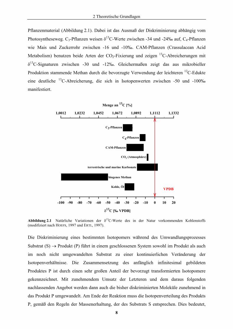
Pflanzenmaterial (Abbildung 2.1). Dabei ist das Ausmaß der Diskriminierung abhängig vom
Photosyntheseweg. C3-Pflanzen weisen �13C-Werte zwischen -34 und -24‰ auf, C4-Pflanzen
wie Mais und Zuckerrohr zwischen -16 und -10‰. CAM-Pflanzen (Crassulacean Acid
Metabolism) benutzen beide Arten der CO2-Fixierung und zeigen 13C-Abreicherungen mit
�13C-Signaturen zwischen -30 und -12‰. Gleichermaßen zeigt das aus mikrobieller
Produktion stammende Methan durch die bevorzugte Verwendung der leichteren 12C-Edukte
eine deutliche 13C-Abreicherung, die sich in Isotopenwerten zwischen -50 und -100‰
manifestiert.
Abbildung 2.1 Natürliche Variationen der �13C-Werte des in der Natur vorkommenden Kohlenstoffs
(modifiziert nach HOEFS, 1997 und ERTL, 1997).
Die Diskriminierung eines bestimmten Isotopomers während des Umwandlungsprozesses
Substrat (S) � Produkt (P) führt in einem geschlossenen System sowohl im Produkt als auch
im noch nicht umgewandelten Substrat zu einer kontinuierlichen Veränderung der
Isotopenverhältnisse. Die Zusammensetzung des anfänglich infinitesimal gebildeten
Produktes P ist durch einen sehr großen Anteil der bevorzugt transformierten Isotopomere
gekennzeichnet. Mit zunehmendem Umsatz der Letzteren und dem daraus folgenden
nachlassenden Angebot werden dann auch die bisher diskriminierten Moleküle zunehmend in
das Produkt P umgewandelt. Am Ende der Reaktion muss die Isotopenverteilung des Produkts
P, gemäß den Regeln der Massenerhaltung, der des Substrats S entsprechen. Dies bedeutet,
�13C [‰ VPDB]
-100 -90 -80 -70 -60 -50 -40 -30 -20 -10 0 10 20
Menge an 13C [%]
1,0012 1,0232 1,0452 1,0672 1,0892 1,1112 1,1332
C3-Pflanzen
C4-Pflanzen
CAM-Pflanzen
CO2 (Atmosphäre)
terrestrische und marine Karbonate
biogenes Methan
Kohle, Öl VPDB
2 Theoretische Grundlagen
9
dass die Intensität, also das quantitative Ausmaß der Fraktionierung zeitabhängig ist und
somit nicht durch die alleinige Angabe des Isotopenverhältnisses charakterisiert werden kann.
Vielmehr beschreibt man die Isotopenfraktionierung mit dem stoffspezifischen
Fraktionierungsfaktor ��
SP R/R�� . (2-2)
RP und RS bezeichnen die Isotopenverhältnisse des selteneren zum häufigsten Isotop im
Produkt bzw. Substrat. Unter der Voraussetzung, dass die Häufigkeit des nachzuweisenden
Isotops (z.B. 13C, 2H) gegenüber der des leichteren (12C, 1H) vernachlässigbar ist, kann
ausgehend von Gleichung (2-2), wie im Anhang (Kapitel A.2.2) detailliert beschrieben, ein
Zusammenhang zwischen der Konzentrationsabnahme des Substrats S und dessen Änderung
des Isotopenverhältnisses relativ zu dem des Ausgangssubstrats abgeleitet werden:
� � fln1RR
ln0,S
t,S����
�
�
�
��
�
. (2-3)
RS,t und RS,0 stehen für das Isotopenverhältnis des Restsubstrats zum Zeitpunkt t bzw. des
Ausgangssubstrats zum Zeitpunkt t = 0. Der Faktor f bezeichnet den Quotienten aus der
Substratkonzentration nach dem Zeitpunkt t (Ct) und der Konzentration des Substrats zu
Beginn des Abbaus (C0). Der Fraktionierungsfaktor wird in der Literatur häufig durch den
anschaulicheren Anreicherungsfaktors ausgedrückt:
� � 10001 ����� . (2-4)
Mit Gleichung (2-4) folgt aus Gleichung (2-3):
flnRR
ln10000,S
t,S���
�
�
�
��
�
� . (2-5)
Gleichungen (2-3) und (2-5) werden in der Isotopengeochemie allgemein als Rayleigh-
Gleichung bezeichnet (HOEFS, 1997). Sie wurden von Lord Rayleigh für die Beschreibung der
fraktionierten Destillation gemischter Flüssigkeiten abgeleitet und werden in jüngerer Zeit auf
die während des Abbaus einiger Grundwasserkontaminanten beobachtete Isotopenfraktionie-
rung angewendet (siehe Kapitel 5–8).
2 Theoretische Grundlagen
10
2.2 Grundwasserkontaminationen Nach Angaben der Energy-Information-Administration stieg der weltweite Bedarf an Rohöl in
nur 30 Jahren von 51,7 (1971) auf 76,7 Millionen Barrel (1 Barrel = 158,98 L) pro Tag an
(2001) (EIA, 2001). Aufgrund der Tatsache, dass die Hauptkonsumenten nicht mit den Öl
produzierenden Ländern übereinstimmen, hat der Transport und die Lagerung von Rohöl und
der daraus hergestellten Veredlungsprodukte demzufolge weltweit massiv zugenommen
(CRAWFORD and CRAWFORD, 1996). Insbesondere in den hochindustrialisierten Nationen
führen die z.T. unsachgemäßen Produktions-, Lagerungs- und Entsorgungstechniken zu einem
steigenden Eintrag von organischen Substanzen in die Umwelt.
Über die ungesättigte Zone können die teilweise kanzerogenen und mutagenen Verbindungen
in den Grundwasserleiter gelangen und somit dessen Nutzung als Trinkwasserreservoir
gefährden bzw. verhindern. Die häufigsten Kontaminanten im Grundwasserabstrom von
Schadensfällen stellen hierbei die CKW und die MKW inklusive der BTEX dar (SCHIEDEK et
al., 1997). Neben den schon seit mehreren Jahren im Grundwasser nachgewiesenen PAK
(HAESELER et al., 1999), den sprengstoffspezifischen Nitroaromaten (WEISSMAHR et al., 1999;
GRUPE und RÖßNER, 2000), einer großen Anzahl von Pestiziden (KOLPIN et al., 1996) und
Phenolen (FLYVBJERG et al., 1993) konnten in jüngster Vergangenheit zunehmend auch
oktanzahlerhöhende Benzininhaltstoffe wie Methyltertiärbutylether (MTBE; DAKHEL et al.,
2003) sowie Pharmakainhaltstoffe (HALLING-SØRENSEN et al., 1997) nachgewiesen werden.
Dabei lagen die Konzentrationen häufig über den Grenzwerten der Trinkwasserverordnung
(MENDEL et al., 2001). Dies impliziert in erster Linie die Notwendigkeit der Vermeidung von
Grundwasserverunreinigungen und einen akuten Handlungsbedarf für die schon
kontaminierten Standorte. Jedoch können geeignete Sanierungsmaßnahmen erst zur
Anwendung kommen, wenn das Transport- und Abbauverhalten von Xenobiotika im
Grundwasser hinreichend bekannt ist.
2 Theoretische Grundlagen
11
2.3 Schadstofffahnen im Grundwasser Der Eintrag eines Schadstoffes in den Grundwasserleiter wird vornehmlich durch seine
Wasserlöslichkeit bestimmt. Je wasserlöslicher eine Verbindung ist, desto größer ist die
Freisetzungsrate aus den i.a. als Reinphasen (Nonaqueous Phase Liquid, NAPL) vorhandenen
Schadstoffpools, und je schneller ist ihre Ausbreitung im Untergrund. Indessen führen
Sorptionsprozesse aufgrund der Wechselwirkung mit der organischen Fraktion der
Bodenmatrix zu einer Verteilung der Schadstoffe auf die wässrige und die feste Phase, was
einer Erniedrigung der Transportgeschwindigkeit gleichkommt. Diese Verteilung wird mit
Hilfe des Nernst’schen Verteilungssatzes beschrieben, nach dem das Verhältnis der
Konzentration eines gelösten Stoffes in Phase x (Cx) und y (Cy) einer dimensionslosen
Konstanten Kxy entspricht:
.CCK
y
xxy � (2-6)
Im betrachteten Fall der Adsorption steht Cx für die Konzentration der aus der Wasserphase y
an der Aquifermatrix sorbierten Spezies. Da n-Oktanol häufig als Surrogat für die organische
Bodenfraktion benutzt wird, kann die Sorptionsfähigkeit einer Komponente im Aquifer auch
annäherungsweise durch den Oktanol-Wasser-Verteilungskoeffizienten KOW
(= COktanol/CWasser) bzw. durch seinen dekadischen Logarithmus log KOW abgeschätzt werden
(SCHWARZENBACH et al., 2002). Der Zusammenhang zwischen Ausbreitung
(Wasserlöslichkeit) und Rückhaltekapazität (Sorption), ausgedrückt durch den KOW,
ermöglicht eine erste Abschätzung der Mobilität von verschiedenen Schadstoffgruppen im
Grundwasserleiter. Vereinfacht lässt sich feststellen, dass Stoffe mit geringer
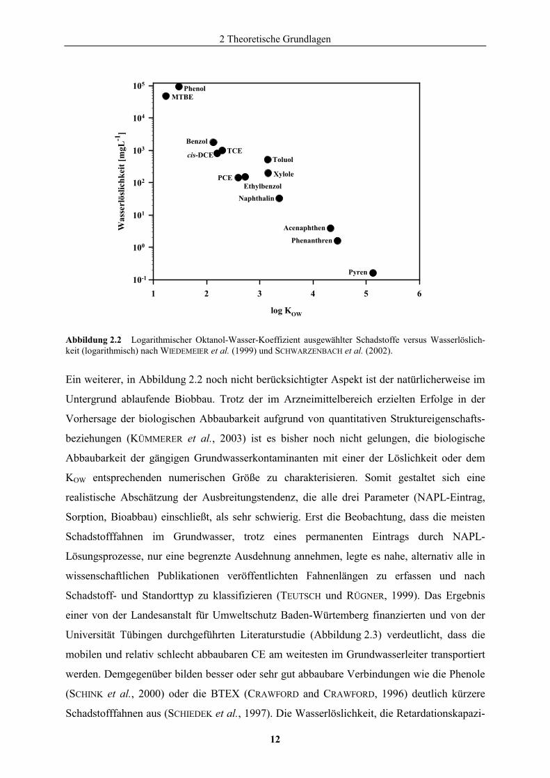
Wasserlöslichkeit und hohem KOW nur sehr langsam im Aquifer transportiert werden. Wie aus
Abbildung 2.2 ersichtlich, sind die ausgewählten PAK (Acenaphthen, Phenanthren, Pyren)
relativ immobil und sollten demzufolge nur in geringer Entfernung vom jeweiligen
Schadensherd anzutreffen sein. Anders verhalten sich die mobilen Schadstoffgruppen wie z.B.
die Phenole, das MTBE, die BTEX oder die chlorierten Ethene (CE), die, sofern sie nicht
abgebaut werden, über weite Strecken im Aquifer transportiert werden können.
2 Theoretische Grundlagen
12
Abbildung 2.2 Logarithmischer Oktanol-Wasser-Koeffizient ausgewählter Schadstoffe versus Wasserlöslich-keit (logarithmisch) nach WIEDEMEIER et al. (1999) und SCHWARZENBACH et al. (2002).
Ein weiterer, in Abbildung 2.2 noch nicht berücksichtigter Aspekt ist der natürlicherweise im
Untergrund ablaufende Biobbau. Trotz der im Arzneimittelbereich erzielten Erfolge in der
Vorhersage der biologischen Abbaubarkeit aufgrund von quantitativen Struktureigenschafts-
beziehungen (KÜMMERER et al., 2003) ist es bisher noch nicht gelungen, die biologische
Abbaubarkeit der gängigen Grundwasserkontaminanten mit einer der Löslichkeit oder dem
KOW entsprechenden numerischen Größe zu charakterisieren. Somit gestaltet sich eine
realistische Abschätzung der Ausbreitungstendenz, die alle drei Parameter (NAPL-Eintrag,
Sorption, Bioabbau) einschließt, als sehr schwierig. Erst die Beobachtung, dass die meisten
Schadstofffahnen im Grundwasser, trotz eines permanenten Eintrags durch NAPL-
Lösungsprozesse, nur eine begrenzte Ausdehnung annehmen, legte es nahe, alternativ alle in
wissenschaftlichen Publikationen veröffentlichten Fahnenlängen zu erfassen und nach
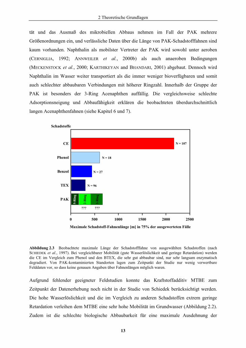
Schadstoff- und Standorttyp zu klassifizieren (TEUTSCH und RÜGNER, 1999). Das Ergebnis
einer von der Landesanstalt für Umweltschutz Baden-Würtemberg finanzierten und von der
Universität Tübingen durchgeführten Literaturstudie (Abbildung 2.3) verdeutlicht, dass die
mobilen und relativ schlecht abbaubaren CE am weitesten im Grundwasserleiter transportiert
werden. Demgegenüber bilden besser oder sehr gut abbaubare Verbindungen wie die Phenole
(SCHINK et al., 2000) oder die BTEX (CRAWFORD and CRAWFORD, 1996) deutlich kürzere
Schadstofffahnen aus (SCHIEDEK et al., 1997). Die Wasserlöslichkeit, die Retardationskapazi-
MTBE
log KOW
1 2 3 4 5 6
Was
serl
öslic
hkei
t [m
gL-1
]
10-1
100
101
102
103
104
105
Phenanthren
Acenaphthen
Naphthalin
Toluol
Xylole
Benzol
cis-DCE TCE
PCEEthylbenzol
Phenol
Pyren
2 Theoretische Grundlagen
13
tät und das Ausmaß des mikrobiellen Abbaus nehmen im Fall der PAK mehrere
Größenordnungen ein, und verlässliche Daten über die Länge von PAK-Schadstofffahnen sind
kaum vorhanden. Naphthalin als mobilster Vertreter der PAK wird sowohl unter aeroben
(CERNIGLIA, 1992; ANNWEILER et al., 2000b) als auch anaeroben Bedingungen
(MECKENSTOCK et al., 2000; KARTHIKEYAN and BHANDARI, 2001) abgebaut. Dennoch wird
Naphthalin im Wasser weiter transportiert als die immer weniger bioverfügbaren und somit
auch schlechter abbaubaren Verbindungen mit höherer Ringzahl. Innerhalb der Gruppe der
PAK ist besonders der 3-Ring Acenaphthen auffällig. Die vergleichsweise schlechte
Adsorptionsneigung und Abbaufähigkeit erklären die beobachteten überdurchschnittlich
langen Acenaphthenfahnen (siehe Kapitel 6 und 7).
Maximale Schadstoff-Fahnenlänge [m] in 75% der ausgewerteten Fälle
0 500 1000 1500 2000 2500
Schadstoffe
CE
Phenol
Benzol
TEX
PAK
N = 107
N = 18
N = 27
N = 96
5-R
ing
2-R
ing
3-R
ing
??? ???
3-R
ing
Abbildung 2.3 Beobachtete maximale Länge der Schadstofffahne von ausgewählten Schadstoffen (nach SCHIEDEK et al., 1997). Bei vergleichbarer Mobilität (gute Wasserlöslichkeit und geringe Retardation) werden die CE im Vergleich zum Phenol und den BTEX, die sehr gut abbaubar sind, nur sehr langsam enzymatisch degradiert. Von PAK-kontaminierten Standorten lagen zum Zeitpunkt der Studie nur wenig verwertbare Felddaten vor, so dass keine genauen Angaben über Fahnenlängen möglich waren.
Aufgrund fehlender geeigneter Feldstudien konnte das Kraftstoffadditiv MTBE zum
Zeitpunkt der Datenerhebung noch nicht in der Studie von Schiedek berücksichtigt werden.
Die hohe Wasserlöslichkeit und die im Vergleich zu anderen Schadstoffen extrem geringe
Retardation verleihen dem MTBE eine sehr hohe Mobilität im Grundwasser (Abbildung 2.2).
Zudem ist die schlechte biologische Abbaubarkeit für eine maximale Ausdehnung der
2 Theoretische Grundlagen
14
Schadstofffahne verantwortlich, die annähernd mit der eines konservativen Tracers wie dem
Chloridion vergleichbar ist. Die beobachtete maximale Länge von MTBE-Schadstofffahnen
liegt somit mindestens im Bereich der Fahnenlänge der CE. MTBE ist aus diesen Gründen
einer der problematischsten Grundwasserkontaminanten, für den sicherlich differenziertere
Sanierungsstrategien als ein einfaches NA-Konzept eingesetzt werden müssen (SCHIRMER et
al., 2000).
2.4 Immissionspumpversuche Die Erkundung eines Aquifers im Abstrom einer Verdachtsfläche basiert in der Regel auf den
einzelnen Proben der am Standort abgeteuften Grundwassermessstellen. Auf der Grundlage
von meist wenigen Punktwerten wird unter Verwendung von Interpolationsansätzen auf die
Gesamtbelastung an einem Standort geschlossen (BOCKELMANN et al., 2000). Besonders für
heterogene Grundwasserleiter mit komplexer Hydrogeologie und multiplen sowie häufig nicht
genau lokalisierten Kontaminationsquellen ist eine auf einzelnen Messpunkten beruhende
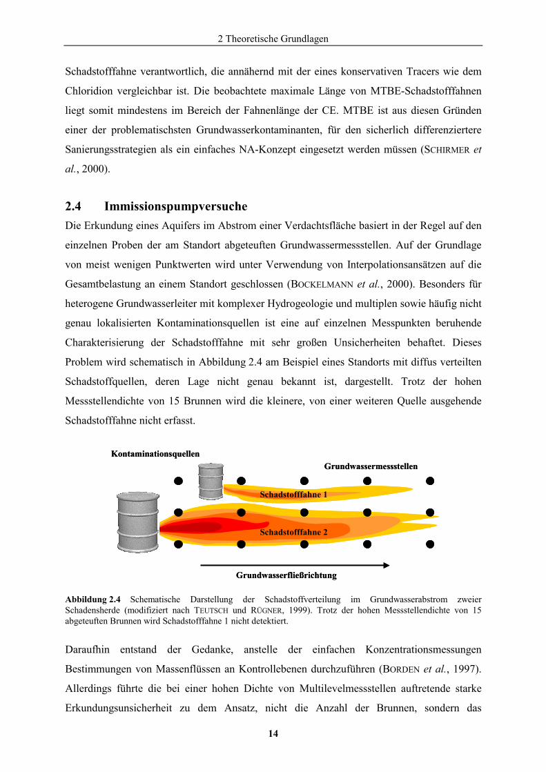
Charakterisierung der Schadstofffahne mit sehr großen Unsicherheiten behaftet. Dieses
Problem wird schematisch in Abbildung 2.4 am Beispiel eines Standorts mit diffus verteilten
Schadstoffquellen, deren Lage nicht genau bekannt ist, dargestellt. Trotz der hohen
Messstellendichte von 15 Brunnen wird die kleinere, von einer weiteren Quelle ausgehende
Schadstofffahne nicht erfasst.
Abbildung 2.4 Schematische Darstellung der Schadstoffverteilung im Grundwasserabstrom zweier Schadensherde (modifiziert nach TEUTSCH und RÜGNER, 1999). Trotz der hohen Messstellendichte von 15 abgeteuften Brunnen wird Schadstofffahne 1 nicht detektiert.
Daraufhin entstand der Gedanke, anstelle der einfachen Konzentrationsmessungen
Bestimmungen von Massenflüssen an Kontrollebenen durchzuführen (BORDEN et al., 1997).
Allerdings führte die bei einer hohen Dichte von Multilevelmessstellen auftretende starke
Erkundungsunsicherheit zu dem Ansatz, nicht die Anzahl der Brunnen, sondern das
Grundwasserfließrichtung
Grundwassermessstellen
Schadstofffahne 1
Schadstofffahne 2
Kontaminationsquellen
Grundwasserfließrichtung
Grundwassermessstellen
Schadstofffahne 1
Schadstofffahne 2
Kontaminationsquellen
2 Theoretische Grundlagen
15
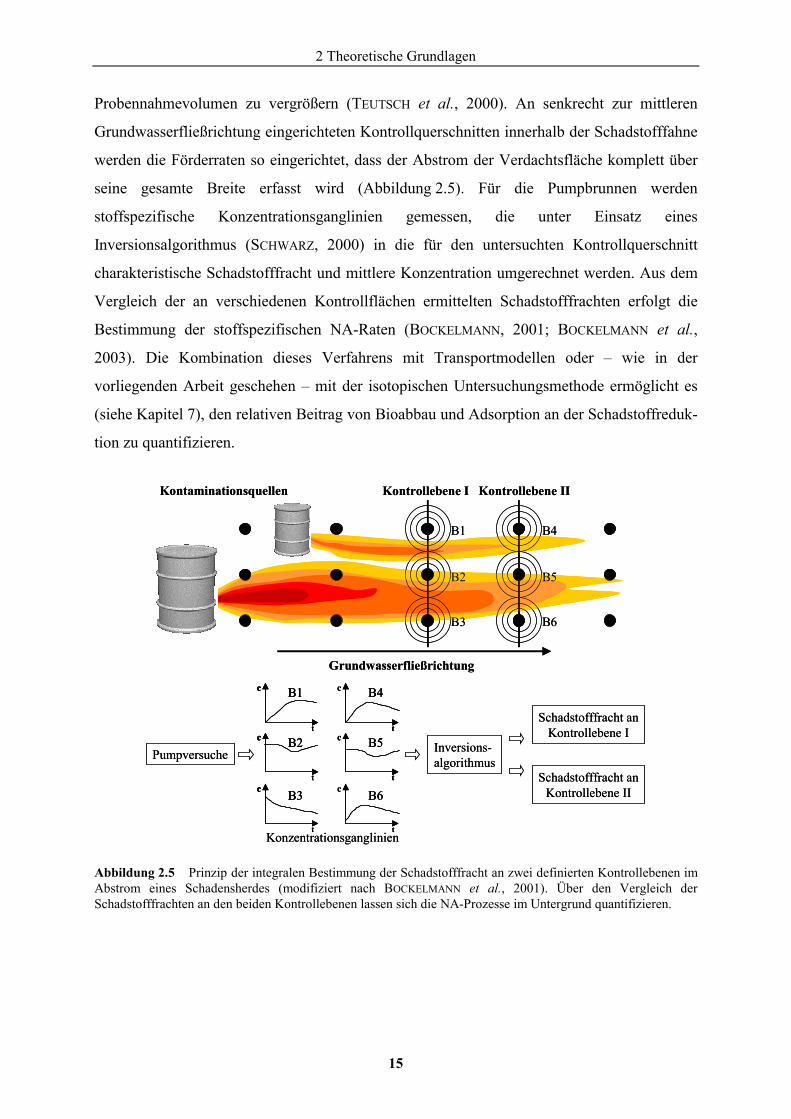
Probennahmevolumen zu vergrößern (TEUTSCH et al., 2000). An senkrecht zur mittleren
Grundwasserfließrichtung eingerichteten Kontrollquerschnitten innerhalb der Schadstofffahne
werden die Förderraten so eingerichtet, dass der Abstrom der Verdachtsfläche komplett über
seine gesamte Breite erfasst wird (Abbildung 2.5). Für die Pumpbrunnen werden
stoffspezifische Konzentrationsganglinien gemessen, die unter Einsatz eines
Inversionsalgorithmus (SCHWARZ, 2000) in die für den untersuchten Kontrollquerschnitt
charakteristische Schadstofffracht und mittlere Konzentration umgerechnet werden. Aus dem
Vergleich der an verschiedenen Kontrollflächen ermittelten Schadstofffrachten erfolgt die
Bestimmung der stoffspezifischen NA-Raten (BOCKELMANN, 2001; BOCKELMANN et al.,
2003). Die Kombination dieses Verfahrens mit Transportmodellen oder – wie in der
vorliegenden Arbeit geschehen – mit der isotopischen Untersuchungsmethode ermöglicht es
(siehe Kapitel 7), den relativen Beitrag von Bioabbau und Adsorption an der Schadstoffreduk-
tion zu quantifizieren.
Abbildung 2.5 Prinzip der integralen Bestimmung der Schadstofffracht an zwei definierten Kontrollebenen im Abstrom eines Schadensherdes (modifiziert nach BOCKELMANN et al., 2001). Über den Vergleich der Schadstofffrachten an den beiden Kontrollebenen lassen sich die NA-Prozesse im Untergrund quantifizieren.
Grundwasserfließrichtung
Kontaminationsquellen
B4
Kontrollebene II
B5
B6
B1
Kontrollebene I
B2
B3
t
Pumpversuche
Konzentrationsganglinien
Inversions-algorithmus
Schadstofffracht anKontrollebene I
c
t
c
c
t
B1
B2
B3
c
c
ct
t
B4
B5
B6
t
Schadstofffracht anKontrollebene II
Grundwasserfließrichtung
Kontaminationsquellen
B4
Kontrollebene II
B5
B6
B1
Kontrollebene I
B2
B3
t
Pumpversuche
Konzentrationsganglinien
Inversions-algorithmus
Schadstofffracht anKontrollebene I
c
t
c
c
t
B1
B2
B3
c
t
c
c
t
B1
B2
B3
c
c
ct
t
B4
B5
B6
t
t
B4
B5
B6
t
Schadstofffracht anKontrollebene II
2 Theoretische Grundlagen
16
2.5 Sanierungsstrategien Grundsätzlich unterscheidet man bei Boden- und Grundwassersanierungsverfahren zwischen
Ex-situ- (mit Bodenaushub) und In-situ-Techniken (ohne Bodenaushub).
2.5.1 Ex-situ-Sanierung
Ex-situ-Sanierungen werden je nach Ort der Behandlungsanlage als On-site- (am Ort) oder
Off-site-Verfahren (außerhalb des Sanierungsorts) betrieben. Klassische Ex-situ-Verfahren
wie z.B die Mietentechnik oder die Reaktorverfahren sind ungeachtet der Tatsache, ob sie in
der On-site- oder Off-site-Variante angewendet werden, mit der Bewegung von großen
Mengen an kontaminiertem Material verbunden und stellen demnach ein hohes
Gefährdungspotenzial für Mensch und Umwelt dar. Die hydraulischen Sanierungs-
maßnahmen, bei denen das kontaminierte Wasser nach oben gepumpt, dort behandelt und
wieder in den Aquifer eingeleitet wird (“Pump-and-Treat“), weisen auch nach langen
Betriebszeiten noch hohe Schadstoffrestkonzentrationen auf (MACKAY and CHERRY, 1989;
WIEDEMEIER et al., 1999). Zudem ist der durch das permanente Pumpen von Wasser bedingte
Energiebedarf erheblich.
Diese Beispiele und die Erfahrungen der letzten 20 Jahre verdeutlichen, dass die aufwändigen,
meist sehr kostspieligen Ex-situ-Sanierungsmaßnahmen nur in seltenen Fällen zum Erfolg
führen.
2.5.2 In-situ-Sanierung
Aufgrund der o.g. Nachteile von Ex-situ-Sanierungen werden zunehmend passive In-situ-
Sanierungsverfahren, welche die Verunreinigungen durch natürliche oder stimulierte Prozesse
direkt im Untergrund behandeln, als viel versprechende Alternativen diskutiert. Für die
biologisch leicht abbaubaren Xenobiotika sind speziell die Sanierungsmethoden, die auf der
Selbstreinigungskraft der Natur beruhen, von besonderer Bedeutung. Im Fall von nur sehr
langsam abbaubaren Schadstoffen gelten Reinigungswände gegenwärtig als eine der
erfolgsversprechenden Technologien zur Sanierung von Grundwasserkontaminationen.
2.5.2.1 In-situ-Bioremediation (Natural Attenuation)
Im Jahr 1993 kam eine Kommission des amerikanischen nationalen Forschungsrates (National
Research Council, NRC), die mit der Untersuchung und Anwendbarkeit der natürlicherweise
im Untergrund ablaufenden Abbauprozesse beauftragt war, zu dem Ergebnis, dass
2 Theoretische Grundlagen
17
Mikroorganismen einen Großteil der in den Grundwasserleiter eingebrachten Kontaminanten
abbauen können (NATIONAL RESEARCH COUNCIL, 1993). In dieser Studie wurde strikt
zwischen natürlicher (Intrinsic- oder In-Situ-Bioremediation) und technischer Bioremediation
(Engineered Bioremediation) unterschieden. Seinerzeit war das Vertrauen in die natürliche
Reinigungskraft des Aquifers nicht allzu groß, und in den Anwendungen beschränkte man
sich fast ausschließlich auf die Stimulierung, Verstärkung und Erweiterung des natürlichen
Bioremediationspotenzials. Daher ist es nicht verwunderlich, dass speziell zu dieser Zeit
diverse Infiltrations- und Belüftungsverfahren eingesetzt wurden. Dennoch wurde Intrinsic-
Bioremediation in den Jahren nach 1993 bei einer zunehmenden Zahl von Schadensfällen als
Sanierungsstrategie akzeptiert. Diese Entwicklung wurde durch die Tatsache begünstigt, dass
neben den Abbauprozessen zunehmend auch nichtdestruktive Rückhalteprozesse wie
Dispersion, Verdünnung, Sorption, und Verflüchtigung als Schadstoffsenken erkannt wurden.
Die Gesamtheit dieser In-situ-Prozesse, inklusive dem in natürlichen Systemen
vernachlässigbaren chemischen Abbau, wurden unter dem Begriff NA zusammengefasst. Die
einsetzende, teilweise unkritische Anwendung von NA als Sanierungstechnik für
kontaminiertes Grundwasser sorgte in den USA für kontroverse Diskussionen. Kritiker des
NA-Konzepts warfen den Sanierungspflichtigen vor, sich durch die Berufung auf die
Selbstreinigungskraft des Aquifers aus der Verantwortung stehlen zu wollen. Es sei nicht
damit getan, so lautete der Vorwurf, das Nichtstun mit einem wohlwollenden Namen zu
versehen (WIENBERG, 1997). In der Zwischenzeit wird NA in den USA schon seit ein paar
Jahren in Verbindung oder im Anschluss an aktive Maßnahmen für eher kleinräumige, leicht
abbaubare Dieselölkontaminationen angewendet. Der Übergang zwischen NA und aktiven
Sanierungsmaßnahmen ist dort fließend. Voraussetzung für die erfolgreiche Anwendung von
NA als Sanierungsoption (ohne menschlichen Einfluss) war sicherlich die aus der Diskussion
hervorgegangene Forderung der amerikanischen Umweltbehörde (Environmental Protection
Agency, EPA) nach einer Langzeitüberwachung der Prozesse (Monitored Natural Attenuation,
MNA; TRACK und MICHELS, 1999).
Ende der 90er Jahre erreichte diese Diskussion auch Deutschland. Hier stieß das MNA-
Konzept anfänglich allerdings auf wenige Anhänger. Die hier gültigen gesetzlichen
Regelungen standen bisher der Nutzung von MNA als Sanierungsstrategie entgegen (MEIER-
LÖHR und BATTERMANN, 2000). Zudem fehlten neben einer eindeutigen Begrifflichkeit und
Definition Konzepte für die sinnvolle Aufeinanderfolge der Planungsschritte. Gegenwärtig
besteht Einigkeit darüber, dass die natürlicherweise im Untergrund ablaufenden Prozesse
2 Theoretische Grundlagen
18
verstanden werden müssen. Vor diesem Hintergrund sollte diskutiert werden, inwieweit die
natürlichen Prozesse in eine, wie auch immer geartete Sanierungsstrategie integriert werden
können.
NA-Prozesse Wie schon erwähnt, wird der Begriff NA verwendet, um sämtliche natürlichen Prozesse zu
beschreiben, die eine Erniedrigung der Schadstoffkonzentration bewirken. Nachfolgend
werden die wichtigsten Parameter diskutiert, die einen Einfluss auf die Ausbreitung der
Schadstoffe im Untergrund besitzen.
Xenobiotika gelangen überwiegend als NAPL-Phase in die ungesättigte Zone und sinken unter
dem Einfluss der Schwerkraft bis zur wassergesättigten Zone, wo sie entsprechend ihrer
Wasserlöslichkeit und Lösungskinetik im Grundwasser gelöst werden. Je nach physikalischer
Dichte der Xenobiotika verbleibt die Reinphase auf der Grundwasseroberfläche (Low NAPL,
LNAPL; z.B. BTEX) oder sinkt weiter durch die Grundwassersäule bis auf den Aquitard ab
(Dense NAPL, DNAPL; z.B. CKW). Physikalische Prozesse wie die Advektion und die
hydrodynamische Dispersion transportieren die gelösten Kontaminanten in
Grundwasserfließrichtung. Die permanente Nachlösung aus den NAPL ist für die weitere
Ausbreitung der Schadstofffahne verantwortlich. Allerdings können Sorptionsprozesse, d.h.
die Wechselwirkung zwischen der organischen Aquifermatrix und den gelösten
Kontaminanten, diesen Transport verlangsamen.
Prozesse wie die Verdampfung sowie der biotische und der abiotische Abbau bewirken eine
Erniedrigung der Konzentration der Schadstoffe im Grundwasser und können im Idealfall die
Nachlieferung von Kontaminanten (durch Advektion, Dispersion, Diffusion und Sorption)
kompensieren. Man spricht in diesem Fall von einer räumlich und zeitlich stationären
Schadstofffahne. Dadurch, dass die Verdampfung im Allgemeinen nur zu einem geringen
Anteil zur Schadstoffreduktion im Grundwasser beiträgt (WEBER, 2002) und der chemische
Abbau der Kontaminanten sehr langsam verläuft, stellt die biologische Degradation die
wichtigste Schadstoffsenke innerhalb des NA-Konzepts dar. Zudem wirkt sie destruktiv auf
die Xenobiotika und reduziert somit ihre Masse im Aquifer. Dagegen sind die abiotischen
Prozesse (Sorption, Dispersion, Verdünnung und Verdampfung) hinsichtlich ihrer Wirkung
auf den Schadstoff nichtdestruktiv. Der beobachtete Konzentrationsrückgang beruht auf einer
Umverteilung der Schadstoffe, ohne ihre eigentliche Masse im Untergrund zu reduzieren.
Nachfolgend wird auf den einzigen bedeutenden destruktiven Teil von NA, den Bioabbau,
näher eingegangen.
2 Theoretische Grundlagen
19
Bioabbau Gelangen organische Schadstoffe in den Grundwasserleiter, so werden diese meist aufgrund
der raschen Vermehrung der autochtonen (standorteigenen) Bakterien relativ schnell unter
Verwendung des im Wasser molekular gelösten Sauerstoffs, d.h. unter aeroben Bedingungen,
abgebaut. Die Mikroorganismen benutzen den Schadstoff als Kohlenstoffquelle und gewinnen
die für das Wachstum und die biologische Aktivität benötigte Energie aus den
Elektronenübergängen (primärer Metabolismus). Reine Kohlenwasserstoffe dienen dabei in
der Regel als Elektronendonatoren und werden vom Elektronenakzeptor Sauerstoff oxidiert.
Nach dem Verbrauch des nur begrenzt vorhandenen elementaren Sauerstoffs stellen sich bei
Grundwasserkontaminationen relativ rasch anaerobe Milieuverhältnisse ein (� 0,5 mg L-1 O2),
und Sauerstoff steht nur noch in gebundener Form zur Verfügung. Dann veratmen fakultativ
oder obligat anaerobe Mikroorganismen zunächst die Elektronenakzeptoren Nitrat, dann die
Mangan- und Eisenoxide und zuletzt Sulfat. Dabei liefern die verschiedenen Redoxprozesse
der Zelle unterschiedliche Mengen an Energie. So ist die Sauerstoffreduktion
thermodynamisch günstiger als die Nitratreduktion; diese wiederum liefert mehr Energie als
die Mangan-, Eisen- oder die Sulfatreduktion. Bei Verfügbarkeit der entsprechenden
Elektronenakzeptoren und Bakterienkulturen läuft der Prozess ab, der den Zellen den höchsten
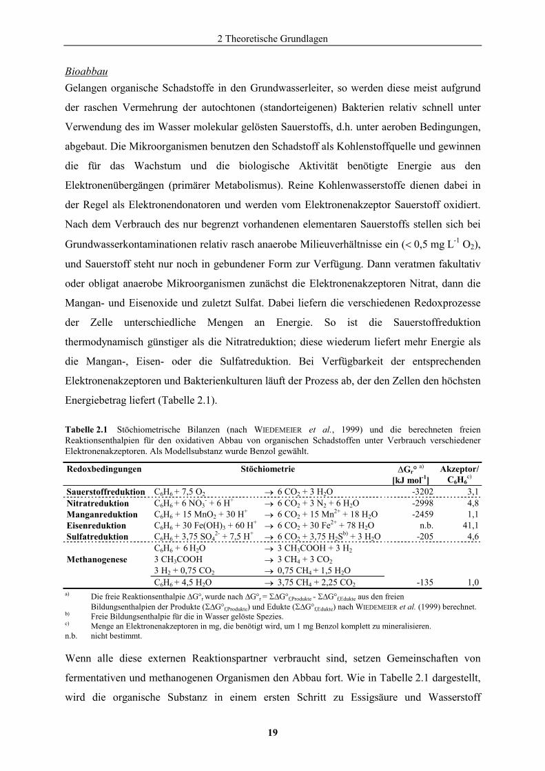
Energiebetrag liefert (Tabelle 2.1).
Tabelle 2.1 Stöchiometrische Bilanzen (nach WIEDEMEIER et al., 1999) und die berechneten freien Reaktionsenthalpien für den oxidativen Abbau von organischen Schadstoffen unter Verbrauch verschiedener Elektronenakzeptoren. Als Modellsubstanz wurde Benzol gewählt.
Redoxbedingungen Stöchiometrie �Gr° a) [kJ mol-1]
Akzeptor/C6H6
c) Sauerstoffreduktion C6H6 + 7,5 O2 � 6 CO2 + 3 H2O -3202 3,1Nitratreduktion C6H6 + 6 NO3
- + 6 H+ � 6 CO2 + 3 N2 + 6 H2O -2998 4,8Manganreduktion C6H6 + 15 MnO2 + 30 H+ � 6 CO2 + 15 Mn2+ + 18 H2O -2459 1,1Eisenreduktion C6H6 + 30 Fe(OH)3 + 60 H+
� 6 CO2 + 30 Fe2+ + 78 H2O n.b. 41,1Sulfatreduktion C6H6 + 3,75 SO4
2- + 7,5 H+ � 6 CO2 + 3,75 H2Sb) + 3 H2O -205 4,6 C6H6 + 6 H2O � 3 CH3COOH + 3 H2 Methanogenese 3 CH3COOH � 3 CH4 + 3 CO2 3 H2 + 0,75 CO2 � 0,75 CH4 + 1,5 H2O C6H6 + 4,5 H2O � 3,75 CH4 + 2,25 CO2 -135 1,0
a) Die freie Reaktionsenthalpie �G°r wurde nach �G°r = ��G°f,Produkte - ��G°f,Edukte aus den freien
Bildungsenthalpien der Produkte (��G°f,Produkte) und Edukte (��G°f,Edukte) nach WIEDEMEIER et al. (1999) berechnet. b) Freie Bildungsenthalpie für die in Wasser gelöste Spezies. c) Menge an Elektronenakzeptoren in mg, die benötigt wird, um 1 mg Benzol komplett zu mineralisieren. n.b. nicht bestimmt.
Wenn alle diese externen Reaktionspartner verbraucht sind, setzen Gemeinschaften von
fermentativen und methanogenen Organismen den Abbau fort. Wie in Tabelle 2.1 dargestellt,
wird die organische Substanz in einem ersten Schritt zu Essigsäure und Wasserstoff
2 Theoretische Grundlagen
20
fermentiert. In einem weiteren Schritt setzen die methanogenen Bakterien H2
(Elektronendonator) mit im Aquifer vorhanden CO2 (Elektronenakzeptor) zu CH4 und H2O
um. Ein anderer Teil des CH4 stammt aus der Disproportionierung der Essigsäure (SCHLEGEL
und ZABOROSCH, 1992).
Eine besondere Rolle kommt den CE zu, da sie durch direkte aerobe und anaerobe Oxidation,
durch Halorespiration sowie kometabolisch degradiert werden können (WIEDEMEIER et al.,
1999). Der Abbauweg wird neben den im Aquifer herrschenden geo- und biochemischen
Randbedingungen durch die Oxidationszahl der entsprechenden Verbindung bestimmt.
Speziell der biologische Abbau von höher chlorierten Verbindungen läuft nur unter strikt
anaeroben Bedingungen ab. Im Zuge des kometabolischen Abbaus werden von der
Degradation des Auxiliarsubstrats stammende Elektronen nahezu beliebig auf die CE
übertragen, die dabei reduktiv dechloriert werden. Im Unterschied zu den in Tabelle 2.1
besprochenen Kohlenwasserstoffen werden die CE dabei weder als Kohlenstoff- noch als
Energiequelle zum Wachstum der Bakterien genutzt. Während beim kometabolischen Abbau
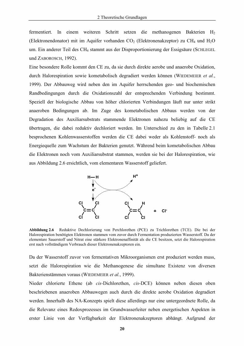
die Elektronen noch vom Auxiliarsubstrat stammen, werden sie bei der Halorespiration, wie
aus Abbildung 2.6 ersichtlich, vom elementaren Wasserstoff geliefert.
Abbildung 2.6 Reduktive Dechlorierung von Perchlorethen (PCE) zu Trichlorethen (TCE). Die bei der Halorespiration benötigten Elektronen stammen vom zuvor durch Fermentation produzierten Wasserstoff. Da der elementare Sauerstoff und Nitrat eine stärkere Elektronenaffinität als die CE besitzen, setzt die Halorespiration erst nach vollständigem Verbrauch dieser Elektronenakzeptoren ein.
Da der Wasserstoff zuvor von fermentativen Mikroorganismen erst produziert werden muss,
setzt die Halorespiration wie die Methanogenese die simultane Existenz von diversen
Bakterienstämmen voraus (WIEDEMEIER et al., 1999).
Nieder chlorierte Ethene (ab cis-Dichlorethen, cis-DCE) können neben diesen oben
beschriebenen anaeroben Abbauwegen auch durch die direkte aerobe Oxidation degradiert
werden. Innerhalb des NA-Konzepts spielt diese allerdings nur eine untergeordnete Rolle, da
die Relevanz eines Redoxprozesses im Grundwasserleiter neben energetischen Aspekten in
erster Linie von der Verfügbarkeit der Elektronenakzeptoren abhängt. Aufgrund der
CCCl
Cl
Cl
ClCC
Cl
Cl
H
Cl
H+
e-
Cl-
H H
2 Theoretische Grundlagen
21
limitierten Nachlieferung des Sauerstoffs ins Fahneninnere, beschränkt sich der aerobe
Schadstoffabbau in den meisten Feldstudien auf den Fahnenrandbereich. So beträgt z.B. die
relative, aus 38 Feldstudien berechnete Abbaukapazität des aeroben BTEX-Abbaus nur 3%
der gesamten mikrobiell abgebauten BTEX-Masse (WIEDEMEIER et al., 1999).
Sulfatreduzierer oder methanogene Konsortien sind nach den Ergebnissen dieser Studie für 70
bzw. 16% der abgebauten BTEX-Masse verantwortlich.
2.5.2.2 Reaktive Wände
Die langsame und unvollständig verlaufende kometabolische Dechlorierung und die nur unter
speziellen biogeochemischen Bedingungen begünstigte reduktive Halorespiration haben zur
Folge, dass sich an sehr vielen Standorten lange CE-Fahnen im Aquifer ausbilden (siehe
Abbildung 2.3). Aus diesen Gründen erweist sich eine Sanierung dieser Standorte mit dem
NA-Konzept, speziell für die höher chlorierten Spezies, oft als problematisch (WIEDEMEIER et
al., 1999). Entsprechend bemerkte das NRC im Jahr 2000:
„Natural Attenuation of chlorinated solvents is not given, many sites are
inappropriate for this technique” (NATIONAL RESEARCH COUNCIL, 2000).
Als viel versprechende In-situ-Alternative gelten die “Permeablen Reaktiven Barrieren“
(PRB), auch Reaktionswand, geochemische Barriere oder auch “Funnel-and-Gate-System“
genannt. PRB sind permeable Reaktorsegmente, die quer zum Grundwasserabstrom eines
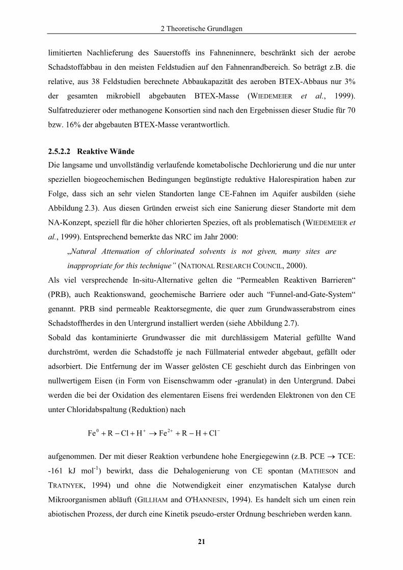
Schadstoffherdes in den Untergrund installiert werden (siehe Abbildung 2.7).
Sobald das kontaminierte Grundwasser die mit durchlässigem Material gefüllte Wand
durchströmt, werden die Schadstoffe je nach Füllmaterial entweder abgebaut, gefällt oder
adsorbiert. Die Entfernung der im Wasser gelösten CE geschieht durch das Einbringen von
nullwertigem Eisen (in Form von Eisenschwamm oder -granulat) in den Untergrund. Dabei
werden die bei der Oxidation des elementaren Eisens frei werdenden Elektronen von den CE
unter Chloridabspaltung (Reduktion) nach
���
������� ClHRFeHClRFe 20
aufgenommen. Der mit dieser Reaktion verbundene hohe Energiegewinn (z.B. PCE � TCE:
-161 kJ mol-1) bewirkt, dass die Dehalogenierung von CE spontan (MATHESON and
TRATNYEK, 1994) und ohne die Notwendigkeit einer enzymatischen Katalyse durch
Mikroorganismen abläuft (GILLHAM and O'HANNESIN, 1994). Es handelt sich um einen rein
abiotischen Prozess, der durch eine Kinetik pseudo-erster Ordnung beschrieben werden kann.
2 Theoretische Grundlagen
22
Abbildung 2.7 Schematische Darstellung einer Reaktionswand.
Obwohl die Verwendung von elementaren Metallen als Dehalogenierungsmittel bei der
Synthese organischer Substanzen schon auf das Jahr 1874 zurückgeht (MARCH and SMITH,
2000), erkannte erst Gillham im Jahre 1989 die Bedeutung dieser Reaktion für mit CE
kontaminierte Grundwasserleiter. Seitdem werden PRB vor allem in den USA und Kanada in
steigendem Maße entwickelt, untersucht und angewendet.
LNAPL
DNAPL
Schadstoffquelle
Reaktionsw
and
Schadstofffahne
Aquiferbasis
Ungesättigte Zone
Grundwasser-entnahme
2 Theoretische Grundlagen
23
2.6 Nachweis des biologischen Abbaus
2.6.1 Drei Beweisniveaus (Lines of evidence)
Voraussetzung für die Nutzung des intrinsischen Abbaupotenzials innerhalb des NA-
Konzepts ist ein schlüssiger Nachweis des In-situ-Abbaus von Schadstoffen. Da
Degradationsprozesse selbst in Fällen mit überschaubaren hydrogeologischen Bedingungen
aufgrund der Vielfalt der im Untergrund vorhandenen potenziellen Reaktionspartner und der
schlechten Zugänglichkeit des Grundwassers oft nicht zweifelsfrei nachgewiesen werden
können, forderte das NRC 1993 den Nachweis des Bioabbaus durch drei voneinander
unabhängige Beweisniveaus (BN; NATIONAL RESEARCH COUNCIL, 1993).
BN1: Das erste BN umfasst Konzentrationsmessungen über einen längeren Zeitraum, die eine
Abnahme der Schadstoffmasse oder -konzentration belegen.
BN2: Das zweite BN stellt sicher, dass die unter BN1 festgestellte Schadstoffreduktion auch
tatsächlich auf dem enzymatischen Abbau des Schadstoffs beruht. Dieser Nachweis
kann z.B. indirekt über die Erhebung biogeochemischer Daten wie des Verbrauches von
Elekronenakzeptoren oder der Entstehung von abbauspezifischen Metaboliten erbracht
werden. Als direkter Nachweis gilt der mikrobiologische Abbau des betreffenden
Schadstoffs in Batch- und Säulenversuchen mit Standortmaterial.
BN3: Ungleich schwieriger ist die Erfüllung des dritten BNs, welches sicherstellen soll, dass
die im Labor unter kontrollierten Bedingungen abbaubaren Xenobiotika auch im Feld
mikrobiell degradiert werden.
Die Wichtigkeit von BN3 wird vor allem am Beispiel des Benzinzusatzes MTBE deutlich.
Während MTBE in mehreren Laborstudien von verschiedenen, überwiegend aeroben
Mikroorganismen degradiert wird (SALANITRO et al., 1994; BRADLEY et al., 1999; SCHIRMER
et al., 2003), ist der Nachweis des mikrobiologischen Abbaus unter Feldbedingungen äußerst
schwierig (SCHMIDT et al., 2002).
2 Theoretische Grundlagen
24
2.6.2 Nachweis des biologischen Abbaus im Feld mittels Isotopenfraktionierung und Immissionspumpversuchen
Art und Ausmaß des biologischen In-situ-Abbaus von Xenobiotika haben einen
entscheidenden Einfluss darauf, ob die Sanierung eines kontaminierten Aquifers durch die
Nutzung der natürlichen Selbstreinigungskraft (MNA), durch gezielte Stimulierung derselben
(Enhanced Natural Attenuation, ENA) oder durch andere In-situ-Verfahren (z.B. PRB)
erfolgen kann. Im Rahmen dieser Fragestellung ist es erforderlich, die mikrobielle
Degradation im Feld mit wissenschaftlich fundierten und allseits anerkannten Methoden
nachzuweisen. Dafür sind neben der klassischen Berechnung der Abbaukapazität über den
Verbrauch an Elektronenakzeptoren (KAMPBELL et al., 1995) vor allem die in den
Kapiteln 2.1 und 2.4 beschriebenen isotopischen und integralen Untersuchungsmethoden von
großer Bedeutung.
Isotopenfraktionierung während des biologischen Abbaus Neuere Untersuchungen zeigen, dass Fraktionierungen auch bei der biotischen Degradation
von Grundwasserkontaminanten auftreten können. So wurde während des mikrobiellen
Abbaus von Alkanen (STAHL, 1980), aromatischen (MECKENSTOCK et al., 1999; RICHNOW et
al., 2003) und chlorierten Kohlenwasserstoffen (HUNKELER and ARAVENA, 2000a;
SHERWOOD LOLLAR et al., 2001) sowie dem Benzinadditiv MTBE (HUNKELER et al., 2001b;
GRAY et al., 2002; KOLHATKAR et al., 2002) eine Fraktionierung der Kohlenstoffisotope im
noch nicht abgebauten Substrat beobachtet. Aufgrund der Tatsache, dass abiotische
Konzentrationssenken wie Verdampfung (HARRINGTON et al., 1999; HUANG et al., 1999;
POULSON and DREVER, 1999), Adsorption (HARRINGTON et al., 1999; SLATER et al., 2000;
SCHÜTH et al., 2003b) und Verdünnung (MARIOTTI et al., 1981) die Isotopensignatur nur
unwesentlich verändern, kann der biologische In-situ-Abbau vieler Schadstoffe somit durch
Isotopenmessungen erfasst werden. Neben den Kohlenstoffisotopen lässt sich auch das stabile
Isotopenpaar des Wasserstoffs nutzen, um Aussagen über die im Aquifer ablaufenden
Prozesse zu erhalten. In zahlreichen Untersuchungen konnte gezeigt werden, dass die mit dem
Bioabbau verbundene Fraktionierung der stabilen Wasserstoffisotope die der Kohlenstoff-
isotope um mehr als eine Größenordnung übersteigt (WARD et al., 2000; GRAY et al., 2002;
MANCINI et al., 2003).
Es sei noch erwähnt, dass sich das Konzept der Isotopenfraktionierung nicht nur auf
mikrobiologisch katalysierte Reaktionen beschränkt. Sowohl bei der abiotischen Oxidation
von TCE (POULSON and NARAOKA, 2002; HUNKELER et al., 2003) als auch bei der
2 Theoretische Grundlagen
25
Dechlorierung von CE an elementarem Eisen (DAYAN et al., 1999; BILL et al., 2001; SLATER
et al., 2002) traten signifikante 13C-Anreicherungen im residualen Produkt auf.
Nach der Rayleigh-Gleichung (2-3) stehen diese beobachteten isotopischen Fraktionierungen
mit der Konzentrationsabnahme eines Schadstoffs über den Fraktionierungsfaktor � in
Relation. Diese Korrelation ermöglicht es, den durch biotische (siehe Kapitel 5–7) bzw.
abiotische Abbauprozesse (siehe Kapitel 8) degradierten Schadstoffanteil (1-f) über die
Änderung der Isotopensignatur und den in Laborexperimenten bestimmten
Fraktionierungsfaktor �, unabhängig von abiotischen Konzentrationssenken wie
Verflüchtigung, Verdünnung oder Sorption, zu berechnen (SHERWOOD LOLLAR et al., 2001;
MANCINI et al., 2002; RICHNOW et al., 2003).
Immissionspumpversuche Die an zwei Kontrollebenen senkrecht zur mittleren Grundwasserfließrichtung bestimmten
Massenflüsse im Abstrom einer Schadstoffquelle erlauben eine komponentenspezifische
Bestimmung der Massenflussabnahme. Diese kann direkt mit den NA-Prozessen
Verdampfung, Sorption und Bioabbau korreliert werden. Eine anschließende
Transportmodellierung und die Abschätzung der Verdampfungsrate erlauben die Erfassung
des biologischen Schadstoffabbaus (siehe Kapitel 7).
3 Material und Methoden
26
3 Material und Methoden
3.1 Probennahme
3.1.1 Punktbeprobung Feld
Testfeld Süd Die Vorgehensweise bei der Probennahme orientierte sich an den Richtlinien des Deutschen
Verbandes für Wasserwirtschaft und Kulturbau e.V. (DVWK; DVWK, 1992). Die Beprobung
an den Grundwassermessstellen erfolgte mittels Hochleistungstauchpumpen (CONRAD BWV
01, Hamburg), während bei den Multilevelmessstellen Peristaltikpumpen (WATSON MARLOW
303D, Fulmouth, England) eingesetzt wurden. Die Entnahmetiefe bei allen konventionellen
Grundwassermessstellen lag bei 1 m unter dem Grundwasserspiegel. Der Ruhewasserspiegel
wurde mit Hilfe eines Lichtlotes bestimmt. Das blasenfrei geförderte Wasser wurde mittels
eines Tygonschlauches CR 100 (CARL ROTH GmbH & Co. KG, Karlsruhe) in eine
Durchflussmesszelle geleitet, in der die physiko-chemischen Parameter Temperatur, pH-Wert,
Redoxpotenzial und elektrische Leitfähigkeit (WTW pH 91 und WTW LF 91; WTW GmbH &
Co. KG, Weilheim) im Förderstrom gemessen wurden. Erst als diese Parameter konstante
Werte anzeigten, erfolgte die Entnahme der Probe nach zweimaligem Spülen der
Probengefäße durch Eintauchen des Schlauches bis zum Gefäßboden. Die Proben wurden
sofort im Anschluss an die Probennahme auf 2°C gekühlt und innerhalb der nächsten Stunden
mit n-Pentan extrahiert (siehe Kapitel 3.2.1). Alle benutzten Glasgeräte wurden vor Gebrauch
4 h bei 400°C geglüht.
Standort Rheine Die Grundwasserprobennahme am Standort Rheine erfolgte nach den DVWK-Richtlinien
durch das Institut für Geowissenschaften der Universität Kiel. Die Förderrate der eingesetzten
Tauchpumpen (GRUNDFOS MP1, Erkrath) wurde so eingeregelt, dass die Absenkung des
Grundwasserspiegels maximal 10% der Aquifermächtigkeit betrug. Die Proben wurden
entsprechend ihrer weiteren Aufbereitung direkt in geeignete Vials überführt und bis zu ihrer
Analyse bei 4°C im Dunkeln aufbewahrt. Die Konzentrationsbestimmungen übernahm das
Geowissenschaftliche Institut der Universität Kiel. Die Verhältnisse der stabilen
Kohlenstoffisotope wurden im Rahmen der vorliegenden Arbeit mittels SPME (Kapitel 3.2.2)
bestimmt.
3 Material und Methoden
27
3.1.2 Immissionspumpversuche
Die Beprobung von zwei Messstellen des Testfelds Süd im Rahmen der integralen
Pumpversuche erfolgte zu definierten Zeiten (siehe Kapitel 7) unter Nutzung der
rechnergestützten Messeinrichtungen der Universität Tübingen. Das in erheblichen Mengen
anfallende kontaminierte Grundwasser wurde in zwei hintereinander geschalteten
Aktivkohlefässern (PRANTNER GMBH Verfahrenstechnik, Reutlingen) gereinigt. Für die
Probenaufbereitung gilt das in Kapitel 3.2.1 Gesagte. Weitere Einzelheiten zu der
Durchführung der integralen Pumpversuche sind dem Kapitel 7 zu entnehmen.
3.1.3 Säulenversuche
Nach 79 (frischer Eisenschwamm), 56 (Eisenschwamm aus Reaktionswand) und 93
(Graugusseisengranulat aus Reaktionswand) ausgetauschten Porenvolumina wurden Proben
an den entlang der Säule installierten Probeports (siehe Anhang A.3) entgegen der
Fließrichtung von oben nach unten entnommen und über Celluloseacetat-Filter (0,2 mm)
filtriert. Fraktionen für die Isotopenbestimmung wurden wie schon bei den Feldversuchen
sofort abgefüllt und bis zur Festphasenmikroextraktion bei 4°C im Dunkeln gelagert (siehe
Kapitel 8).
3.2 Methodenentwicklung Die Bestimmung der Konzentrationen (BRUZZONITI et al., 2000) und des Isotopengehalts
(DEMPSTER et al., 1997; HUNKELER and ARAVENA, 2000b) von in Wasser gelösten
organischen Substanzen erfordert spezielle Methoden zur Abtrennung und Anreicherung der
interessierenden Analyten. Speziell die Bestimmung der Isotopenverhältnisse von organischen
Verbindungen beschränkte sich in den bislang veröffentlichten Arbeiten (DEMPSTER et al.,
1997; DAYAN et al., 1999) aufgrund der geringen Empfindlichkeit der CSIA nur auf
Konzentrationen in der unmittelbare Nähe von Kontaminationsquellen. Umfassende
Informationen über das Schicksal von Kontaminanten erhält man allerdings nur durch
Messungen über den gesamten Bereich der Schadstofffahne. Somit müssen herkömmliche
Anreicherungsverfahren wie die LLE (DEMPSTER et al., 1997), die SPME (PAWLISZYN, 1997;
HUNKELER and ARAVENA, 2000b; MÜLLER et al., 2000), die Purge-and-Trap-Extraktion
(BIANCHI et al., 2002; MARTÍNEZ et al., 2002) und die Head-Space-Methode (SLATER et al.,
1999) in ihrer Empfindlichkeit weiter verbessert werden. Weiterhin muss über die übliche
Methodenvalidierung hinaus überprüft werden, inwiefern Anreicherungs- und Trenntechniken
eine Isotopenfraktionierung verursachen.
3 Material und Methoden
28
Die Trennung der meist komplex zusammengesetzten Analytengemische in die
Einzelkomponenten wird zunehmend durch instrumentelle physikalisch-chemische Verfahren
wie die Gaschromatographie (GC; EICEMAN, 2002) und die Hochleistungsflüssigkeits-
chromatographie (HPLC) übernommen.
Die Auswahl des richtigen Detektorsystems richtet sich nach Art und Menge der im
Analytengemisch vorliegenden Zielstoffgruppen. Man unterscheidet zwischen Summen-
detektoren, die alle Stoffe erfassen (Wärmeleitfähigkeitsdetektor, Massenspektrometer), und
gruppen- sowie stoffspezifischen Detektoren (z.B. Flammenionisations-, Elektroneneinfang-
oder Stickstoff-Phosphordetektor) für das selektivere Schadstoffscreening.
Im Rahmen dieser Arbeit wurden die leicht automatisierbare und feldtaugliche Flüssig-
Flüssig-Extraktion (für BTEX und PAK) und die Festphasenmikroextraktion (für CE) im
Hinblick auf die Bestimmung der Isotopensignatur evaluiert.
3.2.1 Flüssig-Flüssig-Extraktion (LLE)
Die klassische LLE dient der Überführung und Aufkonzentrierung des Analyten aus einer
Wasserprobe in eine organische Phase und basiert auf der unterschiedlichen
Gleichgewichtsverteilung des Analyten in der nicht miteinander mischbaren wässrigen und
organischen Phase. Je hydrophober die zu extrahierende Substanz, d.h. je größer der KOW,
desto stärker ist der Anreicherungsgrad in der organischen Phase.
Bei der Auswahl des Extraktionsmittels erhielt n-Pentan den Vorzug vor seinem lipophileren
und deutlich weniger flüchtigen höheren Homolog n-Hexan, da es als einziges bei
Raumtemperatur flüssiges n-Alkan unter gaschromatographischen Bedingungen deutlich vor
Benzol eluiert (DEMPSTER et al., 1997). Vorversuche zur Auswahl der Extraktionstechnik
zeigten weiterhin, dass der Überkopfmischer Reax 20 (HEIDOLPH, Schwabach) effizienter und
vor allem reproduzierbarer extrahiert als konventionelle Laborschüttler.
Das im Testfeld zwischen Kontaminationszentrum und nördlicher Abstromfahne beobachtete
starke Konzentrationsgefälle (ANNWEILER, 1999) wurde in Anlehnung an die DIN-Norm (DIN
38407 T9, Ausgabe 5/1991) in mehrere Konzentrationsbereiche unterteilt. Allerdings mussten
aufgrund der höheren Anforderungen an die Nachweisgrenze die in der DIN-Norm
angegebenen Verhältnisse der Extraktionsvolumina in Richtung größerer VProbe/Vn-Pentan-
Quotienten verschoben werden (Tabelle 3.1).
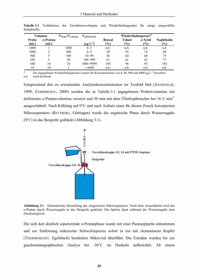
3 Material und Methoden
29
Tabelle 3.1 Verhältnisse der Extraktionsvolumina und Wiederfindungsraten für einige ausgewählte Schadstoffe.
Volumen VProbe/Vn-Pentan CBTEX/PAK Wiederfindungsratea) Probe [mL]
n-Pentan [mL]
[�g L-1] Benzol
[%] Toluol
[%] o-Xylol
[%] Naphthalin
[%] 1000 1 1000 0–3 n.b. n.b. n.b. n.b. 1000 2 500 4–9 29 55 74 68 500 5 100 10–99 56 64 68 75 250 5 50 100–999 61 61 62 77 100 10 10 1000–9999 105 96 95 103 10 10 1 � 9999 n.b. n.b. n.b. n.b.
a) Die angegebenen Wiederfindungsraten wurden für Konzentrationen von 8, 80, 800 und 4000 �g L-1 berechnet. n.b. nicht bestimmt.
Entsprechend den zu erwartenden Analytenkonzentrationen im Testfeld Süd (ANNWEILER,
1999; ZAMIFIRESCU, 2000) wurden die in Tabelle 3.1 angegebenen Probenvolumina mit
definierten n-Pentanvolumina versetzt und 30 min mit dem Überkopfmischer bei 16 U min-1
ausgeschüttelt. Nach Kühlung auf 0°C und nach Aufsatz eines für diesen Zweck konzipierten
Mikroseparators (RETTBERG, Göttingen) wurde die organische Phase durch Wasserzugabe
(0°C) in das Steigrohr gedrückt (Abbildung 3.1).
Abbildung 3.1 Schematische Darstellung des eingesetzten Mikroseparators. Nach dem Ausschütteln wird das n-Pentan durch Wasserzugabe in das Steigrohr gedrückt. Die Spritze dient während der Wasserzugabe dem Druckausgleich.
Die sich dort deutlich separierende n-Pentanphase wurde mit einer Pasteurpipette entnommen
und zur Entfernung reduzierter Schwefelspezies sofort in ein mit elementarem Kupfer
(THERMOQUEST, Egelsbach) bestücktes Mikrovial überführt. Die Extrakte wurden bis zur
gaschromatographischen Analyse bei -36°C im Dunkeln aufbewahrt. Ab einem
Verschlusskappe GL 14 mit PTFE-Septum
Steigrohr
Verschlusskappe GL 45
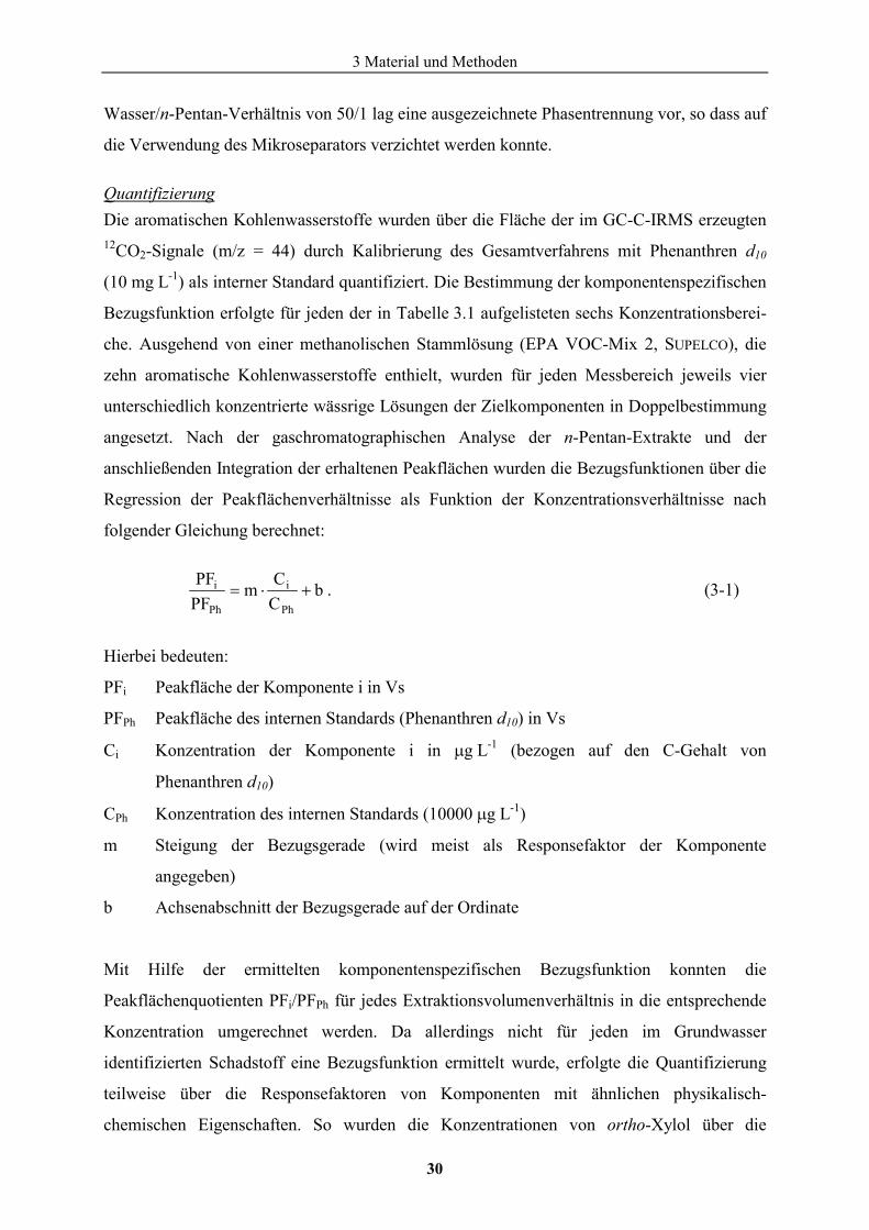
3 Material und Methoden
30
Wasser/n-Pentan-Verhältnis von 50/1 lag eine ausgezeichnete Phasentrennung vor, so dass auf
die Verwendung des Mikroseparators verzichtet werden konnte.
Quantifizierung Die aromatischen Kohlenwasserstoffe wurden über die Fläche der im GC-C-IRMS erzeugten 12CO2-Signale (m/z = 44) durch Kalibrierung des Gesamtverfahrens mit Phenanthren d10
(10 mg L-1) als interner Standard quantifiziert. Die Bestimmung der komponentenspezifischen
Bezugsfunktion erfolgte für jeden der in Tabelle 3.1 aufgelisteten sechs Konzentrationsberei-
che. Ausgehend von einer methanolischen Stammlösung (EPA VOC-Mix 2, SUPELCO), die
zehn aromatische Kohlenwasserstoffe enthielt, wurden für jeden Messbereich jeweils vier
unterschiedlich konzentrierte wässrige Lösungen der Zielkomponenten in Doppelbestimmung
angesetzt. Nach der gaschromatographischen Analyse der n-Pentan-Extrakte und der
anschließenden Integration der erhaltenen Peakflächen wurden die Bezugsfunktionen über die
Regression der Peakflächenverhältnisse als Funktion der Konzentrationsverhältnisse nach
folgender Gleichung berechnet:
bCCm
PFPF
Ph
i
Ph
i��� . (3-1)
Hierbei bedeuten:
PFi Peakfläche der Komponente i in Vs
PFPh Peakfläche des internen Standards (Phenanthren d10) in Vs
Ci Konzentration der Komponente i in �g L-1 (bezogen auf den C-Gehalt von
Phenanthren d10)
CPh Konzentration des internen Standards (10000 �g L-1)
m Steigung der Bezugsgerade (wird meist als Responsefaktor der Komponente
angegeben)
b Achsenabschnitt der Bezugsgerade auf der Ordinate
Mit Hilfe der ermittelten komponentenspezifischen Bezugsfunktion konnten die
Peakflächenquotienten PFi/PFPh für jedes Extraktionsvolumenverhältnis in die entsprechende
Konzentration umgerechnet werden. Da allerdings nicht für jeden im Grundwasser
identifizierten Schadstoff eine Bezugsfunktion ermittelt wurde, erfolgte die Quantifizierung
teilweise über die Responsefaktoren von Komponenten mit ähnlichen physikalisch-
chemischen Eigenschaften. So wurden die Konzentrationen von ortho-Xylol über die
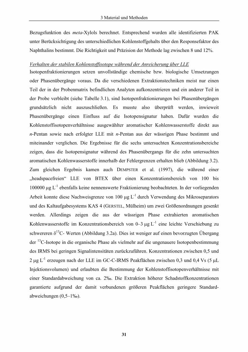
3 Material und Methoden
31
Bezugsfunktion des meta-Xylols berechnet. Entsprechend wurden alle identifizierten PAK
unter Berücksichtigung des unterschiedlichen Kohlenstoffgehalts über den Responsefaktor des
Naphthalins bestimmt. Die Richtigkeit und Präzision der Methode lag zwischen 8 und 12%.
Verhalten der stabilen Kohlenstoffisotope während der Anreicherung über LLE Isotopenfraktionierungen setzen unvollständige chemische bzw. biologische Umsetzungen
oder Phasenübergänge voraus. Da die verschiedenen Extraktionstechniken meist nur einen
Teil der in der Probenmatrix befindlichen Analyten aufkonzentrieren und ein anderer Teil in
der Probe verbleibt (siehe Tabelle 3.1), sind Isotopenfraktionierungen bei Phasenübergängen
grundsätzlich nicht auszuschließen. Es musste also überprüft werden, inwieweit
Phasenübergänge einen Einfluss auf die Isotopensignatur haben. Dafür wurden die
Kohlenstoffisotopenverhältnisse ausgewählter aromatischer Kohlenwasserstoffe direkt aus
n-Pentan sowie nach erfolgter LLE mit n-Pentan aus der wässrigen Phase bestimmt und
miteinander verglichen. Die Ergebnisse für die sechs untersuchten Konzentrationsbereiche
zeigen, dass die Isotopensignatur während des Phasenübergangs für die zehn untersuchten
aromatischen Kohlenwasserstoffe innerhalb der Fehlergrenzen erhalten blieb (Abbildung 3.2).
Zum gleichen Ergebnis kamen auch DEMPSTER et al. (1997), die während einer
„headspacefreien“ LLE von BTEX über einen Konzentrationsbereich von 100 bis
100000 �g L-1 ebenfalls keine nennenswerte Fraktionierung beobachteten. In der vorliegenden
Arbeit konnte diese Nachweisgrenze von 100 �g L-1 durch Verwendung des Mikroseparators
und des Kaltaufgabesystems KAS 4 (GERSTEL, Mülheim) um zwei Größenordnungen gesenkt
werden. Allerdings zeigen die aus der wässrigen Phase extrahierten aromatischen
Kohlenwasserstoffe im Konzentrationsbereich von 0–3 �g L-1 eine leichte Verschiebung zu
schwereren �13C- Werten (Abbildung 3.2a). Dies ist weniger auf einen bevorzugten Übergang
der 13C-Isotope in die organische Phase als vielmehr auf die ungenauere Isotopenbestimmung
des IRMS bei geringen Signalintensitäten zurückzuführen. Konzentrationen zwischen 0,5 und
2 �g L-1 erzeugen nach der LLE im GC-C-IRMS Peakflächen zwischen 0,3 und 0,4 Vs (5 �L
Injektionsvolumen) und erlaubten die Bestimmung der Kohlenstoffisotopenverhältnisse mit
einer Standardabweichung von ca. 2‰. Die Extraktion höherer Schadstoffkonzentrationen
garantierte aufgrund der damit verbundenen größeren Peakflächen geringere Standard-
abweichungen (0,5–1‰).
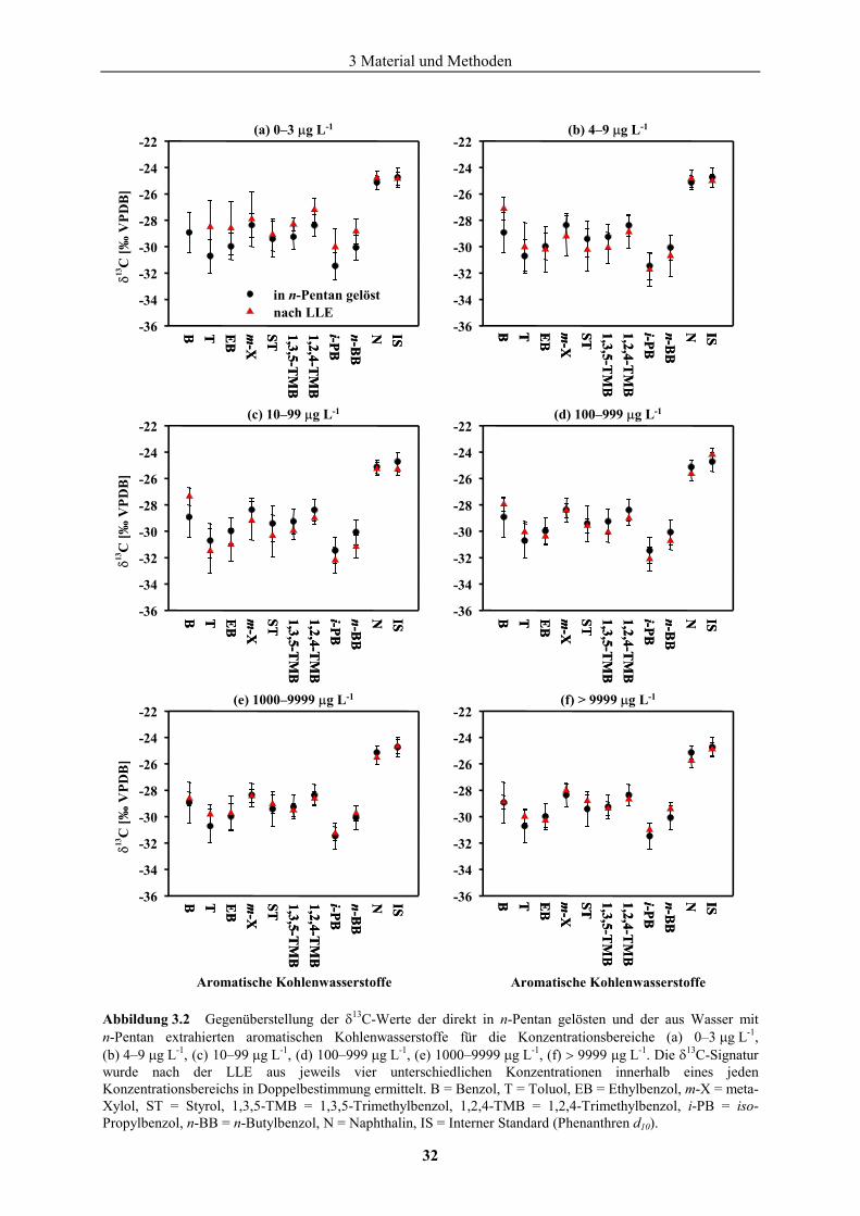
3 Material und Methoden
32
Abbildung 3.2 Gegenüberstellung der �13C-Werte der direkt in n-Pentan gelösten und der aus Wasser mit n-Pentan extrahierten aromatischen Kohlenwasserstoffe für die Konzentrationsbereiche (a) 0–3 �g L-1, (b) 4–9 �g L-1, (c) 10–99 �g L-1, (d) 100–999 �g L-1, (e) 1000–9999 �g L-1, (f) � 9999 �g L-1. Die �13C-Signatur wurde nach der LLE aus jeweils vier unterschiedlichen Konzentrationen innerhalb eines jeden Konzentrationsbereichs in Doppelbestimmung ermittelt. B = Benzol, T = Toluol, EB = Ethylbenzol, m-X = meta-Xylol, ST = Styrol, 1,3,5-TMB = 1,3,5-Trimethylbenzol, 1,2,4-TMB = 1,2,4-Trimethylbenzol, i-PB = iso-Propylbenzol, n-BB = n-Butylbenzol, N = Naphthalin, IS = Interner Standard (Phenanthren d10).
B T EB
m-X
ST 1,3,5-TM
B1,2,4-T
MB
i-PBn-B
BN IS-36
-34
-32
-30
-28
-26
-24
-22
in n-Pentan gelöstnach LLE
-36
-34
-32
-30
-28
-26
-24
-22
-36
-34
-32
-30
-28
-26
-24
-22
-36
-34
-32
-30
-28
-26
-24
-22
Aromatische Kohlenwasserstoffe
-36
-34
-32
-30
-28
-26
-24
-22
Aromatische Kohlenwasserstoffe
-36
-34
-32
-30
-28
-26
-24
-22
B T EB
m-X
ST 1,3,5-TM
B1,2,4-T
MB
i-PBn-B
BN IS
B T EB
m-X
ST 1,3,5-TM
B1,2,4-T
MB
i-PBn-B
BN IS B T E
Bm
-XST 1,3,5-T
MB
1,2,4-TM
Bi-PBn-B
BN IS
B T EB
m-X
ST 1,3,5-TM
B1,2,4-T
MB
i-PBn-B
BN IS B T E
Bm
-XST 1,3,5-T
MB
1,2,4-TM
Bi-PBn-B
BN IS
�13
C [‰
VPD
B]
�13
C [‰
VPD
B]
�13
C [‰
VPD
B]
(a) 0–3 �g L-1 (b) 4–9 �g L-1
(c) 10–99 �g L-1 (d) 100–999 �g L-1
(e) 1000–9999 �g L-1 (f) > 9999 �g L-1
B T EB
m-X
ST 1,3,5-TM
B1,2,4-T
MB
i-PBn-B
BN ISB T E
Bm
-XST 1,3,5-T
MB
1,2,4-TM
Bi-PBn-B
BN IS-36
-34
-32
-30
-28
-26
-24
-22
in n-Pentan gelöstnach LLE
-36
-34
-32
-30
-28
-26
-24
-22
-36
-34
-32
-30
-28
-26
-24
-22
-36
-34
-32
-30
-28
-26
-24
-22
Aromatische Kohlenwasserstoffe
-36
-34
-32
-30
-28
-26
-24
-22
Aromatische Kohlenwasserstoffe
-36
-34
-32
-30
-28
-26
-24
-22
B T EB
m-X
ST 1,3,5-TM
B1,2,4-T
MB
i-PBn-B
BN ISB T E
Bm
-XST 1,3,5-T
MB
1,2,4-TM
Bi-PBn-B
BN IS
B T EB
m-X
ST 1,3,5-TM
B1,2,4-T
MB
i-PBn-B
BN ISB T E
Bm
-XST 1,3,5-T
MB
1,2,4-TM
Bi-PBn-B
BN IS B T E
Bm
-XST 1,3,5-T
MB
1,2,4-TM
Bi-PBn-B
BN ISB T E
Bm
-XST 1,3,5-T
MB
1,2,4-TM
Bi-PBn-B
BN IS
B T EB
m-X
ST 1,3,5-TM
B1,2,4-T
MB
i-PBn-B
BN ISB T E
Bm
-XST 1,3,5-T
MB
1,2,4-TM
Bi-PBn-B
BN IS B T E
Bm
-XST 1,3,5-T
MB
1,2,4-TM
Bi-PBn-B
BN ISB T E
Bm
-XST 1,3,5-T
MB
1,2,4-TM
Bi-PBn-B
BN IS
�13
C [‰
VPD
B]
�13
C [‰
VPD
B]
�13
C [‰
VPD
B]
(a) 0–3 �g L-1 (b) 4–9 �g L-1
(c) 10–99 �g L-1 (d) 100–999 �g L-1
(e) 1000–9999 �g L-1 (f) > 9999 �g L-1
3 Material und Methoden
33
Verhalten der stabilen Wasserstoffisotope während der Anreicherung über LLE Wie schon oben für die Kohlenstoffisotopie beschrieben, wurde auch die LLE auf mögliche
Wasserstoffisotopenfraktionierungen während des Phasenübergangs untersucht. Im Vergleich
zu den direkt in n-Pentan gelösten aromatischen Kohlenwasserstoffen waren die �2H-Werte
nach der Extraktion zwischen 5 und 10‰ zu schwereren Werten hin verschoben
(Abbildung 3.3). In der gleichen Größenordnung und Richtung bewegt sich auch die
Fraktionierung während der LLE von E-2-Hexenal und E-2-Hexenol mit n-Pentan (HÖR et al.,
2001). Im Vergleich zu der während des Bioabbaus von monoaromatischen
Kohlenwasserstoffen beobachteten starken Fraktionierung der stabilen Wasserstoffisotope von
bis zu 60‰ (WARD et al., 2000; GRAY et al., 2002; MANCINI et al., 2002) sind diese mit der
Probenaufbereitung verbundenen Isotopeneffekte allerdings vernachlässigbar.
Abbildung 3.3 Gegenüberstellung der �2H-Werte der direkt in n-Pentan gelösten und der aus Wasser mit n-Pentan extrahierten aromatischen Kohlenwasserstoffe für die Konzentrationsbereiche (a) 20–99 �g L-1, (b) 100–999 �g L-1, (c) 1000–9999 �g L-1, (d) � 9999 �g L-1.
-260-240-220-200-180-160-140-120-100
-80-60-40-20
0
Aromatische Kohlenwasserstoffe
B T EB
m-X
ST 1,3,5-TM
B
1,2,4-TM
Bi-PBn-B
BN-260
-240-220-200-180-160-140-120-100
-80-60-40-20
0
Aromatische Kohlenwasserstoffe
-260-240-220-200-180-160-140-120-100
-80-60-40-20
0
B T EB
m-X
ST 1,3,5-TM
B1,2,4-T
MB
i-PBn-B
BN
B T EB
m-X
ST 1,3,5-TM
B1,2,4-T
MB
i-PBn-B
BN
-260-240-220-200-180-160-140-120-100
-80-60-40-20
0
direkt in n-Pentan gelöstnach LLE
B T EB
m-X
ST 1,3,5-TM
B
1,2,4-TM
Bi-PBn-B
BN
�2 H
[‰ S
MO
W]
�2 H
[‰ S
MO
W]
(a) 20–99 �g L-1 (b) 100–999 �g L-1
(c) 1000–9999 �g L-1 (d) > 9999 �g L-1
-260-240-220-200-180-160-140-120-100
-80-60-40-20
0
Aromatische Kohlenwasserstoffe
B T EB
m-X
ST 1,3,5-TM
B
1,2,4-TM
Bi-PBn-B
BNB T E
Bm
-X
ST 1,3,5-TM
B
1,2,4-TM
Bi-PBn-B
BN-260
-240-220-200-180-160-140-120-100
-80-60-40-20
0
Aromatische Kohlenwasserstoffe
-260-240-220-200-180-160-140-120-100
-80-60-40-20
0
B T EB
m-X
ST 1,3,5-TM
B1,2,4-T
MB
i-PBn-B
BNB T E
Bm
-X
ST 1,3,5-TM
B1,2,4-T
MB
i-PBn-B
BN
B T EB
m-X
ST 1,3,5-TM
B1,2,4-T
MB
i-PBn-B
BNB T E
Bm
-X
ST 1,3,5-TM
B1,2,4-T
MB
i-PBn-B
BN
-260-240-220-200-180-160-140-120-100
-80-60-40-20
0
direkt in n-Pentan gelöstnach LLE
B T EB
m-X
ST 1,3,5-TM
B
1,2,4-TM
Bi-PBn-B
BNB T E
Bm
-X
ST 1,3,5-TM
B
1,2,4-TM
Bi-PBn-B
BN
�2 H
[‰ S
MO
W]
�2 H
[‰ S
MO
W]
(a) 20–99 �g L-1 (b) 100–999 �g L-1
(c) 1000–9999 �g L-1 (d) > 9999 �g L-1
3 Material und Methoden
34
3.2.2 Festphasenmikroextraktion (SPME)
Aufgrund einer unzureichenden chromatographischen Trennung von Lösungsmittel und
Zielkomponenten scheidet die LLE als Anreicherungstechnik für in Wasser gelöste CE aus.
Darüber hinaus erfordern die bei den Säulenversuchen (Kapitel 8) anfallenden geringen
Probenvolumina ein leistungsstarkes Extraktionsverfahren, das mit nur wenigen Millilitern
Probe auskommt. Eine interessante Alternative bietet die Ende der 80er Jahre an der
Universität Waterloo (Ontario, Kanada) von Pawliszyn (ARTHUR and PAWLISZYN, 1990;
PAWLISZYN, 1997) entwickelte SPME. Nach den ersten viel versprechenden Vorversuchen mit
auf Quarzglas aufgebrachten festen oder flüssigen Polymerphasen wurde in der nächsten
Entwicklungsphase der Kolben einer HAMILTON-Mikrospritze (7000) zur besseren
Handhabung durch eine Mikrokanüle mit inkorporierter beweglicher Quarzglasfaser ersetzt
(ARTHUR and PAWLISZYN, 1990). Dieses Grundprinzip wurde in den folgenden Jahren alleinig
vom Hersteller SUPELCO modifiziert und anschließend kommerzialisiert. Die derzeit im
Handel angebotenen Fasern sind über einen (in einer Feder gelagerten) Metalldraht mit dem
Stempel des Faserhalters verbunden, über den sie während der Adsorption bzw. Desorption
aus einer Hohlnadel herausgeschoben werden können. Die Beprobung erfolgt, nach dem
Durchstechen des Probenseptums mit der Hohlnadel, durch das Eintauchen der Faser in die
flüssige (Direct-SPME, d-SPME) oder gasförmige (Headspace-SPME, h-SPME) Phase der
Probe. Entsprechend ihrem Verteilungskoeffizienten werden die Analyten aus der Wasser-
oder Gasphase auf der Faser konzentriert. Nach Abschluss der Extraktion wird die Faser
wieder in die Nadel eingezogen, aus dem Probengefäß herausgezogen und zur Desorption
direkt in den heißen Injektor des GC (Abbildung 3.4) oder das Interface des HPLC eingeführt.
Nach der kurzen Erläuterung einiger für die Optimierung wichtiger Einflussgrößen wird im
Folgenden untersucht, inwieweit die SPME-Methode für die Bestimmung der Kohlenstoff-
isotopenverhältnisse für in Wasser gelöste CE herangezogen werden kann. Dabei stehen, wie
schon im Kapitel 3.2.1 für die LLE beschrieben, niedrige Nachweisgrenzen und annähernd
fraktionierungsfreie Phasenübergänge im Vordergrund. Die Konzentrationsbestimmung
erfolgte über die Headspace-Methode und wurde vom Geowissenschaftlichen Institut der
Universität Kiel übernommen (siehe Kapitel 8).
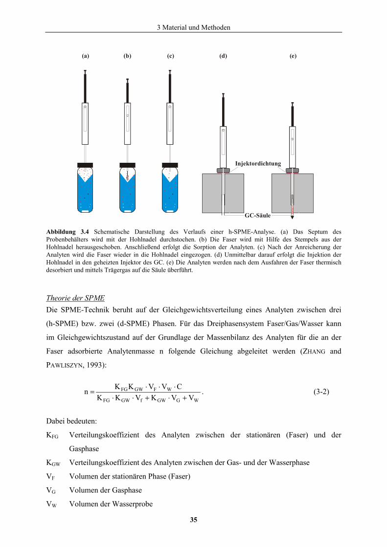
3 Material und Methoden
35
Abbildung 3.4 Schematische Darstellung des Verlaufs einer h-SPME-Analyse. (a) Das Septum des Probenbehälters wird mit der Hohlnadel durchstochen. (b) Die Faser wird mit Hilfe des Stempels aus der Hohlnadel herausgeschoben. Anschließend erfolgt die Sorption der Analyten. (c) Nach der Anreicherung der Analyten wird die Faser wieder in die Hohlnadel eingezogen. (d) Unmittelbar darauf erfolgt die Injektion der Hohlnadel in den geheizten Injektor des GC. (e) Die Analyten werden nach dem Ausfahren der Faser thermisch desorbiert und mittels Trägergas auf die Säule überführt.
Theorie der SPME Die SPME-Technik beruht auf der Gleichgewichtsverteilung eines Analyten zwischen drei
(h-SPME) bzw. zwei (d-SPME) Phasen. Für das Dreiphasensystem Faser/Gas/Wasser kann
im Gleichgewichtszustand auf der Grundlage der Massenbilanz des Analyten für die an der
Faser adsorbierte Analytenmasse n folgende Gleichung abgeleitet werden (ZHANG and
PAWLISZYN, 1993):
WGGWfGWFG
WFGWFG
VVKVKKCVVKKn�����
���
� . (3-2)
Dabei bedeuten:
KFG Verteilungskoeffizient des Analyten zwischen der stationären (Faser) und der
Gasphase
KGW Verteilungskoeffizient des Analyten zwischen der Gas- und der Wasserphase
VF Volumen der stationären Phase (Faser)
VG Volumen der Gasphase
VW Volumen der Wasserprobe
(a) (b) (c) (d) (e)
Injektordichtung
GC-Säule
3 Material und Methoden
36
C Konzentration des Analyten in der Wasserprobe
Ist der Dampfdruck des Lösungsmittels vernachlässigbar, so kann KFG�KGW durch KFW, den
Verteilungskoeffizienten des Analyten zwischen der stationären (Faser) und der wässrigen
Phase, substituiert werden (SPORKERT, 2002). Somit folgt aus Gleichung (3-2):
WGGWFFW
WFFW
VVKVKCVVK
n����
���
� . (3-3)
Ausgehend von der Annahme, dass das Gasvolumen VG gegenüber dem Probenvolumen VW
klein gehalten wird und dass KGW entsprechend dem Henry-Koeffizienten ebenfalls klein ist,
wird der Term KGWVG vernachlässigbar und Gleichung (3-3) geht in die das
Zweiphasensystem (Faser/Wasser) charakterisierende Gleichung (3-4) über:
.VVK
CVVKn
WFFW
WFFW
��
���
� (3-4)
Da sich das Faservolumen VF im �L-Bereich bewegt (Faserlänge: 1 cm, Faserbeschichtung:
7–100 �m) ist der Faktor KFWVF auch bei hohen Faser-Wasser-Verteilungskoeffizienten
gegenüber dem Volumen der Wasserprobe VW vernachlässigbar. Diese Vereinfachung
(VW » KFWVF) führt zu:
.CVKn FFW ��� (3-5)
Demnach ist die extrahierte Stoffmenge direkt proportional zum Verteilungskoeffizienten
KFW, zum Faservolumen VF und zur Analytenkonzentration C in der Probe. Gleichung (3-5)
verdeutlicht, dass unter den oben gemachten Annahmen die von der Faser extrahierte Menge
an Analyt unabhängig vom Probenvolumen VW ist.
Optimierung der SPME-Parameter Der erste Schritt bei der Optimierung der SPME-Methode bestand in der Bestimmung einer
geeigneten Extraktionsstrategie. Diese umfasste die Auswahl des Fasertyps und des richtigen
Extraktionsmodus (h-SPME oder d-SPME). Anschließend wurde untersucht, inwieweit die
Ergebnisse durch Salzzugabe und Rühren sowie durch richtige Dimensionierung der
entsprechenden Phasen verbessert werden konnten. Erst als diese Parameter festgelegt waren,
erfolgte die eigentliche Optimierung der Sorptions- bzw. Desorptionsbedingungen.
3 Material und Methoden
37
Faserpolarität
Gemäß dem alten empirischen Leitsatz der Chemiker „Similia similibus solventur“ (Gleiches
löst sich in Gleichem) werden unpolare Analyten am effektivsten mit nichtpolaren Fasern
extrahiert. Für die unpolare Polydimethylsiloxan-Faser (PDMS) kann somit der
Verteilungskoeffizient KFW in den Gleichungen (3-3) bis (3-5) sehr gut durch den KOW-Wert,
als Maß für die Hydrophobie einer Verbindung, ersetzt werden (CHAI et al., 1993). Je größer
der KOW-Wert, desto größer ist in der Regel auch die Affinität zu der PDMS-Faser.
Dementsprechend nahm die Anreicherung auf der 100 �m-PDMS-Faser in der Reihenfolge
abnehmender log KOW-Werte vom PCE zum cis-DCE ab (Tabelle 3.2). Eine Erhöhung der
Empfindlichkeit wurde durch die Faserkombination Carboxen/PDMS erzielt (POPP and
PASCHKE, 1997). Hierbei handelt es sich um eine aus graphitiertem Ruß und PDMS
bestehende Faser mit sehr großer spezifischer Oberfläche. Gemäß den Ergebnissen aus
Tabelle 3.2 zeigten speziell die kleineren Moleküle eine hohe Affinität zu dieser Faser.
Tabelle 3.2 Die für die Fasertypen Carboxen/PDMS bzw. PDMS mit dem GC-C-IRMS-System bestimmten Peakflächen (PF) nach der Extraktion einer jeweils 1000 �g L-1 enthaltenden wässrigen Lösung von PCE, TCE und cis-DCE. Sorptions- und Desorptionsparameter sind der Zusammenstellung am Ende dieses Kapitels zu entnehmen.
Analyt log KOW PF [Vs]
PFCarboxen/PDMS /PFCarboxen
75 �m-Carboxen/PDMS 100 �m-PDMS cis-DCE 2,2a) 87,7 � 11,9 1,1 � 0,3 80
TCE 2,4b) 88,3 � 7,0 2,6 � 0,2 34 PCE 2,9b) 76,7 � 9,4 5,6 � 0,7 14
a) EPA, 1998. b) SCHWARZENBACH et al., 2002.
Aus Tabelle 3.2 geht hervor, dass unter den am Ende dieses Kapitels angegebenen
Extraktionsbedingungen die 75 �m-Carboxen/PDMS-Faser eine um den Faktor 80 höhere
Affinität zum cis-DCE aufweist als die 100 �m-PDMS-Faser. Die Extraktion von PCE konnte
entsprechend um den Faktor 14 verbessert werden. Folglich wurden Proben mit hoher PCE-
Konzentration mit der PDMS- und die schwächer konzentrierten Proben mit der
Carboxen/PDMS-Faser extrahiert.
d-SPME im Vergleich zu h-SPME Die Wahl für einen speziellen SPME-Modus (h-SPME oder d-SPME) hängt entscheidend von
der vorliegenden Probenmatrix sowie den Verteilungskoeffizienten KGW und KFW der
Analyten ab. Da KGW in erster Näherung durch den Henry-Koeffizienten KH (ZHANG and
PAWLISZYN, 1993) und KFW durch KOW approximiert werden kann, lässt sich die
Empfindlichkeit für die zwei SPME-Modi anhand der für die meisten Analyten bekannten
3 Material und Methoden
38
KOW- und KH-Werte abschätzen. Für die CE mit log KOW-Werten zwischen 2 und 3
(Tabelle 3.2) empfiehlt sich eine Extraktion im Headspace-Modus (PAWLISZYN, 1997). Ein
weiterer Vorteil der h-SPME liegt in der Vermeidung des direkten Kontakts zwischen
Fasermaterial und Probenmatrix, da dieser bei stark kontaminierten Proben die
chromatographische Auflösung negativ beeinflussen kann. Außerdem besteht beim d-SPME-
Modus die Gefahr, dass in der Probe gelöste Elektrolyte oder Schwebstoffe in die Hohlnadel
gelangen und somit den Bewegungsmechanismus der Faser beschädigen (CASSADA et al.,
2000).
Salzzugabe, Phasenvolumina und Agitation Eine weitere Steigerung der Extraktionsausbeute im Headspace-Modus konnte durch
Aussalzen der Probenlösung mit Natriumchlorid (NaCl) erzielt werden. Der Zusatz von
starken Elektrolyten zur Probe bewirkt, dass diese im Wasser sehr stark hydratisieren, den
gelösten Analyten die Hydrathülle entziehen und somit deren Löslichkeit in der Probe
erniedrigen. Dadurch wird die Analytenkonzentration im Gasraum erhöht (Dampfdruck-
erhöhung) und die Extraktionsausbeute gesteigert. Dabei ist die extrahierte Menge der
Analyten direkt proportional zur Anzahl der in der Probe gelösten NaCl-Teilchen
(PAWLISZYN, 1997). Da die Überschreitung der Löslichkeitskonzentration zu keiner weiteren
Empfindlichkeitssteigerung führt und da Salzkristalle im System aus den o.g. Gründen
vermieden werden sollten, erfolgte die Salzzugabe in der Form (5,3 g NaCl auf 15 mL Probe),
dass die maximale Wasserlöslichkeit von 358 g L-1 (20°C) knapp unterschritten wurde.
Eine zusätzliche Erhöhung des Verteilungskoeffizienten KGW konnte durch die Erniedrigung
des Phasenverhältnisses VG/VW auf 1/3 erzielt werden. Eine weitere Reduzierung des
Gasvolumens scheiterte an der Dimensionierung der SPME-Faser, da die 1 cm lange Faser im
h-SPME-Modus keinen direkten Kontakt zur Wasseroberfläche haben durfte. Weitere
Sensitivitätssteigerungen wurden durch Rühren der Probe mittels Magnetrührer und durch die
Auswahl geeigneter Rührfische erzielt. Durch die höhere Konvektion in der Probe wird der
infolge des Verdampfens auftretende Konzentrationsgradient in der Probenoberfläche durch
Rühren annähernd ausgeglichen.
Aufnahme der Extraktionszeitprofile Beachtung verdient auch der Massentranfer von der Gasphase in die inneren Schichten der
Polymerfaser. Nach Gleichung (3-5) steigt die aus der Probe extrahierbare Stoffmenge n mit
zunehmendem Faservolumen und zunehmendem Verteilungskoeffizienten KFW an. Aufgrund
der sehr kleinen Diffusionskoeffizienten in der Faser läuft jedoch der Transport der auf der
3 Material und Methoden
39
Faseroberfläche adsorbierten Analytenmoleküle in das Innere der Faser sehr langsam ab.
Daher wird der zu Beginn der Extraktion sich rasch aufbauende Konzentrationsgradient in der
Faser nur langsam bis zum Erreichen des Gleichgewichtszustandes abgebaut. Die
Massendiffusion in der Faser stellt somit den geschwindigkeitsbestimmenden Schritt der
Extraktion dar, da frei werdende Plätze an der Faseroberfläche aufgrund der hohen
Diffusionskoeffizienten in der Gasphase schnell wieder besetzt werden. Dies bedeutet, dass
die Menge n der auf der Faser angereicherten Analyten bis zum Erreichen des
Gleichgewichtszustands durch Verlängerung der Adsorptionszeit maximiert werden kann.
Demzufolge muss bei der Entwicklung einer SPME-Methode ein Kompromiss zwischen
erforderlicher Analyseempfindlichkeit und vertretbarer Analysezeit ermittelt werden. Dies
geschieht über die Bestimmung des Zeitpunktes der Gleichgewichtseinstellung zwischen
Probe und Faser mit Hilfe von experimentell bestimmbaren Extraktionszeitprofilen. Führt
eine unendliche Verlängerung der Adsorptionszeit zu keiner nennenswerten Zunahme der
extrahierten Analytenmenge, dann befindet sich das System im Gleichgewicht. Wässrige
Lösungen, welche die zu untersuchenden CE in einer Konzentration von 1000 �g L-1 (für die
PDMS-Faser) und 100 �g L-1 (für die Carboxen/PDMS-Faser) enthalten, wurden, unter
Variation der Adsorptionszeiten bei sonst konstanten Messbedingungen, extrahiert. Aus
Abbildung 3.5 geht hervor, dass die extrahierte cis-DCE-, TCE- und PCE-Menge mit
zunehmender Adsorptionszeit für beide Fasertypen bis zum Erreichen des Gleichgewichts-
zustands ansteigt. Je größer die Affinität der Analyten zu der Faser, desto mehr Moleküle
diffundieren in das Fasermaterial und desto länger dauert die Gleichgewichtseinstellung. Das
polarere cis-DCE wird auf der polareren Carboxen/PDMS-Faser wesentlich stärker
angereichert als auf der unpolaren PDMS-Faser (siehe Tabelle 3.2). Entsprechend
unterschiedlich ist auch der Zeitpunkt der Gleichgewichtseinstellung. Während die maximale
Anreicherung des cis-DCE auf der PDMS-Faser bereits nach 5 min erzielt wurde, stellte sich
der Gleichgewichtszustand im Fall der Carboxen/PDMS-Faser erst nach ca. 90 min ein.
Eine Erhöhung der Analytenkonzentration von 100 auf 1000 �g L-1 würde eine weitere
Verlängerung der Adsorptionszeit für die Carboxen/PDMS-Faser verursachen. Solche langen
Adsorptionszeiten sind aus ökonomischen Aspekten und aufgrund des hohen
Probenaufkommens allerdings nicht sehr sinnvoll. Somit stellt sich die Frage nach einer
möglichen Verkürzung der Extraktionszeit. In diesem Zusammenhang ist die Abhängigkeit
der auf der Faser angereicherten Stoffmenge n von der Extraktionszeit von zentraler
Bedeutung. Auf der Grundlage des ersten Fickschen Diffusionsgesetzes kann gezeigt werden,
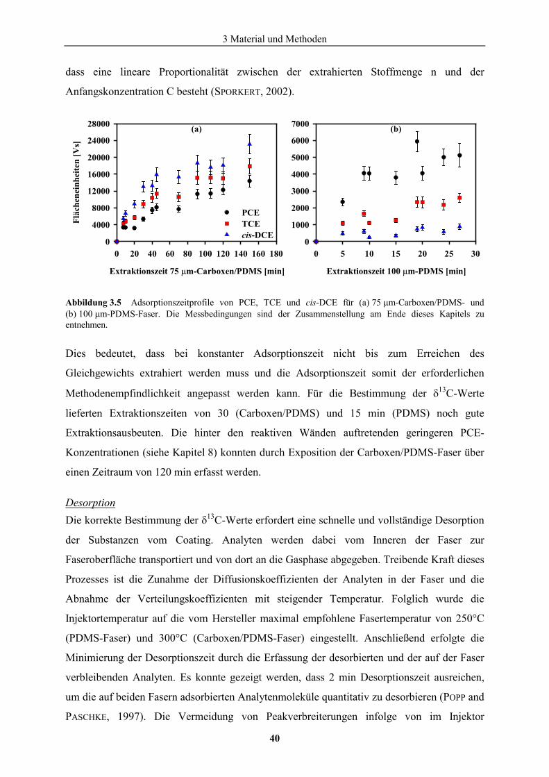
3 Material und Methoden
40
dass eine lineare Proportionalität zwischen der extrahierten Stoffmenge n und der
Anfangskonzentration C besteht (SPORKERT, 2002).
Abbildung 3.5 Adsorptionszeitprofile von PCE, TCE und cis-DCE für (a) 75 �m-Carboxen/PDMS- und (b) 100 �m-PDMS-Faser. Die Messbedingungen sind der Zusammenstellung am Ende dieses Kapitels zu entnehmen.
Dies bedeutet, dass bei konstanter Adsorptionszeit nicht bis zum Erreichen des
Gleichgewichts extrahiert werden muss und die Adsorptionszeit somit der erforderlichen
Methodenempfindlichkeit angepasst werden kann. Für die Bestimmung der �13C-Werte
lieferten Extraktionszeiten von 30 (Carboxen/PDMS) und 15 min (PDMS) noch gute
Extraktionsausbeuten. Die hinter den reaktiven Wänden auftretenden geringeren PCE-
Konzentrationen (siehe Kapitel 8) konnten durch Exposition der Carboxen/PDMS-Faser über
einen Zeitraum von 120 min erfasst werden.
Desorption Die korrekte Bestimmung der �13C-Werte erfordert eine schnelle und vollständige Desorption
der Substanzen vom Coating. Analyten werden dabei vom Inneren der Faser zur
Faseroberfläche transportiert und von dort an die Gasphase abgegeben. Treibende Kraft dieses
Prozesses ist die Zunahme der Diffusionskoeffizienten der Analyten in der Faser und die
Abnahme der Verteilungskoeffizienten mit steigender Temperatur. Folglich wurde die
Injektortemperatur auf die vom Hersteller maximal empfohlene Fasertemperatur von 250°C
(PDMS-Faser) und 300°C (Carboxen/PDMS-Faser) eingestellt. Anschließend erfolgte die
Minimierung der Desorptionszeit durch die Erfassung der desorbierten und der auf der Faser
verbleibenden Analyten. Es konnte gezeigt werden, dass 2 min Desorptionszeit ausreichen,
um die auf beiden Fasern adsorbierten Analytenmoleküle quantitativ zu desorbieren (POPP and
PASCHKE, 1997). Die Vermeidung von Peakverbreiterungen infolge von im Injektor
Extraktionszeit 75 �m-Carboxen/PDMS [min]
0 20 40 60 80 100 120 140 160 180
Fläc
hene
inhe
iten
[Vs]
0
4000
8000
12000
16000
20000
24000
28000
PCETCEcis-DCE
(a)
Extraktionszeit 100 �m-PDMS [min]
0 5 10 15 20 25 30
Fläc
hene
inhe
iten
[Vs]
0
1000
2000
3000
4000
5000
6000
7000 (b)
3 Material und Methoden
41
auftretenden Verwirbelungen wurde durch die Verwendung eines speziell für SPME-
Anwendungen konzipierten Liners (GERSTEL, Mülheim/Ruhr) umgangen. Der im Vergleich
zu herkömmlichen Linern geringere Innendurchmesser von 1 mm erhöht die lineare
Trägergasgeschwindigkeit im Injektor und garantiert nach der Desorption die rasche
Überführung der Analyten auf die chromatographische Säule. Durch die Verwendung des
septumfreien Aufgabekopfes (GERSTEL, Mülheim) konnten Injektorverunreinigungen und
Beschädigungen am Bewegungsmechanismus der Faser minimiert werden.
Zusammenfassung der SPME-Parameter Die manuelle Durchführung der SPME erfolgte mit einem SPME-Faserhalter der Firma
GERSTEL (Mühlheim/Ruhr). Für die in diesem Kapitel beschriebenen Anreicherungen wurden
folgende Fasertypen von der Firma SUPELCO (Deisenhofen) bezogen:
�� 100 �m-PDMS
�� 75 �m-Carboxen/PDMS.
Adsorption:
SPME-Modus h-SPME
Probengefäß 20 mL-SPME-Vial, 75,5�22,5 mm (IVA Analysentechnik e.K.,
Meerbusch)
Probenvolumen 15 mL
Gasvolumen 5 mL
Natriumchloridzugabe 5,3 g auf 15 mL Probe (353,3 g L-1)
Rührmodus Magnetrührer (IKA-Werke GmbH & Co. KG, Staufen)
Rührgeschwindigkeit 1200 min-1
Magnetrührstab zylindrisch, PTFE-ummantelt, Abmessungen: 15�6 mm
Extraktionstemperatur 20°C
Adsorptionszeit 30 min (Carboxen/PDMS-Faser)
15 min (PDMS-Faser)
Desorption:
Insertliner 1 mm I.D. (GERSTEL, Mülheim)
Desorptionstemperatur 300°C (Carboxen/PDMS-Faser)
250°C (PDMS-Faser)
Desorptionszeit 2 min (für beide Fasertypen)
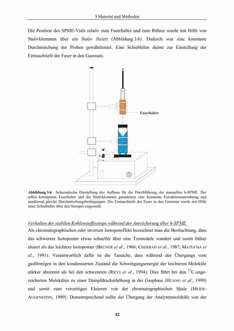
3 Material und Methoden
42
Die Position des SPME-Vials relativ zum Faserhalter und zum Rührer wurde mit Hilfe von
Stativklemmen über ein Stativ fixiert (Abbildung 3.6). Dadurch war eine konstante
Durchmischung der Proben gewährleistet. Eine Schieblehre diente zur Einstellung der
Eintauchtiefe der Faser in den Gasraum.
Abbildung 3.6 Schematische Darstellung des Aufbaus für die Durchführung der manuellen h-SPME. Der selbst konzipierte Faserhalter und die Stativklemmen garantieren eine konstante Extraktionsanordnung und annähernd gleiche Durchmischungsbedingungen. Die Eintauchtiefe der Faser in den Gasraum wurde mit Hilfe einer Schieblehre über den Stempel eingestellt.
Verhalten der stabilen Kohlenstoffisotope während der Anreicherung über h-SPME Als chromatographischen oder inversen Isotopeneffekt bezeichnet man die Beobachtung, dass
das schwerere Isotopomer etwas schneller über eine Trennsäule wandert und somit früher
eluiert als das leichtere Isotopomer (BRUNER et al., 1966; CHERRAH et al., 1987; MATUCHA et
al., 1991). Verantwortlich dafür ist die Tatsache, dass während des Übergangs vom
gasförmigen in den kondensierten Zustand die Schwingungsenergie der leichteren Moleküle
stärker abnimmt als bei den schwereren (RICCI et al., 1994). Dies führt bei den 13C-ange-
reicherten Molekülen zu einer Dampfdruckerhöhung in der Gasphase (HUANG et al., 1999)
und somit zum vorzeitigen Eluieren von der chromatographischen Säule (MEIER-
AUGENSTEIN, 1999). Dementsprechend sollte der Übergang der Analytenmoleküle von der
Faserhalter
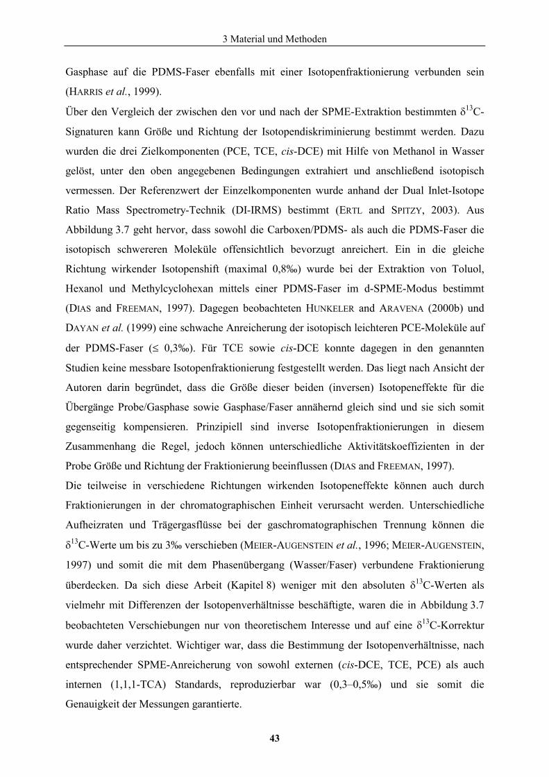
3 Material und Methoden
43
Gasphase auf die PDMS-Faser ebenfalls mit einer Isotopenfraktionierung verbunden sein
(HARRIS et al., 1999).
Über den Vergleich der zwischen den vor und nach der SPME-Extraktion bestimmten �13C-
Signaturen kann Größe und Richtung der Isotopendiskriminierung bestimmt werden. Dazu
wurden die drei Zielkomponenten (PCE, TCE, cis-DCE) mit Hilfe von Methanol in Wasser
gelöst, unter den oben angegebenen Bedingungen extrahiert und anschließend isotopisch
vermessen. Der Referenzwert der Einzelkomponenten wurde anhand der Dual Inlet-Isotope
Ratio Mass Spectrometry-Technik (DI-IRMS) bestimmt (ERTL and SPITZY, 2003). Aus
Abbildung 3.7 geht hervor, dass sowohl die Carboxen/PDMS- als auch die PDMS-Faser die
isotopisch schwereren Moleküle offensichtlich bevorzugt anreichert. Ein in die gleiche
Richtung wirkender Isotopenshift (maximal 0,8‰) wurde bei der Extraktion von Toluol,
Hexanol und Methylcyclohexan mittels einer PDMS-Faser im d-SPME-Modus bestimmt
(DIAS and FREEMAN, 1997). Dagegen beobachteten HUNKELER and ARAVENA (2000b) und
DAYAN et al. (1999) eine schwache Anreicherung der isotopisch leichteren PCE-Moleküle auf
der PDMS-Faser (� 0,3‰). Für TCE sowie cis-DCE konnte dagegen in den genannten
Studien keine messbare Isotopenfraktionierung festgestellt werden. Das liegt nach Ansicht der
Autoren darin begründet, dass die Größe dieser beiden (inversen) Isotopeneffekte für die
Übergänge Probe/Gasphase sowie Gasphase/Faser annähernd gleich sind und sie sich somit
gegenseitig kompensieren. Prinzipiell sind inverse Isotopenfraktionierungen in diesem
Zusammenhang die Regel, jedoch können unterschiedliche Aktivitätskoeffizienten in der
Probe Größe und Richtung der Fraktionierung beeinflussen (DIAS and FREEMAN, 1997).
Die teilweise in verschiedene Richtungen wirkenden Isotopeneffekte können auch durch
Fraktionierungen in der chromatographischen Einheit verursacht werden. Unterschiedliche
Aufheizraten und Trägergasflüsse bei der gaschromatographischen Trennung können die
�13C-Werte um bis zu 3‰ verschieben (MEIER-AUGENSTEIN et al., 1996; MEIER-AUGENSTEIN,
1997) und somit die mit dem Phasenübergang (Wasser/Faser) verbundene Fraktionierung
überdecken. Da sich diese Arbeit (Kapitel 8) weniger mit den absoluten �13C-Werten als
vielmehr mit Differenzen der Isotopenverhältnisse beschäftigte, waren die in Abbildung 3.7
beobachteten Verschiebungen nur von theoretischem Interesse und auf eine �13C-Korrektur
wurde daher verzichtet. Wichtiger war, dass die Bestimmung der Isotopenverhältnisse, nach
entsprechender SPME-Anreicherung von sowohl externen (cis-DCE, TCE, PCE) als auch
internen (1,1,1-TCA) Standards, reproduzierbar war (0,3–0,5‰) und sie somit die
Genauigkeit der Messungen garantierte.

3 Material und Methoden
44
Die entwickelte SPME-Methode ist eine genaue, leicht durchführbare Anreicherungstechnik,
die die Bestimmung der Kohlenstoffisotopenverhältnisse von CE bis zu einer Konzentration
von 4 �g L-1 aus einem Probenvolumen von nur 15 mL erlaubt.
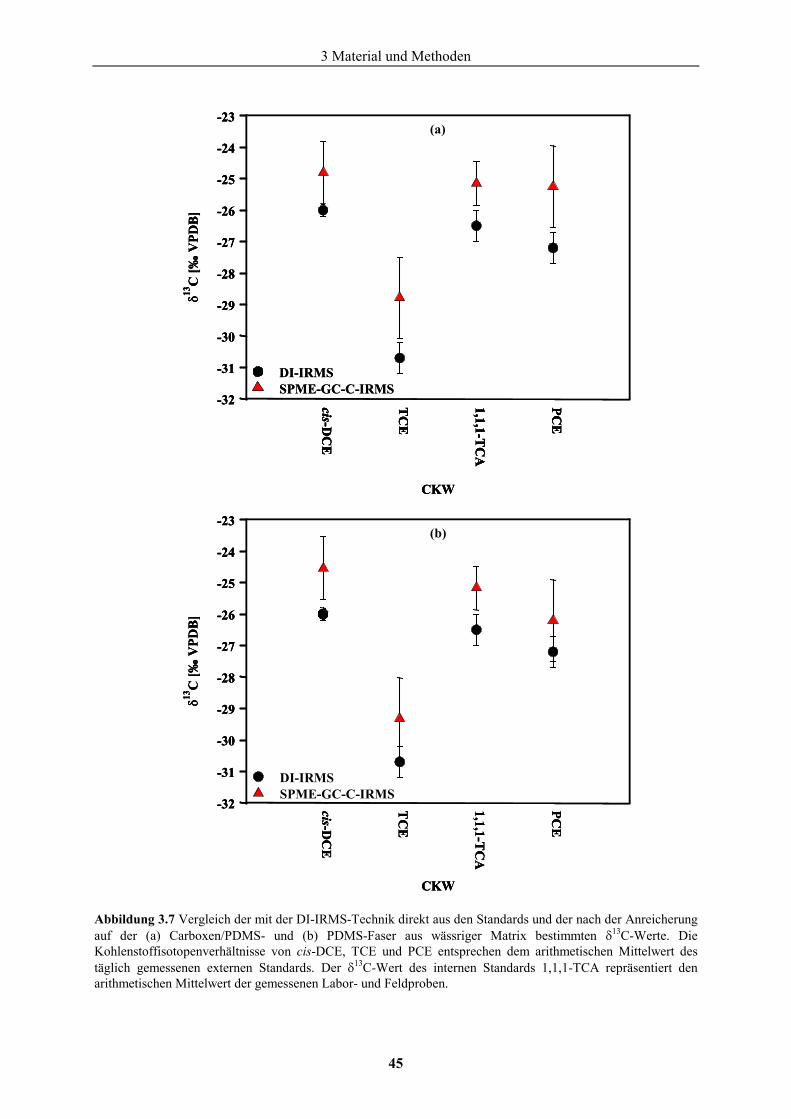
3 Material und Methoden
45
Abbildung 3.7 Vergleich der mit der DI-IRMS-Technik direkt aus den Standards und der nach der Anreicherung auf der (a) Carboxen/PDMS- und (b) PDMS-Faser aus wässriger Matrix bestimmten �13C-Werte. Die Kohlenstoffisotopenverhältnisse von cis-DCE, TCE und PCE entsprechen dem arithmetischen Mittelwert des täglich gemessenen externen Standards. Der �13C-Wert des internen Standards 1,1,1-TCA repräsentiert den arithmetischen Mittelwert der gemessenen Labor- und Feldproben.
CKW
-32
-31
-30
-29
-28
-27
-26
-25
-24
-23
DI-IRMSSPME-GC-C-IRMS
�13
C [‰
VPD
B]
cis-DC
E
TC
E
1,1,1-TC
A
PCE
(a)
CKW
cis-DC
E
TC
E
1,1,1-TC
A
PCE
�13
C [‰
VPD
B]
-32
-31
-30
-29
-28
-27
-26
-25
-24
-23
DI-IRMSSPME-GC-C-IRMS
(b)
CKW
-32
-31
-30
-29
-28
-27
-26
-25
-24
-23
DI-IRMSSPME-GC-C-IRMS
�13
C [‰
VPD
B]
cis-DC
E
TC
E
1,1,1-TC
A
PCE
(a)
CKW
-32
-31
-30
-29
-28
-27
-26
-25
-24
-23
DI-IRMSSPME-GC-C-IRMSDI-IRMSSPME-GC-C-IRMS
�13
C [‰
VPD
B]
cis-DC
E
TC
E
1,1,1-TC
A
PCE
cis-DC
E
TC
E
1,1,1-TC
A
PCE
(a)
CKW
cis-DC
E
TC
E
1,1,1-TC
A
PCE
�13
C [‰
VPD
B]
-32
-31
-30
-29
-28
-27
-26
-25
-24
-23
DI-IRMSSPME-GC-C-IRMS
(b)
CKW
cis-DC
E
TC
E
1,1,1-TC
A
PCE
�13
C [‰
VPD
B]
-32
-31
-30
-29
-28
-27
-26
-25
-24
-23
DI-IRMSSPME-GC-C-IRMS
(b)
3 Material und Methoden
46
3.3 Geräte und Chemikalien
Identifizierung Die Identifizierung der im Grundwasser gelösten Schadstoffe erfolgte durch den Vergleich der
Retentionszeiten der Probensignale mit den Retentionszeiten von externen Standards. Eine
weitere Identifizierungsmöglichkeit waren die substanzspezifischen Fragmentierungsmuster
der Massenspektren.
Kapillargaschromatographie Die Gaschromatographie ist eine Trennmethode, bei der ein Stoffgemisch mit Hilfe eines
inerten Trägergasstroms über eine flüssige stationäre Phase geleitet und dabei in die
Einzelkomponenten aufgetrennt wird (EICEMAN, 2002). Grundvoraussetzung für die
gaschromatographische Trennung ist, dass der Analyt in einem bestimmten Temperaturfenster
(bis 330°C) unzersetzt verdampfbar ist.
Vorversuche zur Bestimmung der Extraktionstechnik bzw. -effizienz wurden unter folgenden
Analysebedingungen durchgeführt:
Detektor FID
Gaschromatograph GC-6000 Vega Series 2 (CARLO ERBA Instruments,
Milan)
Injektor On column
Injektionsvolumen 0,1–1,0 �L (per Hand)
Trägergas Wasserstoff
Trennsäule DB-5 (Länge 50 m, I.D. 0,32 mm, Filmdicke 0,25 �m,
J&W Scientific)
Temperaturprogramm 40°C (10 min) � 4°C min-1 � 240°C � 10°C min-1
� 280°C (10 min)
Datenaufzeichnung/Auswertung ChromStar (BRUKER-FRANZEN Analytik GmbH,
Bremen)
Gaschromatographie-Massenspektrometrie (GC-MS) Für den Nachweis und die Identifizierung von unbekannten Kontaminanten in
Substanzgemischen wurde die kombinierte Gaschromatographie-Massenspektrometrie
(GC-MS) eingesetzt. Nach der gaschromatographischen Auftrennung und der nachfolgenden
massenspektrometrischen Fragmentierung der Einzelkomponenten erfolgt die Identifizierung
3 Material und Methoden
47
über den Vergleich des Spektrums der unbekannten Verbindung mit Referenzspektren aus der
Spektrenbibliothek. Die Aufnahme der Spektren erfolgte unter folgenden Bedingungen:
Massenspektrometer Quattro II (MICROMASS, Attrincham, UK)
Gaschromatograph HP 6890 GC
Injektor On column
Injektionsvolumen 0,3–1,0 �L (per Hand)
Trägergas Helium
Trennsäule DB-5 (Länge 30 m, I.D. 0,32 mm, Filmdicke 0,25 �m,
J&W Scientific)
Temperaturprogramm 40°C (10 min) � 4°C min-1 � 240°C � 10°C min-1
� 280°C (10 min)
Ionisierungsenergie 70 eV
Emmissionsstrom 200 �A
Ionenquelltemperatur 250°C
Datenaufzeichnung/Auswertung MassLynx Version 3.4 (MICROMASS, Attrinchham, UK)
Bestimmung der Kohlenstoffisotopenverhältnisse ��13C mittels GC-C-IRMS Die Kopplung zwischen Gaschromatograph und Isotopenmassenspektrometer erlaubt die
Bestimmung des Verhältnisses der stabilen Kohlenstoffisotope einzelner organischer
Verbindungen aus komplexen Stoffgemischen. Nach gaschromatographischer Auftrennung
werden die eluierenden Komponenten in einem Oxidationsreaktor bei 940°C zu CO2 und H2O
umgesetzt. Nach Entfernung des Wassers in einer mit Helium durchströmten Nafion-
Membran wird das CO2 on-line über ein Splitsystem einem Massenspektrometer zugeführt.
Die Bestimmung der 13C/12C-Isotopenverhältnisse erfolgt durch die kontinuierliche Aufnahme
der Massenspuren m/z 44, 45 und 46. Das zur Kalibrierung verwendete Kohlendioxid
(�13C = -22,2‰ � 0,2‰) ist relativ zum VPDB-Standard geeicht. Die Überprüfung der
gemessenen �13C-Werte erfolgte routinemäßig durch externe und interne Standards mit
bekannter Isotopensignatur.
3 Material und Methoden
48
��13C-Bestimmung von aromatischen Kohlenwasserstoffen
Die im Grundwasser gelösten BTEX und PAK wurden mittels LLE (Kapitel 3.2.1)
angereichert und unter folgenden Bedingungen am GC-C-IRMS vermessen.
Massenspektrometer MAT Deltaplus-XL (FINNIGAN MAT, Bremen)
Gaschromatograph HP 6890 GC
Injektor GERSTEL KAS 4 (Kaltaufgabesystem)
Programm Kaltaufgabesystem 16°C (0 s) � 12°C s-1 � 300°C (600 s)
Injektionsvolumen 0,3–5,0 �L (Autoinjektion mit CTC A 200S-
Autosampler)
Trägergas Helium
Trennsäule HP-PONA (Länge 60 m, I.D. 0,2 mm, Filmdicke
0,2 �m, HEWLETT PACKARD Company)
Temperaturprogramm 30°C (10 min) � 6°C min-1 � 245°C � 10°C min-1
� 280°C (10 min)
Oxidationsreaktor NiO/CuO/Pt (940°C)
Datenaufzeichnung/Auswertung ISODATTM (FINNIGAN, Bremen)
��13C-Bestimmung chlorierter Kohlenwasserstoffe
Im Grundwasser gelöste CE wurden mittels SPME aufkonzentriert (Kapitel 3.2.2) und unter
folgenden Bedingungen am GC-C-IRMS vermessen.
Massenspektrometer MAT Deltaplus-XL (FINNIGAN MAT, Bremen)
Gaschromatograph HP 6890 GC
Injektor GERSTEL KAS 4 (Kaltaufgabesystem)
Injektortemperatur 250°C (PDMS-Faser), 300°C (Carboxen/PDMS-Faser)
Injektionsweise Thermodesorption der Analyten im Injektor (SPME)
Trägergas Helium
Trennsäule GS-GasPro (Länge 30 m, I.D. 0,32 mm, J&W
Scientific)
Temperaturprogramm 30°C (2 min) � 6°C min-1 � 220°C (5 min)
Oxidationsreaktor NiO/CuO/Pt (1010°C)
Datenaufzeichnung/Auswertung ISODATTM (FINNIGAN, Bremen)
3 Material und Methoden
49
��2H-Bestimmung von aromatischen Kohlenwasserstoffen
Für die Bestimmung der �2H-Werte der im Grundwasser gelösten aromatischen
Kohlenwasserstoffe wird das oben beschriebene GC-C-IRMS-System auf den
Thermokonversionsmodus (GC-TC-IRMS) umgestellt. Die von der Säule eluierenden
Kohlenwasserstoffe werden in einem Hochtemperaturkeramikofen bei 1440°C zu C, CO und
H2 umgesetzt (SESSIONS et al., 1999) und zur Aufzeichnung der Massenspuren m/z 2 und 3
dem Massenspektrometer über ein Splitsystem zugeführt (HILKERT et al., 1999). Die Eichung
erfolgt gegen Wasserstoffgas (MESSER, Frankfurt) mit bekannter Isotopensignatur
(�2H = -208‰ � 5‰). Ein H3-Korrekturfaktor, der die Bildung von H3+-Ionen in der
Ionenquelle berücksichtigt (SESSIONS et al., 2000; SESSIONS et al., 2001), wurde täglich
bestimmt.
Massenspektrometer MAT Deltaplus-XL (FINNIGAN MAT, Bremen)
Gaschromatograph HP 6890 GC
Injektor GERSTEL KAS 4 (Kaltaufgabesystem)
Programm Kaltaufgabesystem 16°C (0 s) � 12°C s-1 � 300°C (600 s)
Injektionsvolumen 1,0–5,0 �L (Autoinjektion mit CTC A 200S-
Autosampler)
Trägergas Helium
Trennsäule HP-PONA (Länge 60 m, I.D. 0,2 mm, Filmdicke
0,2 �m, HEWLETT PACKARD Company)
Temperaturprogramm 30°C (10 min) � 6°C min-1 � 245°C � 10°C min-1
� 280°C (10 min)
Hochtemperaturofen Al2O3 (1440°C)
Datenaufzeichnung/Auswertung ISODATTM (FINNIGAN, Bremen)
�
Untersuchungen zur Richtigkeit und Präzision der Messungen im Thermokonversionsmodus
zeigten in gewissen Konzentrationsbereichen eine Abhängigkeit der �2H-Werte von der in das
MS injizierten Analytenmenge. Die mittels GC-TC-IRMS ermittelten �2H-Signaturen der
direkt in n-Pentan gelösten aromatischen Kohlenwasserstoffe wurden für verschiedene
Konzentrationen bestimmt und mit dem durch EA-P-IRMS ermittelten �2H-Wert
(Arbeitsgruppe Prof. Dr. Schreier, Universität Würzburg) der reinen Phase verglichen. Wie
aus Abbildung 3.8 ersichtlich, stimmen die durch den Elementaranalysator und durch den
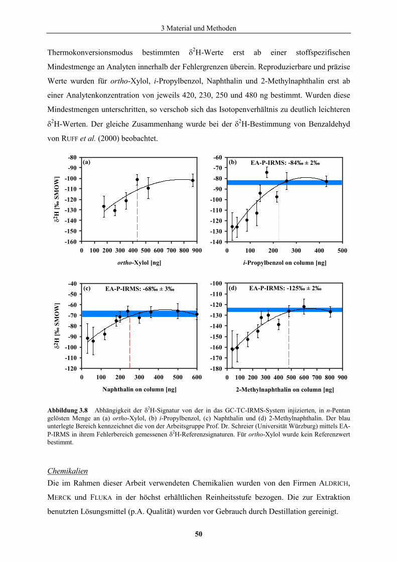
3 Material und Methoden
50
Thermokonversionsmodus bestimmten �2H-Werte erst ab einer stoffspezifischen
Mindestmenge an Analyten innerhalb der Fehlergrenzen überein. Reproduzierbare und präzise
Werte wurden für ortho-Xylol, i-Propylbenzol, Naphthalin und 2-Methylnaphthalin erst ab
einer Analytenkonzentration von jeweils 420, 230, 250 und 480 ng bestimmt. Wurden diese
Mindestmengen unterschritten, so verschob sich das Isotopenverhältnis zu deutlich leichteren
�2H-Werten. Der gleiche Zusammenhang wurde bei der �2H-Bestimmung von Benzaldehyd
von RUFF et al. (2000) beobachtet.
Abbildung 3.8 Abhängigkeit der �2H-Signatur von der in das GC-TC-IRMS-System injizierten, in n-Pentan gelösten Menge an (a) ortho-Xylol, (b) i-Propylbenzol, (c) Naphthalin und (d) 2-Methylnaphthalin. Der blau unterlegte Bereich kennzeichnet die von der Arbeitsgruppe Prof. Dr. Schreier (Universität Würzburg) mittels EA-P-IRMS in ihrem Fehlerbereich gemessenen �2H-Referenzsignaturen. Für ortho-Xylol wurde kein Referenzwert bestimmt.
Chemikalien Die im Rahmen dieser Arbeit verwendeten Chemikalien wurden von den Firmen ALDRICH,
MERCK und FLUKA in der höchst erhältlichen Reinheitsstufe bezogen. Die zur Extraktion
benutzten Lösungsmittel (p.A. Qualität) wurden vor Gebrauch durch Destillation gereinigt.
(a)
(c)
ortho-Xylol [ng]
0 100 200 300 400 500 600 700 800 900
�2 H
[‰ S
MO
W]
-160
-150-140
-130-120
-110-100
-90-80
EA-P-IRMS: -68‰ ± 3‰
Naphthalin on column [ng]
0 100 200 300 400 500 600
�2 H
[‰ S
MO
W]
-120
-110
-100
-90
-80
-70
-60
-50
-40
i-Propylbenzol on column [ng]
0 100 200 300 400 500-140
-130
-120
-110
-100
-90
-80
-70-60
EA-P-IRMS: -84‰ ± 2‰
EA-P-IRMS: -125‰ ± 2‰
2-Methylnaphthalin on column [ng]
0 100 200 300 400 500 600 700 800 900-180
-170
-160
-150
-140
-130
-120
-110
-100
(b)
(d)
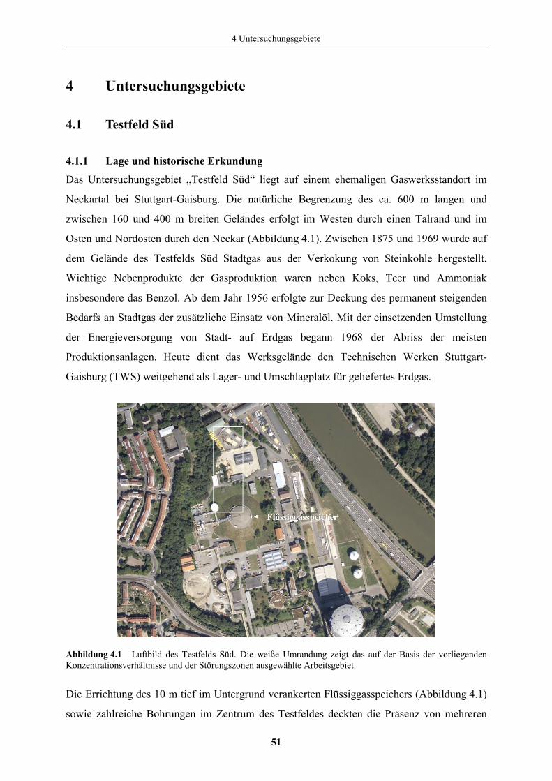
4 Untersuchungsgebiete
51
4 Untersuchungsgebiete
4.1 Testfeld Süd
4.1.1 Lage und historische Erkundung
Das Untersuchungsgebiet „Testfeld Süd“ liegt auf einem ehemaligen Gaswerksstandort im
Neckartal bei Stuttgart-Gaisburg. Die natürliche Begrenzung des ca. 600 m langen und
zwischen 160 und 400 m breiten Geländes erfolgt im Westen durch einen Talrand und im
Osten und Nordosten durch den Neckar (Abbildung 4.1). Zwischen 1875 und 1969 wurde auf
dem Gelände des Testfelds Süd Stadtgas aus der Verkokung von Steinkohle hergestellt.
Wichtige Nebenprodukte der Gasproduktion waren neben Koks, Teer und Ammoniak
insbesondere das Benzol. Ab dem Jahr 1956 erfolgte zur Deckung des permanent steigenden
Bedarfs an Stadtgas der zusätzliche Einsatz von Mineralöl. Mit der einsetzenden Umstellung
der Energieversorgung von Stadt- auf Erdgas begann 1968 der Abriss der meisten
Produktionsanlagen. Heute dient das Werksgelände den Technischen Werken Stuttgart-
Gaisburg (TWS) weitgehend als Lager- und Umschlagplatz für geliefertes Erdgas.
Abbildung 4.1 Luftbild des Testfelds Süd. Die weiße Umrandung zeigt das auf der Basis der vorliegenden Konzentrationsverhältnisse und der Störungszonen ausgewählte Arbeitsgebiet.
Die Errichtung des 10 m tief im Untergrund verankerten Flüssiggasspeichers (Abbildung 4.1)
sowie zahlreiche Bohrungen im Zentrum des Testfeldes deckten die Präsenz von mehreren
4 Untersuchungsgebiete
52
NAPL-Phasen an Basis und/oder Top des Grundwasserleiters auf. Dieser massive
Schadstoffaustrag in die Umgebung rührte, neben dem unsachgemäßen Betrieb der
Steinkohleverkokung und der damit verbundenen Begleitprozesse, vor allem von der nahezu
kompletten Zerstörung der gesamten Produktionsanlagen und Speichergebäude durch
Bombenangriffe während des zweiten Weltkrieges her. Auf der Grundlage von vorliegenden
Altlastengutachten und der geochemischen Befunde von mehreren im Testfeld tätigen
Arbeitsgruppen konnte im Abstrom der Verdachtsfläche eine etwa 280 m lange und etwa
120 m breite, nach Norden gerichtete Kontaminationsfahne kartiert werden (BOCKELMANN,
2001). Hauptbestandteile sind BTEX, PAK und Phenole.
4.1.2 Geologie und Hydrogeologie
Die hydrogeologischen Verhältnisse im Testfeld sind durch einen ausgeprägten Stockwerkbau
der beiden erschlossenen Grundwasserleiter gekennzeichnet. Das untere Stockwerk besteht
aus Ton- und Mergelsteinen des unteren und mittleren Gipskeupers, dessen einzelne
wasserführende Horizonte teilweise im Untersuchungsgebiet ausstreichen (HERFORT et al.,
1998). Bei einer Restmächtigkeit des Gipskeupers von ca. 5 bis 17 m liegt die Tiefenlage der
Gipskeuper-Tonsteine im Mittel 8,5 m unter der Geländeoberkante. Der im Talbereich
überlagernde, teilweise stark durchlässige quartäre Grundwasserleiter besitzt eine Mächtigkeit
zwischen 3,4 und 6,1 m und besteht hauptsächlich aus Mittelkies und eingelagerten Anteilen
feinerkörnigen Materials. Infolge der Überschwemmungsereignisse des Neckars steht über
dem Neckarkies der quartäre Auelehm an. Dieser wird durch anthropogene Auffüllungen aus
lehmigem Material, Gipskeuperfragmenten oder Bauschutt überdeckt.
Eine lokale Besonderheit im Zentrum des Testfeldes stellt der in der Sohle des Neckarkieses
verankerte Flüssiggasspeicher dar. Sowohl die durch die Stickstoffkühlung verursachte
Temperaturerniedrigung in den umliegenden Messstellen als auch die reduzierte
Aquifermächtigkeit besitzen einen starken Einfluss auf das Transport- und Abbauverhalten
der aus den südlichen Kontaminationsquellen stammenden Schadstoffe. Des Weiteren wurde
aus dem oberen Muschelkalk aufsteigendes hochmineralisiertes Wasser in den im Quartär
verfilterten Messstellen nachgewiesen (EISWIRTH et al., 1998). Diese speziell im Nordosten
beobachteten punktuellen Zumischungen beeinflussen die Grundwasserströmung und den
Wasserchemismus und könnten nachhaltige Auswirkungen auf den mikrobiologischen Abbau
organischer Schadstoffe haben. Zuflüsse von nitrathaltigem Hangwasser aus dem
Keupergestein des Talrandes in den Aquifer wurden für die (süd)westlichen Messstellen im
Testfeld beobachtet (SCHÄFLE, 1997). Auch hier ist eine Beeinflussung des enzymatischen
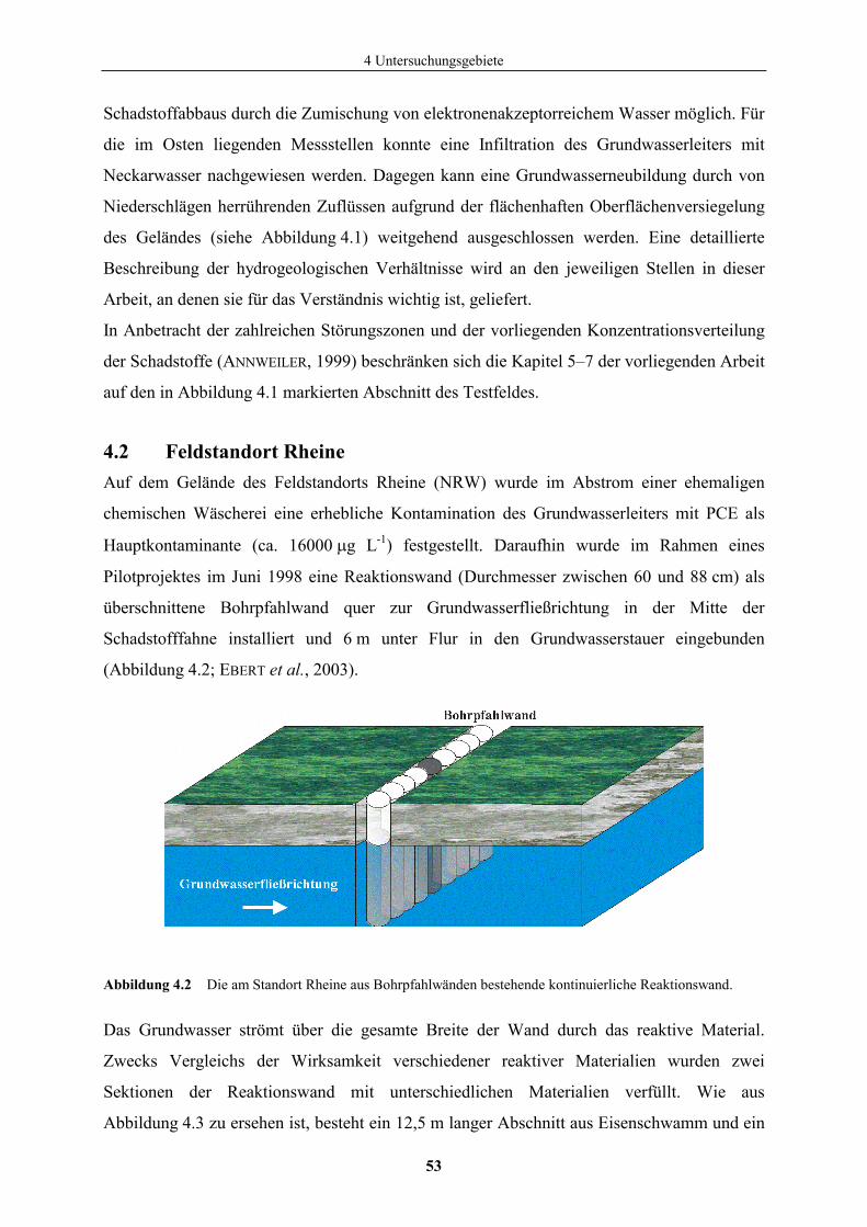
4 Untersuchungsgebiete
53
Schadstoffabbaus durch die Zumischung von elektronenakzeptorreichem Wasser möglich. Für
die im Osten liegenden Messstellen konnte eine Infiltration des Grundwasserleiters mit
Neckarwasser nachgewiesen werden. Dagegen kann eine Grundwasserneubildung durch von
Niederschlägen herrührenden Zuflüssen aufgrund der flächenhaften Oberflächenversiegelung
des Geländes (siehe Abbildung 4.1) weitgehend ausgeschlossen werden. Eine detaillierte
Beschreibung der hydrogeologischen Verhältnisse wird an den jeweiligen Stellen in dieser
Arbeit, an denen sie für das Verständnis wichtig ist, geliefert.
In Anbetracht der zahlreichen Störungszonen und der vorliegenden Konzentrationsverteilung
der Schadstoffe (ANNWEILER, 1999) beschränken sich die Kapitel 5–7 der vorliegenden Arbeit
auf den in Abbildung 4.1 markierten Abschnitt des Testfeldes.
4.2 Feldstandort Rheine Auf dem Gelände des Feldstandorts Rheine (NRW) wurde im Abstrom einer ehemaligen
chemischen Wäscherei eine erhebliche Kontamination des Grundwasserleiters mit PCE als
Hauptkontaminante (ca. 16000 �g L-1) festgestellt. Daraufhin wurde im Rahmen eines
Pilotprojektes im Juni 1998 eine Reaktionswand (Durchmesser zwischen 60 und 88 cm) als
überschnittene Bohrpfahlwand quer zur Grundwasserfließrichtung in der Mitte der
Schadstofffahne installiert und 6 m unter Flur in den Grundwasserstauer eingebunden
(Abbildung 4.2; EBERT et al., 2003).
Abbildung 4.2 Die am Standort Rheine aus Bohrpfahlwänden bestehende kontinuierliche Reaktionswand.
Das Grundwasser strömt über die gesamte Breite der Wand durch das reaktive Material.
Zwecks Vergleichs der Wirksamkeit verschiedener reaktiver Materialien wurden zwei
Sektionen der Reaktionswand mit unterschiedlichen Materialien verfüllt. Wie aus
Abbildung 4.3 zu ersehen ist, besteht ein 12,5 m langer Abschnitt aus Eisenschwamm und ein
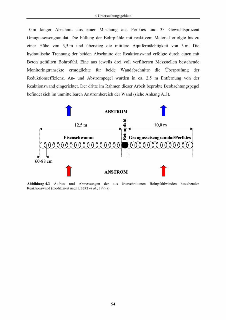
4 Untersuchungsgebiete
54
10 m langer Abschnitt aus einer Mischung aus Perlkies und 33 Gewichtsprozent
Graugusseisengranulat. Die Füllung der Bohrpfähle mit reaktivem Material erfolgte bis zu
einer Höhe von 3,5 m und überstieg die mittlere Aquifermächtigkeit von 3 m. Die
hydraulische Trennung der beiden Abschnitte der Reaktionswand erfolgte durch einen mit
Beton gefüllten Bohrpfahl. Eine aus jeweils drei voll verfilterten Messstellen bestehende
Monitoringtransekte ermöglichte für beide Wandabschnitte die Überprüfung der
Reduktionseffizienz. An- und Abstrompegel wurden in ca. 2,5 m Entfernung von der
Reaktionswand eingerichtet. Der dritte im Rahmen dieser Arbeit beprobte Beobachtungspegel
befindet sich im unmittelbaren Anstrombereich der Wand (siehe Anhang A.3).
Abbildung 4.3 Aufbau und Abmessungen der aus überschnittenen Bohrpfahlwänden bestehenden Reaktionswand (modifiziert nach EBERT et al., 1999a).
Eisenschwamm Graugusseisengranulat/Perlkies
60-88 cm
12,5 m 10,0 mB
eton
pfah
l
ANSTROM
ABSTROM
Eisenschwamm Graugusseisengranulat/Perlkies
60-88 cm
12,5 m 10,0 mB
eton
pfah
l
ANSTROM
ABSTROM
5 Combined �13C and �2H monitoring of in situ biodegradation of aromatic hydrocarbons…
55
Combined �13C and �2H monitoring of in situ biodegradation of
aromatic hydrocarbons in a contaminated aquifer
In Geochemical Processes in Soil and Groundwater,
Measurement - Modelling - Upscaling,
pp. 169-181
Steinbach A. and Michaelis W.
5 Combined �13C and �2H monitoring of in situ biodegradation of aromatic hydrocarbons…
56
5.1 Introduction Petroleum hydrocarbons are involved in major industrial processes. Consequently, their
extraction, transport and refinement lead inevitably to the entry into the groundwater. In
particular the light aromatic hydrocarbons such as benzene, toluene, ethylbenzene, and the
xylenes (BTEX) are of major concern. In the vadose zone these highly mobile compounds
percolate vertically downward until they reach the groundwater table, where they form a
contaminant plume in groundwater flow direction.
Due to various performance limitations of other commonly applied remedial technologies
natural attenuation has recently received increased attention (WIEDEMEIER et al., 1999). But
for its acceptance it is essential to predict the fate of contaminants and to differentiate between
destructive (biodegradation) and nondestructive (dispersion, sorption, volatilisation and
dilution) attenuation processes. Instead of destroying, the latter processes only transfer
contaminants from one medium to another or just cause dilution. Attempts to assess the
biodegradation potential in aquifers actually encompass the measurement of contaminants,
their metabolites formed, and the geochemical indicators of biodegradation activity. Although
these approaches provide important information, the difficulty of assessing the extent of
biodegradation in heterogeneous subsurface environments still exists.
Recent studies on compound specific isotope analysis (CSIA) have shown that isotope
fractionation is a powerful new tool to trace biodegradation of hydrocarbons (MECKENSTOCK
et al., 1999; WARD et al., 2000; HUNKELER et al., 2001a; MANCINI et al., 2002; STEINBACH et
al., 2004). The method relies on the preferential reaction of the lighter isotope (1H, 12C) during
biodegradation, leading to an enrichment of the heavier isotope (2H, 13C) in the nondegraded
residual hydrocarbon fraction. As described in the Rayleigh equation
fln)11(
CC
CC
lnC
012
13t
12
13
��
�
�����
�
�
�����
�
�
� �
�
�
� �
�
(5-1)
the isotopic fractionation can be related to the remaining fraction f of the reactant via the
fractionation factor �C. (13C/12C)t is the isotopic composition at any value of f and (13C/12C)0
is the isotopic composition at the beginning of the reaction (f = 1). Provided that the
fractionation factor and the variation in the isotopic composition of the substrate is known,
5 Combined �13C and �2H monitoring of in situ biodegradation of aromatic hydrocarbons…
57
this correlation allows to estimate the extent of microbial degradation (SHERWOOD LOLLAR et
al., 2001). However, the application presumes the absence of abiotic fractionation processes, a
constant fractionation factor for different redox conditions and a unique source in a roughly
closed system. Toluene degradation studies with four distinct toluene-degrading bacterial
strains grown in batch cultures revealed that the 13C/12C isotope ratio of the residual toluene
fraction increased significantly with decreasing concentration, providing similar kinetic
fractionation factors �C for varying redox conditions. In control experiments with aquifer
material no carbon isotope fractionation from soil-hydrocarbon interactions, like sorption or
other physical processes, were observed (MECKENSTOCK et al., 1999). This suggests that
isotope fractionation during biodegradation can be used to identify the microbial degradation,
independent of nonfractionating, abiotic processes.
Combined specific carbon and hydrogen isotope analyses were applied to assess intrinsic
biodegradation in the aquifer of a former manufactured gas plant heavily contaminated with
monocyclic, heterocyclic and polycyclic aromatic hydrocarbons. In the present study a
sensitive method for the determination of stable carbon and hydrogen isotope ratios of various
hydrocarbons in the ppb range was developed, and the occurrence and magnitude of carbon
and hydrogen isotope fractionation due to biodegradation was evaluated in relation to natural
attenuation processes.
5.2 Method
5.2.1 Test site
The study site is a former manufactured gas plant located in a Quaternary valley in the south-
west of Germany. Coal gasification was performed between 1875 and 1969. Multiple spills
during the manufacturing process and the destruction during World War II led to a wide
spread contamination all over the site. Consequently, nonaqueous phase liquids could be
detected in many parts of the aquifer. Hydrogeology is highly heterogeneous and preferential
streamlines could be observed. A more detailed site description is given elsewhere (HERFORT,
2000).
This study focuses on the contaminant plume in the north-west of the test site (Figure 5.1)
with mono-, hetero- and polycyclic aromatic hydrocarbons as the main contaminants.
Decreasing concentrations, the highly negative redox potential and a considerable sulfate
depletion (EISWIRTH et al., 1998) along the groundwater flow path point to significant
microbiological degradation activity.
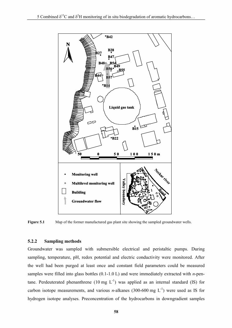
5 Combined �13C and �2H monitoring of in situ biodegradation of aromatic hydrocarbons…
58
Figure 5.1 Map of the former manufactured gas plant site showing the sampled groundwater wells.
5.2.2 Sampling methods
Groundwater was sampled with submersible electrical and peristaltic pumps. During
sampling, temperature, pH, redox potential and electric conductivity were monitored. After
the well had been purged at least once and constant field parameters could be measured
samples were filled into glass bottles (0.1-1.0 L) and were immediately extracted with n-pen-
tane. Perdeuterated phenanthrene (10 mg L-1) was applied as an internal standard (IS) for
carbon isotope measurements, and various n-alkanes (300-600 mg L-1) were used as IS for
hydrogen isotope analyses. Preconcentration of the hydrocarbons in downgradient samples
0 5 0 1 0 0 1 5 0 m50
N
•
•
• •
•
°
•°
•
•
°°°
°
B15
B22
B42
B27B28
B47
B54B48B49
B56
B44 B57
B14
B55
••
•• •
•••
°
•••
••
•••
• •
•• •• • • ••
••••
•
••
••
•° °••°•
°•••
°°°°
•
•
•••
•
•
•• • •
• •Valley boundary
••
•• •
•••
°
•••
••
•••
• •
•• •• • • ••
••••
•
••
••
•° °••°•
°•••
°°°°
•
•
•••
•
•
•• • •
• •
Neckar river
Monitoring well
Multilevel monitoring well
Building
Groundwater flow
•
°
Liquid gas tank
Road
0 5 0 1 0 0 1 5 0 m50 0 5 0 1 0 0 1 5 0 m50
NN
•
•
• •
•
°
•°
•
•
°°°
°
B15
B22
B42
B27B28
B47
B54B48B49
B56
B44 B57
B14
B55
••
•• •
•••
°
•••
••
•••
• •
•• •• • • ••
••••
•
••
••
•° °••°•
°•••
°°°°
•
•
•••
•
•
•• • •
• •Valley boundary
••
•• •
•••
°
•••
••
•••
• •
•• •• • • ••
••••
•
••
••
•° °••°•
°•••
°°°°
•
•
•••
•
•
•• • •
• •
Neckar river
Monitoring well
Multilevel monitoring well
Building
Groundwater flow
•
°
Liquid gas tank
Road
5 Combined �13C and �2H monitoring of in situ biodegradation of aromatic hydrocarbons…
59
was achieved by extracting large water volumes (1.0 L) with small n-pentane volumes
(0.5-1.0 mL). A microseparator facilitated the n-pentane separation. Reduced copper was
added to the n-pentane extract to remove elemental sulfur.
5.2.3 Compound specific isotope analysis 13C/12C isotope ratios of the extracted aromatic hydrocarbons were measured using a gas
chromatography-combustion-isotope ratio mass spectrometry (GC-C-IRMS) system. In this
technique a HP 6890 gas chromatograph is connected to a combustion furnace (CuO/NiO/Pt,
940°C). Water was removed via a Nafion� membrane. The isotopic composition of the
purified carbon dioxide (atomic masses of 45 for 13CO2 and 44 for 12CO2) is continuously
analysed using a FINNIGAN MAT Deltaplus-XL mass spectrometer. Differences in isotopic
composition are expressed in terms of the conventional delta notation (�13C), giving the per
mil (‰) deviation of the isotope ratio of the sample relative to the Vienna Peedee Belemnite
(VPDB) standard
10001RR
Cdardtans
sample13 ����
����
�� (5-2)
where Rsample is the 13C/12C ratio of the corresponding aromatic hydrocarbon and Rstandard is the 13C/12C ratio of the standard reference material.
Hydrogen isotope measurements were performed using a gas chromatography-thermo
conversion-isotope ratio mass spectrometry (GC-TC-IRMS) system. The effluent from the
chromatographic system was transferred to a ceramic tube (Al2O3) held at 1440°C, where the
hydrocarbons were quantitatively converted to graphite, CO and H2 gas (HILKERT et al.,
1999). The Deltaplus-XL mass spectrometer simultaneously recorded the masses 2 (1H1H) and
3 (1H2H), correcting automatically for contributions of H3+ ions. Hydrogen isotope data are
reported using the conventional �2H notation
10001RR
Hdardtans
sample2 ����
����
�� (5-3)
where Rsample and Rstandard are the 2H/1H isotope ratios corresponding to the sample and the
conventional standard mean ocean water (SMOW), respectively.
For both carbon and hydrogen isotope analyses aliquots of 0.5-5.0 �L samples were injected
splitless at 16°C in a cooled injection system with subsequent heating to 300°C at a rate of
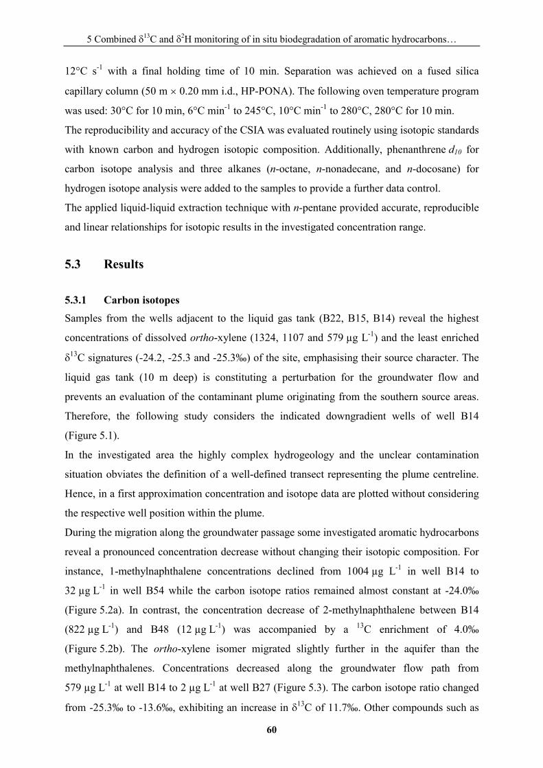
5 Combined �13C and �2H monitoring of in situ biodegradation of aromatic hydrocarbons…
60
12°C s-1 with a final holding time of 10 min. Separation was achieved on a fused silica
capillary column (50 m � 0.20 mm i.d., HP-PONA). The following oven temperature program
was used: 30°C for 10 min, 6°C min-1 to 245°C, 10°C min-1 to 280°C, 280°C for 10 min.
The reproducibility and accuracy of the CSIA was evaluated routinely using isotopic standards
with known carbon and hydrogen isotopic composition. Additionally, phenanthrene d10 for
carbon isotope analysis and three alkanes (n-octane, n-nonadecane, and n-docosane) for
hydrogen isotope analysis were added to the samples to provide a further data control.
The applied liquid-liquid extraction technique with n-pentane provided accurate, reproducible
and linear relationships for isotopic results in the investigated concentration range.
5.3 Results
5.3.1 Carbon isotopes
Samples from the wells adjacent to the liquid gas tank (B22, B15, B14) reveal the highest
concentrations of dissolved ortho-xylene (1324, 1107 and 579 µg L-1) and the least enriched
�13C signatures (-24.2, -25.3 and -25.3‰) of the site, emphasising their source character. The
liquid gas tank (10 m deep) is constituting a perturbation for the groundwater flow and
prevents an evaluation of the contaminant plume originating from the southern source areas.
Therefore, the following study considers the indicated downgradient wells of well B14
(Figure 5.1).
In the investigated area the highly complex hydrogeology and the unclear contamination
situation obviates the definition of a well-defined transect representing the plume centreline.
Hence, in a first approximation concentration and isotope data are plotted without considering
the respective well position within the plume.
During the migration along the groundwater passage some investigated aromatic hydrocarbons
reveal a pronounced concentration decrease without changing their isotopic composition. For
instance, 1-methylnaphthalene concentrations declined from 1004 µg L-1 in well B14 to
32 µg L-1 in well B54 while the carbon isotope ratios remained almost constant at -24.0‰
(Figure 5.2a). In contrast, the concentration decrease of 2-methylnaphthalene between B14
(822 µg L-1) and B48 (12 µg L-1) was accompanied by a 13C enrichment of 4.0‰
(Figure 5.2b). The ortho-xylene isomer migrated slightly further in the aquifer than the
methylnaphthalenes. Concentrations decreased along the groundwater flow path from
579 µg L-1 at well B14 to 2 µg L-1 at well B27 (Figure 5.3). The carbon isotope ratio changed
from -25.3‰ to -13.6‰, exhibiting an increase in �13C of 11.7‰. Other compounds such as
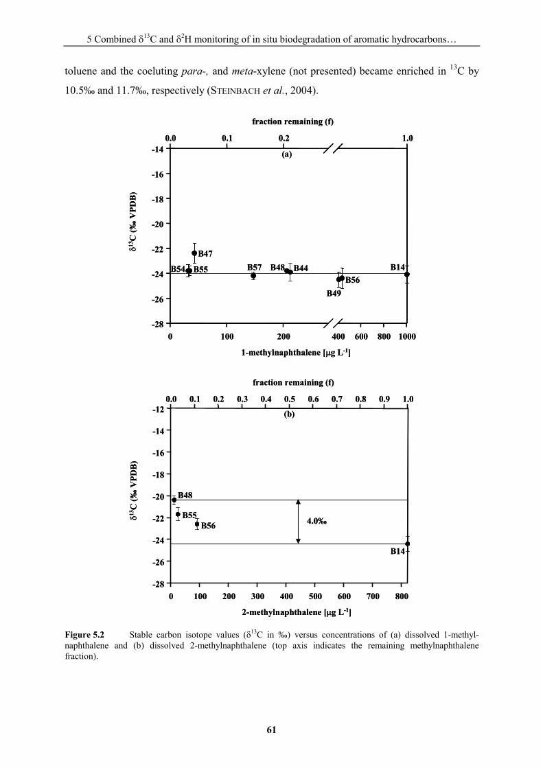
5 Combined �13C and �2H monitoring of in situ biodegradation of aromatic hydrocarbons…
61
toluene and the coeluting para-, and meta-xylene (not presented) became enriched in 13C by
10.5‰ and 11.7‰, respectively (STEINBACH et al., 2004).
Figure 5.2 Stable carbon isotope values (�13C in ‰) versus concentrations of (a) dissolved 1-methyl-naphthalene and (b) dissolved 2-methylnaphthalene (top axis indicates the remaining methylnaphthalene fraction).
1-methylnaphthalene [�g L-1]
0 100 200 400 600 800 1000
�13
C (‰
VPD
B)
-28
-26
-24
-22
-20
-18
-16
-14
fraction remaining (f)
0.0 0.1 0.2 1.0
B14
B49B56
B48B47
B55B54 B44B57
(a)
1-methylnaphthalene [�g L-1]
0 100 200 400 600 800 1000
�13
C (‰
VPD
B)
-28
-26
-24
-22
-20
-18
-16
-14
fraction remaining (f)
0.0 0.1 0.2 1.0
B14
B49B56
B48B47
B55B54 B44B57
(a)
B14
B56
B48
B55
2-methylnaphthalene [�g L-1]
0 100 200 300 400 500 600 700 800
�13
C(‰
VPD
B)
-28
-26
-24
-22
-20
-18
-16
-14
-12
fraction remaining (f)
0.0 0.1 0.2 0.3 0.4 0.5 0.6 0.7 0.8 0.9 1.0
(b)
4.0‰
B14
B56
B48
B55
2-methylnaphthalene [�g L-1]
0 100 200 300 400 500 600 700 800
�13
C(‰
VPD
B)
-28
-26
-24
-22
-20
-18
-16
-14
-12
fraction remaining (f)
0.0 0.1 0.2 0.3 0.4 0.5 0.6 0.7 0.8 0.9 1.0
(b)
4.0‰
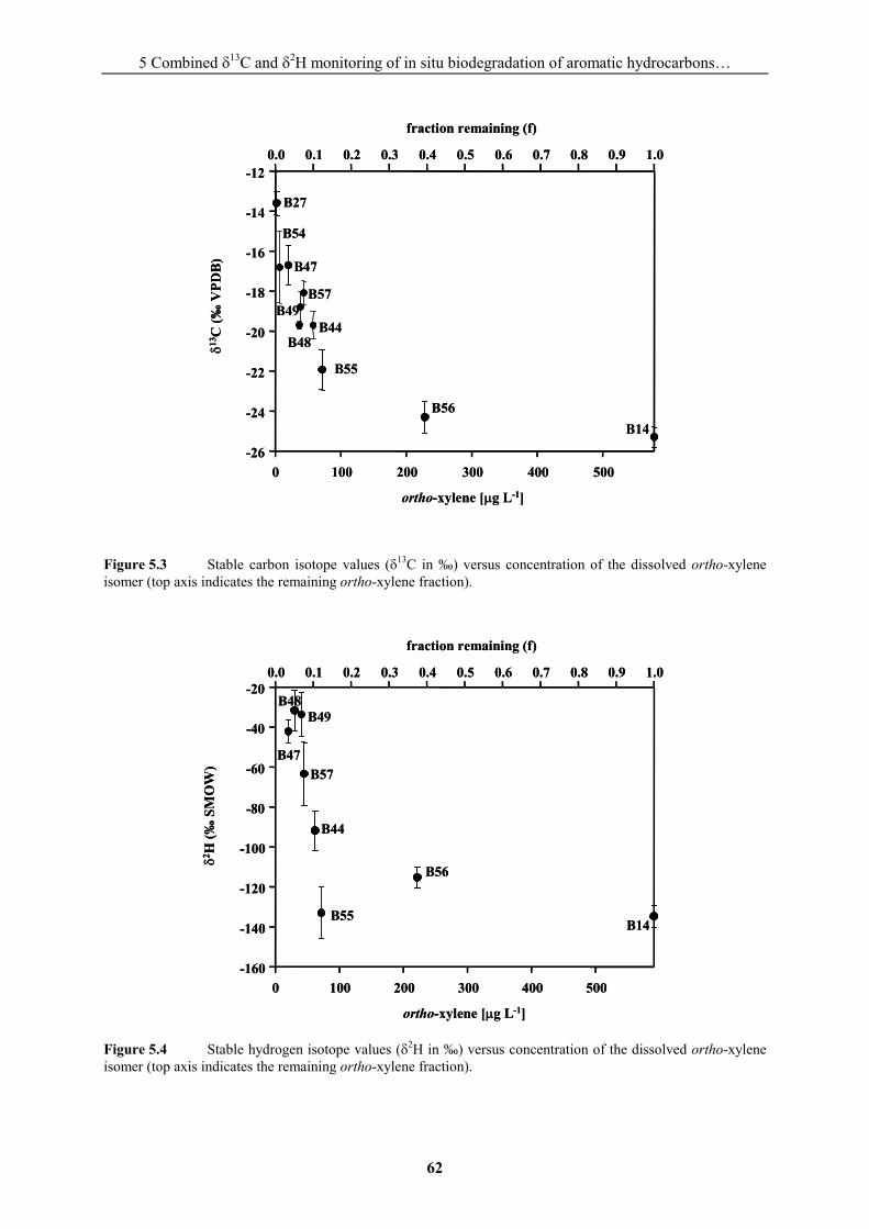
5 Combined �13C and �2H monitoring of in situ biodegradation of aromatic hydrocarbons…
62
Figure 5.3 Stable carbon isotope values (�13C in ‰) versus concentration of the dissolved ortho-xylene isomer (top axis indicates the remaining ortho-xylene fraction).
Figure 5.4 Stable hydrogen isotope values (�2H in ‰) versus concentration of the dissolved ortho-xylene isomer (top axis indicates the remaining ortho-xylene fraction).
B14B56
B48
B47
B27
0 100 200 300 400 500
�13
C(‰
VPD
B)
-26
-24
-22
-20
-18
-16
-14
-12
fraction remaining (f)
ortho-xylene [�g L-1]
0.0 0.1 0.2 0.3 0.4 0.5 0.6 0.7 0.8 0.9 1.0
B55
B49
B54
B44
B57
B14B56
B48
B47
B27
0 100 200 300 400 500
�13
C(‰
VPD
B)
-26
-24
-22
-20
-18
-16
-14
-12
fraction remaining (f)
ortho-xylene [�g L-1]
0.0 0.1 0.2 0.3 0.4 0.5 0.6 0.7 0.8 0.9 1.0
B55
B49
B54
B44
B57
B14
B56
B48
B47
ortho-xylene [�g L-1]
0 100 200 300 400 500
�2 H
(‰ S
MO
W)
-160
-140
-120
-100
-80
-60
-40
-20
fraction remaining (f)
0.0 0.1 0.2 0.3 0.4 0.5 0.6 0.7 0.8 0.9 1.0
B55
B49
B44
B57
B14
B56
B48
B47
ortho-xylene [�g L-1]
0 100 200 300 400 500
�2 H
(‰ S
MO
W)
-160
-140
-120
-100
-80
-60
-40
-20
fraction remaining (f)
0.0 0.1 0.2 0.3 0.4 0.5 0.6 0.7 0.8 0.9 1.0
B55
B49
B44
B57
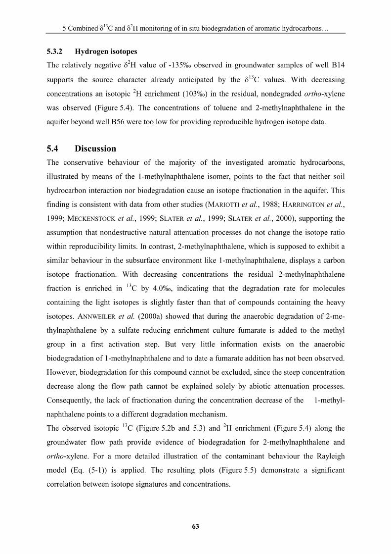
5 Combined �13C and �2H monitoring of in situ biodegradation of aromatic hydrocarbons…
63
5.3.2 Hydrogen isotopes
The relatively negative �2H value of -135‰ observed in groundwater samples of well B14
supports the source character already anticipated by the �13C values. With decreasing
concentrations an isotopic 2H enrichment (103‰) in the residual, nondegraded ortho-xylene
was observed (Figure 5.4). The concentrations of toluene and 2-methylnaphthalene in the
aquifer beyond well B56 were too low for providing reproducible hydrogen isotope data.
5.4 Discussion The conservative behaviour of the majority of the investigated aromatic hydrocarbons,
illustrated by means of the 1-methylnaphthalene isomer, points to the fact that neither soil
hydrocarbon interaction nor biodegradation cause an isotope fractionation in the aquifer. This
finding is consistent with data from other studies (MARIOTTI et al., 1988; HARRINGTON et al.,
1999; MECKENSTOCK et al., 1999; SLATER et al., 1999; SLATER et al., 2000), supporting the
assumption that nondestructive natural attenuation processes do not change the isotope ratio
within reproducibility limits. In contrast, 2-methylnaphthalene, which is supposed to exhibit a
similar behaviour in the subsurface environment like 1-methylnaphthalene, displays a carbon
isotope fractionation. With decreasing concentrations the residual 2-methylnaphthalene
fraction is enriched in 13C by 4.0‰, indicating that the degradation rate for molecules
containing the light isotopes is slightly faster than that of compounds containing the heavy
isotopes. ANNWEILER et al. (2000a) showed that during the anaerobic degradation of 2-me-
thylnaphthalene by a sulfate reducing enrichment culture fumarate is added to the methyl
group in a first activation step. But very little information exists on the anaerobic
biodegradation of 1-methylnaphthalene and to date a fumarate addition has not been observed.
However, biodegradation for this compound cannot be excluded, since the steep concentration
decrease along the flow path cannot be explained solely by abiotic attenuation processes.
Consequently, the lack of fractionation during the concentration decrease of the 1-methyl-
naphthalene points to a different degradation mechanism.
The observed isotopic 13C (Figure 5.2b and 5.3) and 2H enrichment (Figure 5.4) along the
groundwater flow path provide evidence of biodegradation for 2-methylnaphthalene and
ortho-xylene. For a more detailed illustration of the contaminant behaviour the Rayleigh
model (Eq. (5-1)) is applied. The resulting plots (Figure 5.5) demonstrate a significant
correlation between isotope signatures and concentrations.
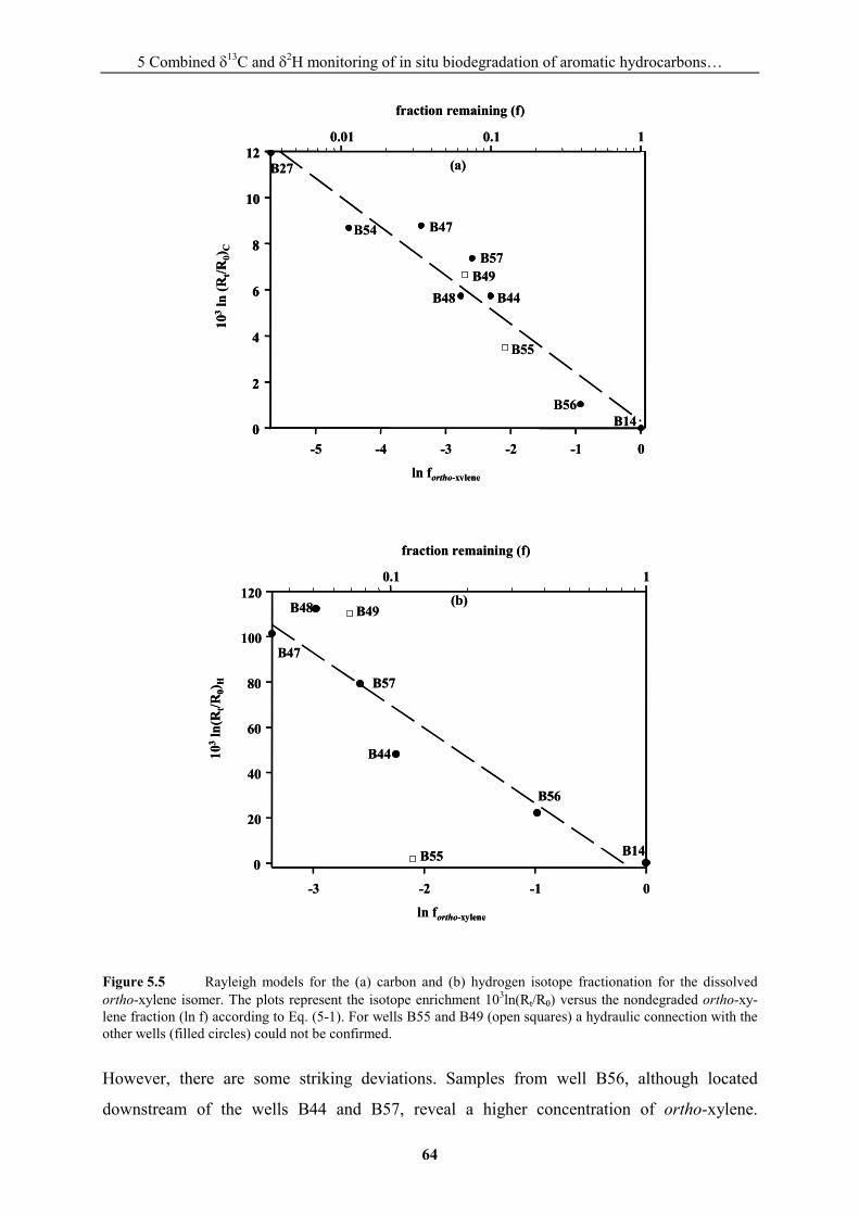
5 Combined �13C and �2H monitoring of in situ biodegradation of aromatic hydrocarbons…
64
Figure 5.5 Rayleigh models for the (a) carbon and (b) hydrogen isotope fractionation for the dissolved ortho-xylene isomer. The plots represent the isotope enrichment 103ln(Rt/R�) versus the nondegraded ortho-xy-lene fraction (ln f) according to Eq. (5-1). For wells B55 and B49 (open squares) a hydraulic connection with the other wells (filled circles) could not be confirmed.
However, there are some striking deviations. Samples from well B56, although located
downstream of the wells B44 and B57, reveal a higher concentration of ortho-xylene.
(a)
ln fortho-xylene
-5 -4 -3 -2 -1 0
103
ln(R
t/R0)
C
0
2
4
6
8
10
12
fraction remaining (f)
0.01 0.1 1
B56
B55
B49B48
B47B54
B27
B14
B44
B57
(a)
ln fortho-xylene
-5 -4 -3 -2 -1 0
103
ln(R
t/R0)
C
0
2
4
6
8
10
12
0
2
4
6
8
10
12
fraction remaining (f)
0.01 0.1 1
B56
B55
B49B48
B47B54
B27
B14
B44
B57
ln fortho-xylene
-3 -2 -1 0
103
ln(R
t/R0)
H
0
20
40
60
80
100
120
fraction remaining (f)
0.1 1
B14
B56
B49B48
B47
B44
B57
(b)
B55
ln fortho-xylene
-3 -2 -1 0
103
ln(R
t/R0)
H
0
20
40
60
80
100
120
fraction remaining (f)
0.1 1
B14
B56
B49B48
B47
B44
B57
(b)
B55
ln fortho-xylene
-3 -2 -1 0
103
ln(R
t/R0)
H
0
20
40
60
80
100
120
fraction remaining (f)
0.1 1
B14
B56
B49B48
B47
B44
B57
(b)
B55
5 Combined �13C and �2H monitoring of in situ biodegradation of aromatic hydrocarbons…
65
Moreover, the isotope values for ortho-xylene show a depletion in 13C (Figure 5.5a) and 2H
(Figure 5.5b) compared to wells B44 and B57. Obviously the influence of an additional source
of marginally biodegraded ortho-xylene accounts for the shifts observed in the application of
the Rayleigh model. This finding conflicts with the assumption of closed system conditions
and thus obviates the quantitative assessment of biodegradation in this area. However,
between wells B44 and B47 dilution and mixing processes could be largely excluded
(STEINBACH et al., 2004), indicating that the observed concentration decrease for ortho-xylene
(66%) is nearly exclusively due to biodegradation.
Stable hydrogen isotope analysis as an additional tool not only substantiates the results of the
carbon isotope study but also provides useful additional information. For example in the
Rayleigh plot for the hydrogen isotopes of ortho-xylene (Figure 5.5b) data of well B55 deviate
from the general trend, whereas carbon isotope fractionation (Figure 5.5a) lies in the expected
linearity of the Rayleigh plot. Ortho-xylene in wells B14 and B55 exhibits similar �2H values
(-135‰ and -133‰, respectively) though the observed 13C enrichment at well B55 (-21.9‰)
relative to well B14 (-25.3‰) points to an advanced biodegradation. A possible explanation
for this behaviour is that well B55 is a downgradient well of an additional northern source
area with a more negative �2H than that observed at well B14. It can be assumed that
ortho-xylene in well B55 is not derived from the supposed source well B14. This finding
could only be recognised by analysis of the hydrogen isotopes and would not have been
detected by consideration of the carbon isotopes alone.
5.5 Conclusions The results of this study suggest that isotope fractionation provide excellent evidence for
biodegradation of aromatic hydrocarbons in the field. In zones where mixing and dilution
processes can be excluded a quantitative assessment of biodegradation can be given. The
example of well B55 illustrates that combined analyses of carbon and hydrogen isotopes may
be a more promising approach to discriminate between different contaminant plumes than
only measuring carbon isotopes.
5.6 Acknowledgements We acknowledge financial support from the DFG. The measurements of��13C and �2H of our
standards by Siegmund Ertl and Peter Schreier (Universität Würzburg) are gratefully
acknowledged. We thank the two anonymous reviewers for constructive comments, which
improved the quality of the paper.
6 Hydrogen and carbon isotope fractionation during anaerobic biodegradation of aromatic...
66
Hydrogen and carbon isotope fractionation during anaerobic
biodegradation of aromatic hydrocarbons - a field study
Environmental Science and Technology
in press
Steinbach A., Seifert R., Annweiler E., and Michaelis W.
6 Hydrogen and carbon isotope fractionation during anaerobic biodegradation of aromatic...
67
6.1 Abstract The aquifer of a former manufactured gas plant site, highly contaminated by dissolved
monocyclic, heterocyclic, and polycyclic aromatic hydrocarbons, was studied to evaluate the
applicability of carbon and hydrogen isotope fractionation to prove ongoing biodegradation of
these compounds even in complex aquifer settings. The loss of toluene, o-xylene, p, m-xylene,
and 2-methylnaphthalene was accompanied by a considerable carbon isotope fractionation.
Additionally, a strong 2H enrichment in residual o-xylene was detected. All isotope
fractionations observed could be related to established biochemical degradation mechanisms,
each involving a C-H bond cleavage in the rate-determining step. In contrast, other
compounds such as 1-methylnaphthalene, methylbenzofuran, and acenaphthene exhibited a
uniform stable carbon isotope composition. However, a decrease in concentration for these
compounds was observed in the flowpath of the aquifer. High threshold concentrations of
acenaphthene downgradient indicate that this contaminant is, if at all, only marginally
biodegraded. Detailed analyses of xylenes provided support that compound specific isotope
analyses and subsequent application of the Rayleigh model may provide a valuable basis to
distinguish between different biodegradation mechanisms as well as dissolution processes in
heterogeneous aquifers.
6.2 Introduction Groundwater contamination with aromatic hydrocarbons is a widespread environmental
problem. Major contributions arise from leaking underground storage tanks and pipelines,
accidental spills, inappropriate disposal techniques, and industrial discharges (CHRISTENSEN et
al., 1994; CONRAD et al., 1999; DAVIS et al., 1999; AHEL and TEPIC, 2000). Due to the lack of
efficient, cost-effective active remediation technologies, passive remediation strategies have
emerged as promising alternatives (WIEDEMEIER et al., 1999). Already in 1993 the National
Research Council’s Committee on in situ bioremediation concluded that intrinsic
bioremediation is a scientifically valid and technically feasible method (NATIONAL RESEARCH
COUNCIL, 1993). Recently, the natural attenuation (NA) concept gained increasing attention
(NATIONAL RESEARCH COUNCIL, 2000). Besides intrinsic bioremediation, NA includes natural
abiotic processes (volatilization, dilution, dispersion, and sorption) that reduce the
concentration of dissolved contaminants in a groundwater plume. NA was considered as a
remediation strategy for a steadily growing number of polluted sites and contaminants.
However, a crucial drawback to the widespread acceptance of NA is the difficulty to provide
6 Hydrogen and carbon isotope fractionation during anaerobic biodegradation of aromatic...
68
evidence that decreasing contaminant concentrations in groundwater truly result from
destructive (biodegradation) rather than from nondestructive processes. At present, quanti-
fication of biodegradation relies on a broad basis of hydrogeological, geochemical and
microbiological data. The main difficulties are to establish accurate mass balances of
contaminants, electron donors and end products in heterogeneous groundwater systems.
Compound specific isotope analysis provides a powerful tool to assess in situ biodegradation
rates in aquifers. The two elements in hydrocarbons with their stable isotopes (13C, 12C; 2H, 1H) allow a combination of isotopic studies which can enhance the understanding of
biodegradation in field studies. Bonds involving the heavier isotopes are more difficult to
break. Consequently, bonds in hydrocarbons consisting of the lighter isotopes are degraded
preferentially and cause an enrichment of the heavier isotopes in the residual, nondegraded
substrate, while the product is depleted in the heavy isotopes. This shift in the isotope ratios is
denoted as isotope fractionation. The preferential use of the lighter 12C isotope has been
shown for multiple biochemical reactions, for example the bacterial formation (GAMES et al.,
1978) and oxidation (COLEMAN et al., 1981) of methane. Recent laboratory and field studies
have illustrated, that microbial degradation can lead to carbon isotope fractionation also for
compounds of higher molecular mass such as alkanes (STAHL, 1980), chlorinated ethenes
(HUNKELER et al., 1999; SHERWOOD LOLLAR et al., 1999; SLATER et al., 2001), methyl tert-
butyl ether (MTBE; HUNKELER et al., 2001b; GRAY et al., 2002; KOLHATKAR et al., 2002),
and some aromatic hydrocarbons (AHAD et al., 2000; WILKES et al., 2000; PETER et al., 2003).
In contrast, abiotic nondegrading processes such as sorption (HARRINGTON et al., 1999;
SLATER et al., 2000), dispersion, dilution (MARIOTTI et al., 1988), and volatilization (HUANG
et al., 1999; SLATER et al., 1999) do not change the isotope ratio within reproducibility limits.
Therefore, isotope fractionation can be used to distinguish biodegradation in the aquifer from
nondestructive processes.
Improvements in the sensitivity of isotope ratio mass spectrometers facilitated the
investigation of carbon isotope signatures at very low concentrations and, moreover, the on-
line analysis of 2H/1H isotope ratios for individual compounds. Recent laboratory studies
showed that the biodegradation of benzene (MANCINI et al., 2003), toluene (WARD et al.,
2000; MORASCH et al., 2001), and MTBE (GRAY et al., 2002) involves large hydrogen isotope
effects. However, the applicability of combined carbon and hydrogen isotope analyses in field
studies has rarely been tested for aromatic hydrocarbons (MANCINI et al., 2002).
6 Hydrogen and carbon isotope fractionation during anaerobic biodegradation of aromatic...
69
The major objective of the present study was to evaluate the occurrence and magnitude of
carbon and hydrogen isotope fractionation during biodegradation of aromatic hydrocarbons at
a field site. Observed isotope fractionations were analysed with regard to established
biochemical degradation mechanisms. The second objective was to test if �13C and �2H values
have the potential to elucidate the interaction of biodegradation, dilution, and dissolution
processes in a highly heterogeneous aquifer. To meet these objectives, data of o-xylene were
interpreted by using a Rayleigh distillation model.
6.3 Materials and methods
6.3.1 Field site
The investigated former manufactured gas plant site is located in the Neckar Valley near
Stuttgart in the south-west of Germany. The site is limited by Triassic hills in the west and the
river Neckar in the east (Figure 6.1). Between 1875 and 1969, town gas was produced by coal
gasification. During this period soil and groundwater was contaminated by leaking tar pits,
pipelines, and storage tanks and accidental spills as well as by a severe destruction during the
end of World War II. Consequently, various nonaqueous phase liquids (NAPL) still persist in
the subsurface and continue to leach into the through-flowing groundwater. The replacement
of the produced town gas by natural gas was completed in 1974 when the old production
facilities were destructed and a subsurface gas storage tank for liquid gas was built.
The ca. 3.5 m thick Quaternary aquifer consists mainly of gravels and sands with interbedded
layers of sand and silt leading to heterogeneous geochemical and hydraulic properties. The
groundwater table is generally between 2 and 4 m below ground surface. The average
hydraulic conductivity at the site determined by pumping tests is 2.5�10-3 m s-1, and the
effective porosities vary between 0.06 and 0.37 (HERFORT, 2000). The groundwater flow
direction is from south to north/north-west with flow velocities between 4.2 and 2.0 m d-1
(BÖSEL et al., 2000). The average transmissivity is 9�10-4 m2 s-1 and the hydraulic gradient
ranges between 0.036% and 1% (ZAMIFIRESCU, 2000).
The field site is equipped with a network of conventional groundwater monitoring wells
(125-150 mm i.d.) that are fully screened within the Quaternary aquifer and multilevel
groundwater monitoring wells which are equipped with a multilevel packer system
(150 mm i.d., vertical spacing between 50 and 100 cm; SCHIRMER et al., 1995). The major
zones of contamination by mono- and polyaromatic hydrocarbons (MAH and PAH) as well as
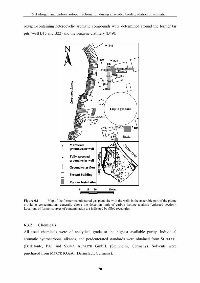
6 Hydrogen and carbon isotope fractionation during anaerobic biodegradation of aromatic...
70
oxygen-containing heterocyclic aromatic compounds were determined around the former tar
pits (well B15 and B22) and the benzene distillery (B49).
Figure 6.1 Map of the former manufactured gas plant site with the wells in the anaerobic part of the plume providing concentrations generally above the detection limit of carbon isotope analysis (enlarged section). Locations of former sources of contamination are indicated by filled rectangles.
6.3.2 Chemicals
All used chemicals were of analytical grade or the highest available purity. Individual
aromatic hydrocarbons, alkanes, and perdeuterated standards were obtained from SUPELCO,
(Bellefonte, PA) and SIGMA ALDRICH GmbH, (Steinheim, Germany). Solvents were
purchased from MERCK KGaA, (Darmstadt, Germany).
B42
B27
•
•
• •
•
°
•°
•
•
°°°
°
B28B47
B48
B14
B15
B22
B55
B54
B49
B44B57
B56
Liquid gas tank
Valley
boundary
N
••
•• •
•••
°
•••
• ••••
• •
•• •• • • ••
••••
•
••
••
•° °••°•
°•••
°°°°
•
•
•••
•
•
•• • •
• •
Neckar river
Valley
boundary
0 25 50 100 m
Street
Benzene distillery1914-1945
Benzene distillery1958-1974
Tar pits
1910-1979
1934
•
Multilevel groundwater well
Fully screenedgroundwater well
Groundwater flow
Present building
Former installation
•
Multilevel groundwater well
Fully screenedgroundwater well
Groundwater flow
Present building
Former installation
6 Hydrogen and carbon isotope fractionation during anaerobic biodegradation of aromatic...
71
6.3.3 Groundwater sampling and extraction
Groundwater samples were taken in November 2000 (�13C) and March 2001 (�2H) from fully
screened groundwater wells using submersible electrical pumps (CONRAD BWV 01,
Hamburg, Germany) with Tygon tubing CR (R-1000; CARL ROTH GmbH & Co. KG,
Karlsruhe, Germany). Peristaltic pumps (WATSON MARLOW, Fulmouth, England) were used
for multilevel groundwater wells. Depending on the sampling depth, pumping rates varied
between 10 and 18 L min-1 for the submersible pumps and 1 and 5 L min-1 for the peristaltic
pumps. The Tygon� tubing was connected to an in-line flow cell and the field parameters
temperature, pH, redox potential (WTW pH 91; WTW GmbH & Co. KG, Weilheim,
Germany), and specific conductivity (WTW LF 91; WTW GmbH & Co. KG, Weilheim,
Germany) were registered. After the wells had been purged at least with one well volume and
all the measured parameters reached constant values, samples were taken, spiked with internal
standards, and immediately extracted with n-pentane (liquid-liquid extraction, LLE) for
30 min on an overhead mixer (HEIDOLPH Instruments, Schwabach, Germany).
Phenanthrene d10 (10 mg L-1) was applied as the internal standard for carbon isotope
measurements; n-octane (600 mg L-1) and n-nonadecane (400 mg L-1) were used as internal
standards for hydrogen isotope analyses. Since low contaminant concentrations in the
groundwater required the extraction of a large water volume (1000 mL) with a very small n-
pentane volume (0.5-1 mL), a microseparator for the recovery of the n-pentane phase was
used. Reduced copper was added to the n-pentane extract to remove elemental sulfur. Samples
were stored at -30°C in the dark until analysis. The relative standard uncertainty of the
concentration measurement was �10%.
6.3.4 Gas chromatography (GC) and GC-mass spectrometry (GC-MS)
Identification of aromatic hydrocarbons was based on mass spectra and retention times of
authentic standards. Gas chromatographic analyses of solvent extracts were performed on a
GC-6000 Vega Series 2 (CARLO ERBA Instruments, Milan, Italy) equipped with a fused silica
capillary column (DB-5, 50 m length, 0.32 mm i.d., 0.25 �m film thickness, J&W Scientific,
USA) and a flame ionization detector. The temperature program was 40°C (10 min
isothermal), 40-240°C (4°C min-1), 240-280°C (10°C min-1), and 280°C (10 min isothermal).
Hydrogen was used as carrier gas. The injection mode was on column. GC-MS measurements
were performed with a HP 6890 GC (HEWLETT PACKARD Company, Wilmington, DE)
coupled to the MS (Quattro II, MICROMASS, U.K.) using a 30 m capillary column (DB-5,
0.32 mm i.d., 0.25 �m film thickness, J&W Scientific, USA) with helium as the carrier gas.
6 Hydrogen and carbon isotope fractionation during anaerobic biodegradation of aromatic...
72
The temperature program was the same as for the GC analyses. MS conditions were as
follows: ionization mode, electron impact; ionization energy, 70 eV; emission current, 200
�A. The source temperature was 250°C, and the mass range covered m/z 50 to 400.
6.3.5 Compound specific isotope analysis
Carbon isotope ratios were determined by gas chromatography-combustion-isotope ratio mass
spectrometry (GC-C-IRMS). The system consists of a HP 6890 GC connected via a
combustion unit (combustion interface; FINNIGAN, Bremen, Germany) to a FINNIGAN MAT
Deltaplus-XL mass spectrometer (FINNIGAN, Bremen, Germany). Aliquots of 0.5–5 �L of the
n-pentane extracts were injected in splitless mode at 16°C in a cooled injection system
(CIS 4; GERSTEL, Muelheim, Germany) with subsequent heating to 300°C at a rate of 12°C s-1
with a final holding time of 10 min. Baseline separation of most of the aromatic hydrocarbons
was achieved on a 50 m fused silica column (HP-PONA, 0.25 mm i.d., 0.5 �m film thickness,
HEWLETT PACKARD Co.) with helium as the carrier gas. The GC temperature program was
30°C for 10 min, 6°C min-1 to 245°C, 10°C min-1 to 280°C, 280°C for 10 min. The separated
aromatic hydrocarbons and helium carrier gas eluting from the column were carried via
deactivated fused silica capillary tubing to the combustion furnace, where they were
successively oxidised to CO2 and H2O. After water separation the effluent stream was
transferred on-line via an open split to the mass spectrometer (MERRIT et al., 1995). For
isotopic standardization, CO2 reference gas (MESSER, Frankfurt, Germany) with a known
isotopic composition (�13CVPDB = -22.2‰ � 0.2‰) was automatically introduced into the mass
spectrometer in a series of pulses at the beginning and the end of each analysis. Isotopic
values of the individual aromatic hydrocarbons are reported in the delta notation (�13C) in per
mil (‰) units referenced to VPDB (Vienna Peedee Belemnite).
Hydrogen isotope ratios were determined by using a gas chromatography-thermoconversion-
isotope ratio mass spectrometry (GC-TC-IRMS) system. After the chromatographic
separation, the eluting compounds pass through an alumina tube, which is heated to 1440°C to
quantitatively convert organic hydrogen to H2 (BURGOYNE and HAYES, 1998). The H2 gas is
then introduced into the FINNIGAN MAT Deltaplus-XL mass spectrometer simultaneously
recording the masses 2 (1H1H) and 3 (1H2H). Since the formation of H3+ ions contributes to the
mass-3 signal, a correction factor was determined daily. Samples were run against external H2
isotopic standards (MESSER, Frankfurt, Germany) with a known isotopic composition
6 Hydrogen and carbon isotope fractionation during anaerobic biodegradation of aromatic...
73
(�2HVSMOW = -208‰ � 5‰). The hydrogen isotope ratio is expressed in the delta notation
(�2H) in per mil (‰) units referenced to VSMOW (Vienna Standard Mean Ocean Water).
The parameters of the cooled injection system and of the GC were identical to those used for
carbon isotope determination.
Assessing reproducibility and accuracy �
13C and �2H values of selected MAH and PAH standards after n-pentane extraction were
identical to those analysed after direct dissolution in n-pentane without extraction. HÖR et al.
(2001) reported negligible hydrogen isotope fractionation during the LLE of 2-hexenal and
2-hexenol with n-pentane, and DEMPSTER et al. (1997) did not observe any significant carbon
isotope fractionation during the LLE of benzene, toluene, ethylbenzene, and xylenes (BTEX)
with n-pentane.
The GC-C-IRMS system was checked with a mixture of 15 n-alkanes (available from
A. Schimmelmann, Biogeochemical Laboratories, Indiana University; USA) with known
carbon and hydrogen isotopic composition. Additionally, phenanthrene d10 (-24.4‰) for
carbon isotope analysis and two alkanes (n-octane, -91‰; n-nonadecane, -51‰) for hydrogen
isotope analysis were added to the samples to provide a further control of data quality. Due to
the dependence of stable isotope signatures on the amount of injected sample, the
concentration range providing accurate and reproducible data had to be determined for each
individual compound. A series of experiments with MAH and PAH standards of known
isotopic composition revealed that for reliable hydrogen isotope measurements, approximately
200-400 ng (signal areas � 2.5 Vs) of the individual compound was required. The accuracy
and precision of �2H determinations was between 4 and 15‰. For stable carbon isotopes, the
same procedure revealed that for reproducible and accurate measurements, peak areas in the
range of 0.3-50 Vs are needed. Accordingly, the n-pentane/sample ratio and the injection
volumes (0.3-5 ml) were varied to produce the required signal areas. Compound
concentrations of 2 �g L-1 produced signal areas of approximately 0.35 Vs and resulted in
standard deviations between 0.6 and 2‰.
6.3.6 Rayleigh calculations
Isotope fractionation during biodegradation can be quantified using the Rayleigh model. If the
advancement of the reaction is depicted as the fraction f of substrate remaining, then the
classical equation of Rayleigh is expressed as
6 Hydrogen and carbon isotope fractionation during anaerobic biodegradation of aromatic...
74
� � fln1RR
ln0
t ������
����
(6-1)
where Rt and R0 represent the 13C/12C ratios at any value of f and at f = 1, respectively
(MARIOTTI et al., 1981; CLARK and FRITZ, 1997). The isotopic fractionation factor � can be
determined by using linear regression based on Eq. (6-1) and is indicated as an enrichment
factor (in ‰) that is related to the fractionation factor � by
� � 10001 ����� . (6-2)
6.4 Results Concentrations of dissolved MAHs (benzene, toluene, ethylbenzene, xylenes, propylbenzenes,
and trimethylbenzenes) and PAHs (including heterocyclic aromatic compounds) are illustrated
in Figure 6.2a-b. The hot spots of the contamination are located close to well B15 with up to
20 mg L-1 for the MAHs and around well B22 and B15 with up to 32 mg L-1 for the PAHs.
Along the groundwater flow path a pronounced concentration decrease was observed. While
the concentration of the MAHs dropped below the detection limit beyond wells B27 and B28,
the PAHs migrate until the northern boundary of the site. Local variations of the contaminant
concentration probably point to the occurrence of additional entries (B14, B56, B49) or
infiltration with pristine water (B12, B27) from the adjacent hills. These assumptions agree
with the location of the former benzene distillery near well B49 (Figure 6.1), NAPL of
different composition present in waters from wells B14, B15, B22, B49, B55, and B56
(ZAMFIRESCU and GRATHWOHL, 2001), and the enhanced nitrate and oxygen concentrations in
wells B12 and B27 (SCHÄFLE, 1997).
The redox potential Eh increased along the groundwater flow path from -350 mV in the south
of the site (B22) to -100 mV in well B42 mirroring anaerobic conditions for the entire
investigated part of the plume (Figure 6.2c).
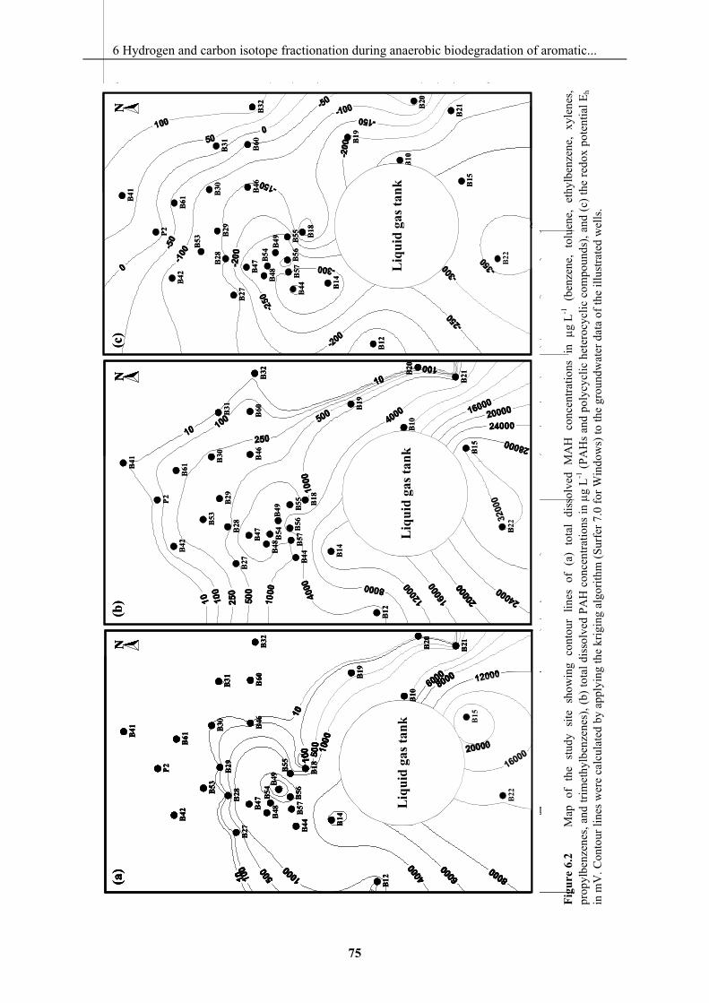
6 Hydrogen and carbon isotope fractionation during anaerobic biodegradation of aromatic...
75
Figu
re 6
.2
Map
of
the
stud
y si
te s
how
ing
cont
our
lines
of
(a)
tota
l di
ssol
ved
MA
H c
once
ntra
tions
in
�g
L-1 (
benz
ene,
tol
uene
, et
hylb
enze
ne,
xyle
nes,
prop
ylbe
nzen
es, a
nd tr
imet
hylb
enze
nes)
, (b)
tota
l dis
solv
ed P
AH
con
cent
ratio
ns in
�g
L-1 (P
AH
s an
d po
lycy
clic
het
eroc
yclic
com
poun
ds),
and
(c) t
he re
dox
pote
ntia
l Eh
in m
V. C
onto
ur li
nes w
ere
calc
ulat
ed b
y ap
plyi
ng th
e kr
igin
g al
gorit
hm (S
urfe
r 7.0
for W
indo
ws)
to th
e gr
ound
wat
er d
ata
of th
e ill
ustra
ted
wel
ls.
B10
B12
B15
B18
B19
B20
B21
B22
B27
B28
B29
B30
B31
B32
B41
B42
B44
B46
B47
B48
B49
B14
B53
B54
B55
B56
B57
B60
B61
P2
Liq
uid
gas t
ank
(a)
N
B10
B12
B15
B18
B19
B20
B21
B22
B27
B28
B29
B30
B31
B32
B41
B42
B44
B46
B47
B48
B49
B14
B53
B54
B55
B56
B57
B60
B61
P2
Liq
uid
gas t
ank
(b)
N
B10
B12
B15
B18
B19
B20
B21
B22
B27
B28
B29
B30
B31
B32
B41
B42
B44
B46
B47
B48
B49
B14
B53
B54
B55
B56
B57
B60
B61
P2
Liq
uid
gas t
ank
(c)
N
B10
B12
B15
B18
B19
B20
B21
B22
B27
B28
B29
B30
B31
B32
B41
B42
B44
B46
B47
B48
B49
B14
B53
B54
B55
B56
B57
B60
B61
P2
Liq
uid
gas t
ank
(a)
N
B10
B12
B15
B18
B19
B20
B21
B22
B27
B28
B29
B30
B31
B32
B41
B42
B44
B46
B47
B48
B49
B14
B53
B54
B55
B56
B57
B60
B61
P2
Liq
uid
gas t
ank
(a)
N
B10
B12
B15
B18
B19
B20
B21
B22
B27
B28
B29
B30
B31
B32
B41
B42
B44
B46
B47
B48
B49
B14
B53
B54
B55
B56
B57
B60
B61
P2
Liq
uid
gas t
ank
(a)
NN
B10
B12
B15
B18
B19
B20
B21
B22
B27
B28
B29
B30
B31
B32
B41
B42
B44
B46
B47
B48
B49
B14
B53
B54
B55
B56
B57
B60
B61
P2
Liq
uid
gas t
ank
(b)
N
B10
B12
B15
B18
B19
B20
B21
B22
B27
B28
B29
B30
B31
B32
B41
B42
B44
B46
B47
B48
B49
B14
B53
B54
B55
B56
B57
B60
B61
P2
Liq
uid
gas t
ank
(b)
NN
B10
B12
B15
B18
B19
B20
B21
B22
B27
B28
B29
B30
B31
B32
B41
B42
B44
B46
B47
B48
B49
B14
B53
B54
B55
B56
B57
B60
B61
P2
Liq
uid
gas t
ank
(c)
N
B10
B12
B15
B18
B19
B20
B21
B22
B27
B28
B29
B30
B31
B32
B41
B42
B44
B46
B47
B48
B49
B14
B53
B54
B55
B56
B57
B60
B61
P2
Liq
uid
gas t
ank
(c)
NN
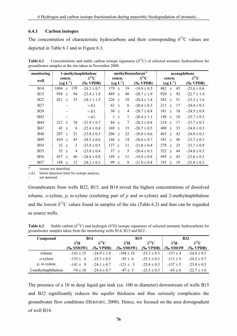
6 Hydrogen and carbon isotope fractionation during anaerobic biodegradation of aromatic...
76
6.4.1 Carbon isotopes
The concentration of characteristic hydrocarbons and their corresponding �13C values are
depicted in Table 6.1 and in Figure 6.3.
Table 6.1 Concentrations and stable carbon isotope signatures (�13C) of selected aromatic hydrocarbons for groundwater samples at the site taken in November 2000.
monitoring 1-methylnaphthalene methylbenzofurana) acenaphthene
well concn. (�g L-1)
�13C (‰ VPDB)
concn. (�g L-1)
�13C (‰ VPDB)
concn. (�g L-1)
�13C (‰ VPDB)
B14 1004 � 120 -24.1 � 0.7 179 � 19 -19.8 � 0.5 482 � 45 -23.6 � 0.6 B15 958 � 94 -23.4 � 1.8 489 � 48 -20.7 � 1.9 920 � 92 -22.7 � 1.4 B22 421 � 35 -24.1 � 1.5 226 � 18 -20.4 � 1.4 582 � 51 -23.3 � 1.6 B27 - � d.l. 62 � 6 -20.4 � 0.3 211 � 17 -24.4 � 0.3 B28 - � d.l. 30 � 4 -20.7 � 0.8 181 � 18 -24.5 � 0.8 B42 - � d.l. 3 � 1 -20.4 � 1.1 148 � 10 -23.7 � 0.3 B44 213 � 18 -23.9 � 0.7 84 � 7 -20.3 � 0.8 214 � 17 -23.7 � 0.3 B47 43 � 6 -22.4 � 0.8 169 � 15 -20.7 � 0.5 400 � 33 -24.0 � 0.5 B48 207 � 21 -23.8 � 0.3 206 � 22 -20.8 � 0.6 463 � 42 -24.0 � 0.3 B49 410 � 45 -24.5 � 0.6 146 � 14 -20.6 � 0.7 541 � 46 -23.7 � 0.3 B54 32 � 2 -23.8 � 0.5 137 � 11 -21.0 � 0.4 278 � 25 -23.7 � 0.9 B55 35 � 4 -23.8 � 0.4 37 � 5 -20.4 � 0.3 522 � 44 -24.0 � 0.3 B56 437 � 46 -24.4 � 0.8 149 � 11 -19.8 � 0.8 495 � 45 -23.6 � 0.3 B57 148 � 12 -24.2 � 0.3 99 � 8 -21.0 � 0.4 193 � 19 -23.8 � 0.3
a) isomer not identified.
� d.l. below detection limit for isotope analysis. - not detected.
Groundwaters from wells B22, B15, and B14 reveal the highest concentrations of dissolved
toluene, o-xylene, p, m-xylene (coeluting pair of p and m-xylene) and 2-methylnaphthalene
and the lowest �13C values found in samples of the site (Table 6.2) and thus can be regarded
as source wells.
Table 6.2 Stable carbon (�13C) and hydrogen (�2H) isotope signatures of selected aromatic hydrocarbons for groundwater samples taken from the monitoring wells B14, B15 and B22.
Compound B14 B15 B22
�2H (‰ SMOW)
�13C (‰ VPDB)
�2H (‰ SMOW)
�13C (‰ VPDB)
�2H (‰ SMOW
�13C (‰ VPDB)
toluene -143 � 15 -24.9 � 1.0 -104 � 10 -25.3 � 0.3 -157 � 4 -24.8 � 0.5 o-xylene -135 � 6 -25.3 � 0.5 -95 � 6 -25.3 � 0.3 -111 � 9 -24.2 � 0.7
p, m-xylene -141 � 9 -24.1 � 0.7 -121 � 5 -25.0 � 0.3 -137 � 5 -23.8 � 0.5 2-methylnaphthalene -74 � 10 -24.4 � 0.7 -87 � 5 -23.5 � 0.3 -65 � 6 -22.7 � 1.6
The presence of a 10 m deep liquid gas tank (ca. 100 m diameter) downstream of wells B15
and B22 significantly reduces the aquifer thickness and thus seriously complicates the
groundwater flow conditions (HERFORT, 2000). Hence, we focused on the area downgradient
of well B14.
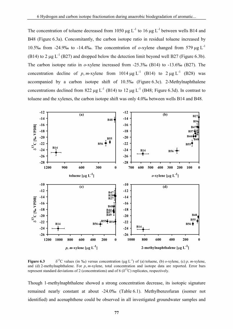
6 Hydrogen and carbon isotope fractionation during anaerobic biodegradation of aromatic...
77
The concentration of toluene decreased from 1050 �g L-1 to 16 �g L-1 between wells B14 and
B48 (Figure 6.3a). Concomitantly, the carbon isotope ratio in residual toluene increased by
10.5‰ from -24.9‰ to -14.4‰. The concentration of o-xylene changed from 579 �g L-1
(B14) to 2 �g L-1 (B27) and dropped below the detection limit beyond well B27 (Figure 6.3b).
The carbon isotope ratio in o-xylene increased from -25.3‰ (B14) to -13.6‰ (B27). The
concentration decline of p, m-xylene from 1014 �g L-1 (B14) to 2 �g L-1 (B28) was
accompanied by a carbon isotope shift of 10.5‰ (Figure 6.3c). 2-Methylnaphthalene
concentrations declined from 822 �g L-1 (B14) to 12 �g L-1 (B48; Figure 6.3d). In contrast to
toluene and the xylenes, the carbon isotope shift was only 4.0‰ between wells B14 and B48.
Figure 6.3 �13C values (in ‰) versus concentration (�g L-1) of (a) toluene, (b) o-xylene, (c) p, m-xylene, and (d) 2-methylnaphthalene. For p, m-xylene, total concentration and isotope data are reported. Error bars represent standard deviations of 2 (concentrations) and of 6 (�13C) replicates, respectively.
Though 1-methylnaphthalene showed a strong concentration decrease, its isotopic signature
remained nearly constant at about -24.0‰ (Table 6.1). Methylbenzofuran (isomer not
identified) and acenaphthene could be observed in all investigated groundwater samples and
toluene [�g L-1]
03006009001200
�13
C [‰
VPD
B]
-28
-26
-24
-22
-20
-18
-16
-14
-12
B14B56
B48
B55
(a)
p, m-xylene [�g L-1]
020040060080010001200
�13
C [‰
VPD
B]
-26
-24
-22
-20
-18
-16
-14
-12
-10
B14 B56B55 B54
(c)
B49B57B44B48
B47B28B27
o-xylene [�g L-1]
0100200300400500600700-28
-26
-24
-22
-20
-18
-16
-14
-12
B14 B56
B55
(b)
B44B48
B49B57
B47
B54
B27
a)d)
2-methylnaphthalene [�g L-1]
02004006008001000-26
-24
-22
-20
-18
-16
-14
-12
-10
B14B56
B55B48
(d)
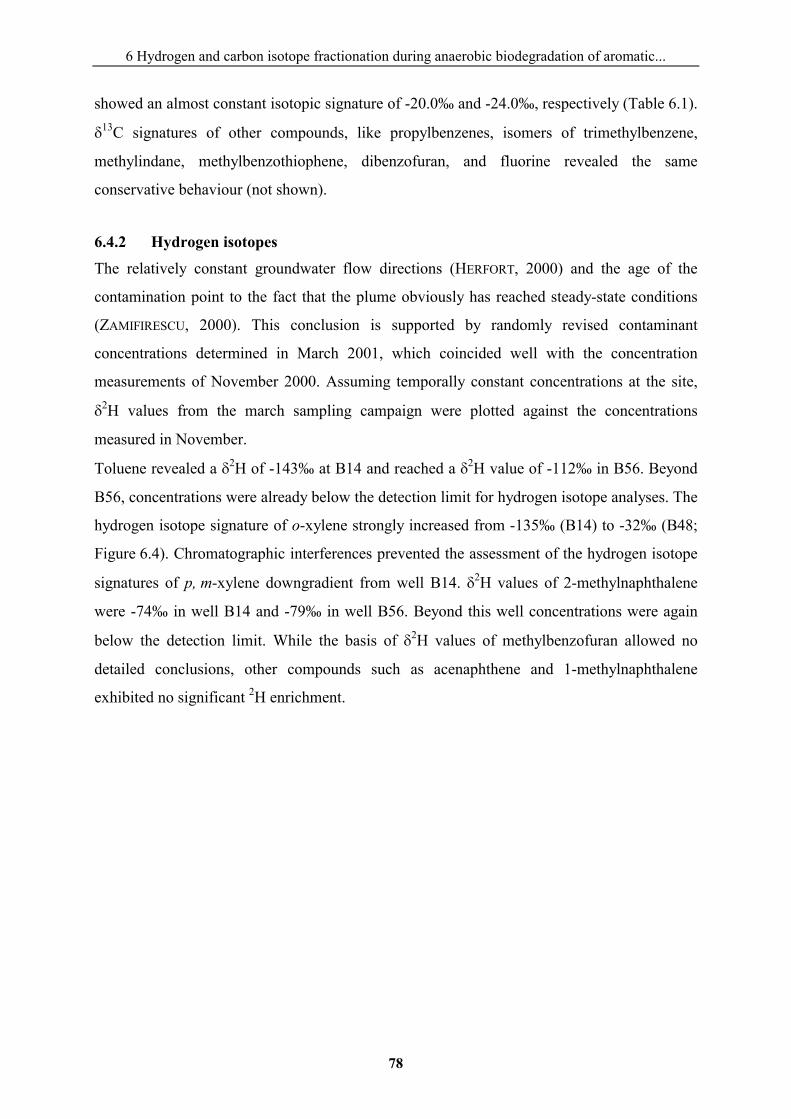
6 Hydrogen and carbon isotope fractionation during anaerobic biodegradation of aromatic...
78
showed an almost constant isotopic signature of -20.0‰ and -24.0‰, respectively (Table 6.1).
�13C signatures of other compounds, like propylbenzenes, isomers of trimethylbenzene,
methylindane, methylbenzothiophene, dibenzofuran, and fluorine revealed the same
conservative behaviour (not shown).
6.4.2 Hydrogen isotopes
The relatively constant groundwater flow directions (HERFORT, 2000) and the age of the
contamination point to the fact that the plume obviously has reached steady-state conditions
(ZAMIFIRESCU, 2000). This conclusion is supported by randomly revised contaminant
concentrations determined in March 2001, which coincided well with the concentration
measurements of November 2000. Assuming temporally constant concentrations at the site,
�2H values from the march sampling campaign were plotted against the concentrations
measured in November.
Toluene revealed a �2H of -143‰ at B14 and reached a �2H value of -112‰ in B56. Beyond
B56, concentrations were already below the detection limit for hydrogen isotope analyses. The
hydrogen isotope signature of o-xylene strongly increased from -135‰ (B14) to -32‰ (B48;
Figure 6.4). Chromatographic interferences prevented the assessment of the hydrogen isotope
signatures of p, m-xylene downgradient from well B14. �2H values of 2-methylnaphthalene
were -74‰ in well B14 and -79‰ in well B56. Beyond this well concentrations were again
below the detection limit. While the basis of �2H values of methylbenzofuran allowed no
detailed conclusions, other compounds such as acenaphthene and 1-methylnaphthalene
exhibited no significant 2H enrichment.
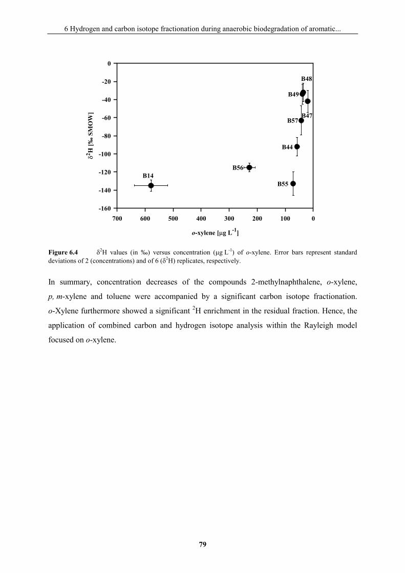
6 Hydrogen and carbon isotope fractionation during anaerobic biodegradation of aromatic...
79
Figure 6.4 �2H values (in ‰) versus concentration (�g L-1) of o-xylene. Error bars represent standard deviations of 2 (concentrations) and of 6 (�2H) replicates, respectively.
In summary, concentration decreases of the compounds 2-methylnaphthalene, o-xylene,
p, m-xylene and toluene were accompanied by a significant carbon isotope fractionation.
o-Xylene furthermore showed a significant 2H enrichment in the residual fraction. Hence, the
application of combined carbon and hydrogen isotope analysis within the Rayleigh model
focused on o-xylene.
a)
o-xylene [�g L-1]
0100200300400500600700
�2 H
[‰ S
MO
W]
-160
-140
-120
-100
-80
-60
-40
-20
0
B14B56
B48
B55
B47
B44
B57
B49
6 Hydrogen and carbon isotope fractionation during anaerobic biodegradation of aromatic...
80
6.5 Discussion
6.5.1 Isotopic fractionation
The occurrence of an isotope effect in the rate-determining step is considered as a prerequisite
for isotopic fractionation. A strong primary kinetic isotope effect with respect to an element
occurs if in the rate-limiting step a bond containing this element is formed or broken
(HUNKELER et al., 2003). Additionally, weaker, secondary isotope effects are observed when
the element in question is adjacent to the bond that is broken or formed (HUNKELER et al.,
2001b; GRAY et al., 2002; KOLHATKAR et al., 2002). In a former study we found that under
sulfate-reducing conditions 2-methylnaphthalene is activated by fumarate addition to the
methyl group, which includes a preceding C-H bond breakage in the rate-limiting step
(ANNWEILER et al., 2000a). Consistently, in our study biodegradation of 2-methylnaphthalene
was associated with a carbon isotope fractionation (Figure 6.3d). Similarly, we observed a
significant 13C enrichment during the biodegradation of toluene (Figure 6.3a), o-xylene
(Figure 6.3b), and p, m-xylene (Figure 6.3c). Probably these fractionations were also caused
by a C-H bond cleavage (KRIEGER et al., 1999) during the enzymatic attack of fumarate on the
methyl group(s) of both, toluene and xylenes (BIEGERT et al., 1996; BELLER and SPORMANN,
1997a; BELLER, 2000; BELLER and EDWARDS, 2000). This conclusion is also supported by the
large 2H enrichment in the residual o-xylene fraction (Figure 6.4). Conversely, we did not
observe any resolvable isotope fractionation for the concentration decrease of 1-methyl-
naphthalene (Table 6.1). Either 1-methylnaphthalene was not biodegraded or the degradation
was not initiated by benzylsuccinate synthase with a corresponding preliminary C-H bond
scission in the rate-determining step. For several reasons the latter possibility is favoured:
(1) 1-methylnaphthalene displayed a concentration decrease similar to 2-methylnaphthalene,
that apparently was biodegraded. (2) In several studies biodegradation of 1-methylnaphthalene
under anaerobic conditions was observed (SHARAK GENTHNER et al., 1997; ROTHERMICH et
al., 2002). (3) To our knowledge, the addition of fumarate to the methyl group of 1-me-
thylnaphthalene in the rate-determining step could not be demonstrated by laboratory studies.
Due to additional entries (B49) and the slow concentration decrease along the groundwater
flow path, acenaphthene could be detected in significant concentrations (148 �g L-1) until the
northern boundary of the site (B42). This finding agrees with the frequently observed
resistance of 3-ring PAH to anaerobic biodegradation (ARONSON and HOWARD, 1997). The
lack of an observable isotope effect in these samples (Table 6.1) may also be explained by the
6 Hydrogen and carbon isotope fractionation during anaerobic biodegradation of aromatic...
81
fact that particularly for the small enrichment factors expected for large molecules
(HARRINGTON et al., 1999), significant isotopic shifts can only be detected when a large
percentage of the contaminant is degraded.
Although we observed a pronounced concentration decrease for methylbenzofuran from 489
to 3 �g L-1, derivatives of benzofuran, containing a ring-ether bond, are considered to be
recalcitrant in anaerobic groundwaters (ROCKNE and STRAND, 1998; ZAMFIRESCU and
GRATHWOHL, 2001). At this point, we can only conclude that the data for both acenaphthene
and methylbenzofuran are consistent with either no biodegradation, or no observable isotope
effect associated with biodegradation. However, further laboratory studies, elucidating the
biochemical degradation pathways are needed at this point.
6.5.2 Biodegradation, dilution, and dissolution processes in the Rayleigh model
The application of the Rayleigh model can lead to a successful evaluation of biodegradation in
field studies. If other processes, like dissolution from NAPL or dilution, are involved, the
typical Rayleigh behaviour is not detected. Concentration and isotope data of several wells
(Figure 6.5, field site well numbers in brackets) either show a strong Rayleigh behaviour or
suggest major influences from other processes than biodegradation. Biodegradation is
associated with decreasing concentrations (ln f is shifted to more negative values) as well as
increasing Rt values [103ln(Rt/R0) is increasing] resulting in the indicated shift (Figure 6.5a).
In contrast, concurrent dissolution from NAPL (with identical isotope signature as the
presumed source) shows a trend toward the original �13C value [103ln(Rt/R0) is decreasing]
and elevates the concentration (ln f is increasing; Figure 6.5b). Processes other than
biodegradation (e.g., dilution, sorption, dispersion) causing a decrease of concentration are
thought to induce hardly any isotope effect (HARRINGTON et al., 1999; SLATER et al., 2000).
Thus, in the Rayleigh plot these processes would shift the position of resulting data points
horizontally to a position of lower concentration to the right (Figure 6.5c).
In general, if the presence of NAPLs can be excluded, data points at the extreme left side of
the diagram represent the wells least influenced by sorption, dispersion, or dilution.
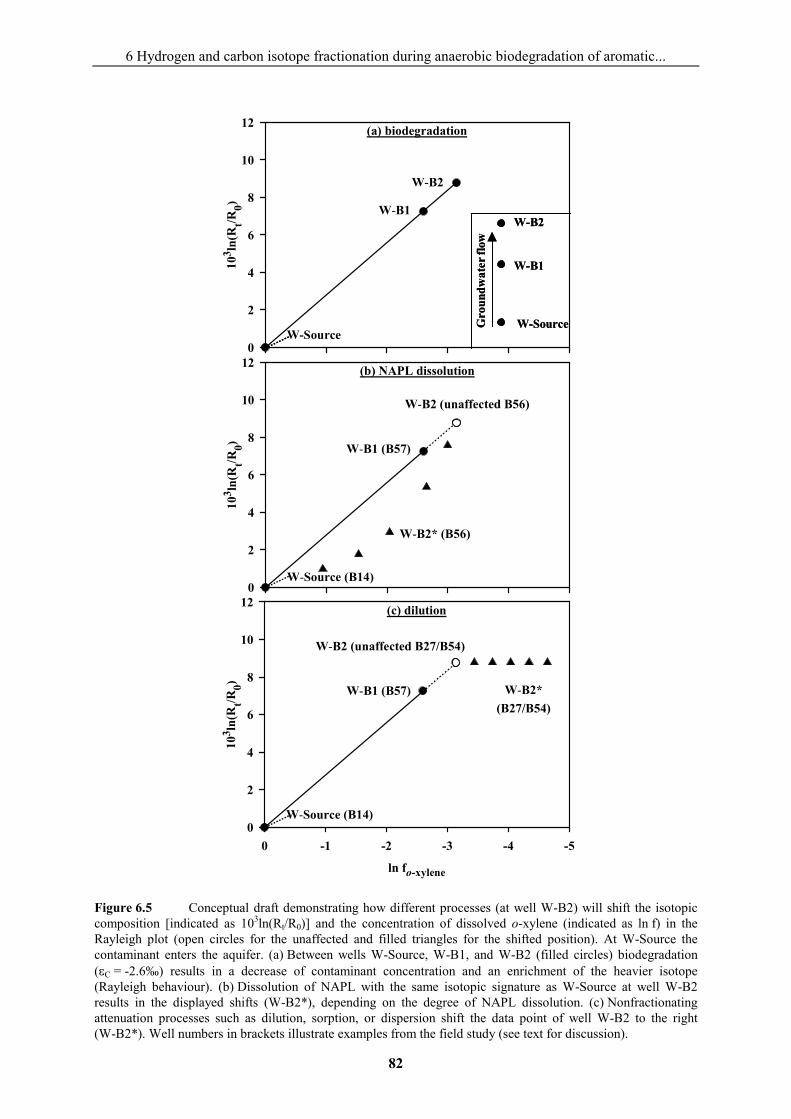
6 Hydrogen and carbon isotope fractionation during anaerobic biodegradation of aromatic...
82
Figure 6.5 Conceptual draft demonstrating how different processes (at well W-B2) will shift the isotopic composition [indicated as 103ln(Rt/R0)] and the concentration of dissolved o-xylene (indicated as ln f) in the Rayleigh plot (open circles for the unaffected and filled triangles for the shifted position). At W-Source the contaminant enters the aquifer. (a) Between wells W-Source, W-B1, and W-B2 (filled circles) biodegradation (�C = -2.6‰) results in a decrease of contaminant concentration and an enrichment of the heavier isotope (Rayleigh behaviour). (b) Dissolution of NAPL with the same isotopic signature as W-Source at well W-B2 results in the displayed shifts (W-B2*), depending on the degree of NAPL dissolution. (c) Nonfractionating attenuation processes such as dilution, sorption, or dispersion shift the data point of well W-B2 to the right (W-B2*). Well numbers in brackets illustrate examples from the field study (see text for discussion).
B14
103 ln
(Rt/R
0)
0
2
4
6
8
10
12
W-Source
W-B1
(a) biodegradation
W-B2
B14
103 ln
(Rt/R
0)
0
2
4
6
8
10
12
W-Source (B14)
W-B1 (B57)
(b) NAPL dissolution
W-B2 (unaffected B56)
W-B2* (B56)
B14
ln fo-xylene
-5-4-3-2-10
103 ln
(Rt/R
0)
0
2
4
6
8
10
12
W-Source (B14)
W-B1 (B57)
(c) dilution
W-B2 (unaffected B27/B54)
W-B2*(B27/B54)
W-Source
W-B1
W-B2
Gro
undw
ater
flow
B14
103 ln
(Rt/R
0)
0
2
4
6
8
10
12
W-Source
W-B1
(a) biodegradation
W-B2
B14
103 ln
(Rt/R
0)
0
2
4
6
8
10
12
W-Source (B14)
W-B1 (B57)
(b) NAPL dissolution
W-B2 (unaffected B56)
W-B2* (B56)
B14
ln fo-xylene
-5-4-3-2-10
103 ln
(Rt/R
0)
0
2
4
6
8
10
12
W-Source (B14)
W-B1 (B57)
(c) dilution
W-B2 (unaffected B27/B54)
W-B2*(B27/B54)
W-Source
W-B1
W-B2
Gro
undw
ater
flow
W-Source
W-B1
W-B2
Gro
undw
ater
flow
6 Hydrogen and carbon isotope fractionation during anaerobic biodegradation of aromatic...
83
For o-xylene, ln(Rt/R0) of our field data was plotted versus ln f according to Eq. (6-1)
(Figure 6.6a). Recent studies indicate that the subsurface area at wells B44, B57, and B47 was
nearly free of NAPLs (ZAMFIRESCU and GRATHWOHL, 2001; BOCKELMANN et al., 2003).
Consequently, starting from B14, the effect of biodegradation is best illustrated at these four
wells. Using least-squares linear regression, a carbon isotope enrichment factor of
C = -2.6‰ � 0.7‰ was calculated. While the consideration of all data points in Figure 6.6a
provides a similar carbon isotope enrichment factor (C = -2.2‰ � 0.5‰), the resulting
correlation factor r2 (0.96) is inferior to that calculated from the four-well approach (0.99).
These findings suggest that despite the complexity of the site, the enrichment factors
calculated by using only four wells, or using them all are quite robust. However, the better
correlation between isotope and concentration data strengthens the performed exclusion of
particular wells. Hence, quantifications should be restricted to the wells lying on the transect
B14-B47. Accordingly, o-xylene loss from 58 �g L-1 (B44) to 20 �g L-1 (B47) is almost
exclusively caused by biodegradation. The carbon isotope enrichment factor
C = -2.6‰ � 0.7‰ (Figure 6a) calculated from our field study data (wells B14, B44, B57,
B47) is much larger than that observed for the biodegradation of o-xylene in laboratory studies
(C = -1.1‰; VIETH et al., 2001). A very similar enrichment factor of -2.1‰ for o-xylene was
obtained by GRIEBLER et al. (2003) for the same field site. This underlines the difficulties in
extrapolating laboratory derived enrichment factors to field situations. While the anaerobic
toluene degradation by distinct bacterial strains was associated with a similar enrichment
factor (MECKENSTOCK et al., 1999), recent studies on the anaerobic degradation of chlorinated
ethenes (SLATER et al., 2001) and benzene (MANCINI et al., 2003) by different microbial
consortia revealed a considerable variability in carbon isotope fractionation. Additionally, the
determination of a-field derived enrichment factor comprehends various sources of error.
Unlike the controlled conditions in the laboratory, where decreasing concentrations are
exclusively caused by biodegradation, abiotic processes in field studies (even if
biodegradation is the dominant process) cannot be ruled out and might alter the observed
enrichment factor.
Well B56, although located downstream of the wells B44 and B57, shows a higher o-xylene
concentration and 13C depleted isotope values (-24.3‰) compared to wells B44 (-19.7‰) and
B57 (-18.1‰). The trend toward the original �13C value (-25.3‰) and enhanced
concentrations relative to wells B57 and B44 indicates the influence of an additional source of
o-xylene at (or close to) well B56 (compare to Figure 6.5b). This is substantiated by the
6 Hydrogen and carbon isotope fractionation during anaerobic biodegradation of aromatic...
84
reported presence of NAPL in well B56 (ZAMFIRESCU and GRATHWOHL, 2001; BOCKELMANN
et al., 2003) and our data, suggesting �13C values in the range from -25.3‰ to -24.2‰ for the
o-xylene sources (Table 6.2). Data points of wells B54 and B27 are shifted to lower
concentrations, suggesting dilution processes. Dilution is also indicated by a relatively low
dissolved organic carbon content (DOC) for both wells (ANNWEILER, 1999) and enhanced
nitrate concentration at well B27 (SCHÄFLE, 1997). Apparently, at well B27 the contaminated
groundwater is diluted by pristine water from the adjacent Keuper hills. For well B49 tracer
tests demonstrated the lack of a hydraulic connection with the majority of the other wells
shown in Figure 6.6a (HERFORT, 2000). For well B55 no tracer tests are available, but due to
the determined groundwater flow direction from south to north/northwest, a hydrologic
conjunction with the other considered wells is very unlikely.
The Rayleigh plot for the stable hydrogen isotopes of the o-xylene (Figure 6.6b), while
substantiating the presence of NAPL phase close to well B56, provides useful additional
information. The stable hydrogen isotope enrichment factor for the o-xylene biodegradation
between wells B14, B44, B57, and B47 accounts for H = -29.6‰ and is very similar to that
(-29‰) determined by MANCINI et al. (2003) for benzene biodegradation under nitrate-
reducing conditions. o-xylene in samples from the wells B14 and B55 shows similar �2H
values (-135‰ and -133‰, respectively) however, the measured 13C enrichment at well B55
(-21.9‰) points to an advanced biodegradation. Unlike the �13C values, the �2H signatures of
hydrocarbons from different sources can cover a wide isotopic range (HUNKELER et al., 2001a;
POND et al., 2002). This applies also for the �2H values of possible o-xylene sources in our
field study (Table 6.2). Hence, well B55 may be influenced by an additional source in the
north, characterized by lower hydrogen isotope values than those observed at well B14, B15,
or B22. The hydrogen isotope signature suggests that there is no hydraulic connection between
wells B55 and B14.
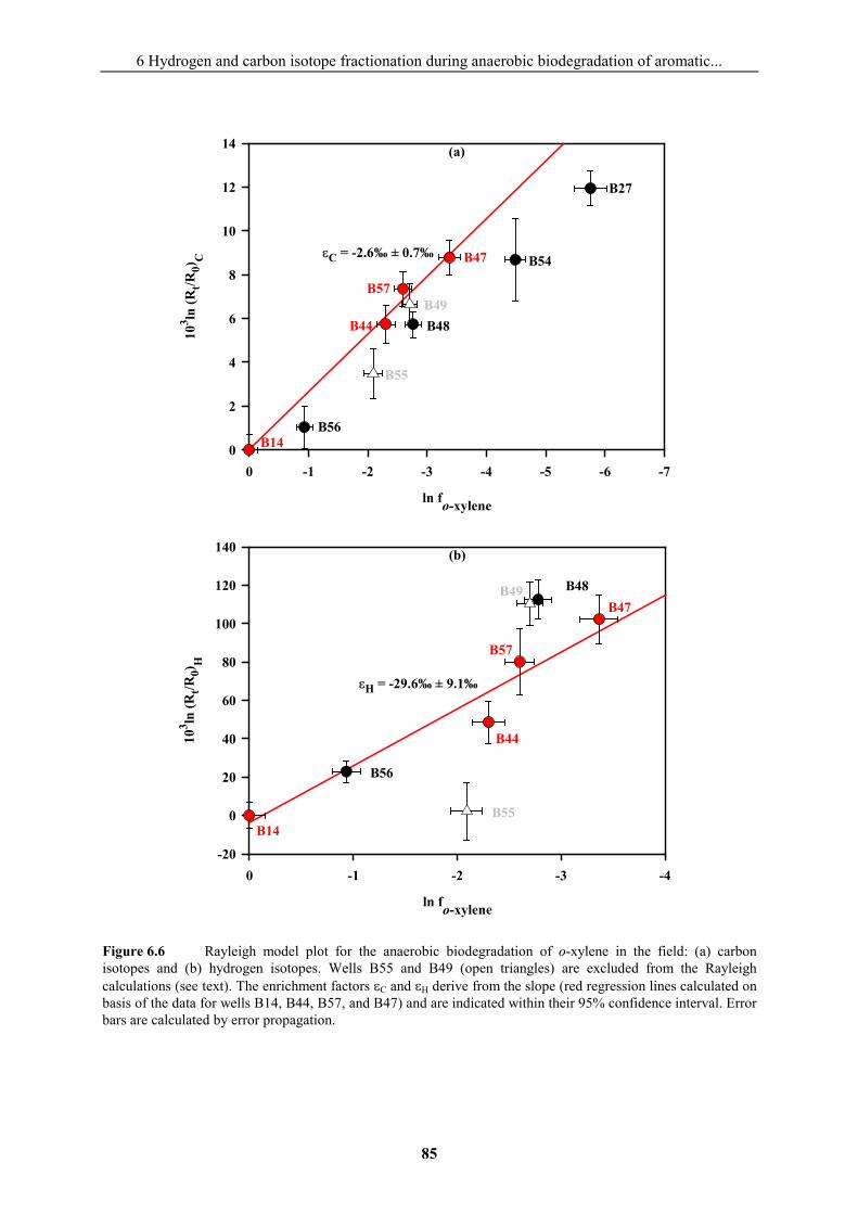
6 Hydrogen and carbon isotope fractionation during anaerobic biodegradation of aromatic...
85
Figure 6.6 Rayleigh model plot for the anaerobic biodegradation of o-xylene in the field: (a) carbon isotopes and (b) hydrogen isotopes. Wells B55 and B49 (open triangles) are excluded from the Rayleigh calculations (see text). The enrichment factors �C and �H derive from the slope (red regression lines calculated on basis of the data for wells B14, B44, B57, and B47) and are indicated within their 95% confidence interval. Error bars are calculated by error propagation.
B14
ln fo-xylene
-4-3-2-10
103 ln
(Rt/R
0)H
-20
0
20
40
60
80
100
120
140
B56
B55
B49 B48B47
B14
B44
B57
�H = -29.6‰ ± 9.1‰
(b)
B14
ln fo-xylene
-7-6-5-4-3-2-10
103 ln
(Rt/R
0)C
0
2
4
6
8
10
12
14
B56
B55
B49B48
B47 B54
B27
B14
B44
B57
(a)
�C = -2.6‰ ± 0.7‰
B14
ln fo-xylene
-4-3-2-10
103 ln
(Rt/R
0)H
-20
0
20
40
60
80
100
120
140
B56
B55
B49 B48B47
B14
B44
B57
�H = -29.6‰ ± 9.1‰
(b)
B14
ln fo-xylene
-7-6-5-4-3-2-10
103 ln
(Rt/R
0)C
0
2
4
6
8
10
12
14
B56
B55
B49B48
B47 B54
B27
B14
B44
B57
(a)
�C = -2.6‰ ± 0.7‰
6 Hydrogen and carbon isotope fractionation during anaerobic biodegradation of aromatic...
86
6.5.3 Implications
Major goal of the present study was to apply simultaneous carbon and hydrogen isotope
analyses of contaminants in a complex field site. The method was expected to provide useful
information on different processes influencing the dynamics of the spilled compounds:
(1) extent of biodegradation, (2) microbiological degradation pathways, (3) dissolution from
NAPL, and (4) dilution by uncontaminated groundwater. Recent reports on laboratory studies
postulated that the initial step in the enzymatic transformation of benzene and toluene
determines the isotope fractionation (HUNKELER et al., 2001a; MORASCH et al., 2001;
MANCINI et al., 2003). This suggestion appears to be also appropriate for the biotic and abiotic
degradation of trichloroethene (BARTH et al., 2002; POULSON and NARAOKA, 2002;
HUNKELER et al., 2003) and the aerobic transformation of 1,2-dichloroethane (HUNKELER and
ARAVENA, 2000a). Our field data provided evidence for this concept in the case of the
anaerobic in situ degradation of toluene. In addition, the isotope fractionations observed for
o-xylene, p, m-xylene, and 2-methylnaphthalene could well be related to established
biochemical degradation pathways, each involving a C-H bond cleavage in the rate-
determining step. In contrast, the conservative isotopic behaviour of 1-methylnaphthalene
suggests, that the supposed biodegradation probably is not initiated by benzylsuccinate
synthase as in the case of 2-methylnaphthalene. Data of acenaphthene and methylbenzofuran
do not allow the use of isotopic fractionation for mechanistic interpretations at present.
Furthermore, the approach can be successfully applied even in complex aquifer systems with
effects such as dissolution from NAPL, infiltration of pristine water, and the lack of hydraulic
connections between wells.
6.6 Acknowledgements This paper represents a publication of the Priority Program 546 "Geochemical processes with
long-term effects in anthropogenically-affected seepage- and ground-water". Financial support
was provided by the Deutsche Forschungsgemeinschaft. The authors thank Dr. Siegmund Ertl
for measuring �13C values of organic standards, Frank Schellig for his support during the
sampling campaigns, and Martin Blumenberg for technical support. Furthermore, the authors
thank Prof. Dr. Peter Schreier for �2H measurements of our standards via EA-P-IRMS. We
also thank the anonymous reviewers, whose comments have improved the quality of this
paper.
7 Assessing microbial degradation of o-xylene at field-scale from the reduction in mass flow rate…
87
Assessing microbial degradation of o-xylene at field-scale from the
reduction in mass flow rate combined with compound-specific
isotope analyses
Journal of Contaminant Hydrology
in press
Peter A., Steinbach A., Liedl R., Ptak T., Michaelis W., and Teutsch G.
7 Assessing microbial degradation of o-xylene at field-scale from the reduction in mass flow rate…
88
7.1 Abstract In recent years Natural Attenuation (NA) has evolved into a possible remediation alternative,
especially in the case of BTEX spills. In order to be approved by the regulators,
biodegradation needs to be demonstrated which requires efficient site investigation and
monitoring tools. Three methods - the Integral Groundwater Investigation method, the
compound specific isotope analysis and a newly developed combination of both - were used in
this work to quantify at field scale the biodegradation of o-xylene at a former gasworks site
which is heavily contaminated with BTEX and PAHs. First, the Integral Groundwater
Investigation method (SCHWARZ et al., 1998; TEUTSCH et al., 2000) was applied, that allows
the determination of mass flow rates of o-xylene by integral pumping tests. Concentration
time series obtained during pumping at two wells were used to calculate inversely
contaminant mass flow rates at the two control planes that are defined by the diameter of the
maximum isochrone. A reactive transport model was used within a Monte Carlo approach to
identify biodegradation as the dominant process for reduction in the contaminant mass flow
rate between the two consecutive control planes. Secondly, compound-specific carbon isotope
analyses of o-xylene were performed on the basis of point-scale samples from the same two
wells. The Rayleigh equation was used to quantify the degree of biodegradation that occurred
between the wells. Thirdly, a combination of the Integral Groundwater Investigation method
and the compound-specific isotope analysis was developed and applied. It comprises isotope
measurements during the integral pumping tests and the evaluation of �13C time series by an
inversion algorithm to obtain spatially integrated mean isotope values at the control planes. It
was shown that the Rayleigh equation is applicable to spatially integrated mean isotope values
in order to obtain the mean biodegradation between the consecutive control planes. All three
approaches yielded consistently a 98-99% degradation of o-xylene.
7.2 Introduction The growing importance of natural attenuation (NA) as part of an overall site remediation
strategy requires the development of tools to confirm the evidence that NA is occurring at a
specific site. Several strategies, such as dense spatial and temporal monitoring of contaminant
and electron acceptor concentrations at the considered sites have been applied (e.g. GIEG et
al., 1999). However, due to subsurface heterogeneity, the investigation by point-scale
measurements of groundwater head or concentration obtained at single wells might lead to
unacceptable levels of uncertainty with respect to the flow and/or contamination situation. In
7 Assessing microbial degradation of o-xylene at field-scale from the reduction in mass flow rate…
89
contrast to concentration measurements, mass flow rates determined at several control planes
consecutively downgradient of the contaminant source allow an estimate on the mass decrease
over space and/or time. Mass flow rates can be determined for instance by sampling a “fence”
of densely located multilevel wells across the suspected contaminant plume (BORDEN et al.,
1997; KING et al., 1999). Summing up the product of the contaminant concentration and the
respective volumetric discharge at each sampling point then yields a contaminant mass flow
rate for the complete groundwater fence or control plane. However, even a spatially highly
resolved monitoring network may not allow the determination of mass flow rates at a high
level of certainty due to subsurface heterogeneity as pointed out before. Alternatively, the
Integral Groundwater Investigation method increases the reliability and requires only a
reduced number of monitoring wells. The idea of this method is to increase the sampling
volume by pumping and sampling over a considerable period of time at each well (TEUTSCH et
al., 2000). This enlargement of the sampling volume reduces the uncertainty by sampling the
heterogeneous flow system without resolving it spatially. Thus, also low conductivity zones
contribute according to their flow weighted discharge to the sampled water. By applying an
inversion algorithm, the concentration time series obtained during pumping is transformed
into a spatial concentration distribution along the control plane (SCHWARZ et al., 1998;
TEUTSCH et al., 2000). The control plane is defined by the diameter of the maximum
isochrone perpendicular to groundwater flow. The spatial concentration distribution at the
control plane allows the determination of a spatially averaged concentration and consequently
of the mass flow rate across the control plane. The Integral Groundwater Investigation method
was successfully applied e.g. by BOCKELMANN et al. (2001) and BAUER et al. (2003). At a
former gasworks site in Southwest Germany, BOCKELMANN et al. (2001) could demonstrate a
significant decrease in BTEX and PAH mass flow rates at distances of 140 and 280 m
downgradient of the source. A method comparison between the groundwater fence method
and the Integral Groundwater Investigation method was performed at the Borden site
(BÉLAND-PELLETIER et al., 2003). The total BTEX mass flow rates determined by both
methods deviated by 33%, which lay within the calculated range of uncertainty of, in this case,
34-41% for both methods.
The reduction of contaminant mass in the plume along the flow path is a direct proof of
natural attenuation at field scale. A further method to demonstrate microbial degradation
directly at field scale is the compound-specific isotope analysis (CSIA). During the microbial
degradation of benzene (HUNKELER et al., 2001a), toluene (MECKENSTOCK et al., 1999; AHAD
7 Assessing microbial degradation of o-xylene at field-scale from the reduction in mass flow rate…
90
et al., 2000; STEINBACH et al., 2004), methyl tert-butyl ether (HUNKELER et al., 2001b;
KOLHATKAR et al., 2002) and chlorinated compounds (HUNKELER et al., 1999; SLATER et al.,
2001) an enrichment of the 13C isotope in the remaining nondegraded contaminant fraction
was observed. This kinetic isotope effect occurs because molecular bonds formed by 12C have
a higher vibrational energy than those containing 13C and hence are easier to break.
Accordingly, the resulting differences in reaction rates lead to an enrichment of the heavy
isotopes in the remaining contaminant fraction, while the product is enriched in 12C. The
relation between the changed isotope ratio R of a compound caused by biodegradation and the
decreased concentration C compared to the initial isotope ratio R0 and concentration C0 can be
expressed by the Rayleigh equation (MARIOTTI, 1986):
1
00 C C
R R
��
���
����
�� (7-1)
where � denotes the fractionation factor.
Two major prerequisites have to be fulfilled for a field-scale application of CSIA in
combination with the Rayleigh equation as a means for demonstrating and quantifying biode-
gradation: First, biodegradation has to be the only process that causes a significant
fractionation of the considered isotopes and secondly, for quantifying biodegradation the
appropriate fractionation factor � for field conditions has to be known. Several studies
revealed that physico-chemical processes like volatilisation from both the aqueous and the
organic phase as well as sorption do not produce significant isotope fractionation
(HARRINGTON et al., 1999; SLATER et al., 2000). Furthermore, SLATER et al. (1999) and
HUNKELER and ARAVENA (2000b) demonstrated that analytical sampling and preconcentration
techniques do not produce measurable changes in the isotope ratios. The second important
prerequisite for the application of the Rayleigh model is that the laboratory derived
fractionation factors can be transferred to field-scale. HUNKELER et al. (1999) investigated
fractionation during dechlorination of perchloroethylene (PCE) in both microcosm and field
studies. Although they did not quantify the fractionation using the Rayleigh equation,
fractionation patterns of PCE and its products corresponded well, so that they concluded that
microcosm data can be used for the interpretation of isotope data obtained in the field.
Toluene degradation studies with four distinct toluene-degrading bacterial strains provided a
similar fractionation factor for varying redox conditions (MECKENSTOCK et al., 1999). Since
the anaerobic toluene degradation with different bacteria is initiated by benzylsuccinate
7 Assessing microbial degradation of o-xylene at field-scale from the reduction in mass flow rate…
91
synthase (BELLER, 2000), the carbon isotope fractionation factor for toluene apparently
depends on the first enzyme reaction in the degradation pathway (MORASCH et al., 2001). The
initial activation step for o-xylene degradation with sulfate reducing and denitrifying bacteria
comprises - like for toluene - the addition of fumarate to the methyl group (BELLER and
SPORMANN, 1997b; WILKES et al., 2000). Accordingly, the only so far available fractionation
factor for the anaerobic o-xylene degradation, determined under sulfate reducing conditions
(VIETH et al., 2001), should also be valid for other anoxic redox conditions. Recently, this
fractionation factor was successfully applied to quantify the extent of in situ biodegradation of
o-xylene in a contaminated anoxic aquifer (RICHNOW et al., 2003). Additionally, it could be
proven that variations in temperature had no influence on the isotope fractionation (MORASCH
et al., 2001). SHERWOOD LOLLAR et al. (2001) measured carbon isotope ratios of PCE and
trichloroethylene (TCE) at the Dover Air Force Base along a transect and observed a
significant 13C enrichment in the nondegraded fraction. By using fractionation factors from the
literature, they quantified the degree of biodegradation of TCE using the Rayleigh equation to
be between 40.5-66.2%.
The application of the compound specific isotope analysis requires that the hydraulic
conditions at a field site are well known in order to ensure that the contaminant observed at
single wells indeed originate from the suspected upstream source. Furthermore, as in the case
of point-scale concentration measurements, the point-scale isotope values obtained from
single well sampling need to be representative for the aquifer system. Here again the hydraulic
as well as the hydrogeochemical heterogeneity of the system may require a very large number
of observation wells, which is usually not found at a field site in practice. A reliable and
representative determination of the degree of biodegradation based on CSIA therefore requires
a dense monitoring network that covers both the fringes and the centre of the contaminant
plume(s).
To overcome these limitations, in this paper a combined approach comprising the CSIA and
the Integral Groundwater Investigation method is developed and demonstrated in the field.
Combining both methods increases the applicability and reliability of the commonly used
CSIA as the sampling volume for the isotope measurements is enlarged due to pumping and,
thus, the data derived is more representative than point-scale measurements in a potentially
heterogeneous aquifer. These integral scale compound-specific isotope analyses then allow the
determination of spatially integrated mean isotope concentrations at individual control planes
by applying the inversion algorithm. By comparing the change of mean isotope values
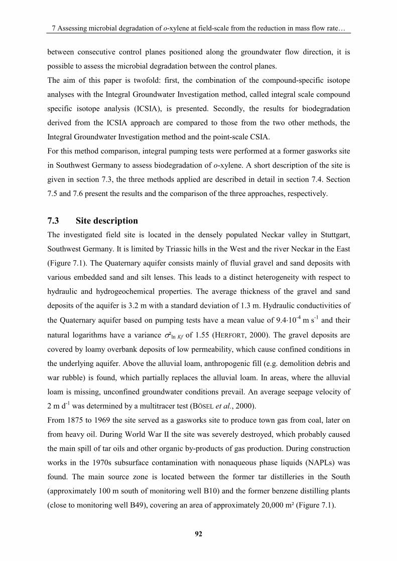
7 Assessing microbial degradation of o-xylene at field-scale from the reduction in mass flow rate…
92
between consecutive control planes positioned along the groundwater flow direction, it is
possible to assess the microbial degradation between the control planes.
The aim of this paper is twofold: first, the combination of the compound-specific isotope
analyses with the Integral Groundwater Investigation method, called integral scale compound
specific isotope analysis (ICSIA), is presented. Secondly, the results for biodegradation
derived from the ICSIA approach are compared to those from the two other methods, the
Integral Groundwater Investigation method and the point-scale CSIA.
For this method comparison, integral pumping tests were performed at a former gasworks site
in Southwest Germany to assess biodegradation of o-xylene. A short description of the site is
given in section 7.3, the three methods applied are described in detail in section 7.4. Section
7.5 and 7.6 present the results and the comparison of the three approaches, respectively.
7.3 Site description The investigated field site is located in the densely populated Neckar valley in Stuttgart,
Southwest Germany. It is limited by Triassic hills in the West and the river Neckar in the East
(Figure 7.1). The Quaternary aquifer consists mainly of fluvial gravel and sand deposits with
various embedded sand and silt lenses. This leads to a distinct heterogeneity with respect to
hydraulic and hydrogeochemical properties. The average thickness of the gravel and sand
deposits of the aquifer is 3.2 m with a standard deviation of 1.3 m. Hydraulic conductivities of
the Quaternary aquifer based on pumping tests have a mean value of 9.4�10-4 m s-1 and their
natural logarithms have a variance �²ln Kf of 1.55 (HERFORT, 2000). The gravel deposits are
covered by loamy overbank deposits of low permeability, which cause confined conditions in
the underlying aquifer. Above the alluvial loam, anthropogenic fill (e.g. demolition debris and
war rubble) is found, which partially replaces the alluvial loam. In areas, where the alluvial
loam is missing, unconfined groundwater conditions prevail. An average seepage velocity of
2 m d-1 was determined by a multitracer test (BÖSEL et al., 2000).
From 1875 to 1969 the site served as a gasworks site to produce town gas from coal, later on
from heavy oil. During World War II the site was severely destroyed, which probably caused
the main spill of tar oils and other organic by-products of gas production. During construction
works in the 1970s subsurface contamination with nonaqueous phase liquids (NAPLs) was
found. The main source zone is located between the former tar distilleries in the South
(approximately 100 m south of monitoring well B10) and the former benzene distilling plants
(close to monitoring well B49), covering an area of approximately 20,000 m² (Figure 7.1).
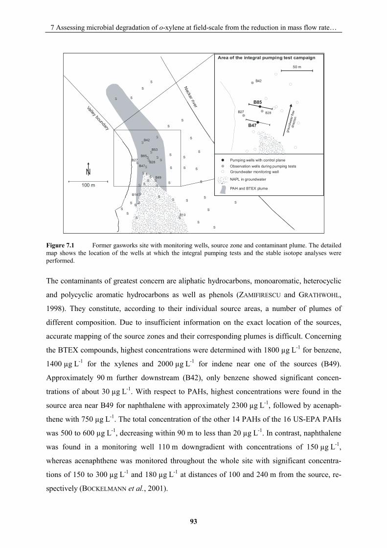
7 Assessing microbial degradation of o-xylene at field-scale from the reduction in mass flow rate…
93
Figure 7.1 Former gasworks site with monitoring wells, source zone and contaminant plume. The detailed map shows the location of the wells at which the integral pumping tests and the stable isotope analyses were performed.
The contaminants of greatest concern are aliphatic hydrocarbons, monoaromatic, heterocyclic
and polycyclic aromatic hydrocarbons as well as phenols (ZAMIFIRESCU and GRATHWOHL,
1998). They constitute, according to their individual source areas, a number of plumes of
different composition. Due to insufficient information on the exact location of the sources,
accurate mapping of the source zones and their corresponding plumes is difficult. Concerning
the BTEX compounds, highest concentrations were determined with 1800 µg L-1 for benzene,
1400 µg L-1 for the xylenes and 2000 µg L-1 for indene near one of the sources (B49).
Approximately 90 m further downstream (B42), only benzene showed significant concen-
trations of about 30 µg L-1. With respect to PAHs, highest concentrations were found in the
source area near B49 for naphthalene with approximately 2300 µg L-1, followed by acenaph-
thene with 750 µg L-1. The total concentration of the other 14 PAHs of the 16 US-EPA PAHs
was 500 to 600 µg L-1, decreasing within 90 m to less than 20 µg L-1. In contrast, naphthalene
was found in a monitoring well 110 m downgradient with concentrations of 150 µg L-1,
whereas acenaphthene was monitored throughout the whole site with significant concentra-
tions of 150 to 300 µg L-1 and 180 µg L-1 at distances of 100 and 240 m from the source, re-
spectively (BOCKELMANN et al., 2001).
#S
#S
#S#S
#S
#S
#S #S
#S
#S
#S
#S
#S
#S#S
#S#S #S
#S
#S
#S
#S
#S
#S
#S
#S
#S
#S#S
#S#S
#S#S
#S
#S
#S
#S
#S
#S#S#S
#S
#S
#S
#S
# #S
#S#S
#S
B47
B49
B53
B14
B27 B28
B42
B10
B85
100 m
N
Valley boundary
Neckar river
B47
B85
B42
B27 B28
50 m
grou
ndwa
ter f
lowdir
ect io
n
Area of the integral pumping test campaign
Pumping wells with control plane Observation wells during pumping tests
NAPL in groundwater
Groundwater monitoring well
PAH and BTEX plume
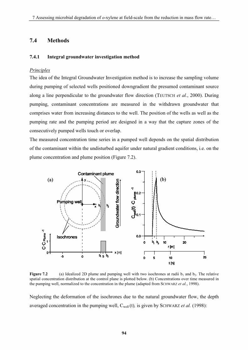
7 Assessing microbial degradation of o-xylene at field-scale from the reduction in mass flow rate…
94
7.4 Methods
7.4.1 Integral groundwater investigation method
Principles The idea of the Integral Groundwater Investigation method is to increase the sampling volume
during pumping of selected wells positioned downgradient the presumed contaminant source
along a line perpendicular to the groundwater flow direction (TEUTSCH et al., 2000). During
pumping, contaminant concentrations are measured in the withdrawn groundwater that
comprises water from increasing distances to the well. The position of the wells as well as the
pumping rate and the pumping period are designed in a way that the capture zones of the
consecutively pumped wells touch or overlap.
The measured concentration time series in a pumped well depends on the spatial distribution
of the contaminant within the undisturbed aquifer under natural gradient conditions, i.e. on the
plume concentration and plume position (Figure 7.2).
Figure 7.2 (a) Idealized 2D plume and pumping well with two isochrones at radii b1 and b2. The relative spatial concentration distribution at the control plane is plotted below. (b) Concentrations over time measured in the pumping well, normalized to the concentration in the plume (adapted from SCHWARZ et al., 1998).
Neglecting the deformation of the isochrones due to the natural groundwater flow, the depth
averaged concentration in the pumping well, Cwell (t), is given by SCHWARZ et al. (1998):
Pumping well
Contaminant plume
Isochrones
b1 2
0x [m]
5-5
1
0bb1 2
x
y
b
Gro
undw
ater
flow
dire
ctio
n
C·C
-1
Plum
e
0 10 20r [m]
0.0
0.1
0.2
0.3
b1 2b
C wel
l(t)·
C
-1pl
ume
t [h]0 255 10
Pumping well
Contaminant plume
Isochrones
b1 2
0x [m]
5-5
1
0bb1 2
x
y
b
Gro
undw
ater
flow
dire
ctio
n
C·C
-1
Plum
e
0 10 20r [m]
0.0
0.1
0.2
0.3
b1 2b
C wel
l(t)·
C
-1pl
ume
t [h]0 255 10
0 10 20r [m]
0.0
0.1
0.2
0.3
b1 2b
C wel
l(t)·
C
-1pl
ume
t [h]0 255 10
(a) (b)
Pumping well
Contaminant plume
Isochrones
b1 2
0x [m]
5-5
1
0bb1 2
x
y
b
Gro
undw
ater
flow
dire
ctio
n
C·C
-1
Plum
e
0 10 20r [m]
0.0
0.1
0.2
0.3
b1 2b
C wel
l(t)·
C
-1pl
ume
t [h]0 255 10
Pumping well
Contaminant plume
Isochrones
b1 2
0x [m]
5-5
1
0bb1 2
x
y
b
Gro
undw
ater
flow
dire
ctio
n
C·C
-1
Plum
e
0 10 20r [m]
0.0
0.1
0.2
0.3
b1 2b
C wel
l(t)·
C
-1pl
ume
t [h]0 255 10
0 10 20r [m]
0.0
0.1
0.2
0.3
b1 2b
C wel
l(t)·
C
-1pl
ume
t [h]0 255 10
(a) (b)
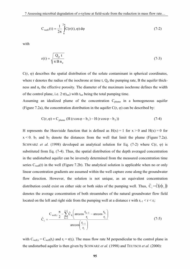
7 Assessing microbial degradation of o-xylene at field-scale from the reduction in mass flow rate…
95
��
���
�
2
0well d ) ),t(r(C
21)t(C (7-2)
with
e
p
n B t Q
)t(r�
� (7-3)
C(r, �) describes the spatial distribution of the solute contaminant in spherical coordinates,
where r denotes the radius of the isochrone at time t, Qp the pumping rate, B the aquifer thick-
ness and ne the effective porosity. The diameter of the maximum isochrone defines the width
of the control plane, i.e. 2·r(ttot) with ttot being the total pumping time.
Assuming an idealized plume of the concentration Cplume in a homogeneous aquifer
(Figure 7.2a), the concentration distribution in the aquifer C(r, �) can be described by:
))bcosr( H )bcosr( (H C) ,r(C 21plume ������� (7-4)
H represents the Heaviside function that is defined as H(x) = 1 for x > 0 and H(x) = 0 for
x < 0. b1 and b2 denote the distances from the well that limit the plume (Figure 7.2a).
SCHWARZ et al. (1998) developed an analytical solution for Eq. (7-2) where C(r, �) is
substituted from Eq. (7-4). Thus, the spatial distribution of the depth averaged concentration
in the undisturbed aquifer can be inversely determined from the measured concentration time
series Cwell(t) in the well (Figure 7.2b). The analytical solution is applicable when no or only
linear concentration gradients are assumed within the well capture zone along the groundwater
flow direction. However, the solution is not unique, as an equivalent concentration
distribution could exist on either side or both sides of the pumping well. Thus, iC = � �� �itrC
denotes the average concentration of both streamtubes of the natural groundwater flow field
located on the left and right side from the pumping well at a distance r with ri-1 < r < ri:
���
����
�
���
����
���
�
�
�
�
�
�
i
1i
1i
1k i
k
i
1kki,well
i
rr
arccos
rr
arccosr
rarccosC
2C
C (7-5)
with Cwell,i = Cwell(ti) and ri = r(ti). The mass flow rate M perpendicular to the control plane in
the undisturbed aquifer is then given by SCHWARZ et al. (1998) and TEUTSCH et al. (2000):
7 Assessing microbial degradation of o-xylene at field-scale from the reduction in mass flow rate…
96
��
�
n
1iii Q C2M (7-6)
with
� �i1ii rr B h kQ ����
, (7-7)
where n denotes the total number of concentration measurements at the well, Qi the
volumetric discharge perpendicular to the control plane within the left respective the right
streamtube, k the hydraulic conductivity and h� the hydraulic gradient of the undisturbed
aquifer. The radius ri is defined by Eq. (7-3). From the mass flow rate obtained in the control
plane (Eq. (7-6)), a mean flux averaged concentration can be calculated by dividing the
contaminant mass flow rate by the volumetric discharge of water across the entire control
plane.
Design of pumping tests for the Integral Groundwater Investigation approach The integral pumping tests were performed at two control planes along a transect in
groundwater flow direction (Figure 7.1). At the centre of each control plane one pumping well
was located. The wells were positioned so that the capture zone of the downgradient well
comprises all streamlines of the capture zone of the upgradient well. Information from a
multitracer experiment (BÖSEL et al., 2000) helped to determine the well positions and the
maximum isochrone extent. The wells had to be located not too close to the source area, to
avoid pumping of the NAPL present, but also not too far downgradient, as concentrations may
drop rapidly below the detection limit for the carbon isotope analysis. As indicated in
Figure 7.1, the two wells B47 and B85 were selected for the integral pumping tests combined
with isotope measurements. Both wells are fully screened within the Quaternary aquifer, i.e.
the screened intervals reach from 4.5 to 7.2 m (B47) and 4.3 to 7.3 m (B85) below ground
surface.
Both wells were pumped subsequently for approximately 1.5 days each, with a pumping rate
of 3.97 L s-1. In order to minimize a possible disturbance of the contaminant plume, the
downgradient well B85 was pumped first. After two days of recovery, pumping at B47 was
started. With each 2 m increment of the isochrone radius samples for both, the contaminant
concentration and the contaminant specific isotope analyses were taken. Under the assumption
of no natural groundwater flow which is a prerequisite for the application of the inversion
algorithm, a maximum isochrone radius of about 20 m would be reached for each well after
7 Assessing microbial degradation of o-xylene at field-scale from the reduction in mass flow rate…
97
approximately 37 hours of pumping. Although the seepage velocity is high in the respective
area (see also section 7.5.1), the maximum isochrones are not expected to deviate strongly
from circular shape if groundwater flow was considered. Using the formula provided by BEAR
and JACOBS (1965) to calculate the shape of the maximum isochrone in consideration of the
seepage velocity, the maximum isochrone radius perpendicular to the groundwater flow is less
than 5% smaller than the isochrones assuming no natural groundwater flow.
During pumping, the drawdown was automatically recorded at the pumping well and at two
additional observation wells. Furthermore, standard parameters like temperature, pH, redox
potential, electrical conductivity and oxygen concentration of the pumped groundwater were
automatically monitored during the entire experiment. Ten groundwater samples were taken
during each pumping test and analysed for BTEX, PAHs (16 EPA-PAHs, 1-methyl-
naphthalene, 2-methylnaphthalene) and inorganic ions at the laboratory of the University of
Tübingen (Germany). The samples were taken in brown glass bottles equipped with PTFE
septums and stored at 4°C to minimize microbial activity. BTEX compounds were analysed
within 24 hours by Purge-and-Trap/GC-MS. PAHs were extracted with cyclohexane and also
analysed via GC-MS. The detection limit for BTEX and PAH compounds was 0.02 µg L-1 and
0.025 µg L-1, respectively. A detailed description of the BTEX and PAH analyses is given by
ZAMFIRESCU and GRATHWOHL (2001). Ions except for iron and manganese were analysed
using ion chromatography (IC), whereas iron and manganese analysis was performed using
atomic absorption spectroscopy (AAS).
7.4.2 Compound specific isotope analysis (CSIA)
Principles Microbial degradation of a considerable number of compounds leads to an enrichment of the
heavier carbon isotopes 13C in the remaining nondegraded contaminant fraction. The isotopic
ratio R is defined as the ratio of 13C and 12C concentrations, i.e. R = C13C/C12C. The shift of the
isotopic ratio in the nondegraded contaminant fraction compared to the initial isotope ratio is
described by the Rayleigh equation (Eq. (7-1)). Thus, if the fractionation factor � is known,
the extent of biodegradation can be determined by analysing the isotopic ratio R0 of the initial
substrate and the isotopic ratio R of the remaining fraction f:
11
0R Rf
��
��
�
�
��
�
�� (7-8)
7 Assessing microbial degradation of o-xylene at field-scale from the reduction in mass flow rate…
98
where f is the remaining fraction of the contaminant and (1-f)�100% is the percentage of the
original contaminant mass that was removed by biodegradation.
The application of the Rayleigh equation for the quantification of biodegradation at field sites
generally implies that the temporal dependency of biodegradation, that is reflected by the
isotope ratios R and R0, can be transferred to a spatial dependency, i.e. that the isotope ratio R
of a sample taken downgradient of a source zone with a known ratio R0 follow the Rayleigh
equation (Eqs. (7-1) and (7-8)). In several studies this assumption was used and biodegra-
dation was determined at field-scale (STURCHIO et al., 1998; SHERWOOD LOLLAR et al., 2001;
VIETH et al., 2001; RICHNOW et al., 2003; STEINBACH and MICHAELIS, 2003).
In order to use this standard isotope investigation approach, samples at both wells B47 and
B85 were taken after approximately 20-30 min of pumping. In contrast to the integral samples
taken over longer time periods these samples represent point-scale values of concentration and
isotope ratios, respectively.
Analytical techniques Prior to extraction with n-pentane, samples were spiked with phenanthrene d10 as an internal
standard. Since low contaminant concentrations in the groundwater required the extraction of
large water volumes with small n-pentane volumes (0.3-1.0 mL) a microseparator (RETTBERG,
Goettingen, Germany) for the n-pentane separation was used. Reduced copper was added to
remove elemental sulphur. Extracts were stored on ice and transported to the Isotope Mass
Spectrometry Unit at the Institute of Biogeochemistry and Marine Chemistry (University of
Hamburg).
Stable carbon isotope analyses of extracted aromatic hydrocarbons were performed using a
gas chromatography-combustion-isotope ratio mass spectrometry system (GC-C-IRMS). In
this technique, a gas chromatograph (HEWLETT-PACKARD Company, Wilmington, DE, USA)
was coupled via a combustion unit (Combustion interface; FINNIGAN, Bremen, Germany) to a
FINNIGAN MAT Deltaplus-XL mass spectrometer (FINNIGAN, Bremen, Germany). Aliquots of
0.5-5.0 µL of n-pentane extracts were injected in splitless mode at 16°C in a cooled injection
system (CIS 4; GERSTEL, Muelheim, Germany) with subsequent heating up to 300°C at a rate
of 12°C s-1 with a final holding time of 10 min. Baseline separation of target compounds was
achieved on a HP-PONA column (50 m � 0.2 mm i.d. � 0.5 µm film thickness, HEWLETT
PACKARD Company, USA). The initial column oven temperature was held at 30°C for 10 min
and then ramped at 6°C min-1 to 245°C and at 10°C min-1 to 280°C, where it was held for 10
min. The 940°C combustion furnace equipped with NiO, Pt and CuO wires oxidized the
7 Assessing microbial degradation of o-xylene at field-scale from the reduction in mass flow rate…
99
separated hydrocarbons successively to CO2 and H2O. After the cogenerated water vapour was
removed via a Nafion� dryer, the CO2 was swept via an open split assembly into the isotope
ratio mass spectrometer, where the carbon isotope composition of separated hydrocarbons was
measured. All isotope data are reported in terms of the conventional delta notation (�13C),
giving the per mil (‰) deviation of the isotope ratio of the sample relative to the Vienna
Peedee Belemnite (VPDB) standard:
10001R RCδ
S
13 ����
����
�� (7-9)
where R and RS are the 13C/12C isotope ratios corresponding to the sample and the standard,
respectively. The Vienna Peedee Belemnite (VPDB) standard ratio RS is defined as 0.0112372
(CLARK and FRITZ, 1997).
Reproducibility and accuracy of the measurements were evaluated routinely using an aromatic
hydrocarbon standard with known carbon isotopic compositions. Additionally, the �13C value
(-24.4‰) of the internal standard (phenanthrene d10) provided a further data control for each
analysed sample.
Carbon isotope ratios as shown in Figure 7.6 and Figure 7.7 represent mean values of at least
six replicates. Reproducibility and accuracy of isotope analyses range between 0.5-1.0‰ for
concentrations � 4.0 µg L-1 and 1.0-2.2‰ for concentrations � 4.0 µg L-1. The newly
developed extraction technique in combination with the cooled injection system significantly
improved the sensitivity of the method as reported so far (DEMPSTER et al., 1997). The lower
detection limit (0.3-0.5 �g L-1 for o-xylene) facilitates the measurement of carbon isotope
ratios in zones of low dissolved contaminant concentration (e.g. the fringe zones of a plume)
and thus improves the spatial resolution.
7.4.3 Combination of Integral Groundwater Investigation method with CSIA (ICSIA)
The combination of the Integral Groundwater Investigation method and the CSIA allows a
spatially integrated quantification of mass flow rates and biodegradation based on isotope
analyses at the control planes. With respect to the isotope analyses, this combination implies
that the sampling volume for the isotope analyses is enlarged to obtain an integrated value of
isotope ratios at a control plane. This enlargement of the observation scale increases the
reliability and representativity of the results when compared to point-scale samples.
Furthermore, the time series of concentrations and isotope ratios measured during pumping
7 Assessing microbial degradation of o-xylene at field-scale from the reduction in mass flow rate…
100
allow a qualitative evaluation of the plume extent and plume position relative to the well, as
well as an indication of microbial activity at the plume fringes.
For this integral scale CSIA method (ICSIA), the analytical inversion algorithm presented in
Eqs. (7-5)-(7-7) is applied to the time series of the isotope concentrations for each compound.
The isotope concentrations of 13C and 12C are calculated from the isotope ratios R and the
compound concentration C:
R1C
C C12C
�
� (7-10)
and
R11
CC C
13C�
� (7-11)
with
��� CCC (7-12)
where C12C and C13C denote the concentrations of the isotopes 12C and 13C of the specific
compound, CC is the carbon concentration of the compound and denotes the weight fraction
of carbon to the total molecular weight.
Applying the inversion algorithm to the C13C and C12C time series results in spatially averaged
isotope concentrations C of 13C and 12C at the control plane. From these, a mean isotope ratio
R and, according to Eq. (7-9), a mean � 13C value can be determined.
Two questions arise in conjunction with the determination of mean isotope ratios at control
planes and their application in the Rayleigh model.
(1) Does the inversion algorithm provide reasonable results for R and � 13C if contaminant
concentrations and correspondingly the isotope ratios change along a pathline within the
area of the captured groundwater?
(2) Is the Rayleigh equation valid for mean isotope ratios and mean concentrations obtained
from the inversion algorithm?
Concerning the first question, a numerical scenario was set up that simulates a contaminant
plume with contaminant concentrations and isotope values as close as possible to the situation
found at the site (PETER, 2002). Assuming a linear concentration gradient in flow direction, it
7 Assessing microbial degradation of o-xylene at field-scale from the reduction in mass flow rate…
101
was possible to show that mean isotope values obtained from the integral pumping test and
the inversion of the data lead to an overall accuracy of 0.1‰ for the isotope values
synthetically measured at the control plane (PETER, 2002).
The second question deals with the validity of the Rayleigh equation applied to mean isotope
ratios obtained by the analytical inversion algorithm. Assuming streamtubes of different
concentrations that are captured in the well by the maximum isochrone, the mean isotope ratio
R at the control plane is defined by the unknown concentrations Ci and unknown isotope
ratios Ri of the different streamtubes i:
�
�
�
�
�
� n
1ii
n
1iii
C
RCR (7-13)
where n is the number of streamtubes.
Assuming that the differences in isotope ratios within the various streamtubes i are not caused
by an isotopically heterogeneous source zone, but are due to biodegradation, Ri in Eq. (7-13)
can then be replaced by the Rayleigh equation (Eq. (7-1)). Rearranging of Eq. (7-13) yields:
C
Cn1
CR
C
C
CR
C
CCRC
R
n
1ii
10
0n
1ii
n
1ii
10
0n
1ii
n
1i
1
0
i0i �
�
�
�
��
�
��
�
�
�
��
�
�
��
����
��
�
�
��
�
�
���
����
���
� (7-14)
where C denotes the mean concentration at the control plane, and C0 and R0 the
concentration and isotope ratio of the source, respectively. To obtain an approximation of the
sum of �
iC on the right hand side of Eq. (7-14), a Taylor series expansion is performed for
�
iC and �C with �= 1 as centre of expansion:
� � iiii ClnC1CC ������ (7-15)
� � ClnC1CC ������ (7-16)
Calculating the arithmetic mean for �
iC in Eq. (7-15) leads to:
7 Assessing microbial degradation of o-xylene at field-scale from the reduction in mass flow rate…
102
� �������
� ����
n
1iii
n
1ii
n
1ii ClnC
n1C
n1C
n1 (7-17)
Subtracting Eq. (7-17) from Eq. (7-16) results in:
� � � �
� � � �
� �� ��
��
���
�
��
���
��
���
�
��
���
�
���
��
���
������
n
1iii
n
1iii
n
1ii
n
1iii
n
1ii
n
1ii
ClnClnCn
1
ClnCClnCn
1
ClnCn1ClnC1C
n1CC
n1C
(7-18)
As fractionation factors � are generally very close to unity, the first factor on the right hand
side of Eq. (7-18) tends towards zero. In addition, also the sum on the right hand side will be
very small as the sum contains positive as well as negative deviations from ( iClnCln � ).
Thus, it can be assumed that:
��
��
�
n
1iiC
n1C (7-19)
Substituting Eq. (7-19) in Eq. (7-14) yields:
1
001
0
0
C CR
CC
CR
R��
�
�� ��
����
����� (7-20)
Eq. (7-20) resembles the Rayleigh equation (Eq. (7-1)) but uses spatially averaged
concentrations and mean isotope ratios instead of concentrations and isotope ratios of a single
streamtube. Thus, under the aforementioned assumption, the application of the Rayleigh
equation to mean isotope values obtained from the analytical inversion algorithm is valid.
To demonstrate the qualitative effect of varying concentrations with time during an integral
pumping test and its influence on the isotope values measured during pumping, Figure 7.3
shows two simplified scenarios of pumping tests and the corresponding concentration and
�13C time series of the remaining contaminant fraction. Scenario 1 reveals rising concen-
trations with time which can be interpreted by isochrones that expand from the pumping well
into the contaminant plume. As low concentrations at the fringes are correlated with a higher
microbial activity due to a better supply of electron acceptors compared to the plume centre,
isotope values of the first samples will show an enrichment of 13C. Consequently, with
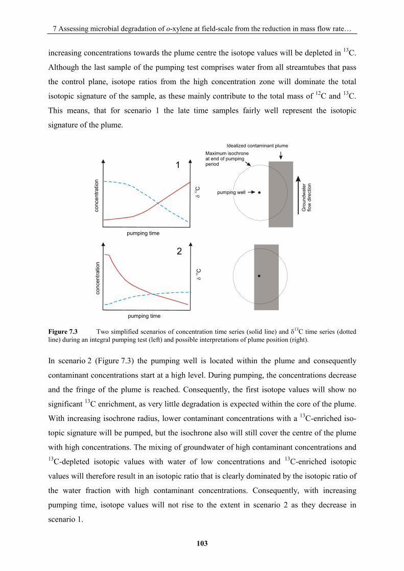
7 Assessing microbial degradation of o-xylene at field-scale from the reduction in mass flow rate…
103
increasing concentrations towards the plume centre the isotope values will be depleted in 13C.
Although the last sample of the pumping test comprises water from all streamtubes that pass
the control plane, isotope ratios from the high concentration zone will dominate the total
isotopic signature of the sample, as these mainly contribute to the total mass of 12C and 13C.
This means, that for scenario 1 the late time samples fairly well represent the isotopic
signature of the plume.
Figure 7.3 Two simplified scenarios of concentration time series (solid line) and �13C time series (dotted line) during an integral pumping test (left) and possible interpretations of plume position (right).
In scenario 2 (Figure 7.3) the pumping well is located within the plume and consequently
contaminant concentrations start at a high level. During pumping, the concentrations decrease
and the fringe of the plume is reached. Consequently, the first isotope values will show no
significant 13C enrichment, as very little degradation is expected within the core of the plume.
With increasing isochrone radius, lower contaminant concentrations with a 13C-enriched iso-
topic signature will be pumped, but the isochrone also will still cover the centre of the plume
with high concentrations. The mixing of groundwater of high contaminant concentrations and 13C-depleted isotopic values with water of low concentrations and 13C-enriched isotopic
values will therefore result in an isotopic ratio that is clearly dominated by the isotopic ratio of
the water fraction with high contaminant concentrations. Consequently, with increasing
pumping time, isotope values will not rise to the extent in scenario 2 as they decrease in
scenario 1.
conc
entra
tion
pumping time
2
conc
entra
tion
pumping time
1
�
C13
�
C13
Idealized contaminant plumeMaximum isochrone at end of pumping period
pumping well
Gro
undw
ater
flo
w d
irect
ion
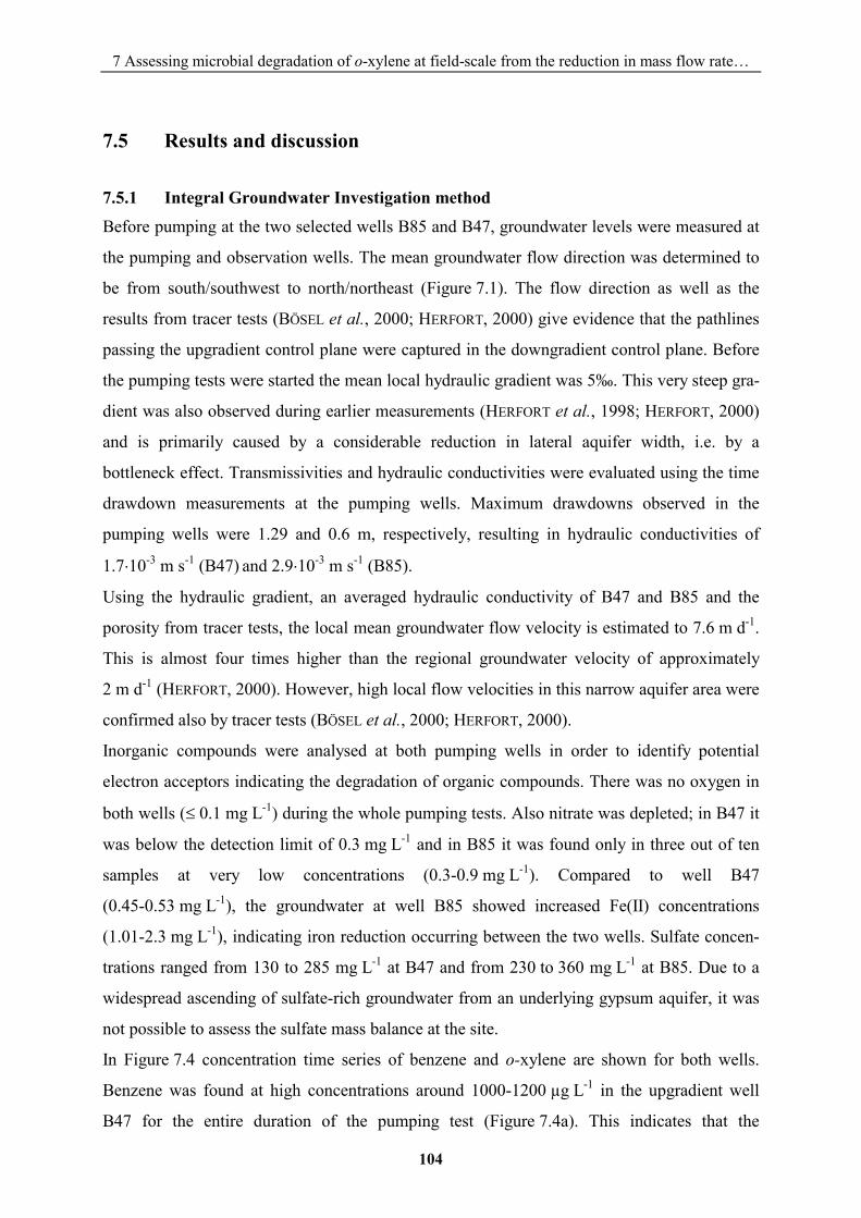
7 Assessing microbial degradation of o-xylene at field-scale from the reduction in mass flow rate…
104
7.5 Results and discussion
7.5.1 Integral Groundwater Investigation method
Before pumping at the two selected wells B85 and B47, groundwater levels were measured at
the pumping and observation wells. The mean groundwater flow direction was determined to
be from south/southwest to north/northeast (Figure 7.1). The flow direction as well as the
results from tracer tests (BÖSEL et al., 2000; HERFORT, 2000) give evidence that the pathlines
passing the upgradient control plane were captured in the downgradient control plane. Before
the pumping tests were started the mean local hydraulic gradient was 5‰. This very steep gra-
dient was also observed during earlier measurements (HERFORT et al., 1998; HERFORT, 2000)
and is primarily caused by a considerable reduction in lateral aquifer width, i.e. by a
bottleneck effect. Transmissivities and hydraulic conductivities were evaluated using the time
drawdown measurements at the pumping wells. Maximum drawdowns observed in the
pumping wells were 1.29 and 0.6 m, respectively, resulting in hydraulic conductivities of
1.7�10-3 m s-1 (B47) and 2.9�10-3 m s-1 (B85).
Using the hydraulic gradient, an averaged hydraulic conductivity of B47 and B85 and the
porosity from tracer tests, the local mean groundwater flow velocity is estimated to 7.6 m d-1.
This is almost four times higher than the regional groundwater velocity of approximately
2 m d-1 (HERFORT, 2000). However, high local flow velocities in this narrow aquifer area were
confirmed also by tracer tests (BÖSEL et al., 2000; HERFORT, 2000).
Inorganic compounds were analysed at both pumping wells in order to identify potential
electron acceptors indicating the degradation of organic compounds. There was no oxygen in
both wells (� 0.1 mg L-1) during the whole pumping tests. Also nitrate was depleted; in B47 it
was below the detection limit of 0.3 mg L-1 and in B85 it was found only in three out of ten
samples at very low concentrations (0.3-0.9 mg L-1). Compared to well B47
(0.45-0.53 mg L-1), the groundwater at well B85 showed increased Fe(II) concentrations
(1.01-2.3 mg L-1), indicating iron reduction occurring between the two wells. Sulfate concen-
trations ranged from 130 to 285 mg L-1 at B47 and from 230 to 360 mg L-1 at B85. Due to a
widespread ascending of sulfate-rich groundwater from an underlying gypsum aquifer, it was
not possible to assess the sulfate mass balance at the site.
In Figure 7.4 concentration time series of benzene and o-xylene are shown for both wells.
Benzene was found at high concentrations around 1000-1200 µg L-1 in the upgradient well
B47 for the entire duration of the pumping test (Figure 7.4a). This indicates that the
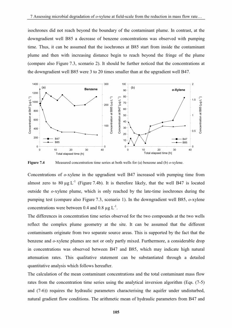
7 Assessing microbial degradation of o-xylene at field-scale from the reduction in mass flow rate…
105
isochrones did not reach beyond the boundary of the contaminant plume. In contrast, at the
downgradient well B85 a decrease of benzene concentrations was observed with pumping
time. Thus, it can be assumed that the isochrones at B85 start from inside the contaminant
plume and then with increasing distance begin to reach beyond the fringe of the plume
(compare also Figure 7.3, scenario 2). It should be further noticed that the concentrations at
the downgradient well B85 were 3 to 20 times smaller than at the upgradient well B47.
Figure 7.4 Measured concentration time series at both wells for (a) benzene and (b) o-xylene.
Concentrations of o-xylene in the upgradient well B47 increased with pumping time from
almost zero to 80 µg L-1 (Figure 7.4b). It is therefore likely, that the well B47 is located
outside the o-xylene plume, which is only reached by the late-time isochrones during the
pumping test (compare also Figure 7.3, scenario 1). In the downgradient well B85, o-xylene
concentrations were between 0.4 and 0.8 µg L-1.
The differences in concentration time series observed for the two compounds at the two wells
reflect the complex plume geometry at the site. It can be assumed that the different
contaminants originate from two separate source areas. This is supported by the fact that the
benzene and o-xylene plumes are not or only partly mixed. Furthermore, a considerable drop
in concentrations was observed between B47 and B85, which may indicate high natural
attenuation rates. This qualitative statement can be substantiated through a detailed
quantitative analysis which follows hereafter.
The calculation of the mean contaminant concentrations and the total contaminant mass flow
rates from the concentration time series using the analytical inversion algorithm (Eqs. (7-5)
and (7-6)) requires the hydraulic parameters characterising the aquifer under undisturbed,
natural gradient flow conditions. The arithmetic mean of hydraulic parameters from B47 and
0 10 20 30 40Total elapsed time �h�
0
10
20
30
40
50
60
70
80
90
100
Con
cent
ratio
n at
B47
��g
L-1�
0
0.5
1
1.5
2
Con
cent
ratio
n at
B85
��g
L-1�
B47B85
o-Xylene(b)
0 10 20 30 40Total elapsed time �h�
0
200
400
600
800
1000
1200
1400
Con
cent
ratio
n at
B47
��g
L-1�
0
100
200
300
Con
cent
ratio
n at
B85
��g
L-1�
B47B85
Benzene(a)
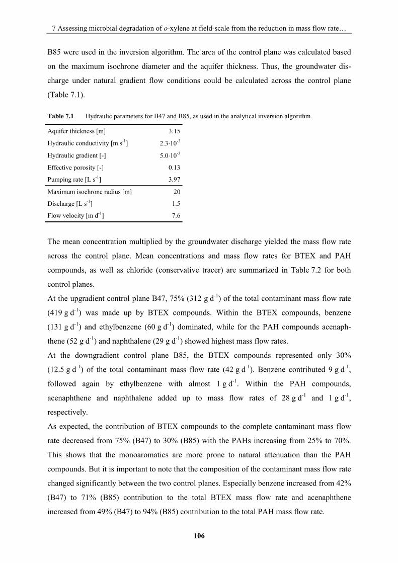
7 Assessing microbial degradation of o-xylene at field-scale from the reduction in mass flow rate…
106
B85 were used in the inversion algorithm. The area of the control plane was calculated based
on the maximum isochrone diameter and the aquifer thickness. Thus, the groundwater dis-
charge under natural gradient flow conditions could be calculated across the control plane
(Table 7.1).
Table 7.1 Hydraulic parameters for B47 and B85, as used in the analytical inversion algorithm.
Aquifer thickness [m] 3.15
Hydraulic conductivity [m s-1] 2.3�10-3
Hydraulic gradient [-] 5.0�10-3
Effective porosity [-] 0.13
Pumping rate [L s-1] 3.97
Maximum isochrone radius [m] 20
Discharge [L s-1] 1.5
Flow velocity [m d-1] 7.6
The mean concentration multiplied by the groundwater discharge yielded the mass flow rate
across the control plane. Mean concentrations and mass flow rates for BTEX and PAH
compounds, as well as chloride (conservative tracer) are summarized in Table 7.2 for both
control planes.
At the upgradient control plane B47, 75% (312 g d-1) of the total contaminant mass flow rate
(419 g d-1) was made up by BTEX compounds. Within the BTEX compounds, benzene
(131 g d-1) and ethylbenzene (60 g d-1) dominated, while for the PAH compounds acenaph-
thene (52 g d-1) and naphthalene (29 g d-1) showed highest mass flow rates.
At the downgradient control plane B85, the BTEX compounds represented only 30%
(12.5 g d-1) of the total contaminant mass flow rate (42 g d-1). Benzene contributed 9 g d-1,
followed again by ethylbenzene with almost 1 g d-1. Within the PAH compounds,
acenaphthene and naphthalene added up to mass flow rates of 28 g d-1 and 1 g d-1,
respectively.
As expected, the contribution of BTEX compounds to the complete contaminant mass flow
rate decreased from 75% (B47) to 30% (B85) with the PAHs increasing from 25% to 70%.
This shows that the monoaromatics are more prone to natural attenuation than the PAH
compounds. But it is important to note that the composition of the contaminant mass flow rate
changed significantly between the two control planes. Especially benzene increased from 42%
(B47) to 71% (B85) contribution to the total BTEX mass flow rate and acenaphthene
increased from 49% (B47) to 94% (B85) contribution to the total PAH mass flow rate.
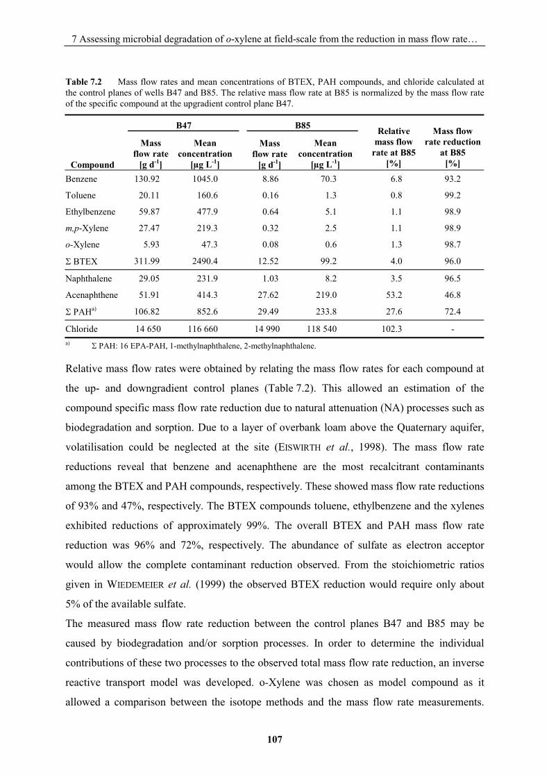
7 Assessing microbial degradation of o-xylene at field-scale from the reduction in mass flow rate…
107
Table 7.2 Mass flow rates and mean concentrations of BTEX, PAH compounds, and chloride calculated at the control planes of wells B47 and B85. The relative mass flow rate at B85 is normalized by the mass flow rate of the specific compound at the upgradient control plane B47.
B47 B85
Compound
Mass flow rate
[g d-1]
Mean concentration
[µg L-1]
Mass flow rate
[g d-1]
Mean concentration
[µg L-1]
Relative mass flow
rate at B85 [%]
Mass flow rate reduction
at B85 [%]
Benzene 130.92 1045.0 8.86 70.3 6.8 93.2
Toluene 20.11 160.6 0.16 1.3 0.8 99.2
Ethylbenzene 59.87 477.9 0.64 5.1 1.1 98.9
m,p-Xylene 27.47 219.3 0.32 2.5 1.1 98.9
o-Xylene 5.93 47.3 0.08 0.6 1.3 98.7
� BTEX 311.99 2490.4 12.52 99.2 4.0 96.0
Naphthalene 29.05 231.9 1.03 8.2 3.5 96.5
Acenaphthene 51.91 414.3 27.62 219.0 53.2 46.8
� PAHa) 106.82 852.6 29.49 233.8 27.6 72.4
Chloride 14 650 116 660 14 990 118 540 102.3 - a)
� PAH: 16 EPA-PAH, 1-methylnaphthalene, 2-methylnaphthalene.
Relative mass flow rates were obtained by relating the mass flow rates for each compound at
the up- and downgradient control planes (Table 7.2). This allowed an estimation of the
compound specific mass flow rate reduction due to natural attenuation (NA) processes such as
biodegradation and sorption. Due to a layer of overbank loam above the Quaternary aquifer,
volatilisation could be neglected at the site (EISWIRTH et al., 1998). The mass flow rate
reductions reveal that benzene and acenaphthene are the most recalcitrant contaminants
among the BTEX and PAH compounds, respectively. These showed mass flow rate reductions
of 93% and 47%, respectively. The BTEX compounds toluene, ethylbenzene and the xylenes
exhibited reductions of approximately 99%. The overall BTEX and PAH mass flow rate
reduction was 96% and 72%, respectively. The abundance of sulfate as electron acceptor
would allow the complete contaminant reduction observed. From the stoichiometric ratios
given in WIEDEMEIER et al. (1999) the observed BTEX reduction would require only about
5% of the available sulfate.
The measured mass flow rate reduction between the control planes B47 and B85 may be
caused by biodegradation and/or sorption processes. In order to determine the individual
contributions of these two processes to the observed total mass flow rate reduction, an inverse
reactive transport model was developed. o-Xylene was chosen as model compound as it
allowed a comparison between the isotope methods and the mass flow rate measurements.
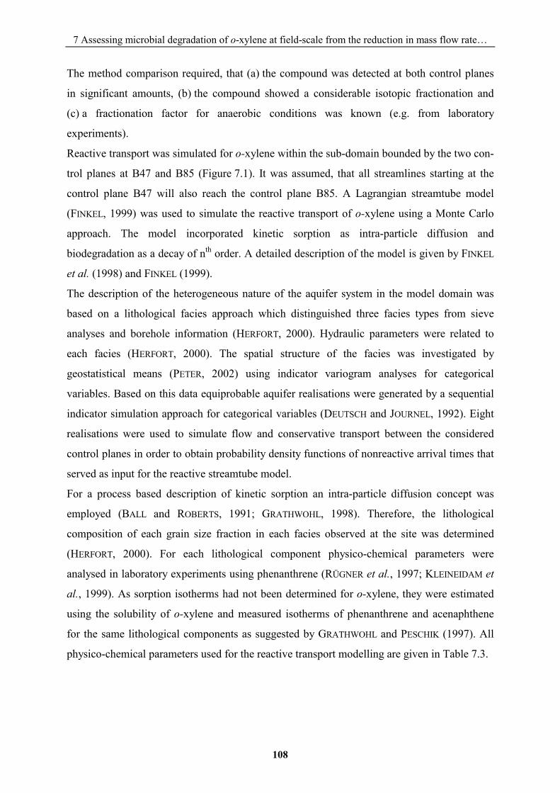
7 Assessing microbial degradation of o-xylene at field-scale from the reduction in mass flow rate…
108
The method comparison required, that (a) the compound was detected at both control planes
in significant amounts, (b) the compound showed a considerable isotopic fractionation and
(c) a fractionation factor for anaerobic conditions was known (e.g. from laboratory
experiments).
Reactive transport was simulated for o-xylene within the sub-domain bounded by the two con-
trol planes at B47 and B85 (Figure 7.1). It was assumed, that all streamlines starting at the
control plane B47 will also reach the control plane B85. A Lagrangian streamtube model
(FINKEL, 1999) was used to simulate the reactive transport of o-xylene using a Monte Carlo
approach. The model incorporated kinetic sorption as intra-particle diffusion and
biodegradation as a decay of nth order. A detailed description of the model is given by FINKEL
et al. (1998) and FINKEL (1999).
The description of the heterogeneous nature of the aquifer system in the model domain was
based on a lithological facies approach which distinguished three facies types from sieve
analyses and borehole information (HERFORT, 2000). Hydraulic parameters were related to
each facies (HERFORT, 2000). The spatial structure of the facies was investigated by
geostatistical means (PETER, 2002) using indicator variogram analyses for categorical
variables. Based on this data equiprobable aquifer realisations were generated by a sequential
indicator simulation approach for categorical variables (DEUTSCH and JOURNEL, 1992). Eight
realisations were used to simulate flow and conservative transport between the considered
control planes in order to obtain probability density functions of nonreactive arrival times that
served as input for the reactive streamtube model.
For a process based description of kinetic sorption an intra-particle diffusion concept was
employed (BALL and ROBERTS, 1991; GRATHWOHL, 1998). Therefore, the lithological
composition of each grain size fraction in each facies observed at the site was determined
(HERFORT, 2000). For each lithological component physico-chemical parameters were
analysed in laboratory experiments using phenanthrene (RÜGNER et al., 1997; KLEINEIDAM et
al., 1999). As sorption isotherms had not been determined for o-xylene, they were estimated
using the solubility of o-xylene and measured isotherms of phenanthrene and acenaphthene
for the same lithological components as suggested by GRATHWOHL and PESCHIK (1997). All
physico-chemical parameters used for the reactive transport modelling are given in Table 7.3.
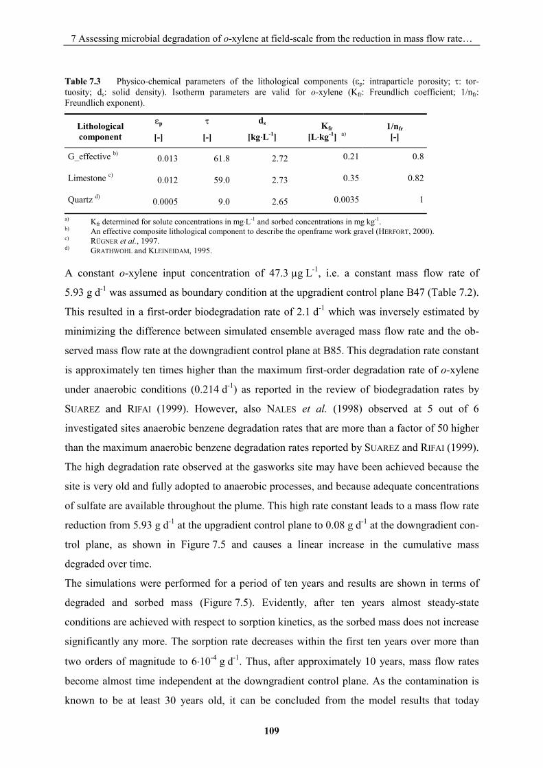
7 Assessing microbial degradation of o-xylene at field-scale from the reduction in mass flow rate…
109
Table 7.3 Physico-chemical parameters of the lithological components (�p: intraparticle porosity; �: tor-tuosity; ds: solid density). Isotherm parameters are valid for o-xylene (Kfr: Freundlich coefficient; 1/nfr: Freundlich exponent).
Lithological component
�p
[-]
��
[-]
ds
[kg�L-1] Kfr
[L�kg-1] a) 1/nfr [-]
G_effective b) 0.013 61.8 2.72 0.21 0.8
Limestone c) 0.012 59.0 2.73 0.35 0.82
Quartz d) 0.0005 9.0 2.65 0.0035 1
a) Kfr determined for solute concentrations in mg�L-1 and sorbed concentrations in mg kg-1. b) An effective composite lithological component to describe the openframe work gravel (HERFORT, 2000). c) RÜGNER et al., 1997. d) GRATHWOHL and KLEINEIDAM, 1995.
A constant o-xylene input concentration of 47.3 µg L-1, i.e. a constant mass flow rate of
5.93 g d-1 was assumed as boundary condition at the upgradient control plane B47 (Table 7.2).
This resulted in a first-order biodegradation rate of 2.1 d-1 which was inversely estimated by
minimizing the difference between simulated ensemble averaged mass flow rate and the ob-
served mass flow rate at the downgradient control plane at B85. This degradation rate constant
is approximately ten times higher than the maximum first-order degradation rate of o-xylene
under anaerobic conditions (0.214 d-1) as reported in the review of biodegradation rates by
SUAREZ and RIFAI (1999). However, also NALES et al. (1998) observed at 5 out of 6
investigated sites anaerobic benzene degradation rates that are more than a factor of 50 higher
than the maximum anaerobic benzene degradation rates reported by SUAREZ and RIFAI (1999).
The high degradation rate observed at the gasworks site may have been achieved because the
site is very old and fully adopted to anaerobic processes, and because adequate concentrations
of sulfate are available throughout the plume. This high rate constant leads to a mass flow rate
reduction from 5.93 g d-1 at the upgradient control plane to 0.08 g d-1 at the downgradient con-
trol plane, as shown in Figure 7.5 and causes a linear increase in the cumulative mass
degraded over time.
The simulations were performed for a period of ten years and results are shown in terms of
degraded and sorbed mass (Figure 7.5). Evidently, after ten years almost steady-state
conditions are achieved with respect to sorption kinetics, as the sorbed mass does not increase
significantly any more. The sorption rate decreases within the first ten years over more than
two orders of magnitude to 6�10-4 g d-1. Thus, after approximately 10 years, mass flow rates
become almost time independent at the downgradient control plane. As the contamination is
known to be at least 30 years old, it can be concluded from the model results that today
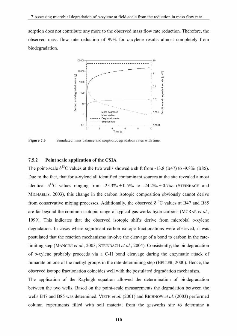
7 Assessing microbial degradation of o-xylene at field-scale from the reduction in mass flow rate…
110
sorption does not contribute any more to the observed mass flow rate reduction. Therefore, the
observed mass flow rate reduction of 99% for o-xylene results almost completely from
biodegradation.
Figure 7.5 Simulated mass balance and sorption/degradation rates with time.
7.5.2 Point scale application of the CSIA
The point-scale �13C values at the two wells showed a shift from -13.8 (B47) to -9.8‰ (B85).
Due to the fact, that for o-xylene all identified contaminant sources at the site revealed almost
identical �13C values ranging from -25.3‰ � 0.5‰ to -24.2‰ � 0.7‰ (STEINBACH and
MICHAELIS, 2003), this change in the carbon isotopic composition obviously cannot derive
from conservative mixing processes. Additionally, the observed �13C values at B47 and B85
are far beyond the common isotopic range of typical gas works hydrocarbons (MCRAE et al.,
1999). This indicates that the observed isotopic shifts derive from microbial o-xylene
degradation. In cases where significant carbon isotope fractionations were observed, it was
postulated that the reaction mechanisms involve the cleavage of a bond to carbon in the rate-
limiting step (MANCINI et al., 2003; STEINBACH et al., 2004). Consistently, the biodegradation
of o-xylene probably proceeds via a C-H bond cleavage during the enzymatic attack of
fumarate on one of the methyl groups in the rate-determining step (BELLER, 2000). Hence, the
observed isotope fractionation coincides well with the postulated degradation mechanism.
The application of the Rayleigh equation allowed the determination of biodegradation
between the two wells. Based on the point-scale measurements the degradation between the
wells B47 and B85 was determined. VIETH et al. (2001) and RICHNOW et al. (2003) performed
column experiments filled with soil material from the gasworks site to determine a
0 2 4 6 8 10Time �a�
0.1
1
10
100
1000
10000
100000
Sorb
ed a
nd d
egra
ded
mas
s �g�
0.0001
0.001
0.01
0.1
1
10
Sorp
tion
and
degr
adat
ion
rate
�g d
-1�
Mass degradedMass sorbedDegradation rateSorption rate
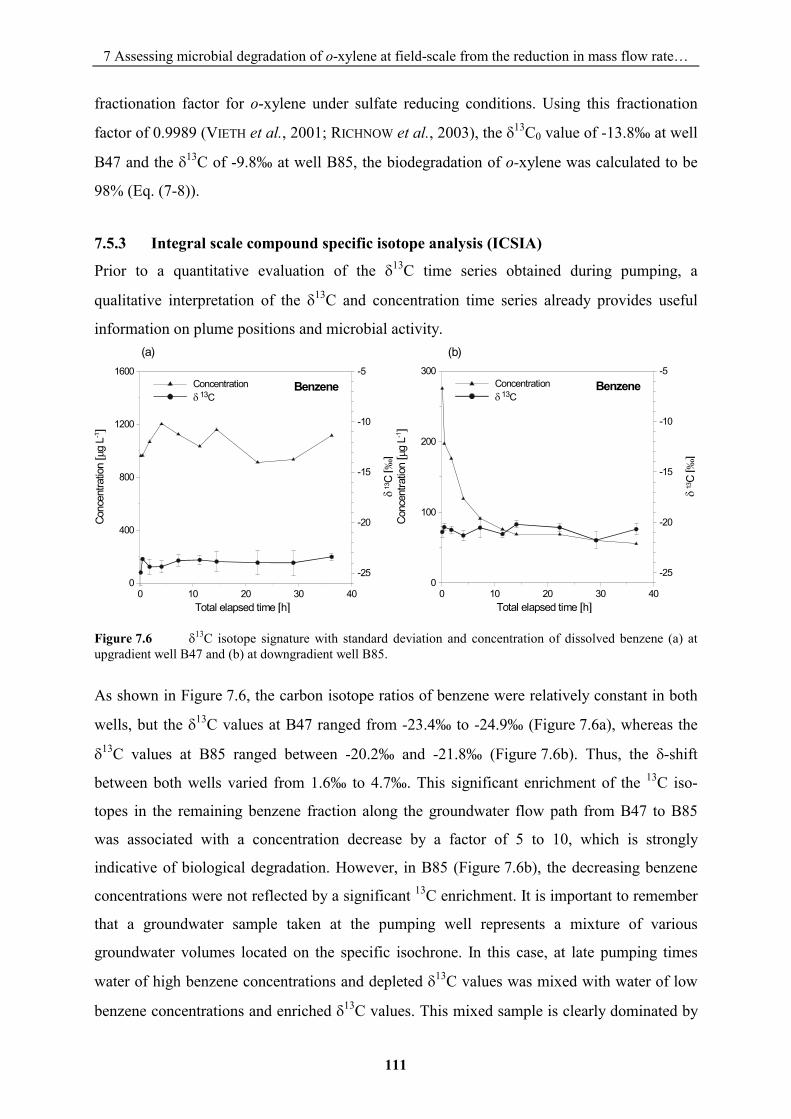
7 Assessing microbial degradation of o-xylene at field-scale from the reduction in mass flow rate…
111
fractionation factor for o-xylene under sulfate reducing conditions. Using this fractionation
factor of 0.9989 (VIETH et al., 2001; RICHNOW et al., 2003), the �13C0 value of -13.8‰ at well
B47 and the �13C of -9.8‰ at well B85, the biodegradation of o-xylene was calculated to be
98% (Eq. (7-8)).
7.5.3 Integral scale compound specific isotope analysis (ICSIA)
Prior to a quantitative evaluation of the �13C time series obtained during pumping, a
qualitative interpretation of the �13C and concentration time series already provides useful
information on plume positions and microbial activity.
Figure 7.6 �13C isotope signature with standard deviation and concentration of dissolved benzene (a) at
upgradient well B47 and (b) at downgradient well B85.
As shown in Figure 7.6, the carbon isotope ratios of benzene were relatively constant in both
wells, but the �13C values at B47 ranged from -23.4‰ to -24.9‰ (Figure 7.6a), whereas the
�13C values at B85 ranged between -20.2‰ and -21.8‰ (Figure 7.6b). Thus, the �-shift
between both wells varied from 1.6‰ to 4.7‰. This significant enrichment of the 13C iso-
topes in the remaining benzene fraction along the groundwater flow path from B47 to B85
was associated with a concentration decrease by a factor of 5 to 10, which is strongly
indicative of biological degradation. However, in B85 (Figure 7.6b), the decreasing benzene
concentrations were not reflected by a significant 13C enrichment. It is important to remember
that a groundwater sample taken at the pumping well represents a mixture of various
groundwater volumes located on the specific isochrone. In this case, at late pumping times
water of high benzene concentrations and depleted �13C values was mixed with water of low
benzene concentrations and enriched �13C values. This mixed sample is clearly dominated by
0 10 20 30 40Total elapsed time �h�
0
400
800
1200
1600
Conc
entra
tion ��
g L-1�
-25
-20
-15
-10
-5�
13C �‰
�Concentration� 13C
Benzene
(a)
0 10 20 30 40Total elapsed time �h�
0
100
200
300
Conc
entra
tion ��
g L-1�
-25
-20
-15
-10
-5
� 13
C �‰
�
Concentration� 13C
Benzene
(b)
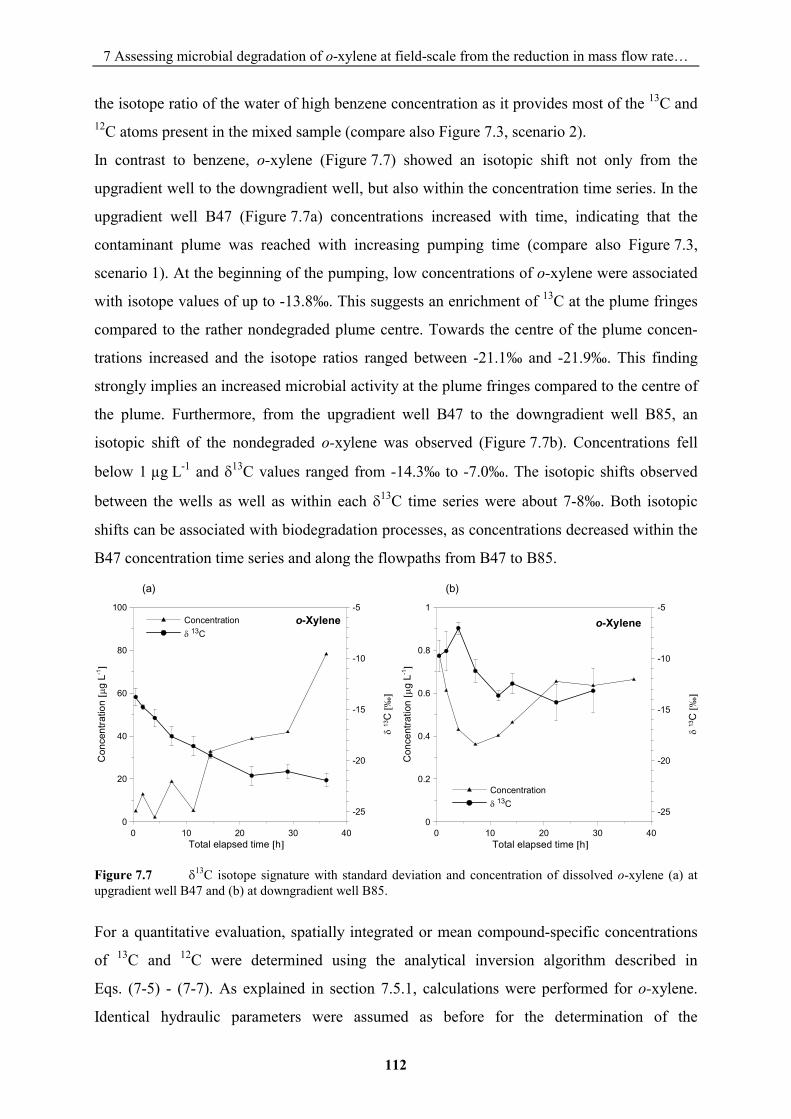
7 Assessing microbial degradation of o-xylene at field-scale from the reduction in mass flow rate…
112
the isotope ratio of the water of high benzene concentration as it provides most of the 13C and 12C atoms present in the mixed sample (compare also Figure 7.3, scenario 2).
In contrast to benzene, o-xylene (Figure 7.7) showed an isotopic shift not only from the
upgradient well to the downgradient well, but also within the concentration time series. In the
upgradient well B47 (Figure 7.7a) concentrations increased with time, indicating that the
contaminant plume was reached with increasing pumping time (compare also Figure 7.3,
scenario 1). At the beginning of the pumping, low concentrations of o-xylene were associated
with isotope values of up to -13.8‰. This suggests an enrichment of 13C at the plume fringes
compared to the rather nondegraded plume centre. Towards the centre of the plume concen-
trations increased and the isotope ratios ranged between -21.1‰ and -21.9‰. This finding
strongly implies an increased microbial activity at the plume fringes compared to the centre of
the plume. Furthermore, from the upgradient well B47 to the downgradient well B85, an
isotopic shift of the nondegraded o-xylene was observed (Figure 7.7b). Concentrations fell
below 1 µg L-1 and �13C values ranged from -14.3‰ to -7.0‰. The isotopic shifts observed
between the wells as well as within each �13C time series were about 7-8‰. Both isotopic
shifts can be associated with biodegradation processes, as concentrations decreased within the
B47 concentration time series and along the flowpaths from B47 to B85.
Figure 7.7 �13C isotope signature with standard deviation and concentration of dissolved o-xylene (a) at
upgradient well B47 and (b) at downgradient well B85.
For a quantitative evaluation, spatially integrated or mean compound-specific concentrations
of 13C and 12C were determined using the analytical inversion algorithm described in
Eqs. (7-5) - (7-7). As explained in section 7.5.1, calculations were performed for o-xylene.
Identical hydraulic parameters were assumed as before for the determination of the
0 10 20 30 40Total elapsed time �h�
0
20
40
60
80
100
Con
cent
ratio
n ��
g L-1
�
-25
-20
-15
-10
-5
� 13
C �‰
�
Concentration� 13C
o-Xylene
(a)
0 10 20 30 40Total elapsed time �h�
0
0.2
0.4
0.6
0.8
1
Con
cent
ratio
n ��
g L-1
�
-25
-20
-15
-10
-5
� 13
C �‰
�
Concentration� 13C
o-Xylene
(b)
7 Assessing microbial degradation of o-xylene at field-scale from the reduction in mass flow rate…
113
contaminant mass flow rates (Table 7.1). Using Eq. (7-9) mean �13C values of o-xylene were
calculated based on the mean carbon isotope concentrations at the control planes (Table 7.4).
The mean isotopic shift between both control planes amounted to 5.3‰ which clearly
indicates microbial degradation between the control planes.
Table 7.4 Mean isotope concentrations for o-xylene as derived from the application of the analytical inversion algorithm and mean δ 13C values.
Control plane
C 13C [ng L-1]
C 12C [ng L-1]
δ 13C [‰]
B47 466.3 42405.5 -21.4
B85 5.9 533.7 -16.1
Using the mean isotope ratios determined at both control planes as input for the Rayleigh
equation (Eq. (7-20)), the mean contaminant reduction due to biodegradation was determined.
As derived in section 7.4.3, the application of the Rayleigh equation to mean isotope ratios
using the same fractionation factor as for point-scale isotope ratios is valid. Based on a
fractionation factor of 0.9989 for o-xylene as determined by VIETH et al. (2001) and δ 13C0
and δ 13C values of -21.4‰ and -16.1‰, respectively, the fraction of the remaining
contaminant is calculated to be about 1%. In other words, 99% of the o-xylene detected at the
upgradient control plane was biodegraded along the flowpaths to the downgradient control
plane.
7.6 Method comparison and conclusions Three different, independently applied methods were used to assess the biodegradation of
o-xylene between two wells. Those were (1) the Integral Groundwater Investigation method
combined with reactive transport modelling, (2) the point-scale compound-specific isotope
analysis (CSIA) and (3) the newly developed compound-specific isotope analysis at integral
scale (ICSIA). All three methods yielded consistent results, suggesting that 98-99% of the
o-xylene was biodegraded between the considered wells or the respective control planes. It is
important to see that the quantification of the mass flow rate reduction between consecutive
control planes in combination with a reactive transport modelling led to the same results as
the entirely different approach using the isotope fractionation. The combination of the Integral
Groundwater Investigation method and compound specific isotope analyses led to an even
more reliable estimate because local scale heterogeneities and preferential flow paths are
7 Assessing microbial degradation of o-xylene at field-scale from the reduction in mass flow rate…
114
mostly averaged out. Because of the overall consistency of the three results, the methods can
be considered as field validated.
In summary, the advantages and drawbacks of the three methods are as follows. Method 1, the
Integral Groundwater Investigation method, provides contaminant mass flow rates at control
planes. For the field case presented the mass flow rates of o-xylene were determined at two
consecutive control planes along the natural flow path, downgradient of the source area. As
the total mass flow rates were measured by capturing all groundwater passing the control
planes, the reliability of the results is far superior to individual point-scale concentration
measurements which will vary based on the heterogeneity of the flow field and the plume
geometry. Thus, the integral scale mass flow rates compare to point-scale concentration
measurements in the same way as hydraulic conductivities from pumping tests compare to
hydraulic conductivities obtained from e.g. flowmeter measurements in a well. The significant
larger scale of observation leads in both cases to far more representative results.
One of the drawbacks of the Integral Groundwater Investigation method is that the costs for
the treatment of the contaminated groundwater at the well may be considerable. However,
when compared to the classical contaminant plume mapping with numerous wells, the smaller
number of boreholes required will most likely compensate these extra costs. Limitations of the
inversion algorithm used to determine mass flow rates from the measured concentration time
series might arise if concentration gradients within the captured isochrone strongly deviate
from a linear shape, i.e. if higher-order degradation processes prevail. Furthermore, it should
be mentioned that it is not sufficient to demonstrate mass flow rate reductions in order to
prove or quantify biodegradation to occur. Other processes like kinetic sorption and
volatilisation need to be considered as well and might require additional measurements and
interpretation work (e.g. reactive transport modelling). However, depending on the type of
contaminant and the age of the contamination, sorption and/or volatilization might be
neglected.
In comparison to the integral mass flow rate measurements, the point-scale compound-specific
isotope analysis is relatively easy to perform. Instead of several days of pumping and a
possible treatment of the pumped water, the compound-specific isotope data provide a first
evidence of biodegradation occurring at a field site. In order to calculate the extent of
biodegradation, it is necessary to know the isotopic ratio of the source, or the ratio in a well
that is definitely located upgradient. This implies an a priori knowledge of the hydraulic flow
conditions at the site. One should be aware of the fact that the representativeness of the point-
7 Assessing microbial degradation of o-xylene at field-scale from the reduction in mass flow rate…
115
scale isotope samples can be very limited, because the sample is a product of subsurface
heterogeneity and contaminant distribution. The method is restricted to compounds that are
subject to fractionation during biodegradation. Some compounds, like e.g. 1-methyl-
naphthalene, apparently biodegrade without any fractionation (STEINBACH et al., 2004).
Another limitation of the method is the usually higher detection limit for the isotope analyses
compared to contaminant concentration analyses. That restriction is accompanied by the fact
that specifically for carbon isotope analyses a reliable and significant isotope fractionation can
only be detected after a considerable removal of the original contaminant mass.
The integral scale compound-specific isotope analysis provides to a large extent the
advantages of both aforementioned methods. In a qualitative way, important information on
the plume position and microbial activity can be obtained by evaluating the time series of
isotope values during pumping. Enrichment in 13C isotopes originating from the plume fringes
clearly indicate high microbial activity and furthermore the relative location of the well with
respect to the plume can be assessed. A quantitative evaluation of the isotope time series
allows the determination of the spatially integrated �13C values at the control planes. One
further advantage is that due to the direct association to a single process, the method directly
leads to a quantification of biodegradation, i.e. it does not require a further tool like reactive
transport modelling to quantify biodegradation. As both integral methods provide an
equivalent degree of reliability and representativeness, this advantage may be crucial.
However, the additional costs for pumping and possibly treating the contaminated water needs
to be considered as well.
From a practical perspective, the approach to be recommended is to use the Integral
Groundwater Investigation method to directly quantify the mass flow rate reduction along the
groundwater flow path and at the same time to monitor and analyse the compound specific
�13C values in order to obtain an additional and independent data set which provides a
consistency check or validation for the results obtained.
7.7 Acknowledgements This work was part of the Priority Program 546 “Geochemical processes with long-term
effects in anthropogenically affected seepage- and groundwater”. Financial support was kindly
provided by the Deutsche Forschungsgemeinschaft. We also thank the reviewers for their
helpful comments on the manuscript.
8 Stable carbon isotope fractionation during the reductive dehalogenation of tetrachloroethene…
116
Stable carbon isotope fractionation during the reductive
dehalogenation of tetrachloroethene (PCE) by zero valent iron: a
tool to map the efficiency of iron treatment walls
Chemosphere
submitted
Ebert M., Steinbach A., Michaelis W., and Dahmke A.
8 Stable carbon isotope fractionation during the reductive dehalogenation of tetrachloroethene…
117
8.1 Abstract Stable carbon isotope fractionation during reductive dehalogenation of chlorinated ethenes
was suggested currently for the performance evaluation of permeable reactive barriers under
field conditions. Actually field applications are missing. Three column experiments were
performed to determine isotope fractionation factors for PCE. The columns were filled with
aged granular zero valent iron excavated from the pilot scale PRB at Rheine (Germany) and
with unaltered reference material. Groundwater from the site spiked with 12 mg L-1 PCE was
used as input solution. In all column experiments an isotope fractionation of PCE during
reductive dechlorination consistent to a Rayleigh model was observed. While the observed
pseudo first order rate constants varied between 1.64�10-2 and 4.02�10-2 h-1, a mean enrichment
factor (�) of -11.6‰ � 0.7‰ was determined for all experiments within a 95% confidence
interval. Field results from the Rheine site showed a decrease of PCE concentrations along
two monitoring transects from 2795 to 5.1 µg L-1 and 6177 to 1583 µg L-1 between upgradient
and downgradient monitoring wells at two sections of the PRB. Simultaneously, the
remaining PCE fractions were significantly enriched in 13C, indicating ongoing reductive
degradation. However, the enrichment factors were not consistent with the laboratory results.
A mixture of different degraded PCE fractions within the barrier and a desorption of PCE
downgradient of the barrier was the most reasonable explanation. Both processes led to �13C
values that are smaller than expected from the concentration measurements. Although an
exact quantification of the extent of PCE degradation was therefore not possible, isotope
fractionation is a powerful monitoring tool for elucidating the origin of contaminants within or
downgradient the wall.
8.2 Introduction Permeable reactive barriers (PRBs) to remediate groundwater contaminations are of
increasing interest as they are efficient and cost effective alternatives compared to traditional
pump-and-treat techniques. Since the initial work by GILLHAM and O’HANNESIN (1994) iron
treatment walls for the clean up of dissolved chlorinated hydrocarbons (CHC) by reductive
dehalogenation are the most applied PRBs (EPA, 1999). In the past many studies focused on
reaction mechanisms, kinetics and reaction by-products (ARNOLD and ROBERTS, 2000). By
now monitoring of PRB applications has become of main interest because the number of
installations has increased world wide. Monitoring the performance of a PRB is quite a
serious problem, because the interpretation of concentration patterns in terms of reactivity and
8 Stable carbon isotope fractionation during the reductive dehalogenation of tetrachloroethene…
118
effectiveness is often insufficient. Changing concentrations within a PRB are not obligatorily
indicative of a variable reactivity because variations in inflow concentrations or flow
directions may affect the processes. Furthermore, an increase in downgradient CHC
concentrations may also result from bypassing of the PRB as well as desorption processes
behind the PRB or incomplete reaction within the reactive zone. Thus, a quantitative
assessment of the efficiency by the comparison of concentration measurements along a
monitoring transect is questionable and will be rather an approximation.
In this context stable carbon isotope measurements seem to be a potential tool to improve the
usual monitoring and to achieve a more detailed efficiency assessment. A strong shift in
carbon isotopic composition during the reductive dechlorination by zero valent iron was
shown for tetrachloroethene (PCE), trichloroethene (TCE) and dichloroethene (DCE; SLATER
et al., 1998; DAYAN et al., 1999; BILL et al., 2001; SLATER et al., 2002; SCHÜTH et al.,
2003a). Other degradation processes like oxidation by permanganate (e.g. POULSON and
NARAOKA, 2002; HUNKELER et al., 2003) or biodegradation (e.g. ARAVENA et al., 1998;
HUNKELER et al., 1999; SHERWOOD LOLLAR et al., 1999; SLATER et al., 2001; BARTH et al.,
2002; SONG et al., 2002; STEINBACH and MICHAELIS, 2003) also result in a change of the
isotopic composition, while nondegrading processes such as evaporation (HUANG et al., 1999;
POULSON and DREVER, 1999; SLATER et al., 1999), sorption (SCHÜTH et al., 2003b) or
dissolution (SLATER et al., 1998) show only minor or no effects within 95% confidence
intervals.
Because different isotope fractionations were found for the dechlorination of the same
contaminant at different iron granulates and at different experimental conditions, it was
suggested that prior to the application of this method to field scale the fractionation factor
should be determined for a particular system (DAYAN et al., 1999; SLATER et al., 2002;
SCHÜTH et al., 2003b).
The aim of this paper is to evaluate the quantitative assessment for the performance of a PRB
using isotope measurements. PCE fractionation factors were determined from laboratory
experiments using iron granulates excavated from the pilot scale continuous iron PRB at the
Rheine site (Germany) 3.5 years after installation. Additionally, an experiment with reference
material was used to determine potential differences between the unused and the aged iron
from the PRB. Furthermore, this paper outlines a new convenient solid-phase micro extraction
(SPME) technique, that has the potential to assess �13C values of dissolved chlorinated
hydrocarbons at low concentration levels.
8 Stable carbon isotope fractionation during the reductive dehalogenation of tetrachloroethene…
119
8.3 Materials and methods Three column experiments were performed to examine differences in iron reactivity due to
aging effects under field conditions. For this reason vertical core drillings (10 cm i.d.) were
carried out at the Rheine site PRB 3.5 years after installation. The pilot scale continuous PRB
was constructed in June 1998 using two different reactive materials (MÖLLER, 1998; EBERT et
al., 1999b), i.e. iron sponge (ISPAT AG, Hamburg, Germany) and a mixture of 30 vol.% cast
iron granulate (GOTTHART-MAYER AG, Rheinfelden, Germany) and gravel. Two vertical
drillings were carried out in each section of the PRB covering the transition between the
aquifer and the iron fillings at the upgradient and downgradient end. Core analyses and
sediment sampling were done directly after drilling within a glove-box at an inert argon
atmosphere. The sampled material was stored in glass bottles with oxygen free groundwater
and without headspace at 4°C. Prior to the filling of the columns the material was carefully
sieved (1 mm) using oxygen free water at argon atmosphere in a glove-box. In addition to the
columns filled with aged reactive material, unaltered reference material from the PRB
construction was used in the column experiments. This material has been stored in a dry
atmosphere since PRB construction and was treated in the same way as the aged material
during column construction. Results from the experiments with iron sponge reference material
(experiment 1) and with material from the upgradient drillings, i.e. aged iron sponge
(experiment 2) and aged mixture of cast iron and gravel (experiment 3) are presented.
8.3.1 Experimental set up
Chemicals All solvents and chemicals used were of the highest purity commercially available. Standards
of PCE, TCE and 1,1,1-Trichloroethane (TCA) were purchased from FLUKA (Buchs,
Switzerland). Cis-dichloroethene (cis-DCE), vinyl chloride (VC) and monochlorobenzene
(MCB) were obtained from SUPELCO (Bellefonte, USA). A set of standard solutions for
concentration measurements were prepared from mixed stock solutions supplied by
PROMOCHEM (Wesel, Germany). PCE (Merck, Darmstadt, Germany) stock solution for the
column experiments was prepared by adding a surplus of PCE phase to groundwater deriving
from the site and stirring permanently until saturation.
8 Stable carbon isotope fractionation during the reductive dehalogenation of tetrachloroethene…
120
Solutions (isotope measurements)
A mixed external standard stock solution containing PCE, TCE, cis-DCE (1000 ng �L-1) and
MCB (200 ng �L-1) was prepared from the neat compounds in methanol (analytical-reagent
grade). Aqueous calibration standards were prepared daily by dissolving an aliquot of the
stock solution in 15 mL of bidistilled degassed water. A solution of TCA in methanol
(401 �g mL-1) served as an internal stock solution for isotope measurements.
Column systems The set up of the column experiments is described in detail in DAHMKE et al. (2000). In brief,
the used HDPE (high density polyethylene) columns with a length of 112 cm, an inner
diameter of 10 cm, and a wall thickness of 13 mm were packed with 12 cm to 15 cm gravel
(S40T; SCHLINGMEIER Quartzsand GmbH, Braunschweig, Germany) followed by 97 cm to
100 cm of the reactive material. Whereas nine sampling ports (stainless steel) were installed
along the column an influent sampling port allowed the determination of the initial
contaminant concentration. All experiments were performed at room temperature (21°C).
A peristaltic pump (ISMATEC Laboratoriumstechnik, Wertheim-Mondfeld, Germany) was used
to percolate the columns from the bottom to the top with groundwater from the field site
spiked with PCE. The mean flow rates varied between 1.0 and 1.25 mL min-1. The
groundwater from the site was stored in 30 L HDPE canisters until using and was transferred
into 40 L Tedlar® bags for the experiments. The PCE concentration within the Tedlar® bag
reservoirs was determined, afterwards aliquots of PCE saturated groundwater were spiked to
reach a final PCE concentration of 12 mg L-1. Degradation products of PCE were also
detected in the groundwater but no additional spiking was done. All used tubes were of
Viton® to minimize sorption and diffusion effects.
Sampling was performed at regular intervals (3-4 weeks) to observe alterations of the
reactivity. Samples were taken against the flow direction from the top to the bottom of the
columns using a syringe. For gas chromatography analyses 5 mL samples were filled in a
20 mL headspace vial and the vial was sealed with Teflon faced septa. Usually three parallel
samples were taken from each sampling port. For isotopic analyses three vials were filled
headspace free and were sent to the University of Hamburg. Usually samples for anion and
cation analyses were also taken but results are not presented here. All samples were stored at
4°C until concentration measurements. The results herein presented are from sampling events
after 79 exchanged pore volumes (PV) for the fresh iron sponge column, 56 PV for aged iron
sponge and 93 PV for aged cast iron gravel mixture.
8 Stable carbon isotope fractionation during the reductive dehalogenation of tetrachloroethene…
121
8.3.2 Groundwater sampling
A monitoring transect along the flow direction almost at the middle of each section of the
Rheine site PRB was used for the performance assessment. Each transect consists of three
wells. One was ~ 2.5 m in front of the PRB (upgradient), one was directly within the reactive
filling (PRB), and one ~ 2.5 m behind the PRB (downgradient). An immersion pump
(GRUNDFOS MP1, Erkrath, Germany) was positioned at the lower end of the full screened
monitoring wells (2'') for groundwater sampling. The pumping rate was between 0.5 and
1 L min-1 and the drawdown of the water table was smaller than 10% of the aquifer thickness.
Samples were taken after the on-line measurements of pH, Eh, temperature, oxygen content
and electrical conductivity reached constant values. Samples were handled in the same way as
described for column experiments and were immediately transported to the laboratory for
analysis.
8.3.3 Concentration analysis
A HEWLETT PACKARD 6890 Plus II gas chromatograph equipped with a HEWLETT PACKARD
7694 Headspace autosampler was used for the measurement of PCE and its by-products TCE,
trans- and 1,1-dichloroethene (1,1-DCE) and VC as well as the concentration of methane,
ethane, ethene, ethine, propane, propene, i-butane, n-butane, i-butene, cis-2-butene,
trans-2-butene, n-pentane and n-hexane. The chromatograph was equipped with a ALLTECH
AT-Q capillary column (30 m length, 0.53 mm i.d.) combined with a back splitter
(Y-PressFit-Splitter, deactivated) and a 63Ni µ-electron capture detector (µECD) as well as a
flame ionisation detector (FID). Samples were equilibrated at an injection temperature of
80°C shaking them for 30 min. Injection loop and transfer line temperature was 90°C and the
split/splitless inlet temperature was 230°C (split ratio 10:1, split flow 40 mL min-1). The gas
chromatograph temperature program used was 35°C hold for 4 min, increase to 170°C at
20°C min-1, hold for 2 min then increase to 220°C at 20°C min-1 and hold for 10 min. The
µECD temperature was 230°C with a N2-makeup flow of 48 mL min-1. The FID temperature
was 230°C and the flow rates were H2: 35 mL min-1, air: 400 mL min-1, N2-makeup:
20 mL min-1. The carrier gas was helium. External standards were prepared having the same
volume of liquid and headspace as the experimental vials and covering the range of
concentration observed in the samples. Reproducibility on standard analyses was typically
within � 5%.
8 Stable carbon isotope fractionation during the reductive dehalogenation of tetrachloroethene…
122
8.3.4 Compound specific isotope analysis
SPME injections were performed using a SPME manual sampling holder equipped with a
100 �m polydimethylsiloxan (PDMS) or a 75 �m Carboxen/PDMS fiber (SUPELCO, Belle-
fonte, USA). Since the latter revealed a higher sensitivity for the target compounds PCE, TCE
and cis-DCE, it was applied only to samples of low concentrations. Accordingly, high
concentrated PCE samples were extracted using the 100 �m PDMS fiber. Before first
experimental use and after each 10th analysis coatings were conditioned for 60 min at 250°C
(PDMS) and 30 min at 280°C (Carboxen/PDMS). Between 60 and 80 injections could be
performed with the fibers without any observed performance impairment.
Prior to extraction, 15 mL of sample were placed in a 20 mL vial (IVA Analysentechnik e.K.,
Meerbusch, Germany) with 5.3 g NaCl and a 15 mm magnetic stirring bar. Subsequently, the
sample was spiked with 100 �L (40.1 �g) of the methanolic TCA stock solution (internal
isotope standard) and tightly sealed with a PTFE-faced silicone septum (SUPELCO, Bellefonte,
USA). Chlorinated hydrocarbons were extracted by submerging the fibers for 15 min (PDMS)
and 30 min (Carboxen/PDMS) into the headspace of the samples. For the assessment of very
low chlorinated hydrocarbon concentrations (e.g. field samples) the extraction time for the
Carboxen/PDMS fiber was extended to 180 min. All extractions were performed at the same
fiber position at 20°C in continuously stirred samples (1200 min-1). For SPME injections, the
standard splitless liner in the split/splitless GC injection port was replaced with a narrow
1 mm i.d. liner (GERSTEL, Muelheim, Germany). The reduced volume increased the linear gas
velocity through the liner and thus significantly improved peak shape and height. Thermal
desorption of the extracted analytes was achieved by inserting the PDMS and
Carboxen/PDMS fiber in the GC injection port (CIS 4; GERSTEL, Muelheim, Germany), held
at 250°C and 300°C, respectively. Under these conditions a desorption time of 2 min excluded
carryover of analytes from both fiber types. The injection port was operated in the splitless
injection mode and during injection the split vent was closed for 1 min. 13C/12C isotope ratios were determined by gas chromatography-combustion-isotope ratio mass
spectrometry (GC-C-IRMS). The system consists of a HP 6890 GC connected via a
combustion unit (Combustion interface; FINNIGAN, Bremen, Germany) to a FINNIGAN MAT
Deltaplus-XL mass spectrometer (FINNIGAN, Bremen, Germany). Baseline separation of the
chlorinated hydrocarbons was achieved on a 30 m fused silica column (GS-GasPro, 0.32 mm
i.d., J&W Scientific, USA) with helium as carrier gas. The initial column temperature was
30°C, which was held for 2 min, followed by an increase to 220°C at 6°C min-1 and a final
8 Stable carbon isotope fractionation during the reductive dehalogenation of tetrachloroethene…
123
5 min hold at 220°C. The separated chlorinated hydrocarbons and helium carrier gas eluting
from the column were carried via deactivated fused silica capillary tubing to the combustion
furnace (CuO/NiO/Pt wires, 1010°C), where they were successively oxidised to CO2 and H2O.
After water separation the effluent stream was transferred on-line via an open split to the mass
spectrometer (MERRIT et al., 1995). For isotopic standardization, CO2 reference gas (MESSER,
Frankfurt, Germany) with a known isotopic composition was automatically introduced into
the mass spectrometer in a series of pulses at the beginning and the end of each analysis. The
carbon isotope ratio is expressed in a permil deviation from the Vienna Pee Dee Belemnite
(VPDB) standard in the usual delta notation (Eq. (8-1))
10001
CC
CC
C
dardtans12
13sample
12
13
VPDB13 �
������
�
�
������
�
�
�
���
����
�
���
����
�
. (8-1)
According to outlined studies reductive dehalogenation of chlorinated aliphatics by zero
valent iron was associated with significant 13C enrichments in the nondegraded fraction,
successfully described by the Rayleigh model. The latter can be applied if the fractionation
factor alpha (�) is constant in an irreversible one step process (MARIOTTI et al., 1981). Due to
the independency of the fractionation factor to the course of the reaction, � can be used for the
comparison of changes in isotopic compositions in different experiments. In case of a
Rayleigh model the relationship of the remaining fraction of the chlorinated contaminant
(f = C/C0) to �13C can be delineated using Eq. (8-2):
� � 10001000C1000C
lnflnfln110000CHC
13CHC
13
���
�
�
��
�
�
�
��� � (8-2)
where �13CCHC and �13CCHCo are the isotopic compositions of the chlorinated contaminant at a
given time and the initial time, respectively. The fractionation factor � can be determined by
using least square regression based on Eq. (8-2) and can be indicated as an enrichment factor �
(� = (�-1)�1000). By means of this correlation, a degradation reaction can be proven and the
progress of a reaction can be quantified based on the extent of the isotopic shift.
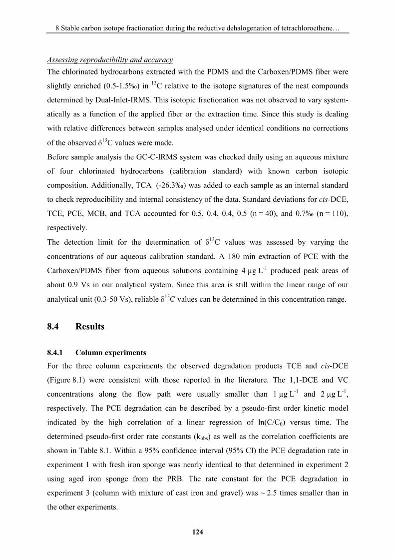
8 Stable carbon isotope fractionation during the reductive dehalogenation of tetrachloroethene…
124
Assessing reproducibility and accuracy The chlorinated hydrocarbons extracted with the PDMS and the Carboxen/PDMS fiber were
slightly enriched (0.5-1.5‰) in 13C relative to the isotope signatures of the neat compounds
determined by Dual-Inlet-IRMS. This isotopic fractionation was not observed to vary system-
atically as a function of the applied fiber or the extraction time. Since this study is dealing
with relative differences between samples analysed under identical conditions no corrections
of the observed �13C values were made.
Before sample analysis the GC-C-IRMS system was checked daily using an aqueous mixture
of four chlorinated hydrocarbons (calibration standard) with known carbon isotopic
composition. Additionally, TCA (-26.3‰) was added to each sample as an internal standard
to check reproducibility and internal consistency of the data. Standard deviations for cis-DCE,
TCE, PCE, MCB, and TCA accounted for 0.5, 0.4, 0.4, 0.5 (n = 40), and 0.7‰ (n = 110),
respectively.
The detection limit for the determination of �13C values was assessed by varying the
concentrations of our aqueous calibration standard. A 180 min extraction of PCE with the
Carboxen/PDMS fiber from aqueous solutions containing 4 µg L-1 produced peak areas of
about 0.9 Vs in our analytical system. Since this area is still within the linear range of our
analytical unit (0.3-50 Vs), reliable �13C values can be determined in this concentration range.
8.4 Results
8.4.1 Column experiments
For the three column experiments the observed degradation products TCE and cis-DCE
(Figure 8.1) were consistent with those reported in the literature. The 1,1-DCE and VC
concentrations along the flow path were usually smaller than 1 µg L-1 and 2 µg L-1,
respectively. The PCE degradation can be described by a pseudo-first order kinetic model
indicated by the high correlation of a linear regression of ln(C/C0) versus time. The
determined pseudo-first order rate constants (kobs) as well as the correlation coefficients are
shown in Table 8.1. Within a 95% confidence interval (95% CI) the PCE degradation rate in
experiment 1 with fresh iron sponge was nearly identical to that determined in experiment 2
using aged iron sponge from the PRB. The rate constant for the PCE degradation in
experiment 3 (column with mixture of cast iron and gravel) was ~ 2.5 times smaller than in
the other experiments.
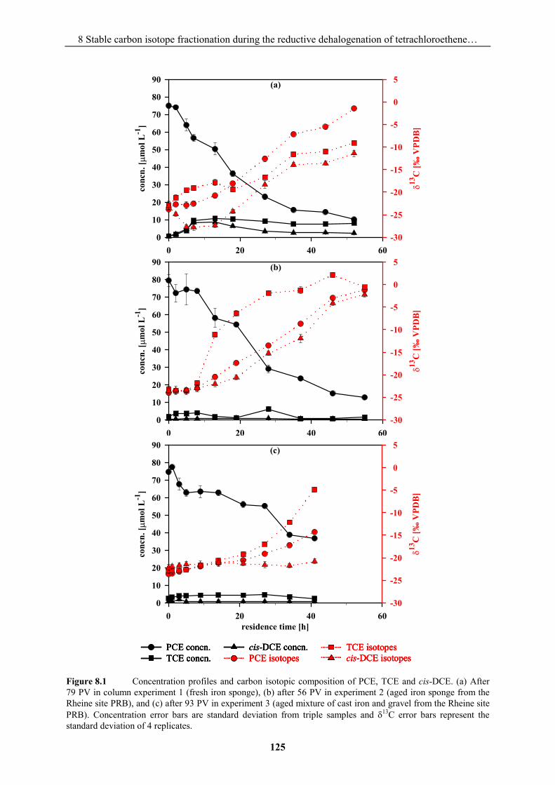
8 Stable carbon isotope fractionation during the reductive dehalogenation of tetrachloroethene…
125
Figure 8.1 Concentration profiles and carbon isotopic composition of PCE, TCE and cis-DCE. (a) After 79 PV in column experiment 1 (fresh iron sponge), (b) after 56 PV in experiment 2 (aged iron sponge from the Rheine site PRB), and (c) after 93 PV in experiment 3 (aged mixture of cast iron and gravel from the Rheine site PRB). Concentration error bars are standard deviation from triple samples and �13C error bars represent the standard deviation of 4 replicates.
B14
0 20 40 60
conc
n. [ �
mol
L-1
]
0
10
20
30
40
50
60
70
80
90
�13
C [‰
VPD
B]
-30
-25
-20
-15
-10
-5
0
5(b)
B14
0 20 40 60
conc
n. [ �
mol
L-1
]
0
10
20
30
40
50
60
70
80
90
�13
C [‰
VPD
B]
-30
-25
-20
-15
-10
-5
0
5(a)
PCE concn.TCE concn.
cis-DCE concn.PCE isotopes
TCE isotopescis-DCE isotopes
residence time [h]
B14
0 20 40 60
conc
n. [ �
mol
L-1
]
0
10
20
30
40
50
60
70
80
90
�13
C [‰
VPD
B]
-30
-25
-20
-15
-10
-5
0
5(c)
B14
0 20 40 60
conc
n. [ �
mol
L-1
]
0
10
20
30
40
50
60
70
80
90
�13
C [‰
VPD
B]
-30
-25
-20
-15
-10
-5
0
5(b)
B14
0 20 40 60
conc
n. [ �
mol
L-1
]
0
10
20
30
40
50
60
70
80
90
�13
C [‰
VPD
B]
-30
-25
-20
-15
-10
-5
0
5(a)
PCE concn.TCE concn.
cis-DCE concn.PCE isotopes
TCE isotopescis-DCE isotopes
PCE concn.TCE concn.PCE concn.TCE concn.
cis-DCE concn.PCE isotopescis-DCE concn.PCE isotopes
TCE isotopescis-DCE isotopesTCE isotopescis-DCE isotopes
residence time [h]
B14
0 20 40 60
conc
n. [ �
mol
L-1
]
0
10
20
30
40
50
60
70
80
90
�13
C [‰
VPD
B]
-30
-25
-20
-15
-10
-5
0
5(c)
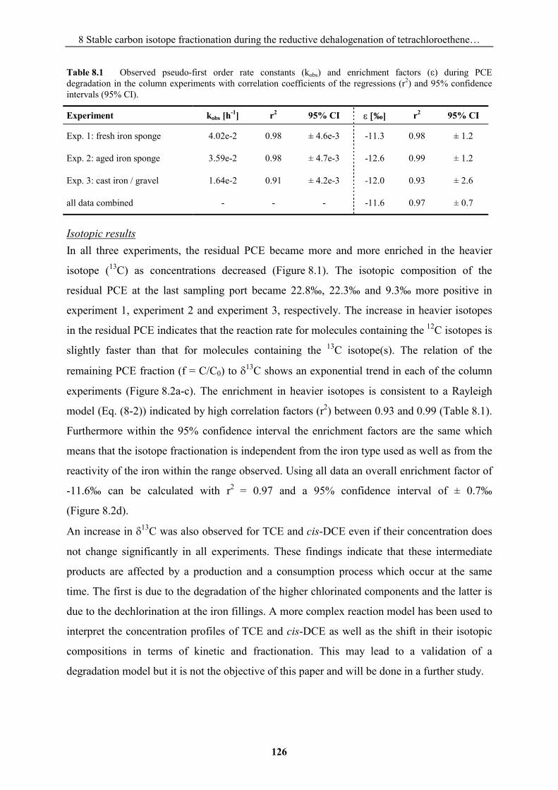
8 Stable carbon isotope fractionation during the reductive dehalogenation of tetrachloroethene…
126
Table 8.1 Observed pseudo-first order rate constants (kobs) and enrichment factors (�) during PCE degradation in the column experiments with correlation coefficients of the regressions (r2) and 95% confidence intervals (95% CI).
Experiment kobs [h-1] r2 95% CI ���‰]� r2 95% CI
Exp. 1: fresh iron sponge 4.02e-2 0.98 ± 4.6e-3 -11.3 0.98 ± 1.2
Exp. 2: aged iron sponge 3.59e-2 0.98 ± 4.7e-3 -12.6 0.99 ± 1.2
Exp. 3: cast iron / gravel 1.64e-2 0.91 ± 4.2e-3 -12.0 0.93 ± 2.6
all data combined - - - -11.6 0.97 ± 0.7
Isotopic results In all three experiments, the residual PCE became more and more enriched in the heavier
isotope (13C) as concentrations decreased (Figure 8.1). The isotopic composition of the
residual PCE at the last sampling port became 22.8‰, 22.3‰ and 9.3‰ more positive in
experiment 1, experiment 2 and experiment 3, respectively. The increase in heavier isotopes
in the residual PCE indicates that the reaction rate for molecules containing the 12C isotopes is
slightly faster than that for molecules containing the 13C isotope(s). The relation of the
remaining PCE fraction (f = C/C0) to �13C shows an exponential trend in each of the column
experiments (Figure 8.2a-c). The enrichment in heavier isotopes is consistent to a Rayleigh
model (Eq. (8-2)) indicated by high correlation factors (r2) between 0.93 and 0.99 (Table 8.1).
Furthermore within the 95% confidence interval the enrichment factors are the same which
means that the isotope fractionation is independent from the iron type used as well as from the
reactivity of the iron within the range observed. Using all data an overall enrichment factor of
-11.6‰ can be calculated with r2 = 0.97 and a 95% confidence interval of ± 0.7‰
(Figure 8.2d).
An increase in �13C was also observed for TCE and cis-DCE even if their concentration does
not change significantly in all experiments. These findings indicate that these intermediate
products are affected by a production and a consumption process which occur at the same
time. The first is due to the degradation of the higher chlorinated components and the latter is
due to the dechlorination at the iron fillings. A more complex reaction model has been used to
interpret the concentration profiles of TCE and cis-DCE as well as the shift in their isotopic
compositions in terms of kinetic and fractionation. This may lead to a validation of a
degradation model but it is not the objective of this paper and will be done in a further study.
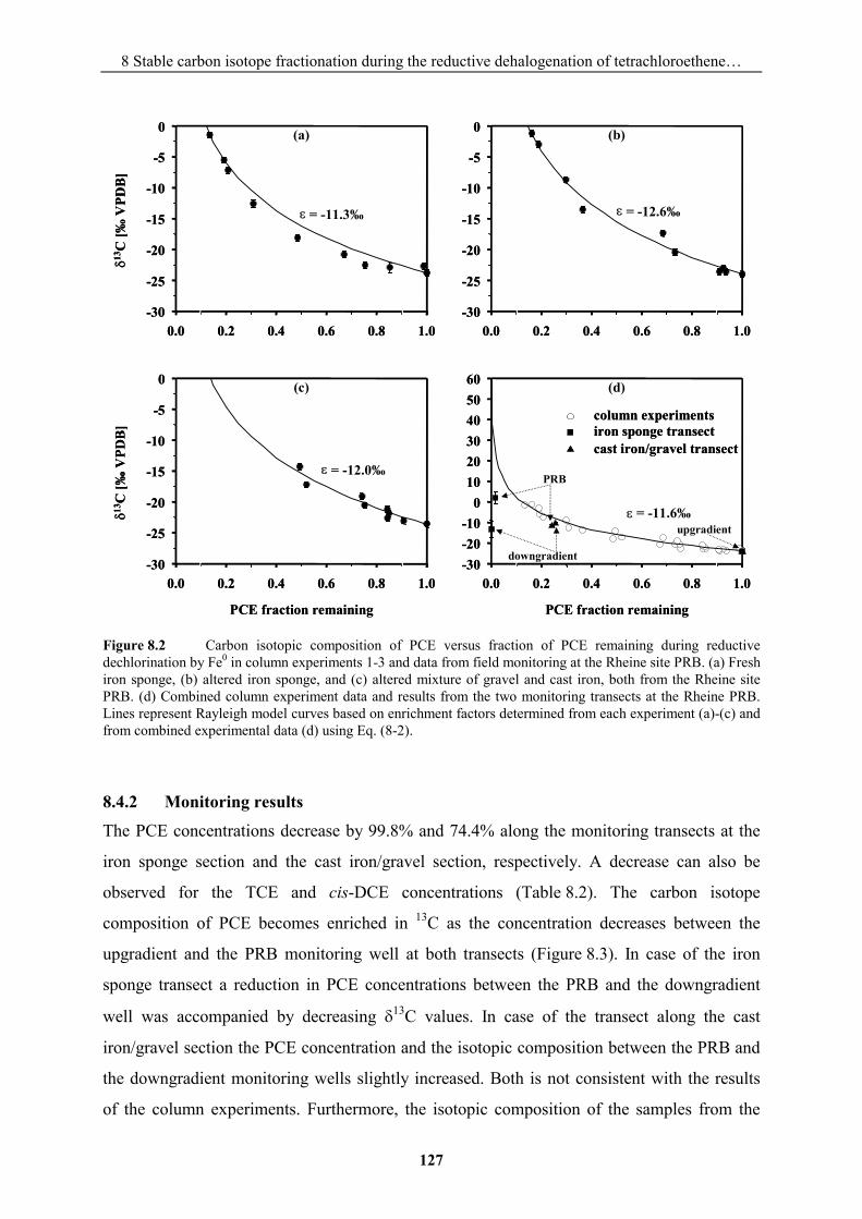
8 Stable carbon isotope fractionation during the reductive dehalogenation of tetrachloroethene…
127
Figure 8.2 Carbon isotopic composition of PCE versus fraction of PCE remaining during reductive dechlorination by Fe0 in column experiments 1-3 and data from field monitoring at the Rheine site PRB. (a) Fresh iron sponge, (b) altered iron sponge, and (c) altered mixture of gravel and cast iron, both from the Rheine site PRB. (d) Combined column experiment data and results from the two monitoring transects at the Rheine PRB. Lines represent Rayleigh model curves based on enrichment factors determined from each experiment (a)-(c) and from combined experimental data (d) using Eq. (8-2).
8.4.2 Monitoring results
The PCE concentrations decrease by 99.8% and 74.4% along the monitoring transects at the
iron sponge section and the cast iron/gravel section, respectively. A decrease can also be
observed for the TCE and cis-DCE concentrations (Table 8.2). The carbon isotope
composition of PCE becomes enriched in 13C as the concentration decreases between the
upgradient and the PRB monitoring well at both transects (Figure 8.3). In case of the iron
sponge transect a reduction in PCE concentrations between the PRB and the downgradient
well was accompanied by decreasing �13C values. In case of the transect along the cast
iron/gravel section the PCE concentration and the isotopic composition between the PRB and
the downgradient monitoring wells slightly increased. Both is not consistent with the results
of the column experiments. Furthermore, the isotopic composition of the samples from the
(a)
e = -11.3‰
0.0 0.2 0.4 0.6 0.8 1.0
�13
C [‰
VPD
B]
-30
-25
-20
-15
-10
-5
0 (a)
� = -11.3‰
0.0 0.2 0.4 0.6 0.8 1.0-30
-25
-20
-15
-10
-5
0 (b)
PCE fraction remaining
0.0 0.2 0.4 0.6 0.8 1.0-30
-25
-20
-15
-10
-5
0 (c)
� = -12.0‰
� = -12.6‰
PCE fraction remaining
0.0 0.2 0.4 0.6 0.8 1.0-30-20-10
0102030405060
column experimentsiron sponge transectcast iron/gravel transect
� = -11.6‰
(d)
�13
C [‰
VPD
B]
upgradient
PRB
downgradient
(a)
e = -11.3‰
0.0 0.2 0.4 0.6 0.8 1.0
�13
C [‰
VPD
B]
-30
-25
-20
-15
-10
-5
0 (a)
� = -11.3‰
0.0 0.2 0.4 0.6 0.8 1.0-30
-25
-20
-15
-10
-5
0 (b)
PCE fraction remaining
0.0 0.2 0.4 0.6 0.8 1.0-30
-25
-20
-15
-10
-5
0 (c)
� = -12.0‰
� = -12.6‰
PCE fraction remaining
0.0 0.2 0.4 0.6 0.8 1.0-30-20-10
0102030405060
column experimentsiron sponge transectcast iron/gravel transect
column experimentsiron sponge transectcast iron/gravel transect
� = -11.6‰
(d)
�13
C [‰
VPD
B]
upgradient
PRB
downgradient
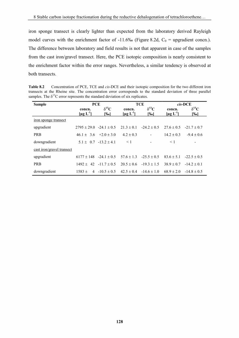
8 Stable carbon isotope fractionation during the reductive dehalogenation of tetrachloroethene…
128
iron sponge transect is clearly lighter than expected from the laboratory derived Rayleigh
model curves with the enrichment factor of -11.6‰ (Figure 8.2d, C0 = upgradient concn.).
The difference between laboratory and field results is not that apparent in case of the samples
from the cast iron/gravel transect. Here, the PCE isotopic composition is nearly consistent to
the enrichment factor within the error ranges. Nevertheless, a similar tendency is observed at
both transects.
Table 8.2 Concentration of PCE, TCE and cis-DCE and their isotopic composition for the two different iron transects at the Rheine site. The concentration error corresponds to the standard deviation of three parallel samples. The �13C error represents the standard deviation of six replicates.
Sample PCE TCE cis-DCE
concn. [µg L-1]
�13C
[‰] concn. [µg L-1]
�13C
[‰] concn. [µg L-1]
�13C
[‰] iron sponge transect
upgradient 2795 � 29.0 -24.1 � 0.5 21.3 � 0.1 -24.2 � 0.5 27.6 � 0.5 -21.7 � 0.7
PRB 46.1 � 3.6 +2.0 � 3.0 4.2 � 0.3 - 14.2 � 0.3 -9.4 � 0.6
downgradient 5.1 � 0.7 -13.2 � 4.1 < 1 - < 1 -
cast iron/gravel transect
upgradient 6177 � 148 -24.1 � 0.5 57.6 � 1.3 -25.5 � 0.5 83.6 � 5.1 -22.5 � 0.5
PRB 1492 � 42 -11.7 � 0.5 20.5 � 0.6 -19.3 � 1.5 38.9 � 0.7 -14.2 � 0.1
downgradient 1583 � 4 -10.5 � 0.5 42.5 � 0.4 -14.6 � 1.0 68.9 � 2.0 -14.8 � 0.5
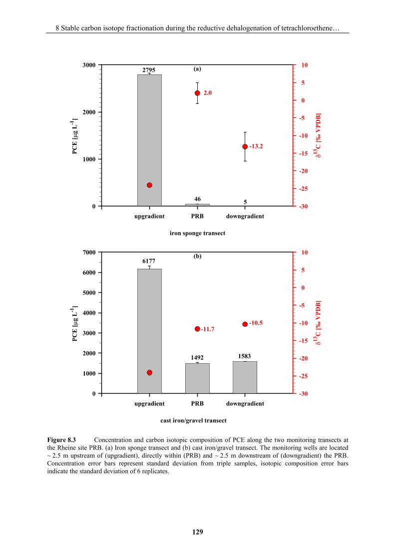
8 Stable carbon isotope fractionation during the reductive dehalogenation of tetrachloroethene…
129
Figure 8.3 Concentration and carbon isotopic composition of PCE along the two monitoring transects at the Rheine site PRB. (a) Iron sponge transect and (b) cast iron/gravel transect. The monitoring wells are located ~ 2.5 m upstream of (upgradient), directly within (PRB) and ~ 2.5 m downstream of (downgradient) the PRB. Concentration error bars represent standard deviation from triple samples, isotopic composition error bars indicate the standard deviation of 6 replicates.
B14
upgradient PRB downgradient
PCE
[ �g
L-1
]
0
1000
2000
3000
�13
C [‰
VPD
B]
-30
-25
-20
-15
-10
-5
0
5
102795
46 5
2.0
-13.2
iron sponge transect
(a)
B14
upgradient PRB downgradient
PCE
[ �g
L-1
]
0
1000
2000
3000
4000
5000
6000
7000
�13
C [‰
VPD
B]
-30
-25
-20
-15
-10
-5
0
5
106177
1492 1583
-11.7-10.5
cast iron/gravel transect
(b)
B14
upgradient PRB downgradient
PCE
[ �g
L-1
]
0
1000
2000
3000
�13
C [‰
VPD
B]
-30
-25
-20
-15
-10
-5
0
5
102795
46 5
2.0
-13.2
iron sponge transect
(a)
B14
upgradient PRB downgradient
PCE
[ �g
L-1
]
0
1000
2000
3000
4000
5000
6000
7000
�13
C [‰
VPD
B]
-30
-25
-20
-15
-10
-5
0
5
106177
1492 1583
-11.7-10.5
cast iron/gravel transect
(b)
8 Stable carbon isotope fractionation during the reductive dehalogenation of tetrachloroethene…
130
8.5 Interpretation of the monitoring results Due to the higher difference between the results deriving from the iron sponge transect and the
laboratory, only this case will be examined in detail. Besides different fractionation factors
which are discussed later, a mixture of PCE at different stages of degradation is the most
reasonable established explanation for the lighter isotopic composition at the PRB monitoring
point. Simplifying the problems of heterogeneity, a two-component mixture scheme can be
used to describe the system. A mixture of two different solutions M1 and M2 with the
concentrations CM1 and CM2 is described by Eq. (8-3):
F2M1M CCyCx ���� and 1yx �� (8-3)
where x and y are the mixing fractions of solution M1 and M2, respectively. CF is the
concentration of the final solution. The isotopic composition of the solutions M1 and M2 can
be calculated using Eq. (8-4):
� � 10001000CfC 2,1M_0131000
2,1M13
������
�
(8-4)
where �13C0_M1,2 is the isotopic composition of the initial solutions M1_0 and M2_0 with PCE
concentrations of C0_M1 and C0_M2, respectively. So f = CM1,2/C0_M1,2 is the PCE fraction
remaining. The isotopic composition of the final solution, �13CF, can be calculated using
Eq. (8-5):
� �� � � �
������
�������
1M2M2M1M
2M13
1M13
2M1MF
13
CCCyCxCCCC
C
� � � �1000
CCC1000CC1000C
1M2M
1M1M13
2M2M13
��
������� (8-5)
At given C0 and CF concentrations as well as initial and final isotopic compositions and a
known enrichment factor, six unknown variables are within only five independent equations.
The simple two-component mixture scheme is under-determined due to the different mixing
relations of concentration and isotopic composition. Nevertheless, not every mixing ratio
fulfils the boundary conditions and a miscibility range can be calculated. Assuming the same
enrichment factor for PCE at field conditions as determined from the column experiments and
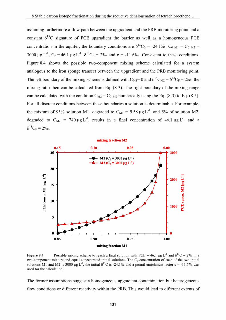
8 Stable carbon isotope fractionation during the reductive dehalogenation of tetrachloroethene…
131
assuming furthermore a flow path between the upgradient and the PRB monitoring point and a
constant �13C signature of PCE upgradient the barrier as well as a homogeneous PCE
concentration in the aquifer, the boundary conditions are �13C0 = -24.1‰, C0_M1 = C0_M2 =
3000 µg L-1, CF = 46.1 µg L-1, �13CF = 2‰ and � = -11.6‰. Consistent to these conditions,
Figure 8.4 shows the possible two-component mixing scheme calculated for a system
analogous to the iron sponge transect between the upgradient and the PRB monitoring point.
The left boundary of the mixing scheme is defined with CM1= 0 and �13CM2 = �13CF = 2‰, the
mixing ratio then can be calculated from Eq. (8-3). The right boundary of the mixing range
can be calculated with the condition CM2 = C0_M2 numerically using the Eq. (8-3) to Eq. (8-5).
For all discrete conditions between these boundaries a solution is determinable. For example,
the mixture of 95% solution M1, degraded to CM1 = 9.58 µg L-1, and 5% of solution M2,
degraded to CM2 = 740 µg L-1, results in a final concentration of 46.1 µg L-1 and a
�13CF = 2‰.
Figure 8.4 Possible mixing scheme to reach a final solution with PCE = 46.1 µg L-1 and �13C = 2‰ in a two-component mixture and equal concentrated initial solutions. The Co-concentration of each of the two initial solutions M1 and M2 is 3000 µg L-1, the initial �13C is -24.1‰ and a permil enrichment factor � = -11.6‰ was used for the calculation.
The former assumptions suggest a homogeneous upgradient contamination but heterogeneous
flow conditions or different reactivity within the PRB. This would lead to different extents of
B14
mixing fraction M1
0.85 0.90 0.95 1.00
PCE
con
cn. M
1 [�
g L
-1]
0
5
10
15
20
25
mixing fraction M2
0.000.050.100.15
PCE
con
cn. M
2 [�
g L
-1]
0
1000
2000
3000M1 (C0 = 3000 �g L-1)M2 (C0 = 3000 �g L-1)
B14
mixing fraction M1
0.85 0.90 0.95 1.00
PCE
con
cn. M
1 [�
g L
-1]
0
5
10
15
20
25
mixing fraction M2
0.000.050.100.15
PCE
con
cn. M
2 [�
g L
-1]
0
1000
2000
3000M1 (C0 = 3000 �g L-1)M2 (C0 = 3000 �g L-1)M1 (C0 = 3000 �g L-1)M2 (C0 = 3000 �g L-1)
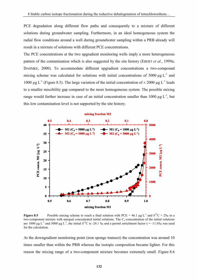
8 Stable carbon isotope fractionation during the reductive dehalogenation of tetrachloroethene…
132
PCE degradation along different flow paths and consequently to a mixture of different
solutions during groundwater sampling. Furthermore, in an ideal homogeneous system the
radial flow conditions around a well during groundwater sampling within a PRB already will
result in a mixture of solutions with different PCE concentrations.
The PCE concentrations at the two upgradient monitoring wells imply a more heterogeneous
pattern of the contamination which is also suggested by the site history (EBERT et al., 1999a;
DAHMKE, 2000). To accommodate different upgradient concentrations a two-compound
mixing scheme was calculated for solutions with initial concentrations of 5000 µg L-1 and
1000 µg L-1 (Figure 8.5). The large variation of the initial concentration of ± 2000 µg L-1 leads
to a smaller miscibility gap compared to the more homogeneous system. The possible mixing
range would further increase in case of an initial concentration smaller than 1000 µg L-1, but
this low contamination level is not supported by the site history.
Figure 8.5 Possible mixing scheme to reach a final solution with PCE = 46.1 µg L-1 and �13C = 2‰ in a two-component mixture with unequal concentrated initial solutions. The Co-concentration of the initial solutions are 1000 µg L-1 and 5000 µg L-1, the initial �13C is -24.1 ‰ and a permil enrichment factor � = -11.6‰ was used for the calculation.
At the downgradient monitoring point (iron sponge transect) the concentration was around 10
times smaller than within the PRB whereas the isotopic composition became lighter. For this
reason the mixing range of a two-component mixture becomes extremely small. Figure 8.6
PCE
con
cn. M
1 [�
g L
-1]
PCE
con
cn. M
2 [�
g L
-1]
B14
mixing fraction M1
0.5 0.6 0.7 0.8 0.9 1.00
5
10
15
20
25
30
35
40
mixing fraction M2
0.00.10.20.30.40.5
0
1000
2000
3000
4000
5000M1 (C0 = 5000 �g L-1)M2 (C0 = 1000 �g L-1)
M1 (C0 = 1000 �g L-1)M2 (C0 = 5000 �g L-1)
PCE
con
cn. M
1 [�
g L
-1]
PCE
con
cn. M
2 [�
g L
-1]
B14
mixing fraction M1
0.5 0.6 0.7 0.8 0.9 1.00
5
10
15
20
25
30
35
40
mixing fraction M2
0.00.10.20.30.40.5
0
1000
2000
3000
4000
5000M1 (C0 = 5000 �g L-1)M2 (C0 = 1000 �g L-1)
M1 (C0 = 1000 �g L-1)M2 (C0 = 5000 �g L-1)
M1 (C0 = 5000 �g L-1)M2 (C0 = 1000 �g L-1)
M1 (C0 = 1000 �g L-1)M2 (C0 = 5000 �g L-1)
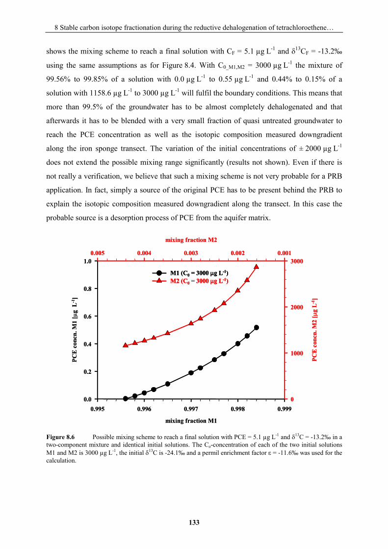
8 Stable carbon isotope fractionation during the reductive dehalogenation of tetrachloroethene…
133
shows the mixing scheme to reach a final solution with CF = 5.1 µg L-1 and �13CF = -13.2‰
using the same assumptions as for Figure 8.4. With C0_M1,M2 = 3000 µg L-1 the mixture of
99.56% to 99.85% of a solution with 0.0 µg L-1 to 0.55 µg L-1 and 0.44% to 0.15% of a
solution with 1158.6 µg L-1 to 3000 µg L-1 will fulfil the boundary conditions. This means that
more than 99.5% of the groundwater has to be almost completely dehalogenated and that
afterwards it has to be blended with a very small fraction of quasi untreated groundwater to
reach the PCE concentration as well as the isotopic composition measured downgradient
along the iron sponge transect. The variation of the initial concentrations of ± 2000 µg L-1
does not extend the possible mixing range significantly (results not shown). Even if there is
not really a verification, we believe that such a mixing scheme is not very probable for a PRB
application. In fact, simply a source of the original PCE has to be present behind the PRB to
explain the isotopic composition measured downgradient along the transect. In this case the
probable source is a desorption process of PCE from the aquifer matrix.
Figure 8.6 Possible mixing scheme to reach a final solution with PCE = 5.1 µg L-1 and �13C = -13.2‰ in a two-component mixture and identical initial solutions. The Co-concentration of each of the two initial solutions M1 and M2 is 3000 µg L-1, the initial �13C is -24.1‰ and a permil enrichment factor � = -11.6‰ was used for the calculation.
mixing fraction M1
0.995 0.996 0.997 0.998 0.9990.0
0.2
0.4
0.6
0.8
1.0
mixing fraction M2
0.0010.0020.0030.0040.005
0
1000
2000
3000
M1 (C0 = 3000 �g L-1)M2 (C0 = 3000 �g L-1)
PCE
con
cn. M
2 [�
g L
-1]
PCE
con
cn. M
1 [�
g L
-1]
mixing fraction M1
0.995 0.996 0.997 0.998 0.9990.0
0.2
0.4
0.6
0.8
1.0
mixing fraction M2
0.0010.0020.0030.0040.005
0
1000
2000
3000
M1 (C0 = 3000 �g L-1)M2 (C0 = 3000 �g L-1)M1 (C0 = 3000 �g L-1)M2 (C0 = 3000 �g L-1)
PCE
con
cn. M
2 [�
g L
-1]
PCE
con
cn. M
1 [�
g L
-1]
8 Stable carbon isotope fractionation during the reductive dehalogenation of tetrachloroethene…
134
8.6 Discussion
8.6.1 Laboratory studies
A few studies were outlined on stable carbon isotope fractionation of PCE during degradation
under different conditions. More investigations were done concerning lower chlorinated
ethenes particularly TCE and cis-DCE. Table 8.3 compares enrichment factors determined in
this study to those obtained by others. Enrichment factors determined from biodegradation
experiments are smaller than those calculated from experiments with zero valent iron or
permanganate oxidation. The enrichment factor for PCE during reductive dehalogenation at
zero valent iron derived from DAYAN et al. (1999) is more than twice as high than the results
presented here and the reasons for this high variety are not clear. Probably the differences in
the two experimental set ups cause diverse preferred PCE degradation pathways
(hydrogenolysis and -elimination) which may lead to distinct enrichment factors. DAYAN et
al. (1999) used pre-treated electrolytic iron (methanol washed, acid cleaned) in batch
experiments with unbuffered nanopure water and the initial pH (5.6) drifted to 5.2 during the
course of the reaction. In the column experiments presented the initial pH of the site
groundwater was usually between 7.1 and 7.4 and increased to values of 9.9 and 10.8 at the
last sampling ports. DAYAN et al. (1999) suppose a preference of hydrogenolysis in their
experiments due to the lower pH relating to a difference in degradation rates compared to
other studies (GILLHAM and O'HANNESIN, 1994). The lack in 1,1-DCE and VC as breakdown
products in our column experiments is consistent to a preference of the -elimination
degradation pathway of the higher chlorinated ethenes as it was shown by ARNOLD and
ROBERTS (2000). However, without a clear evidence of diverse degradation pathways, it is
comprehensible that the preference of another rate limiting step may lead to different isotope
fractionation factors.
Different surface conditions compared to the acid-cleaned electrolytic iron used by DAYAN et
al. (1999) might be another reason for the observed variability in �. SLATER et al. (2002)
found a significant effect of surface pre-treatment (acid cleaned and autoclaved) for the carbon
isotopic fractionation during dehalogenation of TCE by electrolytic iron in batch experiments.
They showed a relation between surface oxidation and the alternation in fractionation factor
and hypothesised a connection between required activation energy and differences in
enrichment factors. However, SLATER et al. (2002) did not find a significant variation in �
during TCE dehalogenation by Perrles iron in batch reactors nor by Connelly cast iron in
8 Stable carbon isotope fractionation during the reductive dehalogenation of tetrachloroethene…
135
column experiments. But there is also a high variety in outlined enrichment factors for the
reductive TCE dechlorination by different zero valent iron granulates between -8.6‰ and
-24.8‰ (SLATER et al., 1998; DAYAN et al., 1999; BILL et al., 2001; SLATER et al., 2002;
SCHÜTH et al., 2003a) and the reasons are not understood up to now.
Table 8.3 Enrichment factors of PCE during different destructive processes.
Process ���‰�� source degradation by Fe0 -11.6 this study degradation by Fe0 -25.3 DAYAN et al., 1999 biodegradation -2a) HUNKELER et al., 1999 biodegradation -5.2 (-2.7 / -5.5b)) SLATER et al., 2001 permanganate oxidation -17 (-12.9 / -22.1c)) POULSON and NARAOKA, 2002 a) roughly estimated. b) enrichment factors with low correlation. c) probable variety during reaction.
However, in our experiments the isotopic fractionation of PCE appears to be independent of
the observed degradation rates, at least within the presented range. Additionally the different
iron types and their surface specification regarding aging as well as the course of the reaction
show no effect on the fractionation. This is indicative of comparable reaction mechanisms
comprising identical rate-limiting steps. Furthermore, this points to the fact that differences in
surface conditions like precipitations and impurities had no influence on the isotopic
fractionation in our experiments. SCHÜTH et al. (2003a) present similar results concerning
isotope fractionation during TCE dehalogenation by aged iron granulates from field sites in
Belfast (Ireland) and Tübingen (Germany). This observation is important for the application of
isotope measurements for the performance monitoring at the field site. The enrichment factor
determined in the laboratory can be considered to be at least as site specific because it was
determined from column experiments using iron granulates as well as groundwater from the
particular field site.
8.6.2 Field monitoring
The shift in PCE isotopic composition from -24.1‰ to +2‰ (iron sponge) and to -11.7‰
(cast iron/gravel) proves that degradation of PCE is responsible for the decreasing
contaminant concentrations along the monitoring transects at the Rheine site PRB.
Nevertheless, the quantitative verification of degradation is not successful by using simply the
change in the isotopic composition and the enrichment factor of -11.6‰. The �13C value of
2‰ within the iron sponge PRB section corresponds to a remaining PCE fraction of 0.103.
For a homogeneous system this would correspond to an initial upgradient PCE concentration
of ~ 450 µg L-1. A contamination at such a low level is not supported by the site history
8 Stable carbon isotope fractionation during the reductive dehalogenation of tetrachloroethene…
136
(Table 8.2). Similarly, the downgradient PCE concentration and the corresponding �13C
values require a PCE start concentration of ~ 13 µg L-1. These considerations indicate more
complex processes taking place at field conditions. An effect of biodegradation may have led
to smaller enrichment factors (ARAVENA et al., 1998; HUNKELER et al., 1999; SLATER et al.,
2001). However, the microbial characterisation of material withdrawn from core samples from
the PRB does not suggest a significant influence of bacteria on dehalogenation of PCE in the
PRB (STEIOF, 2002). Even the application of another enrichment factor for the field conditions
than that derived from our laboratory experiments cannot explain the results. Hence, a mixture
of different degraded PCE fractions is the most probable explanation for the monitoring
results. The shown two-component mixing schemes certainly simplify the real conditions but
they illustrate that within the PRB the required mixing ratio is within a realistic range, even
more in case of a heterogeneous C0-concentration. The required mixing ratio downgradient of
the PRB is certainly not in a potential range for a PRB application. Therefore we assume that
a desorption of small amounts of original undegraded PCE downgradient of the PRB effects
the measurements. SCHÜTH et al. (2003b) show that sorption of TCE, DCE and VC on
carbonaceous material does not result in a noticeable �13C isotope fractionation and this may
also be valid for PCE sorption processes.
Slight heterogeneities can be presumed in almost every PRB application. Different flow
patterns, erratic contaminant loads, irregular passivation along single flow paths or simple
mixing during groundwater sampling are inherent at natural systems. Whatever hetero-
geneities may affect the measurement, the �13C value will always be lower than expected from
the concentration in case of mixed fractions of different degraded chlorinated ethenes.
Therefore more information is required to interpret isotope measurements in terms of
quantitative performance monitoring. For example, the isotope composition of the breakdown
products may be useful if a degradation model can be applied to the data. A relationship
between the degree of CHC degradation and the change of inorganic groundwater
composition was suggested by Ebert et al. (2002) concerning reactivity assessment of PRB's.
Such a correlation, when validated, can be used to improve mixing calculations. Additionally,
isotope fractionation of chlorine or hydrogen isotopes might be a promising option for the
assessment of degradation pathways. However, the observed strong carbon isotopic effect
during PCE degradation by zero valent iron indicates the high potential to monitor the
performance of a PRB, even if not only the isotope fractionation has to be more investigated
but also the effects of heterogeneity have to be considered for the application at field sites.
8 Stable carbon isotope fractionation during the reductive dehalogenation of tetrachloroethene…
137
8.7 Conclusions The dehalogenation of PCE and its breakdown products by zero valent iron leads to a strong
isotope fractionation which in case of PCE can be described by a Rayleigh model. The
determined enrichment factors appear to be independent of the aging conditions of the used
granular iron from the Rheine site PRB. Therefore an assignment of the enrichment factor
from the laboratory experiments to field conditions is regarded to be possible. The stable
carbon isotope composition of groundwater samples can be used to prove if dehalogenation
occurs at the PRB. A quantitative monitoring using only the isotope composition and the
influent concentration of PCE is not feasible because heterogeneities inherent at natural
systems effect the measurements. Within a PRB the mixture of differential degraded PCE and
downgradient of a PRB additional desorption processes in the aquifer lead to �13C values that
are smaller than expected from the concentration measurements.
8.8 Acknowledgements The research was founded by the German Federal Ministry for Education and Research
(BMBF), Project number: 02WR0208. The project is part of the German PRB network
RUBIN. We would like to thank also the laboratory technical staff as well as the students for
their assistance.
9 Zusammenfassung
138
9 Zusammenfassung Die zunehmende Verarbeitung von Wasser gefährdenden organischen Substanzen und die
Überschätzung des Reinigungs- und Rückhaltevermögens der das Grundwasser überlagernden
Bodenschichten haben speziell in den hoch industrialisierten Ländern zu starken
Grundwasserverunreinigungen geführt. Aufgrund der Tatsache, dass sich aktive Ex-situ-
Sanierungen weder unter ökologischen noch unter ökonomischen Aspekten bewährt haben,
avancierten passive In-Situ-Ansätze wie Natural Attenuation und die reaktiven Wände zu viel
versprechenden Alternativen. Allerdings setzt die Anwendung einer wie auch immer gearteten
In-situ-Sanierung die Kenntnis der im Untergrund ablaufenden Transformationsprozesse
voraus. Da dies jedoch selbst in Schadensfällen mit überschaubaren hydrogeologischen
Bedingungen schon eine große Herausforderung ist, besteht ein Bedarf an direkten Methoden,
die sowohl biotische als auch abiotische Abbauprozesse unabhängig von anderen
Schadstoffsenken wie Verdünnung oder Sorption standortspezifisch erfassen.
Neben der Entwicklung einer ausreichend empfindlichen Isotopenanalytik demonstriert die
vorliegende Dissertationsschrift am Beispiel von zwei Schadensfällen, dass die im Untergrund
ablaufenden biotischen und abiotischen Transformationsprozesse über die Isotopen-
fraktionierung direkt charakterisiert werden können.
Die erste Feldstudie ist ein mit vorwiegend aromatischen Kohlenwasserstoffen kontaminierter
Grundwasserleiter eines ehemaligen Gaswerksgeländes (Testfeld Süd). Die Anreicherung der
im Wasser gelösten BTEX und PAK erfolgte durch die Flüssig-Flüssig-Extraktion mit n-Pen-
tan. Sowohl die Kohlenstoff- als auch die Wasserstoffisotopenverhältnisse ausgewählter
aromatischer Verbindungen unterlagen während des Phasenübergangs Wasser/n-Pentan für
die überprüften Konzentrationsbereiche keiner Fraktionierung. Des Weiteren konnte die
Nachweisgrenze für die komponentenspezifische Isotopenbestimmungen von BTEX um zwei
Größenordnungen von 100 (DEMPSTER et al., 1997) auf 0,5 �g L-1 gesenkt werden.
Verantwortlich dafür war zum einen die Verwendung eines speziell konzipierten
Mikroseparators, der Extraktionen bis zu einem n-Pentan/Wasser-Volumenverhältnis von
1:1000 ermöglichte. Zum anderen gestattete der Einsatz eines Kaltaufgabesystems die
Splitless-Injektion von 5 �L Lösungsmittelextrakt. Die Nachweisgrenze für die Bestimmung
der �2H-Signatur war stark komponentenabhängig (ca. 20 �g L-1 für ortho-Xylol), erlaubte
aber zumindest für das ortho-Xylol eine isotopische Kartierung der Hauptschadstofffahne.
9 Zusammenfassung
139
Für den nordöstlichen Teil des Aquifers des Testfelds Süd konnte trotz der heterogenen
hydrogeologischen Verhältnisse und der multiplen Schadstoffeinträge ein ausgeprägtes
Konzentrationsgefälle für fast alle identifizierten BTEX und PAK festgestellt werden. Nur
Acenaphthen und Methylbenzofuran waren noch bis zur nördlichsten untersuchten Messstelle
B42 des Untersuchungsgebiets detektierbar. Die Konzentrationen aller anderen Verbindungen
in diesem Bereich lagen unter der Nachweisgrenze für Isotopenbestimmungen von 0,5 �g L-1
(�13C). Für Toluol, die Xylole und 2-Methylnaphthalin konnte mit abnehmender
Konzentration entlang des Fließpfads eine zunehmende Anreicherung des 13C-Isotops in der
noch nicht abgebauten Schadstofffraktion nachgewiesen werden. Damit wird ein biologischer
Abbau deutlich gekennzeichnet. Von besonderem Interesse war, dass für den anaeroben
enzymatischen Abbau der fraktionierenden Komponenten die gleiche Initialisierungsreaktion
– die Spaltung einer Kohlenstoff-Wasserstoffbindung mit anschließender Anlagerung eines
Fumarsäuremoleküls unter Bildung eines Derivats der Benzylbernsteinsäure – nachgewiesen
werden konnte (ANNWEILER et al., 2000a; BELLER, 2000). Wird im geschwindigkeits-
bestimmenden Schritt (GBS) der Reaktion eine Bindung zu einem aus mehreren Isotopen
bestehenden Element gebildet oder gebrochen, so induzieren die unterschiedlichen
Reaktionsgeschwindigkeiten für die verschiedenen Isotopen (primärer Isotopeneffekt) eine
Isotopenfraktionierung bezüglich des betreffenden Elements. Im Umkehrschluss bedeutet dies
für die konservativen – keine Fraktionierung zeigenden – Schadstoffe, dass sie entweder nicht
bzw. nur zu einem geringen Teil biologisch abgebaut wurden, oder dass während ihrer
Biotransformation kein Isotopeneffekt im GBS auftrat. Während Acenaphthen als
persistentester Schadstoff im Testfeld der ersten Kategorie zugeordnet wurde, konnte für das
1-Methylnaphthalin postuliert werden, dass der zugehörige – bisher nur in Ansätzen
aufgeklärte – Abbaumechanismus im Untergrund des Testfelds weder über eine C-H- noch
eine C-C-Bindungsspaltung im GBS verlief. Die Bedeutung von Isotopenstudien für die
Aufklärung von Reaktionsmechanismen wird damit besonders verdeutlicht.
Zusätzlich zu diesen mechanistischen Informationen konnte im Rahmen der Arbeit zum ersten
Mal nachgewiesen werden, dass der Schadstofftransport im Testfeld neben dem biologischen
Abbau in einigen Bereichen außerdem durch abiotische Lösungs- und Verdünnungsprozesse
beeinflusst wurde. Insbesondere mit Hilfe der kombinierten Anwendung von �13C- und �2H-
Messungen ist es gelungen, die Vermischung einer schon wesentlich vom Bioabbau
gekennzeichneten Schadstofffraktion mit noch nicht oder nur geringfügig abgebauten
Kontaminanten aus NAPL-Löseprozessen qualitativ nachzuweisen. Die gemessene
9 Zusammenfassung
140
Isotopensignatur wird sowohl durch den biologischen Abbau als auch durch die
Schadstoffnachlieferung beeinflusst. Quantifizierungen des enzymatischen Abbaus auf
Grundlage der gemessenen Isotopenwerte müssen sich daher auf den NAPL-freien Bereich der
nördlichen Schadstofffahne beschränken. Jedoch stellt sich auch hier die Frage, inwieweit
eine auf der Regionalisierung von isotopischen Punktmessungen beruhende Bewertung der
intrinsischen Abbauleistung für das untersuchte, äußerst heterogene Testfeld gerechtfertigt ist.
Um dieser Frage nachzugehen, wurde das für die Modellsubstanz ortho-Xylol über
Isotopenmessungen bestimmte Ausmaß des mikrobiologischen Abbaus zwischen den
Brunnen B47 und B85 mit dem aus dem kombinierten integralen Mess- und Modellieransatz
verglichen. Darüber hinaus wurde eine Methode entwickelt, die „Integral Scale Compound
Specific Isotope Analysis“, die im Rahmen von Isotopenuntersuchungen an integral
bepumpten Brunnen erstmals mittlere Isotopenwerte an senkrecht zur mittleren
Grundwasserfließrichtung, im Abstrom der Schadensfläche, eingerichteten Kontroll-
querschnitten bestimmte. Auf Basis der an den Kontrollquerschnitten bestimmten mittleren
�13C-Werte von -21,4‰ (B47) und -16,1‰ (B85), konnte unter Verwendung des im Labor
bestimmten Fraktionierungsfaktors (VIETH et al., 2001) der mikrobiologische ortho-Xylol-
Abbau auf 99% bestimmt werden. Sowohl die auf Punktmessung beruhende Rayleigh-
Anwendung als auch der kombinierte integrale Mess- und Modellieransatz bestätigen dieses
Ergebnis. Die Quantifizierung der natürlichen Abbauleistung ermöglicht fundierte Prognosen
zum Langzeitverhalten der Kontamination und erlaubt somit die Auswahl einer geeigneten
Sanierungsstrategie.
Ein Vergleich der Gesamtschadstofffrachten zwischen den beiden Kontrollebenen B47 und
B85 ergab für die BTEX eine Frachtreduktion von 96% und für die PAK von 72,4%. Dabei
sanken die relativen Anteile an der Gesamtschadstofffracht für die BTEX von 75% (B47) auf
30% (B85), während sie umgekehrt für die PAK von 25% (B47) auf 70% (B85) anstiegen.
Dieses Ergebnis stimmt mit der aus vielen Untersuchungen bekannten leichteren
Abbaubarkeit der BTEX überein (siehe Kapitel 2.3) und erlaubt zumindest für diese
Komponentenklasse eine Sanierung mittels Monitored Natural Attenuation. Der Anteil des
Acenaphthens an der PAK-Schadstofffracht von 49% (B47) erhöhte sich auf 94% (B85) und
verdeutlicht die schlechte Abbaubarkeit des Acenaphthens. Das NA-Konzept erweist sich
somit für diesen Schadstoff als ungeeignet. Vielmehr bietet sich für die Sanierung von
resistenten organischen Schadstoffen wie die PAK der Einsatz von Sorptionswänden an
(DAHMKE, 1997).
9 Zusammenfassung
141
Eine viel versprechende Variante – die Eisen-Reaktionswand – ist Gegenstand des zweiten im
Rahmen dieser Arbeit untersuchten Schadensfalles. Untersuchungsgebiet ist der Standort
Rheine (NRW) mit einer quer zum PCE-kontaminierten Grundwasserabstrom einer
ehemaligen chemischen Reinigung installierten Reaktionswand. Da die bisherigen, teilweise
widersprüchlichen Erkenntnisse zum Einfluss der Oberflächenbeschaffenheit des Eisens auf
den Dehalogenierungsverlauf einen ausgeprägten testfeldabhängigen Charakter besitzen
(EBERT et al., 2003), setzt die isotopische Interpretation der Feldergebnisse die Bestimmung
von standortspezifischen Fraktionierungsfaktoren voraus. Dazu wurden neben der
Verwendung von PCE-kontaminiertem Grundwasser aus dem Feldstandort zwei verschiedene
Eisenspezies aus den beiden Abschnitten der Reaktionswand in Laborsäulenversuchen
eingesetzt. Zusammen mit Abbauversuchen an unverbrauchtem Eisenmaterial kann so die
Abhängigkeit des Fraktionierungsfaktors von der Oberflächenbeschaffenheit des Eisens und
damit von der Betriebsdauer der Eisenwand ermittelt werden.
Die Bestimmung der Kohlenstoffisotopenverhältnisse der PCE-Fraktion und der entstandenen
Metaboliten erfolgte über die Festphasenmikroextraktion. Abgesehen von den ökologischen
und ökonomischen Vorteilen, überzeugt diese Anreicherungstechnik speziell durch die aus
nur wenigen Millilitern Probe (Laborversuche) erzielbaren niedrigen Nachweisgrenzen für
�13C-Messungen (4 �g L-1 für PCE) und die nahezu fraktionierungsfreien Phasenübergänge.
Obwohl in den Laborsäulenversuchen die reduktive Dehalogenierung von PCE an fünf Jahre
altem Graugussgranulat (k = 1,64�10-2 h-1) langsamer verlief als an gleichaltrigem
Eisenschwamm (k = 3,59�10-2 h-1) und neuem Eisenschwamm (k = 4,02�10-2 h-1), war der er-
mittelte Anreicherungsfaktor � innerhalb der Fehlergrenzen mit -11,6‰ � 0,7‰ für die drei
Eisenspezies gleich. Dies deutet auf eine identische Initialisierungsreaktion im GBS und
damit auf einen ähnlichen, wenn nicht sogar identischen Abbaumechanismus. Infolgedessen
konnte für die isotopische Interpretation der Abbauleistung der Reaktionswand, unabhängig
vom Alterungsgrad und der Oberflächenbeschaffenheit, der gleiche Anreicherungsfaktor
eingesetzt werden.
Beim Durchfließen der mit Eisenschwamm bzw. Eisengranulat gefüllten Wandabschnitte
wurde für die noch nicht abgebaute PCE-Fraktion eine signifikante 13C-Anreicherung
beobachtet. Diese Fraktionierung konnte jedoch aufgrund von feldinhärenten Heterogenitäten
nicht zur Quantifizierung des PCE-Abbaus herangezogen werden. Insbesondere im Fall der
PCE-Dehalogenierung am Eisenschwamm stimmten die beobachteten Isotopenfraktionierun-
gen und residualen Konzentrationen weder in der Reaktionswand noch im Abstrom mit dem
9 Zusammenfassung
142
in Laborsäulenversuchen bestimmten Anreicherungsfaktor überein. Dennoch konnte auf
Grundlage von binären Mischungsrechnungen und der Kontaminationssituation im Feld auf
eine Mischung von unterschiedlich abgebauten PCE-Fraktionen in der PRB geschlossen
werden. Entsprechend erklärt sich die hinter der Reaktionswand bei abnehmender
Konzentration wieder leichter werdende �13C-Signatur durch eine Vermischung von schon
sehr stark abgebautem, 13C-angereichertem PCE mit aus der Gesteinsmatrix desorbiertem
PCE mit Ausgangsisotopensignatur (-24,1‰). Innerhalb der mit Eisengranulat gefüllten
Reaktionswand korrelieren die gemessenen Konzentrations- und Isotopendaten im Rahmen
der Fehlergrenzen mit dem in den Säulenabbauversuchen bestimmten Anreicherungsfaktor.
Allerdings ist auch in diesem Wandsegment die Desorption von PCE (-24,1‰) für die
leichteren �13C-Werte hinter der PRB verantwortlich.
Die in dieser Arbeit vorgestellten Ergebnisse zur Isotopenfraktionierung tragen wesentlich
zum Verständnis der in kontaminierten Aquiferen ablaufenden biotischen und abiotischen
Abbauprozesse von Schadstoffen bei und stellen somit ein sehr gutes Instrument für die
Implementierung von passiven In-situ-Sanierungstechnologien bereit. Neben der Möglichkeit,
Hinweise auf die Präsenz von NAPL und Abbaumechanismen zu erhalten, besitzen
Isotopenuntersuchungen bei Kenntnis der Fließstrecke das Potenzial, den Abbau quantitativ
zu erfassen. Während dies bei homogenen Aquiferverhältnissen noch durch die punktuelle
CSIA geleistet werden kann, empfiehlt sich für Standorte mit ausgeprägter
Aquiferheterogenität und inhomogener Verteilung der Kontaminanten die integrale Erfassung
der Isotopensignatur.
10 Literatur
143
10 Literatur Ahad J. M. E., Sherwood Lollar B., Edwards E. A., Slater G. F., and Sleep B. E. (2000)
Carbon isotope fractionation during anaerobic biodegradation of toluene: implications
for intrinsic bioremediation. Environ. Sci. Technol. 34, 892-896.
Ahel M. and Tepic N. (2000) Distribution of polycyclic aromatic hydrocarbons in a municipal
solid waste landfill and underlying soil. Bull. Environ. Contam. Toxicol. 65, 236-243.
Annweiler E. (1999) Untersuchungen zur Aufklärung und Bewertung der Transformation
organischer Schadstoffe in einem Aquifer. Dissertation, Universität Hamburg,
Hamburg.
Annweiler E., Materna A., Safinowski M., Kappler A., Richnow H. H., Michaelis W., and
Meckenstock R. U. (2000a) Anaerobic degradation of 2-methylnaphthalene by a
sulfate reducing enrichment culture. Appl. Environ. Microbiol. 66, 5329-5333.
Annweiler E., Richnow H. H., Antranikian G., Francke W., Franke S., Garms C.,
Hebenbrock S., and Michaelis W. (2000b) Naphthalene degradation and incorporation
of naphthalene derived carbon into biomass by the thermophilic Bacillus
thermoleovorans. Appl. Environ. Microbiol. 66, 518-523.
Aravena R., Beneteau K. M., Frape S. K., and Butler B. J. (1998) Application of isotopic
fingerprinting for biodegradation studies of chlorinated solvents in groundwater. In
Risk, Resource, and Regultory Issues: Remediation of Chlorinated and Recalcitrant
Compounds (eds. G. B. Wickramanayake and R. E. Hinchee), Battelle Press,
Columbus, OH, pp. 67-71.
Arnold W. A. and Roberts A. L. (2000) Pathways and kinetics of chlorinated ethylene and
chlorinated acetylene reaction with Fe(0) particles. Environ. Sci. Technol. 34,
1794-1805.
Aronson D. and Howard P. H. (1997) Anaerobic Biodegradation of Organic Chemicals in
Groundwater: A Summary of Field and Laboratory Studies. American Petroleum
Institute, Washington, DC, pp. 263.
Arthur C. L. and Pawliszyn J. (1990) Solid phase microextraction with thermal desorption
fused silica optical fibres. Anal. Chem. 62, 2145-2148.
Ball W. P. and Roberts P. V. (1991) Long-term sorption of halogenated organic chemicals by
aquifer material. 2. Intraparticle diffusion. Environ. Sci. Technol. 25, 1237-1249.
Barth J. A. C., Slater G. F., Schüth C., Bill M., Downey A., Larkin M. J., and Kalin R. M.
(2002) Carbon isotope fractionation during aerobic biodegradation of trichloroethene
10 Literatur
144
by Burkholderia cepacia G4: a tool to map degradation mechanisms. Appl. Environ.
Microbiol. 68, 1728-1734.
Bauer S., Holder T., Bayer-Raich M., Ptak T., Kolesar C., and Müller D. (2003)
Quantification of groundwater contamination in an urban area using integral pumping
tests. J. Contam. Hydrol. submitted.
Bear J. and Jacobs M. (1965) On the movement of water bodies injected into aquifers.
J. Hydrol. 3, 37-57.
Béland-Pelletier C., Barker J. F., Bockelmann A., and Ptak T. (2003) The use of contaminant
mass discharge estimates in natural attenuation assessment: a comparison of two
approaches. J. Contam. Hydrol. submitted.
Beller H. R. and Spormann A. M. (1997a) Benzylsuccinate formation as a means of anaerobic
toluene activation by sulfate-reducing strain PRTOL1. Appl. Environ. Microbiol. 63,
3729-3731.
Beller H. R. and Spormann A. M. (1997b) Anaerobic activation of toluene and o-xylene by
addition to fumarate in denitrifying strain T. J. Bacteriol. 179, 670-676.
Beller H. R. (2000) Metabolic indicators for detecting in situ alkylbenzene degradation.
Biodegradation 11, 125-139.
Beller H. R. and Edwards E. A. (2000) Anaerobic toluene activation by benzylsuccinate
synthase in a highly enriched methanogenic culture. Appl. Environ. Microbiol. 66,
5503-5505.
Bianchi F., Careri M., Marengo E., and Musci M. (2002) Use of experimental design for the
purge-and-trap-gas chromatography-mass spectrometry determination of methyl tert.-
butyl ether, tert.-butyl alcohol and BTEX in groundwater at trace level. J. Chromat. A
975, 113-121.
Biegert T., Fuchs G., and Heider J. (1996) Evidence that anaerobic oxidation of toluene in the
denitrifying bacterium Thauera aromatica is initiated by formation of benzylsuccinate
from toluene and fumarate. Eur. J. Biochem. 238, 661-668.
Bill M., Schüth C., Barth J. A. C., and Kalin R. M. (2001) Carbon isotope fractionation during
abiotic reductive dehalogenation of trichloroethylene (TCE). Chemosphere 44,
1281-1286.
Bockelmann A., Ptak T. und Teutsch G. (2000) Quantifizierung des natürlichen Rückhalte-
und Abbaupotentials im Feldmaßstab am Beispiel des Testfelds Süd. In Resümee und
Beiträge zum 2. Symposium Natural Attenuation: Neue Erkenntnisse, Konflikte und
10 Literatur
145
Anwendungen, 07. bis 08. Dezember 2000 (Ed. G. Kreysa, T. Track, J. Michels und J.
Wiesner), DECHEMA Gesellschaft für Chemische Technik und Biotechnologie e.V.,
Frankfurt am Main, pp. 121-128.
Bockelmann A. (2001) Natural attenuation of organic contaminants: integral mass flux
estimation and reactive transport modelling in heterogeneous porous media.
Dissertation, Eberhard Karls Universität Tübingen, Tübingen.
Bockelmann A., Ptak T., and Teutsch G. (2001) An analytical quantification of mass fluxes
and natural attenuation rate constants at a former gasworks site. J. Contam. Hydrol. 53,
429-453.
Bockelmann A., Zamfirescu D., Ptak T., Grathwohl P., and Teutsch G. (2003) Quantification
of mass fluxes and natural attenuation rates at an industrial site with a limited
monitoring network: a case study. J. Contam. Hydrol. 60, 97-121.
Borden C. R., Daniel R. A., LeBrun L. E., and Davis C. W. (1997) Intrinsic biodegradation of
MTBE and BTEX. Water Resour. Res. 33, 1105-1115.
Bösel D., Herfort M., Ptak T., and Teutsch G. (2000) Design, performance, evaluation and
modeling of a natural gradient multitracer transport experiment in a contaminated
heterogeneous porous aquifer. In Tracers and Modelling in Hydrogeology:
Proceedings of TraM`2000 Conference, May 2000, Liège, Belgium (ed. A. Dassar-
gues), IAHS Publication 262, pp. 45-51.
Bradley P. M., Landmeyer J. E., and Chapelle F. H. (1999) Aerobic mineralization of MTBE
and tert-butyl alcohol by stream-bed sediment microorganisms. Environ. Sci. Technol.
33, 1877-1879.
Bruner F., Cartoni G. P., and Liberti A. (1966) Gas chromatography of isotopic molecules on
open tubular columns. Anal. Chem. 38, 298-303.
Bruzzoniti M. C., Sarzanini C., and Mentasti E. (2000) Preconcentration of contaminants in
water analysis. J. Chromat. A 902, 289-309.
Burgoyne T. W. and Hayes J. M. (1998) Quantitative production of H2 by pyrolysis of gas
chromatographic effluents. Anal. Chem. 70, 5136-5141.
Carr C. and Hughes J. B. (1998) High-rate dechlorination of PCE: comparison of lactate,
methanol and hydrogen as electron donors. Environ. Sci. Technol. 30, 1817-1824.
Cassada D. A., Zhang Y., Snow D. D., and Spalding R. F. (2000) Trace analysis of ethanol,
MTBE, and related oxygenate compounds in water using solid-phase microextraction
and gas chromatography/mass spectrometry. Anal. Chem. 72, 4654-4658.
10 Literatur
146
Cerniglia C. E. (1992) Biodegradation of polycyclic aromatic hydrocarbons. Biodegradation
3, 351-368.
Chai M., Arthur C., Pratt K., Pawliszyn J., and Belardi R. (1993) Determination of volatile
chlorinated hydrocarbons in air and water with solid-phase microextraction. Analyst
118, 1501.
Cherrah Y., Falconnet J. B., Desage M., Brazier J. L., Zini R., and Tillement J. P. (1987)
Study of deuterium isotope effects on protein binding by gas chromatography/mass
spectrometry. Caffeine and deuterated isotopomers. Biomed. Environ. Mass Spectrom.
14, 653-657.
Christensen T. H., Kjeldsen P., Albrechtsen H. J., Heron G., Nielson P. H., Bjerg P. L., and
Holm P. E. (1994) Attenuation of landfill leachate pollutants in aquifers. Environ. Sci.
Technol. 24, 119-202.
Clark I. D. and Fritz P. (1997) Environmental Isotopes in Hydrogeology. Lewis Publishers,
Boca Raton, FL, pp. 352.
Coleman D. D., Risatti J. B., and Schoell M. (1981) Fractionation of carbon and hydrogen
isotopes by methane-oxidizing bacteria. Geochim. Cosmochim. Acta 45, 1033-1037.
Conrad M. E., Templeton A. S., Daley P. F., and Alvarez-Cohen L. (1999) Isotopic evidence
for biological controls on migration of petroleum hydrocarbons. Org. Geochem. 30,
843-859.
Cozzarelli I. M., Suflita J. M., Ulrich G. A., Harris S. H., Scholl M. A., Schlottmann J. L., and
Christenson S. (2000) Geochemical and microbiological methods for evaluating
anaerobic processes in an aquifer contaminated by landfill leachate. Environ. Sci.
Technol. 34, 4025-4033.
Crawford D. L. and Crawford R. L. (1996) Bioremediation: Principles and Applications.
Cambridge University Press, New-York, pp. 412.
Dahmke A. (1997) Aktualisierung der Literaturstudie „Reaktive Wände“ pH-Redox-reaktive
Wände. In Texte und Berichte zur Altlastenbearbeitung, 33, Landesanstalt für
Umweltschutz Baden-Würtemberg, pp. 72.
Dahmke A. (2000) Konstruktion und Optimierung von passiven geochemischen Barrieren zur
In-situ-Sicherung und Sanierung CKW-kontaminierter Aquifere. WT9546/2 BMBF.
Dakhel N., Pasteris G., Werner D., and Höhener P. (2003) Small-volume releases of gasoline
in the vadose zone: impact of the additives MTBE and ethanol on groundwater quality.
Environ. Sci. Technol. 37, 2127-2133.
10 Literatur
147
Davis G. B., Barber C., Power T. R., Thierrin J., Patterson B. M., Rayner J. L., and Wu Q.
(1999) The variability and intrinsic remediation of a BTEX plume in anaerobic
sulphate-rich groundwater. J. Contam. Hydrol. 36, 265-290.
Dayan H., Abrajano T., Sturchio N. C., and Winsor L. (1999) Carbon isotopic fractionation
during reductive dehalogenation of chlorinated ethenes by metallic iron. Org.
Geochem. 30, 755-763.
Dempster H. S., Sherwood Lollar B., and Feenstra S. (1997) Tracing organic contaminants in
groundwater: a new methodology using compound-specific isotopic analysis. Environ.
Sci. Technol. 31, 3193-3197.
Deutsch C. V. and Journel A. G. (1992) GSLIB-Geostatistical Software Library and User's
Guide. Oxford University Press, Oxford, pp. 340.
Dias R. F. and Freeman K. H. (1997) Carbon isotope analyses of semivolatile organic
compounds in aqueous media using solid-pase microextraction and isotope ratio
monitoring GC/MS. Anal. Chem. 69, 944-950.
DIN 38407 T9 (Ausgabe 5/1991) Deutsche Einheitsverfahren zur Wasser-, Abwasser- und
Schlammuntersuchung; Gemeinsam erfassbare Stoffgruppen (Gruppe F); Bestimmung
von Benzol und einigen Derivaten mittels Gaschromatographie (F 9). Beuth Verlag
GmbH, Berlin, pp. 36.
DVWK (1992) Entnahme und Untersuchungsumfang von Grundwasserproben:
Grundwasseruntersuchung und Probennahme. In Regeln zur Wasserwirtschaft 128,
Kommissionsvertrieb Verlag Paul-Parey, Hamburg, Berlin.
Ebert M., Möller W. und Wegener M. (1999a) F+E-Vorhaben Reaktive Wand in Rheine –
aktuelle Ergebnisse. Altlasten Spektrum 2, 109-112.
Ebert M., Möller W. und Wegener M. (1999b) Abiotischer Abbau von chlorierten
Kohlenwasserstoffen in Eisengranulaten. DBU.
Ebert M., Dahmke A., Köber R., Silva S. R. und Parbs A. (2002) Bewertung und
Weiterentwicklung von Voruntersuchungs-Monitoring und Qualitätsmanagement-
ansätzen für Reaktionswände – eine vergleichende Labor- und Standortstudie unter
besonderer Berücksichtigung vollständiger, stoffspezifischer Bilanzen des Schadstoff-
umsatzes beim Einsatz reaktiver Wände. In BMBF-Antrag, Kiel, pp. 39.
Ebert M., Wegner M., Parbs A., Plagentz V., Schäfer D., Köber R. und Dahmke A. (2003)
Prognostizierte und tatsächliche Langzeitstabilität von Fe0-Reaktionswänden.
Grundwasser accepted.
10 Literatur
148
EIA (2001) World oil supply. In International Petroleum Monthly (http://www.
eia.doe.gov/ipm).
Eiceman G. A. (2002) Gas chromatography. Anal. Chem. 74, 2771-2780.
Eiswirth M., Hötzl H., Reichert B. und Weber K. (1998) Grundwasser- und Bodenluft-
untersuchungen im Testfeld Süd. Grundwasser 4, 151-158.
EPA Office of Ground Water and Drinking Water (1998) Technical Factsheet on: 1,2-Di-
chloroethylene. In National Primary Drinking Water Regulations.
EPA (1999) Field applications of in situ remediation technologies: permeable reactive
barriers. EPA 542-R-99-002. Washington, DC.
Ertl S., Seibel F., Eichinger L., Frimmel F. H., and Kettrup A. (1996) Determination of the 13C/12C isotope ratio of organic compounds for the biological degradation of
tetrachlorethene (PCE) and trichlorethene (TCE). Acta Hydrochim. Hydrobiol. 24,
16-21.
Ertl S. (1997) Herkunftsbestimmung organischer Schadstoffe durch Untersuchung des
natürlichen Isotopengehaltes. Dissertation, Technische Universität München,
München.
Ertl S. and Spitzy A. (2003) Low temperature sealed tube combustion of gaseous, liquid and
solid organic compounds for 13C/12C-ratio and 14C analysis. Isotopes Environ. Health
Stud. in press.
Finkel M., Liedl R., and Teutsch G. (1998) Modelling surfactant influenced PAH migration.
Phys. Chem. Earth 23, 245-250.
Finkel M. (1999) Quantitative Beschreibung des Transports von polyzyklischen aromatischen
Kohlenwasserstoffen (PAK) und Tensiden in porösen Medien. Dissertation, Eberhard
Karls Universität Tübingen, Tübingen.
Flyvbjerg J., Arvin E., Jensen B. K., and Olsen S. K. (1993) Microbial degradation of phenols
and aromatic hydrocarbons in creosote-contaminated groundwater under nitrate-
reducing conditions. J. Contam. Hydrol. 12, 133-150.
Frater H. (2000) Phänomene der Erde: Wasser & Eis. Springer, Heidelberg.
Games L. M., Hayes J. M., and Gunsalus R. P. (1978) Methane-producing bacteria: natural
fractionations of the stable carbon isotopes. Geochim. Cosmochim. Acta 42,
1295-1297.
10 Literatur
149
Gieg L. M., Kolhatkar R., McInerney M. J., Tanner R. S., Harris S. H., Sublette K. L., and
Suflita J. M. (1999) Intrinsic bioremediation of petroleum hydrocarbons in a gas
condensate-contaminated aquifer. Environ. Sci. Technol. 33, 2550-2560.
Gillham R. W. and O'Hannesin S. F. (1994) Enhanced degradation of halogenated aliphatics
by zero-valent iron. Ground Water 32, 958-967.
Grathwohl P. and Kleineidam S. (1995) Impact of heterogeneous aquifer materials on sorption
capacities and sorption dynamics of organic contaminants. In GQ'95 Groundwater
Quality: Remediation and Protection (eds. K. Kovar and J. Krasny), IAHS Publication
225, pp. 79-86.
Grathwohl P. and Peschik G. (1997) Permeable sorptive walls for treatment of hydrophobic
organic contaminant plumes in groundwater. In Conference Proceedings on
International Containment Technology, U.S. Dep. of Energy, DuPont Company and
U.S. EPA, St. Petersburg, Florida, USA, pp. 711-717.
Grathwohl P. (1998) Diffusion in Natural Porous Media: Contaminant Transport, Sorption,
Desorption and Dissolution Kinetics. Kluwer Academic Publishers, Boston, pp. 228.
Gray J. R., Lacrampe-Couloume G., Gandhi D., Scow K. M., Wilson R. D., Mackay D. M.,
and Sherwood Lollar B. (2002) Carbon and hydrogen isotope fractionation during
biodegradation of methyl tert-butyl ether. Environ. Sci. Technol. 36, 1931-1938.
Griebler C., Safinowski M., Vieth A., Richnow H. H., and Meckenstock R. U. (2004)
Combined application of stable carbon isotope analysis and specific metabolites
determination for assessing in situ degradation of aromatic hydrocarbons in a tar oil-
contaminated aquifer. Environ. Sci. Technol. in press.
Grupe S. und Rößner U. (2000) Quantifizierung des in-situ Transformationspotentials
sprengstofftypischer Verbindungen im Grundwasserleiter. In Resümee und Beiträge
zum 2. Symposium Natural Attenuation: Neue Erkenntnisse, Konflikte und Anwen-
dungen, 07. bis 08. Dezember 2000 (Ed. G. Kreysa, T. Track, J. Michels und
J. Wiesner), DECHEMA Gesellschaft für Chemische Technik und Biotechnologie
e.V., Frankfurt am Main, pp. 35-47.
Haeseler F., Blanchet D., Druelle V., Werner P., and Vandecasteele J.-P. (1999) Analytical
characterization of contaminated soils from former manufactured gas plants. Environ.
Sci. Technol. 33, 825-830.
10 Literatur
150
Halling-Sørensen B., Nielsen S. N., Lanzky P. F., Ingerslev F., Lutzhoft H. C. H., and
Jørgensen S. E. (1997) Occurrence, fate and effects of pharmaceutical substances in
the environment - a review. Chemosphere 36, 357-393.
Harrington R. R., Poulson S. R., Drever J. I., Colberg P. J. S., and Kelly E. F. (1999) Carbon
isotope systematics of monoaromatic hydrocarbons: vaporization and adsorption
experiments. Org. Geochem. 30, 765-775.
Harris S. A., Whiticar M. J., and Eek M. K. (1999) Molecular and isotopic analysis of oils by
solid phase microextraction of gasoline range hydrocarbons. Org. Geochem. 30,
721-737.
Herfort M., Ptak T., Hümmer O., Teutsch G. und Dahmke A. (1998) Testfeld Süd:
Einrichtung der Testfeldinfrastruktur und Erkundung hydraulisch-hydrogeochemischer
Parameter. Grundwasser 4, 159-166.
Herfort M. (2000) Reactive transport of organic compounds within a heterogeneous porous
aquifer. Dissertation, Eberhardt Karls Universität Tübingen, Tübingen.
Hilkert A. W., Douthitt C. B., Schlüter H. J., and Brand W. A. (1999) Isotope ratio monitoring
gas chromatography/mass spectrometry of D/H by high temperature conversion isotope
ratio mass spectrometry. Rapid Commun. Mass Spectrom. 13, 1226-1230.
Hoefs J. (1997) Stable Isotope Geochemistry. Springer-Verlag, Berlin, pp. 208.
Hollemann A. F. und Wieberg E. (1985) Lehrbuch der anorganischen Chemie. Walter de
Gruyter, Berlin-New York, pp. 1451.
Hör K., Ruff C., Weckerle B., König T., and Schreier P. (2001) Flavor authenticity studies by 2H/1H ratio determination using on-line gas chromatography pyrolysis isotope ratio
mass spectrometry. J. Agric. Food Chem. 49, 21-25.
Huang L., Sturchio N. C., Abrajano T. Jr., Heraty L. J., and Holt B. D. (1999) Carbon and
chlorine isotope fractionation of chlorinated aliphatic hydrocarbons by evaporation.
Org. Geochem. 30, 777-785.
Hunkeler D., Aravena R., and Butler B. J. (1999) Monitoring microbial dechlorination of
tetrachloroethene (PCE) in groundwater using compound-specific stable carbon
isotope ratios: microcosm and field studies. Environ. Sci. Technol. 33, 2733-2738.
Hunkeler D. and Aravena R. (2000a) Evidence of substantial carbon isotope fractionation
among substrate, inorganic carbon, and biomass during aerobic mineralization of
1,2-dichloroethane by Xanthobacter autotrophicus. Appl. Environ. Microbiol. 66,
4870-4876.
10 Literatur
151
Hunkeler D. and Aravena R. (2000b) Determination of compound-specific carbon isotope
ratios of chlorinated methanes, ethanes, and ethenes in aqueous samples. Environ. Sci.
Technol. 34, 2839-2844.
Hunkeler D., Anderson N., Aravena R., Bernasconi S. M., and Butler B. J. (2001a) Hydrogen
and carbon isotope fractionation during aerobic biodegradation of benzene. Environ.
Sci. Technol. 35, 3462-3467.
Hunkeler D., Butler B. J., Aravena R., and Barker J. F. (2001b) Monitoring biodegradation of
methyl tert-butyl ether (MTBE) using compound-specific carbon isotope analysis.
Environ. Sci. Technol. 35, 676-681.
Hunkeler D., Aravena R., Parker B. L., Cherry J. A., and Diao X. (2003) Monitoring oxidation
of chlorinated ethenes by permanganate in groundwater using stable isotopes:
laboratory and field studies. Environ. Sci. Technol. 37, 798-804.
Kampbell D. H., Wiedemeier T. H., and Hansen J. E. (1995) Intrinsic bioremediation of fuel
contamination in ground water at a field site. J. Hazard. Mater. 49, 197-204.
Karthikeyan R. and Bhandari A. (2001) Anaerobic biotransformation of aromatic and
polycyclic aromatic hydrocarbons in soil microcosms: a review. J. Hazard. Subst. Res.
3, 1-19.
King M. W. G., Barker J. F., Devlin J. T., and Butler B. J. (1999) Migration and natural fate
of a coal tar creosote plume 2. Mass balance and biodegradation indicators. J. Contam.
Hydrol. 39, 281-307.
Kleineidam S., Rügner H., Ligouis B., and Grathwohl P. (1999) Organic matter facies and
equilibrium sorption of phenanthrene. Environ. Sci. Technol. 33, 1637-1644.
Kolhatkar R., Kuder T., Philp R., Allen J., and Wilson J.-T. (2002) Use of compound-specific
stable carbon isotope analyses to demonstrate anaerobic biodegradation of MTBE in
groundwater at a gasoline release site. Environ. Sci. Technol. 36, 5139-5146.
Kolpin D. W., Thurman E. M., and Goolsby D. A. (1996) Occurrence of selected pesticides
and their metabolites in near-surface aquifers of the midwestern United States.
Environ. Sci. Technol. 30, 335-340.
Krieger C. J., Beller H. R., Reinhard M., and Spormann A. M. (1999) Initial reactions in
anaerobic oxidation of m-xylene by the denitrifying bacterium Azoarcus sp. strain T.
J. Bacteriol. 181, 6403-6410.
Kümmerer K., Klopman G. und Saiakhov R. (2003) Quantitative Struktureigenschafts-
beziehungen zur Berechnung der biologischen Abbaubarkeit von Arzneimitteln im
10 Literatur
152
Closed Bottle Test (OECD 301D). In Kurzfassungen zur Jahrestagung der
Wasserchemischen Gesellschaft – Fachgruppe in der Gesellschaft Deutscher
Chemiker, Stade, pp. 346-348.
Mackay D. M. and Cherry J. A. (1989) Groundwater contamination: limits of pump-and-treat
remediation. Environ. Sci. Technol. 23, 630-636.
Mancini S. A., Lacrampe-Couloume G., Jonker H., van Breukelen B. M., Groen J.,
Volkering F., and Sherwood Lollar B. (2002) Hydrogen isotopic enrichment: an
indicator of biodegradation at a petroleum hydrocarbon contaminated field site.
Environ. Sci. Technol. 36, 2464-2470.
Mancini S. A., Ulrich A. C., Lacrampe-Couloume G., Sleep B., Edwards E. A., and Sherwood
Lollar B. (2003) Carbon and hydrogen isotopic fractionation during anaerobic
biodegradation of benzene. Appl. Environ. Microbiol. 69, 191-198.
March J. and Smith M. B. (2000) March's Advanced Organic Chemistry: Reactions,
Mechanisms, and Structure. John Wiley & Sons, New York, pp. 2112.
Mariotti A., Germon J. C., Hubert P., Kaiser P., Letolle R., Tardieux A., and Tardieux P.
(1981) Experimental determination of nitrogen kinetic isotope fractionation: some
principles, illustration for the denitrification and nitrification processes. Plant Soil 62,
413-430.
Mariotti A. (1986) La dénitrification dans les eaux souterraines; principes et méthodes de son
identification: une revue. J. Hydrol. 88, 1-23.
Mariotti A., Landreau A., and Simon B. (1988) 15N isotope biogeochemistry and natural
denitrification process in groundwater: application to the chalk aquifer of northern
France. Geochim. Cosmochim. Acta 52, 1869-1878.
Martínez E., Lacorte S., Llobet I., Viana P., and Barceló D. (2002) Multicomponent analysis
of volatile organic compounds in water by automated purge and trap coupled to gas
chromatography-mass spectrometry. J. Chromat. A 959, 181-190.
Matheson L. J. and Tratnyek P. G. (1994) Reductive dehalogenation of chlorinated methanes
by iron metal. Environ. Sci. Technol. 28, 2045-2053.
Matucha M., Jockisch W., Verner P., and Anders G. (1991) Isotope effect in gas-liquid
chromatography of labelled compounds. J. Chromat. A 588, 251-258.
McRae C., Sun C.-G., Snape C. E., Fallick A. E., and Taylor D. (1999) �13C values of coal-
derived PAHs from different processes and their application to source apportionment.
Org. Geochem. 30, 881-889.
10 Literatur
153
Meckenstock R. U., Morasch B., Warthmann R., Schink B., Annweiler E., Michaelis W., and
Richnow H. H. (1999) 13C/12C isotope fractionation of aromatic hydrocarbons during
microbial degradation. Environ. Microbiol. 1, 409-414.
Meckenstock R. U., Annweiler E., Michaelis W., Richnow H. H., and Schink B. (2000)
Anaerobic naphthalene degradation by a sulfate-reducing enrichment culture. Appl.
Environ. Microbiol. 66, 2743-2747.
Meier-Augenstein W., Watt P. W., and Langhans C.-D. (1996) Influence of gas
chromatographic parameters on measurement of 13C/12C isotope ratios by gas-liquid
chromatography-combustion isotope ratio mass spectrometry. J. Chromat. A 752,
233-241.
Meier-Augenstein W. (1997) The chromatographic side of isotope ratio mass spectrometry:
pitfalls and answers. LC/GC 15, 244-252.
Meier-Augenstein W. (1999) Applied gas chromatography coupled to isotope ratio mass
spectrometry (review). J. Chromat. A 842, 351-371.
Meier-Löhr M. und Battermann G. (2000) Sanierung durch überwachte Selbstreinigung am
Beispiel einer Kerosinverunreinigung. TerraTech 1, 39-44.
Mendel B., Ließfeld R. und Castell-Exner C. (2001) Die neue Trinkwasserverordnung, Teil 2.
Energie Wasser Praxis 5, 32-37.
Merrit D. A., Freeman K. H., Ricci M. P., Studley S. A., and Hayes J. M. (1995) Performance
and optimization of a combustion interface for isotope ratio monitoring gas
chromatography/mass spectrometry. Anal. Chem. 67, 2461-2473.
Möller W. (1998) Bau einer „Reaktiven Wand“ als F+E Vorhaben in Rheine. TerraTech 4.
Morasch B., Richnow H. H., Schink B., and Meckenstock R. U. (2001) Stable hydrogen and
carbon isotope fractionation during microbial toluene degradation: mechanistic and
environmental aspects. Appl. Environ. Microbiol. 67, 4842-4849.
Müller L., Górecki T., and Pawliszyn J. (2000) Solid-phase microextraction in analysis of
pollutants in the field. In Encyclopedia of Analytical Chemistry (ed. R. A. Meyers),
John Wiley & Sons Ltd., Chichester, pp. 3815-3831.
Nales M., Butler B. J., and Edwards E. A. (1998) Anaerobic benzene biodegradation: a
microcosm survey. Bioremed. J. 2, 125-144.
National Research Council (1993) In Situ Biodegradation: When Does it Work? National
Academy Press, Washington, DC, pp. 224.
10 Literatur
154
National Research Council (2000) Natural Attenuation for Groundwater Remediation.
National Academy Press, Washington, DC, pp. 292.
O'Leary M. H. (1981) Carbon isotope fractionation in plants. Phytochemistry 20, 553-567.
Pawliszyn J. (1997) Solid Phase Microextraction: Theory and Practice. Wiley-VCH, New
York, pp. 248.
Peter A. (2002) Assessing natural attenuation at field scale by stochastic reactive transport
modelling. Dissertation (http://w210.ub.uni-tuebingen.de/dbt/volltexte/2002/580),
Eberhard Karls Universität Tübingen, Tübingen.
Peter A., Steinbach A., Liedl R., Ptak T., Michaelis W., and Teutsch G. (2003) Assessing
microbial degradation of o-xylene at field-scale from the reduction in mass flow rate
combined with compound-specific isotope analyses. J. Contam. Hydrol. in press.
Pond K. L., Huang Y., Wang Y., and Kulpa C. F. (2002) Hydrogen isotopic composition of
individual n-alkanes as an intrinsic tracer for bioremediation and source identification
of petroleum contamination. Environ. Sci. Technol. 36, 724-728.
Popp P. and Paschke A. (1997) Solid-phase microextraction of volatile organic compounds
using carboxen-polydimethylsiloxane fibers. Chromatographia 6, 419-424.
Poulson S. R. and Drever J. I. (1999) Stable carbon (C, Cl, and H) fractionation during
vaporization of trichloroethylene. Environ. Sci. Technol. 33, 3689-3694.
Poulson S. R. and Naraoka H. (2002) Carbon isotope fractionation during permanganate
oxidation of chlorinated ethylenes (cDCE, TCE, PCE). Environ. Sci. Technol. 36,
3270-3274.
Ricci M. P., Merritt D. A., Freeman K. H., and Hayes J. M. (1994) Acquisition and processing
of data for isotope-ratio-monitoring mass spectrometry. Org. Geochem. 21, 561-571.
Richnow H. H., Annweiler E., Michaelis W., and Meckenstock R. U. (2003) Microbial in situ
degradation of aromatic hydrocarbons in a contaminated aquifer monitored by carbon
isotope fractionation. J. Contam. Hydrol. 65, 101-120.
Rockne K. J. and Strand S. E. (1998) Biodegradation of bicyclic and polycyclic aromatic
hydrocarbons in anaerobic enrichments. Environ. Sci. Technol. 32, 3962-3967.
Rothermich M. M., Hayes L. A., and Lovley D. R. (2002) Anaerobic, sulfate-dependent
degradation of polycyclic aromatic hydrocarbons in petroleum-contaminated harbor
sediment. Environ. Sci. Technol. 36, 4811-4817.
10 Literatur
155
Ruff C., Hör K., Weckerle B., and Schreier P. (2000) 2H/1H ratio analysis of flavor
compounds by on-line gas chromatography pyrolysis isotope ratio mass spectrometry
(HRGC-P-IRMS): benzaldehyde. J. High Resol. Chromatogr. 23, 357-359.
Rügner H., Kleineidam S. und Grathwohl P. (1997) Sorptionsverhalten organischer
Schadstoffe in heterogenem Aquifermaterial am Beispiel des Phenanthrens.
Grundwasser 3, 133-138.
Salanitro J. P., Diaz L. A., Williams M. P., and Wisniewski H. L. (1994) Isolation of a
bacterial culture that degrades methyl t-butyl ether. Appl. Environ. Microbiol. 60,
2593-2596.
Schäfle B. (1997) Regionale und saisonale Veränderungen im Grundwasser der Technischen
Werke Stuttgart-Gaisburg (TWS). Diplomarbeit, Universität Karlsruhe, Karlsruhe.
Schiedek T., Teutsch G. und Grathwohl P. (1997) Literaturstudie zum natürlichen
Rückhalt/Abbau von Schadstoffen im Grundwasser – Texte und Berichte zur Alt-
lastenbearbeitung 35/97. In Handbuch Altlasten und Grundwasserschadensfälle,
Landesanstalt für Umweltschutz Baden-Württemberg, Karlsruhe, pp. 52.
Schink B., Philipp B., and Müller J. (2000) Anaerobic degradation of phenolic compounds.
Naturwissenschaften 87, 12-23.
Schirmer M., Jones I., Teutsch G., and Lerner D. N. (1995) Development and testing of
multiport sock samplers for groundwater. J. Hydrol. 171, 239-257.
Schirmer M., Effenberger M., Popp P. und Weiß H. (2000) Methyltertiärbutylether (MTBE)
als Benzininhaltstoff – Probleme mit dem „Natural-Attenuation“ – Ansatz bei Benzin-
schadensfällen. In Resümee und Beiträge zum 2. Symposium Natural Attenuation:
Neue Erkenntnisse, Konflikte und Anwendungen, 07. bis 08. Dezember 2000 (Ed.
G. Kreysa, T. Track, J. Michels und J. Wiesner), DECHEMA Gesellschaft für
Chemische Technik und Biotechnologie e.V., Frankfurt am Main, pp. 35-47.
Schirmer M., Butler B. J., Church C. D., Barker J. F., and Nadarajah N. (2003) Laboratory
evidence of MTBE biodegradation in Borden aquifer material. J. Contam. Hydrol. 60,
229-249.
Schlegel H. G. und Zaborosch C. (1992) Allgemeine Mikrobiologie. Thieme, Stuttgart-New
York, pp. 634.
Schmidt T., Haderlein S. B. und Zwank L. (2002) Gefährdet der Benzinzusatz Methyl-tert-
butylether (MTBE) das Grundwasser? EAWAG news 53d, 18-20.
10 Literatur
156
Schüth C., Bill M., Barth J. A. C., Slater G. F., and Kalin R. M. (2003a) Carbon isotope
fractionation during reductive dehalogenation of TCE in batch-experiments with iron
samples from reactive barriers. J. Contam. Hydrol. 66, 25-37.
Schüth C., Taubald H., Bolano N., and Maciejczyk K. (2003b) Carbon and hydrogen isotope
effects during sorption of organic contaminants on carbonaceous materials. J. Contam.
Hydrol. 64, 269-281.
Schwarz R., Ptak T., Holder T., and Teutsch G. (1998) Groundwater risk assessment at
contaminated sites: a new investigation approach. In GQ'98 Groundwater Quality:
Remediation and Protection. IAHS Publication 250 (eds. M. Herbert and K. Kovar),
pp. 68-71.
Schwarz R. (2000) Grundwasser-Gefährdungsabschätzung durch Emmissions- und
Immissionsmessungen an Deponien und Altlasten. Dissertation, Eberhard Karls
Universität Tübingen, Tübingen.
Schwarzenbach R. P., Gschwend P., and Imboden D. M. (2002) Environmental Organic
Chemistry. John Wiley & Sons, New York, pp. 1314.
Sessions A. L., Burgoyne T. W., Schimmelmann A., and Hayes J. M. (1999) Fractionation of
hydrogen isotopes in lipid biosynthesis. Org. Geochem. 30, 1193-1200.
Sessions A. L., Burgoyne T. W., and Hayes J. M. (2000) Determination of the H3 factor in
hydrogen isotope ratio monitoring mass spectrometry. Anal. Chem. 73, 200-207.
Sessions A. L., Burgoyne T. W., and Hayes J. M. (2001) Correction of H3+ contributions in
hydrogen isotope ratio monitoring mass spectrometry. Anal. Chem. 73, 192-199.
Sharak Genthner B. R., Townsend G. T., Lantz S. E., and Mueller J. G. (1997) Persistence of
polycyclic aromatic hydrocarbon components of creosote under anaerobic enrichment
conditions. Arch. Environ. Contam. Toxicol. 32, 99-105.
Sherwood Lollar B., Slater G. F., Ahad J. M. E., Sleep B., Spivack J., Brennan M., and
MacKenzie P. (1999) Contrasting carbon isotope fractionation during biodegradation
of trichloroethylene and toluene: implications for intrinsic bioremediation. Org.
Geochem. 30, 813-820.
Sherwood Lollar B., Slater G. F., Sleep B., Witt M., Klecka G. M., Harkness M., and
Spivack J. (2001) Stable carbon isotope evidence for intrinsic bioremediation of
tetrachloroethene and trichloroethene at area 6, Dover Air Force Base. Environ. Sci.
Technol. 35, 261-269.
10 Literatur
157
Slater G. F., Dempster H. S., and Sherwood Lollar B. (1998) Isotopic tracers of degradation of
dissolved chlorinated solvents. In Natural Attenuation: Chlorinated and Recalcitrant
Compounds (eds. G. B. Wickramanayake and R. E. Hinchee), Battelle Press,
Columbus, OH, pp. 133-138.
Slater G. F., Dempster H. S., Sherwood Lollar B., and Ahad J. M. E. (1999) Headspace
analysis: a new application for isotopic characterization of dissolved organic contami-
nants. Environ. Sci. Technol. 33, 190-194.
Slater G. F., Ahad J. M. E., Sherwood Lollar B., Allen-King R., and Sleep B. (2000) Carbon
isotope effects resulting from equilibrium sorption of dissolved VOCs. Anal. Chem.
72, 5669-5672.
Slater G. F., Sherwood Lollar B., Sleep B. E., and Edwards E. A. (2001) Variability in carbon
isotopic fractionation during biodegradation of chlorinated ethenes: implications for
field applications. Environ. Sci. Technol. 35, 901-907.
Slater G. F., Sherwood Lollar B., Allen King R., and O'Hannesin S. (2002) Isotopic
fractionation during reductive dechlorination of trichloroethene by zero-valent iron:
influence of surface treatment. Chemosphere 49, 587-596.
Song D. L., Conrad M. E., Sorenson K. S., and Alvarez-Cohen L. (2002) Stable carbon
isotope fractionation during enhanced in situ bioremediation of trichloroethene.
Environ. Sci. Technol. 36, 2262-2268.
Sporkert F. (2002) Anwendungen der Headspace-Festphasenmikroextraktion in der
forensischen Analytik unter besonderer Berücksichtigung der Haaranalyse. Disser-
tation, Humboldt Universität zu Berlin, Berlin.
Stahl W. J. (1980) Compositional changes and 13C/12C fractionations during the degradation
of hydrocarbons by bacteria. Geochim. Cosmochim. Acta 44, 1903-1907.
Steinbach A. and Michaelis W. (2003) Combined �13C and �2H monitoring of in situ
biodegradation of aromatic hydrocarbons in a contaminated aquifer. In Geochemical
processes in soil and groundwater, Measurement - Modelling - Upscaling (eds.
H. D. Schulz and A. Hadeler), Wiley-VCH, Weinheim, pp. 169-181.
Steinbach A., Seifert R., Annweiler E., and Michaelis W. (2004) Hydrogen and carbon isotope
fractionation during anaerobic biodegradation of aromatic hydrocarbons - a field study.
Environ. Sci. Technol. in press.
Steiof M. (2002) Personal communication, Technische Universität Berlin.
10 Literatur
158
Sturchio N. C., Clausen J. L., Heraty L. J., Huang L., Holt B. D., and Abrajano T. A., Jr.
(1998) Chlorine isotope investigation of natural attenuation of trichloroethene in an
aerobic aquifer. Environ. Sci. Technol. 32, 3037-3042.
Suarez M. P. and Rifai H. S. (1999) Biodegradation rates for fuel hydrocarbons and
chlorinated solvents in groundwater. Bioremed. J. 3, 337-362.
Teutsch G., Grathwohl P., Schad H. und Werner P. (1996) In-situ-Reaktionswände – ein neuer
Ansatz zur passiven Sanierung von Boden- und Grundwasserverunreinigungen.
Grundwasser 1, 12-20.
Teutsch G. und Rügner H. (1999) Quantifizierung von Natural Attenuation im Feldmaßstab –
Möglichkeiten und Grenzen. In Resümee und Beiträge zum 1. Symposium Natural
Attenuation: Möglichkeiten und Grenzen naturnaher Sanierungsstrategien, 27. bis 28.
Oktober 1999 (Ed. G. Kreysa, T. Track, J. Michels und J. Wiesner), DECHEMA
Gesellschaft für Chemische Technik und Biotechnologie e.V., Frankfurt am Main,
pp. 43-58.
Teutsch G., Ptak T., Schwarz R. und Holder T. (2000) Ein neues integrales Verfahren zur
Quantifizierung der Grundwasserimmission, Teil I: Beschreibung und Grundlagen.
Grundwasser 4, 170-175.
Track T. und Michels J. (1999) Resümee des 1. Symposiums „Natural Attenuation –
Möglichkeiten und Grenzen naturnaher Sanierungsstrategien“. In Resümee und
Beiträge zum 1. Symposium Natural Attenuation: Möglichkeiten und Grenzen
naturnaher Sanierungsstrategien, 27. bis 28. Oktober 1999 (Ed. G. Kreysa, T. Track,
J. Michels und J. Wiesner), DECHEMA Gesellschaft für Chemische Technik und
Biotechnologie e.V., Frankfurt am Main, pp. 3-15.
Umweltbundesamt (2001) Der Wassersektor in Deutschland – Methoden und Erfahrungen.
Bundesministerium für Umwelt, Naturschutz und Reaktorsicherheit, Berlin, pp. 150.
UNESCO (2003) Water for people, Water for life. In United Nations World Water
Development Report, Executive summary, UNESCO Publishing, Berghahn Books,
Paris, France, pp. 36.
Vieth A., Kästner M., Morasch B., Meckenstock R. U. und Richnow H. H. (2001)
Charakterisierung des biologischen Abbaus von BTEX im Grundwasser über
Isotopenfraktionierung – Feldstudien. TerraTech 5, 37-41.
Ward J. A. M., Ahad J. M. E., Lacrampe-Couloume G., Slater G. F., Edwards E. A., and
Sherwood Lollar B. (2000) Hydrogen isotope fractionation during methanogenic
10 Literatur
159
degradation of toluene: potential for direct verification of bioremediation. Environ. Sci.
Technol. 34, 4577-4581.
Weber K. (2002) Bilanzierung und Modellierung des BTEX-Austrags aus dem Grundwasser
eines Gaswerksgeländes. Dissertation, Universität Karlsruhe, Karlsruhe.
Weissmahr K. W., Hildenbrand M., Schwarzenbach R. P., and Haderlein S. B. (1999)
Laboratory and field scale evaluation of geochemical controls on groundwater
transport of nitroaromatic ammunition residues. Environ. Sci. Technol. 33, 2593-2600.
Wiedemeier T. H., Newell C. J., Rifai H. S., and Wilson J. T. (1999) Natural Attenuation of
Fuels and Chlorinated Solvents in the Subsurface. John Wiley & Sons, New York,
pp. 617.
Wienberg R. (1997) Nichtstun und beobachten – eine alternative Grundwasser-
Sanierungstechnik? Altlasten Spektrum 6, 55-56.
Wilkes H., Boreham C., Harms G., Zengler K., and Rabus R. (2000) Anaerobic degradation
and carbon isotopic fractionation of alkylbenzenes in crude oil by sulfate-reducing
bacteria. Org. Geochem. 31, 101-115.
Zamfirescu D. and Grathwohl P. (2001) Occurrence and attenuation of specific organic
compounds in the groundwater plume at a former gasworks site. J. Contam. Hydrol.
53, 407-427.
Zamifirescu D. and Grathwohl P. (1998) Release of various organic pollutants by dissolution
and desorption: long-term impact on groundwater quality. In GQ'98 Groundwater
Quality: Remediation and Protection. IAHS Publication 250 (eds. M. Herbert and
K. Kovar), pp. 57-59.
Zamifirescu D. (2000) Release and fate of specific organic contaminants at a former gasworks
site. Dissertation, Eberhard Karls Universität Tübingen, Tübingen.
Zhang Z. and Pawliszyn J. (1993) Headspace solid-phase microextraction. Anal. Chem. 65,
1843-1852.
Anhang
160
Anhang A.1 Abbildungs- und Tabellenverzeichnis..................................................................161
A.1.1 Abbildungsverzeichnis .....................................................................................161 A.1.2 Tabellenverzeichnis ..........................................................................................163
A.2 Mathematische Herleitungen ................................................................................164 A.2.1 Dissoziationsenergien verschiedener Isotopomere...........................................164 A.2.2 Rayleigh-Gleichung..........................................................................................167
A.3 Säulenaufbau..........................................................................................................171 A.4 Messergebnisse .......................................................................................................173
A.4.1 Punkmessungen Testfeld Süd (Kapitel 5 und 6) ..............................................173 A.4.2 Immissionspumpversuche (Kapitel 7) ..............................................................175
A.4.2.1 Physiko-chemische Parameter ..................................................................175 A.4.2.2 Ionen..........................................................................................................177 A.4.2.3 Organik .....................................................................................................178
A.4.3 Laborsäulenversuche (Kapitel 8)......................................................................183
Anhang
161
A.1 Abbildungs- und Tabellenverzeichnis
A.1.1 Abbildungsverzeichnis
Abbildung 2.1 Natürliche Variationen der �13C-Werte des in der Natur vorkommenden Kohlenstoffs.
8
Abbildung 2.2 Logarithmischer Oktanol-Wasser-Koeffizient ausgewählter Schadstoffe versus Wasserlöslichkeit.
12
Abbildung 2.3 Beobachtete maximale Länge der Schadstofffahne von ausgewählten Schadstoffen.
13
Abbildung 2.4 Schematische Darstellung der Schadstoffverteilung im Grundwasserabstrom zweier Schadensherde.
14
Abbildung 2.5 Prinzip der integralen Bestimmung der Schadstofffracht an zwei definierten Kontrollebenen im Abstrom eines Schadensherdes.
15
Abbildung 2.6 Reduktive Dechlorierung von Perchlorethen (PCE) zu Trichlorethen (TCE). 20
Abbildung 2.7 Schematische Darstellung einer Reaktionswand. 22
Abbildung 3.1 Schematische Darstellung des eingesetzten Mikroseparators. 29
Abbildung 3.2 Gegenüberstellung der �13C-Werte der direkt in n-Pentan gelösten und der aus Wasser mit n-Pentan extrahierten aromatischen Kohlenwasserstoffe.
32
Abbildung 3.3 Gegenüberstellung der �2H-Werte der direkt in n-Pentan gelösten und der aus Wasser mit n-Pentan extrahierten aromatischen Kohlenwasserstoffe.
33
Abbildung 3.4 Schematische Darstellung des Verlaufs einer h-SPME-Analyse. 35
Abbildung 3.5 Adsorptionszeitprofile von PCE, TCE und cis-DCE für (a) 75 �m-Carboxen/PDMS- und (b) 100 �m-PDMS-Faser.
40
Abbildung 3.6 Schematische Darstellung des Aufbaus für die Durchführung der manuellen h-SPME.
42
Abbildung 3.7 Vergleich der mit der DI-IRMS-Technik direkt aus den Standards und der nach der Anreicherung auf der (a) Carboxen/PDMS- und (b) PDMS-Faser aus wässriger Matrix bestimmten �13C-Werte.
45
Abbildung 3.8 Abhängigkeit der �2H-Signatur von der in das GC-TC-IRMS-System
injizierten, in n-Pentan gelösten Menge an (a) ortho-Xylol, (b) i-Propyl-benzol, (c) Naphthalin und (d) 2-Methylnaphthalin.
50
Abbildung 4.1 Luftbild des Testfelds Süd. 51
Abbildung 4.2 Die am Standort Rheine aus Bohrpfahlwänden bestehende kontinuierliche Reaktionswand.
53
Abbildung 4.3 Aufbau und Abmessungen der aus überschnittenen Bohrpfahlwänden bestehenden Reaktionswand.
54
Figure 5.1 Map of the former manufactured gas plant site showing the sampled groundwater wells.
58
Figure 5.2 Stable carbon isotope values (�13C in ‰) versus concentration of (a) dissolved 1-methylnaphthalene and (b) dissolved 2-methylnaphthalene.
61
Anhang
162
Figure 5.3 Stable carbon isotope values (�13C in ‰) versus concentration of the dissolved ortho-xylene.
62
Figure 5.4 Stable hydrogen isotope values (�2H in ‰) versus concentration of the dissolved ortho-xylene isomer.
62
Figure 5.5 Rayleigh models for the (a) carbon and (b) hydrogen isotope fractionation for the dissolved ortho-xylene isomer.
64
Figure 6.1 Map of the former manufactured gas plant site. 70
Figure 6.2 Map of the study site showing contour lines of (a) total MAH concentrations, (b) total PAH concentrations, and (c) redox potential.
75
Figure 6.3 �13C values versus concentration of (a) toluene, (b) o-xylene, (c) p, m-xylene and (d) 2-methylnaphthalene.
77
Figure 6.4 �2H values versus concentration of o-xylene. 79
Figure 6.5 Conceptual Rayleigh draft. 82
Figure 6.6 Rayleigh model plot for the anaerobic biodegradation of o-xylene in the field (a) carbon isotopes and (b) hydrogen isotopes.
85
Figure 7.1 Former gasworks site. 93
Figure 7.2 (a) Idealized 2D plume and pumping well with two isochrones at radii b1 and b2. (b) Concentrations over time measured in the pumping well.
94
Figure 7.3 Two simplified scenarios of concentration time series and �13C time series. 103
Figure 7.4 Measured concentration time series at both wells for (a) benzene and (b) o-xylene.
105
Figure 7.5 Simulated mass balance and sorption/degradation rates with time. 110
Figure 7.6 �13C isotope signature with standard deviation and concentration of
dissolved benzene (a) at upgradient well B47 and (b) at downgradient well B85.
111
Figure 7.7 �13C isotope signature with standard deviation and concentration of dissolved o-xylene (a) at upgradient well B47 and (b) at downgradient well B85.
112
Figure 8.1 Concentration profiles and carbon isotopic composition of PCE, TCE and cis-DCE.
125
Figure 8.2 Carbon isotopic composition of PCE versus fraction of PCE remaining during reductive dechlorination by Fe0 in column experiments.
127
Figure 8.3 Concentration and carbon isotopic composition of PCE along the two monitoring transects at the Rheine site PRB.
129
Figure 8.4 Possible mixing scheme to reach a final solution with PCE = 46.1 �g L-1 and �13C = 2‰ in a two component mixture and equal concentrated initial solutions.
131
Figure 8.5 Possible mixing scheme to reach a final solution with PCE = 46.1 �g L-1 and �13C = 2‰ in a two component mixture with unequal concentrated initial solutions.
132
Figure 8.6 Possible mixing scheme to reach a final solution with PCE = 5.1 µg L-1 and �13C = -13.2‰ in a two-component mixture and identical initial solutions.
133
Anhang
163
A.1.2 Tabellenverzeichnis
Tabelle 2.1 Stöchiometrische Bilanzen und die berechneten freien Reaktionsenthalpien für den oxidativen Abbau von organischen Schadstoffen unter Verbrauch verschiedener Elektronenakzeptoren.
19
Tabelle 3.1 Verhältnisse der Extraktionsvolumina und Wiederfindungsraten für einige ausgewählte Schadstoffe.
29
Tabelle 3.2 Die für die Fasertypen Carboxen/PDMS bzw. PDMS mit dem GC-C-IRMS-System bestimmten Peakflächen nach der Extraktion einer jeweils 1000 �g L-1 enthaltenden wässrigen Lösung von PCE, TCE und cis-DCE.
37
Table 6.1 Concentrations and stable carbon isotope signatures of selected aromatic hydrocarbons for groundwater samples at the site taken in November 2000.
76
Table 6.2 Stable carbon (�13C) and hydrogen (�2H) isotope signatures of selected aromatic hydrocarbons for groundwater samples taken from the monitoring wells B14, B15 and B22.
76
Table 7.1 Hydraulic parameters for B47 and B85. 106
Table 7.2 Mass flow rates and mean concentrations. 107
Table 7.3 Physico-chemical parameters of the lithological components. 109
Table 7.4 Mean isotope concentrations for o-xylene as derived from the application of the analytical inversion algorithm and mean δ 13C values.
113
Table 8.1 Observed pseudo-first order rate constants (kobs) and enrichment factors (�) during PCE degradation in the column experiments.
126
Table 8.2 Concentration of PCE, TCE and cis-DCE and their isotopic composition for the two different iron transects at the Rheine site.
128
Table 8.3 Enrichment factors of PCE during different destructive processes. 135
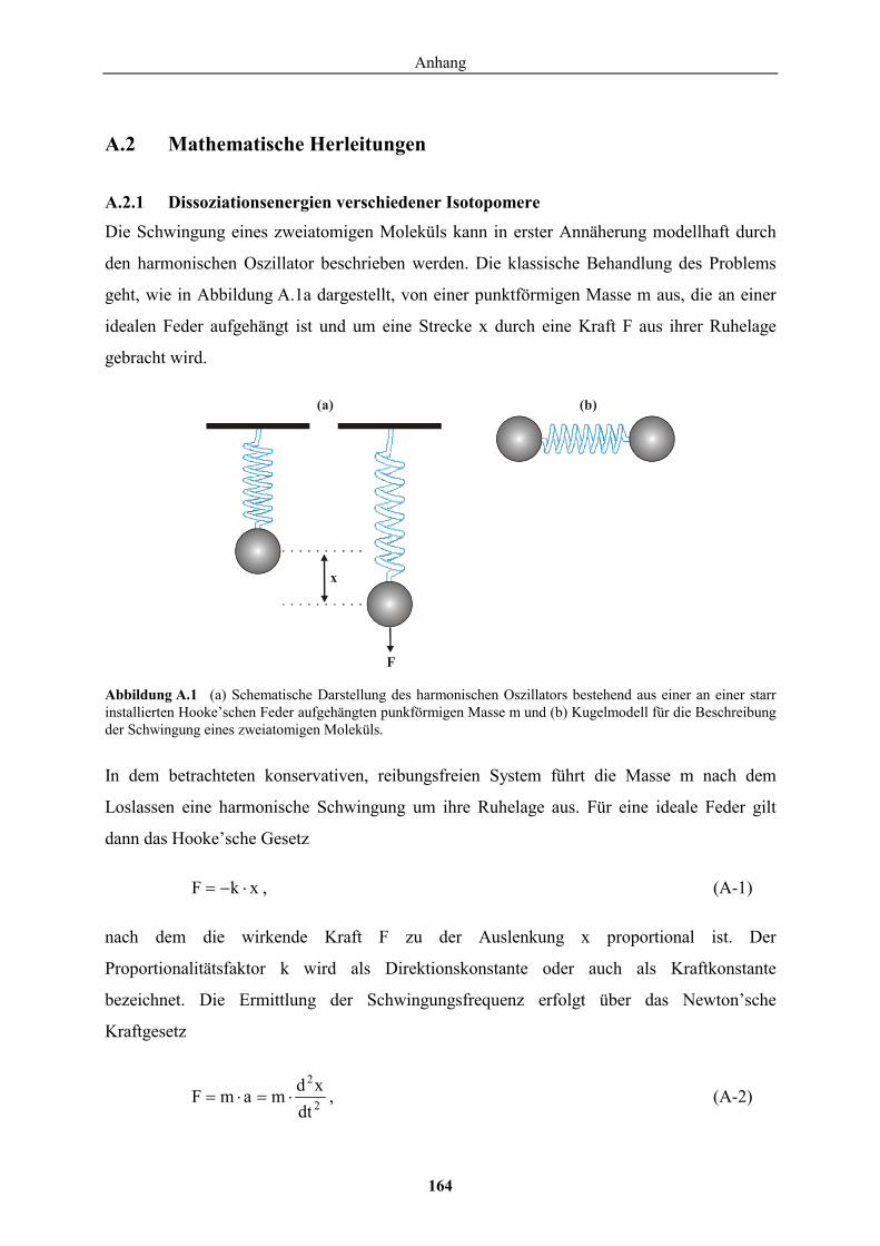
Anhang
164
A.2 Mathematische Herleitungen
A.2.1 Dissoziationsenergien verschiedener Isotopomere
Die Schwingung eines zweiatomigen Moleküls kann in erster Annäherung modellhaft durch
den harmonischen Oszillator beschrieben werden. Die klassische Behandlung des Problems
geht, wie in Abbildung A.1a dargestellt, von einer punktförmigen Masse m aus, die an einer
idealen Feder aufgehängt ist und um eine Strecke x durch eine Kraft F aus ihrer Ruhelage
gebracht wird.
Abbildung A.1 (a) Schematische Darstellung des harmonischen Oszillators bestehend aus einer an einer starr installierten Hooke’schen Feder aufgehängten punkförmigen Masse m und (b) Kugelmodell für die Beschreibung der Schwingung eines zweiatomigen Moleküls.
In dem betrachteten konservativen, reibungsfreien System führt die Masse m nach dem
Loslassen eine harmonische Schwingung um ihre Ruhelage aus. Für eine ideale Feder gilt
dann das Hooke’sche Gesetz
xkF ��� , (A-1)
nach dem die wirkende Kraft F zu der Auslenkung x proportional ist. Der
Proportionalitätsfaktor k wird als Direktionskonstante oder auch als Kraftkonstante
bezeichnet. Die Ermittlung der Schwingungsfrequenz erfolgt über das Newton’sche
Kraftgesetz
2
2
dtxdmamF ���� , (A-2)
x
F
(a) (b)
Anhang
165
das die Beschleunigung a der Masse m beschreibt. Die Kombination der Gleichungen (A-1)
und (A-2) liefert nach Umstellung die Differentialgleichung
0xmk
dtxd2
2�� . (A-3)
Mit dem Lösungsansatz x = A cos t erhält man
0tcosAmktcosA 2
������ (A-4)
und daraus = (k/m)1/2. Nach der Zeit
km2t �� (A-5)
ist die Ausgangslage wieder erreicht. Daraus folgt für die Frequenz �� (�� = 1/t)
mk
21
0�
�� . (A-6)
Die Frequenz der harmonischen Schwingungsbewegung ist somit eine Funktion der
Federkonstanten k und der Masse m. Gleichung (A-6) beschreibt die Schwingungsenergie
einer Feder, an deren Ende sich eine Masse m und eine unendlich schwere Gegenmasse (die
Aufhängung der Feder) befinden. Werden diese Massen durch zwei endliche Massen m1 und
m2 ersetzt, so gilt bei Einführung einer reduzierten Masse � (=m1m2/(m1+m2) für die
Schwingung eines zweiatomigen Moleküls (Abbildung A.1b)
����
k21
0 . (A-7)
Die quantenmechanische Behandlung der harmonischen Schwingung führt zu den
Eigenwerten der Energie Ev
)2/1v(hE 0v ��� (A-8)
Anhang
166
mit der Schwingungsquantenzahl v. Im energetisch niedrigsten Zustand (v = 0) ist immer noch
eine Schwingungsenergie vom Betrag 1/2h�0, die so genannte Nullpunktsenergie, vorhanden.
Substituiert man die Kraft F in Gleichung (A-1) mit
dxdVF �� , (A-9)
wenn V die potentielle Energie darstellt und integriert nach der Auslenkung x, so erhält man
den Zusammenhang zwischen der Auslenkung und der potentiellen Energie
2Dx21V � . (A-10)
Für den harmonischen Oszillator bedeutet dies, dass in einem Molekül sehr hohe Energien
gespeichert werden können, ohne dass dies zu einer Bindungsspaltung führt (Abbildung A.2,
rot gestrichelte Kurve). Die Erfahrung lehrt uns allerdings, dass alle Moleküle dissoziieren,
wenn nur genügend Energie zugeführt wird. Formalistisch wird dieser Zusammenhang im
anharmonischen Oszillator (Abbildung A.2, schwarze Kurve) berücksichtigt. Empirische
Ansätze sorgen dafür, dass mit zunehmendem Bindungsabstand die potentielle Energie einen
konstanten Wert annimmt. Zudem muss der der Realität angepasste linke Ast der
Potentialkurve wesentlich steiler verlaufen als der des harmonischen Oszillators, da sich
aufgrund der Coulombschen Abstoßung zwei Atome bei großer Schwingungsenergie nicht
beliebig weit nähern können.
Die Differenz zwischen den Nullpunktsenergien und dem horizontalen Ast der Potentialkurve
entspricht der Dissoziationsenergie. Nach Gleichung (A-7) und (A-8) schwingen schwerere
Isotopomere mit kleinerer Schwingungsfrequenz � und besitzen demnach auch eine geringere
Nullpunktsenergie E. Daraus folgt, dass für die Dissoziation des schwereren Isotopomers ein
höherer Energiebetrag aufgewendet werden muss, als für die Dissoziation des leichteren
Isotopomers (Abbildung A.2). Dies impliziert, dass die mit höherer Frequenz schwingenden
leichteren Bindungen (12C-12C, 1H-1H) sowohl bei der biotischen als auch abiotischen
Degradation präferentiell gespalten werden und sich somit die schwereren Isotopomere im
residualen, noch nicht abgebauten Substrat anreichern.

Anhang
167
Abbildung A.2 Potentialkurve des anharmonischen Oszillators (rot gestrichelt: harmonischer Oszillator) am Beispiel der 12C-12C- bzw. 12C-13C-Bindung.
A.2.2 Rayleigh-Gleichung
Entwicklung nach Mariotti Der Fraktionierungsfaktor für die unvollständige, unidirektionale Reaktion Substrat (S) �
Produkt (P) ist nach MARIOTTI et al. (1981) definiert als
SP R/R�� . (A-11)
RP entspricht dem Isotopenverhältnis (13C/12C) der unendlich kleinen Menge an Produkt, das
in einer infinitesimal kurzen Zeit t gebildet wird. RS entspricht dem Isotopenverhältnis des
Substrats zur gleichen Zeit. Daraus ergibt sich
S12
S13
P12
P13
C/CCd/Cd
�� . (A-12)
Mit Hilfe von d13CP = -d13CS und d12CP = -d12CS folgt aus Gleichung (A-12)
S12
S13
S12
S12
S13
S13
ClndClnd
C/CdC/Cd
��� . (A-13)
Ist der Fraktionierungsfaktor unabhängig von der Zeit, so erhalten wir durch Umstellung
Pote
ntie
lle E
nerg
ie
Atomabstand
Dissoziationsenergie 12C-12C
Dissoziationsenergie 12C-13C
12C-13C12C-12C
dissoziierte Isotope
Gleichgewichtsabstand
Pote
ntie
lle E
nerg
ie
Atomabstand
Dissoziationsenergie 12C-12C
Dissoziationsenergie 12C-13C
12C-13C12C-12C
dissoziierte Isotope
Gleichgewichtsabstand
Anhang
168
�� ��
t,S13
0,S13
t,S12
0,S12
C
CS
13C
CS
12 ClndClnd . (A-14)
Die Integration dieser Gleichung zwischen 12CS,0 und 12CS,t bzw. 13CS,0 und 13CS,t liefert
��
�
�
��
�
��
��
�
�
��
�
��
0,S13
t,S13
0,S12
t,S12
CC
lnCC
ln , (A-15)
wobei 12CS,0 und 13CS,0 die Mengen der zwei Isotope zur Zeit t = 0 darstellen. Die zum
Zeitpunkt t noch nicht umgesetzte Menge an Substrat bezeichnen wir im Folgenden mit f; CS
bezeichnet die gesamte Menge an Kohlenstoff zur Zeit t (CS = 12CS + 13CS):
0,S13
0,S12
t,S13
t,S12
0,S
t,S
CCCC
CC
f�
�
�� . (A-16)
Da in natürlichen Systemen die Häufigkeit von 13C (1,11%) im Vergleich zu 12C (98,89%)
sehr gering ist, gilt annähernd 12C ≃ 12C + 13C, und somit ist f ≃ 12CS,t/12CS,0. Damit folgt für
Gleichung (A-15)
��
�
�
��
�
���
0,S13
t,S13
CC
lnfln , (A-17)
und ausgedrückt durch das Isotopenverhältnis des schweren zum häufigsten Isotop R (13C/12C)
folgt
� ���
�
�
��
�
��
��
��
�
��
�
��
�
���
����
�
���
����
�
���0,S
t,S
0,S12
13t,S
12
13
RR
ln
CC
CC
lnfln1 . (A-18)
Die Substitution der Isotopenverhältnisse mit Hilfe der „Delta-Notation“ liefert für Gleichung
(A-18)
� ���
�
�
��
�
�
��
���
1000C1000C
lnfln10,S
13t,S
13
. (A-19)
Anhang
169
Entwicklung nach Coleman Die Herleitung der Rayleigh-Gleichung nach COLEMAN et al. (1981) erfolgt über einen
kinetischen Ansatz am Beispiel der Methanoxidation:
OH2COO2CH 2212k
2412 1
����� (A-20)
und
OH2COO2CH 2213k
2413 2
����� . (A-21)
Die Geschwindigkeit mit der die Konzentration der Methanisotope abnimmt, ist proportional
zu der Konzentration [yCH4]. Demnach erhalten wir
� � � �412
14
12
CHkdtCHd
�� (A-22)
und
� � � �413
24
13
CHkdtCHd
�� . (A-23)
Die Proportionalitätskonstanten k1 und k2 bezeichnen die Geschwindigkeitskonstanten der
Reaktion für die zwei verschiedenen Isotopomere. Integration der Gleichungen (A-22) und
(A-23) innerhalb der Grenzen t = 0 und t liefert
� � � � tk04
12t4
12 1eCHCH �
�� (A-24)
� � � � tk04
13t4
13 2eCHCH �
�� . (A-25)
Division der Gleichung (A-24) durch (A-25) und die Einführung der „Delta-Notation“ führen
zu
1000C1000C
e
CHCH
CHCH
013
t13
t)kk(
412
413
t412
413
21
0
��
����
��
���
��
���
� . (A-26)
Anhang
170
Aus 12CH4 » 13CH4 folgt f ≃ [12CH4]t/[12CH4]0. Damit ergibt sich aus Gleichung (A-24)
1kflnt �
� , (A-27)
und substituiert in (A-26) folgt
flnk
kk1000C1000C
ln1
12
013
t13
���
����
� ���
�
�
�
��
�
�
. (A-28)
Gleichung (A-28) ist identisch mit Gleichung (A-19), wenn k2/k1dem Fraktionierungsfaktor �
entspricht.
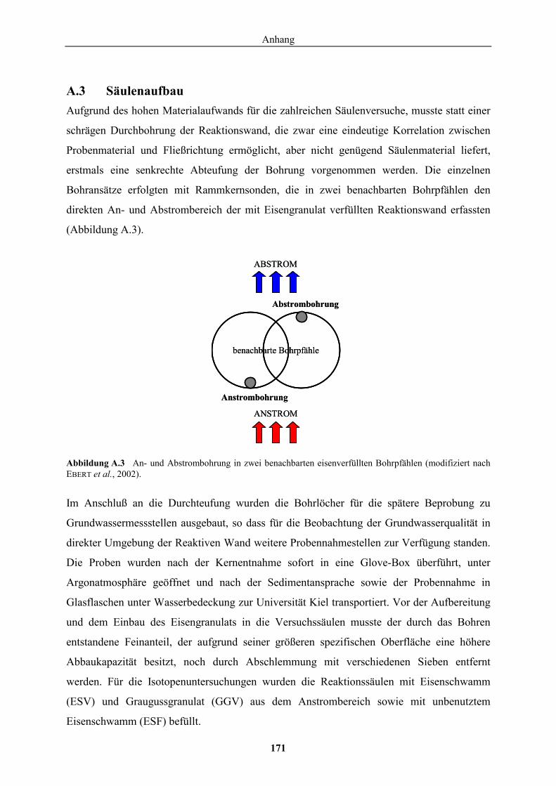
Anhang
171
A.3 Säulenaufbau Aufgrund des hohen Materialaufwands für die zahlreichen Säulenversuche, musste statt einer
schrägen Durchbohrung der Reaktionswand, die zwar eine eindeutige Korrelation zwischen
Probenmaterial und Fließrichtung ermöglicht, aber nicht genügend Säulenmaterial liefert,
erstmals eine senkrechte Abteufung der Bohrung vorgenommen werden. Die einzelnen
Bohransätze erfolgten mit Rammkernsonden, die in zwei benachbarten Bohrpfählen den
direkten An- und Abstrombereich der mit Eisengranulat verfüllten Reaktionswand erfassten
(Abbildung A.3).
Abbildung A.3 An- und Abstrombohrung in zwei benachbarten eisenverfüllten Bohrpfählen (modifiziert nach EBERT et al., 2002).
Im Anschluß an die Durchteufung wurden die Bohrlöcher für die spätere Beprobung zu
Grundwassermessstellen ausgebaut, so dass für die Beobachtung der Grundwasserqualität in
direkter Umgebung der Reaktiven Wand weitere Probennahmestellen zur Verfügung standen.
Die Proben wurden nach der Kernentnahme sofort in eine Glove-Box überführt, unter
Argonatmosphäre geöffnet und nach der Sedimentansprache sowie der Probennahme in
Glasflaschen unter Wasserbedeckung zur Universität Kiel transportiert. Vor der Aufbereitung
und dem Einbau des Eisengranulats in die Versuchssäulen musste der durch das Bohren
entstandene Feinanteil, der aufgrund seiner größeren spezifischen Oberfläche eine höhere
Abbaukapazität besitzt, noch durch Abschlemmung mit verschiedenen Sieben entfernt
werden. Für die Isotopenuntersuchungen wurden die Reaktionssäulen mit Eisenschwamm
(ESV) und Graugussgranulat (GGV) aus dem Anstrombereich sowie mit unbenutztem
Eisenschwamm (ESF) befüllt.
benachbarte Bohrpfähle
Abstrombohrung
Anstrombohrung
ANSTROM
ABSTROM
benachbarte Bohrpfähle
Abstrombohrung
Anstrombohrung
ANSTROM
ABSTROM
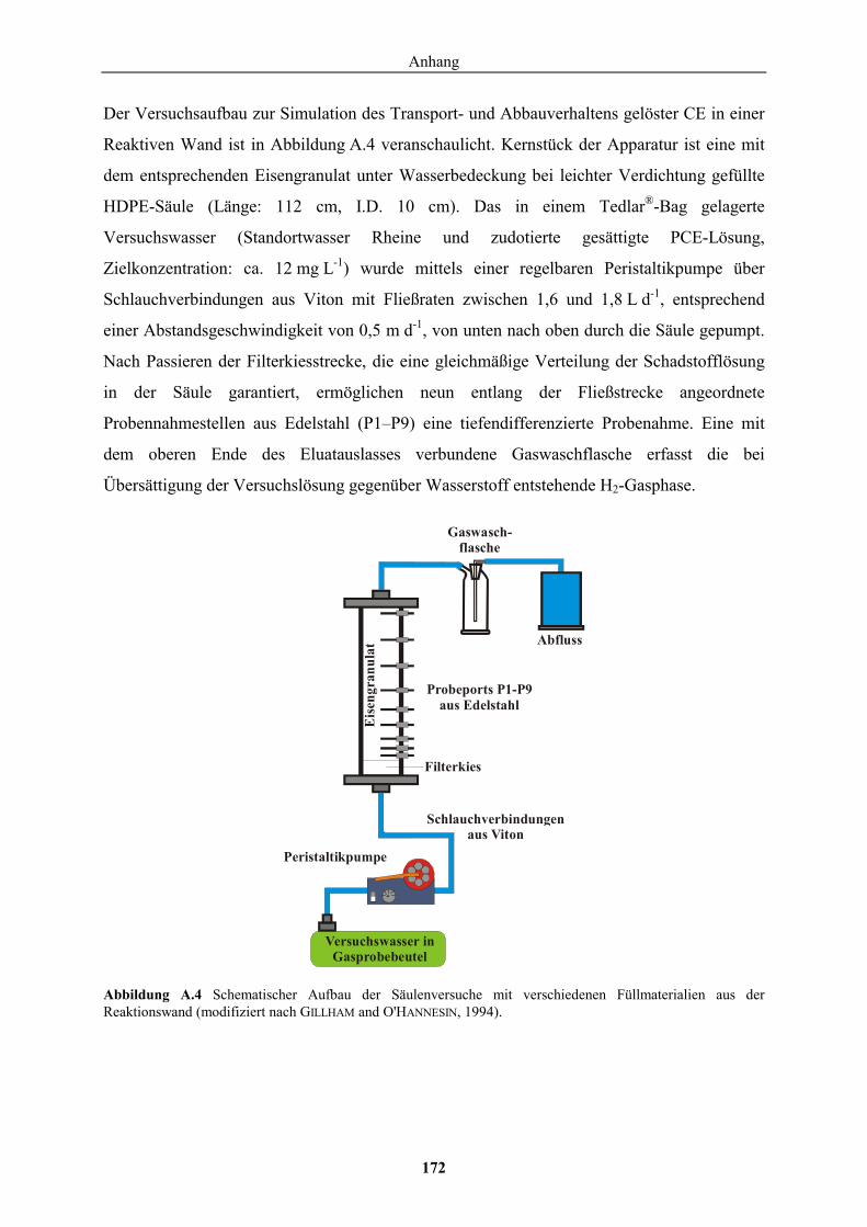
Anhang
172
Der Versuchsaufbau zur Simulation des Transport- und Abbauverhaltens gelöster CE in einer
Reaktiven Wand ist in Abbildung A.4 veranschaulicht. Kernstück der Apparatur ist eine mit
dem entsprechenden Eisengranulat unter Wasserbedeckung bei leichter Verdichtung gefüllte
HDPE-Säule (Länge: 112 cm, I.D. 10 cm). Das in einem Tedlar®-Bag gelagerte
Versuchswasser (Standortwasser Rheine und zudotierte gesättigte PCE-Lösung,
Zielkonzentration: ca. 12 mg L-1) wurde mittels einer regelbaren Peristaltikpumpe über
Schlauchverbindungen aus Viton mit Fließraten zwischen 1,6 und 1,8 L d-1, entsprechend
einer Abstandsgeschwindigkeit von 0,5 m d-1, von unten nach oben durch die Säule gepumpt.
Nach Passieren der Filterkiesstrecke, die eine gleichmäßige Verteilung der Schadstofflösung
in der Säule garantiert, ermöglichen neun entlang der Fließstrecke angeordnete
Probennahmestellen aus Edelstahl (P1–P9) eine tiefendifferenzierte Probenahme. Eine mit
dem oberen Ende des Eluatauslasses verbundene Gaswaschflasche erfasst die bei
Übersättigung der Versuchslösung gegenüber Wasserstoff entstehende H2-Gasphase.
Abbildung A.4 Schematischer Aufbau der Säulenversuche mit verschiedenen Füllmaterialien aus der Reaktionswand (modifiziert nach GILLHAM and O'HANNESIN, 1994).
Abfluss
Gaswasch-flasche
Probeports P1-P9aus Edelstahl
Eis
engr
anul
at
Filterkies
Schlauchverbindungenaus Viton
Peristaltikpumpe
Versuchswasser in Gasprobebeutel
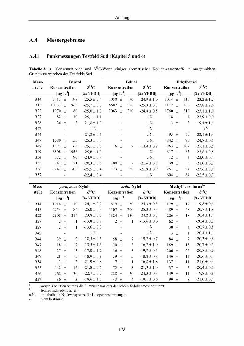
Anhang
173
A.4 Messergebnisse
A.4.1 Punkmessungen Testfeld Süd (Kapitel 5 und 6)
Tabelle A.1a Konzentrationen und �13C-Werte einiger aromatischer Kohlenwasserstoffe in ausgewählten Grundwasserproben des Testfelds Süd.
Mess- Benzol Toluol Ethylbenzol stelle Konzentration �13C Konzentration �13C Konzentration �13C
[�g L-1] [‰ VPDB] [�g L-1] [‰ VPDB] [�g L-1] [‰ VPDB] B14 2412 � 198 -25,5 � 0,4 1050 � 90 -24,9 � 1,0 1014 � 116 -23,2 � 1,2B15 10733 � 965 -25,7 � 0,5 6607 � 518 -25,3 � 0,3 1117 � 186 -23,8 � 2,0B22 1070 � 80 -25,0 � 1,0 2063 � 210 -24,8 � 0,5 1760 � 210 -23,1 � 1,0B27 82 � 10 -25,1 � 1,1 - u.N. 18 � 4 -23,9 � 0,9B28 26 � 5 -21,8 � 1,0 - u.N. 3 � 2 -19,4 � 1,4B42 - u.N. - u.N. - u.N. B44 - -21,3 � 0,6 - u.N. 495 � 70 -22,1 � 1,4B47 1080 � 153 -25,3 � 0,5 - u.N. 842 � 96 -24,8 � 0,5B48 1123 � 65 -25,1 � 0,5 16 � 2 -14,4 � 0,8 863 � 107 -25,1 � 0,5B49 8808 � 1056 -25,8 � 1,0 - u.N. 617 � 83 -23,8 � 0,5B54 772 � 90 -24,9 � 0,8 - u.N. 12 � 4 -23,0 � 0,4B55 143 � 21 -20,3 � 0,5 100 � 7 -21,6 � 0,5 39 � 5 -21,0 � 0,3B56 3242 � 500 -25,5 � 0,4 173 � 20 -21,9 � 0,9 251 � 24 -23,6 � 0,8B57 - -22,4 � 0,4 - u.N. 604 � 64 -22,5 � 0,7
Mess- para, meta-Xylola) ortho-Xylol Methylbenzofuranb) stelle Konzentration �13C Konzentration �13C Konzentration �13C
[�g L-1] [‰ VPDB] [�g L-1] [‰ VPDB] [�g L-1] [‰ VPDB] B14 1014 � 110 -24,1 � 0,7 579 � 60 -25,3 � 0,5 179 � 19 -19,8 � 0,5B15 2254 � 184 -25,0 � 0,3 1107 � 200 -25,3 � 0,3 489 � 48 -20,7 � 1,9B22 2608 � 214 -23,8 � 0,5 1324 � 150 -24,2 � 0,7 226 � 18 -20,4 � 1,4B27 2 � 1 -13,8 � 0,9 2 � 1 -13,6 � 0,6 62 � 6 -20,4 � 0,3B28 2 � 1 -13,6 � 2,3 - u.N. 30 � 4 -20,7 � 0,8B42 - u.N. - u.N. 3 � 1 -20,4 � 1,1B44 39 � 3 -18,5 � 0,5 58 � 7 -19,7 � 0,7 84 � 7 -20,3 � 0,8B47 18 � 2 -13,5 � 1,6 20 � 3 -16,7 � 1,0 169 � 15 -20,7 � 0,5B48 27 � 3 -17,0 � 1,2 36 � 3 -19,7 � 0,3 206 � 22 -20,8 � 0,6B49 28 � 3 -18,9 � 0,9 39 � 3 -18,8 � 0,8 146 � 14 -20,6 � 0,7B54 3 � 3 -21,9 � 0,8 7 � 1 -16,8 � 1,8 137 � 11 -21,0 � 0,4B55 142 � 15 -21,8 � 0,6 72 � 8 -21,9 � 1,0 37 � 5 -20,4 � 0,3B56 268 � 30 -22,7 � 0,7 228 � 20 -24,3 � 0,8 149 � 11 -19,8 � 0,8B57 30 � 3 -18,6 � 1,3 43 � 4 -18,1 � 0,6 99 � 8 -21,0 � 0,4
a) wegen Koelution wurden die Summenparameter der beiden Xylolisomere bestimmt. b) Isomer nicht identifiziert. u.N. unterhalb der Nachweisgrenze für Isotopenbestimmungen. - nicht bestimmt.
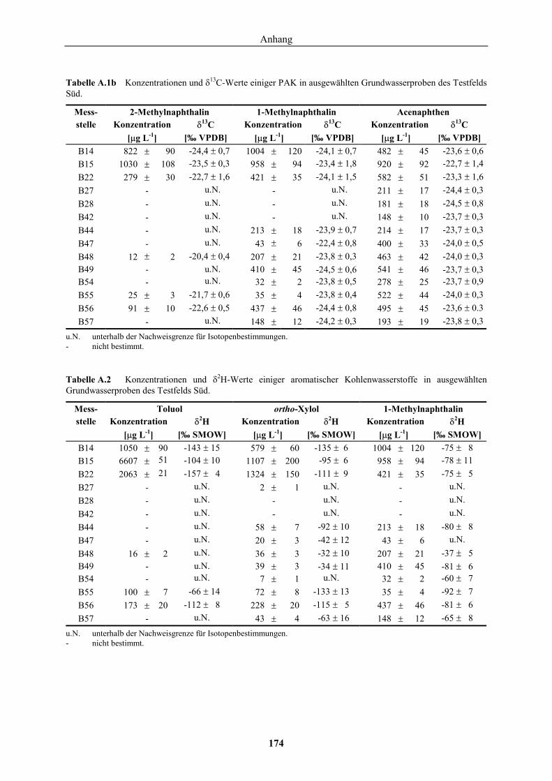
Anhang
174
Tabelle A.1b Konzentrationen und �13C-Werte einiger PAK in ausgewählten Grundwasserproben des Testfelds Süd.
Mess- 2-Methylnaphthalin 1-Methylnaphthalin Acenaphthen stelle Konzentration �13C Konzentration �13C Konzentration �13C
[�g L-1] [‰ VPDB] [�g L-1] [‰ VPDB] [�g L-1] [‰ VPDB] B14 822 � 90 -24,4 � 0,7 1004 � 120 -24,1 � 0,7 482 � 45 -23,6 � 0,6B15 1030 � 108 -23,5 � 0,3 958 � 94 -23,4 � 1,8 920 � 92 -22,7 � 1,4B22 279 � 30 -22,7 � 1,6 421 � 35 -24,1 � 1,5 582 � 51 -23,3 � 1,6B27 - u.N. - u.N. 211 � 17 -24,4 � 0,3B28 - u.N. - u.N. 181 � 18 -24,5 � 0,8B42 - u.N. - u.N. 148 � 10 -23,7 � 0,3B44 - u.N. 213 � 18 -23,9 � 0,7 214 � 17 -23,7 � 0,3B47 - u.N. 43 � 6 -22,4 � 0,8 400 � 33 -24,0 � 0,5B48 12 � 2 -20,4 � 0,4 207 � 21 -23,8 � 0,3 463 � 42 -24,0 � 0,3B49 - u.N. 410 � 45 -24,5 � 0,6 541 � 46 -23,7 � 0,3B54 - u.N. 32 � 2 -23,8 � 0,5 278 � 25 -23,7 � 0,9B55 25 � 3 -21,7 � 0,6 35 � 4 -23,8 � 0,4 522 � 44 -24,0 � 0,3B56 91 � 10 -22,6 � 0,5 437 � 46 -24,4 � 0,8 495 � 45 -23,6 � 0.3B57 - u.N. 148 � 12 -24,2 � 0,3 193 � 19 -23,8 � 0,3
u.N. unterhalb der Nachweisgrenze für Isotopenbestimmungen. - nicht bestimmt.
Tabelle A.2 Konzentrationen und �2H-Werte einiger aromatischer Kohlenwasserstoffe in ausgewählten Grundwasserproben des Testfelds Süd.
Mess- Toluol ortho-Xylol 1-Methylnaphthalin stelle Konzentration �2H Konzentration �2H Konzentration �2H
[�g L-1] [‰ SMOW] [�g L-1] [‰ SMOW] [�g L-1] [‰ SMOW] B14 1050 � 90 -143 � 15 579 � 60 -135 � 6 1004 � 120 -75 � 8 B15 6607 � 51 -104 � 10 1107 � 200 -95 � 6 958 � 94 -78 � 11 B22 2063 � 21 -157 � 4 1324 � 150 -111 � 9 421 � 35 -75 � 5 B27 - u.N. 2 � 1 u.N. - u.N. B28 - u.N. - u.N. - u.N. B42 - u.N. - u.N. - u.N. B44 - u.N. 58 � 7 -92 � 10 213 � 18 -80 � 8 B47 - u.N. 20 � 3 -42 � 12 43 � 6 u.N. B48 16 � 2 u.N. 36 � 3 -32 � 10 207 � 21 -37 � 5 B49 - u.N. 39 � 3 -34 � 11 410 � 45 -81 � 6 B54 - u.N. 7 � 1 u.N. 32 � 2 -60 � 7 B55 100 � 7 -66 � 14 72 � 8 -133 � 13 35 � 4 -92 � 7 B56 173 � 20 -112 � 8 228 � 20 -115 � 5 437 � 46 -81 � 6 B57 - u.N. 43 � 4 -63 � 16 148 � 12 -65 � 8
u.N. unterhalb der Nachweisgrenze für Isotopenbestimmungen. - nicht bestimmt.
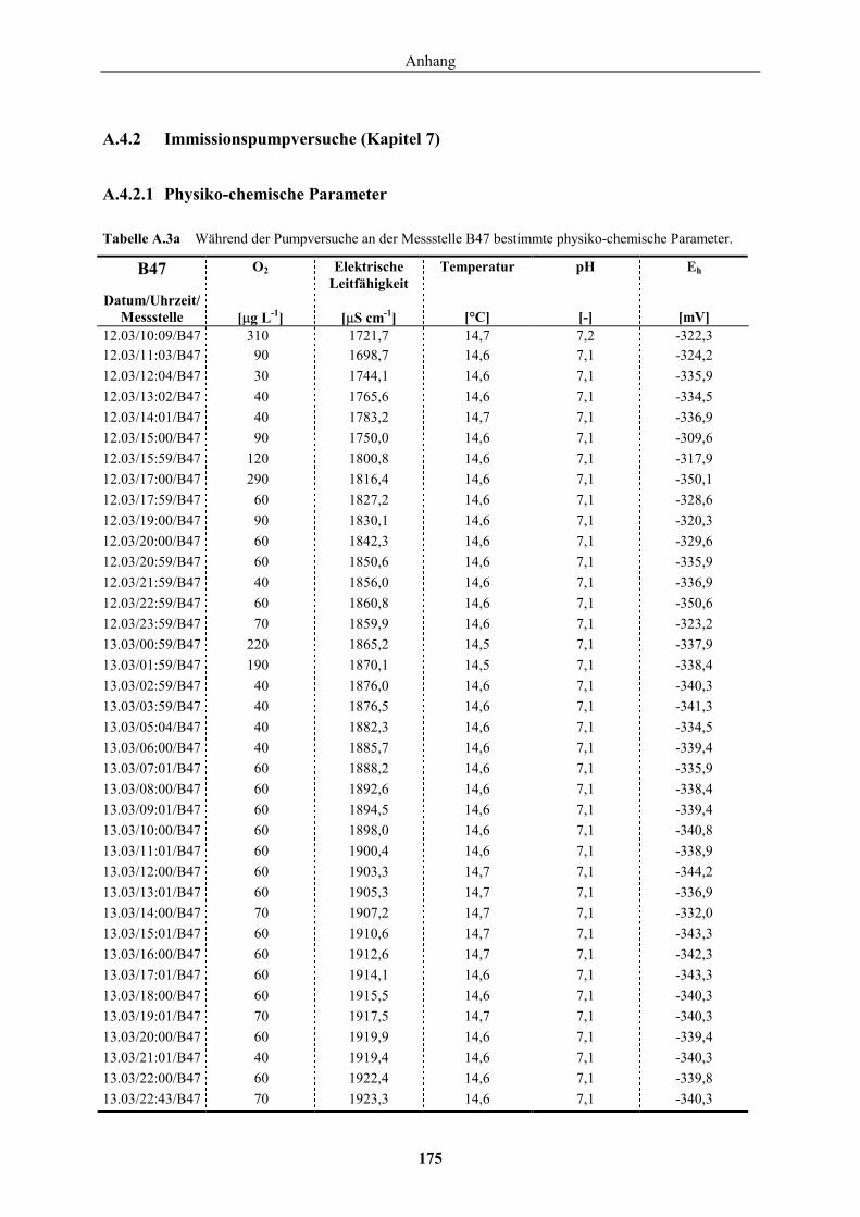
Anhang
175
A.4.2 Immissionspumpversuche (Kapitel 7)
A.4.2.1 Physiko-chemische Parameter
Tabelle A.3a Während der Pumpversuche an der Messstelle B47 bestimmte physiko-chemische Parameter.
B47 O2 Elektrische Leitfähigkeit
Temperatur pH Eh
Datum/Uhrzeit/ Messstelle
[�g L-1]
[�S cm-1]
[°C]
[-]
[mV]
12.03/10:09/B47 310 1721,7 14,7 7,2 -322,3 12.03/11:03/B47 90 1698,7 14,6 7,1 -324,2 12.03/12:04/B47 30 1744,1 14,6 7,1 -335,9 12.03/13:02/B47 40 1765,6 14,6 7,1 -334,5 12.03/14:01/B47 40 1783,2 14,7 7,1 -336,9 12.03/15:00/B47 90 1750,0 14,6 7,1 -309,6 12.03/15:59/B47 120 1800,8 14,6 7,1 -317,9 12.03/17:00/B47 290 1816,4 14,6 7,1 -350,1 12.03/17:59/B47 60 1827,2 14,6 7,1 -328,6 12.03/19:00/B47 90 1830,1 14,6 7,1 -320,3 12.03/20:00/B47 60 1842,3 14,6 7,1 -329,6 12.03/20:59/B47 60 1850,6 14,6 7,1 -335,9 12.03/21:59/B47 40 1856,0 14,6 7,1 -336,9 12.03/22:59/B47 60 1860,8 14,6 7,1 -350,6 12.03/23:59/B47 70 1859,9 14,6 7,1 -323,2 13.03/00:59/B47 220 1865,2 14,5 7,1 -337,9 13.03/01:59/B47 190 1870,1 14,5 7,1 -338,4 13.03/02:59/B47 40 1876,0 14,6 7,1 -340,3 13.03/03:59/B47 40 1876,5 14,6 7,1 -341,3 13.03/05:04/B47 40 1882,3 14,6 7,1 -334,5 13.03/06:00/B47 40 1885,7 14,6 7,1 -339,4 13.03/07:01/B47 60 1888,2 14,6 7,1 -335,9 13.03/08:00/B47 60 1892,6 14,6 7,1 -338,4 13.03/09:01/B47 60 1894,5 14,6 7,1 -339,4 13.03/10:00/B47 60 1898,0 14,6 7,1 -340,8 13.03/11:01/B47 60 1900,4 14,6 7,1 -338,9 13.03/12:00/B47 60 1903,3 14,7 7,1 -344,2 13.03/13:01/B47 60 1905,3 14,7 7,1 -336,9 13.03/14:00/B47 70 1907,2 14,7 7,1 -332,0 13.03/15:01/B47 60 1910,6 14,7 7,1 -343,3 13.03/16:00/B47 60 1912,6 14,7 7,1 -342,3 13.03/17:01/B47 60 1914,1 14,6 7,1 -343,3 13.03/18:00/B47 60 1915,5 14,6 7,1 -340,3 13.03/19:01/B47 70 1917,5 14,7 7,1 -340,3 13.03/20:00/B47 60 1919,9 14,6 7,1 -339,4 13.03/21:01/B47 40 1919,4 14,6 7,1 -340,3 13.03/22:00/B47 60 1922,4 14,6 7,1 -339,8 13.03/22:43/B47 70 1923,3 14,6 7,1 -340,3
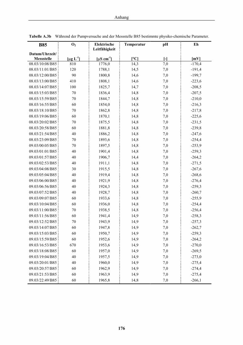
Anhang
176
Tabelle A.3b Während der Pumpversuche and der Messstelle B85 bestimmte physiko-chemische Parameter.
B85 O2 Elektrische Leitfähigkeit
Temperatur pH Eh
Datum/Uhrzeit/ Messstelle
[�g L-1]
[�S cm-1]
[°C]
[-]
[mV]
08.03/10:08/B85 810 1776,0 14,3 7,0 -170,4 08.03/11:01/B85 120 1788,1 14,5 7,0 -191,4 08.03/12:00/B85 90 1800,8 14,6 7,0 -199,7 08.03/13:00/B85 410 1808,1 14,6 7,0 -223,6 08.03/14:07/B85 100 1825,7 14,7 7,0 -208,5 08.03/15:03/B85 70 1836,4 14,8 7,0 -207,5 08.03/15:59/B85 70 1844,7 14,8 7,0 -210,0 08.03/16:55/B85 60 1854,0 14,8 7,0 -216,3 08.03/18:10/B85 70 1862,8 14,8 7,0 -217,8 08.03/19:06/B85 60 1870,1 14,8 7,0 -225,6 08.03/20:02/B85 70 1875,5 14,8 7,0 -231,5 08.03/20:58/B85 60 1881,8 14,8 7,0 -239,8 08.03/21:54/B85 40 1886,2 14,8 7,0 -247,6 08.03/23:09/B85 70 1893,6 14,8 7,0 -254,4 09.03/00:05/B85 70 1897,5 14,8 7,0 -253,9 09.03/01:01/B85 40 1901,4 14,8 7,0 -259,3 09.03/01:57/B85 40 1906,7 14,4 7,0 -264,2 09.03/02:53/B85 40 1911,1 14,8 7,0 -271,5 09.03/04:08/B85 30 1915,5 14,8 7,0 -267,6 09.03/05:04/B85 40 1919,4 14,8 7,0 -268,6 09.03/06:00/B85 40 1921,9 14,8 7,0 -276,4 09.03/06:56/B85 40 1924,3 14,8 7,0 -259,3 09.03/07:52/B85 40 1928,7 14,8 7,0 -260,7 09.03/09:07/B85 60 1933,6 14,8 7,0 -255,9 09.03/10:04/B85 60 1936,0 14,8 7,0 -254,4 09.03/11:00/B85 70 1938,5 14,8 7,0 -256,4 09.03/11:56/B85 60 1941,4 14,9 7,0 -258,3 09.03/12:52/B85 70 1943,9 14,9 7,0 -257,3 09.03/14:07/B85 60 1947,8 14,9 7,0 -262,7 09.03/15:03/B85 60 1950,7 14,9 7,0 -259,3 09.03/15:59/B85 60 1952,6 14,9 7,0 -264,2 09.03/16:53/B85 670 1953,6 14,9 7,0 -270,0 09.03/18:08/B85 60 1957,0 14,9 7,0 -269,5 09.03/19:04/B85 40 1957,5 14,9 7,0 -273,0 09.03/20:01/B85 40 1960,0 14,9 7,0 -275,4 09.03/20:57/B85 60 1962,9 14,9 7,0 -274,4 09.03/21:53/B85 60 1963,9 14,9 7,0 -275,4 09.03/22:49/B85 60 1965,8 14,8 7,0 -266,1
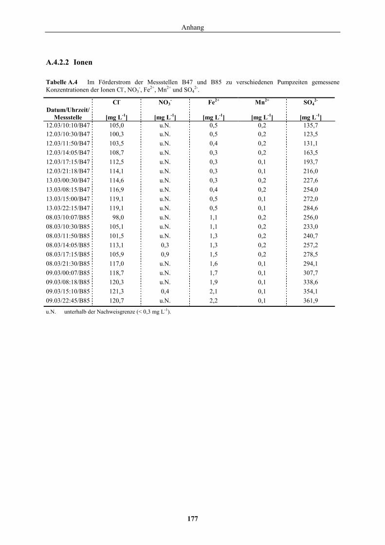
Anhang
177
A.4.2.2 Ionen
Tabelle A.4 Im Förderstrom der Messstellen B47 und B85 zu verschiedenen Pumpzeiten gemessene Konzentrationen der Ionen Cl-, NO3
-, Fe2+, Mn2+ und SO42-.
Cl- NO3- Fe2+ Mn2+ SO4
2- Datum/Uhrzeit/
Messstelle
[mg L-1]
[mg L-1]
[mg L-1]
[mg L-1]
[mg L-1] 12.03/10:10/B47 105,0 u.N. 0,5 0,2 135,7 12.03/10:30/B47 100,3 u.N. 0,5 0,2 123,5 12.03/11:50/B47 103,5 u.N. 0,4 0,2 131,1 12.03/14:05/B47 108,7 u.N. 0,3 0,2 163,5 12.03/17:15/B47 112,5 u.N. 0,3 0,1 193,7 12.03/21:18/B47 114,1 u.N. 0,3 0,1 216,0 13.03/00:30/B47 114,6 u.N. 0,3 0,2 227,6 13.03/08:15/B47 116,9 u.N. 0,4 0,2 254,0 13.03/15:00/B47 119,1 u.N. 0,5 0,1 272,0 13.03/22:15/B47 119,1 u.N. 0,5 0,1 284,6 08.03/10:07/B85 98,0 u.N. 1,1 0,2 256,0 08.03/10:30/B85 105,1 u.N. 1,1 0,2 233,0 08.03/11:50/B85 101,5 u.N. 1,3 0,2 240,7 08.03/14:05/B85 113,1 0,3 1,3 0,2 257,2 08.03/17:15/B85 105,9 0,9 1,5 0,2 278,5 08.03/21:30/B85 117,0 u.N. 1,6 0,1 294,1 09.03/00:07/B85 118,7 u.N. 1,7 0,1 307,7 09.03/08:18/B85 120,3 u.N. 1,9 0,1 338,6 09.03/15:10/B85 121,3 0,4 2,1 0,1 354,1 09.03/22:45/B85 120,7 u.N. 2,2 0,1 361,9
u.N. unterhalb der Nachweisgrenze (< 0,3 mg L-1).
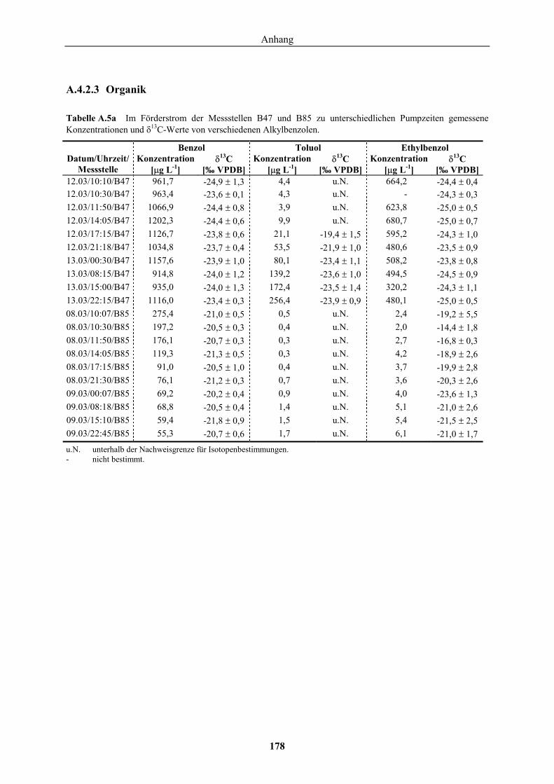
Anhang
178
A.4.2.3 Organik
Tabelle A.5a Im Förderstrom der Messstellen B47 und B85 zu unterschiedlichen Pumpzeiten gemessene Konzentrationen und �13C-Werte von verschiedenen Alkylbenzolen.
Benzol Toluol Ethylbenzol Datum/Uhrzeit/
Messstelle Konzentration
[�g L-1] �13C
[‰ VPDB]Konzentration
[�g L-1] �13C
[‰ VPDB]Konzentration
[�g L-1] �13C
[‰ VPDB]12.03/10:10/B47 961,7 -24,9 � 1,3 4,4 u.N. 664,2 -24,4 � 0,4 12.03/10:30/B47 963,4 -23,6 � 0,1 4,3 u.N. - -24,3 � 0,3 12.03/11:50/B47 1066,9 -24,4 � 0,8 3,9 u.N. 623,8 -25,0 � 0,5 12.03/14:05/B47 1202,3 -24,4 � 0,6 9,9 u.N. 680,7 -25,0 � 0,7 12.03/17:15/B47 1126,7 -23,8 � 0,6 21,1 -19,4 � 1,5 595,2 -24,3 � 1,0 12.03/21:18/B47 1034,8 -23,7 � 0,4 53,5 -21,9 � 1,0 480,6 -23,5 � 0,9 13.03/00:30/B47 1157,6 -23,9 � 1,0 80,1 -23,4 � 1,1 508,2 -23,8 � 0,8 13.03/08:15/B47 914,8 -24,0 � 1,2 139,2 -23,6 � 1,0 494,5 -24,5 � 0,9 13.03/15:00/B47 935,0 -24,0 � 1,3 172,4 -23,5 � 1,4 320,2 -24,3 � 1,1 13.03/22:15/B47 1116,0 -23,4 � 0,3 256,4 -23,9 � 0,9 480,1 -25,0 � 0,5 08.03/10:07/B85 275,4 -21,0 � 0,5 0,5 u.N. 2,4 -19,2 � 5,5 08.03/10:30/B85 197,2 -20,5 � 0,3 0,4 u.N. 2,0 -14,4 � 1,8 08.03/11:50/B85 176,1 -20,7 � 0,3 0,3 u.N. 2,7 -16,8 � 0,3 08.03/14:05/B85 119,3 -21,3 � 0,5 0,3 u.N. 4,2 -18,9 � 2,6 08.03/17:15/B85 91,0 -20,5 � 1,0 0,4 u.N. 3,7 -19,9 � 2,8 08.03/21:30/B85 76,1 -21,2 � 0,3 0,7 u.N. 3,6 -20,3 � 2,6 09.03/00:07/B85 69,2 -20,2 � 0,4 0,9 u.N. 4,0 -23,6 � 1,3 09.03/08:18/B85 68,8 -20,5 � 0,4 1,4 u.N. 5,1 -21,0 � 2,6 09.03/15:10/B85 59,4 -21,8 � 0,9 1,5 u.N. 5,4 -21,5 � 2,5 09.03/22:45/B85 55,3 -20,7 � 0,6 1,7 u.N. 6,1 -21,0 � 1,7 u.N. unterhalb der Nachweisgrenze für Isotopenbestimmungen. - nicht bestimmt.
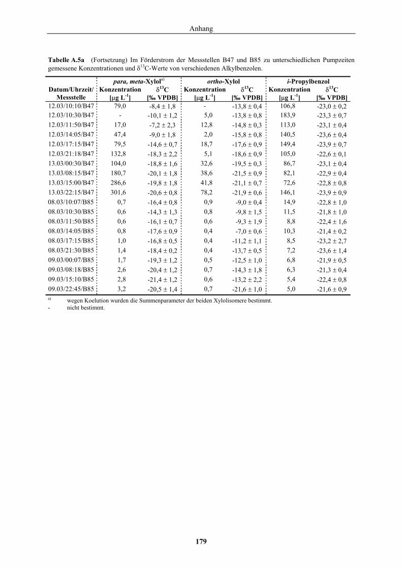
Anhang
179
Tabelle A.5a (Fortsetzung) Im Förderstrom der Messstellen B47 und B85 zu unterschiedlichen Pumpzeiten gemessene Konzentrationen und �13C-Werte von verschiedenen Alkylbenzolen.
para, meta-Xylola) ortho-Xylol i-Propylbenzol Datum/Uhrzeit/
Messstelle Konzentration
[�g L-1] �13C
[‰ VPDB]Konzentration
[�g L-1] �13C
[‰ VPDB]Konzentration
[�g L-1] �13C
[‰ VPDB]12.03/10:10/B47 79,0 -8,4 � 1,8 - -13,8 � 0,4 106,8 -23,0 � 0,2 12.03/10:30/B47 - -10,1 � 1,2 5,0 -13,8 � 0,8 183,9 -23,3 � 0,7 12.03/11:50/B47 17,0 -7,2 � 2,3 12,8 -14,8 � 0,3 113,0 -23,1 � 0,4 12.03/14:05/B47 47,4 -9,0 � 1,8 2,0 -15,8 � 0,8 140,5 -23,6 � 0,4 12.03/17:15/B47 79,5 -14,6 � 0,7 18,7 -17,6 � 0,9 149,4 -23,9 � 0,7 12.03/21:18/B47 132,8 -18,3 � 2,2 5,1 -18,6 � 0,9 105,0 -22,6 � 0,1 13.03/00:30/B47 104,0 -18,8 � 1,6 32,6 -19,5 � 0,3 86,7 -23,1 � 0,4 13.03/08:15/B47 180,7 -20,1 � 1,8 38,6 -21,5 � 0,9 82,1 -22,9 � 0,4 13.03/15:00/B47 286,6 -19,8 � 1,8 41,8 -21,1 � 0,7 72,6 -22,8 � 0,8 13.03/22:15/B47 301,6 -20,6 � 0,8 78,2 -21,9 � 0,6 146,1 -23,9 � 0,9 08.03/10:07/B85 0,7 -16,4 � 0,8 0,9 -9,0 � 0,4 14,9 -22,8 � 1,0 08.03/10:30/B85 0,6 -14,3 � 1,3 0,8 -9,8 � 1,5 11,5 -21,8 � 1,0 08.03/11:50/B85 0,6 -16,1 � 0,7 0,6 -9,3 � 1,9 8,8 -22,4 � 1,6 08.03/14:05/B85 0,8 -17,6 � 0,9 0,4 -7,0 � 0,6 10,3 -21,4 � 0,2 08.03/17:15/B85 1,0 -16,8 � 0,5 0,4 -11,2 � 1,1 8,5 -23,2 � 2,7 08.03/21:30/B85 1,4 -18,4 � 0,2 0,4 -13,7 � 0,5 7,2 -23,6 � 1,4 09.03/00:07/B85 1,7 -19,3 � 1,2 0,5 -12,5 � 1,0 6,8 -21,9 � 0,5 09.03/08:18/B85 2,6 -20,4 � 1,2 0,7 -14,3 � 1,8 6,3 -21,3 � 0,4 09.03/15:10/B85 2,8 -21,4 � 1,2 0,6 -13,2 � 2,2 5,4 -22,4 � 0,8 09.03/22:45/B85 3,2 -20,5 � 1,4 0,7 -21,6 � 1,0 5,0 -21,6 � 0,9 a) wegen Koelution wurden die Summenparameter der beiden Xylolisomere bestimmt. - nicht bestimmt.
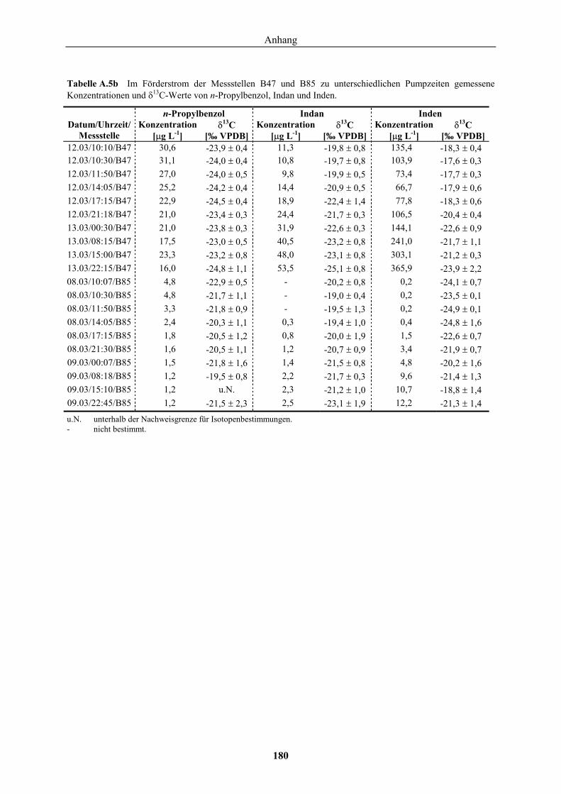
Anhang
180
Tabelle A.5b Im Förderstrom der Messstellen B47 und B85 zu unterschiedlichen Pumpzeiten gemessene Konzentrationen und �13C-Werte von n-Propylbenzol, Indan und Inden.
n-Propylbenzol Indan Inden Datum/Uhrzeit/
Messstelle Konzentration
[�g L-1] �13C
[‰ VPDB]Konzentration
[�g L-1] �13C
[‰ VPDB]Konzentration
[�g L-1] �13C
[‰ VPDB]12.03/10:10/B47 30,6 -23,9 � 0,4 11,3 -19,8 � 0,8 135,4 -18,3 � 0,4 12.03/10:30/B47 31,1 -24,0 � 0,4 10,8 -19,7 � 0,8 103,9 -17,6 � 0,3 12.03/11:50/B47 27,0 -24,0 � 0,5 9,8 -19,9 � 0,5 73,4 -17,7 � 0,3 12.03/14:05/B47 25,2 -24,2 � 0,4 14,4 -20,9 � 0,5 66,7 -17,9 � 0,6 12.03/17:15/B47 22,9 -24,5 � 0,4 18,9 -22,4 � 1,4 77,8 -18,3 � 0,6 12.03/21:18/B47 21,0 -23,4 � 0,3 24,4 -21,7 � 0,3 106,5 -20,4 � 0,4 13.03/00:30/B47 21,0 -23,8 � 0,3 31,9 -22,6 � 0,3 144,1 -22,6 � 0,9 13.03/08:15/B47 17,5 -23,0 � 0,5 40,5 -23,2 � 0,8 241,0 -21,7 � 1,1 13.03/15:00/B47 23,3 -23,2 � 0,8 48,0 -23,1 � 0,8 303,1 -21,2 � 0,3 13.03/22:15/B47 16,0 -24,8 � 1,1 53,5 -25,1 � 0,8 365,9 -23,9 � 2,2 08.03/10:07/B85 4,8 -22,9 � 0,5 - -20,2 � 0,8 0,2 -24,1 � 0,7 08.03/10:30/B85 4,8 -21,7 � 1,1 - -19,0 � 0,4 0,2 -23,5 � 0,1 08.03/11:50/B85
/ /3,3 -21,8 � 0,9 - -19,5 � 1,3 0,2 -24,9 � 0,1
08.03/14:05/B85 2,4 -20,3 � 1,1 0,3 -19,4 � 1,0 0,4 -24,8 � 1,6 08.03/17:15/B85 1,8 -20,5 � 1,2 0,8 -20,0 � 1,9 1,5 -22,6 � 0,7 08.03/21:30/B85 1,6 -20,5 � 1,1 1,2 -20,7 � 0,9 3,4 -21,9 � 0,7 09.03/00:07/B85 1,5 -21,8 � 1,6 1,4 -21,5 � 0,8 4,8 -20,2 � 1,6 09.03/08:18/B85 1,2 -19,5 � 0,8 2,2 -21,7 � 0,3 9,6 -21,4 � 1,3 09.03/15:10/B85 1,2 u.N. 2,3 -21,2 � 1,0 10,7 -18,8 � 1,4 09.03/22:45/B85 1,2 -21,5 � 2,3 2,5 -23,1 � 1,9 12,2 -21,3 � 1,4 u.N. unterhalb der Nachweisgrenze für Isotopenbestimmungen. - nicht bestimmt.
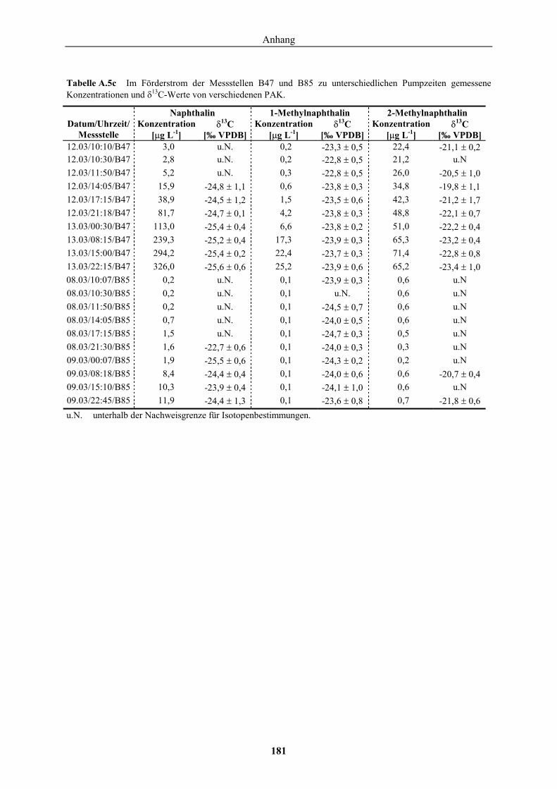
Anhang
181
Tabelle A.5c Im Förderstrom der Messstellen B47 und B85 zu unterschiedlichen Pumpzeiten gemessene Konzentrationen und �13C-Werte von verschiedenen PAK.
Naphthalin 1-Methylnaphthalin 2-Methylnaphthalin Datum/Uhrzeit/
Messstelle Konzentration
[�g L-1] �13C
[‰ VPDB]Konzentration
[�g L-1] �13C
[‰ VPDB]Konzentration
[�g L-1] �13C
[‰ VPDB]12.03/10:10/B47 3,0 u.N. 0,2 -23,3 � 0,5 22,4 -21,1 � 0,2 12.03/10:30/B47 2,8 u.N. 0,2 -22,8 � 0,5 21,2 u.N 12.03/11:50/B47 5,2 u.N. 0,3 -22,8 � 0,5 26,0 -20,5 � 1,0 12.03/14:05/B47 15,9 -24,8 � 1,1 0,6 -23,8 � 0,3 34,8 -19,8 � 1,1 12.03/17:15/B47 38,9 -24,5 � 1,2 1,5 -23,5 � 0,6 42,3 -21,2 � 1,7 12.03/21:18/B47 81,7 -24,7 � 0,1 4,2 -23,8 � 0,3 48,8 -22,1 � 0,7 13.03/00:30/B47 113,0 -25,4 � 0,4 6,6 -23,8 � 0,2 51,0 -22,2 � 0,4 13.03/08:15/B47 239,3 -25,2 � 0,4 17,3 -23,9 � 0,3 65,3 -23,2 � 0,4 13.03/15:00/B47 294,2 -25,4 � 0,2 22,4 -23,7 � 0,3 71,4 -22,8 � 0,8 13.03/22:15/B47 326,0 -25,6 � 0,6 25,2 -23,9 � 0,6 65,2 -23,4 � 1,0 08.03/10:07/B85 0,2 u.N. 0,1 -23,9 � 0,3 0,6 u.N 08.03/10:30/B85 0,2 u.N. 0,1 u.N. 0,6 u.N 08.03/11:50/B85 0,2 u.N. 0,1 -24,5 � 0,7 0,6 u.N 08.03/14:05/B85 0,7 u.N. 0,1 -24,0 � 0,5 0,6 u.N 08.03/17:15/B85 1,5 u.N. 0,1 -24,7 � 0,3 0,5 u.N 08.03/21:30/B85 1,6 -22,7 � 0,6 0,1 -24,0 � 0,3 0,3 u.N 09.03/00:07/B85 1,9 -25,5 � 0,6 0,1 -24,3 � 0,2 0,2 u.N 09.03/08:18/B85 8,4 -24,4 � 0,4 0,1 -24,0 � 0,6 0,6 -20,7 � 0,4 09.03/15:10/B85 10,3 -23,9 � 0,4 0,1 -24,1 � 1,0 0,6 u.N 09.03/22:45/B85 11,9 -24,4 � 1,3 0,1 -23,6 � 0,8 0,7 -21,8 � 0,6 u.N. unterhalb der Nachweisgrenze für Isotopenbestimmungen.
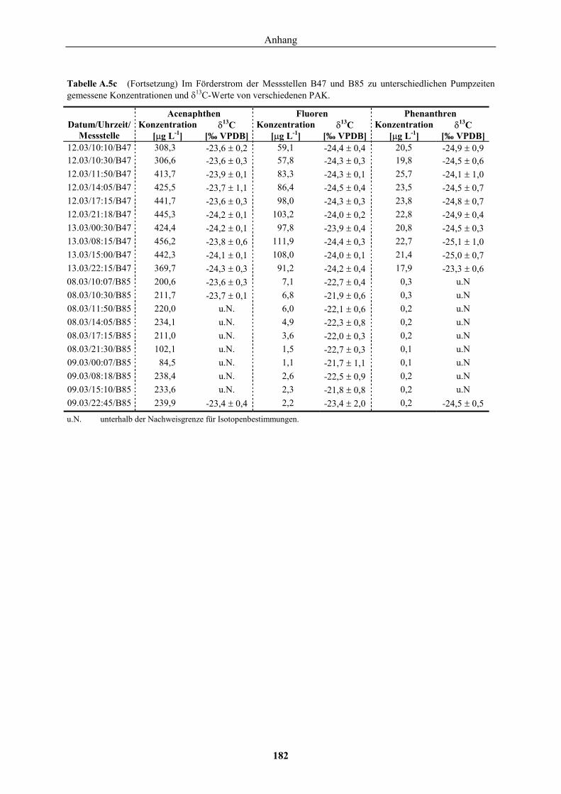
Anhang
182
Tabelle A.5c (Fortsetzung) Im Förderstrom der Messstellen B47 und B85 zu unterschiedlichen Pumpzeiten gemessene Konzentrationen und �13C-Werte von verschiedenen PAK.
Acenaphthen Fluoren Phenanthren Datum/Uhrzeit/
Messstelle Konzentration
[�g L-1] �13C
[‰ VPDB]Konzentration
[�g L-1] �13C
[‰ VPDB]Konzentration
[�g L-1] �13C
[‰ VPDB]12.03/10:10/B47 308,3 -23,6 � 0,2 59,1 -24,4 � 0,4 20,5 -24,9 � 0,9 12.03/10:30/B47 306,6 -23,6 � 0,3 57,8 -24,3 � 0,3 19,8 -24,5 � 0,6 12.03/11:50/B47 413,7 -23,9 � 0,1 83,3 -24,3 � 0,1 25,7 -24,1 � 1,0 12.03/14:05/B47 425,5 -23,7 � 1,1 86,4 -24,5 � 0,4 23,5 -24,5 � 0,7 12.03/17:15/B47 441,7 -23,6 � 0,3 98,0 -24,3 � 0,3 23,8 -24,8 � 0,7 12.03/21:18/B47 445,3 -24,2 � 0,1 103,2 -24,0 � 0,2 22,8 -24,9 � 0,4 13.03/00:30/B47 424,4 -24,2 � 0,1 97,8 -23,9 � 0,4 20,8 -24,5 � 0,3 13.03/08:15/B47 456,2 -23,8 � 0,6 111,9 -24,4 � 0,3 22,7 -25,1 � 1,0 13.03/15:00/B47 442,3 -24,1 � 0,1 108,0 -24,0 � 0,1 21,4 -25,0 � 0,7 13.03/22:15/B47 369,7 -24,3 � 0,3 91,2 -24,2 � 0,4 17,9 -23,3 � 0,6 08.03/10:07/B85 200,6 -23,6 � 0,3 7,1 -22,7 � 0,4 0,3 u.N 08.03/10:30/B85 211,7 -23,7 � 0,1 6,8 -21,9 � 0,6 0,3 u.N 08.03/11:50/B85 220,0 u.N. 6,0 -22,1 � 0,6 0,2 u.N 08.03/14:05/B85 234,1 u.N. 4,9 -22,3 � 0,8 0,2 u.N 08.03/17:15/B85 211,0 u.N. 3,6 -22,0 � 0,3 0,2 u.N 08.03/21:30/B85 102,1 u.N. 1,5 -22,7 � 0,3 0,1 u.N 09.03/00:07/B85 84,5 u.N. 1,1 -21,7 � 1,1 0,1 u.N 09.03/08:18/B85 238,4 u.N. 2,6 -22,5 � 0,9 0,2 u.N 09.03/15:10/B85 233,6 u.N. 2,3 -21,8 � 0,8 0,2 u.N 09.03/22:45/B85 239,9 -23,4 � 0,4 2,2 -23,4 � 2,0 0,2 -24,5 � 0,5 u.N. unterhalb der Nachweisgrenze für Isotopenbestimmungen.
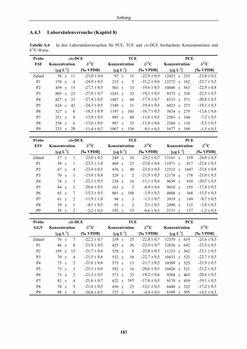
Anhang
183
A.4.3 Laborsäulenversuche (Kapitel 8)
Tabelle A.6 In den Laborsäulenversuchen für PCE, TCE und cis-DCE beobachtete Konzentrationen und �
13C-Werte.
Probe cis-DCE TCE PCE ESF Konzentration �13C Konzentration �13C Konzentration �13C
[�g L-1] [‰ VPDB] [�g L-1] [‰ VPDB] [�g L-1] [‰ VPDB] Zulauf 58 � 11 -23,0 � 0,9 97 � 15 -22,9 � 0,9 12423 � 233 -23,8 � 0,5
P1 174 � 4 -24,9 � 0,5 215 � 5 -21,2 � 0,6 12272 � 182 -22,7 � 0,5P2 459 � 15 -27,7 � 0,5 501 � 33 -19,6 � 0,5 10600 � 561 -22,9 � 0,8P3 805 � 22 -27,8 � 0,7 1243 � 32 -19,1 � 0,5 9375 � 338 -22,5 � 0,5P4 827 � 33 -27,4 � 0,5 1407 � 60 -17,9 � 0,7 8333 � 571 -20,8 � 0,5P5 624 � 42 -24,3 � 0,5 1349 � 31 -19,4 � 0,5 6023 � 273 -18,1 � 0,5P6 327 � 6 -18,3 � 0,9 1197 � 105 -16,7 � 0,5 3834 � 279 -12,6 � 0,6P7 251 � 8 -13,9 � 0,5 985 � 49 -11,6 � 0,5 2581 � 104 -7,2 � 0,5P8 258 � 6 -13,6 � 0,5 987 � 35 -11,0 � 0,6 2384 � 110 -5,5 � 0,5P9 233 � 20 -11,4 � 0,7 1067 � 156 -9,1 � 0,5 1677 � 168 -1,5 � 0,5
Probe cis-DCE TCE PCE ESV Konzentration �13C Konzentration �13C Konzentration �13C
[�g L-1] [‰ VPDB] [�g L-1] [‰ VPDB] [�g L-1] [‰ VPDB]Zulauf 57 � 1 -23,6 � 0,5 249 � 10 -23,2 � 0,7 13161 � 539 -24,0 � 0,5
P1 58 � 1 -23,5 � 1,0 469 � 23 -23,6 � 0,6 11971 � 817 -23,6 � 0,5P2 67 � 4 -23,4 � 0,5 476 � 40 -23,6 � 0,5 12313 � 1447 -23,6 � 0,8P3 70 � 1 -23,0 � 0,8 529 � 2 -21,9 � 0,5 12178 � 178 -23,0 � 0,5P4 76 � 3 -22,1 � 0,5 238 � 16 -11,1 � 0,6 9639 � 910 -20,5 � 0,5P5 84 � 1 -20,6 � 0,5 161 � 3 -6,4 � 0,6 9010 � 195 -17,4 � 0,5P6 85 � 7 -15,3 � 0,5 801 � 188 -1,9 � 0,5 4808 � 368 -13,5 � 0,5P7 61 � 2 -11,9 � 1,0 94 � 3 -1,3 � 0,7 3919 � 149 -8,7 � 0,5P8 39 � 1 -4,1 � 0,5 93 � 2 2,1 � 0,5 2490 � 115 -3,0 � 0,5P9 38 � 2 -2,2 � 0,5 192 � 15 -0,6 � 0,5 2131 � 137 -1,2 � 0,5
Probe cis-DCE TCE PCE GGV Konzentration �13C Konzentration �13C Konzentration �13C
[�g L-1] [‰ VPDB] [�g L-1] [‰ VPDB] [�g L-1] [‰ VPDB] Zulauf 76 � 7 -22,2 � 0,7 339 � 25 -22,8 � 0,7 12370 � 619 -23,6 � 0,5
P1 86 � 8 -21,9 � 0,5 425 � 26 -22,9 � 0,7 12836 � 642 -23,5 � 0,5P2 195 � 15 -21,7 � 0,6 529 � 8 -22,8 � 0,5 11233 � 562 -23,1 � 0,5P3 70 � 4 -21,5 � 0,6 532 � 10 -22,7 � 0,5 10433 � 522 -22,7 � 0,5P4 73 � 2 -21,6 � 0,8 575 � 13 -21,7 � 0,5 10509 � 525 -21,9 � 0,5P5 73 � 3 -21,1 � 0,8 592 � 16 -20,6 � 0,5 10426 � 521 -21,2 � 0,5P6 73 � 2 -21,3 � 0,5 573 � 23 -19,2 � 0,6 9304 � 465 -20,6 � 0,5P7 82 � 4 -21,6 � 0,7 622 � 165 -17,0 � 0,5 9179 � 459 -19,1 � 0,5P8 78 � 3 -21,8 � 0,5 456 � 23 -12,1 � 0,5 6440 � 322 -17,2 � 0,5P9 88 � 4 -20,8 � 0,5 325 � 6 -4,9 � 0,5 6109 � 305 -14,3 � 0,5


![Enzymkinetik - uni-frankfurt.deuser.uni-frankfurt.de/~dingerma/Podcast/09-Enzymkinetik_WS2010.pdf · [S] K M + [S] Mittwoch, 12. Januar 2011. Michaelis-Menten-Auftragung Enzymkinetik](https://img.pdfslide.org/doc/110x75/60b4d7f7c28542624d7371d3/enzymkinetik-uni-dingermapodcast09-enzymkinetikws2010pdf-s-k-m-s.jpg)