Lecture with Computer Exercises:

Modelling and Simulating Social Systems with

MATLAB

Project Report

IRRIGATION PLANNING

Jonathan Gheyssens & Claudia Casarotto

Zürich

December 2009

2

Eigenständigkeitserklärung

Hiermit erkläre ich, dass ich diese Gruppenarbeit selbständig verfasst habe,

keine anderen als die angegebenen Quellen-Hilsmittel verwenden habe, und alle

Stellen, die wörtlich oder sinngemäß aus veröffentlichen Schriften entnommen

wurden, als solche kenntlich gemacht habe. Darüber hinaus erkläre ich, dass

diese Gruppenarbeit nicht, auch nicht auszugsweise, bereits für andere Prüfung

ausgefertigt wurde.

Jonathan Gheyssens Claudia Casarotto

3

Agreement for free-download

We hereby agree to make our source code of this project freely available

for download from the web pages of the SOMS chair. Furthermore, we assure

that all source code is written by ourselves and is not violating any copyright

restrictions.

Jonathan Gheyssens Claudia Casarotto

4

TABLE OF CONTENTS

1. INTRODUCTION ........................................................................................................... 5

2. CONCISE LITERATURE REVIEW ............................................................................. 6

3. THE MODEL .................................................................................................................... 7

3.1 Yield Functions ........................................................................................................... 8

3.2 Net Profit Function ..................................................................................................... 8

3.3 Rainfall ........................................................................................................................ 9

3.4 Stochastic component ................................................................................................ 12

3.5 Optimization ............................................................................................................. 15

4. RESULTS ........................................................................................................................ 16

5. REFERENCES ................................................................................................................ 21

5

1. INTRODUCTION

Water is essential in agriculture and plays a fundamental role in economic growth and development. The demand for water and the ability to control its allocation and quality are becoming critical with the competing demand for municipal, industrial, and agricultural uses in the arid regions. In this context and within the irrigated agriculture, it is important to develop a better understanding of alternate irrigation water allocation strategies with a greater emphasis on the most efficient use of water. However, the most efficient use of water for crop production does not always coincide with the highest return for the farmer and the problem of allocation is one of optimization and trade-off. The farmer, therefore, must choose among the irrigation and production alternatives, the highest return per unit water used which satisfies his economic goals.

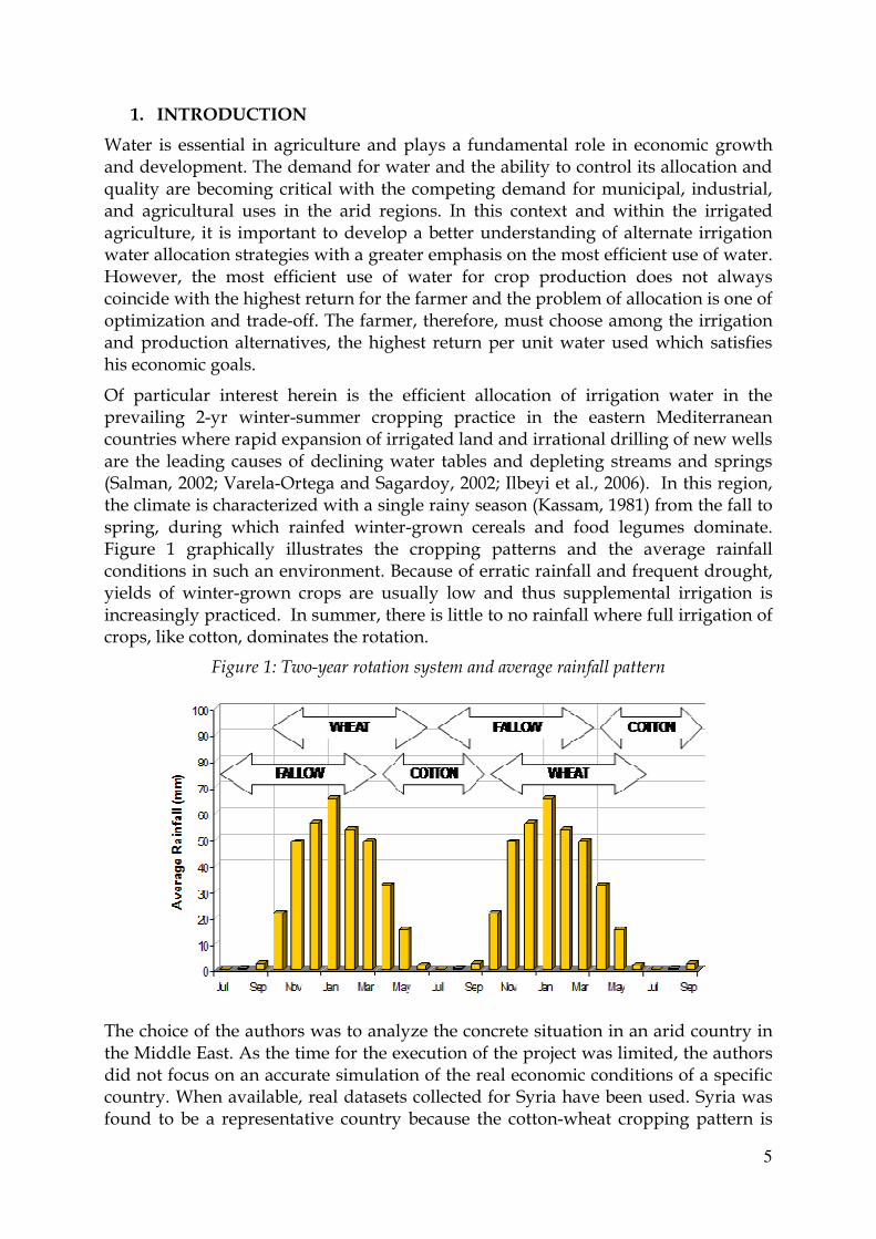
Of particular interest herein is the efficient allocation of irrigation water in the prevailing 2-yr winter-summer cropping practice in the eastern Mediterranean countries where rapid expansion of irrigated land and irrational drilling of new wells are the leading causes of declining water tables and depleting streams and springs (Salman, 2002; Varela-Ortega and Sagardoy, 2002; Ilbeyi et al., 2006). In this region, the climate is characterized with a single rainy season (Kassam, 1981) from the fall to spring, during which rainfed winter-grown cereals and food legumes dominate. Figure 1 graphically illustrates the cropping patterns and the average rainfall conditions in such an environment. Because of erratic rainfall and frequent drought, yields of winter-grown crops are usually low and thus supplemental irrigation is increasingly practiced. In summer, there is little to no rainfall where full irrigation of crops, like cotton, dominates the rotation.

Figure 1: Two-year rotation system and average rainfall pattern

The choice of the authors was to analyze the concrete situation in an arid country in the Middle East. As the time for the execution of the project was limited, the authors did not focus on an accurate simulation of the real economic conditions of a specific country. When available, real datasets collected for Syria have been used. Syria was found to be a representative country because the cotton-wheat cropping pattern is

6

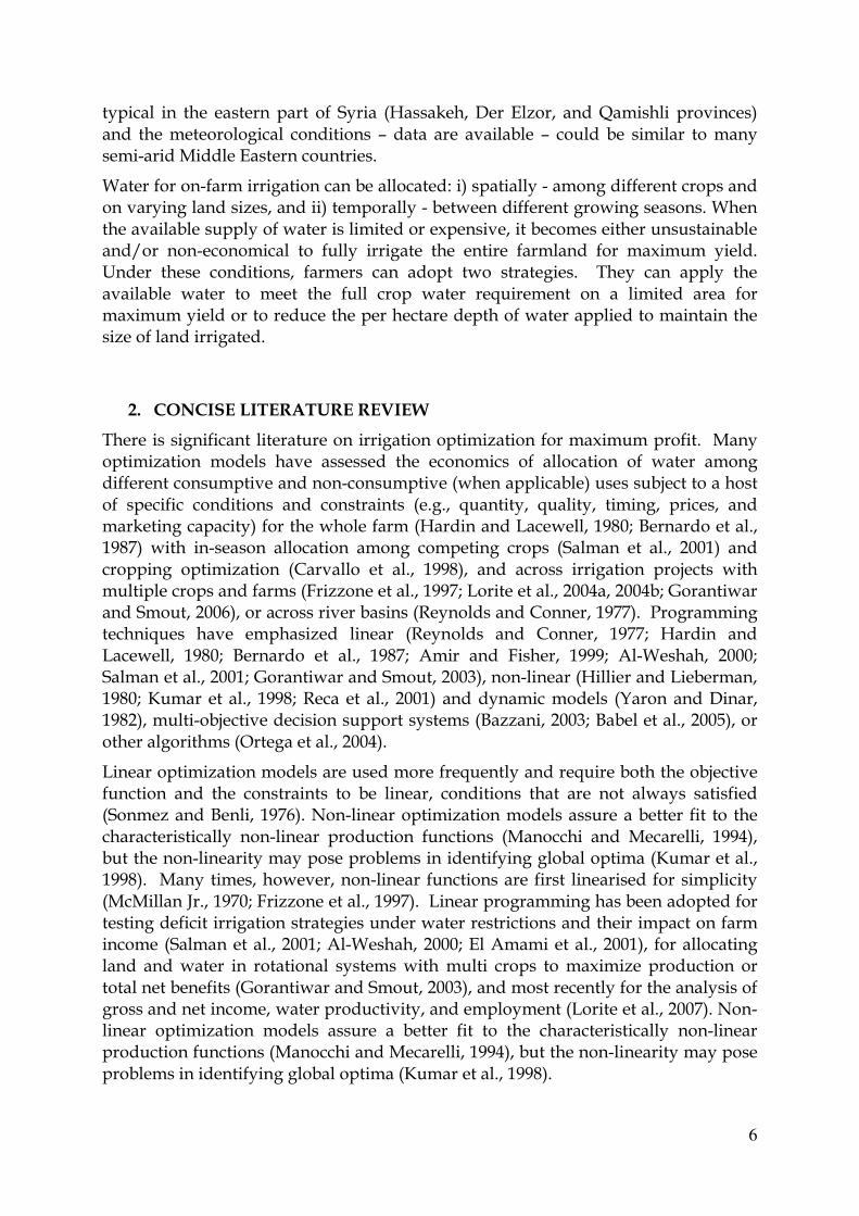
typical in the eastern part of Syria (Hassakeh, Der Elzor, and Qamishli provinces) and the meteorological conditions – data are available – could be similar to many semi-arid Middle Eastern countries.

Water for on-farm irrigation can be allocated: i) spatially - among different crops and on varying land sizes, and ii) temporally - between different growing seasons. When the available supply of water is limited or expensive, it becomes either unsustainable and/or non-economical to fully irrigate the entire farmland for maximum yield. Under these conditions, farmers can adopt two strategies. They can apply the available water to meet the full crop water requirement on a limited area for maximum yield or to reduce the per hectare depth of water applied to maintain the size of land irrigated.

2. CONCISE LITERATURE REVIEW

There is significant literature on irrigation optimization for maximum profit. Many optimization models have assessed the economics of allocation of water among different consumptive and non-consumptive (when applicable) uses subject to a host of specific conditions and constraints (e.g., quantity, quality, timing, prices, and marketing capacity) for the whole farm (Hardin and Lacewell, 1980; Bernardo et al., 1987) with in-season allocation among competing crops (Salman et al., 2001) and cropping optimization (Carvallo et al., 1998), and across irrigation projects with multiple crops and farms (Frizzone et al., 1997; Lorite et al., 2004a, 2004b; Gorantiwar and Smout, 2006), or across river basins (Reynolds and Conner, 1977). Programming techniques have emphasized linear (Reynolds and Conner, 1977; Hardin and Lacewell, 1980; Bernardo et al., 1987; Amir and Fisher, 1999; Al-Weshah, 2000; Salman et al., 2001; Gorantiwar and Smout, 2003), non-linear (Hillier and Lieberman, 1980; Kumar et al., 1998; Reca et al., 2001) and dynamic models (Yaron and Dinar, 1982), multi-objective decision support systems (Bazzani, 2003; Babel et al., 2005), or other algorithms (Ortega et al., 2004).

Linear optimization models are used more frequently and require both the objective function and the constraints to be linear, conditions that are not always satisfied (Sonmez and Benli, 1976). Non-linear optimization models assure a better fit to the characteristically non-linear production functions (Manocchi and Mecarelli, 1994), but the non-linearity may pose problems in identifying global optima (Kumar et al., 1998). Many times, however, non-linear functions are first linearised for simplicity (McMillan Jr., 1970; Frizzone et al., 1997). Linear programming has been adopted for testing deficit irrigation strategies under water restrictions and their impact on farm income (Salman et al., 2001; Al-Weshah, 2000; El Amami et al., 2001), for allocating land and water in rotational systems with multi crops to maximize production or total net benefits (Gorantiwar and Smout, 2003), and most recently for the analysis of gross and net income, water productivity, and employment (Lorite et al., 2007). Non-linear optimization models assure a better fit to the characteristically non-linear production functions (Manocchi and Mecarelli, 1994), but the non-linearity may pose problems in identifying global optima (Kumar et al., 1998).

7

A particularly interesting group of linear programming models accounted for the fact that farmers, like business people, have multiple goals or objectives in their decisions (Patrick and Blake, 1980). A multi-goal programming was formulated by ranking the goals in the order of importance (lexicographic ordering) where the positive deviations from the highest priority goal are maximized first, switching then to satisfying lower priority goals (Lee, 1972, ). In an alternate formulation (Wheeler and Russell, 1977; Barnett at al., 1982), ranking of goals was not necessary (i.e., all assumed to be equally desirable); therefore the decision maker can substitute the achievement of one goal for that of another to increase the level of satisfaction.

3. THE MODEL

The model to be formulated will consider the efficient allocation of water in the prevailing winter-summer cropping practice in the eastern Mediterranean countries. Two crops – wheat and cotton – are considered (but the analysis can easily be extended to include additional crops) due to their high agricultural and social importance in arid developing countries (FAO, 2003).

The optimality in the irrigation planning, in economic terms, is reached when the difference between gross income and production cost (i.e., net profit), subject to specific restrictions imposed on the production system, is maximized. The problem at hand is rationally solved by a mathematical programming model whose main objective is to establish the optimum irrigation amount and cropped land for maximum farm profit.

The model will, at first, estimate the demand functions for water for the two crops considered, based on water crop functions and on crop yield functions. The functions will describe the crops requirements in terms of water (always meant as rainfall plus irrigation) and the related yields that can be obtained. These functions could be either derived from literature, depending on the average conditions in the area of study (e.g., Howell et al., 2004; Jalota et al., 2006; Kashefipour et al., 2006; DeTar, 2008), or indicatively estimated by the researchers. Uncertainty in meteorological conditions (rainfall and evaporation) will be accounted for. Net profit functions will then be estimated, considering the variable – which depend on the water applied - and fixed costs of production.

A simplified non-linear optimization model for the determination of the optimum cropping pattern, irrigation amount, and farm income will be developed to reveal the global optimal solution. This model will solve the optimization problem by determining the size of the land and the level of irrigation deficit. The model will be run S times (for S different states) to explore all plausible stochastic intra-year variations in rainfall. All the S runs will be performed over T time periods where the actual trend in rainfall – found to be decreasing – will be simulated so to unveil the optimal cropping patterns over different degrees of water scarcity.

The overall optimization procedure will lead to the identification of a Pareto frontier that will explore all the optima solutions of the model for different levels of water supply both in terms of allocation of land and water.

8

3.1 Yield Functions

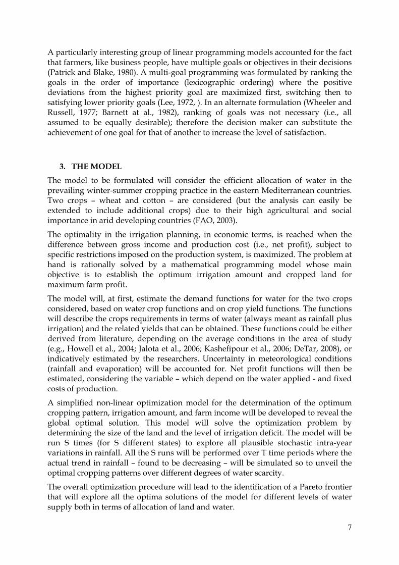
For cotton, many studies have reported yield functions (e.g., Howell et al., 2004; Jalota et al., 2006; Kashefipour et al., 2006; DeTar, 2008; Farahani et al., 2008). Taking insights from these functions, continuous non-linear yield functions have been derived. A cubic relation has been chosen to represent the yield function for cotton, while a quadratic function has been used for wheat. The relations are function of the amount of water applied:

������ = −0.0004�� + 0.28��� ������ = −0.14��� + 101�� Figure 2: Crop yield functions

It is easily recognized that wheat can be considered as a “safe” crop as its yield is sustained even with little quantities of water. Cotton, instead, gives higher yields but larger quantities of water should be applied. In terms of yields, therefore, the farmers would prefer cotton, but, being a summer crop, it would require large irrigation water supply in the season when rainfall is not available.

3.2 Net Profit Function

As a first step the per-hectare Net Profit functions for the two crops have been calculated. The selling prices for cotton and wheat are assumed to be fixed respectively at 12 SL/kg and 11 SL/kg.

Fixed costs are also included as a constant amount; they are costs attaining to the agricultural operations (i.e., tillage, seed-bed preparation, planting, hoeing and weeding). Those inputs either do not depend on the amount of water applied or are assumed constant across irrigation regimes (i.e., seeding rate). Variable costs, which depend on the amount of irrigation water withdrawn, such as energy, labour, and the fertilizer amounts and applications are considered.

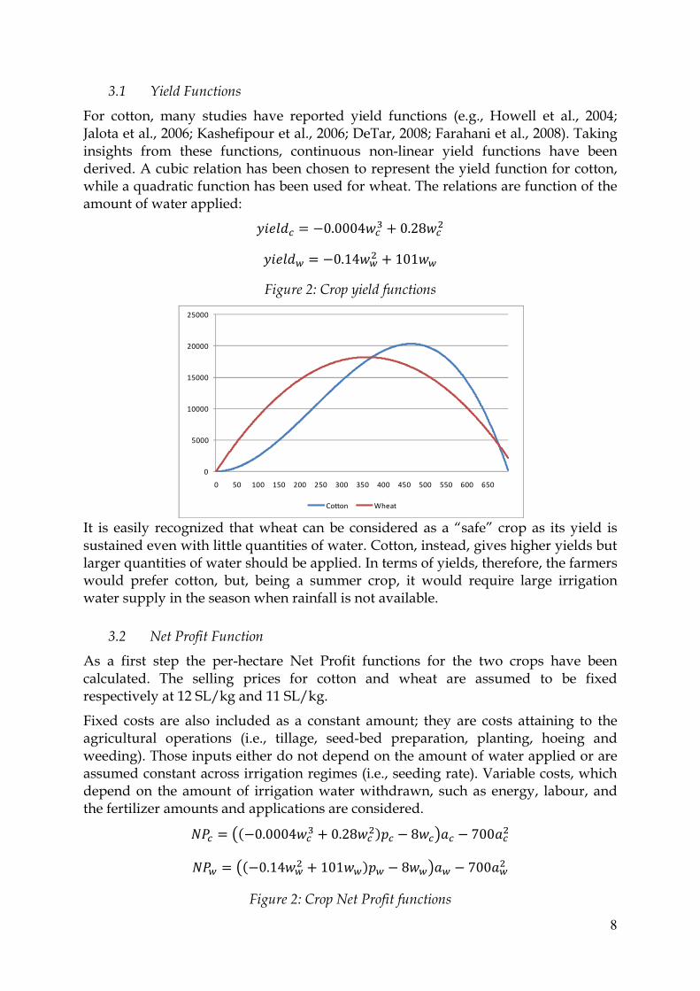
��� = ��−0.0004�� + 0.28������ − 8����� − 700��� ��� = ��−0.14��� + 101����� − 8����� − 700���

Figure 2: Crop Net Profit functions

0

5000

10000

15000

20000

25000

0 50 100 150 200 250 300 350 400 450 500 550 600 650

Cotton Wheat

9

The single crop net profit functions have been aggregated into a Total Net Profit function to be, in a second stage, maximized. The net profit is described by a function indicating the total farmer’s net income for the period of interest multiplied by the land area cropped with each crop. Weights have been included in order to eventually perform a multi-objective optimization, but they are kept equal to 1. In the Matlab formulation:

-(((((a_c*x(3)^3)+(b_c*x(3)^2)+(c_c*x(3)+d_c))*p_c-alpha_c*x(3))*x(1)-

700*x(1)^2)*W_c + ((((a_w*(x(4))^2)+(b_w*(x(4)))+c_w)*p_w -

alpha_w*x(4))*x(2)-700*x(2)^2)*W_w)

Where:

W_c=1; W_w=1; p_w=11; p_c=12; beta_c =0; beta_w =0; alpha_c=8; alpha_w=8; a_c=-0.0004; b_c=0.28; c_c=0; d_c=0; a_w=-0.14; b_w=101; c_w=0;

3.3 Rainfall

Rainfall data for Syria were available to the researchers. The rainfall pattern is strongly seasonal, with values close to zero in the months of June, July, and August and the peak in rainfall between November and January. The dataset SYRain.txt includes monthly average rainfall data for every month starting from January 1979 until December 2006.

As the optimization model will run on yearly time steps – justified by the fact that the farmer’s decision horizon is a one year period, as the cropping pattern decisions could be adjusted at the end of every year, thus stopping the crop rotation before its completion – the seasonal trend in the rainfall pattern had to be eliminated. The

0

20

40

60

80

100

120

140

160

180

200

0 100 200 300 400 500 600 700

NP cotton NP wheat

10

method used separates a time series into a smooth component whose mean varies over time (the trend) and a stationary component (the cycle). The cycle it the needed output as it clearly shows a rainfall trend over the years without seasonal “disturbances”. The non-parametric method for obtaining the trend ensures that short term changes in trend are not associated with the current level of the cycle.

At first the text file with the monthly data is imported and basic descriptive statistics calculated. The data series are saved as time series with time frame of 1 year for each step. Autoregressive models using the “ar” function are calculated with different lags (1, 2, and 12) to get an idea of the behaviour of the original dataset. Finally the AIC test (Akaike information criterion) is performed to compare the various models.

rf=importdata('SYRain.txt'); mean(rf) std(rf) max(rf) min(rf) x=iddata(rf,[],1,'Time','month'); arrain01=ar(x,1,'fb') arrain02=ar(x,2,'fb') arrain012=ar(x,12,'fb') fp0 = fpe(arrain01,arrain02,arrain012) aic0 = aic(arrain01,arrain02,arrain012) bode(arrain01,arrain02,arrain012)

The code used to detrend the rainfall time series was adapted from Rotemberg (1999a) who adopted such code to derive smooth trends from economic time-series data (in particular, the method was applied to trend in US military purchases and unemployment rate, but never to rainfall). The outputs of the program are lambda and the detrended series rftr (which has a lower boundary at zero) and a plot of rf and rftr1. This program calls the program betav (Rotemberg, 1999b). The parameters k and v were suggested (Rotemberg, 1999a) but could be modified.

k=16; v=5; ob=length(rf); jam =8e11; jamh=jam; betah=betav(rf,k,jam,v); if betah<0; ind=1; else jam=10; jaml=jam; betal=betav(rf,k,jam,v); if betal>0; ind=1; else ind=0; end; end; if ind<1 for i=1:50, jam=(jaml+jamh)/2; betax=betav(rf,k,jam,v); 'iteration number',i lambda=jam beta=betax if betax <0 jaml=jam;betal=betax; elseif betax>0

11

jamh=jam;betah=betax; else jaml=jam;jamh=jam;betah=betax;betal=betax; end; end; end; 'Final estimate of lambda is' lambda 'with associated beta of' beta

rfe=[rf(k+1:ob,1);zeros(k,1)]; rfa=[zeros(k,1);rf(1:ob-k)];

bas1=[jam*eye(ob-4),zeros(ob-4,4)]; bas2=[zeros(ob-4,1),-4*jam*eye(ob-4),zeros(ob-4,3)]; bas3=[zeros(ob-4,2),(0+6*jam)*eye(ob-4),zeros(ob-4,2)]; bas4=[zeros(ob-4,3),-4*jam*eye(ob-4),zeros(ob-4,1)]; bas5=[zeros(ob-4,4),jam*eye(ob-4)]; bb=bas1+bas2+bas3+bas4+bas5; bb1=[0+jam,-2*jam,jam,zeros(1,ob-3)]; bb2=[-2*jam,0+5*jam,-4*jam,jam,zeros(1,ob-4)]; bbl1=[zeros(1,ob-3),jam,-2*jam,0+jam]; bbl2=[zeros(1,ob-4),jam,-4*jam,0+5*jam,-2*jam]; bbb=[bb1;bb2;bb;bbl2;bbl1]; klas=[zeros(ob-k,k),.5*eye(ob-k);zeros(k,ob)]; kfis=[zeros(k,ob);.5*eye(ob-k),zeros(ob-k,k)]; bbnh=bbb+klas+kfis; ccj=inv(bbnh); rftr=ccj*((rfe+rfa)/2);

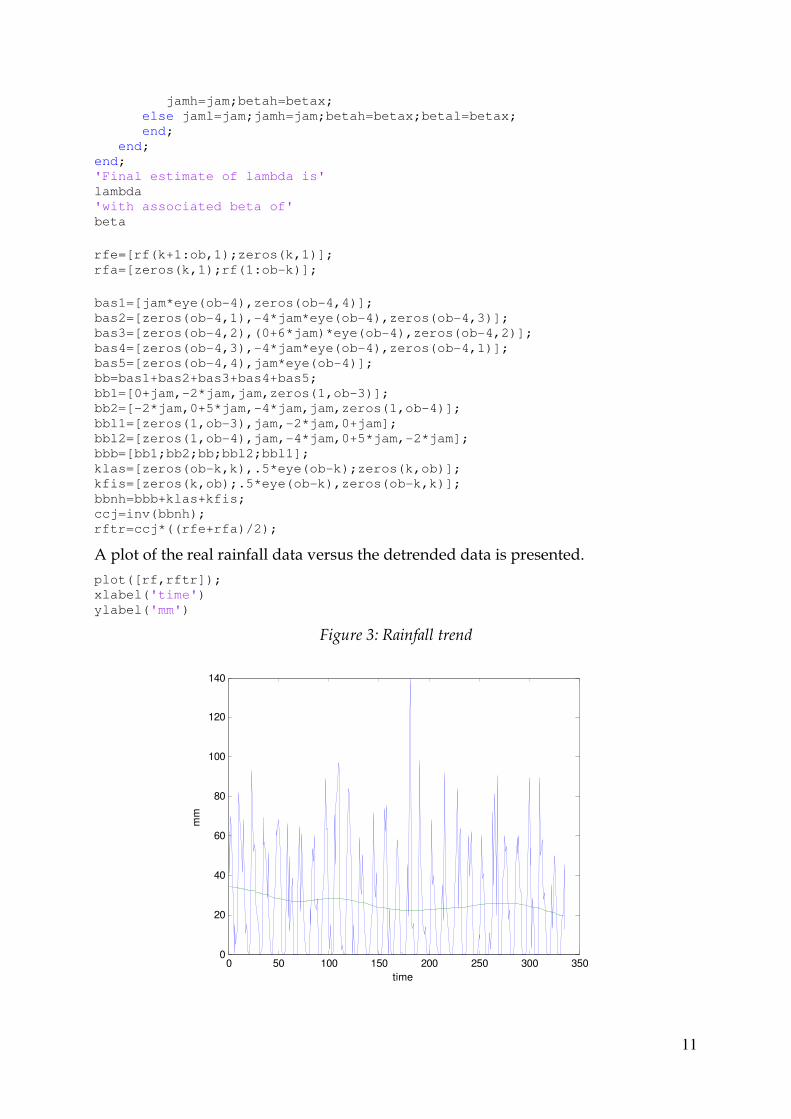
A plot of the real rainfall data versus the detrended data is presented.

plot([rf,rftr]); xlabel('time') ylabel('mm')

Figure 3: Rainfall trend

0 50 100 150 200 250 300 3500

20

40

60

80

100

120

140

time

mm

12

Using the detrended dataset an AR model is performed again. Also in this case the autoregressive model is computed for 1, 2, and 12 lags. In order to make a better informed choice of the model to be adopted, also the third and fourth lags are included. As before the goodness of fit of the models is compared using the AIC test and the result suggests adopting either a 2 or 3 lags model. It can also be notices that with the detrended dataset all models perform better than the same models calculated on the original dataset – as expected.

x1=iddata(rftr,[],1,'Time','month'); arrain1=ar(x1,1,'fb') arrain2=ar(x1,2,'fb') arrain3=ar(x1,3,'fb') arrain4=ar(x1,4,'fb') arrain12=ar(x1,12,'fb') fp1 = fpe(arrain1,arrain2,arrain3,arrain4,arrain12) aic1 = aic(arrain1,arrain2,arrain3,arrain4,arrain12)

From the AIC results, an AR(2) has been selected to fit the rainfall time series. From this analysis the parameters beta1 and beta2 can be calculated. These parameters will be used to include the autoregressive model in the calculation of the total water availability I in the optimization model (see next section).

beta1=1.999; beta2=0.9992;

3.4 Stochastic component

Since we model the optimal allocation of water (irrigation and rainfall), we want to assess the sensitivity of results for different specifications of water distribution. To do so, we design a distribution of possible rainfalls that acts as a stochastic disturbance around a deterministic and dynamic irrigation allocation. The dynamic nature of the irrigation (an autoregressive process of order 2) was explained in the previous section. In our model, we therefore have two parts: the deterministic part and the stochastic error component such that:

�� = � + !��"! + ���"� + #� As in traditional stochastic models, the error term is drawn from a normal distribution, which is designed specifically in MATLAB to respect certain criteria.

We define a level for the initial deterministic part W0 through the parameter d_WL and a scale of distribution through L_Scale. Hence we have fixed a first mode of our water distribution.

We set the two parameters of the normal distribution of the rainfall disturbance. The mean (e_mean) is set to 0 and the variance (e_var) is kept flexible but fixed in our particular run at four times the scale of the distribution. The variance of the error component is defined by the distribution scale ensuring that the stochastic part is always significant in terms of size.

We need to generate discrete values for our error terms since we want to cover the entire distribution (and not just draw one value as in the most common models). Since the normal distribution is a continuous distribution, we need to discretize it across specific ranges of values that we call states in the model. The states divide the

13

support of the rainfall distribution. For instance, having simply two states means that the entire support of value is just represented by two discretized values.

Since there is no close formula for the CDF of the normal and since we want to work with a high degree of parameterization, for each state, we compute the mean and the mass probability of the band by integration such that:

$%&�' = (�) = * &�( + +,

-"!

!�. /( + +

,0�+

An important element of our model is the numerical precision we want to achieve when integrating. This precision is defined by 2n, which represents the number of steps in the integration process. If n is small, the integration has large steps and the

result is coarse. At the limit when n = +∞, the integration is quasi-continuous. However there is a trade in the use of n because the larger n we choose, the longer it is required for MATLAB to compute the results. Since the precision is exponential in n, the precision is rapidly achieved for small values of n with improvements rapidly diminishing for large values of n. In our calibration of the model, we use an in-between value of 10, which ensures a precision of 99% with acceptable speed. n is also dependent on the number of states: with a very large number of states, n is not required to be as high.

Since the normal distribution has R as support ([-∞, +∞]), we constrain it for our model to ensure non-negative total water values, using:

min_e=-2*e_var; max_e=1*e_var;

Those boundaries correspond to the first and the last bands, therefore constraining rainfall values to be between those two parameters.

The constrained supported is then divided between a number of bands that corresponds to the number of states. When the band value is calculated, it is iteratively applied to get the boundary values (int_step) between different states (the limit values needed to integrate):

%Define intervals (bendwith) of states int = S-2; %To account for deterministic mean and min,max %Define intervals of integration for state band = (max_e-min_e)/int; int_step=zeros(S-1,1); int_step_max = S-1; int_step(1,1)=min_e; %First value int_step(S-1,1)=max_e; %Last value for i=2:int_step_max-1 int_step(i,1)= int_step(i-1,1)+ band ; end

Once the support is set and the bands defined, we use nested loops to get the integration results. We store all the results in a e_value matrix (S x 4). The first two columns are for the computation of the lower and upper boundaries, the third column is to store the result of the mean and the fourth column stores the cumulated probability for the band.

14

%Definition of error value matrix and probability weight e_value = zeros(S,4); %Two firt columns are for boudaries of values, column 3 is for mean and column 4 is probability weight e_value(1,1)= min_e; e_value(1,2)= min_e; e_value(S,1) = max_e; e_value(S,2)= max_e; % First and last value e_value(1,3)= min_e; e_value(S,3) = max_e; %First and last CDF values e_value(1,4)= cdf('Normal',min_e,e_mean,e_var); e_value(S,4) = 1-cdf('Normal',max_e,e_mean,e_var); %Set the boundaries values for each state for i=2:S-1 e_value(i,1)=int_step(i-1,1); e_value(i,2)=int_step(i,1); end

We calculate each band having a top loop that ensures that they are all covered:

for i=2:S-1 %Set the granula matrix for numerical estimation of each state granul_e_min = e_value(i,1); granul_e_max = e_value(i,2);

Then we discretize each band according to our degree of precision 2n. For each of the granularity band, we calculate a mean value and a cumulated probability. Additionally, we calculate a relative cumulated probability value but we do not use it in this application of the model:

for i=2:S-1 %Set the granula matrix for numerical estimation of each state granul_e_min = e_value(i,1); granul_e_max = e_value(i,2); %Set the approximation matrix for each state granul_matrix = zeros((2^n+1),4); granul_int = abs((granul_e_max - granul_e_min)/(2^n)); granul_matrix(1,1) = granul_e_min; granul_matrix(1,2) = 0; granul_matrix((2^n)+1,1) = granul_e_max; granul_matrix((2^n)+1,2) = 0; for j=2:(2^n) %Define step of granularity granul_matrix(j,1)=granul_matrix(j-1,1)+granul_int; %Define probability weight inside granularity granul_matrix(j,2)=abs(cdf('Normal',granul_matrix(j,1),e_mean,e_var)- cdf('Normal',granul_matrix(j-1,1),e_mean,e_var)); %Average of value inside granularity granul_matrix(j,4)=granul_matrix(j-1,1)+(abs(granul_int)/2); end %Relative weight share to get the average error value within a state for g=2:(2^n) granul_matrix(g,3)= granul_matrix(g,2)/(ones((2^n)+1,1)'*granul_matrix(:,2)); end

We compute the mean value for state s and the cumulated probability value for the state by summing the granularity band values:

temp_vect_1 = granul_matrix(:,3); %List of proportional CDF share temp_vect_2 = granul_matrix(:,4); %List of values temp_vect_3 = granul_matrix(:,2); % List of absolute CDF share e_value(i,3) = temp_vect_1'*temp_vect_2; %Mean value for

15

state s temp_one = ones((2^n)+1,1); e_value(i,4) = temp_one'*temp_vect_3; % Probability weight for state s

Moreover we use the sum of the cumulated value to test for the precision of this

process. If we get, one, our distribution is complete with a satisfying degree of

precision: %Test of weighted probability WP_test=ones(S,1)'*e_value(:,4);

Finally, we add the rainfall error component to the deterministic part.

for i=1:S value(i,1) = value(((S-1)/2)+1,1)+e_value(i,3); end for i=1:S value(i,2) = value(((S-1)/2)+1,2)+e_value(i,3); end for j=3:T for i=1:S value(i,j) = beta1*value(((S-1)/2)+1,j-1)-beta2*value(((S-1)/2)+1,j-

2)+e_value(i,3); end end

3.5 Optimization

To prepare the optimization the function “optim_profit_social4” is defined as follows:

function [x, fval] =

optim_profit_social4(a_c,b_c,c_c,d_c,a_w,b_w,c_w,W_c,W_w,alpha_c,alpha_w,p_

w,p_c,I,x0,options) [x,fval] = fmincon(@profit_social,x0,[1 1 0

0],[200],[],[],[0,0,1,1],[Inf,Inf,Inf,Inf],@constraints,options); function [f] = profit_social(x) f = -(((((a_c*x(3)^3)+(b_c*x(3)^2)+(c_c*x(3)+d_c))*p_c-alpha_c*x(3))*x(1)-

700*x(1)^2)*W_c + ((((a_w*(x(4))^2)+(b_w*(x(4)))+c_w)*p_w -

alpha_w*x(4))*x(2)-700*x(2)^2)*W_w); end function [c,ceq] = constraints(x) c(1) = (x(2)*x(4)) +(x(1)*x(3)) - I; ceq = []; end end

The function includes the total net profit function as described in the previous sections and uses the following equality and inequality constraints:

���� + ���� ≤ 2 �� ≥ 1 �� ≥ 1 �� + �� ≤ 200 The function “fmincon” has been adopted because it is the only function embedded in Malab which can solve non-linear optimization problems constrained with both equality and inequality constraints. At the moment all the constraints are inequalities, but the model could be easily adapted to include equality constraints.

16

As a first step, the table for the results is built. The results will be displayed as a 5 columns per 5010 rows matrix, as 10 are the time periods analyzed over 501 possible stochastic scenarios for rainfall. The five columns correspond to the output of the model, namely: land allocated to cotton, land allocated to wheat, per hectare water applied to cotton, per hectare water applied to wheat, and, finally, total net profit of the cropping system.

optim_results_social=zeros(S*T,5);

Then the optimization routine is launched. The optimization procedure includes two “for” cycles to perform the optimization on both the 10 time periods and the S (S=501) stochastic states of rainfall. I, the water applied, is defined as the matrix R which, in turn, is the matrix which includes a constant surface water availability, a time trend or rainfall and the stochastic values of rainfall.

for i=1:S for j=1:T I=R(i,j); E=e_value(i,3); [x, fval] =

optim_profit_social4(a_c,b_c,c_c,d_c,a_w,b_w,c_w,W_c,W_w,alpha_c,alpha_w,p_

w,p_c,I,x0,options); optim_results_social(i+S*(j-1),1)=x(1,1); optim_results_social(i+S*(j-1),2)=x(1,2); optim_results_social(i+S*(j-1),3)=x(1,3); optim_results_social(i+S*(j-1),4)=x(1,4); optim_results_social(i+S*(j-1),5)=fval(1,1); x0 = [x(1,1),x(1,2),x(1,3),x(1,4)]; end end

4. RESULTS

As mentioned above, the main results of the model include allocation rules for land and water across time and between crop. The results obtain give a very clear overview of the change in decision rules depending on rainfall availability and in a context of decreasing total water supply over time.

It is obviously not possible to present here all the 501 stochastic scenarios for the 10 years (but the output matrix is available when running the complete Matlab code), and a choice has been made in order to illustrate the main results in a clear and concise way.

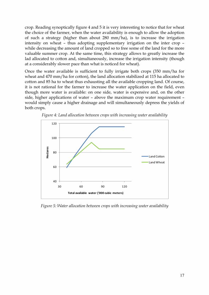
At first the results obtained across the S stochastic rainfall states are presented. Figure 4 illustrates the land allocation between wheat and cotton. It can be noticed that with low water availability (lower than about 170 millimeters of water per hectare) most of the land is allocated to wheat, being wheat the safest crop under conditions of water scarcity. In this fist period, the water availability is not sufficient to irrigate all the available land, so the choice of the farmer is to irrigate up to a satisfactory level (as it can be seen in Figure 5, we do not reach full irrigation yet!) the crops but on a lower land area.

After the threshold for water availability is trespassed, then the land allocated to cotton increases and more land is allocated to the summer crop than to the winter

17

crop. Reading synoptically figure 4 and 5 it is very interesting to notice that for wheat the choice of the farmer, when the water availability is enough to allow the adoption of such a strategy (higher than about 280 mm/ha), is to increase the irrigation intensity on wheat – thus adopting supplementary irrigation on the inter crop – while decreasing the amount of land cropped so to free some of the land for the more valuable summer crop. At the same time, this strategy allows to greatly increase the lad allocated to cotton and, simultaneously, increase the irrigation intensity (though at a considerably slower pace than what is noticed for wheat).

Once the water available is sufficient to fully irrigate both crops (350 mm/ha for wheat and 470 mm/ha for cotton), the land allocation stabilized at 115 ha allocated to cotton and 85 ha to wheat thus exhausting all the available cropping land. Of course, it is not rational for the farmer to increase the water application on the field, even though more water is available: on one side, water is expensive and, on the other side, higher applications of water – above the maximum crop water requirement – would simply cause a higher drainage and will simultaneously depress the yields of both crops.

Figure 4: Land allocation between crops with increasing water availability

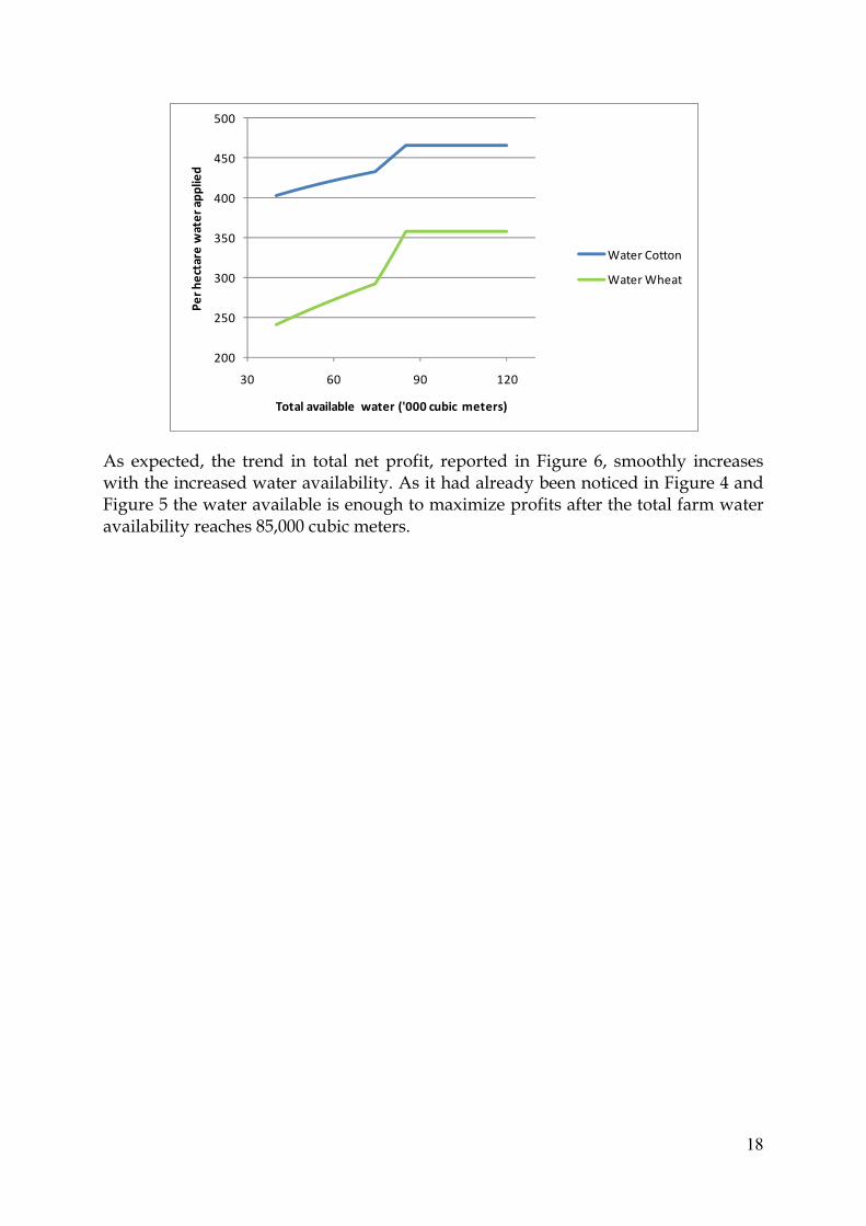
Figure 5: Water allocation between crops with increasing water availability

40

60

80

100

120

30 60 90 120

He

cta

res

Total available water ('000 cubic meters)

Land Cotton

Land Wheat

18

As expected, the trend in total net profit, reported in Figure 6, smoothly increases with the increased water availability. As it had already been noticed in Figure 4 and Figure 5 the water available is enough to maximize profits after the total farm water availability reaches 85,000 cubic meters.

200

250

300

350

400

450

500

30 60 90 120

Pe

r h

ect

are

wa

ter

ap

pli

ed

Total available water ('000 cubic meters)

Water Cotton

Water Wheat

19

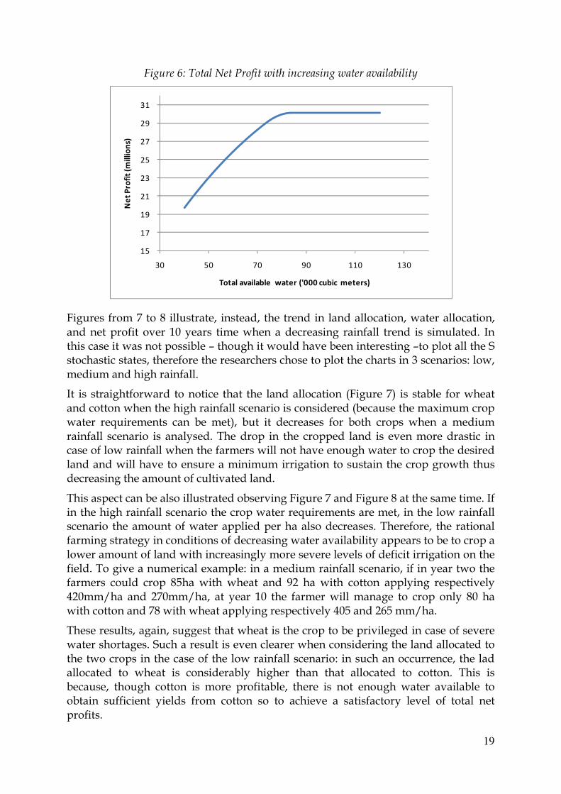
Figure 6: Total Net Profit with increasing water availability

Figures from 7 to 8 illustrate, instead, the trend in land allocation, water allocation, and net profit over 10 years time when a decreasing rainfall trend is simulated. In this case it was not possible – though it would have been interesting –to plot all the S stochastic states, therefore the researchers chose to plot the charts in 3 scenarios: low, medium and high rainfall.

It is straightforward to notice that the land allocation (Figure 7) is stable for wheat and cotton when the high rainfall scenario is considered (because the maximum crop water requirements can be met), but it decreases for both crops when a medium rainfall scenario is analysed. The drop in the cropped land is even more drastic in case of low rainfall when the farmers will not have enough water to crop the desired land and will have to ensure a minimum irrigation to sustain the crop growth thus decreasing the amount of cultivated land.

This aspect can be also illustrated observing Figure 7 and Figure 8 at the same time. If in the high rainfall scenario the crop water requirements are met, in the low rainfall scenario the amount of water applied per ha also decreases. Therefore, the rational farming strategy in conditions of decreasing water availability appears to be to crop a lower amount of land with increasingly more severe levels of deficit irrigation on the field. To give a numerical example: in a medium rainfall scenario, if in year two the farmers could crop 85ha with wheat and 92 ha with cotton applying respectively 420mm/ha and 270mm/ha, at year 10 the farmer will manage to crop only 80 ha with cotton and 78 with wheat applying respectively 405 and 265 mm/ha.

These results, again, suggest that wheat is the crop to be privileged in case of severe water shortages. Such a result is even clearer when considering the land allocated to the two crops in the case of the low rainfall scenario: in such an occurrence, the lad allocated to wheat is considerably higher than that allocated to cotton. This is because, though cotton is more profitable, there is not enough water available to obtain sufficient yields from cotton so to achieve a satisfactory level of total net profits.

15

17

19

21

23

25

27

29

31

30 50 70 90 110 130

Ne

t P

rofi

t (m

illi

on

s)

Total available water ('000 cubic meters)

20

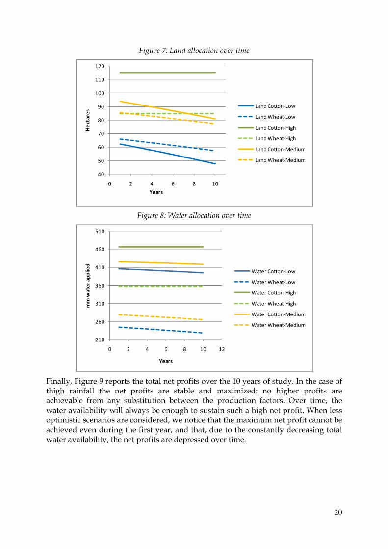
Figure 7: Land allocation over time

Figure 8: Water allocation over time

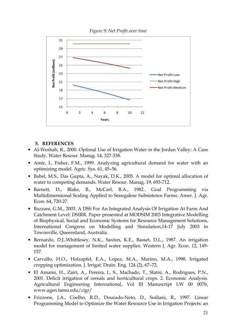
Finally, Figure 9 reports the total net profits over the 10 years of study. In the case of thigh rainfall the net profits are stable and maximized: no higher profits are achievable from any substitution between the production factors. Over time, the water availability will always be enough to sustain such a high net profit. When less optimistic scenarios are considered, we notice that the maximum net profit cannot be achieved even during the first year, and that, due to the constantly decreasing total water availability, the net profits are depressed over time.

40

50

60

70

80

90

100

110

120

0 2 4 6 8 10

He

cta

res

Years

Land Cotton-Low

Land Wheat-Low

Land Cotton-High

Land Wheat-High

Land Cotton-Medium

Land Wheat-Medium

210

260

310

360

410

460

510

0 2 4 6 8 10 12

mm

wa

ter

ap

pli

ed

Years

Water Cotton-Low

Water Wheat-Low

Water Cotton-High

Water Wheat-High

Water Cotton-Medium

Water Wheat-Medium

21

Figure 9: Net Profit over time

5. REFERENCES

• Al-Weshah, R., 2000. Optimal Use of Irrigation Water in the Jordan Valley: A Case Study. Water Resour. Manag. 14, 327-338.

• Amir, I., Fisher, F.M., 1999. Analyzing agricultural demand for water with an optimizing model. Agric. Sys. 61, 45–56.

• Babel, M.S., Das Gupta, A., Nayak, D.K., 2005. A model for optimal allocation of water to competing demands. Water Resour. Manag. 19, 693-712.

• Barnett, D., Blake, B., McCarl, B.A., 1982.. Goal Programming via Multidimensional Scaling Applied to Senegalese Subsistence Farms. Amer. J. Agr. Econ. 64, 720-27.

• Bazzani, G.M., 2003. A DSS For An Integrated Analysis Of Irrigation At Farm And Catchment Level: DSIRR. Paper presented at MODSIM 2003 Integrative Modelling of Biophysical, Social and Economic Systems for Resource Management Solutions, International Congress on Modelling and Simulation,14-17 July 2003 in Townsville, Queensland, Australia.

• Bernardo, D.J.,Whittlesey, N.K., Saxton, K.E., Basset, D.L., 1987. An irrigation model for management of limited water supplies. Western J. Agr. Econ. 12, 149-157.

• Carvallo, H.O., Holzapfel, E.A., Lopez, M.A., Marino, M.A., 1998. Irrigated cropping optimization. J. Irrigat. Drain. Eng. 124 (2), 67–72.

• El Amami, H., Zairi, A., Pereira, L. S., Machado, T., Slatni, A., Rodrigues, P.N., 2001. Deficit irrigation of cereals and horticultural crops. 2. Economic Analysis. Agricultural Engineering International, Vol III Manuscript LW 00 007b, www.agen.tamu.edu/cigr/

• Frizzone, J.A., Coelho, R.D., Dourado-Neto, D., Soiliani, R., 1997. Linear Programming Model to Optimize the Water Resource Use in Irrigation Projects: an

15

17

19

21

23

25

27

29

31

0 2 4 6 8 10 12

Ne

t P

rofi

t (m

illi

on

s)

Years

Net Profit-Low

Net Profit-High

Net Profit-Medium

22

Application to the Senator Nilo Coelho Project. Sciencia Agricola, Piracicaba, 54 (Numero Especial), 136-148.

• Gorantiwar, S.D., Smout, I.K., 2003. Allocation of scarce water resources using deficit irrigation in rotational systems. J. Irrigat. Drain. Eng. 129 (3), 155–163.

• Gorantiwar, S.D., Smout, I.K., 2006. Model for performance based land area and water allocation within irrigation schemes. Irr. and Drain. Sys. 20, 345-36.

• Hardin, D.C., Lacewell, R.D., 1980. Temporal Implications of Limitations on Annual Irrigation Water Pumped from an Exhaustible Aquifer. Western J. Agr. Econ., 5, 37-44.

• Hillier, F.S., Lieberman, G.J., 1980. Introduction to Operations Research, Third Edition. Holden-Day, San Francisco.

• Ilbeyi, A., Ustun, H., Oweis, T., Pala, M., Benli, B., 2006. Wheat water productivity and yield in a cool highland environment: Effect of early sowing with supplemental irrigation. Agric. Water Manage. 82, 399–410

• Kumar C. N., Indrasenan, N., Elango, K., 1998. Nonlinear programming model for extensive irrigation , J. of Irri. and Drain. Engr. 124, 123-126..

• Lee, S.M., 1972. Goal Programming for Decision Analysis. Philadelphia: Auerbach.

• Lorite, I.J., Mateos, L., Fereres, E., 2004a. Evaluating irrigation performance in a Mediterranean environment - I. Model and general assessment of an irrigation scheme. Irr. Sci. 23, 77–84.

• Lorite, I.J., Mateos, L., Fereres, E., 2004b. Evaluating irrigation performance in a Mediterranean environment - II. Variability among crops and farmers. Irr. Sci. 23, 85–92.

• Manocchi, F., Mecarelli, P., 1994. Optimization analysis of deficit irrigation systems. J. Irrigat. Drain. Eng., ASCE, 120 (3), 484–503.

• McMillan Jr., C., 1970. Mathematical Programming: An introduction to the design and application of optimal decision machines. New York: John Wiley, 1970. 495p.

• Ortega, J.F., de Juan, J.A., Tarjuelo, J.M., López, E., 2004. MOPECO: an economic optimization model for irrigation water management. Irr. Sci. 23, 61-75.

• Patrick, G.F., Blake, B.F., 1980. Measurement and modeling of farmers’ goals: an evaluation and suggestions. Southern J. Agr. Econ. , July,1980.

• Reca, J., Roldán, J., Alcaide, M., López, R., Camacho, E., 2001. Optimization model for water allocation in deficit irrigation systems. I. Description of the model. Agric. Water Manage. 48, 103-116.

• Reynolds, J.E., Conner, R., 1977. Spatial and temporal water allocation in the Kissimmee River Basin. Southern J. Agr. Econ., July 1977.

• Rotemberg, J.J., 1999a. A Heuristic Method for Extracting Smooth Trends from Economic Time Series. NBER Working Papers number 7439

• Rotemberg, J.J., 1999b. "Matlab code for A Method for Decomposing Time Series into Trend and Cycle Components," QM&RBC Codes 75, Quantitative Macroeconomics & Real Business Cycles. Downloadable on: http://ideas.repec.org/c/dge/qmrbcd/75.html

23

• Salman, Z., Al-Karablieh, E.K., Fisher, F.M., 2001. An inter-seasonal agricultural water allocation system (SAWAS) Agric. Sys. 68 (3), 233-252.

• Salman, M., 2002. Survey on Irrigation Modernization – Case Study from Syria. http://www.fao.org/AG/aGL/AGLW/watermanagement/docs/MOD_Syria.pdf

• Sonmez, N., Benli, E., 1976. Linear programming as a means in project evaluation and application to the Alpu irrigation project. Faculty of Agriculture, University, no. 25, Ankara.

• Wheeler, B.M., Russell, J.R.M., 1977. Goal Programming and Agricultural Planning. Oper. Res. Quart. 28, 21-32.

• Yaron, D., Dinar, A., 1982. Optimal Allocation of Farm Irrigation Water During Peak Seasons. Amer. J. Agr. Econ. 64, 681-689.