Embed Size (px)
Citation preview
Kinematics of 3D Folding Structures for Nanostructured OrigamiTM
Diplomarbeit
submitted by
cand.-ing. Tilman Buchner
December, 2003
Department of Mechanical Engineering
3D Optical Systems Group
Prof. George Barbastathis, PhD
RHEINISCH-WESTFÄLISCHETECHNISCHEHOCHSCHULEAACHEN
Werkzeugmaschinenlabor
Steuerungstechnik und Automatisierung
Prof. Dr.-Ing. Dr.-Ing. E.h. M. Weck
Advisor: Dipl.-Ing. Frank Possel-Dölken
1
Abstract The 3D Optical Systems Group at MIT investigates Nanostructured OrigamiTM 3D fabrication and assembly. The idea is to assemble complex hybrid (chemical or bio-logical reactors, optical sensing, digital electronic logic, mechanical motion) systems in 3D by using exclusively 2D lithography technology. The 3D shape is obtained by folding the initial 2D membrane in a prescribed way, in a manner reminiscent of the Japanese art of origami (paper-folding). The patterning method (2D nanolithography, nanoimprinting and other techniques) as well as the actuation principle (Lorentz force actuation) which is responsible for initializing the folding process have already been developed and established. The knowledge of the dynamic folding process itself, needed to reach any desired 3D shape from a 2D initial state is to-date unexplored. Hence, the primary objective of this thesis is to determine the motions required to reach the goal (folded state) from a given initial state (unfolded). Hereto general folding operations will be analyzed and a new method to describe its kinematics for any arbitrary structure will be developed. We propose to use origami mathematics in combination with kinematical formulations in the area of robotics and gearing. The most attractive feature of origami is that one can construct a wide variety of complex shapes using a few axioms, simple fixed ini-tial conditions and one mechanical operation, a fold. In a second step, the idea will be pursued to transfer this paper folding concept to a more generally admitted ap-proach which uncouples the paper aspect from the folding operation. Hereby a com-bination of bodies, which are connected by joints, is used to describe the crease structure. As a result, the crease structure is represented in terms of a closed-loop Multi Body System (MBS) with the property that a change of relative motion at one location in-duces a change of relative motion elsewhere. To describe this system, a well-known mathematical method, called screw calculus will be applied. Screw calculus is based on Poinsot’s result that an arbitrary rigid body motion can be described in terms of a translation cascaded with a rotation around the translation axis. The “screw” then is a matrix exponential describing the motion. By cascading several screws together one can describe the motion of articulated rigid body systems, such as robotic manipula-tors and, in our case, origami. The results of the theoretical investigation will be implemented in a design and simu-lation software tool. The application has features to verify and create folding struc-tures as well as to visualize the folding operation on the basis of the above men-tioned kinematics approach.
2
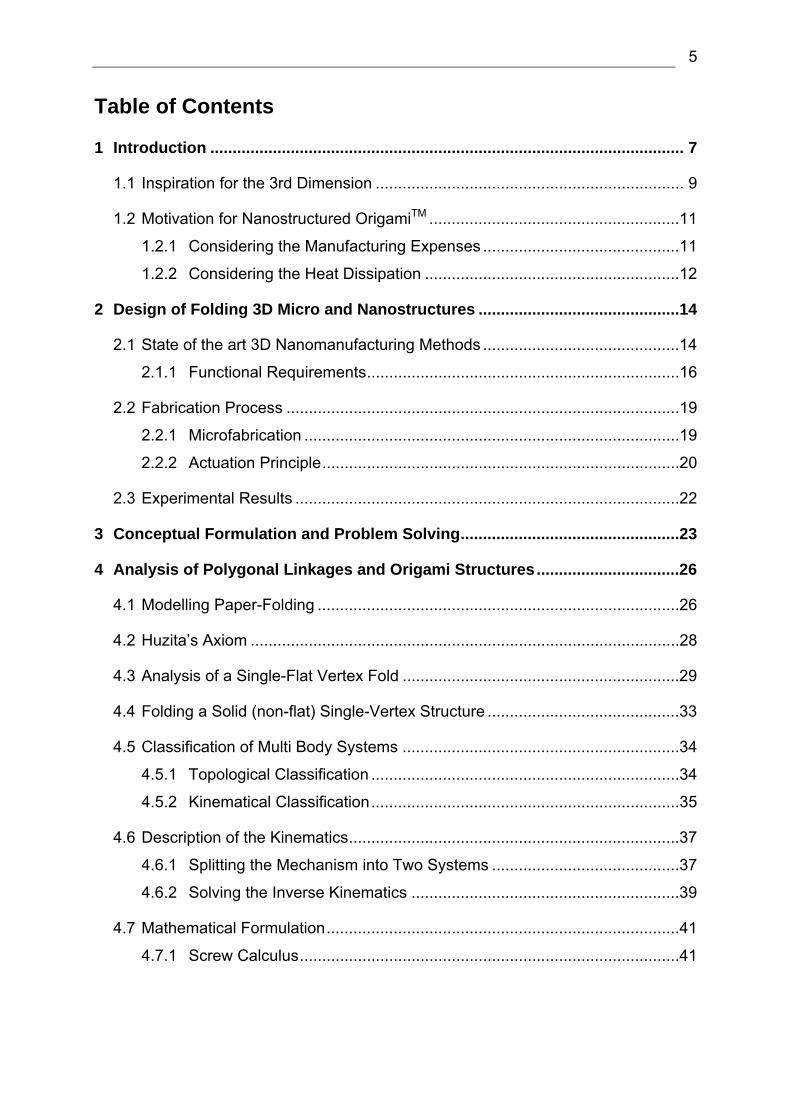
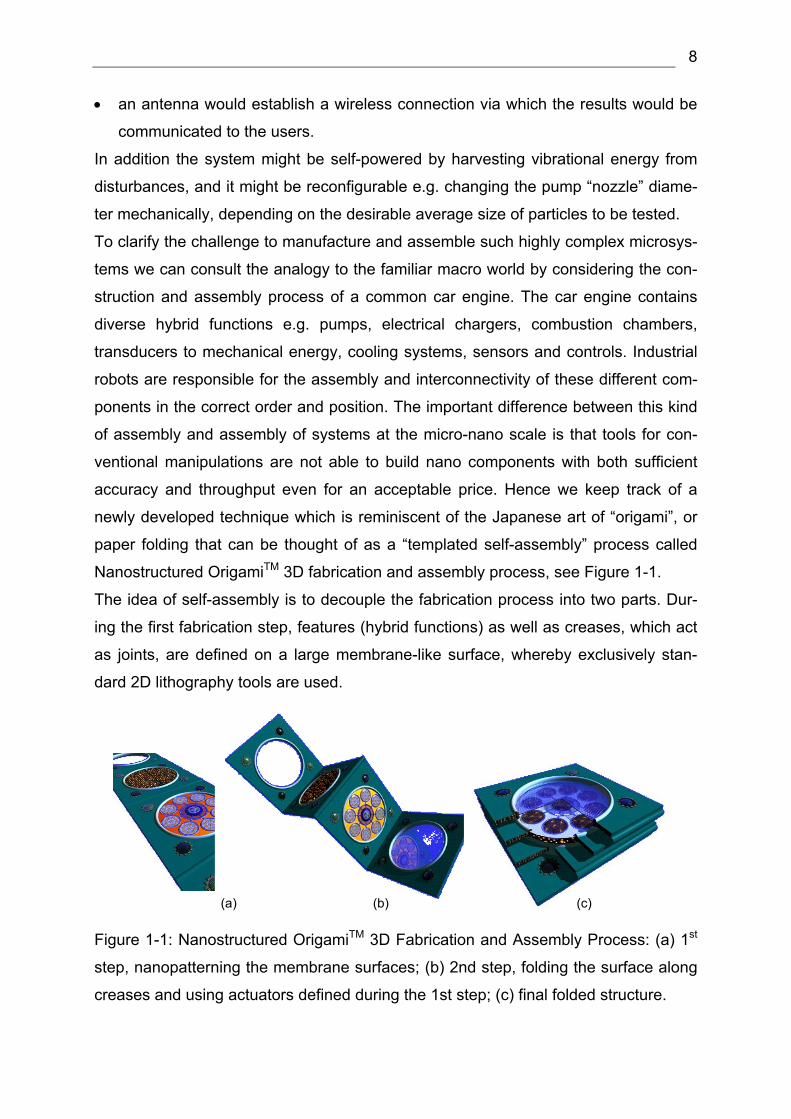
List of Figures Figure 1-1: Nanostructured OrigamiTM 3D Fabrication and Assembly Process. ......... 8
Figure 1-2: Diverse methods of construction are reflected in 2D/3D landscapes ....... 9
Figure 1-3: Volume filling strategies in biology [Schm 02], [Pal 96] .......................... 10
Figure 2-1: The principle of microstereolithography [Jurg 03]................................... 14
Figure 2-2: 3D photonic crystal fabricated from 2D plates [AoId+ 03]....................... 15
Figure 2-3: Miniaturize macroscopic hinges [Jurg 03] .............................................. 16
Figure 2-4: Permalloy actuation by integrated coils [Jurg 03] ................................... 17
Figure 2-5: University of Tokyo's Lorentz force actuator [IsOH 98]........................... 17
Figure 2-6: Electrical and optical interconnections between layers [BJH+ 03].......... 18
Figure 2-7: Microfabrication process flow ................................................................. 19
Figure 2-8: Lorentz Force Actuation principle, plastic deformation of hinges ........... 21
Figure 2-9: Experimental results (magnetic actuation) ............................................. 22
Figure 3-1: Conceptual formulation, two use cases.................................................. 24
Figure 3-2: Use case analysis in detail ..................................................................... 25
Figure 4-1: Basic origami terminology ...................................................................... 27
Figure 4-2: Huzita's axioms to model crease structures [Huzi 03] ............................ 28
Figure 4-3: MV assignment....................................................................................... 30
Figure 4-4: Number of possible MV assignments ..................................................... 30
Figure 4-5: Example how to compute number of valid MV assignments .................. 32
Figure 4-6: The corner cube as example for a solid single-vertex fold ..................... 33
Figure 4-7: Topological classification of Multi Body Systems ................................... 34
Figure 4-8: Kinematical classification of Multi Body Systems ................................... 35
Figure 4-9: Necessary joint configuration to model an openCorner.......................... 36
Figure 4-10: How to model the kinematics ............................................................... 38
Figure 4-11: Splitting the system into a forward and inverse kinematic part ............. 39
Figure 4-12: Two different solutions of the inverse kinematic equations .................. 40
Figure 4-13: Screw Calculus in detail ....................................................................... 42
Figure 5-1: Kinematic configuration of the open corner demonstration model.......... 43
Figure 5-2: Illustration of a 4R overconstrained mechanism..................................... 44
Figure 5-3: Application of Screw Calculus theory ..................................................... 45
Figure 5-4: Kinematic configuration in detail............................................................. 46
Figure 5-5: Polynomial Curve Fitting: 4th degree ..................................................... 47
Figure 5-6: Second fold about 5Θ ............................................................................ 48
3
Figure 6-1: Collecting the geometrical shape [Stre 03]............................................. 51
Figure 6-2: Triangulation, expansive motion............................................................. 51
Figure 6-3: Unfolding on the base of the triangulation approach .............................. 52
Figure 7-1: Functional specification of the software.................................................. 54
Figure 7-2: General Software Architecture ............................................................... 56
Figure 7-3: Crease Generator Architecture in detail ................................................. 57
Figure 7-4: Four folds created with the CG and stored in the CC............................. 57
Figure 7-5: Applying a crease pattern....................................................................... 58
Figure 7-6: Transformation concept.......................................................................... 59
Figure 7-7: Data architecture in detail....................................................................... 60
Figure 7-8: Kinematical Concept .............................................................................. 60
Figure 7-9: Motion recording concept ....................................................................... 61
Figure 8-1: Technologies to implement the architecture........................................... 64
Figure 9-1: Realization of OrigamiKinematicsPlus ...................................................... 65
Figure 9-2: Graphic User Interfac in detail ................................................................ 66
Figure 9-3: Navigation Panel in detail ....................................................................... 67
Figure 9-4: Data flow in detail ................................................................................... 68
Figure 9-5: Create crease structure.......................................................................... 69
Figure 9-6: Compute consecutive sequence ............................................................ 70
Figure 9-7: Specify crease pattern............................................................................ 71
Figure 9-8: Specify Folding Properties ..................................................................... 72
Figure 9-9: Segmentation of the axis of rotation ....................................................... 73
Figure 9-10: Transformation of the reference system............................................... 73
Figure 9-11: Two communication principles ............................................................. 74
Figure 9-12: Kinematical computation in MATLAB in detail ...................................... 76
Figure 9-13: Folding motion of the first fold .............................................................. 77
Figure 9-14: Computing the object coordinates ........................................................ 79
Figure 9-15: Functional principle of the OpenGL Geometry Pipeline........................ 80
Figure 9-16: Functional principle of the Folding Manager......................................... 81
Figure 9-17: Compute current position in 3D space ................................................. 82
Figure 9-18: Starting position for the second fold ..................................................... 83
Figure 10-1: Creation of the open corner crease pattern.......................................... 84
Figure 10-2: Verifying crease structure..................................................................... 85
Figure 10-3: Complete transformation from 2D into 3D ............................................ 86

4
Figure 10-4: Free choice in the view of the folding motion ....................................... 86
Figure 11-1: Reconfigurable soldier identification tag............................................... 89
5
Table of Contents
1 Introduction .......................................................................................................... 7
1.1 Inspiration for the 3rd Dimension ..................................................................... 9
1.2 Motivation for Nanostructured OrigamiTM ........................................................11
1.2.1 Considering the Manufacturing Expenses ............................................11
1.2.2 Considering the Heat Dissipation .........................................................12
2 Design of Folding 3D Micro and Nanostructures .............................................14
2.1 State of the art 3D Nanomanufacturing Methods ............................................14
2.1.1 Functional Requirements......................................................................16
2.2 Fabrication Process ........................................................................................19
2.2.1 Microfabrication ....................................................................................19
2.2.2 Actuation Principle................................................................................20
2.3 Experimental Results ......................................................................................22
3 Conceptual Formulation and Problem Solving.................................................23
4 Analysis of Polygonal Linkages and Origami Structures................................26
4.1 Modelling Paper-Folding .................................................................................26
4.2 Huzita’s Axiom ................................................................................................28
4.3 Analysis of a Single-Flat Vertex Fold ..............................................................29
4.4 Folding a Solid (non-flat) Single-Vertex Structure ...........................................33
4.5 Classification of Multi Body Systems ..............................................................34
4.5.1 Topological Classification .....................................................................34
4.5.2 Kinematical Classification.....................................................................35
4.6 Description of the Kinematics..........................................................................37
4.6.1 Splitting the Mechanism into Two Systems ..........................................37
4.6.2 Solving the Inverse Kinematics ............................................................39
4.7 Mathematical Formulation...............................................................................41
4.7.1 Screw Calculus.....................................................................................41
6
5 Folding of Polygonal Linkages ..........................................................................43
5.1 The Open Corner Demonstration Model .........................................................43
5.2 Polynomial Linkages .......................................................................................49
5.3 Dynamics of Folding Objects ..........................................................................49
5.4 Self Collision Detection of Folding Objects .....................................................49
6 Unfolding of polygonal Linkages.......................................................................50
6.1 Pseudo Triangulation Approach......................................................................50
7 Software Architecture of a General Solution ....................................................53
7.1 Requirements on Software Architecture..........................................................53
7.2 Architecture Concept ......................................................................................55
7.2.1 Crease Component ..............................................................................56
7.2.2 Transformation Component..................................................................58
7.2.3 Kinematic Component ..........................................................................60
7.2.4 Visualization Component......................................................................61
8 Implementation of the Architecture ...................................................................63
8.1 Technologies to Implement the Architecture ...................................................63
9 Realization of the Software Architecture ..........................................................65
9.1 Graphic User Interface....................................................................................66
9.2 Dataflow at Run-Time .....................................................................................68
9.3 Specification of the Crease Pattern.................................................................69
9.4 Specification of the Folding Properties............................................................72
9.5 Realization of the Kinematic Computation ......................................................74
9.6 Graphical Visualization with the use of OpenGL .............................................78
9.7 Realization of the Folding Manager ................................................................81
10 Example Scenario ...............................................................................................84
11 Conclusion...........................................................................................................88
12 Abbreviations ......................................................................................................91
13 References...........................................................................................................92
7
1 Introduction
The 3D Optical Systems Group at MIT investigates a new manufacturing method to
assemble three-dimensional (3D) intelligent microsystems with complex hybrid func-
tions like chemical or biological reactors, optical sensing, digital electronic logic, me-
chanical motion for movement or energy harvesting, with nanoscale components
from lower dimensional (2D) elements.
The development of current architectures for VLSI (Very Large Scale Integration) in-
tegrated circuits and microelectromechanical systems (MEMS) are quickly reaching a
point where 2D structures have become utilized and can no longer become denser.
In the realm of microelectronics, the 3rd dimension promises a large spectrum of op-
portunities in numerous technological domains when feature size of planar electron-
ics reaches its minimum physical limit [Jurg 03].
The interactions between the different modalities and its small form factor with a
nanoscale of less then 100nm predestine this technology to new physical properties
and hence unprecedented functional capabilities. Three dimensional MEMS devices
will see wide use in both military and commercial areas, with applications ranging
from automobiles and fighter aircraft to printers and munitions [Tang 00]. The De-
fense Advanced Research Projects Agency (DARPA), for example, is soliciting re-
search proposals in the area of MEMS with the object to co-locate the functions of
sense, computation, actuation, control, communication, and power. From the integra-
tion of these functions into macro systems they expect a radical change concerning
the way people and machines interact with the physical world [Micro 98].
As an example of an intelligent microsystem that could be fabricated with this new
manufacturing method, a biochemical sensor can be considered. This would require
the following components [Barb 03]:
• the top of the structure would function as a suction pump which captures particle
specimens from the environment;
• the next recipient of the captured particles would be a biochemical reactor which
would produce a clearly identifiable chemical result depending on the nature of
the captured particles
• optical sensing (a miniature high-resolution spectrometer) would be used to de-
tect the results of the bio-chemical reaction
• digital electronics would process the results of the detection, and
8
• an antenna would establish a wireless connection via which the results would be
communicated to the users.
In addition the system might be self-powered by harvesting vibrational energy from
disturbances, and it might be reconfigurable e.g. changing the pump “nozzle” diame-
ter mechanically, depending on the desirable average size of particles to be tested.
To clarify the challenge to manufacture and assemble such highly complex microsys-
tems we can consult the analogy to the familiar macro world by considering the con-
struction and assembly process of a common car engine. The car engine contains
diverse hybrid functions e.g. pumps, electrical chargers, combustion chambers,
transducers to mechanical energy, cooling systems, sensors and controls. Industrial
robots are responsible for the assembly and interconnectivity of these different com-
ponents in the correct order and position. The important difference between this kind
of assembly and assembly of systems at the micro-nano scale is that tools for con-
ventional manipulations are not able to build nano components with both sufficient
accuracy and throughput even for an acceptable price. Hence we keep track of a
newly developed technique which is reminiscent of the Japanese art of “origami”, or
paper folding that can be thought of as a “templated self-assembly” process called
Nanostructured OrigamiTM 3D fabrication and assembly process, see Figure 1-1.
The idea of self-assembly is to decouple the fabrication process into two parts. Dur-
ing the first fabrication step, features (hybrid functions) as well as creases, which act
as joints, are defined on a large membrane-like surface, whereby exclusively stan-
dard 2D lithography tools are used.
(a) (b) (c)
Figure 1-1: Nanostructured OrigamiTM 3D Fabrication and Assembly Process: (a) 1st
step, nanopatterning the membrane surfaces; (b) 2nd step, folding the surface along
creases and using actuators defined during the 1st step; (c) final folded structure.
9
During the second manufacturing step, the Lorentz force actuation principle is used
to initiate the folding process along the creases, which results in the 2D membrane
finding itself in its intended final folded structure in 3D space. This method achieves
high throughput for highly complex, non-periodic 3D structures and provides the
manufacturing process with accuracy, reliability and throughput comparable to those
of conventional 2D lithography.
The manufacturing process itself as well as the following actuating principle is al-
ready accurately described. Against these results, the knowledge of the dynamic
folding process itself, needed to reach any desired 3D shape from a 2D initial state is
to-date unexplored. Hence, the primary objective of this thesis is to determine the
motions required to reach the goal from a given initial state in order to manufacture
more complex 3D structures and to make the Nanostructured OrigamiTM approach
applicable to the industry. Hereto general folding operations will be analyzed and a
new method to describe its kinematics for any arbitrary structure will be developed.
The results of this design will be implemented in a design and simulation software
tool to create, verify and visualize folding structures for Nanostructured OrigamiTM
devices.
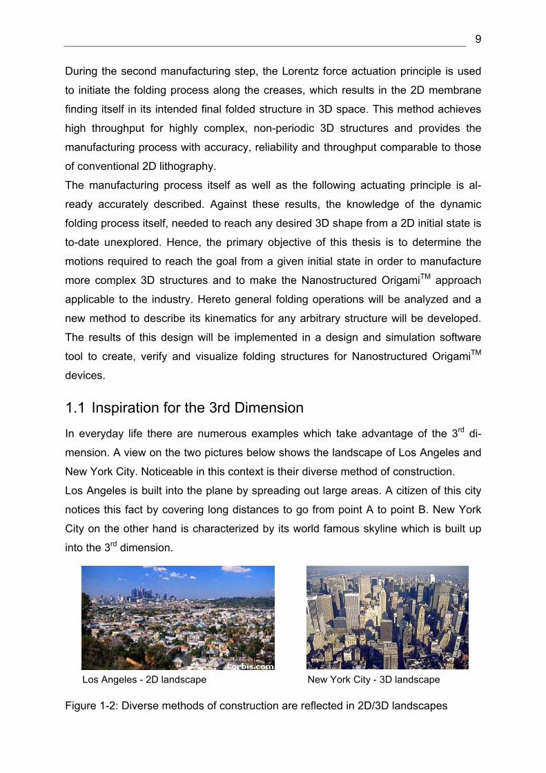
1.1 Inspiration for the 3rd Dimension
In everyday life there are numerous examples which take advantage of the 3rd di-
mension. A view on the two pictures below shows the landscape of Los Angeles and
New York City. Noticeable in this context is their diverse method of construction.
Los Angeles is built into the plane by spreading out large areas. A citizen of this city
notices this fact by covering long distances to go from point A to point B. New York
City on the other hand is characterized by its world famous skyline which is built up
into the 3rd dimension.
Los Angeles - 2D landscape New York City - 3D landscape
Figure 1-2: Diverse methods of construction are reflected in 2D/3D landscapes
10
To go from point A to point B you can move in horizontal as well as in vertical direc-
tions, this fact reduces the time to reach the final goal position significantly, see
Figure 1-2. There are a few other examples even in biology which show that every
time the proposition of space is low, nature tries to aim for filling 3D space.
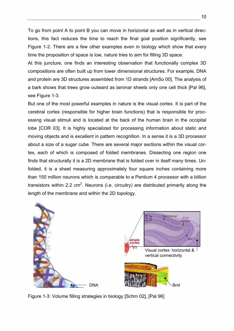
At this juncture, one finds an interesting observation that functionally complex 3D
compositions are often built up from lower dimensional structures. For example, DNA
and protein are 3D structures assembled from 1D strands [AmSo 00]. The analysis of
a bark shows that trees grow outward as laminar sheets only one cell thick [Pal 96],
see Figure 1-3.
But one of the most powerful examples in nature is the visual cortex. It is part of the
cerebral cortex (responsible for higher brain functions) that is responsible for proc-
essing visual stimuli and is located at the back of the human brain in the occipital
lobe [COR 03]. It is highly specialized for processing information about static and
moving objects and is excellent in pattern recognition. In a sense it is a 3D processor
about a size of a sugar cube. There are several major sections within the visual cor-
tex, each of which is composed of folded membranes. Dissecting one region one
finds that structurally it is a 2D membrane that is folded over in itself many times. Un-
folded, it is a sheet measuring approximately four square inches containing more
than 150 million neurons which is comparable to a Pentium 4 processor with a billion
transistors within 2.2 cm2. Neurons (i.e. circuitry) are distributed primarily along the
length of the membrane and within the 2D topology.
DNA
Visual cortex: horizontal & vertical connectivity
Brid
Figure 1-3: Volume filling strategies in biology [Schm 02], [Pal 96]
11
But neurons also grow between the folded regions of the membrane (vertical), but to
a much lesser degree. The final result is an anisotropic, 3D distribution of intercon-
nections [Jurg 03]. One can make the inference that evolution selected toward an
anisotropic arrangement of connectivity rather than full isotropic distribution for com-
plexity management reasons [Schm 02]. For the reasons of connectivity and maximi-
zation of surface area, the membrane folding concept is attractive for 3D micro- and
nanomanufacturing.
1.2 Motivation for Nanostructured OrigamiTM
The evolution of living conditions may serve as an important lesson for the future of
3D micro- and nanosystems. As demonstrated in the illustration of the landscape of
Los Angeles and New York City, every time land price is expensive or the population
density is enormous, living space was to be built up upwards (buildings are taller than
they are wide).
This progression might be the case for MEMS sensors and nano devices over the
next decade. The number of active elements squeezed into a planer chip is ever in-
creasing and the demand for smaller consumer electronics will probably never be
satiated [Reed 03]. These competing demands necessitate the building of 3D de-
vices just as skyscrapers have evolved and now dominate the urban landscape.
But before we try to transfer the principle of membrane folding to nanotechnology we
will examine the two main criteria of microchip fabrication, the manufacturing ex-
penses as well as the problem of heat dissipation which is directly linked with the
increase of chip capability. Only if both criteria are satisfied the Nanostructured Ori-
gami approach represents a suitable technology for future MEMS fabrication.
1.2.1 Considering the Manufacturing Expenses
In order to induce a change towards new technology there must be a sufficiently im-
portant reason to gain market acceptance. Beside new functionality which is the pri-
mary motivation, lower costs are followed, in terms of capital investment, by devel-
opment, and production. Radical changes to machinery or processes are also a se-
vere hurdle because it is very difficult to change the momentum of industry.
A state-of-the art fabrication plant for silicon microchips, for example, now costs ap-
proximately $3 billion to be built. On the other hand conventional chip fabrication
technology is on a collision course with economics. Today’s best computer chips
have silicon features as small as 90 nanometers. But the smaller the features, the
12
more expensive the optical equipment needed to manufacture those [Tris 03]. Com-
plete mask sets cost millions of dollars. In a layer by layer process, each level re-
quires its own set of unique masks. This means, the cost of the complete mask set
will scale directly proportional to the number of layers. At long sight, the microchip
industry is forced to develop new technologies.
The membrane folding concept lends oneself to solve this problem. It only requires a
single mask set no matter how many layers are to be built. To create these layers it
also seeks to use existing microfabrication tools. Additionally, the decoupled process
of fabrication and 3D assembly would reduce the development costs and new ad-
vances in micro and nanotechnology could be integrated with ease. Considering pro-
duction, the membrane folding approach represents a time and money saving ap-
proach.
1.2.2 Considering the Heat Dissipation
Beside the aspect of costs, one has to take into consideration the importance of heat
dissipation for 3D devices. As devices expand into 3rd dimension and increase in vol-
ume, the relative amount of surface area decreases. Removing heat becomes more
difficult. Especially the development of new generations of wires continues to have
smaller cross sectional areas, and more wires are packed closer together. The result
is that Joule heating will present some significant challenges to chip designers [Jurg
03]. In the style of nature, the human brain is cooled by circulating fluids. A compari-
son between our brain which is much more massive than a microprocessor shows
that the architecture of our human brain generates only 25 watts, whereas the Pen-
tium 4 in its 2.2 square centimeter package dissipates 80 watts [Lee 02].
This benefit of such an intelligent well dimensioned architecture can be transferred to
the nanotechnology by accommodating spacing between layers inside the folded
structure. Forced convection for example by blowing air or pumping dielectric fluid
through the spacing would constitute an ideal solution for the anticipated heat dissi-
pation problem.
Compendious, the analysis of the most critical points by introducing a new technol-
ogy are fulfilled and the concept of membrane folding represents a very qualified
method which should be pursued in 3D micro and nanotechnology.
13
The benefits of this approach for building in the 3rd dimension are in a nutshell:
• higher density, volumetric packing of nano features
• Greater connectivity (shorter distance, smaller latency)
• Quick realization of 3D space filling, alignment
• System integration (hybrid components)
• Better thermal management and low power consumption
• Low development and production costs
• Organized architecture
• Seamless integration of new advanced technologies (Nanoimprinting, X-Ray
and e-Beam lithography)
To point out the value of such nanostructured devices, we refer at this point to the
conclusion which discusses future applications of nanostructured MEMS.
In the following chapter the necessary 2D manufacturing technology as well as the
connected actuation principle to fabricate wholly integrated 3D systems of sensors
and actuators, will be presented. In addition, the conceptional formulation follows in
terms of use case analysis for Nanostructured OrigamiTM in order to determine the
functional specification of this thesis.
14
2 Design of Folding 3D Micro and Nanostructures
In the following we will compare the state-of-the art 3D nanomanufacturing methods
and pointing out the advantages of Nanostructured OrigamiTM as well as the func-
tional requirements which need to be achieved to ensure the product acceptance.
Further on the manufacturing process will be described in detail and the actuation
principle will be presented. Afterwards the practicability of Nanostructured OrigamiTM
will be explored in experiment results.
2.1 State of the art 3D Nanomanufacturing Methods
The major methods proposed for creating 3D microstructures can be classified as
layered vs. self assembly technologies respectively serial vs. parallel methods. The
most established methods are the microstereolithography, the two-photon lithiogra-
phy, the interference lithiography, and self assembling techniques.
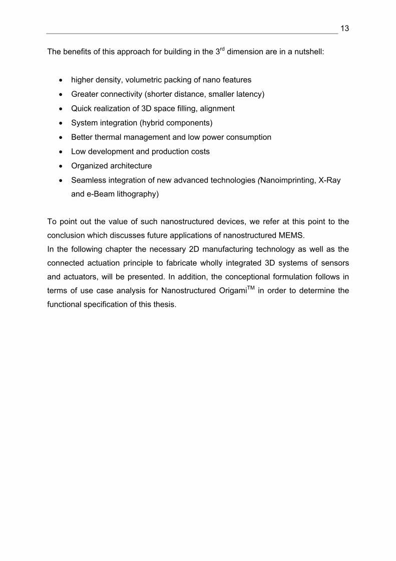
The microstereolithography (µSL) technology creates complex 3D shapes in a liquid
polymer one layer at a time [ZhJS 99]. A liquid polymer is spread to a thickness rang-
ing from one to ten microns; hereupon a UV laser scans the surface and solidifies the
exposed portions. A new, thin layer of polymer is spread and the process is repeated.
The benefits are aspect ratios up to 16:1, the ability to create overhung features (re-
sembling cliffs), and the capability to incorporate “exotic” materials such as shape
memory alloys and metal powders for use in MEMS actuators [Sent 01].
The limitations are that the UV beam spot size is only 1-2µm, and the vertical slices
are limited to the thickness of polymer spread. Crucial is the fact that in this form of
manufacturing, fabrication of wires and layering different materials consecutively is
not possible, see Figure 2-1.
Figure 2-1: The principle of microstereolithography [Jurg 03]
15
The two-photon lithography is based on a different physical and functional method to
create structures in 3D. The polymerization is stimulated by two-photon absorption.
Instead of being layer by layer, two-photon writes features with a pulsed laser, a high
numerical lens, and linear stages to scan the highly focused spot in three spaces.
The properties of this method might someday be useful but the set of material is lim-
ited, and creating features a single point at a time in three dimensions can be enor-
mously slow and does not scale well.
A typical example for layer by layer fabrication is Matrix Semiconductor, a pioneer on
3D memory and 3D transistors. Matrix builds its 3D memory very similar to traditional
2D chips, but by stacking memory arrays vertically [Matr 03]. The disadvantage of
this technique is that heat becomes a concern as the number of layers increase.
Standard 2D chips already require cooling fins and fans to dissipate an average of 80
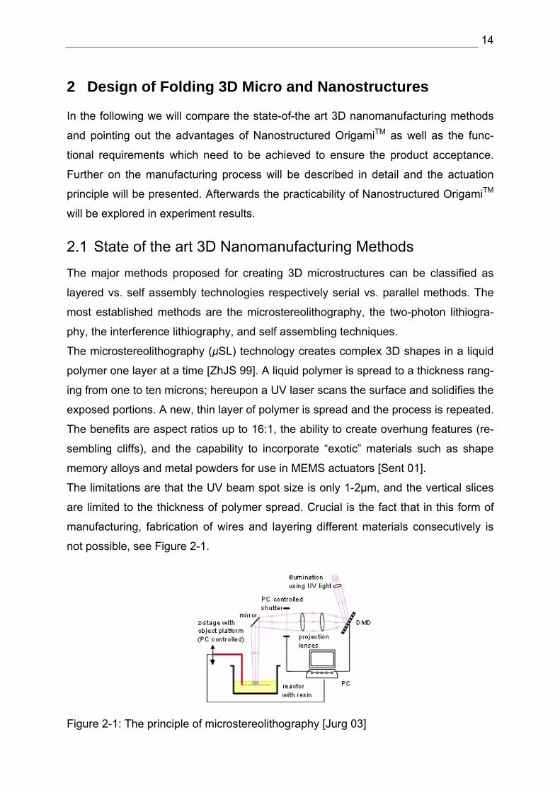
watts over a 2.2 square centimeters Pentium 5 [Lee 02]. Another approach is the
very recent presentation of 3D photo crystals created by assembling individual plates
of 2D photonic crystals [AoId+ 03]. The plates are assembled with the aid of a cus-
tom micromanipulation system inside of a scanning electron microscope (SEM). Four
two twenty plates are brought together and stacked with alignment tolerances of less
than 50nm, see Figure 2-2. This method seems very promising, especially consider-
ing the alignment reported but the assembly is extremely time-consuming since each
plate is handled individually, and manually assembled.
Figure 2-2: 3D photonic crystal fabricated from 2D plates [AoId+ 03]
The Nanostructured OrigamiTM method which will be described in the following has all
the benefits and none of the limitations we have pointed out before. The fundamental
advantage is its independence between the 2D fabrication process and the 3D as-
sembly. This permits to utilize all of the existing technologies as well as to incorpo-
rate any new advances.
16
2.1.1 Functional Requirements
To realize the idea of 2D manufacturing and 3D assembly there are five main func-
tional requirements that must be satisfied. The functional requirements are: hinge
support, actuation, connectivity, alignment, and latching.
To analyze a useful hinge technology the actuation principle has to be taken into
consideration because there is an intended relationship between the hinge and the
actuation method. In general you distinguish between chemical, stress based and
magnetic actuation principles. To choose a suitable method one needs to keep in
mind that the actuation must be compatible with and capable of folding the selected
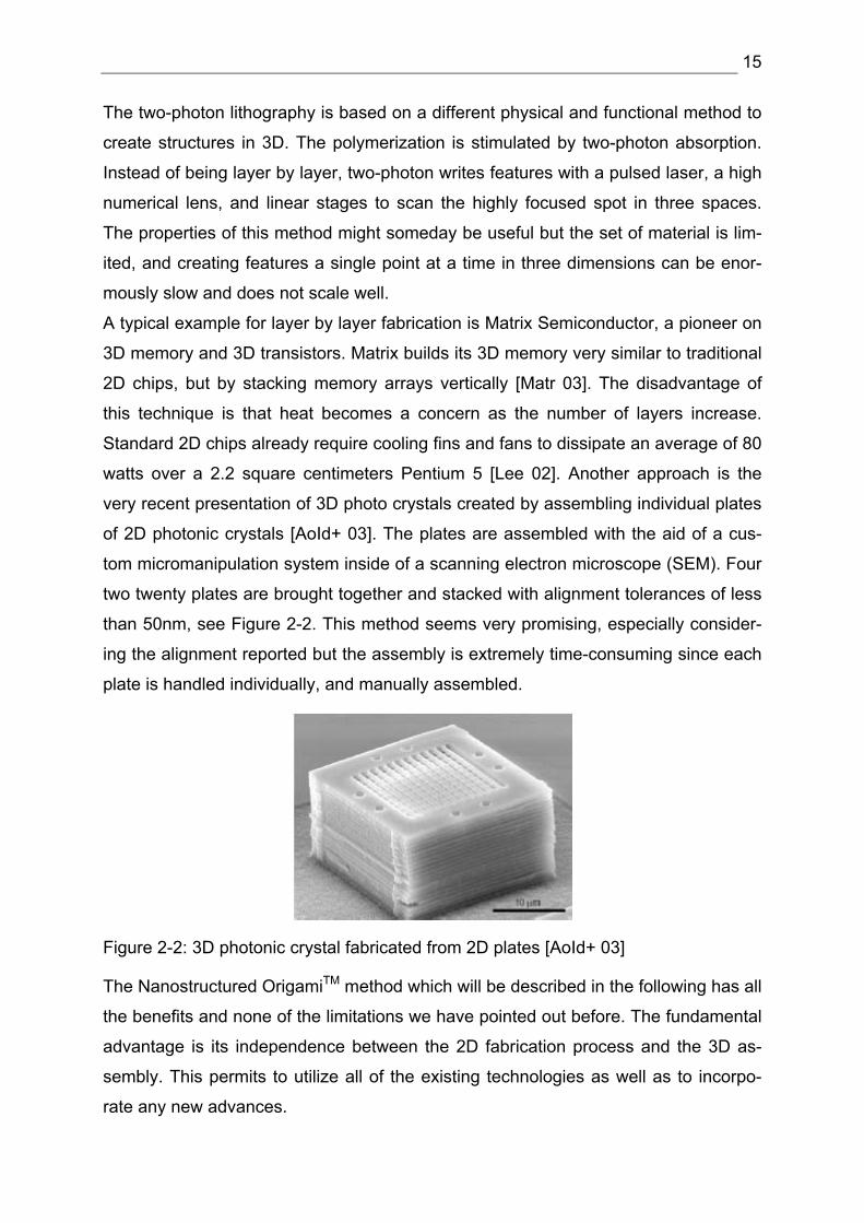
hinge. A few approaches like miniaturizing macroscopic hinges are out of question
because of their limitations in the actuation principle. Typically they are using a probe
tip to fold the structure, see Figure 2-3. Photoresist joints have also been proposed
for rotating silicon micro flaps. Squares of photoresist are patterned between inde-
pendent segments of silicon. Heating the photoresist, the flaps rotate out of the plane
because the surface tension of the photoresist clings to the flaps. This surface ten-
sion method represents a coupled design where the hinge and actuation are insepa-
rable. From the axiomatic design point of view this is a suboptimal design because,
thermal actuation is highly parallel, to address an individual device is nearly impossi-
ble. Other methods like Bilayers, flexible circuits (as common place in laptop com-
puters) or plastically deformed metals are practicable as basic material for hinges.
Other actuating methods like the Permalloy actuation do not support an on or off
switching that means that all devices on a wafer are actuated simultaneously. This
principle is based on magnetic material patterned on the hinges flaps so that when
an external magnetic field is applied, the Permalloy experiences a torque up until the
shape anisotropy is aligned with the field, see Figure 2-4.
Figure 2-3: Miniaturize macroscopic hinges [Jurg 03]
17
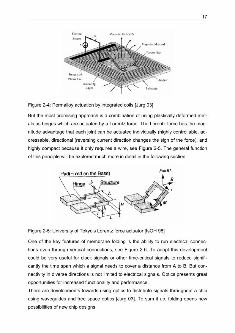
Figure 2-4: Permalloy actuation by integrated coils [Jurg 03]
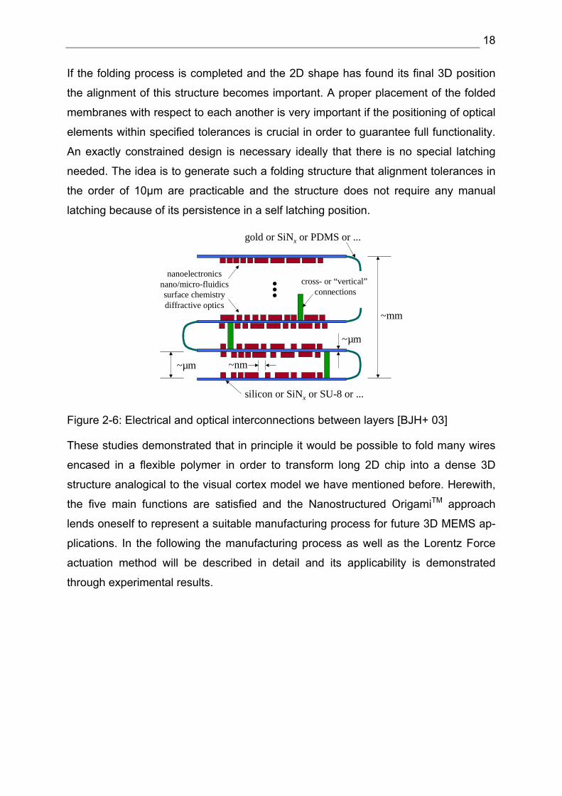
But the most promising approach is a combination of using plastically deformed met-
als as hinges which are actuated by a Lorentz force. The Lorentz force has the mag-
nitude advantage that each joint can be actuated individually (highly controllable, ad-
dressable, directional (reversing current direction changes the sign of the force), and
highly compact because it only requires a wire, see Figure 2-5. The general function
of this principle will be explored much more in detail in the following section.
Figure 2-5: University of Tokyo's Lorentz force actuator [IsOH 98]
One of the key features of membrane folding is the ability to run electrical connec-
tions even through vertical connections, see Figure 2-6. To adopt this development
could be very useful for clock signals or other time-critical signals to reduce signifi-
cantly the time span which a signal needs to cover a distance from A to B. But con-
nectivity in diverse directions is not limited to electrical signals. Optics presents great
opportunities for increased functionality and performance.
There are developments towards using optics to distribute signals throughout a chip
using waveguides and free space optics [Jurg 03]. To sum it up, folding opens new
possibilities of new chip designs.
18
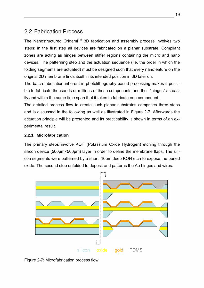
If the folding process is completed and the 2D shape has found its final 3D position
the alignment of this structure becomes important. A proper placement of the folded
membranes with respect to each another is very important if the positioning of optical
elements within specified tolerances is crucial in order to guarantee full functionality.
An exactly constrained design is necessary ideally that there is no special latching
needed. The idea is to generate such a folding structure that alignment tolerances in
the order of 10µm are practicable and the structure does not require any manual
latching because of its persistence in a self latching position.
~nm~µm
~µm
silicon or SiNx or SU-8 or ...
gold or SiNx or PDMS or ...
...
~mm
nanoelectronicsnano/micro-fluidicssurface chemistrydiffractive optics
cross- or “vertical” connections
Figure 2-6: Electrical and optical interconnections between layers [BJH+ 03]
These studies demonstrated that in principle it would be possible to fold many wires
encased in a flexible polymer in order to transform long 2D chip into a dense 3D
structure analogical to the visual cortex model we have mentioned before. Herewith,
the five main functions are satisfied and the Nanostructured OrigamiTM approach
lends oneself to represent a suitable manufacturing process for future 3D MEMS ap-
plications. In the following the manufacturing process as well as the Lorentz Force
actuation method will be described in detail and its applicability is demonstrated
through experimental results.
19
2.2 Fabrication Process
The Nanostructured OrigamiTM 3D fabrication and assembly process involves two
steps; in the first step all devices are fabricated on a planar substrate. Compliant
zones are acting as hinges between stiffer regions containing the micro and nano
devices. The patterning step and the actuation sequence (i.e. the order in which the
folding segments are actuated) must be designed such that every nanofeature on the
original 2D membrane finds itself in its intended position in 3D later on.
The batch fabrication inherent in photolithography-based processing makes it possi-
ble to fabricate thousands or millions of these components and their “hinges” as eas-
ily and within the same time span that it takes to fabricate one component.
The detailed process flow to create such planar substrates comprises three steps
and is discussed in the following as well as illustrated in Figure 2-7. Afterwards the
actuation principle will be presented and its practicability is shown in terms of an ex-
perimental result.
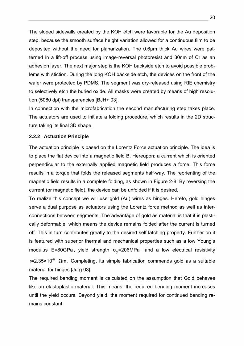
2.2.1 Microfabrication
The primary steps involve KOH (Potassium Oxide Hydrogen) etching through the
silicon device (500µm×500µm) layer in order to define the membrane flaps. The sili-
con segments were patterned by a short, 10µm deep KOH etch to expose the buried
oxide. The second step enfolded to deposit and patterns the Au hinges and wires.
silicon oxide gold PDMS
Figure 2-7: Microfabrication process flow
20
The sloped sidewalls created by the KOH etch were favorable for the Au deposition
step, because the smooth surface height variation allowed for a continuous film to be
deposited without the need for planarization. The 0.6µm thick Au wires were pat-
terned in a lift-off process using image-reversal photoresist and 30nm of Cr as an
adhesion layer. The next major step is the KOH backside etch to avoid possible prob-
lems with stiction. During the long KOH backside etch, the devices on the front of the
wafer were protected by PDMS. The segment was dry-released using RIE chemistry
to selectively etch the buried oxide. All masks were created by means of high resolu-
tion (5080 dpi) transparencies [BJH+ 03].
In connection with the microfabrication the second manufacturing step takes place.
The actuators are used to initiate a folding procedure, which results in the 2D struc-
ture taking its final 3D shape.
2.2.2 Actuation Principle
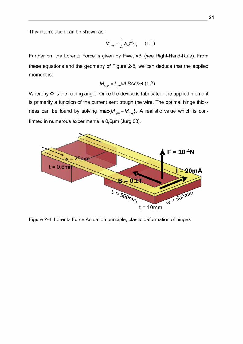
The actuation principle is based on the Lorentz Force actuation principle. The idea is
to place the flat device into a magnetic field B. Hereupon; a current which is oriented
perpendicular to the externally applied magnetic field produces a force. This force
results in a torque that folds the released segments half-way. The reorienting of the
magnetic field results in a complete folding, as shown in Figure 2-8. By reversing the
current (or magnetic field), the device can be unfolded if it is desired.
To realize this concept we will use gold (Au) wires as hinges. Hereto, gold hinges
serve a dual purpose as actuators using the Lorentz force method as well as inter-
connections between segments. The advantage of gold as material is that it is plasti-
cally deformable, which means the device remains folded after the current is turned
off. This in turn contributes greatly to the desired self latching property. Further on it
is featured with superior thermal and mechanical properties such as a low Young’s
modulus E=80GPa , yield strength yσ =206MPa, and a low electrical resistivity
-8r=2.35×10 Ωm . Completing, its simple fabrication commends gold as a suitable
material for hinges [Jurg 03].
The required bending moment is calculated on the assumption that Gold behaves
like an elastoplastic material. This means, the required bending moment increases
until the yield occurs. Beyond yield, the moment required for continued bending re-
mains constant.
21
This interrelation can be shown as:
214req h h yM w t σ= (1.1)
Further on, the Lorentz Force is given by pF=w i×B (see Right-Hand-Rule). From
these equations and the geometry of Figure 2-8, we can deduce that the applied
moment is:
max cosappM I wLB= Θ (1.2)
Whereby Φ is the folding angle. Once the device is fabricated, the applied moment
is primarily a function of the current sent trough the wire. The optimal hinge thick-
ness can be found by solving max app reqM M− . A realistic value which is con-
firmed in numerous experiments is 0,6µm [Jurg 03].
w = 500mmL = 500mmt = 10mm
B = 0.1TI = 20mA
F = 10-4N
t = 0.6mmw = 25mm
Figure 2-8: Lorentz Force Actuation principle, plastic deformation of hinges
22
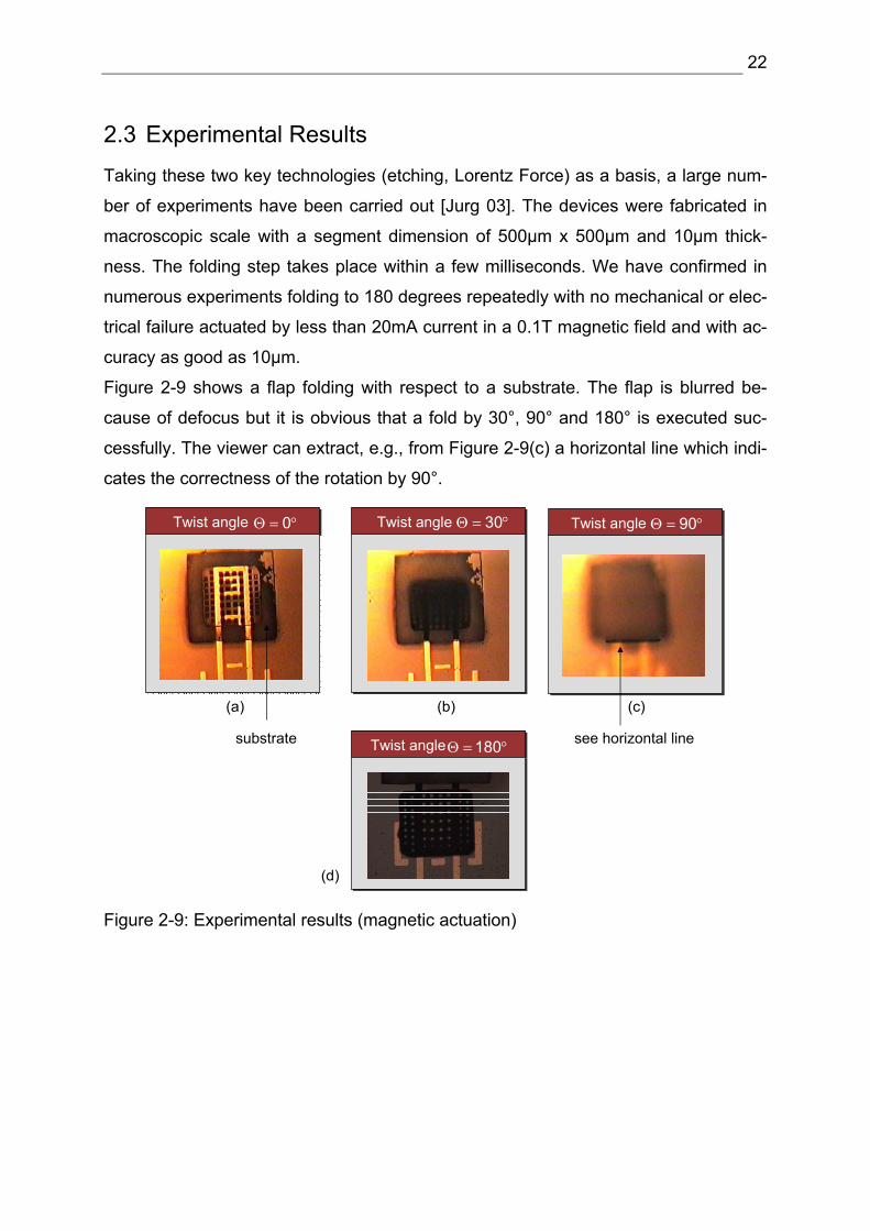
2.3 Experimental Results
Taking these two key technologies (etching, Lorentz Force) as a basis, a large num-
ber of experiments have been carried out [Jurg 03]. The devices were fabricated in
macroscopic scale with a segment dimension of 500µm x 500µm and 10µm thick-
ness. The folding step takes place within a few milliseconds. We have confirmed in
numerous experiments folding to 180 degrees repeatedly with no mechanical or elec-
trical failure actuated by less than 20mA current in a 0.1T magnetic field and with ac-
curacy as good as 10µm.
Figure 2-9 shows a flap folding with respect to a substrate. The flap is blurred be-
cause of defocus but it is obvious that a fold by 30°, 90° and 180° is executed suc-
cessfully. The viewer can extract, e.g., from Figure 2-9(c) a horizontal line which indi-
cates the correctness of the rotation by 90°.
Twist angle 180Θ = °
Twist angle Twist angle Twist angle0Θ = ° 30Θ = ° 90Θ = °
see horizontal linesubstrate
(a) (b) (c)
(d)
Figure 2-9: Experimental results (magnetic actuation)
23
3 Conceptual Formulation and Problem Solving
These experimental results reflect the potential of the Nanostructured OrigamiTM 3D
fabrication and assembly process and its great value as a flexible platform for seam-
less integration of many types of micro and nano fabrication into dense volume. The
folding process does not exclude material selection or exotic fabrication require-
ments. NOFA surpasses all other approaches in terms of 3D connectivity and heat
dissipation. Development costs are reduced by fewer masks and parallel fabrication
of multiple layers. Capital investment remains in steady state as no new tools are
needed because it does not impose any limits on new fabrication technologies. But
the essence of creating functional 3D micro and nanostructures through folding 2D
substrates is that the fabrication of discrete devices (i.e. biological reactors, optical
sensing, and digital electronic logic) is decoupled from the proper assembly process.
The basic technologies which are required to manufacture 3D nanostructured com-
ponents from 2D structures are developed and its feasibility is proven as shown
above.
To expand the field of applications to more complex structures which meets future
industry needs, the actual folding process as well as its preliminary definition of the
folding structure (creases) needs to be explored. For this we will analyze first of all
the modus operandi for a future case study of Nanostructured OrigamiTM. Hereto we
assume that the standard manufacturing process starts with an incoming order of a
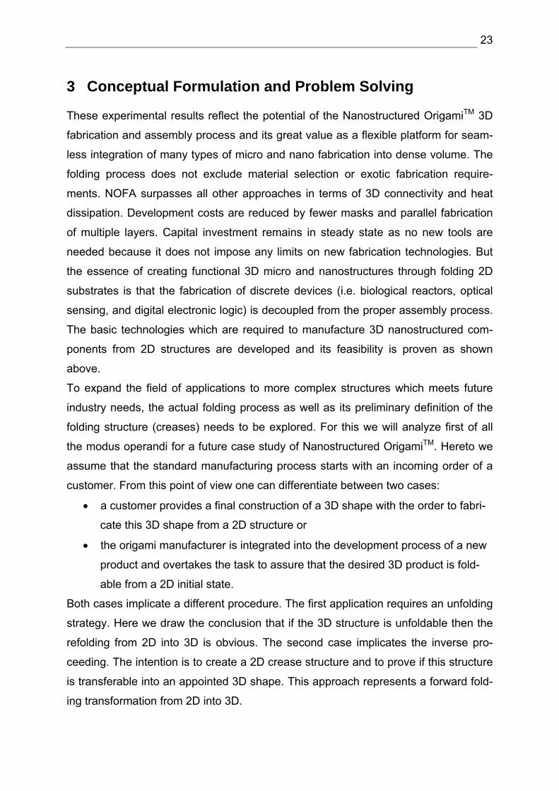
customer. From this point of view one can differentiate between two cases:
• a customer provides a final construction of a 3D shape with the order to fabri-
cate this 3D shape from a 2D structure or
• the origami manufacturer is integrated into the development process of a new
product and overtakes the task to assure that the desired 3D product is fold-
able from a 2D initial state.
Both cases implicate a different procedure. The first application requires an unfolding
strategy. Here we draw the conclusion that if the 3D structure is unfoldable then the
refolding from 2D into 3D is obvious. The second case implicates the inverse pro-
ceeding. The intention is to create a 2D crease structure and to prove if this structure
is transferable into an appointed 3D shape. This approach represents a forward fold-
ing transformation from 2D into 3D.
24
Micro FabricationMicro Fabrication
Activate Folding MechanismActivate Folding Mechanism
Fabr
icat
ion
Cus
tom
er Desired 3D shape available New construction of 3D shape
Decompose into flat 2D shape Create 2D crease modelInverse folding approach Forward folding approach
?
-
Figure 3-1: Conceptual formulation, two use cases
If both cases are satisfied, the above presented manufacturing and actuation meth-
ods are applicabe to complete the Nanostructured OrigamiTM manufacturing process,
see Figure 3-1.
Therefore there is an essential need to do research in the area of object folding to
complete the NOFA process. Here we pursue the idea to determine the motion re-
quired to reach the goal from a given initial state by developing a mathematical nota-
tion which describes its kinematics. Further on we anticipate that the result of this
work will be realized in a comprehensive software package which permits the easy,
hands-on definition of foldable structures and their complete kinematic and dynamic
analysis for design and verification in any given manufacturing challenge. To achieve
this object the thesis is organized as follows, see Figure 3-2.
In the first place we present a general introduction to folding by first highlighting some
general legality about origami and in particular about origami crease pattern. In addi-
tion the idea will be pursued to transfer the paper folding concept to a more generally
admitted approach which uncouples the paper aspect from the folding operation. In
chapter 4.2 the topological and kinematical classification of Multi-Body-Systems
(MBS) will be pointed out and a well known mathematical formulation to describe the
kinematical system will be established. In chapter 5 the folding and unfolding of
25
polygonal linkages are presented. Next a general procedure of how to solve the ki-
nematic problem of a folding operation will be derived by considering the open corner
demonstration model. The solution of the kinematic equations follows additionally
with the object to compile the transfer functions for this example to permit a homoge-
neous animation of the folding process later on.
Further on we will shortly address the dynamics and self collision detection of folding
objects. In connection to the folding approach we will outline the approach of Ileana
Streinu (Smith College) concerning unfolding of polygonal linkages on the basis of a
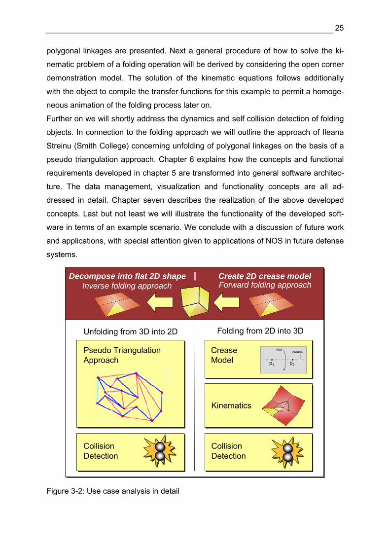
pseudo triangulation approach. Chapter 6 explains how the concepts and functional
requirements developed in chapter 5 are transformed into general software architec-
ture. The data management, visualization and functionality concepts are all ad-
dressed in detail. Chapter seven describes the realization of the above developed
concepts. Last but not least we will illustrate the functionality of the developed soft-
ware in terms of an example scenario. We conclude with a discussion of future work
and applications, with special attention given to applications of NOS in future defense
systems.
Decompose into flat 2D shape Create 2D crease modelInverse folding approach Forward folding approach
Folding from 2D into 3DUnfolding from 3D into 2D
p1 p2
creasefold
Kinematics
Crease Model
Collision Detection
Collision Detection
Pseudo Triangulation Approach
Figure 3-2: Use case analysis in detail
26
4 Analysis of Polygonal Linkages and Origami Structures
Folding is a very common process in our lives, ranging from the macroscopic level
like paper folding or gift wrapping to the microscopic level like protein folding [AmSo
00]. Therefore, folding as well as the inverse proceeding unfolding are interesting
research topics and have been studied in several domains of application. Determin-
ing the laws of folding – the “protein folding problem” – is one of the premier open
questions in science. All fields of research have in common that they try to reach a
desired final state, e.g., the gift package should be wrapped, or the protein's structure
should be obtained; hence it is actually the knowledge of determining the motions
required to reach the goal from a given initial state which must be understood.
For this reason, we believe that the use of origami structures in combination with
perceptions in robotics and gearing technology has great potential to describe the
kinematics of folding operations. The most attractive feature of origami is that one
can construct a wide variety of complex shapes using a few axioms, simple fixed ini-
tial conditions and one mechanical operation, a fold. In the following chapter an intro-
duction to the world of origami will be presented and some general legality will be
pointed out. In addition the idea will be pursued to transfer the paper folding concept
to a more generally admitted approach which uncouples the paper aspect from the
folding operation. Hereto the analysis of polygonal linkages by consideration of its
topological and kinematical classification will be presented.
4.1 Modelling Paper-Folding
The art and process of paper folding is called Origami. Origami comes from the two
Japanese words ORI (to fold) and KAMI (paper) and was adopted into English as
Origami [Mitc 03]. Origami is based on a modular conception which means that a
number of individual "units," each folded from a single sheet of paper, are combined
to form a compound structure [Weiss 99]. In order to describe an origami model and
its geometric and combinatorial problems we have to establish first some terminol-
ogy. To create a paper-folding model you have to think about the mechanics of put-
ting creases into paper. To create a crease, in reality, you have to hold a fragment
stationary, and fold the rest of the paper flat along the proposed crease line. Hereby
we assume that our model has zero thickness and that our creases have no width
and represent straight lines. The crease lines 1,..., nl l are enumerated in counter-
27
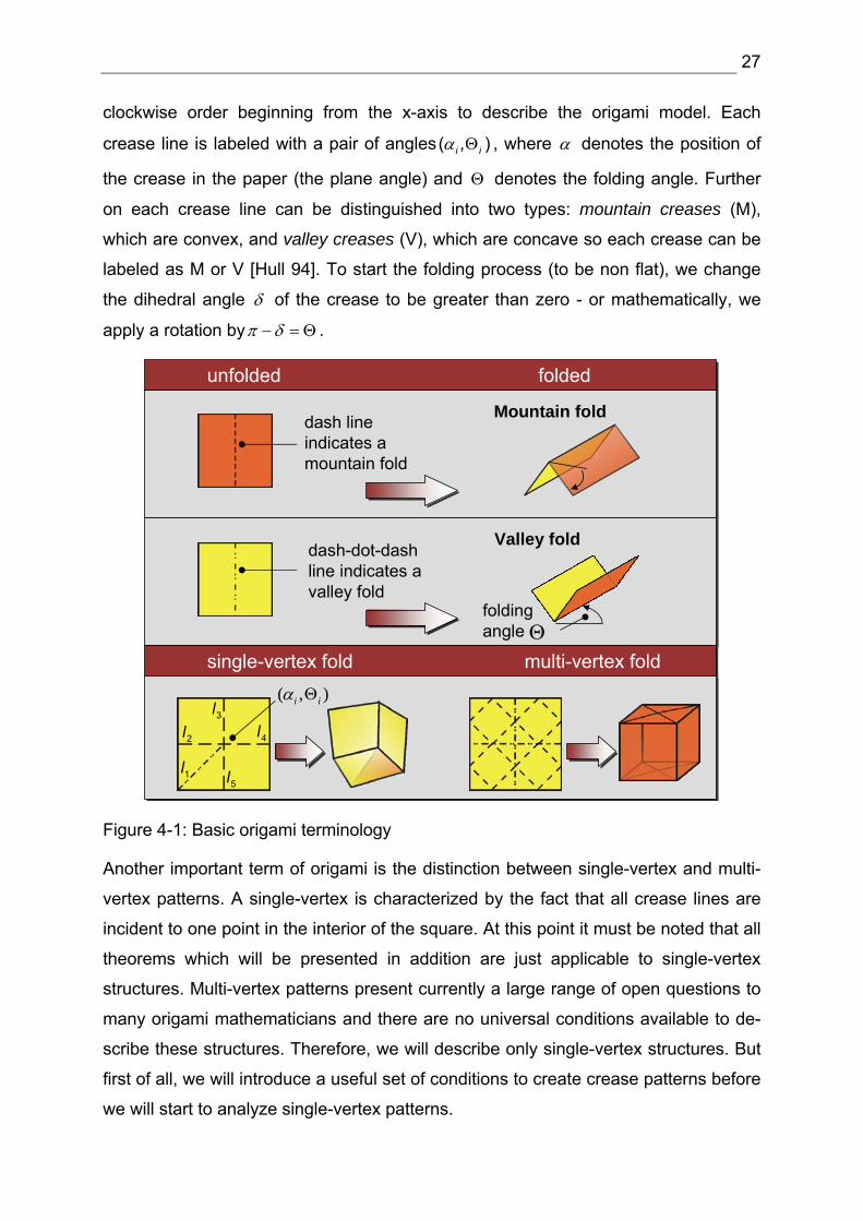
clockwise order beginning from the x-axis to describe the origami model. Each
crease line is labeled with a pair of angles( , )i iα Θ , where α denotes the position of
the crease in the paper (the plane angle) and Θ denotes the folding angle. Further
on each crease line can be distinguished into two types: mountain creases (M),
which are convex, and valley creases (V), which are concave so each crease can be
labeled as M or V [Hull 94]. To start the folding process (to be non flat), we change
the dihedral angle δ of the crease to be greater than zero - or mathematically, we
apply a rotation byπ δ− = Θ .
Mountain fold
unfolded folded
dash line indicates a mountain fold
Valley fold
Θfolding angle
dash-dot-dash line indicates a valley fold
single-vertex fold multi-vertex fold
1l
2l3l
4l
5l
( , )Θi iα
Figure 4-1: Basic origami terminology
Another important term of origami is the distinction between single-vertex and multi-
vertex patterns. A single-vertex is characterized by the fact that all crease lines are
incident to one point in the interior of the square. At this point it must be noted that all
theorems which will be presented in addition are just applicable to single-vertex
structures. Multi-vertex patterns present currently a large range of open questions to
many origami mathematicians and there are no universal conditions available to de-
scribe these structures. Therefore, we will describe only single-vertex structures. But
first of all, we will introduce a useful set of conditions to create crease patterns before
we will start to analyze single-vertex patterns.
28
4.2 Huzita’s Axiom
To create arbitrary crease structures, the Italian-Japanese mathematician Humiaki
Huzita has formulated (1992) the most powerful known set of axioms related to ori-
gami crease patterns. These axioms do not describe all possible origami folds but its
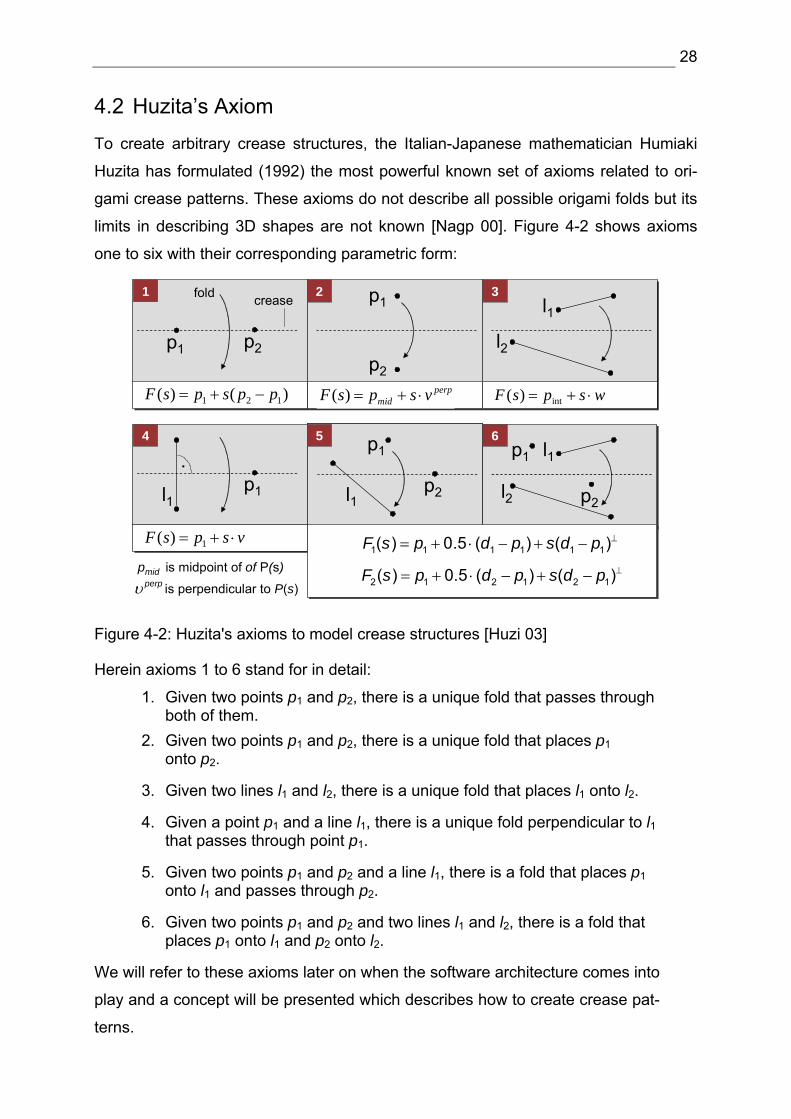
limits in describing 3D shapes are not known [Nagp 00]. Figure 4-2 shows axioms
one to six with their corresponding parametric form:
p1
p2
2l1
l2
3
p1
l1p2
5 p1
l1p2
5l1
l2
p1
p2
6
p1 p2
)()( 121 ppspsF −+=
1creasefold
p1l1
vspsF ⋅+= 1)(
4
.
wspsF ⋅+= int)(perpmid vspsF ⋅+=)(
pmid is midpoint of of P(s)
is perpendicular to P(s) υ perp
⊥= + ⋅ − + −1 1 1 1 1 1( ) 0.5 ( ) ( )F s p d p s d p⊥= + ⋅ − + −2 1 2 1 2 1( ) 0.5 ( ) ( )F s p d p s d p
Figure 4-2: Huzita's axioms to model crease structures [Huzi 03]
Herein axioms 1 to 6 stand for in detail:
1. Given two points p1 and p2, there is a unique fold that passes through both of them.
2. Given two points p1 and p2, there is a unique fold that places p1 onto p2.
3. Given two lines l1 and l2, there is a unique fold that places l1 onto l2.
4. Given a point p1 and a line l1, there is a unique fold perpendicular to l1 that passes through point p1.
5. Given two points p1 and p2 and a line l1, there is a fold that places p1 onto l1 and passes through p2.
6. Given two points p1 and p2 and two lines l1 and l2, there is a fold that places p1 onto l1 and p2 onto l2.
We will refer to these axioms later on when the software architecture comes into
play and a concept will be presented which describes how to create crease pat-
terns.
29
Huzita has proven that the axioms can not only construct all plane Euclidean con-
structions, but also solve polynomials of degree three. Thereby some three dimen-
sional origami models are featured with one specific characteristic; they are flat fold-
able – without adding or undoing any crease. In the following a set of theorems will
be presented that provides necessary conditions for this property.
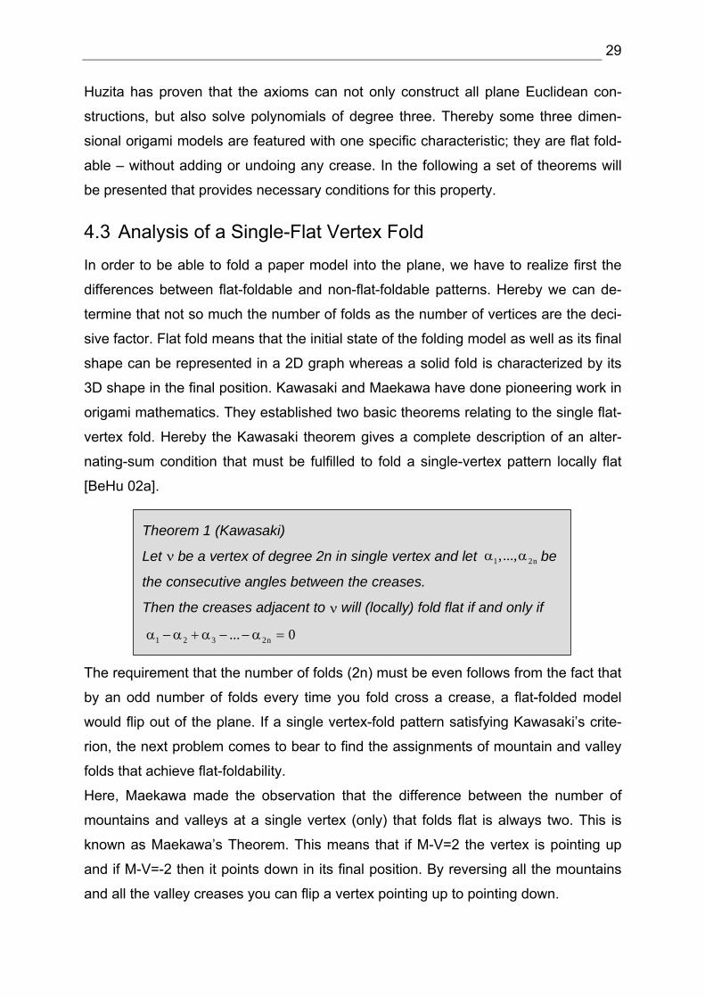
4.3 Analysis of a Single-Flat Vertex Fold
In order to be able to fold a paper model into the plane, we have to realize first the
differences between flat-foldable and non-flat-foldable patterns. Hereby we can de-
termine that not so much the number of folds as the number of vertices are the deci-
sive factor. Flat fold means that the initial state of the folding model as well as its final
shape can be represented in a 2D graph whereas a solid fold is characterized by its
3D shape in the final position. Kawasaki and Maekawa have done pioneering work in
origami mathematics. They established two basic theorems relating to the single flat-
vertex fold. Hereby the Kawasaki theorem gives a complete description of an alter-
nating-sum condition that must be fulfilled to fold a single-vertex pattern locally flat
[BeHu 02a].
Theorem 1 (Kawasaki)
Let be a vertex of degree 2n in single vertex and let be
the consecutive angles between the creases.
Then the creases adjacent to will (locally) fold flat if and only if
ν 1 2n,...,α α
1 2 3 2n... 0α − α + α − − α =
ν
The requirement that the number of folds (2n) must be even follows from the fact that
by an odd number of folds every time you fold cross a crease, a flat-folded model
would flip out of the plane. If a single vertex-fold pattern satisfying Kawasaki’s crite-
rion, the next problem comes to bear to find the assignments of mountain and valley
folds that achieve flat-foldability.
Here, Maekawa made the observation that the difference between the number of
mountains and valleys at a single vertex (only) that folds flat is always two. This is
known as Maekawa’s Theorem. This means that if M-V=2 the vertex is pointing up
and if M-V=-2 then it points down in its final position. By reversing all the mountains
and all the valley creases you can flip a vertex pointing up to pointing down.
30
Theorem 2 (Maekawa)
Let M be the number of mountains and V be the number of valley
creases adjacent to a vertex in a single vertex fold.
Then 2M V− = ±
ν
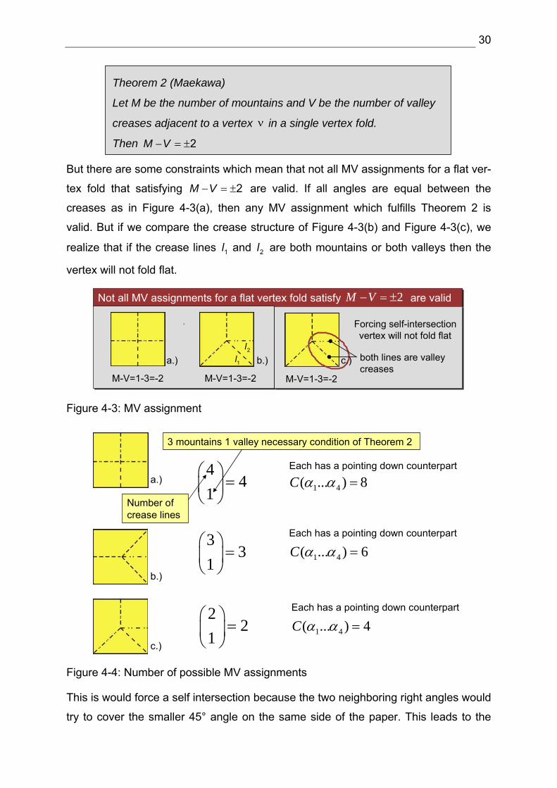
But there are some constraints which mean that not all MV assignments for a flat ver-
tex fold that satisfying 2M V− = ± are valid. If all angles are equal between the
creases as in Figure 4-3(a), then any MV assignment which fulfills Theorem 2 is
valid. But if we compare the crease structure of Figure 4-3(b) and Figure 4-3(c), we
realize that if the crease lines 1l and 2l are both mountains or both valleys then the
vertex will not fold flat.
Not all MV assignments for a flat vertex fold satisfy are validNot all MV assignments for a flat vertex fold satisfy are valid2M V− = ±
.
M-V=1-3=-2M-V=1-3=-2
Forcing self-intersectionvertex will not fold flat
M-V=1-3=-2
both lines are valley creases
a.) b.) c.)1l2l
Figure 4-3: MV assignment
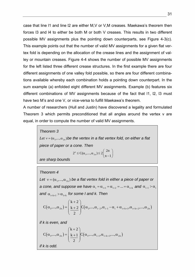
3 mountains 1 valley necessary condition of Theorem 2
44
1⎛ ⎞
=⎜ ⎟⎝ ⎠Number of
crease lines
Each has a pointing down counterpart
1 4( ... ) 8C α α =
33
1⎛ ⎞
=⎜ ⎟⎝ ⎠
1 4( ... ) 6C α α =Each has a pointing down counterpart
22
1⎛ ⎞
=⎜ ⎟⎝ ⎠
1 4( ... ) 4C α α =Each has a pointing down counterpart
a.)
b.)
c.)
Figure 4-4: Number of possible MV assignments
This is would force a self intersection because the two neighboring right angles would
try to cover the smaller 45° angle on the same side of the paper. This leads to the
31
case that line l1 and line l2 are either M,V or V,M creases. Maekawa’s theorem then
forces l3 and l4 to either be both M or both V creases. This results in two different
possible MV assignments plus the pointing down counterparts, see Figure 4-3(c).
This example points out that the number of valid MV assignments for a given flat ver-
tex fold is depending on the allocation of the crease lines and the assignment of val-
ley or mountain creases. Figure 4-4 shows the number of possible MV assignments
for the left listed three different crease structures. In the first example there are four
different assignments of one valley fold possible, so there are four different combina-
tions available whereby each combination holds a pointing down counterpart. In the
sum example (a) enfolded eight different MV assignments. Example (b) features six
different combinations of MV assignments because of the fact that l1, l2, l3 must
have two M’s and one V, or vice-versa to fulfill Maekawa’s theorem.
A number of researchers (Hull and Justin) have discovered a legality and formulated
Theorem 3 which permits preconditioned that all angles around the vertex v are
equal, in order to compute the number of valid MV assignments.
Theorem 3
Let be the vertex in a flat vertex fold, on either a flat
piece of paper or a cone. Then
are sharp bounds
1 2n( ,..., )ν = α α
n1 2n
2n2 C( ,..., ) 2
n 1⎛ ⎞
≤ α α ≤ ⎜ ⎟−⎝ ⎠
Theorem 4
Let be a flat vertex fold in either a piece of paper or
a cone, and suppose we have and
and for some I and k. Then
if k is even, and
if k is odd.
1 2n( ,..., )ν = α α
i i 1 i 2 i k...+ + +α = α = α = = α i 1 i−α > α
i k 1 1 k+ + +α > α
( ) ( )1 2n 1 i 2 i 1 i i k 1 i k 2 2n
k 2C ,..., C ,..., , , ,...,k 2
2− − + + + +
+⎛ ⎞⎜ ⎟α α = α α α −α + α α α+⎜ ⎟⎜ ⎟⎝ ⎠
( ) ( )1 2n 1 i 1 i k 1 2n
k 2C ,..., C ,..., , ,...,k 1
2− + +
+⎛ ⎞⎜ ⎟α α = α α α α+⎜ ⎟⎜ ⎟⎝ ⎠
32
If the assignment of angles is not equal the equal-angle-in-row concept seems out of
reach [see [Hull xx] for a full proof]. Hull has expanded Theorem 3 by using recursive
formulae and created a universally valid theorem, see Theorem 4.
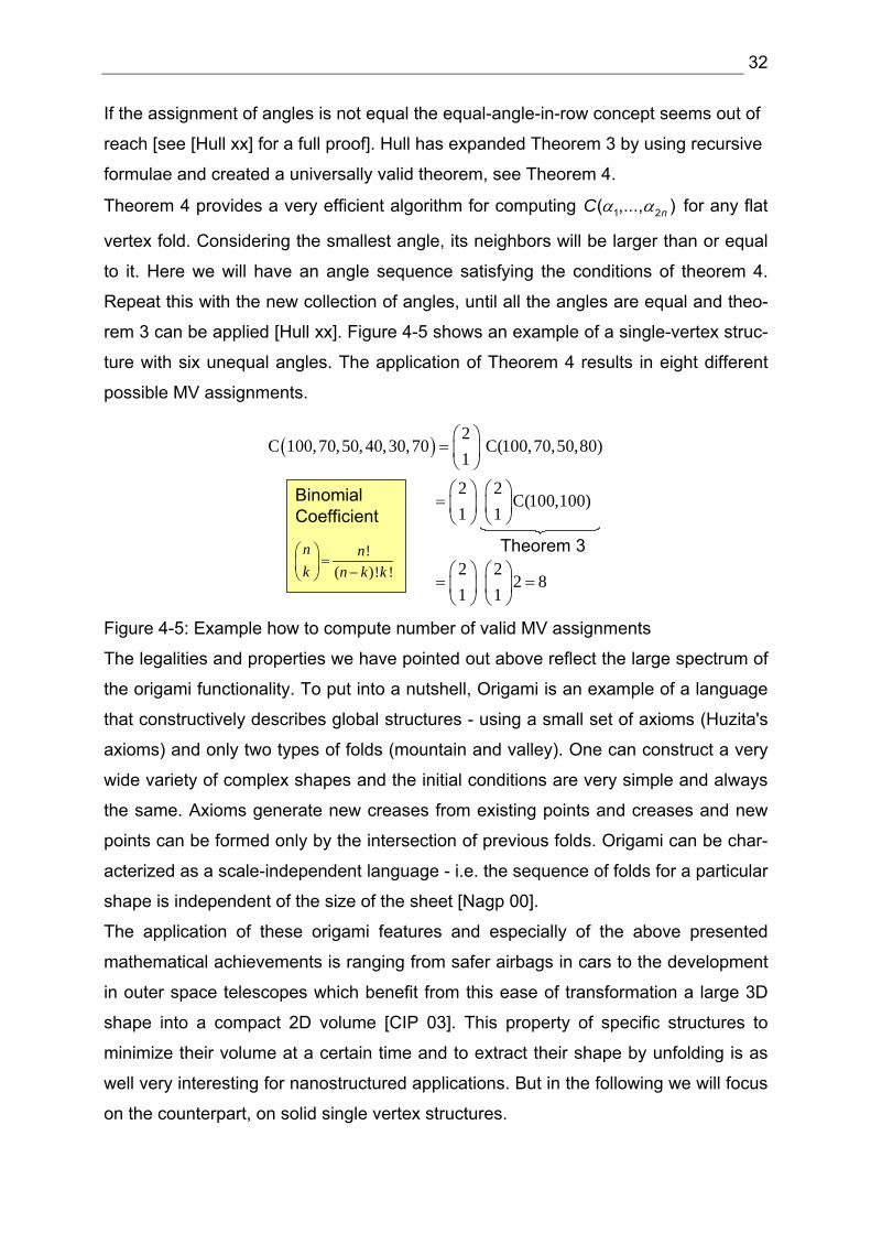
Theorem 4 provides a very efficient algorithm for computing 1 2( ,..., )nC α α for any flat
vertex fold. Considering the smallest angle, its neighbors will be larger than or equal
to it. Here we will have an angle sequence satisfying the conditions of theorem 4.
Repeat this with the new collection of angles, until all the angles are equal and theo-
rem 3 can be applied [Hull xx]. Figure 4-5 shows an example of a single-vertex struc-
ture with six unequal angles. The application of Theorem 4 results in eight different
possible MV assignments.
( )2
C 100,70,50, 40,30,70 C(100,70,50,80)1
2 2C(100,100)
1 1
2 2 2 8
1 1
⎛ ⎞= ⎜ ⎟⎝ ⎠⎛ ⎞ ⎛ ⎞
= ⎜ ⎟ ⎜ ⎟⎝ ⎠ ⎝ ⎠
⎛ ⎞ ⎛ ⎞= =⎜ ⎟ ⎜ ⎟⎝ ⎠ ⎝ ⎠
Theorem 3
Binomial Coefficient
!( )! !
⎛ ⎞=⎜ ⎟ −⎝ ⎠
n nk n k k
Figure 4-5: Example how to compute number of valid MV assignments
The legalities and properties we have pointed out above reflect the large spectrum of
the origami functionality. To put into a nutshell, Origami is an example of a language
that constructively describes global structures - using a small set of axioms (Huzita's
axioms) and only two types of folds (mountain and valley). One can construct a very
wide variety of complex shapes and the initial conditions are very simple and always
the same. Axioms generate new creases from existing points and creases and new
points can be formed only by the intersection of previous folds. Origami can be char-
acterized as a scale-independent language - i.e. the sequence of folds for a particular
shape is independent of the size of the sheet [Nagp 00].
The application of these origami features and especially of the above presented
mathematical achievements is ranging from safer airbags in cars to the development
in outer space telescopes which benefit from this ease of transformation a large 3D
shape into a compact 2D volume [CIP 03]. This property of specific structures to
minimize their volume at a certain time and to extract their shape by unfolding is as
well very interesting for nanostructured applications. But in the following we will focus
on the counterpart, on solid single vertex structures.
33
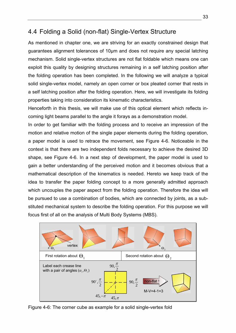
4.4 Folding a Solid (non-flat) Single-Vertex Structure
As mentioned in chapter one, we are striving for an exactly constrained design that
guarantees alignment tolerances of 10µm and does not require any special latching
mechanism. Solid single-vertex structures are not flat foldable which means one can
exploit this quality by designing structures remaining in a self latching position after
the folding operation has been completed. In the following we will analyze a typical
solid single-vertex model, namely an open corner or box pleated corner that rests in
a self latching position after the folding operation. Here, we will investigate its folding
properties taking into consideration its kinematic characteristics.
Henceforth in this thesis, we will make use of this optical element which reflects in-
coming light beams parallel to the angle it forays as a demonstration model.
In order to get familiar with the folding process and to receive an impression of the
motion and relative motion of the single paper elements during the folding operation,
a paper model is used to retrace the movement, see Figure 4-6. Noticeable in the
context is that there are two independent folds necessary to achieve the desired 3D
shape, see Figure 4-6. In a next step of development, the paper model is used to
gain a better understanding of the perceived motion and it becomes obvious that a
mathematical description of the kinematics is needed. Hereto we keep track of the
idea to transfer the paper folding concept to a more generally admitted approach
which uncouples the paper aspect from the folding operation. Therefore the idea will
be pursued to use a combination of bodies, which are connected by joints, as a sub-
stituted mechanical system to describe the folding operation. For this purpose we will
focus first of all on the analysis of Multi Body Systems (MBS).
First rotation about Second rotation about
vertex
1Θ1Θ
2Θ2Θ
( , )Θi iαLabel each crease line with a pair of angles
45,−π
90 ,2π
90,2π
90,2π
45,π
non-flat !
M-V=4-1=3
Figure 4-6: The corner cube as example for a solid single-vertex fold
34
4.5 Classification of Multi Body Systems
The use of MBS in terms of a substituted mechanical system is already applied in the
area of animation software tools to describe the motion of body parts or in the field of
robotics to describe the relative motion of robot arms. In general MBS are consisting
of nB bodies, nJ joints and fJi degree of freedom and can be classified into two sys-
tems: Tree-Type Systems (TTS) and Multi Close Loop Systems (MCLS).
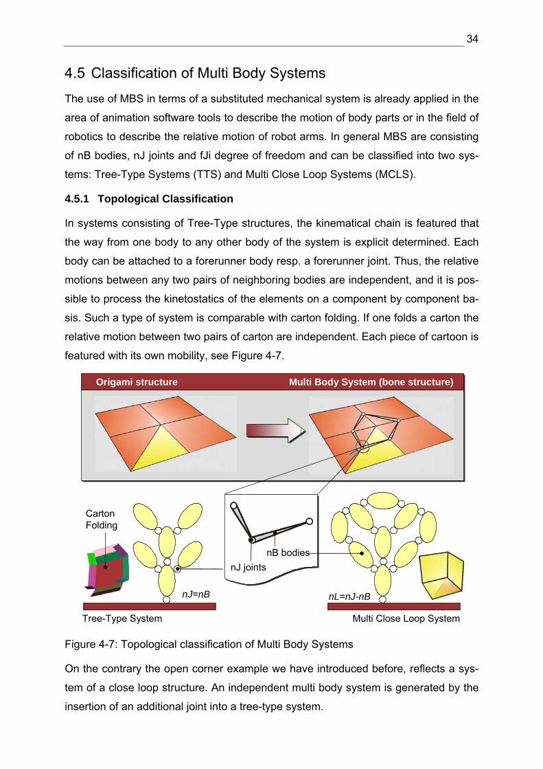
4.5.1 Topological Classification
In systems consisting of Tree-Type structures, the kinematical chain is featured that
the way from one body to any other body of the system is explicit determined. Each
body can be attached to a forerunner body resp. a forerunner joint. Thus, the relative
motions between any two pairs of neighboring bodies are independent, and it is pos-
sible to process the kinetostatics of the elements on a component by component ba-
sis. Such a type of system is comparable with carton folding. If one folds a carton the
relative motion between two pairs of carton are independent. Each piece of cartoon is
featured with its own mobility, see Figure 4-7.
Tree-Type System Multi Close Loop System
nB bodiesnJ joints
Origami structure Multi Body System (bone structure)
Carton Folding
nJ=nB nL=nJ-nB
Figure 4-7: Topological classification of Multi Body Systems
On the contrary the open corner example we have introduced before, reflects a sys-
tem of a close loop structure. An independent multi body system is generated by the
insertion of an additional joint into a tree-type system.
35
Single or Multi Close Loop Systems are characterized by the fact that the relative
motions within the loop become dependent; a change of relative motion at one loca-
tion induces a change of relative motion elsewhere. This effect is noticeable during
the most folding processes of origami models, as traceable in the open corner exam-
ple, see Figure 4-6. Herewith the open corner representative for all single-vertex
structures belongs to the topological classification of multi body systems. Next the
kinematical classification of this model will be considered to constrict its kinematic
motion.
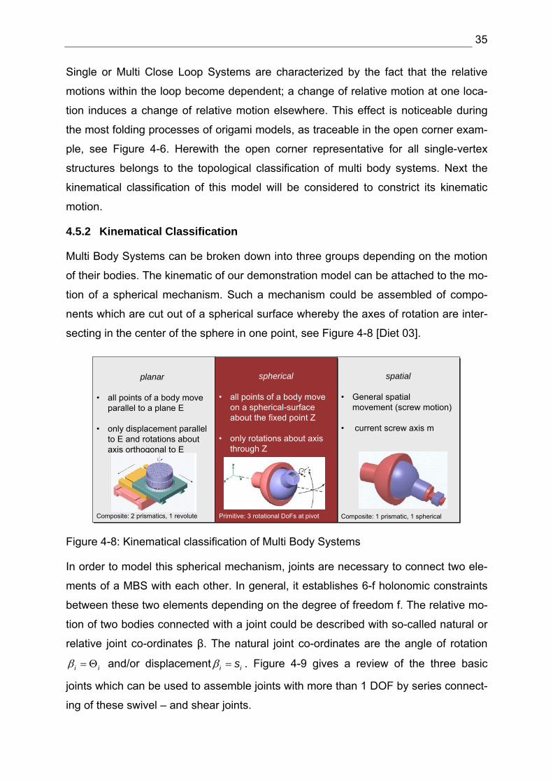
4.5.2 Kinematical Classification
Multi Body Systems can be broken down into three groups depending on the motion
of their bodies. The kinematic of our demonstration model can be attached to the mo-
tion of a spherical mechanism. Such a mechanism could be assembled of compo-
nents which are cut out of a spherical surface whereby the axes of rotation are inter-
secting in the center of the sphere in one point, see Figure 4-8 [Diet 03].
planar
• all points of a body move parallel to a plane E
• only displacement parallel to E and rotations about axis orthogonal to E
spherical
• all points of a body move on a spherical-surface about the fixed point Z
• only rotations about axis through Z
spatial
• General spatial movement (screw motion)
• current screw axis m
Composite: 1 prismatic, 1 sphericalPrimitive: 3 rotational DoFs at pivotComposite: 2 prismatics, 1 revolute
Figure 4-8: Kinematical classification of Multi Body Systems
In order to model this spherical mechanism, joints are necessary to connect two ele-
ments of a MBS with each other. In general, it establishes 6-f holonomic constraints
between these two elements depending on the degree of freedom f. The relative mo-
tion of two bodies connected with a joint could be described with so-called natural or
relative joint co-ordinates β. The natural joint co-ordinates are the angle of rotation
i iβ = Θ and/or displacement i isβ = . Figure 4-9 gives a review of the three basic
joints which can be used to assemble joints with more than 1 DOF by series connect-
ing of these swivel – and shear joints.
36
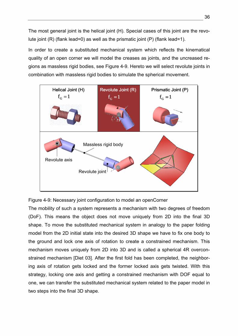
The most general joint is the helical joint (H). Special cases of this joint are the revo-
lute joint (R) (flank lead=0) as well as the prismatic joint (P) (flank lead=1).
In order to create a substituted mechanical system which reflects the kinematical
quality of an open corner we will model the creases as joints, and the uncreased re-
gions as massless rigid bodies, see Figure 4-9. Hereto we will select revolute joints in
combination with massless rigid bodies to simulate the spherical movement.
Helical Joint (H)
Gf 1=Helical Joint (H)
Gf 1=Revolute Joint (R)
Gf 1=Revolute Joint (R)
Gf 1=Prismatic Joint (P)
Gf 1=Prismatic Joint (P)
Gf 1=
Massless rigid body
Revolute axis
Revolute joint
Figure 4-9: Necessary joint configuration to model an openCorner The mobility of such a system represents a mechanism with two degrees of freedom
(DoF). This means the object does not move uniquely from 2D into the final 3D
shape. To move the substituted mechanical system in analogy to the paper folding
model from the 2D initial state into the desired 3D shape we have to fix one body to
the ground and lock one axis of rotation to create a constrained mechanism. This
mechanism moves uniquely from 2D into 3D and is called a spherical 4R overcon-
strained mechanism [Diet 03]. After the first fold has been completed, the neighbor-
ing axis of rotation gets locked and the former locked axis gets twisted. With this
strategy, locking one axis and getting a constrained mechanism with DOF equal to
one, we can transfer the substituted mechanical system related to the paper model in
two steps into the final 3D shape.
37
The characteristic of an overconstrained mechanism is mobility over a finite range of
motion. Further on it must be mentioned that the Gruebner criteria with which it is
possible to compute the mobility of general MBS can not applied to this kind of
mechanism. In general one can compute the mobility of a system containing joints
and with one link fixed to the ground with the Gruebner criteria whereby iu repre-
sents the constraints and if the freedom of a joint:
6 ( 1) with 6
6 ( 1) 6
6 ( 1)
6 (5 5 1) 6 1 1
B i i i
B i
B i i
i
M n u u f
n f
n j f
= ⋅ − − + =
= ⋅ − − −
= ⋅ − − +
= ⋅ − − − − = −
∑∑
∑
∑
(1.3)
But there is a restriction of Gruebners formula if the mechanism is characterized as
an overconstrained mechanism; equation (1.3) delivers a false result (-1) because
particular connections are interdependent.
As a result the open corner represents a spherical mechanism which moves from 2D
into a unique 3D shape by blocking respectively one axis of rotation. The axis of rota-
tion can be modeled by revolving joints which are connected with each other by
massless rigid bodies. The connection of these links represents a close loop multi
body system whose kinematics will be analyzed additionally, and well-known mathe-
matical methods will be applied to explicitly solve the kinematical equations.
4.6 Description of the Kinematics
The basic principle of solving kinematical systems is to reduce the degree of com-
plexity to the minimum. In this case if we consider the folding operation we can de-
termine that only a specific part of the complete system is moving, the other one is
still not in motion. This is obvious because by locking one axis of rotation we transfer
the system from a 5R overconstrained mechanism into a 4R overconstrained system.
Therefore the backward link represents the immobile part.
4.6.1 Splitting the Mechanism into Two Systems
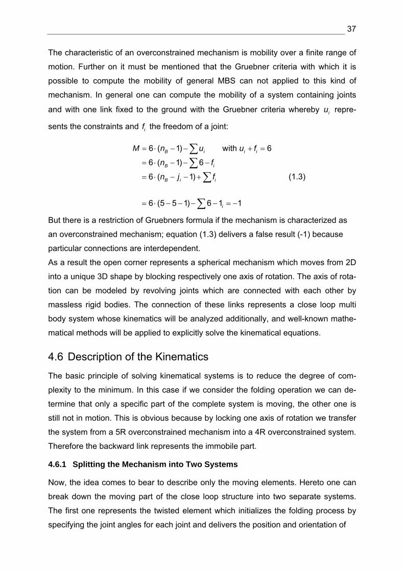
Now, the idea comes to bear to describe only the moving elements. Hereto one can
break down the moving part of the close loop structure into two separate systems.
The first one represents the twisted element which initializes the folding process by
specifying the joint angles for each joint and delivers the position and orientation of
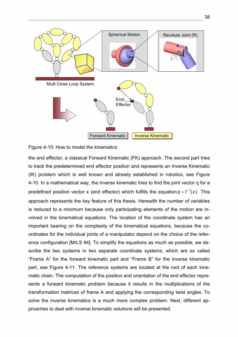
38
Multi Close Loop System
Revolute Joint (R)Spherical Motion
Forward Kinematic Inverse Kinematic
End-Effector
Figure 4-10: How to model the kinematics
the end effector, a classical Forward Kinematic (FK) approach. The second part tries
to track the predetermined end effector position and represents an Inverse Kinematic
(IK) problem which is well known and already established in robotics, see Figure
4-10. In a mathematical way, the inverse kinematic tries to find the joint vector q for a
predefined position vector x (end effector) which fulfills the equation 1( )q f x−= . This
approach represents the key feature of this thesis. Herewith the number of variables
is reduced to a minimum because only participating elements of the motion are in-
volved in the kinematical equations. The location of the coordinate system has an
important bearing on the complexity of the kinematical equations, because the co-
ordinates for the individual joints of a manipulator depend on the choice of the refer-
ence configuration [MrLS 94]. To simplify the equations as much as possible, we de-
scribe the two systems in two separate coordinate systems, which are so called
“Frame A” for the forward kinematic part and “Frame B” for the inverse kinematic
part, see Figure 4-11. The reference systems are located at the root of each kine-
matic chain. The computation of the position and orientation of the end effector repre-
sents a forward kinematic problem because it results in the multiplications of the
transformation matrices of frame A and applying the corresponding twist angles. To
solve the inverse kinematics is a much more complex problem. Next, different ap-
proaches to deal with inverse kinematic solutions will be presented.
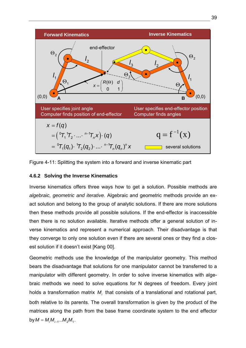
39
Forward Kinematics Inverse Kinematics
end-effector
( )0 1
R dx
Θ⎛ ⎞= ⎜ ⎟⎝ ⎠
1q f (x)−=
User specifies joint angleComputer finds position of end-effector
User specifies end-effector positionComputer finds angles
( )0 1 11 2
0 1 11 1 2 2
( )
... ( )
( ) ( ) ... ( )
nn
n nn n
x f q
T T T x q
T q T q T q x
−
−
=
= ⋅ ⋅ ⋅
= ⋅ ⋅ ⋅
A B(0,0)
1Θ
2Θ
1l
2l
1l
2l3l
1Θ
2Θ
(0,0)
several solutions
3Θ
Figure 4-11: Splitting the system into a forward and inverse kinematic part
4.6.2 Solving the Inverse Kinematics
Inverse kinematics offers three ways how to get a solution. Possible methods are
algebraic, geometric and iterative. Algebraic and geometric methods provide an ex-
act solution and belong to the group of analytic solutions. If there are more solutions
then these methods provide all possible solutions. If the end-effector is inaccessible
then there is no solution available. Iterative methods offer a general solution of in-
verse kinematics and represent a numerical approach. Their disadvantage is that
they converge to only one solution even if there are several ones or they find a clos-
est solution if it doesn’t exist [Kang 00].
Geometric methods use the knowledge of the manipulator geometry. This method
bears the disadvantage that solutions for one manipulator cannot be transferred to a
manipulator with different geometry. In order to solve inverse kinematics with alge-
braic methods we need to solve equations for N degrees of freedom. Every joint
holds a transformation matrix iM that consists of a translational and rotational part,
both relative to its parents. The overall transformation is given by the product of the
matrices along the path from the base frame coordinate system to the end effector
by 1 2 1...i iM M M M M−= .
40
With the use of this matrix multiplication M the forward kinematics can be computed
in terms of the position and orientation of the end effector. The position and orienta-
tion of the end effector vector x in the parent's coordinate system is found by multi-
plying the position vector of the end effectorq , in its own coordinate system with the
transformation matrix M.
( )x f q= (1.4)
In contrast to that, the inverse kinematics is needed to compute the state vector q for
a given position and orientation of the end effector x which is the inverse function of
(1.4)
1( )q f x−= (1.5)
The solution of (1.5) is not simple because the function f is not linear and consisting
of terms of cosine and sine to describe the manipulator geometry. There is a one-
valued function for (1.4) but for (1.5) there are more solutions q for one x as illus-
trated in Figure 4-11.
Analytic Solution Numerical Solution
1 1cos( )a Θ 2 1 2cos( )a Θ +Θ x
y
1Θ
2Θ
1 1cos( )a Θ 2 1 2cos( )a Θ +Θ x
y
1Θ
2Θ
( )f Θ
x xδ+
goalx
( )goalf x
x
( )f Θ
x xδ+
goalx
( )goalf x
x
Iterate1( )J xδ δ−Θ = Θ
( )f δΘ + Θ
1 1
1 2
2 2
1 2
1 1 2 1 2 2 1 2
1 1 2 1 2 2 1 2
sin sin( ) sin( )cos cos( ) cos( )
f fx x
Jf fx x
a a aa a a
δ δδ δδ δδ δ
⎡ ⎤⎢ ⎥⎢ ⎥=⎢ ⎥⎢ ⎥⎣ ⎦− Θ − Θ +Θ − Θ +Θ⎡ ⎤
= ⎢ ⎥Θ + Θ +Θ Θ +Θ⎣ ⎦
1 1 1 2 1 2
1 1 1 2 1 2
( ) cos( ) cos( )( ) sin( ) sin( )
x f a ay f a a= Θ = Θ + Θ +Θ
= Θ = Θ + Θ +Θ
Equations can be solved analytically2 equations 2 variables
1 2... ...Θ = ∧ Θ =Solution
Figure 4-12: Two different solutions of the inverse kinematic equations
If the manipulator is changing its geometrical conformation, a numerical solution like
the iterative approach offers a nice opportunity to compute its inverse kinematics. An
Iterative solution is based on matrix inversion or on any form of optimization.
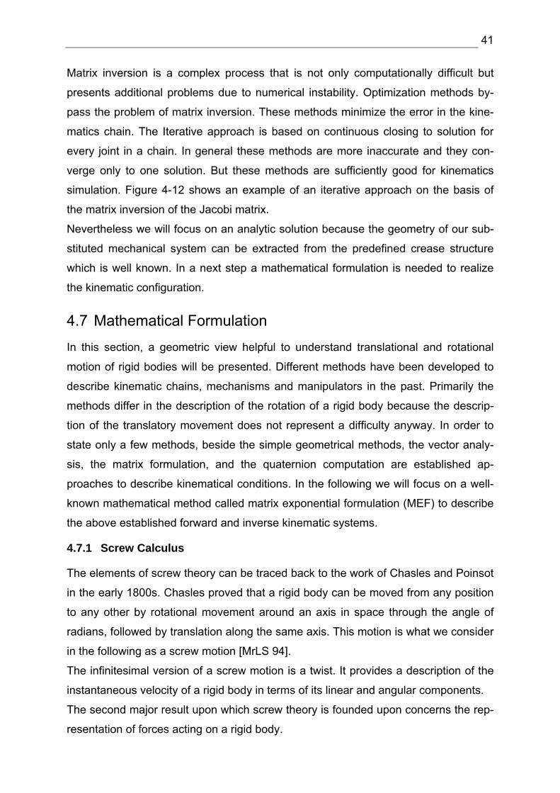
41
Matrix inversion is a complex process that is not only computationally difficult but
presents additional problems due to numerical instability. Optimization methods by-
pass the problem of matrix inversion. These methods minimize the error in the kine-
matics chain. The Iterative approach is based on continuous closing to solution for
every joint in a chain. In general these methods are more inaccurate and they con-
verge only to one solution. But these methods are sufficiently good for kinematics
simulation. Figure 4-12 shows an example of an iterative approach on the basis of
the matrix inversion of the Jacobi matrix.
Nevertheless we will focus on an analytic solution because the geometry of our sub-
stituted mechanical system can be extracted from the predefined crease structure
which is well known. In a next step a mathematical formulation is needed to realize
the kinematic configuration.
4.7 Mathematical Formulation
In this section, a geometric view helpful to understand translational and rotational
motion of rigid bodies will be presented. Different methods have been developed to
describe kinematic chains, mechanisms and manipulators in the past. Primarily the
methods differ in the description of the rotation of a rigid body because the descrip-
tion of the translatory movement does not represent a difficulty anyway. In order to
state only a few methods, beside the simple geometrical methods, the vector analy-
sis, the matrix formulation, and the quaternion computation are established ap-
proaches to describe kinematical conditions. In the following we will focus on a well-
known mathematical method called matrix exponential formulation (MEF) to describe
the above established forward and inverse kinematic systems.
4.7.1 Screw Calculus
The elements of screw theory can be traced back to the work of Chasles and Poinsot
in the early 1800s. Chasles proved that a rigid body can be moved from any position
to any other by rotational movement around an axis in space through the angle of
radians, followed by translation along the same axis. This motion is what we consider
in the following as a screw motion [MrLS 94].
The infinitesimal version of a screw motion is a twist. It provides a description of the
instantaneous velocity of a rigid body in terms of its linear and angular components.
The second major result upon which screw theory is founded upon concerns the rep-
resentation of forces acting on a rigid body.
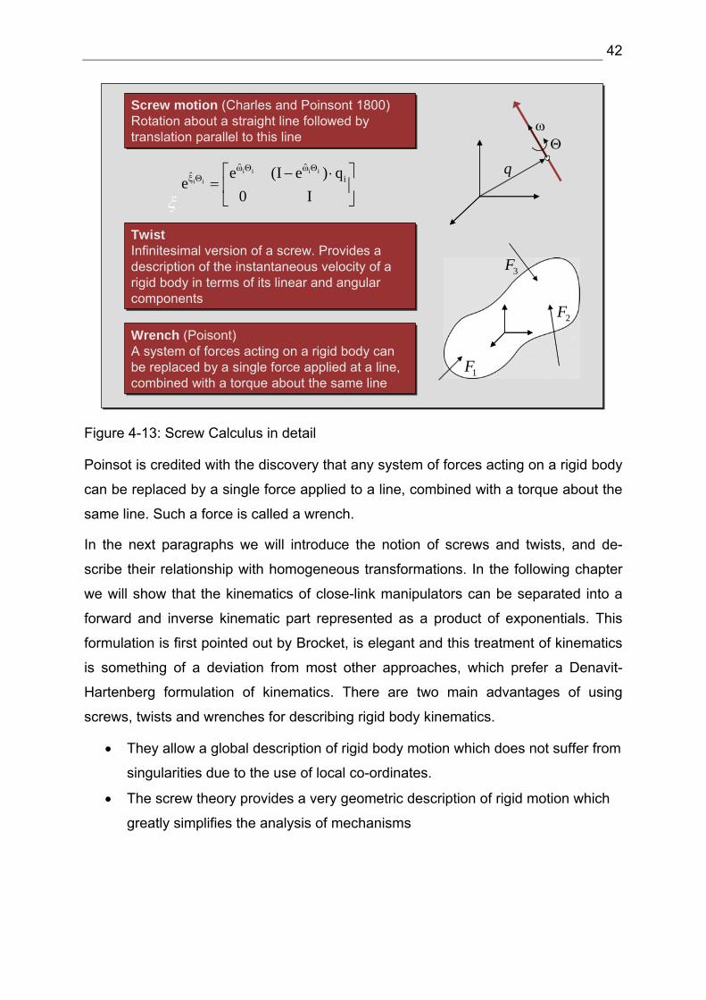
42
Screw motion (Charles and Poinsont 1800)Rotation about a straight line followed by translation parallel to this line
Screw motion (Charles and Poinsont 1800)Rotation about a straight line followed by translation parallel to this line
TwistInfinitesimal version of a screw. Provides a description of the instantaneous velocity of a rigid body in terms of its linear and angular components
TwistInfinitesimal version of a screw. Provides a description of the instantaneous velocity of a rigid body in terms of its linear and angular components
Wrench (Poisont)A system of forces acting on a rigid body can be replaced by a single force applied at a line, combined with a torque about the same line
Wrench (Poisont)A system of forces acting on a rigid body can be replaced by a single force applied at a line, combined with a torque about the same line
1F
2F
3F
q
ω
ξ
Θ
i i i ii i
ˆ ˆˆ ie (I e ) q
e0 I
ω Θ ωΘξ Θ ⎡ ⎤− ⋅
= ⎢ ⎥⎣ ⎦
Figure 4-13: Screw Calculus in detail
Poinsot is credited with the discovery that any system of forces acting on a rigid body
can be replaced by a single force applied to a line, combined with a torque about the
same line. Such a force is called a wrench.
In the next paragraphs we will introduce the notion of screws and twists, and de-
scribe their relationship with homogeneous transformations. In the following chapter
we will show that the kinematics of close-link manipulators can be separated into a
forward and inverse kinematic part represented as a product of exponentials. This
formulation is first pointed out by Brocket, is elegant and this treatment of kinematics
is something of a deviation from most other approaches, which prefer a Denavit-
Hartenberg formulation of kinematics. There are two main advantages of using
screws, twists and wrenches for describing rigid body kinematics.
• They allow a global description of rigid body motion which does not suffer from
singularities due to the use of local co-ordinates.
• The screw theory provides a very geometric description of rigid motion which
greatly simplifies the analysis of mechanisms
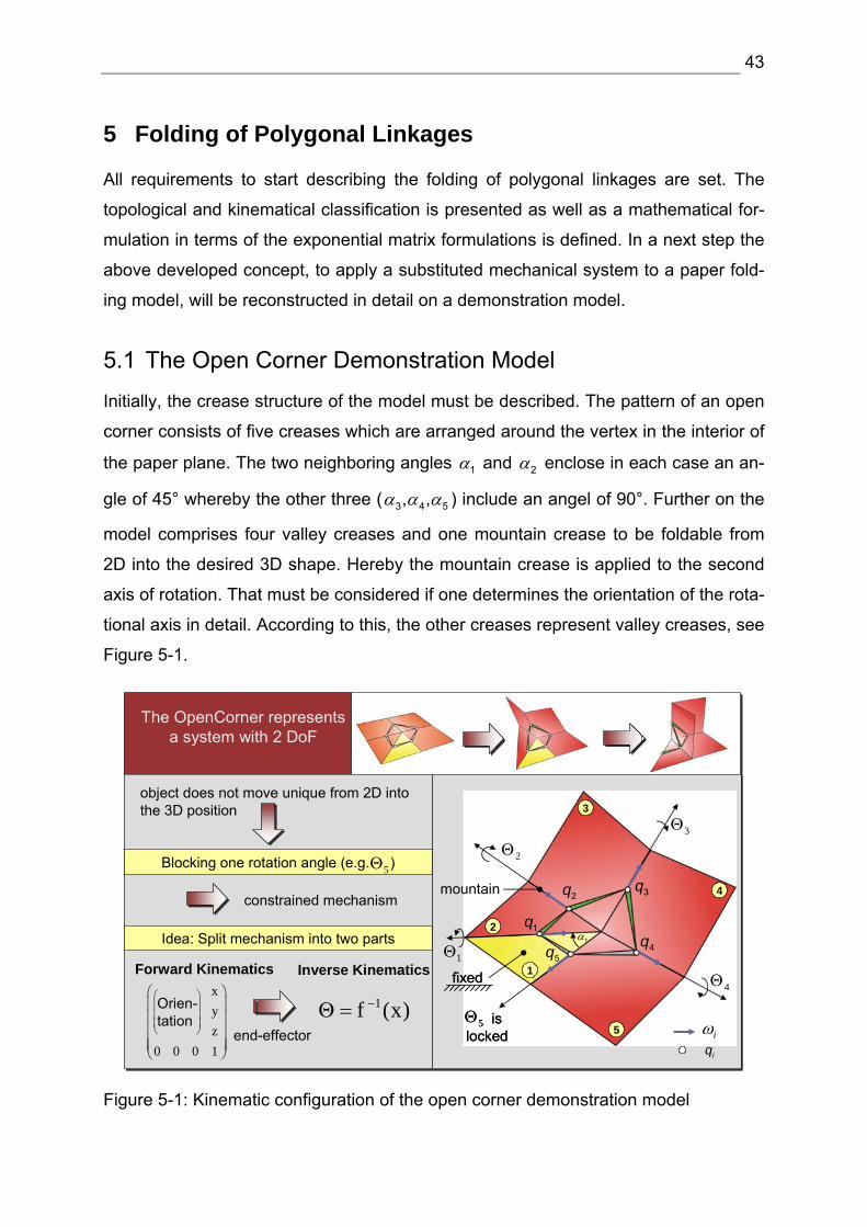
43
5 Folding of Polygonal Linkages
All requirements to start describing the folding of polygonal linkages are set. The
topological and kinematical classification is presented as well as a mathematical for-
mulation in terms of the exponential matrix formulations is defined. In a next step the
above developed concept, to apply a substituted mechanical system to a paper fold-
ing model, will be reconstructed in detail on a demonstration model.
5.1 The Open Corner Demonstration Model
Initially, the crease structure of the model must be described. The pattern of an open
corner consists of five creases which are arranged around the vertex in the interior of
the paper plane. The two neighboring angles 1α and 2α enclose in each case an an-
gle of 45° whereby the other three ( 3 4 5, ,α α α ) include an angel of 90°. Further on the
model comprises four valley creases and one mountain crease to be foldable from
2D into the desired 3D shape. Hereby the mountain crease is applied to the second
axis of rotation. That must be considered if one determines the orientation of the rota-
tional axis in detail. According to this, the other creases represent valley creases, see
Figure 5-1.
The OpenCorner represents a system with 2 DoF
object does not move unique from 2D into the 3D position
constrained mechanism
Blocking one rotation angle (e.g. )
Idea: Split mechanism into two parts
Forward Kinematics Inverse Kinematics
end-effector
xyz
0 0 0 1
⎛ ⎞⎜ ⎟⎜ ⎟⎜ ⎟⎜ ⎟⎜ ⎟⎝ ⎠
1f (x)−Θ =
3Θ
4Θ1Θ
2Θ
5Θ is locked
5Θ is locked
5Θ
Orien-tation
⎛ ⎞⎜ ⎟⎜ ⎟⎜ ⎟⎝ ⎠
fixedfixed
iωiq
mountain
1q
2q 3q
4q5q
1α
1
2
3
4
5
Figure 5-1: Kinematic configuration of the open corner demonstration model
44
After the crease structure is defined, the substituted mechanical system can be ap-
plied. As mentioned in chapter 4 the spherical movement will be modeled by revolute
joints which are connected with rigid bodies around the vertex. Therefore each
crease line will be replaced with a revolute joint consisting of a line item specification
in respect to its corresponding reference system and an orientation with regard to the
rotational direction (mountain or valley crease). Among each other, all joints are con-
nected by bodies to form a close loop structure, see Figure 5-1.
Transferred to the exponential matrix notation this means that each joint is character-
ized by the point nq , where the axis of rotation is going through and the unit vector iω
in the direction of the twist axis. Hereby the joint vectors nq are pointing from the cor-
responding reference system to the joints. In the first instance, all joint vectors will be
described in reference to a base co-ordinate system in the interior of the plane. If all
creases are replaced by joints and described with the use of the two parameters nq
and iω , the actual description of the folding operation can be as follows.
Similar to the paper folding model, where one holds a fragment stationary, and fold
the rest of the paper flat along the proposed crease line, one body (1) will be con-
nected to the ground. Hereupon two possible axes of rotation 1 2( , )Θ Θ to initialize the
folding operation come to bear, see Figure 5-1.
Spherical motion from 2D into 3D
1Θ
2Θ
3Θ
4Θ
Frame AFrame A
Frame BFrame B
End-EffectorInverse Kinematics (IK)
Forward Kinematics (FK)
modeled with revolute joints
d
Figure 5-2: Illustration of a 4R overconstrained mechanism
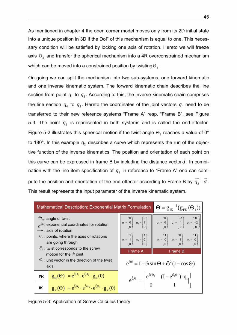
45
As mentioned in chapter 4 the open corner model moves only from its 2D initial state
into a unique position in 3D if the DoF of this mechanism is equal to one. This neces-
sary condition will be satisfied by locking one axis of rotation. Hereto we will freeze
axis 2Θ and transfer the spherical mechanism into a 4R overconstrained mechanism
which can be moved into a constrained position by twisting 1Θ .
On going we can split the mechanism into two sub-systems, one forward kinematic
and one inverse kinematic system. The forward kinematic chain describes the line
section from point 1q to 2q . According to this, the inverse kinematic chain comprises
the line section 4q to 2q . Hereto the coordinates of the joint vectors iq need to be
transferred to their new reference systems “Frame A” resp. “Frame B”, see Figure
5-3. The point 2q is represented in both systems and is called the end-effector.
Figure 5-2 illustrates this spherical motion if the twist angle 1Θ reaches a value of 0°
to 180°. In this example 2q describes a curve which represents the run of the objec-
tive function of the inverse kinematics. The position and orientation of each point on
this curve can be expressed in frame B by including the distance vectord . In combi-
nation with the line item specification of 2q in reference to “Frame A” one can com-
pute the position and orientation of the end effector according to Frame B by 2q d− .
This result represents the input parameter of the inverse kinematic system.
Mathematical Description: Exponential Matrix Formulation 1IK FK 1g (g ( ))−Θ = Θ
: angle of twist: exponential coordinates for rotation: axis of rotation: points, where the axes of rotations are going through
: twist corresponds to the screw motion for the ith joint
: unit vector in the direction of the twist axis
iξ
nΘ
nq
iω
Θξe
34 2ˆˆ ˆ
st stg ( ) e e e g (0)ξΘξΘ ξΘΘ = ⋅ ⋅ ⋅
1 2ˆ ˆ
st stg ( ) e e g (0)ξΘ ξΘΘ = ⋅ ⋅
IK
FK
1
000
q⎛ ⎞⎜ ⎟= ⎜ ⎟⎜ ⎟⎝ ⎠
2
010
q⎛ ⎞⎜ ⎟= ⎜ ⎟⎜ ⎟⎝ ⎠
4
000
q⎛ ⎞⎜ ⎟= ⎜ ⎟⎜ ⎟⎝ ⎠
2
02
0q
⎛ ⎞⎜ ⎟= −⎜ ⎟⎜ ⎟⎝ ⎠
3
110
q−⎛ ⎞⎜ ⎟= ⎜ ⎟⎜ ⎟⎝ ⎠
1
110
ω⎛ ⎞⎜ ⎟= ⎜ ⎟⎜ ⎟⎝ ⎠
2
100
ω⎛ ⎞⎜ ⎟= ⎜ ⎟⎜ ⎟⎝ ⎠
2
100
ω⎛ ⎞⎜ ⎟= ⎜ ⎟⎜ ⎟⎝ ⎠
4
100
ω⎛ ⎞⎜ ⎟= ⎜ ⎟⎜ ⎟⎝ ⎠
4
010
ω⎛ ⎞⎜ ⎟= ⎜ ⎟⎜ ⎟⎝ ⎠
Frame A Frame B
i i i ii i
ˆ ˆˆ ie (I e ) q
e0 I
ωΘ ω Θξ Θ ⎡ ⎤− ⋅
= ⎢ ⎥⎣ ⎦
ˆ 2ˆ ˆe I sin (1 cos )ωΘ = +ω Θ+ω − Θ
Figure 5-3: Application of Screw Calculus theory
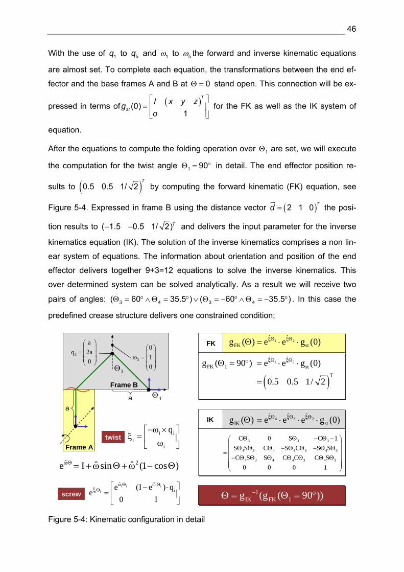
46
With the use of 1q to 5q and 1ω to 5ω the forward and inverse kinematic equations
are almost set. To complete each equation, the transformations between the end ef-
fector and the base frames A and B at 0Θ = stand open. This connection will be ex-
pressed in terms of ( )(0)1
T
stI x y zgo
⎡ ⎤= ⎢ ⎥⎢ ⎥⎣ ⎦
for the FK as well as the IK system of
equation.
After the equations to compute the folding operation over 1Θ are set, we will execute
the computation for the twist angle 1 90Θ = ° in detail. The end effector position re-
sults to ( )0.5 0.5 1/ 2T
by computing the forward kinematic (FK) equation, see
Figure 5-4. Expressed in frame B using the distance vector ( )2 1 0 Td = the posi-
tion results to ( 1.5 0.5 1/ 2)T− − and delivers the input parameter for the inverse
kinematics equation (IK). The solution of the inverse kinematics comprises a non lin-
ear system of equations. The information about orientation and position of the end
effector delivers together 9+3=12 equations to solve the inverse kinematics. This
over determined system can be solved analytically. As a result we will receive two
pairs of angles: 3 4 3 4( 60 35.5 ) ( 60 35.5 )Θ = ° ∧Θ = ° ∨ Θ = − ° ∧ Θ = − ° . In this case the
predefined crease structure delivers one constrained condition;
3
aq 2a
0
⎛ ⎞⎜ ⎟= ⎜ ⎟⎜ ⎟⎝ ⎠
3
010
⎛ ⎞⎜ ⎟ω = ⎜ ⎟⎜ ⎟⎝ ⎠
Frame A
aa
twisti i
ii
q−ω ×⎡ ⎤ξ = ⎢ ⎥ω⎣ ⎦
i i i ii i
ˆ ˆˆ ie (I e ) q
e0 I
ω Θ ωΘξ Θ ⎡ ⎤− ⋅
= ⎢ ⎥⎣ ⎦
screw
iΘ
Frame B
1 2ˆ ˆ
FK stg ( ) e e g (0)ξΘ ξΘΘ = ⋅ ⋅FK
34 2ˆˆ ˆ
IK stg ( ) e e e g (0)ξΘξΘ ξΘΘ = ⋅ ⋅ ⋅IK
1IK FK 1g (g ( 90 ))−Θ = Θ = °
3 3 3
4 3 4 4 3 4 3
4 3 4 4 3 4 3
C 0 S C 1S S C S C S SC S S C C C S
0 0 0 1
Θ Θ − Θ −⎛ ⎞⎜ ⎟Θ Θ Θ − Θ Θ − Θ Θ⎜ ⎟=⎜ ⎟− Θ Θ Θ Θ Θ Θ Θ⎜ ⎟⎜ ⎟⎝ ⎠
4Θ
3Θ
ˆ 2ˆ ˆe I sin (1 cos )ωΘ = +ω Θ+ω − Θ
( )1 2
ˆ ˆFK 1 st
T
g ( 90 ) e e g (0)
0.5 0.5 1/ 2
ξΘ ξΘΘ = ° = ⋅ ⋅
=
Figure 5-4: Kinematic configuration in detail
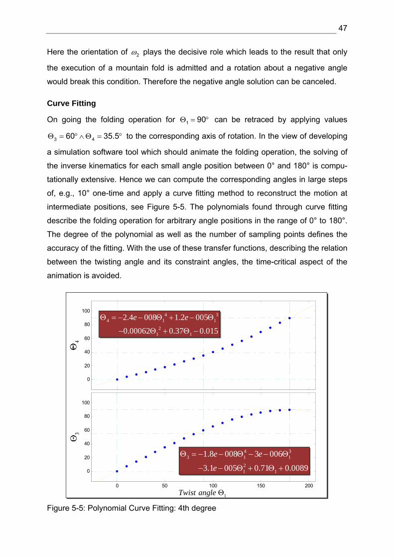
47
Here the orientation of 2ω plays the decisive role which leads to the result that only
the execution of a mountain fold is admitted and a rotation about a negative angle
would break this condition. Therefore the negative angle solution can be canceled.
Curve Fitting
On going the folding operation for 1 90Θ = ° can be retraced by applying values
3 460 35.5Θ = ° ∧ Θ = ° to the corresponding axis of rotation. In the view of developing
a simulation software tool which should animate the folding operation, the solving of
the inverse kinematics for each small angle position between 0° and 180° is compu-
tationally extensive. Hence we can compute the corresponding angles in large steps
of, e.g., 10° one-time and apply a curve fitting method to reconstruct the motion at
intermediate positions, see Figure 5-5. The polynomials found through curve fitting
describe the folding operation for arbitrary angle positions in the range of 0° to 180°.
The degree of the polynomial as well as the number of sampling points defines the
accuracy of the fitting. With the use of these transfer functions, describing the relation
between the twisting angle and its constraint angles, the time-critical aspect of the
animation is avoided.
0 50 100 150 200
0
20
40
60
80
100
θ3
0
20
40
60
80
100
θ 4
1 Twist angle Θ
4 33 1 1
21 1
1.8 008 3 006
3.1 005 0.71 0.0089
e e
e
Θ = − − Θ − − Θ
− − Θ + Θ +
4 34 1 1
21 1
2.4 008 1.2 005
0.00062 0.37 0.015
e eΘ = − − Θ + − Θ
− Θ + Θ −
Figure 5-5: Polynomial Curve Fitting: 4th degree
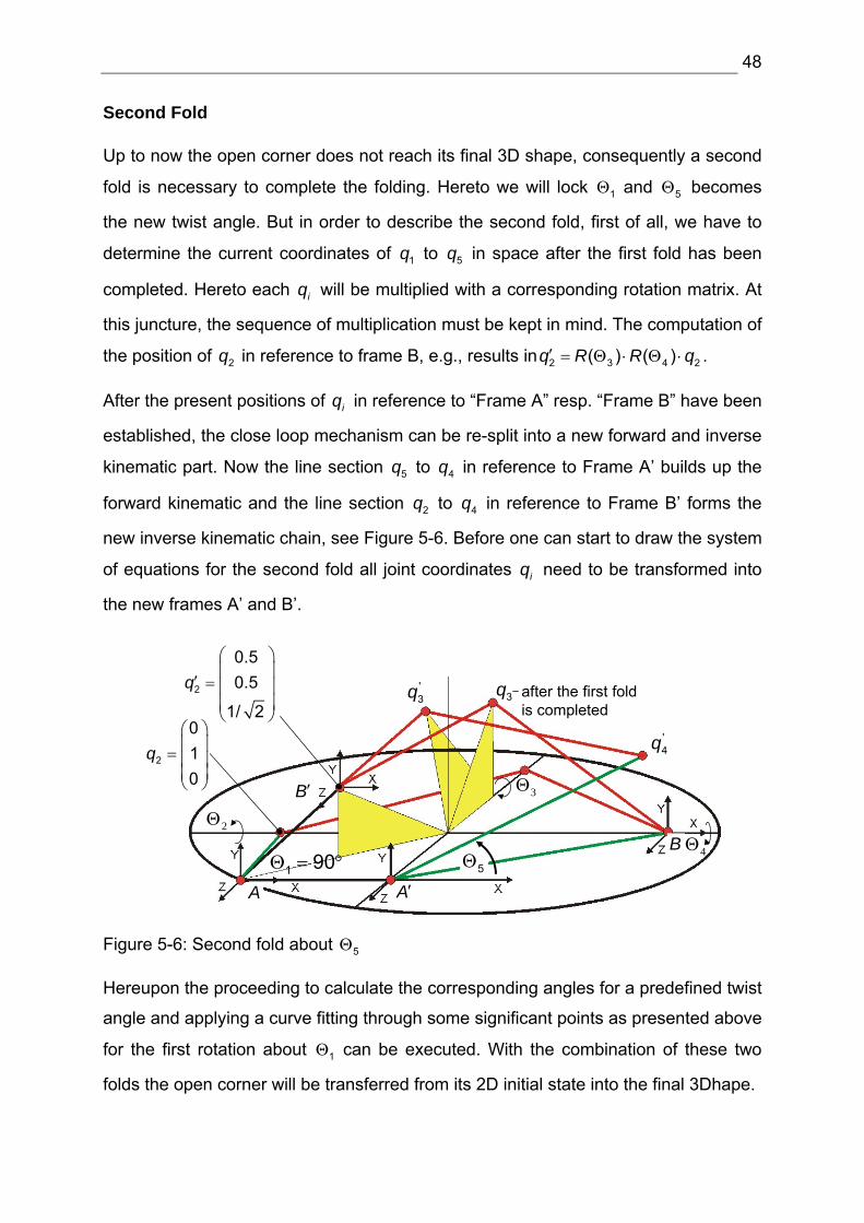
48
Second Fold
Up to now the open corner does not reach its final 3D shape, consequently a second
fold is necessary to complete the folding. Hereto we will lock 1Θ and 5Θ becomes
the new twist angle. But in order to describe the second fold, first of all, we have to
determine the current coordinates of 1q to 5q in space after the first fold has been
completed. Hereto each iq will be multiplied with a corresponding rotation matrix. At
this juncture, the sequence of multiplication must be kept in mind. The computation of
the position of 2q in reference to frame B, e.g., results in 2 3 4 2( ) ( )q R R q′ = Θ ⋅ Θ ⋅ .
After the present positions of iq in reference to “Frame A” resp. “Frame B” have been
established, the close loop mechanism can be re-split into a new forward and inverse
kinematic part. Now the line section 5q to 4q in reference to Frame A’ builds up the
forward kinematic and the line section 2q to 4q in reference to Frame B’ forms the
new inverse kinematic chain, see Figure 5-6. Before one can start to draw the system
of equations for the second fold all joint coordinates iq need to be transformed into
the new frames A’ and B’.
5Θ1 90Θ = °A′
B′
B
A
2
0.50.5
1/ 2
q⎛ ⎞⎜ ⎟
′ = ⎜ ⎟⎜ ⎟⎝ ⎠
2
010
q⎛ ⎞⎜ ⎟= ⎜ ⎟⎜ ⎟⎝ ⎠
2Θ
3Θ
4Θ
3q'3q
'4q
after the first fold is completed
Figure 5-6: Second fold about 5Θ
Hereupon the proceeding to calculate the corresponding angles for a predefined twist
angle and applying a curve fitting through some significant points as presented above
for the first rotation about 1Θ can be executed. With the combination of these two
folds the open corner will be transferred from its 2D initial state into the final 3Dhape.
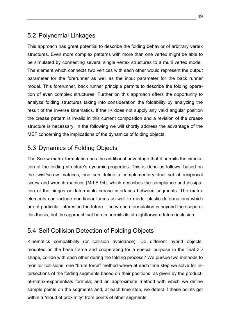
49
5.2 Polynomial Linkages
This approach has great potential to describe the folding behavior of arbitrary vertex
structures. Even more complex patterns with more than one vertex might be able to
be simulated by connecting several single vertex structures to a multi vertex model.
The element which connects two vertices with each other would represent the output
parameter for the forerunner as well as the input parameter for the back runner
model. This forerunner, back runner principle permits to describe the folding opera-
tion of even complex structures. Further on this approach offers the opportunity to
analyze folding structures taking into consideration the foldability by analyzing the
result of the inverse kinematics. If the IK does not supply any valid angular position
the crease pattern is invalid in this current composition and a revision of the crease
structure is necessary. In the following we will shortly address the advantage of the
MEF concerning the implications of the dynamics of folding objects.
5.3 Dynamics of Folding Objects
The Screw matrix formulation has the additional advantage that it permits the simula-
tion of the folding structure’s dynamic properties. This is done as follows: based on
the twist/screw matrices, one can define a complementary dual set of reciprocal
screw and wrench matrices [MrLS 94], which describes the compliance and dissipa-
tion of the hinges or deformable crease interfaces between segments. The matrix
elements can include non-linear forces as well to model plastic deformations which
are of particular interest in the future. The wrench formulation is beyond the scope of
this thesis, but the approach set herein permits its straightforward future inclusion.
5.4 Self Collision Detection of Folding Objects
Kinematics compatibility (or collision avoidance): Do different hybrid objects,
mounted on the base frame and cooperating for a special purpose in the final 3D
shape, collide with each other during the folding process? We pursue two methods to
monitor collisions: one “brute force” method where at each time step we solve for in-
tersections of the folding segments based on their positions, as given by the product-
of-matrix-exponentials formula; and an approximate method with which we define
sample points on the segments and, at each time step, we detect if these points get
within a “cloud of proximity” from points of other segments.
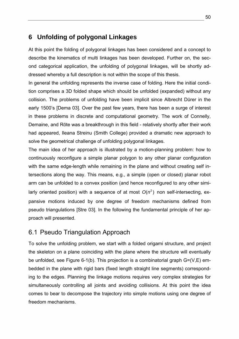
50
6 Unfolding of polygonal Linkages
At this point the folding of polygonal linkages has been considered and a concept to
describe the kinematics of multi linkages has been developed. Further on, the sec-
ond categorical application, the unfolding of polygonal linkages, will be shortly ad-
dressed whereby a full description is not within the scope of this thesis.
In general the unfolding represents the inverse case of folding. Here the initial condi-
tion comprises a 3D folded shape which should be unfolded (expanded) without any
collision. The problems of unfolding have been implicit since Albrecht Dürer in the
early 1500’s [Dema 03]. Over the past few years, there has been a surge of interest
in these problems in discrete and computational geometry. The work of Connelly,
Demaine, and Röte was a breakthrough in this field - relatively shortly after their work
had appeared, Ileana Streinu (Smith College) provided a dramatic new approach to
solve the geometrical challenge of unfolding polygonal linkages.
The main idea of her approach is illustrated by a motion-planning problem: how to
continuously reconfigure a simple planar polygon to any other planar configuration
with the same edge-length while remaining in the plane and without creating self in-
tersections along the way. This means, e.g., a simple (open or closed) planar robot
arm can be unfolded to a convex position (and hence reconfigured to any other simi-
larly oriented position) with a sequence of at most 2( )O n non self-intersecting, ex-
pansive motions induced by one degree of freedom mechanisms defined from
pseudo triangulations [Stre 03]. In the following the fundamental principle of her ap-
proach will presented.
6.1 Pseudo Triangulation Approach
To solve the unfolding problem, we start with a folded origami structure, and project
the skeleton on a plane coinciding with the plane where the structure will eventually
be unfolded, see Figure 6-1(b). This projection is a combinatorial graph G=(V,E) em-
bedded in the plane with rigid bars (fixed length straight line segments) correspond-
ing to the edges. Planning the linkage motions requires very complex strategies for
simultaneously controlling all joints and avoiding collisions. At this point the idea
comes to bear to decompose the trajectory into simple motions using one degree of
freedom mechanisms.
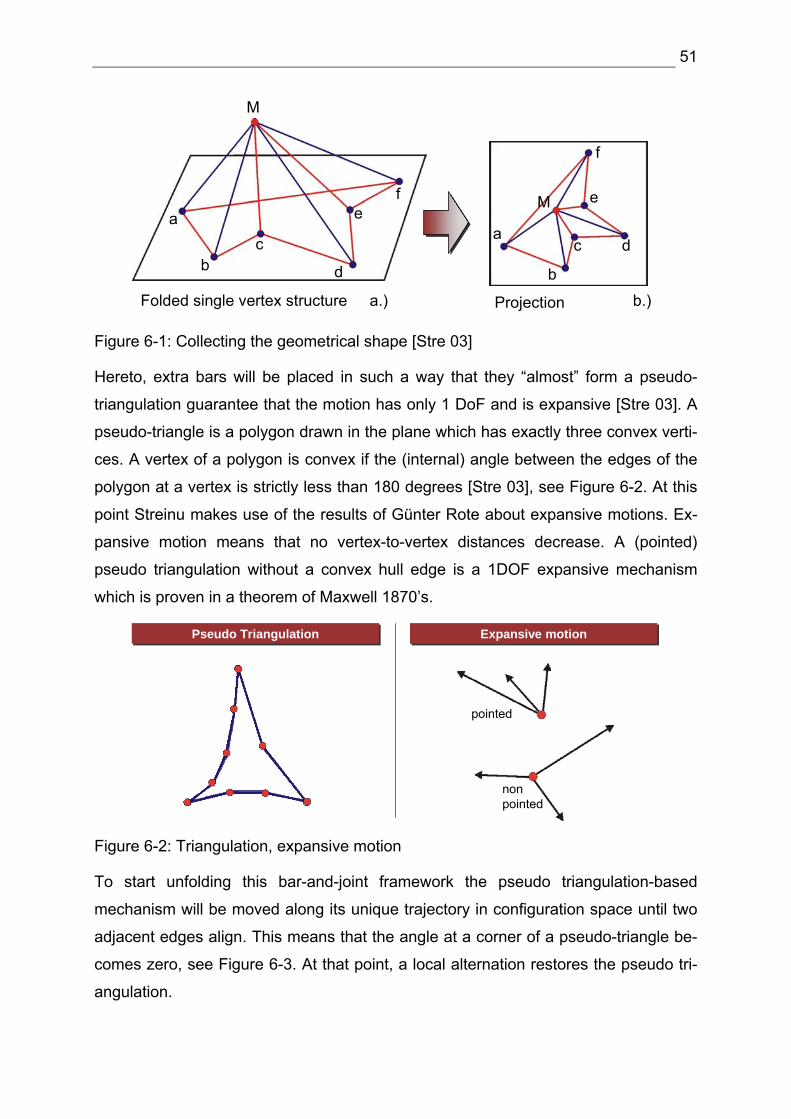
51
M
a
bc
d
ef
a
b
c d
e
f
M
ProjectionFolded single vertex structure a.) b.)
Figure 6-1: Collecting the geometrical shape [Stre 03]
Hereto, extra bars will be placed in such a way that they “almost” form a pseudo-
triangulation guarantee that the motion has only 1 DoF and is expansive [Stre 03]. A
pseudo-triangle is a polygon drawn in the plane which has exactly three convex verti-
ces. A vertex of a polygon is convex if the (internal) angle between the edges of the
polygon at a vertex is strictly less than 180 degrees [Stre 03], see Figure 6-2. At this
point Streinu makes use of the results of Günter Rote about expansive motions. Ex-
pansive motion means that no vertex-to-vertex distances decrease. A (pointed)
pseudo triangulation without a convex hull edge is a 1DOF expansive mechanism
which is proven in a theorem of Maxwell 1870’s.
Expansive motionExpansive motionPseudo TriangulationPseudo Triangulation
pointed
non pointed
Figure 6-2: Triangulation, expansive motion
To start unfolding this bar-and-joint framework the pseudo triangulation-based
mechanism will be moved along its unique trajectory in configuration space until two
adjacent edges align. This means that the angle at a corner of a pseudo-triangle be-
comes zero, see Figure 6-3. At that point, a local alternation restores the pseudo tri-
angulation.
52
[Ileana Streinu, Smith College]
Add bars to restrict the motion: the morebars, the less freedom you have Bars placed in such a way that they “almost”
form a pseudo-triangulation guarantee that the motion has only 1-degree-of-freedom and is expansive
Events: alignment of adjacent barsReadjust the mechanism to maintain expansiveness
2
2
1
1
. . .
Expansion
Bars
Figure 6-3: Unfolding on the base of the triangulation approach
These points are called “event points” and readjustments takes place. The motion
continues for 2( )O n steps until all the points are in convex position and the object is
expanded or so called unfolded. This approach has great potential to verify the given
3D structure. If the bar-and-joint framework is expandable by avoiding collisions it is
obvious that one can conclude that this structure is as well foldable from 2D back into
its 3D initial shape.
With the use of these two fundamental concepts of folding and unfolding of polygonal
linkages all applications which have been drawn up during the use case analysis are
realizable. Given polygonal linkage configurations could be verified if they represent
foldable structures and the following folding operation can be executed on the basis
of the above presented kinematical description.
In addition, the general software architecture to verify and visualize the folding and
unfolding operation on the basis of the above developed concepts will be pointed out.
Hereby the implementation of the kinematical concept in terms of software architec-
ture as well as its further realization is taking center stage.
53
7 Software Architecture of a General Solution
The two main concepts concerning the folding and unfolding of polygonal linkages
are set. Consequently the theoretical consideration of the two previously analyzed
use cases is completed. At this point we anticipate that the result of the above devel-
oped concepts will be realized in a comprehensive software package. The software
should permit the easy, hands-on definition of foldable structures and their complete
kinematic and dynamic analysis for design and verification in any given manufactur-
ing challenge. To achieve this goal a preliminary functional specification is neces-
sary. Hereto we will be geared to the results of chapter 4 concerning paper modeling
to define the standard of a software package.
On the basis of these requirements the general software architecture will be devel-
oped. At this point we state clearly that the presented architecture as well as imple-
mentation is restricted to the folding of polygonal linkages. The pseudo triangulation
approach will be shortly addressed in the general configuration of the software archi-
tecture.
Continued in chapter 8, a set of useful technologies will be presented in order to real-
ize certain points of the architecture. In addition, the specification of the design will be
presented in detail. Here the implementation of the data structure as well as the in-
formation flow between the different components is taking center stage. Concluding,
the functionality of the newly developed software package will be verified in terms of
an example scenario.
7.1 Requirements on Software Architecture
The analysis of the paper modeling and the adjacent folding process leads to classify
the requirements into two category groups. The first subject area comprises the re-
quirements to create a crease model whereas the second category specifies the re-
quirements to initiate the folding process and the subsequently graphical visualization
of the folding motion.
The specifications to model a user-defined crease pattern arise from the considera-
tion of creased origami sheets of paper. An origami crease pattern is characterized
by different types of crease lines. Their arrangement on a paper represents the plac-
ing of a fold whereas their type (dashed/dotted) reflects the orientation. To model this
proceeding there is a data model required that enables to assign both, the position of
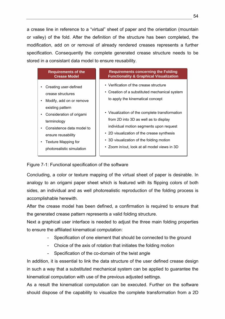
54
a crease line in reference to a “virtual” sheet of paper and the orientation (mountain
or valley) of the fold. After the definition of the structure has been completed, the
modification, add on or removal of already rendered creases represents a further
specification. Consequently the complete generated crease structure needs to be
stored in a consistant data model to ensure reusability.
Requirements of theCrease Model
Requirements of theCrease Model
Requirements concerning the FoldingFunctionality & Graphical VisualizationRequirements concerning the FoldingFunctionality & Graphical Visualization
• Verification of the crease structure
• Creation of a substituted mechanical system
to apply the kinematical concept
• Visualization of the complete transformation
from 2D into 3D as well as to display
individual motion segments upon request
• 2D visualization of the crease synthesis
• 3D visualization of the folding motion
• Zoom in/out, look at all model views in 3D
• Creating user-defined
crease structures
• Modify, add on or remove
existing pattern
• Consideration of origami
terminology
• Consistence data model to
ensure reusability
• Texture Mapping for
photorealistic simulation
Figure 7-1: Functional specification of the software
Concluding, a color or texture mapping of the virtual sheet of paper is desirable. In
analogy to an origami paper sheet which is featured with its flipping colors of both
sides, an individual and as well photorealistic reproduction of the folding process is
accomplishable herewith.
After the crease model has been defined, a confirmation is required to ensure that
the generated crease pattern represents a valid folding structure.
Next a graphical user interface is needed to adjust the three main folding properties
to ensure the affiliated kinematical computation:
- Specification of one element that should be connected to the ground
- Choice of the axis of rotation that initiates the folding motion
- Specification of the co-domain of the twist angle
In addition, it is essential to link the data structure of the user defined crease design
in such a way that a substituted mechanical system can be applied to guarantee the
kinematical computation with use of the previous adjusted settings.
As a result the kinematical computation can be executed. Further on the software
should dispose of the capability to visualize the complete transformation from a 2D
55
initial state into the 3D final shape. This requirement demands to be able to compute
and visualize a variety of single folds over a specific twist axis in a row. Further on it
is preferable to display individual motion segments available on request. The gratifi-
cation of this requirement results in a folding simulation that is able to imitate a real
“hand” fold. The skillfulness of professional origami designers to fold first about one
axis, then about another and subsequently again about the first one to complete a
fold could be retraced with this software in ease. Thereby the perspective of the visu-
alization should be free of choice. In order to permit the creation of a crease pattern
in analogy to an origami designer who looks perpendicularly at a sheet of paper dur-
ing the creation of crease patterns, a 2D visualization of the crease synthesis is de-
sirable. Accordingly a 3D visualization is demanded to simulate the folding motion.
Furthermore the graphical visualization should enfold the functionality to zoom in and
out as well as to modify the perspective of the model view even during the folding
operation to achieve a maximum transparency of this proceeding.
7.2 Architecture Concept
Ongoing the above listed functional requirements will be implemented in modular
constructed software architecture. The design of the architecture will be realized ac-
cording to the classification of the system specification but makes as well allowances
in its configuration for an implementation of the unfolding concept in the future.
Thus the overall software design can be subdivided into two main parts, the unfold-
ing- as well as the folding of polygonal-linkages. Each part will be implemented in
terms of a component based architecture which consists of a trisection. In the follow-
ing we will focus on the implementation of the forward folding architecture and point
out its configuration in detail. Hereby the tripartition comprises a module to ensure
the generation of a crease structure as well as one transformation model to make
sure that the crease configuration is available in a processable design for the inverse
kinematics computation. Completing, a visualization model is used to display the mo-
tion of the folding operation on the basis of the kinematic results.
This modular architecture contributes to an easy expansion of the application in order
to append further functionality, such as the incorporation of the dynamics or a self
collision detection during the folding operation. In the following we will illustrate the
design of each component in detail and take up with the crease component.
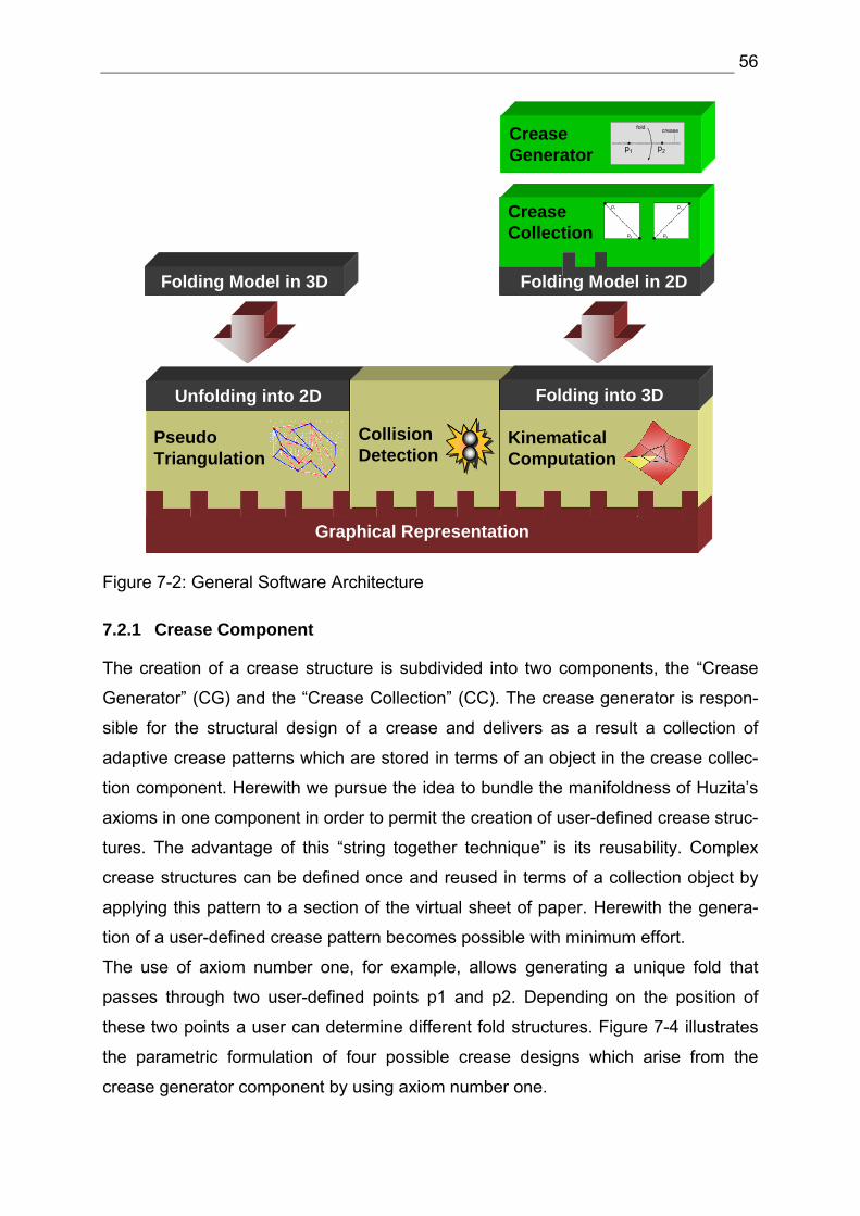
56
Crease Generator
Graphical Representation
Pseudo Triangulation
Unfolding into 2D
Collision Detection
KinematicalComputation
Folding into 3D
Folding Model in 3D
Crease Collection
p1 p2
creasefold
Folding Model in 2D
1p
2p
1p
2p
Figure 7-2: General Software Architecture
7.2.1 Crease Component
The creation of a crease structure is subdivided into two components, the “Crease
Generator” (CG) and the “Crease Collection” (CC). The crease generator is respon-
sible for the structural design of a crease and delivers as a result a collection of
adaptive crease patterns which are stored in terms of an object in the crease collec-
tion component. Herewith we pursue the idea to bundle the manifoldness of Huzita’s
axioms in one component in order to permit the creation of user-defined crease struc-
tures. The advantage of this “string together technique” is its reusability. Complex
crease structures can be defined once and reused in terms of a collection object by
applying this pattern to a section of the virtual sheet of paper. Herewith the genera-
tion of a user-defined crease pattern becomes possible with minimum effort.
The use of axiom number one, for example, allows generating a unique fold that
passes through two user-defined points p1 and p2. Depending on the position of
these two points a user can determine different fold structures. Figure 7-4 illustrates
the parametric formulation of four possible crease designs which arise from the
crease generator component by using axiom number one.
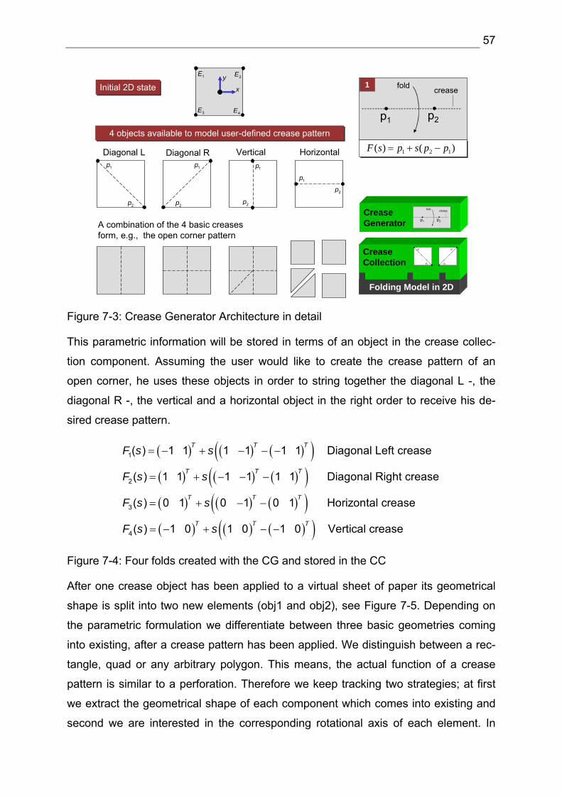
57
Crease Generator
Crease Collection
p1 p2
creasefold
Folding Model in 2D
Initial 2D stateInitial 2D state
4 objects available to model user-defined crease pattern4 objects available to model user-defined crease pattern
A combination of the 4 basic creases form, e.g., the open corner pattern
Vertical HorizontalDiagonal L Diagonal R1p
2p
1p
2p
1p
2p2p
1p
p1 p2
)()( 121 ppspsF −+=
1creasefold
1E
3E
2E
4E
1p
2p
1p
2p
x
y
Figure 7-3: Crease Generator Architecture in detail
This parametric information will be stored in terms of an object in the crease collec-
tion component. Assuming the user would like to create the crease pattern of an
open corner, he uses these objects in order to string together the diagonal L -, the
diagonal R -, the vertical and a horizontal object in the right order to receive his de-
sired crease pattern.
( ) ( ) ( )( )( ) ( ) ( )( )( ) ( ) ( )( )( ) ( ) ( )( )
1
2
3
4
( ) 1 1 1 1 1 1 Diagonal Left crease
( ) 1 1 1 1 1 1 Diagonal Right crease
( ) 0 1 0 1 0 1 Horizontal crease
( ) 1 0 1 0 1 0 Vertical crease
T T T
T T T
T T T
T T T
F s s
F s s
F s s
F s s
= − + − − −
= + − − −
= + − −
= − + − −
Figure 7-4: Four folds created with the CG and stored in the CC
After one crease object has been applied to a virtual sheet of paper its geometrical
shape is split into two new elements (obj1 and obj2), see Figure 7-5. Depending on
the parametric formulation we differentiate between three basic geometries coming
into existing, after a crease pattern has been applied. We distinguish between a rec-
tangle, quad or any arbitrary polygon. This means, the actual function of a crease
pattern is similar to a perforation. Therefore we keep tracking two strategies; at first
we extract the geometrical shape of each component which comes into existing and
second we are interested in the corresponding rotational axis of each element. In
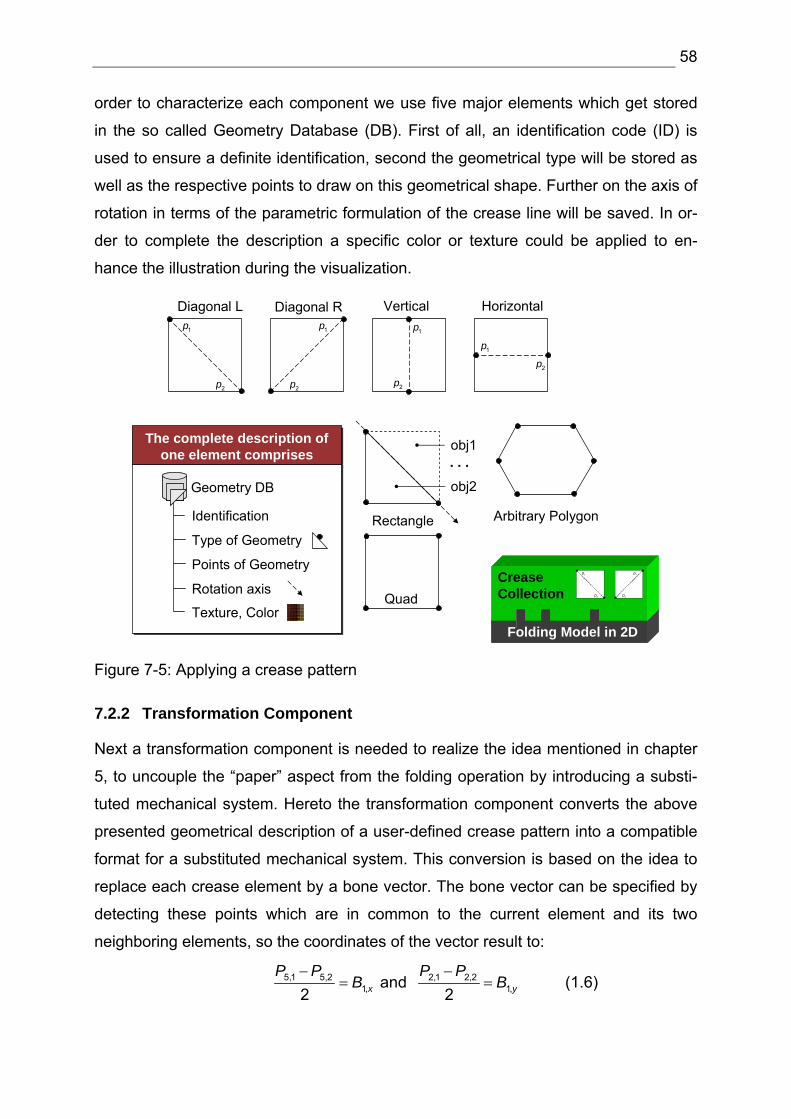
58
order to characterize each component we use five major elements which get stored
in the so called Geometry Database (DB). First of all, an identification code (ID) is
used to ensure a definite identification, second the geometrical type will be stored as
well as the respective points to draw on this geometrical shape. Further on the axis of
rotation in terms of the parametric formulation of the crease line will be saved. In or-
der to complete the description a specific color or texture could be applied to en-
hance the illustration during the visualization.
The complete description of one element comprises
The complete description of one element comprises
Crease Collection
Folding Model in 2D
Vertical HorizontalDiagonal L Diagonal R1p
2p
1p
2p
1p
2p2p
1p
Rectangle
Quad
Arbitrary Polygon
. . .
Identification
Type of Geometry
Points of Geometry
Rotation axis
Texture, Color
1p
2p
1p
2p
obj1
obj2Geometry DB
Figure 7-5: Applying a crease pattern
7.2.2 Transformation Component
Next a transformation component is needed to realize the idea mentioned in chapter
5, to uncouple the “paper” aspect from the folding operation by introducing a substi-
tuted mechanical system. Hereto the transformation component converts the above
presented geometrical description of a user-defined crease pattern into a compatible
format for a substituted mechanical system. This conversion is based on the idea to
replace each crease element by a bone vector. The bone vector can be specified by
detecting these points which are in common to the current element and its two
neighboring elements, so the coordinates of the vector result to:
5,1 5,2 2,1 2,21, 1, and
2 2x y
P P P PB B
− −= = (1.6)
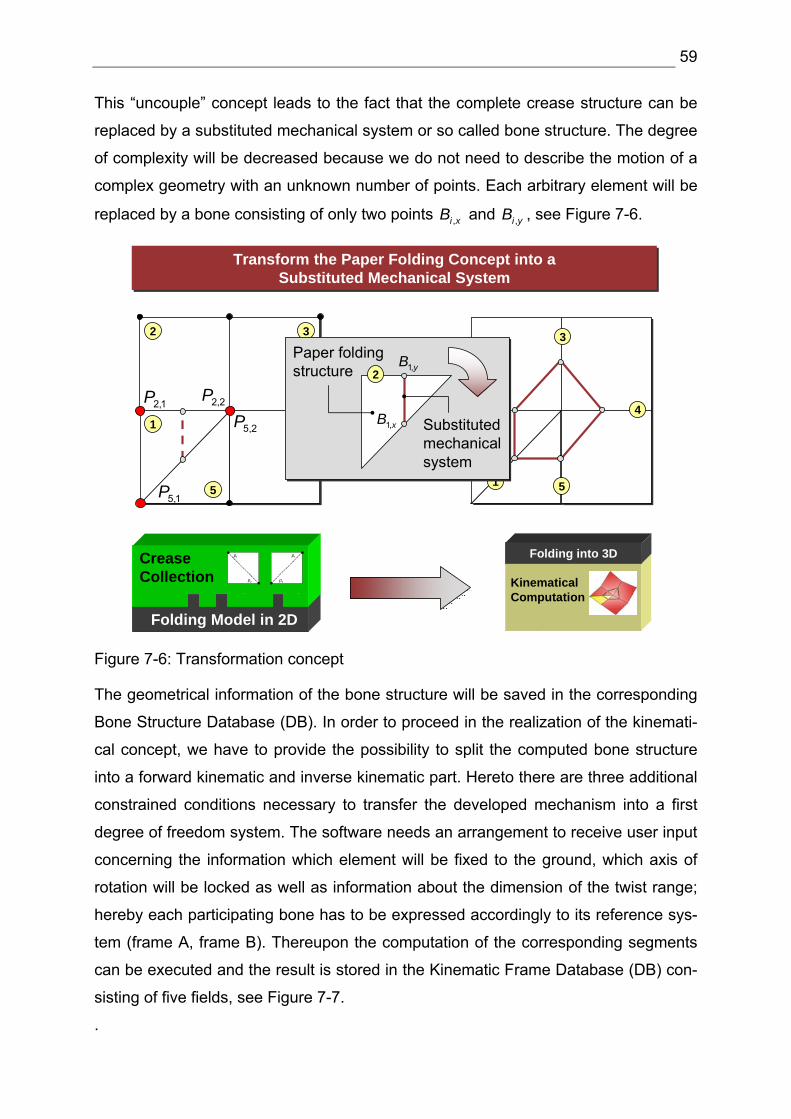
59
This “uncouple” concept leads to the fact that the complete crease structure can be
replaced by a substituted mechanical system or so called bone structure. The degree
of complexity will be decreased because we do not need to describe the motion of a
complex geometry with an unknown number of points. Each arbitrary element will be
replaced by a bone consisting of only two points ,i xB and ,i yB , see Figure 7-6.
1
2 3
4
5
Transform the Paper Folding Concept into a Substituted Mechanical System
Transform the Paper Folding Concept into a Substituted Mechanical System
Crease Collection
Folding Model in 2D
1
2
3
4
5
1p
2p
1p
2p
2
Paper foldingstructure
Substituted mechanical system
1,xB
1,yB
KinematicalComputation
Folding into 3D
5,1P
5,2P2,2P2,1P
Figure 7-6: Transformation concept
The geometrical information of the bone structure will be saved in the corresponding
Bone Structure Database (DB). In order to proceed in the realization of the kinemati-
cal concept, we have to provide the possibility to split the computed bone structure
into a forward kinematic and inverse kinematic part. Hereto there are three additional
constrained conditions necessary to transfer the developed mechanism into a first
degree of freedom system. The software needs an arrangement to receive user input
concerning the information which element will be fixed to the ground, which axis of
rotation will be locked as well as information about the dimension of the twist range;
hereby each participating bone has to be expressed accordingly to its reference sys-
tem (frame A, frame B). Thereupon the computation of the corresponding segments
can be executed and the result is stored in the Kinematic Frame Database (DB) con-
sisting of five fields, see Figure 7-7.
.
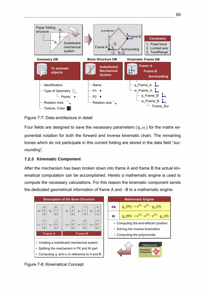
60
4
2
2
Paper foldingstructure
Substituted mechanical system
To animate objects
Substituted Mechanical System
Frame A
Frame B
end-effector
Frame AFrame B
Surrounding
Surrounding
Identification
Type of Geometry
Points
Rotation Axis
Texture, Color
Name
P1
P2
Rotation axisFrame_Sur
q_Frame_Aw_Frame_A
w_Frame_Bq_Frame_B
ConstraintConstraint
1. Fixed bone2. Locked axis3. TwistRange
1. Fixed bone2. Locked axis3. TwistRange
1,xB
1,yB
1
3
Geometry DB Bone Structure DB Kinematic Frame DB
Figure 7-7: Data architecture in detail
Four fields are designed to save the necessary parameters ( ,i iq ω ) for the matrix ex-
ponential notation for both the forward and inverse kinematic chain. The remaining
bones which do not participate in this current folding are stored in the data field “sur-
rounding”.
7.2.3 Kinematic Component
After the mechanism has been broken down into frame A and frame B the actual kin-
ematical computation can be accomplished. Hereto a mathematic engine is used to
compute the necessary calculations. For this reason the kinematic component sends
the dedicated geometrical information of frame A and - B to a mathematic engine.
Description of the Bone StructureDescription of the Bone Structure Mathematic Engine Mathematic Engine
1
000
q⎛ ⎞⎜ ⎟= ⎜ ⎟⎜ ⎟⎝ ⎠
2
010
q⎛ ⎞⎜ ⎟= ⎜ ⎟⎜ ⎟⎝ ⎠
4
000
q⎛ ⎞⎜ ⎟= ⎜ ⎟⎜ ⎟⎝ ⎠
2
02
0q
⎛ ⎞⎜ ⎟= −⎜ ⎟⎜ ⎟⎝ ⎠
3
110
q−⎛ ⎞⎜ ⎟= ⎜ ⎟⎜ ⎟⎝ ⎠
1
110
ω⎛ ⎞⎜ ⎟= ⎜ ⎟⎜ ⎟⎝ ⎠
2
100
ω⎛ ⎞⎜ ⎟= ⎜ ⎟⎜ ⎟⎝ ⎠
2
100
ω⎛ ⎞⎜ ⎟= ⎜ ⎟⎜ ⎟⎝ ⎠
4
100
ω⎛ ⎞⎜ ⎟= ⎜ ⎟⎜ ⎟⎝ ⎠
4
010
ω⎛ ⎞⎜ ⎟= ⎜ ⎟⎜ ⎟⎝ ⎠
Frame A Frame B
1 2ˆ ˆ
st stg ( ) e e g (0)ξΘ ξΘΘ = ⋅ ⋅FK
34 2ˆˆ ˆ
st stg ( ) e e e g (0)ξΘξΘ ξΘΘ = ⋅ ⋅ ⋅IK
• Computing the end-effector position
• Solving the inverse kinematics
• Computing the polynomials
• Creating a substituted mechanical system
• Splitting the mechanism in FK and IK part
• Computing and in reference to A and B
• Creating a substituted mechanical system
• Splitting the mechanism in FK and IK part
• Computing and in reference to A and Biq iωKinematicalComputation
Folding into 3D
Figure 7-8: Kinematical Concept
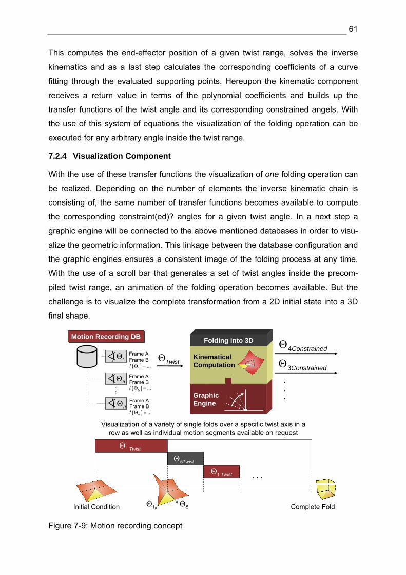
61
This computes the end-effector position of a given twist range, solves the inverse
kinematics and as a last step calculates the corresponding coefficients of a curve
fitting through the evaluated supporting points. Hereupon the kinematic component
receives a return value in terms of the polynomial coefficients and builds up the
transfer functions of the twist angle and its corresponding constrained angels. With
the use of this system of equations the visualization of the folding operation can be
executed for any arbitrary angle inside the twist range.
7.2.4 Visualization Component
With the use of these transfer functions the visualization of one folding operation can
be realized. Depending on the number of elements the inverse kinematic chain is
consisting of, the same number of transfer functions becomes available to compute
the corresponding constraint(ed)? angles for a given twist angle. In a next step a
graphic engine will be connected to the above mentioned databases in order to visu-
alize the geometric information. This linkage between the database configuration and
the graphic engines ensures a consistent image of the folding process at any time.
With the use of a scroll bar that generates a set of twist angles inside the precom-
piled twist range, an animation of the folding operation becomes available. But the
challenge is to visualize the complete transformation from a 2D initial state into a 3D
final shape.
Graphic Engine
KinematicalComputation
Folding into 3D
TwistΘ3ConstrainedΘ4ConstrainedΘ
.
.
.
Initial Condition Complete Fold
1 TwistΘ
Visualization of a variety of single folds over a specific twist axis in a row as well as individual motion segments available on request
5TwistΘ
1 TwistΘ . . .
Motion Recording DBMotion Recording DB
Frame AFrame B
Frame AFrame B
Frame AFrame B
1Θ
5Θ
nΘ
...
5Θ1Θ
( )1 ...f Θ =
( )5 ...f Θ =
( ) ...nf Θ =
Figure 7-9: Motion recording concept
62
Therefore the software requires the feature to visualize a variety of single folds over a
specific twist axis in a row as well as to display individual motion segments available
on request. This requirement will be met by using a Motion Recording component.
The Motion Recording database stores the coordinates of frame A, frame B and the
Surrounding in space as well as its corresponding transfer functions after a single
fold has been completed. On the basis of this information a new fold about another
twist axis can be planed, computed and executed. Further on this strategy facilitates
the restoration of the initial condition of each fold. Herewith the jump into any arbi-
trary position inside the folding sequence becomes available and animates a com-
plete fold beginning with the 2D initial condition until the final 3D shape is reached.
The motion recording component represents an essential part of the architecture and
ensures maximum transparency of the folding operation.
Up to this point all requirements which have been enumerated in the functional speci-
fication are implemented in general software architecture. In the next chapter the re-
alization of this architecture will be discussed.
63
8 Implementation of the Architecture
After the general architecture has been established the implementation of the soft-
ware follows. In the first place, some technologies will be presented on which the re-
alization of the architecture is based. Ongoing the integration of specific components
into the development environment will be pointed out and the Graphic User Interface
(GUI) will be illustrated. Then the functionality of each component will be broken
down to its bottom layer and its interrelationship will be visualized in a dataflow dia-
gram. Further on the realization of each specific component will be explained in detail
while focusing on the implementation of the GUI as well considering the program-
ming aspects.
8.1 Technologies to Implement the Architecture
There are three basic technologies required to start implementing the architecture. A
development environment has to be chosen first, second a dedicated mathematic
engine which ensures the data exchange in two directions, from the host application
to the mathematic engine and vice versa. Further on a graphic engine is needed to
enable the graphical representation. An analysis of diverse distributable software
tools reaches in the following result.
The Implementation of the architecture is based on the Visual Basic development
environment. This programming language in combination with OpenGL as embedded
component is highly suitable for the creation of interactive 2D and 3D graphical appli-
cations. Since its introduction in 1992, OpenGL has become the industry's most
widely used and supported 2D and 3D graphics application programming interface
(API) [Open 03]. The extensive mathematical computation of the kinematics will be
implemented by making use of the mathematic software tool, Matrix Laboratory
(MATLAB). Here the choice for MATLAB is due to its modular architecture which is
highly adapted for the implementation into our configuration. The use of the MATLAB
Mathematical Function Library which represents a vast collection of computational
algorithms ranging from elementary functions like sum, sine, cosine, and complex
arithmetic, to more sophisticated functions like matrix inverse, matrix eigenvalues,
and fast Fourier transforms can be utilized to implement the kinematical computation
[Math 03].
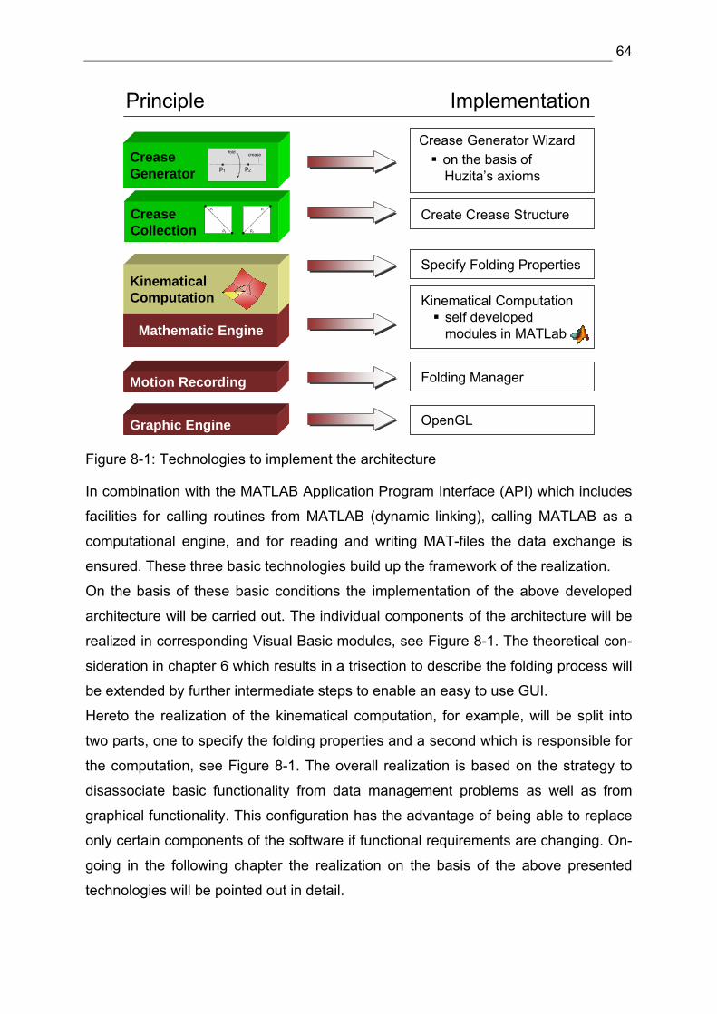
64
Principle
Crease Collection
1p
2p
1p
2p
Mathematic Engine
KinematicalComputation
Implementation
Crease Generator p1 p2
creasefoldCrease Generator p1 p2
creasefold
Graphic Engine
Kinematical Computationself developed modules in MATLab
on the basis of Huzita’s axioms
Crease Generator Wizard
Create Crease Structure
Specify Folding Properties
Motion Recording Folding Manager
OpenGL
Figure 8-1: Technologies to implement the architecture
In combination with the MATLAB Application Program Interface (API) which includes
facilities for calling routines from MATLAB (dynamic linking), calling MATLAB as a
computational engine, and for reading and writing MAT-files the data exchange is
ensured. These three basic technologies build up the framework of the realization.
On the basis of these basic conditions the implementation of the above developed
architecture will be carried out. The individual components of the architecture will be
realized in corresponding Visual Basic modules, see Figure 8-1. The theoretical con-
sideration in chapter 6 which results in a trisection to describe the folding process will
be extended by further intermediate steps to enable an easy to use GUI.
Hereto the realization of the kinematical computation, for example, will be split into
two parts, one to specify the folding properties and a second which is responsible for
the computation, see Figure 8-1. The overall realization is based on the strategy to
disassociate basic functionality from data management problems as well as from
graphical functionality. This configuration has the advantage of being able to replace
only certain components of the software if functional requirements are changing. On-
going in the following chapter the realization on the basis of the above presented
technologies will be pointed out in detail.
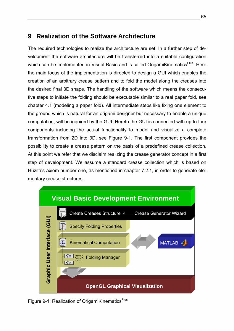
65
9 Realization of the Software Architecture
The required technologies to realize the architecture are set. In a further step of de-
velopment the software architecture will be transferred into a suitable configuration
which can be implemented in Visual Basic and is called OrigamiKinematicsPlus. Here
the main focus of the implementation is directed to design a GUI which enables the
creation of an arbitrary crease pattern and to fold the model along the creases into
the desired final 3D shape. The handling of the software which means the consecu-
tive steps to initiate the folding should be executable similar to a real paper fold, see
chapter 4.1 (modeling a paper fold). All intermediate steps like fixing one element to
the ground which is natural for an origami designer but necessary to enable a unique
computation, will be inquired by the GUI. Hereto the GUI is connected with up to four
components including the actual functionality to model and visualize a complete
transformation from 2D into 3D, see Figure 9-1. The first component provides the
possibility to create a crease pattern on the basis of a predefined crease collection.
At this point we refer that we disclaim realizing the crease generator concept in a first
step of development. We assume a standard crease collection which is based on
Huzita’s axiom number one, as mentioned in chapter 7.2.1, in order to generate ele-
mentary crease structures.
Gra
phic
Use
r Int
erfa
ce (G
UI)
Kinematical Computation MATLAB
OpenGL Graphical Visualization
Specify Folding Properties
Create Creases Structure Crease Generator Wizard
Visual Basic Development Environment
Folding ManagerFrame AFrame B
1Θ
( )1 .. .f Θ =
nΘ
Figure 9-1: Realization of OrigamiKinematicsPlus
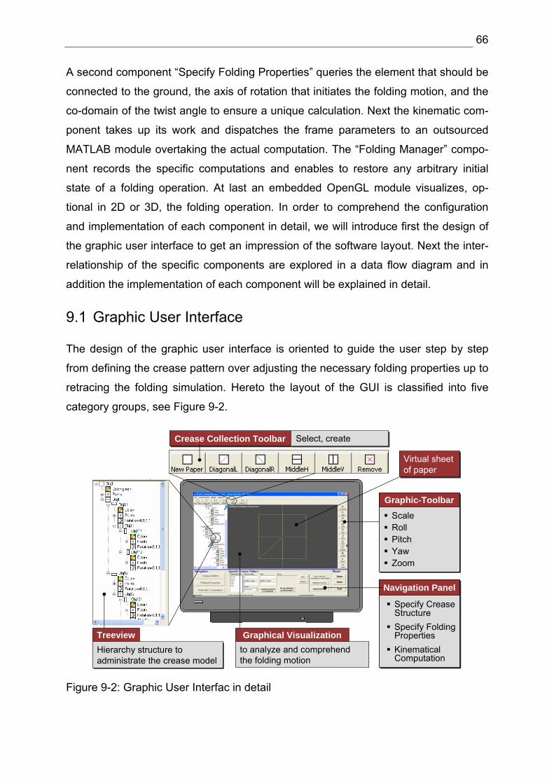
66
A second component “Specify Folding Properties” queries the element that should be
connected to the ground, the axis of rotation that initiates the folding motion, and the
co-domain of the twist angle to ensure a unique calculation. Next the kinematic com-
ponent takes up its work and dispatches the frame parameters to an outsourced
MATLAB module overtaking the actual computation. The “Folding Manager” compo-
nent records the specific computations and enables to restore any arbitrary initial
state of a folding operation. At last an embedded OpenGL module visualizes, op-
tional in 2D or 3D, the folding operation. In order to comprehend the configuration
and implementation of each component in detail, we will introduce first the design of
the graphic user interface to get an impression of the software layout. Next the inter-
relationship of the specific components are explored in a data flow diagram and in
addition the implementation of each component will be explained in detail.
9.1 Graphic User Interface
The design of the graphic user interface is oriented to guide the user step by step
from defining the crease pattern over adjusting the necessary folding properties up to
retracing the folding simulation. Hereto the layout of the GUI is classified into five
category groups, see Figure 9-2.
Navigation PanelNavigation Panel
Graphic-ToolbarGraphic-Toolbar
Hierarchy structure to administrate the crease modelHierarchy structure to administrate the crease model
to analyze and comprehend the folding motionto analyze and comprehend the folding motion
Crease Collection ToolbarCrease Collection Toolbar Select, create
Specify CreaseStructureSpecify Folding PropertiesKinematical Computation
Graphical VisualizationTreeview
ScaleRollPitchYawZoom
Virtual sheet of paperVirtual sheet of paper
Figure 9-2: Graphic User Interfac in detail
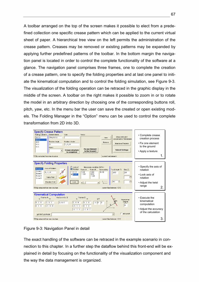
67
A toolbar arranged on the top of the screen makes it possible to elect from a prede-
fined collection one specific crease pattern which can be applied to the current virtual
sheet of paper. A hierarchical tree view on the left permits the administration of the
crease pattern. Creases may be removed or existing patterns may be expanded by
applying further predefined patterns of the toolbar. In the bottom margin the naviga-
tion panel is located in order to control the complete functionality of the software at a
glance. The navigation panel comprises three frames, one to complete the creation
of a crease pattern, one to specify the folding properties and at last one panel to initi-
ate the kinematical computation and to control the folding simulation, see Figure 9-3.
The visualization of the folding operation can be retraced in the graphic display in the
middle of the screen. A toolbar on the right makes it possible to zoom in or to rotate
the model in an arbitrary direction by choosing one of the corresponding buttons roll,
pitch, yaw, etc. In the menu bar the user can save the created or open existing mod-
els. The Folding Manager in the “Option” menu can be used to control the complete
transformation from 2D into 3D.
1.
2.
3.
• Complete crease creation process
• Fix one element to the ground
• Apply a texture
• Specify the axis of rotation
• Lock axis of rotation
• Adjust the twist range
• Execute the kinematical computation
• Adjust the accuracy of the calculation
Figure 9-3: Navigation Panel in detail
The exact handling of the software can be retraced in the example scenario in con-
nection to this chapter. In a further step the dataflow behind this front-end will be ex-
plained in detail by focusing on the functionality of the visualization component and
the way the data management is organized.
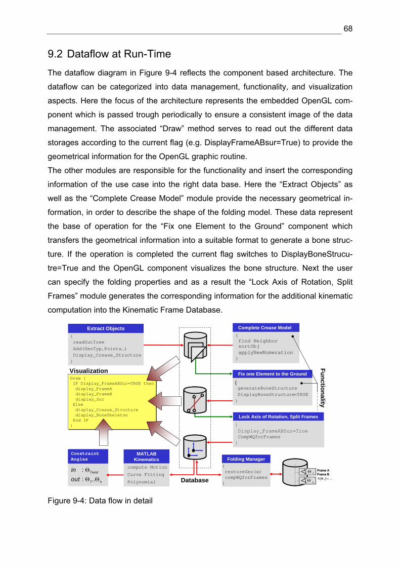
68
9.2 Dataflow at Run-Time
The dataflow diagram in Figure 9-4 reflects the component based architecture. The
dataflow can be categorized into data management, functionality, and visualization
aspects. Here the focus of the architecture represents the embedded OpenGL com-
ponent which is passed trough periodically to ensure a consistent image of the data
management. The associated “Draw” method serves to read out the different data
storages according to the current flag (e.g. DisplayFrameABsur=True) to provide the
geometrical information for the OpenGL graphic routine.
The other modules are responsible for the functionality and insert the corresponding
information of the use case into the right data base. Here the “Extract Objects” as
well as the “Complete Crease Model” module provide the necessary geometrical in-
formation, in order to describe the shape of the folding model. These data represent
the base of operation for the “Fix one Element to the Ground” component which
transfers the geometrical information into a suitable format to generate a bone struc-
ture. If the operation is completed the current flag switches to DisplayBoneStrucu-
tre=True and the OpenGL component visualizes the bone structure. Next the user
can specify the folding properties and as a result the “Lock Axis of Rotation, Split
Frames” module generates the corresponding information for the additional kinematic
computation into the Kinematic Frame Database.
Lock Axis of Rotation, Split Frames
ConstraintAngles
1 n
: : ..
Twistinout
Θ
Θ Θ
ConstraintAngles
1 n
: : ..
Twistinout
Θ
Θ Θ
Draw IF Display_FrameABSur=TRUE thendisplay_FrameAdisplay_FrameBdisplay_SurElsedisplay_Crease_Structuredisplay_BoneSkeletonEnd IF
Draw IF Display_FrameABSur=TRUE thendisplay_FrameAdisplay_FrameBdisplay_Sur
Elsedisplay_Crease_Structuredisplay_BoneSkeleton
End IF
MATLABKinematics
compute Motion
Curve Fitting
Polynomial
Extract ObjectsExtract Objects
Add(GeoTyp,Points,...)
readOutTreeAdd(GeoTyp,Points…)Display_Crease_Structure
Frame A1Θ
( )1 ...f Θ =nΘ
Frame BFrame A
1Θ( )1 ...f Θ =
nΘFrame B
Folding Manager
find NeighborsortObjapplyNewNumeration
find NeighborsortObjapplyNewNumeration
Complete Crease Model
generateBoneStructureDisplayBoneStructure=TRUE
Fix one Element to the Ground
Display_FrameABSur=TrueCompWQforFrames
restoreGeo(x)compWQforFramesDatabase
Visualization
Functionality
Figure 9-4: Data flow in detail
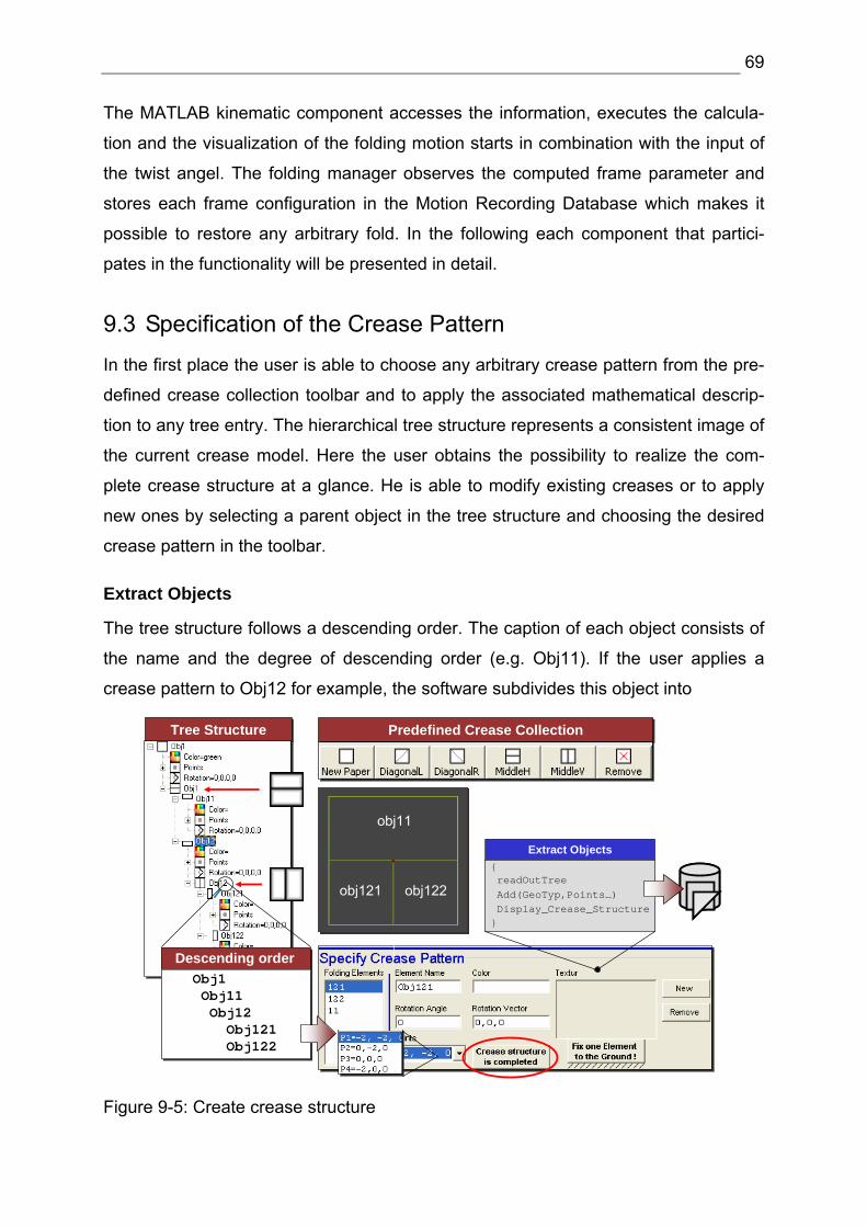
69
The MATLAB kinematic component accesses the information, executes the calcula-
tion and the visualization of the folding motion starts in combination with the input of
the twist angel. The folding manager observes the computed frame parameter and
stores each frame configuration in the Motion Recording Database which makes it
possible to restore any arbitrary fold. In the following each component that partici-
pates in the functionality will be presented in detail.
9.3 Specification of the Crease Pattern
In the first place the user is able to choose any arbitrary crease pattern from the pre-
defined crease collection toolbar and to apply the associated mathematical descrip-
tion to any tree entry. The hierarchical tree structure represents a consistent image of
the current crease model. Here the user obtains the possibility to realize the com-
plete crease structure at a glance. He is able to modify existing creases or to apply
new ones by selecting a parent object in the tree structure and choosing the desired
crease pattern in the toolbar.
Extract Objects
The tree structure follows a descending order. The caption of each object consists of
the name and the degree of descending order (e.g. Obj11). If the user applies a
crease pattern to Obj12 for example, the software subdivides this object into
Extract ObjectsExtract Objects
Add(GeoTyp,Points,...)
readOutTreeAdd(GeoTyp,Points…)Display_Crease_Structure
Predefined Crease CollectionPredefined Crease CollectionTree StructureTree Structure
Descending orderObj1Obj11Obj12
Obj121Obj122
obj11
obj121 obj122
Figure 9-5: Create crease structure
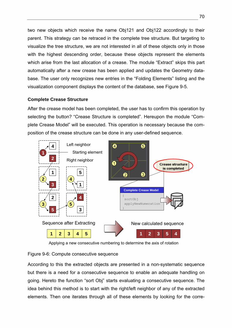
70
two new objects which receive the name Obj121 and Obj122 accordingly to their
parent. This strategy can be retraced in the complete tree structure. But targeting to
visualize the tree structure, we are not interested in all of these objects only in those
with the highest descending order, because these objects represent the elements
which arise from the last allocation of a crease. The module “Extract” skips this part
automatically after a new crease has been applied and updates the Geometry data-
base. The user only recognizes new entries in the “Folding Elements” listing and the
visualization component displays the content of the database, see Figure 9-5.
Complete Crease Structure
After the crease model has been completed, the user has to confirm this operation by
selecting the button? “Crease Structure is completed”. Hereupon the module “Com-
plete Crease Model” will be executed. This operation is necessary because the com-
position of the crease structure can be done in any user-defined sequence.
14
21
4
2
21
32
1
3
32
53
2
5
45
14
5
1
54
35
4
3
Left neighbor
Right neighbor
Starting element
1 2 3 5 4
New calculated sequence
1 2 3 4 5
Sequence after Extracting
Applying a new consecutive numbering to determine the axis of rotation
2
1
54
3
sortObjapplyNewNumeration
Complete Crease Model
Figure 9-6: Compute consecutive sequence
According to this the extracted objects are presented in a non-systematic sequence
but there is a need for a consecutive sequence to enable an adequate handling on
going. Hereto the function “sort Obj” starts evaluating a consecutive sequence. The
idea behind this method is to start with the right/left neighbor of any of the extracted
elements. Then one iterates through all of these elements by looking for the corre-
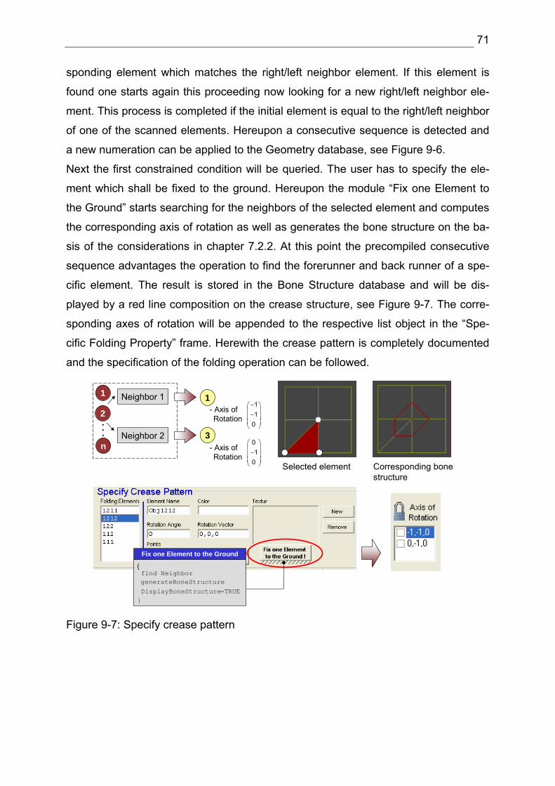
71
sponding element which matches the right/left neighbor element. If this element is
found one starts again this proceeding now looking for a new right/left neighbor ele-
ment. This process is completed if the initial element is equal to the right/left neighbor
of one of the scanned elements. Hereupon a consecutive sequence is detected and
a new numeration can be applied to the Geometry database, see Figure 9-6.
Next the first constrained condition will be queried. The user has to specify the ele-
ment which shall be fixed to the ground. Hereupon the module “Fix one Element to
the Ground” starts searching for the neighbors of the selected element and computes
the corresponding axis of rotation as well as generates the bone structure on the ba-
sis of the considerations in chapter 7.2.2. At this point the precompiled consecutive
sequence advantages the operation to find the forerunner and back runner of a spe-
cific element. The result is stored in the Bone Structure database and will be dis-
played by a red line composition on the crease structure, see Figure 9-7. The corre-
sponding axes of rotation will be appended to the respective list object in the “Spe-
cific Folding Property” frame. Herewith the crease pattern is completely documented
and the specification of the folding operation can be followed.
Corresponding bone structure
Selected element
2
Neighbor 1
Neighbor 2
1
3...n
- Axis of Rotation
- Axis of Rotation
111
0
−⎛ ⎞⎜ ⎟−⎜ ⎟⎜ ⎟⎝ ⎠
01
0
⎛ ⎞⎜ ⎟−⎜ ⎟⎜ ⎟⎝ ⎠
generateBoneStructureDisplayBoneStructure=TRUE
Fix one Element to the Ground
find Neighbor
Figure 9-7: Specify crease pattern
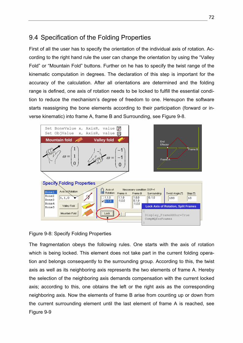
72
9.4 Specification of the Folding Properties
First of all the user has to specify the orientation of the individual axis of rotation. Ac-
cording to the right hand rule the user can change the orientation by using the “Valley
Fold” or “Mountain Fold” buttons. Further on he has to specify the twist range of the
kinematic computation in degrees. The declaration of this step is important for the
accuracy of the calculation. After all orientations are determined and the folding
range is defined, one axis of rotation needs to be locked to fulfill the essential condi-
tion to reduce the mechanism’s degree of freedom to one. Hereupon the software
starts reassigning the bone elements according to their participation (forward or in-
verse kinematic) into frame A, frame B and Surrounding, see Figure 9-8.
Set BoneValue x, AxisR, valueSet ObjValue x, AxisR, valueSet BoneValue x, AxisR, valueSet ObjValue x, AxisR, value
110
ω⎛ ⎞⎜ ⎟= ⎜ ⎟⎜ ⎟⎝ ⎠
ω−⎛ ⎞⎜ ⎟= −⎜ ⎟⎜ ⎟⎝ ⎠
11
0
Mountain fold Valley fold
Frame A
Frame B
End Effector
Lock Axis of Rotation, Split FramesDisplay_FrameABSur=TrueCompWQforFrames
Figure 9-8: Specify Folding Properties
The fragmentation obeys the following rules. One starts with the axis of rotation
which is being locked. This element does not take part in the current folding opera-
tion and belongs consequently to the surrounding group. According to this, the twist
axis as well as its neighboring axis represents the two elements of frame A. Hereby
the selection of the neighboring axis demands compensation with the current locked
axis; according to this, one obtains the left or the right axis as the corresponding
neighboring axis. Now the elements of frame B arise from counting up or down from
the current surrounding element until the last element of frame A is reached, see
Figure 9-9
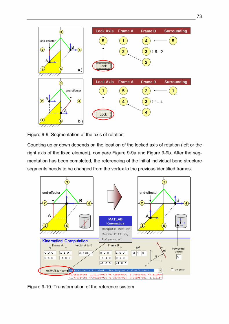
73
Frame A Frame B SurroundingLock Axis
2
1 54
3
2
5
5…2
21
4 3
5
1…4
1
4
Frame A Frame B SurroundingLock Axis
A
B
A
B
end-effector
end-effector
1
2
3
4
5
1
2
3
4
5 a.)
b.)
Figure 9-9: Segmentation of the axis of rotation
Counting up or down depends on the location of the locked axis of rotation (left or the
right axis of the fixed element), compare Figure 9-9a and Figure 9-9b. After the seg-
mentation has been completed, the referencing of the initial individual bone structure
segments needs to be changed from the vertex to the previous identified frames.
A
B
end-effector
1
2
3
4
5
B
end-effector
1
2
3
4
5
AMATLAB
Kinematicscompute Motion
Curve Fitting
Polynomial
MATLABKinematics
compute Motion
Curve Fitting
Polynomial
Figure 9-10: Transformation of the reference system
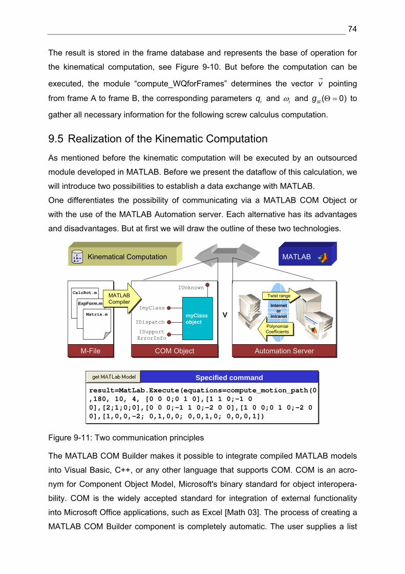
74
The result is stored in the frame database and represents the base of operation for
the kinematical computation, see Figure 9-10. But before the computation can be
executed, the module “compute_WQforFrames” determines the vector v pointing
from frame A to frame B, the corresponding parameters iq and iω and ( 0)stg Θ = to
gather all necessary information for the following screw calculus computation.
9.5 Realization of the Kinematic Computation
As mentioned before the kinematic computation will be executed by an outsourced
module developed in MATLAB. Before we present the dataflow of this calculation, we
will introduce two possibilities to establish a data exchange with MATLAB.
One differentiates the possibility of communicating via a MATLAB COM Object or
with the use of the MATLAB Automation server. Each alternative has its advantages
and disadvantages. But at first we will draw the outline of these two technologies.
Specified commandSpecified command
Kinematical Computation MATLAB
Automation ServerAutomation ServerCOM ObjectCOM Object
result=MatLab.Execute(equations=compute_motion_path(0,180, 10, 4, [0 0 0;0 1 0],[1 1 0;-1 0 0],[2;1;0;0],[0 0 0;-1 1 0;-2 0 0],[1 0 0;0 1 0;-2 0 0],[1,0,0,-2; 0,1,0,0; 0,0,1,0; 0,0,0,1])
Internet or
Intranet
Polynomial CoefficientsPolynomial Coefficients
Twist rangeTwist range
myClassobject
ImyClass
IDispatch
ISupportErrorInfo
IUnknownCalcRot.m
ExpForm.m
Matrix.m
MATLABCompilerMATLABCompiler
M-FileM-File
V
Figure 9-11: Two communication principles
The MATLAB COM Builder makes it possible to integrate compiled MATLAB models
into Visual Basic, C++, or any other language that supports COM. COM is an acro-
nym for Component Object Model, Microsoft's binary standard for object interopera-
bility. COM is the widely accepted standard for integration of external functionality
into Microsoft Office applications, such as Excel [Math 03]. The process of creating a
MATLAB COM Builder component is completely automatic. The user supplies a list

75
of M-files to process and a few additional pieces of information, i.e., the component
name, the class names, and the version number. The build process that follows in-
volves code generation, compiling, linking, and registration of the finished compo-
nent. The library can be linked into any Visual Basic project and the resulting call
syntax from Visual Basic is systematically mapped to the syntax of the original
MATLAB function.
The MATLAB Automation Sever on the other hand makes use of the Microsoft Win-
dows COM Automation server capabilities. Automation is a COM protocol that allows
one application or component (the controller) to control another application or com-
ponent (the server). Thus, MATLAB can be launched and controlled by any Windows
program that can be an Automation Controller. Using Automation, you can execute
MATLAB commands, and get and put information from and to the MATLAB work-
space [Math 03]. The following Visual Basic code fragment invokes the MATLAB
Automation Execute method.
Dim MatLab As ObjectDim Result As StringSet MatLab = CreateObject("Matlab.Application")Result = MatLab.Execute("surf(peaks)")
The Execute method takes a command string as an argument and returns the results
as a string. The command string can be any command that would normally be typed
in the command window; the result contains any output that would have been printed
to the command window as a result of executing the string, including errors.
The advantage of the MATLAB COM Object is its small size because it only com-
prises the functionality predefined in the compiled MATLAB M-Module. Further on its
availability adds to its advantages because the use of such a library does not pre-
sume any MATLAB installation. The MATLAB Automation Server on the other hand
is based on the idea of establishing a connection, e.g., from a Visual Basic host ap-
plication to a MATLAB instance running on the same PC or to build up a connection
via the internet or intranet to a MATLAB Server. The advantage of this technology is
its disposability of the complete MATLAB functionality to a COM communicating ap-
plication. The disadvantage is the resource consuming proceeding to establish a
connection as well as the time consuming process of a calculation request. But there
is one significant disadvantage of the MATLAB COM Object which scales down the
value of this technology for complex mathematic problems. The current release 13 of
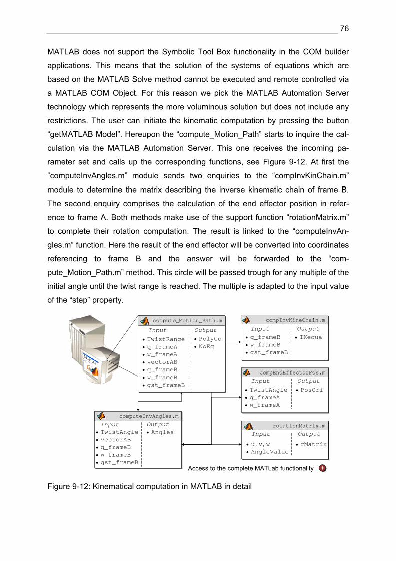
76
MATLAB does not support the Symbolic Tool Box functionality in the COM builder
applications. This means that the solution of the systems of equations which are
based on the MATLAB Solve method cannot be executed and remote controlled via
a MATLAB COM Object. For this reason we pick the MATLAB Automation Server
technology which represents the more voluminous solution but does not include any
restrictions. The user can initiate the kinematic computation by pressing the button
“getMATLAB Model”. Hereupon the “compute_Motion_Path” starts to inquire the cal-
culation via the MATLAB Automation Server. This one receives the incoming pa-
rameter set and calls up the corresponding functions, see Figure 9-12. At first the
“computeInvAngles.m” module sends two enquiries to the “compInvKinChain.m”
module to determine the matrix describing the inverse kinematic chain of frame B.
The second enquiry comprises the calculation of the end effector position in refer-
ence to frame A. Both methods make use of the support function “rotationMatrix.m”
to complete their rotation computation. The result is linked to the “computeInvAn-
gles.m” function. Here the result of the end effector will be converted into coordinates
referencing to frame B and the answer will be forwarded to the “com-
pute_Motion_Path.m” method. This circle will be passed trough for any multiple of the
initial angle until the twist range is reached. The multiple is adapted to the input value
of the “step” property.
computeInvAngles.mcomputeInvAngles.mcomputeInvAngles.mcomputeInvAngles.m
rotationMatrix.mrotationMatrix.mrotationMatrix.mrotationMatrix.m• TwistAngle• vectorAB • q_frameB • w_frameB• gst_frameB
• u,v,w• AngleValue
Input Output• Angles Input Output
• rMatrix
compInvKineChain.mcompInvKineChain.m
compEndEffectorPos.mcompEndEffectorPos.m
• TwistAngle• q_frameA• w_frameA
Input Output• PosOri
• q_frameB• w_frameB• gst_frameB
Input Output• IKequa
compute_Motion_Path.mcompute_Motion_Path.mcompute_Motion_Path.mcompute_Motion_Path.m
• TwistRange• q_frameA• w_frameA• vectorAB • q_frameB • w_frameB • gst_frameB
Input Output• PolyCo • NoEq
Access to the complete MATLab functionality +
Figure 9-12: Kinematical computation in MATLAB in detail
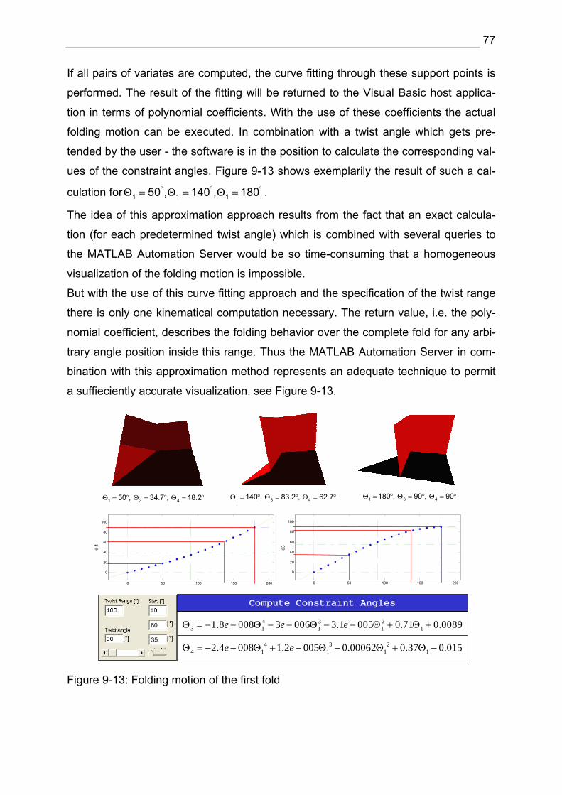
77
If all pairs of variates are computed, the curve fitting through these support points is
performed. The result of the fitting will be returned to the Visual Basic host applica-
tion in terms of polynomial coefficients. With the use of these coefficients the actual
folding motion can be executed. In combination with a twist angle which gets pre-
tended by the user - the software is in the position to calculate the corresponding val-
ues of the constraint angles. Figure 9-13 shows exemplarily the result of such a cal-
culation for 1 1 150 , 140 , 180° ° °Θ = Θ = Θ = .
The idea of this approximation approach results from the fact that an exact calcula-
tion (for each predetermined twist angle) which is combined with several queries to
the MATLAB Automation Server would be so time-consuming that a homogeneous
visualization of the folding motion is impossible.
But with the use of this curve fitting approach and the specification of the twist range
there is only one kinematical computation necessary. The return value, i.e. the poly-
nomial coefficient, describes the folding behavior over the complete fold for any arbi-
trary angle position inside this range. Thus the MATLAB Automation Server in com-
bination with this approximation method represents an adequate technique to permit
a suffieciently accurate visualization, see Figure 9-13.
Compute Constraint Angles
4 3 23 1 1 1 11.8 008 3 006 3.1 005 0.71 0.0089Θ = − − Θ − − Θ − − Θ + Θ +e e e
4 3 24 1 1 1 12.4 008 1.2 005 0.00062 0.37 0.015Θ = − − Θ + − Θ − Θ + Θ −e e
0 50 100 150 200 0 50 100 150 200
0
20
40
60
80
100
θ3
0
20
40
60
80
100
θ 4
1 3 450 , 34.7 , 18.2Θ = ° Θ = ° Θ = ° 1 3 4140 , 83.2 , 62.7Θ = ° Θ = ° Θ = ° 1 3 4180 , 90 , 90Θ = ° Θ = ° Θ = °
35
60
Figure 9-13: Folding motion of the first fold
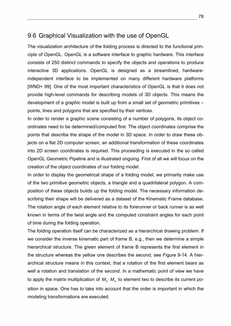
78
9.6 Graphical Visualization with the use of OpenGL
The visualization architecture of the folding process is directed to the functional prin-
ciple of OpenGL. OpenGL is a software interface to graphic hardware. This interface
consists of 250 distinct commands to specify the objects and operations to produce
interactive 3D applications. OpenGL is designed as a streamlined, hardware-
independent interface to be implemented on many different hardware platforms
[WND+ 99]. One of the most important characteristics of OpenGL is that it does not
provide high-level commands for describing models of 3D objects. This means the
development of a graphic model is built up from a small set of geometric primitives –
points, lines and polygons that are specified by their vertices.
In order to render a graphic scene consisting of a number of polygons, its object co-
ordinates need to be determined/computed first. The object coordinates comprise the
points that describe the shape of the model in 3D space. In order to draw these ob-
jects on a flat 2D computer screen, an additional transformation of these coordinates
into 2D screen coordinates is required. This proceeding is executed in the so called
OpenGL Geometric Pipeline and is illustrated ongoing. First of all we will focus on the
creation of the object coordinates of our folding model.
In order to display the geometrical shape of a folding model, we primarily make use
of the two primitive geometric objects, a triangle and a quadrilateral polygon. A com-
position of these objects builds up the folding model. The necessary information de-
scribing their shape will be delivered as a dataset of the Kinematic Frame database.
The rotation angle of each element relative to its forerunner or back runner is as well
known in terms of the twist angle and the computed constraint angles for each point
of time during the folding operation.
The folding operation itself can be characterized as a hierarchical drawing problem. If
we consider the inverse kinematic part of frame B, e.g., then we determine a simple
hierarchical structure. The green element of frame B represents the first element in
the structure whereas the yellow one describes the second, see Figure 9-14. A hier-
archical structure means in this context, that a rotation of the first element bears as
well a rotation and translation of the second. In a mathematic point of view we have
to apply the matrix multiplication of 3 4M M⋅ to element two to describe its current po-
sition in space. One has to take into account that the order is important in which the
modeling transformations are executed.
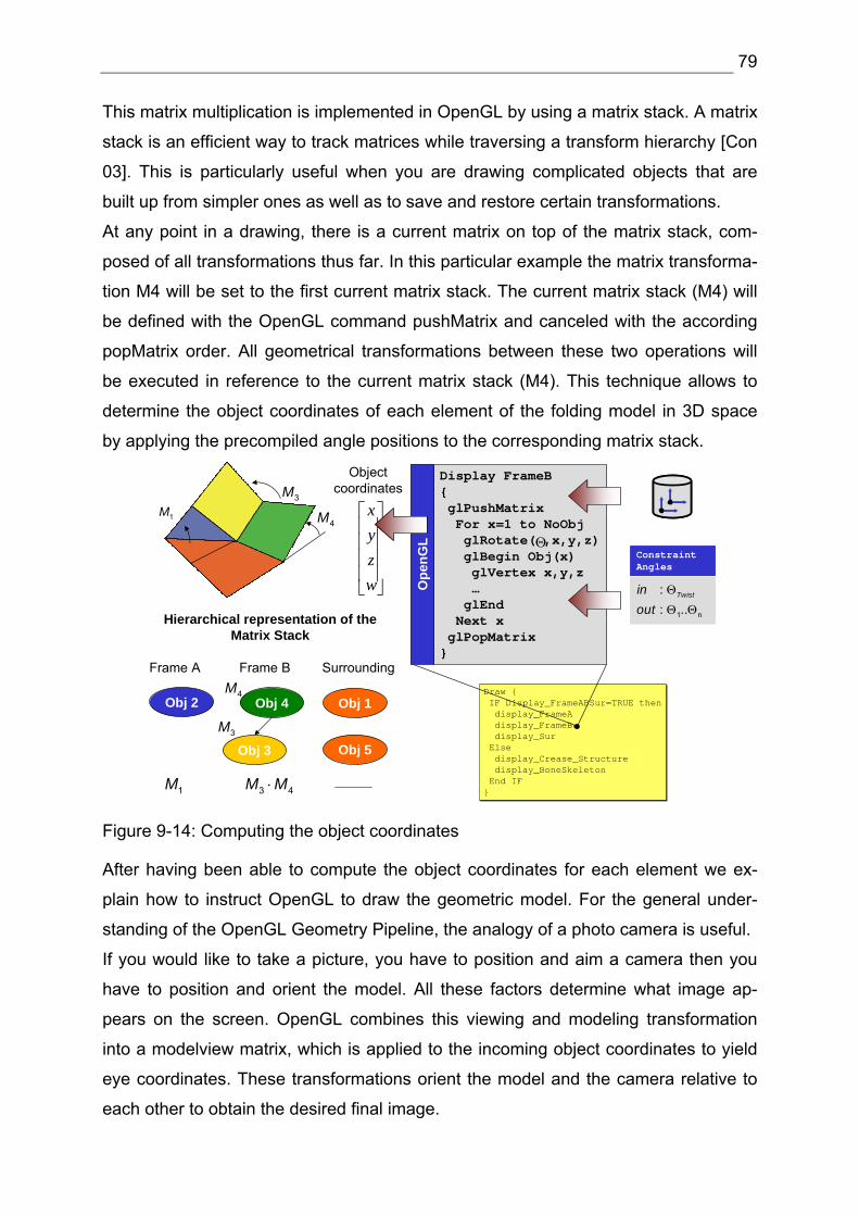
79
This matrix multiplication is implemented in OpenGL by using a matrix stack. A matrix
stack is an efficient way to track matrices while traversing a transform hierarchy [Con
03]. This is particularly useful when you are drawing complicated objects that are
built up from simpler ones as well as to save and restore certain transformations.
At any point in a drawing, there is a current matrix on top of the matrix stack, com-
posed of all transformations thus far. In this particular example the matrix transforma-
tion M4 will be set to the first current matrix stack. The current matrix stack (M4) will
be defined with the OpenGL command pushMatrix and canceled with the according
popMatrix order. All geometrical transformations between these two operations will
be executed in reference to the current matrix stack (M4). This technique allows to
determine the object coordinates of each element of the folding model in 3D space
by applying the precompiled angle positions to the corresponding matrix stack.
ConstraintAngles
1 n
: : ..
Twistinout
Θ
Θ Θ
ConstraintAngles
1 n
: : ..
Twistinout
Θ
Θ Θ
Draw IF Display_FrameABSur=TRUE thendisplay_FrameAdisplay_FrameBdisplay_SurElsedisplay_Crease_Structuredisplay_BoneSkeletonEnd IF
Draw IF Display_FrameABSur=TRUE thendisplay_FrameAdisplay_FrameBdisplay_SurElsedisplay_Crease_Structuredisplay_BoneSkeletonEnd IF
Display FrameB glPushMatrixFor x=1 to NoObjglRotate( ,x,y,z)glBegin Obj(x)glVertex x,y,z…glEndNext x
glPopMatrix
Obj 4
Obj 3
4M
3M
3 4M M⋅
Obj 2 Obj 1
Obj 5
Frame A Frame B Surrounding
1M
Hierarchical representation of the Matrix Stack
Θ4M
3M
Ope
nGL
⎥⎥⎥⎥
⎦
⎤
⎢⎢⎢⎢
⎣
⎡
wzyx
Objectcoordinates
1M
Figure 9-14: Computing the object coordinates
After having been able to compute the object coordinates for each element we ex-
plain how to instruct OpenGL to draw the geometric model. For the general under-
standing of the OpenGL Geometry Pipeline, the analogy of a photo camera is useful.
If you would like to take a picture, you have to position and aim a camera then you
have to position and orient the model. All these factors determine what image ap-
pears on the screen. OpenGL combines this viewing and modeling transformation
into a modelview matrix, which is applied to the incoming object coordinates to yield
eye coordinates. These transformations orient the model and the camera relative to
each other to obtain the desired final image.
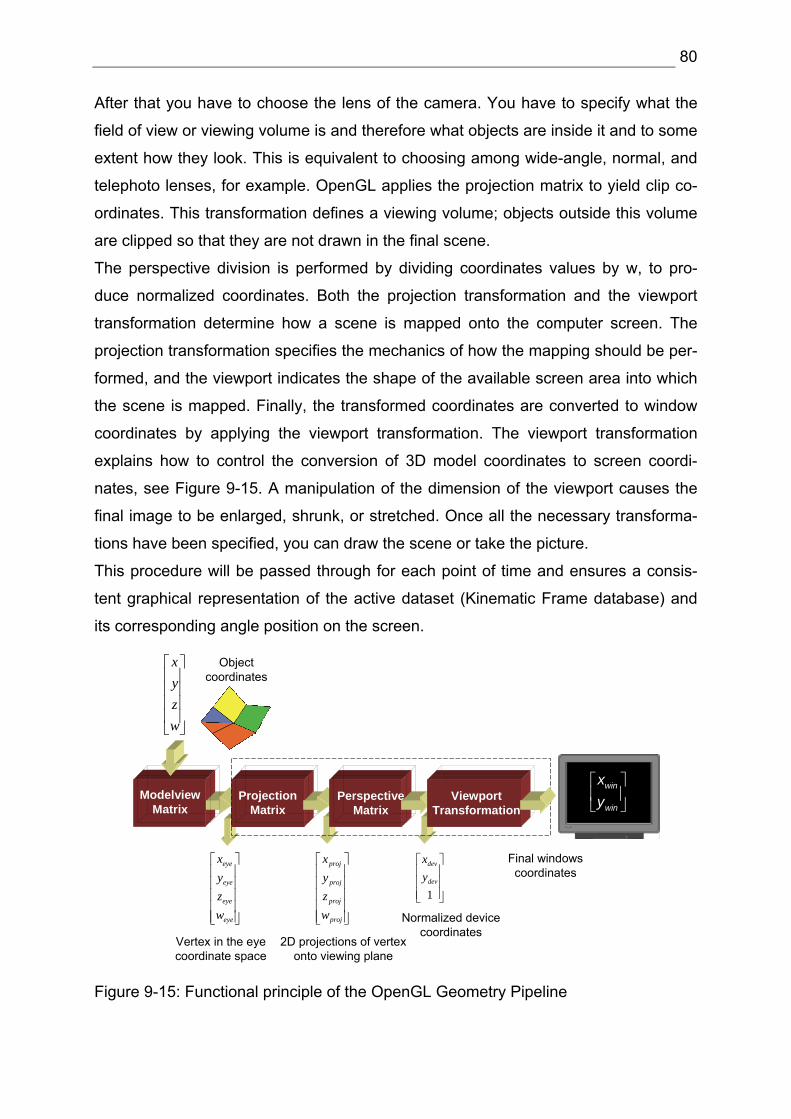
80
After that you have to choose the lens of the camera. You have to specify what the
field of view or viewing volume is and therefore what objects are inside it and to some
extent how they look. This is equivalent to choosing among wide-angle, normal, and
telephoto lenses, for example. OpenGL applies the projection matrix to yield clip co-
ordinates. This transformation defines a viewing volume; objects outside this volume
are clipped so that they are not drawn in the final scene.
The perspective division is performed by dividing coordinates values by w, to pro-
duce normalized coordinates. Both the projection transformation and the viewport
transformation determine how a scene is mapped onto the computer screen. The
projection transformation specifies the mechanics of how the mapping should be per-
formed, and the viewport indicates the shape of the available screen area into which
the scene is mapped. Finally, the transformed coordinates are converted to window
coordinates by applying the viewport transformation. The viewport transformation
explains how to control the conversion of 3D model coordinates to screen coordi-
nates, see Figure 9-15. A manipulation of the dimension of the viewport causes the
final image to be enlarged, shrunk, or stretched. Once all the necessary transforma-
tions have been specified, you can draw the scene or take the picture.
This procedure will be passed through for each point of time and ensures a consis-
tent graphical representation of the active dataset (Kinematic Frame database) and
its corresponding angle position on the screen.
Objectcoordinates
⎥⎥⎥⎥
⎦
⎤
⎢⎢⎢⎢
⎣
⎡
wzyx
Vertex in the eye coordinate space
2D projections of vertex onto viewing plane
⎥⎥⎥⎥⎥
⎦
⎤
⎢⎢⎢⎢⎢
⎣
⎡
eye
eye
eye
eye
wzyx
⎥⎥⎥⎥⎥
⎦
⎤
⎢⎢⎢⎢⎢
⎣
⎡
proj
proj
proj
proj
wzyx
⎥⎥⎥
⎦
⎤
⎢⎢⎢
⎣
⎡
1dev
dev
yx
Normalized device coordinates
Final windowscoordinates
ProjectionMatrix
PerspectiveMatrix
ModelviewMatrix
ViewportTransformation
win
win
xy⎡ ⎤⎢ ⎥⎣ ⎦
Figure 9-15: Functional principle of the OpenGL Geometry Pipeline
81
9.7 Realization of the Folding Manager
So far the implementation of the visualization of one fold is completed. As mentioned
before, to ensure the transformation from a 2D initial state into the desired 3D shape
we are interestied in displaying several folds in a row resp. to repeat selective sec-
tions of one fold upon request. This required functional specification is implemented
in the Folding Manager.
The Folding Manager can be addressed in the menu “Option”. After the first fold has
been completed, the user presses the button “StoreCurrentGeometry” and generates
a new starting position to trigger any other fold. The procedure “restoreGeo” calcu-
lates the current position of each element participating in the folding in 3D space.
Further on it stores the new position in the Geometry database and generates on the
basis of this data a new bone structure frame, see Figure 9-16. Hereto the position of
each point of the folding model needs be multiplied with a corresponding transforma-
tion matrix which describes its current position in space. In order to compute the ma-
trix multiplication we make use of a self developed MATLAB COM Object, the so
called Transformation library which provides the function “computeRotatedPoint” to
the “restoreGeo” procedure of the Visual Basic host application.
5Θ
0 180°→ °0 90°→ °2 Folds
1Θ
Folding ManagerrestoreGeo(x)compWQforFrames
Folding ManagerrestoreGeo(x)compWQforFrames
Frame A1Θ
( )1 ...f Θ =nΘ
Frame BFrame A
1Θ( )1 ...f Θ =
nΘFrame B
Figure 9-16: Functional principle of the Folding Manager
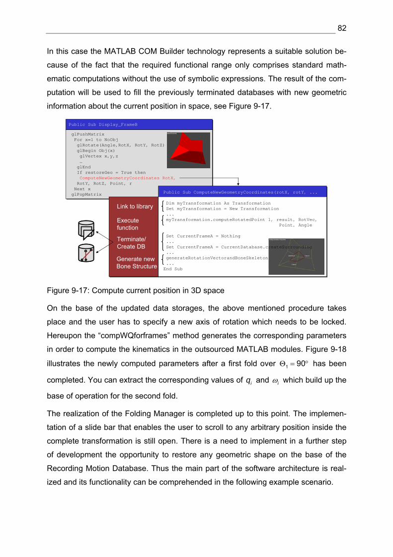
82
In this case the MATLAB COM Builder technology represents a suitable solution be-
cause of the fact that the required functional range only comprises standard math-
ematic computations without the use of symbolic expressions. The result of the com-
putation will be used to fill the previously terminated databases with new geometric
information about the current position in space, see Figure 9-17.
Public Sub Display_FrameBPublic Sub Display_FrameB
glPushMatrixFor x=1 to NoObjglRotate(Angle,RotX, RotY, RotZ)glBegin Obj(x)glVertex x,y,z…glEndIf restoreGeo = True then ComputeNewGeometryCoordinates RotX,RotY, RotZ, Point, r
Next xglPopMatrix
glPushMatrixFor x=1 to NoObjglRotate(Angle,RotX, RotY, RotZ)glBegin Obj(x)glVertex x,y,z…glEndIf restoreGeo = True then ComputeNewGeometryCoordinates RotX,RotY, RotZ, Point, r
Next xglPopMatrix Public Sub ComputeNewGeometryCoordinates(rotX, rotY, ...
Dim myTransformation As TransformationSet myTransformation = New Transformation ...myTransformation.computeRotatedPoint 1, result, RotVec,
Point, Angle
Set CurrentFrameA = Nothing...Set CurrentFrameA = CurrentDatabase.createSurrounding...generateRotationVectorandBoneSkeleton...End Sub
Generate new Bone Structure
Terminate/ Create DB
Execute function
Link to library
Figure 9-17: Compute current position in 3D space
On the base of the updated data storages, the above mentioned procedure takes
place and the user has to specify a new axis of rotation which needs to be locked.
Hereupon the “compWQforframes” method generates the corresponding parameters
in order to compute the kinematics in the outsourced MATLAB modules. Figure 9-18
illustrates the newly computed parameters after a first fold over 1 90Θ = ° has been
completed. You can extract the corresponding values of iq and iω which build up the
base of operation for the second fold.
The realization of the Folding Manager is completed up to this point. The implemen-
tation of a slide bar that enables the user to scroll to any arbitrary position inside the
complete transformation is still open. There is a need to implement in a further step
of development the opportunity to restore any geometric shape on the base of the
Recording Motion Database. Thus the main part of the software architecture is real-
ized and its functionality can be comprehended in the following example scenario.
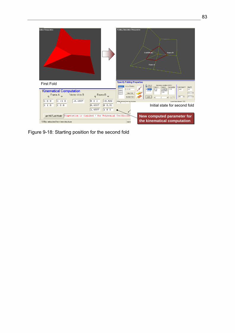
83
First Fold
Initial state for second fold
New computed parameter for the kinematical computationNew computed parameter for the kinematical computation
Figure 9-18: Starting position for the second fold
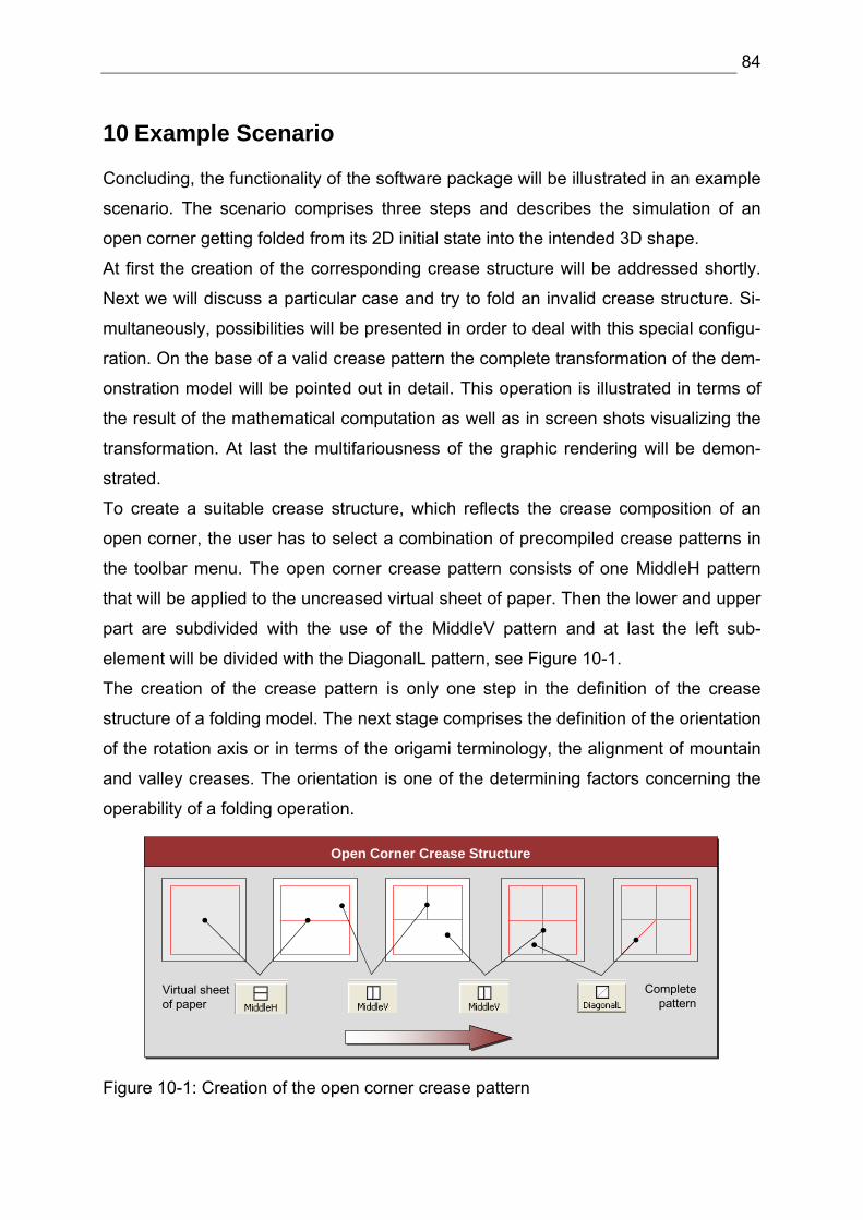
84
10 Example Scenario
Concluding, the functionality of the software package will be illustrated in an example
scenario. The scenario comprises three steps and describes the simulation of an
open corner getting folded from its 2D initial state into the intended 3D shape.
At first the creation of the corresponding crease structure will be addressed shortly.
Next we will discuss a particular case and try to fold an invalid crease structure. Si-
multaneously, possibilities will be presented in order to deal with this special configu-
ration. On the base of a valid crease pattern the complete transformation of the dem-
onstration model will be pointed out in detail. This operation is illustrated in terms of
the result of the mathematical computation as well as in screen shots visualizing the
transformation. At last the multifariousness of the graphic rendering will be demon-
strated.
To create a suitable crease structure, which reflects the crease composition of an
open corner, the user has to select a combination of precompiled crease patterns in
the toolbar menu. The open corner crease pattern consists of one MiddleH pattern
that will be applied to the uncreased virtual sheet of paper. Then the lower and upper
part are subdivided with the use of the MiddleV pattern and at last the left sub-
element will be divided with the DiagonalL pattern, see Figure 10-1.
The creation of the crease pattern is only one step in the definition of the crease
structure of a folding model. The next stage comprises the definition of the orientation
of the rotation axis or in terms of the origami terminology, the alignment of mountain
and valley creases. The orientation is one of the determining factors concerning the
operability of a folding operation.
Open Corner Crease StructureOpen Corner Crease Structure
Virtual sheet of paper
Complete pattern
Figure 10-1: Creation of the open corner crease pattern
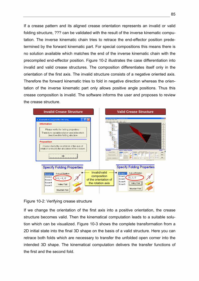
85
If a crease pattern and its aligned crease orientation represents an invalid or valid
folding structure, ??? can be validated with the result of the inverse kinematic compu-
tation. The inverse kinematic chain tries to retrace the end-effector position prede-
termined by the forward kinematic part. For special compositions this means there is
no solution available which matches the end of the inverse kinematic chain with the
precompiled end-effector position. Figure 10-2 illustrates the case differentiation into
invalid and valid crease structures. The composition differentiates itself only in the
orientation of the first axis. The invalid structure consists of a negative oriented axis.
Therefore the forward kinematic tries to fold in negative direction whereas the orien-
tation of the inverse kinematic part only allows positive angle positions. Thus this
crease composition is invalid. The software informs the user and proposes to review
the crease structure.
Invalid Crease StructureInvalid Crease Structure Valid Crease StructureValid Crease Structure
Invalid/valid composition
of the orientation of the rotation axis
Invalid/valid composition
of the orientation of the rotation axis
Figure 10-2: Verifying crease structure
If we change the orientation of the first axis into a positive orientation, the crease
structure becomes valid. Then the kinematical computation leads to a suitable solu-
tion which can be visualized. Figure 10-3 shows the complete transformation from a
2D initial state into the final 3D shape on the basis of a valid structure. Here you can
retrace both folds which are necessary to transfer the unfolded open corner into the
intended 3D shape. The kinematical computation delivers the transfer functions of
the first and the second fold.
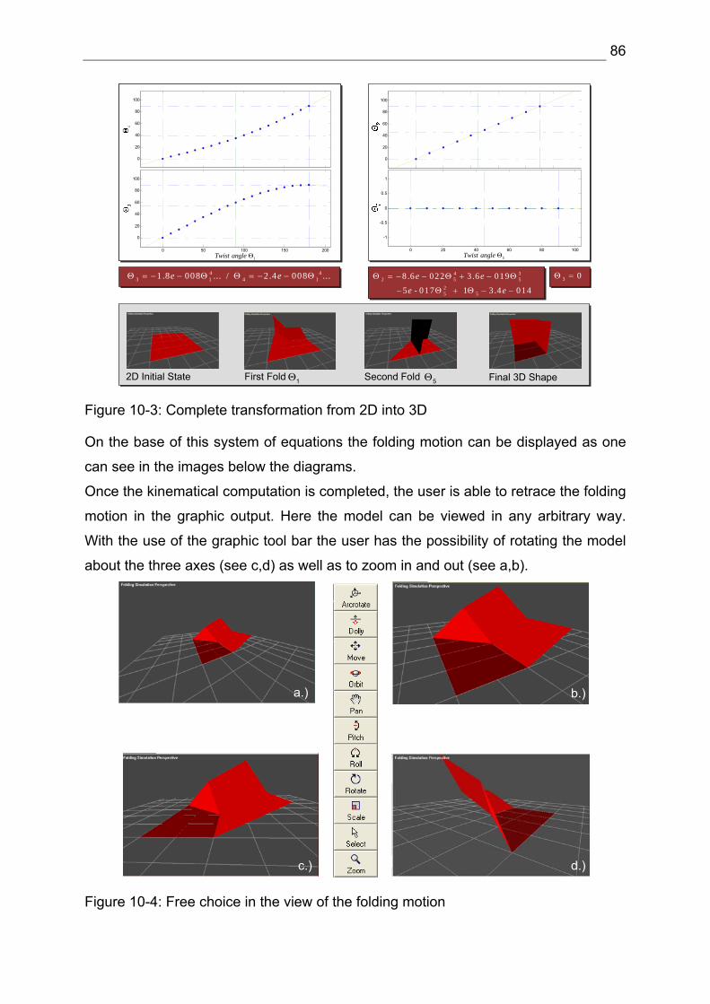
86
0 50 100 150 200
0
20
40
60
80
100
θ3
0
20
40
60
80
100
θ 4
1 Twist angle Θ0 50 100 150 200
0
20
40
60
80
100
θ3
0
20
40
60
80
100
θ 4
1 Twist angle Θ
3 0Θ =4 32 5 5
25 5
8 .6 022 3 .6 019
5 - 017 1 3 .4 014
Θ = − − Θ + − Θ
− Θ + Θ − −
e e
e e
0
20
40
60
80
100
0 20 40 60 80 100
-1
-0.5
0
0.5
1
5 ΘTwist angle
4 43 1 4 11 .8 008 ... / 2 .4 008 ...Θ = − − Θ Θ = − − Θe e
Final 3D Shape2D Initial State First Fold Second Fold1Θ 5Θ
Figure 10-3: Complete transformation from 2D into 3D
On the base of this system of equations the folding motion can be displayed as one
can see in the images below the diagrams.
Once the kinematical computation is completed, the user is able to retrace the folding
motion in the graphic output. Here the model can be viewed in any arbitrary way.
With the use of the graphic tool bar the user has the possibility of rotating the model
about the three axes (see c,d) as well as to zoom in and out (see a,b).
a.) b.)
c.) d.)
Figure 10-4: Free choice in the view of the folding motion

87
The opportunity to observe the model from all sides, from the top, from behind or
from the bottom of the model, supports the comprehension of the folding motion. Es-
pecially concerning typical engineering tasks, this photorealistic visualization contrib-
utes to retrace the construction. Finally, the fading of a grid relieves the orientation in
3D space by rotating the model.
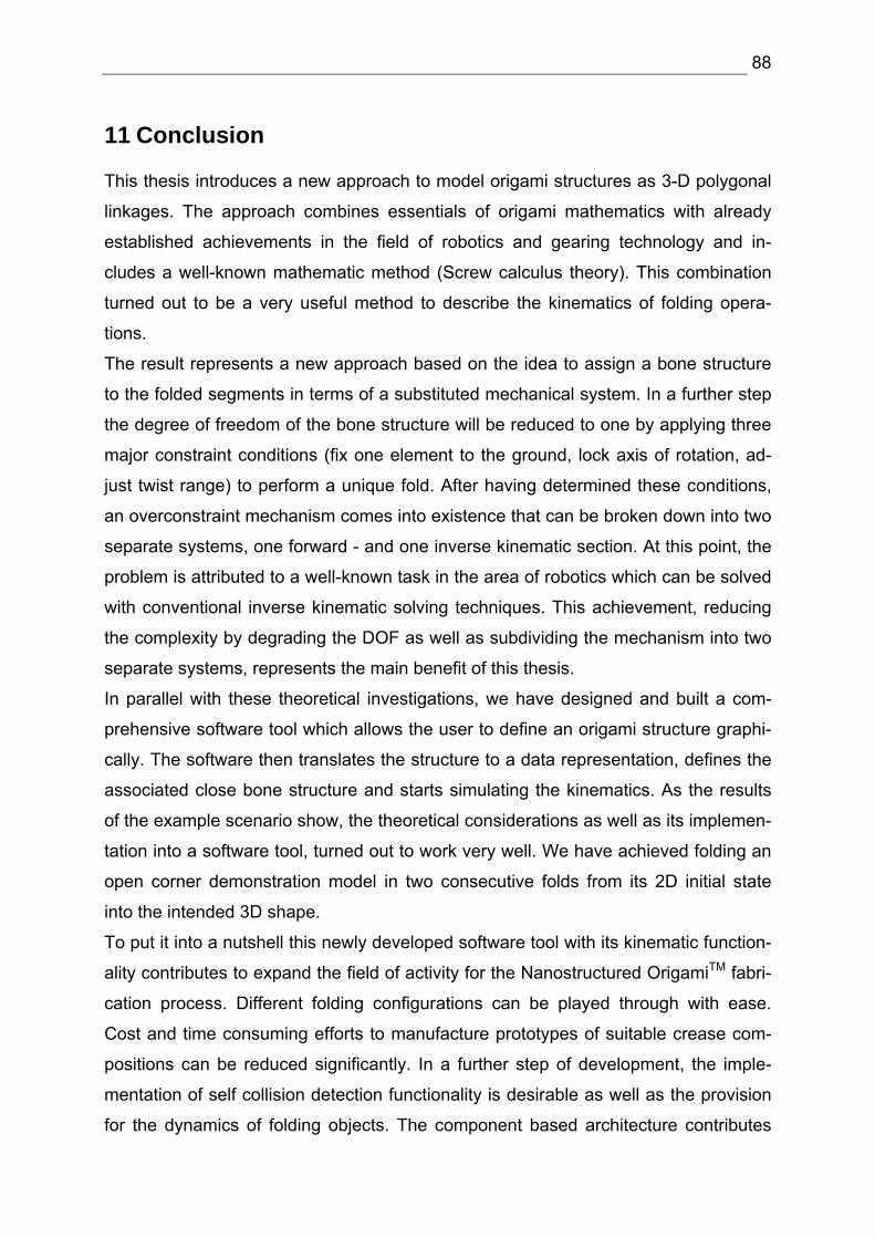
88
11 Conclusion
This thesis introduces a new approach to model origami structures as 3-D polygonal
linkages. The approach combines essentials of origami mathematics with already
established achievements in the field of robotics and gearing technology and in-
cludes a well-known mathematic method (Screw calculus theory). This combination
turned out to be a very useful method to describe the kinematics of folding opera-
tions.
The result represents a new approach based on the idea to assign a bone structure
to the folded segments in terms of a substituted mechanical system. In a further step
the degree of freedom of the bone structure will be reduced to one by applying three
major constraint conditions (fix one element to the ground, lock axis of rotation, ad-
just twist range) to perform a unique fold. After having determined these conditions,
an overconstraint mechanism comes into existence that can be broken down into two
separate systems, one forward - and one inverse kinematic section. At this point, the
problem is attributed to a well-known task in the area of robotics which can be solved
with conventional inverse kinematic solving techniques. This achievement, reducing
the complexity by degrading the DOF as well as subdividing the mechanism into two
separate systems, represents the main benefit of this thesis.
In parallel with these theoretical investigations, we have designed and built a com-
prehensive software tool which allows the user to define an origami structure graphi-
cally. The software then translates the structure to a data representation, defines the
associated close bone structure and starts simulating the kinematics. As the results
of the example scenario show, the theoretical considerations as well as its implemen-
tation into a software tool, turned out to work very well. We have achieved folding an
open corner demonstration model in two consecutive folds from its 2D initial state
into the intended 3D shape.
To put it into a nutshell this newly developed software tool with its kinematic function-
ality contributes to expand the field of activity for the Nanostructured OrigamiTM fabri-
cation process. Different folding configurations can be played through with ease.
Cost and time consuming efforts to manufacture prototypes of suitable crease com-
positions can be reduced significantly. In a further step of development, the imple-
mentation of self collision detection functionality is desirable as well as the provision
for the dynamics of folding objects. The component based architecture contributes
89
outstandingly to this development. Completing the functionality range, it is of major
interest to include the inverse case in future which means the unfolding of polygonal
linkages by implementing Ileana Streinu’s pseudo triangulation approach.
Finally we will give a short example of a possible area of application for this new
manufacturing process for future defense systems. One idea which will be pursued
by the 3D Optical Systems Group at MIT is to build up a reconfigurable soldier identi-
fication tag (RSIT) that is able to deliver a general-purpose status of a soldier’s identi-
fication and condition available upon request. The miniature device of sub-mm3 vol-
ume can be mounted on a soldier’s breast pocket as a pin, or resp. on his helmet or
backpack. To request his status, a low-power, eye-safe laser beam is used to retro-
reflect the soldier’s identification modulated on the reflected wavefront, see Figure
11-1.
probe beam
response beams
Figure 11-1: Reconfigurable soldier identification tag
The operation of RSIT is based on the open corner demonstration model with one
additional specification - a diffractive optical element (DOE) patterned on the inner
surfaces. The DOE imprints the identification information on the retro-reflected wave-
front. The geometric shape of the open corner contributes to the fact that the RSIT
can be read out from virtually a 2π solid angle. The design of the device can be ar-
ranged to retro-reflect the correct information only when probed by a specific wave-
front. This feature is called key-based operation and is used to respond only to a
specific wavefront modulated on the probe beam, whereas if an adversary attempts
to read the tag without using the correct key, the adversary will simply receive a dif-
fusely reflected beam without any meaningful information.
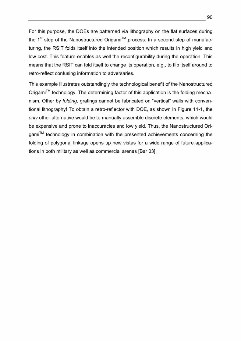
90
For this purpose, the DOEs are patterned via lithography on the flat surfaces during
the 1st step of the Nanostructured OrigamiTM process. In a second step of manufac-
turing, the RSIT folds itself into the intended position which results in high yield and
low cost. This feature enables as well the reconfigurability during the operation. This
means that the RSIT can fold itself to change its operation, e.g., to flip itself around to
retro-reflect confusing information to adversaries.
This example illustrates outstandingly the technological benefit of the Nanostructured
OrigamiTM technology. The determining factor of this application is the folding mecha-
nism. Other by folding, gratings cannot be fabricated on “vertical” walls with conven-
tional lithography! To obtain a retro-reflector with DOE, as shown in Figure 11-1, the
only other alternative would be to manually assemble discrete elements, which would
be expensive and prone to inaccuracies and low yield. Thus, the Nanostructured Ori-
gamiTM technology in combination with the presented achievements concerning the
folding of polygonal linkage opens up new vistas for a wide range of future applica-
tions in both military as well as commercial arenas [Bar 03].

91
12 Abbreviations
2D Two Dimensional
3D Three Dimensional
API Application Interface
CC Crease Collection
CG Crease Generator
COM Component Object Model
DARPA Defense Advanced Research Projects Agency
DB Database
DNA Deoxyribonucleic Acid
DOE Diffractive Optical Element
DOF Degree of Freedom
FK Forward Kinematic
GUI Graphic User Interface
ID Identification Code
IK Inverse Kinematic
MATLAB Matrix Laboratory
MBS Multi Body System
MCLS Multi Close Loop System
MEF Matrix Exponential Formulation
MEMS Micro Electro Mechanical System
MIT Massachusetts Institute of Technology
RSIT Reconfigurable Soldier Identification Tag
TTS Tree Type System
VLSI Very Large Scale Integrator
92
13 References
[AmSo 00] Amato, N.; Song, G.: Motion Planning Approach to Folding: From Pa-per Craft to Protein Structured Prediction, Technical Report 00-001 Department of Computer Science Texas A&M University Jan 17,2000
[AoId+ 03] Aoki, K.; Ideki, T., et. al.: Microassembly of Semiconductor Three Di-mensional Photonic Crystals, Nature Materials, Vol. 2, February 2003
[Barb 03] Conversation with: Prof. George Barbastathis, 3D Optical Systems Group, MIT 2003, date: 05. Oct. 2003
[BeHu 02a] Belcastro, S.; Hull, T.: A Mathematical Model for non-Flat Origami; Ori-gami3, The Third International Meeting of Origami Science, Mathemat-ics and Education published by AK Peters, 2002
[BeHu 02b] Belcastro, S.; Hull, T.: Modelling the folding of paper into three dimen-sional using affine transformations, Linear Algebra and its Application 348 (2002) pp.273-282
[BJH+ 03] Barbastathis, G.; Jurga, S.; Hidrovo, C.; Niemczura, J. Et al.: Nanostrucutred Origami, IEEE-Nano 2003, August 12, 2003
[BTC+ 97] Bowden, N.; Terfort, A.; Carbeck J.; Whitesides, G.: Self-Assembly of Mesoscale Objects into Ordered Two-Dimensional Arrays, Science, Vol. 276, April 1997
[Con 03] Controlling the Order of Transformations: GL3.2 Version 4.1 for AIX: Programming Concepts, http://as400bks.rochester.ibm.com/doc_link/en_US/a_doc_lib/aixprggd/gl32prgd/cntrltransfrms.htm publication date: -, released order date: 15 Dec. 2003
[Dema 03] Demaine, E.D.: Folding and Unfolding Linkages, Paper, and Polyhedra, Department of Computer Science, University of Waterloo
[Diet 03] Conversation with: Univ.-Prof. Dipl.-Ing. Dr.techn. Peter Dietmaier, In-stitut für allgemeine Mechanik, Technische Universität Graz, date: 28. Oct. 2003
[Hull 94] Hull, T.: On the Mathematics of Flat Origamis, Congressus Numeran-tium, Vol. 100 (1994) pp. 215-224
[Hull xx] Hull, T.: Counting Mountain-Valley Assignments for Flat Folds”, Ars Combinatoria, Department of Mathematics, Merrimack College, North Andover, MA 01845
[Huzi 03] Huzita's axioms, Wikipedia the free encyclopedia http://en2.wikipedia.org/wiki/Huzita’s_axioms publication date:17 Jun. 2003, released order date: 19 Nov. 2003
[Huzi 92] Huzita, H.: Understanding Geometry through Origami Axioms, Pro-ceedings of the First International Conference on Origami in Education and Therapy (COET91), J. Smith ed., British Origami Society, 1992, pp. 37-70
93
[IsOH 98] Isao, S.; Osamu, K.; Hirofumi, M.: 3D Micro-structures Folded by Lor-entz Force, The Eleventh Annual International Workshop on Micro Electro Mechanical Systems, 1998
[Jurg 03] Jurga, S.; 3D Micro and Nanomanufacturing via Folding of 2D Mem-branes, Master thesis MIT, June 2003
[Kang 00] Kang, T.G.: Solving Inverse Kinematics Constraint Problems for Highly Articulated Models, Technical Report CS-2000-19, Waterloo, Ontario, Canada, 2000
[Lee 02] Lee, T.H.: A Vertical Leap for Microchips, Scientific American, January 2002
[Math 03] The MathWorks, Inc: What is MATLAB ? http://www.mathworks.com/access/helpdesk/help/techdoc/learn_matlab/learn_matlab.shtml publication date: 2003, released order date: 10 Dec. 2003
[Matr 03] Matrix Semiconductor, http://www.matrixsemi.com/3dtech.shtml?26, released order date: 05 Dec. 2003
[Micro 98] Microelectromechanical Systems (MEMS), Commerce Business Daily, Publication Date: November 6, 1998; Issue No.: PSA-2217
[Mitc 03] Mitchell, D.: Origami Heaven, http://www.origamiheaven.com released order date: 01 Dec. 2003
[MrLS 94] Murray; Li; Sastry: Mathematical Introduction to Robotic Manipulation, CRC Press1994
[Nagp 00] Nagpal, R.: Origami Programmable Cell Sheet, Amorphous Computing Group, MIT Artificial Intelligence Lab, Dec. 2000
[Open 03] OpenGL.org: OpenGL - The Industry's Foundation for High Perforance Graphics, http://www.opengl.org/about/overview.html#1 publication date: 2003, released order date: 10 Dec. 2003
[Pal 96] Palmer, B.; Tree Rings http://www.conservation.state.mo.us/conmag/1996/oct/7.html publication date: Oct. 1996, released order date: 24 Oct. 2003
[Reed 03] Reed, D.: Consumer electronics drives chip design technology, EEdes-ign, 18 Jul. 2003
[Schm 02] Schmolesky, M.: The Primary Visual Cortex http://webvision.med.utah.edu/VisualCortex.html publication date: Dec. 2002, released order date: 01 Dec. 2003
[Sent 01] Senturia, S.D.: Microsystem Design, MIT, KAP 2001
[Stre 03] Streinu, Ileana: A Combinatorial Approach to Planar Non-colliding Ro-bot Arm Motion Planning, Department of Computer Science, Smith Col-lege, Northampton, MA USA
[Tang 00] Tang, C.W.: DARPA MEMS PROGRAM, Vision statement http://www.darpa.mil/mto/mems/vision/index.html, publication date: Jan. 2000, released order date: 02 Nov. 2003

94
[Tris 03] Tristram, C.: The Transistor Reinventing, MIT Technology Review 09/2003 p. 56
[Weiss 99] Weissstein, E. W.: Origami, Wolfram Research, 1999 CRC Press LLC http://mathworld.wolfram.com/Origami.html publication date:1999, released order date: 19 Nov. 2003
[WND+ 99] Woo, M.; Neider, J.; Davis, T.; Shreiner, D.: OpenGL Programming Guide, Third Edition, Addison-Wesley, 1999
[ZhJS 99] Zhang, X.; Jiang, X.N.; Sun, C.: Micro-Stereolithography of Polymeric and Ceramic Microstructures, Sensors and Actuators 77, 149-156, 1999.


![Kinetic Folding of RNA - Theoretical Biochemistry Group · 2003-08-18 · the yield of correctly folded product [17, 68, 78, 120, 139]. Some of them where shown can to slow down folding](https://img.pdfslide.org/doc/110x75/5e4c9c5d0314b51fbe52efad/kinetic-folding-of-rna-theoretical-biochemistry-2003-08-18-the-yield-of-correctly.jpg)