Embed Size (px)
Citation preview
Local Equilibrium States
in Quantum Field Theory
in Curved Spacetime
Dissertation
zur Erlangung des mathematisch-naturwissenschaftlichen Doktorgrades
Doctor rerum naturalium
der Georg-August-Universität zu Göttingen
vorgelegt von
Christoph Solveen
aus Bernburg (Saale)
Göttingen, 2012
Referent: Prof. Dr. Karl-Henning RehrenKoreferent: Prof. Dr. Detlev BuchholzTag der mündlichen Prüfung: 11. April 2012
Zusammenfassung
In der vorliegenden Arbeit wird der konzeptionellen Frage nachgegangen, unter welchen Bedin-gungen Zuständen in der Quantenfeldtheorie auf gekrümmten Raumzeiten thermische Parameterzugewiesen werden können. Der Untersuchung dieses Problems wird das Konzept des lokalenGleichgewichts im Sinne von Buchholz, Ojima und Roos zugrundegelegt. In diesem Zugang wer-den punktweise lokalisierte Quantenfelder - sogenannte thermische Observable - verwendet, ummakroskopischen Systemen, die lokal nicht zu weit vom thermischen Gleichgewicht abweichen,thermische Parameter zuzuordnen. Im Gegensatz zu den meisten existierenden Ansätzen erlaubtdies eine konzeptionell klare Beschreibung von Nichtgleichgewichtsphänomenen, wie sie z.B. in derKosmologie diskutiert werden. Zur Illustration der Resultate wird das Beispiel des masselosen,konform gekoppelten, freien Skalarfeldes herangezogen.Es wird zunächst die Struktur der Menge der thermischen Observablen untersucht. Es zeigt
sich, dass diese in gekrümmter Raumzeit keinen Vektorraum bildet und als linear unabhängiggewählt werden muss. Zwischen den entsprechenden lokalen thermischen Parametern können al-lerdings Relationen auftreten, die durch lineare Zustandsgleichungen hervorgerufen werden. Eswird gezeigt, dass diese Beziehungen in gekrümmter Raumzeit zu Evolutionsgleichungen für dielokalen thermischen Parameter führen.Zu thermischen Observablen, für die keine solchen Relationen bestehen, existieren in der Min-
kowskiraumzeit Zustände, denen in beschränkten Raumzeitgebieten die entsprechenden lokalenthermischen Parameter zugeordnet werden können. Ferner existieren unter einer natürlichen An-nahme an das Spektrum der thermischen Observablen Zustände, die sich an jedem gegebenenPunkt einer gekrümmten Raumzeit im Gleichgewicht benden.
Weiterhin wird gezeigt, dass KMS Zuständen in stationären gekrümmten Raumzeiten nicht
diesselbe Bedeutung zukommt wie den globalen Gleichgewichtszuständen in der Minkowskiraum-
zeit. Der KMS Parameter β kann nicht notwendigerweise als eine inverse Temperatur interpretiert
werden, sondern setzt sich aus Beiträgen der Krümmung, der Beschleunigung des Beobachters und
der lokalen Temperatur zusammen. Die bei dieser Untersuchung verwendeten thermischen Obser-
vablen weisen Renormierungsfreiheiten auf, die durch die Messungen in den KMS Zuständen durch
physikalisch interpretierbare Parameter xiert werden.
Abstract
The present work concerns itself with the conceptual problem of assigning thermal parametersto states in quantum eld theory in curved spacetime, and is based on the concept of localthermal equilibrium in the sense of Buchholz, Ojima and Roos. In this approach, point-likelocalized quantum elds, so called thermal observables, are used to attach thermal parametersto macroscopic systems, with the proviso that these systems do not deviate too far from thermalequilibrium. In contrast to many of the existing approaches, this allows for a conceptually cleardescription of non-equilibrium phenomena, for example in cosmology. The results are illustratedusing the massless, conformally coupled, free scalar eld.Initially, the structure of the set of thermal observables is discussed and it is found that in curved
spacetime these objects do not form a vector space and must be chosen as linearly independent.However, there can be relations between the corresponding local thermal parameters which areinduced by linear equations of state. It is shown that these relations lead to evolution equationsfor the local thermal parameters in curved spacetime.For thermal observables where no such linear relations hold, there exist states to which the cor-
responding local thermal parameters can be assigned in bounded regions in Minkowski spacetime.Using a natural assumption regarding the spectrum of the thermal observables, it is shown thatstates exist which are in equilibrium at any given point in a curved spacetime.
Following on, it is argued that KMS states in stationary curved spacetimes may not be viewed
i
in analogy to global thermal equilibrium states in Minkowski spacetime. The KMS parameter β
cannot necessarily be interpreted as an inverse temperature, but consists of contributions from the
curvature, the acceleration of the observer, and the local temperature. The thermal observables
used in this investigation exhibit some renormalization freedom, which can be xed in terms of
physically meaningful parameters.
ii
Contents
0 Introduction 1
1 Quantum Field Theory in Curved Spacetime 7
1.1 Locally Covariant Quantum Field Theory . . . . . . . . . . . . . . . . . . 7
1.1.1 Spacetime Geometry . . . . . . . . . . . . . . . . . . . . . . . . . . 8
1.1.2 Observables and General Covariance . . . . . . . . . . . . . . . . . 11
1.1.3 States . . . . . . . . . . . . . . . . . . . . . . . . . . . . . . . . . . 14
1.2 The Free Scalar Field and Wick Polynomials . . . . . . . . . . . . . . . . . 16
1.2.1 The Klein Gordon Equation and Quantization . . . . . . . . . . . . 16
1.2.2 Hadamard States and the Extended Algebra of Observables . . . . 20
1.2.3 Locally Covariant Wick Polynomials . . . . . . . . . . . . . . . . . 26
2 Local Thermal Equilibrium 33
2.1 Local Thermal Equilibrium States in Minkowski Spacetime . . . . . . . . 33
2.1.1 Basic Denitions . . . . . . . . . . . . . . . . . . . . . . . . . . . . 33
2.1.2 Existence of Local Thermal Equilibrium States . . . . . . . . . . . 37
2.2 Local Thermal Equilibrium States in Curved Spacetime . . . . . . . . . . 40
2.2.1 Denition of Local Equilibrium in Curved Backgrounds . . . . . . 40
2.2.2 Existence of Local Equilibrium in Curved Backgrounds . . . . . . . 46
2.2.3 Unboundedness and Scaling Limits . . . . . . . . . . . . . . . . . . 49
3 Local Thermal Equilibrium States for the Free Scalar Field 55
3.1 Basic Thermal Observables and Thermal Functions . . . . . . . . . . . . . 55
3.2 Local Thermal Equilibrium and KMS States in Stationary Spacetimes . . 67
4 Conclusion & Perspectives 83
Bibliography 92
Acknowledgements 93
iii
Contents
iv
0 Introduction
In the description of macroscopic physical systems, one often nds the term local temper-
ature, meaning that there is a spacetime dependent parameter that somehow takes the
rôle of temperature in systems which are not everywhere and at any time (i.e. globally)
in equilibrium. However, it is only for systems in global equilibrium where thermostatic
quantities like temperature are well-dened. While global equilibrium is of course an ide-
alization and local temperature is an important tool in physics [ZMR96], the conceptual
basis for the notion of local equilibrium is often quite unclear.
In the context of quantum eld theory (QFT) in Minkowski spacetime, Buchholz, Ojima
and Roos have presented a way to dene states which can be considered to be in local
thermal equilibrium (LTE) [BOR02]. One of several promising features of this method
is that thermal parameters like temperature are attached to these states, depending on
their microscopic properties, in a conceptually clear and mathematically precise manner.
Since the denition is purely local, Buchholz and Schlemmer were subsequently able to
give a generalization of LTE states to QFT in curved spacetime [BS07].
This is quite important; while the notion of LTE is relevant already in at spacetime, it
should be an indispensable tool in the description of macroscopic systems in the presence
of spacetime curvature, which, in general, prevents any system from being in global equi-
librium. Cosmological models are a good illustration of this point: being non-stationary
spacetimes they do not allow strict global equilibrium and one has to resort to local
concepts. As a consequence, one often nds intensive macroscopic observables like tem-
perature, entropy densities and pressure which are supposed to vary in cosmological time
(and in space).
For example, the cosmic microwave background (CMB) is nearly thermal and hence
carries a local temperature that uctuates on very small scales. This feature is captured
in inationary cosmology, where quantum uctuations of some primordial eld are be-
lieved to be the origin of the observed inhomogeneities [Wei08]. However, notions like
temperature and thermality ultimately draw their justication from physical concepts
which are based in Minkowski spacetime. Other examples for this include the homoge-
neous and isotropic models with matter content given by a perfect uid or as dust, which
- due to the equations of state involved - can be seen as thermodynamic in origin.1
1Another example for LTE in curved backgrounds is found in the use of Boltzmann's equation in big
1
CHAPTER 0. Introduction
While there is the paradigm that certain thermal eects in the early universe allow for
an "adiabatic" treatment, where one usually neglects curvature and uses Minkowskian
concepts in the description of thermodynamics2, the question remains whether there is
a notion of equilibrium which also captures possible eects due to curvature. It has to
be local in nature and one is forced to ask if and in which way exactly notions from
thermostatics of global equilibrium are recovered in curved spacetime3. We conclude that
while in many regimes it is justied to use concepts which only make sense in QFT in
Minkowski spacetime, it is important to formulate criteria for local equilibrium in the full
quantum eld theory on (cosmological) curved spacetimes, in order to check whether all
features of the macroscopic physics are truly captured in these situations. For example,
it could well be that LTE has something to say about the direction of the arrow of time
or maybe forms of energy that are not accounted for in standard treatments [Buc03].
The denition of LTE states in [BOR02] and [BS07] makes use of point-like localized
thermal observables, whose expectation values are compared with the corresponding
expectation values when measured in a set of thermal reference states4. The state in
question is considered to be in LTE if these values match, i.e. if it looks like a global
equilibrium state (distinguished by the KMS condition) when tested with the thermal
observables. The laws of thermostatics may be applied to the reference states and thus
one may dene spacetime dependent expectation values of interesting thermal functions
in LTE states. Equations of state may also continue to hold, often taking the form of
dynamical constraints on the spacetime dependence of the local thermal functions.
With the denition of LTE at hand, one is faced with an important conceptual problem:
do LTE states exist in any physically meaningful QFT model? While there are interesting
examples for LTE states in free eld models, see e.g. [Buc03] for LTE in Minkowski
spacetime and [Sch10] for LTE in a class of Robertson-Walker spacetimes5, it is still
important to prove the existence of LTE states in a model independent setting. We
attack this problem in Chapter 2 of this thesis, with the following results. Under the
assumption that there are no global linear equations of state, i.e. no linear relations
between the macroscopic observables corresponding to the set of thermal observables, we
bang nucleosynthesis [KT90]. See [HL10] for a treatment of the Boltzmann equation in the context of
QFT.2The reason for this is that the interaction time scales are thought to be much larger than the correspond-
ing curvature scales in the early universe. This includes discussions of Baryogenesis and Leptogenesis
[Wei08].3For example, local equations of state ought to be inuenced by curvature.4The idea to attach thermal parameters to non-equilibrium states in curved spacetime by use of point-like
thermal observables [BS07] requires use of locally covariant quantum elds, as developed in [HW01]
and [BFV03], in order to compare measurements in dierent background spacetimes.5Other examples have been discussed in [Bah06, Uec05, Hüb05, Sch05, Pet07, Sto09].
2
establish existence of states which are in LTE in compact regions of Minkowski spacetime.
Moreover, we nd that the original denition of LTE in curved backgrounds given in
[BS07] is too restrictive: one cannot use vector spaces of thermal observables to dene
LTE in curved spacetime. Instead, one has to use sets of thermal observables without
any additional structure, meaning that linear combinations of thermal observables are
not thermal observables again. As a consequence, we nd interesting dynamical relations
for the macroscopic observables in LTE states, which also take the background geometry
into account. We also show existence of states which are in LTE at any given point in
curved spacetime. In the absence of equations of state, they retain this property in a
neighbourhood of that point.
A major assumption in our proof of existence of point-wise LTE states is unboundedness
of linear combinations of the thermal observables (in the sense of quadratic forms). This
is physically meaningful, since unboundedness of point-like quantum elds is expected
due to the uncertainty relations. Using an argument by Fewster [Few05], we relate this
to scaling limits of the corresponding quantum elds, which allows us to prove existence
of point-wise LTE states for concrete sets of thermal observables in Chapter 3, where we
deal with the free scalar eld.
The thermal observables in this particular model are given by locally covariant Wick
polynomials, which have been constructed in [HW01], up to certain universal renormal-
ization constants6 due to the coupling to curvature. These ambiguities cannot be xed
without further input, which is reminiscent of the situation in particle physics, where
quantities like mass and charge are renormalized and their values are xed by experimen-
tal data. However, the situation is dierent here, because we lack simple observables in
order to x the values of the renormalization parameters that appear even in free theories
in QFT in curved spacetime. However, as was observed in [BS07], the concept of LTE can
be used to x some of these numbers. Namely, as we have mentioned before, there exist
interesting examples for LTE for the free scalar eld: in particularly symmetric curved
spacetimes, there are KMS states ωβ for certain classes of observers, and one is tempted
to claim that at least some of these states should be in local equilibrium. Since the de-
nition of local thermality depends on the renormalization constants (because the thermal
observables do), this provides criteria to x some of these numbers for all spacetimes.
We briey illustrate this for the conformally coupled free scalar eld (− + 16R)φ = 0
and its locally covariant Wick square :φ2:, which is a thermal observable corresponding
to the local temperature T (x) = (12ω(:φ2:(x)))−12 . The denition of :φ2: is unique up to
a constant α0 ∈ R:
:φ2:→ :φ2: + α0R,
6Universal here means that these constants are the same for all spacetimes.
3
CHAPTER 0. Introduction
where R is the Ricci scalar. In (Anti) de Sitter spacetimes, one nds KMS states ωβ with
respect to particular sets of observers in certain wedges. Due to curvature, it is unclear
whether the KMS parameter βKMS =: 1/TKMS can be interpreted as a temperature in
the sense of the zeroth law.7 Building on work by Buchholz and Schlemmer [BS07] and
Stottmeister [Sto09], we make a proposal to x α0 such that the conformal vacua in these
spacetimes have a local temperature of zero. We are then able to relate TKMS to the local
temperature T (x) (+ de Sitter, − Anti de Sitter):
TKMS(x) =
ñ 1
(2πα)2+a2(x)(2π)2
+ T 2(x). (0.1)
The rst term under the square root is a curvature term (α denotes the radius of (Anti)
de Sitter spacetime), the second includes the acceleration a of the observer and the third
term is the local temperature squared, as measured by devices that are gauged in global
equilibrium states in Minkowski spacetime. This is a generalization of formulas found
earlier in the literature [NPT96, DL97, Jac98].
Thus the constant α0 is xed and hence a particular locally covariant Wick square has
been chosen. It turns out, however, that for certain values of β the intrinsic KMS ωβ states
are nowhere in LTE, which cannot be avoided by any choice of α0. But this is expected,
as these states, though passive with respect to some (in general non-geodesic) observers,
are by no means guaranteed to have all the properties of equilibrium as required by the
zeroth law. Formula (0.1) can be used to understand this situation: there are several
contributions that have to contribute in a particular way in order to render a state KMS
(and hence passive) with respect to the dynamics in question. These are displayed in (0.1),
and it is only the third contribution that is due to local thermality, while the geometry of
the underlying spacetime and the motion of the observer account for the rest.
We also discuss sets of thermal observables of dierentiated Wick powers such as the
thermal energy tensor εab, which was introduced in [BOR02] already and adapted for use in
curved spacetime in [SV08]. Using our denition of LTE without vector spaces of thermal
observables and εab, we nd interesting evolution equations for the local temperature in
LTE states. We also discuss and adopt a new denition of the thermal energy tensor, a
choice which we illustrate in examples from intrinsic" KMS states in curved spacetime
in Chapter 3.
Finally, we also mention that a consistent denition of LTE can be seen as selection
criterion to single out states of physical interest. For example, in QFT in curved space-
time, it is an important task to nd states for the primordial quantum elds mentioned
previously. Some interesting proposals exist which are of use in inationary cosmology,
e.g. low order adiabatic vacua used to predict the CMB-spectrum [Str06], which however
7I am grateful to Prof. D. Buchholz for pointing this out to me.
4
lack physical motivation as states to which one may actually attach thermal attributes.
Other proposals in case of free elds include states of low energy [Olb07] or minimal free
energy [Küs08], which are better motivated but seem more dicult to handle in compu-
tations. Equilibrium-like states for free elds in cosmological spacetimes have also been
constructed in [Hac10] and [DHP11], based on [DMP09]. However, it seems that without
a good notion of LTE, thermal functions can be attached to these states only by some ad
hoc procedure on a case-by-case basis. The notion of LTE discussed here may therefore
help to clarify the local thermal properties of the states in these examples.
In this work, we use units where ~ = c = G = 1 and we usually measure temperature
in units of energy, i.e. we put kB = 1. See [Wal84, Appendix F] for discussion and details
on units. We use Einstein's summation convention and employ abstract indices a, b, . . .
and indices µ, ν, . . . pertaining to a particular frame (coordinate or non-coordinate). We
use the curvature conventions of Misner, Thorne & Wheeler [MTW73] and Wald's book
[Wal84] (the conventions for curvature quantities are the same as in [HE73]). That is,
our sign convention for the metric gab is (−,+,+,+) and in a local chart, the Riemann
curvature tensor is given by
Rµνρσ = Γσµρ,ν − Γσνρ,µ + ΓαµρΓσαν − ΓανρΓσαµ.
The Ricci tensor and Ricci scalar are dened by
Rab = Rcacb and R = gabRab.
5

6
1 Quantum Field Theory in Curved
Spacetime
In this chapter we recall preliminary material essential to this thesis. We provide basics
on Quantum Field Theory in Curved Spacetime in its modern appearance, locally covari-
ant Quantum Field Theory [BFV03], which is needed in order to discuss local thermal
equilibrium in curved spacetime. Since we discuss local thermal equilibrium states for the
Klein Gordon eld in Chapter 3, we also provide some material on the free scalar eld
and the corresponding Wick powers.
The three classical textbooks on quantum eld theory in curved spacetime are [BD84,
Ful89, Wal94], while a more recent treatment dealing also with locally covariant quantum
eld theory can be found in [BF09]. The material covered in this chapter is well known
and details can be found in the literature as indicated.
1.1 Locally Covariant Quantum Field Theory
Quantum Field Theory (QFT) in Curved Spacetime describes quantum elds in the pres-
ence of gravitational elds in regimes where the quantum nature of gravity does not play
an important rôle. While the back-reaction of the quantum elds on the metric is an im-
portant topic in this eld of research1, it is usually neglected and we shall discuss neither
the sources nor the dynamics of the gravitational eld. Gravity is therefore described by
a classical spacetime as in general relativity: it is a connected, oriented four-dimensional
manifold M , equipped with a smooth Lorentzian metric g. Standard references include
[HE73, MTW73] and [Wal84].
The initial successes that sparked interest in QFT in curved spacetime were the dis-
covery of particle creation in expanding universes [Par69], the prediction of black hole
radiation [Haw75] and - closely related - a nite temperature registered by observers that
are uniformly accelerating through a vacuum state [Unr76]. A recent application was
found in inationary cosmology, where uctuations of quantum elds are used to under-
stand initial density uctuations in the early universe, see [Wei08] for example.
1See for example [Hac10] and references therein.
7
CHAPTER 1. Quantum Field Theory in Curved Spacetime
However, the study of QFT on manifolds is rewarding in itself; it has led to a deeper
understanding for the structure of QFT and opened a clearer perspective on which parts
of the theory are tied to specic spacetimes and their symmetries, and which are yet more
fundamental. The existence of a vacuum state, a well dened particle picture and global
equilibrium states in Minkowski spacetime are prime examples for structures that do not
generalize straight-forwardly to curved spacetimes [Wal94]. It was learned that it is the
algebra of observables that must be seen as more fundamental than these concepts - the
construction of a theory has to proceed in a manner that is independent of particular
states on this algebra2.
More recently, it was even realized that there are tremendous conceptual advantages
in constructing QFT simultaneously on a large class of spacetimes in accord with the
principle of general covariance known from classical general relativity [HW01, BFV03].
This novel approach, known as locally covariant Quantum Field Theory (lcQFT), has led
to new model independent results in QFT in curved spacetime such as the spin-statistics
connection [Ver01], partial results on the Reeh-Schlieder property [San09], the analysis
of superselection sectors [BR07, BR09] and new ideas on quantum energy inequalities
[Few07, FP06]. Furthermore, the principles of locality and covariance have been essential
in the perturbative construction of interacting QFT in curved spacetime [BF00], see also
[HW01, HW02]. Moreover, new approaches to questions in cosmology have been found,
see [DHMP10], [DFP08] and [DV10].
Since the denition of local thermal equilibrium in curved spacetime relies on locally
covariant quantum elds [BS07, Sol10], we give an introduction to lcQFT here. Inspired
in part by [Few11] and [HW10], we also give a (somewhat heuristic) motivation for its
structure.
1.1.1 Spacetime Geometry
Before we begin our recapitulation of lcQFT, let us summarize some concepts from
Lorentzian geometry3. Consider a Lorentzian manifold (M, g). Choosing the signature of
the metric g as (−,+,+,+), a vector X ∈ TxM is space-like if gx(X,X) > 0, time-like
if gx(X,X) < 0 and light-like gx(X,X) = 0. The zero vector X = 0 is dened to be
space-like. A piecewise C1-curve is space-like, time-like or light-like if its tangent vectors
possess the corresponding property everywhere along the path. The class of causal curves
consists of all piecewise C1-curves which are time-like or light-like.
2This issue is relevant already when dealing with QFT in Minkowski spacetime (Algebraic QFT, see
[Haa96]), but it becomes even more important in the presence of curvature.3Apart from the references on general relativity mentioned before, we refer to [O'N83] and [BEE96] for
detailed expositions.
8
1.1. Locally Covariant Quantum Field Theory
The set of time-like vectors at x ∈M consists of two connected components. We desig-
nate one of them as future and the other one as past. Doing so in a continuous fashion for
all x ∈M yields a time orientation for the Lorentzian manifold (M, g). Correspondingly,
a time-like or light-like curve is called future (past) directed if its tangent vectors lie in the
closure of the future (past) everywhere along the path. For later reference, we also dene
the future light cone V +x (past light cone V −x ) at x, which consists of all future (past)
directed light-like vectors in TxM .
It is necessary to introduce some further causal structures. The causal future (past)
JM+ (x) (JM− (x)) of a point x ∈ M consists of x itself and of all points which can be
reached by a future (past) directed causal curve in M . We write
JM (x) := JM+ (x) ∪ JM− (x),
which means that JM (x) comprises all points that can be reached by causal curves emerg-
ing from x. For a subset O ⊂M , we write
JM... (O) := ∪x∈OJM... (x).
Finally, we collect all information on the geometrical structure of a spacetime in the
following notation.
Denition 1.1.1. The spacetime M consists of the Lorentzian manifold (M, g) together
with an orientation and a time orientation.
In lcQFT, the topological and geometrical data that constitute spacetime serve as back-
ground structure for the formulation of the theory. It is therefore natural to be interested
in maps between spacetimes that preserve these structures in a suitable sense.
Denition 1.1.2. A map ψ : M → N is called hyperbolic embedding of M into N if it
is an orientation and time orientation preserving isometry4 such that ψ(M) is a causally
convex subset of N, i.e. every causal curve in N that begins and ends in ψ(M) is contained
wholly in ψ(M).
If ψ : M → N is a hyperbolic embedding, one may view N as an enlargement of M.
In this regard it is worth noting that the natural embeddings of subspacetimes of a given
spacetime are special cases of hyperbolic embeddings. Symmetries may also constitute
hyperbolic embeddings, for example the proper orthochronous Poincaré transformations
of Minkowski spacetime into itself. This particular symmetry is needed for the charac-
terization of global equilibrium states in Chapter 2, because the action of the proper
4An isometry ψ : (M, g)→ (N,h) is a dieomorphism such that ψ∗g = h|ψ(M) for the inverse pull-back
ψ∗g := (ψ−1)∗g of g.
9
CHAPTER 1. Quantum Field Theory in Curved Spacetime
orthochronous Poincaré group symbolizes that there are inertial trajectories with respect
to which a system can be in equilibrium.
With our geometrical notation in place, we are now in a position to start discussing the
physical principles underlying lcQFT. Firstly, it seems natural to assume that physical
experiments, if conducted in isolation from the rest of the world, range over a nite
timespan and over nite spatial extent. Given a spacetime M, a reasonable requirement
is therefore that
JM+ (p) ∩ JM− (q) is compact for all p, q ∈M. (1.1)
Moreover, one would like to be able to distinguish a before and after for an experi-
ment. A more formal statement is that M should not contain any closed causal curves.
Technically, one should even impose the stronger condition that spacetime contains no
almost closed causal curves. This is called strong causality, see [Wal84, Chapter 8.2] for
a precise denition.
A further restriction on the geometry of M arises from the need to assign sensible
dynamics to any physical system propagating on it, for example quantum elds. A subset
ofM is called a Cauchy surface if each inextendible time-like curve intersects it at precisely
one point. Cauchy surfaces are therefore reminiscent of surfaces of constant time in at
spacetime. If M contains a Cauchy surface Σ, any sensible notion of dynamics should thus
allow prediction and retrodiction of the behaviour of the system on all of M by knowledge
of suitable initial data on Σ.
Theorem 1.1.3. The following three conditions are equivalent:
(i) M is strongly causal and (1.1) holds.
(ii) There exists a Cauchy surface in M.
(iii) (M, g) is isometric to (R × S,−f dt + ht). Here, f is a smooth positive function
and ht is a Riemannian metric depending smoothly on t and for each t, t × S is
a smooth Cauchy surface for M .
Although known for a long time [HE73, Wal84, O'N83], a formal proof of this important
result was completed only recently [BS05]. Any spacetime satisfying one (and hence all)
of the three conditions is called globally hyperbolic. It can be seen from condition (iii)
that on each globally hyperbolic spacetime M there exists a time function, i.e. a smooth
function t : M → R whose gradient is future-directed time-like at every x ∈M and all of
whose level-sets5 are Cauchy surfaces.
5By this we mean the sets t−1(s) ⊂M for s in the range of t.
10
1.1. Locally Covariant Quantum Field Theory
In section 1.2 we review the initial value problem for normally hyperbolic dierential
operators like the Klein Gordon operator, which turns out to be well-posed on globally
hyperbolic spacetimes [BGP07]. This is of importance for the construction of examples
in Chapter 3.
One is thus led to consider the class of globally hyperbolic spacetimes as physically
relevant background structure in the denition of lcQFT. Many prominent spacetimes like
Minkowski spacetime M0, de Sitter spacetime and all of the Robertson-Walker spacetimes
are in fact globally hyperbolic.6
Denition 1.1.4. We dene the category Loc, whose objects are globally hyperbolic
spacetimes. Morphisms between objects M and N are hyperbolic embeddings of M into
N.
1.1.2 Observables and General Covariance
In quantum theory, observables are represented by self-adjoint elements of a unital topo-
logical ∗-algebra A, the algebra of observables. For mathematical convenience, A is usually
taken as a C∗-algebra, but for us it is more suitable to consider algebras which are gener-
ated by polynomials of smeared quantum elds7, because the thermal observables used in
the denition of local equilibrium are of this type. They typically cannot be represented
by bounded operators.
Denition 1.1.5. We dene the category Alg whose objects are unital topological ∗-algebras A. Morphisms are unit-preserving, continuous injective ∗-homomorphisms.
The existence of a morphism A → A′ means that A may be viewed as a subsystem of
A′, i.e. morphisms represent embeddings of physical systems into larger ones.
The principle of locality expresses the idea that in the theoretical description of an
experiment, the only background structure used in the construction of observables refers
to a specic spacetime M and does not make use of data from the rest of any of the larger
spacetimes N that possibly extend M (in the sense that there is a hyperbolic embedding
ψ : M→ N). In a local theory, observables are therefore associated with spacetimes - and
it is useful to keep in mind that in the previous example M can be an arbitrarily small
neighbourhood of any point in N.
For a given quantum system, locality implies that for any globally hyperbolic spacetime
M there is an object in Alg, denoted by A(M), that serves as the algebra of observables
on M. Let ψ : M → N be a hyperbolic embedding. Since N can be seen as an enlarged
6An important example that is not globally hyperbolic is given by Anti de Sitter spacetime.7See [Sch90] for a mathematically precise treatment.
11
CHAPTER 1. Quantum Field Theory in Curved Spacetime
version of M it is natural to assume that A(ψ(M)) ⊂ A(N). Also, in a local theory no
experiment taking place in M should depend on the spacetime structure outside of M, so
one expects a close relationship between A(M) and A(ψ(M)). Put dierently, one expects
the assignment M 7→ A(M) to behave covariantly under hyperbolic embeddings. This
is close in spirit to the notion of general covariance in classical general relativity.
We can now construct a theory that is independent of any particular background space-
time, if we formulate it simultaneously on all globally hyperbolic spacetimes. Only then
can we judge whether the theory is constructed locally and covariantly by testing how it
behaves under a change of background structure, for example the metric.
This point of view is emphasized in the following denition [BFV03].
Denition 1.1.6. A locally covariant Quantum Field Theory is a covariant functor Afrom Loc to Alg.
A lcQFT A assigns to each spacetime M the algebra of observables A(M) for M. If
there is a hyperbolic embedding ψ : M → N, functoriality means that the following
diagram commutes:
Mψ−−−−→ N
Ay yA
A(M)αψ−−−−→ A(N) .
Here and henceforth, we write αψ instead of A(ψ). In case there are two hyperbolic
embeddings Mψ→ N
ψ′→M′, one has αψψ′ = αψ αψ′ . Moreover, αidM= idA(M).
While the denition captures the aspects of locality and covariance from the previous
discussion, it is necessary to supplement it with additional conditions on dynamics and
causality.
Denition 1.1.7. Let A be a lcQFT. A obeys the time slice axiom if the following holds:
for any morphism ψ : M→ N such that ψ(M) contains a Cauchy surface of N, the map
αψ : A(M)→ A(N) is a ∗-isomorphism.
Moreover, let ψ : M → N and ψ′ : M′ → N be hyperbolic embeddings and assume
that their images are space-like in N: JN (ψ(M)) ∩ ψ′(M′) = ∅. A is said to be causal if
it holds that
[αψ(A(M)), αψ′(A(M′))] = 0. 8
The time slice axiom is the formal statement that there exists a dynamical law which
allows prediction of the behaviour of the system just by knowledge of it in a neighbourhood
of any Cauchy surface. Causality, on the other hand, ensures that observables which are
space-like localized are commensurable in the sense of quantum theory. As is explained in
8Given two algebras A,A′, [A,A′] = 0 indicates AA′ −A′A = 0 ∀ A ∈ A, A′ ∈ A′.
12
1.1. Locally Covariant Quantum Field Theory
[BFV03], any lcQFT that obeys causality and fulls the time-slice axiom may be viewed as
a generalization of the Haag-Kastler approach to QFT in Minkowski spacetime [Haa96].
It is sometimes necessary to compare results of measurements with specic observables
carried out at dierent spacetime locations9, possibly taking into account the motion
of the apparatus with respect to local inertial frames. This is the main reason why in
this thesis we work with locally covariant quantum eld theory; in the denition of local
thermal equilibrium in a curved spacetime M, one compares expectation values of thermal
observables in M with those of the corresponding observables in Minkowski spacetime
M0 [BS07]. For this purpose, a lcQFT A as such is not specic enough since it deals
with algebras of observables.10 What is needed is a locally covariant denition of specic
observables themselves, i.e. the notion of a locally covariant quantum eld [HW01, BFV03].
These objects can be dened as natural transformations in the following way.
Denition 1.1.8. The objects of the category Top are topological spaces, while the
morphisms are continuous maps. We dene the functor
D : Loc→ Top
that assigns to each object M in Loc the space of compactly supported smooth functions
D(M), equipped with the usual topology. Hyperbolic embeddings ψ : M→ N are mapped
to their push forwards ψ∗, extended by 0 outside of ψ(M).
Denition 1.1.9. Given a lcQFT A, a locally covariant (scalar) quantum eld φ is a
natural transformation between the functors D and A.
In plain terms, a locally covariant quantum eld φ assigns to each globally hyperbolic
spacetime M a quantum eld φM . This means that on M, φM is a distribution taking
values in the ∗-algebra A(M):
D(M) 3 f 7→ φM(f) ∈ A(M).
Locality and covariance are accounted for by the properties of a natural transformation.
If ψ : M→ N is a hyperbolic embedding, then it holds that
αψ φM = φN ψ∗.
9This should be important in any statistical theory, as repetitions of measurements are done at dierent
spacetime locations.10It is an intriguing question whether a given lcQFT really describes the same physics on all spacetimes
[FV11]. However, as we deal with specic elds instead of whole algebras here, this issue should not
be relevant for the denition of local equilibrium.
13
CHAPTER 1. Quantum Field Theory in Curved Spacetime
Thus φ is simply a family of quantum elds φM indexed by all globally hyperbolic space-times M, i.e. a master eld subject to the afore-mentioned transformation behaviour
under hyperbolic embeddings. It is this viewpoint that allows comparison of the same"
measurements in dierent spacetimes, which is crucial in the denition of local equilibrium
in curved spacetime.
More generally, we may consider a locally covariant (r, s)-tensor quantum eld φ. By
this we mean that if e is a local frame represented by a Lorentz tetrad11 eµ3µ=0, then
there exist locally covariant quantum elds
φM
µ1...µrµ1...µs : D(M)→ A(M)
called the components of φM in the frame e, which are subject to the usual transformation
law of tensors12.
Finally, it should be noted that observable quantum elds are by denition real. In the
scalar case this simply means that φM(f)∗ = φM(f), where ∗ is the ∗ - operation in A(M)
and f denotes the complex conjugate of f .
1.1.3 States
So far we have introduced observables and their locality properties. In order to describe
measurements, however, one needs states - dened as expectation value functionals on the
algebra of observables, see the discussion in [Ara00]. Recall that, mathematically, a state
of an algebra A with unit 1 is a continuous linear functional ω : A → C which is positive,
i.e. ω(AA∗) ≥ 0 for all A ∈ A, and normalized, i.e. ω(1) = 1. If ω indeed models a
physical state, then given an observable A = A∗, the number ω(A) is real and interpreted
as the expectation value of a large number of measurements of A on the system in the
state ω.
We denote the set of states of A by Sts(A). Note that Sts(A) is convex, i.e. if ω1, ω2 ∈Sts(A) then
λω1 + (1− λ)ω2 ∈ Sts(A) for all 0 ≤ λ ≤ 1.
We call a subset S ⊂ Sts(A) closed under operations if it holds that if ω ∈ S then
ω(A ·A∗)/ω(AA∗) ∈ S for all A ∈ A with ω(AA∗) 6= 0.
11This means that the tetrad is orthonormal with respect to diag(−1,+1,+1,+1) and e0 is time-like
future pointing.12Other vector valued elds can also be accommodated in the locally covariant framework, as can locally
covariant spinor elds, in which case one has to use the category of globally hyperbolic spacetimes
with spin structure instead of Loc, see [San08] or [Hac10].
14
1.1. Locally Covariant Quantum Field Theory
We mention that each state gives rise to a Hilbert space representation of A via the well
known GNS construction, see for example [Sch90], which allows recovery of the usual
Hilbert space setting of quantum theory once a particular state has been chosen.
A class of states that are both mathematically and physically important are KMS states,
dened here for later reference.
Denition 1.1.10. Let t 7→ αt be a one parameter group of automorphisms of A. A
state ω ∈ Sts(A) is called (αt,β)-KMS state if for each pair of operators A,B ∈ A there is
some function FA,B which is analytic in the strip z ∈ C | 0 < =(z) < β and continuous
at the boundaries such that
FA,B(t) = ωβ(AαtB) and GA,B(t) := FA,B(t+ iβ) = ωβ((αtB)A) for t ∈ R.
KMS states are a natural generalization of the Gibbs ensembles used in quantum sta-
tistical mechanics [HHW67]. We further discuss their rôle as thermal reference states in
Chapter 2.
In view of a denition of states in the framework of lcQFT, we dene the following
category.
Denition 1.1.11. We dene the category Sts whose objects are all convex subsets of
Sts(A) which are closed under operations, for all objects A of Alg. Morphisms are given
by ane maps, i.e. maps that preserve convex combinations.
While quantum elds can be locally covariant, it is important to realize that the idea
of locally covariant states as a family of states ωM, indexed by all globally hyperbolic
spacetimes M, is doomed to fail. States are non-local objects and as such do not transform
in the desired way under hyperbolic embeddings. While individual states do not show the
desired behaviour, there are sets of states which are in fact locally covariant [BFV03].
Denition 1.1.12. Given a lcQFT A, let S be a contravariant functor from Loc to Sts
such that S(M) ⊂ Sts(A(M)) for all M. S is called locally covariant state space for A if
for each hyperbolic embedding ψ : M→ N there holds
S(ψ) = α∗ψ|S(N),
where α∗ψ denotes the dual map of αψ. For each spacetime M, we call S(M) the state
space for M.
A theory is thus specied by a pair of functors (A,S). However, one needs criteria for
the physical interpretation of the states and local thermal equilibrium may prove to be
important in this regard.
15
CHAPTER 1. Quantum Field Theory in Curved Spacetime
Usually, quantum elds are rather singular objects and it is necessary to view them
as operator valued distributions. However, we also need to discuss point-like localized
quantum elds, as they are needed as thermal observables in the denition of local thermal
equilibrium. As examples show (see the next section), with a suitable choice of locally
covariant state space S, one may be able to dene point-like elds in the form sense as
follows. Given a lcQFT A and a locally covariant quantum eld φ, let S be such that for
each globally hyperbolic spacetime M and for each ω ∈ S(M)
ω(φM(f)) =∫Mω(φM(x)) f(x) dµg(x)
for all f ∈ D(M) with some smooth function x 7→ ω(φM(x)). For each x ∈ M we
may then dene the point-like eld φM(x) as a linear form on the linear span of S(M).
There is some literature regarding point-like elds in relation to algebras of observables
in Minkowski spacetime, see [FH81] and [Bos00] in particular.
1.2 The Free Scalar Field and Wick Polynomials
A simple physically relevant example of a lcQFT arises by quantization of the free Klein
Gordon eld [BFV03, BGP07]. In the discussion of local equilibrium in the following
chapters, we draw our examples from this theory.
1.2.1 The Klein Gordon Equation and Quantization
The Klein Gordon equation on a spacetime M can be derived from an action principle
with action functional [Wal84]
SKG[φ] :=∫M
dµg LKG[φ] (1.2)
with Lagrangian density
LKG[φ] :=12∇aφ∇aφ+
12
(ξR+m2)φ2. (1.3)
The resulting equation of motion is the Klein Gordon equation:
Pφ := (− +m2 + ξR)φ = 0, (1.4)
with mass m and curvature coupling ξ ∈ R. Here := gab∇a∇b is the d'Alembert
operator on M. Regarding the choice of ξ, there are two special cases of interest: ξ = 0,
minimal coupling, and ξ = 16 , conformal coupling. The latter bears its name because
the conformally coupled, massless (m = 0) Klein Gordon equation is invariant under
conformal transformations of the metric, g 7→ Ω2 g for any smooth function Ω : M → R.We discuss this in more depth in chapter 3.
16
1.2. The Free Scalar Field and Wick Polynomials
Before we proceed, let us introduce some standard notation regarding spaces of func-
tions and distributions on M. E(M) and D(M) denote the spaces of smooth functions
C∞(M) and smooth compactly supported functions C∞0 (M) on M respectively, equipped
with their usual locally convex topologies. D′(M) denotes the space of distributions,
i.e. the topological dual of D(M) consisting of continuous linear functionals D(M)→ C,whereas E ′(M) denotes the topological dual of E(M), i.e. the space of compactly supported
distributions. Clearly D(M) ⊂ E(M) and also E ′(M) ⊂ D′(M).
The theory of the Klein Gordon equation is well understood on globally hyperbolic
spacetimes.
Theorem 1.2.1. We consider the Klein Gordon operator P = −+m2+ξR on a globally
hyperbolic spacetime M.
1. Let f ∈ D(M), Σ be a smooth Cauchy surface of M with future directed time-like
unit normal vector eld n and u0, u1 ∈ D(Σ). Then the Cauchy Problem
Pφ = f, φ Σ = u0, ∇nφ Σ = u1 (1.5)
has a unique solution φ ∈ E(M) with suppφ ⊂ JM (supp f ∪ suppu0 ∪ suppu1).
2. There exist unique advanced (+) and retarded (−) Green's operators G± for P , that
are continuous linear maps G± : D(M) → E(M) with (i) P G± = idD(M), (ii)
G± P D(M)= idD(M) and (iii) supp(G±φ) ⊂ JM± (suppφ) for all φ ∈ D(M).
3. The maps G+ and G− are formal adjoints of each other, i.e.∫Mf · (G±g) dµg =
∫M
(G∓f) · g dµg ∀ f, g ∈ D(M). (1.6)
A detailed proof is given in [BGP07]. Results 1. and 2. are not conned to the Klein
Gordon operator, but apply to any normally hyperbolic dierential operator, i.e. a dier-
ential operator with metric principal part, written in local coordinates as
P = − +Aµ∂µ +B (1.7)
with smooth functions Aµ and B. Result 3. of the theorem applies to any normally
hyperbolic operator that is also formally selfadjoint.
Note that it is essential for the result that M is globally hyperbolic. In non-globally
hyperbolic spacetimes, existence of advanced and retarded Green's operators is not guar-
anteed. If such maps do exist, they are in general not unique and one must supply
additional boundary conditions. This accounts for the loss or inux of information dur-
ing propagation of the system on the non-globally hyperbolic manifold. In chapter 3 we
encounter Anti de Sitter spacetime as an example of this.
17
CHAPTER 1. Quantum Field Theory in Curved Spacetime
Let us now dene the causal Green's operator G := G− − G+, which is a continuous
map D(M)→ E(M). Since E(M) ⊂ D′(M) and G is continuous, the map
∆(f, g) :=∫Mf · (Gg) dµg, f, g ∈ D(M) (1.8)
denes a distribution ∆ ∈ D′(M2), which we call the causal propagator. By item 2.
of Theorem 1.2.1 one nds that ∆(f, g) vanishes whenever the supports of f and g are
space-like separated. Result 3. of the theorem shows that ∆ is antisymmetric: ∆(f, g) =
−∆(g, f).
As is explained in many standard textbooks on QFT in Minkowski spacetime, see e.g.
[IZ80], the idea of quantization is to replace the classical eld observables with their
quantum counterparts such that equal time canonical commutation relations (CCR)
between the eld and its canonical momentum are satised. More generally, in keeping
with the relativistic symmetry, the commutator function should be given by the causal
propagator. We have seen in theorem 1.2.1 that this object is well dened and unique on
any globally hyperbolic spacetime. We make use of this fact in order to dene an algebra
of observables for the free scalar eld on curved spacetime.
Denition 1.2.2. Let M be a globally hyperbolic spacetime. The Borchers-Uhlmann
algebra for the free scalar eld is dened as
K(M) := BU(M)/J ,
where BU(M) is the algebraic direct sum13
BU(M) :=∞⊕n=0
D(Mn), D(M0) := C,
equipped with the following structures. Let f = ⊕lfl, g = ⊕lgl ∈ BU(M). We dene:
1. a product (f ⊗ g)n(x1, . . . , xn) :=∑n
l=0 fl(x1, . . . , xl)gn−l(xl+1, . . . , xn);
2. a ∗-operation (f∗)n(x1, . . . , xn) := fn(xn, . . . , x1), extended antilinearly;
3. a topology such that a sequence fkk = ⊕lfkl k converges to f = ⊕lfl if fkl → fl
in the locally convex topology of D(M l) for all l and there exists an N such that
fkl = 0 for all l > N and all k.
Moreover, J is the closed ∗-ideal generated by elements of the form −i∆(f, g)⊕ (f ⊗ g−g ⊗ f) or Pf . Finally, the ∗-algebra A(M) is equipped with product, ∗-operation and
topology descending from BU(M).13It consists of elements where only a nite number of terms in the sum are non-zero.
18
1.2. The Free Scalar Field and Wick Polynomials
The eld itself is dened by
φM(f) := [(0⊕ f ⊕ 0⊕ . . . )] ∈ K(M)
which implies in particular that f 7→ φM(f) is C-linear. The map φM is interpreted as a
quantum eld smeared with a test function f . Formally
φM(f) “ = ”∫MφM(x)f(x) dµg(x).
It should be noted that the equivalence classes corresponding to the quotient BU(M)/Jare quite large. They contain functions with support in arbitrary small neighbourhoods
of any Cauchy surface in M, a consequence of the properties of ∆ and the following well
known result (see e.g. [San08, Lemma 3.1.16]).
Lemma 1.2.3. Let M be a globally hyperbolic spacetime and let OΣ be a neighbourhood
of a Cauchy surface Σ in M. Every f ∈ D(M) can be written as f = g + Ph, where
g ∈ D(OΣ) and h ∈ D(M).
This result is a strong statement about the dynamics of the free quantum eld. For any
f ∈ D(M) and any Cauchy surface Σ in M , φM(f) = φM(g) for some g that is compactly
supported in a neighbourhood of Σ. Roughly speaking, we can predict observables at
any time if we know them in a small time interval. This leads to the conclusion that the
lcQFT for the free scalar eld obeys the time slice axiom (see Proposition 1.2.5).
Let us briey show why the ∗-algebra K(M) is suitable for the description of the quan-
tized real free scalar eld14. Using the denition of φM , the ∗ - operation reads
[φM(f1) . . . φM(fn)]∗ = φM(fn) . . . φM(f1),
extended antilinearly to the whole algebra. The reality of the eld is thus accounted for
by the fact that φM(f)∗ = φM(f) for real-valued f . The set of observables consists of all
eld polynomials P with P = P∗.Additionally, φM obeys the Klein Gordon equation in the sense of distributions:
φM(Pf) = 0 (1.9)
for all f ∈ D(M). Lastly, the CCR read:
[φM(f), φM(g)] := φM(f)φM(g)− φM(g)φM(f) = i∆(f, g)1, (1.10)
where ∆ is the causal propagator on M. This is indeed a generalization of the usual equal
time CCR, as can be seen from the following lemma [Dim80, Cor. 1.2].15
14There is also quantization of the real scalar eld in terms of C∗-algebras, the so-called Weyl algebras,
see [BGP07].15See also the well-written exposition in [Hac10].
19
CHAPTER 1. Quantum Field Theory in Curved Spacetime
Lemma 1.2.4. Let Σ be a Cauchy surface for M with future directed time-like unit normal
vector eld n. For all f ∈ D(Σ) it holds that
∇nGf Σ = f and Gf Σ = 0. (1.11)
Formally speaking, the lemma tells us that
∇n∆(x, y) Σ = δΣ(x, y) and ∆(x, y) Σ = 0,
with δΣ denoting the delta distribution with respect to the metric-induced measure on Σ.
As we have mentioned, a Cauchy surface may be viewed as surface of constant time
for some observer. Thus, if x and y are of equal time with regard to that observer, i.e. if
x, y ∈ Σ, it holds that
[∇nφM(x), φM(y)] = i∇n∆(x, y) = i δΣ(x, y) and
[φM(x), φM(y)] = ∆(x, y) = 0
on the level of formal distribution kernels. But these are just the usual equal time CCR
for the eld φM(x) and its canonical momentum ∇nφM(x).
For the construction of the lcQFT of the free scalar eld, we note that if there is a
hyperbolic embedding ψ : M → N between two globally hyperbolic spacetimes one may
dene an injective ∗-homomorphism BU(M)→ BU(N) determined by
(0⊕ f ⊕ 0⊕ . . . ) 7→ (0⊕ ψ∗f ⊕ 0⊕ . . . ),
where ψ∗f = f ψ−1, extended by 0 outside of ψ(M). One can show that this map
descends to an injective ∗-homomorphism αψ : A(M)→ A(N) [San08, Prop. 3.1.10].
Proposition 1.2.5. We dene the functor K from Loc into Alg that assigns to each
object M in Loc the Borchers-Uhlmann algebra of the free scalar eld K(M) and to each
morphism ψ : M→ N the injective ∗-homomorphism αψ : K(M)→ K(N).
It follows that K is a lcQFT which is causal and obeys the time slice axiom. Moreover,
M 7→ φM is a locally covariant quantum eld.
The result is well known for the Weyl algebraic approach [BFV03, BGP07] and details
on the unbounded case are presented in [San08].
1.2.2 Hadamard States and the Extended Algebra of Observables
The lcQFT of the free scalar eld given by the functor K is not sucient for many
purposes. In perturbative QFT, where a non-linear interacting theory is approximated
20
1.2. The Free Scalar Field and Wick Polynomials
by a formal expansion around the corresponding linear theory, the quantities of physical
interest areWick polynomials and their time ordered products, i.e. elds that are generated
by products of the basic eld and their derivatives, evaluated at the same spacetime point.
These objects are formally innite and therefore are not elements of K(M). They must
be dened via a suitable generalization of normal ordering, known from textbook QFT in
Minkowski spacetime [IZ80].
While perturbative QFT is not discussed in this thesis, we note that even for the de-
scription of the free theory, the functor K is not satisfactory. One of the most important
physical observables, the energy momentum tensor, is a Wick polynomial and is therefore
not included in K(M). What is most important for us is that thermal observables are
among the Wick polynomials (e.g. the Wick square, which turns out to be a good ther-
mometer). We thus review the construction of an enlargement of the algebra K(M) which
also includes these elds. It turns out that a suitable restriction on the small distance
(i.e. high energy) behaviour of the states of K(M) is needed, i.e. a replacement of the
spectrum condition known from QFT in Minkowski spacetime.
A state ω of K(M) is determined by its n-point functions
ω(n)(f1, . . . , fn) := ω(φM(f1) . . . φM(fn)).
By the continuity of ω and the Schwartz kernel theorem, the ωn are distributions in
D′(Mn).
Denition 1.2.6. A state ω on A(M) is called even if it is invariant under the trans-
formation φM(f) 7→ −φM(f).16 A state ω is called quasi-free, if the ω(n) for odd n > 1
vanish and, moreover,
ω(2n)(f1, . . . , f2n) =∑π∈Πn
ω(2)(fπ(1), fπ(2)) . . . ω(2)(fπ(2n−1), fπ(2n)),
where Πn is the set of permutations of 1, . . . , 2n with π(1) < π(3) < · · · < π(2n − 1)
and π(2i− 1) < π(2i), i = 1, . . . , n.
Quasi-free states are closely related to a Fock space picture, see e.g. [BR96]17.
One denes normally ordered products with respect to any quasi-free state ω on K(M)
16Clearly, the n-point functions of an even state vanish for odd n.17Quasi-free states are also called Gaussian states, because they satisfy ω(eiφM (f)) = exp(− 1
2ω(2)(f, f))
in the sense of formal power series.
21
CHAPTER 1. Quantum Field Theory in Curved Spacetime
recursively via the relations
:φM :def.= φM ,
:φM(x1) . . . φM(xn+1): def.= :φM(x1) . . . φM(xn):φM(xn+1) (1.12)
−n∑i=1
:φM(x1) . . . φM(xi) . . . φM(xn):ω(2)(xi, xn+1),
where ˇ indicates that the corresponding factor is omitted. Note that the normally ordered
products
Wn(x1, . . . , xn) def.= :φM(x1) . . . φM(xn): (1.13)
are symmetric in all of their arguments and, when smeared with test functions, are ele-
ments of K(M). The sought for enlargement of K(M) is generated by Wn smeared not
only with test functions, but also with certain compactly supported distributions. This is
because Wick products are dened by restriction of theWn to the diagonal x1 = · · · = xn,
which can be achieved by smearing Wn with the distribution fδn. Here f ∈ D(M) and
δn ∈ D′(Mn) is the diagonal distribution∫h(x1, . . . , xn)δn(x1, . . . , xn) dµg(x1) . . . dµg(x1) =
∫h(x, . . . , x) dµg(x). (1.14)
Thus the denition of Wick powers involves taking the pointwise product of distributions,
which is in general ill-dened.
In Minkowski spacetime M0, normal ordering can be done with the help of the distin-
guished vacuum state ω∞ on A(M0). The state ω∞ is quasi-free and in the massless case,
which we consider here for simplicity, the corresponding two-point function is given by
ω(2)∞ (x, y) = lim
ε→0
14π2
1(x− y)2 + iε(x0 − y0) + ε2
(1.15)
in global inertial coordinates, where (x−y)2 is the Minkowski inner product derived from
the Minkowski metric. Note that (1.15) is to be understood in the sense of the the usual
ε-prescription, i.e. the limit must be taken after smearing with test functions.
We see that the two-point function is smooth for space-like and time-like related x and
y, while it singular for (x − y)2 = 0. Loosely speaking, this indicates that the product
of elds φM0(x)φM0
(y) is singular at (x − y)2 = 0 and the square of the eld must be
dened using normal ordering, i.e. by subtraction of the singularity18. The result is that
Wick polynomials can be evaluated in any state ω with the property that ω(2) − ω(2)∞ is
suciently regular.
18This is equivalent to the more commonly known reordering of creation and annihilation operators in
momentum space in the usual Fock space picture from which normal ordering derives its name.
22
1.2. The Free Scalar Field and Wick Polynomials
However, since the Wick polynomials are elements of an algebra, we must also worry
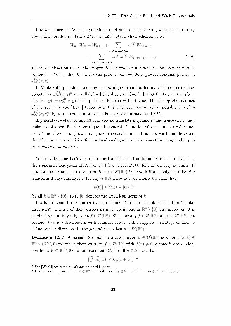
about their products. Wick's Theorem [IZ80] states that, schematically,
Wn ·Wm = Wn+m +∑
1 contraction
ω(2)Wn+m−2
+∑
2 contractions
ω(2) ω(2)Wn+m−4 + . . . , (1.16)
where a contraction means the suppression of two arguments in the subsequent normal
products. We see that by (1.16) the product of two Wick powers contains powers of
ω(2)∞ (x, y).
In Minkowski spacetime, one may use techniques from Fourier analysis in order to show
objects like ω(2)∞ (x, y)n are well dened distributions. One nds that the Fourier transform
of w(x− y) := ω(2)∞ (x, y) has support in the positive light cone. This is a special instance
of the spectrum condition [Haa96] and it is this fact that makes it possible to dene
ω(2)∞ (x, y)n by n-fold convolution of the Fourier transforms of w [RS75].
A general curved spacetime M possesses no translation symmetry and hence one cannot
make use of global Fourier techniques. In general, the notion of a vacuum state does not
exist19 and there is no global analogue of the spectrum condition. It was found, however,
that the spectrum condition nds a local analogue in curved spacetime using techniques
from micro-local analysis.
We provide some basics on micro-local analysis and additionally refer the reader to
the standard monograph [Hör90] or to [RS75, Str09, BF00] for introductory accounts. It
is a standard result that a distribution u ∈ E ′(Rn) is smooth if and only if its Fourier
transform decays rapidly, i.e. for any n ∈ N there exist constants Cn such that
|u(k)| ≤ Cn(1 + |k|)−n
for all k ∈ Rn \ 0. Here |k| denotes the Euclidean norm of k.
If u is not smooth the Fourier transform may still decrease rapidly in certain regular
directions. The set of these directions is an open cone in Rn \ 0 and moreover, it is
stable if we multiply u by some f ∈ D(Rn). Since for any f ∈ D(Rn) and u ∈ D′(Rn) the
product f · u is a distribution with compact support, this suggests a strategy on how to
dene regular directions in the general case when u ∈ D′(Rn).
Denition 1.2.7. A regular direction for a distribution u ∈ D′(Rn) is a point (x, k) ∈Rn × (Rn \ 0) for which there exist an f ∈ D(Rn) with f(x) 6= 0, a conic20 open neigh-
bourhood V ⊂ Rn \ 0 of k and constants Cn for all n ∈ N such that
|(f · u)(k)| ≤ Cn(1 + |k|)−n
19See [Wal94] for further elaboration on this point.20Recall that an open subset V ⊂ Rn is called conic if q ∈ V entails that λq ∈ V for all λ > 0.
23
CHAPTER 1. Quantum Field Theory in Curved Spacetime
for all k ∈ V . The wave front set WF(u) of a distribution u ∈ D′(Rn) is dened as
WF(u) := (x, k) ∈ Rn × (Rn \ 0) | (x, k) is not a regular direction for u.
The wave front set not only encodes the singular support of a distribution but also
the directions in Fourier space in which the distribution fails to be rapidly decreasing.
If u ∈ D′(Rn) is smooth, WF(u) = ∅. Moreover, WF(Du) ⊂ WF(u) for any partial
dierential operator D and WF(fu) ⊂WF(u) for smooth f .
The notion of a wave front set of a distribution can be lifted to any smooth manifold.
Lemma 1.2.8. The wave front set transforms covariantly under dieomorphisms as a
subset of T ∗Rn. One can therefore extend its denition to distributions on general mani-
folds M by patching together the wave front sets in dierent coordinate patches of M . For
u ∈ D′(M) one nds WF(u) ⊂ T ∗M \ 0, where 0 denotes the zero section of T ∗M .
The mathematically precise condition concerning when the pointwise product of distri-
butions exists makes use of wave front sets.
Theorem 1.2.9. Let u, v ∈ D′(M) and dene
WF(u)⊕WF(v) := (x, k + l) | (x, k) ∈WF(u), (x, l) ∈WF(v).
If WF(u) ⊕WF(u) does not contain the zero section of T ∗M , then one can dene the
pointwise product u · v ∈ D′(M) with WF(u · v) ⊂WF(u)∪WF(v)∪WF(u)⊕WF(v). If
u and v are smooth, u ·v reduces to the usual pointwise product between smooth functions.
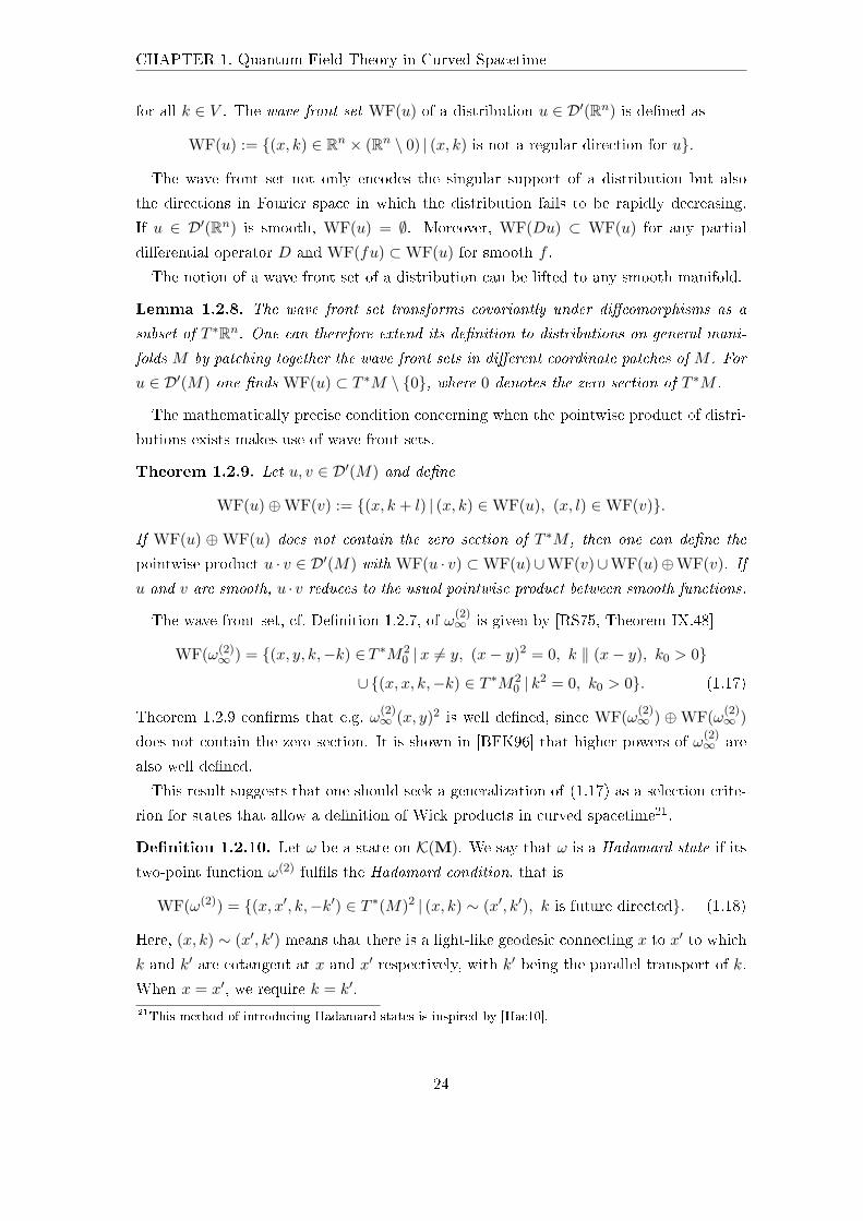
The wave front set, cf. Denition 1.2.7, of ω(2)∞ is given by [RS75, Theorem IX.48]
WF(ω(2)∞ ) = (x, y, k,−k) ∈T ∗M2
0 |x 6= y, (x− y)2 = 0, k ‖ (x− y), k0 > 0
∪ (x, x, k,−k) ∈ T ∗M20 | k2 = 0, k0 > 0. (1.17)
Theorem 1.2.9 conrms that e.g. ω(2)∞ (x, y)2 is well dened, since WF(ω(2)
∞ ) ⊕WF(ω(2)∞ )
does not contain the zero section. It is shown in [BFK96] that higher powers of ω(2)∞ are
also well dened.
This result suggests that one should seek a generalization of (1.17) as a selection crite-
rion for states that allow a denition of Wick products in curved spacetime21.
Denition 1.2.10. Let ω be a state on K(M). We say that ω is a Hadamard state if its
two-point function ω(2) fulls the Hadamard condition, that is
WF(ω(2)) = (x, x′, k,−k′) ∈ T ∗(M)2 | (x, k) ∼ (x′, k′), k is future directed. (1.18)
Here, (x, k) ∼ (x′, k′) means that there is a light-like geodesic connecting x to x′ to which
k and k′ are cotangent at x and x′ respectively, with k′ being the parallel transport of k.
When x = x′, we require k = k′.
21This method of introducing Hadamard states is inspired by [Hac10].
24
1.2. The Free Scalar Field and Wick Polynomials
Hadamard states exist on any globally hyperbolic spacetime [FNW81]. Moreover, the
set of Hadamard states on a given spacetime is closed under operations [San08, Prop.
3.1.9.], so we can dene a locally covariant state space, i.e. a contravariant functor S that
maps globally hyperbolic spacetimes to the set of Hadamard states S(M) on K(M).
It is important to note is that the dierence between the two-point functions of two
Hadamard states is smooth. This is why the expectation values of Wick powers (wrt.
some quasi-free Hadamard state ω) exist in any Hadamard state ω′, i.e. we may restrict
ω′(Wn(x1, . . . , xn)) to the total diagonal x1 = · · · = xn. Thus it follows that Wick powers
and their derivatives may be dened as point-like elds, i.e. as linear forms on the linear
span of S(M). This is crucial for the present work: as was mentioned before, the thermal
observables are Wick polynomials and it is therefore important that we are able to measure
them at points.
In order to discuss the algebraic structure of the normally ordered products, let us
dene the following subset of E ′(Mn), n ∈ N:
E ′n(M) :=t ∈ E ′(Mn) | t is symmetric,
WF(t) ⊂ (T ∗M)n \( ⋃x∈M
(V +x ) ∪
⋃x∈M
(V −x ))
. (1.19)
By denition, the sought for extension of K(M) consists of the unit 1 ∈ K(M) and
normally ordered products smeared with elements from E ′(Mn). It is the condition on
the wave front set of these distributions that guarantees that the smeared objects are well
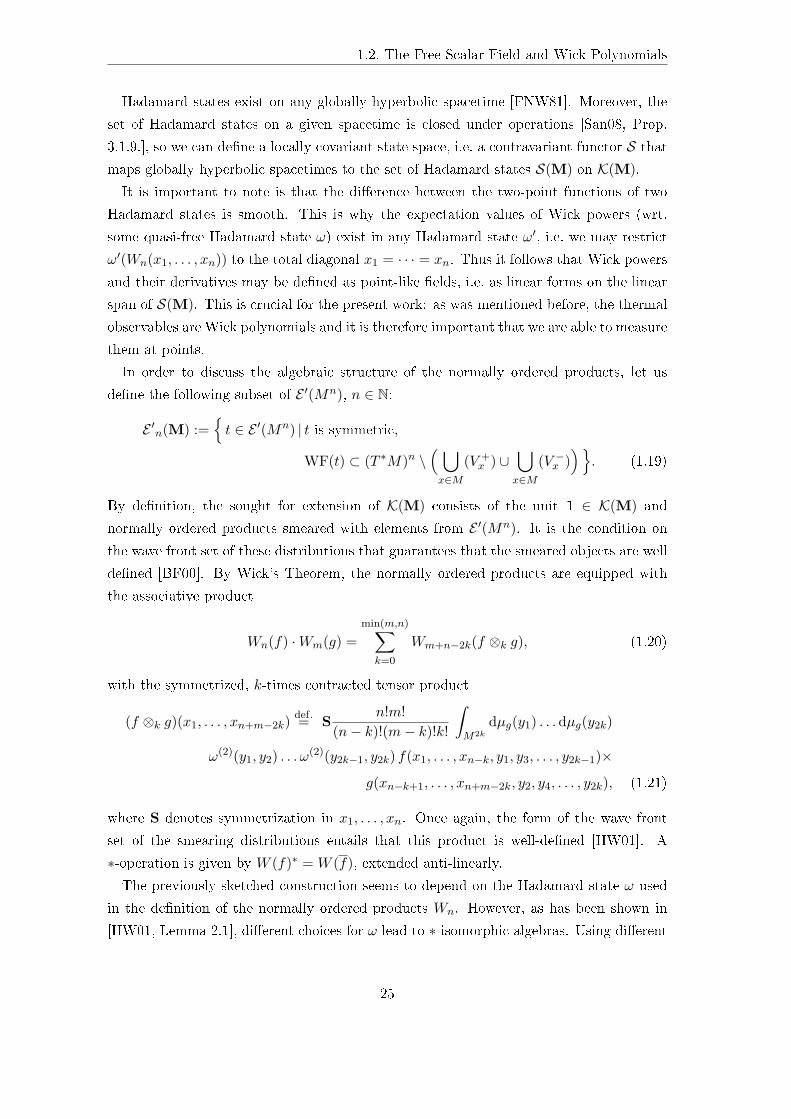
dened [BF00]. By Wick's Theorem, the normally ordered products are equipped with
the associative product
Wn(f) ·Wm(g) =min(m,n)∑k=0
Wm+n−2k(f ⊗k g), (1.20)
with the symmetrized, k-times contracted tensor product
(f ⊗k g)(x1, . . . , xn+m−2k)def.= S
n!m!(n− k)!(m− k)!k!
∫M2k
dµg(y1) . . . dµg(y2k)
ω(2)(y1, y2) . . . ω(2)(y2k−1, y2k) f(x1, . . . , xn−k, y1, y3, . . . , y2k−1)×
g(xn−k+1, . . . , xn+m−2k, y2, y4, . . . , y2k), (1.21)
where S denotes symmetrization in x1, . . . , xn. Once again, the form of the wave front
set of the smearing distributions entails that this product is well-dened [HW01]. A
∗-operation is given by W (f)∗ = W (f), extended anti-linearly.
The previously sketched construction seems to depend on the Hadamard state ω used
in the denition of the normally ordered products Wn. However, as has been shown in
[HW01, Lemma 2.1], dierent choices for ω lead to ∗-isomorphic algebras. Using dierent
25
CHAPTER 1. Quantum Field Theory in Curved Spacetime
states just amounts to using a dierent set of generators for the same abstract algebra,
which we denote by W(M) henceforth.
Denition 1.2.11. The ∗-algebra W(M) constructed above will be referred to as the
extended algebra of observables for the free scalar eld on the globally hyperbolic spacetime
M.
The extended algebra of observables W(M) can be equipped with a notion of conver-
gence of sequences, based on so-called Hörmander pseudo-topologies [BF00, HW01, HR02],
which has the property that K(M) is dense in W(M).
The assignment M 7→ W(M) is a lcQFT [HW01, Lemma 3.1], which moreover fulls the
time slice axiom [CF09]. It follows from results in [HR02] and [San10] that continuous22
states on W(M) are in one-to-one correspondence to Hadamard states on K(M) that are
extended toW(M). We continue to call these states Hadamard states. Thus it is justied
to regard the set of Hadamard states S(M) as the suitable space of states on the extended
algebra W(M) and we will look for LTE states in S(M) in Chapter 3.
A slightly dierent formulation of the above constructions, allowing a unied description
of the algebraic structure of the classical and the quantum eld theory, goes under the
name deformation quantization. An early reference for this approach is [DF01].
1.2.3 Locally Covariant Wick Polynomials
In this section we describe how Wick polynomials can be constructed in a locally covariant
manner. Again, this is of importance, because in the denition of LTE one needs locally
covariant thermal observables. Candidates for Wick monomials of all orders can be found
in the enlarged algebra W(M), because the diagonal distribution δn is an element of
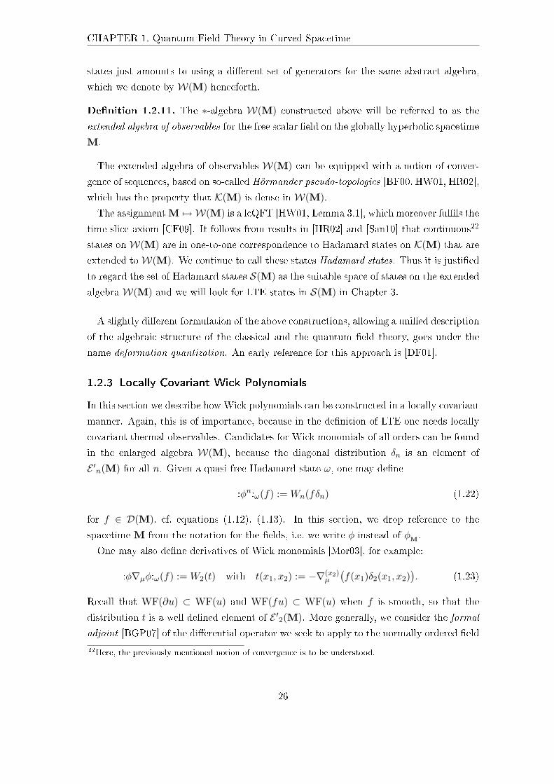
E ′n(M) for all n. Given a quasi-free Hadamard state ω, one may dene
:φn:ω(f) := Wn(fδn) (1.22)
for f ∈ D(M), cf. equations (1.12), (1.13). In this section, we drop reference to the
spacetime M from the notation for the elds, i.e. we write φ instead of φM .
One may also dene derivatives of Wick monomials [Mor03], for example:
:φ∇µφ:ω(f) := W2(t) with t(x1, x2) := −∇(x2)µ
(f(x1)δ2(x1, x2)
). (1.23)
Recall that WF(∂u) ⊂ WF(u) and WF(fu) ⊂ WF(u) when f is smooth, so that the
distribution t is a well dened element of E ′2(M). More generally, we consider the formal
adjoint [BGP07] of the dierential operator we seek to apply to the normally ordered eld
22Here, the previously mentioned notion of convergence is to be understood.
26
1.2. The Free Scalar Field and Wick Polynomials
and apply it to the smearing distribution (test function) · δn. Fields such as :∇µφ∇νφ:can be dened with the help of parallel transport in a natural way, see [Hac10], for
example. It is worth noting that the Leibniz rule applies, e.g. ∇µ:φ2:ω = 2 :φ∇µφ:ω.
The previous denitions have the major defect that they do not give rise to locally
covariant quantum elds. The construction of elds like :φn:ω depends on the Hadamard
state ω, which is an inherently non-local object, see [HW01, BFV03] for details. In order to
remedy this shortcoming, we rst introduce a more concrete characterization of Hadamard
states, which is also more suited for performing calculations with them.
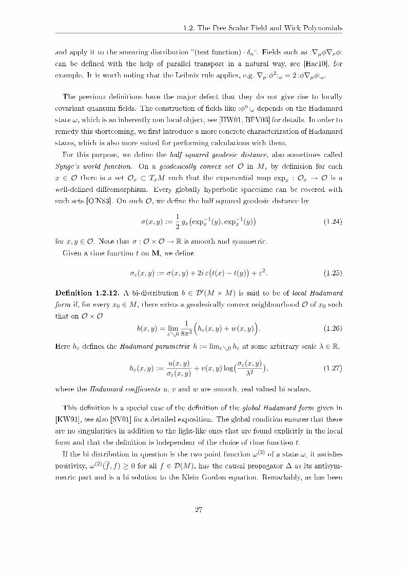
For this purpose, we dene the half squared geodesic distance, also sometimes called
Synge's world function. On a geodesically convex set O in M , by denition for each
x ∈ O there is a set Ox ⊂ TxM such that the exponential map expx : Ox → O is a
well-dened dieomorphism. Every globally hyperbolic spacetime can be covered with
such sets [O'N83]. On such O, we dene the half squared geodesic distance by
σ(x, y) :=12gx(exp−1
x (y), exp−1x (y)
)(1.24)
for x, y ∈ O. Note that σ : O ×O → R is smooth and symmetric.
Given a time function t on M, we dene
σε(x, y) := σ(x, y) + 2i ε(t(x)− t(y)
)+ ε2. (1.25)
Denition 1.2.12. A bi-distribution b ∈ D′(M ×M) is said to be of local Hadamard
form if, for every x0 ∈M , there exists a geodesically convex neighbourhood O of x0 such
that on O ×Ob(x, y) = lim
ε0
18π2
(hε(x, y) + w(x, y)
). (1.26)
Here hε denes the Hadamard parametrix h := limε0 hε at some arbitrary scale λ ∈ R,
hε(x, y) :=u(x, y)σε(x, y)
+ v(x, y) log(σε(x, y)
λ2
), (1.27)
where the Hadamard coecients u, v and w are smooth, real-valued bi-scalars.
This denition is a special case of the denition of the global Hadamard form given in
[KW91], see also [SV01] for a detailed exposition. The global condition ensures that there
are no singularities in addition to the light-like ones that are found explicitly in the local
form and that the denition is independent of the choice of time function t.
If the bi-distribution in question is the two-point function ω(2) of a state ω, it satises
positivity, ω(2)(f, f) ≥ 0 for all f ∈ D(M), has the causal propagator ∆ as its antisym-
metric part and is a bi-solution to the Klein Gordon equation. Remarkably, as has been
27
CHAPTER 1. Quantum Field Theory in Curved Spacetime
shown in [Rad96a], these conditions entail that if ω(2) has local Hadamard form, it also
has global Hadamard form.
An even more remarkable result, also due to Radzikowski [Rad96b], is the following23:
Theorem 1.2.13. Let ω be a state on A(M). Then ω is Hadamard in the sense of
denition 1.2.10 if and only if the two-point function ω(2) is of global Hadamard form.
By the above discussion, we can replace the term global with local in this theorem.
Therefore, the rather abstract characterization of Hadamard states in terms of micro-local
analysis is indeed equivalent to the more concrete realization that was used much earlier in
the renormalization of the energy momentum tensor, see [Wal94] and references therein.
The fact that ω(2) is also bi-solution of the Klein Gordon equation allows one to draw
strong conclusions about the Hadamard coecients. Usually, v is expressed in terms of a
series expansion in σ:
v =∞∑n=0
vn σn, (1.28)
where the vn are smooth bi-scalar coecients. This expansion is convergent on analytic
spacetimes, but not necessarily so on smooth spacetimes. Therefore, the series is usually
truncated at some order n and in turn one requires w in (1.26) only to be of regularity
Cn.
The property Pxω(2) = 0 together with the fact that we have ω(2) = h + w for some
smooth w entails that
Pxh = −Pxw,
and hence Pxh must be smooth. This condition is satised if terms proportional to σ−1
and lnσ in Pxh vanish and this, in turn, is achieved if Hadamard's recursion relations are
satised.
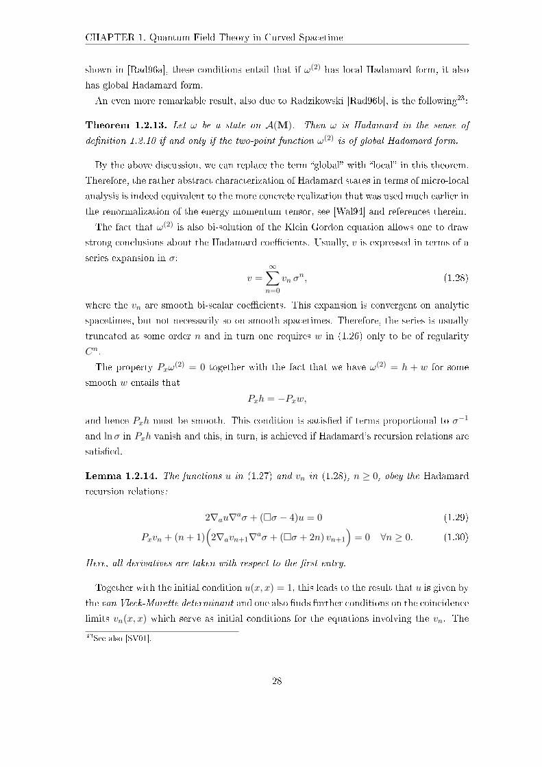
Lemma 1.2.14. The functions u in (1.27) and vn in (1.28), n ≥ 0, obey the Hadamard
recursion relations:
2∇au∇aσ + (σ − 4)u = 0 (1.29)
Pxvn + (n+ 1)(
2∇avn+1∇aσ + (σ + 2n) vn+1
)= 0 ∀n ≥ 0. (1.30)
Here, all derivatives are taken with respect to the rst entry.
Together with the initial condition u(x, x) = 1, this leads to the result that u is given by
the van Vleck-Morette determinant and one also nds further conditions on the coincidence
limits vn(x, x) which serve as initial conditions for the equations involving the vn. The
23See also [SV01].
28

1.2. The Free Scalar Field and Wick Polynomials
resulting initial value problems have uniquely determined smooth solutions, see [DB60,
Ful89, PPV11] or [BGP07].
It follows that u is solely determined by the local geometry of the spacetime, while
v also depends on the parameters ξ and m2 present in the Klein Gordon operator P .
Therefore, the singular part of the two-point function ω(2) of a Hadamard state ω is, in
fact, state independent and the state dependent information of the two-point function is
contained in the smooth function w, which is also symmetric by the CCR.
Following [HW01], we can now dene Wick powers in a locally covariant manner24. In
the denition of the normal ordered productsWn (1.12), we replace the two-point function
ω(2) with the Hadamard parametrix h. In this way, we have traded the non-local object
ω(2) for a purely local quantity that has the same wave front set so that smearing with
elements of E ′n(M) is still well dened. Note, however, that h is dened in a geodesic
normal neighbourhood O, so strictly speaking we have dened :φn:h(f) for f ∈ D(O) only.
However, a global denition can be given using a partition of unity argument [Mor03].
When considering Wick powers as point-like elds, this does not matter, because only
coincidence limits are relevant for the denition. The series expansion of v in σ may not
converge on smooth but non-analytic spacetimes. This is not an issue, however, in the
coincidence limit: one truncates the series at order n, where n is the order of the highest
derivative that appears in the Wick monomial in question.
We have identied elements of the extended algebra of observablesW(M) as candidates
for locally covariant Wick monomials. According to [HW01], the latter are expected to
full certain physically motivated requirements. Firstly, there should be a notion of con-
tinuity (analyticity) of the elds under smooth (analytic) variations of the metric and the
coupling parameters ξ,m2. Secondly, the elds should exhibit a certain behaviour under
rescaling of the metric and ξ,m2. Hollands and Wald have shown that Wick monomials
satisfying the aforementioned requirements are unique up to certain local curvature terms
[HW01, Theorem 5.1]:
:φn:(x) = :φn:h(x) +n−2∑k=0
(n
k
)Cn−k(x) :φk:h(x), (1.31)
where :φi:h(x) are the Wick powers dened previously with the help of the Hadamard
parametrix h. The functions Ci(x) are polynomials with real coecients in the metric,
curvature andm2, which scale as Ci(x) 7→ µiCi(x) under rescalings g 7→ µ−2g,m2 7→ µ2m2
and ξ 7→ ξ. The real coecients mentioned here thus constitute the renormalization
freedom for locally covariant Wick polynomials. Similar conclusions can be drawn for
24See [HW02] for local and covariant time ordered products.
29
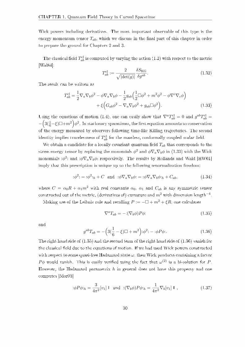
CHAPTER 1. Quantum Field Theory in Curved Spacetime
Wick powers including derivatives. The most important observable of this type is the
energy momentum tensor Tab, which we discuss in the nal part of this chapter in order
to prepare the ground for Chapters 2 and 3.
The classical eld T clab is computed by varying the action (1.2) with respect to the metric
[Wal84]:
T clab :=
2√|det(g)|
δSKG
δgab. (1.32)
The result can be written as
T clab =
12∇a∇bφ2 − φ∇a∇bφ−
12gab
(12φ2 +m2φ2 − φ∇c∇cφ
)+ ξ(Gabφ
2 −∇a∇bφ2 + gabφ2). (1.33)
Using the equations of motion (1.4), one can easily show that ∇aT clab = 0 and gabT cl
ab =
−(
3(16−ξ)+m2
)φ2. In stationary spacetimes, the rst equation amounts to conservation
of the energy measured by observers following time-like Killing trajectories. The second
identity implies tracelessness of T clab for the massless, conformally coupled scalar eld.
We obtain a candidate for a locally covariant quantum eld Tab that corresponds to the
stress energy tensor by replacing the monomials φ2 and φ∇a∇bφ in (1.33) with the Wick
monomials :φ2: and :φ∇a∇bφ: respectively. The results by Hollands and Wald [HW01]
imply that this prescription is unique up to the following renormalization freedom:
:φ2: = :φ2:h + C and :φ∇a∇bφ: = :φ∇a∇bφ:h + Cab, (1.34)
where C = α0R + α1m2 with real constants α0, α1 and Cab is any symmetric tensor
constructed out of the metric, (derivatives of) curvature and m2 with dimension length−4.
Making use of the Leibniz rule and recalling P := − +m2 + ξR, one calculates
∇aTab = −:(∇bφ)Pφ: (1.35)
and
gabTab = −(
3(16− ξ) +m2
):φ2:− :φPφ:. (1.36)
The right hand side of (1.35) and the second term of the right hand side of (1.36) vanish for
the classical eld due to the equations of motion. If we had used Wick powers constructed
with respect to some quasi-free Hadamard state ω, then Wick products containing a factor
Pφ would vanish. This is easily veried using the fact that ω(2) is a bi-solution for P .
However, the Hadamard parametrix h in general does not have this property and one
computes [Mor03]
:φPφ:h =3
4π2[v1]1 and :(∇bφ)Pφ:h =
14π2∇b[v1]1 , (1.37)
30
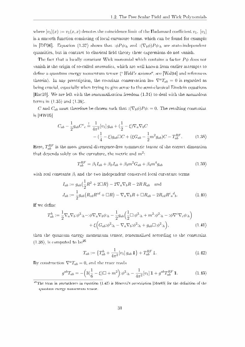
1.2. The Free Scalar Field and Wick Polynomials
where [v1](x) := v1(x, x) denotes the coincidence limit of the Hadamard coecient v1. [v1]
is a smooth function consisting of local curvature terms, which can be found for example
in [DF06]. Equation (1.37) shows that :φPφ:h and :(∇bφ)Pφ:h are state-independent
quantities, but in contrast to classical eld theory these expressions do not vanish.
The fact that a locally covariant Wick monomial which contains a factor Pφ does not
vanish is the origin of so-called anomalies, which are well known from earlier attempts to
dene a quantum energy momentum tensor (Wald's axioms, see [Wal94] and references
therein). In any prescription, the covariant conservation law ∇aTab = 0 is regarded as
being crucial, especially when trying to give sense to the semi-classical Einstein equations
[Hac10]. We are left with the renormalization freedom (1.34) to deal with the anomalous
terms in (1.35) and (1.36).
C and Cab must therefore be chosen such that :(∇bφ)Pφ: = 0. The resulting constraint
is [HW05]
Cab −12gabC
cc
!=1
4π2[v1] gab + (
12− ξ)∇a∇bC
− (14− ξ)gabC + (ξGab −
12m2gab)C − TRFab . (1.38)
Here, TRFab is the most general divergence-free symmetric tensor of the correct dimension
that depends solely on the curvature, the metric and m2:
TRFab = β1Iab + β2Jab + β3m2Gab + β4m
4gab (1.39)
with real constants βi and the two independent conserved local curvature terms
Iab := gab(1
2R2 + 2R
)− 2∇a∇bR− 2RRab and
Jab :=12gab(RcdR
cd + R)−∇a∇bR+ Rab − 2RcdRcadb. (1.40)
If we dene
T hab :=12∇a∇b:φ2:h−:φ∇a∇bφ:h −
12gab
(12:φ2:h +m2:φ2:h − :φ∇c∇cφ:h
)+ ξ(Gab:φ
2:h −∇a∇b:φ2:h + gab:φ2:h
), (1.41)
then the quantum energy momentum tensor, renormalized according to the constraint
(1.38), is computed to be25
Tab :=T hab +
14π2
[v1] gab 1
+ TRFab 1. (1.42)
By construction ∇aTab = 0, and the trace reads
gabTab = −(
3(16− ξ) +m2
):φ2:h −
14π2
[v1]1+ gabTRFab 1. (1.43)
25The term in parentheses in equation (1.42) is Moretti's prescription [Mor03] for the denition of the
quantum energy momentum tensor.
31
CHAPTER 1. Quantum Field Theory in Curved Spacetime
Note that TRFab cannot be chosen such that the state independent terms in (1.43) cancel
each other. This means in particular that in the conformally coupled, massless case Tab
is not traceless. This is often referred to as the conformal anomaly. It can be shown
that anomalies cannot be avoided when dealing with locally covariant Wick polynomials
[HW05]. Nevertheless, this discussion shows that physical principles like the conserva-
tion of the energy momentum tensor can be used to reduce the possible renormalization
freedom appearing in the denition of locally covariant Wick products. As we discuss in
chapter 3, there may be a possibility to x the remaining free constants with the help
of thermal data, as proposed in [BS07]. Another possibility to restrict the range of the
constants with the help of the semi-classical Einstein equation and data from cosmology
is described in [DHMP10].
The constructions which we have reviewed in this section show that the physically in-
teresting observables for the quantized free scalar eld can be constructed on globally
hyperbolic spacetimes, in accord with the principles of locality and covariance. The ther-
mal observables used in Chapter 3 are among them.
32
2 Local Thermal Equilibrium
This chapter deals with the denition of local thermal equilibrium (LTE) states in a model-
independent setting. In Section 2.1 we review the denition of LTE states given by
Buchholz, Ojima and Roos [BOR02], and we discuss its generalization to curved spacetime
[BS07] in Section 2.2. In this chapter we also present our own results on the structure of
the set of thermal observables and on the existence of LTE states. Most of these results
have been published in [Sol10].
2.1 Local Thermal Equilibrium States in Minkowski
Spacetime
2.1.1 Basic Denitions
In quantum eld theory global equilibrium states are to be described by use of the KMS
condition [Haa96], cf. Denition 1.1.10. Global equilibrium states have interesting proper-
ties, among them the fact that only a few global parameters play a rôle in the description
of their macroscopic behaviour, for example temperature. Apart from being subject to the
laws of thermostatics, these macroscopic observables also usually obey certain equations
of state.
Many macroscopic systems of interest, however, are at best locally close to an equi-
librium situation (hydrodynamic ows, steady states, perturbations of equilibrium), and
one cannot expect to be able to assign global thermal parameters to them. Instead one
should be able to attach local thermal parameters to such states, for example a tempera-
ture parameter that is spacetime dependent. At the same time, equations of state should
become local" in the sense that they are possibly replaced by evolution equations for the
local macroscopic observables. The denition given in [BOR02] captures these aspects of
local equilibrium.
Before we give a denition of LTE based on [BOR02], we need to recall the charac-
terization of global thermal equilibrium for QFT in Minkowski spacetime. In view of a
generalization of LTE to curved spacetime, we assume that we are dealing with a locally
covariant quantum eld theory A with locally covariant state space S. We use abbrevia-
33
CHAPTER 2. Local Thermal Equilibrium
tions like A0 := A(M0) and S0 := S(M0) for objects in Minkowski spacetime M0.
M0 is maximally symmetric and hence there is a ten-dimensional symmetry group
acting on M0 by hyperbolic embeddings. It is the proper orthochronous Poincaré group
P↑+ := R4 oL↑+, i.e. the semi-direct product of translations and the proper orthochronous
Lorentz group L↑+1. Since A is a lcQFT, there is an automorphic action P↑+ on A0:
P↑+ 3 (a,Λ) 7→ αa,Λ ∈ Aut(A0).
In the case of a pure translation, we write a 7→ αa instead of αa,1.
The dynamics of an inertial observer is given by time translations, i.e. time-like isome-
tries ιt(x) = x + te for some e ∈ R4 with e2 = −1 and e0 > 0. The corresponding
one-parameter group of automorphisms acting on A0 is t 7→ αte. If a state ωβ ∈ S0 is
a (αte,β)-KMS state2 for some time-like unit vector e2 = −1, e0 > 0, it is viewed as a
global equilibrium state at temperature T = 1β by any inertial observer moving along a
trajectory γ with γ′ = e.
The justication for this is found in the fact that KMS states are generalizations of nite
volume Gibbs ensembles to the innite medium [HHW67]. There are also several other
results that relate natural characterizations of global equilibrium to KMS states, either by
their behaviour under small perturbations of the dynamics [HB74], their characterization
via passivity, related to the second law of thermodynamics [PW78], or through the prin-
ciple of detailed balance and the zeroth law [KFGV77]. See [BR96] for more information
on KMS states.
As in [BOR02], we encode the information on the rest frame e and on the inverse
temperature β ∈ R+ into a single time-like vector β ·e, again denoted by β, the temperaturevector. The set of KMS states at any given temperature vector is known to form a simplex,
which implies that the elements of these sets can be distinguished with the help of central
observables (classical observables) such as chemical potentials or some mean energy
density.
Let us denote by V + the set of vectors v with v2 < 0 and v0 > 0. In the following, we
assume for simplicity that to each β ∈ V + there is exactly one KMS state. Physically,
this means that we consider systems with a single phase only. One of the consequences of
this assumption is a simple behaviour of the KMS states under Poincaré transformations.
Namely, given a KMS state ωβ and a transformation (Λ, a) ∈ P↑+, the transformed state
is by denition ωβ α−1Λ,a. From the KMS condition it follows that ωβ α−1
Λ,a is a KMS
state with temperature vector Λβ. Therefore, by the uniqueness assumption
ωβ α−1Λ,a = ωΛβ. (2.1)
1See for example [Haa96] for details.2Recall Denition 1.1.10.
34
2.1. Local Thermal Equilibrium States in Minkowski Spacetime
This means that the ωβ are invariant under translations. In their rest systems, they are
also isotropic.
We also assume that the functions β 7→ ωβ(A) are continuous for all A ∈ A0. Thus,
mixtures of KMS states may be formed by means of integration with suitable measures ρ
on V +. The set C ⊂ S0 of reference states consists of states
ωρ :=∫
dρ(β)ωβ. (2.2)
Reference states are generally not KMS states, but they retain the property of passivity
[PW78] and a suitable generalization of thermostatics applies to them [BOR02].
Since by assumption for each β ∈ V + there exists a unique KMS state ωβ , every
intensive thermodynamic quantity F attached to these states (thermal energy density,
entropy density etc.) can be expressed as a function of β alone. These functions β 7→ F (β)
are called thermal functions. As explained before, they characterize the macroscopic
properties of the KMS states ωβ completely. Thus we may write F (β) = ωβ(F ) and
interpret F as a macroscopic (central) observable. Evaluated in a reference state ωρ ∈ C,one obtains the mean value of F with regard to the measure ρ, cf. equation (2.2):
ωρ(F ) =∫
dρ(β)F (β).
Hence, thermodynamic quantities may also be attached to the reference states.
The basic idea for the denition of LTE states is that an ensemble which is in LTE at a
given point x ∈M0 should not be distinguishable from some (mixture of) global thermal
equilibrium states with regard to measurements performed with thermal observables
localized at x. These thermal observables are quantum elds which can be point-like
localized. Let us therefore assume that A0 is generated by a set of locally covariant
quantum elds, denoted by φM0=: φ0 etc. . We also assume that the state space S0 is
chosen such that the φ0(x) can be dened as linear forms on the linear span of S0 for all
x, as described at the end of section 1.1.3.
Given a quantum eld φ0(x) we dene the corresponding functions
β 7→ Φ(β) := ωβ(φ0(x)
). (2.3)
Note that by translation invariance of the KMS states, the right hand side does not
depend on x ∈M0. Moreover, it follows from our assumptions that the functions Φ are
continuous. To see this, take any test function f with∫f(x) d4x = 1. By assumption,
ωβ(φ0(f)) is continuous in β and by translation invariance of the KMS states, one has
ωβ(φ0(f)) = ωβ(φ0(x)) = Φ(β), hence β 7→ Φ(β) is continuous.
As is discussed in [BOR02], not every quantum eld in A0 is a good candidate for
being a thermal observable, as not all elds are sensitive to the thermal properties of
35
CHAPTER 2. Local Thermal Equilibrium
the system. It seems reasonable to choose the set of thermal observables T0 such that
one may reproduce (or at least approximate) all relevant thermal functions F by use of
equation (2.3), schematically:
F (β) = “ limi
Φ(i)(β) ”
for some sequence φ(i)0 ∈ T0. This provides a consistent link between the microscopic and
the macroscopic properties of the reference states. A simple example would be a local
thermometer, i.e. a scalar quantum eld φ0(x) such that the corresponding Φ(β) is a
simple function of β that may be inverted. Thus the eld φ0(x) allows one to distinguish
KMS states at dierent temperatures T = 1β , but in order to distinguish the rest frames
e ∈ V +, one also needs tensor elds.
Let us assume that a set T0 of thermal observables has been chosen and that the
functions corresponding to these elds by (2.3) are physically relevant thermal functions.
Denition 2.1.1. A state ω ∈ S is called T0(x)-thermal if there exists a normalized
measure ρx, supported in V +, such that
ω(φ(x)) = ωρx(φ(x)) (2.4)
for all φ(x) ∈ T0(x).
Note that the x-dependence of the right-hand side of (2.4) lies entirely in the measure ρx,
since the reference states in C are translationally invariant by our uniqueness assumption.
The reason why we regard T0(x)-thermal states as LTE states is that we may attach
thermal functions to them, depending on the size of T0. To see this, note that we can lift
any T0(x)-thermal state ω to a linear functional on the space of thermal functions by
ω(Φ)(x) := ω(φ(x)), φ ∈ T0, (2.5)
where Φ is the thermal function corresponding to the thermal observable φ(x) by (2.3).
We interpret ω(Φ)(x) as the expectation value of the thermal function Φ in the LTE state
ω at the point x ∈M0. This is a well dened linear functional, since by T0(x)-thermality
we have ω(φ1(x)) = ω(Φ)(x) = ω(φ2(x)) if Φ is a thermal function corresponding to both
φ1(x) and φ2(x). A situation where two distinct thermal observables give rise to the same
thermal function marks the occurrence of an equation of state, see the comment after the
proof of Proposition 2.1.3.
In order to consider states in which the thermal functions can vary over spacetime, we
extend Denition 2.1.1 to states that are in LTE in a region O of Minkowski spacetime.
Denition 2.1.2. A state ω is called T0(O)-thermal if it is T0(x)-thermal for all x ∈ O.
36
2.1. Local Thermal Equilibrium States in Minkowski Spacetime
The spatio-temporal behaviour of the thermal functions in the state ω is thus encoded in
the functions x 7→ ω(Φ)(x) obtained via (2.5). In [BOR02] it is shown that the microscopic
dynamics of the thermal observables may give rise to equations governing the spacetime
dependence of the macroscopic observables.
2.1.2 Existence of Local Thermal Equilibrium States
In the following we wish to discuss the basic question whether there exist any non-trivial
LTE states (apart from the obvious ones in C). This issue has been adressed in [BOR02]
already, where it was found that for nite sets of thermal observables T0 there exist
non-trivial T0(x)-thermal states. Here, we extend this result and show that one can nd
T0(O)-thermal states for any compact region O in Minkowski spacetime, cf. [Sol10].
We assume that T0 is nite. For each point x in Minkowski spacetime, we introduce
vector spaces
S(x) := spanφ(x) : φ ∈ T0, (2.6)
which are nite-dimensional by assumption. Moreover, the S(x) are generated by lo-
cally covariant quantum elds and hence αxS(0) = S(x). This implies that all S(x) are
isomorphic as vector spaces.
On each of the spaces S(x) we dene the semi-norms
τB(φ(x)
):= sup
β∈B|ωβ(φ(x)
)| (2.7)
for compact subsets B ⊂ V +. Note that we denote each of these semi-norms by τB,
disregarding on which space S(x) they are dened.
Proposition 2.1.3. Let O be a compact subregion of Minkowski spacetime. Assume that
there is some compact B ⊂ V + such that τB constitutes a norm on S(0). Then, there
exist T0(O)-thermal states in S0 which are not in C.
Proof. We pick any state ω0 ∈ S0 with ω0 /∈ C. In the following, we use ω0 to construct
an LTE state ω that is not in the set of reference states C.Since τB is a norm on S(0), it is also on each S(x), x ∈ O. Both this and the nite-
dimensionality of the S(x) imply that for each x ∈ O there is a positive real number Cx
such that
|ω0(φ(x))| ≤ Cx τB(φ(x)) for all φ(x) ∈ S(x). (2.8)
This in turn implies that for each x ∈ O we can lift ω0 to become a linear functional
on the subspace of the thermal functions corresponding to T0 by (2.3). This is done by
setting ω0(Φ)(x) := ω0(φ(x)), where Φ is the thermal function corresponding to φ(x) (cf.
(2.3)). In particular Φ ≡ 0 entails ω0(Φ)(x) = 0, so the (normalized) functionals ω0(·)(x)
37
CHAPTER 2. Local Thermal Equilibrium
are well-dened for each x ∈ O. Moreover, they are bounded by the norm τB and thus we
may extend them to the space of continuous complex-valued functions on B, C0(B), by
use of the Hahn-Banach theorem. We choose these extensions, denoted by ω0(·)(x) once
again, to be Hermitian. For each x ∈ O we nd
|ω0(F )(x)| ≤ Cx ||F ||B for all F ∈ C0(B),
where || · ||B is the supremum norm on C0(B), with respect to which this space is a
commutative C∗-algebra with unit. Any normalized Hermitian linear functional on this
algebra can be represented by a normalized signed measure σx [Coh80], decomposable
into two positive measures: σx = σ+x − σ−x . Thus, for each x ∈ O,
ω0(F )(x) =∫Bdσx(β) F (β). (2.9)
Assume that we are given a positive measure τ such that the sum σx + τ is a positive
measure for all x ∈ O and let us dene the state
ω := (1 + τ(B))−1(ω0 +
∫Bdτ(β)ωβ
). (2.10)
It is easy to see that for any x ∈ O and for all φ(x) ∈ S(x), we have ω(φ(x)) =∫B dρx(β)ωβ(φ(x)) with measure
ρx := (1 + τ(B))−1(σx + τ
). (2.11)
In other words, ω is a T0(x)-thermal state for all x ∈ O, i.e. ω is T0(O)-thermal. It is
not a reference state in general, since ω0 is not.
It remains to construct a suitable measure τ . We have obtained the functionals ω0(·)(x)
for each x on the space of thermal functions corresponding to elements of S(0). However,
S(0) is a nite dimensional vector space and hence we may express each of the ω0(·)(x)
in terms of a nite basis of Hermitian functionals ωini=1:
ω0(·)(x) =n∑i=1
ai(x)ωi
for some ai(x) ∈ R. Due to the continuity of x 7→ ω0(φ(x)) for all φ(x) ∈ S(x) (which is
guaranteed by our choice of S0), we nd that x 7→ ω0(Φ)(x) is continuous for all thermal
functions Φ corresponding to T0(x). The coecient functions ai : O → R are therefore
continuous and, by compactness of O, bounded by positive constants Ci. Again, we may
use the Hahn-Banach theorem to extend the functionals ωi to Hermitian functionals on all
of C0(B), which we also denote by ωi. As before, each of the ωi corresponds to a signed
measure σi = σi,+ − σi,− and it follows that the measures σx in (2.9) can be written as
38
2.1. Local Thermal Equilibrium States in Minkowski Spacetime
σx =∑n
i=1 ai(x)σi. Therefore, the x-dependence of the signed measures σx is contained
in the functions ai. We now dene the positive measure
τ :=n∑i=1
Ci |σi|,
where |σi| := σi,+ + σi,− denote the variations of the signed measures σi, which are by
denition positive. It is easy to see that σx + τ is a positive measure for all x ∈ O. Thisconcludes the proof.
The LTE states we have constructed are of the form indicated in (2.10) and may there-
fore be interpreted as a perturbation (given by ω0) around the thermal reference state1
τ(B)
∫B dτ(β)ωβ with appropriate measure τ . In these states, the thermal functions cor-
responding to T0 will exhibit non-trivial spacetime dependence as may be seen by the fact
that ω(Φ)(x) = ωρx(φ(0)) for all x ∈ O. The measure ρx, given by equation (2.11), clearly
depends non-trivially on x, because the function x 7→ ω0(φ(x)) depends non-trivially on
x.
Let us comment on the assumptions we made. As was shown in [BOR02], the fact
that τB is a norm on the spaces S(x) is equivalent to non-existence of linear constraints
emerging from equations of state, i.e. non-existence of linear relations between the thermal
functions corresponding to T0. To see this more clearly, note that if τB is a norm, it
follows that φ(x) = 0 whenever the corresponding thermal function Φ vanishes on B:
Φ(β) = 0 ∀β ∈ B. Therefore there are no linear relations between the thermal functions
that are not found among the elds themselves and hence no linear equations of state. Note
that equations of state typically impose non-linear relations between the basic thermal
functions and therefore do not present an obstruction in the sense discussed here.3
It is shown in [BOR02] that the argument for the existence of T0(x)-thermal states
at one point x can be extended to the case where τB is only a semi-norm, which then
covers systems with linear equations of state. However, it is not clear whether the same
reasoning may be adopted in case of T0(O)-thermality.
This, in fact, also presents a diculty in exhibiting the existence of LTE states in
regions of curved spacetime, as shown in the next section. It turns out that - for a
small set of thermal observables for the free scalar eld - linear equations of state yield
non-trivial dynamical constraints on LTE states. Currently, we lack a method to show
existence of states satisfying these conditions. However, there are examples of LTE states
for linear equations of state in curved spacetime (see Chapter 3), so in principle this is no
obstruction.
3Think of the Stefan-Boltzmann law, for example, which will play a rôle in Chapter 3.
39
CHAPTER 2. Local Thermal Equilibrium
2.2 Local Thermal Equilibrium States in Curved Spacetime
In this section, we discuss the denition of LTE states for quantum eld theory in curved
spacetime. As was described in the introduction, the main motivation for this is that we
would like to be able to attach thermal parameters to states of interest, for example in
cosmological models. In the presence of curvature, this directly leads to the concept of
local equilibrium, since there are no KMS states on a general curved spacetime M and
hence no obvious candidates for states that represent ensembles which are in thermal
equilibrium. This also leads to problems when trying to dene LTE, unlike in Minkowski
spacetime, as there are no reference states in S(M).
2.2.1 Denition of Local Equilibrium in Curved Backgrounds
As before, we assume that there is a lcQFT A with locally covariant state space S such
that in Minkowski spacetime, S0 includes a set C of reference states which satises the
assumptions laid down in Subsection 2.1.1. Moreover, in Minkowski spacetime, let there
be a nite set of thermal observables
T0 := φ(1)0 , . . . , φ
(n)0 .
It follows from the discussion in the previous section that it is meaningful to dene a state
ω0 ∈ S0 to be in LTE at x ∈M0, if the vector of expectation values
ω0(T0(x)) :=(ω0(φ(1)
0 (x)), . . . , ω0(φ(n)0 (x))
)∈ Rn
takes its values in a certain range, namely inside the convex set
TC := (ωρ(φ
(1)0 (x)), . . . , ωρ(φ
(n)0 (x))
)| ωρ ∈ C ⊂ Rn.4 (2.12)
The basic strategy to dene LTE in a curved background M is the same: one uses
some set of point-like thermal observables and records their expectation values in a given
state ω ∈ S(M) in order to test whether the vector of their values lies within a specied
range R ⊂ Rn. Since the local thermal observables in Minkowski spacetime are sensitive
to the thermal properties of the states, it seems natural to use their curved spacetime
counterparts for the denition of LTE in M. In plain terms, if φ0 = φM0is a thermal
observable in Minkowski spacetime, we use φM as a thermal observable in M . The
4This point of view makes it clear why linear equations of state have an eect on proofs of existence
of LTE states - in contrast to non-linear equations of state, they reduce the convex dimension of TC .
While one may nd a state with vector of expectation values in TC at some x, one also needs to make
sure that for points close to x, the vector of expectation values stays in TC . But this is not guaranteed
even by continuity, since TC is not open.
40
2.2. Local Thermal Equilibrium States in Curved Spacetime
physical picture behind this is that our measuring devices are gauged in regions far away
from any sources of gravity, where spacetime is essentially at, and then moved to the
region in which we want to probe, which may be curved.
Therefore, what matters are the locally covariant quantum elds φ, i.e. the assignments
M 7→ φM (cf. Denition 1.1.9). However, in general, there are many choices for φ such that
φM0equals a given quantum eld φ0. Hence there is some leeway in the determination
of the thermal observables in curved spacetime. This will become apparent when we deal
with the scalar eld in Chapter 3.
Since there are no reference states in S(M), the next question is what the set R should
be. Buchholz and Schlemmer [BS07] argue that since thermal observables are gauged
in at spacetime, one should choose R = TC . This means that we distinguish LTE
states in curved spacetime by requesting that they respond like thermal reference states
in Minkowski spacetime when tested with thermal observables.
For notational simplicity, let us assume that the elds φ(i) in T correspond to con-
travariant tensors of rank r(i). For x ∈ M, we dene the set T(x) to consist of all the
components of the elds φ(i)M, i = 1, . . . , n, in some local Lorentz frame eµ(x) at x. At
the origin 0 of Minkowski spacetime M0, we thus also have the set T0(0), dened with
respect to some Lorentz frame eµ(0). For the comparison of measurements performed
at x ∈M and at 0 ∈M0, we have to identify the tangent spaces at these points, which
is done by identication of the frames eµ(x) and eµ(0). More specically, we identify
(ϕx)∗φM with (ϕ0)∗φM0, where ϕx := ex exp−1
x are normal coordinates on some geodesic
normal neighbourhood O ⊂ M of x, with ex being the isomorphism between exp−1x (O)
and its image, aorded by eµ(x) (similarly for ϕ0 and eµ(0)).
Denition 2.2.1. A state ω ∈ S(M) is T(x)-thermal if for some reference state ωρx ∈ Cit holds that
ω(φ(i)M, µ1...µr(i)
(x)) = ωρx(φ(i)M0
, µ1...µr(i)(0))
for all µ1, . . . , µr(i) for all i = 1, . . . , n.
Using the identication of (ϕx)∗φM with (ϕ0)∗φM0in the geodesic normal set O, we
can extend the denition of LTE to regions. Thus we say that ω ∈ S(M) is T(O)-thermal
if it is T(y)-thermal for all y ∈ O with respect to this identication of frames.
Thermal functions can now be attached to an T(x)-thermal state ω as in Minkowski
spacetime, i.e.
ω(Φµ1...µr(i))(x) := ω(φ(i)M, µ1...µr(i)
(x)), (2.13)
where Φ is the thermal function corresponding to φM0= φ0 by equation (2.3).
The identication of the two frames eµ(x) and eµ(0) by use of normal coordinates
is arbitrary. The denition of LTE is not aected by this choice, as the following example
41
CHAPTER 2. Local Thermal Equilibrium
illustrates. Let ω ∈ S(M) be in LTE at x with regard to some thermal observable φM, µ(x)
under the identication of eµ(x) and eµ(0). For simplicity, suppose ω has a denite
temperature vector β ∈ V + at x. This means
ω(φM, µ(x)) = ωβ(φM0, µ(0)). (2.14)
Choosing another frame e′(x) = e(x)Λ−1 (where Λ is some (proper) local Lorentz trans-
formation of TxM), we nd
ω(φM, µ′(x)) = (Λ−1)µµ′ ω(φM, µ(x))
(2.14)= (Λ−1)µµ′ ωβ(φ0, µ(0))
= ωΛβ(φ0, µ(0)),
where the last equality follows from the transformation law of the KMS states under the
Poincaré group (2.1). Had we now identied e′µ′(x) and eµ(0), we would still conclude
that ω is in LTE with the same scalar temperature β ∈ R+. However, the thermal function
Φµ corresponding to φ0, µ is transformed according to the transformation of the local frame
in M.
Observation 2.2.2. Using some local Lorentz frame e(x), let ω ∈ S(M) be T(x)-thermal
and let ω(Φ)(x) be the local thermal function corresponding to some φ ∈ T. If e(x)Λ−1(x)
is another frame, then ω is also T(x)-thermal with respect to this new frame and the local
thermal function corresponding to φ is ω(Λ∗Φ)(x).
This is the local equivalent of the transformation behaviour of global equilibrium states
under Poincaré transformations of M0.
It should also be noted here that in the context of curved spacetimes, it is not possible
to work with vector spaces of thermal observables, as originally proposed in [BOR02] and
[BS07]. As was pointed out in [Sol10], linear combinations of thermal observables are
generally not thermal observables.
Let us illustrate this in the example of the massless, conformally coupled scalar eld
Pφ := ( + 16R)φ = 0 (cf. Section 1.2.1), the thermostatics of which we treat in the next
chapter. The set of locally covariant thermal observables which we use here is given by
[SV08]
T(2) := 1 , :φ2: , εab. (2.15)
Here, the tensor εab is the thermal energy tensor [BOR02, SV08], the components of which
are given at x ∈M by
εµν(x) := −:φ(∇µ∇νφ):(x) +14∇µ∇ν :φ2:(x).5 (2.16)
5Note that, using the Leibniz rule, one can express this tensor in dierent ways.
42
2.2. Local Thermal Equilibrium States in Curved Spacetime
After choosing an identication of frames as described before, the condition of T(2)(x)-
thermality of a state ω ∈ S(M) is
ω(:φ2:(x)) =ωρx(:φ2:0(0)) and
ω(εµν(x)) =ωρx(ε0,µν(0)) for µ, ν = 0, 1, 2, 3 (2.17)
for some thermal reference state ωρx in Minkowski spacetime.
At x ∈M, we have6
εµµ(x) =14:φ2:(x)− 1
6R:φ2:(x) + :φPφ:(x).
It follows from the discussion at the end of Section 1.2.3 that
:φPφ:(x) = U(x)1
with some smooth function U , which is determined by local curvature terms. This con-
tribution is related to the conformal anomaly in equation (1.43), see Chapter 3, equation
(3.31), for its explicit form. Hence
εµµ(x) =14:φ2:− 1
6R:φ2:(x) + U(x)1, (2.18)
yet at the origin of Minkowski spacetime the same linear combination yields
ε0µµ(0) =
14:φ2:0(0). (2.19)
Therefore, the locally covariant quantum eld :φ2:, which is actually a linear combination
of the elements of T(2), cannot itself be a thermal observable. This instead would require
ω(:φ2:(x)) = ωρx(:φ2:0(0)) = ωρx(:φ2:0(0)) = 0
(by translation invariance of the reference state ωρx) and thus by equations (2.18), (2.19)
and T(2)(x)-thermality of ω it follows that 16R(x)ωρx(:φ2:0(0)) = U(x). Since the Wick
square is, up to a constant, the mean of the local temperature squared, it follows that, at
x, the expectation value of the local temperature takes a xed value (determined by the
ratio U(x)/R(x)) for all LTE states. This, of course, is not a sensible prediction.
Observation 2.2.3. The identication of T(2)(x) and T(2)(0), provided by the locally
covariant quantum elds, cannot be extended to a linear map between spanT(2)(x) andspanT(2)(0).6Recall that :φ2:(x) = ηµν∇µ∇ν :φ2:(x), since the frame is taken to be orthonormal at x. Here, ηµν
are the entries of the diagonal matrix diag(−1, 1, 1, 1).
43
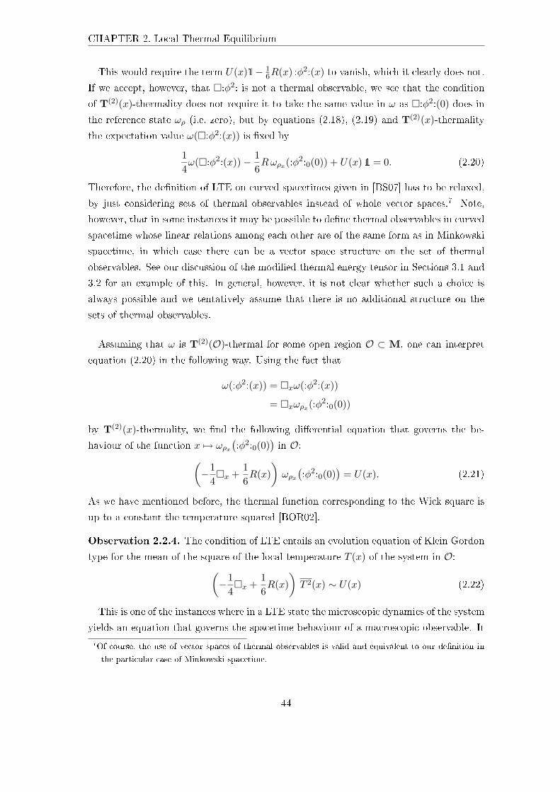
CHAPTER 2. Local Thermal Equilibrium
This would require the term U(x)1− 16R(x) :φ2:(x) to vanish, which it clearly does not.
If we accept, however, that :φ2: is not a thermal observable, we see that the condition
of T(2)(x)-thermality does not require it to take the same value in ω as :φ2:(0) does in
the reference state ωρ (i.e. zero), but by equations (2.18), (2.19) and T(2)(x)-thermality
the expectation value ω(:φ2:(x)) is xed by
14ω(:φ2:(x))− 1
6Rωρx(:φ2:0(0)) + U(x)1 = 0. (2.20)
Therefore, the denition of LTE on curved spacetimes given in [BS07] has to be relaxed,
by just considering sets of thermal observables instead of whole vector spaces.7 Note,
however, that in some instances it may be possible to dene thermal observables in curved
spacetime whose linear relations among each other are of the same form as in Minkowski
spacetime, in which case there can be a vector space structure on the set of thermal
observables. See our discussion of the modied thermal energy tensor in Sections 3.1 and
3.2 for an example of this. In general, however, it is not clear whether such a choice is
always possible and we tentatively assume that there is no additional structure on the
sets of thermal observables.
Assuming that ω is T(2)(O)-thermal for some open region O ⊂ M, one can interpret
equation (2.20) in the following way. Using the fact that
ω(:φ2:(x)) = xω(:φ2:(x))
= xωρx(:φ2:0(0))
by T(2)(x)-thermality, we nd the following dierential equation that governs the be-
haviour of the function x 7→ ωρx(:φ2:0(0)
)in O:(
−14x +
16R(x)
)ωρx(:φ2:0(0)
)= U(x). (2.21)
As we have mentioned before, the thermal function corresponding to the Wick square is
up to a constant the temperature squared [BOR02].
Observation 2.2.4. The condition of LTE entails an evolution equation of Klein Gordon
type for the mean of the square of the local temperature T (x) of the system in O:(−1
4x +
16R(x)
)T 2(x) ∼ U(x) (2.22)
This is one of the instances where in a LTE state the microscopic dynamics of the system
yields an equation that governs the spacetime behaviour of a macroscopic observable. It
7Of course, the use of vector spaces of thermal observables is valid and equivalent to our denition in
the particular case of Minkowski spacetime.
44
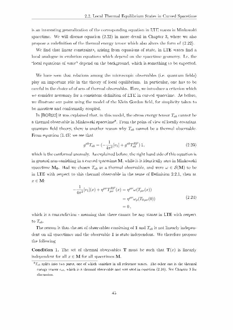
2.2. Local Thermal Equilibrium States in Curved Spacetime
is an interesting generalization of the corresponding equation in LTE states in Minkowski
spacetime. We will discuss equation (2.22) in more detail in Chapter 3, where we also
propose a redenition of the thermal energy tensor which also alters the form of (2.22).
We nd that linear constraints, arising from equations of state, in LTE states nd a
local analogue in evolution equations which depend on the spacetime geometry. I.e. the
local equations of state" depend on the background, which is something to be expected.
We have seen that relations among the microscopic observables (i.e. quantum elds)
play an important rôle in the theory of local equilibrium. In particular, one has to be
careful in the choice of of sets of thermal observables. Here, we introduce a criterion which
we consider necessary for a consistent denition of LTE in curved spacetime. As before,
we illustrate our point using the model of the Klein Gordon eld, for simplicity taken to
be massless and conformally coupled.
In [BOR02] it was explained that, in this model, the stress energy tensor Tab cannot be
a thermal observable in Minkowski spacetime8. From the point of view of locally covariant
quantum eld theory, there is another reason why Tab cannot be a thermal observable.
From equation (1.43) we see that
gabTab = (− 14π2
[v1] + gabTRFab )1, (2.23)
which is the conformal anomaly. As explained before, the right hand side of this equation is
in general non-vanishing in a curved spacetime M, while it is identically zero in Minkowski
spacetime M0. Had we chosen Tab as a thermal observable, and were ω ∈ S(M) to be
in LTE with respect to this thermal observable in the sense of Denition 2.2.1, then at
x ∈M:
− 14π2
[v1](x) + ηµνTRFµν (x) = ηµνω(Tµν(x))
= ηµνωρ(T0µν(0))
= 0 ,
(2.24)
which is a contradiction - meaning that there cannot be any states in LTE with respect
to Tab.
The reason is that the set of observables consisting of 1 and Tab is not linearly indepen-
dent on all spacetimes and the observable 1 is state independent. We therefore propose
the following
Condition 1. The set of thermal observables T must be such that T(x) is linearly
independent for all x ∈M for all spacetimes M.
8Tab splits into two parts, one of which vanishes in all reference states. The other one is the thermal
energy tensor εab, which is a thermal observable and was used in equation (2.16). See Chapter 3 for
discussion.
45
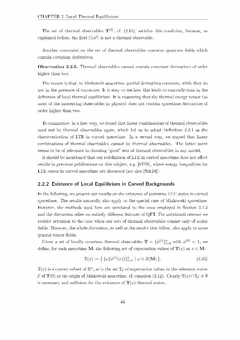
CHAPTER 2. Local Thermal Equilibrium
The set of thermal observables T(2), cf. (2.15), satises this condition, because, as
explained before, the eld :φ2: is not a thermal observable.
Another constraint on the set of thermal observables concerns quantum elds which
contain covariant derivatives.
Observation 2.2.5. Thermal observables cannot contain covariant derivatives of order
higher than two.
The reason is that, in Minkowski spacetime, partial derivatives commute, while they do
not in the presence of curvature. It is easy to see how this leads to contradictions in the
denition of local thermal equilibrium. It is reassuring that the thermal energy tensor (as
most of the interesting observables in physics) does not contain spacetime derivatives of
order higher than two.
To summarize: in a rst step, we found that linear combinations of thermal observables
need not be thermal observables again, which led us to adopt Denition 2.2.1 as the
characterization of LTE in curved spacetime. In a second step, we argued that linear
combinations of thermal observables cannot be thermal observables. The latter point
seems to be of relevance in choosing good sets of thermal observables in any model.
It should be mentioned that our redenition of LTE in curved spacetime does not aect
results in previous publications on this subject, e.g. [SV08], where energy inequalities for
LTE states in curved spacetime are discussed (see also [Sch10]).
2.2.2 Existence of Local Equilibrium in Curved Backgrounds
In the following, we present our results on the existence of pointwise LTE states in curved
spacetime. The results naturally also apply to the special case of Minkowski spacetime.
However, the methods used here are unrelated to the ones employed in Section 2.1.2
and the discussion relies on entirely dierent features of QFT. For notational reasons we
restrict attention to the case when our sets of thermal observables consist only of scalar
elds. However, the whole discussion, as well as the results that follow, also apply to more
general tensor elds.
Given a set of locally covariant thermal observables T = φ(i)ni=0 with φ(0) = 1, we
dene, for each spacetime M, the following set of expectation values of T(x) at x ∈M:
T(x) :=ω(φ(i)(x)
)ni=1 | ω ∈ S(M)
. (2.25)
T(x) is a convex subset of Rn, as is the set TC of expectation values in the reference states
C of T(0) at the origin of Minkowski spacetime, cf. equation (2.12). Clearly T(x)∩TC 6= ∅is necessary and sucient for the existence of T(x)-thermal states.
46
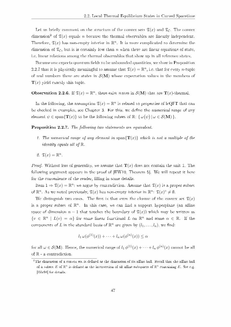
2.2. Local Thermal Equilibrium States in Curved Spacetime
Let us briey comment on the structure of the convex sets T(x) and TC . The convex
dimension9 of T(x) equals n because the thermal observables are linearly independent.
Therefore, T(x) has non-empty interior in Rn. It is more complicated to determine the
dimension of TC , but it is certainly less than n when there are linear equations of state,
i.e. linear relations among the thermal observables that show up in all reference states.
Because one expects quantum elds to be unbounded quantities, we show in Proposition
2.2.7 that it is physically meaningful to assume that T(x) = Rn, i.e. that for every n-tuple
of real numbers there are states in S(M) whose expectation values in the members of
T(x) yield exactly this tuple.
Observation 2.2.6. If T(x) = Rn, there exist states in S(M) that are T(x)-thermal.
In the following, the assumption T(x) = Rn is related to properties of lcQFT that can
be checked in examples, see Chapter 3. For this, we dene the numerical range of any
element ψ ∈ spanT(x) to be the following subset of R: ω(ψ)|ω ∈ S(M) .
Proposition 2.2.7. The following two statements are equivalent.
1. The numerical range of any element in spanT(x) which is not a multiple of the
identity equals all of R.
2. T(x) = Rn.
Proof. Without loss of generality, we assume that T(x) does not contain the unit 1. The
following argument appears in the proof of [HW10, Theorem 5]. We will repeat it here
for the convenience of the reader, lling in some details.
Item 1⇒ T(x) = Rn: we argue by contradiction. Assume that T(x) is a proper subset
of Rn. As we noted previously, T(x) has non-empty interior in Rn: T(x) 6= ∅.We distinguish two cases. The rst is that even the closure of the convex set T(x)
is a proper subset of Rn. In this case, we can nd a support hyperplane (an ane
space of dimension n − 1 that touches the boundary of T(x)) which may be written as
v ∈ Rn | L(v) = α for some linear functional L on Rn and some α ∈ R. If the
components of L in the standard basis of Rn are given by (l1, . . . , ln), we nd:
l1 ω(φ(1)(x)) + · · ·+ ln ω(φ(n)(x)) ≤ α
for all ω ∈ S(M). Hence, the numerical range of l1 φ(1)(x) + · · ·+ ln φ
(n)(x) cannot be all
of R - a contradiction.
9The dimension of a convex set is dened as the dimension of its ane hull. Recall that the ane hull
of a subset E of Rn is dened as the intersection of all ane subspaces of Rn containing E. See e.g.
[Hör94] for details.
47
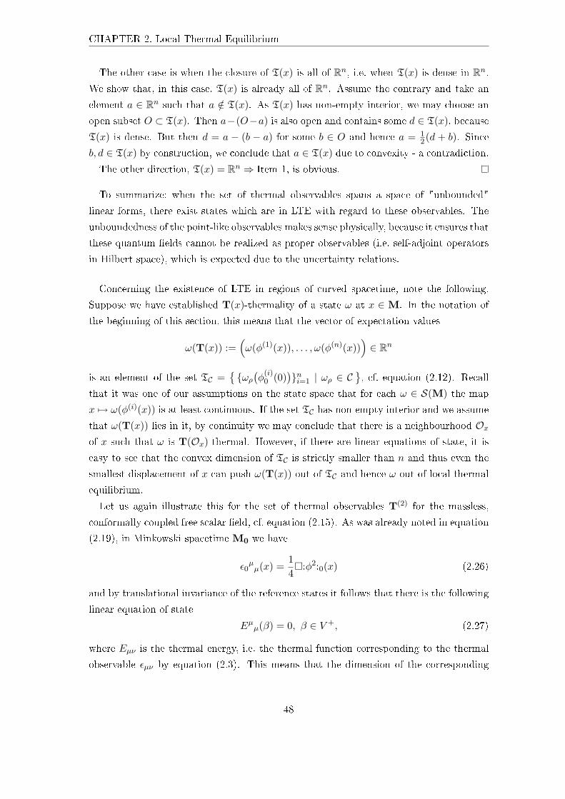
CHAPTER 2. Local Thermal Equilibrium
The other case is when the closure of T(x) is all of Rn, i.e. when T(x) is dense in Rn.
We show that, in this case, T(x) is already all of Rn. Assume the contrary and take an
element a ∈ Rn such that a /∈ T(x). As T(x) has non-empty interior, we may choose an
open subset O ⊂ T(x). Then a−(O−a) is also open and contains some d ∈ T(x), because
T(x) is dense. But then d = a − (b − a) for some b ∈ O and hence a = 12(d + b). Since
b, d ∈ T(x) by construction, we conclude that a ∈ T(x) due to convexity - a contradiction.
The other direction, T(x) = Rn ⇒ Item 1, is obvious.
To summarize: when the set of thermal observables spans a space of "unbounded"
linear forms, there exist states which are in LTE with regard to these observables. The
unboundedness of the point-like observables makes sense physically, because it ensures that
these quantum elds cannot be realized as proper observables (i.e. self-adjoint operators
in Hilbert space), which is expected due to the uncertainty relations.
Concerning the existence of LTE in regions of curved spacetime, note the following.
Suppose we have established T(x)-thermality of a state ω at x ∈M. In the notation of
the beginning of this section, this means that the vector of expectation values
ω(T(x)) :=(ω(φ(1)(x)), . . . , ω(φ(n)(x))
)∈ Rn
is an element of the set TC =ωρ(φ
(i)0 (0)
)ni=1 | ωρ ∈ C
, cf. equation (2.12). Recall
that it was one of our assumptions on the state space that for each ω ∈ S(M) the map
x 7→ ω(φ(i)(x)) is at least continuous. If the set TC has non-empty interior and we assume
that ω(T(x)) lies in it, by continuity we may conclude that there is a neighbourhood Oxof x such that ω is T(Ox)-thermal. However, if there are linear equations of state, it is
easy to see that the convex dimension of TC is strictly smaller than n and thus even the
smallest displacement of x can push ω(T(x)) out of TC and hence ω out of local thermal
equilibrium.
Let us again illustrate this for the set of thermal observables T(2) for the massless,
conformally coupled free scalar eld, cf. equation (2.15). As was already noted in equation
(2.19), in Minkowski spacetime M0 we have
ε0µµ(x) =
14:φ2:0(x) (2.26)
and by translational invariance of the reference states it follows that there is the following
linear equation of state
Eµµ(β) = 0, β ∈ V +, (2.27)
where Eµν is the thermal energy, i.e. the thermal function corresponding to the thermal
observable εµν by equation (2.3). This means that the dimension of the corresponding
48
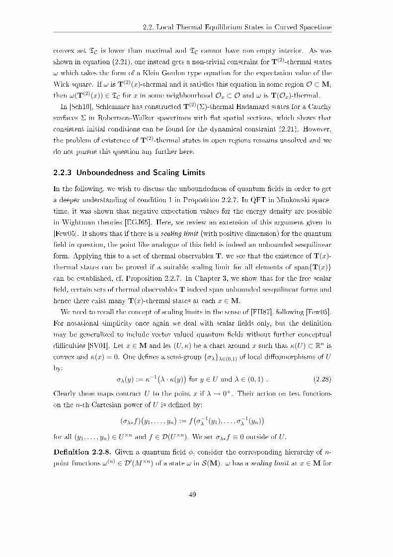
2.2. Local Thermal Equilibrium States in Curved Spacetime
convex set TC is lower than maximal and TC cannot have non-empty interior. As was
shown in equation (2.21), one instead gets a non-trivial constraint for T(2)-thermal states
ω which takes the form of a Klein Gordon type equation for the expectation value of the
Wick square. If ω is T(2)(x)-thermal and it satises this equation in some region O ⊂M,
then ω(T(2)(x)) ∈ TC for x in some neighbourhood Ox ⊂ O and ω is T(Ox)-thermal.
In [Sch10], Schlemmer has constructed T(2)(Σ)-thermal Hadamard states for a Cauchy
surfaces Σ in Robertson-Walker spacetimes with at spatial sections, which shows that
consistent initial conditions can be found for the dynamical constraint (2.21). However,
the problem of existence of T(2)-thermal states in open regions remains unsolved and we
do not pursue this question any further here.
2.2.3 Unboundedness and Scaling Limits
In the following, we wish to discuss the unboundedness of quantum elds in order to get
a deeper understanding of condition 1 in Proposition 2.2.7. In QFT in Minkowski space-
time, it was shown that negative expectation values for the energy density are possible
in Wightman theories [EGJ65]. Here, we review an extension of this argument given in
[Few05]. It shows that if there is a scaling limit (with positive dimension) for the quantum
eld in question, the point-like analogue of this eld is indeed an unbounded sesquilinear
form. Applying this to a set of thermal observables T, we see that the existence of T(x)-
thermal states can be proved if a suitable scaling limit for all elements of spanT(x)can be established, cf. Proposition 2.2.7. In Chapter 3, we show that for the free scalar
eld, certain sets of thermal observables T indeed span unbounded sesquilinear forms and
hence there exist many T(x)-thermal states at each x ∈M.
We need to recall the concept of scaling limits in the sense of [FH87], following [Few05].
For notational simplicity once again we deal with scalar elds only, but the denition
may be generalized to include vector valued quantum elds without further conceptual
diculties [SV01]. Let x ∈M and let (U, κ) be a chart around x such that κ(U) ⊂ Rn is
convex and κ(x) = 0. One denes a semi-group σλλ∈(0,1) of local dieomorphisms of U
by:
σλ(y) := κ−1(λ · κ(y)
)for y ∈ U and λ ∈ (0, 1) . (2.28)
Clearly these maps contract U to the point x if λ → 0+. Their action on test functions
on the n-th Cartesian power of U is dened by:
(σλ∗f)(y1, . . . , yn
):= f
(σ−1λ (y1), . . . , σ−1
λ (yn))
for all (y1, . . . , yn) ∈ U×n and f ∈ D(U×n). We set σλ∗f ≡ 0 outside of U .
Denition 2.2.8. Given a quantum eld φ, consider the corresponding hierarchy of n-
point functions ω(n) ∈ D′(M×n) of a state ω in S(M). ω has a scaling limit at x ∈M for
49
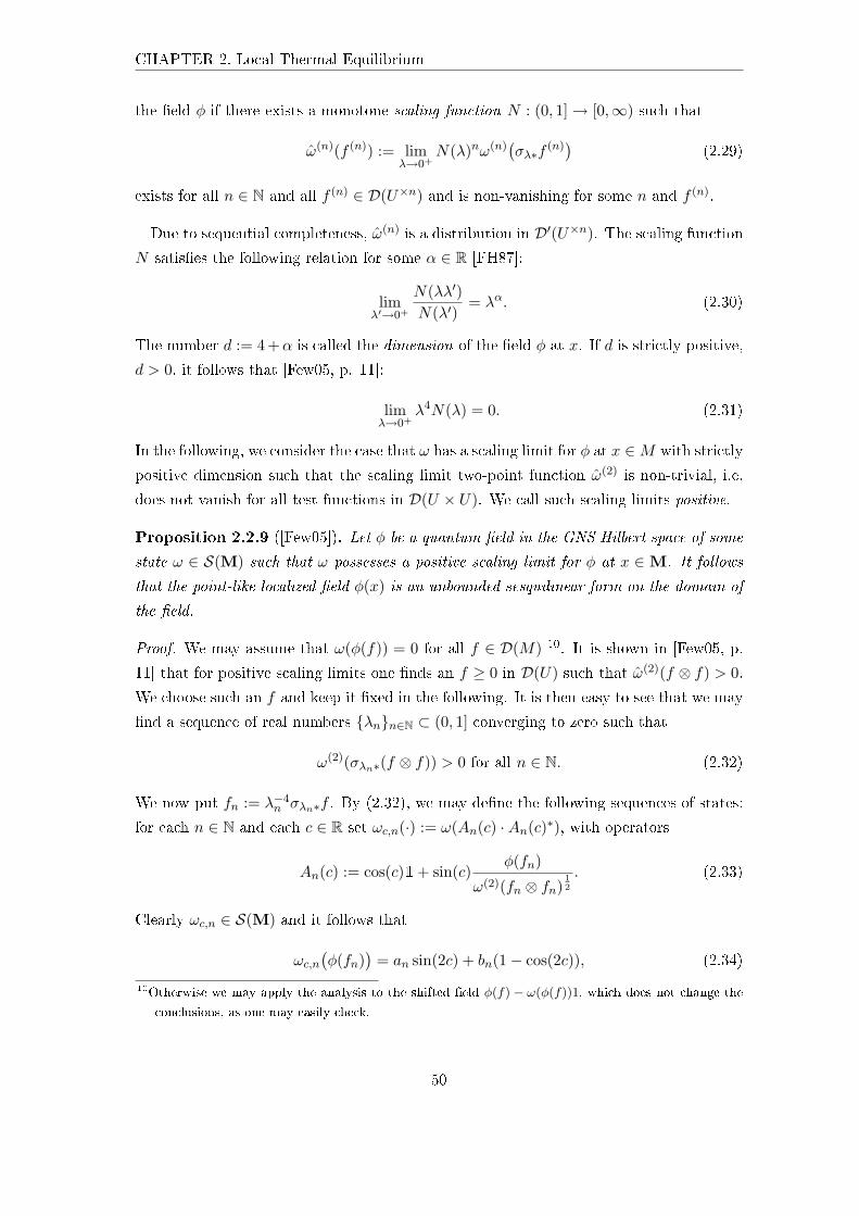
CHAPTER 2. Local Thermal Equilibrium
the eld φ if there exists a monotone scaling function N : (0, 1]→ [0,∞) such that
ω(n)(f (n)) := limλ→0+
N(λ)nω(n)(σλ∗f
(n))
(2.29)
exists for all n ∈ N and all f (n) ∈ D(U×n) and is non-vanishing for some n and f (n).
Due to sequential completeness, ω(n) is a distribution in D′(U×n). The scaling function
N satises the following relation for some α ∈ R [FH87]:
limλ′→0+
N(λλ′)N(λ′)
= λα. (2.30)
The number d := 4 +α is called the dimension of the eld φ at x. If d is strictly positive,
d > 0, it follows that [Few05, p. 11]:
limλ→0+
λ4N(λ) = 0. (2.31)
In the following, we consider the case that ω has a scaling limit for φ at x ∈M with strictly
positive dimension such that the scaling limit two-point function ω(2) is non-trivial, i.e.
does not vanish for all test functions in D(U × U). We call such scaling limits positive.
Proposition 2.2.9 ([Few05]). Let φ be a quantum eld in the GNS Hilbert space of some
state ω ∈ S(M) such that ω possesses a positive scaling limit for φ at x ∈M. It follows
that the point-like localized eld φ(x) is an unbounded sesquilinear form on the domain of
the eld.
Proof. We may assume that ω(φ(f)) = 0 for all f ∈ D(M) 10. It is shown in [Few05, p.
11] that for positive scaling limits one nds an f ≥ 0 in D(U) such that ω(2)(f ⊗ f) > 0.
We choose such an f and keep it xed in the following. It is then easy to see that we may
nd a sequence of real numbers λnn∈N ⊂ (0, 1] converging to zero such that
ω(2)(σλn∗(f ⊗ f)) > 0 for all n ∈ N. (2.32)
We now put fn := λ−4n σλn∗f . By (2.32), we may dene the following sequences of states:
for each n ∈ N and each c ∈ R set ωc,n(·) := ω(An(c) ·An(c)∗), with operators
An(c) := cos(c)1+ sin(c)φ(fn)
ω(2)(fn ⊗ fn)12
. (2.33)
Clearly ωc,n ∈ S(M) and it follows that
ωc,n(φ(fn)
)= an sin(2c) + bn(1− cos(2c)), (2.34)
10Otherwise we may apply the analysis to the shifted eld φ(f) − ω(φ(f))1, which does not change the
conclusions, as one may easily check.
50
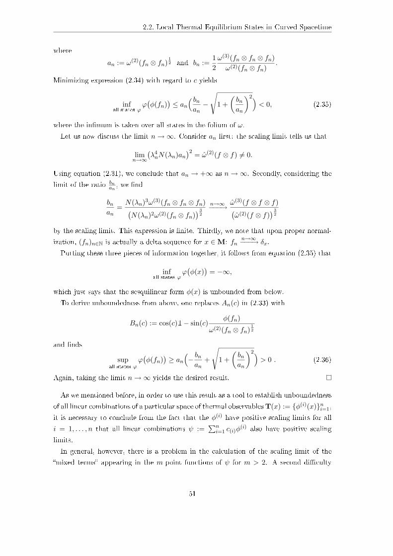
2.2. Local Thermal Equilibrium States in Curved Spacetime
where
an := ω(2)(fn ⊗ fn)12 and bn :=
12ω(3)(fn ⊗ fn ⊗ fn)ω(2)(fn ⊗ fn)
.
Minimizing expression (2.34) with regard to c yields
infall states ϕ
ϕ(φ(fn)
)≤ an
( bnan−
√1 +
(bnan
)2)< 0, (2.35)
where the inmum is taken over all states in the folium of ω.
Let us now discuss the limit n→∞. Consider an rst: the scaling limit tells us that
limn→∞
(λ4nN(λn)an
)2 = ω(2)(f ⊗ f) 6= 0.
Using equation (2.31), we conclude that an → +∞ as n→∞. Secondly, considering the
limit of the ratio bnan, we nd
bnan
=N(λn)3ω(3)(fn ⊗ fn ⊗ fn)(N(λn)2ω(2)(fn ⊗ fn)
) 32
n→∞−−−→ ω(3)(f ⊗ f ⊗ f)(ω(2)(f ⊗ f)
) 32
by the scaling limit. This expression is nite. Thirdly, we note that upon proper normal-
ization, (fn)n∈N is actually a delta sequence for x ∈M: fnn→∞−−−→ δx.
Putting these three pieces of information together, it follows from equation (2.35) that
infall states ϕ
ϕ(φ(x)
)= −∞,
which just says that the sesquilinear form φ(x) is unbounded from below.
To derive unboundedness from above, one replaces An(c) in (2.33) with
Bn(c) := cos(c)1− sin(c)φ(fn)
ω(2)(fn ⊗ fn)12
and nds
supall states ϕ
ϕ(φ(fn)
)≥ an
(− bnan
+
√1 +
(bnan
)2)> 0 . (2.36)
Again, taking the limit n→∞ yields the desired result.
As we mentioned before, in order to use this result as a tool to establish unboundedness
of all linear combinations of a particular space of thermal observablesT(x) := φ(i)(x)ni=1,
it is necessary to conclude from the fact that the φ(i) have positive scaling limits for all
i = 1, . . . , n that all linear combinations ψ :=∑n
i=1 c(i)φ(i) also have positive scaling
limits.
In general, however, there is a problem in the calculation of the scaling limit of the
mixed terms appearing in the m-point functions of ψ for m > 2. A second diculty
51
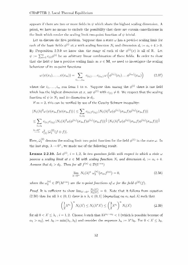
CHAPTER 2. Local Thermal Equilibrium
appears if there are two or more elds in ψ which share the highest scaling dimension. A
priori, we have no means to exclude the possibility that there are certain cancellations in
the limit which render the scaling limit two-point function of ψ trivial.
Let us discuss the rst problem. Suppose that a state ω has a positive scaling limit for
each of the basic elds φ(i) at x with scaling function Ni and dimension di := αi + 4 > 0.
By Proposition 2.2.9 we know that the range of each of the φ(i)(x) is all of R. Let
ψ :=∑n
i=1 c(i)φ(i) be an arbitrary linear combination of these elds. In order to show
that the eld ψ has a positive scaling limit at x ∈M, we need to investigate the scaling
behaviour of its m-point functions
ω (ψ(x1), . . . , ψ(xm)) =∑
i1,...,im
c(i1) . . . c(im) ω(φ(i1)(x1) . . . φ(im)(xm)
)(2.37)
where the i1, . . . , im run from 1 to n. Suppose that among the φ(i) there is one eld
which has the highest dimension at x, say φ(1) with c(1) 6= 0. We suspect that the scaling
function of ψ is N1 and its dimension is d1.
If m = 2, this can be veried by use of the Cauchy Schwarz inequality:
|N1(λ)2ω (ψ(σλ∗f)ψ(σλ∗f)) | ≤∑i1,i2
c(i1)c(i2) |N1(λ)2ω(φ(i1)(σλ∗f)φ(i2)(σλ∗f))|
≤∑i1,i2
c(i1)c(i2) |N1(λ)2ω(φ(i1)(σλ∗f)φ(i1)(σλ∗f))|12 |N1(λ)2ω(φ(i2)(σλ∗f)φ(i2)(σλ∗f))|
12
λ→0+
−→ c2(1) |ω
(2)1 (f ⊗ f)|.
Here, ω(2)1 denotes the scaling limit two-point function for the eld φ(1) in the state ω. In
the last step, λ→ 0+, we made use of the following result.
Lemma 2.2.10. Let φ(i), i = 1, 2, be two quantum elds with respect to which a state ω
possess a scaling limit at x ∈ M with scaling function Ni and dimension di := αi + 4.
Assume that d1 > d2. Then for all f (n) ∈ D(U×n)
limλ→0+
N1(λ)n ω(n)2
(σλ∗f
(n))
= 0, (2.38)
where the ω(n)2 ∈ D′(M×n) are the n-point functions of ω for the eld φ(2)(f).
Proof. It is sucient to show limλ′→0+N1(λ′)N2(λ′) = 0. Note that it follows from equation
(2.30) that for all λ ∈ (0, 1) there is a λi ∈ (0, 1] (depending on αi and λ) such that(12λαi)n
Ni(λ′) ≤ Ni(λnλ′) ≤(
32λαi)n
Ni(λ′) (2.39)
for all 0 < λ′ ≤ λi , i = 1, 2. Choose λ such that 3λα1−α2 < 1 (which is possible because of
α1 > α2), set λ0 := min(λ1, λ2) and consider the sequence λn := λnλ0. For 0 < λ′ ≤ λ0,
52
2.2. Local Thermal Equilibrium States in Curved Spacetime
dene the number n(λ′) by λ′ ∈ [λn(λ′)+1, λn(λ′)). Clearly, limλ′→0+ n(λ′) = ∞. We can
now make use of the fact that the Ni's are monotonous functions. Assume, for example,
thatN1 is monotonically increasing whileN2 is monotonically decreasing. Then, by (2.39),
it follows that for all 0 < λ′ ≤ λ0 one has
N1(λ′)N2(λ′)
≤N1(λn(λ′))N2(λn(λ′))
≤ (3λα1−α2)n(λ′) N1(λ0)N2(λ0)
→ 0
as λ′ → 0+. The other cases can be treated in the same way.
In other words, when considering the scaling limit of a linear combination of elds ψ,
in case of the two-point function m = 2 one may suppress contributions from elds of
lower dimension by using the scaling function of the eld with highest dimension and only
the scaling limit of this eld survives. However, if m ≥ 3, the same conclusion cannot be
drawn so easily. In order to estimate the mixed terms appearing there, one cannot use
the Cauchy Schwarz inequality in an obvious way. One therefore needs information on
the scaling behaviour of products of the elds as in the case of Wick's theorem for the
Wick products of the Klein Gordon eld, cf. section 1.2.2. We will discuss this example
in the next chapter.
As mentioned previously, if there are two or more distinct elds in T which have the
same dimension at x, one needs to check carefully whether the scaling limit two-point
functions of every possible linear combination of the two are still non-trivial, as cancel-
lations in the scaling limit could occur. Examples where this may be a problem can be
found among thermal observables which are dierent components of the same tensor, as
is for the components of the thermal energy tensor for the free scalar eld.
53

54
3 Local Thermal Equilibrium States for
the Free Scalar Field
In this chapter, we discuss local thermal equilibrium states for the free scalar eld. In
Section 3.1, we introduce the thermal observables we are dealing with, putting special
emphasis on the thermal energy tensor and proposing a redenition of this observable.
Moreover, we consider higher Wick powers as thermal observables, nding that the renor-
malization freedom is greatly reduced if we introduce a natural condition concerning the
combinatorics of quasi-free LTE states. We also introduce conformally covariant quantum
elds at this stage, because later, we argue that the Wick square should be renormalized
such that it becomes a conformally covariant quantum eld in the sense of [Pin09]. This
is justied by results for the Wick square in KMS states in certain simple stationary
spacetimes, which we consider in Section 3.2. We also use our abstract results of Chapter
2 to show existence of LTE states in the model treated here.
3.1 Basic Thermal Observables and Thermal Functions
The concept of equilibrium makes reference to a notion of dynamics, which, in lcQFT,
is implemented by one-parameter groups of time-like isometries, which give rise to auto-
morphisms of the algebra of observables. While any KMS state with respect to such a
one-parameter group of automorphisms is passive (i.e. no observer can extract energy from
the state running a cyclic engine), it is only for global equilibrium states in Minkowski
spacetime, dened with respect to inertial observers, that the KMS parameter β has clear
interpretation as an inverse temperature in the sense of the zeroth law of thermostatics.1
This is why thermal observables are gauged exactly in these states.
On the other hand, one can use these thermal observables to test KMS states that
are connected with certain time evolutions in curved spacetime. This may help to reveal
the physical eects that give rise to passivity in these cases and, moreover, to elucidate
the rôle of the KMS parameter and its relation to the local temperature in these states.
1Recall that temperature is a parameter that identies macroscopic systems which are mutually in
thermal equilibrium.
55
CHAPTER 3. Local Thermal Equilibrium States for the Free Scalar Field
In some cases, this allows one to draw conclusions about the relation between the local
temperature and the Hawking-Unruh temperature, as we see later.
Denition 3.1.1. A spacetime M is called stationary if there exists a one-parameter-
group of time-like isometries χtt∈R or, equivalently, if there is a time-like Killing vector
eld K in M. M is called static, if there is a family of space-like hypersurfaces orthogonal
to K everywhere.2
In a lcQFT A, the maps χt get lifted to automorphisms αt on A(M). Hence, there
exists a one-parameter-group of automorphisms αtt∈R on A(M), which is interpreted
as dynamics along the trajectories induced by χtt∈R. With respect to this notion of
dynamics, one can then dene (β, αt)-KMS states ωβ .
We stress again that it would be premature to envisage these states in analogy to the
global equilibrium states in Minkowski spacetime M0. There is no well-dened ther-
mostatics for M, since many of the concepts involved in the formulation of this theory
implicitly make use of the homogeneity of space (additivity of the entropy, for example).
In particular, there is no variant of the zeroth law in curved spacetime. Hence, the KMS
parameter β needs to be interpreted in terms of the local temperature.
For the explicit construction of KMS states for the free scalar eld, one needs the fol-
lowing well-known result [HHW67], which is a useful reformulation of the KMS condition
of Denition 1.1.10.
Proposition 3.1.2. In the notation of Denition 1.1.10, a state ω ∈ S(M) is (αt,β)-KMS
if and only if the Fourier transforms FAB and GAB of FAB and GAB satisfy
FAB|R = eβ(·)GAB|R (3.1)
in the sense of tempered distributions for all A,B ∈ A(M).3
Recall the functors which describe the quantum theory of the free scalar eld, in par-
ticular the lcQFTs K and W with state space S, as described in Section 1.2. For the
moment, we leave the mass m2 and the curvature coupling ξ unspecied.
We begin by reviewing the construction of KMS states for this theory. Assume that M
is stationary and let ∆ be the causal propagator for the free eld as dened in equation
(1.8). Given the one-parameter-group of time-like isometries χtt∈R on M, we dene
∆f,g(t) := ∆(f, g χ−1t ) for f, g ∈ D(M).
2If M is globally hyperbolic, these hypersurfaces are Cauchy surfaces.3More precisely, this has to be understood as rst restricting GAB to D(R), then multiplying with eβ(·),
and nally uniquely extending the result to a tempered distribution again.
56
3.1. Basic Thermal Observables and Thermal Functions
As a consequence of the CCR, cf. equation (1.10), the elements A := φM(f1) . . . φM(fn)
and B := φM(fn+1) of A(M) satisfy the algebraic relation
[A,αt(B)] =n∑k=1
i∆fk,fn+1(t)φM(f1) . . . φM(fk) . . . φM(fn), (3.2)
where ˇ indicates that the corresponding eld is omitted.
Let ω be an (αt,β)-KMS state on K(M), then, from equation (3.1), it follows that for
the elements A and B one has
(1− e−β(·))FAB|R = FAB|R − GAB|R
=n∑k=1
i ∆fk,fn+1(·)ω(n−1)(f1, . . . , fk, . . . , fn)
with the Fourier transform ∆fk,fn+1 of ∆fk,fn+1 . Similar arguments for B involving more
than one eld show that the n-point functions of a KMS state can expressed through their
(n− 2)-point function, and thus, ultimately, via its two-point function. This implies that
KMS states are quasi-free states, but not necessarily even. If, however, ω is even, which
we assume from now on, ω(1) = 0 and one obtains for the two-point function (putting
n = 1 in the denition of A):
ω(2)(f1, f2) =i√2π
∫ ∞−∞
dk∆f1,f2(k)1− e−βk
=i
2π
∫ ∞−∞
dk1
1− e−βk
∫ ∞−∞
dt∆f1,f2(t) e−ikt, (3.3)
which determines ω completely.
For simplicity, we now specialize to the massless (m2 = 0), conformally coupled (ξ = 16)
scalar eld. In Minkowski spacetime M0, the corresponding causal propagator is given
by the formal kernel
∆(x, y) =−12πε(x0 − y0)δ((x− y)2), (3.4)
with ε denoting the sign function. In the massless case, the Hadamard parametrix is equal
to the vacuum two-point function given in equation (1.15), i.e.
h(x, y) = limε→0
14π2
1(x− y)2 + iε(x0 − y0) + ε2
(3.5)
One can thus calculate the expectation values for the locally covariant Wick powers in the
quasi-free (primary) KMS states ωβ with respect to the time evolution x 7→ x + te with
e ∈ V +.4 The result of the straightforward calculation is, in case of the Wick square,
ωβ(:φ20:(x)) =
112β2
. (3.6)
4Note that in the massive case, the Hadamard parametrix diers from the vacuum two-point function
and thus the locally covariant Wick powers dier from Wick powers that are regularised by subtraction
of the vacuum. See [SV08] for details.
57
CHAPTER 3. Local Thermal Equilibrium States for the Free Scalar Field
This means that in any spacetime, :φ2: can be used as a local thermometer and any state
with ω(:φ2:(x)) ≥ 0 is locally thermal at x with regard to this observable.
In the case of the thermal energy tensor, one has
ωβ(ε0,ab(x)) =π2
90β4(4eaeb + ηab), (3.7)
cf. [BOR02]. Here, η denotes the Minkowski metric η = g0.
Equations (3.6) and (3.7) x the thermal functions for the thermal observables we are
interested in.5
It is important to note that the thermal energy tensor is traceless in the reference
states, which, as was mentioned before, leads to a linear constraint on LTE states. The
corresponding equation of state is E = 3P , where E is the (thermal) energy density in the
rest system e and P is the pressure. Moreover, the temperature dependence of E is given
by a Stefan-Boltzmann type law, E(β) = π2
30β4 , as expected in a massless theory. This is
an example for a non-linear equation of state, in this case between the thermal functions
corresponding to :φ2: and ε00.
As we discuss in the next section, the Wick powers of the massless, conformally coupled
free eld should be conformally covariant. This can be done with a certain choice of
renormalization for these elds. We review the concept of locally conformally covariant
quantum elds in the sense of Pinamonti [Pin09] here, also correcting a mistake in the
original work. In this approach, conformal embeddings between two spacetimes M1 and
M2 play an important rôle, i.e. maps ψ : M1 →M2 which act like hyperbolic embeddings,
cf. Denition 1.1.2, except that they are not isometries. Rather there is a smooth function
Ω : M2 → R such that ψ∗g1 = Ω−2g2|ψ(M1). Details can be found e.g. in [Wal84, Appendix
D]. The weighted action of the conformal embedding ψ with weight λ ∈ N on test functions
is given by the map
ψ(λ)∗ : D(M1)→ D(ψ(M1)), ψ
(λ)∗ f(x) := Ω−λ(x) f(ψ−1(x)). (3.8)
Pinamonti generalized the notion of lcQFT to locally conformally covariant QFT by using
the category CLoc instead of Loc, which uses conformal embeddings instead of hyperbolic
embeddings as morphisms. In other words, a conformally locally covariant QFT is a
covariant functor A between CLoc and Alg. Hence, if ψ : M1 → M2 is a conformal
5In the massive case, the thermal functions look more complicated, but the Wick square is still a
monotonous function of β and can thus be used as a local thermometer. Details are presented in
[Hüb05], see also [SV08].
58
3.1. Basic Thermal Observables and Thermal Functions
embedding, the following diagram commutes, and we write αψ := A(ψ):
M1ψ−−−−→ M2
Ay yA
A(M1)αψ−−−−→ A(M2) .
A conformally covariant quantum eld of weight λ transforms under the action of ψ ac-
cording to the formula
αψ φ(λ)M1
= φ(λ)M2 ψ(4−λ)∗ , (3.9)
or, in terms of formal kernels,
αψφ(λ)M1
(x) = Ωλ(ψ(x))φ(λ)M2
(ψ(x)),
for x ∈M1.
In contrast to lcQFT, this notion of covariance allows one to transplant observables and
states from one spacetime to another not only when one is isometrically embedded into
the other, but more generally when there is a conformal embedding between them.
Pinamonti has shown that, with a certain choice of renormalization constants, the
Wick powers of the massless conformally coupled free scalar eld without derivatives are
conformally covariant quantum elds. We outline the argument for the case of the Wick
square.
Lemma 3.1.3 ([Pin09]). Consider the locally covariant Wick square :φ2:M = :φ2:h+α0Rg
for the massless, conformally coupled scalar eld. Let ψ : M1 → M2 be a conformal
embedding, then for f ∈ D(M1)
αψ:φ2:M1
(f)−:φ2:M2(ψ(2)∗ f) =
(α0 −
1288π2
)·
·∫M1
(Rg1(x)− Ω2(ψ(x))Rψ∗g1(ψ(x))
)f(x) dµg1(x). (3.10)
Therefore, M 7→ :φ2:M is a conformally covariant quantum eld of weight two if and only
if the renormalization constant is chosen as α0 = 1288π2 .
6
Proof. Let O1 be a geodesic normal neighbourhood in M1 such that ψ(O1) lies inside of
a geodesic normal neighbourhood O2 in M2. We denote by h1 and h2 the Hadamard
parametrices for the conformally coupled eld on O1 and O2 respectively. Consider an
6Due to two mistakes in the calculations in [Pin09], this result diers from the original. See the proof
for an explanation. I am grateful to N. Pinamonti for his support in the identication of these errors.
59
CHAPTER 3. Local Thermal Equilibrium States for the Free Scalar Field
f ∈ D(M1) with supp(f) ⊂ O1.7 Formally, one has
αψ:φ2:M1
(f) =∫M1
(αψφM1
(x)αψφM1(y)− h1(x, y) + cRg1(x)
)·
· f(x)δ(x, y) dµg1(x) dµg1(y)
and
:φ2:M2(ψ(2)∗ f) =
∫ψ(M1)
(φM2
(ψ(x))φM2(ψ(y))− h2(ψ(x), ψ(y)) + cRψ∗g1(ψ(x))
)·
· Ω−2(ψ(x))f(x)δ(ψ(x), ψ(y)) dµψ∗g1(ψ(x)) dµψ∗g1(ψ(y))
=∫M1
(φM2
(ψ(x))φM2(ψ(y))− h2(ψ(x), ψ(y)) + cRψ∗g1(ψ(x))
)· Ω(ψ(x))Ω(ψ(y))f(x)δ(ψ(x), ψ(y)) dµg1(x) dµg1(y),
where we made use of the relation dµψ∗g1(ψ(x)) = Ω4(ψ(x)) dµg1(x).
As the conformally coupled free scalar eld φM is a conformally covariant quantum eld
of weight one [Pin09, Prop. 3.2], one obtains
αψ:φ2:M1
(f)− :φ2:M2(ψ(2)∗ f) =
∫M1
( [Ω(ψ(x))h2(ψ(x), ψ(y)) Ω(ψ(y))− h1(x, y)
]δ(x, y)
+ α0
[Rg1(x)− Ω2(ψ(x))Rψ∗g1(ψ(x))
])f(x) dµg1(x) dµg1(y).
The coincidence limit of the term involving the Hadamard parametrices has been calcu-
lated in [Pin09, Appendix A.2]. Yet there, the Hadamard parametrices are normalized
incorrectly; they are in fact one-half of the standard ones which we use here. The thus
corrected result reads
limx→y
(Ω(ψ(x))h2(ψ(x), ψ(y)) Ω(ψ(y))− h1(x, y)
)=
− 1288π2
(Rg1(x)− Ω2(ψ(x))Rψ∗g1(ψ(x))
)and (3.10) follows.8
Pinamonti has also shown that the renormalization constants can be chosen such that
the higher Wick powers become conformally covariant. These elds also play an important
rôle as thermal observables, which we see in the following.
Let us choose
T2n := 1, :φ2:, . . . , :φ2n: (3.11)
7For general f ∈ D(M1) one can use a partition of unity argument in order to reduce the proof to the
case at hand.8There is also a sign error in the nal result of [Pin09], so that the constant α0 is negative while it should
be α0 = 1288π2 . This value agrees with the remark in [Pag82], below equation (29).
60
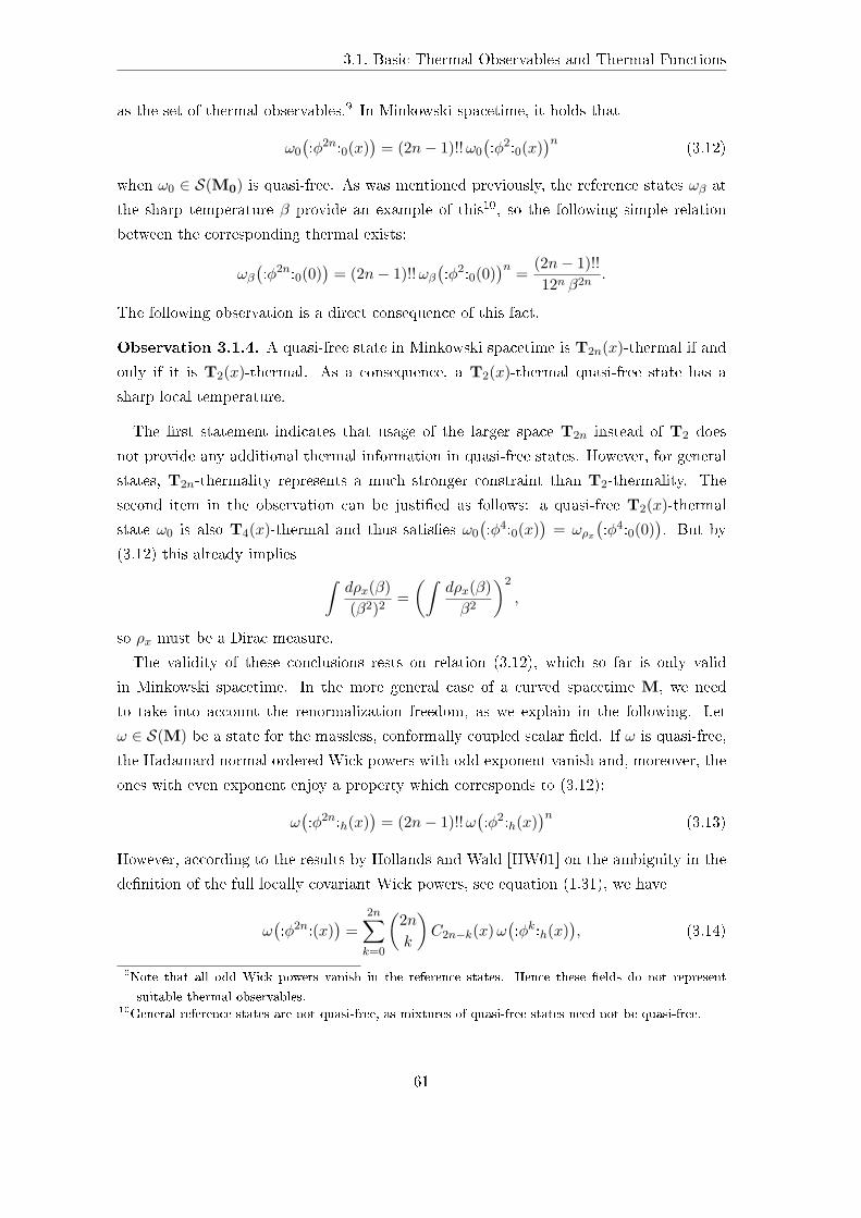
3.1. Basic Thermal Observables and Thermal Functions
as the set of thermal observables.9 In Minkowski spacetime, it holds that
ω0
(:φ2n:0(x)
)= (2n− 1)!!ω0
(:φ2:0(x)
)n(3.12)
when ω0 ∈ S(M0) is quasi-free. As was mentioned previously, the reference states ωβ at
the sharp temperature β provide an example of this10, so the following simple relation
between the corresponding thermal exists:
ωβ(:φ2n:0(0)
)= (2n− 1)!!ωβ
(:φ2:0(0)
)n =(2n− 1)!!12n β2n
.
The following observation is a direct consequence of this fact.
Observation 3.1.4. A quasi-free state in Minkowski spacetime is T2n(x)-thermal if and
only if it is T2(x)-thermal. As a consequence, a T2(x)-thermal quasi-free state has a
sharp local temperature.
The rst statement indicates that usage of the larger space T2n instead of T2 does
not provide any additional thermal information in quasi-free states. However, for general
states, T2n-thermality represents a much stronger constraint than T2-thermality. The
second item in the observation can be justied as follows: a quasi-free T2(x)-thermal
state ω0 is also T4(x)-thermal and thus satises ω0
(:φ4:0(x)
)= ωρx
(:φ4:0(0)
). But by
(3.12) this already implies ∫dρx(β)(β2)2
=(∫
dρx(β)β2
)2
,
so ρx must be a Dirac measure.
The validity of these conclusions rests on relation (3.12), which so far is only valid
in Minkowski spacetime. In the more general case of a curved spacetime M, we need
to take into account the renormalization freedom, as we explain in the following. Let
ω ∈ S(M) be a state for the massless, conformally coupled scalar eld. If ω is quasi-free,
the Hadamard normal ordered Wick powers with odd exponent vanish and, moreover, the
ones with even exponent enjoy a property which corresponds to (3.12):
ω(:φ2n:h(x)
)= (2n− 1)!!ω
(:φ2:h(x)
)n(3.13)
However, according to the results by Hollands and Wald [HW01] on the ambiguity in the
denition of the full locally covariant Wick powers, see equation (1.31), we have
ω(:φ2n:(x)
)=
2n∑k=0
(2nk
)C2n−k(x)ω
(:φk:h(x)
), (3.14)
9Note that all odd Wick powers vanish in the reference states. Hence these elds do not represent
suitable thermal observables.10General reference states are not quasi-free, as mixtures of quasi-free states need not be quasi-free.
61
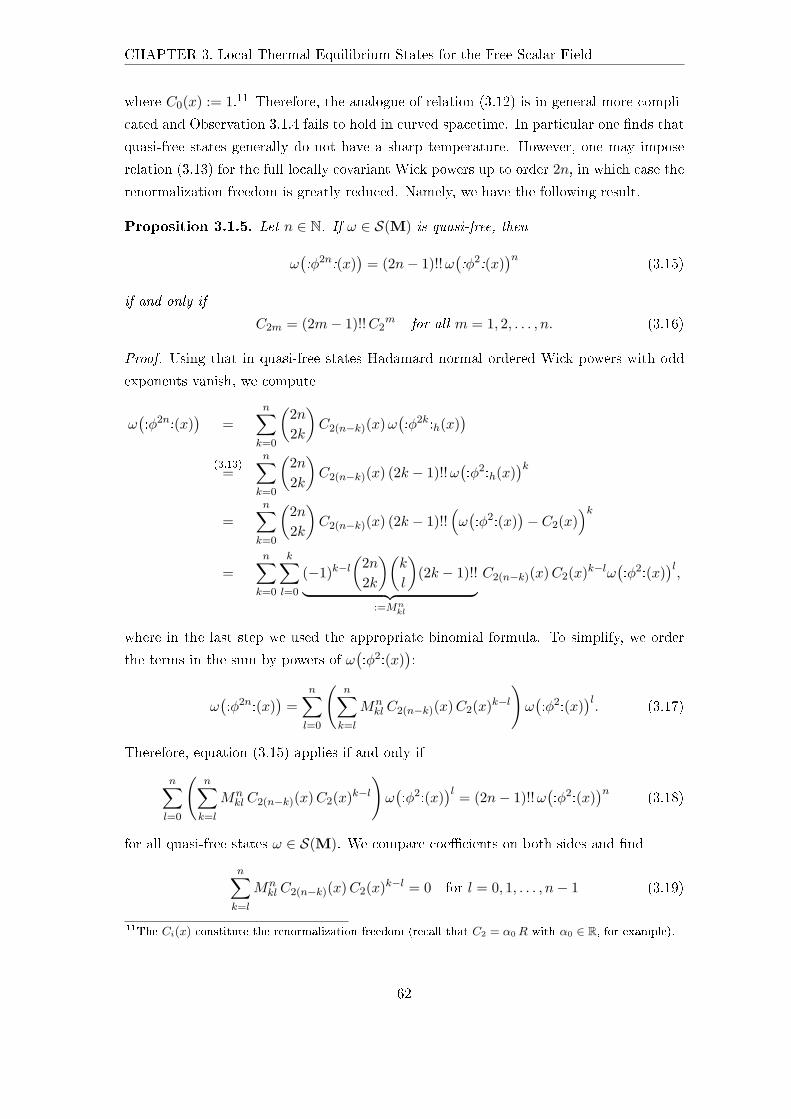
CHAPTER 3. Local Thermal Equilibrium States for the Free Scalar Field
where C0(x) := 1.11 Therefore, the analogue of relation (3.12) is in general more compli-
cated and Observation 3.1.4 fails to hold in curved spacetime. In particular one nds that
quasi-free states generally do not have a sharp temperature. However, one may impose
relation (3.13) for the full locally covariant Wick powers up to order 2n, in which case the
renormalization freedom is greatly reduced. Namely, we have the following result.
Proposition 3.1.5. Let n ∈ N. If ω ∈ S(M) is quasi-free, then
ω(:φ2n:(x)
)= (2n− 1)!!ω
(:φ2:(x)
)n(3.15)
if and only if
C2m = (2m− 1)!!C2m for all m = 1, 2, . . . , n. (3.16)
Proof. Using that in quasi-free states Hadamard normal ordered Wick powers with odd
exponents vanish, we compute
ω(:φ2n:(x)
)=
n∑k=0
(2n2k
)C2(n−k)(x)ω
(:φ2k:h(x)
)(3.13)
=n∑k=0
(2n2k
)C2(n−k)(x) (2k − 1)!!ω
(:φ2:h(x)
)k=
n∑k=0
(2n2k
)C2(n−k)(x) (2k − 1)!!
(ω(:φ2:(x)
)− C2(x)
)k=
n∑k=0
k∑l=0
(−1)k−l(
2n2k
)(k
l
)(2k − 1)!!︸ ︷︷ ︸
:=Mnkl
C2(n−k)(x)C2(x)k−lω(:φ2:(x)
)l,
where in the last step we used the appropriate binomial formula. To simplify, we order
the terms in the sum by powers of ω(:φ2:(x)
):
ω(:φ2n:(x)
)=
n∑l=0
(n∑k=l
Mnkl C2(n−k)(x)C2(x)k−l
)ω(:φ2:(x)
)l. (3.17)
Therefore, equation (3.15) applies if and only if
n∑l=0
(n∑k=l
Mnkl C2(n−k)(x)C2(x)k−l
)ω(:φ2:(x)
)l = (2n− 1)!!ω(:φ2:(x)
)n(3.18)
for all quasi-free states ω ∈ S(M). We compare coecients on both sides and nd
n∑k=l
Mnkl C2(n−k)(x)C2(x)k−l = 0 for l = 0, 1, . . . , n− 1 (3.19)
11The Ci(x) constitute the renormalization freedom (recall that C2 = α0R with α0 ∈ R, for example).
62
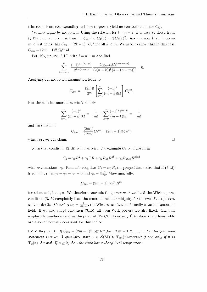
3.1. Basic Thermal Observables and Thermal Functions
(the coecients corresponding to the n-th power yield no constraints on the Ci).
We now argue by induction. Using the relation for l = n − 2, it is easy to check from
(3.19) that our claim is true for C4, i.e. C4(x) = 3C2(x)2. Assume now that for some
m < n it holds that C2k = (2k− 1)!!C2k for all k < m. We need to show that in this case
C2m = (2m− 1)!!C2m also.
For this, we use (3.19) with l = n−m and nd
n∑k=n−m
(−1)k−(n−m)
2k−(n−m)
C2(n−k)C2k−(n−m)
(2(n− k))! (k − (n−m))!= 0.
Applying our induction assumption leads to
C2m = −(2m)!2m
[m∑k=1
(−1)k
(m− k)!k!
]C2
m.
But the sum in square brackets is simply
m∑k=1
(−1)k
(m− k)!k!= − 1
m!+
m∑k=0
(−1)k1m−k
(m− k)!k!= − 1
m!
and we thus nd
C2m =(2m)!2mm!
C2m = (2m− 1)!!C2
m,
which proves our claim.
Note that condition (3.16) is non-trivial. For example C4 is of the form
C4 = γ0R2 + γ1R+ γ2RabR
ab + γ3RabcdRabcd
with real constants γi. Remembering that C2 = α0R, the proposition states that if (3.15)
is to hold, then γ1 = γ2 = γ3 = 0 and γ0 = 3α20. More generally,
C2m = (2m− 1)!!αm0 Rm
for all m = 1, 2, . . . , n. We therefore conclude that, once we have xed the Wick square,
condition (3.15) completely xes the renormalization ambiguity for the even Wick powers
up to order 2n. Choosing α0 = 1288π2 , the Wick square is a conformally covariant quantum
eld. If we also adopt condition (3.15), all even Wick powers are also xed. One can
employ the methods used in the proof of [Pin09, Theorem 3.1] to show that these elds
are also conformally covariant for this choice.
Corollary 3.1.6. If C2m = (2m− 1)!! αm0 Rm for all m = 1, 2, . . . , n, then the following
statement is true: A quasi-free state ω ∈ S(M) is T2n(x)-thermal if and only if it is
T2(x)-thermal. If n ≥ 2, then the state has a sharp local temperature.
63
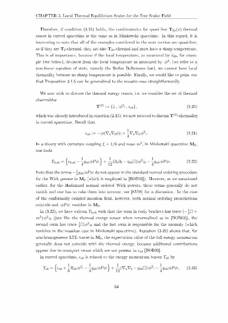
CHAPTER 3. Local Thermal Equilibrium States for the Free Scalar Field
Therefore, if condition (3.15) holds, the combinatorics for quasi-free T2n(x)-thermal
states in curved spacetime is the same as in Minkowski spacetime. In this regard, it is
interesting to note that all of the examples considered in the next section are quasi-free,
so if they are T2-thermal, they are also T2n-thermal and must have a sharp temperature.
This is of importance, because if the local temperature, as measured by ε00, for exam-
ple (see below), deviates from the local temperature as measured by :φ2: (we refer to a
non-linear equation of state, namely the Stefan Boltzmann law), we cannot have local
thermality because no sharp temperature is possible. Finally, we would like to point out
that Proposition 3.1.5 can be generalized to the massive case straightforwardly.
We now wish to discuss the thermal energy tensor, i.e. we consider the set of thermal
observables
T(2) := 1 , :φ2: , εab, (3.20)
which was already introduced in equation (2.15), we now proceed to discussT(2)-thermality
in curved spacetime. Recall that
εab := −:φ(∇a∇bφ): +14∇a∇b:φ2:. (3.21)
In a theory with curvature coupling ξ = 1/6 and mass m2, in Minkowski spacetime M0,
one nds
T0,ab =ε0,ab −
14gab:φPφ:
+
112
(∂a∂b − ηab):φ2:0 −14gab:φPφ:. (3.22)
Note that the terms −14gab:φPφ: do not appear in the standard normal ordering procedure
for the Wick powers in M0 (which is employed in [BOR02]). However, as we mentioned
earlier, for the Hadamard normal ordered Wick powers, these terms generally do not
vanish and one has to take them into account, see [SV08] for a discussion. In the case
of the conformally coupled massless eld, however, both normal ordering prescriptions
coincide and :φPφ: vanishes in M0.
In (3.22), we have written T0,ab such that the term in curly brackets has trace (−14 +
m2):φ2:0 (just like the thermal energy tensor when renormalized as in [BOR02]), the
second term has trace 14:φ2:0 and the last term is responsible for the anomaly (which
vanishes in the massless case in Minkowski spacetime). Equation (3.22) shows that, for
non-homogeneous LTE states in M0, the expectation value of the full energy momentum
generally does not coincide with the thermal energy, because additional contributions
appear due to transport terms which are not present in εab [BOR02].
In curved spacetime, εab is related to the energy momentum tensor Tab by
Tab =εab +
16Rab:φ
2:− 14gab:φPφ:
+
112
(∇a∇b − gab):φ2:− 14gab:φPφ:, (3.23)
64
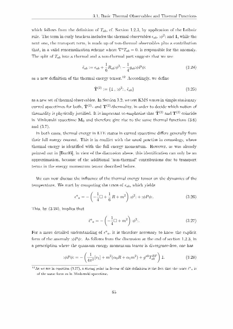
3.1. Basic Thermal Observables and Thermal Functions
which follows from the denition of Tab, cf. Section 1.2.3, by application of the Leibniz
rule. The term in curly brackets includes the thermal observables εab, :φ2: and 1, while the
next one, the transport term, is made up of non-thermal observables plus a contribution
that, in a valid renormalization scheme where ∇aTab = 0, is responsible for the anomaly.
The split of Tab into a thermal and a non-thermal part suggests that we use
εab := εab +16Rab:φ
2:− 14gab:φPφ: (3.24)
as a new denition of the thermal energy tensor.12 Accordingly, we dene
T(2) := 1 , :φ2: , εab (3.25)
as a new set of thermal observables. In Section 3.2, we test KMS states in simple stationary
curved spacetimes for both, T(2)- and T(2)-thermality, in order to decide which notion of
thermality is physically justied. It is important to emphasize that T(2) and T(2) coincide
in Minkowski spacetime M0 and therefore give rise to the same thermal functions (3.6)
and (3.7).
In both cases, thermal energy in LTE states in curved spacetime diers generally from
their full energy content. This is in conict with the usual practise in cosmology, where
thermal energy is identied with the full energy momentum. However, as was already
pointed out in [Buc03], in view of the discussion above, this identication can only be an
approximation, because of the additional non-thermal contributions due to transport
terms in the energy momentum tensor described before.
We can now discuss the inuence of the thermal energy tensor on the dynamics of the
temperature. We start by computing the trace of εab, which yields
εaa = −(−1
4 +
16R+m2
):φ2: + :φPφ:. (3.26)
This, by (3.24), implies that
εaa = −(−1
4 +m2
):φ2:. (3.27)
For a more detailed understanding of εaa, it is therefore necessary to know the explicit
form of the anomaly :φPφ:. As follows from the discussion at the end of section 1.2.3, in
a prescription where the quantum energy momentum tensor is divergence-free, one has
:φPφ: = −(
14π2
[v1] +m2(α0R+ α1m2) + gabTRFab
)1. (3.28)
12As we see in equation (3.27), a strong point in favour of this denition is the fact that the trace εaa is
of the same form as in Minkowski spacetime.
65
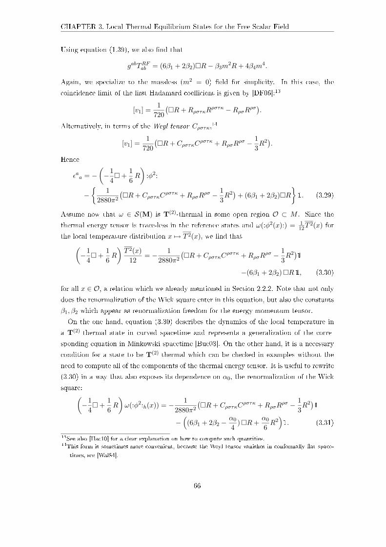
CHAPTER 3. Local Thermal Equilibrium States for the Free Scalar Field
Using equation (1.39), we also nd that
gabTRFab = (6β1 + 2β2)R− β3m2R+ 4β4m
4.
Again, we specialize to the massless (m2 = 0) eld for simplicity. In this case, the
coincidence limit of the rst Hadamard coecient is given by [DF06]:13
[v1] =1
720(R+RρστκR
ρστκ −RρσRρσ).
Alternatively, in terms of the Weyl tensor Cρστκ,14
[v1] =1
720(R+ CρστκC
ρστκ +RρσRρσ − 1
3R2).
Hence
εaa = −(−1
4 +
16R
):φ2:
−
12880π2
(R+ CρστκC
ρστκ +RρσRρσ − 1
3R2)
+ (6β1 + 2β2)R1. (3.29)
Assume now that ω ∈ S(M) is T(2)-thermal in some open region O ⊂ M . Since the
thermal energy tensor is trace-less in the reference states and ω(:φ2(x):) = 112T
2(x) for
the local temperature distribution x 7→ T 2(x), we nd that(−1
4 +
16R
)T 2(x)
12= − 1
2880π2
(R+ CρστκC
ρστκ +RρσRρσ − 1
3R2)1
−(6β1 + 2β2) R1, (3.30)
for all x ∈ O, a relation which we already mentioned in Section 2.2.2. Note that not only
does the renormalization of the Wick square enter in this equation, but also the constants
β1, β2 which appear as renormalization freedom for the energy momentum tensor.
On the one hand, equation (3.30) describes the dynamics of the local temperature in
a T(2)-thermal state in curved spacetime and represents a generalization of the corre-
sponding equation in Minkowski spacetime [Buc03]. On the other hand, it is a necessary
condition for a state to be T(2)-thermal which can be checked in examples without the
need to compute all of the components of the thermal energy tensor. It is useful to rewrite
(3.30) in a way that also exposes its dependence on α0, the renormalization of the Wick
square:(−1
4 +
16R
)ω(:φ2:h(x)) = − 1
2880π2
(R+ CρστκC
ρστκ +RρσRρσ − 1
3R2)1
−(
(6β1 + 2β2 −α0
4) R+
α0
6R2)1. (3.31)
13See also [Hac10] for a clear explanation on how to compute such quantities.14This form is sometimes more convenient, because the Weyl tensor vanishes in conformally at space-
times, see [Wal84].
66
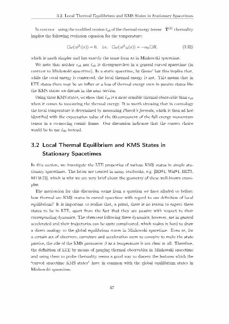
3.2. Local Thermal Equilibrium and KMS States in Stationary Spacetimes
In contrast - using the modied version εab of the thermal energy tensor - T(2)-thermality
implies the following evolution equation for the temperature:
ω(:φ2:(x)) = 0, i.e. ω(:φ2:h(x)) = −α0 R, (3.32)
which is much simpler and has exactly the same form as in Minkowski spacetime.
We note that neither εab nor εab is divergence-free in a general curved spacetime (in
contrast to Minkowski spacetime). In a static spacetime, by Gauss' law this implies that,
while the total energy is conserved, the local thermal energy is not. This means that in
LTE states there may be an inux or a loss of thermal energy even in passive states like
the KMS states we discuss in the next section.
Using these KMS states, we show that εab is a more sensible thermal observable than εab
when it comes to measuring the thermal energy. It is worth stressing that in cosmology
the local temperature is determined by measuring Planck's formula, which is then ad hoc
identied with the expectation value of the 00-component of the full energy momentum
tensor in a co-moving cosmic frame. Our discussion indicates that the correct choice
would be to use ε00 instead.
3.2 Local Thermal Equilibrium and KMS States in
Stationary Spacetimes
In this section, we investigate the LTE properties of various KMS states in simple sta-
tionary spacetimes. The latter are treated in many textbooks, e.g. [BD84, Wal84, HE73,
MTW73], which is why we are very brief about the geometry of these well-known exam-
ples.
The motivation for this discussion stems from a question we have alluded to before:
how thermal are KMS states in curved spacetime with regard to our denition of local
equilibrium? It is important to realize that, a priori, there is no reason to expect these
states to be in LTE, apart from the fact that they are passive with respect to their
corresponding dynamics. The observers following these dynamics, however, are in general
accelerated and their trajectories can be quite complicated, which makes it hard to draw
a direct analogy to the global equilibrium states in Minkowski spacetime. Even as, for
a certain set of observers, curvature and acceleration seem to conspire to make the state
passive, the rôle of the KMS parameter β as a temperature is not clear at all. Therefore,
the denition of LTE by means of gauging thermal observables in Minkowski spacetime
and using them to probe thermality seems a good way to discern the features which the
curved spacetime KMS states have in common with the global equilibrium states in
Minkowski spacetime.
67
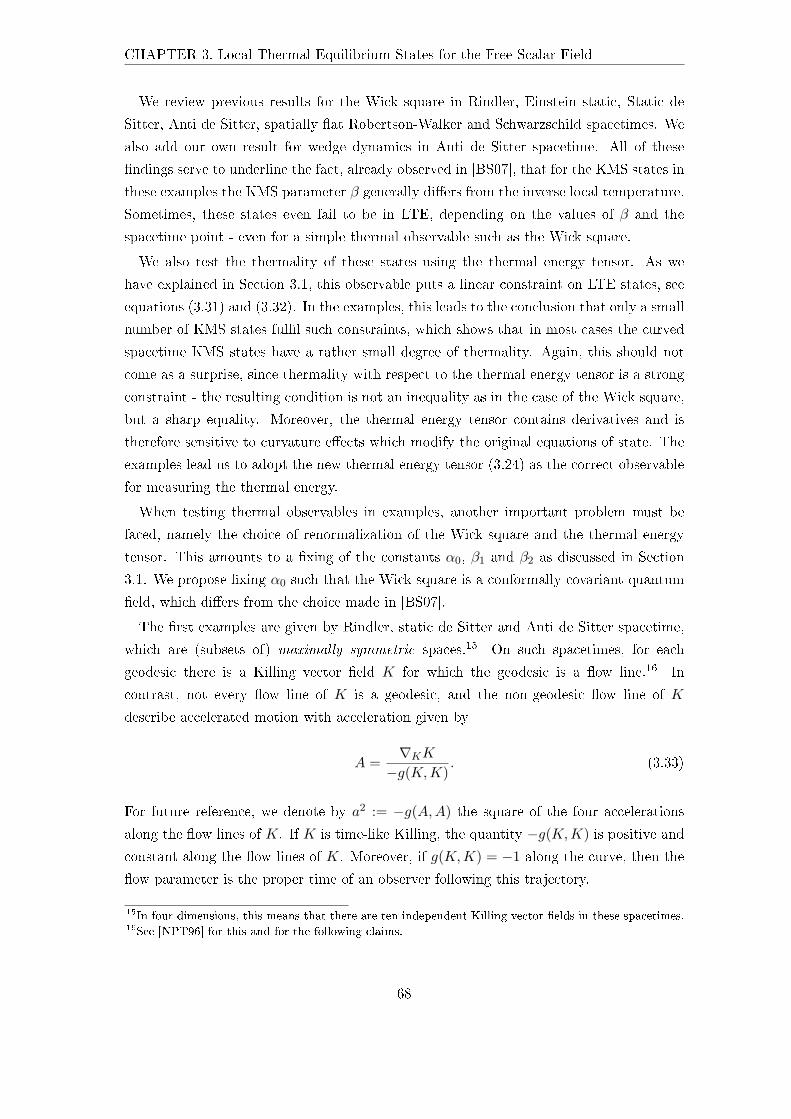
CHAPTER 3. Local Thermal Equilibrium States for the Free Scalar Field
We review previous results for the Wick square in Rindler, Einstein static, Static de
Sitter, Anti de Sitter, spatially at Robertson-Walker and Schwarzschild spacetimes. We
also add our own result for wedge dynamics in Anti de Sitter spacetime. All of these
ndings serve to underline the fact, already observed in [BS07], that for the KMS states in
these examples the KMS parameter β generally diers from the inverse local temperature.
Sometimes, these states even fail to be in LTE, depending on the values of β and the
spacetime point - even for a simple thermal observable such as the Wick square.
We also test the thermality of these states using the thermal energy tensor. As we
have explained in Section 3.1, this observable puts a linear constraint on LTE states, see
equations (3.31) and (3.32). In the examples, this leads to the conclusion that only a small
number of KMS states full such constraints, which shows that in most cases the curved
spacetime KMS states have a rather small degree of thermality. Again, this should not
come as a surprise, since thermality with respect to the thermal energy tensor is a strong
constraint - the resulting condition is not an inequality as in the case of the Wick square,
but a sharp equality. Moreover, the thermal energy tensor contains derivatives and is
therefore sensitive to curvature eects which modify the original equations of state. The
examples lead us to adopt the new thermal energy tensor (3.24) as the correct observable
for measuring the thermal energy.
When testing thermal observables in examples, another important problem must be
faced, namely the choice of renormalization of the Wick square and the thermal energy
tensor. This amounts to a xing of the constants α0, β1 and β2 as discussed in Section
3.1. We propose xing α0 such that the Wick square is a conformally covariant quantum
eld, which diers from the choice made in [BS07].
The rst examples are given by Rindler, static de Sitter and Anti de Sitter spacetime,
which are (subsets of) maximally symmetric spaces.15 On such spacetimes, for each
geodesic there is a Killing vector eld K for which the geodesic is a ow line.16 In
contrast, not every ow line of K is a geodesic, and the non-geodesic ow line of K
describe accelerated motion with acceleration given by
A =∇KK−g(K,K)
. (3.33)
For future reference, we denote by a2 := −g(A,A) the square of the four accelerations
along the ow lines of K. If K is time-like Killing, the quantity −g(K,K) is positive and
constant along the ow lines of K. Moreover, if g(K,K) = −1 along the curve, then the
ow parameter is the proper time of an observer following this trajectory.
15In four dimensions, this means that there are ten independent Killing vector elds in these spacetimes.16See [NPT96] for this and for the following claims.
68
3.2. Local Thermal Equilibrium and KMS States in Stationary Spacetimes
Rindler spacetime We start with Rindler spacetime R. This at spacetime can be
realized as the subset x ∈ R4 | x1 > |x0| of Minkowski spacetime, the metric g being
the Minkowski metric, restricted to this subset. There is a positive time-like Killing vector
K = x1∂0 − x0∂1 which generates the Lorentz boosts in x1-direction. Petersen [Pet07]
has investigated the corresponding KMS states ωβ . His result for the Wick square reads:
ωβ(:φ2:(x)) =1
−gx(K,K)
(1
12β2− 1
12(2π)2
). (3.34)
Note that this is equal to the expectation value of the Hadamard normal ordered Wick
square, because the renormalization freedom is not present due to the atness of Rindler
spacetime. Note also that1
−gx(K,K)= a2(x),
where a2(x) is the square of the four acceleration of the trajectory passing through x. ω2π
is the Unruh state (i.e. the restriction of the Minkowski vacuum), which has ω2π(:φ2:) = 0,
i.e. a local temperature of zero. KMS-States with β > 2π are not in local equilibrium,
because in that case ωβ(:φ2:) < 0.
Applying the linear constraint arising from εab (3.30) or εab (3.32) to (3.34) immediately
yields the constraint β!= 2π in both cases, which shows that of all the β-KMS states with
respect to the dynamics of an uniformly accelerated observer in Minkowski spacetime,
only the Unruh state can be in LTE with regard to the thermal energy tensor. Already in
this example we witness the restrictive nature of the linear constraint which arises from
the trace of the thermal energy tensor.
de Sitter spacetime The next example is de Sitter spacetime dSα, which is maximally
symmetric with constant positive curvature. dSα can be represented as hyperboloid,
embedded in R5,
dSα := x ∈ R5 | − x20 + x2
1 + x22 + x2
3 + x24 = α2,
where α ∈ R \ 0 is the radius of dSα. The metric g is given by the Minkowski metric of
ambient R5, restricted to dSα.
In de Sitter spacetime, there are no time-like vector elds which are also geodesic.
Moreover, a freely falling observer following a geodesic world line γ does not have a
global notion of dynamics, because the corresponding Killing vector eld is not time-like
everywhere and hence the union of the past and the future of γ is not all of dSα. By
symmetry17, we can focus attention to the Killing vector eld which can be written as
17The symmetry group of dSα is the restriction of the proper orthochronous Lorentz group of ambient
R5 to dSα.
69
CHAPTER 3. Local Thermal Equilibrium States for the Free Scalar Field
K1 := x1∂0 − x0∂1. K1 is positive time-like only in the wedge
W+ = x ∈ dSα | |x0| < x1.
The Killing ow generated by K1 can be represented as
χ : t 7→
cosh(t) sinh(t)
sinh(t) cosh(t)
13
. (3.35)
W+1 is the causal completion of the geodesic γ0(t) := χt(y). Here, y := (0, α, 0, 0, 0) and
t is the Killing ow parameter, which is related to the proper time s, as measured by
an observer following γ0, by s = αt. We note that W+1 is also the causal completion of
any other time-like curve contained in it and moreover it is bounded by a bifurcate event
horizon at x0 = x1. As a globally hyperbolic spacetime, the interior of the wedge is called
static de Sitter spacetime, which we denote by dSα,stat.
We denote by αtt∈R the one-parameter group of automorphisms induced by χtt∈R,
acting on the extended algebra of observables W(dSα,stat). For β > 0, one may construct
(β, αt)-KMS states ωβ , and Buchholz and Schlemmer [BS07, Sch05] have calculated the
expectation value of the Wick square in these states:18
ωβ(:φ2:(x)) =1
−gx(K1,K1)
(1
12β2− 1
12(2π)2
)− 1
24π2α2+ α0
12α2. (3.36)
Note that apart from the special case β = 2π, the Gibbons-Hawking state, the ωβ cannot
be extended to Hadamard states on W(dSα) [NPT96].
The quantity −gx(K1,K1) > 0, being constant along the ow lines of K1, is a char-
acteristic of the Killing trajectory through x ∈ W+. It is related to the acceleration
a2(x) := gx(A,A), cf. equation (3.33), by
1−gx(K1,K1)
= a2(x) +1α2. (3.37)
18In fact, there has been some confusion regarding this result as presented in [BS07]. On page 5, as
Stottmeister [Sto09, p. 64] has pointed out, there is an error in the expansion of the Hadamard
parametrix (it should read · · ·+ R192π2 instead of the value given there), which then reappears in the
equations on page 6 (namely in the calculation preceding eqn. (11)). However, Schlemmer calculated
the expectation values of the Hadamard normal ordered Wick square correctly in his Diploma thesis
[Sch05, p. 53], on which [BS07, eqn. (11)] and the value of α0 = 1192π2 given there are based. Thus
the errors mentioned here merely occur in the presentation of the steps leading to these nal results,
which are indeed correct. Unfortunately, Stottmeister took these mistakes into account when he gave
a corrected constant α0 and used it in the interpretation of his results for Einstein Static and Anti de
Sitter Spacetime. Even though he computed the expectation values of the Hadamard normal ordered
Wick square correctly in these examples, his conclusions therefore need to be re-examined. I am
grateful for the support of the authors in the identication of these errors.
70
3.2. Local Thermal Equilibrium and KMS States in Stationary Spacetimes
Note that an observer following the Killing trajectory through x ∈ W+1 has proper time
s(x) =√−gx(K1,K1)t, where t is the Killing ow parameter of K1. The dynamics of
these observers is implemented by the one parameter group of automorphisms αs(x)tand it is easy to see that the ωβ are KMS states with respect to this one parameter group
of automorphisms, albeit with new parameter
β(x) :=β√
−gx(K1,K1). (3.38)
Therefore, these observers feel a shift in the KMS parameter of these states; sometimes
called the Tolman redshift.
Using R = 12/α2, RρσRρσ − 1
3R2 = −12/α4 and the fact that dSα,stat is conformally
at (i.e. the Weyl tensor vanishes), we nd the following constraint resulting from the
dynamics of the temperature, (3.31):
α2
−gx(K1,K1)
(1
−gx(K1,K1)+
12α2
)(1
12β2− 1
12(2π)2
)− 1
12π2α2=
1240π2α2
− 24α2α0.
(3.39)
This equation seems quite restrictive, but if we use εab instead, we obtain the condition(1
−gx(K1,K1)+
12α2
)(1
12β2− 1
12(2π)2
)= 0, (3.40)
which shows that the Gibbons Hawking state is the only KMS state which is in LTE with
respect to this thermal observable, because the rst factor is always positive in dSα,stat.
Recall that in Rindler spacetime, we have the same result for the Unruh state. This leads
us to adopt εab as the correct choice for the thermal energy tensor.
Anti de Sitter spacetime The next example is Anti de Sitter spacetime. Proper Anti
de Sitter spacetime AdS′α is the maximally symmetric spacetime with constant negative
curvature. As de Sitter spacetime, AdS′α is realized as a hyperquadric in R5:
AdS′α := x ∈ R5 | − (x0)2 − (x1)2 + (x2)2 + (x3)2 + (x4)2 = −α2, (3.41)
where α ∈ R \ 0 again denotes the radius. The metric g is the Minkowski metric of
ambient R5, restricted to AdS′α. However, unlike the other maximally symmetric space-
times M0 and dSα, proper Anti de Sitter spacetime AdS′α is not globally hyperbolic (cf.
Theorem 1.1.3). It is neither causal (quite obviously, there are closed time-like curves)
nor does equation (1.1) hold. The rst problem can be avoided by passing to the uni-
versal cover AdSα, to which we refer as Anti de Sitter spacetime. However, it can be
shown that the second problem cannot be avoided. Therefore, even AdSα is not globally
hyperbolic. However, QFT in Anti de Sitter spacetime has received much attention for
many years now, and this provides motivation to perform our investigation despite these
71
CHAPTER 3. Local Thermal Equilibrium States for the Free Scalar Field
causal pathologies. Moreover, due to its simple structure and its similarity to de Sitter
spacetime, AdSα provides an interesting testing ground for the ideas discussed here.19
There are two kinds of (locally) time-like Killing vector elds in AdSα. The rst we
call L; it is time-like everywhere and gives rise to the Killing ow
φ : t 7→
cos(t) sin(t)
− sin(t) cos(t)
13
. (3.42)
The corresponding trajectories are not geodesic except for γ0(t) := φt(y) with y :=
(0, α, 0, 0, 0).
Stottmeister [Sto09] has computed the expectation value of the Wick square for β-KMS
states with respect to this ow. His result is
ωβ(:φ2:(x)) =1
−gx(L,L)· 1
4π2
( ∞∑n=0
n
enβ − 1+
12
∞∑n=1
1cosh(βn)− 1
)
+1
24π2α2− 12α2α0. (3.43)
The series appearing in this formula tend to zero as β →∞, so the expectation value in
the corresponding ground state reads
limβ→∞
ωβ(:φ2:(x)) =1
24π2α2− 12α2α0. (3.44)
Using εab, the dynamics of the local temperature (3.32) yields the constraint:
(1
−gx(L,L)+
1α2
)1
4π2
( ∞∑n=0
n
enβ − 1+
12
∞∑n=1
1cosh(βn)− 1
)= 0, (3.45)
which shows that the ground state β →∞ is in local thermal equilibrium.
The second type of Killing elds is time-like only in wedge-shaped regions, similar to the
ones appearing in de Sitter spacetime. Of the several possibilities, we focus our attention
19Given a lcQFT A, there is a method of constructing an algebra of observables A(M) on a non-globally
hyperbolic spacetime M. It essentially requires that every point in M possesses a globally hyperbolic
neighbourhood N (with some choice of time orientation) such that the subalgebra A(M; N) of A(M)
consisting of eld polynomials smeared with test functions with support in N coincides with the
intrinsic algebra A(N), obtained by the functor A. See [FH96] and references therein for details. We
do not comment further on this approach, but assume that the free scalar quantum eld and its Wick
powers have been constructed in AdSα, choosing transparent boundary conditions for the Green's
operators of the eld, see [Sto09] for discussion.
72
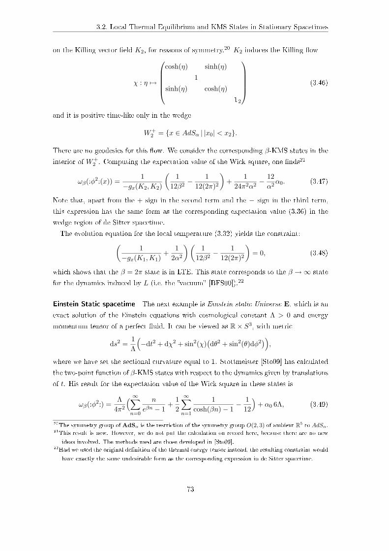
3.2. Local Thermal Equilibrium and KMS States in Stationary Spacetimes
on the Killing vector eld K2, for reasons of symmetry.20 K2 induces the Killing ow
χ : η 7→
cosh(η) sinh(η)
1
sinh(η) cosh(η)
12
(3.46)
and it is positive time-like only in the wedge
W+2 = x ∈ AdSα | |x0| < x2.
There are no geodesics for this ow. We consider the corresponding β-KMS states in the
interior of W+2 . Computing the expectation value of the Wick square, one nds21
ωβ(:φ2:(x)) =1
−gx(K2,K2)
(1
12β2− 1
12(2π)2
)+
124π2α2
− 12α2α0. (3.47)
Note that, apart from the + sign in the second term and the − sign in the third term,
this expression has the same form as the corresponding expectation value (3.36) in the
wedge region of de Sitter spacetime.
The evolution equation for the local temperature (3.32) yields the constraint:(1
−gx(K1,K1)+
12α2
)(1
12β2− 1
12(2π)2
)= 0, (3.48)
which shows that the β = 2π state is in LTE. This state corresponds to the β →∞ state
for the dynamics induced by L (i.e. the vacuum [BFS00]).22
Einstein Static spacetime The next example is Einstein static Universe E, which is an
exact solution of the Einstein equations with cosmological constant Λ > 0 and energy
momentum tensor of a perfect uid. It can be viewed as R× S3, with metric
ds2 =1Λ
(−dt2 + dχ2 + sin2(χ)
(dθ2 + sin2(θ)dφ2
)),
where we have set the sectional curvature equal to 1. Stottmeister [Sto09] has calculated
the two-point function of β-KMS states with respect to the dynamics given by translations
of t. His result for the expectation value of the Wick square in these states is
ωβ(:φ2:) =Λ
4π2
( ∞∑n=0
n
eβn − 1+
12
∞∑n=1
1cosh(βn)− 1
− 112
)+ α0 6Λ, (3.49)
20The symmetry group of AdSα is the restriction of the symmetry group O(2, 3) of ambient R5 to AdSα.21This result is new. However, we do not put the calculation on record here, because there are no new
ideas involved. The methods used are those developed in [Sto09].22Had we used the original denition of the thermal energy tensor instead, the resulting constraint would
have exactly the same undesirable form as the corresponding expression in de Sitter spacetime.
73
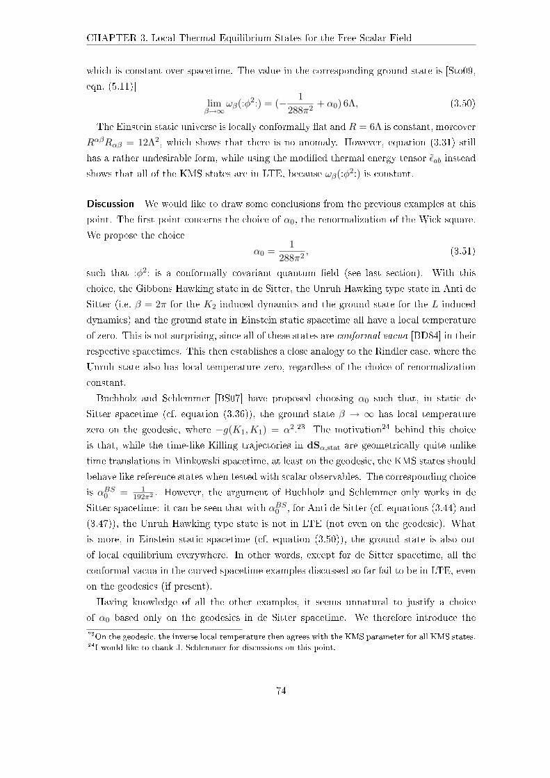
CHAPTER 3. Local Thermal Equilibrium States for the Free Scalar Field
which is constant over spacetime. The value in the corresponding ground state is [Sto09,
eqn. (5.11)]
limβ→∞
ωβ(:φ2:) = (− 1288π2
+ α0) 6Λ, (3.50)
The Einstein static universe is locally conformally at and R = 6Λ is constant, moreover
RαβRαβ = 12Λ2, which shows that there is no anomaly. However, equation (3.31) still
has a rather undesirable form, while using the modied thermal energy tensor εab instead
shows that all of the KMS states are in LTE, because ωβ(:φ2:) is constant.
Discussion We would like to draw some conclusions from the previous examples at this
point. The rst point concerns the choice of α0, the renormalization of the Wick square.
We propose the choice
α0 =1
288π2, (3.51)
such that :φ2: is a conformally covariant quantum eld (see last section). With this
choice, the Gibbons Hawking state in de Sitter, the Unruh Hawking type state in Anti de
Sitter (i.e. β = 2π for the K2-induced dynamics and the ground state for the L-induced
dynamics) and the ground state in Einstein static spacetime all have a local temperature
of zero. This is not surprising, since all of these states are conformal vacua [BD84] in their
respective spacetimes. This then establishes a close analogy to the Rindler case, where the
Unruh state also has local temperature zero, regardless of the choice of renormalization
constant.
Buchholz and Schlemmer [BS07] have proposed choosing α0 such that, in static de
Sitter spacetime (cf. equation (3.36)), the ground state β → ∞ has local temperature
zero on the geodesic, where −g(K1,K1) = α2.23 The motivation24 behind this choice
is that, while the time-like Killing trajectories in dSα,stat are geometrically quite unlike
time translations in Minkowski spacetime, at least on the geodesic, the KMS states should
behave like reference states when tested with scalar observables. The corresponding choice
is αBS0 = 1192π2 . However, the argument of Buchholz and Schlemmer only works in de
Sitter spacetime: it can be seen that with αBS0 , for Anti de Sitter (cf. equations (3.44) and
(3.47)), the Unruh Hawking type state is not in LTE (not even on the geodesic). What
is more, in Einstein static spacetime (cf. equation (3.50)), the ground state is also out
of local equilibrium everywhere. In other words, except for de Sitter spacetime, all the
conformal vacua in the curved spacetime examples discussed so far fail to be in LTE, even
on the geodesics (if present).
Having knowledge of all the other examples, it seems unnatural to justify a choice
of α0 based only on the geodesics in de Sitter spacetime. We therefore introduce the
23On the geodesic, the inverse local temperature then agrees with the KMS parameter for all KMS states.24I would like to thank J. Schlemmer for discussions on this point.
74
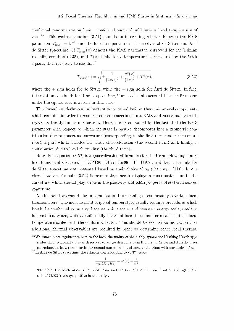
3.2. Local Thermal Equilibrium and KMS States in Stationary Spacetimes
conformal renormalization here - conformal vacua should have a local temperature of
zero.25 This choice, equation (3.51), entails an interesting relation between the KMS
parameter TKMS = β−1 and the local temperature in the wedges of de Sitter and Anti
de Sitter spacetime. If TKMS(x) denotes the KMS parameter, corrected for the Tolman
redshift, equation (3.38), and T (x) is the local temperature as measured by the Wick
square, then it is easy to see that26
TKMS(x) =
ñ 1
(2πα)2+a2(x)(2π)2
+ T 2(x), (3.52)
where the + sign holds for de Sitter, while the − sign holds for Anti de Sitter. In fact,
this relation also holds for Rindler spacetime, if one takes into account that the rst term
under the square root is absent in that case.
This formula underlines an important point raised before: there are several components
which combine in order to render a curved spacetime state KMS and hence passive with
regard to the dynamics in question. Here, this is embodied by the fact that the KMS
parameter with respect to which the state is passive decomposes into a geometric con-
tribution due to spacetime curvature (corresponding to the rst term under the square
root), a part which encodes the eect of acceleration (the second term) and, nally, a
contribution due to local thermality (the third term).
Note that equation (3.52) is a generalization of formulas for the Unruh-Hawking states
rst found and discussed in [NPT96, DL97, Jac98]. In [BS07], a dierent formula for
de Sitter spacetime was presented based on their choice of α0 (their eqn. (11)). In our
view, however, formula (3.52) is favourable, since it displays a contribution due to the
curvature, which should play a rôle in the passivity and KMS property of states in curved
spacetime.
At this point we would like to comment on the meaning of conformally covariant local
thermometers. The measurement of global temperature usually requires procedures which
break the conformal symmetry, because a time scale, and hence an energy scale, needs to
be xed in advance, while a conformally covariant local thermometer means that the local
temperature scales with the conformal factor. This should be seen as an indication that
additional thermal observables are required in order to determine other local thermal
25We attach more signicance here to the local thermality of the highly symmetric Hawking-Unruh type
states than to ground states with respect to wedge dynamics as in Rindler, de Sitter and Anti de Sitter
spacetime. In fact, these particular ground states are out of local equilibrium with our choice of α0.26In Anti de Sitter spacetime, the relation corresponding to (3.37) reads
1
−gx(K1,K1)= a2(x)− 1
α2.
Therefore, the acceleration is bounded below and the sum of the rst two terms on the right hand
side of (3.52) is always positive in the wedge.
75
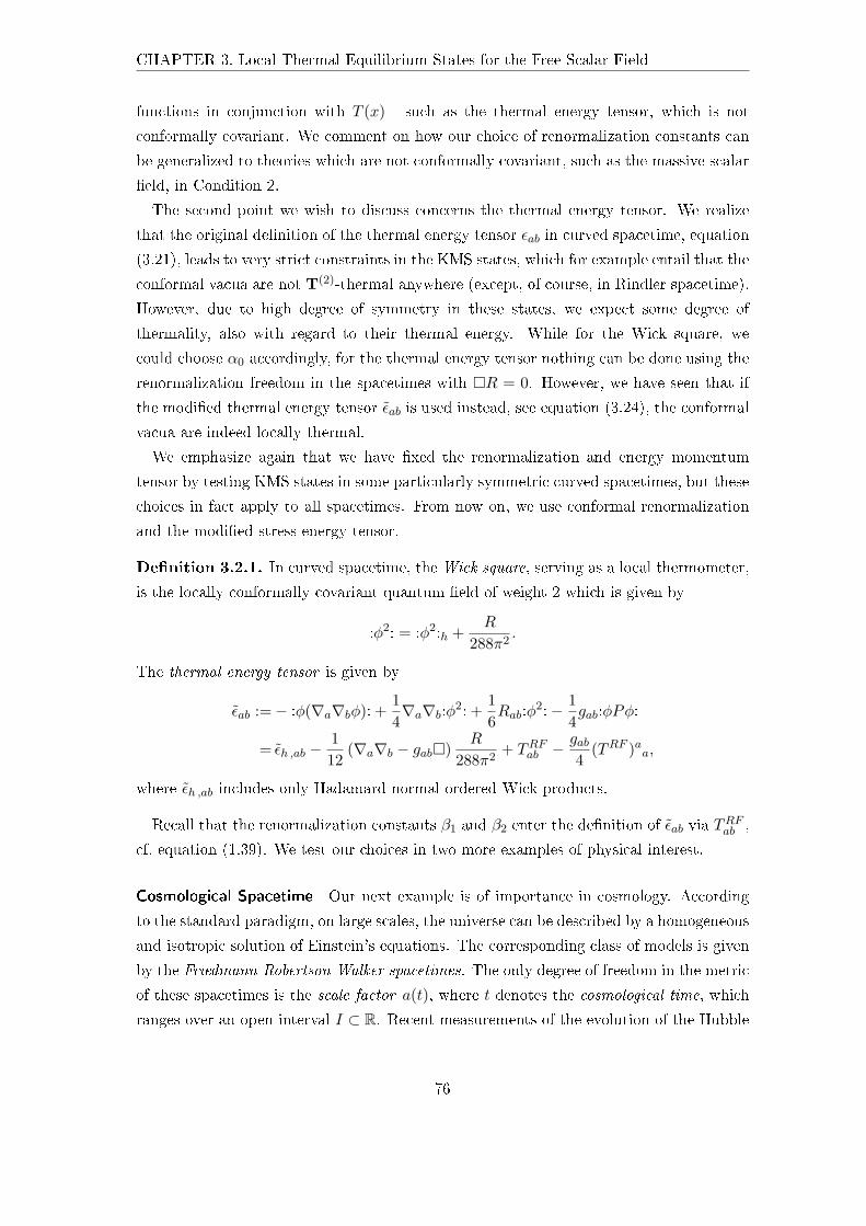
CHAPTER 3. Local Thermal Equilibrium States for the Free Scalar Field
functions in conjunction with T (x) - such as the thermal energy tensor, which is not
conformally covariant. We comment on how our choice of renormalization constants can
be generalized to theories which are not conformally covariant, such as the massive scalar
eld, in Condition 2.
The second point we wish to discuss concerns the thermal energy tensor. We realize
that the original denition of the thermal energy tensor εab in curved spacetime, equation
(3.21), leads to very strict constraints in the KMS states, which for example entail that the
conformal vacua are not T(2)-thermal anywhere (except, of course, in Rindler spacetime).
However, due to high degree of symmetry in these states, we expect some degree of
thermality, also with regard to their thermal energy. While for the Wick square, we
could choose α0 accordingly, for the thermal energy tensor nothing can be done using the
renormalization freedom in the spacetimes with R = 0. However, we have seen that if
the modied thermal energy tensor εab is used instead, see equation (3.24), the conformal
vacua are indeed locally thermal.
We emphasize again that we have xed the renormalization and energy momentum
tensor by testing KMS states in some particularly symmetric curved spacetimes, but these
choices in fact apply to all spacetimes. From now on, we use conformal renormalization
and the modied stress energy tensor.
Denition 3.2.1. In curved spacetime, the Wick square, serving as a local thermometer,
is the locally conformally covariant quantum eld of weight 2 which is given by
:φ2: = :φ2:h +R
288π2.
The thermal energy tensor is given by
εab :=− :φ(∇a∇bφ): +14∇a∇b:φ2: +
16Rab:φ
2:− 14gab:φPφ:
= εh ,ab −112
(∇a∇b − gab)R
288π2+ TRFab −
gab4
(TRF )aa,
where εh ,ab includes only Hadamard normal ordered Wick products.
Recall that the renormalization constants β1 and β2 enter the denition of εab via TRFab ,
cf. equation (1.39). We test our choices in two more examples of physical interest.
Cosmological Spacetime Our next example is of importance in cosmology. According
to the standard paradigm, on large scales, the universe can be described by a homogeneous
and isotropic solution of Einstein's equations. The corresponding class of models is given
by the Friedmann-Robertson-Walker spacetimes. The only degree of freedom in the metric
of these spacetimes is the scale factor a(t), where t denotes the cosmological time, which
ranges over an open interval I ⊂ R. Recent measurements of the evolution of the Hubble
76
3.2. Local Thermal Equilibrium and KMS States in Stationary Spacetimes
function suggest that a model with at spatial sections is appropriate, in contrast to
spherical or hyperbolic models.
A spatially at Friedmann-Robertson-Walker spacetime Fa is given by I × R3 with
metric
gFa = −dt2 + a2(t) (dx2 + dy2 + dz2). (3.53)
Introducing the conformal time τ from the dierential relation dτ := dta(t) and writing
a(τ) := a(t(τ)), the metric becomes
gFa = a2(τ)(−dτ2 + dx2 + dy2 + dz2), (3.54)
which shows that Fa is conformally embedded into Minkowski spacetime. Clearly, the
conformal embedding ψ : Fa →M0 is given by ψ(τ, ~x) = (τ, ~x) and the conformal factor
is Ω(ψ(τ, ~x)) = 1/a(τ).
One can now introduce so-called conformal KMS states for the massless, conformally
coupled eld by using KMS states in Minkowski spacetime.27 Using e = ∂τ ∈ V + we use
the KMS state ω0β in Minkowski spacetime to dene the state
ωβ = ω0β αψ (3.55)
in Fa, which is Hadamard [Pin09, DHP11].
Since the Wick square is a conformally covariant quantum eld, it is easy to see that
ωβ(:φ2:(τ)) =1
12 a2(τ)β2, (3.56)
which means that the inverse local temperature in these states scales with a(τ), i.e. β(τ) =
a(τ)β, which is expected from a conformally covariant theory in zeroth order cosmology.
In the states ωβ , the dynamics of the local temperature (3.32) results in the condition
a = 0 (3.57)
for all β. Here, ˙ denotes the derivative with respect to cosmological time.28 Depending
on the initial conditions, this condition can accommodate power law ination and also
Minkowski spacetime. This result shows that only in a special cosmology, the conformal
KMS states can be in LTE with respect to the thermal energy tensor. Of course, the
model of the massless, conformally coupled free scalar eld is too simple to be able to fully
27This works in the same way as for conformal vacua, as discussed in [BD84]. Note that conformal KMS
states are well known and recently appeared as special cases of the approximate KMS states dened
in [DHP11].28Had we used εab instead of εab, the resulting equation would be a non-linear third order dierential
equation in the Hubble parameter H := a/a, depending on the inverse temperature β and a linear
combination of the renormalization constants β1 and β2.
77
CHAPTER 3. Local Thermal Equilibrium States for the Free Scalar Field
describe quantum eects in the early universe. However, our discussion shows that linear
constraints arising from the LTE condition and equations of state might have a bearing
on cosmological parameters in more realistic models. See also [Ver11] for a discussion on
LTE in cosmology.
Schwarzschild spacetime Our last example is Schwarzschild spacetime SM surrounding
a static black hole of mass M . SM proves to be an interesting testing ground for LTE,
since it is a curved spacetime which is not conformally at (in contrast to our previous
examples) and is a vacuum solution to Einstein's equations. The latter point implies that
the renormalization ambiguity of the Wick square is not present, as R = 0.
This paragraph is based on an interesting early attempt to dene local temperature
in QFT by measuring the Wick square, namely Page's work in the eighties [Pag82].29
The author calculates the expectation value of the Wick square and the energy momen-
tum tensor in thermal states for the conformally coupled free scalar eld in backgrounds
with static Einstein metrics30, where he uses the so-called Bekenstein-Parker Gaussian
approximation.31
Exterior Schwarzschild spacetime can be covered by coordinates (t, r, θ, ϕ) ∈ R ×(2M,∞)× S2 and the metric is given by
g = −(
1− 2Mr
)dt2 +
(1− 2M
r
)−1
dr2 + r2(
dθ2 + sin(θ)2 dϕ2), (3.58)
which is obviously static with time-like Killing vector K := ∂t. Schwarzschild spacetime,
as a vacuum solution, is an Einstein spacetime with Λ = 0. Page thus used his result
to compute the Wick square in the Hartle Hawking state, which is KMS with respect to
the dynamics induced by K, at the Hawking Temperature β = 8πM [Wal94]. The Wick
square in this state takes the value
ω8Mπ(:φ2:(x)) ≈ 112(2π)2
(1 +
2Mr
+(
2Mr
)2
+(
2Mr
)3), (3.59)
which approaches 112(2π)2
for r →∞, i.e. the inverse local temperature of ω8Mπ at innity
is β(∞) = 2π.
Turning to the thermal energy tensor and applying equation (3.32) to (3.59) yields the
constraint
1− 4Mr− 36M2
r2≈ 0, (3.60)
29I am grateful to K. Fredenhagen and N. Pinamonti for bringing this reference to my attention.30Recall that a spacetime M with metric g is called Einstein, if there is a constant Λ ∈ R such that
Rab = Λ gab. All of the previous examples are Einstein spacetimes, except for Robertson Walker
spacetimes with non-constant a(τ).31The corresponding approximation was slightly improved in [CH84], but this does not change our dis-
cussion here.
78
3.2. Local Thermal Equilibrium and KMS States in Stationary Spacetimes
which entails that only at r ≈ 9M can the Hartle Hawking state be in LTE.32 This
result shows that even for the modied thermal energy tensor, the Hartle Hawking state
is almost nowhere in LTE. However, this is not unexpected: as we have mentioned several
times before, there is no reason to expect that KMS states in curved spacetime have a
high degree of local thermality, especially with respect to non-scalar observables. These
simply measure the degree to which the state resembles a reference state.
We can interpret the result for the Wick square as follows: for the Hartle Hawking state
at spatial innity, the local temperature agrees with the Tolman redshifted KMS Temper-
ature, up to a factor of 14M (the surface gravity of exterior Schwarzschild spacetime). This
resembles the situation for the Unruh state in Rindler spacetime, where at spatial innity
the Tolman shifted KMS temperature is zero, agreeing with the local temperature, cf.
equation (3.34). Recall that for both spacetimes, these ndings are not inuenced by the
choice of α0. At spatial innity, in both spacetimes, the trajectories with respect to which
the states in question are KMS resemble inertial time-like trajectories in Minkowski space-
time (here, the asymptotic atness of Schwarzschild spacetime comes into play). These
results are therefore consistent.
Choosing coordinates appropriate for the wedge-dynamics induced by K2 in Anti de
Sitter spacetime, one can show that the Tolman redshifted KMS temperature for the
Hawking-Unruh type state (β = 2π) tends to zero at innity (which is time-like for Anti-
de Sitter). This can be seen as a conrmation of our choice of renormalization constant
α0, because the local temperature in this state is zero at innity (in fact, everywhere).
This therefore establishes an analogy to the Schwarzschild and Rindler spacetime and
provides support for our choice of α0.
In general, when there is no conformal symmetry available, like in the massive case, we
propose the following prescription for xing the corresponding renormalization constants.
This requirement supplements Condition 1 in Section 2.2.1 as criterion for the choice of
thermal observables.
Condition 2. Let there be given KMS states for a Killing ow for which there exist
sequences of Killing trajectories, which in some limit resemble inertial trajectories in
Minkowski spacetime. In that limit the inverse local temperature must resemble the
Tolman redshifted KMS parameter for Hawking-Unruh type states in spacetimes where
the latter exist.
We also want to reiterate an important point: as the examples have shown, KMS states
in curved spacetime do not always possess a local temperature, i.e. in certain regions
and for certain ranges of the corresponding KMS parameter, these states are out of local
32We note that there exist time-like geodesics with closed orbits at that radius.
79
CHAPTER 3. Local Thermal Equilibrium States for the Free Scalar Field
equilibrium even with regard to the Wick square. However, our abstract results in Chapter
2 and also Corollary 3.1.6 allow us to draw the conclusion that even in such regions there
are states which are T2n(x)-thermal for any n. Here, we display two results of this type.
Proposition 3.2.2. Let O ⊂M be a compact subset of some spacetime M and let n ∈ N.If the Wick powers are chosen such that C2m = (2m− 1)!! αm0 Rm for all m = 1, 2, . . . , n,
then there are (not necessarily quasi-free) T2n(O)-thermal states in S(M).
Proof. A state is T2(x)-thermal if the corresponding expectation value of :φ2:(x) is pos-
itive. We can construct a state with this property for all x ∈ O as follows. We pick
any state ω ∈ S(M) with non-vanishing one-point function ω(1) and modify its two-point
function ω(2) by adding another term
ω(2)c := ω(2) + c ω(1) ⊗ ω(1)
with some c ∈ R. Recall that since ω ∈ S(M), the ω(1) are smooth. ω(2)c is a valid
two-point function and we can consider the corresponding quasi-free state ωc. Clearly
ωc(:φ2:(x)) = ω(:φ2:(x)) + c (ω(1)(x))2.
Due to the compactness of O, we may choose the constant c such that ωc(:φ2:(x)) > 0
for all x ∈ O. There are obviously many states which satisfy this inequality and are
consequently T2(O)-thermal. By Corollary 3.1.6 this means that these states, being
quasi-free, are T2n(O)-thermal as well.
Now we use the fact that T2n(O)-thermality is stable under convex combinations. We
simply mix the so-constructed quasi-free states and thus construct states which are not
quasi-free but still T2n(O)-thermal.
The method discussed in Section 2.2.3 provides an alternative way to show the existence
of T2n(x)-thermal states for x ∈ M. Namely, the results in Chapter 2 entail that there
exist T2n(x)-thermal states if any linear combination
ψ(x) :=n∑i=0
ci :φ2i:(x), ci ∈ R, (3.61)
has a positive scaling limit, cf. Proposition 2.2.9.
Lemma 3.2.3. The scaling limit of a quasi-free Hadamard state ω ∈ S(M) at x ∈ M
exists for the Wick powers :φ2n: for all n ∈ N. The scaling limit two-point function is
non-trivial and the dimension of the eld is 2n.33
33Since derivatives only increase the dimension, we note that a similar result holds for dierentiated Wick
powers :(∇o(1)φ)(∇o(2)φ) . . . (∇o(n)φ):.
80
3.2. Local Thermal Equilibrium and KMS States in Stationary Spacetimes
Proof. One starts by computing the m-point functions of ω with respect to the eld :φ2n:,
making use of Wick's theorem (1.16). On nds a sum of expectation values of certain
Wick powers in ω, the highest of which is :φ2nm:. The most singular term is thus the one
given by a product of nm Hadamard parametrices h. Therefore, we only need to know the
scaling limit of h, but this follows from [SV01, Lemma A.3]. One nds that the scaling
function for the Wick powers :φ2n: is given by N(λ) = λ2n−4, i.e. d = 2n. We omit the
details of the calculation.
This lemma, together with Wick's theorem (1.16), allows us to compute the scaling limit
of the eld ψ in some quasi-free Hadamard state. As there are no relations in the limit
and no elds sharing the same dimension (see the discussion in Section 2.2.3), we deduce
that the scaling limit is determined by the highest Wick power which appears in the linear
combination ψ and is thus positive. By Proposition 2.2.9, all elements of spanT2n aretherefore unbounded and Proposition 2.2.7 allows us to conclude that there are many
T2n(x)-thermal states. T2n-thermality pertains in a neighbourhood of x, because there
are no linear constraints, see the argument at the end of Section 2.2.2.
81

82
4 Conclusion & Perspectives
In this thesis, we were concerned with the conceptual question under which circumstances
states in quantum eld theory in curved spacetime are in thermal equilibrium and when
it is therefore meaningful to attach local thermal parameters to them. For the purpose
of illustrating our results, we have predominantly considered the massless, conformally
coupled, free scalar eld. However, most of our conclusions also hold in realistic models
and it would be worthwhile to consider LTE states in perturbative QFT, for example.
We have given arguments explaining that thermal observables do not form a vector
space in curved spacetime and, moreover, must be chosen to be linearly independent.1 We
have seen that in certain cases there are relations between corresponding local thermal
parameters which are induced by linear equations of state. It is interesting that these
relations lead to evolution equations for the local thermal parameters.
Choosing thermal observables for which no such relations hold, we have shown that
there exist states to which the corresponding local thermal parameters can be assigned in
bounded regions of Minkowski spacetime. Moreover, with a natural assumption regarding
the numerical range of the thermal observables, there exist states which are in equilibrium
at any given point in a curved spacetime. Again, in the absence of linear constraints, the
thermality of these states extends to neighbourhoods.
Furthermore, we have argued that KMS states in stationary curved spacetimes, though
passive with respect to certain observers, may not be viewed in analogy to global thermal
equilibrium states in Minkowski spacetime. Indeed, not all of these states are in local
equilibrium. For those that are, the parameter β cannot necessarily be interpreted as
an inverse temperature. In fact, β decomposes into contributions from the curvature,
the acceleration of the observer and the local temperature. Usage of the thermal observ-
ables to obtain information on the KMS states in curved spacetime also allowed us to x
the renormalization freedom exhibited by these elds in terms of physically meaningful
parameters.
Finally, we wish to point out possible directions for further research. Regarding our
existence proof for LTE states in Minkowski spacetime, it would be interesting to clarify
whether it can be extended to thermal observables for which there are constraints arising
1Taking advantage of the freedom inherent to the choice of thermal observables in curved spacetime, in
some cases it is possible to recover a linear structure on these sets.
83
CHAPTER 4. Conclusion & Perspectives
from linear equations of state. Additionally, a deeper understanding of the requirements
for local equilibrium in regions of curved spacetime is, of course, desirable. In particular,
this involves showing that in case of linear constraints, there are states which satisfy the
resulting evolution equations in open regions in curved spacetime. While we have seen
that these evolution equations are satised in some KMS states in certain spacetimes, a
more general result has yet to be obtained.
84
Bibliography
[Ara00] H. Araki, Mathematical Theory of Quantum Fields, Oxford University Press,
2000.
[Bah06] B. Bahr, The Hot Bang State of massless Fermions, Lett.Math.Phys (2006),
no. 78, 3954.
[BD84] N. D. Birrell and P. Davies, Quantum Fields in Curved Space, Cambridge
University Press, 1984.
[BEE96] J. K. Beem, P. Ehrlich, and K. Easley, Global Lorentzian Geometry, 2nd ed.,
Pure and Applied Mathematics, CRC Press, 1996.
[BF00] R. Brunetti and K. Fredenhagen, Microlocal Analysis and Interacting Quan-
tum Field Theories: Renormalization on Physical Backgrounds, Comm. Math.
Phys. 208 (2000), 623661.
[BF09] C. Bär and K. Fredenhagen, Quantum Field Theory on Curved Spacetime:
Concepts and Mathematical Foundations, Lecture Notes in Physics, no. 786,
Springer Heidelberg Berlin, 2009.
[BFK96] R. Brunetti, K. Fredenhagen, and M. Köhler, The microlocal spectrum condi-
tion and Wick polynomials of free elds on curved spacetimes, Comm. Math.
Phys. 180 (1996), no. 3, 633652.
[BFS00] D. Buchholz, M. Florig, and S. J. Summers, Hawking-Unruh temperature and
Einstein causality in anti-de Sitter space-time, Class. Quant. Grav. 17 (2000),
L31L37.
[BFV03] R. Brunetti, K. Fredenhagen, and R. Verch, The Generally Covariant Locality
Principle - A New Paradigm for Local Quantum Field Theory, Comm. Math.
Phys. 237 (2003), 3168.
[BGP07] C. Bär, N. Ginoux, and F. Päe, Wave equations on Lorentzian manifolds
and quantization, ESI Lectures in Mathematics and Physics, European Math-
ematical Society Publishing House, 2007.
85
Bibliography
[BOR02] D. Buchholz, I. Ojima, and H. Roos, Thermodynamic Properties of Non-
equilibrium States in Quantum Field Theory, Ann. Physics 297 (2002), 219
242.
[Bos00] H. Bostelmann, Lokale Algebren und Operatorprodukte am Punkt, Ph.D. the-
sis, Universität Göttingen, 2000.
[BR96] O. Bratelli and D.W. Robinson, Operator algebras and quantum statistical me-
chanics. Vol. 2: Equilibrium states. Models in quantum statistical mechanics,
Springer Berlin, Germany, 1996.
[BR07] R. Brunetti and G. Ruzzi, Superselection sectors and general covariance I,
Comm. Math. Phys. 270 (2007), 69108.
[BR09] , Quantum charges and spacetime topology: The emergence of new
superselection sectors, Comm. Math. Phys. 287 (2009), 523563.
[BS05] A. N. Bernal and M. Sánchez, Smoothness of Time Functions and the Metric
Splitting of Globally Hyperbolic Spacetimes, Comm. Math. Phys. 257 (2005),
4350.
[BS07] D. Buchholz and J. Schlemmer, Local Temperature in Curved Spacetime, Clas-
sical Quantum Gravity 24 (2007), F25F31.
[Buc03] D. Buchholz, On Hot Bangs and the Arrow of Time in Relativistic Quantum
Field Theory, Comm. Math. Phys. 237 (2003), 271288.
[CF09] B. Chilian and K. Fredenhagen, The Time Slice Axiom in Perturbative Quan-
tum Field Theory on Globally Hyperbolic Spacetimes, Comm. Math. Phys. 287
(2009), 513522.
[CH84] P. Candelas and K. W. Howard, Vacuum 〈ϕ2〉 in Schwarzschild spacetime,
Phys. Rev. D 29 (1984), 16181625.
[Coh80] D.L. Cohn, Measure Theory, Birkhäuser, Boston, 1980.
[DB60] B.S. DeWitt and R.W. Brehme, Radiation Damping in a Gravitational Field,
Ann. Phys. 9 (1960), 220.
[DF01] M. Dütsch and K. Fredenhagen, Perturbative algebraic eld theory, and de-
formation quantization, Mathematical Physics in Mathematics and Physics:
Quantum and Operator Algebraic Aspects (R. Longo, ed.), Fields Institute
Communications, Providence, RI, 2001.
86
Bibliography
[DF06] Y. Décanini and A. Folacci, O-diagonal coecients of the DeWitt-Schwinger
and Hadamard representations of the Feynman propagator, Phys. Rev. D 73
(2006), no. 4.
[DFP08] C. Dappiaggi, K. Fredenhagen, and N. Pinamonti, Stable cosmological models
driven by a free quantum scalar eld, Phys. Rev. D77 (2008).
[DHMP10] C. Dappiaggi, T.-P. Hack, J. Möller, and N. Pinamonti, Dark Energy from
Quantum Matter, arXiv:1007.5009v1 [astro-ph.CO], 2010.
[DHP11] C. Dappiaggi, T.-P. Hack, and N. Pinamonti, Approximate KMS states for
scalar and spinor elds in Friedmann-Robertson-Walker spacetimes, Annales
Henri Poincare 12 (2011), 14491489.
[Dim80] J. Dimock, Algebras of Local Observables on a Manifold, Comm. Math. Phys.
77 (1980), 219228.
[DL97] S. Deser and O. Levin, Accelerated detectors and temperature in (anti-) de
Sitter spaces, Class. Quant. Grav. 14 (1997), 163168.
[DMP09] C. Dappiaggi, V. Moretti, and N. Pinamonti, Distinguished quantum states
in a class of cosmological spacetimes and their Hadamard property, J. Math.
Phys. 50 (2009).
[DV10] A. Degner and R. Verch, Cosmological particle creation in states of low energy,
Journal of Mathematical Physics 51 (2010).
[EGJ65] H. Epstein, V Glaser, and A. Jae, Nonpositivity of the Energy Density in
Quantized Field Theories, Nuovo Cimento (1965), no. 36, 10161022.
[Few05] C.J. Fewster, Energy Inequalities in Quantum Field Theory, ArXiv: math-
ph/0501073v1, 2005.
[Few07] C. J. Fewster, Quantum energy inequalities and local covariance II: categorical
formulation, Gen. Rel. Grav. 39 (2007), 18551890.
[Few11] C.J. Fewster, On the notion of "the same physics in all spacetimes" , Quan-
tum Field Theory and Gravity. Conceptual and mathematical advances in
the search for a unied framework. (F. Finster, O. Müller, M. Nardmann,
J. Tolksdorf, and E. Zeidler, eds.), Birkhäuser, 2011.
[FH81] K. Fredenhagen and J. Hertel, Local algebras of observables and pointlike lo-
calized elds, Comm. Math. Phys. 80 (1981), 555561.
87
Bibliography
[FH87] K. Fredenhagen and R. Haag, Generally covariant quantum eld theory and
scaling limits, Comm. Math. Phys. 108 (1987), 91115.
[FH96] C.J. Fewster and A. Higuchi, Quantum eld theory on certain nonglobally
hyperbolic space-times, Class. Quant. Grav. 13 (1996), 5162.
[FNW81] S.A. Fulling, F.J. Narcowich, and R.M. Wald, Singularity Structure of the Two
Point Function in Quantum Field Theory in Curved Space-Time II, Annals
Phys. (1981), no. 136, 243.
[FP06] C. J. Fewster and M. J. Pfenning, Quantum energy inequalities and local
covariance. I. Globally hyperbolic spacetimes, Journal of Mathematical Physics
47 (2006).
[Ful89] S. A. Fulling, Aspects of Quantum Field Theory in Curved Spacetime, Cam-
bridge University Press, 1989.
[FV11] C. J Fewster and R. Verch, Dynamical locality and covariance: What makes a
physical theory the same in all spacetimes?, ArXiv: math-ph/1106.4785, 2011.
[Haa96] R. Haag, Local Quantum Physics, 2nd ed., Springer, Berlin, 1996.
[Hac10] T. P. Hack, On the Backreaction of Scalar and Spinor Quantum Fields in
Curved Spacetimes, Ph.D. thesis, Universität Hamburg, 2010.
[Haw75] S.W. Hawking, Particle Creation by Black Holes, Comm. Math. Phys. 43
(1975), 199220.
[HB74] R. Haag and Trych-Pohlmeyer B., Stability and equilibrium states, Comm.
Math. Phys. 38 (1974), no. 3, 173193.
[HE73] S. W. Hawking and G. F. Ellis, The large scale structure of space-time, Uni-
versity Press, Cambridge [Eng.], 1973.
[HHW67] R. Haag, N. Hugenholtz, and M. Winnik, On the equilibrium states in quantum
statistical mechanics, Comm. Math. Phys. (1967), no. 5, 215236.
[HL10] S. Hollands and G. Leiler, On the derivation of the Boltzmann equa-
tion in quantum eld theory: Flat spacetime, ArXiv: cond-mat.stat-
mech/1003.1621v1, 2010.
[Hör90] L. Hörmander, The Analysis of Linear Partial Dierential Operators I,
Springer, 1990.
88
Bibliography
[Hör94] , Notions of Convexity, Birkhäuser, 1994.
[HR02] S. Hollands and W. Ruan, The State Space of Perturbative Quantum Field
Theory in Curved Spacetimes, Ann. Henri Poincaré 3 (2002), 635657.
[Hüb05] R. Hübener, Lokale Gleichgewichtszustände massiver Bosonen, Diploma The-
sis, Universität Göttingen, 2005.
[HW01] S. Hollands and R. M. Wald, Local Wick Polynomials and Time Ordered Prod-
ucts of Quantum Fields in Curved Spacetime, Comm. Math. Phys. 223 (2001),
289326.
[HW02] , Existence of Local Covariant Time Ordered Products of Quantum
Fields in Curved Spacetime, Comm. .Math. Phys. 231 (2002), 309345.
[HW05] , Conservation of the Stress Tensor in Perturbative Interacting Quan-
tum Field Theory in Curved Spacetimes, Reviews in Mathematical Physics 17
(2005), 227311.
[HW10] S. Hollands and R.M. Wald, Axiomatic Quantum Field Theory in Curved
Spacetime, Comm. Math. Phys. 293 (2010), 85125.
[IZ80] C. Itzykson and J.B. Zuber, Quantum Field Theory, McGraw-Hill Inc., New
York, 1980.
[Jac98] T. Jacobson, Comment on: Accelerated detectors and temperature in (anti-)
de Sitter spaces, Class. Quant. Grav. 15 (1998), 251253.
[KFGV77] A. Kossakowski, A. Frigerio, V. Gorini, and M. Verri, Quantum Detailed Bal-
ance and KMS Condition, Comm. Math. Phys. 57 (1977), 97110.
[KT90] E.W. Kolb and M.S. Turner, The early universe, Frontiers in Physics, Adison-
Wesley Publishing Company, 1990.
[Küs08] M. Küskü, A class of almost equilibrium states in Robertson-Walker space-
times, Ph.D. thesis, Universität Hamburg, 2008.
[KW91] B. S. Kay and R. M. Wald, Theorems on the uniqueness and thermal proper-
ties of stationary, nonsingular, quasifree states on spacetimes with a bifurcate
killing horizon, Phys. Rep. 207 (1991), 49136.
[Mor03] V. Moretti, Comments on the Stress-Energy Tensor Operator in Curved Space-
time, Comm. Math. Phys. 232 (2003), 189221.
89
Bibliography
[MTW73] C. Misner, K. Thorne, and J. Wheeler, Gravitation, W. H. Freeman, 1973.
[NPT96] H. Narnhofer, I. Peter, and W. Thirring, How hot is the de Sitter space?, Int.
J. Mod. Phys. B 10 (1996), 15071520.
[Olb07] H. Olbermann, States of Low Energy on Robertson-Walker Spacetimes, Class.
Quant. Grav. 24 (2007), 50115030.
[O'N83] B. O'Neill, Semi-Riemannian Geometry With Applications to Relativity, Pure
and Applied Mathematics, Academic Press, 1983.
[Pag82] D. N. Page, Thermal stress tensors in static Einstein spaces, Phys. Rev. D 25
(1982), 14991509.
[Par69] L. Parker, Quantized Fields and Particle Creation in Expanding Universes. I,
Phys. Rev. 183 (1969), 10571068.
[Pet07] R. Petersen, Lokale Temperaturen auf gekrümmten Raumzeiten, Diploma The-
sis, Universität Hamburg, 2007.
[Pin09] N. Pinamonti, Conformal Generally Covariant Quantum Field Theory: The
Scalar Field and its Wick Products, Comm. Math. Phys. 288 (2009), 1117
1135.
[PPV11] E. Poisson, A. Pound, and I. Vega, The Motion of Point Particles in Curved
Spacetime, Living Reviews in Relativity 14 (2011), no. 7.
[PW78] W. Pusz and S.L. Woronowicz, Passive states and KMS states for general
quantum systems, Comm. Math. Phys. 58 (1978), no. 3, 273290.
[Rad96a] M.J. Radzikowski, A local to global singularity theorem for quantum eld the-
ory on curved space-time, Comm. Math. Phys. 180 (1996), 1.
[Rad96b] , Micro-Local Approach to the Hadamard Condition in Quantum Field
Theory on Curved Space-Time, Comm. Math. Phys. 179 (1996), 529.
[RS75] M. Reed and B. Simon, Methods of Modern Mathematical Physics II, Aca-
demic Press, New York, 1975.
[San08] K. Sanders, Aspects of locally covariant quantum eld theory, Ph.D. thesis,
University of York (U.K.), 2008.
[San09] K. Sanders, On the Reeh-Schlieder property in curved spacetime, Comm. Math.
Phys. 288 (2009), 271285.
90
Bibliography
[San10] , Equivalence of the (generalised) Hadamard and microlocal spectrum
condition for (generalised) free elds in curved spacetime, Comm. Math. Phys.
295 (2010), 485501.
[Sch90] K. Schmüdgen, Unbounded operator algebras and representation theory, Op-
erator theory, advances and applications, Birkhäuser, 1990.
[Sch05] J. Schlemmer, Gleichgewichtszustände auf der de Sitter-Raumzeit, Diploma
Thesis, Universität Göttingen, 2005.
[Sch10] J. Schlemmer, Local Thermal Equilibrium on Cosmological Spacetimes, Ph.D.
thesis, Universität Leipzig, 2010.
[Sol10] C. Solveen, Local Thermal Equilibrium in Quantum Field Theory on Flat and
Curved Spacetimes, Class. Quant. Grav. 27 (2010), 235002.
[Sto09] A. Stottmeister, Zur Thermodynamik gekrümmter Raumzeiten, Diploma The-
sis, Universität Göttingen, 2009.
[Str06] N. Straumann, From primordial quantum uctuations to the anisotropies of
the cosmic microwave background radiation, Ann. Phys. 15 (2006), 701847.
[Str09] A. Strohmeier, Microlocal Analysis, Quantum Field Theory on Curved Space-
time: Concepts and Mathematical Foundations (C. Bär and K. Fredenhagen,
eds.), Lecture Notes in Physics, no. 786, Springer Heidelberg Berlin, 2009.
[SV01] H. Sahlmann and R. Verch, Microlocal Spectrum Condition and Hadamard
Form for Vector-Valued Quantum Fields In Curved Spacetime, Rev. Math.
Phys. 13 (2001), 12031246.
[SV08] J. Schlemmer and R. Verch, Local Thermal Equilibrium States and Quantum
Energy Inequalities, Ann. Henri Poincaré 9 (2008), 945978.
[Uec05] M. Uecker, Lokale Gleichgewichtszustände des elektromagnetischen Feldes,
Diploma Thesis, Universität Göttingen, 2005.
[Unr76] W.G. Unruh, Notes on Black Hole Evaporation, Phys. Rev. D14 (1976), 870.
[Ver01] R. Verch, A spin-statistics theorem for quantum elds on curved spacetime
manifolds in a generally covariant framework, Comm. Math. Phys. 223 (2001),
261288.
[Ver11] , Local covariance, renormalization ambiguity, and local thermal equi-
librium in cosmology, Quantum Field Theory and Gravity. Conceptual and
91
Bibliography
mathematical advances in the search for a unied framework. (F. Finster,
O. Müller, M. Nardmann, J. Tolksdorf, and E. Zeidler, eds.), Birkhäuser,
2011.
[Wal84] R.M. Wald, General Relativity, University Of Chicago Press, 1984.
[Wal94] , Quantum Field Theory in Curved Spacetime and Black Hole Ther-
modynamics, University of Chicago Press, Chicago, 1994.
[Wei08] S. Weinberg, Cosmology, Oxford University Press, Oxford, 2008.
[ZMR96] D. Zubarev, V. Morozov, and G. Röpke, Statistical Mechanics of Nonequilib-
rium Processes, vol. 1, Akademie Verlag, Berlin, 1996.
92
Acknowledgements
First, I would like to thank Prof. D. Buchholz for giving me the opportunity to work on
this inspiring topic. His ideas on local thermal equilibrium form the basis of this thesis
and without his constant help and encouragement this work would not have been possible.
I would also like to thank Prof. K.-H. Rehren for agreeing to become part of my committee
and for nding funding for me during the last part of this thesis.
I have greatly beneted from discussions with many people, but in particular I would
like to mention K. Sanders, who was always glad to answer my questions on QFT in curved
spacetime during his time in Göttingen. A. Stottmeister and J. Schlemmer have also been
valuable partners for discussion. Their work on particular examples of KMS states in
curved spacetime helped me to draw some of my conclusions in Chapter 3. R. Verch was
helpful for his criticism on my results about the structure of sets of thermal observables.
I would also like to thank K. Fredenhagen for pointing out to me an important reference
on thermal states in Schwarzschild spacetime. N. Pinamonti provided this reference and
also helped in nding an error in one of his works. I am grateful to T.-P. Hack for
taking interest in my work and our discussion on LTE in cosmological spacetime. C.
Fewster helped me to better understand scaling limits at an early stage of this work,
while H. Bostelmann corrected a misconception of mine on operator product expansions
and scaling limits. Special thanks go to J. Fish for proof-reading the whole manuscript.
Several other people have contributed in one way or the other, if only by making me
feel comfortable at the institute. In no particular order: P. Martinetti, D. Cadamuro, T.
Fischer, K. Daoulas, A. Braun, F. Dradi, G. Tedesco, Y. Tanimoto, L. Wallenhorst, S.
Filor, M. Bischo, J. Slowik, A. Kukhtina, C. Köhler, S. Becker, J. Queva and others.
Financial support from GrK 1493 Mathematische Strukturen in der Modernen Quan-
tenphysik is gratefully acknowledged.
On a personal note, I would like to thank Maria, Charly, Gösta and Jonathan. I am
privileged to call them my friends. Finally, I would like to thank my parents. Without
them, I would be nowhere.
93
Bibliography
94
Lebenslauf
Name: Christoph Solveen
Geboren: 25. April 1980 in Bernburg (Saale)
Adresse: Tieckweg 4, 37075 Göttingen
Staatsangehörigkeit: Deutsch
Ausbildung und Beruicher Werdegang
06/1999 Abitur an der Schule Schloss Salem,
Notendurchschnitt 1.6
09/1999 07/2000 Wehrdienst beim Stabs- und Fernmelderegiment 410, Geltow
10/2000 06/2002 Studium der Betriebswirtschaftslehre, Universität Leipzig
10/2002 04/2008 Studium der Physik, Universität Leipzig
Diplomarbeit Quantum Field Theory on
Manifolds with Arbitrary Dimension, Diplom: 1,0
10/2005 06/2006 Part Three Mathematics, University of Cambridge (United Kingdom)
Master of Advanced Studies in Mathematics: Merit
07/2008 - Promotion Physik an der Georg-August-Universität Göttingen
Publikation
• C. Solveen, Local Thermal Equilibrium in Quantum Field Theory on Flat and Curved Space-
times, Class. Quant. Grav. 27 235002 (2010)
95


![Quantum Simulations of Out-of-Equilibrium Phenomena · Quantum Simulations of Out-of-Equilibrium Phenomena ... Systeme, z.B. die anisotrope XY Kette, ... explosion [Fey82] of the](https://img.pdfslide.org/doc/110x75/5b9d375d09d3f253158bcf73/quantum-simulations-of-out-of-equilibrium-phenomena-quantum-simulations-of-out-of-equilibrium.jpg)