SPECIAL FEATURE: PERSPECTIVE

Mass and heat transfer between evaporation andcondensation surfaces: Atomistic simulation andsolution of Boltzmann kinetic equationVasily V. Zhakhovsky (Василий Жаховский)a,1, Alexei P. Kryukovb, Vladimir Yu. Levashovb,c,Irina N. Shishkovab, and Sergey I. Anisimovd

Edited by William A. Goddard III, California Institute of Technology, Pasadena, CA, and approved March 21, 2018 (received for reviewDecember 25, 2017)

Boundary conditions required for numerical solution of the Boltzmann kinetic equation (BKE) for mass/heattransfer between evaporation and condensation surfaces are analyzed by comparison of BKE results withmolecular dynamics (MD) simulations. Lennard–Jones potential with parameters corresponding to solidargon is used to simulate evaporation from the hot side, nonequilibrium vapor flow with a Knudsennumber of about 0.02, and condensation on the cold side of the condensed phase. The equilibrium densityof vapor obtained in MD simulation of phase coexistence is used in BKE calculations for consistency of BKEresults with MD data. The collision cross-section is also adjusted to provide a thermal flux in vapor identicalto that in MD. Our MD simulations of evaporation toward a nonreflective absorbing boundary show thatthe velocity distribution function (VDF) of evaporated atoms has the nearly semi-Maxwellian shape be-cause the binding energy of atoms evaporated from the interphase layer between bulk phase and vapor ismuch smaller than the cohesive energy in the condensed phase. Indeed, the calculated temperature anddensity profiles within the interphase layer indicate that the averaged kinetic energy of atoms remainsnear-constant with decreasing density almost until the interphase edge. Using consistent BKE and MDmethods, the profiles of gas density, mass velocity, and temperatures together with VDFs in a gap of manymean free paths between the evaporation and condensation surfaces are obtained and compared. Wedemonstrate that the best fit of BKE results with MD simulations can be achieved with the evaporation andcondensation coefficients both close to unity.

evaporation | condensation | Boltzmann kinetic equation |molecular dynamics

Evaporation and condensation can be realized indifferent natural phenomena and technologies. Apeculiarity of these processes is the coupled massand heat transfer from evaporation to condensationsurface. Nowadays, a correct description of the trans-port processes across the interfacial surfaces is requiredfor the development of new advanced technologiesand solution of the known engineering problems.Among them, the problem of removing heat fromspace vehicles, developing technologies based on theinteraction of matter in the form of cryogenic corpus-cular targets with high-energy beams, evaporation ofdroplets on superhydrophobic surfaces using liquid

droplets as the molecular concentrators of ultradilutesolutions, the development of effective vacuum dryingmethods—all of these tasks are inextricably linked withthe solution of the evaporation–condensation problem.

The main goal in considering the coupled mass/heattransfer is an accurate evaluation of the masses ofevaporated or condensed material. Determination ofthese quantities is important because a significant heatcan be diverted from the interfacial surface, which, as aconsequence, leads to cooling of the condensed phase.For example, when considering the evaporation of aliquid droplet placed in a steam–gas mixture, the inac-curacies in calculating the evaporation rate can lead to

aCenter for Fundamental and Applied Research, Dukhov Research Institute of Automatics, Moscow 127055, Russia; bDepartment of Low Temperatures,Moscow Power Engineering Institute, Moscow 111250, Russia; cInstitute of Mechanics, Lomonosov Moscow State University, Moscow 119192,Russia; and dLandau Institute for Theoretical Physics, Russian Academy of Science, Chernogolovka 142432, RussiaAuthor contributions: S.I.A. designed research; V.V.Z., A.P.K., V.Y.L., and I.N.S. performed research; V.V.Z., A.P.K., V.Y.L., and S.I.A. analyzed data;and V.V.Z., A.P.K., and V.Y.L. wrote the paper.The authors declare no conflict of interest.This article is a PNAS Direct Submission.Published under the PNAS license.1To whom correspondence should be addressed. Email: 6asi1z@gmail.com.This article contains supporting information online at www.pnas.org/lookup/suppl/doi:10.1073/pnas.1714503115/-/DCSupplemental.

www.pnas.org/cgi/doi/10.1073/pnas.1714503115 PNAS Latest Articles | 1 of 9

SPECIA

LFEATURE:

PERSPECTIV

E

Dow

nloa

ded

by g

uest

on

May

10,

202

0

errors in determining the pattern of temperature changes at the in-terfacial surface, which may result in inaccurate forecasts of the drop-let temperature and a complete evaporation time.

As noted in ref. 1, despite the simplicity of the formulation ofthe evaporation–condensation problem, its solution encounterscertain difficulties in the general case. Traditionally, it is assumedthat the heat coming to the interphase boundary is spent onevaporation and heating of the particles, and the resulting vaporis diverted from the evaporation surface by diffusion. It is believedthat the concentration of the evaporated gas near the interphaseboundary is equal to the equilibrium vapor concentration. Thisassumption was first used in ref. 2 to consider evaporation of aspherical drop. However, this is not the case, since the vapor nearthe interfacial surface will be saturated only if a diffusion rate ofgas escape is lower than an arrival rate of molecules from theinterphase boundary. Ref. 3 showed the existence of a concentra-tion jump near the interphase boundary. One of the refinementsof the evaporation–condensation theory can be achieved by in-voking the kinetics of interaction of vapor molecules with thesurface of the liquid phase and also with each other. In refs. 4and 5, using the methods of molecular–kinetic theory, a mass fluxof evaporated molecules was evaluated. A disadvantage of theformula proposed in these papers lies in the fact that it wasobtained for a free molecular flow of the evaporated gas—thatis, for the conditions where emitted particles do not interact withmolecules presented near the surface.

The next stage in the study of evaporation–condensation datesback to the 1960s, when the dynamics of rarefied gases was de-veloped rapidly. The needs of technology development led to theemergence of more rigorous calculation techniques based on theexact or approximate solution of the Boltzmann kinetic equation(BKE). A linear theory was being formulated at this time. Thebeginning was laid by the work in ref. 6, in which the form ofthe velocity distribution function (VDF) near the interphaseboundary was adopted rather than in the derivation of theHertz–Knudsen formula (4, 5). The authors suggested that theVDF for molecules moving to this boundary is the same as for anegative half-space of velocities at a considerable distancefrom the interface of the phases. Then, by writing down theexpression for the mass flow from definition, they obtained aresult that was two times different from the mass flow calcu-lated by the Hertz–Knudsen formula.

Linearized, or more simply a linear theory of, evaporation andcondensation was developed by Labuntsov and Muratova in refs.7 and 8. At about the same time, many researchers (9–16) andAnisimov et al. (17–19) were focused on the solution of nonlinearevaporation–condensation problems with the use of the kinetictheory of gases.

With the advancement of computers, the direct numericalsolution of the BKE began to be applied to the evaporation–con-densation problems (20–24). For solving the BKE, it is necessary tospecify the correct boundary conditions for the VDFs of evapo-rated and condensed molecules. The shapes of VDFs togetherwith the evaporation and condensation coefficients, determiningthe corresponding fluxes through the evaporation and condensa-tion surfaces, are involved in those boundary conditions. In thepreviously listed works, a semi-Maxwellian VDF with zero trans-port velocity was taken as such a function. However, as noted inref. 25, “no serious theoretical conclusion of such a boundarycondition is known to us.”

The measured evaporation and condensation coefficients mayvary greatly from experiment to experiment. The condensationcoefficient for water ranges from ∼0.01 to 1 as noted in the review(26). It seems likely that such a wide spread can be explained by

the fact that those coefficients were measured not at the interfacebut over a distance of many mean free paths in the vapor. More-over, even the small differences between the experimental con-ditions (such as chemical impurities on the interface and variationof surface temperatures of liquids being investigated) may have adramatic effect on the measurement results. The dependence ofevaporation and condensation coefficients from the surface tem-perature is also reported in simulation works (27, 28). It was foundthat those coefficients, which are close to unity at low tempera-tures, begin to decrease if the surface temperature is increasedwell above the triple point.

It should be noted that the molecular–kinetic approach allowsus to correctly describe the change in the macroparameters of thevapor/gas near the interfacial surface, but it is assumed that thestate of the condensed phase remains unchanged. On the otherhand, the VDF of molecules escaping from the surface can beaffected by processes occurring near this surface, both from theliquid side and from the vapor side. In this connection, the ap-proach in which both the condensed and vapor phases are con-sidered within the framework of a single modeling method isobvious. As a research method, the molecular dynamics (MD) simu-lation has beenwidely used presently. There are several knownworksin which the calculation of the VDF of molecules emitted from theinterphase boundary layer is performed by the MD method (25, 29–31) and the analysis of the simulation results lead to the conclusionabout the proximity of the VDF of vapor molecules “flying” from theinterphase to the Maxwellian distribution.

In refs. 28 and 32, the problem of recondensation through asmall vapor gap with the thickness of about 7 nm, which leads to aKnudsen flow with Kn∼ 1 roughly, is investigated via MD simula-tion and by the solution of the Enskog–Vlasov equation with theDirect Simulation Monte Carlo (DSMC) method. The authors cameto the following conclusion: “On the basis of the results of thisstudy, we constructed the kinetic boundary conditions (KBC) forthe hard-sphere molecules in consideration of the liquid temper-ature dependence in the course of a steady net evaporation andcondensation; however, the application of the KBC during un-steady net evaporation-condensation is extremely important.”Furthermore, the same two-surface method used in refs. 28 and32 was applied in ref. 33 to study the evaporation–condensationin an unsteady transient regime on a short MD time scale. Theauthors of ref. 34 noted that there is a deviation from the Maxwel-lian VDF for particles flying in the direction normal to the interfa-cial surface: “However, the detailed mechanism of the deviationhas not been clarified yet.”

Numerous papers using the MD method indicate that animportant question in determining the KBC is at which position ofthe boundary between the liquid and gas phases those KBCshould be determined (27, 32, 34, 35). The authors of ref. 35discuss the influence of the KBC position on the mass flow ofthe evaporating substance.

It seems obvious the way in which a joint (cross-linked) versionof the description is used. That is, the liquid phase and the regionnear the interphase boundary layer are described by the MDmethod, next the methods of the kinetic theory of gases are used,and finally the continuum mechanics approaches are applied ondistances larger than the 10 to 20 mean free paths. However, suchattempts are faced with certain problems and difficulties. Thecharacteristic time scale of the MD processes and the kinetic re-laxation time differ approximately by a factor of 104. Therefore, morethan 105 simulation steps must be taken to trace the behavior of anatomic system during the average interatomic collision time. The MDmethod deals with the coordinates and velocities of the particles, butfor a molecular–kinetic approach, “this description of the motion of

2 of 9 | www.pnas.org/cgi/doi/10.1073/pnas.1714503115 Zhakhovsky et al.

Dow

nloa

ded

by g

uest

on

May

10,

202

0

the gas is unnecessarily complete. Therefore, we must resort to a lesscomplete statistical description of the behavior of the system” as anote in ref. 36. Also, the results of molecular–kinetic calculations in theform of VDF cannot be used to obtain information on the particlecoordinates and velocities necessary for MD simulation. Accordingly,themutual exchange of results of calculations obtained bymolecular–kinetic and MD methods becomes problematic.

In this work, a nonequilibrium vapor flow from the evaporationto condensation boundary layer is considered in detail on anatomic scale using the MD method, which provides the classicaltrajectories of interacting atoms starting from a hot bulk materialand reaching a cold material after traveling through a gas gap. Tosimplify the modeling of gas flow, the exact atom positions ri andvelocities vi can be replaced by a probability density functionf ðr, v, tÞ to find dN molecules having positions near r and veloci-ties near v within a phase-space volume drdv at time t such asdN ¼ f ðr, v, tÞdrdv. Upon integrating f ðr, v, tÞ, also called a distri-bution function, over a whole range of velocity, we obtain a localnumber density nðr, tÞ of molecules. In a volume with spatiallyuniform distribution of molecules, a VDF Fðv, tÞ can be obtainedby integrating f ðr, v, tÞdr over the volume.

The BKE (36) describing evolution of the f ðr, v, tÞ at the ab-sence of external forces is given by

∂f∂t

+ v∂f∂r

¼ I, [1]

where rðx, y, zÞ are Cartesian coordinates, vðυx , υy , υzÞ is themolecule velocity in a laboratory coordinate system at time t,and I is a collision integral. The different forms of the collisionalintegral are considered in refs. 20 and 21. Here in this work, thesimplest form for the hard sphere collisions is used.

Our prime goal is to make a bridge from atomistic simulation toa probabilistic approach through a more penetrating insight intothe atomic-scale mechanism of evaporation and condensation,which determines the VDFs at the corresponding interfaces. We

performed the large-scale MD simulations to find the bestboundary conditions, including their positions, evaporation andcondensation coefficients, and the shapes of VDFs, which can beused in the solution of BKE providing the best agreement with dataobtained from theMD simulations. For consistency of BKE with MDresults, the saturated vapor density and transport cross-sectionwere precomputed by MD and then used in the BKE method.

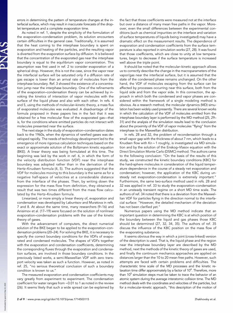
Simulation TechniquesEquilibrium evaporation and condensation processes take place in aninterphase transition layer between the coexisting condensed phaseand its vapor. For MD simulation of nonequilibrium evaporation–condensation, the two surfaces of condensed phase at differenttemperatures are required. This condition can be complied with usingboth sides of a single film as illustrated in Fig. 1, where the condensedphase of argon is placed in the middle of the MD computationaldomain. Periodical boundary conditions are imposed on all three di-mensions of the domain, which has typical dimensions of Lx ¼ 400nmand Ly ¼ Lz ¼ 200nm. The total number of atoms was about29.15 million in our MD simulations of evaporation–condensation.

To establish both evaporation and condensation processes in asingle simulation, a temperature gradient is maintained by the Lan-gevin thermostat with target temperature TðxÞ depending on atomposition in the film. The thermostat is only applied to atomsmoving ina gray zone nearby the center of film as shown in Fig. 1; thus, theinterphase layers between the condensed phase and vapor are notacted uponby the thermostat forces. The Langevin forces are given by

mid~υi=dt ¼~ξi � γ�~υi � ~ux

�, [2]

where the force acting on each atom i is a sum of a Gaussian-distributed random force~ξi and a frictional damping term (37).The last is determined by a friction coefficient γ and a thermalvelocity of atom in reference to a target flow velocity ~ux . Toreproduce the temperature gradient within the film, the dis-persion hξ2i of random forces and the friction coefficient mustsatisfy the condition hξ2iΔt=2γ ¼ TðxÞ, where Δt is an MD sim-ulation time step. Then, the dispersion becomes a function of

-200 -100 0 100 200position x (nm)

0.1

1

10

0.20.30.5

235

20

0.05

num

ber

dens

ity n

(ato

ms/n

m3 )

65

70

75

80

85

tem

pera

ture

s T x

and

Ty

(K)

thermostat

evaporationcondensation

200

nm

Th

Tc

nTxTy

Fig. 1. MD computational domain for evaporation from the right hotside of liquid film and condensation on the left cold side of the samefilm placed in periodical conditions. Profiles of atom number density,longitudinal Tx, and transverse Ty temperatures are taken from MDsimulationprovidingTc ¼ 72.3 for a cold surface andTh ¼ 80.4K for a hotone. The Langevin thermostatmaintains a required temperature gradientfor atoms in a gray zone xi ∈ [�7,7nm] inside the film with a thickness of32.7nm. The thermostat also keeps the mass center of film at rest byadjusting the mass flow velocity from the cold to the hot side. Here thisflow velocity is ≈ux ¼ 0.129m=s at the x ¼ 0. See details in Fig. S1.

T

-4

-3

-2

-1

0

1

n s3

-1

0

1

2

3

4

P

PPns

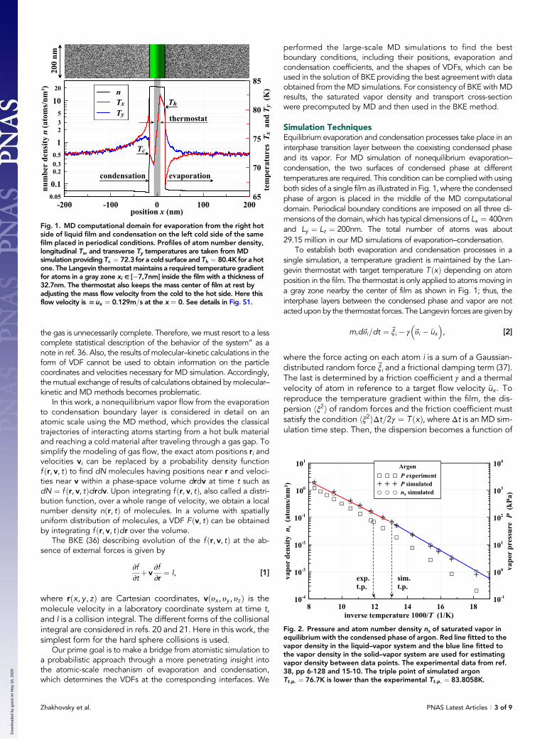
Fig. 2. Pressure and atom number density ns of saturated vapor inequilibrium with the condensed phase of argon. Red line fitted to thevapor density in the liquid–vapor system and the blue line fitted tothe vapor density in the solid–vapor system are used for estimatingvapor density between data points. The experimental data from ref.38, pp 6-128 and 15-10. The triple point of simulated argonTt.p. ¼ 76.7K is lower than the experimental Tt.p. ¼ 83.8058K.

Zhakhovsky et al. PNAS Latest Articles | 3 of 9

Dow

nloa

ded

by g

uest

on

May

10,

202

0

atom position xi because the friction coefficient is set to aconstant in our MD simulation.

To maintain the steady positive atom flux across the MD do-main and keep the film at rest, the Langevin target velocity ~ux iscoupled with a displacement of film mass center using a negativefeedback control. After reaching the stationary regime of vaporflow, such feedback control provides almost a fixed position of thefilm with negligible irregular fluctuations of mass center in therange less than ±0.01nm, which is much smaller than a thicknessof the interphase layer of ∼ 2nm for liquid argon at T ¼ 80K. Forsteady evaporation–condensation, the atom flux in direction x is aconstant everywhere regardless of local density. As a result, the massvelocity at the center of the film is less than gas flow speed by a factorequal to a density ratio between condensed phase and vapor. In thesimulation shown in Fig. 1, the vapor mass velocity is about 40m=s inthe middle of the gap between evaporation and condensation sur-faces, while the liquid flows with 0.129m=s near the center of film,with the thickness of 32.7nmdefined as a distance between positionsof hot and cold surfaces having temperatures Th and Tc, respectively.Determination of surface positions is discussed in Evaporation Co-efficient from MD Simulation. The detailed profiles of target tem-perature and flow variables in the film and surrounding vapor arepresented in SI Appendix.

MD simulations were performed with a smoothed Lennard–Jones (L–J) potential (39) given by

ϕðrÞ ¼ 4"hð�=rÞ12 � ð�=rÞ6

i+ a2x2 � a3x3, [3]

where r is an interatomic distance and x¼ðr=�Þ2�ðr0=�Þ2. Thecoefficients "¼1.0312kJ=mol, �¼0.33841nm, a2¼1.3647�10�4kJ=mol, and a3¼2.4614�10�4kJ=mol are fitted to repro-duce argon fcc crystal at zero temperature, which has thelattice parameter of 0.524673 nm and the cohesive energyof 7.74005 kJ/mol. The position of the potential minimumr0¼21=6� is identical to that in the original L–J potential.The smoothing coefficients a2 and a3 were chosen to satisfythe conditions ϕðrcÞ¼0 and ϕ′ðrcÞ¼0 at the cutoff radiusrc¼0.8125nm.

A density of vapor in equilibrium with the condensed phase isrequired to run the BKE calculation of evaporation and conden-sation because the density nsðTÞof saturated vapor is used to set aboundary condition for VDF. Using the smoothed L-J potential Eq.3 the vapor pressure and atom number density are evaluated in

several MD simulations of equilibrium liquid-vapor and solid-vapor systems. Fig. 2 shows the calculated and experimentalvalues for argon. The visible difference in vapor pressure indicatesthat the smoothed L–J potential, fitted to the experimentalparameters of solid Ar, overestimates the pressure. Using thephase-coexistence MD method, we obtained all three phasesin equilibrium at the triple point Tt.p. ¼ 76.7K of simulated ar-gon, which is appreciably lower than the experimental triplepoint Tt.p. ¼ 83.8058K (38).

Numerical solution of BKE of the evaporation–condensationproblem is performed only for vapor gaps between two interfacesdefined from MD simulated profiles as the outer boundaries of in-terphase transition layers from the bulk condensed phase to vapor.While the results of BKE calculations are almost insensitive to thedelimitation of interfaces, they depend highly on the definition ofinterface temperatures. Those temperatures are also evaluatedfrom MD simulated profiles at some position inside the transitionlayer. The interface definitions are introduced in the next section.

With the vapor density function, positions of interfaces, and theirtemperatures provided by MD simulations, the BKE Eq. 1 can besolved numerically in the vapor gap. We use a finite-differencecomputational method described in refs. 20, 21, and 40, in whicha spherical velocity domain is represented by a discrete 3D mesh ofvelocity nodes. The discretized BKE equation for each node is solvedin two steps. First, the spatial displacements are calculated withoutcollisions, and the Courant condition used for a time step Δt guar-antees that even fastest nodes cannot move more than one spatialstep Δx. Then the collisions are calculated and taken into account.

The collisional integral is evaluated by the quasi Monte Carlomethod using the Korobov’s pseudorandom sequences (21). Forsimplicity, the interatomic collision of L–J atoms is considered asa collision between hard spheres of diameter d. The last is anadjustable parameter that must be determined from MD simu-lation for consistency between BKE and MD methods. Thecollision cross-section determined by the diameter d is ad-justed to provide a steady heat flux close to that derived from

-200 -100 0 100 200position x (nm)

70

80

90

tem

pera

ture

s T x

and

Ty

(K)

0.028

0.032

0.036

dens

ity n

(ato

ms/n

m-3)

nTxTy

246 kW/m2

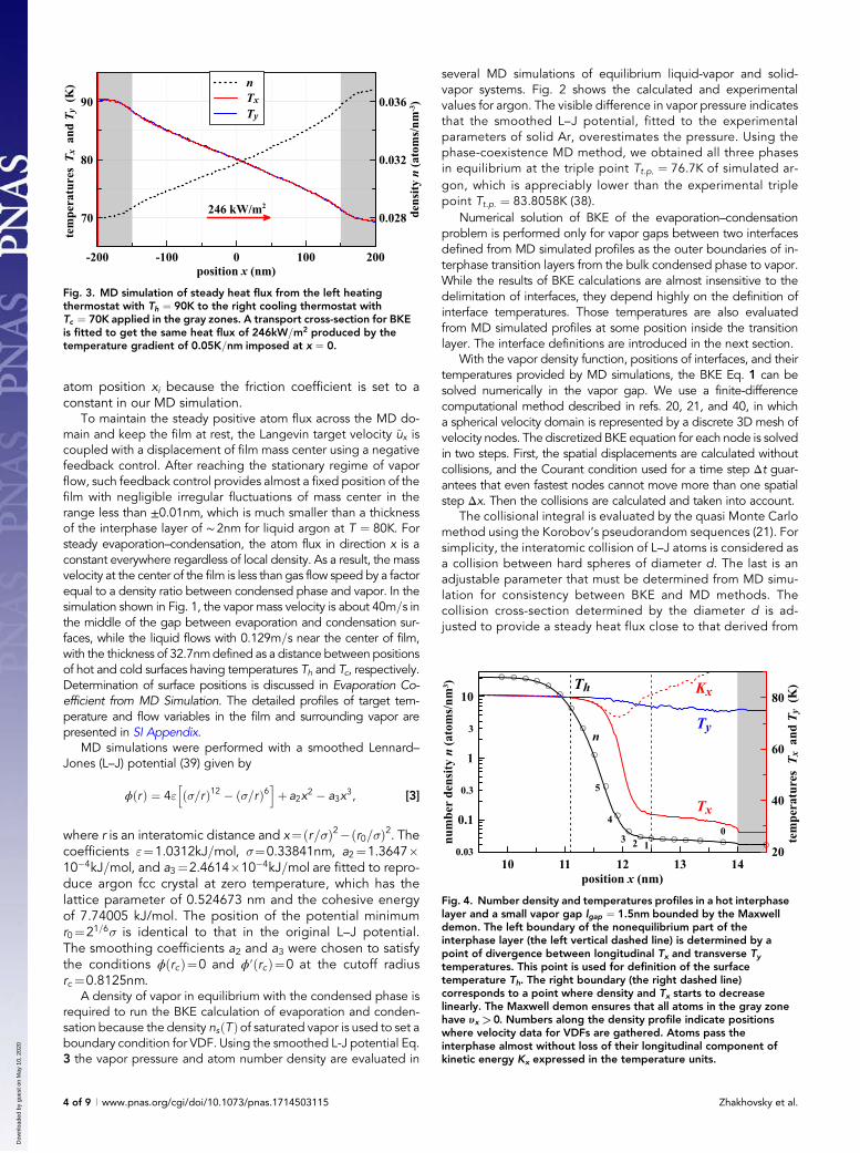
Fig. 3. MD simulation of steady heat flux from the left heatingthermostat with Th ¼ 90K to the right cooling thermostat withTc ¼ 70K applied in the gray zones. A transport cross-section for BKEis fitted to get the same heat flux of 246kW=m2 produced by thetemperature gradient of 0.05K=nm imposed at x ¼ 0.

x

0.3

3

0.03

n3

T xT y

Tx

Tyn

0123

4

5

KxTh

Fig. 4. Number density and temperatures profiles in a hot interphaselayer and a small vapor gap lgap ¼ 1.5nm bounded by the Maxwelldemon. The left boundary of the nonequilibrium part of theinterphase layer (the left vertical dashed line) is determined by apoint of divergence between longitudinal Tx and transverse Tytemperatures. This point is used for definition of the surfacetemperature Th. The right boundary (the right dashed line)corresponds to a point where density and Tx starts to decreaselinearly. The Maxwell demon ensures that all atoms in the gray zonehave υx >0. Numbers along the density profile indicate positionswhere velocity data for VDFs are gathered. Atoms pass theinterphase almost without loss of their longitudinal component ofkinetic energy Kx expressed in the temperature units.

4 of 9 | www.pnas.org/cgi/doi/10.1073/pnas.1714503115 Zhakhovsky et al.

Dow

nloa

ded

by g

uest

on

May

10,

202

0

MD simulation of heat transfer between hot and cold zones ofgas gap shown in Fig. 3. L–J atoms within the left hot and rightcold zones in the MD domain with a rigid wall at ±200  nm aresubjected to two Langevin thermostats supporting 90K and 70K,respectively. Initially atoms were placed in the domain at a constantdensity of n ¼ 0.032nm�3. After reaching a steady regime, the heatflux, the number density, and temperature gradient weremeasuredat the center x ¼ 0. Using those MD data, the cross-section wasfound to equal d ¼ 0.55nm to reproduce the almost identical heatflux of 245kW=m2 in BKE calculations.

For the vapor density n ¼ 0.0963nm�3 in equilibrium with L–Jliquid at T ¼ 80K, a mean free path in a hard sphere system is� ¼ 1=

ffiffiffi2

pn�d2 ¼ 7.73 nm, which gives the Knudsen number

Kn ¼ �=Lgap ¼ 0.021 for the vapor gap length of Lgap ¼ 364.3nmshown in Fig. 1.

To obtain evaporation and condensation coefficients, whichare the basic parameters governing the boundary conditions inthe BKE method, we use the flow profiles and VDFs gained fromatomistic trajectories simulated by the MD method. The mostappropriated coefficients can be found via comparison of VDFsfrom numerical solution of BKE with VDFs obtained from the MDsimulation. The VDFs in a steady vapor flow at x positions arecalculated as Fðx, υx , tÞ ¼

Rdydz

Rdυydυz f ðr, v, tÞ. For steady

flow, the distributions are independent of time, which allows us toaccumulate atom position and velocity statistics during MD sim-ulation. Further integration over υx gives an atom number densityprofile nðxÞ ¼ R

dυxFðx, υxÞ.The steady profiles of density, mass flow velocity, and tem-

perature are obtained by averaging the corresponding values inspatial slabs with the small thickness of 0.02nm along the x–axisand during the entire time of productive MD simulation, which isperformed after the attainment of a steady regime. The profile of

flow velocity uxðxÞ ¼ hυxi, the longitudinal TxðxÞ ¼ mkBhðυx � uxÞ2i,

and transverse TyðxÞ ¼ m2kB

hυ2y + υ2z i temperatures are calculatedfrom the corresponding components of atom velocities υx, υy,and υz.

Evaporation Coefficient from MD SimulationThe transition of atoms from bulk phase to vapor can beimagined as a jump over a potential barrier with the heightequal to the atom binding energy "b in the condensed phase.It is assumed in this naive model that the barrier is infinitelythin and an atom should spend its kinetic energy to over-come the barrier. As a result, the atoms with kinetic energy "lin direction x toward the vapor exceeding the binding en-ergy "l >"b can go to the vapor phase, where the subscript lindicates a condensed phase. Taking into account a new ki-netic energy of atom in vapor " ¼ "l � "b after passing thebarrier, one can obtain d" ¼ mυdυ ¼ d"l ¼ mυldυl, where veloci-ties are along the x–axis. Hence, assuming the Maxwellian VDF forυl, the evaporated atoms obtain a new VDF given by ref. 41:

fxdυ ¼ Amυdυffiffiffiffiffiffiffiffiffiffiffiffiffiffi4�kBT

p ffiffiffiffiffiffiffiffiffiffiffiffiffiffiffiffiffiffiffiffiffiffiffiffi"b +mυ2=2

p exp�� "b +mυ2

�2

kBT

�, [4]

where a new atom velocity υ is positive (i.e., directed towardthe vapor) and A is a normalization factor (41). The VDFs fy andfz do not change during evaporation.

The above-stated simple model ignores the density re-distribution and energy transfer inside the interphase boundarylayer having the finite thickness, which makes a real evaporationprocess not as easy as it seems. Using large-scale MD simulationof nonequilibrium evaporation, we demonstrate below thatevaporated atoms are released from the interphase layer almostwithout spending their kinetic energies, because they have a near-zero binding energy at the interphase edge. The main work re-quired for evaporation is provided by the bulk phase, whichsupports via interatomic collisions a relatively slow drift of atomsthrough the interphase by a temperature gradient. Because thecharacteristic time of interatomic collisions in the condensedphase is much shorter than the drift time through the interphase(hundreds of picoseconds), the temperature remains in equilibrium

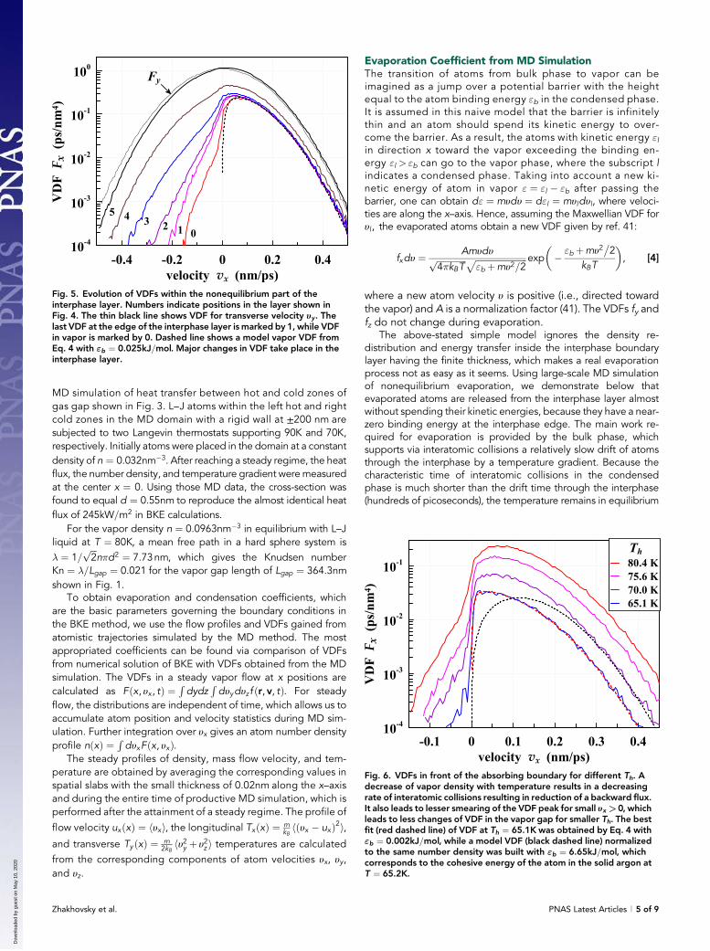
Fig. 5. Evolution of VDFs within the nonequilibrium part of theinterphase layer. Numbers indicate positions in the layer shown inFig. 4. The thin black line shows VDF for transverse velocity υy. Thelast VDF at the edge of the interphase layer is marked by 1, while VDFin vapor is marked by 0. Dashed line shows a model vapor VDF fromEq. 4 with "b ¼ 0.025kJ=mol. Major changes in VDF take place in theinterphase layer.

Fig. 6. VDFs in front of the absorbing boundary for different Th. Adecrease of vapor density with temperature results in a decreasingrate of interatomic collisions resulting in reduction of a backward flux.It also leads to lesser smearing of the VDF peak for small υx >0, whichleads to less changes of VDF in the vapor gap for smaller Th. The bestfit (red dashed line) of VDF at Th ¼ 65.1K was obtained by Eq. 4 with"b ¼ 0.002kJ=mol, while a model VDF (black dashed line) normalizedto the same number density was built with "b ¼ 6.65kJ=mol, whichcorresponds to the cohesive energy of the atom in the solid argon atT ¼ 65.2K.

Zhakhovsky et al. PNAS Latest Articles | 5 of 9

Dow

nloa

ded

by g

uest

on

May

10,

202

0

in the interphase until the density drops by one order of magnitudenear the interphase edge. Thus, VDF changes gradually with de-creasing density inside the interphase from a symmetrical Max-wellian form in the bulk of condensed phase to an almost semi-Maxwellian VDF for evaporated atoms, which has a form describedby Eq. 4 with the binding energy "b ∼ 0.

Evaporation is always associated with condensation of evap-orated atoms gaining a backward velocity due to interatomiccollisions in a vapor gap. Probability of such collisions increaseswith the length of gap lgap. An additional flux j�c toward the hotsurface is generated by evaporation from a cold surface facing thehot surface. To eliminate the flux j�c from the opposite cold surfaceandminimize the backward flux produced by collisions, we placeda nonreflective absorbing boundary on the gap lgap of severalnanometers from the evaporation surface. In contrast to the largevapor gap Lgap ¼ 365nmused in the preceding and next sections,here the small vapor gaps lgap � Lgap are used to achieve Kn � 1to reduce the probability of atom collisions in the gap. Such asimple approach allows us to estimate an evaporation coefficientfrom an intact evaporation flux undistorted by the atoms arrivingto the hot surface, and those may reflect back, without monitoringof atom trajectories, which is hard to perform in the multimillionatom simulations.

The absorbing boundary is implemented with the Maxwelldemon,which watches over atom velocities in a gray zone beyond theboundary at 1.5 nm from the interphase edge, as shown in Fig. 4.If an atom gains a negative velocity υx, the Maxwell demonsubroutine replaced it by a small positive value. Atoms passingthe gray zone return back to the cold side of the film like in Fig. 1;that is, Fig. 4 shows only part of the MD simulation domain toprovide a better spatial resolution for density and temperatureprofiles in a thin interphase layer. Thus, a steady regime of evap-oration, almost entirely uncoupled from condensation, is estab-lished from the hot side of film.

The interphase layer can be divided into two almost equalparts. First is the inner part between the bulk phase and a positionwhere the temperature profile splits into the longitudinal Tx andtransverse Ty temperatures, which is denoted by the left dashedline in Fig. 4. The temperature equilibrium in the inner part ofinterphase is well supported because the drift velocity is too small,and atoms required more than 200ps to pass this part. It is rea-sonable to take the position and temperature Th ¼ 80.4K at thepoint of temperature divergence as the surface/boundary pa-rameters for the numerical solution of BKE.

With decreasing density by 3.5 times at the end of innerequilibrium part, the temperature Tx begins to drop, and the driftvelocity is accelerated to ux > 0.005nm=ps, which is recognized asa beginning of the outer nonequilibrium part of the interphase.Acceleration of mass flow to about 0.1nm=ps to the edge of thispart shown by a right vertical line on Fig. 4 reduces a drift time ofatoms through the outer part to about 20 ps, which is comparablewith a collision time there. It leads to the large changes in VDFshape with the approach to the right edge. Fig. 5 shows VDFsconstructed from velocity data accumulated in MD simulationduring about 1.2ns. VDF wings with negative velocities are re-duced and shrunken much in approach to the right edge of theinterphase, while the width of positive VDF remains almost intact.As a result of such evolution, the longitudinal Tx drops dramati-cally, but the averaged kinetic energy of evaporated atoms is littleaffected, as it is illustrated in Fig. 4 by the longitudinal kineticenergy Kx ¼ m

kBhυ2xi expressed in the temperature units. The trans-

verse Ky ¼ m2kB

hυ2y + υ2z i ¼ Ty by definition.The VDF marked by 0 is accumulated in a thin layer with the

thickness of 0.5 nm at the end of vapor gap just before the ab-sorbing boundary controlled by the Maxwell demon. Neverthe-less, a negative velocity tail is formed here due to mostly paircollisions. Such collision conserving the total energy and Px, Py,and Pz momenta may result in the negative velocity of one atomalong x, even though the colliding atoms have both positive ve-locities υx. To get the negative atom velocity under such condi-tions, the required kinetic energy is redistributed from the y and zdegrees of freedom of a colliding pair of atoms, which leads to adecrease of Ty seen in Fig. 4. Such collisions increase a backwardflux from the absorbing boundary to the interphase edge, but thetotal flux remains constant everywhere. Thus, we see a largernumber of atoms having negative velocities in the interphaseedge VDF marked by 1 in Fig. 5.

The backward flux in vapor can be reduced by decreasingthe vapor density, which can be achieved with a decreasing

10 12 14 16 18 20 22 24position x (nm)

30

40

50

60

70

80

tem

pera

ture

s Tx

and

Ty (

K)

-5

-4

-3

-2

-1

0

pote

ntia

l ene

rgy

E (k

J/m

ol)

0.1

1

10

0.2

0.5

2

5

20

0.05

dens

ity n

(ato

ms/

nm3 )

0

20

40

60

80

100

120

140

flow

vel

ocity

ux

(m/s)

E

E

Ty

Tx

Maxwell demonabove 14 nm

ux

n

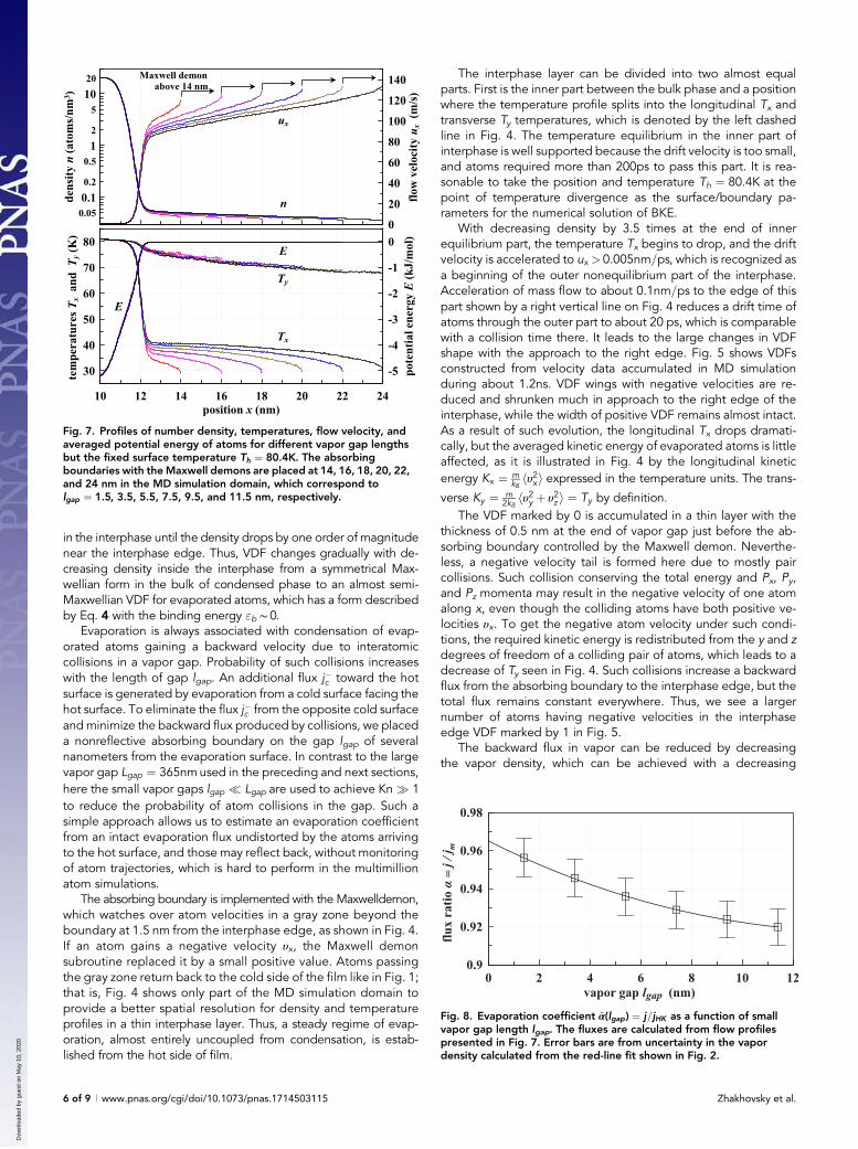
Fig. 7. Profiles of number density, temperatures, flow velocity, andaveraged potential energy of atoms for different vapor gap lengthsbut the fixed surface temperature Th ¼ 80.4K. The absorbingboundaries with theMaxwell demons are placed at 14, 16, 18, 20, 22,and 24 nm in the MD simulation domain, which correspond tolgap ¼ 1.5, 3.5, 5.5, 7.5, 9.5, and 11.5 nm, respectively.

lgap

α =

j / j

m

Fig. 8. Evaporation coefficient ~α(lgap) ¼ j=jHK as a function of smallvapor gap length lgap. The fluxes are calculated from flow profilespresented in Fig. 7. Error bars are from uncertainty in the vapordensity calculated from the red-line fit shown in Fig. 2.

6 of 9 | www.pnas.org/cgi/doi/10.1073/pnas.1714503115 Zhakhovsky et al.

Dow

nloa

ded

by g

uest

on

May

10,

202

0

temperature of evaporation surface Th. The VDFs presented onFig. 6 were built for Th in the range of 65.1 to 80.4 K in the systemssimilar to one shown on Fig. 4. The condensed phases were insolid state at 65.1 and 70 K. The Maxwell demon is always placedbeyond the nonreflective absorbing boundary at the position of14 nm, and the small vapor gaps lgap vary between 1.5 and 2 nm.The collision rate drops for a larger Knudsen number at a lowerdensity in the vapor gap, resulting in a smaller negative wing ofVDF. It also prevents the large changes of VDF shape in the vaporflow from the interphase to the absorbing boundary. The lessersmearing of the VDF peak for small υx > 0 for lower temperaturesproduces a lesser impact on the almost semi-Maxwellian VDF foratoms evaporated from the solid argon at Th ¼ 65.1K. Such VDFillustrates the idea of zero binding energy for evaporated atomseven better than VDFs obtained for higher temperatures. In theseconditions, the simulated vapor flux j� 1.02jHK for Th ¼ 65.1K isvery close to the jHK provided by the Hertz–Knudsen formula

jHK ¼ nsffiffiffiffiffiffiffiffiffiffiffiffiffiffiffiffiffiffiffiffikBT=2�m

p, [5]

which gives the exact flux of atoms in vapor in equilibrium witha condensed phase, where a Maxwell VDF can be formallydivided by two semi-Maxwellian functions at υx ¼ 0 for posi-tive and negative fluxes, respectively.

Thus, the net evaporation coefficient defined here as~α ¼ j=jHK � 1.02 is even slightly higher than unity, which we at-tribute to uncertainties in the determination of surface temper-ature and corresponding equilibrium vapor density estimatedfrom MD data profiles and the fit of vapor density presentedin Fig. 2.

We show above that the interatomic collisions produce abackward flux in vapor, which increases with approach to theevaporation surface. To study the effect of the vapor gap lengthon vapor flow, we performed several MD simulations with differ-ent positions of the absorbing boundary (see Fig. 7). The higherlongitudinal temperatures Tx observed in vapor for larger gaplengths are associated with the wider VDFs, which have larger

wings of negative velocities produced by collisions and trans-ported by the backward flux to an observation point from outervapor layers. In contrast to this, the Ty profiles for the different gaplengths remain almost identical because there is no transverse fluxand the energy transfer from transverse degrees of freedom tolongitudinal ones depends on a local density, which does notchange much. Decreasing flow velocity ux with the gap length isalso explained by the widening of the negative wings of VDFs,similarly to Tx.

Fig. 7 demonstrates that the averaged potential energy ofatoms E decreases about twice in the inner part of the in-terphase and drops almost to zero at the end of the outernonequilibrium part of the interface layer. Thus, the atoms re-leasing from the edge of interphase have a near-zero bindingenergy, which leads to an almost semi-Maxwellian VDF ofevaporated atoms, as already demonstrated by Figs. 5 and 6.Such semi-Maxwellian VDF with T �Th gives the flux j� jHK,which corresponds to α� 1. Thus, the suggested evaporationmechanism with a near-zero binding energy yields the evapo-ration coefficient close to unity.

The net evaporation coefficient calculated as a function of thevapor gap length is shown in Fig. 8. It is defined as a ratio~αðlgapÞ ¼ j=jHK. The evaporation coefficient as a parameter α for anumerical solution of BKE can be obtained as a limit of ~αðlgapÞ→ α

at lgap → 0, at which the backward flux vanishes. It can be esti-mated as α� 0.97± 0.01. However, this formal procedure mayhave no physical meaning for an lgap smaller than the interactioncutoff distance of 0.8125nm or the diameter 0.55nm of collisioncross-section. Also, it is worth noting that another definition oftemperature of evaporation surface can lead to the differentvapor density ns, which gives the different evaporation co-efficient, as an example ~α� 0.8 obtained in MD simulation of L–Jevaporation (25).

Because the vapor fluxes calculated for temperatures in therange of 65 to 80 K are all close to jHK, and due to uncertainty inthe definition of the surface temperature and equilibrium vapordensity, we assume that the evaporation coefficient α ¼ 1 for usein the numerical solution of BKE.

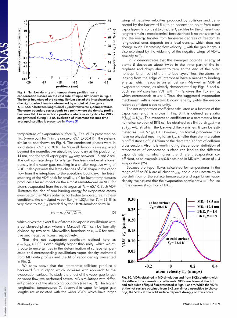
-20 -19 -18 -17 -16 -15position x (nm)

0.1

1

10

0.20.3

0.5

23

5

2030

0.05

num

ber

dens

ity n

(ato

ms/n

m3 )

70

72

74

76

78

80

82

84

tem

pera

ture

s T x

and

Ty

(K)

Tx

Ty

n

Tc

Fig. 9. Number density and temperatures profiles near acondensation surface on the cold side of liquid film shown in Fig. 1.The inner boundary of the nonequilibrium part of the interphase layer(the right dashed line) is determined by a point of divergenceTc ¼ 72.4  K between longitudinal Tx and transverse Ty temperatures.The outer boundary corresponds to a point where the density profilebecomes flat. Circles indicate positions where velocity data for VDFsare gathered during 1.5 ns. Evolution of instantaneous (not time-averaged) profiles is presented in Movie S1.

Fig. 10. VDFs obtained in MD simulation and from BKE solutions withthe different condensation coefficients. VDFs are taken at the hotand cold sides of liquid film presented in Figs. 1 and 9.While the VDFsat the hot surface obtained from BKE are almost insensitive to choiceof β, the VDFs at the cold surface depend strongly on this choice.

Zhakhovsky et al. PNAS Latest Articles | 7 of 9

Dow

nloa

ded

by g

uest

on

May

10,

202

0

Condensation Coefficient from Evaporation–CondensationCalculated by MD and BKE MethodsFor the numerical solution of BKE in a vapor flow between theevaporation and condensation surfaces, the positions and tem-peratures of which are determined from MD simulation, theboundary conditions have to be imposed on VDFs on these sur-faces. Assuming that the hot surface with temperature Th is lo-cated on the left end of the gap, the positive flux j+h from thesurface is represented by a sum of evaporated and reflected atomfluxes. It is supposed that an atom coming to the surface with anegative flux j– may be absorbed with probability β, which de-termines a condensation coefficient. Thus, the reflected atomsform the reflected flux ð1� βÞjj�j, which together with the evap-orated atom flux expressed as αjHK using Eq. 5 results in thepositive flux j+h ¼ αjHK + ð1� βÞjj�j. The required boundary VDFmust yield this flux.

As we demonstrated in Evaporation Coefficient from MDSimulation, the VDF of evaporated atoms is represented by thesemi-Maxwellian VDF fHK ðThÞ for Th, which yields the Hertz–Knudsen flux. The VDF of reflected atoms can also be representedby a similar semi-Maxwellian function ∼ fHK, because the reflectionis assumed to be diffuse with perfect accommodation to thesurface temperature. To produce the reflected flux, the VDF fHKmust be normalized by the jHK and multiplied by the ð1� βÞjj�j.Therefore, the left boundary condition applied for a positive wingof VDF at the surface is given by

f+h ¼ ðα+ ð1� βÞjj�j�jHK ÞfHK ðThÞ ¼ ~αfHK ðThÞ. [6]

The negative wing βf� is eliminated on the left boundary.Similarly, the right boundary condition imposed on the cold

surface at Tc is given by

f�c ¼ ðα+ ð1� βÞjj+j�jHK ÞfHK ðTcÞ, [7]

where we assume that the α is equal to that on the hot surface.As indicated in Evaporation Coefficient from MD Simulation,the evaporation coefficient is almost independent of temperature,

and α� 1 in MD simulation of evaporation; hence, α ¼ 1 is ap-plied on both boundaries in BKE calculations. The unknown con-densation coefficient β is also taken to be independent ofsurface temperature.

Definition of position and temperature of the cold surface issimilar to that for the hot surface introduced in the discussion ofFig. 4. The density and temperature profiles with a point of di-vergence between the longitudinal Tx and transverse Ty temper-atures on the cold side of the film presented in Fig. 1 in the vicinityof the interphase layer are shown in Fig. 9. Thus, the position andtemperature of the right boundary used in BKE calculations aredetermined at the end of the equilibrium part of the cold in-terphase layer formed in MD simulation of steady evaporation–condensation.

By varying the β, governing both boundary conditions in Eqs. 6and 7, the VDFs obtained by MD and BKE methods can becompared with the aim to find an optimal condensation co-efficient leading to a good agreement between those VDFs. Wefind numerical solutions of BKE with β ¼ 0.8; 0.9; 1 for two evap-oration–condensation systems with ThjTc ¼ 80.4j72.4K in the va-por gap Lgap ¼ 364.3nm and ThjTc ¼ 79.4j60.5K in the vapor gapLgap ¼ 366.7nm. See details of simulations in SI Appendix. Fig. 10shows the VDFs taken at hot and cold surfaces of liquid film forβ ¼ 0.9; 1. The VDFs for β ¼ 0.8 are not shown because they givethe largest deviation from the VDFs obtained in MD. One can seethat the VDFs from BKE are weakly dependent on β at the hotsurface, while BKE solution at the cold surface is very sensitive tothe variation of β.

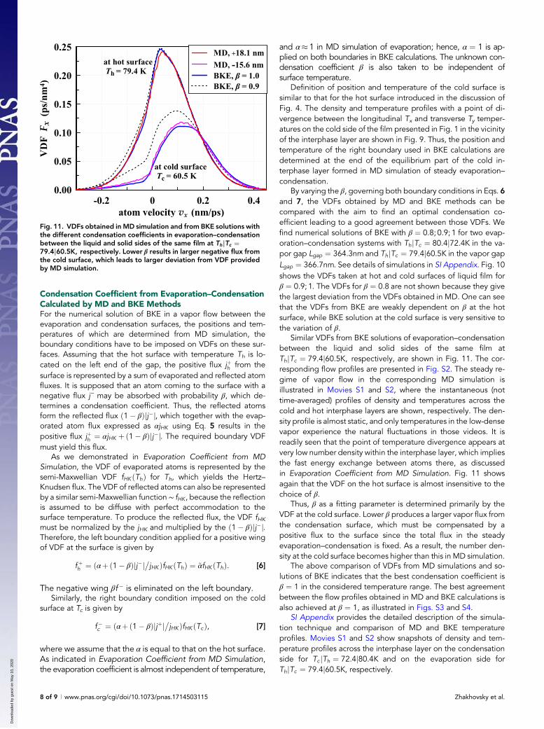
Similar VDFs from BKE solutions of evaporation–condensationbetween the liquid and solid sides of the same film atThjTc ¼ 79.4j60.5K, respectively, are shown in Fig. 11. The cor-responding flow profiles are presented in Fig. S2. The steady re-gime of vapor flow in the corresponding MD simulation isillustrated in Movies S1 and S2, where the instantaneous (nottime-averaged) profiles of density and temperatures across thecold and hot interphase layers are shown, respectively. The den-sity profile is almost static, and only temperatures in the low-densevapor experience the natural fluctuations in those videos. It isreadily seen that the point of temperature divergence appears atvery low number density within the interphase layer, which impliesthe fast energy exchange between atoms there, as discussedin Evaporation Coefficient from MD Simulation. Fig. 11 showsagain that the VDF on the hot surface is almost insensitive to thechoice of β.

Thus, β as a fitting parameter is determined primarily by theVDF at the cold surface. Lower β produces a larger vapor flux fromthe condensation surface, which must be compensated by apositive flux to the surface since the total flux in the steadyevaporation–condensation is fixed. As a result, the number den-sity at the cold surface becomes higher than this in MD simulation.

The above comparison of VDFs from MD simulations and so-lutions of BKE indicates that the best condensation coefficient isβ ¼ 1 in the considered temperature range. The best agreementbetween the flow profiles obtained in MD and BKE calculations isalso achieved at β ¼ 1, as illustrated in Figs. S3 and S4.

SI Appendix provides the detailed description of the simula-tion technique and comparison of MD and BKE temperatureprofiles. Movies S1 and S2 show snapshots of density and tem-perature profiles across the interphase layer on the condensationside for Tc jTh ¼ 72.4j80.4K and on the evaporation side forThjTc ¼ 79.4j60.5K, respectively.

Fig. 11. VDFs obtained in MD simulation and from BKE solutions withthe different condensation coefficients in evaporation–condensationbetween the liquid and solid sides of the same film at ThjTc ¼79.4j60.5K, respectively. Lower β results in larger negative flux fromthe cold surface, which leads to larger deviation from VDF providedby MD simulation.

8 of 9 | www.pnas.org/cgi/doi/10.1073/pnas.1714503115 Zhakhovsky et al.

Dow

nloa

ded

by g

uest

on

May

10,

202

0

ConclusionsConsistent application of MD and BKE methods to the problemof evaporation–condensation bridges the gap between theatomistic representation of complex atom motion and probabi-listic evolution of velocity distributions between two surfaces ofthe condensed material. Using multimillion atom simulation, wedemonstrate that, contrary to intuition, atoms are released from acondensed phase without the use of their kinetic energy but withthe support from collisions with other atoms in the interphaselayer. This effectively means that the evaporated atoms have anear-zero binding energy, which leads to the virtually semi-Maxwellian VDF of evaporated atoms and evaporation coeffi-cient close to unity.

We also find that the best agreement between the steady flowprofile and VDFs obtained by MD and BKE methods is achieved ifboth evaporation and condensation coefficients are close to unityin the considered conditions.

We think that the evaporation–condensation of liquid metals,water, and polyatomic molecular liquids should be studied next toverify the applicability of our results to more complex materials.Such studies may provide more appropriate boundary conditionsfor use in continuum mechanics approaches to the evaporation–condensation problem.

AcknowledgmentsThis work was supported by Russian Foundation for Basic Research Grant 17-08-00805. S.I.A. was supported by Russian Science Foundation Grant 14-19-01599.

1 Kozyrev AV, Sitnikov AG (2001) Evaporation of a spherical droplet in a moderate-pressure gas. Phys Usp 44:725–733.2 Maxwell JC (1890) The Scientific Papers of James Clerk Maxwell, ed Niven WD (Cambridge Univ Press, Cambridge, UK), Vol 2.3 Langmuir I (1915) The dissociation of hydrogen into atoms. [Part II] Calculation of the degree of dissociation and the heat of formation. J Am Chem Soc37:417–458.

4 Hertz H (1882) Ueber die verdunstung der Flüssigkeiten, insbesondere des quecksilbers, im luftleeren raume. Ann Phys 253:177–193.5 Knudsen M (1915) Die maximale verdampfungsgeschwindigkeit des quecksilbers. Ann Phys 352:697–708.6 Kucherov RY, Rikenglaz LE (1960) On hydrodynamic boundary conditions for evaporation and condensation. Sov Phys JETP 37:88–89.7 Labuntsov DA (1967) An analysis of the processes of evaporation and condensation. High Temp 5:579–647.8 Muratova TM, Labuntsov DA (1969) Kinetic analysis of the processes of evaporation and condensation. High Temp 7:959–967.9 Kogan MN, Makashev NK (1971) Role of the Knudsen layer in the theory of heterogeneous reactions and in flows with surface reactions. Fluid Dyn 6:913–920.

10 Pao Y-P (1971) Application of kinetic theory to the problem of evaporation and condensation. Phys Fluids 14:306–312.11 Yen SM (1973) Numerical solutions of non-linear kinetic equations for a one-dimensional evaporation-condensation problem. Comput Fluids 1:367–377.12 Fischer J (1976) Distribution of pure vapor between two parallel plates under the influence of strong evaporation and condensation. Phys Fluids 19:1305–1311.13 Aoki K, Cercignani C (1983) Evaporation and condensation on two parallel plates at finite Reynolds numbers. Phys Fluids 26:1163–1164.14 Cercignani C, Fiszdon W, Frezzotti A (1985) The paradox of the inverted temperature profiles between an evaporating and a condensing surface. Phys Fluids

28:3237–3240.15 Hermans LJF, Beenakker JJM (1986) The temperature paradox in the kinetic theory of evaporation. Phys Fluids 29:4231–4232.16 Koffman LD, Plesset MS, Lees L (1984) Theory of evaporation and condensation. Phys Fluids 27:876–880.17 Anisimov SI (1968) Vaporization of metal absorbing laser radiation. Sov Phys JETP 27:182–183.18 Anisimov SI, Imas YA, Romanov GS, Khodyko YV (1971) Effects of High-Power Radiation on Metals (Joint Publications Research Service, Washington, DC).19 Anisimov SI, Rakhmatulina AK (1973) The dynamics of the expansion of a vapor when evaporated into a vacuum. Sov Phys JETP 37:441–444.20 Tcheremissine FG (2006) Solution to the Boltzmann kinetic equation for high-speed flows. Comput Math Math Phys 46:315–329.21 Aristov VV (2001) Direct Methods for Solving the Boltzmann Equation and Study of Nonequilibrium Flows. Fluid Mechanics and its Applications, ed Moreau R

(Springer, Dordrecht, The Netherlands), Vol 60.22 Kryukov A, Levashov V, Shishkova I (2001) Numerical analysis of strong evaporation–condensation through the porous matter. Int J Heat Mass Transfer

44:4119–4125.23 Kryukov AP, et al. (2006) Selective water vapor cryopumping through argon. J Vac Sci Technol A 24:1592–1596.24 Kryukov A, Levashov V, Shishkova I (2009) Evaporation in mixture of vapor and gas mixture. Int J Heat Mass Transfer 52:5585–5590.25 Zhakhovskii V, Anisimov S (1997) Molecular-dynamics simulation of evaporation of a liquid. J Exp Theor Phys 84:734–745.26 Marek R, Straub J (2001) Analysis of the evaporation coefficient and the condensation coefficient of water. Int J Heat Mass Transfer 44:39–53.27 Ishiyama T, Fujikawa S, Kurz T, Lauterborn W (2013) Nonequilibrium kinetic boundary condition at the vapor-liquid interface of argon. Phys Rev E 88:042406.28 Kon M, Kobayashi K, Watanabe M (2016) Liquid temperature dependence of kinetic boundary condition at vapor–liquid interface. Int J Heat Mass Transfer

99:317–326.29 Meland R, Ytrehus T (2007) Molecular dynamics simulation of evaporation of two-component liquid. Proceedings of 25th International Symposium on Rarefied

Gas Dynamics, eds Ivanov MS, Rebrov AK (Publ. House of the Siberian Branch of the Russian Acad. of Sciences, Novosibirsk), pp 1229–1232.30 Yang T, Pan C (2005) Molecular dynamics simulation of a thin water layer evaporation and evaporation coefficient. Int J Heat Mass Transfer 48:3516–3526.31 Cheng S, Lechman JB, Plimpton SJ, Grest GS (2011) Evaporation of Lennard-Jones fluids. J Chem Phys 134:224704.32 Kon M, Kobayashi K, Watanabe M (2014) Method of determining kinetic boundary conditions in net evaporation/condensation. Phys Fluids 26:072003.33 Kon M, Kobayashi K, Watanabe M (2017) Kinetic boundary condition in vapor-liquid two-phase system during unsteady net evaporation/condensation. Eur J

Mech B Fluids 64:81–92.34 Kobayashi K, Sasaki K, Kon M, Fujii H, Watanabe M (2017) Kinetic boundary conditions for vapor–gas binary mixture. Microfluid Nanofluid 21:53.35 Kobayashi K, Hori K, Kon M, Sasaki K, Watanabe M (2016) Molecular dynamics study on evaporation and reflection of monatomic molecules to construct kinetic

boundary condition in vapor–liquid equilibria. Heat Mass Transfer 52:1851–1859.36 Kogan MN (1969) Rarefield Gas Dynamics (Plenum, New York).37 Heerman DW (1986) Computer Simulation Methods in Theoretical Physics (Springer, Berlin).38 Haynes WM, ed (2017) CRC Handbook of Chemistry and Physics (CRC Press, Boca Raton, FL), 97th Ed, pp 6-128 and 15-10.39 Zhakhovskii VV, Zybin SV, Nishihara K, Anisimov SI (1999) Shock wave structure in Lennard-Jones crystal via molecular dynamics. Phys Rev Lett 83:1175–1178.40 Shishkova IN, Sazhin SS (2006) A numerical algorithm for kinetic modelling of evaporation processes. J Comput Phys 218:635–653.41 Gerasimov DN, Yurin EI (2014) The atom velocity distribution function in the process of liquid evaporation. High Temp 52:366–373.

Zhakhovsky et al. PNAS Latest Articles | 9 of 9

Dow

nloa

ded

by g

uest

on

May

10,

202

0