Embed Size (px)
Citation preview
EinfuhrungDas Bradley-Terry-Luce Modell
Das BTL-Modell als GLMBezug zum Raschmodell
WeiterentwicklungReferences
Ludwig-Maximilians-Universitat Munchen
Institut fur Statistik
Seminar: Psychometrische Modelle: Theorie und Anwendungen
Paarvergleichsmodelle
Mila Petkova
07. Juni 2014
Mila Petkova Paarvergleichsmodelle
EinfuhrungDas Bradley-Terry-Luce Modell
Das BTL-Modell als GLMBezug zum Raschmodell
WeiterentwicklungReferences
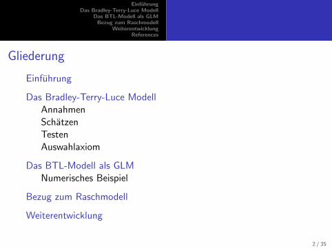
Gliederung
Einfuhrung
Das Bradley-Terry-Luce ModellAnnahmenSchatzenTestenAuswahlaxiom
Das BTL-Modell als GLMNumerisches Beispiel
Bezug zum Raschmodell
Weiterentwicklung
2 / 35

EinfuhrungDas Bradley-Terry-Luce Modell
Das BTL-Modell als GLMBezug zum Raschmodell
WeiterentwicklungReferences
Motivation
Idee der Paarvergleichsmodellen:
ein Paar von Reizen, Objekten oder Subjekten wird verglichen, umzu einer Bewertung der einzelnen Elementen zu gelangen.
↪→ Ziel: eine Praferenzordnung zu machen!
Anwendung
I sensorische Wahrnehmung
I Marktforschung
I Sport
I Politik
3 / 35
EinfuhrungDas Bradley-Terry-Luce Modell
Das BTL-Modell als GLMBezug zum Raschmodell
WeiterentwicklungReferences
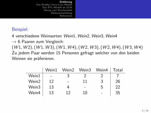
Beispiel:
4 verschiedene Weinsorten Wein1,Wein2,Wein3,Wein4→ 6 Paaren zum Vergleich:(W 1,W 2), (W 1,W 3), (W 1,W 4), (W 2,W 3), (W 2,W 4), (W 3,W 4)Zu jedem Paar werden 15 Personen gefragt welcher von den beidenWeinen sie praferieren.
Wein1 Wein2 Wein3 Wein4 Total
Wein1 - 3 2 2 7Wein2 12 - 11 3 26Wein3 13 4 - 5 22Wein4 13 12 10 - 35
4 / 35
EinfuhrungDas Bradley-Terry-Luce Modell
Das BTL-Modell als GLMBezug zum Raschmodell
WeiterentwicklungReferences
I Erster Ansatz in Zermelo (1929): Spielstarke vonSchachspielern aus ihren Turnierergebnissen zu folgern
I Nach der Idee von Thurstone (1927): das psychologischeKontinuum → Messung wie Stimuli (Reize) wahrgenommenwerden (und nicht deren physikalische Eigenschaften)
I Wiederentdeckung des Modells durch Bradley and Terry(1952)
I Auswahlaxiom von Luce (1959)
⇒ Das Model auch als Bradley-Terry-Luce-Modell (BTL-Modell)bekannt.
5 / 35
EinfuhrungDas Bradley-Terry-Luce Modell
Das BTL-Modell als GLMBezug zum Raschmodell
WeiterentwicklungReferences
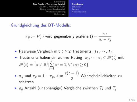
AnnahmenSchatzenTestenAuswahlaxiom
Grundgleichung des BT-Modells:
πij := P( i wird gegenuber j praferiert) =πi
πi + πj
I Paarweise Vergleich mit t ≥ 2 Treatments, T1, · · · ,Tt
I Treatments haben ein wahres Rating π1, · · · , πt ∈P(t) mit
P(t) = {π ∈ Rt |t∑
i=1πi = 1,∀i : πi ≥ 0}
I πij und πji = 1− πij , alsot(t − 1)
2Wahrscheinlichkeiten zu
schatzen
I nij Anzahl (unabhangige) Vergleiche zwischen Ti und Tj
6 / 35
EinfuhrungDas Bradley-Terry-Luce Modell
Das BTL-Modell als GLMBezug zum Raschmodell
WeiterentwicklungReferences
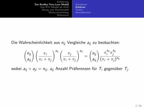
AnnahmenSchatzenTestenAuswahlaxiom
Die Wahrscheinlichkeit aus nij Vergleiche aij zu beobachten:(nijaij
)(πi
πi + πj
)aij(
πjπi + πj
)aji
=
(nijaij
)πaiji π
ajij
(πi + πj)nij
wobei aij + aji = nij , aij Anzahl Praferenzen fur Ti gegenuber Tj .
7 / 35
EinfuhrungDas Bradley-Terry-Luce Modell
Das BTL-Modell als GLMBezug zum Raschmodell
WeiterentwicklungReferences
AnnahmenSchatzenTestenAuswahlaxiom
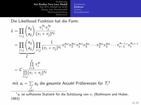
Die Likelihood Funktion hat die Form:
L =∏i<j
(nijaij
)πaiji π
ajij
(πi + πj)nij
=∏i<j
(nijaij
)︸ ︷︷ ︸
C
∏i<j
1
(πi + πj)nijπa121 πa212 πa131 πa313 · · ·π
a232 πa323 · · ·π
at−1,t
t−1 πat,t−1t
= C
t∏i=1
πaii∏i<j
(πi + πj)nij
mit ai =∑j
j 6=i
aij die gesamte Anzahl Praferenzen fur Ti1
1ai ist suffiziente Statistik fur die Schatzung von πi (Buhlmann and Huber,1963)
8 / 35
EinfuhrungDas Bradley-Terry-Luce Modell
Das BTL-Modell als GLMBezug zum Raschmodell
WeiterentwicklungReferences
AnnahmenSchatzenTestenAuswahlaxiom
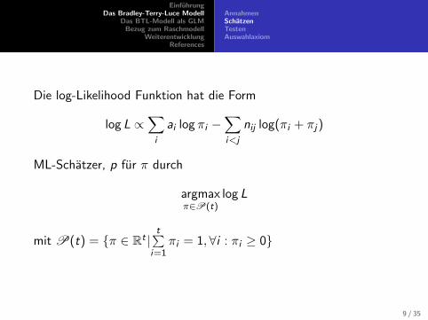
Die log-Likelihood Funktion hat die Form
log L ∝∑i
ai log πi −∑i<j
nij log(πi + πj)
ML-Schatzer, p fur π durch
argmaxπ∈P(t)
log L
mit P(t) = {π ∈ Rt |t∑
i=1πi = 1, ∀i : πi ≥ 0}
9 / 35
EinfuhrungDas Bradley-Terry-Luce Modell
Das BTL-Modell als GLMBezug zum Raschmodell
WeiterentwicklungReferences
AnnahmenSchatzenTestenAuswahlaxiom
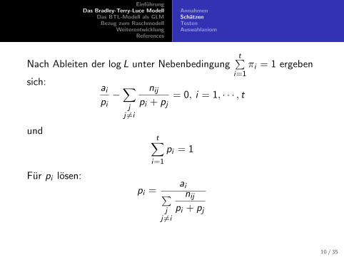
Nach Ableiten der log L unter Nebenbedingungt∑
i=1πi = 1 ergeben
sich:aipi−∑j
j 6=i
nijpi + pj
= 0, i = 1, · · · , t
undt∑
i=1
pi = 1
Fur pi losen:
pi =ai∑
jj 6=i
nijpi + pj
10 / 35

EinfuhrungDas Bradley-Terry-Luce Modell
Das BTL-Modell als GLMBezug zum Raschmodell
WeiterentwicklungReferences
AnnahmenSchatzenTestenAuswahlaxiom
Iterative Losung:
Wahle Startwerte fur p(0)i = 1/t, i = 1, · · · , t
Berechne:p(k)i =
ai∑j
j 6=i
nij
p(k−1)i + p
(k−1)j
p(1)i = ai
ni1
p(0)i + p
(0)1
+ · · ·+ ni ,i−1
p(0)i + p
(0)i−1
+ni ,i+1
p(0)i + p
(0)i+1
+ · · ·
+nit
p(0)i + p
(0)t
−1
p(2)i = · · ·
p(3)i = · · ·
11 / 35
EinfuhrungDas Bradley-Terry-Luce Modell
Das BTL-Modell als GLMBezug zum Raschmodell
WeiterentwicklungReferences
AnnahmenSchatzenTestenAuswahlaxiom
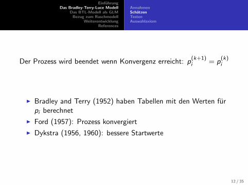
Der Prozess wird beendet wenn Konvergenz erreicht: p(k+1)i = p
(k)i
I Bradley and Terry (1952) haben Tabellen mit den Werten furpi berechnet
I Ford (1957): Prozess konvergiert
I Dykstra (1956, 1960): bessere Startwerte
12 / 35
EinfuhrungDas Bradley-Terry-Luce Modell
Das BTL-Modell als GLMBezug zum Raschmodell
WeiterentwicklungReferences
AnnahmenSchatzenTestenAuswahlaxiom
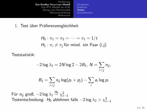
1. Test uber Praferenzengleichheit
H0 : π1 = π2 = · · · = πt = 1/t
H1 : πi 6= πj fur mind. ein Paar (i,j)
Teststatistik:
−2 log λ1 = 2N log 2− 2B1, N =∑i<j
nij ,
B1 =∑i<j
nij log(pi + pj)−∑i
ai log pi
Fur nij groß, −2 log λ1H0∼ χ2
t−1Testentscheidung: H0 ablehnen falls −2 log λ2 > χ2
t−1
13 / 35
EinfuhrungDas Bradley-Terry-Luce Modell
Das BTL-Modell als GLMBezug zum Raschmodell
WeiterentwicklungReferences
AnnahmenSchatzenTestenAuswahlaxiom
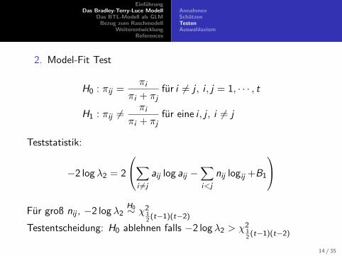
2. Model-Fit Test
H0 : πij =πi
πi + πjfur i 6= j , i , j = 1, · · · , t
H1 : πij 6=πi
πi + πjfur eine i , j , i 6= j
Teststatistik:
−2 log λ2 = 2
∑i 6=j
aij log aij −∑i<j
nij logij +B1
Fur groß nij , −2 log λ2
H0∼ χ212(t−1)(t−2)
Testentscheidung: H0 ablehnen falls −2 log λ2 > χ212(t−1)(t−2)
14 / 35
EinfuhrungDas Bradley-Terry-Luce Modell
Das BTL-Modell als GLMBezug zum Raschmodell
WeiterentwicklungReferences
AnnahmenSchatzenTestenAuswahlaxiom
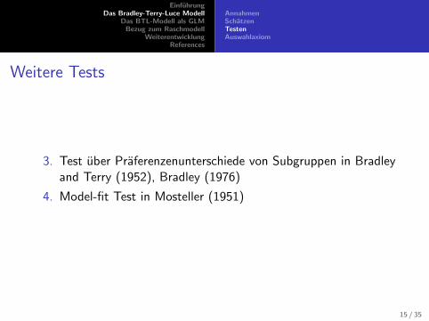
Weitere Tests
3. Test uber Praferenzenunterschiede von Subgruppen in Bradleyand Terry (1952), Bradley (1976)
4. Model-fit Test in Mosteller (1951)
15 / 35
EinfuhrungDas Bradley-Terry-Luce Modell
Das BTL-Modell als GLMBezug zum Raschmodell
WeiterentwicklungReferences
AnnahmenSchatzenTestenAuswahlaxiom
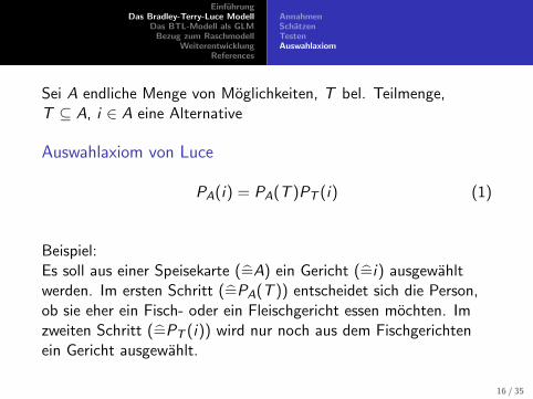
Sei A endliche Menge von Moglichkeiten, T bel. Teilmenge,T ⊆ A, i ∈ A eine Alternative
Auswahlaxiom von Luce
PA(i) = PA(T )PT (i) (1)
Beispiel:Es soll aus einer Speisekarte (=A) ein Gericht (=i) ausgewahltwerden. Im ersten Schritt (=PA(T )) entscheidet sich die Person,ob sie eher ein Fisch- oder ein Fleischgericht essen mochten. Imzweiten Schritt (=PT (i)) wird nur noch aus dem Fischgerichtenein Gericht ausgewahlt.
16 / 35
EinfuhrungDas Bradley-Terry-Luce Modell
Das BTL-Modell als GLMBezug zum Raschmodell
WeiterentwicklungReferences
AnnahmenSchatzenTestenAuswahlaxiom
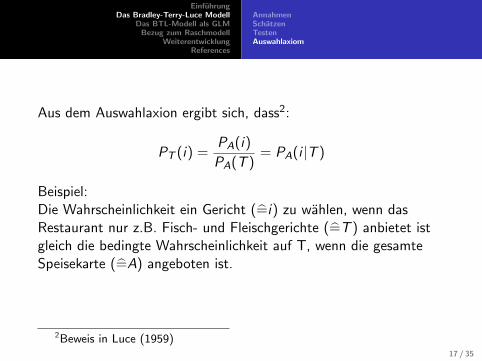
Aus dem Auswahlaxion ergibt sich, dass2:
PT (i) =PA(i)
PA(T )= PA(i |T )
Beispiel:Die Wahrscheinlichkeit ein Gericht (=i) zu wahlen, wenn dasRestaurant nur z.B. Fisch- und Fleischgerichte (=T ) anbietet istgleich die bedingte Wahrscheinlichkeit auf T, wenn die gesamteSpeisekarte (=A) angeboten ist.
2Beweis in Luce (1959)17 / 35
EinfuhrungDas Bradley-Terry-Luce Modell
Das BTL-Modell als GLMBezug zum Raschmodell
WeiterentwicklungReferences
AnnahmenSchatzenTestenAuswahlaxiom
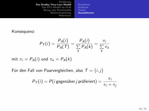
Konsequenz:
PT (i) =PA(i)
PA(T )=
PA(i)∑kPA(k)
=πi∑
kπk
mit πi = PA(i) und πk = PA(k)
Fur den Fall von Paarvergleichen, also T = {i , j}
PT (i) = P(i gegenuber j praferiert) =πi
πi + πj
18 / 35
EinfuhrungDas Bradley-Terry-Luce Modell
Das BTL-Modell als GLMBezug zum Raschmodell
WeiterentwicklungReferences
Numerisches Beispiel
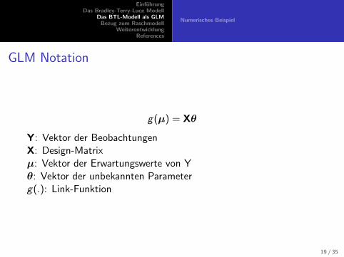
GLM Notation
g(µ) = Xθ
Y: Vektor der BeobachtungenX: Design-Matrixµ: Vektor der Erwartungswerte von Yθ: Vektor der unbekannten Parameterg(.): Link-Funktion
19 / 35
EinfuhrungDas Bradley-Terry-Luce Modell
Das BTL-Modell als GLMBezug zum Raschmodell
WeiterentwicklungReferences
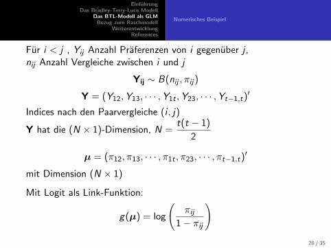
Numerisches Beispiel
Fur i < j , Yij Anzahl Praferenzen von i gegenuber j ,nij Anzahl Vergleiche zwischen i und j
Yij ∼ B(nij , πij)
Y = (Y12,Y13, · · · ,Y1t ,Y23, · · · ,Yt−1,t)′
Indices nach den Paarvergleiche (i , j)
Y hat die (N × 1)-Dimension, N =t(t − 1)
2
µ = (π12, π13, · · · , π1t , π23, · · · , πt−1,t)′
mit Dimension (N × 1)
Mit Logit als Link-Funktion:
g(µ) = log
(πij
1− πij
)20 / 35
EinfuhrungDas Bradley-Terry-Luce Modell
Das BTL-Modell als GLMBezug zum Raschmodell
WeiterentwicklungReferences
Numerisches Beispiel
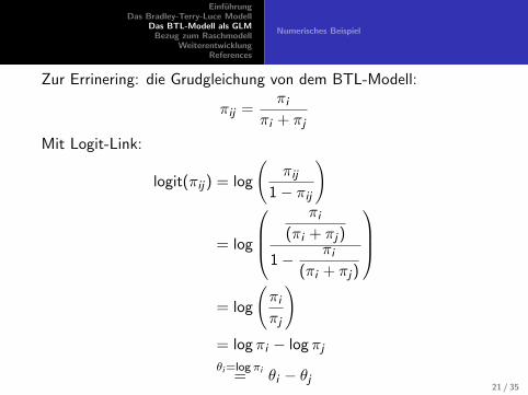
Zur Errinering: die Grudgleichung von dem BTL-Modell:
πij =πi
πi + πj
Mit Logit-Link:
logit(πij) = log
(πij
1− πij
)
= log
πi
(πi + πj)
1− πi(πi + πj)
= log
(πiπj
)= log πi − log πjθi=log πi= θi − θj
21 / 35
EinfuhrungDas Bradley-Terry-Luce Modell
Das BTL-Modell als GLMBezug zum Raschmodell
WeiterentwicklungReferences
Numerisches Beispiel
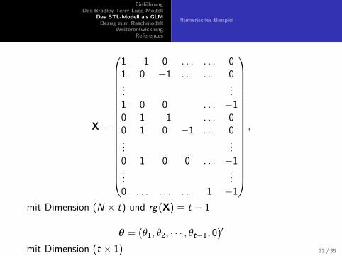
X =
1 −1 0 . . . . . . 01 0 −1 . . . . . . 0...
...1 0 0 . . . −10 1 −1 . . . 00 1 0 −1 . . . 0...
...0 1 0 0 . . . −1...
...0 . . . . . . . . . 1 −1
,
mit Dimension (N × t) und rg(X) = t − 1
θ = (θ1, θ2, · · · , θt−1, 0)′
mit Dimension (t × 1) 22 / 35
EinfuhrungDas Bradley-Terry-Luce Modell
Das BTL-Modell als GLMBezug zum Raschmodell
WeiterentwicklungReferences
Numerisches Beispiel
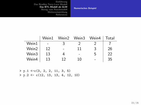
Wein1 Wein2 Wein3 Wein4 Total
Wein1 - 3 2 2 7Wein2 12 - 11 3 26Wein3 13 4 - 5 22Wein4 13 12 10 - 35
> y.1 <-c(3, 2, 2, 11, 3, 5)
> y.2 <- c(12, 13, 13, 4, 12, 10)
23 / 35
EinfuhrungDas Bradley-Terry-Luce Modell
Das BTL-Modell als GLMBezug zum Raschmodell
WeiterentwicklungReferences
Numerisches Beispiel
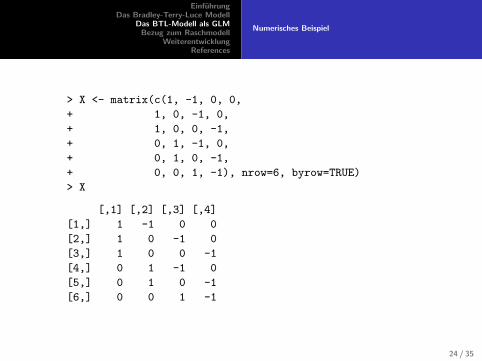
> X <- matrix(c(1, -1, 0, 0,
+ 1, 0, -1, 0,
+ 1, 0, 0, -1,
+ 0, 1, -1, 0,
+ 0, 1, 0, -1,
+ 0, 0, 1, -1), nrow=6, byrow=TRUE)
> X
[,1] [,2] [,3] [,4]
[1,] 1 -1 0 0
[2,] 1 0 -1 0
[3,] 1 0 0 -1
[4,] 0 1 -1 0
[5,] 0 1 0 -1
[6,] 0 0 1 -1
24 / 35
EinfuhrungDas Bradley-Terry-Luce Modell
Das BTL-Modell als GLMBezug zum Raschmodell
WeiterentwicklungReferences
Numerisches Beispiel
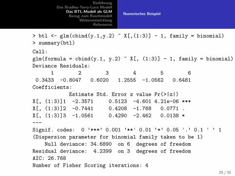
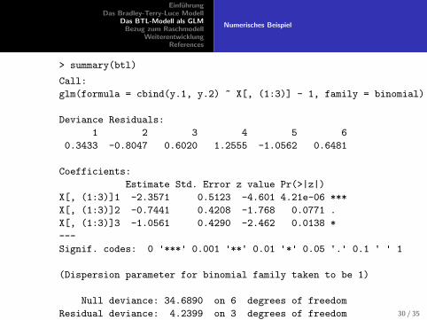
> btl <- glm(cbind(y.1,y.2) ~ X[,(1:3)] - 1, family = binomial)
> summary(btl)
Call:
glm(formula = cbind(y.1, y.2) ~ X[, (1:3)] - 1, family = binomial)
Deviance Residuals:
1 2 3 4 5 6
0.3433 -0.8047 0.6020 1.2555 -1.0562 0.6481
Coefficients:
Estimate Std. Error z value Pr(>|z|)
X[, (1:3)]1 -2.3571 0.5123 -4.601 4.21e-06 ***
X[, (1:3)]2 -0.7441 0.4208 -1.768 0.0771 .
X[, (1:3)]3 -1.0561 0.4290 -2.462 0.0138 *
---
Signif. codes: 0 '***' 0.001 '**' 0.01 '*' 0.05 '.' 0.1 ' ' 1
(Dispersion parameter for binomial family taken to be 1)
Null deviance: 34.6890 on 6 degrees of freedom
Residual deviance: 4.2399 on 3 degrees of freedom
AIC: 26.768
Number of Fisher Scoring iterations: 425 / 35
EinfuhrungDas Bradley-Terry-Luce Modell
Das BTL-Modell als GLMBezug zum Raschmodell
WeiterentwicklungReferences
Numerisches Beispiel
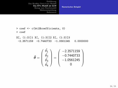
> coef <- c(btl$coefficients, 0)
> coef
X[, (1:3)]1 X[, (1:3)]2 X[, (1:3)]3
-2.3571159 -0.7440733 -1.0561245 0.0000000
θ =
θ1θ2θ3θ4
=
−2.3571159−0.7440733−1.0561245
0
26 / 35
EinfuhrungDas Bradley-Terry-Luce Modell
Das BTL-Modell als GLMBezug zum Raschmodell
WeiterentwicklungReferences
Numerisches Beispiel
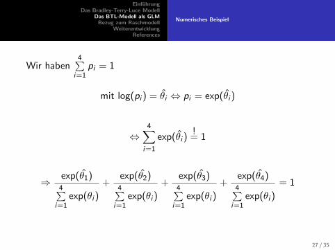
Wir haben4∑
i=1pi = 1
mit log(pi ) = θi ⇔ pi = exp(θi )
⇔4∑
i=1
exp(θi )!= 1
⇒ exp(θ1)4∑
i=1exp(θi )
+exp(θ2)4∑
i=1exp(θi )
+exp(θ3)4∑
i=1exp(θi )
+exp(θ4)4∑
i=1exp(θi )
= 1
27 / 35
EinfuhrungDas Bradley-Terry-Luce Modell
Das BTL-Modell als GLMBezug zum Raschmodell
WeiterentwicklungReferences
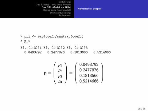
Numerisches Beispiel
> p_i <- exp(coef)/sum(exp(coef))
> p_i
X[, (1:3)]1 X[, (1:3)]2 X[, (1:3)]3
0.0493792 0.2477876 0.1813666 0.5214666
p =
p1p2p3p4
=
0.04937920.24778760.18136660.5214666
28 / 35
EinfuhrungDas Bradley-Terry-Luce Modell
Das BTL-Modell als GLMBezug zum Raschmodell
WeiterentwicklungReferences
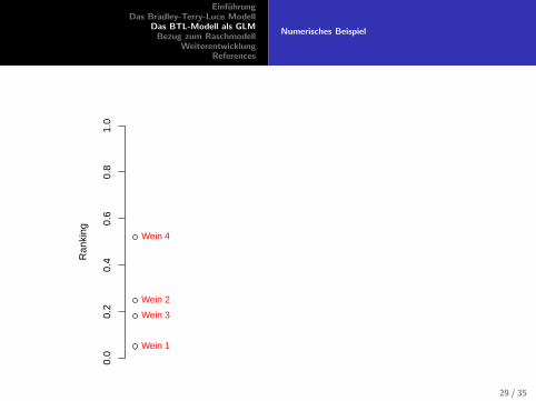
Numerisches Beispiel
Plot
Ran
king
0.0
0.2
0.4
0.6
0.8
1.0
Wein 1
Wein 2
Wein 3
Wein 4
29 / 35
EinfuhrungDas Bradley-Terry-Luce Modell
Das BTL-Modell als GLMBezug zum Raschmodell
WeiterentwicklungReferences
Numerisches Beispiel
> summary(btl)
Call:
glm(formula = cbind(y.1, y.2) ~ X[, (1:3)] - 1, family = binomial)
Deviance Residuals:
1 2 3 4 5 6
0.3433 -0.8047 0.6020 1.2555 -1.0562 0.6481
Coefficients:
Estimate Std. Error z value Pr(>|z|)
X[, (1:3)]1 -2.3571 0.5123 -4.601 4.21e-06 ***
X[, (1:3)]2 -0.7441 0.4208 -1.768 0.0771 .
X[, (1:3)]3 -1.0561 0.4290 -2.462 0.0138 *
---
Signif. codes: 0 '***' 0.001 '**' 0.01 '*' 0.05 '.' 0.1 ' ' 1
(Dispersion parameter for binomial family taken to be 1)
Null deviance: 34.6890 on 6 degrees of freedom
Residual deviance: 4.2399 on 3 degrees of freedom
AIC: 26.768
Number of Fisher Scoring iterations: 4
30 / 35
EinfuhrungDas Bradley-Terry-Luce Modell
Das BTL-Modell als GLMBezug zum Raschmodell
WeiterentwicklungReferences
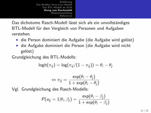
Das dichotome Rasch-Modell lasst sich als ein unvollstandigesBTL-Modell fur den Vergleich von Personen und Aufgabenverstehen.
I die Person dominiert die Aufgabe (die Aufgabe wird gelost)I die Aufgabe dominiert die Person (die Aufgabe wird nicht
gelost)
Grundgleichung des BTL-Modells:
logit(πij) = log(πij/(1− πij)) = θi − θj
⇔ πij =exp(θi − θj)
1 + exp(θi − θj)Vgl. Grundgleichung des Rasch-Modells:
P(uij = 1|θi , βj) =exp(θi − βj)
1 + exp(θi − βj)
31 / 35
EinfuhrungDas Bradley-Terry-Luce Modell
Das BTL-Modell als GLMBezug zum Raschmodell
WeiterentwicklungReferences
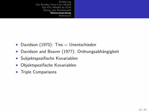
I Davidson (1970): Ties = Unentschieden
I Davidson and Beaver (1977): Ordnungsabhangigkeit
I Subjektspezifische Kovariablen
I Objektspezifische Kovariablen
I Triple Comparisons
32 / 35
EinfuhrungDas Bradley-Terry-Luce Modell
Das BTL-Modell als GLMBezug zum Raschmodell
WeiterentwicklungReferences
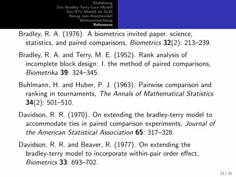
Bradley, R. A. (1976). A biometrics invited paper. science,statistics, and paired comparisons, Biometrics 32(2): 213–239.
Bradley, R. A. and Terry, M. E. (1952). Rank analysis ofincomplete block design: I. the method of paired comparisons,Biometrika 39: 324–345.
Buhlmann, H. and Huber, P. J. (1963). Pairwise comparison andranking in tournaments, The Annals of Mathematical Statistics34(2): 501–510.
Davidson, R. R. (1970). On extending the bradley-terry model toaccommodate ties in paired comparison experiments, Journal ofthe American Statistical Association 65: 317–328.
Davidson, R. R. and Beaver, R. (1977). On extending thebradley-terry model to incorporate within-pair order effect,Biometrics 33: 693–702.
33 / 35
EinfuhrungDas Bradley-Terry-Luce Modell
Das BTL-Modell als GLMBezug zum Raschmodell
WeiterentwicklungReferences
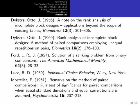
Dykstra, Otto, J. (1956). A note on the rank analysis ofincomplete block designs – applications beyond the scope ofexisting tables, Biometrics 12(3): 301–306.
Dykstra, Otto, J. (1960). Rank analysis of incomplete blockdesigns: A method of paired comparisons employing unequalrepetitions on pairs, Biometrics 16(2): 176–188.
Ford, L. R., J. (1957). Solution of a ranking problem from binarycomparisons, The American Mathematical Monthly64(8): 28–33.
Luce, R. D. (1959). Individual Choice Behavior, Wiley, New York.
Mosteller, F. (1951). Remarks on the method of pairedcomparisons: Iii. a test of significance for paired comparisonswhen equal standard deviations and equal correlations areassumed, Psychometrika 16: 207–218.
34 / 35
EinfuhrungDas Bradley-Terry-Luce Modell
Das BTL-Modell als GLMBezug zum Raschmodell
WeiterentwicklungReferences
Thurstone, L. L. (1927). A law of comparative judgment,Psychological Review 34: 273–286.
Zermelo, E. (1929). Die berechnung der turnier-ergebnisse als einmaximum-problem der wahrscheinlichkeitsrechnung, Math.Zeitschrift 29: 436–460.
35 / 35


![Industrielle Druckmesswandler Standard-Industrie Modell S ... · Bauteil Modell S Modell E Modell T Medienberührt Interne Membran (25 bar [362 psi, 2,5 MPa, 25,5 kg/cm2, 2500 kPa]](https://img.pdfslide.org/doc/110x75/5e2134d84e91925a545cfa09/industrielle-druckmesswandler-standard-industrie-modell-s-bauteil-modell-s-modell.jpg)