Deformed Starobinsky model in gravity’s rainbow

Phongpichit Channuie1, 2, 3, ∗

1College of Graduate Studies, Walailak University,

Thasala, Nakhon Si Thammarat, 80160, Thailand

2School of Science, Walailak University, Thasala,

Nakhon Si Thammarat, 80160, Thailand

3Thailand Center of Excellence in Physics,

Ministry of Education, Bangkok 10400, Thailand

(Dated: July 27, 2021)

In the context of gravity’s rainbow, we study the deformed Starobinsky model in which

the deformations take the form f(R) ∼ R2(1−α), with R the Ricci scalar and α a positive

parameter. We show that the spectral index of curvature perturbation and the tensor-to-

scalar ratio can be written in terms of N, λ and α, with N being the number of e-foldings,

λ a rainbow parameter. We compare the predictions of our models with Planck data. With

the sizeable number of e-foldings and proper choices of parameters, we discover that the

predictions of the model are in excellent agreement with the Planck analysis. Interestingly,

we obtain the upper limit and the lower limit of a rainbow parameter λ and a positive

constant α, respectively.

PACS numbers:

I. INTRODUCTION

The prediction of a minimal measurable length in order of Planck length in various theories

of quantum gravity restricts the maximum energy that any particle can attain to the Planck

energy. This could be implied the modification of linear momentum and also quantum commutation

relations and results the modified dispersion relation. Moreover, as an effective theory of gravity,

the Einstein general theory of gravity is valid in the low energy (IR) limit, while at very high

energy regime (UV) the Einstein theory could in principle be improved.

One of the interesting approaches that naturally deals with modified dispersion relations is called

doubly special relativity [1–3]. Then Magueijo and Smolin [4] generalized this idea by including

curvature. The modification of the dispersion relation results by replacing the standard one, i.e.

∗Electronic address: channuie@gmail.com

arX

iv:1

903.

0599

6v1

[gr

-qc]

9 M

ar 2

019

2

ε2 − p2 = m2, with the form ε2f2(ε) − p2g2(ε) = m2 where functions f(ε) and g(ε) are commonly

known as the rainbow functions. It is worth noting that the rainbow functions are chosen in such

a way that they produce, at a low-energy IR limit ε/M → 0, the standard energy-momentum

relation and they are required to satisfy f(ε)→ 1 and g(ε)→ 1 where M is the energy scale that

quantum effects of gravity become important.

Notice that the gravity’s rainbow is motivated by modification of usual dispersion relation in

the UV limit and captures a modification of the geometry at that limit. Hence, the geometry of

the space-time in gravity’s rainbow depends on energy of the test particles. Therefore, each test

particle of different energy will feel a different geometry of space-time. This displays a family of

metrics, namely a rainbow metrics, parametrized by ε to describe the background of the space-time

instead of a single metric. In gravitys rainbow, the modified metric can be expressed as

g(ε) = ηµν eµ(ε)⊗ eν(ε) , (1)

with the energy dependence of the frame field eµ(ε) can be written in terms of the energy inde-

pendence frame field eµ as e0(ε) = e0/f(ε) and ei(ε) = ei/g(ε) where i, 1, 2, 3. In the cosmological

viewpoint, the conventional FLRW metric for the homogeneous and isotropic universe is replaced

by a rainbow metric of the form

ds2 = − 1

f2(ε)dt2 + a(t)2δijdx

idxj , (2)

where a(t) is a scale factor. For convenience, we choose g(ε) = 1 and only focus on the spatially

flat case. As suggested in Ref.[12], this formalism can be generalized to study semi-classical effects

of relativistic particles on the background metric during a longtime process. For the very early

universe, we consider the evolution of the probes energy with cosmic time, denoted as ε(t). Hence

the rainbow functions f(ε) depends on time implicitly through the energy of particles.

In recent years, gravity’s rainbow has attracted a lot of attentions and became the subject of

much interest in the literature. In the context of such gravity, the various physical properties of

the black holes are investigated, see e.g. [14–21]. In addition, the effects of the rainbow functions

have also been discussed in several other scenarios, see for instance [22–24]. Moreover, the gravity’s

rainbow was investigated in Gauss-Bonnet gravity [25], massive gravity [26] and f(R) gravity [27].

More specifically, the gravitys rainbow has also been used for analyzing the effects of rainbow

functions on the Starobinsky model of f(R) gravity [9].

One of the intriguing features of the Starobinsky model [10] is that gravity itself is directly

responsible for the inflationary period of the universe without resorting to the introduction of new

3

ad hoc scalar fields. The authors of Ref.[11] studied quantum-induced marginal deformations of

the Starobinsky gravitational action of the form R2(1α), with R the Ricci scalar and α a positive

parameter smaller than one half. The model predicted sizable primordial tensor modes. In the

present work, we consider the model proposed by Ref.[11] in the context of gravity’s rainbow.

This paper is organized as follows: In section II, we revisit the formalism in f(R) theory [7, 8]

in the framework of gravity’s rainbow [9]. We then focus on the deformed Starobinskys model [11]

in which f(R) takes the form f(R) ∼ R2(1−α). We take a short recap of a cosmological linear

perturbation in the context of the gravitys rainbow generated during inflation and calculate the

spectral index of scalar perturbation and the tensor-to-scalar ratio of the model in section III. In

section IV, we compare the predicted results with Planck data. We conclude our findings in the

last section.

II. f(R) THEORIES WITH GRAVITY’S RAINBOW EFFECT

As is well known, the modification to general relativity are expected to be plausible in very early

universe where possible corrections to Einstein’s theory may in principle emerge at high curvature.

One of the simplest classes of such modifications is f(R) theories where the Einstein-Hilbert term

in the action is replaced by a generic function of the Ricci scalar. We start with the traditionally

4-dimensional action in f(R) gravity [7, 8].

S =1

2κ2

∫d4x√−gf(R) +

∫d4x√−gLM (gµν ,ΨM ) , (3)

where κ2 = 8πG, g is the determinant of the metric gµν , and the matter field Lagrangian LM

depends on gµν and matter fields ΨM . We can derive the field equation by varying the action (3)

with respect to gµν to obtain [7, 8]

F (R)Rµν(g)− 1

2f(R)gµν −∇µ∇νF (R) + gµν�F (R) = κ2T (M)

µν , (4)

where F (R) = ∂f(R)/∂R and the operator � is defined by � ≡ (1/√−g)∂µ(

√−ggµν∂ν).

Traditionally, the energy-momentum tensor of the matter fields is given by T(M)µν =

(−2/√−g)δ(

√−gLM )/δgµν . Here it satisfies the continuity equation such that ∇µT (M)

µν = 0. Note

that the right side of Eq.(4) follows the continuity equation. Using the modified FLRW metric,

we can show that the Ricci scalar can be written in terms of the Hubble parameter and a rainbow

function as

R = 6f2

(2H2 + H +H

˙f

f

). (5)

4

The (0, 0)-component of Eq.(4) yields the following differential equation:

3FH2 = −3HF − F˙f

f+FR− f(R)

2f2+κ2ρM

f2, (6)

and the (i, j)-component of Eq.(4) reads

2F

(H +H

˙f

f

)= −F +HF − κ2

f2

(ρM + PM

). (7)

It is worth noting that the above two equations are modified by the rainbow function and these

equations can be transformed to the standard ones when setting f = 1. Let us next consider the

deformed Starobinsky model in which f(R) takes the following form [11]:

f(R) = R+R2(1−α)

6M2, (8)

where 1/(6M2) = 2hm4α−2pl and we assume that α is a real parameter with 2|α| < 1 and h

is a dimensionless parameter. It is worth noting that the Starobinsky model is recovered when

α = 0. Note that in the standard Starobinsky scenario the R2 plays a key role in the very early

universe instead of relativistic matter. In the scalar field framework, the Starobinsky theory can

be equivalent to the system of one scalar field (an inflaton). It is reasonable if we assume here

that the inflaton dominates the very early universe and hence in what follows we can neglect the

contributions from matter and radiation, i.e. ρM = 0 and PM = 0.

The combination of Eqs.(5), (6) and (7) give us the following system of differential equations:

R+ 3HR+4R

˙f

3f+M2

f2

(R+

2α

M2R2(1−α)

)= 0 , (9)

and

1

f(t)2H(t)

˙f(t)3 +

(2

˙f(t)

(H(t)

¨f(t) +

˙f(t)

(3H(t) + 7H(t)2

))+ 3M2H(t)2

)−2f(t)

(H(t)

(˙f(t)

(−13H(t)− 15H(t)2

)− 3H(t)

¨f(t)

)− ˙f(t)H(t)

)+6f(t)2H(t)

(H(t) + 5H(t)H(t) + 2H(t)3

)+ 31−2α4−α(2α− 1)

(H(t)

˙f(t)

+f(t)(H(t) + 2H(t)2

))2 (f(t)

(H(t)

˙f(t) + f(t)

(H(t) + 2H(t)2

)))−2α= 0 . (10)

Note here that when setting α = 0 our results given in Eqs.(9) and (10) nicely convert to those

present in Ref.[9]. In addition, when setting both α = 0 and f(t) = 1 our results here reduce to

5

those obtained in the Starobinsky model. Using f ≈ (H/M)λ, we obtain

6(α− 1)(2α− 1)(λ+ 1)HH

(H

M

)2λ

+ 3H2

(36αM2

((H

M

)2λ ((λ+ 1)H + 2H2

))2α

+2(α(8α− 9) + 3)(λ+ 1)H

(H

M

)2λ)

+4(α− 1)(2α− 1)λ2(λ+ 1)H3

(HM

)2λH2

+(2α− 1)(λ+ 1)((20α− 17)λ+ 3)H2

(H

M

)2λ

+2(α− 1)(2α− 1)λ(λ+ 1)HH

(HM

)2λH

+ 12αH4

(H

M

)2λ

= 0. (11)

Since we are only interested in an inflationary solution, it is natural to assume the slow-roll approx-

imation, namely the terms containing H and higher power in H can be neglected in this particular

regime. Therefore the Eq.(11) is reduced to

H ' −M2

(HM

)−2λ6(λ+ 1)

−

(HM

)−2λ6(λ+ 1)

(2M2 log

(12H2

(HM

)2λ)+ 4H2

(H

M

)2λ

+ 3M2)α+O(α2) .(12)

Setting only α = 0, we obtain the same result given in Ref.[9]. Moreover, setting both α and λ to

vanish, the result converts to the standard Starobinsky model [10]. Despite the fact that one can

numerically solve this equation for the Hubble parameter during inflation, we can find a simple

analytical solution to this equation provided the second term on the RHS can be ignored since we

are considering a small deviation from the Starobinsky model. Given this further approximation

one obtains

H ' Hi −M2

(HM

)−2λ6(λ+ 1)

(t− ti)

−

(HM

)−2λ6(λ+ 1)

(2M2 log

(12H2

(HM

)2λ)+ 4H2

(H

M

)2λ

+ 3M2)α(t− ti) +O(α2) , (13)

and

a ' ai exp

{Hi(t− ti)−

M2(HM

)−2λ6(λ+ 1)

(t− ti)2

−

(HM

)−2λ6(λ+ 1)

(2M2 log

(12H2

(HM

)2λ)+ 4H2

(H

M

)2λ

+ 3M2)α(t− ti)2 +O(α2)

},(14)

where Hi and ai are respectively the Hubble parameter and the scale factor at the onset of inflation

(t = ti). The slow-roll parameter ε1 is defined by ε1 ≡ −H/H2 which in this case can be estimated

6

to the first order of α as

ε1 'H−2(λ+1)M2λ+2

6(λ+ 1)

+H−2(λ+1)

2(λ+ 1)

(1

3

(4H2(λ+1) + M2λ+2 log

(144H4(λ+1)M4λ

))+ M2λ+2

)α . (15)

Note that this parameter is less than unity during inflation (H2 � M2) and we find when setting

α = 0 that ε1 ' H−2(λ+1)M2λ+2

6(λ+1) . One can simply determine the end of inflation (t = tf ) by the

condition ε(tf ) ' 1, tf is approximately given by

tf ' ti + 6(λ+ 1)H2λ+1i

M2λ+2

+ 6(λ+ 1)H2λ+1i

M4(λ+1)

(−4H2λ+2

i − M2λ+2(

log(

144H2(λ+1)i M4λ

)+ 3))

α . (16)

The number of e-foldings from ti to tf is then given by

N ≡∫ tf

ti

Hdt ' Hi(t− ti)−M2

(HM

)−2λ6(λ+ 1)

(t− ti)2

−

(HM

)−2λ6(λ+ 1)

(2M2 log

(12H2

(HM

)2λ)+ 4H2

(H

M

)2λ

+ 3M2)α(t− ti)2 . (17)

Using the expressions (16) and (15) the parameter N is thus given by to the first order of α:

N ' 3(λ+ 1)H2λ+2

M2λ+2

+3(λ+ 1)H2λ+2

M4(λ+1)

(− 4H2λ+2 − M2λ+2

(log(

144H4(λ+1)M4λ)

+ 3))α =

1

2ε1(ti). (18)

Note that when λ = 0 = α the result is the same as that of the Starobinsky model.

III. COSMOLOGICAL PERTURBATION IN GRAVITY’S RAINBOW REVISITED

In this section, we will take a short recap of a cosmological linear perturbation in the context

of the gravity’s rainbow generated during inflation proposed by Ref.[9]. We here begin with a

scalar perturbation (since scalar and tensor evolve separately at the linear level) via the following

perturbed flat FRW metric taking into account the rainbow effect

ds2 = −1 + 2Φ

f2(t)dt2 + a2(t)(1− 2Ψ)d~x2 , (19)

where f(t) denotes the rainbow function. Notice that this perturbed metric has been written in

the Newtonian gauge. Let us define a new variable A ≡ 3(HΦ + Ψ). With the metric (19) and

7

Eq.(4), we obtain the following system of equations [9]

−∇2Ψ

a2+ f2HA = − 1

2F

[3f2

(H2 + H +

˙f

f

)δF +

∇2δF

a2− 3f2HδF

+ 3f2HFΦ + f2FA+ κ2δρM

], (20)

HΦ + Ψ = − 1

2F(HδF + FΦ− δF ) , (21)

and

A+

(2H +

˙f

f

)A+ 3HΦ +

∇2Φ

a2f2+

3HΦ˙f

f=

1

2F

[3δF + 3

(H +

˙f

f

)δF

− 6H2δF − ∇2δF

a2f2− 3F Φ− FA− 3

(H +

˙f

f

)FΦ− 6FΦ +

κ2

f2(3δPM + δρM )

]. (22)

Note that the equations given above can be used to describe evolution of the cosmological scalar

perturbations. In what follows, we will solve these equations within the inflationary framework.

We first study scalar perturbations generated during inflation and consider not to take into account

the perfect fluid, i.e. δρM = 0 and δPM = 0. Here we choose the gauge condition δF = 0, so that

R = ψ = −Ψ. Note that the spatial curvature (3)R on the constant-time hypersurface is related

to ψ via the relation (3)R = −4∇2ψ/a2. Using δF = 0, we obtain from Eq.(21)

Φ =R

H + F /2F, (23)

and from the equation (20), we find

A = − 1

H + F /2F

[∇2Ra2f2

+3HF R

2F (H + F /2F )

]. (24)

Using the background equation (7), we find from Eq.(22)

A+

(2H +

F

2F

)A+

˙fA

f+

3F Φ

2F+

[3F + 6HF

2F+∇2

a2f2

]Φ +

3F

2F

Φ˙f

f= 0. (25)

Substituting Eq.(23) and (24) into Eq.(25), we find in Fourier space that the curvature perturbation

satisfies the following equation

R+1

a3Qs

d

dt(a3Qs)R+

˙f

fR+

k2

a2f2R = 0 , (26)

where k is a comoving wave number and Qs is defined by

Qs ≡3F 2

2κ2F (H + F /2F )2. (27)

8

Introducing new variables zs = a√Qs and u = zsR, Eq.(26) can be reduced and then can be

expressed as

u′′ +

(k2 − z′′s

zs

)u = 0 , (28)

where a prime denotes a derivative with respect to the new time coordinates η =∫

(af)−1dt. In

order to determine the spectrum of curvature perturbations we define slow-roll parameters as

ε1 ≡ −H

H2, ε2 ≡

F

2HF, ε3 ≡

E

2HE, (29)

where E ≡ 3F 2/2κ2. As a result, Qs can be recast as

Qs =E

FH2(1 + ε2)2. (30)

Here parameters εi are assumed to be nearly constant during the inflation and f ' (H/M)λ. These

allow us to calculate η as η = −1/[(1− (1 + λ)ε1)faH]. If εi ' 0, a term z′′s /zs satisfies

z′′szs

=ν2R − 1/4

η2, (31)

with

ν2R =1

4+

(1 + ε1 − ε2 + ε3)(2− λε1 − ε2 + ε3)

(1− (λ+ 1)ε1)2. (32)

Therefore we find the solution of Eq.(28) written in terms of a linear combination of Hankel

functions

u =

√π|η|2

ei(1+2νR)π/4[c1H

(1)νR(k|η|) + c2H

(2)νR(k|η|)

], (33)

where c1, c2 are integration constants and H(1)νR(k|η|), H

(2)νR(k|η|) are the Hankel functions of the

first kind and the second kind respectively. In the asymptotic past kη → −∞, we find from Eq.(33)

u→ e−ikη/√

2k. This implies c1 = 1 and c2 = 0 giving the following solutions

u =

√π|η|2

ei(1+2νR)π/4H(1)νR(k|η|) . (34)

By defining the power spectrum of curvature perturbations

PR ≡4πk3

(2π)3|R|2 , (35)

and using Eq.(34) and u = zsR, we obtain

PR =1

Qs

[(1− (1 + λ)ε1)

Γ(νR)H

2πΓ(3/2)

(H

M

)λ]2(k|η|2

)3−2νR, (36)

9

where we have used H(1)νR(k|η|) → −(i/π)Γ(νR)(k|η|/2)−νR for k|η| → 0. Since R is frozen after

the Hubble radius crossing, PR should be evaluated at k = aH. Now we define the spectral index

nR as

nR − 1 =dlnPRdlnk

∣∣∣∣k=aH

= 3− 2νR . (37)

The spectral index can be written in terms of the slow-roll parameters as

nR − 1 ' −2(λ+ 2)ε1 + 2ε2 − 2ε3 , (38)

where during the inflationary epoch, we have assumed that |εi| � 1. Notice that the spectrum is

nearly scale-invariant when |εi| are much smaller than unity, i.e. nR ' 1. Subsequently, the power

spectrum of curvature perturbation takes the form

PR ≈1

Qs

(H

2π

)2(HM

)2λ

. (39)

Note that we obtain the standard result when setting λ = 0 [8]. We next consider the tensor

perturbation. In general hij can be generally written as

hij = h+e+ij + h×e

×ij , (40)

where e+ij and e×ij are the polarization tensors corresponding to the two polarization states of hij .

Let ~k be in the direction along the z-axis, then the non-vanishing components of polarization

tensors are e+xx = −e+yy = 1 and e×xy = e×yx = 1. Without taking into account the scalar and vector

perturbation, the perturbed FLRW metric can be written as

ds2 = − dt2

f(ε)2+ a2(t)h×dxdy + a2(t)

[(1 + h+)dx2 + (1− h+)dy2 + dz2

]. (41)

Using Eq.(4), we can show that the Fourier components hχ satisfy the following equation

hχ +(a3F )·

a3Fhχ +

˙f

fhχ +

k2

a2f2hχ = 0 , (42)

where χ denotes polarizations + and ×. Following a similar procedure to the case of curvature

perturbation, let us introduce the new variables zt = a√F and uχ = zthχ/

√2κ2. Therefore Eq.

(42) can be written as

u′′χ +

(k2 − z′′t

zt

)uχ = 0 . (43)

Notice that for a massless scalar field uχ has dimension of mass. By choosing εi = 0, we obtain

z′′tzt

=ν2t − 1/4

η2, (44)

10

where

ν2t =1

4+

(1 + ε2)(2− (1 + λ)ε1 + ε2)

(1− (1 + λ)ε1)2. (45)

Similarly the solution to Eq.(43) can be also expressed in terms of a linear combination of Hankel

functions. Taking into account polarization states, the power spectrum of tensor perturbations PT

after the Hubble radius crossing reads

PT = 4× 2κ2

a2F

4πk3

(2π)3|uχ|2

=16

π

(H

MP

)2 1

F

[(1− (1 + λ)ε1)

Γ(νt)

Γ(3/2)

(H

M

)λ]2(k|η|2

)3−2νt, (46)

where we have used f ' (H/M)λ. Therefore νt can be estimated by assuming that the slow-roll

parameters are very small during inflation as

νt '3

2+ (1 + λ)ε1 + ε2 . (47)

In addition, the spectral index of tensor perturbations is determined via

nT =dlnPTdlnk

∣∣∣∣k=aH

= 3− 2νt ' −2(1 + λ)ε1 − 2ε2 . (48)

The power spectrum PT can also be rewritten as

PT '16

π

(H

MP

)2 1

F

(H

M

)2λ

. (49)

The tensor-to-scalar ratio r can be obtained as

r ≡ PTPR' 64π

M2P

QsF

. (50)

Substituting Qs from Eq.(30), we therefore obtain

r = 48ε22 . (51)

Let us next examine relations among the slow-roll parameters. Having assumed that |εi| � 1

during the inflation and matter field, Eq.(7) gives us

ε2 ' −(1 + λ)ε1 . (52)

Compared with the Starobinsky model, we have similar form of f(R) = R+ R2(1−α)

6M2. Here inflation

occurred in the limit R � M2 and |H| � H2. We can approximate F (R) ' (12H2f2)1−2α(1 −

α)/3M2. By assuming that |εi| � 1 during the inflation, this leads to

ε4 ' −(1 + 2λ− 4α(λ+ 1))ε1 . (53)

11

Considering Eq.(39), we obtain

PR '144α (ε1 + 1) 2M2α+2

12π(1− 2α)2(1− α)(λ+ 1)2m2plε

21

. (54)

Since nR − 1 ' −2(λ + 2)ε1 + 2ε3 − 2ε4 and r = 48ε23, one obtains the spectral index of scalar

perturbations and the tensor-to-scalar ratio rewritten in terms of ε1 as follows:

nR − 1 ' −4(1 + 2α(λ+ 1))ε1 and r ' 48(λ+ 1)2ε21. (55)

Let tk be the time at the Hubble radius crossing (k = aH). From Eq.(13), as long as the condition

Hi � M2(tk−ti)6(1+λ) (M/Hi)

2λ + O(α2) is satisfied, we can approximate H(tk) ' Hi. The number of

e-fold from t = tk to the end of the inflation can be estimated as Nk ' 1/2ε1(tk). We also find

from Eq.(54) to the leading order of α that

PR 'M2N2

3π(λ+ 1)2m2pl

+

(5M2 + M2 log(144M2)

)N2

3π(λ+ 1)2m2pl

α . (56)

According to the relation (18), both nR and r can be rewritten in terms of the number of e-foldings

as

nR − 1 = − 2

N− 4α(λ+ 1)

N(57)

and

r =12(λ+ 1)2

N2. (58)

Notice that the spectral index of scalar perturbations nR does depend on both α and the rainbow

parameter, λ.

IV. CONTACT WITH OBSERVATION

In this section, we compare our predicted results with Planck 2015 data. We find from

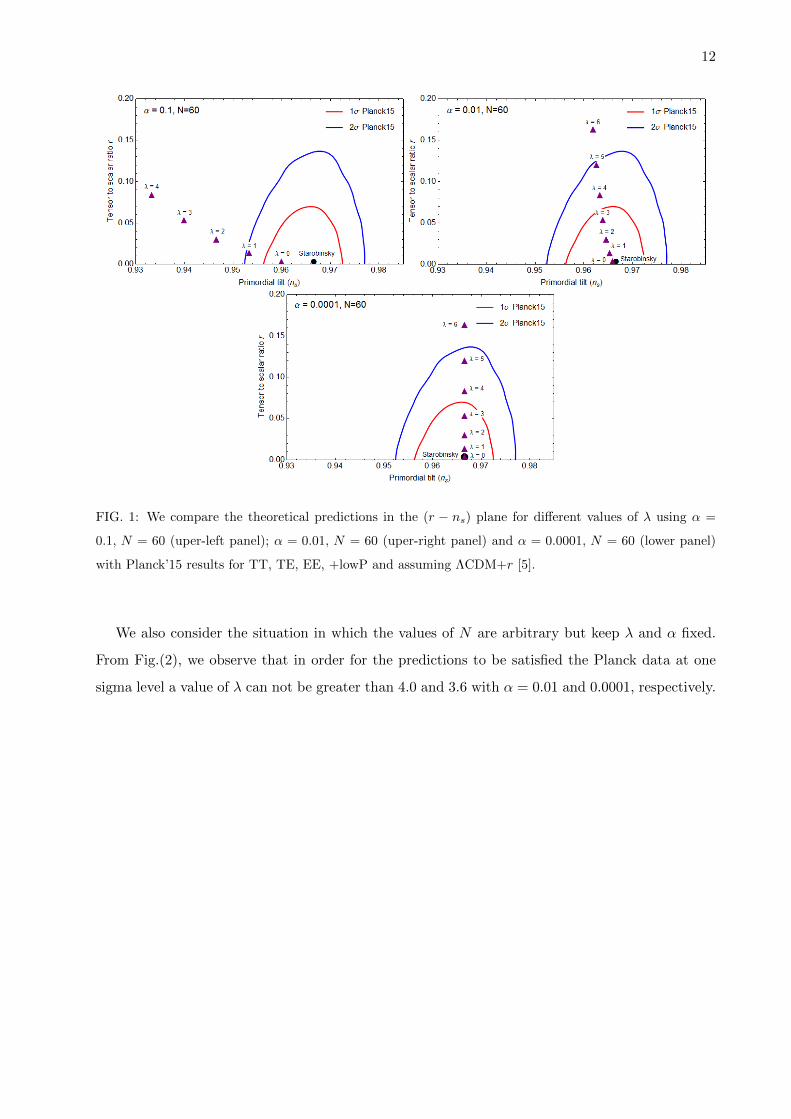
Fig.(1)that the predictions are consistent with the Planck data at two sigma confidence level for

N = 60 only when λ . 1.00, 5.00 and 5.50 for α = 0.1, 0.01 and 0.0001, respectively.

12

FIG. 1: We compare the theoretical predictions in the (r − ns) plane for different values of λ using α =

0.1, N = 60 (uper-left panel); α = 0.01, N = 60 (uper-right panel) and α = 0.0001, N = 60 (lower panel)

with Planck’15 results for TT, TE, EE, +lowP and assuming ΛCDM+r [5].

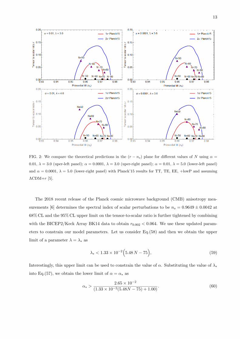
We also consider the situation in which the values of N are arbitrary but keep λ and α fixed.

From Fig.(2), we observe that in order for the predictions to be satisfied the Planck data at one

sigma level a value of λ can not be greater than 4.0 and 3.6 with α = 0.01 and 0.0001, respectively.

13

FIG. 2: We compare the theoretical predictions in the (r − ns) plane for different values of N using α =

0.01, λ = 3.0 (uper-left panel); α = 0.0001, λ = 3.0 (uper-right panel); α = 0.01, λ = 5.0 (lower-left panel)

and α = 0.0001, λ = 5.0 (lower-right panel) with Planck’15 results for TT, TE, EE, +lowP and assuming

ΛCDM+r [5].

The 2018 recent release of the Planck cosmic microwave background (CMB) anisotropy mea-

surements [6] determines the spectral index of scalar perturbations to be ns = 0.9649± 0.0042 at

68% CL and the 95% CL upper limit on the tensor-to-scalar ratio is further tightened by combining

with the BICEP2/Keck Array BK14 data to obtain r0.002 < 0.064. We use these updated param-

eters to constrain our model parameters. Let us consider Eq.(58) and then we obtain the upper

limit of a parameter λ = λ∗ as

λ∗ < 1.33× 10−2(

5.48N − 75), (59)

Interestingly, this upper limit can be used to constrain the value of α. Substituting the value of λ∗

into Eq.(57), we obtain the lower limit of α = α∗ as

α∗ >2.65× 10−2

(1.33× 10−2(5.48N − 75) + 1.00). (60)

14

Since a value demanded in most inflationary scenarios is at least N = 50−60, we obtain λ∗ < 3.382

and α∗ > 6.06×10−3 for N = 60. In addition, we compare the theoretical predictions in the (r−ns)

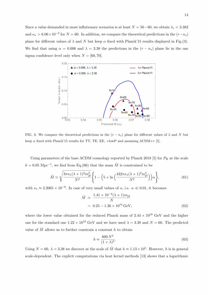
plane for different values of λ and N but keep α fixed with Planck’15 results displayed in Fig.(3).

We find that using α = 0.006 and λ = 3.38 the predictions in the (r − ns) plane lie in the one

sigma confidence level only when N = [60, 70].

FIG. 3: We compare the theoretical predictions in the (r − ns) plane for different values of λ and N but

keep α fixed with Planck’15 results for TT, TE, EE, +lowP and assuming ΛCDM+r [5].

Using parameters of the base ΛCDM cosmology reported by Planck 2018 [5] for PR at the scale

k = 0.05 Mpc−1, we find from Eq.(66) that the mass M is constrained to be

M '

√3πκ1(λ+ 1)2m2

pl

N2

{1−

(5 + ln

(432πκ1(λ+ 1)2m2pl

N2

))α

}, (61)

with κ1 ≈ 2.2065× 10−9. In case of very small values of α, i.e. α� 0.01, it becomes

M '1.41× 10−4(λ+ 1)mpl

N

∼ 0.25− 1.26× 1014 GeV, (62)

where the lower value obtained for the reduced Planck mass of 2.44 × 1018 GeV and the higher

one for the standard one 1.22× 1019 GeV and we have used λ = 3.38 and N = 60. The predicted

value of M allows us to further constrain a constant h to obtain

h ≈ 600N2

(1 + λ)2. (63)

Using N = 60, λ = 3.38 we discover at the scale of M that h ≈ 1.13×105. However, h is in general

scale-dependent. The explicit computations via heat kernel methods [13] shows that a logarithmic

15

form of h can be induced by leading order quantum fluctuations. The RG improved treatment of

h can be found in Ref.[11].

V. CONCLUSION

In this work, we studied the deformed Starobinsky model in which the deformations take the

form R2(1−α), with R the Ricci scalar and α a positive parameter [11]. We started by revisiting the

formalism in f(R) theory [7, 8] in the framework of gravity’s rainbow [9]. We took a short recap of

a cosmological linear perturbation in the context of the gravitys rainbow generated during inflation

and calculated the spectral index of scalar perturbation and the tensor-to-scalar ratio predicted

by the model. We compared the predicted results with Planck data. With the sizeable number of

e-foldings and proper choices of parameters, we discovered that the predictions of the model are

in excellent agreement with the Planck analysis. Interestingly, we obtained the upper limit of a

rainbow parameter λ < 1.33× 10−2(

5.48N − 75)

and found the lower limit of a positive constant

α > 2.65× 10−2(

1.33× 10−2(5.48N − 75) + 1.00)−1

.

Regarding our present work, the study the cosmological dynamics of isotropic and anisotropic

universe in f(R) gravity, see e.g. [8, 31, 32] and references therein, via the dynamical system

technique can be further studied. Interestingly, the swampland criteria in the deformed Starobinsky

model can be worth investigating by following the work done by Ref.[28]. The reheating process

in the present work is worth investigating [29, 30].

Acknowledgments The author thanks Vicharit Yingcharoenrat for his early-state collaboration

in the present work.

[1] G. Amelino-Camelia, Phys. Lett. B 510, 255 (2001)

[2] G. Amelino-Camelia, Int. J. Mod. Phys. D 11 (2002) 35

[3] G. Amelino-Camelia, J. Kowalski-Glikman, G. Mandanici and A. Procaccini, Int. J. Mod. Phys. A 20

(2005) 6007

[4] J. Magueijo and L. Smolin, Class. Quant. Grav. 21, 1725 (2004)

[5] P. A. R. Ade et al. [Planck Collaboration], Astron. Astrophys. 594, A20 (2016)

[6] Y. Akrami et al. [Planck Collaboration], arXiv:1807.06211 [astro-ph.CO].

[7] T. P. Sotiriou and V. Faraoni, Rev. Mod. Phys. 82, 451 (2010)

[8] A. De Felice and S. Tsujikawa, Living Rev. Rel. 13, 3 (2010)

16

[9] A. Chatrabhuti, V. Yingcharoenrat and P. Channuie, Phys. Rev. D 93, no. 4, 043515 (2016)

[10] A. A. Starobinsky, Phys. Lett. B 91, 99 (1980) [Phys. Lett. 91B, 99 (1980)] [Adv. Ser. Astrophys.

Cosmol. 3, 130 (1987)]

[11] A. Codello, J. Joergensen, F. Sannino and O. Svendsen, JHEP 1502, 050 (2015)

[12] Y. Ling, JCAP 0708, 017 (2007)

[13] I. G. Avramidi, Lect. Notes Phys. Monogr. 64, 1 (2000)

[14] Z. W. Feng, S. Z. Yang, H. L. Li and X. T. Zu, arXiv:1608.06824 [physics.gen-ph].

[15] S. H. Hendi, S. Panahiyan, S. Upadhyay and B. Eslam Panah, Phys. Rev. D 95, no. 8, 084036 (2017)

[16] Z. W. Feng and S. Z. Yang, Phys. Lett. B 772, 737 (2017)

[17] S. H. Hendi and M. Momennia, Phys. Lett. B 777, 222 (2018)

[18] S. Panahiyan, S. H. Hendi and N. Riazi, Nucl. Phys. B 938, 388 (2019)

[19] M. Dehghani, Phys. Lett. B 777 (2018) 351

[20] S. Upadhyay, S. H. Hendi, S. Panahiyan and B. Eslam Panah, PTEP 2018, no. 9, 093E01 (2018)

[21] M. Dehghani, Phys. Lett. B 785, 274 (2018)

[22] D. Momeni, S. Upadhyay, Y. Myrzakulov and R. Myrzakulov, Astrophys. Space Sci. 362, no. 9, 148

(2017)

[23] X. M. Deng and Y. Xie, Phys. Lett. B 772, 152 (2017)

[24] C. Xu and Y. Yang, J. Math. Phys. 59, no. 3, 032501 (2018)

[25] S. H. Hendi, M. Momennia, B. Eslam Panah and M. Faizal, Astrophys. J. 827, no. 2, 153 (2016)

[26] S. H. Hendi, M. Momennia, B. Eslam Panah and S. Panahiyan, Universe 16, 26 (2017)

[27] S. H. Hendi, B. Eslam Panah, S. Panahiyan and M. Momennia, Adv. High Energy Phys. 2016, 9813582

(2016)

[28] M. Artymowski and I. Ben-Dayan, arXiv:1902.02849 [gr-qc].

[29] A. Nishizawa and H. Motohashi, Phys. Rev. D 89, no. 6, 063541 (2014)

[30] V. K. Oikonomou, Mod. Phys. Lett. A 32, no. 33, 1750172 (2017)

[31] X. Liu, P. Channuie and D. Samart, Phys. Dark Univ. 17, 52 (2017)

[32] N. Goheer, J. A. Leach and P. K. S. Dunsby, Class. Quant. Grav. 24 (2007) 5689