Embed Size (px)
Citation preview
TECHNISCHE UNIVERSITAT MUNCHEN
Professur fur Hydromechanik
Numerical investigation of mass transfer atnon-miscible interfaces including Marangoni force
Tianshi Sun
Vollstandiger Abdruck der an der Ingenieurfakultat Bau Geo Umwelt der TechnischenUniversitat Munchen zur Erlangung des akademischen Grades eines
Doktor-Ingenieurs
genehmigten Dissertation.
Vorsitzender: Prof. Dr.-Ing. habil. F. DuddeckPrufer der Dissertation:
1. Prof. Dr.-Ing. M. Manhart2. Prof. Dr. J.G.M. Kuerten
Die Dissertation wurde am 31. 08. 2018 bei der Technischen Universitat Munchen eingereichtund durch die Ingenieurfakultat Bau Geo Umwelt am 11. 12. 2018 angenommen.

Zusammenfassung
Diese Studie untersucht den mehrphasigen Stofftransport einer nicht-wassrigen flussigkeit(”Non-aqueous phase liquid”, NAPL) im Porenmaßstab, einschließlich der Auswirkungenvon Oberflachenspannungs und Marangoni-Kraften. Fur die Mehrphasenstromung wurdedie Methode ”Conservative Level Set” (CLS) implementiert, um die Grenzflache zu verfol-gen, wahrend die Oberflachenspannungskraft mit der Methode ”Sharp Surface Tension Force”(SSF) simuliert wird. Zur Messung des Kontaktwinkels zwischen der Oberflache der Flus-sigkeit und der Kontur der Kontaktflache wird ein auf der CLS-Methode basierendes Kon-taktlinienmodell verwendet; das ”Continuum Surface Force” (CSF)-Modell wird zur Model-lierung des durch einen Konzentrationsgradienten induzierten Marangoni-Effekts verwendet;ein neues Stofftransfermodell, das einen Quellterm in der Konvektions-Diffusionsgleichungenverwendet, wird zur Untersuchung des Stoffubergangs verwendet.
Ein zweidimensionales Hohlraummodell, das den Marangoni-Effekt vernachlassigt, wird mitveriierendem Stromungsbedingungen (z.B. unterschiedliche Weberzahlen, Reynoldszahlenund Beschleunigungszeitskalenverhaltnisse) implementiert, um die Massentransferrate unddas Verhalten der Grenzflache zu untersuchen. Aufgrund der geringen Loslichkeit der NAPLwird nur der konvektive Stoffaustausch berucksichtigt. Die Ergebnisse zeigen, dass dieWeber-Zahl und das Zeitskalenverhaltnis die wichtigsten Faktoren sind, die das Verhaltender Grenzflache bzw. der Stoffubergangsrate beeinflussen.
Ein zweidimensionales Stofftransfermodell, das den Marangoni-Effekt berucksichtigt, wirdqualitativ untersucht. Der Marangoni-Effekt beeinflusst das lokale Geschwindigkeitsfeld inder Nahe der Grenzflache und erzeugt damit ein Zirkulationsmuster. Damit erhoht derMarangoni-Effekt auch die lokale Stoffubergangsrate, was in guter qualitativer Ubereinstim-mung mit der theoretischen Analyse und Experimenten steht.
I

II
Abstract
This study investigates pore-scale multiphase mass transport, including the effects of sur-face tension forces and Marangoni forces of a Non-Aqueous Phase Liquid (NAPL) into water.For the multiphase flow, the Conservative Level Set (CLS) method has been implementedto track the interface, while the surface tension force is simulated by the Sharp Surfacetension Force (SSF) method. A contact line model based on the CLS method is used tomeasure the contact angle between the surface of the liquid and the outline of the contactsurface; the Continuum Surface Force (CSF) model is applied to model the Marangoni effectinduced by a concentration gradient; a new mass transfer model, adding a source term inthe convection-diffusion equations, is employed to investigate the mass transfer rate.
A two-dimensional cavity model that neglects the Marangoni effect is implemented with var-ious flow conditions (such as different Weber numbers, Reynolds numbers and accelerationtime scale ratios) to examine the mass transfer rate and the behavior of the interface. Due tothe low solubility of the NAPL, only the convective mass transfer will be taken into account.The results show that the Weber number and the time scale ratio are the most significantfactors affecting the behavior of the interface and mass transfer rate, respectively.
A two-dimensional mass transfer model, influenced by the Marangoni effect, is qualitativelyinvestigated. As a circulation pattern appears close to the interface, the Marangoni effectbegins to impact the local velocity field near the interface. Furthermore, the Marangonieffect also promotes the local mass transfer rate, which is in good agreement with the theo-retical analysis and previous simulations.
III

IV

Acknowledgements
I would like to express my deepest gratitude to my supervisor Prof. Dr.-Ing. habil. MichaelManhart, for his constant encouragement, support and guidance. I have greatly benefitedfrom his broad knowledge and instruction.
I gratefully thank Prof. Dr. J.G.M. Kuerten, not only for being my project mentor, but alsofor being my dissertation reviewer. Additionally, I thank you for giving me the opportunityto work in TU/e for three-month to experience the different academic atmosphere.
I thank my project team leader Dr.-Ing. Daniel Quosdorf. I am also grateful to my colleagueDr.-Ing. Alexander McCluskey for proofreading a draft of this dissertation. I thank all mycolleagues at the Chair of Hydromechanics.
I thank the International Graduate School of Science and Engineering (IGSSE) at Tech-nische Universitat Munchen, which funded my project 9.03, Mass transfer at interfaces tonon-aqueous phases (Marangoni). I also thank Carina Wismeth and PD Dr. Thomas Bau-mann for the interesting discussions.
Finally, I would especially like to thank my parents and family for their continuous supportand encouragement.
V

VI
Contents
Zusammenfassung I
Abstract III
Preface V
List of Tables XI
List of Figures XI
Nomenclature 1
1 Introduction 11.1 Background . . . . . . . . . . . . . . . . . . . . . . . . . . . . . . . . . . . . 11.2 Motivation . . . . . . . . . . . . . . . . . . . . . . . . . . . . . . . . . . . . . 11.3 Outline . . . . . . . . . . . . . . . . . . . . . . . . . . . . . . . . . . . . . . . 2
2 Theory 52.1 Single-phase flows . . . . . . . . . . . . . . . . . . . . . . . . . . . . . . . . . 52.2 Multiphase flows . . . . . . . . . . . . . . . . . . . . . . . . . . . . . . . . . 6
2.2.1 Characteristics of multiphase flows . . . . . . . . . . . . . . . . . . . 62.2.2 Numerical methods of multiphase flows . . . . . . . . . . . . . . . . . 7
2.3 Surface tension . . . . . . . . . . . . . . . . . . . . . . . . . . . . . . . . . . 82.3.1 Physics . . . . . . . . . . . . . . . . . . . . . . . . . . . . . . . . . . 82.3.2 Numerical modeling . . . . . . . . . . . . . . . . . . . . . . . . . . . 9
2.4 Contact angle models . . . . . . . . . . . . . . . . . . . . . . . . . . . . . . . 102.4.1 Mechanisms . . . . . . . . . . . . . . . . . . . . . . . . . . . . . . . . 102.4.2 Numerical models for the contact angle . . . . . . . . . . . . . . . . . 12
2.5 Marangoni effect . . . . . . . . . . . . . . . . . . . . . . . . . . . . . . . . . 122.5.1 Relevance . . . . . . . . . . . . . . . . . . . . . . . . . . . . . . . . . 122.5.2 Mechanisms . . . . . . . . . . . . . . . . . . . . . . . . . . . . . . . . 132.5.3 Numerical models . . . . . . . . . . . . . . . . . . . . . . . . . . . . . 14
2.6 Mass transfer over interfaces . . . . . . . . . . . . . . . . . . . . . . . . . . . 152.6.1 Mass transfer due to the temperature gradient (phase change) . . . . 162.6.2 Mass transfer due to the concentration gradient . . . . . . . . . . . . 19
3 Code basis and state at the beginning 233.1 MGLET . . . . . . . . . . . . . . . . . . . . . . . . . . . . . . . . . . . . . . 23
3.1.1 Finite volume method . . . . . . . . . . . . . . . . . . . . . . . . . . 23
VII
VIII Contents
3.1.2 Staggered grid . . . . . . . . . . . . . . . . . . . . . . . . . . . . . . . 243.2 Conservative level set method . . . . . . . . . . . . . . . . . . . . . . . . . . 25
3.2.1 Level set advection . . . . . . . . . . . . . . . . . . . . . . . . . . . . 253.2.2 Level set reinitialization . . . . . . . . . . . . . . . . . . . . . . . . . 253.2.3 Distance function and normal vector . . . . . . . . . . . . . . . . . . 273.2.4 Interface curvature . . . . . . . . . . . . . . . . . . . . . . . . . . . . 293.2.5 Surface tension . . . . . . . . . . . . . . . . . . . . . . . . . . . . . . 30
4 Current implementations 334.1 A contact line treatment for the CLS method . . . . . . . . . . . . . . . . . 33
4.1.1 The reinitialization function for CLS . . . . . . . . . . . . . . . . . . 334.1.2 Boundary conditions . . . . . . . . . . . . . . . . . . . . . . . . . . . 34
4.2 Marangoni effect . . . . . . . . . . . . . . . . . . . . . . . . . . . . . . . . . 374.3 Mass transfer . . . . . . . . . . . . . . . . . . . . . . . . . . . . . . . . . . . 39
4.3.1 Interfacial fluxes conservation . . . . . . . . . . . . . . . . . . . . . . 414.3.2 Interfacial dissolution equilibrium . . . . . . . . . . . . . . . . . . . . 43
4.4 Time integration . . . . . . . . . . . . . . . . . . . . . . . . . . . . . . . . . 44
5 Validation 475.1 Static drop . . . . . . . . . . . . . . . . . . . . . . . . . . . . . . . . . . . . 475.2 Capillary waves . . . . . . . . . . . . . . . . . . . . . . . . . . . . . . . . . . 505.3 Two-dimensional droplet on a wall under zero-gravity conditions . . . . . . . 53
5.3.1 Cox’ theory . . . . . . . . . . . . . . . . . . . . . . . . . . . . . . . . 545.3.2 Results . . . . . . . . . . . . . . . . . . . . . . . . . . . . . . . . . . . 54
5.4 Mass transfer of a two-dimensional droplet with negligible external resistance 58
6 Application 1: Purging of non-aqueous phase liquids from a 2D cavity model 616.1 Cavity flows . . . . . . . . . . . . . . . . . . . . . . . . . . . . . . . . . . . . 616.2 Model set-up . . . . . . . . . . . . . . . . . . . . . . . . . . . . . . . . . . . 626.3 Two-dimensional and three dimensional model . . . . . . . . . . . . . . . . . 646.4 Flushing the cavity . . . . . . . . . . . . . . . . . . . . . . . . . . . . . . . . 666.5 Influencing factors of mass transfer rate for cavity model . . . . . . . . . . . 80
6.5.1 Effect of the flow acceleration . . . . . . . . . . . . . . . . . . . . . . 806.5.2 Effect of the surface tension . . . . . . . . . . . . . . . . . . . . . . . 816.5.3 Effect of the Reynolds number . . . . . . . . . . . . . . . . . . . . . . 816.5.4 Effect of the density ratio . . . . . . . . . . . . . . . . . . . . . . . . 826.5.5 Effect of the viscosity ratio . . . . . . . . . . . . . . . . . . . . . . . . 836.5.6 Effect of the gravitational force . . . . . . . . . . . . . . . . . . . . . 846.5.7 Sensitive analysis . . . . . . . . . . . . . . . . . . . . . . . . . . . . . 84
7 Application 2: Mass transfer with the Marangoni effect 877.1 Objectives . . . . . . . . . . . . . . . . . . . . . . . . . . . . . . . . . . . . . 877.2 Model set-up . . . . . . . . . . . . . . . . . . . . . . . . . . . . . . . . . . . 887.3 Velocity fields . . . . . . . . . . . . . . . . . . . . . . . . . . . . . . . . . . . 90
7.3.1 Mechanisms . . . . . . . . . . . . . . . . . . . . . . . . . . . . . . . . 907.3.2 Influencing factors of the velocity field . . . . . . . . . . . . . . . . . 91

Contents IX
7.4 Mass transfer . . . . . . . . . . . . . . . . . . . . . . . . . . . . . . . . . . . 97
8 Conclusions 101
References 110

X Contents
List of Tables
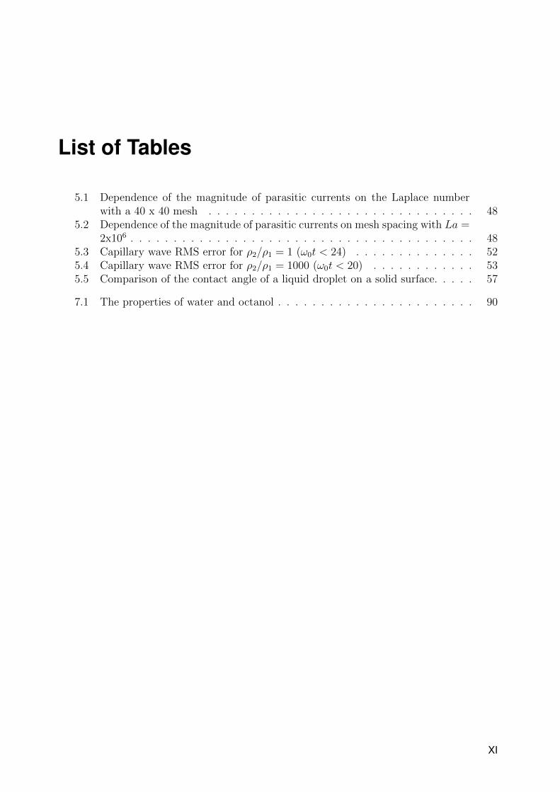
5.1 Dependence of the magnitude of parasitic currents on the Laplace numberwith a 40 x 40 mesh . . . . . . . . . . . . . . . . . . . . . . . . . . . . . . . 48
5.2 Dependence of the magnitude of parasitic currents on mesh spacing with La =2x10⁶ . . . . . . . . . . . . . . . . . . . . . . . . . . . . . . . . . . . . . . . . 48
5.3 Capillary wave RMS error for ρ2/ρ1 = 1 (ω0t < 24) . . . . . . . . . . . . . . 525.4 Capillary wave RMS error for ρ2/ρ1 = 1000 (ω0t < 20) . . . . . . . . . . . . 535.5 Comparison of the contact angle of a liquid droplet on a solid surface. . . . . 57
7.1 The properties of water and octanol . . . . . . . . . . . . . . . . . . . . . . . 90
XI
List of Figures
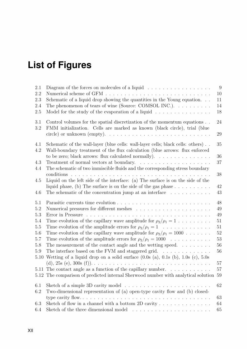
2.1 Diagram of the forces on molecules of a liquid . . . . . . . . . . . . . . . . . 92.2 Numerical scheme of GFM . . . . . . . . . . . . . . . . . . . . . . . . . . . . 102.3 Schematic of a liquid drop showing the quantities in the Young equation. . . 112.4 The phenomenon of tears of wine (Source: COMSOL INC.). . . . . . . . . . 142.5 Model for the study of the evaporation of a liquid . . . . . . . . . . . . . . . 18
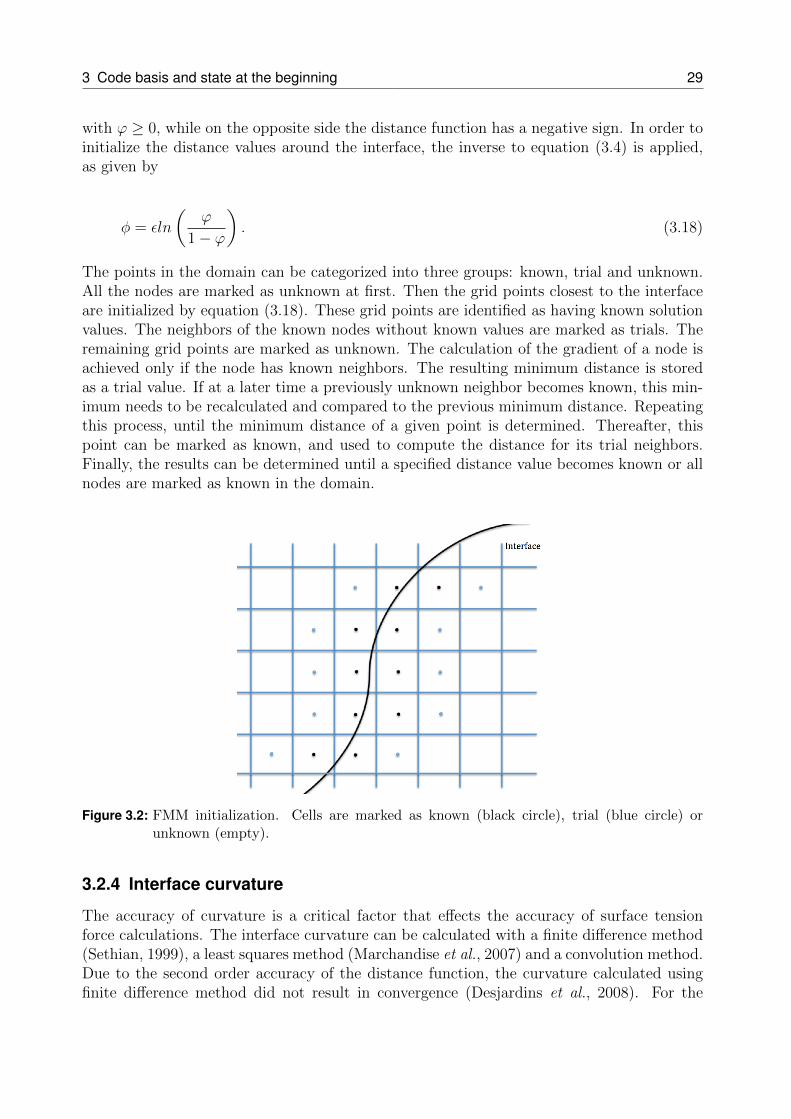
3.1 Control volumes for the spatial discretization of the momentum equations . . 243.2 FMM initialization. Cells are marked as known (black circle), trial (blue
circle) or unknown (empty). . . . . . . . . . . . . . . . . . . . . . . . . . . . 29
4.1 Schematic of the wall-layer (blue cells: wall-layer cells; black cells: others) . . 354.2 Wall-boundary treatment of the flux calculation (blue arrows: flux enforced
to be zero; black arrows: flux calculated normally). . . . . . . . . . . . . . . 364.3 Treatment of normal vectors at boundary. . . . . . . . . . . . . . . . . . . . 374.4 The schematic of two immiscible fluids and the corresponding stress boundary
conditions . . . . . . . . . . . . . . . . . . . . . . . . . . . . . . . . . . . . . 384.5 Liquid on the left side of the interface: (a) The surface is on the side of the
liquid phase, (b) The surface is on the side of the gas phase . . . . . . . . . . 424.6 The schematic of the concentration jump at an interface . . . . . . . . . . . 43
5.1 Parasitic currents time evolution . . . . . . . . . . . . . . . . . . . . . . . . . 485.2 Numerical pressures for different meshes . . . . . . . . . . . . . . . . . . . . 495.3 Error in Pressure . . . . . . . . . . . . . . . . . . . . . . . . . . . . . . . . . 495.4 Time evolution of the capillary wave amplitude for ρ2/ρ1 = 1 . . . . . . . . . 515.5 Time evolution of the amplitude errors for ρ2/ρ1 = 1 . . . . . . . . . . . . . 515.6 Time evolution of the capillary wave amplitude for ρ2/ρ1 = 1000 . . . . . . . 525.7 Time evolution of the amplitude errors for ρ2/ρ1 = 1000 . . . . . . . . . . . 535.8 The measurement of the contact angle and the wetting speed. . . . . . . . . 565.9 The interface based on the FVM and staggered grid. . . . . . . . . . . . . . 565.10 Wetting of a liquid drop on a solid surface (0.0s (a), 0.1s (b), 1.0s (c), 5.0s
(d), 25s (e), 300s (f)). . . . . . . . . . . . . . . . . . . . . . . . . . . . . . . . 575.11 The contact angle as a function of the capillary number. . . . . . . . . . . . 575.12 The comparison of predicted internal Sherwood number with analytical solution 59
6.1 Sketch of a simple 3D cavity model . . . . . . . . . . . . . . . . . . . . . . . 626.2 Two-dimensional representation of (a) open-type cavity flow and (b) closed-
type cavity flow. . . . . . . . . . . . . . . . . . . . . . . . . . . . . . . . . . . 636.3 Sketch of flow in a channel with a bottom 2D cavity . . . . . . . . . . . . . . 646.4 Sketch of the three dimensional model . . . . . . . . . . . . . . . . . . . . . 65
XII
List of Figures XIII
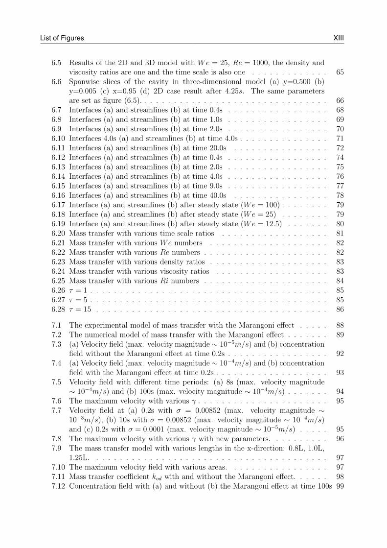
6.5 Results of the 2D and 3D model with We = 25, Re = 1000, the density andviscosity ratios are one and the time scale is also one . . . . . . . . . . . . . 65
6.6 Spanwise slices of the cavity in three-dimensional model (a) y=0.500 (b)y=0.005 (c) x=0.95 (d) 2D case result after 4.25s. The same parametersare set as figure (6.5). . . . . . . . . . . . . . . . . . . . . . . . . . . . . . . . 66
6.7 Interfaces (a) and streamlines (b) at time 0.4s . . . . . . . . . . . . . . . . . 686.8 Interfaces (a) and streamlines (b) at time 1.0s . . . . . . . . . . . . . . . . . 696.9 Interfaces (a) and streamlines (b) at time 2.0s . . . . . . . . . . . . . . . . . 706.10 Interfaces 4.0s (a) and streamlines (b) at time 4.0s . . . . . . . . . . . . . . . 716.11 Interfaces (a) and streamlines (b) at time 20.0s . . . . . . . . . . . . . . . . 726.12 Interfaces (a) and streamlines (b) at time 0.4s . . . . . . . . . . . . . . . . . 746.13 Interfaces (a) and streamlines (b) at time 2.0s . . . . . . . . . . . . . . . . . 756.14 Interfaces (a) and streamlines (b) at time 4.0s . . . . . . . . . . . . . . . . . 766.15 Interfaces (a) and streamlines (b) at time 9.0s . . . . . . . . . . . . . . . . . 776.16 Interfaces (a) and streamlines (b) at time 40.0s . . . . . . . . . . . . . . . . 786.17 Interface (a) and streamlines (b) after steady state (We = 100) . . . . . . . . 796.18 Interface (a) and streamlines (b) after steady state (We = 25) . . . . . . . . 796.19 Interface (a) and streamlines (b) after steady state (We = 12.5) . . . . . . . 806.20 Mass transfer with various time scale ratios . . . . . . . . . . . . . . . . . . 816.21 Mass transfer with various We numbers . . . . . . . . . . . . . . . . . . . . 826.22 Mass transfer with various Re numbers . . . . . . . . . . . . . . . . . . . . . 826.23 Mass transfer with various density ratios . . . . . . . . . . . . . . . . . . . . 836.24 Mass transfer with various viscosity ratios . . . . . . . . . . . . . . . . . . . 836.25 Mass transfer with various Ri numbers . . . . . . . . . . . . . . . . . . . . . 846.26 τ = 1 . . . . . . . . . . . . . . . . . . . . . . . . . . . . . . . . . . . . . . . . 856.27 τ = 5 . . . . . . . . . . . . . . . . . . . . . . . . . . . . . . . . . . . . . . . . 856.28 τ = 15 . . . . . . . . . . . . . . . . . . . . . . . . . . . . . . . . . . . . . . . 86
7.1 The experimental model of mass transfer with the Marangoni effect . . . . . 887.2 The numerical model of mass transfer with the Marangoni effect . . . . . . . 897.3 (a) Velocity field (max. velocity magnitude∼ 10−5m/s) and (b) concentration
field without the Marangoni effect at time 0.2s . . . . . . . . . . . . . . . . . 927.4 (a) Velocity field (max. velocity magnitude∼ 10−4m/s) and (b) concentration
field with the Marangoni effect at time 0.2s . . . . . . . . . . . . . . . . . . . 937.5 Velocity field with different time periods: (a) 8s (max. velocity magnitude
∼ 10−4m/s) and (b) 100s (max. velocity magnitude ∼ 10−4m/s) . . . . . . . 947.6 The maximum velocity with various γ . . . . . . . . . . . . . . . . . . . . . . 957.7 Velocity field at (a) 0.2s with σ = 0.00852 (max. velocity magnitude ∼
10−3m/s), (b) 10s with σ = 0.00852 (max. velocity magnitude ∼ 10−4m/s)and (c) 0.2s with σ = 0.0001 (max. velocity magnitude ∼ 10−5m/s) . . . . . 95
7.8 The maximum velocity with various γ with new parameters. . . . . . . . . . 967.9 The mass transfer model with various lengths in the x-direction: 0.8L, 1.0L,
1.25L. . . . . . . . . . . . . . . . . . . . . . . . . . . . . . . . . . . . . . . . 977.10 The maximum velocity field with various areas. . . . . . . . . . . . . . . . . 977.11 Mass transfer coefficient kod with and without the Marangoni effect. . . . . . 987.12 Concentration field with (a) and without (b) the Marangoni effect at time 100s 99

XIV List of Figures
7.13 Concentration along the x-direction at y = 0.9L with and without the Marangonieffect. . . . . . . . . . . . . . . . . . . . . . . . . . . . . . . . . . . . . . . . 100
Nomenclature
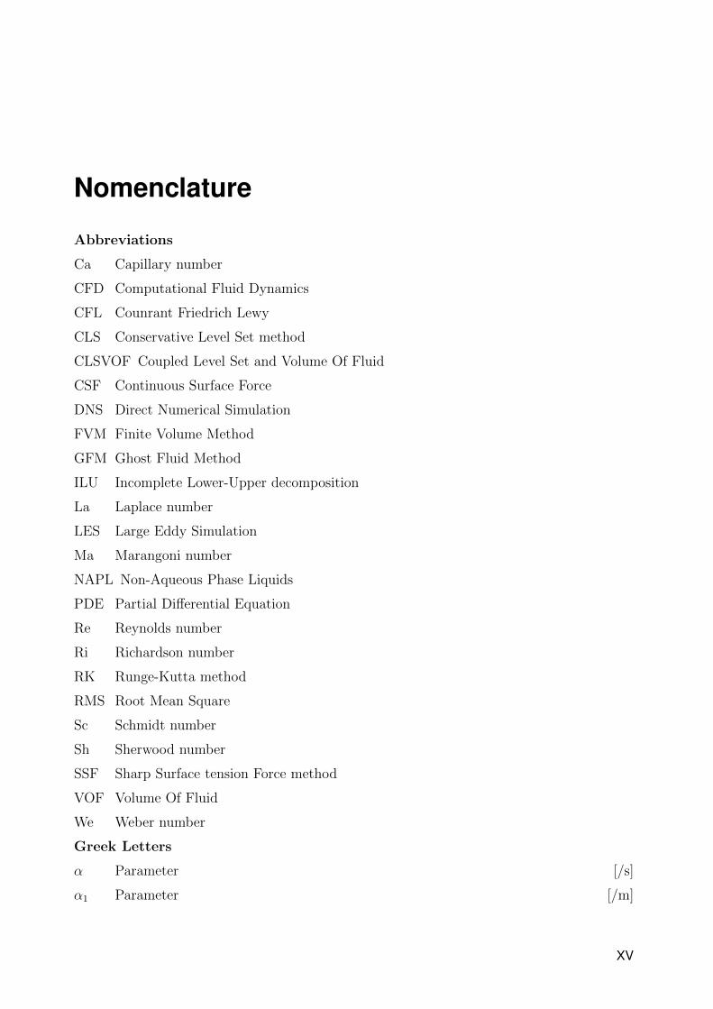
Abbreviations
Ca Capillary number
CFD Computational Fluid Dynamics
CFL Counrant Friedrich Lewy
CLS Conservative Level Set method
CLSVOF Coupled Level Set and Volume Of Fluid
CSF Continuous Surface Force
DNS Direct Numerical Simulation
FVM Finite Volume Method
GFM Ghost Fluid Method
ILU Incomplete Lower-Upper decomposition
La Laplace number
LES Large Eddy Simulation
Ma Marangoni number
NAPL Non-Aqueous Phase Liquids
PDE Partial Differential Equation
Re Reynolds number
Ri Richardson number
RK Runge-Kutta method
RMS Root Mean Square
Sc Schmidt number
Sh Sherwood number
SSF Sharp Surface tension Force method
VOF Volume Of Fluid
We Weber number
Greek Letters
α Parameter [/s]
α1 Parameter [/m]
XV
XVI List of Figures
α2 Parameter [/s]
δ Delta function [−]
ε Artificial diffusion number [−]
γLG Liquid-vapor interfacial energy [N/m]
γSG Solid-vapor interfacial energy [N/m]
γSL Solid-liquid interfacial energy [N/m]
γ Constant [−]
κ Surface curvature [−]
λ Wavelength [m]
µ Dynamic viscosity of fluid [Ns/m2]
µ1 Dynamic viscosity of fluid 1 [Ns/m2]
µ2 Dynamic viscosity of fluid 2 [Ns/m2]
ν Kinematic Viscosity of fluid [m2/s]
ν1 Kinematic Viscosity of fluid 1 [m2/s]
ν2 Kinematic Viscosity of fluid 2 [m2/s]
ω0 Inviscid oscillation frequency [s]
Φ Potential [N/m]
φ Distance function [−]
ρ Density of fluid [kg/m3]
ρ1 Density of fluid 1 [kg/m3]
ρ2 Density of fluid 2 [kg/m3]
σ Surface tension [N/m]
τ Time scale ratio [−]
τ0 Time scale [s]
τp Dimensionless time step [−]
τLS Pseudo time step [s]
θC Contact angle [−]
θD Macroscopic dynamic contact angle [−]
θs Static contact angle [−]
ϕ Level set function [−]
Mathematical Operators
· Scalar multiplication
∆ Difference
List of Figures XVII
〈〉 Jump condition
∇ Gradient
∂ Partial differential
Roman Letters
Fd Driving force [N]
Fsu Surface tension force [N]
g Gravity [m/s2]
n Normal vector [−]
t Tangential vector [−]
m Mass flow rate [N]
A0 Initial wave amplitude [m]
C Color function [−]
c Concentration [kmol/m3]
cG Concentration of the gas [kmol/m3]
cL Concentration of the liquid [kmol/m3]
D Diffusion coefficient [m2/s]
d Constant [−]
Dd Diameter of a drop [m]
DG Diffusion coefficient of the gas [m2/s]
DL Diffusion coefficient of the liquid [m2/s]
Fi Body force [N]
fLG Error function [kmol]
h Grid space [m]
HD Distribution coefficient [−]
K Convective mass transfer coefficient [m/s]
kod Mass transfer coefficient [m/s]
L Characteristic length [m]
p Pressure [N/m2]
r Radius [m]
S Surface area [m2]
s Time [s]
T Temperature [K]
u, v, w Velocity vector components in x−, y− and z− direction [m/s]

XVIII List of Figures
V Volume [m3]
x, y, z Coordinates [m]
Y Mass fraction [−]
1 Introduction
1.1 Background
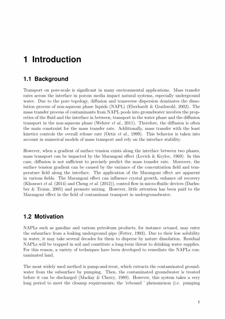
Transport on pore-scale is significant in many environmental applications. Mass transferrates across the interface in porous media impact natural systems, especially undergroundwater. Due to the pore topology, diffusion and transverse dispersion dominates the disso-lution process of non-aqueous phase liquids (NAPL) (Eberhardt & Grathwohl, 2002). Themass transfer process of contaminants from NAPL pools into groundwater involves the prop-erties of the fluid and the interface in between, transport in the water phase and the diffusiontransport in the non-aqueous phase (Wehrer et al., 2011). Therefore, the diffusion is oftenthe main constraint for the mass transfer rate. Additionally, mass transfer with the leastkinetics controls the overall release rate (Ortiz et al., 1999). This behavior is taken intoaccount in numerical models of mass transport and rely on the interface stability.
However, when a gradient of surface tension exists along the interface between two phases,mass transport can be impacted by the Marangoni effect (Levich & Krylov, 1969). In thiscase, diffusion is not sufficient to precisely predict the mass transfer rate. Moreover, thesurface tension gradient can be caused by the variance of the concentration field and tem-perature field along the interface. The application of the Marangoni effect are apparentin various fields. The Marangoni effect can influence crystal growth, enhance oil recovery(Khosravi et al. (2014) and Cheng et al. (2012)), control flow in micro-fluidic devices (Darhu-ber & Troian, 2005) and promote mixing. However, little attention has been paid to theMarangoni effect in the field of contaminant transport in undergroundwater.
1.2 Motivation
NAPLs such as gasoline and various petroleum products, for instance octanol, may enterthe subsurface from a leaking underground pipe (Fetter, 1993). Due to their low solubilityin water, it may take several decades for them to disperse by nature dissolution. ResidualNAPLs will be trapped in soil and constitute a long-term threat to drinking water supplies.For this reason, a variety of techniques have been developed to remediate the NAPLs con-taminated land.
The most widely used method is pump-and-treat, which extracts the contaminated ground-water from the subsurface by pumping. Then, the contaminated groundwater is treatedbefore it can be discharged (Mackay & Cherry, 1989). However, this system takes a verylong period to meet the cleanup requirements; the ’rebound ’ phenomenon (i.e. pumping
1
2 1.3 Outline
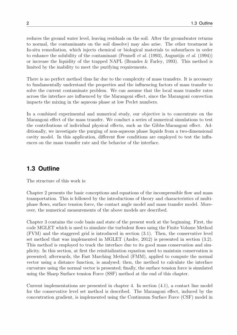
reduces the ground water level, leaving residuals on the soil. After the groundwater returnsto normal, the contaminants on the soil dissolve) may also arise. The other treatment isIn-situ remediation, which injects chemical or biological materials to subsurfaces in orderto enhance the solubility of the contaminant (Pennell et al. (1993), Augustijn et al. (1994))or increase the liquidity of the trapped NAPL (Brandes & Farley, 1993). This method islimited by the inability to meet the purifying requirements.
There is no perfect method thus far due to the complexity of mass transfers. It is necessaryto fundamentally understand the properties and the influencing factors of mass transfer tosolve the current contaminate problem. We can assume that the local mass transfer ratesacross the interface are influenced by the Marangoni effect, since the Marangoni convectionimpacts the mixing in the aqueous phase at low Peclet numbers.
In a combined experimental and numerical study, our objective is to concentrate on theMarangoni effect of the mass transfer. We conduct a series of numerical simulations to testthe contributions of individual physical effects, such as the Gibbs-Marangoni effect. Ad-ditionally, we investigate the purging of non-aqueous phase liquids from a two-dimensionalcavity model. In this application, different flow conditions are employed to test the influ-ences on the mass transfer rate and the behavior of the interface.
1.3 Outline
The structure of this work is:
Chapter 2 presents the basic conceptions and equations of the incompressible flow and masstransportation. This is followed by the introductions of theory and characteristics of multi-phase flows, surface tension force, the contact angle model and mass transfer model. More-over, the numerical measurements of the above models are described.
Chapter 3 contains the code basis and state of the present work at the beginning. First, thecode MGLET which is used to simulate the turbulent flows using the Finite Volume Method(FVM) and the staggered grid is introduced in section (3.1). Then, the conservative levelset method that was implemented in MGLET (Andre, 2012) is presented in section (3.2).This method is employed to track the interface due to its good mass conservation and sim-plicity. In this section, at first the reinitialization equation used to maintain conservation ispresented; afterwards, the Fast Marching Method (FMM), applied to compute the normalvector using a distance function, is analysed; then, the method to calculate the interfacecurvature using the normal vector is presented; finally, the surface tension force is simulatedusing the Sharp Surface tension Force (SSF) method at the end of this chapter.
Current implementations are presented in chapter 4. In section (4.1), a contact line modelfor the conservative level set method is described. The Marangoni effect, induced by theconcentration gradient, is implemented using the Continuum Surface Force (CSF) model in
1 Introduction 3
section (4.2). The mass transfer model across the interface in multiphase flows is describedin section (4.3). Finally, in section (4.4), the time step size limited by different effects isexamined.
Four test cases are presented in chapter 5 to validate different numerical models: the firsttest case is applied to test the accuracy of the surface tension force; the second one is appliedto validate the interaction between the viscous force and surface tension force; the third onevalidates the contact line model based on the CLS method; and the fourth one is imple-mented to validate the mass transfer model.
In chapter 6, we present the results of the mass transfer from a two-dimensional cavity model.Section (6.1) introduces the cavity model. The numerical configuration of the cavity modelis shown in section (6.2). Afterwards, the two-dimensional and three-dimensional results arecompared in section (6.3) to investigate whether additional effects exist. The behavior of theinterface, influenced by various Weber numbers, is examined in section (6.4). The results ofthe mass transfer rate, influenced by different flow conditions (e.g., the Weber number, theReynolds number and time scale ratio), are presented in section (6.5).
In chapter 7, the results of the mass transfer rate impacted by the Marangoni effect arepresented. The objective and the numerical model are introduced in section (7.1) and sec-tion (7.2), respectively. Section (7.3) examines the velocity field influenced by the differentparameters. The mass transfer rate, influenced by the Marangoni effect, is presented insection (7.4).
The conclusions and outlook for future study are provided in chapter 8.

4 1.3 Outline
2 Theory
In this chapter, we introduce the theoretical foundation and numerical models of the presentwork. Single-phase flows are described by the governing equations: the three-dimensionalNavier-Stokes equations in section (2.1). Afterwards, in section (2.2) the numerical methodswhich are used to track the interfaces for multiphase flows are discussed. Next, some addi-tional effects due to the multiphase flows, such as the surface tension force, the contact linemodel and the Marangoni effect, are presented in section (2.3), (2.4) and (2.5). Finally, weconclude with the description of the numerical model of mass transfer.
2.1 Single-phase flows
We solve the Navier-Stokes equations for incompressible flows of a Newtonian fluid withexternal forces. The equations of the conservation laws of mass and momentum are indicatedby
∂ui∂xi
= 0, (2.1)
∂ui∂t
+ uj∂ui∂xj
= −1
ρ
∂p
∂xi+
∂
∂xj
[ν
(∂ui∂xj
+∂uj∂xi
)]+ Fi, (2.2)
where ui refers to the instantaneous velocities, ρ indicates the density, p is the pressure, νdenotes the kinematic viscosity, and Fi represents the body forces, including the gravita-tional force, surface tension force and Marangoni force (see section (4.2)).
The convection-diffusion equation is used to solve the scalar transportation,
∂Φ
∂t+ ui
∂Φ
∂xi= D
∂2Φ
∂x2i, (2.3)
where Φ is the scalar field (i.e. level set, temperature) and D is the diffusivity.
5
6 2.2 Multiphase flows
2.2 Multiphase flows
In some special cases when liquid and gas occur simultaneously, a two-phase flow modelcan solve them. The relatively simple relationships between variables of a single-phase flowmodel cannot satisfy the analysis of two-phase flows or multiphase flows. By definition, amultiphase flow is an interactive flow of two or more different phases with common inter-faces. Each of the phases is regarded as having a separately defined volume fraction (or massfraction) and has its own properties, temperature, and velocity.
Multiphase flows can be divided into two categories:
• Materials with different states or phases (e.g. water-steam mixture and a liquid-solidsystem).
• Materials with different chemical properties but in the same state or phase (i.e. liquid-liquid systems, such as oil droplets in water).
Multiphase flows in industry have a large variety of applications. For example, in aerospaceand marine engineering, some research are related to atomization and free surface flow. Inthe chemical and process industries, the design of separation systems and mixers requiresmultiphase flow analyses. In power engineering, the multiphase flow models need to be em-ployed to interpret certain phenomena, e.g. cavitation and combustion.
2.2.1 Characteristics of multiphase flows
All multiphase flow problems have features which differ from those existing in single-phaseflows.
• Multiphase flows contain a variety of immiscible phases, each with a set of flow vari-ables, even if the two-phase flow can be divided into gas-liquid, gas-solid, liquid-liquid,and liquid-solid. Therefore, more parameters describe the multiphase flow than thosefor the single-phase flow.
• The behavior of the interface is an important factor affecting the multiphase flow,which also poses a challenge for research. For example, when cavitation occurs in thepump, as the fluid moves from the low pressure zone to the high pressure zone, theshape of the interface between the cavitation bubble and the environmental liquid maychange. Furthermore, there are many forms of instability in multiphase flows.
• The spatial distribution of the various phases in the flow field strongly influences flowbehavior.
• When the densities of different phases vary greatly, the effect of gravity on the multi-phase flow is significantly more important than the single-phase flow.
Regardless of the experimental studies or the numerical simulations, the treatment of multi-phase flow problems is much more complicated than the single-phase flow, and even containssome issues that cannot be solved using current state of the art.
2 Theory 7
2.2.2 Numerical methods of multiphase flows
The numerical simulation of multiphase flows is a vast and complicated topic. Current ex-perimental methods are insufficient for visualizing phenomena appearing on scales of spaceand time. In such cases, numerical simulations for fluid-fluid and gas-fluid systems may bea useful tool to validate or explain the concept of the physicist, engineer, or mathematician.
There have been several methods to simulate the interface of multiphase flows numerically,including the volume of fluid (VOF) (Hirt & Nichols (1981), Tryggvason et al. (2011) andRider & Kothe (1998)), level set method (Sussman et al. (1994), Sethian (1999) and Osher& Fedkiw (2002)), and front tracking method (Unverdi & Tryggvason (1992b) and (Popinet& Zaleski, 1999)).
The VOF method is a surface-tracking technique implemented into a Eulerian coordinatesystem, where Navier-Stokes equations which indicate the motion of the flow have to besolved separately. In this manner, the interface is represented implicitly by a volume frac-tion or color function C which is discontinuous and varies between the constant value 1 infull cells to 0 in empty cells, while the intermediate value of C in the transition region de-fines the location of the interface. The interface reconstruction has to be carried out in eachcell using a stair-stepped (Hirt & Nichols, 1981), piecewise linear (Rider & Kothe, 1998) orother approaches at each advection step. The VOF method is known to maintain good massconservation properties and to allow for topology changes, such as those occurring duringreconnection or breakup, which are implicit in the algorithm. Moreover, it is straightforwardto extend to three-dimensional space and simple to implement. However, since the geomet-ric information of the interface is not stored directly, the interface reconstruction and thesurface tension forces have to be taken good care of to ensure that simulations are physicallyaccurate. Also, due to the discontinuity of the color function, the higher order methodscannot be applied, resulting in inaccurate results (Olsson & Kreiss, 2005).
The level set method is a numerical technique used for tracking interfaces and modelingshapes. In this method, the interface is defined as an iso-contour of a smooth scalar func-tion. The advantage of the level set method is that the evolving curves and surfaces can benumerically calculated on a fixed Cartesian grid (Osher & Sethian, 1988). It is not necessaryto parameterize these objects. Another advantage of the level set method is that it is con-venient to track the topological changes of an object, such as when the shape of the objectis divided into two. All of these make the level set method a powerful tool for modeling.However, some problems can arise when using this technique to simulate multiphase flows.As the function is advected by the flow field, it may lose smoothness (Sussman et al., 1994).In terms of mass conservation, many deficiencies also exist. Several attempts have beenmade to improve mass conservation by adding a reinitialization constraint (Sussman et al.(1998), Sussman & Fatemi (1999), Olsson & Kreiss (2005) and Olsson et al. (2007)).
In the method of Sussman et al. (1998) and Sussman & Fatemi (1999), a distance function isdefined as the level set function to track the interface. The distance function is determinedby solving a particular form of the Hamilton-Jacobi partial differential equation known asthe Eikonal equation. In this case, after reinitialization, the level set function becomes the
8 2.3 Surface tension
distance function without changing its zero level set, where the interface is located.
Olsson & Kreiss (2005) and Olsson et al. (2007) use an alternative smeared out Heavisidefunction as the level set function, i.e. a function being zero in one fluid and one in the other.The value varies smoothly from zero to one over the interface. The advection of the level setfunction is performed using a conservative scheme with a reinitialization step that maintainsthe thickness of the interface. The reinitialization step is achieved by solving a reinitializa-tion equation, which contains both advection and diffusion terms that can be discretizedconservatively using the finite volume method (FVM). These two terms can prevent thetransition region from smearing out and maintain the smoothness of the interface, respec-tively. Furthermore, as opposed to the discontinuous color function, the smoothness of thelevel set function makes our method easy to extend to a higher order (Olsson & Kreiss, 2005).
2.3 Surface tension
Physically, the definition of surface tension, in the narrow sense, refers to the tendency ofliquids to attempt to obtain the minimum surface potential energy; broadly speaking, all thetension at the interface between two different phases is called surface tension. The dimensionof surface tension is force per unit length or energy per unit area.
The most common example of surface tension occurs at the interface between a liquid andsome other media. For example, the surface tension of water comes from the cohesion causedby van der Waals forces. When solids, such as water striders, run on the water, the surfacetension will be as flat as possible to maintain the water surface in order to achieve the leastsurface potential energy. If the water strider remains its weight limits, there will be only afew hollows on the surface, which is why water striders can move on water.
2.3.1 Physics
Surface tension can be defined in terms of force or energy:
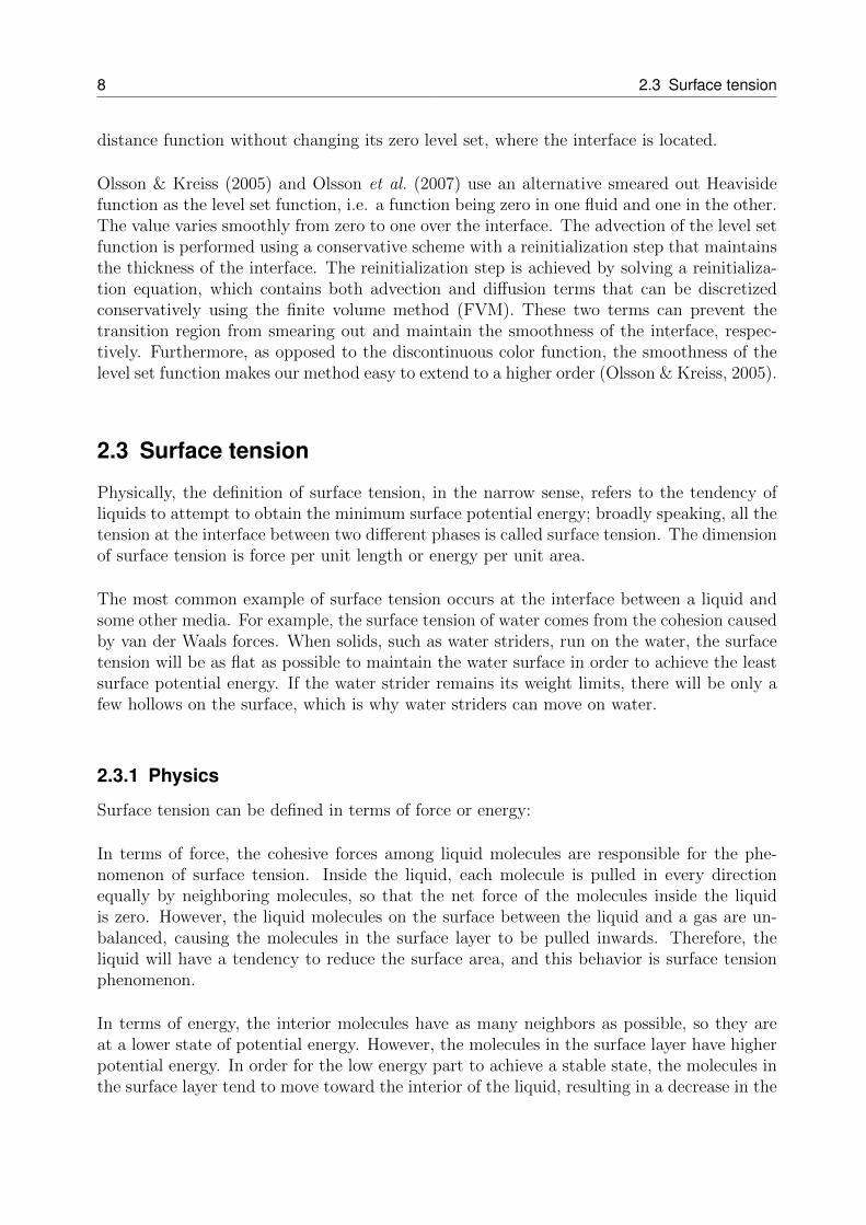
In terms of force, the cohesive forces among liquid molecules are responsible for the phe-nomenon of surface tension. Inside the liquid, each molecule is pulled in every directionequally by neighboring molecules, so that the net force of the molecules inside the liquidis zero. However, the liquid molecules on the surface between the liquid and a gas are un-balanced, causing the molecules in the surface layer to be pulled inwards. Therefore, theliquid will have a tendency to reduce the surface area, and this behavior is surface tensionphenomenon.
In terms of energy, the interior molecules have as many neighbors as possible, so they areat a lower state of potential energy. However, the molecules in the surface layer have higherpotential energy. In order for the low energy part to achieve a stable state, the molecules inthe surface layer tend to move toward the interior of the liquid, resulting in a decrease in the
2 Theory 9
Figure 2.1: Diagram of the forces on molecules of a liquid
number of molecules in the surface layer and a reduction in the liquid surface area (White,1948).
2.3.2 Numerical modeling
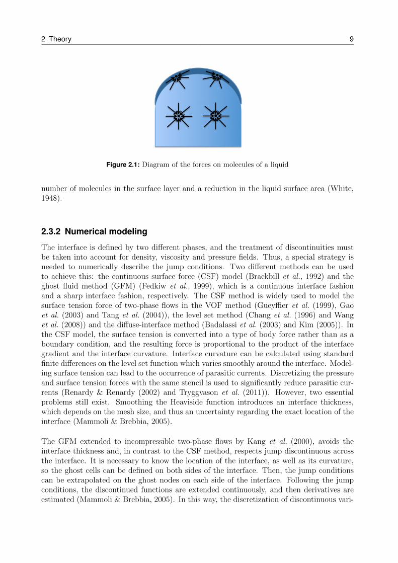
The interface is defined by two different phases, and the treatment of discontinuities mustbe taken into account for density, viscosity and pressure fields. Thus, a special strategy isneeded to numerically describe the jump conditions. Two different methods can be usedto achieve this: the continuous surface force (CSF) model (Brackbill et al., 1992) and theghost fluid method (GFM) (Fedkiw et al., 1999), which is a continuous interface fashionand a sharp interface fashion, respectively. The CSF method is widely used to model thesurface tension force of two-phase flows in the VOF method (Gueyffier et al. (1999), Gaoet al. (2003) and Tang et al. (2004)), the level set method (Chang et al. (1996) and Wanget al. (2008)) and the diffuse-interface method (Badalassi et al. (2003) and Kim (2005)). Inthe CSF model, the surface tension is converted into a type of body force rather than as aboundary condition, and the resulting force is proportional to the product of the interfacegradient and the interface curvature. Interface curvature can be calculated using standardfinite differences on the level set function which varies smoothly around the interface. Model-ing surface tension can lead to the occurrence of parasitic currents. Discretizing the pressureand surface tension forces with the same stencil is used to significantly reduce parasitic cur-rents (Renardy & Renardy (2002) and Tryggvason et al. (2011)). However, two essentialproblems still exist. Smoothing the Heaviside function introduces an interface thickness,which depends on the mesh size, and thus an uncertainty regarding the exact location of theinterface (Mammoli & Brebbia, 2005).
The GFM extended to incompressible two-phase flows by Kang et al. (2000), avoids theinterface thickness and, in contrast to the CSF method, respects jump discontinuous acrossthe interface. It is necessary to know the location of the interface, as well as its curvature,so the ghost cells can be defined on both sides of the interface. Then, the jump conditionscan be extrapolated on the ghost nodes on each side of the interface. Following the jumpconditions, the discontinued functions are extended continuously, and then derivatives areestimated (Mammoli & Brebbia, 2005). In this way, the discretization of discontinuous vari-
10 2.4 Contact angle models
Figure 2.2: Numerical scheme of GFM
ables is more accurate, and the velocity field has much smaller spurious currents than whenusing the CSF method.
2.4 Contact angle models
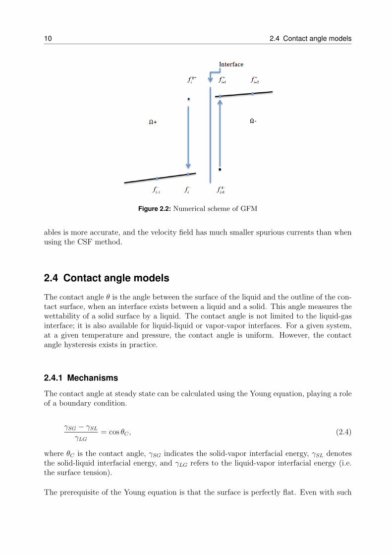
The contact angle θ is the angle between the surface of the liquid and the outline of the con-tact surface, when an interface exists between a liquid and a solid. This angle measures thewettability of a solid surface by a liquid. The contact angle is not limited to the liquid-gasinterface; it is also available for liquid-liquid or vapor-vapor interfaces. For a given system,at a given temperature and pressure, the contact angle is uniform. However, the contactangle hysteresis exists in practice.
2.4.1 Mechanisms
The contact angle at steady state can be calculated using the Young equation, playing a roleof a boundary condition.
γSG − γSLγLG
= cos θC , (2.4)
where θC is the contact angle, γSG indicates the solid-vapor interfacial energy, γSL denotesthe solid-liquid interfacial energy, and γLG refers to the liquid-vapor interfacial energy (i.e.the surface tension).
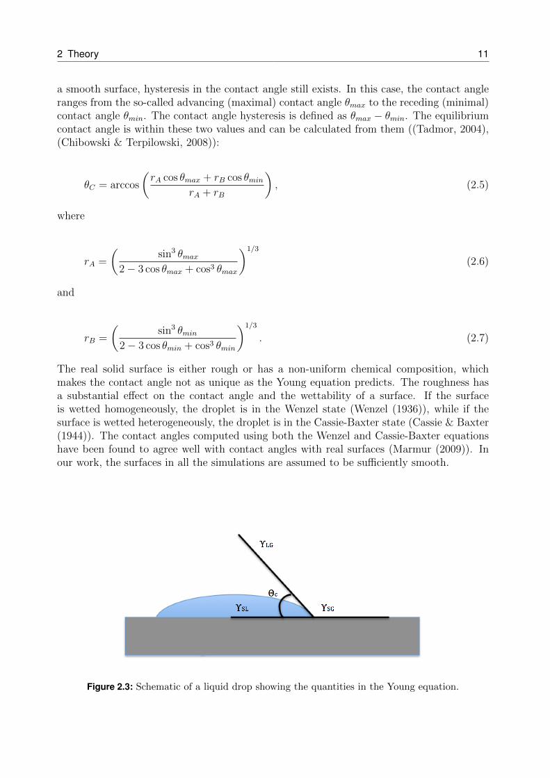
The prerequisite of the Young equation is that the surface is perfectly flat. Even with such
2 Theory 11
a smooth surface, hysteresis in the contact angle still exists. In this case, the contact angleranges from the so-called advancing (maximal) contact angle θmax to the receding (minimal)contact angle θmin. The contact angle hysteresis is defined as θmax − θmin. The equilibriumcontact angle is within these two values and can be calculated from them ((Tadmor, 2004),(Chibowski & Terpilowski, 2008)):
θC = arccos
(rA cos θmax + rB cos θmin
rA + rB
), (2.5)
where
rA =
(sin3 θmax
2− 3 cos θmax + cos3 θmax
)1/3
(2.6)
and
rB =
(sin3 θmin
2− 3 cos θmin + cos3 θmin
)1/3
. (2.7)
The real solid surface is either rough or has a non-uniform chemical composition, whichmakes the contact angle not as unique as the Young equation predicts. The roughness hasa substantial effect on the contact angle and the wettability of a surface. If the surfaceis wetted homogeneously, the droplet is in the Wenzel state (Wenzel (1936)), while if thesurface is wetted heterogeneously, the droplet is in the Cassie-Baxter state (Cassie & Baxter(1944)). The contact angles computed using both the Wenzel and Cassie-Baxter equationshave been found to agree well with contact angles with real surfaces (Marmur (2009)). Inour work, the surfaces in all the simulations are assumed to be sufficiently smooth.
Figure 2.3: Schematic of a liquid drop showing the quantities in the Young equation.
12 2.5 Marangoni effect
2.4.2 Numerical models for the contact angle
Zahedi et al. (2009) developed an algorithm for CLS method. However, this method is onlyavailable for two-dimensional computation. Furthermore, it also requires two additional nu-merical parameters, which are obtained by numerical experiments and test-case dependent.Sato & Niceno (2012) developed a new method suitable for both two- and three-dimensionalcomputations. Their method modifies the reinitialization step from the original CLS, with-out adding parameters. The layer of cells adjacent to the wall is referred as to the walllayer and treated separately from other layers. In this layer, the level set function is onlysharpened in the tangential direction of the wall. Meanwhile, the conservation is satisfied.This model has been implemented in MGLET in present work, as discussed in detail insection (4.1).
Many studies have been carried out on the contact line model in the context of some otherconservative methods, such as VOF and CLSVOF. Bussmann et al. (1999) and Bussmannet al. (2000) first calculated the drop impact phenomena using a three-dimensional VOFcode. Meanwhile, in Afkhami & Bussmann (2009), a height function was used in the VOFmethod to simulate the contact line model. This method enables the contact line phenomenato be simulated in both static and dynamic conditions. A contact line model for CLSVOF,developed by Sussman (2001) and Sussman (2005), incorporates an embedded boundary ap-proach (Colella et al., 1999) in which a solid-body shape can be displayed within a Cartesiangrid. With the help of the contact line model, contact line dynamics problems can be re-solved: for instance, free surface flow around a solid body (Yang & Stern, 2009), free surfacedeformation due to a wall adhesion force without gravity (Himeno & Watanabe, 2005), anddrop impact phenomena (Yokoi, 2011).
2.5 Marangoni effect
The Marangoni effect occurs when a surface tension gradient exists along the interface be-tween two phases. In most cases, this two-phase interface is a liquid-gas interface. As thesolute concentration, surfactant concentration, and temperature change along the interface,a surface tension gradient is usually generated.
2.5.1 Relevance
The applications of the Marangoni effect have been observed in various fields. This effecthas to be considered during the welding process, since it influences the stresses within thematerial as well as deformation. Forces that generated from the Marangoni effect can alsoaffect crystal growth, leading to defects within the structure, which can inhibit the mate-rial’s semiconducting capabilities. During the electron beam melting process, the Marangonieffect can be caused in the melting process by large thermal gradients. These forces have anegative impact on the quality of the material.
2 Theory 13
There are various ways to define a Marangoni number, a dimensionless number quantifyingthe influence of the Marangoni effect. One possibility is:
Ma = −L∆σ
µD, (2.8)
where L is the characteristic length, µ is the dynamic viscosity and σ is the surface ten-sion.
2.5.2 Mechanisms
When two liquids are in contact with each other, the liquid with stronger surface tensionpulls more strongly on the surrounding liquid than one with lower surface tension, so thatthe liquid flows away from regions of low surface tension.
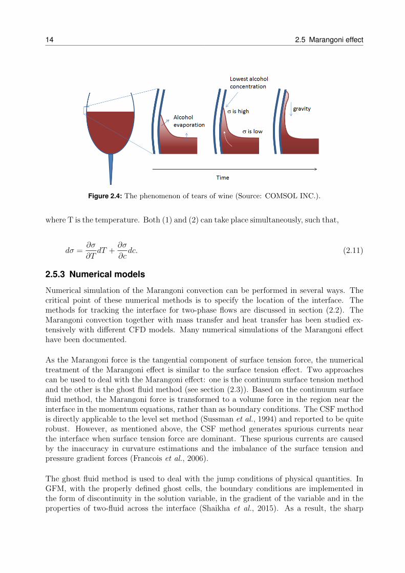
Tears of wine is a typical phenomenon caused by Marangoni effect. Its mechanism is vi-sualized in figure (2.4). It forms at the three-phase junction of glass walls, wine, and air.At this junction, the fluid remains on the surface of the glass. Since the vapor pressure ofalcohol is higher than that of water, the alcohol in the wine continues to evaporate fromthe surface, evaporating faster than water. The alcohol concentration in the thin film dropsquickly, because of their small volume and relatively large surface area. This establishes aconcentration difference between the thin film and the flat contact surface, between the wineand the air, which in turn causes a surface tension gradient that moves the thin film up thewall of the glass.
As alcohol is further volatilized, a greater surface tension gradient is created. More wine isdrawn to the glass wall until droplets form. At this point gravity will pull the tears of winealong the glass wall back to the main body of the wine.
There are two special cases of the Marangoni effect: (1) In the case where the change insurface tension is driven by concentration, the Marangoni effect is referred to as the soluto-capillary effect:
dσ =∂σ
∂cdc, (2.9)
where c is the concentration. (2) In the case where the surface tension varies due to thetemperature, the Marangoni effect is referred to as the thermo-capillary effect (Levich &Krylov, 1969):
dσ =∂σ
∂TdT, (2.10)
14 2.5 Marangoni effect
Figure 2.4: The phenomenon of tears of wine (Source: COMSOL INC.).
where T is the temperature. Both (1) and (2) can take place simultaneously, such that,
dσ =∂σ
∂TdT +
∂σ
∂cdc. (2.11)
2.5.3 Numerical models
Numerical simulation of the Marangoni convection can be performed in several ways. Thecritical point of these numerical methods is to specify the location of the interface. Themethods for tracking the interface for two-phase flows are discussed in section (2.2). TheMarangoni convection together with mass transfer and heat transfer has been studied ex-tensively with different CFD models. Many numerical simulations of the Marangoni effecthave been documented.
As the Marangoni force is the tangential component of surface tension force, the numericaltreatment of the Marangoni effect is similar to the surface tension effect. Two approachescan be used to deal with the Marangoni effect: one is the continuum surface tension methodand the other is the ghost fluid method (see section (2.3)). Based on the continuum surfacefluid method, the Marangoni force is transformed to a volume force in the region near theinterface in the momentum equations, rather than as boundary conditions. The CSF methodis directly applicable to the level set method (Sussman et al., 1994) and reported to be quiterobust. However, as mentioned above, the CSF method generates spurious currents nearthe interface when surface tension force are dominant. These spurious currents are causedby the inaccuracy in curvature estimations and the imbalance of the surface tension andpressure gradient forces (Francois et al., 2006).
The ghost fluid method is used to deal with the jump conditions of physical quantities. InGFM, with the properly defined ghost cells, the boundary conditions are implemented inthe form of discontinuity in the solution variable, in the gradient of the variable and in theproperties of two-fluid across the interface (Shaikha et al., 2015). As a result, the sharp
2 Theory 15
interface is maintained without smearing. The discontinuous variables are discretized moreaccurately in GFM, thus the spurious currents are much lower as compared to the CSFmethod. However, the GFM is not a conservative method because it solves two single fluidproblems rather than the two-phase problem. Therefore, the numerical flux is calculatedtwice at the interface (Liu et al., 2011).
The Marangoni effect is widely used in many fields. Davis (1987) examined the instabilitiesleading to the Marangoni effect. The impact of the Marangoni effect on crystal growth wasconsidered by Okano et al. (1991), Kobayashi et al. (1997), Galazka & Wilke (2000), andKawaji et al. (2003). The thermo-capillary effect of a droplet in a non-uniform temperaturefield was studied in Bassano (2003). The impacts of the Marangoni convection on binarymixture, in which the surface tension depends on both the temperature and the solute con-centration was investigated in a series of papers ((Bergeron et al., 1994), (Bergeron et al.,1998) and (Bahloul et al., 2003)). The Marangoni convection can be also used in absorptionprocesses (Kim et al., 2004). The numerical simulation of the Marangoni effect induced byinterphase mass transfer to/from drops, especially for mass transfer to/from a deformabledrop were conducted in Mao & Chen (2004) and Wang et al. (2008).
2.6 Mass transfer over interfaces
Mass transfer describes the passing of mass from one point to another and is the centralissue in transport phenomena. In multi-physics systems, mass transfer can take place in asingle phase as well as over phase boundaries. Although mass transfer also exists betweensolid-phase materials, in most engineering problems mass transfer involves at least one fluidphase (gas or liquid).
In many cases, mass transfer of a substance occurs in conjunction with chemical reactions.This means that the flux of a chemical substance within a volume element does not haveto be conserved, because the chemical substances can be generated and consumed in thisvolume element. The chemical reaction is the source or sink of this flux balance.
The mass transfer theory allows for the computation of the mass flux, and the temporal andspatial distribution of different substances in a system (including in the presence of chem-ical reactions). The purpose of such calculations is to understand, design or control suchsystems. Explaining the mechanisms of mass transfer is essential, not only for the designof mass transfer equipment, but also for reactor design, especially if it relates to reactionsthat are controlled by mass transfer. In addition, mass transfer plays an important role inenvironmental engineering, space technology, and biomedical engineering.
Mass transfer results from the effect of the chemical potential caused by concentration, tem-perature and pressure gradients. The driving force Fd can be written as:
Fd = −∇Φ, (2.12)
16 2.6 Mass transfer over interfaces
where Φ is the potential in the system.
The dimensionless number which is used to measure the ratio of the convective mass transferto the rate of diffusive mass transport is given by the Sherwood number (Sh):
Sh =K
D/L, (2.13)
where L is the characteristic length, K is the convective mass transfer coefficient and D is themass diffusivity. Once the Sherwood number is calculated, then the mass transfer coefficientcan be obtained. Furthermore, the Sherwood number can also be defined as a function ofthe Reynolds number (Re) and the Schmidt number (Sc):
Sh = f(Re, Sc). (2.14)
Depending on different model configurations and different flow conditions, the relationshipbetween the Sherwood number, the Reynolds number and the Schmidt number is various.The Reynolds number is the ratio of inertial forces to viscous forces in the fluid:
Re =ρuL
µ=uL
ν, (2.15)
where µ is the dynamic viscosity of the fluid.
The Schmidt number is a dimensionless number defined as the ratio of momentum diffusivity(kinematic viscosity) and mass diffusivity:
Sc =ν
D=
µ
ρD. (2.16)
The primary challenge of mass transfer is to determine the concentration distribution andmass transfer rate. Many studies have been discussed on the mass transfer rate under dif-ferent numerical and experimental conditions.
2.6.1 Mass transfer due to the temperature gradient (phasechange)
Evaporation is a common form of mass transfer caused by temperature gradients. From themicroscopic perspective, evaporation is the process of liquid molecules leaving the liquid sur-face. Molecules in a liquid move constantly and irregularly, with their average kinetic energydependent on the temperature of the liquid. Due to the random movement and collision ofmolecules there are always some molecules that have higher kinetic energy than the average
2 Theory 17
instantaneous kinetic energy. Molecules with sufficient kinetic energy to overcome the forcesbetween the molecules of the liquid, such as those near the surface of the liquid, will ’escape’and enter the surrounding air in gaseous phase.
As the molecules with higher kinetic energy escape from the liquid, the energy removed fromthe vaporized liquid reduces the average kinetic energy and the temperature of the liquid,resulting in evaporative cooling.
For different flow conditions and different model configurations, the mass transfer rate canbe defined in various ways, as discussed below:
Mass transfer by evaporation at a flat interface
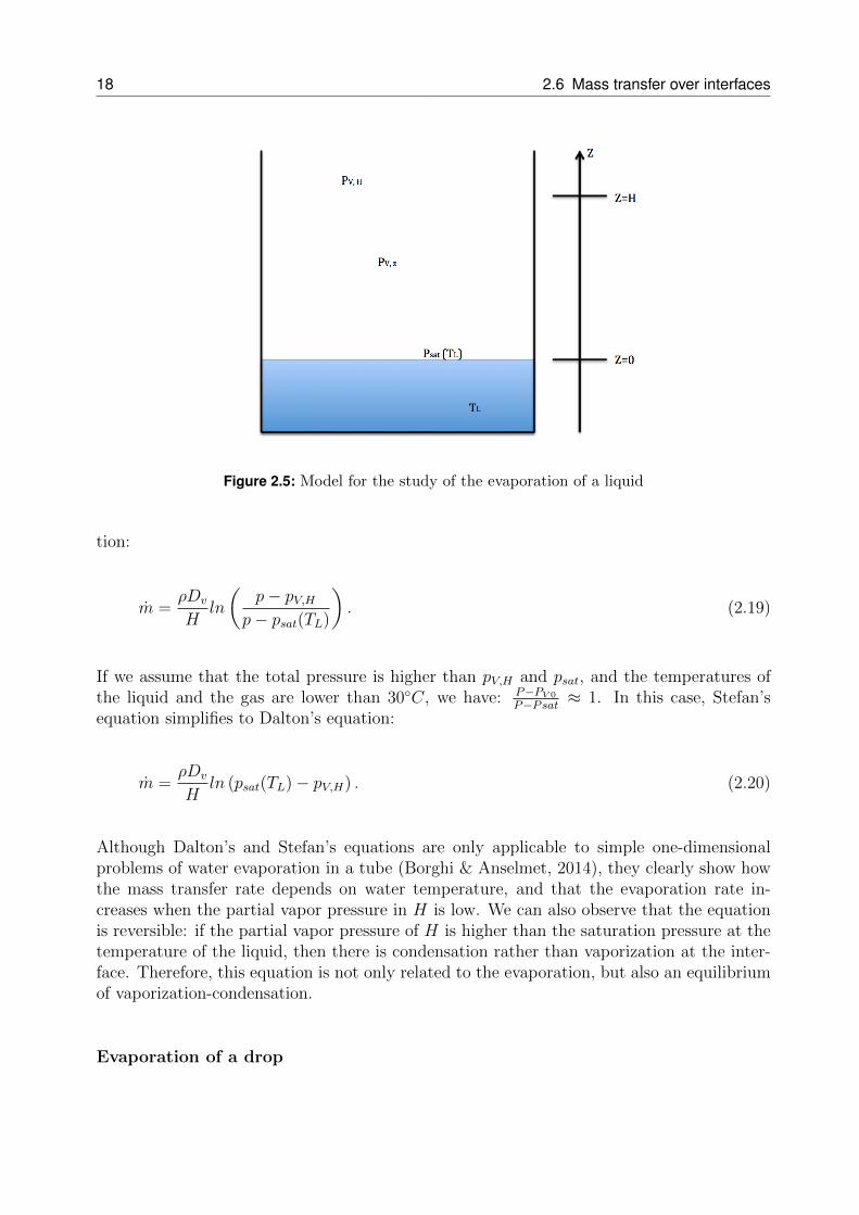
If we consider a liquid at a given temperature TL, and the constant partial vapor pressure(lower than the saturated pressure psat) at a certain distance H from the interface (seefigure (2.5)), we are able to calculate the mass transfer rate of the evaporation at steadystate (Borghi & Anselmet, 2014):
m =ρDv
Hln
(1− YV,H
1− YV sat(TL)
), (2.17)
where m is the mass transfer rate, Dv is the diffusion coefficient of the vapor in the air, YV,His the mass fraction of vapor at H, YV sat is the mass fraction of the vapor at interface. Hshould be sufficiently small to ensure that the pressure between the point H and the interfacelinearly and monotonously depends on the distance H.
The evaporation process contains three phenomena (Borghi & Anselmet, 2014): Firstly, themovement of vapor molecules in the gas phase due to the gradient of the partial pressure,which is molecular diffusion. Secondly, the transformation of the liquid-vapor at the surfacemaintains the equilibrium between the liquid and the vapor, which is influenced by the be-havior of the molecular diffusion. Thirdly, the motion of the interface, in which the liquidmoves towards the interface and the vapor moves away from the interface.
If the gas mixture is a perfect mixture, then
pV = pMmix
MV
YV , (2.18)
where pV is the partial pressure, p is the total pressure in the gas and can be assumed to beknown, Mmix is the molar mass of the mixture and MV is the molar mass of the vapor.
Stefan’s equation expresses the relationship between the partial pressure and the mass frac-
18 2.6 Mass transfer over interfaces
Figure 2.5: Model for the study of the evaporation of a liquid
tion:
m =ρDv
Hln
(p− pV,H
p− psat(TL)
). (2.19)
If we assume that the total pressure is higher than pV,H and psat, and the temperatures ofthe liquid and the gas are lower than 30C, we have: P−PV 0
P−Psat ≈ 1. In this case, Stefan’sequation simplifies to Dalton’s equation:
m =ρDv
Hln (psat(TL)− pV,H) . (2.20)
Although Dalton’s and Stefan’s equations are only applicable to simple one-dimensionalproblems of water evaporation in a tube (Borghi & Anselmet, 2014), they clearly show howthe mass transfer rate depends on water temperature, and that the evaporation rate in-creases when the partial vapor pressure in H is low. We can also observe that the equationis reversible: if the partial vapor pressure of H is higher than the saturation pressure at thetemperature of the liquid, then there is condensation rather than vaporization at the inter-face. Therefore, this equation is not only related to the evaporation, but also an equilibriumof vaporization-condensation.
Evaporation of a drop
2 Theory 19
Another case of the local evaporation rate is the vaporization of a drop in a gas phase. Thiscase has been studied both theoretically and experimentally (Sirignano, 1999).
The drop is assumed to be isolated and spherical in shape without gravity, so that theprofiles of the velocity and temperature fields remain spherical. Then the mass flow rateof the vaporization from the drop can be obtained similarly to the case of the flat inter-face:
m = 4πrdρgDvln
(1− YV∞
1− YV sat(Ts)
), (2.21)
where rg is the radius of the drop, ρg is the density of the gas, Dv = const. is the massdiffusivity of the vapor. Ts is the temperature at the surface. Then the mass flow rate persurface unit is:
m =ρgDv
rdln
(1− YV∞
1− YV sat(Ts)
). (2.22)
In recent years, new methods have been developed to compute phase change, with the helpof interface tracking techniques, which have been discussed in section (2.2). Juric & Tryg-gvason (1998) showed a front tracking approach to simulate the boiling flow. In this case, thesingle field formulation is applied to describe the entire flow field. Welch & Wilson (2000)introduced a volume of fluid method for phase change. A coupled level set and volume offluid method was used in Tomar et al. (2005) to calculate the film boiling. In Tanguy et al.(2007) a combination of the level set method and the ghost fluid method was implementedto handle the two-dimensional vaporizing issues.
2.6.2 Mass transfer due to the concentrationgradient
Mass transfer driven by the concentration gradient without considering the temperature fieldis discussed in this section. It is widely used in chemical engineering, especially liquid-liquidreactions and solvent extraction. Many of these industrial processes are related to the masstransfer of moving drops or bubbles (rising or falling). The main challenge in the numericalsimulation of mass transfer to/from a buoyancy driven drop is that the motion of a deformeddrop with simultaneous mass transfer must be solved with the un-determined topology ofa surface (Petera & Weatherley, 2001). Key to this challenge is understanding the masstransfer mechanism by considering the drop deformation and the mass transfer process it-self. Due to the complexity of the mass transfer, many empirical and theoretical equationsfor mass transfer coefficients for various drop and bubble conditions can be looked up (Clift
20 2.6 Mass transfer over interfaces
et al., 1978).
In addition to experiments, a number of numerical simulations have been performed recently.Mao et al. (2001) concentrated grid points near the bubble by using a body-fitted coordinatesystem. Davidson & Rudman (2002) and Gupta et al. (2010) simulated mass transfer with avolume of fluid method. Unverdi & Tryggvason (1992a) and Aboulhasanzadeh et al. (2012)computed the bubble motion with mass transfer using the front tracking method. The lat-ter approach applies a multi-scale computation technique to significantly reduce the overallgrid resolutions. Wang et al. (2008), Ganguli & Kenig (2011a), Ganguli & Kenig (2011b)and Hayashi & Tomiyama (2011) implemented the level set method tracking the interfaceto measure the mass transfer rate and, to observe the behavior of bubbles. Especially forGanguli & Kenig (2011a) and Ganguli & Kenig (2011b), the conservative version of the levelset method was applied by adding two source terms in the momentum equations. However,in most of these studies, the volume of the bubbles was assumed to remain constant. OnlyHayashi & Tomiyama (2011) considered the shrinkage of the bubbles as gas diffused to theliquid.
The overall liquid mass transfer coefficient kod influenced by the concentration gradient canbe estimated by
V∂cL∂t
= Skod
(cL −
cGHD
), (2.23)
where kod is the mass transfer coefficient, V is the volume of the liquid, S is the surfacearea of the liquid, HD is the dimensionless distribution coefficient, cL and cG are the con-centrations in the liquid phase and gas phase, respectively. cG/HD means the concentrationin equilibrium in the liquid phase due to the Henry’s law. The Henry’s law and HD will bediscussed in detail in section (4.3).
If the time interval is sufficiently small, integrating equation (2.23) gives:
kod = −VS
1
t2 − t1ln
(cG/HD − cL,t1cG/HD − cL,t2
), (2.24)
where t1 and t2 are the two measurement times and cL is the average concentration of thedrop at any time.
The difference between the mass transfer coefficient kod and the mass flux m is a factor ρ(i.e., kod = m/ρ). Here, the concentration term is taken into account, rather than the massfraction term or the pressure term in the formula of evaporation rate.
Additionally, two interfacial boundary conditions need to be considered in this case:
• flux continuity at the interface

2 Theory 21
• interfacial dissolution equilibrium
The method used to implement these two interfacial boundary conditions will be discussedin section (4.3).

22 2.6 Mass transfer over interfaces
3 Code basis and state at the beginning
In this chapter, the code MGLET is introduced in detail, which is used to solve the governingequations of turbulent flows. Furthermore, the conservative version of the level set method(CLS), already implemented into MGLET as part of a master’s thesis (Andre, 2012) will bediscussed.
3.1 MGLET
The main objective of MGLET is to predict turbulent flows in and along complex geometrieswith Direct Numerical Simulation (DNS) and Large Eddy Simulation (LES). This code isbased on the finite volume method in the Cartesian coordinate system. It has been par-allelized and tested on a high-performance computer (more than 109 grid cells). Recently,several research groups (e.g., NTNU Trondheim, DLR Institute of atmosphere physics) havebeen adopting this code to various applications, such as bluff body flow and wake vortices.
Recent developments to this code include:
• Conservative Immersed Boundary method for arbitrary geometries in a Cartesian grid.
• Zonal grid refinement and hierarchical grids for high Schmidt number scalar fields.
• Particle dynamics and fiber suspension.
• Fourth-order Finite Volume schemes.
• Multiphase flows.
MGLET is implemented on a Cartesian grid with the staggered variable arrangement of com-putations (Manhart & Friedrich (2002), Manhart (2004)). Convective and diffusive fluxes atcell faces are discretized with central space approximations (second and fourth order). Timeintegration is achieved by a third-order Runge-Kutta (RK) method. The pressure in thePoisson equation is solved by an Incomplete Lower-Upper (ILU) decomposition of secondorder accuracy.
3.1.1 Finite volume method
The finite volume method is a numerical algorithm to solve partial differential equations(PDE) which is widely used in computational fluid dynamics (CFD). This method is basedon conservation of the integral form rather than the differential form. In the finite volumemethod, volume integrals in a partial differential equation can be handled by calculatingthe values of variables averaged across the volume in conservation form. If volume integralscontain a divergence term, they can be converted to surface integrals using the divergence
23
24 3.1 MGLET
theorem (Gauss theorem). These terms may then be treated as fluxes at the surfaces of eachcontrol volume.
The advantages of finite volume method are:
• Consistent with the law of conservation (Because the flux entering a given volume isidentical to that leaving the adjacent volume).
• Highly adaptable to the unstructured meshes.
3.1.2 Staggered grid
For a staggered grid, scalar variables (i.e. pressure, density, viscous, level set, etc.) arestored at the center of each control volume cell, and the velocities are allocated at the centerof the surface of each cell. This is in contrast to a collocated grid arrangement, in which allthe variables are stored in the same positions in the center of the control volume for each cell.
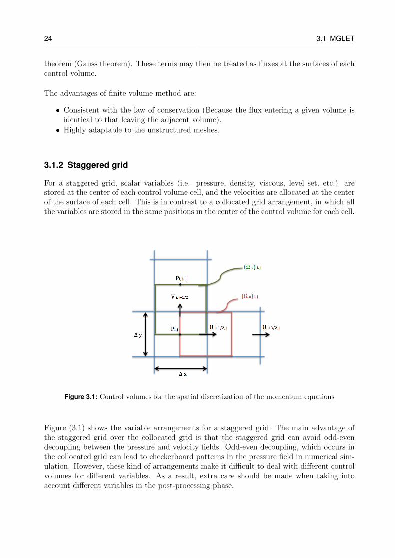
Figure 3.1: Control volumes for the spatial discretization of the momentum equations
Figure (3.1) shows the variable arrangements for a staggered grid. The main advantage ofthe staggered grid over the collocated grid is that the staggered grid can avoid odd-evendecoupling between the pressure and velocity fields. Odd-even decoupling, which occurs inthe collocated grid can lead to checkerboard patterns in the pressure field in numerical sim-ulation. However, these kind of arrangements make it difficult to deal with different controlvolumes for different variables. As a result, extra care should be made when taking intoaccount different variables in the post-processing phase.
3 Code basis and state at the beginning 25
3.2 Conservative level set method
The CLS method has been chosen as the numerical method to track the interface, due to itsability to conserve mass and simplicity. It was first implemented in the MGLET within amaster thesis (Andre, 2012). The CLS method has been reprogrammed from its initial formto comply with recent updates to MGLET. To validate the implementation, some test caseswere computed (see Chapter 5). In the following, the current implementation will be detailed.
3.2.1 Level set advection
The level set ϕ is advected by equation (3.1):
∂ϕ
∂t+ u ·∇ϕ = 0. (3.1)
For a divergence free velocity field, this can be re-written as
∂ϕ
∂t+∇ · (ϕu) = 0. (3.2)
Equation (3.2) has a number of benefits: It is effective in keeping the scalar ϕ conserva-tive, ensuring that volumes of each fluid approach constant values as the level set functionconverges to a step function. The advection equation is discretized using the finite volumemethod.
In MGLET, a preprocessing step is implemented to improve resolution properties of loworder numerical schemes (Schwertfirm et al., 2008). This method is employed to calculatethe level set function to improve the accuracy during the advection step.
3.2.2 Level set reinitialization
In order to deal with the inconsistency with the mass conservation of the level set method,Olsson & Kreiss (2005) introduced an alternative reinitialization equation which was furtherrefined by Olsson et al. (2007). The reinitialization equation is given by
∂ϕ
∂τ+∇ · (ϕ(1− ϕ)n) = ε∇ · ((∇ϕ · n)n), (3.3)
where τ is the pseudo time step, ε is the artificial diffusion number and n is the interfacenormal vector.
To comprehend the reinitialization equation, each term in equation (3.3) has been examinedseparately. The second term on the left side of equation (3.3) is referred to as the compres-
26 3.2 Conservative level set method
sion term which is used to sharpen the definition of the interface profile. The term on theright side is referred to as the diffusion term, which is used to prevent the interface frombeing too sharp, maintaining the smoothness of the interface.
The steady state solution of equation (3.3) discussed by Olsson et al. (2007) is given by:
ϕ =1
2
(tanh
(φ
2ε
)). (3.4)
Increasing ε tends to smear out the interface profile while decreasing ε tends to sharpen theinterface profile. Olsson & Kreiss (2005) suggested to define the artificial diffusion term εand the pseudo time step size τ as follows:
ε =h1−d
2(3.5)
and
∆τ =h1+d
2, (3.6)
where is d = 0.1, and h is the grid spacing. In this case, as opposed to others, it is not onlysufficient to obtain convergence, but also maintain a sharp interface.
In Olsson & Kreiss (2005), the level set function is advected with a total variation di-minishing (TVD) method. The equation used to calculate the interface normal vectoris:
n =∇ϕ|∇ϕ|
. (3.7)
The non-TVD advection schemes cannot avoid all oscillations occurring in the level setfield. These oscillations lead to rapid fluctuation of the normal vector n near the interface.Desjardins et al. (2008) used a distance function φ free of oscillations to compute the normalvector n,
n =∇φ|∇φ|
(3.8)
is to make the level set method more robust.
The distance function in the CLS is in fact the level set function in the original level setmethod, while the level set function in the CLS is defined using a hyperbolic tangent profile
3 Code basis and state at the beginning 27
rather than the signed distance function in the original version of the level set method. Themethod used to determine the distance function is discussed in section (3.2.3).
When solving the Navier-Stokes equations, density and viscosity fields need to be clari-fied. While these two fields are assumed to be constant within each fluid, jump condi-tions around the interface lead to density and viscosity not being constant. The densityand viscosity fields are defined using the level set function as followed (Olsson & Kreiss,2005):
ρ = ρ1 + (ρ1 − ρ2)ϕ (3.9)
and
µ = µ1 + (µ1 − µ2)ϕ. (3.10)
3.2.3 Distance function and normal vector
The Fast Marching Method (FMM) used to compute the distance function is a numerical al-gorithm for solving boundary value problems of the Eikonal equation (Sethian, 1999):
|∇φ| = 1 for φ ∈ Ω (3.11a)
φ = 0 for φ ∈ ∂Ω. (3.11b)
The general principle of equation (3.11) is to find a path with the shortest travel time from apoint in the modeling domain to the boundary. In other words, the direction of the steepestdescent needs to be specified.
Using the multi-dimensional approximation from Osher & Sethian (1988), the discrete formof equation (3.11) is given by
|∇φ|2 ≈ max(D−xφi,j,k, 0)2 +min(D+xφi,j,k, 0)2
+max(D−yφi,j,k, 0)2 +min(D+yφi,j,k, 0)2
+max(D−zφi,j,k, 0)2 +min(D+zφi,j,k, 0)2
= 1. (3.12)
The version of the first order forward and backward operators, take x-direction as an example,can be defined as,
D+xφi,j,k =φi+1,j,k − φi,j,k
∆x(3.13)
28 3.2 Conservative level set method
and
D−xφi,j,k =φi,j,k − φi−1,j,k
∆x. (3.14)
However, the first order version is not sufficient to obtain the accurate values. Therefore, asecond order discretization of the above equations is employed, in the x-direction:
D+xφi,j,k =φi+1,j,k − φi,j,k
∆x+ S+∆x
2
φi+2,j,k − 2φi+1,j,k + φi,j,k∆x2
(3.15)
and
D−xφi,j,k =φi,j,k − φi−1,j,k
∆x+ S−
∆x
2
φi,j,k − 2φi−1,j,k + φi−2,j,k∆x2
. (3.16)
The operators of S+ and S− are defined as followed,
S+x(φi,j,k) =
1 if φi+1,j,k and φi+2,j,k are known, and φi+2,j,k ≤ φi+1,j,k
0 else
for the forward derivative in the x-direction, and
S−x(φi,j,k) =
1 if φi−1,j,k and φi−2,j,k are known, and φi−2,j,k ≤ φi−1,j,k
0 else
for the backward derivative in the x-direction. Equations for y-direction and z-directionfollow similarly.
A more practical formulation is noted by Sethian (1999):
|∇φ|2 ≈ max(D−xφi,j,k,−D+xφi,j,k, 0)2
+max(D−yφi,j,k,−D+yφi,j,k, 0)2
+max(D−zφi,j,k,−D+zφi,j,k, 0)2
= 1. (3.17)
With this approach, the distance function φ is approximately second order accurate. Sincethey are calculated from the gradient of φ (see equation (3.8)), the normal vectors are ex-pected to be first order accurate.
In the level set method, the distance function has a positive sign on the side of the interface
3 Code basis and state at the beginning 29
with ϕ ≥ 0, while on the opposite side the distance function has a negative sign. In order toinitialize the distance values around the interface, the inverse to equation (3.4) is applied,as given by
φ = εln
(ϕ
1− ϕ
). (3.18)
The points in the domain can be categorized into three groups: known, trial and unknown.All the nodes are marked as unknown at first. Then the grid points closest to the interfaceare initialized by equation (3.18). These grid points are identified as having known solutionvalues. The neighbors of the known nodes without known values are marked as trials. Theremaining grid points are marked as unknown. The calculation of the gradient of a node isachieved only if the node has known neighbors. The resulting minimum distance is storedas a trial value. If at a later time a previously unknown neighbor becomes known, this min-imum needs to be recalculated and compared to the previous minimum distance. Repeatingthis process, until the minimum distance of a given point is determined. Thereafter, thispoint can be marked as known, and used to compute the distance for its trial neighbors.Finally, the results can be determined until a specified distance value becomes known or allnodes are marked as known in the domain.
Figure 3.2: FMM initialization. Cells are marked as known (black circle), trial (blue circle) orunknown (empty).
3.2.4 Interface curvature
The accuracy of curvature is a critical factor that effects the accuracy of surface tensionforce calculations. The interface curvature can be calculated with a finite difference method(Sethian, 1999), a least squares method (Marchandise et al., 2007) and a convolution method.Due to the second order accuracy of the distance function, the curvature calculated usingfinite difference method did not result in convergence (Desjardins et al., 2008). For the
30 3.2 Conservative level set method
convolution method, which has been already used to calculate the derivative of the colorfunction in VOF (Cummins et al., 2005), the curvature can be determined by computing thedivergence of the normal vectors:
κ = −∇ · n, (3.19)
where κ is the curvature.
The advantage of this approach is that the additional computational cost of equation (3.19)is small. However, the disadvantage is that the curvature stencil size is larger, which mayresult in lower accuracy.
3.2.5 Surface tension
The surface tension force is included in the momentum equations (2.2) as a volumetric force(Brackbill et al., 1992):
Fsu = κσnδ(x− xs), (3.20)
where σ is the constant surface tension coefficient, xs is the point on the interface and δ isa delta function defined as:
δ(x) =
+∞ if x = 0
0 if x 6= 0
and
∫ +∞
−∞δ(x) = 1.
The role of the delta function is to transform the surface tension force from a volume inte-gral to a surface integral over the domain of the interface. In the CSF method, nδ(x −xs) can be replaced with the gradient of the level set function ∇ϕ (Olsson & Kreiss,2005):
FCSFsu = κσ∇ϕ. (3.21)
The surface tension force is not zero if the gradient of the level set function ∇ϕ is notzero. However, as mentioned in section (2.3), the interface curvature calculated by CSFmodel may lead to less accurate results. An alternative method, similar to the sharp surface
3 Code basis and state at the beginning 31
tension force (SSF) method (Brackbill et al., 1992) is used to compute the surface tensionforce:
FSSFsu = κσ
1
∆x, (3.22)
which is still treated as the volume integral, rather than the surface integral in the momen-tum equations. It also results in a jump condition in the Poisson equation similar to theGFM (Liu et al., 2000). In this case, the surface tension force only exists at interfaces atwhich the distance function φ changes sign. For example, if the interface is located betweenthe cell (i, j) and (i + 1, j), the surface tension force applied in x-direction can be definedas:
Fi+1/2,j,k = sign(φi+1,j,k − φi,j,k)σκ
∆x, (3.23)
and, in the y-direction,
Fi,j+1/2,k = sign(φi,j+1,k − φi,j,k)σκ
∆x. (3.24)
The curvature at the interface can be calculated from values at neighboring cells, throughan interpolation process, using the distance function
κ =|φi+1,j,k|κi,j,k + |φi,j,k|κi+1,j,k
|φi+1,j,k|+ |φi,j,k|. (3.25)
The advantage of this method is that the points used to calculate the curvature of the in-terface are close to the interface, while the CSF method spreads the surface tension over theentire transition region of the level set function.

32 3.2 Conservative level set method
4 Current implementations
In the framework of this dissertation, models for the contact angle, the Marangoni force andmass transfer over a fluid-fluid interface have been implemented in MGLET. In section (4.1),a new contact line model for the conservative level set method is described. Then, theMarangoni model is implemented in MGLET by adding a volume force in the momentumequations shown in section (4.2). Section (4.3) introduces the mass transfer model due tothe concentration gradient. Finally, in section (4.4) the time step restrictions for advancingthe flow variables are presented.
4.1 A contact line treatment for the CLSmethod
A contact line model for the CLS method is discussed in this part. As mentioned above,many studies of the contact line model are based on the volume of fluid and sharp levelset method. However, not many studies are related to the conservative level set method.Recently, only two models have focused on the CLS, Zahedi et al. (2009) and Sato & Niceno(2012). In Zahedi et al. (2009), two additional parameters which are test-case dependent areintroduced to be implemented in the reinitialization step. However, this method is limitedto two-dimensional cases. Sato & Niceno (2012) modify the reinitialization step from theoriginal CLS, and this method enables the model to solve both two- and three-dimensionalproblems. In present study, the latter one is implemented.
In section (4.1.1), the revised reinitialization step based on the original CLS is described.Then the boundary conditions for the contact line model of Sato & Niceno (2012) are intro-duced in section (4.1.2). This model is validated in section (5.3).
4.1.1 The reinitialization function for CLS
The reinitialization function proposed by Olsson et al. (2007) has been introduced in sec-tion 3.2. Therein, equation (3.3) the diffusion term on the right side is limited to the normaldirection only. This avoids diffusion in tangential direction. Since the flux in the directiontangential to the interface will not be balanced by any compression effects, the tangentialdiffusion might move the interface which is suppressed by the reinitialization function, equa-tion (3.3). However, in the new contact line model, the tangential diffusion effects of thelevel set function in the reinitialization step are also significant for the movement of theinterface at the wall layer; thus, the original reinitialization function is needed (Olsson &
33
34 4.1 A contact line treatment for the CLS method
Kreiss, 2005):
∂ϕ
∂τ+∇ · (ϕ(1− ϕ)n) = ε∇ · (∇ϕ). (4.1)
The discretized form of the reinitialization function, using the finite volume method, iswritten as (Sato & Niceno, 2012):
V∂ϕ
∂τ+∑
((ϕ(1− ϕ)n) · S) =∑
ε(∇ϕ) · S, (4.2)
where V is the volume of the cell, and S is the area vector of the cell faces. In our study,the level set function and the normal vectors are stored at the cell centers.
4.1.2 Boundary conditions
In the following sections, we will introduce how to deal with the boundary conditions withrespect to the level set function and the normal vector.
Level set function
Since the velocity at the wall surface is zero (no-slip boundary condition is applied), thefluxes of the level set function at the wall surface should also be zero. Therefore, a specialtreatment is needed in which the fluxes of the compression term and the diffusion term in thenormal direction of the wall are forced to be zero at a wall layer. These boundary conditionsare written as:
(ϕ(1− ϕ)n) · Swall = 0 (4.3)
and
(∇ϕ) · Swall = 0, (4.4)
respectively, where Swall is the area vector of the wall.
The layer of cells adjacent to the wall is treated differently from the other layers. Therefore,this layer is denoted as the wall layer as shown in figure (4.1). In this wall layer, fluxesof the level set function are only in the tangential direction of the wall (i.e., no fluxes inthe normal direction of the wall), rather than in all directions in other layers. Therefore,the governing equation of the reinitialization equation of the wall-layer can be re-written
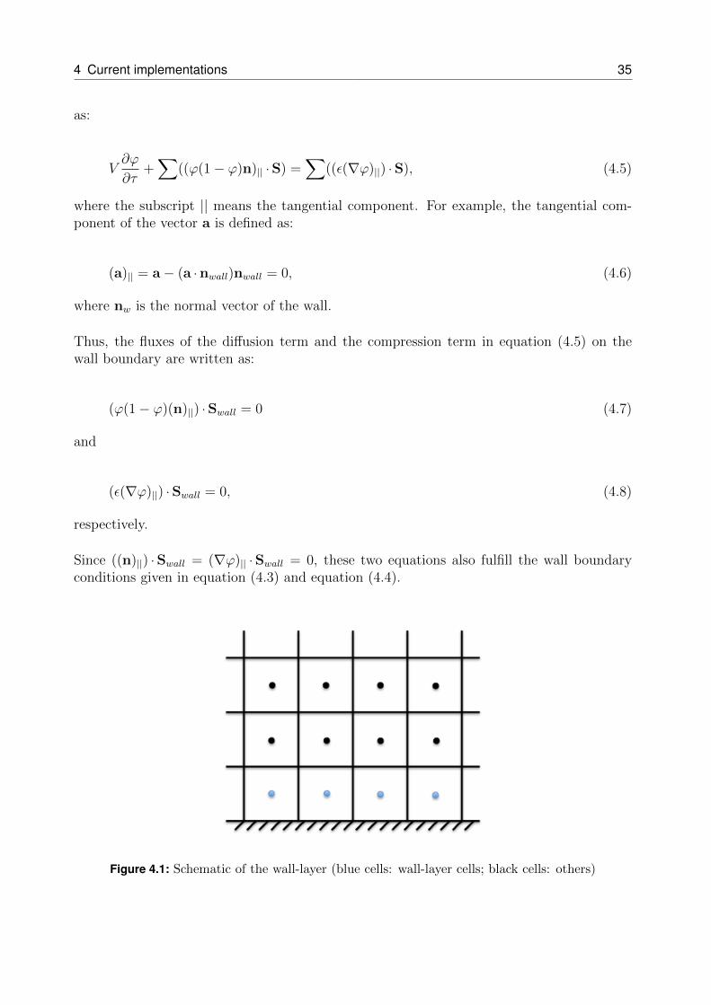
4 Current implementations 35
as:
V∂ϕ
∂τ+∑
((ϕ(1− ϕ)n)|| · S) =∑
((ε(∇ϕ)||) · S), (4.5)
where the subscript || means the tangential component. For example, the tangential com-ponent of the vector a is defined as:
(a)|| = a− (a · nwall)nwall = 0, (4.6)
where nw is the normal vector of the wall.
Thus, the fluxes of the diffusion term and the compression term in equation (4.5) on thewall boundary are written as:
(ϕ(1− ϕ)(n)||) · Swall = 0 (4.7)
and
(ε(∇ϕ)||) · Swall = 0, (4.8)
respectively.
Since ((n)||) · Swall = (∇ϕ)|| · Swall = 0, these two equations also fulfill the wall boundaryconditions given in equation (4.3) and equation (4.4).
Figure 4.1: Schematic of the wall-layer (blue cells: wall-layer cells; black cells: others)
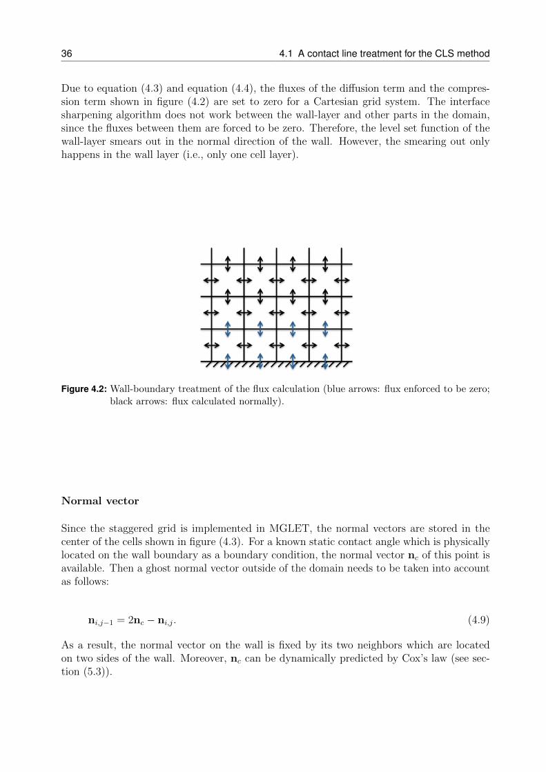
36 4.1 A contact line treatment for the CLS method
Due to equation (4.3) and equation (4.4), the fluxes of the diffusion term and the compres-sion term shown in figure (4.2) are set to zero for a Cartesian grid system. The interfacesharpening algorithm does not work between the wall-layer and other parts in the domain,since the fluxes between them are forced to be zero. Therefore, the level set function of thewall-layer smears out in the normal direction of the wall. However, the smearing out onlyhappens in the wall layer (i.e., only one cell layer).
Figure 4.2: Wall-boundary treatment of the flux calculation (blue arrows: flux enforced to be zero;black arrows: flux calculated normally).
Normal vector
Since the staggered grid is implemented in MGLET, the normal vectors are stored in thecenter of the cells shown in figure (4.3). For a known static contact angle which is physicallylocated on the wall boundary as a boundary condition, the normal vector nc of this point isavailable. Then a ghost normal vector outside of the domain needs to be taken into accountas follows:
ni,j−1 = 2nc − ni,j. (4.9)
As a result, the normal vector on the wall is fixed by its two neighbors which are locatedon two sides of the wall. Moreover, nc can be dynamically predicted by Cox’s law (see sec-tion (5.3)).
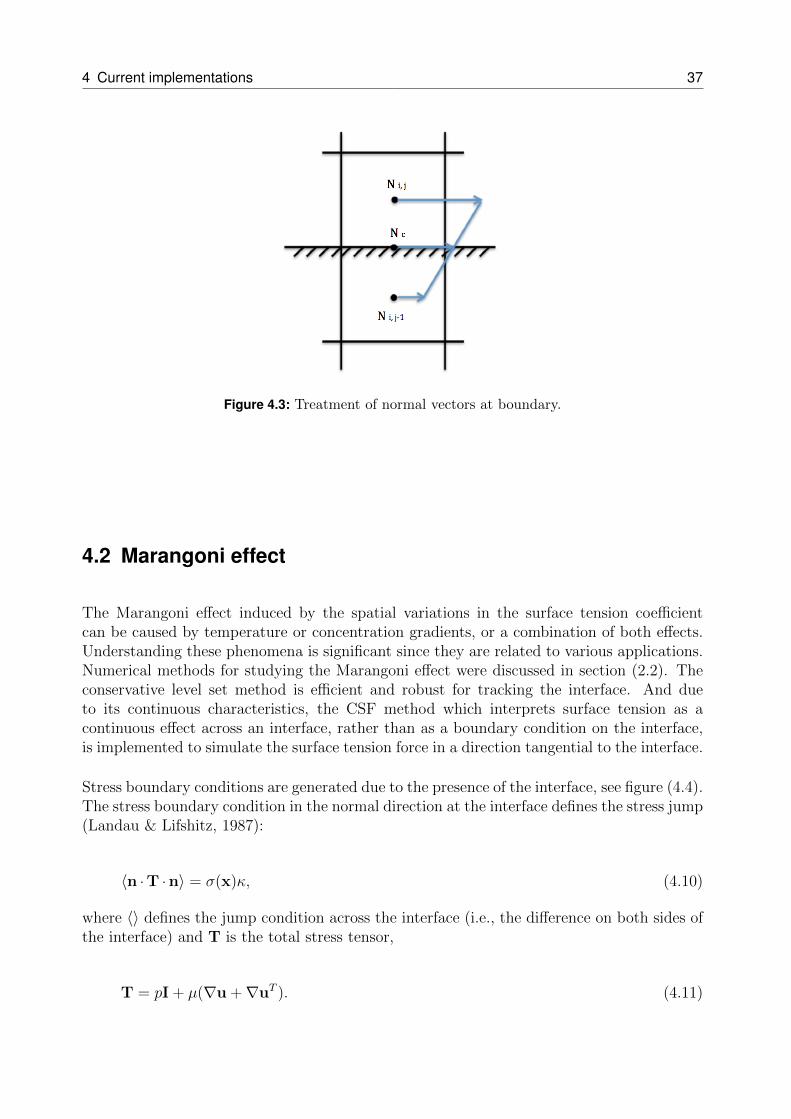
4 Current implementations 37
Figure 4.3: Treatment of normal vectors at boundary.
4.2 Marangoni effect
The Marangoni effect induced by the spatial variations in the surface tension coefficientcan be caused by temperature or concentration gradients, or a combination of both effects.Understanding these phenomena is significant since they are related to various applications.Numerical methods for studying the Marangoni effect were discussed in section (2.2). Theconservative level set method is efficient and robust for tracking the interface. And dueto its continuous characteristics, the CSF method which interprets surface tension as acontinuous effect across an interface, rather than as a boundary condition on the interface,is implemented to simulate the surface tension force in a direction tangential to the interface.
Stress boundary conditions are generated due to the presence of the interface, see figure (4.4).The stress boundary condition in the normal direction at the interface defines the stress jump(Landau & Lifshitz, 1987):
〈n · T · n〉 = σ(x)κ, (4.10)
where 〈〉 defines the jump condition across the interface (i.e., the difference on both sides ofthe interface) and T is the total stress tensor,
T = pI + µ(∇u +∇uT ). (4.11)
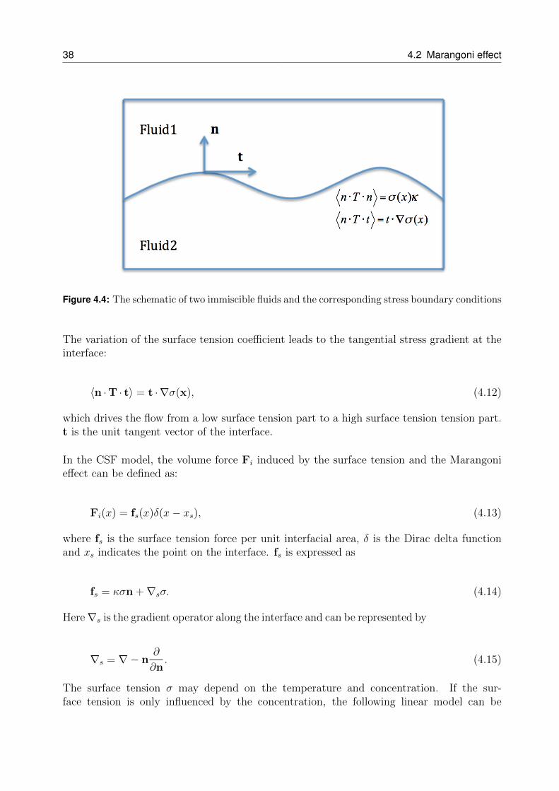
38 4.2 Marangoni effect
Figure 4.4: The schematic of two immiscible fluids and the corresponding stress boundary conditions
The variation of the surface tension coefficient leads to the tangential stress gradient at theinterface:
〈n · T · t〉 = t ·∇σ(x), (4.12)
which drives the flow from a low surface tension part to a high surface tension tension part.t is the unit tangent vector of the interface.
In the CSF model, the volume force Fi induced by the surface tension and the Marangonieffect can be defined as:
Fi(x) = fs(x)δ(x− xs), (4.13)
where fs is the surface tension force per unit interfacial area, δ is the Dirac delta functionand xs indicates the point on the interface. fs is expressed as
fs = κσn +∇sσ. (4.14)
Here∇s is the gradient operator along the interface and can be represented by
∇s = ∇− n∂
∂n. (4.15)
The surface tension σ may depend on the temperature and concentration. If the sur-face tension is only influenced by the concentration, the following linear model can be
4 Current implementations 39
assumed:
σ = σ0(1 + γc), (4.16)
where σ0 is the surface tension of a pure system, and γ is a negative constant value in mostcases. Then equation (4.11) can be rewritten as:
fs = κσn +∂σ
∂c(I− nn) ·∇c. (4.17)
The body force Fi in the momentum equations (2.2) can now be written as:
Fi(x) =
(κσn +
∂σ
∂c(I− nn) ·∇c
)δ(x− xs). (4.18)
4.3 Mass transfer
In this section, the mass transfer due to the concentration gradient is examined. This masstransfer model was first developed by Ganguli & Kenig (2011a). To implement this method,some prerequisites are needed for the fluid-fluid system:
• Newtonian incompressible fluids.
• No chemical reaction.
• Isothermal system.
• Laminar flow.
• No surface active contaminants.
The governing mass transport equation for the incompressible fluid flow is as follows:
∂c
∂t+ u ·∇c = ∇ · (D∇c). (4.19)
Here, c is the concentration. Next, let us consider a two-phase flow system comprising a gasbubble (denoted as G) and a liquid phase (denoted as L). Then the mass transport equationcan be re-written as:
∂cG∂t
+ u ·∇cG = ∇ · (DG∇cG) (4.20)
and
∂cL∂t
+ u ·∇cL = ∇ · (DL∇cL), (4.21)
40 4.3 Mass transfer
where DG and DL are the mass diffusion coefficients for the gas phase and liquid phase,respectively. For the mass transport equation, two interfacial boundary conditions need tobe fulfilled. First, the interfacial dissolution equilibrium is defined by the thermodynamicequilibrium assumption:
cG = HDcL. (4.22)
Here, HD is the distribution coefficient that is used to measure the interfacial concentrationjump. In the gas-liquid system, the amount of dissolved gas is proportional to its partialpressure in the gas phase. HD is the proportional factor. In the liquid-liquid system, HD
is defined as a partition constant by the liquid-liquid solubility and varies from the val-ues of solubility (Ramachandran, 2018). Second, the interfacial fluxes obey the continuitycondition:
DL∂cL∂n
= DG∂cG∂n
. (4.23)
The main idea of the mass transfer model is to combine the two interfacial boundary condi-tions (e.g., equation (4.22) and equation (4.23)) with the governing mass transfer equationsfor two-phase flow (e.g., equation (4.20) and equation (4.21). The interfacial boundary con-ditions are fulfilled only in the region very close to the interface, while outside this regionthe original mass transfer equations are applied.
In this way, the interfacial boundary conditions are directly implemented in the mass transferequations as source terms and the following extended equations are obtained (Ganguli &Kenig, 2011a):
∂cG∂t
+ u ·∇cG = ∇ · (DG∇cG) + α1
(DL
∂cL∂n−DG
∂cG∂n
)(4.24)
and
∂cL∂t
+ u ·∇cL = ∇ · (DL∇cL) + α2
(cL −
cGHD
). (4.25)
Here, α1 and α2 are two coefficients. In order to make sure the boundary conditions areonly fulfilled at the interface, the values of α1 and α2 are set sufficiently high here (e.g., 105)and zero in the rest of the computational domain. The limitation of this strategy created byGanguli & Kenig (2011a) is that, with regards to convergence, the values of α1 and α2 canbe changed from 103 to 105, and the values of HD can be set from 20 to 40.
These two extended mass transfer equations should run iteratively like reinitialization func-tion for the conservative level set method. The iterations are terminated when the iterative
4 Current implementations 41
error is smaller than the tolerance error. Here, the first boundary condition (equation (4.23))has the function of mass transfer. The second one can be regarded as a convergence criterion.For each iterative step, equation (4.23) is used to control how much mass can be transferredfrom one side of the interface to the other; equation (4.22) is a stop criterion to determinewhen to move to the next time step, until this condition is fulfilled.
This method is available for any fluid-fluid system, and not limited to binary mass transfer.It can also be extended to multicomponent systems (Ganguli & Kenig, 2011a).
In Ganguli & Kenig (2011a), the mass transfer model is implemented using the Finite Ele-ment Method (FEM) in an interface-conforming grid. In order to adapt the mass transfermodel to MGLET, which is applied with FVM, several modifications are employed. Im-plementing these two interfacial boundary conditions in MGLET is a great challenge: (1)How to maintain the mass conservation in the FVM after applying equation (4.23), (2) howto implement equation (4.22) on the arbitrary interface in the Cartesian coordinate systemdefined by the level set function. In the following, an alternative strategy to implement themass transfer model will be discussed in detail.
4.3.1 Interfacial fluxes conservation
In the FVM, in order to maintain mass conservation, the flux entering a given volume isidentical to that leaving the adjacent volume. Therefore, after initializing the interface lo-cated between cell centers i and i+ 1, one needs to determine on which side of the interfaceis the surface shared by points i and i+ 1 located (see figure (4.5)).
We consider the mass transfer from the gas phase to the liquid phase in the x-direction. First,the case of the liquid phase on the left side of the interface is examined. If the surface is onthe side of the liquid phase shown in figure (4.5) a), a linear extrapolation is done to computethe concentration on the interface cgG from the gas phase,
cgG =3
2ci+1,j,k −
1
2ci+2,j,k. (4.26)
Here, ci+1,j,k and ci+2,j,k are the concentrations in the gas phase. Moreover, equation (4.21)can be rewritten as:
DLcL − ci,j,k
∆x/2ni,j,k = DG
ci+1,j,k − cgG∆x/2
ni+1,j,k, (4.27)
where cL is the real concentration on the surface in the liquid phase. Substituting equa-
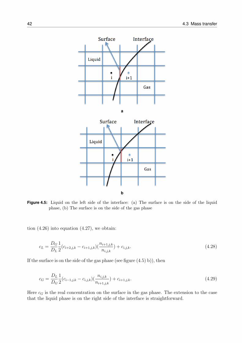
42 4.3 Mass transfer
a
b
Figure 4.5: Liquid on the left side of the interface: (a) The surface is on the side of the liquidphase, (b) The surface is on the side of the gas phase
tion (4.26) into equation (4.27), we obtain:
cL =DG
DL
1
2(ci+2,j,k − ci+1,j,k)(
ni+1,j,k
ni,j,k) + ci,j,k. (4.28)
If the surface is on the side of the gas phase (see figure (4.5) b)), then
cG =DL
DG
1
2(ci−1,j,k − ci,j,k)(
ni,j,kni+1,j,k
) + ci+1,j,k. (4.29)
Here cG is the real concentration on the surface in the gas phase. The extension to the casethat the liquid phase is on the right side of the interface is straightforward.
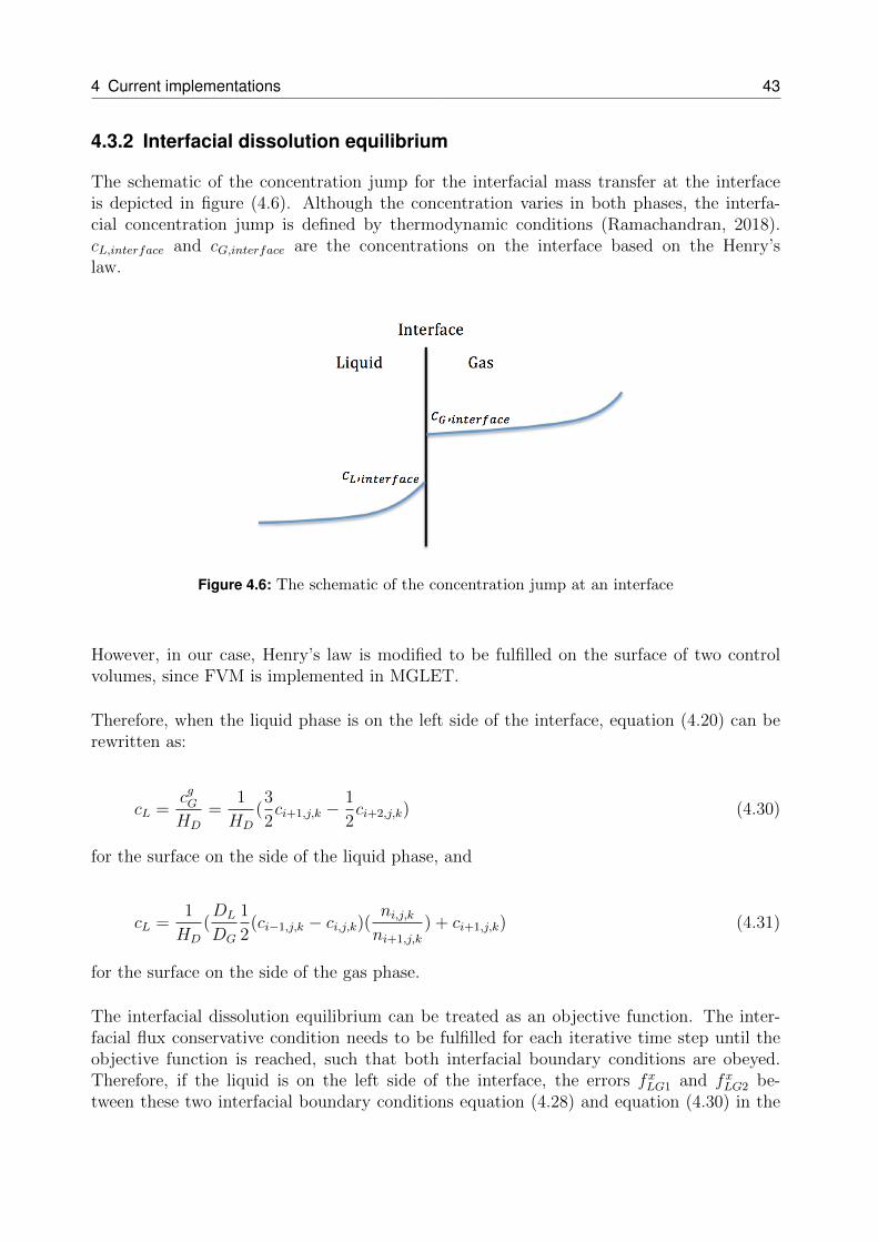
4 Current implementations 43
4.3.2 Interfacial dissolution equilibrium
The schematic of the concentration jump for the interfacial mass transfer at the interfaceis depicted in figure (4.6). Although the concentration varies in both phases, the interfa-cial concentration jump is defined by thermodynamic conditions (Ramachandran, 2018).cL,interface and cG,interface are the concentrations on the interface based on the Henry’slaw.
Figure 4.6: The schematic of the concentration jump at an interface
However, in our case, Henry’s law is modified to be fulfilled on the surface of two controlvolumes, since FVM is implemented in MGLET.
Therefore, when the liquid phase is on the left side of the interface, equation (4.20) can berewritten as:
cL =cgGHD
=1
HD
(3
2ci+1,j,k −
1
2ci+2,j,k) (4.30)
for the surface on the side of the liquid phase, and
cL =1
HD
(DL
DG
1
2(ci−1,j,k − ci,j,k)(
ni,j,kni+1,j,k
) + ci+1,j,k) (4.31)
for the surface on the side of the gas phase.
The interfacial dissolution equilibrium can be treated as an objective function. The inter-facial flux conservative condition needs to be fulfilled for each iterative time step until theobjective function is reached, such that both interfacial boundary conditions are obeyed.Therefore, if the liquid is on the left side of the interface, the errors fxLG1 and fxLG2 be-tween these two interfacial boundary conditions equation (4.28) and equation (4.30) in the
44 4.4 Time integration
x-direction can be obtained:
fxLG1 =1
HD
(3
2ci+1,j,k −
1
2ci+2,j,k)−
DG
DL
1
2(ci+2,j,k − ci+1,j,k)(
ni+1,j,k
ni,j,k)− ci,j,k (4.32)
and
fxLG2 =1
HD
(DL
DG
1
2(ci,j,k − ci−1,j,k)(
ni,j,kni+1,j,k
)− ci+1,j,k) + (3
2ci,j,k −
1
2ci−1,j,k) (4.33)
for the surface in the liquid phase and gas phase, respectively. For other locations and di-rections of the interface, the condition can be written accordingly.
Thus, the extended mass transfer equations (4.24) and (4.25) can be re-written as:
∂c
∂t+ u ·∇c = ∇ · (D∇c) + αfLG, (4.34)
where α is a coefficient that is set sufficiently high close to the interface and zero in the restof the computational domain. Since the two interfacial boundary conditions are combined,in this case, we only need to apply the combined boundary condition once on either side ofthe interface.
A validation of this method will be given in section (5.4).
4.4 Time integration
A third order RK method is applied to the Navier-Stokes equations, level set advection andthe transient mass transfer equation, while a second order RK method is applied to thereinitialization steps and the contact angle model. Because of these explicit algorithms, thetime step size ∆t must fulfill the Counrant-Friedrich-Lewy (CFL) conditions and also therestrictions due to gravity, viscous terms, surface tension, and diffusivity to stabilize thenumerical simulations.
The convective time step is defined as
∆tconv =h
|u|. (4.35)
The diffusive time step is defined as
∆tdiff =ρh2
4µ. (4.36)
4 Current implementations 45
The capillary time step is defined as (Brackbill et al., 1992)
∆tcap =
√(ρ1 + ρ2)h3
4πσ. (4.37)
The gravity time step is defined as
∆tgra =
√h
g. (4.38)
The mass diffusivity time step is defined as
∆tdiffm =h2
4D. (4.39)
When selecting a time step size, a regulation is given as
∆t ≤ min(∆tconv,∆tdiff ,∆tcap,∆tgra,∆tdiffm). (4.40)
The main steps of the algorithm are as follows:
1. Initialize all the parameters (density ρ, viscosity µ, surface tension σ, diffusivity D,concentration c, level set function ϕ, velocity field u and some coefficients) in eachphase.
2. Construct the distance function φ from the level set function ϕ near the interface usingFMM.
3. Calculate new density field ρ, viscosity field µ and concentration field c from the levelset function ϕ, and curvature from the distance function φ.
4. Advance the flow variables, like velocity, pressure p and level set function, in time forone Runge-Kutta sub-step.
5. Compute the concentration iteratively, until the tolerance error is larger than the nu-merical one at the interface.
6. Repeat steps from 2 to 5 for each Runge-Kutta sub-step to obtain the new values forvelocities, pressure, level set and concentration.
7. Reinitialize the level set ϕ iterativly with pseudo time step size ∆τ and artificial dif-fusion number ε, which is similar to the concentration field in step 3, to maintainconservation.

46 4.4 Time integration
5 Validation
Four test cases will be introduced in this chapter: in the first test case, a static pressuredrop is used to test the accuracy of the surface tension force. These results are comparedto previous studies to validate the current code. In the second test case, the capillary waveamplitude is discussed. The results of this test case can be used to predict capillary waves onan interface between two immiscible fluids with a density ratio of 1 and 1000. These resultsare also compared to previous studies to show the accuracy of the current implementation.The above two test cases are applied in Andre (2012) to validate the implementation of theCLS method. In the third test case, the case of a two-dimensional droplet on a wall withoutgravity is presented. The purpose of this test case is to show the improvements in the accu-racy of the new contact line treatment for the CLS method. Finally, the result of the masstransfer with negligible external resistance is presented to validate the mass transfer modelbased on the CLS method (see section (4.3)).
5.1 Static drop
A method similar to the SSF model is used to model the surface tension force. In order tocheck the accuracy of this method, a static drop is simulated to investigate the strength ofthe parasitic currents. In numerical simulations, parasitic currents and pressure fluctuationstend to occur due to the inaccuracies in the curvature calculation.
The drop at diameter Dd = 0.4 is placed in the center of a unit domain. The velocityfield is defined as zero in the whole domain. The analytical solution is zero and a pressuredifference of ∆p = 5 across the interface for the velocity field and pressure field, respec-tively. The Laplace number is used to characterize the static drop problem and definedas:
La =σρ2Dd
µ22
. (5.1)
The surface tension coefficient is defined as a constant σ = 1, the viscosity for both fluids isset to µ = 0.1, and the value of the capillary time step size of 1
2∆tcap (see section (4.4)) is used.
The density ratio and viscosity ratio are both set to unity. The dimensionless capillary num-ber is defined with the maximum magnitude of the velocity:
Ca =|Umax|µ2
σ, (5.2)
47
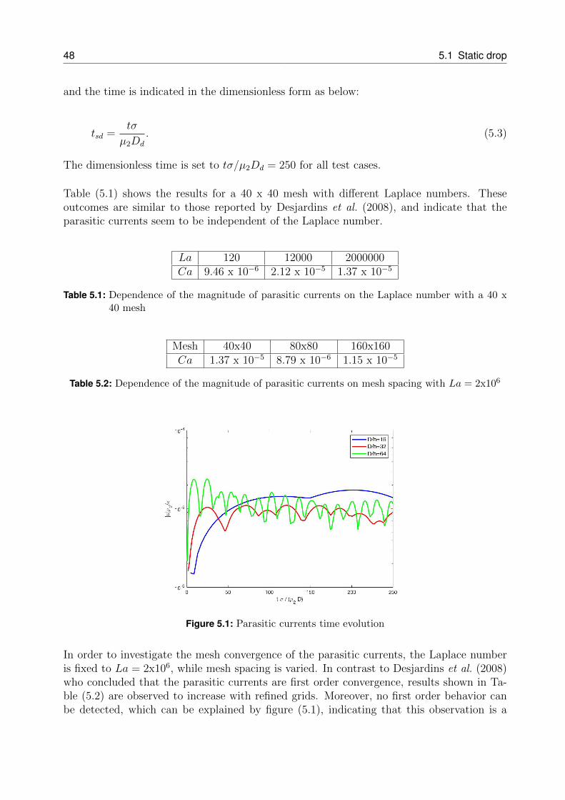
48 5.1 Static drop
and the time is indicated in the dimensionless form as below:
tsd =tσ
µ2Dd
. (5.3)
The dimensionless time is set to tσ/µ2Dd = 250 for all test cases.
Table (5.1) shows the results for a 40 x 40 mesh with different Laplace numbers. Theseoutcomes are similar to those reported by Desjardins et al. (2008), and indicate that theparasitic currents seem to be independent of the Laplace number.
La 120 12000 2000000Ca 9.46 x 10⁻⁶ 2.12 x 10⁻⁵ 1.37 x 10⁻⁵
Table 5.1: Dependence of the magnitude of parasitic currents on the Laplace number with a 40 x40 mesh
Mesh 40x40 80x80 160x160Ca 1.37 x 10⁻⁵ 8.79 x 10⁻⁶ 1.15 x 10⁻⁵
Table 5.2: Dependence of the magnitude of parasitic currents on mesh spacing with La = 2x10⁶
Figure 5.1: Parasitic currents time evolution
In order to investigate the mesh convergence of the parasitic currents, the Laplace numberis fixed to La = 2x10⁶, while mesh spacing is varied. In contrast to Desjardins et al. (2008)who concluded that the parasitic currents are first order convergence, results shown in Ta-ble (5.2) are observed to increase with refined grids. Moreover, no first order behavior canbe detected, which can be explained by figure (5.1), indicating that this observation is a
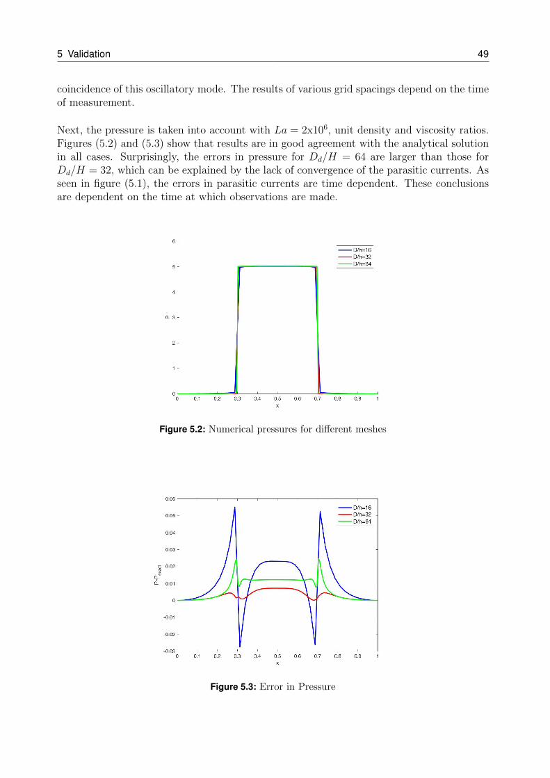
5 Validation 49
coincidence of this oscillatory mode. The results of various grid spacings depend on the timeof measurement.
Next, the pressure is taken into account with La = 2x10⁶, unit density and viscosity ratios.Figures (5.2) and (5.3) show that results are in good agreement with the analytical solutionin all cases. Surprisingly, the errors in pressure for Dd/H = 64 are larger than those forDd/H = 32, which can be explained by the lack of convergence of the parasitic currents. Asseen in figure (5.1), the errors in parasitic currents are time dependent. These conclusionsare dependent on the time at which observations are made.
Figure 5.2: Numerical pressures for different meshes
Figure 5.3: Error in Pressure
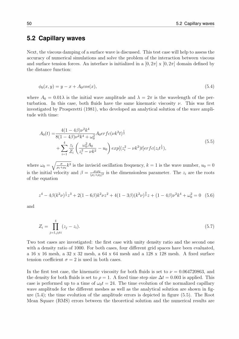
50 5.2 Capillary waves
5.2 Capillary waves
Next, the viscous damping of a surface wave is discussed. This test case will help to assess theaccuracy of numerical simulations and solve the problem of the interaction between viscousand surface tension forces. An interface is initialized in a [0, 2π] x [0, 2π] domain defined bythe distance function:
φ0(x, y) = y − x+ A0cos(x), (5.4)
where A0 = 0.01λ is the initial wave amplitude and λ = 2π is the wavelength of the per-turbation. In this case, both fluids have the same kinematic viscosity ν. This was firstinvestigated by Prosperetti (1981), who developed an analytical solution of the wave ampli-tude with time:
A0(t) =4(1− 4β)ν2k4
8(1− 4β)ν2k4 + ω20
A0erfc(νk2t)
12
+4∑i=1
ziZi
(ω20A0
z2i − νk2− u0
)exp[(z2i − νk2)t]erfc(zit
12 ),
(5.5)
where ω0 =√
σρ1+ρ2
k3 is the inviscid oscillation frequency, k = 1 is the wave number, u0 = 0
is the initial velocity and β = ρ1ρ2(ρ1+ρ2)2
is the dimensionless parameter. The zi are the rootsof the equation
z4 − 4β(k2ν)12 z3 + 2(1− 6β)k2νz2 + 4(1− 3β)(k2ν)
32 z + (1− 4β)ν2k4 + ω2
0 = 0 (5.6)
and
Zi =4∏
j=1,j 6=i
(zj − zi). (5.7)
Two test cases are investigated: the first case with unity density ratio and the second onewith a density ratio of 1000. For both cases, four different grid spaces have been evaluated,a 16 x 16 mesh, a 32 x 32 mesh, a 64 x 64 mesh and a 128 x 128 mesh. A fixed surfacetension coefficient σ = 2 is used in both cases.
In the first test case, the kinematic viscosity for both fluids is set to ν = 0.064720863, andthe density for both fluids is set to ρ = 1. A fixed time step size ∆t = 0.003 is applied. Thiscase is performed up to a time of ω0t = 24. The time evolution of the normalized capillarywave amplitude for the different meshes as well as the analytical solution are shown in fig-ure (5.4); the time evolution of the amplitude errors is depicted in figure (5.5). The RootMean Square (RMS) errors between the theoretical solution and the numerical results are
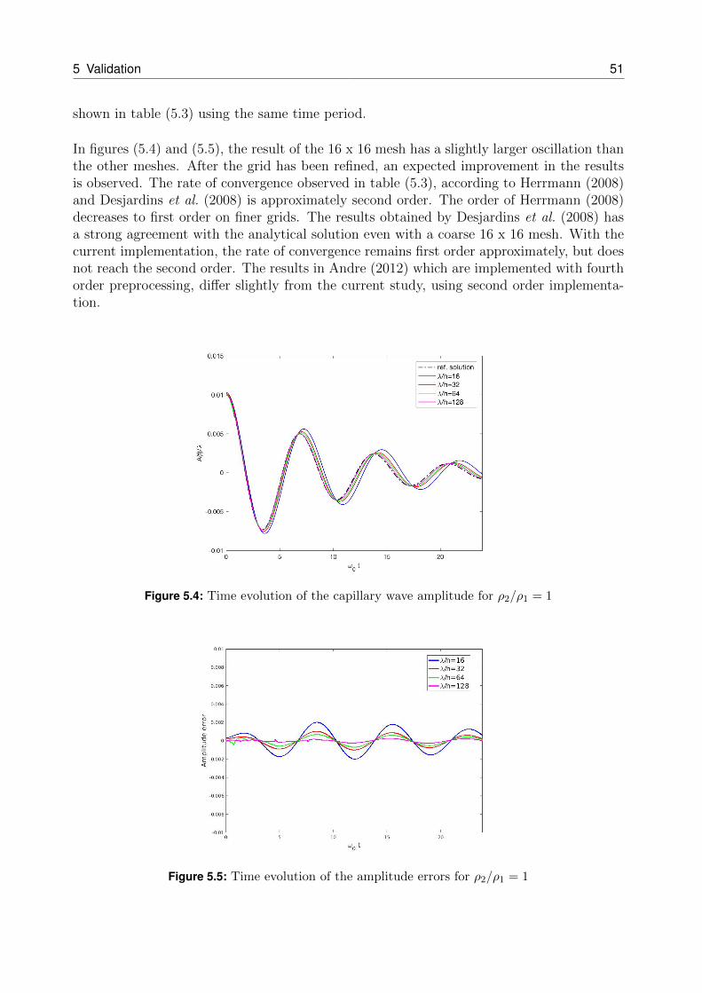
5 Validation 51
shown in table (5.3) using the same time period.
In figures (5.4) and (5.5), the result of the 16 x 16 mesh has a slightly larger oscillation thanthe other meshes. After the grid has been refined, an expected improvement in the resultsis observed. The rate of convergence observed in table (5.3), according to Herrmann (2008)and Desjardins et al. (2008) is approximately second order. The order of Herrmann (2008)decreases to first order on finer grids. The results obtained by Desjardins et al. (2008) hasa strong agreement with the analytical solution even with a coarse 16 x 16 mesh. With thecurrent implementation, the rate of convergence remains first order approximately, but doesnot reach the second order. The results in Andre (2012) which are implemented with fourthorder preprocessing, differ slightly from the current study, using second order implementa-tion.
Figure 5.4: Time evolution of the capillary wave amplitude for ρ2/ρ1 = 1
Figure 5.5: Time evolution of the amplitude errors for ρ2/ρ1 = 1
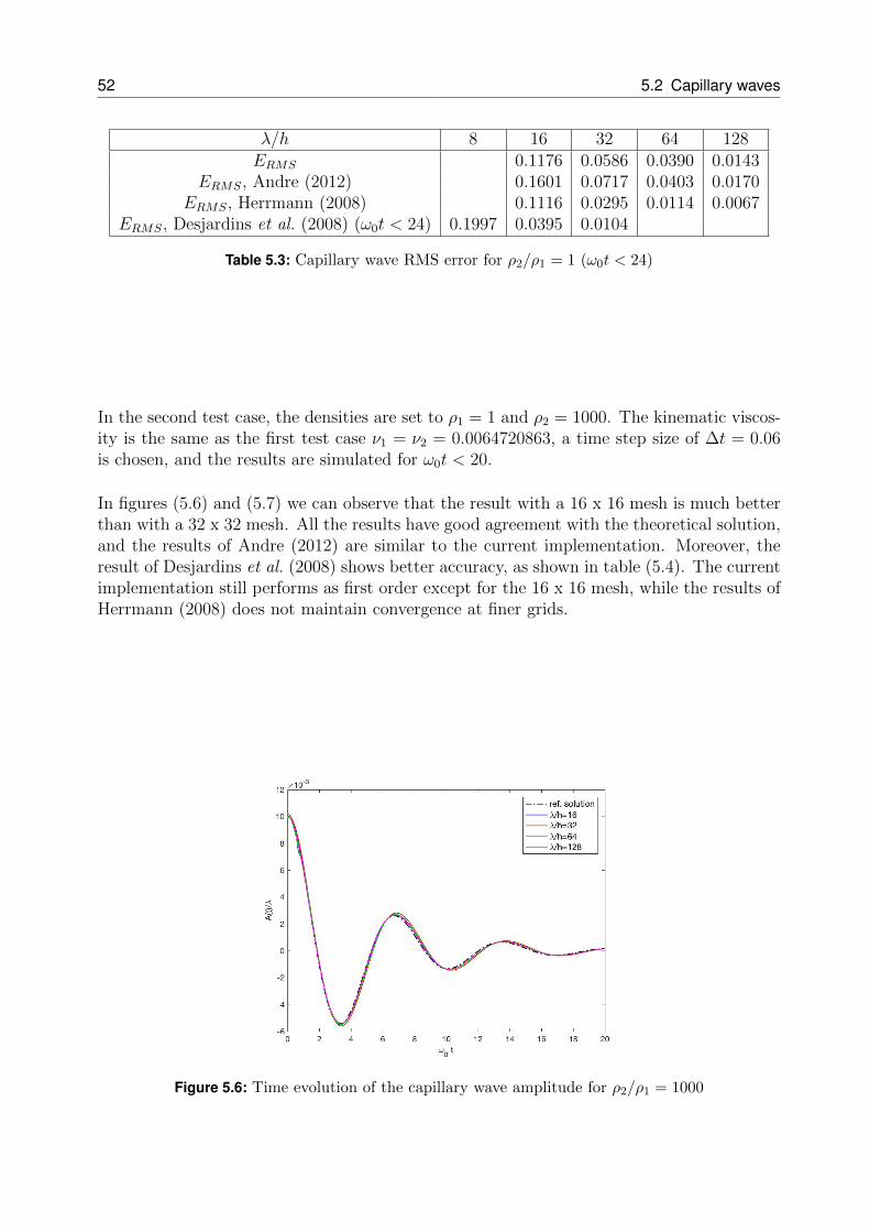
52 5.2 Capillary waves
λ/h 8 16 32 64 128ERMS 0.1176 0.0586 0.0390 0.0143
ERMS, Andre (2012) 0.1601 0.0717 0.0403 0.0170ERMS, Herrmann (2008) 0.1116 0.0295 0.0114 0.0067
ERMS, Desjardins et al. (2008) (ω0t < 24) 0.1997 0.0395 0.0104
Table 5.3: Capillary wave RMS error for ρ2/ρ1 = 1 (ω0t < 24)
In the second test case, the densities are set to ρ1 = 1 and ρ2 = 1000. The kinematic viscos-ity is the same as the first test case ν1 = ν2 = 0.0064720863, a time step size of ∆t = 0.06is chosen, and the results are simulated for ω0t < 20.
In figures (5.6) and (5.7) we can observe that the result with a 16 x 16 mesh is much betterthan with a 32 x 32 mesh. All the results have good agreement with the theoretical solution,and the results of Andre (2012) are similar to the current implementation. Moreover, theresult of Desjardins et al. (2008) shows better accuracy, as shown in table (5.4). The currentimplementation still performs as first order except for the 16 x 16 mesh, while the results ofHerrmann (2008) does not maintain convergence at finer grids.
Figure 5.6: Time evolution of the capillary wave amplitude for ρ2/ρ1 = 1000
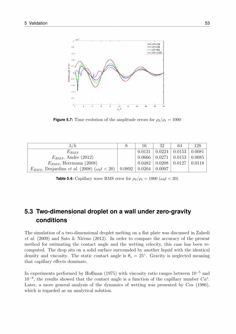
5 Validation 53
Figure 5.7: Time evolution of the amplitude errors for ρ2/ρ1 = 1000
λ/h 8 16 32 64 128ERMS 0.0131 0.0224 0.0153 0.0081
ERMS, Andre (2012) 0.0666 0.0271 0.0153 0.0085ERMS, Herrmann (2008) 0.0482 0.0208 0.0127 0.0118
ERMS, Desjardins et al. (2008) (ω0t < 20) 0.0892 0.0204 0.0097
Table 5.4: Capillary wave RMS error for ρ2/ρ1 = 1000 (ω0t < 20)
5.3 Two-dimensional droplet on a wall under zero-gravityconditions
The simulation of a two-dimensional droplet melting on a flat plate was discussed in Zahediet al. (2009) and Sato & Niceno (2012). In order to compare the accuracy of the presentmethod for estimating the contact angle and the wetting velocity, this case has been re-computed. The drop sits on a solid surface surrounded by another liquid with the identicaldensity and viscosity. The static contact angle is θs = 25. Gravity is neglected meaningthat capillary effects dominate.
In experiments performed by Hoffman (1975) with viscosity ratio ranges between 10−5 and10−8, the results showed that the contact angle is a function of the capillary number Ca∗.Later, a more general analysis of the dynamics of wetting was presented by Cox (1986),which is regarded as an analytical solution.
54 5.3 Two-dimensional droplet on a wall under zero-gravity conditions
5.3.1 Cox’ theory
For a given system of two immiscible fluids with viscosity ratio λ, Cox’s theory assumesthat
g(θD, λ)− g(θs, λ) = Ca∗ln(δ−1c ), (5.8)
where θD is the macroscopic dynamic contact angle, δc is a constant term, θs is the staticangle and the function g(θ, λ) is defined as
g(θD, λ) =
∫ θ
0
dθ
f(θ, λ), (5.9)
where
f(θ, λ) =2 sin θ(λ2(θ2 − sin2 θ) + 2λ(θπ − θ) + sin2 θ) + (π − θ)2 − sin2 θ
λ(θ2 − sin2 θ)((π − θ) + sin θ cos θ) + ((π − θ)2 − sin2 θ)(θ − sin θ cos θ). (5.10)
Therefore, Cox’s theory is used to predict the macroscopic dynamic contact angle for twoimmiscible fluids. When the system reaches the steady state, the contact line speed Ca∗ iszero. Thus, the macroscopic dynamic contact angle θD becomes the static contact angle θsas expected.
Results from Hoffman’s profile for all values of the dynamic contact angle (except those veryclose to 180) have good agreement with the formula obtained from Tornberg & Engquist(2000). Zahedi et al. (2009) confirmed that a value of δ ≈ 10−4 minimizes the relativedifference between the contact-line speeds Ca∗ obtained from Hoffman’s experiments usingsilicone fluid with λ = 0 and θs = 0 and those obtained from Cox’s theory. In the followingpart, δ = 10−4 will be applied.
5.3.2 Results
The interface of the droplet is initialized in a [−2, 2] x [0, 2] domain. The location of thedroplet is around x = 0 with radius Lx/r = 8. At initial time, the contact angle betweenthe drop and the solid wall is applied with 156. The Reynolds number and the Capillarynumber are defined as
Re =ρul
µ= 1, (5.11)
where l is the diameter of the droplet. And the dimensionless contact-line speed is expressed
5 Validation 55
as:
Ca∗ =2√
2µu
3σ= 1. (5.12)
A time step size is according to the capillary limitation (see section (4.4)). If the staticcontact angle is θs = 25 at the wall, we obtain
tan(90 − θs) = tan65 = |nynx|, (5.13)
since the vector is normalized, thus
n2y + n2
x = 1. (5.14)
Therefore, the boundary condition for the normal vector field discussed in section (4.1) isset as:
nwall = (nx, ny) = (−sign(x)0.4226,−0.9063). (5.15)
The Neumann boundary conditions are implemented for the other boundaries.
The dynamic contact angle is calculated between the tangential line from the inflexion pointand the wall as shown in figure (5.8). The inflexion point is a point on a continuously differ-entiable curve at which the curve changes from concave to convex, or vice versa. Thus, theinflexion point can be obtained by calculating the local minimum or maximum tangent. Thewetting speed is measured by the position of the intersection point on the wall at differenttime steps.
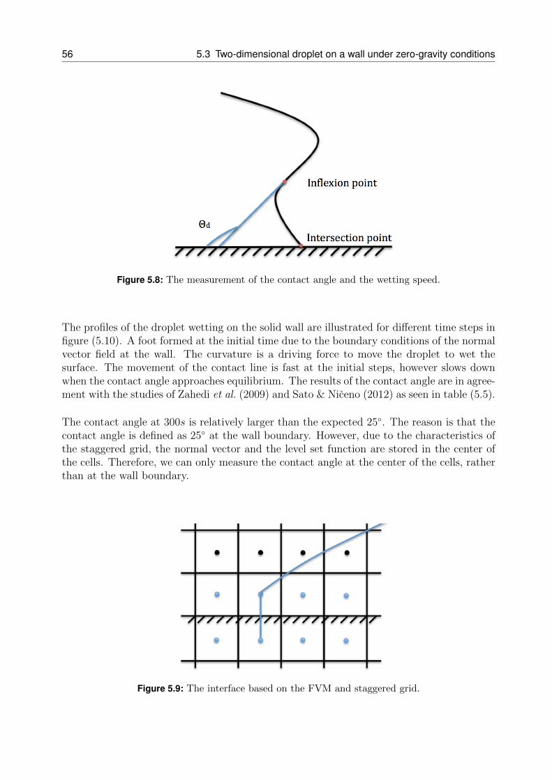
56 5.3 Two-dimensional droplet on a wall under zero-gravity conditions
Figure 5.8: The measurement of the contact angle and the wetting speed.
The profiles of the droplet wetting on the solid wall are illustrated for different time steps infigure (5.10). A foot formed at the initial time due to the boundary conditions of the normalvector field at the wall. The curvature is a driving force to move the droplet to wet thesurface. The movement of the contact line is fast at the initial steps, however slows downwhen the contact angle approaches equilibrium. The results of the contact angle are in agree-ment with the studies of Zahedi et al. (2009) and Sato & Niceno (2012) as seen in table (5.5).
The contact angle at 300s is relatively larger than the expected 25. The reason is that thecontact angle is defined as 25 at the wall boundary. However, due to the characteristics ofthe staggered grid, the normal vector and the level set function are stored in the center ofthe cells. Therefore, we can only measure the contact angle at the center of the cells, ratherthan at the wall boundary.
Figure 5.9: The interface based on the FVM and staggered grid.
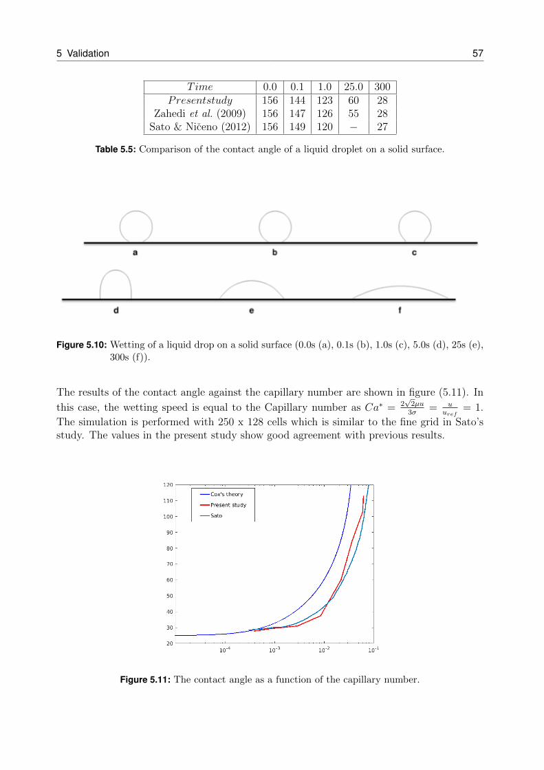
5 Validation 57
Time 0.0 0.1 1.0 25.0 300Presentstudy 156 144 123 60 28
Zahedi et al. (2009) 156 147 126 55 28Sato & Niceno (2012) 156 149 120 − 27
Table 5.5: Comparison of the contact angle of a liquid droplet on a solid surface.
Figure 5.10: Wetting of a liquid drop on a solid surface (0.0s (a), 0.1s (b), 1.0s (c), 5.0s (d), 25s (e),300s (f)).
The results of the contact angle against the capillary number are shown in figure (5.11). In
this case, the wetting speed is equal to the Capillary number as Ca∗ = 2√2µu3σ
= uuref
= 1.
The simulation is performed with 250 x 128 cells which is similar to the fine grid in Sato’sstudy. The values in the present study show good agreement with previous results.
Figure 5.11: The contact angle as a function of the capillary number.
58 5.4 Mass transfer of a two-dimensional droplet with negligible external resistance
5.4 Mass transfer of a two-dimensional droplet with negligibleexternal resistance
A test case is calculated to validate the mass transfer model implemented in MGLET. A dropis located in the center of a unit domain with slip boundary conditions. The velocity field isset to zero in the whole domain. For a stagnant spherical drop with negligible external masstransfer resistance, the analytical Sherwood number can be derived by Newman’s equation(Newman, 1931):
Shod =2π2
3
∞∑n=1
exp(−n2π2τp)/∞∑n=1
1
n2exp(−n2π2τp), (5.16)
where τp = Dtr2
is the dimensionless time step. Therefore, the steady asymptotic valueis:
(Shod)τp→∞ =2π2
3= 6.58. (5.17)
The mass transfer coefficient to a single drop dominated by internal resistance can be eval-uated by equation (2.23). In the two-dimensional case, V/S = r/2. The correspondingSherwood number is
Shod = kod2r
D. (5.18)
Both phases have the same density, kinematic viscosity and mass diffusivity. Additional, thedistribution coefficientHD is set to 1. The concentration field is initialized as:
c1 = 1 at t=0 (continuous phase) (5.19a)
c2 = 0 at t=0 (drop phase). (5.19b)
Figure (5.12) shows the results of three different grid spacings and the analytical solution.As the grid is refined, the predicted Sherwood number converges close to the analyticalsolution. The relatively error of the grid with 400 x 400 nodes is 5%. This grid spacing isqualitatively sufficient for spatial computational accuracy and applied in the following (seeChapter 7).
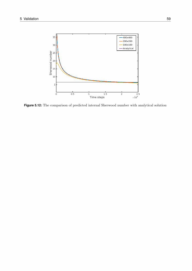
5 Validation 59
Figure 5.12: The comparison of predicted internal Sherwood number with analytical solution

60 5.4 Mass transfer of a two-dimensional droplet with negligible external resistance
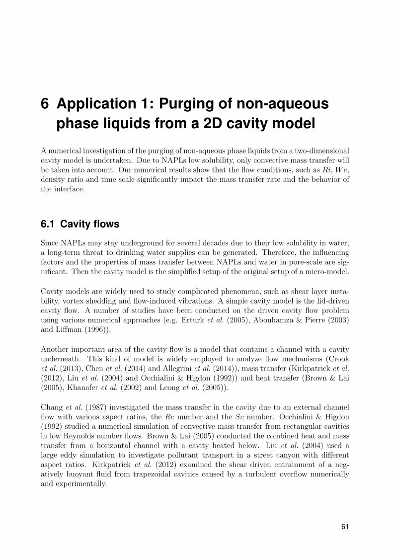
6 Application 1: Purging of non-aqueousphase liquids from a 2D cavity model
A numerical investigation of the purging of non-aqueous phase liquids from a two-dimensionalcavity model is undertaken. Due to NAPLs low solubility, only convective mass transfer willbe taken into account. Our numerical results show that the flow conditions, such as Ri, We,density ratio and time scale significantly impact the mass transfer rate and the behavior ofthe interface.
6.1 Cavity flows
Since NAPLs may stay underground for several decades due to their low solubility in water,a long-term threat to drinking water supplies can be generated. Therefore, the influencingfactors and the properties of mass transfer between NAPLs and water in pore-scale are sig-nificant. Then the cavity model is the simplified setup of the original setup of a micro-model.
Cavity models are widely used to study complicated phenomena, such as shear layer insta-bility, vortex shedding and flow-induced vibrations. A simple cavity model is the lid-drivencavity flow. A number of studies have been conducted on the driven cavity flow problemusing various numerical approaches (e.g. Erturk et al. (2005), Abouhamza & Pierre (2003)and Liffman (1996)).
Another important area of the cavity flow is a model that contains a channel with a cavityunderneath. This kind of model is widely employed to analyze flow mechanisms (Crooket al. (2013), Chen et al. (2014) and Allegrini et al. (2014)), mass transfer (Kirkpatrick et al.(2012), Liu et al. (2004) and Occhialini & Higdon (1992)) and heat transfer (Brown & Lai(2005), Khanafer et al. (2002) and Leong et al. (2005)).
Chang et al. (1987) investigated the mass transfer in the cavity due to an external channelflow with various aspect ratios, the Re number and the Sc number. Occhialini & Higdon(1992) studied a numerical simulation of convective mass transfer from rectangular cavitiesin low Reynolds number flows. Brown & Lai (2005) conducted the combined heat and masstransfer from a horizontal channel with a cavity heated below. Liu et al. (2004) used alarge eddy simulation to investigate pollutant transport in a street canyon with differentaspect ratios. Kirkpatrick et al. (2012) examined the shear driven entrainment of a neg-atively buoyant fluid from trapezoidal cavities caused by a turbulent overflow numericallyand experimentally.
61
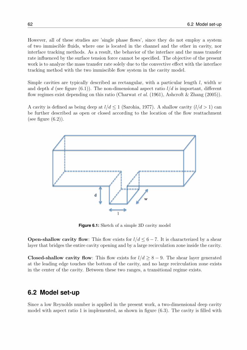
62 6.2 Model set-up
However, all of these studies are ’single phase flows’, since they do not employ a systemof two immiscible fluids, where one is located in the channel and the other in cavity, norinterface tracking methods. As a result, the behavior of the interface and the mass transferrate influenced by the surface tension force cannot be specified. The objective of the presentwork is to analyze the mass transfer rate solely due to the convective effect with the interfacetracking method with the two immiscible flow system in the cavity model.
Simple cavities are typically described as rectangular, with a particular length l, width wand depth d (see figure (6.1)). The non-dimensional aspect ratio l/d is important, differentflow regimes exist depending on this ratio (Charwat et al. (1961), Ashcroft & Zhang (2005)).
A cavity is defined as being deep at l/d ≤ 1 (Sarohia, 1977). A shallow cavity (l/d > 1) canbe further described as open or closed according to the location of the flow reattachment(see figure (6.2)).
Figure 6.1: Sketch of a simple 3D cavity model
Open-shallow cavity flow: This flow exists for l/d ≤ 6− 7. It is characterized by a shearlayer that bridges the entire cavity opening and by a large recirculation zone inside the cavity.
Closed-shallow cavity flow: This flow exists for l/d ≥ 8 − 9. The shear layer generatedat the leading edge touches the bottom of the cavity, and no large recirculation zone existsin the center of the cavity. Between these two ranges, a transitional regime exists.
6.2 Model set-up
Since a low Reynolds number is applied in the present work, a two-dimensional deep cavitymodel with aspect ratio 1 is implemented, as shown in figure (6.3). The cavity is filled with
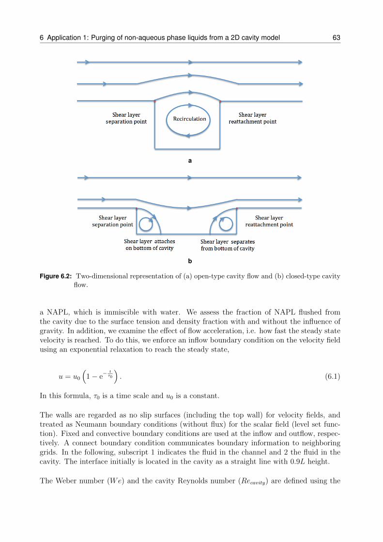
6 Application 1: Purging of non-aqueous phase liquids from a 2D cavity model 63
a
b
Figure 6.2: Two-dimensional representation of (a) open-type cavity flow and (b) closed-type cavityflow.
a NAPL, which is immiscible with water. We assess the fraction of NAPL flushed fromthe cavity due to the surface tension and density fraction with and without the influence ofgravity. In addition, we examine the effect of flow acceleration, i.e. how fast the steady statevelocity is reached. To do this, we enforce an inflow boundary condition on the velocity fieldusing an exponential relaxation to reach the steady state,
u = u0
(1− e
− tτ0
). (6.1)
In this formula, τ0 is a time scale and u0 is a constant.
The walls are regarded as no slip surfaces (including the top wall) for velocity fields, andtreated as Neumann boundary conditions (without flux) for the scalar field (level set func-tion). Fixed and convective boundary conditions are used at the inflow and outflow, respec-tively. A connect boundary condition communicates boundary information to neighboringgrids. In the following, subscript 1 indicates the fluid in the channel and 2 the fluid in thecavity. The interface initially is located in the cavity as a straight line with 0.9L height.
The Weber number (We) and the cavity Reynolds number (Recavity) are defined using the
64 6.3 Two-dimensional and three dimensional model
properties of the fluid in the cavity,
We =ρ2u
20L
σ(6.2)
and
Recavity =ρ2u0L
µ2
, (6.3)
where u0 is the inflow velocity coefficient and L is the depth of the cavity.
Figure 6.3: Sketch of flow in a channel with a bottom 2D cavity
6.3 Two-dimensional and three dimensionalmodel
The two-dimensional model is employed in this chapter. Since the deep cavity model is ap-plied (i.e., the streamline connects the entire cavity opening), three-dimensional model is notnecessarily needed to be conducted. However, in order to investigate if there are several ad-ditional effects will happen in the three-dimensional model, rather than the two-dimensionalmodel, results of the two-dimensional and three-dimensional models are compared in thissection. The configuration of the three-dimensional model is shown in figure (6.4). Themodel extends three times in the spanwise direction for the channel part, and the cavity islocated in the center of the bottom surface of the channel.
The comparison is shown in figure (6.5). The mass left in the cavity is normalized by the massat the original state. In the beginning phase, the results of the two-dimensional and three-dimensional models are nearly the same. After approximately one second, the differencebetween the two cases becomes visually. Then after reaching the steady state, the resultsconverge to 0.89 and 0.92 for two-dimensional and three-dimensional cases, respectively (i.e.the mass left in the three-dimensional case is more than that in the two-dimensional case).
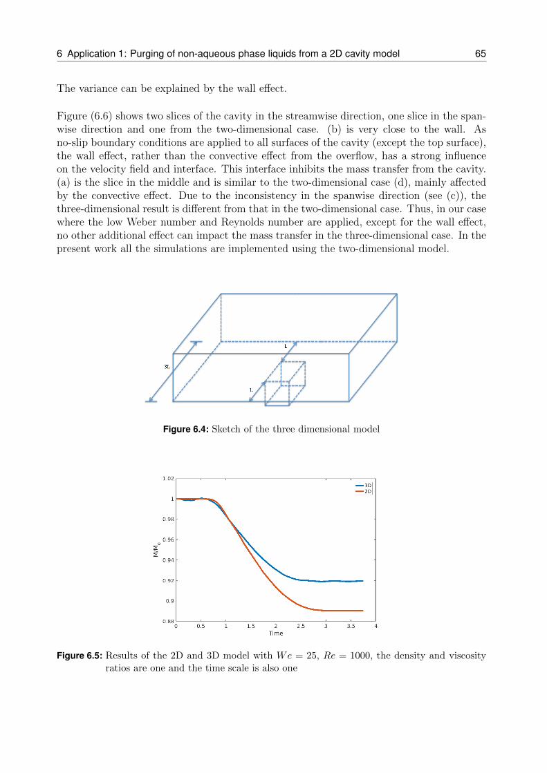
6 Application 1: Purging of non-aqueous phase liquids from a 2D cavity model 65
The variance can be explained by the wall effect.
Figure (6.6) shows two slices of the cavity in the streamwise direction, one slice in the span-wise direction and one from the two-dimensional case. (b) is very close to the wall. Asno-slip boundary conditions are applied to all surfaces of the cavity (except the top surface),the wall effect, rather than the convective effect from the overflow, has a strong influenceon the velocity field and interface. This interface inhibits the mass transfer from the cavity.(a) is the slice in the middle and is similar to the two-dimensional case (d), mainly affectedby the convective effect. Due to the inconsistency in the spanwise direction (see (c)), thethree-dimensional result is different from that in the two-dimensional case. Thus, in our casewhere the low Weber number and Reynolds number are applied, except for the wall effect,no other additional effect can impact the mass transfer in the three-dimensional case. In thepresent work all the simulations are implemented using the two-dimensional model.
Figure 6.4: Sketch of the three dimensional model
Figure 6.5: Results of the 2D and 3D model with We = 25, Re = 1000, the density and viscosityratios are one and the time scale is also one
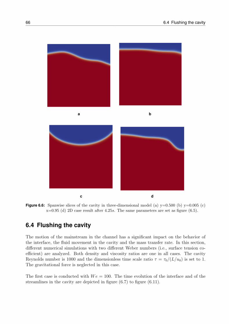
66 6.4 Flushing the cavity
a b
c d
Figure 6.6: Spanwise slices of the cavity in three-dimensional model (a) y=0.500 (b) y=0.005 (c)x=0.95 (d) 2D case result after 4.25s. The same parameters are set as figure (6.5).
6.4 Flushing the cavity
The motion of the mainstream in the channel has a significant impact on the behavior ofthe interface, the fluid movement in the cavity and the mass transfer rate. In this section,different numerical simulations with two different Weber numbers (i.e., surface tension co-efficient) are analyzed. Both density and viscosity ratios are one in all cases. The cavityReynolds number is 1000 and the dimensionless time scale ratio τ = τ0/(L/u0) is set to 1.The gravitational force is neglected in this case.
The first case is conducted with We = 100. The time evolution of the interface and of thestreamlines in the cavity are depicted in figure (6.7) to figure (6.11).
6 Application 1: Purging of non-aqueous phase liquids from a 2D cavity model 67
Figure (6.7) shows the interface and streamlines at t = 0.4s after flow initiation. At thistime, no NAPL has been pushed out of the cavity by the overflow, while at the leadingcorner of the cavity the interface has been pushed down slightly. Additionally, two smallvortices are generated near the leading and trailing corners.
In Figure (6.8), mass being pushed out of the cavity at the trailing corner. The vortex closeto the leading edge grows, while the one near the trailing edge disappears. Several stream-lines from the mainstream can be observed entering and traversing the cavity, then exitingat the trailing corner.
Figure (6.9) indicates that the vortex close to the leading corner of the cavity becomesconsiderably large, while the process of mass transfer continues. The crest observed in theinterface contour is now being rolled up by the vortex. The exiting part of the mass in thechannel impacts the distribution of the streamlines.
The results at t = 4s after initiation are represented in figure (6.10). The splash of theNAPL has now completely exited the cavity and is being convected to the boundary by theoverflow. The vortex, initially located at the leading corner, has moved across the cavity andis nearly touching the trailing wall. At the same time, the vortex has become considerablylarge and almost fills the cavity. Furthermore, it starts to separate into two parts. Contraryto results in figure (6.9), no streamlines enter and traverse the cavity, since the mass transferprocess is complete.
Two steady state vortices are shown in figure (6.11). The streamlines indicate that onevortex center is located near the trailing wall with a clockwise rotation, while a counter-clockwise-rotating vortex has formed in the lower part of the cavity near the leading corner.At this time all mass in the channel has been transported outside the domain. The interface,initially defined as a horizontal line between the overflow and the NAPL, has now changedinto an inclined line in the cavity once steady state is reached, due to the high Weber num-ber. The interface is located between these two vortices.
While the short initiation is uneventful, mass transfer starts and completes relatively quickly.The flow acceleration is inviscid in the initiation phase. This is the phase in which mass ispushed out of the cavity. In this phase, mass transfer mainly depends on the potential flow,rather than the complicated flow mechanisms in the following transient phase. Afterwards,the interface tends to reach the minimum energy state under the effect of the surface ten-sion force. Finally, after reaching steady state, the interface becomes an inclined line in thecavity. The location of the interface is between the two vortices in the cavity. Moreover, theinterface is parallel to the streamlines, rather than cross the streamlines which drives themovement of the interface before the steady state.
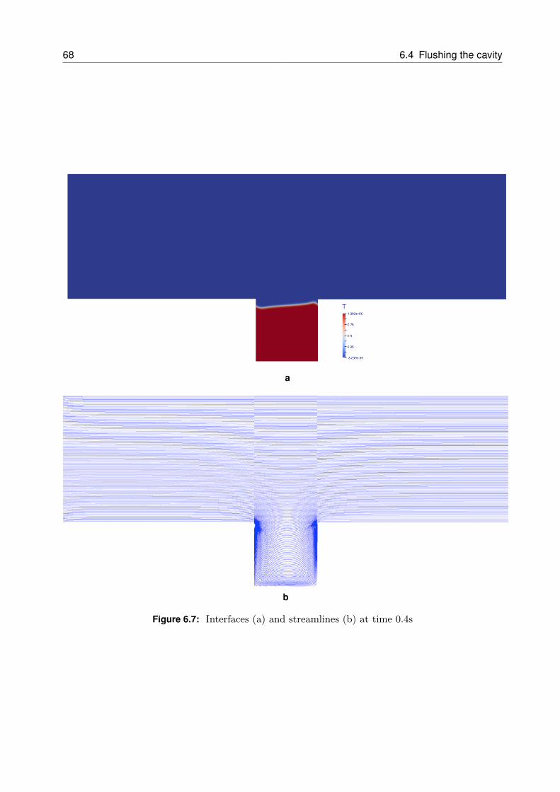
68 6.4 Flushing the cavity
a
b
Figure 6.7: Interfaces (a) and streamlines (b) at time 0.4s
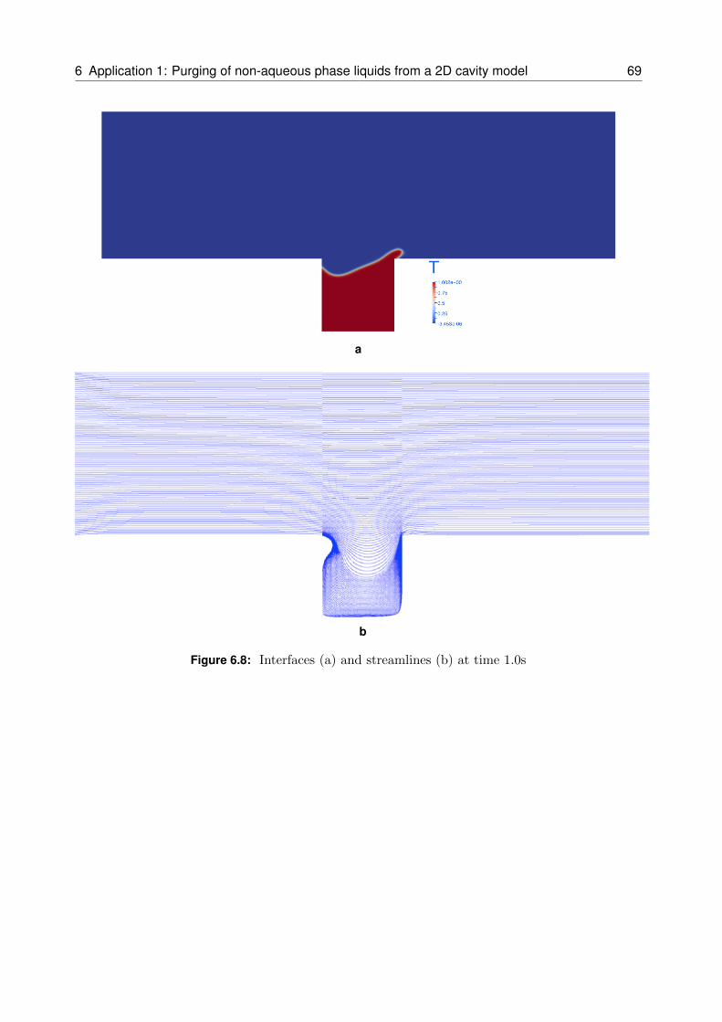
6 Application 1: Purging of non-aqueous phase liquids from a 2D cavity model 69
a
b
Figure 6.8: Interfaces (a) and streamlines (b) at time 1.0s
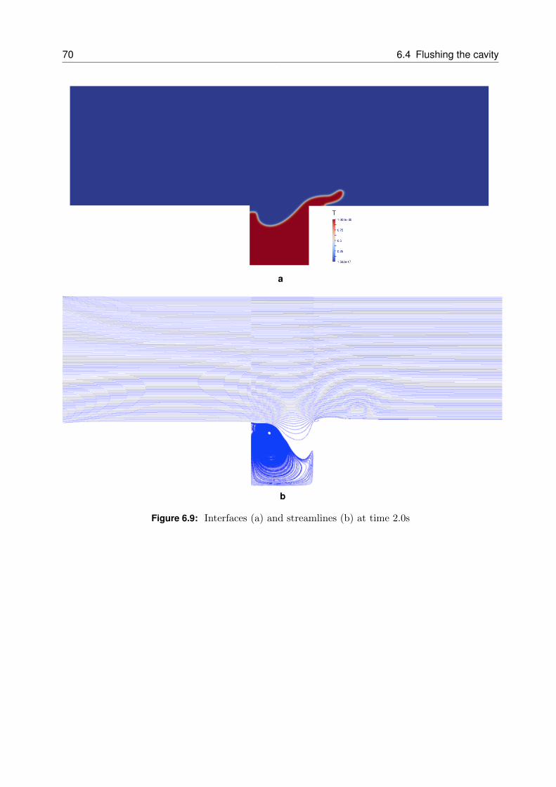
70 6.4 Flushing the cavity
a
b
Figure 6.9: Interfaces (a) and streamlines (b) at time 2.0s
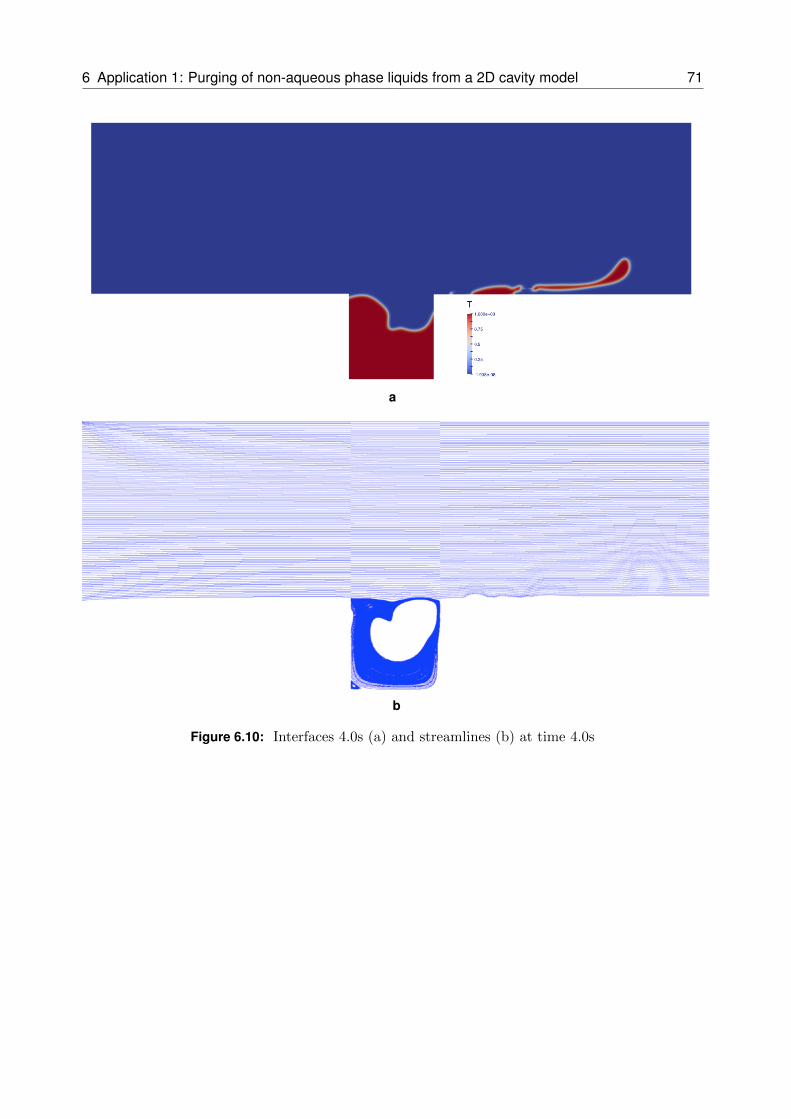
6 Application 1: Purging of non-aqueous phase liquids from a 2D cavity model 71
a
b
Figure 6.10: Interfaces 4.0s (a) and streamlines (b) at time 4.0s
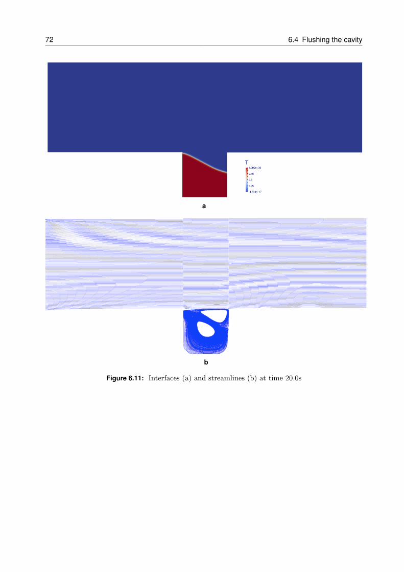
72 6.4 Flushing the cavity
a
b
Figure 6.11: Interfaces (a) and streamlines (b) at time 20.0s
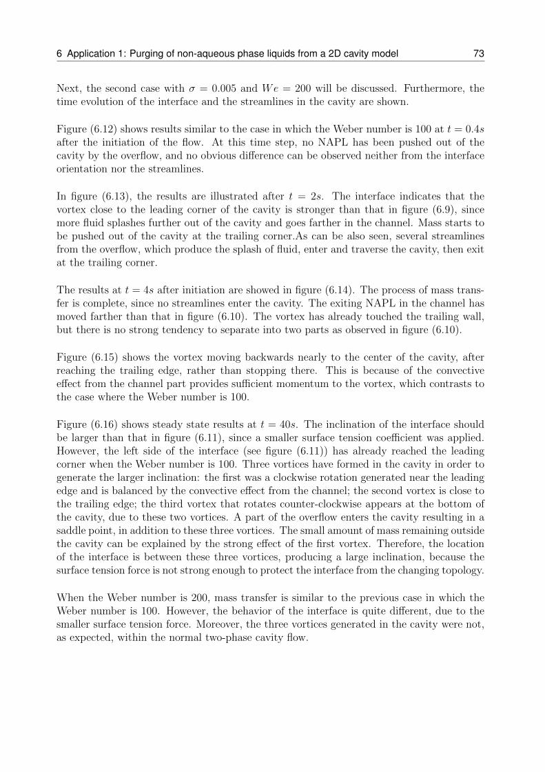
6 Application 1: Purging of non-aqueous phase liquids from a 2D cavity model 73
Next, the second case with σ = 0.005 and We = 200 will be discussed. Furthermore, thetime evolution of the interface and the streamlines in the cavity are shown.
Figure (6.12) shows results similar to the case in which the Weber number is 100 at t = 0.4safter the initiation of the flow. At this time step, no NAPL has been pushed out of thecavity by the overflow, and no obvious difference can be observed neither from the interfaceorientation nor the streamlines.
In figure (6.13), the results are illustrated after t = 2s. The interface indicates that thevortex close to the leading corner of the cavity is stronger than that in figure (6.9), sincemore fluid splashes further out of the cavity and goes farther in the channel. Mass starts tobe pushed out of the cavity at the trailing corner.As can be also seen, several streamlinesfrom the overflow, which produce the splash of fluid, enter and traverse the cavity, then exitat the trailing corner.
The results at t = 4s after initiation are showed in figure (6.14). The process of mass trans-fer is complete, since no streamlines enter the cavity. The exiting NAPL in the channel hasmoved farther than that in figure (6.10). The vortex has already touched the trailing wall,but there is no strong tendency to separate into two parts as observed in figure (6.10).
Figure (6.15) shows the vortex moving backwards nearly to the center of the cavity, afterreaching the trailing edge, rather than stopping there. This is because of the convectiveeffect from the channel part provides sufficient momentum to the vortex, which contrasts tothe case where the Weber number is 100.
Figure (6.16) shows steady state results at t = 40s. The inclination of the interface shouldbe larger than that in figure (6.11), since a smaller surface tension coefficient was applied.However, the left side of the interface (see figure (6.11)) has already reached the leadingcorner when the Weber number is 100. Three vortices have formed in the cavity in order togenerate the larger inclination: the first was a clockwise rotation generated near the leadingedge and is balanced by the convective effect from the channel; the second vortex is close tothe trailing edge; the third vortex that rotates counter-clockwise appears at the bottom ofthe cavity, due to these two vortices. A part of the overflow enters the cavity resulting in asaddle point, in addition to these three vortices. The small amount of mass remaining outsidethe cavity can be explained by the strong effect of the first vortex. Therefore, the locationof the interface is between these three vortices, producing a large inclination, because thesurface tension force is not strong enough to protect the interface from the changing topology.
When the Weber number is 200, mass transfer is similar to the previous case in which theWeber number is 100. However, the behavior of the interface is quite different, due to thesmaller surface tension force. Moreover, the three vortices generated in the cavity were not,as expected, within the normal two-phase cavity flow.
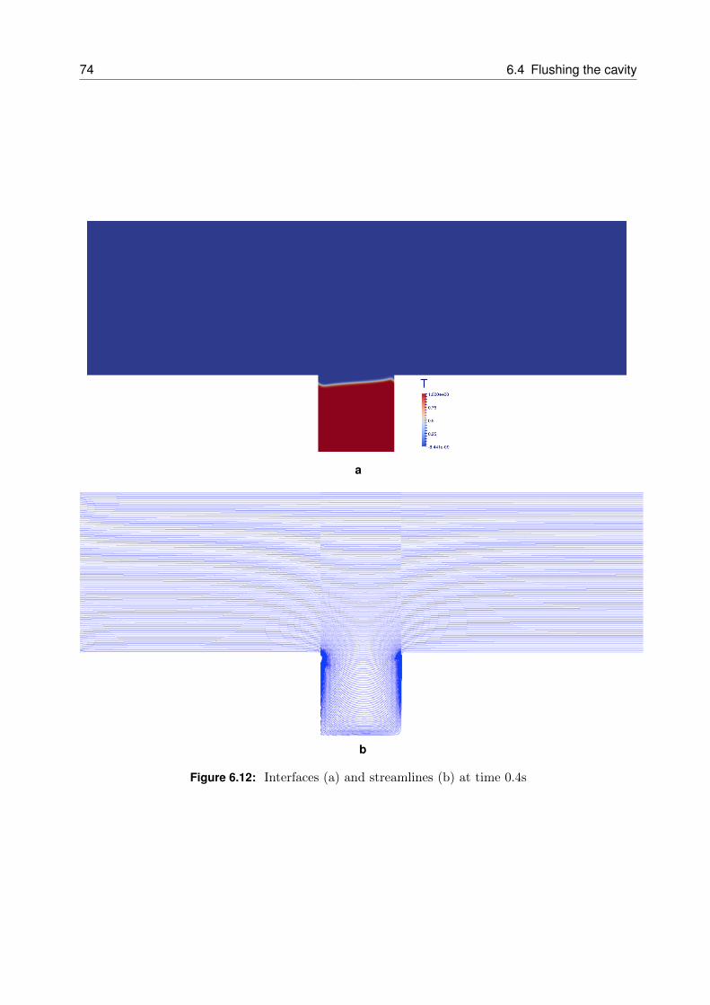
74 6.4 Flushing the cavity
a
b
Figure 6.12: Interfaces (a) and streamlines (b) at time 0.4s
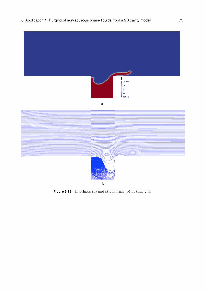
6 Application 1: Purging of non-aqueous phase liquids from a 2D cavity model 75
a
b
Figure 6.13: Interfaces (a) and streamlines (b) at time 2.0s
76 6.4 Flushing the cavity
a
b
Figure 6.14: Interfaces (a) and streamlines (b) at time 4.0s
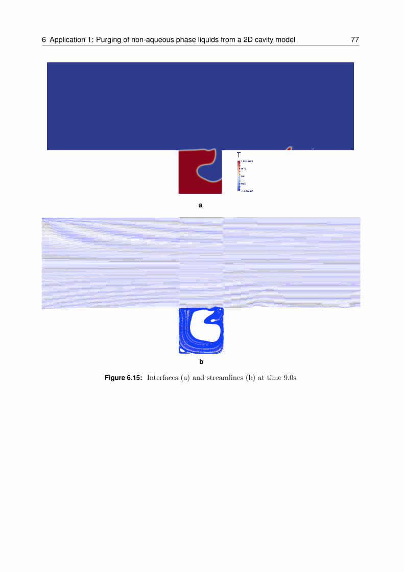
6 Application 1: Purging of non-aqueous phase liquids from a 2D cavity model 77
a
b
Figure 6.15: Interfaces (a) and streamlines (b) at time 9.0s
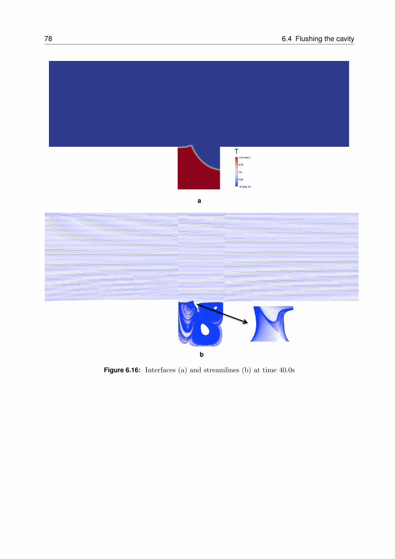
78 6.4 Flushing the cavity
a
b
Figure 6.16: Interfaces (a) and streamlines (b) at time 40.0s
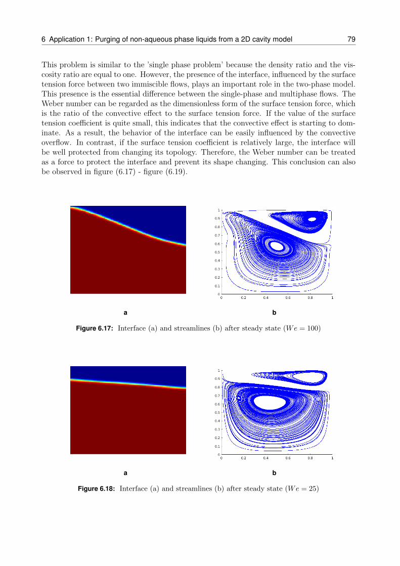
6 Application 1: Purging of non-aqueous phase liquids from a 2D cavity model 79
This problem is similar to the ’single phase problem’ because the density ratio and the vis-cosity ratio are equal to one. However, the presence of the interface, influenced by the surfacetension force between two immiscible flows, plays an important role in the two-phase model.This presence is the essential difference between the single-phase and multiphase flows. TheWeber number can be regarded as the dimensionless form of the surface tension force, whichis the ratio of the convective effect to the surface tension force. If the value of the surfacetension coefficient is quite small, this indicates that the convective effect is starting to dom-inate. As a result, the behavior of the interface can be easily influenced by the convectiveoverflow. In contrast, if the surface tension coefficient is relatively large, the interface willbe well protected from changing its topology. Therefore, the Weber number can be treatedas a force to protect the interface and prevent its shape changing. This conclusion can alsobe observed in figure (6.17) - figure (6.19).
a b
Figure 6.17: Interface (a) and streamlines (b) after steady state (We = 100)
a b
Figure 6.18: Interface (a) and streamlines (b) after steady state (We = 25)
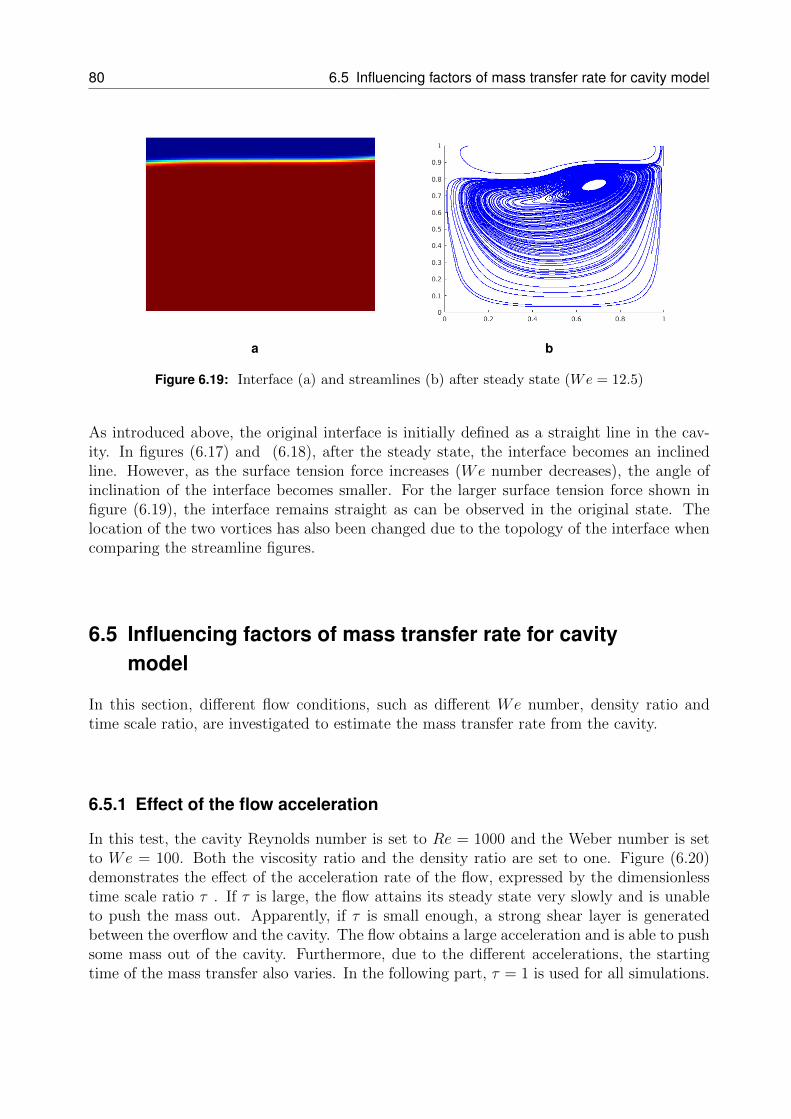
80 6.5 Influencing factors of mass transfer rate for cavity model
a b
Figure 6.19: Interface (a) and streamlines (b) after steady state (We = 12.5)
As introduced above, the original interface is initially defined as a straight line in the cav-ity. In figures (6.17) and (6.18), after the steady state, the interface becomes an inclinedline. However, as the surface tension force increases (We number decreases), the angle ofinclination of the interface becomes smaller. For the larger surface tension force shown infigure (6.19), the interface remains straight as can be observed in the original state. Thelocation of the two vortices has also been changed due to the topology of the interface whencomparing the streamline figures.
6.5 Influencing factors of mass transfer rate for cavitymodel
In this section, different flow conditions, such as different We number, density ratio andtime scale ratio, are investigated to estimate the mass transfer rate from the cavity.
6.5.1 Effect of the flow acceleration
In this test, the cavity Reynolds number is set to Re = 1000 and the Weber number is setto We = 100. Both the viscosity ratio and the density ratio are set to one. Figure (6.20)demonstrates the effect of the acceleration rate of the flow, expressed by the dimensionlesstime scale ratio τ . If τ is large, the flow attains its steady state very slowly and is unableto push the mass out. Apparently, if τ is small enough, a strong shear layer is generatedbetween the overflow and the cavity. The flow obtains a large acceleration and is able to pushsome mass out of the cavity. Furthermore, due to the different accelerations, the startingtime of the mass transfer also varies. In the following part, τ = 1 is used for all simulations.
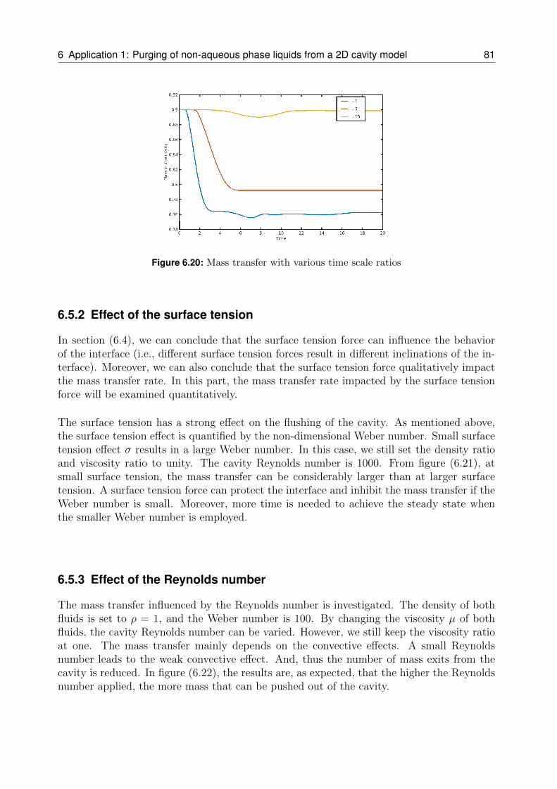
6 Application 1: Purging of non-aqueous phase liquids from a 2D cavity model 81
Figure 6.20: Mass transfer with various time scale ratios
6.5.2 Effect of the surface tension
In section (6.4), we can conclude that the surface tension force can influence the behaviorof the interface (i.e., different surface tension forces result in different inclinations of the in-terface). Moreover, we can also conclude that the surface tension force qualitatively impactthe mass transfer rate. In this part, the mass transfer rate impacted by the surface tensionforce will be examined quantitatively.
The surface tension has a strong effect on the flushing of the cavity. As mentioned above,the surface tension effect is quantified by the non-dimensional Weber number. Small surfacetension effect σ results in a large Weber number. In this case, we still set the density ratioand viscosity ratio to unity. The cavity Reynolds number is 1000. From figure (6.21), atsmall surface tension, the mass transfer can be considerably larger than at larger surfacetension. A surface tension force can protect the interface and inhibit the mass transfer if theWeber number is small. Moreover, more time is needed to achieve the steady state whenthe smaller Weber number is employed.
6.5.3 Effect of the Reynolds number
The mass transfer influenced by the Reynolds number is investigated. The density of bothfluids is set to ρ = 1, and the Weber number is 100. By changing the viscosity µ of bothfluids, the cavity Reynolds number can be varied. However, we still keep the viscosity ratioat one. The mass transfer mainly depends on the convective effects. A small Reynoldsnumber leads to the weak convective effect. And, thus the number of mass exits from thecavity is reduced. In figure (6.22), the results are, as expected, that the higher the Reynoldsnumber applied, the more mass that can be pushed out of the cavity.
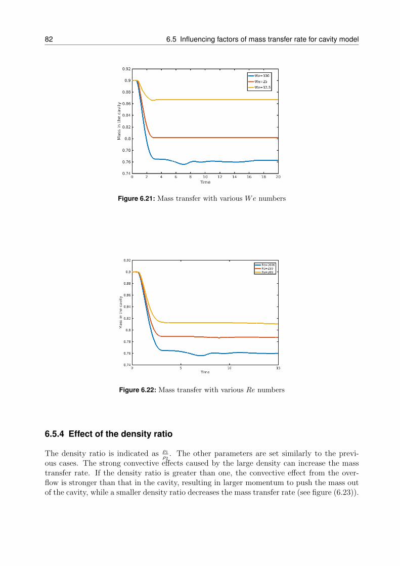
82 6.5 Influencing factors of mass transfer rate for cavity model
Figure 6.21: Mass transfer with various We numbers
Figure 6.22: Mass transfer with various Re numbers
6.5.4 Effect of the density ratio
The density ratio is indicated as ρ1ρ2
. The other parameters are set similarly to the previ-ous cases. The strong convective effects caused by the large density can increase the masstransfer rate. If the density ratio is greater than one, the convective effect from the over-flow is stronger than that in the cavity, resulting in larger momentum to push the mass outof the cavity, while a smaller density ratio decreases the mass transfer rate (see figure (6.23)).
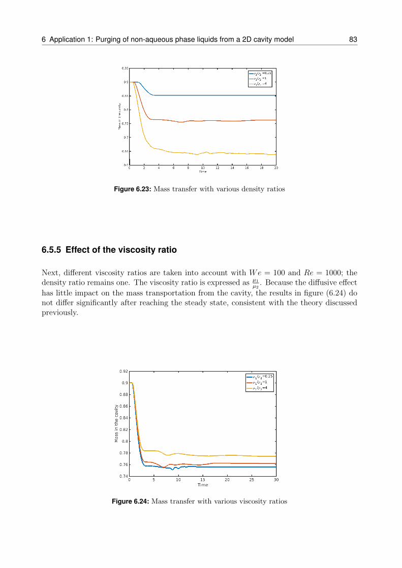
6 Application 1: Purging of non-aqueous phase liquids from a 2D cavity model 83
Figure 6.23: Mass transfer with various density ratios
6.5.5 Effect of the viscosity ratio
Next, different viscosity ratios are taken into account with We = 100 and Re = 1000; thedensity ratio remains one. The viscosity ratio is expressed as µ1
µ2. Because the diffusive effect
has little impact on the mass transportation from the cavity, the results in figure (6.24) donot differ significantly after reaching the steady state, consistent with the theory discussedpreviously.
Figure 6.24: Mass transfer with various viscosity ratios
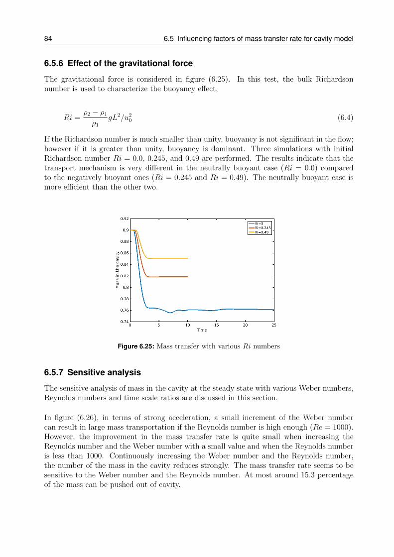
84 6.5 Influencing factors of mass transfer rate for cavity model
6.5.6 Effect of the gravitational force
The gravitational force is considered in figure (6.25). In this test, the bulk Richardsonnumber is used to characterize the buoyancy effect,
Ri =ρ2 − ρ1ρ1
gL2/u20 (6.4)
If the Richardson number is much smaller than unity, buoyancy is not significant in the flow;however if it is greater than unity, buoyancy is dominant. Three simulations with initialRichardson number Ri = 0.0, 0.245, and 0.49 are performed. The results indicate that thetransport mechanism is very different in the neutrally buoyant case (Ri = 0.0) comparedto the negatively buoyant ones (Ri = 0.245 and Ri = 0.49). The neutrally buoyant case ismore efficient than the other two.
Figure 6.25: Mass transfer with various Ri numbers
6.5.7 Sensitive analysis
The sensitive analysis of mass in the cavity at the steady state with various Weber numbers,Reynolds numbers and time scale ratios are discussed in this section.
In figure (6.26), in terms of strong acceleration, a small increment of the Weber numbercan result in large mass transportation if the Reynolds number is high enough (Re = 1000).However, the improvement in the mass transfer rate is quite small when increasing theReynolds number and the Weber number with a small value and when the Reynolds numberis less than 1000. Continuously increasing the Weber number and the Reynolds number,the number of the mass in the cavity reduces strongly. The mass transfer rate seems to besensitive to the Weber number and the Reynolds number. At most around 15.3 percentageof the mass can be pushed out of cavity.
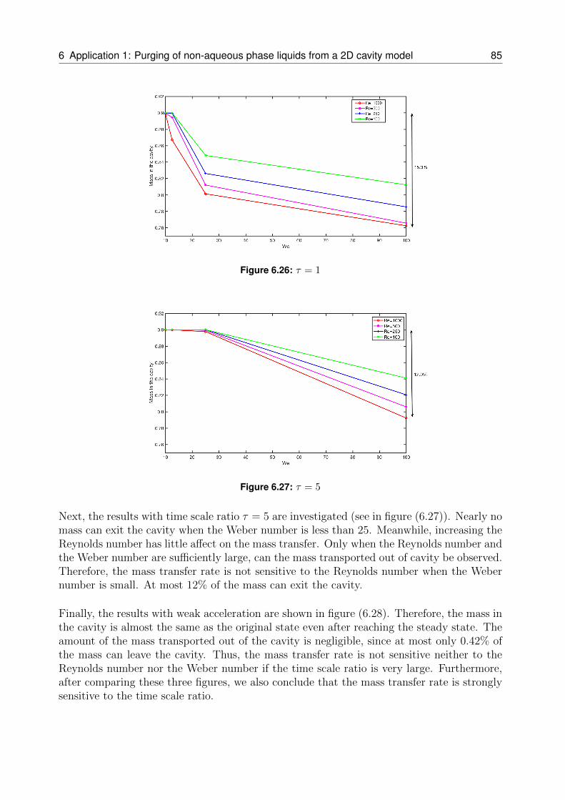
6 Application 1: Purging of non-aqueous phase liquids from a 2D cavity model 85
Figure 6.26: τ = 1
Figure 6.27: τ = 5
Next, the results with time scale ratio τ = 5 are investigated (see in figure (6.27)). Nearly nomass can exit the cavity when the Weber number is less than 25. Meanwhile, increasing theReynolds number has little affect on the mass transfer. Only when the Reynolds number andthe Weber number are sufficiently large, can the mass transported out of cavity be observed.Therefore, the mass transfer rate is not sensitive to the Reynolds number when the Webernumber is small. At most 12% of the mass can exit the cavity.
Finally, the results with weak acceleration are shown in figure (6.28). Therefore, the mass inthe cavity is almost the same as the original state even after reaching the steady state. Theamount of the mass transported out of the cavity is negligible, since at most only 0.42% ofthe mass can leave the cavity. Thus, the mass transfer rate is not sensitive neither to theReynolds number nor the Weber number if the time scale ratio is very large. Furthermore,after comparing these three figures, we also conclude that the mass transfer rate is stronglysensitive to the time scale ratio.
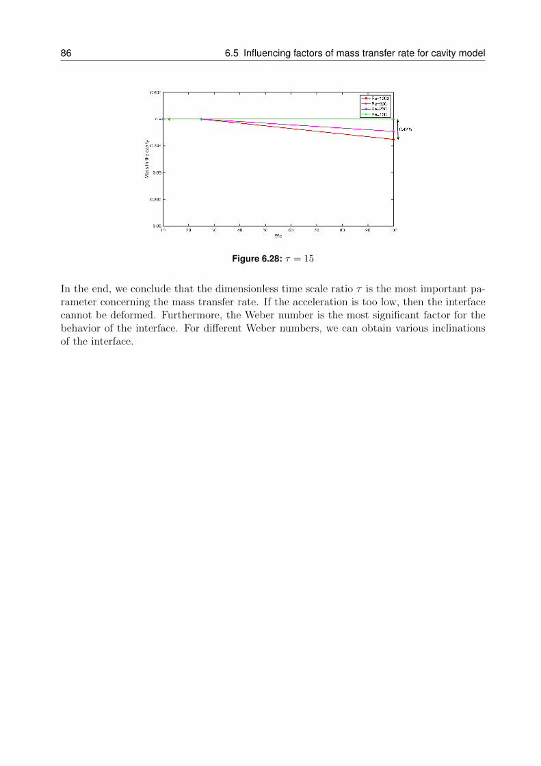
86 6.5 Influencing factors of mass transfer rate for cavity model
Figure 6.28: τ = 15
In the end, we conclude that the dimensionless time scale ratio τ is the most important pa-rameter concerning the mass transfer rate. If the acceleration is too low, then the interfacecannot be deformed. Furthermore, the Weber number is the most significant factor for thebehavior of the interface. For different Weber numbers, we can obtain various inclinationsof the interface.
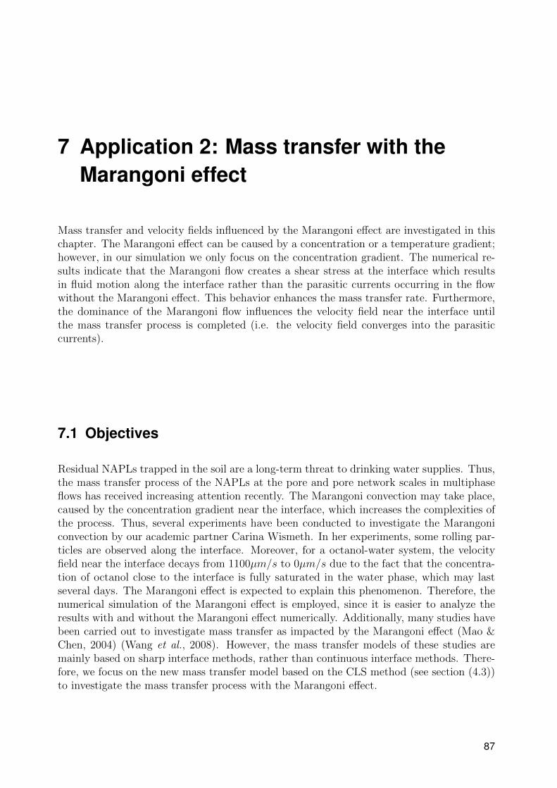
7 Application 2: Mass transfer with theMarangoni effect
Mass transfer and velocity fields influenced by the Marangoni effect are investigated in thischapter. The Marangoni effect can be caused by a concentration or a temperature gradient;however, in our simulation we only focus on the concentration gradient. The numerical re-sults indicate that the Marangoni flow creates a shear stress at the interface which resultsin fluid motion along the interface rather than the parasitic currents occurring in the flowwithout the Marangoni effect. This behavior enhances the mass transfer rate. Furthermore,the dominance of the Marangoni flow influences the velocity field near the interface untilthe mass transfer process is completed (i.e. the velocity field converges into the parasiticcurrents).
7.1 Objectives
Residual NAPLs trapped in the soil are a long-term threat to drinking water supplies. Thus,the mass transfer process of the NAPLs at the pore and pore network scales in multiphaseflows has received increasing attention recently. The Marangoni convection may take place,caused by the concentration gradient near the interface, which increases the complexities ofthe process. Thus, several experiments have been conducted to investigate the Marangoniconvection by our academic partner Carina Wismeth. In her experiments, some rolling par-ticles are observed along the interface. Moreover, for a octanol-water system, the velocityfield near the interface decays from 1100µm/s to 0µm/s due to the fact that the concentra-tion of octanol close to the interface is fully saturated in the water phase, which may lastseveral days. The Marangoni effect is expected to explain this phenomenon. Therefore, thenumerical simulation of the Marangoni effect is employed, since it is easier to analyze theresults with and without the Marangoni effect numerically. Additionally, many studies havebeen carried out to investigate mass transfer as impacted by the Marangoni effect (Mao &Chen, 2004) (Wang et al., 2008). However, the mass transfer models of these studies aremainly based on sharp interface methods, rather than continuous interface methods. There-fore, we focus on the new mass transfer model based on the CLS method (see section (4.3))to investigate the mass transfer process with the Marangoni effect.
87
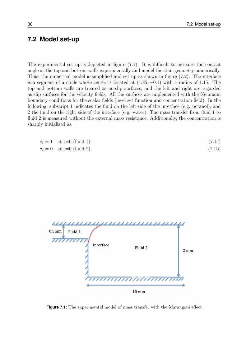
88 7.2 Model set-up
7.2 Model set-up
The experimental set up is depicted in figure (7.1). It is difficult to measure the contactangle at the top and bottom walls experimentally and model the stair geometry numerically.Thus, the numerical model is simplified and set up as shown in figure (7.2). The interfaceis a segment of a circle whose center is located at (1.85,−0.1) with a radius of 1.15. Thetop and bottom walls are treated as no-slip surfaces, and the left and right are regardedas slip surfaces for the velocity fields. All the surfaces are implemented with the Neumannboundary conditions for the scalar fields (level set function and concentration field). In thefollowing, subscript 1 indicates the fluid on the left side of the interface (e.g. octanol), and2 the fluid on the right side of the interface (e.g. water). The mass transfer from fluid 1 tofluid 2 is measured without the external mass resistance. Additionally, the concentration issharply initialized as:
c1 = 1 at t=0 (fluid 1) (7.1a)
c2 = 0 at t=0 (fluid 2). (7.1b)
Figure 7.1: The experimental model of mass transfer with the Marangoni effect
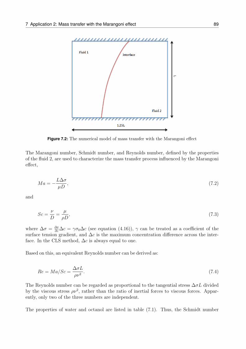
7 Application 2: Mass transfer with the Marangoni effect 89
Figure 7.2: The numerical model of mass transfer with the Marangoni effect
The Marangoni number, Schmidt number, and Reynolds number, defined by the propertiesof the fluid 2, are used to characterize the mass transfer process influenced by the Marangonieffect,
Ma = −L∆σ
µD, (7.2)
and
Sc =ν
D=
µ
ρD, (7.3)
where ∆σ = ∂σ∂c
∆c = γσ0∆c (see equation (4.16)), γ can be treated as a coefficient of thesurface tension gradient, and ∆c is the maximum concentration difference across the inter-face. In the CLS method, ∆c is always equal to one.
Based on this, an equivalent Reynolds number can be derived as:
Re = Ma/Sc =∆σL
ρν2. (7.4)
The Reynolds number can be regarded as proportional to the tangential stress ∆σL dividedby the viscous stress ρν2, rather than the ratio of inertial forces to viscous forces. Appar-ently, only two of the three numbers are independent.
The properties of water and octanol are listed in table (7.1). Thus, the Schmidt number
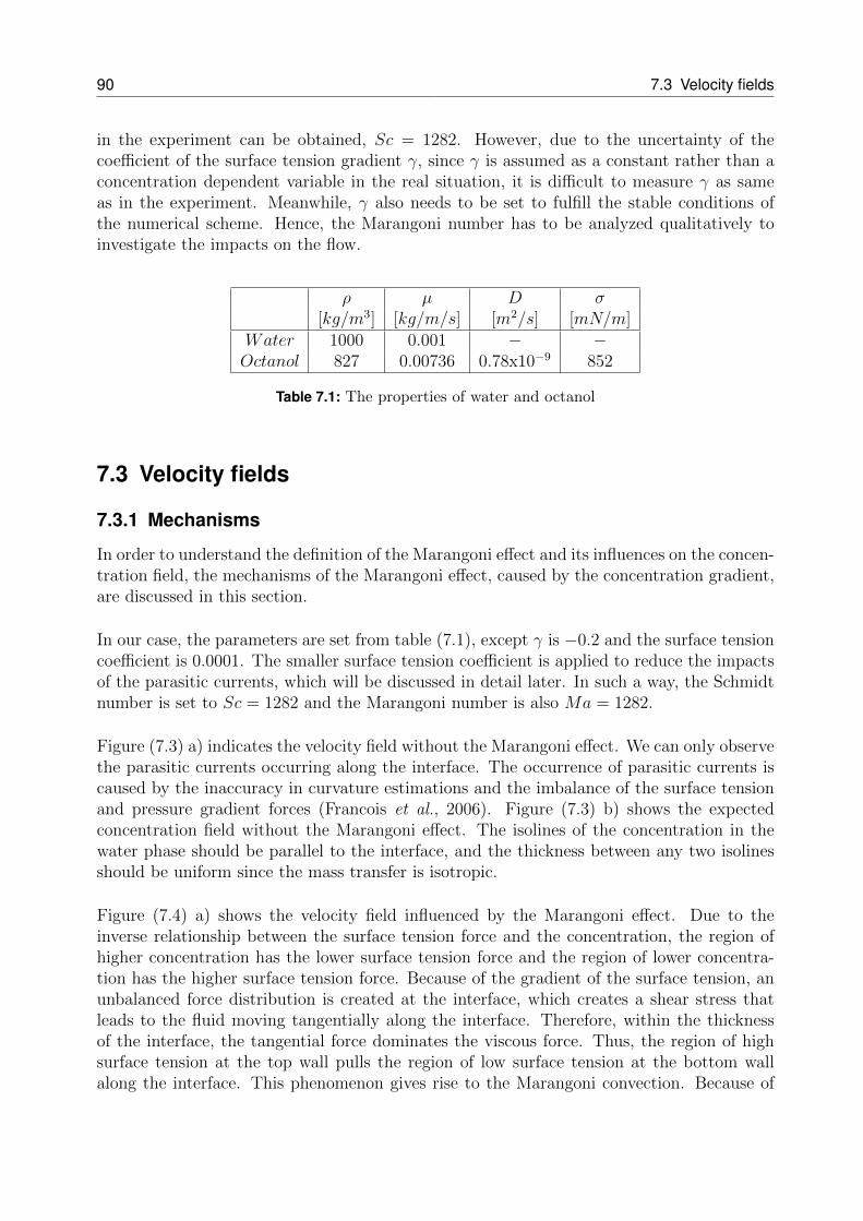
90 7.3 Velocity fields
in the experiment can be obtained, Sc = 1282. However, due to the uncertainty of thecoefficient of the surface tension gradient γ, since γ is assumed as a constant rather than aconcentration dependent variable in the real situation, it is difficult to measure γ as sameas in the experiment. Meanwhile, γ also needs to be set to fulfill the stable conditions ofthe numerical scheme. Hence, the Marangoni number has to be analyzed qualitatively toinvestigate the impacts on the flow.
ρ µ D σ[kg/m3] [kg/m/s] [m2/s] [mN/m]
Water 1000 0.001 − −Octanol 827 0.00736 0.78x10⁻⁹ 852
Table 7.1: The properties of water and octanol
7.3 Velocity fields
7.3.1 Mechanisms
In order to understand the definition of the Marangoni effect and its influences on the concen-tration field, the mechanisms of the Marangoni effect, caused by the concentration gradient,are discussed in this section.
In our case, the parameters are set from table (7.1), except γ is −0.2 and the surface tensioncoefficient is 0.0001. The smaller surface tension coefficient is applied to reduce the impactsof the parasitic currents, which will be discussed in detail later. In such a way, the Schmidtnumber is set to Sc = 1282 and the Marangoni number is also Ma = 1282.
Figure (7.3) a) indicates the velocity field without the Marangoni effect. We can only observethe parasitic currents occurring along the interface. The occurrence of parasitic currents iscaused by the inaccuracy in curvature estimations and the imbalance of the surface tensionand pressure gradient forces (Francois et al., 2006). Figure (7.3) b) shows the expectedconcentration field without the Marangoni effect. The isolines of the concentration in thewater phase should be parallel to the interface, and the thickness between any two isolinesshould be uniform since the mass transfer is isotropic.
Figure (7.4) a) shows the velocity field influenced by the Marangoni effect. Due to theinverse relationship between the surface tension force and the concentration, the region ofhigher concentration has the lower surface tension force and the region of lower concentra-tion has the higher surface tension force. Because of the gradient of the surface tension, anunbalanced force distribution is created at the interface, which creates a shear stress thatleads to the fluid moving tangentially along the interface. Therefore, within the thicknessof the interface, the tangential force dominates the viscous force. Thus, the region of highsurface tension at the top wall pulls the region of low surface tension at the bottom wallalong the interface. This phenomenon gives rise to the Marangoni convection. Because of
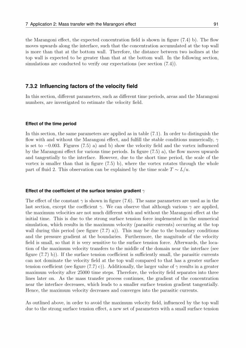
7 Application 2: Mass transfer with the Marangoni effect 91
the Marangoni effect, the expected concentration field is shown in figure (7.4) b). The flowmoves upwards along the interface, such that the concentration accumulated at the top wallis more than that at the bottom wall. Therefore, the distance between two isolines at thetop wall is expected to be greater than that at the bottom wall. In the following section,simulations are conducted to verify our expectations (see section (7.4)).
7.3.2 Influencing factors of the velocity field
In this section, different parameters, such as different time periods, areas and the Marangoninumbers, are investigated to estimate the velocity field.
Effect of the time period
In this section, the same parameters are applied as in table (7.1). In order to distinguish theflow with and without the Marangoni effect, and fulfill the stable conditions numerically, γis set to −0.003. Figures (7.5) a) and b) show the velocity field and the vortex influencedby the Marangoni effect for various time periods. In figure (7.5) a), the flow moves upwardsand tangentially to the interface. However, due to the short time period, the scale of thevortex is smaller than that in figure (7.5) b), where the vortex rotates through the wholepart of fluid 2. This observation can be explained by the time scale T ∼ L/u.
Effect of the coefficient of the surface tension gradient γ
The effect of the constant γ is shown in figure (7.6). The same parameters are used as in thelast section, except the coefficient γ. We can observe that although various γ are applied,the maximum velocities are not much different with and without the Marangoni effect at theinitial time. This is due to the strong surface tension force implemented in the numericalsimulation, which results in the maximum velocity (parasitic currents) occurring at the topwall during this period (see figure (7.7) a)). This may be due to the boundary conditionsand the pressure gradient at the boundaries. Furthermore, the magnitude of the velocityfield is small, so that it is very sensitive to the surface tension force. Afterwards, the loca-tion of the maximum velocity transfers to the middle of the domain near the interface (seefigure (7.7) b)). If the surface tension coefficient is sufficiently small, the parasitic currentscan not dominate the velocity field at the top wall compared to that has a greater surfacetension coefficient (see figure (7.7) c)). Additionally, the larger value of γ results in a greatermaximum velocity after 25000 time steps. Therefore, the velocity field separates into threelines later on. As the mass transfer process continues, the gradient of the concentrationnear the interface decreases, which leads to a smaller surface tension gradient tangentially.Hence, the maximum velocity decreases and converges into the parasitic currents.
As outlined above, in order to avoid the maximum velocity field, influenced by the top walldue to the strong surface tension effect, a new set of parameters with a small surface tension
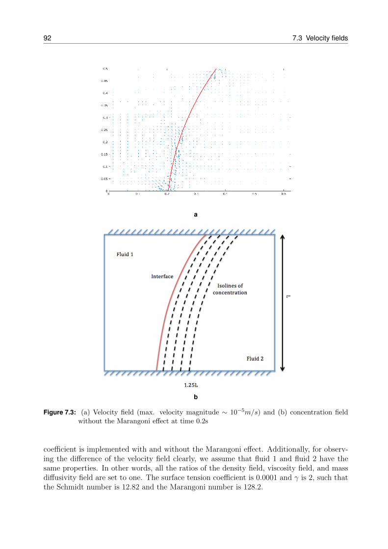
92 7.3 Velocity fields
a
b
Figure 7.3: (a) Velocity field (max. velocity magnitude ∼ 10−5m/s) and (b) concentration fieldwithout the Marangoni effect at time 0.2s
coefficient is implemented with and without the Marangoni effect. Additionally, for observ-ing the difference of the velocity field clearly, we assume that fluid 1 and fluid 2 have thesame properties. In other words, all the ratios of the density field, viscosity field, and massdiffusivity field are set to one. The surface tension coefficient is 0.0001 and γ is 2, such thatthe Schmidt number is 12.82 and the Marangoni number is 128.2.
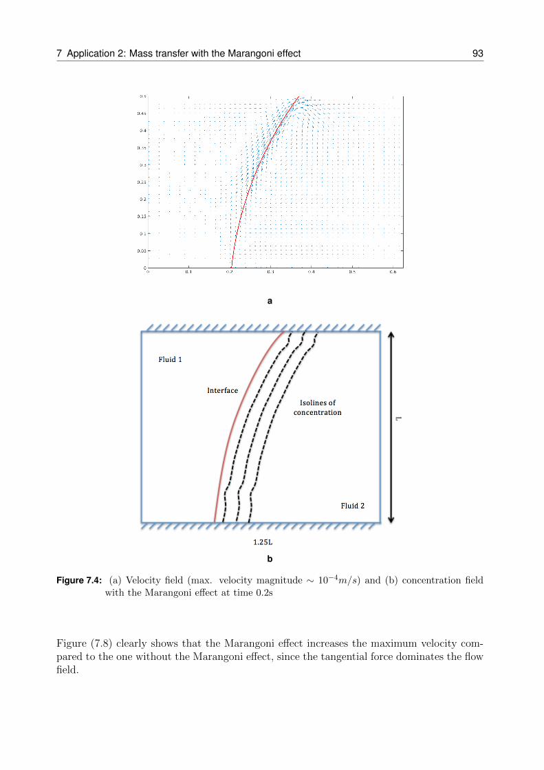
7 Application 2: Mass transfer with the Marangoni effect 93
a
b
Figure 7.4: (a) Velocity field (max. velocity magnitude ∼ 10−4m/s) and (b) concentration fieldwith the Marangoni effect at time 0.2s
Figure (7.8) clearly shows that the Marangoni effect increases the maximum velocity com-pared to the one without the Marangoni effect, since the tangential force dominates the flowfield.
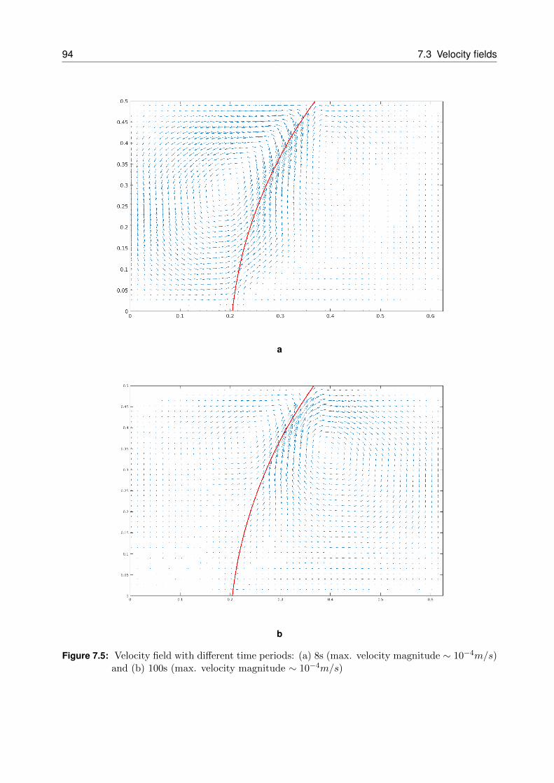
94 7.3 Velocity fields
a
b
Figure 7.5: Velocity field with different time periods: (a) 8s (max. velocity magnitude ∼ 10−4m/s)and (b) 100s (max. velocity magnitude ∼ 10−4m/s)
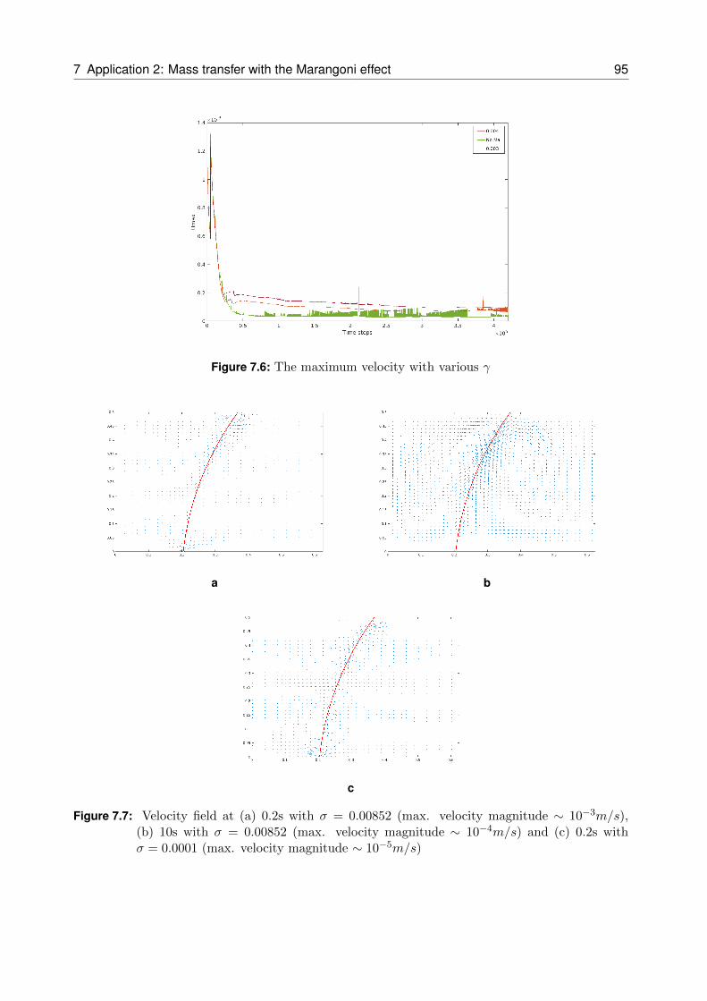
7 Application 2: Mass transfer with the Marangoni effect 95
Figure 7.6: The maximum velocity with various γ
a b
c
Figure 7.7: Velocity field at (a) 0.2s with σ = 0.00852 (max. velocity magnitude ∼ 10−3m/s),(b) 10s with σ = 0.00852 (max. velocity magnitude ∼ 10−4m/s) and (c) 0.2s withσ = 0.0001 (max. velocity magnitude ∼ 10−5m/s)
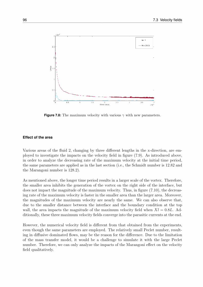
96 7.3 Velocity fields
Figure 7.8: The maximum velocity with various γ with new parameters.
Effect of the area
Various areas of the fluid 2, changing by three different lengths in the x-direction, are em-ployed to investigate the impacts on the velocity field in figure (7.9). As introduced above,in order to analyze the decreasing rate of the maximum velocity at the initial time period,the same parameters are applied as in the last section (i.e., the Schmidt number is 12.82 andthe Marangoni number is 128.2).
As mentioned above, the longer time period results in a larger scale of the vortex. Therefore,the smaller area inhibits the generation of the vortex on the right side of the interface, butdoes not impact the magnitude of the maximum velocity. Thus, in figure (7.10), the decreas-ing rate of the maximum velocity is faster in the smaller area than the larger area. Moreover,the magnitudes of the maximum velocity are nearly the same. We can also observe that,due to the smaller distance between the interface and the boundary condition at the topwall, the area impacts the magnitude of the maximum velocity field when Xl = 0.8L. Ad-ditionally, these three maximum velocity fields converge into the parasitic currents at the end.
However, the numerical velocity field is different from that obtained from the experiments,even though the same parameters are employed. The relatively small Peclet number, result-ing in diffusive dominated flows, may be the reason for the difference. Due to the limitationof the mass transfer model, it would be a challenge to simulate it with the large Pecletnumber. Therefore, we can only analyze the impacts of the Marangoni effect on the velocityfield qualitatively.
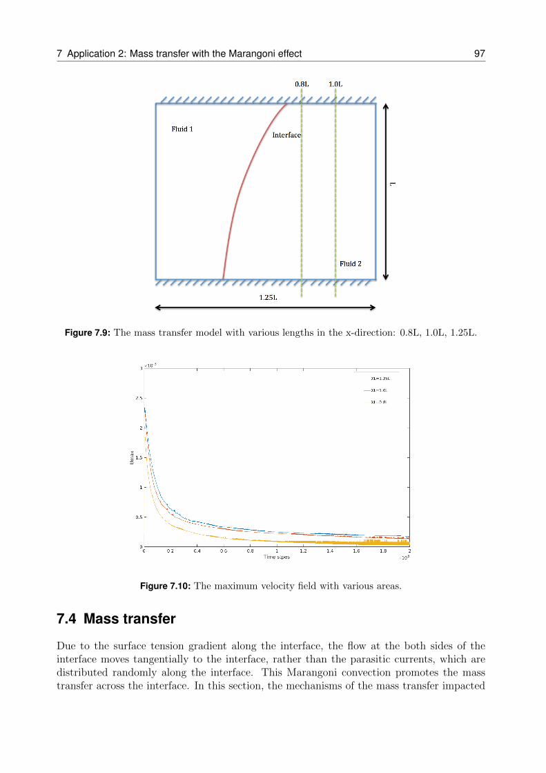
7 Application 2: Mass transfer with the Marangoni effect 97
Figure 7.9: The mass transfer model with various lengths in the x-direction: 0.8L, 1.0L, 1.25L.
Figure 7.10: The maximum velocity field with various areas.
7.4 Mass transfer
Due to the surface tension gradient along the interface, the flow at the both sides of theinterface moves tangentially to the interface, rather than the parasitic currents, which aredistributed randomly along the interface. This Marangoni convection promotes the masstransfer across the interface. In this section, the mechanisms of the mass transfer impacted
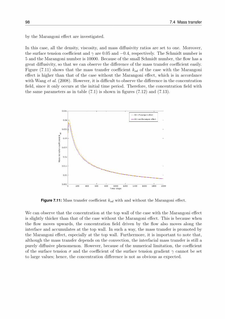
98 7.4 Mass transfer
by the Marangoni effect are investigated.
In this case, all the density, viscosity, and mass diffusivity ratios are set to one. Moreover,the surface tension coefficient and γ are 0.05 and −0.4, respectively. The Schmidt number is5 and the Marangoni number is 10000. Because of the small Schmidt number, the flow has agreat diffusivity, so that we can observe the difference of the mass transfer coefficient easily.Figure (7.11) shows that the mass transfer coefficient kod of the case with the Marangonieffect is higher than that of the case without the Marangoni effect, which is in accordancewith Wang et al. (2008). However, it is difficult to observe the difference in the concentrationfield, since it only occurs at the initial time period. Therefore, the concentration field withthe same parameters as in table (7.1) is shown in figures (7.12) and (7.13).
Figure 7.11: Mass transfer coefficient kod with and without the Marangoni effect.
We can observe that the concentration at the top wall of the case with the Marangoni effectis slightly thicker than that of the case without the Marangoni effect. This is because whenthe flow moves upwards, the concentration field driven by the flow also moves along theinterface and accumulates at the top wall. In such a way, the mass transfer is promoted bythe Marangoni effect, especially at the top wall. Furthermore, it is important to note that,although the mass transfer depends on the convection, the interfacial mass transfer is still apurely diffusive phenomenon. However, because of the numerical limitation, the coefficientof the surface tension σ and the coefficient of the surface tension gradient γ cannot be setto large values; hence, the concentration difference is not as obvious as expected.
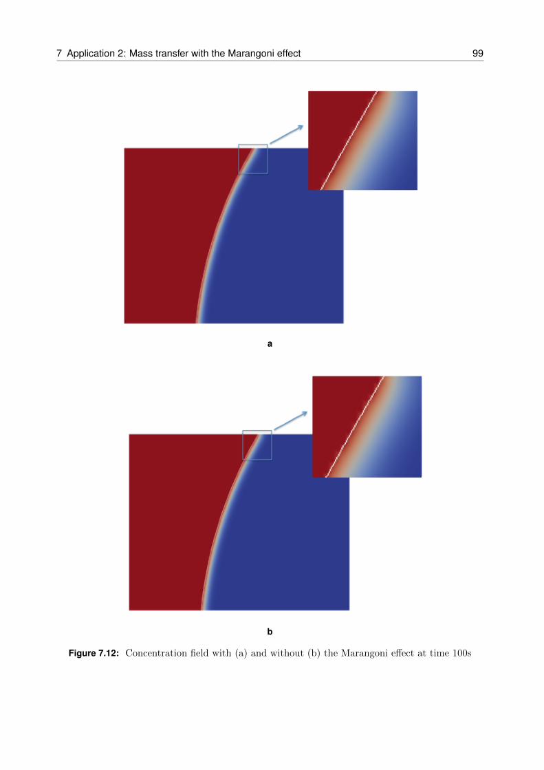
7 Application 2: Mass transfer with the Marangoni effect 99
a
b
Figure 7.12: Concentration field with (a) and without (b) the Marangoni effect at time 100s
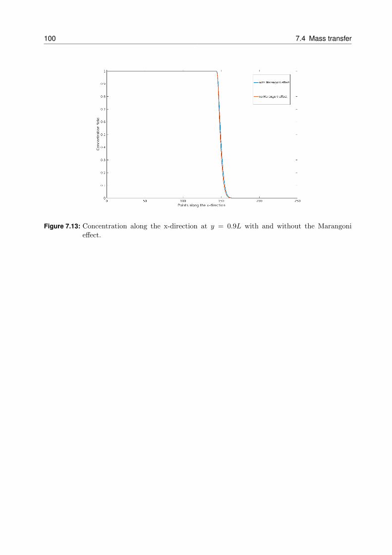
100 7.4 Mass transfer
Figure 7.13: Concentration along the x-direction at y = 0.9L with and without the Marangonieffect.
8 Conclusions
Multiphase mass transport on a pore-scale, including the effects of surface tension forces andMarangoni forces, has been investigated in this work. In order to simulate this phenomenon,several numerical models are implemented. The conservative level set method is employedto track the interface for multiphase flows. Due to the presence of the interface, the surfacetension force needs to be simulated using the sharp surface tension force method. These twomodels have already been completed in a master work (Andre, 2012). Additionally, in orderto quantify the wettability of a solid surface by a liquid numerically, a contact angle modelbased on the conservative level set method (Sato & Niceno, 2012) is used to measure thecontact angle between the surface of the liquid and the outline of the contact surface. Dueto the complexity of the mass transport on the pore-scale, the Marangoni effect may arisefrom the concentration gradient. The Marangoni effect impacts the mass transfer processand the velocity field. Hence, the continuum surface force model is applied to model theMarangoni effect induced by the concentration gradient tangentially to the interface. Fi-nally, a new mass transfer model based on the conservative level set method and the finitevolume method, adding a source term in the scalar transportation equations, is employed toinvestigate the mass transport. To the best of the author’s knowledge, this is a new masstransfer model based on the continuous interface method and the finite volume method. Allthe above numerical methods have been validated qualitatively and quantitatively.
With the help of these numerical models, two applications are conducted to analyze the masstransfer process.
A two-dimensional cavity model, neglecting the Marangoni effect, is conducted for the firstapplication. Due to the low solubility of the Non-aqueous phase liquid, we only considerthe convective mass transfer. Various flow conditions are employed to examine the masstransfer and the behavior of the interface. The results show that the Weber number is themost significant factor affecting the behavior of the interface. Thus, the Weber number canbe treated as a force which protects the interface and prevents its shape changing. Moreover,since different Weber numbers are implemented for the cavity flow, various inclinations ofthe interface occur, resulting in different velocity manners in the cavity. The results alsoindicate that the time scale ratio strongly impacts the mass transfer rate. The small dimen-sionless time scale ratio leads to the large acceleration. Therefore, the flow obtains a strongshear layer and is able to push more mass out of the cavity. Furthermore, we found out thatthe starting time of the mass transfer varies because of the different accelerations.
In the second application, a two-dimensional model is applied with the Marangoni effect toinvestigate the mass transfer process. The external mass transfer resistance is neglected.The results show that, due to the Marangoni effect, a circulation occurs tangentially to the
101
102
interface, rather than the parasitic currents in the case without the Marangoni effect. Thispattern of the velocity field enhances the mixture process, such that the mass transfer rateis larger for the Marangoni effect than without considering the Marangoni effect. The con-centration field also verifies this conclusion, that the concentration at the top wall is morethan that of the case without the Marangoni effect. Furthermore, the maximum velocityfield influenced by various conditions is presented as well.
A number of extensions to this dissertation are addressed in the following directions: thesimulation of the conservative level set method in complex geometries would be an inter-esting extension to this work. This requires the combination of the immersed boundarymethod and the conservative level set method. Another extension would be the simulationwith a large Peclet number. So far, only diffusive dominated flows have been simulated inthe second application based on the new mass transfer model. This may be a reason thatthe maximum velocity field differs from the experimental results. Moreover, the time steplimitation, which is due to the numerical stable conditions, prevents simulating with longertime. Therefore, the numerical model needs to be further refined and improved. The three-dimensional simulation would also be a possible extension. As the Marangoni effect and thecontact angle are three-dimensional phenomena in nature, it would be interesting to extendthese models to three dimensions.
Bibliography
Abouhamza, A. & Pierre, R. 2003 A neutral stability curve for incompressible flows ina rectangular driven cavity. Mathematical and Computer Modelling 38 (141-157).
Aboulhasanzadeh, B., Thomas, S., Taeibi-Rahni, M. & Tryggvason, G. 2012Multiscale computations of mass transfer from buoyant bubbles. Chemical EngineeringScience 75 (456-467).
Afkhami, S. & Bussmann, M. 2009 Height functions for applying contact angles to 3dvof simulations. Int. J. Numer. Methods Fluids 61 (827-847).
Allegrini, Jonas, Dorera, Viktor & Carmeliet, Jan 2014 Buoyant flows in streetcanyons: Validation of cfd simulations with wind tunnel measurements. Building andEnvironment 72 (63-74).
Andre, M. 2012 Conservative level set method for direct numerical simulation of two-phaseflows. Master’s thesis, Technische Universitat Munchen.
Ashcroft, G. & Zhang, X. 2005 Vortical structures over rectangular cavities at lowspeed. Phys. Fluids 17 (015104).
Augustijn, D. C. M., Jessup, R. E., Rao, P. S. C. & Wood, A. L. 1994 Remediationof contaminated soils by solvent flushing. J. Environ. Eng. 120 (42-57).
Badalassi, V. E., Ceniceros, H. D. & Banerjee, S. 2003 Computation of multiphasesystems with phase field models. J. Comput. Phys. 190 (371-397).
Bahloul, A., Delahaye, R., Vasseur, P. & Robillard, L. 2003 Effect of surfacetension on convection in a binary fluid layer under a zero gravity environment. Int J HeatMass Transfer 46(10) (1759-1771).
Bassano, E. 2003 Numerical simulation of thermo-solutal-capillary migration of a dissolv-ing drop in a cavity. Int J Num Meth Fluids 41(7) (765-788).
Bergeron, A., Henry, D. & Benhadid, H. 1994 Marangoni-benard instability in mi-crogravity conditions with soret effect. Int J Heat Mass Transfer 37(11) (1545-1562).
Bergeron, A., Henry, D., Benhadid, H. & Tuckerman, L. S. 1998 Marangoniconvection in binary mixture with soret effect. J Fluid Mech. 375 (143-177).
Borghi, R. & Anselmet, F. 2014 Turbulent multiphase flows with heat and mass trans-fer.. WILEY press.
Brackbill, J. U., Kothe, D. B. & Zemach, C. 1992 A continuum method for modelingsurface tension. J. Comput. Phys. 100 (335-354).
103
104 Bibliography
Brandes, D. & Farley, K. J. 1993 Importance of phase-behavior on the removal ofresidual dnapls from porous media by alcohol flooding. Water Environ. Res. 65 (869-878).
Brown, N.M. & Lai, F.C. 2005 Correlations for combined heat and mass transfer froman open cavity in a horizontal channel. International Communications in Heat and MassTransfer 32 (1000-1008).
Bussmann, M., Chandra, S. & Mostaghimi, J. 2000 Modeling the splash of a dropletimpacting a solid surface. Phys. Fluids 12 (3121-3132).
Bussmann, M., Mostaghimi, J. & Chandra, S. 1999 On a three-dimensional volumetracking model of droplet impact. Phys. Fluids 11 (1406-1417).
Cassie, A. B. D. & Baxter, S. 1944 Wettability of porous surfaces. Trans. Faraday Soc.40 (546-551).
Chang, H. N., Ryu, H. W., Park, D.H ., Yong, S. P. & Park, J. K. 1987 Effect ofexternal laminar channel flow on mass transfer in a cavity. Int. J. Heat Mass Transfer 30(10) (2137-2149).
Chang, Y. C., Hou, T. Y., Merriman, B. & Osher, S. 1996 A level set formulationof eulerian interface capturing methods for incompressible fluid flows. J. Comput. Phys.124 (449-464).
Charwat, A. F., Foos, J. N., Dewey, F. C. & Hitz, J. A. 1961 An investigation ofseparated flows. part 1. the pressure field. J. Aero. Sci. 28(6) (457-70).
Chen, H., Zhong, Q., Wang, X. K. & Li, D. X. 2014 Reynolds number dependence offlow past a shallow open cavity. SCIENCE CHINA: Technological Sciences 57 (11) (2161-2171).
Cheng, P., Bestehorn, M. & Firoozabadi, A. 2012 Effect of permeability anisotropyon buoyancy-driven flow for co2 sequestration in saline aquifers. Water Resourc. Res.48 (W09539).
Chibowski, E. & Terpilowski, K. 2008 Surface free energy of sulfur-revisited i. yel-low and orange samples solidified against glass surface. Journal of Colloid and InterfaceScience 319(2) (505-513).
Clift, R., Grace, J. R. & Weber, M. E. 1978 Bubbles, drops, and particles.. Academicpress.
Colella, P., Graves, D.T., Modiano, D., Puckett, E.G. & Sassman, M. 1999 Anembedded boundary/volume of fluid method for free surface flows in irregular geometries.In Proceedings of the 3rd ASME/JSME Joint Fluids Engineering Conference, numberFEDSM99-7108, San Francisco, CA.
Cox, R.G. 1986 The dynamics of the spreading of liquids on a solid surface. Part 1, J.Fluid Mech. 168 (169-194).
Crook, S. D., Lau, T. C. W. & Kels, R. M. 2013 Three-dimensional flow withinshallow, narrow cavities. J. Fluid Mech. 735 (587-612).
Bibliography 105
Cummins, S.J., Francois, M.M. & Kothe, D.B. 2005 Estimating curvature from vol-ume fractions. J. Comput. Struct. 83 (6-7) (425-434).
Darhuber, A. A. & Troian, S. M. 2005 Principles of microfluidic actuation by modu-lation of surface stresses. Annu. Rev. Fluid Mech. 37 (425-455).
Davidson, M. R. & Rudman, M. 2002 Volume-of-fluid calculation of heat or mass transferacross deforming interfaces in two-fluid flow. Numer. Heat Transfer, Part B: Fundam.41 (291-308).
Davis, S.H. 1987 Thermo-capillary instabilities. Annu. Rev. Fluid Mech. 19 (403-435).
Desjardins, O., Moureau, V. & Pitsch, H. 2008 An accurate conservative levelset/ghost fluid method for simulating turbulent atomization. J. Comput. Phys. 227 (8395-8416).
Eberhardt, C. & Grathwohl, P. 2002 Time scales of organic contaminant dissolutionfrom complex source zones: coal tar pools vs. blobs. J. Cont. Hydrol 59 (45-66).
Erturk, E., Corke, T. C. & Gokcol, C. 2005 Numerical solutions of 2-d steadyincompressible driven cavity flow at high reynolds numbers. International Journal forNumerical Methods in Fluids 48 (747-774).
Fedkiw, Ronald P., Aslam, Tariq, Merriman, Barry & Osher, Stanley 1999A non-oscillatory eulerian approach to interfaces in multimaterial flows (the ghost fluidmethod). J. Comput. Phys. 152 (457-492).
Fetter, C.W. 1993 Contaminant Hydrogeology . Macmillan, New York, NY (458).
Francois, M.M., Cummins, S.J., Dendy, E.D., Kothe, D.B., Sicilian, J.M. &Williams, M.W. 2006 A balanced-force algorithm for continuous and sharp interfacialsurface tension models within a volume tracking framework. J. Comput. Phys. 213 (141-173).
Galazka, Z. & Wilke, H. 2000 Influence of marangoni convection on the flow patternin the melt during growth of y3al5o12 single crystals by the czochralski method. J CrystalGrowth 216(1-4) (389-398).
Ganguli, A. A. & Kenig, E. Y. 2011a A cfd-based approach to the interfacial masstransfer at free gas-liquid interfaces. Chem. Eng. Sci. 66 (3301-3308).
Ganguli, A. A. & Kenig, E. Y. 2011b Prediction of interfacial mass transfer in liquid-liquid systems with moving interfaces. Chem. Eng. Trans. 24 (1357-1362).
Gao, D., Morley, N. B. & Dhir, V. 2003 Numerical simulation of wavy falling filmflow using vof method. J. Comput. Phys. 192 (624-642).
Gueyffier, D., Li, Jie, Nadim, Ali, Scardovelli, R. & Zaleski, S. 1999 Volume-of-fluid interface tracking with smoothed surface stress methods for three-dimensional flows.J. Comput. Phys. 152 (423-456).
Gupta, R., Fletcher, D. F. & Haynes, B. S. 2010 Cfd modelling of flow and heattransfer in the taylor flow regime. Chem. Eng. Sci. 65 (2094-2107).
106 Bibliography
Hayashi, K. & Tomiyama, A. 2011 Interface tracking simulation of mass transfer from adissolving bubble. J. Comput. Multiphase Flows 3 (247-262).
Herrmann, M. 2008 A balanced force refined level set grid method for two-phase flows onunstructured flow solver grids. J. Comput. Phys. 227 (2674-2706).
Himeno, T. & Watanabe, T. 2005 Numerical analysis for propellant management inrocket tanks. J. Propulsion Power 21 (76-86).
Hirt, C. W. & Nichols, B. D. 1981 Volume of fluid (vof) method for the dynamics offree boundaries. J. Comput. Phys. 39 (201-225).
Hoffman, R.L. 1975 A study of the advancing interface. J. Colloid Interface Sci. 50 (228-241).
Juric, D. & Tryggvason, G. 1998 Computations of boiling flows. Int. J. MultiphaseFlow 24 (387-410).
Kang, M., Fedkiw, R. P. & Liu, Xudong 2000 A boundary condition capturing methodfor multiphase incompressible flow. J. Scientific Computing 15 (323-360).
Kawaji, M., Gamache, O., Hwang, D. H., Ichikawa, N., Viola, J. P. & Sygusch,J. 2003 Investigation of marangoni and natural convection during protein crystal growth.J Crystal Growth 258(3-4) (420-430).
Khanafer, Khalil, Vafai, Kambiz & Lightstone, Marilyn 2002 Mixed convectionheat transfer in two-dimensional open-ended enclosures. International Journal of Heat andMass Transfer 45 (5171-5190).
Khosravi, M., Bahramian, A., Emadi, M., Rostami, B. & Roayaie, E. 2014 Effectof marangoni flow on recovery of bypassed oil during co2 injection. J. Petrol. Sci. Eng.114 (91-98).
Kim, Junseok 2005 A continuous surface tension force formulation for diffuse-interfacemodels. J. Comput. Phys. 204 (784-804).
Kim, J., Choi, C. K. & Kang, Y. T. 2004 Instability analysis of marangoni convectionfor absorption process accompanied by heat transfer. Int J Heat Mass Transfer 47(10-11) (2395-2402).
Kirkpatrick, M. P., Armfield, S. W. & Williamson, N. 2012 Shear driven purgingof negatively buoyant fluid from trapezoidal depressions and cavities. Physics of Fluids24 (161-164).
Kobayashi, M., Tsukuda, T. & Hozawa, M. 1997 Effect of internal radiative heattransfer on the convection in cz oxide melt. J Crystal Growth 180(1) (157-166).
Landau, L. D. & Lifshitz, E. M. 1987 Fluid Mechanics, 2nd, vol. 6 . Pergamon press,Oxford.
Leong, J.C., Brown, N.M. & Lai, F.C. 2005 Mixed convection from an open cavity ina horizontal channel. International Communications in Heat and Mass Transfer 32 (583-592).
Bibliography 107
Levich, V. G. & Krylov, V. S. 1969 Surface-tension-driven phenomena. Annu. Rev.Fluid Mech. 1 (293-316).
Liffman, K. 1996 Comments on a collocation spectral solver for the helmholtz equation.Journal of Computational Physics. 128 (254-258).
Liu, C. H., Barth, M. C. & Leung, D. Y. C. 2004 Large-eddy simulation of flow andpollutant transport in street canyons of different building-height-to-street-width ratios.Journal of Applied Meteorology 43 (1410-1424).
Liu, W., Yuan, L. & Shu, C. W. 2011 A conservative modification to the ghost fluidmethod for compressible multiphase flows. Communications in Computational Physics10(4) (785-806).
Liu, X.-D., Fedkiw, R.P. & Kang, M. 2000 A boundary condition capturing methodfor poisson’s equation on irregular domains. J. Comput. Phys. 160 (151-178).
Mackay, D. M. & Cherry, J. A. 1989 Groundwater contamination: pump-and-treatremediation. Environ. Sci. Technol. 23 (630-636).
Mammoli, A. A. & Brebbia, C. A. 2005 Computational Methods In Multiphase FlowIII.. WIT press.
Manhart, M. 2004 A zonal grid algorithm for dns of turbulent boundary layer. Comput.Fluids 33(3) (435-461).
Manhart, M. & Friedrich, R. 2002 Dns of a turbulent boundary layer with separation.Int. J. Heat Fluid Flow 23(5) (572-581).
Mao, Z. S. & Chen, J. Y. 2004 Numerical simulation of the marangoni effect on masstransfer to single slowly moving drops in the liquid-liquid system. Chem Eng Sci 59(8-9) (1815-1828).
Mao, Z. S., Li, T. & Chen, J. 2001 Numerical simulation of steady and transient masstransfer to a single drop dominated by external resistance. Int. J. Heat Mass Transfer44 (1235-1247).
Marchandise, E., Geuzaine, P., Chevaugeon, N. & Remacle, J.-F. 2007 A stabi-lizing finite element method using a discontinuous level set approach for the computationof bubble dynamics. J. Comput. Phys. 225 (949-974).
Marmur, A. 2009 Solid-surface characterization by wetting. Annual Review of MaterialsResearch 39 (473-489).
Newman, A. B. 1931 The drying of porous solids: diffusion and surface emission equations.Transactions AlChE 27 (203-220).
Occhialini, J. M. & Higdon, J. J. L. 1992 Convective mass transport from rectangularcavities in viscous flow. J. Electronchem. Soc. 139 (10) (2845).
Okano, Y., Fukuda, T., Hirata, A., Takano, N., Tsukuda, T., Hozawa, M. &Imaishi, N. 1991 Numerical study on czochralski growth of oxide single crystals. J CrystalGrowth 109(1-4) (94-98).
108 Bibliography
Olsson, E. & Kreiss, G. 2005 A conservative level set method for two phase flow. J.Comput. Phys. 210 (225-246).
Olsson, E., Kreiss, G. & Zahedi, S. 2007 A conservative level set method for two phaseflow ii. J. Comput. Phys. 225 (785-807).
Ortiz, E., Kraatz, M. & Luthy, R. G. 1999 Organic phase resistance to dissolution ofpoly-cyclic aromatic hydrocarbon compounds. Environ. Sci. Technol. 33 (235-242).
Osher, S. & Fedkiw, R. 2002 Level set methods and dynamic implicit surfaces. AppliedMathematical Sciences 153, springer-Verlag, New York.
Osher, S. & Sethian, J. A. 1988 Fronts propagating with curvature-dependent speed:Algorithms based on hamilton-jacobi formulations. J. Comput. Phys. 79 (12?49).
Pennell, K. D., Abriola, L. M. & Weber, W. J. Jr. 1993 Surfactant-enhancedsolubilization of residual dodecane in soil columns: 1. experimental investigation. Environ.Sci. Technol. 27 (2332-2340).
Petera, J. & Weatherley, L. R. 2001 Modelling of mass transfer from falling drops.Chemical Engineering Science 56 (4929-4947).
Popinet, S. & Zaleski, S. 1999 A front-tracking algorithm for accurate representation ofsurface tension. Int. J. Numer. Meth. Fluids 30 (6) (775-793).
Prosperetti, A. 1981 Motion of two superposed viscous fluids. Phys. Fluids 24(7) (1217-1223).
Ramachandran, P. A. 2018 Mass transfer processes: modeling, computations, and design.Prentice Hall.
Renardy, Y. & Renardy, M. 2002 Prost: A parabolic reconstruction of surface tensionfor the volume-of-fluid method. J. Comput. Phys. 183 (400-421).
Rider, W. J. & Kothe, D. B. 1998 Reconstructing volume tracking. J. Comput. Phys.141 (112-152).
Sarohia, V. 1977 Experimental investigation of oscillations in flows over shallow cavities.AIAA J 15 (984-991).
Sato, Y. & Niceno, B. 2012 A new contact line treatment for a conservative level setmethod. J. Comput. Phys. 231 (3887-3895).
Schwertfirm, F., Mathew, J. & Manhart, M. 2008 Improving spatial resolutioncharacteristics of finite difference and finite volume schemes by approximate deconvolutionpreprocessing. Comput. Fluids 37 (9) (1092-1102).
Sethian, J. A. 1999 Level Set Methods and Fast Marching Methods, second ed.. CambridgeUniversity Press, Cambridge, UK.
Shaikha, J., Bhardwaj, R & Sharma, A. 2015 A ghost fluid method based sharpinterface level set method for evaporating droplet. Procedia IUTAM 15 (124-131).
Bibliography 109
Sirignano, W.A. 1999 Fluid dynamics and transport of droplets and sprays.. CambridgeUniversity press.
Sussman, M. 2001 An adaptive mesh algorithm for free surface flows in general geometries.In Adaptive Method of Lines, Chapman and Hall/CRC (ed. A. Vande Wouwer, Ph. Saucez& W.E. Schiesser).
Sussman, M. 2005 A parallelized adaptive algorithm for multiphase flows in general ge-ometries. Computers and Structures 83 (435-444).
Sussman, M. & Fatemi, E. 1999 An efficient, interface-preserving level set redistancingalgorithm and its application to interfacial incompressible fluid flow. SIAM J. Sci. Comput.20 (4) (1165-1191).
Sussman, M., Fatemi, E., Smereka, P. & Osher, S. 1998 An improved level setmethod for incompressible two-phase flows. Comput. Fluids 27 (5-6) (663-680).
Sussman, M., Smereka, P. & Osher, S. 1994 A level set approach for computingsolutions to incompressible two-phase flow. J. Comput. Phys. 114 (146-159).
Tadmor, R. 2004 Line energy and the relation between advancing, receding, and youngcontact angles. Langmuir 20(18) (7659-7664).
Tang, Hao, Wrobel, L. C. & Fan, Z. 2004 Tracking of immiscible interfaces in multiple-material mixing processes. Comp. Mater. Sci. 29 (103-118).
Tanguy, S., Me?nard, T & Berlemont, A. 2007 A level set method for vaporizingtwo-phase flows. Journal of Computational Physics 221 (837-853).
Tomar, G., Biswas, G., Sharma, A. & Agrawal, A. 2005 Numerical simulation ofbubble growth in film boiling using a coupled level-set and volume-of-fluid method. Phys.Fluid 14 (112103).
Tornberg, A.-K. & Engquist, B. 2000 A finite element based level set method formultiphase flow applications. Comput. Visualiz. Sci. 3 (93-101).
Tryggvason, G., Scardovelli, R. & Zaleski, S. 2011 Direct Numerical Simulationsof Gas-Liquid Multiphase Flows.. Cambridge University Press, Cambridge, UK.
Unverdi, O. S. & Tryggvason, G. 1992a A front-tracking method for viscous, incom-pressible, multi-fluid flows. Journal of Computational Physics 100 (25-37).
Unverdi, S. O. & Tryggvason, G. 1992b A front-tracking method for viscous, incom-pressible, multi-fluid flows. J. Comput. Phys. 100 (25-37).
Wang, Jianfeng, Yang, Chao & Mao, Zaisha 2008 Numerical simulation of marangonieffects of single drops induced by interphase mass transfer in liquid-liquid extraction sys-tems by the level set method. Science in China Series B: Chemistry 51 (684-694).
Wehrer, M., Rennert, T., Mansfeldt, T. & Totsche, K. U. 2011 Contaminantsat former manufactured gas plants: sources, properties, and processes. Crit. Rev. Environ.Sci. Technol. 41 (1883-1969).
110 References
Welch, S. & Wilson, J. 2000 A volume of fluid based method for fluid flows with phasechange. J. Comput. Phys. 160 (662).
Wenzel, R. N. 1936 Resistance of solid surfaces to wetting by water. Ind. Eng. Chem.28(8) (988-994).
White, H.E. 1948 Modern College Physics.. van Nostrand.
Yang, J. & Stern, F. 2009 Sharp interface immersed-boundary/level-set method forwave-body interactions. J. Comput. Phys. 228 (6590-6616).
Yokoi, K. 2011 Numerical studies of droplet splashing on a dry surface: triggering a splashwith the dynamic contact angle. Soft Matter 7 (5120-5123).
Zahedi, S., Gustavsson, K. & Kreiss, G. 2009 A conservative level set method forcontact line dynamics. J. Comput. Phys. 228 (6361-6375).