Embed Size (px)
Citation preview
Forschungszentrum Karlsruhe in der Helmholtz-Gemeinschaftt Wissenschaftliche Berichte FZKA 7243 General Guidelines for the Estimation of Committed Effective Dose from Incorporation Monitoring Data (Project IDEAS – EU Contract No. FIKR-CT2001-00160) H. Doerfel, A. Andrasi, M. Bailey, V. Berkovski, E. Blanchardon, C.-M. Castellani, C. Hurtgen, B. LeGuen, I. Malatova, J. Marsh, J. Stather Hauptabteilung Sicherheit August 2006

Forschungszentrum Karlsruhe
in der Helmholtz-Gemeinschaft
Wissenschaftliche Berichte
FZKA 7243
GENERAL GUIDELINES FOR THE ESTIMATION OF COMMITTED EFFECTIVE DOSE FROM INCORPORATION MONITORING DATA
(Project IDEAS – EU Contract No. FIKR-CT2001-00160)
H. Doerfel, A. Andrasi 1, M. Bailey 2, V. Berkovski 3, E. Blanchardon 6, C.-M. Castellani 4, C. Hurtgen 5, B. LeGuen 7,
I. Malatova 8, J. Marsh 2, J. Stather 2
Hauptabteilung Sicherheit
1 KFKI Atomic Energy Research Institute, Budapest, Hungary 2 Health Protection Agency, Radiation Protection Division,
(formerly National Radiological Protection Board), Chilton, Didcot, United Kingdom 3 Radiation Protection Institute, Kiev, Ukraine
4 ENEA Institute for Radiation Protection, Bologna, Italy 5 Belgian Nuclear Research Centre, Mol, Belgium
7 Institut de Radioprotection et de Sûreté Nucléaire, Fontenay-aux-Roses, France 8 Electricité de France (EDF), Saint-Denis, France
9 National Radiation Protection Institute, Praha, Czech Republic
Forschungszentrum Karlsruhe GmbH, Karlsruhe 2006

Für diesen Bericht behalten wir uns alle Rechte vor
Forschungszentrum Karlsruhe GmbH Postfach 3640, 76021 Karlsruhe
Mitglied der Hermann von Helmholtz-Gemeinschaft Deutscher Forschungszentren (HGF)
ISSN 0947-8620
urn:nbn:de:0005-072434
IDEAS General Guidelines – June 2006
3
Abstract
Doses from intakes of radionuclides cannot be measured but must be assessed from monitoring, such as whole body counting or urinary excretion measurements. Such assessments require application of a biokinetic model and estimation of the exposure time, material properties, etc. Because of the variety of parameters involved, the results of such assessments may vary over a wide range, according to the skill and the experience of the assessor. The need for harmonisation of assessment procedures has been recognised in a research project carried out under the EU 5th Framework Programme. The aim of the project IDEAS (partly funded by the European Commission under contract No. FIKR-CT2001-00160) was to develop general guidelines for assessments of intakes and internal doses from individual monitoring data. The IDEAS project started in October 2001 and ended in June 2005.
To ensure that the guidelines are applicable to a wide range of practical situations, a database was compiled of cases of internal contamination that include monitoring data suitable for assessment. About 50 cases from the database were analized by different assessors, the results were collated, and differences in assumptions identified, with their effects on the assessed doses. From the results, and other investigations, draft guidelines were prepared, to provide a systematic procedure for estimating the required parameter values that are not part of the measurement data. A virtual workshop was held on the Internet, open to internal dosimetry professionals, to discuss the draft guidelines, which were revised accordingly. In collaboration with the IAEA, an intercomparison exercise on internal dose assessment was then conducted, which was also open to all involved in internal dosimetry. Six cases were developed and circulated with a copy of the revised guidelines, which participants were encouraged to follow, to test their applicability and effectiveness. The results were collated and a Workshop held to discuss the results with the participants. The guidelines were refined on the basis of the experience and discussion.
The guidelines are based on a general philosophy of:
• Harmonisation: by following the Guidelines any two assessors should obtain the same estimate of dose from a given data set.
• Accuracy: the "best" estimate of dose should be obtained from the available data.
• Proportionality: the effort applied to the evaluation should be proportionate to the dose - the lower the dose, the simpler the process should be.
Following these principles, the Guidelines use the following "Levels of task" to structure the approach to an evaluation: Level 0: Annual dose <0.1 mSv. No dose evaluation; Level 1: Simple evaluation normally using ICRP reference parameter values (typical dose 0.1 - 1 mSv); Level 2: Sophisticated evaluation using additional information to give more realistic assessment (typical dose 1 - 6 mSv); Level 3: More sophisticated evaluation, for cases with comprehensive data (typical dose > 6 mSv).
The guidelines provide:
• Background information about the biokinetic models and the corresponding bioassay functions for the interpretation of monitoring data.
• Detailed information about the handling and evaluation of monitoring data.
• A structured approach to dose assessment consisting of a step-by-step procedure described in well-defined flowcharts with accompanying explanatory text.

4
The guidelines have been put forward as a basis for national and international guidance. They were developed in close collaboration with the ICRP Committee 2 Task Group on Internal Dosimetry (INDOS), which is developing a Guidance Document on internal dose assessment. The draft ICRP Guidance Document is following similar principles, and a similar structured approach to assessments based on the IDEAS Guidelines, but will relate to revised ICRP biokinetic models currently under development by INDOS.
IDEAS General Guidelines – June 2006
5
ALLGEMEINE RICHTLINIEN ZUR ABSCHÄTZUNG DER EFFEKTIVEN FOLGEÄQUIVALENTDOSIS AUS DEN DATEN DER INKORPORATIONSÜBERWACHUNG Zusammenfassung
Die durch Inkorporation radioaktiver Stoffe bedingte Dosis kann nicht direkt gemessen werden, sondern sie muss aus den Messdaten der Inkorporationsüberwachung (z.B. Ganzkörper-messungen oder Urinausscheidungsmessungen) berechnet werden. Diese Berechnungen erfordern ein passendes biokinetisches Modell sowie zutreffende Annahmen hinsichtlich der Expositionsbedin-gungen, Materialeigenschaften etc.. Aufgrund der Vielfalt der involvierten Parameter können die Ergebnisse dieser Berechnungen je nach Qualifikation und Erfahrung der auswertenden Fachleute in einem weiten Bereich variieren. Um zu einer besseren Übereinstimmung der Ergebnisse zu kommen, wurde im 5th Framework Programme der EU ein Forschungsprojekt zur Harmonisierung der internen Dosimetrie durchgeführt. Das Ziel des Projekts IDEAS (gefördert von der EU unter dem Kontrakt No. FIKR-CT2001-00160) war die Entwicklung von allgemeinen Richtlinien zur Standardisierung der Verfahren zur Bestimmung der Aktivitätszufuhr und der Folgeäquivalentdosis aus den Inkorpora-tionsmessdaten. Das Projekt begann im Oktober 2001 und endete im Juni 2005.
Um sicher zu stellen, dass die Richtlinien einen möglichst weiten Bereich der in der Praxis auftretenden Situationen abdecken, wurde zunächst eine Datenbank mit relevanten Inkorporations-fällen aus der Literatur aufgebaut. Etwa 50 Fälle aus dieser Datenbank wurden jeweils von mehreren Fachleuten interpretiert. Die Ergebnisse der Interpretationen wurden zusammengestellt und speziell in Hinblick auf die Modellannahmen und deren Auswirkungen auf die Dosisabschätzung analysiert. Auf der Basis der hierbei gewonnenen Erfahrungen sowie weiterer Untersuchungen wurde ein erster Richtlinienentwurf erarbeitet, mit dessen Hilfe die zur Auswertung der Inkorporationsmessdaten erforderlichen Parameter systematisch ermittelt werden können. Der Entwurf wurde im Rahmen eines virtuellen Workshops im Internet mit Fachleuten aus aller Welt diskutiert und weiterentwickelt. Zum praktischen Test der Richtlinien wurde in Zusammenarbeit mit der IAEA ein internationales Vergleichsprogramm zur Bestimmung der Dosis aus Inkorporationsmessdaten durchgeführt. Die Teil-nehmer an diesem Vergleich erhielten jeweils sechs Fallstudien, die sie nach den Richtlinien aus-werten sollten. Die Ergebnisse wurden zusammengestellt und im Rahmen eines zweiten Workshops mit den Teilnehmern des Vergleichs und weiteren interessierten Fachleuten diskutiert. Auf der Basis der Ergebnisse dieses Workshops wurden die Richtlinien nochmals überarbeitet und in die endgültige Form gebracht.
Die Richtlinien basieren auf der folgenden allgemeinen Philosophie:
• Harmonisierung: Jeder Anwender sollte von einem gegebenen Satz von Inkorporations-messdaten zur gleichen Aktivitätszufuhr bzw. zur gleichen Folgeäquivalentdosis kommen.
• Genauigkeit: Das Ergebnis sollte die Best-Abschätzung repräsentieren.
• Angemessenheit: Der Aufwand zur Auswertung sollte sich an der Dosis orientieren – je geringer die Dosis, umso geringer sollte der Aufwand zur Auswertung sein.
Auf der Basis dieser Philosophie wurde eine abgestufte Auswertung der Inkorporations-messdaten definiert und in Form von Flussdiagrammen strukturiert. Hierbei wird zwischen den folgenden Auswertestufen (Levels of task) unterschieden: Level 1: Einfache Auswertung unter Benutzung der Referenzparameter der ICRP (bei Jahresdosiswerten zwischen 0,1 und 1 mSv); Level 2: Spezielle Auswertung unter Einbeziehung zusätzlicher fallspezifischer Informationen (bei Dosis-werten zwischen 1 und 6 mSv); Level 3: Sehr detaillierte Auswertung bei Fällen mit umfassendem Datenmaterial (bei Dosiswerten oberhalb von 6 mSv).
6
Die Richtlinien umfassen:
• Hintergrundinformationen über die biokinetischen Modelle und die entsprechenden biokine-tischen Funktionen zur Interpretation der Inkorporationsmessdaten
• Detaillierte Informationen zur Behandlung und Auswertung von Inkorporationsmessdaten
• Einen strukturierten Ansatz zur Bestimmung der internen Dosis mit detaillierten Flussdia-grammen und begleitenden Erklärungen zur schrittweisen Bestimmung der inneren Dosis entsprechend der Level-of-task-Struktur
Die Richtlinien sollen eine Basis für nationale und internationale Regelwerke zur internen Dosimetrie bilden. Die Erarbeitung der Richtlinien erfolgte in enger Zusammenarbeit mit der ICRP Committee 2 Task Group on Internal Dosimetry (INDOS), die zur Zeit an ähnlichen Leitlinien arbeitet (Guidance Document on internal dose assessment). Die ICRP-Leitlinien folgen den gleichen Prinzi-pien wie die IDEAS-Richtlinien, sie orientieren sich allerdings bereits an der nächsten Generation von biokinetischen Modellen, die zur Zeit von INDOS erarbeitet wird.
IDEAS General Guidelines – June 2006
7
CONTENTS
1 Introduction......................................................................................................................... 9 1.1 Background ......................................................................................................................... 9 1.2 State of the art ..................................................................................................................... 9 1.3 General requirements ........................................................................................................ 10
2 The ideas project ............................................................................................................... 11 2.1 Work package 1 ................................................................................................................ 12 2.2 Work package 2 ................................................................................................................ 13 2.3 Work package 3 ................................................................................................................ 13 2.4 Work package 4 ................................................................................................................ 14 2.5 Work package 5 ................................................................................................................ 14
3 Biokinetic Models ............................................................................................................. 15 3.1 Human Respiratory Tract Model (HRTM) ....................................................................... 16
3.1.1 Deposition ............................................................................................................ 16 3.1.2 Clearance.............................................................................................................. 18 3.1.3 Gases and Vapours............................................................................................... 22
3.2 Model for the gastrointestinal tract ................................................................................... 23 3.2.1 Stomach................................................................................................................ 23 3.2.2 Small intestine...................................................................................................... 23 3.2.3 Upper large intestine ............................................................................................ 23 3.2.4 Lower large intestine............................................................................................ 23
3.3 Biokinetic Models for Systemic Activity.......................................................................... 24 3.4 Excretion Pathways........................................................................................................... 24 3.5 Biokinetic functions .......................................................................................................... 25
4 Handling of Monitoring data............................................................................................. 29 4.1 General aspects ................................................................................................................. 29
4.1.1 Single data point................................................................................................... 30 4.1.2 Multiple data sets ................................................................................................. 30 4.1.3 Extended exposures.............................................................................................. 34 4.1.4 Number and type of data required for assessment of dose................................... 35
4.2 Special aspects .................................................................................................................. 36 4.2.1 Data processing before use .................................................................................. 36 4.2.2 Assessment of uncertainty on data....................................................................... 37 4.2.3 Handling of data below limits of detection .......................................................... 41 4.2.4 Handling of data influenced by chelation therapy ............................................... 41 4.2.5 Identification of rogue data .................................................................................. 42 4.2.6 Criteria for rejecting fit ........................................................................................ 42
5 Evaluation of monitoring data........................................................................................... 44 5.1 Introduction....................................................................................................................... 44
5.1.1 Harmonisation...................................................................................................... 44 5.1.2 Accuracy .............................................................................................................. 44 5.1.3 Proportionality ..................................................................................................... 45
5.2 Levels of task .................................................................................................................... 45 6 Structured Approach to Dose Assessment ........................................................................ 48
6.1 Introduction....................................................................................................................... 48 6.2 Stage 1. Level 0, and for higher exposures ....................................................................... 48
8
6.3 Stage 2. Level 1, and for higher exposures: Check on significance of new measurement and consistency with previous evaluations................................................ 49
6.4 Stage 3. Standard evaluation procedure at Level 1 ........................................................... 51 6.5 Stage 4. Identification of pathway of intake for special evaluation above Level 1........... 53 6.6 Stage 5. Special procedure for inhalation cases above Level 1......................................... 55
6.6.1 Overview.............................................................................................................. 55 6.6.2 Stage 5A............................................................................................................... 56 6.6.3 Stage 5B ............................................................................................................... 58 6.6.4 Stage 5C ............................................................................................................... 63
6.7 Stage 6. Special procedure for ingestion cases above Level 1.......................................... 66 6.7.1 Overview.............................................................................................................. 66 6.7.2 Stage 6A............................................................................................................... 68 6.7.3 Stage 6B ............................................................................................................... 69 6.7.4 Stage 6C ............................................................................................................... 72
6.8 Stage 7. Special procedure for mixed inhalation and ingestion cases above Level 1 ....... 74 6.8.1 Overview.............................................................................................................. 74 6.8.2 Stage 7A............................................................................................................... 76 6.8.3 Stage 7B ............................................................................................................... 78 6.8.4 Stage 7C ............................................................................................................... 84
7 References ......................................................................................................................... 87 8 Glossary ............................................................................................................................ 93
1 INTRODUCTION
1.1 Background
During the last few years the International Commission on Radiological Protection (ICRP) has developed a new generation of more realistic internal dosimetry models, including the Human Respiratory Tract Model (ICRP Publication 66 [ICRP 1994]) and recycling systemic models for actinides (ICRP Publications 67 and 69 [ICRP 1993, ICRP 1995])). The 3rd European Intercomparison Exercise on Internal Dose Assessment gave special consideration to the effects of the new models and the choice of input parameters on the assessment of internal doses from monitoring results [Doerfel et al. 2000]). It also took into account some aspects which had not been considered in previous exercises, such as air monitoring, natural radionuclides, exposure of the public, artificially created cases and artificially reduced information. Seven case scenarios were distributed, dealing with H-3, Sr-90, I-125, Cs-137, Po-210, U-238 and Pu-239, and covering different intake scenarios and all monitoring techniques. Results were received from 50 participants, 43 representing 18 European countries and 7 from five countries outside Europe. So it was by far the largest exercise of this type carried out to date. Most participants attempted more than half of the cases. Thus on average there were 35 responses per case with a total of about 240 answers, giving a good overview of the state of the art of internal dosimetry. The results in terms of intake and committed effective dose appeared to be log-normally distributed with the geometric standard deviation ranging from 1.15 for the cases dealing with H-3 and Cs-137, up to 2.4 for the cases dealing with Pu-239. These figures reflect to large differences in the individual results which varied in the worst case over a range of five orders of magnitude. A key feature of the exercise was a Workshop, involving most of the participants, at which each case and the various approaches taken to assessing it were discussed. Several reasons for the differences in the results were identified, including different assumptions about the pattern of intake, and the choice of model.
The most important conclusion of the exercise was the need to develop agreed guidelines for internal dose evaluation procedures in order to promote harmonisation of assessments between organisations and countries, which has special importance in the European Union, because of the mobility of workers between member states. This was the reason to launch the IDEAS project in the 5th EU Framework Programme (EU Contract No. FIKR-CT2001-00160).
1.2 State of the art
There are some broad guidelines for routine, special and task-related individual monitoring recommended by ICRP in Publication 54 [ICRP 1988] and Publication 78 [ICRP 1998]. These guidelines have the following general features:
• Routine monitoring is carried out at regular time intervals during normal operations, and for the interpretation of routine monitoring data it is assumed that an acute intake occurs at the mid-point of the monitoring interval.
• In special and task-related monitoring it is assumed that an acute intake has occurred at the corresponding time.
• The reconstruction of an intake is usually performed on a basis of a single data point in a time series of measurements. If more than 10% of the actual measured quantity can be attributed to intakes in previous monitoring intervals, making a corresponding correction is recommended.
• In case of inhalation, all types of interpretation schemes require a priori information about the Lung Absorption Type and the aerosol particle size. If no information about the particle size is
10
available, it is recommended to assume the default value for the activity median aerodynamic diameter (AMAD) of 5 μm [ICRP 1998].
These guidelines leave most of the assumptions open, this resulting in many different approaches for the interpretation of monitoring data as demonstrated by the 3rd European Intercomparison Exercise on Internal Dose Assessment [Doerfel et al. 2000]. Recently, there has been some progress in developing guides for the application of the models, the most important of which being the "Guide for the Practical Application of the ICRP Human Respiratory Tract Model" [ICRP 2002a]. These guides, however, refer only to special issues of internal dosimetry. Consequently, there is a need for general guidelines covering consistently all relevant issues for the interpretation of monitoring data.
1.3 General requirements
Recent intercomparison exercises have shown that there is a wide variety of evaluation procedures, depending on the experience and the skill of the assessor as well as on the hardware and software tools available. However, for a given set of internal monitoring data in terms of body/organ activity and/or urine/faecal activity there should be one standard estimate for the intake and the committed equivalent dose. This standard estimate is defined by the monitoring data, the biokinetic models for the description of the metabolism, dosimetric models, and – if available – some additional information, such as time of intake, route of intake, aerosol size, respiratory tract absorption Type, gastro-intestinal (GI) tract absorption factor (f1 value) and previous internal exposures. The aim of the IDEAS project is to provide general guidelines that enable all assessors to derive this standard estimate for any given set of data. This is of great importance for the harmonisation of internal dose assessment in Europe, and elsewhere.
The results of internal dosimetry in terms of committed dose should be comparable to the results of external dosimetry with respect to accuracy and reproducibility. If two persons are exposed to the same external irradiation field then their dosimeter readings are consistent with each other, and they are considered to give the best estimate of the exposure. In some special cases the dose reading might be wrong because of some uncommon photon energy or some uncommon radiation incidence angle, but nobody worries about it so long as the dose reading is below the investigation level. In internal dosimetry we should come to a similar philosophy, that means if two persons have the same internal exposure then the results of internal monitoring in terms of committed dose should be consistent with each other, and the results should be considered to be the best estimate. Similarly, in some special cases the results might be wrong because of some uncommon pattern of intake or some uncommon physical/chemical properties of the incorporated material, but nobody should worry about it as long as the committed dose is unlikely to exceed the legal dose limit.
So, in internal dosimetry the reproducibility of the results should have the same priority as in external dosimetry. This means, first of all, that the monitoring procedure should be optimised in such a way that the monitoring results, in terms of activity, are representative for the real exposure. This optimisation recently has been provided by the OMINEX project (Optimisation of Monitoring for Internal Exposure). The second step is the optimisation of the evaluation of the monitoring data, which is provided by the IDEAS project. So both projects focus on the same goal, but with clearly distinct approaches: OMINEX optimising the procedures for carrying out monitoring, and IDEAS optimising the procedures for assessing doses from the results of monitoring.
IDEAS General Guidelines – June 2006
11
2 THE IDEAS PROJECT
The IDEAS project commenced in October 2001 and was completed in June 2005. The following partner institutions were involved in the project:
1. Forschungszentrum Karlsruhe (FZK), Germany. Co-ordinator and Leader of Work Package 4.
2. Belgian Nuclear Research Centre (SCK•CEN), Belgium. Leader of Work Package 1.
3. Electricité de France (EDF), France.
4. Italian National Agency for New Technology, Energy and the Environment (ENEA), Italy. Leader of Work Package 3.
5. Institut de Radioprotection et de Sûreté Nucléaire (IRSN), formerly Institut de Protection et de Sûreté Nucléaire (IPSN), France.
6. KFKI Atomic Energy Research Institute (AEKI), Hungary. Leader of Work Package 5.
7. Radiation Protection Institute (RPI), Ukraine. Leader of Work Package 2.
8. Health Protection Agency, Radiation Protection Division, (HPA-RPD), formerly National Radiological Protection Board (NRPB), United Kingdom.
The consortium consisting of representatives of the above eight institutions came together through common interest in the problems to be addressed, complementary expertise, and contacts established through previous co-operation. Although the principal scientific personnel are all involved in internal dose assessment, they have a wide variety of backgrounds, being qualified in chemistry, radiobiology, engineering, medicine, pharmacology, and physics. Similarly, their involvement in internal dose assessment comes from different directions. In most cases it mainly complements monitoring, both in vivo and bioassay measurements (EdF, ENEA, FZK, AEKI, SCK•CEN). However, in other cases it is mainly related to involvement in development of models used to relate intakes of radionuclides to organ doses and excretion (IRSN, HPA), and/or to development of computer programs to implement such models and hence to calculate intakes and doses from monitoring data (RPI). The organisations involved have a range of functions: research institutes (ENEA, FZK, AEKI, SCK•CEN, IRSN), national radiation protection authorities (HPA, RPI), and nuclear power production (EdF), and so bring different perspectives.
There was close co-operations between IDEAS and the ICRP Task Group on Internal Dosimetry (INDOS) and with the IAEA. There was also information exchange between IDEAS and other 5th Framework Programme EU Projects such as OMINEX (Design and Implementation of Monitoring Programmes for Internal Exposure) and IDEA (Internal Dosimetry – Enhancements in Application).
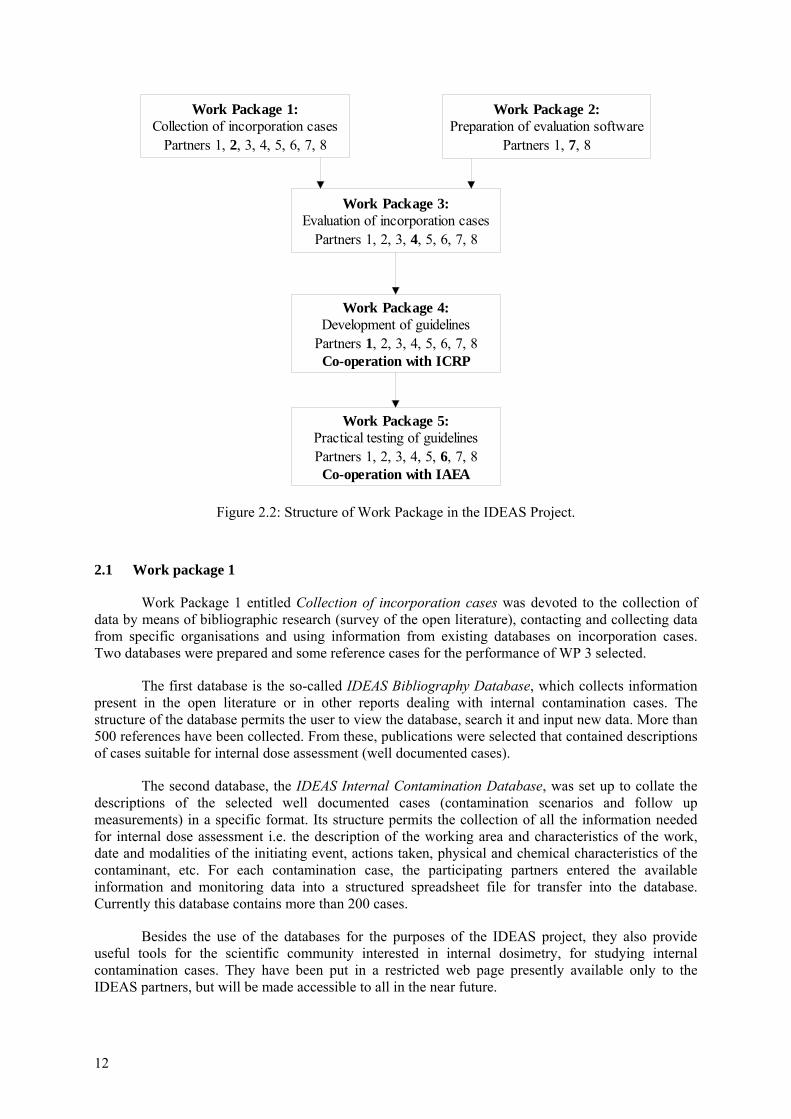
The IDEAS project was divided into Work Packages (WP), one for each of the five major tasks. The structure of the project and the interaction between Work Packages and the major co-operations are shown in Figure 2.1.
12
Work Package 1:Collection of incorporation cases
Partners 1, 2, 3, 4, 5, 6, 7, 8
Work Package 2:Preparation of evaluation software
Partners 1, 7, 8
Work Package 3:Evaluation of incorporation cases
Partners 1, 2, 3, 4, 5, 6, 7, 8
Work Package 4:Development of guidelines
Partners 1, 2, 3, 4, 5, 6, 7, 8Co-operation with ICRP
Work Package 5:Practical testing of guidelinesPartners 1, 2, 3, 4, 5, 6, 7, 8
Co-operation with IAEA
Figure 2.2: Structure of Work Package in the IDEAS Project.
2.1 Work package 1
Work Package 1 entitled Collection of incorporation cases was devoted to the collection of data by means of bibliographic research (survey of the open literature), contacting and collecting data from specific organisations and using information from existing databases on incorporation cases. Two databases were prepared and some reference cases for the performance of WP 3 selected.
The first database is the so-called IDEAS Bibliography Database, which collects information present in the open literature or in other reports dealing with internal contamination cases. The structure of the database permits the user to view the database, search it and input new data. More than 500 references have been collected. From these, publications were selected that contained descriptions of cases suitable for internal dose assessment (well documented cases).
The second database, the IDEAS Internal Contamination Database, was set up to collate the descriptions of the selected well documented cases (contamination scenarios and follow up measurements) in a specific format. Its structure permits the collection of all the information needed for internal dose assessment i.e. the description of the working area and characteristics of the work, date and modalities of the initiating event, actions taken, physical and chemical characteristics of the contaminant, etc. For each contamination case, the participating partners entered the available information and monitoring data into a structured spreadsheet file for transfer into the database. Currently this database contains more than 200 cases.
Besides the use of the databases for the purposes of the IDEAS project, they also provide useful tools for the scientific community interested in internal dosimetry, for studying internal contamination cases. They have been put in a restricted web page presently available only to the IDEAS partners, but will be made accessible to all in the near future.
IDEAS General Guidelines – June 2006
13
2.2 Work package 2
In Work Package 2 (Preparation of evaluation software) an existing computer code was to be used as a platform for testing existing methods and approaches for bioassay data interpretation and methods developed in the project. The IMIE (Individual Monitoring of the Internal Exposure, [Berkovski 2002]) computer code was chosen for evaluation of the selected reference case studies. IMIE was developed for the purposes of retrospective dosimetry. It gives to the assessor a powerful and flexible tool for the analysis and interpretation of multiple bioassay measurements. IMIE helps the assessor to make judgements about the history of intakes and corresponding doses on the basis of individual monitoring data. In particular it permits the user to review and compare simultaneously, different possible exposure condition combinations and to select the degree of automation from fully automated to completely manual. Within WP2 the IMIE code was improved and fitted to the special requirements of the IDEAS project. For example, a new optimisation algorithm of numerical deconvolution of monitoring data was developed and a new probabilistic algorithm based on statistical methods was introduced. WP2 thus provided the participants with a useful and flexible tool for the dose evaluation process of WP3.
2.3 Work package 3
In Work Package 3, Evaluation of incorporation cases, selected reference cases from WP1 were evaluated using the IMIE software provided by WP2. The current version of another computer code IMBA Expert™ [Birchall et al 2003] was also made available to the participants to support the evaluation procedures [Castellani 2004].
The choice of cases to be evaluated was made on the basis of the characteristics of the radioisotope or mixture present in the case scenario, the complexity present in the monitoring data set (e.g. multiple types of monitoring data) and special issues to be considered in the guidelines. The evaluation and analysis of selected cases was carried out in accordance with the scheduled work program of WP3. For this purpose 68 cases covering different circumstances and 17 radionuclides were selected from the IDEAS Internal Contamination Database and distributed among the partners for detailed evaluation. Fifty-two of the 68 selected cases have been evaluated, 29 of them by two or more assessors. For some cases the same assessor provided additional evaluations related to different radioisotopes.
The selected cases were evaluated using the IMIE and IMBA Expert™ codes using different assumptions and making relevant comments. The best estimates of the calculated intake and committed effective dose were given for each case, together with notes on important issues related to the guidelines. The results were presented in detail as Microsoft® Word documents and summarised in Microsoft® Excel files in a fixed format. They were collected in the IDEAS Evaluation of Cases Database established for this purpose. Ninety-five independent evaluations on 52 cases have been collected in the database. The IDEAS Evaluation of Cases Database provides possibilities, among others, to view the results of evaluations, to search within the database according to different aspects, to compare different evaluations on the same case and has links to the IDEAS Internal Contamination Database.
From the evaluations various items were identified where guidance is needed. One important set refers to the handling of the monitoring data (i.e. assessment of uncertainty on data, handling of data below the lower limit of detection, identification of rogue data etc.). Another set refers to the definition of parameter values for the evaluation of the monitoring data (i.e. definition of the time pattern of intake, identification of the pathway of intake, selection of absorption type, AMAD value, f1 values and GI tract transit times etc.). Other items include special aspects of data handling, such as the handling of early data, data affected by DTPA therapy, and 241Am ingrowth in vivo due to 241Pu decay.
14
The task of WP 3 was completed by defining the general features of the evaluation of monitoring data, thus providing a basis for the general guidelines. Nevertheless the IDEAS Evaluation of Cases Database will be open for further entries after completion of the project. Thus the IDEAS Evaluation of Cases Database of WP 3 would be together with the IDEAS Bibliography Database and the IDEAS Internal Contamination Database of Work Package 1 a powerful tool not only for the project itself but also for education and training of internal dose assessors worldwide.
2.4 Work package 4
In Work Package 4, Development of the general guidelines, the partners derived a common strategy for the evaluation of monitoring data, drafted the general guidelines and discussed it with internal dosimetry experts by means of a “virtual” workshop based on the internet (www.ideas-workshop.de). The discussion was used to improve the common strategy and the general guidelines.
Some of the IDEAS contractors were members of the ICRP Working Party on Bioassay Interpretation, which was involved in the development of an ICRP Supporting Guidance Document on The Interpretation of Bioassay Data. The aim is for this to complement the planned Occupational Intakes of Radionuclides (OIR) document that will replace ICRP Publications 30, 54, 68 and 78. Work on the ICRP Guidance Document is now carried out within the ICRP Committee 2 Task Group on Internal Dosimetry (INDOS), of which several members of the IDEAS consortium are also members. The aims of this Guidance Document are similar to those of the IDEAS project. Thus the development of both documents has been done in close cooperation, to ensure that the IDEAS guidelines and the ICRP Guidance Document are consistent with each other. There are, however, some differences in scope. In particular, the ICRP Guidance Document will relate to the forthcoming ICRP Recommendations and the revised biokinetic and dosimetric models being applied in the OIR Document (such as the Human Alimentary Tract Model, HATM), whereas the IDEAS Guidelines relate to the current models. However, the draft ICRP Guidance Document is following similar principles and a structured approach to assessments, based on the IDEAS Guidelines.
2.5 Work package 5
In Work Package 5 (Practical testing of general guidelines) the validity of the draft guidelines was to be tested by means of a dose assessment intercomparison exercise open to participants from all over the world (4th European Intercomparison Exercise on Internal Dose Assessment).
In parallel, the IAEA had planned to organise a new intercomparison exercise on internal dose assessment among the member states of the Agency. In view of the common goals, many advantages were identified in organising a joint IDEAS/IAEA exercise. This would save effort and costs for both the IDEAS project and the IAEA and it would probably result in the largest intercomparison exercise ever, providing much more information about the state of the art of internal dosimetry than an exercise on a European scale could do. The joint IDEAS/IAEA intercomparison exercise was organised in a similar way to the IDEAS Virtual Workshop on the internet (www.ideas-workshop.de).
Some 72 participants provided answers to all or some of the 6 cases proposed for evaluation. The 6 cases covered a wide range of practices in the nuclear fuel cycle and medical applications. The cases were:
1. Acute intake of HTO
2. Acute inhalation of fission products 137Cs and 90Sr
3. Intake of 60Co

IDEAS General Guidelines – June 2006
15
4. Repeated intakes of 131I
5. Intake of enriched uranium
6. Single intake of Pu radionuclides and 241Am
The results of the joint IDEAS/IAEA intercomparison exercise were discussed with the participants in a workshop organised by the IAEA in Vienna. These results have been evaluated and discussed in a report (Hurtgen 2005). Based on these discussions the IDEAS general guidelines were finalised.
The last step of WP5 was the publication of the final version of the IDEAS general guidelines and their submission to national and international bodies for approval.
3 BIOKINETIC MODELS
Knowledge of the behaviour of radioactive materials within the human body is essential for the assessment of intake or committed effective dose from measurements of activity in the body or in excreta. This Chapter gives a general description of the routes of intake of radionuclides into the body, and subsequent transfers within and out of the body. It also gives an overview of the current ICRP biokinetic models used to calculate body or organ content and daily urinary or faecal excretion at specified times after intake. See the original reports (ICRP, 1979, 1989, 1993, 1994a, 1995b, c) for details.
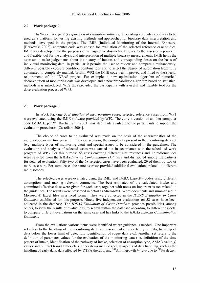
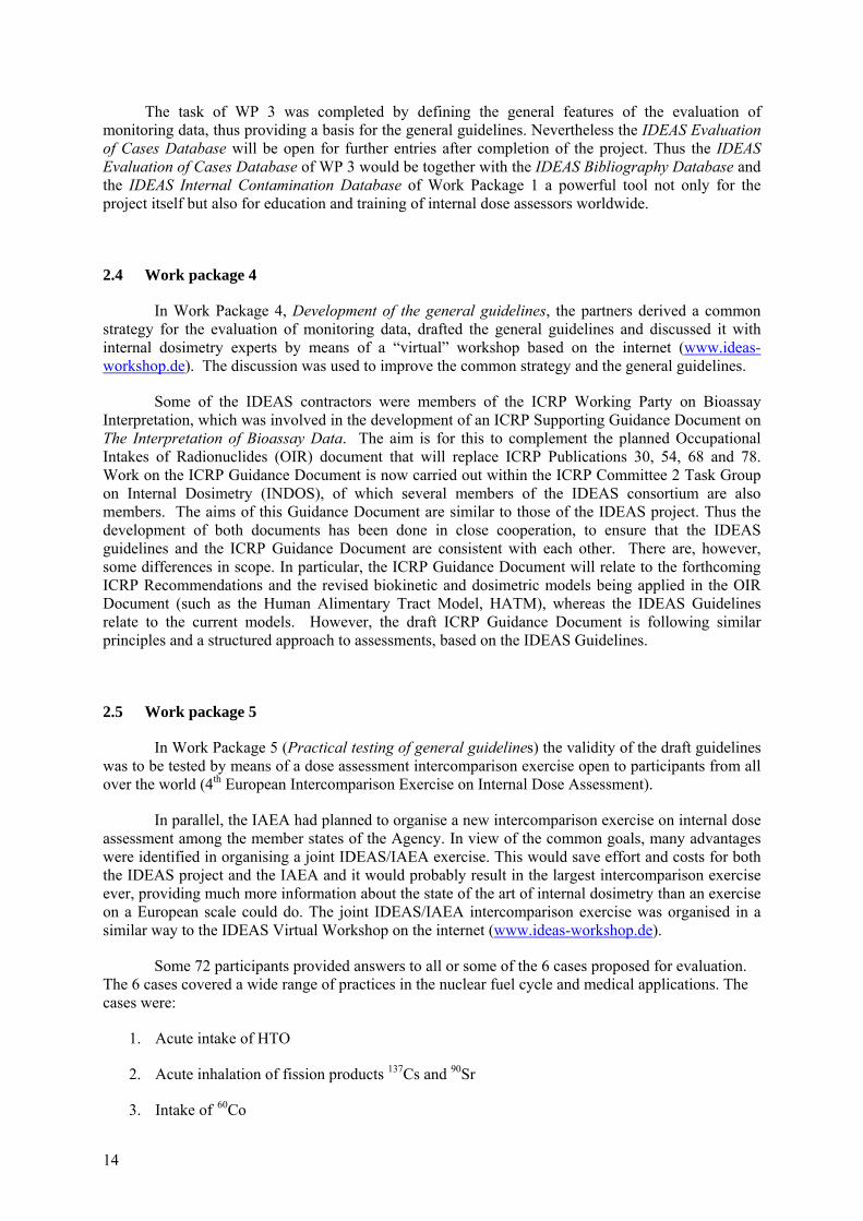
Figure 3.1 summarises the routes of intake, internal transfers, and excretion. The respiratory
tract, the gastrointestinal (GI) tract, the intact skin, and wounds are the principal routes of entry to the body. A proportion of the activity is absorbed into blood and hence body fluids. Activity reaching body fluids (transfer compartment) in this way is known as systemic material. The activity then undergoes various transfers which determine its distribution within the body and its route and rate of elimination. The distribution of systemic activity in the body can be diffuse and relatively homogeneous, e.g. with tritiated water, or localised in certain organs or tissues, e.g. with iodine (thyroid), alkaline earth metals (bone), plutonium (bone and liver).
Removal of deposited material from the body occurs principally by urinary and faecal excretion. Urinary excretion is the removal in urine of material from the plasma and extracellular fluid. Faecal excretion has two components: systemic faecal excretion which represents removal of systemic material via the GI tract; and direct faecal excretion of the material passing unabsorbed through the GI tract.
The models for the major routes of intake (inhalation and ingestion) are described in the following Sections. For some radionuclides, it is also necessary to consider direct uptake from contamination on the skin. There is no general model of entry of radionuclides through the skin because of the large variability of situations which may occur. Many factors must be taken into account: the chemical form of the compound, the location and the surface of the contaminated area as well as the physiological state of the skin. Intact skin is a good barrier against entry of a substance into the body. Generally, radionuclides do not cross the intact skin to any significant extent. However, a few elements may be transferred rapidly. The most important is tritiated water and this is the only case considered specifically by ICRP (1979; 1995c). However, absorption through skin is not included in the derivation of the dose coefficient for tritiated water (ICRP, 1995c). Iodine may also be taken up through skin, but to a lesser extent.
16
Other organs Kidney
Urinarybladder
Gastro-intestinal
tract
Inhalation Exhalation Ingestion
FaecesUrine
Extrinsic removal
Sweat
Wound
Direct absorption
Skin
Skin
Lymph nodes
Liver
Subcutaneoustissue
Transfercompartment
Respiratorytract
Figure 3.1: Summary of the main routes in intake, transfers and excretion of radionuclides in the body.
3.1 Human Respiratory Tract Model (HRTM)
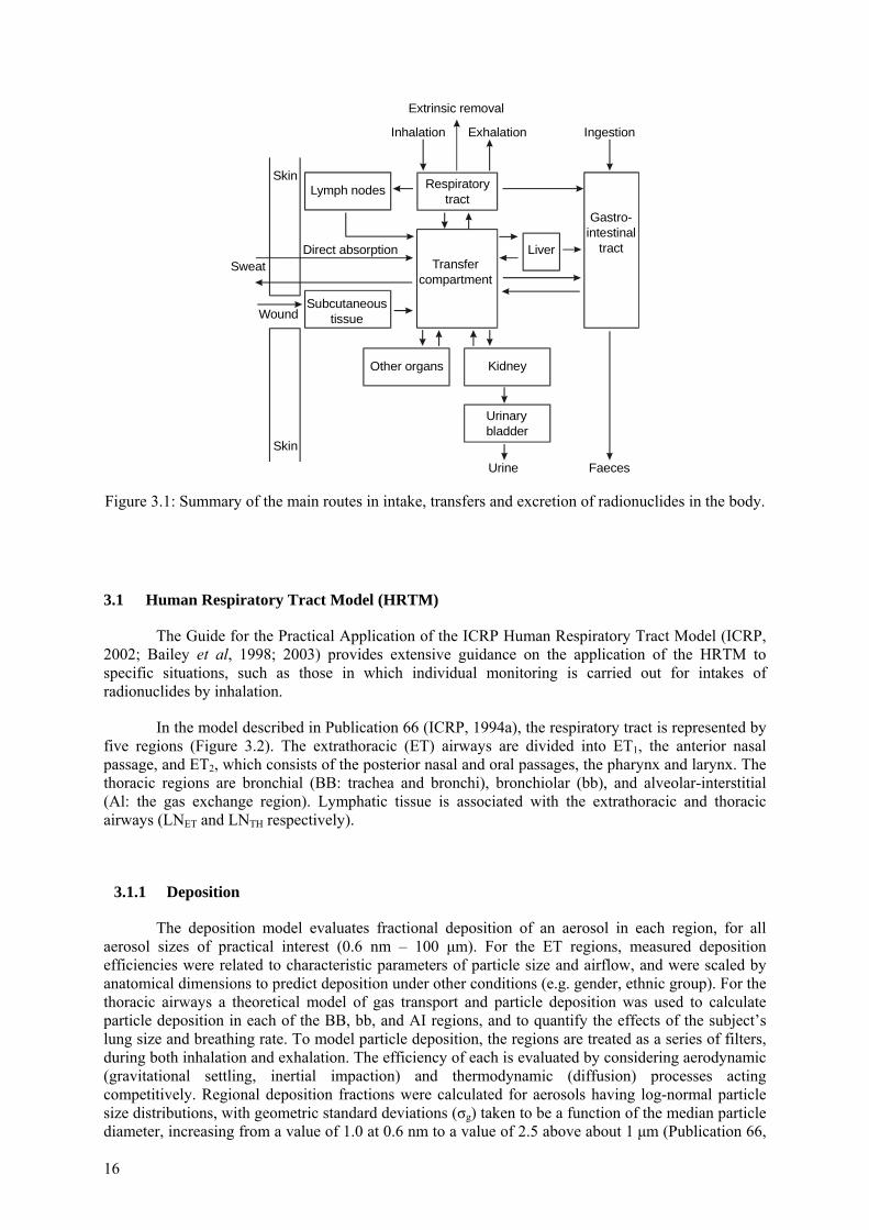
The Guide for the Practical Application of the ICRP Human Respiratory Tract Model (ICRP, 2002; Bailey et al, 1998; 2003) provides extensive guidance on the application of the HRTM to specific situations, such as those in which individual monitoring is carried out for intakes of radionuclides by inhalation.
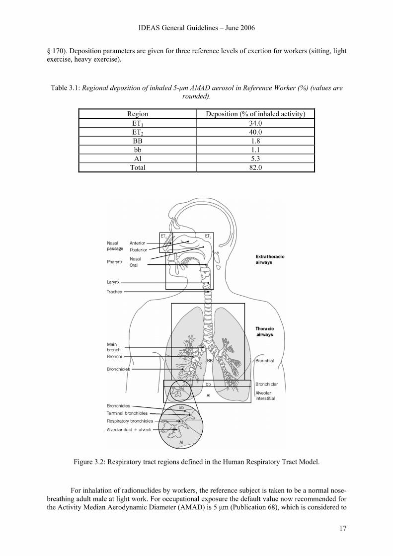
In the model described in Publication 66 (ICRP, 1994a), the respiratory tract is represented by five regions (Figure 3.2). The extrathoracic (ET) airways are divided into ET1, the anterior nasal passage, and ET2, which consists of the posterior nasal and oral passages, the pharynx and larynx. The thoracic regions are bronchial (BB: trachea and bronchi), bronchiolar (bb), and alveolar-interstitial (Al: the gas exchange region). Lymphatic tissue is associated with the extrathoracic and thoracic airways (LNET and LNTH respectively).
3.1.1 Deposition
The deposition model evaluates fractional deposition of an aerosol in each region, for all aerosol sizes of practical interest (0.6 nm – 100 μm). For the ET regions, measured deposition efficiencies were related to characteristic parameters of particle size and airflow, and were scaled by anatomical dimensions to predict deposition under other conditions (e.g. gender, ethnic group). For the thoracic airways a theoretical model of gas transport and particle deposition was used to calculate particle deposition in each of the BB, bb, and AI regions, and to quantify the effects of the subject’s lung size and breathing rate. To model particle deposition, the regions are treated as a series of filters, during both inhalation and exhalation. The efficiency of each is evaluated by considering aerodynamic (gravitational settling, inertial impaction) and thermodynamic (diffusion) processes acting competitively. Regional deposition fractions were calculated for aerosols having log-normal particle size distributions, with geometric standard deviations (σg) taken to be a function of the median particle diameter, increasing from a value of 1.0 at 0.6 nm to a value of 2.5 above about 1 μm (Publication 66,
IDEAS General Guidelines – June 2006
17
§ 170). Deposition parameters are given for three reference levels of exertion for workers (sitting, light exercise, heavy exercise).
Table 3.1: Regional deposition of inhaled 5-μm AMAD aerosol in Reference Worker (%) (values are rounded).
Region Deposition (% of inhaled activity)
ET1 34.0 ET2 40.0 BB 1.8 bb 1.1 Al 5.3
Total 82.0
Figure 3.2: Respiratory tract regions defined in the Human Respiratory Tract Model.
For inhalation of radionuclides by workers, the reference subject is taken to be a normal nose-breathing adult male at light work. For occupational exposure the default value now recommended for the Activity Median Aerodynamic Diameter (AMAD) is 5 μm (Publication 68), which is considered to
18
be more representative of workplace aerosols than the 1 μm default value adopted in Publication 30. Fractional deposition in each region of the respiratory tract of the reference worker is given in Table 3.1 for aerosols of 5 μm AMAD.
3.1.2 Clearance
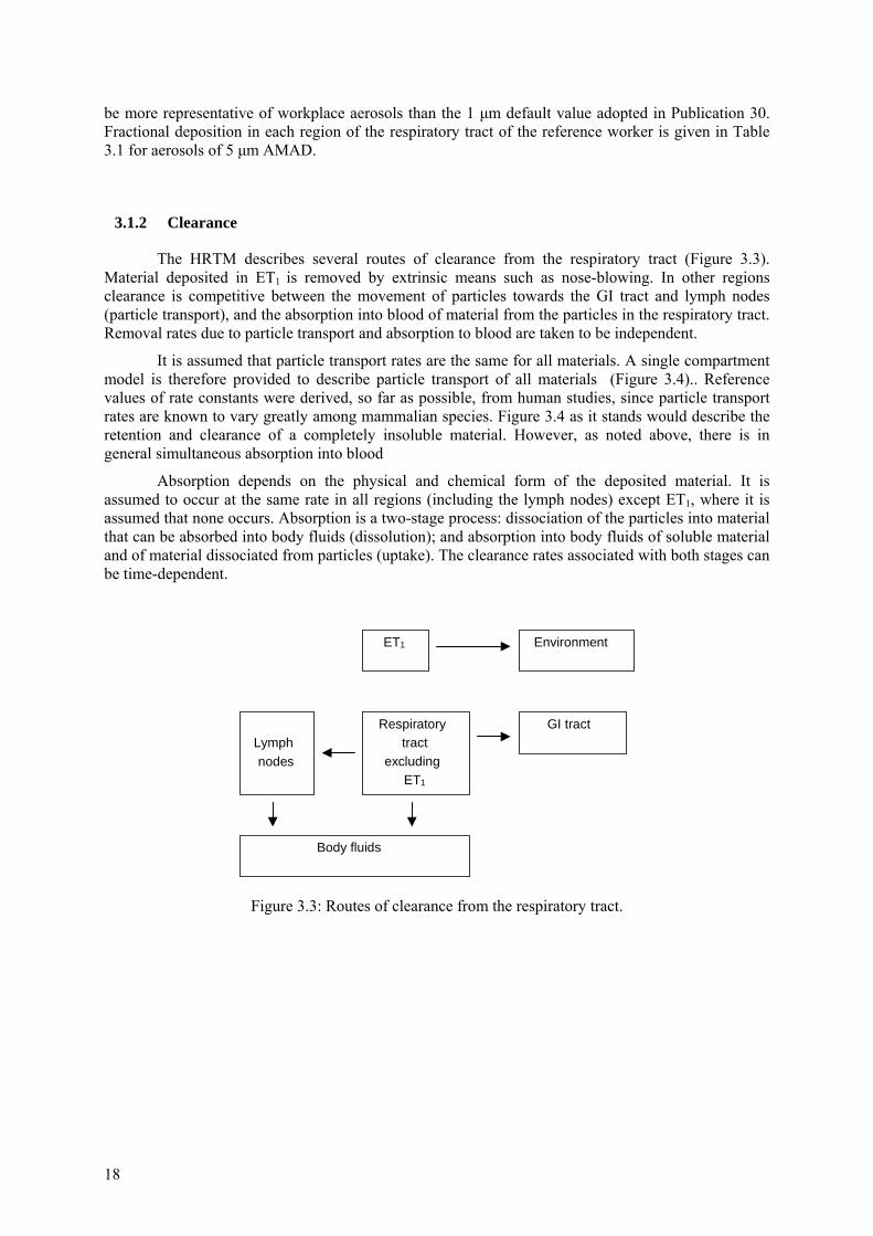
The HRTM describes several routes of clearance from the respiratory tract (Figure 3.3). Material deposited in ET1 is removed by extrinsic means such as nose-blowing. In other regions clearance is competitive between the movement of particles towards the GI tract and lymph nodes (particle transport), and the absorption into blood of material from the particles in the respiratory tract. Removal rates due to particle transport and absorption to blood are taken to be independent.
It is assumed that particle transport rates are the same for all materials. A single compartment model is therefore provided to describe particle transport of all materials (Figure 3.4).. Reference values of rate constants were derived, so far as possible, from human studies, since particle transport rates are known to vary greatly among mammalian species. Figure 3.4 as it stands would describe the retention and clearance of a completely insoluble material. However, as noted above, there is in general simultaneous absorption into blood
Absorption depends on the physical and chemical form of the deposited material. It is assumed to occur at the same rate in all regions (including the lymph nodes) except ET1, where it is assumed that none occurs. Absorption is a two-stage process: dissociation of the particles into material that can be absorbed into body fluids (dissolution); and absorption into body fluids of soluble material and of material dissociated from particles (uptake). The clearance rates associated with both stages can be time-dependent.
ET1
Lymphnodes
Respiratorytract
excludingET1
Environment
GI tract
Body fluids
Figure 3.3: Routes of clearance from the respiratory tract.
IDEAS General Guidelines – June 2006
19
Extrathoracic
LNET
ET1
ET2′0.001
Environment
GI tractETseq
1
100
Thoracic
LNTH
0.01BBseq BB2 BB1
bbseq0.01
bb2 bb1
AI3 AI2 AI1
0.001 0.020.0001
0.00002
2
10
0.03
0.03
Anteriornasal
Naso-oropharynx/larynx
Bronchi
Bronchioles
Alveolarinterstitial
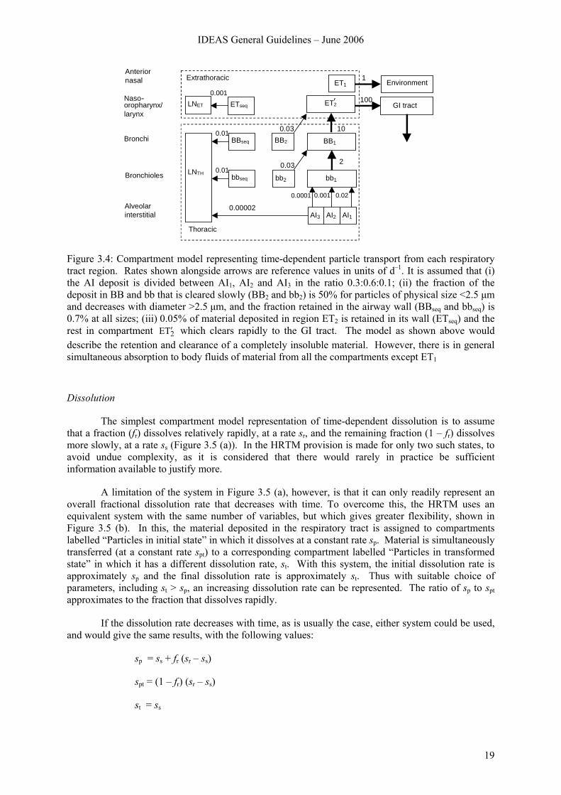
Figure 3.4: Compartment model representing time-dependent particle transport from each respiratory tract region. Rates shown alongside arrows are reference values in units of d–1. It is assumed that (i) the AI deposit is divided between AI1, AI2 and AI3 in the ratio 0.3:0.6:0.1; (ii) the fraction of the deposit in BB and bb that is cleared slowly (BB2 and bb2) is 50% for particles of physical size <2.5 μm and decreases with diameter >2.5 μm, and the fraction retained in the airway wall (BBseq and bbseq) is 0.7% at all sizes; (iii) 0.05% of material deposited in region ET2 is retained in its wall (ETseq) and the rest in compartment 2TE ′ which clears rapidly to the GI tract. The model as shown above would describe the retention and clearance of a completely insoluble material. However, there is in general simultaneous absorption to body fluids of material from all the compartments except ET1
Dissolution
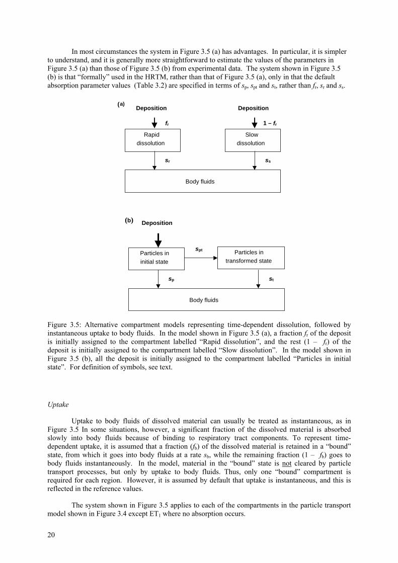
The simplest compartment model representation of time-dependent dissolution is to assume that a fraction (fr) dissolves relatively rapidly, at a rate sr, and the remaining fraction (1 – fr) dissolves more slowly, at a rate ss (Figure 3.5 (a)). In the HRTM provision is made for only two such states, to avoid undue complexity, as it is considered that there would rarely in practice be sufficient information available to justify more.
A limitation of the system in Figure 3.5 (a), however, is that it can only readily represent an overall fractional dissolution rate that decreases with time. To overcome this, the HRTM uses an equivalent system with the same number of variables, but which gives greater flexibility, shown in Figure 3.5 (b). In this, the material deposited in the respiratory tract is assigned to compartments labelled “Particles in initial state” in which it dissolves at a constant rate sp. Material is simultaneously transferred (at a constant rate spt) to a corresponding compartment labelled “Particles in transformed state” in which it has a different dissolution rate, st. With this system, the initial dissolution rate is approximately sp and the final dissolution rate is approximately st. Thus with suitable choice of parameters, including st > sp, an increasing dissolution rate can be represented. The ratio of sp to spt approximates to the fraction that dissolves rapidly.
If the dissolution rate decreases with time, as is usually the case, either system could be used, and would give the same results, with the following values:
sp = ss + fr (sr – ss)
spt = (1 – fr) (sr – ss)
st = ss
20
In most circumstances the system in Figure 3.5 (a) has advantages. In particular, it is simpler to understand, and it is generally more straightforward to estimate the values of the parameters in Figure 3.5 (a) than those of Figure 3.5 (b) from experimental data. The system shown in Figure 3.5 (b) is that “formally” used in the HRTM, rather than that of Figure 3.5 (a), only in that the default absorption parameter values (Table 3.2) are specified in terms of sp, spt and st, rather than fr, sr and ss.
1 – frfr
Rapiddissolution
Slowdissolution
Body fluids
sssr
Deposition Deposition(a)
Particles ininitial state
Particles intransformed state
Body fluids
Deposition
spt
sp st
(b)
Figure 3.5: Alternative compartment models representing time-dependent dissolution, followed by instantaneous uptake to body fluids. In the model shown in Figure 3.5 (a), a fraction fr of the deposit is initially assigned to the compartment labelled “Rapid dissolution”, and the rest (1 – fr) of the deposit is initially assigned to the compartment labelled “Slow dissolution”. In the model shown in Figure 3.5 (b), all the deposit is initially assigned to the compartment labelled “Particles in initial state”. For definition of symbols, see text.
Uptake
Uptake to body fluids of dissolved material can usually be treated as instantaneous, as in Figure 3.5 In some situations, however, a significant fraction of the dissolved material is absorbed slowly into body fluids because of binding to respiratory tract components. To represent time-dependent uptake, it is assumed that a fraction (fb) of the dissolved material is retained in a “bound” state, from which it goes into body fluids at a rate sb, while the remaining fraction (1 – fb) goes to body fluids instantaneously. In the model, material in the “bound” state is not cleared by particle transport processes, but only by uptake to body fluids. Thus, only one “bound” compartment is required for each region. However, it is assumed by default that uptake is instantaneous, and this is reflected in the reference values.
The system shown in Figure 3.5 applies to each of the compartments in the particle transport model shown in Figure 3.4 except ET1 where no absorption occurs.
IDEAS General Guidelines – June 2006
21
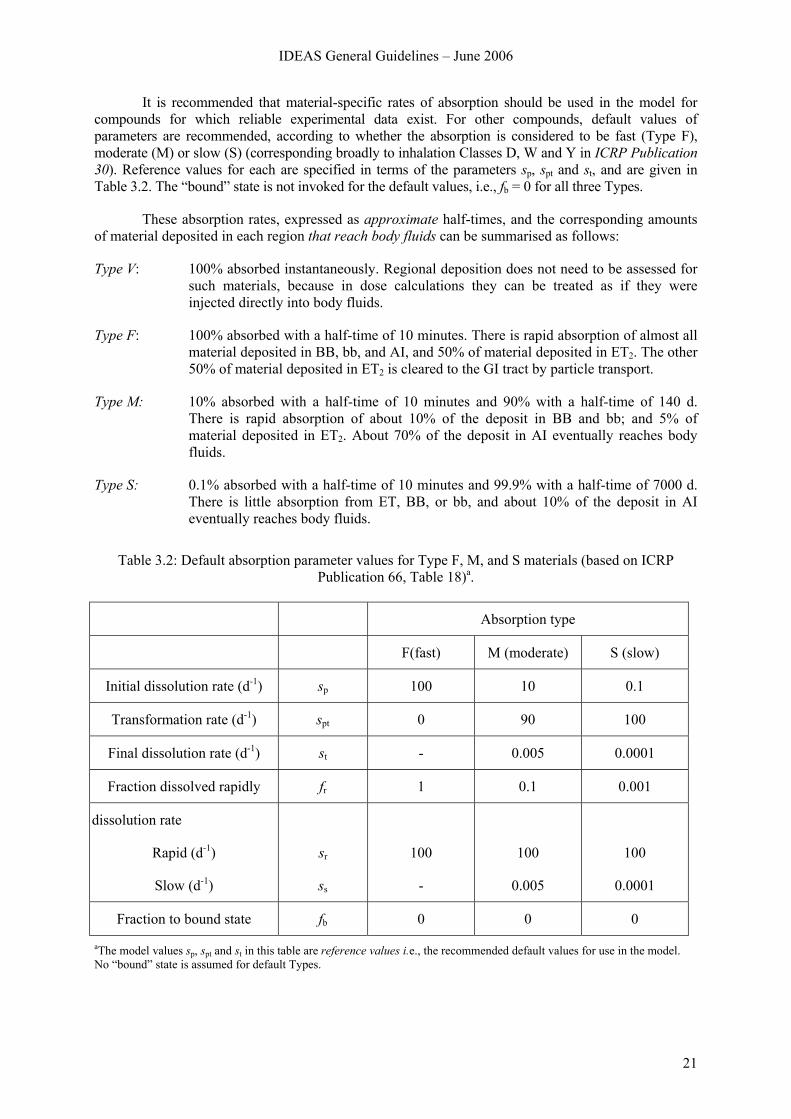
It is recommended that material-specific rates of absorption should be used in the model for compounds for which reliable experimental data exist. For other compounds, default values of parameters are recommended, according to whether the absorption is considered to be fast (Type F), moderate (M) or slow (S) (corresponding broadly to inhalation Classes D, W and Y in ICRP Publication 30). Reference values for each are specified in terms of the parameters sp, spt and st, and are given in Table 3.2. The “bound” state is not invoked for the default values, i.e., fb = 0 for all three Types.
These absorption rates, expressed as approximate half-times, and the corresponding amounts of material deposited in each region that reach body fluids can be summarised as follows:
Type V: 100% absorbed instantaneously. Regional deposition does not need to be assessed for such materials, because in dose calculations they can be treated as if they were injected directly into body fluids.
Type F: 100% absorbed with a half-time of 10 minutes. There is rapid absorption of almost all material deposited in BB, bb, and AI, and 50% of material deposited in ET2. The other 50% of material deposited in ET2 is cleared to the GI tract by particle transport.
Type M: 10% absorbed with a half-time of 10 minutes and 90% with a half-time of 140 d. There is rapid absorption of about 10% of the deposit in BB and bb; and 5% of material deposited in ET2. About 70% of the deposit in AI eventually reaches body fluids.
Type S: 0.1% absorbed with a half-time of 10 minutes and 99.9% with a half-time of 7000 d. There is little absorption from ET, BB, or bb, and about 10% of the deposit in AI eventually reaches body fluids.
Table 3.2: Default absorption parameter values for Type F, M, and S materials (based on ICRP
Publication 66, Table 18)a.
Absorption type
F(fast) M (moderate) S (slow)
Initial dissolution rate (d-1) sp 100 10 0.1
Transformation rate (d-1) spt 0 90 100
Final dissolution rate (d-1) st - 0.005 0.0001
Fraction dissolved rapidly fr 1 0.1 0.001
dissolution rate
Rapid (d-1)
Slow (d-1)
sr
ss
100
-
100
0.005
100
0.0001
Fraction to bound state fb 0 0 0
aThe model values sp, spt and st in this table are reference values i.e., the recommended default values for use in the model. No “bound” state is assumed for default Types.
22
For absorption Types F, M, and S, all the material deposited in ET1 is removed by extrinsic means. Most of the deposited material that is not absorbed is cleared to the GI tract by particle transport. The small amounts transferred to lymph nodes continue to be absorbed into body fluids at the same rate as in the respiratory tract.
The choice between the default absorption Types F, M, and S is the most common one to be made in applying the HRTM.
ICRP Publication 66 does not give criteria for assigning compounds to absorption Types on the basis of experimental results. Guidance on the choice of default Type, and hence of the reference values of the absorption parameters, is given in ICRP Publication 68 for occupational exposure and in ICRP Publication 71 for exposure of the public (for the 31 elements covered).
In ICRP Publication 68, which gives inhalation dose coefficients for workers, compounds for which clearance was previously given as “inhalation Class” D, W or Y in ICRP Publication 30, were generally assigned to “absorption Type” F, M or S respectively. A listing of the classifications is given in Table 3.3 (ICRP Publication 68, Annexe F).
Criteria for assigning compounds to absorption Types on the basis of experimental results were developed in ICRP Publication 71. They are described, with examples of their application, in ICRP 2002 (Annexe C) which is based on ICRP Publication 71, Annexe D.
3.1.3 Gases and Vapours
For radionuclides inhaled as particles (solid or liquid) the HRTM assumes that total and regional depositions in the respiratory tract are determined only by the size distribution of the aerosol particles. The situation is different for gases and vapours, for which deposition in the respiratory tract depends entirely on the chemical form. In this context, deposition refers to how much of the material in the inhaled air remains behind after exhalation. Almost all inhaled gas molecules contact airway surfaces, but usually return to the air unless they dissolve in, or react with, the surface lining. The fraction of an inhaled gas or vapour that is deposited in each region thus depends on its solubility and reactivity.
As a general default approach the HRTM assigns gases and vapours to three classes, on the basis of the initial pattern of respiratory tract deposition (ICRP Publication 66, Chapter 6):
• Class SR-0 insoluble and non-reactive: negligible deposition in the respiratory tract.
• Class SR-1 soluble or reactive: deposition may occur throughout the respiratory tract. In the absence of information 100% total deposition is assumed, with the following distribution: 10% ET1, 20% ET2, 10% BB, 20% bb and 40% AI (ICRP Publication 66, Paragraph 221).
• Class SR-2 highly soluble or reactive: 100% deposition in the extrathoracic airways (ET2).
For Classes SR-1 and SR-2, subsequent retention in the respiratory tract and absorption to body fluids are determined by the chemical properties of the specific gas or vapour. By default, reference values for an Absorption Type are used, normally Type F (absorption rate 100 d-1) or Type V (instantaneous absorption).
Guidance on many of the more-commonly encountered radioactive gases and vapours is given in ICRP Publications 68 and 71 for workers and the public, respectively. For convenience, most of it is brought together in ICRP (2002) in which some additional guidance is given.
IDEAS General Guidelines – June 2006
23
3.2 Model for the gastrointestinal tract
Material may reach the GI tract directly by ingestion, by transfer from the respiratory tract as described above, or by transfer from other body organs. The GI tract model defined in ICRP Publication 30 Part 1 (ICRP, 1979) was used in ICRP Publications 67, 68, 69, 71, 72 and 78 to describe the behaviour of radionuclides in the GI tract, and to calculate doses from radionuclides in the contents of the GI tract. In the near future this model will be replaced by the Human Alimentary Tract Model, HATM, (Métivier, 2003).
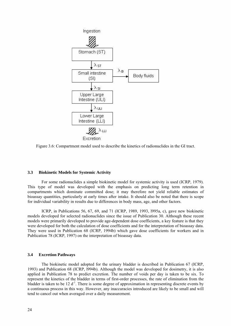
In the current (ICRP 30) model, the GI tract is represented by four compartments, each of which clears to the next at a constant rate (Figure 3.6). Material from the mouth or ET2 enters the stomach (ST), and passes in turn to the small intestine (SI), upper large intestine (ULI), and lower large intestine (LLI), from which it is excreted in faeces. The rates of transfer of material are taken to be independent of the material, and of the age and sex of the subject.
3.2.1 Stomach
The mean residence time is taken to be 1 hour. It is assumed that no absorption takes place from the stomach and that material passes on to the small intestine.
3.2.2 Small intestine
The mean residence time is taken to be 4 hours. This is the compartment from which absorption takes place. It is normal to quantify absorption by using the ‘f1 value’ which is the fraction of material reaching body fluids following ingestion.
λ + λ
λSIB
B1 = f
λB = rate constant for transfer from SI to body fluids
λSI = rate constant for transfer from small intestine to upper large intestine.
Values of f1 currently recommended by ICRP for occupational exposure are given in Table 3.3.
3.2.3 Upper large intestine
The mean residence time is taken to be 13 hours. In practice water is absorbed from the gut content in the upper large intestine.
3.2.4 Lower large intestine
The mean residence time is taken to be 24 hours. The lower large intestine may be the most heavily irradiated organ if the gut uptake factor is low.
24
Figure 3.6: Compartment model used to describe the kinetics of radionuclides in the GI tract.
3.3 Biokinetic Models for Systemic Activity
For some radionuclides a simple biokinetic model for systemic activity is used (ICRP, 1979). This type of model was developed with the emphasis on predicting long term retention in compartments which dominate committed dose; it may therefore not yield reliable estimates of bioassay quantities, particularly at early times after intake. It should also be noted that there is scope for individual variability in results due to differences in body mass, age, and other factors.
ICRP, in Publications 56, 67, 69, and 71 (ICRP, 1989, 1993, l995a, c), gave new biokinetic models developed for selected radionuclides since the issue of Publication 30. Although these recent models were primarily developed to provide age-dependent dose coefficients, a key feature is that they were developed for both the calculation of dose coefficients and for the interpretation of bioassay data. They were used in Publication 68 (ICRP, 1994b) which gave dose coefficients for workers and in Publication 78 (ICRP, 1997) on the interpretation of bioassay data.
3.4 Excretion Pathways
The biokinetic model adopted for the urinary bladder is described in Publication 67 (ICRP, 1993) and Publication 68 (ICRP, l994b). Although the model was developed for dosimetry, it is also applied in Publication 78 to predict excretion. The number of voids per day is taken to be six. To represent the kinetics of the bladder in terms of first-order processes, the rate of elimination from the bladder is taken to be 12 d-1. There is some degree of approximation in representing discrete events by a continuous process in this way. However, any inaccuracies introduced are likely to be small and will tend to cancel out when averaged over a daily measurement.
IDEAS General Guidelines – June 2006
25
The activity present in the upper and lower large intestine includes material which entered the GI tract from the systemic circulation into the upper large intestine.
For bioassay interpretation it should be remembered that the transit time through the GI tract is subject to particularly large inter (and intra-) subject variations. Moreover, while for ease of computation transit through the GI tract is represented by a series of compartments that clear exponentially, in practice, the movement is more like “slug” flow. It is therefore unlikely that individual daily faecal clearance measurements in the first few days after intake will follow the predicted pattern, and so it is best to consider cumulative excretion over the first few days.
The rate of loss of systemic activity from the body through the routes of excretion is given explicitly in some of the ICRP biokinetic models. For others, it was necessary to partition the excreted systemic activity between urine and faeces according to a constant ratio (ICRP Publication 68, Table 6).
3.5 Biokinetic functions
The ICRP biokinetic models outlined above allow for the calculation of biokinetic functions for the interpretation of incorporation monitoring data, i.e. the time dependence of the activity content of the whole body or an organ under investigation (retention function) or the time dependence of the activity excreted via urine or faeces (excretion function). Typically the biokinetic functions are calculated for a single intake by inhalation, ingestion and injection. For protracted intakes the biokinetic functions should be integrated (if given as a continuous function) or obtained by superposition (if tabulated at discrete times) (see Section 4.1.3).
There are a number of publications which give biokinetic functions for radionuclides using the current ICRP Models, including: ICRP (1997); Phipps et al (1998); Potter (2002); Ishigure et al (2003); IAEA (2004).
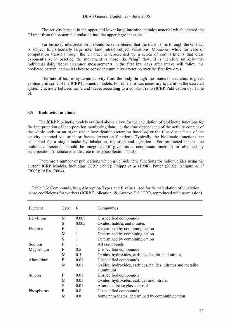
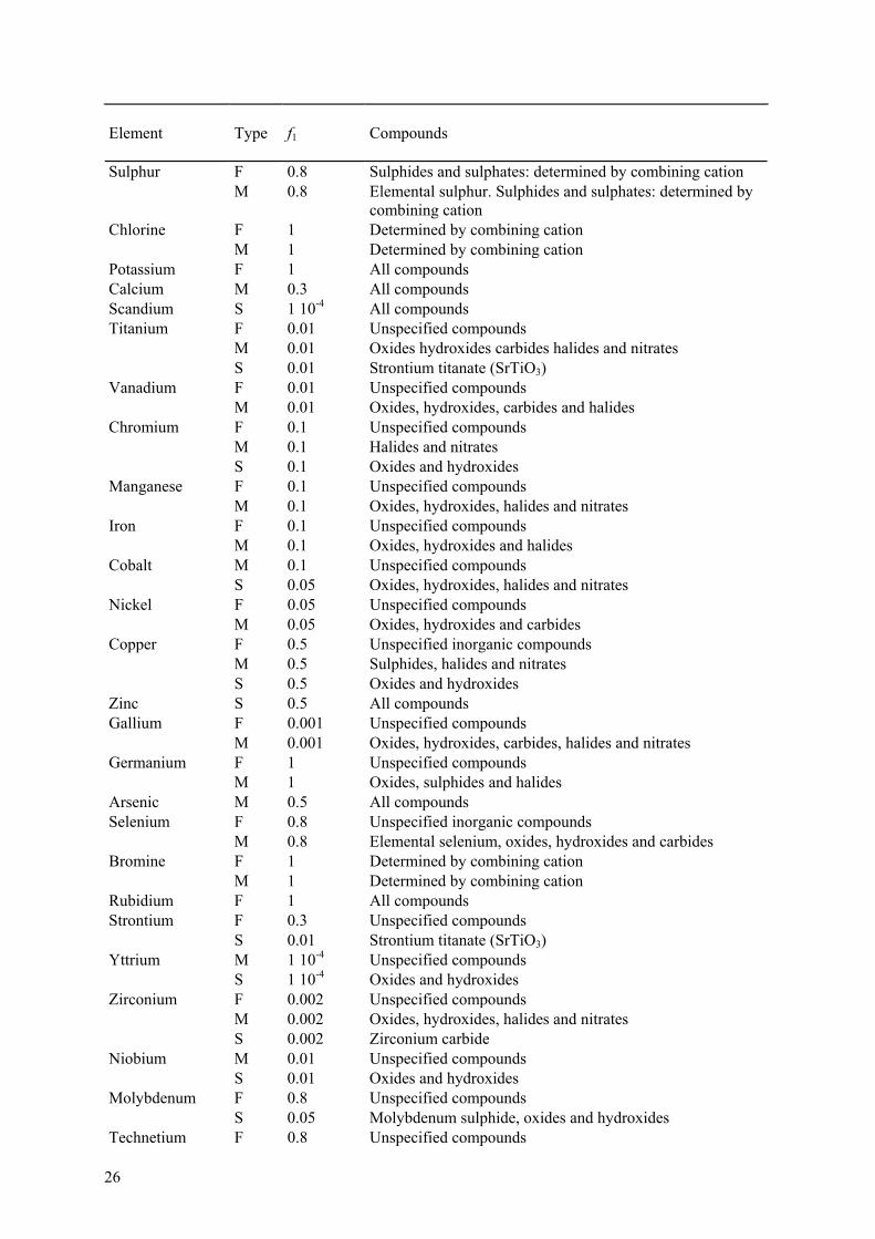
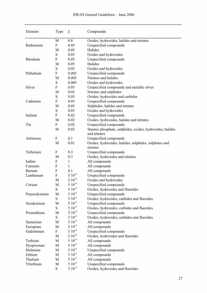
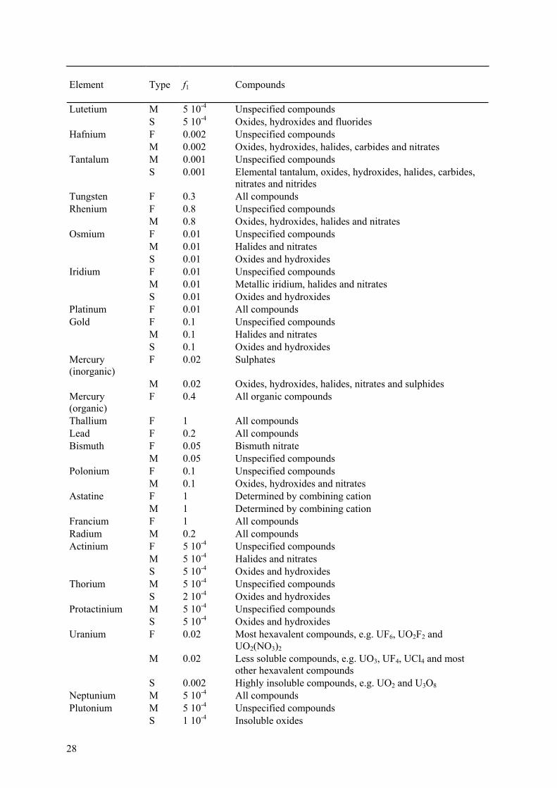
Table 3.3: Compounds, lung Absorption Types and f1 values used for the calculation of inhalation dose coefficients for workers (ICRP Publication 68, Annexe F © ICRP, reproduced with permission)
Element
Type
f1
Compounds
Beryllium M 0.005 Unspecified compounds S 0.005 Oxides, halides and nitrates Fluorine F 1 Determined by combining cation M 1 Determined by combining cation S 1 Determined by combining cation Sodium F 1 All compounds Magnesium F 0.5 Unspecified compounds M 0.5 Oxides, hydroxides, carbides, halides and nitrates Aluminium F 0.01 Unspecified compounds M 0.01 Oxides, hydroxides, carbides, halides, nitrates and metallic
aluminium Silicon F 0.01 Unspecified compounds M 0.01 Oxides, hydroxides, carbides and nitrates S 0.01 Aluminosilicate glass aerosol Phosphorus F 0.8 Unspecified compounds M 0.8 Some phosphates: determined by combining cation
26
Element
Type
f1
Compounds
Sulphur F 0.8 Sulphides and sulphates: determined by combining cation M 0.8 Elemental sulphur. Sulphides and sulphates: determined by
combining cation Chlorine F 1 Determined by combining cation M 1 Determined by combining cation Potassium F 1 All compounds Calcium M 0.3 All compounds Scandium S 1 10-4 All compounds Titanium F 0.01 Unspecified compounds M 0.01 Oxides hydroxides carbides halides and nitrates S 0.01 Strontium titanate (SrTiO3) Vanadium F 0.01 Unspecified compounds M 0.01 Oxides, hydroxides, carbides and halides Chromium F 0.1 Unspecified compounds M 0.1 Halides and nitrates S 0.1 Oxides and hydroxides Manganese F 0.1 Unspecified compounds M 0.1 Oxides, hydroxides, halides and nitrates Iron F 0.1 Unspecified compounds M 0.1 Oxides, hydroxides and halides Cobalt M 0.1 Unspecified compounds S 0.05 Oxides, hydroxides, halides and nitrates Nickel F 0.05 Unspecified compounds M 0.05 Oxides, hydroxides and carbides Copper F 0.5 Unspecified inorganic compounds M 0.5 Sulphides, halides and nitrates S 0.5 Oxides and hydroxides Zinc S 0.5 All compounds Gallium F 0.001 Unspecified compounds M 0.001 Oxides, hydroxides, carbides, halides and nitrates Germanium F 1 Unspecified compounds M 1 Oxides, sulphides and halides Arsenic M 0.5 All compounds Selenium F 0.8 Unspecified inorganic compounds M 0.8 Elemental selenium, oxides, hydroxides and carbides Bromine F 1 Determined by combining cation M 1 Determined by combining cation Rubidium F 1 All compounds Strontium F 0.3 Unspecified compounds S 0.01 Strontium titanate (SrTiO3) Yttrium M 1 10-4 Unspecified compounds S 1 10-4 Oxides and hydroxides Zirconium F 0.002 Unspecified compounds M 0.002 Oxides, hydroxides, halides and nitrates S 0.002 Zirconium carbide Niobium M 0.01 Unspecified compounds S 0.01 Oxides and hydroxides Molybdenum F 0.8 Unspecified compounds S 0.05 Molybdenum sulphide, oxides and hydroxides Technetium F 0.8 Unspecified compounds
IDEAS General Guidelines – June 2006
27
Element
Type
f1
Compounds
M 0.8 Oxides, hydroxides, halides and nitrates Ruthenium F 0.05 Unspecified compounds M 0.05 Halides S 0.05 Oxides and hydroxides Rhodium F 0.05 Unspecified compounds M 0.05 Halides S 0.05 Oxides and hydroxides Palladium F 0.005 Unspecified compounds M 0.005 Nitrates and halides S 0.005 Oxides and hydroxides Silver F 0.05 Unspecified compounds and metallic silver M 0.05 Nitrates and sulphides S 0.05 Oxides, hydroxides and carbides Cadmium F 0.05 Unspecified compounds M 0.05 Sulphides, halides and nitrates S 0.05 Oxides and hydroxides Indium F 0.02 Unspecified compounds M 0.02 Oxides, hydroxides, halides and nitrates Tin F 0.02 Unspecified compounds M 0.02 Stannic phosphate, sulphides, oxides, hydroxides, halides
and nitrates Antimony F 0.1 Unspecified compounds M 0.01 Oxides, hydroxides, halides, sulphides, sulphates and
nitrates Tellurium F 0.3 Unspecified compounds M 0.3 Oxides, hydroxides and nitrates Iodine F 1 All compounds Caesium F 1 All compounds Barium F 0.1 All compounds Lanthanum F 5 10-4 Unspecified compounds M 5 10-4 Oxides and hydroxides Cerium M 5 10-4 Unspecified compounds S 5 10-4 Oxides, hydroxides and fluorides Praseodymium M 5 10-4 Unspecified compounds S 5 10-4 Oxides, hydroxides, carbides and fluorides Neodymium M 5 10-4 Unspecified compounds S 5 10-4 Oxides, hydroxides, carbides and fluorides Promethium M 5 10-4 Unspecified compounds S 5 10-4 Oxides, hydroxides, carbides and fluorides Samarium M 5 10-4 All compounds Europium M 5 10-4 All compounds Gadolinium F 5 10-4 Unspecified compounds M 5 10-4 Oxides, hydroxides and fluorides Terbium M 5 10-4 All compounds Dysprosium M 5 10-4 All compounds Holmium M 5 10-4 Unspecified compounds Erbium M 5 10-4 All compounds Thulium M 5 10-4 All compounds Ytterbium M 5 10-4 Unspecified compounds S 5 10-4 Oxides, hydroxides and fluorides
28
Element
Type
f1
Compounds
Lutetium M 5 10-4 Unspecified compounds S 5 10-4 Oxides, hydroxides and fluorides Hafnium F 0.002 Unspecified compounds M 0.002 Oxides, hydroxides, halides, carbides and nitrates Tantalum M 0.001 Unspecified compounds S 0.001 Elemental tantalum, oxides, hydroxides, halides, carbides,
nitrates and nitrides Tungsten F 0.3 All compounds Rhenium F 0.8 Unspecified compounds M 0.8 Oxides, hydroxides, halides and nitrates Osmium F 0.01 Unspecified compounds M 0.01 Halides and nitrates S 0.01 Oxides and hydroxides Iridium F 0.01 Unspecified compounds M 0.01 Metallic iridium, halides and nitrates S 0.01 Oxides and hydroxides Platinum F 0.01 All compounds Gold F 0.1 Unspecified compounds M 0.1 Halides and nitrates S 0.1 Oxides and hydroxides Mercury (inorganic)
F 0.02 Sulphates
M 0.02 Oxides, hydroxides, halides, nitrates and sulphides Mercury (organic)
F 0.4 All organic compounds
Thallium F 1 All compounds Lead F 0.2 All compounds Bismuth F 0.05 Bismuth nitrate M 0.05 Unspecified compounds Polonium F 0.1 Unspecified compounds M 0.1 Oxides, hydroxides and nitrates Astatine F 1 Determined by combining cation M 1 Determined by combining cation Francium F 1 All compounds Radium M 0.2 All compounds Actinium F 5 10-4 Unspecified compounds M 5 10-4 Halides and nitrates S 5 10-4 Oxides and hydroxides Thorium M 5 10-4 Unspecified compounds S 2 10-4 Oxides and hydroxides Protactinium M 5 10-4 Unspecified compounds S 5 10-4 Oxides and hydroxides Uranium F 0.02 Most hexavalent compounds, e.g. UF6, UO2F2 and
UO2(NO3)2 M 0.02 Less soluble compounds, e.g. UO3, UF4, UCl4 and most
other hexavalent compounds S 0.002 Highly insoluble compounds, e.g. UO2 and U3O8 Neptunium M 5 10-4 All compounds Plutonium M 5 10-4 Unspecified compounds S 1 10-4 Insoluble oxides
IDEAS General Guidelines – June 2006
29
Element
Type
f1
Compounds
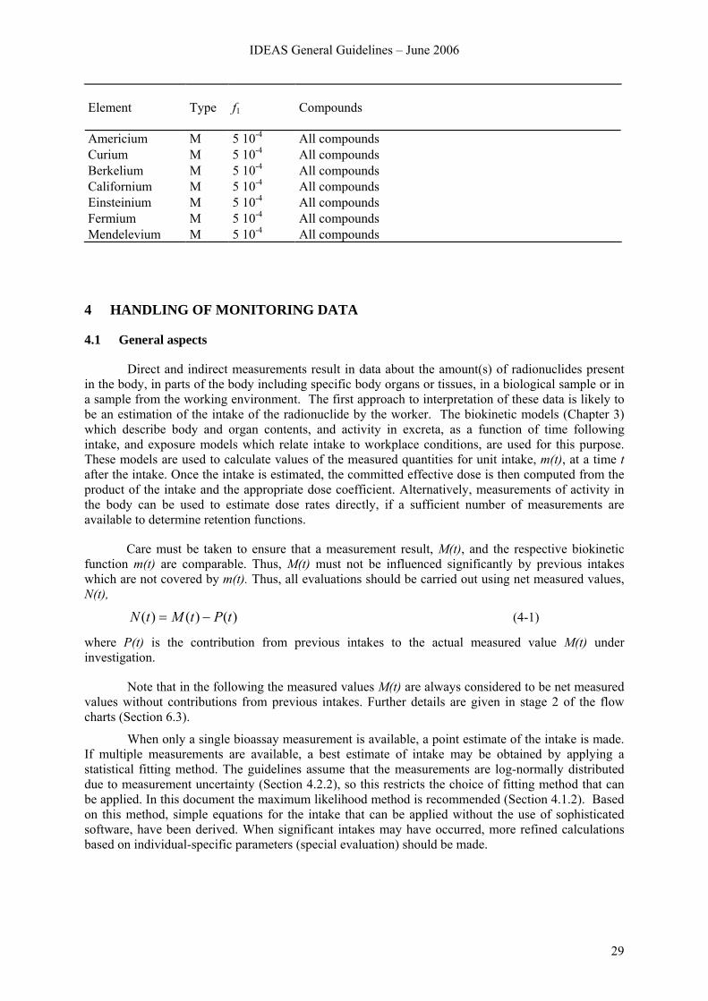
Americium M 5 10-4 All compounds Curium M 5 10-4 All compounds Berkelium M 5 10-4 All compounds Californium M 5 10-4 All compounds Einsteinium M 5 10-4 All compounds Fermium M 5 10-4 All compounds Mendelevium M 5 10-4 All compounds
4 HANDLING OF MONITORING DATA
4.1 General aspects
Direct and indirect measurements result in data about the amount(s) of radionuclides present in the body, in parts of the body including specific body organs or tissues, in a biological sample or in a sample from the working environment. The first approach to interpretation of these data is likely to be an estimation of the intake of the radionuclide by the worker. The biokinetic models (Chapter 3) which describe body and organ contents, and activity in excreta, as a function of time following intake, and exposure models which relate intake to workplace conditions, are used for this purpose. These models are used to calculate values of the measured quantities for unit intake, m(t), at a time t after the intake. Once the intake is estimated, the committed effective dose is then computed from the product of the intake and the appropriate dose coefficient. Alternatively, measurements of activity in the body can be used to estimate dose rates directly, if a sufficient number of measurements are available to determine retention functions.
Care must be taken to ensure that a measurement result, M(t), and the respective biokinetic function m(t) are comparable. Thus, M(t) must not be influenced significantly by previous intakes which are not covered by m(t). Thus, all evaluations should be carried out using net measured values, N(t),
)()()( tPtMtN −= (4-1)
where P(t) is the contribution from previous intakes to the actual measured value M(t) under investigation.
Note that in the following the measured values M(t) are always considered to be net measured values without contributions from previous intakes. Further details are given in stage 2 of the flow charts (Section 6.3).
When only a single bioassay measurement is available, a point estimate of the intake is made. If multiple measurements are available, a best estimate of intake may be obtained by applying a statistical fitting method. The guidelines assume that the measurements are log-normally distributed due to measurement uncertainty (Section 4.2.2), so this restricts the choice of fitting method that can be applied. In this document the maximum likelihood method is recommended (Section 4.1.2). Based on this method, simple equations for the intake that can be applied without the use of sophisticated software, have been derived. When significant intakes may have occurred, more refined calculations based on individual-specific parameters (special evaluation) should be made.
30
4.1.1 Single data point
4.1.1.1 Special monitoring
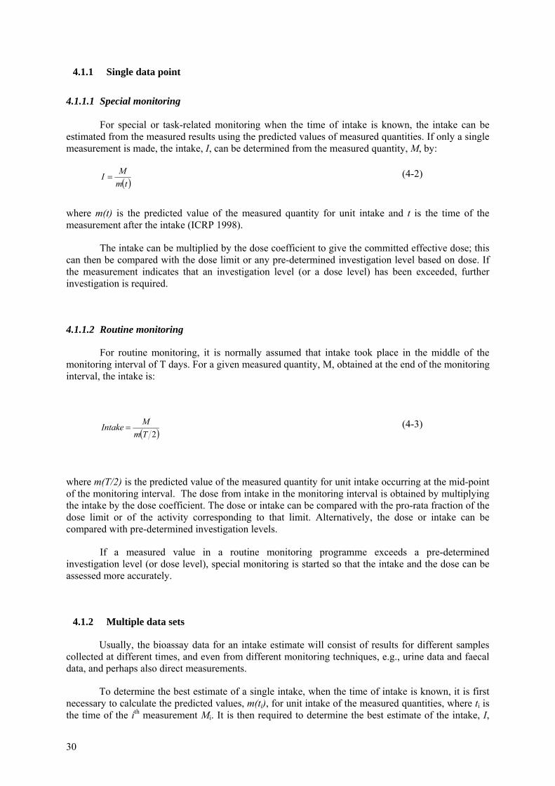
For special or task-related monitoring when the time of intake is known, the intake can be estimated from the measured results using the predicted values of measured quantities. If only a single measurement is made, the intake, I, can be determined from the measured quantity, M, by:
( )tmMI = (4-2)
where m(t) is the predicted value of the measured quantity for unit intake and t is the time of the measurement after the intake (ICRP 1998).
The intake can be multiplied by the dose coefficient to give the committed effective dose; this can then be compared with the dose limit or any pre-determined investigation level based on dose. If the measurement indicates that an investigation level (or a dose level) has been exceeded, further investigation is required.
4.1.1.2 Routine monitoring
For routine monitoring, it is normally assumed that intake took place in the middle of the monitoring interval of T days. For a given measured quantity, M, obtained at the end of the monitoring interval, the intake is:
( )2TmMIntake = (4-3)
where m(T/2) is the predicted value of the measured quantity for unit intake occurring at the mid-point of the monitoring interval. The dose from intake in the monitoring interval is obtained by multiplying the intake by the dose coefficient. The dose or intake can be compared with the pro-rata fraction of the dose limit or of the activity corresponding to that limit. Alternatively, the dose or intake can be compared with pre-determined investigation levels.
If a measured value in a routine monitoring programme exceeds a pre-determined investigation level (or dose level), special monitoring is started so that the intake and the dose can be assessed more accurately.
4.1.2 Multiple data sets
Usually, the bioassay data for an intake estimate will consist of results for different samples collected at different times, and even from different monitoring techniques, e.g., urine data and faecal data, and perhaps also direct measurements.
To determine the best estimate of a single intake, when the time of intake is known, it is first necessary to calculate the predicted values, m(ti), for unit intake of the measured quantities, where ti is the time of the ith measurement Mi. It is then required to determine the best estimate of the intake, I,
IDEAS General Guidelines – June 2006
31
such that the product I m(ti) “best fits” the measurement data (Mi, ti). In cases where multiple types of bioassay data sets are available, it is recommended to assess the intake and dose by fitting predicted values to the different types of measurement data simultaneously. For example, if urine and faecal data sets are available then, the intake is assessed by fitting predicted values to both data sets simultaneously (Section 4.1.2.2).
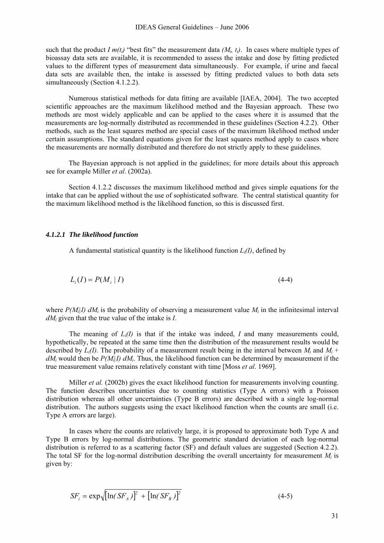
Numerous statistical methods for data fitting are available [IAEA, 2004]. The two accepted scientific approaches are the maximum likelihood method and the Bayesian approach. These two methods are most widely applicable and can be applied to the cases where it is assumed that the measurements are log-normally distributed as recommended in these guidelines (Section 4.2.2). Other methods, such as the least squares method are special cases of the maximum likelihood method under certain assumptions. The standard equations given for the least squares method apply to cases where the measurements are normally distributed and therefore do not strictly apply to these guidelines.
The Bayesian approach is not applied in the guidelines; for more details about this approach see for example Miller et al. (2002a).
Section 4.1.2.2 discusses the maximum likelihood method and gives simple equations for the intake that can be applied without the use of sophisticated software. The central statistical quantity for the maximum likelihood method is the likelihood function, so this is discussed first.
4.1.2.1 The likelihood function
A fundamental statistical quantity is the likelihood function Li(I), defined by
)|()( IMPIL ii = (4-4)
where P(Mi|I) dMi is the probability of observing a measurement value Mi in the infinitesimal interval dMi given that the true value of the intake is I.
The meaning of Li(I) is that if the intake was indeed, I and many measurements could, hypothetically, be repeated at the same time then the distribution of the measurement results would be described by Li(I). The probability of a measurement result being in the interval between Mi and Mi + dMi would then be P(Mi|I) dMi. Thus, the likelihood function can be determined by measurement if the true measurement value remains relatively constant with time [Moss et al. 1969].
Miller et al. (2002b) gives the exact likelihood function for measurements involving counting. The function describes uncertainties due to counting statistics (Type A errors) with a Poisson distribution whereas all other uncertainties (Type B errors) are described with a single log-normal distribution. The authors suggests using the exact likelihood function when the counts are small (i.e. Type A errors are large).
In cases where the counts are relatively large, it is proposed to approximate both Type A and Type B errors by log-normal distributions. The geometric standard deviation of each log-normal distribution is referred to as a scattering factor (SF) and default values are suggested (Section 4.2.2). The total SF for the log-normal distribution describing the overall uncertainty for measurement Mi is given by:
[ ] [ ]2B2
Ai )SF()SF(SF lnlnexp += (4-5)
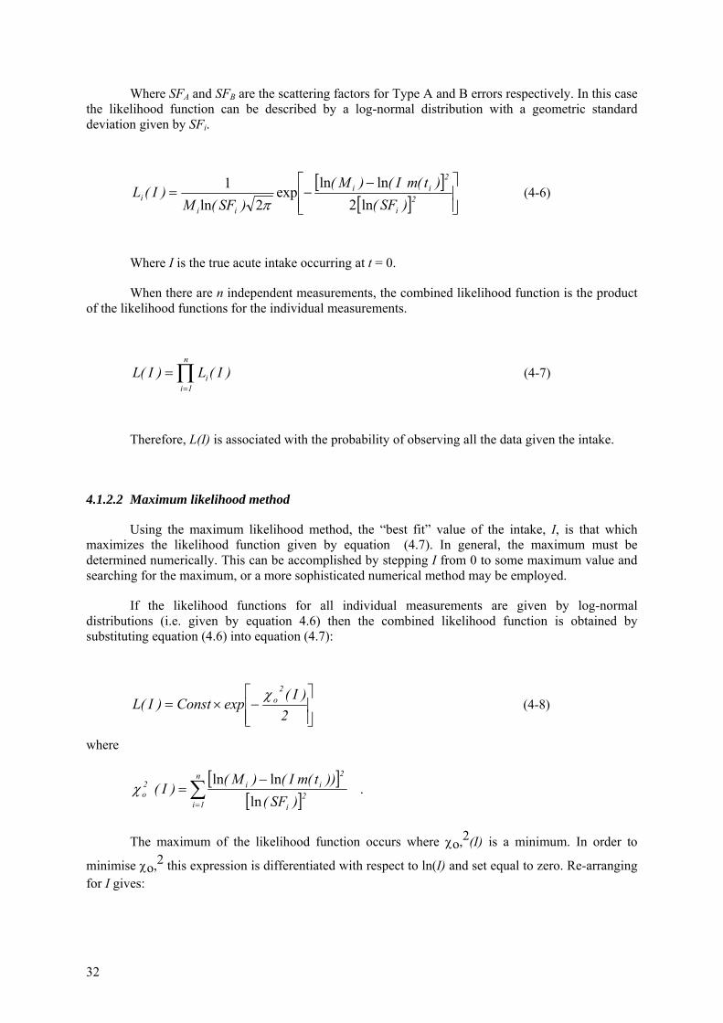
32
Where SFA and SFB are the scattering factors for Type A and B errors respectively. In this case the likelihood function can be described by a log-normal distribution with a geometric standard deviation given by SFi.
[ ][ ] ⎥
⎥⎦
⎤
⎢⎢⎣
⎡ −−= 2
i
2ii
iii )SF(
)t(mI()M()SF(M
)I(Lln2
lnlnexp
2ln1
π (4-6)
Where I is the true acute intake occurring at t = 0.
When there are n independent measurements, the combined likelihood function is the product of the likelihood functions for the individual measurements.
∏=
=n
1ii )I(L)I(L (4-7)
Therefore, L(I) is associated with the probability of observing all the data given the intake.
4.1.2.2 Maximum likelihood method
Using the maximum likelihood method, the “best fit” value of the intake, I, is that which maximizes the likelihood function given by equation (4.7). In general, the maximum must be determined numerically. This can be accomplished by stepping I from 0 to some maximum value and searching for the maximum, or a more sophisticated numerical method may be employed.
If the likelihood functions for all individual measurements are given by log-normal distributions (i.e. given by equation 4.6) then the combined likelihood function is obtained by substituting equation (4.6) into equation (4.7):
⎥⎥⎦
⎤
⎢⎢⎣
⎡−×=
2)I(
expConst)I(L2
oχ (4-8)
where
[ ][ ]∑
=
−=
n
1i2
i
2ii2
o )SF())t(mI()M(
)I(ln
lnlnχ .
The maximum of the likelihood function occurs where χo,2(I) is a minimum. In order to
minimise χo,2 this expression is differentiated with respect to ln(I) and set equal to zero. Re-arranging for I gives:
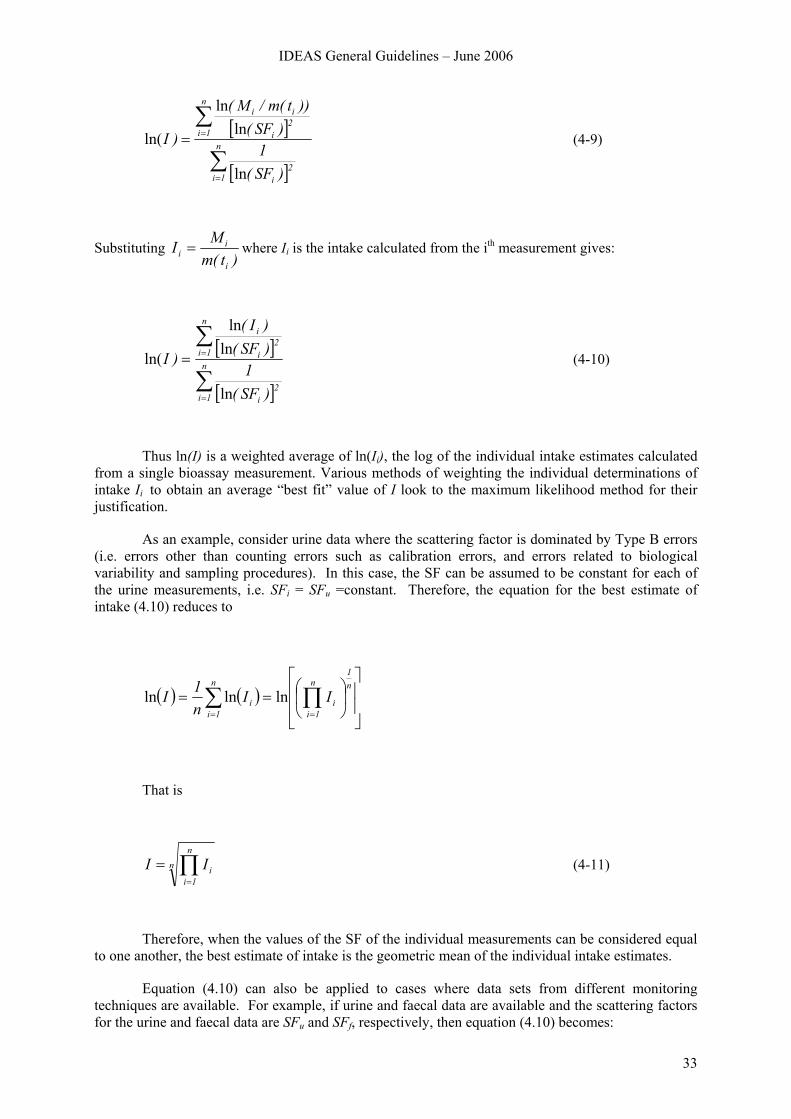
IDEAS General Guidelines – June 2006
33
[ ]
[ ]∑
∑
=
== n
1i2
i
n
1i2
i
ii
)SF(1
)SF())t(m/M(
)I
ln
lnln
ln( (4-9)
Substituting )t(m
MIi
ii = where Ii is the intake calculated from the ith measurement gives:
[ ]
[ ]∑
∑
=
== n
1i2
i
n
1i2
i
i
)SF(1
)SF()I(
)I
ln
lnln
ln( (4-10)
Thus ln(I) is a weighted average of ln(Ii), the log of the individual intake estimates calculated from a single bioassay measurement. Various methods of weighting the individual determinations of intake Ii to obtain an average “best fit” value of I look to the maximum likelihood method for their justification.
As an example, consider urine data where the scattering factor is dominated by Type B errors (i.e. errors other than counting errors such as calibration errors, and errors related to biological variability and sampling procedures). In this case, the SF can be assumed to be constant for each of the urine measurements, i.e. SFi = SFu =constant. Therefore, the equation for the best estimate of intake (4.10) reduces to
( ) ( )⎥⎥
⎦
⎤
⎢⎢
⎣
⎡⎟⎠
⎞⎜⎝
⎛== ∏∑==
n1
n
1ii
n
1ii II
n1I lnlnln
That is
nn
1iiII ∏
=
= (4-11)
Therefore, when the values of the SF of the individual measurements can be considered equal to one another, the best estimate of intake is the geometric mean of the individual intake estimates.
Equation (4.10) can also be applied to cases where data sets from different monitoring techniques are available. For example, if urine and faecal data are available and the scattering factors for the urine and faecal data are SFu and SFf, respectively, then equation (4.10) becomes:
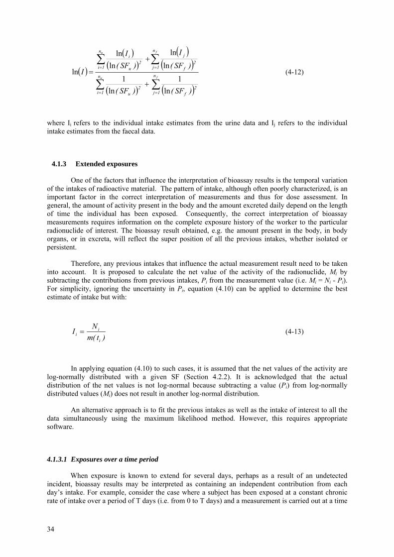
34
( )
( )( )
( )( )
( ) ( )∑ ∑
∑∑
= =
==
+
+
=u f
fu
n
1i
n
1j2
f2
u
n
1j2
f
jn
1i2
u
i
)SF()SF(
)SF(
I
)SF(I
I
ln1
ln1
ln
ln
lnln
ln (4-12)
where Ii refers to the individual intake estimates from the urine data and Ij refers to the individual intake estimates from the faecal data.
4.1.3 Extended exposures
One of the factors that influence the interpretation of bioassay results is the temporal variation of the intakes of radioactive material. The pattern of intake, although often poorly characterized, is an important factor in the correct interpretation of measurements and thus for dose assessment. In general, the amount of activity present in the body and the amount excreted daily depend on the length of time the individual has been exposed. Consequently, the correct interpretation of bioassay measurements requires information on the complete exposure history of the worker to the particular radionuclide of interest. The bioassay result obtained, e.g. the amount present in the body, in body organs, or in excreta, will reflect the super position of all the previous intakes, whether isolated or persistent.
Therefore, any previous intakes that influence the actual measurement result need to be taken into account. It is proposed to calculate the net value of the activity of the radionuclide, Mi by subtracting the contributions from previous intakes, Pi from the measurement value (i.e. Mi = Ni - Pi). For simplicity, ignoring the uncertainty in Pi, equation (4.10) can be applied to determine the best estimate of intake but with:
)t(m
NIi
ii = (4-13)
In applying equation (4.10) to such cases, it is assumed that the net values of the activity are log-normally distributed with a given SF (Section 4.2.2). It is acknowledged that the actual distribution of the net values is not log-normal because subtracting a value (Pi) from log-normally distributed values (Mi) does not result in another log-normal distribution.
An alternative approach is to fit the previous intakes as well as the intake of interest to all the data simultaneously using the maximum likelihood method. However, this requires appropriate software.
4.1.3.1 Exposures over a time period
When exposure is known to extend for several days, perhaps as a result of an undetected incident, bioassay results may be interpreted as containing an independent contribution from each day’s intake. For example, consider the case where a subject has been exposed at a constant chronic rate of intake over a period of T days (i.e. from 0 to T days) and a measurement is carried out at a time
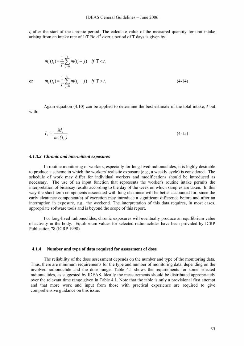
IDEAS General Guidelines – June 2006
35
ti after the start of the chronic period. The calculate value of the measured quantity for unit intake arising from an intake rate of 1/T Bq d-1 over a period of T days is given by:
ij
iic tifjtmT
tm <−= ∑=
T)(1)(T
0
or ij
iic tifjtmT
tm >−= ∑=
T)(1)(it
0 (4-14)
Again equation (4.10) can be applied to determine the best estimate of the total intake, I but with:
)t(mM
Iic
ii = (4-15)
4.1.3.2 Chronic and intermittent exposures
In routine monitoring of workers, especially for long-lived radionuclides, it is highly desirable to produce a scheme in which the workers' realistic exposure (e.g., a weekly cycle) is considered. The schedule of work may differ for individual workers and modifications should be introduced as necessary. The use of an input function that represents the worker's routine intake permits the interpretation of bioassay results according to the day of the week on which samples are taken. In this way the short-term components associated with lung clearance will be better accounted for, since the early clearance component(s) of excretion may introduce a significant difference before and after an interruption in exposure, e.g., the weekend. The interpretation of this data requires, in most cases, appropriate software tools and is beyond the scope of this report.
For long-lived radionuclides, chronic exposures will eventually produce an equilibrium value of activity in the body. Equilibrium values for selected radionuclides have been provided by ICRP Publication 78 (ICRP 1998).
4.1.4 Number and type of data required for assessment of dose
The reliability of the dose assessment depends on the number and type of the monitoring data. Thus, there are minimum requirements for the type and number of monitoring data, depending on the involved radionuclide and the dose range. Table 4.1 shows the requirements for some selected radionuclides, as suggested by IDEAS. Ideally the measurements should be distributed appropriately over the relevant time range given in Table 4.1. Note that the table is only a provisional first attempt and that more work and input from those with practical experience are required to give comprehensive guidance on this issue.
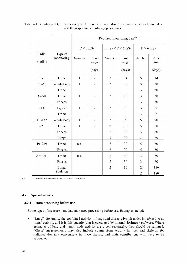
36
Table 4.1: Number and type of data required for assessment of dose for some selected radionuclides and the respective monitoring procedures.
Required monitoring data(a)
D < 1 mSv 1 mSv < D < 6 mSv D > 6 mSv
Radio-
nuclide
Type of monitoring Number Time
range
(days)
Number Time range
(days)
Number Time range
(days)
H-3 Urine 1 - 3 14 5 14
Co-60 Whole body
Urine
1 - 3 30 5
3
30
30
Sr-90 Urine
Faeces
1 - 3 30 3
3
30
30
I-131 Thyroid
Urine
1 - 3 7 3
3
7
7
Cs-137 Whole body 1 - 3 90 5 90
U-235 Urine
Faeces
Lungs
1 - 2
2
2
30
30
30
5
3
3
60
60
60
Pu-239 Urine
Faeces
n.a. - 3
3
30
30
5
5
60
60
Am-241 Urine
Faeces
Lungs Skeleton
n.a. - 2
2
2
30
30
30
3
3
2
2
60
60
180
180 (a) These measurements are desirable if facilities are available.
4.2 Special aspects
4.2.1 Data processing before use
Some types of measurement data may need processing before use. Examples include:
• “Lung”. Generally, the combined activity in lungs and thoracic lymph nodes is referred to as ‘lung’ activity, and it is this quantity that is calculated by internal dosimetry software. Where estimates of lung and lymph node activity are given separately, they should be summed. “Chest” measurements may also include counts from activity in liver and skeleton for radionuclides that concentrate in these tissues, and their contributions will have to be subtracted.
IDEAS General Guidelines – June 2006
37
• Faeces. The transit time through the GI tract is subject to large inter (and intra-) subject variations. Moreover, while for ease of computation transit through the GI tract is represented by a series of compartments that clear exponentially, in practice, the movement is more like “slug” flow. It is therefore unlikely that individual daily faecal clearance measurements in the first few days after intake will follow the predicted pattern, and so it is best to consider cumulative excretion over the first few days.
• Urine. If the data are given in terms of Bq/litre then this can be normalised to daily excretion rates by assuming 1.6 litres of urine are excreted per day (reference value for man, ICRP Publication 89 (2002)).
• Plutonium. Assume that “Pu” (if not qualified) refers to total Pu alpha-activity (238Pu, 239Pu, and 240Pu). Assume that “239Pu” (if not qualified) actually represents 239Pu+240Pu, because these cannot be separated by alpha spectrometry. If 241Pu is not measured then assume a typical ratio to total plutonium alpha activity, for use as default. See table of typical plutonium isotopic ratios, which should be used with caution as default in those cases where no specific information is available.
• Uranium. Excretion data (especially faecal) may need correction for dietary intakes of uranium. Doses need to be included for isotopes in addition to those measured. In particular, for enriched uranium 235U may be measured, while the highest dose comes from 234U. See table of typical uranium isotopic ratios for depleted, natural, high- and low-enriched uranium.
4.2.2 Assessment of uncertainty on data
The uncertainties on the data are of great importance for the evaluation for several reasons:
• They enable an objective decision to be made on whether a measured value is due to a new intake, or due to previous intakes that already have been evaluated.
• They enable an objective decision to be made on whether a measured value is consistent with previous evaluations, or if it indicates the previous evaluations to be wrong.
• They can have a strong influence on all evaluations using weighted fitting procedures (i.e. where there is more than one data point).
• They enable rogue data to be identified objectively.
• They enable objective (statistical) criteria (goodness-of-fit) to be calculated, which are used to determine whether the predictions of the biokinetic model (with a given set of parameter values) used to assess the intake and dose are inconsistent with the data.
• They enable statistics, such as the χ2, to be calculated, which are used to compare the fits to the data of different models/parameter values.
Generally, the uncertainties in the measurement are difficult to estimate. When activity levels are low and close to the limit of detection, uncertainties due to counting statistics may dominate the overall uncertainty. For radionuclides that are easily detected and present in sufficient quantity, uncertainties due to counting statistics will be small compared to other sources of uncertainty. Consideration must also be given to systematic uncertainties in other parts of the measurement procedure, e.g. calibration, or correction for body size of in vivo measurements. These uncertainties apply to the measurement of activity in the sample or person. With excretion measurements, the activity in the sample is used to provide an estimate of the subject’s average excretion rate over 24 hours for comparison with the model predictions. If the samples are collected over periods less than 24
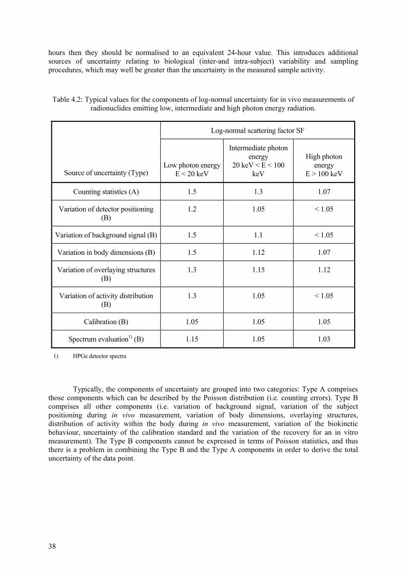
38
hours then they should be normalised to an equivalent 24-hour value. This introduces additional sources of uncertainty relating to biological (inter-and intra-subject) variability and sampling procedures, which may well be greater than the uncertainty in the measured sample activity.
Table 4.2: Typical values for the components of log-normal uncertainty for in vivo measurements of radionuclides emitting low, intermediate and high photon energy radiation.
Log-normal scattering factor SF
Source of uncertainty (Type) Low photon energy
E < 20 keV
Intermediate photon energy
20 keV < E < 100 keV
High photon energy
E > 100 keV
Counting statistics (A) 1.5 1.3 1.07
Variation of detector positioning (B)
1.2 1.05 < 1.05
Variation of background signal (B) 1.5 1.1 < 1.05
Variation in body dimensions (B) 1.5 1.12 1.07
Variation of overlaying structures (B)
1.3 1.15 1.12
Variation of activity distribution (B)
1.3 1.05 < 1.05
Calibration (B) 1.05 1.05 1.05
Spectrum evaluation1) (B) 1.15 1.05 1.03
1) HPGe detector spectra
Typically, the components of uncertainty are grouped into two categories: Type A comprises those components which can be described by the Poisson distribution (i.e. counting errors). Type B comprises all other components (i.e. variation of background signal, variation of the subject positioning during in vivo measurement, variation of body dimensions, overlaying structures, distribution of activity within the body during in vivo measurement, variation of the biokinetic behaviour, uncertainty of the calibration standard and the variation of the recovery for an in vitro measurement). The Type B components cannot be expressed in terms of Poisson statistics, and thus there is a problem in combining the Type B and the Type A components in order to derive the total uncertainty of the data point.
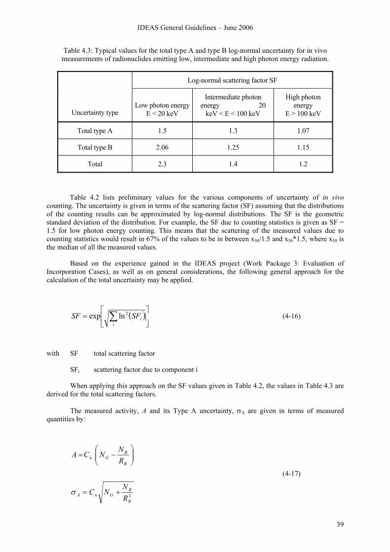
IDEAS General Guidelines – June 2006
39
Table 4.3: Typical values for the total type A and type B log-normal uncertainty for in vivo measurements of radionuclides emitting low, intermediate and high photon energy radiation.
Log-normal scattering factor SF
Uncertainty type Low photon energy
E < 20 keV
Intermediate photon energy 20
keV < E < 100 keV
High photon energy
E > 100 keV
Total type A 1.5 1.3 1.07
Total type B 2.06 1.25 1.15
Total 2.3 1.4 1.2
Table 4.2 lists preliminary values for the various components of uncertainty of in vivo counting. The uncertainty is given in terms of the scattering factor (SF) assuming that the distributions of the counting results can be approximated by log-normal distributions. The SF is the geometric standard deviation of the distribution. For example, the SF due to counting statistics is given as SF = 1.5 for low photon energy counting. This means that the scattering of the measured values due to counting statistics would result in 67% of the values to be in between x50/1.5 and x50*1.5, where x50 is the median of all the measured values.
Based on the experience gained in the IDEAS project (Work Package 3: Evaluation of Incorporation Cases), as well as on general considerations, the following general approach for the calculation of the total uncertainty may be applied.
( )⎥⎦
⎤⎢⎣
⎡= ∑
iiSFSF 2lnexp (4-16)
with SF total scattering factor
SFi scattering factor due to component i
When applying this approach on the SF values given in Table 4.2, the values in Table 4.3 are derived for the total scattering factors.
The measured activity, A and its Type A uncertainty, σA are given in terms of measured quantities by:
2B
BGnA
B
BGn
RN
NC
RNNCA
+=
⎟⎟⎠
⎞⎜⎜⎝
⎛−=
σ
(4-17)
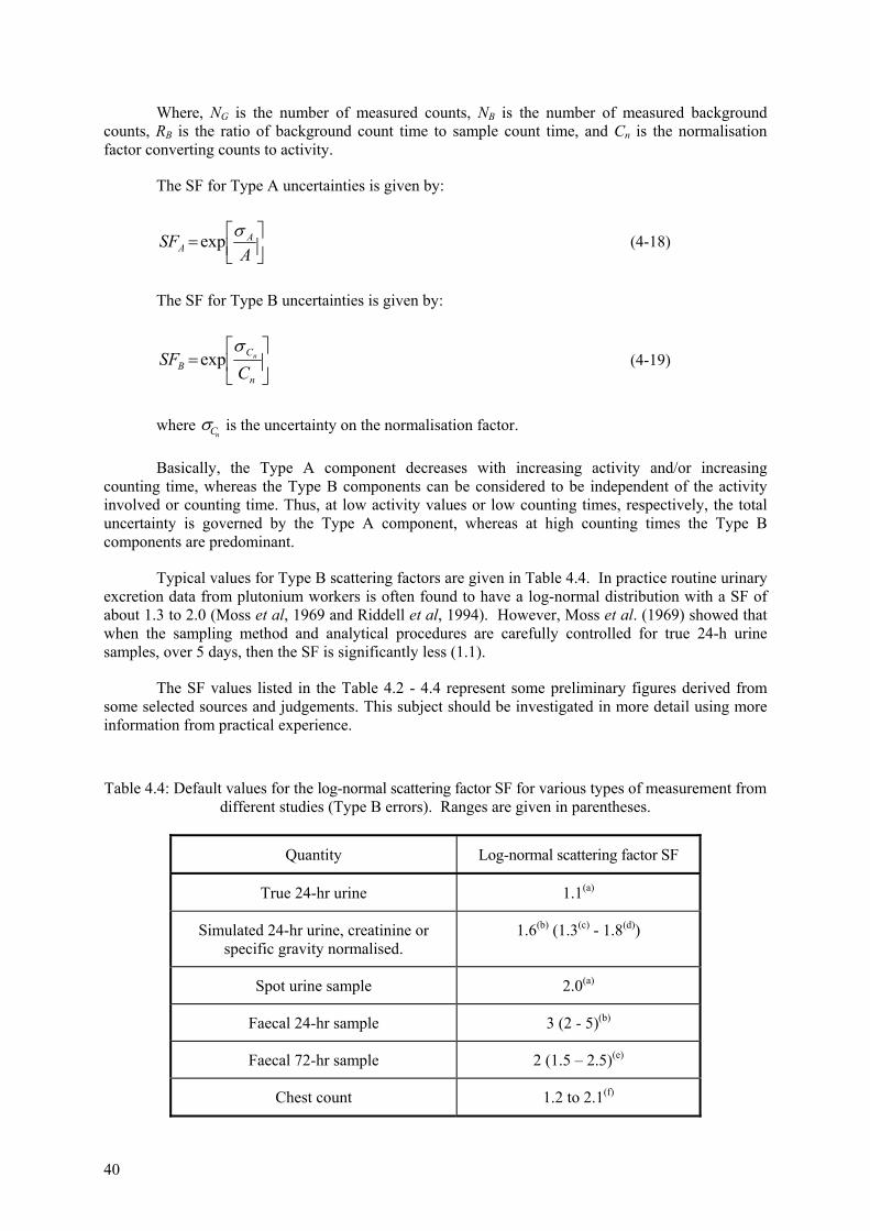
40
Where, NG is the number of measured counts, NB is the number of measured background counts, RB is the ratio of background count time to sample count time, and Cn is the normalisation factor converting counts to activity.
The SF for Type A uncertainties is given by:
⎥⎦⎤
⎢⎣⎡=
ASF A
Aσexp (4-18)
The SF for Type B uncertainties is given by:
⎥⎦
⎤⎢⎣
⎡=
n
CB C
SF nσ
exp (4-19)
where nCσ is the uncertainty on the normalisation factor.
Basically, the Type A component decreases with increasing activity and/or increasing counting time, whereas the Type B components can be considered to be independent of the activity involved or counting time. Thus, at low activity values or low counting times, respectively, the total uncertainty is governed by the Type A component, whereas at high counting times the Type B components are predominant.
Typical values for Type B scattering factors are given in Table 4.4. In practice routine urinary excretion data from plutonium workers is often found to have a log-normal distribution with a SF of about 1.3 to 2.0 (Moss et al, 1969 and Riddell et al, 1994). However, Moss et al. (1969) showed that when the sampling method and analytical procedures are carefully controlled for true 24-h urine samples, over 5 days, then the SF is significantly less (1.1).
The SF values listed in the Table 4.2 - 4.4 represent some preliminary figures derived from some selected sources and judgements. This subject should be investigated in more detail using more information from practical experience.
Table 4.4: Default values for the log-normal scattering factor SF for various types of measurement from different studies (Type B errors). Ranges are given in parentheses.
Quantity Log-normal scattering factor SF
True 24-hr urine 1.1(a)
Simulated 24-hr urine, creatinine or specific gravity normalised.
1.6(b) (1.3(c) - 1.8(d))
Spot urine sample 2.0(a)
Faecal 24-hr sample 3 (2 - 5)(b)
Faecal 72-hr sample 2 (1.5 – 2.5)(e)
Chest count 1.2 to 2.1(f)
IDEAS General Guidelines – June 2006
41
(a) Value given by Moss et al, 1969 based on plutonium in urine measurements of workers at Los Alamos.
(b) Value based on judgement and experience. (c) At Los Alamos, Type B uncertainties, in terms of the coefficient of variation, for urine samples
normalised using volume and specific gravity has been found to be 30% (i.e. a SF of 1.3). (d) Value given by Riddell et al, 1994 based on plutonium in urine measurements of Sellafield
workers. Because sampling procedures and measurements techniques have improved over the years recent measurements are likely to have a SF less than 1.8.
(e) SF values for 72-hr faecal samples are consistent with 24-hr faecal samples. (f) See Table 4.3
4.2.3 Handling of data below limits of detection
It is recommended to keep records on the original counting statistic and associated information (duration of the measurement, background effect count rate, duration of the background effect measurement, assessed uncertainty of estimated activity, etc) for all data, including results, assessed as less than a decision threshold (ISO 2000a, 2000b, 2000c). The substitution of the original data by an expression “less than the decision threshold” or “less than the detection limit” is not recommended. All original data may be involved into the dose assessment with taking into account the uncertainty associated with each result. Details of processing of such data are given in ISO standards (ISO 2005a, 2005b).
If data are reported as being below the lower limit of detection (LLD) and only the LLD value is recorded then it is recommended to use the maximum likelihood method to obtain the best estimate of intake. It can be shown that this method leads to an unbiased estimate of the intake (Marsh 2002).
If the application of this method is not possible because of the lack of available software, then several other simplifying assumptions are possible. One such assumption is to treat each LLD value as a positive value at that measurement. This will clearly lead to an overestimate of the intake, but there is no simple method to quantify the degree of overestimation. In the example cases studied in WP3, it was found that that setting the LLD values to positive values at LLD/2 gave similar results as the application of the Maximum Likelihood Method. It is acknowledged that this method has no strong foundation in mathematics, and may not be universally applicable, but, in the interest of harmonisation and proportionality, it therefore recommended here, that if the maximum likelihood cannot be applied, then LLD data should be treated in this way.
4.2.4 Handling of data influenced by chelation therapy
Generally, it can be assumed that data of Pu and Am content in urine are affected by DTPA therapy. If DTPA has been effective in reducing systemic uptake then systemic organ retention and systemic faecal excretion will also be affected. Lung data are not affected by DTPA therapy.
The method of Jech et al (1973) is proposed here: exclude urinary excretion data that have been affected by DTPA. Following La Bone (1994, 2002) it is proposed that data up to 100 days following chelation should be excluded.
The alternative approach is to use a model for the urinary excretion of the chelated actinide, to compensate for the enhanced excretion (Hall method, La Bone, 1994). This is preferable, when an early assessment is required, because it makes more use of the available information, but the IDEAS partners were unable to propose a suitable formula at this time.
42
4.2.5 Identification of rogue data
A systematic basis to identify outliers and criteria to exclude them are needed. Outliers above and below the trend of the other data have different significance. A point above the trend might indicate another intake. A point below is more likely to result from a transcription or measurement error.
The problem of deciding how to identify outliers is not straightforward. Ideally, outliers should be identified before fitting model predictions to the data. If not, then the assessor faces a dilemma when the model does not fit the data (Section 4.2.6): should the model parameters be varied to obtain a fit, or should the data that does not fit be rejected. So ideally, the trend of the data should be obtained first by, for example, fitting a sum of exponentials to the data and then using a statistical test to reject the data. In practice, it is realised that this procedure could be time consuming, and many assessors will rely on judgement when deciding to reject certain data. Specifically, care must be taken in excluding data, particularly if a group of data at early or late times does not appear to be predicted by the model, then model parameters should be varied in preference to excluding data.
For measurement data suspected of being “rogue” a check should be made on whether inclusion or exclusion significantly affects the intake and dose. If it does not, there is no point in expending effort on justifying excluding it: it should be included. If it does have an effect, then a statistical test should be carried out to determine if it is an outlier. If it is an outlier then it should be excluded.
To identify outliers the following statistical test is proposed. A measurement value is an outlier if it is more than a factor of SF3 away from the trend of the other data, where SF is the scattering factor.
If the data set is limited after excluding outliers, then further measurements may be required for assessment of dose (Section 4.1.4).
4.2.6 Criteria for rejecting fit
In assessing intakes and doses, the underlying starting assumption is that:
• the structure of the biokinetic model is a realistic representation of the physical and biological processes, and
• the model parameter values are correct.
Estimates of bioassay quantities will be unbiased only if these conditions are met. These assumptions are analogous to the null hypothesis in classical statistics. In cases where the model predictions are inconsistent with the data (i.e. fits are inadequate) this indicates that either the model parameter values, or the structure of the model is incorrect. The classical statistical approach is to reject the model and to repeat the assessment with different model parameter values or with a new model structure so that the predictions are not inconsistent with the data. Before the model structure itself can be rejected, it is necessary to first consider changes to the model parameter values. In these guidelines only changes to the parameter values are considered, not to the model structure.
It is important to remember that it is not possible to prove that the null hypothesis is true. Test statistics are used to indicate that the null hypothesis is false. The criteria for rejecting the null hypothesis, (i.e. stating the fit is inadequate), needs to be defined before the assessment is carried out.
IDEAS General Guidelines – June 2006
43
A comprehensive discussion of all the possible statistics that can be used to quantify whether a fit is inadequate is beyond the scope of this document. Only the chi-squared test statistic, χ0
2 is considered here.
If it is assumed that each measurement, Mi, is taken from a log-normal distribution with a scattering factor of SFi then for n measurements, χ0
2 is defined as:
[ ]∑=
⎟⎟⎠
⎞⎜⎜⎝
⎛ −=
n
i i
iio SF
tmIM1
22
)ln()(ln)ln(χ (4-20)
The product I m(ti) is the predicted value.
The above formulae do not apply to data that are reported as below the lower limit of detection (<LLD).
When fitting predicted values to different types of data simultaneously, the overall χ02 is
equal to the sum of the calculated χ02 values for each data set.
If the predictions are inconsistent with the data, then the calculated value of χ02 is inconsistent
with the theoretical chi-squared (χ2) distribution with (n-1) degrees of freedom. The expected value of χ2 is equal to the number of degrees of freedom (i.e. n-1).
The actual number of degrees of freedom when varying l parameters for a linear model (with respect to its parameters) is n-l. In this case the biokinetic model is not linear with respect to most of its parameters, other than the intake. If the fit is rejected assuming n-1 degrees of freedom then the fit would also be rejected if the actual number of degrees of freedom is less. For cases where there are comprehensive data so that n>>l, it is proposed to assume n-1 degrees of freedom for each step of the procedure given in the flow charts (Chapter 6).
The probability of observing a larger χ2 value than χ02 for (n-1) degrees of freedom is given
by the p-value, which can be obtained from Statistical Tables. The p-value is the fraction of the theoretical χ2 distribution that lies above the calculated χ0
2 value. So if the p-value is very small, the calculated χ0
2 value is very much larger than expected and therefore it can be concluded that the predictions are likely to be inconsistent with the data and the assumed uncertainties.
The χ2 test uses the assumed uncertainties. If the assumed uncertainties are overestimated then χ0
2 is too small. The converse is also true; if the assumed uncertainties are underestimated then χ0
2 is too large. This is one of the reasons why it is important assess realistic uncertainties (Section 4.2.2).
It is proposed that the fits to the data are judged to be inadequate if:
• the probability that χ2 is greater than χ02 is 5% or less (i.e. if p-value < 0.05). In other words the
fit is inadequate at the 5% level of significance, or if
• the fit displayed graphically looks unreasonable by eye.
It is also acknowledged that whether or not the fit displayed graphically looks unreasonable by eye is a subjective judgement. Generally, however, a fit would be considered unreasonable if all, or a long series, of data were systematically underestimated or overestimated.
44
If a series of data were systematically underestimated or overestimated then this can be quantified objectively by the use of other test statistics such as the auto correlation coefficient (Chatfield, 2004) and Durbin Watson statistic (Durbin and Watson 1970). These statistics have the advantage that they are relatively insensitive to the magnitude of the assumed measurement uncertainties. However, they are not considered further in the current IDEAS Guidelines.
5 EVALUATION OF MONITORING DATA
5.1 Introduction
In carrying out the assessment (evaluation) of internal committed doses from monitoring data, the assessor may well have to make assumptions about factors such as the pattern of intake and properties of the material. When more than one measurement is available, issues such as the weighting applied to the different data can substantially affect the result. Recent intercomparison exercises have shown the wide range in doses that can be assessed from the same data set as a result of such factors, and hence the need for guidance to harmonise evaluations.
The procedures proposed in this chapter, are based on the following principles:
• Harmonisation: by following the procedures any two assessors should obtain the same estimate of dose from a given data set
• Accuracy: the “best” estimate of dose should be obtained from the available data
• Proportionality: the effort applied to the evaluation should be proportionate to the dose – the lower the dose, the simpler the process should be.
5.1.1 Harmonisation
A well-defined procedure is needed and for this reason the process is defined here primarily by means of a series of flow-charts. So far as possible, the process has been made widely applicable, i.e., it does not assume that the assessor has the use of sophisticated bioassay interpretation software. For routine monitoring situations, where typically there is only one measurement relating to each intake, it is reasonably straightforward to define a procedure. However, in special monitoring situations, where typically there is more than one measurement and quite possibly more than one type of measurement (urine, faeces…) different options for data handling can easily lead to different evaluated doses, even when the same model, parameter values and software are used. Another range of options, and opportunities for different evaluated doses, arises in situations where it is appropriate to consider changing parameter values from the ICRP defaults. Proposals are made here for a systematic approach to dose assessment in all these situations.
5.1.2 Accuracy
It is recognised that the uncertainties associated with assessed internal dose can be considerable, especially for actinides which are difficult to detect in the body and have relatively high dose coefficients (Sv Bq-1). If the initial estimate of dose exceeds 1 mSv, it could well be that the possibility of a substantially higher dose (e.g. 6 mSv) cannot easily be excluded. It is then important to make best use of the available information. To do so may well involve changing parameter values from their ICRP default values and guidance is therefore needed on which parameter values might reasonably be varied according to the circumstances.
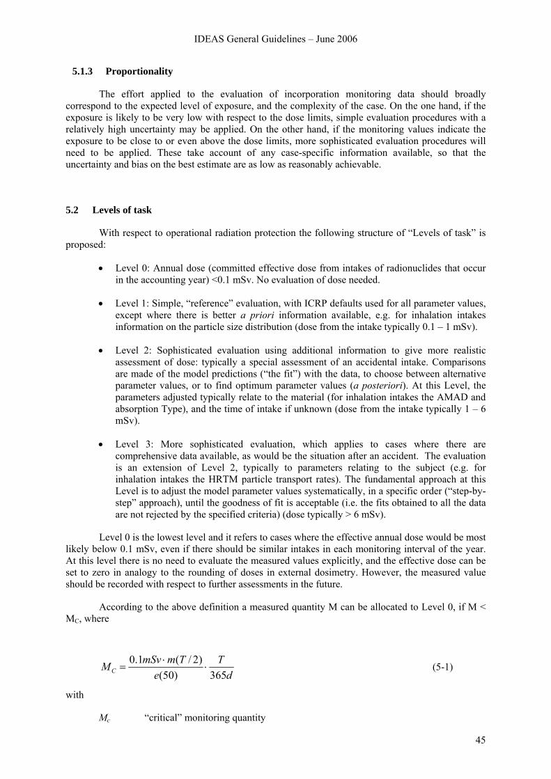
IDEAS General Guidelines – June 2006
45
5.1.3 Proportionality
The effort applied to the evaluation of incorporation monitoring data should broadly correspond to the expected level of exposure, and the complexity of the case. On the one hand, if the exposure is likely to be very low with respect to the dose limits, simple evaluation procedures with a relatively high uncertainty may be applied. On the other hand, if the monitoring values indicate the exposure to be close to or even above the dose limits, more sophisticated evaluation procedures will need to be applied. These take account of any case-specific information available, so that the uncertainty and bias on the best estimate are as low as reasonably achievable.
5.2 Levels of task
With respect to operational radiation protection the following structure of “Levels of task” is proposed:
• Level 0: Annual dose (committed effective dose from intakes of radionuclides that occur in the accounting year) <0.1 mSv. No evaluation of dose needed.
• Level 1: Simple, “reference” evaluation, with ICRP defaults used for all parameter values, except where there is better a priori information available, e.g. for inhalation intakes information on the particle size distribution (dose from the intake typically 0.1 – 1 mSv).
• Level 2: Sophisticated evaluation using additional information to give more realistic assessment of dose: typically a special assessment of an accidental intake. Comparisons are made of the model predictions (“the fit”) with the data, to choose between alternative parameter values, or to find optimum parameter values (a posteriori). At this Level, the parameters adjusted typically relate to the material (for inhalation intakes the AMAD and absorption Type), and the time of intake if unknown (dose from the intake typically 1 – 6 mSv).
• Level 3: More sophisticated evaluation, which applies to cases where there are comprehensive data available, as would be the situation after an accident. The evaluation is an extension of Level 2, typically to parameters relating to the subject (e.g. for inhalation intakes the HRTM particle transport rates). The fundamental approach at this Level is to adjust the model parameter values systematically, in a specific order (“step-by-step” approach), until the goodness of fit is acceptable (i.e. the fits obtained to all the data are not rejected by the specified criteria) (dose typically > 6 mSv).
Level 0 is the lowest level and it refers to cases where the effective annual dose would be most likely below 0.1 mSv, even if there should be similar intakes in each monitoring interval of the year. At this level there is no need to evaluate the measured values explicitly, and the effective dose can be set to zero in analogy to the rounding of doses in external dosimetry. However, the measured value should be recorded with respect to further assessments in the future.
According to the above definition a measured quantity M can be allocated to Level 0, if M < MC, where
dT
eTmmSvM C 365)50(
)2/(1.0⋅
⋅= (5-1)
with
Mc “critical” monitoring quantity
46
T monitoring interval for the monitoring quantity considered
m(T/2) corresponding retention or excretion function for the monitoring quantity at time t = T/2 (i.e. it is assumed that the intake occurs at the mid-point of the monitoring interval)
e(50) effective dose coefficient
The critical monitoring quantity MC defined by the equation (5.1) is listed in Tabel 5.1 for some selected radionuclides. As can be seen, Mc is typically above, or close to, the lower limit of detection (LLD) for the fission and activation products whereas it is below the LLD for the actinides considered. So in the case of the actinides, any significant monitoring value is likely to result in a dose of more than 0.1 mSv and thus has to be evaluated. In the case of the fission and activation products, however, there might be significant monitoring values which result in a dose of less than 0.1 mSv. Thus, Level 1 applies typically to those radionuclides, which are easy to measure and which have low effective dose coefficients (i.e. H-3, Cs-137 etc).
Note that there is growing interest in the application of the “dose per unit content” function, z(t) = e(50)/ m(t), which represents the committed effective dose per unit organ (body) radionuclide content or per unit radionuclide content in the 24-hour excreta sample at time t after an acute intake. Thus E = M z(t), where E is the committed effective dose, and M is the measured value. Its use simplifies the dose evaluation to a single step, instead of the traditional method of first applying the retention or excretion function m(t) to calculate the intake, and then the dose coefficient e(50) to calculate the resulting effective dose. Hence in the equation above, m(T/2)/ e(50) could be replaced by z-1(T/2).
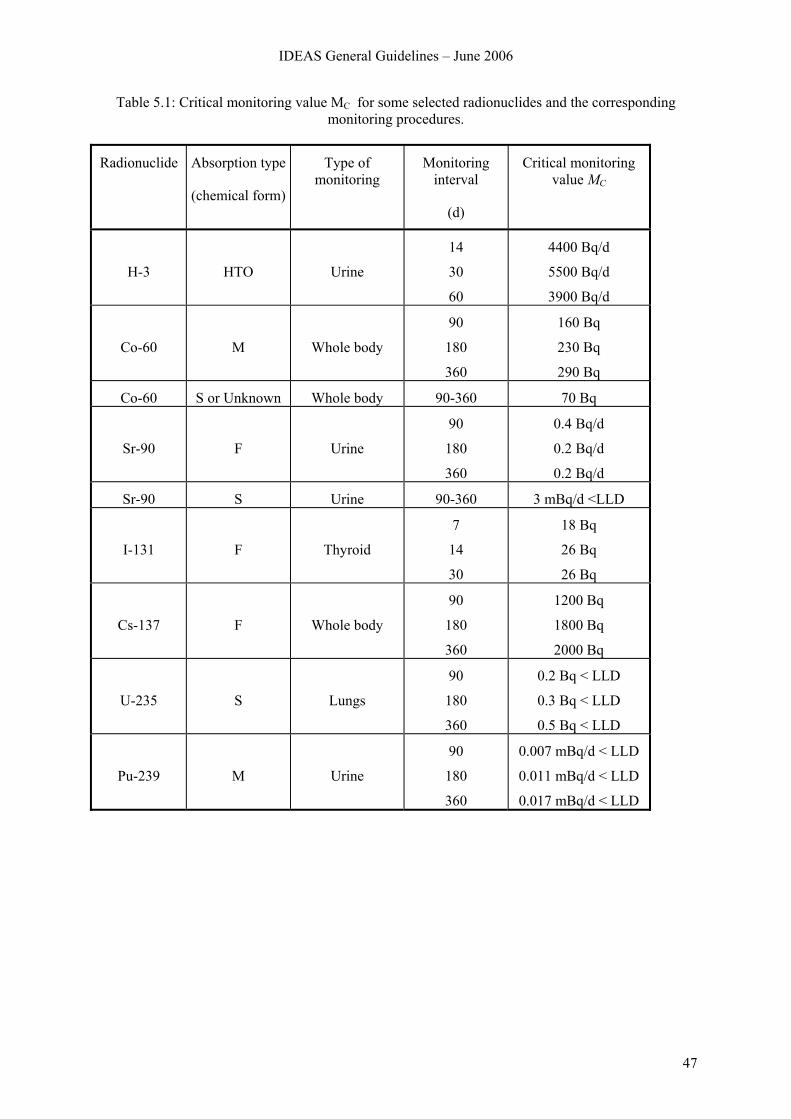
IDEAS General Guidelines – June 2006
47
Table 5.1: Critical monitoring value MC for some selected radionuclides and the corresponding monitoring procedures.
Radionuclide Absorption type
(chemical form)
Type of monitoring
Monitoring interval
(d)
Critical monitoring value MC
H-3
HTO
Urine
14
30
60
4400 Bq/d
5500 Bq/d
3900 Bq/d
Co-60
M
Whole body
90
180
360
160 Bq
230 Bq
290 Bq
Co-60 S or Unknown Whole body 90-360 70 Bq
Sr-90
F
Urine
90
180
360
0.4 Bq/d
0.2 Bq/d
0.2 Bq/d
Sr-90 S Urine 90-360 3 mBq/d <LLD
I-131
F
Thyroid
7
14
30
18 Bq
26 Bq
26 Bq
Cs-137
F
Whole body
90
180
360
1200 Bq
1800 Bq
2000 Bq
U-235
S
Lungs
90
180
360
0.2 Bq < LLD
0.3 Bq < LLD
0.5 Bq < LLD
Pu-239
M
Urine
90
180
360
0.007 mBq/d < LLD
0.011 mBq/d < LLD
0.017 mBq/d < LLD
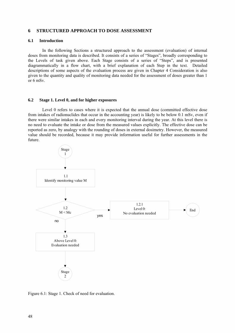
48
6 STRUCTURED APPROACH TO DOSE ASSESSMENT
6.1 Introduction
In the following Sections a structured approach to the assessment (evaluation) of internal doses from monitoring data is described. It consists of a series of “Stages”, broadly corresponding to the Levels of task given above. Each Stage consists of a series of “Steps”, and is presented diagrammatically in a flow chart, with a brief explanation of each Step in the text. Detailed descriptions of some aspects of the evaluation process are given in Chapter 4 Consideration is also given to the quantity and quality of monitoring data needed for the assessment of doses greater than 1 or 6 mSv.
6.2 Stage 1. Level 0, and for higher exposures
Level 0 refers to cases where it is expected that the annual dose (committed effective dose from intakes of radionuclides that occur in the accounting year) is likely to be below 0.1 mSv, even if there were similar intakes in each and every monitoring interval during the year. At this level there is no need to evaluate the intake or dose from the measured values explicitly. The effective dose can be reported as zero, by analogy with the rounding of doses in external dosimetry. However, the measured value should be recorded, because it may provide information useful for further assessments in the future.
Stage 1
1.1Identify monitoring value M
1.2M < Mc
1.2.1Level 0:
No evaluation neededEnd
Stage 2
yesno
1.3Above Level 0:
Evaluation needed
Figure 6.1: Stage 1. Check of need for evaluation.
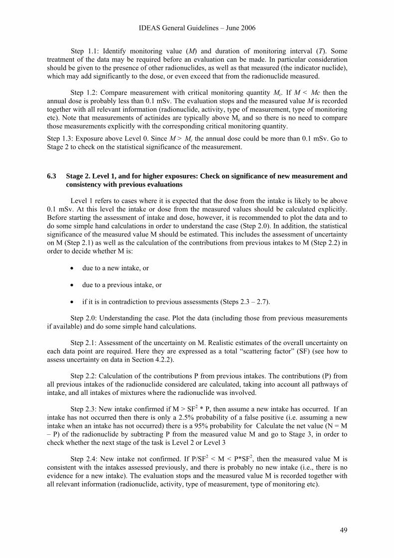
IDEAS General Guidelines – June 2006
49
Step 1.1: Identify monitoring value (M) and duration of monitoring interval (T). Some treatment of the data may be required before an evaluation can be made. In particular consideration should be given to the presence of other radionuclides, as well as that measured (the indicator nuclide), which may add significantly to the dose, or even exceed that from the radionuclide measured.
Step 1.2: Compare measurement with critical monitoring quantity Mc. If M < Mc then the annual dose is probably less than 0.1 mSv. The evaluation stops and the measured value M is recorded together with all relevant information (radionuclide, activity, type of measurement, type of monitoring etc). Note that measurements of actinides are typically above Mc and so there is no need to compare those measurements explicitly with the corresponding critical monitoring quantity.
Step 1.3: Exposure above Level 0. Since M > Mc the annual dose could be more than 0.1 mSv. Go to Stage 2 to check on the statistical significance of the measurement.
6.3 Stage 2. Level 1, and for higher exposures: Check on significance of new measurement and consistency with previous evaluations
Level 1 refers to cases where it is expected that the dose from the intake is likely to be above 0.1 mSv. At this level the intake or dose from the measured values should be calculated explicitly. Before starting the assessment of intake and dose, however, it is recommended to plot the data and to do some simple hand calculations in order to understand the case (Step 2.0). In addition, the statistical significance of the measured value M should be estimated. This includes the assessment of uncertainty on M (Step 2.1) as well as the calculation of the contributions from previous intakes to M (Step 2.2) in order to decide whether M is:
• due to a new intake, or
• due to a previous intake, or
• if it is in contradiction to previous assessments (Steps 2.3 – 2.7).
Step 2.0: Understanding the case. Plot the data (including those from previous measurements if available) and do some simple hand calculations.
Step 2.1: Assessment of the uncertainty on M. Realistic estimates of the overall uncertainty on each data point are required. Here they are expressed as a total “scattering factor” (SF) (see how to assess uncertainty on data in Section 4.2.2).
Step 2.2: Calculation of the contributions P from previous intakes. The contributions (P) from all previous intakes of the radionuclide considered are calculated, taking into account all pathways of intake, and all intakes of mixtures where the radionuclide was involved.
Step 2.3: New intake confirmed if M > SF2 * P, then assume a new intake has occurred. If an intake has not occurred then there is only a 2.5% probability of a false positive (i.e. assuming a new intake when an intake has not occurred) there is a 95% probability for Calculate the net value (N = M – P) of the radionuclide by subtracting P from the measured value M and go to Stage 3, in order to check whether the next stage of the task is Level 2 or Level 3
Step 2.4: New intake not confirmed. If P/SF2 < M < P*SF2, then the measured value M is consistent with the intakes assessed previously, and there is probably no new intake (i.e., there is no evidence for a new intake). The evaluation stops and the measured value M is recorded together with all relevant information (radionuclide, activity, type of measurement, type of monitoring etc).
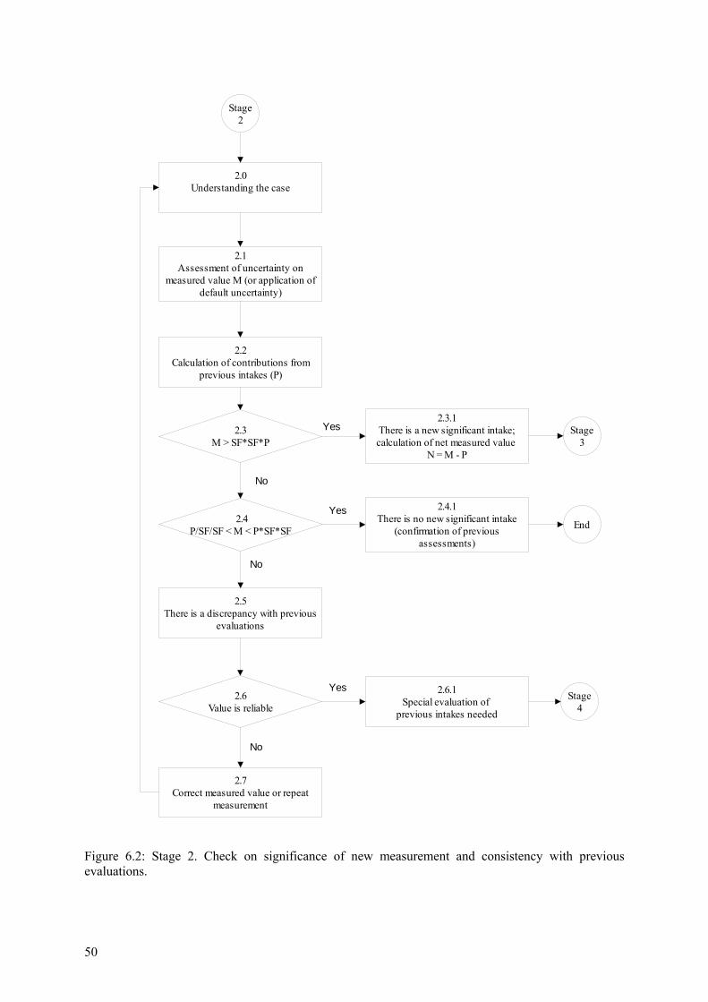
50
Stage 2
2.1Assessment of uncertainty on
measured value M (or application of default uncertainty)
2.2Calculation of contributions from
previous intakes (P)
2.3M > SF*SF*P
Stage 3
2.4P/SF/SF < M < P*SF*SF End
2.3.1There is a new significant intake; calculation of net measured value
N = M - P
2.4.1There is no new significant intake
(confirmation of previous assessments)
2.5There is a discrepancy with previous
evaluations
2.6Value is reliable
2.7Correct measured value or repeat
measurement
2.6.1Special evaluation of
previous intakes needed
Stage 4
Yes
No
Yes
No
Yes
No
2.0Understanding the case
Figure 6.2: Stage 2. Check on significance of new measurement and consistency with previous evaluations.
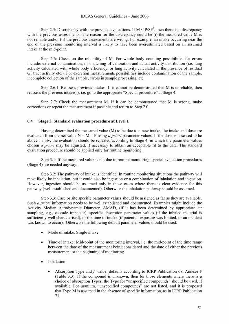
IDEAS General Guidelines – June 2006
51
Step 2.5: Discrepancy with the previous evaluations. If M < P/SF2, then there is a discrepancy with the previous assessments. The reason for the discrepancy could be (i) the measured value M is not reliable and/or (ii) the previous assessments are wrong. For example, an intake occurring near the end of the previous monitoring interval is likely to have been overestimated based on an assumed intake at the mid-point.
Step 2.6: Check on the reliability of M. For whole body counting possibilities for errors include: external contamination, mismatching of calibration and actual activity distribution (i.e. lung activity calculated with whole body efficiency, or lung activity calculated in the presence of residual GI tract activity etc.). For excretion measurements possibilities include contamination of the sample, incomplete collection of the sample, errors in sample processing, etc..
Step 2.6.1: Reassess previous intakes. If it cannot be demonstrated that M is unreliable, then reassess the previous intake(s), i.e. go to the appropriate “Special procedure” at Stage 4.
Step 2.7: Check the measurement M. If it can be demonstrated that M is wrong, make corrections or repeat the measurement if possible and return to Step 2.0.
6.4 Stage 3. Standard evaluation procedure at Level 1
Having determined the measured value (M) to be due to a new intake, the intake and dose are evaluated from the net value N = M – P using a priori parameter values. If the dose is assessed to be above 1 mSv, the evaluation should be repeated according to Stage 4, in which the parameter values chosen a priori may be adjusted, if necessary to obtain an acceptable fit to the data. The standard evaluation procedure should be applied only for routine monitoring.
Step 3.1: If the measured value is not due to routine monitoring, special evaluation procedures (Stage 4) are needed anyway.
Step 3.2: The pathway of intake is identified. In routine monitoring situations the pathway will most likely be inhalation, but it could also be ingestion or a combination of inhalation and ingestion. However, ingestion should be assumed only in those cases where there is clear evidence for this pathway (well established and documented). Otherwise the inhalation pathway should be assumed.
Step 3.3: Case or site specific parameter values should be assigned as far as they are available. Such a priori information needs to be well established and documented. Examples might include the Activity Median Aerodynamic Diameter, AMAD, (if it has been determined by appropriate air sampling, e.g., cascade impactor), specific absorption parameter values (if the inhaled material is sufficiently well characterised), or the time of intake (if potential exposure was limited, or an incident was known to occur). Otherwise the following default parameter values should be used:
• Mode of intake: Single intake
• Time of intake: Mid-point of the monitoring interval, i.e. the mid-point of the time range between the date of the measurement being considered and the date of either the previous measurement or the beginning of monitoring
• Inhalation:
• Absorption Type and f1 value: defaults according to ICRP Publication 68, Annexe F (Table 3.3). If the compound is unknown, then for those elements where there is a choice of absorption Types, the Type for “unspecified compounds” should be used, if available. For uranium, “unspecified compounds” are not listed, and it is proposed that Type M is assumed in the absence of specific information, as in ICRP Publication 71.
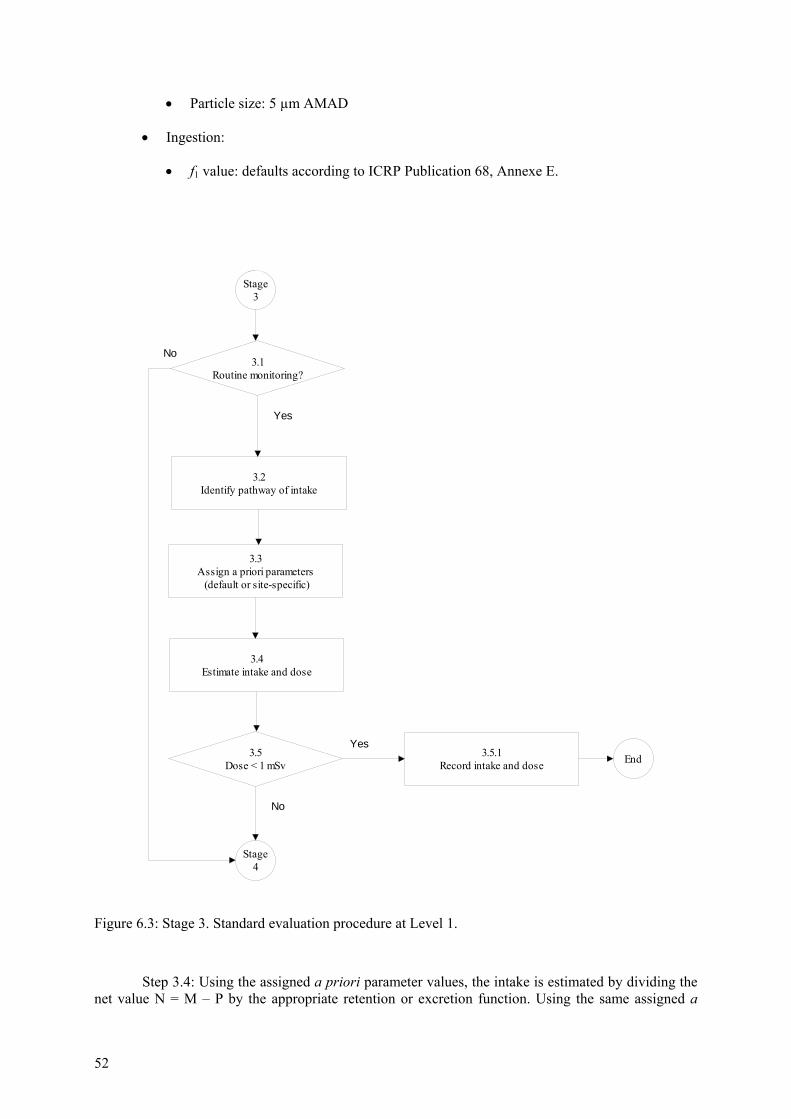
52
• Particle size: 5 µm AMAD
• Ingestion:
• f1 value: defaults according to ICRP Publication 68, Annexe E.
Stage
3
3.5Dose < 1 mSv
3.4Estimate intake and dose
End
Stage 4
3.2Identify pathway of intake
3.3Assign a priori parameters (default or site-specific)
Yes
No
3.5.1Record intake and dose
3.1Routine monitoring?
No
Yes
Figure 6.3: Stage 3. Standard evaluation procedure at Level 1.
Step 3.4: Using the assigned a priori parameter values, the intake is estimated by dividing the net value N = M – P by the appropriate retention or excretion function. Using the same assigned a
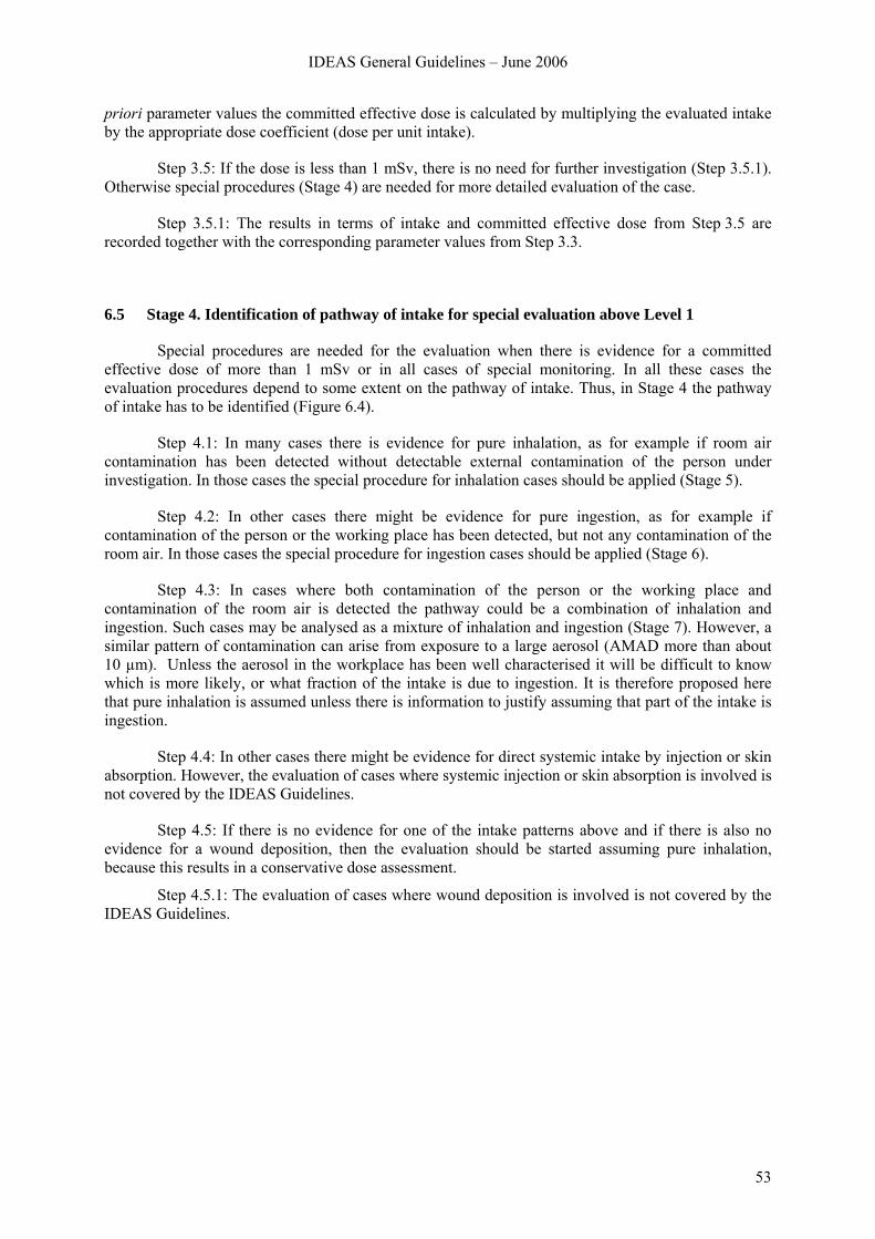
IDEAS General Guidelines – June 2006
53
priori parameter values the committed effective dose is calculated by multiplying the evaluated intake by the appropriate dose coefficient (dose per unit intake).
Step 3.5: If the dose is less than 1 mSv, there is no need for further investigation (Step 3.5.1). Otherwise special procedures (Stage 4) are needed for more detailed evaluation of the case.
Step 3.5.1: The results in terms of intake and committed effective dose from Step 3.5 are recorded together with the corresponding parameter values from Step 3.3.
6.5 Stage 4. Identification of pathway of intake for special evaluation above Level 1
Special procedures are needed for the evaluation when there is evidence for a committed effective dose of more than 1 mSv or in all cases of special monitoring. In all these cases the evaluation procedures depend to some extent on the pathway of intake. Thus, in Stage 4 the pathway of intake has to be identified (Figure 6.4).
Step 4.1: In many cases there is evidence for pure inhalation, as for example if room air contamination has been detected without detectable external contamination of the person under investigation. In those cases the special procedure for inhalation cases should be applied (Stage 5).
Step 4.2: In other cases there might be evidence for pure ingestion, as for example if contamination of the person or the working place has been detected, but not any contamination of the room air. In those cases the special procedure for ingestion cases should be applied (Stage 6).
Step 4.3: In cases where both contamination of the person or the working place and contamination of the room air is detected the pathway could be a combination of inhalation and ingestion. Such cases may be analysed as a mixture of inhalation and ingestion (Stage 7). However, a similar pattern of contamination can arise from exposure to a large aerosol (AMAD more than about 10 µm). Unless the aerosol in the workplace has been well characterised it will be difficult to know which is more likely, or what fraction of the intake is due to ingestion. It is therefore proposed here that pure inhalation is assumed unless there is information to justify assuming that part of the intake is ingestion.
Step 4.4: In other cases there might be evidence for direct systemic intake by injection or skin absorption. However, the evaluation of cases where systemic injection or skin absorption is involved is not covered by the IDEAS Guidelines.
Step 4.5: If there is no evidence for one of the intake patterns above and if there is also no evidence for a wound deposition, then the evaluation should be started assuming pure inhalation, because this results in a conservative dose assessment.
Step 4.5.1: The evaluation of cases where wound deposition is involved is not covered by the IDEAS Guidelines.
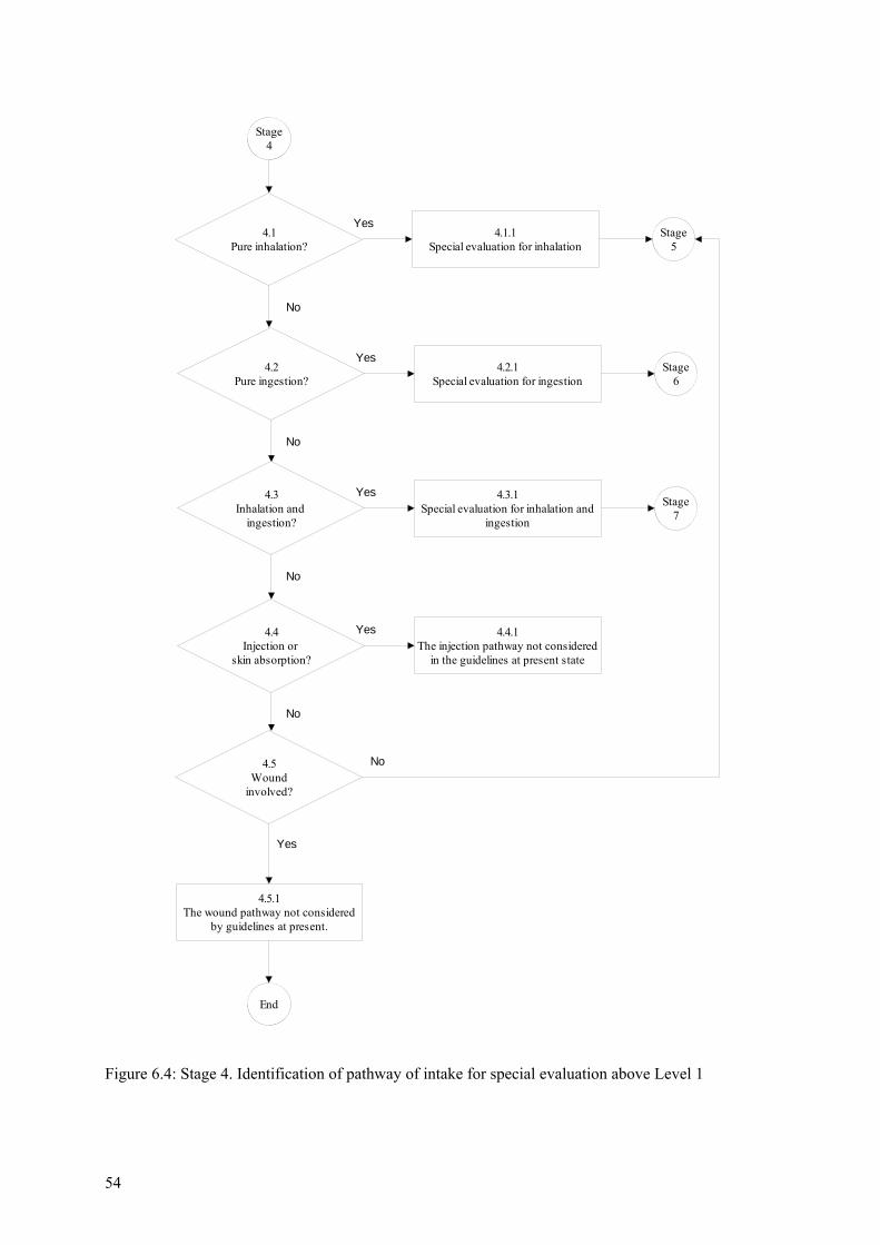
54
Stage 4
4.1Pure inhalation?
Stage 5
End
Yes
No
4.1.1Special evaluation for inhalation
4.2Pure ingestion?
Stage 6
Yes4.2.1
Special evaluation for ingestion
4.3Inhalation and
ingestion?
Stage 7
Yes 4.3.1Special evaluation for inhalation and
ingestion
No
4.5.1The wound pathway not considered
by guidelines at present.
No
4.5Wound
involved?
No
Yes
4.4Injection or
skin absorption?
Yes 4.4.1The injection pathway not considered
in the guidelines at present state
No
Figure 6.4: Stage 4. Identification of pathway of intake for special evaluation above Level 1
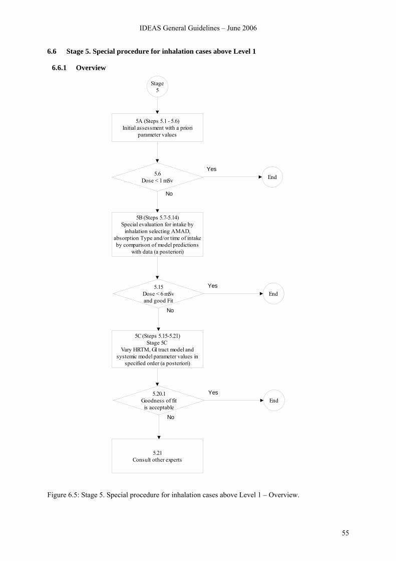
IDEAS General Guidelines – June 2006
55
6.6 Stage 5. Special procedure for inhalation cases above Level 1
6.6.1 Overview
Stage 5
5A (Steps 5.1 - 5.6)Initial assessment with a priori
parameter values
5B (Steps 5.7-5.14)Special evaluation for intake by
inhalation selecting AMAD, absorption Type and/or time of intake by comparison of model predictions
with data (a posteriori)
5.6Dose < 1 mSv End
Yes
No
5C (Steps 5.15-5.21)Stage 5C
Vary HRTM, GI tract model and systemic model parameter values in
specified order (a posteriori)
5.15Dose < 6 mSvand good Fit
EndYes
No
5.21Consult other experts
5.20.1Goodness of fitis acceptable
EndYes
No
Figure 6.5: Stage 5. Special procedure for inhalation cases above Level 1 – Overview.
56
The special procedure is grouped in three subsequent stages (see Figure 6.5). In the first stage (5A), a simple evaluation is carried out using parameter values chosen a priori: before the evaluation is carried out. The procedure is very similar to the “Standard procedure” (Stage 3). The main difference is that in a special procedure there should be more than one measurement.
In the second stage (5B), procedures are applied for varying the two main factors related to the inhaled material: the AMAD and absorption Type, and also the time of intake, if not known, using the measurement data (a posteriori).
In the third stage (5C), an advanced evaluation is carried out. It applies to cases where there are comprehensive data available. The fundamental approach of this stage is that the model parameter values are adjusted systematically, in a specific order, until the goodness of fit is acceptable (i.e. the fits obtained to all the data are not rejected by the specified criteria).
6.6.2 Stage 5A
In this stage, a simple evaluation is carried out using parameter values chosen a priori: before the evaluation is carried out. The procedure is very similar to the “Standard procedure” (Stage 3). The main difference is that in a special procedure there should be more than one measurement.
Step 5.1: Identification and preparation of measurement data. It is expected that there will be more than one measurement available for a special assessment (Mi for i = 1 to n). It is therefore important that realistic uncertainties are assigned to the data (“scattering factor”, SF, Step 2.1) There may be more than one type of measurement (urine, faeces, etc), and there may be measurements of more than one radionuclide involved in the exposure. If a specific incident (and hence time of intake) was not identified, the results of workplace monitoring, such as personal or room air sampling, should be checked to give guidance on the time course of intake.
Step 5.2: (As Step 2.3 for a single measurement.) The contributions (Pi) from all previous intakes of the radionuclide considered are calculated, taking into account all pathways of intake, and all intakes of mixtures where the radionuclide was involved. The net values (Ni = Mi – Pi) of the radionuclide are calculated by subtracting Pi from the measured value Mi.
Step 5.3: (As Step 3.2 in the Standard Procedure, Stage 3, except for time of intake). Case or site specific parameter values should be assigned as far as they are available. Such a priori information needs to be well established and documented. Examples might include the Activity Median Aerodynamic Diameter, AMAD, (if it has been determined by appropriate air sampling, e.g., cascade impactor), specific absorption parameter values (if the inhaled material is sufficiently well characterised), or the time of intake (if potential exposure was limited, or an incident was known to occur). Otherwise the following default parameter values should be used:
• Mode of intake: Single intake
• Absorption Type and f1 value: defaults according to ICRP Publication 68, Annexe F (see Table 3.3). If the compound is unknown, then for those elements where there is a choice of absorption Types, the Type for “unspecified compounds” should be used, if available. For uranium, “unspecified compounds” are not listed, and it is proposed that Type M is assumed in the absence of specific information, as in ICRP Publication 71 (1995).
• Particle size: 5 µm AMAD
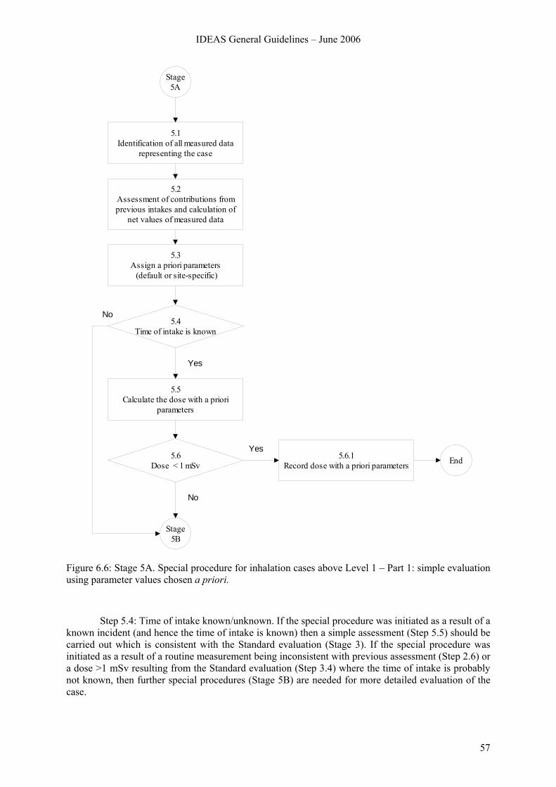
IDEAS General Guidelines – June 2006
57
Stage 5A
5.1Identification of all measured data
representing the case
5.2Assessment of contributions from previous intakes and calculation of
net values of measured data
5.3Assign a priori parameters (default or site-specific)
5.5Calculate the dose with a priori
parameters
5.6Dose < 1 mSv
5.6.1Record dose with a priori parameters End
5.4Time of intake is known
No
Yes
Yes
Stage5B
No
Figure 6.6: Stage 5A. Special procedure for inhalation cases above Level 1 – Part 1: simple evaluation using parameter values chosen a priori.
Step 5.4: Time of intake known/unknown. If the special procedure was initiated as a result of a known incident (and hence the time of intake is known) then a simple assessment (Step 5.5) should be carried out which is consistent with the Standard evaluation (Stage 3). If the special procedure was initiated as a result of a routine measurement being inconsistent with previous assessment (Step 2.6) or a dose >1 mSv resulting from the Standard evaluation (Step 3.4) where the time of intake is probably not known, then further special procedures (Stage 5B) are needed for more detailed evaluation of the case.
58
Step 5.5: (As step 3.3 in the Standard Procedure, Stage 3, but for more than one measurement). Using the assigned a priori parameter values, an estimate of intake Ii is obtained by dividing the net measured value Ni = Mi – Pi by the appropriate retention or excretion function mi(t). The best estimate of intake can be calculated according to Chapter 4 with the equation:
[ ]
[ ]∑
∑
=
== n
i i
n
i i
ii
SF
SFtmN
I
12
12
)(ln1
)(ln))(/(ln
)ln(
where SFi is the scattering factor of the net measured value Ni . If the scattering factor is the same for all measurements, the equation results in
n
n
i i
i
tmN
I ∏=
=1 )(
i.e. the best estimate of the intake is the geometric mean of the intakes
( )i
ii tm
NI =
calculated from the single measurements. Using the same assigned a priori parameter values the committed effective dose is calculated by multiplying the “best estimate” of intake by the appropriate dose coefficient (dose per unit intake).
Step 5.6: If the effective dose estimated in step 5.5 (taking into account all available monitoring data) is less than 1 mSv, there is no need for further investigation (Step 5.6.1). (The dose from the intake under consideration, rather than the “annual dose” as in Step 3.4, is the criterion, because intakes requiring special assessment procedures should be unusual for any individual worker.) Otherwise further special procedures (Stage 5B) are needed for more detailed evaluation of the case. Caution must be taken when the default absorption type does not lead to a conservative estimate of the dose, for example in the case of Sr.
Step 5.6.1: The results in terms of intake and committed effective dose from Step 5.6 are recorded together with the corresponding parameter values from Step 5.3.
6.6.3 Stage 5B
In this stage, procedures are described for varying the two main factors related to the inhaled material: the AMAD and absorption Type, and also the time of intake, if not known, using the measurement data (a posteriori). Note, however, that if material specific absorption parameter values were assigned a priori, (Step 5.3) default absorption Types should not be used (Steps 5.11, 5.12, 5.13 and 5.14): if an acceptable fit is not obtained with the assigned parameter values, they can be varied a posteriori, in Stage 5C.
In this Stage, and in Stage 5C that follows, parameter values are selected on the basis of the “fit” of the model predictions to the observations (data). A check on whether the fit is adequate is used to decide whether to stop the evaluation, or to go on to further steps. A measure of the “Goodness of fit” (GOF) and the criteria for deciding that the fit is good enough are therefore critical issues. There may be conflict between “harmonisation” and “accuracy”. Generally the better the data (quality and quantity) the more likely it is that a statistical test will show that the data are inconsistent with the
IDEAS General Guidelines – June 2006
59
model. If the data are poor it is more likely that the model will fit – in the extreme case of a single measurement any model will fit. It is therefore important that there should be sufficient data available for assessment of a significant dose, and the higher the dose, the better the data should be. Proposals are therefore made for the minimum amounts of data that would be acceptable (“sufficient”, see Section 4.1.4).
Step 5.7: Are there sufficient data? As noted in the introduction, criteria for the “sufficient” number (and types) of relevant data, duration of monitoring etc, are proposed according to the dose. In this Step, the numbers for the range 1 mSv <Dose <6 mSv are appropriate, because a special procedure is generally initiated on the assumption that the dose could exceed 1 mSv, and doses greater than 6 mSv are considered in steps 5.11.2 and 5.12.2 below.
Step 5.7.1: Get additional dose relevant data. This assumes that the evaluation is being carried out in real time, so that the opportunity exists to obtain more measurements if those available are insufficient. (For historical cases, where it is not possible to obtain more measurements, it should be recorded that the data are insufficient, and therefore the result should be treated with caution.) When the additional data have been obtained, a simple re-evaluation Stage 5A is made.
Step 5.8: Is the time of intake known? As noted in the introduction, there are two main alternative routes through this stage of the process, according to whether or not the time of intake is known. Generally, Special Procedures follow from an identified incident for which the time is known: Steps 5.9 to 5.11, and if necessary 5.13 are followed. However, previously unidentified intakes are sometimes found through e.g. routine monitoring, and so the time of intake is unknown, or known only to be within a certain interval. Step 5.12 and if necessary 5.14 are followed, but provide less opportunity for a posteriori characterisation of the material.
Step 5.9: Are early lung and faeces data available? During the first few days after an accidental inhalation intake of a relatively insoluble material (Type M or Type S) most of the activity will be in the respiratory tract, or cleared through the GI tract to the faeces. In the event of such an incident with potential for a significant intake it would therefore be expected that if feasible, measurements of lung and faeces would be made. If the cumulative faecal excretion over the first few days, and a measurement on which the initial lung deposit can be estimated are available, then an estimate can be made of the effective AMAD (Step 5.10).
Step 5.10: Derive effective AMAD from early lung and faeces data. Although recent reviews of reported measurements of AMAD in workplaces (e.g. Dorrian and Bailey 1995) support the ICRP publication 66/68 default value of 5 μm for occupational exposure, they also show that a wide range (about 1–20 μm) has been observed. If the airborne contamination in the workplace has been well characterised, it may be possible to use a more realistic value based on measurements of the activity size distribution. Alternatively, if there are suitable early measurement data available, an “effective” AMAD can be inferred a posteriori from the measurements. The main effect of the aerosol AMAD is to determine the relative amounts deposited (i) in the upper respiratory tract (extrathoracic airways, ET, bronchi, BB, and bronchioles, bb, in the HRTM), which (if not absorbed into blood) is mainly cleared rapidly to the GI tract and hence to faeces within a few days, and (ii) in the lower respiratory tract (alveolar-interstitial, AI, region in the HRTM), which is mainly cleared slowly from the lungs. ICRP Supporting Guidance 3 (ICRP 2002) showed that for a relatively insoluble (Type M or S) material inhaled by a Reference Worker, the ratio of cumulative faecal excretion over the first 3 days to lung activity on day 3 increased almost linearly with AMAD over the range 1 to 10 μm (Figure 6.7). Hence the observed ratio could be used to infer the “effective” AMAD. It is referred to as “effective”, because the ratio will be determined not only by the aerosol size, but also by the subject’s breathing pattern (especially if it involves mouth-breathing) and inter-subject variation in deposition under any given set of conditions. Because it takes account of these, it is preferable for dose assessment than a priori measurements of the AMAD.
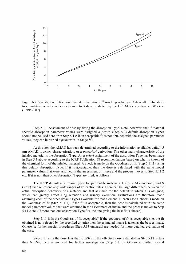
60
0
2
4
6
8
10
12
14
0 1 2 3 4 5 6 7 8 9 10
AMAD, µm
Cum
ulat
ive
activ
ity in
faec
es fr
om 1
to 3
day
s /
activ
ity in
lung
on
day
3Type M
Type S
Figure 6.7: Variation with fraction inhaled of the ratio of 241Am lung activity at 3 days after inhalation, to cumulative activity in faeces from 1 to 3 days predicted by the HRTM for a Reference Worker. (ICRP 2002)
Step 5.11: Assessment of dose by fitting the absorption Type. Note, however, that if material specific absorption parameter values were assigned a priori, (Step 5.3) default absorption Types should not be used here or in Step 5.13: if an acceptable fit is not obtained with the assigned parameter values, they can be varied a posteriori, in Stage 5C.
At this step the AMAD has been determined according to the information available: default 5 µm AMAD, a priori characterisation, or a posteriori derivation. The other main characteristic of the inhaled material is the absorption Type. An a priori assignment of the absorption Type has been made in Step 5.3 above according to the ICRP Publication 68 recommendations based on what is known of the chemical form of the inhaled material. A check is made on the Goodness of fit (Step 5.11.1) using this default absorption Type. If it is acceptable, then the dose is calculated with the same model parameter values that were assumed in the assessment of intake and the process moves to Step 5.11.2 etc. If it is not, then other absorption Types are tried, as follows.
The ICRP default absorption Types for particulate materials: F (fast), M (moderate) and S (slow) each represent very wide ranges of absorption rates. There can be large differences between the actual absorption behaviour of a material and that assumed for the default to which it is assigned, which can greatly affect lung retention and urinary excretion. Evaluations are therefore made assuming each of the other default Types available for that element. In each case a check is made on the Goodness of fit (Step 5.11.1). If the fit is acceptable, then the dose is calculated with the same model parameter values that were assumed in the assessment of intake and the process moves to Step 5.11.2 etc. (If more than one absorption Type fits, the one giving the best fit is chosen).
Step 5.11.1: Is the Goodness of fit acceptable? If the goodness of fit is acceptable (i.e. the fit obtained is not rejected by the specified criteria) then the estimated intake is taken as the best estimate. Otherwise further special procedures (Step 5.13 onwards) are needed for more detailed evaluation of the case.
Step 5.11.2: Is the dose less than 6 mSv? If the effective dose estimated in Step 5.11 is less than 6 mSv, there is no need for further investigation (Step 5.11.3). Otherwise further special
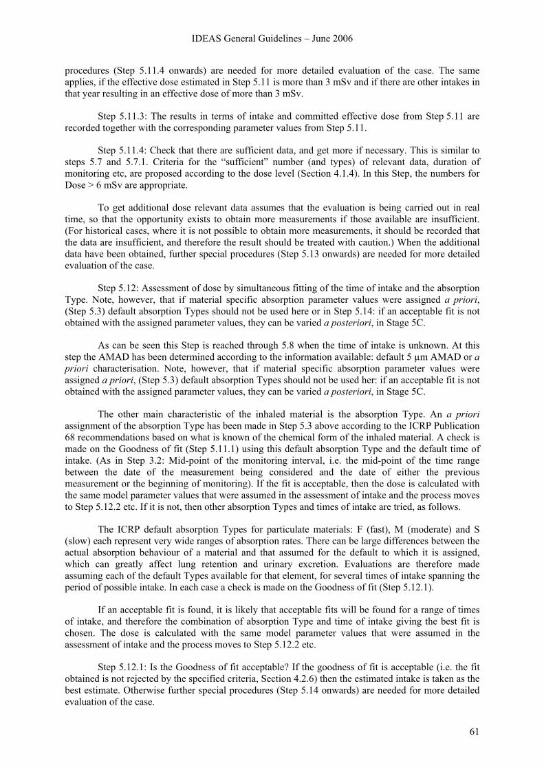
IDEAS General Guidelines – June 2006
61
procedures (Step 5.11.4 onwards) are needed for more detailed evaluation of the case. The same applies, if the effective dose estimated in Step 5.11 is more than 3 mSv and if there are other intakes in that year resulting in an effective dose of more than 3 mSv.
Step 5.11.3: The results in terms of intake and committed effective dose from Step 5.11 are recorded together with the corresponding parameter values from Step 5.11.
Step 5.11.4: Check that there are sufficient data, and get more if necessary. This is similar to steps 5.7 and 5.7.1. Criteria for the “sufficient” number (and types) of relevant data, duration of monitoring etc, are proposed according to the dose level (Section 4.1.4). In this Step, the numbers for Dose > 6 mSv are appropriate.
To get additional dose relevant data assumes that the evaluation is being carried out in real time, so that the opportunity exists to obtain more measurements if those available are insufficient. (For historical cases, where it is not possible to obtain more measurements, it should be recorded that the data are insufficient, and therefore the result should be treated with caution.) When the additional data have been obtained, further special procedures (Step 5.13 onwards) are needed for more detailed evaluation of the case.
Step 5.12: Assessment of dose by simultaneous fitting of the time of intake and the absorption Type. Note, however, that if material specific absorption parameter values were assigned a priori, (Step 5.3) default absorption Types should not be used here or in Step 5.14: if an acceptable fit is not obtained with the assigned parameter values, they can be varied a posteriori, in Stage 5C.
As can be seen this Step is reached through 5.8 when the time of intake is unknown. At this step the AMAD has been determined according to the information available: default 5 µm AMAD or a priori characterisation. Note, however, that if material specific absorption parameter values were assigned a priori, (Step 5.3) default absorption Types should not be used her: if an acceptable fit is not obtained with the assigned parameter values, they can be varied a posteriori, in Stage 5C.
The other main characteristic of the inhaled material is the absorption Type. An a priori assignment of the absorption Type has been made in Step 5.3 above according to the ICRP Publication 68 recommendations based on what is known of the chemical form of the inhaled material. A check is made on the Goodness of fit (Step 5.11.1) using this default absorption Type and the default time of intake. (As in Step 3.2: Mid-point of the monitoring interval, i.e. the mid-point of the time range between the date of the measurement being considered and the date of either the previous measurement or the beginning of monitoring). If the fit is acceptable, then the dose is calculated with the same model parameter values that were assumed in the assessment of intake and the process moves to Step 5.12.2 etc. If it is not, then other absorption Types and times of intake are tried, as follows.
The ICRP default absorption Types for particulate materials: F (fast), M (moderate) and S (slow) each represent very wide ranges of absorption rates. There can be large differences between the actual absorption behaviour of a material and that assumed for the default to which it is assigned, which can greatly affect lung retention and urinary excretion. Evaluations are therefore made assuming each of the default Types available for that element, for several times of intake spanning the period of possible intake. In each case a check is made on the Goodness of fit (Step 5.12.1).
If an acceptable fit is found, it is likely that acceptable fits will be found for a range of times of intake, and therefore the combination of absorption Type and time of intake giving the best fit is chosen. The dose is calculated with the same model parameter values that were assumed in the assessment of intake and the process moves to Step 5.12.2 etc.
Step 5.12.1: Is the Goodness of fit acceptable? If the goodness of fit is acceptable (i.e. the fit obtained is not rejected by the specified criteria, Section 4.2.6) then the estimated intake is taken as the best estimate. Otherwise further special procedures (Step 5.14 onwards) are needed for more detailed evaluation of the case.
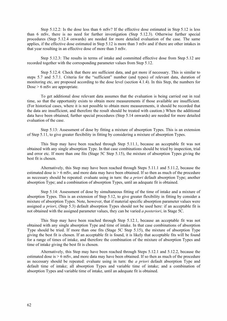
62
Step 5.12.2: Is the dose less than 6 mSv? If the effective dose estimated in Step 5.12 is less than 6 mSv, there is no need for further investigation (Step 5.12.3). Otherwise further special procedures (Step 5.12.4 onwards) are needed for more detailed evaluation of the case. The same applies, if the effective dose estimated in Step 5.12 is more than 3 mSv and if there are other intakes in that year resulting in an effective dose of more than 3 mSv.
Step 5.12.3: The results in terms of intake and committed effective dose from Step 5.12 are recorded together with the corresponding parameter values from Step 5.12.
Step 5.12.4: Check that there are sufficient data, and get more if necessary. This is similar to steps 5.7 and 5.7.1. Criteria for the “sufficient” number (and types) of relevant data, duration of monitoring etc, are proposed according to the dose level (section 4.1.4). In this Step, the numbers for Dose > 6 mSv are appropriate.
To get additional dose relevant data assumes that the evaluation is being carried out in real time, so that the opportunity exists to obtain more measurements if those available are insufficient. (For historical cases, where it is not possible to obtain more measurements, it should be recorded that the data are insufficient, and therefore the result should be treated with caution.) When the additional data have been obtained, further special procedures (Step 5.14 onwards) are needed for more detailed evaluation of the case.
Step 5.13: Assessment of dose by fitting a mixture of absorption Types. This is an extension of Step 5.11, to give greater flexibility in fitting by considering a mixture of absorption Types.
This Step may have been reached through Step 5.11.1, because an acceptable fit was not obtained with any single absorption Type. In that case combinations should be tried by inspection, trial and error etc. If more than one fits (Stage 5C Step 5.15), the mixture of absorption Types giving the best fit is chosen.
Alternatively, this Step may have been reached through Steps 5.11.1 and 5.11.2, because the estimated dose is > 6 mSv, and more data may have been obtained. If so then as much of the procedure as necessary should be repeated: evaluate using in turn: the a priori default absorption Type; another absorption Type; and a combination of absorption Types, until an adequate fit is obtained.
Step 5.14: Assessment of dose by simultaneous fitting of the time of intake and a mixture of absorption Types. This is an extension of Step 5.12, to give greater flexibility in fitting by consider a mixture of absorption Types. Note, however, that if material specific absorption parameter values were assigned a priori, (Step 5.3) default absorption Types should not be used here: if an acceptable fit is not obtained with the assigned parameter values, they can be varied a posteriori, in Stage 5C.
This Step may have been reached through Step 5.12.1, because an acceptable fit was not obtained with any single absorption Type and time of intake. In that case combinations of absorption Type should be tried. If more than one fits (Stage 5C Step 5.15), the mixture of absorption Type giving the best fit is chosen. If an acceptable fit is found, it is likely that acceptable fits will be found for a range of times of intake, and therefore the combination of the mixture of absorption Types and time of intake giving the best fit is chosen.
Alternatively, this Step may have been reached through Steps 5.12.1 and 5.12.2, because the estimated dose is > 6 mSv, and more data may have been obtained. If so then as much of the procedure as necessary should be repeated: evaluate using in turn: the a priori default absorption Type and default time of intake; all absorption Types and variable time of intake; and a combination of absorption Types and variable time of intake, until an adequate fit is obtained.
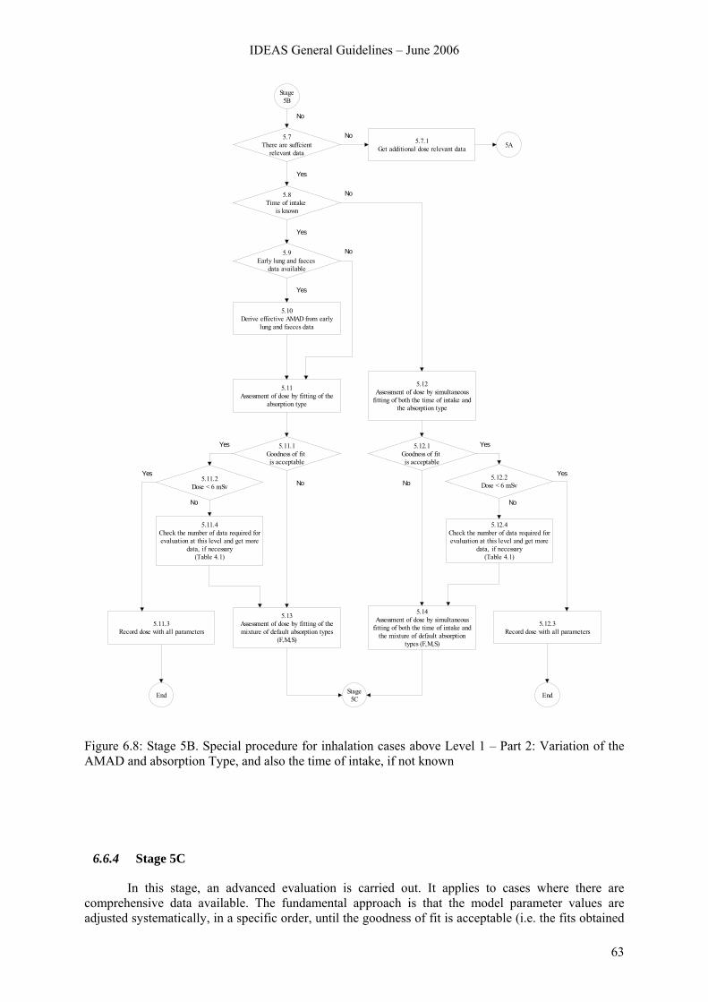
IDEAS General Guidelines – June 2006
63
5A
5.8Time of intake
is known
5.9Early lung and faeces
data available
5.10Derive effective AMAD from early
lung and faeces data
5.11Assessment of dose by fitting of the
absorption type
5.12Assessment of dose by simultaneous
fitting of both the time of intake and the absorption type
5.7.1Get additional dose relevant data
5.7There are suffcient
relevant data
5.11.1Goodness of fit is acceptable
5.13Assessment of dose by fitting of the mixture of default absorption types
(F,M,S)
5.14Assessment of dose by simultaneous
fitting of both the time of intake and the mixture of default absorption
types (F,M,S)
5.12.3Record dose with all parameters
5.12.1Goodness of fit is acceptable
5.11.2Dose < 6 mSv
5.11.4Check the number of data required for evaluation at this level and get more
data, if necessary(Table 4.1)
5.12.2Dose < 6 mSv
5.12.4Check the number of data required for evaluation at this level and get more
data, if necessary(Table 4.1)
No
No
Yes
No
Yes
No
Yes
Yes
NoYes
No
Yes
NoYes
No
5.11.3Record dose with all parameters
Stage5B
Stage5CEnd End
Figure 6.8: Stage 5B. Special procedure for inhalation cases above Level 1 – Part 2: Variation of the AMAD and absorption Type, and also the time of intake, if not known
6.6.4 Stage 5C
In this stage, an advanced evaluation is carried out. It applies to cases where there are comprehensive data available. The fundamental approach is that the model parameter values are adjusted systematically, in a specific order, until the goodness of fit is acceptable (i.e. the fits obtained
64
to all the data are not rejected by the specified criteria). If the fit is acceptable then the estimated intake is taken as the best estimate and the effective dose is calculated with the same model parameter values that were assumed in the assessment of intake. These results (intake and committed effective dose) are then recorded together with the corresponding parameter values (Step 5.15.1). Thus after each Step in which a parameter value is varied (5.17 to 5.22) there is a corresponding Step (5.17.1 to 5.22.1 respectively) to test the goodness of fit. Since these are all very similar to Step 5.15, explanatory text is not given.
If the time of intake is unknown, then by the start of this Stage it may have been assessed, based on simultaneous fitting of the model to the data with a mixture of absorption Types (Step 5.12). In that case, if any of the parameter values are changed in the Steps below, the time of intake should be re-assessed.
It is recommended, in cases where multiple types of bioassay data sets are available, that the intake and dose are assessed by fitting predicted values to the different types of data simultaneously.
Step 5.15: Is the goodness of fit acceptable? If the goodness of fit is acceptable (i.e. the fit obtained is not rejected by the specified criteria, Section 4.2.6) then the estimated intake is taken as the best estimate. The effective dose is then calculated with the same model parameter values that were assumed in the assessment of intake. However if the fit is rejected then proceed to next (step 5.16).
Step 5.16: Determine specific HRTM absorption parameter values: For materials that are moderately to very insoluble (typically absorption Types M or S), determine specific values for fr and ss by fitting fr, ss and intake to the data with sr fixed at 100 d-1. For most materials there is no evidence for binding to the respiratory tract so the bound fraction fb is taken to be zero. However, if relevant values of sr and/or of fb and sb have been determined from in vivo experimental data then use these values.
Step 5.17: Determine specific f1 value: Generally, it is not justifiable to change the f1 value as well as the HRTM absorption parameter values. Occasionally, for inhaled materials that are relatively insoluble, it is necessary to reduce the value of f1 so that the predicted systemic activities or urinary excretion rates are consistent with the data.
Step 5.18: Determine specific HRTM particle transport values: The parameter values that describe particle transport from the respiratory tract in the HRTM were based so far as possible on human experimental data, which enable typical lung clearance rates to be determined for a year or so after particle deposition in the lungs. However, the values were chosen to be average values for healthy non-smokers. The experimental data from which they were derived show considerable inter-subject variation even among healthy subjects, and indicate that clearance would generally be slower in smokers and patients with lung disease (ICRP Publication 66, 1994). If there are comprehensive lung and/or faecal excretion data available, it may be necessary to vary particle transport rates to improve the fits to the data.
It should be noted that adjusting particle transport rates also affects the amount absorbed into blood, because clearance from the lung is competitive between absorption into blood and particle transport to the GI tract. Thus in some cases it is necessary to readjust HRTM absorption parameter values (i.e. repeat step 5.16) after varying the particle transport rates.
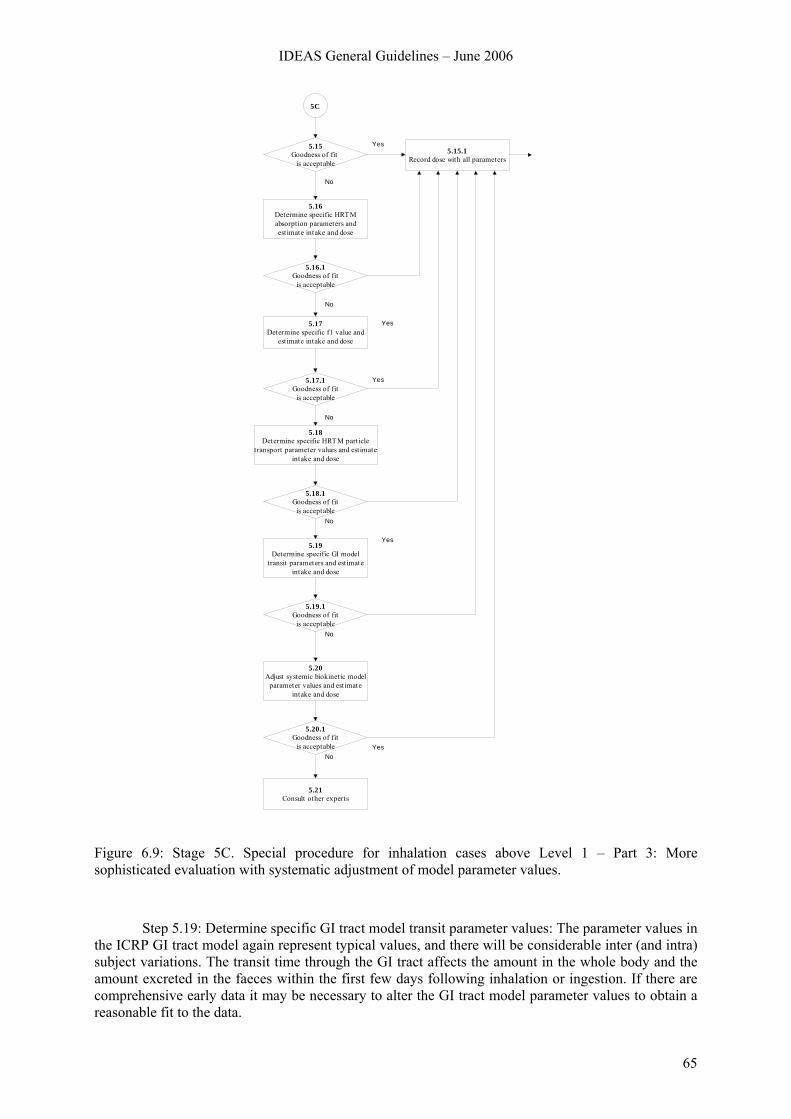
IDEAS General Guidelines – June 2006
65
5C
5.15Goodness of fit
is acceptable
5.15.1Record dose with all parameters
5.16Determine specific HRTM absorption parameters and est imate intake and dose
5.16.1Goodness of fit
is acceptable
5.17Determine specific f1 value and
est imate intake and dose
5.17.1Goodness of fit
is acceptable
5.18Determine specific HRTM part icle
transport parameter values and estimate intake and dose
5.18.1Goodness of fit
is acceptable
Yes
No
Yes
No
Yes
No
Yes5.19
Determine specific GI model transit parameters and est imate
intake and dose
No
5.19.1Goodness of fit
is acceptableNo
5.20Adjust systemic biokinetic model
parameter values and est imate intake and dose
5.20.1Goodness of fit
is acceptable
5.21Consult other experts
NoYes
Figure 6.9: Stage 5C. Special procedure for inhalation cases above Level 1 – Part 3: More sophisticated evaluation with systematic adjustment of model parameter values.
Step 5.19: Determine specific GI tract model transit parameter values: The parameter values in the ICRP GI tract model again represent typical values, and there will be considerable inter (and intra) subject variations. The transit time through the GI tract affects the amount in the whole body and the amount excreted in the faeces within the first few days following inhalation or ingestion. If there are comprehensive early data it may be necessary to alter the GI tract model parameter values to obtain a reasonable fit to the data.
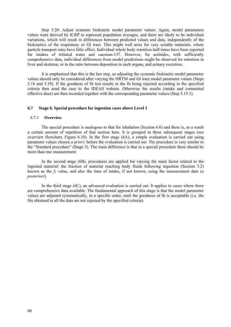
66
Step 5.20: Adjust systemic biokinetic model parameter values: Again, model parameters values were derived by ICRP to represent population averages, and there are likely to be individual variations, which will result in differences between predicted values and data, independently of the biokinetics of the respiratory or GI tract. This might well arise for very soluble materials, where particle transport rates have little effect. Individual whole body retention half-times have been reported for intakes of tritiated water and caesium-137. However, for actinides, with sufficiently comprehensive data, individual differences from model predictions might be observed for retention in liver and skeleton, or in the ratio between deposition in such organs, and urinary excretion.
It is emphasised that this is the last step, so adjusting the systemic biokinetic model parameter values should only be considered after varying the HRTM and GI tract model parameter values (Steps 5.18 and 5.19). If the goodness of fit test results in the fit being rejected according to the specified criteria then send the case to the IDEAS website. Otherwise the results (intake and committed effective dose) are then recorded together with the corresponding parameter values (Step 5.15.1).
6.7 Stage 6. Special procedure for ingestion cases above Level 1
6.7.1 Overview
The special procedure is analogous to that for inhalation (Section 6.6) and there is, as a result a certain amount of repetition of that section here. It is grouped in three subsequent stages (see overview flowchart, Figure 6.10). In the first stage (6A), a simple evaluation is carried out using parameter values chosen a priori: before the evaluation is carried out. The procedure is very similar to the “Standard procedure” (Stage 3). The main difference is that in a special procedure there should be more than one measurement.
In the second stage (6B), procedures are applied for varying the main factor related to the ingested material: the fraction of material reaching body fluids following ingestion (Section 3.2) known as the f1 value, and also the time of intake, if not known, using the measurement data (a posteriori).
In the third stage (6C), an advanced evaluation is carried out. It applies to cases where there are comprehensive data available. The fundamental approach of this stage is that the model parameter values are adjusted systematically, in a specific order, until the goodness of fit is acceptable (i.e. the fits obtained to all the data are not rejected by the specified criteria).
IDEAS General Guidelines – June 2006
67
Stage 6
6A (Steps 6.1 - 6.6)Initial assessment with a priori
parameter values
6B (Steps 6.7-6.12)Select f1 value and/or time of intake
(if unknown) by comparison of model predictions with data (a posteriori)
6.6Dose < 1 mSv End
Yes
No
6C (Steps 6.13-6.17) Vary GI tract and systemic model
parameter values in specified order (a posteriori)
6.12Dose < 6 mSvand good Fit
EndYes
No
6.17Consult other experts
6.16.1Goodness of fitis acceptable
EndYes
No
Figure 6.10: Stage 6. Special procedure for ingestion cases above Level 1 – Overview.
68
6.7.2 Stage 6A
In this stage, a simple evaluation is carried out using parameter values chosen a priori: before the evaluation is carried out. The procedure is very similar to the “Standard procedure” (Stage 3). The main difference is that in a special procedure there should be more than one measurement.
Step 6.1: Identification and preparation of measurement data. It is expected that there will be more than one measurement available for a special assessment (Mi for i = 1 to n). It is therefore important that realistic uncertainties are assigned to the data (“scattering factor”, SF, Step 2.1) There may be more than one type of measurement (urine, faeces, etc), and there may be measurements of more than one radionuclide involved in the exposure.
Step 6.2: (As Step 2.3 for a single measurement.) The contributions (Pi) from all previous intakes of the radionuclide considered are calculated, taking into account all pathways of intake, and all intakes of mixtures where the radionuclide was involved. The net values (Ni = Mi – Pi) of the radionuclide are calculated by subtracting Pi from the measured value Mi.
Step 6.3: (As Step 3.2 in the Standard Procedure, Stage 3, except for time of intake).
Case or site specific parameter values should be assigned as far as they are available. Such a priori information needs to be well established and documented. Examples might include the fraction of the ingested activity that is absorbed into the systemic circulation: the “f1 value” – if it has been determined by an appropriate in vivo experiment (although such experiments are uncommon), or the time of intake, if potential exposure was limited, or an incident was known to occur. Otherwise the following default parameter values should be used:
• Mode of intake: Single intake
• f1 value: defaults according to ICRP Publication 68, Annexe E.
Step 6.4: Time of intake known/unknown. If the special procedure was initiated as a result of a known incident (and hence the time of intake is known) then a simple assessment (Step 6.5) should be carried out which is consistent with the Standard evaluation (Stage 3). If the special procedure was initiated as a result of a routine measurement being inconsistent with previous assessment (Step 2.6) or a dose >1 mSv resulting from the Standard evaluation (Step 3.4) where the time of intake is probably not known, then further special procedures (Stage 6B) are needed for more detailed evaluation of the case.
Step 6.5: (As step 3.3 in the Standard Procedure, Stage 3, but for more than one measurement). Using the assigned a priori parameter values, an estimate of intake Ii is obtained by dividing the net value Ni = Mi – Pi by the appropriate retention or excretion function. The geometric mean of the value of Ii gives the “best estimate” of intake (see step 5.5). Using the same assigned a priori parameter values the committed effective dose is calculated by multiplying the “best estimate” of intake by the appropriate dose coefficient (dose per unit intake).
Step 6.6: If the effective dose estimated in Step 6.5 is less than 1 mSv, there is no need for further investigation (Step 6.6.1). (The dose from the intake under consideration, rather than the “annual dose” as in Step 3.4, is the criterion, because intakes requiring special assessment procedures should be unusual for any individual worker.) Otherwise further special procedures (Stage 6B) are needed for more detailed evaluation of the case.
Step 6.6.1: The results in terms of intake and committed effective dose from Step 6.6 are recorded together with the corresponding parameter values from Step 6.3.
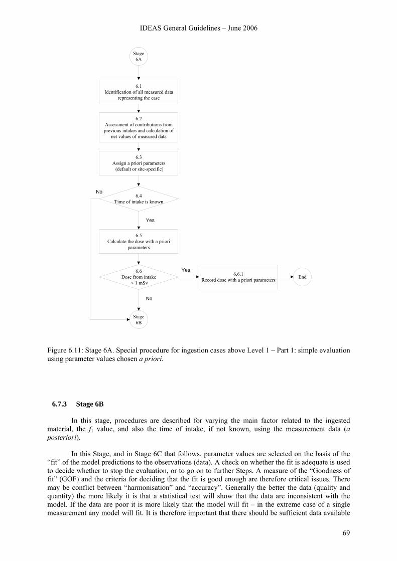
IDEAS General Guidelines – June 2006
69
Stage 6A
6.1Identification of all measured data
representing the case
6.2Assessment of contributions from previous intakes and calculation of
net values of measured data
6.3Assign a priori parameters (default or site-specific)
6.5Calculate the dose with a priori
parameters
6.6Dose from intake
< 1 mSv
6.6.1Record dose with a priori parameters End
6.4Time of intake is known
No
Yes
Yes
Stage6B
No
Figure 6.11: Stage 6A. Special procedure for ingestion cases above Level 1 – Part 1: simple evaluation using parameter values chosen a priori.
6.7.3 Stage 6B
In this stage, procedures are described for varying the main factor related to the ingested material, the f1 value, and also the time of intake, if not known, using the measurement data (a posteriori).
In this Stage, and in Stage 6C that follows, parameter values are selected on the basis of the “fit” of the model predictions to the observations (data). A check on whether the fit is adequate is used to decide whether to stop the evaluation, or to go on to further Steps. A measure of the “Goodness of fit” (GOF) and the criteria for deciding that the fit is good enough are therefore critical issues. There may be conflict between “harmonisation” and “accuracy”. Generally the better the data (quality and quantity) the more likely it is that a statistical test will show that the data are inconsistent with the model. If the data are poor it is more likely that the model will fit – in the extreme case of a single measurement any model will fit. It is therefore important that there should be sufficient data available
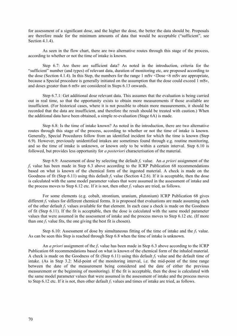
70
for assessment of a significant dose, and the higher the dose, the better the data should be. Proposals are therefore made for the minimum amounts of data that would be acceptable (“sufficient”, see Section 4.1.4).
As seen in the flow chart, there are two alternative routes through this stage of the process, according to whether or not the time of intake is known.
Step 6.7: Are there are sufficient data? As noted in the introduction, criteria for the “sufficient” number (and types) of relevant data, duration of monitoring etc, are proposed according to the dose (Section 4.1.4). In this Step, the numbers for the range 1 mSv <Dose <6 mSv are appropriate, because a Special procedure is generally initiated on the assumption that the dose could exceed 1 mSv, and doses greater than 6 mSv are considered in Steps 6.13 onwards.
Step 6.7.1: Get additional dose relevant data. This assumes that the evaluation is being carried out in real time, so that the opportunity exists to obtain more measurements if those available are insufficient. (For historical cases, where it is not possible to obtain more measurements, it should be recorded that the data are insufficient, and therefore the result should be treated with caution.) When the additional data have been obtained, a simple re-evaluation (Stage 6A) is made.
Step 6.8: Is the time of intake known? As noted in the introduction, there are two alternative routes through this stage of the process, according to whether or not the time of intake is known. Generally, Special Procedures follow from an identified incident for which the time is known (Step 6.9). However, previously unidentified intakes are sometimes found through e.g. routine monitoring, and so the time of intake is unknown, or known only to be within a certain interval. Step 6.10 is followed, but provides less opportunity for a posteriori characterisation of the material.
Step 6.9: Assessment of dose by selecting the default f1 value. An a priori assignment of the f1 value has been made in Step 6.3 above according to the ICRP Publication 68 recommendations based on what is known of the chemical form of the ingested material. A check is made on the Goodness of fit (Step 6.11) using this default f1 value (Section 4.2.6). If it is acceptable, then the dose is calculated with the same model parameter values that were assumed in the assessment of intake and the process moves to Step 6.12 etc. If it is not, then other f1 values are tried, as follows.
For some elements (e.g. cobalt, strontium, uranium, plutonium) ICRP Publication 68 gives different f1 values for different chemical forms. It is proposed that evaluations are made assuming each of the other default f1 values available for that element. In each case a check is made on the Goodness of fit (Step 6.11). If the fit is acceptable, then the dose is calculated with the same model parameter values that were assumed in the assessment of intake and the process moves to Step 6.12 etc. (If more than one f1 value fits, the one giving the best fit is chosen).
Step 6.10: Assessment of dose by simultaneous fitting of the time of intake and the f1 value. As can be seen this Step is reached through Step 6.8 when the time of intake is unknown.
An a priori assignment of the f1 value has been made in Step 6.3 above according to the ICRP Publication 68 recommendations based on what is known of the chemical form of the inhaled material. A check is made on the Goodness of fit (Step 6.11) using this default f1 value and the default time of intake. (As in Step 3.2: Mid-point of the monitoring interval, i.e. the mid-point of the time range between the date of the measurement being considered and the date of either the previous measurement or the beginning of monitoring). If the fit is acceptable, then the dose is calculated with the same model parameter values that were assumed in the assessment of intake and the process moves to Step 6.12 etc. If it is not, then other default f1 values and times of intake are tried, as follows.
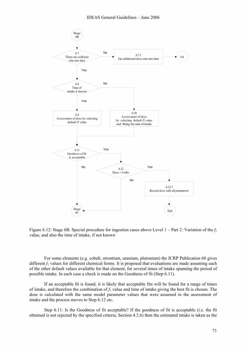
IDEAS General Guidelines – June 2006
71
6A
6.8Time of
intake is known
6.9Assessment of dose by selecting
default f1 value
6.10Assessment of dose
by selecting default f1 value and fitting the time of intake
6.7.1Get additional dose relevant data
6.7There are suffcient
relevant data
6.12.1Record dose with all parameters
End
6.11Goodness of fit
is acceptable
6.12Dose < 6 mSv
No
Yes
No
Yes
Yes
No Yes
Stage6C
Stage 6B
No
Figure 6.12: Stage 6B. Special procedure for ingestion cases above Level 1 – Part 2: Variation of the f1 value, and also the time of intake, if not known
For some elements (e.g. cobalt, strontium, uranium, plutonium) the ICRP Publication 68 gives different f1 values for different chemical forms. It is proposed that evaluations are made assuming each of the other default values available for that element, for several times of intake spanning the period of possible intake. In each case a check is made on the Goodness of fit (Step 6.11).
If an acceptable fit is found, it is likely that acceptable fits will be found for a range of times of intake, and therefore the combination of f1 value and time of intake giving the best fit is chosen. The dose is calculated with the same model parameter values that were assumed in the assessment of intake and the process moves to Step 6.12 etc.
Step 6.11: Is the Goodness of fit acceptable? If the goodness of fit is acceptable (i.e. the fit obtained is not rejected by the specified criteria, Section 4.2.6) then the estimated intake is taken as the
72
best estimate. Otherwise further special procedures (Step 6.13 onwards) are needed for more detailed evaluation of the case.
Step 6.12: Is the dose less than 6 mSv? If the effective dose estimated in Step 6.9 or 6.10 is less than 6 mSv, there is no need for further investigation (Step 6.12.1). Otherwise further special procedures (Step 6.13 onwards) are needed for more detailed evaluation of the case. The same applies, if the effective dose estimated in Step 6.9 or 6.10 is more than 3 mSv and if there are other intakes in that year resulting in an effective dose of more than 3 mSv.
Step 6.12.1: The results in terms of intake and committed effective dose from Step 6.12 are recorded together with the corresponding parameter values from Step 6.9 or 6.10.
6.7.4 Stage 6C
In this stage, an advanced evaluation is carried out. It applies to cases where there are comprehensive data available. The fundamental approach is that the model parameter values are adjusted systematically, in a specific order, until the goodness of fit is acceptable (i.e. the fits obtained to all the data are not rejected by the specified criteria). If the fit is acceptable, then the estimated intake is taken as the best estimate and the effective dose is calculated with the same model parameter values that were assumed in the assessment of intake. These results (intake and committed effective dose) are then recorded together with the corresponding parameter values (Step 6.12.1). Thus after each Step in which a parameter value is varied (6.14 to 6.16) there is a corresponding Step (6.14.1 to 6.16.1 respectively) to test the goodness of fit. Since these are all very similar, explanatory text is only given for Step 6.14.1.
If the time of intake is unknown, then by the start of this Stage it may have been assessed, based on simultaneous fitting of the model to the data with the f1 value (Step 6.10). In that case, if any of the parameter values are changed in the Steps below, the time of intake should be re-assessed.
It is recommended, in cases where multiple types of bioassay data sets are available, that the intake and dose are assessed by fitting predicted values to the different types of data simultaneously.
Step 6.13: Check that there are sufficient data, and get more if necessary. This is similar to Steps 6.7 and 6.7.1 (Stage 6B). Criteria for the “sufficient” number (and types) of relevant data, duration of monitoring etc, are proposed according to the dose level. In this Step, the numbers for Dose > 6 mSv are appropriate.
To get additional dose relevant data assumes that the evaluation is being carried out in real time, so that the opportunity exists to obtain more measurements if those available are insufficient. (For historical cases, where it is not possible to obtain more measurements, it should be recorded that the data are insufficient, and therefore the result should be treated with caution.) When the additional data have been obtained, further special procedures (Step 6.14 onwards) are needed for more detailed evaluation of the case.
Step 6.14: Determine specific f1 value. The f1 value is the main variable related to the ingested material. The default values recommended by ICRP are generally typical values representing the wide ranges that might arise in practice, especially when a single value is given for all chemical forms of an element. GI tract absorption can also vary according to factors such as how recently a meal was taken. Hence it is reasonable to consider values different from the ICRP default. If sufficiently comprehensive data are available, especially if it is possible to estimate both the intake and the total amount absorbed into blood (e.g. if early faecal and urine data are available), then it may be necessary to change the f1 value to obtain a reasonable fit to the data.
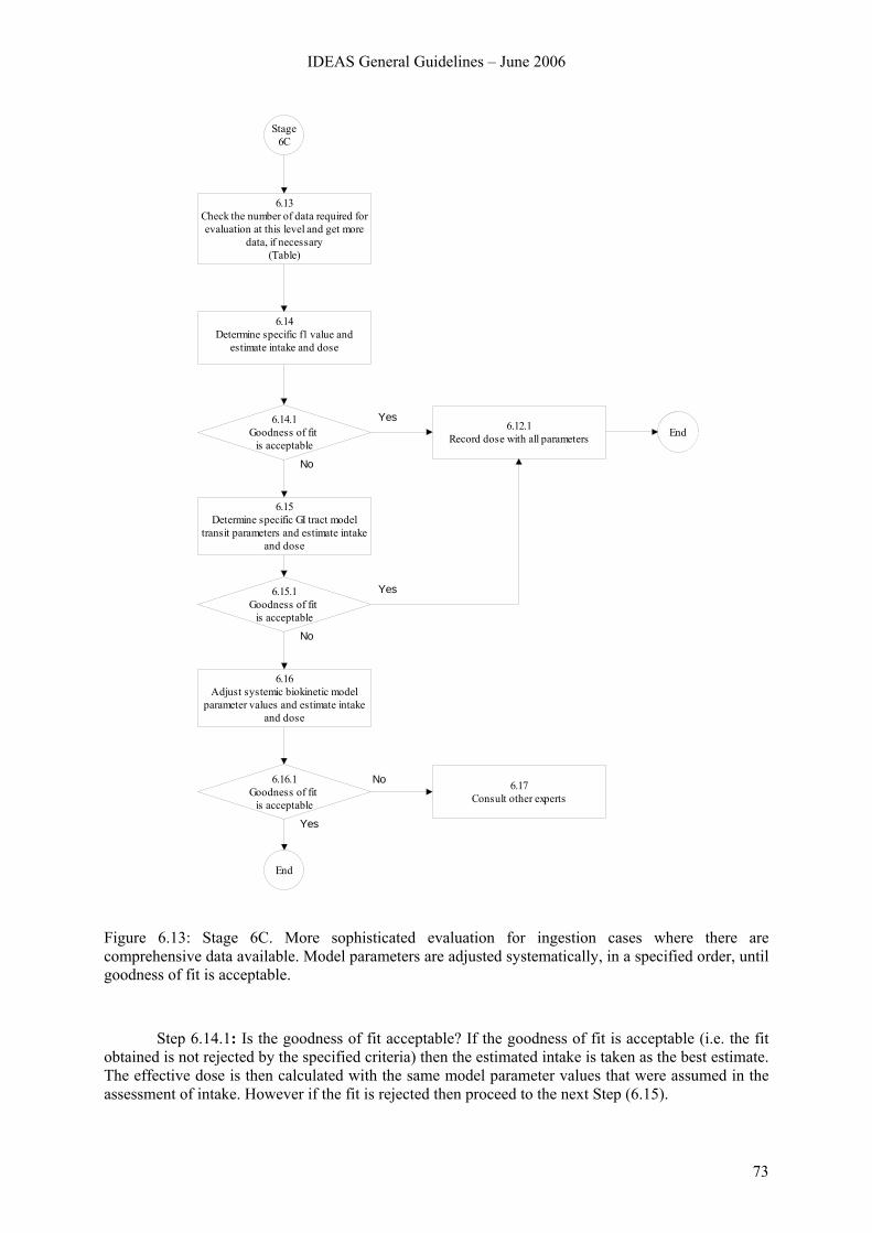
IDEAS General Guidelines – June 2006
73
Stage6C
6.12.1Record dose with all parameters End
6.13Check the number of data required for evaluation at this level and get more
data, if necessary(Table)
6.14Determine specific f1 value and
estimate intake and dose
6.14.1Goodness of fit
is acceptable
6.15.1Goodness of fit
is acceptable
6.16.1Goodness of fit
is acceptable
6.15Determine specific GI tract model
transit parameters and estimate intake and dose
6.16Adjust systemic biokinetic model
parameter values and estimate intake and dose
6.17Consult other experts
End
Yes
No
Yes
No
No
Yes
Figure 6.13: Stage 6C. More sophisticated evaluation for ingestion cases where there are comprehensive data available. Model parameters are adjusted systematically, in a specified order, until goodness of fit is acceptable.
Step 6.14.1: Is the goodness of fit acceptable? If the goodness of fit is acceptable (i.e. the fit obtained is not rejected by the specified criteria) then the estimated intake is taken as the best estimate. The effective dose is then calculated with the same model parameter values that were assumed in the assessment of intake. However if the fit is rejected then proceed to the next Step (6.15).
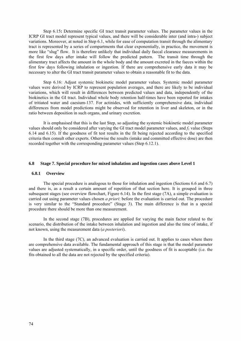
74
Step 6.15: Determine specific GI tract transit parameter values. The parameter values in the ICRP GI tract model represent typical values, and there will be considerable inter (and intra-) subject variations. Moreover, at noted in Step 6.1, while for ease of computation transit through the alimentary tract is represented by a series of compartments that clear exponentially, in practice, the movement is more like “slug” flow. It is therefore unlikely that individual daily faecal clearance measurements in the first few days after intake will follow the predicted pattern. The transit time through the alimentary tract affects the amount in the whole body and the amount excreted in the faeces within the first few days following inhalation or ingestion. If there are comprehensive early data it may be necessary to alter the GI tract transit parameter values to obtain a reasonable fit to the data.
Step 6.16: Adjust systemic biokinetic model parameter values. Systemic model parameter values were derived by ICRP to represent population averages, and there are likely to be individual variations, which will result in differences between predicted values and data, independently of the biokinetics in the GI tract. Individual whole body retention half-times have been reported for intakes of tritiated water and caesium-137. For actinides, with sufficiently comprehensive data, individual differences from model predictions might be observed for retention in liver and skeleton, or in the ratio between deposition in such organs, and urinary excretion.
It is emphasised that this is the last Step, so adjusting the systemic biokinetic model parameter values should only be considered after varying the GI tract model parameter values, and f1 value (Steps 6.14 and 6.15). If the goodness of fit test results in the fit being rejected according to the specified criteria then consult other experts. Otherwise the results (intake and committed effective dose) are then recorded together with the corresponding parameter values (Step 6.12.1).
6.8 Stage 7. Special procedure for mixed inhalation and ingestion cases above Level 1
6.8.1 Overview
The special procedure is analogous to those for inhalation and ingestion (Sections 6.6 and 6.7) and there is, as a result a certain amount of repetition of that section here. It is grouped in three subsequent stages (see overview flowchart, Figure 6.14). In the first stage (7A), a simple evaluation is carried out using parameter values chosen a priori: before the evaluation is carried out. The procedure is very similar to the “Standard procedure” (Stage 3). The main difference is that in a special procedure there should be more than one measurement.
In the second stage (7B), procedures are applied for varying the main factor related to the scenario, the distribution of the intake between inhalation and ingestion and also the time of intake, if not known, using the measurement data (a posteriori).
In the third stage (7C), an advanced evaluation is carried out. It applies to cases where there are comprehensive data available. The fundamental approach of this stage is that the model parameter values are adjusted systematically, in a specific order, until the goodness of fit is acceptable (i.e. the fits obtained to all the data are not rejected by the specified criteria).
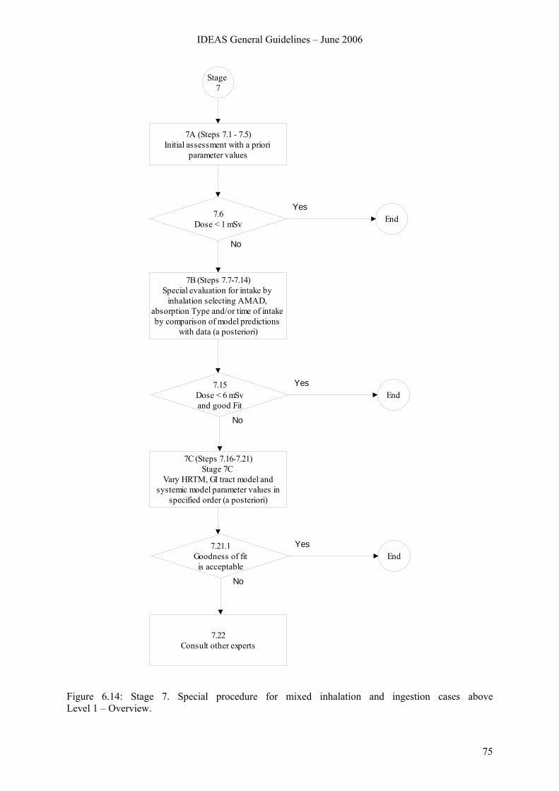
IDEAS General Guidelines – June 2006
75
Stage 7
7A (Steps 7.1 - 7.5)Initial assessment with a priori
parameter values
7B (Steps 7.7-7.14)Special evaluation for intake by
inhalation selecting AMAD, absorption Type and/or time of intake by comparison of model predictions
with data (a posteriori)
7.6Dose < 1 mSv End
Yes
No
7C (Steps 7.16-7.21)Stage 7C
Vary HRTM, GI tract model and systemic model parameter values in
specified order (a posteriori)
7.15Dose < 6 mSvand good Fit
EndYes
No
7.22Consult other experts
7.21.1Goodness of fitis acceptable
EndYes
No
Figure 6.14: Stage 7. Special procedure for mixed inhalation and ingestion cases above Level 1 – Overview.
76
6.8.2 Stage 7A
In this Stage, a simple evaluation is carried out using parameter values chosen a priori: before the evaluation is carried out. The procedure is very similar to the “Standard procedure” (Stage 3). The main difference is that in a special procedure there should be more than one measurement.
Step 7.1: Identification and preparation of measurement data. It is expected that there will be more than one measurement available for a special assessment (Mi for i = 1 to n). It is therefore important that realistic uncertainties are assigned to the data (“scattering factor”, SF, Step 2.1) There may be more than one type of measurement (urine, faeces, etc), and there may be measurements of more than one radionuclide involved in the exposure.
Step 7.2: (As Step 2.3 for a single measurement.) The contributions (Pi) from all previous intakes of the radionuclide considered are calculated, taking into account all pathways of intake, and all intakes of mixtures where the radionuclide was involved. The net values (Ni = Mi – Pi) of the radionuclide are calculated by subtracting Pi from the measured value Mi.
Step 7.3: (As Step 3.2 in the Standard Procedure, Stage 3, except for time of intake). Case or site specific parameter values should be assigned as far as they are available. Such a priori information needs to be well established and documented. Examples might include the Activity Median Aerodynamic Diameter (AMAD) – if it has been determined by appropriate air sampling (e.g., cascade impactor), or the time of intake, if potential exposure was limited, or an incident was known to occur. Otherwise the following default parameter values should be used:
• Mode of intake: Single intake. By default assume 50% inhalation; 50% ingestion.
• Absorption Type and f1 value for inhalation: defaults according to ICRP Publication 68. If the compound is unknown, then for those elements where there is a choice of absorption Types, the Type for “unspecified compounds” should be used.
• f1 value for ingestion: defaults according to ICRP Publication 68.
• Particle size: 5 µm AMAD.
Step 7.4: Time of intake known/unknown. If the special procedure was initiated as a result of a known incident (and hence the time of intake is known) then a simple assessment (Step 7.5) should be carried out which is consistent with the Standard evaluation (Stage 3). If the special procedure was initiated as a result of a routine measurement being inconsistent with previous assessments (Step 2.6) or a dose >1 mSv resulting from the Standard evaluation (Step 3.4) where the time of intake is probably not known, then further special procedures (Stage 7B) are needed for more detailed evaluation of the case.
Step 7.5: (As Step 3.3 in the Standard Procedure, Stage 3, but for more than one measurement). Using the assigned a priori parameter values, an estimate of intake Ii is obtained by dividing the net value Ni = Mi – Pi by the appropriate retention or excretion function. The geometric mean of the value of Ii gives the “best estimate” of intake (see step 5.5). Using the same assigned a priori parameter values the committed effective dose is calculated by multiplying the “best estimate” of intake by the appropriate dose coefficient (dose per unit intake).
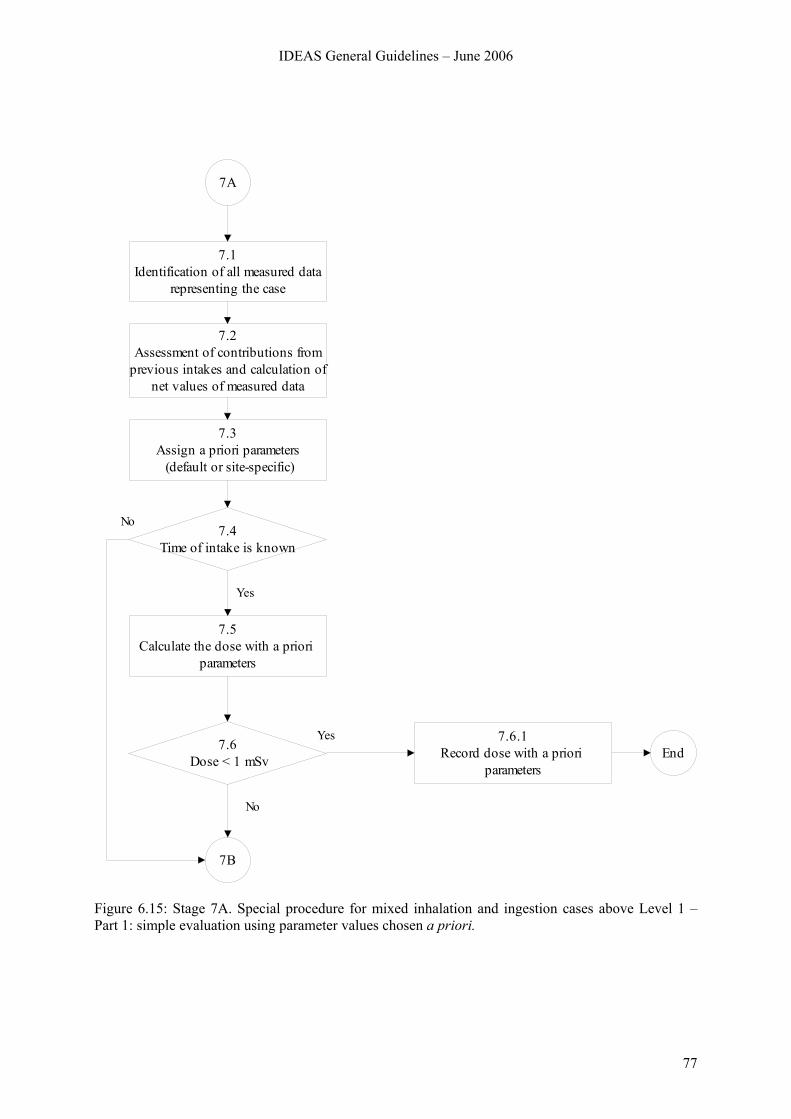
IDEAS General Guidelines – June 2006
77
7.1Identification of all measured data
representing the case
7.2Assessment of contributions from
previous intakes and calculation of net values of measured data
7.3Assign a priori parameters (default or site-specific)
7.5Calculate the dose with a priori
parameters
7.6 Dose < 1 mSv
7.6.1Record dose with a priori
parametersEnd
7.4Time of intake is known
7A
No
Yes
No
7B
Yes
Figure 6.15: Stage 7A. Special procedure for mixed inhalation and ingestion cases above Level 1 – Part 1: simple evaluation using parameter values chosen a priori.
78
Step 7.6: If the effective dose estimated in Step 7.5 is less than 1 mSv, there is no need for further investigation (Step 7.6.1). (The dose from the intake under consideration, rather than the “annual dose” as in Step 3.4, is the criterion, because intakes requiring special assessment procedures should be unusual for any individual worker.) Otherwise further special procedures (Stage 7B) are needed for more detailed evaluation of the case.
Step 7.6.1: The results in terms of intake and committed effective dose from Step 7.6 are recorded together with the corresponding parameter values from Step 7.3.
6.8.3 Stage 7B
In this Stage, procedures are described for varying (i) the pathway of intake (inhalation versus ingestion), (ii) the absorption Type of the inhaled material, and (iii) the time of intake (if not known), using the measurement data (a posteriori). The procedure is very similar to the corresponding special procedure for mixed inhalation cases (Stage 5B), except that the pathway of intake is an additional variable, and it cannot be varied a posteriori as well as the aerosol AMAD (compare Step 7.10 with Step 5.10).
In this Stage, and in Stage 7C that follows, parameter values are selected on the basis of the “fit” of the model predictions to the observations (data). A check on whether the fit is adequate is used to decide whether to stop the evaluation, or to go on to further Steps. A measure of the “Goodness of fit” (GOF) and the criteria for deciding that the fit is good enough are therefore critical issues. There may be conflict between “harmonisation” and “accuracy”. Generally the better the data (quality and quantity) the more likely it is that a statistical test will show that the data are inconsistent with the model. If the data are poor it is more likely that the model will fit – in the extreme case of a single measurement any model will fit. It is therefore important that there should be sufficient data available for assessment of a significant dose, and the higher the dose, the better the data should be. Proposals are therefore made for the minimum amounts of data that would be acceptable (“sufficient”, see Section 4.1.4).
As seen in the flow chart, there are two main alternative routes through this Stage of the process, according to whether or not the time of intake is known.
Step 7.7: Are there are sufficient data? As noted in the introduction, criteria for the “sufficient” number (and types) of relevant data, duration of monitoring etc, are proposed according to the dose. In this Step, the numbers for the range 1 mSv <Dose <6 mSv are appropriate (Section 4.1.4), because a Special procedure is generally initiated on the assumption that the dose could exceed 1 mSv, and doses greater than 6 mSv are considered in Steps 7.11.2 and 7.12.2 below.
Step 7.7.1: Get additional dose relevant data. This assumes that the evaluation is being carried out in real time, so that the opportunity exists to obtain more measurements if those available are insufficient. (For historical cases, where it is not possible to obtain more measurements, it should be recorded that the data are insufficient, and therefore the result should be treated with caution.) When the additional data have been obtained, a simple re-evaluation as in Stage 7A is made.
Step 7.8: Is the time of intake known? As noted in the introduction, there are two main alternative routes through this Stage of the process, according to whether or not the time of intake is known. Generally, Special Procedures follow from an identified incident for which the time is known: Steps 7.9 to 7.11, and if necessary 7.13 are followed. However, previously unidentified intakes are sometimes found through e.g. routine monitoring, and so the time of intake is unknown, or known only to be within a certain interval. Step 7.12 and if necessary 7.14 are followed, but provide less opportunity for a posteriori characterisation of the material.
IDEAS General Guidelines – June 2006
79
Step 7.9: Are early lung and faeces data available? During the first few days after an accidental inhalation intake of a relatively insoluble material (Type M or Type S) most of the activity will be in the respiratory tract, or cleared through the alimentary tract to the faeces. In the event of such an incident with potential for a significant intake it would therefore be expected that if feasible, measurements of lung and faeces would be made. If the AMAD is well known a priori for the exposure situation, and if both the cumulative faecal excretion over the first few days, and a measurement on which the initial lung deposit can be estimated are available, then an estimate can be made of the effective pathway of intake, i.e., the fractions of the intake via inhalation and ingestion (Step 7.10).
Step 7.10: Derive effective pathway of intake from early lung and faeces data. Suppose that the AMAD is well known from measurements of the activity-size distribution in the workplace, and it is considered that inhalation was accompanied by ingestion (e.g. from measurements of external contamination or high faecal excretion).
If early lung retention and faecal excretion data are available, it is possible to derive an “effective” fraction inhaled in the same way as the effective AMAD was derived in Stage 5B. If the fraction inhaled is Finh, then the fraction ingested is 1 – Finh. At 3 days after inhalation, the fractions of inhaled activity in lungs and cumulative faecal excretion are FL and Ffinh. At 3 days after ingestion, the fraction of ingested activity in cumulative faecal excretion is Ffing. Then the ratio of activity in lungs to that in cumulative faecal excretion is:
R(L/F) = (Finh FL) / [Finh Ffinh + (1 – Finh) Ffing]
For example, for 241Am, Ffing = 87% at 3 days. FL and Ffinh are as follows for 1 and 5 μm AMAD Types M and S:
Table 6.1: Fraction of inhaled activity in Lungs and cumulative faecal excretion.( Values of Finh and Ffing can be obtained from tables published by C. Potter [Potter 2002]).
AMAD, μm Type FL (%) Ffinh (%)
1 M 10.5 18.6
1 S 11.8 19.6
5 M 5.5 34.3
5 S 6.2 36.12
Using these values, the dependence of the ratio of lung activity to faecal excretion on fraction inhaled is shown in Figure 6.16.
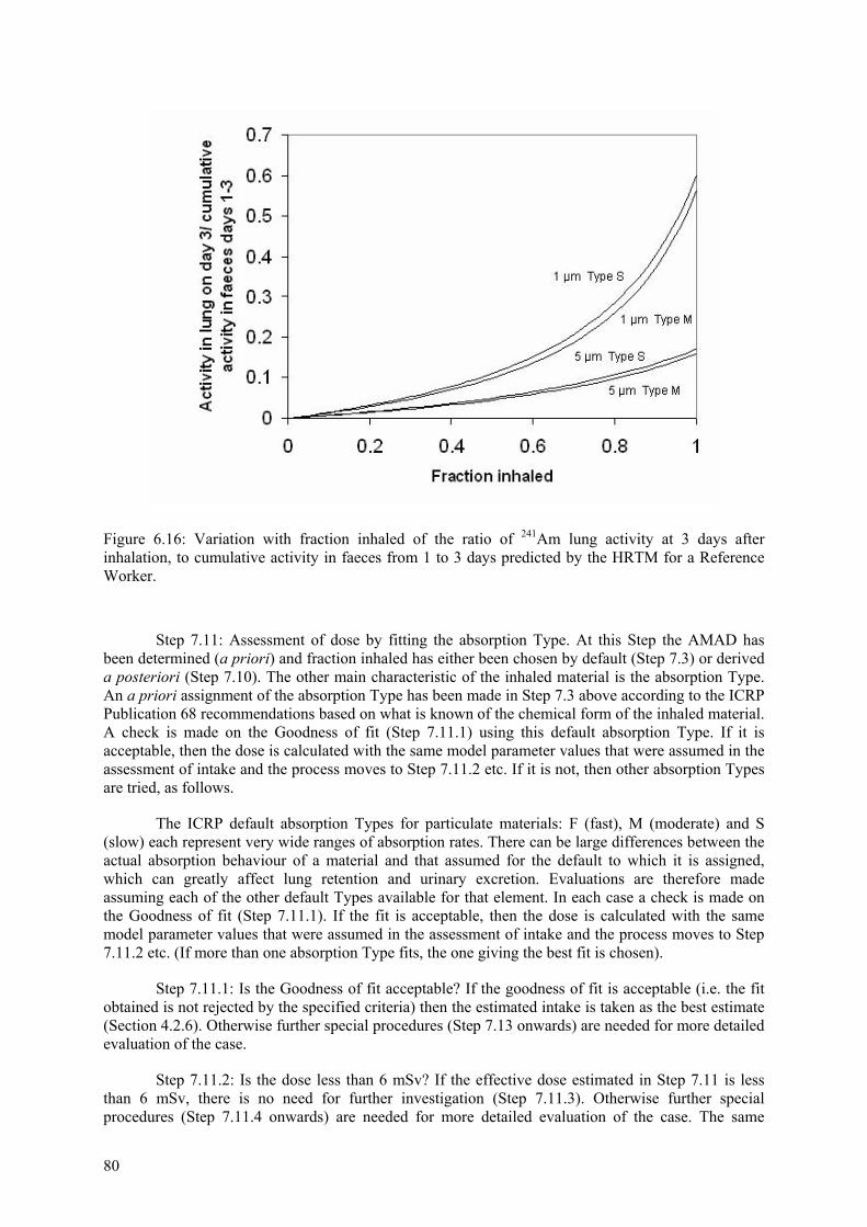
80
Figure 6.16: Variation with fraction inhaled of the ratio of 241Am lung activity at 3 days after inhalation, to cumulative activity in faeces from 1 to 3 days predicted by the HRTM for a Reference Worker.
Step 7.11: Assessment of dose by fitting the absorption Type. At this Step the AMAD has been determined (a priori) and fraction inhaled has either been chosen by default (Step 7.3) or derived a posteriori (Step 7.10). The other main characteristic of the inhaled material is the absorption Type. An a priori assignment of the absorption Type has been made in Step 7.3 above according to the ICRP Publication 68 recommendations based on what is known of the chemical form of the inhaled material. A check is made on the Goodness of fit (Step 7.11.1) using this default absorption Type. If it is acceptable, then the dose is calculated with the same model parameter values that were assumed in the assessment of intake and the process moves to Step 7.11.2 etc. If it is not, then other absorption Types are tried, as follows.
The ICRP default absorption Types for particulate materials: F (fast), M (moderate) and S (slow) each represent very wide ranges of absorption rates. There can be large differences between the actual absorption behaviour of a material and that assumed for the default to which it is assigned, which can greatly affect lung retention and urinary excretion. Evaluations are therefore made assuming each of the other default Types available for that element. In each case a check is made on the Goodness of fit (Step 7.11.1). If the fit is acceptable, then the dose is calculated with the same model parameter values that were assumed in the assessment of intake and the process moves to Step 7.11.2 etc. (If more than one absorption Type fits, the one giving the best fit is chosen).
Step 7.11.1: Is the Goodness of fit acceptable? If the goodness of fit is acceptable (i.e. the fit obtained is not rejected by the specified criteria) then the estimated intake is taken as the best estimate (Section 4.2.6). Otherwise further special procedures (Step 7.13 onwards) are needed for more detailed evaluation of the case.
Step 7.11.2: Is the dose less than 6 mSv? If the effective dose estimated in Step 7.11 is less than 6 mSv, there is no need for further investigation (Step 7.11.3). Otherwise further special procedures (Step 7.11.4 onwards) are needed for more detailed evaluation of the case. The same
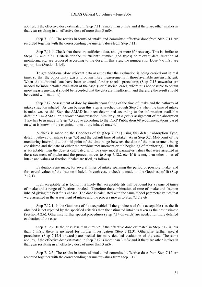
IDEAS General Guidelines – June 2006
81
applies, if the effective dose estimated in Step 7.11 is more than 3 mSv and if there are other intakes in that year resulting in an effective dose of more than 3 mSv.
Step 7.11.3: The results in terms of intake and committed effective dose from Step 7.11 are recorded together with the corresponding parameter values from Step 7.11.
Step 7.11.4: Check that there are sufficient data, and get more if necessary. This is similar to Steps 7.7 and 7.7.1. Criteria for the “sufficient” number (and types) of relevant data, duration of monitoring etc, are proposed according to the dose. In this Step, the numbers for Dose > 6 mSv are appropriate (Section 4.1.4).
To get additional dose relevant data assumes that the evaluation is being carried out in real time, so that the opportunity exists to obtain more measurements if those available are insufficient. When the additional data have been obtained, further special procedures (Step 7.13 onwards) are needed for more detailed evaluation of the case. (For historical cases, where it is not possible to obtain more measurements, it should be recorded that the data are insufficient, and therefore the result should be treated with caution.)
Step 7.12: Assessment of dose by simultaneous fitting of the time of intake and the pathway of intake (fraction inhaled). As can be seen this Step is reached through Step 7.8 when the time of intake is unknown. At this Step the AMAD has been determined according to the information available: default 5 µm AMAD or a priori characterisation. Similarly, an a priori assignment of the absorption Type has been made in Step 7.3 above according to the ICRP Publication 68 recommendations based on what is known of the chemical form of the inhaled material.
A check is made on the Goodness of fit (Step 7.12.1) using this default absorption Type, default pathway of intake (Step 7.3) and the default time of intake. (As in Step 3.2: Mid-point of the monitoring interval, i.e. the mid-point of the time range between the date of the measurement being considered and the date of either the previous measurement or the beginning of monitoring). If the fit is acceptable, then the dose is calculated with the same model parameter values that were assumed in the assessment of intake and the process moves to Step 7.12.2 etc. If it is not, then other times of intake and values of fraction inhaled are tried, as follows.
Evaluations are made, for several times of intake spanning the period of possible intake, and for several values of the fraction inhaled. In each case a check is made on the Goodness of fit (Step 7.12.1).
If an acceptable fit is found, it is likely that acceptable fits will be found for a range of times of intake and a range of fractions inhaled. Therefore the combination of time of intake and fraction inhaled giving the best fit is chosen. The dose is calculated with the same model parameter values that were assumed in the assessment of intake and the process moves to Step 7.12.2 etc.
Step 7.12.1: Is the Goodness of fit acceptable? If the goodness of fit is acceptable (i.e. the fit obtained is not rejected by the specified criteria) then the estimated intake is taken as the best estimate (Section 4.2.6). Otherwise further special procedures (Step 7.14 onwards) are needed for more detailed evaluation of the case.
Step 7.12.2: Is the dose less than 6 mSv? If the effective dose estimated in Step 7.12 is less than 6 mSv, there is no need for further investigation (Step 7.12.3). Otherwise further special procedures (Step 7.12.4 onwards) are needed for more detailed evaluation of the case. The same applies, if the effective dose estimated in Step 7.12 is more than 3 mSv and if there are other intakes in that year resulting in an effective dose of more than 3 mSv.
Step 7.12.3: The results in terms of intake and committed effective dose from Step 7.12 are recorded together with the corresponding parameter values from Step 7.12.
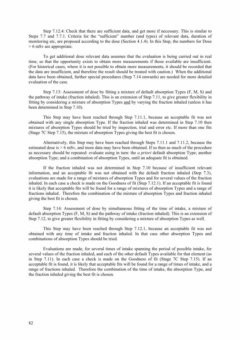
82
Step 7.12.4: Check that there are sufficient data, and get more if necessary. This is similar to Steps 7.7 and 7.7.1. Criteria for the “sufficient” number (and types) of relevant data, duration of monitoring etc, are proposed according to the dose (Section 4.1.4). In this Step, the numbers for Dose > 6 mSv are appropriate.
To get additional dose relevant data assumes that the evaluation is being carried out in real time, so that the opportunity exists to obtain more measurements if those available are insufficient. (For historical cases, where it is not possible to obtain more measurements, it should be recorded that the data are insufficient, and therefore the result should be treated with caution.) When the additional data have been obtained, further special procedures (Step 7.14 onwards) are needed for more detailed evaluation of the case.
Step 7.13: Assessment of dose by fitting a mixture of default absorption Types (F, M, S) and the pathway of intake (fraction inhaled). This is an extension of Step 7.11, to give greater flexibility in fitting by considering a mixture of absorption Types and by varying the fraction inhaled (unless it has been determined in Step 7.10).
This Step may have been reached through Step 7.11.1, because an acceptable fit was not obtained with any single absorption Type. If the fraction inhaled was determined in Step 7.10 then mixtures of absorption Types should be tried by inspection, trial and error etc. If more than one fits (Stage 7C Step 7.15), the mixture of absorption Types giving the best fit is chosen.
Alternatively, this Step may have been reached through Steps 7.11.1 and 7.11.2, because the estimated dose is > 6 mSv, and more data may have been obtained. If so then as much of the procedure as necessary should be repeated: evaluate using in turn: the a priori default absorption Type; another absorption Type; and a combination of absorption Types, until an adequate fit is obtained.
If the fraction inhaled was not determined in Step 7.10 because of insufficient relevant information, and an acceptable fit was not obtained with the default fraction inhaled (Step 7.3), evaluations are made for a range of mixtures of absorption Types and for several values of the fraction inhaled. In each case a check is made on the Goodness of fit (Step 7.12.1). If an acceptable fit is found it is likely that acceptable fits will be found for a range of mixtures of absorption Types and a range of fractions inhaled. Therefore the combination of the mixture of absorption Types and fraction inhaled giving the best fit is chosen.
Step 7.14: Assessment of dose by simultaneous fitting of the time of intake, a mixture of default absorption Types (F, M, S) and the pathway of intake (fraction inhaled). This is an extension of Step 7.12, to give greater flexibility in fitting by considering a mixture of absorption Types as well.
This Step may have been reached through Step 7.12.1, because an acceptable fit was not obtained with any time of intake and fraction inhaled. In that case other absorption Types and combinations of absorption Types should be tried.
Evaluations are made, for several times of intake spanning the period of possible intake, for several values of the fraction inhaled, and each of the other default Types available for that element (as in Step 7.11). In each case a check is made on the Goodness of fit (Stage 7C Step 7.15). If an acceptable fit is found, it is likely that acceptable fits will be found for a range of times of intake, and a range of fractions inhaled. Therefore the combination of the time of intake, the absorption Type, and the fraction inhaled giving the best fit is chosen.
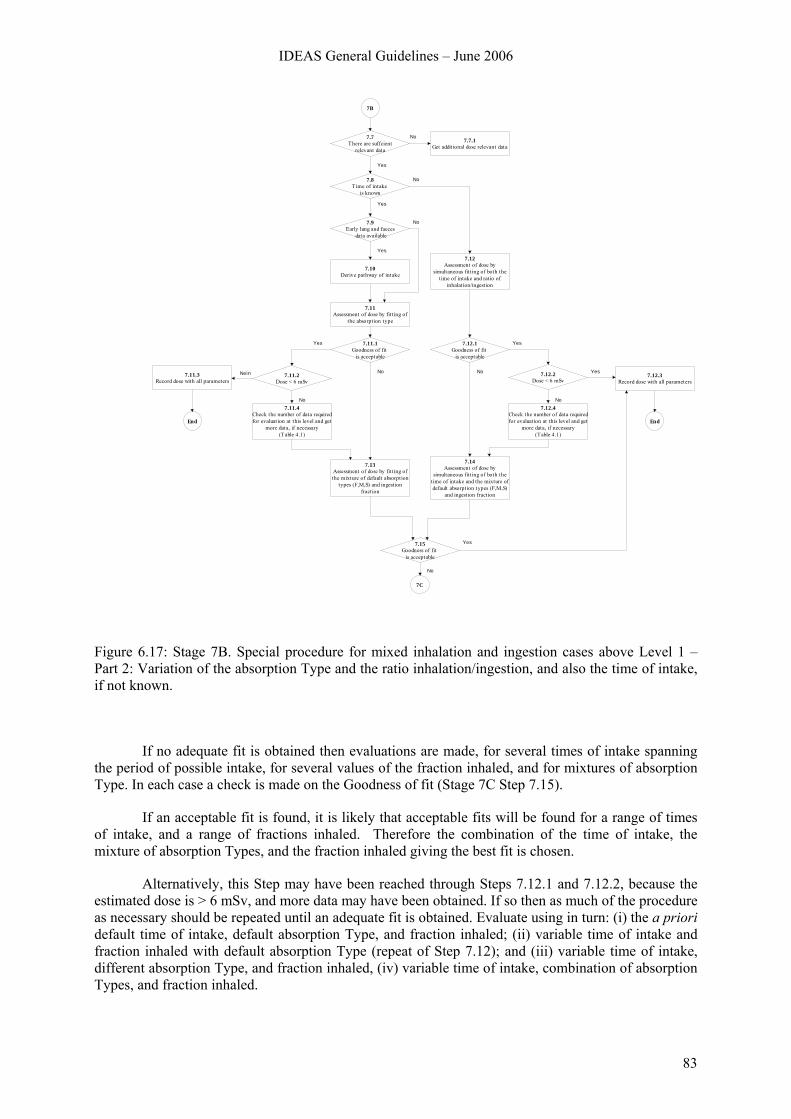
IDEAS General Guidelines – June 2006
83
7.8Time of intake
is known
7.9Early lung and faeces
data available
7.10Derive pathway of intake
7.11Assessment of dose by fitt ing of
the absorption type
7.12Assessment of dose by
simultaneous fitting of both the time of intake and rat io of
inhalation/ingestion
7.7.1Get additional dose relevant data
7.7There are suffcient
relevant data
7.11.1Goodness of fit
is acceptable
7.13Assessment of dose by fitting of the mixture of default absorption
types (F,M,S) and ingestion fraction
7.14Assessment of dose by
simultaneous fitting of both the time of intake and the mixture of default absorption types (F,M,S)
and ingest ion fraction
7.15Goodness of fit
is acceptable
7.12.3Record dose with all parameters
7.12.1Goodness of fit
is acceptable
7.11.2Dose < 6 mSv
7.11.4Check the number of data required for evaluat ion at this level and get
more data, if necessary(Table 4.1)
7.12.2Dose < 6 mSv
7.12.4Check the number of data required for evaluation at this level and get
more data, if necessary(Table 4.1)
7B
No
Yes
No
Yes
No
Yes
Yes
No
No
Yes
No Yes
No
Yes
No
7.11.3Record dose with all parameters
Nein
7C
EndEnd
Figure 6.17: Stage 7B. Special procedure for mixed inhalation and ingestion cases above Level 1 – Part 2: Variation of the absorption Type and the ratio inhalation/ingestion, and also the time of intake, if not known.
If no adequate fit is obtained then evaluations are made, for several times of intake spanning the period of possible intake, for several values of the fraction inhaled, and for mixtures of absorption Type. In each case a check is made on the Goodness of fit (Stage 7C Step 7.15).
If an acceptable fit is found, it is likely that acceptable fits will be found for a range of times of intake, and a range of fractions inhaled. Therefore the combination of the time of intake, the mixture of absorption Types, and the fraction inhaled giving the best fit is chosen.
Alternatively, this Step may have been reached through Steps 7.12.1 and 7.12.2, because the estimated dose is > 6 mSv, and more data may have been obtained. If so then as much of the procedure as necessary should be repeated until an adequate fit is obtained. Evaluate using in turn: (i) the a priori default time of intake, default absorption Type, and fraction inhaled; (ii) variable time of intake and fraction inhaled with default absorption Type (repeat of Step 7.12); and (iii) variable time of intake, different absorption Type, and fraction inhaled, (iv) variable time of intake, combination of absorption Types, and fraction inhaled.
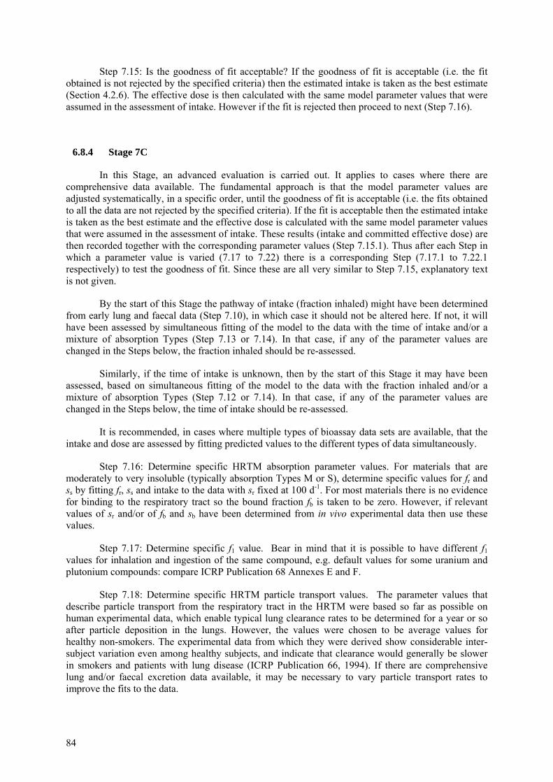
84
Step 7.15: Is the goodness of fit acceptable? If the goodness of fit is acceptable (i.e. the fit obtained is not rejected by the specified criteria) then the estimated intake is taken as the best estimate (Section 4.2.6). The effective dose is then calculated with the same model parameter values that were assumed in the assessment of intake. However if the fit is rejected then proceed to next (Step 7.16).
6.8.4 Stage 7C
In this Stage, an advanced evaluation is carried out. It applies to cases where there are comprehensive data available. The fundamental approach is that the model parameter values are adjusted systematically, in a specific order, until the goodness of fit is acceptable (i.e. the fits obtained to all the data are not rejected by the specified criteria). If the fit is acceptable then the estimated intake is taken as the best estimate and the effective dose is calculated with the same model parameter values that were assumed in the assessment of intake. These results (intake and committed effective dose) are then recorded together with the corresponding parameter values (Step 7.15.1). Thus after each Step in which a parameter value is varied (7.17 to 7.22) there is a corresponding Step (7.17.1 to 7.22.1 respectively) to test the goodness of fit. Since these are all very similar to Step 7.15, explanatory text is not given.
By the start of this Stage the pathway of intake (fraction inhaled) might have been determined from early lung and faecal data (Step 7.10), in which case it should not be altered here. If not, it will have been assessed by simultaneous fitting of the model to the data with the time of intake and/or a mixture of absorption Types (Step 7.13 or 7.14). In that case, if any of the parameter values are changed in the Steps below, the fraction inhaled should be re-assessed.
Similarly, if the time of intake is unknown, then by the start of this Stage it may have been assessed, based on simultaneous fitting of the model to the data with the fraction inhaled and/or a mixture of absorption Types (Step 7.12 or 7.14). In that case, if any of the parameter values are changed in the Steps below, the time of intake should be re-assessed.
It is recommended, in cases where multiple types of bioassay data sets are available, that the intake and dose are assessed by fitting predicted values to the different types of data simultaneously.
Step 7.16: Determine specific HRTM absorption parameter values. For materials that are moderately to very insoluble (typically absorption Types M or S), determine specific values for fr and ss by fitting fr, ss and intake to the data with sr fixed at 100 d-1. For most materials there is no evidence for binding to the respiratory tract so the bound fraction fb is taken to be zero. However, if relevant values of sr and/or of fb and sb have been determined from in vivo experimental data then use these values.
Step 7.17: Determine specific f1 value. Bear in mind that it is possible to have different f1 values for inhalation and ingestion of the same compound, e.g. default values for some uranium and plutonium compounds: compare ICRP Publication 68 Annexes E and F.
Step 7.18: Determine specific HRTM particle transport values. The parameter values that describe particle transport from the respiratory tract in the HRTM were based so far as possible on human experimental data, which enable typical lung clearance rates to be determined for a year or so after particle deposition in the lungs. However, the values were chosen to be average values for healthy non-smokers. The experimental data from which they were derived show considerable inter-subject variation even among healthy subjects, and indicate that clearance would generally be slower in smokers and patients with lung disease (ICRP Publication 66, 1994). If there are comprehensive lung and/or faecal excretion data available, it may be necessary to vary particle transport rates to improve the fits to the data.
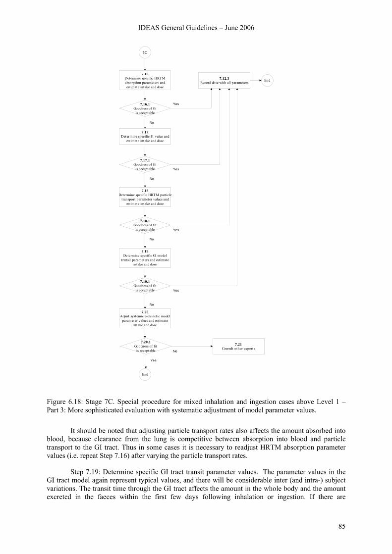
IDEAS General Guidelines – June 2006
85
7.12.3Record dose with all parameters End
7.16Determine specific HRTM absorption parameters and estimate intake and dose
7.19Determine specific GI model
transit parameters and estimate intake and dose
7.21Consult other experts
7C
Yes
No
Yes
Yes
No
Yes
No
No
7.18Determine specific HRTM particle
transport parameter values and estimate intake and dose
No
7.16.1Goodness of fit
is acceptable
7.17Determine specific f1 value and
est imate intake and dose
7.17.1Goodness of fit
is acceptable
7.18.1Goodness of fit
is acceptable
7.19.1Goodness of fit
is acceptable
7.20Adjust systemic biokinetic model
parameter values and estimate intake and dose
7.20.1Goodness of fit
is acceptable
Yes
End
Figure 6.18: Stage 7C. Special procedure for mixed inhalation and ingestion cases above Level 1 – Part 3: More sophisticated evaluation with systematic adjustment of model parameter values.
It should be noted that adjusting particle transport rates also affects the amount absorbed into blood, because clearance from the lung is competitive between absorption into blood and particle transport to the GI tract. Thus in some cases it is necessary to readjust HRTM absorption parameter values (i.e. repeat Step 7.16) after varying the particle transport rates.
Step 7.19: Determine specific GI tract transit parameter values. The parameter values in the GI tract model again represent typical values, and there will be considerable inter (and intra-) subject variations. The transit time through the GI tract affects the amount in the whole body and the amount excreted in the faeces within the first few days following inhalation or ingestion. If there are
86
comprehensive early data it may be necessary to alter the GI tract model parameter values to obtain a reasonable fit to the data.
Step 7.20: Adjust systemic biokinetic model parameter values. Again, model parameters values were derived by ICRP to represent population averages, and there are likely to be individual variations, which will result in differences between predicted values and data, independently of the biokinetics of the respiratory or alimentary tract. This might well arise for very soluble materials, where particle transport rates have little effect. Individual whole body retention half-times have been reported for intakes of tritiated water and caesium-137. However, for actinides, with sufficiently comprehensive data, individual differences from model predictions might be observed for retention in liver and skeleton, or in the ratio between deposition in such organs, and urinary excretion.
It is emphasised that this is the last Step, so adjusting the systemic biokinetic model parameter values should only be considered after varying the HRTM and GI tract model parameter values, (Steps 7.16, 7.17, 7.18, and 7.19). If the goodness of fit test results in the fit being rejected according to the specified criteria then consult other experts. Otherwise the results (intake and committed effective dose) are then recorded together with the corresponding parameter values (Step 7.15.1).
IDEAS General Guidelines – June 2006
87
7 REFERENCES
Ansoborlo 2002 Ansoborlo, E., Chazel, V., Hengé-Napoli, M. H., Pihet, P., Rannou, A., Bailey, M. R., Stradling, N. (2002) Review of the physico-chemical properties, biokinetics and dose coefficients of uranium compounds handled during nuclear fuel fabrication in France. Health Phys. 82: 279-289 (2002).
Ansoborlo 2003 Ansoborlo E., Bérard P., Eckerman K., Berkovski V., Birchall A., Fry F., Guilmette R., Miller G., Ishigure N., Lipsztein J. and Nosske D. Review of methods and computer codes for interpretation of bioassay data, Radiat. Prot. Dosim. 105: 341-346 (2003).
Batchelor 1980 Batchelor, A. L., Buckley, P., Gore, D. J., Jenner, T. J., Major, I. R. and Bailey, M. R. The carcinogenic effect of localised fission fragment irradiation of rat lung. Int. J. Radiat. Biol. 37: 249-266 (1980).
Bailey 1998 Bailey M. R., Guilmette R. A., Jarvis N. S. and Roy M. Practical application of the new ICRP Human Respiratory Tract Model. Radiat. Prot. Dosim. 79: 17–22 (1998).
Bailey 2003 Bailey M. R., Guilmette R. A., Ansoborlo E. and Paquet F. Practical application of the ICRP Human Respiratory Tract Model. Radiat. Prot. Dosim. 105: 71–76 (2003).
Beach 1964 Beach S A, and Dolphin G W Determination of plutonium body burdens from measurements of daily urine excretion. In Assessment of Radioactivity in Man Vienna IAEA, Vol. 2 pp. 603-15 (1964).
Bende 1999 Bende E. E., Plutonium burning in a Pebble Bed Type High Temperature Nuclear Reactor. Ph.D Thesis (1999).
Berkovski 1998 V. Berkovski et al. Internal Dosimetry Support System: Multipurpose Research Computer Code Radiat. Prot. Dosim. 79: 371-374 (1998).
Berkovski 2000 Berkovski, V., Application of the Internal Dosimetry Support System for Interpretation of In Vivo and Bioassay Measurements. Radiat. Prot. Dosim. 89: 271-274 (2000).
Berkovski 2002 Berkovski, V., IMIE Individual Monitoring of the Internal Exposure Computer Code User’s Guide 8.8.1, Kiev, 2002
Birchall 1995 Birchall, A., Bailey, M. R. and Jarvis, N. S. Application of the New ICRP Respiratory Tract Model to Inhaled Plutonium Nitrate using Experimental Biokinetic Data. In: Proc. British Nuclear Energy Society (BNES). Int. Conf. on Radiation Dose Management in the Nuclear Industry. Windermere, Cumbria, UK, 9–11 October 1995. pp. 216–223 (1995).
Birchall 1998 Birchall A., Jarvis N.S., Peace M.S., Riddell A.E. and Battersby W.P. The IMBA Suite: Integrated Modules for Bioassay Analysis Radiat. Prot. Dosim. 79: 107-110, (1998).
Birchall 2003 Birchall A., Puncher M., James A.C., Marsh J.W., Jarvis N.S., Peace M.S., Davis K. and King D.J. IMBA ExpertTM: Internal Dosimetry Made Simple, Radiat. Prot. Dosim. 105: 421-425 (2003).
88
Castellani 2004 Castellani C.-M., Luciani A., Andrasi A., Bailey M., Marsh J., Puncher M., Berkovski V., Blanchardon E., Jourdain J.-R., Doerfel H., Hurtgen C. and LeGuen B.: IDEAS Work Package 3, Evaluation of Incorporation Cases. RT/2004/2/ION, ENEA (2004).
Doerfel 2000 H. Doerfel, A. Andrasi, M.R. Bailey, A. Birchall, C.-M. Castellani, C. Hurtgen, N. Jarvis, L. Johansson, B. LeGuen and G. Tarroni: Third European Intercomparison Exercise on Internal Dose Assessment, (Results of a Research Programme in the Framework of the EULEP/EURADOS Action Group „Derivation of Parameter Values for Application to the New Respiratory Tract for Occupational Exposure” 1997-1999), Research Center Karlsruhe, Research Report FZKA 6457 (Karlsruhe, April 2000), ISSN 0947-8620
Dorrian 1995 Dorrian, M. D. and Bailey, M. R. Particle size distributions of radioactive aerosols measured in workplaces. Radiat. Prot. Dosim. 60: 119–133 (1995).
Hodgson 2000 Hodgson A, Moody J C, Stradling G N, Bailey M R and Birchall, A. (2000) Application of the ICRP human respiratory tract model to uranium compounds produced during the manufacture of nuclear fuel. Chilton, NRPB-M1156.
Hodgson 2001 Hodgson A, Ansoborlo A, Stradling G N, Bailey M R, Birchall A and Chazel V., (2001) Application of the ICRP human respiratory tract model to uranium compounds produced during the manufacture of nuclear fuel. IN Proceedings of the International Conference on Radiation Dose Management in the Nuclear Industry, Windermere, May 14–16, 2001. London, British Nuclear Energy Society.
Hurtgen 2003 Hurtgen C., C. Cossonnet Uncertainty on Bioassay Measurements OMINEX Work Package 3: A Survey of European Laboratories Report SCK.CEN-BLG-935, Mol, April 2003.
Hurtgen 2004 Hurtgen, C., Bailey, M.R., Marsh, J., LeGuen, B., Communication 2004.
Hurtgen 2005 Hurtgen C., Andrasi A., Bailey M.R., Birchall A., Blanchardon E., Berkovski V., Castellani C.-M., Cruz-Suarez R., Davis K., Doerfel H., LeGuen B., Malatova I., Marsh J. and Zeger J. IDEAS / IAEA Intercomparison Exercise on Internal Dose Assessment. Scientific Report SCK·CEN – BLG-1018. SCK·CEN, Mol, Belgium, October 2005.
Hyung-Kook ? Hyung-Kook J., Young-Jin K. Potential of a thorium based fuel cycle for 900 Mwe PWR core to incinerate plutonium. (www.iaea.org/inis/aws/fnss/fulltext /tdi33008_8.pdf).
ICRP 1975 International Commission on Radiological Protection. Report on the Task Group on Reference Man. ICRP Publication 23. Pergamon Press, Oxford (1975).
ICRP 1977 International Commission on Radiological Protection. Recommendations of the International Commission on Radiological Protection. ICRP Publication 26. Ann. of the ICRP. 1 (3) (1977) Reprinted (with additions) in 1977.
ICRP 1979 International Commission on Radiological Protection. Limits for Intakes of Radionuclides by Workers. ICRP Publication 30, Part 1. Ann. of the ICRP. 2 (3/4), Pergamon Press, Oxford (1979).
IDEAS General Guidelines – June 2006
89
ICRP 1980a International Commission on Radiological Protection. Limits for Intakes of Radionuclides by Workers. ICRP Publication 30, Part 2. Ann. of the ICRP. 4 (3/4), Pergamon Press, Oxford (1980).
ICRP 1980b International Commission on Radiological Protection. Limits for Intakes of Radionuclides by Workers. ICRP Publication 30, Part 3. Ann. of the ICRP. 6 (2/3), Pergamon Press, Oxford (1980).
ICRP 1980c International Commission on Radiological Protection. Biological Effects of Inhaled Radionuclides. ICRP Publication 31. Ann. of the ICRP. 4 (1/2), Pergamon Press, Oxford (1980).
ICRP 1983 International Commission on Radiological Protection. Radionuclide Transformations: Energy and Intensity of Emissions. ICRP Publication 38. Ann. of the ICRP. 11-13. Pergamon Press (1983).
ICRP 1986 International Commission on Radiological Protection. The Metabolism of Plutonium and Related Elements. ICRP Publication 48. Ann. of the ICRP. 16 (2/3). Pergamon Press, Oxford (1986).
ICRP 1988 International Commission on Radiological Protection. Individual Monitoring for Intakes of Radionuclides by Workers: Design and Interpretation. ICRP Publication 54, Annals of the ICRP. 19 (1-3). Pergamon Press, Oxford (1988).
ICRP 1989 International Commission on Radiological Protection. Age-dependent Doses to Members of the Public from Intake of Radionuclides. ICRP Publication 56, Part 1. Ann. of the ICRP. 20 (2). Pergamon Press, Oxford (1989).
ICRP 1991 International Commission on Radiological Protection. 1990 Recommendations of the ICRP. ICRP Publication 60. Ann. of the ICRP. 21 (1-3). Pergamon Press, Oxford (1991).
ICRP 1993 International Commission on Radiological Protection. Age-dependent Doses to Members of the Public from Intakes of Radionuclides: Part 2. Ingestion Dose Coefficients. ICRP Publication 67, Annals of the ICRP. 23 (3/4). Pergamon Press, Oxford (1993).
ICRP 1994 International Commission on Radiological Protection. Human Respiratory Tract Model for Radiological Protection. ICRP Publication 66, Annals of the ICRP. 24 (1-3). Pergamon Press, Oxford (1994).
ICRP 1995a International Commission on Radiological Protection. Dose Coefficients for Intakes of Radionuclides by workers Replacement of ICRP Publication 61, ICRP Publication 68, Annals of the ICRP. 24 (4). Pergamon Press, Oxford (1995).
ICRP 1995b International Commission on Radiological Protection. Age-dependent Doses to Members of the Public from Intakes of Radionuclides: Part 3. Ingestion Dose Coefficients. ICRP Publication 69, Annals of the ICRP. 25 (1). Pergamon Press, Oxford (1995).
ICRP 1995c International Commission on Radiological Protection. Age-dependent Doses to Members of the Public from Intake of Radionuclides: Part 4, Inhalation Dose Coefficients. ICRP Publication 71. Ann. of the ICRP. 25 (3-4). Pergamon Press, Oxford (1995).
90
ICRP 1996 International Commission on Radiological Protection. Age-dependent Doses to Members of the Public from Intake of Radionuclides: Part 5 Compilation of Ingestion and Inhalation Dose Coefficients. ICRP Publication 72. Ann. of the ICRP. 26 (1). Pergamon Press, Oxford (1996).
ICRP 1997 International Commission on Radiological Protection. General Principles for the Radiation Protection of Workers. ICRP Publication 75. Ann. of the ICRP. 27 (1). Pergamon Press, Oxford (1997).
ICRP 1998 International Commission on Radiological Protection. Individual Monitoring for Internal Exposure of Workers. ICRP Publication 78, Annals of the ICRP. 27 (3/4). Pergamon Press, Oxford (1998).
ICRP 2002a International Commission on Radiological Protection. Guide for the Practical Applications of the ICRP Human Respiratory Tract Model. Supporting Guidance 3. Ann. of the ICRP. 32 (1-2) Pergamon Press, Oxford (2002).
ICRP 2002b International Commission on Radiological Protection. Basic Anatomical and Physiological Data for Use in Radiological Protection: Reference Values. ICRP Publication 89. Annals of the ICRP. 32 (3-4). Pergamon Press, Oxford (2002).
IAEA 1996 INTERNATIONAL ATOMIC ENERGY AGENCY, Direct Methods for Measuring Radionuclides in Man. Safety Series 114 (1996). IAEA, Vienna.
IAEA 1999a INTERNATIONAL ATOMIC ENERGY AGENCY, Intercomparison and biokinetic model validation of radionuclide intake assessment, Report of a co-ordinated research project 1996-1998, IAEA-TECDOC-1071, (1999).
IAEA 1999b INTERNATIONAL ATOMIC ENERGY AGENCY, Assessment of Occupational Exposure Due to Intakes of Radionuclides, Safety Standards Series No. RS-G-1.2, IAEA, Vienna (1999).
IAEA 2004 INTERNATIONAL ATOMIC ENERGY AGENCY, Methods for Assessing Occupational Radiation Doses from Intakes of Radionuclides. Safety Reports Series no 37. IAEA, Vienna (2004).
ISO 2000a INTERNATIONAL ORGANISATION FOR STANDARDIZATION. Determination of the detection limit and decision threshold for ionizing radiation measurements. Part 1. Fundamentals and application to counting measurements without the influence of sample treatment.ISO 1129-1:2000. ISO, Geneva (2000).
ISO 2000b INTERNATIONAL ORGANISATION FOR STANDARDIZATION. Determination of the detection limit and decision threshold for ionizing radiation measurements. Part 2. Fundamentals and application to counting measurements with the influence of sample treatment. ISO 1129-2:2000. ISO, Geneva (2000).
ISO 2000c INTERNATIONAL ORGANISATION FOR STANDARDIZATION. Determination of the detection limit and decision threshold for ionizing radiation measurements. Part 3. Fundamentals and application to counting measurements by high resolution gamma spectrometry, without the influence of sample treatment. ISO 1129-3:2000. ISO, Geneva (2000).
IDEAS General Guidelines – June 2006
91
ISO 2005a INTERNATIONAL ORGANISATION FOR STANDARDIZATION. Determination of the detection limit and decision threshold for ionizing radiation measurements. Part 7. Fundamentals and general applications. ISO 1129-7:2005. ISO, Geneva (2005).
ISO 2005b INTERNATIONAL ORGANISATION FOR STANDARDIZATION. Determination of the detection limit and decision threshold for ionizing radiation measurements. Part 8. Fundamentals and general application to unfolding of spectrometric measurements without the influence of sample treatment. ISO 1129-8:2005. ISO, Geneva (2005).
Ishigure 2003 Ishigure, N. Nakano, T. Matsumoto M. and Enomoto. H. Database of calculated values of retention and excretion for members of the public following acute intake of radionuclides. Radiat. Prot. Dosim. 105: 311-316 (2003).
James 2003 James, A. C., Filipy R. E., Russell, J. J., McInroy, J. F. USTUR Case 0259 whole body donation: a comprehensive test of the current ICRP models for the behaviour of inhaled 238PuO2 ceramic particles. Health Phys. 84: 2-33, (2003).
Jech 1972 Jech, J. J., Andersen, B. V., Heid, K. R., Interpretation of human urinary excretion of plutonium for cases treated with DTPA. Health Physics, 22, 787-792, (1972).
La Bone 1994 La Bone, T. R. Evaluation of Intakes of Transuranics Influences by Chelation Therapy, Internal Radiation Dosimetry, (1994).
La Bone 2002 La Bone, T. R. A comparison of methods used to evaluate intakes of transuranics influenced by chelation therapy (U). Health Physics Summer School on Practical Applications of Internal Dosimetry. University of Florida, Florida, June 10-14, 2002. WSRC-MS-2002-00417 (2002).
Marsh 2002 Marsh J.W et al. Validation of IMBA and IMBA Expert presented at the European IRPA Congress 2002 “Towards Harmonization of Radiation Protection in Europe” Florence , Italy, 8-11 October 2002.
Martell 1975 Martell E. A. Actinides in the Environment and Their Uptake by Man. NCAR Technical Note (NCAR-TN/STR-110) (1975). Atmospheric Quality and Modification Division, National Center for Atmospheric Research, Boulder, Colorado, U.S.A.
Metivier 2003 Métivier, H. A new model for the human alimentary tract: the work of a Committee 2 task group. Radiat. Prot. Dosim. 105: 43-48 (2003).
Miller 2002a Miller G., Martz H.F., Little T. and Guilmette R. Bayesian internal dosimetry calculation using Markov Chain Monte Carlo. Rad. Prot. Dosim. 98: 191-198 (2002).
Miller 2002b Miller G., Martz H.F., Little T. and Guilmette R. Using exact Poisson likelihood functions in Bayesian interpretation of counting measurements. Health Phys. 83: 512-518 (2002).
Miller 2003 Miller G., Little T. and Guilmette R. Internal dosimetry intake estimation using Bayesian methods. Rad. Prot. Dosim. 105: 333-338 (2003).
92
Moody 1993 Moody J. C., et al. Biokinetics of Plutonium in the Rat after the Pulmonary Deposition of Three Nitrate Bearing Materials: Implications for Human Exposure. NRPB-M427 (1993). National Radiological Protection Board, Chilton, Didcot, U.K.
Phipps 1998 Phipps, A. W., Jarvis, N. S., Silk, T. J. and Birchall, A. Time-dependent functions to represent the bioassay quantities given in ICRP Publication 78. NRPB-M824, Chilton, National Radiological Protection Board (1998).
Potter 2002 Potter, C. A. Intake retention fractions developed from models used in the determination of dose coefficients developed for ICRP Publication 68-particulate inhalation. Health Physics. 83(5): 594-789 (2002).
Skrable 1988 Skrable, K.W., Chabot, G.E., French, C.S., Labone, T.R., Intake retention functions and their applications to bioassay and the estimation of internal radiation doses, Health Phys. 55(6), 933-950 (1988).
Skrable 2002 Skrable, K. W. et al. Variance Models for Estimating Intakes from Repetitive Bioassay Measurements IN: Practical Applications of Internal Dosimetry, W. E. Bolch eds.Medical Physics Publishing, Madison Wi, (2002).
Speed 2003 J. Speed et al. UK Laboratory Intercomparison on Internal Dosimetry, Radiat. Prot. Dosim. 104: 221-229 (2003).
Stradling 2002 Stradling, N., Hodgson, A., Ansoborlo, E., Bérard, P., Etherington, G., Fell, T., Rance, E. and Le Guen, B., Industrial Uranium Compound: Exposure limits, Assessment of Intake and Toxicity after Inhalation, Report NRPB-W22, NRPB, Chilton, Oct. 2002.
Stradling 1995 G N Stradling, S A Gray, M J Pearce, I Wilson, J C Moody, A Hodgson and K N Raymond. Efficacy of TREN-(Me-3,2-HOPO), 5_LI_(Me-3,2_HOPO) and DTPA for removing plutonium and americium from the rat after inhalation and wound contamination as nitrates: Comparison with 3,4,3-LI(1,2-HOPO). NRPB-M534 Memorandum. National Radiological Protection Board, Chilton, Didcot. (1995).
Strom 2003 D. J. Strom, IMBA Expert USDOE-Edition Phase I Version 2.0.22 Health Phys. 84: 115-116 (2003).
IDEAS General Guidelines – June 2006
93
8 GLOSSARY
Absorbed dose
The physical dose quantity given by
dm
edD =
where de is the mean energy imparted by ionising radiation to the matter in a volume element and dm is the mass of the matter in the volume element. The SI unit for absorbed dose is joule per kilogram (J kg-1) and its name is Gray (Gy).
Absorption
Movement of material to blood regardless of mechanism. In the respiratory tract, it generally applies to dissociation of particles and the uptake into blood of soluble substances and material dissociated from particles
Absorption type
Classification of inhaled materials according to the absorption rate into the body fluids. The absorption types are defined in ICRP 66 and 71 as follows
Type F materials (deposited materials that are readily absorbed into body fluids from the respiratory tract; fast rate of absorption)
Type M materials (deposited materials that have intermediate rates of absorption into body fluids from the respiratory tract; moderate rate of absorption)
Type S materials (deposited materials that are relative insoluble in the respiratory tract; slow rate of absorption)
Type V materials (deposited materials that are assumed, for dosimetric purposes, to be instantaneously absorbed into body fluids from the respiratory tract - applied only to certain gases and vapours - very rapid absorption.)
Activity
Physical quantity for the number of disintegrations per unit time (s) of a radioactive material. The SI-unit of the activity is Becquerel (Bq): 1 Bq = 1 s-1
94
Activity Median Aerodynamic Diameter (AMAD)
Physical parameter for the description of the particle size of radioactive aerosols. Fifty percent of the activity in the aerosol is associated with particles of aerodynamic diameter (dae) greater than the AMAD. The AMAD is used for particle sizes for which deposition depends principally on inertial impaction and sedimentation: typically those greater than about 0.5 μm. For smaller particles, deposition typically depends primarily on diffusion, and the activity median thermodynamic diameter (AMTD) - defined in an analogous way to the AMAD, but with reference to the thermodynamic diameter of the particles - is used.
Bioassay
Any procedure used to determine the nature, activity, location or retention of radionuclides in the body by direct (in vivo) measurement or by indirect (in vitro) analysis of material excreted or otherwise removed from the body.
Biokinetic model
A mathematical model describing the intake, uptake and retention of a radionuclide in various organs or tissues of the body and the subsequent excretion from the body by various pathways.
Biokinetic function
A mathematical function describing the time course of the activity in the body (retention function) or the activity excreted via urine or faeces (excretion function) following a single intake at time t = 0. In general, the retention functions represent the body or organ activity at the time t after the intake, whereas the excretion functions represent the integral of the excretion rate from t – 1d until t.
Biological half-life
The time taken for the quantity of a material in a specified tissue, organ or region of the body (or any other specified biota) to halve as a result of biological processes.
Committed Effective Dose (E(τ))
The sum of the products of the committed equivalent doses in organs or tissues and the appropriate organ or tissue weighting factors (wT), where τ is the integration time in years following the intake. The integration time is 50 y for workers.
Committed Equivalent Dose (HT(τ))
IDEAS General Guidelines – June 2006
95
The time integral of the equivalent dose rate in a particular tissue or organ that will be received by an individual following intake of radioactive material into the body, where τ is the integration time in years following the intake. The integration time is 50 y for workers.
Compartment
Pool of radioactive materials in the body which can be characterised by first order kinetics; a compartment can be an organ (as for example the liver), a part of an organ (as for example the RES of the liver), a tissue (as for example the bone), a part of a tissue (as for example the bone surface) or another substance of the body (as for example the body fluids)
Deposition
The initial processes determining how much of a material in inhaled air remains in the respiratory tract after exhalation. Deposition of material may occur during both inhalation and exhalation. The distribution of the deposition of inhaled materials in the different regions of the respiratory tract depends on factors including the Activity Median Aerodynamic Diameter (AMAD) and the breathing pattern of the subject.
Direct measurement
Generic term for any kind of in vivo measurement of incorporated radionuclides (i.e. whole body counting, lung counting, thyroid counting etc.)
Dose Coefficient
Committed equivalent dose in organ or tissue T per unit intake hT(τ) or committed effective dose per unit intake e(τ), where τ is the time period in years over which the dose is calculated. The integration time is 50 y for adults
Effective Dose (E)
The sum of the weighted equivalent doses in all tissues and organs of the body, given by the expression:
∑ ⋅=T
TT HwE
where HT is the equivalent dose in tissue or organ, T, and wT is the weighting factor for tissue T.
96
Equivalent dose (HT)
The equivalent dose, HT,R , in tissue or organ T due to radiation R, is given by:
RTRRT DwH ,, ⋅=
where DT,R is the average absorbed dose from radiation R in tissue T and wR is the radiation weighting factor which is based on the quality of the radiation emitted by the source. Since wR is dimensionless, the unit is the same as for absorbed dose, J kg-1, and its name is Sievert (Sv). The total equivalent dose, HT, is the sum of HT,R over all radiation types
∑ ⋅=R
RTRT DwH ,
Excretion analysis
Procedure for the assessment of the activity in the urine or faeces or in the exhaled air. The excretion analysis includes radiochemical separation, preparation of measuring samples and the evaluation of the measuring samples by spectrometric or other techniques (i.e. α-spectrometry or ICP-MS)
Excretion rate
In general, the excretion rate is the amount of activity which is excreted via urine or faeces during 24 hours, with the decay of the radionuclide having been corrected for the end of the 24 hour sampling period. A special case is HTO where the excretion rate in general is given in terms of the activity concentration in the excreted material.
Fractional absorption in the gastrointestinal tract (f1)
The f1 value is the fraction of an element directly absorbed from the gut to body fluids.
Human Respiratory Tract Model (HRTM)
Biokinetic model for describing the deposition, translocation and absorption of inhaled materials in the human respiratory tract; published in ICRP Publication 66; the HRTM defines the following regions:
Extrathoracic (ET) airways.
The anterior nose (ET1) and the posterior nasal passages, mouth, pharynx and larynx (ET2).
IDEAS General Guidelines – June 2006
97
Bronchial (BB) region.
The trachea and bronchi.
Bronchiolar (bb) region.
The bronchioles and terminal bronchioles.
Alveolar-interstitial (AI) region.
The respiratory bronchioles, alveolar ducts and sacs with their alveoli, and the interstitial connective tissue.
Intake
The activity of radioactive material entering the body, the principal routes being inhalation, ingestion or through intact or wounded skin (note in the case of inhalation of aerosols the intake is greater than the amount which is deposited in the body).
Acute intake
An intake occurring within a time period short enough that it can be treated as instantaneous for the purposes of assessing the resulting committed dose.
Chronic intake
An intake over an extended period of time, such that it cannot be treated as a single instantaneous intake for the purposes of assessing the resulting committed dose.
Minimum detectable activity (MDA)
The minimum detectable activity (frequently also referred to as detection limit or lower limit of detection) is an a priori calculated value, which specifies the minimum body contribution that can be detected by a defined measurement procedure. The detection limit is complementary to the decision threshold, i.e. when considering the detection limit the wrong decision that there exists only a background effect when there is in fact a contribution from the body (Type II error), occurs with a well-defined probability β. Thus, the detection limit is closely related to the decision threshold defined by the Type I error probability α. By definition the detection limit is given in terms of body or organ activity and it can be compared directly with guideline values. See also ISO 2000a, 2000b, 2000c, 2005a, 2005b.
Minimum significant activity (MSA)
The minimum significant activity (frequently also referred to as decision threshold or critical level) is an a posteriori calculated value at which the decision can be made, whether the registered pulses include contributions from the measured sample or are solely due to background. If this decision rule is observed, a wrong decision that there is a contribution from the measured sample when actually only a background effect exists (Type I error), occurs with a well-defined probability α. By definition the decision threshold is given in terms
98
of pulses but for practical application it is frequently transferred to the corresponding activity value. See also ISO 2000a, 2000b, 2000c, 2005a, 2005b.
Occupational exposure
Exposure to radiation incurred at work as the result of situations that can reasonably be regarded as the responsibility of the operating management.
Transfer compartment
The compartment introduced for mathematical convenience into most of the biokinetic models used in ICRP and IAEA publications to account for the translocation of the radioactive material through the body fluids from where they are deposited in tissues.
Uptake
The processes by which radionuclides enter the body fluids from the respiratory tract, gastrointestinal tract or through the skin, or the fraction of an intake that enters the body fluids by these processes.