X-RAY SPECTROMETRY, VOL. 18, 89-100 (1989)

Quantification of Continuous and Characteristic Tube Spectra for Fundamental Parameter Analysis

H. Ebel, M. F. Ebel, J. Wernisch, Ch. Poehn and H. Wiederschwinger Institut fur Angewandte und Technische Physik, Technische Universitat Wien, Wiedner Hauptstrape 8-10, A-1040 Vienna, Austria

The response of white radiation, expressed as the number of photons per second and energy interval versus energy, is an essential quantity in quantitative x-ray fluorescence analysis using fundamental parameters. Our investiga- tions gave the best fit of experimental results obtained from ten elements (6 < Z < 82) in the energy range of photons from 3 to 30 keV by the equation

n, = const.’ x iAEAtZ($ - 1)’ exp [ -x,pd&)]

INTRODUCTION

For application of the fundamental parameter approach’ to quantitative x-ray fluorescence analysis we have tried to develop an empirical algorithm for the spectral distribution function of incident x-radiation. The historical development of a description of white radiation goes back to Whiddington,’ Kulenkampff3 and K r a m e r ~ . ~ The essential steps for a modern theo- retical description are Bethe’s’ treatment of stopping of electrons in matter, cross-sections as derived by Sommerfeld6 and modified by Sauter7 and its applica- tion to the production of continuous x-radiation according to Kirkpatrick and Wiedmann.8

To our knowledge, the last paper on this subject was published by Trebbia.’ In principle it deals with the description of the ‘cross-sections’ nB as given by Smith and Gold :lo

Lifshin:’ ’

Rao Sahib and Wittry:”

(Eo - Ev)”

E” uB = kZ” x

Read:I3

Z E o - E , bB = k x - x -

E,“ E V

(3)

(4)

and Chapman et al.:I4 7 2

0049-8246/89/030089-12 $06.00 0 1989 by John Wiley & Sons, Ltd.

Other papers on this subject were given, e.g., by Bru- netto and Riveros15 (for absorption correction see Andersen and WittryI6), Pella et al.,” Markowicz et a1.18 and Myklebust et ~ 1 . ’ ~

With the exception of Chapman et al.3 de~cription,’~ there exists in all cases a similarity to the original Kramers distribution of white photons in the energy range E , to E , + AE :4

Eo - Ev E V

n(Ev) = KiZAtAE x ~

Since several other have been published dealing with the theoretical, semi-theoretical, semi- empirical or purely empirical treatment of the spectral response, it was our aim just to optimize the evaluation of measured white spectra for their application in quan- titative x-ray fluorescence analysis.

We first dealt with the production of white radiation in comparison with characteristic radiation. Workers in electron probe microanalysis carry out their back- ground calculations using some models which are mostly supported by tracer measurements and Monte Carlo calculations. As an example, Statham’s paper” gives information on the depth distribution of the pro- duction of white compared with characteristic photons. Castellano and RiveroZ4 described the effective depth of production of white radiation in molybdenum as a func- tion of electron energy. ReedI3 and Statham” found a shift of the distribution of the production of continuous radiation with depth in comparison with characteristic radiation of identical energy. Summarizing these results, the effective depth, d e f f , which has to be defined, is approximately identical for both radiations.

FIVE MODELS FOR THE EFFECTIVE DEPTH, L r

According to Reedi3 and Statham,” the characteristic energy E, is replaced by E, of the white spectrum. Ener- gies are given in keV and potentials in kV.

Received 15 October 1988 Accepted 7 January 1989

90 H. EBEL ET AL.

1. Love and Scott (equidistributi~n)~~

The in-depth distribution, 4(pzv), of the rate of pro- duction of photons is assumed to be constant from the surface to a depth 2pzv:

xv = zv/sin E (7) is the photoabsorption of x-rays in matter for an escape angle E (to the surface). The mass photoabsorption coef- ficient, z,, is obtained from McMaster et a2.3 tables.30 Some of the x-ray photons which have been produced by electrons of energy E > Ev are absorbed and the absorption is described by

1 - exp( - 2xp.2,) f (xv) =

2XPZV The mean range of penetration, pZ,, is found from the maximum range of penetration, pz,:29,31

pz, = (A/2)(0.787 x 10-5J”2

x E;” + 0.735 x 10-6EoZ) (9)

~ ‘ v = Pzm

0.49269 - 1.09871 + 0.78557~~ X

0.70256 - 1.098651 + 1.00461’ + In Uo,v

x In u0.v (10) where Uo, = Eo/Ev and the backscattering coefficient, q,32 is given by

1 = EOmeC (1 1)

(1la)

where m = 0.1382 - 0.9211Z-1/2

ec = 0.1904 - 0.2236 In 2 + 0.1292(1n 2)’ - 0.01491(ln Z)3 (llb)

with a mean ionization potential of

J = 0.01352 (12) This is the description of J according to B l o ~ h . ~ ~ The signal is proportional to 2pZv and f(xV). Thus, with absorption (y,) and without absorption (yo),

Y v =f(xv) x 2PZv

z, + 0 Yo, v = 2PZv (13)

~v = YO, v e x ~ C - ~ v Pde,,, v(1)I (14)

are obtained. In order to define deff, we use

and consequently it follows that

x v P

2. Packwood and Brown34 modified by Tirira Saa and Riveros” (Gaussian distribution)

and the in-depth distribution of production of white photons is

4v(P4 = Yo, v exPC- %2(Pz)21

x [1 - ( Y o , r y ~ ~ 0 3 v ) exp(-&pz)] (17)

The quantities a,, yo, v , 40, and Bv are given by 71.16

3. Sewell et al.36 (quadrilateral distribution)

In u0.v ~ ‘ v = Psm x (2.4 + 0.072) In Uo, + 1.04 + 0.481

A Z

p s , = - x (0.773 x 10-5~1/2~;’2

+ 0.735 x 10-6EoZ) (26)

and pz,, from the quadratic equation

(Pzm, v)2 + hv(pzr, v)’ + hv P Z ~ , v P Z , v p z , = 3 ( ~ ~ m , v + h v PZ,, v )

TUBE SPECTRA FOR FUNDAMENTAL PARAMETERS 91

There remains h, , which is given by

h, = a, - a2 exp( - a3 U$, ,)

a, = 2.2 + 1.88 x 10-32

a3 = 0.01 + 7.19 x 10-32

(28) with

a, = (a, - 1) x exp a3

5 = 1.23 - 1 .25~ (29)

Sewell et al. use J as described by Ruste:37

J = C10.04 + 8.25 exp(-2/11.22)]/1000 (30) The expression for d , , , (3) is identical with Eqn. (15).

4. Packwood and Brown34 modified by Bastin et aL3' (Gaussian distribution)

Bastin et al. introduced into Eqns (16) and (17) the fol- lowing expressions to describe 8, , u, and yo, ,:

x [ln(U,,, + 1) - 5 + 5(U0,, + 1)-0.23 (31)

8, = a, Z q / A (32)

uy = Eh.25(U0, 1.75 x - 105 l)0.55 [ln(1.166Eo/J)]o.5 EV (33)

(34) z ' = 0.4765 + 0.54732

The mean ionization potential J is here the second version according to R ~ s t e : ~ '

J = [9.292(1 + 1.2872-2'3)]/1000 (3 5)

and 40, , is from Love et al. :40

4 0 , v = 1 + - ' x [ I , + G, ln(1 + q)] I + ?

(36)

where

10.78720 10.97628 3.62286 -- U; , , (37) I, = 3.43378 - +

uo, v G, v

and

21.55329 G, = -0.59299 +

uo. v

30.55248 9.59218 +- - G, V u;, , (38)

The expression for deff, , (4) is identical with Eqn (22).

5. Our own model of a single d,,, which is representative of all E,

As will be seen from Fig. 3, deff, as obtained by models

1-4 above, is a function of E,. We describe white dis- tributions simply by a constant deff(5).

EXPERIMENTAL

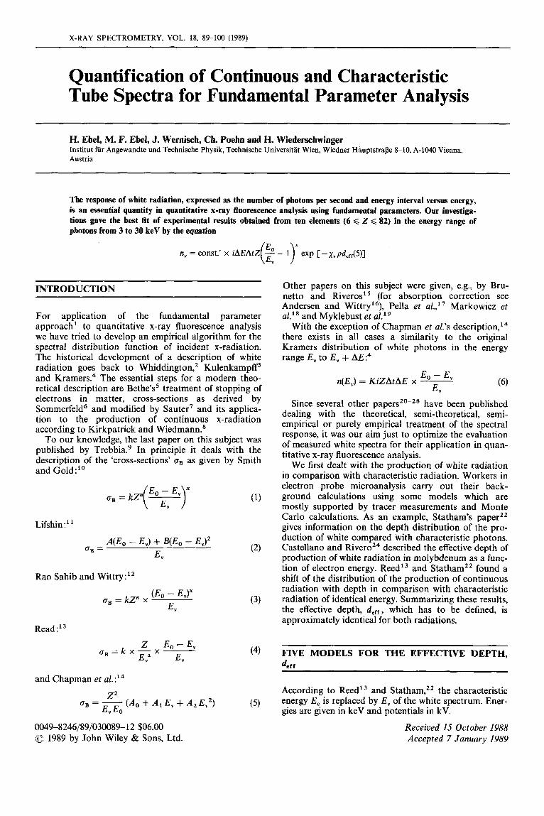
We used a scanning electron microscope with an energy-dispersive detection system. Ten different pure elements were investigated, covering the 2 range from 6 to 82. In order to avoid excitation of white radiation by backscattered electrons in the detector window,22 we installed a beryllium foil of thickness D,, = 11 pm between the target and detector. The geometry of the setup is shown in Fig. 1. A takeoff angle E of 30" was used and the acceleration voltage was 30 kV. Great care was taken to define E , = 30 kV and it was found to be accurate within k 0.2 kV.

Beam currents suffer from greater uncertainties (as much as k 5%). Further efforts were made to determine the contributions to our measured spectra originating from scattered radiation and radiation due to back- scattered electrons. These contributions were deter- mined to be not more than 1% of our spectral signals and therefore were neglected.

For our Si-Li detector we used the following charac- teristic data: thickness of Be front window, d,, = 8 pm; thickness of Au layer, dAu = 20 nm; thickness of inactive Si layer, dsici,, = 0.1 pm; and thickness of active Si layer,

= 2 mm. Originally the last thickness was assumed to be 3 mm, but the evaluations of the high- energy portions of white spectra, as described below, gave systematic deviations for energies higher than 25 keV. These deviations became smaller when dsici,, was reduced and became evident again in the opposite direc- tion for values smaller than 2 mm.

Further care was taken to avoid influences of artifacts on our experimental results. Such sources are pulse pile- up, escape peaks and incomplete charge collection. Pulse pile-up and escape peak formation were investi- gated in a series of experiments and we found no evi- dence for pile-ups in our spectra. Escape peaks were removed by means of the software. Hence only incom- plete charge collection at energies down to 2 keV from characteristic peaks was observed in our white spectra. For this reason we rejected all experimental results from the energy ranges EK - 2 < E, < EK or EL - 2 < E, < EL, where EK and EL are the energies of the strongest K or L lines expressed in keV.

Figure 1. Geometry of the setup in the electron probe micro- analyser.

92 H. EBEL ET AL.

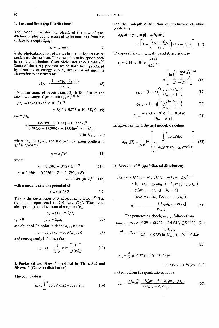
A final comment should be made about the pro- cedure for data collection and documentation. Beam currents i of 2&50 pA were used and gave reasonable pulse pile-up rejection rates. Hence the measured and the true time of data collection did not differ too much. Consequently, we performed our measurements over a period of 500 s. Subsequently, the spectra were sub- jected to a single smoothing and escape peak reduction routine. A width, of 40 eV for the energy window, AE, gave, for energy steps of 1 keV, a sufficient resolution and, in addition, a reasonable signal n, (expressed in counts per 500 s and per 40 eV). An estimation of the relative statistical error in percent gave (l/,,K,) x 100 and led to the rejection of signals of less than n, = 10. Such low signals were especially observed in the high- energy portion for low-Z elements. Times of data collec- tion, At, of less than 500 s caused an increasing number of n, values of less than 10 and an increase to much more than 500 s gave rise to increasing uncertainty owing to instability of the beam current. Finally, the integrated signals of characteristic Kcr and KP or La and LP lines after background subtraction are given in Table 1 also.

EVALUATION

Following Love and Scott29 the number of character-

istic photons per electron in pure elements is pro- portional to

n = poRf(x) (39) Since we are dealing with white radiation, no transition probability p or fluorescence yield o has to be recog- nized and since, as shown above,f(X) is identical with exp( - Xpd,,,), we replace the expression for n by

n, = const. x R, exp( - j ( , pdeff, ,) (40) In the case of the Gaussian profiles (models 2 and 4), d,,,, , contains the influence of backscattering and there- fore needs no further r e ~ o g n i t i o n ~ ~ of the backscatter- ing factor R , .

n, = const. x exp( - 1, pd,,,, ,) (41) In order to correct for backscattering in models 1 and

3 proposed by Love and S ~ o t t , ~ ~ , ~ ~ we apply a formal- ism proposed by August and Wernisch4’ for white radi- ation which used backscattering coefficients q(E) given by Czyzewski,4’ cross-sections according to Green and Co~slett:~ stopping power dE/dpz from Love and co- w o r k e r ~ ~ ~ and mean ionization potential J from R ~ s t e . ~ ~ In Appendix 1 numerical values for the calcu- lation of R,(Z, E ) are given.

Since, according to Reedt3 and Statham,22 deff for white and characteristic radiation are not identical, but should be comparable, we replace in Eqns (40) and (41)

Table 1. Experimental results

Z i (PA) E, (kev)

3 3.52 4 5 6 7 9

10 11 12 13 14 15 16 17 18 19 20 21 22 23 24 25 26 27 28 29

Ka KB La v

6 13 22 29 45 51 65 74 79 82 48 40 36 33 28 26 24 22 22 21

”” 458 489 1227 1152 1545 1129 995

366 542 265 510 215 438 177 378

97 224 76 205 71 167 54 149 44 118 43 98 32 82 32 73 22 54 19 44

11 30 26 17 13 11

484 483

345 308 265 237 193 171 149 123 103 75 68 55 36 27 28 20 12

489 200 50 953

1242 1172

461 423 367 338 286 249 246 192 162 130

86 71 60 37 34 25 15 10

293 450 43 503

921 1065 1124 1053

791 71 1 642 541 472 420 350 303 263

62 49 42 23 17 10

10 677 1757

91 5 984 981 91 3 769 688 601 535 464 41 5 336 309 256 209 180 139 112 88 74 56 39 26 16

1865

1111 1024 966 91 7 837 741 672 609 532 451 377 31 1 255 209 166 133 109 72 55 31 19

189410 1 55 980

1501 1694 1704

908 737 670 594 524 466 403 339 31 6 233 195 156 120 97 74 52 36 22

133 820 92 288

1166 1355 1390

727

529 476 41 7 358 31 2 263 21 7 188 147 113 97 68 48 34 16

83 426 54 261

1374 1461 1634 1614 1561

424 382 31 3 270 228 185 157 118 108 81 63 42 24 15

62 286 38 647

TUBE SPECTRA FOR FUNDAMENTAL PARAMETERS 93

deff, , by kdeff, , and expect after evaluation of our experiments k values close to unity. Two versions of the distribution function are discussed : version A according to Rao Sahib and Wittry12 [Eqn (3)] and version B according to Smith and Gold” [Eqn (l)]. Consequent- ly, we have to replace in Eqns (40) and (41) const. x R , and const., respectively, for version A of models 1 and 3, indicated in the following discussions by A1 and A3, by

(42) ( E , - Ev)” R , const. x R , = const.’ x Z x

EV version A for models 2 and 4 (A2, A4):

(43) (Eo - E,)”

EV const. = const.’ x Z x

version B for models 1 and 3 (BI, B3):

const. x R , = const.‘ x Z(E, /E, - 1)”R, (44) and version B for models 2 and 4 (B2, B4):

const. = const.’ x Z(E, /E, - 1)” (45) As an example, we describe our measured results by B4. This is a ‘Kramers-like’ distribution of type B [Eqn (l)] with derf, , according to model 4:

n,, theor = AEAtiD, const.‘

x ‘(EOIEv - 1)” exPC-Xvpkdeff, d4)1 (46) or we use a description according to A3. This is dis- tribution A [Eqn (3)] and model 3 and gives

n,, theory = AEAtiD, const.’

x Z R J E , - EvY/Ev x ~ X P C - ~v Pkdef,, v(3)l (47) For our own model of a single deff we replace kd,,,, ,(j) (j = 1, 2, 3,4) by deff(5) and obtain for A5

n,, theory = AEAtiD, const.’

x Z(E0 - EvY/Ev x Rv ~ X P C - X V ~deff(5)l (48) and for B5

n,, theor = AEAtiD, const.‘

x W W E , - 1)” exP[ - x v Pdeff(5)I (49) It should be mentioned that we used z instead of p in all of our attenuation expressions, because z describes true attenuation and p includes scattering. However, some of the radiation originally directed towards the detector is lost by scattering and a comparable amount is scattered from an arbitrary direction into the solid angle of detec- tion. Hence the recognition of scattering by the use of p is not justified. D , is the detector efficiency, expressed by

z v , Au P A u dAu

)XP( - COS E

zv , Be P B e dBe D,=exp - ( COS E

exp[ - COS E 1 r v , s i Psi dsi( in)

~ v , s i P s i &(active)

cos E x {I - exp[ --

x exp( - T v , Be P B e D B e

COS E

We include the absorption in the foil (see Fig. 1) of thickness DB, = 11 pm in D. z,, B e , zv, Au and T,, si were calculated from McMaster et d ’ s tables3, as a function of E , .

For the determination of the unknowns const.’, x and k [or deff(5)] we performed a least-squares fitting of n,, meaS to n,, theor. Weighted relative errors should be used as an error quantity. An evaluation with absolute errors would cause a dominating fitting within the range of low and medium photons energies, E , , where the measured count rates are about two orders of mag- nitude higher than in the range of high E , (see Table 1). The relative errors are

J (51) v , = nv, j , meas - nv, j , theor

nv, j , theor

and the weight w, has been taken as proportional to the statistical error:

From m

C wjv; =min (53) j = 1

and

axwj v j 2 axwj v j 2 a z w j oj2 = 0; = 0; a const.‘ ax = 0 (54)

ak

these unknowns are available. More details of the least- squares fitting are given in Appendix 2.

A measure of the quality of fitting is the standard deviation of relative errors :

cr = /m m - 1 j = l (55 )

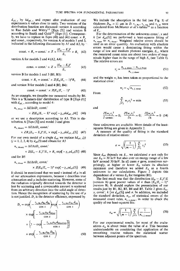
Since deff depends on E , , we calculated cr not only for our E , = 30 keV but also over an energy range of a few keV around 30 keV. In all cases 0 gave, sometimes sur- prisingly, at higher or lower E , values its absolute minimum and therefore we added E , as a fourth unknown to our calculations. Figure 2 depicts this dependence of cr versus E , for tungsten (Bl).

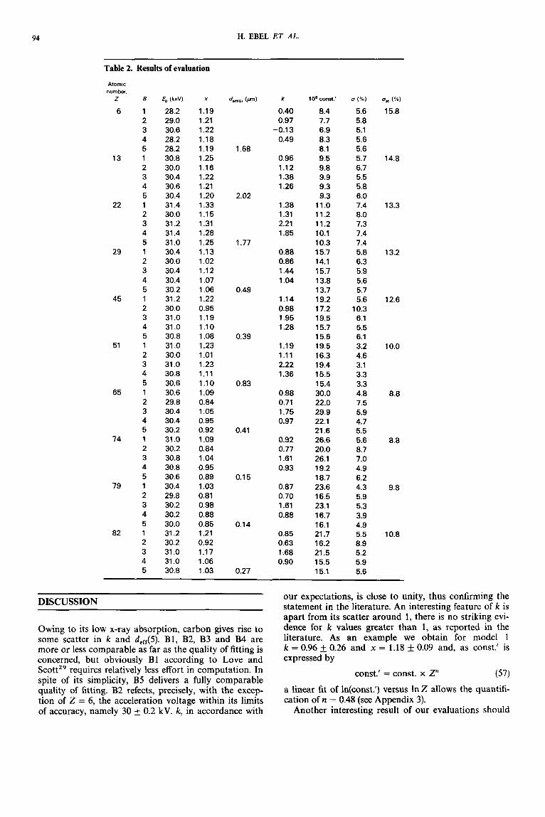
The first result was that the distribution ( E , - E,)”/E (version A) gave poorer values of 0 than (E, /E, - 1)” (version B). It should explain the presentation of our results just by B1, B2, B3, B4 and B5. Table 2 gives E , , x, const.’, k [or deff(5)] and 0. In addition, we included the standard deviation, crs,, of statistical errors of the measured count rates, n,,j,meas, in order to check the quality of our least-squares fits:

For our experimental results, for most of the evalu- ations nst is about twice the value of cr. This becomes understandable on considering that application of the smoothing routine reduces the statistical scatter between adjacent points of the spectrum.

94 H. EBEL ET AL.

Table 2. Results of evaluation Atomic number Z

6

13

22

29

45

51

65

74

79

82

6

1 2 3 4 5 1 2 3 4 5 1 2 3 4 5 1 2 3 4 5 1 2 3 4 5 1 2 3 4 5 1 2 3 4 5 1 2 3 4 5 1 2 3 4 5 1 2 3 4 5

Eo (keW

28.2 29.0 30.6 28.2 28.2 30.8 30.0 30.4 30.6 30.4 31.4 30.0 31.2 31.4 31 .O 30.4 30.0 30.4 30.4 30.2 31.2 30.0 31 .O 31 .O 30.8 31 .O 30.0 31 .O 30.8 30.6 30.6 29.8 30.4 30.4 30.2 31 .O 30.2 30.8 30.8 30.6 30.4 29.8 30.2 30.2 30.0 31.2 30.2 31 .O 31 .O 30.8

X

1.19 1.21 1.22 1.18 1.19 1.25 1.16 1.22 1.21 1.20 1.33 1.15 1.31 1.28 1.25 1.13 1.02 1.12 1.07 1.06 1.22 0.95 1.19 1.10 1.08 1.23 1.01 1.23 1.11 1.10 1.09 0.84 1.05 0.95 0.92 1.09 0.84 1.04 0.95 0.89 1.03 0.81 0.98 0.88 0.85 1.21 0.92 1.17 1.06 1.03

d,",,, (P)

1.68

2.02

1.77

0.49

0.39

0.83

0.41

0.1 5

0.14

0.27

k lo8 const.' u (%)

0.40 8.4 5.6 0.97 7.7 5.8

-0.1 3 6.9 5.1 0.49 8.3 5.6

8.1 5.6 0.96 9.5 5.7 1.12 9.8 6.7 1.38 9.9 5.5 1.26 9.3 5.8

9.3 6.0 1.38 11.0 7.4 1.31 11.2 8.0 2.21 11.2 7.3 1.85 10.1 7.4

10.3 7.4 0.88 15.7 5.8 0.86 14.1 6.3 1.44 15.7 5.9 1.04 13.8 5.6

13.7 5.7 1.14 19.2 5.6 0.98 17.2 10.3 1.95 19.5 6.1 1.28 15.7 5.5

15.6 6.1 1.19 19.5 3.2 1.11 16.3 4.6 2.22 19.4 3.1 1.36 15.5 3.3

15.4 3.3 0.98 30.0 4.8 0.71 22.0 7.5 1.75 29.9 5.9 0.97 22.1 4.7

21.6 5.5 0.92 26.6 5.6 0.77 20.0 8.7 1.61 26.1 7.0 0.93 19.2 4.9

18.7 6.2 0.87 23.6 4.3 0.70 16.5 5.9 1.61 23.1 5.3 0.88 16.7 3.9

16.1 4.9 0.85 21.7 5.5 0.63 16.2 8.9 1.68 21.5 5.2 0.90 15.5 5.9

15.1 5.6

u,t (%)

15.8

14.8

13.3

13.2

12.6

10.0

8.8

8.8

9.8

10.8

DISCUSSION

Owing to its low x-ray absorption, carbon gives rise to some scatter in k and deff(5). B1, B2, B3 and B4 are more or less comparable as far as the quality of fitting is concerned, but obviously B1 according to Love and Scottz9 requires relatively less effort in computation. In spite of its simplicity, B5 delivers a fully comparable quality of fitting. B2 refects, precisely, with the excep- tion of Z = 6, the acceleration voltage within its limits of accuracy, namely 30 f 0.2 kV. k, in accordance with

our expectations, is close to unity, thus confirming the statement in the literature. An interesting feature of k is apart from its scatter around 1, there is no striking evi- dence for k values greater than l , as reported in the literature. As an example we obtain for model 1 k = 0.96 f 0.26 and x = 1.18 f 0.09 and, as const.' is expressed by

const.' = const. x Z"

a linear fit of In(const.') versus 1nZ allows the quantifi- cation of n = 0.48 (see Appendix 3).

Another interesting result of our evaluations should

(57)

TUBE SPECTRA FOR FUNDAMENTAL PARAMETERS 95

00 ' I

29 30 31 32

Eo [keVI - Figure 2. Standard deviation, a, of relative errors as a function of E, for Love and Scott's equidistribution and (Eo/€, - 1)'. The experiment was performed with €, = 30 keV.

be mentioned as it gives an idea of the contributions of the parameters const.', x, E , and k [or deff(5)]. For this purpose we increased systematically the number of free parameters (unknowns); we started with const.', then added k [or deff(5)] followed by x, and finally we evalu- ated for const.', k [or deff(5)], x and E , . The results expressed by o and oav are shown in Table 3.

The mean value oav of (r represents the series of results obtained from ten different elements and con- firms the necessity to evaluate for four unknowns. As the fitting procedure is dedicated to a numerical description of white responses for the fundamental parameter approach to quantitative x-ray fluorescence analysis, we recommend B5 from the overall experience gained from our evaluations.

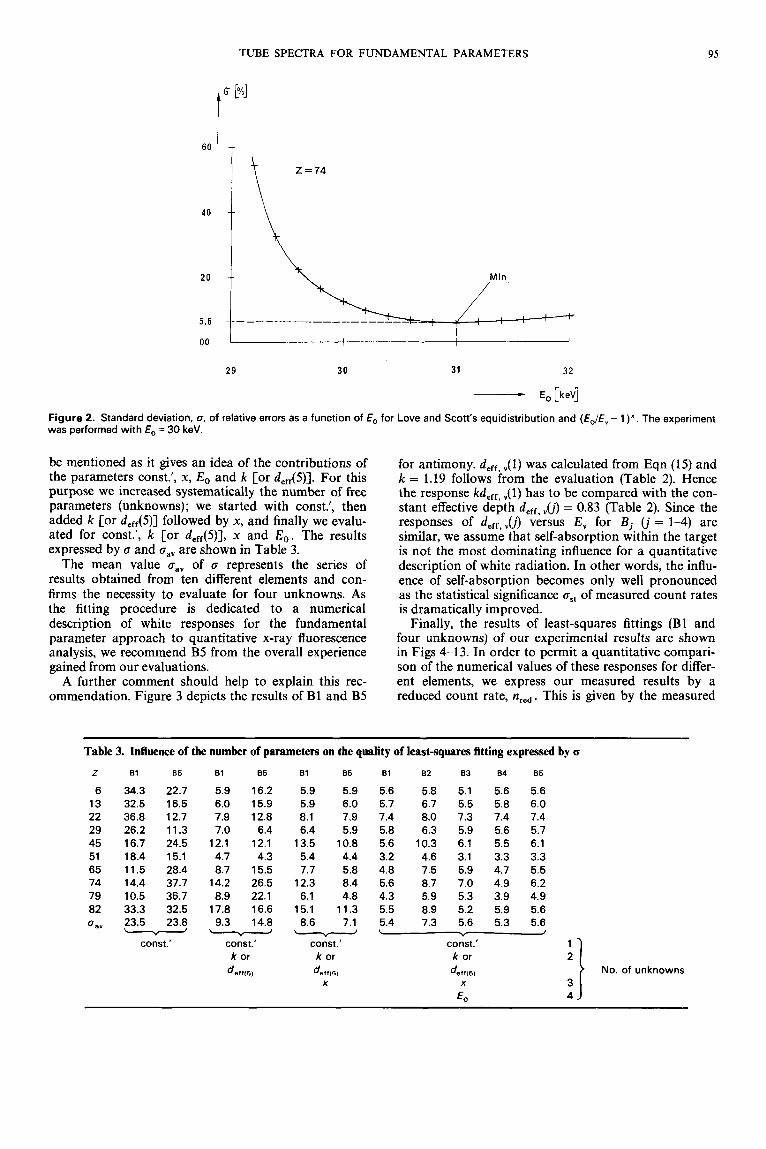
A further comment should help to explain this rec- ommendation. Figure 3 depicts the results of B1 and B5

for antimony. deff, ,(If was calculated from Eqn (15) and k = 1.19 follows from the evaluation (Table 2). Hence the response kdeff, .(1) has to be compared with the con- stant effective depth deff, ,('j) = 0.83 (Table 2). Since the responses of deff, ,,('j) versus E , for Bj ('j = 1-4) are similar, we assume that self-absorption within the target is not the most dominating influence for a quantitative description of white radiation. In other words, the influ- ence of self-absorption becomes only well pronounced as the statistical significance o,, of measured count rates is dramatically improved.

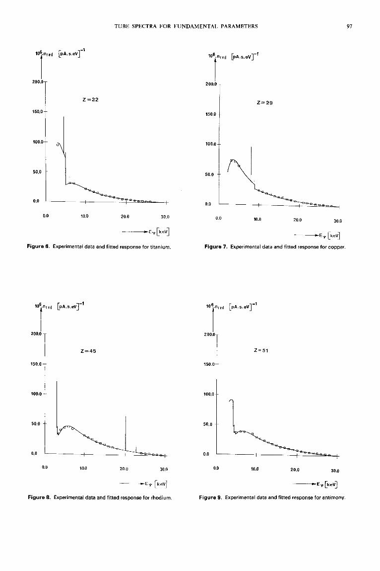
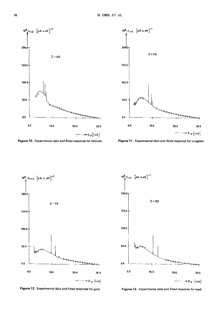
Finally, the results of least-squares fittings (B1 and four unknowns) of our experimental results are shown in Figs 4-13. In order to permit a quantitative compari- son of the numerical values of these responses for differ- ent elements, we express our measured results by a reduced count rate, nred. This is given by the measured

~~ - ~~ ~ ~ ~

Table 3. Influence of the number of parameters on the quality of least-squares fitting expressed by u

z B1 85 B1 85 B1 B5 8 1 82 83 84 85

6 13 22 29 45 51 65 74 79 82 *a"

34.3 22.7 32.5 16.5 36.8 12.7 26.2 11.3 16.7 24.5 18.4 15.1 11.5 28.4 14.4 37.7 10.5 36.7 33.3 32.5 23.5 23.8

" const.'

5.9 16.2 6.0 15.9 7.9 12.8 7.0 6.4 12.1 12.1 4.7 4.3 8.7 15.5 14.2 26.5 8.9 22.1 17.8 16.6 9.3 14.8 -

const.' k or

d e f f , l ,

5.9 5.9 5.9 6.0 8.1 7.9 6.4 5.9 13.5 10.8 5.4 4.4 7.7 5.8 12.3 8.4 6.1 4.8 15.1 11.3 8.6 7.1 -

const.' k or

4 f f ( l )

X

5.6 5.8 5.1 5.6 5.6 5.7 6.7 5.5 5.8 6.0 7.4 8.0 7.3 7.4 7.4 5.8 6.3 5.9 5.6 5.7 5.6 10.3 6.1 5.5 6.1 3.2 4.6 3.1 3.3 3.3 4.8 7.5 5.9 4.7 5.5 5.6 8.7 7.0 4.9 6.2 4.3 5.9 5.3 3.9 4.9 5.5 8.9 5.2 5.9 5.6 5.4 7.3 5.6 5.3 5.6

const.' k or

\ v J

No. of unknowns

4

deff(5)

€0

X

96 H. EBEL ET AL.

Ym1 1.00

0.83

0.50

0.00

Z = 51 7

I I

0.0 10.0 20.0 30.0

E+Vl

Figure 3. Comparison of deff(l ) and kd,, ,( l) of model 1 with deff(5) of model 5 for antimony.

count rate, n v , j , divided by the detector efficiency, Dy, j , atomic number, 2, current, i, in PA, time of data accumulation, At = 500 s, and energy interval, A E = 40 eV, or

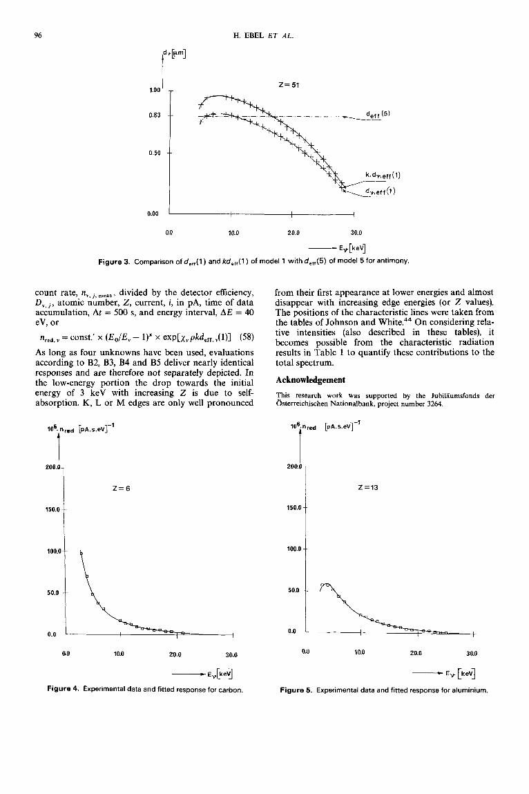
% d , v = const.’ - ’)” exp[Xvpkdeff,v(l)l (58 ) As long as four unknowns have been used, evaluations according to B2, B3, B4 and B5 deliver nearly identical responses and are therefore not separately depicted. In the low-energy portion the drop towards the initial energy of 3 keV with increasing 2 is due to self- absorption. K, L or M edges are only well pronounced

from their first appearance at lower energies and almost disappear with increasing edge energies (or 2 values). The positions of the characteristic lines were taken from the tables of Johnson and On considering rela- tive intensities (also described in these tables), it becomes possible from the characteristic radiation results in Table 1 to quantify these contributions to the total spectrum.

Acknowledgement This research work was supported by the Jubilaumsfonds der Osterreichischen Nationalbank, project number 3264.

lo6. nred [pA.s.eV]-’

1 I 200.0

I5O.O i

i t 100.0

Z = 6

200.0

150.0

100.0

50.0

0.0

Z = I 3

a0 10.0 20.0 30.0

___r

Figure 4. Experimental data and fitted response for carbon.

0.0 10.0 20.0 30.0

E, [ k 4

Figure 5. Experimental data and fitted response for aluminium.

TUBE SPECTRA FOR FUNDAMENTAL PARAMETERS

200.0-

150.0--

100.0--

50.0

91

--

-1 101 n e d [PA. s . eV]

z =22

0.0

0.0 10.0 20.0 30.0

Figure 6. Experimental data and fitted response for titanium.

200.0

150.0

z=45

I 200.0

150.0

I

100.0 1

Z= 29

20.0 30.0 0.0 10.0

-Ev [keV]

Figure 7. Experimental data and fitted response for copper.

106.nr,d [pA.s.eV]-l

I 2 00.0

z=51

t 150.0

100.0 1

10.0 20.0 30.0 0.0

-Ey keV C I Figure 8. Experimental data and fitted response for rhodium.

20.0 30.0 0.0 10.0 - E y [keV]

Figure 9. Experimental data and fitted response for antimony.

98

150.0-

100.0--

50.0

H. EBEL ET AL.

-- Id-

200.0

150.0

0.0 10.0 20.0 30.0

EvCkeVI __L

Figure 10. Experimental data and fitted response for terbium.

1 200.0

150.0

t 100.0

2=79

l l

106. nred [pA.s.eV]-l

I 2001h

z= 74

0.0 :

0.0 10.0 20.0 30.0

E y [keV]

Figure 11. Experimental data and fitted response for tungsten.

T 200.0

t 150.0

t 100.0

Z = 8 2

10.0 20.0 30.0 0.0

Ev [keq -

Figure 12. Experimental data and fitted response for gold.

10.0 20.0 30.0 0.0

- ) E y [keV]

Figure 13. Experimental data and fitted response for lead.

-

TUBE SPECTRA FOR FUNDAMENTAL PARAMETERS 99

REFERENCES

1. J. W. Criss and L. S. Birks, Anal. Chem. 40,1080 (1 968). 2. R. Whiddington, Proc. R. SOC. London, Ser. A 86, 390

3. H. Kulenkampff,Ann. Phys. (Leipzig) 69, 548 (1 923). 4. H. A. Kramers, Philos. Mag. 46,836 (1 923). 5. H. A. Betthe,Ann. Phys. (Leipzig) 5, 325 (1930); H. A. Bethe

and J. Ashkin, Experimental Nuclear Physics. Wiley, New York (1953).

(1 91 2); 89,554 (1914).

6. A. Sommerfeld,Ann. Phys. (Leipzig) 11, 257 (1931). 7. F. Sauter, Ann. Phys. (Leipzig) 18, 486 (1 933). 8. P. Kirkpatrick and L. Wiedmann, Phys. Rev. 67, 321 (1945). 9. P. Trebbia, J. Microsc. Spectrosc. Electron 13, 241 (1988).

10. D. G. W. Smith and C. M. Gold, Microbeam Analysis, p. 273. San Francisco Press, San Francisco (1979); D. G. W. Smith, C. M. Gold and D. A. Tomlinson, X-Ray Spectrom. 4, 149 (1975).

11. E. Lifshin, paper presented at the 9th Annual Conference on Electron Probe Microprobe Analysis, MAS, Ottawa, 1 974, paper 53;Adv.X-RayAnal. 19,113 (1976).

12. T. S. Rao Sahib and D. B. Wittry, J. Appl. Phys. 45, 5060 (1974); in Proceedings of the 6th Conference on X-Ray Optics and Microanalysis, pp. 131 -1 37. University of Tokyo Press, Tokyo (1 972).

13. S. J. B. Reed, X-Ray Spectrom. 4, 14 (1 975). 14. J. N. Chapman, C. C. Gray, B. W. Robertson and W. A. P.

Nicholson, X-Ray Spectrom. 4,153 and 163 (1 983). 15. M. G. Brunetto and J. A. Riveros, X-Ray Spectrom. 13, 60

(1 984). 16. C. A. Andersen and D. B. Wittry, Br. J. Appl. Phys. 1, 529

(1 968). 17. P. A. Pella, L.-Y. Feng and J. A. Small, X-Ray Spectrom. 14,

125 (1985). 18. A. Markowicz, H. Storms and R. Van Grieken, X-Ray Spec-

from. 15, 131 (1986). 19. R. L. Myklebust, C. E. Fiori and K. F. J. Heinrich, Nat. Bur.

Stand. (U.S . ) Spec. Publ. No. 604, 365 (1981). 20. D. R. Beaman, L. F. Solosky and L. A. Settlemeyer, tutorial

session notes, in Proceedings o f 8th National Conference on €PA, p. 73. EPASA, New Orleans (1973).

21. N. G. Ware and S. J. 8. Reed, J. Phys. E 6, 286 (1 973). 22. P. J. Statham, X-Ray Spectrom. 5,154 (1976). 23. J. V. Gilfrich and L. S. Birks,Anal. Chem. 40, 1077 (1968).

24. E. E. Castellano and B. E. Rivero, X-Ray Spectrom. 5, 223

25. D. Laguitton and W. Parrish, X-Ray Spectrom. 6,201 (1 977). 26. M. Murata and H. Shibahara, X-Ray Spectrom. 10,41 (1981). 27. D. G. W. Smith and S. J. B. Reed, X-Ray Spectrom., 10, 198

(1 981 ). 28. J. N. Chapman, W. A. P. Nicholson and P. A. Crozier, J.

Microsc. 136, 1 79 (1 984). 29. G. Love and V. D. Scott, J. Phys. D 13,995 (1980); G. Love,

M. G. Cox and V. D. Scott, J. Phys. D 11, 7 (1978); G. Love and V. D. Scott, Scanning 4, 11 1 (1 981 ).

30 W. H. McMaster, N. K. del Grande, J. H. Mallett and J. H. Hubbell, Compilation o f X-Ray Cross-Sections, UCRL-50174, Sect. 11, Rev. 1. Lawrence Radiation Laboratory, University of California, Livermore, CA. (1 969).

(1976).

31. H. E. Bishop, J. Phys. D 7,2009 (1974). 32. H. J. Hunger and L. Kuchler, Phys. Status Solidi A 56, K45

(1 979) 33. F. Bloch, Z. Phys. 81,363 (1933). 34. R. H. Packwood and J. D. Brown, X-Ray Spectrom. 10, 138

(1981); J. D. Brown and R. H. Packwood, X-Ray Spectrom. 11,187 (1982).

35. J. H. Tirira SaB and J. A. Riveros, X-Ray Spectrom. 16, 27 (1987); J. H. Tirira Sah, M. A. del Giorgio and J. A. Riveros, X-Ray Spectrom. 16,243 (1 987).

36. D. A. Sewell, G. Love and V. D. Scott, J. Phys. D 18, 1233, 1245,1269 (1 985).

37. J. Ruste, Thesis, University of Nancy (1 976). 38 G. F. Bastin, F. J. J. van Loo and H. J. M. Heijligers, X-Ray

Spectrom. 13, 91 (1984); G. F. Bastin, H. J. M. Heijligers and F. J. J. van Loo, Scanning 8,45 (1 986).

39 J. Ruste, J. Microsc. Spectr. Electron 4,123 (1979). 40. G. Love, M. G. Cox and V. D. Scott, J. Phys. D 11,23 (1 978). 41. H. J. August and J. Wernisch, Radex Rundsch. 624 (1 988). 42. 2. Czyzewski, Phys. Status SolidiA 92, 563 (1 985). 43. M. Green and V. E. Cosslett, Proc. Phys. SOC. 78, 1206

(1 961 ). 44. G. G. Johnson, Jr and E. W. White, X-Ray Emission Wave-

lengths and ke V Tables for Nondiffractive Analysis. ASTM Data Series DS 46. American Society for Testing and Materials, Philadelphia. (1 970).

APPENDIX 1

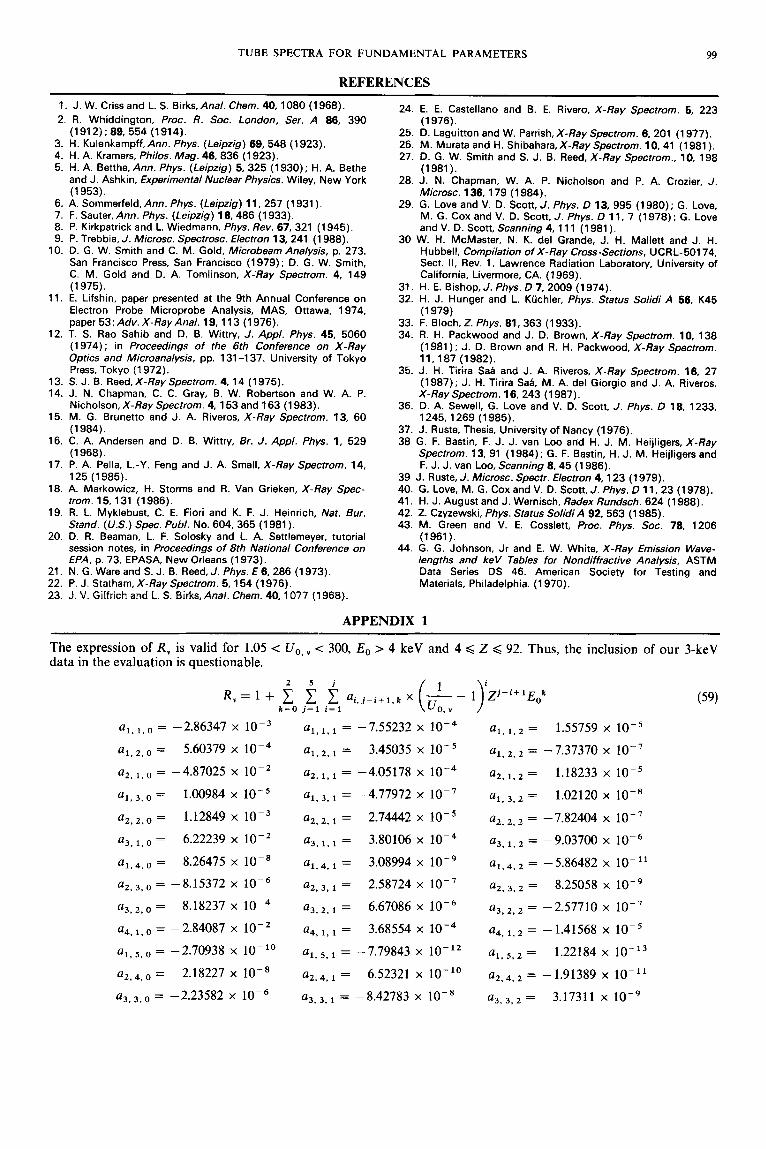
The expression of R, is valid for 1.05 < U,, , < 300, E , =- 4 keV and 4 < Z < 92. Thus, the inclusion of our 3-keV data in the evaluation is questionable.

Z S j i

R v = l + c c % , j - i + l , k ( -- u;, , 1) Zj-'+'Eok (59) k = O j = 1 i = l

al, l , o = -2.86347 x l op3

~ 1 , 2 , 0 = 5.60379 x lop4

~ 2 , 1 , 0 = -4.87025 x lo-'

~ 1 , 3 , 0 = - 1.00984 x

uZ.Z,O = 1.12849 x

a3, 1 , = -6.22239 x lo-'

al,4, 0 = 8.26475 x lo-'

a z , 3 , 0 = -8.15372 x

u ~ , ~ , , = 8.18237 x lop4

a4, 1 , , = -2.84087 x lo-' al, 5 , , = -2.70938 x lo-''

~ 2 , 4 , 0 = 2.18227 x lo-' a3 ,3 ,0 = -2.23582 x

u ~ , ~ , ~ = -7.55232 x

u1, 2, = 3.45035 x

u ~ , ~ , ~ = -4.05178 x

u1, 3,

u2, z, = 2.74442 x

u ~ , ~ , ~ = 3.80106 x

= -4.77972 x lop7

~ 1 . 4 , = 3.08994 x

a2, 3 , = -2.58724 x lo-' u3, ', = 6.67086 x

u ~ , ~ , ~ = 3.68554 x

~ 1 , s , 1 = -7.79843 x 10-l'

az,4,1 = 6.52321 x lo-'' ~ 3 . 3 . 1 = -8.42783 x lo-*

u1, 1 , = 1.55759 x

u1, z, = -7.37370 x

az, 1, = 1.18233 x lo-'

q 3 , z = 1.02120 x lo-'

u ~ . ~ , ~ = -7.82404 x

~ 3 , 1 , 2 = -9.03700 x

~ 1 , 4 , 2 = - 5.86482 x 10- l 1

az, 3, = 8.25058 x

~ 3 , ' , ~ = -2.57710 x

u4, l ,z = -1.41568 x

u ~ , s, = 1.22184 x

~ 2 . 4 . 2 = - 1.91389 x 10-l' = 3.17311 x lo-'

100 H. EBEL ET AL.

u ~ , ~ , , = 2.40083 x a4, 2, = -4.45352 x a4, 2, = 1.04058 x lo-'

u5, = -1.38772 x u5, 1, = -7.39649 x u5, 1 , = - 1.66242 x

In order to estimate the difference in the results when Evaluating again k, x and n [Eqn (57)] for all the Rv is either used or neglected, the values for Cu (2 = 29) elements considered with neglect of Rv gives for B1 are compared. With Rv one obtains E, = 30.4 k = 0.94 +_ 0.20, a smaller x = 1.08 & 0.13 and n keV, x = 1.13, k = 0.88, const.' = 15.7 x and reduces to n = 0.39. As one concentrates the emphasis 0 = 5.8% and without R, Eo = 30.4 keV, x = 1.07, on 0 there is no substantial difference between the two k = 0.83, const.' = 13.7 x and 0 = 5.5%. kinds of evaluation.

APPENDIX 2

A slight modification of uj:

- 1 (60) %, j , meas - 'v, j , theor - 'v, j , meas

nv, j, theor

u . = - n v , j , theor

gives

(61)

and allows for small uj (e.g. uj = 0.1 for 10% relative error) the approximation

ln(1 + V j ) = In 0 nv, j, theor

lnfl + uj) G uj (62) or, in the case of B1, e.g.

uj I In nv, J , meas - ln(const.' x D , AtAEiR, Z)

- x ln(Eo/E,. j - 1) + kdeff, v, j ( 1 ) x v P (63) Introducing the abbreviations

Y j = In (nv , j . meaJAj) (64) A j = D , AtAEiR, Z (65)

Bj = ln(E,/Ev, - 1) (66)

D . = J -d eff, v, j(1)xv P (67) we define our problem by

m ( y j - In const.' - x B j - kDj)'wj = min (68)

j = 1

From the derivatives it follows that

= o (69) ax

a In const.'

In const.' x X q + xZBj wj + kZDj wj = X y j wj (70) ax ax - = o

In const.' x CB, wj + xZBj2wj

+ kXBjDj wj = C B j y j wj (72)

-- - 0 ax ak (73)

In const.' x CDj wj + xXBj Dj wj

+ kXDj2wj = C D j y j wj (74)

Equations (70), (72) and (74) form a system of three inhomogeneous and linear equations in the unknowns In const.', x and k.

APPENDIX 3

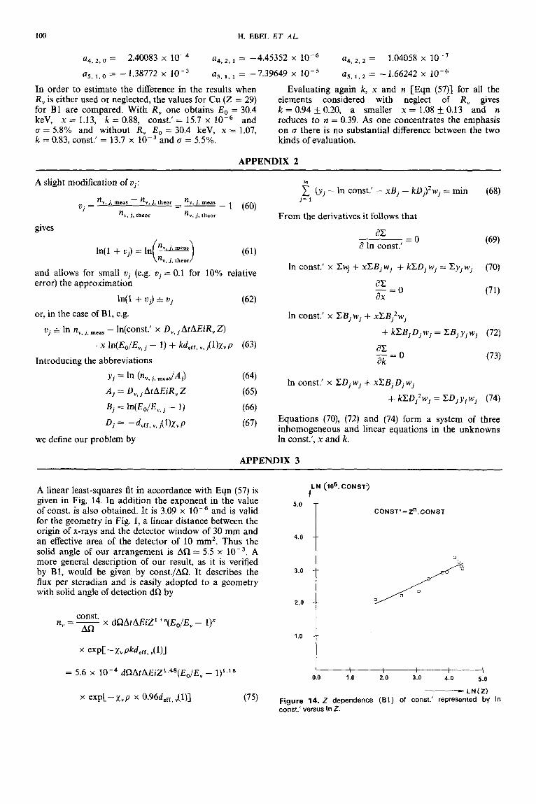
A linear least-squares fit in accordance with Eqn (57) is given in Fig. 14. In addition the exponent in the value of const. is also obtained. It is 3.09 x lop6 and is valid for the geometry in Fig. 1, a linear distance between the origin of x-rays and the detector window of 30 mm and an effective area of the detector of 10 mm2. Thus the solid angle of our arrangement is AQ = 5.5 x A more general description of our result, as it is verified by B1, would be given by const./AQ. It describes the flux per steradian and is easily adopted to a geometry with solid angle of detection dQ by

const. AQ

n, = - x dQAtAEiZ'+"(E,/E, - 1)"

= 5.6 x lo-' dQAtAEiZ'.48(Eo/Ev -

,LN (106. CON ST^

CONST' =z". CONST

4.0 t

1.0 -+

I 'd !

0.0 1 .o 2.0 3.0 4.0 5.0 - LN(Z) Figure 14. Z dependence (61) of const.' represented by In const.' versus In Z.