Quantum aspects of spinning strings

in AdS3 × S3 × T 4 with RR-flux

Diploma thesis at theII. Institute for theoretical Physics,

University of Hamburg

- Preliminary version -

Manuel Hohmann

February 28, 2007

II. Institut fur theoretische PhysikUniversitat HamburgLuruper Chaussee 149

22761 HamburgGermany

VORWORT

Diese Arbeit widmet sich der Untersuchung eines wichtigen Beispiels der Dualitat zwischenEichtheorie und Stringtheorie, namlich der AdS/CFT-Korrespondenz auf AdS3 × S3 × T 4 mitRR-Fluss. Das Hauptaugenmerk liegt dabei auf der Seite der Stringtheorie. Zunachst wirdgezeigt, dass der klassische Superstring auf diesem Raum integrabel ist. Danach werden einigeLosungen mit rotierenden Strings konstruiert und ihre Energien sowohl klassisch als auch unterBerucksichtigung von Quantenkorrekturen berechnet. Die Kenntnis der String-Energien istwichtig um die AdS/CFT-Korrespondenz zu testen, die eine Entsprechung der Energien vonStrings und der anomalen Dimensionen von Operatoren in der Eichtheorie beinhaltet.

ABSTRACT

In this work we shall examine an important example for a duality between gauge theory andstring theory, namely the AdS/CFT correspondence on AdS3×S3×T 4 with RR-flux. Attentionwill be payed mainly to the string theory side of the correspondence. Firstly, we will showthat the classical superstring on this space is integrable. Secondly, we will construct severalspinning string solutions and compute their energies at the classical level as well as their leadingquantum corrections. The knowledge of the string energies is important for testing the AdS/CFTcorrespondence, which conjectures that the spectrum of string energies is identical to that ofanomalous dimensions of planar gauge theory operators.

CONTENTS

1. Introduction . . . . . . . . . . . . . . . . . . . . . . . . . . . . . . . . . . . . . . . . . . 7

2. AdS/CFT correspondence . . . . . . . . . . . . . . . . . . . . . . . . . . . . . . . . . . 9

2.1 Statement of the AdS/CFT correspondence . . . . . . . . . . . . . . . . . . . . . 9

2.2 Tests of the correspondence . . . . . . . . . . . . . . . . . . . . . . . . . . . . . . 12

2.3 Anomalous dimensions and Bethe ansatz . . . . . . . . . . . . . . . . . . . . . . . 13

2.3.1 Anomalous dimensions and spin-chains . . . . . . . . . . . . . . . . . . . . 13

2.3.2 The Bethe ansatz . . . . . . . . . . . . . . . . . . . . . . . . . . . . . . . . 14

2.4 Spinning strings . . . . . . . . . . . . . . . . . . . . . . . . . . . . . . . . . . . . . 16

2.4.1 General method . . . . . . . . . . . . . . . . . . . . . . . . . . . . . . . . 16

2.4.2 AdS5 × S5 case . . . . . . . . . . . . . . . . . . . . . . . . . . . . . . . . . 16

2.4.3 AdS3 × S3 × T 4 case . . . . . . . . . . . . . . . . . . . . . . . . . . . . . . 16

3. Strings on AdS3 × S3 × T 4 . . . . . . . . . . . . . . . . . . . . . . . . . . . . . . . . . 18

3.1 The supergeometry of AdS3 × S3 × T 4 with RR-flux . . . . . . . . . . . . . . . . 18

3.2 The superstring action . . . . . . . . . . . . . . . . . . . . . . . . . . . . . . . . . 19

3.3 Equations of motion . . . . . . . . . . . . . . . . . . . . . . . . . . . . . . . . . . 19

3.4 Conserved charges . . . . . . . . . . . . . . . . . . . . . . . . . . . . . . . . . . . 20

4. Classical integrability . . . . . . . . . . . . . . . . . . . . . . . . . . . . . . . . . . . . 21

4.1 The psu(1, 1|2)× psu(1, 1|2) sigma model . . . . . . . . . . . . . . . . . . . . . . 21

4.2 Flat currents . . . . . . . . . . . . . . . . . . . . . . . . . . . . . . . . . . . . . . 21

4.3 Classical solutions . . . . . . . . . . . . . . . . . . . . . . . . . . . . . . . . . . . 23

4.3.1 AdS3 × S1 with S1 ⊂ S3 . . . . . . . . . . . . . . . . . . . . . . . . . . . . 23

4.3.2 AdS3 × S1 with S1 ⊂ T 4 . . . . . . . . . . . . . . . . . . . . . . . . . . . 23

4.3.3 R× S3 . . . . . . . . . . . . . . . . . . . . . . . . . . . . . . . . . . . . . . 24

5. Quantum corrections . . . . . . . . . . . . . . . . . . . . . . . . . . . . . . . . . . . . . 25

Contents 5

5.1 General method . . . . . . . . . . . . . . . . . . . . . . . . . . . . . . . . . . . . . 25

5.1.1 Bosonic part . . . . . . . . . . . . . . . . . . . . . . . . . . . . . . . . . . 25

5.1.2 Fermionic part . . . . . . . . . . . . . . . . . . . . . . . . . . . . . . . . . 26

5.2 AdS3 × S1 with S1 ⊂ S3 . . . . . . . . . . . . . . . . . . . . . . . . . . . . . . . . 27

5.2.1 Bosonic part . . . . . . . . . . . . . . . . . . . . . . . . . . . . . . . . . . 27

5.2.2 Fermionic part . . . . . . . . . . . . . . . . . . . . . . . . . . . . . . . . . 28

5.3 AdS3 × S1 with S1 ⊂ T 4 . . . . . . . . . . . . . . . . . . . . . . . . . . . . . . . . 29

5.3.1 Bosonic part . . . . . . . . . . . . . . . . . . . . . . . . . . . . . . . . . . 29

5.3.2 Fermionic part . . . . . . . . . . . . . . . . . . . . . . . . . . . . . . . . . 29

5.4 R× S3 . . . . . . . . . . . . . . . . . . . . . . . . . . . . . . . . . . . . . . . . . . 30

5.4.1 Bosonic part . . . . . . . . . . . . . . . . . . . . . . . . . . . . . . . . . . 30

5.4.2 Fermionic part . . . . . . . . . . . . . . . . . . . . . . . . . . . . . . . . . 31

5.4.3 Large 1/J expansion . . . . . . . . . . . . . . . . . . . . . . . . . . . . . . 32

5.4.4 Analytic Terms . . . . . . . . . . . . . . . . . . . . . . . . . . . . . . . . . 32

5.4.5 Discussion . . . . . . . . . . . . . . . . . . . . . . . . . . . . . . . . . . . . 33

6. Conclusion . . . . . . . . . . . . . . . . . . . . . . . . . . . . . . . . . . . . . . . . . . 34

Appendix 35

A. Conventions and notation . . . . . . . . . . . . . . . . . . . . . . . . . . . . . . . . . . 36

A.1 Coordinate indices . . . . . . . . . . . . . . . . . . . . . . . . . . . . . . . . . . . 36

A.2 Convention for gamma matrices . . . . . . . . . . . . . . . . . . . . . . . . . . . . 36

B. Bases of psu(1, 1|2)× psu(1, 1|2) . . . . . . . . . . . . . . . . . . . . . . . . . . . . . . 37

B.1 The canonical basis . . . . . . . . . . . . . . . . . . . . . . . . . . . . . . . . . . . 37

B.2 The covariant basis . . . . . . . . . . . . . . . . . . . . . . . . . . . . . . . . . . . 38

B.3 The light cone basis . . . . . . . . . . . . . . . . . . . . . . . . . . . . . . . . . . 38

C. Construction of invariant charges . . . . . . . . . . . . . . . . . . . . . . . . . . . . . . 40

C.1 Derivation of Maurer-Cartan equations . . . . . . . . . . . . . . . . . . . . . . . . 40

C.2 Variation of Cartan 1-forms . . . . . . . . . . . . . . . . . . . . . . . . . . . . . . 42

C.3 Supersymmetric string action . . . . . . . . . . . . . . . . . . . . . . . . . . . . . 44

C.4 Equations of Motion . . . . . . . . . . . . . . . . . . . . . . . . . . . . . . . . . . 47

Contents 6

D. Mathematica packages . . . . . . . . . . . . . . . . . . . . . . . . . . . . . . . . . . . . 49

D.1 Grassmann.m . . . . . . . . . . . . . . . . . . . . . . . . . . . . . . . . . . . . . . 49

D.2 Clifford.m . . . . . . . . . . . . . . . . . . . . . . . . . . . . . . . . . . . . . . . . 50

D.3 Listings . . . . . . . . . . . . . . . . . . . . . . . . . . . . . . . . . . . . . . . . . 51

D.3.1 Grassmann.m . . . . . . . . . . . . . . . . . . . . . . . . . . . . . . . . . . 51

D.3.2 Clifford.m . . . . . . . . . . . . . . . . . . . . . . . . . . . . . . . . . . . . 59

Bibliography . . . . . . . . . . . . . . . . . . . . . . . . . . . . . . . . . . . . . . . . . . . 66

1. INTRODUCTION

The original discovery that led to the development of string theory was the observation of alinear dependence between meson masses and their spins. This relation could be explained byVeneziano [1], using a model of a rotating, open string. Today, string theory has evolved to beone of the most promising candidates for a unified theory of gravity, quantum mechanics andall forces of nature. Its basic idea is to replace the notion of pointlike, elementary particles byone-dimensional, extended objects which can oscillate similar to a violin string - giving themtheir popular name.

Although string theory has more and more become a unified theory of gravity and quantumfield theory than a pure theory of strong interactions, the original idea of writing a stronglycoupled gauge theory in terms of a string theory is still of particular interest. The basic idea ofrelating gauge theory and string theory was developed by ’t Hooft [2], who proposed that gaugetheory and string theory provide holographically equivalent descriptions of the same problem.He conjectured that there exists an even deeper equivalence between these two types of theories,in a sense that they do not only lead to equivalent descriptions, but may be viewed as differentaspects of the same theory.

The most explicit example for this equivalence has been introduced by Maldacena [3] in hisfamous conjecture of an equivalence between type IIB string theory on AdS5 × S5 and N = 4super yang mills theory in four dimensions. Several other equivalences relating string theorieson anti-de-Sitter spacetimes and conformal field theories have been proposed, summarized underthe notion of AdS/CFT correspondence. It relates the fundamental objects of both theories toeach other, string states on the one side and gauge invariant operators on the other. An extensivereview can be found in [4].

Since the AdS/CFT correspondence is a conjecture, the question arises how this conjecture mightbe tested. The most intuitive test is the comparison of string spectra with their gauge operatorcounterparts on the CFT side. An important difficulty here is that the conjecture relates theweakly coupled regime of string theory to the strongly coupled regime of CFT and vice versa,which makes a direct comparison of the two theories difficult. To circumvent this problem, it isfruitful to make use of the high amount of symmetry present on both sides of the conjecture.Considering states that are invariant under parts of the supersymmetry, so called BPS states,which thanks to non-renormalization theorems are protected, one can easily extrapolate fromweak to strong coupling. However beyond the BPS spectrum, other means of comparing the twotheories have to be found. What is potentially obstructing to such endeavors is the difficulty ofquantizing string theory in AdS5 × S5.

A very fruitful direction in testing the AdS/CFT correspondence, which has been initiated by thework of Berenstein, Maldacena, Nastase [16], Frolov, Tseytlin [?], Gubser, Klebanov, Polyakov[8], is to study a subclass of states with large quantum numbers. Consider e.g. the rotationalsymmetries of the S5 component, corresponding to the R-symmetry of the CFT. On the string

1. Introduction 8

theory side, this leads to the classical limit of string solutions with high angular momentum,known as spinning strings. The advantage in considering these states is that semi-classical quan-tization can be used to compute quantum corrections to their classical energies. On the gaugetheory side, the corresponding states are operators with a large number of field insertions, whichcan be represented by spin chains and thus can be investigated by techniques from condensedmatter physics, known as the Bethe ansatz.

In the case of the AdS5/CFT4 correspondence much mileage has been gained by investigating thesubclass of states with large angular momentum, which lead to strong support of the conjecturedcorrespondence.

In this thesis, we will advance these methods in the case of AdS3/CFT2 correspondence. Ourmain focus is the string theory side, where we elaborate on the classical integrable structure. Weshall investigate different spinning string solutions on AdS3×S3×T 4 and compute their classicalenergies as well as quantum corrections. The second chapter gives a short introduction into thetopic of AdS/CFT correspondence and its possible tests, especially using spinning strings. Inthe third chapter we will state some geometrical properties of AdS3×S3×T 4 with RR-flux andderive the equations of motion and conserved charges from the superstring action. The fourthchapter covers classical integrability and the construction of flat currents. This establishes theclassical integrability of the theory. Finally, the fifth chapter is devoted to quantum correctionsto the energy of various spinning string configurations.

Appendix A lists the conventions and notation used in this thesis. The symmetry algebrapsu(1, 1|2) × psu(1, 1|2) and different bases of this algebra are reviewed in appendix B. A de-tailed derivation of invariant charges can be found in appendix C. Appendix D describes twoMathematica packages that have been written for this thesis.

2. ADS/CFT CORRESPONDENCE

2.1 Statement of the AdS/CFT correspondence

It has been proposed by ’t Hooft [2] that, although string theory is quite different from gaugetheory, there still exists a relationship between these two theories. The basic idea that led to thisdiscovery was again the aim to gain a deeper understanding of QCD. ’t Hooft suggested that theSU(N) theory might simplify if N is large, especially in the limit N →∞ the theory should besolvable. This would allow the N = 3 case to be solved by performing an expansion in 1

N . Wewill show that the diagrammatic expansion of the field theory suggests that the large N theoryis equivalent to a free string theory.

The idea of a gauge / string duality also applies to more general gauge theories. A particularclass of gauge theories are theories, in which the gauge coupling does not depend on the energyscale. These theories are known to be conformally invariant. The conformal field theory, thathas been investigated most intensively in the context of gauge / string duality, is N = 4 superYang-Mills theory. It has the maximal number of supersymmetry generators in four dimensionsand its gauge group is SU(N). The theory contains the gauge fields (gluons) Aµ, four fermions(which can be written as a 16 component 10d Majorana-Weyl spinor χα, α = 1, . . . , 16) and sixscalars φi, i = 1, . . . , 6. All fields transform in the adjoint representation of the gauge group. TheLagrangian is completely determined by supersymmetry and reads [5]

S =2

g2YM

∫d4x Tr

(14FµνF

µν +12(Dµφi)(Dµφi)−

14

[φi, φj ] [φi, φj ] +12χ /Dχ− i

2χΓi [φi, χ]

),

(2.1.1)with the covariant derivative Dµ = ∂µ−i [Aµ, .] and /D = DµΓµ. The field strength Fµν is definedas Fµν = ∂µAν − ∂νAµ. (Γµ,Γi) are the 10d gamma matrices. The only two parameters of thetheory are the Yang-Mills coupling gYM and the rank of the gauge group N . An important aspectis how to scale the coupling in the limit N → ∞. A natural choice that has been motivatedby QCD is the ’t Hooft limit, scaling gYM such that the ’t Hooft coupling λ = g2

YMN remainsconstant.

Besides the gauge symmetry, the theory has a global su(4) ∼= so(6) R-symmetry and the conformalsymmetry with symmetry algebra so(4, 2) in four dimensions. It is thus intuitive to claim thatthese symmetries should also be found on the dual string theory side.

The most natural space that exhibits an SO(4, 2) symmetry is five dimensional anti-de-Sitterspace AdS5, which is the maximally symmetric Lorentzian space with constant negative curva-ture. Since superstring theory requires ten dimensions in order to be consistent, another fivedimensions have to be added. The obvious choice is to put these dimensions into a five sphereS5, since it also introduces the SO(6) symmetry into our theory. Furthermore the combinedspace is an exact solution to string theory. This vaguely suggests that N = 4 super Yang-Millstheory is related to a superstring theory on AdS5 × S5. It has been motivated by Maldacena [3]

2. AdS/CFT correspondence 10

that the dual string theory of N = 4 super Yang-Mills theory is indeed type IIB string theoryon AdS5 × S5.

In string theory, there are again two parameters: the string coupling gs and the tension 12πα′ . A

third parameter, the common radius R of AdS5 and S5, can be absorbed by rescaling the embed-ding space coordinates. Type IIB string theory on AdS5 × S5 involves the bosonic coordinatesxm,m = 0, . . . , 9 of AdS5 × S5 and two D = 10 Majorana-Weyl spinors θI , I = 1, 2, with thedynamics given by an action of the form

S =1

2πα′

∫d2σ

(R2

2√−ggµνGmn(x)∂µxm∂νxn + i(

√−ggµνδIJ − εµνsIJ)θIρµDνθ

J + . . .

),

(2.1.2)where µ, ν = 1, 2 labels the string coordinates, sIJ = diag(1,−1) and higher terms have beenomitted.

A motivation for the correspondence is given in [4] and will be briefly summarized here. Considerat first the gauge theory side and its perturbative expansion in terms of Feynman diagrams. Eachdiagram can be viewed as a tiling (or simplicial decomposition) of a two dimensional, orientedmanifold. The numbers of vertices V , propagators E and loops F correspond to the numbersof corners, edges and surfaces of the tiling. To determine the powers of the ’t Hooft couplingλ = g2

YMN and N associated with this diagram, assume that each 3-point vertex carries a factorgYM and each 4-point vertex carries a factor g2

YM . The contribution of the vertices can thus bewritten as gn3+2n4

YM , where n3 is the number of 3-point vertices and n4 is the number of 4-pointvertices. Since V = n3 +n4 and 2E = 3n3 +4n4, we can also write this as g2E−2V

YM . Finally, eachloop contributes a factor N since we have to sum over N indices for each loop. It follows thatthe overall factor of a diagram has the form

g2E−2VYM NF = λE−VNF−E+V = λE−VNχ = λE−VN2−2g, (2.1.3)

where F − E + V = χ = 2 − 2g is the Euler characteristic of the manifold and g its genus. Inthe ’t Hooft limit N →∞, λ = const. we find a diagrammatic expansion of the form

∞∑g=0

N2−2g∞∑l=0

cg,lλl =

∞∑g=0

N2−2gfg(λ). (2.1.4)

In the limit N → ∞, only diagrams with genus g = 0, so-called planar diagrams, contributewhile all other diagrams are suppressed by a factor 1

N2g .

In perturbative string theory, a similar genus expansion exists. [5] A closer examination andcomparison to the expansion derived above shows that there is also a correspondence betweenthe parameters of the two theories, allowing us to identify

gs = g2YM =

λ

N, α′ =

R2

√λ. (2.1.5)

From this we see that in the N →∞ limit, the string theory becomes non-interacting and stringworldsheet corrections correspond to 1√

λcorrections.

Since the fundamental objects in CFT are gauge invariant operators, there should be some dualto these objects in string theory. The fundamental objects in string theory are strings, so itseems natural to propose that there exists a correspondence between gauge invariant operatorsand string states. Both objects transform in representations of a symmetry algebra, which is the

2. AdS/CFT correspondence 11

conformal and R-symmetry algebra in the case of CFT and the isometry of AdS5 × S5 in thecase of string theory. Both algebras match, leading to the conclusion that dual objects in thesense of the correspondence should belong to the same representation of the symmetry algebra.Especially, the charges of both objects under the symmetry algebra should be identical. Oneof these charges is the energy E of the string, corresponding to the scaling dimension ∆ of thegauge invariant operator on the CFT side. This leads to the conclusion that there should bea one to one correspondence between the energies of string states and the scaling dimensionsof gauge invariant operators. In a similar fashion, the other conformal charges of the CFT arefound to be corresponding to spins of AdS5, whereas the R-symmetry charges correspond to S5

spins on the string theory side.

Another motivation of the correspondence arises from superstring theory in flat Minkowski spacewith D-branes. Consider type IIB string theory in ten dimensional Minkowski space with Nparallel D3-branes placed very close to each other. In this case there are two types of stringexcitations: open strings that end on the D-branes and closed strings, propagating through thebulk. In the low energy limit, only massless states can be excited, leading to an effective action

S = Sbulk + Sbrane + Sint. (2.1.6)

The bulk action describes the closed strings in the bulk and is given by type IIB supergravity. Thebrane action corresponds to the open string excitations of the D-branes, which are represented bymaximally supersymmetric (N = 4) super Yang-Mills theory in 3 + 1 dimensions. Finally, Sint

contains the interactions between open and closed strings. In the low energy limit, this couplingbecomes weak and the brane modes decouple from supergravity.

On the other hand, one may view the D-branes as massive charged objects and, thus, sourcesof a supergravity field. Considering the low energy limit as in the previous picture leads onceagain to a decoupling of free type IIB supergravity from the remaining theory. But in thiscase the remaining theory is type IIB string theory in the near horizon region of the D-branes.More precisely, since the near horizon geometry of the D-branes is AdS5 × S5 with RR-flux, theremaining theory is type IIB string theory on AdS5 × S5.

The same theory, viewed from different points of view, decouples into type IIB supergravityon flat Minkowski space plus some extra theory, which is a conformal field theory in one caseand a string theory on AdS space in the other case. This leads to the natural conclusion, that(N = 4) super Yang-Mills theory in 3 + 1 dimensions is equivalent, or dual, to IIB string theoryon AdS5 × S5 with RR-flux.

It is easy to construct similar correspondences. For example, one may consider a set of D(p−2)-branes instead of D3-branes. In this case the near horizon geometry is AdSp × S10−p and thereis a different CFT which is conjectured to be dual to the string theory in this geometry. Anothervery well studied and very important case is that of AdS3 × S3 × M4, where M4 is some 4-dimensional, compact manifold. The most simple choice of M4 is the 4-dimensional torus T 4,leading to the space AdS3×S3×T 4. [4] Unlike AdS3×S3×M4 with NSNS flux this backgroundcannot easily be studied by means of world-sheet CFT, although some progress in this directionhas been obtained in [6, 7]. In this thesis, we will examine the case of a non-vanishing RR-fluxin more detail.

2. AdS/CFT correspondence 12

2.2 Tests of the correspondence

Given the correspondence between N = 4 SYM theory and string theory on AdS5 × S5, thequestion arises how to test this conjecture. The main problem in testing the correspondence isdirectly caused by the nature of the duality, which relates the weakly coupled regime of stringtheory to the strongly coupled regime of gauge theory and vice versa. Thus, if the states can beeasily computed on one side of the correspondence, it is hard to find an approximation on theother site, which makes it difficult to compare those states and their counterparts.

A possible test of the correspondence arises from supersymmetry. States that are invariantunder parts of the supersymmetry generators, named BPS states after Bogomol’nyi, Prasadand Sommerfeld, are not modified by quantum corrections and do not depend on the couplingconstant. It is thus possible to compute them in the weak coupling regime and conclude that thespectrum is the same in the strong coupling regime, where it can be compared to the spectrumcomputed in the dual theory.

Another way to circumvent the problem of weak - strong coupling duality is to make use of thehigh amount of symmetry that is present on both sides of the correspondence. Both theorieshave the symmetry algebra su(2, 2) ⊕ su(4) ∼= so(2, 4) ⊕ so(6). In particular, these are foundto be the charges of the conformal algebra and R-symmetry charges on the CFT side, whichcorrespond the the AdS5 spins and S5 spins on the side of the string theory.

For testing the correspondence, it is useful to consider states where at least one of the R-symmetrycharges (in the language of CFT), resp. S5 spins (in the language of string theory) J is large.This allows a rescaling of the ’t Hooft coupling by

λ′ =λ

J2. (2.2.1)

The expansion of string energies / anomalous dimensions 2.1.3 then takes the form [9]

E = J

(1 +

∞∑n=1

λ′n∞∑i=0

g(n)i

J i

). (2.2.2)

The coefficients g(n)i need to be determined separately on the string theory side and on the gauge

theory side.

Since the CFT is weakly coupled when λ is small, one may perform an expansion in λ to computethe anomalous dimensions. Afterwards, considering the large J limit leads to an expansion in λ′

as quoted above. This limit corresponds to a weakly coupled CFT in the limit of large spin, i.e.the limit of large gauge invariant operators.

On the string side of the correspondence, one can at first consider the limit J →∞ with λ′ fixedto perform an expansion in 1

J . In this limit, the string is rotating at high speed along the S5

directions. The key point in considering this limit is that α′ ∼ 1√λ∼ 1

J becomes small and thusquantum corrections to the classical solution can be computed semiclassically.

Both sides of the correspondence show that the same expansion in λ′ and 1J is possible, which

allows us to compare not only the overall result, but also every single coefficient found in thisexpansion. Studying the behavior of both theories in the large J limit thus leads to a powerfultest of the conjecture. A simple way to construct this kind of states will be explained in thefollowing sections.

2. AdS/CFT correspondence 13

A similar treatment may be applied to the case of AdS3 × S3 × T 4. Since the symmetry algebraof AdS3 × S3 is su(1, 1)2 ⊕ su(2)2 ∼= so(2, 2)⊕ so(4), it is again possible to consider states largeR-symmetry charges or S3 spins, respectively.

2.3 Anomalous dimensions and Bethe ansatz

2.3.1 Anomalous dimensions and spin-chains

As mentioned in the previous section, it is fruitful to consider states carrying large charges. Sincethere are many possible ways to construct these states, it turns out to be useful to restrict oneselfto an even smaller subset of states. We will present a short reminder of how such states can beconstructed. For a detailed analysis, see [10].

Starting from N = 4 super Yang-Mills theory, one may consider states that are built up fromfour of the six scalar fields, combined into two complex scalars:

Z = φ1 + iφ2, W = φ3 + iφ4. (2.3.1)

A simple way to construct local, gauge-invariant operators from these fields is given by

O = Tr(ZL−MWM + permutations

), (2.3.2)

where the terms in this sum are weighted by some phase factors. Since the theory is invariantunder the conformal algebra, the states form representations of that algebra. In particular, theyhave to be eigenstates of the Casimir operators of the conformal algebra. One of them is thegenerator of scaling transformation, known as the dilatation operator. Up to one-loop order inperturbation theory, the dilatation operator acting on O is given by

D = L+λ

16π2

L∑l=1

(1− σl · σl+1) +O(λ2) (2.3.3)

with the set of Pauli matrices σl acting on the SU(2) doublet W,Z at position l. The leadingorder term, L, is the classical scaling dimension. It arises from the fact that the classical scalingdimension of each of the fields is 1 and the product consists of L fields in total. The correctionto this classical scaling dimension is called the anomalous dimension and arises from quantumcorrections.

As the previous formula suggests, there exists a relationship to a set of L spin- 12 particles. One

may reinterpret O as a spin chain with M spins down and L−M spins up by the identificationsZ ↔↑ and W ↔↓. The cyclicity of the trace implies that this spin chain is closed. In this picture,the one-loop dilatation operator acts as the Hamiltonian of a Heisenberg XXX spin chain withnearest neighbor interactions. Thus we have mapped the original problem to a problem with awell-known solution, that can be constructed using the Bethe ansatz.

The Bethe ansatz has the important property that many properties of the constructed states canbe evaluated in the thermodynamic limit, i.e. in the limit M →∞ with L

M fixed. [11] From thiswe may deduce that the Bethe ansatz is a good method for computing the anomalous dimensionsof large gauge theory operators that arise in the context of AdS/CFT correspondence. It has tobe tested whether this is actually the case. For the AdS5 case, it has been shown that the Betheansatz does not reproduce the spectrum completely. [23] Thus, it is an important task to checkhow accurate the Bethe ansatz is on string backgrounds other than AdS5 × S5 and whether itneeds to be modified to compute the string spectrum.

2. AdS/CFT correspondence 14

2.3.2 The Bethe ansatz

An extensive review of the Bethe ansatz can be found in [11, 12, 13]. The original problemthat has been solved by the Bethe ansatz method in 1931 is the Heisenberg model for a closedspin chain. In its most simple form, the Heisenberg model describes a linear chain of N spin-12 particles with nearest neighbor interactions. A useful basis of the Hilbert space is given by|σ1, . . . , σN 〉 , σi =↑, ↓. The Hamiltonian is given by

H = −JN∑n=1

Sn · Sn+1 = −JN∑n=1

(12(S+n S

−n+1 + S−n S

+n+1

)+ SznS

zn+1

), (2.3.4)

where Sn = (Sxn, Syn, S

zn) is the spin operator at position n and S±n = Sxn ± iSyn are the ladder

operators with

Sz |. . . ↑ . . .〉 =12|. . . ↑ . . .〉 Sz |. . . ↓ . . .〉 = −1

2|. . . ↓ . . .〉 , (2.3.5a)

S+ |. . . ↑ . . .〉 = 0 S+ |. . . ↓ . . .〉 = |. . . ↑ . . .〉 , (2.3.5b)

S− |. . . ↑ . . .〉 = |. . . ↓ . . .〉 S− |. . . ↓ . . .〉 = 0. (2.3.5c)

They satisfy the commutation relations[Sim, S

jn

]= εijkδmnS

km,

[Szm, S

±n

]= ±δmnS±m,

[S+m, S

−n

]= 2δmnSzm (2.3.6)

with i, j, k = x, y, z, which are the commutation relations of N sets of su(2) generators.

An important property of this model is the fact that the total spin S =∑Nn=1 Sn commutes

with the Hamiltonian, since

[H,Sj

]= −J

N∑m,n=1

[SinS

in+1, S

jm

]= −J

N∑m,n=1

εijkδm,n+1SinS

kn+1 + εijkδm,nS

knS

in+1

= −JN∑n=1

εijk(SinS

kn+1 + SknS

in+1

)= 0

(2.3.7)

As a consequence, the total spin is conserved. This allows us to choose the eigenstates of theHamiltonian to be linear combinations of eigenstates of one spin component (say, Sz) withcommon eigenvalue. A basis with eigenstates of Sz thus puts H into block diagonal form and isthe first step towards the Bethe ansatz.

The second symmetry that will be used is the symmetry under discrete translations. Let T bethe operator that shifts the spin chain by one position, i.e.

T |σ1, . . . , σN 〉 = |σ2, . . . , σN , σ1〉 (2.3.8)

From this we can deduce

TSnT−1 |σ1, . . . , σN 〉 = TSn |σN , σ1, . . . , σN−1〉 = Sn+1 |σ1, . . . , σN 〉 (2.3.9)

2. AdS/CFT correspondence 15

and, since the basis is complete, TSnT−1 = Sn+1. This leads to

THT−1 = −JN∑n=1

TSn · Sn+1T−1 = −J

N∑n=1

TSnT−1 · TSn+1T

−1 = −JN∑n=1

Sn+1 · Sn+2 = H

(2.3.10)which implies [H,T ] = 0. Similarly we find [S, T ] = 0, such that we can choose a basis in whichboth Sz and T are diagonal and H is block diagonal. This basis is the second step towards theBethe ansatz.

In the following we will present the Bethe ansatz in its most general form and then restrictourselves to two simple examples. Let

|n1, . . . , nr〉 = S−n1. . . S−nr

|↑ . . . ↑〉 , 1 ≤ n1 < . . . < nr ≤ N (2.3.11)

be a state with r spins pointing down. Obviously it is an eigenstate of Sz with Sz |n1, . . . , nr〉 =(N2 − r

)|n1, . . . , nr〉. Every linear combination of these states with a common number of down

spins is another eigenstate of Sz with the same eigenvalue. We now consider

|ψ〉 =∑

1≤n1<...<nr≤N

a(n1, . . . , nr) |n1, . . . , nr〉 (2.3.12)

with

a(n1, . . . , nr) =∑P∈Sr

exp

i r∑j=1

kPjnj +i

2

∑1≤i<j≤r

θPiPj

(2.3.13)

which is known as the Bethe ansatz. ki, i = 1, . . . , r and θij = −θji are called the momenta andphase angles, respectively. It is easy to check that |ψ〉 is an eigenstate of the translation operatorT . Since

T |n1, . . . , nr〉 = TS−n1. . . S−nr

|↑ . . . ↑〉 = S−n1+1 . . . S−nr+1T |↑ . . . ↑〉 = |n1 + 1, . . . , nr + 1〉

(2.3.14)we have

T |ψ〉 =∑

1≤n1<...<nr≤N

a(n1 − 1, . . . , nr − 1) |n1, . . . , nr〉 (2.3.15)

Finally,

a(n1 − 1, . . . , nr − 1) =∑P∈Sr

exp

i r∑j=1

kPj(nj − 1) +i

2

∑1≤i<j≤r

θPiPj

= exp

−i r∑j=1

kj

a(n1, . . . , nr)

= e−ika(n1, . . . , nr)

(2.3.16)

where we introduced the wave number k =∑rj=1 kj . Thus we find T |ψ〉 = e−ik |ψ〉. The periodic

boundary conditions require a(n1, . . . , nr) = a(n2, . . . , nr, n1 +N) which leads to

eikiN = exp

i∑j 6=i

θij

(2.3.17)

2. AdS/CFT correspondence 16

After taking logarithms and introducing the Bethe quantum numbers λ1, . . . , λr ∈ {0, 1, . . . , N−1} we end up with

Nki = 2πλi +∑j 6=i

θij (2.3.18)

It can be shown [11] that |ψ〉 is an eigenstate of H if

eiθij = − ei(ki+kj) + 1− 2eiki

ei(ki+kj) + 1− 2eikj(2.3.19)

or, equivalently,

2 cotθij2

= cotki2− cot

kj2

(2.3.20)

Equations 2.3.18 and 2.3.19 are known as the Bethe ansatz equations.

This method can be used to compute 1-loop anomalous dimensions, as we explained earlier.[10, 14, 15] Here we need to consider the thermodynamic limit of the spin chain, i.e. the caseN →∞ where the spin flip ratio r

N (which corresponds to the magnetization in condensed matterphysics) remains fixed. The Bethe ansatz can also be evaluated in this limit.

2.4 Spinning strings

2.4.1 General method

We have seen that there exists a way to construct eigenstates of the dilatation operator on thegauge theory side, which are built from gauge invariant operators with a large number of fieldinsertions. Thus one may ask which are the corresponding states on the string theory side.Many different solutions have been constructed and it turned out that the string theory dualsare solutions with large quantum numbers, which are known as spinning strings. [5]

2.4.2 AdS5 × S5 case

As already mentioned before, the symmetry algebra of AdS5×S5 is so(2, 4)⊕ so(6) ∼= su(2, 2)⊕su(4), where the symmetry algebra so(2, 4) ∼= su(2, 2) of the AdS5 component corresponds to theconformal symmetry of the gauge theory and the so(6) ∼= su(4) symmetry of the S5 componentcorresponds to the R-symmetry. The conserved charges, which are the representation labelsbelonging to the generators of the Cartan subalgebra, are the energy E, two AdS5 spins S1, S2

and three S5 spins J1, J2, J3.

One example is the plane-wave limit. In this case one considers a point-like string with infinitespin J . The effective background is then exactly solvable [16, 17]. More general spinning stringsolutions can be found, where the string is not point-like, but extends along various directionsin AdS5 × S5. Depending on the string configuration, one or more of the spin quantum num-bers S1, S2, J1, J2, J3 are large. The energy E of the string may then be written as a functionE(S1, S2, J1, J2, J3) of the string quantum numbers.

2.4.3 AdS3 × S3 × T 4 case

On AdS3×S3×T 4, the situation is similar to the AdS5×S5 case. Here, the dual gauge theory isa two-dimensional CFT, which is the N ’th symmetrical product of the T 4 CFT. The symmetry

2. AdS/CFT correspondence 17

algebra is composed of su(1, 1)2 ∼= so(2, 2) (the conformal symmetry of the CFT, correspondingto the symmetry of AdS3), su(2)2 ∼= so(4) (the R-symmetry of the gauge theory, correspondingto the symmetry of S3) and four copies of u(1) for the T 4 directions. The conserved chargesgiven by the generators of the Cartan subalgebra are the energy E, the AdS3 spins S, two S3

spins J1, J2 and four T 4 momenta P1, P2, P3, P4.

There are three solutions that will be of particular interest in this thesis. For the first solution,the non-vanishing charges (besides the energy) are the two spins S and J1, such that the stringeffectively rotates in an AdS3×S1 subspace with the S1 component embedded in S3. An obviousvariation of this solution is given by embedding the S1 in T 4 instead of S3. In this case, J1

vanishes, while the string acquires a non-vanishing T 4 momentum P1. Both solutions correspondto the su(1, 1) sector of the dual CFT. In contrast, one may consider a solution correspondingto the su(2) sector. This solution has two non-vanishing S3 spins J1, J2 and effectively rotatesin R× S3. Only the solution with equal spins J ′ = J1 = J2 will be investigated in detail.

3. STRINGS ON ADS3 × S3 × T 4

3.1 The supergeometry of AdS3 × S3 × T 4 with RR-flux

The superspace examined in this thesis is composed of three-dimensional anti-de-Sitter spaceAdS3, a three-sphere S3 and a four-torus T 4, along with 16 fermionic degrees of freedom. Thebosonic part of this space can be canonically embedded into R1,3×R4×T 4, which greatly simplifiesthe parametrization. The fact that the motion of the string is restricted to the embeddedAdS3×S3×T 4 subspace will be incorporated later by introducing Lagrange multipliers into thestring action. The coordinates of R1,3, R4 and T 4 will be denoted YS , S = 0, . . . , 3, XP , P =1, . . . , 4 and Zv, v = 1, . . . , 4. It is convenient to use complex coordinates Ys, s = 0, 1 andXp, p = 1, 2, which are defined as

Y0 = Y3 + iY0, Y1 = Y1 + iY2, (3.1.1a)X1 = X1 + iX2, X2 = X3 + iX4. (3.1.1b)

We finally end up with the following situation:

AdS3 × S3 × T 4

⊃ ⊃ ⊃

R1,3 × R4 × T 4

∈ ∈ ∈

Ys Xp Zv

(3.1.2)

The metric readsds 2 = dY ∗s dY s + dX∗

p dXp + dZv dZv (3.1.3)

Here we introduced Y s = ηstYt with ηst = diag(−+). A common parametrization of AdS3 × S3

is given by

Y0 = eit cosh ρ, Y1 = eiχ sinh ρ (3.1.4a)

X1 = eiψ cos γ, X2 = eiφ sin γ (3.1.4b)

Using these coordinates, we find the metric

ds 2 = −dt 2 cosh2 ρ+ dχ 2 sinh2 ρ+ dρ 2 + dψ 2 cos2 γ+ dφ 2 sin2 γ+ dγ 2 + dZ v dZ v (3.1.5)

The set t, χ, ρ, ψ, φ, γ, Z1, . . . , Z4 of bosonic AdS3 × S3 × T 4 coordinates will be denoted byXm,m = 0 . . . 9. In addition, we need a set of fermionic coordinates θI , I = 1, 2, where θI is a10d Majorana-Weyl spinor.

3. Strings on AdS3 × S3 × T 4 19

3.2 The superstring action

The complete superstring action can be found in [18]. It can be written in the form

I =√λ

∫dτ∫ 2π

0

dσ2π√−g(LB + LF ) (3.2.1)

where LB denotes the bosonic and LF the fermionic part of the Lagrangian. Using the superspacecoordinates that were introduced in the previous section we can write the bosonic part as

LB = −12gµν

(∂µX

∗p∂νXp + ∂µY

∗s ∂νY

s + ∂µZv∂νZv)

+12

(Λ(X∗

pXp − 1) + Λ(Y ∗s Ys + 1)

)(3.2.2)

The Lagrange multipliers Λ, Λ have been introduced to restrict the motion of the string to theembedded AdS3 × S3 space by imposing the constraints

X∗pXp − 1 = Y ∗s Y

s + 1 = 0 (3.2.3)

The fermionic part of the Lagrangian is more involved and only the part L(2)F that is quadratic

in the fermion fields is required in this work. It can be written as

L(2)F = i(ηµνδIJ − εµνsIJ)θIρµDνθ

J (3.2.4)

with sIJ = diag(1,−1). Here we used the projected Dirac matrices ρµ = ΓMeMµ , where eMµ =EMm (X )∂µXm is the projected vielbein and EMm is the AdS3 × S3 × T 4 vielbein

EMm = diag(cosh ρ, 1, sinh ρ, 1, cos γ, sin γ, 1, 1, 1, 1) (3.2.5)

The covariant derivative is defined as

DµθI =

(δIJ

(∂µ +

14ωMNµ ΓMN

)+i

4εIJeAµΓ0Γ1Γ2ΓA

)θJ (3.2.6)

Here ωMNµ denotes the Lorentz connection ωMN

µ = ∂µXmωMNm . The only non-vanishing compo-

nents of ωMNm (up to symmetry) are

ω010 = sinh ρ, ω12

2 = − cosh ρ, ω344 = sin γ, ω35

5 = − cos γ (3.2.7)

3.3 Equations of motion

The classical equations of motion can be computed by variation of the string action 3.2.1. Letus consider the purely bosonic fields. Variation of the Lagrange multipliers Λ,Λ′ yields theconstraint equations

X∗pXp − 1 = Y ∗s Y

s + 1 = 0 (3.3.1)

which is, of course, what we expect. Variation of the fields Xp, Ys, Zv leads to

∂µ(√−ggµν∂νXp

)+ ΛXp = ∂µ

(√−ggµν∂νYs

)+ ΛYs = ∂µ

(√−ggµν∂νZv

)= 0 (3.3.2)

Finally, the metric gµν has to be varied, leading to the Virasoro constraints

∂µX∗p∂νXp + ∂µY

∗s ∂νY

s + ∂µZv∂νZv −12gµνg

ρσ(∂ρX

∗p∂σXp + ∂ρY

∗s ∂σY

s + ∂ρZv∂σZv)

= 0

(3.3.3)

3. Strings on AdS3 × S3 × T 4 20

In conformal gauge, the last two equations take the simple and well-known form

(� + Λ)Xp = (� + Λ)Ys = �Zv = 0 (3.3.4)

and

X∗p Xp + Y ∗s Y

s + ZvZv +X ′∗p X

′p + Y ′∗s Y

s′ + Z ′vZ′v = X∗

pX′p + Y ∗s Y

s′ + ZvZ′v = 0. (3.3.5)

Here we introduced the abbreviations

˙=∂

∂τand ′ =

∂

∂σ(3.3.6)

for the derivatives with respect to the parameters of the string worldsheet.

3.4 Conserved charges

Writing the bosonic part of the action 3.2.2 in terms of the coordinates Xm, we find

LB = −12gµν(−∂µt∂νt cosh2 ρ+ ∂µχ∂νχ sinh2 ρ+ ∂µρ∂νρ

+ ∂µψ∂νψ cos2 γ + ∂µφ∂νφ sin2 γ + ∂µγ∂νγ + ∂µZv∂νZv)(3.4.1)

From this, we see that t, χ, ψ, φ, Zv are cyclic coordinates, i.e. the Lagrangian is invariant underthe transformations t → t + ∆t, χ → χ + ∆χ, ψ → ψ + ∆ψ, φ → φ + ∆φ,Zv → Zv + ∆Zv.According to the Noether theorem, each of them corresponds to a conserved quantity. In ourcase, the conserved charges are the energy E, AdS3 spin S, S3 spins J1, J2 and T 4 momenta Pv.They are given by

E =√λ

∫ 2π

0

dσ2π

t cosh2 ρ, (3.4.2a)

S =√λ

∫ 2π

0

dσ2π

χ sinh2 ρ, (3.4.2b)

J1 =√λ

∫ 2π

0

dσ2π

ψ cos2 γ, (3.4.2c)

J2 =√λ

∫ 2π

0

dσ2π

φ sin2 γ, (3.4.2d)

Pv =√λ

∫ 2π

0

dσ2π

Zv. (3.4.2e)

The conserved charges, divided by their common factor√λ, will be denoted E ,S,J1,J2,Pv,

respectively.

4. CLASSICAL INTEGRABILITY

In this chapter we shall show that the string on AdS3 × S3 × T 4 with RR flux is classicallyintegrable. This is done by constructing an infinite set of commuting charges. This approach issimilar to [19], where two one-parameter sets of flat currents have been constructed, i.e. one-formsa satisfying

da + a ∧ a = 0. (4.0.1)

4.1 The psu(1, 1|2)× psu(1, 1|2) sigma model

The symmetry algebra of the AdS3 × S3 with RR 3-form background may be represented as adirect sum of two copies of psu(1, 1|2) superalgebra, i.e. as G := psu(1, 1|2) ⊕ psu(1, 1|2). [18]This algebra psu(1, 1|2) is generated by the (2|2)× (2|2) supermatrices(

mαβ qαβ′

qα′

β mα′

β′

)(4.1.1)

with mαβ ∈ su(1, 1), mα′

β′∈ su(2) and 8 fermionic generators qαα′ , q

β′

β . For other bases, seeappendix B.

The purely bosonic part of the algebra psu(1, 1|2) is su(1, 1) ⊕ su(2). It is generated by thebosonic elements mα

β , mα′

β′. Since G contains two copies of psu(1, 1|2), the bosonic subalgebras

can be grouped as su(1, 1)2 ⊕ su(2)2 ∼= so(2, 2) ⊕ so(4). Thus we obtain the bosonic symmetryalgebra of AdS3 × S3.

An important property of the algebra G is the fact that it obeys a Z4 grading, i.e. the algebracan be decomposed into four subspaces

G = G0 + G1 + G2 + G3 (4.1.2)

and the equation[Gm,Gn} ⊆ Gm+n (4.1.3)

holds for m,n ∈ Z4. Here [., .} denotes the anticommutator between two fermionic operators andthe commutator otherwise.

4.2 Flat currents

Our construction of flat currents will be similar to [19] for AdS5 × S5 and we are using thebasis stated in B.1. We start with a two-dimensional sigma model with the target space

4. Classical integrability 22

SU(1, 1|2)2/(SO(1, 2) × SO(3)). Let G denote the Lie supergroup of G and g(x) a field takingvalues in G. From the Lagrangian L ∝ Tr(∂ig−1∂ig) we obtain a global left and right multipli-cation symmetry. The conserved current L = g−1 dg corresponding to right multiplication takesvalues in G. Writing L as a one-form, we see that

dL + L ∧ L = 0 (4.2.1)

Using the Basis stated in B.1, we can write the current as

L = LaPa +12LabJab +

12LIQI +

12QILI (4.2.2)

Since the algebra has a Z4 grading with

G0 = {Jab, Ja′b′}, G1 = {Q1, Q1}, G2 = {Pa, Pa′}, G3 = {Q2, Q2} (4.2.3)

we can decompose the current according to the grading

H = −12LabJab, P = −LaPa, QI = −1

2LIQI − 1

2QILI (4.2.4)

By construction, L satisfies the Maurer Cartan equation 4.2.1. This equation can be decomposedaccording to the grading, which leads to

dH = H ∧H + P ∧ P +Q1 ∧Q2 +Q2 ∧Q1 (4.2.5a)

dP = H ∧ P + P ∧H +Q1 ∧Q1 +Q2 ∧Q2 (4.2.5b)

dQ1 = H ∧Q1 +Q1 ∧H + P ∧Q2 +Q2 ∧ P (4.2.5c)

dQ2 = H ∧Q2 +Q2 ∧H + P ∧Q1 +Q1 ∧ P (4.2.5d)

After a basis transformation

Q = Q1 +Q2, Q′ = Q1 −Q2 (4.2.6)

the Maurer Cartan equations translate to

dH = H ∧H + P ∧ P +12(Q ∧Q−Q′ ∧Q′) (4.2.7a)

dP = H ∧ P + P ∧H +12(Q ∧Q+Q′ ∧Q′) (4.2.7b)

dQ = H ∧Q+Q ∧H + P ∧Q+Q ∧ P (4.2.7c)dQ′ = H ∧Q′ +Q′ ∧H + P ∧Q′ +Q′ ∧ P (4.2.7d)

To construct the flat currents, we use the lowercase forms defined by h = gHg−1, p = gPg−1, q =gQg−1, q′ = gQ′g−1. Expressing the Maurer Cartan equations in terms of the lowercase formsyields

dh = −h ∧ h+ p ∧ p− (h ∧ p+ p ∧ h)− (h ∧ q + q ∧ h) +12(q ∧ q − q′ ∧ q′) (4.2.8a)

dp = −2p ∧ p− (p ∧ q + q ∧ p) +12(q ∧ q + q′ ∧ q′) (4.2.8b)

dq = −2q ∧ q (4.2.8c)dq′ = −2(p ∧ q′ + q′ ∧ p)− (q ∧ q′ + q′ ∧ q) (4.2.8d)

4. Classical integrability 23

The equations of motion are obtained from the action [20]

S = −12

∫ (La ∧ ∗La + La

′∧ ∗La

′− L1 ∧ L2 − L2 ∧ L1

)(4.2.9)

and can be written in terms of the lowercase 1-forms as [20]

d∗p = p ∧ ∗q + ∗q ∧ p+12(q ∧ q′ + q′ ∧ q) (4.2.10a)

0 = p ∧ (∗q − q′) + (∗q − q′) ∧ p (4.2.10b)0 = p ∧ (q − ∗q′) + (q − ∗q′) ∧ p (4.2.10c)

These equations are identical to the AdS5 × S5 case discussed in [19]. From this we know thatthere are two one-parameter families of flat connections a given by

a = αp+ β∗p+ γq + δq′ (4.2.11)

where

α = −2 sinh2 λ (4.2.12a)β = ∓2 sinhλ coshλ (4.2.12b)γ = 1± coshλ (4.2.12c)δ = sinhλ (4.2.12d)

4.3 Classical solutions

4.3.1 AdS3 × S1 with S1 ⊂ S3

This solution can also be found in the AdS5×S5 sigma model [21] since it does not make use ofthe T 4 component of the considered space. It can be parametrized as

Y0 = r0eiκτ , Y1 = r1e

iwτ+ikσ, X1 = eiwτ+imσ (4.3.1)

and X2 = Zv = 0. The constraint equations 3.3.1 are satisfied if r20− r21 = 1. From the equationsof motion 3.3.4 we get

Λ = m2 − w2,Λ′ = −κ2 = k2 − w2 (4.3.2)

Finally, the Virasoro constraints read

m2 + w2 − κ2r20 + (k2 + w2)r21 = mw + kwr21 = 0 (4.3.3)

The non-vanishing charges are

E = r20κ, S = r21w, J1 = w (4.3.4)

4.3.2 AdS3 × S1 with S1 ⊂ T 4

A simple variation of the previous solution can be obtained by choosing the S1 to be part of T 4

instead of S3. This solution is given by

Y0 = r0eiκτ , Y1 = r1e

iwτ+ikσ, X1 = 1, Z1 = wτ +mσ (4.3.5)

4. Classical integrability 24

and X2 = Z2 = Z3 = Z4 = 0. To satisfy the constraints, we require r20 − r21 = 1. The equationsof motion imply

Λ = 0, Λ′ = −κ2 = k2 − w2 (4.3.6)

The Virasoro constraints are identical to the previous case, given by

m2 + w2 − κ2r20 + (k2 + w2)r21 = mw + kwr21 = 0 (4.3.7)

The non-vanishing charges are

E = r20κ, S = r21w, P1 = w (4.3.8)

4.3.3 R× S3

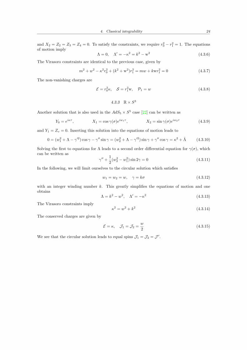
Another solution that is also used in the AdS5 × S5 case [22] can be written as

Y0 = eiκτ , X1 = cos γ(σ)eiw1τ , X2 = sin γ(σ)eiw2τ (4.3.9)

and Y1 = Zv = 0. Inserting this solution into the equations of motion leads to

0 = (w21 + Λ− γ′2) cos γ − γ′′ sin γ = (w2

2 + Λ− γ′2) sin γ + γ′′ cos γ = κ2 + Λ (4.3.10)

Solving the first to equations for Λ leads to a second order differential equation for γ(σ), whichcan be written as

γ′′ +12(w2

2 − w21) sin 2γ = 0 (4.3.11)

In the following, we will limit ourselves to the circular solution which satisfies

w1 = w2 = w, γ = kσ (4.3.12)

with an integer winding number k. This greatly simplifies the equations of motion and oneobtains

Λ = k2 − w2, Λ′ = −κ2 (4.3.13)

The Virasoro constraints implyκ2 = w2 + k2 (4.3.14)

The conserved charges are given by

E = κ, J1 = J2 =w

2(4.3.15)

We see that the circular solution leads to equal spins J1 = J2 = J ′.

5. QUANTUM CORRECTIONS

We have seen that classically the AdS3×S3 string is very similar to the AdS5×S5 string theory,e.g. many classical solutions can be reproduced therein. However, as has been shown in theAdS5×S5 case, the quantum corrections obtain contributions from the full geometry (includingfermions), so that it is clear that the quantum corrections to the same classical solutions willbe different in the two backgrounds. We shall now compute the quantum corrections in AdS3 ×S3 × T 4.

5.1 General method

5.1.1 Bosonic part

We start by expanding the bosonic fields around a classical solution Xp → Xp + Xp, Ys →Ys + Ys, Zv → Zv + Zv and expressing the fluctuation Lagrangian in terms of the fluctuationfields. The resulting Lagrangian is given by

LB = −12gµν

(∂µX

∗p∂νXp + ∂µY

∗s ∂ν Y

s + ∂µZv∂νZv

)+

12

(ΛX∗

p Xp + ΛY ∗s Ys)

(5.1.1)

The fluctuation fields have to be restricted to the embedded AdS3×S3×T 4 space and thus satisfythe constraints that were imposed by including the Lagrange multipliers. These constraints arefound to be

X∗p Xp + X∗

pXp = Y ∗s Ys + Y ∗s Y

s = 0 (5.1.2)

These constraints can be simplified by using a coordinate system that is moving along the classicalsolution. It can be written as(

X1

X2

)=(eiψ 00 eiφ

)(cos γ − sin γsin γ cos γ

)(g1 + if1g2 + if2

)(5.1.3a)(

Y0

Y1

)=(eit 00 eiχ

)(cosh ρ sinh ρsinh ρ cosh ρ

)(G0 + iF0

G1 + iF1

)(5.1.3b)

with fp, gp, Fs, Gs real. The constraints simplify to

g1 = G0 = 0 (5.1.4)

The only remaining fields are f1, f2, g1, F0, F1, G1, zv = Zv. In conformal gauge, the Lagrangiancan be brought in the form

L = xp2 − x′2p +Kpqxpxq +Wpqxpx

′q +Mpqxpxq (5.1.5)

5. Quantum corrections 26

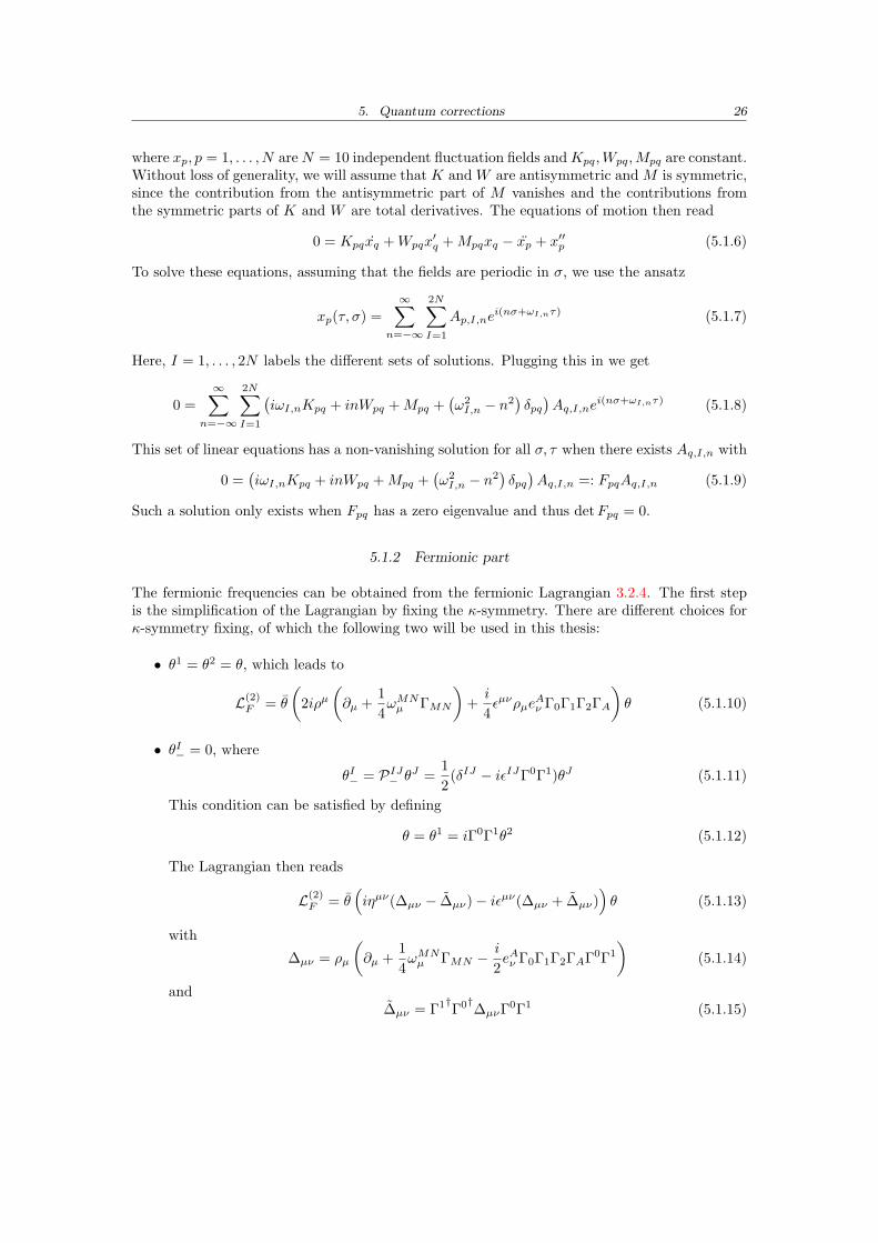
where xp, p = 1, . . . , N areN = 10 independent fluctuation fields andKpq,Wpq,Mpq are constant.Without loss of generality, we will assume that K and W are antisymmetric and M is symmetric,since the contribution from the antisymmetric part of M vanishes and the contributions fromthe symmetric parts of K and W are total derivatives. The equations of motion then read

0 = Kpqxq +Wpqx′q +Mpqxq − xp + x′′p (5.1.6)

To solve these equations, assuming that the fields are periodic in σ, we use the ansatz

xp(τ, σ) =∞∑

n=−∞

2N∑I=1

Ap,I,nei(nσ+ωI,nτ) (5.1.7)

Here, I = 1, . . . , 2N labels the different sets of solutions. Plugging this in we get

0 =∞∑

n=−∞

2N∑I=1

(iωI,nKpq + inWpq +Mpq +

(ω2I,n − n2

)δpq)Aq,I,ne

i(nσ+ωI,nτ) (5.1.8)

This set of linear equations has a non-vanishing solution for all σ, τ when there exists Aq,I,n with

0 =(iωI,nKpq + inWpq +Mpq +

(ω2I,n − n2

)δpq)Aq,I,n =: FpqAq,I,n (5.1.9)

Such a solution only exists when Fpq has a zero eigenvalue and thus detFpq = 0.

5.1.2 Fermionic part

The fermionic frequencies can be obtained from the fermionic Lagrangian 3.2.4. The first stepis the simplification of the Lagrangian by fixing the κ-symmetry. There are different choices forκ-symmetry fixing, of which the following two will be used in this thesis:

• θ1 = θ2 = θ, which leads to

L(2)F = θ

(2iρµ

(∂µ +

14ωMNµ ΓMN

)+i

4εµνρµe

Aν Γ0Γ1Γ2ΓA

)θ (5.1.10)

• θI− = 0, where

θI− = PIJ− θJ =12(δIJ − iεIJΓ0Γ1)θJ (5.1.11)

This condition can be satisfied by defining

θ = θ1 = iΓ0Γ1θ2 (5.1.12)

The Lagrangian then reads

L(2)F = θ

(iηµν(∆µν − ∆µν)− iεµν(∆µν + ∆µν)

)θ (5.1.13)

with

∆µν = ρµ

(∂µ +

14ωMNµ ΓMN −

i

2eAν Γ0Γ1Γ2ΓAΓ0Γ1

)(5.1.14)

and∆µν = Γ1†Γ0†∆µνΓ0Γ1 (5.1.15)

5. Quantum corrections 27

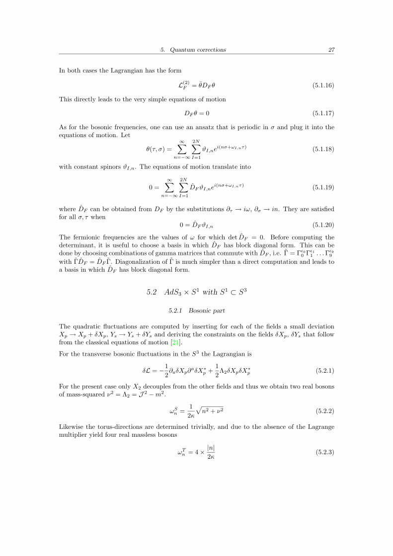
In both cases the Lagrangian has the form

L(2)F = θDF θ (5.1.16)

This directly leads to the very simple equations of motion

DF θ = 0 (5.1.17)

As for the bosonic frequencies, one can use an ansatz that is periodic in σ and plug it into theequations of motion. Let

θ(τ, σ) =∞∑

n=−∞

2N∑I=1

ϑI,nei(nσ+ωI,nτ) (5.1.18)

with constant spinors ϑI,n. The equations of motion translate into

0 =∞∑

n=−∞

2N∑I=1

DFϑI,nei(nσ+ωI,nτ) (5.1.19)

where DF can be obtained from DF by the substitutions ∂τ → iω, ∂σ → in. They are satisfiedfor all σ, τ when

0 = DFϑI,n (5.1.20)

The fermionic frequencies are the values of ω for which det DF = 0. Before computing thedeterminant, it is useful to choose a basis in which DF has block diagonal form. This can bedone by choosing combinations of gamma matrices that commute with DF , i.e. Γ = Γε00 Γε11 . . .Γε99with ΓDF = DF Γ. Diagonalization of Γ is much simpler than a direct computation and leads toa basis in which DF has block diagonal form.

5.2 AdS3 × S1 with S1 ⊂ S3

5.2.1 Bosonic part

The quadratic fluctuations are computed by inserting for each of the fields a small deviationXp → Xp + δXp, Ys → Ys + δYs and deriving the constraints on the fields δXp, δYs that followfrom the classical equations of motion [21].

For the transverse bosonic fluctuations in the S3 the Lagrangian is

δL = −12∂aδXp∂

aδX∗p +

12Λ2δXpδX

∗p (5.2.1)

For the present case only X2 decouples from the other fields and thus we obtain two real bosonsof mass-squared ν2 = Λ2 = J 2 −m2.

ωSn =12κ

√n2 + ν2 (5.2.2)

Likewise the torus-directions are determined trivially, and due to the absence of the Lagrangemultiplier yield four real massless bosons

ωTn = 4× |n|2κ

(5.2.3)

5. Quantum corrections 28

The fluctuations in the internal bosonic directions (i.e., along the AdS3 × S1) can be computedthe same way as in [21] by a method explained in 5.1.1. Starting from the Lagrangian 5.1.1 andsetting

δX1 = eiwτ+imσ(g1 + if1),(δY0

δY1

)=(eiκτ 00 eiwτ+ikσ

)(r0 r1r1 r0

)(G0 + iF0

G1 + iF1

)(5.2.4)

δX1 = eiwτ+imσ(g1 + if1), δY0 = eiκτ (G0 + iF0), δY1 = eiwτ+ikσ(G1 + iF1) (5.2.5)

and solving the constraints 3.3.1 we find the final form for the Lagrangian

δL =12

((w2 −m2)f2

1 − κ2F 20 + (w2 − k2)(F 2

1 +G21)−

r1r0κ2G2

1

)+

12

(f1

2− f ′21 − F0

2+ F ′20 + F1

2 − F ′21 +1r20G1

2 − 1r20G′21

)+ κ

r1r0F0G1 + F1(kG′1 − wG1)−G1

(κr1r0F0 − wF1 + kF ′1

) (5.2.6)

Since κ2 = w2 − k2 and ν2 = w2 −m2, the first line can be written as

12ν2(g2

1 + f21 ) +

12κ2(−F 2

0 −G20 + F 2

1 +G21) ≡ 0 (5.2.7)

After rescaling F0 → iF0, G1 → r0G1 we follow the procedure stated in the appendix. Thebosonic frequencies are the solutions to the equation

0 = (n− ω)2(n+ ω)2(

(ω2 − n2)2 + 4r21κ2ω2 − 4(1 + r21)

(√κ2 + k2ω − kn

)2)

(5.2.8)

The first two factors correspond to massless modes which are canceled by the conformal ghostcontributions.

5.2.2 Fermionic part

We start by computing the vielbein, which can be written as

EMm = diag(cosh ρ, 1, sinh ρ, 1, 1, 0, 1, 1, 1, 1) (5.2.9)

One of the components vanishes due to a metric singularity at γ = 0. The non-vanishingcomponents of the Lorentz connection are (up to symmetry)

ω010 = sinh ρ, ω12

2 = − cosh ρ, ω355 = −1 (5.2.10)

After projecting onto the classical solution, we find for the vielbein

e0τ = κ cosh ρ, e2τ = w sinh τ, e4τ = w, e2σ = k sinh ρ, e4σ = m (5.2.11)

and the Lorentz connection

ω01τ = κ sinh ρ, ω12

τ = −w cosh ρ, ω12σ = −k cosh ρ (5.2.12)

A further computation of the fermionic frequencies has been attempted, but failed due to thelarge complexity of the resulting expression for detDF . An extensive use of computer algebrasystems and simplifications did not solve the problem. More work and further simplifications areneeded, but would exceed the completion time of this thesis.

5. Quantum corrections 29

5.3 AdS3 × S1 with S1 ⊂ T 4

5.3.1 Bosonic part

From the S3 directions, we get 3 free bosons with mass squared ν2 = Λ2 = J 2 −m2,

ωSn =12κ

√n2 + ν2 (5.3.1)

The torus directions also decouple and contribute 4 massless bosons

ωTn = 4× |n|2κ

(5.3.2)

For the internal AdS3 directions we use the same computation as in the previous case. Setting(δY0

δY1

)=(eiκτ 00 eiwτ+ikσ

)(r0 r1r1 r0

)(G0 + iF0

G1 + iF1

)(5.3.3)

and solving the constraints 3.3.1 we find the final form for the Lagrangian

δL =12

(−κ2F 2

0 + (w2 − k2)(F 21 +G2

1)−r1r0κ2G2

1

)+

12

(−F0

2+ F ′20 + F1

2 − F ′21 +1r20G1

2 − 1r20G′21

)+ κ

r1r0F0G1 + F1(kG′1 − wG1)−G1

(κr1r0F0 − wF1 + kF ′1

) (5.3.4)

Similarly to the S1 ⊂ S3 case, the first line can be written as

12κ2(−F 2

0 −G20 + F 2

1 +G21) ≡ 0 (5.3.5)

After rescaling F0 → iF0, G1 → r0G1 we follow the procedure stated at the beginning of thischapter. The bosonic frequencies are the solutions to the equation

0 = (n− ω)(n+ ω)(

(ω2 − n2)2 + 4r21κ2ω2 − 4(1 + r21)

(√κ2 + k2ω − kn

)2)

(5.3.6)

The massless modes originating from the first two factors are again canceled by the conformalghosts.

5.3.2 Fermionic part

We start by computing the vielbein, which can be written as

EMm = diag(cosh ρ, 1, sinh ρ, 1, 1, 0, 1, 1, 1, 1) (5.3.7)

One of the components vanishes due to a metric singularity at γ = 0. The non-vanishingcomponents of the Lorentz connection are (up to symmetry)

ω010 = sinh ρ, ω12

2 = − cosh ρ, ω355 = −1 (5.3.8)

5. Quantum corrections 30

After projecting onto the classical solution, we find for the vielbein

e0τ = κ cosh ρ, e2τ = w sinh τ, e6τ = w, e2σ = k sinh ρ, e6σ = m (5.3.9)

and the Lorentz connection

ω01τ = κ sinh ρ, ω12

τ = −w cosh ρ, ω12σ = −k cosh ρ (5.3.10)

As in the S1 ⊂ §3 case, a computation of the fermionic frequencies has been attempted withoutsuccess. The expression obtained for detDF is slightly simpler than in the previous case, butstill too complex to solve it before this thesis has to be finished.

5.4 R× S3

5.4.1 Bosonic part

Once again, we start from the fluctuation Lagrangian obtained by replacing Xp → Xp + δXp.The torus directions contribute 4 massless bosons

ωTn = 4× |n|2κ

(5.4.1)

Y1 decouples and yields 2 massive bosons with mass squared κ2 = Λ1:

ωSn =12κ

√n2 + κ2 (5.4.2)

For the internal bosonic directions, we set(δX1

δX2

)= eiwτ

(cos kσ − sin kσsin kσ cos kσ

)(g1 + if1g2 + if2

), δY0 = eiκτ (G0 + iF0) (5.4.3)

The constraints implyg1 = G0 = 0 (5.4.4)

Plugging this in, we end up with the Lagrangian

δL =12((w2 − k2)(f2

1 + f22 + g2

2)− κ2F 20

)+

12

(f1

2− f ′21 + f2

2− f ′22 + g2

2 − g′22 − F02

+ F ′20

)+ f2(kf ′1 − wg2)− kf1f ′2 + wg2f2

(5.4.5)

The first line can be written as

12κ2(f2

1 + g21 + f2

2 + g22 − F 2

0 −G20) ≡ 0 (5.4.6)

After rescaling F0 → iF0 we can apply the procedure from 5.1.1 and find the bosonic frequenciesas solutions of the equation

0 = (n− ω)2(n+ ω)2(ω4 − 2(n2 + 2w2)ω2 + n4 − 4k2n2

)(5.4.7)

As in the previous cases, the contributions from the first two factors are canceled by the conformalghost contributions.

5. Quantum corrections 31

5.4.2 Fermionic part

We start by computing the vielbein, which can be written as

EMm = diag(1, 1, 0, 1, cos(kσ), sin(kσ), 1, 1, 1, 1) (5.4.8)

The vanishing component is due to a metric singularity at ρ = 0 (the center of AdS3), but itwill not have any impact on the following computation. The non-vanishing components of theLorentz connection are (up to symmetry)

ω122 = −1, ω34

4 = sin(kσ), ω355 = − cos(kσ) (5.4.9)

After projecting onto the classical solution, we find for the vielbein

e0τ = κ, e4τ = w cos(kσ), e5τ = w sin(kσ), e3σ = k (5.4.10)

and the Lorentz connection

ω34τ = w sin(kσ), ω35

τ = −w cos(kσ) (5.4.11)

The operator DF computed using these coefficients is given by

DF = iκωΓ0 −ikw

2cos(kσ)Γ01234 −

ikw

2sin(kσ)Γ01235 +

wκ

2sin(kσ)Γ034 −

wκ

2cos(kσ)Γ035

+ikκ

2Γ123 − iknΓ3 +

w2

2Γ345 + iwω cos(kσ)Γ4 + iwω sin(kσ)Γ5

(5.4.12)

The σ dependence can be eliminated by performing a rotation in the 45-plane. Replacing

DF → S−1DFS, S = exp(−1

2kσΓ45

)(5.4.13)

we end up with

DF = iκωΓ0 −ikw

2Γ01234 −

wκ

2Γ035 +

ikκ

2Γ123 − iknΓ3 +

w2

2Γ345 + iwωΓ4 (5.4.14)

A possible choice for a maximal subset of mutually commuting combinations of gamma matricesthat commute with DF is given by Γ12,Γ67,Γ89. Since the gamma matrices Γ6,Γ7,Γ8,Γ9 do notcontribute to DF , we can restrict ourselves to a representation of the first 6 gamma matrices.Then the determinant of DF is found to be

detDF =k8

256

(κ4 − 4

(k2 − 6n2 + 2ω2

)κ2 + 4

(k2 − 2n2 + 2ω2

)2)2

(5.4.15)

The fermionic frequencies are the roots of this determinant. We see that

ω = ±12

√−2k2 + 4n2 + κ2 ± 4inκ (5.4.16)

In addition, there are four free fermions from the T 4 component of the superspace. Thus thesum of the fermionic frequencies (weighted with appropriate signs) is given by

ωFn = −4n− 2(√−2k2 + 4n2 + κ2 − 4inκ+

√−2k2 + 4n2 + κ2 + 4inκ

)= −4n− 2

(√J 2 − k2 + 4n

(n− i

√J 2 + k2

)+√J 2 − k2 + 4n

(n+ i

√J 2 + k2

))(5.4.17)

5. Quantum corrections 32

5.4.3 Large 1/J expansion

It is now straight forward to obtain the λ′ expansion of the one-loop energy shift

δE = δE0 + 2∞∑n=1

ωSn + ωTn + ωAdSn + ωFn . (5.4.18)

• Analytic terms O( 1J 2n ) (via zeta-function regularization): first expand in 1

J , and thenzeta-function regularize the sums at each order. See [23].

• Non-analytic terms O( 1J 2n+1 ): integral approximation. See [24, 25, 26].

• Exponential terms e1J [26]

Given the above results for the fluctuation frequencies at one-loop we obtain

δE = δE0 +∞∑n=1

ωbosonicn + ωFn

=∞∑n=1

(2√J 2 + k2 + n2

+√

2J 2 + n2 − 2√J 4 + (J 2 + k2)n2 +

√2J 2 + n2 + 2

√J 4 + (J 2 + k2)n2

− 2√J 2 − k2 + 4n

(n− i

√J 2 + k2

)− 2√J 2 − k2 + 4n

(n+ i

√J 2 + k2

))(5.4.19)

This sum in particular converges as the summand is order O( 1n2 ) for large n.

We wish to evaluate this in the large J expansion, in particular, in order to compare to theAdS5 × S5 case and also possibly to a quantum string Bethe ansatz. We shall present theevaluation by computing the analytic terms via zeta-function regularization.

5.4.4 Analytic Terms

The analytic terms which come in a power series expansion in 1J 2 are obtained by expanding the

summand naively in 1J and then summing at each order in 1

J . We get for the non-zero modes

δE|non−zeromodes =∑n

12

(6k2 − 29n2 + n

√n2 − 4k2

) 1J 2

+∑n

18

(2k4 − 194n2k2 + 765n4 − n3

√n2 − 4k2

) 1J 4

+∑n

116

(6k6 − 474n2k4 + 6403n4k2 − 18429n6 + n3

√n2 − 4k2

(n2 − k2

)) 1J 6

+O

(1J 8

)(5.4.20)

5. Quantum corrections 33

As in the AdS5 × S5 case, the partial sums at each order diverge and we can evaluate themformally by ζ-function evaluation. Let us denote the energies at each order in 1

J p by E(p).

At order 1J 2 the sums have asymptotics −14n2 + 2k2 + O( 1

n2 ). Zeta function regularizationmeans that the following definition of the sums via the Riemann ζ-function are used

ζ(s) =∞∑n=1

1ns

(5.4.21)

Furthermoreζ(−m) = −Bm+1

m+ 1, m ∈ N . (5.4.22)

In particular, ζ(0) = − 12 and for all even m the terms vanish.

Thus by zeta-function regularization at order 1J 2 we need to subtract −14n2 + 2k2 and add

− 12 (2k2). Then

δE(2) =12

(n√n2 − 4k2 − n2

). (5.4.23)

LikewiseδE(4) =

18

(−4k4 − 2n2k2 + n3

(n−

√n2 − 4k2

)), (5.4.24)

andδE(6) =

116

(3k2n4 − n6 + n3

√n2 − 4k2

(n2 − k2

)). (5.4.25)

5.4.5 Discussion

We see that the quantum corrections that have been obtained in our computation have a formwhich is similar to the quantum corrections in the AdS5 × S5 case. [26] The difference in theanalytic terms reflects the fact that the quantum corrections are influenced not only by theclassical string trajectory, but receive contributions from the whole supergeometry of the stringbackground. More work is required to compute the non-analytic and exponential terms.

6. CONCLUSION

In this work we have shown that the AdS3 × S3 × T 4 superstring with RR flux is a classicallyintegrable model. We have shown that an infinite set of conserved charges exists and computedthe conserved charges in different bases of the symmetry superalgebra.

We have furthermore constructed several spinning string solutions and computed their energies atthe classical level and quantum corrections at one-loop order. We have seen that the divergentterms in the bosonic and fermionic contributions to the quantum corrections cancel, as onewould expect from a supersymmetric model. We have then computed the analytic terms of the1J expansion. From this derivation we have seen that the results are have a similar structure asthose obtained for spinning strings in AdS5 × S5.

During this work, an extensive use of Mathematica has shown to be useful. Two Mathematicapackages have been developed for algebraic simplifications and applied to the computations donein this work. The Grassmann package helps in dealing with Grassmann algebras and in con-structing representations of superalgebras. The Clifford package performs various simplificationsin Clifford algebras and utilizes a simple, but fast algorithm to compute products and inversesof Clifford algebra elements.

There are various possibilities for further studies:

• As in the AdS5×S5 case, the spectrum may be computed using a string Bethe ansatz andcompared to the result obtained by explicit one-loop calculations. [23, 27] This gives us thepossibility to test whether the Bethe ansatz is valid for the computation of string spectraand may give some hints on how the different backgrounds influence the structure of thequantum corrections.

• The origin of analytic, non-analytic and exponential terms in the 1J expansion may be

analyzed in more detail. [26]

• The effects of zeta-function regularization on the evaluation of quantum corrections tospinning strings may be discussed as it has been done in the case of AdS5 × S5. [25]

• Exact expressions for the quantum corrections may be computed as in [26].

• The AdS3 × S1 solutions may be examined in more detail, as it has already be done forthe R× S3 solution.

APPENDIX

A. CONVENTIONS AND NOTATION

A.1 Coordinate indices

We use the following convention for the indices:

a, b, . . . = 1, 2, 3 AdS3 tangent space indicesa′, b′, . . . = 1′, 2′, 3′ S3 tangent space indicesa, b, . . . = 1, 2, 3, 4 T 4 tangent space indices

a, b, . . . = 1, 2, 3, 1′, 2′, 3′ AdS3 × S3 tangent space indicesA,A′, A, A same as above for labeling vielbeins

m,n, . . . = 1, 2, 3, 1′, 2′, 3′, 1, 2, 3, 4 AdS3 × S3 × T 4 tangent space indicesM,N, . . . AdS3 × S3 × T 4 vielbein indices

P,Q, . . . = 0, 1, 2, 3 R1,3 ⊃ AdS3 coordinate indicesp, q, . . . = 0, 1 R1,3 ⊃ AdS3 coordinate indices (complexified)

S, T, . . . = 1, 2, 3, 4 R4 ⊃ S3 coordinate indicess, t, . . . = 1, 2 R4 ⊃ S3 coordinate indices (complexified)

v, w, . . . = 1, 2, 3, 4 T 4 coordinate indicesi, j, . . . = 0, 1, 2, 3 SO(2, 2) vector indices

i′, j′, . . . = 0′, 1′, 2′, 3′ SO(4) vector indicesI, J, . . . = 1, 2 labels the two sets of spinorsµ, ν, . . . = τ, σ world sheet coordinates

A.2 Convention for gamma matrices

The gamma matrices of the 6-dimensional Clifford algebra used in this thesis can be written as

γ0 = iσ3 ⊗ 12 ⊗ σ1 γ1 = σ1 ⊗ 12 ⊗ σ1 γ2 = σ2 ⊗ 12 ⊗ σ1 (A.2.1a)

γ3 = 12 ⊗ σ1 ⊗ σ2 γ4 = 12 ⊗ σ2 ⊗ σ2 γ5 = 12 ⊗ σ3 ⊗ σ2 (A.2.1b)

From these, the 10-dimensional gamma matrices are obtained by defining ΓA = γA ⊗ 14, ΓA′=

γA′ ⊗ 14 and

Γ6 = 14 × σ3 ×(12 00 −12

)Γ7 = 14 × σ3 ×

(0 iσ1

−iσ1 0

)(A.2.2)

Γ8 = 14 × σ3 ×(

0 iσ2

−iσ2 0

)Γ9 = 14 × σ3 ×

(0 iσ3

−iσ3 0

)(A.2.3)

B. BASES OF PSU(1, 1|2)× PSU(1, 1|2)

B.1 The canonical basis

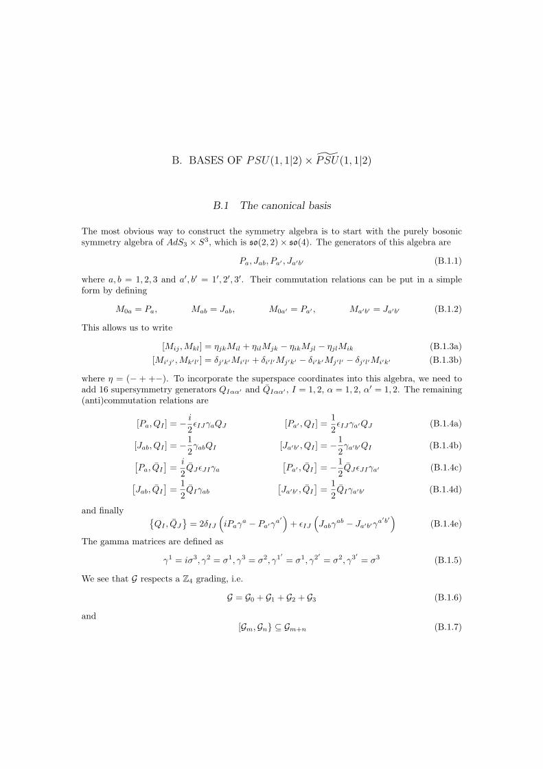
The most obvious way to construct the symmetry algebra is to start with the purely bosonicsymmetry algebra of AdS3 × S3, which is so(2, 2)× so(4). The generators of this algebra are

Pa, Jab, Pa′ , Ja′b′ (B.1.1)

where a, b = 1, 2, 3 and a′, b′ = 1′, 2′, 3′. Their commutation relations can be put in a simpleform by defining

M0a = Pa, Mab = Jab, M0a′ = Pa′ , Ma′b′ = Ja′b′ (B.1.2)

This allows us to write

[Mij ,Mkl] = ηjkMil + ηilMjk − ηikMjl − ηjlMik (B.1.3a)[Mi′j′ ,Mk′l′ ] = δj′k′Mi′l′ + δi′l′Mj′k′ − δi′k′Mj′l′ − δj′l′Mi′k′ (B.1.3b)

where η = (− + +−). To incorporate the superspace coordinates into this algebra, we need toadd 16 supersymmetry generators QIαα′ and QIαα′ , I = 1, 2, α = 1, 2, α′ = 1, 2. The remaining(anti)commutation relations are

[Pa, QI ] = − i2εIJγaQJ [Pa′ , QI ] =

12εIJγa′QJ (B.1.4a)

[Jab, QI ] = −12γabQI [Ja′b′ , QI ] = −1

2γa′b′QI (B.1.4b)[

Pa, QI]

=i

2QJεJIγa

[Pa′ , QI

]= −1

2QJεJIγa′ (B.1.4c)[

Jab, QI]

=12QIγab

[Ja′b′ , QI

]=

12QIγa′b′ (B.1.4d)

and finally {QI , QJ

}= 2δIJ

(iPaγ

a − Pa′γa′)

+ εIJ

(Jabγ

ab − Ja′b′γa′b′)

(B.1.4e)

The gamma matrices are defined as

γ1 = iσ3, γ2 = σ1, γ3 = σ2, γ1′ = σ1, γ2′ = σ2, γ3′ = σ3 (B.1.5)

We see that G respects a Z4 grading, i.e.

G = G0 + G1 + G2 + G3 (B.1.6)

and[Gm,Gn} ⊆ Gm+n (B.1.7)

B. Bases of psu(1, 1|2) × psu(1, 1|2) 38

for m,n ∈ Z4. Here [., .} denotes the anticommutator between two fermionic operators and thecommutator otherwise. We find that

Ja′b′ , Jab ∈ G0, Q1αα′ , Q1αα′ ∈ G1, Pa, Pa′ ∈ G2, Q2αα′ , Q2αα′ ∈ G3 (B.1.8)

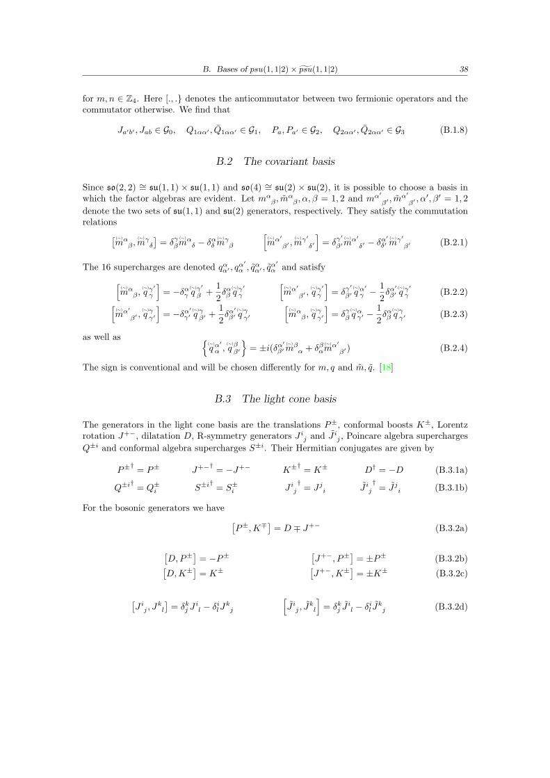
B.2 The covariant basis

Since so(2, 2) ∼= su(1, 1) × su(1, 1) and so(4) ∼= su(2) × su(2), it is possible to choose a basis inwhich the factor algebras are evident. Let mα

β , mαβ , α, β = 1, 2 and mα′

β′, mα′

β′, α′, β′ = 1, 2

denote the two sets of su(1, 1) and su(2) generators, respectively. They satisfy the commutationrelations[ (∼)

mαβ ,

(∼)

mγδ

]= δγβ

(∼)

mαδ − δαδ

(∼)

mγβ

[(∼)

mα′

β′ ,(∼)

mγ′

δ′

]= δγ

′

β′(∼)

mα′

δ′ − δα′

δ′(∼)

mγ′

β′ (B.2.1)

The 16 supercharges are denoted qαα′ , qα′

α , qαα′ , q

α′

α and satisfy[(∼)

mαβ ,

(∼)

q γ′

γ

]= −δαγ

(∼)

q γ′

β +12δαβ

(∼)

q γ′

γ

[(∼)

mα′

β′ ,(∼)

q γ′

γ

]= δγ

′

β′(∼)

q α′

γ −12δα

′

β′(∼)

q γ′

γ (B.2.2)[(∼)

mα′

β′ ,(∼)

q γγ′]

= −δα′

γ′(∼)

q γβ′ +12δα

′

β′(∼)

q γγ′[

(∼)

mαβ ,

(∼)

q γγ′]

= δγβ(∼)

q αγ′ −12δαβ

(∼)

q γγ′ (B.2.3)

as well as {(∼)

q α′

α ,(∼)

q ββ′}

= ±i(δα′

β′(∼)

mβα + δβα

(∼)

mα′

β′) (B.2.4)

The sign is conventional and will be chosen differently for m, q and m, q. [18]

B.3 The light cone basis

The generators in the light cone basis are the translations P±, conformal boosts K±, Lorentzrotation J+−, dilatation D, R-symmetry generators J ij and J ij , Poincare algebra superchargesQ±i and conformal algebra supercharges S±i. Their Hermitian conjugates are given by

P±† = P± J+−† = −J+− K±† = K± D† = −D (B.3.1a)

Q±i†

= Q±i S±i†

= S±i J ij†

= Jji J ij†

= Jji (B.3.1b)

For the bosonic generators we have [P±,K∓] = D ∓ J+− (B.3.2a)

[D,P±

]= −P±

[J+−, P±

]= ±P± (B.3.2b)[

D,K±] = K± [J+−,K±] = ±K± (B.3.2c)

[J ij , J

kl

]= δkj J

il − δilJkj

[J ij , J

kl

]= δkj J

il − δil Jkj (B.3.2d)

B. Bases of psu(1, 1|2) × psu(1, 1|2) 39

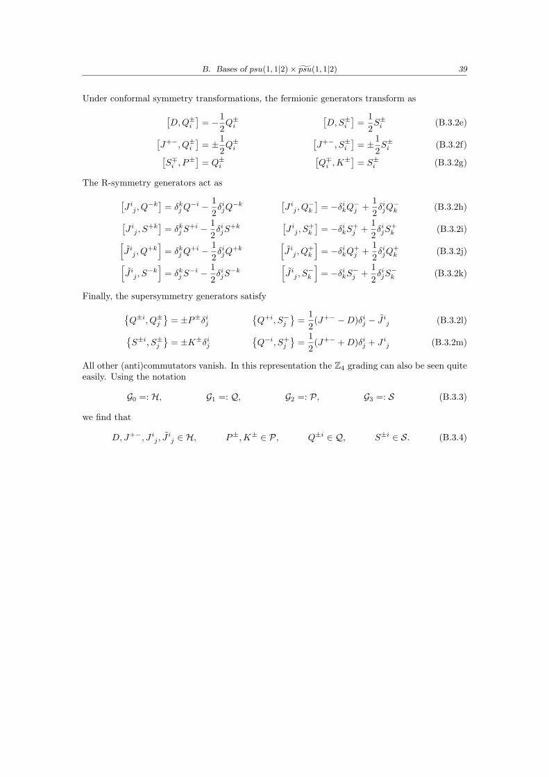
Under conformal symmetry transformations, the fermionic generators transform as[D,Q±i

]= −1

2Q±i

[D,S±i

]=

12S±i (B.3.2e)[

J+−, Q±i]

= ±12Q±i

[J+−, S±i

]= ±1

2S±i (B.3.2f)[

S∓i , P±] = Q±i

[Q∓i ,K

±] = S±i (B.3.2g)

The R-symmetry generators act as[J ij , Q

−k] = δkjQ−i − 1

2δijQ

−k [J ij , Q

−k

]= −δikQ−j +

12δijQ

−k (B.3.2h)[

J ij , S+k]

= δkj S+i − 1

2δijS

+k[J ij , S

+k

]= −δikS+

j +12δijS

+k (B.3.2i)[

J ij , Q+k]

= δkjQ+i − 1

2δijQ

+k[J ij , Q

+k

]= −δikQ+

j +12δijQ

+k (B.3.2j)[

J ij , S−k]

= δkj S−i − 1

2δijS

−k[J ij , S

−k

]= −δikS−j +

12δijS

−k (B.3.2k)

Finally, the supersymmetry generators satisfy{Q±i, Q±j

}= ±P±δij

{Q+i, S−j

}=

12(J+− −D)δij − J ij (B.3.2l){

S±i, S±j}

= ±K±δij{Q−i, S+

j

}=

12(J+− +D)δij + J ij (B.3.2m)

All other (anti)commutators vanish. In this representation the Z4 grading can also be seen quiteeasily. Using the notation

G0 =: H, G1 =: Q, G2 =: P, G3 =: S (B.3.3)

we find that

D,J+−, J ij , Jij ∈ H, P±,K± ∈ P, Q±i ∈ Q, S±i ∈ S. (B.3.4)

C. CONSTRUCTION OF INVARIANT CHARGES

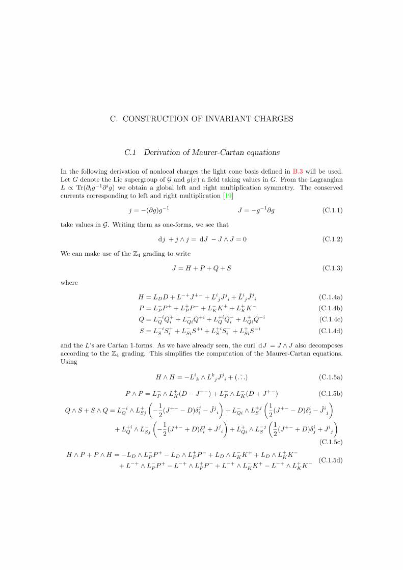
C.1 Derivation of Maurer-Cartan equations

In the following derivation of nonlocal charges the light cone basis defined in B.3 will be used.Let G denote the Lie supergroup of G and g(x) a field taking values in G. From the LagrangianL ∝ Tr(∂ig−1∂ig) we obtain a global left and right multiplication symmetry. The conservedcurrents corresponding to left and right multiplication [19]

j = −(∂g)g−1 J = −g−1∂g (C.1.1)

take values in G. Writing them as one-forms, we see that

dj + j ∧ j = dJ − J ∧ J = 0 (C.1.2)

We can make use of the Z4 grading to write

J = H + P +Q+ S (C.1.3)

where

H = LDD + L−+J+− + LijJji + Lij J

ji (C.1.4a)

P = L−PP+ + L+

PP− + L−KK

+ + L+KK

− (C.1.4b)

Q = L−iQ Q+i + L−QiQ

+i + L+iQ Q−i + L+

QiQ−i (C.1.4c)

S = L−iS S+i + L−SiS

+i + L+iS S−i + L+

SiS−i (C.1.4d)

and the L’s are Cartan 1-forms. As we have already seen, the curl dJ = J ∧ J also decomposesaccording to the Z4 grading. This simplifies the computation of the Maurer-Cartan equations.Using

H ∧H = −Lik ∧ LkjJji + ( ˜. . .) (C.1.5a)

P ∧ P = L−P ∧ L+K(D − J+−) + L+

P ∧ L−K(D + J+−) (C.1.5b)

Q ∧ S + S ∧Q = L−iQ ∧ L+Sj

(−1

2(J+− −D)δji − J

ji

)+ L−Qi ∧ L

+jS

(12(J+− −D)δij − J ij

)+ L+i

Q ∧ L−Sj

(−1

2(J+− +D)δji + Jji

)+ L+

Qi ∧ L−jS

(12(J+− +D)δij + J ij

)(C.1.5c)

H ∧ P + P ∧H = −LD ∧ L−PP+ − LD ∧ L+

PP− + LD ∧ L−KK

+ + LD ∧ L+KK

−

+ L−+ ∧ L−PP+ − L−+ ∧ L+

PP− + L−+ ∧ L−KK

+ − L−+ ∧ L+KK

− (C.1.5d)

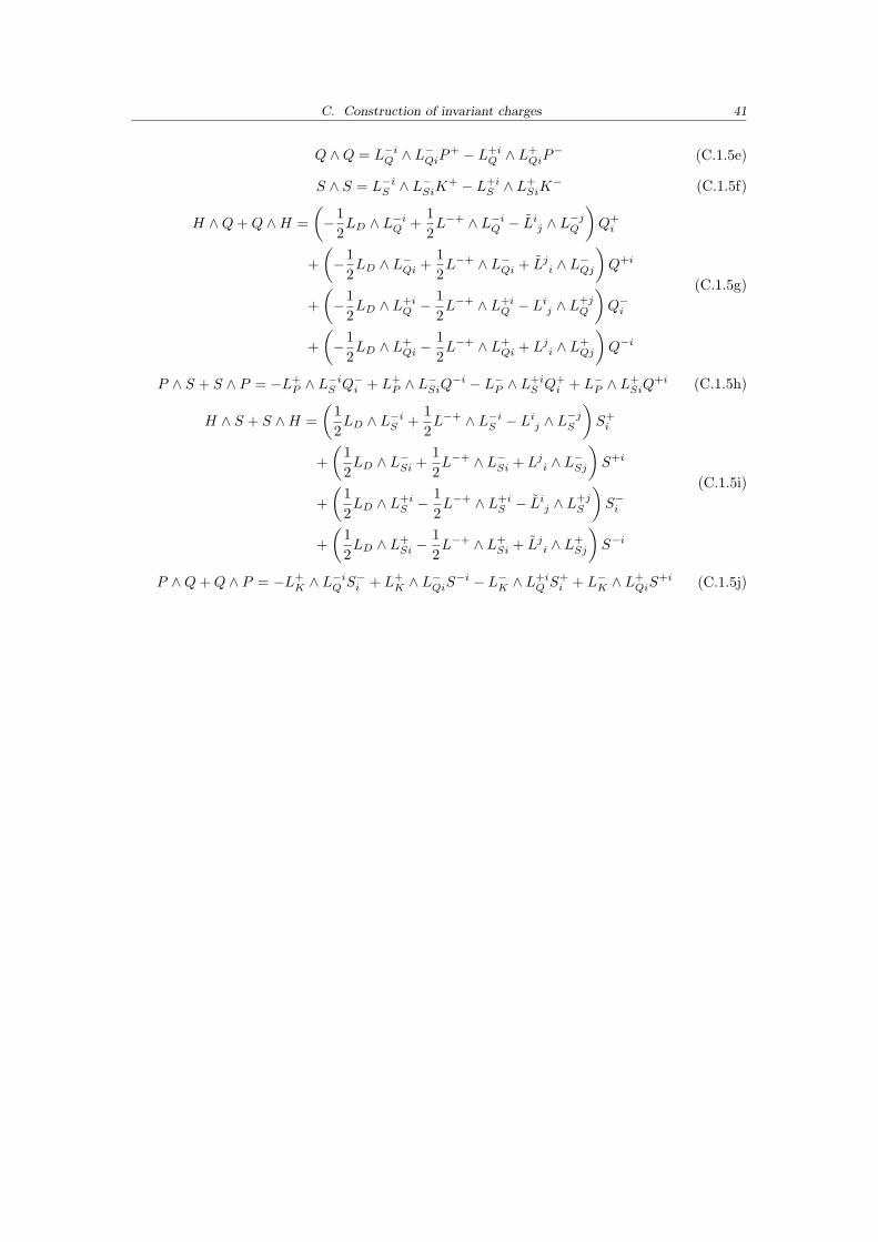
C. Construction of invariant charges 41

Q ∧Q = L−iQ ∧ L−QiP

+ − L+iQ ∧ L

+QiP

− (C.1.5e)

S ∧ S = L−iS ∧ L−SiK

+ − L+iS ∧ L

+SiK

− (C.1.5f)

H ∧Q+Q ∧H =(−1

2LD ∧ L−iQ +

12L−+ ∧ L−iQ − L

ij ∧ L

−jQ

)Q+i

+(−1

2LD ∧ L−Qi +

12L−+ ∧ L−Qi + Lji ∧ L−Qj

)Q+i

+(−1

2LD ∧ L+i

Q −12L−+ ∧ L+i

Q − Lij ∧ L

+jQ

)Q−i

+(−1

2LD ∧ L+

Qi −12L−+ ∧ L+

Qi + Lji ∧ L+Qj

)Q−i

(C.1.5g)

P ∧ S + S ∧ P = −L+P ∧ L

−iS Q−i + L+

P ∧ L−SiQ

−i − L−P ∧ L+iS Q+

i + L−P ∧ L+SiQ

+i (C.1.5h)

H ∧ S + S ∧H =(

12LD ∧ L−iS +

12L−+ ∧ L−iS − L

ij ∧ L

−jS

)S+i

+(

12LD ∧ L−Si +

12L−+ ∧ L−Si + Lji ∧ L−Sj

)S+i

+(

12LD ∧ L+i

S −12L−+ ∧ L+i

S − Lij ∧ L

+jS

)S−i

+(

12LD ∧ L+

Si −12L−+ ∧ L+

Si + Lji ∧ L+Sj

)S−i

(C.1.5i)

P ∧Q+Q ∧ P = −L+K ∧ L

−iQ S−i + L+

K ∧ L−QiS

−i − L−K ∧ L+iQ S+

i + L−K ∧ L+QiS

+i (C.1.5j)

C. Construction of invariant charges 42

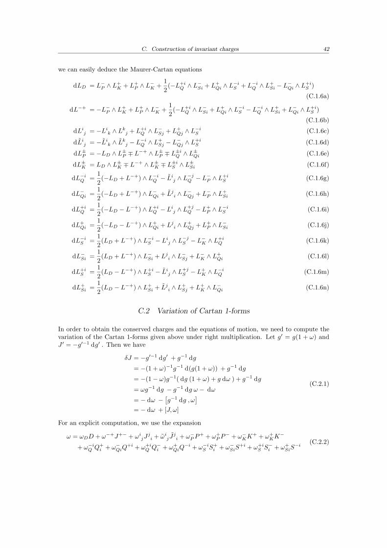
we can easily deduce the Maurer-Cartan equations

dLD = L−P ∧ L+K + L+

P ∧ L−K +

12(−L+i

Q ∧ L−Si + L+

Qi ∧ L−iS + L−iQ ∧ L

+Si − L

−Qi ∧ L

+iS )

(C.1.6a)

dL−+ = −L−P ∧ L+K + L+

P ∧ L−K +

12(−L+i

Q ∧ L−Si + L+

Qi ∧ L−iS − L

−iQ ∧ L

+Si + L−Qi ∧ L

+iS )

(C.1.6b)

dLij = −Lik ∧ Lkj + L+iQ ∧ L

−Sj + L+

Qj ∧ L−iS (C.1.6c)

dLij = −Lik ∧ Lkj − L−iQ ∧ L+Sj − L

−Qj ∧ L

+iS (C.1.6d)

dL±P = −LD ∧ L±P ∓ L−+ ∧ L±P ∓ L

±iQ ∧ L

±Qi (C.1.6e)

dL±K = LD ∧ L±K ∓ L−+ ∧ L±K ∓ L

±iS ∧ L

±Si (C.1.6f)

dL−iQ =12(−LD + L−+) ∧ L−iQ − L

ij ∧ L

−jQ − L

−P ∧ L

+iS (C.1.6g)

dL−Qi =12(−LD + L−+) ∧ L−Qi + Lji ∧ L−Qj + L−P ∧ L

+Si (C.1.6h)

dL+iQ =

12(−LD − L−+) ∧ L+i

Q − Lij ∧ L

+jQ − L

+P ∧ L

−iS (C.1.6i)

dL+Qi =

12(−LD − L−+) ∧ L+

Qi + Lji ∧ L+Qj + L+

P ∧ L−Si (C.1.6j)

dL−iS =12(LD + L−+) ∧ L−iS − L

ij ∧ L

−jS − L

−K ∧ L

+iQ (C.1.6k)

dL−Si =12(LD + L−+) ∧ L−Si + Lji ∧ L−Sj + L−K ∧ L

+Qi (C.1.6l)

dL+iS =

12(LD − L−+) ∧ L+i

S − Lij ∧ L

+jS − L

+K ∧ L

−iQ (C.1.6m)

dL+Si =

12(LD − L−+) ∧ L+

Si + Lji ∧ L+Sj + L+

K ∧ L−Qi (C.1.6n)

C.2 Variation of Cartan 1-forms

In order to obtain the conserved charges and the equations of motion, we need to compute thevariation of the Cartan 1-forms given above under right multiplication. Let g′ = g(1 + ω) andJ ′ = −g′−1 dg′ . Then we have

δJ = −g′−1 dg′ + g−1 dg

= −(1 + ω)−1g−1 d(g(1 + ω)) + g−1 dg

= −(1− ω)g−1( dg (1 + ω) + g dω ) + g−1 dg

= ωg−1 dg − g−1 dg ω − dω

= − dω −[g−1 dg , ω

]= − dω + [J, ω]

(C.2.1)

For an explicit computation, we use the expansion

ω = ωDD + ω−+J+− + ωijJji + ωij J

ji + ω−P P

+ + ω+PP

− + ω−KK+ + ω+

KK−

+ ω−iQ Q+i + ω−QiQ

+i + ω+iQ Q−i + ω+

QiQ−i + ω−iS S+

i + ω−SiS+i + ω+i

S S−i + ω+SiS

−i (C.2.2)

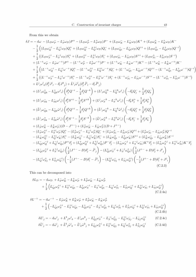
C. Construction of invariant charges 43

From this we obtain

δJ = − dω − (LDω−P − L−PωD)P+ − (LDω+

P − L+PωD)P− + (LDω−K − L

−KωD)K+ + (LDω+

K − L+KωD)K−

− 12

((LDω−iQ − L

−iQ ωD)Q+

i + (LDω+iQ − L

+iQ ωD)Q−i + (LDω−Qi − L

−QiωD)Q+i + (LDω+

Qi − L+QiωD)Q−i

)+

12((LDω−iS − L

−iS ωD)S+

i + (LDω+iS − L

+iS ωD)S−i + (LDω−Si − L

−SiωD)S+i + (LDω+

Si − L+SiωD)S−i

)+ (L−+ω−P − L

−Pω

−+)P+ − (L−+ω+P − L

+Pω

−+)P− + (L−+ω−K − L−Kω

−+)K+ − (L−+ω+K − L

+Kω

−+)K−

+12

((L−+ω−iQ − L

−iQ ω−+)Q+

i − (L−+ω+iQ − L

+iQ ω−+)Q−i + (L−+ω−Qi − L

−Qiω

−+)Q+i − (L−+ω+Qi − L

+Qiω

−+)Q−i)

+12((L−+ω−iS − L

−iS ω−+)S+

i − (L−+ω+iS − L

+iS ω−+)S−i + (L−+ω−Si − L

−Siω

−+)S+i − (L−+ω+Si − L

+Siω

−+)S−i)

+ Ljiωlk(δ

kj J

il − δilJkj) + Ljiω

lk(δ

kj J

il − δil Jkj)

+ (Ljiω+Qk − L

+Qkω

ji)(δkjQ

−i − 12δijQ

−k)

+ (Ljiω+kQ − L

+kQ ωji)

(−δikQ−j +

12δijQ

−k

)+ (Ljiω

−Sk − L

−Skω

ji)(δkj S

+i − 12δijS

+k

)+ (Ljiω

−kS − L

−kS ωji)

(−δikS+

j +12δijS

+k

)+ (Ljiω

−Qk − L

−Qkω

ji)(δkjQ

+i − 12δijQ

+k

)+ (Ljiω

−kQ − L

−kQ ωji)

(−δikQ+

j +12δijQ

+k

)+ (Ljiω

+Sk − L

+Skω

ji)(δkj S

−i − 12δijS

−k)

+ (Ljiω+kS − L

+kS ωji)

(−δikS−j +

12δijS

−k

)+ (L−Pω

+K − L

+Kω

−P )(D − J+−) + (L+

Pω−K − L

−Kω

+P )(D + J+−)

− (L−Pω+iS − L

+iS ω−P )Q+

i − (L+Pω

−iS − L

−iS ω+

P )Q−i + (L−Pω+Si − L

+Siω

−P )Q+i + (L+

Pω−Si − L

−Siω

+P )Q−i

− (L−Kω+iQ − L

+iQ ω−K)S+

i − (L+Kω

−iQ − L

−iQ ω+

K)S−i + (L−Kω+Qi − L

+Qiω

−K)S+i + (L+

Kω−Qi − L

−Qiω

+K)S−i

− (L−Qiω−jQ + L−jQ ω−Qi)P

+δij + (L+Qiω

+jQ + L+j

Q ω+Qi)P

−δij − (L−Siω−jS + L−jS ω−Si)K

+δij + (L+Siω

+jS + L+j

S ω+Si)K

−δij

− (L−Qiω+jS + L+j

S ω−Qi)(

12(J+− −D)δij − J ij

)− (L+

Qiω−jS + L−jS ω+

Qi)(

12(J+− +D)δij + J ij

)− (L−iQ ω+

Sj + L+Sjω

−iQ )(−1

2(J+− −D)δji − J

ji

)− (L+i

Q ω−Sj + L−Sjω+iQ )(−1

2(J+− +D)δji + Jji

)(C.2.3)

This can be decomposed into

δLD = − dωD + L−Pω+K − L

+Kω

−P + L+

Pω−K − L

−Kω

+P

+12

(L−Qiω

+iS + L+i

S ω−Qi − L+Qiω

−iS − L

−iS ω+

Qi − L−iQ ω+

Si − L+Siω

−iQ + L+i

Q ω−Si + L−Siω+iQ

)(C.2.4a)

δL−+ = − dω−+ − L−Pω+K + L+

Kω−P + L+

Pω−K − L

−Kω

+P

+12

(−L−Qiω

+iS − L

+iS ω−Qi − L

+Qiω

−iS − L

−iS ω+

Qi + L−iQ ω+Si + L+

Siω−iQ + L+i

Q ω−Si + L−Siω+iQ

)(C.2.4b)

δLij = − dωij + Lkjωik − Likωkj − L+

Qjω−iS − L

−iS ω+

Qj − L+iQ ω−Sj − L

−Sjω

+iQ (C.2.4c)

δLij = − dωij + Lkjωik − Likωkj + L−Qjω

+iS + L+i

S ω−Qj + L−iQ ω+Sj + L+

Sjω−iQ (C.2.4d)

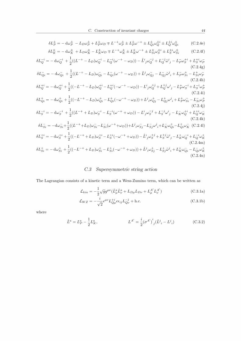
C. Construction of invariant charges 44

δL±P = − dω±P − LDω±P + L±PωD ∓ L

−+ω±P ± L±Pω

−+ ± L±Qiω±iQ ± L

±iQ ω±Qi (C.2.4e)

δL±K = − dω±K + LDω±K − L

±KωD ∓ L

−+ω±K ± L±Kω

−+ ± L±Siω±iS ± L

±iS ω±Si (C.2.4f)

δL−iQ = − dω−iQ +12((L−+ − LD)ω−iQ − L

−iQ (ω−+ − ωD))− Lijω

−jQ + L−jQ ωij − L−Pω

+iS + L+i

S ω−P(C.2.4g)

δL−Qi = − dω−Qi +12((L−+ − LD)ω−Qi − L

−Qi(ω

−+ − ωD)) + Ljiω−Qj − L

−Qjω

ji + L−Pω

+Si − L

+Siω

−P

(C.2.4h)

δL+iQ = −dω+i

Q +12((−L−+−LD)ω+i

Q −L+iQ (−ω−+−ωD))−Lijω

+jQ +L+j

Q ωij−L+Pω

−iS +L−iS ω+

P

(C.2.4i)

δL+Qi = −dω+

Qi +12((−L−+−LD)ω+

Qi−L+Qi(−ω

−+−ωD))+Ljiω+Qj −L

+Qjω

ji+L+

Pω−Si−L

−Siω

+P

(C.2.4j)

δL−iS = − dω−iS +12((L−+ + LD)ω−iS − L

−iS (ω−+ + ωD))− Lijω

−jS + L−jS ωij − L−Kω

+iQ + L+i

Q ω−K(C.2.4k)

δL−Si = −dω−Si+12((L−++LD)ω−Si−L

−Si(ω

−++ωD))+Ljiω−Sj−L

−Sjω

ji+L

−Kω

+Qi−L

+Qiω

−K (C.2.4l)

δL+iS = −dω+i

S +12((−L−+ +LD)ω+i

S −L+iS (−ω−+ +ωD))− Lijω

+jS +L+j

S ωij−L+Kω

−iQ +L−iQ ω+

K

(C.2.4m)

δL+Si = − dω+

Si +12((−L−+ +LD)ω+

Si−L+Si(−ω

−+ +ωD)) + Ljiω+Sj −L

+Sjω

ji +L+

Kω−Qi−L

−Qiω

+K

(C.2.4n)

C.3 Supersymmetric string action

The Lagrangian consists of a kinetic term and a Wess-Zumino term, which can be written as

Lkin = −12√ggµν(LaµL

aν + LDµLDν + LA

′

µ LA′

ν ) (C.3.1a)

LWZ = − i√2εµνL+i

QµcεijL−jQν + h.c. (C.3.1b)

where

La = LaP −12LaK , LA

′=i

2(σA

′)i

j(Lji − Lji) (C.3.2)

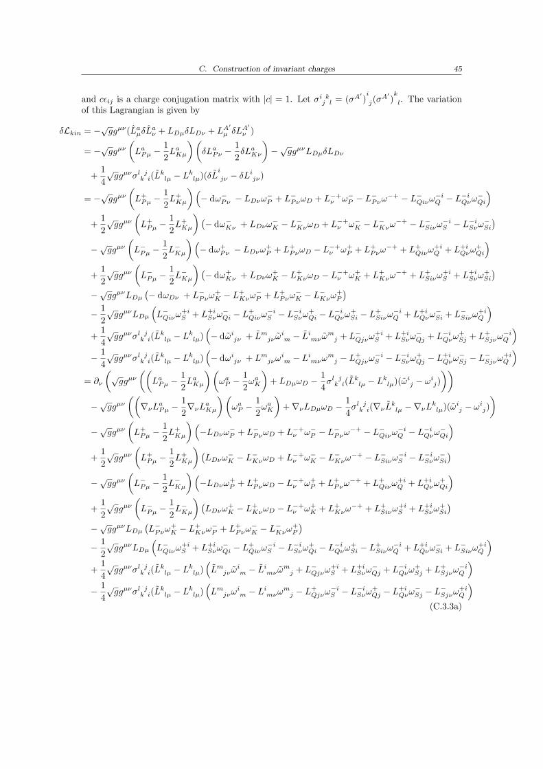
C. Construction of invariant charges 45

and cεij is a charge conjugation matrix with |c| = 1. Let σi kj l = (σA′)i

j(σA′)

k

l. The variationof this Lagrangian is given by

δLkin = −√ggµν(LaµδLaν + LDµδLDν + LA′

µ δLA′

ν )

= −√ggµν(LaPµ −

12LaKµ

)(δLaPν −

12δLaKν

)−√ggµνLDµδLDν

+14√ggµνσl jk i(L

klµ − Lklµ)(δL

i

jν − δLijν)

= −√ggµν(L+Pµ −

12L+Kµ

)(− dω−Pν − LDνω

−P + L−PνωD + L−+

ν ω−P − L−Pνω

−+ − L−Qiνω−iQ − L

−iQνω

−Qi

)+

12√ggµν

(L+Pµ −

12L+Kµ

)(− dω−Kν + LDνω

−K − L

−KνωD + L−+

ν ω−K − L−Kνω

−+ − L−Siνω−iS − L

−iSνω

−Si

)−√ggµν

(L−Pµ −

12L−Kµ

)(− dω+

Pν − LDνω+P + L+

PνωD − L−+ν ω+

P + L+Pνω

−+ + L+Qiνω

+iQ + L+i

Qνω+Qi

)+

12√ggµν

(L−Pµ −

12L−Kµ

)(− dω+

Kν + LDνω+K − L

+KνωD − L

−+ν ω+

K + L+Kνω

−+ + L+Siνω

+iS + L+i

Sνω+Si

)−√ggµνLDµ

(− dωDν + L−Pνω

+K − L

+Kνω

−P + L+

Pνω−K − L

−Kνω

+P

)− 1

2√ggµνLDµ

(L−Qiνω

+iS + L+i

Sνω−Qi − L

+Qiνω

−iS − L

−iSνω

+Qi − L

−iQνω

+Si − L

+Siνω

−iQ + L+i

Qνω−Si + L−Siνω

+iQ

)+

14√ggµνσl jk i(L

klµ − Lklµ)

(− dωijν + Lmjν ω

im − Limν ωmj + L−Qjνω

+iS + L+i

Sνω−Qj + L−iQνω

+Sj + L+

Sjνω−iQ

)− 1

4√ggµνσl jk i(L

klµ − Lklµ)

(− dωijν + Lmjνω

im − Limνωmj − L+

Qjνω−iS − L

−iSνω

+Qj − L

+iQνω

−Sj − L

−Sjνω

+iQ

)= ∂ν

(√ggµν

((LaPµ −

12LaKµ

)(ωaP −

12ωaK

)+ LDµωD −

14σl jk i(L

klµ − Lklµ)(ωij − ωij)

))−√ggµν

((∇νLaPµ −

12∇νLaKµ

)(ωaP −

12ωaK

)+∇νLDµωD −

14σl jk i(∇νLklµ −∇νLklµ)(ωij − ωij)

)−√ggµν

(L+Pµ −

12L+Kµ

)(−LDνω−P + L−PνωD + L−+

ν ω−P − L−Pνω

−+ − L−Qiνω−iQ − L

−iQνω

−Qi

)+

12√ggµν

(L+Pµ −

12L+Kµ

)(LDνω

−K − L

−KνωD + L−+

ν ω−K − L−Kνω

−+ − L−Siνω−iS − L

−iSνω

−Si

)−√ggµν

(L−Pµ −

12L−Kµ

)(−LDνω+

P + L+PνωD − L

−+ν ω+

P + L+Pνω

−+ + L+Qiνω

+iQ + L+i

Qνω+Qi

)+

12√ggµν

(L−Pµ −

12L−Kµ

)(LDνω

+K − L

+KνωD − L

−+ν ω+

K + L+Kνω

−+ + L+Siνω

+iS + L+i

Sνω+Si

)−√ggµνLDµ

(L−Pνω

+K − L

+Kνω

−P + L+

Pνω−K − L

−Kνω

+P

)− 1

2√ggµνLDµ

(L−Qiνω

+iS + L+i

Sνω−Qi − L

+Qiνω

−iS − L

−iSνω

+Qi − L

−iQνω

+Si − L

+Siνω

−iQ + L+i

Qνω−Si + L−Siνω

+iQ

)+

14√ggµνσl jk i(L

klµ − Lklµ)

(Lmjν ω

im − Limν ωmj + L−Qjνω

+iS + L+i

Sνω−Qj + L−iQνω

+Sj + L+

Sjνω−iQ

)− 1

4√ggµνσl jk i(L

klµ − Lklµ)

(Lmjνω

im − Limνωmj − L+

Qjνω−iS − L

−iSνω

+Qj − L

+iQνω

−Sj − L

−Sjνω

+iQ

)(C.3.3a)

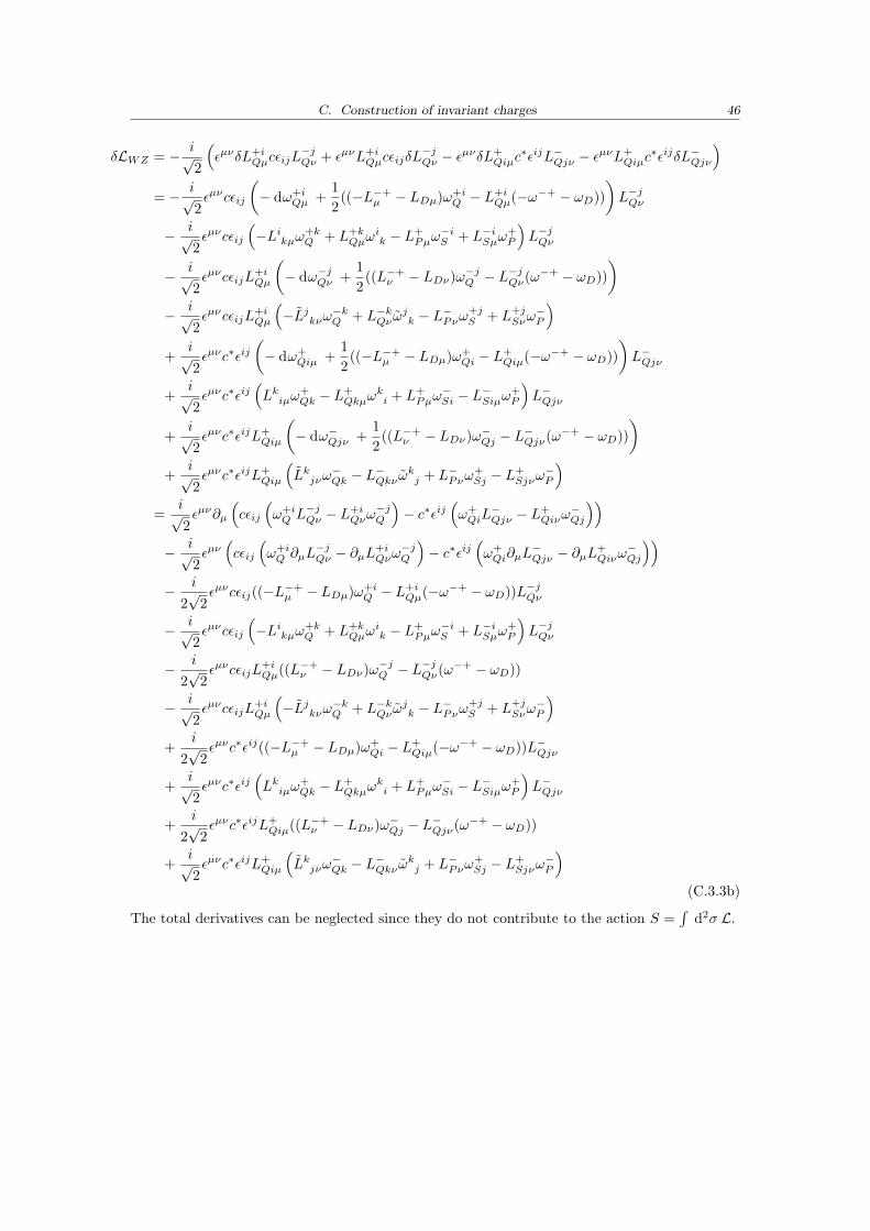
C. Construction of invariant charges 46

δLWZ = − i√2

(εµνδL+i

QµcεijL−jQν + εµνL+i

QµcεijδL−jQν − ε

µνδL+Qiµc

∗εijL−Qjν − εµνL+

Qiµc∗εijδL−Qjν

)= − i√

2εµνcεij

(− dω+i

Qµ +12((−L−+

µ − LDµ)ω+iQ − L

+iQµ(−ω

−+ − ωD)))L−jQν

− i√2εµνcεij

(−Likµω+k

Q + L+kQµω

ik − L+

Pµω−iS + L−iSµω

+P

)L−jQν

− i√2εµνcεijL

+iQµ

(− dω−jQν +

12((L−+

ν − LDν)ω−jQ − L−jQν(ω

−+ − ωD)))

− i√2εµνcεijL

+iQµ

(−Ljkνω−kQ + L−kQν ω

jk − L−Pνω

+jS + L+j

Sνω−P

)+

i√2εµνc∗εij

(− dω+

Qiµ +12((−L−+

µ − LDµ)ω+Qi − L

+Qiµ(−ω

−+ − ωD)))L−Qjν

+i√2εµνc∗εij

(Lkiµω

+Qk − L

+Qkµω

ki + L+

Pµω−Si − L

−Siµω

+P

)L−Qjν

+i√2εµνc∗εijL+

Qiµ

(− dω−Qjν +

12((L−+

ν − LDν)ω−Qj − L−Qjν(ω

−+ − ωD)))

+i√2εµνc∗εijL+

Qiµ

(Lkjνω

−Qk − L

−Qkν ω

kj + L−Pνω

+Sj − L

+Sjνω

−P

)=

i√2εµν∂µ

(cεij

(ω+iQ L−jQν − L

+iQνω

−jQ

)− c∗εij

(ω+QiL

−Qjν − L

+Qiνω

−Qj

))− i√

2εµν(cεij

(ω+iQ ∂µL

−jQν − ∂µL

+iQνω

−jQ

)− c∗εij

(ω+Qi∂µL

−Qjν − ∂µL

+Qiνω

−Qj

))− i

2√

2εµνcεij((−L−+

µ − LDµ)ω+iQ − L

+iQµ(−ω

−+ − ωD))L−jQν

− i√2εµνcεij

(−Likµω+k

Q + L+kQµω

ik − L+

Pµω−iS + L−iSµω

+P

)L−jQν

− i

2√

2εµνcεijL

+iQµ((L

−+ν − LDν)ω−jQ − L

−jQν(ω

−+ − ωD))

− i√2εµνcεijL

+iQµ

(−Ljkνω−kQ + L−kQν ω

jk − L−Pνω

+jS + L+j

Sνω−P

)+

i

2√

2εµνc∗εij((−L−+

µ − LDµ)ω+Qi − L

+Qiµ(−ω

−+ − ωD))L−Qjν

+i√2εµνc∗εij

(Lkiµω

+Qk − L

+Qkµω

ki + L+

Pµω−Si − L

−Siµω

+P

)L−Qjν

+i

2√

2εµνc∗εijL+

Qiµ((L−+ν − LDν)ω−Qj − L

−Qjν(ω

−+ − ωD))

+i√2εµνc∗εijL+

Qiµ

(Lkjνω

−Qk − L

−Qkν ω

kj + L−Pνω

+Sj − L

+Sjνω

−P

)(C.3.3b)

The total derivatives can be neglected since they do not contribute to the action S =∫

d2σ L.

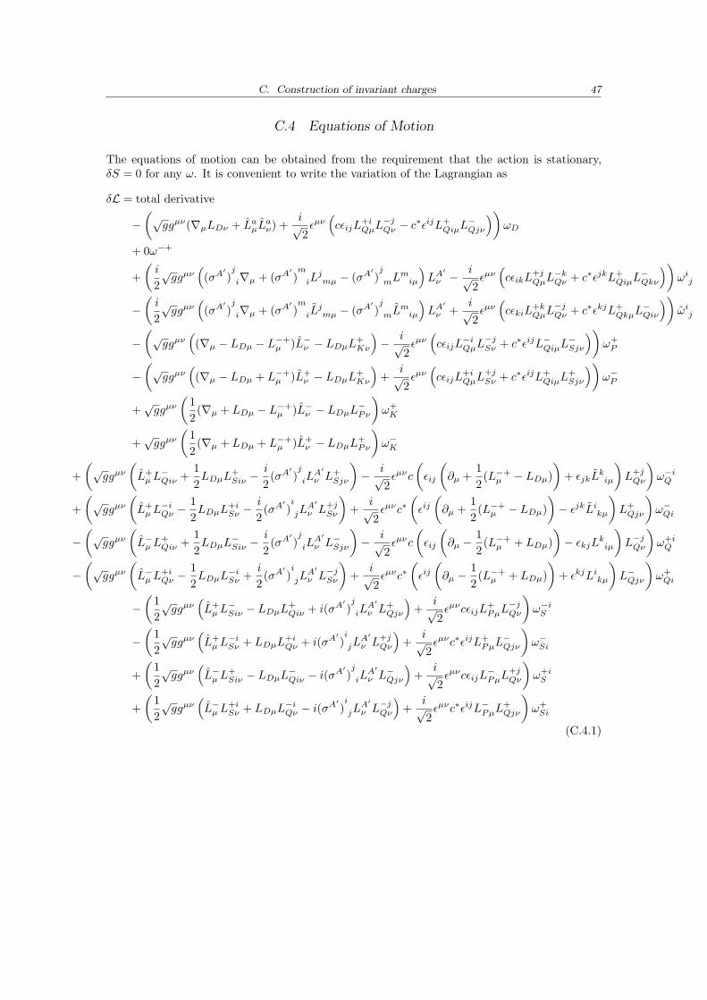
C. Construction of invariant charges 47

C.4 Equations of Motion

The equations of motion can be obtained from the requirement that the action is stationary,δS = 0 for any ω. It is convenient to write the variation of the Lagrangian as

δL = total derivative

−(√ggµν(∇µLDν + LaµL

aν) +

i√2εµν(cεijL

+iQµL

−jQν − c

∗εijL+QiµL

−Qjν

))ωD

+ 0ω−+

+(i

2√ggµν

((σA

′)j

i∇µ + (σA′)m

iLjmµ − (σA

′)j

mLmiµ

)LA

′

ν −i√2εµν(cεikL

+jQµL

−kQν + c∗εjkL+

QiµL−Qkν

))ωij

−(i

2√ggµν

((σA

′)j

i∇µ + (σA′)m

iLjmµ − (σA

′)j

mLmiµ

)LA

′

ν +i√2εµν(cεkiL

+kQµL

−jQν + c∗εkjL+

QkµL−Qiν

))ωij

−(√ggµν

((∇µ − LDµ − L−+

µ )L−ν − LDµL+Kν

)− i√

2εµν(cεijL

−iQµL

−jSν + c∗εijL−QiµL

−Sjν

))ω+P

−(√ggµν

((∇µ − LDµ + L−+

µ )L+ν − LDµL+

Kν

)+

i√2εµν(cεijL

+iQµL

+jSν + c∗εijL+

QiµL+Sjν

))ω−P

+√ggµν

(12(∇µ + LDµ − L−+

µ )L−ν − LDµL−Pν)ω+K

+√ggµν

(12(∇µ + LDµ + L−+

µ )L+ν − LDµL+

Pν

)ω−K

+(√ggµν

(L+µL

−Qiν +

12LDµL

+Siν −

i

2(σA

′)j

iLA′

ν L+Sjν

)− i√

2εµνc

(εij

(∂µ +

12(L−+

µ − LDµ))

+ εjkLkiµ

)L+jQν

)ω−iQ

+(√ggµν

(L+µL

−iQν −

12LDµL

+iSν −

i

2(σA

′)i

jLA′

ν L+jSν

)+

i√2εµνc∗

(εij(∂µ +

12(L−+

µ − LDµ))− εjkLikµ

)L+Qjν

)ω−Qi

−(√ggµν

(L−µL

+Qiν +

12LDµL

−Siν −

i

2(σA

′)j

iLA′

ν L−Sjν

)− i√

2εµνc

(εij

(∂µ −

12(L−+

µ + LDµ))− εkjLkiµ

)L−jQν

)ω+iQ

−(√ggµν

(L−µL

+iQν −

12LDµL

−iSν +

i

2(σA

′)i

jLA′

ν L−jSν

)+

i√2εµνc∗

(εij(∂µ −

12(L−+

µ + LDµ))

+ εkjLikµ

)L−Qjν

)ω+Qi

−(

12√ggµν

(L+µL

−Siν − LDµL

+Qiν + i(σA

′)j

iLA′

ν L+Qjν

)+

i√2εµνcεijL

+PµL

−jQν

)ω−iS

−(

12√ggµν

(L+µL

−iSν + LDµL

+iQν + i(σA

′)i

jLA′

ν L+jQν

)+

i√2εµνc∗εijL+

PµL−Qjν

)ω−Si

+(

12√ggµν

(L−µL

+Siν − LDµL

−Qiν − i(σ

A′)j

iLA′

ν L−Qjν

)+

i√2εµνcεijL

−PµL

+jQν

)ω+iS

+(

12√ggµν

(L−µL

+iSν + LDµL

−iQν − i(σ

A′)i

jLA′

ν L−jQν

)+

i√2εµνc∗εijL−PµL

+Qjν

)ω+Si

(C.4.1)

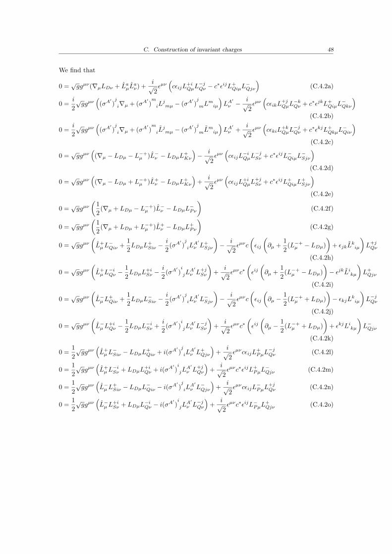
C. Construction of invariant charges 48

We find that

0 =√ggµν(∇µLDν + LaµL

aν) +

i√2εµν(cεijL

+iQµL

−jQν − c

∗εijL+QiµL

−Qjν

)(C.4.2a)

0 =i

2√ggµν

((σA

′)j

i∇µ + (σA′)m

iLjmµ − (σA

′)j

mLmiµ

)LA

′

ν −i√2εµν(cεikL

+jQµL

−kQν + c∗εjkL+

QiµL−Qkν

)(C.4.2b)

0 =i

2√ggµν

((σA

′)j

i∇µ + (σA′)m

iLjmµ − (σA

′)j

mLmiµ

)LA

′

ν +i√2εµν(cεkiL

+kQµL

−jQν + c∗εkjL+

QkµL−Qiν

)(C.4.2c)

0 =√ggµν

((∇µ − LDµ − L−+

µ )L−ν − LDµL+Kν

)− i√

2εµν(cεijL

−iQµL

−jSν + c∗εijL−QiµL

−Sjν

)(C.4.2d)

0 =√ggµν

((∇µ − LDµ + L−+

µ )L+ν − LDµL+

Kν

)+

i√2εµν(cεijL

+iQµL

+jSν + c∗εijL+

QiµL+Sjν

)(C.4.2e)

0 =√ggµν

(12(∇µ + LDµ − L−+

µ )L−ν − LDµL−Pν)

(C.4.2f)

0 =√ggµν

(12(∇µ + LDµ + L−+

µ )L+ν − LDµL+

Pν

)(C.4.2g)

0 =√ggµν

(L+µL

−Qiν +

12LDµL

+Siν −

i

2(σA

′)j

iLA′

ν L+Sjν

)− i√

2εµνc

(εij

(∂µ +

12(L−+

µ − LDµ))

+ εjkLkiµ

)L+jQν

(C.4.2h)

0 =√ggµν

(L+µL

−iQν −

12LDµL

+iSν −

i

2(σA

′)i

jLA′

ν L+jSν

)+

i√2εµνc∗

(εij(∂µ +

12(L−+

µ − LDµ))− εjkLikµ

)L+Qjν

(C.4.2i)

0 =√ggµν

(L−µL

+Qiν +

12LDµL

−Siν −

i

2(σA

′)j

iLA′

ν L−Sjν

)− i√

2εµνc

(εij

(∂µ −

12(L−+

µ + LDµ))− εkjLkiµ

)L−jQν

(C.4.2j)

0 =√ggµν

(L−µL

+iQν −

12LDµL

−iSν +

i

2(σA

′)i

jLA′

ν L−jSν

)+

i√2εµνc∗

(εij(∂µ −

12(L−+

µ + LDµ))

+ εkjLikµ

)L−Qjν

(C.4.2k)

0 =12√ggµν

(L+µL

−Siν − LDµL

+Qiν + i(σA

′)j

iLA′

ν L+Qjν

)+

i√2εµνcεijL

+PµL

−jQν (C.4.2l)

0 =12√ggµν

(L+µL

−iSν + LDµL

+iQν + i(σA

′)i

jLA′

ν L+jQν

)+

i√2εµνc∗εijL+

PµL−Qjν (C.4.2m)

0 =12√ggµν

(L−µL

+Siν − LDµL

−Qiν − i(σ

A′)j

iLA′

ν L−Qjν

)+

i√2εµνcεijL

−PµL

+jQν (C.4.2n)

0 =12√ggµν

(L−µL

+iSν + LDµL

−iQν − i(σ

A′)i

jLA′

ν L−jQν

)+

i√2εµνc∗εijL−PµL

+Qjν (C.4.2o)

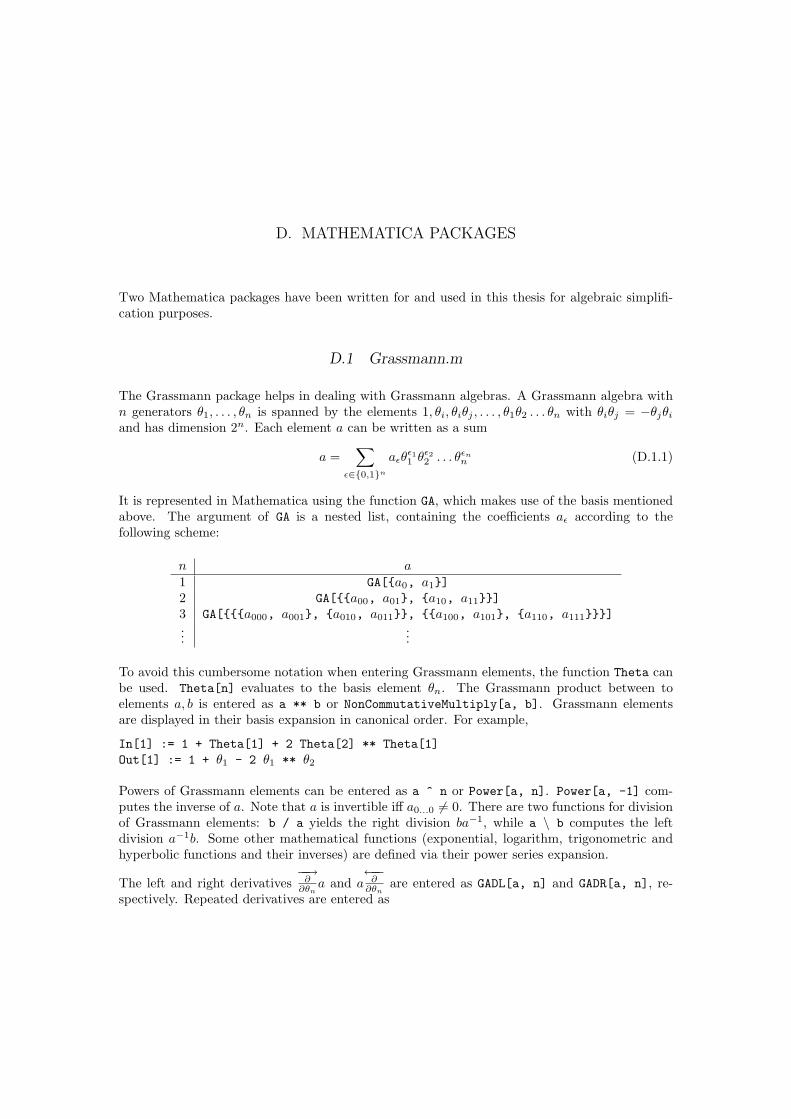
D. MATHEMATICA PACKAGES

Two Mathematica packages have been written for and used in this thesis for algebraic simplifi-cation purposes.

D.1 Grassmann.m

The Grassmann package helps in dealing with Grassmann algebras. A Grassmann algebra withn generators θ1, . . . , θn is spanned by the elements 1, θi, θiθj , . . . , θ1θ2 . . . θn with θiθj = −θjθiand has dimension 2n. Each element a can be written as a sum

a =∑

ε∈{0,1}n

aεθε11 θ

ε22 . . . θεnn (D.1.1)

It is represented in Mathematica using the function GA, which makes use of the basis mentionedabove. The argument of GA is a nested list, containing the coefficients aε according to thefollowing scheme:

n a1 GA[{a0, a1}]2 GA[{{a00, a01}, {a10, a11}}]3 GA[{{{a000, a001}, {a010, a011}}, {{a100, a101}, {a110, a111}}}]...

...

To avoid this cumbersome notation when entering Grassmann elements, the function Theta canbe used. Theta[n] evaluates to the basis element θn. The Grassmann product between toelements a, b is entered as a ** b or NonCommutativeMultiply[a, b]. Grassmann elementsare displayed in their basis expansion in canonical order. For example,

In[1] := 1 + Theta[1] + 2 Theta[2] ** Theta[1]Out[1] := 1 + θ1 - 2 θ1 ** θ2

Powers of Grassmann elements can be entered as a ^ n or Power[a, n]. Power[a, -1] com-putes the inverse of a. Note that a is invertible iff a0...0 6= 0. There are two functions for divisionof Grassmann elements: b / a yields the right division ba−1, while a \ b computes the leftdivision a−1b. Some other mathematical functions (exponential, logarithm, trigonometric andhyperbolic functions and their inverses) are defined via their power series expansion.

The left and right derivatives−−→∂∂θn

a and a←−−∂∂θn

are entered as GADL[a, n] and GADR[a, n], re-spectively. Repeated derivatives are entered as

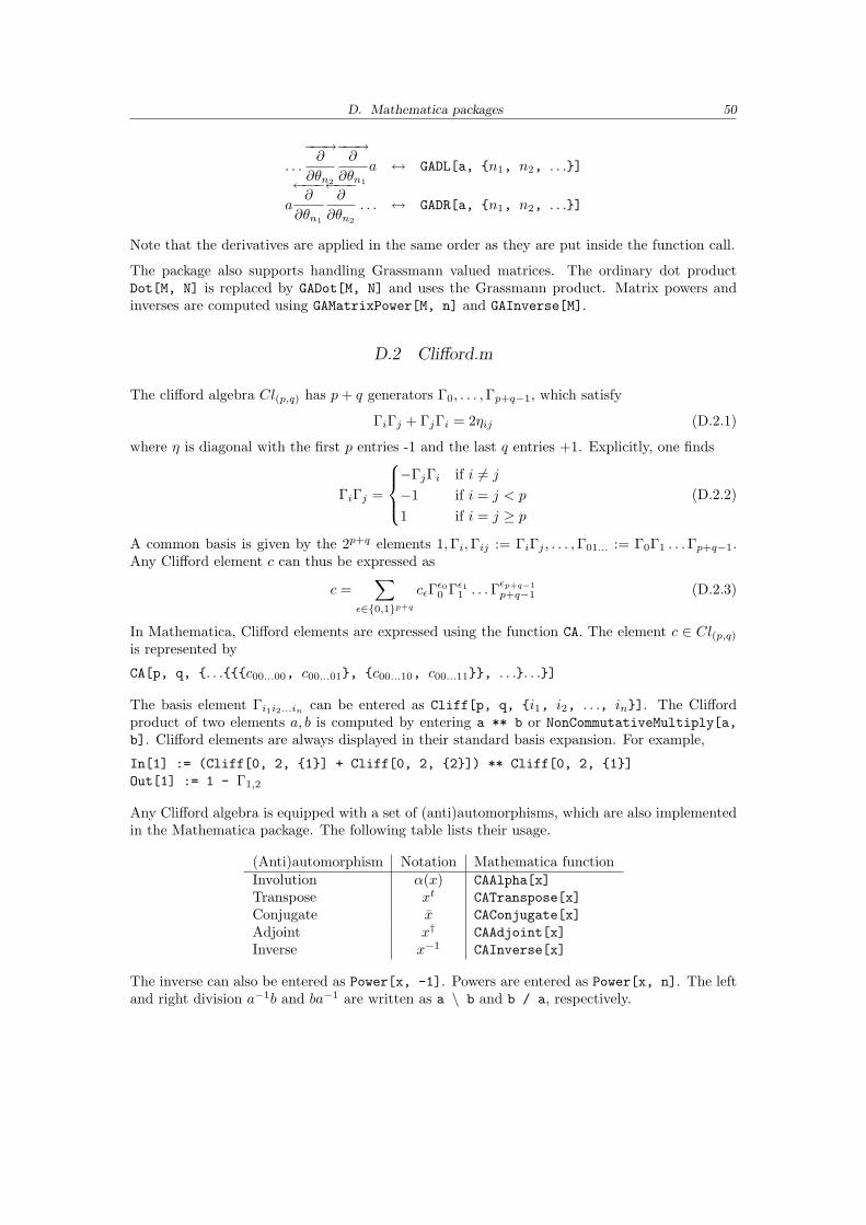
D. Mathematica packages 50

. . .

−−−→∂

∂θn2

−−−→∂

∂θn1

a ↔ GADL[a, {n1, n2, . . .}]

a

←−−−∂

∂θn1

←−−−∂

∂θn2

. . . ↔ GADR[a, {n1, n2, . . .}]

Note that the derivatives are applied in the same order as they are put inside the function call.

The package also supports handling Grassmann valued matrices. The ordinary dot productDot[M, N] is replaced by GADot[M, N] and uses the Grassmann product. Matrix powers andinverses are computed using GAMatrixPower[M, n] and GAInverse[M].

D.2 Clifford.m

The clifford algebra Cl(p,q) has p+ q generators Γ0, . . . ,Γp+q−1, which satisfy

ΓiΓj + ΓjΓi = 2ηij (D.2.1)

where η is diagonal with the first p entries -1 and the last q entries +1. Explicitly, one finds

ΓiΓj =

−ΓjΓi if i 6= j

−1 if i = j < p

1 if i = j ≥ p(D.2.2)

A common basis is given by the 2p+q elements 1,Γi,Γij := ΓiΓj , . . . ,Γ01... := Γ0Γ1 . . .Γp+q−1.Any Clifford element c can thus be expressed as

c =∑

ε∈{0,1}p+q

cεΓε00 Γε11 . . .Γεp+q−1p+q−1 (D.2.3)

In Mathematica, Clifford elements are expressed using the function CA. The element c ∈ Cl(p,q)is represented by

CA[p, q, {. . .{{{c00...00, c00...01}, {c00...10, c00...11}}, . . .}. . .}]

The basis element Γi1i2...in can be entered as Cliff[p, q, {i1, i2, . . ., in}]. The Cliffordproduct of two elements a, b is computed by entering a ** b or NonCommutativeMultiply[a,b]. Clifford elements are always displayed in their standard basis expansion. For example,

In[1] := (Cliff[0, 2, {1}] + Cliff[0, 2, {2}]) ** Cliff[0, 2, {1}]Out[1] := 1 - Γ1,2

Any Clifford algebra is equipped with a set of (anti)automorphisms, which are also implementedin the Mathematica package. The following table lists their usage.

(Anti)automorphism Notation Mathematica functionInvolution α(x) CAAlpha[x]Transpose xt CATranspose[x]Conjugate x CAConjugate[x]Adjoint x† CAAdjoint[x]Inverse x−1 CAInverse[x]

The inverse can also be entered as Power[x, -1]. Powers are entered as Power[x, n]. The leftand right division a−1b and ba−1 are written as a \ b and b / a, respectively.

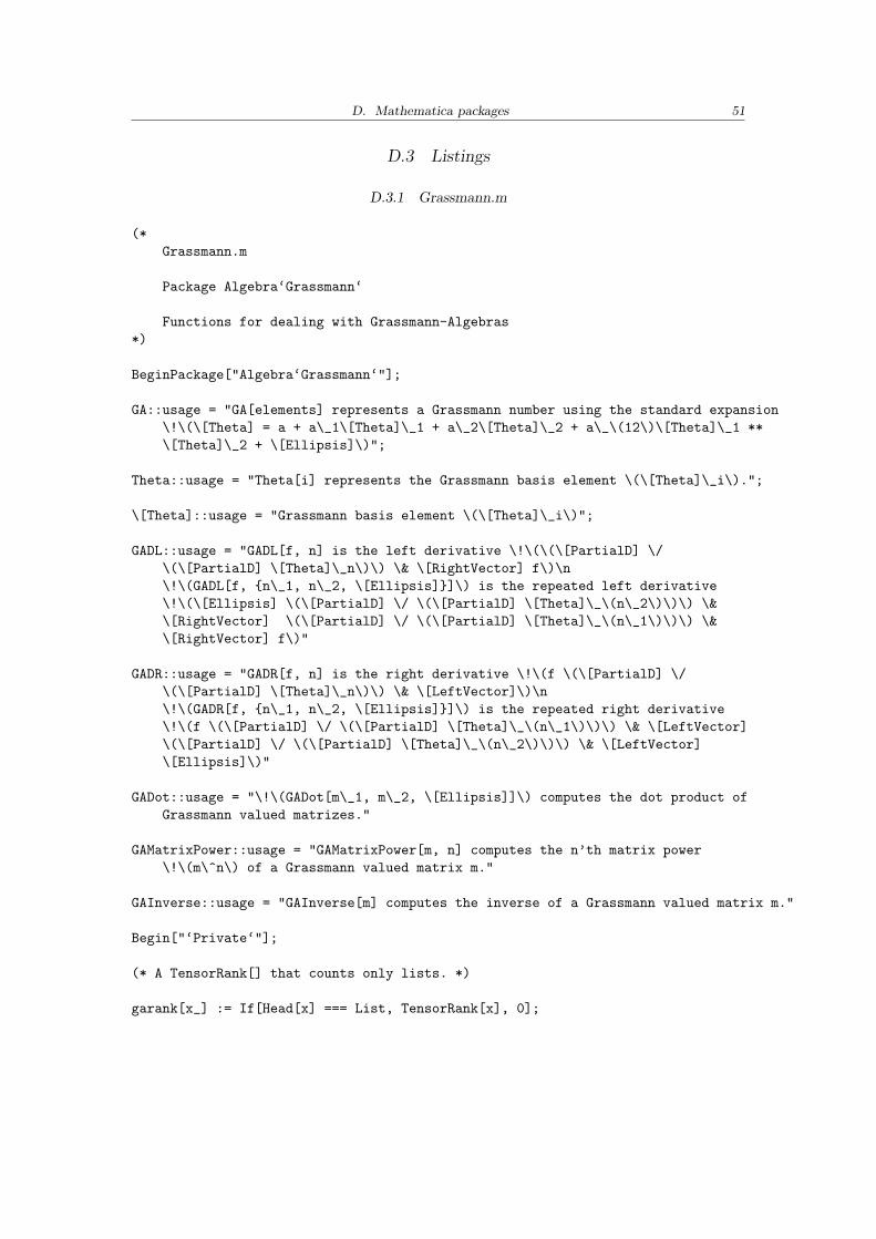
D. Mathematica packages 51

D.3 Listings

D.3.1 Grassmann.m

(*Grassmann.m

Package Algebra‘Grassmann‘

Functions for dealing with Grassmann-Algebras*)

BeginPackage["Algebra‘Grassmann‘"];

GA::usage = "GA[elements] represents a Grassmann number using the standard expansion\!\(\[Theta] = a + a\_1\[Theta]\_1 + a\_2\[Theta]\_2 + a\_\(12\)\[Theta]\_1 **\[Theta]\_2 + \[Ellipsis]\)";

Theta::usage = "Theta[i] represents the Grassmann basis element \(\[Theta]\_i\).";

\[Theta]::usage = "Grassmann basis element \(\[Theta]\_i\)";

GADL::usage = "GADL[f, n] is the left derivative \!\(\(\[PartialD] \/\(\[PartialD] \[Theta]\_n\)\) \& \[RightVector] f\)\n\!\(GADL[f, {n\_1, n\_2, \[Ellipsis]}]\) is the repeated left derivative\!\(\[Ellipsis] \(\[PartialD] \/ \(\[PartialD] \[Theta]\_\(n\_2\)\)\) \&\[RightVector] \(\[PartialD] \/ \(\[PartialD] \[Theta]\_\(n\_1\)\)\) \&\[RightVector] f\)"

GADR::usage = "GADR[f, n] is the right derivative \!\(f \(\[PartialD] \/\(\[PartialD] \[Theta]\_n\)\) \& \[LeftVector]\)\n\!\(GADR[f, {n\_1, n\_2, \[Ellipsis]}]\) is the repeated right derivative\!\(f \(\[PartialD] \/ \(\[PartialD] \[Theta]\_\(n\_1\)\)\) \& \[LeftVector]\(\[PartialD] \/ \(\[PartialD] \[Theta]\_\(n\_2\)\)\) \& \[LeftVector]\[Ellipsis]\)"

GADot::usage = "\!\(GADot[m\_1, m\_2, \[Ellipsis]]\) computes the dot product ofGrassmann valued matrizes."

GAMatrixPower::usage = "GAMatrixPower[m, n] computes the n’th matrix power\!\(m\^n\) of a Grassmann valued matrix m."

GAInverse::usage = "GAInverse[m] computes the inverse of a Grassmann valued matrix m."

Begin["‘Private‘"];

(* A TensorRank[] that counts only lists. *)

garank[x_] := If[Head[x] === List, TensorRank[x], 0];

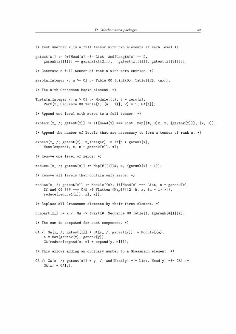
D. Mathematica packages 52

(* Test whether x is a full tensor with two elements at each level.*)

gatest[x_] := Or[Head[x] =!= List, And[Length[x] == 2,garank[x[[1]]] == garank[x[[2]]], gatest[x[[1]]], gatest[x[[2]]]]];

(* Generate a full tensor of rank n with zero entries. *)

zero[n_Integer /; n >= 0] := Table @@ Join[{0}, Table[{2}, {n}]];

(* The n’th Grassmann basis element. *)

Theta[n_Integer /; n > 0] := Module[{t}, t = zero[n];Part[t, Sequence @@ Table[1, {n - 1}], 2] = 1; GA[t]];

(* Append one level with zeros to a full tensor. *)

expand1[x_ /; gatest[x]] := If[Head[x] === List, Map[{#, 0}&, x, {garank[x]}], {x, 0}];

(* Append the number of levels that are necessary to form a tensor of rank n. *)

expand[x_ /; gatest[x], n_Integer] := If[n > garank[x],Nest[expand1, x, n - garank[x]], x];

(* Remove one level of zeros. *)

reduce1[x_ /; gatest[x]] := Map[#[[1]]&, x, {garank[x] - 1}];

(* Remove all levels that contain only zeros. *)

reduce[x_ /; gatest[x]] := Module[{n}, If[Head[x] === List, n = garank[x];If[And @@ ((# === 0)& /@ Flatten[{Map[#[[2]]&, x, {n - 1}]}]),reduce[reduce1[x]], x], x]];

(* Replace all Grassmann elements by their first element. *)

numpart[x_] := x /. GA -> (Part[#, Sequence @@ Table[1, {garank[#]}]]&);

(* The sum is computed for each component. *)

GA /: GA[x_ /; gatest[x]] + GA[y_ /; gatest[y]] := Module[{n},n = Max[garank[x], garank[y]];GA[reduce[expand[x, n] + expand[y, n]]]];

(* This allows adding an ordinary number to a Grassmann element. *)

GA /: GA[x_ /; gatest[x]] + y_ /; And[Head[y] =!= List, Head[y] =!= GA] :=GA[x] + GA[y];

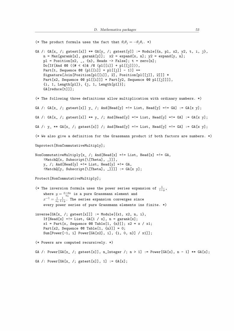
D. Mathematica packages 53

(* The product formula uses the fact that θiθj = −θjθi. *)

GA /: GA[x_ /; gatest[x]] ** GA[y_ /; gatest[y]] := Module[{n, pl, x2, y2, t, i, j},n = Max[garank[x], garank[y]]; x2 = expand[x, n]; y2 = expand[y, n];pl = Position[x2, _, {n}, Heads -> False]; t = zero[n];Do[If[And @@ ((# < 4)& /@ (pl[[i]] + pl[[j]])),Part[t, Sequence @@ (pl[[i]] + pl[[j]] - 1)] +=Signature[Join[Position[pl[[i]], 2], Position[pl[[j]], 2]]] *Part[x2, Sequence @@ pl[[i]]] * Part[y2, Sequence @@ pl[[j]]]],{i, 1, Length[pl]}, {j, 1, Length[pl]}];GA[reduce[t]]];

(* The following three definitions allow multiplication with ordinary numbers. *)

GA /: GA[x_ /; gatest[x]] y_ /; And[Head[y] =!= List, Head[y] =!= GA] := GA[x y];

GA /: GA[x_ /; gatest[x]] ** y_ /; And[Head[y] =!= List, Head[y] =!= GA] := GA[x y];

GA /: y_ ** GA[x_ /; gatest[x]] /; And[Head[y] =!= List, Head[y] =!= GA] := GA[x y];

(* We also give a definition for the Grassmann product if both factors are numbers. *)

Unprotect[NonCommutativeMultiply];

NonCommutativeMultiply[x_ /; And[Head[x] =!= List, Head[x] =!= GA,!MatchQ[x, Subscript[\[Theta], _]]],y_ /; And[Head[y] =!= List, Head[y] =!= GA,!MatchQ[y, Subscript[\[Theta], _]]]] := GA[x y];

Protect[NonCommutativeMultiply];

(* The inversion formula uses the power series expansion of 11+y,

where y = x−a0a0

is a pure Grassmann element and

x−1 = 1a0

11+y. The series expansion converges since

every power series of pure Grassmann elements ins finite. *)

inverse[GA[x_ /; gatest[x]]] := Module[{x1, x2, n, i},If[Head[x] =!= List, GA[1 / x], n = garank[x];x1 = Part[x, Sequence @@ Table[1, {n}]]; x2 = x / x1;Part[x2, Sequence @@ Table[1, {n}]] = 0;Sum[Power[-1, i] Power[GA[x2], i], {i, 0, n}] / x1]];

(* Powers are computed recursively. *)

GA /: Power[GA[x_ /; gatest[x]], n_Integer /; n > 1] := Power[GA[x], n - 1] ** GA[x];

GA /: Power[GA[x_ /; gatest[x]], 1] := GA[x];

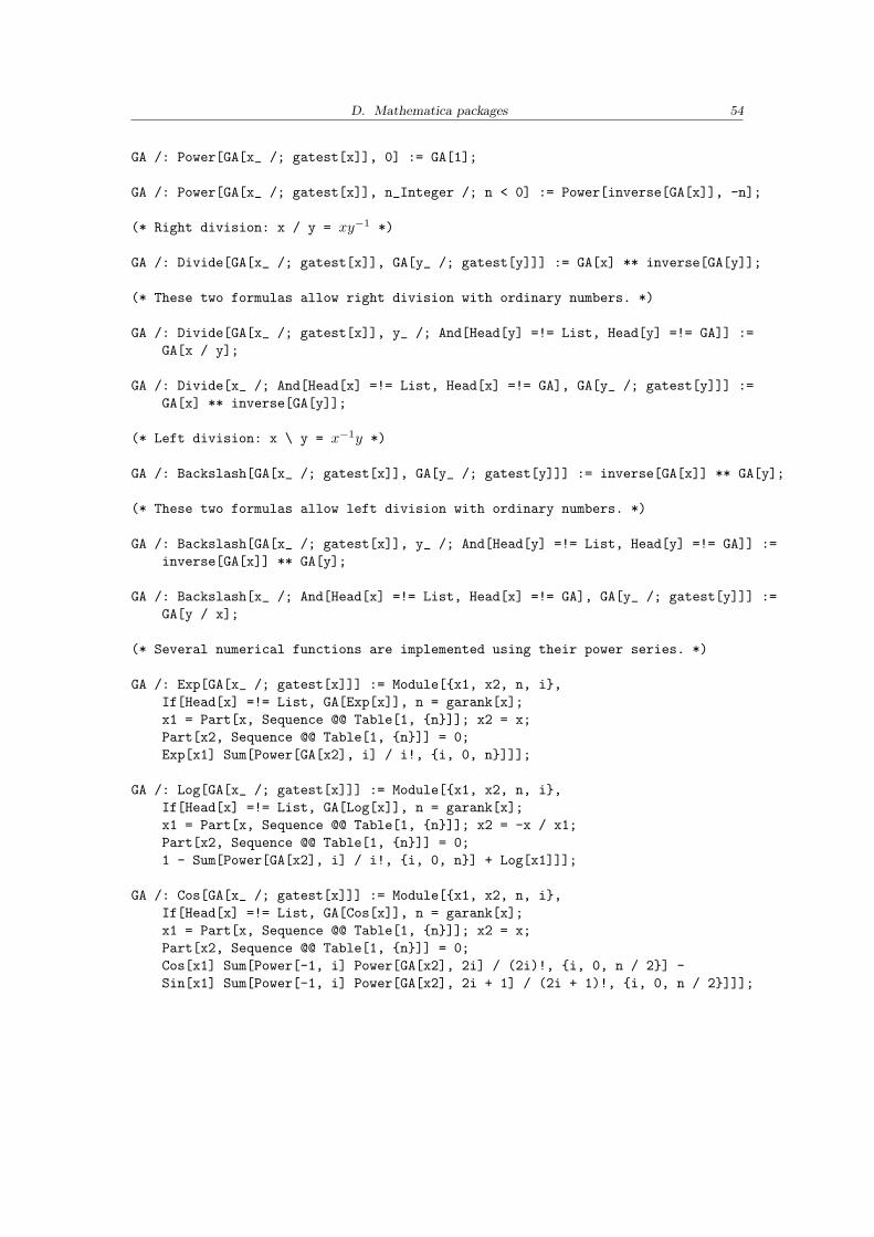
D. Mathematica packages 54

GA /: Power[GA[x_ /; gatest[x]], 0] := GA[1];

GA /: Power[GA[x_ /; gatest[x]], n_Integer /; n < 0] := Power[inverse[GA[x]], -n];

(* Right division: x / y = xy−1 *)

GA /: Divide[GA[x_ /; gatest[x]], GA[y_ /; gatest[y]]] := GA[x] ** inverse[GA[y]];

(* These two formulas allow right division with ordinary numbers. *)

GA /: Divide[GA[x_ /; gatest[x]], y_ /; And[Head[y] =!= List, Head[y] =!= GA]] :=GA[x / y];

GA /: Divide[x_ /; And[Head[x] =!= List, Head[x] =!= GA], GA[y_ /; gatest[y]]] :=GA[x] ** inverse[GA[y]];

(* Left division: x \ y = x−1y *)

GA /: Backslash[GA[x_ /; gatest[x]], GA[y_ /; gatest[y]]] := inverse[GA[x]] ** GA[y];

(* These two formulas allow left division with ordinary numbers. *)

GA /: Backslash[GA[x_ /; gatest[x]], y_ /; And[Head[y] =!= List, Head[y] =!= GA]] :=inverse[GA[x]] ** GA[y];

GA /: Backslash[x_ /; And[Head[x] =!= List, Head[x] =!= GA], GA[y_ /; gatest[y]]] :=GA[y / x];

(* Several numerical functions are implemented using their power series. *)

GA /: Exp[GA[x_ /; gatest[x]]] := Module[{x1, x2, n, i},If[Head[x] =!= List, GA[Exp[x]], n = garank[x];x1 = Part[x, Sequence @@ Table[1, {n}]]; x2 = x;Part[x2, Sequence @@ Table[1, {n}]] = 0;Exp[x1] Sum[Power[GA[x2], i] / i!, {i, 0, n}]]];

GA /: Log[GA[x_ /; gatest[x]]] := Module[{x1, x2, n, i},If[Head[x] =!= List, GA[Log[x]], n = garank[x];x1 = Part[x, Sequence @@ Table[1, {n}]]; x2 = -x / x1;Part[x2, Sequence @@ Table[1, {n}]] = 0;1 - Sum[Power[GA[x2], i] / i!, {i, 0, n}] + Log[x1]]];

GA /: Cos[GA[x_ /; gatest[x]]] := Module[{x1, x2, n, i},If[Head[x] =!= List, GA[Cos[x]], n = garank[x];x1 = Part[x, Sequence @@ Table[1, {n}]]; x2 = x;Part[x2, Sequence @@ Table[1, {n}]] = 0;Cos[x1] Sum[Power[-1, i] Power[GA[x2], 2i] / (2i)!, {i, 0, n / 2}] -Sin[x1] Sum[Power[-1, i] Power[GA[x2], 2i + 1] / (2i + 1)!, {i, 0, n / 2}]]];

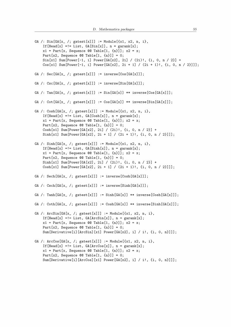
D. Mathematica packages 55

GA /: Sin[GA[x_ /; gatest[x]]] := Module[{x1, x2, n, i},If[Head[x] =!= List, GA[Sin[x]], n = garank[x];x1 = Part[x, Sequence @@ Table[1, {n}]]; x2 = x;Part[x2, Sequence @@ Table[1, {n}]] = 0;Sin[x1] Sum[Power[-1, i] Power[GA[x2], 2i] / (2i)!, {i, 0, n / 2}] +Cos[x1] Sum[Power[-1, i] Power[GA[x2], 2i + 1] / (2i + 1)!, {i, 0, n / 2}]]];

GA /: Sec[GA[x_ /; gatest[x]]] := inverse[Cos[GA[x]]];

GA /: Csc[GA[x_ /; gatest[x]]] := inverse[Sin[GA[x]]];

GA /: Tan[GA[x_ /; gatest[x]]] := Sin[GA[x]] ** inverse[Cos[GA[x]]];

GA /: Cot[GA[x_ /; gatest[x]]] := Cos[GA[x]] ** inverse[Sin[GA[x]]];

GA /: Cosh[GA[x_ /; gatest[x]]] := Module[{x1, x2, n, i},If[Head[x] =!= List, GA[Cosh[x]], n = garank[x];x1 = Part[x, Sequence @@ Table[1, {n}]]; x2 = x;Part[x2, Sequence @@ Table[1, {n}]] = 0;Cosh[x1] Sum[Power[GA[x2], 2i] / (2i)!, {i, 0, n / 2}] +Sinh[x1] Sum[Power[GA[x2], 2i + 1] / (2i + 1)!, {i, 0, n / 2}]]];

GA /: Sinh[GA[x_ /; gatest[x]]] := Module[{x1, x2, n, i},If[Head[x] =!= List, GA[Sinh[x]], n = garank[x];x1 = Part[x, Sequence @@ Table[1, {n}]]; x2 = x;Part[x2, Sequence @@ Table[1, {n}]] = 0;Sinh[x1] Sum[Power[GA[x2], 2i] / (2i)!, {i, 0, n / 2}] +Cosh[x1] Sum[Power[GA[x2], 2i + 1] / (2i + 1)!, {i, 0, n / 2}]]];

GA /: Sech[GA[x_ /; gatest[x]]] := inverse[Cosh[GA[x]]];

GA /: Csch[GA[x_ /; gatest[x]]] := inverse[Sinh[GA[x]]];

GA /: Tanh[GA[x_ /; gatest[x]]] := Sinh[GA[x]] ** inverse[Cosh[GA[x]]];

GA /: Coth[GA[x_ /; gatest[x]]] := Cosh[GA[x]] ** inverse[Sinh[GA[x]]];

GA /: ArcSin[GA[x_ /; gatest[x]]] := Module[{x1, x2, n, i},If[Head[x] =!= List, GA[ArcSin[x]], n = garank[x];x1 = Part[x, Sequence @@ Table[1, {n}]]; x2 = x;Part[x2, Sequence @@ Table[1, {n}]] = 0;Sum[Derivative[i][ArcSin][x1] Power[GA[x2], i] / i!, {i, 0, n}]]];

GA /: ArcCos[GA[x_ /; gatest[x]]] := Module[{x1, x2, n, i},If[Head[x] =!= List, GA[ArcCos[x]], n = garank[x];x1 = Part[x, Sequence @@ Table[1, {n}]]; x2 = x;Part[x2, Sequence @@ Table[1, {n}]] = 0;Sum[Derivative[i][ArcCos][x1] Power[GA[x2], i] / i!, {i, 0, n}]]];

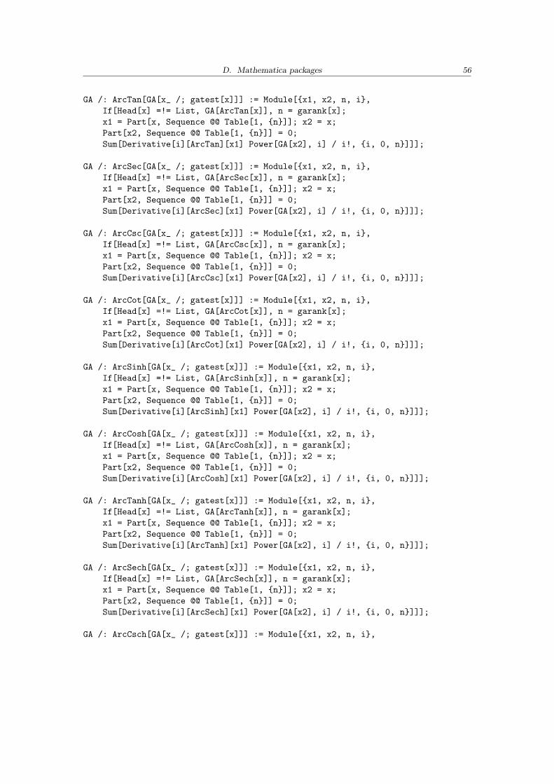
D. Mathematica packages 56

GA /: ArcTan[GA[x_ /; gatest[x]]] := Module[{x1, x2, n, i},If[Head[x] =!= List, GA[ArcTan[x]], n = garank[x];x1 = Part[x, Sequence @@ Table[1, {n}]]; x2 = x;Part[x2, Sequence @@ Table[1, {n}]] = 0;Sum[Derivative[i][ArcTan][x1] Power[GA[x2], i] / i!, {i, 0, n}]]];

GA /: ArcSec[GA[x_ /; gatest[x]]] := Module[{x1, x2, n, i},If[Head[x] =!= List, GA[ArcSec[x]], n = garank[x];x1 = Part[x, Sequence @@ Table[1, {n}]]; x2 = x;Part[x2, Sequence @@ Table[1, {n}]] = 0;Sum[Derivative[i][ArcSec][x1] Power[GA[x2], i] / i!, {i, 0, n}]]];

GA /: ArcCsc[GA[x_ /; gatest[x]]] := Module[{x1, x2, n, i},If[Head[x] =!= List, GA[ArcCsc[x]], n = garank[x];x1 = Part[x, Sequence @@ Table[1, {n}]]; x2 = x;Part[x2, Sequence @@ Table[1, {n}]] = 0;Sum[Derivative[i][ArcCsc][x1] Power[GA[x2], i] / i!, {i, 0, n}]]];

GA /: ArcCot[GA[x_ /; gatest[x]]] := Module[{x1, x2, n, i},If[Head[x] =!= List, GA[ArcCot[x]], n = garank[x];x1 = Part[x, Sequence @@ Table[1, {n}]]; x2 = x;Part[x2, Sequence @@ Table[1, {n}]] = 0;Sum[Derivative[i][ArcCot][x1] Power[GA[x2], i] / i!, {i, 0, n}]]];

GA /: ArcSinh[GA[x_ /; gatest[x]]] := Module[{x1, x2, n, i},If[Head[x] =!= List, GA[ArcSinh[x]], n = garank[x];x1 = Part[x, Sequence @@ Table[1, {n}]]; x2 = x;Part[x2, Sequence @@ Table[1, {n}]] = 0;Sum[Derivative[i][ArcSinh][x1] Power[GA[x2], i] / i!, {i, 0, n}]]];

GA /: ArcCosh[GA[x_ /; gatest[x]]] := Module[{x1, x2, n, i},If[Head[x] =!= List, GA[ArcCosh[x]], n = garank[x];x1 = Part[x, Sequence @@ Table[1, {n}]]; x2 = x;Part[x2, Sequence @@ Table[1, {n}]] = 0;Sum[Derivative[i][ArcCosh][x1] Power[GA[x2], i] / i!, {i, 0, n}]]];

GA /: ArcTanh[GA[x_ /; gatest[x]]] := Module[{x1, x2, n, i},If[Head[x] =!= List, GA[ArcTanh[x]], n = garank[x];x1 = Part[x, Sequence @@ Table[1, {n}]]; x2 = x;Part[x2, Sequence @@ Table[1, {n}]] = 0;Sum[Derivative[i][ArcTanh][x1] Power[GA[x2], i] / i!, {i, 0, n}]]];

GA /: ArcSech[GA[x_ /; gatest[x]]] := Module[{x1, x2, n, i},If[Head[x] =!= List, GA[ArcSech[x]], n = garank[x];x1 = Part[x, Sequence @@ Table[1, {n}]]; x2 = x;Part[x2, Sequence @@ Table[1, {n}]] = 0;Sum[Derivative[i][ArcSech][x1] Power[GA[x2], i] / i!, {i, 0, n}]]];

GA /: ArcCsch[GA[x_ /; gatest[x]]] := Module[{x1, x2, n, i},

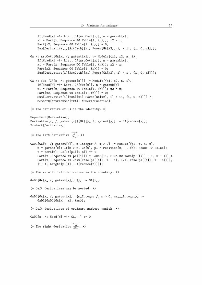
D. Mathematica packages 57

If[Head[x] =!= List, GA[ArcCsch[x]], n = garank[x];x1 = Part[x, Sequence @@ Table[1, {n}]]; x2 = x;Part[x2, Sequence @@ Table[1, {n}]] = 0;Sum[Derivative[i][ArcCsch][x1] Power[GA[x2], i] / i!, {i, 0, n}]]];

GA /: ArcCoth[GA[x_ /; gatest[x]]] := Module[{x1, x2, n, i},If[Head[x] =!= List, GA[ArcCoth[x]], n = garank[x];x1 = Part[x, Sequence @@ Table[1, {n}]]; x2 = x;Part[x2, Sequence @@ Table[1, {n}]] = 0;Sum[Derivative[i][ArcCoth][x1] Power[GA[x2], i] / i!, {i, 0, n}]]];

GA /: fkt_[GA[x_ /; gatest[x]]] := Module[{x1, x2, n, i},If[Head[x] =!= List, GA[fkt[x]], n = garank[x];x1 = Part[x, Sequence @@ Table[1, {n}]]; x2 = x;Part[x2, Sequence @@ Table[1, {n}]] = 0;Sum[Derivative[i][fkt][x1] Power[GA[x2], i] / i!, {i, 0, n}]]] /;MemberQ[Attributes[fkt], NumericFunction];

(* The derivative of GA is the identity. *)

Unprotect[Derivative];Derivative[x_ /; gatest[x]][GA][y_ /; gatest[y]] := GA[reduce[x]];Protect[Derivative];

(* The left derivative−−→∂∂θm

. *)

GADL[GA[x_ /; gatest[x]], m_Integer /; m > 0] := Module[{pl, t, i, n},n = garank[x]; If[m > n, GA[0], pl = Position[x, _, {n}, Heads -> False];t = zero[n]; Do[If[pl[[i,m]] == 1,Part[t, Sequence @@ pl[[i]]] = Power[-1, Plus @@ Take[pl[[i]] - 1, m - 1]] *Part[x, Sequence @@ Join[Take[pl[[i]], m - 1], {2}, Take[pl[[i]], m - n]]]],{i, 1, Length[pl]}]; GA[reduce[t]]]];

(* The zero’th left derivative is the identity. *)

GADL[GA[x_ /; gatest[x]], {}] := GA[x];

(* Left derivatives may be nested. *)

GADL[GA[x_ /; gatest[x]], {m_Integer /; m > 0, mm___Integer}] :=GADL[GADL[GA[x], m], {mm}];

(* Left derivatives of ordinary numbers vanish. *)

GADL[x_ /; Head[x] =!= GA, _] := 0

(* The right derivative←−−∂∂θm

. *)

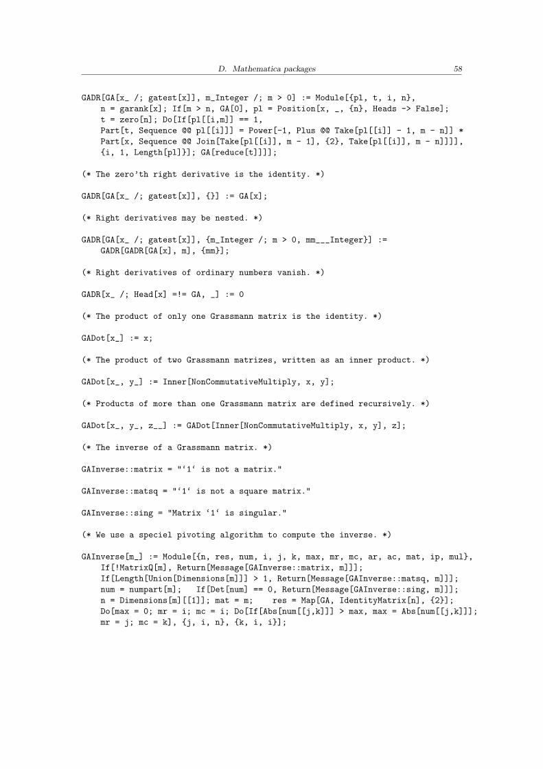
D. Mathematica packages 58

GADR[GA[x_ /; gatest[x]], m_Integer /; m > 0] := Module[{pl, t, i, n},n = garank[x]; If[m > n, GA[0], pl = Position[x, _, {n}, Heads -> False];t = zero[n]; Do[If[pl[[i,m]] == 1,Part[t, Sequence @@ pl[[i]]] = Power[-1, Plus @@ Take[pl[[i]] - 1, m - n]] *Part[x, Sequence @@ Join[Take[pl[[i]], m - 1], {2}, Take[pl[[i]], m - n]]]],{i, 1, Length[pl]}]; GA[reduce[t]]]];

(* The zero’th right derivative is the identity. *)

GADR[GA[x_ /; gatest[x]], {}] := GA[x];

(* Right derivatives may be nested. *)

GADR[GA[x_ /; gatest[x]], {m_Integer /; m > 0, mm___Integer}] :=GADR[GADR[GA[x], m], {mm}];

(* Right derivatives of ordinary numbers vanish. *)

GADR[x_ /; Head[x] =!= GA, _] := 0

(* The product of only one Grassmann matrix is the identity. *)

GADot[x_] := x;

(* The product of two Grassmann matrizes, written as an inner product. *)

GADot[x_, y_] := Inner[NonCommutativeMultiply, x, y];

(* Products of more than one Grassmann matrix are defined recursively. *)

GADot[x_, y_, z__] := GADot[Inner[NonCommutativeMultiply, x, y], z];

(* The inverse of a Grassmann matrix. *)

GAInverse::matrix = "‘1‘ is not a matrix."

GAInverse::matsq = "‘1‘ is not a square matrix."

GAInverse::sing = "Matrix ‘1‘ is singular."

(* We use a speciel pivoting algorithm to compute the inverse. *)

GAInverse[m_] := Module[{n, res, num, i, j, k, max, mr, mc, ar, ac, mat, ip, mul},If[!MatrixQ[m], Return[Message[GAInverse::matrix, m]]];If[Length[Union[Dimensions[m]]] > 1, Return[Message[GAInverse::matsq, m]]];num = numpart[m]; If[Det[num] == 0, Return[Message[GAInverse::sing, m]]];n = Dimensions[m][[1]]; mat = m; res = Map[GA, IdentityMatrix[n], {2}];Do[max = 0; mr = i; mc = i; Do[If[Abs[num[[j,k]]] > max, max = Abs[num[[j,k]]];mr = j; mc = k], {j, i, n}, {k, i, i}];

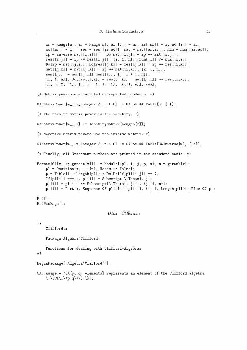
D. Mathematica packages 59

ar = Range[n]; ac = Range[n]; ar[[i]] = mr; ar[[mr]] = i; ac[[i]] = mc;ac[[mc]] = i; res = res[[ar,ac]]; mat = mat[[ar,ac]]; num = num[[ar,ac]];ip = inverse[mat[[i,i]]]; Do[mat[[i,j]] = ip ** mat[[i,j]];res[[i,j]] = ip ** res[[i,j]], {j, 1, n}]; num[[i]] /= num[[i,i]];Do[ip = mat[[j,i]]; Do[res[[j,k]] = res[[j,k]] - ip ** res[[i,k]];mat[[j,k]] = mat[[j,k]] - ip ** mat[[i,k]], {k, 1, n}];num[[j]] -= num[[j,i]] num[[i]], {j, i + 1, n}],{i, 1, n}]; Do[res[[j,k]] = res[[j,k]] - mat[[j,i]] ** res[[i,k]],{i, n, 2, -1}, {j, i - 1, 1, -1}, {k, 1, n}]; res];

(* Matrix powers are computed as repeated products. *)

GAMatrixPower[m_, n_Integer /; n > 0] := GADot @@ Table[m, {n}];

(* The zero’th matrix power is the identity. *)

GAMatrixPower[m_, 0] := IdentityMatrix[Length[m]];

(* Negative matrix powers use the inverse matrix. *)

GAMatrixPower[m_, n_Integer /; n < 0] := GADot @@ Table[GAInverse[m], {-n}];

(* Finally, all Grassmann numbers are printed in the standard basis. *)

Format[GA[x_ /; gatest[x]]] := Module[{pl, i, j, p, n}, n = garank[x];pl = Position[x, _, {n}, Heads -> False];p = Table[1, {Length[pl]}]; Do[Do[If[pl[[i,j]] == 2,If[p[[i]] === 1, p[[i]] = Subscript[\[Theta], j],p[[i]] = p[[i]] ** Subscript[\[Theta], j]]], {j, 1, n}];p[[i]] = Part[x, Sequence @@ pl[[i]]] p[[i]], {i, 1, Length[pl]}]; Plus @@ p];

End[];EndPackage[];

D.3.2 Clifford.m

(*Clifford.m

Package Algebra‘Clifford‘

Functions for dealing with Clifford-Algebras*)

BeginPackage["Algebra‘Clifford‘"];

CA::usage = "CA[p, q, elements] represents an element of the Clifford algebra\!\(Cl\_\(p,q\)\).\)";

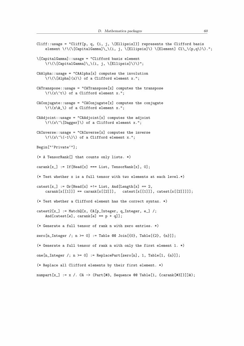
D. Mathematica packages 60

Cliff::usage = "Cliff[p, q, {i, j, \[Ellipsis]}] represents the Clifford basiselement \!\(\[CapitalGamma]\_\(i, j, \[Ellipsis]\) \[Element] Cl\_\(p,q\)\).";

\[CapitalGamma]::usage = "Clifford basis element\!\(\[CapitalGamma]\_\(i, j, \[Ellipsis]\)\)";

CAAlpha::usage = "CAAlpha[x] computes the involution\!\(\[Alpha](x)\) of a Clifford element x.";

CATranspose::usage = "CATranspose[x] computes the transpose\!\(x\^t\) of a Clifford element x.";

CAConjugate::usage = "CAConjugate[x] computes the conjugate\!\(x\&_\) of a Clifford element x.";

CAAdjoint::usage = "CAAdjoint[x] computes the adjoint\!\(x\^\[Dagger]\) of a Clifford element x.";

CAInverse::usage = "CAInverse[x] computes the inverse\!\(x\^\(-1\)\) of a Clifford element x.";

Begin["‘Private‘"];

(* A TensorRank[] that counts only lists. *)

carank[x_] := If[Head[x] === List, TensorRank[x], 0];

(* Test whether x is a full tensor with two elements at each level.*)

catest[x_] := Or[Head[x] =!= List, And[Length[x] == 2,carank[x[[1]]] == carank[x[[2]]], catest[x[[1]]], catest[x[[2]]]]];

(* Test whether a Clifford element has the correct syntax. *)

catest2[x_] := MatchQ[x, CA[p_Integer, q_Integer, e_] /;And[catest[e], carank[e] == p + q]];

(* Generate a full tensor of rank n with zero entries. *)

zero[n_Integer /; n >= 0] := Table @@ Join[{0}, Table[{2}, {n}]];

(* Generate a full tensor of rank n with only the first element 1. *)

one[n_Integer /; n >= 0] := ReplacePart[zero[n], 1, Table[1, {n}]];

(* Replace all Clifford elements by their first element. *)

numpart[x_] := x /. CA -> (Part[#3, Sequence @@ Table[1, {carank[#3]}]]&);

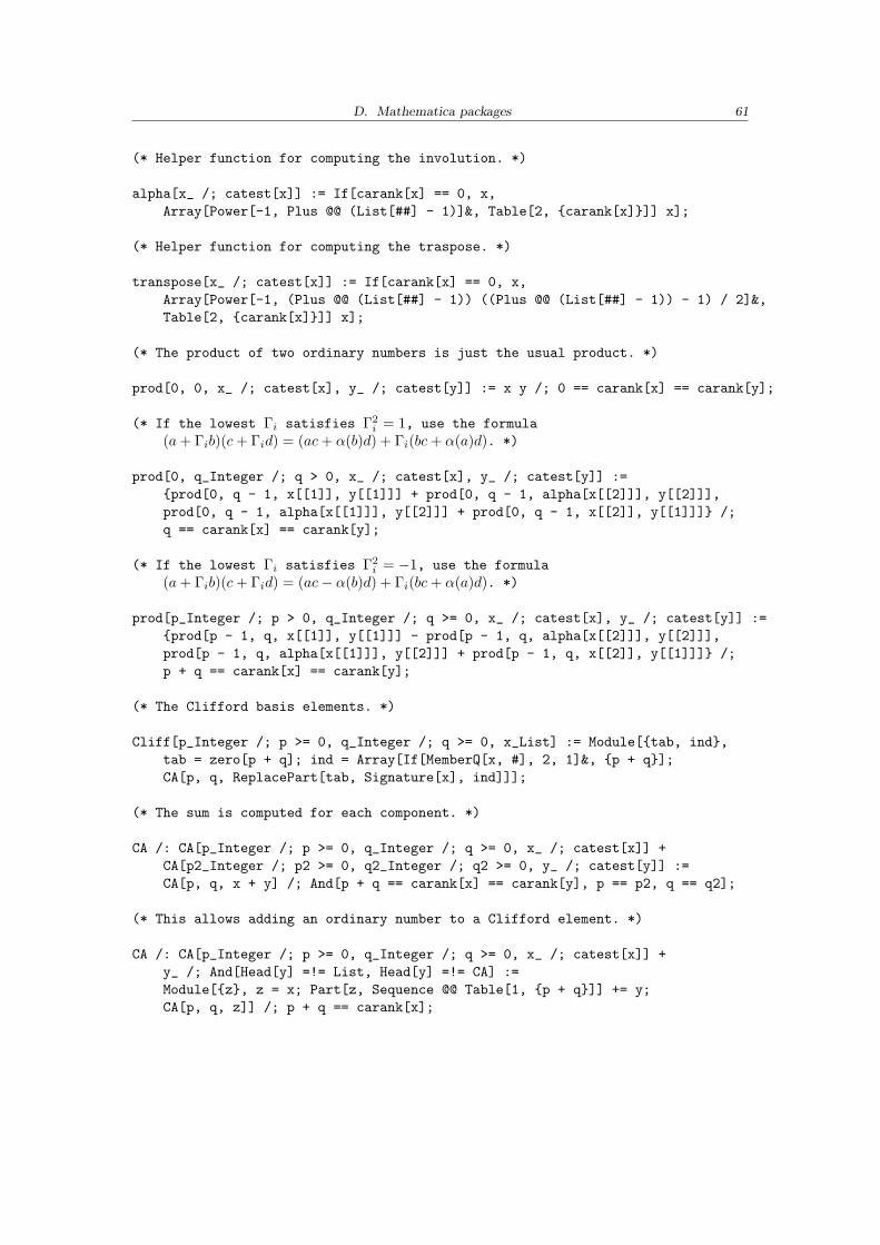
D. Mathematica packages 61

(* Helper function for computing the involution. *)

alpha[x_ /; catest[x]] := If[carank[x] == 0, x,Array[Power[-1, Plus @@ (List[##] - 1)]&, Table[2, {carank[x]}]] x];

(* Helper function for computing the traspose. *)

transpose[x_ /; catest[x]] := If[carank[x] == 0, x,Array[Power[-1, (Plus @@ (List[##] - 1)) ((Plus @@ (List[##] - 1)) - 1) / 2]&,Table[2, {carank[x]}]] x];

(* The product of two ordinary numbers is just the usual product. *)

prod[0, 0, x_ /; catest[x], y_ /; catest[y]] := x y /; 0 == carank[x] == carank[y];

(* If the lowest Γi satisfies Γ2i = 1, use the formula

(a+ Γib)(c+ Γid) = (ac+ α(b)d) + Γi(bc+ α(a)d). *)

prod[0, q_Integer /; q > 0, x_ /; catest[x], y_ /; catest[y]] :={prod[0, q - 1, x[[1]], y[[1]]] + prod[0, q - 1, alpha[x[[2]]], y[[2]]],prod[0, q - 1, alpha[x[[1]]], y[[2]]] + prod[0, q - 1, x[[2]], y[[1]]]} /;q == carank[x] == carank[y];

(* If the lowest Γi satisfies Γ2i = −1, use the formula

(a+ Γib)(c+ Γid) = (ac− α(b)d) + Γi(bc+ α(a)d). *)

prod[p_Integer /; p > 0, q_Integer /; q >= 0, x_ /; catest[x], y_ /; catest[y]] :={prod[p - 1, q, x[[1]], y[[1]]] - prod[p - 1, q, alpha[x[[2]]], y[[2]]],prod[p - 1, q, alpha[x[[1]]], y[[2]]] + prod[p - 1, q, x[[2]], y[[1]]]} /;p + q == carank[x] == carank[y];

(* The Clifford basis elements. *)

Cliff[p_Integer /; p >= 0, q_Integer /; q >= 0, x_List] := Module[{tab, ind},tab = zero[p + q]; ind = Array[If[MemberQ[x, #], 2, 1]&, {p + q}];CA[p, q, ReplacePart[tab, Signature[x], ind]]];

(* The sum is computed for each component. *)

CA /: CA[p_Integer /; p >= 0, q_Integer /; q >= 0, x_ /; catest[x]] +CA[p2_Integer /; p2 >= 0, q2_Integer /; q2 >= 0, y_ /; catest[y]] :=CA[p, q, x + y] /; And[p + q == carank[x] == carank[y], p == p2, q == q2];

(* This allows adding an ordinary number to a Clifford element. *)

CA /: CA[p_Integer /; p >= 0, q_Integer /; q >= 0, x_ /; catest[x]] +y_ /; And[Head[y] =!= List, Head[y] =!= CA] :=Module[{z}, z = x; Part[z, Sequence @@ Table[1, {p + q}]] += y;CA[p, q, z]] /; p + q == carank[x];

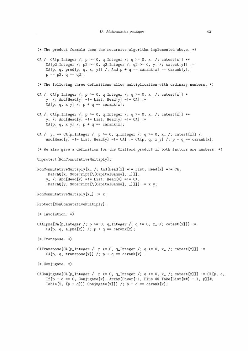
D. Mathematica packages 62

(* The product formula uses the recursive algorithm implemented above. *)

CA /: CA[p_Integer /; p >= 0, q_Integer /; q >= 0, x_ /; catest[x]] **CA[p2_Integer /; p2 >= 0, q2_Integer /; q2 >= 0, y_ /; catest[y]] :=CA[p, q, prod[p, q, x, y]] /; And[p + q == carank[x] == carank[y],p == p2, q == q2];

(* The following three definitions allow multiplication with ordinary numbers. *)

CA /: CA[p_Integer /; p >= 0, q_Integer /; q >= 0, x_ /; catest[x]] *y_ /; And[Head[y] =!= List, Head[y] =!= CA] :=CA[p, q, x y] /; p + q == carank[x];

CA /: CA[p_Integer /; p >= 0, q_Integer /; q >= 0, x_ /; catest[x]] **y_ /; And[Head[y] =!= List, Head[y] =!= CA] :=CA[p, q, x y] /; p + q == carank[x];

CA /: y_ ** CA[p_Integer /; p >= 0, q_Integer /; q >= 0, x_ /; catest[x]] /;And[Head[y] =!= List, Head[y] =!= CA] := CA[p, q, x y] /; p + q == carank[x];

(* We also give a definition for the Clifford product if both factors are numbers. *)

Unprotect[NonCommutativeMultiply];

NonCommutativeMultiply[x_ /; And[Head[x] =!= List, Head[x] =!= CA,!MatchQ[x, Subscript[\[CapitalGamma], _]]],y_ /; And[Head[y] =!= List, Head[y] =!= CA,!MatchQ[y, Subscript[\[CapitalGamma], _]]]] := x y;

NonCommutativeMultiply[x_] := x;

Protect[NonCommutativeMultiply];

(* Involution. *)

CAAlpha[CA[p_Integer /; p >= 0, q_Integer /; q >= 0, x_ /; catest[x]]] :=CA[p, q, alpha[x]] /; p + q == carank[x];

(* Transpose. *)

CATranspose[CA[p_Integer /; p >= 0, q_Integer /; q >= 0, x_ /; catest[x]]] :=CA[p, q, transpose[x]] /; p + q == carank[x];

(* Conjugate. *)

CAConjugate[CA[p_Integer /; p >= 0, q_Integer /; q >= 0, x_ /; catest[x]]] := CA[p, q,If[p + q == 0, Conjugate[x], Array[Power[-1, Plus @@ Take[List[##] - 1, p]]&,Table[2, {p + q}]] Conjugate[x]]] /; p + q == carank[x];

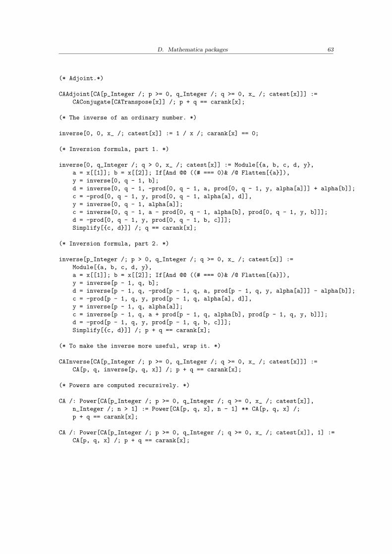
D. Mathematica packages 63

(* Adjoint.*)

CAAdjoint[CA[p_Integer /; p >= 0, q_Integer /; q >= 0, x_ /; catest[x]]] :=CAConjugate[CATranspose[x]] /; p + q == carank[x];

(* The inverse of an ordinary number. *)

inverse[0, 0, x_ /; catest[x]] := 1 / x /; carank[x] == 0;

(* Inversion formula, part 1. *)

inverse[0, q_Integer /; q > 0, x_ /; catest[x]] := Module[{a, b, c, d, y},a = x[[1]]; b = x[[2]]; If[And @@ ((# === 0)& /@ Flatten[{a}]),y = inverse[0, q - 1, b];d = inverse[0, q - 1, -prod[0, q - 1, a, prod[0, q - 1, y, alpha[a]]] + alpha[b]];c = -prod[0, q - 1, y, prod[0, q - 1, alpha[a], d]],y = inverse[0, q - 1, alpha[a]];c = inverse[0, q - 1, a - prod[0, q - 1, alpha[b], prod[0, q - 1, y, b]]];d = -prod[0, q - 1, y, prod[0, q - 1, b, c]]];Simplify[{c, d}]] /; q == carank[x];

(* Inversion formula, part 2. *)

inverse[p_Integer /; p > 0, q_Integer /; q >= 0, x_ /; catest[x]] :=Module[{a, b, c, d, y},a = x[[1]]; b = x[[2]]; If[And @@ ((# === 0)& /@ Flatten[{a}]),y = inverse[p - 1, q, b];d = inverse[p - 1, q, -prod[p - 1, q, a, prod[p - 1, q, y, alpha[a]]] - alpha[b]];c = -prod[p - 1, q, y, prod[p - 1, q, alpha[a], d]],y = inverse[p - 1, q, alpha[a]];c = inverse[p - 1, q, a + prod[p - 1, q, alpha[b], prod[p - 1, q, y, b]]];d = -prod[p - 1, q, y, prod[p - 1, q, b, c]]];Simplify[{c, d}]] /; p + q == carank[x];

(* To make the inverse more useful, wrap it. *)

CAInverse[CA[p_Integer /; p >= 0, q_Integer /; q >= 0, x_ /; catest[x]]] :=CA[p, q, inverse[p, q, x]] /; p + q == carank[x];

(* Powers are computed recursively. *)

CA /: Power[CA[p_Integer /; p >= 0, q_Integer /; q >= 0, x_ /; catest[x]],n_Integer /; n > 1] := Power[CA[p, q, x], n - 1] ** CA[p, q, x] /;p + q == carank[x];

CA /: Power[CA[p_Integer /; p >= 0, q_Integer /; q >= 0, x_ /; catest[x]], 1] :=CA[p, q, x] /; p + q == carank[x];

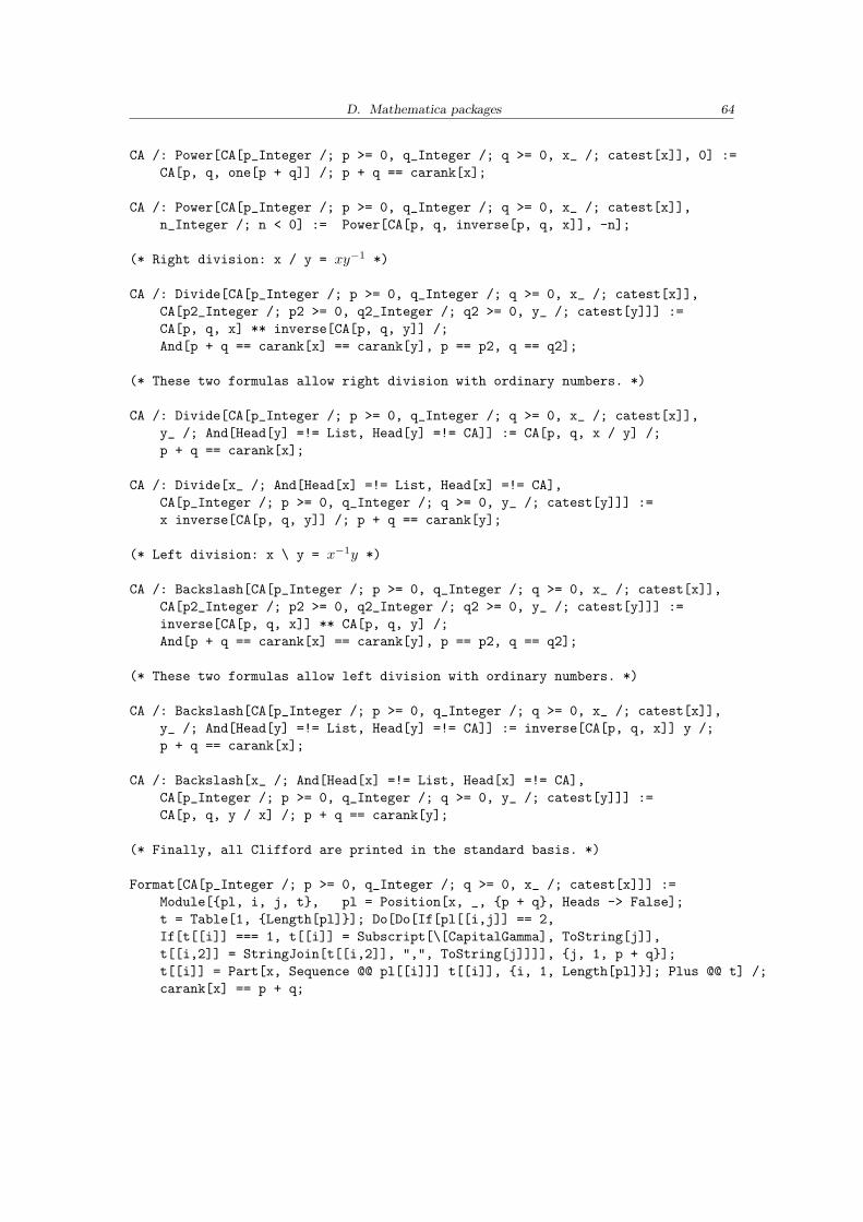
D. Mathematica packages 64

CA /: Power[CA[p_Integer /; p >= 0, q_Integer /; q >= 0, x_ /; catest[x]], 0] :=CA[p, q, one[p + q]] /; p + q == carank[x];

CA /: Power[CA[p_Integer /; p >= 0, q_Integer /; q >= 0, x_ /; catest[x]],n_Integer /; n < 0] := Power[CA[p, q, inverse[p, q, x]], -n];

(* Right division: x / y = xy−1 *)

CA /: Divide[CA[p_Integer /; p >= 0, q_Integer /; q >= 0, x_ /; catest[x]],CA[p2_Integer /; p2 >= 0, q2_Integer /; q2 >= 0, y_ /; catest[y]]] :=CA[p, q, x] ** inverse[CA[p, q, y]] /;And[p + q == carank[x] == carank[y], p == p2, q == q2];

(* These two formulas allow right division with ordinary numbers. *)

CA /: Divide[CA[p_Integer /; p >= 0, q_Integer /; q >= 0, x_ /; catest[x]],y_ /; And[Head[y] =!= List, Head[y] =!= CA]] := CA[p, q, x / y] /;p + q == carank[x];

CA /: Divide[x_ /; And[Head[x] =!= List, Head[x] =!= CA],CA[p_Integer /; p >= 0, q_Integer /; q >= 0, y_ /; catest[y]]] :=x inverse[CA[p, q, y]] /; p + q == carank[y];

(* Left division: x \ y = x−1y *)

CA /: Backslash[CA[p_Integer /; p >= 0, q_Integer /; q >= 0, x_ /; catest[x]],CA[p2_Integer /; p2 >= 0, q2_Integer /; q2 >= 0, y_ /; catest[y]]] :=inverse[CA[p, q, x]] ** CA[p, q, y] /;And[p + q == carank[x] == carank[y], p == p2, q == q2];

(* These two formulas allow left division with ordinary numbers. *)

CA /: Backslash[CA[p_Integer /; p >= 0, q_Integer /; q >= 0, x_ /; catest[x]],y_ /; And[Head[y] =!= List, Head[y] =!= CA]] := inverse[CA[p, q, x]] y /;p + q == carank[x];

CA /: Backslash[x_ /; And[Head[x] =!= List, Head[x] =!= CA],CA[p_Integer /; p >= 0, q_Integer /; q >= 0, y_ /; catest[y]]] :=CA[p, q, y / x] /; p + q == carank[y];

(* Finally, all Clifford are printed in the standard basis. *)

Format[CA[p_Integer /; p >= 0, q_Integer /; q >= 0, x_ /; catest[x]]] :=Module[{pl, i, j, t}, pl = Position[x, _, {p + q}, Heads -> False];t = Table[1, {Length[pl]}]; Do[Do[If[pl[[i,j]] == 2,If[t[[i]] === 1, t[[i]] = Subscript[\[CapitalGamma], ToString[j]],t[[i,2]] = StringJoin[t[[i,2]], ",", ToString[j]]]], {j, 1, p + q}];t[[i]] = Part[x, Sequence @@ pl[[i]]] t[[i]], {i, 1, Length[pl]}]; Plus @@ t] /;carank[x] == p + q;

D. Mathematica packages 65

End[];EndPackage[];

BIBLIOGRAPHY

[1] G. Veneziano, Construction of a crossing - symmetric, regge behaved amplitude for linearlyrising trajectories, Nuovo. Cim. A57 (1968) 190–197.

[2] G. ’t Hooft, A planar diagram theory for strong interactions, Nucl. Phys. B72 (1974) 461.

[3] J. M. Maldacena, The large n limit of superconformal field theories and supergravity, Adv.Theor. Math. Phys. 2 (1998) 231–252, [hep-th/9711200].

[4] O. Aharony, S. S. Gubser, J. M. Maldacena, H. Ooguri, and Y. Oz, Large n field theories,string theory and gravity, Phys. Rept. 323 (2000) 183–386, [hep-th/9905111].

[5] J. Plefka, Spinning strings and integrable spin chains in the AdS/CFT correspondence,hep-th/0507136.

[6] G. Gotz, T. Quella, and V. Schomerus, The wznw model on psu(1,1—2), hep-th/0610070.

[7] V. Schomerus, Non-compact string backgrounds and non-rational cft, Phys. Rept. 431(2006) 39–86, [hep-th/0509155].

[8] S. S. Gubser, I. R. Klebanov, and A. M. Polyakov, A semi-classical limit of thegauge/string correspondence, Nucl. Phys. B636 (2002) 99–114, [hep-th/0204051].

[9] A. A. Tseytlin, Semiclassical strings in ads(5) x s**5 and scalar operators in n = 4 symtheory, Comptes Rendus Physique 5 (2004) 1049–1059, [hep-th/0407218].

[10] V. A. Kazakov, A. Marshakov, J. A. Minahan, and K. Zarembo, Classical / quantumintegrability in AdS/CFT, JHEP 05 (2004) 024, [hep-th/0402207].

[11] M. Karbach and G. Muller, Introduction to the bethe ansatz i, Computers in Physics 11(1997) 36, [cond-mat/9809162].

[12] M. Karbach, K. Hu, and G. Muller, Introduction to the bethe ansatz ii, cond-mat/9809163.

[13] M. Karbach, K. Hu, and G. Muller, Introduction to the bethe ansatz iii,cond-mat/0008018.

[14] N. Beisert, V. A. Kazakov, and K. Sakai, Algebraic curve for the so(6) sector of ads/cft,Commun. Math. Phys. 263 (2006) 611–657, [hep-th/0410253].

[15] S. Schafer-Nameki, The algebraic curve of 1-loop planar N = 4 SYM, Nucl. Phys. B714(2005) 3–29, [hep-th/0412254].

[16] D. Berenstein, J. M. Maldacena, and H. Nastase, Strings in flat space and pp waves fromN = 4 super Yang Mills, JHEP 04 (2002) 013, [hep-th/0202021].

Bibliography 67

[17] R. Penrose, Any spacetime has a plane wave as a limit, in Differential geometry andrelativity, pp. 271–275. Reidel, Dordrecht, 1976.

[18] R. R. Metsaev and A. A. Tseytlin, Superparticle and superstring in ads(3) x s(3) ramond-ramond background in light-cone gauge, J. Math. Phys. 42 (2001) 2987–3014,[hep-th/0011191].

[19] I. Bena, J. Polchinski, and R. Roiban, Hidden symmetries of the AdS(5) x S(5)superstring, Phys. Rev. D69 (2004) 046002, [hep-th/0305116].

[20] B. Chen, Y.-L. He, P. Zhang, and X.-C. Song, Flat currents of the green-schwarzsuperstrings in ads(5) x s**1 and ads(3) x s**3 backgrounds, Phys. Rev. D71 (2005)086007, [hep-th/0503089].

[21] I. Y. Park, A. Tirziu, and A. A. Tseytlin, Spinning strings in AdS(5) x S(5): One-loopcorrection to energy in SL(2) sector, JHEP 03 (2005) 013, [hep-th/0501203].

[22] S. Frolov and A. A. Tseytlin, Rotating string solutions: AdS/CFT duality in non-supersymmetric sectors, Phys. Lett. B570 (2003) 96–104, [hep-th/0306143].

[23] S. Schafer-Nameki, M. Zamaklar, and K. Zarembo, Quantum corrections to spinningstrings in AdS(5) x S(5) and Bethe ansatz: A comparative study, JHEP 09 (2005) 051,[hep-th/0507189].

[24] N. Beisert and A. A. Tseytlin, On quantum corrections to spinning strings and Betheequations, Phys. Lett. B629 (2005) 102–110, [hep-th/0509084].

[25] S. Schafer-Nameki and M. Zamaklar, Stringy sums and corrections to the quantum stringBethe ansatz, JHEP 10 (2005) 044, [hep-th/0509096].

[26] S. Schafer-Nameki, Exact expressions for quantum corrections to spinning strings,hep-th/0602214.

[27] S. Schafer-Nameki, M. Zamaklar, and K. Zarembo, How accurate is the quantum stringbethe ansatz?, JHEP 12 (2006) 020, [hep-th/0610250].

ERKLARUNG GEMAß DIPLOMPRUFUNGSORDNUNG

Ich versichere, diese Arbeit selbststandig und nur unter Benutzung der angegebenen Hilfsmittelund Quellen angefertigt zu haben. Ich gestatte die Veroffentlichung dieser Arbeit.

Manuel Hohmann

DANKSAGUNG

Ich danke Herrn Prof. Dr. Jan Louis (Universitat Hamburg) fur den Vorschlag des Themas unddie hilfreichen, beratenden Gesprache.Des weiteren danke ich Frau Dr. Sakura Schafer-Nameki (California Institute of Technology,Pasadena) fur die intensive Betreuung meiner Diplomarbeit auch aus der Ferne und die zahlre-ichen Diskussionen, Hilfestellungen und Korrekturen.Mein Dank gilt weiterhin Herrn Florian Schwennsen (Universitat Hamburg) fur die Hilfe bei derLosung von Computerproblemen, die mir bei der Anfertigung dieser Arbeit im Wege standen.