Embed Size (px)
Citation preview
i
Three Essays on Behavioral Aspects in Accounting and Economics
Inauguraldissertation zur
Erlangung des Doktorgrades der
Wirtschafts- und Sozialwissenschaftlichen Fakultät der
Universität zu Köln
2015
vorgelegt von
Diplom-Kaufmann Timo Gores
aus
Köln

ii
Referent: Univ.-Prof. Dr. Carsten Homburg
Korreferent: Univ.-Prof. Dr. Michael Overesch
Tag der Promotion: 02.06.2015

iii
Danksagungen
Die vorliegende Dissertation entstand während meiner Zeit als Promotionsstudent an der
Cologne Graduate School in Management, Economics and Social Sciences der Universität zu
Köln. An dieser Stelle möchte ich mich bei den Personen bedanken, die mich während der
Promotionszeit unterstützt und somit zum Gelingen meines Promotionsvorhabens
beigetragen haben.
An erster Stelle danke ich meinem Doktorvater Herrn Professor Homburg für die
umfangreiche Unterstützung, die ich im Rahmen der Erstellung dieser Arbeit erfahren habe.
In diesem Zusammenhang bin ich außerdem dankbar dafür, dass er mir die Freiheit gelassen
hat, die notwendig war, um meine Forschungsinteressen verwirklichen zu können. Ebenso
bedanke ich mich bei Herrn Professor Overesch für die Erstellung des Zweitgutachtens,
sowie bei Herrn Professor Kuntz für die Leitung der Disputation. Zu großem Dank bin ich
auch Frau Juniorprofessorin Julia Nasev verpflichtet, die mein Promotionsvorhaben von
Anfang an begleitet und ebenfalls mit wertvollem Feedback unterstützt hat.
Außerdem möchte ich mich bei der Cologne Graduate School in Management, Economics
and Social Sciences für die finanzielle Unterstützung bedanken, die dieses
Promotionsvorhaben erst ermöglicht hat. Ich habe die dortige Arbeitsatmosphäre als sehr
angenehm und überaus inspirierend empfunden. Hieran hatten neben Frau Doktor Weiler
natürlich auch meine zahlreichen Kollegen großen Anteil. Darüberhinaus danke ich meinen
Freunden für ihre moralische Unterstützung. Insbesondere möchte ich mich bei Christoph,
Holger, Michael und Stefan dafür bedanken, dass sie immer ein offenes Ohr für meine
Belange hatten. Zu guter Letzt danke ich meinen Eltern und meinen beiden Brüdern Nicolai
und David für ihre kontinuierliche Unterstützung, die für mich, und damit auch für diese
Arbeit, von unermesslichem Wert war.
iv
Contents
List%of%Figures%.................................................................................................................................%vi!
List%of%Tables%..................................................................................................................................%vii!
1! Introduction%..............................................................................................................................%1!
2! Managerial%Overconfidence%and%Cost%Stickiness%........................................................%11!
2.1! Introduction%..................................................................................................................................%11!
2.2! Hypothesis%Development%.........................................................................................................%16!
2.3! Research%Design%..........................................................................................................................%19!
2.3.1! Sample!Selection!....................................................................................................................................!19!
2.3.2! Overconfidence!.......................................................................................................................................!20!
2.3.3! Cost!Stickiness!Measurement!...........................................................................................................!22!
2.3.4! Model!Specification!...............................................................................................................................!23!
2.4! Results%............................................................................................................................................%25!
2.4.1! Descriptive!Statistics!............................................................................................................................!25!
2.4.2! Test!of!H1!..................................................................................................................................................!27!
2.4.3! Addressing!Alternative!Explanations!for!H1!.............................................................................!30!
2.4.4! Robustness!Checks!for!H1!..................................................................................................................!37!
2.4.5! Test!of!H2!..................................................................................................................................................!39!
2.5! Conclusion%.....................................................................................................................................%46!
3! The%Impact%of%Investor%Sentiment%on%Operating%Expenditure%–%a%Catering%
Perspective%.....................................................................................................................................%49!
3.1! Introduction%..................................................................................................................................%49!
3.2! Hypothesis%Development%and%Related%Literature%...........................................................%53!
3.2.1! Investor!Sentiment!................................................................................................................................!53!
3.2.2! Investor!Sentiment!and!Operating!Expenditure!......................................................................!56!
3.3! Research%Design%..........................................................................................................................%60!
3.3.1! Sample!Selection!....................................................................................................................................!60!
3.3.2! Investor!Sentiment!Measurement!..................................................................................................!60!
3.3.3! Research!Design!of!H1!.........................................................................................................................!63!
3.3.4! Research!Design!of!H2!.........................................................................................................................!65!
3.4! Results%............................................................................................................................................%71!
v
3.4.1! Test!of!H1!..................................................................................................................................................!71!
3.4.2! CrossLSectional!Analyses!....................................................................................................................!72!
3.4.3! Test!of!H2!..................................................................................................................................................!80!
3.4.4! Alternative!Explanations!....................................................................................................................!82!
3.4.5! Robustness!...............................................................................................................................................!85!
3.5! Conclusion%.....................................................................................................................................%87!
4! Attention,%Media%and%Fuel%Efficiency%..............................................................................%89!
4.1! Introduction%..................................................................................................................................%89!
4.2! Hybrid%Vehicle%Market%and%Consumer%Attitudes%.............................................................%93!
4.3! Data%..................................................................................................................................................%95!
4.4! What%Drives%the%Attention%Devoted%to%Hybrid%Vehicles?%............................................%100!
4.5! Attention%and%Hybrid%Vehicle%Purchases%..........................................................................%113!
4.6! Conclusion%...................................................................................................................................%119!
5! Conclusion%............................................................................................................................%121!
6! Appendix%...............................................................................................................................%125!
References%...................................................................................................................................%129!

vi
List of Figures
Figure 4.1: Gasoline Price, Media Coverage and Attention Devoted to Hybrid Vehicles
Figure 4.2: Gasoline Price, Media Coverage and Attention Devoted to Fuel Economy
Figure 4.3: Gasoline Price, Attention and Registrations of Hybrid Vehicles
vii
List of Tables
Table 2.1: Descriptive Statistics
Table 2.2: Correlations
Table 2.3: The Effect of Managerial Overconfidence on Cost Stickiness
Table 2.4: Estimating the Effect of Managerial Overconfidence on Cost Stickiness
Controlling for Investment
Table 2.5: Estimating the Effect of Managerial Overconfidence on Cost Stickiness
Conditional on Prior Sales Changes (BBCM Framework)
Table 2.6: Future Earnings, Cost Stickiness and Managerial Overconfidence
Table 2.7: Variable Definitions
Table 3.1: Variable Definitions
Table 3.2: Descriptive Statistics
Table 3.3: Correlations
Table 3.4: The Association between Operating Expenditure and Investor Sentiment
Table 3.5: The Association between Operating Expenditure and Investor Sentiment
Differentiating between High and Low SG&A Future Value Creation
Table 3.6: The Association between Operating Expenditure and Investor Sentiment
Differentiating between High and Low Investor Trading Volume
Table 3.7: The Association between Operating Expenditure and Investor Sentiment
Differentiating between High and Low Stock Return Volatility
Table 3.8: The Moderating Impact of Earnings Targets on the Association between
Operating Expenditure and Investor Sentiment
Table 3.9: The Association between Operating Expenditure and Investor Sentiment
Controlling for Investment
viii
Table 3.10: The Association between Operating Expenditure and Investor Sentiment
Controlling for Managerial Optimism
Table 4.1: Average Monthly US Google Search Volume for Fuel Efficiency Related
Terms
Table 4.2: List of Newspapers Used in the Analysis
Table 4.3: Hybrid Vehicle Technology and Attention
Table 4.4: Fuel Economy Technology and Attention
Table 4.5: Hybrid Vehicle Registrations and Attention
Table 4.6: Hybrid Technology’s Market Share and Attention
Table A.1: LexisNexis Database Search Queries for all Newspapers
Table A.2: Summary Statistics
1
1 Introduction
The core of this thesis is based on three essays. While the individual parts can be read
independently, all three essays are connected by taking on a behavioral view on accounting
and economics. Defined loosely, behavioral research draws on insights from cognitive
psychology and attempts to narrow the gap between human behavior and behavior in
economic models (Kahneman 2003). It goes back at least to Simon (1957), who coins the
term of bounded rationality to describe behavior that deviates from perfect rationality.
DellaVigna and Pollet (2009) organize behavioral research around the following three
building blocks. The first block deals with nonstandard preferences, suggesting that
individuals (i) make decisions that are time-inconsistent, (ii) evaluate gains and losses
relative to reference points, (iii) or care about the welfare of others. The second block draws
on psychological evidence indicating that belief formation deviates from perfect rationality in
that it can be affected by cognitive biases (nonstandard beliefs). And, third, given preferences
and beliefs, research on nonstandard decision making shows that individuals use simple
heuristics to solve complex problems or are able to process only part of the available
information due to constraints such as limited attention.
The first two essays of this thesis contribute to the field of nonstandard beliefs. More
specifically, the second chapter allows managerial behavior to deviate from perfect
rationality, examining the influence of managerial overconfidence on cost behavior. Chapter
three draws on the concept of investor sentiment and is concerned with real consequences
that arise from less than perfectly rational investor behavior. The fourth chapter is related to
the field of nonstandard decision making. Turning to consumer behavior, it applies the
concept of limited attention to the field of behavioral energy economics, examining which
factors drive consumers’ attention devoted to fuel-efficient technologies. In the following, I
2
provide some background information on each chapter and present key results.
In recent years, much work has been devoted to understanding the consequences arising
from managerial overconfidence. 1 Research in accounting associates two biases with
overconfidence (Libby and Rennekamp 2012; Hribar and Yang 2013). The first bias is
referred to as miscalibration in the psychology literature (Fischhoff, Slovic, and Lichtenstein
1977; Moore 1977; Oskamp 1965). Miscalibration describes the tendency to overestimate the
precision of the own knowledge (Hirshleifer 2001; Odean 1998), which is modeled as
underestimation of variance in the behavioral finance literature (Baker and Wurgler 2011).
The second bias associated with overconfidence is referred to as dispositional optimism in the
psychology literature (Scheier and Carver 1985; Taylor and Brown 1988; Weinstein 1980).
Dispositional optimism, a stable character trait, describes the tendency to hold generalized
favorable expectations about future events. In the behavioral accounting and finance
literature, dispositional optimism is defined as overestimation of the mean of uncertain
outcomes (Baker and Wurgler 2011).
While research in psychology documents that overconfidence is widespread and affects a
variety of decisions, two questions arise. First, why do individuals not learn from past
mistakes and, hence, overcome biases? Sharot, Korn, and Dolan (2011) document an
asymmetry in belief updating. More specifically, they show that individuals learn more
strongly from pleasant or confirming information than from unpleasant information that
conflicts with or challenges prior beliefs. Hence, Sharot et al. (2011) provide evidence for
what can be described as selective updating. In addition, Johnson and Fowler (2011) make an
evolutionary argument explaining why individuals may be overconfident. Johnson and
Fowler (2011) model a situation in which two contestants compete about a valuable resource,
assuming that both contestants have imperfect information about each other’s capabilities.
1 See, for example, Ahmed and Duellman (2013), Hilary and Hsu (2011), Hirshleifer, Low, and Teoh (2012), Libby and Rennekamp (2012), Malmendier and Tate (2005, 2008), or Schrand and Zechman (2012).
3
Their evidence suggests that overconfidence may prevail in many environments because
overconfident individuals will be more likely to claim resources than their rational (or
underconfident) counterparts who will back off more frequently. As long as the resource at
stake exceeds the cost of competing for it, overconfidence may be evolutionary stable,
contrary to intuition that natural selection works against individuals with biased beliefs.
Second, does the evidence on overconfidence from psychological studies extend to
corporate executives? Goel and Thakor (2008) address this question, arguing that it is more
likely that an overconfident than a non-overconfident manager gets appointed as CEO. Goel
and Thakor (2008) argue that promotion depends on past performance, which, in turn,
depends on the amount of risk taken by managers. Underestimation of risk induces
overconfident managers to choose riskier projects than non-overconfident managers, thereby
increasing the variance of their performance. Hence, there is reason to believe that
overconfident managers will be over-represented in the high-performance group from which
board of directors eventually choose a CEO. In addition, Malmendier and Tate (2005) argue
that factors that predict overconfidence are particularly likely to be present in the context of
executive decision making, e.g., abstract reference points, illusion of control, and
commitment (also see Camerer and Malmendier 2007). Survey evidence confirms the
arguments made in these studies. Ben-David, Graham, and Harvey (2012) conduct a survey
with top financial executives, documenting both dispositional optimism and miscalibration.
Similarly, the evidence in Graham, Harvey, and Puri (2013) shows that executives are more
optimistic than the lay population. Finally, Libby and Rennekamp (2012, p. 200) conduct
interviews with experienced managers who “strongly agree that managers are, in general,
overconfident”.
The second chapter of this thesis, which is based on a study with Clara Xiaoling Chen and
4
Julia Nasev2, questions if managerial overconfidence affects cost behavior. In an influential
study, Anderson, Banker, and Janakiraman (2003) document that costs are sticky. That is,
variable costs decline less following a decline in activity than they increase following an
increase in activity of equal magnitude. The concept of cost stickiness highlights the role of
managerial discretion in the process of resource adjustment, which contrasts with traditional
cost models, assuming that variable costs mechanically respond to changes in activity
(Anderson et al. 2003).
Building on the psychology literature and its application in behavioral accounting and
finance, we expect a positive association between managerial overconfidence and cost
stickiness. Prior literature documents that overconfident managers overestimate future
demand (Malmendier, Tate, and Yan 2011), and that demand expectations are key to the
concept of cost stickiness (Banker et al. 2014). We, therefore, expect that overconfident
managers assess reductions in demand as less permanent than their non-overconfident
counterparts. If overconfident managers expect demand to restore in the next period, they
should be more likely to keep unutilized resources following a decline in demand, which
should increase cost stickiness. We further predict that cost stickiness driven by managerial
overconfidence should be less efficient than cost stickiness driven by economic reasons. If
this is the case, we expect cost stickiness driven by managerial overconfidence to negatively
affect future firm performance compared to cost stickiness that is not driven by
overconfidence.
To test our first prediction, we use a sample of 20,615 firm-years from the intersection of
ExecuComp, CRSP, and Compustat over the period 1992-2011. Consistent with our
expectation, we find that cost stickiness increases with managerial overconfidence. More
specifically, our results show that overconfident CEOs are more likely to keep excess
2 Chen, Gores and Nasev, 2013, Managerial Overconfidence and Cost Stickiness, Working Paper.
5
resources than non-overconfident CEOs when sales decrease but overconfident CEOs do not
build up excess resources when sales increase. The test of our second prediction is based on
the fundamental analysis literature (Abarbanell and Bushee 1997; Anderson et al. 2007; Lev
and Thiagarajan 1993). Confirming our expectation, we find evidence indicating that cost
behavior driven by managerial overconfidence is suboptimal. Collectively, the results of our
analyses show that managerial overconfidence affects cost behavior.
The third chapter of this thesis, based on a study with Carsten Homburg and Julia Nasev3,
builds on the concept of investor sentiment. It grounds on three assumptions. The first
assumption differentiates between two types of investors: Rational arbitrageurs and irrational
or noise traders subject to sentiment. Baker and Wurgler (2007, p.127) define investor
sentiment as “a belief about future cash flows and investment risks that is not justified by the
facts at hand”. This definition builds on prior literature offering plenty of examples
concerning investor behavior that is difficult to reconcile with perfect rationality. Shiller
(1984), for instance, argues that stock prices are affected by social movements. Black (1986)
uses the term noise traders to describe trading that is based on noise as opposed to news.
Other studies document that overconfidence (Barber and Odean 2001), conservatism and
representativeness (Barberis, Shleifer, and Vishny 1998), or sensation-seeking (Grinblatt and
Keloharju 2009) affect trading or stock prices.4
The second assumption is concerned with the limits of arbitrage. For one, arbitrage may be
limited due to implementation costs or short sale constraints (Miller 1977). To the extent that
it is not possible to find perfect substitutes, arbitrage additionally requires bearing of
fundamental risk (Barberis and Thaler 2003). Most importantly, however, a combination of
noise trader risk and agency problems may limit the effectiveness of arbitrage (De Long et al.
1990; Shleifer and Vishny 1997). Noise trader risk can limit arbitrage because arbitrageurs 3 Gores, Homburg, and Nasev, 2015, The Impact of Investor Sentiment on Operating Expenditure – a Catering Perspective, Working Paper. 4 See Barberis and Thaler (2003) or Hirshleifer (2001) for surveys of the literature.
6
are exposed to unpredictable fluctuations in noise traders’ future opinions (De Long et al.
1990). If an arbitrageur, for example, shorts a stock that is overpriced he has to bear the risk
that – in the short term – noise traders get even more bullish and push the price even further
away from its intrinsic value (De Long et al. 1990). This implies that arbitrageurs have to be
able and willing to bear potentially steep short-term losses. This insight is important because
arbitrageurs likely do not invest their own money but that of their capital lenders (Shleifer
and Vishny 1997). In absent of perfect information, it is reasonable to assume that capital
lenders will try to infer the ability or skill of their investors based on the returns they generate
(Barberis and Thaler 2003). Recognizing that bad performance may motivate capital lenders
to withdraw their funds, arbitrageurs may decide to not bet against mispricing given that
arbitrage can deteriorate short-term performance. Hence, a separation of “brains and
resources” may limit the effectiveness of arbitrage (Shleifer and Vishny 1997, p.36).
Finally, noise traders’ misperceptions have to be systematic. Kumar and Lee (2006)
provide empirical support for this assumption. Using a large-scale data set of retail investor
transactions, they show that retail trading is systematically correlated. Moreover, Kumar and
Lee (2006) find that these trades more strongly affect those stocks that are more likely to be
held by retail investors. Hence, there is evidence supporting the assumption that retail
investors trade in concert.
These assumptions imply that noise traders can affect asset prices. Several studies support
this prediction. Baker and Wurgler (2006, 2007), for example, document that stocks that are
more likely to be held by noise traders realize lower returns than stocks that are less likely to
be held by noise traders following periods of high sentiment. Other studies reach similar
conclusions (Brown and Cliff 2005; Lemmon and Portniaguina 2006).
Building on this evidence, chapter three is concerned with real implications of investor
sentiment. The so-called catering theory explains how noise trading can affect corporate
7
policies. In essence, the theory predicts that managers can boost the current stock price if they
adjust their corporate policies to the misperceptions of noise traders (Baker and Wurgler
2011; Stein 1996).5 In this study, we examine the association between investor sentiment and
operating expenditure. We expect there are two opposing channels linking investor sentiment
and operating expenditure. First, prior literature argues that noise traders have optimistically
biased expectations about future cash flows in periods of high sentiment (Baker and Wurgler
2006, 2007; Stein 1996). Such overestimation of investment opportunities may create
pressure on managers’ investment behavior. Given that operating expenditure such as
research and development (Eberhart, Maxwell, and Siddique 2004; Lev and Sougiannis 1996;
Sougiannis 1994), advertising (Chan, Lakonishok, and Sougiannis 2001; Hirschey and
Weygandt 1985; Madden, Fehle, and Fournier 2006), and selling, general and administrative
(SG&A) resources (Anderson et al. 2007; Banker, Huang, and Natarajan 2011; Tronconi and
Marzetti 2011) has long-term value-relevance, we argue that managers will cater to investors’
optimistic investment expectations by overspending on operating expenditure in periods of
high relative to periods of average sentiment.
Second, prior literature documents that investors’ have inflated earnings expectations in
periods of high sentiment (Hribar and McInnis 2012; Mian and Sankaraguruswamy 2012;
Seybert and Yang 2012). Literature on real earnings management shows that operating
expenditures, such as research and development (R&D) expenses, are easy targets that can be
manipulated to meet earnings expectations (Baber, Fairfield, and Haggard 1991; Burgstahler
and Dichev 1997; Roychowdhury 2006). Hence, managers may alternatively reduce spending
on operating expenditure to meet earnings targets. We, therefore, argue that managers face a
trade-off between catering to noise traders’ investment and earnings expectations. While we
expect to observe a positive association for firms that do not face earnings targets, we argue 5 The theory implicitly assumes that managers are able to recognize investor sentiment. Hribar and Quinn (2013) provide support for this assumption, documenting that managers’ trades are negatively associated with investor sentiment.
8
the association between operating expenditure and investor sentiment should be less
pronounced or may even turn negative for those firms that have incentives to meet earnings.
Empirically, we find support for our predictions. Our results suggests that managers
increase spending on R&D expenditure, advertisement and SG&A resources as means of
catering to noise traders’ misperceptions. Results from further analyses indicate that (i)
catering per SG&A resources increases as the value-relevance of these resources increases,
(ii) catering is more pronounced for those firms that are more strongly affected by investor
sentiment, and (iii) catering increases as managers’ horizons decrease. Finally, our results
suggest that managers refrain from overspending on operating expenditure when facing
earnings targets, indicating a trade-off between catering to noise traders’ investment and
earnings expectations. Taken together, our results show that investor sentiment affects
spending on operating expenditure.
The fourth chapter, joint work with Stefan Thoenes6, builds on the capacity model of
attention following Kahneman (1973). This chapter takes on a behavioral view on energy
economics, attempting to contribute to our understanding of when and why consumers invest
in fuel-efficient technologies such as hybrid vehicles. Answering this question is important
because increasing the fuel-efficiency of vehicles is considered as a promising way to reduce
greenhouse gas emissions (Enkvist, Nauclér, and Rosander 2007). While fuel-efficient
technologies have higher initial purchasing prices, the advanced technology results in lower
energy consumption and, therefore, lower fuel costs over the lifetime of the investment.
Hence, just like any other investment, the profitability of fuel-efficient technologies should
be evaluated by computing net present values of future cash flows, which – in this case –
depend on future gasoline prices or fuel costs. Allcott (2011), however, presents survey
evidence indicating that about 40% of US consumers do not think about fuel costs at all when
6 Thoenes and Gores, 2012, Attention, Media and Fuel Efficiency, Working Paper.
9
purchasing a vehicle. Similarly, Turrentine and Kurani (2007) document that consumers are
not able to thoroughly assess fuel costs when purchasing automobiles. Given these results, it
becomes an important question to understand how consumers make their purchase decisions.
The fourth chapter of this thesis relies on the concept of limited attention to analyze
consumers’ decision-making. The capacity model of attention following Kahneman (1973)
views attention as a resource that is necessary to process information. It further assumes that
the supply of attention is limited, suggesting that attention is a scarce resource that has to be
allocated among alternative or competing activities. The concept of limited attention, hence,
implies that individuals are limited in their ability of processing information. In this regard,
the model differs from neo-classical economics which implicitly assumes that individuals are
able to process all information (DellaVigna and Pollet 2009). The framework further suggests
that individuals are more likely to process salient information that grabs their attention.
Barber and Odean (2008), for example, show that individual investors are net buyers of
stocks that are excessively covered in the news or stock that experience large one day returns.
Similarly, Yuan (2011) shows that attention-grabbing events, such as record levels of the
Dow Jones index or prominent media coverage, i.e., front page articles about the stock
market, affect trading behavior of individual investors.
We expect two channels to alter the attention that consumers devote to hybrid vehicles.
First, we expect that changes in gasoline prices affect consumers’ attention because changes
in gasoline prices determine the profitability of investments in fuel-efficient technologies. In
this regard, we additionally focus on new or all time record prices. Tversky and Kahneman
(1991) suggest that gains and losses are evaluated relative to reference points. We assume
that consumers regard prior record prices as reference points. Price increases that exceed
existing reference points may be perceived as losses, resulting in a stronger reaction because
of loss aversion. Second, we expect that media coverage on topics related to hybrid vehicles
10
and gasoline costs affects consumers’ attention, assuming that media has the potential to
influence which topics are perceived as important McCombs and Shaw (1972).
To test our prediction, we construct a weekly panel data set for 19 metropolitan areas in
the United States. For each metro area, we obtain Google search queries related to hybrid
vehicles as our measure of consumer attention. We further collect data on local newspaper
coverage related to hybrid vehicles for each metro area. Empirically, we relate consumer
attention to local newspaper coverage, gasoline prices, record prices and national television
and national newspaper reports. Consistent with our expectation, we find that changes in
gasoline prices, unprecedented record prices, and local newspaper coverage affect the
attention that consumers devote to hybrid vehicles.
Our results, thus, document the presence of limited attention in the context of long-lived
consumer goods. We thereby extend prior literature, which has primarily focused on
consequences arising from limited attention, by documenting which factors likely influence
attention. Our results, therefore, should be of interest for policy makers interested in
increasing the adoption of fuel-efficient technologies in that we show when consumers are
likely to pay attention to the topic of fuel efficiency.
11
2 Managerial Overconfidence and Cost Stickiness
2.1 Introduction
A growing accounting and finance literature examines the impact of specific managerial
characteristics, such as ability, reputation, integrity, and overconfidence, on managerial
decisions and firm outcomes (Ahmed and Duellman 2013; Cianci and Kaplan 2010; Das
1986; Demerjian et al. 2013; Libby and Rennekamp 2012; Schrand and Zechman 2012). In
particular, research in finance has examined the effect of managerial overconfidence on
capital expenditures (Malmendier and Tate 2005), merger and acquisitions (Malmendier and
Tate 2008), and financing decisions (Malmendier et al. 2011). However, we know very little
about how managerial characteristics in general and managerial overconfidence in particular
affect managers’ cost management decisions. It is important to examine the effect of
overconfidence on managers’ cost decisions because even though merger and acquisitions
and capital expenditures examined in prior finance literature are major decisions made by
management, they are relatively rare. In contrast, cost decisions are made more frequently by
managers and have important impact on firm performance.
Our study takes the first step toward understanding the impact of managerial
characteristics on cost management decisions. Understanding cost behavior is one of the
central issues in management accounting because it is important for several stakeholders. It is
important for managers and board of directors who monitor managers’ cost decisions.
Effective cost management can be key in building and sustaining a firm’s competitive
advantage such as cost leadership (Porter 1985). In addition, cost management matters for
investors and analysts because it signals operational efficiency and thus provides key inputs
to earnings predictions and firm valuation (Anderson et al. 2007; Lev and Thiagarajan 1993).
We examine the following two related research questions: (1) How does managerial
overconfidence influence cost stickiness? (2) How does cost stickiness driven by managerial
12
overconfidence influence subsequent firm performance?
Anderson et al. (2003) provide robust and economically significant evidence of “cost
stickiness”. Costs are “sticky” if they decrease less following a decrease in activity than they
increase following an increase in activity of equal magnitude. In contrast to traditional cost
models, which assume that variable costs mechanically follow activity changes, this
asymmetric cost behavior suggests an important role for managerial discretion in the resource
adjustment process (Anderson et al. 2003). Focusing on cost stickiness enables us to examine
managers’ cost decisions in sales decreasing periods relative to the sales increasing periods.
Cost control in sales decreasing periods could be a particular challenge for overconfident
CEOs, which we will discuss below.
Drawing on the psychology and finance literatures on overconfidence, we expect
managerial overconfidence to increase the degree of cost stickiness. This is because
overconfident managers are likely to overestimate expected future demand (Malmendier et al.
2011) and positive future demand expectations are an important driver of cost stickiness
(Banker et al. 2014). Specifically, we expect overconfident managers to assess demand
reductions as less permanent than non-overconfident managers. If this is the case,
overconfident managers will be more likely to keep unutilized resources when sales decline,
resulting in greater cost stickiness. Since overconfidence is a behavioral bias, cost stickiness
driven by overconfidence should be less efficient than cost stickiness driven by legitimate
economic reasons. Therefore, our second hypothesis predicts that cost stickiness driven by
overconfidence will be associated with lower future performance than cost stickiness not
driven by overconfidence.
Our main measure of overconfidence is based on CEOs’ option exercising behavior (e.g.,
Malmendier and Tate 2005; Malmendier et al. 2011; Campbell et al. 2011; Ahmed and
Duellman 2013; Hirshleifer et al. 2012). Following this literature, we consider CEOs as
13
overconfident who persistently fail to exercise options that are deep in-the-money. We
measure cost stickiness using the dummy interaction specification suggested by Anderson et
al. (2003) and control for economic and agency factors that have been documented to
influence the degree of cost stickiness (Anderson et al. 2003; Chen, Lu, and Sougiannis 2012;
Dierynck, Landsman, and Renders 2012; Kama and Weiss 2013).
We test our first hypothesis using a sample of 20,615 firm-years from the intersection of
ExecuComp, CRSP, and Compustat over the period 1992-2011. Consistent with our
prediction, we find a positive association between CEO overconfidence and cost stickiness.
Our results show that overconfident CEOs keep more costs than non-overconfident CEOs
when sales decline but do not differ in their cost behavior when sales increase. To assess the
sensitivity of our results, we conduct a large number of robustness tests including different
cost categories, alternative option- and investment-based measures of CEO overconfidence
and alternative control variables. We additionally demonstrate that our finding reflects the
effect of an innate personality trait rather than optimistic demand expectations conditioned by
external cues such as past sales trends (Banker et al. 2014).
To test our second hypothesis, we draw on the fundamental analysis literature (Abarbanell
and Bushee 1997; Anderson et al. 2007; Lev and Thiagarajan 1993). Our prior results show
that cost stickiness due to overconfidence is driven primarily by differences in cost behavior
when sales decrease. If overconfident CEOs indeed erroneously overestimate future demand
and, therefore, keep more costs than non-overconfident CEOs when sales decline, the cost
behavior of overconfident CEOs should have a negative impact on future earnings compared
to the cost behavior of non-overconfident CEOs when sales decline. Our empirical analysis
supports this conjecture. This finding is robust to alternative measures of performance and
alternative measures of overconfidence.
Our study makes two primary contributions to the accounting literature. First, we
14
contribute to a growing accounting literature that examines how specific managerial
characteristics affect managerial decisions (Ahmed and Duellman 2013; Cianci and Kaplan
2010; Das 1986; Demerjian et al. 2013; Schrand and Zechman 2012; Seiler and Bartlett
1982). Our study is one of the first empirical studies on the relation between managers’
personality traits and their cost management decisions. In so doing, our paper also extends
the accounting literature on overconfidence. Prior studies have documented that
overconfidence increases the likelihood of accounting fraud (Schrand and Zechman 2012),
the likelihood of issuing management forecasts, the optimism in these forecasts (Hilary and
Hsu 2011; Hribar and Yang 2013; Libby and Rennekamp 2012) and accounting conservatism
(Ahmed and Duellman 2013). Our study documents the impact of overconfidence on cost
decisions and cost behavior.
Second, we extend the cost stickiness literature by providing a behavioral explanation for
cost stickiness. This behavioral explanation differs fundamentally from the economic
explanations suggested in prior studies (e.g., Anderson et al. 2003; Balakrishnan and Gruca
2008; Banker et al. 2014). While economic explanations assume unbiased managerial
expectations, overconfidence reflects a persistent managerial characteristic that indicates a
positive bias in CEOs’ expectations. Our explanation also differs from agency-based
explanations documented in prior literature. While CEOs motivated by agency considerations
keep or cut excess resources for opportunistic reasons, e.g., to build empires (Chen et al.
2012) or to manage earnings (Dierynck et al. 2012; Kama and Weiss 2013), overconfident
CEOs keep excess resources because they believe they act in the best interest of shareholders.
By focusing on a manager-level factor, our results provide strong support for the role of
managerial discretion in cost management.
Our study complements a recent study by Banker et al. (2014), which finds that prior
sales changes affect managers’ demand expectations for future sales, which, in turn, influence
15
cost stickiness. Banker et al. (2014) consider the results consistent with either managers’
rational statistical inferences or a behavioral bias to extrapolate past trends, or both. In this
study, we identify a specific behavioral bias, overconfidence, and show its effect on cost
stickiness. Our study differs from prior studies because measures of optimism used in prior
cost stickiness literature such as past sales trends and GDP growth capture managers’ beliefs
that are conditioned by external cues. Extrapolation of sales trends, for example, implies that
managers overreact to recent news (Barberis et al. 1998; De Bondt 1993). Our study, in
contrast, identifies aspects of optimism that are driven by innate personality traits of the
manager and thus are not conditioned by external cues. We show that our overconfidence
measure is incrementally informative about managers’ cost decisions even after controlling
for the other optimism proxies such as past sales trends used in prior literature.
Our study has important practical implications. Our finding that overconfidence affects
cost management has important implications for corporate governance and labor market
practices. In particular, unlike cost decisions driven by agency problems or other incentive-
related issues, cost decisions driven by managerial overconfidence cannot be addressed with
incentive contract design because overconfident CEOs believe they are maximizing firm
value. More promising ways to mitigate overconfidence-driven cost decisions include
questioning and challenging the expectations of overconfident CEOs. These endeavors need
not be limited to the board of directors. Sophisticated market participants and the media can
use the option-based overconfidence classification to identify overconfident CEOs and
question the CEOs’ expectations about future sales and associated cost decisions. Our
findings also have implications for labor market practices. When cost management is
particularly important for an organization, the organization needs to be cautious in hiring an
overconfident CEO.
The remainder of the paper is organized as follows. We review the literature on
16
overconfidence and develop the hypotheses in section 2. In section 3, we discuss the sample
selection, measures, and research design. Section 4 presents the results and section 5
concludes.
2.2 Hypothesis Development
A large body of research in psychology shows that individuals tend to be overconfident
(Alicke 1985; Svenson 1981; Scheier and Carver 1985; Weinstein 1980; Fischhoff et al.
1977). Building on the psychology literature, research in corporate finance examines the
effect of overconfidence at the executive-level on corporate policies such as capital
expenditures (Malmendier and Tate 2005), merger and acquisitions (Malmendier and Tate
2008), dividends (Cordeiro 2009), financing decisions (Malmendier et al. 2011), and
innovation (Hirshleifer et al. 2012). However, little is known about how overconfidence
affects managers’ cost management decisions. Although merger and acquisitions and
investment examined in prior studies are major decisions made by managers, they are
relatively rare. By contrast, costs decisions are made more frequently by managers and have
important impact on firm performance.
We examine the effect of managerial overconfidence on a well-documented cost behavior:
Cost stickiness. Cost stickiness, i.e., costs fall less when sales decline than they rise when
sales increase, arises from asymmetric adjustment costs for sales increasing vs. decreasing
periods (Anderson et al. 2003). Following an increase in demand, managers ramp up
resources in so far as to accommodate additional sales (Anderson et al. 2003). Adjustment
costs are relatively low when demand increases. However, when demand decreases, firms
must incur greater adjustment costs to dispose of unutilized resources and to replace those
resources later if demand is restored. Such adjustment costs include both tangible and
intangible costs. The former comprises costs such as severance pay upon dismissal of
employees or search and training costs upon hiring of new employees. The latter comprises
17
costs such as reduction in employee morale and productivity due to dismissals and layoffs.
Therefore, when demand decreases, managers have to weigh the expected costs of keeping
excess resources during periods of low demand against the anticipated adjustment costs of
first reducing and then having to ramp up resources when demand rebounds in the future
(Anderson et al. 2003). The expected adjustment costs critically hinge on future demand
expectations (Banker et al. 2014). In particular, if managers have positive demand
expectations, they may keep excess resources in sales decreasing periods to avoid the costs of
adding resources when sales rebound in the future.
We expect managerial overconfidence to increase the degree of cost stickiness. More
specifically, we expect overconfidence to affect managers’ future demand expectations and,
as a consequence, drive up the asymmetry in adjustment costs for increasing vs. decreasing
sales, resulting in greater cost stickiness. The main behavioral bias associated with
overconfidence that we rely on is referred to as dispositional optimism in the psychology
literature (Scheier and Carver 1985; Weinstein 1980; Taylor and Brown 1988).7 In the
behavioral accounting and finance literature, dispositional optimism is frequently defined as
the overestimation of the mean of uncertain outcomes (Hribar and Yang 2013; Baker and
Wurgler 2011). Malmendier et al. (2011), for example, argue that overconfident CEOs
overestimate their firms’ future cash flows. 8 In our setting, dispositional optimism
(overestimating the mean) implies that overconfident managers will overestimate expected
future sales.
We next discuss in more detail how overconfidence-induced overestimation of future
7 For example, Scheier and Carver (1985, p. 219) define optimism as individuals’ expectations “that good rather than bad things will happen to them.”. According to Weinstein (1980, p. 806) people are unrealistically optimistic if they “expect others to be victims of misfortune, not themselves” implying “not merely a hopeful outlook on life, but an error in judgment”. When the overestimation is relative to others it is referred to as the better-than-average effect (Larwood and Whittaker 1977; Svenson 1981; Alicke 1985; Alicke et al. 1995; Camerer and Lovallo 1999). 8 Additionally, Larwood and Whittaker (1977) provide experimental evidence that overconfident managers tend to overestimate the sales growth of their firms.
18
demand affects cost stickiness. When current sales decline, overconfident CEOs are expected
to assess a demand reduction as less permanent than non-overconfident CEOs. If
overconfident CEOs expect demand to restore sufficiently fast, they should be more likely to
keep excess resources, resulting in greater cost stickiness.
When current sales increase, there are two possible scenarios. In the first scenario, the
assumption is that expanding resources cannot be accomplished just in time to accommodate
sales increases, so managers will build up excess resources in the current period when sales
increase to prepare for accommodating expected future demand increases. Because
overconfident managers overestimate expected future sales, they may also build up more
excess resources required in future periods when current sales increase. For firms with
overconfident managers, this would result in greater cost increases when sales increase,
magnifying cost stickiness. In this scenario, overconfident mangers will differ from non-
overconfident managers in their cost management practices both when sales increase and
when sales decrease, resulting in more pronounced cost stickiness.
In the second, a more likely scenario suggested by prior literature (Anderson et al. 2003),
expanding resources can be done just in time to accommodate demand increases. Thus, both
overconfident and non-overconfident CEOs are expected to expand resources to the extent
necessary to accommodate increased demand in the current period. Overconfident managers
are likely to ramp up resources when necessary in future periods when demand further
increases rather than start building up excess capacity in the current period. In this scenario,
overconfident managers will not differ from non-overconfident managers in their cost
management practices when sales increase and the effect of managerial overconfidence on
cost stickiness will be driven primarily by differences in cost behavior when sales decrease.
Which scenario dominates remains an empirical question. However, regardless of which
scenario is assumed for cost behavior under increasing demand, we expect an overall positive
19
association between managerial overconfidence and cost stickiness. We expect this positive
association to be magnified under the first scenario. Thus, we posit the following hypothesis:
HYPOTHESIS 1: Managerial overconfidence is positively associated with cost stickiness.
As overconfidence implies a misassessment of future demand, cost decisions based on
such inaccurate estimates should be suboptimal. Specifically, cost stickiness leads to a
smaller cost adjustment when activity level declines, and hence, results in idle capacity costs
and lower cost savings for a firm (see also Weiss 2010). Other things being equal, idle
capacity costs and lower cost savings, in turn, should lead to lower future firm performance.
Thus, we predict that suboptimal cost decisions driven by managerial overconfidence will be
negatively associated with future firm performance.
HYPOTHESIS 2: Cost stickiness driven by overconfidence is negatively associated with
future firm performance.
2.3 Research Design
2.3.1 Sample Selection
Our sample is based on the intersection of ExecuComp, Compustat, and CRSP over the
period 1992-2011. First, we merge ExecuComp with Compustat to construct the
overconfidence and agency variables. Second, we use the merged CRSP and Compustat
database by WRDS and follow the sample selection procedure in Anderson et al. (2003) to
construct the cost stickiness and economic variables. We drop (1) financial firms and utilities
(sic codes 6000 to 6999 and 4900 to 4999), (2) firm-years with negative sales or negative
SG&A costs, and (3) observations for which SG&A costs are larger than sales. Finally, we
merge the ExecuComp-Compustat sample with the CRSP-Compustat sample. We winsorize
the top and bottom 1% of all continuous variables. The final sample comprises 20,615 firm-
years.
20
2.3.2 Overconfidence
2.3.2.1 Overconfidence Measurement
In our main analyses, we measure overconfidence based on the option-exercising behavior
of CEOs following the approach suggested by Malmendier and Tate (2005). Option-based
measures exploit the fact that CEOs are overexposed to their own firms’ idiosyncratic risk
(Malmendier and Tate 2005). CEOs are typically compensated with large amounts of stocks
and options of their own firms. To align the CEOs’ interests with those of the shareholders,
they can neither trade nor hedge their options. In addition, the CEOs’ human capital is
invested in their firms. Negative firm performance, thus, affects both the CEOs’ direct
holdings and the CEOs’ labor market opportunities. Several studies on executive
compensation and stock option design, therefore, argue that risk-averse and under-diversified
CEOs have incentives to exercise options that are deep in-the-money in order to reduce their
exposure to their firms’ idiosyncratic risk (Hall and Murphy 2000, 2002; Huddart 1994;
Lambert, Larcker, and Verrecchia 1991; Meulbroek 2001). Malmendier et al. (2011) argue
that overconfident CEOs overestimate their firms’ future cash flows and, as a consequence,
delay the exercise of in-the-money options to benefit from the expected increase in firm
performance. Not exercising deep in-the-money options, thus, should indicate CEOs’ overly
optimistic outlook concerning their own firms, reflecting the overestimation of mean future
cash flows. In our setting, the overestimation of future cash flows (or demand) should affect
cost decisions and lead to more pronounced cost stickiness.
We follow Malmendier and Tate (2005) and Hirshleifer et al. (2012) and define a CEO as
overconfident if the average intrinsic value of his options exceeds 67% of the average
exercise price (Overconfi,t). The classification starts with the first time an option has been
21
held too long.9 Since Malmendier and Tate (2005) use proprietary data, we follow Hirshleifer
et al. (2012) and determine option moneyness as follows (also see Campbell et al. 2011).
First, we compute the average realizable value per option by dividing the total realizable
value of all unexercised but exercisable options by the number of exercisable options held by
the CEO (ExecuComp mnemonics OPT_UNEX_EXER_EST_VAL and OPT_UNEX_
EXER_NUM, respectively). We then compute the strike price as the fiscal year end stock
price (PRCCF) minus the average realizable value per option. We obtain average option
moneyness by dividing the fiscal year end stock price by the estimated strike price minus one.
Note that the analysis includes only options that are exercisable to ensure that CEOs choose
to hold rather than exercise their options.10
Malmendier and Tate (2005) provide an in-depth discussion of potential alternative
explanations related to the overconfidence measure. Because Malmendier and Tate (2005)
are able to rule out alternative explanations, their measure of overconfidence is widely used
in studies that analyze consequences of overconfidence. Recent studies that either directly
follow or use measures that are similar in concept to Malmendier and Tate (2005) include
Ahmed and Duellman (2013), Campbell et al. (2011), Hirshleifer et al. (2012) and
Malmendier et al. (2011).
Here, we refer to Malmendier and Tate (2005) and discuss inside information as an
example for one potential alternative explanation. The concern is that instead of
overconfidence early option exercising may reflect positive inside information. First, positive
inside information and overconfidence differ in persistence. While overconfidence represents
a persistent character trait, private information is transitory by nature. It is very unlikely that
the same CEO holds favorable inside information in multiple years of his tenure. An 9 Malmendier and Tate (2005) justify the benchmark of 67% in two ways. First, they use the theoretical model by Hall and Murphy (2002) to derive the benchmark. Second, they vary the threshold between 50% and 150% and show that the results remain qualitatively similar. 10 We split-adjust the fiscal year end stock price (PRCCF) and the number of options held by the CEO (OPT_UNEX_ EXER_NUM) by dividing and multiplying with the split adjustment factor (AJEX), respectively.
22
explanation based on inside information, therefore, predicts that CEOs hold options when
they have favorable and exercise options when they have unfavorable inside information.
Malmendier and Tate (2005), in contrast, document that CEOs either persistently exercise
options late or persistently exercise options early. This phenomenon is inconsistent with the
transitory nature of inside information. Instead, this phenomenon is more consistent with an
explanation based on overconfidence in that the non-exercise of deep in-the-money options
reflects CEOs’ overly optimistic outlook concerning their own firms.
The second main difference between inside information and overconfidence is
performance. An explanation based on private information implies that CEOs fail to exercise
their options because they have positive inside information, which should result in abnormal
returns. However, Malmendier and Tate (2005) document that CEOs who fail to exercise
their options do not earn abnormal returns. In fact, Malmendier and Tate (2005) show that, on
average, CEOs would have been better off if they had exercised their deep in-the-money
options and invested in a broad index.
Collectively, Malmendier and Tate (2005) present strong evidence against the conjecture
that their measurement of overconfidence reflects inside information. Despite this compelling
evidence, to further separate overconfidence from inside information, we control for future
stock returns when testing our first hypothesis. Finally, in the robustness section, we also
present and discuss various alternative measures of overconfidence including additional
option-based and investment-based measures.
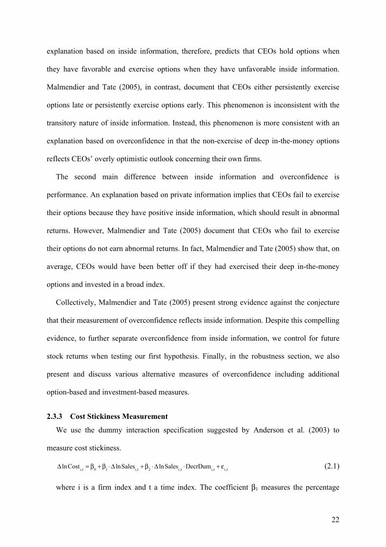
2.3.3 Cost Stickiness Measurement
We use the dummy interaction specification suggested by Anderson et al. (2003) to
measure cost stickiness.
Δ lnCosti,t = β0 +β1 ⋅Δ lnSalesi,t +β2 ⋅Δ lnSalesi,t ⋅DecrDumi,t + εi,t (2.1)
where i is a firm index and t a time index. The coefficient β1 measures the percentage
23
increase in costs with a 1% increase in sales. Since the value of DecrDum is one when sales
decrease, the sum of (β1 + β2) measures the percentage decrease in costs if sales decrease by
1%. A positive and significant coefficient β1 and a significantly negative coefficient β2 would
be consistent with cost stickiness, indicating a smaller cost reaction when sales decrease than
when sales increase (Anderson et al. 2003).
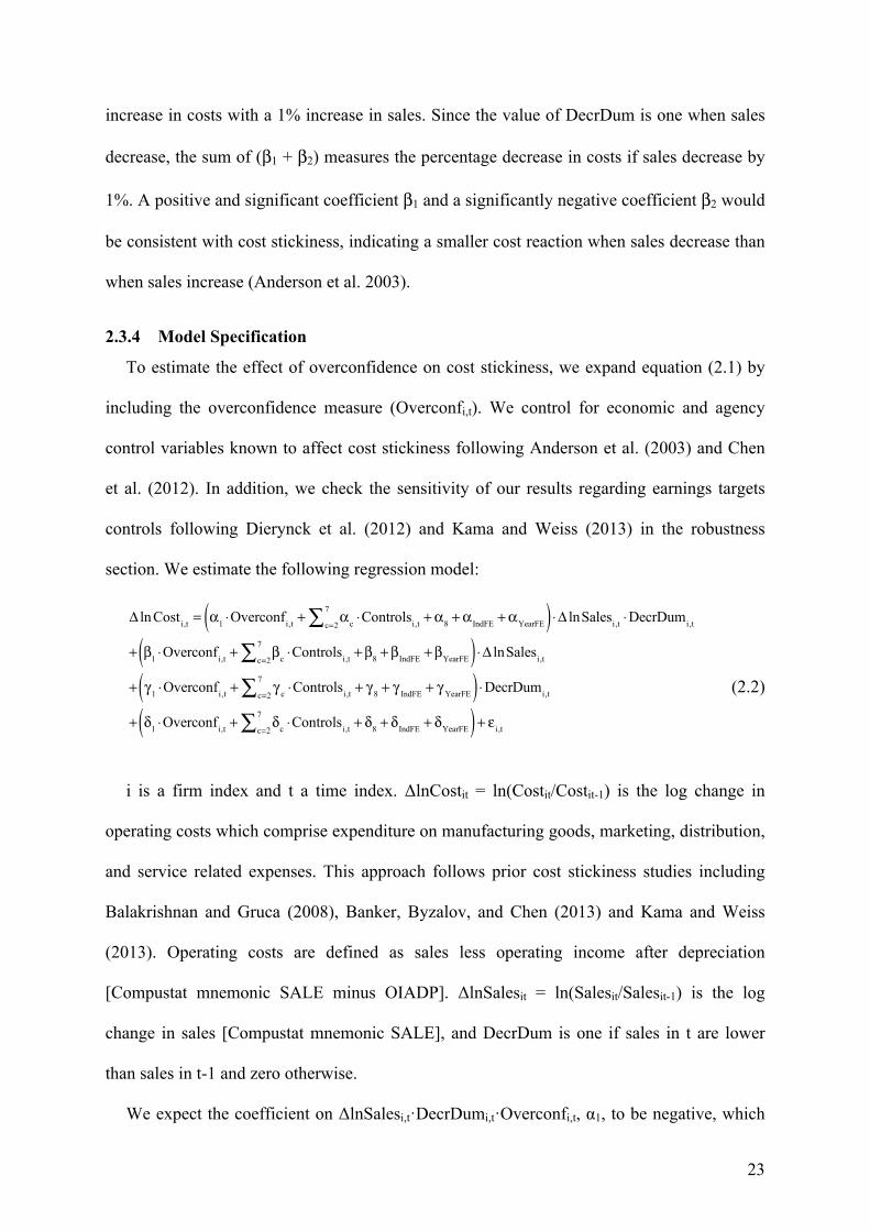
2.3.4 Model Specification
To estimate the effect of overconfidence on cost stickiness, we expand equation (2.1) by
including the overconfidence measure (Overconfi,t). We control for economic and agency
control variables known to affect cost stickiness following Anderson et al. (2003) and Chen
et al. (2012). In addition, we check the sensitivity of our results regarding earnings targets
controls following Dierynck et al. (2012) and Kama and Weiss (2013) in the robustness
section. We estimate the following regression model:
Δ lnCosti,t = α1 ⋅Overconfi,t + αc ⋅Controlsi,tc=2
7∑ +α8 +α IndFE +αYearFE( ) ⋅Δ lnSalesi,t ⋅DecrDumi,t
+ β1 ⋅Overconfi,t + βc ⋅Controlsi,tc=2
7∑ +β8 +βIndFE +βYearFE( ) ⋅Δ lnSalesi,t
+ γ 1 ⋅Overconfi,t + γ c ⋅Controlsi,tc=2
7∑ + γ 8 + γ IndFE + γ YearFE( ) ⋅DecrDumi,t
+ δ1 ⋅Overconfi,t + δc ⋅Controlsi,tc=2
7∑ + δ8 + δIndFE + δYearFE( )+ εi,t
(2.2)
i is a firm index and t a time index. ΔlnCostit = ln(Costit/Costit-1) is the log change in
operating costs which comprise expenditure on manufacturing goods, marketing, distribution,
and service related expenses. This approach follows prior cost stickiness studies including
Balakrishnan and Gruca (2008), Banker, Byzalov, and Chen (2013) and Kama and Weiss
(2013). Operating costs are defined as sales less operating income after depreciation
[Compustat mnemonic SALE minus OIADP]. ΔlnSalesit = ln(Salesit/Salesit-1) is the log
change in sales [Compustat mnemonic SALE], and DecrDum is one if sales in t are lower
than sales in t-1 and zero otherwise.
We expect the coefficient on ΔlnSalesi,t·DecrDumi,t·Overconfi,t, α1, to be negative, which
24
would indicate greater cost stickiness for firms with overconfident CEOs. We report three
specifications based on equation (2.2). In the first specification, we add overconfidence to the
baseline cost stickiness model in Anderson et al. (2003). In the second specification, we add
economic and agency control variables following Anderson et al. (2003) and Chen et al.
(2012). In the third specification, we additionally include year- and industry-fixed effects.
Year-fixed effects control for potentially unobserved factors that change over time but affect
all firms in a similar way such as macroeconomic changes that we do not capture with the
economic control variables. Industry-fixed effects control for potentially unobserved industry
specific factors that are constant over time. Specifically, industry-fixed effects help rule out
the alternative explanation that overconfident CEOs are overrepresented in industries with
greater cost stickiness. In this specification, industry fixed-effects are based on Fama-French
12 industry dummy variables. We use the third specification as our main specification
(equation (2.2), model (3) in Table 2.3). All standard errors are clustered at the firm level
allowing for heteroskedasticity and arbitrary within-firm correlation (Petersen 2009).
In addition to year- and industry-fixed effects, we follow prior literature and include two
sets of control variables: Economic and agency variables. We control for four economic
factors that may affect the asymmetry in cost behavior. First, we control for employee and
asset intensity. As proxies for adjustment costs, both are expected to result in more
pronounced cost stickiness (Anderson et al. 2003). Employee intensity (EmplInt) is the
natural logarithm of the number of employees divided by sales [Compustat mnemonics EMP
and SALE], and asset intensity (AssetInt) is defined as the natural logarithm of total assets
divided by sales [Compustat mnemonics AT and SALE]. Second, we follow Anderson et al.
(2003) and control for successive sales decreases, expecting that managers will regard
decreases in demand as more persistent if demand declines in two consecutive years. The
dummy variable SD equals one if sales are lower in year t-1 than in year t-2, otherwise the
25
variable is set to zero. Finally, we follow Chen et al. (2012) and control for stock
performance (StockPerf), which is the natural logarithm of one plus the annual raw stock
return measured at the beginning of the fiscal year. If higher stock performance reflects a
more efficient cost control, it should have a negative effect on cost stickiness. If, however,
higher stock performance signals positive expectations of future performance, it may have a
positive effect on cost stickiness because managers may want to keep excess resources in
anticipation of higher future capacity utilization. This control variable is also important to
rule out the possibility that delayed option exercise reflects positive future performance
expectations instead of overconfidence.
Following Chen et al. (2012), we control for two agency factors. First, we control for free
cash flow (FCF), which is calculated as cash flow from operating activities [Compustat
mnemonic OANCF] less common and preferred dividends [Compustat mnemonics DVC and
DVP] divided by total assets [Compustat mnemonic AT]. High levels of FCF allow managers
to overinvest when demand increases and to postpone cost cuts when demand decreases.
Hence, higher levels of FCF should increase cost stickiness (Chen et al. 2012). Second, we
control for CEO fixed pay because prior studies suggest that executive compensation affects
empire building incentives (Kanniainen 2000). We measure fixed pay (FixedPay) as the sum
of salary and bonus which we divide by total compensation. The latter comprises salary,
bonus, value of restricted stocks and options, and all other annual payouts (Chen et al. 2012).
2.4 Results
2.4.1 Descriptive Statistics
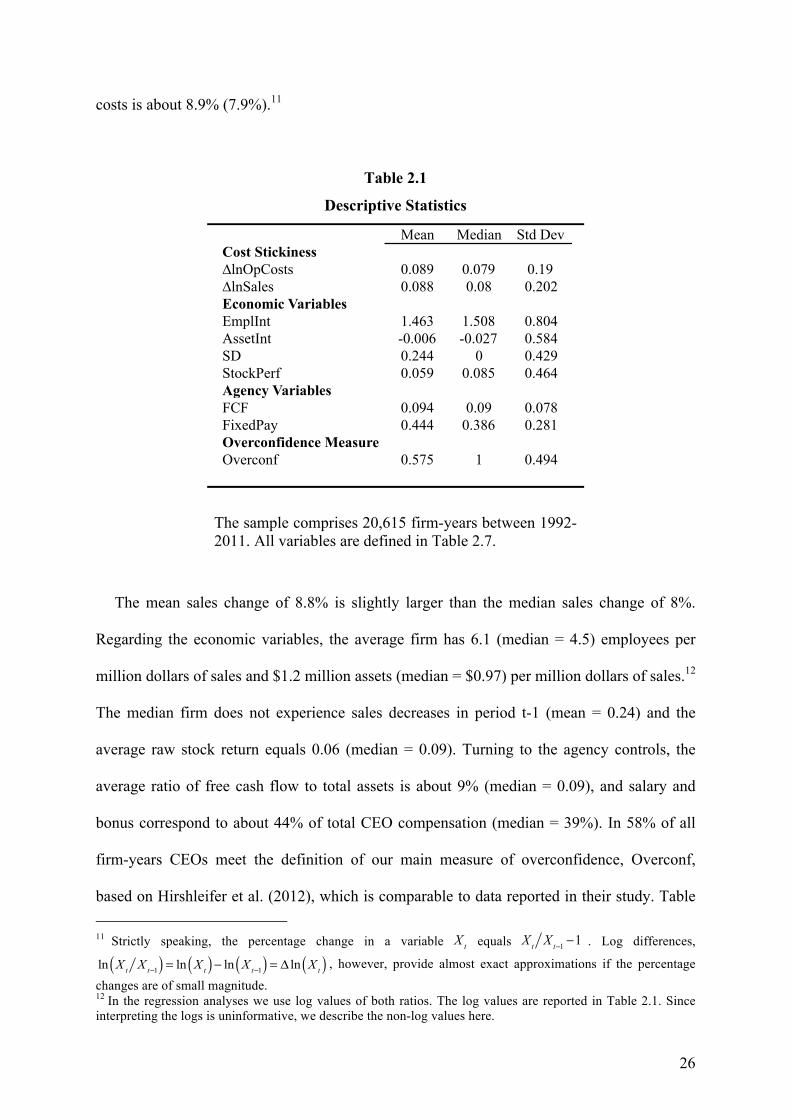
Table 2.1 provides descriptive statistics. The sample comprises 20,615 observations for
the period between 1992-2011. The mean (median) annual percentage changes in operating
26
costs is about 8.9% (7.9%).11
Table 2.1
Descriptive Statistics
The sample comprises 20,615 firm-years between 1992-2011. All variables are defined in Table 2.7.
The mean sales change of 8.8% is slightly larger than the median sales change of 8%.
Regarding the economic variables, the average firm has 6.1 (median = 4.5) employees per
million dollars of sales and $1.2 million assets (median = $0.97) per million dollars of sales.12
The median firm does not experience sales decreases in period t-1 (mean = 0.24) and the
average raw stock return equals 0.06 (median = 0.09). Turning to the agency controls, the
average ratio of free cash flow to total assets is about 9% (median = 0.09), and salary and
bonus correspond to about 44% of total CEO compensation (median = 39%). In 58% of all
firm-years CEOs meet the definition of our main measure of overconfidence, Overconf,
based on Hirshleifer et al. (2012), which is comparable to data reported in their study. Table 11 Strictly speaking, the percentage change in a variable equals . Log differences,
, however, provide almost exact approximations if the percentage
changes are of small magnitude. 12 In the regression analyses we use log values of both ratios. The log values are reported in Table 2.1. Since interpreting the logs is uninformative, we describe the non-log values here.
Mean Median Std DevCost Stickiness∆lnOpCosts 0.089 0.079 0.19∆lnSales 0.088 0.08 0.202Economic VariablesEmplInt 1.463 1.508 0.804AssetInt -0.006 -0.027 0.584SD 0.244 0 0.429StockPerf 0.059 0.085 0.464Agency VariablesFCF 0.094 0.09 0.078FixedPay 0.444 0.386 0.281Overconfidence MeasureOverconf 0.575 1 0.494
Xt Xt X t−1 −1
ln Xt X t−1( ) = ln Xt( )− ln Xt−1( ) = Δ ln Xt( )
27
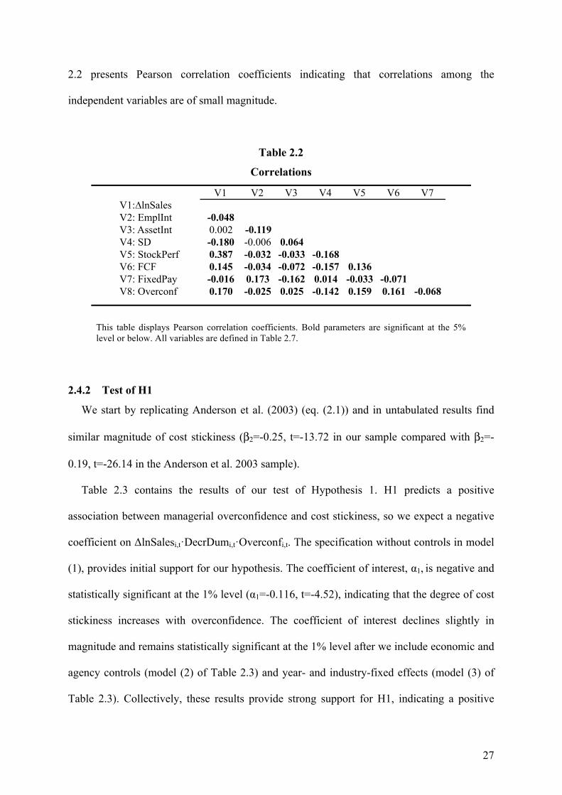
2.2 presents Pearson correlation coefficients indicating that correlations among the
independent variables are of small magnitude.
Table 2.2
Correlations
This table displays Pearson correlation coefficients. Bold parameters are significant at the 5% level or below. All variables are defined in Table 2.7.
2.4.2 Test of H1
We start by replicating Anderson et al. (2003) (eq. (2.1)) and in untabulated results find
similar magnitude of cost stickiness (β2=-0.25, t=-13.72 in our sample compared with β2=-
0.19, t=-26.14 in the Anderson et al. 2003 sample).
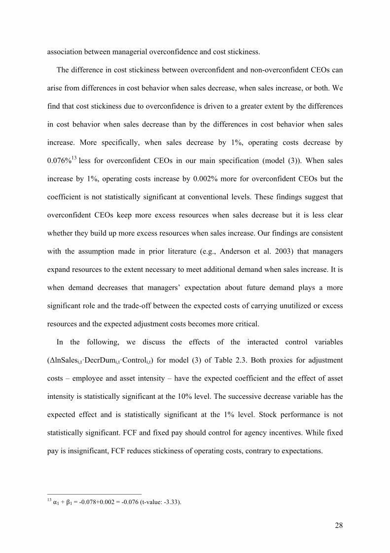
Table 2.3 contains the results of our test of Hypothesis 1. H1 predicts a positive
association between managerial overconfidence and cost stickiness, so we expect a negative
coefficient on ΔlnSalesi,t·DecrDumi,t·Overconfi,t. The specification without controls in model
(1), provides initial support for our hypothesis. The coefficient of interest, α1, is negative and
statistically significant at the 1% level (α1=-0.116, t=-4.52), indicating that the degree of cost
stickiness increases with overconfidence. The coefficient of interest declines slightly in
magnitude and remains statistically significant at the 1% level after we include economic and
agency controls (model (2) of Table 2.3) and year- and industry-fixed effects (model (3) of
Table 2.3). Collectively, these results provide strong support for H1, indicating a positive
V1 V2 V3 V4 V5 V6 V7V1:∆lnSalesV2: EmplInt -0.048V3: AssetInt 0.002 -0.119V4: SD -0.180 -0.006 0.064V5: StockPerf 0.387 -0.032 -0.033 -0.168V6: FCF 0.145 -0.034 -0.072 -0.157 0.136V7: FixedPay -0.016 0.173 -0.162 0.014 -0.033 -0.071V8: Overconf 0.170 -0.025 0.025 -0.142 0.159 0.161 -0.068
28
association between managerial overconfidence and cost stickiness.
The difference in cost stickiness between overconfident and non-overconfident CEOs can
arise from differences in cost behavior when sales decrease, when sales increase, or both. We
find that cost stickiness due to overconfidence is driven to a greater extent by the differences
in cost behavior when sales decrease than by the differences in cost behavior when sales
increase. More specifically, when sales decrease by 1%, operating costs decrease by
0.076%13 less for overconfident CEOs in our main specification (model (3)). When sales
increase by 1%, operating costs increase by 0.002% more for overconfident CEOs but the
coefficient is not statistically significant at conventional levels. These findings suggest that
overconfident CEOs keep more excess resources when sales decrease but it is less clear
whether they build up more excess resources when sales increase. Our findings are consistent
with the assumption made in prior literature (e.g., Anderson et al. 2003) that managers
expand resources to the extent necessary to meet additional demand when sales increase. It is
when demand decreases that managers’ expectation about future demand plays a more
significant role and the trade-off between the expected costs of carrying unutilized or excess
resources and the expected adjustment costs becomes more critical.
In the following, we discuss the effects of the interacted control variables
(ΔlnSalesi,t·DecrDumi,t·Controli,t) for model (3) of Table 2.3. Both proxies for adjustment
costs – employee and asset intensity – have the expected coefficient and the effect of asset
intensity is statistically significant at the 10% level. The successive decrease variable has the
expected effect and is statistically significant at the 1% level. Stock performance is not
statistically significant. FCF and fixed pay should control for agency incentives. While fixed
pay is insignificant, FCF reduces stickiness of operating costs, contrary to expectations.
13 α1 + β1 = -0.078+0.002 = -0.076 (t-value: -3.33).
29
Table 2.3
The Effect of Managerial Overconfidence on Cost Stickiness
The dependent variable is log change in operating costs. All variables are defined in Table 2.7. Standard errors are clustered at the firm level. T-statistics are in parentheses. *,**,*** represent significance at the 10%, 5% and 1% level.
Main Variables∆lnSales*DecrDum*Overconf -0.116*** (-4.52) -0.088*** (-3.64) -0.078*** (-3.14)∆lnSales*Overconf 0.002 (0.19) 0.004 (0.37) 0.002 (0.13)∆lnSales*DecrDum -0.058*** (-3.70) -0.112*** (-3.67) -0.046 (-0.36)∆lnSales 0.905*** (78.10) 0.949*** (52.33) 0.970*** (24.35)DecrDum*Overconf 0 (0.11) 0.001 (0.14) 0.001 (0.20)Overconf 0.002 (1.36) 0.001 (0.86) 0.002 (1.02)DecrDum 0.003 (1.18) 0.013** (2.30) 0.016 (1.41)Economic Controls∆lnSales*DecrDum*EmplInt -0.018 (-1.33) -0.018 (-1.39)∆lnSales*DecrDum*AssetInt -0.065*** (-2.89) -0.042* (-1.88)∆lnSales*DecrDum*SD 0.194*** (7.19) 0.133*** (4.58)∆lnSales*DecrDum*StockPerf 0.031 (1.28) 0.018 (0.63)∆lnSales*EmplInt 0.033*** (4.85) 0.017** (2.52)∆lnSales*AssetInt -0.058*** (-5.24) -0.052*** (-4.18)∆lnSales*SD -0.153*** (-8.38) -0.108*** (-5.76)∆lnSales*StockPerf -0.001 (-0.11) 0.004 (0.30)DecrDum*EmplInt 0.005* (1.80) 0.001 (0.57)DecrDum*AssetInt 0.010** (2.35) 0.010** (2.37)DecrDum*SD -0.018*** (-4.89) -0.015*** (-3.78)DecrDum*StockPerf 0.011** (2.55) 0.009* (1.81)EmplInt -0.003** (-2.24) -0.001 (-0.70)AssetInt 0.004** (2.12) 0.005** (2.49)SD -0.007*** (-3.22) -0.007*** (-3.15)StockPerf 0 (0.16) 0 (0.15)Agency Controls∆lnSales*DecrDum*FCF 0.675*** (4.84) 0.565*** (4.08)∆lnSales*DecrDum*FixedPay 0.074* (1.83) 0.052 (1.35)∆lnSales*FCF -0.414*** (-5.15) -0.368*** (-4.84)∆lnSales*FixedPay -0.032* (-1.80) -0.030* (-1.72)DecrDum*FCF -0.067** (-2.00) -0.064* (-1.94)DecrDum*FixedPay 0.008 (1.29) 0.001 (0.18)FCF -0.027 (-1.64) -0.026 (-1.64)FixedPay -0.001 (-0.44) -0.001 (-0.16)Constant 0.003** (2.25) 0.012*** (4.10) 0.007 (1.39)Year-Fixed EffectsFF 12 Ind.-Fixed EffectsN R2adj
+ Economic and + Year- and Industry(1) (2) (3)
Main VariablesAgency Controls Fixed Effects
206150.859
NoNo
20615Yes
206150.8643
Yes
0.8444
NoNo
30
2.4.3 Addressing Alternative Explanations for H1
In this section, we address potential alternative explanations. We first demonstrate that the
association between overconfidence and cost behavior we document in our study is distinct
from the association between overconfidence and investment documented in prior literature.
We then show that our results are driven by an innate personality trait, managerial
overconfidence, rather than by optimistic expectations of future demand conditioned by past
sales trends (Banker et al. 2014) by controlling for prior sales changes and still documenting
an incremental effect of our overconfidence measure on cost stickiness. Finally, we alleviate
self-selection concerns by additionally controlling for time-constant unobserved factors and
time-varying factors that may be associated with selection mechanisms.
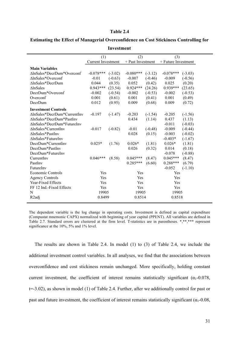
2.4.3.1 Cost Behavior vs. Investment
Since Malmendier and Tate (2005) show that overconfident CEOs exhibit heightened
investment-cash flow sensitivity, one may argue that firms with overconfident CEOs who
initiate new investment projects will mechanically exhibit more pronounced cost stickiness.
To document that overconfidence has an independent effect on cost behavior beyond its
effect on investment, we additionally control for investment. Following Malmendier and Tate
(2005), we define investment as capital expenditure (Compustat mnemonic CAPX)
normalized with beginning of year capital (PPENT). We then replicate our main analysis
controlling for (i) investment in period t, (ii) investment in both period t and t-1, and (iii)
investment in period t, t-1 and t+1.
31
Table 2.4
Estimating the Effect of Managerial Overconfidence on Cost Stickiness Controlling for
Investment
The dependent variable is the log change in operating costs. Investment is defined as capital expenditure (Compustat mnemonic CAPX) normalized with beginning of year capital (PPENT). All variables are defined in Table 2.7. Standard errors are clustered at the firm level. T-statistics are in parentheses. *,**,*** represent significance at the 10%, 5% and 1% level.
The results are shown in Table 2.4. In model (1) to (3) of Table 2.4, we include the
additional investment control variables. In all analyses, we find that the associations between
overconfidence and cost stickiness remain unchanged. More specifically, holding constant
current investment, the coefficient of interest remains statistically significant (α1-0.078,
t=-3.02), as shown in model (1) of Table 2.4. Further, after we additionally control for past or
past and future investment, the coefficient of interest remains statistically significant (α1-0.08,
Main Variables∆lnSales*DecrDum*Overconf -0.078*** (-3.02) -0.080*** (-3.12) -0.078*** (-3.03)∆lnSales*Overconf -0.01 (-0.63) -0.007 (-0.46) -0.009 (-0.56)∆lnSales*DecrDum 0.044 (0.35) 0.052 (0.42) 0.025 (0.20)∆lnSales 0.943*** (23.54) 0.924*** (24.26) 0.939*** (23.65)DecrDum*Overconf -0.002 (-0.54) -0.002 (-0.53) -0.002 (-0.53)Overconf 0.001 (0.61) 0.001 (0.41) 0.001 (0.49)DecrDum 0.012 (0.95) 0.009 (0.68) 0.009 (0.72)Investment Controls∆lnSales*DecrDum*CurrentInv -0.197 (-1.47) -0.203 (-1.54) -0.205 (-1.56)∆lnSales*DecrDum*PastInv 0.434 (1.14) 0.437 (1.13)∆lnSales*DecrDum*FutureInv -0.011 (-0.03)∆lnSales*CurrentInv -0.017 (-0.82) -0.01 (-0.48) -0.009 (-0.44)∆lnSales*PastInv 0.028 (0.15) -0.003 (-0.02)∆lnSales*FutureInv -0.403* (-1.67)DecrDum*CurrentInv 0.025* (1.76) 0.026* (1.81) 0.026* (1.81)DecrDum*PastInv 0.026 (0.32) 0.014 (0.18)DecrDum*FutureInv -0.078 (-0.88)CurrentInv 0.046*** (8.58) 0.045*** (8.47) 0.045*** (8.47)PastInv 0.285*** (6.60) 0.288*** (6.79)FutureInv -0.052 (-1.10)Economic ControlsAgency ControlsYear-Fixed EffectsFF 12 Ind.-Fixed EffectsN R2adj
Yes Yes YesYes Yes Yes
+ Past Investment + Future Investment(1) (2) (3)
Current Investment
Yes Yes YesYes Yes Yes
19905 19905 199050.8499 0.8514 0.8518
32
t=-3.12 and α1-0.078, t=-3.03, respectively), as shown in model (2) and (3). Taken together,
these results suggest that the association between overconfidence and cost behavior is distinct
from the association between overconfidence and investment. Thus, the results we document
in our study cannot be explained by the link between overconfidence and overinvestment
documented by Malmendier and Tate (2005).
2.4.3.2 Controlling for Prior Sales Changes
In this section, we check the sensitivity of our results to using an alternative cost stickiness
model. The analysis builds on the framework of Banker et al. (2014) (hereafter “BBCM”)
who refine the model of Anderson et al. (2003). In particular, BBCM highlight the role of
managers’ demand expectations.14 BBCM use prior sales changes as a proxy for managers’
expectations of future demand, relying on two arguments to justify this choice. First, since
sales changes are positively correlated, sales increases in prior periods point to a greater
likelihood of further sales increases in future periods, thereby increasing managers’
expectations about future sales. Second, since behavioral studies suggest that managers are
likely to extrapolate past trends, BBCM argue that managers will anticipate further increases
in sales and, hence, will be more optimistic about future demand following a prior sales
increase.
After a prior period’s sales increase, BBCM predict cost stickiness. If prior sales increased,
managers are more optimistic about future sales and more willing to retain unutilized
resources should current sales decline. Conversely, should current sales continue to increase,
BBCM expect managers to ramp up resources proportionally to meet the additional demand.
Thus, the cost reaction following two consecutive sales increases should be of larger extent
than the cost reaction following an increase in the prior but a decrease in the current period,
14 BBCM also extend the cost stickiness model in Anderson et al. (2003) by allowing for anti-stickiness, i.e., costs decrease more when sales decrease compared to the extent they increase when sales increase. Since we do not make predictions regarding the anti-stickiness case, we do not discuss it here.
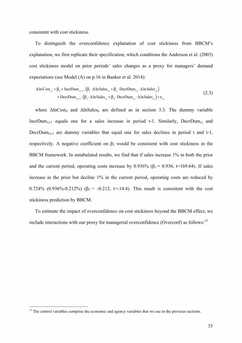
33
consistent with cost stickiness.
To distinguish the overconfidence explanation of cost stickiness from BBCM’s
explanation, we first replicate their specification, which conditions the Anderson et al. (2003)
cost stickiness model on prior periods’ sales changes as a proxy for managers’ demand
expectations (see Model (A) on p.16 in Banker et al. 2014):
Δ lnCosti,t = β0 + IncrDumi,t−1 ⋅ β1 ⋅Δ lnSalesi,t +β2 ⋅DecrDumi,t ⋅Δ lnSalesi,t( ) + DecrDumi,t−1 ⋅ β3 ⋅Δ lnSalesi,t +β4 ⋅DecrDumi,t ⋅Δ lnSalesi,t( )+ εi,t
(2.3)
where ΔlnCostit and ΔlnSalesit are defined as in section 3.3. The dummy variable
IncrDumi,t-1 equals one for a sales increase in period t-1. Similarly, DecrDumi,t and
DecrDumi,t-1 are dummy variables that equal one for sales declines in period t and t-1,
respectively. A negative coefficient on β2 would be consistent with cost stickiness in the
BBCM framework. In untabulated results, we find that if sales increase 1% in both the prior
and the current period, operating costs increase by 0.936% (β1 = 0.936, t=169.64). If sales
increase in the prior but decline 1% in the current period, operating costs are reduced by
0.724% (0.936%-0.212%) (β2 = -0.212, t=-14.4). This result is consistent with the cost
stickiness prediction by BBCM.
To estimate the impact of overconfidence on cost stickiness beyond the BBCM effect, we
include interactions with our proxy for managerial overconfidence (Overconf) as follows:15
15 The control variables comprise the economic and agency variables that we use in the previous sections.
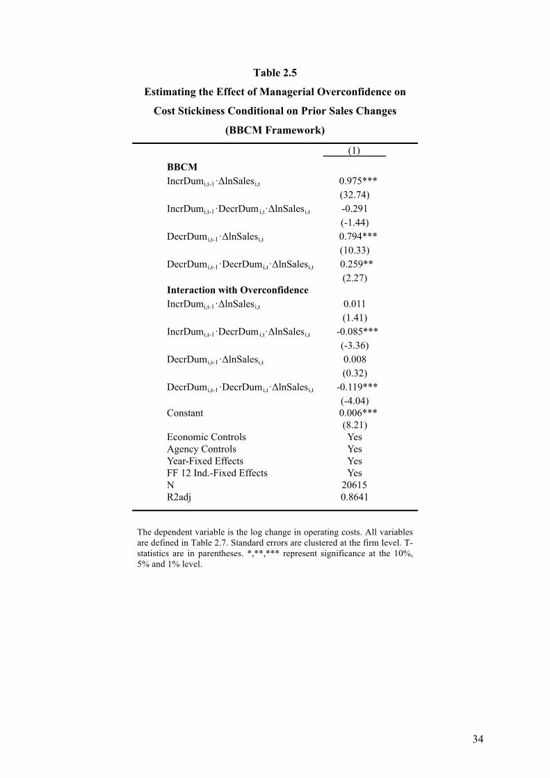
34
Table 2.5
Estimating the Effect of Managerial Overconfidence on
Cost Stickiness Conditional on Prior Sales Changes
(BBCM Framework)
The dependent variable is the log change in operating costs. All variables are defined in Table 2.7. Standard errors are clustered at the firm level. T-statistics are in parentheses. *,**,*** represent significance at the 10%, 5% and 1% level.
(1)
BBCMIncrDumi,t-1·ΔlnSalesi,t 0.975***
(32.74)IncrDumi,t-1·DecrDumi,t·ΔlnSalesi,t -0.291
(-1.44)DecrDumi,t-1·ΔlnSalesi,t 0.794***
(10.33)DecrDumi,t-1·DecrDumi,t·ΔlnSalesi,t 0.259**
(2.27)Interaction with OverconfidenceIncrDumi,t-1·ΔlnSalesi,t 0.011
(1.41)IncrDumi,t-1·DecrDumi,t·ΔlnSalesi,t -0.085***
(-3.36)DecrDumi,t-1·ΔlnSalesi,t 0.008
(0.32)DecrDumi,t-1·DecrDumi,t·ΔlnSalesi,t -0.119***
(-4.04)Constant 0.006*** (8.21)Economic Controls YesAgency Controls YesYear-Fixed Effects YesFF 12 Ind.-Fixed Effects YesN 20615R2adj 0.8641
35
Δ ln Costi,t = β0 + IncrDumi,t−1 ⋅ β1 ⋅Δ lnSalesi,t +β2 ⋅DecrDumi,t ⋅Δ lnSalesi,t( +β3 ⋅Δ lnSalesi,t ⋅Overconfi,t +β4 ⋅DecrDumi,t ⋅Δ lnSalesi,t ⋅Overconfi,t
+βControl ⋅Δ lnSalesi,t ⋅Controlsi,t +βControl ⋅DecrDumi,t ⋅Δ lnSalesi,t ⋅Controlsi,t
+βIndustry ⋅Δ lnSalesi,t +βIndustry ⋅DecrDumi,t ⋅Δ lnSalesi,t
+βYear ⋅Δ lnSalesi,t +βYear ⋅DecrDumi,t ⋅Δ lnSalesi,t ) + DecrDumi,t−1 ⋅ β5 ⋅Δ lnSalesi,t +β6 ⋅DecrDumi,t ⋅Δ lnSalesi,t( +β7 ⋅Δ lnSalesi,t ⋅Overconfi,t +β8 ⋅DecrDumi,t ⋅Δ lnSalesi,t ⋅Overconfi,t
+βControl ⋅Δ lnSalesi,t ⋅Controlsi,t +βControl ⋅DecrDumi,t ⋅Δ lnSalesi,t ⋅Controlsi,t
+βIndustry ⋅Δ lnSalesi,t +βIndustry ⋅DecrDumi,t ⋅Δ lnSalesi,t
+βYear ⋅Δ lnSalesi,t +βYear ⋅DecrDumi,t ⋅Δ lnSalesi,t )+ εi,t
(2.4)
We predict that cost stickiness will increase in the degree of overconfidence after
controlling for management demand expectations reflected in prior sales. Thus, we expect β4
to take on a negative sign. Consistent with our prediction, results in Table 2.5 show that β4 is
significantly negative (β4 = -0.085, t= -3.36). This result suggests that overconfidence has an
impact on cost stickiness above and beyond managerial demand expectations reflected in
prior sales changes.
2.4.3.3 Addressing Self-Selection
In this section we address the possibility that the positive association between managerial
overconfidence and cost stickiness could be affected by self-selection. If overconfident CEOs
are more likely to self-select into or be hired by firms with certain characteristics, and firms
with these characteristics have greater cost stickiness, then our result might be driven by self-
selection.
To the extent that self-selection is driven by characteristics that are constant across
industries, we control for these factors with industry-fixed effects. Model (3) of Table 2.3
reports results using Fama-French 12 industry dummies and in the robustness section we
discuss results using two-digit SIC code industry dummies. In both specifications, we
document a significantly positive association between managerial overconfidence and cost
36
stickiness.16
While the previous tests control for potentially omitted variables that are constant at the
industry-level, we next control for time-varying factors that may be associated with selection
mechanisms. If overconfident CEOs are associated with growth firms and if growth firms
exhibit more pronounced cost stickiness, then growth potential may be an omitted variable.
We therefore rerun our analyses by controlling for two proxies of growth potential. We first
control for Tobin’s Q since high values of Q indicate future growth potential (Tobin 1969).17
Alternatively, we control for demand volatility, assuming that higher demand volatility
characterizes growth firms (Banker et al. 2011).18 Untabulated results suggest that our results
are robust to controlling for both proxies of growth (α1=-0.08, t=-2.89 and α1=-0.076, t=-3.11,
respectively).
Finally, we follow Hirshleifer et al. (2012) and estimate our main specification on a
restricted sample that focuses on firm-years that are supposed to be less strongly affected by
self-selection. The test builds on the idea that overconfidence is a persistent character trait
that remains stable over time. In contrast, firm characteristics that may induce self-selection,
such as growth opportunities, vary over time as the firm environment changes. To the extent
that there is self-selection, potential matching effects will be most severe in the first years of
each CEO’s tenure. Hirshleifer et al. (2012), therefore, suggest excluding the first years of
each CEO’s tenure as these years are most likely to reflect self-selection. The remaining
sample should be less affected by self-selection. We rerun our main specification excluding
the first two, three and four years of each CEO’s tenure. In all specification, we obtain results
that are comparable with our main analysis (α1=-0.072, t=-2.44, α1=-0.074, t=-2.02 and
16 The tables of all further sensitivity checks are available on request. 17 We define Tobin’s Q as the market value of equity (Compustat mnemonic CSHO·PRCCF) plus total assets (AT) minus book value of equity (CEQ + TXDB), divided by total assets (Chen, Chen, and Wei 2011). 18 We define demand volatility as the “standard deviation of sales revenue over the five years prior to the event year divided by the mean of sales revenue over the five years prior to the event year“ (Banker et al. 2011, p. 801).
37
α1=-0.09, t=-1.98 respectively), further mitigating self-selection concerns.
Collectively, the evidence presented in this section suggests that our main result is not
driven by sticky firms selecting overconfident CEOs or overconfident CEOs selecting to
work for cost sticky firms.
2.4.4 Robustness Checks for H1
To assess the robustness of the association between managerial overconfidence and cost
stickiness, we conduct the following sensitivity analyses: we (1) examine alternative cost
categories, (2) employ alternative overconfidence measures, (3) control for earnings targets
following the recent studies of Dierynck et al. (2012) and Kama and Weiss (2013), (4)
address the criticism of Anderson and Lanen (2009) by following their treatment of
influential observations and of Balakrishnan, Labro, and Soderstrom (2014) by estimating a
linear instead of the logarithmic specification, (5) use alternative agency controls, (6) check
the robustness to an alternative industry classification, and (7) control for future stock returns.
The tables of all robustness results are available upon request. Below we briefly describe the
findings.
First, we test other cost categories. We alternatively examine (i) selling, general, and
administrative costs (Compustat mnemonic XSGA), (ii), cost of good sold (COGS), (iii) total
cost (SALE - IB) and (iv) employment (EMP). In all analyses, we find qualitatively similar
results (α1=-0.082, t=-2.15, α1=-0.113, t=-3.35, α1=-0.096, t=-2.52, and , α1=-0.101, t=-2.3619,
respectively).
Second, we re-estimate equation (2.2) using additional option- and investment-based
overconfidence measures. All overconfidence measures are defined in Table 2.7. Regarding
the option-based measures, we use the option exercising measure following Malmendier et al.
(2011) and Campbell et al. (2011). The measure of Malmendier et al. (2011) requires CEOs
19 We do not control for employee intensity when analyzing employment stickiness.
38
to twice hold options that are more than 67% in-the-money to be classified as overconfident.
The option exercising measure following Campbell et al. (2011) requires CEOs to twice hold
options that are more than 100% in-the-money. In addition, the measure allows for
reclassifications upon early option exercise. In both analyses, we find qualitatively similar
results (α1=-0.076, t=-2.95 and α1=-0.094, t=-3.35, respectively). Concerning the investment-
based measures, we use the capital expenditure measure following Ahmed and Duellman
(2013) and the investment measure following Campbell et al. (2011). While the investment
measure following Ahmed and Duellman (2013) is not statistically significant (α1=-0.031,
t=-1.04), we find similar results using the investment-based overconfidence measure
following Campbell et al. (2011) (α1=-0.121, t=-2.95).
Third, we augment our main model (equation (2.2)) and additionally control for the
influence of earnings targets and managerial incentives on cost stickiness following the
recent studies of Dierynck et al. (2012) and Kama and Weiss (2013). Our conclusion remains
unchanged after controlling for small positive earnings (α1=-0.078, t=-3.15) or small
increases in earnings (α1=-0.082, t=-3.31) as defined in Kama and Weiss (2013, p. 211).
Fourth, we address the criticism of Anderson and Lanen (2009) and follow their
suggestion to exclude observations when costs and sales move in opposite directions.
Additionally, we follow the approach suggested in Balakrishnan et al. (2014) and estimate a
linear model instead of the logarithmic specification (we divide both the change in costs and
sales by lagged sales) and obtain comparable results (α1=-0.07, t=-3.40 and α1=-0.074,
t=-2.88, respectively).20
Fifth, to control for agency factors and variables correlated with stock options influencing
cost stickiness, we follow Chen et al. (2012) and include free cash flow and fixed pay as
controls in our main regression model. We alternatively use the following controls instead of
20 We refer to Banker and Byzalov (2013) for an in-depth discussion of both concerns.
39
fixed pay: (1) Following Malmendier and Tate (2005) we use stock ownership and vested
options, (2) following Ahmed and Duellman (2013) we use stock ownership, and (3)
following Schrand and Zechman (2012), we control for salary, bonus, option grants and total
holdings (unexercised options and shares owned). All variables are defined in Table 2.7.
Using all three specifications, we obtain similar results (α1=-0.078, t=-3.27, α1=-0.081,
t=-3.21, and α1=-0.074, t=-2.73).
Sixth, we also find qualitatively similar results if we construct industry dummies based on
the two-digit SIC codes following Hirshleifer et al. (2012) instead of Fama-French 12
industries (α1=-0.074, t=-2.84). Finally, our conclusion remains unchanged if we control for
future stock returns (α1=-0.082, t=-3.20).
2.4.5 Test of H2
So far, we provide strong evidence for a positive association between managerial
overconfidence and cost stickiness. Our second hypothesis predicts that cost stickiness driven
by managerial overconfidence should be negatively associated with future firm performance
compared to cost stickiness not driven by managerial overconfidence.
To test our H2, we proceed as follows. Our prior results show that overconfident CEOs
exhibit more pronounced cost stickiness than non-overconfident CEOs. More specifically,
our results show that cost stickiness due to overconfidence is driven to a greater extent by
differences in cost behavior when sales decrease than by differences in cost behavior when
sales increase. If overconfident CEOs indeed erroneously overestimate future demand and,
therefore, keep more costs than non-overconfident CEOs when sales decline, the cost
behavior of overconfident CEOs when sales decline should have a negative impact on future
earnings compared to the cost behavior of non-overconfident CEOs when sales decline.
Empirically, we use the following specification. We first define a dummy variable that is
one if a CEO is overconfident and sales decline (OC_Deci,t). To ensure that we compare
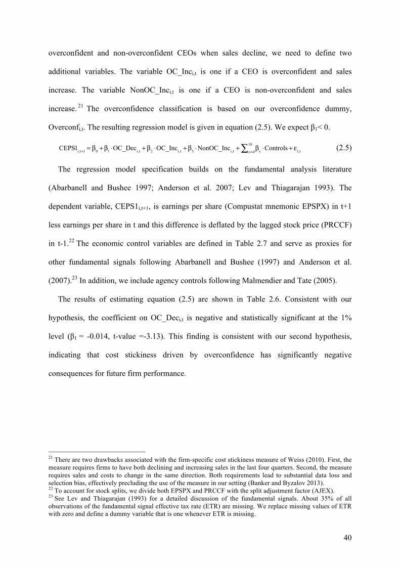
40
overconfident and non-overconfident CEOs when sales decline, we need to define two
additional variables. The variable OC_Inci,t is one if a CEO is overconfident and sales
increase. The variable NonOC_Inci,t is one if a CEO is non-overconfident and sales
increase. 21 The overconfidence classification is based on our overconfidence dummy,
Overconfi,t. The resulting regression model is given in equation (2.5). We expect β1< 0.
CEPS1i,t+1 = β0 +β1 ⋅OC_Deci,t +β2 ⋅OC_Inci,t +β3 ⋅NonOC_Inci,t + βc ⋅Controlsc=4
18∑ + εi,t (2.5)
The regression model specification builds on the fundamental analysis literature
(Abarbanell and Bushee 1997; Anderson et al. 2007; Lev and Thiagarajan 1993). The
dependent variable, CEPS1i,t+1, is earnings per share (Compustat mnemonic EPSPX) in t+1
less earnings per share in t and this difference is deflated by the lagged stock price (PRCCF)
in t-1.22 The economic control variables are defined in Table 2.7 and serve as proxies for
other fundamental signals following Abarbanell and Bushee (1997) and Anderson et al.
(2007).23 In addition, we include agency controls following Malmendier and Tate (2005).
The results of estimating equation (2.5) are shown in Table 2.6. Consistent with our
hypothesis, the coefficient on OC_Deci,t is negative and statistically significant at the 1%
level (β1 = -0.014, t-value =-3.13). This finding is consistent with our second hypothesis,
indicating that cost stickiness driven by overconfidence has significantly negative
consequences for future firm performance.
21 There are two drawbacks associated with the firm-specific cost stickiness measure of Weiss (2010). First, the measure requires firms to have both declining and increasing sales in the last four quarters. Second, the measure requires sales and costs to change in the same direction. Both requirements lead to substantial data loss and selection bias, effectively precluding the use of the measure in our setting (Banker and Byzalov 2013). 22 To account for stock splits, we divide both EPSPX and PRCCF with the split adjustment factor (AJEX). 23 See Lev and Thiagarajan (1993) for a detailed discussion of the fundamental signals. About 35% of all observations of the fundamental signal effective tax rate (ETR) are missing. We replace missing values of ETR with zero and define a dummy variable that is one whenever ETR is missing.
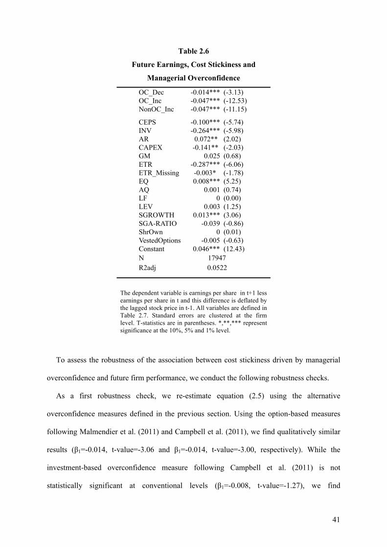
41
Table 2.6
Future Earnings, Cost Stickiness and
Managerial Overconfidence
The dependent variable is earnings per share in t+1 less earnings per share in t and this difference is deflated by the lagged stock price in t-1. All variables are defined in Table 2.7. Standard errors are clustered at the firm level. T-statistics are in parentheses. *,**,*** represent significance at the 10%, 5% and 1% level.
To assess the robustness of the association between cost stickiness driven by managerial
overconfidence and future firm performance, we conduct the following robustness checks.
As a first robustness check, we re-estimate equation (2.5) using the alternative
overconfidence measures defined in the previous section. Using the option-based measures
following Malmendier et al. (2011) and Campbell et al. (2011), we find qualitatively similar
results (β1=-0.014, t-value=-3.06 and β1=-0.014, t-value=-3.00, respectively). While the
investment-based overconfidence measure following Campbell et al. (2011) is not
statistically significant at conventional levels (β1=-0.008, t-value=-1.27), we find
OC_Dec -0.014*** (-3.13)OC_Inc -0.047*** (-12.53)NonOC_Inc -0.047*** (-11.15)
CEPS -0.100*** (-5.74)INV -0.264*** (-5.98)AR 0.072** (2.02)CAPEX -0.141** (-2.03)GM 0.025 (0.68)ETR -0.287*** (-6.06)ETR_Missing -0.003* (-1.78)EQ 0.008*** (5.25)AQ 0.001 (0.74)LF 0 (0.00)LEV 0.003 (1.25)SGROWTH 0.013*** (3.06)SGA-RATIO -0.039 (-0.86)ShrOwn 0 (0.01)VestedOptions -0.005 (-0.63)Constant 0.046*** (12.43)NR2adj
179470.0522
42
qualitatively similar results using the investment-based overconfidence measure following
Ahmed and Duellman (2013) (β1=-0.03, t-value=-6.53).
As a second robustness check, we re-estimate equation (2.5) using alternative performance
measures. If we alternatively define the dependent variable as change in net income, scaled
by lagged assets, or as change in income before extraordinary items, scaled by lagged assets,
we find qualitatively similar results (β1=-0.005, t-value=-1.91 and β1=-0.005, t-value=-1.90,
respectively). Third, we obtain qualitatively similar results after controlling for industry- and
year-fixed effects (β1 =-0.017, t-value=-3.74). Fourth, our results are similar if we
alternatively drop missing values of the fundamental signal effective tax rate instead of
setting them to zero (β1 =-0.014, t-value=-2.35). Finally, our conclusion remains unchanged if
we – in addition to our variables of interest – allow our set of control variables to vary with
decreasing and increasing sales (β1 =-0.016, t-value=-3.49).
Overall, the above results provide strong evidence in support of H2, indicating that cost
stickiness driven by overconfidence has significantly negative consequences for future firm
performance.
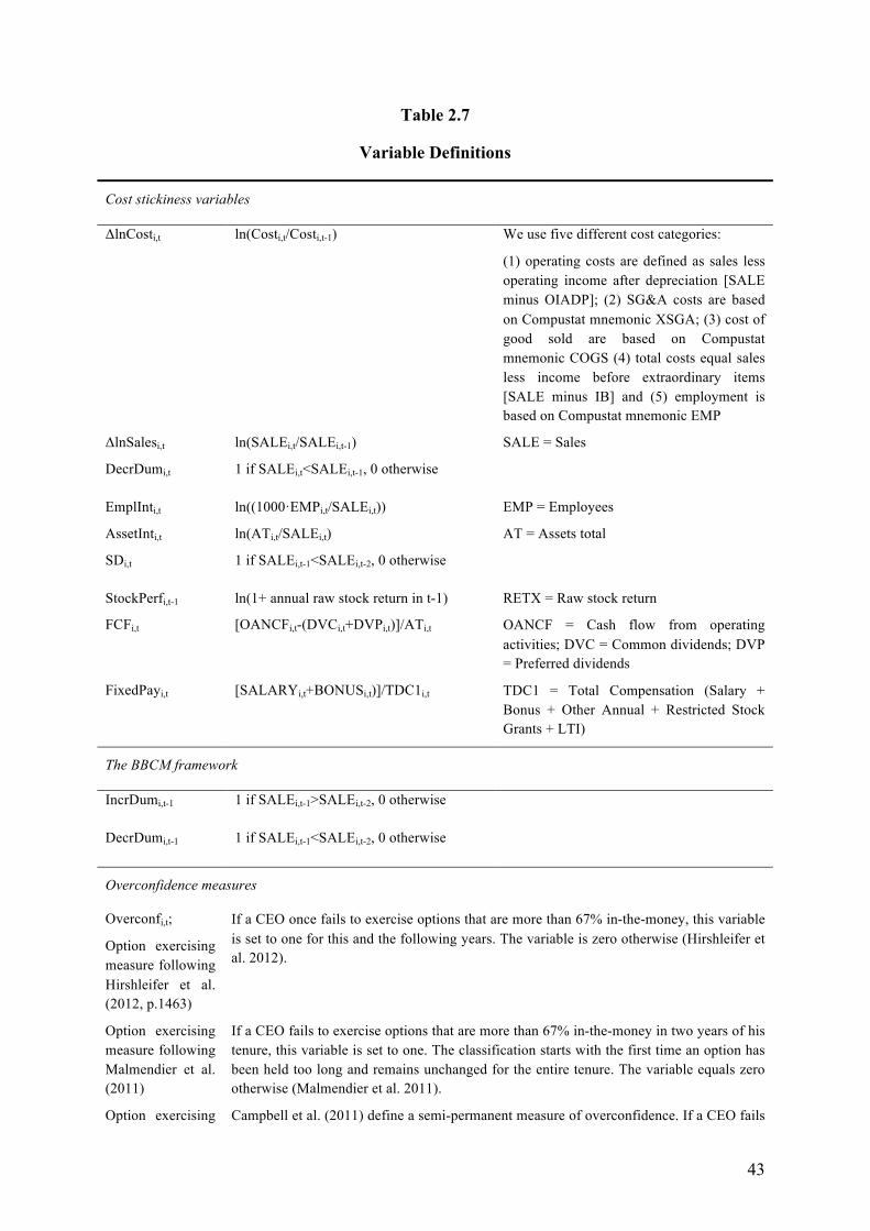
43
Table 2.7
Variable Definitions
Cost stickiness variables
ΔlnCosti,t ln(Costi,t/Costi,t-1) We use five different cost categories:
(1) operating costs are defined as sales less operating income after depreciation [SALE minus OIADP]; (2) SG&A costs are based on Compustat mnemonic XSGA; (3) cost of good sold are based on Compustat mnemonic COGS (4) total costs equal sales less income before extraordinary items [SALE minus IB] and (5) employment is based on Compustat mnemonic EMP
ΔlnSalesi,t ln(SALEi,t/SALEi,t-1) SALE = Sales
DecrDumi,t 1 if SALEi,t<SALEi,t-1, 0 otherwise
EmplInti,t ln((1000·EMPi,t/SALEi,t)) EMP = Employees
AssetInti,t ln(ATi,t/SALEi,t) AT = Assets total
SDi,t 1 if SALEi,t-1<SALEi,t-2, 0 otherwise
StockPerfi,t-1 ln(1+ annual raw stock return in t-1) RETX = Raw stock return
FCFi,t [OANCFi,t-(DVCi,t+DVPi,t)]/ATi,t OANCF = Cash flow from operating activities; DVC = Common dividends; DVP = Preferred dividends
FixedPayi,t [SALARYi,t+BONUSi,t)]/TDC1i,t TDC1 = Total Compensation (Salary +
Bonus + Other Annual + Restricted Stock Grants + LTI)
The BBCM framework
IncrDumi,t-1 1 if SALEi,t-1>SALEi,t-2, 0 otherwise
DecrDumi,t-1 1 if SALEi,t-1<SALEi,t-2, 0 otherwise
Overconfidence measures
Overconfi,t;
Option exercising measure following Hirshleifer et al. (2012, p.1463)
If a CEO once fails to exercise options that are more than 67% in-the-money, this variable is set to one for this and the following years. The variable is zero otherwise (Hirshleifer et al. 2012).
Option exercising measure following Malmendier et al. (2011)
If a CEO fails to exercise options that are more than 67% in-the-money in two years of his tenure, this variable is set to one. The classification starts with the first time an option has been held too long and remains unchanged for the entire tenure. The variable equals zero otherwise (Malmendier et al. 2011).
Option exercising Campbell et al. (2011) define a semi-permanent measure of overconfidence. If a CEO fails
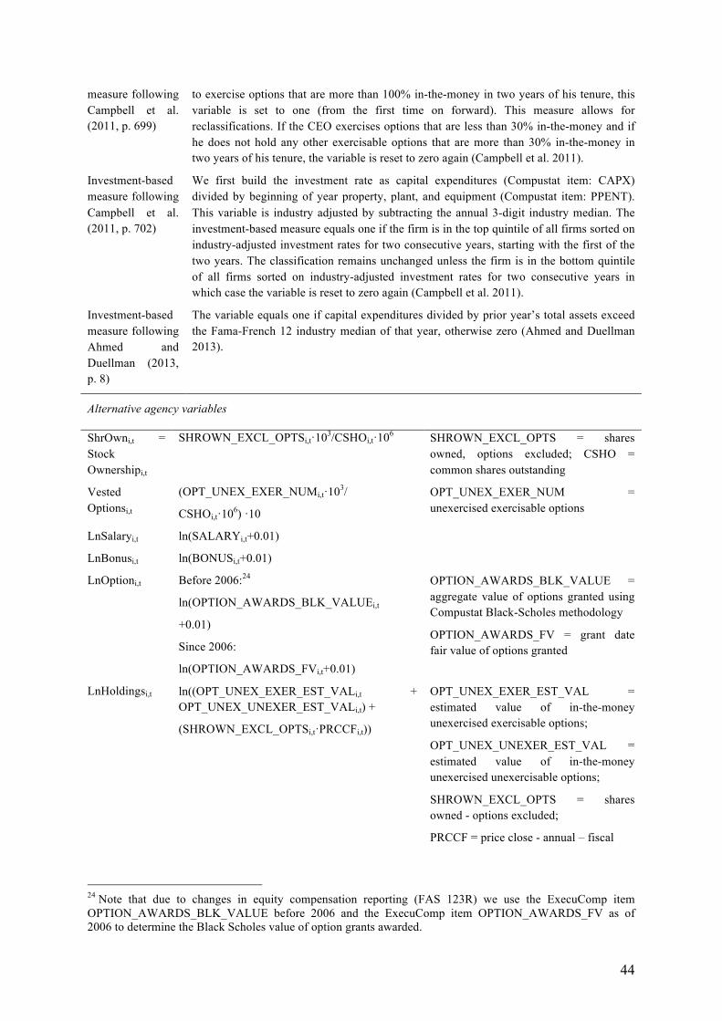
44
measure following Campbell et al. (2011, p. 699)
to exercise options that are more than 100% in-the-money in two years of his tenure, this variable is set to one (from the first time on forward). This measure allows for reclassifications. If the CEO exercises options that are less than 30% in-the-money and if he does not hold any other exercisable options that are more than 30% in-the-money in two years of his tenure, the variable is reset to zero again (Campbell et al. 2011).
Investment-based measure following Campbell et al. (2011, p. 702)
We first build the investment rate as capital expenditures (Compustat item: CAPX) divided by beginning of year property, plant, and equipment (Compustat item: PPENT). This variable is industry adjusted by subtracting the annual 3-digit industry median. The investment-based measure equals one if the firm is in the top quintile of all firms sorted on industry-adjusted investment rates for two consecutive years, starting with the first of the two years. The classification remains unchanged unless the firm is in the bottom quintile of all firms sorted on industry-adjusted investment rates for two consecutive years in which case the variable is reset to zero again (Campbell et al. 2011).
Investment-based measure following Ahmed and Duellman (2013, p. 8)
The variable equals one if capital expenditures divided by prior year’s total assets exceed the Fama-French 12 industry median of that year, otherwise zero (Ahmed and Duellman 2013).
Alternative agency variables
ShrOwni,t = Stock Ownershipi,t
SHROWN_EXCL_OPTSi,t·103/CSHOi,t·106 SHROWN_EXCL_OPTS = shares owned, options excluded; CSHO = common shares outstanding
Vested Optionsi,t
(OPT_UNEX_EXER_NUMi,t·103/
CSHOi,t·106) ·10
OPT_UNEX_EXER_NUM = unexercised exercisable options
LnSalaryi,t ln(SALARYi,t+0.01)
LnBonusi,t ln(BONUSi,t+0.01)
LnOptioni,t Before 2006:24
ln(OPTION_AWARDS_BLK_VALUEi,t
+0.01)
Since 2006:
ln(OPTION_AWARDS_FVi,t+0.01)
OPTION_AWARDS_BLK_VALUE = aggregate value of options granted using Compustat Black-Scholes methodology
OPTION_AWARDS_FV = grant date fair value of options granted
LnHoldingsi,t ln((OPT_UNEX_EXER_EST_VALi,t + OPT_UNEX_UNEXER_EST_VALi,t) +
(SHROWN_EXCL_OPTSi,t·PRCCFi,t))
OPT_UNEX_EXER_EST_VAL = estimated value of in-the-money unexercised exercisable options;
OPT_UNEX_UNEXER_EST_VAL = estimated value of in-the-money unexercised unexercisable options;
SHROWN_EXCL_OPTS = shares owned - options excluded;
PRCCF = price close - annual – fiscal
24 Note that due to changes in equity compensation reporting (FAS 123R) we use the ExecuComp item OPTION_AWARDS_BLK_VALUE before 2006 and the ExecuComp item OPTION_AWARDS_FV as of 2006 to determine the Black Scholes value of option grants awarded.
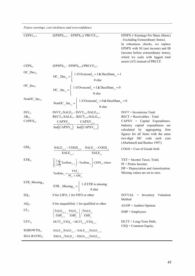
45
Future earnings, cost stickiness and overconfidence
CEPS1i,t+1 (EPSPXi,t+1 – EPSPXi,t)/ PRCCFi,t-1 EPSPX (=Earnings Per Share (Basic) - Excluding Extraordinary Items). In robustness checks, we replace EPSPX with NI (net income) and IB (income before extraordinary items), which we scale with lagged total assets (AT) instead of PRCCF.
CEPSi,t (EPSPXi,t – EPSPXi,t-1)/PRCCFi,t-1
OC_Deci,t
OC_ Deci,t =1 if Overconfi,t =1& DecrDumi,t =1
0 else
⎧⎨⎪
⎩⎪ OC_Inci,t
OC_ Inci,t =1 if Overconfi,t =1& DecrDumi,t = 0
0 else
⎧⎨⎪
⎩⎪ NonOC_Inci,t
NonOC_ Inci,t =1 if Overconfi,t = 0 & DecrDumi,t = 0
0 else
⎧⎨⎪
⎩⎪ INVi,t INVTi,t/SALEi,t - INVTi,t-1/SALEi,t-1
INVT = Inventories Total
ARi,t RECTi,t/SALEi,t - RECTi,t-1/SALEi,t-1
RECT = Receivables - Total
CAPEXi,t CAPXVi,tInd CAPXVi,t( ) −
CAPXVi,t−1Ind CAPXVi,t−1( )
CAPXV = Capital Expenditures. Industry capital expenditures are calculated by aggregating firm figures for all firms with the same two-digit SIC code each year (Abarbanell and Bushee 1997).
GMi,t
SALEi,t−1 −COGSi,t−1SALEi,t−1
−SALEi,t −COGSi,t
SALEi,t
COGS = Cost of Goods Sold
ETRi,t 1
3TaxRatei,t−τ
τ=1
3
∑⎛⎝⎜
⎞⎠⎟−TaxRatei,t
⎡
⎣⎢⎢
⎤
⎦⎥⎥⋅CEPSi,t ,where
TaxRatei,t =TXTi,t
PIi,t +AMi,t
TXT = Income Taxes, Total; PI = Pretax Income; DP = Depreciation and Amortization. Missing values are set to zero.
ETR_Missingi,t ETR _ Missingi,t =
1 if ETR is missing0 else
⎧⎨⎪
⎩⎪ EQi,t 0 for LIFO, 1 for FIFO or other
INVVAL = Inventory Valuation Method
AQi,t 0 for unqualified, 1 for qualified or other AUOP = Auditor Opinion
LFi,t SALEi,t−1EMPi,t−1
−SALEi,tEMPi,t
⎛
⎝⎜
⎞
⎠⎟
SALEi,tEMPi,t
EMP = Employees
LEVi,t DLTTi,t CEQi,t −DLTTi,t−1 CEQi,t−1
DLTT = Long-Term Debt, CEQ = Common Equity,
SGROWTHi,t SALEi,t SALEi,t−1 −SALEi,t−1 SALEi,t.−2
SGA-RATIOi,t XSGAi,t SALEi,t −XSGAi,t−1 SALEi,t−1
46
2.5 Conclusion
In this study, we examine the association between a managerial characteristic,
overconfidence, and cost stickiness. We find strong support for our prediction of a positive
association between managerial overconfidence and cost stickiness. Our results are robust to
many sensitivity checks, including alternative measures of overconfidence, different cost
categories and controlling for managers’ rational expectations of future demand. We also find
that the effect of managerial overconfidence on cost stickiness is primarily driven by the
differences in cost behavior when sales decline.
Furthermore, we predict and find that cost stickiness driven by managerial overconfidence
is negatively associated with future firm performance compared to cost stickiness not driven
by managerial overconfidence. The results are similar for alternative performance measures
and alternative overconfidence proxies. Overall, the results of this analysis provide support
for our argument that overconfident CEOs erroneously overestimate future demand, and
hence, make suboptimal cost adjustment decisions.
Our study extends a growing accounting literature on the effect of personality traits and
other managerial characteristics on managerial decisions by providing one of the first
empirical evidence on the relation between a managerial characteristic and cost management
decisions. Our results also contribute to the debate on the role of managerial overconfidence
in managerial decision-making. Prior studies have documented some of the potential benefits
and costs of managerial overconfidence. For example, Malmendier and Tate (2008)
document that overconfident CEOs conduct value-destroying mergers, while Hirshleifer et al.
(2012) find that overconfident CEOs are better innovators. Our study contributes to this
discussion by presenting evidence of the influence of managerial overconfidence on cost
behavior and the resulting consequences.
In addition, our study contributes to the cost stickiness literature by documenting a
managerial characteristic as a determinant of cost stickiness. In doing so, we provide strong
47
and direct support for the role of managerial discretion in cost management. More generally,
our study represents a first step towards understanding the impact of managerial
characteristics on cost decisions and cost behavior.
Our findings that overconfidence affects cost management and potentially reduces future
firm performance have important practical implications.
First, our study has practical implications for the design of corporate governance
mechanisms. When cost stickiness is driven by legitimate economic reasons (e.g. rational
expectations about future demand, capacity utilization, or adjustment costs), boards of
directors should not intervene in managers’ cost decisions. When cost stickiness is driven by
agency explanations (e.g. empire building incentives), strengthening corporate governance
would help deter overspending on the part of the managers. In contrast to these two types of
cost stickiness, what we document in our study is a type of cost stickiness that is driven for
well-intentioned (but misguided) reasons due to a behavioral bias. Under these circumstances,
modifying the incentive system design would not help mitigate overconfidence-driven cost
mismanagement. We suggest that a more effective way is to mitigate managers’ upward bias
in expectations. For example, boards of directors can take measures to challenge the
expectation assumptions of overconfident CEOs and enhance overconfident CEOs’
awareness of their own potential behavioral biases.
Second, to the extent that sophisticated market participants and the media can use the
option-based overconfidence classification to identify overconfident CEOs, market
participants can also mitigate the potential negative impact of managerial overconfidence by
challenging overconfident CEOs’ expectations about future sales and associated cost
decisions.
Third, our findings also have implications for labor market practices. When cost
management is particularly important for an organization, the organization needs to be

48
especially cautious in hiring an overconfident CEO.
Finally, our results that cost stickiness driven by managerial overconfidence has negative
impact on future firm performance also generate new insights for financial accounting
research. Managers’ cost decisions influence cost behavior, which affects earnings behavior
and ultimately impacts firm valuations. For example, the results of our study have
implications for earnings properties, earnings prediction models, and analyst forecasts.
49
3 The Impact of Investor Sentiment on Operating Expenditure –
a Catering Perspective
3.1 Introduction
This study belongs to a stream of literature that intends to increase our understanding of
how investor sentiment can affect corporate policies. The concept of investor sentiment
relaxes the assumption of perfect rationality, differentiating between two types of investors:
Rational arbitrageurs and irrational (or noise) traders (Baker and Wurgler 2006, 2007). The
so-called catering theory states that the existence of noise traders allows managers to boost
the short-term stock price by adjusting their corporate policies to noise traders’
misperceptions (Stein 1996; Baker and Wurgler 2011). Drawing on this theory, prior
literature documents that investor sentiment affects a variety of corporate decisions, including
decisions on corporate name changes, corporate disclosure, or dividends.25 Most closely
related to our study is the finding that catering affects decisions on long-term investment
projects (Polk and Sapienza 2009). So far, there is, however, no evidence on how investor
sentiment affects short-term or operating expenditure. While the catering theory predicts an
unambiguously positive association between capital expenditure and investor sentiment, we
argue that there are two opposing channels linking investor sentiment and operating
expenditure.
First, prior literature suggests that noise traders have optimistically biased cash flow
expectations in periods of high sentiment (Baker and Wurgler 2006, 2007; Stein 1996). If
noise traders overestimate investment opportunities, managers may feel pressure to alter their
investment behavior. There is ample evidence documenting the long-term value-creating
potential for research and development (R&D) expenditure (Eberhart et al. 2004; Lev and
Sougiannis 1996; Sougiannis 1994), advertising expenses (Chan et al. 2001; Hirschey and
25 See Cooper, Dimitrov, and Rau (2001); Cooper et al. (2005); Bergman and Roychowdhury (2008); Brown
et al. (2012); Baker and Wurgler (2004); Li and Lie (2006).
50
Weygandt 1985; Madden et al. 2006), and selling, general and administrative (SG&A)
resources (Anderson et al. 2007; Banker et al. 2011; Tronconi and Marzetti 2011). To the
extent that managers cater to investors’ optimistic investment expectations, we, therefore,
expect to observe a positive association between investor sentiment and operating
expenditure.
Second, there is evidence indicating that investors have overly optimistic earnings
expectations in periods of high sentiment (Hribar and McInnis 2012; Mian and
Sankaraguruswamy 2012; Seybert and Yang 2012; Walther and Willis 2013). Exacerbated
earnings expectations may induce managers to reduce spending on operating expenditure
because reducing operating expenditure allows to boost current-period income (Baber et al.
1991; Burgstahler and Dichev 1997; Roychowdhury 2006). Managers will be less likely to
consider current-period income effects when making decisions on capital expenditure, given
that capital expenditure is depreciated over multiple periods and, hence, has little effect on
current earnings (Baber et al. 1991; Dechow and Sloan 1991). In our setting, we, therefore,
argue that mangers face a trade-off between catering to investors’ cash flow and catering to
investors’ earnings expectations. In absence of incentives to meet earnings, we expect to
observe a positive association between investor sentiment and operating expenditure. For
firms that face earnings targets, we, however, argue the expected positive association should
be significantly less pronounced or may even turn negative.
In the empirical analysis, we measure investor sentiment using the annual sentiment index
proposed by Baker and Wurgler (2006). They extract the common component underlying
several sentiment measures that have been used in prior literature on investor sentiment. The
index measures investor sentiment at the aggregate market level and is widely used by
subsequent studies (e.g., Brown et al. 2012; Hribar and McInnis 2012; McLean and Zhao
2014; Mian and Sankaraguruswamy 2012).
51
To test the catering hypothesis, we regress changes in operating expenditure on changes in
sentiment controlling for both firm- and macro-level determinants of operating expenditure.
Our sample is based on the intersection of Compustat, CRSP and data on GDP, comprising
105,885 observations from 1972 till 2010. Consistent with the catering theory, we find a
positive association between investor sentiment and operating expenditure. More specifically,
we find that managers increase spending on R&D expenditure, advertisement and various
components of SG&A costs in response to high sentiment. We also document that catering
extends to employment decisions in that managers hire more aggressively in periods of high
relative to periods of average sentiment.
In further analyses, we find results that are consistent with cross-sectional predictions of
the catering theory. First, our results indicate that managers tend to increase spending on
SG&A resources if these resources have high future value creating potential. Second, we find
catering tendencies to increase as managers’ horizons decrease, and, third, our results indicate
that catering is more pronounced for those firms that are more strongly affected by investor
sentiment.
Finally, our results suggest that the association between investor sentiment and SG&A
costs, R&D expenditure and employment is significantly less pronounced if firms face
incentives to avoid losses. These results support our second hypothesis indicating that
managers are less likely to increase spending on operating expenditure when facing earnings
targets.
We make two contributions to prior literature. We first contribute to prior literature that
examines real effects of investor sentiment. Existing studies show that investor sentiment
affects management earnings forecasts (Bergman and Roychowdhury 2008), pro-forma
earnings disclosure (Brown et al. 2012), or accrual-based earnings management (Simpson
2013; Ali and Gurun 2009). More closely related to our study are the findings that managers
52
cater to investors’ misperceptions by changing their dividend policy (Baker and Wurgler
2004; Li and Lie 2006) and by overspending on capital expenditure (Polk and Sapienza 2009).
We contribute to this literature by documenting that catering extends to decisions on research
and development expenditure, advertisement and selling, general and administrative costs.
Since caterers act in the interest of short-term shareholders only, our study has monitoring
implications for board of directors. This is particularly relevant since SG&A costs, for
example, make up about one third of total assets.26
In a related vein, our finding that managers cater to investors’ misperceptions by hiring
more aggressively complements the findings in McLean and Zhao (2014). They likewise
build on the model of Stein (1996) but test the equity instead of the catering channel, which
suggests that investor sentiment can influence corporate policies because it reduces the cost
of external finance (Baker and Wurgler 2011; Stein 1996). Hence, while McLean and Zhao
(2014) show that investor sentiment affects employment decisions through the equity channel,
we show how investor sentiment affects employment decisions through the catering
channel.27
Second, this study contributes to our understanding of how managerial discretion affects
cost behavior. In an influential study, Anderson et al. (2003) document that many cost
changes arise as a result of deliberate managerial decisions, which contrasts with the
traditional model of fixed and variable costs postulating that cost behavior is mechanically
related to changes in activity. Building on this finding, Chen et al. (2012) show that empire
building incentives affect cost behavior in that empire builders refrain from reducing costs
when sales fall. Banker et al. (2011) show that equity incentives induce managers to increase
spending on SG&A resources when these resources create high future value. We contribute
26 In our sample, the average ratio of SG&A to total assets is about 34%. This number is comparable to other studies. Banker et al. (2011), for example, document an average ratio of SG&A to total assets of 31%. 27 To control for the equity channel, we follow Polk and Sapienza (2009) and include equity issuance as a control variable in all our analyses.
53
to this literature by documenting that catering incentives induce managers to increase
spending on various components of operating expenditure as means of addressing investment
expectations in periods of high sentiment.
In addition, our study contributes to prior literature examining how incentives to meet
earnings targets affect managers’ cost decisions. Dierynck et al. (2012) and Kama and Weiss
(2013) document that earnings targets affect managers’ cost decisions in that managers are
less likely to keep costs when sales decline upon facing earnings targets. Prior literature on
real earnings management further shows that managers cut costs in order to avoid reporting
losses, to meet last year’s earnings or analysts’ expectations (Baber et al. 1991; Burgstahler
and Dichev 1997; Graham, Harvey, and Rajgopal 2005; Roychowdhury 2006). We contribute
to this literature by documenting that incentives to meet earnings targets reduce managers
catering incentives, thereby providing support for the role of managerial discretion in the
process of resource adjustment.
The remainder of the paper is organized as follows: In section 2, we discuss our
hypothesis development. In section 3, we present our research design. We present our results
in section 4. Section 5 concludes.
3.2 Hypothesis Development and Related Literature
3.2.1 Investor Sentiment
This section provides background on the concept of investor sentiment, discusses the
underlying assumptions, and provides additional information on the catering theory.
The concept of investor sentiment grounds on four assumptions (Baker and Wurgler 2011).
The first assumption allows investor behavior to deviate from perfect rationality. The
behavioral accounting and finance literature, thus, differentiates between two types of
investors: Rational arbitrageurs and irrational or noise traders (Baker and Wurgler 2007).
Irrationality can stem from a variety of sources. Early explanations include Shiller (1984)
54
who argues that social movements affect asset prices, or Black (1986) who argues that
irrational investors trade on noise rather than news. The theoretical model of Daniel,
Hirshleifer, and Subrahmanyam (1998) allows investors to be overconfident about the
accuracy of their private information signals and to further exhibit biased self-attribution
which implies that investors attribute favorable outcomes to their own decisions and
unfavorable outcomes to bad luck (also see Barber and Odean 2001). In Barberis et al. (1998),
investor behavior is characterized by both representativeness and conservatism. Grinblatt and
Keloharju (2009) analyze the association between trading activity and sensation seeking.
Hong and Stein (1999), in contrast, focus less on particular cognitive biases but more on the
interplay between two types of boundedly rational investors, news-watchers and momentum
traders, who are not able to process the entire amount of publicly available information.
Baker and Wurgler (2007, 129) try to combine the various facets of noise trading by defining
investor sentiment as “a belief about future cash flows and investment risks that is not
justified by the facts at hand”.
In order for noise traders to persist, arbitrage has to be limited. The second assumption
thus deals with arbitrage constraints. Miller (1977), for example, argues that short-sale
constraints can move prices away from fundamental value (also see Berkman et al. 2009). In
De Long et al. (1990), the unpredictability of noise traders’ future opinions creates a risk that
dampens the willingness of rational arbitrageurs, who have short horizons and are risk-averse,
to bet against them. Shleifer and Vishny (1997) highlight the role of agency problems and
information asymmetries between professional investors, the arbitrage force in financial
markets, and their capital lenders that may limit the effectiveness of arbitrage.
Third, the biases of investors have to be systematic, otherwise they would cancel out. In
this regard, Kumar and Lee (2006) provide large scale empirical evidence documenting that
retail investor trading is correlated across individuals and across groups of stocks. These
55
effects are more pronounced for stocks that are more costly to arbitrage and have higher
individual investor concentration. Collectively, the evidence of Kumar and Lee (2006)
suggests that retail investors trade in concert.
Combining these three assumptions, noise traders can affect stock prices. Baker and
Wurgler (2006, 2007) document that periods of high sentiment result in overvaluation and
subsequently are followed by low stock returns as prices revert to their intrinsic value.
Lemmon and Portniaguina (2006) and Brown and Cliff (2005) obtain similar results.
The fourth assumption characterizes the behavior of managers. Whereas investors’
earnings expectations are upwardly biased in periods of high sentiment (Hribar and McInnis
2012; Seybert and Yang 2012; Stein 1996), managers are assumed to both form rational
expectations and be able to perceive variations in sentiment (Hribar and Quinn 2013). Given
the existence of investor sentiment, Baker and Wurgler (2011) argue that managers balance
two conflicting goals. The first goal consists in maximizing fundamental value. The second
goal consists in maximizing the current stock price. While both goals are the same in a
rational world, maximizing the short-term stock price turns into a distinct objective once
investor behavior is allowed to differ from perfect rationality.
The catering theory implies that managers who are interested in maximizing the short-term
stock price have to adjust their corporate polices to the sentiment-driven demands of
investors by “packaging the firm and its securities in a way that maximizes appeal to
investors” (Baker and Wurgler 2011, 13). If investors, for example, overvalue the prospects
of a firm’s assets, managers can, in fact, boost the short-term stock price by investing more
aggressively in these assets (Stein 1996). This may, e.g., imply that managers should be
willing to invest in negative NPV projects as long as noise traders perceive these projects as
profitable (Baker and Wurgler 2011; Polk and Sapienza 2009; Stein 1996). More generally,
catering refers to corporate policies that intend to exploit or encourage stock market
56
mispricing in order to increase the short-term stock price (Baker and Wurgler 2011). This
tendency should be more pronounced as managers’ horizons shorten (Baker and Wurgler
2011). Notably, even managers with long horizons will not completely ignore sentiment but
potentially cater to investors’ short-term demands, too. Since managers with long horizons
act in the interest of long-term shareholders, they may decide to exploit the current
mispricing by, for example, issuing overvalued or repurchasing undervalued shares (see for
example Baker and Wurgler 2000; Graham and Campbell 2001).
In addition to distorting asset prices, there, hence, are real consequences of investor
sentiment. Prior literature has shown that the presence of noise traders affects corporate
decisions such as investment (Gilchrist, Himmelberg, and Huberman 2005; Polk and
Sapienza 2009), equity issuance (Baker and Wurgler 2002), initiating dividends (Baker and
Wurgler 2004; Li and Lie 2006), earnings management (Simpson 2013; Ali and Gurun 2009)
or disclosure (Hribar and McInnis 2012; Seybert and Yang 2012).
3.2.2 Investor Sentiment and Operating Expenditure
To link operating expenditure and investor sentiment we build on the catering theory.
Essentially, the theory states that managers can boost the short-term stock price by adjusting
their corporate policies to noise traders’ misperceptions (Stein 1996; Baker and Wurgler
2011). Drawing on the catering theory, we expect that there are two opposing channels
linking investor sentiment and operating expenditure. First, several studies suggest that
investors have optimistically biased cash flow expectations in periods of high sentiment
(Baker and Wurgler 2006, 2007; Stein 1996). We argue that increasing operating expenditure
is one way of catering to investors’ overly optimistic investment expectations. This view
builds on prior literature documenting that operating expenditure has long-term value-
creating potential. With regard to research and development expenditure, Sougiannis (1994)
documents that R&D expenditure has a positive effect on operating income that persists up to
57
seven years. Lev and Sougiannis (1996) find that R&D capital is associated with abnormal
subsequent stock returns. Similarly, Eberhart et al. (2004) document that R&D increases
result in both long-term abnormal stock returns and long-term abnormal operating
performance. Further, several studies show that the value creation of advertising expenditure
is not limited to the period in which the expenses are incurred. Hirschey and Weygandt
(1985) show that advertising has a positive effect on the market value of the firm, persisting
between one and five years. In addition, Chan et al. (2001) and Madden et al. (2006)
document that advertising-intensive firms earn abnormal returns.
Also, there is evidence from recent research on fundamental analysis (Anderson et al.
2007; Baumgarten, Bonenkamp, and Homburg 2010), executive compensation (Banker et al.
2011) and organization capital (Lev and Radhakrishnan 2005; De and Dutta 2007; Tronconi
and Marzetti 2011) documenting that selling, general and administrative (SG&A) resources
have a positive impact on future firm performance. While Lev and Thiagarajan (1993) find a
negative association between future stock returns and SG&A costs, Abarbanell and Bushee
(1997) fail to find an association between future earnings and SG&A. In contrast, Anderson
et al. (2007) and Baumgarten et al. (2010) document that increases in SG&A are positively
associated with future earnings in revenue-declining periods and if these increases can be
seen as intentional by the management, respectively. Further, providing evidence from
research on executive compensation, Banker et al. (2011) document that managers increase
spending on SG&A expenditure upon receiving equity incentives when SG&A resources
create high future value. More generally, Matejka (2011) regards the key contribution of
Banker et al. (2011) in documenting the long-term value creating potential of SG&A
resources.
The literature on organization capital provides additional evidence on the value relevance
of SG&A cost. Building on Lev and Radhakrishnan (2005), several studies advocate the use
58
of SG&A expenditure as a measure of organization capital given that SG&A comprises
expenditure on employee training, brand enhancement, information technology, human
resource development or customer relationship management (Eisfeldt and Papanikolaou
2013; Eisfeldt and Papanikolaou 2014). Further, Lev and Radhakrishnan (2005) document
that organization capital has a positive impact on firm performance. Measuring organization
capital by capitalizing SG&A expenditure, Tronconi and Marzetti (2011) and Eisfeldt and
Papanikolaou (2013) obtain similar results (also see De and Dutta 2007).
Collectively, there is ample evidence indicating that various components of operating
expenditure create long-term value. Hence, to the extent that managers cater to investors’
optimistic investment expectations, we expect to observe a positive association between
operating expenditure and investor sentiment.
H1: Managers cater to investors’ sentiment driven demands by overspending on operating
expenditure in periods of high relative to periods of average sentiment.
The second channel draws on prior literature documenting that investors have upwardly
biased earnings expectations in periods of high sentiment (Hribar and McInnis 2012; Mian
and Sankaraguruswamy 2012; Seybert and Yang 2012; Walther and Willis 2013). Facing
exaggerated earnings expectations, managers may alternative decide to reduce rather than
increase spending on operating expenditure. This view builds on prior literature that
examines managers’ responses to earnings targets. There are several studies documenting that
managers reduce spending on, e.g., R&D if these expenditures hamper reporting positive or
increasing income in the current period, Baber et al. (1991) is one example. Similarly,
Roychowdhury (2006) finds evidence indicting that managers reduce R&D and SG&A
expenditure to avoid reporting losses or to meet analysts’ forecasts. Further, Gunny (2010)
finds reductions in spending on R&D and SG&A for firms that just meet zero or last year’
earnings. Graham et al. (2005) extend the findings of these archival studies by providing
59
survey evidence. Most of the CFOs they interview state that companies should or would take
actions such as postponing or reducing R&D to meet earnings targets.
We argue the insights of these studies should be particularly relevant in periods of high
sentiment since several studies document that investors’ earnings expectations are upwardly
biased when there is high sentiment. For example, Hribar and McInnis (2012) show that
analysts’ earnings forecasts are optimistically biased in periods of high sentiment (also see
Walther and Willis 2013). Since analysts can clearly be seen as sophisticated investors, this
finding should likely extend to nonprofessional investors. Focusing on management earnings
forecasts, Seybert and Yang (2012) likewise show that investors have overly optimistic
earnings expectations in periods of high sentiment (also see Mian and Sankaraguruswamy
2012; Skinner and Sloan 2002).
Building on this literature, we assume that the cost of, for example, reporting losses
increases as investors’ earnings expectations increase. Given that operating expenditure is
completely charged and expensed against the earnings of the period in which it is incurred
(Banker et al. 2011), we argue that managers will be less likely to cater by overspending on
operating expenditure if it increases the risk of falling short of investors’ earnings
expectations. In sum, we expect that firms that have incentives to meet earnings targets cater
less than firms that do not have incentives to meet earnings targets in periods of high
sentiment. Depending on the distance to the earnings targets, there are two possible scenarios.
First, if it suffices to cater less to reach investors’ earnings expectations, the association
between investor sentiment and operating expenditure should be of smaller magnitude in the
presence of earnings targets. If, however, reaching investors’ inflated earnings expectations
requires cutting of operating expenditure, the association between investor sentiment and
operating expenditure may even turn negative conditional on earnings targets.
60
H2: Managers are less likely to cater by overspending on operating expenditure in
periods of high relative to periods of average sentiment if catering entails a risk of missing
earnings targets.
3.3 Research Design
3.3.1 Sample Selection
Our sample is based on the intersection of CRSP/Compustat, GDP and investor sentiment
data. From CRSP/Compustat we drop (1) financial firms and utilities (sic codes 6000 to 6999
and 4900 to 4999), (2) firm-years with negative sales or negative selling, general and
administrative (SG&A) costs, and (3) require the currency to be USD. We obtain both data
on real GDP and the GDP deflator from the Federal Reserve Bank of St. Louis and adjust all
monetary variables for inflation by dividing with the GDP deflator.28 The investor sentiment
data is available on Jeffrey Wurgler’s homepage.29 The final sample comprises 105,885 firm-
years from 1972 to 2010. We winsorize the top and bottom 1% of all continuous variables.
3.3.2 Investor Sentiment Measurement
In the empirical analysis, we use the annual sentiment index by Baker and Wurgler (2006).
The index is an attempt to capture the common sentiment component of several sentiment
proxies that have been identified and used in prior literature: The closed-end fund discount,
trading volume (NYSE share turnover), the number and average first-day returns on initial
public offerings (IPOs), the dividend premium and the equity share in new issues. The index
is defined as the first principal component of these variables and captures sentiment at the
aggregate market level.
Since Baker and Wurgler (2006, 2007) discuss the choice of the individual proxies in great
detail, we only provide brief motivation for two variables. With regard to the closed-end fund
(CEF) discount, for example, Lee, Shleifer, and Thaler (1991) argue that changes in the 28 http://www.research.stlouisfed.org/ 29 http://people.stern.nyu.edu/jwurgler/
61
discounts on closed-end funds result from variation in investor sentiment. A CEF is an
investment company that issues a fixed number of shares that then trade at secondary markets
(Anderson, Born, and Schnusenberg 2010). Closed-end funds usually trade at a discount
which corresponds to the difference between the funds’ net asset value and its market value.
Prior literature has offered a number of explanations for why there are discounts on closed-
end funds, including agency costs (e.g., excessive management fees), illiquidity of assets
(suggesting that CEFs’ net asset values are overstated) and tax liabilities (Lee et al. 1991).
However, none of the prior approaches has been able to provide a thorough explanation.
Lee et al. (1991) argue that investor sentiment drives the discount on closed-end funds.
They build on the work of De Long et al. (1990) who theoretically model how noise traders
can affect stock prices. Essentially, De Long et al. (1990) argue that the existence of noise
traders creates an additional source of risk on assets’ resale prices. Key to the model is the
assumption that changes in noise traders’ sentiment are stochastic and unpredictable. Further,
De Long et al. (1990) assume that rational investors have short horizons, i.e., they are
interested in the interim resale price of their assets. Since rational investors cannot know
whether noise traders are bullish or bearish when they intend to sell their assets, rational
investors will not be willing to hold assets that are affected by noise traders’ sentiment unless
they are compensated for bearing the risk that arises from the unpredictability of future
sentiment. De Long et al. (1990), hence, argue that unpredictable fluctuations in noise traders’
future opinions create a further source of risk for the stocks they trade.
Lee et al. (1991) provide evidence that noise traders rather invest in closed-end funds than
their underlying assets. Holding closed-end funds, therefore, is riskier than holding the
underlying portfolio. Hence, closed-end funds have to yield, on average, higher required rates
of return than their underlying portfolios. This implies that, on average, closed-end funds
must sell at a discount to their net asset value due to the unpredictability of changes in noise
62
traders’ sentiment. Taken together, the evidence in Lee et al. (1991) suggests that variation in
discounts on closed-end funds proxies for changes in investor sentiment. Hence, Baker and
Wurgler (2006, 2007) use the (value-weighted) average discount on closed-end funds as one
proxy for investor sentiment.
As an alternative proxy for investor sentiment, Baker and Wurgler (2006, 2007) focus on
the market for IPOs. Derrien (2005), for example, argues that investor optimism contributes
to the often tremendous initial returns on initial public offerings (IPO). Similarly, Ritter
(1991) argues the underperformance of IPOs over longer horizons is indicative of market
timing in that firms go public when investors are overly optimistic. The sentiment-index,
therefore, reflects both the number and the average first-day returns of IPOs.30
While the choice of the individual sentiment proxies is guided by prior literature, which
identifies the proxies as measures of investor sentiment, a natural question is whether the
index may, nonetheless, reflect economic fundamentals. The main findings of Baker and
Wurgler (2006, 2007), however, help to rule out the conjecture that the sentiment index
simply reflects economic fundamentals and, hence, captures systematic risk.
Baker and Wurgler (2006, 2007) analyze the association between future stock returns and
investor sentiment, arguing that the effect of investor sentiment on firms’ stock prices varies
cross-sectionally. Compared to bond-like firms that have long earnings histories, pay
dividends and have tangible assets, investor sentiment should have a stronger effect on the
stock prices of firms that are relatively young, currently unprofitable, have opaque assets but
at the same time exhibit high growth potential since valuations of these firms are both
subjective and difficult to arbitrage. In periods of high sentiment, investor optimism, hence,
should push stock prices of these difficult-to-arbitrage firms to a larger extent than those of
bond-like firms. This, however, implies that difficult-to-arbitrage firms should realize lower
30 See Baker and Wurgler (2006, 2007) for an in-depth motivation of the remaining sentiment proxies.
63
future stock returns than bond-like firms as fundamentals revert and the mispricing gets
corrected. Baker and Wurgler (2006, 2007) confirm this conjecture empirically. While one
may clearly argue that young firms that are unprofitable and have opaque assets are more
risky than bond-like firms, risk-based asset pricing models, such as the capital-asset pricing
model, predict them to earn higher expected returns. This prediction, however, contrasts with
the findings in Baker and Wurgler (2006, 2007) who, in fact, document the opposite. Their
finding that firms, which are more risky realize lower expected returns than firms that are less
risky following periods of high sentiment helps to alleviate concerns that the index is
contaminated by economic fundamentals. Despite this compelling evidence, we test the
sensitivity of our results to using an alternative index of investor sentiment that has been
orthogonalized to a set of macroeconomic variables in the robustness section.
3.3.3 Research Design of H1
To test H1, we relate changes in operating expenditure to changes in investor sentiment
controlling for both firm and macro level determinants of operating expenditure. We estimate
the following regression model:
ΔOpExi,t = βo +β1 ⋅ΔSentt +β2 ⋅ΔSalei,t +β3 ⋅ΔCashFlowi,t +β4 ⋅ΔLeveragei,t+β5 ⋅ΔEqIssi,t +β6 ⋅Δ lnGDPt +β7 ⋅Δ lnGDPt−1 + εi,t
(3.1)
i is a firm index, t is a time index, ∆ is the difference operator and ln is the natural
logarithm. Depending on the specification, ΔOpExi,t is the change in selling, general and
administrative costs (Compustat mnemonic XSGA), scaled by lagged total assets (AT), or the
log change in employment (EMP). In further analyses, we split SG&A costs in research and
development expenses (XRD), advertisement expenditures (XAD) and other SG&A (XSGA-
XRD-XAD). We likewise scale the change in these variables with lagged total assets.
Sentt is the annual sentiment index by Baker and Wurgler (2006). In our regressions, we
use the first difference of the index, which we standardize to have a mean of zero and a
64
standard deviation of one.
When using panel data, there are two approaches to control for unobserved heterogeneity:
First differences (FD) and firm-fixed effects (FE). Both alternatives enable to control for all
variables that are time-constant at the firm level and potentially correlate with both investor
sentiment and operating expenditure. FE is appropriate if the variable of interest has an
impact on the long-term level of the dependent variable. FD, in contrast, is appropriate if the
variable of interest has an impact on the change of the dependent variable between two
adjacent periods (Andreß, Golsch, and Schmidt 2013). Given that investors’ misperceptions
eventually revert (Baker and Wurgler 2006, 2007; Brown and Cliff 2005; Lemmon and
Portniaguina 2006), the catering theory implies that investor sentiment has a short-term, as
opposed to long-term, impact on corporate policies (Baker and Wurgler 2011). Hence, we
favor FD over FE in our setting and estimate equation (3.1) using first differences.
To differentiate between investor sentiment and managers’ demand expectations, we
include two sets of control variables. To control for firm-specific factors that affect managers’
demand expectations, we control for changes in sales since sales drive many of the
components of operating expenditure. The change in sales also controls for growth options.
We expect changes in sales to be positively associated with changes in operating expenditure.
To control for the macroeconomic environment that may likewise affect managers’ demand
expectations and, hence, spending on operating expenditure, we control for both current and
lagged growth in real GDP (Anderson et al. 2003). These controls are further important to
rule out the alternative explanation that our variable of interest may reflect macroeconomic
conditions rather than investor sentiment. Note that Baker and Wurgler (2006) document that
the index does not reflect economic fundamentals, see section 3.2.
We further control for changes in cash flow because increasing cash flow may induce
managers to overspend regardless of changes in investor sentiment and, hence, catering
65
incentives (Chen et al. 2012). Since our dependent variable is expenditure on SG&A, we use
pre SG&A cash flow (Banker et al. 2011), which equals earnings before extraordinary items
plus SG&A expenditure minus total accruals. We expect this variable to take on a positive
coefficient. We control for change in leverage since firms may be less likely to cater to
investors’ misperceptions if catering increases the risk of violating debt covenants (Duke and
Hunt 1990). We expect a negative association between leverage and operating expenditure.
Finally, we follow Polk and Sapienza (2009) and control for change in equity issuance
because prior research shows that equity financing influences how investor sentiment affects
corporate policies (Baker, Stein, and Wurgler 2003; McLean and Zhao 2014). A positive
coefficient on equity issuance is expected.
We cluster standard errors at the firm level allowing for heteroskedasticity and arbitrary
within-firm correlation (Petersen 2009).
If managers cater to investors’ misperceptions through operating expenditure, we expect
β1>0.
3.3.4 Research Design of H2
To test our second hypothesis, we estimate eq. (3.2):
ΔOpExi,t = βo +β1 ⋅ΔSentt +β2 ⋅EarningsTargeti,t +β3 ⋅ΔSentt ⋅EarningsTargeti,t+β4 ⋅ΔSalei,t +β5 ⋅ΔCashFlowi,t +β6 ⋅ΔLeveragei,t +β7 ⋅ΔEqIssi,t+β8 ⋅Δ lnGDPt +β9 ⋅Δ lnGDPt−1 + εi,t
(3.2)
i is a firm index, t is a time index, ∆ is the difference operator and ln denotes the natural
logarithm. ΔOpExi,t is defined as in section 3.3.31 We use the same set of controls as in
equation (3.1) and cluster standard errors by firm.
The variable of interest is the interaction between our sentiment measure ΔSentt and the
31 Depending on the specification, ΔOpExi,t is the change in selling, general and administrative costs (Compustat mnemonic XSGA), scaled by lagged total assets (AT), or the log change in employment (EMP). In further analyses, we split SG&A costs in research and development expenses (XRD), advertisement expenditures (XAD) and other SG&A (XSGA-XRD-XAD). We likewise scale the change in these variables with lagged total assets.
66
dummy variable EarningsTargeti,t, which is one if net income (Compustat mnemonic NI)
divided by lagged total assets (AT) is in the interval between 0 and 0.01. The focus on small
positive earnings as a measure of incentives to reach earnings targets follows prior literature
on managerial myopia and real earnings management (Baber et al. 1991; Burgstahler and
Dichev 1997; Roychowdhury 2006). Our second hypothesis predicts that catering tendencies
should be attenuated if managers face earnings targets: β3<0.
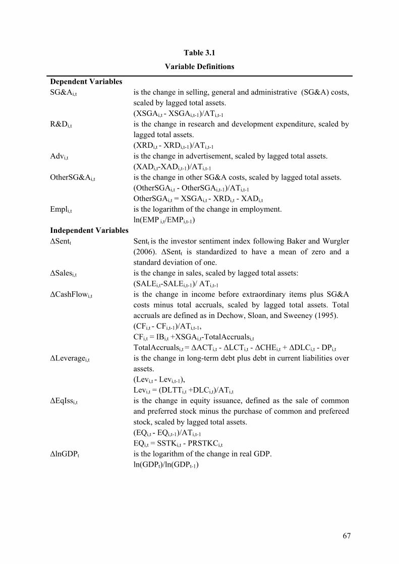
67
Table 3.1
Variable Definitions
Dependent Variables SG&Ai,t is the change in selling, general and administrative (SG&A) costs,
scaled by lagged total assets. (XSGAi,t - XSGAi,t-1)/ATi,t-1
R&Di,t is the change in research and development expenditure, scaled by lagged total assets. (XRDi,t - XRDi,t-1)/ATi,t-1
Advi,t is the change in advertisement, scaled by lagged total assets. (XADi,t-XADi,t-1)/ATi,t-1
OtherSG&Ai,t is the change in other SG&A costs, scaled by lagged total assets. (OtherSGAi,t - OtherSGAi,t-1)/ATi,t-1 OtherSGAi,t = XSGAi,t - XRDi,t - XADi,t
Empli,t is the logarithm of the change in employment. ln(EMP i,t/EMPi,t-1)
Independent Variables ΔSentt Sentt is the investor sentiment index following Baker and Wurgler
(2006). ΔSentt is standardized to have a mean of zero and a standard deviation of one.
ΔSalesi,t is the change in sales, scaled by lagged total assets: (SALEi,t-SALEi,t-1)/ ATi,t-1
ΔCashFlowi,t is the change in income before extraordinary items plus SG&A costs minus total accruals, scaled by lagged total assets. Total accruals are defined as in Dechow, Sloan, and Sweeney (1995). (CFi,t - CFi,t-1)/ATi,t-1, CFi,t = IBi,t +XSGAi,t-TotalAccrualsi,t
TotalAccrualsi,t = ΔACTi,t - ΔLCTi,t - ΔCHEi,t + ΔDLCi,t - DPi,t ΔLeveragei,t is the change in long-term debt plus debt in current liabilities over
assets. (Levi,t - Levi,t-1), Levi,t = (DLTTi,t +DLCi,t)/ATi,t
ΔEqIssi,t is the change in equity issuance, defined as the sale of common and preferred stock minus the purchase of common and prefereed stock, scaled by lagged total assets. (EQi,t - EQi,t-1)/ATi,t-1 EQi,t = SSTKi,t - PRSTKCi,t
ΔlnGDPt is the logarithm of the change in real GDP. ln(GDPt)/ln(GDPt-1)
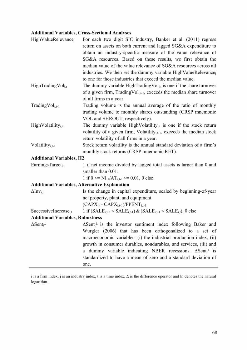
68
Additional Variables, Cross-Sectional Analyses HighValueRelevancej For each two digit SIC industry, Banker et al. (2011) regress
return on assets on both current and lagged SG&A expenditure to obtain an industry-specific measure of the value relevance of SG&A resources. Based on these results, we first obtain the median value of the value relevance of SG&A resources across all industries. We then set the dummy variable HighValueRelevancej to one for those industries that exceed the median value.
HighTradingVoli,t The dummy variable HighTradingVoli,t is one if the share turnover of a given firm, TradingVoli,t-1, exceeds the median share turnover of all firms in a year.
TradingVoli,t-1 Trading volume is the annual average of the ratio of monthly trading volume to monthly shares outstanding (CRSP mnemonic VOL and SHROUT, respectively).
HighVolatilityi,t The dummy variable HighVolatilityi,t is one if the stock return volatility of a given firm, Volatilityi,t-1, exceeds the median stock return volatility of all firms in a year.
Volatilityi,t-1 Stock return volatility is the annual standard deviation of a firm’s monthly stock returns (CRSP mnemonic RET).
Additional Variables, H2 EarningsTargeti,t 1 if net income divided by lagged total assets is larger than 0 and
smaller than 0.01: 1 if 0 <= NIi,t/ATi,t-1 <= 0.01, 0 else
Additional Variables, Alternative Explanation ΔInvi,t Is the change in capital expenditure, scaled by beginning-of-year
net property, plant, and equipment. (CAPXi,t - CAPXi,t-1)/PPENTi,t-1
SuccessiveIncreasei,t 1 if (SALEi,t-2 < SALEi,t-1) & (SALEi,t-1 < SALEi,t), 0 else Additional Variables, Robustness ΔSentt⊥ ΔSentt⊥ is the investor sentiment index following Baker and
Wurgler (2006) that has been orthogonalized to a set of macroeconomic variables: (i) the industrial production index, (ii) growth in consumer durables, nondurables, and services, (iii) and a dummy variable indicating NBER recessions. ΔSentt⊥ is standardized to have a mean of zero and a standard deviation of one.
i is a firm index, j is an industry index, t is a time index, ∆ is the difference operator and ln denotes the natural logarithm.
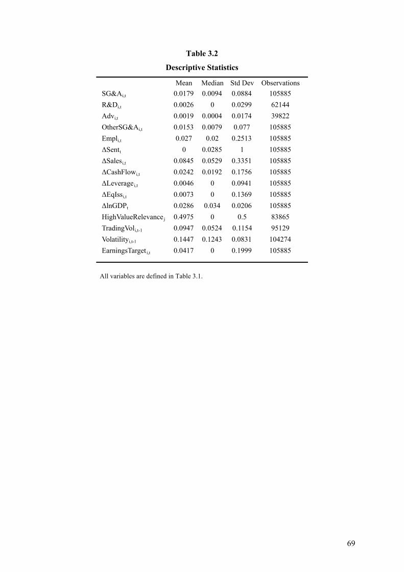
69
Table 3.2
Descriptive Statistics
All variables are defined in Table 3.1.
Mean Median Std Dev ObservationsSG&Ai,t 0.0179 0.0094 0.0884 105885R&Di,t 0.0026 0 0.0299 62144Advi,t 0.0019 0.0004 0.0174 39822OtherSG&Ai,t 0.0153 0.0079 0.077 105885Empli,t 0.027 0.02 0.2513 105885ΔSentt 0 0.0285 1 105885ΔSalesi,t 0.0845 0.0529 0.3351 105885ΔCashFlowi,t 0.0242 0.0192 0.1756 105885ΔLeveragei,t 0.0046 0 0.0941 105885ΔEqIssi,t 0.0073 0 0.1369 105885ΔlnGDPt 0.0286 0.034 0.0206 105885HighValueRelevancej 0.4975 0 0.5 83865TradingVoli,t-1 0.0947 0.0524 0.1154 95129Volatilityi,t-1 0.1447 0.1243 0.0831 104274EarningsTargeti,t 0.0417 0 0.1999 105885
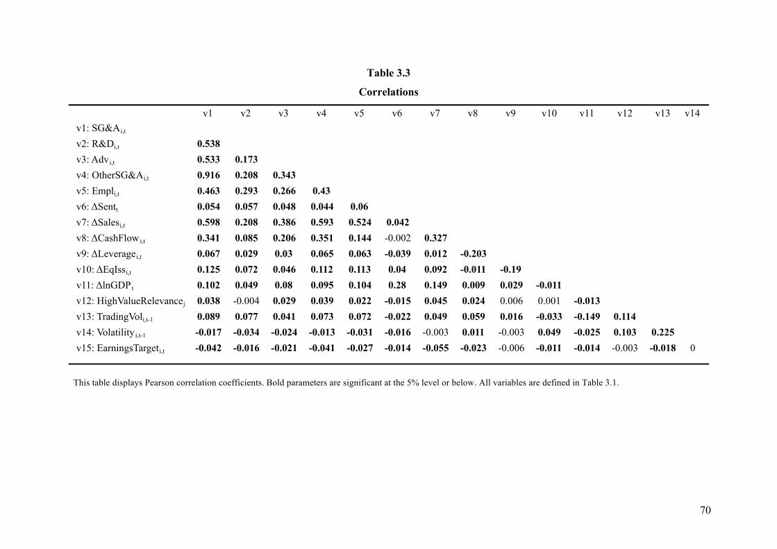
70
Table 3.3
Correlations
This table displays Pearson correlation coefficients. Bold parameters are significant at the 5% level or below. All variables are defined in Table 3.1.
v1 v2 v3 v4 v5 v6 v7 v8 v9 v10 v11 v12 v13 v14v1: SG&Ai,t
v2: R&Di,t 0.538v3: Advi,t 0.533 0.173v4: OtherSG&Ai,t 0.916 0.208 0.343v5: Empli,t 0.463 0.293 0.266 0.43v6: ΔSentt 0.054 0.057 0.048 0.044 0.06v7: ΔSalesi,t 0.598 0.208 0.386 0.593 0.524 0.042v8: ΔCashFlowi,t 0.341 0.085 0.206 0.351 0.144 -0.002 0.327v9: ΔLeveragei,t 0.067 0.029 0.03 0.065 0.063 -0.039 0.012 -0.203v10: ΔEqIssi,t 0.125 0.072 0.046 0.112 0.113 0.04 0.092 -0.011 -0.19v11: ΔlnGDPt 0.102 0.049 0.08 0.095 0.104 0.28 0.149 0.009 0.029 -0.011v12: HighValueRelevancej 0.038 -0.004 0.029 0.039 0.022 -0.015 0.045 0.024 0.006 0.001 -0.013v13: TradingVoli,t-1 0.089 0.077 0.041 0.073 0.072 -0.022 0.049 0.059 0.016 -0.033 -0.149 0.114v14: Volatilityi,t-1 -0.017 -0.034 -0.024 -0.013 -0.031 -0.016 -0.003 0.011 -0.003 0.049 -0.025 0.103 0.225v15: EarningsTargeti,t -0.042 -0.016 -0.021 -0.041 -0.027 -0.014 -0.055 -0.023 -0.006 -0.011 -0.014 -0.003 -0.018 0
71
3.4 Results
3.4.1 Test of H1
Table 3.4 presents estimation results of equation (3.1) testing the impact of investor
sentiment on operating expenditure. When the dependent variable is based on SG&A costs
(model (1)), the coefficient on ∆Sentt is positive (β1=0.0033) and significant at the 1% level
(t=12.93). In terms of economic magnitude, the change in SG&A as a percentage of total
assets increases by an additional 0.33% in response to a one standard deviation increase of
investor sentiment. Compared to the annual sample mean of the change in SG&A as a
percentage of total assets (1.79%, see Table 3.2), this effect is economically large,
corresponding to approximately 18% of the sample mean.32 When decomposing SG&A into
R&D expenses, advertisement and other SG&A costs, we find qualitatively similar results, as
shown in models (2) to (4) of Table 3.4.
When the dependent variable in equation (3.1) is the log change in employment, the
coefficient on our measure of investor sentiment is positive (β1=0.0072) and significant at the
1% level (t=9.88). If sentiment increases by one standard deviation, employment increases by
an additional 0.72%, which corresponds to approximately 27% of the sample mean of the log
change in employment (which equals 2.7%, see Table 3.2). Collectively, the results in Table
3.4 provide support for the hypothesis that managers increase spending on operating
expenditure in response to rising sentiment.
Turning to the control variables, we find that managers increase spending on operating
expenditure in response to increasing sales, as shown by the positive and significant
coefficient on ΔSalesi,t. Further, we find that spending on operating expenditure is
significantly positively associated with cash flow and leverage. In addition, managers invest
part of funds raised per equity issuance in SG&A resources or employment. Finally, we find
32 0.0033/0.0179 = 0.184 ≈ 18%.
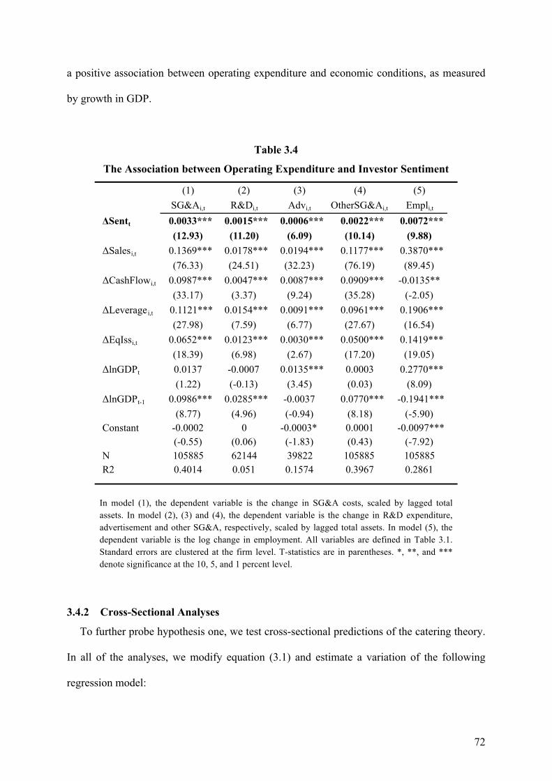
72
a positive association between operating expenditure and economic conditions, as measured
by growth in GDP.
Table 3.4
The Association between Operating Expenditure and Investor Sentiment
In model (1), the dependent variable is the change in SG&A costs, scaled by lagged total assets. In model (2), (3) and (4), the dependent variable is the change in R&D expenditure, advertisement and other SG&A, respectively, scaled by lagged total assets. In model (5), the dependent variable is the log change in employment. All variables are defined in Table 3.1. Standard errors are clustered at the firm level. T-statistics are in parentheses. *, **, and *** denote significance at the 10, 5, and 1 percent level.
3.4.2 Cross-Sectional Analyses
To further probe hypothesis one, we test cross-sectional predictions of the catering theory.
In all of the analyses, we modify equation (3.1) and estimate a variation of the following
regression model:
(1) (2) (3) (4) (5)SG&Ai,t R&Di,t Advi,t OtherSG&Ai,t Empli,t
ΔSentt 0.0033*** 0.0015*** 0.0006*** 0.0022*** 0.0072***(12.93) (11.20) (6.09) (10.14) (9.88)
ΔSalesi,t 0.1369*** 0.0178*** 0.0194*** 0.1177*** 0.3870***(76.33) (24.51) (32.23) (76.19) (89.45)
ΔCashFlowi,t 0.0987*** 0.0047*** 0.0087*** 0.0909*** -0.0135** (33.17) (3.37) (9.24) (35.28) (-2.05)
ΔLeveragei,t 0.1121*** 0.0154*** 0.0091*** 0.0961*** 0.1906***(27.98) (7.59) (6.77) (27.67) (16.54)
ΔEqIssi,t 0.0652*** 0.0123*** 0.0030*** 0.0500*** 0.1419***(18.39) (6.98) (2.67) (17.20) (19.05)
ΔlnGDPt 0.0137 -0.0007 0.0135*** 0.0003 0.2770***(1.22) (-0.13) (3.45) (0.03) (8.09)
ΔlnGDPt-1 0.0986*** 0.0285*** -0.0037 0.0770*** -0.1941***(8.77) (4.96) (-0.94) (8.18) (-5.90)
Constant -0.0002 0 -0.0003* 0.0001 -0.0097***(-0.55) (0.06) (-1.83) (0.43) (-7.92)
N 105885 62144 39822 105885 105885R2 0.4014 0.051 0.1574 0.3967 0.2861
73
ΔOpExi,t = βo +β1 ⋅ΔSentt +β2 ⋅Z +β3 ⋅ΔSentt ⋅Z
+β4 ⋅ΔSalei,t +β5 ⋅ΔCashFlowi,t +β6 ⋅ΔLeveragei,t +β7 ⋅ΔEqIssi,t+β8 ⋅Δ lnGDPt +β9 ⋅Δ lnGDPt−1 + εi,t
(3.3)
i is a firm index, t is a time index, ∆ is the difference operator and ln denotes the natural
logarithm. The dependent variables are defined as in the section 3.3.33 We use the same set of
controls as in equation (3.1) and cluster standard errors by firm. Depending on the
specification, the dummy variable Z is either a firm or industry characteristic that moderates
the association between operating expenditure and investor sentiment. In all analyses, we
expect β3>0.
3.4.2.1 The Association between Operating Expenditure and Investor Sentiment
Differentiating between High and Low SG&A Future Value Creation
The concept of investor sentiment implies that managers cater to investors’ short-term
demand by investing in those assets that noise traders are optimistic about (Stein 1996; Baker
and Wurgler 2011). We, therefore, analyze whether catering through SG&A resources
increases as the value relevance of SG&A resources increases, assuming that investors are
more likely to be optimistic about the prospects of SG&A resources, the greater the future
value potential of these resources for a given firm. To test this prediction, we allow the effect
of sentiment to differ with respect to the future value relevance of SG&A expenditures
following Banker et al. (2011).
For each two digit SIC industry, Banker et al. (2011) regress return on assets on both
current and lagged SG&A expenditure to obtain an industry-specific measure of the value
relevance of SG&A resources (see Table 2 of Banker et al. 2011). Based on these results, we
first obtain the median value of the value relevance of SG&A resources across all industries.
When estimating equation (3.3), we set the dummy variable Z to one for those industries that
33 As before, ΔOpExi,t is the change in selling, general and administrative costs (Compustat mnemonic XSGA), scaled by lagged total assets (AT), or the log change in employment (EMP). In further analyses, we split SG&A costs in research and development expenses (XRD), advertisement expenditures (XAD) and other SG&A (XSGA-XRD-XAD) and we scale the change in these variables with lagged total assets.
74
exceed the median value. We expect the coefficient on the interaction between ΔSentt and Z
to be positive: β3 > 0.
The results are shown in Table 3.5. We find that catering via SG&A resources is more
pronounced for firms that operate in industries for which SG&A costs exhibit high compared
to low value relevance (β3=0.0034, t=6.47). This result provides support for our prediction,
indicating that managers are more likely to cater to investors’ misperceptions by increasing
SG&A resources as the value-relevance of these resources increases. Decomposing SG&A
costs, we obtain qualitatively similar results for R&D expenditure (β3=0.0006, t=2.36) and
other SG&A (β3=0.003, t=6.71) but not for advertisement. Compared to the data that is
available on SG&A, we, however, note that the sample size is reduced by about 40% for
advertisement. Since cross-sectional analyses require further partitioning of the sample, loss
of statistical power may be one potential explanation for this result.
3.4.2.2 The Association between Operating Expenditure and Investor Sentiment
Differentiating between High and Low Investor Trading Volume
The catering theory predicts that managers are more likely to follow investors’
misperceptions as managers’ horizon decrease, as more emphasis is put on the short-term
stock price (Stein 1996; Baker and Wurgler 2011). Following Polk and Sapienza (2009), we
use share turnover to proxy for the relative amount of trading activities by short-term
investors, assuming that investor short-termism results in managerial short-termism (Bushee
1998; Shleifer and Vishny 1990; Stein 1988). We define share turnover as the annual average
of the ratio of monthly trading volume to monthly shares outstanding (CRSP mnemonic VOL
and SHROUT, respectively). In equation (3.3), we set Z to one if the share turnover of a
given firm is above the median share turnover of the year, assuming that the high trading
volume group comprises managers who act more myopically. We expect β3>0.
The results are shown in Table 3.6. Consistent with our expectation, we find that catering
75
via SG&A resources increases as managers’ horizon decrease. Our results show that
managers who likely have shorter horizons cater by an additional 0.22% in response to a one
standard deviation increase in sentiment compared to managers who likely have longer
horizons (β3=0.0022, t=4.81). When analyzing components of SG&A costs, we find
qualitatively similar results for R&D expenditure and other SG&A, while the association
between advertisement and investors sentiment does not differ with horizon, as shown in
model (2) to (4) of Table 3.6. Turning to employment, our results suggest that catering via
employment increases as managers’ horizon decrease (β3=0.0062, t=4.48). Taken together,
the analysis provides support for our prediction.
3.4.2.3 The Association between Operating Expenditure and Investor Sentiment
Differentiating between High and Low Stock Return Volatility
Baker and Wurgler (2007) argue that investor sentiment should more strongly affect those
firms that have higher stock return volatility. On the one hand, Baker and Wurgler (2007)
argue that a firm’s speculative appeal increases as the firm’s stock return volatility increases.
To the extent that investor sentiment reflects the propensity to speculate by noise traders,
sentiment should have a stronger effect on those firms that exhibit higher stock return
volatility. Alternatively, since the risk of arbitrage increases with stock return volatility,
sentiment should reduce the willingness of arbitrageurs to bet against high-volatility stocks.
Both channels suggest that investor sentiment more strongly affects those firms that exhibit
higher stock return volatility. We, therefore, expect catering to be more pronounced for those
firms that are more strongly affected by investor sentiment.
When estimating equation (3.3), we set Z to one if the stock return volatility of a given
firm exceeds the median stock return volatility of all firms in a year. We define stock return
volatility as the standard deviation of a firm’s monthly stock returns (CRSP mnemonic RET)
following Baker and Wurgler (2007). A positive β3 would be consistent with our prediction.
76
Table 3.7 contains the results. When the dependent variable is the change in SG&A cost
scaled by total assets, we find results that are consistent with our expectation, as shown by
the significantly positive coefficient on the interaction between our measure of investor
sentiment and the dummy variable indicating high stock return volatility (β3=0.0045,
t=10.26). We obtain similar results when analyzing R&D and advertisement expenditure as
well as other SG&A. The last column of Table 3.7 shows that catering via employment
increases as stock return volatility increases (β3=0.0081, t=6.09). Collectively, our results
provide support for our prediction, suggesting that catering is more pronounced for those
firms that are more strongly affected by investor sentiment.
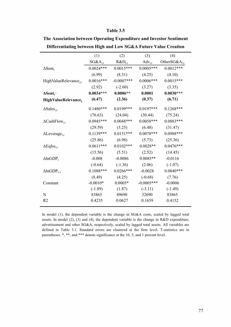
77
Table 3.5
The Association between Operating Expenditure and Investor Sentiment
Differentiating between High and Low SG&A Future Value Creation
In model (1), the dependent variable is the change in SG&A costs, scaled by lagged total assets. In model (2), (3) and (4), the dependent variable is the change in R&D expenditure, advertisement and other SG&A, respectively, scaled by lagged total assets. All variables are defined in Table 3.1. Standard errors are clustered at the firm level. T-statistics are in parentheses. *, **, and *** denote significance at the 10, 5, and 1 percent level.
(1) (2) (3) (4)SG&Ai,t R&Di,t Advi,t OtherSG&Ai,t
ΔSentt 0.0024*** 0.0015*** 0.0005*** 0.0012***(6.99) (8.31) (4.25) (4.10)
HighValueRelevancej,t 0.0016*** -0.0007*** 0.0006*** 0.0015***(2.92) (-2.60) (3.27) (3.35)
ΔSentt· 0.0034*** 0.0006** 0.0001 0.0030***HighValueRelevancej (6.47) (2.36) (0.37) (6.71)
ΔSalesi,t 0.1480*** 0.0199*** 0.0197*** 0.1268***(76.63) (24.04) (30.44) (75.24)
ΔCashFlowi,t 0.0945*** 0.0048*** 0.0058*** 0.0883***(29.59) (3.25) (6.48) (31.47)
ΔLeveragei,t 0.1139*** 0.0151*** 0.0078*** 0.0988***(25.86) (6.98) (5.73) (25.36)
ΔEqIssi,t 0.0611*** 0.0102*** 0.0028** 0.0476***(15.56) (5.51) (2.52) (14.45)
ΔlnGDPt -0.008 -0.0086 0.0085** -0.0116(-0.64) (-1.36) (2.06) (-1.07)
ΔlnGDPt-1 0.1088*** 0.0266*** -0.0028 0.0840***(8.49) (4.25) (-0.68) (7.76)
Constant -0.0010* 0.0005* -0.0005*** -0.0006(-1.89) (1.87) (-3.11) (-1.49)
N 83865 49690 32690 83865R2 0.4235 0.0627 0.1659 0.4152
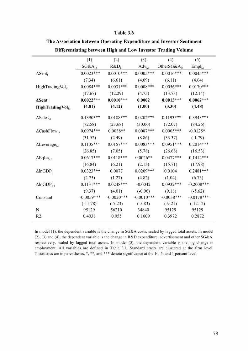
78
Table 3.6
The Association between Operating Expenditure and Investor Sentiment
Differentiating between High and Low Investor Trading Volume
In model (1), the dependent variable is the change in SG&A costs, scaled by lagged total assets. In model (2), (3) and (4), the dependent variable is the change in R&D expenditure, advertisement and other SG&A, respectively, scaled by lagged total assets. In model (5), the dependent variable is the log change in employment. All variables are defined in Table 3.1. Standard errors are clustered at the firm level. T-statistics are in parentheses. *, **, and *** denote significance at the 10, 5, and 1 percent level.
(1) (2) (3) (4) (5)SG&Ai,t R&Di,t Advi,t OtherSG&Ai,t Empli,t
ΔSentt 0.0023*** 0.0010*** 0.0005*** 0.0016*** 0.0045***(7.34) (6.61) (4.09) (6.11) (4.64)
HighTradingVoli,t 0.0084*** 0.0031*** 0.0008*** 0.0056*** 0.0170***(17.67) (12.29) (4.75) (13.73) (12.14)
ΔSentt· 0.0022*** 0.0010*** 0.0002 0.0013*** 0.0062***HighTradingVoli,t (4.81) (4.12) (1.00) (3.30) (4.48)
ΔSalesi,t 0.1390*** 0.0188*** 0.0202*** 0.1193*** 0.3943***(72.58) (23.68) (30.06) (72.07) (84.26)
ΔCashFlowi,t 0.0974*** 0.0038** 0.0087*** 0.0905*** -0.0125* (31.52) (2.49) (8.86) (33.37) (-1.79)
ΔLeveragei,t 0.1105*** 0.0157*** 0.0083*** 0.0951*** 0.2014***(26.85) (7.05) (5.78) (26.68) (16.53)
ΔEqIssi,t 0.0617*** 0.0118*** 0.0026** 0.0477*** 0.1414***(16.84) (6.21) (2.13) (15.71) (17.98)
ΔlnGDPt 0.0323*** 0.0077 0.0209*** 0.0104 0.2481***(2.75) (1.27) (4.82) (1.04) (6.73)
ΔlnGDPt-1 0.1131*** 0.0248*** -0.0042 0.0932*** -0.2008***(9.37) (4.01) (-0.96) (9.18) (-5.62)
Constant -0.0059*** -0.0020*** -0.0010*** -0.0038*** -0.0178*** (-11.78) (-7.23) (-5.83) (-9.21) (-12.12)N 95129 56210 34840 95129 95129R2 0.4038 0.055 0.1609 0.3972 0.2872
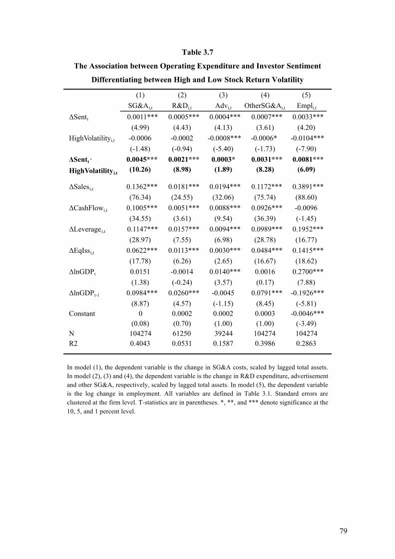
79
Table 3.7
The Association between Operating Expenditure and Investor Sentiment
Differentiating between High and Low Stock Return Volatility
In model (1), the dependent variable is the change in SG&A costs, scaled by lagged total assets. In model (2), (3) and (4), the dependent variable is the change in R&D expenditure, advertisement and other SG&A, respectively, scaled by lagged total assets. In model (5), the dependent variable is the log change in employment. All variables are defined in Table 3.1. Standard errors are clustered at the firm level. T-statistics are in parentheses. *, **, and *** denote significance at the 10, 5, and 1 percent level.
(1) (2) (3) (4) (5)SG&Ai,t R&Di,t Advi,t OtherSG&Ai,t Empli,t
ΔSentt 0.0011*** 0.0005*** 0.0004*** 0.0007*** 0.0033***(4.99) (4.43) (4.13) (3.61) (4.20)
HighVolatilityi,t -0.0006 -0.0002 -0.0008*** -0.0006* -0.0104***(-1.48) (-0.94) (-5.40) (-1.73) (-7.90)
ΔSentt· 0.0045*** 0.0021*** 0.0003* 0.0031*** 0.0081***HighVolatilityi,t (10.26) (8.98) (1.89) (8.28) (6.09)
ΔSalesi,t 0.1362*** 0.0181*** 0.0194*** 0.1172*** 0.3891***(76.34) (24.55) (32.06) (75.74) (88.60)
ΔCashFlowi,t 0.1005*** 0.0051*** 0.0088*** 0.0926*** -0.0096(34.55) (3.61) (9.54) (36.39) (-1.45)
ΔLeveragei,t 0.1147*** 0.0157*** 0.0094*** 0.0989*** 0.1952***(28.97) (7.55) (6.98) (28.78) (16.77)
ΔEqIssi,t 0.0622*** 0.0113*** 0.0030*** 0.0484*** 0.1415***(17.78) (6.26) (2.65) (16.67) (18.62)
ΔlnGDPt 0.0151 -0.0014 0.0140*** 0.0016 0.2700***(1.38) (-0.24) (3.57) (0.17) (7.88)
ΔlnGDPt-1 0.0984*** 0.0260*** -0.0045 0.0791*** -0.1926***(8.87) (4.57) (-1.15) (8.45) (-5.81)
Constant 0 0.0002 0.0002 0.0003 -0.0046***(0.08) (0.70) (1.00) (1.00) (-3.49)
N 104274 61250 39244 104274 104274R2 0.4043 0.0531 0.1587 0.3986 0.2863
80
3.4.3 Test of H2
Results from estimating equation (3.2), testing H2, are shown in Table 3.8. Focusing on
SG&A costs first, consistent with our previous results, we find a significantly positive
association between SG&A costs and investor sentiment for those firms that do not face
earnings targets (β1=0.0035, t=13.25). Next, turning to firms that have incentives to meet
earnings targets, while we do find a negative association between SG&A costs and investor
sentiment, the coefficient is not statistically significant at conventional levels
(β1+β3=0.0035-0.0042=-0.0007, t=-0.99). This shows that investor sentiment does not induce
managers to cut costs conditional on earnings targets. What our results, however, do suggest
is that managers who face earnings targets increase SG&A costs by less than managers who
do not face earnings targets, as shown by the significantly negative coefficient on the
interaction between our measure of investor sentiment and earnings targets (β3=-0.0042,
t=-5.26), indicating that earnings targets moderate catering through SG&A costs. This
difference is economically large. The change in SG&A costs as a percentage of total assets is
0.42% less pronounced for firms that face earnings targets compared to firms that do not face
earnings targets, which corresponds to about 23% of the sample mean.
Decomposing SG&A costs, we find similar results for research and development
expenditure and other SG&A but not for advertisement (β3=-0.0014, t=-3.24, β3=-0.0033,
t=-4.64, and β3=-0.0004, t=-1.27, respectively). Further, our results suggest that earnings
targets moderate catering via employment (β3=-0.0061, t=-1.94, respectively). While we
report these results for completeness, we note that studies on real earnings management focus
on R&D or SG&A rather than employment and advertisement expenses (e.g., Baber et al.
1991; Bushee 1998; Dechow, Kothari, and Watts 1998). Taken together, we argue the results
provide support for H2, indicating that managers are less likely to overspend on operating
expenditure as means of addressing investors’ misperceptions when facing earnings targets.
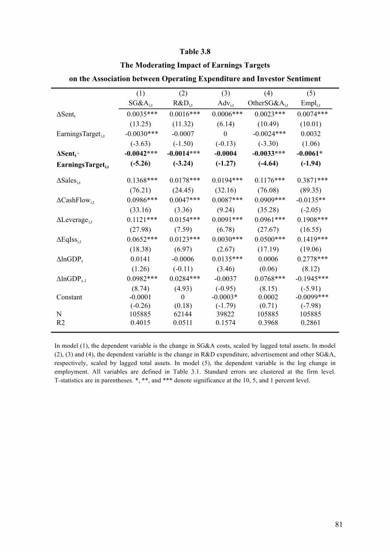
81
Table 3.8
The Moderating Impact of Earnings Targets
on the Association between Operating Expenditure and Investor Sentiment
In model (1), the dependent variable is the change in SG&A costs, scaled by lagged total assets. In model (2), (3) and (4), the dependent variable is the change in R&D expenditure, advertisement and other SG&A, respectively, scaled by lagged total assets. In model (5), the dependent variable is the log change in employment. All variables are defined in Table 3.1. Standard errors are clustered at the firm level. T-statistics are in parentheses. *, **, and *** denote significance at the 10, 5, and 1 percent level.
(1) (2) (3) (4) (5)SG&Ai,t R&Di,t Advi,t OtherSG&Ai,t Empli,t
ΔSentt 0.0035*** 0.0016*** 0.0006*** 0.0023*** 0.0074***(13.25) (11.32) (6.14) (10.49) (10.01)
EarningsTargeti,t -0.0030*** -0.0007 0 -0.0024*** 0.0032(-3.63) (-1.50) (-0.13) (-3.30) (1.06)
ΔSentt· -0.0042*** -0.0014*** -0.0004 -0.0033*** -0.0061* EarningsTargeti,t (-5.26) (-3.24) (-1.27) (-4.64) (-1.94)
ΔSalesi,t 0.1368*** 0.0178*** 0.0194*** 0.1176*** 0.3871***(76.21) (24.45) (32.16) (76.08) (89.35)
ΔCashFlowi,t 0.0986*** 0.0047*** 0.0087*** 0.0909*** -0.0135** (33.16) (3.36) (9.24) (35.28) (-2.05)
ΔLeveragei,t 0.1121*** 0.0154*** 0.0091*** 0.0961*** 0.1908***(27.98) (7.59) (6.78) (27.67) (16.55)
ΔEqIssi,t 0.0652*** 0.0123*** 0.0030*** 0.0500*** 0.1419***(18.38) (6.97) (2.67) (17.19) (19.06)
ΔlnGDPt 0.0141 -0.0006 0.0135*** 0.0006 0.2778***(1.26) (-0.11) (3.46) (0.06) (8.12)
ΔlnGDPt-1 0.0982*** 0.0284*** -0.0037 0.0768*** -0.1945***(8.74) (4.93) (-0.95) (8.15) (-5.91)
Constant -0.0001 0 -0.0003* 0.0002 -0.0099*** (-0.26) (0.18) (-1.79) (0.71) (-7.98)N 105885 62144 39822 105885 105885R2 0.4015 0.0511 0.1574 0.3968 0.2861
82
3.4.4 Alternative Explanations
In this section, we address two potential alternative explanations. We document that the
association between operating expenditure and investor sentiment is robust to controlling for
investment, and we document that our conclusions remains unchanged when controlling for
managerial optimism.
3.4.4.1 Controlling for Investment
Since Polk and Sapienza (2009) show that managers cater by increasing capital
expenditure, we re-estimate equation (3.1) and additionally control for changes in both
current and past capital expenditure to rule out that catering based on operating expenditure is
mechanically driven by catering based on capital expenditure. If the association between
operating expenditure and investor sentiment is driven by changes in capital expenditure only,
the effect of sentiment on costs should disappear once we control for capital expenditure.
Conversely, if the association between operating expenditure and investor sentiment remains
unchanged, this would provide support for an independent catering effect via operating
expenditure.
The results are shown in Table 3.9. Consistent with our previous results, we find a positive
association between SG&A costs and investor sentiment (β1=0.0027, t=11.28) as well as
employment and investor sentiment (β1=0.0053, t=7.61). Further, decomposing SG&A, the
association between research and development expenditure and investor sentiment remains
positive and statistically significant at the 1% level (β1=0.0012, t=9.57). Likewise, the
association between advertisement (β1=0.0005, t=5.23) and other SG&A (β1=0.0018, t=8.78)
and investor sentiment remains statistically significant at conventional levels. Taken together,
we argue the results indicate that catering via operating expenditure is not mechanically
driven by catering via capital expenditure, suggesting an independent operating expenditure
effect.
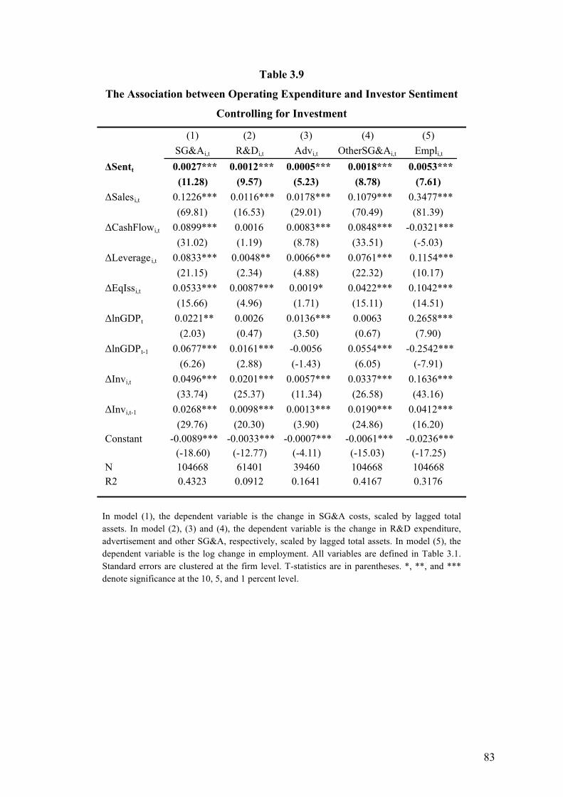
83
Table 3.9
The Association between Operating Expenditure and Investor Sentiment
Controlling for Investment
In model (1), the dependent variable is the change in SG&A costs, scaled by lagged total assets. In model (2), (3) and (4), the dependent variable is the change in R&D expenditure, advertisement and other SG&A, respectively, scaled by lagged total assets. In model (5), the dependent variable is the log change in employment. All variables are defined in Table 3.1. Standard errors are clustered at the firm level. T-statistics are in parentheses. *, **, and *** denote significance at the 10, 5, and 1 percent level.
(1) (2) (3) (4) (5)SG&Ai,t R&Di,t Advi,t OtherSG&Ai,t Empli,t
ΔSentt 0.0027*** 0.0012*** 0.0005*** 0.0018*** 0.0053***(11.28) (9.57) (5.23) (8.78) (7.61)
ΔSalesi,t 0.1226*** 0.0116*** 0.0178*** 0.1079*** 0.3477***(69.81) (16.53) (29.01) (70.49) (81.39)
ΔCashFlowi,t 0.0899*** 0.0016 0.0083*** 0.0848*** -0.0321***(31.02) (1.19) (8.78) (33.51) (-5.03)
ΔLeveragei,t 0.0833*** 0.0048** 0.0066*** 0.0761*** 0.1154***(21.15) (2.34) (4.88) (22.32) (10.17)
ΔEqIssi,t 0.0533*** 0.0087*** 0.0019* 0.0422*** 0.1042***(15.66) (4.96) (1.71) (15.11) (14.51)
ΔlnGDPt 0.0221** 0.0026 0.0136*** 0.0063 0.2658***(2.03) (0.47) (3.50) (0.67) (7.90)
ΔlnGDPt-1 0.0677*** 0.0161*** -0.0056 0.0554*** -0.2542***(6.26) (2.88) (-1.43) (6.05) (-7.91)
ΔInvi,t 0.0496*** 0.0201*** 0.0057*** 0.0337*** 0.1636***(33.74) (25.37) (11.34) (26.58) (43.16)
ΔInvi,t-1 0.0268*** 0.0098*** 0.0013*** 0.0190*** 0.0412***(29.76) (20.30) (3.90) (24.86) (16.20)
Constant -0.0089*** -0.0033*** -0.0007*** -0.0061*** -0.0236***(-18.60) (-12.77) (-4.11) (-15.03) (-17.25)
N 104668 61401 39460 104668 104668R2 0.4323 0.0912 0.1641 0.4167 0.3176
84
3.4.4.2 Controlling for Managerial Optimism
In this section, we intend to differentiate our explanation from an explanation based on
managerial optimism. Prior literature documents variation in managerial optimism (Graham
et al. 2013). Optimistic managers have been shown to overestimate future demand
(Malmendier et al. 2011). Overly optimistic demand expectations may induce managers to
overspend on operating expenditure. Hence, while an explanation based on the catering
theory predicts that rational managers perceive changes in investor sentiment and adjust their
corporate policies accordingly, an explanation based on managerial optimism predicts that
overly optimistic demand expectations induce managers to overspend on operating
expenditure, regardless of catering incentives.
To differentiate between managerial optimism and investor sentiment, we proceed as
follows. In a recent study, Banker et al. (2014) document that managerial optimism affects
cost behavior. Empirically, Banker et al. (2014) argue that successive sales changes affect
managers demand expectations, reflecting rational statistical inference and behavioral biases.
First, since sales changes are positively correlated, sales increases in consecutive periods
point to a greater likelihood of sales increases in future periods, thereby increasing managers’
expectations about future demand. Second, Banker et al. (2014) argue that managers are
likely to extrapolate sales trends, which likewise suggests that managers will be more likely
to expect future sales increases following successive sales increases. Hence, to differentiate
between managerial optimism and investor sentiment, we augment equation (3.1) with a
dummy variable indicating successive sales increases and replicate our prior analysis.
The results are shown in Table 3.10. Consistent with our prior results, we find a positive
association between operating expenditure and investor sentiment. When the dependent
variable is based on SG&A costs, the coefficient on ∆Sentt is positive and statistically
significant at the 1% level (β1=0.0031, t=12.34). We obtain similar results for R&D,
advertisement and other SG&A, as shown in model (2) to (4) of Table 3.10. Finally, the last
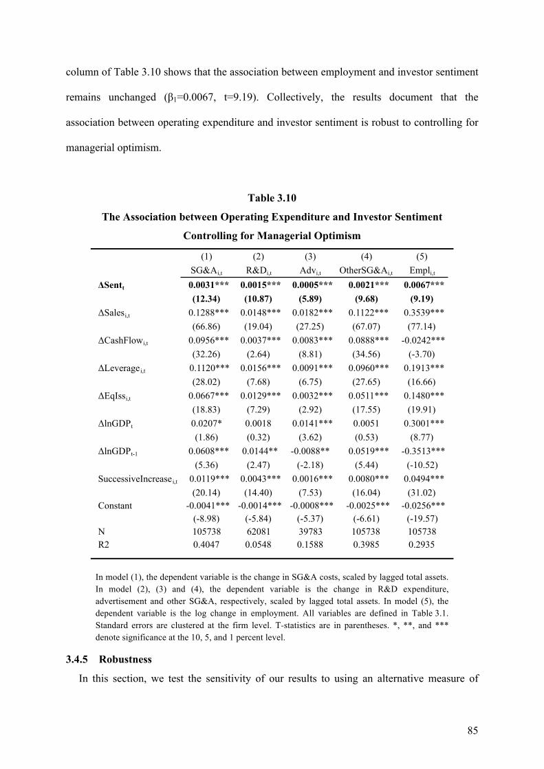
85
column of Table 3.10 shows that the association between employment and investor sentiment
remains unchanged (β1=0.0067, t=9.19). Collectively, the results document that the
association between operating expenditure and investor sentiment is robust to controlling for
managerial optimism.
Table 3.10
The Association between Operating Expenditure and Investor Sentiment
Controlling for Managerial Optimism
In model (1), the dependent variable is the change in SG&A costs, scaled by lagged total assets. In model (2), (3) and (4), the dependent variable is the change in R&D expenditure, advertisement and other SG&A, respectively, scaled by lagged total assets. In model (5), the dependent variable is the log change in employment. All variables are defined in Table 3.1. Standard errors are clustered at the firm level. T-statistics are in parentheses. *, **, and *** denote significance at the 10, 5, and 1 percent level.
3.4.5 Robustness
In this section, we test the sensitivity of our results to using an alternative measure of
(1) (2) (3) (4) (5)SG&Ai,t R&Di,t Advi,t OtherSG&Ai,t Empli,t
ΔSentt 0.0031*** 0.0015*** 0.0005*** 0.0021*** 0.0067***(12.34) (10.87) (5.89) (9.68) (9.19)
ΔSalesi,t 0.1288*** 0.0148*** 0.0182*** 0.1122*** 0.3539***(66.86) (19.04) (27.25) (67.07) (77.14)
ΔCashFlowi,t 0.0956*** 0.0037*** 0.0083*** 0.0888*** -0.0242***(32.26) (2.64) (8.81) (34.56) (-3.70)
ΔLeveragei,t 0.1120*** 0.0156*** 0.0091*** 0.0960*** 0.1913***(28.02) (7.68) (6.75) (27.65) (16.66)
ΔEqIssi,t 0.0667*** 0.0129*** 0.0032*** 0.0511*** 0.1480***(18.83) (7.29) (2.92) (17.55) (19.91)
ΔlnGDPt 0.0207* 0.0018 0.0141*** 0.0051 0.3001***(1.86) (0.32) (3.62) (0.53) (8.77)
ΔlnGDPt-1 0.0608*** 0.0144** -0.0088** 0.0519*** -0.3513***(5.36) (2.47) (-2.18) (5.44) (-10.52)
SuccessiveIncreasei,t 0.0119*** 0.0043*** 0.0016*** 0.0080*** 0.0494***(20.14) (14.40) (7.53) (16.04) (31.02)
Constant -0.0041*** -0.0014*** -0.0008*** -0.0025*** -0.0256***(-8.98) (-5.84) (-5.37) (-6.61) (-19.57)
N 105738 62081 39783 105738 105738R2 0.4047 0.0548 0.1588 0.3985 0.2935
86
investor sentiment and to clustering standard errors at the firm- and year level. The tables of
all further robustness checks are available on request. We, here, briefly discuss the findings.
As a first robustness check, we test the sensitivity of our results to using an alternative
sentiment index. In constructing the sentiment index that we have used so far, Baker and
Wurgler (2006) combine six proxies for investor sentiment via principal component analysis.
Even though the choice of the underlying variables follows prior literature on investor
sentiment (see section 3.2 for motivation), one may criticize this procedure arguing that the
index reflects a common business cycle rather than a common investor sentiment component.
To address this concern, Baker and Wurgler (2006) regress each of the six sentiment
measures on a set of macroeconomic variables comprising (1) growth in the industrial
production, (2) growth in consumer durables, nondurables, and services, (3) and a dummy
variable indicating NBER recessions. Baker and Wurgler (2006) combine the residuals from
these regressions via principal component analysis and form an index that has been
orthogonalized to macroeconomic conditions. The data on this alternative index is available
on Jeffrey Wurgler’s homepage.34
Consistent with our previous results, we find a positive association between expenditure
on SG&A and investor sentiment (β1=0.0025, t=10.54) when re-estimating equation (3.1)
using the alternative investor sentiment index. Likewise, the association between research
and development expenditure (β1=0.0011, t=9.07), advertisement (β1=0.0004, t=5.2), and
other SG&A (β1=0.0015, t=7.64) remains positive. Further, we find a positive association
between employment and investor sentiment (β1=0.0069, t=10.03). Collectively, our
conclusion remains unchanged with the alternative measure of investor sentiment.
Finally, we re-estimate equation (3.1) when clustering standard errors at the firm and year
level. When clustering standard errors at the firm and year level, we continue to find a
34 http://people.stern.nyu.edu/jwurgler/
87
positive association between investor sentiment and SG&A costs (β1=0.0033, t=3.04), R&D
(β1=0.0015, t=4.14) and advertisement expenditure (β1=0.0006, t=3.18), other SG&A
(β1=0.0022, t=2.38) and employment (β1=0.0072, t=2.98).
3.5 Conclusion
This paper intends to increase our understanding of real consequences that arise from
investor sentiment. Building on the catering theory (Baker and Wurgler 2011; Stein 1996),
our results suggests that mangers overspend on research and development expenditure,
advertisement, selling, general and administrative costs and employment in order to cater to
investors’ misperceptions in periods of high relative to periods of average sentiment. In
further analyses, we find results that are consistent with cross-sectional predictions of the
catering theory: (1) Managers are more likely to overspend on SG&A costs when these
resources have high value creating potential, (2) managers with short-horizons, and (3)
managers’ of firms that are particularly affected by investor sentiment are more likely to cater
by overspending on operating expenditure. However, our results indicate that managers
refrain from overspending through operating expenditure when facing earnings targets, which
suggests a trade-off between catering to investors’ real and financial expectations.

88
89
4 Attention, Media and Fuel Efficiency
4.1 Introduction
The emissions of motor vehicles are one of the major sources of greenhouse gas emissions
leading to climate change. For example, in the United States, the transportation sector
accounts for 34% of the carbon dioxide emissions.35 These emissions could be decreased
with improved technologies that offer a better fuel efficiency.36 For this reason, it is crucial to
understand which factors are relevant for the diffusion of fuel-efficient technologies.
We argue that the consumer purchasing decision process and the question when
consumers are willing to invest in fuel efficiency play an important role in this context. As
Allcott (2011) indicates, 40% of US consumers do not consider a vehicle’s gasoline
consumption when purchasing a car. Therefore, the amount of attention devoted to energy
efficient vehicles and fuel costs should be a major determinant for the diffusion of new
technologies. Following this rationale, we attempt to capture the dynamics of the consumers’
attention to hybrid electric vehicles.37 However, attention is not directly observable and thus,
finding an adequate measure for attention is challenging. We make use of Google’s search
query data as a direct and observable proxy for the revealed attention. By analyzing online
search behavior, we effectively examine the consumers’ process of gathering information
about the topic to which they pay attention. Data on aggregate regional online search
behavior is obtained from the service “Google Insights for Search”, enabling us to track the
development of the search volume of a specific query.
It is expected that there are two main channels that alter the attention devoted to 35 Source: United States Department of Energy, “Emissions of Greenhouse Gases in the United States 2009”, DOE/EIA-0573(2009), Figure 4.3, U.S. energy-related carbon dioxide emissions by sector, 2009. 36 The fuel economy of a vehicle is defined as the output (miles) per input (gallons of gasoline). In contrast, fuel efficiency, as a form of thermal efficiency, is the ratio of energy used for propulsion compared to the total amount of energy consumed. Thus, a small vehicle with a high fuel economy could still be less fuel-efficient than a larger vehicle with a lower fuel economy, e.g. because a vehicle with a heavier weight also requires more physical work to drive the same distance. 37 We focus on hybrid electric vehicles as they are considered to be a promising technology for increasing fuel efficiency. Furthermore, Enkvist et al. (2007) indicate that increasing the fuel efficiency of vehicles is one of the least costly ways to reduce the overall global greenhouse gas emissions.
90
environmentally friendly vehicles. First, as the reduced gasoline consumption is the main
advantage of energy efficient vehicles, the gasoline price should be an important determinant
of the consumers’ attention devoted to hybrid vehicles. Tversky and Kahneman (1991)
indicate that consumers also evaluate prices based on reference points. If the gasoline price is
higher than such a reference point, consumers would consider a price increase as a loss and
may show a stronger reaction due to loss aversion. Thus, unprecedented record gasoline
prices could have an additional effect on the consumers’ attention if the highest previous
gasoline price is such a reference point. Second, consumers may react to media coverage of
topics such as hybrid vehicles and gasoline costs.38 We draw upon the agenda-setting theory
by McCombs and Shaw (1972), arguing that mass media influences the public agenda by
determining which topics are seen as important.
However, the causality of whether media covers topics of general interest or whether
media determines the general interest is not always clear. For our case, it is difficult to
identify the causal influence of media because the consumers’ attention and media coverage
are both directly affected by gasoline prices and other possibly unobserved factors. Similar to
Engelberg and Parsons (2011), we circumvent this problem by observing the behavior of
different geographical groups. These groups react to the same underlying event, but are
exposed to different information sources, i.e. their local newspaper. Our analysis is based on
a novel weekly panel dataset consisting of 19 metropolitan areas in the United States
covering the years 2004 to 2011. We control for local gasoline prices, national television
reports and national newspaper coverage. In order to estimate the causal effect of local
newspaper coverage on our attention measure, we allow each local newspaper to have an
38 This hypothesis is supported by several studies indicating that economic actions are affected by media coverage. For example, Eisensee and Strömberg (2007) analyze the impact of mass media coverage on the US relief for natural disasters. To identify the effect of media coverage, they use an instrument variable, which measures the availability of other newsworthy events that crowd out media coverage of marginally newsworthy natural disasters. Tetlock (2007) analyzes the relationship between the content of newspaper articles and stock market outcomes. He shows that the sentiment of media has a distinct impact on stock prices.
91
effect on all other metropolitan areas. Thus, we estimate the supplemental effect that a
newspaper has in its own region compared to the effect on all other regions. This
identification strategy allows us to disentangle the underlying event and the causal media
effect.
Our results indicate that the consumers’ attention devoted to hybrid vehicles is affected by
both channels. We find that local media coverage causally affects the consumers’ attention
and that consumers react to both gasoline price changes and unprecedented levels of the
gasoline price. Building on these findings, we validate that our proxy for the attention to
hybrid vehicles is relevant to the purchasing behavior. We use a panel dataset of monthly
state-level hybrid vehicle registrations and market shares for the period covering the years
2006 to 2011 to show that our attention measure is robustly related to actual consumer
purchasing decisions. Overall, our findings suggest that attention effects have a distinct
impact on the market for hybrid vehicles.
This is the first study to analyze the determinants of the consumers’ attention to a
long-lived consumer good. Until now, most studies in the area focus on showing how
attention effects influence economic decision making, but do not systematically analyze the
determinants of the attention. The most advanced analysis of the impact of attention effects
on economic choices is primarily in the finance literature. Barber and Odean (2008) show
that the stock purchasing decision of individual investors is influenced by the attention to a
certain choice. Given the scarcity of the resource attention and the large set of possible
investments, attention-based decision making implies that investors are more likely to buy
investments that grab their attention. Da, Engelberg, and Gao (2011) indicate that Google
search queries are a valid direct measure of retail investor attention, which is found to affect
92
the retail investors’ behavior in financial markets.39 In the context of consumer behavior,
Chetty, Looney, and Kroft (2009) show that the consumers’ reaction to taxation depends on
the salience of the tax. Masatlioglu, Nakajima, and Ozbay (2012) provide a theoretical
framework for limited attention effects. Their model describes a decision process under the
constraint of a limited consideration set and examines the implications for revealed
preferences and revealed attention.
Our study also extends the literature on the consumer search behavior in reaction to
gasoline price changes. There is a range of literature (see for example Chandra and Tappata
2011) that focuses on the relationship between the consumer search behavior and the price
dispersion between different gas stations, or more broadly the competition in gasoline
markets. In contrast to these studies, we do not focus on the search behavior related to the
gasoline purchasing decision, but rather on the long-term reaction, i.e. the search behavior
accompanying the vehicle purchase. Lewis and Marvel (2011) find that the consumers’
reaction to price changes is not symmetric. Consumers increase their search effort when
faced with rising gasoline prices, but do not react strongly to falling prices. Our findings are
similar regarding the asymmetric consumer search behavior. Additionally, we identify a
distinguished attention effect for record gasoline prices. This evidence is consistent with the
results in the finance literature. For example, Yuan (2011) measures the impact of
attention-grabbing events like record levels of the Dow Jones index and front page articles
about the stock market. It is shown that attention influences trading behavior of individual
investors. Similarly, Li and Yu (2012) show that psychological reference points of past
record levels can also have an impact on aggregate stock market outcomes.
The remainder of the article is organized as follows: Section 2 describes the market for 39 There are several other studies about attention effects in financial markets. For example, DellaVigna and Pollet (2009) indicate the existence of weekday effects due to investors’ limited attention. Gilbert et al. (2012) argue that inattention leads to a temporary market reaction to stale information. Engelberg, Sasseville, and Williams (2012) examine the market impact of television stock recommendations, which are interpreted as shocks to the retail investors’ attention.
93
hybrid vehicles and discusses the consumers’ purchasing motives. Section 3 gives detailed
information about the construction of our unique dataset. In section 4, we analyze how media
coverage and gasoline prices affect the attention devoted to hybrid vehicles. In section 5, we
show that online search queries are a relevant measure and have a robust correlation with
actual sales volumes. Finally, we give a short conclusion of our findings in section 6.
4.2 Hybrid Vehicle Market and Consumer Attitudes
Hybrid electric vehicles have both an internal combustion engine and an electric motor.
This combination allows improved fuel efficiency compared to similar non-hybrid vehicles
because the combustion engine is mostly used to support the electric motor. The battery of
the electric motor is recharged while driving with gasoline and also while recovering the
braking energy. Thus, as for most fuel-efficient technologies, hybrid electric vehicles have a
higher purchasing price due to the increased complexity of including advanced technological
parts such as an electric motor, a lithium-ion battery and a braking energy recovery system.
The upfront investment expenses result in lower gasoline consumption and lower costs
during the lifetime of the vehicle. Therefore, the profitability of the investment in fuel
efficiency depends on future gasoline prices.
In 1999, the Honda Insight was the first hybrid vehicle to be introduced in the United
States. The Toyota Prius, still the best selling hybrid vehicle in the US, was introduced in
2000. However, in the first six years, only a total of 197,483 hybrid vehicles were sold. In the
following two years, during 2005 and 2006, there were 462,347 hybrid vehicles sold in the
US.40 Even at the start of our sample period in December 2006, the market share of all hybrid
vehicles was still at a rather low level of 1.65%. Thus, the hybrid car market can be
considered a new market, which means that the initial awareness related to this market is
relatively low.
40 Source: US Department of Energy, http://www.afdc.energy.gov/afdc/data/vehicles.html
94
Several studies show that the hybrid vehicle market is mainly driven by three factors:
Gasoline prices, government subsidies and non-monetary factors like symbolic values or
environmental concern. There are a range of studies focusing on the impact and effectiveness
of government programs that foster the sales of hybrid vehicles. For example, Beresteanu and
Li (2011) find that both high gasoline prices and tax incentives have a significantly positive
effect on hybrid sales. Gallagher and Muehlegger (2011) present similar results and show that
sales tax waivers have a much higher impact than income tax waivers, which are less salient
and transparent. Chandra, Gulati, and Kandlikar (2010) find that government incentives have
a positive effect on hybrid sales but are not very cost effective. Diamond (2009) indicates that
gasoline prices may have a higher impact than government incentives.
The literature also identifies several distinct, non-monetary factors that influence the
hybrid vehicle market. Kahn (2007) shows that environmental concern is one aspect that
influences purchase decisions, as green party voters are more likely to buy hybrid vehicles.
Heffner, Kurani, and Turrentine (2007) argue that in addition to economic factors, hybrid car
owners incorporate different symbolic values in their decision. These range from obvious
stereotypes, like overall environmental concern, to other factors such as wanting to be seen as
a moral and intelligent person, opposing war, opposing oil producers or possessing the latest
technology. In this context, Griskevicius, Tybur, and Van Den Bergh (2010) find that social
motives and concern for status are important factors for purchasing decisions in general.
From a psychological perspective, seemingly altruistic behavior, like publicly demonstrating
ownership of green products, can be seen as a costly signal to improve social status.
Following this rationale, Sexton and Sexton (2011) show that the Toyota Prius benefits from
its distinct recognizability as a hybrid car, which makes the Prius more attractive for status-
concerned car buyers.
However, these non-monetary factors are subject to changes in the public agenda. Thus,
95
the hybrid vehicle market should be affected by agenda-setting, in terms of media coverage
increasing the general public awareness about the existence and the environmental benefits of
hybrid cars.
Several considerations about the hybrid car market can also be extended to the more
general topic of fuel efficiency. Despite the fact that the gasoline price is found to have an
impact on consumer decisions, there is evidence that consumers are not able to fully assess
the value of fuel efficiency. For example, Turrentine and Kurani (2007) use a survey
approach to show that many consumers are not able to calculate the lifetime cost of their
vehicle or to make informed decisions about the fuel efficiency of a car they would like to
purchase. The authors point out that drivers know the price paid at the gas station a few
weeks ago, but do not use a decision-making process that is consistent with economic
assumptions and theories. Furthermore, consumers also assign a symbolic value to fuel
efficiency. The consumers’ decision process described by Turrentine and Kurani (2007)
suggests that the attention devoted to the gasoline price and fuel efficiency should have an
even stronger effect than the gasoline price itself. If vehicle buyers cannot assess the present
value of the investment, non-monetary effects will have a stronger impact.41
The question of how consumers value fuel efficiency is a topic of ongoing discussion and
research. Greene (2010) reviews 28 econometric studies from the years 1995 to 2010, which
do not draw a conclusive picture whether consumers undervalue or overvalue fuel efficiency.
The attention and media effects found in the present article are factors that need to be
considered in such studies.
4.3 Data
In this study, two unique panel datasets for the United States are considered. Our empirical
41 This view is also supported by Baker and Wurgler (2007), who show that investor sentiment has a stronger effect on stocks that are more speculative and difficult to arbitrage or value. This argument also holds for our setting, as vehicles are relatively illiquid assets and consumers have difficulties assessing the life-time fuel costs.
96
setup focuses on four types of data: Attention measures, media coverage, gasoline prices and
vehicle registrations. In the main analysis, we use local news coverage and weekly online
searches in 19 metropolitan areas in the US. The dataset is an unbalanced panel from January
4th, 2004 to October 23rd, 2011 and is used to determine the causal impact of local media
coverage on attention. Additionally, we test whether there is a robust relationship between
our measure of attention and actual sales volumes. For this purpose, we use monthly US
state-level car registration data, which was kindly provided by R. L. Polk & Co. The panel
for vehicle registration data ranges from December 2006 to February 2011. We analyze the
number of hybrid vehicle registrations and the hybrid technology’s market share.
As a proxy for attention, we use Google search query data as a direct measure of the
public interest. Time series of regional search trends are available at “Google Insights for
Search” and range back to January 2004.42 We collect weekly search trends for the terms
“hybrid” and “mileage” in the category “Autos and Vehicles”.43 These queries represent the
interest in the technology of hybrid vehicles and in fuel economy in general. We obtain
weekly search trends for the 19 metropolitan areas and additionally aggregate weekly
state-level search trends in order to derive a monthly search measure for the analysis in
section 5. Google constructs the trend index by calculating the amount of search queries that
are associated with the term of interest. That number is then divided by the total number of
search queries within this period and region, which yields a time series of the relative interest
for the search term. The final index scales this time series to have a maximum value of 100.
Table 4.1 shows that search terms related to automotive fuel efficiency and hybrid vehicles
have several million search queries per month.
42 Available at http://www.google.com/insights/search. 43 Google Insights for Search does not report a search index if the amount of searches is below a certain threshold. This happens frequently during the earlier years and for smaller states or metropolitan areas. Thus, we focus on the search trends for the terms “hybrid” and “mileage” as they represent the highest search volumes for each topic. Search volumes for other relevant terms are presented in Table 4.1.
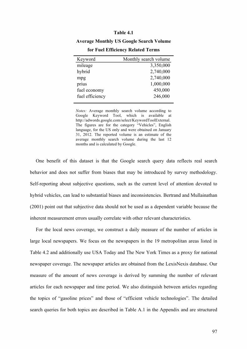
97
Table 4.1
Average Monthly US Google Search Volume
for Fuel Efficiency Related Terms
Notes: Average monthly search volume according to Google Keyword Tool, which is available at http://adwords.google.com/select/KeywordToolExternal. The figures are for the category “Vehicles”, English language, for the US only and were obtained on January 31, 2012. The reported volume is an estimate of the average monthly search volume during the last 12 months and is calculated by Google.
One benefit of this dataset is that the Google search query data reflects real search
behavior and does not suffer from biases that may be introduced by survey methodology.
Self-reporting about subjective questions, such as the current level of attention devoted to
hybrid vehicles, can lead to substantial biases and inconsistencies. Bertrand and Mullainathan
(2001) point out that subjective data should not be used as a dependent variable because the
inherent measurement errors usually correlate with other relevant characteristics.
For the local news coverage, we construct a daily measure of the number of articles in
large local newspapers. We focus on the newspapers in the 19 metropolitan areas listed in
Table 4.2 and additionally use USA Today and The New York Times as a proxy for national
newspaper coverage. The newspaper articles are obtained from the LexisNexis database. Our
measure of the amount of news coverage is derived by summing the number of relevant
articles for each newspaper and time period. We also distinguish between articles regarding
the topics of “gasoline prices” and those of “efficient vehicle technologies”. The detailed
search queries for both topics are described in Table A.1 in the Appendix and are structured
Keyword Monthly search volumemileage 3,350,000hybrid 2,740,000mpg 2,740,000prius 1,000,000fuel economy 450,000fuel efficiency 246,000
98
to be a reasonable compromise between relevancy and completeness. We generate the
newspaper coverage variable by counting the number of relevant articles for each newspaper
and time period (i.e. weekly or monthly). Therefore, the purpose is not to analyze the content
but rather to focus on the mere presence of media coverage. The methodology has the
drawback that the sentiment of media coverage may be positive or negative, which may
influence both the attention and sales impact. Regarding this point, Berger, Sorensen, and
Rasmussen (2010) show that new and less-known products benefit from both positive and
negative publicity. Thus, we assume that all media coverage can be treated equally in our
setup because hybrid vehicles are still a relatively new and less-known product.
Additionally, we use data on television news coverage from the Vanderbilt Television
News Archive. The Vanderbilt database provides access to the evening news of the four
major US national broadcast networks: ABC, CBS, NBC, and CNN. We construct two daily
time series of television news coverage, one for the topic of “gasoline prices and fuel
economy” and one for “hybrid vehicles and efficiency technologies”. For the first topic, we
use the following keywords: Gasoline, gas price, mileage, gallon and mpg. For the second
topic, we use the keywords: Hybrid and fuel efficiency. Then, we eliminate all duplicates
within each topic and hand-check for the relevancy of each news segment. We generate our
variables by counting the total number of news segments across all networks for each topic
and for a given time period (i.e. weekly or monthly).
Two different datasets of gasoline prices are obtained from the US Energy Information
Administration (EIA). In section 4, for the analysis of the determinants of consumers’
attention, we use weekly retail gasoline prices for all grades and formulations. Depending on
data availability, we match our 19 metropolitan areas with gasoline prices on a regional or
state level. For the analysis of the actual purchasing behavior in section 5, we use the
monthly state-level retail price of motor gasoline.
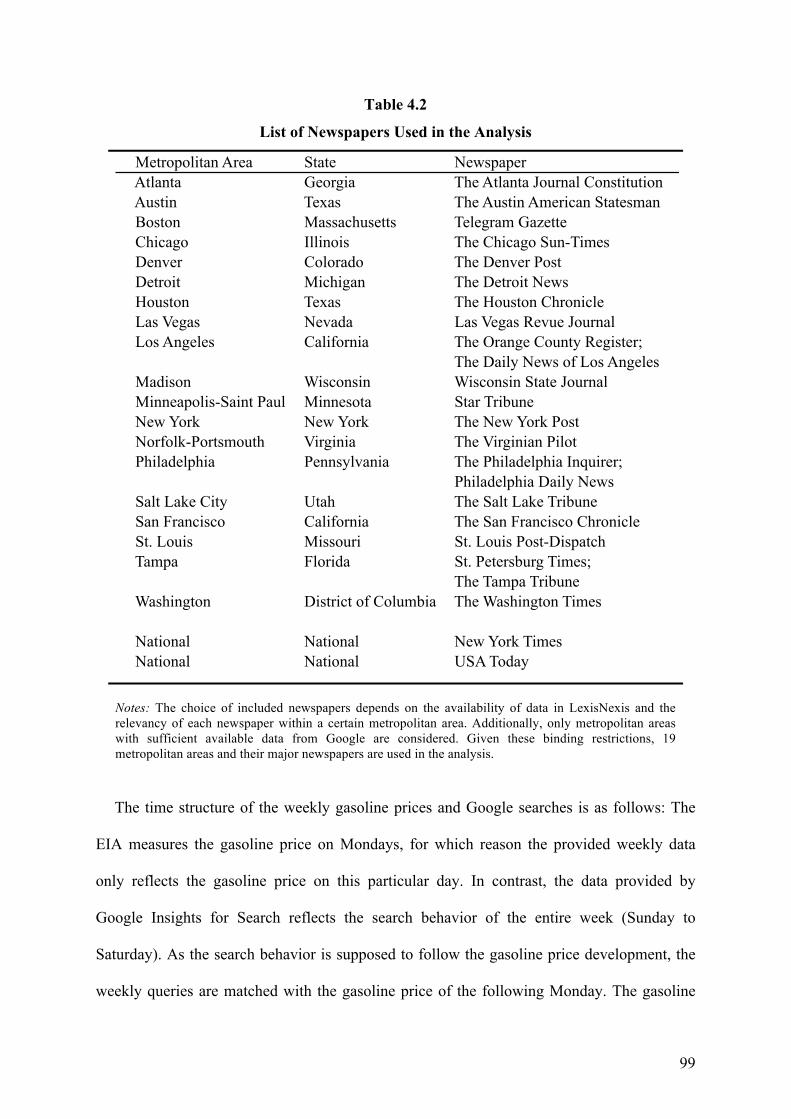
99
Table 4.2
List of Newspapers Used in the Analysis
Notes: The choice of included newspapers depends on the availability of data in LexisNexis and the relevancy of each newspaper within a certain metropolitan area. Additionally, only metropolitan areas with sufficient available data from Google are considered. Given these binding restrictions, 19 metropolitan areas and their major newspapers are used in the analysis.
The time structure of the weekly gasoline prices and Google searches is as follows: The
EIA measures the gasoline price on Mondays, for which reason the provided weekly data
only reflects the gasoline price on this particular day. In contrast, the data provided by
Google Insights for Search reflects the search behavior of the entire week (Sunday to
Saturday). As the search behavior is supposed to follow the gasoline price development, the
weekly queries are matched with the gasoline price of the following Monday. The gasoline
Metropolitan Area State Newspaper Atlanta Georgia The Atlanta Journal Constitution Austin Texas The Austin American Statesman Boston Massachusetts Telegram Gazette Chicago Illinois The Chicago Sun-Times Denver Colorado The Denver Post Detroit Michigan The Detroit News Houston Texas The Houston Chronicle Las Vegas Nevada Las Vegas Revue Journal Los Angeles California The Orange County Register;
The Daily News of Los Angeles Madison Wisconsin Wisconsin State Journal Minneapolis-Saint Paul Minnesota Star Tribune New York New York The New York Post Norfolk-Portsmouth Virginia The Virginian Pilot Philadelphia Pennsylvania The Philadelphia Inquirer;
Philadelphia Daily News Salt Lake City Utah The Salt Lake Tribune San Francisco California The San Francisco Chronicle St. Louis Missouri St. Louis Post-Dispatch Tampa Florida St. Petersburg Times;
The Tampa Tribune Washington District of Columbia The Washington Times National National New York Times National National USA Today
100
price changes from the current week are reflected in the subsequent – and not the
contemporaneous – gasoline price. All media variables are built from daily data and match
the time structure of the Google searches. Table A.2 in the Appendix reports summary
statistics for both panel datasets used for the analyses presented in sections 4 and 5.
4.4 What Drives the Attention Devoted to Hybrid Vehicles?
In this section, we investigate which factors influence the attention devoted to hybrid
vehicles. As outlined in the introduction, we focus on two main channels: The observable
gasoline price and the media coverage concerning hybrid vehicles. The causal influence of
both unprecedented record gasoline prices and local media coverage is of particular interest.
However, one issue related to this analysis is that the effect of media is expected to be limited
if consumers are well informed. As a robustness test, this hypothesis is tested in a
supplementary analysis using the local newspaper coverage concerning gasoline prices and
the online search queries for “mileage” as a proxy for the attention to fuel economy.
We begin with the analysis of the determinants of the consumer’s attention devoted to
hybrid vehicles. Before proceeding with the regression analysis, the relationship between the
relevant variables is discussed. Figure 4.1 shows the weekly US gasoline price in US Dollars
per gallon, the number of television news segments covering hybrid vehicles, the sum of
newspaper articles about hybrid vehicles or fuel efficiency in all sample newspapers and the
search trend for “hybrid” for the time period from January 2004 to September 2011. The
shaded areas indicate weeks with a high relative interest in hybrid vehicles.
Graphical inspection suggests that the variation of searches is closely connected to the
gasoline price and news coverage. Figure 4.1 also shows that in 2005 and 2008, there were
new record price levels that lead to the highest interest during the sample period. The actual
search behavior far exceeds the amount of searches that can be explained as a proportional
reaction to the gasoline price increase only. When the price drops after a period of very high
101
prices, there is a strong sign of relief, which is mirrored by a plunge in consumers’ interest in
hybrid vehicles. The graphical analysis also suggests that consumers and media react to price
increases rather than to high price levels. Once the gasoline price stops rising, but remains at
a high level, both consumers and media quickly lose their interest.
The periods of high attention levels always coincide with periods having steep gasoline
price increases, record gasoline prices or a high media coverage on hybrid vehicles. However,
there is one peak of news coverage in the first week of December 2008, which is not reflected
in the Google searches. This peak of news coverage is due to the US Big Three car
manufacturers’ bailout discussion and their CEOs using hybrid vehicles for the journey to the
Senate hearing. Another event leading to increased news coverage on hybrid vehicles is the
North American International Auto Show in Detroit, which takes place every year in January.
In the following part, we examine the impact of local media coverage and record gasoline
prices on the attention devoted to hybrid vehicles. We thereby proceed in three steps. First,
we describe the variables used in our setup, second we discuss our regression model
specifications and third we present the results from estimating our regression models.
For our identification strategy, we rely on local newspaper coverage. Despite the
omnipresence of the internet, local newspapers are usually read only within one city and its
surroundings. Compared to media coverage on a national level, focusing on local media
therefore allows to have varying media exposure for the same event and to subsequently
observe the reactions of metropolitan areas which have been exposed to a different degree of
media coverage. Thus, all regression models are estimated using panel data for 19 US
metropolitan areas, which enables us to examine more precisely whether local newspaper
coverage affects the attention to hybrid vehicles when controlling for other news coverage or
102
time-fixed effects.44 We make use of several control variables for national media coverage.
For the specifications without time-fixed effects, we use national television news coverage on
gasoline prices and on hybrid vehicles as controls. Additionally, we include the news
coverage in two national newspapers, USA Today and The New York Times.
Gasoline price changes are expected to have a major influence on the attention devoted to
hybrid vehicles. We include asymmetric specifications of gasoline price changes as rising and
falling prices may have a different influence on attention.45 There are three different time
frames included: The change (i.e. log difference) during the current week, the short-term
price movement (week t-2 to t-6) and the mid-term perspective (week t-7 to t-18). The results
of Yuan (2011) indicate that record gasoline prices may have a distinct effect on attention.
Thus, we include the variable “Record Price Length” to count the consecutive number of
weeks with an unprecedented price level during a price surge.46 The variable reflects the fact
that the attention rises directly with the duration of an intense price increase.
Government incentives such as tax credits are not taken into account explicitly. However,
our fixed effects specification controls for all state-specific incentives that do not vary over
time. Furthermore, the time-fixed effects account for all federal incentives. As the hybrid
vehicle market matures, government incentives become less substantial compared to the early
phase before our sample period. Marketing expenditures could be another source of an
omitted variable bias that may influence both the attention and the purchasing decision
modeled in section 5. There is no data available on regional marketing focusing on hybrid
vehicles or fuel efficiency; however it is likely that large and influential marketing campaigns
44 Note that our setup directly controls for the possibility that a local newspaper is also read by non-local readers and vice versa. A higher share of non-local readers makes it less likely to find a causal effect of local media coverage. 45 This specification is consistent with the findings of Lewis and Marvel (2011). 46 For instance, if there are five record prices in a row then the variable equals 5 in the last week. In order to account for minor gaps within such periods, the variable stagnates in case of a single week without an unprecedented price level if another record price follows afterwards. If – in our example – there has been a break in the fourth week, the variable would twice indicate that three weeks of record prices occurred and would end with a count of 4 in the last week.
103
are targeted at a national audience and are thus captured by our time-fixed effects.
We estimate our regression models using five different specifications. In the first
specification, we control for the gasoline price, national television coverage, national
newspaper coverage, year-fixed effects and time-invariant characteristics of metropolitan
areas by fixed effects. However, we do not control for spillover effects of local news
coverage in other metropolitan areas. Therefore, we estimate the average effect of local
newspaper coverage, which can be interpreted as the correlation between newspaper
coverage and online searches.
The second specification additionally includes all local newspapers as control variables.
Thus, each local newspaper is also allowed to have an effect on the non-local metropolitan
areas. Following Engelberg and Parsons (2011), the impact of local newspapers is now
identified by the difference in the reaction between a newspaper’s local and non-local
readership. If there is a significant positive marginal effect of the local newspaper coverage,
it can be concluded that local newspaper treatment has a causal effect on the readers’
attention. For example, a newspaper may feature an article about the benefits of hybrid
vehicle technology. The article could have an influence on the readership by increasing the
awareness about hybrid vehicles and by encouraging the readership to search for more
information online. In this case, there is an increased search volume in the metropolitan area
with the newspaper coverage of the hybrid vehicle technology, whereas the metropolitan
areas without a local news treatment do not exhibit an increased level of attention.
For robustness reasons, we also employ alternative estimation techniques and setups. The
third specification includes time-fixed effects, for which reason only variables with local
variation will be included. The fourth and fifth specification explicitly account for the
underlying panel data structure, which is characterized by many time periods and relatively
few units of observation (large T and small N). Using a panel consisting of regional groups,
104
such as metropolitan areas, makes it important to control for cross-sectional correlation, as it
is very unlikely that the patterns in different geographical areas are mutually independent.
Besides accounting for this kind of spatial correlation, it is also necessary to adequately
model the serial correlation of the error term as the number of time periods increases. The
fourth specification therefore estimates the same model as the second specification, but uses a
Prais-Winsten type feasible GLS panel estimator with a panel-specific AR(1) structure and
panel-corrected standard errors. Alternatively, the fifth specification uses robust
Driscoll-Kraay standard errors, which account for general forms of cross-sectional
correlations, autocorrelation and heteroskedasticity.
Table 4.3 shows the panel regression results for our model with Google searches for
“hybrid” as the dependent variable. The dependent variable measures the search volume in
each of the 19 metropolitan areas. Our results show that local newspaper coverage of topics
related to hybrid vehicles (“Local Newspaper Hybrid”) has a significant impact on the
consumers’ attention, regardless of the specification. For specifications (2) - (5), the local
newspaper variable measures the supplemental effect that each local newspaper has in its
own region, which we interpret as a causal effect following Engelberg and Parsons (2011).
Our results suggest that local newspapers influence the local attention devoted to hybrid
vehicles, despite other information sources available. Television news coverage about
gasoline prices has a significant correlation with the search volumes for hybrid. This finding
is intuitive as the gasoline price affects the profitability of an investment in a hybrid vehicle.
The effect of television news coverage regarding hybrid vehicles has a positive, but not
conclusive, effect on the searches for hybrid.
The impact of record gasoline prices is significant in most specifications. This finding
supports the hypothesis that consumers react to reference points. Following Tversky and
Kahneman (1991), consumers perceive a price increase as a loss if it is above the reference
105
point of the most recent record price. In this case, loss aversion leads to a stronger reaction in
the amount of search volumes reflecting a higher level of attention.
An alternative explanation for the record price effect could be that the consumers’
expectations of future gasoline prices are not consistent with the random walk hypothesis.47
The profitability of an investment in automotive fuel efficiency depends on future gasoline
prices. If consumers expect that trends of rising gasoline prices will continue in the future, the
consumers’ attention would rise disproportionately during periods of extended price increases.
However, Anderson et al. (2011) show that it is generally a reasonable approach to assume a
no-change forecast for consumers’ fuel price expectations, which is consistent with the
random walk hypothesis. Nevertheless, our alternative explanation cannot be ruled out
completely because Anderson et al. (2011) still observe a large dispersion of individual
forecasts during periods of extreme price fluctuations as seen in the year 2008.
In conclusion, the regression models indicate that consumers react to movements of the
gasoline price by adjusting their search intensity. Additionally, unprecedented record
gasoline prices and local media coverage raise the attention devoted to hybrid vehicles in a
causal relationship.
We proceed with the supplementary analysis and examine whether local media coverage
regarding gasoline prices likewise affects the attention devoted to fuel economy. As the
gasoline price is directly observable, media coverage is expected to have a less distinct effect.
The gasoline price is the most obvious factor that influences the attention devoted to fuel
economy. When gasoline prices rise, consumers are likely to be forced to change their
general consumption behavior. For example, Gicheva, Hastings, and Villas-Boas (2010) and
Ma et al. (2011) show that increases in gasoline prices lead to changes in the grocery
purchasing behavior due to changes in residual disposable income. The pressure to change
47 The random walk hypothesis assumes that the current price is the best estimate for future prices regardless of the price history.
106
general consumption patterns could also lead to an increased interest in fuel economy.
The variables for the supplementary analysis are displayed in Figure 4.2, which shows the
weekly US gasoline price, the number of television news segments covering the gasoline
price or fuel economy, the sum of newspaper articles about gasoline prices in all sample
newspapers and the search trend for “mileage” for the time period from January 2004 to
September 2011. The shaded areas indicate weeks with a high relative interest in fuel
economy.
Similar to the setup for hybrid vehicles, the variation of searches for fuel economy is
closely connected to the gasoline price and media coverage. Comparing Figures 4.1 and 4.2,
the newspaper coverage of “hybrid vehicles and fuel efficiency” is noisier than the coverage
of “gasoline prices”. However, the topic of efficient technologies has a more general
character and is not as closely tied to the gasoline price movement. Furthermore, the search
trends for “mileage” and “hybrid” are very similar. This finding indicates that the increased
fuel efficiency of hybrid vehicles is indeed perceived as the major advantage of hybrid
vehicles.
In April 2006, there was a peak of television coverage on gasoline prices, with up to 35
relevant news segments in one week. During this time, several economic and political events
occurred that constituted the increased television reporting. First, there was a strong increase
of gasoline prices from $2.41 on March 13th to $2.96 on April 24th. Second, on April 25th,
George W. Bush held a speech on energy policy, which was widely covered by the media.
Lastly, discussions about oil companies’ high profits and a windfall profit tax gained
increased media attention.
Table 4.4 presents the results of regressing Google searches for “mileage” on media
coverage, record gasoline prices and gasoline price changes. The basic setup of the regression
model is the same as for the results shown in Table 4.3. However, all newspaper variables are
107
now constructed to reflect the news coverage on gasoline prices.48
The results shown in Table 4.4 indicate that the relationship between the local news
coverage concerning gasoline prices and the attention to fuel economy is as expected. Only in
the first specification, there is a significant relationship between the two variables. As in
Table 4.3, the first specification estimates the average effect of local newspaper coverage
without controlling for other local news coverage in the remaining metropolitan areas or for
time-fixed effects. Thus, we find a strong positive correlation between newspaper coverage
and searches. However, when estimating effects with a causal interpretation (i.e. the
supplemental regional effect of local newspaper coverage on the attention devoted to
mileage), the results indicate that the interest in searching for mileage is unaffected by media
coverage. Therefore, it can be concluded that the treatment of local newspaper coverage in
regards to gasoline prices has no causal influence on the attention devoted to fuel economy.
However, the length of unprecedented gasoline prices has a positive impact on the attention
level. This finding indicates that gasoline expenditures become a “top of mind” topic when
the prices reach new all-time highs.
Overall, the aim of the main analysis is to examine which factors influence the attention
devoted to hybrid vehicles. We demonstrate that both local media coverage and
unprecedented record gasoline prices significantly increase the attention devoted to hybrid
vehicles. The supplementary analysis examines whether local media coverage concerning
gasoline prices similarly affects the attention devoted to fuel economy. We observe a strong
correlation, but we do not find a causal effect. An intuitive explanation for this finding is that
consumers can be assumed to be rather well informed about the current gasoline price, which
can be easily observed at gas stations. Therefore, the media coverage concerning gasoline
prices does not provide much additional information and has consequently no causal effect on
48 See Table A.1 for a precise definition of the relevant search terms.

108
attention. In contrast, hybrid vehicles are a relatively new fuel-efficient technology and
consumers may not be fully aware of the existence and benefits of hybrid vehicles. Thus,
media coverage has the ability to increase the amount of attention devoted hybrid vehicles.
The finding that media coverage alters the consumers’ attention to hybrid vehicles is of
interest in two regards. First, this result indicates that consumers would most likely invest
more in new, efficient technologies if they had a deeper knowledge of the topic. This insight
may be of importance to both policymakers and car manufacturers dealing with the
distribution of environmentally friendly vehicles. Second, and more generally, our finding is
interesting concerning the role of the media as a part of an individual’s decision-making
process. Our results seem to reject the hypothesis that the media merely replicates publically
available information and does not influence the consumers’ considerations. However, the
impact of media coverage depends on the specific topic considered and cannot be generalized
for all circumstances.
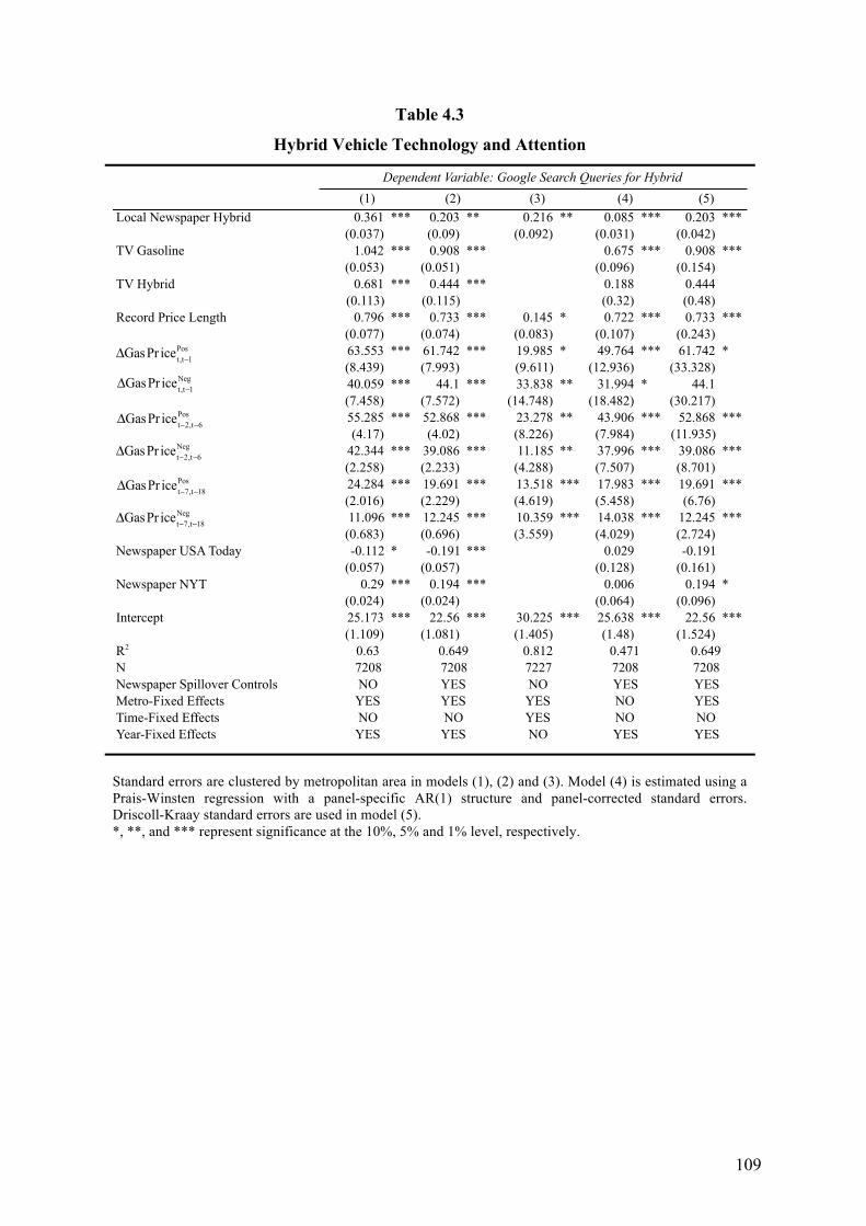
109
Table 4.3
Hybrid Vehicle Technology and Attention
Standard errors are clustered by metropolitan area in models (1), (2) and (3). Model (4) is estimated using a Prais-Winsten regression with a panel-specific AR(1) structure and panel-corrected standard errors. Driscoll-Kraay standard errors are used in model (5). *, **, and *** represent significance at the 10%, 5% and 1% level, respectively.
Local Newspaper Hybrid 0.361 *** 0.203 ** 0.216 ** 0.085 *** 0.203 *** (0.037) (0.09) (0.092) (0.031) (0.042) TV Gasoline 1.042 *** 0.908 *** 0.675 *** 0.908 *** (0.053) (0.051) (0.096) (0.154) TV Hybrid 0.681 *** 0.444 *** 0.188 0.444 (0.113) (0.115) (0.32) (0.48) Record Price Length 0.796 *** 0.733 *** 0.145 * 0.722 *** 0.733 *** (0.077) (0.074) (0.083) (0.107) (0.243)
63.553 *** 61.742 *** 19.985 * 49.764 *** 61.742 * (8.439) (7.993) (9.611) (12.936) (33.328)
40.059 *** 44.1 *** 33.838 ** 31.994 * 44.1 (7.458) (7.572) (14.748) (18.482) (30.217)
55.285 *** 52.868 *** 23.278 ** 43.906 *** 52.868 *** (4.17) (4.02) (8.226) (7.984) (11.935)
42.344 *** 39.086 *** 11.185 ** 37.996 *** 39.086 *** (2.258) (2.233) (4.288) (7.507) (8.701)
24.284 *** 19.691 *** 13.518 *** 17.983 *** 19.691 *** (2.016) (2.229) (4.619) (5.458) (6.76)
11.096 *** 12.245 *** 10.359 *** 14.038 *** 12.245 *** (0.683) (0.696) (3.559) (4.029) (2.724) Newspaper USA Today -0.112 * -0.191 *** 0.029 -0.191 (0.057) (0.057) (0.128) (0.161) Newspaper NYT 0.29 *** 0.194 *** 0.006 0.194 * (0.024) (0.024) (0.064) (0.096) Intercept 25.173 *** 22.56 *** 30.225 *** 25.638 *** 22.56 *** (1.109) (1.081) (1.405) (1.48) (1.524) R2
NNewspaper Spillover Controls Metro-Fixed Effects Time-Fixed Effects Year-Fixed Effects YES
0.4717208YESNONOYES
0.6497208YESYESNO
YESNOYES
0.8127227NOYESYES
(5)Dependent Variable: Google Search Queries for Hybrid
YES
(1) (2) (3) (4)
0.637208NO
YESNO
NO
0.6497208YES
ΔGasPr icet,t−1Pos
ΔGasPr icet,t−1Neg
ΔGasPr icet−2,t−6Pos
ΔGasPr icet−2,t−6Neg
ΔGasPr icet−7,t−18Pos
ΔGasPr icet−7,t−18Neg
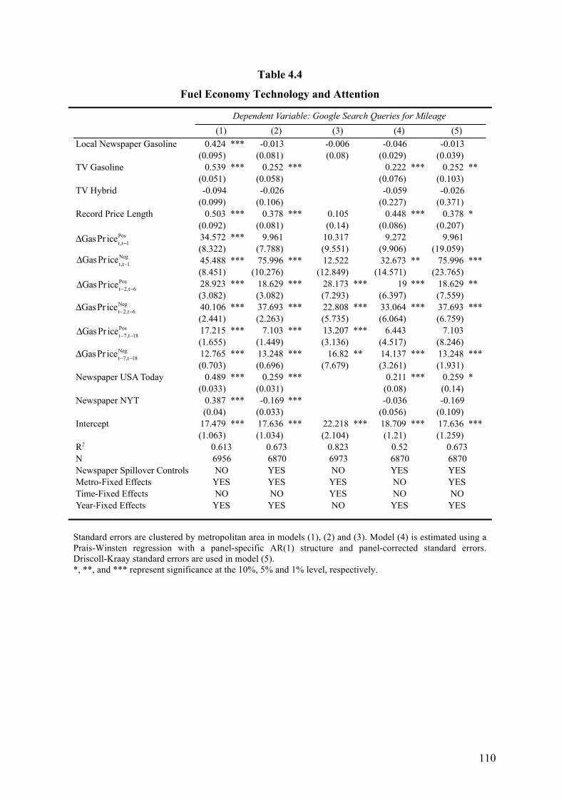
110
Table 4.4
Fuel Economy Technology and Attention
Standard errors are clustered by metropolitan area in models (1), (2) and (3). Model (4) is estimated using a Prais-Winsten regression with a panel-specific AR(1) structure and panel-corrected standard errors. Driscoll-Kraay standard errors are used in model (5). *, **, and *** represent significance at the 10%, 5% and 1% level, respectively.
Local Newspaper Gasoline 0.424 *** -0.013 -0.006 -0.046 -0.013 (0.095) (0.081) (0.08) (0.029) (0.039) TV Gasoline 0.539 *** 0.252 *** 0.222 *** 0.252 ** (0.051) (0.058) (0.076) (0.103) TV Hybrid -0.094 -0.026 -0.059 -0.026 (0.099) (0.106) (0.227) (0.371) Record Price Length 0.503 *** 0.378 *** 0.105 0.448 *** 0.378 * (0.092) (0.081) (0.14) (0.086) (0.207)
34.572 *** 9.961 10.317 9.272 9.961 (8.322) (7.788) (9.551) (9.906) (19.059)
45.488 *** 75.996 *** 12.522 32.673 ** 75.996 *** (8.451) (10.276) (12.849) (14.571) (23.765)
28.923 *** 18.629 *** 28.173 *** 19 *** 18.629 ** (3.082) (3.082) (7.293) (6.397) (7.559)
40.106 *** 37.693 *** 22.808 *** 33.064 *** 37.693 *** (2.441) (2.263) (5.735) (6.064) (6.759)
17.215 *** 7.103 *** 13.207 *** 6.443 7.103 (1.655) (1.449) (3.136) (4.517) (8.246)
12.765 *** 13.248 *** 16.82 ** 14.137 *** 13.248 *** (0.703) (0.696) (7.679) (3.261) (1.931) Newspaper USA Today 0.489 *** 0.259 *** 0.211 *** 0.259 * (0.033) (0.031) (0.08) (0.14) Newspaper NYT 0.387 *** -0.169 *** -0.036 -0.169 (0.04) (0.033) (0.056) (0.109) Intercept 17.479 *** 17.636 *** 22.218 *** 18.709 *** 17.636 *** (1.063) (1.034) (2.104) (1.21) (1.259) R2
NNewspaper Spillover Controls Metro-Fixed Effects Time-Fixed Effects Year-Fixed Effects
(5)Dependent Variable: Google Search Queries for Mileage
YES
(1) (2) (3) (4)
0.6136956NO
YESNO
NO
0.6736870YESYESNOYES
0.8236973NOYESYES
YES
0.526870YESNONO
YES
0.6736870YESYESNO
ΔGasPr icet,t−1Pos
ΔGasPr icet,t−1Neg
ΔGasPr icet−2,t−6Pos
ΔGasPr icet−2,t−6Neg
ΔGasPr icet−7,t−18Pos
ΔGasPr icet−7,t−18Neg
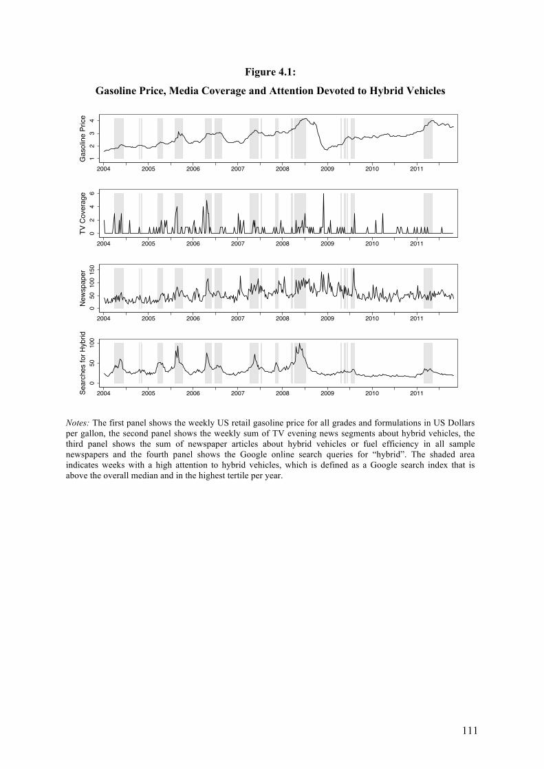
111
Figure 4.1:
Gasoline Price, Media Coverage and Attention Devoted to Hybrid Vehicles
Notes: The first panel shows the weekly US retail gasoline price for all grades and formulations in US Dollars per gallon, the second panel shows the weekly sum of TV evening news segments about hybrid vehicles, the third panel shows the sum of newspaper articles about hybrid vehicles or fuel efficiency in all sample newspapers and the fourth panel shows the Google online search queries for “hybrid”. The shaded area indicates weeks with a high attention to hybrid vehicles, which is defined as a Google search index that is above the overall median and in the highest tertile per year.
12
34
Gas
olin
e Pr
ice
2004 2005 2006 2007 2008 2009 2010 2011
02
46
TV C
over
age
2004 2005 2006 2007 2008 2009 2010 2011
050
100
150
New
spap
er
2004 2005 2006 2007 2008 2009 2010 2011
050
100
Sear
ches
for H
ybrid
2004 2005 2006 2007 2008 2009 2010 2011
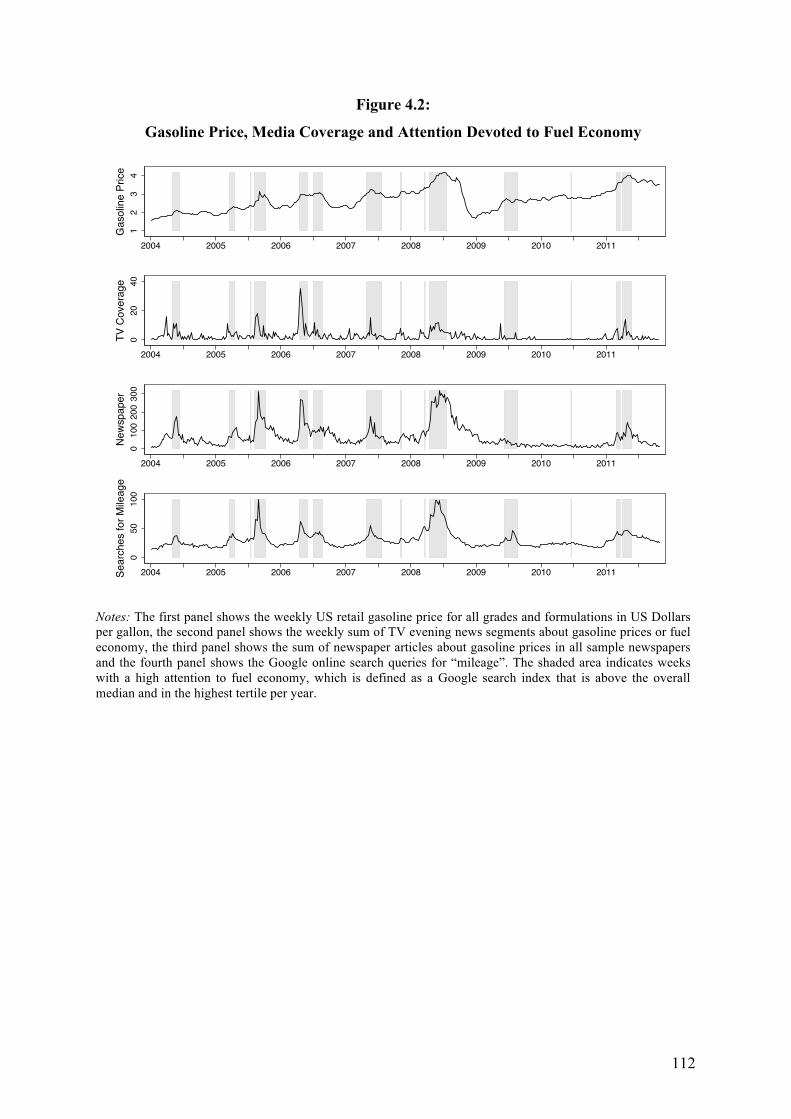
112
Figure 4.2:
Gasoline Price, Media Coverage and Attention Devoted to Fuel Economy
Notes: The first panel shows the weekly US retail gasoline price for all grades and formulations in US Dollars per gallon, the second panel shows the weekly sum of TV evening news segments about gasoline prices or fuel economy, the third panel shows the sum of newspaper articles about gasoline prices in all sample newspapers and the fourth panel shows the Google online search queries for “mileage”. The shaded area indicates weeks with a high attention to fuel economy, which is defined as a Google search index that is above the overall median and in the highest tertile per year.
12
34
Gas
olin
e Pr
ice
2004 2005 2006 2007 2008 2009 2010 2011
020
40TV
Cov
erag
e
2004 2005 2006 2007 2008 2009 2010 2011
010
020
030
0N
ewsp
aper
2004 2005 2006 2007 2008 2009 2010 2011
050
100
Sear
ches
for M
ileag
e
2004 2005 2006 2007 2008 2009 2010 2011
113
4.5 Attention and Hybrid Vehicle Purchases
In this section, we examine the validity of our attention measure by analyzing the
relationship between monthly state-level hybrid vehicle registrations and online search
queries. First, the relation between our key variables is graphically illustrated. Figure 4.3
shows the monthly US retail gasoline price for all grades and formulations (in US Dollars per
gallon), the Google online search queries for “hybrid” as a measure of attention, the monthly
number of hybrid vehicle registrations in the US (in thousands per month) and the market
share of hybrid vehicles (in %). The shaded area indicates months with a high attention.
The graphical analysis shows that the changes in the gasoline price and the search volume
are closely related to both the total number and the market share of hybrid vehicle
registrations. Figure 4.3 also reveals the effect of one-time events that have a major influence
on the hybrid vehicle market. For instance, the impact of the Cash Allowance Rebate System
(C.A.R.S.), commonly known as “Cash for Clunkers”, can be seen in the increase of sales
and hybrid vehicle market shares during July and August 2009. The drop in sales after March
2011 is partially due to supply chain problems resulting from the disastrous earthquake and
tsunami in Japan.49
In the next step, we use monthly state-level registration data to examine the actual hybrid
vehicle purchasing behavior. Table 4.5 shows the results of the regression analysis for the
hybrid vehicle registrations as the dependent variable. Similarly, the results in Table 4.6
represent the same model specifications, but use the market share of hybrid vehicles as the
dependent variable. The Google variable measures the monthly state-level search queries for
“hybrid” and is supposed to mirror the consumers’ attention related to hybrid vehicles. As
both the dependent variables and the Google variables are transformed into logarithms, the
regression parameters can be interpreted as elasticities. The variable “Record Price” is built
as a dummy indicating months with an unprecedented high gasoline price. 49 These one-time events do not affect our analysis as the time-fixed effects account for such occurrences.
114
In specification (1), we use state-fixed effects, year-fixed effects and control for national
media coverage, gasoline price movements and record price levels. Specifications (4) and (5)
include the same variables, but are estimated with a Prais-Winsten type panel estimator and
Driscoll-Kraay standard errors, respectively. Specifications (2) and (3) include state- and
time-fixed effects, and Specification (3) uses an alternative gasoline price variable, i.e. the
logarithm of the gasoline price instead of price changes.
Focusing first on Table 4.5, we show that Google searches for “hybrid” have a
significantly positive effect on hybrid vehicle registrations for all specifications. Our
estimates indicate that an increase of the search volume by 1% is associated with an increase
of hybrid vehicle purchases in the range between 0.12% and 0.22%. Thus, it can be
concluded that our attention measure is valid and robustly related to sales volumes.
The results of the regressions with the market share of hybrid vehicles as the dependent
variable are shown in Table 4.6. The evidence for the relationship to our attention measure is
positive, but not as strong as for the number of registrations. Given the definition of our
Google variable, which reflects the number of search queries related to a topic, a less distinct
relationship between searches and market shares is plausible. If the search queries for hybrid
vehicles were expressed as a share of all search queries in the automotive category, we would
expect a more distinct relationship with market shares rather than sales volumes.
The television news coverage on gasoline prices and fuel economy has a significantly
positive effect on the number of hybrid vehicle registrations. However, the television news
coverage on hybrid vehicles is not significant, which may be caused by the fact that the
overall amount of news coverage is very low. In the regression with the market share of
hybrid vehicles as the dependent variable, the results for television coverage are similar.
The results for the gasoline price variables are in line with economic intuition. Since the
profitability of hybrid cars depends on the gasoline price, a positive association between
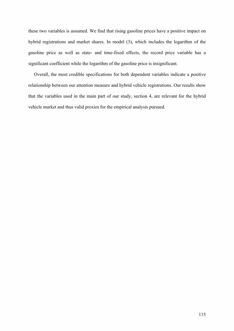
115
these two variables is assumed. We find that rising gasoline prices have a positive impact on
hybrid registrations and market shares. In model (3), which includes the logarithm of the
gasoline price as well as state- and time-fixed effects, the record price variable has a
significant coefficient while the logarithm of the gasoline price is insignificant.
Overall, the most credible specifications for both dependent variables indicate a positive
relationship between our attention measure and hybrid vehicle registrations. Our results show
that the variables used in the main part of our study, section 4, are relevant for the hybrid
vehicle market and thus valid proxies for the empirical analysis pursued.
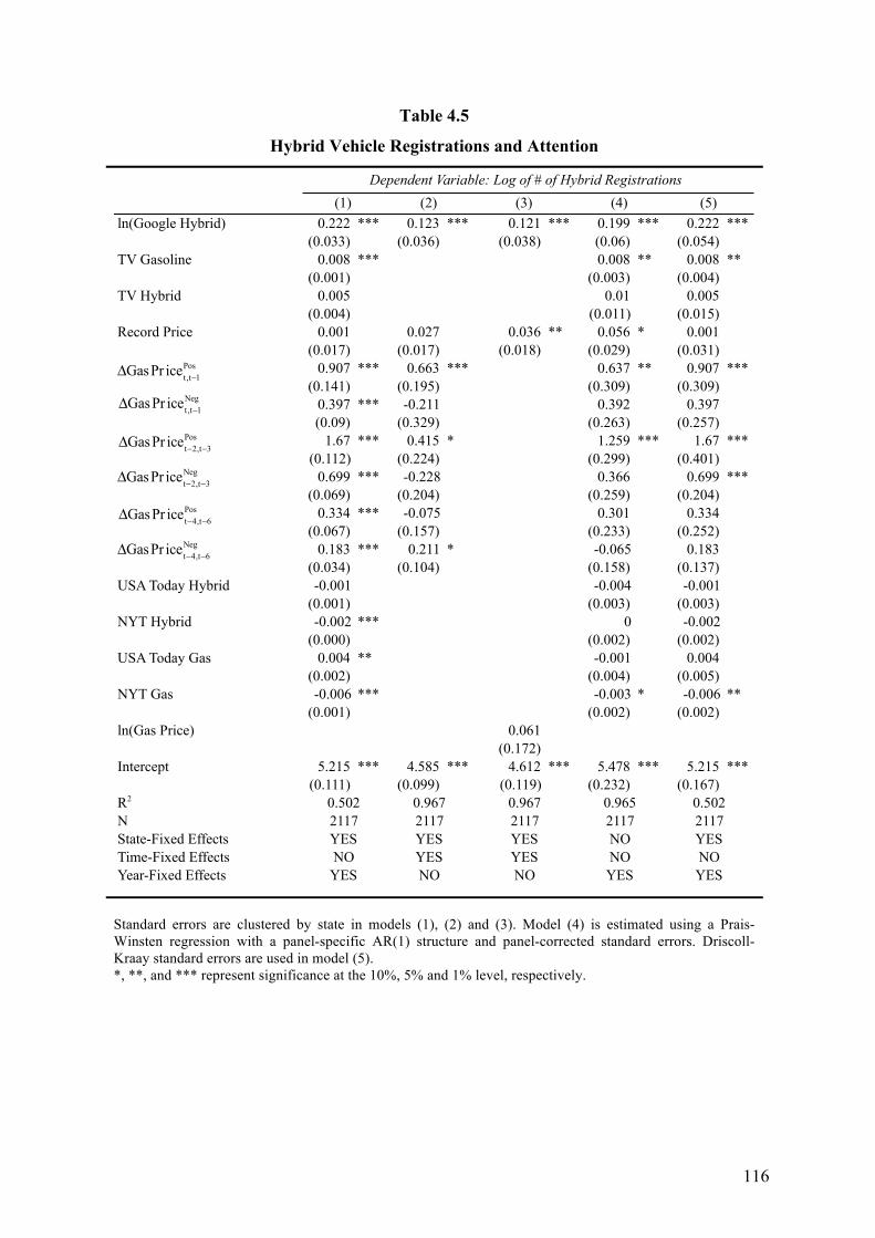
116
Table 4.5
Hybrid Vehicle Registrations and Attention
Standard errors are clustered by state in models (1), (2) and (3). Model (4) is estimated using a Prais-Winsten regression with a panel-specific AR(1) structure and panel-corrected standard errors. Driscoll-Kraay standard errors are used in model (5). *, **, and *** represent significance at the 10%, 5% and 1% level, respectively.
ln(Google Hybrid) 0.222 *** 0.123 *** 0.121 *** 0.199 *** 0.222 *** (0.033) (0.036) (0.038) (0.06) (0.054)TV Gasoline 0.008 *** 0.008 ** 0.008 ** (0.001) (0.003) (0.004)TV Hybrid 0.005 0.01 0.005 (0.004) (0.011) (0.015)Record Price 0.001 0.027 0.036 ** 0.056 * 0.001 (0.017) (0.017) (0.018) (0.029) (0.031)
0.907 *** 0.663 *** 0.637 ** 0.907 *** (0.141) (0.195) (0.309) (0.309)
0.397 *** -0.211 0.392 0.397 (0.09) (0.329) (0.263) (0.257)
1.67 *** 0.415 * 1.259 *** 1.67 *** (0.112) (0.224) (0.299) (0.401)
0.699 *** -0.228 0.366 0.699 *** (0.069) (0.204) (0.259) (0.204)
0.334 *** -0.075 0.301 0.334 (0.067) (0.157) (0.233) (0.252)
0.183 *** 0.211 * -0.065 0.183 (0.034) (0.104) (0.158) (0.137)USA Today Hybrid -0.001 -0.004 -0.001
(0.001) (0.003) (0.003)NYT Hybrid -0.002 *** 0 -0.002
(0.000) (0.002) (0.002)USA Today Gas 0.004 ** -0.001 0.004
(0.002) (0.004) (0.005)NYT Gas -0.006 *** -0.003 * -0.006 **
(0.001) (0.002) (0.002)ln(Gas Price) 0.061
(0.172)Intercept 5.215 *** 4.585 *** 4.612 *** 5.478 *** 5.215 ***
(0.111) (0.099) (0.119) (0.232) (0.167)R2
NState-Fixed Effects Time-Fixed Effects Year-Fixed Effects YES
0.9652117NONO
YES
0.5022117YESNO
NO
0.9672117YESYES
(5)Dependent Variable: Log of # of Hybrid Registrations
YES
(1) (2) (3) (4)
0.5022117YESNO
NO
0.9672117YESYES
ΔGasPr icet,t−1Pos
ΔGasPr icet,t−1Neg
ΔGasPr icet−2,t−3Pos
ΔGasPr icet−2,t−3Neg
ΔGasPr icet−4,t−6Pos
ΔGasPr icet−4,t−6Neg
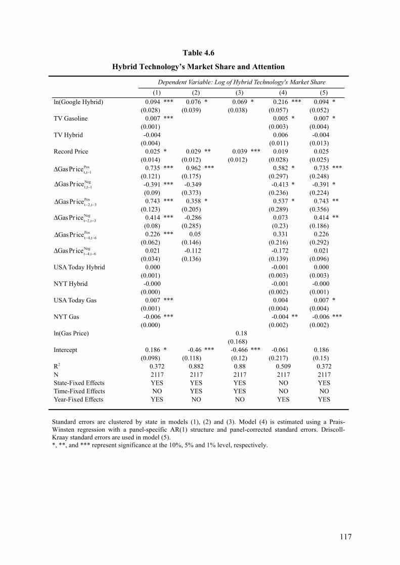
117
Table 4.6
Hybrid Technology’s Market Share and Attention
Standard errors are clustered by state in models (1), (2) and (3). Model (4) is estimated using a Prais-Winsten regression with a panel-specific AR(1) structure and panel-corrected standard errors. Driscoll-Kraay standard errors are used in model (5). *, **, and *** represent significance at the 10%, 5% and 1% level, respectively.
ln(Google Hybrid) 0.094 *** 0.076 * 0.069 * 0.216 *** 0.094 * (0.028) (0.039) (0.038) (0.057) (0.052)TV Gasoline 0.007 *** 0.005 * 0.007 * (0.001) (0.003) (0.004)TV Hybrid -0.004 0.006 -0.004 (0.004) (0.011) (0.013)Record Price 0.025 * 0.029 ** 0.039 *** 0.019 0.025 (0.014) (0.012) (0.012) (0.028) (0.025)
0.735 *** 0.962 *** 0.582 * 0.735 *** (0.121) (0.175) (0.297) (0.248)
-0.391 *** -0.349 -0.413 * -0.391 * (0.09) (0.373) (0.236) (0.224)
0.743 *** 0.358 * 0.537 * 0.743 ** (0.123) (0.205) (0.289) (0.356)
0.414 *** -0.286 0.073 0.414 ** (0.08) (0.285) (0.23) (0.186)
0.226 *** 0.05 0.331 0.226 (0.062) (0.146) (0.216) (0.292)
0.021 -0.112 -0.172 0.021 (0.034) (0.136) (0.139) (0.096)USA Today Hybrid 0.000 -0.001 0.000
(0.001) (0.003) (0.003)NYT Hybrid -0.000 -0.001 -0.000
(0.000) (0.002) (0.001)USA Today Gas 0.007 *** 0.004 0.007 *
(0.001) (0.004) (0.004)NYT Gas -0.006 *** -0.004 ** -0.006 ***
(0.000) (0.002) (0.002)ln(Gas Price) 0.18
(0.168)Intercept 0.186 * -0.46 *** -0.466 *** -0.061 0.186
(0.098) (0.118) (0.12) (0.217) (0.15)R2
NState-Fixed Effects Time-Fixed Effects Year-Fixed Effects
(5)Dependent Variable: Log of Hybrid Technology's Market Share
YES
(1) (2) (3) (4)
0.3722117YESNO
NO
0.8822117YESYESNO
0.882117YESYES
YES
0.5092117NONO
YES
0.3722117YESNO
ΔGasPr icet,t−1Pos
ΔGasPr icet,t−1Neg
ΔGasPr icet−2,t−3Pos
ΔGasPr icet−2,t−3Neg
ΔGasPr icet−4,t−6Pos
ΔGasPr icet−4,t−6Neg
118
Figure 4.3:
Gasoline Price, Attention and Registrations of Hybrid Vehicles
Notes: The first panel shows the monthly US retail gasoline price for all grades and formulations in US Dollars per gallon, the second panel shows the Google online search queries for “hybrid”, the third panel shows the monthly number of hybrid vehicle registrations in the US (in thousands per month) and the fourth panel shows the market share of hybrid vehicles (in %). The shaded area indicates months with a high attention, which is defined as a Google search index that is above the overall median and in the highest tertile per year.
23
4G
asol
ine
Pric
e
2007 2008 2009 2010 2011
050
100
Sear
ches
for H
ybrid
2007 2008 2009 2010 2011
025
50H
ybrid
Reg
istra
tions
2007 2008 2009 2010 2011
1.5
2.5
3.5
Mar
ket S
hare
2007 2008 2009 2010 2011
119
4.6 Conclusion
The study extends the research on consumer attention effects to the area of energy
efficiency. Specifically, the analysis indicates which factors alter the consumers’ attention
devoted to fuel-efficient technologies like hybrid vehicles. We use a novel panel dataset to
show that the revealed consumer attention to hybrid vehicles depends on the gasoline price,
unprecedented record gasoline price levels and media coverage. In our empirical setup,
attention is measured by Google online search behavior. As search queries reflect real-life
actions of millions of United States citizens, this data most importantly does not suffer from
possible survey biases. The accuracy of our attention measure is validated by the robust
relationship to the actual purchasing behavior. Given that we analyze a market for high-cost
durable goods, a setting in which consumers should exhibit a high effort in decision making,
the empirical findings from this study are also of relevance to economic decisions in other
markets.
The finding that attention effects influence the diffusion of innovative and energy efficient
technologies leads to important policy implications. In order to limit greenhouse gas
emissions and to reduce the dependency on oil imports, fuel-efficient technologies must
become a “top of mind” topic in any vehicle purchasing decision. Initiatives aiming at
increasing awareness and education about such technologies may be an important tool to
foster the adoption of hybrid vehicles. A more general finding is that periods of rising
gasoline prices are more effective at drawing temporary attention to fuel efficiency than
periods of steadily high gasoline prices. In fact, volatile gasoline prices provoke strong
reactions of both the media and consumers. Therefore, it can be inferred that volatile gasoline
prices, as they occurred in the years 2005 to 2008, have a positive impact on the diffusion of
green technologies.
Given that consumers’ attention levels have a fluctuating nature, car manufacturers should
consider the current level of the attention devoted to efficient vehicles when planning their
120
marketing effort and campaign contents. During periods of steep gasoline price increases or
record gasoline prices, consumers have a much higher interest and are more receptive to
information about fuel-efficient technologies.
Despite the fact that our study focuses on one specific market, the results have wide
implications. We argue that firms should generally be aware of how and why their customers’
attention fluctuates. Future research could highlight the interaction of marketing and attention
as it is defined in our framework. Interesting questions include how marketing efforts are able
to influence attention or how the efficiency of marketing campaigns depends on the current
attention level.
121
5 Conclusion
This thesis makes several contributions to prior literature. The second chapter contributes
to the recently developing accounting literature which examines how managerial
characteristics affect corporate policies. Prior studies in behavioral accounting show that
managerial overconfidence affects management forecasts (Hilary and Hsu 2011; Hribar and
Yang 2013; Libby and Rennekamp 2012), accounting conservatism (Ahmed and Duellman
2013), and financial misreporting (Schrand and Zechman 2012). We contribute to this
literature by documenting how managerial overconfidence affects cost behavior. Prior
literature in behavioral finance shows that managerial overconfidence affects capital
expenditures (Malmendier and Tate 2005) or merger and acquisitions (Malmendier and Tate
2008). Given that mergers and acquisitions, for example, are relatively rare events, we argue
that it is important to examine the association between managerial overconfidence and cost
behavior because cost decisions are made more frequently and are key to firm profitability
(Porter 1985).
In addition, this study further contributes to the cost stickiness literature. While prior
studies have examined how economic considerations and agency problems affect cost
stickiness, we document the influence of managerial overconfidence on cost stickiness. Our
explanation differs from both existing views on cost stickiness. The economic view implies
that managers’ demand expectations are unbiased (Anderson et al. 2003; Balakrishnan and
Gruca 2008; Balakrishnan, Petersen, and Soderstrom 2004), whereas we allow
overconfidence to affect demand expectations. In addition, we differ from prior studies
examining the role of agency conflicts on cost stickiness. In contrast to the agency view,
which implies that cost stickiness results from empire building (Chen et al. 2012) or earnings
management incentives (Dierynck et al. 2012; Kama and Weiss 2013) of self-interested
managers, we argue that overconfident managers intend to maximize firm value but are
122
affected by behavioral biases. Collectively, our study provides strong support for the role of
managerial discretion in resource adjustment.
This study further entails practical implications. Our finding that managerial
overconfidence affects cost behavior should be of interest for board of directors. While it is
well known that agency costs, such as empire building, can be addressed per incentive pay
(Murphy 1999), behavioral costs, such as managerial overconfidence (Shefrin 2001), cannot
be addressed with incentive pay because overconfident CEOs believe they are maximizing
firm value. This insight should be especially of importance if cost behavior lies at the heart of
a firm’s competitive advantage.
The third chapter of this thesis contributes to our understanding of real consequences
arising from investor sentiment. Prior literature shows that investor sentiment affects earnings
forecasts (Bergman and Roychowdhury 2008), earnings management (Ali and Gurun 2009;
Simpson 2013), pro-forma earnings disclosure (Brown et al. 2012), dividend policies (Baker
and Wurgler 2004; Li and Lie 2006) and decisions on capital expenditure (Polk and Sapienza
2009). We extend the findings in these studies by documenting that catering extends to
decisions on research and development expenditure, advertisement and selling, general and
administrative costs. Further, we complement the findings in McLean and Zhao (2014) who
show that investor sentiment affects employment decisions. While McLean and Zhao (2014)
argue that investor sentiment affects corporate policies because it lowers the cost of external
finance, we show that catering incentives affect employment decisions.
This essay further contributes to prior literature examining how managerial discretion
affects cost behavior. Chen et al. (2012) show that empire-building incentives motivate
managers to refrain from cutting costs when sales decline. Banker et al. (2011) document that
managers increase spending on SG&A resources upon receiving equity incentives. We
contribute to this literature by documenting that catering incentives induce managers to
123
increase spending on various components of operating expenditure.
Finally, our results contribute to prior literature examining how incentives to meet
earnings targets affect cost behavior. Prior literature shows that managers cut discretionary
expenditure in order to meet last year’s earnings, to avoid reporting losses, or to meet
analysts’ earnings forecasts (Baber et al. 1991; Burgstahler and Dichev 1997; Roychowdhury
2006). Other studies show that managers keep less costs when sales decline upon facing
earnings targets (Dierynck et al. 2012; Kama and Weiss 2013). We contribute to this
literature by documenting that managers refrain from overspending on operating expenditure
when it conflicts with meeting investors’ earnings expectations in periods of high relative to
periods of average sentiment. Our findings, thus, confirm the notion that managerial
discretion affects cost behavior from a behavioral setting.
Our results should be of interest for board of directors because managers who address
noise traders’ misperceptions act in the interest of short-term shareholders only. The fact that
SG&A costs make up about one third of total assets reinforces this argument.50
The fourth chapter of this thesis contributes to our understanding of limited attention.
While prior literature in behavioral accounting and finance recognizes the importance of
limited attention, there is only scarce evidence in the field of behavioral energy economics.
More specifically, prior accounting research suggests that limited attention may be one
reason explaining why investors primarily fixate on earnings and do not consider separately
the components of earnings – cash flows and accruals (Hirshleifer and Teoh 2003; Ali and
Gurun 2009). Similarly, research in finance documents the influence of limited attention on
individual investors’ trading behavior (Barber and Odean 2008; Da et al. 2011). Turning to
consumer behavior, Chetty et al. (2009) show that the salience of taxes affects consumer’
attention and, hence, their reaction to taxation. We contribute to this literature by examining
50 In Banker et al. (2011), the average ratio of SG&A costs to total assets is about 31%, suggesting that data used in our sample is comparable to that used in other studies.
124
factors that are able to alter consumers’ attention devoted to a long-lived consumer good.
These findings should be of interest for policy makers. Our results suggest that informational
campaigns may be one method to inform consumers about fuel-efficient technologies such as
hybrid vehicles. Similarly, our results should be of interest for car manufactures. Examining
when and why consumers’ attention fluctuates may allow improving efficiency of marketing
campaigns.
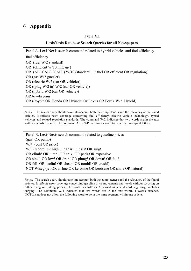
125
6 Appendix
Table A.1
LexisNexis Database Search Queries for all Newspapers
Notes: The search query should take into account both the completeness and the relevancy of the found articles. It reflects news coverage concerning fuel efficiency, electric vehicle technology, hybrid vehicles and related regulation standards. The command W/2 indicates that two words are in the text within 2 words distance. The command ALLCAPS requires a word to be written in capital letters.
Notes: The search query should take into account both the completeness and the relevancy of the found articles. It reflects news coverage concerning gasoline price movements and levels without focusing on either rising or sinking prices. The syntax as follows: ! is used as a wild card, e.g. surg! includes surging. The command W/4 indicates that two words are in the text within 4 words distance. NOTW/seg does not allow the following word to be in the same segment within one article.
Panel A. LexisNexis search command related to hybrid vehicles and fuel efficiencyfuel efficiency OR (fuel W/2 standard) OR (efficient W/10 mileage) OR (ALLCAPS (CAFE) W/10 (standard OR fuel OR efficient OR regulation)) OR (gas W/2 guzzler) OR (electric W/2 (car OR vehicle)) OR ((plug W/2 in) W/2 (car OR vehicle)) OR (hybrid W/2 (car OR vehicle)) OR toyota prius OR ((toyota OR Honda OR Hyundai Or Lexus OR Ford) W/2 Hybrid)
Panel B. LexisNexis search command related to gasoline prices(gas! OR pump) W/4 (cost OR price) W/6 (record OR high OR soar! OR ris! OR surg! OR climb! OR jump! OR spik! OR peak OR expensive OR sink! OR low! OR drop! OR plung! OR down! OR fall! OR fell OR declin! OR cheap! OR tumbl! OR crash!) NOT W/seg (jet OR airline OR kerosine OR kerosene OR shale OR natural)
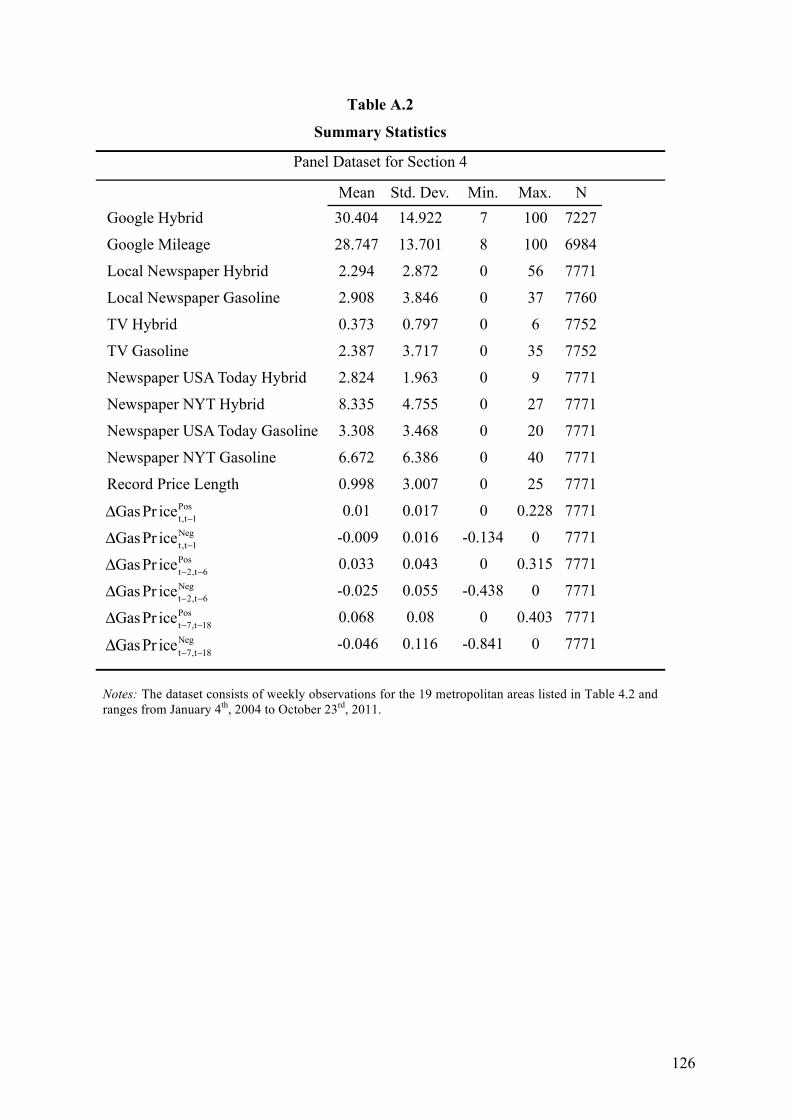
126
Table A.2
Summary Statistics
Panel Dataset for Section 4
Notes: The dataset consists of weekly observations for the 19 metropolitan areas listed in Table 4.2 and ranges from January 4th, 2004 to October 23rd, 2011.
Mean Std. Dev. Min. Max. NGoogle Hybrid 30.404 14.922 7 100 7227
Google Mileage 28.747 13.701 8 100 6984
Local Newspaper Hybrid 2.294 2.872 0 56 7771
Local Newspaper Gasoline 2.908 3.846 0 37 7760
TV Hybrid 0.373 0.797 0 6 7752
TV Gasoline 2.387 3.717 0 35 7752
Newspaper USA Today Hybrid 2.824 1.963 0 9 7771
Newspaper NYT Hybrid 8.335 4.755 0 27 7771
Newspaper USA Today Gasoline 3.308 3.468 0 20 7771
Newspaper NYT Gasoline 6.672 6.386 0 40 7771
Record Price Length 0.998 3.007 0 25 7771
0.01 0.017 0 0.228 7771
-0.009 0.016 -0.134 0 7771
0.033 0.043 0 0.315 7771
-0.025 0.055 -0.438 0 7771
0.068 0.08 0 0.403 7771
-0.046 0.116 -0.841 0 7771
ΔGasPr icet,t−1Pos
ΔGasPr icet,t−1Neg
ΔGasPr icet−2,t−6Pos
ΔGasPr icet−2,t−6Neg
ΔGasPr icet−7,t−18Pos
ΔGasPr icet−7,t−18Neg
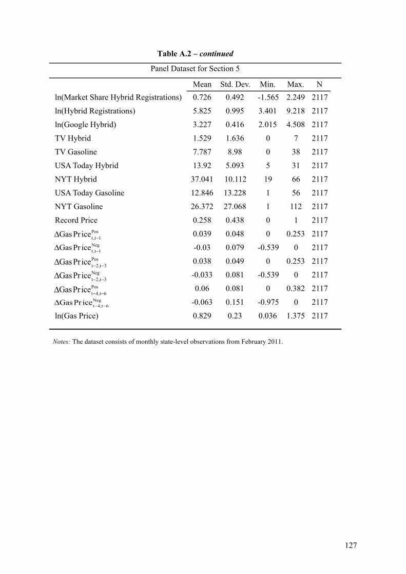
127
Table A.2 – continued
Panel Dataset for Section 5
Notes: The dataset consists of monthly state-level observations from February 2011.
Mean Std. Dev. Min. Max. Nln(Market Share Hybrid Registrations) 0.726 0.492 -1.565 2.249 2117
ln(Hybrid Registrations) 5.825 0.995 3.401 9.218 2117
ln(Google Hybrid) 3.227 0.416 2.015 4.508 2117
TV Hybrid 1.529 1.636 0 7 2117
TV Gasoline 7.787 8.98 0 38 2117
USA Today Hybrid 13.92 5.093 5 31 2117
NYT Hybrid 37.041 10.112 19 66 2117
USA Today Gasoline 12.846 13.228 1 56 2117
NYT Gasoline 26.372 27.068 1 112 2117
Record Price 0.258 0.438 0 1 2117
0.039 0.048 0 0.253 2117
-0.03 0.079 -0.539 0 2117
0.038 0.049 0 0.253 2117
-0.033 0.081 -0.539 0 2117
0.06 0.081 0 0.382 2117
-0.063 0.151 -0.975 0 2117
ln(Gas Price) 0.829 0.23 0.036 1.375 2117
ΔGasPr icet,t−1Pos
ΔGasPr icet,t−1Neg
ΔGasPr icet−2,t−3Pos
ΔGasPr icet−2,t−3Neg
ΔGasPr icet−4,t−6Pos
ΔGasPr icet−4,t−6Neg

128
129
References
Abarbanell, J. S., and B. J. Bushee. 1997. Fundamental Analysis, Future Earnings, and Stock Prices. Journal of Accounting Research 35 (1): 1-24.
Ahmed, A. S., and S. Duellman. 2013. Managerial Overconfidence and Accounting Conservatism. Journal of Accounting Research 51 (1): 1-30.
Ali, A., and U. G. Gurun. 2009. Investor Sentiment, Accruals Anomaly, and Accruals Management. Journal of Accounting, Auditing & Finance 24 (3): 415-431.
Alicke, M. D. 1985. Global Self-Evaluation as Determined by the Desirability and Controllability of Trait Adjectives. Journal of Personality and Social Psychology 49 (6): 1621-1630.
Alicke, M. D., M. L. Klotz, D. L. Breitenbecher, T. J. Yurak, and D. S. Vredenburg. 1995. Personal Contact, Individuation, and the Better-Than-Average Effect. Journal of Personality and Social Psychology 68 (5): 804-825.
Allcott, H. 2011. Consumers' Perceptions and Misperceptions of Energy Costs. American Economic Review 101 (3): 98-104.
Anderson, M. C., R. D. Banker, R. Huang, and S. N. Janakiraman. 2007. Cost Behavior and Fundamental Analysis of SG&A Costs. Journal of Accounting, Auditing & Finance 22 (1): 1-28.
Anderson, M. C., R. D. Banker, and S. N. Janakiraman. 2003. Are Selling, General, and Administrative Costs "Sticky"? Journal of Accounting Research 41 (1): 47-63.
Anderson, S. C., J. A. Born, and O. Schnusenberg. 2010. Closed-end funds, exchange-traded funds, and hedge funds : Origins, functions, and literature. New York: Springer US.
Anderson, S. T., R. Kellogg, J. M. Sallee, and R. T. Curtin. 2011. Forecasting Gasoline Prices Using Consumer Surveys. American Economic Review 101 (3): 110-114.
Anderson, S. W., and W. N. Lanen. 2009. Understanding Cost Management: What Can We Learn from the Empirical Evidence on “Sticky Costs? Working Paper, University of Melbourne.
Andreß, H.-J., K. Golsch, and A. W. Schmidt. 2013. Applied Panel Data Analysis for Economic and Social Surveys. Berlin: Springer-Verlag.
Baber, W. R., P. M. Fairfield, and J. A. Haggard. 1991. The Effect of Concern about Reported Income on Discretionary Spending Decisions: The Case of Research and Development. The Accounting Review 66 (4): 818-829.
130
Baker, M., J. C. Stein, and J. Wurgler. 2003. When Does the Market Matter? Stock Prices and the Investment of Equity-Dependent Firms. Quarterly Journal of Economics 118 (3): 969-1005.
Baker, M., and J. Wurgler. 2000. The Equity Share in New Issues and Aggregate Stock Returns. The Journal of Finance LV (5): 2219-2257.
———. 2002. Market Timing and Capital Structure. The Journal of Finance LVII (1): 1-32.
———. 2004. A Catering Theory of Dividends. The Journal of Finance 59 (3): 1125-1165.
———. 2006. Investor Sentiment and the Cross-Section of Stock Returns. The Journal of Finance LXI (4): 1645-1680.
———. 2007. Investor Sentiment in the Stock Market. Journal of Economic Perspectives 21 (2): 129-151.
———. 2011. Behavioral Corporate Finance: An Updated Survey. Working Paper, National Bureau of Economic Research.
Balakrishnan, R., and T. S. Gruca. 2008. Cost Stickiness and Core Competency: A Note. Contemporary Accounting Research 25 (4): 993-1006.
Balakrishnan, R., E. Labro, and N. S. Soderstrom. 2014. Cost Structure and Sticky Costs. Journal of Management Accounting Research 26 (2): 91-116.
Balakrishnan, R., M. J. Petersen, and N. S. Soderstrom. 2004. Does Capacity Utilization Affect the "Stickiness" of Cost? Journal of Accounting, Auditing & Finance 19 (3): 283-299.
Banker, R. D., and D. Byzalov. 2013. Asymmetric Cost Behavior. Working Paper, Temple University.
Banker, R. D., D. Byzalov, and L. T. Chen. 2013. Employment protection legislation, adjustment costs and cross-country differences in cost behavior. Journal of Accounting and Economics 55 (1): 111-127.
Banker, R. D., D. Byzalov, M. Ciftci, and R. Mashruwala. 2014. The Moderating Effect of Prior Sales Changes on Asymmetric Cost Behavior. Journal of Management Accounting Research 26 (2): 221-242.
Banker, R. D., R. Huang, and R. Natarajan. 2011. Equity Incentives and Long-Term Value Created by SG&A Expenditure. Contemporary Accounting Research 28 (3): 794-830.
Barber, B. M., and T. Odean. 2001. Boys will be Boys: Gender, Overconfidence, and Common Stock Investment. Quarterly Journal of Economics 116 (1): 261-292.
131
———. 2008. All That Glitters: The Effect of Attention and News on the Buying Behavior of Individual and Institutional Investors. The Review of Financial Studies 21 (2): 785-818.
Barberis, N., A. Shleifer, and R. W. Vishny. 1998. A model of investor sentiment. Journal of Financial Economics 49 (3): 307-343.
Barberis, N., and R. H. Thaler. 2003. A SURVEY OF BEHAVIORAL FINANCE. In Handbook of the Economics of Finance, ed. Constantinides, G. M., M. Harris and R. M. Stulz, 799-1612. Amsterdam: Elsevier.
Baumgarten, D., U. Bonenkamp, and C. Homburg. 2010. The Information Content of the SG&A Ratio. Journal of Management Accounting Research 22 (1): 1-22.
Ben-David, I., J. R. Graham, and C. R. Harvey. 2012. MANAGERIAL MISCALIBRATION. Working Paper, The Ohio State University.
Beresteanu, A., and S. Li. 2011. Gasoline Prices, Government Support, and the Demand for Hybrid Vehicles in the United States. International Economic Review 52 (1): 161-182.
Berger, J., A. T. Sorensen, and S. J. Rasmussen. 2010. Positive Effects of Negative Publicity: When Negative Reviews Increase Sales. Marketing Science 29 (5): 815–827.
Bergman, N. K., and S. Roychowdhury. 2008. Investor Sentiment and Corporate Disclosure. Journal of Accounting Research 46 (5): 1057-1083.
Berkman, H., V. Dimitrov, P. C. Jain, P. D. Koch, and S. Tice. 2009. Sell on the news: Differences of opinion, short-sales constraints, and returns around earnings announcements. Journal of Financial Economics 92 (3): 376–399.
Bertrand, M., and S. Mullainathan. 2001. Do People Mean What They Say? Implications for Subjective Survey Data. American Economic Review 91 (2): 67-72.
Black, F. 1986. Noise. The Journal of Finance XLI (3): 529-543.
Brown, G. W., and M. T. Cliff. 2005. Investor Sentiment and Asset Valuation. The Journal of Business 78 (2): 405-440.
Brown, N. C., T. E. Christensen, B. W. Elliot, and R. D. Mergenthaler. 2012. Investor Sentiment and Pro Forma Earnings Disclosures. Journal of Accounting Research 50 (1): 1-40.
Burgstahler, D., and I. Dichev. 1997. Earnings management to avoid earnings decreases and losses. Journal of Accounting and Economics 24 (1): 99-126.
132
Bushee, B. J. 1998. The Influence of Institutional Investors on Myopic R&D Investment Behavior. The Accounting Review 73 (3): 305-333.
Camerer, C., and D. Lovallo. 1999. Overconfidence and Excess Entry: An Experimental Approach. American Economic Review 89 (1): 306-318.
Camerer, C., and U. Malmendier. 2007. Behavioral Economics of Organizations. In Behavioral Economics and Its Applications, ed. Diamond, P. and H. Vartiainen, 235-281. Princeton and Oxford: Princeton University Press.
Campbell, T. C., M. Gallmeyer, S. A. Johnson, J. Rutherford, and B. W. Stanley. 2011. CEO Optimism and Forced Turnover. Journal of Financial Economics 101 (3): 695-712.
Chan, L. K. C., J. Lakonishok, and T. Sougiannis. 2001. The Stock Market Valuation of Research and Development Expenditures. Journal of Finance LVI (6): 2431-2456.
Chandra, A., S. Gulati, and M. Kandlikar. 2010. Green drivers or free riders? An analysis of tax rebates for hybrid vehicles. Journal of Environmental Economics and Management 60 (2): 78-93.
Chandra, A., and M. Tappata. 2011. Consumer Search and Dynamic Price Dispersion: An Application to Gasoline Markets. The RAND Journal of Economics 42 (4): 681-704.
Chen, C. X., H. Lu, and T. Sougiannis. 2012. The Agency Problem, Corporate Governance, and the Asymmetrical Behavior of Selling, General, and Administrative Costs. Contemporary Accounting Research 29 (1): 252-282.
Chen, K. C. W., Z. Chen, and K. C. J. W. Wei. 2011. Agency Costs of Free Cash Flow and the Effect of Shareholder Rights on the Implied Cost of Equity Capital. JOURNAL OF FINANCIAL AND QUANTITATIVE ANALYSIS 46 (1): 171-207.
Chetty, R., A. Looney, and K. Kroft. 2009. Salience and Taxation: Theory and Evidence. American Economic Review 99 (4): 1145–1177.
Cianci, A. M., and S. E. Kaplan. 2010. The effect of CEO reputation and explanations for poor performance on investors’ judgments about the company’s future performance and management. Accounting, Organizations and Society 35 (4): 478-495.
Cooper, M. J., O. Dimitrov, and P. R. Rau. 2001. A Rose.com by Any Other Name. The Journal of Finance LVI (2371-2388).
Cooper, M. J., A. Khorana, I. Osobov, A. Patel, and P. R. Rau. 2005. Managerial actions in response to a market downturn: valuation effects of name changes in the dot.com decline. Journal of Corporate Finance 11 (1-2): 319-335.
133
Cordeiro, L. 2009. Managerial Overconfidence and Dividend Policy. Working Paper, London Business School.
Da, Z., J. Engelberg, and P. Gao. 2011. In Search of Attention. Journal of Finance LXVI (5): 1461-1499.
Daniel, K., D. Hirshleifer, and A. Subrahmanyam. 1998. Investor Psychology and Security Market Under- and Overreactions. The Journal of Finance LIII (6): 1839-1885.
Das, H. 1986. ORGANIZATIONAL AND DECISION CHARACTERISTICS AND PERSONALITY AS DETERMINANTS OF CONTROL ACTIONS: A LABORATORY EXPERIMENT. Accounting, Organizations and Society 11 (3): 215-231.
De Bondt, W. F. M. 1993. Betting on trends: Intuitive forecasts of financial risk and return. International Journal of Forecasting 9 (3): 355-371.
De Long, J. B., A. Shleifer, L. H. Summers, and R. J. Waldmann. 1990. Noise Trader Risk in Financial Markets. Journal of Political Economy 98 (4): 703-738.
De, S., and D. Dutta. 2007. Impact of Intangible Capital on Productivity and Growth: Lessons from the Indian Information Technology Software Industry. The Economic Record 83: 73-86.
Dechow, P. M., S. P. Kothari, and R. L. Watts. 1998. The relation between earnings and cash flows. Journal of Accounting and Economics 25 (2): 133-168.
Dechow, P. M., and R. G. Sloan. 1991. Executive Incentives and the Horizon Problem. Journal of Accounting and Economics 14 (1): 51-89.
Dechow, P. M., R. G. Sloan, and A. P. Sweeney. 1995. Detecting Earnings Management. The Accounting Review 70 (2): 193-225.
DellaVigna, S., and J. M. Pollet. 2009. Investor Inattention and Friday Earnings Announcements. The Journal of Finance 64 (2): 709-749.
Demerjian, P. R., B. Lev, M. F. Lewis, and S. E. Mc Vay. 2013. Managerial Ability and Earnings Quality. The Accounting Review 88 (2): 463-498.
Derrien, F. 2005. IPO Pricing in “Hot” Market Conditions: Who Leaves Money on the Table? The Journal of Finance LX (1): 487-521.
Diamond, D. 2009. The impact of government incentives for hybrid-electric vehicles: Evidence from US states. Energy Policy 37 (3): 972-983.
134
Dierynck, B., W. R. Landsman, and A. Renders. 2012. Do Managerial Incentives Drive Cost Behavior? Evidence about the Role of the Zero Earnings Benchmark for Labor Cost Behavior in Private Belgian Firms. The Accounting Review 87 (4): 1219-1246.
Duke, J. C., and H. G. Hunt. 1990. An empirical examination of debt covenant restrictions and accounting-related debt proxies. Journal of Accounting and Economics 12 (1-3): 45-63.
Eberhart, A. C., W. F. Maxwell, and A. R. Siddique. 2004. An Examination of Long-Term Abnormal Stock Returns and Operating Performance Following R&D Increases. Journal of Finance LIX (2): 623-650.
Eisensee, T., and D. Strömberg. 2007. News droughts, news floods, and U. S. disaster relief. Quarterly Journal of Economics 122 (2): 693-728.
Eisfeldt, A. L., and D. Papanikolaou. 2013. Organization Capital and the Cross-Section of Expected Returns. Journal of Finance LXVIII (4): 1365-1406.
Eisfeldt, A. L., and D. Papanikolaou. 2014. The Value and Ownership of Intangible Capital. American Economic Review 104 (5): 189-194.
Engelberg, J., and C. A. Parsons. 2011. The Causal Impact of Media in Financial Markets. The Journal of Finance 66 (1): 67-97.
Engelberg, J., C. Sasseville, and J. Williams. 2012. Market Madness? The Case of Mad Money. Management Science 58 (2): 351-364.
Enkvist, P.-A., T. Nauclér, and J. Rosander. 2007. A Cost Curve for Greenhouse Gas Reduction. The McKinsey Quarterly (1): 35-45.
Fischhoff, B., P. Slovic, and S. Lichtenstein. 1977. Knowing with Certainty: The Appropriateness of Extreme Confidence. Journal of Experimental Psychology: Human Perception and Performance 3 (4): 552-564.
Gallagher, K. S., and E. Muehlegger. 2011. Giving green to get green? Incentives and consumer adoption of hybrid vehicle technology. Journal of Environmental Economics and Management 61 (1): 1-15.
Gicheva, D., J. Hastings, and S. Villas-Boas. 2010. Investigating Income Effects in Scanner Data: Do Gasoline Prices Affect Grocery Purchases? American Economic Review 100 (2): 480-484.
Gilbert, T., S. Kogan, L. Lochstoer, and A. Ozyildirim. 2012. Investor Inattention and the Market Impact of Summary Statistics. Management Science 58 (2): 336-350.
135
Gilchrist, S., C. P. Himmelberg, and G. Huberman. 2005. Do stock price bubbles influence corporate investment? Journal of Monetary Economics 52 (4): 805–827.
Goel, A. M., and A. V. Thakor. 2008. Overconfidence, CEO Selection, and Corporate Governance. The Journal of Finance LXIII (6).
Graham, J. R., and R. H. Campbell. 2001. The theory and practice of corporate finance: evidence from the field. Journal of Financial Economics 60 (2-3): 187-243.
Graham, J. R., C. R. Harvey, and M. Puri. 2013. Managerial attitudes and corporate actions. Journal of Financial Economics 109 (1): 103-121.
Graham, J. R., C. R. Harvey, and S. Rajgopal. 2005. The economic implications of corporate financial reporting. Journal of Accounting and Economics 40 (1-3): 3-73.
Greene, D. L. 2010. How Consumers Value Fuel Economy: A Literature Review. EPA-420-R-10-008, U.S. Environmental Protection Agency.
Grinblatt, M., and M. Keloharju. 2009. Sensation Seeking, Overconfidence, and Trading Activity. The Journal of Finance LXIV (2).
Griskevicius, V., J. M. Tybur, and B. Van Den Bergh. 2010. Going green to be seen: status, reputation, and conspicuous conservation. Journal of Personality and Social Psychology 98 (3): 392-404.
Gunny, K. A. 2010. The Relation Between Earnings Management Using Real Activities Manipulation and Future Performance: Evidence from Meeting Earnings Benchmarks. Contemporary Accounting Research 27 (3): 855-888.
Hall, B. J., and K. J. Murphy. 2000. Optimal Exercise Prices for Executive Stock Options. American Economic Review 90 (2): 209-214.
———. 2002. Stock Options for Undiversified Executives. Journal of Accounting and Economics 33 (1): 3-42.
Heffner, R. R., K. S. Kurani, and T. S. Turrentine. 2007. Symbolism in California's early market for hybrid electric vehicles. Transportation Research Part D: Transport and Environment 12 (6): 396-413.
Hilary, G., and C. Hsu. 2011. Endogenous overconfidence in managerial forecasts. Journal of Accounting and Economics 51 (3): 300-313.
Hirschey, M., and J. J. Weygandt. 1985. Amortization Policy for Advertising and Research and Development Expenditures. Journal of Accounting Research 23 (1): 326-335.
136
Hirshleifer, D. 2001. Investor Psychology and Asset Pricing. The Journal of Finance LVI (4): 1533-1597.
Hirshleifer, D., A. Low, and S. H. Teoh. 2012. Are Overconfident CEOs Better Innovators? The Journal of Finance LXVII (4): 1457-1498.
Hirshleifer, D., and S. H. Teoh. 2003. Limited attention, information disclosure, and financial reporting. Journal of Accounting and Economics 36 (1-3): 337-386.
Hong, H., and J. C. Stein. 1999. A Unified Theory of Underreaction, Momentum Trading, and Overreaction in Asset Markets. The Journal of Finance LIV (6): 2143-2184.
Hribar, P., and J. McInnis. 2012. Investor Sentiment and Analysts’ Earnings Forecast Errors. Management Science 58 (2): 293-307.
Hribar, P., and P. Quinn. 2013. Managers and Investor Sentiment. Working Paper, University of Iowa.
Hribar, P., and H. Yang. 2013. CEO Overconfidence and Management Forecasting. Working Paper, University of Iowa.
Huddart, S. 1994. Employee stock options. Journal of Accounting and Economics 18 (2): 207-231.
Johnson, D. D. P., and J. H. Fowler. 2011. The evolution of overconfidence. Nature 477 (7364): 317–320.
Kahn, M. E. 2007. Do greens drive hummers or hybrids? Environmental ideology as a determinant of consumer choice. Journal of Environmental Economics and Management 54 (2): 129-145.
Kahneman, D. 1973. Attention and Effort. New Jersey: Prentice-Hall.
———. 2003. A Psychological Perspective on Economics. American Economic Review 93 (2): 162-168.
Kama, I., and D. Weiss. 2013. Do Earnings Targets and Managerial Incentives Affect Sticky Costs? Journal of Accounting Research 51 (1): 201-224.
Kanniainen, V. 2000. Empire building by corporate managers: The corporation as a savings instrument. Journal of Economic Dynamics & Control 24 (1): 127-142.
Kumar, A., and C. M. C. Lee. 2006. Retail Investor Sentiment and Return Comovements. The Journal of Finance LXI (5): 2451-2486.
137
Lambert, R. A., D. F. Larcker, and R. E. Verrecchia. 1991. Portfolio Considerations in Valuing Executive Compensation. Journal of Accounting Research 29 (1): 129-149.
Larwood, L., and W. Whittaker. 1977. Managerial Myopia: Self-Serving Biases in Organizational Planning. Journal of Applied Psychology 62 (2): 194-198.
Lee, C. M. C., A. Shleifer, and R. H. Thaler. 1991. Investor Sentiment and the Closed-End Fund Puzzle. The Journal of Finance 46 (1): 75-109.
Lemmon, M., and E. Portniaguina. 2006. Consumer Confidence and Asset Prices: Some Empirical Evidence. The Review of Financial Studies 1 (19): 1499-1529.
Lev, B., and S. Radhakrishnan. 2005. The Valuation of Organization Capital. In Measuring Capital in the New Economy, ed. Carol Corrado, J. H. a. D. S., 73-110. Chicago: University of Chicago Press.
Lev, B., and T. Sougiannis. 1996. The capitalization, amortization, and value-relevance of R&D. Journal of Accounting and Economics 21 (1): 107-138.
Lev, B., and S. R. Thiagarajan. 1993. Fudamental Information Analysis. Journal of Accounting Research 31 (2): 190-215.
Lewis, M. S., and H. P. Marvel. 2011. When do Consumers Search? The Journal of Industrial Economics 59 (3): 457-483.
Li, J., and J. Yu. 2012. Investor attention, psychological anchors, and stock return predictability. Journal of Financial Economics 104 (2): 401-419.
Li, W., and E. Lie. 2006. Dividend changes and catering incentives. Journal of Financial Economics 80 (2): 293–308.
Libby, R., and K. Rennekamp. 2012. Self-Serving Attribution Bias, Overconfidence, and the Issuance of Management Forecasts. Journal of Accounting Research 50 (1): 197-231.
Ma, Y., K. L. Ailawadi, D. K. Gauri, and D. Grewal. 2011. An Empirical Investigation of the Impact of Gasoline Prices on Grocery Shopping Behavior. Journal of Marketing 75 (2): 18-35.
Madden, T. J., F. Fehle, and S. Fournier. 2006. Brands Matter: An Empirical Demonstration of the Creation of Shareholder Value Through Branding. Journal of the Academy of Marketing Science 34 (2): 224-235.
Malmendier, U., and G. Tate. 2005. CEO Overconfidence and Corporate Investment. The Journal of Finance LX (6): 2661-2700.
138
———. 2008. Who makes acquisitions? CEO overconfidence and the market's reaction. Journal of Financial Economics 89 (1): 20-43.
Malmendier, U., G. Tate, and J. Yan. 2011. Overconfidence and Early-Life Experiences: The Effect of Managerial Traits on Corporate Financial Policies. The Journal of Finance LXVI (5): 1687-1733.
Masatlioglu, Y., D. Nakajima, and E. Y. Ozbay. 2012. Revealed Attention. American Economic Review 102 (5): 2183-2205.
Matejka, M. 2011. Discussion of ‘‘Equity Incentives and Long-Term Value Created by SG&A Expenditure’’. Contemporary Accounting Research 28 (3): 831-836.
McCombs, M. E., and D. L. Shaw. 1972. The Agenda-Setting Function of Mass Media. Public Opinion Quarterly 36 (2): 176-187.
McLean, R. D., and M. Zhao. 2014. The Business Cycle, Investor Sentiment, and Costly External Finance. The Journal of Finance 69 (3): 1377–1409.
Meulbroek, L. K. 2001. The Efficiency of Equity-Linked Compensation: Understanding the Full Cost of Awarding Executive Stock Options. Financial Management 30 (2): 5-44.
Mian, G. M., and S. Sankaraguruswamy. 2012. Investor Sentiment and Stock Market Response to Earnings News. The Accounting Review 87 (4): 1357-1384.
Miller, E. M. 1977. Risk, Uncertainty, and Divergence of Opinion. The Journal of Finance 32 (4): 1151-1168.
Moore, P. G. 1977. The Manager's Struggles with Uncertainty. Journal of the Royal Statistial Society 140 (2): 129-165.
Murphy, K. J. 1999. Executive Compensation. In Handbook of Labor Economics, ed. Card, D. and O. Ashenfelter, 2485–2563. Amsterdam: Elsevier.
Odean, T. 1998. Volume, Volatility, Price, and Profit When All Traders Are Above Average. The Journal of Finance LIII (6): 1887-1934.
Oskamp, S. 1965. Overconfidence in case-study judgments. Journal of consulting psychology 29 (3): 261-265.
Petersen, M. A. 2009. Estimating Standard Errors in Finance Panel Data Sets: Comparing Approaches. Review of Financial Studies 22 (1): 435-480.
Polk, C., and P. Sapienza. 2009. The Stock Market and Corporate Investment: A Test of Catering Theory. The Review of Financial Studies 22 (1): 187-217.
139
Porter, M. E. 1985. Competitive advantage. New York: Free Press.
Ritter, J. R. 1991. The Long-Run Performance of initial Public Offerings. The Journal of Finance XLVI (1): 3-27.
Roychowdhury, S. 2006. Earnings management through real activities manipulation. Journal of Accounting and Economics 42 (3): 335-370.
Scheier, M. F., and C. S. Carver. 1985. Optimism, Coping, and Health: Assessment and Implications of Generalized Outcome Expectancies. Health Psychology 4 (3): 219-247.
Schrand, C. M., and S. L. C. Zechman. 2012. Executive overconfidence and the slippery slope to financial misreporting. Journal of Accounting and Economics 53 (1-2): 311-329.
Seiler, R. E., and R. W. Bartlett. 1982. PERSONALITY VARIABLES AS PREDICTORS OF BUDGET SYSTEM CHARACTERISTICS. Accounting, Organizations and Society 7 (4): 381-403.
Sexton, S. E., and A. L. Sexton. 2011. Conspicuous Conservation: The Prius Halo and Willingness to Pay for Environmental Bona Fides. UC Center for Energy and Environmental Economic Working Paper Series 29.
Seybert, N., and H. I. Yang. 2012. The Party's Over: The Role of Earnings Guidance in Resolving Sentiment-Driven Overvaluation. Management Science 58 (2): 308-319.
Sharot, T., C. W. Korn, and R. J. Dolan. 2011. How unrealistic optimism is maintained in the face of reality. Nature Neuroscience 14 (11): 1475-1479.
Shefrin, H. 2001. Behavioral Corporate Finance. Journal of Applied Corporate Finance 14 (3): 113–126.
Shiller, R. J. 1984. Stock Prices and Social Dynamics. Brookings Papers on Economic Activity 1984 (2): 457-510.
Shleifer, A., and R. W. Vishny. 1990. Equilibrium Short Horizons of Investors and Firms. American Economic Review 80 (2): 148-153.
———. 1997. The Limits of Arbitrage The Journal of Finance LII (1): 35-55.
Simon, H. A. 1957. Models of Man, Social and Rational: Mathematical Essays on Rational Human Behavior in a Social Setting. New York: Wiley and Sons.
Simpson, A. 2013. Does Investor Sentiment Affect Earnings Management? Journal of Business Finance & Accounting 40 (7-8): 869-900.
140
Skinner, D. J., and R. G. Sloan. 2002. Earnings Surprises, Growth Expectations, and Stock Returns or Don’t Let an Earnings Torpedo Sink Your Portfolio. Review of Accounting Studies 7 (2-3): 289–312.
Sougiannis, T. 1994. The Accounting Based Valuation of Corporate R&D. The Accounting Review 69 (1): 44-68.
Stein, J. C. 1988. Takeover Threats and Managerial Myopia. Journal of Political Economy 96 (1): 61-80.
———. 1996. Rational capital budgeting in an irrational world. Journal of Business 69 (4): 429.
Svenson, O. 1981. Are we all less risky and more skillful than our fellow drivers? Acta Psychologica 47 (2): 143-148.
Taylor, S. E., and J. D. Brown. 1988. Illusion and Well-Being: A Social Psychological Perspective on Mental Health. Psychological Bulletin 103 (2): 193-210.
Tetlock, P. C. 2007. Giving Content to Investor Sentiment: The Role of Media in the Stock Market. The Journal of Finance 62 (3): 1139-1168.
Tobin, J. 1969. A General Equilibrium Approach To Monetary Theory. Journal of Money, Credit and Banking 1 (1): 15-29.
Tronconi, C., and G. V. Marzetti. 2011. Organization capital and firm performance. Empirical evidence for European firms. Economic Letters 112 (2): 141-143.
Turrentine, T. S., and K. S. Kurani. 2007. Car buyers and fuel economy? Energy Policy 35 (2): 1213-1223.
Tversky, A., and D. Kahneman. 1991. Loss Aversion in Riskless Choice: A Reference-Dependent Model. Quarterly Journal of Economics 106 (4): 1039-1061.
Walther, B. R., and R. H. Willis. 2013. Do investor expectations affect sell-side analysts’ forecast bias and forecast accuracy? Review of Accounting Studies 18 (1): 207-227.
Weinstein, N. D. 1980. Unrealistic Optimism About Future Life Events. Journal of Personality and Social Psychology 39 (5): 806-820.
Weiss, D. 2010. Cost Behavior and Analysts’ Earnings Forecasts. The Accounting Review 85 (4): 1441-1471.
Yuan, Y. 2011. Attention and Trading. Working Paper, University of Pennsylvania.