Berlin, Dezember 1993 OCR Output

worden.getragenen Sonderforschungsbereiches 288 entstanden und als Manuskript vewielfatigtDiese Arbeit ist mit Unterstiitzung des von der Deutschen Forschungsgemeinschaft

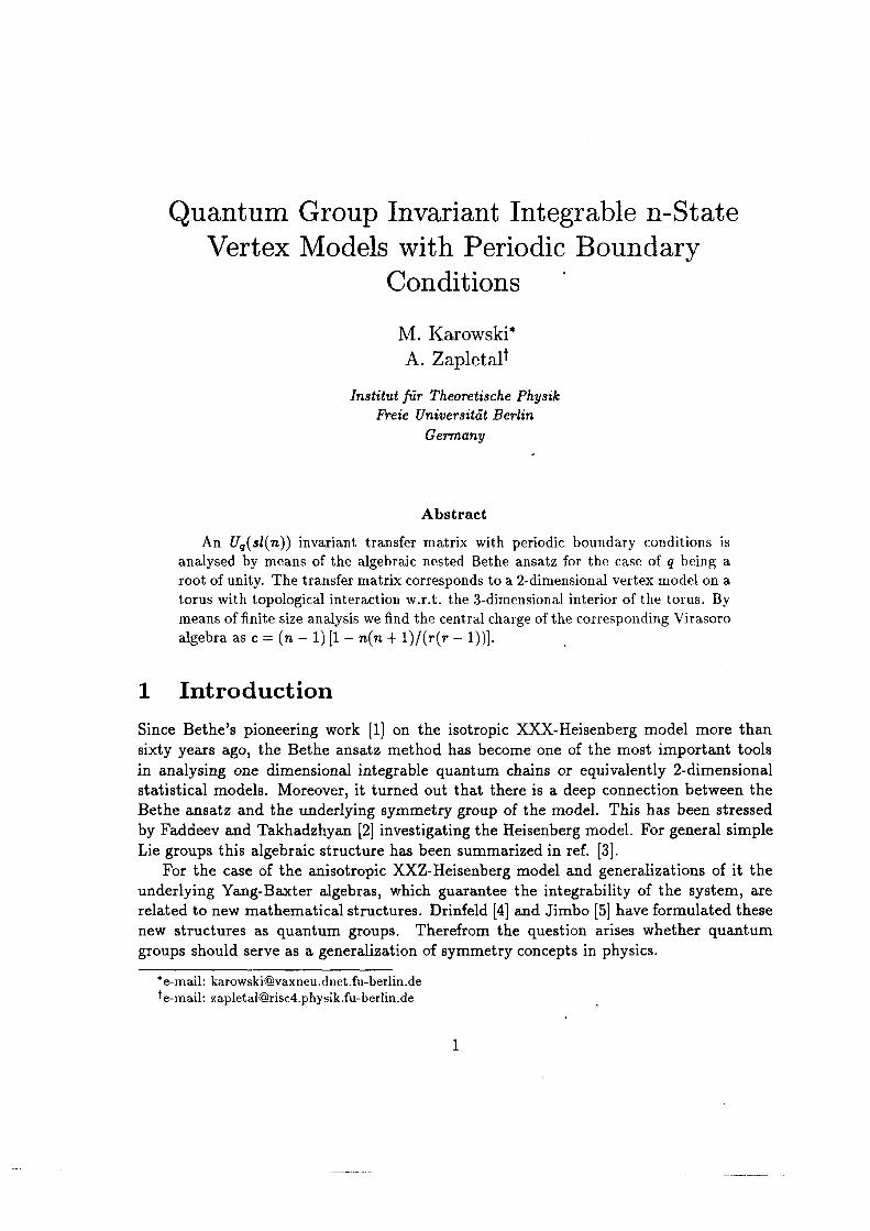
SFB 288 Preprint No. 97

A. ZapletalM. Karowski

Boundary Conditionsn—State Vertex Models with PeriodicQuantum Group Invariant Integrable

e-mail: zapletal@risc4.physik.fu—berlin.de OCR Output

*e-mail: karowski@vaxneu.dnet.fu-berlin.de

groups should serve as a generalization of symmetry concepts in physics.new structures as quantum groups. Therefrom the question arises whether quantumrelated to new mathematical structures. Drinfeld [4] and Jimbo [5] have formulated theseunderlying Yang-Baxter algebras, which guarantee the integrability of the system, are

For the case of the anisotropic XXZ-Heisenberg model and generalizations of it theLie groups this algebraic structure has been summarized in ref.by Faddeev and Takhadzhyan [2] investigating the Heisenberg model. For general simpleBethe ansatz and the underlying symmetry group of the model. This has been stressedstatistical models. Moreover, it turned out that there is a deep connection between thein analysing one dimensional integrable quantum chains or equivalently 2-dimensionalsixty years ago, the Bethe ansatz method has become one of the most important toolsSince Bethe’s pioneering work [1] on the isotropic XXX-Heisenberg model more than

1 Introduction

algebra as c : (n - 1)[1- n(n +1)/(r(r —means of finite size analysis we find the central charge of the corresponding Virasorotorus with topological interaction w.r.t. the 3—dimensional interior of the torus. Byroot of unity. The transfer matrix corresponds to a 2—dimensional vertex model on aanalysed by means of the algebraic nested Bethe ansatz for the case of q being a

An Uq(sl(n)) invariant transfer matrix with periodic boundary conditions is

Abstract

Germany

Freie Universiteit Berlin

Institut fdr Thecretische Physik

A. Zapletal

M. Karowski*

Conditions

Vertex Models with Periodic BoundaryQuantum Group Invariant Integrable n-State

However, the transfer matrix and the Hamiltonian may formally be extended to generic values of q. OCR Output

[17][18]. This will be explained in more details in Appendix A.

This model is similar to cr-models with Chern-Simons term or the WZNW—models

with the interior of the 3-manifold. However, this interaction is of topological nature.on the torus (or cylinder) but in addition there is a local interaction of the vertices

ii. The partition function (1) does not only describe a two dimensional vertex model

only for quantum groups where q is a root of unity.2

i. The invariants of 3-manifolds and therefore also these vertex models are defined

compared to the open one. We should add two remarks:lt turns out that it is much easier to solve the nested Bethe ansatz for the periodic case,planar graphs preserves the cyclic invariance of the models which is obvious from Fig. 1.quantum group invariant and belong to periodic boundary conditions. This transition toas well as for the Hamiltonian eq. (2) expressions in terms of planar graphs which areof invariants of planar graphs. As a result we obtain for the transfer matrix of eq. (1)the techniques as formulated in ref. [16] we can write the partition function (1) in termsof invariants of graphs in order to define the vertex model of eq. (1) and Fig. 1. Usingdefined for the quantum group case if q is equal to a root of unity. We use this definition

theories. The surfaces are considered as boundaries of 3-manifolds. These invariants areinvariants of graphs on Riemann surfaces using the language of topological quantum fieldFig. 1. In ref. [16] one of the authors of the present paper and Schrader gave a definition oftopology of the space, i.e. of the graph formed by the square lattice on the cylinder of

For models with periodic boundary conditions one has to take care of the nontrivialPS3, in eq. (3) which means open boundary conditions, as mentioned above.One possibility to get a quantum group invariant Hamiltonian is to cancel the projectorgroup invariant. Therefore one should also have a quantum group invariant projectorbreaks quantum group invariance, whereas the projectors given by eq. (5) are quantumThe traditional answer [6] which means symmetrizing the projectors as given by eq. (5)is defined or how the periodicity for the transfer matrix in eq. (1) has to be formulated.H]? are no longer symmetric with respect to i and k. Therefore it is not obvious how P3`}Due to the non-cocommutative coproduct of the quantum group Uq(sl(n)) the q—projectors

¤¢B

<5>Rt: = <q + me Z (q“i"`(“"°)E£‘2. s ESQ — EE.? ® ES?

M,,',,(C) for i > k (lattice point i on the left of lattice point k) (see also [10])quantum group case. The q-projectors can be written in terms of the unit matrices inexchange of i and k. Therefore it is obvious how to define This changes for theFor the case of q : 1 (S U (n)—symmetry) these projectors are symmetric under the

A1 ® A1 = 2A] EB A2. (4)

associated to the lattice points i and k according toThe Pi]? in eq. (2) project onto the representation A2 contained in the product A1 ® A1

1Sometimes these models are formulated such that the open boundary conditions are not quite obvious. OCR Output

(3)9=V,o‘*®·--®W‘*.

acting in the tensor product space

(2)‘H=P,§‘,§,,_,+...+P;=+P{,$,

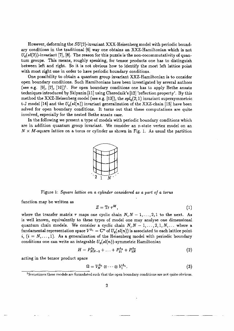
conditions one can write an integrable Uq(sl(n))-symmetric Hamiltonian1], = N,. . . ,1). As a generalization of the Heisenberg model with periodic boundaryfundamental representation space VM : C" of Uq(sl(n)) is associated to each lattice pointquantum chain models. We consider a cyclic chain N,N —- 1,.. .,2,1,N,... where ais well known, equivalently to these types of model one may analyse one dimensionalwhere the transfer matrix r maps one cyclic chain N ,N — 1,...,2, 1 to the next. As

(1)Z = Tr ·rM,function may be written as

Figure 1: Square lattice on a. cylinder considered as 0. part of a. torus

2 1 N ·

N >< M -square lattice on a torus or cylinder as shown in Fig. 1. As usual the partitionare in addition quantum group invariant. We consider an n—state vertex model on an

In the following we present a type of models with periodic boundary conditions whichinvolved, especially for the nested Bethe ansatz case.solved for open boundary conditions. It turns out that these computations are quitet-J model [14] and the Uq(l(n)) invariant generalization of the XXZ-chain [15] have beenmethod the XXZ-Heisenberg model (see e.g. [13]), the .splq(2, 1) invariant supersymmetrictechniques introduced by Sklyanin [11] using Cherednik’s [12] ’reflection property’. By this(see e.g. [9], [7], [10])1. For open boundary conditions one has to apply Bethe ansatzopen boundary conditions. Such Hamiltonians have been investigated by several authors

One possibility to obtain a quantum group invariant XXZ-Hamiltonian is to considerwith most right one in order to have periodic boundary conditions.between left and right. So it is not obvious how to identify the most left lattice pointtum groups. This means, roughly speaking, for tensor products one has to distinguishUq(sl(2))—invariant [7], The reason for this puzzle is the non-cocommutativity of quanary conditions in the traditional [6] way one obtains an XXZ-Hamiltonian which is not

However, deforming the S U (2)-invariant XXX-Heisenberg model with periodic bound

summation over internal lines is always assumed. OCR Outputwhere over the states of the internal lines is summed with the weights (14). In the following

(15)Z (In I andK) \/\ " _"Ql ,

with the Markov property

°‘ | - ,_·n+1—2a

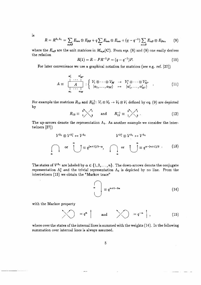
intertwiners (13) we obtain the ”Markov trace”representation A; and the trivial representation A0 is depicted by no line. From theThe states of VM are labeled by a E {1, 2, . . . ,12,}. The down-arrows denote the conjugate

,Or E q(n+1)/2-a m Um U or : a¤—(n+1)/2 . (13)

VA; ® VA1 (_+ VAOVA1 ® VA; H VA0

twiners [27])The up-arrows denote the representation A1. As another example we consider the inter

(12)R12 E 1and R;21 E A22\ 12 /1%

For example the matrices R12 and RQ: V1 ® lé—> VQ ® IQ defined by eq. (9) are depicted

Q1 QM

(I],...,aM) I-} Id1,...,(XM1)

V . . . V V' . . . V' I

¤i °i4·

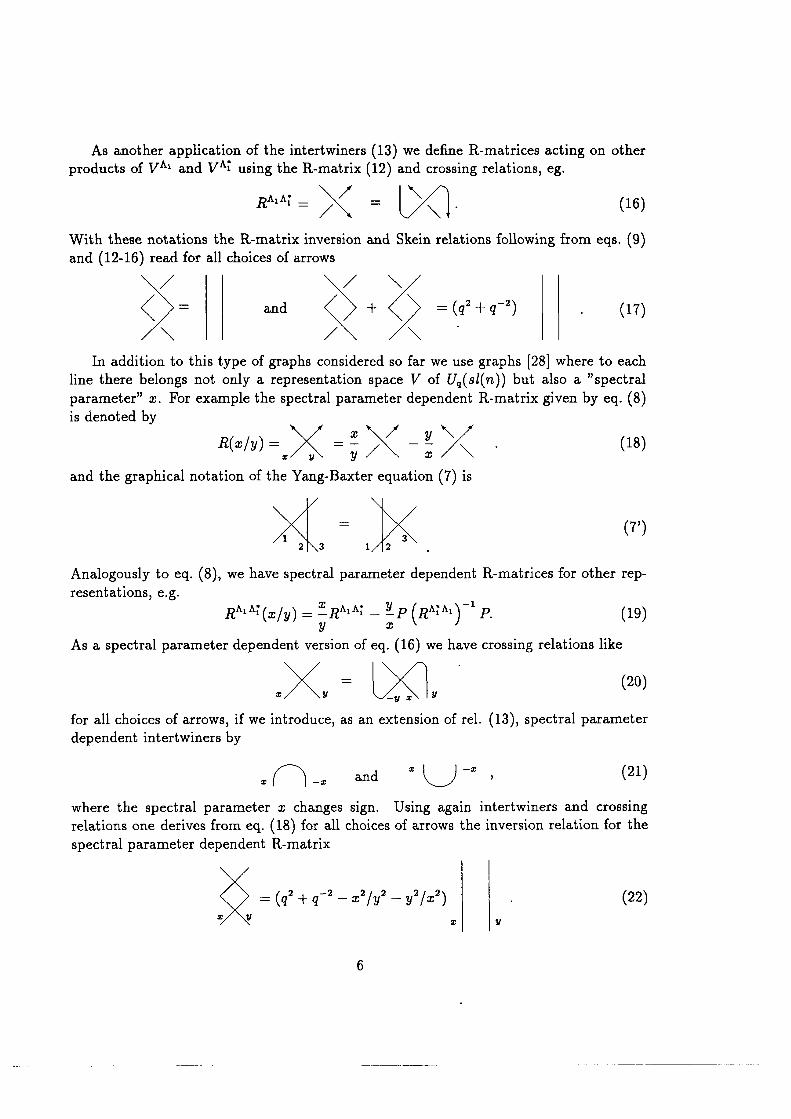
For later convenience we use a graphical notation for matrices (see e.g. ref. [27])

(10)R(1) :1-2-1>R·11> = (q——q”1)P.the relationwhere the Eup are the unit matrices in M,,',,(C). From eqs. and (9) one easily derives

¤>B¤·¢¤

R : RAIAI : E Eaa ® EBB `i' qi Eaa ® Eaa 'l' (q " q-1) E Euli ® EEG:1s

matrix acting on the tensor product of two fundamental representation spaces V®OCR OutputM VAIwhere P is the permutation operator P(<x ® B) : ,8 ® cx for cx,[3 E V. The constant R

(8)R(a:) = :vR — :z`1PR`1P

[26] can be written in terms of the ” constant R-matrix”parameter :1:;;, = :1:;/:1:;, and acts on IG ® W,. The ”trigonometric” Uq(sZ(n))-solution [25],act on the tensor product space IQ ® IQ ®l@. The matrix R,k(:v,k) depends on the spectral

R12($12)R13(x13)R23($23) I R23(x23)R13(m13)R12($12) (7)

Both sides of the Yang-Baxter equation

2 Yang-Baxter Equation

group invariance of the transfer matrix and the Hamiltonian.relation between Yang—Baxter algebra and quantum groups is used to prove the quantumof topological quantum field theory as developed in ref. [16]. Finally in Appendix B thepaper. We define the partition function of the vertex model on a torus using techniquescharge. In Appendix A we sketch the derivation of the transfer matrix investigated in thisWe perform the finite size analysis of the ground state energy and obtain the centralHamiltonian (2) for periodic boundary conditions is obtained from the transfer matrix.and obtain the Bethe ansatz equations. In Section 4 we show how the Uq(.sZ(·n.))-invarianteigenvalue equation of the transfer matrix by means of the algebraic nested Bethe ansatzand derive commutation rules from the Yang-Baxter relations. Using these we solve theperiodic boundary conditions of eq. (1) and Fig. 1. We define monodromy matricesrelation. In Section 3 we present the transfer matrix of the n—state vertex model withrelations as unitarity, crossing relations, Markov properties and Cherednik’s reflectionthis context to clarify the complicated algebraic structures.` We write some fundamentalsolution of the Yang-Baxter equation. We use a graphical notation which is useful in

This paper is organized as follows. In Section 2 we recall the trigonometric Uq(sl(n))conditions which use Baxter’s SOS-picture of the models see e.g. refs. [8], [22] and [24].method. For approaches to quantum group symmetric models with periodic boundaryobtained in [22] for the Uq(sl(·n,))-RSOS model using Baxter’s [23] corner transfer matrixwith that obtained from the extended coset construction for A,,-1 [20] [21]. It has also beenfor the Uq(sl(n))-model with q = exp(i1r/r), (r = n+ 2, n+ 3, . . This formula coincides

(6)n(·n, + 1) c-(n 1)1(T(T_1))charge of the Virasoro algebra of the corresponding conformal quantum field theoryenergy using the techniques developed in [19] and Therefrom we obtain the centralequations. As an application we calculate the finite size corrections of the ground stateHamiltonian by means of the algebraic nested Bethe ansatz and obtain the Bethe ansatzIn the present paper we solve the eigenvalue equation of the transfer matrix and the

¤N ¤¢z ¤1

mv |¤=¤ Im

(26) OCR Outputr£'(¢, {¤=¤}) =

¤£¤i

field theory developed in [16] that this transfer matrix is given by the graphUq(.sl(·n,)) invariant. We show in Appendix A using the techniques of topological quantummodel depicted in Fig. 1 corresponds to periodic boundary conditions and should be aninvariant transfer matrix. However, the transfer matrix of eq. (1) associated to the vertex"r|q=1 = 2;:1 T;. For the quantum group case this trace does not yield an Uq(sZ(n.))boundary conditions as the trace over the horizontal space of the monodromy matrix (24);For the rational case q = 1, one obtains an S U (n)-invariant transfer matrix for periodic

(25)Q:V,$*®...®I€A‘.

A1 is associated. We have omitted the indices which belong to the vertical spacewhere to all lines (the horizontal one and the vertical ones) the fundamental representation

¥¤N $2 $1 G

° (24)Tf(=¤,{¤¤s}) ¤= [R(¤=~/=¤)-·-R(m¤/$)R($1/xl];Z \—[»<]_]_¥spectral parameter dependent R-matrices as followsvertex model of eq. (1). As usual [2] we introduce a monodromy matrix as a product ofIn order to solve the eigenvalue equation for the Hamiltonian (2) we introduce the n-state

3 The algebraic nested Bethe ansatz

Bethe ansatz.

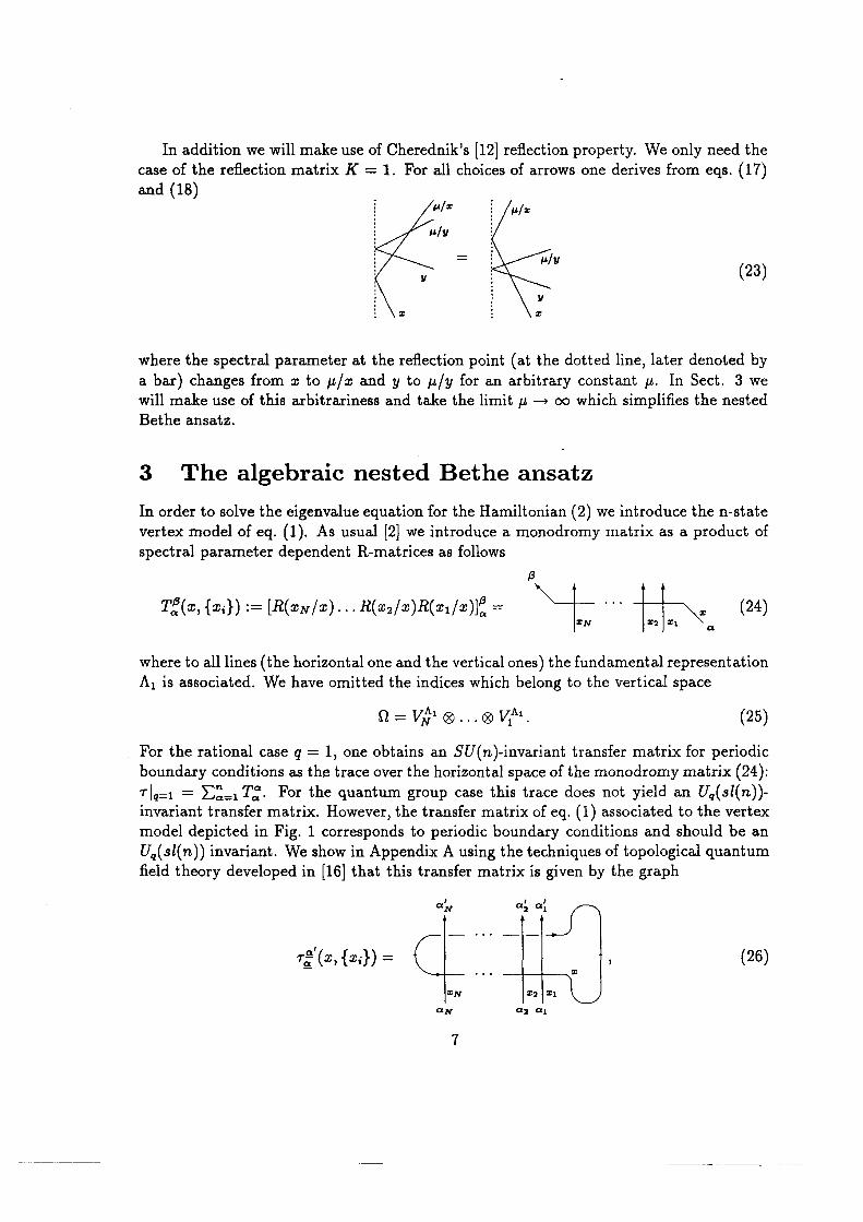
will make use of this arbitrariness and take the limit p. —> oo which simplifies the nesteda bar) changes from 1: to p/ :1: and y to p,/y for an arbitrary constant p. In Sect. 3 wewhere the spectral parameter at the reflection point (at the dotted line, later denoted by

(23)/ " U

u/v

, U #/= ; /»/¤=and (18)case of the reflection matrix K = 1. For all choices of arrows one derives from eqs. (17)

In addition we will make use of Cherednik’s [12] reflection property. We only need the

¤ 1 1 y

(22) OCR Output= (q2 + q‘” - =¤’/212 — 212/$2)ii ’”spectral parameter dependent R—matrixrelations one derives from eq. (18) for all choices of arrows the inversion relation for thewhere the spectral parameter :1: changes sign. Using again intertwiners and crossing

x I I _mx m _x and (21)

dependent intertwiners byfor all choices of arrows, if we introduce, as an extension of rel. (13), spectral parameter

<2¤>>< = OO I U _y 1 UAs a spectral parameter dependent version of eq. (16) we have crossing relations like

19 <>RM? : -RM? - P 12AiM "1¤. <-/y> )?”Qy m (resentations, e.g.Analogously to eq. (8), we have spectral parameter dependent R-matrices for other rep

<7>><( I 2 3 1 2and the graphical notation of the Yang-Baxter equation (7) is

R<-/y> -- — <18>IU / y V $>§ Q X E \is denoted byparameter" rc. For example the spectral parameter dependent R—matrix given by eq. (8)line there belongs not only a representation space V of Uq(sl(n)) but also a "spectral

In addition to this type of graphs considered so far we use graphs [28] where to each

\ / \/ \ and K + ) =(¢12 + ¢1`2)

and (12-16) read for all choices of arrowsWith these notations the R—matrix inversion and Skein relations following from eqs. (9)

. \_ / (16)U / \ RM Z \- 1products of VAI and VA; using the R-matrix (12) and crossing relations, eg.

As another application of the intertwiners (13) we define R-matrices acting on other

C°'(=¤, {=¤¤})*I’

0, gé·1>OCR OutputB¤(=¤» {<¤e})‘I’

7?S(<¤, {¢¢})‘I’ <36>6E‘1g<I>

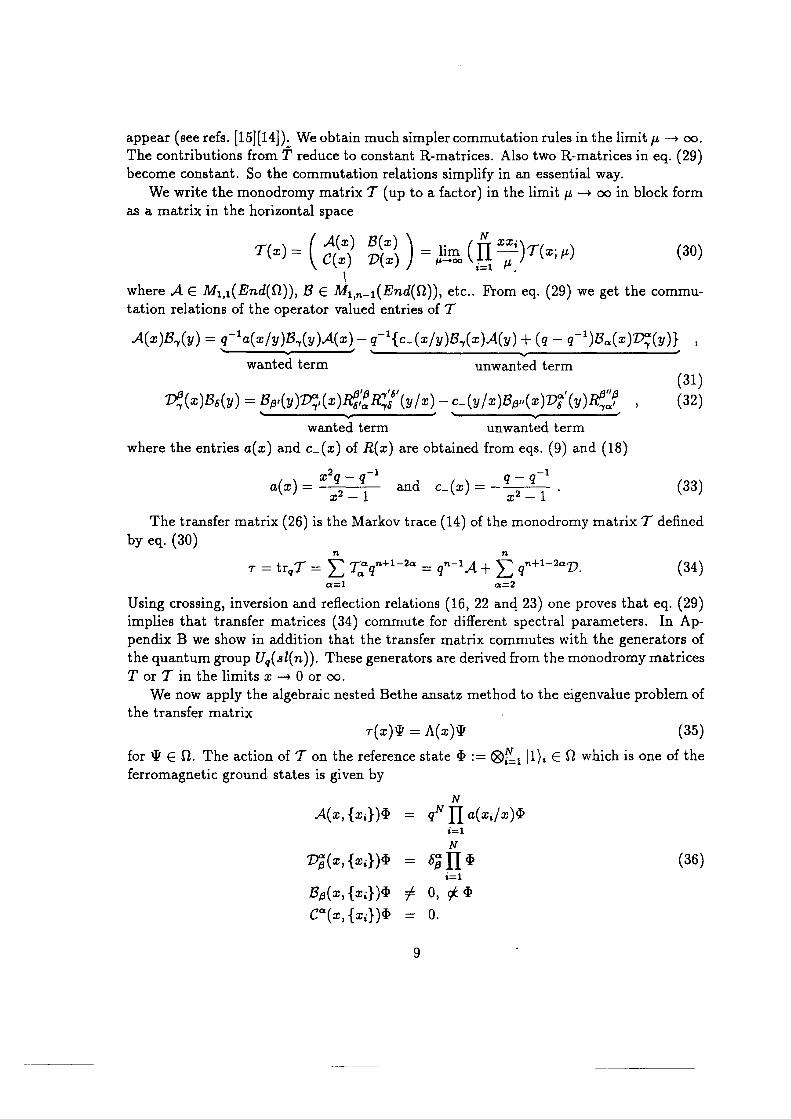
A(a:, {;¤,})¢ qNl;]%a(:z:;/:1:)<I>

ferromagnetic ground states is given byfor \I! E D. The action of T on the reference state Q z: @@1 |1)i 6 S`2 which is one of the

v·(a:)\I/ : A(x)\I' (35)the transfer matrix

We now apply the algebraic nested Bethe ansatz method to the eigenvalue problem of

T or T in the limits :1: —-> 0 or oo.the quantum group Uq(sl(n)). These generators are derived from the monodromy matricespendix B we show in addition that the transfer matrix commutes with the generators ofimplies that transfer matrices (34) commute for different spectral parameters. In ApUsing crossing, inversion and reflection relations (16, 22 and 23) one proves that eq. (29)

a=1 ¤=2

7. Z trqT : Z Ygaqn-{-1—2a : qn—1A + Si qn.-§-1-2uD.

by eq. (30)The transfer matrix (26) is the Markov trace (I4) of the monodromy matrix T defined

—•lG($) I and C_(fD)1' ···;q —<1‘1=¤”q — q'

where the entries a(a:) and c-(a:) of R(z:) are obtained from eqs. (9) and (18)

wanted term unwanted term

BB 6[ HUB D$(=¤)B6(3/) = B¤*(y)D$»($)R6laRZa (31/w) —¢—(y/¤¤)B¤~(¤>)D? (y)R,.,# » (32)II!

unwanted termW&11t€d t€fH1

A(=¤)B~(y) = q`1¤(=¤/y)B7(y)A(¤=)_—<1`1{¢-(¤>/y)B~(<¤)A(y) + (q - <1`*)B¤(¤¤)D$(y)} »

tation relations of the operator valued entries of Twhere A G M1,1(E·n.d(S2)), B G ML,,-1(End(Q)), etc.. From eq. (29) we get the commu

__ mi — <3<>>.A(:1:) B(:1:) _ . N mm; _ ( qw) W) - grngo ( ?)¢<¤», »>as a matrix in the horizontal space

We write the monodromy matrix T (up to a factor) in the limit p —+ oo in block formbecome constant. So the commutation relations simplify in an essential way.The contributions from T reduce to constant R-matrices. Also two R·matrices in eq. (29)appear (scc refs. [15][14]). We obtain much simpler commutation rules in the limit p ·—> oo.

complicated. The usual decomposition into ”wanted" and ”unwanted" terms does not OCR OutputCompared to the case of the monodromy matrix T these commutation relations are more

IN *:1:;*:1:1 my *:n;|.:c;_

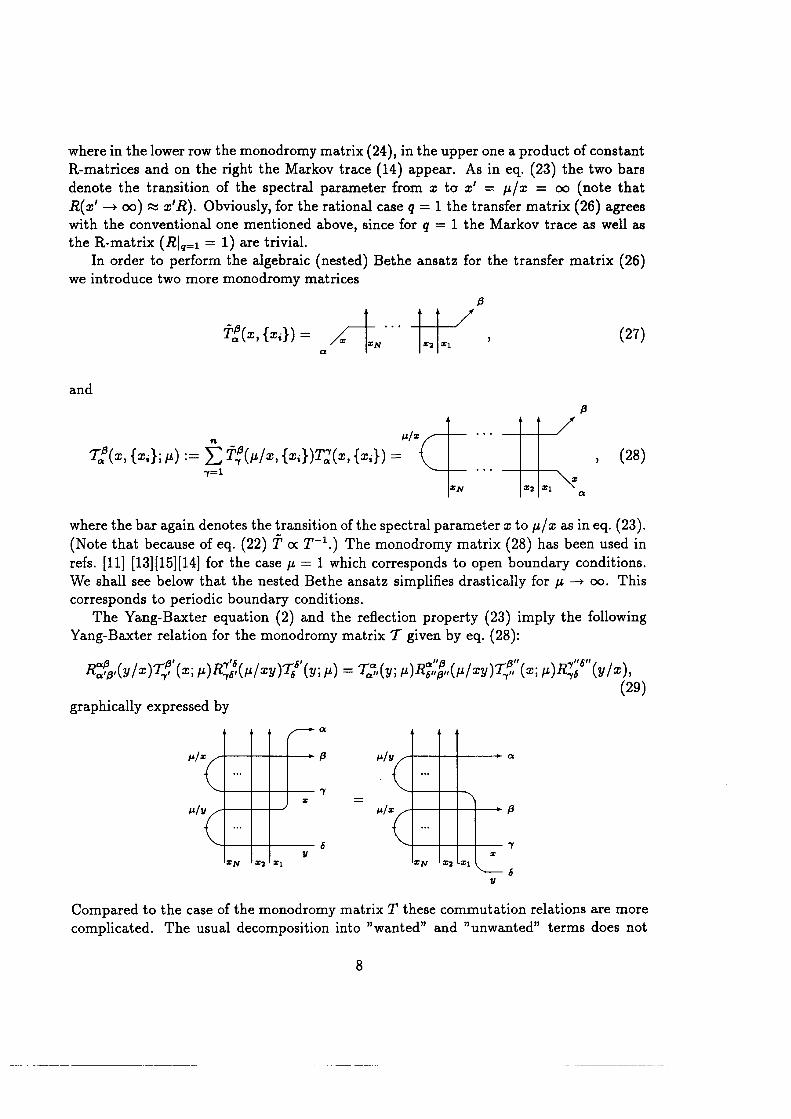
#/11 M/=I Z

M/¤= B 14/v

graphically expressed by, 29

*’*’ ’""’

R:F.,<y/m>z?<¤»; »»>R1Z<»/$y>v:.<y. in = ccmy; t>Rz,i£~<»/my>v;?,<¤»; »>R;Z<y/mg.Yang-Baxter relation for the monodromy matrix T given by eq. (28):

The Yang—Baxter equation (2) and the reflection property (23) imply the followingcorresponds to periodic boundary conditions.We shall see below that the nested Bethe ansatz simplifies drastically for ;1. -—> oo. Thisrefs. [11] [13][15][14] for the case p : 1 which corresponds to open boundary conditions.(Note that because of eq. (22) T oc T`1.) The monodromy matrix (28) has been used inwhere the bar again denotes the transition of the spectral parameter :1: to ;i/ 1: as in eq. (23).

ZN II; I I1 \ a

131

» (28)~ 7Z.°(¤¤.{¤¤e}; M) == Z T$()»/¤¤.{<¤¢})T2(¤¤,{¤¤i}) =u/=

and

T.,(¤=» {=¤·}) /, mQ LN ln I,

we introduce two more monodromy matricesIn order to perform the algebraic (nested) Bethe ansatz for the transfer matrix (26)

the R-matrix (R],,=1 = 1) are trivial.with the conventional one mentioned above, since for q = 1 the Markov trace as well asR(x' -> oo) z :z:'R). Obviously, for the rational case q = 1 the transfer matrix (26) agreesdenote the transition of the spectral parameter from 2; to x' = p/sn = oo (note thatR-matrices and on the right the Markov trace (14) appear. As in eq. (23) the two barswhere in the lower row the monodromy matrix (24), in the upper one a product of constant

11 OCR Output

pendix A relies on methods of topological quantum field theory and here we can give(45) describe models with periodic boundary conditions. However, the derivation in Ap

on a torus. Therefrom it it obvious that the transfer matrix as well as the Hamiltonian

In Appendix A we derive the transfer matrix ·r from a cyclic invariant vertex modelunity operator the Hamiltonian of eq. (2) as a sum of projectors PATherefore we get (with const. = -1/2(q — q“‘)/(q + q‘1)) up to terms proportional to the

(47)PR : qP2A* - q·*1>A=.projectors has been usedwhere the following decomposition (4) of the R-matrix [29] and the completeness of the

q_q- _ A R1m—Rx=———PR+R1P=——-—1-2P’, 46 ()()-4( ) _1( ) ( )

q ‘i' qid 1 ) ( dmx:1 q_q

The dotted crossings mean the matrix (see eq.

N 2 1N {+1 { 1

::3;:],dm

(45).. H = const. ———ln ·r(2:,{a:;}| = const. N *1 .. E I X - .. J · __ _]The Hamiltonian (2) may be obtained from the transfer matrix (26) as follows

4 The Hamiltonian and finite size analysis

H,,_k, (k : 1,. . . ,n — 1) of the Bethe ansatz vector \I¤ (see Appendix B).where 1;,,-;, = rk+1 —— 2rk + 1-;,-1 are the eigenvalues of the Uq(sl(n)) Cartan elements

—--——-- , k : 1 ,..., -1 , 44 {E1 sinh (gg:) _ ,%:-1)) ( ” ) ( )€f’ ) lLM-1 sinh (0<’=> - 0‘14 iq

{F1 sinh (Hg:— aff— icy) ;,=1 sinh (Og:— 0g— iq___ ._. ____2 +,1 k q 7\— ) ) H ) °+1)$11111 (ay;) - aff) +17) Tsinh (ai}? - 0$f+‘)

system of Bethe ansatz equations:analytical function in :1:. Writing xsf= exp Gif) and q = exp i7 we obtain the coupled)parameter :1: approaches one of the Bethe ansatz parameters wgk), because r(a:) is ancan be obtained from the property that A(m) must have finite values when the spectralThe Bethe ansatz equations are equivalent to the vanishing of all unwanted terms. They

j=1{:1

H (/)H (/j, (,, )()__ »\1,(:¤)= q"·····*+*~·*~—1 amz$'°“1)am§'°’m14 :1 ...11. 43Tu-1

where

10

k=1

(42) OCR OutputMw) = Z »\k(¢)»

eq. (35) is solved and the eigenvalue A(a:) consists of the wanted coefficients AkIn case all unwanted terms cancel, the eigenvalue equation of the transfer matrix

") n_1)·r, ro = O, mg= :1:;, IB$= :2,.by the number of the corresponding Bethe ansatz level, in particular 1*,, = N, ·r,,-1 =equation (35). In the following, all operators, Bethe ansatz parameters etc. will be labeledThus iterating the procedure described above from level n to 1 we solve the eigenvalueis fulfilled. This problem agrees with the original one (35) where n, is replaced by ·n. —- 1.

+*1/ : A\I! (41)A A A

eigenvalue equationThe first term (wanted term) on the right hand side of eq. (39) is proportional to \If if the

c¢=1

6; Z Z »]·Qxqn+1-2a'n—1

where we have introduced an Uq(sI(n — 1)) monodromy matrix T and a transfer matrix

e1...c,.=2

(39)1= H Bp,(5;1). . .Bp,(é,){q‘1+\¤}<I> + uwt,

><¢1”+1`2°‘R?§ZI"RZZfl€,(fr/=¤) - - -R€fZ. R12€‘(¤?»/¤¤)‘i’°""°' l1>$:<1> + uwt(Z ¤=2q...c,·=2

= E B¤r(§=1)·· -B¤.(¤?>r)

0::2 ¤¢=2

E q”+1_2°"D:(:n)\If = Z q"+1`2°"D:(:1;)E B€,(:i1)...B€,(:?:,)‘I!°1"'°’ }<1>{ q...e,.:.-2and

{:1 j=1

(38)= qN"+”"1 H a.(:c/:2:;) H a(:z:j/m)\I! + uwt

q””1A(:z:)\I! = q”`1A(x)Z B€,(£1)...B,,(:i,)\1#°*""’ ) Q{ E]_...€,.:2terms in eqs. (31) and (32) together with (36) yieldeq. (35) we commute them through all B ’s to the right and apply them to Q. The wantedand admitting only states |2), . . . , To compute the action of A and 'D in the eigenvaluewhere \I! is an element of the reduced quantum space Q representing a chain of length r

(37)»1¤({s,}) ;: Z Bc,(:i1)...B,,(5c,)\1#°‘"‘°’ } <1> ,( q...c,-:2on Q

We construct a Bethe ansatz vector by repeated action (r times) of creation operators B

13 OCR Output

matrix is dominated by the term A,,(z). The following calculation may be easily performedFor large lattice size N and :1: z 1 the eigenvalue A(:1:) (see eq. (42)) of the transfer

sinh(vr — q)z sinh nqa: sinh qa: ’——- = (1 P(1))** k < I.»-—- -1 sinh rm: sinh(n — k)q:v sinh lqa: —· I ,

is given by the symmetric matrixthe matrix (1 — p' —<I>')k; appearing in the integral equation (58). Its Fourier transformof Bethe ansatz holes as well as finite size corrections. For this purpose one has to invertpk(u) = 21r EE; 6(u —·u.$) may be written in terms of ¢p,,(·u.), which describes the density’°)The convolution is defined by (f*g)(·u.) : fdu’/(21r)f(u —u')g(u'). The densities of rootswhere the matrices p' and <I>’ are given by pi, : 2,,6% 6p; p' and QL, = 5k;<I*', respectively.

(58)ZL = Pk + sm. = N6k,n-ip' + Z(p’ + <I>')kz * pz

we find the following matrix equationlooking for real roots of the Bethe ansatz equations (54). Taking the derivative of eq. (55)we want to analyse the finite size behaviour of the ground state eigen value, we are onlyThe eqs. (55-57) may be generalized to include string solutions as well. However, since

(57)- ‘ h -. - ~ P'(¤¤) = and ‘I>'(¤:) = 1- 2cosh qa; p’(:1:).

The Fourier transforms f == f du/(2vr)e“‘”f of the derivatives p' and <I`·' are

sinh %(·u. + iq) sinh %(*u, - 2iq)(56)6,,,0,) : sinh %(·u, — iq) and eign) Z sinh %(u + 2iq)·

to one. The functions p(u) and <I>(u) are given bywhere Lk = {Z : k :1; 1; O < I < 71.}. The inhomogeneities :1:, have been taken to be equal

IGL1. {

MZkiu) Z N6k.¤—1p(u) + Z Zpiu ` uio) ‘l` E @(*4 ‘ US) `l'_(2 + 7/k)'Y> (55)

k) k)where we have introduced the “rapidities” ul: iq(k — 71.)+ 29Eand the phase functions

_] :1,...,1*;,, k=1,...,n,—1,, (54)

k)zk(u§¤=>) : 2,rI§k>l {i6 (Z + $1) F1l>·v»(·<><>)/27F»¤’¤»(<><>)/27Fl

Taking the logarithm of the Bethe ansatz equation (44) we obtainthe finite size behaviour of Amu belonging to the antiferromagnetic ground state.algebra. Using the techniques developed in [19] the central charge can be calculated fromwhere f is the free energy per site and c is the central charge of the corresponding Virasoro

12

(53) OCR OutputAmn z exp( — Nf + c, (N —> oo)%%)

invariance implies for the maximal eigenvalue Amu of the transfer matrixlimit conformal invariance of the system is expected. As shown by Cardy [30] conformalinvestigate the finite size behaviour of the ground state energy. In the thermodynamic

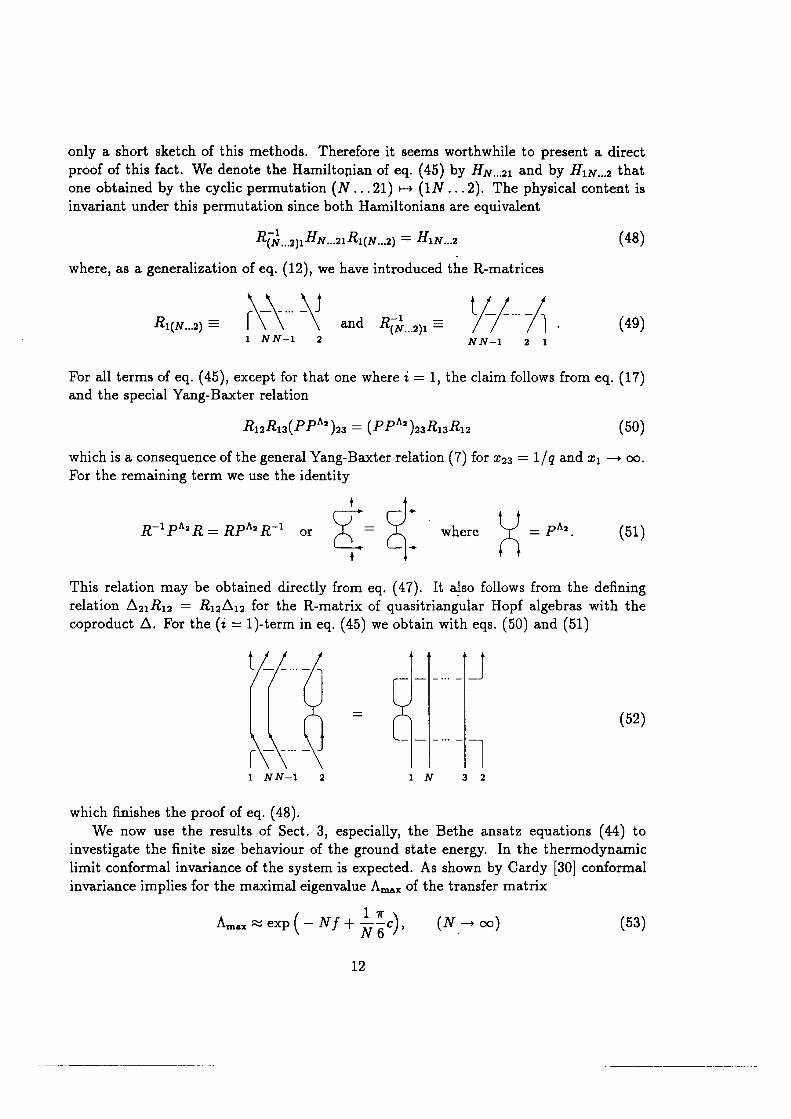
We now use the results of Sect. 3, especially, the Bethe ansatz equations (44) towhich finishes the proof of eq. (48).

1 N s 21 NN-1 2

coproduct A. For the (i : 1)-term in eq. (45) we obtain with eqs. (50) and (51)relation AZIRI2 : RNA]; for the R-matrix of quasitriangular Hopf algebras with theThis relation may be obtained directly from eq. (47). It also follows from the defining

+

()R`1PA’R = RPM R`1 or I where HJ = PA'. 51% E ¢

For the remaining term we use the identitywhich is a consequence of the general Yang-Baxter relation (7) for :1:23 : 1 / q and :1:1 —> oo.

(50)R12R1a(PPA° )23 = (PPA°)2sR1sR12

and the special Yang—Ba.xter relationFor all terms of eq. (45), except for that one where i : 1, the claim follows from eq. (17)

NN-1 2 11 N N -1 2

(49)R1(N...2) E \ and R?]\l___2)1 E %lwhere, as a generalization of eq. (12), we have introduced the R-matrices

Q,___2)11v...211(1v...2) 1N...2 (48)RiHR= H

invariant under this permutation since both Hamiltonians are equivalentone obtained by the cyclic permutation (N ...21) v——> (1N ...2). The physical content isproof of this fact. We denote the Hamiltonian of eq. (45) by H N___21 and by H1N___2 thatonly a short sketch of this methods. Therefore it seems worthwhile to present a direct

15 OCR Output

set is a colouring of all 1-simplexes of X and J a colouring of all plaquettes obtainedthe colours are the irreducible representations = 0,1/2,1,.. . ,1*/ 2 — 1) of S lq(2). Thea triangulation BX of OM. The sum of eq. (65) runs over all set of colours and J_, whereThe right hand side is defined in terms of a triangulation X of the 3—manifold M inducing

.11;}.

(65)Z(M» @(2)) = Z W(;,I)(X, @(2))

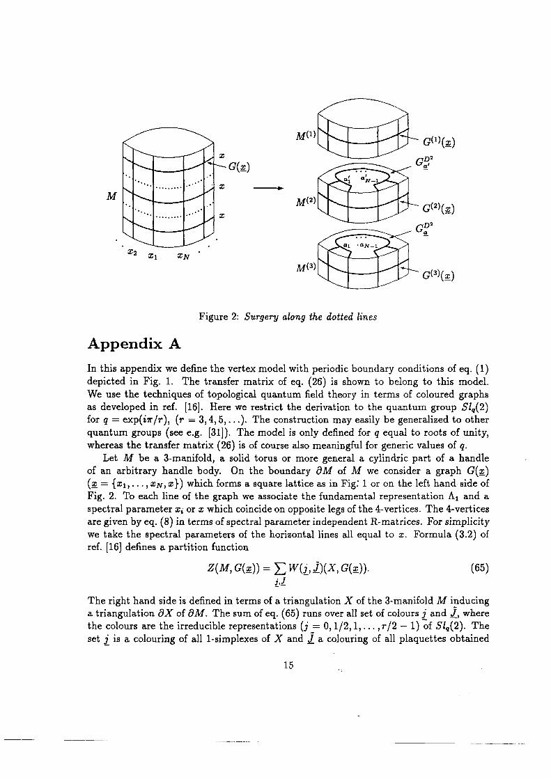
ref. [16] defines a partition functionwe take the spectral parameters of the horizontal lines all equal to :1:. Formula (3.2) ofare given by eq. (8) in terms of spectral parameter independent R-matrices. For simplicityspectral parameter m, or sz: which coincide on opposite legs of the 4-vertices. The 4-verticesFig. 2. To each line of the graph we associate the fundamental representation A1 and a(g = {2:1, . . . , :1:N, which forms a square lattice as in Figf 1 or on the left hand side ofof an arbitrary handle body. On the boundary BM of M we consider a graph G(g)

Let M be a 3-manifold, a solid torus or more general a cylindric part of a handlewhereas the transfer matrix (26) is of course also meaningful for generic values of q.quantum groups (see e.g. [31]). The model is only defined for q equal to roots of unity,for q = exp(i1r/r), (r = 3,4,5,. . The construction may easily be generalized to otheras developed in ref. [16]. Here we restrict the derivation to the quantum group Slq(2)We use the techniques of topological quantum field theory in terms of coloured graphsdepicted in Fig. 1. The transfer matrix of eq. (26) is shown to belong to this model.In this appendix we define the vertex model with periodic boundary conditions of eq. (1)

Appendix A

Figure 2: Surgery along the dotted lines

G(3)(§)M(3)

$2 :1:1 :1:N01 ·¤N-1

G<2><s>(2) M

37 ——-—>

°si i~r—ime G5

GU)M (1)

14 OCR Output

. positivity, unitarity e.t.c., these will be investigated elsewhere.to obtain higher representations. In this paper we have not mentioned questions abouttransform trivially under the quantum group. We will analyse more general situationsFor the case of trivial topology of the interior of a torus there exist only states whichogy of the interior of the 3-manifold, on whose boundary the vertex model is defined.Appendix A the quantum group representation of the states are determined by the topoltion spectrum, also for other models related to other quantum groups. As mentioned in

In a forthcoming paper we will in addition to the ground· state also discuss the excitathe extended coset algebras constructions of ref. [20] for general simply laced Lie algebras.respectively). This formula coincides (see [21]) with the formula for the central charges ofwhere g is the dual Coxeter number (for A;,D;,E6,E7,E8: g = l+ 1,2l — 2,l2,18,30,

_ c—l (64)+ _ hr/r _ , q-e , r-g+2,g—|—3,...,(1 T(T_1)One easily can calculate the sums and finds

(63)' 12 (6,- - ——A;.1). gi ’ r(r - 1) ’

for general simply laced q-Lie algebras (A, D, E) of rank l to beis just j times the Cartan matrix A (see e.g. We expect the central charge of modelstransfer matrix method for the A,,-1 RSOS-models. Note that the matrix (1 — p' —<I>’)(0)

This formula has previously been obtained in ref. [22] by means of Baxters [23] corner

(62)(·n—1)1— , q=e‘”/', r·=n+2,n+3,1()

Taking eq. (59) at :1: = 0 we can perform the sums and obtain

k,l:1 T(61)C = Z (6M · 7 (1-P'- ‘I")n (0)

**-1 12 ~ -1

ref. [19] we find with eq. (53) for the central charge of the Virasoro algebra the formulawhere fw is the free energy per site in the thermodynamic limit. Using the techniques of

= —Nf°° + , _ _ Z zp(u — 20) (1 — p' —¢I>')”i,’k(u — u') qpk(u) — zsy, (60)/ — / —— 21r 21r ,::1du du' "`1

_ _ log /\,,(0,~y) = Nloga — - zp(u — 20) p,,-1(·u) — 1.7du. f 51r

(56) and (58) we obtainalso for excitations but for simplicity we restrict here to the ground state. From eqs. (43),

17

(73) OCR OutputL+T(=¤) = H T(y) r(¤=)·N *2*1 gg, (gy) £=1 *Quantum group invariance of the transfer matrix is now shown by applying Li, e.g.the elements E,,F} and q*H‘. Ais an algebra homomorphism U —+ U ®® U./2w)These commutation rules are equivalent [33] [32] to the defining relations of Uq(.sl(·n.)) for

(72)** *=RL;L;Z L;L§R and 1zL;L; Z L;L;R.

matrices implies the commutation rulesThe H; = W] — W;+1 are the Cartan elements. The Yang-Baxter equation for monodromy

lth'Z1

P2 = A(”’(f.)=Z1®...®1®_f._®q’“®...®q"*,

1111[:1

E, Z A(”)(e,) Z 24;**** ®...®q"‘* ®_e,’®1 @...03) 1,

fundamental representation A1 of U = Uq(sI(n)) associated to each lattice site:fold coproduct of the generating elements q‘*"‘*/2, e, and fi, : 1,. . .,77. — 1) in thein eq. (9) (see also ref. [32]). The entries E,,H and q*W‘ of L* are given by the NThese forms of the matrices L+ and L" follow from the triangular form of the R-matrix

0 10 q·W·· I \ 0` · 0 —GFn-1

1-,0(70)L- Z lim z~T($) Z

' . ° 1—W 0 q °

q·W· 0 0 \{1 Zazq

=•= aE,,-1 1 / \ O 0 qW"

(69)L+ I ‘”-NT("’) I I QE] 1 w 0 q 2

1 0 0\/qW= 0 0

by eq. (24)We define the matrices Li by the limits :1: to oo or O of the monodromy matrix T given

Appendix B

values of q.whereas the transfer matrices *r§(:z:, and ·r,§'(:z:, are also meaningful for generic

'

Z(M(2),G(2)(_:1;) U G5U Ggh) of eq. (68) is defined only for q equal to roots of unity,:

16 OCR Output

paper we will discuss this more general situation. We stress again that the invariantobtained for nontrivial topology of the interior of the 3-manifold M. In a forthcomingbasis, projected to the sector of total spin J = O. We remark that the other sectors areequivalent to the transfer matrix T£’((lI, given by eq. (26), represented in the tensorThe transfer matrix ·r§'(:z:, given by eq. (68) is represented in the path basis. It iswhere the 3-vertices are given by intertwiners V“‘® V1/2 —+ V“*+* as explained in ref. [16].

xy [xg [::1

» (68)Z(M» G(;¤.) U GBU GF) = T§(¤=» {¤¤¤}) E(°)(2); `'

with the interior of the 3-manifold disappears andG(2)(g) LJ GBU GEis planar. In ref. [16] is shown that for planar graphs the interaction

: N

(2M ) is topological equivalent to the ball D3 with boundary OD3 = S2 and the graphthe following also holds, if M and M stay connected after the surgery. The piece(1) (3)The (finite) summation is over all colourings g and gf of the canonical graphs. Note thatOn the bottoms of M and M there are the mirror graphs Ggand Gfi , respectively.(1) (2) h z

where GE: as depicted in Fig. 2, the canonical graph of the disc D2, is defined in ref. [16].

<¤>"<3><=*>Xz(M, cw;) U G5? U Gy) z(M, G(§) U GF). (67)

Z(M,G(;)) = Zwfwf z(M<1>,o<1>(§) U Gg")

[16] we havealong two discs D2 as shown in Fig. 2. Applying the general surgery formula (7.3) of ref.

(66)G(s) = G(@) U G(&) U G(3)(@)(1)(°)

M = M6) Um M") Um M(")

ary as followsWe decompose M and the square lattice represented by the graph G(g) on the bound

l17ll18l·Thus this model is similar to 0-models with Chern-Simons term or the WZNW-models

with the interior of the 3-manifold M. However, this interaction is of topological nature.model on the torus or cylinder but in addition there is a local interaction of the vertices

Note that the partition function (65) does not only describes a two dimensional vertexwith a vertex model on its boundary OM given by the graphtriangulation X of M and therefore defines an invariant of the 3-manifold M equippedR-matrices. Moreover it is shown that the r.h.s. of eq. (65) does not depend on thehow the weights W(j,J_)(X, are given in terms of q-dimensions, 6j-symbols andfrom the graph OX U G(~g), where OX is the dual graph of BX. In ref. [16] it is explained

19 OCR Output

Groups and Lie Algebras’, Algebra and Analysis (Russian) 1.1 (1989) 118-206.L.D., Faddeev, N.Yu. Reshetikhin and L.A.Ta.kha.dzhyan, ’Quantization of Lie[33]

J. Ding and 1.B. Frenkel Commun. Math. Phys. 156 (1993) 277.[32]

Graphs for Quantum Groups’, SF B 288-preprint No. 78 (1993).A. Beliakova and B. Durhuus, ’Topological Quantum Field Theory and lnvariants of[31]

J.L. Cardy, Nucl. Phys. B270 (1986) 186.[30]

et al. (World Scientific, 1989)p. 111.M. Jimbo, in Braid Group, Knot Theory and Statistical Mechanics, ed. C.N. Yang[29]

M. Karowski and H.J. Thun, Nucl. Phys. B130(1977) 295.[28]

(Part I)’, LOMI E—4-87 (1988).N.Yu. Reshetikhin, ’Quantized Univ. Envel. Algebras, YBE and Invariants of Links[27]

[26] M. Jimbo, Lett. Math. Ph. 11 (1986) 247.

O. Babelon, H.J. de Vega. and C.M. Viallet, Nucl. Phys. B190 (1981) 542.[25]

V.V. Bazhanov and N.Yu. Reshetikhin, Int. Journ. Mod. Phys. A1 (1989) 115.[24]

don, New York (1982).R.J Baxter, ’Exactly Solved Models in Statistical Mechanics’, Academic Press, Lon[23]

M. Jimbo, T. Miwa and M. Okado, Nucl. Phys. B300 [FS22] (1988) 74.[22]

(Academic Press, 1989).Bouwknegt, P. in Conformal Invariance and String Theory, p. 115, ed. P. Dita et al.{21]

P. Goddard, A. Kent and D. Olive, Phys. Lett. B152 (1985) 88.[20]

M. Karowski, Nucl. Phys. B300 (1988) 473.[19]

E. Witten, Commun. Math. Phys. 92 (1984) 455.[18]

18

[17] S.P. Novikov, Usp. Mat. Nauk. 37 (1982).

[16] M. Karowski and R. Schrader, Commun. Math. Phys. 151 (1993) 335.

Spin Chains’, LPTHE-PAR 93/38 (1993).[15] H.J. de Vega and A. Gonzalez-Ruiz, ’Exact Solution of the S Uq(n) Invariant Quantum

[14] A. Férster and M. Karowski, Nucl. Phys. B408 (1993) 512.

[13] C. Destri and H.J. de Vega, Nucl. Phys B361 (1992) 361.

[12] I. Cherednik, Theor. Mat. Fiz. 61 (1984) 35.

[11] E.K. Sklyanin, J. Phys. A21 (1988) 2375.

[10] P.P. Martin and V. Rittenberg, Int. J. Phys. A7, Suppl. 1B (1992) 707.

A20 (1987) 6397.F.C. Alcaraz, M.N. Barber, M.T. Batchelor, R.Baxter and G.R.W. Quispel, J. Phys.[9]

[8] M. Karowski, in Quantum Groups, Lecture Notes in Physics, Springer (1990) 183.

V. Pasquier and H. Saleur, Nucl. Phys. B330 (1990) 523.[7]

E.H. Lieb, Phys. Rev. 162 (1967) 162.C.N. Yang and C.P. Yang, Phys. Rev. 150 (1966) 321;[6]

[5] M. Jimbo, Lett. Math. Phys. 10 (1985) 63.

[4] V.G. Drinfeld, Proc. Int. Cong. Math., Berkeley (1986).

[3] E. Ogievetsky and P. Wiegmann, Phys. Lett. 168B (1986) 360.

134.

One-Dimensional Isotropic Heisenberg Model’, Zap. Nauch. Semin. LOMI 109 (1981)L.D. Faddeev and L.A. Takhadzhyan, ’Spectrum and Scattering of Excitations in the[2]

[1] H.A. Bethe, Z. Physik. 71 (1931) 205.

References

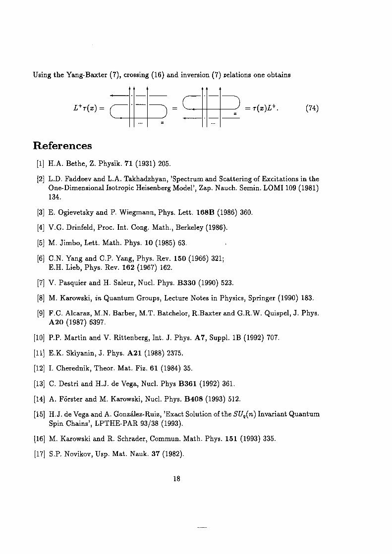
(74)L+·r(:v) = = ·r(z)L+

Using the Yang-Baxter (7), crossing (16) and inversion (7) relations one obtains