Master Project

Seminar Report: Semantic Data-analysisand Automated Decision Support Systems

written by

Fabian Karl

Fakultät für Mathematik, Informatik und NaturwissenschaftenFachbereich InformatikArbeitsbereich Wissenschaftliches Rechnen

Course of Study: Intelligent Adaptive SystemsStudent-ID: 6886047

Advisors: Anastasiia Novikova, Yevhen Alforov

Hamburg, March 26, 2018

AbstractHuge amounts of new data are generated, analyzed and stored every day. Scientificresearch is creating data with every experiment or observation. Since storing moredata means spending more money on physical data storage, compressing data becomesincreasingly important.

The first issue this paper tackles is the compression of scientific data. Hardware isgetting better by the month and compression algorithms are increasing in performance,but is there a way to increase compression performance without increasing the capabilityof hardware or software?

By finding optimal matches between datasets and compression algorithms based on thesemantic information the dataset carries, one can increase the performance of compressionalgorithms without having to invest in better hard- or software. A benchmark studywith scientific datasets was implemented, executed and analyzed thoroughly in this paper.

The second part of this work deals with the question of how to further automatethe process of making decisions based on (un)structured and difficult to understanddatasets. Machine learning in a unsupervised or supervised fashion is proposed, explainedand theoretical use-cases are presented.

Contents1. Motivation and Introduction 5

2. Scientific Data and Compression 72.1. Data . . . . . . . . . . . . . . . . . . . . . . . . . . . . . . . . . . . . . . 7

2.1.1. Climate Data . . . . . . . . . . . . . . . . . . . . . . . . . . . . . 72.1.2. Geographical/Biological Data . . . . . . . . . . . . . . . . . . . . 82.1.3. Protein Corpus . . . . . . . . . . . . . . . . . . . . . . . . . . . . 82.1.4. Electrical Engineering and Robot Data . . . . . . . . . . . . . . . 92.1.5. Medical Imaging Data . . . . . . . . . . . . . . . . . . . . . . . . 92.1.6. Astronomical Data . . . . . . . . . . . . . . . . . . . . . . . . . . 9

2.2. Compression . . . . . . . . . . . . . . . . . . . . . . . . . . . . . . . . . . 102.2.1. Lossless and lossy compression . . . . . . . . . . . . . . . . . . . . 102.2.2. Level of compression . . . . . . . . . . . . . . . . . . . . . . . . . 112.2.3. Lempel-Ziv algorithms . . . . . . . . . . . . . . . . . . . . . . . . 12

3. Experiment: Compression Benchmark with lzBench 143.1. Experiment Design . . . . . . . . . . . . . . . . . . . . . . . . . . . . . . 14

3.1.1. lzBench . . . . . . . . . . . . . . . . . . . . . . . . . . . . . . . . 143.1.2. Algorithms . . . . . . . . . . . . . . . . . . . . . . . . . . . . . . 153.1.3. Methods . . . . . . . . . . . . . . . . . . . . . . . . . . . . . . . . 15

3.2. Results . . . . . . . . . . . . . . . . . . . . . . . . . . . . . . . . . . . . . 183.3. Discussion . . . . . . . . . . . . . . . . . . . . . . . . . . . . . . . . . . . 243.4. Conclusion . . . . . . . . . . . . . . . . . . . . . . . . . . . . . . . . . . . 26

4. Decision Support Systems with Machine Learning 274.1. Decisions . . . . . . . . . . . . . . . . . . . . . . . . . . . . . . . . . . . . 274.2. Unsupervised Learning . . . . . . . . . . . . . . . . . . . . . . . . . . . . 284.3. Supervised learning . . . . . . . . . . . . . . . . . . . . . . . . . . . . . . 30

4.3.1. k-Nearest-Neighbor . . . . . . . . . . . . . . . . . . . . . . . . . . 304.3.2. Neural Networks . . . . . . . . . . . . . . . . . . . . . . . . . . . 314.3.3. Decision Tree . . . . . . . . . . . . . . . . . . . . . . . . . . . . . 334.3.4. Example: Compression Algorithms . . . . . . . . . . . . . . . . . 34

4.4. Conclusion . . . . . . . . . . . . . . . . . . . . . . . . . . . . . . . . . . . 35

5. Final Conclusion 36

References 37

3

A. Appendix 41

List of Figures 49

List of Tables 50

4

1. Motivation and IntroductionScientific research is flourishing more than ever before. At the same time observationtechniques and devices are getting better and more precise. More raw data can beextracted from experiments or from simply observing processes in nature. More datahopefully means more information and more information can lead to more knowledgeabout underlying mechanisms and structures.More and larger data-files mean more storage space is needed and transmitting the

data from one place to another takes longer. Compressing files before sending or storingthem is one solution to this problem. But to counter the exponential growth of data,compression algorithms have to improve in performance just as the size of datasetsincreases. Better hardware assists this process, but cannot fully solve this problem alone.

A different approach to the problem of compressing files is to first look at the semanticinformation carried by the dataset before compressing it with the next best compressionalgorithm. Semantic information here means, what the data represents in a human sense.The semantics of words and sentences describes their meaning to humans. The same waydata has a meaning to us. Does data describe a time-sequence of events, is it a catalogof entities, does it represent changes in a system or does it represent measurements froma medical test?Using this information can help, when deciding about whether a dataset will have

a high or low compression ratio or speed. Different datasets inherently have differentcharacteristics when it comes to compression. Since most algorithms exploit repetitionsof numbers or sequences, random data is almost incompressible. A dataset with lotsof repetitions on the other hand can be compressed to a fraction of its original size. Ifknowing a dataset will compress very badly, one might save time on trying to compressit nevertheless, and instead focus on solving the problem in a different way. It goes thesame way for the opposite case: If one assumes or knows, that a certain dataset can becompressed quite well, a big file-size will be less of a problem.The second big advantage arises, when the semantic information of datasets is used

to decide on an optimal compression algorithms for a specific dataset. Depending onthe dataset, compression algorithms can have different performances. Finding optimalpairs between algorithms and semantic data-types can increase compression ratio as wellas compression speed. To summarize, semantic information of different datasets shouldbe exploited as much as possible, since it can save time and allow better compressionperformance without new hardware or software.

The first research questions of this work is of exploratory nature: How much infor-mation about the compression characteristics of a dataset can be extracted by a semanticdata analysis?

5

This includes two subquestion:

1. How much do the semantic information and the structure of a dataset influencethe general compression performance for this dataset?

2. How much advantage, with regards to compression ratio, compression speed anddecompression speed can be achieved, by using an optimally suited compressionalgorithm for different datasets?

The second part of this work covers a related but different topic: Decision SupportSystems (DSS). More data also means more complex methods for analyzing the dataare needed. Analyzing huge, high-dimensional datasets without computer systems ishardly possible. Automated DSS are needed, that either help humans in analyzing dataor to make automated decisions all together. This is one of many reasons why machinelearning, big data and data science are getting more and more important. These fieldstry to facilitate or automate the process of interpreting and analyzing data as much aspossible.

Human decision making is often based on intuition and gut feeling. Taking every singlepiece of information into account when making complex decisions is often impossible.

DSS have been around for a long time (Haagsma & Johanns, 1970) in order to assisthuman decision making. Recent advances in machine learning offer new ways of lookingat how automated decision processes can be formalized. A theoretical overview ondifferent unsupervised and supervised methods is given as well as practical examples inorder to answer the second research question.How can decision processes be automated and optimized? More concrete: What

possibilities offers machine learning when it comes to DSS?

6

2. Scientific Data and CompressionIn this Chapter various scientific datasets will be presented and described semantically(meaning the information they hold and represent). After that, compression will beexplained in a general way. Especially the family of compression algorithms used in laterthe benchmark study will be explained in more detail.

2.1. DataClassic compression corpora like the Canterbury corpus (Witten, Moffat, & Bell, 1999)or the Silesia corpus (Deorowicz, 2003) often use images, text, html-files and othermulti media datasets in order to compare compression performance. In this study, onlyscientific datasets were used for the benchmark. So what restrictions are in place here?The datasets used in this paper are all from scientific sources. This means, they are

measurements from an executed experiment or a process in nature that was observedand logged. The data that is compressed, consists only of actual data-points, no headeror other information is compressed. Most of the datasets used are arrays of float values,stored in a byte or float representation. Since different fields of science can have wildlydifferent measurements or observations, the resulting dataset can have very varyingstructures and forms. It was tried to cover as many different scientific research areasas possible in order to create a more representative result. In this chapter every useddataset will be presented and described in a short fashion.

2.1.1. Climate DataObserving the climate and the changes of climate on our planet can create an almostunlimited amount of data. Every part of the world offers hundreds of different observationsevery second. In order to analyze and work with all this data, it has to be stored first.The more efficient this is possible, the more data can be collected and studied.

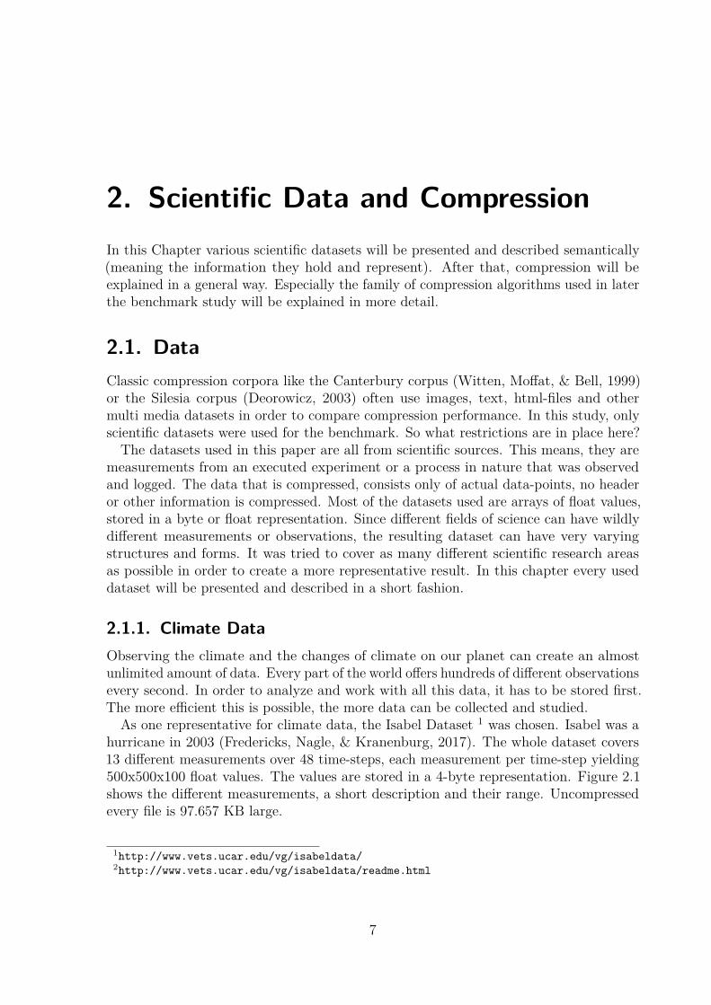
As one representative for climate data, the Isabel Dataset 1 was chosen. Isabel was ahurricane in 2003 (Fredericks, Nagle, & Kranenburg, 2017). The whole dataset covers13 different measurements over 48 time-steps, each measurement per time-step yielding500x500x100 float values. The values are stored in a 4-byte representation. Figure 2.1shows the different measurements, a short description and their range. Uncompressedevery file is 97.657 KB large.

1http://www.vets.ucar.edu/vg/isabeldata/2http://www.vets.ucar.edu/vg/isabeldata/readme.html

7

2

Figure 2.1.: The different measurements from the Isabel Datasets.

2.1.2. Geographical/Biological DataRight next to the climate, the processes of nature and life are also ever changing andevolving. Measuring or observing the changes in plant or animal life is one of the oldestand most fundamental forms of research.The dataset chosen from this research area comes from the University of Frankfurt,

Germany and is a measurement about the growing rates of crops. The dataset containsthe Monthly Growing Area Grids (MGAG) for 26 irrigated and rainfed crops. Thedataset is called MIRCA2000 (Portmann, Siebert, Bauer, & Döll, 2008). It also containsfloat values stored as bytes.Each of the 52 files contains information about one plant either being irrigated or

rainfed. Each file covers 4320 x 2160 grid cells over the period of 12 months. The valuesin every grid cell represent the growing area in hectare. Uncompressed every file is437.400 KB large. Because the files were very big, not all algorithms from the benchmarkcould be used when testing these files.3

https://www.gfbio.org/data/search offers further Geographical datasets.

2.1.3. Protein CorpusThe Protein Corpus (Abel, 2002) is a set of four files, which were used in the article’Protein is incompressible’ (Nevill-Manning & Witten, 1999). Every file describes adifferent protein with a string made up by a sequence of 20 different amino acids. Everyamino acid is represented by one character. Protein is hard to compress, because it haslittle repeating sequences. This makes it a good candidate for compression benchmarks.The files are between 400 to 3.300 KB in size.

http://gdb.unibe.ch/downloads/ offers further Chemical datasets.

3used algorithms: lzlib,xz,zstd,lzma,csc,brotli,lz4fast,pithy,snappy,lzo1x

8

2.1.4. Electrical Engineering and Robot DataThe used dataset comes from the testing of 193 Xilinx Spartan (XC3S500E) Field Pro-grammable Gate Arrays (FPGAs)4. One hundred frequency samples were taken of eachof the 512 ring oscillators on the Spartan board. The measurements were taken with thedevice operating in a regular room-temperature environment (around 25C°) and with aninput voltage of the standard 1.2V. Every dataset contains only float-values and wassaved as a csv-file with 395 Kb each.

Datasets from robotic sensors can be found on http://kos.informatik.uni-osnabrueck.de/3Dscans/ or http://asrl.utias.utoronto.ca/datasets/mrclam/#Download, butwere not tested for this work.

2.1.5. Medical Imaging DataMedical imaging is a standard procedure in every hospital. There are different ways togather informations about the inner life of a human or other animal non-invasively. Twoexample datasets are used in this benchmark.The Lukas Corpus (Abel, 2002) contains the measurements of radiography (x-ray).

The dataset includes four sets of files containing either two or three dimensional resultsfrom radiography. Only the data from the first set of measurements was used in thisstudy. The tested files are a set of two dimensional 16 bit radiographs in DICOM format.The files are between 6.000 and 8.000 KB large.

A second dataset comes from a functional Magnetic Resonance Imaging (fMRI)study (Hanke et al., 2015). The data contains high-resolution, ultra high-field (7 Tesla)fMRI data from human test persons. Twenty participants were repeatedly stimulatedwith a total of 25 music clips, with and without speech content, from five different genresusing a slow event-related paradigm. The resulting physiological phenomena in the brainare partly captured by the fMRI. Files are 275.401 KB large.

2.1.6. Astronomical DataThe last set of data comes from the scientific field of Astronomy. The used files containthe entire Smithsonian Astrophysical Observatory (SAO) Star Catalog 5 of 258,996 stars,including B1950 positions, proper motions, magnitudes, and, usually, spectral types in alocally-developed binary format described below. The catalog comes in two formates,one is 7.082 KB, the other one is 8.094 KB large.

4http://rijndael.ece.vt.edu/puf/download.html5http://tdc-www.harvard.edu/software/catalogs/sao.html

9

2.2. CompressionCompression plays an important role in the digital world we live in today (Chen &Fowler, 2014). Storing and transmitting files, pictures, videos and information in general,is done in every second of every day. Since physical storage is expensive and the time forsending, receiving and storing data increases with its size, compression of data is crucialto a fast and economically working digital information system. Especially in scientificenvironments, huge amounts of data can result from experiments or observations.Compression describes the process of decreasing the size of the data needed in order

to save the same (or almost the same) information (Sayood, 2000; Lelewer & Hirschberg,1987). When performing a data compression, the resulting size divided by the originalsize will result in the compression ratio. The ratio is often the most important metric ofa compression.

The time it takes to compress a file is represented in the compression speed. It shows,how many Bytes the algorithm compresses every second. The decompression speed ismeasured the same way.

Further metrics that might be interesting are the memory usage of the algorithm duringthe compression and the energy usage of the program. Especially when compression isdone on a small hardware device or a microprocessor.Often the use-case and the situation determine the most important metric and thus

the choice of the algorithms. Is the prime aspect of compression to store it with as littlespace-usage as possible? Or is it important that data is compressed fast, so that it canbe send somewhere fast? Or maybe the hardware constraints do not allow for too muchmemory usage?The fact, that different use-cases will have different demands on compression, makes

it hard to define the optimal compression algorithm for one dataset. One could try tocome up with some sort of score to weight all the different metrics together to one value.But this again would be highly subjective. For simplicity in this study, ratio will mostlybe taken as the most important metric and will often define the optimal algorithms.

Mahoney (2012) offers a nice theoretical and practical overview on the most commonlyused algorithms. It offers nice examples and gives a quick and intuitive understandingabout compression. For the ones seeking more theoretical and thorough information onthe topic of compression, Salomon and Motta (2010) is recommended.

2.2.1. Lossless and lossy compressionCompression algorithms can be separated in two classes: lossless and lossy compression.As the names already suggest, the first loses nothing where the second one does. Thething they lose is precision or accuracy of information.This is often accepted, when the information, that is lost was redundant or not

visible for humans anyway. Most famously, lossy compression is used for images e.g.JPEG (Acharya & Tsai, 2005), for videos e.g. MPEG (Sikora, 1997) and for audio, likethe well known MP3 (Brandenburg & Stoll, 1994). The loss in information, is normally

10

not noticeable for humans. This acceptance of loss on the other hand allows for muchbetter and faster compression.

Lossless compression does not allow this. Every bit has to be the same after compressionand decompression. This is often necessary, when a loss of information would destroythe data. A very obvious example is storing any sort of key or password. The exactreplication of the original data is crucial. The benchmark used in this study only useslossless compression algorithms, thus they are more important at this point. Famouslossless compression strategies are: Run-length Encoding (Robinson & Cherry, 1967),Huffman Encoding (Huffman, 1952), Prediction-by-partial matching (Cleary & Witten,1984) or Lempel-Ziv Compression (Chapter 2.2.3).

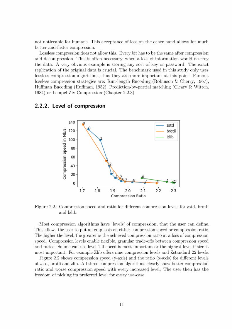
2.2.2. Level of compression

Figure 2.2.: Compression speed and ratio for different compression levels for zstd, brotliand lzlib.

Most compression algorithms have ’levels’ of compression, that the user can define.This allows the user to put an emphasis on either compression speed or compression ratio.The higher the level, the greater is the achieved compression ratio at a loss of compressionspeed. Compression levels enable flexible, granular trade-offs between compression speedand ratios. So one can use level 1 if speed is most important or the highest level if size ismost important. For example Zlib offers nine compression levels and Zstandard 22 levels.

Figure 2.2 shows compression speed (y-axis) and the ratio (x-axis) for different levelsof zstd, brotli and zlib. All three compression algorithms clearly show better compressionratio and worse compression speed with every increased level. The user then has thefreedom of picking its preferred level for every use-case.

11

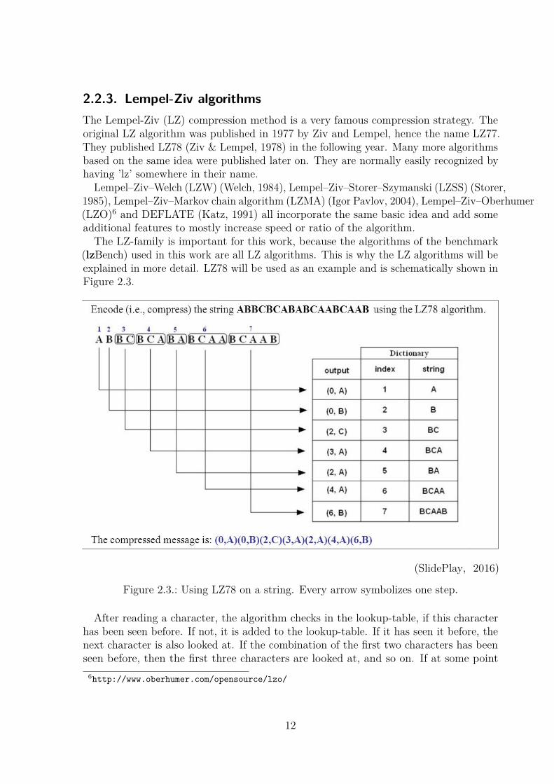
2.2.3. Lempel-Ziv algorithmsThe Lempel-Ziv (LZ) compression method is a very famous compression strategy. Theoriginal LZ algorithm was published in 1977 by Ziv and Lempel, hence the name LZ77.They published LZ78 (Ziv & Lempel, 1978) in the following year. Many more algorithmsbased on the same idea were published later on. They are normally easily recognized byhaving ’lz’ somewhere in their name.

Lempel–Ziv–Welch (LZW) (Welch, 1984), Lempel–Ziv–Storer–Szymanski (LZSS) (Storer,1985), Lempel–Ziv–Markov chain algorithm (LZMA) (Igor Pavlov, 2004), Lempel–Ziv–Oberhumer(LZO)6 and DEFLATE (Katz, 1991) all incorporate the same basic idea and add someadditional features to mostly increase speed or ratio of the algorithm.The LZ-family is important for this work, because the algorithms of the benchmark

(lzBench) used in this work are all LZ algorithms. This is why the LZ algorithms will beexplained in more detail. LZ78 will be used as an example and is schematically shown inFigure 2.3.

(SlidePlay, 2016)

Figure 2.3.: Using LZ78 on a string. Every arrow symbolizes one step.

After reading a character, the algorithm checks in the lookup-table, if this characterhas been seen before. If not, it is added to the lookup-table. If it has seen it before, thenext character is also looked at. If the combination of the first two characters has beenseen before, then the first three characters are looked at, and so on. If at some point

6http://www.oberhumer.com/opensource/lzo/

12

the algorithm finds a sequence of characters it has not seen before, it will replace allthe characters except the last one with the address of that character sequence (becauseit has to have seen that sequence before) and save it plus the new character. This canbe seen in the ’output’ column. By doing this, the algorithm builds longer and longerknown sequences, that it can reuse.

13

3. Experiment: CompressionBenchmark with lzBench

Compression benchmarks are quite popular and very useful. Because of the flood ofdifferent compression algorithms, that all claim to be faster and better than the rest, itis important to create a valid and reliable competition between them.

The Idea is simple: Different algorithms compress, decompress and validate the samedata-sample on the same hardware. Important metrics like ratio, speed, memory usage,energy usage and more are collected and can be compared afterwards. This creates avalid and usable comparison between the algorithms and one can decide which algorithmsuits one’s needs best.

3.1. Experiment Design3.1.1. lzBenchThe benchmark chosen for this paper is lzBench1. The authors describe lzBench in theirGithub Readme with the following: ’lzbench is an in-memory benchmark of open-sourceLZ77/LZSS/LZMA compressors. It joins all compressors into a single exe. At thebeginning an input file is read to memory. Then all compressors are used to compressand decompress the file and decompressed file is verified.’

LZ77 stands for Lempel–Ziv 1977, LZSS for Lempel–Ziv–Storer–Szymanski and LZMAfor Lempel–Ziv–Markov Algorihtm. All these algorithms are part of the Lempel-Zivfamily described in Section 2.2.3. Even though, they are based on the same generalprinciple, the three subfamilies have their own mechanisms and ideas in order to createbetter compression algorithms. The same way, every individual implementation can havea focus on a different aspect of compression, making it favorable for specific tasks ordatasets.LzBench was chosen because of its simplicity and its big number of algorithms (see

Section 3.1.2). It is freely available and allows the user a high degree of manual adaptation.Figure 3.1 shows the options one can set when running the benchmark tool.When executing lzBench, it will use all set algorithms (option ’-e#’) with all their

possible levels of compression (see Chapter 2.2.2). It will run X compression runs and Ydecompression runs for every algorithm. X and Y are defined by the option ’-iX,Y’. ’-p#’will then decide what measurement will be printed in the end (fastest, average, median).

1https://github.com/inikep/lzbench/

14

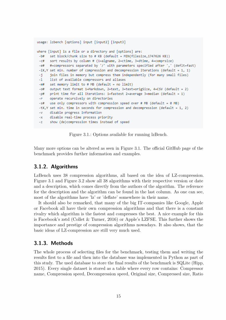
Figure 3.1.: Options available for running lzBench.

Many more options can be altered as seen in Figure 3.1. The official GitHub page of thebenchmark provides further information and examples.

3.1.2. AlgorithmsLzBench uses 38 compression algorithms, all based on the idea of LZ-compression.Figure 3.1 and Figure 3.2 show all 38 algorithms with their respective version or dateand a description, which comes directly from the authors of the algorithm. The referencefor the description and the algorithm can be found in the last column. As one can see,most of the algorithms have ’lz’ or ’deflate’ somewhere in their name.It should also be remarked, that many of the big IT-companies like Google, Apple

or Facebook all have their own compression algorithms and that there is a constantrivalry which algorithm is the fastest and compresses the best. A nice example for thisis Facebook’s zstd (Collet & Turner, 2016) or Apple’s LZFSE. This further shows theimportance and prestige of compression algorithms nowadays. It also shows, that thebasic ideas of LZ-compression are still very much used.

3.1.3. MethodsThe whole process of selecting files for the benchmark, testing them and writing theresults first to a file and then into the database was implemented in Python as part ofthis study. The used database to store the final results of the benchmark is SQLite (Hipp,2015). Every single dataset is stored as a table where every row contains: Compressorname, Compression speed, Decompression speed, Original size, Compressed size, Ratio

15

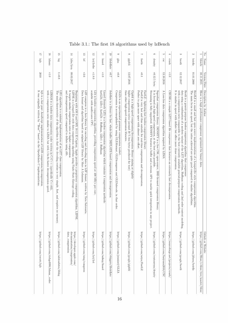
Table 3.1.: The first 18 algorithms used by lzBench

No

Nam

eVersion/D

ateDescription

byAuthor

Github

orWebsite

1blosclz

10.11.2015Blosc

isahigh

performance

compressor

optimized

forbinary

data.https://github.com

/Blosc/c-blosc/tree/master/blosc

2brieflz

01.01.2000BriefLZ

isasm

allandfast

opensource

implem

entationofa

Lempel-Ziv

stylecom

pressionalgorithm

.The

main

focusis

onspeed,but

theratios

achievedare

quitegood

compared

tosim

ilaralgorithm

s.https://github.com

/jibsen/brieflz

3brotli

12.12.2017

Brotliisageneric-purpose

losslesscom

pressionalgorithm

thatcom

pressesdata

usingacom

binationofa

modern

variantofthe

LZ77algorithm

,Huffm

ancoding

and2nd

ordercontext

modeling,

with

acom

pressionratio

comparable

tothe

bestcurrently

availablegeneral-purpose

compression

methods.

Itis

similar

inspeed

with

deflatebut

offersmore

densecom

pression.

https://github.com/google/brotli

4crush

v1.0CRU

SHis

asim

pleLZ77-based

filecom

pressorthat

featuresan

extremely

fastdecom

pression.https://sourceforge.net/projects/crush/

5csc

13.10.2016A

Loss-lessdata

compression

algorithminspired

byLZM

Ahttps://github.com

/fusiyuan2010/CSC

6density

v0.12.5beta

Superfastcom

pressionlibrary.

DEN

SITY

isafree

C99,open-source,BSD

licensedcom

pressionlibrary.

Itis

focusedon

high-speedcom

pression,atthe

bestratio

possible.Stream

ingis

fullysupported.

DEN

SITY

featuresabuffer

andastream

APIto

enablequick

integrationin

anyproject.

https://github.com/centaurean/density

7fastlz

v0.1FastLZ

-lightning-fastlossless

compression

library.FastLZ

isvery

fastand

thussuitable

forreal-tim

ecom

pressionand

decompression.

Perfectto

gainmore

spacewith

almost

zeroeffort.

https://github.com/ariya/FastLZ

8gipfeli

13.07.2016Gipfeliis

ahigh-speed

compression/decom

pressionlibrary

aiming

atslightly

highercom

pressionratios

(around30

%less

bytesproduced

fortext)

thanother

high-speedcom

pressionlibraries.

https://github.com/google/gipfeli

9glza

v0.8GLZA

isan

experimentalgram

mar

compression

toolset.Com

pressionis

accomoplished

byusing

GLZA

format,G

LZAcom

pressand

GLZA

decode,inthat

order.https://github.com

/jrmuizel/G

LZA

10libdeflate

v0.7ibdeflate

isalibrary

forfast,w

hole-bufferDEFLAT

E-basedcom

pressionand

decompression.

https://github.com/ebiggers/libdeflate

11lizard

v1.0Lizard

(formerly

LZ5)is

alossless

compression

algorithmwhich

contains4com

pressionmethods:

fastLZ4,LIZv1,fastLZ4+

Huffm

an,LIZv1+

Huffm

anhttps://github.com

/inikep/lizard

12lz4/lz4hc

v1.8.0LZ4

islossless

compression

algorithm,providing

compression

speedat

400MB/s

percore,

scalablewith

multi-cores

CPU

.https://github.com

/lz4/lz4

13lzf

v3.6LZF-com

pressis

aJava

libraryfor

encodingand

decodingdata

inLZF

format,w

rittenby

TatuSaloranta.

Data

format

andalgorithm

basedon

originalLZFlibrary

byMarc

ALehm

ann.https://github.com

/ning/compress

14lzfse/lzvn

08.03.2017

Beginningwith

iOS9and

OSX

10.11ElC

apitan,Apple

providesaproprietary

compression

algorithm,LZFSE.

LZFSEis

aLem

pel-Zivstyle

datacom

pressionalgorithm

usingFinite

StateEntropy

coding.It

targetssim

ilarcom

pressionrates

athigher

compression

anddecom

pressionspeed

compared

todeflate

usingzlib.

https://developer.apple.com/

documentation/com

pression/data_

compression

15lzg

1.v0.8LZG

algorithmis

aminim

alimplem

entationofan

LZ77class

compression.

The

main

characteristicofthe

algorithmis

thatthe

decodingroutine

isvery

simple,fast,and

requiresno

mem

ory.https://github.com

/mbitsnbites/liblzg

16lzham

v1.0LZH

AM

isalossless

datacom

pressioncodec

written

inC/C

++

(specificallyC++03),

with

acom

pressionratio

similar

toLZM

Abut

with

1.5x-8xfaster

decompression

speed.https://github.com

/richgel999/lzham_codec

17lzjb

2010lzjb

isafast

pureJavaScript

implem

entationofLZJB

compression/decom

pression.It

wasoriginally

written

by""Bear""based

onthe

OpenSolaris

Cim

plementations.

https://github.com/cscott/lzjb

16

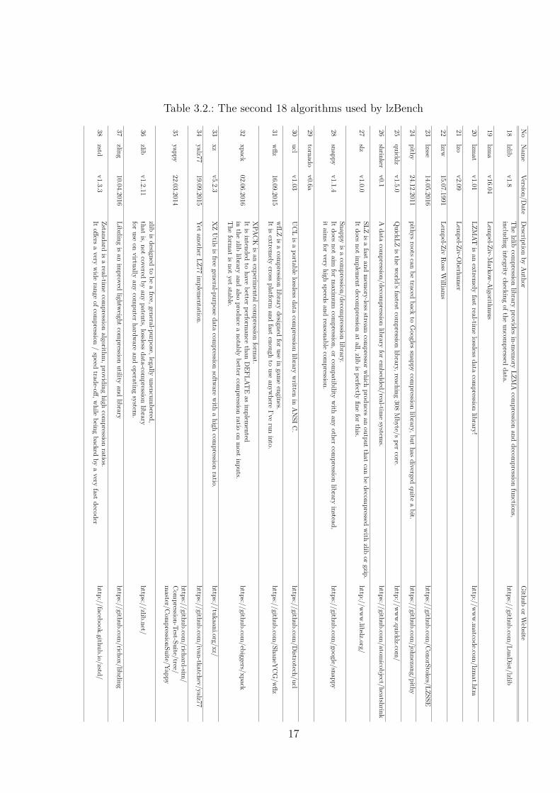
Table 3.2.: The second 18 algorithms used by lzBench

No

Nam

eVersion/D

ateDescription

byAuthor

Github

orWebsite

18lzlib

v1.8The

lzlibcom

pressionlibrary

providesin-m

emory

LZMA

compression

anddecom

pressionfunctions,

includingintegrity

checkingofthe

uncompressed

data.https://github.com

/LuaDist/lzlib

19lzm

av16.04

Lempel-Ziv-M

arkow-A

lgorithmus

20lzm

atv1.01

LZMAT

isan

extremely

fastreal-tim

elossless

datacom

pressionlibrary!

http://www.m

atcode.com/lzm

at.htm

21lzo

v2.09Lem

pel-Ziv-Oberhum

er

22lzrw

15.07.1991Lem

pel-ZivRoss

William

s

23lzsse

14.05.2016https://github.com

/ConorStokes/LZSSE

24pithy

24.12.2011pithys

rootscan

betraced

backto

Googles

snappycom

pressionlibrary,but

hasdiverged

quiteabit.

https://github.com/johnezang/pithy

25quicklz

v1.5.0QuickLZ

isthe

world’sfastest

compression

library,reaching308

Mbyte/s

percore.

http://www.quicklz.com

/

26shrinker

v0.1A

datacom

pression/decompression

libraryfor

embedded/real-tim

esystem

s.https://github.com

/atomicobject/heatshrink

27slz

v1.0.0SLZ

isafast

andmem

ory-lessstream

compressor

which

producesan

outputthat

canbe

decompressed

with

zlibor

gzip.It

doesnot

implem

entdecom

pressionat

all,zlibis

perfectlyfine

forthis.

http://www.libslz.org/

28snappy

v1.1.4Snappy

isacom

pression/decompression

library.It

doesnot

aimfor

maxim

umcom

pression,orcom

patibilitywith

anyother

compression

libraryinstead,

itaim

sfor

veryhigh

speedsand

reasonablecom

pression.https://github.com

/google/snappy

29tornado

v0.6a

30ucl

v1.03UCLis

aportable

losslessdata

compression

librarywritten

inANSIC

.https://github.com

/Distrotech/ucl

31wflz

16.09.2015wfLZ

isacom

pressionlibrary

designedfor

usein

gameengines.

Itis

extremely

crossplatform

andfast

enoughto

useanyw

hereI’ve

runinto.

https://github.com/ShaneY

CG/w

flz

32xpack

02.06.2016

XPA

CK

isan

experimentalcom

pressionform

at.It

isintended

tohave

betterperform

ancethan

DEFLAT

Eas

implem

entedin

thezlib

libraryand

alsoproduce

anotably

bettercom

pressionratio

onmost

inputs.The

format

isnot

yetstable.

https://github.com/ebiggers/xpack

33xz

v5.2.3XZUtils

isfree

general-purposedata

compression

softwarewith

ahigh

compression

ratio.https://tukaani.org/xz/

34yalz77

19.09.2015Yet

anotherLZ77

implem

entation.https://github.com

/ivan-tkatchev/yalz77

35yappy

22.03.2014https://github.com

/richard-sim/

Com

pression-Test-Suite/tree/master/C

ompressionSuite/Yappy

36zlib

v1.2.11zlib

isdesigned

tobe

afree,general-purpose,legally

unencumbered,

thatis,not

coveredby

anypatents,lossless

data-compression

libraryfor

useon

virtuallyany

computer

hardwareand

operatingsystem

.https://zlib.net/

37zling

10.04.2016Libzling

isan

improved

lightweightcom

pressionutility

andlibrary

https://github.com/richox/libzling

38zstd

v1.3.3Zstandard

isareal-tim

ecom

pressionalgorithm

,providinghigh

compression

ratios.It

offersavery

wide

rangeofcom

pression/speed

trade-off,while

beingbacked

byavery

fastdecoder

http://facebook.github.io/zstd/

17

and Filename. Every table contains one row for every used level of algorithm. When twolevels have too similar results, only one of them is stored. On average every benchmarkrun creates 170 to 200 rows of measurements. LzBench is mostly written in C and C++,with an easy to use shell interface. Executing C programs from Python is not impossible,but executing a shell command is much more handy.Implemented methods for testing include:

A method (lzBench_on_folder) that will take an input-file or folder and an output-folder as arguments, will then run the benchmark and save the result file in the givendirectory. Options for lzBench can also be given as parameters. This method createsone bash script for every file, that is executed on a cluster. Number of nodes to use andwhich partition to use can also be given as parameters for the method. By doing this,the procedure of testing can easily be parallelized on different nodes.

import_folder_to_DB will import the given folder into the given sqlite3 database.Existing tables will be overwritten.

The same Python script contains different methods for analyzing the results storedin the database.

get_table will return the whole table for a given table name. It will be sorted bya given metric (default = ratio) and an n can be given if only the top n rows shall bereturned.

get_best_algorithms will return all tested data samples with their n best algorithmsregarding a chosen metric (ratio, compression speed, decompression speed). By adding aregex one can filter the tables that are returned.

get_best_files_per_algorithm will return the previously mentioned dictionary re-versed. This function takes the best algorithms for every dataset and creates a dictionarymapping from algorithm to datasets, that this algorithm had the best performance on.

get_averages returns a list of all datasets and their average ratio, compression speedand decompression speed over all algorithms.

3.2. ResultsVisualizing and presenting the results of a compression benchmark can be tricky. Thebenchmark includes different algorithms, which all measure different metrics. And everybenchmark is performed on various datasets. This means, three important factors interact(algorithm, metric, dataset) and the different effects between those can be observed.It is very hard, though to show all of them in one plot or table, since at least three

18

dimensions would be needed for that. Effects that might be interesting are: How well isthe performance of different algorithms on one dataset? Do different sorts of data sharecertain characteristics when it comes to compression? What algorithms show overall thebest performance? Is there a relation between the different metrics?

In order to answer these questions in the discussion, the results are shown and plottedfrom different angles in this chapter.

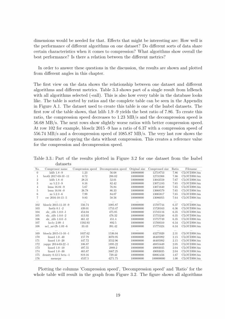
The first view on the data shows the relationship between one dataset and differentalgorithms and different metrics. Table 3.3 shows part of a single result from lzBenchwith all algorithms selected (-eall). This is also how every table in the database lookslike. The table is sorted by ratios and the complete table can be seen in the Appendixin Figure A.1. The dataset used to create this table is one of the Isabel datasets. Thefirst row of the table shows, that lzlib 1.9 -9 yields the best ratio of 7.86. To create thisratio, the compression speed decreases to 1.23 MB/s and the decompression speed is56.68 MB/s. The next rows show slightly worse ratios with better compression speed.At row 102 for example, blosclz 2015 -9 has a ratio of 6.37 with a compression speed of556.74 MB/s and a decompression speed of 1085.87 MB/s. The very last row shows themeasurements of copying the data without compression. This creates a reference valuefor the compression and decompression speed.

Table 3.3.: Part of the results plotted in Figure 3.2 for one dataset from the Isabeldatasets

No. Compressor name Compression speed Decompression speed Original size Compressed size Ratio Filename0 lzlib 1.8 -9 1.23 56.68 100000000 12718753 7.86 CLOUDf08.bin1 brotli 2017-03-10 -11 0.72 288.82 100000000 12731988 7.86 CLOUDf08.bin2 lzlib 1.8 -0 28.21 52.01 100000000 13043559 7.67 CLOUDf08.bin3 xz 5.2.3 -9 8.16 82.42 100000000 13071183 7.65 CLOUDf08.bin4 lzma 16.04 -9 5.67 76.84 100000000 13071640 7.65 CLOUDf08.bin5 lzma 16.04 -0 26.78 86.33 100000000 13068579 7.65 CLOUDf08.bin6 xz 5.2.3 -6 7.99 84.07 100000000 13065817 7.65 CLOUDf08.bin7 csc 2016-10-13 -5 9.83 58.56 100000000 13086055 7.64 CLOUDf08.bin... ... ... ... ... ... ... ...102 blosclz 2015-11-10 -9 556.74 1085.87 100000000 15707744 6.37 CLOUDf08.bin103 fastlz 0.1 -2 439.01 1753.47 100000000 15720163 6.36 CLOUDf08.bin104 slz_zlib 1.0.0 -1 454.04 475.85 100000000 15745116 6.35 CLOUDf08.bin105 slz_zlib 1.0.0 -2 413.92 476.32 100000000 15755240 6.35 CLOUDf08.bin106 slz_zlib 1.0.0 -3 461.42 451.4 100000000 15757749 6.35 CLOUDf08.bin107 lzo1y 2.09 -1 1592.93 892.5 100000000 15769310 6.34 CLOUDf08.bin108 ucl_nrv2b 1.03 -6 33.43 391.42 100000000 15775324 6.34 CLOUDf08.bin... ... ... ... ... ... ... ...169 blosclz 2015-11-10 -1 1037.62 1536.04 100000000 43275920 2.31 CLOUDf08.bin170 lizard 1.0 -40 157.79 3070.95 100000000 46405992 2.15 CLOUDf08.bin171 lizard 1.0 -20 447.72 3552.96 100000000 46405992 2.15 CLOUDf08.bin172 yappy 2014-03-22 -1 106.87 1895.22 100000000 48855449 2.05 CLOUDf08.bin173 lizard 1.0 -10 497.55 2889.2 100000000 49093035 2.04 CLOUDf08.bin174 lizard 1.0 -30 465.87 3467.25 100000000 49093035 2.04 CLOUDf08.bin175 density 0.12.5 beta -1 819.16 729.42 100000000 60061456 1.67 CLOUDf08.bin176 memcpy 4537.5 4271.75 100000000 100000000 1.00 CLOUDf08.bin

Plotting the columns ’Compression speed’, ’Decompression speed’ and ’Ratio’ for thewhole table will result in the graph from Figure 3.2. The figure shows all algorithms

19

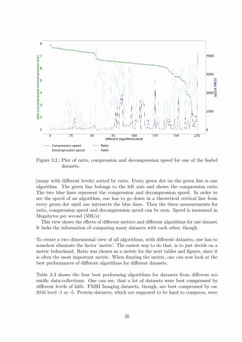
Figure 3.2.: Plot of ratio, compression and decompression speed for one of the Isabeldatasets.

(many with different levels) sorted by ratio. Every green dot on the green line is onealgorithm. The green line belongs to the left axis and shows the compression ratio.The two blue lines represent the compression and decompression speed. In order tosee the speed of an algorithm, one has to go down in a theoretical vertical line fromevery green dot until one intersects the blue lines. Then the three measurements forratio, compression speed and decompression speed can be seen. Speed is measured inMegabytes per second (MB/s).

This view shows the effects of different metrics and different algorithms for one dataset.It lacks the information of comparing many datasets with each other, though.

To create a two dimensional view of all algorithms, with different datasets, one has tosomehow eliminate the factor ’metric’. The easiest way to do that, is to just decide on ametric beforehand. Ratio was chosen as a metric for the next tables and figures, since itis often the most important metric. When fixating the metric, one can now look at thebest performances of different algorithms for different datasets.

Table 3.3 shows the four best performing algorithms for datasets from different sci-entific data-collections. One can see, that a lot of datasets were best compressed bydifferent levels of lzlib. FMRI Imaging datasets, though, are best compressed by csc2016 level -1 or -5. Protein datasets, which are supposed to be hard to compress, were

20

compressed best by brotli 2017 level -11 followed by zstd 1.3.1 and csc 2016. The tableonly shows a part of all the datasets used in the benchmark. The complete list of datasetscan be found in the Appendix in Tables A.2 to A.8.

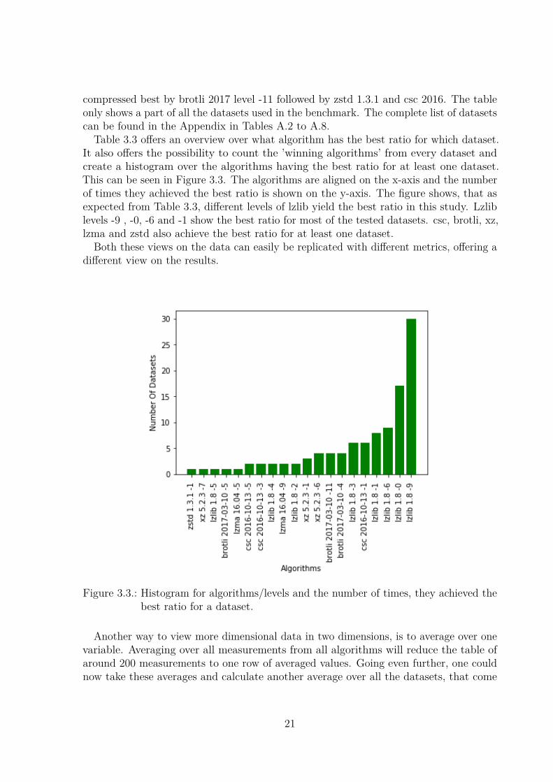
Table 3.3 offers an overview over what algorithm has the best ratio for which dataset.It also offers the possibility to count the ’winning algorithms’ from every dataset andcreate a histogram over the algorithms having the best ratio for at least one dataset.This can be seen in Figure 3.3. The algorithms are aligned on the x-axis and the numberof times they achieved the best ratio is shown on the y-axis. The figure shows, that asexpected from Table 3.3, different levels of lzlib yield the best ratio in this study. Lzliblevels -9 , -0, -6 and -1 show the best ratio for most of the tested datasets. csc, brotli, xz,lzma and zstd also achieve the best ratio for at least one dataset.

Both these views on the data can easily be replicated with different metrics, offering adifferent view on the results.

Figure 3.3.: Histogram for algorithms/levels and the number of times, they achieved thebest ratio for a dataset.

Another way to view more dimensional data in two dimensions, is to average over onevariable. Averaging over all measurements from all algorithms will reduce the table ofaround 200 measurements to one row of averaged values. Going even further, one couldnow take these averages and calculate another average over all the datasets, that come

21

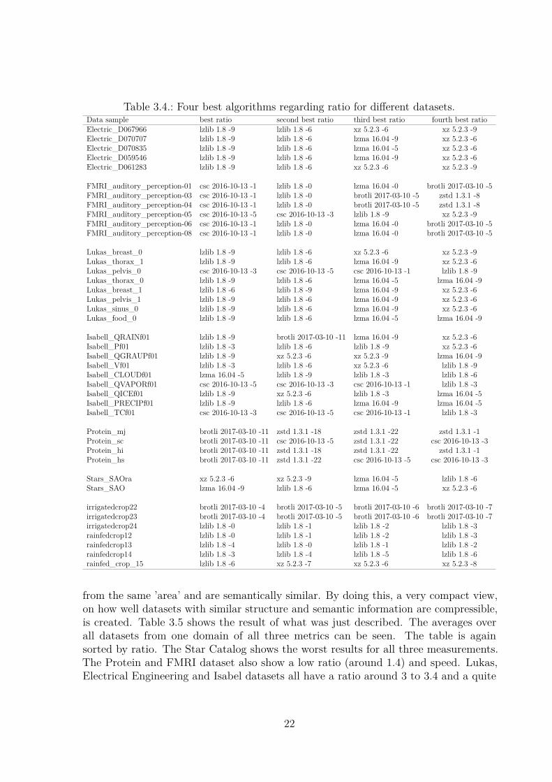
Table 3.4.: Four best algorithms regarding ratio for different datasets.Data sample best ratio second best ratio third best ratio fourth best ratioElectric_D067966 lzlib 1.8 -9 lzlib 1.8 -6 xz 5.2.3 -6 xz 5.2.3 -9Electric_D070707 lzlib 1.8 -9 lzlib 1.8 -6 lzma 16.04 -9 xz 5.2.3 -6Electric_D070835 lzlib 1.8 -9 lzlib 1.8 -6 lzma 16.04 -5 xz 5.2.3 -6Electric_D059546 lzlib 1.8 -9 lzlib 1.8 -6 lzma 16.04 -9 xz 5.2.3 -6Electric_D061283 lzlib 1.8 -9 lzlib 1.8 -6 xz 5.2.3 -6 xz 5.2.3 -9

FMRI_auditory_perception-01 csc 2016-10-13 -1 lzlib 1.8 -0 lzma 16.04 -0 brotli 2017-03-10 -5FMRI_auditory_perception-03 csc 2016-10-13 -1 lzlib 1.8 -0 brotli 2017-03-10 -5 zstd 1.3.1 -8FMRI_auditory_perception-04 csc 2016-10-13 -1 lzlib 1.8 -0 brotli 2017-03-10 -5 zstd 1.3.1 -8FMRI_auditory_perception-05 csc 2016-10-13 -5 csc 2016-10-13 -3 lzlib 1.8 -9 xz 5.2.3 -9FMRI_auditory_perception-06 csc 2016-10-13 -1 lzlib 1.8 -0 lzma 16.04 -0 brotli 2017-03-10 -5FMRI_auditory_perception-08 csc 2016-10-13 -1 lzlib 1.8 -0 lzma 16.04 -0 brotli 2017-03-10 -5

Lukas_breast_0 lzlib 1.8 -9 lzlib 1.8 -6 xz 5.2.3 -6 xz 5.2.3 -9Lukas_thorax_1 lzlib 1.8 -9 lzlib 1.8 -6 lzma 16.04 -9 xz 5.2.3 -6Lukas_pelvis_0 csc 2016-10-13 -3 csc 2016-10-13 -5 csc 2016-10-13 -1 lzlib 1.8 -9Lukas_thorax_0 lzlib 1.8 -9 lzlib 1.8 -6 lzma 16.04 -5 lzma 16.04 -9Lukas_breast_1 lzlib 1.8 -6 lzlib 1.8 -9 lzma 16.04 -9 xz 5.2.3 -6Lukas_pelvis_1 lzlib 1.8 -9 lzlib 1.8 -6 lzma 16.04 -9 xz 5.2.3 -6Lukas_sinus_0 lzlib 1.8 -9 lzlib 1.8 -6 lzma 16.04 -9 xz 5.2.3 -6Lukas_food_0 lzlib 1.8 -9 lzlib 1.8 -6 lzma 16.04 -5 lzma 16.04 -9

Isabell_QRAINf01 lzlib 1.8 -9 brotli 2017-03-10 -11 lzma 16.04 -9 xz 5.2.3 -6Isabell_Pf01 lzlib 1.8 -3 lzlib 1.8 -6 lzlib 1.8 -9 xz 5.2.3 -6Isabell_QGRAUPf01 lzlib 1.8 -9 xz 5.2.3 -6 xz 5.2.3 -9 lzma 16.04 -9Isabell_Vf01 lzlib 1.8 -3 lzlib 1.8 -6 xz 5.2.3 -6 lzlib 1.8 -9Isabell_CLOUDf01 lzma 16.04 -5 lzlib 1.8 -9 lzlib 1.8 -3 lzlib 1.8 -6Isabell_QVAPORf01 csc 2016-10-13 -5 csc 2016-10-13 -3 csc 2016-10-13 -1 lzlib 1.8 -3Isabell_QICEf01 lzlib 1.8 -9 xz 5.2.3 -6 lzlib 1.8 -3 lzma 16.04 -5Isabell_PRECIPf01 lzlib 1.8 -9 lzlib 1.8 -6 lzma 16.04 -9 lzma 16.04 -5Isabell_TCf01 csc 2016-10-13 -3 csc 2016-10-13 -5 csc 2016-10-13 -1 lzlib 1.8 -3

Protein_mj brotli 2017-03-10 -11 zstd 1.3.1 -18 zstd 1.3.1 -22 zstd 1.3.1 -1Protein_sc brotli 2017-03-10 -11 csc 2016-10-13 -5 zstd 1.3.1 -22 csc 2016-10-13 -3Protein_hi brotli 2017-03-10 -11 zstd 1.3.1 -18 zstd 1.3.1 -22 zstd 1.3.1 -1Protein_hs brotli 2017-03-10 -11 zstd 1.3.1 -22 csc 2016-10-13 -5 csc 2016-10-13 -3

Stars_SAOra xz 5.2.3 -6 xz 5.2.3 -9 lzma 16.04 -5 lzlib 1.8 -6Stars_SAO lzma 16.04 -9 lzlib 1.8 -6 lzma 16.04 -5 xz 5.2.3 -6

irrigatedcrop22 brotli 2017-03-10 -4 brotli 2017-03-10 -5 brotli 2017-03-10 -6 brotli 2017-03-10 -7irrigatedcrop23 brotli 2017-03-10 -4 brotli 2017-03-10 -5 brotli 2017-03-10 -6 brotli 2017-03-10 -7irrigatedcrop24 lzlib 1.8 -0 lzlib 1.8 -1 lzlib 1.8 -2 lzlib 1.8 -3rainfedcrop12 lzlib 1.8 -0 lzlib 1.8 -1 lzlib 1.8 -2 lzlib 1.8 -3rainfedcrop13 lzlib 1.8 -4 lzlib 1.8 -0 lzlib 1.8 -1 lzlib 1.8 -2rainfedcrop14 lzlib 1.8 -3 lzlib 1.8 -4 lzlib 1.8 -5 lzlib 1.8 -6rainfed_crop_15 lzlib 1.8 -6 xz 5.2.3 -7 xz 5.2.3 -6 xz 5.2.3 -8

from the same ’area’ and are semantically similar. By doing this, a very compact view,on how well datasets with similar structure and semantic information are compressible,is created. Table 3.5 shows the result of what was just described. The averages overall datasets from one domain of all three metrics can be seen. The table is againsorted by ratio. The Star Catalog shows the worst results for all three measurements.The Protein and FMRI dataset also show a low ratio (around 1.4) and speed. Lukas,Electrical Engineering and Isabel datasets all have a ratio around 3 to 3.4 and a quite

22

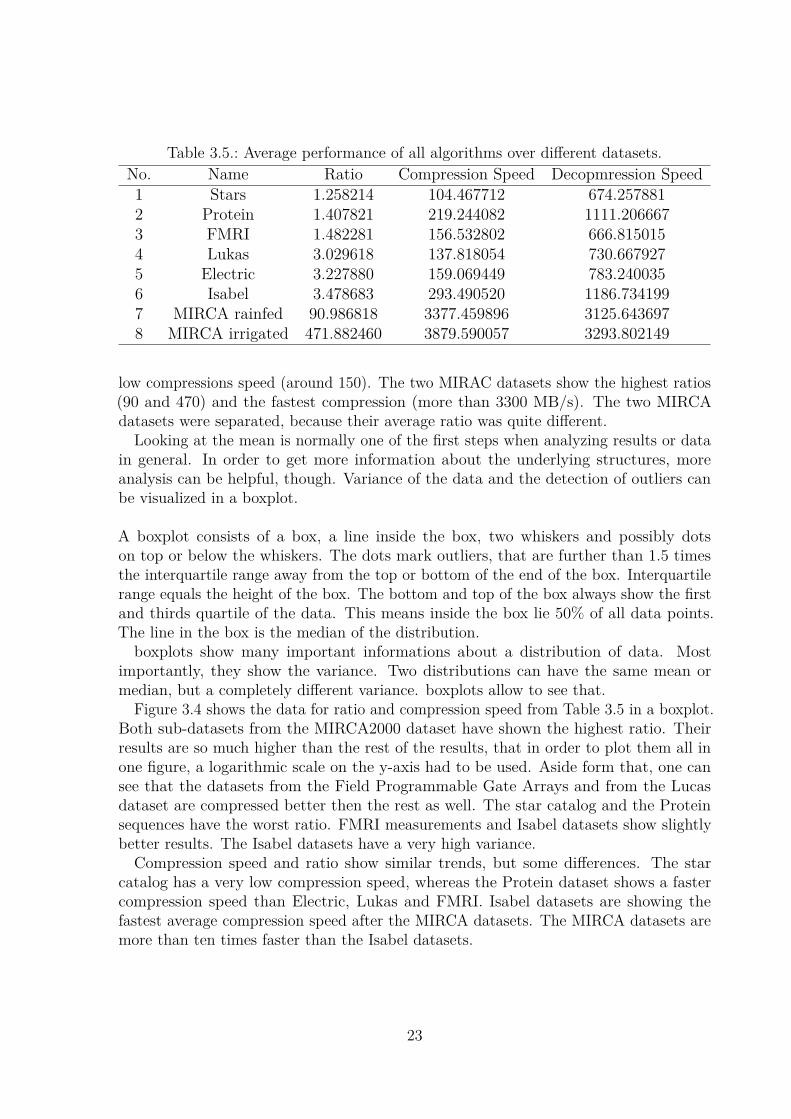
Table 3.5.: Average performance of all algorithms over different datasets.No. Name Ratio Compression Speed Decopmression Speed1 Stars 1.258214 104.467712 674.2578812 Protein 1.407821 219.244082 1111.2066673 FMRI 1.482281 156.532802 666.8150154 Lukas 3.029618 137.818054 730.6679275 Electric 3.227880 159.069449 783.2400356 Isabel 3.478683 293.490520 1186.7341997 MIRCA rainfed 90.986818 3377.459896 3125.6436978 MIRCA irrigated 471.882460 3879.590057 3293.802149

low compressions speed (around 150). The two MIRAC datasets show the highest ratios(90 and 470) and the fastest compression (more than 3300 MB/s). The two MIRCAdatasets were separated, because their average ratio was quite different.

Looking at the mean is normally one of the first steps when analyzing results or datain general. In order to get more information about the underlying structures, moreanalysis can be helpful, though. Variance of the data and the detection of outliers canbe visualized in a boxplot.

A boxplot consists of a box, a line inside the box, two whiskers and possibly dotson top or below the whiskers. The dots mark outliers, that are further than 1.5 timesthe interquartile range away from the top or bottom of the end of the box. Interquartilerange equals the height of the box. The bottom and top of the box always show the firstand thirds quartile of the data. This means inside the box lie 50% of all data points.The line in the box is the median of the distribution.

boxplots show many important informations about a distribution of data. Mostimportantly, they show the variance. Two distributions can have the same mean ormedian, but a completely different variance. boxplots allow to see that.

Figure 3.4 shows the data for ratio and compression speed from Table 3.5 in a boxplot.Both sub-datasets from the MIRCA2000 dataset have shown the highest ratio. Theirresults are so much higher than the rest of the results, that in order to plot them all inone figure, a logarithmic scale on the y-axis had to be used. Aside form that, one cansee that the datasets from the Field Programmable Gate Arrays and from the Lucasdataset are compressed better then the rest as well. The star catalog and the Proteinsequences have the worst ratio. FMRI measurements and Isabel datasets show slightlybetter results. The Isabel datasets have a very high variance.Compression speed and ratio show similar trends, but some differences. The star

catalog has a very low compression speed, whereas the Protein dataset shows a fastercompression speed than Electric, Lukas and FMRI. Isabel datasets are showing thefastest average compression speed after the MIRCA datasets. The MIRCA datasets aremore than ten times faster than the Isabel datasets.

23

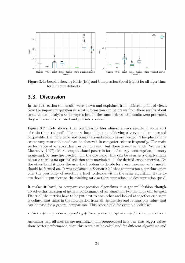
Figure 3.4.: boxplot showing Ratio (left) and Compression Speed (right) for all algorithmsfor different datasets.

3.3. DiscussionIn the last section the results were shown and explained from different point of views.Now the important question is, what information can be drawn from these results aboutsemantic data analysis and compression. In the same order as the results were presented,they will now be discussed and put into context.

Figure 3.2 nicely shows, that compressing files almost always results in some sortof ratio-time trade-off. The more focus is put on achieving a very small compressedoutput-file, the more time and computational resources are needed. This phenomenaseems very reasonable and can be observed in computer science frequently. The mainperformance of an algorithm can be increased, but there is no free lunch (Wolpert &Macready, 1997). More computational power in form of energy consumption, memoryusage and/or time are needed. On the one hand, this can be seen as a disadvantagebecause there is no optimal solution that maximizes all the desired output metrics. Onthe other hand it gives the user the freedom to decide for every use-case, what metricshould be focused on. It was explained in Section 2.2.2 that compression algorithms oftenoffer the possibility of selecting a level to decide within the same algorithm, if the fo-cus should be put more on the resulting ratio or the compression and decompression speed.

It makes it hard, to compare compression algorithms in a general fashion though.To solve this question of general performance of an algorithm two methods can be used:Either all the metrics have to be put next to each other and looked at together or a scoreis defined that takes in the information from all the metrics and returns one value, thatcan be used for a general comparison. This score could for example look like:

ratio ∗ x + compression_speed ∗ y + decompression_speed ∗ z + further_metrics ∗ c

Assuming that all metrics are normalized and preprocessed in a way that bigger valuesshow better performance, then this score can be calculated for different algorithms and

24

compared directly. The weights for the different metrics are still to be decided by the user.

Taking a closer look at Table 3.4, it seems, that even though lzlib overall shows the bestratio, certain complicated and not well structured datasets are better compressed byother algorithms. The star catalog for example shows little repeating structure, due to itbeing a catalog, and were best compressed by other algorithms than lzlib. When thedata was more structured like in the climate measurements, or the crop growing datasets(irrigatedcrop and rainfedcrop) lzlib outperforms the other algorithms most of the timewith regards to ratio.

When averaging over the compression algorithms and also the different datasets from thesame dataset corpus, one can have a close look at the overall performance on differentclasses of datasets. Table 3.5 and Figure 3.4 both offer that view. Especially the boxplotshows clearly, that some datasets with the same underlying semantic information arecompressible very good and very fast. It can be assumed, that the MIRCA datasetseither have a lot of repeating patterns or a lot of repeating numbers. It makes sense,when thinking about what the datasets represent. The monthly growing areas in hectaresfor the same plant is likely quite similar at different positions. If the crop is growingvery similar, the resulting numbers are all very similar and might often be the same.This allows for a easy and good compression. Protein and Star datasets on the otherhand have almost no repeating features and have a very low ratio compared to the restof the datasets. Especially the Star catalog has a ratio close to one, meaning that it ishardly compressed at all. A catalog often is a list of different items. There is not muchconnection between the items, that show patterns or repeating numbers.The boxplot shows similar results as Table 3.4. What can be seen in the right figure

is that the Isabel dataset has a very high variance. This is due to the fact, that theIsabel datasets contains 13 different measurements, all merged into one average. Thehigh variance shows, that these different measurements have different properties when itcomes to compression. Testing all 13 datasets individually would be very time intensiveand create many more different datasets. Since there is some assumed similarity betweenthe different Isabel datasets and to save time and space, the datasets were averagedtogether. The very low variance of the Star dataset is because it only contains two files,which are two representations of the same catalog. Protein, Electric and FMRI datasetsall have a very low variance and all seem to be semantically very similar. All datasetsshow a low variance when it comes to compression speed.This discussion shows, that the semantic information carried by different datasets

is highly responsible for the general compressibility of a dataset and also has a bigimpact on how well compression algorithms will perform on said dataset. By knowingthe semantic information of a dataset beforehand, one could now assume if the file willcompress well and what algorithm to use.

25

3.4. ConclusionThis chapter covered the compression of different scientific datasets, analyzing the resultsfrom different angles and discussing the implications of the results.

It was clearly visible, that different datasets with different semantic information reactvery differently to compression. It was also shown, that certain algorithms perform betteror worse depending on the dataset. Knowing where the dataset comes from and whatsort of semantic information it carries, can thus be highly informative about the generalcompressibility and maybe even the performance of different algorithms.

The connection between the datasets used in this study and the field of research theyrepresent should only be drawn with care. Mordern scientific research in one filed is nolonger limited to one or two different methods of measuring or observing, resulting infew different datasets. On the contrary, as seen in the Isabel dataset, one scientific filedcan create various datasets with different measurements and data-structures.

This chapter builds a foundation for testing and analyzing scientific datasets in or-der to find optimal compression algorithms for different datasets from scientific sources.The implementations created alongside this work are general and can be used for differentbenchmarks and datasets, in order to create an easy and fast way to benchmark variousalgorithms against many datasets.

26

4. Decision Support Systems withMachine Learning

This chapter will cover Decision Support Systems (DSS) (Power, Sharda, & Burstein, 2015;Arnott & Pervan, 2008). DSS is a quite broad term, covering basically all systems fromfacilitating decisions slightly to systems making decisions on their own. Support Systemsalso have changed a lot in the past 50 years, and will keep changing in the future (Shimet al., 2002). This paper will focus on recently developed DSS (Marakas, 2003): Systemsthat are sophisticated and proactive. They try not only to aid decision making, but topropose a decision for the user or to even make a decision on its own (Bojarski et al.,2016).

In the end of this chapter, the use-case of choosing an optimal compression algorithmfor new and unknown data will be used to give theoretical ideas a more practical use-case.

4.1. DecisionsDSS can look very differently. They can be a simple program that restructures, visualizesor highlights data (Li, Feng, & Li, 2001). They can make easy mathematic operationslike averaging over a list of values. In this case, the decision itself will still be placedin human hands though. The system will not propose anything, it just makes the datamore easily accessible. In machine learning, unsupervised learning falls in this category.When the only thing available is data, clustering can help to structure the data in amore understandable way. Then a human can make a decision.On the other hand one can think of a DSS that is aware of the different decisions

that are available (Goldman, Hartman, Fisher, & Sarel, 2004). It could for example beexplicitly implemented, that there are 38 different compression algorithms to choosefrom in the end. In many use-cases this decision will be binary. A system predictingthe development of shares on the stock market (Zhang, Fuehres, & Gloor, 2011; Huang,Nakamori, & Wang, 2005) for example should produce either a one for buying or azero for not-buying. Systems like that are often stochastic systems, that will return aprobability distribution over all existing categories or decision-options. Every decisionprocess can be modeled as a categorization problem. There is some sort of informationavailable in order to make a decision. The information will be used as the input for thecategorization algorithms and the decision will be the discrete output. So basically everydecision is a function mapping from information (input) to a decision (discrete value). Ifone has a dataset of inputs and correct outputs, that data can be used for a supervisedlearning model. These models will optimize a function to map every input as close as

27

possible to every given output.

4.2. Unsupervised LearningUnsupervised Learning is one of the two main classes of machine learning (Hastie,Tibshirani, & Friedman, 2009). It describes the discovery of structures or underlyinginformations in data. One can use unsupervised learning for unlabeled data. That meansjust the plain data. Labeled data on the other hand describes data, that has alreadybeen solved in a way (Seeger et al., 2001). Labeled data is only used to train a model.More information will be given in Section 4.3.Clustering data (Berkhin, 2006) can allow humans to make better judgment about

data and maybe help them come to a decision. Clustering means, to split the datasetinto a number of clusters or groups of data-points. A very famous and simple algorithmto do this is the k-Means Algorithm (MacQueen, 1967; Lloyd, 1982).

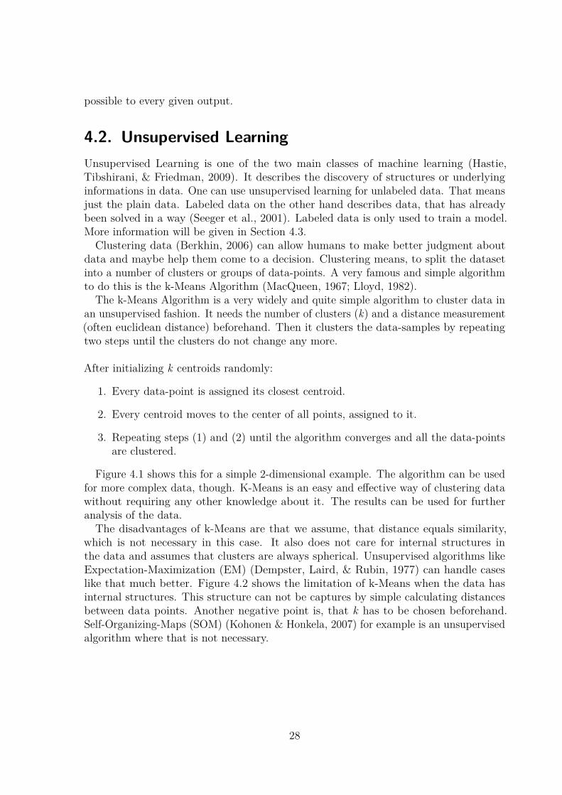
The k-Means Algorithm is a very widely and quite simple algorithm to cluster data inan unsupervised fashion. It needs the number of clusters (k) and a distance measurement(often euclidean distance) beforehand. Then it clusters the data-samples by repeatingtwo steps until the clusters do not change any more.

After initializing k centroids randomly:

1. Every data-point is assigned its closest centroid.

2. Every centroid moves to the center of all points, assigned to it.

3. Repeating steps (1) and (2) until the algorithm converges and all the data-pointsare clustered.

Figure 4.1 shows this for a simple 2-dimensional example. The algorithm can be usedfor more complex data, though. K-Means is an easy and effective way of clustering datawithout requiring any other knowledge about it. The results can be used for furtheranalysis of the data.The disadvantages of k-Means are that we assume, that distance equals similarity,

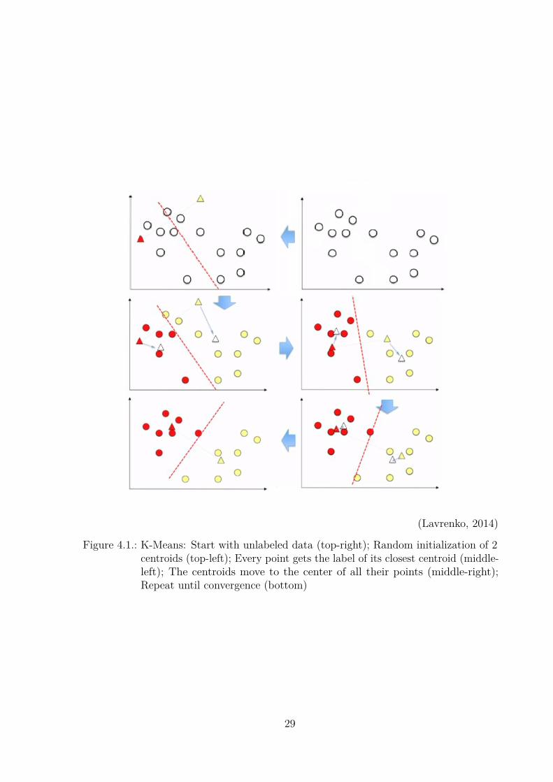
which is not necessary in this case. It also does not care for internal structures inthe data and assumes that clusters are always spherical. Unsupervised algorithms likeExpectation-Maximization (EM) (Dempster, Laird, & Rubin, 1977) can handle caseslike that much better. Figure 4.2 shows the limitation of k-Means when the data hasinternal structures. This structure can not be captures by simple calculating distancesbetween data points. Another negative point is, that k has to be chosen beforehand.Self-Organizing-Maps (SOM) (Kohonen & Honkela, 2007) for example is an unsupervisedalgorithm where that is not necessary.

28

(Lavrenko, 2014)

Figure 4.1.: K-Means: Start with unlabeled data (top-right); Random initialization of 2centroids (top-left); Every point gets the label of its closest centroid (middle-left); The centroids move to the center of all their points (middle-right);Repeat until convergence (bottom)

29

(Chire, 2010)

Figure 4.2.: K-Means does not assume any underlying structures. Expectation-Maximization can have a better prediction in that case.

4.3. Supervised learningUnsupervised algorithms do not have the ability to propose any decision. Supervisedalgorithms (Caruana & Niculescu-Mizil, 2006) do. In order to do so, they need labeleddata. That means, data-samples, that have already been labeled with the correct decisionor prediction. Coming back to the example of predicting the rise or the fall of a share:In this case labeled data would contain the actual data (information about the companyand the economical situation e.g.) and the actual outcome: did the share actually rise orfall in the situation, that is described by the input data.Only when data, with already known solutions is available, we can train a system to

learn the correlation between the input data and the output, the target.

4.3.1. k-Nearest-NeighborTo start with an easy example of a supervised algorithm, the k-Nearest-Neighbor (Altman,1992; Burba, Ferraty, & Vieu, 2009) algorithm will be explained. This algorithm doesnot actually learn any mapping from input to output, but it uses the same heuristic ask-means: Distance.If there are a number of data-points, that already have their correct label, than one

can do something very similar to what k-Means does. The k-Nearest-Neighbor algorithmcalculates the distance between a new unlabeled data-point and every other alreadylabeled data-point. It then looks at the k closest data-points and at their label. Thenew data-point simply gets the most common label under the k closest neighboringdata-points.

This again is a very simple, but very effective way of assigning a label and thus a classto a new data-point. The disadvantages are almost the same as for k-Means: Distance

30

as a measurement for similarity is assumed, structures in the data are not taken intoaccount and k has to be decided on beforehand. Additionally, computation time canbe quite high, if many, high dimensional data-points are available, since for every newdata-point, the distances to all other points have to be calculated.

4.3.2. Neural NetworksNeural Networks (Schmidhuber, 2015; Haykin & Network, 2004) are probably the mostfamous algorithm in machine learning right now. Even though there are many moresophisticated models like Convolutional Neural Networks (LeCun et al., 1989) andRecurrent Neural Networks (Hochreiter & Schmidhuber, 1997), the principles of NeuralNetworks are always the same. Every Neural Network - and every supervised learningalgorithm - ultimately is doing function approximation (Ferrari & Stengel, 2005). Thething, that makes Neural Networks so unique and popular is, that they are able to modelvery complex and high dimensional functions better than many other techniques.

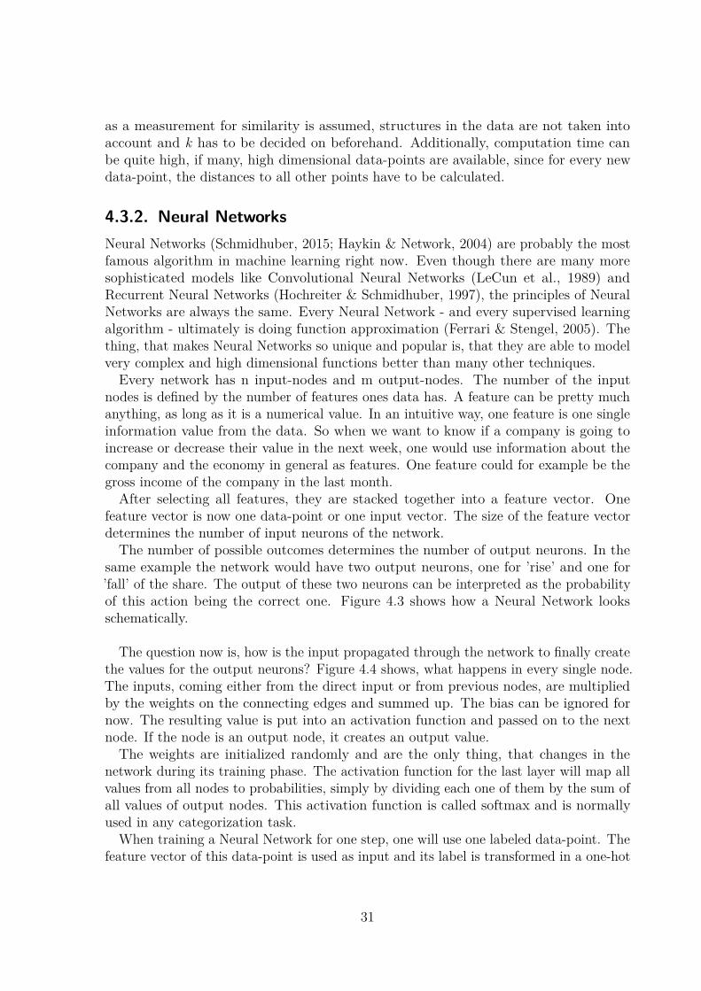
Every network has n input-nodes and m output-nodes. The number of the inputnodes is defined by the number of features ones data has. A feature can be pretty muchanything, as long as it is a numerical value. In an intuitive way, one feature is one singleinformation value from the data. So when we want to know if a company is going toincrease or decrease their value in the next week, one would use information about thecompany and the economy in general as features. One feature could for example be thegross income of the company in the last month.After selecting all features, they are stacked together into a feature vector. One

feature vector is now one data-point or one input vector. The size of the feature vectordetermines the number of input neurons of the network.The number of possible outcomes determines the number of output neurons. In the

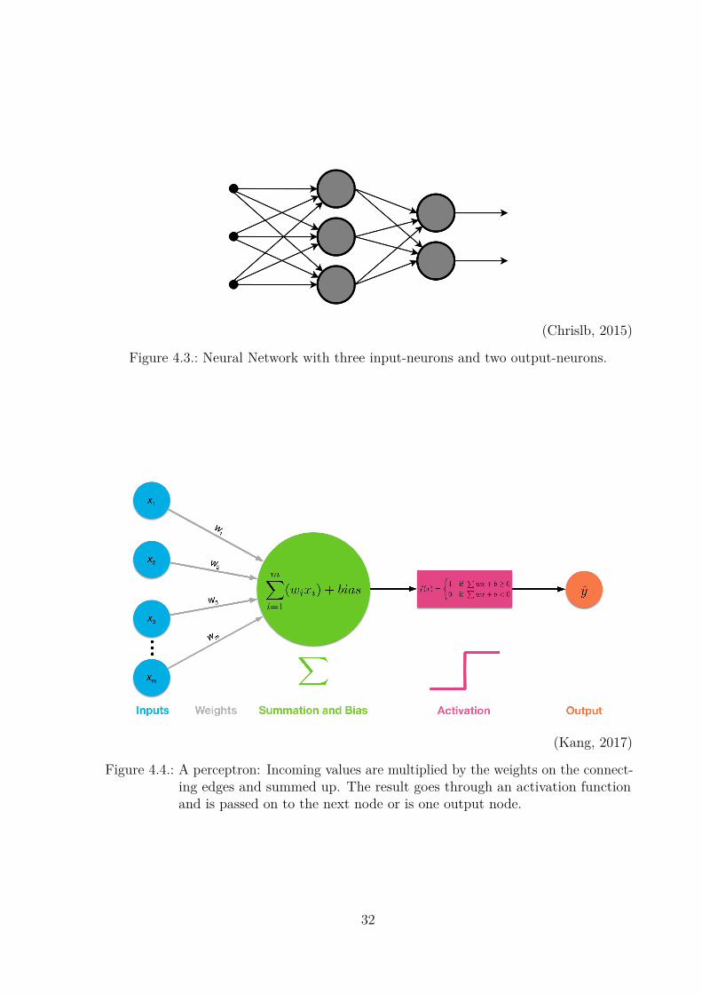
same example the network would have two output neurons, one for ’rise’ and one for’fall’ of the share. The output of these two neurons can be interpreted as the probabilityof this action being the correct one. Figure 4.3 shows how a Neural Network looksschematically.

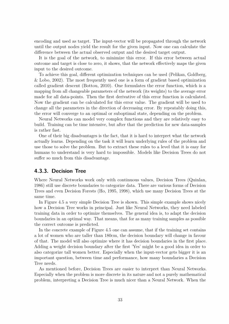
The question now is, how is the input propagated through the network to finally createthe values for the output neurons? Figure 4.4 shows, what happens in every single node.The inputs, coming either from the direct input or from previous nodes, are multipliedby the weights on the connecting edges and summed up. The bias can be ignored fornow. The resulting value is put into an activation function and passed on to the nextnode. If the node is an output node, it creates an output value.The weights are initialized randomly and are the only thing, that changes in the

network during its training phase. The activation function for the last layer will map allvalues from all nodes to probabilities, simply by dividing each one of them by the sum ofall values of output nodes. This activation function is called softmax and is normallyused in any categorization task.

When training a Neural Network for one step, one will use one labeled data-point. Thefeature vector of this data-point is used as input and its label is transformed in a one-hot

31

(Chrislb, 2015)

Figure 4.3.: Neural Network with three input-neurons and two output-neurons.

(Kang, 2017)

Figure 4.4.: A perceptron: Incoming values are multiplied by the weights on the connect-ing edges and summed up. The result goes through an activation functionand is passed on to the next node or is one output node.

32

encoding and used as target. The input-vector will be propagated through the networkuntil the output nodes yield the result for the given input. Now one can calculate thedifference between the actual observed output and the desired target output.It is the goal of the network, to minimize this error. If this error between actual

outcome and target is close to zero, it shows, that the network effectively maps the giveninput to the desired outcome.

To achieve this goal, different optimization techniques can be used (Pelikan, Goldberg,& Lobo, 2002). The most frequently used one is a form of gradient based optimizationcalled gradient descent (Bottou, 2010). One formulates the error function, which is amapping from all changeable parameters of the network (its weights) to the average errormade for all data-points. Then the first derivative of this error function is calculated.Now the gradient can be calculated for this error value. The gradient will be used tochange all the parameters in the direction of decreasing error. By repeatably doing this,the error will converge to an optimal or suboptimal state, depending on the problem.Neural Networks can model very complex functions and they are relatively easy to

build. Training can be time intensive, but after that the prediction for new data-samplesis rather fast.

One of their big disadvantages is the fact, that it is hard to interpret what the networkactually learns. Depending on the task it will learn underlying rules of the problem anduse those to solve the problem. But to extract these rules to a level that it is easy forhumans to understand is very hard to impossible. Models like Decision Trees do notsuffer so much from this disadvantage.

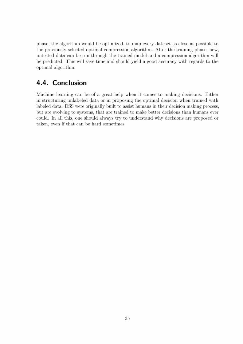
4.3.3. Decision TreeWhere Neural Networks work only with continuous values, Decision Trees (Quinlan,1986) still use discrete boundaries to categorize data. There are various forms of DecisionTrees and even Decision Forests (Ho, 1995, 1998), which use many Decision Trees at thesame time.

In Figure 4.5 a very simple Decision Tree is shown. This simple example shows nicelyhow a Decision Tree works in principal. Just like Neural Networks, they need labeledtraining data in order to optimize themselves. The general idea is, to adapt the decisionboundaries in an optimal way. That means, that for as many training samples as possiblethe correct outcome is predicted.

In the concrete example of Figure 4.5 one can assume, that if the training set containsa lot of women who are taller than 180cm, the decision boundary will change in favourof that. The model will also optimize where it has decision boundaries in the first place.Adding a weight decision boundary after the first ’Yes’ might be a good idea in order toalso categorize tall women better. Especially when the input-vector gets bigger it is animportant question, between time and performance, how many boundaries a DecisionTree needs.

As mentioned before, Decision Trees are easier to interpret than Neural Networks.Especially when the problem is more discrete in its nature and not a purely mathematicalproblem, interpreting a Decision Tree is much nicer than a Neural Network. When the

33

(Brownlee, 2016)

Figure 4.5.: Very simple example of a Decision Tree. The sex of a person is to bedetermined by other information about the person.

problem becomes very complex and high-dimensional, Decision Trees might performworse than more complex models, like Neural Networks.

4.3.4. Example: Compression AlgorithmsIn order to link the two chapters together, this section will describe, how a decision unitfor the task of choosing an optimal compression algorithm for new, unseen data couldlook like. Two situations could be imagined.The first is, that there are plenty of different datasets and none of them are tested

with a compression benchmark yet. In this case unsupervised learning could be used,to cluster the different data-samples into groups of similar data-samples. K-Means forexample could be used to cluster all the datasets in a fast and simple way. Then a certainnumber of data-samples could be run through a compression benchmark and the resultscould be analyzed. If many samples from one cluster are all compressed in a good oroptimal fashion by the same algorithm, one can choose that algorithm for the rest of thedata-samples from that cluster. This is a fast way to determine a compression algorithmfor every data-sample, without having to test all of them.

The second case would be, if there is already a number of data-samples, tested with abenchmark and their results are stored. One can now take every data-sample that isalready tested and use an optimal compression algorithm with regards to a metric. E.g.one could always take the algorithm with the best ratio as label for every data-sample. Bydoing this, a labeled dataset is created. This dataset can now be used for any supervisedlearning technique. A Neural Network or a Decision Tree with one dataset as inputand 38 different compression algorithms as output could be created. In the training

34

phase, the algorithm would be optimized, to map every dataset as close as possible tothe previously selected optimal compression algorithm. After the training phase, new,untested data can be run through the trained model and a compression algorithm willbe predicted. This will save time and should yield a good accuracy with regards to theoptimal algorithm.

4.4. ConclusionMachine learning can be of a great help when it comes to making decisions. Eitherin structuring unlabeled data or in proposing the optimal decision when trained withlabeled data. DSS were originally built to assist humans in their decision making process,but are evolving to systems, that are trained to make better decisions than humans evercould. In all this, one should always try to understand why decisions are proposed ortaken, even if that can be hard sometimes.

35

5. Final ConclusionThis paper covered two important topics. The compression benchmark of scientificdatasets and the theoretical construction of DSS.

It was shown, how important semantical differences in datasets can be, when com-pressing them. Data is defined by its underlying information and the structure of howthis information is stored. By acquiring and using this semantic information in a smartway, time an resources can be saved. Realizing that certain datasets will only compressvery little while other can be reduced to a fraction of their original size can safe preciousof time.

This benchmark study should show, that these differences between datasets exists andthat they can be visualized by rigorous testing. More importantly it should have shown,that creating an intuition for datasets and the information they represent can often savethe time and effort of analyzing ever single dataset.After the data is stored in an efficient way, it can then be used to gather further

informations and make decisions based on those insights. The usage of computer basedmodels, automated visualizations, data clustering or even supervised models can greatlyincrease the performance of any company or research institute. DSS help when makingdecisions based on complex and unstructured data.

Deciding if data will be compressible well and if so which algorithm will achieve optimalsolutions is of course also a decision problem. This is why all the Methods presented inthe second chapter can be applied to this problem.

This trend of big data will further increase. The amount of data produced every dayis rising exponentially. Systems for measurements are getting better every day. Socialmedia creates millions of data-samples in the form of images, videos, tweets or commentsevery second. Dealing with this massive amount of unstructured and high-dimensionaldata will be a big task of computer science and data science. The goal: To store data asefficient as possible, to automatically acquire all the information the dataset containsand finally, to make the optimal decisions based on the give data.

36

ReferencesAbel, D.-I. J. (2002). The data compression resource on the internet. Retrieved March

26, 2018, from www.data-compression.infoAcharya, T., & Tsai, P.-S. (2005). JPEG2000 Standard for Image Compression: Concepts,

Algorithms and VLSI Architectures. Hoboken, New Jersey: John Wiley & Sons.Altman, N. S. (1992). An introduction to kernel and nearest-neighbor nonparametric

regression. The American Statistician, 46 (3), 175-185. Retrieved from http://www.tandfonline.com/doi/abs/10.1080/00031305.1992.10475879 doi: 10.1080/00031305.1992.10475879

Arnott, D., & Pervan, G. (2008). Eight key issues for the decision support systemsdiscipline. Decision Support Systems, 44 (3), 657–672.

Berkhin, P. (2006). A survey of clustering data mining techniques. In Groupingmultidimensional data (pp. 25–71). Springer.

Bojarski, M., Testa, D. D., Dworakowski, D., Firner, B., Flepp, B., Goyal, P., . . . Zieba,K. (2016). End to end learning for self-driving cars. CoRR, abs/1604.07316 . Re-trieved from http://dblp.uni-trier.de/db/journals/corr/corr1604.html#BojarskiTDFFGJM16

Bottou, L. (2010). Large-scale machine learning with stochastic gradient descent. InProceedings of compstat’2010 (pp. 177–186). Springer.

Brandenburg, K., & Stoll, G. (1994). ISO/MPEG-1 audio: A generic standard for codingof high-quality digital audio. Journal of the Audio Engineering Society, 42 (10),780–792.

Brownlee, J. (2016). Classification and regression trees for machine learning. RetrievedMarch 26, 2018, from https://machinelearningmastery.com/classification-and-regression-trees-for-machine-learning/

Burba, F., Ferraty, F., & Vieu, P. (2009). k-nearest neighbour method in functionalnonparametric regression. Journal of Nonparametric Statistics, 21 (4), 453-469.Retrieved from https://doi.org/10.1080/10485250802668909 doi: 10.1080/10485250802668909

Caruana, R., & Niculescu-Mizil, A. (2006). An empirical comparison of supervisedlearning algorithms. In Proceedings of the 23rd international conference on machinelearning (pp. 161–168).

Chen, M., & Fowler, M. L. (2014). The importance of data compression for energyefficiency in sensor networks. In Hopkins university.

Chire. (2010). Different cluster analysis results on ’mouse’ data set. Retrieved March26, 2018, from https://en.wikipedia.org/wiki/K-means_clustering

Chrislb. (2015). Multi-layer neural network-english version. Retrieved March26, 2018, from https://commons.wikimedia.org/wiki/File:Single-Layer

37

_Neural_Network-Vector-Blank.svgCleary, J., & Witten, I. (1984). Data compression using adaptive coding and partial

string matching. IEEE transactions on Communications, 32 (4), 396–402.Collet, Y., & Turner, C. (2016). Smaller and faster data compression with zs-

tandard. Retrieved March 26, 2018, from https://code.facebook.com/posts/1658392934479273/smaller-and-faster-data-compression-with-zstandard/

Dempster, A. P., Laird, N. M., & Rubin, D. B. (1977). Maximum likelihood fromincomplete data via the em algorithm. Journal of the royal statistical society.Series B (methodological), 1–38.

Deorowicz, S. (2003). Silesia compression corpus. Retrieved March 26, 2018, fromhttp://sun.aei.polsl.pl/~sdeor/index.php?page=silesia

Ferrari, S., & Stengel, R. F. (2005). Smooth function approximation using neuralnetworks. IEEE Transactions on Neural Networks, 16 (1), 24–38.

Fredericks, X., Nagle, D. B., & Kranenburg, C. J. (2017). Eaarl coastal topographycape hatteras, north carolina, pre- and post-hurricane isabel, 2003. U.S. GeologicalSurvey. doi: 10.5066/f76w9879

Goldman, A. J., Hartman, J., Fisher, J., & Sarel, S. (2004, November 16). Method andtool for data mining in automatic decision making systems. Google Patents. (USPatent 6,820,070)

Haagsma, I., & Johanns, R. (1970). Decision support systems: An integrated anddistributed approach. WIT Transactions on Ecology and the Environment, 6 .

Hanke, M., Dinga, R., Häusler, C., Guntupalli, J., Casey, M., Kaule, F., & Stadler,J. (2015). High-resolution 7-tesla fmri data on the perception of musical genres– an extension to the studyforrest dataset [version 1; referees: 2 approved withreservations]. F1000Research, 4 (174). doi: 10.12688/f1000research.6679.1

Hastie, T., Tibshirani, R., & Friedman, J. (2009). Unsupervised learning. In Theelements of statistical learning (pp. 485–585). Springer.

Haykin, S., & Network, N. (2004). A comprehensive foundation. Neural networks,2 (2004), 41.

Hipp, D. R. (2015). Sqlite. Retrieved March 26, 2018, from https://www.sqlite.org/download.html

Ho, T. K. (1995). Random decision forests. In Document analysis and recognition, 1995.,proceedings of the third international conference on (Vol. 1, pp. 278–282).

Ho, T. K. (1998). The random subspace method for constructing decision forests. IEEEtransactions on pattern analysis and machine intelligence, 20 (8), 832–844.

Hochreiter, S., & Schmidhuber, J. (1997, November). Long short-term memory. NeuralComput., 9 (8), 1735–1780. Retrieved from http://dx.doi.org/10.1162/neco.1997.9.8.1735 doi: 10.1162/neco.1997.9.8.1735

Huang, W., Nakamori, Y., & Wang, S.-Y. (2005). Forecasting stock market movementdirection with support vector machine. Computers & Operations Research, 32 (10),2513–2522.

Huffman, D. A. (1952). A method for the construction of minimum-redundancy codes.Proceedings of the IRE , 40 (9), 1098–1101.

38

Kang, N. (2017). Multi-layer neural networks with sigmoid function— deep learningfor rookies. Retrieved March 26, 2018, from https://towardsdatascience.com/multi-layer-neural-networks-with-sigmoid-function-deep-learning-for-rookies-2-bf464f09eb7f

Katz, P. (1991, September 24). String searcher, and compressor using same. GooglePatents. Retrieved from https://www.google.com/patents/US5051745 (USPatent 5,051,745)

Kohonen, T., & Honkela, T. (2007). Kohonen network. Scholarpedia, 2 (1), 1568. (revision#122029) doi: 10.4249/scholarpedia.1568

Lavrenko, V. (2014). K-means clustering: how it works. Retrieved March 26, 2018, fromhttp://bit.ly/K-means

LeCun, Y., Boser, B., Denker, J. S., Henderson, D., Howard, R. E., Hubbard, W., &Jackel, L. D. (1989, December). Backpropagation applied to handwritten zip coderecognition. Neural Comput., 1 (4), 541–551. Retrieved from http://dx.doi.org/10.1162/neco.1989.1.4.541 doi: 10.1162/neco.1989.1.4.541

Lelewer, D. A., & Hirschberg, D. S. (1987, September). Data compression. ACMComput. Surv., 19 (3), 261–296. Retrieved from http://doi.acm.org/10.1145/45072.45074 doi: 10.1145/45072.45074

Li, T., Feng, S., & Li, L. X. (2001). Information visualization for intelligent decisionsupport systems. Knowledge-Based Systems, 14 (5-6), 259–262.

Lloyd, S. (1982). Least squares quantization in pcm. IEEE transactions on informationtheory, 28 (2), 129–137.

MacQueen, J. (1967). Some methods for classification and analysis of multivariateobservations. In Proceedings of the fifth berkeley symposium on mathematicalstatistics and probability, volume 1: Statistics (pp. 281–297). Berkeley, Calif.:University of California Press. Retrieved from https://projecteuclid.org/euclid.bsmsp/1200512992

Mahoney, M. (2012). Data compression explained. mattmahoney. net, updated May, 7 .Marakas, G. M. (2003). Decision support systems in the 21st century (Vol. 134). Prentice

Hall Upper Saddle River, NJ.Nevill-Manning, C. G., & Witten, I. H. (1999). Protein is incompressible. In Data

compression conference, 1999. proceedings. dcc’99 (pp. 257–266).Pelikan, M., Goldberg, D. E., & Lobo, F. G. (2002). A survey of optimization by building

and using probabilistic models. Computational optimization and applications, 21 (1),5–20.

Portmann, F. T., Siebert, S., Bauer, C., & Döll, P. (2008). Global dataset of monthlygrowing areas of 26 irrigated crops : version 1.0 (No. 6).

Power, D. J., Sharda, R., & Burstein, F. (2015). Decision support systems. Wiley OnlineLibrary.

Quinlan, J. R. (1986). Induction of decision trees. Machine learning, 1 (1), 81–106.Robinson, A., & Cherry, C. (1967). Results of a prototype television bandwidth

compression scheme. Proceedings of the IEEE , 55 (3), 356–364.Salomon, D., & Motta, G. (2010). Handbook of data compression. Springer Science &

Business Media.

39

Sayood, K. (2000). Introduction to data compression. Morgan Kaufman Publishers.Schmidhuber, J. (2015). Deep learning in neural networks: An overview. Neural networks,

61 , 85–117.Seeger, M., et al. (2001). Learning with labeled and unlabeled data (Tech. Rep.). technical

report, University of Edinburgh.Shim, J. P., Warkentin, M., Courtney, J. F., Power, D. J., Sharda, R., & Carlsson, C.

(2002). Past, present, and future of decision support technology. Decision supportsystems, 33 (2), 111–126.

Sikora, T. (1997, Feb). The MPEG-4 video standard verification model. IEEETransactions on Circuits and Systems for Video Technology, 7 (1), 19-31. doi:10.1109/76.554415

SlidePlay. ( 2016). Lempel-ziv compression techniques. Retrieved March 26, 2018, fromhttp://slideplayer.com/slide/5173265/

Storer, J. A. (1985). Textual substitution techniques for data compression. In A. Apos-tolico & Z. Galil (Eds.), Combinatorial algorithms on words (pp. 111–129). Berlin,Heidelberg: Springer Berlin Heidelberg.

Welch, T. A. (1984, June). A technique for high-performance data compression. Computer ,17 (6), 8-19. doi: 10.1109/MC.1984.1659158

Witten, I. H., Moffat, A., & Bell, T. C. (1999). Managing gigabytes: Compressing andindexing documents and images (2nd ed.). San Francisco, CA: Morgan Kaufmann.

Wolpert, D. H., & Macready, W. G. (1997, April). No free lunch theorems for optimization.Trans. Evol. Comp, 1 (1), 67–82. Retrieved from http://dx.doi.org/10.1109/4235.585893 doi: 10.1109/4235.585893

Zhang, X., Fuehres, H., & Gloor, P. A. (2011). Predicting stock market indicatorsthrough twitter “i hope it is not as bad as i fear”. Procedia-Social and BehavioralSciences, 26 , 55–62.

Ziv, J., & Lempel, A. (1977). A universal algorithm for sequential data compression.IEEE TRANSACTIONS ON INFORMATION THEORY , 23 (3), 337–343.

Ziv, J., & Lempel, A. (1978, September). Compression of individual sequences viavariable-rate coding. IEEE Transactions on Information Theory, 24 (5), 530-536.doi: 10.1109/TIT.1978.1055934

40

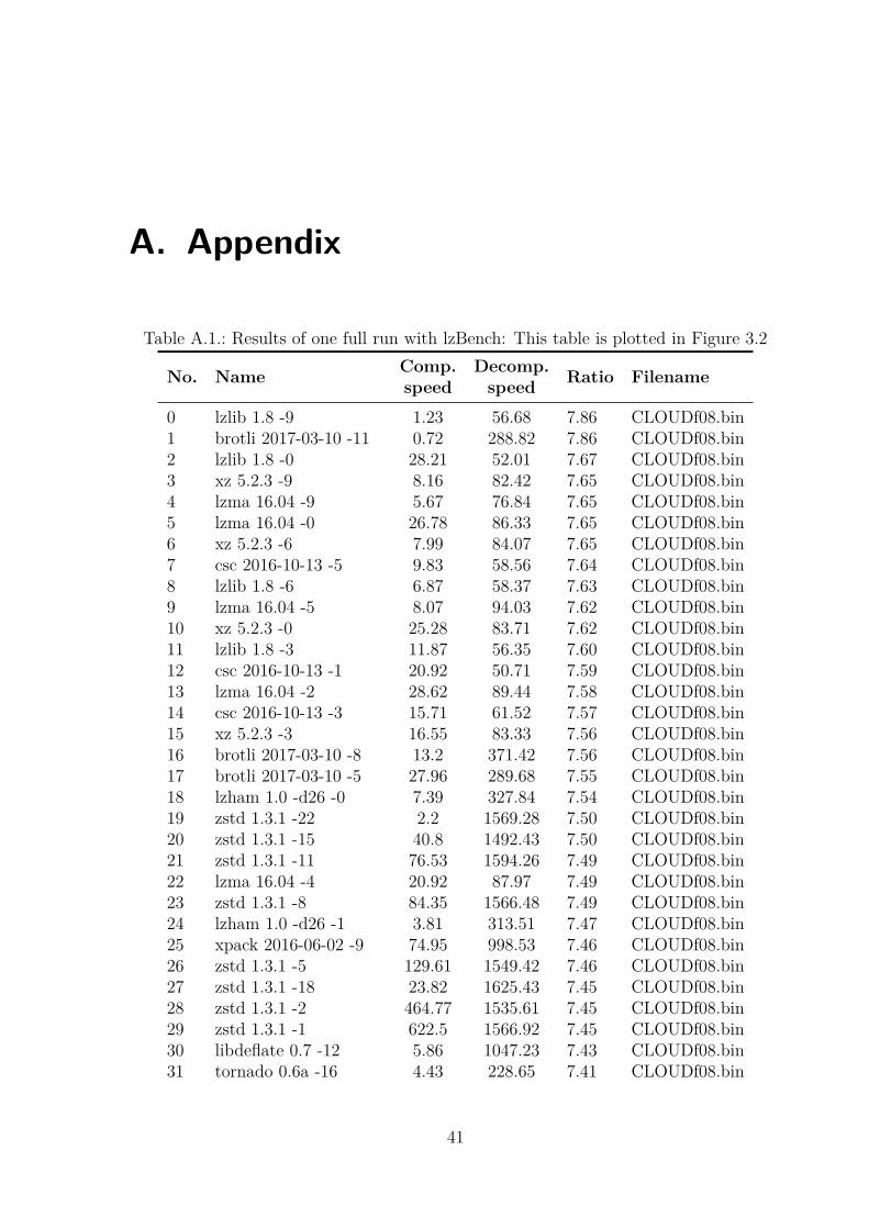
A. Appendix

Table A.1.: Results of one full run with lzBench: This table is plotted in Figure 3.2

No. Name Comp.speed

Decomp.speed Ratio Filename

0 lzlib 1.8 -9 1.23 56.68 7.86 CLOUDf08.bin1 brotli 2017-03-10 -11 0.72 288.82 7.86 CLOUDf08.bin2 lzlib 1.8 -0 28.21 52.01 7.67 CLOUDf08.bin3 xz 5.2.3 -9 8.16 82.42 7.65 CLOUDf08.bin4 lzma 16.04 -9 5.67 76.84 7.65 CLOUDf08.bin5 lzma 16.04 -0 26.78 86.33 7.65 CLOUDf08.bin6 xz 5.2.3 -6 7.99 84.07 7.65 CLOUDf08.bin7 csc 2016-10-13 -5 9.83 58.56 7.64 CLOUDf08.bin8 lzlib 1.8 -6 6.87 58.37 7.63 CLOUDf08.bin9 lzma 16.04 -5 8.07 94.03 7.62 CLOUDf08.bin10 xz 5.2.3 -0 25.28 83.71 7.62 CLOUDf08.bin11 lzlib 1.8 -3 11.87 56.35 7.60 CLOUDf08.bin12 csc 2016-10-13 -1 20.92 50.71 7.59 CLOUDf08.bin13 lzma 16.04 -2 28.62 89.44 7.58 CLOUDf08.bin14 csc 2016-10-13 -3 15.71 61.52 7.57 CLOUDf08.bin15 xz 5.2.3 -3 16.55 83.33 7.56 CLOUDf08.bin16 brotli 2017-03-10 -8 13.2 371.42 7.56 CLOUDf08.bin17 brotli 2017-03-10 -5 27.96 289.68 7.55 CLOUDf08.bin18 lzham 1.0 -d26 -0 7.39 327.84 7.54 CLOUDf08.bin19 zstd 1.3.1 -22 2.2 1569.28 7.50 CLOUDf08.bin20 zstd 1.3.1 -15 40.8 1492.43 7.50 CLOUDf08.bin21 zstd 1.3.1 -11 76.53 1594.26 7.49 CLOUDf08.bin22 lzma 16.04 -4 20.92 87.97 7.49 CLOUDf08.bin23 zstd 1.3.1 -8 84.35 1566.48 7.49 CLOUDf08.bin24 lzham 1.0 -d26 -1 3.81 313.51 7.47 CLOUDf08.bin25 xpack 2016-06-02 -9 74.95 998.53 7.46 CLOUDf08.bin26 zstd 1.3.1 -5 129.61 1549.42 7.46 CLOUDf08.bin27 zstd 1.3.1 -18 23.82 1625.43 7.45 CLOUDf08.bin28 zstd 1.3.1 -2 464.77 1535.61 7.45 CLOUDf08.bin29 zstd 1.3.1 -1 622.5 1566.92 7.45 CLOUDf08.bin30 libdeflate 0.7 -12 5.86 1047.23 7.43 CLOUDf08.bin31 tornado 0.6a -16 4.43 228.65 7.41 CLOUDf08.bin

41

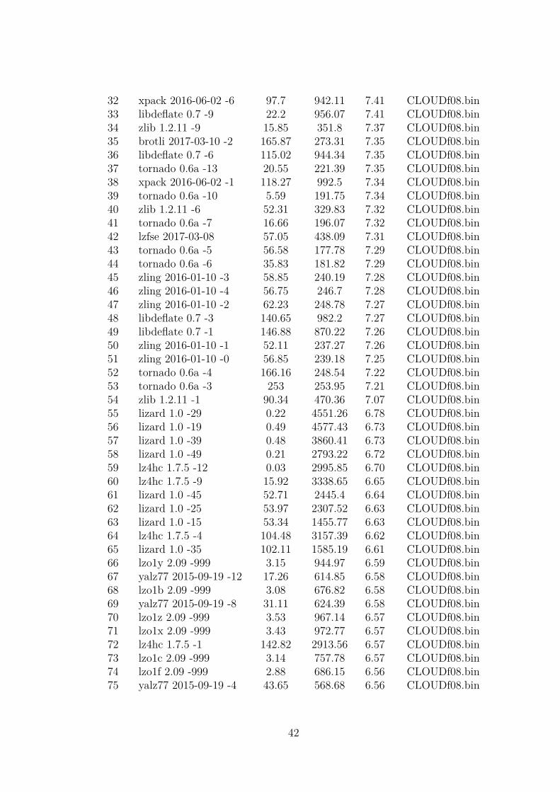
32 xpack 2016-06-02 -6 97.7 942.11 7.41 CLOUDf08.bin33 libdeflate 0.7 -9 22.2 956.07 7.41 CLOUDf08.bin34 zlib 1.2.11 -9 15.85 351.8 7.37 CLOUDf08.bin35 brotli 2017-03-10 -2 165.87 273.31 7.35 CLOUDf08.bin36 libdeflate 0.7 -6 115.02 944.34 7.35 CLOUDf08.bin37 tornado 0.6a -13 20.55 221.39 7.35 CLOUDf08.bin38 xpack 2016-06-02 -1 118.27 992.5 7.34 CLOUDf08.bin39 tornado 0.6a -10 5.59 191.75 7.34 CLOUDf08.bin40 zlib 1.2.11 -6 52.31 329.83 7.32 CLOUDf08.bin41 tornado 0.6a -7 16.66 196.07 7.32 CLOUDf08.bin42 lzfse 2017-03-08 57.05 438.09 7.31 CLOUDf08.bin43 tornado 0.6a -5 56.58 177.78 7.29 CLOUDf08.bin44 tornado 0.6a -6 35.83 181.82 7.29 CLOUDf08.bin45 zling 2016-01-10 -3 58.85 240.19 7.28 CLOUDf08.bin46 zling 2016-01-10 -4 56.75 246.7 7.28 CLOUDf08.bin47 zling 2016-01-10 -2 62.23 248.78 7.27 CLOUDf08.bin48 libdeflate 0.7 -3 140.65 982.2 7.27 CLOUDf08.bin49 libdeflate 0.7 -1 146.88 870.22 7.26 CLOUDf08.bin50 zling 2016-01-10 -1 52.11 237.27 7.26 CLOUDf08.bin51 zling 2016-01-10 -0 56.85 239.18 7.25 CLOUDf08.bin52 tornado 0.6a -4 166.16 248.54 7.22 CLOUDf08.bin53 tornado 0.6a -3 253 253.95 7.21 CLOUDf08.bin54 zlib 1.2.11 -1 90.34 470.36 7.07 CLOUDf08.bin55 lizard 1.0 -29 0.22 4551.26 6.78 CLOUDf08.bin56 lizard 1.0 -19 0.49 4577.43 6.73 CLOUDf08.bin57 lizard 1.0 -39 0.48 3860.41 6.73 CLOUDf08.bin58 lizard 1.0 -49 0.21 2793.22 6.72 CLOUDf08.bin59 lz4hc 1.7.5 -12 0.03 2995.85 6.70 CLOUDf08.bin60 lz4hc 1.7.5 -9 15.92 3338.65 6.65 CLOUDf08.bin61 lizard 1.0 -45 52.71 2445.4 6.64 CLOUDf08.bin62 lizard 1.0 -25 53.97 2307.52 6.63 CLOUDf08.bin63 lizard 1.0 -15 53.34 1455.77 6.63 CLOUDf08.bin64 lz4hc 1.7.5 -4 104.48 3157.39 6.62 CLOUDf08.bin65 lizard 1.0 -35 102.11 1585.19 6.61 CLOUDf08.bin66 lzo1y 2.09 -999 3.15 944.97 6.59 CLOUDf08.bin67 yalz77 2015-09-19 -12 17.26 614.85 6.58 CLOUDf08.bin68 lzo1b 2.09 -999 3.08 676.82 6.58 CLOUDf08.bin69 yalz77 2015-09-19 -8 31.11 624.39 6.58 CLOUDf08.bin70 lzo1z 2.09 -999 3.53 967.14 6.57 CLOUDf08.bin71 lzo1x 2.09 -999 3.43 972.77 6.57 CLOUDf08.bin72 lz4hc 1.7.5 -1 142.82 2913.56 6.57 CLOUDf08.bin73 lzo1c 2.09 -999 3.14 757.78 6.57 CLOUDf08.bin74 lzo1f 2.09 -999 2.88 686.15 6.56 CLOUDf08.bin75 yalz77 2015-09-19 -4 43.65 568.68 6.56 CLOUDf08.bin

42

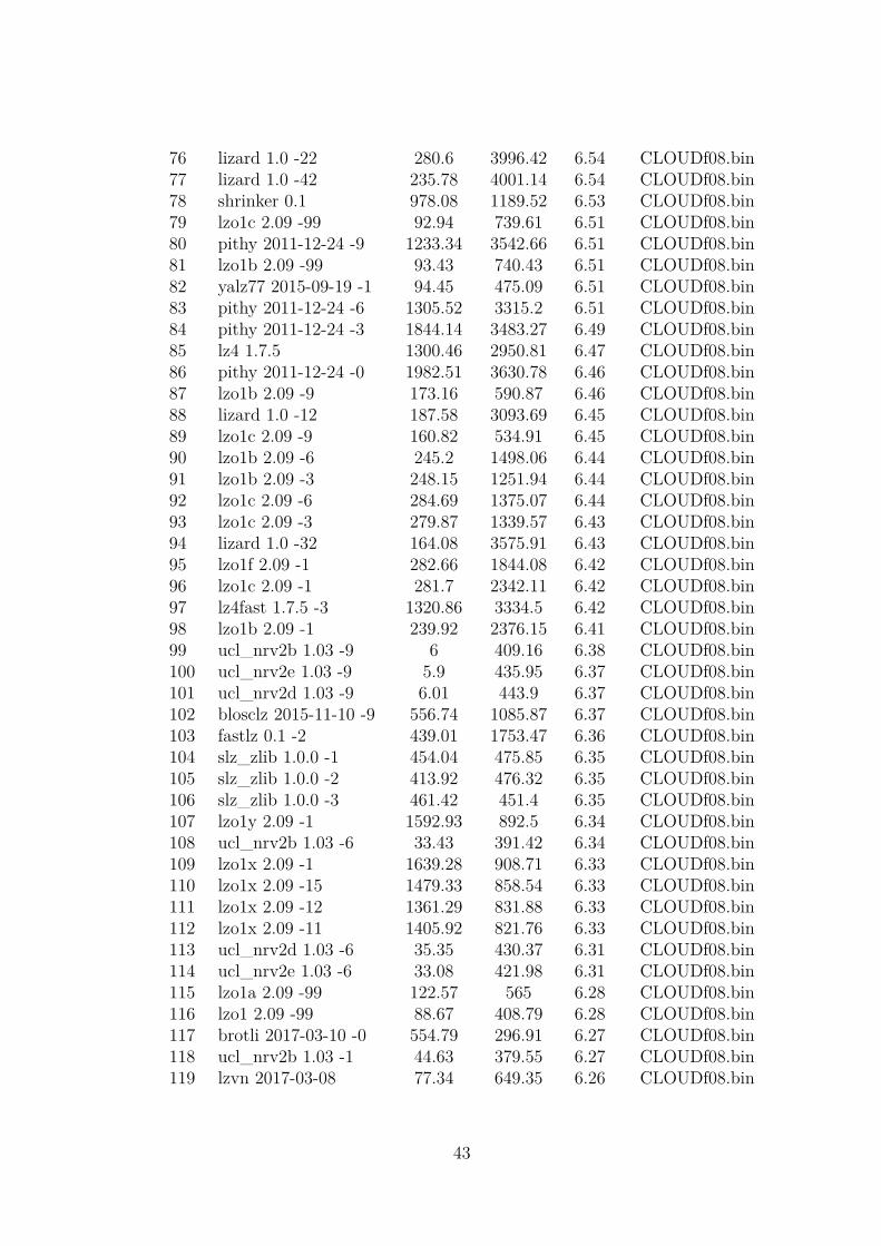
76 lizard 1.0 -22 280.6 3996.42 6.54 CLOUDf08.bin77 lizard 1.0 -42 235.78 4001.14 6.54 CLOUDf08.bin78 shrinker 0.1 978.08 1189.52 6.53 CLOUDf08.bin79 lzo1c 2.09 -99 92.94 739.61 6.51 CLOUDf08.bin80 pithy 2011-12-24 -9 1233.34 3542.66 6.51 CLOUDf08.bin81 lzo1b 2.09 -99 93.43 740.43 6.51 CLOUDf08.bin82 yalz77 2015-09-19 -1 94.45 475.09 6.51 CLOUDf08.bin83 pithy 2011-12-24 -6 1305.52 3315.2 6.51 CLOUDf08.bin84 pithy 2011-12-24 -3 1844.14 3483.27 6.49 CLOUDf08.bin85 lz4 1.7.5 1300.46 2950.81 6.47 CLOUDf08.bin86 pithy 2011-12-24 -0 1982.51 3630.78 6.46 CLOUDf08.bin87 lzo1b 2.09 -9 173.16 590.87 6.46 CLOUDf08.bin88 lizard 1.0 -12 187.58 3093.69 6.45 CLOUDf08.bin89 lzo1c 2.09 -9 160.82 534.91 6.45 CLOUDf08.bin90 lzo1b 2.09 -6 245.2 1498.06 6.44 CLOUDf08.bin91 lzo1b 2.09 -3 248.15 1251.94 6.44 CLOUDf08.bin92 lzo1c 2.09 -6 284.69 1375.07 6.44 CLOUDf08.bin93 lzo1c 2.09 -3 279.87 1339.57 6.43 CLOUDf08.bin94 lizard 1.0 -32 164.08 3575.91 6.43 CLOUDf08.bin95 lzo1f 2.09 -1 282.66 1844.08 6.42 CLOUDf08.bin96 lzo1c 2.09 -1 281.7 2342.11 6.42 CLOUDf08.bin97 lz4fast 1.7.5 -3 1320.86 3334.5 6.42 CLOUDf08.bin98 lzo1b 2.09 -1 239.92 2376.15 6.41 CLOUDf08.bin99 ucl_nrv2b 1.03 -9 6 409.16 6.38 CLOUDf08.bin100 ucl_nrv2e 1.03 -9 5.9 435.95 6.37 CLOUDf08.bin101 ucl_nrv2d 1.03 -9 6.01 443.9 6.37 CLOUDf08.bin102 blosclz 2015-11-10 -9 556.74 1085.87 6.37 CLOUDf08.bin103 fastlz 0.1 -2 439.01 1753.47 6.36 CLOUDf08.bin104 slz_zlib 1.0.0 -1 454.04 475.85 6.35 CLOUDf08.bin105 slz_zlib 1.0.0 -2 413.92 476.32 6.35 CLOUDf08.bin106 slz_zlib 1.0.0 -3 461.42 451.4 6.35 CLOUDf08.bin107 lzo1y 2.09 -1 1592.93 892.5 6.34 CLOUDf08.bin108 ucl_nrv2b 1.03 -6 33.43 391.42 6.34 CLOUDf08.bin109 lzo1x 2.09 -1 1639.28 908.71 6.33 CLOUDf08.bin110 lzo1x 2.09 -15 1479.33 858.54 6.33 CLOUDf08.bin111 lzo1x 2.09 -12 1361.29 831.88 6.33 CLOUDf08.bin112 lzo1x 2.09 -11 1405.92 821.76 6.33 CLOUDf08.bin113 ucl_nrv2d 1.03 -6 35.35 430.37 6.31 CLOUDf08.bin114 ucl_nrv2e 1.03 -6 33.08 421.98 6.31 CLOUDf08.bin115 lzo1a 2.09 -99 122.57 565 6.28 CLOUDf08.bin116 lzo1 2.09 -99 88.67 408.79 6.28 CLOUDf08.bin117 brotli 2017-03-10 -0 554.79 296.91 6.27 CLOUDf08.bin118 ucl_nrv2b 1.03 -1 44.63 379.55 6.27 CLOUDf08.bin119 lzvn 2017-03-08 77.34 649.35 6.26 CLOUDf08.bin

43

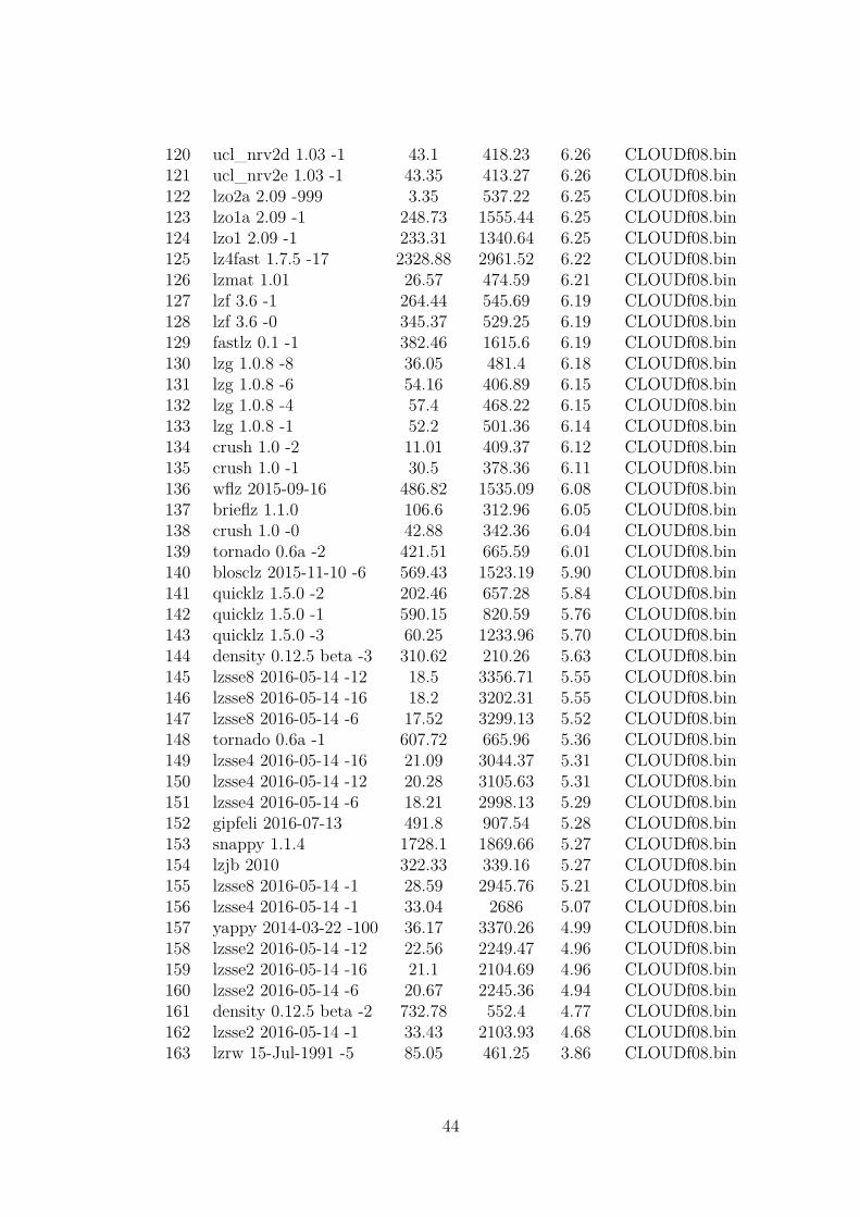
120 ucl_nrv2d 1.03 -1 43.1 418.23 6.26 CLOUDf08.bin121 ucl_nrv2e 1.03 -1 43.35 413.27 6.26 CLOUDf08.bin122 lzo2a 2.09 -999 3.35 537.22 6.25 CLOUDf08.bin123 lzo1a 2.09 -1 248.73 1555.44 6.25 CLOUDf08.bin124 lzo1 2.09 -1 233.31 1340.64 6.25 CLOUDf08.bin125 lz4fast 1.7.5 -17 2328.88 2961.52 6.22 CLOUDf08.bin126 lzmat 1.01 26.57 474.59 6.21 CLOUDf08.bin127 lzf 3.6 -1 264.44 545.69 6.19 CLOUDf08.bin128 lzf 3.6 -0 345.37 529.25 6.19 CLOUDf08.bin129 fastlz 0.1 -1 382.46 1615.6 6.19 CLOUDf08.bin130 lzg 1.0.8 -8 36.05 481.4 6.18 CLOUDf08.bin131 lzg 1.0.8 -6 54.16 406.89 6.15 CLOUDf08.bin132 lzg 1.0.8 -4 57.4 468.22 6.15 CLOUDf08.bin133 lzg 1.0.8 -1 52.2 501.36 6.14 CLOUDf08.bin134 crush 1.0 -2 11.01 409.37 6.12 CLOUDf08.bin135 crush 1.0 -1 30.5 378.36 6.11 CLOUDf08.bin136 wflz 2015-09-16 486.82 1535.09 6.08 CLOUDf08.bin137 brieflz 1.1.0 106.6 312.96 6.05 CLOUDf08.bin138 crush 1.0 -0 42.88 342.36 6.04 CLOUDf08.bin139 tornado 0.6a -2 421.51 665.59 6.01 CLOUDf08.bin140 blosclz 2015-11-10 -6 569.43 1523.19 5.90 CLOUDf08.bin141 quicklz 1.5.0 -2 202.46 657.28 5.84 CLOUDf08.bin142 quicklz 1.5.0 -1 590.15 820.59 5.76 CLOUDf08.bin143 quicklz 1.5.0 -3 60.25 1233.96 5.70 CLOUDf08.bin144 density 0.12.5 beta -3 310.62 210.26 5.63 CLOUDf08.bin145 lzsse8 2016-05-14 -12 18.5 3356.71 5.55 CLOUDf08.bin146 lzsse8 2016-05-14 -16 18.2 3202.31 5.55 CLOUDf08.bin147 lzsse8 2016-05-14 -6 17.52 3299.13 5.52 CLOUDf08.bin148 tornado 0.6a -1 607.72 665.96 5.36 CLOUDf08.bin149 lzsse4 2016-05-14 -16 21.09 3044.37 5.31 CLOUDf08.bin150 lzsse4 2016-05-14 -12 20.28 3105.63 5.31 CLOUDf08.bin151 lzsse4 2016-05-14 -6 18.21 2998.13 5.29 CLOUDf08.bin152 gipfeli 2016-07-13 491.8 907.54 5.28 CLOUDf08.bin153 snappy 1.1.4 1728.1 1869.66 5.27 CLOUDf08.bin154 lzjb 2010 322.33 339.16 5.27 CLOUDf08.bin155 lzsse8 2016-05-14 -1 28.59 2945.76 5.21 CLOUDf08.bin156 lzsse4 2016-05-14 -1 33.04 2686 5.07 CLOUDf08.bin157 yappy 2014-03-22 -100 36.17 3370.26 4.99 CLOUDf08.bin158 lzsse2 2016-05-14 -12 22.56 2249.47 4.96 CLOUDf08.bin159 lzsse2 2016-05-14 -16 21.1 2104.69 4.96 CLOUDf08.bin160 lzsse2 2016-05-14 -6 20.67 2245.36 4.94 CLOUDf08.bin161 density 0.12.5 beta -2 732.78 552.4 4.77 CLOUDf08.bin162 lzsse2 2016-05-14 -1 33.43 2103.93 4.68 CLOUDf08.bin163 lzrw 15-Jul-1991 -5 85.05 461.25 3.86 CLOUDf08.bin

44

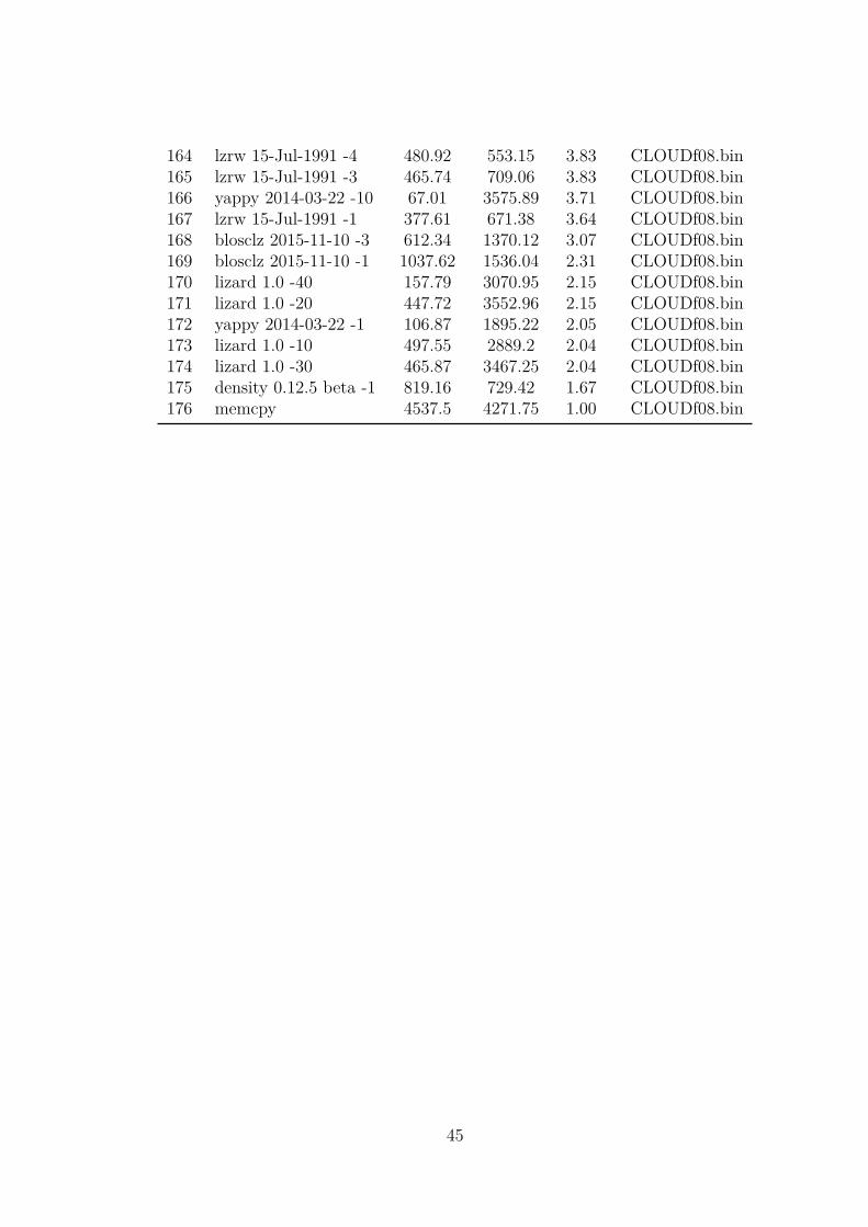
164 lzrw 15-Jul-1991 -4 480.92 553.15 3.83 CLOUDf08.bin165 lzrw 15-Jul-1991 -3 465.74 709.06 3.83 CLOUDf08.bin166 yappy 2014-03-22 -10 67.01 3575.89 3.71 CLOUDf08.bin167 lzrw 15-Jul-1991 -1 377.61 671.38 3.64 CLOUDf08.bin168 blosclz 2015-11-10 -3 612.34 1370.12 3.07 CLOUDf08.bin169 blosclz 2015-11-10 -1 1037.62 1536.04 2.31 CLOUDf08.bin170 lizard 1.0 -40 157.79 3070.95 2.15 CLOUDf08.bin171 lizard 1.0 -20 447.72 3552.96 2.15 CLOUDf08.bin172 yappy 2014-03-22 -1 106.87 1895.22 2.05 CLOUDf08.bin173 lizard 1.0 -10 497.55 2889.2 2.04 CLOUDf08.bin174 lizard 1.0 -30 465.87 3467.25 2.04 CLOUDf08.bin175 density 0.12.5 beta -1 819.16 729.42 1.67 CLOUDf08.bin176 memcpy 4537.5 4271.75 1.00 CLOUDf08.bin

45

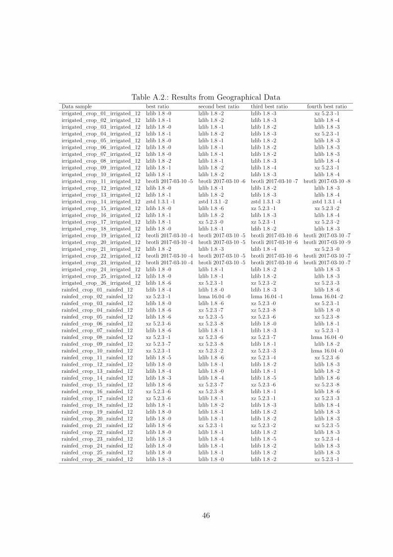
Table A.2.: Results from Geographical DataData sample best ratio second best ratio third best ratio fourth best ratioirrigated_crop_01_irrigated_12 lzlib 1.8 -0 lzlib 1.8 -2 lzlib 1.8 -3 xz 5.2.3 -1irrigated_crop_02_irrigated_12 lzlib 1.8 -1 lzlib 1.8 -2 lzlib 1.8 -3 lzlib 1.8 -4irrigated_crop_03_irrigated_12 lzlib 1.8 -0 lzlib 1.8 -1 lzlib 1.8 -2 lzlib 1.8 -3irrigated_crop_04_irrigated_12 lzlib 1.8 -1 lzlib 1.8 -2 lzlib 1.8 -3 xz 5.2.3 -1irrigated_crop_05_irrigated_12 lzlib 1.8 -0 lzlib 1.8 -1 lzlib 1.8 -2 lzlib 1.8 -3irrigated_crop_06_irrigated_12 lzlib 1.8 -0 lzlib 1.8 -1 lzlib 1.8 -2 lzlib 1.8 -3irrigated_crop_07_irrigated_12 lzlib 1.8 -0 lzlib 1.8 -1 lzlib 1.8 -2 lzlib 1.8 -3irrigated_crop_08_irrigated_12 lzlib 1.8 -2 lzlib 1.8 -1 lzlib 1.8 -3 lzlib 1.8 -4irrigated_crop_09_irrigated_12 lzlib 1.8 -1 lzlib 1.8 -2 lzlib 1.8 -4 xz 5.2.3 -1irrigated_crop_10_irrigated_12 lzlib 1.8 -1 lzlib 1.8 -2 lzlib 1.8 -3 lzlib 1.8 -4irrigated_crop_11_irrigated_12 brotli 2017-03-10 -5 brotli 2017-03-10 -6 brotli 2017-03-10 -7 brotli 2017-03-10 -8irrigated_crop_12_irrigated_12 lzlib 1.8 -0 lzlib 1.8 -1 lzlib 1.8 -2 lzlib 1.8 -3irrigated_crop_13_irrigated_12 lzlib 1.8 -1 lzlib 1.8 -2 lzlib 1.8 -3 lzlib 1.8 -4irrigated_crop_14_irrigated_12 zstd 1.3.1 -1 zstd 1.3.1 -2 zstd 1.3.1 -3 zstd 1.3.1 -4irrigated_crop_15_irrigated_12 lzlib 1.8 -0 lzlib 1.8 -6 xz 5.2.3 -1 xz 5.2.3 -2irrigated_crop_16_irrigated_12 lzlib 1.8 -1 lzlib 1.8 -2 lzlib 1.8 -3 lzlib 1.8 -4irrigated_crop_17_irrigated_12 lzlib 1.8 -1 xz 5.2.3 -0 xz 5.2.3 -1 xz 5.2.3 -2irrigated_crop_18_irrigated_12 lzlib 1.8 -0 lzlib 1.8 -1 lzlib 1.8 -2 lzlib 1.8 -3irrigated_crop_19_irrigated_12 brotli 2017-03-10 -4 brotli 2017-03-10 -5 brotli 2017-03-10 -6 brotli 2017-03-10 -7irrigated_crop_20_irrigated_12 brotli 2017-03-10 -4 brotli 2017-03-10 -5 brotli 2017-03-10 -6 brotli 2017-03-10 -9irrigated_crop_21_irrigated_12 lzlib 1.8 -2 lzlib 1.8 -3 lzlib 1.8 -4 xz 5.2.3 -0irrigated_crop_22_irrigated_12 brotli 2017-03-10 -4 brotli 2017-03-10 -5 brotli 2017-03-10 -6 brotli 2017-03-10 -7irrigated_crop_23_irrigated_12 brotli 2017-03-10 -4 brotli 2017-03-10 -5 brotli 2017-03-10 -6 brotli 2017-03-10 -7irrigated_crop_24_irrigated_12 lzlib 1.8 -0 lzlib 1.8 -1 lzlib 1.8 -2 lzlib 1.8 -3irrigated_crop_25_irrigated_12 lzlib 1.8 -0 lzlib 1.8 -1 lzlib 1.8 -2 lzlib 1.8 -3irrigated_crop_26_irrigated_12 lzlib 1.8 -6 xz 5.2.3 -1 xz 5.2.3 -2 xz 5.2.3 -3rainfed_crop_01_rainfed_12 lzlib 1.8 -4 lzlib 1.8 -0 lzlib 1.8 -3 lzlib 1.8 -6rainfed_crop_02_rainfed_12 xz 5.2.3 -1 lzma 16.04 -0 lzma 16.04 -1 lzma 16.04 -2rainfed_crop_03_rainfed_12 lzlib 1.8 -0 lzlib 1.8 -6 xz 5.2.3 -0 xz 5.2.3 -1rainfed_crop_04_rainfed_12 lzlib 1.8 -6 xz 5.2.3 -7 xz 5.2.3 -8 lzlib 1.8 -0rainfed_crop_05_rainfed_12 lzlib 1.8 -6 xz 5.2.3 -5 xz 5.2.3 -6 xz 5.2.3 -8rainfed_crop_06_rainfed_12 xz 5.2.3 -6 xz 5.2.3 -8 lzlib 1.8 -0 lzlib 1.8 -1rainfed_crop_07_rainfed_12 lzlib 1.8 -6 lzlib 1.8 -1 lzlib 1.8 -3 xz 5.2.3 -1rainfed_crop_08_rainfed_12 xz 5.2.3 -1 xz 5.2.3 -6 xz 5.2.3 -7 lzma 16.04 -0rainfed_crop_09_rainfed_12 xz 5.2.3 -7 xz 5.2.3 -8 lzlib 1.8 -1 lzlib 1.8 -2rainfed_crop_10_rainfed_12 xz 5.2.3 -1 xz 5.2.3 -2 xz 5.2.3 -3 lzma 16.04 -0rainfed_crop_11_rainfed_12 lzlib 1.8 -5 lzlib 1.8 -6 xz 5.2.3 -4 xz 5.2.3 -6rainfed_crop_12_rainfed_12 lzlib 1.8 -0 lzlib 1.8 -1 lzlib 1.8 -2 lzlib 1.8 -3rainfed_crop_13_rainfed_12 lzlib 1.8 -4 lzlib 1.8 -0 lzlib 1.8 -1 lzlib 1.8 -2rainfed_crop_14_rainfed_12 lzlib 1.8 -3 lzlib 1.8 -4 lzlib 1.8 -5 lzlib 1.8 -6rainfed_crop_15_rainfed_12 lzlib 1.8 -6 xz 5.2.3 -7 xz 5.2.3 -6 xz 5.2.3 -8rainfed_crop_16_rainfed_12 xz 5.2.3 -6 xz 5.2.3 -8 lzlib 1.8 -1 lzlib 1.8 -6rainfed_crop_17_rainfed_12 xz 5.2.3 -6 lzlib 1.8 -1 xz 5.2.3 -1 xz 5.2.3 -3rainfed_crop_18_rainfed_12 lzlib 1.8 -1 lzlib 1.8 -2 lzlib 1.8 -3 lzlib 1.8 -4rainfed_crop_19_rainfed_12 lzlib 1.8 -0 lzlib 1.8 -1 lzlib 1.8 -2 lzlib 1.8 -3rainfed_crop_20_rainfed_12 lzlib 1.8 -0 lzlib 1.8 -1 lzlib 1.8 -2 lzlib 1.8 -3rainfed_crop_21_rainfed_12 lzlib 1.8 -6 xz 5.2.3 -1 xz 5.2.3 -2 xz 5.2.3 -5rainfed_crop_22_rainfed_12 lzlib 1.8 -0 lzlib 1.8 -1 lzlib 1.8 -2 lzlib 1.8 -3rainfed_crop_23_rainfed_12 lzlib 1.8 -3 lzlib 1.8 -4 lzlib 1.8 -5 xz 5.2.3 -4rainfed_crop_24_rainfed_12 lzlib 1.8 -0 lzlib 1.8 -1 lzlib 1.8 -2 lzlib 1.8 -3rainfed_crop_25_rainfed_12 lzlib 1.8 -0 lzlib 1.8 -1 lzlib 1.8 -2 lzlib 1.8 -3rainfed_crop_26_rainfed_12 lzlib 1.8 -3 lzlib 1.8 -0 lzlib 1.8 -2 xz 5.2.3 -1

46

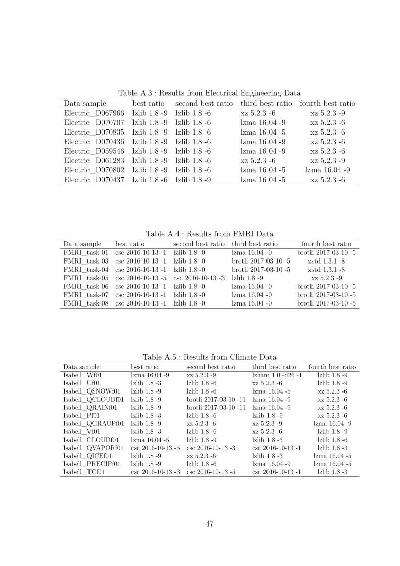
Table A.3.: Results from Electrical Engineering DataData sample best ratio second best ratio third best ratio fourth best ratioElectric_D067966 lzlib 1.8 -9 lzlib 1.8 -6 xz 5.2.3 -6 xz 5.2.3 -9Electric_D070707 lzlib 1.8 -9 lzlib 1.8 -6 lzma 16.04 -9 xz 5.2.3 -6Electric_D070835 lzlib 1.8 -9 lzlib 1.8 -6 lzma 16.04 -5 xz 5.2.3 -6Electric_D070436 lzlib 1.8 -9 lzlib 1.8 -6 lzma 16.04 -9 xz 5.2.3 -6Electric_D059546 lzlib 1.8 -9 lzlib 1.8 -6 lzma 16.04 -9 xz 5.2.3 -6Electric_D061283 lzlib 1.8 -9 lzlib 1.8 -6 xz 5.2.3 -6 xz 5.2.3 -9Electric_D070802 lzlib 1.8 -9 lzlib 1.8 -6 lzma 16.04 -5 lzma 16.04 -9Electric_D070437 lzlib 1.8 -6 lzlib 1.8 -9 lzma 16.04 -5 xz 5.2.3 -6

Table A.4.: Results from FMRI DataData sample best ratio second best ratio third best ratio fourth best ratioFMRI_task-01 csc 2016-10-13 -1 lzlib 1.8 -0 lzma 16.04 -0 brotli 2017-03-10 -5FMRI_task-03 csc 2016-10-13 -1 lzlib 1.8 -0 brotli 2017-03-10 -5 zstd 1.3.1 -8FMRI_task-04 csc 2016-10-13 -1 lzlib 1.8 -0 brotli 2017-03-10 -5 zstd 1.3.1 -8FMRI_task-05 csc 2016-10-13 -5 csc 2016-10-13 -3 lzlib 1.8 -9 xz 5.2.3 -9FMRI_task-06 csc 2016-10-13 -1 lzlib 1.8 -0 lzma 16.04 -0 brotli 2017-03-10 -5FMRI_task-07 csc 2016-10-13 -1 lzlib 1.8 -0 lzma 16.04 -0 brotli 2017-03-10 -5FMRI_task-08 csc 2016-10-13 -1 lzlib 1.8 -0 lzma 16.04 -0 brotli 2017-03-10 -5

Table A.5.: Results from Climate DataData sample best ratio second best ratio third best ratio fourth best ratioIsabell_Wf01 lzma 16.04 -9 xz 5.2.3 -9 lzham 1.0 -d26 -1 lzlib 1.8 -9Isabell_Uf01 lzlib 1.8 -3 lzlib 1.8 -6 xz 5.2.3 -6 lzlib 1.8 -9Isabell_QSNOWf01 lzlib 1.8 -9 lzlib 1.8 -6 lzma 16.04 -5 xz 5.2.3 -6Isabell_QCLOUDf01 lzlib 1.8 -9 brotli 2017-03-10 -11 lzma 16.04 -9 xz 5.2.3 -6Isabell_QRAINf01 lzlib 1.8 -9 brotli 2017-03-10 -11 lzma 16.04 -9 xz 5.2.3 -6Isabell_Pf01 lzlib 1.8 -3 lzlib 1.8 -6 lzlib 1.8 -9 xz 5.2.3 -6Isabell_QGRAUPf01 lzlib 1.8 -9 xz 5.2.3 -6 xz 5.2.3 -9 lzma 16.04 -9Isabell_Vf01 lzlib 1.8 -3 lzlib 1.8 -6 xz 5.2.3 -6 lzlib 1.8 -9Isabell_CLOUDf01 lzma 16.04 -5 lzlib 1.8 -9 lzlib 1.8 -3 lzlib 1.8 -6Isabell_QVAPORf01 csc 2016-10-13 -5 csc 2016-10-13 -3 csc 2016-10-13 -1 lzlib 1.8 -3Isabell_QICEf01 lzlib 1.8 -9 xz 5.2.3 -6 lzlib 1.8 -3 lzma 16.04 -5Isabell_PRECIPf01 lzlib 1.8 -9 lzlib 1.8 -6 lzma 16.04 -9 lzma 16.04 -5Isabell_TCf01 csc 2016-10-13 -3 csc 2016-10-13 -5 csc 2016-10-13 -1 lzlib 1.8 -3

47

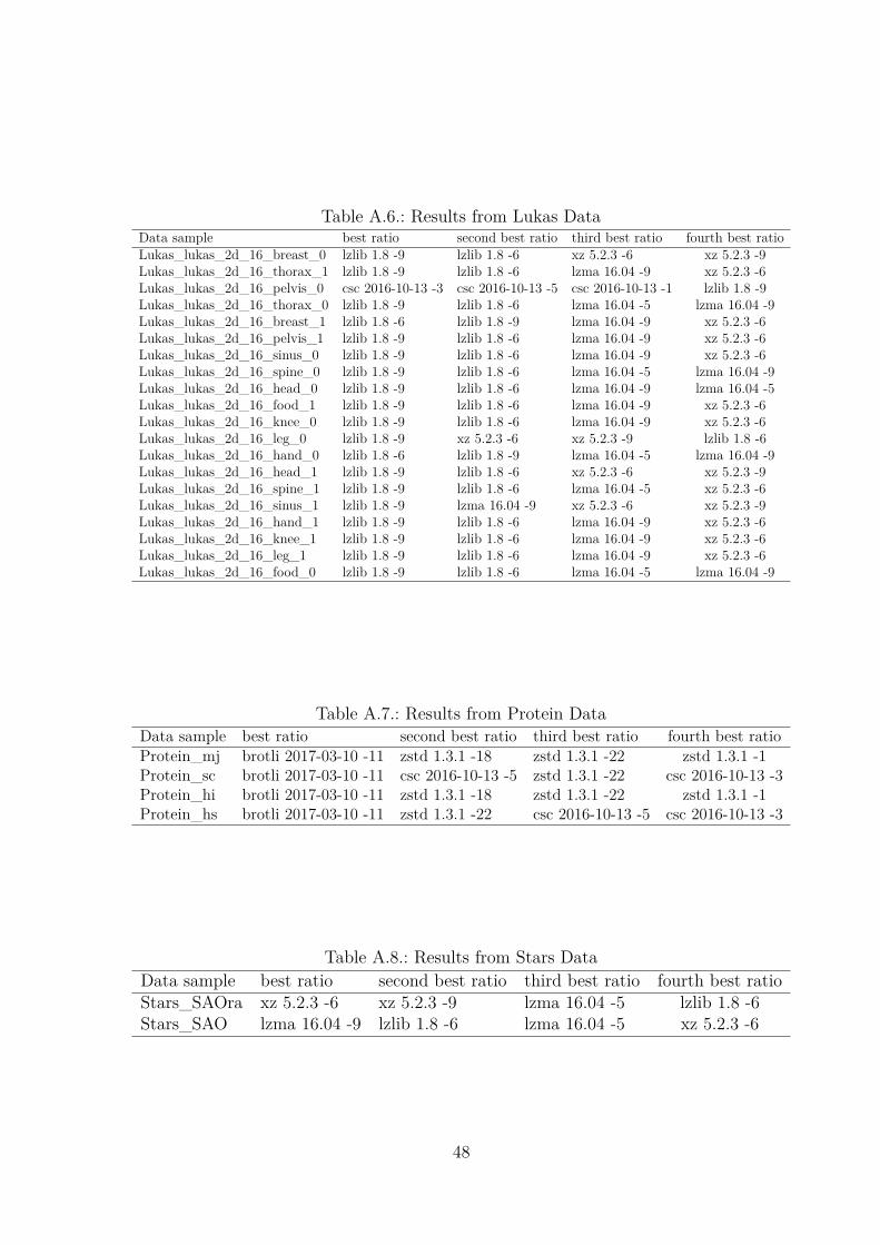
Table A.6.: Results from Lukas DataData sample best ratio second best ratio third best ratio fourth best ratioLukas_lukas_2d_16_breast_0 lzlib 1.8 -9 lzlib 1.8 -6 xz 5.2.3 -6 xz 5.2.3 -9Lukas_lukas_2d_16_thorax_1 lzlib 1.8 -9 lzlib 1.8 -6 lzma 16.04 -9 xz 5.2.3 -6Lukas_lukas_2d_16_pelvis_0 csc 2016-10-13 -3 csc 2016-10-13 -5 csc 2016-10-13 -1 lzlib 1.8 -9Lukas_lukas_2d_16_thorax_0 lzlib 1.8 -9 lzlib 1.8 -6 lzma 16.04 -5 lzma 16.04 -9Lukas_lukas_2d_16_breast_1 lzlib 1.8 -6 lzlib 1.8 -9 lzma 16.04 -9 xz 5.2.3 -6Lukas_lukas_2d_16_pelvis_1 lzlib 1.8 -9 lzlib 1.8 -6 lzma 16.04 -9 xz 5.2.3 -6Lukas_lukas_2d_16_sinus_0 lzlib 1.8 -9 lzlib 1.8 -6 lzma 16.04 -9 xz 5.2.3 -6Lukas_lukas_2d_16_spine_0 lzlib 1.8 -9 lzlib 1.8 -6 lzma 16.04 -5 lzma 16.04 -9Lukas_lukas_2d_16_head_0 lzlib 1.8 -9 lzlib 1.8 -6 lzma 16.04 -9 lzma 16.04 -5Lukas_lukas_2d_16_food_1 lzlib 1.8 -9 lzlib 1.8 -6 lzma 16.04 -9 xz 5.2.3 -6Lukas_lukas_2d_16_knee_0 lzlib 1.8 -9 lzlib 1.8 -6 lzma 16.04 -9 xz 5.2.3 -6Lukas_lukas_2d_16_leg_0 lzlib 1.8 -9 xz 5.2.3 -6 xz 5.2.3 -9 lzlib 1.8 -6Lukas_lukas_2d_16_hand_0 lzlib 1.8 -6 lzlib 1.8 -9 lzma 16.04 -5 lzma 16.04 -9Lukas_lukas_2d_16_head_1 lzlib 1.8 -9 lzlib 1.8 -6 xz 5.2.3 -6 xz 5.2.3 -9Lukas_lukas_2d_16_spine_1 lzlib 1.8 -9 lzlib 1.8 -6 lzma 16.04 -5 xz 5.2.3 -6Lukas_lukas_2d_16_sinus_1 lzlib 1.8 -9 lzma 16.04 -9 xz 5.2.3 -6 xz 5.2.3 -9Lukas_lukas_2d_16_hand_1 lzlib 1.8 -9 lzlib 1.8 -6 lzma 16.04 -9 xz 5.2.3 -6Lukas_lukas_2d_16_knee_1 lzlib 1.8 -9 lzlib 1.8 -6 lzma 16.04 -9 xz 5.2.3 -6Lukas_lukas_2d_16_leg_1 lzlib 1.8 -9 lzlib 1.8 -6 lzma 16.04 -9 xz 5.2.3 -6Lukas_lukas_2d_16_food_0 lzlib 1.8 -9 lzlib 1.8 -6 lzma 16.04 -5 lzma 16.04 -9

Table A.7.: Results from Protein DataData sample best ratio second best ratio third best ratio fourth best ratioProtein_mj brotli 2017-03-10 -11 zstd 1.3.1 -18 zstd 1.3.1 -22 zstd 1.3.1 -1Protein_sc brotli 2017-03-10 -11 csc 2016-10-13 -5 zstd 1.3.1 -22 csc 2016-10-13 -3Protein_hi brotli 2017-03-10 -11 zstd 1.3.1 -18 zstd 1.3.1 -22 zstd 1.3.1 -1Protein_hs brotli 2017-03-10 -11 zstd 1.3.1 -22 csc 2016-10-13 -5 csc 2016-10-13 -3

Table A.8.: Results from Stars DataData sample best ratio second best ratio third best ratio fourth best ratioStars_SAOra xz 5.2.3 -6 xz 5.2.3 -9 lzma 16.04 -5 lzlib 1.8 -6Stars_SAO lzma 16.04 -9 lzlib 1.8 -6 lzma 16.04 -5 xz 5.2.3 -6

48

List of Figures2.1. The different measurements from the Isabel Datasets. . . . . . . . . . . . 82.2. Compression speed and ratio for different compression levels for zstd,

brotli and lzlib. . . . . . . . . . . . . . . . . . . . . . . . . . . . . . . . . 112.3. Using LZ78 on a string. Every arrow symbolizes one step. . . . . . . . . 12

3.1. Options available for running lzBench. . . . . . . . . . . . . . . . . . . . 153.2. Plot of ratio, compression and decompression speed for one of the Isabel

datasets. . . . . . . . . . . . . . . . . . . . . . . . . . . . . . . . . . . . . 203.3. Histogram for algorithms/levels and the number of times, they achieved

the best ratio for a dataset. . . . . . . . . . . . . . . . . . . . . . . . . . 213.4. boxplot showing Ratio (left) and Compression Speed (right) for all algo-

rithms for different datasets. . . . . . . . . . . . . . . . . . . . . . . . . . 24

4.1. K-Means: Start with unlabeled data (top-right); Random initializationof 2 centroids (top-left); Every point gets the label of its closest centroid(middle-left); The centroids move to the center of all their points (middle-right); Repeat until convergence (bottom) . . . . . . . . . . . . . . . . . 29

4.2. K-Means does not assume any underlying structures. Expectation-Maximization can have a better prediction in that case. . . . . . . . . . . 30

4.3. Neural Network with three input-neurons and two output-neurons. . . . . 324.4. A perceptron: Incoming values are multiplied by the weights on the

connecting edges and summed up. The result goes through an activationfunction and is passed on to the next node or is one output node. . . . . 32

4.5. Very simple example of a Decision Tree. The sex of a person is to bedetermined by other information about the person. . . . . . . . . . . . . 34

49

List of Tables3.1. The first 18 algorithms used by lzBench . . . . . . . . . . . . . . . . . . . 163.2. The second 18 algorithms used by lzBench . . . . . . . . . . . . . . . . . 173.3. Part of the results plotted in Figure 3.2 for one dataset from the Isabel

datasets . . . . . . . . . . . . . . . . . . . . . . . . . . . . . . . . . . . . 193.4. Four best algorithms regarding ratio for different datasets. . . . . . . . . 223.5. Average performance of all algorithms over different datasets. . . . . . . . 23

A.1. Results of one full run with lzBench: This table is plotted in Figure 3.2 . 41A.2. Results from Geographical Data . . . . . . . . . . . . . . . . . . . . . . . 46A.3. Results from Electrical Engineering Data . . . . . . . . . . . . . . . . . . 47A.4. Results from FMRI Data . . . . . . . . . . . . . . . . . . . . . . . . . . . 47A.5. Results from Climate Data . . . . . . . . . . . . . . . . . . . . . . . . . . 47A.6. Results from Lukas Data . . . . . . . . . . . . . . . . . . . . . . . . . . . 48A.7. Results from Protein Data . . . . . . . . . . . . . . . . . . . . . . . . . . 48A.8. Results from Stars Data . . . . . . . . . . . . . . . . . . . . . . . . . . . 48

50