Embed Size (px)
Citation preview
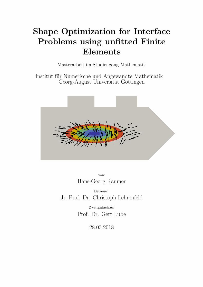
Shape Optimization for InterfaceProblems using unfitted Finite
ElementsMasterarbeit im Studiengang Mathematik
Institut für Numerische und Angewandte MathematikGeorg-August Universität Göttingen
von:
Hans-Georg RaumerBetreuer:
Jr.-Prof. Dr. Christoph LehrenfeldZweitgutachter:
Prof. Dr. Gert Lube
28.03.2018

Eigenständigkeitserklärung
Hiermit versichere ich, dass ich die vorliegende Arbeit selbstständig verfasst und keineanderen als die angegebenen Quellen und Hilfsmittel benutzt habe.
Göttingen, den 28.03.2018
2

Acknowledgements
I would like to sincerely thank Jr.-Prof. Dr. Christoph Lehrenfeld for his great supportduring the supervision of this thesis. Thanks for many hours of discussions and sharingyour expertise with me.Many thanks also to Prof. Dr. Gert Lube, the second assessor of this thesis, whoheld most of my lectures and seminars in numerical mathematics for teaching me manyaspects of numerics of partial differential equations.Last but not least, I want to thank Fabian Heimann and Henry von Wahl for valuablehints on the implementation with NGSolve and the layout of this thesis.
3
Contents
1 Introduction 5
2 Theory of Shape Optimization 92.1 Basic Definitions and Theorems . . . . . . . . . . . . . . . . . . . . . . . . 92.2 Shape Functions with PDE Constraints . . . . . . . . . . . . . . . . . . . 142.3 Optimization Aspects . . . . . . . . . . . . . . . . . . . . . . . . . . . . . 15
3 Shape Optimization for two Model Problems 193.1 Stationary Heat Transport Problem . . . . . . . . . . . . . . . . . . . . . 193.2 One-phase Poisson Problem . . . . . . . . . . . . . . . . . . . . . . . . . . 31
4 Level Set Representation of the Geometry 334.1 Continuous Level Set Functions . . . . . . . . . . . . . . . . . . . . . . . . 334.2 FE Discretization of the Level Set Function and the Level Set Transport . 34
5 FE Approximation of the One-phase Problem 405.1 Fictitious Domain Method . . . . . . . . . . . . . . . . . . . . . . . . . . . 405.2 Approximation of the Descent Direction . . . . . . . . . . . . . . . . . . . 43
6 FE Approximation of the Optimal Interface Problem 486.1 The unfitted Finite Element Method (XFEM and CutFEM) . . . . . . . . 486.2 Shape Optimization Procedure for an Interface Problem . . . . . . . . . . 51
6.2.1 An unfitted Nitsche Method for the State and Adjoint State . . . . 516.2.2 Construction of a Descent Direction . . . . . . . . . . . . . . . . . 556.2.3 Optimization Algorithm . . . . . . . . . . . . . . . . . . . . . . . . 59
7 Numerical Results 617.1 Comparison of Volume and Boundary Expression . . . . . . . . . . . . . . 617.2 Approximation Spaces for the Descent Direction . . . . . . . . . . . . . . 647.3 Full Geometry Optimization . . . . . . . . . . . . . . . . . . . . . . . . . . 687.4 Velocity Extension . . . . . . . . . . . . . . . . . . . . . . . . . . . . . . . 737.5 Geometry and Residual Error . . . . . . . . . . . . . . . . . . . . . . . . . 75
8 Conclusion and Outlook 788.1 Summary . . . . . . . . . . . . . . . . . . . . . . . . . . . . . . . . . . . . 788.2 Open Problems . . . . . . . . . . . . . . . . . . . . . . . . . . . . . . . . . 78
A Auxiliary Proofs 82
4
Chapter 1
Introduction
Optimization of geometries is a task that is highly interesting from a practical pointof view and is very commonly used in many fields of engineering and physics. To givethe reader an impression on how diverse those applications can be, we will list a fewexamples.
Acoustics: One is often interested in the reduction of noise stemming from machinesor motors. For example road traffic, aircrafts or machine noise in large factory halls.Usually this leads to a coupled problem of acoustic-structure-interaction. A nice overviewon possible numerical strategies and techniques for such problems is presented in [Mar02].The interesting application of optimizing noise barriers is considered in [Duh06]. It isalso possible to optimize the structure of walls and ceilings in concert halls with respectto acoustical effects. The Grand Hall of the Elbphilharmonie Hamburg represents afamous case where such techniques were succesfully used [Kor18].
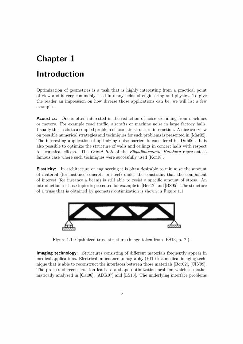
Elasticity: In architecture or engineering it is often desirable to minimize the amountof material (for instance concrete or steel) under the constraint that the componentof interest (for instance a beam) is still able to resist a specific amount of stress. Anintroduction to those topics is presented for example in [Her12] and [BS95]. The structureof a truss that is obtained by geometry optimization is shown in Figure 1.1.
Figure 1.1: Optimized truss structure (image taken from [BS13, p. 2]).
Imaging technology: Structures consisting of different materials frequently appear inmedical applications. Electrical impedance tomography (EIT) is a medical imaging tech-nique that is able to reconstruct the interfaces between those materials [Bor02], [CIN99].The process of reconstruction leads to a shape optimization problem which is mathe-matically analyzed in [Cal06], [ADK07] and [LS13]. The underlying interface problems
5
6 Chapter 1 Introduction
are also closely related to those we will consider in this thesis.
There are many approaches and techniques to solve geometry optimization problems.What they have in common is that a function depending on the geometry (shape func-tion) has to be mimimized (or maximized). It is investigated how the shape functionbehaves under variations of the geometry. This procedure is also known as sensitivityanalysis in the literature. There exist different possibilities to perfom such a variationof the geometry and each possibility is linked to a branch of geometry optimization. Wewill mention three important branches here.
Variation of parameters (parametric optimization): For this class of problems thereexists a finite set of parameters that describes the geometry (for example control pointsof Bézier curves). The sensitivity analysis leads to a finite dimensional optimizationproblem. This structure allows the application of many well understood finite dimen-sional optimization algorithms. A drawback of this approach is that it is very restrictive,since only geometries that can be parametrized by the chosen model are considered.
Variation of topology (topology optimization): We can also investigate how the shapefunction behaves under topology changes (for example insertion of infinitesimal holes).This approach allows much more freedom for the admissible geometries. A mathematicalfoundation for topolgy optimization is given by [NS12].
Variation of boundaries (shape optimization): The idea to consider small perturba-tions of the boundary goes back to J. Hadamard (1908) [Had08] and his research onelastic plates. Since then a rigorous theory for many aspects of the optimization processwas developed, see for instance [SZ92], [DZ11]. The approach of shape optimizationwas chosen for this thesis because the large quantity of mathematical theory makes itpossible to establish a solid theoretical framework for everything that is done afterwards.
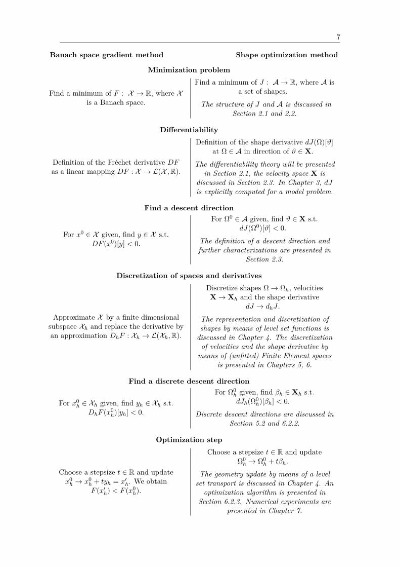
Generic Gradient MethodIn order to solve our shape optimization problem, we will develop a gradient-type opti-mization method in this thesis. To set up a gradient method, several sub problems haveto be solved. We will motivate those sub problems by means of a generic optimizationproblem on a (infinite dimensional) Banach space X . Each problem in the generic settinghas a counterpart in the shape optimization setting. To conclude this introduction andprovide an overview of this thesis, we will list all sub problems of the generic gradientmethod together with their correspondent in shape optimization and references to theassociated chapters/sections.
7
Banach space gradient method Shape optimization method
Minimization problem
Find a minimum of F : X → R, where Xis a Banach space.
Find a minimum of J : A → R, where A isa set of shapes.
The structure of J and A is discussed inSection 2.1 and 2.2.
Differentiability
Definition of the Fréchet derivative DFas a linear mapping DF : X → L(X ,R).
Definition of the shape derivative dJ(Ω)[ϑ]at Ω ∈ A in direction of ϑ ∈ X.
The differentiability theory will be presentedin Section 2.1, the velocity space X is
discussed in Section 2.3. In Chapter 3, dJis explicitly computed for a model problem.
Find a descent direction
For x0 ∈ X given, find y ∈ X s.t.DF (x0)[y] < 0.
For Ω0 ∈ A given, find ϑ ∈ X s.t.dJ(Ω0)[ϑ] < 0.
The definition of a descent direction andfurther characterizations are presented in
Section 2.3.
Discretization of spaces and derivatives
Approximate X by a finite dimensionalsubspace Xh and replace the derivative byan approximation DhF : Xh → L(Xh,R).
Discretize shapes Ω→ Ωh, velocitiesX→ Xh and the shape derivative
dJ → dhJ .
The representation and discretization ofshapes by means of level set functions isdiscussed in Chapter 4. The discretizationof velocities and the shape derivative bymeans of (unfitted) Finite Element spaces
is presented in Chapters 5, 6.
Find a discrete descent direction
For x0h ∈ Xh given, find yh ∈ Xh s.t.
DhF (x0h)[yh] < 0.
For Ω0h given, find βh ∈ Xh s.t.dJh(Ω0
h)[βh] < 0.
Discrete descent directions are discussed inSection 5.2 and 6.2.2.
Optimization step
Choose a stepsize t ∈ R and updatex0h → x0
h + tyh = x′h. We obtainF (x′h) < F (x0
h).
Choose a stepsize t ∈ R and updateΩ0h → Ω0
h + tβh.
The geometry update by means of a levelset transport is discussed in Chapter 4. An
optimization algorithm is presented inSection 6.2.3. Numerical experiments are
presented in Chapter 7.
8 Chapter 1 Introduction
OverviewIn the second chapter we will present the mathematical background from the theoryof shape optimization which results in the definition of a derivative with respect to thedomain, the so called shape derivative or Eulerian semi-derivative. The presented frame-work is taken from the standard literature in shape optimization. Chapter 3 introducestwo scalar PDE constrained shape optimization problems, namely a one-phase and atwo-phase/interface problem. Whereas the one-phase problem is a standard problemfrom the literature, the interface problem is not. Therefore a rigorous proof of the ex-istence of the shape derivative is presented. Chapter 4 discusses the implicit geometryrepresentation by means of a level set function and presents the appropriate numer-ical treatment by suitable continuous and discontinuous Finite Element spaces. Forthe entire thesis we will only consider lowest order (piecewise linear) Finite Elements.In Chapter 5 and 6 we establish the numerical framework to solve shape optimizationproblems of one-phase and two-phase type by means of the Finite Element method. Wechoose unfitted Finite Element discretizations i.e. meshes that are not aligned with theboundary or the interface. Two aspects of the numerical shape optimization procedureare discussed in detail. First, we will compare two different discrete representations ofthe shape derivative (volume expression and boundary expression) and conclude whythe volume expression is superior in a Finite Element context. Second, we will presentthe construction of a specific descent direction with beneficial properties for the level settransport. A proof of approximation properties of this descent direction will be included.The final result of Chapter 6 will be a shape optimization algorithm for the two-phasemodel problem. Chapter 7 presents various numerical examples that illustrate differentaspects of the optimization process.
Chapter 2
Theory of Shape Optimization
In this chapter the theoretical framework from the field of shape optimization will beprovided. It should be emphasized that it presents only a very small part of the wholetheory. We will restrict ourselves to those statements which are essential to set upand understand the numerical methods in the following chapters. This means that wewill present one possibility to derive a "derivative with respect to the domain" withoutgiving any existence or uniqueness theorems of optimal solutions. More aspects are outof scope for this thesis because the main focus will be on the numerical methods and thederivation of a meaningful optimization algorithm. For a deeper investigation of manyaspects of shape optimization we refer to [DZ11], [SZ92] and [Stu15], where also manyof the definitions and proofs in the subsequent chapter are taken from.
2.1 Basic Definitions and TheoremsFirst we introduce the notion of a shape function.
2.1. DEFINITION [shape function] [DZ11, p. 170]Let ∅ 6= Ω0 ⊂ Rd be a set and A ⊂ P(Ω0) = Ω| Ω ⊂ Ω0. Then a function
J : A → R Ω→ J(Ω)
is called shape function.
The superset Ω0 is often called holdall and any set Ω ∈ A admissible set. For a givenshape function a shape optimization problem can be formulated in the most general wayas:
find Ω ∈ A such thatJ(Ω) = min
Ω′∈AJ(Ω′). (2.1)
To obtain statements on existence and/or uniqueness of optimal solutions there is nostraight forward approach. To apply well known theory on optimal solutions we wouldneed a Banach space structure on A which is in general not given. By restrictions on theset A at least weaker structures can be achieved. One of the most common approaches(which will also considered here) is to define A by the image of a reference domain undera family of mappings i.e. A = T (Ωref )|T ∈ T. For a suitable choice of T a group
9
10 Chapter 2 Theory of Shape Optimization
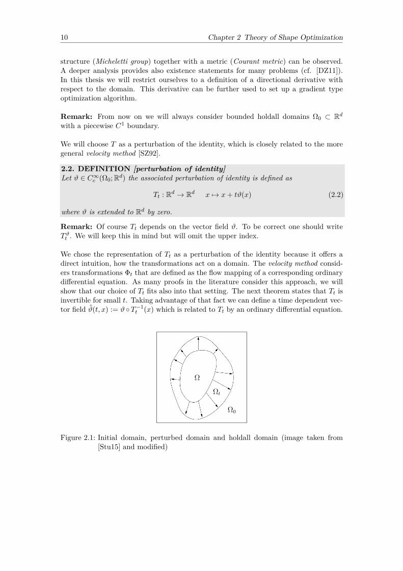
structure (Micheletti group) together with a metric (Courant metric) can be observed.A deeper analysis provides also existence statements for many problems (cf. [DZ11]).In this thesis we will restrict ourselves to a definition of a directional derivative withrespect to the domain. This derivative can be further used to set up a gradient typeoptimization algorithm.
Remark: From now on we will always consider bounded holdall domains Ω0 ⊂ Rdwith a piecewise C1 boundary.
We will choose T as a perturbation of the identity, which is closely related to the moregeneral velocity method [SZ92].
2.2. DEFINITION [perturbation of identity]Let ϑ ∈ C∞c (Ω0;Rd) the associated perturbation of identity is defined as
Tt : Rd → Rd x 7→ x+ tϑ(x) (2.2)
where ϑ is extended to Rd by zero.
Remark: Of course Tt depends on the vector field ϑ. To be correct one should writeT ϑt . We will keep this in mind but will omit the upper index.
We chose the representation of Tt as a perturbation of the identity because it offers adirect intuition, how the transformations act on a domain. The velocity method consid-ers transformations Φt that are defined as the flow mapping of a corresponding ordinarydifferential equation. As many proofs in the literature consider this approach, we willshow that our choice of Tt fits also into that setting. The next theorem states that Tt isinvertible for small t. Taking advantage of that fact we can define a time dependent vec-tor field ϑ(t, x) := ϑ T−1
t (x) which is related to Tt by an ordinary differential equation.
Ω
Ωt
Ω0
Figure 2.1: Initial domain, perturbed domain and holdall domain (image taken from[Stu15] and modified)
2.1 Basic Definitions and Theorems 11
2.3. THEOREM [characterization of Tt] [DZ11, p. 180 ff.]
Let T (t, x) := Tt(x), then ∃τ > 0 s.t.
(i) The mapping T has the following properties:
∀x ∈ Rd, T (·, x) ∈ C1([0, τ ];Rd) and ∃c > 0 s.t.∀x, y ∈ Rd, ‖T (·, x)− T (·, y)‖C1([0,τ ];Rd)≤ c|x− y|
∀t ∈ [0, τ ], x 7→ Tt(x) = T (t, x) is invertible
∀x ∈ Rd, T−1(·, x) ∈ C([0, τ ];Rd) and ∃ c > 0 s.t.∀x, y ∈ Rd, ‖T−1(·, x)− T−1(·, y)‖C([0,τ ];Rd)≤ c|x− y|
(ii) ϑ = ϑ T−1t is well defined on [0, τ ]× Rd and uniformly Lipschitzian i.e.
∀x ∈ Rd, ϑ(·, x) ∈ C([0, τ ];Rd)∃c > 0,∀x, y ∈ Rd, ‖ϑ(·, x)− ϑ(·, y)‖C([0,τ ];Rd)≤ c|x− y| .
(iii) Tt can be characterized as the flow of an ODE
∀x ∈ Rd, t ∈ [0, τ ], γ(t) := Tt(x) = T (t, x)d
dtγ(t) = ϑ(t, γ(t)), γ(0) = x .
(iv) t 7→ DTt and t 7→ (DTt)−1 belong to C([0, τ ];C(Ω0,Rdxd)
)(v) For t < τ , Tt : Ω0 → Ω0 is an homeomorphism with Tt(∂Ω0) = ∂Ω0
Proof. As ϑ ∈ C∞c (Ω0;Rd) , it is in particular uniformly Lipschitzian. Thus we can applyTheorem 4.2 in [DZ11, p. 184] which yields (i) and (ii). Since (i) and (ii) are fulfilled,we can apply Theorem 4.1 [DZ11, p. 181] to obtain statement (iii). For the statement(iv) we refer to Theorem 2.16 in [SZ92, p. 51]. The continuity and the continuity ofthe inverse of Tt has been already proven by the previous steps. We still need that Ttmaps Ω0 onto Ω0. This follows also from Theorem 2.16 in [SZ92, p. 51] if the followingproperty of ϑ holds
x ∈ ∂Ω0 =⇒ ϑ(t, x) · n(x) = 0 (2.3)
where n(x) denotes the outer unit normal on ∂Ω0. For the singular points of ∂Ω0 wherethe unit normal is not defined, we set n(x) = 0. We will show that (2.3) is valid toconclude the proof. Let x ∈ ∂Ω0 where n(x) is well defined, then
Tt(x) = x+ tϑ(x) = x ,
12 Chapter 2 Theory of Shape Optimization
since ϑ has compact support in Ω0. Thus on ∂Ω0 we obtain
x = Tt(x) = T−1t (x) .
Inserting this identity into ϑ(t, ·) yields
ϑ(t, x) · n(x) = ϑ(T−1t (x)) · n(x) = ϑ(x) · n(x) = 0 .
We will point out the main consequences of the last theorem. For an initial domainΩ ⊂ Ω0, we can define the perturbed domain (see Figure 2.1 for a sketch)
Ωt := Tt(Ω). (2.4)
For t sufficiently small (depending on ϑ) the following statements are valid due to The-orem 2.3
• Tt(Ω0) = Ω0 (invariance of the holdall domain).
• Ωt ⊂ Ω0 (preservation of inclusion).
• ∂Ω ∈ C1 ⇒ ∂Ωt ∈ C1 (preservation of smooth boundaries).
• ∂Ω ∈ C0,1 ⇒ ∂Ωt ∈ C0,1 (preservation of Lipschitz boundaries).
Statements (ii) and (iii) show that our choice of Tt can be regarded as a special caseof the velocity method. This is very useful, since most of the results from the literatureconsider transformations defined as a flow mapping. All these results are now directlyvalid for Tt. Many statements of Theorem 2.3 are also later needed to derive differen-tiability properties of quantities related to Tt.
Usually we will consider subsets with smooth or Lipschitz boundaries as admissiblesets i.e. A = Ω ⊂ Ω0 : ∂Ω ∈ C1 or A = Ω ⊂ Ω0 : ∂Ω ∈ C0,1. As mentioned,the characterization theorem (Theorem 2.3) ensures that for sufficiently small t also Ωt
is an admissible set, i.e. Ωt ∈ A. This is all we need to come up with a definition ofa derivative with respect to the domain, the so-called Eulerian semi-derivative or shapederivative.
2.1 Basic Definitions and Theorems 13
2.4. DEFINITION [Eulerian semi-derivative/ shape derivative]Let Ω ⊂ Ω0, then the Eulerian semi-derivative of J at Ω in direction of ϑ is defined asthe limit (if it exists)
dJ(Ω)[ϑ] = limt→0
J(Ωt)− J(Ω)t
. (2.5)
(i) If the limit exists ∀ϑ ∈ C∞c (Ω0,Rd) and ∃k ≥ 0 such that the mapping
ϑ 7→ dJ(Ω)[ϑ] =: G(ϑ)
is linear and continuous with respect to the Ck(Ω0,R)-norm we call J shape dif-ferentiable at Ω and G(·) its shape derivative.
(ii) The smallest integer k ≥ 0 for which G is continuous with respect to the Ck(Ω0,R)norm is called the order of G.
Under further assumptions on the smoothness of the boundary of Ω, the shape derivativecan be represented as a functional that acts only on the boundary. This property wasfirst detected by J. Hadamard (1908) [Had08] for the special case of C∞ boundaries.The statement for Ck+1 boundaries was first proven by J.-P. Zolésio in 1979 [Zol79] andcan be summarized in the famous structure theorem. For more details we refer to [DZ11,Remark 3.2, p. 481].
2.5. THEOREM [structure theorem] [DZ11, p. 479 ff.]Let Ω ⊂ Ω0 with compact boundary ∂Ω and let G be of order k ≥ 0. If ∂Ω ∈ Ck+1,then the outward unit normal n of ∂Ω is well defined and ∃ g ∈ Ck(∂Ω)′ such that∀ϑ ∈ Ckc (Ω0,Rd) holds
dJ(Ω)[ϑ] = 〈g, ϑ|∂Ω·n〉Ck(∂Ω) . (2.6)
If further g ∈ L1(∂Ω)
dJ(Ω)[ϑ] =∫∂Ωg(ϑ · n) . (2.7)
Proof. See [DZ11, Theorem 3.6, p. 479] and [DZ11, Corollary 1, p. 480].
A direct consequence of the structure theorem which is of great importance for thenumerical treatment of shape optimization problems is stated in the next Corollary.
2.6. COROLLARY [normal components]Let the assumptions of Theorem 2.5 be valid and ϑ1, ϑ2 ∈ Ckc (Ω0,Rd) then
ϑ1 · n = ϑ2 · n ⇒ dJ(Ω)[ϑ1] = dJ(Ω)[ϑ2]
14 Chapter 2 Theory of Shape Optimization
Proof. If the assumptions are valid, the shape derivative depends only on the normalcomponents of the vector fields ϑ1, ϑ2
dJ(Ω)[ϑ1] = 〈g, ϑ1|∂Ω·n〉Ck(∂Ω) = 〈g, ϑ2|∂Ω·n〉Ck(∂Ω) = dJ(Ω)[ϑ2] .
2.2 Shape Functions with PDE ConstraintsIn this thesis we will only deal with a special class of shape functions, namely PDEconstrained shape functions. We will clarify this term by the next definition.
2.7. DEFINITION [PDE constrained shape function]Let V (Ω) be a Hilbert space of functions defined ∀Ω ∈ A. We consider a bilinear form
a(Ω, ·, ·) : V (Ω)× V (Ω)→ R
and a linear form
f(Ω, ·) : V (Ω)→ R .
Further let the following variational formulation be uniquely solvable ∀ Ω ∈ A:
find u(Ω) ∈ V (Ω) such that ∀v ∈ V (Ω)a(Ω, u(Ω), v) = f(Ω, v) .
(2.8)
Then the solution u = u(Ω) of (2.8) is called state and a shape function which dependsimplicity on the state i.e.
J(Ω) = J(Ω, u(Ω))
is called PDE constrained shape function.
The approach of our choice to derive the Eulerian semi-derivative of such an J is linkedto differentiability properties of the state u. Since Ωt ∈ A for small t and by constructionof the state equation, there exists a unique ut ∈ V (Ωt) such that
a(Ωt, ut, vt) = f(Ωt, vt) ∀vt ∈ V (Ωt) . (2.9)
And we can define
ut := ut Tt .
Although ut is defined on Ω it is not guaranteed that ut ∈ V (Ω). This leads to animportant property of the spaces V (Ω) which has to be valid and will be stated as anassumption here:
u ∈ V (Ωt)⇔ u Tt ∈ V (Ω) . (A)

2.3 Optimization Aspects 15
Remark: Later we will choose V (Ω) = H1(Ω) or V (Ω) = H10 (Ω), which both fulfill
assumption (A) (see Lemma 3.1).
The crucial point for the existence of the Eulerian semi-derivative is the existence ofthe so-called material derivative.
2.8. DEFINITION [material derivative]Let assumption (A) be valid, then u is defined as the weak/strong limit
u = limt0
ut − ut
,
if it exists.
The whole derivation using the material derivative approach including a rigorous ex-istence proof of the Eulerian semi-derivative will be done in the next chapter for twomodel problems.
2.3 Optimization AspectsFor the moment we will assume existence of the Eulerian semi-derivative and shapedifferentiability of J(Ω) i.e ∃k ≥ 0 such that
dJ(Ω)[·] : C∞c (Ω0,Rd)→ R ϑ 7→ dJ(Ω)[ϑ]
is linear and bounded with respect to the Ckc (Ω0,Rd) norm. We state further an as-sumption on the extension of dJ(Ω):
dJ(Ω) is a linear and bounded functional on X :=[H1
0 (Ω0)]d
. (B)
If we can find a smooth vector field ϑ ∈ C∞c (Ω0,Rd) that fulfills
dJ(Ω)[ϑ] < 0 ,
we can as well find τ > 0 such that ∀t < τ holds:
J(Ωt)− J(Ω)t
< 0 ⇒ J(Ωt) < J(Ω) .
So we reduced the value of our shape function. This motivates the following definition.
16 Chapter 2 Theory of Shape Optimization
2.9. DEFINITION [descent direction]Let assumption (B) be valid, then a vector field β ∈ X is called descent direction of J(Ω)if
dJ(Ω)[β] < 0 .
If even holds that
β ∈ arg min‖ϑ‖X=1
dJ(Ω)[ϑ] , (2.10)
we call β a steepest descent.
Considering the inner product on X =[H1
0 (Ω0)]d
b(β, ψ) =∫
Ω0
∇β : ∇ψ + β · ψ
and the structure theorem 2.5, we get some characterizations of a steepest descent.
2.10. LEMMA [characterizations of a steepest descent]Let β′ be the Riesz representative of −dJ(Ω) i.e
b(β′, ψ) = −dJ(Ω)[ψ] ∀ψ ∈ X .
Let further the assumptions of the structure theorem 2.5 be valid with g ∈ L2(∂Ω), thenthe following expressions define a steepest descent
(i) β1 := (‖β′‖X)−1β′
(ii) any β2 ∈ X with ‖β2‖X= 1 and β2 · n = β1 · n on ∂Ω
(iii) β3 := (‖β‖X)−1β with β ∈ X such that β · n = −g on ∂Ω
Proof. (i) Let ψ ∈ X be arbitrary with ‖ψ‖X= 1, then we compute
dJ(Ω)[β1]− dJ(Ω)[ψ] = (‖β′‖X)−1dJ(Ω)[β′] + b(β′, ψ)= −(‖β′‖X)−1b(β′, β′) + b(β′, ψ)≤ −‖β′‖X+‖β′‖X‖ψ‖X= 0 .
Where we used Cauchy Schwarz in the third line. Thus β1 is a minimizer andnormalized by construction.
(ii) The normal components of β1 and β2 coincide, thus we can apply Corollary 2.6which yields
min‖ϑ‖X=1
dJ(Ω)[ϑ] = dJ(Ω)[β1] = dJ(Ω)[β2]
2.3 Optimization Aspects 17
(iii) Let ψ ∈ X be arbitrary with ‖ψ‖X= 1 and Ctr the constant from the trace theorem,then the structure theorem yields
dJ(Ω)[β3]− dJ(Ω)[ψ] = −(‖β‖X)−1∫∂Ωg2 −
∫∂Ωg(ψ · n)
≤ −(‖β‖X)−1‖g‖2L2(∂Ω)+‖g‖L2(∂Ω)‖ψ · n‖L2(∂Ω)
≤ −(‖β‖X)−1‖β‖2XC2tr + C2
tr‖β‖X= 0 .
Remark: Note that if we omit the scaling for β1 and β3, we still obtain a descentdirection. The lemma shows that a steepest descent is anything else but unique. Thisgives us some freedom in the choice of the descent direction in the optimization methodand we can choose a velocity field which is best suited for the numerical treatment ofthe optimization problem.
For the Riesz representative β′ and the steepest descent β1 from the previous lemma, anadditional regularity result is valid.
2.11. LEMMA [regularity of β1] cf.[BEH+17]Let the assumptions of Lemma 2.10 be valid and ∂Ω ∈ C1 then
β1 ∈[H1
0 (Ω0)]d∩[H2(Ω0\Ω)
]d∩[H2(Ω)
]dProof. For the Riesz representative of −dJ(Ω) holds
b(β′, ψ) = −dJ(Ω)[ψ] ∀ψ ∈ X .
By the structure theorem this can be rewritten as
b(β′, ψ) = −∫∂Ωg(ψ · n) ∀ψ ∈ X .
This is the weak formulation of the vector valued interface problem
−∆β′ + β′ = ~0 in Ω1 and Ω2[[β′]]
= ~0 on Γ[[∇β′ n
]]= g n on Γ
β = ~0 on ∂Ω0,
with the subdomains Ω1 := Ω, Ω2 := Ω0\Ω and the interface Γ := ∂Ω. The jumpoperator [[·]] on the interface is defined by
[[v]] = v|Ω1−v|Ω1 .
18 Chapter 2 Theory of Shape Optimization
The regularity of solutions of such elliptic interface problems is a standard result fromthe literature and states
‖β′‖[H10 (Ω0)]d+‖β
′‖[H2(Ω1]d+‖β′‖[H2(Ω2)]d≤ C‖g‖H1/2(Γ) .
A proof for d = 2 can be found in [CZ98, Theorem 2.1]. Since the regularity result holdsfor β′, the descent direction β1 has the same regularity.
Chapter 3
Shape Optimization for two ModelProblems
In this section the theory from the previous chapter will be applied on two scalar modelproblems. The first problem is a two-phase problem and physically motivated. A rigorousproof of the existence of the corresponding shape derivative will be presented. Similarlyto the statement of the structure theorem, under additional regularity assumptions, theshape derivative can be reformulated as a functional that acts only on the interface. Thesecond problem is well known in the literature and will be used later to highlight someaspects of the numerical analysis. Volume and boundary expression of the correspondingshape derivative will be quoted from the literature for this case.
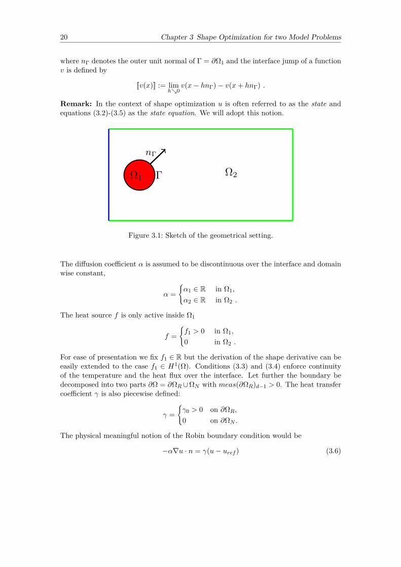
3.1 Stationary Heat Transport ProblemWe consider a bounded domain Ω ⊂ R2 wich can be decomposed into two subdomainsΩ1 and Ω2. The subdomains are separated by the interface Γ := Ω1 ∩ Ω2. Further weassume that Ω1 is fully surrounded by Ω2 which implies Γ ∩ ∂Ω = ∅. The full domainΩ can be regarded as a room which is heated by a heat source located inside Ω1. Someparts of the wall can be fully isolated whereas the remaining parts allow some heat flux.We are interested in minimizing the deviation of the temperature distribution from areference temperature distribution. So let u = u(x, y) denote the temperature in Ω andu ∈ C1(Ω) is some reference temperature distribution. Then we seek to minimize theshape function
J(Ω) =∫Ω
(u− u)2 → min . (3.1)
Where u solves the following interface problem:
−div(α∇u) = f in Ω, (3.2)[[u]] = 0 on Γ, (3.3)
[[−α∇u · nΓ]] = 0 on Γ, (3.4)∇u · n+ γu = 0 on ∂Ω , (3.5)
19
20 Chapter 3 Shape Optimization for two Model Problems
where nΓ denotes the outer unit normal of Γ = ∂Ω1 and the interface jump of a functionv is defined by
[[v(x)]] := limh0
v(x− hnΓ)− v(x+ hnΓ) .
Remark: In the context of shape optimization u is often referred to as the state andequations (3.2)-(3.5) as the state equation. We will adopt this notion.
Ω2ΓΩ1
nΓ
Figure 3.1: Sketch of the geometrical setting.
The diffusion coefficient α is assumed to be discontinuous over the interface and domainwise constant,
α =α1 ∈ R in Ω1,
α2 ∈ R in Ω2 .
The heat source f is only active inside Ω1
f =f1 > 0 in Ω1,
0 in Ω2 .
For ease of presentation we fix f1 ∈ R but the derivation of the shape derivative can beeasily extended to the case f1 ∈ H1(Ω). Conditions (3.3) and (3.4) enforce continuityof the temperature and the heat flux over the interface. Let further the boundary bedecomposed into two parts ∂Ω = ∂ΩR ∪ΩN with meas(∂ΩR)d−1 > 0. The heat transfercoefficient γ is also piecewise defined:
γ =γ0 > 0 on ∂ΩR,
0 on ∂ΩN .
The physical meaningful notion of the Robin boundary condition would be
−α∇u · n = γ(u− uref ) (3.6)
3.1 Stationary Heat Transport Problem 21
with a reference temperature uref . Equation (3.6) shows that the heat flux is propor-tional to the temperature difference between u and uref . For simplicity we set uref tozero in our case. According to this comment, the piecewise defined heat transfer coeffi-cient γ and condition (3.5) model an isolated part of the wall (∂ΩN ) and another partthat allows heat flux (∂ΩR).
In our example only the interface Γ will be moved whereas the outer boundary ∂Ω staysfixed, hence Ω is a natural choice for the holdall domain. Starting with Ωi i ∈ 1, 2 as areference domain we can take any ϑ ∈ C∞c (Ω,R2) and apply the corresponding perturba-tion Tt from the previous chapter. This defines the perturbed subdomains Ωi,t := Tt(Ωi)and the perturbed interface Γt := Tt(Γ) with outer unit normal nΓt . Similarly we get
αt =α1 in Ω1,t,
α2 in Ω2,t
and
ft =f1 > 0 in Ω1,t,
0 in Ω2,t .
Please note that by construction f = ft Tt and α = αt Tt. Since Tt keeps theouter boundary ∂Ω fixed, nothing has to be changed there. Canonically this defines theperturbed state equation i.e. we seek ut (perturbed state) that solves:
−div(α∇ut) = ft in Ω (3.7)[[ut]] = 0 on Γt (3.8)
[[−αt∇ut · nΓt ]] = 0 on Γt (3.9)∇ut · n+ γu = 0 on ∂Ω (3.10)
The state equation and the perturbed state equation can be reformulated as a variationalproblem which reads as:
find u ∈ H1(Ω) such that ∀v ∈ H1(Ω)2∑i=1
αi
∫Ωi∇u · ∇v +
∮∂ΩR
γ0uv =∫
Ωfv
(3.11)
and similarly
find ut ∈ H1(Ω) such that ∀v ∈ H1(Ω)2∑i=1
αi
∫Ωi,t∇ut · ∇v +
∮∂ΩR
γ0utv =∫
Ωftv .
(3.12)
Please note that the outer boundary ∂Ω stays invariant under transformation.
The first important observation is that via the transformation Tt we get an isomorphismon H1(Ω). We will state this as a lemma.
22 Chapter 3 Shape Optimization for two Model Problems
3.1. LEMMA [H1 isomorphism property]For the spaces H1(Ω) and H1
0 (Ω) the isomorphism assumption (A) is valid i.e.
v ∈ H1(Ω)⇔ v Tt ∈ H1(Ω)w ∈ H1
0 (Ω)⇔ w Tt ∈ H10 (Ω)
Proof. The proof can be found in [Zie12, p. 52, Theorem 2.2.2].
Following the notation from the previous chapter we define ut = ut Tt. Now we caninsert ut = ut T−1
t into (3.12) and application of the transformation theorem on thevolume integrals yields∫
Ωi,t∇ut · ∇v =
∫Ωi,t∇(ut T−1
t
)· ∇
((v Tt) T−1
t
)=∫
Ωi,t
(DT−Tt ∇ut
) T−1
t ·(DT−Tt ∇(v Tt)
) T−1
t
=∫
Ωidet (DTt)
(DT−1
t DT−Tt ∇ut)· ∇ (v Tt)
and ∫Ωftv =
∫Ωdet (DTt) f(v Tt) .
To simplify notation we define further auxilliary quantities on Ω0 = Ω
ξ(t) := det(DTt), (3.13)A(t) := ξ(t)(DTt)−1(DTt)−T , (3.14)B(t) := (DTt)−T , (3.15)C(t) := DTt . (3.16)
Remark: Of course all these quantities depend also on the space variable x but we willomit this in the notation for the sake of convenience. When the transformation theoremis applied, we should take the absolute value of the determinant ξ(t). However, we willsee that ξ(t) is positive for small t, therefore we omit the absolute value.
Making use of the previous Lemma and the fact that ut = ut on ∂Ω, we can nowrewrite (3.12) as a variational problem on the reference subdomains.
find ut ∈ H1(Ω) such that ∀v ∈ H1(Ω)2∑i=1
αi
∫Ωi
(A(t)∇ut
)· ∇v +
∮∂ΩR
γ0utv =
∫Ωξ(t)fv .
(3.17)
To obtain existence of the material derivative we would like to differentiate under theintegral in (3.17). To come up with such a statement we need some more properties ofthe auxiliary quantites (3.13)-(3.16), stated by the next two lemmas.
3.1 Stationary Heat Transport Problem 23
3.2. LEMMA [positivity and ellipticity]∃ τ > 0, η1, η2 > 0 such that ∀ t ∈ [0, τ ], ζ ∈ Rd
(i) ξ(t) > 0 ∀x ∈ Ω0
(ii) η1|ζ|2≤ A(t)ζ · ζ ≤ η2|ζ|2
Proof. From Theorem 2.3 we obtain directly that ξ(·) ∈ C([0, τ ];C(Ω0)
)and A(·) ∈
C([0, τ ];C(Ω0,Rd×d)
)with ξ(0) = 1 and A(0) = I. Thus we can apply Proposition 2.12
in [Stu15, p. 16] which yields the claim.
3.3. LEMMA [differentiability properties]For the auxiliary quantities (3.13)-(3.16) the following limit properties hold:
(i) limt0
1t (ξ(t)− 1) = div(ϑ) =: ξ′(0) in C(Ω0,R)
(ii) limt0
1t (C(t)− Id) = Dϑ =: C ′(0) in C
(Ω0,Rd×d
)(iii) lim
t01t (B(t)− Id) = −DϑT =: B′(0) in C
(Ω0,Rd×d
)(iv) lim
t01t (A(t)− I) = div(ϑ)I − (Dϑ+DϑT ) =: A′(0) in C
(Ω0,Rd×d
)Proof. By the characterization theorem (Theorem 2.3) we can identify Tt with a flowmapping and the corresponding speed ϑ is well defined. Lemma 2.31 in [SZ92, p. 64]then states exactely (i).
For the second statement we directly compute for t sufficiently small
limt0
1t(D(Tt)−D(T0)) = lim
t0
1t(tDϑ) = Dϑ
which yields the claim.
For statement (iii) we mimic the proof in [Stu15, p. 17]. For two Banach spaces X,Ythe mapping inv : A 7→ A−1 with A ∈ L(X,Y ) and A−1 ∈ L(Y,X) is continuouslydifferentiable with Fréchet derivative inv′(A)(B) = −A−1BA−1 (see [AE01, p. 222]).By the chain rule we obtian
d
dt(inv(C(t))|t=0= inv′(C(0))(C ′(0)) = −I−1DϑI−1 = −Dϑ .
Finally we can interchange the limit and the transposed which yields the claim.
Statement (iv) follows directy by the product rule.
Remark: For the previous proofs we used the notation Ω0 for the holdall domain. Sincefor our two-phase problem holds Ω0 = Ω, we will replace Ω0 by Ω in the further notation.
24 Chapter 3 Shape Optimization for two Model Problems
The next theorem ensures now that we can differentiate under the integral in (3.17)and that the material derivative exists in a strong sense.
3.4. THEOREM [existence of the material derivative]The sequence wt = 1
t
(ut − u
)converges strongly in H1(Ω) as t 0 and the limit u is
characterized as the unique solution of the variational problem
find u ∈ H1(Ω) such that ∀v ∈ H1(Ω)2∑i=1
αi
∫Ωi∇u · ∇v +
∮∂ΩR
γ0uv = −2∑i=1
αi
∫Ωi
(A′(0)∇u
)· ∇v +
∫Ωξ′(0)fv .
(3.18)
Proof. We consider the following triple norm |‖v‖|2:=2∑i=1
αi∫
Ωi ∇v ·∇v+∮∂ΩR γ0v
2 which
is equivalent to the H1 norm. By the uniform ellipticity of A(t) we have
minη1, 1|‖ut‖|2≤2∑i=1
αi
∫Ωi
(A(t)∇ut
)· ∇ut +
∮∂ΩR
γ0(ut)2,
with the ellipticity constant η1 as in Lemma 3.2. According to Lemma 3.3, ∃ τ > 0 suchthat ξ(t) > 0 for t < τ . Thus, we can use the variational problem to bound the righthand side for t < τ
2∑i=1
αi
∫Ωi
(A(t)∇ut
)· ∇ut +
∮∂ΩR
γ0(ut)2 =∫
Ωξ(t)fut ≤ C‖ξ‖C([0,τ ])‖f‖L2(Ω)|‖ut‖| ,
hence |‖ut‖| is uniformly bounded. Using the definition of the triple norm and thevariational problems (3.11) and (3.17), we can further estimate
|‖ut − u‖|2 =2∑i=1
αi
∫Ωi∇(ut − u) · ∇(ut − u) +
∮∂ΩR
γ0(ut − u)2
=2∑i=1
αi
∫Ωi
((I −A(t))∇ut
)· ∇(ut − u)
+2∑i=1
αi
∫Ωi
(A(t)∇ut
)· ∇(ut − u) +
∮∂ΩR
γ0ut(ut − u)
−( 2∑i=1
αi
∫Ωi∇u · ∇(ut − u) −
∮∂ΩR
γ0u(ut − u))
=2∑i=1
αi
∫Ωi
((I −A(t))∇ut
)· ∇(ut − u)
+∫
Ω(ξ(t)− 1)f(ut − u)
≤ C(‖I −A(t)‖C(Ω,Rd×d)|‖u
t‖|+‖ξ(t)− 1‖C(Ω,R)
)|‖ut − u‖| .
3.1 Stationary Heat Transport Problem 25
We can divide by |‖ut − u‖| and recall the properties of A(t) and ξ(t) from Lemma 3.3as well as the boundedness of ‖ut‖H1(Ω). Hence, the remaining right hand side tends tozero as t 0 and thus ut → u in the triple norm (H1 norm). Dividing by t2 in everystep in the last computation we arrive at
|‖wt‖|2 ≤ C
t
( 2∑i=1
αi
∫Ωi
((I −A(t))∇ut
)· ∇wt
)
+ C
t
(∫Ω
(ξ(t)− 1)fwt)
≤ C‖1t(I −A(t))‖C(Ω,Rd×d)|‖u
t‖||‖wt‖|
+ C‖1t(ξ(t)− 1)‖C(Ω)‖f‖L2(Ω)|‖wt‖| .
Dividing by |‖wt‖| leaves only bounded terms on the right hand side. The boundednessfor ut has been shown and the boundedness of the difference quotients is stated in Lemma3.3. Since |‖wt‖| is uniformly bounded, we can extract a weak convergent subsequencewtk with weak limit w. For v ∈ H1(Ω) arbitrary but fixed we have following equality
2∑i=1
αi
∫Ωi∇wtk · ∇v +
∮∂Ω0
γ0wtkv =
2∑i=1
αi
∫Ωi
( 1tk
(I −A(tk))∇utk)· ∇v
+∫
Ω
( 1tk
(ξ(tk)− 1))fv .
Now we can pass to the limit tk 0 on both sides and arrive at2∑i=1
αi
∫Ωi∇w · ∇v +
∮∂Ω0
γ0wv =2∑i=1
αi
∫Ωi
(−A′(0)∇u
)· ∇v +
∫Ωξ′(0)fv . (3.19)
Since v ∈ H1(Ω) was choosen arbitrary, w is also characterized as the unique solutionof the elliptic problem (3.19). This characterization implies that any subsequence of wtcontains another subsequence which weakly converges towards w. Taking advantage ofthe fact that a bounded sequence in R is either convergent or has at least two accumula-tion points, we get additionally that also the full sequence wt converges weakly towardsw and it remains to show strong convergence. By the two upper equalities we get
limt0
(|‖wt‖|
)= lim
t0
( 2∑i=1
αi
∫Ωi∇wt · ∇wt +
∮∂ΩR
γ0(wt)2)
= limt0
( 2∑i=1
αi
∫Ωi
(1t(I −A(t))∇ut
)· ∇wt +
∫Ω
(1t(ξ(t)− 1)
)fwt
)
=2∑i=1
αi
∫Ωi
(−A′(0)∇u
)· ∇w +
∫Ω
(ξ′(0)
)fw
=2∑i=1
αi
∫Ωi∇w · ∇w +
∮∂ΩR
γ0ww = |‖w‖| .
26 Chapter 3 Shape Optimization for two Model Problems
Thus we have shown so far that wt weakly converges towards w and |‖wt‖|→ |‖w‖|.A well known result from functional analysis states that in uniformly convex Banachspaces (especially Hilbert spaces), weak convergence and convergence of norms implystrong convergence (cf. [Bre10, Proposition 3.32, p.78]). Thus we have shown strongconvergence wt → w and rename w = u.
Also the shape function J can be rewritten as an integral over the reference domain:
J(Ωt) :=∫
Ωt(ut − u)2 =
∫Ωξ(t)(ut − u Tt)2 . (3.20)
According to the last Theorem, we are allowed to differentiate under the integral in(3.20), which yields a first expression of the Eulerian semi-derivative
dJ(Ω)[ϑ] =∫
Ωξ′(0)(u− u)2 − 2
∫Ω
(∇u · ϑ)(u− u) + 2∫
Ωu(u− u)
=∫
Ωdiv(ϑ)(u− u)2 − 2
∫Ω
(∇u · ϑ)(u− u) + 2∫
Ωu(u− u) .
(3.21)
This is still unsatisfactory, since we have an implicit dependency on ϑ via u. That meansto evaluate dJ(Ω) at ϑ, we would have to solve the elliptic problem (3.18) first, which isa different one for every ϑ. To eliminate the material derivative we define an auxiliaryproblem, the adjoint problem.
3.5. DEFINITION [adjoint problem]Let u be the unique solution of (3.11), then the unique solution of the elliptic problem
find u∗ ∈ H1(Ω) such that ∀v ∈ H1(Ω)2∑i=1
αi
∫Ωi∇u∗ · ∇v +
∮∂ΩR
γ0u∗v =
∫Ω
2(u− u)v(3.22)
is called the adjoint state.
Now we are able to eliminate the material derivative in (3.21) by a substitution trick.
3.6. LEMMA [volume expression]Let u, u∗ be the solutions of (3.11) and (3.22), then the Eulerian semi-derivative of J(Ω)can be represented as
dJ(Ω)[ϑ] =∫
Ωdiv(ϑ)
((u− u)2 + fu∗
)−∫
Ω2(∇u · ϑ)(u− u)
−2∑i=1
αi
∫Ωi
div(ϑ)∇u · ∇u∗ +2∑i=1
αi
∫Ωi
((Dϑ+DϑT )∇u
)· ∇u∗
(3.23)
3.1 Stationary Heat Transport Problem 27
Proof. We test the adjoint problem with the material derivative u and use the variationalformulations (3.22) and (3.18) which yields
∫Ω
2(u− u)u =2∑i=1
αi
∫Ωi∇u∗ · ∇u+
∮∂ΩR
γ0u∗u
= −2∑i=1
αi
∫Ωi
(A′(0)∇u
)· ∇u∗ +
∫Ωξ′(0)fu∗ .
Inserting the above identity into (3.21) and using the further identities
A′(0) = div(ϑ)I −Dϑ+DϑT
ξ′(0) = div(ϑ)
yields the claim.
In spirit of the structure theorem we would finally like to find a formulation of dJ(Ω)[·]that consists only of interface integrals. The next lemma shows that such an expressionexists under additional regularity assumptions.
3.7. LEMMA [interface expression]Let u, u∗ ∈ H2(Ω1) ∩ H2(Ω2) and the interface ∂Ω1 = Γ ∈ C1, then (3.23) can beequivalently represented by
dJ(Ω)[ϑ] =∮
Γ(f1u
∗ + 2 [[α(∇u · nΓ)(∇u∗ · nΓ)]]− [[α∇u · ∇u∗]])ϑ · nΓ . (3.24)
Proof. We follow some ideas from [Ber10] and [LS13].
At first we observe that on the subdomains Ωi, i ∈ 1, 2 holds
div(ϑ(u− u)2) = div(ϑ)(u− u)2 + 2(u− u)ϑ · ∇u− 2(u− u)ϑ · ∇u .
Using the above identity and Gauss’s theorem yields for expression (3.21)
dJ(Ω)[ϑ] =∫
Ωdiv(ϑ)(u− u)2 − 2
∫Ω
(∇u · ϑ)(u− u) + 2∫
Ωu(u− u)
=2∑i=1
∫Ωi
div(ϑ(u− u)2) + 2∫
Ω(u− u) (u−∇u · ϑ)
=∮
Γ[[(u− u)2]]ϑ · nΓ + 2
∫Ω
(u− u) (u−∇u · ϑ)
= 2∫
Ω(u− u) (u−∇u · ϑ) .
(3.25)
The interface integral vanishes due to u ∈ C1(Ω) and the continuity condition (3.3).We will also rewrite the right hand side of the variational formulation for the material
28 Chapter 3 Shape Optimization for two Model Problems
derivative (3.18) summand by summand. Similarly as before we obtain by Gauss’stheorem
S1 :=2∑i=1
∫Ωi
div(ϑ)fv =2∑i=1
∫Ωi
div(ϑfv)−∫
Ωf∇v · ϑ =
∮Γ
[[fv]]ϑ · nΓ −∫
Ωf∇v · ϑ .
(3.26)
To modify also the second summand we need the following identity for u, v ∈ H1(Ω) ∩H2(Ωi) with i ∈ 1, 2 (see [Ber10, p. 14])
ϑ · ∇(∇u · ∇v) +((Dϑ+DϑT )∇u
)· ∇v = ∇(ϑ · ∇u) · ∇v +∇(ϑ · ∇v) · ∇u . (3.27)
A proof can be found in the Appendix (Proposition A.1). By (3.27) and integration byparts on the subdomains we obtain for v ∈ H1(Ω) ∩H2(Ωi)
S2 := −2∑i=1
αi
∫Ωi
div(ϑ)∇u · ∇v +2∑i=1
αi
∫Ωi
((Dϑ+DϑT )∇u
)· ∇v
=2∑i=1
αi
∫Ωiϑ · ∇ (∇u · ∇v)−
∮Γ
[[α∇u · ∇v]]ϑ · nΓ +2∑i=1
αi
∫Ωi
((Dϑ+DϑT )∇u
)· ∇v
(3.27)=
2∑i=1
αi
∫Ωi
(∇(ϑ · ∇u) · ∇v +∇(ϑ · ∇v) · ∇u)−∮
Γ[[α∇u · ∇v]]ϑ · nΓ
=2∑i=1
αi
∫Ωi
(−∆v(ϑ · ∇u)−∆u(ϑ · ∇v))
+∮
Γ([[(αϑ · ∇u)(∇v · nΓ)]] + [[(αϑ · ∇v)(∇u · nΓ)]])−
∮Γ
[[α∇u · ∇v]]ϑ · nΓ .
(3.28)
Due to the regularity assumption we can set v = u∗ and together with (3.26)/(3.28) thatyields
2∑i=1
αi
∫Ωi∇u · ∇u∗ +
∮∂ΩR
γ0uu∗ = S1 + S2
=2∑i=1
αi
∫Ωi−∆u∗(ϑ · ∇u)−
∫Ω
(∆u+ f)∇u∗ · ϑ+∮
Γ[[fv]]ϑ · nΓ
+∮
Γ([[(αϑ · ∇u)(∇u∗ · nΓ)]] + [[(αϑ · ∇u∗)(∇u · nΓ)]])−
∮Γ
[[α∇u · ∇u∗]]ϑ · nΓ .
(3.29)
By assumption u is a strong solution of (3.2) and thus the second volume integralvanishes. Similarly to the proof for the volume expression, we can eliminate the materialderivative in (3.25)
3.1 Stationary Heat Transport Problem 29
dJ(Ω)[ϑ] = 2∫
Ω(u− u) (u−∇u · ϑ)
(3.22)=
2∑i=1
αi
∫Ωi∇u · ∇u∗ +
∮∂ΩR
γ0uu∗ −
∫Ω
2(u− u)∇u · ∇ϑ
(3.29)=
2∑i=1
αi
∫Ωi− (∆u∗ + 2(u− u))ϑ · ∇u+
∮Γ
[[fu∗]]ϑ · nΓ
+∮
Γ([[(αϑ · ∇u)(∇u∗ · nΓ)]] + [[(αϑ · ∇u∗)(∇u · nΓ)]])−
∮Γ
[[α∇u · ∇u∗]]ϑ · nΓ
=∮
Γ[[fu∗]]ϑ · nΓ +
∮Γ
( [[(αϑ · ∇u)(∇u∗ · nΓ)]]︸ ︷︷ ︸J1
+ [[(αϑ · ∇u∗)(∇u · nΓ)]]︸ ︷︷ ︸J2
)
−∮
Γ[[α∇u · ∇u∗]]ϑ · nΓ .
The volume integral vanishes because u∗ is a strong solution to (3.22). We found anexpression of the shape derivative that consists only of interface integrals but it hasnot the desired form yet. Since [[u]] = [[u∗]] = 0 on Γ, the tangential gradient ∇Γu =∇u|Γ−nΓn
TΓ∇u|Γ is single valued on the interface (in the L2 sense) i.e.
[[∇Γu]] = 0 in L2(Γ) (3.30)[[∇Γu
∗]] = 0 in L2(Γ) . (3.31)
A proof of this statement can be found in the Appendix (Proposition A.2). This is alsothe point where we need the smoothness assumption Γ ∈ C1. Taking advantage of thecontinuity of ϑ, we can rewrite the jump terms J1, J2 and (3.30) implies
J1 = [[(αϑ · ∇u)(∇u∗ · nΓ)]] = [[(αϑ · ((∇u · nΓ)nΓ +∇Γu)(∇u∗ · nΓ)]]= [[α(∇u · nΓ)(∇u∗ · nΓ)]]ϑ · nΓ + [[α∇u∗ · nΓ]]ϑ · ∇Γu
= [[α(∇u · nΓ)(∇u∗ · nΓ)]]ϑ · nΓ .
(3.32)
Similarly, (3.31) implies
J2 = [[(αϑ · ∇u∗)(∇u · nΓ)]] = [[α(∇u∗ · nΓ)(∇u · nΓ)]]ϑ · nΓ . (3.33)
Further we have by definition of the source (f2 = 0) and [[u∗]] = 0
[[fu∗]] = [[f ]]u∗ = f1u∗ . (3.34)
Inserting the last three identities (3.32),(3.33), (3.34) yields
dJ(Ω)[ϑ] =∮
Γ(f1u
∗ + 2 [[α(∇u · nΓ)(∇u∗ · nΓ)]]− [[α∇u · ∇u∗]])ϑ · nΓ .
30 Chapter 3 Shape Optimization for two Model Problems
Remarks on the Material DerivativeWe consider a sufficiently smooth function u = u(t, x) and the space-time dependentvelocity field T (t, x) = x+ tϑ as defined in the first chapter. The material derivative ofu with respect to the velocity T , well known from fluid dynamics is then defined as
u(t, x) := d
dtu(t, T (t, x)) = ∂tu(t, T (t, x)) + d
dtT (t, x) · ∇u(t, T (t, x))
= ∂tu(t, T (t, x)) + ϑ(x) · ∇u(t, T (t, x)) .
Evaluated at t = 0 we obtain due to T (0, x) = x
u(x) := u(0, x) = ∂tu(0, x) + ϑ(x) · ∇u(0, x) =: ∂tu+ ϑ · ∇u . (3.35)
In the shape optimization context we investigated only differentiability properties ofut(x) = ut(T (t, x)) := u(t, T (t, x)) so far. Having (3.35) in mind, it is natural to ask aswell for differentiability properties of ut(x) = u(t, x) and especially for the existence ofthe limit
u′ = limt0
ut − ut
.
This is the analogue quantity to the partial derivative ∂tu in shape optimization and iscalled local shape derivative. Usually the local shape derivative is defined by means ofthe material derivative [SZ92, p. 111]
u′ := u− ϑ · ∇u .
This definition recovers the usual connection between partial and material derivative.
Similar to the Reynolds transport theorem from fluid dynamics, it is possible to for-mulate a transport theorem that enables us to directly differentiate perturbed integrals[DZ11, Theorem 4.2]
d
dt
(∫Tt(Ω)
Ψ(t)) ∣∣∣∣
t=0=∫
ΩΨ′(0) + div(Ψ(0)ϑ) .
The local shape derivative together with the transport theorem allows for an alternativederivation of boundary/interface expressions of the shape derivative (see [Stu15]). Thisderivation includes a proof of
limt0
ut − ut
= u− ϑ · ∇u in H1(Ω),
which is needed in order to apply the transport theorem.
3.2 One-phase Poisson Problem 31
3.2 One-phase Poisson ProblemThe next model problem is well studied in the literature (cf. [Stu15]), therefore we willonly reference the proofs for the derivation of the shape derivative. The main purpose ofthis problem will be a comparison of the volume and boundary expression of the shapederivative with respect to their approximation quality in a numerical context.
We consider a bounded domain Ω ⊂ Ω0 ⊂ Rd where ∂Ω0 is piecewise smooth. Thestate u ∈ H1
0 (Ω) solves the homogeneous Dirichlet problem
−∆u = f in Ω , (3.36)u = 0 on ∂Ω , (3.37)
with f ∈ H1(Ω0). The shape function is choosen as
J(Ω) =∫
Ω(u− uc)2 (3.38)
where uc ∈ C1(Ω0). Similarly to the two-phase problem we define the adjoint state asthe weak solution u∗ ∈ H1
0 (Ω) of the problem
−∆u∗ = 2(u− uc) in Ω , (3.39)u∗ = 0 on ∂Ω . (3.40)
We will only present the shape derivative for this problem without a detailed derivation.
3.8. LEMMA [shape derivatives for model problem II]The volume expression of the shape derivative of (3.38) is given by
dJ(Ω)[ϑ] =∫
Ωdiv(ϑ)
((u− uc)2 + u∗
)−∫
Ω2 (∇uc · ϑ) (u− uc)
+∫
Ω
((Dϑ+DϑT )∇u
)· ∇u∗ −
∫Ωdiv(ϑ)∇u · ∇u∗ +
∫Ω
(∇f · ϑ)u∗ .(3.41)
If further ∂Ω ∈ C1 and u, u∗ ∈ H10 (Ω)∩H2(Ω), the boundary expression of (3.41) is well
defined and given by
dJ(Ω)[ϑ] =∫∂Ωg(ϑ · n) , (3.42)
where n is the outer unit normal of ∂Ω and
g = (u− uc)2 + (∇u · n) (∇u∗ · n) . (3.43)
Proof. A proof of both statements can be found in [Stu15].
32 Chapter 3 Shape Optimization for two Model Problems
Remark: We will take a closer look at the interface expression of the shape derivativefor the two-phase problem (3.24) compared to the boundary expression for the one-phaseproblem (3.42). The "control function" u does not occur in the interface expressionwhereas the boundary expression depends on uc. This difference is connected to the factthat u ∈ C1(Ω) and thus [[u]] = 0 on the interface Γ. For the one-phase case we didnot assume uc = 0 on ∂Ω. The second difference, we observe is that the source term foccurs in the interface expression but in the boundary expression it does not. For theinterface problem we assumed f to be discontinuous over the interface, i.e. [[f ]] 6= 0 onΓ. For the boundary expression instead, all boundary integrals including the source fvanish, since f is always multiplied with a function w ∈ H1
0 (Ω) and thus fw = 0 on ∂Ω.
Chapter 4
Level Set Representation of the Geometry
In this chapter we will present how the geometries i.e. the subdomains and the inter-face/boundary can be represented by a level set function. The first section introducesthe main ideas of level set methods on the analytical level, especially the level set trans-port equation. In the second section we discuss an appropriate discretization of the levelset function and the transport equation.
4.1 Continuous Level Set FunctionsContinuous Geometry RepresentationWe consider the geometrical setting of the two-phase model problem from Section 3.1.The subdomains Ω1,Ω2 and the interface Γ are represented by a continuous level setfunction φ0 ∈ C(Ω) with the following properties:
x ∈ Γ⇔ φ0(x) = 0,x ∈ Ω1 ⇔ φ0(x) < 0,x ∈ Ω2 ⇔ φ0(x) > 0 .
Remark: For the case of a one-phase problem on a domain Ω ⊂ Ω0, we consider thesame strategy as above and replace Ω by Ω0, Ω1 by Ω and Γ by ∂Ω.
The level set function φ0 is called a signed distance function if additionally holds
|φ0(x)|= dist(x,Γ) .
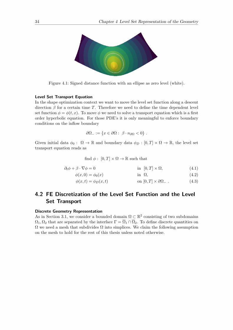
Example: A signed distance function that represents an ellipse is given by
φ0(x, y) =√
(x− xc)2
xs+ (y − yc)2
ys− r
with xc, yc ∈ R and xs, ys, r > 0. We will often use such functions for the domain ini-tialization in numerical experiments (see Figure 4.1 for a sketch).
33
34 Chapter 4 Level Set Representation of the Geometry
Figure 4.1: Signed distance function with an ellipse as zero level (white).
Level Set Transport EquationIn the shape optimization context we want to move the level set function along a descentdirection β for a certain time T . Therefore we need to define the time dependent levelset function φ = φ(t, x). To move φ we need to solve a transport equation which is a firstorder hyperbolic equation. For those PDE’s it is only meaningful to enforce boundaryconditions on the inflow boundary
∂Ω− := x ∈ ∂Ω : β · n∂Ω < 0 .
Given initial data φ0 : Ω → R and boundary data φD : [0, T ] × Ω → R, the level settransport equation reads as
find φ : [0, T ]× Ω→ R such that
∂tφ+ β · ∇φ = 0 in [0, T ]× Ω, (4.1)φ(x, 0) = φ0(x) in Ω, (4.2)φ(x, t) = φD(x, t) on [0, T ]× ∂Ω− . (4.3)
4.2 FE Discretization of the Level Set Function and the LevelSet Transport
Discrete Geometry RepresentationAs in Section 3.1, we consider a bounded domain Ω ⊂ R2 consisting of two subdomainsΩ1,Ω2 that are separated by the interface Γ = Ω1 ∩Ω2. To define discrete quantities onΩ we need a mesh that subdivides Ω into simplices. We claim the following assumptionon the mesh to hold for the rest of this thesis unless noted otherwise.
4.2 FE Discretization of the Level Set Function and the Level Set Transport 35
4.1. Definition/Assumption [mesh properties]Let Th be a family of simplicial triangulations of Ω. For T ∈ Th, hT is defined as thediameter of the smallest ball that contains T and ρT as the diameter of the largest ballcontained in T . The meshsize h is defined as h = maxhT : T ∈ Th.
Shape regularity: A family of triangulations is called shape regular if ∃K > 0such that ρT ≥ hT
K .
Quasi-uniformity: Th is called quasi-uniform if it is shape regular and ∃c > 0such that ∀ T ∈ Th holds ch ≤ hT .
Assumption: We assume that Th is shape regular in the following.
We will approximate the continuous level set function φ by discrete counterparts definedon Finite Element spaces corresponding to the triangulation Th. Whereas the geometryshould be represented by a continuous Finite Element function, for the level set transportit is beneficial to consider discontinuous Finite Element spaces. Therefore we need twodifferent representatives, namely a continuous and a discontinuous one defined by
φconth ∈ Vh := vh ∈ H1(Ω) : vh|T ∈ P1(T ), for T ∈ Th (4.4)φh,0 ∈Wh := wh ∈ L2(Ω) : wh|T ∈ P1(T ), for T ∈ Th. (4.5)
The continuous representative is used to define the discrete interface/domains
Γh := x ∈ Ω : φconth (x) = 0Ω1,h := x ∈ Ω : φconth (x) < 0Ω2,h := x ∈ Ω : φconth (x) > 0 .
Remark: For a piecewise linear geometry approximation holds dist(Γh,Γ) ∼ h2 for asufficiently accurate approximation φh of φ. This will not deteriorate any error estimatesif linear Finite Elements are applied (cf. [LR17, Lemma 3.7]).
To establish accurate definitions we need some more notation. Let T ∈ Th then
Ti := T ∩ Ωi,h, i ∈ 1, 2, (4.6)ΓT := T ∩ Γh, (4.7)T Γh := T : measd−1(T ∩ Γh) > 0, (set of cut elements), (4.8)
ΩΓ := x ∈ T : T ∈ T Γh , (domain of cut elements). (4.9)
Interpolation OperatorsIt is desirable to map between Wh and Vh as well as between C(Ω) and Vh. Thereforewe will define two suitable interpolation operators.
36 Chapter 4 Level Set Representation of the Geometry
To map discontinuous Finite Element functions on continuous ones, we employ the Os-wald interpolation (cf. [LR17], [Osw93]). Let X denote the set of mesh nodes, then wedefine for any xi ∈ X the set of elements that contain xi
ω(xi) := T ∈ Th : xi ∈ T .
For any wh ∈Wh, xi ∈ X we define the local average as
Axi(wh) := 1|ω(xi)|
∑T∈ω(xi)
wh|T (xi) .
The interpolation operator between Wh and Vh is then defined as
Iφ,dch (wh)(xi) := Axi(wh) , (4.10)
which defines an unique element Iφ,dch (wh) ∈ Vh.
The interpolation operator between C(Ω) and Vh is defined by standard nodal inter-polation (cf. [LR13, Definition 5.2])
Iφ,conth : C(Ω)→ Vh, Iφ,conth (ψ)(xi) = ψ(xi) ∀xi ∈ X . (4.11)
Note that this interpolation problem defines an unique element in Vh, since we considerlinear Finite Elements.
DG Level Set TransportIn order to discretize (4.1)-(4.3) we consider the discontinuous level set function φh,0 ∈Wh. A popular method to solve transport equations numerically, is the upwind-DGformulation which we will also use here. To present an accurate definition of this method,we need some more notation
F ih := F = ∂T1 ∩ ∂T2 : T1, T2 ∈ Th, T1 6= T2 (set of inner facets) .
For each F ∈ F ih we consider a master element T1, the second element will be denotedby T2. The unique facet normal nF is then defined as the outer unit normal of ∂T1. Forwh ∈Wh we further define on F ∈ F ih
[[wh]] := wh|T1−wh|T2 (facet jump),
wh := 12 (wh|T1+wh|T2) (facet average) .
Given a discrete descent direction βh ∈ Xh := ψh ∈[H1
0 (Ω)]d : ψh|T∈ [P1(T )]d , T ∈
Th the upwind bilinear form is defined by (cf. [DPE11])
cupwh (wh, vh) :=∫
Ω(βh · ∇wh) vh +
∮∂Ω
(βh · n∂Ω)whvh
−∑F∈Fi
h
∮F
(βh · nF ) [[wh]] vh
+∑F∈Fi
h
∮F
12 |βh · nF |[[wh]] [[vh]] ,
(4.12)
4.2 FE Discretization of the Level Set Function and the Level Set Transport 37
where x = 12(|x|−x) is the negative part. Given a discrete boundary condition φh,D
the corresponding linear form is defined as
F ch(vh) :=∮∂Ω
(βh · n∂Ω) φh,Dvh .
As boundary condition we will choose φh,D = φh,0.
Remark: For a derivation that also motivates the name "upwind-DG" and more de-tails on the method we refer to [Leh10].
Before we are going to define the semidiscrete and fully discrete version of the levelset transport we will have a closer look at the upwind bilinear form cupwh (·, ·). Forvh ∈Wh and F ∈ F ih we define on F
vdownh :=vh|T1 βh · nF < 0,vh|T2 βh · nF > 0 ,
so vdownh always "chooses" the value on the downwind side of the facet F (see Figure 4.2).
T1
T2
Figure 4.2: Two neighboring elements with the velocity field βh (blue) and the downwindfacet (red)
We would like to rewrite the two sums over the inner facets in (4.12). Therefore we haveto distinct two cases.Case 1: βh · nF < 0 and thus vdownh = vh|T1
12 |βh · nF |[[wh]] [[vh]]− (βh · nF ) [[wh]] vh = − (βh · nF ) [[wh]]
(12 [[vh]] + vh
)= − (βh · nF ) [[wh]]
(12(vh|T1−vh|T2)
+ 12(vh|T1+vh|T2)
)= − (βh · nF ) [[wh]] vh|T1
= − (βh · nF ) [[wh]] vdownh .
38 Chapter 4 Level Set Representation of the Geometry
Case 2: βh · nF > 0 and thus vdownh = vh|T2 . Here we conclude similarly
12 |βh · nF |[[wh]] [[vh]]− (βh · nF ) [[wh]] vh = − (βh · nF ) [[wh]] vdownh .
This investigation shows that we have an equivalent formulation of the upwind-DGbilinear form by
cupwh (wh, vh) :=∫
Ω(βh · ∇wh) vh +
∮∂Ω
(βh · n∂Ω)whvh −∑F∈Fi
h
∮F
(βh · nF ) [[wh]] vdownh .
The semidiscrete variational formulation of (4.1)-(4.3) reads as
find φh : [0, T ]→Wh such that ∀wh ∈Wh∫Ω∂tφh(t)wh + cupwh (φh(t), wh) = F ch(wh)
φh(0) = φh,0 .
(4.13)
This is a finite dimensional system of ordinary differential equations which can be fullydiscretized by an appropriate explicit or implicit time stepping scheme. We will choosean implicit Euler scheme. Let N ∈ N denote the number of time steps and ∆t := T
N thetime step size. Starting with the initial condition φ0
h = φh,0 the solution at time instancetn = n∆t for n ∈ 1, . . . , N is then approximated by φnh ≈ φh(tn). The approximationsare defined by the following scheme
for n = 1, . . . , N find φnh such that ∀wh ∈Wh∫Ω
1∆t
(φnh − φn−1
h
)wh + cupwh (φnh, wh) = F ch(wh) .
(4.14)
Let dim(Wh) = L and ωj : j = 1, . . . , L ⊂ Wh a basis of Wh. Then we can represent
φnh with respect to this basis φnh =L∑j=1
cnj ωj with coefficients cnj ∈ R. We obtain the
following quantities
RL 3 φn =(cnj
)Lj=1
RL 3 F = (F ch(ωj))Lj=1
RL×L 3M =((ωj , ωi)L2(Ω)
)Li,j=1
RL×L 3 A =(cupwh (ωj , ωi)
)Li,j=1 .
Now we can rewrite (4.14) as the linear system(M + ∆tA
)φn = M∆φn−1 + ∆tF . (4.15)
4.2 FE Discretization of the Level Set Function and the Level Set Transport 39
Re-initializationUsually the discrete level set function is initialized by an approximate signed distancefunction. During the level set transport, this property gets lost. In order to regain thesigned distance property, the current level set function φh can be replaced after a fewtime steps by an approximate signed distance function φh that has the same zero levelas φh. This process is known as re-initialization in the literature. The fast marchingmethod (first introduced by Sethian [Set96]) is one possibility to implement such a re-initialization. The only information that is needed from the "old" level set function φhis its zero level Γh. Based on geometrical ideas, the values of φh close to the interfaceare assigned and then successively extended to the entire domain. For more details andfurther references we refer to [LR13, Section 9.3.2] and [GR11, Section 7.4.1].
In this thesis we try to avoid the use of re-initialization techniques. The underlyingidea of this approach is, to transport the level set function by a velocity field βh thatdoesn’t deteriorate the signed distance property too much.
Chapter 5
FE Approximation of the One-phaseProblem
In the first part of this chapter we will present an unfitted Finite Element method whichyields solutions of optimal order for the one-phase problem introduced in Chapter 3.2.In the second part we will illustrate why an approximation of the velocity field basedon the volume expression is superior over an approximation based on the boundaryexpression. We will see that the former one yields better approximation properties in aFinite Element context.
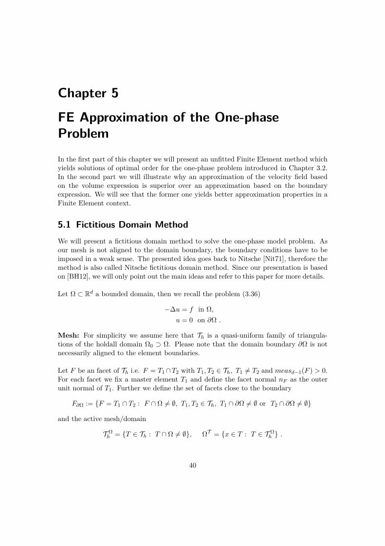
5.1 Fictitious Domain MethodWe will present a fictitious domain method to solve the one-phase model problem. Asour mesh is not aligned to the domain boundary, the boundary conditions have to beimposed in a weak sense. The presented idea goes back to Nitsche [Nit71], therefore themethod is also called Nitsche fictitious domain method. Since our presentation is basedon [BH12], we will only point out the main ideas and refer to this paper for more details.
Let Ω ⊂ Rd a bounded domain, then we recall the problem (3.36)
−∆u = f in Ω,u = 0 on ∂Ω .
Mesh: For simplicity we assume here that Th is a quasi-uniform family of triangula-tions of the holdall domain Ω0 ⊃ Ω. Please note that the domain boundary ∂Ω is notnecessarily aligned to the element boundaries.
Let F be an facet of Th i.e. F = T1∩T2 with T1, T2 ∈ Th, T1 6= T2 and measd−1(F ) > 0.For each facet we fix a master element T1 and define the facet normal nF as the outerunit normal of T1. Further we define the set of facets close to the boundary
F∂Ω := F = T1 ∩ T2 : F ∩ Ω 6= ∅, T1, T2 ∈ Th, T1 ∩ ∂Ω 6= ∅ or T2 ∩ ∂Ω 6= ∅
and the active mesh/domain
T Ωh = T ∈ Th : T ∩ Ω 6= ∅, ΩT = x ∈ T : T ∈ T Ω
h .
40
5.1 Fictitious Domain Method 41
Ω
Ω0
Figure 5.1: Background mesh with active mesh T Ωh (green) and interface Γ (red)
The geometrical setting is sketched in Figure 5.1. We consider a standard Finite Elementspace on the active domain
Vh(ΩT ) = vh ∈ H1(ΩT ) : vh|T∈ P1(T ), T ∈ T Ωh .
For vh ∈ Vh(ΩT ) the flux jump over a facet F = T1 ∩ T2 is defined by
[[∇vh · nF ]] := (∇vh|T1−∇vh|T2) · nF .
Let n denote the outer unit normal of Ω and λ ∈ R, then the Nitsche fictitious domainbilinear form aficth (·, ·) : Vh(ΩT )× Vh(ΩT )→ R reads as
aficth (uh, vh) :=∫
Ω∇uh · ∇vh −
∮∂Ω∇uh · nvh −
∮∂Ω∇vh · nuh +
∮∂Ω
λ
huhvh .
Remark: For the sake of convenience, we assume that all integrals can be evaluatedexactely.
To ensure stability in the case of small cuts (|T ∩ Ω| |T |), an additional stabiliza-tion term is needed, the so called ghost penalty. For a facet F = T1 ∩ T2 we definehF = maxdiam(T1), diam(T2). Let µ ∈ R, then the ghost penalty bilinear form isdefined by
j(uh, vh) :=∑
F∈F∂Ω
µhF
∮F
[[∇uh · nF ]] [[∇vh · nF ]] .
This is all we need to formulate the fictitious domain variational problem for (3.36):
find uh ∈ Vh(ΩT ) such that ∀vh ∈ Vh(ΩT )
Bh(uh, vh) := aficth (uh, vh) + j(uh, vh) =∫
Ωfvh .
(5.1)
42 Chapter 5 FE Approximation of the One-phase Problem
The properties of the solution to (5.1) are stated in the next lemma. The error boundsare given in the discrete energy norm defined by
|‖v‖|2h:=∑T∈T Ω
h
∫T|∇v|2+h
∮∂Ω
(∇v · n)2 + λh−1∮∂Ωv2 + j(v, v) .
Remark: The discrete energy norm is defined on the active domain ΩT that coversΩ. For a function u ∈ H2(Ω) there exists a proper extension E(u) ∈ H2(ΩT ) with‖E(u)‖H2(ΩT )≤ C‖u‖H2(Ω) (cf. [Ste70, Theorem 5, p.181]).
5.1. LEMMA [error bounds for uh (one-phase)]Let u ∈ H2(Ω) be the solution to (3.36). The variational problem (5.1) admits a uniquesolution uh for λ, µ sufficiently large, that fulfills
(i) |‖E(u)− uh‖|h≤ Ch‖u‖H2(Ω)
(ii) ‖u− uh‖L2(Ω)≤ Ch2‖u‖H2(Ω) .
Proof. See [BH12].
Similarly we can define the fictitious domain problem for the adjoint state (3.39) by
find u∗h ∈ Vh(ΩT ) such that ∀vh ∈ Vh(ΩT )
Bh(u∗h, vh) =∫
Ω2(uh − uc)vh =: F ∗h (vh) .
(5.2)
The same statement on the error bounds holds for the adjoint problem.
5.2. LEMMA [error bounds for u∗h (one-phase)]Let u∗ ∈ H2(Ω) be the solution to (3.36). The variational problem (5.2) admits a uniquesolution u∗h for λ, µ sufficiently large, that fulfills
(i) |‖E(u∗)− u∗h‖|h≤ Ch‖u∗‖H2(Ω)
(ii) ‖u∗ − u∗h‖L2(Ω)≤ Ch2‖u∗‖H2(Ω) .
Proof. The proof does not follow directly because the right hand side of the continuousand discrete adjoint problem differ. Therefore we define two auxiliary problems. Thecontinuous problem with the perturbed source term
find w∗ ∈ H10 (Ω) such that ∀v ∈ H1
0 (Ω)
a(w∗, v) :=∫
Ω∇w∗ · ∇v =
∫Ω
2(uh − uc)v .
And the discrete problem with the exact source term
find w∗h ∈ Vh(ΩT ) such that ∀vh ∈ Vh(ΩT )
Bh(w∗h, vh) =∫
Ω2(u− uc)vh .
5.2 Approximation of the Descent Direction 43
By the Poincaré inequality and Cauchy-Schwarz inequality we obtain
‖w∗ − u∗‖2H1(Ω) ≤ Ca(w∗ − u∗, w∗ − u∗)
= C
(∫Ω
2(uh − uc)(w∗ − u∗)−∫
Ω2(u− uc)(w∗ − u∗)
)= 2C
∫Ω
(u− uh)(w∗ − u∗)
≤ C‖w∗ − u∗‖H1(Ω)‖u− uh‖L2(Ω) .
Dividing by ‖w∗ − u∗‖H1(Ω) and application of Lemma 5.1 (ii) yields
‖w∗ − u∗‖H1(Ω)= O(h2) .
An L2 bound for (w∗h − u∗h) can be found by the triangle inequality
‖w∗h − u∗h‖L2(Ω)≤ ‖w∗h − u∗‖L2(Ω)+‖u∗ − w∗‖L2(Ω)+‖w∗ − u∗h‖L2(Ω)= O(h2) .
The order of the second summand was shown above and the order for the first and thirdsummand we can apply the standard error estimate as in Lemmma 5.1 because w∗h, u∗resp. u∗h, w∗ posess the same source term. Now we can apply the triangle ineqality andconclude by using the error bounds above and discrete coercivity of Bh(·, ·) ([BH12,Lemma 6])
|‖E(u∗)− u∗h‖|2h ≤ |‖E(u∗)− w∗h‖|2h+|‖w∗h − u∗h‖|2h≤ C
(h2 +Bh(w∗h − u∗h, w∗h − u∗h)
)= C
(h2 +
∫Ω
2(u− uh)(w∗h − u∗h))
≤ C(h2 + ‖uh − u‖L2(Ω)‖w∗h − u∗h‖L2(Ω)
)= O(h2) +O(h4) .
Taking the square root yields the first claim. The second one is obtained directly by thetriangle inequality
‖u∗ − u∗h‖L2(Ω) ≤ ‖u∗ − w∗‖L2(Ω)+‖w∗ − u∗h‖L2(Ω)
≤ ‖u∗ − w∗‖H1(Ω)+‖w∗ − u∗h‖L2(Ω)= O(h2) .
Where the order of the first summand was shown above and the order of the second onefollows again by the standard estimate in Lemma 5.1.
5.2 Approximation of the Descent DirectionContinuous Descent DirectionsTo highlight the aspect of the choice of the descent direction, we consider the one-phasemodel problem from Section 3.2. Let the assumptions of Lemma 3.8 be valid and u, u∗be the solutions of problem (3.36) and (3.39). According to Lemma 3.8 we have two
44 Chapter 5 FE Approximation of the One-phase Problem
expressions of the shape derivative that are equivalent on the analytical level. Thevolume expression
dV OL[ϑ] :=∫
Ωdiv(ϑ)
((u− uc)2 + u∗
)−∫
Ω2 (∇uc · ϑ) (u− uc)
+∫
Ω
((Dϑ+DϑT )∇u
)· ∇u∗ −
∫Ωdiv(ϑ)∇u · ∇u∗ +
∫Ω
(∇f · ϑ)u∗(5.3)
and the boundary expression
dBND[ϑ] :=∫∂Ωg(ϑ · n), with g = (u− uc)2 + (∇u · n) (∇u∗ · n) . (5.4)
Remark: Since we claimed the assumptions of Lemma 3.8 to hold, we have that g ∈L2(∂Ω). The Cauchy Schwarz inequality and the trace theorem imply further for ϑ ∈X =
[H1
0 (Ω0)]d
dBND[ϑ] =∫∂Ωg(ϑ · n) ≤ ‖g‖L2(∂Ω)‖ϑ‖L2(∂Ω)≤ C‖g‖L2(∂Ω)‖ϑ‖X .
Thus dBND[·] is a linear and continuous functional on X. Because both expressions areequal (on the analytical level), the same statement holds for dV OL[·]. Hence we obtainthat the extension assumption (B) from the first chapter is valid. Under weaker assump-tions dBND[·] may not be well defined at all and dV OL[·] is only a linear and continuousfunctional on W 1,∞(Ω).
To reduce the value of the shape function J(Ω) =∫
Ω(u−uc)2, we want to find a descentdirection β ∈ X. Let b(·, ·) be the inner product on X and β′ the Riesz representativeof −dV OL[·] i.e.
b(β′, ψ) = −dV OL[ψ], ∀ψ ∈ X .
Lemma 2.10 indicates that we have considerable freedom in the choice of β. We willinvestigate two possibilities namely
• βV OL = β′
• βBND with βBND · n = −g on ∂Ω ,
where n is the outer unit normal of ∂Ω.
Remark: For our purpose it is not enough to have a descent direction that is onlydefined on ∂Ω (such as g), since the level set transport equation requires a velocity fieldthat is defined in the entire holdall domain Ω0. Therefore such descent directions re-quire a Finite Element extension on Ω0 before they can be used for the level set transport.
5.2 Approximation of the Descent Direction 45
Discrete Descent DirectionsTo conclude this section we will now present an explanation why a volume based ap-proximation of the descent direction should be preferred over a boundary based approxi-mation. The main proposition of this section, which supports this statement, makesassumptions on error bounds of several discrete quantities. We want to emphasizethat these assumptions need not necessarily to hold but are realistic very often (cf.[BEH+17]).
We consider a shape regular family of simplicial triangulations Th of Ω0. The dis-crete counterparts for βV OL and βBND belong to the Finite Element space
Xh = ψh ∈[H1
0 (Ω0)]d
: τh|T∈ [P1(T )]d , T ∈ Th .
According to Corollary 2.6 for ϑ ∈ X, only the values of the normal component on∂Ω influence the value of the shape derivative. So let β ∈ X be a descent directionand βh ∈ Xh the corresponding discrete approximation, then we are interested in errorbounds of the form
‖(β − βh) · n‖L2(∂Ω)≤ Chq for q > 0 .
The following result is a useful tool to bound Lp norms on the boundary for p ≥ 1 andwill be used later to bound the L2 norm on the boundary.
5.3. LEMMA [trace inequality]Let Ω ⊂ Rd be a bounded domain with Lipschitz boundary. Then for 1 ≤ p ≤ ∞,∃C > 0 such that
‖v‖Lp(∂Ω)≤ C‖v‖1−1/pLp(Ω)‖v‖
1/pW 1,p(Ω) , ∀v ∈W 1,p(Ω) .
Proof. See [BS07, Theorem 1.6.6].
Let uh, u∗h ∈ Vh the solutions to (5.1), (5.2). The discrete version of the shape derivative(volume expression) is then defined by
dV OLh [ϑ] :=∫
Ωdiv(ϑ)
((uh − uc)2 + u∗h
)−∫
Ω2 (∇uc · ϑ) (uh − uc)
+∫
Ω
((Dϑ+DϑT )∇uh
)· ∇u∗h −
∫Ωdiv(ϑ)∇uh · ∇u∗h +
∫Ω
(∇f · ϑ)u∗h .
(5.5)
The discrete Riesz representative is then defined as the unique β′h ∈ Xh such that
b(β′h, ψh) = −dV OLh [ψh], ∀ψh ∈ Xh . (5.6)
According to Lemma 2.11 β′ ∈[H1
0 (Ω0)]d ∩ [H2(Ω0 \ Ω)
]d ∩ [H2(Ω)]d. We assumed fur-
ther that u, u∗ ∈ H2(Ω). That motivates the following assumption on the correspondingerror bounds.
46 Chapter 5 FE Approximation of the One-phase Problem
5.4. Assumption [optimal error bounds]
‖β′ − β′h‖X= O(h1/2), (5.7)‖β′ − β′h‖[L2(Ω0)]d= O(h), (5.8)
‖∇(u− uh) · n‖L2(∂Ω)= O(h1/2), (5.9)
‖∇(u∗ − u∗h) · n‖L2(∂Ω)= O(h1/2) . (5.10)
Remark: In order to proof the first two assumptions, one has to investigate the consis-tency error
supψh∈Xh
|dV OLh [ψh]− dV OL[ψh]|‖ψh‖X
.
If the error bounds from Lemma 5.1 hold, the bounds (5.9)-(5.10) are relatively easyobtained by the use of the trace inequalities and interpolation errors on the boundary.Finally we want to emphasized, that these bounds are realistic and have been proven fora similar problem in [BEH+17].
For the discrete counterparts of βBND and βV OL we have
βBNDh · n = (uh − uc)2 + (∇uh · n) (∇u∗h · n) =: gh on ∂Ω (5.11)βV OLh = β′h in Ω . (5.12)
It is intuitive that the dominating error in eh(g) := ‖g − gh‖L2(∂Ω) will be
‖(∇u · n)(∇u∗ · n)− (∇uh · n)(∇u∗h · n)‖L2(∂Ω) , (5.13)
since in Finite Element methods the gradient of a function is less accurately approx-imated than the function itself. The following assumption is much stronger than As-sumption 5.4 and claims that eh(g) can be controlled by the L2-error of the normalderivatives on the boundary.
5.5. ASSUMPTION [error bound for the boundary representative]
‖g − gh‖L2(∂Ω)≤ C(‖∇(u− uh) · n‖Ł2(∂Ω)+‖∇(u∗ − u∗h) · n‖Ł2(∂Ω)
)(5.14)
Now we can state the main result of this section.
5.6. PROPOSITION [error bounds for discrete descent directions]Consider the discrete descent directions βBNDh , βV OLh as in (5.11), (5.12). If Assumptions5.4 and 5.5 hold, then
‖(βBND − βBNDh
)· n‖L2(∂Ω)= O(h1/2),
‖(βV OL − βV OLh
)· n‖L2(∂Ω)= O(h3/4) .
5.2 Approximation of the Descent Direction 47
Proof. For the first statement we obtain by Assumption 5.5 and Assumption 5.4 (5.9)/(5.10)
‖(βBND − βBNDh
)· n‖2L2(∂Ω) ≤ ‖g − gh‖L2(∂Ω)
≤ C(‖∇(u− uh) · n‖L2(∂Ω)+‖∇(u∗ − u∗h) · n‖L2(∂Ω)
)= O(h1/2) ,
which yields the first claim. For the second statement on βV OLh we obtain, using thetrace inequality Lemma 5.3 and Young’s inequality for r ∈ R arbitrary
‖(βV OL − βV OLh
)· n‖L2(∂Ω) = ‖
(β′ − β′h
)· n‖L2(∂Ω)≤ ‖β′ − β′h‖[L2(∂Ω)]d
5.3≤ C
(‖β′ − β′h‖
1/2[L2(Ω)]d‖β
′ − β′h‖1/2X
)≤ C
(h−r‖β′ − β′h‖[L2(Ω)]d+hr‖β′ − β′h‖X
)≤ C
(h1−r + h
1/2+r),
where we used (5.7)/(5.8) in the last step. The choice r = 1/4 yields the error boundO(h3/4).
The above reasoning should motivate, why we will prefer the descent direction βV OLh
stemming from the volume expression of the shape derivative. Although we privilegedthe boundary expression by the strong assumption on the error bound (Assumption 5.5),the volume expression yielded a more accurate descent direction. Numerical examplesin accordance to the conjectured error bounds will be shown in Chapter 7.
Related WorkAnother aspect that can be considered in this context is to compare the functionalsdV OLh [·] and dBNDh [·], where
dBNDh [ϑ] :=∫
Ωgh(ϑ · n) .
On the analytical level dV OL[·] and dBND[·] are equivalent, which does not hold fortheir discrete approximations. In [HPS15] it is investigated, how the correspondingapproximation erros
sup‖β‖X=1
∣∣∣∣dV OLh [β]− d[β]∣∣∣∣ (5.15)
sup‖β‖X=1
∣∣∣∣dBNDh [β]− d[β]∣∣∣∣ (5.16)
behave. To estimate (5.15) and (5.16), X is replaced by a finite dimensional subspaceY ⊂ C1(Ω). For smooth domains, one can observe an experimental order of O(h2) forthe error of the volume functional and only O(h) for the error of the boundary functional.For more details, the reader is referred to [HPS15].
Chapter 6
FE Approximation of the Optimal InterfaceProblem
This chapter introduces all numerical methods which are needed to discretize the shapeoptimization problem introduced in Section 3.1. In the first section we will present theappropriate Finite Element spaces for unfitted interface problems. The second section ofthis chapter presents the discrete formulation of all sub problems of the full optimizationprocedure. The chapter is concluded by an optimization algorithm for problem (3.1) thatalso summarizes the former substeps.
6.1 The unfitted Finite Element Method (XFEM and CutFEM)Since we work with a level set geometry representation (that moves in every optimiza-tion step) and a fixed mesh Th, the mesh elements are not aligned to the interface Γ.This leads to the fact, that we lose approximation accuracy. To maintain an optimalapproximation order, the standard Finite Element spaces need to be modified.
Approximation OrdersWe consider functions that are domain-wise smooth but can have a strong or weakdiscontinuity over the interface i.e. u ∈ H l(Ω1)∩H l(Ω2) or u ∈ H l(Ω1)∩H l(Ω2)∩H1(Ω)for l ≥ 1. We consider the standard Finite Element spaces
V ch := v ∈ H1(Ω) : v|T∈ P1(T ), T ∈ Th, V dc
h := v ∈ L2(Ω) : v|T∈ P1(T ), T ∈ Th .
For the selected spaces, the following approximation result holds
6.1. LEMMA [approximation order of standard FE spaces]There exist shape regular families of triangulations Th, interfaces Γ ∈ C1 and w ∈H l(Ω1) ∩H l(Ω2), u ∈ H l(Ω1) ∩H l(Ω2) ∩H1(Ω) with l ≥ 2 such that
(i) infvh∈Vh
‖w − vh‖L2(Ω)≥ Ch1/2 , Vh ∈ V c
h , Vdch .
(ii) infvh∈Vh
‖u− vh‖L2(Ω)≥ Ch3/2 , Vh ∈ V c
h , Vdch .
Proof. For (i) see [GR11, Section 7.9.1], for (ii) see Appendix (Proposition A.3).
48
6.1 The unfitted Finite Element Method (XFEM and CutFEM) 49
Remark: The approximation orders in the last lemma do not improve, if the polynomialdegreee is increased to k > 1.
This lack of accuracy needs to be fixed, thus we will introduce FE-spaces that recoverthe domain-wise optimal approximation order globally. To do so wee need more de-grees of freedom in the region of the interface Γ. We define the restriction operator RiL2(Ω)→ L2(Ω) by
Riv =v|Ωi in Ωi
0 in Ω \ Ωi .
Now we can apply the restriction operator on the standard Finite Element spaceVh = vh ∈ H1(Ω) : vh|T ∈ P1(T ), T ∈ Th, which defines the unfitted Finite Elementspace
V Γh := R1Vh ⊕R2Vh .
The above definition describes V Γh as the direct sum of two restriced/cut Finite Element
spaces. Therefore, using this this description is referred to as CutFEM.
For V Γh we obtain now an optimal approximation order again.
6.2. LEMMA [approximation order of V Γh ]
Let u ∈ H2(Ω1) ∩H2(Ω2), then
infvh∈V Γ
h
‖u− vh‖L2(Ω)≤ Ch2(‖u‖H2(Ω1)+‖u‖H2(Ω2)
).
Proof. A proof can be found in [GR11, Theorem 7.9.3, p.254] .
Remark: The approximation result of the last lemma remains valid for higher polyno-mial degrees k > 1 and yields an error bound hk+1 for u ∈ Hk+1(Ω1)∩Hk+1(Ω2). Sincewe only consider low order Finite Elements, the error bound for k = 1 will be sufficientin this thesis.
XFEM CharacterizationThe abstract space V Γ
h can be characterized by an enrichment of the standard FE spaceVh. This approach is referred to as XFEM. We follow [GR11, Section 7.9.2] to constructsuch enrichment basis functions.
Let n = dim(Vh), J = 1, . . . , n and ϕj : j ∈ J a nodal basis of Vh i.e. forthe i-th node xi holds ϕj(xi) = δij . We define the index set of nodes belonging to abasis function close to the interface
JΓ = j ∈ J : Γ ∩ supp(ϕj) 6= ∅ .
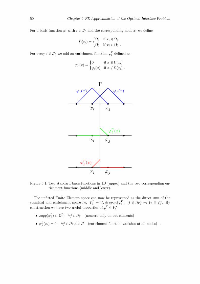
50 Chapter 6 FE Approximation of the Optimal Interface Problem
For a basis function ϕi with i ∈ JΓ and the corresponding node xi we define
Ω(xi) =
Ω1 if xi ∈ Ω1
Ω2 if xi ∈ Ω2 .
For every i ∈ JΓ we add an enrichment function ϕΓi defined as
ϕΓi (x) =
0 if x ∈ Ω(xi)ϕi(x) if x /∈ Ω(xi) .
Γϕi(x) ϕj(x)
ϕΓi (x)
ϕΓj (x)
xi xj
xi xj
xi xj
Figure 6.1: Two standard basis functions in 1D (upper) and the two corresponding en-richment functions (middle and lower).
The unfitted Finite Element space can now be represented as the direct sum of thestandard and enrichment space i.e. V Γ
h = Vh ⊕ spanϕΓj : j ∈ JΓ =: Vh ⊕ V x
h . Byconstruction we have two useful properties of ϕΓ
j ∈ V xh :
• supp(ϕΓj ) ⊂ ΩΓ, ∀j ∈ JΓ (nonzero only on cut elements)
• ϕΓj (xi) = 0, ∀j ∈ JΓ, i ∈ J (enrichment function vanishes at all nodes) .
6.2 Shape Optimization Procedure for an Interface Problem 51
6.2 Shape Optimization Procedure for an Interface ProblemIn this section we will derive an optimization algorithm for the two-phase problem fromSection 3.1. Therefore we will give detailed descriptions of all discrete sub problemswhich need to be solved in each optimization step. This includes a an unfitted Nitscheformulation for the state and adjoint state equation and the construction of a descentdirection for the level set transport equation.
6.2.1 An unfitted Nitsche Method for the State and Adjoint StateWe recall problem (3.2)-(3.5) from the last chapter. With a bounded domain Ω ⊂ R2
that can be decomposed into two subdomains Ω1 and Ω2, separated by the interfaceΓ := Ω1 ∩ Ω2. Further it is assumed that Ω1 is fully surrounded by Ω2.
−div(α∇u) = f in Ω (6.1)[[u]] = 0 on Γ (6.2)
[[−α∇u · nΓ]] = 0 on Γ (6.3)∇u · n+ γu = 0 on ∂Ω (6.4)
The weak formulation of this problem reads as
find u ∈ H1(Ω) such that ∀v ∈ H1(Ω)2∑i=1
αi
∫Ωi∇u · ∇v +
∮∂Ωγuv =
∫Ωfv .
(6.5)
To approximate u by a Finite Element solution we choose the unfitted Finite Elementspace introduced in the first section of this chapter
V Γh = Vh|Ω1⊕Vh|Ω2 .
Remark: Note that we consider the unfitted Finite Element space with respect to thesubdomains Ωi. In fact, the Finite Element spaces are defined with respect to the discretesubdomains Ωi,h but we assume for simplicity that the geometry can be approximatedexactely. A deeper investigation shows that the geometry error does not deteriorate thesubsequent error bounds (cf. [LR17]).
Since V Γh * C0(Ω), a discrete function vh ∈ V Γ
h is in general not single valued onthe interface Γ. Let nΓ be the unit normal of Γ pointing outwards Ω1, s ∈ R and x ∈ Γ,then for any function w we define the two corresponding values of w by
w−(x) := lims0
w(x− snΓ) , w+(x) := lims0
w(x+ snΓ) .
Let κ1, κ2 ≥ 0 with κ1 + κ2 = 1, then we define the jump and average operator (wellknown from discontinuous Galerkin methods) on the interface by
[[w(x)]] = w−(x)− w+(x) , x ∈ Γw(x) = κ1w
−(x) + κ2w+(x), x ∈ Γ .
52 Chapter 6 FE Approximation of the Optimal Interface Problem
We define the discrete bilinear form ah : V Γh × V Γ
h → R by
ah(uh, vh) :=2∑i=1
αi
∫Ωi∇uh · ∇vh +
∮∂Ωγuhvh
−∮
Γ[[uh]] α∇vh · nΓ −
∮Γ
[[vh]] α∇uh · nΓ+∮
Γλ [[uh]] [[vh]] ,
where λ ≥ 0. The method corresponding to the bilinear form ah(·, ·) is often calledNitsche method in the literature. The corresponding linear form Fh : V Γ
h → R isdefined by
F (vh) :=∫
Ωfvh .
Thus the discrete variational problem reads:
find uh ∈ V Γh such that ∀vh ∈ V Γ
h
ah(uh, vh) = F (vh) .(6.6)
For the error analysis of this discrete variational problem we will refer to the results in[LR17], where optimal error bounds are proven for a scalar interface problem with homo-geneous Dirichlet boundary conditions. The paper is focussed on higher order methodsbut the analysis includes k = 1 as a special case. The only difference in the variationalformulation is that we consider a Robin problem. However, since the outer boundary∂Ω is fitted to the mesh, the generalization to this case is straightforward.
The coefficient of the average operator will be element wise defined by
κi = |Ti||T |
, where |T |= measd(T ) ,
this particular choice has been first introduced by Hansbo and Hansbo (cf. [HH02]). Toanalyze the bilinear form ah(·, ·), further norms are needed. The mesh dependent normson the interface
‖v‖21/2,h,Γ:=∑T∈T Γ
h
(α1 + α2)2hT
∫ΓTv2, ‖v‖2−1/2,h,Γ:=
∑T∈T Γ
h
2hT(α1 + α2)
∫ΓTv2
and the full norm
‖v‖2h:=2∑i=1
∫Ωi,h∇v · ∇v +
∮∂ΩR
v2 + ‖α∇v · nΓh‖2−1/2,h,Γ+‖[[v]] ‖21/2,h,Γ .
We quote the following two results.
6.2 Shape Optimization Procedure for an Interface Problem 53
6.3. LEMMA [properties of ah(·, ·)]Let Vreg := H1(Ω) ∩ H2(Ω1) ∩ H2(Ω2), then for λ sufficiently large the bilinear formah(·, ·) has the following properties:
(i) Continuity
ah(u, v) ≤ ‖u‖h‖v‖h ∀u, v ∈ Vreg + V Γh .
(ii) Discrete coercivity
ah(vh, vh) ≥ ‖vh‖2h ∀vh ∈ V Γh .
Proof. The proof is analogue to [Lemma 5.2][LR17].
6.4. LEMMA [interpolation error]There exists an interpolation operator IΓ
h : H1(Ω)→ V Γh such that
‖v − IΓh ‖h≤ Ch
(‖v‖H2(Ω1)+‖v‖H2(Ω2)
)∀v ∈ Vreg.
Proof. The proof is analogue to [Lemma 5.7][LR17].
Those results yield the existence of a unique solution uh of (6.6). The discrete solutionfulfills the following optimal error bounds.
6.5. LEMMA [error bounds for uh (two-phase)]Let u be the solution of (6.5), then
(i) ‖u− uh‖h≤ Ch(‖u‖H2(Ω1)+‖u‖H2(Ω2)
)
(ii) ‖u− uh‖L2(Ω)≤ Ch2(‖u‖H2(Ω1)+‖u‖H2(Ω2)
)Proof. The proof of the first statement is analogue to [Theorem 5.8][LR17]. A proofanalogue to the second statement can be found in [Theorem 6.5][LR18].
Similar to the discretized state equation (6.6) we discretize the adjoint equation (3.22).Therefore we define the discrete linear form
F ∗h (vh) :=∫
Ω2(uh − u)vh .
Thus the discrete adjoint problem reads
find u∗h ∈ V Γh such that ∀vh ∈ V Γ
h
ah(u∗h, vh) = F ∗h (vh) .(6.7)
Similarly to the state problem, the discrete adjoint problem has a unique solution u∗h ∈V Γh that fulfills the same error bounds than uh. To proof this statement, wee need an
additional lemma.
54 Chapter 6 FE Approximation of the Optimal Interface Problem
6.6. LEMMA [consistency of the adjoint problem]Let u, u∗ be the solutions of (6.5)and (3.22) with u∗ ∈ H2(Ω1) ∩H2(Ω2), then
ah(u∗, vh) =∫
Ω2(u− u)vh , ∀vh ∈ V Γ
h .
Proof. Since u∗ is the exact solution of the adjoint problem [[u∗]] = 0 on Γ and thus
ah(u∗, vh) =2∑i=1
αi
∫Ωi∇u∗ · ∇vh +
∮∂Ωγu∗vh −
∮Γ
[[vh]] α∇u∗ · nΓ . (6.8)
To treat the interface integral we note that for the exact solution u∗ holds α∇u∗ ·nΓ =α1∇u∗ · nΓ = α2∇u∗ · nΓ on Γ and α2∇u∗ · n = γu∗ on ∂Ω. Further on the subdomainsΩi holds −αi∆u∗ = 2(u− u). Integration by parts (Green’s formula) yields∮
Γ[[vh]] α∇u∗ · nΓ =
∮∂Ω1
v−h α1∇u∗ · nΓ +∮∂Ω2
v+h α2∇u∗ · n∂Ω2 +
∮∂Ωvhα2∇u∗ · n
=2∑i=1
αi
∫Ωi∇u∗ · ∇vh +
2∑i=1
∫Ωi
(αi∆u∗)vh +∮∂Ωγu∗vh
=2∑i=1
αi
∫Ωi∇u∗ · ∇vh +
∮∂Ωγu∗vh −
∫Ω
2(u− u)vh .
Inserting this identity into (6.8) yields the claim.
Finally we can state a lemma that ensures also optimal error bounds for u∗h.
6.7. LEMMA [error bounds for u∗h (two-phase)]Let u∗ be the solution of (3.22), then
(i) ‖u∗ − u∗h‖h≤ Ch(‖u∗‖H2(Ω1)+‖u∗‖H2(Ω2)
)
(ii) ‖u∗ − u∗h‖L2(Ω)≤ Ch2(‖u∗‖H2(Ω1)+‖u∗‖H2(Ω2)
)Proof. Similarly as in Lemma 5.2, we have to take into account the perturbation on theright hand side. Let F ∗(·) denote the source term corresponding to the exact solutioni.e.
F ∗(v) =∫
Ω2(u− u)v .
Due to the triangle inequality it is sufficient to consider the approximation error, since
‖u∗ − u∗h‖h≤ ‖u∗ − IΓh (u∗)‖h+‖IΓ
h (u∗)− u∗h‖h
6.2 Shape Optimization Procedure for an Interface Problem 55
and the interpolation error can be estimated by Lemma 6.4. For the approximation errorwe obtain using coercivity (Lemma 6.3) and consistency (Lemma 6.6)
‖IΓh (u∗)− u∗h‖2h = ah(IΓ
h (u∗)− u∗h, IΓh (u∗)− u∗h)
= ah(IΓh (u∗)− u∗, IΓ
h (u∗)− u∗h) + ah(u∗ − u∗h, IΓh (u∗)− u∗h)
= ah(IΓh (u∗)− u∗, IΓ
h (u∗)− u∗h) + F ∗(IΓh (u∗)− u∗h)− F ∗h (IΓ
h (u∗)− u∗h)
≤ C‖IΓh (u∗)− u∗h‖h
(‖IΓh (u∗)− u∗‖h+‖u− uh‖L2(Ω)
).
Dividing by ‖IΓh (u∗)− u∗h‖h and application of Lemma 6.4, Lemma 6.5 on the quantities
on the right hand side yields the first claim.
The second statement can be now obtained by a standard duality argument which willbe skipped here.
6.2.2 Construction of a Descent DirectionSo far we did not specify, which discrete velocity field βh should be used in the level settransport equation. We will motivate our particular choice of βh by a variational prob-lem on the domain of cut elements which allows also for an analysis of the approximationerror. The final variational problem will follow the same idea but will be formulated onwhole Ω. This has the purpose to simplify the algorithm and it should be emphasizedthat a globally defined descent direction, for which the error analysis also applies, canbe easily constructed.
In Section 5.2 we already indicated that for the one-phase problem, the volume expres-sion of the shape derivative yields better approximation properties than the boundaryexpression. Therefore we will also for the two-phase problem prefer a descent directionthat is based on the volume expression of the shape derivative. The discrete volumeexpression is given by
dh[ϑ] :=∫
Ωdiv(ϑ)
((uh − u)2 + fu∗h
)−∫
Ω2(∇u · ϑ)(uh − u)
−2∑i=1
αi
∫Ωidiv(ϑ)∇uh · ∇u∗h +
2∑i=1
αi
∫Ωi
((Dϑ+DϑT )∇uh
)· ∇u∗h ,
(6.9)
where uh, u∗h are the solutions of (6.6) and (6.7). Let β′h be the discrete Riesz represen-tative of −dh[·] i.e the unique β′h ∈ Xh with
b(β′h, ψh) = −dh[ψh], ∀ψh ∈ Xh, (6.10)
with the inner product b(β, ψ) =∫
Ω β · ψ +∫
Ω∇β : ∇ψ. According to Lemma 2.10 wewon’t violate the descent property if we change the values of β′h in Ω\Γ. Therefore we willdesign a velocity field that that approximates β′h on Γ and is extended to Ω\Γ in such away that the signed distance property around the interface is (approximately) preserved.
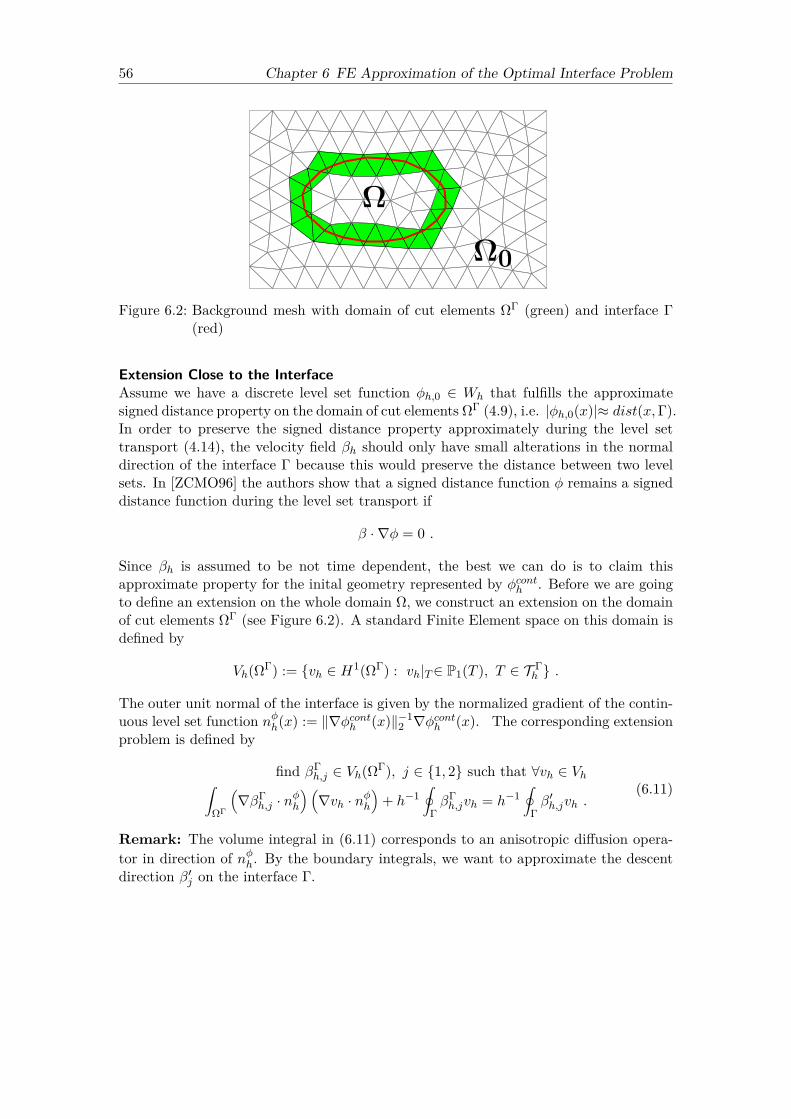
56 Chapter 6 FE Approximation of the Optimal Interface Problem
Ω
Ω0
Figure 6.2: Background mesh with domain of cut elements ΩΓ (green) and interface Γ(red)
Extension Close to the InterfaceAssume we have a discrete level set function φh,0 ∈ Wh that fulfills the approximatesigned distance property on the domain of cut elements ΩΓ (4.9), i.e. |φh,0(x)|≈ dist(x,Γ).In order to preserve the signed distance property approximately during the level settransport (4.14), the velocity field βh should only have small alterations in the normaldirection of the interface Γ because this would preserve the distance between two levelsets. In [ZCMO96] the authors show that a signed distance function φ remains a signeddistance function during the level set transport if
β · ∇φ = 0 .
Since βh is assumed to be not time dependent, the best we can do is to claim thisapproximate property for the inital geometry represented by φconth . Before we are goingto define an extension on the whole domain Ω, we construct an extension on the domainof cut elements ΩΓ (see Figure 6.2). A standard Finite Element space on this domain isdefined by
Vh(ΩΓ) := vh ∈ H1(ΩΓ) : vh|T∈ P1(T ), T ∈ T Γh .
The outer unit normal of the interface is given by the normalized gradient of the contin-uous level set function nφh(x) := ‖∇φconth (x)‖−1
2 ∇φconth (x). The corresponding extensionproblem is defined by
find βΓh,j ∈ Vh(ΩΓ), j ∈ 1, 2 such that ∀vh ∈ Vh∫
ΩΓ
(∇βΓ
h,j · nφh
) (∇vh · nφh
)+ h−1
∮ΓβΓh,jvh = h−1
∮Γβ′h,jvh .
(6.11)
Remark: The volume integral in (6.11) corresponds to an anisotropic diffusion opera-tor in direction of nφh. By the boundary integrals, we want to approximate the descentdirection β′j on the interface Γ.
6.2 Shape Optimization Procedure for an Interface Problem 57
We define the tubular neighborhood of the interface by
Uδ(Γ) := x ∈ Ω : dist(x,Γ) ≤ δ, δ ∈ R .
In order to show an approximation result on the interface, we need the following auxiliarylemma.6.8. LEMMA [estimate on Uδ]Let w ∈ H1(Ω1) ∩H1(Ω2), then
‖w‖L2(Uδ)≤ Cδ1/2(‖w‖H1(Ω1)+‖w‖H1(Ω2)
).
Proof. See [ER13, Lemma 4.10].
From Lemma 2.11 we obtain that for the H1 Riesz representative holds β′ ∈[H2(Ω1)
]d∩[H2(Ω2)
]d :=[H2(Ω1,2)
]d. As discussed in Section 5.2, we want to achieve an accurateapproxmation of β′ at the interface Γ. By considering a discrete representative β′h weintroduce the errors
‖β′ − β′h‖X (6.12)‖β′ − β′h‖[L2(Γ)]d . (6.13)
The extension βΓh introduces an additional approximation error
‖βΓh − β′‖[L2(Γ)]d . (6.14)
The next lemma shows that we can bound (6.14) by means of (6.12) and (6.13).
6.9. LEMMA [approximation error of βΓh ]
The following error bound on the velocity field βΓh holds:
‖βΓh − β′‖[L2(Γ)]d≤ C
(‖β′ − β′h‖[L2(Γ)]d+h‖β′‖[H2(Ω1,2)]d+h
1/2‖β′ − β′h‖X),
where ‖·‖2[H2(Ω1,2)]d := ‖·‖2[H2(Ω1)]d+‖·‖
2[H2(Ω2)]d .
Proof. At first we note, that by the triangle inequality holds
‖βΓh − β′‖[L2(Γ)]d≤ ‖βΓ
h − β′h‖[L2(Γ)]d+‖β′h − β′‖[L2(Γ)]d . (6.15)
We will further derive an estimate for the first summand. For the components of βhholds that βh,j ∈ Vh and thus βh,j |ΩΓ∈ Vh(ΩΓ) is a valid test function for the variationalproblem (6.11). Taking advantage of that fact, we can use the variational formulation(6.11) and Young’s inequality to obtain∫
ΩΓ
(∇(βΓ
h,j − β′h,j) · nφh
)2+ h−1
∮Γ(βΓh,j − β′h,j)2
= h−1∮
Γβ′h,j(βΓ
h,j − β′h,j)−∫
ΩΓ
(∇β′h,j · n
φh
) (∇(βΓ
h,j − β′h,j) · nφh
)− h−1
∮Γβ′h,j(βΓ
h,j − β′h,j)
≤ 14
∫ΩΓ
(∇β′h,j · n
φh
)2+∫
ΩΓ
(∇(βΓ
h,j − β′h,j) · nφh
)2.
58 Chapter 6 FE Approximation of the Optimal Interface Problem
Substracting the second summand on the right hand side, multiplying by h and takingthe square root yields
‖βΓh − β′h‖[L2(Γ)]d≤
12h
1/2
√∫ΩΓ
(∇β′h,j · n
φh
)2≤ h1/2‖∇β′h,j‖[L2(Uh(Γ)]d ,
where we used ΩΓ ⊂ Uh(Γ) in the last estimate. We obtain further by the triangleinequality and Lemma 6.8
h1/2‖∇β′h,j‖[L2(Uh(Γ)]d ≤ h
1/2‖β′ − β′h‖X+h1/2‖∇β′‖[L2(Uh(Γ)]d
≤ h1/2‖β′ − β′h‖X+Ch‖β′j‖H2(Ω1,2) .
All in all we have proven
‖βΓh − β′h‖[L2(Γ)]d≤ C
(h‖β′‖[H2(Ω1,2)]d+h
1/2‖β′ − β′h‖X).
Inserting this identity into (6.15) yields the claim.
Remark: If we assume error bounds similar to Assumption 5.4, the previous lemmashows that the approximation error of βΓ
h can be bounded by the approximation error ofthe discrete Riesz representative β′h and a term of order O(h). Hence, the approximationerror of βΓ
h won’t be worse than the error introduced by β′h.
Global ExtensionA velocity field that is only defined on the band of cut elements ΩΓ is not suitablefor the level set transport, since we need a velocity field that is defined on whole Ω.Motivated by the former lemma we define the global variant of (6.11) by replacing ΩΓ
with Ω. To obtain a descent direction with a moderate scaling, β′h is normalized beforeit is extended.
find βeh,j ∈ Vh, j ∈ 1, 2 such that ∀vh ∈ Vh∫Ω
(∇βeh,j · n
φh
) (∇vh · nφh
)+ h−1
∮Γβeh,jvh = h−1‖β′h‖−1
X
∮Γβ′h,jvh .
(6.16)
The resulting velocity field βeh ∈ [Vh]2 will be used in the level set transport equation(4.14) to move the level set function φh,0.
Remark: The presented error analysis does not apply for the globally defined descentdirection βeh. However, if we would extend the locally defined descent direction βΓ
h toΩ \ ΩΓ with the same strategy, we would obtain a global velocity field that fulfills theerror bounds of Lemma 6.9. In this thesis we chose a direct extension to Ω in order tokeep the optimization algorithm simpler.
6.2 Shape Optimization Procedure for an Interface Problem 59
6.2.3 Optimization AlgorithmAll the previously introduced discrete subproblems can be summarized by an optimiza-tion algorithm that solves problem (3.1). We give a rough summary what happens inone optimization step:
• Compute the discrete state and adjoint state uh, u∗h , (6.6), (6.7).
• Set up the discrete shape derivative dh[·], (6.9).
• Compute the descent direction βeh, (6.16).
• Move the discontinuous level set function along βeh (6.16) by means of (4.14) andobtain φNh at the final time instance.
• Update the geometry by means of the interpolation operator (4.10),φconth = Iφ,dch
(φNh
).
• Compute the new state uh on the updated geometry.
• Check if the value of the shape function is reduced.
The complete procedure corresponding to this workflow is presented in Algorithm 1,which is also the final result of this chapter.
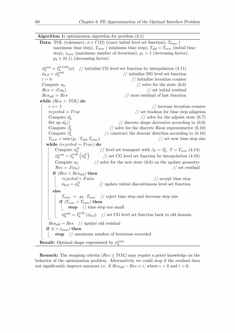
60 Chapter 6 FE Approximation of the Optimal Interface Problem
Algorithm 1: optimization algorithm for problem (3.1)Data: TOL (tolerance), φ ∈ C(Ω) (exact initial level set function), Tmax (
maximum time step), Tmin ( minimum time step), Told = Tnew (initial timestep), imax (maximum number of iterations), p1 > 1 (increasing factor),p2 ∈ (0, 1) (decreasing factor)
φconth = Iφ,conth (φ) // initialize CG level set function by interpolation (4.11)φh,0 = φconth // initialize DG level set functioni = 0 // initialize iteration counterCompute uh // solve for the state (6.6)Res = J(uh) // set initial residualResold = Res // store residual of last iterationwhile (Res > TOL) do
i += 1 // increase iteration counterrejected = True // set boolean for time step adaptionCompute u∗h // solve for the adjoint state (6.7)Set up dh[·] // discrete shape derivative according to (6.9)Compute β′h // solve for the discrete Riesz representative (6.10)Compute βeh // construct the descent direction according to (6.16)Tnew = min (p1 · Told, Tmax) // set new time step sizewhile (rejected = True) do
Compute φNh // level set transport with βh = βeh, T = Tnew (4.14)φconth = Iφ,dch
(φNh
)// set CG level set function by interpolation (4.10)
Compute uh // solve for the new state (6.6) on the update geometryRes = J(uh) // set residualif (Res < Resold) then
rejected = False // accept time stepφh,0 = φNh // update initial discontinuous level set function
elseTnew = p2 · Tnew // reject time step and decrease step sizeif (Tnew < Tmin) then
stop // time step too small
φconth = Iφ,dch (φh,0) // set CG level set function back to old domain
Resold = Res // update old residualif (i > imax) then
stop // maximum number of iterations exceeded
Result: Optimal shape represented by φconth
Remark: The stopping criteria (Res ≤ TOL) may require a priori knowledge on thebehavior of the optimization problem. Alternatively we could stop if the residual doesnot significantly improve anymore i.e. if Resold −Res < ε, where ε > 0 and i > 0.
Chapter 7
Numerical Results
In this chapter we will present numerical experiments to highlight the following aspects
• Section 7.1: Accuracy of descent directions for the one-phase model problem ofSection 3.2 with focus on the comparison between volume and boundary expression.
• Section 7.2: Accuracy of descent directions for the two-phase model problem ofSection 3.1 with focus on the choice of the approximation space.
• Section 7.3: Performance of the full optimization algorithm (Algorithm 1).
• Section 7.4: Comparison of the descent directions β′h (Riesz representative) andβeh (anisotropic extension).
• Section 7.5: Behavior of geometry error and residual error.
All numerical methods and experiments have been implemented in the add-on libraryngsxfem to the Finite Element software NGSolve [Sch14].
7.1 Comparison of Volume and Boundary ExpressionWe recall the setting of Section 5.2. As a model problem we consider Ω0 = [−1,−1]×[1, 1]for the holdall domain and the Dirichlet problem
−∆u = f in Ω (7.1)u = 0 on ∂Ω , (7.2)
with f = 8(0.25− 2(x2 + y2)
)and the shape function
J(Ω) =∫
Ω(u− uc)2 .
We choose uc = (x2 +y2−0.25)2, which is the exact solution to (7.1), where Ω is a circlewith radius 0.5 and center (0, 0). As initial domain we choose an ellipse correspondingto the signed distance function
φ(x, y) =
√x2
1.6 + y2
0.4 − 0.5 .
61
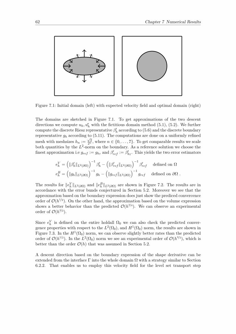
62 Chapter 7 Numerical Results
Figure 7.1: Initial domain (left) with expected velocity field and optimal domain (right)
The domains are sketched in Figure 7.1. To get approximations of the two descentdirections we compute uh, u∗h with the fictitious domain method (5.1), (5.2). We furthercompute the discrete Riesz representative β′h according to (5.6) and the discrete boundaryrepresentative gh according to (5.11). The computations are done on a uniformly refinedmesh with meshsizes hn :=
√2
2n , where n ∈ 0, . . . , 7. To get comparable results we scaleboth quantities by the L2-norm on the boundary. As a reference solution we choose thefinest approximation i.e gref := gh7 and β′ref := β′h7
. This yields the two error estimators
eVh =(‖β′h‖L2(∂Ω)
)−1β′h −
(‖β′ref‖L2(∂Ω)
)−1β′ref defined on Ω
eBh =(‖gh‖L2(∂Ω)
)−1gh −
(‖gref‖L2(∂Ω)
)−1gref defined on ∂Ω .
The results for ‖eVh ‖L2(∂Ω) and ‖eBh ‖L2(∂Ω) are shown in Figure 7.2. The results are inaccordance with the error bunds conjectured in Section 5.2. Moreover we see that theapproxmation based on the boundary expression does just show the prediced convercenceorder of O(h1/2). On the other hand, the approximation based on the volume expressionshows a better behavior than the predicted O(h3/4). We can observe an experimentalorder of O(h3/2).
Since eVh is defined on the entire holdall Ω0 we can also check the predicted conver-gence properties with respect to the L2(Ω0), and H1(Ω0) norm, the results are shown inFigure 7.3. In the H1(Ω0) norm, we can observe slightly better rates than the predictedorder of O(h1/2). In the L2(Ω0) norm we see an experimental order of O(h3/2), which isbetter than the order O(h) that was assumed in Section 5.2.
A descent direction based on the boundary expression of the shape derivative can beextended from the interface Γ into the whole domain Ω with a strategy similar to Section6.2.2. That enables us to employ this velocity field for the level set transport step
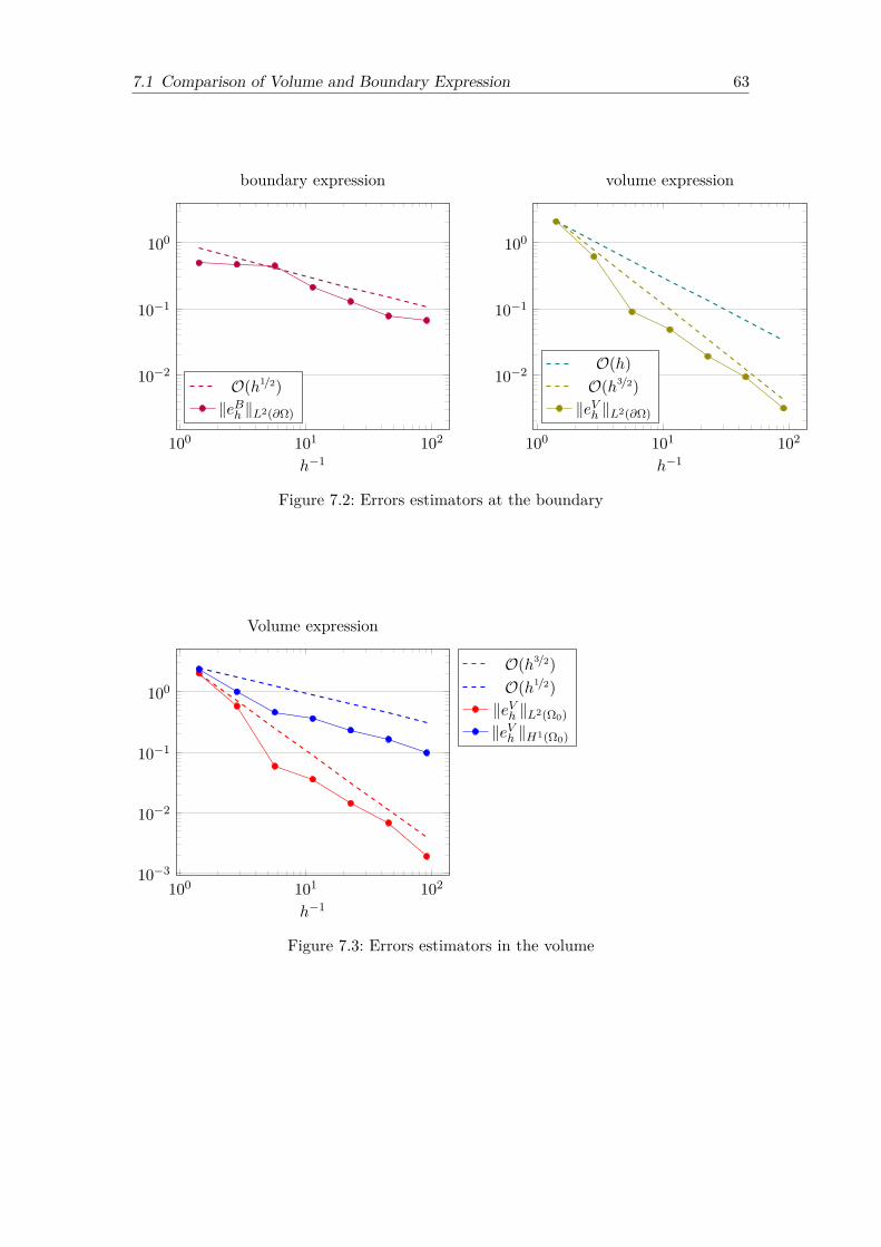
7.1 Comparison of Volume and Boundary Expression 63
100 101 102
10−2
10−1
100
h−1
boundary expression
O(h1/2)‖eBh ‖L2(∂Ω)
100 101 102
10−2
10−1
100
h−1
volume expression
O(h)O(h3/2)‖eVh ‖L2(∂Ω)
Figure 7.2: Errors estimators at the boundary
100 101 10210−3
10−2
10−1
100
h−1
Volume expression
O(h3/2)O(h1/2)‖eVh ‖L2(Ω0)‖eVh ‖H1(Ω0)
Figure 7.3: Errors estimators in the volume
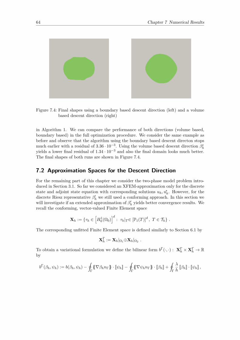
64 Chapter 7 Numerical Results
Figure 7.4: Final shapes using a boundary based descent direction (left) and a volumebased descent direction (right)
in Algorithm 1. We can compare the performance of both directions (volume based,boundary based) in the full optimization procedure. We consider the same example asbefore and observe that the algorithm using the boundary based descent directon stopsmuch earlier with a residual of 3.36 · 10−3. Using the volume based descent direction βehyields a lower final residual of 1.34 · 10−3 and also the final domain looks much better.The final shapes of both runs are shown in Figure 7.4.
7.2 Approximation Spaces for the Descent DirectionFor the remaining part of this chapter we consider the two-phase model problem intro-duced in Section 3.1. So far we considered an XFEM-approximation only for the discretestate and adjoint state equation with corresponding solutions uh, u∗h. However, for thediscrete Riesz representative β′h we still used a conforming approach. In this section wewill investigate if an extended approximation of β′h yields better convergence results. Werecall the conforming, vector-valued Finite Element space
Xh := τh ∈[H1
0 (Ω0)]d
: τh|T∈ [P1(T )]d , T ∈ Th .
The corresponding unfitted Finite Element space is defined similarly to Section 6.1 by
XΓh := Xh|Ω1⊕Xh|Ω2 .
To obtain a variational formulation we define the bilinear form bΓ(·, ·) : XΓh ×XΓ
h → Rby
bΓ(βh, ψh) := b(βh, ψh)−∮
Γ∇βhnΓ · [[ψh]]−
∮Γ∇ψhnΓ · [[βh]] +
∮Γ
λ
h[[βh]] · [[ψh]] ,
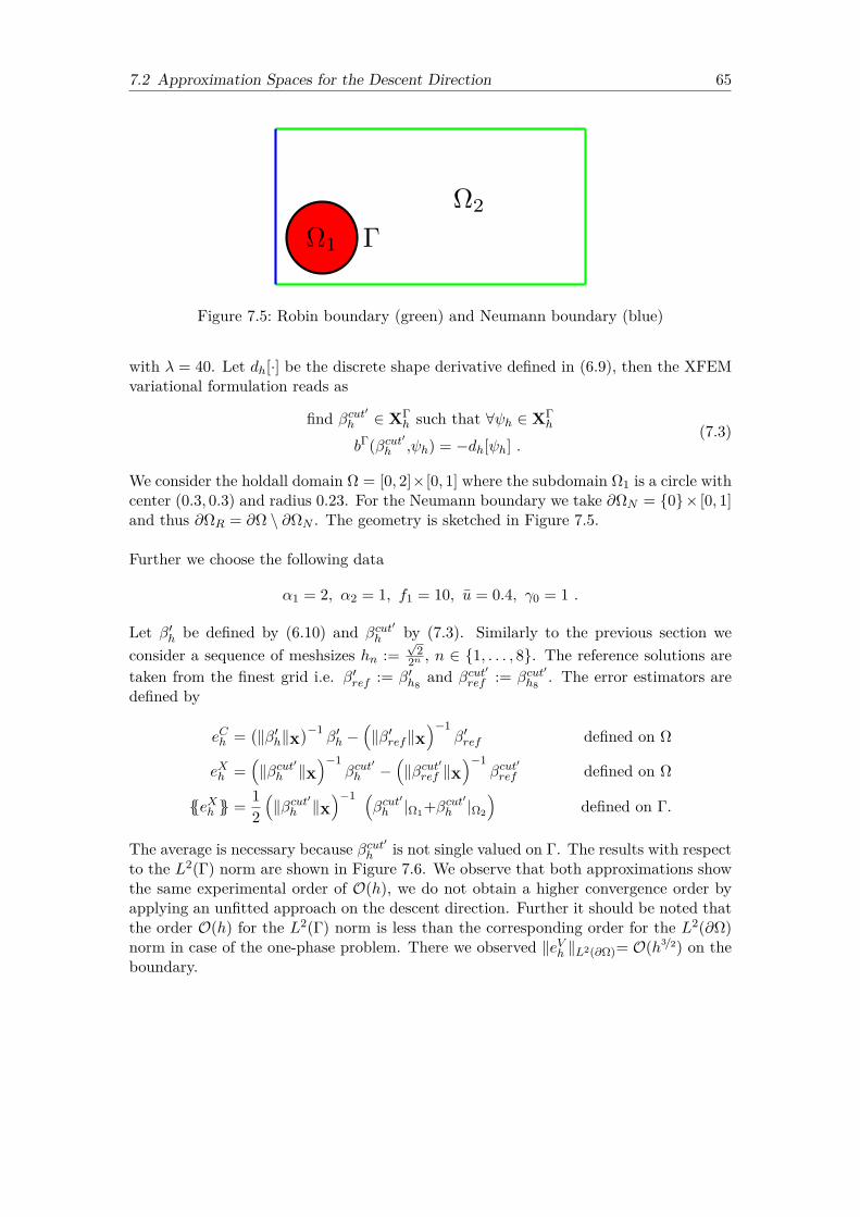
7.2 Approximation Spaces for the Descent Direction 65
Ω2
ΓΩ1
Figure 7.5: Robin boundary (green) and Neumann boundary (blue)
with λ = 40. Let dh[·] be the discrete shape derivative defined in (6.9), then the XFEMvariational formulation reads as
find βcut′h ∈ XΓh such that ∀ψh ∈ XΓ
h
bΓ(βcut′h ,ψh) = −dh[ψh] .(7.3)
We consider the holdall domain Ω = [0, 2]×[0, 1] where the subdomain Ω1 is a circle withcenter (0.3, 0.3) and radius 0.23. For the Neumann boundary we take ∂ΩN = 0× [0, 1]and thus ∂ΩR = ∂Ω \ ∂ΩN . The geometry is sketched in Figure 7.5.
Further we choose the following data
α1 = 2, α2 = 1, f1 = 10, u = 0.4, γ0 = 1 .
Let β′h be defined by (6.10) and βcut′
h by (7.3). Similarly to the previous section weconsider a sequence of meshsizes hn :=
√2
2n , n ∈ 1, . . . , 8. The reference solutions aretaken from the finest grid i.e. β′ref := β′h8
and βcut′ref := βcut′
h8. The error estimators are
defined by
eCh =(‖β′h‖X
)−1β′h −
(‖β′ref‖X
)−1β′ref defined on Ω
eXh =(‖βcut′h ‖X
)−1βcut
′h −
(‖βcut′ref ‖X
)−1βcut
′ref defined on Ω
eXh = 12(‖βcut′h ‖X
)−1 (βcut
′h |Ω1+βcut′h |Ω2
)defined on Γ.
The average is necessary because βcut′h is not single valued on Γ. The results with respectto the L2(Γ) norm are shown in Figure 7.6. We observe that both approximations showthe same experimental order of O(h), we do not obtain a higher convergence order byapplying an unfitted approach on the descent direction. Further it should be noted thatthe order O(h) for the L2(Γ) norm is less than the corresponding order for the L2(∂Ω)norm in case of the one-phase problem. There we observed ‖eVh ‖L2(∂Ω)= O(h3/2) on theboundary.
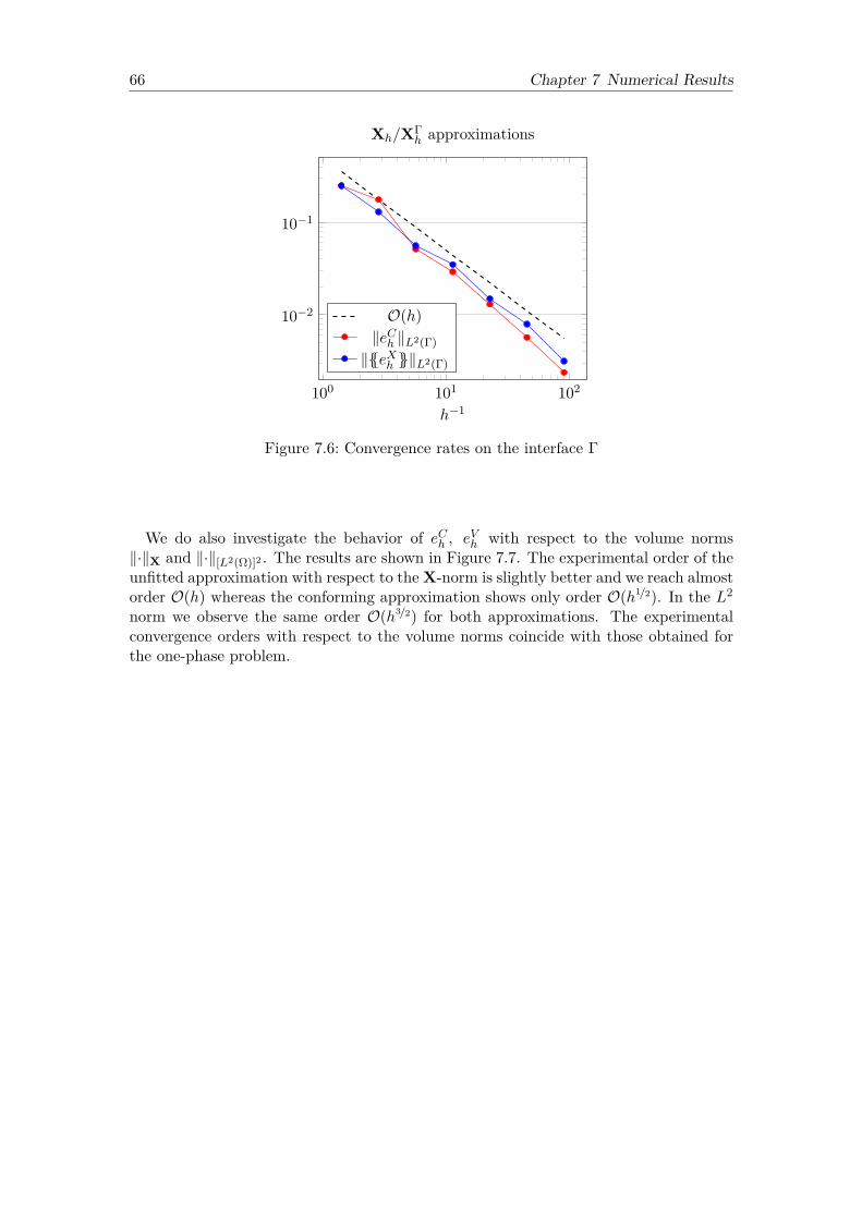
66 Chapter 7 Numerical Results
100 101 102
10−2
10−1
h−1
Xh/XΓh approximations
O(h)‖eCh ‖L2(Γ)‖eXh ‖L2(Γ)
Figure 7.6: Convergence rates on the interface Γ
We do also investigate the behavior of eCh , eVh with respect to the volume norms‖·‖X and ‖·‖[L2(Ω)]2 . The results are shown in Figure 7.7. The experimental order of theunfitted approximation with respect to the X-norm is slightly better and we reach almostorder O(h) whereas the conforming approximation shows only order O(h1/2). In the L2
norm we observe the same order O(h3/2) for both approximations. The experimentalconvergence orders with respect to the volume norms coincide with those obtained forthe one-phase problem.
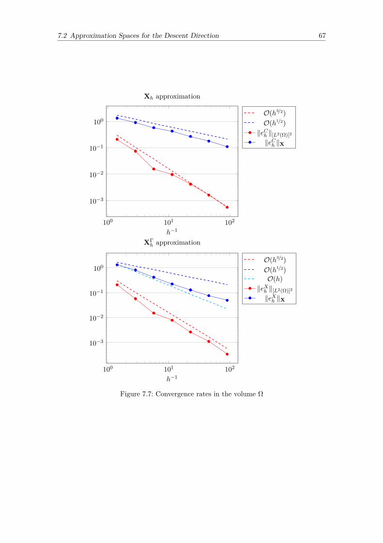
7.2 Approximation Spaces for the Descent Direction 67
100 101 102
10−3
10−2
10−1
100
h−1
Xh approximation
O(h3/2)O(h1/2)‖eCh ‖[L2(Ω)]2
‖eCh ‖X
100 101 102
10−3
10−2
10−1
100
h−1
XΓh approximation
O(h3/2)O(h1/2)O(h)
‖eXh ‖[L2(Ω)]2
‖eXh ‖X
Figure 7.7: Convergence rates in the volume Ω
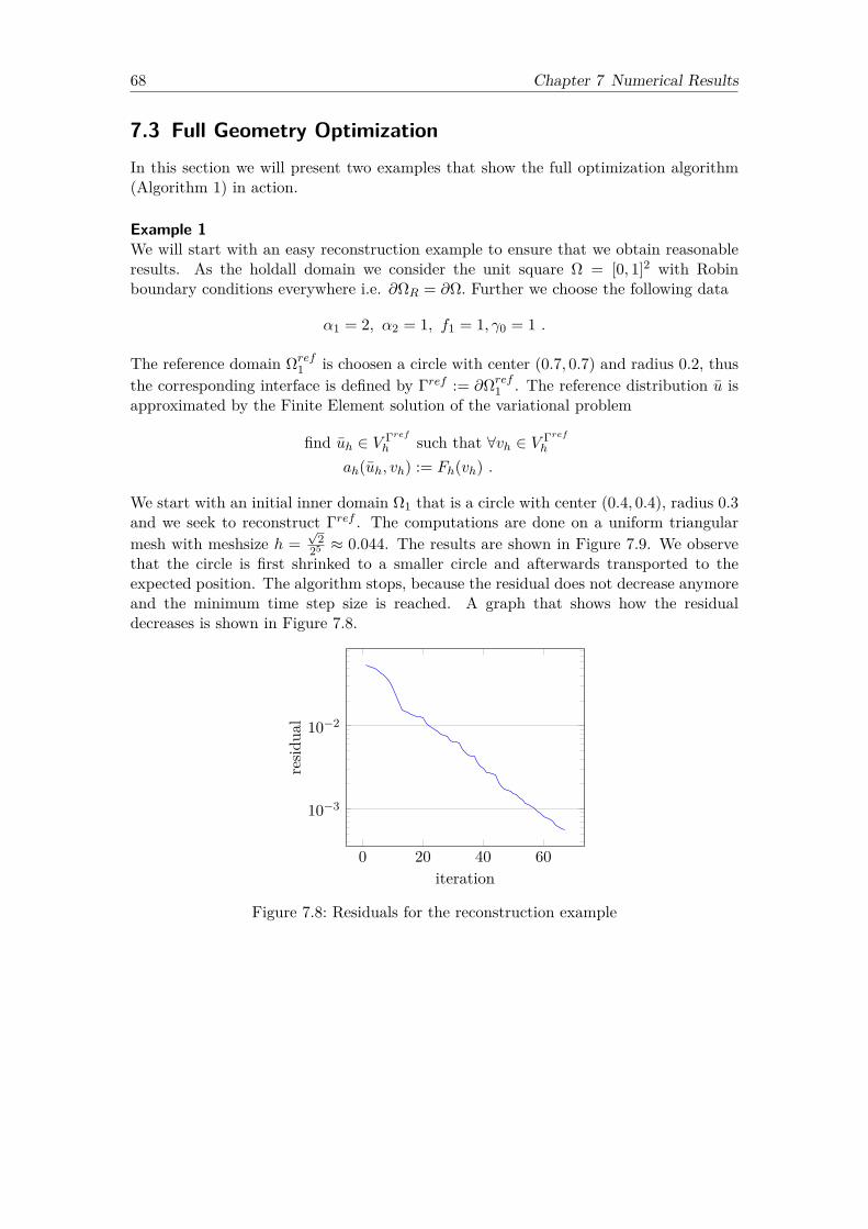
68 Chapter 7 Numerical Results
7.3 Full Geometry OptimizationIn this section we will present two examples that show the full optimization algorithm(Algorithm 1) in action.
Example 1We will start with an easy reconstruction example to ensure that we obtain reasonableresults. As the holdall domain we consider the unit square Ω = [0, 1]2 with Robinboundary conditions everywhere i.e. ∂ΩR = ∂Ω. Further we choose the following data
α1 = 2, α2 = 1, f1 = 1, γ0 = 1 .
The reference domain Ωref1 is choosen a circle with center (0.7, 0.7) and radius 0.2, thus
the corresponding interface is defined by Γref := ∂Ωref1 . The reference distribution u is
approximated by the Finite Element solution of the variational problem
find uh ∈ V Γrefh such that ∀vh ∈ V Γref
h
ah(uh, vh) := Fh(vh) .
We start with an initial inner domain Ω1 that is a circle with center (0.4, 0.4), radius 0.3and we seek to reconstruct Γref . The computations are done on a uniform triangularmesh with meshsize h =
√2
25 ≈ 0.044. The results are shown in Figure 7.9. We observethat the circle is first shrinked to a smaller circle and afterwards transported to theexpected position. The algorithm stops, because the residual does not decrease anymoreand the minimum time step size is reached. A graph that shows how the residualdecreases is shown in Figure 7.8.
0 20 40 60
10−3
10−2
iteration
resid
ual
Figure 7.8: Residuals for the reconstruction example
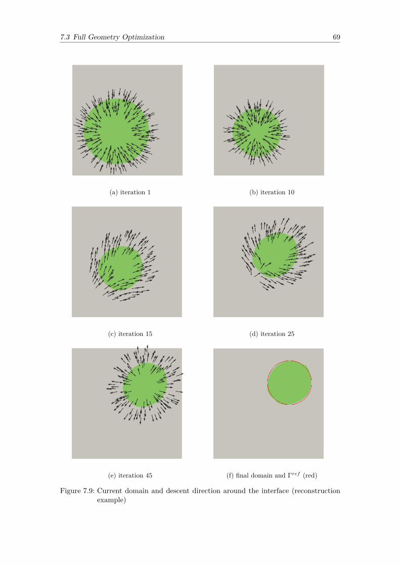
7.3 Full Geometry Optimization 69
(a) iteration 1 (b) iteration 10
(c) iteration 15 (d) iteration 25
(e) iteration 45 (f) final domain and Γref (red)
Figure 7.9: Current domain and descent direction around the interface (reconstructionexample)
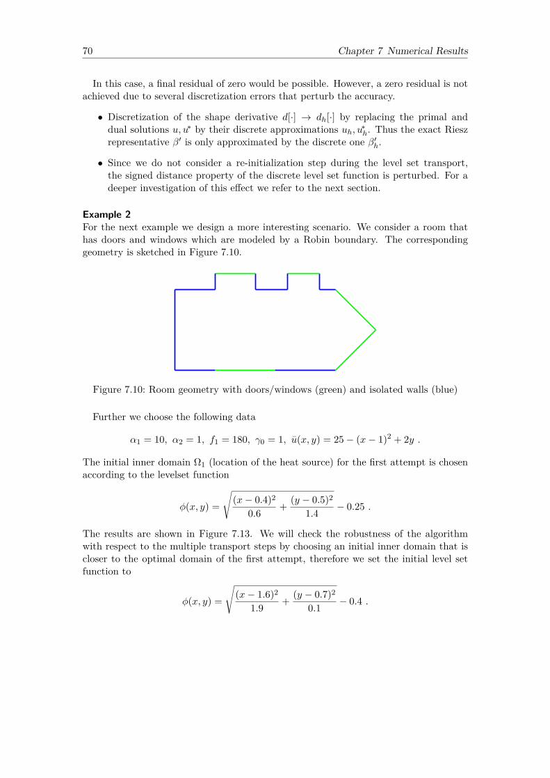
70 Chapter 7 Numerical Results
In this case, a final residual of zero would be possible. However, a zero residual is notachieved due to several discretization errors that perturb the accuracy.
• Discretization of the shape derivative d[·] → dh[·] by replacing the primal anddual solutions u, u∗ by their discrete approximations uh, u∗h. Thus the exact Rieszrepresentative β′ is only approximated by the discrete one β′h.
• Since we do not consider a re-initialization step during the level set transport,the signed distance property of the discrete level set function is perturbed. For adeeper investigation of this effect we refer to the next section.
Example 2For the next example we design a more interesting scenario. We consider a room thathas doors and windows which are modeled by a Robin boundary. The correspondinggeometry is sketched in Figure 7.10.
Figure 7.10: Room geometry with doors/windows (green) and isolated walls (blue)
Further we choose the following data
α1 = 10, α2 = 1, f1 = 180, γ0 = 1, u(x, y) = 25− (x− 1)2 + 2y .
The initial inner domain Ω1 (location of the heat source) for the first attempt is chosenaccording to the levelset function
φ(x, y) =
√(x− 0.4)2
0.6 + (y − 0.5)2
1.4 − 0.25 .
The results are shown in Figure 7.13. We will check the robustness of the algorithmwith respect to the multiple transport steps by choosing an initial inner domain that iscloser to the optimal domain of the first attempt, therefore we set the initial level setfunction to
φ(x, y) =
√(x− 1.6)2
1.9 + (y − 0.7)2
0.1 − 0.4 .
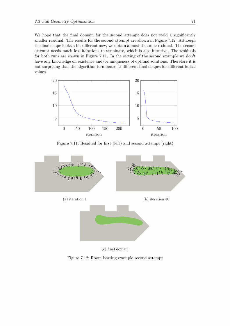
7.3 Full Geometry Optimization 71
We hope that the final domain for the second attempt does not yield a significantlysmaller residual. The results for the second attempt are shown in Figure 7.12. Althoughthe final shape looks a bit different now, we obtain almost the same residual. The secondattempt needs much less iterations to terminate, which is also intuitive. The residualsfor both runs are shown in Figure 7.11. In the setting of the second example we don’thave any knowledge on existence and/or uniqueness of optimal solutions. Therefore it isnot surprising that the algorithm terminates at different final shapes for different initialvalues.
0 50 100 150 200
5
10
15
20
iteration0 50 100
5
10
15
20
iteration
Figure 7.11: Residual for first (left) and second attempt (right)
(a) iteration 1 (b) iteration 40
(c) final domain
Figure 7.12: Room heating example second attempt
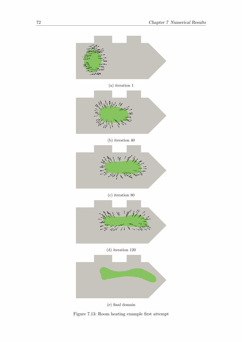
72 Chapter 7 Numerical Results
(a) iteration 1
(b) iteration 40
(c) iteration 80
(d) iteration 120
(e) final domain
Figure 7.13: Room heating example first attempt
7.4 Velocity Extension 73
7.4 Velocity ExtensionIn this section we will give numerical evidence that the construction of the descentdirection according to section 6.2.2 helps to preserve the distance between the isolines ofthe level set function. We consider a model problem on the rectangle [0, 2] × [0, 1] = Ωwith data
α1 = 2, α2 = 1, f1 = 10, γ0 = 0.5 , u = 0.9 .
Again we take the left boundary as Neumann boundary ∂ΩN = 0 × [0, 1] and thus∂ΩR = ∂Ω \ ∂ΩN . The initial domain is an ellipse close to the left boundary and yieldsan initial residual of 0.488. The optimization is done twice, where we change the descentdirection in Algorithm 1 to the normalized discrete Riesz representative ‖β′h‖
−1X β′h (6.10)
for the second run. Please note that this is also a descent direction according to Lemma2.10. The results are shown in Figure 7.14 and 7.15. The algorithm stops when the resid-ual does not decrease anymore and the minimum time step size is reached. This happensin the first run after 271 iterations with a residual of 0.155 and in the second run after136 iterations with a residual of 0.196. Inspecting the level set function, we can clearlysee that βeh preserves the signed distance property at least approximately. In case ofthe modified descent direction, artefacts close to the interface can be observed. Furtherthe signed distance property is not at all preserved since the isolines on the right handside of the interface are extremely close whereas on the left hand side they are far apart.
Remark: This example shows that the quality of the discrete level set function canhave a huge impact on the optimization result. Of course, also the descent direction‖β′h‖
−1X β′h could be used but then it should be combined with a re-initialization method
(cf. Section 4.2).
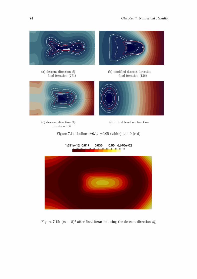
74 Chapter 7 Numerical Results
(a) descent direction βeh
final iteration (271)(b) modified descent direction
final iteration (136)
(c) descent direction βeh
iteration 136(d) initial level set function
Figure 7.14: Isolines ±0.1, ±0.05 (white) and 0 (red)
Figure 7.15: (uh − u)2 after final iteration using the descent direction βeh
7.5 Geometry and Residual Error 75
7.5 Geometry and Residual ErrorIn this section we will consider an interface problem where the optimal solution is knowna priori. That enables us to investigate how the final residual and the final geometryerror decreases under mesh refinements. The holdall domain Ω is the unit circle and theoptimal inner domain Ωopt
1 is a circle with center (0.0) and radius 12 . As Robin boundary
we choose the entire boundary ∂ΩR = ∂Ω. For the data f1 = 1, α1 = 2, α2 = 1, γ0 = 1,the solution of the interface problem (3.2)-(3.5) with Ω1 = Ωopt
1 is given by
u(r) =5+4 log 2
32 − 18r
2 in Ωopt1 ,
−18 log r + 1
8 in Ω \ Ωopt1 ,
where r =√x2 + y2. For the initial geometry we choose the inner domain Ω1 as a circle
with center (0.2, 0.2) and radius 0.3. For a fixed mesh size h let uh be the final discretestate and Γh the final discrete interface (by final we mean the results of Algorithm 1).The quanties of interest are the square root of the final residual i.e. ‖uh − u‖L2(Ω) andthe geometry error, which both ideally converge to zero. The latter one can be esti-mated by means of the signed distance function corresponding to the optimal domainφopt(x, y) =
√x2 + y2− 0.5, evaluated on the discrete interface Γh. We measure the dis-
tance between the final interface and the optimal interface by ‖φopt‖L2(Γh). The resultsfor the sequence of mesh sizes hn = 1
2n , n ∈ 1, . . . , 6 are shown in Figure 7.16. Weobserve that the geometry error decays with a rate of at least O(h1/2) and the residualwith O(h).
As a second example we will consider the same problem with a modified source functionf . Instead of a domain wise constant f , we choose f = 1 in the entire holdall domain Ω.This modification does not exactly fit into the setting which was introduced in Section3.1, nevertheless it will be included here because it yields some interesting results. Thecorresponding exact solution is now given by
u(r) =−1
8r2 + 23
32 in Ωopt1 ,
−14r
2 + 34 in Ω \ Ωopt
1 .
We employ the same convergence studies as in the first case. The results are shown inFigure 7.17. For the geometry error we gain half of an order which results in a decay ofO(h3/2). Concerning ‖uh − u‖L2Ω, the result is even better. We can really see a decayof order O(h2). This is remarkable since that rate is of optimal order. The decay of theresidual for all iterations and both source terms is shown in Figure 7.18.
Increasing the regularity of the source term from L2(Ω) to H1(Ω) seems to affect thedecay of the residual as well as the geometry error. However, since α1 6= α2, the regu-larity of u, u∗ does not increase. Further numerical experiments show that we loose theoptimal order rate of O(h2) for the residual if α1 is increased.
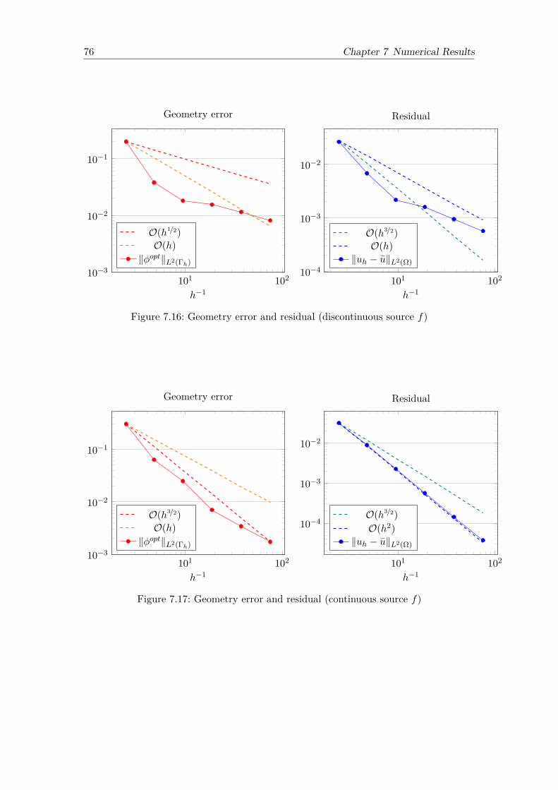
76 Chapter 7 Numerical Results
101 10210−3
10−2
10−1
h−1
Geometry error
O(h1/2)O(h)
‖φopt‖L2(Γh)
101 10210−4
10−3
10−2
h−1
Residual
O(h3/2)O(h)
‖uh − u‖L2(Ω)
Figure 7.16: Geometry error and residual (discontinuous source f)
101 10210−3
10−2
10−1
h−1
Geometry error
O(h3/2)O(h)
‖φopt‖L2(Γh)
101 102
10−4
10−3
10−2
h−1
Residual
O(h3/2)O(h2)
‖uh − u‖L2(Ω)
Figure 7.17: Geometry error and residual (continuous source f)
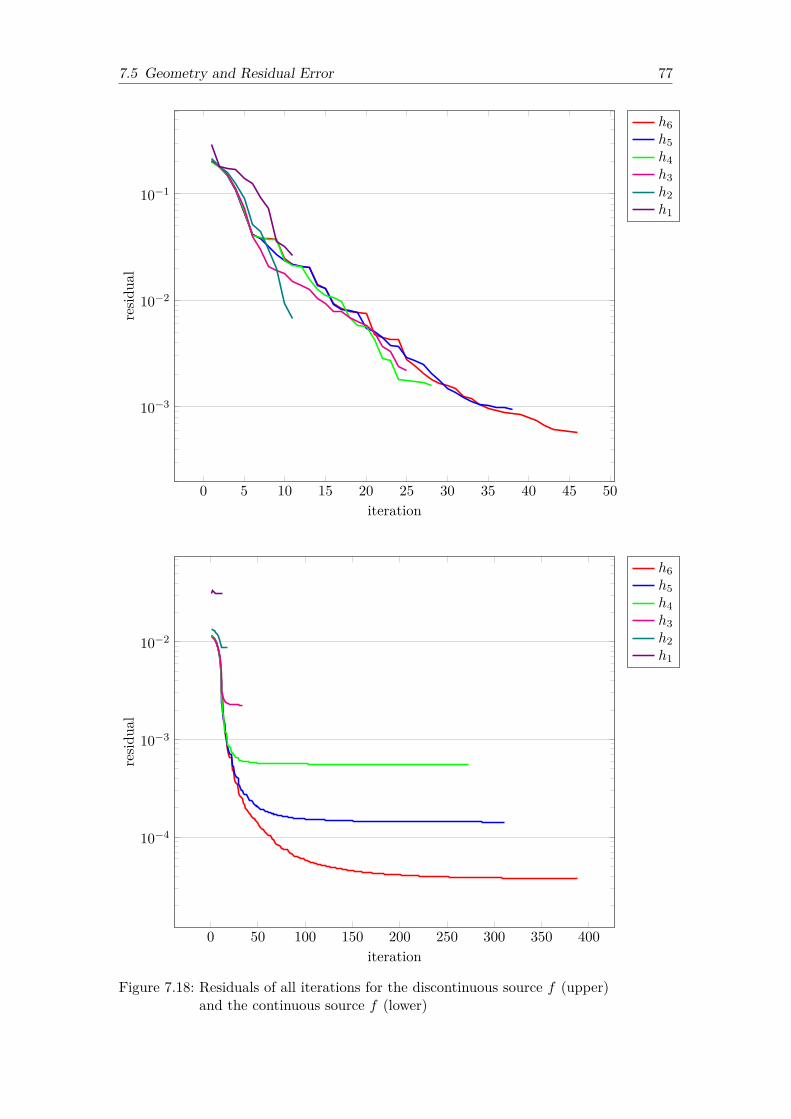
7.5 Geometry and Residual Error 77
0 5 10 15 20 25 30 35 40 45 50
10−3
10−2
10−1
iteration
resid
ual
h6h5h4h3h2h1
0 50 100 150 200 250 300 350 400
10−4
10−3
10−2
iteration
resid
ual
h6h5h4h3h2h1
Figure 7.18: Residuals of all iterations for the discontinuous source f (upper)and the continuous source f (lower)
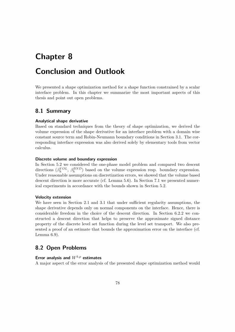
Chapter 8
Conclusion and Outlook
We presented a shape optimization method for a shape function constrained by a scalarinterface problem. In this chapter we summarize the most important aspects of thisthesis and point out open problems.
8.1 SummaryAnalytical shape derivativeBased on standard techniques from the theory of shape optimization, we derived thevolume expression of the shape derivative for an interface problem with a domain wiseconstant source term and Robin-Neumann boundary conditions in Section 3.1. The cor-responding interface expression was also derived solely by elementary tools from vectorcalculus.
Discrete volume and boundary expressionIn Section 5.2 we considered the one-phase model problem and compared two descentdirections (βV OLh , βBNDh ) based on the volume expression resp. boundary expression.Under reasonable assumptions on discretization errors, we showed that the volume baseddescent direction is more accurate (cf. Lemma 5.6). In Section 7.1 we presented numer-ical experiments in accordance with the bounds shown in Section 5.2.
Velocity extensionWe have seen in Section 2.1 and 3.1 that under sufficient regularity assumptions, theshape derivative depends only on normal components on the interface. Hence, there isconsiderable freedom in the choice of the descent direction. In Section 6.2.2 we con-structed a descent direction that helps to preserve the approximate signed distanceproperty of the discrete level set function during the level set transport. We also pre-sented a proof of an estimate that bounds the approximation error on the interface (cf.Lemma 6.9).
8.2 Open ProblemsError analysis and W k,p estimatesA major aspect of the error analysis of the presented shape optimization method would
78
8.2 Open Problems 79
be an error bound on the velocity approximation i.e.
‖β′ − β′h‖X≤ Chq, q ∈ R .
In the following, we will outline the essential ingredients to derive such an estimate. Thepresented ideas are based on the error analysis in [BEH+17]. We assume exact geometryapproximation and recall the definition of the exact shape derivative d[·] (3.23) and thediscrete shape derivative dh[·] (6.9). For the exact/discrete Riesz representatives β′, β′hholds
b(β′, ψ) = −d[ψ] , ∀ψ ∈ X, (8.1)b(β′h, ψh) = −dh[ψh] , ∀ψh ∈ Xh , (8.2)
with the inner product b(·, ·) on X =[H1
0 (Ω)]d. For any ψh ∈ Xh we obtain by (8.1)/(8.2)
‖β′h − ψh‖2X = b(β′h − ψh, β′h − ψh)= b(β′h − β′, β′h − ψh) + b(β′ − ψh, β′h − ψh)
≤∣∣∣d[β′h − ψh]− dh[β′h − ψh]
∣∣∣+ ‖β′ − ψh‖X‖β′h − ψh‖X.
Dividing by ‖β′h − ψh‖X yields further
‖β′h − ψh‖X ≤
∣∣∣d[β′h − ψh]− dh[β′h − ψh]∣∣∣
‖β′h − ψh‖X+ ‖β′ − ψh‖X
≤ supϑh∈Xh
∣∣∣d[ϑh]− dh[ϑh]∣∣∣
‖ϑh‖X+ ‖β′ − ψh‖X
Finally we use the fact that ψh was arbitrary and the triangle inequality to conclude
‖β′ − β′h‖X ≤ 2 infψh∈Xh
‖β′ − ψh‖X+ supϑh∈Xh
∣∣∣d[ϑh]− dh[ϑh]∣∣∣
‖ϑh‖X.
Thus it remains to bound the consistency error, introduced by the discretization of theshape derivative. This requires an additional regularity assumption on the solutions u, u∗of the state/adjoint problem (3.11)/(3.22), namely
u, u∗ ∈W 1,∞(Ωi), i = 1, 2 . (8.3)
Remark: For the case d ≤ 3 (8.3) holds for u, u∗ ∈W 2,4(Ωi) by the Sobolev embeddingtheorem (cf. [Alt12, Satz 8.8, p.342]).
80 Chapter 8 Conclusion and Outlook
We take a closer look at the nominator of the consistency error∣∣∣d[ϑh]− dh[ϑh]∣∣∣ ≤ ∣∣∣ ∫
Ωdiv(ϑh)
((u− u)2 − (uh − u)2
) ∣∣∣+∣∣∣ ∫
Ωdiv(ϑh)f(u∗ − u∗h)
∣∣∣+∣∣∣ ∫
Ω2 (∇u · vh) (u− uh)
∣∣∣+∣∣∣∣∣
2∑i=1
αi
∫Ωi
div(ϑh) [(∇u · ∇u∗)− (∇uh · ∇u∗h)]∣∣∣∣∣
+∣∣∣∣∣
2∑i=1
αi
∫Ωi
[((Dϑh +DϑTh )∇u
)· ∇u∗ −
((Dϑh +DϑTh )∇uh
)· ∇u∗h
] ∣∣∣∣∣=: Q1 +Q2 +Q3 +Q4 +Q5 .
We will present the further treatment of the right hand side in detail for the summandQ4. Let i ∈ 1, 2, then Hölder’s inequality yields∣∣∣ ∫
Ωidiv(ϑh) [(∇u · ∇u∗)− (∇uh · ∇u∗h)]
∣∣∣≤∣∣∣ ∫
Ωidiv(ϑh) [∇(u− uh) · ∇u∗]
∣∣∣+∣∣∣ ∫
Ωidiv(ϑh) [∇u · ∇(u∗ − u∗h)]
∣∣∣+∣∣∣ ∫
Ωidiv(ϑh) [∇(u− uh) · ∇(u∗ − u∗h)]
∣∣∣≤ C‖ϑh‖X ‖u− uh‖W 1,2(Ωi) ‖u
∗‖W 1,∞(Ωi)
+ C‖ϑh‖X ‖u∗ − u∗h‖W 1,2(Ωi) ‖u‖W 1,∞(Ωi)
+ C‖ϑh‖X ‖u− uh‖W 1,4(Ωi) ‖u∗ − u∗h‖W 1,4(Ωi)
and thus we conclude
Q4 ≤ C‖ϑh‖X(‖u− uh‖W 1,2(Ωi)+‖u
∗ − u∗h‖W 1,2(Ω)+‖u− uh‖W 1,4(Ω)‖u∗ − u∗h‖W 1,4(Ω)).
By similar techniques, one derives
Q1 ≤ C‖ϑh‖X ‖u− uh‖L4(Ω) ,
Q2 ≤ C‖ϑh‖X ‖u∗ − u∗h‖L2(Ω) ,
Q3 ≤ C‖ϑh‖X‖u− uh‖L2(Ω) ,
Q5 ≤ C‖ϑh‖X(‖u− uh‖W 1,2(Ωi)+‖u
∗ − u∗h‖W 1,2(Ω)+‖u− uh‖W 1,4(Ω)‖u∗ − u∗h‖W 1,4(Ω)).
We define the overall error boundB(u, uh, u∗, u∗h) := ‖u− uh‖W 1,2(Ωi)+‖u
∗ − u∗h‖W 1,2(Ω)+‖u− uh‖W 1,4(Ω)‖u∗ − u∗h‖W 1,4(Ω)
+ ‖u− uh‖L4(Ω) .
(8.4)
8.2 Open Problems 81
Now we are able to bound the consistency error by means of (8.4)
supϑh∈Xh
∣∣∣d[ϑh]− dh[ϑh]∣∣∣
‖ϑh‖X≤ sup
ϑh∈Xh
C B(u, uh, u∗, u∗h)‖ϑh‖X‖ϑh‖X
= C B(u, uh, u∗, u∗h) .
Unfortunately B(u, uh, u∗, u∗h) containsW k,p estimates for k ∈ 0, 1 and p = 4. Optimalorder W k,p error estimates for piecewise standard linear Finite Elements are known inthe literature (cf. [RS82]). However, it is not clear if such estimates can also be derivedfor piecewise linear unfitted Finite Element spaces. This is an interesting question forfuture research, also isolated from the shape optimization context.
Unfitted approximation of the descent directionThe Riesz representative of the shape derivative posseses only limited global regularitydue to a kink at the interface (cf. Lemma 2.11). For such functions, the best approxi-mation of the standard Finite Element space Xh is limited and can be improved by con-sidering the corresponding unfitted Finite Element space XΓ
h (cf. Section 6.1). However,we have seen in numerical experiments that an unfitted Finite Element discretizationof the descent direction does not significantly improve its approximation properties (cf.Section 7.2). It needs to be investigated why the error bounds do not improve and ifthis issue can be fixed by a modification of the variational formulation (7.3).
Higher order methodsClearly, a natural extension of the presented method is the application of higher orderFinite Element spaces. Increasing the polynomial degree of the approximation spaces(Wh,Vh,Xh) pays off if all components of the approximation process (u,u∗,Γh, β′h) reachhigher order accuracy. For the primal/dual solution and the discrete interface, this ispossible. In [LR17] the authors present an unfitted higher order method that offersoptimal order bounds for the Finite Element and geometry approximation. It remainsto clarify if also the discrete Riesz representative of the shape derivative β′h benefits fromhigher order. In order to achieve higher order bounds for β′h it is necessary to improvethe error bounds for the unfitted low order approximation discussed in the previousparagraph.
Re-initialization and topology changesFor a geometry optimization problem, where the topology of an optimal solution iscompletely unknown, the approach of topology optimization may be better suited. Nev-ertheless, it would be desirable that also the shape optimization approach with a levelset geometry representation allows for topology changes on a basic level, for instancemerging of two domains. In [BEH+17] the authors present a method that employs re-initialization (cf. Section 4.2) and is able to perform basic topology changes in numericalexperiments. It would be interesting to investigate if the method presented in this thesisallows basic topology changes if re-initialization is included in the level set transport.
Appendix A
Auxiliary Proofs
A.1. PROPOSITION [vector identity]Let Ω ⊂ Rd a bounded domain and u, v ∈ H2(Ω), ϑ ∈
[H1(Ω)
]d then the following vectoridentity holds
ϑ · ∇(∇u · ∇v) +((Dϑ+DϑT )∇u
)· ∇v = ∇(ϑ · ∇u) · ∇v +∇(ϑ · ∇v) · ∇u .
Proof. The proof follows by direct calculation and the fact that ∂2u∂xi∂xj
= ∂2u∂xj∂xi
fori, j ∈ 1, . . . , d.
ϑ · ∇(∇u · ∇v) +((Dϑ+DϑT )∇u
)· ∇v
=d∑i=1
ϑi
∂
∂xi
d∑j=1
∂u
∂xj
∂v
∂xj
+d∑i=1
∂v
∂xi
d∑j=1
(∂ϑi∂xj
+ ∂ϑj∂xi
)∂u
∂xj
=
d∑i,j=1
ϑi∂v
∂xj
∂2u
∂xj∂xi+
d∑i,j=1
ϑi∂2v
∂xj∂xi
∂u
∂xj
d∑i,j=1
∂ϑi∂xj
∂u
∂xj
∂v
∂xi+
d∑i,j=1
∂ϑj∂xi
∂u
∂xj
∂v
∂xi
= ∇(ϑ · ∇u) · ∇v +∇(ϑ · ∇v) · ∇u .
Notation/Definition: We give a few definitions that are valid for the subsequent state-ments:Let Ω be a bounded domain in Rd and Ω1 ⊂ Ω with a C1 boundary Γ := ∂Ω1 and outerunit normal nΓ. Further Ω2 := Ω \ Ω1.
A.2. PROPOSITION [tangential gradient continuity]Let u ∈ H1(Ω) ∩H2(Ω1) ∩H2(Ω2) with [[u]] = 0 on Γ.
[[∇Γu]] = (P∇u) |Ω1− (P∇u) |Ω2= 0 in L2(Γ) . (A.1)
With the tangential projection P = I − nΓnTΓ .
82
83
Proof. Denote by ui := u|Ωi , the restrictions of u to the subdomains. Since Γ ∈ C1 wecan find functions vi ∈ C∞(Ωi) smooth up to the interface with ‖ui − vi‖H2(Ωi)< ε (see[Eva10, Theorem 3 p.266]).
To proof the statement we follow the ideas of [Stu15, Remark 3.3]. Let x ∈ Γ arbitrarybut fixed. Further we consider a C1 parametrization of the boundary γ : [0, T ] → Γ,T > 0 with γ(0) = x and γ′(0) =: w. We differentiate [[v]] := v1 − v2 along the interfaceand obtain
0 = d
dt[[v(γ(t))]] = ∇v1 · γ′(0)−∇v2 · γ′(0)
= (P (∇v1 −∇v2)) · w + (∇v1 · nΓ −∇v2 · nΓ)nΓ · w= (P (∇v1 −∇v2)) · w =: [[∇Γv]] · w
Since w was arbitrary but tangential we obtain that [[∇Γv]] is orthogonal to all tangentialvectors on Γ. By construction [[∇Γv]] is also orthogonal to nΓ and hence [[∇Γv]] = 0. Thetrace theorem then implies∮
Γ[[∇Γu]]2 ≤ C
(∮Γ(∇Γu1 −∇Γv1)2 +
∮Γ(∇Γv1 −∇Γv2)2 +
∮Γ(∇Γv2 −∇Γu1)2
)≤ C
(‖u1 − v1‖H2(Ω1)+‖u2 − v2‖H2(Ω2)
)≤ Cε .
Since ε was arbitrary, this yields the claim.
A.3. PROPOSITION [approximation example]There exist shape regular families of triangulations Th, interfaces Γ ∈ C1 and u ∈H l(Ω1) ∩H l(Ω2) ∩H1(Ω) with l ≥ 2 such that
infvh∈V dch
‖u− vh‖L2(Ω)≥ Ch3/2 ,
with the Finite Element space V dch := vh ∈ L2(Ω) : vh|T∈ P1(T ), T ∈ Th.
Proof. We construct an example for d = 1. The idea can be generalized to higher spacedimensions. We choose the following data
Ω = [0, 1]
Γ = 13
T nh = [(j − 1)2−n, j2−n]j=1,...,2n
u(x) =
1− 3x x ≤ 1/3
0 x > 1/3 .
Since u is a piecewise linear polynomial, the approximation error occurs only in theelement TΓ cut by the interface. Let lTΓ be the left endpoint of TΓ then we can define
84 Appendix A Auxiliary Proofs
a mapping Φh that maps the reference element T = [0, 1] onto TΓ by
Φh(x) = lTΓ + hx .
Applying the transformation on u yields
(u Φh)(x) =
1− 3Φh(x) Φh(x) ≤ 1/3
0 Φh(x) > 1/3 .
The left endpoint of TΓ can be rewritten with a real numer θ ∈ (0, 1) to lTΓ = 1/3− θh.In fact θ ∈ 1/3, 2/3 and w.l.o.g. we assume θ = 1/3. Since Φh(x) ≤ 1/3 ⇔ x ≤ 1/3 weobtain
(u Φh)(x) =h(1− 3x) x ≤ 1/3
0 x > 1/3 .= hu(x)
For the bestapproximation error holds
infvh∈V dch
‖u− vh‖2L2(Ω) = infvh∈V dch
‖u− vh‖2L2(TΓ)= infvh∈V dch
∫ lTΓ+h
lTΓ
(u− vh)2
= infvh∈V dch
h
∫ 1
0(u Φh − vh Φh)2 = inf
wh∈P1(Ω)h
∫ 1
0(u Φh − wh)2 .
The bestapproximating element wh ∈ P1(Ω) is uniquely defined due to the orthogonalprojection in Hilbert spaces. We have wh(x) = ax+ b and the coefficients can be easilyidentified by the two orthogonality relations∫ 1
0(u Φh − ax− b) = 0∫ 1
0(u Φh − ax− b)x = 0 .
Solving this linear system for the coefficients a, b yields
wh(x) = h
(−7
9x+ 59
)=: hw(x) .
Inserting this identity into the best approximation error yields
infvh∈V dch
‖u− vh‖2L2(Ω) = infwh∈P1(Ω)
h
∫ 1
0(hu− wh)2
= h3∫ 1
0(u− w)2
and taking the square root yields the claim for C <∫ 1
0 (u− w)2.
Bibliography
[ADK07] Lekbir Afraites, Marc Dambrine, and Djalil Kateb. Shape methods for thetransmission problem with a single measurement. Numerical functional anal-ysis and optimization, 28(5-6):519–551, 2007.
[AE01] Herbert Amann and Joachim Escher. Analysis II. Grundstudium Mathe-matik. Birkhäuser Verlag, Basel, 2001.
[Alt12] Hans Wilhelm Alt. Lineare Funktionalanalysis: Eine anwendungsorientierteEinführung. Springer-Verlag, 2012.
[BEH+17] Erik Burman, Daniel Elfverson, Peter Hansbo, Mats G Larson, and KarlLarsson. A cut finite element method for the bernoulli free boundaryvalue problem. Computer Methods in Applied Mechanics and Engineering,317:598–618, 2017.
[Ber10] Martin Berggren. A unified discrete–continuous sensitivity analysis methodfor shape optimization. In Applied and numerical partial differential equa-tions, pages 25–39. Springer, 2010.
[BH12] Erik Burman and Peter Hansbo. Fictitious domain finite element methodsusing cut elements: II. A stabilized Nitsche method. Applied NumericalMathematics, 62(4):328–341, 2012.
[Bor02] Liliana Borcea. Electrical impedance tomography. Inverse Problems,18(6):R99, 2002.
[Bre10] Haim Brezis. Functional analysis, Sobolev spaces and partial differentialequations. Springer Science & Business Media, 2010.
[BS95] Martin P Bendsøe and Ole Sigmund. Optimization of structural topology,shape, and material, volume 414. Springer, 1995.
[BS07] Susanne Brenner and Ridgway Scott. The mathematical theory of finiteelement methods, volume 15. Springer Science & Business Media, 2007.
[BS13] Martin Philip Bendsoe and Ole Sigmund. Topology optimization: theory,methods, and applications. Springer Science & Business Media, 2013.
[Cal06] Alberto P Calderón. On an inverse boundary value problem. Computational& Applied Mathematics, 25(2-3):133–138, 2006.
85
86 Bibliography
[CIN99] Margaret Cheney, David Isaacson, and Jonathan C Newell. Electricalimpedance tomography. SIAM review, 41(1):85–101, 1999.
[CZ98] Zhiming Chen and Jun Zou. Finite element methods and their conver-gence for elliptic and parabolic interface problems. Numerische Mathematik,79(2):175–202, 1998.
[DPE11] Daniele Antonio Di Pietro and Alexandre Ern. Mathematical aspects of dis-continuous Galerkin methods, volume 69. Springer Science & Business Media,2011.
[Duh06] D Duhamel. Shape optimization of noise barriers using genetic algorithms.Journal of sound and vibration, 297(1-2):432–443, 2006.
[DZ11] M. Delfour and J. Zolésio. Shapes and Geometries. Society for Industrialand Applied Mathematics, second edition, 2011.
[EG13] Alexandre Ern and Jean-Luc Guermond. Theory and practice of finite ele-ments, volume 159. Springer Science & Business Media, 2013.
[ER13] Charles M Elliott and Thomas Ranner. Finite element analysis for a cou-pled bulk–surface partial differential equation. IMA Journal of NumericalAnalysis, 33(2):377–402, 2013.
[Eva10] Lawrence C. Evans. Partial differential equations, volume 19 of GraduateStudies in Mathematics. ams, Providence, Rhode Island, 2010.
[GR11] Sven Gross and Arnold Reusken. Numerical methods for two-phase incom-pressible flows, volume 40. Springer Science & Business Media, 2011.
[Had08] Jacques. Hadamard. Mémoire sur le problème d’analyse relatif à l’équilibredes plaques élastiques encastrées. Mém. Sav. étrang. (2) 33, Nr. 4, 128 S(1908)., 1908.
[Her12] José Herskovits. Advances in structural optimization, volume 25. SpringerScience & Business Media, 2012.
[HH02] Anita Hansbo and Peter Hansbo. An unfitted finite element method, basedon Nitsche’s method, for elliptic interface problems. Computer methods inapplied mechanics and engineering, 191(47-48):5537–5552, 2002.
[HPS15] Ralf Hiptmair, Alberto Paganini, and Sahar Sargheini. Comparison of ap-proximate shape gradients. BIT Numerical Mathematics, 55(2):459–485,2015.
[Kor18] Benjamin S Koren. The grand hall of the Elbphilharmonie Hamburg: De-velopment of parametric and digital fabrication tools in architectural andacoustical design. In Humanizing Digital Reality, pages 141–151. Springer,2018.
Bibliography 87
[Leh10] Christoph Lehrenfeld. Hybrid Discontinuous Galerkin Methods for Incom-pressible Flow Problems. Master’s thesis, RWTH Aachen, May 2010.
[LR13] Eva Loch and Arnold Reusken. The level set method for capturing interfaceswith applications in two-phase flow problems. PhD thesis, Hochschulbiblio-thek der Rheinisch-Westfälischen Technischen Hochschule Aachen, 2013.
[LR17] Christoph Lehrenfeld and Arnold Reusken. Analysis of a high order unfittedfinite element method for an elliptic interface problem. IMA J. Numer. Anal.,00:1–37, 2017. first online.
[LR18] Christoph Lehrenfeld and Arnold Reusken. L2-estimates for a high orderunfitted finite element method for elliptic interface problems. Journal ofNumerical Mathematics, 00:–, 2018. first online.
[LS13] A. Laurain and K. Sturm. Domain Expression of the Shape Derivativeand Application to Electrical Impedance Tomography. Preprint: Weierstraß-Institut für Angewandte Analysis und Stochastik. WIAS, 2013.
[Mar02] Steffen Marburg. Developments in structural-acoustic optimization forpassive noise control. Archives of computational methods in engineering,9(4):291–370, 2002.
[Nit71] Joachim Nitsche. Über ein Variationsprinzip zur Lösung von Dirichlet-Problemen bei Verwendung von Teilräumen, die keinen Randbedingungenunterworfen sind. In Abhandlungen aus dem mathematischen Seminar derUniversität Hamburg, volume 36, pages 9–15. Springer, 1971.
[NS12] Antonio André Novotny and Jan Sokołowski. Topological derivatives in shapeoptimization. Springer Science & Business Media, 2012.
[Osw93] P. Oswald. On a BPX-preconditioner for P1 elements. Computing, 51(2):125–133, 1993.
[RS82] Rolf Rannacher and Ridgway Scott. Some optimal error estimates for piece-wise linear finite element approximations. Math. Comput., 38:437–445, 1982.
[Sch14] Joachim Schöberl. C++11 implementation of finite elements in NGSolve.Technical Report ASC-2014-30, Institute for Analysis and Scientific Com-puting, September 2014.
[Set96] James A Sethian. A fast marching level set method for monotonically ad-vancing fronts. Proceedings of the National Academy of Sciences, 93(4):1591–1595, 1996.
[Ste70] Elias M. Stein. Singular integrals and differentiability properties of functions.Princeton, N.J.: Princeton University Press. XIV, 287 p. (1970)., 1970.
88 Bibliography
[Stu15] Kevin Sturm. On shape optimization with non-linear partial differential equa-tions. PhD thesis, TU Berlin, 2015.
[SZ92] Jan Sokołowski and Jean-Paul Zolesio. Introduction to shape optimization:shape sensitivity analysis. Springer-Verlag, 1992.
[ZCMO96] Hong-Kai Zhao, T. Chan, B. Merriman, and S. Osher. A variational level setapproach to multiphase motion. J. Comput. Phys., 127(1):179–195, 1996.
[Zie12] William P Ziemer. Weakly differentiable functions: Sobolev spaces and func-tions of bounded variation, volume 120. Springer Science & Business Media,2012.
[Zol79] Jean-Paul Zolesio. Identification de domaines par déformations. Universitéde Nice, 1979. Thèse de doctorat d’état.