Embed Size (px)
Citation preview
Stationary solutions of linear ODEs with a randomly
perturbed system matrix and additive noise
H.-J. Starkloff a, R. Wunderlichb
aMartin-Luther-Universität Halle Wittenberg, Fachbereich für Mathematik
und Informatik, 06099 Halle (Saale), Germany
bWestsächsische Hochschule Zwickau (FH), Fachgruppe Mathematik,
PSF 201037, 08056 Zwickau, Germany
Abstract
The paper considers systems of linear first-order ODEs with a randomly per-turbed system matrix and stationary additive noise. For the description of thelong-term behavior of such systems it is necessary to study their stationary solu-tions. We deal with conditions for the existence of stationary solutions as well aswith their representations and the computation of their moment functions.
Assuming small perturbations of the system matrix we apply perturbation tech-niques to find series representations of the stationary solutions and give asymptoticexpansions for their first- and second-order moment functions. We illustrate the fin-dings with a numerical example of a scalar ODE, for which the moment functions ofthe stationary solution still can be computed explicitly. This allows the assessmentof the goodness of the approximations found from the derived asymptotic expansi-ons.
Keywords: stationary solution, randomly perturbed system matrix, perturbationmethod, asymptotic expansions, correlation function
MSC2000 classification scheme numbers: 60G10, 93E03
258 H.-J. Starkloff, R. Wunderlich
1 Introduction
The present paper considers systems of first-order ODEs
z(t, ω) = A(ω)z(t, ω) + f(t, ω) (1.1)
for the random function z = z(t, ω) on R × Ω with values in Cn, n ∈ N, which is
defined on a probability space (Ω,G,P), where G denotes a suitable σ-algebra of subsetsof Ω on which a probability measure P is defined. Further, A denotes an n × n matrixwith random complex entries. The inhomogeneous term contains the random excitationfunction f(t, ω) defined on R × Ω with values in C
n. It is assumed that f is strict- andwide-sense stationary, pathwise and mean-square continuous and is independent of A.In technical applications the random inhomogeneous term f is called additive noise.
The present paper deals with conditions for the existence of stationary solutions z to(1.1) as well as their representation and with the computation of their moment functionsto given A and f .
A random function ξ : R × Ω → Cm, m ∈ N, is said to be stationary (in the strict
sense) if for every sequence t1, . . . , tN ∈ R, N ∈ N, the joint distribution of the randomvectors ξ(t1 + τ), . . . , ξ(tN + τ) is independent of τ ∈ R. Further, a random functionz(t, ω) is called a stationary solution of (1.1) if z pathwise satisfies Eq. (1.1) and if (z, f)is a stationary random function, i.e., z and f are stationarily related.
The above problem arises e.g. in the investigation of the long-term behaviour of theresponse of discrete vibration systems with permanently acting random external excita-tions (see Soong, Grigoriu [16], Preumont [6] and [7, 13, 14]). Moreover equations of thistype arise as result of the semi-discretization of some kinds of partial differential equati-ons (PDEs) with respect to the spatial variables using finite difference or finite elementmethods. For PDEs describing random heat propagation in heterogeneous media (seee.g. [4]) the random matrix A represents a random spatially varying heat conductivitywhile the random process f represents random external heat fluxes on the boundary, heatsources or ambient temperatures. For PDEs describing random vibrations of continuousvibration systems we refer to [10, 11]. In this case the matrix A represents a randomspatially varying bending stiffness and f describes external excitations.
Especially in the mathematical modelling of vibration phenomena the modal analysisand the use of so-called modal coordinates leads to equations of type (1.1) with complexstate variables and parameters. Therefore we consider this general case throughout thispaper and mention that the real-valued case is contained as a special case.
In the case of a non-random matrix A the stability of this matrix, i.e., all eigenvaluesof A possess strictly negative real parts, guarantees that a unique stationary solutionexists and solutions to initial value problems for Eq. (1.1) converge for t → ∞ to thisstationary solution (see Arnold, Wihstutz [2], Bunke [3], p. 45ff). For the computati-on of moment functions of the stationary solution there exist numerous methods, seee.g. Soong, Grigoriu [16], Preumont [6], [7, 13, 14]. In general, these methods can not beapplied to the present case of a randomly perturbed matrix.
Stationary solutions of linear ODEs with a randomly perturbed system matrix 259
The paper is organized as follows. Section 2 gives an explicit analytic representation ofthe stationary solution of Equation (1.1) and proves its uniqueness. This representationis the starting point of the computation of first- and second-order moment functions forthe stationary solution in Section 3. Decomposing the random parameters involved in(1.1) into their respective means and centered fluctuation terms the stationary solutioncan be decomposed in a similar way. Using this decomposition Subsection 3.1 gives ge-neral representations of the considered moment functions. It turns out that an explicitevaluation of the derived formulas is possible only in a very limited number of specialcases. Therefore we present in Subsection 3.2 an approximate computation applying per-turbation techniques and derive the leading as well as first (non-zero) correction terms ofthe corresponding expansions. These expansion terms are evaluated explicitly in Section4. Thereby we restrict to a class of Equation (1.1) for which the correlation function ofthe stationary solution in the case of an unperturbed matrix A is exponentially decaying.
Finally Section 5 presents some numerical results for the case of a scalar Equation (1.1)with real random parameters. This is one of the rare cases where the moment functionscan be computed explicitly and we can study the goodness of the approximations usingthe perturbation techniques.
Throughout the paper we use the following notation.
For a vector x ∈ Cn and a matrix M ∈ C
n×n we denote by ||x|| the norm of x and by||M|| some matrix norm of M which is compatible with the chosen vector norm, i.e., thereholds the relation ||Mx|| ≤ ||M|| ||x|| for all x ∈ C
n. If not specified otherwise the vectornorm ||.|| can be chosen arbitrarily. With x∗ and M∗ we denote the adjoint vector andmatrix.
The expectation w.r.t. the probability measure P is denoted by E ., the conditionalexpectation by E .|. and the conditional probability by P.|.. For random vectorsξ1(ω), ξ2(ω) with values in C
n the covariance matrix is denoted by
cov(ξ1, ξ2) = E (ξ1 − E ξ1)(ξ2 − E ξ2)∗
and for a stationary random vector function y(t, ω), t ∈ R, with values in Cn the
correlation function is defined as
Ryy(τ) = cov(y(t),y(t + τ)), τ ∈ R.
2 Stationary solution
In this section we give an explicit analytic representation of the stationary solution ofEquation (1.1) and prove its uniqueness. This representation is the starting point of thecomputation of first- and second-order moment functions for the stationary solution inSection 3. First we provide the corresponding result for the case of a non-random matrixA which is known from the literature. (see e.g. Bunke [3], Theorem 3.5, p. 45ff; Arnold,Wihstutz [2])
Workshop „Stochastische Analysis“ 27.09.2004 – 29.09.2004
260 H.-J. Starkloff, R. Wunderlich
Lemma 2.1
Assuming a stationary, a.s. pathwise and mean-square continuous excitation function f
and a non-random stable matrix A, i.e., all eigenvalues of A possess negative real parts,then the linear first-order system
z(t, ω) = Az(t, ω) + f(t, ω)
possesses the unique stationary solution
z(t, ω) =
∫ t
−∞
eA(t−u)f(u, ω)du =
∫ ∞
0
eAuf(t − u, ω)du (2.1)
in the a.s. pathwise as well as means-square sense.
If the matrix A is random and stochastically independent of the excitation function f asimilar result can be derived (see also Khasminskij [5]).
Theorem 2.2
Assuming a stationary, a.s. pathwise and mean-square continuous excitation function f
and a random matrix A with E ||A−2|| < ∞, which is a.s. stable and independent off , then the first-order system (1.1) possesses the unique stationary solution
z(t, ω) =
∫ ∞
0
eA(ω)uf(t − u, ω)du (2.2)
in the a.s. pathwise as well as means-square sense.
Proof.
The assumptions on A and f ensure that the integral in (2.2) exists and is well-defined inthe a.s. pathwise as well as mean-square sense. Obviously, z(t, ω) given in (2.2) satisfiesEq. (1.1), i.e., z is a solution in the a.s. pathwise as well as means-square sense.
In order to prove that z(t, ω) is a stationary solution of Eq. (1.1), one has to show thatfor arbitrary N ∈ N, t1, . . . , tN ∈ R and arbitrary Borel sets B1, . . . , BN of C
2n theprobability of the events Cs ∈ G defined by
Cs :=N⋂
i=1
(z(ti + s, ω), f(ti + s, ω)) ∈ Bi
=N⋂
i=1
(∫ ∞
0
eA(ω)uf(ti + s − u, ω)du, f(ti + s, ω))∈ Bi
, s ∈ R,
does not depend on s, i.e., P(Cs) = P(C0).
Denote by FA the (n × n-dimensional) distribution function of the random matrix A.Then for the probability of the events Cs it can be derived
P(Cs) = E PCs|A =
∫
Cn×n
PCs|A = MdFA(M).
Stationary solutions of linear ODEs with a randomly perturbed system matrix 261
Using that A is independent of f and that∫∞
0eMu f(t − u, ω)du is a stationary solution
of (1.1) for a fixed matrix A(ω) = M it follows
PCs|A = M = P
(N⋂
i=1
(∫ ∞
0
eMuf(ti + s − u, ω)du, f(ti + s, ω))∈ Bi
)
= P
(N⋂
i=1
(∫ ∞
0
eMuf(ti − u, ω)du, f(ti, ω))∈ Bi
)
= PC0|A = M,
which implies
P(Cs) =
∫
Cn×n
PC0|A = MdFA(M) = E PC0|A = P(C0)
and proves the stationarity of z. In the evaluation of the conditional expectation in theabove derivation the random matrix A has been replaced by M which is possible due tothe assumed independence of A and f (see e.g. Shiryaev [15], §7, p. 221).
It remains to prove the uniqueness of the solution. To this end two stationary solutionsz1 and z2 of Eq. (1.1) are considered and it is proven that the difference r = z1 − z2
vanishes a.s. for all t ∈ R .
Consider initial value problems for functions x on [t0,∞) × Ω, t0 ∈ R, given by
x(t, ω) = A(ω)x(t, ω) + f(t, ω), x(t0, ω) = x0(ω),
possessing for almost all ω ∈ Ω the unique solution
x(t, ω) = eA(ω)(t−t0)x0(ω) +
t∫
t0
eA(ω)(t−u) f(u, ω) du.
Since z1 and z2 satisfy Eq. (1.1) for all t ∈ R they coincide on [t0,∞) with the solutions ofthe above initial value problem with initial values x0(ω) = z1(t0, ω) and x0(ω) = z2(t0, ω),respectively. For the difference r = z1 − z2 it holds for t ∈ [t0,∞)
r(t, ω) = z1(t, ω) − z2(t, ω) = eA(ω)(t−t0)(z1(t0, ω) − z2(t0, ω)).
Since t0 can be chosen arbitrarily it holds
r(t) = eA(t−s)r(s), for all s, t ∈ R with s ≤ t. (2.3)
There hold the following assertions
1. eA(t−s) a.s.−→0 for s → −∞, since A is assumed to be a.s. stable.
Workshop „Stochastische Analysis“ 27.09.2004 – 29.09.2004
262 H.-J. Starkloff, R. Wunderlich
2. r(s) is stochastically bounded, i.e., sups∈R
P(||r(s)|| > c) → 0 for c → ∞, which follows
from the relation
P(||r(s)|| > c) = P(||z1(s) − z2(s)|| > c) ≤ P(||z1(s)|| + ||z2(s)|| > c)
≤ P(||z1(s)|| >
c
2
)+ P
(||z2(s)|| >
c
2
)
= P(||z1(0)|| >
c
2
)+ P
(||z2(0)|| >
c
2
)−→c→∞
0 ∀s ∈ R,
where the stationarity of z1 and z2 has been used. Hence sups∈R
P(||r(s)|| > c) → 0
for c → ∞.
3.
eA(t−s) r(s)P−→0 for s → −∞,
since for any random function M : R×Ω → Cn×n with ||M(s)|| > 0 a.s. for arbitrary
c > 0 and ε > 0 it holds
P(||M(s) r(s)|| > ε
)≤ P
(||M(s)|| ||r(s)|| > ε
)
= P(
||r(s)|| >ε
||M(s)||
∩ ε
||M(s)||≤ c)
+
P(
||r(s)|| >ε
||M(s)||
∩ ε
||M(s)||> c)
≤ P( ε
||M(s)||≤ c)
+ P(||r(s)|| > c).
Since r(s) is stochastically bounded it holds ∀δ > 0 ∃c = cδ such that P(||r(s)|| >
cδ) < δ2.
Moreover with M(s) = eA(t−s) it follows ∀ε > 0,∀cδ > 0 ∃s0 such that ∀s ≤ s0
P( ε
||M(s)||≤ cδ
)= P
(||M(s)|| ≥
ε
cδ
)= P
( ∣∣∣∣eA(t−s)∣∣∣∣ ≥ ε
cδ
)≤
δ
2
and it yields
∀ε > 0,∀δ > 0 ∃s0 such that ∀s ≤ s0 it holds P( ∣∣∣∣eA(t−s) r(s)
∣∣∣∣ > ε)
< δ
which proves the above assertion.
Relation (2.3) and assertion 3) imply r(t) ≡ 0 a.s. ∀t ∈ R, i.e., z1 and z2 coincide whichproves the uniqueness of the stationary solution.
Stationary solutions of linear ODEs with a randomly perturbed system matrix 263
3 Moment functions of the stationary solution
3.1 Decomposition of the stationary solution
For the subsequent investigation of stationary solutions of Eq. (1.1) we require thatthe assumptions of Theorem 2.2 are fulfilled and we consider the decomposition of theinhomogeneous term
f(t, ω) = f + f(t, ω)
into the non-random constant mean f and the random fluctuation term f(t, ω). This ran-dom process is stationary, pathwise and mean-square continuous, its correlation functioncoincides with the correlation function of f .
Substituting the decomposition f(t, ω) = f + f(t, ω) of the excitation function into the re-presentation (2.2) of the stationary solution z of system (1.1) the following representationof z can be derived
z(t, ω) = z(ω) + z(t, ω)
where z(ω) =
∫ ∞
0
eA(ω)u f du = −A−1(ω) f
and z(t, ω) =
∫ ∞
0
eA(ω)u f(t − u, ω)du.
Here, the random vector z can be considered as the response of the system to the meanexcitation f and the random process z as the response to the random fluctuations of theexcitation f . Theorem 2.2 implies that z is the stationary solution of the system
˙z(t, ω) = A(ω)z(t, ω) + f(t, ω). (3.1)
Lemma 3.1
Under the assumptions of Theorem 2.2 it holds E z(t) = 0.
Proof.
It holds E z(t) =∞∫0
E
eAu f(t − u)
du. For the integrand it can be derived
E
eAu f(t − u)
= EeAu
Ef(t − u)
= 0
since A and f are independent and f has zero mean. This implies E z(t) = 0.
The next theorem states a decomposition of first- and second-order moment functions ofthe stationary solution z to system (1.1) which is helpful for the subsequent computationof moment functions of z.
Workshop „Stochastische Analysis“ 27.09.2004 – 29.09.2004
264 H.-J. Starkloff, R. Wunderlich
Theorem 3.2
Let A−1 possess finite second-order moments and let the assumptions of Theorem 2.2 befulfilled. Then for the mean and the correlation function of the stationary solution z ofsystem (1.1) it holds
E z(t) = E z = −EA−1
f (3.2)
and Rzz(τ) = cov(z, z) + Rezez(τ). (3.3)
Proof.
Using the decomposition z = z + z introduced above it follows E z(t) = E z +E z(t). Since A−1 possesses finite second-order moments E A−1 exists and for the
first term it holds E z = −E A−1 f while Lemma 3.1 implies that the second termvanishes. This proves Eq. (3.2).
To prove Eq. (3.3) again the decomposition z = z + z is used. It holds
Rzz(τ) = cov(z(t), z(t + τ))
= cov(z, z) + cov(z(t), z(t + τ)) + cov(z(t), z) + cov(z, z(t + τ))
= cov(z, z) + Rezez(τ),
since the two last covariances vanish because of
cov(z(t), z) = E z(t) z∗ − E z(t)E z∗
= EE z(t)z∗|A − 0 · E z∗
= E E z(t)|A z∗
= E
∫ ∞
0
eAu Ef(t − u)
∣∣A
du z∗
= 0.
Here it has been used that z = −A−1 f is A-measurable and that f is centered andindependent of A. Analogously cov(z, z(t + τ)) = 0 can be proven.
The above theorem shows that the influence of the random parameters A and f on themoments of z can be separated. The mean Ez depends only on the distribution of A
via E A−1 and linearly on the mean excitation f . For a centered excitation f , i.e., for
f = 0, the stationary solution is centered, too.
The correlation function Rzz(τ) can be decomposed into the covariance of z and thecorrelation function of z. The first term cov(z, z) is invariant w.r.t. τ and depends only
on the distribution of A and on f . It vanishes in case of a centered excitation f . Thesecond term Rezez(τ) depends on the distributions of A and the fluctuating part f of the
excitation but not on the mean excitation f .
The explicit computation of the mean of z requires the computation of E A−1, i.e., themean of the inverse of A. In the multi-dimensional case this is often very cumbersome
Stationary solutions of linear ODEs with a randomly perturbed system matrix 265
or even impossible. The same holds for the computation of
cov(z, z) = EA−1f f∗A∗−1
− Ez (Ez)∗.
For the correlation function of z it holds
Rezez(τ) = E z(t) z∗(t + τ) = E
∫ ∞
0
∫ ∞
0
eAuf(t − u) f∗(t + τ − v)eA∗v du dv
=
∫ ∞
0
∫ ∞
0
EeAuRef ef
(τ + u − v)eA∗v
du dv,
where the independence of A and f had been used. It can be seen that the evaluationRezez(τ) requires only second-order moments of f but the complete distribution of A,since it is involved in the matrix exponentials. In general, an explicit computation ofexpectations of these matrix exponentials fails.
Remark 3.3 Another way for the computation of the above correlation function makesuse of conditional expectations w.r.t. the random matrix A. This approach might beuseful for the computation of approximations of the correlation function Rezez(τ) basedon Monte-Carlo simulations. It holds
Rezez(τ) = EEz(t) z∗(t + τ)
∣∣A
=
∫
Cn×n
E
∫ ∞
0
∫ ∞
0
eAuf(t − u) f∗(t + τ − v)eA∗v du dv∣∣∣A = M
dFA(M)
=
∫
Cn×n
E
∫ ∞
0
∫ ∞
0
eMuf(t − u) f∗(t + τ − v)eM∗ v du dv
dFA(M)
=
∫
Cn×n
RMezez(τ) dFA(M)
where FA(.) denotes the distribution function of the random matrix A and
RMezez(τ) = E
∫ ∞
0
∫ ∞
0
eMu f(t − u) f∗(t + τ − v)eM∗v du dv
=
∫ ∞
0
∫ ∞
0
eMu Refef(τ + u − v)eM∗v du dv
denotes the correlation function of the stationary solution of ˙z = Mz + f , i.e., a systemwith a non-random matrix M. In the evaluation of the conditional expectation in theabove derivation the random matrix A has been replaced by M which is possible due tothe assumed independence of A and f (see e.g. Shiryaev [15], §7, p. 221).
For special choices of the correlation function of the fluctuating part f of the excitation(e.g. weakly or exponential correlated) it is possible to simplify the above double integraland to find explicit representations or power series expansions (see Soong, Grigoriu [16],[7, 8, 12] ).
Workshop „Stochastische Analysis“ 27.09.2004 – 29.09.2004
266 H.-J. Starkloff, R. Wunderlich
In many cases only partial information about the distribution of the random parameters(e.g. only first- and second-order moments) is available. Therefore, in the next sectionapproximate representations of the moments of z in terms of first- and second-ordermoments of A and f are derived by applying perturbation methods.
3.2 Perturbation methods
This section deals with the approximative computation of the mean and the correlationfunction of the stationary solution z of Eq. (1.1). The main idea of the approximation is
the decomposition of the random matrix A(ω) into its constant mean A and a randomfluctuating part which is scaled by a non-negative perturbation parameter η, i.e., it isset
A(ω) = A + ηC(ω), with η ≥ 0.
We consider the random matrix A as a perturbation of the constant matrix A. Thedesired moments of z are expanded in powers of η and for sufficiently small values ofη the appropriately truncated power series can be used as approximations of the exactmoments functions.
If in Eq. (1.1) the random matrix A is replaced by its mean while the excitation term f
remains unchanged the system
y(t, ω) = Ay(t, om) + f(t, ω) (3.4)
arises. We call the above system the ”unperturbed system” since it contains the unper-turbed matrix A. From Lemma 2.1 it is known that
y(t, ω) =
∫ ∞
0
ebAu f(t − u, ω)du
is the unique stationary solution of Eq. (3.4) since A and consequently A = E A is astable matrix.
If in addition to the random matrix A(ω) also the random inhomogeneous term f(t, ω)is replaced by its constant mean, we get the so-called averaged system
x(t) = Ax(t) + f . (3.5)
This is a non-random system possessing the trivial stationary solution x(t) ≡ −A−1 f
which is non-random and does not depend on t. We note that a non-random function isstationary only if it is a constant function.
The mean of stationary solution y of the unperturbed system (3.4) coincides with thesolution of the averaged problem (3.5), i.e., it holds
E y(t) =
∫ ∞
0
ebAu E f(t − u) du = −A−1 f = x.
Stationary solutions of linear ODEs with a randomly perturbed system matrix 267
The so-called ”averaging problem” arises if one compares the solution x of the aboveaveraged system with the average of the stationary solution of the original system (1.1).We will come back to this problem in Remark 3.5 below.
For the existence and uniqueness of the stationary solution z the matrix A(ω) = A +ηC(ω) is supposed to be stable and for the existence of first- and second-order momentsof z finite second-order moments of the inverse matrix A−1(ω) are required. It is noted,that the latter condition implies the existence of first-order moments of A−1(ω).
In order to check these conditions in terms of the perturbation parameter η it is assumedthat A = EA is a stable matrix which implies the existence of A−1. Moreover it isassumed that the matrix C is bounded, i.e., there exists a positive real number c0 suchthat ||C(ω)|| ≤ c0 a.s.. Then for sufficiently small η > 0 the matrix A(ω) = A + ηC(ω)is stable and its inverse possesses finite second-order moments. Define
ηS := supη > 0 : A + ηC(ω) is a.s. stable
ηM := supη > 0 : E
∣∣∣∣∣∣(A + ηC)−1
∣∣∣∣∣∣2
< ∞
then for η < ηS the matrix A is stable and for η < ηM its inverse possesses finitesecond-order moments. It is noted that the a.s. boundedness of the matrix C implies theexistence of first- and second-order moments of C as well as of A = A + ηC.
3.2.1 Moments of z
For the evaluation of Formulas (3.2) and (3.3) the mean and the covariance of z = −A−1 f
are required. Substituting the representation A = A + ηC the inverse of A can berepresented using a Neumann series
A−1 = (A + ηC)−1 = (A(I + ηA−1C))−1
=∞∑
p=0
(−A−1C)p ηp A−1, (3.6)
which is convergent for η <∣∣∣∣∣∣A−1C
∣∣∣∣∣∣−1
a.s. . Let
ηN := supη > 0 : η <∣∣∣∣∣∣A−1C(ω)
∣∣∣∣∣∣−1
a.s.,
then the inequality ∣∣∣∣∣∣A−1C
∣∣∣∣∣∣ ≤
∣∣∣∣∣∣A−1
∣∣∣∣∣∣ ||C|| ≤ c0
∣∣∣∣∣∣A−1
∣∣∣∣∣∣
leads to the lower bound ηN ≥ 1
c0||bA−1||for the radius of convergence of the Neumann
series.
The next theorem provides expansions of the first- and second-order moments of z in-cluding the leading terms and the first correction terms which are of order η2.
Workshop „Stochastische Analysis“ 27.09.2004 – 29.09.2004
268 H.-J. Starkloff, R. Wunderlich
Theorem 3.4
For η < minηS, ηM there hold the following expansions for η ↓ 0
E z =(I + A−1 E
CA−1C
η2)
x + o(η2) (3.7)
and cov(z, z) = A−1E Cxx∗C∗ A∗−1
η2 + o(η2) (3.8)
where x = −A−1 f .
Proof.
The Neumann series expansion (3.6) for A−1 yields for η ↓ 0
z = −A−1 f = −(I − A−1Cη + (A−1C)2η2 + o(η2)
)A−1 f
=(I − A−1Cη + (A−1C)2η2
)x + o(η2) (3.9)
For η < minηS, ηM the moments E z and cov(z, z) are well-defined and fromEq. (3.9) it follows
E z =(I − A−1E C η + A−1E
CA−1C
η2)
x + o(η2)
=(I + A−1E
CA−1C
η2)
x + o(η2)
since E C = 0. This proves (3.7).
The proof of Eq. (3.8) uses the relation cov(z, z) = E (z−E z)(z−E z)∗ and theexpansion
z − E z =(I − A−1Cη + o(η)
)x − (x + o(η))
= −A−1Cx η + o(η)
which follows from (3.7) and (3.9). It results
cov(z, z) = A−1E Cxx∗C∗ A∗−1
η2 + o(η2).
Remark 3.5 With the help of the above theorem there can be given an answer (inan approximative sense) to the so-called averaging problem which consists in the com-putation of the difference between the average of the stationary solution E z(t) andthe stationary solution x of the averaged equation (3.5). While for systems with a non-random linear operator both quantities coincide this is in general not the case for systemscontaining random operators or nonlinearities. It holds
E z(t) − x = E z − x = A−1ECA−1C
η2 x + o(η2).
Stationary solutions of linear ODEs with a randomly perturbed system matrix 269
3.2.2 Correlation function of z
The evaluation of Formula (3.3) for the correlation function of z requires the computationof the correlation function of z which is the stationary solution of system (3.1). To find anexpansion of the latter correlation function in powers of η the function z is representedas a power series
z(t, ω) =∞∑
p=0
pζ(t, ω) ηp (3.10)
with respect to the parameter η. The coefficients 0ζ, 1ζ,... can be found by substitutingseries (3.10) into Eq. (3.1) and equating the coefficients of the powers of η. First, thisprocedure is carried out formally. A verification of the results is given afterwards.
The substitution of series (3.10) into Eq. (3.1) gives
∞∑
p=0
pζ(t, ω) ηp = (A + ηC(ω))∞∑
p=0
pζ(t, ω) ηp + f(t, ω).
For the coefficients pζ it results an infinite sequence of linear first-order systems
0ζ = A 0ζ + f
pζ = A pζ + C p−1ζ, p ≥ 1.
According to Lemma 2.1 for the above linear systems with the non-random matrix A
stationary solutions can be found recursively as follows
0ζ(t, ω) =
∫ ∞
0
ebAu f(t − u, ω)du
(3.11)pζ(t, ω) =
∫ ∞
0
ebAu C(ω) p−1ζ(t − u, ω)du, p ≥ 1,
which imply the following explicit representation of pζ in terms of 0ζ
pζ(t, ω) =
∫
Rp+
p∏
k=1
(e
bAukC(ω))
0ζ(t − u1 − . . . − up, ω)du1 . . . dup, p ≥ 1.
After the investigation of the coefficients of the perturbation series conditions for theconvergence of series (3.10) will be determined. We use the assumption on the stability
of A which implies the stability of A, i.e., it possesses eigenvalues with strictly negative
real parts, only. Then positive real numbers λ0 and v0 exist such that∣∣∣∣∣∣ebAu
∣∣∣∣∣∣ ≤ v0 e−λ0u
for all u ≥ 0. Further, it will be used that the random matrix C is a.s. bounded and thatthe function f is pathwise continuous on R. As an additional condition we impose thepathwise boundedness of f .
Workshop „Stochastische Analysis“ 27.09.2004 – 29.09.2004
270 H.-J. Starkloff, R. Wunderlich
Theorem 3.6
Let the following assumptions be fulfilled
1. the matrix A is stable, there exist positive real numbers λ0 and v0 such that∣∣∣∣∣∣ebAu
∣∣∣∣∣∣ ≤ v0 e−λ0u for u ≥ 0,
2. f is stationary, with a.s. continuous and bounded paths, there exists a positive
random variable f0(ω) such that∣∣∣∣∣∣f(t, ω)
∣∣∣∣∣∣ ≤ f0(ω), ∀ t ∈ R, a.s.,
3. there exists a positive real number c0 such that ||C(ω)|| ≤ c0 a.s. .
Then the series∞∑
p=0
pζ(t) ηp with coefficients pζ(t) given in (3.11) converges almost surely
with respect to ω and uniformly with respect to t ∈ R for η < ηP := λ0
v0c0.
Proof.
In a first step by means of mathematical induction it is proven that ||qζ(t)|| is boundedby
||qζ(t)|| ≤v0f0
λ0
(v0c0
λ0
)q
∀ t ∈ R, q = 0, 1, . . . , a.s.. (3.12)
We start with q = 0 where it holds 0ζ(t) =∫∞
0e
bAu f(t − u)du and
∣∣∣∣0ζ(t)∣∣∣∣ ≤
∫ ∞
0
∣∣∣∣∣∣ebAu
∣∣∣∣∣∣∣∣∣∣∣∣f(t − u)
∣∣∣∣∣∣ du ≤ f0
∫ ∞
0
∣∣∣∣∣∣ebAu
∣∣∣∣∣∣ du ∀t ∈ R, a.s.. (3.13)
Using assumption 1 it follows
∫ ∞
0
∣∣∣∣∣∣ebAu
∣∣∣∣∣∣ du ≤
∫ ∞
0
v0 e−λ0u du =v0
λ0
. (3.14)
Applying inequalities (3.13) and (3.14) it results
∣∣∣∣0ζ(t)∣∣∣∣ ≤ v0f0
λ0
=v0f0
λ0
(v0c0
λ0
)0
∀ t ∈ R, a.s..
Now assuming the assertion (3.12) is valid for q ≤ p the assertion for q = p + 1 will beproven. For p+1ζ(t), it follows
∣∣∣∣p+1ζ(t)∣∣∣∣ =
∣∣∣∣∣∣∣∣∫ ∞
0
ebAuC pζ(t − u) du
∣∣∣∣∣∣∣∣ ≤
∫ ∞
0
∣∣∣∣∣∣ebAu
∣∣∣∣∣∣ ||C|| ||pζ(t − u)|| du, (3.15)
∀t ∈ R, a.s.. Using relation (3.12) for pζ, relation (3.14) and ||C|| ≤ c0 it follows
∣∣∣∣p+1ζ(t)∣∣∣∣ ≤
v0
λ0
· c0 ·v0f0
λ0
(v0c0
λ0
)p
=v0f0
λ0
(v0c0
λ0
)p+1
∀t ∈ R, a.s.
Stationary solutions of linear ODEs with a randomly perturbed system matrix 271
and the assertion (3.12) is proven.
From inequality (3.12) it results for the perturbation series
∣∣∣∣∣
∣∣∣∣∣
∞∑
p=0
pζ(t) ηp
∣∣∣∣∣
∣∣∣∣∣ ≤∞∑
p=0
||pζ(t)|| ηp ≤v0f0
λ0
∞∑
p=0
(v0c0η
λ0
)p
∀t ∈ R, a.s..
Since the majorizing series converges for v0c0η
λ0< 1, a sufficient condition for the conver-
gence of perturbation series (3.10) is η < ηP = λ0
v0c0.
Remark 3.7 If in addition to the stability of the matrix A (see assumption 1 in Theo-
rem 3.6) the diagonalizability of A is supposed as an additional technical condition thenthe positive numbers λ0 and v0 can be further specified. Let there exists a representationA = VΛV−1 with a matrix Λ = diag(λ1, ..., λn), containing the eigenvalues of A on its
diagonal and a regular matrix V. Because of the stability of A the eigenvalues satisfythe relation Re [λi] < 0, i = 1, ..., n.
The above representation of A yields
∣∣∣∣∣∣ebAu
∣∣∣∣∣∣ =
∣∣∣∣V eΛu V−1∣∣∣∣ ≤ ||V||
∣∣∣∣V−1∣∣∣∣ ∣∣∣∣eΛu
∣∣∣∣ .
It holds cond(V) = ||V|| ||V−1|| where cond(.) denotes the condition number of a matrix.If moreover the matrix norm is set to be column-sum, spectral or row-sum norm denotedby ||.||1 , ||.||2 or ||.||∞, respectively, then it holds for the diagonal matrix eΛu
∣∣∣∣eΛu∣∣∣∣
1,2,∞= max
i
∣∣eλiu∣∣ = e
maxi
Re[λi] u= e
−mini
|Re[λi]|u.
Hence the positive numbers λ0 and v0 involved in the inequality∣∣∣∣∣∣ebAu
∣∣∣∣∣∣1,2,∞
≤ v0 e−λ0u,
for all u ∈ R, can be chosen as
λ0 = mini
|Re [λi]| and v0 = cond1,2,∞(V).
For other matrix norms the number v0 has to be modified. If the matrix V can bechosen as a unitary matrix then in case of the spectral norm it holds v0 = cond2(V) =||V||2 ||V
−1||2 = 1.
Assumption 2 of Theorem 3.6 on the pathwise boundedness of the random process f
excludes e.g. Gaussian processes from the consideration. On the other hand the positive
random variable f0(ω) which bounds∣∣∣∣∣∣f(t, ω)
∣∣∣∣∣∣ is not involved in the definition of the
bound ηP for the radius of convergence. Next we show that assumption 2 can be relaxedby requiring the boundedness of f(t) in the mean-square sense. This property is fulfilledfor stationary mean-square continuous random processes. Then it is possible to prove asimilar convergence statement in the mean-square sense (see Theorem 3.8 below). The
Workshop „Stochastische Analysis“ 27.09.2004 – 29.09.2004
272 H.-J. Starkloff, R. Wunderlich
class of mean-square bounded processes contains the pathwise bounded processes butalso Gaussian processes.
Let Q = Q(Ω,G,P; Cn) be the space of random vectors with values in Cn and finite
second-order moments equipped with the the norm
||ξ||Q = (E||ξ||2
)
1
2 ,
where ξ ∈ Q is a random vector and ||.|| denotes some norm in Cn. The space Q is
known to be complete. For the convergence of a sequence (ξm) in the mean-square senseit is necessary and sufficient that (ξm) is fundamental. Moreover if ||ξm||Q ≤ cm withcm ∈ R, ∀m ∈ N and
∑m
cm < ∞ then∑m
ξm converges in the mean-square sense.
Now we formulate the announced convergence theorem.
Theorem 3.8
Let the following assumptions be fulfilled
1. the matrix A is stable, there exist positive real numbers λ0 and v0 such that∣∣∣∣∣∣ebAu
∣∣∣∣∣∣ ≤ v0 e−λ0u for u ≥ 0,
2. f is stationary, mean-square and pathwise continuous on R and there exists a
positive real number f0 such that∣∣∣∣∣∣f(t)
∣∣∣∣∣∣Q
= f0, ∀ t ∈ R,
3. there exists a positive real number c0 such that ||C(ω)|| ≤ c0 a.s. .
Then the series∞∑
p=0
pζ(t) ηp with coefficients pζ(t) given in (3.11) converges in the mean-
square sense with respect to ω and uniformly with respect to t ∈ R for η < ηP := λ0
v0c0.
Proof.
As in the proof of Theorem 3.6 we use the mathematical induction to prove that ||qζ(t)||Qis bounded by
||qζ(t)||Q ≤v0f0
λ0
(v0c0
λ0
)q
∀ t ∈ R, q = 0, 1, . . . . (3.16)
For a non-random matrix M and a random vector ξ ∈ Q there holds the relation
||Mξ||2Q = E||Mξ||2
≤ E
||M||2 ||ξ||2
= ||M||2 E
||ξ||2
= ||M||2 ||ξ||2Q ,
hence we have ||Mξ||Q ≤ ||M|| ||ξ||Q. For q = 0 the above relation yields
∣∣∣∣0ζ(t)∣∣∣∣Q
≤
∫ ∞
0
∣∣∣∣∣∣ebAu
∣∣∣∣∣∣∣∣∣∣∣∣f(t − u)
∣∣∣∣∣∣Q
du = f0
∫ ∞
0
∣∣∣∣∣∣ebAu
∣∣∣∣∣∣ du ∀t ∈ R.
Stationary solutions of linear ODEs with a randomly perturbed system matrix 273
Applying inequality (3.14) to the integral on the right hand side it results
∣∣∣∣0ζ(t)∣∣∣∣Q≤
v0f0
λ0
=v0f0
λ0
(v0c0
λ0
)0
∀ t ∈ R.
Now assuming the assertion (3.12) is valid for q ≤ p the assertion for q = p + 1 will beproven. For p+1ζ(t), it follows
∣∣∣∣p+1ζ(t)∣∣∣∣Q
=
∣∣∣∣∣∣∣∣∫ ∞
0
ebAuC pζ(t − u) du
∣∣∣∣∣∣∣∣Q
≤
∫ ∞
0
∣∣∣∣∣∣ebAuC pζ(t − u)
∣∣∣∣∣∣Q
du
≤
∫ ∞
0
∣∣∣∣∣∣ebAu
∣∣∣∣∣∣ ||C pζ(t − u)||Q du
≤
∫ ∞
0
∣∣∣∣∣∣ebAu
∣∣∣∣∣∣(E||C||2 ||pζ(t − u)||2
) 1
2 du
≤
∫ ∞
0
∣∣∣∣∣∣ebAu
∣∣∣∣∣∣ c0 ||pζ(t − u)||Q du ∀t ∈ R.
Using relation (3.16) for pζ and relation (3.14) it follows
∣∣∣∣p+1ζ(t)∣∣∣∣Q
≤v0
λ0
· c0 ·v0f0
λ0
(v0c0
λ0
)p
=v0f0
λ0
(v0c0
λ0
)p+1
∀t ∈ R
and the assertion (3.16) is proven.
From inequality (3.16) it results for the perturbation series
∣∣∣∣∣
∣∣∣∣∣
∞∑
p=0
pζ(t) ηp
∣∣∣∣∣
∣∣∣∣∣Q
≤
∞∑
p=0
||pζ(t)||Q ηp ≤v0f0
λ0
∞∑
p=0
(v0c0η
λ0
)p
∀t ∈ R.
Since the majorizing series converges for v0c0η
λ0< 1, a sufficient condition for the mean-
square convergence of perturbation series (3.10) is η < ηP = λ0
v0c0.
The a.s. convergence of the series ζ(t) =∞∑
p=0
pζ(t) ηp for η < ηP which follows from
Theorem 3.6 is the key result of the proof of the following theorem.
Theorem 3.9
Let f(t, ω) be a stationary and an a.s. pathwise as well as mean-square continuous random
function. Further, let A(ω) = A + ηC(ω) be a random matrix which is independent of
f and A = E A is assumed to be a stable matrix. Finally, let the assumptions ofTheorem 3.6 be fulfilled and let ηS > 0 be such that for η < ηS the matrix A(ω) isa.s. stable.
Then for η < ηS Equation (3.1)
˙z(t, ω) = A(ω)z(t, ω) + f(t, ω)
Workshop „Stochastische Analysis“ 27.09.2004 – 29.09.2004
274 H.-J. Starkloff, R. Wunderlich
possesses the unique stationary solution
z(t, ω) =
∫ ∞
0
eA(ω)u f(t − u, ω)du
which admits for η < minηS, ηP a representation as perturbation series
z(t) =∞∑
p=0
pζ(t) ηp with coefficients pζ given in (3.11).
Proof.
First, we prove that for η < ηP the perturbation series ζ(t) =∞∑
p=0
pζ(t) ηp is a stationary
process and stationarily related to f . Following the lines of the proof of Theorem 3 in ourpaper [9] by means of mathematical induction it can be deduced that for all N = 0, 1, . . .
the processes f , 0ζ, . . . , Nζ as well as the processes f andN∑
p=0
pζ ηp are stationarily related.
From Theorem 3.6 it is known that for η < ηP the seriesN∑
p=0
pζ(t) ηp converges for N → ∞
almost surely with respect to ω and uniformly with respect to t ∈ R. Consequently, the
limit ζ(t) =∞∑
p=0
pζ(t) ηp is stationarily related to f .
Now, it suffices to prove that ζ satisfies Equation (3.1) for η < minηS, ηP since dueto Theorem 2.2, Eq. (3.1) possesses a unique stationary solution. Therefore, if ζ satisfies(3.1) then it coincides with the stationary solution z given above.
In order to show that ζ satisfies Eq. (3.1) it is first proven that the representation
ζ(t) =∞∑
p=0
pζ(t) ηp is valid for η < ηP . To this end the uniform convergence of the formal
differentiated series ddt
( ∞∑p=0
pζ(t) ηp)
for η < minηS, ηP is checked. Using representation
(3.11) of the coefficients pζ formal differentiation leads to
d
dt
( ∞∑
p=0
pζ(t) ηp
)=
∞∑
p=0
pζ(t) ηp
= A 0ζ + f +∞∑
p=1
(A pζ(t) + C p−1ζ(t)
)ηp
= (A + ηC)∞∑
p=0
pζ(t)ηp + f(t). (3.17)
The uniform convergence of the series on the right hand side for η < minηS, ηP followsimmediately from Theorem 3.6. Moreover, from the above relation it follows ζ(t) =
Aζ + f , i.e., ζ satisfies Eq. (3.1) for η < minηS, ηP.
Stationary solutions of linear ODEs with a randomly perturbed system matrix 275
The series expansion of z given in Theorem 3.9 can be used to find expansions of thecorrelation function of z in powers of η. Using z = 0ζ + 1ζη + 2ζη2 + o(η2) leads to thefollowing result.
Theorem 3.10
Let E ||A−2|| < ∞. Then under the assumptions of Theorem 3.9 the correlation function
of z(t) =∫∞
0eAu f(t − u) du for η < ηS possesses the expansion for η ↓ 0
Rezez(τ) = R0ζ0ζ(τ) + (R2ζ0ζ(τ) + R1ζ1ζ(τ) + R0ζ2ζ(τ))η2 + o(η2),
uniformly for all τ ∈ R where
R2ζ0ζ(τ) =
∞∫
0
∞∫
0
ebAu1E
Ce
bAu2C
R0ζ0ζ(τ + u1 + u2) du1du2,
R1ζ1ζ(τ) =
∞∫
0
∞∫
0
ebAu1E
CR0ζ0ζ(τ + u1 − u2)C
∗
ebA∗u2 du1du2
and R0ζ2ζ(τ) = R∗2ζ0ζ(−τ).
Proof.
The assumption E ||A−2|| < ∞ ensures that the correlation function Rezez(τ) exists andis well-defined.
From the perturbation series representation of z given in Theorem 3.9 it follows z(t) =0ζ(t) + 1ζ(t)η + 2ζ(t)η2 + o(η2) uniformly for all t ∈ R and
Rezez(τ) = R0ζ0ζ(τ) +(R1ζ0ζ(τ) + R0ζ1ζ(τ)
)η
+(R2ζ0ζ(τ) + R1ζ1ζ(τ) + R0ζ2ζ(τ)
)η2 + o(η2) (3.18)
uniformly for all τ ∈ R. Recalling representations (3.11) for 0ζ, 1ζ and 2ζ, i.e.,
0ζ(t) =
∫ ∞
0
ebAu f(t − u) du,
1ζ(t) =
∫ ∞
0
ebAu C 0ζ(t − u) du and
2ζ(t) =
∫ ∞
0
ebAu C 1ζ(t − u) du =
∫ ∞
0
∫ ∞
0
ebAu1 C e
bAu2 C 0ζ(t − u1 − u2) du1du2,
and using the independence of C and f , E C = 0 and Ef(t)
= 0 it follows
E
0ζ(t)
=
∫ ∞
0
ebAu E
f(t − u)
du = 0,
E
1ζ(t)
=
∫ ∞
0
ebAu E C E
0ζ(t − u)
du = 0 and
E
2ζ(t)
=
∫ ∞
0
∫ ∞
0
ebAu1 E
C e
bAu2 C
E
0ζ(t − u1 − u2)
du1du2 = 0.
Workshop „Stochastische Analysis“ 27.09.2004 – 29.09.2004
276 H.-J. Starkloff, R. Wunderlich
Then for the correlation functions involved in (3.18) in the coefficient of η it can bederived
R1ζ0ζ(τ) = E
1ζ(t)0ζ∗(t + τ)
= E
∫ ∞
0
ebAu C 0ζ(t − u) du 0ζ∗(t + τ)
=
∫ ∞
0
ebAu E C E
0ζ(t − u) 0ζ∗(t + τ)
du = 0
and analogously R0ζ1ζ(τ) = 0 while for the correlation functions involved in the coeffi-cient of η2 it holds
R2ζ0ζ(τ) = E
2ζ(t)0ζ∗(t + τ)
= E
∫ ∞
0
∫ ∞
0
ebAu1 C e
bAu2 C 0ζ(t − u1 − u2) du1du20ζ∗(t + τ)
=
∫ ∞
0
∫ ∞
0
ebAu1 E
C e
bAu2 C
E
0ζ(t − u1 − u2)0ζ∗(t + τ)
du1du2
=
∫ ∞
0
∫ ∞
0
ebAu1 E
C e
bAu2 C
R0ζ0ζ(τ + u1 + u2) du1du2
and
R1ζ1ζ(τ) = E
1ζ(t)1ζ∗(t + τ)
= E
∫ ∞
0
ebAu C 0ζ(t − u) du
(∫ ∞
0
ebAu C 0ζ(t + τ − u) du
)∗
=
∫ ∞
0
∫ ∞
0
ebAu1 E
C 0ζ(t − u1)
0ζ∗(t + τ − u2)C∗
ebA∗u2 du1du2.
Since for t1, t2 ∈ R
EC 0ζ(t1)
0ζ∗(t2)C∗
= E EC 0ζ(t1)
0ζ∗(t2)C∗∣∣C
= ECE
0ζ(t1)
0ζ∗(t2)∣∣C
C∗
= ECE
0ζ(t1)
0ζ∗(t2)
C∗
= ECR0ζ0ζ(t2 − t1)C
∗
it follows
R1ζ1ζ(τ) =
∫ ∞
0
∫ ∞
0
ebAu1 E
CR0ζ0ζ(τ + u1 − u2)C
∗
ebA∗u2 du1du2.
Remark 3.11 If the distribution of the random matrix C is symmetric w.r.t. 0 then itcan be shown, that there vanish all terms of the expansion for the correlation functioncorresponding to odd powers of η. In this case the remainder term in the above theoremis of order o(η3) instead of o(η2).
Stationary solutions of linear ODEs with a randomly perturbed system matrix 277
The above theorem allows an approximate computation of the correlation function ofz in terms of the second-order moments of the random matrix C and the correlationfunction of 0ζ which is the stationary solution of the linear system 0ζ = A0ζ + f . Here,the system matrix A is non-random and standard procedures for the computation of thecorrelation function of 0ζ can be applied.
The correlation function of 0ζ coincides with the correlation function of the stationarysolution y of system (3.4) since the excitation terms differ only by the constant vector f .
4 Computation of expansion terms
This section deals with procedures for an efficient computation of the expansion termsfor the mean and the correlation function of the stationary solution z. Based on thedecomposition z(t, ω) = z + z(t, ω) Theorem 3.2 shows that Ez(t) = E z and Rzz(τ) =cov(z, z) + Rezez(τ). For the moments on the right hand sides Theorems 3.4 and 3.10provide the leading and the first non-zero correction terms of expansions in powers of η
where the representation A(ω) = A + ηC(ω) has been used.
While the correction terms of the expansions for E z and cov(z, z) allow a straightforwardcomputation as linear combinations of the covariances of the entries of C the situationin the case of Rezez(τ) is more complicated. Here, the computation of the correction termrequires the evaluation of double integrals containing the covariances of C, the correlation
function of f and matrix exponentials of the form ebAu.
A numerically efficient computation of these double integrals is possible for the special
case of a diagonal matrix A, i.e., A = Λ = diag(λ1, . . . , λn), then it holds ebAu =
diag(eλ1u, . . . , eλnu). In the general case Eq. (1.1) can be transformed into a system with
a diagonal matrix provided A is diagonalizable. Using the substitution z = Vz′ whereV is such that A = VΛV−1 from Eq. (1.1) it follows that z′ satisfies
z′ = V−1(A + ηC)Vz′ + V−1f
= (Λ + ηC′)z′ + f ′, (4.1)
where C′ = V−1CV and f ′ = V−1f . The moments of C′ and f ′ are obtained from thecorresponding moments of C and f , it holds
Ef ′ = V−1 Ef ,
Rf ′f ′(τ) = V−1Rff (τ)V∗−1
,
EC′ = 0 and
E C′(C′)∗ = V−1E CVV∗C∗V∗−1
while the moments of z can be found from the moments of z′ by
Ez = V Ez′ and Rzz(τ) = V Rz′z′(τ) V∗.
Therefore the subsequent computation of expansion terms can be restricted to the caseof a diagonal matrix A.
Workshop „Stochastische Analysis“ 27.09.2004 – 29.09.2004
278 H.-J. Starkloff, R. Wunderlich
Corollary 4.1
Let the assumptions of Theorem 2.2 applied to Eq. (4.1)
z = (Λ + ηC)z + f ,
be fulfilled. Then for η < minηS, ηM there hold the following expansions for η ↓ 0
Ez = Ez =(I +
1
λi
n∑
k=1
1
λk
E CikCkj
ijη2)x + o(η2)
and cov(z, z) = 1
λiλj
n∑
k,l=1
ECikCjl
xkxl
ij
η2 + o(η2),
where x = −Λ−1 f .
Proof.
Applying Theorem 3.4 to Eq. (4.1) it follows
Ez = Ez =(I + Λ−1 E
CΛ−1C
η2)x + o(η2)
and cov(z, z) = Λ−1E Cxx∗C∗Λ∗−1
η2 + o(η2),
from which the assertions follow immediately.
For the correlation function of z Theorem 3.10 gives for η < ηS and τ ∈ R the expansionfor η ↓ 0
Rezez(τ) = R0ζ0ζ(τ) + (R2ζ0ζ(τ) + R1ζ1ζ(τ) + R0ζ2ζ(τ))η2 + o(η2),
where R2ζ0ζ(τ) =
∞∫
0
∞∫
0
eΛu1ECeΛu2C
R0ζ0ζ(τ + u1 + u2) du1du2,
R1ζ1ζ(τ) =
∞∫
0
∞∫
0
eΛu1ECR0ζ0ζ(τ + u1 − u2)C
∗
eΛ∗u2 du1du2
and R0ζ2ζ(τ) = R∗2ζ0ζ(−τ).
For the explicit computation of the expansion terms it is necessary to prescribe a certainform of the correlation function R0ζ0ζ(τ). Here it is assumed that it holds
R0ζ0ζ(τ) =m∑
r=1
ρr(τ) with ρr(τ) =
Qr eΠrτ for τ ≥ 0
e−Π∗
rτQ∗r for τ < 0
(4.2)
where m ∈ N and for r = 1, . . . ,m the Qr are some non-negative definite and Hermitiann × n-matrices and Πr = diag(πr1, . . . , πrn) with Re [πri] < 0.
Stationary solutions of linear ODEs with a randomly perturbed system matrix 279
This type of correlation function arises e.g. if the correlation function of f is chosen tobe Ref ef
(τ) = L eΓτ , τ ≥ 0, where L is some non-negative definite and Hermitian matrixand Γ = diag(γ1, . . . , γn) with Re [γi] < 0, i = 1 . . . , n. Then for τ ≥ 0 it can be derived
R0ζ0ζ(τ) = Q1eΛ∗τ + Q2e
Γτ ,
with some matrices Q1 and Q2 depending on L,Λ and Γ whose sum Q1 + Q2 forms thecovariance matrix of 0ζ.
It is noticed that for a δ-correlated excitation f with the correlation function Ref ef(τ) =
L δ(τ) one obtains for τ ≥ 0
R0ζ0ζ(τ) = Q eΛ∗τ with Q = −Lij
λi + λj
i,j=1,...,n
and for a weakly correlated excitation the above exponential type correlation functionarises in the terms of the expansion of R0ζ0ζ(τ) in powers of the correlation length (see[17] and [7, 8]).
The subsequent evaluations of the entries of the matrix-valued functions R2ζ0ζ(τ),R1ζ1ζ(τ) and R0ζ2ζ(τ) are given for τ ≥ 0. For negative τ the property Rξ
1ξ
2
(τ) =
R∗
ξ2ξ
1.(−τ) can be used.
It holds for i, j = 1, . . . , n
R2ζi0ζj
(τ) =
∞∫
0
∞∫
0
n∑
l=1
eλiu1ECeΛu2C
il
m∑
r=1
ρrlj(τ + u1 + u2, ) du1du2
=
∞∫
0
∞∫
0
n∑
l=1
eλiu1
n∑
k=1
E CikCkl eλku2
m∑
r=1
ρrlj(τ + u1 + u2) du1du2
=m∑
r=1
n∑
k,l=1
E CikCkl J1,rijkl(τ),
where J1,rijkl(τ) =
∞∫
0
∞∫
0
eλiu1+λku2 ρrlj(τ + u1 + u2) du1du2,
R0ζi2ζj
(τ) = R2ζj0ζi
(−τ) =m∑
r=1
n∑
k,l=1
ECjkCkl
J1,rjikl(−τ)
Workshop „Stochastische Analysis“ 27.09.2004 – 29.09.2004
280 H.-J. Starkloff, R. Wunderlich
and R1ζi1ζj
(τ) =
∞∫
0
∞∫
0
eλiu1
[E
C
m∑
r=1
ρr(τ + u1 − u2)C∗
]
ij
eλju2 du1du2
=
∞∫
0
∞∫
0
eλiu1
n∑
k,l=1
ECikCjl
m∑
r=1
ρrkl(τ + u1 − u2) eλju2du1du2
=m∑
r=1
n∑
k,l=1
ECikCjl
J2,rijkl(τ),
where J2,rijkl(τ) =
∞∫
0
∞∫
0
eλiu1+λju2 ρrkl(τ + u1 − u2) du1du2.
Using that the entries of ρr(τ) = ρrij(τ)i,j=1,...,n given in (4.2) can be represented as
ρrij(τ) =
Qrij eπrjτ for τ ≥ 0
Qrji e−πriτ for τ < 0.
the terms J1 and J2 can be computed explicitly. First, J1 is evaluated, it holds
J1,rijkl(τ) =
∞∫
0
∞∫
0
eλiu1+λku2 ρrlj(τ + u1 + u2) du1du2
= Qrlj
∞∫
0
∞∫
0
eλiu1+λku2+πrj(τ+u1+u2) du1du2
= Qrlj eπrjτ
∞∫
0
e(λi+πrj)u1 du1
∞∫
0
e(λk+πrj)u2 du2,
J1,rijkl(τ) =Qrlj
(λi + πrj)(λk + πrj)eπrjτ . (4.3)
Here, the stability of Λ, i.e., Re [λi] < 0, Re [πrii] < 0 for all r, i and the propertyτ + u1 + u2 ≥ 0 for τ ≥ 0 has been used.
Next, J1,rijkl(−τ) is evaluated. In this case it is necessary to split the integral according
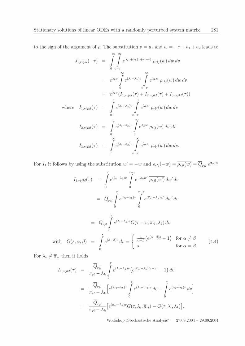
Stationary solutions of linear ODEs with a randomly perturbed system matrix 281
to the sign of the argument of ρ. The substitution v = u1 and w = −τ + u1 + u2 leads to
J1,rijkl(−τ) =
∞∫
0
∞∫
v−τ
eλiv+λk(τ+w−v) ρrlj(w) dw dv
= eλkτ
∞∫
0
e(λi−λk)v
∞∫
v−τ
eλkw ρrlj(w) dw dv
= eλkτ (I1,rijkl(τ) + I2,rijkl(τ) + I3,rijkl(τ))
where I1,rijkl(τ) =
τ∫
0
e(λi−λk)v
0∫
v−τ
eλkw ρrlj(w) dw dv
I2,rijkl(τ) =
τ∫
0
e(λi−λk)v
∞∫
0
eλkw ρrlj(w) dw dv
I3,rijkl(τ) =
∞∫
τ
e(λi−λk)v
∞∫
v−τ
eλkw ρrlj(w) dw dv.
For I1 it follows by using the substitution w′ = −w and ρrlj(−w) = ρrjl(w) = Qrjl eπrl w
I1,rijkl(τ) =
τ∫
0
e(λi−λk)v
τ−v∫
0
e−λkw′
ρrjl(w′) dw′ dv
= Qrjl
τ∫
0
e(λi−λk)v
τ−v∫
0
e(πrl−λk)w′
dw′ dv
= Qrjl
τ∫
0
e(λi−λk)vG(τ − v, πrl, λk) dv
with G(s, α, β) =
s∫
0
e(α−β)v dv =
1
α−β
(e(α−β)s − 1
)for α 6= β
s for α = β.(4.4)
For λk 6= πrl then it holds
I1,rijkl(τ) =Qrjl
πrl − λk
τ∫
0
e(λi−λk)v(e(πrl−λk)(τ−v) − 1
)dv
=Qrjl
πrl − λk
[e(πrl−λk)τ
τ∫
0
e(λi−πrl)v dv −
τ∫
0
e(λi−λk)v dv]
=Qrjl
πrl − λk
[e(πrl−λk)τG(τ, λi, πrl) − G(τ, λi, λk)
].
Workshop „Stochastische Analysis“ 27.09.2004 – 29.09.2004
282 H.-J. Starkloff, R. Wunderlich
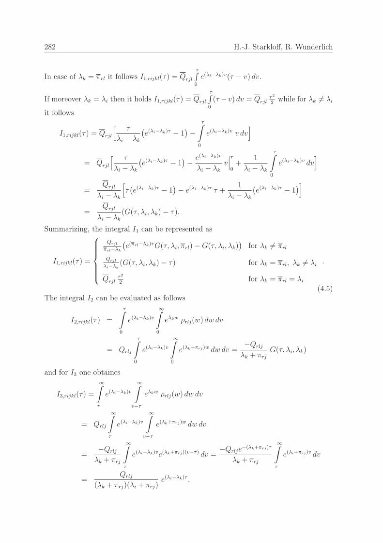
In case of λk = πrl it follows I1,rijkl(τ) = Qrjl
τ∫0
e(λi−λk)v(τ − v) dv.
If moreover λk = λi then it holds I1,rijkl(τ) = Qrjl
τ∫0
(τ −v) dv = Qrjlτ2
2while for λk 6= λi
it follows
I1,rijkl(τ) = Qrjl
[ τ
λi − λk
(e(λi−λk)τ − 1
)−
τ∫
0
e(λi−λk)v v dv]
= Qrjl
[ τ
λi − λk
(e(λi−λk)τ − 1
)−
e(λi−λk)v
λi − λk
v∣∣∣τ
0+
1
λi − λk
τ∫
0
e(λi−λk)v dv]
=Qrjl
λi − λk
[τ(e(λi−λk)τ − 1
)− e(λi−λk)τ τ +
1
λi − λk
(e(λi−λk)τ − 1
)]
=Qrjl
λi − λk
(G(τ, λi, λk) − τ).
Summarizing, the integral I1 can be represented as
I1,rijkl(τ) =
Qrjl
πrl−λk
(e(πrl−λk)τG(τ, λi, πrl) − G(τ, λi, λk)
)for λk 6= πrl
Qrjl
λi−λk(G(τ, λi, λk) − τ) for λk = πrl, λk 6= λi
Qrjlτ2
2for λk = πrl = λi
.
(4.5)The integral I2 can be evaluated as follows
I2,rijkl(τ) =
τ∫
0
e(λi−λk)v
∞∫
0
eλkw ρrlj(w) dw dv
= Qrlj
τ∫
0
e(λi−λk)v
∞∫
0
e(λk+πrj)w dw dv =−Qrlj
λk + πrj
G(τ, λi, λk)
and for I3 one obtaines
I3,rijkl(τ) =
∞∫
τ
e(λi−λk)v
∞∫
v−τ
eλkw ρrlj(w) dw dv
= Qrlj
∞∫
τ
e(λi−λk)v
∞∫
v−τ
e(λk+πrj)w dw dv
=−Qrlj
λk + πrj
∞∫
τ
e(λi−λk)ve(λk+πrj)(v−τ) dv =−Qrlje
−(λk+πrj)τ
λk + πrj
∞∫
τ
e(λi+πrj)v dv
=Qrlj
(λk + πrj)(λi + πrj)e(λi−λk)τ .
Stationary solutions of linear ODEs with a randomly perturbed system matrix 283
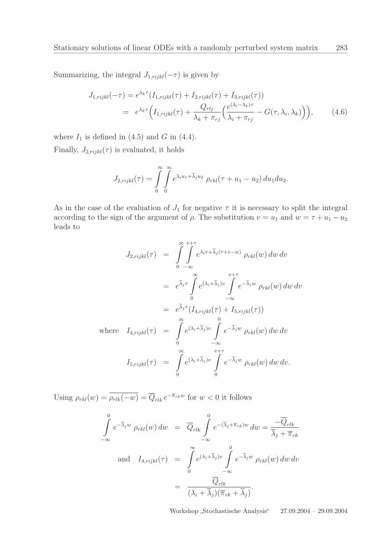
Summarizing, the integral J1,rijkl(−τ) is given by
J1,rijkl(−τ) = eλkτ (I1,rijkl(τ) + I2,rijkl(τ) + I3,rijkl(τ))
= eλkτ(I1,rijkl(τ) +
Qrlj
λk + πrj
(e(λi−λk)τ
λi + πrj
− G(τ, λi, λk)))
, (4.6)
where I1 is defined in (4.5) and G in (4.4).
Finally, J2,rijkl(τ) is evaluated, it holds
J2,rijkl(τ) =
∞∫
0
∞∫
0
eλiu1+λju2 ρrkl(τ + u1 − u2) du1du2.
As in the case of the evaluation of J1 for negative τ it is necessary to split the integralaccording to the sign of the argument of ρ. The substitution v = u1 and w = τ +u1 −u2
leads to
J2,rijkl(τ) =
∞∫
0
v+τ∫
−∞
eλiv+λj(τ+v−w) ρrkl(w) dw dv
= eλjτ
∞∫
0
e(λi+λj)v
v+τ∫
−∞
e−λjw ρrkl(w) dw dv
= eλjτ (I4,rijkl(τ) + I5,rijkl(τ))
where I4,rijkl(τ) =
∞∫
0
e(λi+λj)v
0∫
−∞
e−λjw ρrkl(w) dw dv
I5,rijkl(τ) =
∞∫
0
e(λi+λj)v
v+τ∫
0
e−λjw ρrkl(w) dw dv.
Using ρrkl(w) = ρrlk(−w) = Qrlk e−πrkw for w < 0 it follows
0∫
−∞
e−λjw ρrkl(w) dw = Qrlk
0∫
−∞
e−(λj+πrk)w dw =−Qrlk
λj + πrk
and I4,rijkl(τ) =
∞∫
0
e(λi+λj)v
0∫
−∞
e−λjw ρrkl(w) dw dv
=Qrlk
(λi + λj)(πrk + λj).
Workshop „Stochastische Analysis“ 27.09.2004 – 29.09.2004
284 H.-J. Starkloff, R. Wunderlich
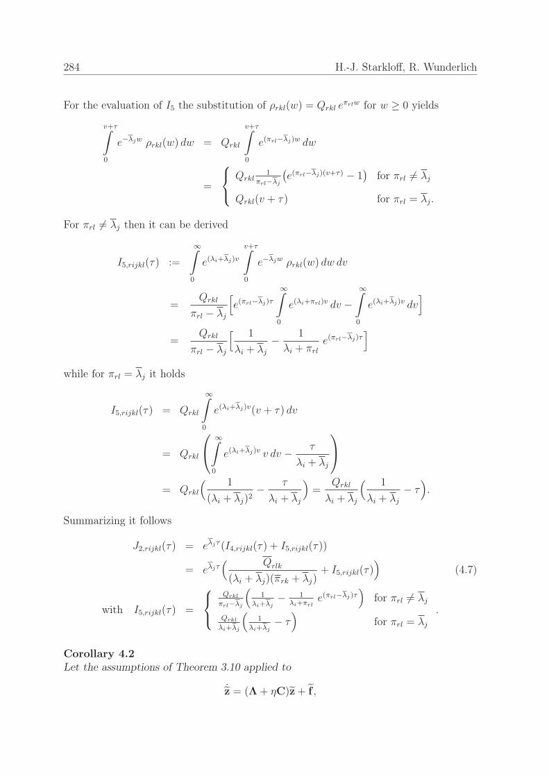
For the evaluation of I5 the substitution of ρrkl(w) = Qrkl eπrlw for w ≥ 0 yields
v+τ∫
0
e−λjw ρrkl(w) dw = Qrkl
v+τ∫
0
e(πrl−λj)w dw
=
Qrkl1
πrl−λj
(e(πrl−λj)(v+τ) − 1
)for πrl 6= λj
Qrkl(v + τ) for πrl = λj.
For πrl 6= λj then it can be derived
I5,rijkl(τ) :=
∞∫
0
e(λi+λj)v
v+τ∫
0
e−λjw ρrkl(w) dw dv
=Qrkl
πrl − λj
[e(πrl−λj)τ
∞∫
0
e(λi+πrl)v dv −
∞∫
0
e(λi+λj)v dv]
=Qrkl
πrl − λj
[ 1
λi + λj
−1
λi + πrl
e(πrl−λj)τ]
while for πrl = λj it holds
I5,rijkl(τ) = Qrkl
∞∫
0
e(λi+λj)v(v + τ) dv
= Qrkl
∞∫
0
e(λi+λj)v v dv −τ
λi + λj
= Qrkl
( 1
(λi + λj)2−
τ
λi + λj
)=
Qrkl
λi + λj
( 1
λi + λj
− τ).
Summarizing it follows
J2,rijkl(τ) = eλjτ (I4,rijkl(τ) + I5,rijkl(τ))
= eλjτ( Qrlk
(λi + λj)(πrk + λj)+ I5,rijkl(τ)
)(4.7)
with I5,rijkl(τ) =
Qrkl
πrl−λj
(1
λi+λj− 1
λi+πrle(πrl−λj)τ
)for πrl 6= λj
Qrkl
λi+λj
(1
λi+λj− τ)
for πrl = λj
.
Corollary 4.2
Let the assumptions of Theorem 3.10 applied to
˙z = (Λ + ηC)z + f ,
Stationary solutions of linear ODEs with a randomly perturbed system matrix 285
be fulfilled and R0ζ0ζ(τ) be of the form (4.2). Then the correlation function of the
stationary solution z for η < ηS and τ ≥ 0, i, j = 1, . . . , n, possesses the expansion forη ↓ 0
Reziezj(τ) =
m∑
r=1
[Qrij eπrjτ + η2
n∑
k,l=1
(E CikCkl J1,rijkl(τ)
+ECjkCkl
J1,rjikl(−τ) + E
CikCjl
J2,rijkl(τ)
)]+ o(η2),
where J1 and J2 are given in (4.3), (4.6) and (4.7).
5 Numerical results
In this section the results of the preceding sections are applied to the special case of areal and scalar equation (1.1) which arises for n = 1 and real-valued random parameters.Thus A(ω) = a(ω) is a real-valued random variable and the excitation f(t, ω) is a scalarreal-valued random process. As before the random parameters are decomposed, i.e.,
a(ω) = a + ηc(ω) and f(t, ω) = f + f(t, ω),
with Ea = a, Ef(t) = f , a centered random variable c(ω) and a centered process f(t, ω).Then Eq. (1.1) reads as
z(t, ω) = (a + ηc(ω)) z(t, ω) + f(t, ω). (5.1)
The random variable c is assumed to be a.s. bounded, i.e., |c(ω)| ≤ c0 where for conve-nience it is set c0 = 1. The stability condition for A(ω) = a(ω) = a + ηc(ω) is satisfiedfor a(ω) < 0 a.s., i.e., for η < ηS = −ba
c0= −a. In this case Eq. (5.1) possesses the unique
stationary solution
z(t, ω) =
∫ ∞
0
ea(ω)u f(t − u, ω) du = z(ω) + z(t, ω)
with z(ω) =
∫ ∞
0
ea(ω)u f du = −a−1(ω) f
and z(t, ω) =
∫ ∞
0
ea(ω)u f(t − u, ω) du.
Due to Theorem 3.2 the mean and the correlation function of z are given by
E z(t) = E z = −Ea−1
f
and Rzz(τ) = D2 z + Rez ez(τ), (5.2)
where D2 z = cov(z, z) denotes the variance of z.
In the considered special case it is possible to compute these moments explicitly in termsof the mean and the correlation function of f and the distribution of c. In order to perform
Workshop „Stochastische Analysis“ 27.09.2004 – 29.09.2004
286 H.-J. Starkloff, R. Wunderlich
numerical experiments which compare these exact moments with approximations fromthe perturbation approach it is assumed that c is uniformly distributed on [−1, 1], thena is uniformly distributed on [a− η, a + η] and we have the following probability densityfunctions
pc(s) =
12
for s ∈ [−1, 1]
0 elseand pa(s) =
12η
for s ∈ [a − η, a + η]
0 else.
Moreover it is assumed that f possesses the exponentially decaying correlation function
Rff (τ) = R ef ef(τ) = σ2 eγ|τ |, σ > 0, γ < 2a,
where σ denotes the standard deviation of f and γ is a parameter describing the decayof the correlation function of f . It is noted that we impose instead of γ < 0 the strongercondition γ < 2a in order to simplify the subsequent calculations. This condition ensuresthat γ does not coincide with the parameter a ∈ [a−η, a+η] ⊂ (2a, 0) since η < ηS = −a.
First- and second-order moments of z exist if E a−2 < ∞. This condition is fulfilledfor η < ηM = −a = ηS since
Ea−2
=
∫ba+η
ba−η
1
s2pa(s)ds ≤
∫ba+η
ba−η
1
(a + η)2pa(s)ds =
1
(a + η)2.
If a is uniformly distributed on [a − η, a + η] for η < ηM it holds
Ez = −Ea−1
f = −f
∫ba+η
ba−η
1
spa(s)ds = −
f
2η
ba+η∫
ba−η
1
sds
=f
2ηln
a − η
a + η, (5.3)
Ez2 = f2∫
ba+η
ba−η
1
s2pa(s)ds =
f2
2η
ba+η∫
ba−η
1
s2ds
=f
2
2η
( 1
a − η−
1
a + η
)=
f2
a2 − η2,
and D2 z = Ez 2 − (Ez)2 = f2( 1
a2 − η2−
1
4η2ln2 a − η
a + η
). (5.4)
For the correlation function of z it holds Rez ez(τ) = Rez ez(−τ) and for τ ≥ 0 it can beevaluated as follows
Rez ez(τ) = E z(t)z(t + τ) = E
∫ ∞
0
∫ ∞
0
eau1 f(t − u1)eau2 f(t + τ − u2) du1 du2
=
∫ ∞
0
∫ ∞
0
Eea(u1+u2)
R ef ef
(τ + u1 − u2) du1 du2,
Stationary solutions of linear ODEs with a randomly perturbed system matrix 287
where the independence of a and f has been applied. Using the substitution v = u1, w =τ + u1 − u2 and the assumption of an exponential decaying correlation function, i.e.,R ef ef
(τ) = σ2eγ|τ |, it follows
Rez ez(τ) =
∞∫
0
v+τ∫
−∞
Eea(τ+2v−w)
R ef ef
(w) dw dv
=
∞∫
0
v+τ∫
−∞
ba+η∫
ba−η
pa(x) ex(τ+2v−w) σ2eγ|w| dx dw dv
= σ2
ba+η∫
ba−η
pa(x)exτJ(x)dx
where J(x) :=
∞∫
0
e2xv
0∫
−∞
e−(γ+x)w dw +
v+τ∫
0
e(γ−x)w dw
dv
=
∞∫
0
e2xv
[−1
γ + x+
1
γ − x
(e(γ−x)(v+τ) − 1
)]dv
=
∞∫
0
e2xv
[−2γ
γ2 − x2+
e(γ−x)τ
γ − xe(γ−x)v
]dv
=γ
x(γ2 − x2)−
e(γ−x)τ
γ2 − x2.
Hence
Rez ez(τ) = σ2
ba+η∫
ba−η
pa(x)
[γ
x(γ2 − x2)exτ −
1
γ2 − x2eγτ
]dx.
If additionally a is uniformly distributed on [a − η, a + η] we have
Rez ez(τ) =σ2
2η
γ
ba+η∫
ba−η
1
x(γ2 − x2)exτ dx −
ba+η∫
ba−η
1
γ2 − x2eγτ dx
=σ2
2η[γI1(τ) − eγτI2] (5.5)
where I1(τ) :=
ba+η∫
ba−η
exτ
x(γ2 − x2)dx and I2 :=
ba+η∫
ba−η
1
γ2 − x2dx.
Workshop „Stochastische Analysis“ 27.09.2004 – 29.09.2004
288 H.-J. Starkloff, R. Wunderlich
The integrand of the integral I1(τ) is bounded and continuous in the domain of integra-tion [a − η, a + η], since γ < 2a and η < ηS = −a has been supposed. So the integral iswell-defined and can be computed using
I1(τ) = H(τ, a + η) − H(τ, a − η)
with the primitive function H(τ, z) :=z∫
exτ
x(γ2−x2)dx. For the evaluation of H(τ, z) we use
partial fraction decomposition and obtain
H(τ, z) =
z∫exτ
x(γ2 − x2)dx =
1
γ2
z∫exτ
(1
x−
1
2(x − γ)−
1
2(x + γ)
)dx
=1
γ2
[H1(τ, z, 0) −
1
2H1(τ, z,−γ) −
1
2H1(τ, z, +γ)
]
where H1(τ, z, b) :=
z∫exτ
x + bdx, b ∈ R.
For the sake of shorter notation we suppress the integration constants in the subse-quent evaluation of the indefinite integrals contained in H and H1. For τ = 0 we haveH1(τ, z, b) = ln |z + b| while for τ > 0 this integral can be expressed in terms of theso-called exponential integral (see Abramowitz, Stegun [1], p.56)
E1(z) :=
∞∫
z
e−u
udu =
−z∫
−∞
ev
vdv for z ∈ R \ 0.
Thereby for z < 0 the integral is understood as a Cauchy principal value integral.
The substitution v = τ(x + b) yields
H1(τ, z, b) =
τ(z+b)∫ev−bτ
vdv = e−bτ
τ(z+b)∫ev
vdv
= e−bτE1(−τ(z + b))
and we obtain
H(τ, z) =
1γ2
(ln |z| − 1
2ln |z − γ| − 1
2ln |z + γ|
), τ = 0
1γ2
(E1(−τz) − eγτ
2E1(−τ(z − γ)) − e−γτ
2E1(−τ(z + γ))
), τ > 0
(5.6)
Stationary solutions of linear ODEs with a randomly perturbed system matrix 289
For the integral I2 one gets
I2 =
ba+η∫
ba−η
1
γ2 − x2dx =
1
2γ
ba+η∫
ba−η
(1
γ + x+
1
γ − x
)dx
=1
2γ
[ln |γ + x| − ln |γ − x|
]ba+η
ba−η
=1
2γln
∣∣∣∣γ + (a + η)
γ − (a + η)
γ − (a − η)
γ + (a − η)
∣∣∣∣
=1
2γln
(γ + η)2 − a2
(γ − η)2 − a2.
Substituting the representations for I1(τ) and I2 into (5.5) it yields
Rez ez(τ) =σ2
2η
[γ(H(τ, a + η) − H(τ, a − η)) −
eγτ
2γln
(γ + η)2 − a2
(γ − η)2 − a2
]
where H is given in (5.6).
Lebesgue’s Theorem on dominated convergence ensures that limτ↓0
Rez ez(τ) = Rez ez(0).
Finally the correlation function of z = z + z can be derived using relation (5.2) whichyields
Rzz(τ) = D2z + Rez ez(τ)
where D2z is given in (5.4).
After the exact computation of the mean, the variance and the correlation functionof z approximations resulting from the perturbation approach presented in Section 3.2are derived. For the approximation of E z and D2 z a Neumann series expansion ofA−1(ω) = a−1(ω) = (a + ηc(ω))−1 has been used. This series is convergent for
η < ηN = supη > 0 : η <∣∣∣∣∣∣A−1C(ω)
∣∣∣∣∣∣−1
= |a−1c(ω)|−1 = |a||c(ω)|−1 a.s..
Since |c| is assumed to be a.s. bounded by c0 = 1 it holds ηN = |a| = ηS = ηM .
The expansions of the moments of z given in Theorem 3.4 applied to the present scalarcase read as
Ez = E z =(1 +
Ec2
a2η2)x + o(η2)
and D2 z =Ec2
a2x2 η2 + o(η2)
where x = −bf
ba.
If additionally c is uniformly distributed on [−1, 1] then Ec2 = 13
and
Workshop „Stochastische Analysis“ 27.09.2004 – 29.09.2004
290 H.-J. Starkloff, R. Wunderlich
E z =(1 +
1
3a2η2) f
−a+ o(η2)
D2 z =1
3a4f
2η2 + o(η2).
It can easily be checked that these expansions coincide with the corresponding Taylorexpansions of the exact results given in (5.3) and (5.4) in powers of η.
For the correlation function Rez ez(τ) Theorem 3.10 provides an expansion for η < ηP = λ0
v0c0with λ0 = −a, v0 = 1 and c0 = 1, i.e., ηP = −a = ηs = ηM = ηN . It can be observedthat in this example all bounds η. coincide.
In the present scalar case Eqs. (1.1) and (4.1) coincide and for the assumed exponen-tially decaying correlation of f the correlation function R0ζ 0ζ(τ) of the solution of theunperturbed equation is for τ ≥ 0
R0ζ 0ζ(τ) =σ2
γ2 − a2
(γ
aebaτ − eγτ
)= q1e
π1τ + q2eπ2τ
where π1 = a, q1 =σ2
γ2 − a2
γ
a
π2 = γ, q2 = −σ2
γ2 − a2.
In view of the prescribed form of the correlation function R0ζ 0ζ(τ) given in Eq. (4.2) wecan set m = 2, Q1 = q1, Q2 = q2, Π1 = π1 = a and Π2 = π2 = γ. Moreover it is n = 1and Λ = a, so we can apply Corollary 4.2 to give an expansion in powers of η for thecorrelation function Rez ez(τ). Thereby we suppress the indices i, j, k, l which in our casetake the value 1, only. It follows for τ ≥ 0
Rez ez(τ) =2∑
r=1
[qre
πrτ + η2Ec2(J1,r(τ) + J1,r(−τ) + J2,r(τ))]+ o(η2). (5.7)
For J1,r(τ) Eq. (4.3) gives
J1,1(τ) =q1
4a2ebaτ and J1,2(τ) =
q2
(a + γ)2eγτ .
J1,r(−τ) can be evaluated using Eq. (4.6), it yields
J1,1(−τ) = q1ebaτ
(τ 2
2−
τ
2a+
1
4a2
)
J1,2(−τ) = −q2ebaτ 2γ
γ2 − a2
(τ +
2a
γ2 − a2
)+ q2e
γτ 1
(a − γ)2
while from Eq. (4.7) it follows for J2,r(τ)
J2,1(τ) = q1ebaτ
(1
2a2−
τ
2a
)
J2,2(τ) = q2ebaτ γ
a(γ2 − a2)− q2e
γτ 1
γ2 − a2.
Stationary solutions of linear ODEs with a randomly perturbed system matrix 291
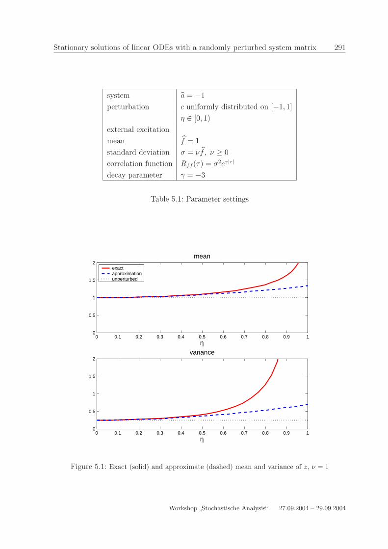
system a = −1
perturbation c uniformly distributed on [−1, 1]
η ∈ [0, 1)
external excitation
mean f = 1
standard deviation σ = νf , ν ≥ 0
correlation function Rff (τ) = σ2eγ|τ |
decay parameter γ = −3
Table 5.1: Parameter settings
0 0.1 0.2 0.3 0.4 0.5 0.6 0.7 0.8 0.9 10
0.5
1
1.5
2mean
η
exactapproximationunperturbed
0 0.1 0.2 0.3 0.4 0.5 0.6 0.7 0.8 0.9 10
0.5
1
1.5
2variance
η
Figure 5.1: Exact (solid) and approximate (dashed) mean and variance of z, ν = 1
Workshop „Stochastische Analysis“ 27.09.2004 – 29.09.2004
292 H.-J. Starkloff, R. Wunderlich
Substituting the above terms into (5.7) we get the following expansion for the correlationfunction of z
Rez ez(τ) = ebaτ
q1 + η2Ec2
[q1
(τ 2
2−
τ
a+
1
a2
)−
q2γ
γ2 − a2
(2τ +
5a2 − γ2
a(γ2 − a2)
)]
+ebγτ
q2 + η2Ec2q2
3a2 + γ2
(γ2 − a2)2
+ o(η2)
=σ2
γ2 − a2
(γ
aebaτ − eγτ
)
+η2Ec2 σ2
γ2 − a2
[ebaτ
γ
a
(τ 2
2−
τ
a+
1
a2
)+
γ
γ2 − a2
(2τ +
5a2 − γ2
a(γ2 − a2)
)
− ebγτ 3a2 + γ2
(γ2 − a2)2
]+ o(η2).
If c is uniformly distributed on [−1, 1] then Ec2 = 13
can be substituted in the aboveformula.
Table 5.1 shows the parameters for the subsequent numerical experiments. It is notedthat the standard deviation σ of the excitation is set proportional to the mean excitationf , i.e., σ = νf , with ν ≥ 0.
It holds ηS = ηM = ηN = ηP = −a = 1, i.e., for η ∈ [0, 1) we have stability andconvergence of the perturbation series.
Remark 5.1 For an optimal view of the subsequent figures we recommend a coloredhardcopy or the electronic version of this paper which is available at http://archiv.tu-chemnitz.de/pub/2005/ or http://www.fh-wickau.de/∼raw.
Figure 5.1 plots for ν = 1 the mean Ez and the variance D2z versus the perturbationparameter η. Moreover the corresponding quantities of the unperturbed equation (η = 0)are drawn. The approximations found from the perturbation approach compare well withthe exact results for η < 0.5. For larger values of η the approximations are less accurateand they are not suited to describe the limiting behaviour for η → ηS = 1. Here the meanas well as the variance of z tends to infinity while approximations grow quadraticallyand remain finite.
Figure 5.2 plots for ν = 0.5 (left) and ν = 2 (right) the exact total variance D2z =D2z + D2z (red, solid) together with the two contributions D2z (blue, dashed) and D2z
(cyan, dotted) versus η. Since z does not depend on f , the variance of z is not influencedby ν while the variance of z is proportional to ν2. It can be seen, that for small η thecontribution of D2z dominates the contribution of D2z while for large η a reversedsituation can be observed.
This phenomenon is also visualized in the two lower plots which show the relative con-tribution of the variance of z to the total variance, i.e., D2bz
D2z= D2bz
D2bz+D2ez. Thereby the
solid line corresponds to the exact values and the dashed line to the approximations.
Stationary solutions of linear ODEs with a randomly perturbed system matrix 293
0 0.2 0.4 0.6 0.8 10
0.5
1
1.5
2
2.5ν =0.50
η
0 0.2 0.4 0.6 0.8 10
0.2
0.4
0.6
0.8
1
η
0 0.2 0.4 0.6 0.8 10
0.5
1
1.5
2
2.5ν =2.00
η
0 0.2 0.4 0.6 0.8 10
0.2
0.4
0.6
0.8
1
η
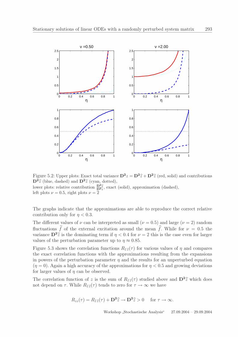
Figure 5.2: Upper plots: Exact total variance D2z = D
2z + D2z (red, solid) and contributions
D2z (blue, dashed) and D
2z (cyan, dotted),
lower plots: relative contribution D2bzD2z
, exact (solid), approximation (dashed),left plots ν = 0.5, right plots ν = 2
The graphs indicate that the approximations are able to reproduce the correct relativecontribution only for η < 0.3.
The different values of ν can be interpreted as small (ν = 0.5) and large (ν = 2) random
fluctuations f of the external excitation around the mean f . While for ν = 0.5 thevariance D2z is the dominating term if η < 0.4 for ν = 2 this is the case even for largervalues of the perturbation parameter up to η ≈ 0.85.
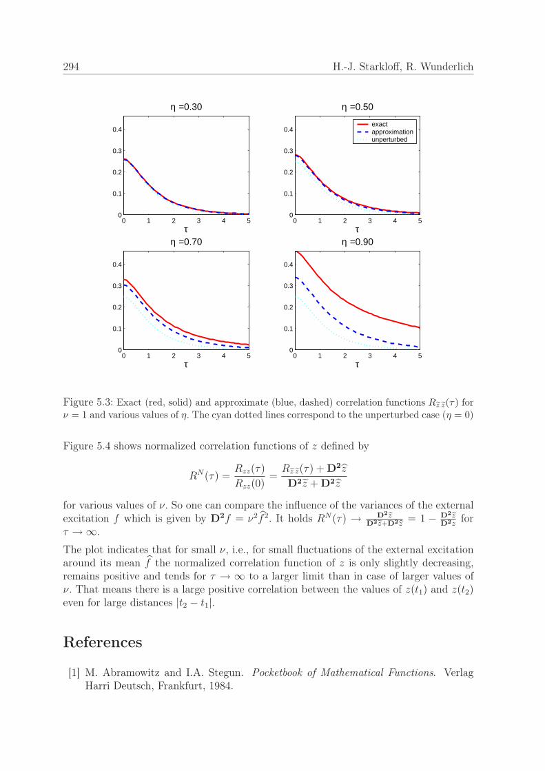
Figure 5.3 shows the correlation functions Rez ez(τ) for various values of η and comparesthe exact correlation functions with the approximations resulting from the expansionsin powers of the perturbation parameter η and the results for an unperturbed equation(η = 0). Again a high accuracy of the approximations for η < 0.5 and growing deviationsfor larger values of η can be observed.
The correlation function of z is the sum of Rez ez(τ) studied above and D2z which doesnot depend on τ . While Rez ez(τ) tends to zero for τ → ∞ we have
Rzz(τ) = Rez ez(τ) + D2z → D2z > 0 for τ → ∞.
Workshop „Stochastische Analysis“ 27.09.2004 – 29.09.2004
294 H.-J. Starkloff, R. Wunderlich
0 1 2 3 4 50
0.1
0.2
0.3
0.4
η =0.30
τ0 1 2 3 4 5
0
0.1
0.2
0.3
0.4
η =0.50
τ
exactapproximationunperturbed
0 1 2 3 4 50
0.1
0.2
0.3
0.4
η =0.70
τ0 1 2 3 4 5
0
0.1
0.2
0.3
0.4
η =0.90
τ
Figure 5.3: Exact (red, solid) and approximate (blue, dashed) correlation functions Rez ez(τ) forν = 1 and various values of η. The cyan dotted lines correspond to the unperturbed case (η = 0)
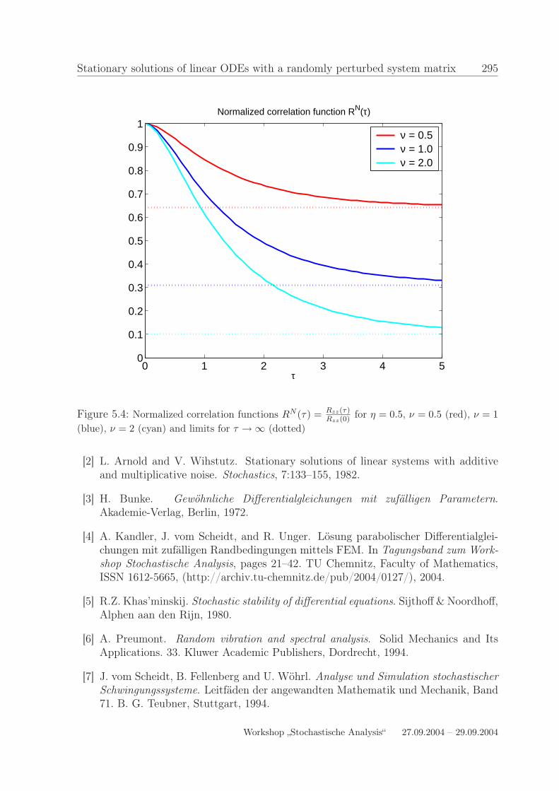
Figure 5.4 shows normalized correlation functions of z defined by
RN(τ) =Rzz(τ)
Rzz(0)=
Rez ez(τ) + D2z
D2z + D2z
for various values of ν. So one can compare the influence of the variances of the externalexcitation f which is given by D2f = ν2f 2. It holds RN(τ) → D2bz
D2ez+D2bz= 1 − D2ez
D2zfor
τ → ∞.
The plot indicates that for small ν, i.e., for small fluctuations of the external excitationaround its mean f the normalized correlation function of z is only slightly decreasing,remains positive and tends for τ → ∞ to a larger limit than in case of larger values ofν. That means there is a large positive correlation between the values of z(t1) and z(t2)even for large distances |t2 − t1|.
References
[1] M. Abramowitz and I.A. Stegun. Pocketbook of Mathematical Functions. VerlagHarri Deutsch, Frankfurt, 1984.
Stationary solutions of linear ODEs with a randomly perturbed system matrix 295
0 1 2 3 4 50
0.1
0.2
0.3
0.4
0.5
0.6
0.7
0.8
0.9
1Normalized correlation function RN(τ)
τ
ν = 0.5ν = 1.0ν = 2.0
Figure 5.4: Normalized correlation functions RN (τ) = Rzz(τ)Rzz(0) for η = 0.5, ν = 0.5 (red), ν = 1
(blue), ν = 2 (cyan) and limits for τ → ∞ (dotted)
[2] L. Arnold and V. Wihstutz. Stationary solutions of linear systems with additiveand multiplicative noise. Stochastics, 7:133–155, 1982.
[3] H. Bunke. Gewöhnliche Differentialgleichungen mit zufälligen Parametern.Akademie-Verlag, Berlin, 1972.
[4] A. Kandler, J. vom Scheidt, and R. Unger. Lösung parabolischer Differentialglei-chungen mit zufälligen Randbedingungen mittels FEM. In Tagungsband zum Work-
shop Stochastische Analysis, pages 21–42. TU Chemnitz, Faculty of Mathematics,ISSN 1612-5665, (http://archiv.tu-chemnitz.de/pub/2004/0127/), 2004.
[5] R.Z. Khas’minskij. Stochastic stability of differential equations. Sijthoff & Noordhoff,Alphen aan den Rijn, 1980.
[6] A. Preumont. Random vibration and spectral analysis. Solid Mechanics and ItsApplications. 33. Kluwer Academic Publishers, Dordrecht, 1994.
[7] J. vom Scheidt, B. Fellenberg and U. Wöhrl. Analyse und Simulation stochastischer
Schwingungssysteme. Leitfäden der angewandten Mathematik und Mechanik, Band71. B. G. Teubner, Stuttgart, 1994.
Workshop „Stochastische Analysis“ 27.09.2004 – 29.09.2004
296 H.-J. Starkloff, R. Wunderlich
[8] J. vom Scheidt, H.-J. Starkloff and R. Wunderlich. Asymptotic expansions of integralfunctionals of ε-correlated processes. Journal for Analysis and its Applications,19(1):255–268, 2000.
[9] J. vom Scheidt, H.-J. Starkloff and R. Wunderlich. Stationary solutions of ran-dom differential equations with polynomial nonlinearities. Stochastic Analysis and
Applications, 6(19):1059-1075, 2001.
[10] J. vom Scheidt, H.-J. Starkloff and R. Wunderlich. Low-dimensional approximati-ons for large-scale systems of random ODEs. Dynamic Systems and Applications,11(2):143–165, 2002.
[11] J. vom Scheidt, H.-J. Starkloff and R. Wunderlich. Random transverse vibrationsof a one-sided fixed beam and model reduction. ZAMM, Z. Angew. Math. Mech.,82(11-12):831–845, 2002.
[12] J. vom Scheidt, H.-J. Starkloff and R. Wunderlich. Remarks on randomly excitedoscillators. ZAMM, Z. Angew. Math. Mech., 82(11-12):847–859, 2002.
[13] J. vom Scheidt and U. Wöhrl. Nonlinear vibration systems with two parallel randomexcitations. Journal for Analysis and its Applications, 16(1):217–228, 1997.
[14] J. vom Scheidt and R. Wunderlich. Nonlinear random vibrations of vehicles. Z.
Angew. Math. Mech., 76(S5):447–448, 1996.
[15] A.N. Shiryaev. Probability. Springer, New York, 1996.
[16] T.T. Soong and M. Grigoriu. Random vibration of mechanical and structural sy-
stems. PTR Prentice Hall, Englewood Cliffs NJ, 1993.
[17] H.-J. Starkloff. Higher order asymptotic expansions for weakly correlated ran-dom functions. Habilitation Thesis, TU Chemnitz, Faculty of Mathematics(http://archiv.tu-chemnitz.de/pub/2005/0012), 2005.