Superlinear dynamics of a scalar parabolic equationgeb.uni-giessen.de/geb/volltexte/2007/5093/pdf/SchulzSven-2007-04-27.pdf · equilibrium solutions is a generic property. The semiﬂow

Dissertation

Superlinear dynamics of a scalarparabolic equation

Sven Schulz

Februar 2007

Fur Alexandra, Anna-Katharina

und Nils

Sven Schulz Zusammenfassung

Zusammenfassung

Die vorliegende Arbeit befasst sich mit dem semilinearen parabolischen Anfangs-Randwertproblem

ut − uxx = f (u), u(·, 0) = u0, u(0) = u(1) = 0. (P)

Dieses Problem ist das einfachste Modell einer Warmeleitungs- oder Reaktions-Diffusionsgleichung. Der von uns betrachtete superlineare Fall spielt insbesonderebei der Modellierung von Verbrennungsprozessen eine Rolle, konkrete Anwen-dungen finden sich in [Hen81, Kapitel 2]. Aus mathematischer Sicht induziert(P) einen Halbfluß ϕ auf dem Zustandsraum H10([0, 1]), an dessen dynamischenEigenschaften wir interessiert sind.

Aus technischer Sicht hat der Halbfluß ϕ sehr gute Eigenschaften: er ist kom-pakt, besitzt eine Gradientenstruktur, und ist ruckwartseindeutig (d.h. die Zeit-1-Abbildung ist injektiv). Zudem ist, vereinfacht gesagt, die Zahl der Nullstellenentlang Losungskurven monoton fallend ([Mat82]). Dieses zweite, diskrete Lyapu-nov Funktional wurde von vielen Autoren genutzt, um weitere Eigenschaften desHalbflusses zu beweisen. So schneiden sich stabile und instabile Mannigfaltig-keiten transversal ([Hen85]), Nichtdegeneriertheit der Gleichgewichtslosungen isteine generische Eigenschaft ([BC84]), und im dissipativen Fall ist der globaleAttraktor des Flusses ein endlichdimensionaler C1-Graph. Im dissipativen Fallwurde daruberhinaus mit Hilfe der Transversalitatseigenschaften und Conley In-dex Methoden von Brunovsky und Fiedler ([BF88, BF89]) die Frage der Existenzverbindender Orbits zwischen den Gleichgewichtslosungen vollstandig gelost.

Im superlinearen Fall gibt es unendlich viele Gleichgewichtslosungen, und furdiesen Fall scheint es keine vergleichbaren Resultate uber verbindende Orbits oderFlussaquivalenz zu geben. Die zahlreichen Arbeiten uber dieses und ahnliche su-perlineare Probleme, z.B. von Marek Fila, Hiroshi Matano, Peter Polacik, PavolQuittner und anderen, befassen sich uberwiegend mit Blow-Up Losungen. Uberglobal beschrankte Losungen scheint wenig bekannt zu sein. In der vorliegendenArbeit gelingt es uns, fur eine sehr große Klasse von superlinearen Nichtlineari-taten genau anzugeben, welche Gleichgewichtslosungen durch heterokline Orbitsverbunden werden, und welche nicht. Fur eine Teilklasse superlinearer Probleme(diese enthalt den Modellfall f (u) = u|u|p oder auch f (u) = u|u|p − λu) konnenwir beweisen, daß bestimmte endlichdimensionale invariante Mengen An,∞ struk-turell stabil sind (d.h. falls f und f

”nahe“ beieinander liegen, so gibt es einen

Homoomorphismus An,∞ → An,∞ der Orbits auf Orbits abbildet, und die zeitli-che Orientierung der Orbits erhalt). Die Mengen An,∞ enthalten auch Blow-UpLosungen (d.h. unbeschrankte Losungen mit endlicher Existenzzeit), d.h. diesepartielle strukturelle Stabilitat erstreckt sich auch auf das Blow-Up Verhalten.

Wir erhalten unsere Resultate auf folgende Weise: Eine superlineare Funktionf wird ausserhalb eines kompakten Intervalls so abgeandert, daß ein dissipati-ver Halbfluss entsteht. Da der Zustandsraum H10([0, 1]) kompakt nach C0([0, 1])

i

Zusammenfassung Sven Schulz

einbettet, stimmt dieser abgeanderte Halbfluss auf einer Nullumgebung mit demursprunglichen Fluß ϕ uberein. Wird nun das Intervall vergroßert, auf dem f un-verandert bleibt, so wachst auch diese Nullumgebung entsprechend, und es lassensich die Ergebnisse uber den dissipativen Fall anwenden und auf ϕ ubertragen.Diese Ergebnisse sind jedoch in der Mehrzahl nur fur hyperbolische Halbflus-se richtig, was den skizzierten Ansatz technisch erschwert. Beim Abschneidender superlinearen Funktion entstehen im modifizierten Fluß notwendig zusatzli-che Gleichgewichtslosungen. Diese durfen naturlich nicht ausgeartet sein. Zudemdurfen sie die Struktur der

”Originalgleichgewichte“ nicht beeinflussen, um eine

Ruckubertragung der Ergebnisse auf den superlinearen Fall zu ermoglichen. Furdas Resultat uber strukturelle Stabilitat ist es daruberhinaus notwendig, auch ste-tige Familien von Funktionen so abzuschneiden, daß wiederum stetige Familienvon Funktionen entstehen. Auch die Position, ab der die Funktionen abgeandertwerden, muß stetig variiert werden konnen.

Dies alles sicherzustellen ist der technische Kern dieser Arbeit (Kapitel 3).Konkret werden die Nichtlinearitaten, nach einem kurzen geglatteten Ubergang,konstant fortgesetzt — damit erfullen sie die Wachstumsbedingung fur die Exis-tenz eines globalen Attraktors. Dabei geht entscheidend ein, daß die Gleichge-wichtslosungen von (P) Losungen gewohnlicher Differentialgleichungen zweiterOrdnung sind. Als zweidimensionales System konnen zur Analyse die Strukturdes Phasenraumes und Shooting-Curve Techniken verwendet werden. Mit Hilfesolcher Shooting-Curve Methoden laßt sich insbesondere auch die Nichtdegene-riertheit von Gleichgewichtslosungen charakterisieren. Einige weitere, spezielleHilfsmittel werden in Abschnitt 3.3.1 entwickelt. Zudem erfullen die Ableitungendieser stationaren Losungen nach verschiedenen Großen lineare Differentialglei-chungen zweiter Ordnung, auf die Sturmsche Vergleichssatze angewandt werdenkonnen.

Mit Hilfe dieser technischen Resultate konstruieren wir in Abschnitt 4.1 eineFolge (ϕn) dissipativer Halbflusse, die jeweils eine wachsende Zahl von Gleich-gewichten der superlinearen Gleichung enthalten. Aus [BF89] folgt leicht, daßunter den angegebenen Bedingungen fur hinreichend große n verbindende Or-bits bezuglich ϕn existieren. Es ist allerdings nicht klar, daß die verbindendenOrbits komplett im unveranderten Bereich des Halbflusses liegen, wenn dies furdie Endpunkte des Orbits gilt. Daher muß noch sichergestellt werden, daß diegefundenen Verbindungen fur n→ ∞ nicht abreißen. Dies gelingt mit Energiear-gumenten und dadurch, daß wir die Nullstellenzahl der zusatzlich entstehendenLosungen in geeigneter Weise kontrollieren konnen.

Um fur”gleichmaßig superlineare“ f genauere Aussagen daruber zu erhalten,

in welchem Sinne ϕ von ϕn approximiert wird, konstruieren wir nun eine stetigeFamilie (ϕν)ν von dissipativen Halbflussen, die fur ganzzahlige ν mit den vorherKonstruierten ubereinstimmen. Somit existiert ein globaler Attraktor von ϕn undes stellt sich die Frage, ob diese invariante Menge fur ν nahe bei n in ϕν erhaltenbleibt. Es stellt sich heraus, daß fur ν ≥ n lokale Attraktoren von ϕν existieren,

ii

Sven Schulz Zusammenfassung

die stetig in ν variieren, und fur n = ν mit dem globalen Attraktor ubereinstim-men. Daruberhinaus sind die Flusse auf diesen lokalen Attraktoren konjugiert,mit anderen Worten: die Struktur bleibt fur alle ν ≥ n erhalten, und wird durchdie mit wachsendem ν nach und nach hinzukommenden energierreicheren Gleich-gewichte nicht beeinflusst.

Mit diesen Resultaten erhalt man dann leicht die Konjugation zweier super-linearer Flusse auf n-dimensionalen invarianten Mengen, die durch Grenzuber-gang aus den genannten lokalen Attraktoren entstehen. Diese Konstruktion lie-fert uberdies eine Interpretation von Blow-Up als Approximation von ∞ durcheine wachsende Folge von (lokalen/globalen) Attraktoren: Die zusatzlich durchdas Abschneiden entstehenden Gleichgewichtslosungen variieren stetig in ν, undkonvergieren in der H10-Norm gegen ∞ fur ν → ∞.

Fur die hervorragende Betreuung der Arbeit danke ich Herrn Thomas Bartsch,ebenso danke ich Herrn Hans-Otto Walther fur die Arbeit als Gutachter. Als Aus-druck meiner Freude uber viele Dinge, die wahrend der Arbeit an dieser Disser-tation geschehen sind, widme ich diese Arbeit Alexandra, Anna-Katharina undNils.

iii

Zusammenfassung Sven Schulz

iv

Contents

1 Introduction 21.1 Notation . . . . . . . . . . . . . . . . . . . . . . . . . . . . . . . . 3

2 The parabolic semiflow 52.1 Existence and basic properties . . . . . . . . . . . . . . . . . . . . 52.2 Dissipative semiflows . . . . . . . . . . . . . . . . . . . . . . . . . 102.3 Non-dissipative semiflows . . . . . . . . . . . . . . . . . . . . . . . 11

3 Technical results 153.1 The zero number . . . . . . . . . . . . . . . . . . . . . . . . . . . 153.2 The T-Map and stationary solutions . . . . . . . . . . . . . . . . 163.3 The cutoff function . . . . . . . . . . . . . . . . . . . . . . . . . . 23

3.3.1 Phase-plane analysis tools . . . . . . . . . . . . . . . . . . 253.3.2 The bridge function . . . . . . . . . . . . . . . . . . . . . . 313.3.3 Proof of the cutoff-proposition . . . . . . . . . . . . . . . . 33

3.4 Local attractors and linearization . . . . . . . . . . . . . . . . . . 40

4 Applications of cut-off 454.1 Connecting orbits . . . . . . . . . . . . . . . . . . . . . . . . . . . 454.2 Continuous approximation of f . . . . . . . . . . . . . . . . . . . 494.3 Orbit equivalence and blow-up . . . . . . . . . . . . . . . . . . . . 53

A Some technical proofs 55A.1 The superposition operator f . . . . . . . . . . . . . . . . . . . . 55A.2 A class of dissipative functions . . . . . . . . . . . . . . . . . . . . 56A.3 Upper semicontinuity of local attractors . . . . . . . . . . . . . . 57A.4 Persistence of transversal intersections . . . . . . . . . . . . . . . 58

1

CHAPTER 1

Introduction

We are concerned with solutions of the onedimensional semilinear parabolic prob-lem

ut − uxx = f (u), u(·, 0) = u0, u(0) = u(1) = 0 (P)

on the unit interval with a smooth nonlinearity f . This problem is the simplestmodel example of an heat or reaction-diffusion equation. With a superlinearnonlinearity problems of that type appear in the theory of combustion. Severalapplications are mentioned in [Hen81, Chapter 2]. This problem induces a differ-entiable semiflow ϕ on H10([0, 1]), the dynamics of which we want to investigate.Definitions and details will be given in section 2.

A very important property of this problem is that, roughly speaking, the num-ber of zeros is nonincreasing along solutions of (P). This was showed by Matano([Mat82]). His result has been used by Angenent ([Ang86]) and Henry ([Hen85])to show that stable and unstable manifold necessarily intersect transversally. Ithas also been proved by Brunovsky and Chow ([BC84]) that nondegeneracy ofequilibrium solutions is a generic property. The semiflow has several nice fea-tures (compactness, backward uniqueness, gradient structure) and finally theequilibrium solutions are solutions of a twodimensional autonomous initial valueproblem. The twodimensional flow resulting from this IVP can be examined byphase-plane analysis and shooting curve techniques. So from a technical point ofview the problem (P) looks rather promising.

There has been a lot of work on the dynamics of ϕ in the dissipative case.Under the growth condition lim sup|t|→∞ t

−1 f (t) < π2 the semiflow ϕ admits acompact global attractor which is the union of the unstable manifolds of all equi-librium (i.e. time-independent) solutions. This means that the essential dynamicsof ϕ can be described on a finite-dimensional invariant set, which happens to bea smooth graph in our case ([Bru90]). This attractor is also the union of the equi-librium solutions and the connecting, or heteroclinic, orbits between equilibria.The question which equilibria are connected by heteroclinic orbits has been solvedcompletely by Brunovsky and Fiedler ([BF88],[BF89]) in the (generic) hyperboliccase. They used the nonincrease of the zero-number and Conley Index argu-ments, extending previous partial results ([CS80], [Hen81, §5.3],[Hen85]). Fordissipative Morse-Smale systems Oliva ([Oli02]) obtained a structural stabilityresult, showing that the flows on the attractors of two ”close” Morse-Smale semi-flows are conjugate. Lu ([Lu94]) transferred a classical result of Palis and Smale([PS70]) to ϕ using the existence of an inertial manifold ([CL88]). He showed

2

Sven Schulz 1.1. Notation

that two close semiflows are conjugate not only on the attractor, but also on anopen neighborhood of the attractor.

The problem (P) (and similar problems) with superlinear nonlinearity is avery active field of research. Several people (e.g. Marek Fila, Hiroshi Matano,Peter Polacik, Pavol Quittner and others) have proved results about blow-upsolutions. About the set of globally bounded solutions however, not much isknown. It is known that in this case infinitely many equilibrium solutions exist(see eg. [Str80]), and trajectories either blow up in finite time or converge to oneof the equilibria. So we will consider both the set of globally bounded solutionsand the union of all unstable manifolds, and finite dimensional approximationsor subsets of these. Our first main results is to extend the results of Brunovskyand Fiedler to give a complete description of the connecting orbit structure of avery large class of superlinear nonlinearities in Theorem 4.2. Apparently thereis no similar result about connecting orbits for superlinear nonlinearities. Thesecond main result is the conjugacy of two close flows on certain finite dimensionalinvariant sets, including a ”stability of blow-up behaviour” result (Theorem 4.5).Although we were not able to prove structural stability w.r.t. one of the infinite-dimensional sets mentioned above, this result also seems to be completely new.This approach could certainly be refined to investigate blow-up phenomena by”dissipative approximation”, cf. section 4.3.

Technically we use a straightforward approach. Modifying a given superlinearf outside a compact interval I we get a dissipative semiflow. Due to the com-pactness of the embedding of the state space H10([0, 1]) in the space of continuousfunctions this modified semiflow coincides with the original one on an open ball inX. Increasing I increases this ball, so we get an sequence of dissipative semiflowsϕn. These ϕn necessarily contain equilibrium solutions that do not exist in ϕ,but we are able to make sure that these additional solutions are nondegenerate.We apply the results on connecting orbits to these ϕn and are able to show, thatthese connections w.r.t. ϕn persist as n→ ∞. For the structural stability resultswe have to construct a continuous family ϕν of dissipative flows approximatingϕ. As ν → ∞ the number of equilibria increases, so necessarily degenerate sta-tionary solutions appear. By controlling the zero number of these solutions weare able to apply results for global attractors to local attractors of ϕn.

The technical part, cutting of a family of superlinear functions appropriately,will be done in chapter 3 after collecting everything we need to know about theparabolic flow in chapter 2. These results will then be applied in chapter 4.

1.1 Notation

We will work mostly in standard Lebesgue- and Sobolev Spaces. Let L2 =L2([0, 1]) be the space of [equivalence classes of] square integrable functions with

the usual norm ‖u‖2 := (∫u2)

12 . The functions in L2 with (weak) derivative in

3

1. Introduction Sven Schulz

L2 form the space H1, endowed with the norm ‖u‖ = (‖u‖22 + ‖ux‖22)12 . Our

basic space is X := H10 , the completion of C∞c ([0, 1]) (C∞ functions with compact

support) wrt. ‖ · ‖. By Poincare inequality (cf. section A.2), ‖u‖22 ≤ π2‖ux‖22for u ∈ X, implying

‖ux‖22 ≤ ‖u‖2 ≤ (1+ π2)‖ux‖22.

Let H2 be the space of functions in L2 with first and second derivative also inL2, and L∞ = L∞([0, 1]) the space of essentially bounded functions on [0, 1] with‖u‖∞ = ess supu(x) : x ∈ [0, 1].

For ǫ > 0 we denote by Uǫ(u) (Bǫ(u)) the open (closed) ball of radius ǫaround u — if it is clear from the context we do not denote the underlying set ortopology, usually it will be R, an interval in R or X.

For a manifold A ⊂ X and x ∈ A TxA is the tangent space of A in x.Two manifolds A, B intersect transversally, A ⊤∩ B, if TxA+ TxB = X for allx ∈ A ∩ B. This implies that A ∩ B is a submanifold of X, the dimension ofwhich is dim A− codim B if both numbers are finite. Two submanifolds A, B ofa manifold C ⊂ X intersect transversally in C, A⊤∩C B, if TxA+ TxB = TxC forevery x ∈ A ∩ B. For manifolds we use the notation ∂A := A \ A.

For x ∈ X, B ⊂ X let dist(x, B) := infy∈B ‖x − y‖. The mapping x 7→dist(x, B) is continuous. For A, B ⊂ X let δ(A, B) := supx∈A dist(x, B) (notethat δ(A, B) 6= δ(B, A) in general). We call a family (At)t of sets upper (lower)

semi-continuous at t0, if δ(At, At0)t→t0−−→ 0

(δ(At0 , At)

t→t0−−→ 0). We call it

continuous at t0 if it is both upper and lower semi-continuous. Two smoothsubmanifolds A, B are ”ǫ-close in the C1-topology”if there is a C1-diffeomorphismχ : A→ B such that ‖χ − id‖C1 < ǫ.

4

CHAPTER 2

The parabolic semiflow

2.1 Existence and basic properties

The equation (P) with a twice differentiable f generates a semiflow on the spaceX (it is well-posed in X, cf. the following proposition). In fact many assertionsused in this work hold for f only C1. We will always assume f to be C2 though– if weaker assumptions are sufficient we will sometimes remark this explicitly.We rewrite (P) in terms of operators to apply a general theory. Let A be theDirichlet realization of u 7→ u′′ in L2: A is defined on H2 ∩ X, self-adjoint and≤ 0 ([CH98, Proposition 2.6.1]), so −A is a sectorial operator and generates ananalytic semigroup ([Hen81, Example 2 on p. 19; Theorem 1.3.4]). Let f : X ∋u 7→ f u ∈ L2([0, 1]) be the superposition operator induced by f (cf. LemmaA.1). Then the following holds:

Proposition 2.1. For every u0 ∈ X there is a maximal Tmax(u0) ∈ (0,∞] suchthat the Cauchy Problem

u(t) + Au(t) = f (u) t > 0

u(0) = u0

has a solution

u ∈ C(I+,X) ∩ C1( ˚I+, L2([0, 1])) ∩ C( ˚I+,H22([0, 1])),

where I+ = I+(u0) := [0, Tmax(u0)). These solutions induce a local continuoussemiflow ϕ on X. We set

D+ = (t, u0) ∈ R+0 × X : t ∈ I+(u0)

and D+ = D+ \ (0 × X). For any s ≥ 0 we also set

Ds = u0 ∈ X : (s, u0) ∈ D+, D∞ =⋂

s≥0Ds.

So we can writeϕt : Dt ∋ u0 7→ ϕ(t, u0) ∈ X

and ϕ has the following additional properties:

5

2. The parabolic semiflow Sven Schulz

(i) If ‖ϕ(t, u0)‖ is uniformly bounded on I(u0) then Tmax(u0) = ∞.

(ii) D is open in [0,∞)× X and Ds is open in X for any s ≥ 0.(iii) ϕ is continuous and C1 in its second argument

(iv) ϕ is compact, meaning that for T ∈ (0,∞], V ⊂ DT, 0 < ǫ1 < ǫ2 < T and

M(ǫi) =⋃

t∈[ǫi,T)

ϕ(t,V), i = 1, 2

boundedness of M(ǫ1) (in X) implies boundedness of M(ǫ2) in H2 and thus(by Sobolev embedding) precompactness of M(ǫ2) (in X). In particular thisimplies that for u0 ∈ D∞ ϕ([0,∞), u0) is precompact if it is bounded.

(v) u is a classical (pointwise) solution of (P) on (0, Tmax(u0)) × Ω, i.e. it isC1 in (t, x) and C2 in x.

(vi) For any t ≥ 0 both ϕt and Dϕt are injective.

Proof. All assertions are stated in Theorems A.3 and B.2 in [AB05]. The hy-potheses of B.2 demand a polynomial bound on f ′. Since in the one-dimensionalcase f is C1 uniformly on bounded sets due to the continuous embedding X −→C([0, 1]) (Lemma A.1), this restriction is not necessary.

Now that we have a semiflow we can recall the following notions:

Remark 2.2. 1. Time independent solutions of (P), i.e. fixed points of ϕ, arecalled equilibria (equilibrium solutions, stationary solutions) of ϕ. Let E denotethe set of equilibria. A solution v ∈ E is hyperbolic or nondegenerate, if 0 is noeigenvalue of the linear operator

Lv : H2 ∩ X → L2 : u 7→ uxx + f ′(v(x))u.

Lu is a densely defined self-adjoint operator and bounded from above (whichfollows from the Kato-Rellich theorem, [RS75, Thm X.12], as L2 ∋ u 7→ f ′(v) ·u ∈ L2 is bounded and symmetric), thus it generates an analytic semigroup e−Lut,see [Hen81, Theorem 1.3.2]. By [Wei76, Satz 8.26] the spectrum of Lu consistsonly of eigenvalues, and these are simple.

We call ϕ hyperbolic if all equilibria are hyperbolic. We call a set M ⊂ Xhyperbolic if all v ∈ E ∩ M are hyperbolic. For v ∈ E let i(v) = |σ(Lv) ∩(0,∞)| < ∞ denote the Morse index of v.

2. Let v ∈ E be hyperbolic, λ1(v), λ2(v), . . . the eigenvalues of the operatorLv defined above with eigenvectors e1(v), e2(v), . . . . These eigenvectors forma complete orthogonal system in L2. As ei(v) ∈ X we can define Xn1 (v) =spane1, . . . , en ⊂ X, Xn(v) = clX(spanen+1, . . . ) and get closed subspacesof X with X = Xn1 (v) ⊕ Xn(v). Let Pn1 (v), P

n(v) denote the correspondingprojections onto these subspaces.

6

Sven Schulz 2.1. Existence and basic properties

3. By the backward uniqueness for u ∈ X there is a minimal Tmin ∈ [−∞, 0] suchthat ϕ(·, u) is defined on

I(u) := (Tmin, Tmax).

Let I−(u) := I(u) ∩ (−∞, 0] and γ±(u) := ϕI±(u) denote the positive/negative

halforbit of u, γ(u) = γ+(u) ∪ γ−(u) the orbit through u. For B ⊂ X let

γ(±)(B) :=⋃

u∈B γ(±)(u).

So we can extend the domain of definition of ϕ to

D = (t, u0) ∈ R × X : t ∈ I(u0)

and also extend the definition of Dt to negative times.

4. A set S ⊂ X is positively/negatively invariant if γ+(S) ⊂ S,γ−(S) ⊂ S re-spectively, and invariant if γ(S) = S. Clearly S is both positively and negativelyinvariant if and only if it is invariant. We call S locally (positively/negatively)invariant if for all x ∈ S there is t > 0 such that ϕ(−t,t)(x) ⊂ S (ϕ[0,t)(x) ⊂ S /

ϕ(−t,0](x) ⊂ S respectively).

5. For B ⊂ X let

ω(B) := u ∈ X : ∃tn → ∞∃un ∈ B ∩Dtn : ϕtn(un) → uα(B) := u ∈ X : ∃tn → ∞∃un ∈ B ∩D−tn : ϕ−tn(un) → u

denote the ω- and α-limit sets of B. If B ⊂ D∞ ∩ D−∞ these definitions areequivalent to the usual formulas for semiflows defined for all times:

ω(B ∩ D∞) =⋂

s≥0

⋃

t≥sϕt(B ∩ D∞), α(B ∩ D−∞) =

⋂

s≥0

⋃

t≥sϕ−t(B ∩ D−∞)

If B = u then ω(B) = ∅, α(B) = ∅ if Tmax(u) < ∞, Tmin(u) > −∞

respectively.

We write α(u) = α(u), ω(u) = ω(u). Often α(u),ω(u) contain only asingle element (cf. Proposition 2.3 a)), in these cases we identify these sets withtheir unique element.

6. Let for v ∈ E

Wu(v) := y ∈ D−∞ : ϕ−t(y) t→∞−−→ vWs(v) := y ∈ D∞ : ϕt(y)

t→∞−−→ v

denote the unstable and stable set of v, respectively.

7


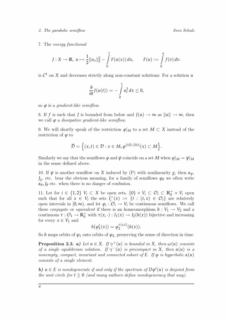
7. The energy functional

J : X → R, u 7→ 1

2‖ux‖22 −

1∫

0

F(u(x)) dx, F(u) :=

u∫

0

f (v) dv.

is C1 on X and decreases strictly along non-constant solutions: For a solution u

∂

∂tJ(u(t)) = −

1∫

0

u2t dx ≤ 0,

so ϕ is a gradient-like semiflow.

8. If f is such that J is bounded from below and J(u) → ∞ as ‖u‖ → ∞, thenwe call ϕ a dissipative gradient-like semiflow.

9. We will shortly speak of the restriction ϕ|M to a set M ⊂ X instead of therestriction of ϕ to

D =

(x, t) ∈ D : x ∈ M, ϕ[t,0]∪[0,t](x) ⊂ M

.

Similarly we say that the semiflows ϕ and ψ coincide on a set M when ϕ|M = ψ|Min the sense defined above.

10. If ψ is another semiflow on X induced by (P) with nonlinearity g, then αψ,Jg, etc. bear the obvious meaning, for a family of semiflows ϕθ we often writeαθ , Jθ etc. when there is no danger of confusion.

11. Let for i ∈ 1, 2 Vi ⊂ X be open sets, 0 × Vi ⊂ Oi ⊂ R+0 × Vi open

such that for all x ∈ Vi the sets I+i (x) := t : (t, x) ∈ Oi are relativelyopen intervals in [0,∞), and let ϕi : Oi → Vi be continuous semiflows. We callthese conjugate or equivalent if there is an homeomorphism h : V1 → V2 and acontinuous τ : O1 → R

+0 with τ(x, ·) : I1(x) → I2(h(x)) bijective and increasing

for every x ∈ V1 and

h(ϕt1(x)) = ϕτ(x,t)2 (h(x)).

So h maps orbits of ϕ1 onto orbits of ϕ2, preserving the sense of direction in time.

Proposition 2.3. a) Let u ∈ X. If γ+(u) is bounded in X, then ω(u) consistsof a single equilibrium solution. If γ−(u) is precompact in X, then α(u) is anonempty, compact, invariant and connected subset of E. If ϕ is hyperbolic α(u)consists of a single element.

b) u ∈ E is nondegenerate if and only if the spectrum of Dϕt(u) is disjoint fromthe unit circle for t ≥ 0 (and many authors define nondegeneracy that way).

8

Sven Schulz 2.1. Existence and basic properties

c) For an hyperbolic u ∈ E the sets Wu(u), Ws(u) are C1 submanifolds of Xwith dim(Wu(u)) = codim(Ws(u)) = i(u).

d) Let f be C2, v ∈ E hyperbolic, n := i(v). Then with the notation from Remark2.2 the following assertions hold:

TvWu(v) = Xn1 (v)

TvWs(v) = Xn(v)

∀u ∈ Wu(v)∃k ∈ 1, . . . , n : ϕt(u) − v‖ϕt(u) − v‖H2

t→−∞−−−→X

±ek‖ek‖H2

∀u ∈ Ws(v)∃k ∈ n, . . . : ϕt(u) − v‖ϕt(u) − v‖H2

t→∞−−→X

±ek‖ek‖H2

.

Proof. If γ+(u) is bounded it is precompact as ϕ is compact, so ω(u) andα(u) are nonempty, closed, invariant, connected and bounded by [Hal88, Lemmas3.1.1,3.1.2]. Now J(γ+(u)) is bounded, so there is a sequence tn → ∞ such thatddt J(ϕtn(u)) = ‖ ddt ϕtn(u)‖22 → 0, so ω(u) (and similarly α(u)) contain at leastone equilibrium solution. By [Mat78, Theorem A] ω(u) has at most one element.If u1, u2 ∈ α(u) choose sequences (sn)n, (tn)n with tn ≤ sn ≤ tn−1 for all n,sn → −∞, tn → −∞ and ϕtn(u) → u1, ϕsn(u) → u2. As J is strictly decreasingalong nonconstant solutions J(u1) = J(u2), which implies α(u) ⊂ E. Equilibriaare critical points of ϕ, so they are isolated if ϕ is hyperbolic. This shows a).

To see b) we note that by [AB05, Theorem A.3] h(t) = Dϕt(v0) is the mildsolution of v(t) − Luv(t) = 0, so Dϕt(v0) = e−Lutv0. Now there are subspacesY1,Y2 of L2([0, 1]) such that L2([0, 1]) = Y1 ⊕ Y2 with dim(Y1) < ∞, the Yibeing invariant w.r.t.. the restrictions Li of Lu to Yi ∩ D(Lu) and σ(L1) =σ(Lu) ∩ (−∞, 0], σ(L2) = σ(Lu) ∩ (0,∞) (see section 1.5 of [Hen81] for all this,cf. also Remark 2.2 2). Now by construction σ(L2) is bounded away from 0, soe−L2t is strictly contracting for t > 0, and σ(L1) = λ1, . . . , λk, so σ(e−L1t) =e−λ1t, . . . , e−λkt and it follows that 0 ∈ σ(Lu) ⇐⇒ 1 ∈ σ(Dϕt(u)).

c) This can be found in Henry [Hen85] in chapter 6. Theorem 6.1.9 in [Hen85]though is false as stated, as simple counterexamples show (this Theorem is usedto globalize the local (un-)stable manifolds). A correct proof for this can be foundin Theorem 2.2 in [AB05] in case of the stable manifold. The same modificationscan be done to prove the unstable case.

Alternatively one can use [Bru90], where unstable manifolds are shown to be

global C1-graphs in the case lim sup|s|→∞f (s)s < π2. If this condition is not

satisfied choose R > 0 and 0 < δ < 1 and make f constant outside [−R− δ, R+δ] with a smoothing on (−R− δ,−R)∪ (R, R+ δ) to make the modified functionC2. Then Wu(v) ∩UR(0) is a C1-submanifold by [Bru90]. By letting R→ ∞ theassertion follows because X is compactly embedded in C0.

d) follows from Theorem 2.1, Lemma 3.1 and Theorem 3.2 in [BF86].

9


Definition 2.4. Let f ∈ C2. If ϕ is hyperbolic, ϕt and Dϕt are injective for allt > 0, and for v,w ∈ E the manifolds Wu(v), Ws(w) intersect transversally ifthey intersect at all, we call ϕ a Morse-Smale semiflow.

For hyperbolic ϕ by [Hen85, Theorem 7] the stable and unstable manifoldsalways intersect transversally for f ∈ C2, so by Proposition 2.1 (vi) ϕ is Morse-Smale if ϕ is hyperbolic.

2.2 Dissipative semiflows

Definition 2.5. a) A set B ⊂ X attracts a set C ⊂ X under ϕ if C ⊂ D∞ andδ(ϕt(C), B) → 0 as t→ ∞.

b) We call ϕ dissipative if there is a bounded set B ⊂ X which attracts eachbounded set of X under ϕ. In this case we will also call f dissipative.

c) An invariant set A is a global attractor if it is a maximal compact invariantset (i.e. it contains any compact invariant set) which attracts each bounded setB ⊂ X. We will most of the time call global attractors just attractors.

d) A set Aλ is a local attractor if it is compact, invariant and there is an openneighborhood U of Aλ such that Aλ attracts U.

So we are ready to define the set of ”dissipative functions”:

Proposition 2.6. Let

Gd :=

f : R → R C2, lim sup|u|→∞

f (u)

u< π2

.

Then for f ∈ Gd the parabolic flow induced by (P) is dissipative and admits aconnected global attractor given by

A = Wu(E) = y ∈ D−∞ : ϕ−t(y) t→∞−−→ E.If f ∈ Gd with

Gd := f ∈ Gd : all equilibria of ϕ are nondegeneratethen E is finite and

A =⋃

u∈EWu(u).

This condition on f to be dissipative is the standard hypothesis, see for ex-ample [Lu94, Bru90, BF89, BF88]. As references for a proof usually [Hen81] or

[Hal88] are given, where the condition on f is lim supf (u)u ≤ 0. The estimates

in the proof have to be sharpened somewhat in our case, we give a detailed proofin appendix A.2.

10

Sven Schulz 2.3. Non-dissipative semiflows

Remark 2.7. The bound on f is sharp: Forf (u)u → π2 the assertion may or

may not hold, but for lim supf (u)u > π2 ϕ is not dissipative. From the proof of

Proposition 2.6 in section A.2 it is easy to see that J(λe1) → −∞ as λ → ∞, sothere cannot be a compact attractor.

We note the following corollary:

Corollary 2.8. For f ∈ Gd ϕ is a (dissipative) Morse-Smale semiflow.

Lemma 2.9. Let f ∈ Gd and A0 a local attractor of ϕ. Then A0 is stable, i.e.

∀V ⊃ A0 open ∃V ⊃ W ⊃ A0 open : γ+ν0

(W) ⊂ V. (2.1)

Proof. A0 is a local attractor, so we can chooseU ⊃ A0 open with δ(ϕt(U),A0) →0. In particular there is t0 > 0 such that ϕ[t0,∞)(U) ⊂ V. Let ǫ := dist(∂V,A0) >

0, u0 ∈ A0, t ∈ [0, t0]. By continuity of ϕ there is an open Uu0,t ∋ u0 such thatϕt(Uu0,t) ⊂ Uǫ(ϕt(u0)). By compactness of [0, t0] there is an open Uu0 ∋ u0 such

that ϕ[0,t0](Uu0) ⊂ Uǫ(A0). By compactness of A0 there is an openU ⊃W ⊃ A0such that ϕ[0,t0](W) ⊂ Uǫ(A0) ⊂ V. As ϕ[t0,∞)(W) ⊂ ϕ[t0,∞)(U) ⊂ V we haveproved (2.1).

2.3 Non-dissipative semiflows

Increasing L = lim supf (u)u the flow ϕ gets ”less and less dissipative”: If for

example π2n2 < limf (u)u < π2(n+ 1)2 there is a n-dimensional subspace Xn1 of

H01 where J(u) → −∞ as ‖u‖ → ∞ while it is bounded from below on (Xn1 )⊥,

cf. section A.2. On the other hand a proof similar to the one of Proposition3.10 b) shows that the number of sign changes and the Morse indices of stationarysolutions are bounded as long as L is finite (this ”zero-number”and its connectionto the Morse index will be discussed in detail below).

We are primarily interested in definite superlinear flows, i.e. the case L = ∞.Now for the non-dissipative semiflow u ∈ X may have an unbounded positivehalforbit existing only for a finite time. Basic tools for this case are a-prioribounds and a ”good” behavior of the energy functional, and to ensure these wewill have to impose stronger conditions than just L = ∞. We define the followingset of functions:

G :=

f : R → R C2 : ∃R > 0, µ > 2 : ∀|u| ≥ R : f (u)u ≥ µF(u),

F(±R) > 0,(2.2)

where F(u) =∫ u0 f (x) dx. In particular for f ∈ G we have F(u) ≥ C · |u|µ for

|u| ≥ R, and thus L = ∞. The reason for considering f ∈ G is the followingLemma:

11


Lemma 2.10 (Quittner). Let f ∈ G.a) Let δ,C0 > 0. Then there exists a constant C = C(δ,C0) such that ‖u0‖ ≤ C0implies

‖ϕt(u0)‖ ≤ C for t ∈ [0, Tmax(u0)− δ), (2.3)

where ∞ − δ = ∞.

b) The mapping X ∋ u0 7→ Tmax(u0) ∈ (0,∞] is continuous. If Tmax(u0) < ∞

thenJ(ϕt(u0)) → −∞ as t ↑ Tmax(u0). (2.4)

Remark 2.11. This Lemma also opens another way to tackle the connectingorbit problem (cf. Definition 3.18). Together with some standard results it provesthat the sets J−1([a, b]) are ”admissible” in the sense of Rybakowski ([Ryb87]),which allows the application of his homotopy index theory.

Proof. This Lemma is Theorem 6.1 in [Qui03], we have to verify the followingfour conditions (stated here for an autonomous f ): There exist nondecreasingfunctions d2, d4 : R

+ → R+ and constants d1, ǫ > 0, µ > 2, ai ≥ 0 (i = 1, . . . , 4)

such that

| f (u)| ≤ d2(|u|) + a2 (2.5)

F(u) ≥ d1|u|2+2ǫ − a1 (2.6)

f (u)u ≥ µF(u) − a3 (2.7)

| f (u) − f (v)| ≤ (a4 + d4(|u| + |v|))|u − v|. (2.8)

For autonomous f (2.5) is always satisfied. As f is locally Lipschitz continuous(2.8) is also clear. Condition (2.7) follows by taking µ, R from the definition of Gand

a3 := min f (u)u − µF(u) : |u| ≤ R.Similarly it is enough to show

∀|u| ≥ R : F(u) ≥ d1|u|2+2ǫ

to verify (2.6). Let ǫ :=µ−22 > 0, w.l.o.g. u > 0. Now

(F(u)

u2+2ǫ

)′=

1

u3+2ǫ

(

f (u)u − (2+ 2ǫ)︸︷︷︸

=µ

F(u))

≥ 0,

i.e. for u ≥ RF(u)

u2+2ǫ≥ F(R)

R2+2ǫ︸︷︷︸

=:d1>0

⇐⇒ F(u) ≥ d1u2+2ǫ.

12

Sven Schulz 2.3. Non-dissipative semiflows

Again we will restrict ourselves to nondegenerate equilibria and most of thetime to a subset of ”uniformly superlinear” functions:

G := f ∈ G : All equilibria of (P) are nondegenerate F := f ∈ G : ∀u 6= 0 : f ′(u)u2 > f (u)u, f ′(0) 6= k2π2 for k ∈ N

We shall prove that F ⊂ G (Corollary 3.12) which is good, as F is a commonclass of superlinear functions and contains the model case u|u|p−1 (p > 2). Onealso easily verifies the following

Lemma 2.12. Let f ∈ F , then f (0) = 0. If f ′(0) ≥ 0 then f ′(x) > 0 for allx 6= 0, if f ′(0) < 0 then f has precisely one positive and one negative zero.

The nondegeneracy condition in the definitions of Gd and G is not easily veri-fied, except in the special case F ⊂ G. But it has been proved that nondegeneracyis a generic condition. To make this precise we fix the topology used:

Definition 2.13. We will use two different topologies on the space C2 = C2(R)of all twice differentiable functions (cf. [Hir76, Chapter 2.1]).a) The weak topology is the topology induced by the metric

d( f , g) :=∞

∑n=1

2−n| f − g|n1+ | f − g|n

where | f |n is the standard C2-Norm on C2([−n, n]). This is the topology of C2-convergence on compact sets, let C2w denote C2 endowed with the weak topology.We will also sometimes use the weak topology on C1w.b) Now let Ki ⊂ R compact for all i ∈ N such that for all x ∈ R there is anKi ∋ x and an open neighborhood Ux ∋ x which intersects only finitely many Ki.Let further ǫii∈N be a family of positive numbers and f ∈ C2. Then the set

g ∈ C2 : ∀i ∈ N∀k ∈ 0, 1, 2∀x ∈ Ki : | f (k)(x) − g(k)(x)| < ǫi

is an open neighborhood of f in the strong topology. The sets of this type forma base for the strong topology (or Whitney topology/fine topology-) , i.e. strong-open sets are unions of sets of the above type. We write C2s for C2 endowed withthis topology.

Remark 2.14. The strong topology is not metrizable. For f ∈ C2

UC2s ,ǫ( f ) := g ∈ C2 : ∀k ∈ 0, 1, 2∀x ∈ R : |g(k)(x) − f (k)(x)| < ǫ ⊂ UC2w,3ǫ

is an open set in C2s . It is easily verified that the weak topology is strictly weakerthan the strong one, that means that open sets in C2w are also open in C2s , butUC2s ,ǫ( f ) is not an open set in C2w for any ǫ > 0.

13


Now we can formulate precisely in which sense hyperbolicity of equilibria is ageneric property of f ∈ Gd ∪ G :

Proposition 2.15. Gd, G are open in C2s , and Gd, G are residual subsets w.r.t.the strong topology (i.e. countable intersections of strong-open subsets) of Gd, Grespectively. This implies that Gd ⊂ Gd, G ⊂ G are dense subsets.

Proof. We first prove that G is open. Let f ∈ G, R,µ as in (2.2) and g ∈ UC2s ,ǫ( f )for

0 < ǫ < min

(

| f (u)| : |u| ≥ R

∪F(R)

R,F(−R)R

)

(this minimum is strictly positive by (2.2). Fix a1, d1, ǫ′ as in (2.6), pick some

µ′ ∈ (2, µ) and let u ≥ R. Then

g(u)u − µ′G(u) ≥ ( f (u) − ǫ)u− µ′u∫

0

f (x) + ǫ dx

(2.2)≥ (µ − µ′)F(u) − ǫ(µ′ + 1)u(2.6)≥ u

[

(µ − µ′)d1u1+2ǫ′ − ǫ(µ′ + 1)

]

− (µ − µ′)a1

so we can choose R′ ≥ R such that g(u)u ≥ µ′G(u) for u ≥ R′ and analogouslyfor u ≤ −R′. By choice of ǫ we also get

G(R′) ≥ F(R) − ǫR+

R′∫

R

f (x) − ǫ dx > 0

and similarly G(−R′) > 0, thus g ∈ G and G is open.By [BC84] the set of hyperbolic f ∈ C2 is a residual subset of C2s . By [Hir76,

Theorem 4.4] residual subsets are dense in C2s . But G is an open subset of C2s , soG is an residual subset of (and thus dense in) G. This implies in particular thatfor any f ∈ G and any ǫ > 0 there exists g ∈ UC2s ,ǫ( f ) ∩ G.

Similarly for f ∈ Gd one easily checks UC2s ,ǫ( f ) ⊂ Gd (for arbitrary ǫ > 0 in

fact), and as above it follows that Gd is a residual subset of Gd.

14

CHAPTER 3

Technical results

3.1 The zero number

Definition 3.1. For u ∈ C([0, 1]) let z(u) be the number of strict sign changesof u in (0, 1), i.e.

z(u) := sup(0 ∪ k ∈ N : ∃x1, . . . , xk+1 ∈ (0, 1), x1 < x2 < · · · < xk,

u(xi) · u(xi+1) < 0 for all 1 ≤ i ≤ k).

We call z(u) the zero number of u.

The zero number is a ”discrete Lyapunov functional” for scalar equations:

Proposition 3.2. a) Let f ∈ C2 with f (0) = 0, u ∈ X, then z(ϕt(u)) is non-increasing.

b) If z(ϕt(u)) is constant on an interval I0 ⊂ I(u), then (ϕt(u))x(0) 6= 0 fort ∈ I0.c) If z(u) < ∞ then the set of times t ∈ I(u) for which ϕt(u) has only simplezeros is open dense in I(u).

d) If f ∈ C2, v ∈ E and u is a solution of (P) defined on an interval I, thenw(t) := u(t) − v satisfies the nonautonomous equation wt − wxx = g(w, x) onI with g(y, x) := f (y + v(x)) − f (v(x)). We have g(0, ·) = 0, z(w(t)) is non-increasing and w has only simple zeros on an open dense subset of I.

e) If f ∈ C2 and v ∈ E is hyperbolic, then i(v) ∈ z(v), z(v) + 1.Proof. a) is proved in Lemma 1.1 of [BF86] for f bounded in C1. This can easilybe transferred to general f ∈ C2 by modifying f outside a compact interval, cf.section 3.3. Assertions b), c) are Lemmas 7.4, 7.3 respectively of [BF88], provedthere for lim sup|u|→∞ f (u)/u < ∞. As above the assertion follows also for

f ∈ C2. Statement d) is easily checked by a direct calculation together with theLemmas in [BF86, BF88] cited above. These can be applied also in this non-

autonomous case, because g satisfies the growth condition lim sup|t|→∞g(t,x)t <

π2 uniformly in x.e) is Lemma 5.1 in [BF88].

15

3. Technical results Sven Schulz

Proposition 3.2 together with 2.3 d) immediately yields the following:

Corollary 3.3. Let f ∈ C2, v ∈ E hyperbolic, then z(u − v) < i(v) for u ∈Wu(v) and z(u− v) ≥ i(v) for u ∈ Ws(v).Lemma 3.4. Let f ∈ Gd, v,w ∈ E, v 6= w and |v′(0)| ≥ |w′(0)|. Thenz(v− w) = z(v) and all zeros of v− w are simple.

Proof. The assertion z(v − w) = z(v) is Lemma 4.2 in [BF88]. The zeros ofv−w are simple by Proposition 3.2 d), c).

3.2 The T-Map and stationary solutions

To get a first idea of the dynamics of the parabolic semiflow we locate the sta-tionary or equilibrium solutions of (P). Equilibria of (P) are solutions of

−u′′ = f (u) u(0) = u(1) = 0, (E)

to find these we examine solutions of the initial value problem

−u′′(t, η) = f (u(t)), u(0) = 0, u′(0) = η (IVP)

(′ = ddt) and try to find η s.t. u(1, η) = 0. Throughout this section we will use

some comparison results about second order ODE. The following is taken from[Har64, Section XI.3]. We consider the equations

−u′′ = q1(t) · u (3.1)

−u′′ = q2(t) · u (3.2)

with q1, q2 ∈ C([0, 1]). We call (3.1) a Sturm majorant of (3.2) if q1 ≤ q2, and astrict Sturm majorant if in addition q1(t) < q2(t) for some t ∈ (0, 1).

Theorem 3.5. a) (Sturm Comparison Theorem) Let (3.1) be a Sturm ma-jorant for (3.2) and u1 be a solution of (3.1) with exactly n ≥ 1 zeros t1 < t2 <

· · · < tn in (0, 1]. Let u2 6≡ 0 be a solution of (3.2) satisfying

u′1(0)u1(0)

≥ u′2(0)

u2(0)(3.3)

(u′i(0)ui(0)

= ∞ if ui(0) = 0). Then u2 has at least n zeros in (0, 1].

If either (3.1) is a strict Sturm majorant for (3.2) or (3.3) holds with strictinequality, then u2 has at least n zeros in (0, 1).

b) (Sturm Separation Theorem) If u1, u2 are linearly independent solutionsof (3.1), then the zeros of u1 separate and are separated by those of u2.

16

Sven Schulz 3.2. The T-Map and stationary solutions

For superlinear f there are infinitely many stationary solutions.

Theorem 3.6 (Struwe). For any f ∈ C2 withf (x)x → ∞ as |x| → ∞ there are

infinitely many solutions to (E). For any sequence (uk)k of distinct solutions with

|u′k(0)| → ∞ we have z(uk)k→∞−−−→ ∞.

Proof. The first assertion is a special case of Theorem 1 in Struwe ([Str80]), theassertion about z(uk) is stated in the proof of that Theorem.

Unless stated otherwise in this section u(·, η, f ) will denote a solution to(IVP).

Definition 3.7. a) For f : R → R locally Lipschitz, η ∈ R let u(·, η) =u(·, η, f ) be the solution of the equation (IVP).

b) Let (for given locally Lipschitz continuous f ) D = D f be the set of all η ∈ R,for which u(x, η, f ) = 0 for some x > 0 and define

Tf = T : D→ R, η 7→ infx > 0 : u(x, η, f ) = 0. (3.4)

Remark 3.8. We can write (IVP) as the twodimensional system

u′ = v

v′ = − f (u) (SYS)

with initial values u(0) = 0 and v(0) = η. The corresponding vectorfieldV(u, v) = (v,− f (u)) is antisymmetric w.r.t. the u-axis, i.e. V(u,−v) =(−v,− f (u)). This simple observation has some important consequences: Or-bits of (SYS) are symmetric w.r.t. the u-axis, in particular for η ∈ D

u′(T(η), η) = −η (3.5)

and

u′(T(η)

2, η

)

= 0.

We also seeη ∈ D ⇐⇒ ∃t > 0 : u′(t, η) = 0,

and that u(t, η) is a (T(η) + T(−η))-periodic solution if η,−η ∈ D. For sucha periodic solution we have u(T(t) + t, η) = u(t,−η). The system (SYS) alsohas a first integral E(u, v) = 1

2v2 + F(u) with F(u) :=

∫ u0 f (t) dt (which makes

it easy to see the v-symmetry of orbits).

By means of the function T equilibrium solutions of (P) and nondegeneracyof these solutions can be characterized as follows:

17


Proposition 3.9. Let f C2, η 6= 0, Ds := D ∩−D.a) If f : R → R is Ck, k ∈ N, then D \ 0 is open and T is Ck+2 in D \ 0.For η ∈ D \ 0 we have

T′(η) =uη(T(η), η)

η.

b) A solution u(·, η0) of (IVP) is a nonnegative (or non-positive) equilibriumsolution of (P) if and only if T(η0) = 1, and nondegenerate if and only ifT′(η0) 6= 0.c) A solution u(·, η0) of (IVP) is an equilibrium solution of (P) with n = 2k+ 1zeroes if and only if the function

T(n) : η 7→ (k+ 1)T(η) + (k+ 1)T(−η)

attains the value 1 at η0, and is nondegenerate if and only if this function hasnon-vanishing derivative at η0.

In this case u(T(η0) + ·, η0) = u(·,−η0) is also an equilibrium solution with nzeros.

d) A solution u(·, η0) of (IVP) is an equilibrium solution of (P) with n = 2kzeroes if and only if the function

T(n) : η 7→ (k+ 1)T(η) + kT(−η)

attains the value 1 at η0, and is nondegenerate if and only if this function hasnon-vanishing derivative at η0. (Of course b) is just a special case of d) statedexplicitly for clarity).

Proof.a) (cf. Brunovsky-Chow [BC84, Thm 2.3]) Fix η0 ∈ D \ 0 and T0 = T(η0).We have u′(T0, η0) = −η0 6= 0 by (3.5), and solutions to (IVP) are Ck+2 if fis Ck. By the Implicit Function Theorem there exists a unique Ck+2 functionτ defined in a neighborhood of η0 such that for (ξ, η) close to (T0, η0) we haveu(ξ, η) = 0 if and only if ξ = τ(η). By the continuous dependence TheoremT and τ are identical in a small neighborhood of η0. So D \ 0 is open andT is Ck+2 on D \ 0. The formula for T′(η) is obtained by differentiating theidentity u(T(η), η) = 0 and (3.5).

The assertion about u(·,−η0) in c) is clear, cf. Remark 3.8. The otherassertions are Theorems 2.5 to 2.7 in [BC84].

Proposition 3.10. a) Let f , fk ∈ C1, fk → f in C1w, η ∈ R, ηk ∈ D fk, ηk → η.If η ∈ D f \ 0 then Tfk(ηk) → Tf (η) and Tf ′k

(ηk) → T′f (η). If η /∈ D f then

Tfk(ηk) → ∞.

18


b) If f is C1, f (0) = 0, then

limη→0T(η) =

π · f ′(0)− 12 f ′(0) > 0

∞ f ′(0) ≤ 0.

c) If f ∈ F then D = R, T′(η) < 0 for η > 0, T′(η) > 0 for η < 0 andT(η) → 0 for |η| → ∞.

d) If f ∈ G then there exists η > 0 such that R \ (−η, η) ⊂ D.

Remark 3.11. In general T is discontinuous at 0, cf. Proposition 3.10 b) whereT(0) = 0.

Proof.a) First consider η ∈ D f \ 0, w.l.o.g. assume η > 0. We have

u(·, ηk , fk) k→∞−−−→ u(·, η, f )

uniformly on compact intervals, and the same is true for u′, uη. If 0 < Tf (η) < ∞

then

∀1 >> ǫ > 0∃kǫ ∈ N : k ≥ kǫ⇒ u(t, ηk , fk)|[ǫ,Tf (η)−ǫ] > 0 ∧ u(Tf (η) + ǫ, ηk, fk) < 0,

and because of u′(0, η, f ) = η 6= 0 and u′(·, ηk, fk) → u′(·, η, f ) uniformly ona neighborhood of 0 we have Tfk(ηk) ∈ (Tf (η) − ǫ, Tf (η) + ǫ). Now T′fk(ηk) →T′f (η) follows from 3.9 a) and the differentiable dependence theorem.

If η /∈ D f then

∀n ∈ N∃kǫ ∈ N : k ≥ kǫ ⇒ ∀x ∈[1

n, n

]

: u(x, ηk, fk) 6= 0,

this implies Tfk(ηk) → ∞ as above.

b) Again w.l.o.g. let η > 0 and

q1(x) = q1(x, η) =

f (u(x,η))u(x,η)

u(x, η) 6= 0f ′(0) u(x, η) = 0,

so u(·, η) solves the homogeneous linear equation

−v′′ = q1(·, η) · v. (3.6)

19


Case 1: f ′(0) > 0. Let v1(x) = sin(√

f ′(0) + ǫ · x), v2(x) = sin

(√

f ′(0)− ǫ ·x)

be solutions of the equations

−v′′ = ( f ′(0) + ǫ)v (3.7)

and−v′′ = ( f ′(0) − ǫ)v (3.8)

respectively for some 0 < ǫ < f ′(0). We have

( f ′(0) − ǫ)x ≤ q1(x, η) ≤ ( f ′(0) + ǫ)x

uniformly for η ≤ ηǫ sufficiently small and x ≤ π√f ′(0)−ǫ

, so by the Sturm

Comparison Theorem we have

π√

f ′(0) − ǫ≥ T(η) ≥ π

√

f ′(0) + ǫ,

and the assertion follows.Case 2: f ′(0) ≤ 0. Let m := limη↓0max u(·, η) ≥ 0. If m = 0 (which is

possible if f ′(0) = 0) let v1 be the solution of −v′′ = ǫv; analogous to case 1 we

conclude π√ǫ

< T(η) uniformly in η small, so T(η)η→0−−→ ∞.

Now consider the case m > 0. As max u(·, η) = u(12T(η), η) we have

u

(1

2T(η), η

)η→0−−→ m. (3.9)

Now suppose lim infη→0 T(η) = T0 < ∞ then there exists a sequence (ηk)k with

ηkk→∞−−−→ 0 such that T(ηk) → T0 as k → ∞. By the continuous dependence

Theorem follows

u

(1

2T(ηk), ηk

)k→∞−−−→ 0

which contradicts (3.9).

c) We use the interpretation of (IVP) as (SYS) and the first integral E(u, v) =12v2 + F(u), i.e. E(u(t)) is constant along solutions. Fix η > 0. From the

definition of F and Lemma 2.12 we see the existence of n−1 ≤ 0 ≤ n1 such thatF(n−1) = F(n1) = 0, F(u)u ≤ 0 on [n−1, n1], F(u)u > 0 on R \ [n−1, n1] andF strictly decreasing on (−∞, n−1] and strictly increasing on [n−1,∞). So thereexist precisely two u−1 < n−1 < n1 < u1 with F(u−1) = F(u1) = 1

2η2. Thus

the only possible intersections with the axes of the (connected component of the)level curves C(η) of E through (0, η) are (0,±η), (u±1, 0). Furthermore C(η)is bounded away from 0, and f 6= 0 on R \ [n−1, n1], so there are no critical

20


points of E on C(η), thus C(η) by the implicit function is a smooth curve whichcoincides with the trajectory through (0, η). It has to be compact, because it isbounded, and as it can intersect the v-axis only in (0,±η) it has to be a closedcurve round the origin. This implies ±η ∈ D. 0 ∈ D follows by f (0) = 0.

We only prove T′(η) < 0 for η > 0 — the assertion for η < 0 followsanalogously (consider − f (−x) instead of f (x)). Now let (un)n be a sequenceof distinct solutions with un(1) = 0 and |u′n(0)| → ∞. By Theorem 3.6 sucha sequence exists and we have z(un) → ∞, which means by Proposition 3.9

T(z(un)+1)(u′n(0)) = 1. This implies T(|u′n(0)|) → 0, so T(η) → 0 as |η| → ∞.By Proposition 3.9 a) it is sufficient to show uη(T(η), η) < 0. Let q1 be

defined as in the proof of b). By the differentiable dependence of the solution onthe initial value we have

−u′′η(x, η) = f ′(u(x, η))uη (x, η)

uη(0, η) = 0

u′η(0, η) = 1.

The same equation is, with different initial values, also solved by u′, so by theSturm Separation Theorem the zeroes of uη separate and are separated by those

of u′. But clearly − 12T(−η), 12T(η), T(η) + 12T(−η) are consecutive zeroes of

u′ and u′(0, η) = 0, so the smallest positive zero N of uη lies in the interval

(12T(η), T(η) + 12T(−η)) (and is the only zero of uη in this interval). From

u′η(0, η) = 1 we conclude that uη is positive on (0,N) and negative on (N, T(η)+12T(−η)). It remains to show N < T(η).

The derivative u′(·, η) solves the linear equation

−v′′ = q2 · v (3.10)

withq2(x) = q2(x, η) := f ′(u(x, η)),

andf (u)u < f ′(u) (for u 6= 0 and f ∈ F) is just the condition for (3.6) to be

a strict Sturm majorant of (3.10) on the interval [0, T(η)], so again by SturmComparison uη has a zero in (0, T(η)), which means N < T(η).

d) By (2.6) there exists K > 0 and n−1 < 0 < n1 such that F(n−1) = F(n1) = Kand F strictly monotone on R \ [n−1, n1]. Take η ≥ η :=

√2K and proceed as

in c).

The Propositions 3.10 and 3.9 together with Remark 3.8 immediately yield acomplete description of the equilibrium solutions of (P) in the case f ∈ F . Forf ∈ G the general structure of equilibria can be described.

21


Corollary 3.12. a) For f ∈ G we write the set of nontrivial equilibrium solu-tions as uk : k ∈ Z \ 0 ordered by their initial slope, i.e. u′−(k+1)(0) <

u′−k(0) < 0 < u′k(0) < u′k+1(0). If z(uk) is odd by Remark 3.8 there exists al ∈ Z such that z(ul) = z(uk) and u′l(0) = −u′k(0).If [u′l(0), u

′l+1(0)] ⊂ Ds \ 0, then z(ul+1) ∈ z(ul) − 1, z(ul), z(ul) + 1. If

z(uk) = n, there exists l ∈ Z with z(ul) = n+ 1.

b) For every f ∈ F and integer n > i(0) the equation (P) has precisely twosolutions un, u−n with n− 1 zeros. These are nondegenerate with i(u±n) = n,u′n(0) > 0 > u′−n(0), and there are no other nontrivial solutions of (P). Inparticular F ⊂ G.

Proof. First let f ∈ G, then all equilibria are nondegenerate. So the set v′(0) :v ∈ E has no accumulation point in R, and we can order the equilibria asstated. Let [u′l(0), u

′l+1(0)] ⊂ Ds \ 0, n := z(ul). Then T(n−1)(u′l(0)) <

T(n)(u′l(0)) = 1 < T(n+1)(u′l(0)). Suppose m := z(ul+1) > n + 1, then

T(n+1)(u′l+1(0)) < T(m)(u′l+1(0)) = 1, so there exists a η ∈ (u′l(0), u′l+1(0))

with T(n+1)(η) = 1. This means there is an equilibrium solution of (P) ”be-tween” ul and ul+1, which is impossible. For m < n− 1 the contradiction followsanalogously.

Now let η0 := infη > 0 : [η,∞) ⊂ Ds. If u′k(0) ∈ (−∞, η0) ∪ (η0,∞),and w.l.o.g. k > 0, there has to be a l > k with z(ul) = n+ 1 by the assertionproved above, because z(um) → ∞ as m→ ∞. If u′k(0) ∈ [−η0, η0], then η0 > 0

and either η0 ∈ R \ D or −η0 ∈ R \ D. So T(η)η↓η0−−→ ∞ or T(η)

η↑−η0−−−→ ∞,

either way for any m ≥ 2 T(m)(η)|η|↓η0−−−→ ∞ by Proposition 3.10 a). Theorem

3.6 implies lim inf|η|→∞ T(m)(η) = 0, so in this case for any m ≥ 2 there are

at least two equilibrium solutions with m zeros. The remaining assertion followsfrom Remark 3.8.

For f ∈ F uniqueness and nondegeneracy of the solutions with n zeros fol-low from Proposition 3.10 c). If f ′(0) < π2 then limη→0 T(η) > 1 by Propo-sition 3.10 b), so there is a positive and a negative equilibrium. If f ′(0) ∈(k2π2, (k+ 1)2π2), then limη→0 T(η) ∈ ( 1k+1 ,

1k ). and i(0) = k. This means

limη→0T(k)(η) > 1 > lim

η→0T(k+1)(η),

so the nontrivial solutions have at least k+ 1 = i(0) + 1 zeros.

Remark 3.13. For f ∈ G and an equilibrium uk of course the relation i(uk) ∈z(uk), z(uk) + 1 from Proposition 3.2 e) still holds, but in general there is norelation between k and i(uk) or z(uk).

22

Sven Schulz 3.3. The cutoff function

3.3 The cutoff function

Given f ∈ G we will construct a function f ∈ Gd such that f = f on a compactinterval [−M−,M+]. Outside the interval [−M− − a−,M+ + a+] f will be con-stant, and in the remaining two gaps we choose a simple construction to make fC2. While doing all this we have to control the function T associated with f .

To be more precise we can find

u′n(0),−u′−n(0) < η1 < u′n+1(0),−u′−(n+1)(0)

and get M+ := max u(·, η1, f ), M− := −min u(·,−η1, f ). We will find a η31(choosing appropriate a+, a−) s.t. T′ has no zeroes outside [−η31, η31]. On(−η31,−η1) and (η1, η31) we will be able to control the values of T to makesure u(1, η, f ) 6= 0 for η in these intervals. Note that it is crucial to have theseintervals symmetric w.r.t. 0 as we have to sum up multiples of T and T(−·) tomake assertions about sign changing solutions. See Figure 3.1 for a schematicpicture of the phase-plane in case of the modified function.

u

u′

η31

η33

η21

η1

−η1η−21

−η33

−η31

−M− − a− −M− M+ M+ + a+

Figure 3.1: phase-space diagram for modified function

As f will be defined piecewise we will first derive properties of equations withconstant right hand side and of those with the ”bridge function”g (in 3.3.2 defined

23


on [0, a] for simplicity as the problem is autonomous) as right hand side. Then wehave to glue together the results for individual parts of trajectories w.r.t. f . Forthese right hand sides we will not only investigate the corresponding functionsTa, Tg, but for the bridge functions we also have to look at trajectories whichreach a in finite time, and thus do not become 0 again. Tools for tackling theseproblems will be derived in the next section. By Remark 3.8 it is sufficient to domost computations for η > 0 only, the case η < 0 follows analogously.

The final construction will still be more complicated, as we will have to cutoff functions fθ depending on an additional parameter (with η1 also dependingon θ continuously) in a continuous way (i.e. θ 7→ fθ ∈ G and also θ 7→ fθ ∈ Gdwill be continuous). The reason for this will become clear in the applications (cf.Proposition 4.4). So we state our cutoff Proposition, the main technical result ofthis work. For v,w ∈ Eθ (the set of equilibria for the right hand side fθ) we writev < w : ⇐⇒ v′(0) < w′(0) and |v| < |w| : ⇐⇒ |v′(0)| < |w′(0)| to shortennotation.

Proposition 3.14. Let fθ ∈ G for θ ∈ [0, 1] such that

[0, 1] ∋ θ 7→ fθ ∈ G ⊂ C2wis continuous, n ∈ N, m ∈ n, n+ 1. Define

Dθ := η ∈ R : ∃t > 0 : u(t, η, fθ) = 0Tθ : Dθ ∋ η 7→ inft > 0 : u(t, η, fθ) = 0 ∈ R

and let uk,θ be the k-th nontrivial solution of

−u′′ = fθ(u), u(0) = u(1) = 0

(cf. Corollary 3.12). Suppose z(um+1) > z(un) and there exists a continuousη1 : [0, 1] → R such that η1(θ) ∈ Dθ for all θ ∈ [0, 1] and

maxu′n,θ(0),−u′−n,θ(0) < η1(θ) < minu′m+1,θ(0),−u′−(m+1),θ(0),T

(n)θ (±η1(θ)) < 1 < T

(m+1)θ (±η1(θ)).

(3.11)

Then for each θ ∈ [0, 1] there exists fθ ∈ Gd, uniquely determined by fθ andη1(θ), such that the mapping

[0, 1] ∋ θ 7→ fθ ∈ Gd ⊂ C2sis continuous and fθ ≡ fθ on [−M(θ),M(θ)] with [0, 1] ∋ θ 7→ M(θ) ∈ (0,∞)continuous and M(θ) uniquely determined by fθ and η1(θ). Consequently ϕθ andϕθ coincide on u ∈ X : ‖u‖∞ ≤ M(θ). If fθ ≡ f for all θ then M(θ) isincreasing if η1(θ) is increasing, and if n→ ∞ both η1(θ) → ∞ and M(θ) → ∞

uniformly in θ.

24


For the set Eθ of stationary solutions of (P) with r.h.s. fθ we have

Eθ = uk,θ : |k| ≤ n ∪ uk,θ : 1 ≤ |k| ≤ n ∪ Rθ

uk,θ nondegenerate, i(uk,θ) = z(uk,θ) = |k| − 1, u′−|k|(0) < 0 < u′|k|(0)

v ∈ Rθ ⇒ n+ 1 ≤ z(v) ≤ m.

The mappings θ 7→ uk,θ and θ 7→ uk,θ are continuous for any k and

u−1 < · · · < u−n < u−n < · · · < u−1 < 0 < u1 < · · · < un < un < · · · < u1,(3.12)

0 < |u±1| < · · · < |u±n| < |u±n| < · · · < |u±1|, (3.13)

The proof will fill the rest of section 3.3. We will first introduce some phase-plane analysis tools. Next we will define the ”bridge function” g and computeseveral properties of the flow induced by g. Finally in 3.3.3 we will put everythingtogether to define fθ and prove Proposition 3.14.

3.3.1 Phase-plane analysis tools

Lemma 3.15. Let a > 0, f : R → R C1. Let u(·, η) denote the solution of theinitial value problem (IVP) and D := η ≥ 0 : ∃t ≥ 0 : u(t, η) = a. For η ∈ Dlet

τ(η) := inft > 0 : u(t, η) = a < ∞

ψ(η) := u′(τ(η), η).

Then τ,ψ are continuous on D, τ is C3 and ψ is C2 on D, and the followingassertions hold:

(i) D is an unbounded subinterval of (0,∞), let η0 := infD. If f |[0,a] > 0 then

D is closed and ψ(D) = [0,∞).

(ii) Let F(x) :=∫ x0 f (t) dt, then

∀η ∈ D : ψ(η) =√

η2 − 2F(a),

in particular if ψ(η0) = 0 then

∀η ∈ D : ψ(η) =√

η2 − η20 .

If f |[0,a] > 0 then ψ′(η) = ηψ(η)

≥ 1.(iii) We have τ′

< 0 and τ(η) → 0, τ′(η) → 0 as η → ∞. The derivative of τis

τ′(η) = −ψ′(η)uη(τ(η), η)

η=

−uη(τ(η), η)

ψ(η).

25


(iv) The derivative uη of u w.r.t. the initial value η satisfies

∀t ∈ (0, τ(η)] : uη(t, η) > 0

and

0 = − f (a)uη (τ(η), η) − u′η(τ(η), η)ψ(η) + η.

(v) Let fk ∈ C1, fk → f in C1w, τk, ψk, Dk be defined for fk as τ, ψ, D for f .If ηk → η ∈ D, then ηk ∈ Dk for k large, and

τk(ηk) → τ(η), τ′k(ηk) → τ′

k(η).

If ηk ∈ Dk, ηk → η0 ∈ D, then

τk(ηk) → τ(η0).

Proof. Setting M > max| f (α)| : 0 ≤ α ≤ a, we first show that [√2aM,∞) ⊂

D. Let V(α, β) = (β,− f (α)) the vectorfield of (SYS), and define for η ≥√2aM

the functions

ζ : [0, a] → [0,∞), α 7→ η + αM

η

ξ : [0, a] → [0,∞), α 7→√

η2 − 2αM.

We will show that trajectories of (SYS) can leave the set

C(η) = (α, β) : 0 ≤ α ≤ a, ξ(α) ≤ β ≤ ζ(α)

through a × (ξ(a), ζ(a)) only. This implies that the trajectory through (0, η)reaches the set a×R, which happens in finite time as (a, 0) is the only possiblezero of V in C(η). Thus η ∈ D. We calculate

ζ′(α) =M

η, ξ′(α) =

−M√

η2 − 2αM

V(α, ζ(α)) =(η + αMη

)·(

1,− f (α)

η + αMη

)

V(α, ξ(α)) =√

η2 − 2αM ·(

1,− f (α)

√

η2 − 2αM

)

.

Now− f (α)

η + αMη<M

η= ζ′(α),

26


so a trajectory being in A(η := graph ζ at some time will be in C(η) immediatelyafterwards. Similarly

− f (α)√

η2 − 2aM>

−M√

η2 − 2aM,

so a trajectories being in graph ξ at some time will also be in C(η) immediatelyafterwards. This proves η ∈ D.

If D ∋ η < η then the trajectory trough (0, η) stays between the trajectorythrough (0, η) and A(η), so η ∈ D and D is an interval.

Let η ∈ D, so u′(τ(η), η) > 0 and consider

U : (t, η) 7→ u(t, η) − a.

Then U is C3, U(τ(η), η) = 0 and Ut(τ(η), η) = u′(τ(η), η) > 0. So by theimplicit function theorem there is a δ > 0 such that τ|(η−δ,η+δ) is C3. Thus τ is

C3 and ψ is C2 because u′ is C2. We will prove the continuity of τ on D belowafter we have shown τ′

< 0.Let η ∈ D, t ∈ [0, τ(η)]. The functions u′, uη solve the initial value problems

u′′′(t, η) = − f ′(u(t, η)) · u′(t, η) u′(0, η) = η u′′(0, η) = − f (0)u′′η (t, η) = − f ′(u(t, η)) · uη(t, η) uη(0, η) = 0 u′η(0, η) = 1

respectively. Multiplying the first equation by uη, the second by u′ and subtract-ing the results we obtain

u′′′(t, η)uη(t, η) − u′′η (t, η)u′(t, η) = 0.

Integrating this from 0 to t ≤ τ(η) yields

0 = u′′(t, η)uη(t, η) − u′η(t, η)u′(t, η) + η, (3.14)

i.e. for t = τ(η)

0 = − f (a)uη(τ(η), η) − u′η(τ(η), η)ψ(η) + η. (3.15)

One easily checks

d

dt

(1

2(u′(t, η))2 + F(u(t, η))

)

= 0

so

∀t : 12

(u′(t, η)

)2+ F(u(t, η)) ≡ 1

2η2 (3.16)

which yields ψ(η)2 + 2F(a) = η2, so ψ(η) =√

η2 − 2F(a). If ψ(η0) = 0 then

η20 = 2F(a) and ψ(η) =√

η2 − η20

27


Differentiating a = u(τ(η), η) w.r.t. η yields

0 = u′(τ(η), η)︸︷︷︸

=ψ(η)

·τ′(η) + uη(τ(η), η). (3.17)

The function u′(·, η) has no zero in [0, τ(η)), so by the Sturm Separation Theoremuη(·, η) cannot have a zero in (0, τ(η)]. By (3.17) we have

τ′(η) = −uη(τ(η), η)

ψ(η), (3.18)

and by (3.14) for 0 ≤ t ≤ τ(η)

uη(t, η) = 0⇒ u′η(t, η) =η

u′(t, η)> 0,

i.e. uη(t, η) > 0 on (0, τ(η)] by the initial values. So τ′(η) < 0 by (3.18).

Now we prove the continuity of τ on D. Suppose η0 ∈ D and let τ0 :=limη↓η0 τ(η) ∈ (0,∞]. First suppose τ0 = ∞. In this case u(·, η) → u(·, η0)uniformly on [0, n] as η ↓ η0 for any n ∈ N. Now n < τ(η) for η sufficiently closeto η0, consequently u(·, η0)|[0,n] < a. This implies τ(η0) = ∞, which contradicts

η0 ∈ D. Next suppose τ0 < ∞, again fix n ∈ N. Then u(·, η) → u(·, η0)uniformly on [0, τ0− 1

n ], so u(t, η0) < a for 0 ≤ t ≤ τ0− 1n ], i.e. τ(η0) ≥ τ0. But

u(τ(η), η) → u(τ0, η0) = a by continuous dependence. This implies τ(η0) ≤ τ0,so τ is continuous in η0.

Let η > η0 and t0 ∈ [0, τ(η)] such that u′(t0, η) = min u′(·, η)|[0,τ(η)] ≥ 0.By (3.16) this means F(u(t0 , η)) = max F|[0,a] =: C, so

min u′(·, η)|[0,τ(η)] =√

η2 − 2C

for any η ∈ D. So we can estimate

a =

τ(η)∫

0

u′(t, η) dt ≥ τ(η)√

η2 − 2C

thus

τ(η) ≤ a√

η2 − 2Cη→∞−−−→ 0.

28


Now for t ≤ τ(η) and M > max| f ′(x)| : x ∈ [0, a] we compute

0 ≤ uη(t, η) =

t∫

0

1−s∫

0

f ′(u(r, η))uη (r, η) dr

ds

≤ t+t∫

0

s∫

0

Muη(r, η)︸︷︷︸

≥0

dr ds

≤ τ(η) +Mτ(η)

t∫

0

uη(r, η) dr.

By Gronwall’s inequality

0 ≤ uη(t, η) ≤ τ(η) · exp

Mτ(η)

t∫

0

1 ds

η→∞−−−→ 0,

so τ′(η) → 0 as η → ∞ by (3.18) (note that ψ(η) → ∞ as η → ∞).Under the assumptions of (v) we get τk(ηk) → τ(η) in both cases, analogously

to the proof of Proposition 3.10 a). Let ηk → η ∈ D, then there is a δ > 0 suchthat I := [η − δ, η + δ] ⊂ D. By continuous dependence and compactness of I

∃ǫ > 0∀η ∈ I : u(τ(η) + ǫ, η) > a.

Also by continuous dependence for k large enough u(τ(η) + ǫ, ηk) > a for allη ∈ I, which means I ⊂ Dk. But then ηk ∈ I ⊂ Dk for all k large enough. Nowτ′k(ηk) → τ′(η) is a consequence of (iii) and the continuous dependence theorem,

so we have proved (v).Finally consider the special case f |[0,a] > 0. For any η ∈ D we have

ψ(η) = η +

τ(η)∫

0

− f (u(t), η) dt ≤ η −min f |[0,a] · τ(η)

⇒ τ(η) ≤ η − ψ(η)

min f |[0,a]≤ η

min f |[0,a].

(In particular ψ(η) ≤ η ⇒ ψ′(η) =η

ψ(η)≥ 1.) That means τ is bounded

on (η0, η0 + 1], thus η0 ∈ D by the continuous dependence Theorem. But thisimplies ψ(η0) = 0, otherwise τ would be defined on a neighborhood of η0 by the

implicit function theorem. From 0 = ψ(η0) =√

η20 − 2F(a) we get η20 = 2F(a),

which yields the formula for ψ−1.

29


Lemma 3.16. In addition to the hypotheses of Lemma 3.15 let 0 < m ≤ f |[0,a] ≤M. Then

√2am ≤ η0 ≤

√2aM and T(η) < ∞ for 0 ≤ η ≤ η0. We further get

the following estimates:

η2

2m≥ max u(·, η) ≥ η2

2M0 ≤ η ≤ η0 (3.19)

τ(η) ≤ η −√

η2 − 2aMM

η ≥√2aM (3.20)

τ(η) ≥ η −√

η2 − 2amm

η ∈ D (3.21)

ψ(η) ≥√

η2 − 2aM η ≥√2aM (3.22)

ψ(η) ≤√

η2 − 2am η ∈ D (3.23)

2η

m≥ T(η) ≥ 2η

M0 ≤ η ≤ η0. (3.24)

Proof. The functions v(t, η) := −m2 t2 + ηt, w(t, η) := −M2 t2 + ηt satisfy thei.v.p. (IVP) with right hand sides m, M respectively. We easily compute

max v(·, η) = v( η

m, η)

=η2

2m, maxw(·, η) = w

( η

M, η)

=η2

2M.

As in the proof of Lemma 3.15 we see η ∈ D for η ≥√2aM, that is

√2aM ≥ η0.

For η ≥ η0 and t ∈ [0, τ(η0)] or for η ≤ η0 and t ∈ [0, T(η)] we get

u′(t, η) = η −t∫

0

f (u(s, η)) ds ≤ η − tm = v′(t, η),

i.e. a = u(τ(η0), η0) ≤ v(τ(η0), η0). As max v(·,√2am) = a and max v(·, η)

increases in η this implies η0 ≥√2am.

Similarly for η ≤ η0 we get v(T(η), η) ≥ 0 ≥ w(T(η), η) and v(t, η) > 0 fort ≤ T(η), thus follows (3.24). Also

η2

2m= max v(·, η) ≥ v

(1

2T(η), η

)

≥ u(1

2T(η), η

)

= max u(·, η)

and asηM ≤ 1

2T(η) by (3.24)

η2

2M= w

( η

M, η)

≤ u( η

M, η)

≤ max u(·, η),

thus follows (3.19).(3.22) and (3.23) are direct consequences of Lemma 3.15 (ii).To see (3.20) let η ≥

√2aM, 0 ≤ t ≤ τ(η), then a = u(τ(η), η) ≥ w(τ(η), η)

and u(t, η) ≥ w(t, η) for all t ≤ τ(η) which implies τ(η) ≤ η−√

η2−2aMM =

mint > 0 : w(t, η) = a by an direct calculation. (3.21) follows analogously.

30


3.3.2 The bridge function

Let c1, c2 ∈ R, 0 < d2 < d1, a > 0 and define the auxiliary functions

σ : R → (0,∞), σ(x) :=

exp( x4

x2−1) |x| < 1

0 |x| ≥ 1p : R → R, p(x) :=

c22x2 + c1x+ (d1 − d2).

By a straightforward calculation σ is C∞ and

σ′(x) = σ(x) · 2x5 − 4x3

(x2 − 1)2

σ′′(x) = σ(x) · x · x(2x4 − 4x2)2 + (10x3 − 12x)(x2 − 1)2 − 4(2x5 − 4x3)(x2 − 1)

(x2 − 1)4 ,

so

σ(0) = 1, σ′(0) = σ′′(0) = 0, σ(1) = σ′(1) = σ′′(1) = 0

‖σ‖∞ = 1, σ′|(0,1) < 0.

Defineg(x) = g(x, a) = g(x; a, c1, c2, d1, d2) := p(x)σ

( x

a

)

+ d2.

Then g is C2 in (x, a) and the mapping

(a, c1, c2, d1, d2) 7→ g(·; a, c1, c2, d1, d2) ∈ C2sis continuous (g(x) = d2 for |x| ≥ a). We calculate

g′(x, a) = (c2x+ c1)σ( x

a

)

+ p(x)σ′(x

a

)1

a

g′′(x, a) = c2σ(x

a

)

+2

a(c2x+ c1)σ′

(x

a

)

+p(x)

a2σ′′(x

a

)

g(0, a) = d1, g′(0, a) = c1, g

′′(0, a) = c2

g(a, a) = d2, g′(a, a) = 0, g′′(a, a) = 0

ga(x, a) :=d

dag(x, a) = −p(x)σ′

(x

a

) x

a2.

Let

a0 = a0(c1, c2, d1, d2) :=

min

√

d1 − d22|c2|

,d1 − d24|c1|

,

√

d1‖σ′‖∞

|c2|,d1‖σ′‖∞

|c1|, 1

,(3.25)

31


so a0 is a continuous function in all variables. Let 0 ≤ x ≤ a ≤ a0, then from(3.25) we get the estimates

|p(x) − (d1 − d2)| ≤|c2|2x2 + |c1|x ≤

d1 − d22

|p′(x) · a| ≤ |c2|a2 + |c1|a ≤ 2d1‖σ′‖∞,

which yield

0 <d1 − d22

≤ p(x) ≤ 32(d1 − d2)

d2 ≤ g(x, a) = p(x)σ(xa

)+ d2 ≤ 3

2(d1 − d2) + d2 ≤ 2d1|g′(x, a)| ≤ |p′(x) · a|

a+ |p(x)| ‖σ′‖∞

a

≤(2d1 + 3

2(d1 − d2)) ‖σ′‖∞

a≤ 4d1‖σ′‖∞

a.

Let G(a) :=∫ a0 g(t, a) dt. On [0, a] by the above estimates we have p > 0 so

ga ≥ 0 and

d

daG(a) = g(a, a)

︸︷︷︸

=d2>0

+

a∫

0

ga(x, a) dx > 0

and G(a) ≤ 2ad1 → 0 as a → 0. Define analogously to section 3.3.1 functionsτ22(·, a), ψ22(·, a) (with f replaced by g(·, a) — the reason for the strange indiceswill become clear in section 3.3.3) defined on [η22(a),∞) and a function T2,a asin section 3.2. By Lemma 3.15 we have

ψ22(η, a) =√

η2 − 2G(a),

so

η22(a) =√

2G(a) → 0 (a → 0)η′22(a) > 0.

(3.26)

By Lemma 3.16 and g(x) ≥ d2 we have for 0 ≤ η ≤ η22(a)

T2,a(η) ≤ 2ηd2

≤ 2η22(a)d2

≤ 2

d2

√

2ad1 → 0 as a→ 0.

For η ≥ η22(a) we derive

τ22(η, a) ≤ τ22(η22(a), a) =1

2T2,a(η22(a)) ≤

1

d2

√

2ad1 → 0 (a → 0). (3.27)

32


We derive another estimate on τ22. Let η33 > 0, η ≥ η32(a) := (ψ22(·, a))−1(η33) =√

η233 + 2G(a) and t ∈ [0, τ22(η, a)]. We have u′(t, η, a) ≥ ψ22(η, a) ≥ η33 be-

cause g > 0, thus

a ≥ τ22(η, a) · η33 ⇒ τ22(η, a) ≤ a

η33. (3.28)

With this we estimate τ′22(η, a) = d

dη τ22(η, a) for η ≥ η32(a). By Lemma 3.15

τ′22(η, a) =

−uη(τ22(η, a), η)

ψ22(η, a)≥ −uη(τ22(η, a), η)

η33.

So next we estimate uη. As uη, u′ satisfy the same linear equation uη(·, η, a)cannot have a zero in (0, τ22(η, a)] by Sturm comparison. Let t ∈ (0, τ22(η, a)]:

uη(t, η, a) = t−t∫

0

s∫

0

g′(u(r, η), a)︸︷︷︸

≥− 4d1‖σ′‖∞a

uη(r, η, a)︸︷︷︸

≥0

dr ds

≤ t+ 4d1‖σ′‖∞

a· τ22(η, a)︸︷︷︸

≤ aη33

·t∫

0

uη(r, η, a) dr.

By Gronwall’s inequality:

uη(t, η, a) ≤ t+ 4d1‖σ′‖∞

η33

t∫

0

s · exp

t∫

s

4d1‖σ′‖∞

η33dr

ds

≤ t+ 4d1‖σ′‖∞

η33exp

[4d1‖σ′‖∞t

η33

]t2

2

t≤τ22≤ aη33≤ a

η33+2d1a

2‖σ′‖∞

η333exp

[

4ad1‖σ′‖∞

η233

]

,

so

τ′22(η, a) ≥ − a

η233− 2d1a

2‖σ′‖∞

η433exp

[

4ad1‖σ′‖∞

η233

]

a→0−−→ 0. (3.29)

3.3.3 Proof of the cutoff-proposition

Figure 3.2 shows (part of) the values defined below in the phase-plane.We write n = k+ + k−, m + 1 = l+ + l− with (k+ − k−), (l+ − l−) ∈

0, 1. Then we have T(n)θ (η) = k+Tθ(η) + k−Tθ(−η), T

(m+1)θ (η) = l+Tθ(η) +

l−Tθ(−η) (cf. Proposition 3.9), and similar decompositions exist for all T-maps.

33


u

u′

η31

ψ(η31) = η32

η21

η22

η1

ψ22(η33) = η33

M+ M+ + a+

Figure 3.2: more detailed phase-space diagram for cut-off function, θ’s omitted

By the hypothesis (θ, u) 7→ fθ(u) and (θ, u) 7→ f ′θ(u) are continuous. By thecontinuous dependence Theorem

(t, η, θ) 7→(u(t, η, fθ)u′(t, η, fθ)

)

is continuous, and as uη satisfies the equation −u′′η = f ′(u)uη also (t, η, θ) 7→uη(t, η, fθ) is continuous. Finally by Proposition 3.10 a) the functions (θ, η) 7→Tθ(η), (θ, η) 7→ T′θ(η) are continuous.

Define for θ ∈ [0, 1]

M+(θ) := max u(·, η1(θ), fθ)

M−(θ) := −min u(·, η1(θ), fθ)

M(θ) := minM+(θ),M−(θ),

which by a look on the phase plane implies

fθ(M+(θ)) > 0 > fθ(−M−(θ)).

34


Let for all k ∈ Z, σ(k, θ) := u′k,θ(0) be the initial slope of the k-th stationary

solution w.r.t. fθ. Let for η ∈ [η1(θ),∞)

τ+1,θ(η) := inft > 0 : u(t, η, θ) ≥ M+(θ)ψ+1(η, θ) := u(τ+1,θ , η, θ)

τ−1,θ(η) := inft > 0 : −u(t,−η, θ) ≥ M−(θ)ψ−1(η, θ) := −u(τ−1,θ ,−η, θ).

Then by Lemma 3.15 (v) the functions (θ, η) 7→ τ±1,θ(η) and (θ, η) 7→ τ′±1,θ(η)

are continuous on (θ, η) : θ ∈ [0, 1], |η| > η1(θ).We construct continuous functions ǫ1, ǫ2 : [0, 1] → (0,∞) such that for all

θ ∈ [0, 1] the following estimates hold:

T(n)θ (η1(θ)) + nǫ1(θ) < 1

T(n)θ (−η1(θ)) + nǫ1(θ) < 1,

(3.30)

∀θ ∈ [0, 1]∀η ∈ [η1(θ), η1(θ) + ǫ2(θ)] :

l+2τ+1,θ(η) + l−2τ−1,θ(η) > 1 (3.31)

0 < uη(τ+1,θ(η), η, fθ) ≤2η1(θ)

fθ(M+(θ))

0 < −uη(τ−1,θ(η),−η, fθ) ≤2η1(θ)

− fθ(−M−(θ)).

(3.32)

We have to justify (3.30)-(3.32). By (3.11) we can take

ǫ1(θ) :=1

2nmin

1− T(n)θ (η1(θ)), 1− T(n)

θ (−η1(θ))

to satisfy (3.30). By (3.11) we have

T(n+1)θ (η1(θ)) = 2l+τ+1,θ(η1(θ)) + 2l−τ−1,θ(η1(θ)) > 1.

By Lemma 3.15 (iv) we have 0 < uη(τ+1,θ(η), η, fθ) for all η > η1(θ), andalso

fθ(M+(θ)) · uη(τ+1,θ(η), η1(θ), fθ) = η1(θ)

⇒ uη(τ+1,θ(η1(θ)), η1(θ), fθ) =η1(θ)

fθ(M+(θ))<

2η1(θ)

fθ(M+(θ)),

(3.33)

and similarly

−uη(τ−1,θ(η1(θ)),−η1(θ), fθ) <2η1(θ)

− fθ(−M−(θ)).

35


To get ǫ2 note that by (3.11) we have

T(n+1)θ (η1(θ)) = 2l+τ+1,θ(η1(θ)) + 2l−τ−1,θ(η1(θ)) > 1,

and for θ fixed η 7→ 2l+τ+1,θ(η) + 2l−τ−1,θ(η) is strictly decreasing by Lemma(iii). So for θ ∈ [0, 1] there is a unique ǫ2(θ) such that

2l+τ+1,θ(η1(θ) + ǫ2(θ)) + 2l−τ−1,θ(η1(θ) + ǫ2(θ)) =T

(n+1)θ (η1(θ)) + 1

2,

and θ 7→ ǫ2(θ) is continuous.Now define

C(θ) := max

|u′η(τ+1,θ(η), η, fθ)|, |u′η(τ−1,θ(−η), η, fθ)| : η ∈[η1(θ), 32η1(θ)

]

> 0

˜ǫ2(θ) := max

0 < ǫ ≤ 12

η1(θ) : ψ+1(η1(θ) + ǫ, θ) ≤ η1(θ)

2C(θ),

ψ−1(η1(θ) + ǫ, θ) ≤ η1(θ)

2C(θ)

.

Then ˜ǫ2 is continuous because θ 7→ η1(θ)2C(θ)

is continuous, and ddη ψ±1(·, θ) > 0. By

Lemma 3.15 (iv) we have 0 < uη(τ1,θ(η1(θ)), η, fθ) for all η ≥ η1(θ), and forη1(θ) ≤ η ≤ η1(θ) + ˜ǫ2(θ)

uη(τ1,θ(η), η, fθ) =η − u′η(τ1,θ(η), η, fθ) · ψ+1(η, θ)

fθ(M+(θ))

≤32η1(θ) + C(θ) +

η1(θ)2C(θ)

fθ(M+(θ))=

2η1(θ)

fθ(M+(θ)).

Similarly for η1(θ) ≤ η ≤ η1(θ) + ˜ǫ2(θ)

−uη(τ−1,θ(η1(θ),−η1(θ), fθ) ≤2η1(θ)

− fθ(−M−(θ)),

so taking ǫ2 := minǫ2, ˜ǫ2 (3.31),(3.32) hold.

Further define

d+2(θ) :=fθ(M

+(θ))

3> 0, d−2(θ) :=

− fθ(−M−(θ))

3> 0

η33(θ) := min

ǫ1(θ) · fθ(M+(θ))

16, ǫ2(θ),

−ǫ1(θ) fθ(−M−(θ))

16

> 0.

(3.34)

36


Now define bridge functions g+θ(·, a+), g−θ(·, a−) as in section 3.3.2 with pa-rameters d+2(θ), d−2(θ) as above, d+1(θ) := fθ(M

+(θ)), d−1(θ) := − fθ(−M−(θ)),c+1(θ) := f ′θ(M

+(θ)), c+2(θ) := f ′′θ (M+(θ)), c−1(θ) := − f ′θ(−M−(θ)), c−2(θ) :=− f ′′θ (−M−(θ)). Also define η±22(a±), τ±22(·, a±),ψ±22(·, a±) as in section 3.3.2.With this we can define

fθ(x) :=

fθ(x) x ∈ [−M−(θ),M+(θ)]

g+θ(x−M+(θ)) x ∈ [M+(θ),M+(θ) + a+]

−g−θ(−x−M−(θ)) x ∈ [−M−(θ) − a−,−M−(θ)]

d+2(θ) x ≥ M+(θ) + a+−d−2(θ) x ≤ −M−(θ) − a−,

where a+ ≤ a0+(θ), a− ≤ a0−(θ) and a0±(θ) are defined as in (3.25). By construc-

tion of g±θ the mapping θ 7→ fθ ∈ C2s is continuous if we choose a± dependingcontinuously on θ — we will do this in (3.35), (3.36).

Defining G±θ(a) :=∫ a0 g±θ(t, a±) dt we get from (3.26)

η+22(θ, a+) =√

2G+θ(a+)

η−22(θ, a−) =√

2G−θ(a−)

d

daη+22(θ, a+) > 0,

d

daη−22(θ, a−) > 0

a+ = maxu(·, η+22(θ, a+), g+θ)

a− = maxu(·, η−22(θ, a−), g−θ).

We calculate (Lemma 3.15 (ii))

η±21(θ, a±) := (ψ+1(·, θ)−1)(η±22(θ, a±))

=√

η1(θ)2 + η±22(θ, a±)2,

η±32(θ, a±) := (ψ±22(·, θ, a±)−1)(η33(θ))

=√

η33(θ)2 + η±22(θ, a±)2,

η±31(θ, a±) := (ψ+1(·, θ)−1)(η±32(θ, a±))

=√

η1(θ)2 + η33(θ)2 + η2±22(θ, a±).

37


With this notation we fix our final a±(θ) in two steps. First define

a1+(θ) :=max

0 < a ≤ a+(θ) :2η+22(θ, a)

d+2(θ)≤ ǫ1(θ)

4,

1

fθ(M+(θ))≥ a

η33(θ)2+2d+1(θ)a2‖σ′‖∞

η433exp

(

4ad+1(θ)‖σ′‖∞

η233

)

,

η+31(θ, a) ≤ η1(θ) + ǫ2(θ)

,

(3.35)

and a1−(θ) analogously. By (3.26) a1± are continuous. Now

a+(θ) := max0 < a ≤ a1+(θ) : η+31(θ, a) ≤ η−31(θ, a1−(θ))a−(θ) := max0 < a ≤ a1−(θ) : η−31(θ, a) ≤ η+31(θ, a1+(θ)).

(3.36)

With these values fixed we suppress the dependence on a± in the remainder ofthe proof. Again by (3.26) θ 7→ a±(θ) are continuous. By (3.36) we have

η31(θ) := η+31(θ) = −η−31(θ) for all θ ∈ [0, 1]

and

η±21(θ) ≤ η31(θ) ≤ η1(θ) + ǫ2(θ).

By Proposition 3.9 it remains to show the following

Claim 1: For all θ ∈ [0, 1] Tθ satisfies

a) Tθ(η) = Tθ(η) for η ∈ [−η1(θ), η1(θ)].

b) T(n)θ (η) < 1 < T

(m+1)θ (η) for η ∈ [η1(θ), η31(θ)] ∪ [−η31(θ),−η1(θ)].

c) T′θ(η) > 0 > T′θ(−η) for η > η31(θ).

Proof a) is clear. We prove b), c) w.l.o.g. only in the case η > 0. First letη ∈ [η1(θ), η+21(θ)]. Let T±a,θ be the T-map induced by the bridge functiong±θ.

38


We have

T(n)θ (η) =2k+ τ+1,θ(η)

︸︷︷︸

≤τ+1,θ(η1(θ))

+k− 2τ−1,θ(η)︸︷︷︸

≤Tθ(−η1(θ))

+ k+ Ta+,θ(ψ+1(η, θ)︸︷︷︸

≤η+22(θ)

)

︸︷︷︸

Lemma 3.15≤ 2η+22(θ)

d+2(θ)

(3.35)≤ ǫ1(θ)

4

+k− Ta−,θ(ψ−1(η, θ))︸︷︷︸

≤ ǫ1(θ)4

≤k+Tθ(η1(θ)) + k−T(−η1(0)) +n

4ǫ1(θ)

=T(n)θ (η1(θ)) +

n

4ǫ1(θ)

(3.30)< 1.

and as η+21(θ) ≤ η31(θ)(3.35)

≤ η1(θ) + ǫ2(θ) by (3.31) we have

T(m+1)θ (η) ≥ 2l+τ+1,θ(η) + 2l−τ−1,θ(η) > 1

Now let η ∈ [η+21(θ), η31(θ)] and Tcd±2(θ)

be the T-map related to the constant

right-hand side d±2(θ) – by Lemma 3.16 Tcd±2(θ)

(η) =2|η|d±2(θ)

. We calculate

T(n)θ (η) = 2k+τ+1,θ(η) + 2k−τ−1,θ(η)

︸︷︷︸

≤T(n)θ (η1(θ))

+ k+2 τ+22,θ(ψ+1,θ(η))︸︷︷︸

≤τ+22,θ(η+22(θ))

+k− 2τ−22,θ(ψ−1,θ(η))︸︷︷︸

≤Ta−,θ(η−22(θ))≤ ǫ1(θ)4

+ k+Tcd+2(θ)(ψ+21,θ(η)

︸︷︷︸

≤η33(θ)

) + k− Tcd−2(θ)(ψ−21,θ(η))︸︷︷︸

≤ 2η33(θ)d−2(θ)

≤T(n)θ (η1(θ)) +

n

4ǫ1(θ) + k+

2η33(θ)

d+2(θ)+ k−

2η33(θ)

d−2(θ)(3.34)≤T(n)

θ (η1(θ)) +n

4ǫ1(θ) +

3n

8ǫ1(θ)

(3.30)< 1.

As above we also have Tθ(η)(m+1)> 1, so we have proved b). Finally let η >

39


η31(θ). We get

T′θ(η) = 2τ′+1,θ(η) + 2τ′

+22(ψ+1,θ(η))ψ′+1,θ(η)

+ Tcd+2(θ)′(ψ+21,θ(η))

︸︷︷︸

= 2d+2(θ)

·ψ′+21,θ(η)︸︷︷︸

=ψ′+22,θ(ψ+1,θ(η))ψ′

+1,θ(η)

3.15 (iii)

= ψ′+1,θ(η)

[

−2uη(τ+1,θ(η), η, fθ)

η︸︷︷︸

(3.32)> − 4η1(θ)

fθ(M+(θ))η1(θ)

+ 2τ′+22,θ(ψ+1,θ(η))

︸︷︷︸

(3.29), (3.35)>

−2fθ (M+(θ))

+2

d+2(θ)ψ′

+22,θ(ψ1,θ(η))︸︷︷︸

Lem 3.15 (ii)≥ 1

]

> 0.

This proves the claim and concludes the proof of the Proposition.

3.4 Local attractors and linearization

First we note that we can linearize ϕ locally at nondegenerate equilibria. This isthe Hartman-Grobman Theorem, proved for scalar parabolic PDE in [Lu91]:

Theorem 3.17 (Lu). If v ∈ E is hyperbolic, then there exist neighborhoods Vof v and U of 0 in X, and a homeomorphism Φ : V → U such that if u(t, x)is a solution of (P) and u(t, ·) ∈ V, then Φ(u(t, x)) is a solution of the linearequation

wt = Lvw w(0) = w(1) = 0. (3.37)

If w(t, x) is a solution of (3.37) and w(t, ·) ∈ U, then Φ−1(w(t, x)) is a solutionof (P).

Definition 3.18. a) Let f ∈ C2, v,w ∈ E. If there is u ∈ X such that α(u) = vand ω(u) = w then γ(u) is called a connecting orbit from v to w and we saythat v connects to w w.r.t. ϕ, vցϕ w (and we often omit ϕ). The union of allconnecting orbits from v to w is the connecting set Cϕ(v,w) (which of coursemay be empty if v 6ցϕ w). In particular vցϕ v and C(v, v) = v.

b) If v0ցϕ v1ցϕ . . .ցϕ vk then we call (v0, . . . , vk) a connecting chain from v0to vk.

In working with connecting orbits the following Lemma is fundamental:

40

Sven Schulz 3.4. Local attractors and linearization

Lemma 3.19 (Global λ-Lemma). Let f ∈ C2, v ∈ E hyperbolic. Let N be anϕ-invariant submanifold of X having a point q of transversal intersection withWs(v). Let Bu be an embedded open disc in Wu(v) centered at v. Then, givenǫ > 0, there exists a submanifold of N ǫ-close to Bu in the C1-sense.

Proof. This is Proposition 6.2.10 in [HMO02]. It is formulated there in thegeneral context of dissipative flows, but only the smoothness of the time-one-mapis used in the proof to apply a local-λ-Lemma for smooth maps (Proposition 6.1.6in [HMO02]).

Now we define a useful short-hand term:

Definition 3.20. Let v ∈ E be hyperbolic, U a neighborhood of v. A setS := ∂U(v) ∩Wu(v) is a fundamental domain for v if all orbits in Wu(v) haveprecisely one point of intersection with S, and the Hartman-Grobman Theoremcan be applied on U(v). Clearly there always exists a fundamental domain.

Proposition 3.21. Let f ∈ C2, v,w, v ∈ E be hyperbolic. Thena) C(v,w) is an (i(v) − i(w))-dimensional C1-submanifold of X.

b) Let vցϕ vցϕ w. Then

∀u1 ∈ C(v, v)∀u2 ∈ C(v,w)∀ǫ > 0∃u0 ∈ C(v,w) : γ(u0) ⊂ Uǫ(γ(u1) ∪ γ(u2)).

In particular vցϕ w.

c) The sets ∂Wu(v), Wu(v) are ϕ-invariant. If C(v,w) is hyperbolic then

∂C(v,w) =⋃

i=1,2, vi∈Evցϕ viցϕ w

C(v1, v2).

Proof. This is proved for f ∈ Gd in Lemma 3.4 in [BF89]. We will give adetailed proof for our case, as ϕ may have degenerate equilibria and orbits maybeunbounded.

a) By definition C(v,w) = Wu(v) ∩Ws(w), this intersection is transversalby [Hen85, Theorem 7]. By Proposition 2.3 c) Wu(v) is an i(v)-dimensionalsubmanifold of X and Ws(w) is an i(w)-codimensional submanifold of X, so theassertion follows.

b) Let u1 ∈ C(v, v), u2 ∈ C(v,w), n := i(v), ǫ > 0. Choose open neigh-borhoods U(v) ⊂ Uǫ(v), U(v) ⊂ Uǫ(v), U(w) ⊂ Uǫ(w) such that ϕ can belinearized on these sets as in Theorem 3.17 and that trajectories leaving one ofthese neighborhoods never return to it. Let B be an open disc in Wu(v)∩U(v),we can assume without loss that u1 ∈ U(v) and u2 ∈ B. Let N0 ⊂ Wu(v)∩U(v)be an n-dimensional open disc centered at u1, N0 ⊂ Wu(v)∩U(v), nowhere tan-gent to ϕ and Ws(v) ⊤∩ N0, W

s(v) ∩ N0 = u1. Then N := γ(N0) is a

41


(n+ 1)-dimensional submanifold of Wu(v), and by construction it is ϕ-invariantand transversal to Ws(v). Note that Ws(w)⊤∩Wu(v) (so Ws(w)⊤∩ B).

Now the global λ-Lemma assures the existence of a sequence of n-dimensionalsubmanifolds Bk of N converging to B in the C1-topology, i.e. there are ψk : B→Bk ⊂ N C1 with ‖ψk − id ‖C1 → 0. Now we apply Lemma A.2 with M1 =B ∩Uδk(u2), δk → 0, M2 = Ws(w), ψ = ψk|M1 and see that for k large enoughBk ∩Ws(w) 6= ∅, so there is a sequence of points wk ∈ Bk ∩Ws(w) ⊂ C(v,w)with wk → u2. In particular C(v,w) 6= ∅.

Let wk := γ(wk) ∩ N0, without loss wk → w0 ∈ N0 ⊂ Wu(v). Clearlydist(v,γ(wk)) = dist(v,γ(wk)) → 0, so there are tk → ∞ such that ϕtk(wk) →v. Suppose w0 /∈ Ws(v). Then by the linearization on U(v) there exists a t0 > 0such that J(ϕt0(w0)) < J(v), so for k large J(ϕt0(wk)) < J(v), which contradictsϕtk(wk) → v. By construction of N we have w0 ∈ γ(u1), so w0 = u1.

Choose t− < 0 < t+ such that ϕt−(u1) ∈ U(v), ϕt

+(u2) ∈ U(w). Now

ϕ(·, wk) → ϕ(·, u1), ϕ(·,wk) → ϕ(·, u2) uniformly on [t−, 0], [0, t+] respectively.

So for k large enough ϕt−(wk) ∈ U(v), ϕt

+(wk) ∈ U(w) and ϕ[t−,0](wk) ⊂

Uǫ(γ(u1)), ϕ[0,t+](wk) ⊂ Uǫ(γ(u2)). As U(v) ∪U(v) ∪U(w) ⊂ Uǫ(γ(u1) ∪γ(u2)) the assertion follows.

c) Now let C(v,w) be hyperbolic. ”⊃”: Let vi ∈ E, vցϕ viցϕ w, i = 1, 2 and

u ∈ C(v1, v2). Then vi ∈Wu(v), so they are hyperbolic. By b) C(v, vi)∪ vi ∪C(vi,w) ⊂ ∂C(v,w). Another application of b) yields C(v1, v2) ⊂ ∂C(v1,w) ⊂∂C(v,w), in particular u ∈ C(v,w).”⊂”: Let u ∈ ∂C(v,w). First suppose u ∈ E, then it is hyperbolic by thehypothesis. Choose ǫ > 0 such that Uǫ(u) ∩ E = u, let uk ∈ C(v,w) ∩Uǫ(u) with uk → u. Let t− := inft > 0 : ‖ϕ−t(uk) − u‖ = ǫ, t+k :=inft > 0 : ‖ϕt(uk) − u‖ = ǫ, u−k = ϕ−t−k (uk), u

+k:= ϕt

+k (uk). The set

u ∈ C(v,w), ‖u − v‖ = ǫ is compact, so w.l.o.g. u±k → u± ∈ C(v,w),

‖u± − u‖ = ǫ. By the ϕ-invariance of C(v,w) and the hyperbolicity assumption

we have α(u±),ω(u±) ∈ Wu(v), and by construction α(u+) = ω(u−) = u.Proceeding inductively we get a connecting chain from v to w containing u. Byb) vցϕ uցϕ w.

Now let u /∈ E, then v1 := α(u), v2 := ω(u) ∈ ∂C(v,w) are hyperbolic andvցϕ viցϕ w.

An important technical property of local attractors needed below is theirupper semicontinuity w.r.t. to a parameter:

Lemma 3.22. Let I0 ⊂ [0,∞), ν0 ∈ I0. For each ν ∈ I0 let fν ∈ Gd, ν 7→ fν ∈C2w continuous. Suppose A0 is a local attractor w.r.t. ϕν0, then there is a h > 0and A0 ⊂ N1 ⊂ X open such that for |ν− ν0| ≤ h the semiflow ϕν has a compactlocal attractor Aν which attracts N1. Moreover δ(Aν,Aν0) → 0 as ν → ν0.

The proof is rather technical and stated in section A.3.

42

Sven Schulz 3.4. Local attractors and linearization

Theorem 3.23. Let f ∈ Gd, A0 be a hyperbolic local attractor, v ∈ E0 :=E ∩ A0, n := maxi(w) : w ∈ E0. Then there is an open neighborhoodU of Pn1 (v)A0 in Xn1 (v) and a C1-function h : U → Xn(v) such that A0 ⊂graph(h) =: N , and N is positively and locally negatively invariant.

Proof. The assertion has been proved by Brunovsky ([Bru90]) for the hyperbolicglobal attractor of a dissipative flow. This proof can be modified in a straightfor-ward way to prove Theorem 3.23. We will not repeat the whole proof here butlist the main steps and how the arguments carry over to our situation.

Step 1 First ([Bru90, §3 up to Proposition 3.3]) A0 is shown to be the graphof a function h by showing that z(v1 − v2) < n for all v1, v2 ∈ A0, using thegeneral fact from Sturm-Liouville theory that z(v−w) ≥ n if v−w ∈ Xn \ 0.In [Bru90, Lemma 3.1] it is shown that z(v1 − v2) < maxi(v) : v ∈ E forf ∈ Gd. We can prove in an identical way that z(v1 − v2) < n for v1, v2 ∈ E0,but only for f ∈ Gd. For f ∈ Gd we can choose fk ∈ Gd with fk → f in C2w byProposition 2.15. By Lemma 3.22 for k large enough ϕk admits a local attractorAk such that δ(Ak,A0) → 0. Let Ek := u ∈ Ak : u is an equilibrium of ϕk,then maxik(v) : v ∈ Ek ≤ n for almost all k. If not then w.l.o.g.

∀k ∈ N ∃vk ∈ Ek : ik(vk) > n.

We can assume vk → v0 ∈ A0, and for t ∈ R we have ϕt(v0) = limk→∞ ϕtk(vk) =v0, so v0 ∈ E0. Now i(v0) ≤ n, and by the phase-plane analysis (Propositions3.10 a) and 3.12) we get ik(vk) ≤ n. So choosing v1, v2 ∈ E0 and vk1, v

k2 ∈ Ek with

vki → vi in C1 (by the implicit function theorem) analogously to [Bru90, Lemma

3.1] we get z(vk1 − vk2) < n. By Proposition 3.2 d), b) v1 − v2 has only simple

zeros, so z(v1 − v2) = limk→∞ z(vk1 − vk2) < n.

The rest of this step ([Bru90, Lemma 3.2, Proposition 3.3]) can be proved exactlyas in [Bru90].

Step 2 Now the map h is shown to be Lipschitz continuous ([Bru90, Lemma3.5, Corollary 3.6]). To get this the existence of a C1 inertial manifold is used.This existence is proved by Chow and Lu ([CL88]) for f ∈ Gd, i.e. without anyhyperbolicity assumption. The following indirect proof of existence of a Lipschitzconstant then can be repeated without any changes in our case.

Step 3 Finally (pp 308-312) the map h is extended to be C1 on a neighborhood ofPn1 (v)A. This extension procedure is done in a finite-dimensional setting by theinertial manifold. It is done inductively, starting with the sources and workingdownwards to the sinks. As mentioned the finite dimensional reduction workswithout hyperbolicity assumption. The induction can be started at ”sources w.r.t.A0”, and as E \ E0 has to be bounded away from A0 (otherwise they wouldaccumulate in the compact global attractor of ϕ, and thus there was a degenerateequilibrium in A0) it can proceed to the sinks within E0 without change of theproof.

43


Corollary 3.24. Let A0 be a hyperbolic local attractor, N as stated in Theorem3.23, v ∈ E∩A0, n = dim(A0). Then ϕ|N is locally conjugate at v to the linearflow induced by

ut = Ln1 (v), u(0) = u(1) = 0

on Xn1 (v) with Ln1 (v) ∈ L(Xn1 (v)) being the restriction of Lv.

Proof. By Theorem 3.23 ϕ|N is conjugate to it’s projection onto Xn1 (v). Butthis finite-dimensional flow can be linearized at hyperbolic equilibria as stated bythe Hartman-Grobman Theorem ([Pug69]).

44

CHAPTER 4

Applications of cut-off

4.1 Connecting orbits

Brunovsky and Fiedler ([BF88], [BF89]) gave a complete description of the con-necting orbit structure in the dissipative case. The following assertion is Theorem1.3 in [BF89]:

Theorem 4.1 (Brunovsky-Fiedler). Let f ∈ Gd, then a given v ∈ E connectsprecisely to those w ∈ E for which i(w) < i(v) and for which there is no w withw′(0) between v′(0) and w′(0) satisfying z(v− w) ≤ z(w− w).

We will be able to show the following result:

Theorem 4.2. The conclusions of Theorem 4.1 are true for f ∈ G. For f ∈ Fand v,w ∈ E this means

vցϕ w ⇐⇒ i(v) > i(w).

Proof. We start with the case f ∈ F . Let v,w ∈ E, N := maxi(v), i(w).We want to apply Proposition 3.14 with fθ ≡ f , n = m > i(0) and a constantη1 = η1(θ). Now either z(un) or z(un+1) is odd, so by Remark 3.8 we have eitheru′n(0) = −u′−n(0) or u′n+1(0) = −u′−(n+1)(0), consequently we can choose

η1 ∈(

maxu′n(0),−u′−n(0), minu′n+1(0),−u′−(n+1)(0))

.

By Proposition 3.10 c) T′(η) < 0 < T′(−η) for all η > 0, so T(n)′(η), T(n+1)′(η) <

0 < T(n)′(−η), T(n+1)′(−η), so the conditions (3.11) are satisfied. This gives usa sequence of fn ∈ Gd and associated hyperbolic parabolic semiflows ϕn on X.The set of equilibria of ϕn is

En = uk ∈ E : |k| ≤ n ∪ uk,n : 1 ≤ |k| ≤ n

where uk,n is nondegenerate, i(uk,n) = z(uk,n) = |k|. By Proposition 3.14 wehave v,w ∈ En for all n ≥ N. We also fix for each n ∈ N a maximal M(n) such

that ϕn ≡ ϕ on u ∈ X : ‖u‖∞ < M(n), clearly M(n)n→∞−−−→ ∞.

Define αn,ωn,Wuloc,n, Jn, Tn for ϕn / fn as for ϕ / f . Let An be the global

attractor of ϕn, then An is a n-dimensional graph (cf. [Bru90]), so ϕn|An is a

45

4. Applications of cut-off Sven Schulz

finite dimensional flow. For B ⊂ An let intn B and ∂nB denote the interior andthe boundary of B relative to An respectively.

By Lemma 2.10 b) Tmax(u0) = ∞ if J(γ+(u0)) is bounded from below, andby Lemma 2.10 a) this implies that in this case ‖ϕt(u0)‖ is uniformly boundedfor all t ≥ 0.

Suppose first i(v) > i(w), then we have

∀n ≥ N : vցϕn w.

This follows from Theorem 4.1 and will be proved separately in Corollary 4.3.We will show that this already implies vցϕ w.

Now choose N′ ≥ N such that M(N′) > ‖v‖∞, then there exists ǫ > 0 suchthat on B := Bǫ(v)∩AN′ all ϕn coincide for n ≥ N′ by the embedding X −→ C0.Thus exist un ∈ ∂N′B with αn(un) = v, ωn(un) = w, and ‖ϕtn(un)‖∞ ≤ M(N′)for t < 0. ∂N′B is compact, so w.l.o.g. there exists u0 ∈ ∂NB such that un → u0.We have ϕt(un) → ϕt(u0) uniformly on [−R, 0] for any R > 0, so ϕt(u0) → vas t→ −∞.

Claim 1: J(ϕt(u0)) ≥ J(w) for all t ∈ (−∞, Tmax(u0)).

Proof Suppose ∃ t0 ∈ (0, Tmax(u0)) : J(ϕt0(u0)) < J(w). Then ∃K > 0 with‖ϕt(u0)‖∞ < K for all 0 ≤ t ≤ t0. Choose NK ∈ N with M(NK) ≥ K, so that

∀n ≥ NK∀0 ≤ t ≤ t0 : ϕtn(u0) = ϕt(u0).

Define t0,n := inft > 0 : ϕtn(un) 6= ϕt(un) ≥ 0 for n ≥ NK.Now there exists N′

K ≥ NK such that for all n ≥ N′K : t0,n > t0. To see this

assume on the contrary that ∀n ∈ N : t0,n ≤ t0, w.l.o.g. t0,n → t0,∞ ∈ [0, t0]. By

the continuous dependence Theorem we get ϕt0,nn (un) = ϕt0,n(un) → ϕt0,∞(u0),

but ‖ϕt0,nn (un)‖∞ ≥ M(n) → ∞ by construction, so ‖ϕt0,n(un)‖ → ∞ which

contradicts t0,∞ ≤ t0 < Tmax.

So for n ≥ N′K we have ϕtn(un) = ϕt(un) for all 0 ≤ t ≤ t0, again by continuous

dependence ϕt0n (un) → ϕt0(u0), i.e. Jn(ϕt0n (un)) = J(ϕt0(un)) < J(w) = Jn(w)for n large enough. This contradicts w = ωn(un), so J(ϕt(u0)) ≥ J(w) for allt ∈ [0, Tmax(u0)) and the claim is proved.

This implies Tmax(u0) = ∞ and we get ω(u0) = v1 ∈ E with J(v) > J(v1) ≥J(w). If v1 = w the proof is complete, so assume v1 6= w.

Choose N1 ≥ N′ such that ϕtN1(u0) = ϕt(u0) for all t ∈ R, ǫ1 > 0 such

that ϕN1 ≡ ϕ on B1 = Bǫ1(v1)∩AN1 , and that by Corollary 3.24 ϕN1 |B1 is orbitequivalent to its linearization at v1. Then by this linearization and the gradientstructure of ϕN1 we can find a closed B1 ⊂ B1 such that any trajectory leavingB1 never reenters B1 and that v1 ∈ intN1 B1.

46

Sven Schulz 4.1. Connecting orbits

Now choose t0 > 0 such that ϕt0(u0) ∈ intN1 B1. As above by the continuousdependence ϕtn(un) → ϕt(u0) uniformly on [0, t0], more precisely for n large‖ϕtn(un)‖∞ ≤ M(N1) on [0, t0], so ϕtn(un) = ϕt(un) for all t ∈ (−∞, t0] andϕt0(un) ∈ intN1 B1. For such n we can define

t(1)n := supt > 0 : ϕtn(un) ∈ B1 < ∞

and

u(1)n := ϕt

(1)n (un) ∈ ∂N1B1

(Clearly ‖ϕt(u(1)n )‖∞ ≤ M(N1) for all t < 0 and ϕt(u

(1)n ) → v as t → −∞).

W.l.o.g. u(1)n → u(1)0 ∈ ∂N1B1.

Claim 2: ϕt(u(1)0 )

t→−∞−−−→ v1Proof By similar arguments as above we see that there exist tn > 0 such that

ϕtn(un) → v1. For n large enough ϕtn(un) ∈ intN1 B1, so sn := tn− t(1)n < 0. If sn

was bounded then w.l.o.g. sn → s0 ≤ 0, then ϕs0(u(1)0 ) = limn→∞ ϕsn(u

(1)n ) = v1

which contradicts v1 ∈ E, so sn is unbounded.

We can assume sn+1 ≤ sn, so by the definition of B1 and by ϕsn(u(1)n ) ∈ B1 for all

n we have ϕsn(u(1)n+k) ∈ B1 for all n, k, thus ϕsn(u

(1)0 ) = limk→∞ ϕsn(u

(1)k ) ∈ B1

which implies ϕt(u(1)0 ) ∈ B1 for all t ≤ 0, this proves the claim.

We can now inductively repeat the same arguments with u(1)n , u

(1)0 instead of

un, u0 and find a sequence v1, v2, · · · ∈ E with J(v) > J(v1) > J(v2) > . . . . Asv ∈ E : J(v) > J(v) ≥ J(w) is finite there is a k ∈ N such that vk = w.

Similar as above ϕtn(u(k−1)n ) can be bounded uniformly on [0,∞) for large n. So

we find that for n large enough ‖ϕtn(un)‖∞ ≤ M(Nk) for all t ∈ R. In otherwords: For n large enough we have ϕt(un) = ϕtn(un) for any t ∈ R.

Now assume vցϕ w and fix u0 ∈ X with α(u0) = v, ω(u0) = w. LetC ≥ ‖γ(u0)‖∞ and n ∈ N such that M(n) ≥ C. Then αn(u0) = v, ω(u0) = w,that is vցϕn w. But by Theorem 4.1 this is only possible if i(v) > i(w). Thiscompletes the proof in the case f ∈ F .

In the case f ∈ G the proof proceeds exactly as the proof of the case f ∈ F ,except that we do not cut off f above every pair of solutions.

All equilibria are nondegenerate, so we can write

E =

uk : k ∈ Z \ 0 0 /∈ Euk : k ∈ Z 0 ∈ E

with u′−(k+1)(0) < u′−k(0) < 0 < u′k(0) < u′k+1(0) for all k ∈ N.

47


By the relation T(n)< T(n+1) for all n ∈ N we have

∀k ∈ Z \ 0, 1 : |z(uk)− z(uk−1)| ∈ 0, 1 (4.1)

(cf. Corollary 3.12). By Theorem 3.6 we also have

z(uk) → ∞ as |k| → ∞. (4.2)

Define

n1 := minn ∈ N : n odd , ∃k : z(uk) = nkn := maxk ∈ N : z(uk) = n1 + 2(n− 1) for n ∈ N

k−n := −maxk ∈ N : z(u−k) = n1 + 2(n− 1) for n ∈ N.

Then for n ∈ N kn+1 ≥ kn + 2, z(ukn) = z(uk−n) odd, and u′kn(0) = −u′k−n(0).By construction T(n1+2(n−1))(η) < 1 for η > u′kn(0), so choosing η1 > u′kn(0)close enough to u′kn(0) this η1 satisfies (3.11). Now apply Proposition 3.14 withn = m = kn, η1 as above and fθ ≡ f .

The rest of the proof can be done in the same way as for f ∈ F : If i(w) <

i(v) and no w ∈ E with w′(0) between v′(0) and w′(0) satisfies z(v − w) ≤z(w − w) then vցϕkn w for all n large enough. As above this implies vցϕ w.If vցϕ w then vցϕkn w for some n, so the given conditions are satisfied byTheorem 4.1.

In the case f ∈ F the connecting orbits w.r.t. ϕn can easily be described inan explicit form:

Corollary 4.3. Let f ∈ F . For v ∈ En let Ωn(v) := w ∈ En : vցϕn w \ v.Let k0 := i(0) + 1, then we have the following result:

Ωn(0) =uk : |k| < k0Ωn(uk)=ul , ul : |l| < |k| ∪ uk

for all k ∈ ±k0, . . . ,±nΩn(uk)=ul : |l| < |k|

for all k ∈ ±1, . . . ,±n.

Proof. For v,w ∈ En we write v < w :⇐⇒ v′(0) < w′(0) and |v| < |w| :⇐⇒|v′(0)| < |w′(0)| to shorten notation. With this notation we have

u−1 < · · · < u−n < u−n < · · · < u−k0 < 0 < uk0 < · · · < un < un < · · · < u1,

0 < |u±k0 | < · · · < |u±n| < |u±n| < · · · < |u±1|,i(uk) = |k| − 1, i(uk) = |k| by Corollary 3.12 and Proposition 3.14.

48

Sven Schulz 4.2. Continuous approximation of f

Let v,w ∈ En, v 6= w, first consider v < w. We want to find out in whichcases we have vցϕn w. We need to consider only w with i(v) > i(w), since thiscondition is necessary.

Case 1: v = u−k for k ∈ 1, . . . , n, then

k− 1 = i(v) > i(w) ⇐⇒ w ∈ u−(k−2), . . . , uk−2 ∪ uk−1, . . . , u1.

If w ∈ u−(k−2), . . . , uk−2 then

z(v− u−k) Lemma 3.4= z(v) = k− 1 = z(u−k) = z(u−k − w),

so u−k blocks the connection and we have v 6ցϕn w. If w ∈ uk−1, . . . , u1 andw ∈ En with v < w < w, then |w| > |v| > |w|. Thus

z(v− w) = z(v) = k− 1 > z(w) = z(w− w)

and vցϕn w.

Case 2: v = u−k, k ∈ k0, . . . , n, then

k = i(v) > i(w) ⇐⇒w ∈ u−(k−1), . . . , u−k0 , 0, uk0 , . . . , uk−1 ∪ uk ∪ uk−1, . . . , u1.

If w ∈ u−(k−1), . . . , u−k0 , 0, uk0 , . . . , uk−1, then |v| > |w| for v < w < w, so

z(v − w) = z(v) = k − 1, and as both z(w), z(w) ≤ k− 2 we get vցϕn w. Ifw = uk then uk blocks the connection: |z(v− uk)| = k− 1 = z(w) = z(w− uk),so v 6ցϕn w.

If finally w ∈ uk−1, . . . , u1 then for v < w < w we have |w| > |w|, soz(w− w) = z(w) ≤ k− 2. Now either |w| ≥ |v| or |w| < |v|. In the first casez(v− w) = z(w) ≥ z(w) = z(w− w), the latter case yields z(v− w) = z(v) =k− 1; either way we get vցϕn w.

Case 3: v ≥ 0, then i(v) > i(w) ⇐⇒ w ∈ uk : k − 1 < i(v). For allv < w < w we have z(v− w) = z(w) > z(w) = z(w− w), so vցϕn w.

For w > v we analogously get symmetric results, so the assertion follows.

4.2 Continuous approximation of f

With the help of Proposition 3.14 and the connecting orbit structure we canapproximate f with a continuum of dissipative functions fν and obtain a moredetailed picture of the dynamics of ϕ, including blow-up behavior.

49


Proposition 4.4. Let f ∈ F , i(0) =: k0, E = 0, u±(k0+1), . . . . Then there

exists a continuous mapping [k0,∞) ∋ ν 7→ fν ∈ Gd ⊂ C2w such that the followingassertions hold:

(i) For the set Eν of stationary solutions of the dissipative flows ϕν the followingholds: Let n ∈ N, n ≥ k0, ν ∈ [n, n+ 1), then

Eν = v ∈ E : i(v) ≤ n∪u±1,ν, . . . , u±n,ν∪Rν,

all u ∈ Eν \ Rν are hyperbolic, the mapping [|k|,∞) ∋ ν 7→ uk,ν ∈ X iscontinuous for all k ∈ Z \ 0, Rn = ∅ and z(v) = n + 1 for v ∈ Rν,ν ∈ (n, n+ 1). Define the following invariant sets:

A :=⋃

v∈EWu(v) B :=u ∈ A : Tmax(u) = ∞

Aν :=Wu(Eν) Bν :=u ∈ Aν : αν(u),ων(u) ∈ EAn,ν :=u ∈ Aν : z(α(u)) < n Bn,ν :=An,ν ∩ Bν

An,∞ :=u ∈ A : z(α(u)) < n Bn,∞ :=An,∞ ∩ B

(ii) An,ν is a n-dimensional local attractor of ϕν.

(iii) For n ≥ k0 and ν ≥ n the semiflows ϕn|An and ϕν|An,ν are conjugate, i.e.there is a homeomorphism hn,ν : An → An,ν mapping orbits onto orbitsand preserving the sense of direction in time. The mapping ν 7→ hn,ν ∈C0(An,X) is continuous.

(iv) ∀n ∈ N∃N ∈ N∀ν ≥ N : Bn,ν = Bn,∞ and ϕ, ϕν coincide on Bn,ν.(v) Let Mν := maxM ∈ (0,∞) : fν ≡ f on (−M,M), then En,ν = u ∈

An,ν : ‖γ−ν (u)‖∞ < Mν ⊂ An,∞ is ascending in ν with

⋃

ν≥n En,ν = An,∞.

(vi) Let v,w ∈ E, ν ≥ n := i(v). Then the connecting manifold Cν(v,w) isconnected.

(vii) Jν(uk,ν)ν→∞−−−→ −∞ for all k ∈ Z \ 0.

(viii) ∀n ≥ k0∃U ⊂ Xn1 (0) open ∃g : U → Xn(0) C1 : Bn,∞ ⊂ An,∞ ⊂ graph g.Proof. (i) is a direct application of Proposition 3.14 together with Proposi-tion 3.10 c). As shown in the proof of 4.2 (case f ∈ F) for k > k0 there aremax|u′±k(0)| < ak < min|u′±(k+1)(0)| — we choose ak :=

12(max|u′±k(0)|+

min|u′±(k+1)(0)|) for uniqueness and continuous dependence on f . Let η1(θ) :=

(1− θ)ak + θak+1 and apply Proposition 3.14 with this η and constant f . Weobtain a continuum fθ and set fν := fθ+k.

(ii): We use that for any t > 0 ϕtν is a continuous mapping from X toC1 = C1([0, 1]). To see this choose a sequence (wk)k in X with wk → w ∈ X.wk : k ∈ N is bounded in X, so ϕtν(wk) : k ∈ N is bounded in H2 byProposition 2.1 (iv). By Sobolev embedding ϕtν(wk) : k ∈ N is precompact in

50

Sven Schulz 4.2. Continuous approximation of f

C1. Thus any subsequence of (ϕtν(wk)) has a subsequence (ϕtν(wkl )) such that

‖ϕtν(wkl) − w‖C1 → 0. This implies ϕtν(wk) → w in X, so w = ϕtν(w) and it

follows that ‖ϕtν(wk)− ϕtν(w)‖C1 → 0.Define

Znν := u ∈ X : ∃t ∈ (0, 1) : z(ϕtν(u)) < n.Then Znν is open: Let w ∈ Znν , t ∈ (0, 1) such that z(ϕtν(w)) < n and all zerosof ϕtν(w) are simple (Proposition 3.2 c)). There is a neighborhood U of ϕtν(w) inC1 such that z|U < n. By the continuity of ϕtν : X → C1 the set (ϕt)−1(U) ⊂ Znνis an open neighborhood of w in X, so Znν is open. Next choose c ∈ R \ J−1ν (Eν)with c > max Jν(An,ν) and let U := Znν ∩ J−1ν ((−∞, c)). Then U is positivelyinvariant, open and bounded because ϕν is a dissipative gradient-like semiflowand Jν is continuous. Given v ∈ Eν choose wk ∈ U with wk → v. There exist

tn such that z(ϕtkν ) < n, we can assume tn → 1 by Proposition 3.2 c). Then

ϕtnν (wk)C1−→ ϕ1ν(v) = v, so z(v) < n and we have proved U ∩ Eν ⊂ An,ν ∩ Eν.

The other inclusion is trivial.Suppose An,ν does not attract U. Then

∃ǫ > 0, tm → ∞,wm ∈ U : dist(ϕtmν (wm),An,ν) ≥ ǫ.

But Aν does attract U, so w.l.o.g. ϕtmν (wm) → w0 ∈ (Aν \ An,ν)∩U. Choosingsk → −∞ such that ‖ϕ

skν (w0)− α(w0)‖ <

1k and an appropriate subsequence of

(tm)m we get

ϕtmk+skν (wmk) → α(w0) ∈ (Aν \ An,ν) ∩U ∩ Eν = ∅,

which is impossible as w0 ∈ Aν.(iii) In [Oli02] it is proved that for functions f , g ∈ Gd being close in the

weak topology there is a homeomorphism A f → Ag mapping orbits onto orbitsand preserving sense of direction in time. The proof can be repeated unchangedfor local attractors, which yields the stated result. The only properties of theattractor used in the proof are it’s compactness and invariance and upper semi-continuity (i.e. δ(Ag,A f ) → 0 as g → f ), maximality of the compact invariantset is not used. The properties of the flow, in particular the existence of a partialorder structure on the set of equilibria induced by vցϕ w, are all satisfied andstated in section 2. The upper semicontinuity of local attractors has been provedin Lemma 3.22. The continuity statement follows from the construction of thehomeomorphisms in [Oli02] by invariant foliations varying smoothly in f ∈ Gd.

(iv): Bn,∞ ∩ E is finite, so by Lemma 2.10 Bn,∞ is bounded in X, thus it isbounded in C0. Defining Mν as in (v) clearly Mν ≥ ‖Bn,∞‖∞ for ν large enough,which implies Bn,∞ ⊂ Bn,ν for ν large enough. The other inclusion follows fromthe proof of Theorem 4.2 (case f ∈ F).

(v) is clear because Mν is nondecreasing by construction of fν.

51


(vi): We can assume without loss that dim(Cν(v,w)) > 0. By (iii) Cν(v,w)is homeomorphic to Cn(v,w), so it is enough to show that Cn(v,w) is connected.

Recall that by Theorem 3.23 for k ∈ N there are open Uk ⊂ Xk1(uk) and

continuously differentiable gk : Uk → Xk(uk) such that Ak ⊂ Nk = graph(gk)and Nk is positively and locally negatively invariant w.r.t. ϕk.

In the case i(w) = n− 1 the restricted flow ϕν|Nn is locally at w conjugateto a linear flow with a one-dimensional stable manifold (cf. Corollary 3.24). Soby this linearization we see that there are precisely two orbits converging to w inNn. But in this case unց w and u−nց w, so the assertion follows.

Now consider the case n− i(w) = k > 1. Again linearize ϕn|Nn in a neigh-borhood U ⊂ Nn of w. By Proposition 3.21

U = (An−1,n ∪ Cn(un,w) ∪ Cn(u−n,w)) ∩U. (4.3)

By Theorem 3.23 An−1,n ∩U = Nn−1 ∩U is a C1-hypersurface in U (decreas-

ing U if necessary), more precisely a graph over Pn−11 (w)U. By Proposition

2.3 d) Wsn(w) is locally a graph over Pi(w)(w)U, so Wsn(w) ⊤∩U An−1,n, and(U ∩Wsn(w)) \ An−1,n has exactly two connected components. By (4.3) (U ∩Ws(w)) \An−1,n = (Cn(un,w)∪Cn(u−n,w))∩U, so Cn(un,w)∩U, Cn(u−n,w)∩U are connected. This proves (vi).

(vii): Let k ∈ Z \ 0, w.l.o.g. k > 0, S a fundamental domain for uk ∈ Ew.r.t. ϕν for all ν ≥ k. Choose a sequence νn ≥ k, νn → ∞, then

∀n ∈ N∃1vn ∈ S : ωνn(vn) = uk,νn .

W.l.o.g. vn → v ∈ S.Claim 1: Tmax(v) < ∞

Proof Suppose not, then ω(v) = w ∈ E with z(w) = i(w) − 1 < i(uk) − 1 =z(uk). Choose N ∈ N with MνN > ‖C(uk ,w)‖∞, so for all n ≥ N we haveγ(v) = γνn(v). Further there is an open neighborhood U of w in AN,νN suchthat ‖U‖∞ < MνN and z|U = z(w) < z(v). This is because AN,νN is (part of) a

smooth graph over the finite-dimensional Xn1 (v), where the X− and C1− normsare equivalent. There is also a finite T > 0 such that ϕt(v) ∈ U for all t ≥ T.So we can conclude for n ≥ N large enough

ϕ[0,T]νn (vn) = ϕ[0,T](vn) ⊂ AN,νn , z(ϕTνn (vn)) = z(w) < z(uk) = z(uk,νn ),

which contradicts ϕtνn(vn) → uk,νn as t→ ∞ and the claim is proved.

Now let tn := Tmax(v)− 1

n > 0 for n large enough. Then as above ϕtnνl (vl)l→∞−−→

ϕtn(v), in particular Jνl(ϕtnνl (vl))l→∞−−→ J(ϕtn(v))

n→∞−−−→ −∞. But for all t we haveJνl(uk,νl ) ≤ Jνl (ϕtνl (vl)), so the assertion is proved.

(viii): This is a direct corollary of Theorem 3.23 and (v).

52

Sven Schulz 4.3. Orbit equivalence and blow-up

4.3 Orbit equivalence and blow-up

For f ∈ F we are now able to transfer global stability results from the dissipativecase. We can prove the stability of n-dimensional subsets of the flow, namelythe sets An,∞ in the following theorem. Note that these sets include blow-uptrajectories, so we can show some kind of stability of blow-up phenomena. Onemore step in this direction is Corollary 4.6, where we show the existence of blow-up trajectories with certain properties.

Theorem 4.5. Let f ∈ F , n > i(0). We use the notation and the dissipativeflows introduced in Proposition 4.4. Choose σ ∈ R from the same connectedcomponent of R \ k2π2 : k ∈ N that f ′(0) lies in, and define f (x) := x3+ σx.Then f ∈ F and the flows ϕν|An,ν and ϕν|An,ν are conjugate for any ν ∈ [n,∞),

as well as the flows ϕ|An,∞ and ϕ|An,∞.

Proof. We will first prove the assertion for ν ∈ [n,∞). By Proposition 4.4 (iii)it is enough to show it for ν = n. For θ ∈ [0, 1], x ∈ R define

hθ(x) = h(θ, x) := (1− θ) f (x) + θ f (x).

Then

h′θ(x) · x2 = (1− θ) f ′(x)x2 + θ f ′(x)x2 > hθ(x)x,

h′θ(0) = (1− θ) f ′(0) + θσ /∈ k2π2 : k ∈ N.

Similarly we check hθ ∈ G, so hθ ∈ F for all θ ∈ [0, 1] (in particular f ∈F) — let ϕθ denote the associated parabolic flow. By construction iθ(0) isindependent of θ. We write the set of equilibria of ϕθ as 0, uθ,±(i(0)+1), . . . .By the continuous dependence Theorem θ 7→ u′θ,l(0) is a continuous function

for all |l| ≥ i(0) + 1. So we can define a continuous function by η1 : [0, 1] →R , η1(θ) := 1

2(maxu′θ,±n(0) +minu′θ,±(n+1)(0)) as in the hypotheses of

Proposition 3.14. Then by construction ϕ0,n = ϕn and ϕ1,n = ϕn.Applying Proposition 3.14 (again with m = n) we get a continuum of functions

hθ ∈ Gd with h0 = fn, h1 = fn. Again ϕθ,n is a dissipative Morse-Smale semiflowfor any θ ∈ [0, 1], so by Oliva [Oli02] ϕn|An,n ∼ ϕn|An,n .

Now choose N ∋ ν ≥ n so large that Mν > ‖Bn,∞‖∞ and Jν(v) < −1 for anyv ∈ En,ν \ E by Proposition 4.4 (vii) and c ∈ (−1, 0) such that c /∈ Jν(Eν). LetA = A(ν) := u ∈ An,ν : Jν(u) > c, by the connecting orbit structure and thechoice of ν and c we have A ∩ Eν = 0, u±i(0)+1, . . . , u±n, A is locally positiveand globally negatively invariant w.r.t. ϕ, and

n⋃

k=i(0)+1

Wuν (u±k) ∪Wuν (0) ⊃ A ⊃ Bn,∞.

53


So there is a T > 0 such that for B := ϕ−Tν (A) we have ‖B‖∞ < Mν, thus

An,∞ ⊃ B ⊃ Bn,∞. By construction of B for u ∈ ∂B we have γ(u) ∩ ∂B = u,and by Lemma 2.10 the mapping X ∋ u 7→ Tmax

ϕ (u) is continuous. This meansthat the mappings

τ : An,∞ \ A→ [0,∞), τ(u) := inft > 0 : ϕ−t(u) ∈ ∂Ag : An,∞ \ A→ ∂A, g(u) := ϕ−τ(u)(u)

are continuous. So we can finally define h : An,∞ → An,∞ by

h(u) :=

h0(u) u ∈ Aϕ(

Tmaxϕ (h0(g(u)) · τ(u)

Tmaxϕ (u)

, h0(g(u)))

u ∈ An,∞ \ A.

This mapping is a homeomorphism An,∞ → An,∞ mapping orbits onto orbitsand preserving sense of direction in time, as is easily verified.

Corollary 4.6. Let f ∈ F , n > i(0), l ∈ Z, |l| ∈ i(0) + 1, . . . n. Then (withthe notation from Proposition 4.4) there is a v0 ∈ An,∞ with ϕt(v0) → ∞ ast→ Tmax(v0) and z(u) = |l| − 1, sign(u′(0)) = sign(l) for all u ∈ γ(v0).

Proof. We will consider the case l > 0, the second case follows analogously.Choose ǫ > 0 and N ≥ n such that

∀k ≥ N : ϕk∣∣Uǫ(ul)∩An,∞ = ϕ

∣∣Uǫ(ul)∩An,∞ , ∂Uǫ(ul) ∩Wu(ul) is closed.

Then∀k ≥ N ∃vk ∈ ∂Uǫ(ul) ∩Wu(ul) : ϕtk(vk)

t→∞−−→ ul,kby Proposition 4.4 and Corollary 4.3. W.l.o.g. vk → v0 ∈ ∂Bǫ(un) ∩Wu(ul).Let t0 ∈ I(v0) = t ∈ I(v0) : ϕt(v0) has only simple zeros, then

z(ϕt0(v0)) = limk→∞z(

ϕt0k (vk))

= l − 1

(z(ϕtk(vk)) = l − 1 for all t because γk(vk) connects two equilibria with l − 1zeros). By Proposition 3.2 c) I(v0) is dense in I(v0), so z(ϕt(v0)) = l− 1 for allt ∈ I(v0). But v ∈ E : z(v) = l− 1 = ul , u−l by Corollary 3.12, α(v0) = ulby construction, and ul 6ցϕ u−l by Theorem 4.2. This means ω(v0) = ∅, so byProposition 2.3 a) ‖γ+(v0)‖ is unbounded. For u ∈ γ(v0) we have u′(0) > 0 byProposition 3.2 b) because u′l(0) > 0.

Remark 4.7. A more detailed analysis of the properties of An,∞ could lead toa better understanding of blow-up phenomena. It could be a first goal to provethat Pn1 (v)An,∞ = X. We were only able to prove P11 (v)u1,ν → ∞, which impliesPn1 (v)un,ν → ∞ if f is odd.

54

APPENDIX A

Some technical proofs

A.1 The superposition operator f

Lemma A.1. For f C1 the operator f : X → L2([0, 1]) is continuously differen-tiable uniformly on bounded sets.

Proof. We have to prove that X ∋ v 7→ f ′(u)v ∈ L2 is the Gateaux - derivativeof f in u, and that the mapping

X ∋ u 7→(

X ∋ v 7→ f ′(u)v ∈ L2)

∈ L(X, L2)

is uniformly continuous on bounded sets. First let u, v ∈ X, t ∈ R and x ∈ [0, 1].Then if v(x) 6= 0

∣∣∣∣

f (u(x) + tv(x)) − f (u(x))t

− f ′(u(x))v(x)∣∣∣∣

=

∣∣∣∣v(x)

(f (u(x) + tv(x)) − f (u(x))

tv(x)− f ′(u(x))

)∣∣∣∣

≤ ‖v‖∞ ·max| f ′(ζ) − f ′(ξ)| : |ζ| ≤ ‖u‖∞, |ξ − ζ| ≤ t‖v‖∞

t→0−−→ 0.The inequality above obviously holds for v(x) = 0 as well, so we have shown

f (u(·) + tv(·)) − f (u(·)t

→ f ′(u(·)) · v(·)

in C0([0, 1]). This implies L2-convergence.By the Sobolev embedding Theorem ([Ada75]) there is a constant C > 0 such

that ‖u‖∞ ≤ C‖u‖ for all u ∈ X. Let u,w, v ∈ X, ‖v‖ = 1, w ∈ U1(u) and M′

the Lipschitz constant of f ′ on [−‖u‖∞ − C, ‖u‖∞ + C]:

‖ f ′(u)v − f ′(w)v‖22 =

1∫

0

(( f ′(u(x)) − f ′(w(x)))v(x)

)2dx

≤1∫

0

M′2|u(x) − w(x)|2v(x)2 dx ≤ M′2C2‖u− w‖22 ≤ M′2C2‖u−w‖,

so this mapping is (Lipschitz) continuous uniformly on bounded sets.

55

A. Some technical proofs Sven Schulz

A.2 A class of dissipative functions

Proof of Proposition 2.6. The assertion follows by Theorem 3.8.5 in [Hal88],if ϕ is a dissipative gradient-like semiflow, E is bounded, and ϕ is asymptoticallysmooth, which means that for any nonempty, closed, bounded and positive inva-riant set B ⊂ X there is a compact set K which attracts B.

By [Hal88, Corollary 3.2.2] asymptotical smoothness follows from the com-pactness of the flow (Proposition 2.1 (iv)), and as ϕ is gradient-like it remainsto show boundedness of E, boundedness of J from below, and J(u) → ∞ as‖u‖ → ∞.

X has an orthogonal base of eigenfunctions e1, e2, . . . of − ∂2

∂x2to the eigenvalues

π2, 22π2, . . . such that u = ∑∞k=1〈ek, u〉ek for u ∈ X. So

‖ux‖22 =

1∫

0

(−uxx)u dx =

1∫

0

(∞

∑k=1

〈ek, u〉k2π2ek)

· u dx

≥ π21∫

0

u2 dx = π2‖u‖22,

which is of course just Poincares inequality implying ‖u‖2 ≤ (1+ π−2)‖ux‖22.Now by the condition on f there is a δ > 0 such that lim sup|s|→∞

f (s)s < π2− δ.

For s > 0 we obtain

F(s) − 12(π2 − δ)s2 =

s∫

0

[f (t)

t− (π2 − δ)

]

t dt ≤ Cδ.

A similar estimate holds for s < 0, so

∃Cδ > 0∀s ∈ R : F(s) ≤ 12(π2 − δ)s2 + Cδ,

and we get the estimate

J(u) =1

2‖ux‖22 −

1∫

0

F(u) dx ≥ 12‖ux‖22 −

1

2(π2 − δ)‖u‖22 − Cδ

≥ δ

2π2‖ux‖22 − Cδ ≥

δ

2π2(1+ π−2)‖u‖2 − Cδ.

So J is bounded from below and J(u)‖u‖→∞−−−−→ ∞.

To see that E is bounded let u ∈ E, so −uxx = f (u) which is equivalent to

∀v ∈ X :1∫

0

uxvx dx =

1∫

0

f (u)v dx.

56

Sven Schulz A.3. Upper semicontinuity of local attractors

By the conditions on f there are constants M, δ > 0 such thatf (s)s < π2 − δ for

all |s| ≥ M, and setting v = u in the equation above we get

‖ux‖22 =

1∫

0

u2x dx =

1∫

0

f (u)u dx =∫

|u|<Mf (u)u dx +

∫

|u|≥Mf (u)u dx

≤ Mmax f |[−M,M]︸︷︷︸

=:K

+

1∫

0

(π2 − δ)u2 dx ≤ K+π2 − δ

π2‖ux‖22,

so ‖u‖21+π−2 ≤ ‖u′‖22 ≤ Kπ2

δ and E is bounded.

A.3 Upper semicontinuity of local attractors

Proof of Lemma 3.22. We have to verify the assumptions of Theorem 2.4in [HLR88] where all assertions of Lemma 3.22 are proved. First choose anyopen bounded neighborhood A0 ⊂ U ⊂ X, ν ∈ I0 and a compact interval I =[t−, t+] ⊂ (0,∞). Choose δ0 > 0 such that U2δ0(A0) ⊂ U, open sets Nk1 ⊃ A0such that γ+

ν0(Nk1 ) ⊂ U δ0

4k

(A0), N2 := U δ02

(An,ν0), N3 := U2δ0(An,ν0) (note that

A0 ist stable by Lemma 2.9). Then clearly Nk1 ⊂ N2 ⊂ Uδ0(N2) ⊂ N3 ⊂ U, andthe following three conditions are easily verified:

1. ∀k ∈ N∀t ≥ 0 : ϕtν0(Nk1 ) ⊂ N2.

2. ∃k ∈ N, t0 > 0 h0 > 0, ∀0 ≤ t ≤ t0 ∀|ν − ν0| ≤ h0 : ϕtν(Nk1) ⊂ N2

(If not, then

∀k ∈ N∃0 ≤ tk ≤1

k∃νk ∈ B 1

k(ν0)∃uk ∈ Nk1 : dist(ϕ

tkνk(uk),A0) ≥

δ02.

But uk ∈ U δ04k

(A0), so w.l.o.g. uk → u ∈ A0 thus ‖ϕtkνk(uk)− u‖ → 0 <

δ02 ,

a contradiction.)

3. ∀|ν − ν0| ≤ 1 ∀u ∈ Uδ0(N2)∃t = t(u, ν) > 0 : ϕ[0,t]ν (u) ⊂ N3.

Fix k ∈ N as given by 2 and let N1 := Nk1 .

Next we have to verify a certain continuity of ϕν w.r.t. ν. We use the variation-of-constants formula

ϕtν(u) = e−Atu+

t∫

0

e−A(t−s) fν(ϕsν(u)) ds (A.1)

57


([Hen81, Lemma 3.3.2]), where A is the Dirichlet realization of −∆ in L2 ande−At is the analytic semigroup induced by A (cf. section 2.1). We also use thefractional powers Aα of A for 0 ≤ α ≤ 1 with domains Xα = D(Aα) with the

graph norms ‖u‖α = ‖Aαu‖L2 . We have X0 = L2, X1 = H2 ∩ X and X12 = X

with ‖ · ‖ and ‖ · ‖ 12

being equivalent norms (see [Hen81], section 1.4.). In this

proof we will write ‖ · ‖L2 instead of ‖ · ‖2 to distinguish it clearly from the graphnorms.

By the assumptions on fν there is a constant C(U) such that

sup| fν0(t) − fν(t)| : ν ∈ Bh(ν0), |t| ≤ sup‖u‖∞ : u ∈ U

≤ C(U) · o(1) as h→ 0.

This means that for any 0 ≤ t ≤ t+ and any u0 ∈ U with ϕ[0,t]ν , ϕ

[0,t]ν0 ⊂ U we

have

‖ϕtν(u0) − ϕtν0(u0)‖ ≤ C ·t∫

0

‖A 12 e−A(t−s)( fν(ϕsν(u0)) − fν0(ϕsν0(u0))‖L2 ds

≤ Ct∫

0

(t− s)− 12(‖ fν0(ϕsν(u0)) − fν0(ϕsν0(u0))‖L2+

‖ fν(ϕsν(u0)) − fν0(ϕsν(u0))‖L2)ds

≤t∫

0

C · (t− s)− 12 ·(C(U) · ‖ϕsν(u0)− ϕsν0(u0)‖ + C(U) · o(1)

)

≤ C(h, I,U) · o(1) +

t∫

0

C(U)(t − s)− 12‖ϕsν(u0)− ϕsν0(u0)‖ ds as h ↓ 0.

By Gronwall’s inequality

‖ϕtν(u0)− ϕtν0(u0)‖ ≤ C(h, I,U) · o(1) as h ↓ 0,which in the notation of [HLR88] means that ”ϕν conditionally approximates ϕν0on U on compact sets of [0,∞)”.

Also, as proved in section A.2, all ϕν are asymptotically smooth, so the as-sumptions of Theorem 2.4 in [HLR88] are satisfied.

A.4 Persistence of transversal intersections

Lemma A.2. Let X be a Banach space, M1,M2 C1-submanifolds of X, dimM1 <

∞, codimM2 < ∞, M1⊤∩ M2, u0 ∈ C := M1 ∩M2, ψ : U := Uǫ(u0)∩M1 → Xcontinuous.

58

Sven Schulz A.4. Persistence of transversal intersections

Then there is an ǫ′ > 0 such that ψ(U) ∩M2 6= ∅ if ‖ψ − id ‖C0 < ǫ′.

Proof. Case 1: dimM1 = codimM2. Then we can assume without loss C =u0, and also u0 = 0. Let Xi = T0Mi, i = 1, 2, then X = X1⊕X2, let Pi be theprojections onto Xi along X3−i. For δ > 0 small enough there are C1-functions

gi : Uδ(0,Xi) → X3−i, i = 1, 2

and an open neighborhood Uδ ⊂ Uǫ of 0 such that

Mi ∩Uδ = graph gi.

Define

h1 : Uδ(0,X1) → X, x1 7→ (x1, g1(x1))

h2 : Uδ → X, (x1, x2) 7→ (x1 − g2(x2), x2).

Now choose U′δ ⊂ Uδ open such that ψ(U′

δ) ⊂ Uδ for all ψ with ‖ψ − id ‖C0 ≤ δ2 ,

and let U1 := h−11 (U′

δ) ⊂ X1. Define

fψ : U1 → X1, fψ = P1 h2 ψ h1,

then

fψ(x) = 0 ⇐⇒ h2 ψ h1(x) ∈ X2⇐⇒ P1(ψ h1(x)) = g2(P2(ψ h1(x))⇐⇒ ψ(h1(x)

︸︷︷︸

∈M1

) ∈ M2 ∩Uδ ⇒ ψ(M1) ∩M2 6= ∅,

so it is sufficient to prove that fψ has a zero in U1 if ‖ψ − id ‖C0 is small enough.We want to prove this using the Brouwer degree. Let

fid : U1 → X1, fid = P1 h2 id h1 = id−g2 g1,

then

fid(x) = 0 ⇐⇒ h2 h2(x) ∈ X2 ⇐⇒ P1(h1(x)) = g2(P2(h1(x)))

⇐⇒ h1(x)︸︷︷︸

∈M1

∈ M2 ⇐⇒ h1(x) = 0

⇐⇒ x = 0.

We haveD fid(0) = id−Dg2(g1(0)) Dg1(0)

︸︷︷︸

=0

= id,

59


so deg( fid,U1, 0) = 1.Now there is an 0 < ǫ′ <

δ2 such that 0 /∈ fψ(∂U1) if ‖ψ − id ‖C0 < ǫ′, so for

such ψdeg( fψ,U1, 0) = deg( fid,U1, 0) = 1.

This implies 0 ∈ fψ(U1).Case 2: dimM1 > codimM2, again let w.l.o.g. u0 = 0. Replace M1

by M1 := (T0C)⊥ ∩ M1 (and decrease ǫ if necessary to make this intersectiontransversal). Then dim M1 = codimM1 C = codimM2 because C ⊂ M1 anddimC = dimM1 − codimM2.

Now apply case 1, and the assertion follows.

60

Bibliography

[AB05] Nils Ackermann and Thomas Bartsch. Superstable manifolds ofsemilinear parabolic problems. J. Dynam. Differential Equations,17(1):115–173, 2005.

[Ada75] Robert A. Adams. Sobolev spaces. Academic Press, Inc., 1975.

[Ang86] S. B. Angenent. The Morse-Smale property for a semilinear parabolicequation. J. Differential Equations, 62(3):427–442, 1986.

[BC84] Pavol Brunovsky and Shui-Nee Chow. Generic properties of stationarystate solutions of reaction-diffusion equations. J. Differential Equa-tions, 53(1):1–23, 1984.

[BF86] Pavol Brunovsky and Bernold Fiedler. Numbers of zeros on invariantmanifolds in reaction-diffusion equations. Nonlinear Anal., 10(2):179–193, 1986.

[BF88] Pavol Brunovsky and Bernold Fiedler. Connecting orbits in scalarreaction diffusion equations. In Dynamics reported, Vol. 1, volume 1of Dynam. Report. Ser. Dynam. Systems Appl., pages 57–89. Wiley,Chichester, 1988.

[BF89] Pavol Brunovsky and Bernold Fiedler. Connecting orbits in scalarreaction diffusion equations. II. The complete solution. J. DifferentialEquations, 81(1):106–135, 1989.

[Bru90] Pavol Brunovsky. The attractor of the scalar reaction diffusion equa-tion is a smooth graph. J. Dynam. Differential Equations, 2(3):293–323, 1990.

[CH98] Thierry Cazenave and Alain Haraux. An introduction to semilinearevolution equations. Translated by Yvan Mantel. Number 13 in OxfordLecture Series in Mathematics and its Applications. Oxford: ClarendonPress, revised edition, 1998.

[CL88] Shui-Nee Chow and Kening Lu. Invariant manifolds for flows in Banachspaces. J. Differential Equations, 74(2):285–317, 1988.

61

A. Bibliography Sven Schulz

[CS80] Charles Conley and Joel Smoller. Topological techniques in reaction-diffusion equations. In Biological growth and spread (Proc. Conf., Hei-delberg, 1979), volume 38 of Lecture Notes in Biomath., pages 473–483.Springer, Berlin, 1980.

[Hal88] Jack K. Hale. Asymptotic behavior of dissipative systems, volume 25of Mathematical Surveys and Monographs. American MathematicalSociety, Providence, RI, 1988.

[Har64] Philip Hartman. Ordinary differential equations. John Wiley & SonsInc., New York, 1964.

[Hen81] Dan Henry. Geometric theory of semilinear parabolic equations. Num-ber 840 in Lecture Notes in Mathematics. Springer-Verlag, 1981.

[Hen85] Daniel B. Henry. Some infinite-dimensional Morse-Smale systems de-fined by parabolic partial differential equations. J. Differential Equa-tions, 59(2):165–205, 1985.

[Hir76] Morris W. Hirsch. Differential topology. Springer-Verlag, New York,1976. Graduate Texts in Mathematics, No. 33.

[HLR88] Jack K. Hale, Xiao-Biao Lin, and Genevieve Raugel. Upper semi-continuity of attractors for approximations of semigroups and partialdifferential equations. Math. Comp., 50(181):89–123, 1988.

[HMO02] Jack K. Hale, Luis T. Magalhaes, and Waldyr M. Oliva. Dynamicsin infinite dimensions, volume 47 of Applied Mathematical Sciences.Springer-Verlag, New York, second edition, 2002. With an appendixby Krzysztof P. Rybakowski.

[Jos98] Jurgen Jost. Postmodern analysis. Transl. from the Germanmanuscript by Hassan Azad. Springer-Verlag, 1998.

[Lu91] Kening Lu. A Hartman-Grobman theorem for scalar reaction-diffusionequations. J. Differential Equations, 93(2):364–394, 1991.

[Lu94] Kening Lu. Structural stability for scalar parabolic equations. J. Dif-ferential Equations, 114(1):253–271, 1994.

[Mat78] Hiroshi Matano. Convergence of solutions of one-dimensional semilin-ear parabolic equations. J. Math. Kyoto Univ., 18(2):221–227, 1978.

[Mat82] Hiroshi Matano. Nonincrease of the lap-number of a solution for a one-dimensional semilinear parabolic equation. J. Fac. Sci. Univ. TokyoSect. IA Math., 29(2):401–441, 1982.

62

Sven Schulz A. Bibliography

[Oli02] Waldyr M. Oliva. Morse-Smale semiflows, openness and A-stability.In Differential equations and dynamical systems (Lisbon, 2000), vol-ume 31 of Fields Inst. Commun., pages 285–307. Amer. Math. Soc.,Providence, RI, 2002.

[PS70] J. Palis and S. Smale. Structural stability theorems. In Global Analysis(Proc. Sympos. Pure Math., Vol. XIV, Berkeley, Calif., 1968), pages223–231. Amer. Math. Soc., Providence, R.I., 1970.

[Pug69] Charles C. Pugh. On a theorem of P. Hartman. Amer. J. Math.,91:363–367, 1969.

[Qui03] Pavol Quittner. Continuity of the blow-up time and a priori boundsfor solutions in superlinear parabolic problems. Houston J. Math.,29(3):757–799 (electronic), 2003.

[RS75] Michael Reed and Barry Simon. Methods of modern mathematicalphysics. II: Fourier-Analysis, Self-Adjointness. Academic Press, 1975.

[Ryb87] Krzysztof P. Rybakowski. The homotopy index and partial differentialequations. Universitext. Springer-Verlag, Berlin, 1987.

[Str80] Michael Struwe. Multiple solutions of anticoercive boundary valueproblems for a class of ordinary differential equations of second order.J. Differential Equations, 37(2):285–295, 1980.

[Wei76] Joachim Weidmann. Lineare Operatoren in Hilbertraumen. Mathema-tische Leitfaden. Teubner, 1976.

63

Documents

Superlinear dynamics of a scalar parabolic equationgeb.uni-giessen.de/geb/volltexte/2007/5093/pdf/SchulzSven-2007-04-27.pdf · equilibrium solutions is a generic property. The semiﬂow