Embed Size (px)
Citation preview
Technische Universität München
Ingenieurfakultät Bau Geo Umwelt
Lehrstuhl für Statik
CAD-INTEGRATED DESIGN AND ANALYSIS OF SHELLSTRUCTURES
Michael Breitenberger
Vollständiger Abdruck der von der Ingenieurfakultät Bau Geo Umwelt derTechnischen Universität München zur Erlangung des akademischenGrades eines
Doktor-Ingenieurs
genehmigten Dissertation.
Vorsitzender:
Univ.-Prof. Dr. rer. nat. Ernst Rank
Prüfer der Dissertation:
1. Univ.-Prof. Dr.-Ing. Kai-Uwe Bletzinger2. Prof. Dr. Thomas J. R. Hughes3. Univ.-Prof. Dr.-Ing. Josef Kiendl
Die Dissertation wurde am 22.06.2016 bei der Technischen UniversitätMünchen eingereicht und durch die Ingenieurfakultät Bau Geo Umweltam 16.11.2016 angenommen.

Schriftenreihe des Lehrstuhls für StatikTU München
Band 34
Michael Breitenberger
CAD-INTEGRATED DESIGN AND ANALYSIS OF SHELLSTRUCTURES
München 2016
Veröffentlicht durch
Kai-Uwe BletzingerLehrstuhl für StatikTechnische Universität MünchenArcisstr. 2180333 München
Telefon: +49(0)89 289 22422Telefax: +49(0)89 289 22421E-Mail: [email protected]: www.st.bgu.tum.de
ISBN: 978-3-943683-41-7
©Lehrstuhl für Statik, TU München
Abstract
A new CAD-integrated design-through-analysis workflow for shellstructures, named Analysis in Computer Aided Design (AiCAD), is pre-sented. In contrast to existing workflows AiCAD uses the CAD geome-try description throughout the entire workflow. Contemporary CADsystems mainly use a non-uniform rational B-Splines (NURBS)-basedboundary representation (B-Rep) for the description of geometries.The usage of such models within AiCAD requires an analysis tech-nique which is able to deal with arbitrarily complex NURBS-basedB-Rep models. For this purpose a new finite element technique isdeveloped with the name isogeometric B-Rep analysis (IBRA). IBRAprovides the framework for creating a direct and complete analysismodel from CAD in a consistent finite-element-like manner. Thenewly developed B-Rep elements are used to handle the discontinu-ous and trimmed geometries incl. gaps and overlaps for structuralanalysis. Thus, IBRA allows analyzing surface CAD models without re-modeling and meshing, even for highly complex geometries. Variousnumerical examples including real industrial problems confirm theaccuracy, flexibility, and robustness of IBRA and thus highlight theadvantages of the realization of a design-through-analysis workflowwith a uniform geometry representation.
The proposed AiCAD concept allows bridging the gap between CADsystems and FE programs efficiently by using a new analysis approachwhich is able to handle CAD models. AiCAD is realized within severalcommercial CAD systems and can compete with established analysistechniques used in industry.
iii
Zusammenfassung
Ein neuer CAD-integrierter Prozess für den Entwurf und die Berech-nung von Schalenstrukturen mit dem Namen Analysis in ComputerAided Design (AiCAD) wird vorgestellt. Im Gegensatz zu anderen Ver-fahren verwendet AiCAD ausschließlich CAD Modelle für die Geome-triebeschreibung. Um CAD Modelle für Strukturanalysen verwendenzu können, wurde die isogeometrische B-Rep Analyse (IBRA), eineneue Finite-Elemente-Methode (FEM), entwickelt. IBRA liefert denRahmen für die Erstellung eines kompletten Berechnungsmodellsauf Basis eines Non-Uniform Rational B-Splines (NURBS)-basiertenBoundary Representation (B-Rep) Modells. Solche Modelle werdenin modernen CAD Systemen am häufigsten verwendet. IBRA ver-wendet neu entwickelte B-Rep Elemente, um die diskontinuierlicheund getrimmte Geometrie unter Berücksichtigung von Lücken undÜberlappungen für Strukturanalysen zugänglich zu machen. Damitermöglicht IBRA die direkte Berechnung von komplexen CAD Flä-chenmodellen in einem FE Programm ohne Vernetzung und ohnezusätzlichen geometrischen Modellierungsaufwand. Eine Vielzahlan numerischen Beispielen inkl. industrieller Problemstellungen de-monstrieren die Genauigkeit, Flexibilität und Robustheit von IBRAund unterstreichen die Vorteile eines CAD-basierten Berechnungs-prozesses.
Das AiCAD Konzept erlaubt eine effiziente Vereinigung von CAD undFEM durch die Verwendung einer neuen FEM Berechnungsmethode,welche CAD Modelle für die Geometriebeschreibung verwendet. Ai-CAD wurde in unterschiedlichen CAD Systemen implementiert underweist sich gegenüber in der Industrie etablierten Berechnungsme-thoden als konkurrenzfähig.
iv

Acknowledgments
This thesis was written from 2011 to 2016 during my time at theChair of Structural Analysis (Lehrstuhl für Statik) at the TechnischeUniversität München, Munich, Germany.
First of all, I would like to thank sincerely Prof. Dr.-Ing. Kai-Uwe Blet-zinger for proving me the possibility to work in this very interestingfield of research and guiding me successfully through my time asa doctoral candidate. I also want to express my thanks to Dr.-Ing.Roland Wüchner for his great support and for initiating my intereston isogeometric analysis after the exam of "Introduction to FiniteElement Methods" in 2009.
Furthermore, I would like to address my thanks to Prof. Dr. Thomas J.R. Hughes, Prof. Dr.-Ing. Josef Kiendl, and Prof. Dr. rer. nat. Ernst Rankfor completing my board of examiners. Their interest in my researchare gratefully appreciated.
Very special thanks goes also to my coworkers at the Chair of StructuralAnalysis for the friendly cooperation and the pleasant time that I hadworking with them.
At this point I would like to express my deepest gratitude to my parentsAnna Maria and Leo. Without their absolute support it would not havebeen possible for me to successfully finish this chapter in my life.
Finally, I want to thank my entire family especially Anna, Johannes,and Suzy for their support and patience.
Michael BreitenbergerTechnische Universität MünchenNovember, 2016
v

LIST OF SYMBOLS
Calligraphic letters
IH Height of integration domain
IW Width of integration domain
D Trimmed domain of a geometry
D Trimmed domain of a trimming curve within the parameter spaceof a surface
∂D Boundary of a trimmed domain
H Parameter domain of a geometry
I Integration domain
Greek letters
αdisp Penalty factor for the displacement
αrot Penalty factor for the rotation
δε Virtual normal strain derived from Green-Lagrange strain tensor
δκ Virtual change in curvature derived from Green-Lagrange straintensor
η Parameter for B-Splines resp. NURBS geometries
Γ Boundary of the physical (shell) domain in the reference configu-ration
vii
List of Symbols
Γi (i )th isogeometric B-Rep edge element
ω Rotation vector
Ξ Knot vector in ξ direction
H Knot vector in η direction
Ω Physical (shell) domain in the reference configuration
ωT2Rotation around boundary vector T2
Ωi j (i , j )th isogeometric (trimmed) element of a patch
θ i Contravariant coordinates
θi Covariant coordinates
Γ Boundary of the shell domain within parameter space
Ω Shell domain within parameter space
ξ Parameter for B-Splines resp. NURBS geometries
ξ Parameter for B-Splines resp. NURBS curves within parameterspace
Mathematical symbols and operators
N Set of natural numbers
2⊗2 Dyadic product
R Set of real numbers
(2 ·2) Inner product
(·),i Partial derivatives w.r.t. to a quantity i
(·)
2L 2-norm
Latin letters
Ti Length of vector Ti
viii
List of Symbols
Ti Orthogonal local coordinate system aligned to a boundary
∆u Displacement increment
δuh Virtual discretized displacement vector
δW Virtual work
δWext External virtual work
δWint Internal virtual work
δu Virtual displacement field
ur r th displacement discretization parameter
X r r th geometry discretization parameter in reference configuration
xr r th geometry discretization parameter in current configuration
A Metric tensor on surface
Ai Contravariant basis on surface
A i Covariant basis on surface
C B-Spline resp. NURBS curve
C visible Set of all visible points of a trimmed curve
ei Global orthonormal coordinate system
K Tangential stiffness matrix
M Moment derived from 2nd Piola Kirchhoff (PK2) stress tensor
N Normal force derived from 2nd Piola Kirchhoff (PK2) stress tensor
P Control point
p External force
R Residual force vector
S B-Spline resp. NURBS surface or 2nd Piola Kirchhoff (PK2) tensor
ix
List of Symbols
Svisible Set of all visible points of a trimmed surface
Ti Orthonormal local coordinate system aligned to a boundary
u Displacement field
w Displacement of the tip of the local base vector t3
X B-Rep Spatial point on a surface boundary
X surf Spatial point on a surface
∂ SE Set of points of an edge
∂ Svisible Boundary of trimmed B-Spline resp. NURBS surface
nΓ Traction force at the boundary derived from 1st Piola Kirchhoff(PK1) stress tensor
C Trimming curve in parameter space
ei Local orthonormal coordinate system aligned to a trimming curvewithin the parameter space of a surface
P Control point in parameter space
T Tangent vector of a trimming curve C within the parameter spaceof a surface
w Weighting factor used for numerical integration
Ai j Contravariant metric coefficients on surface
Ai j Covariant metric coefficients on surface
Bαβ Covariant coefficients of curvature tensor
c Coupling
d Dirichlet
J Jacobian used for different mapping
Kr s (r, s )th component of the stiffness matrix
x
List of Symbols
mT2Moment around the boundary tangent T2 derived from 1st PiolaKirchhoff (PK1) stress tensor
n Neumann
n2 Number of entity 2
p Polynomial degree in ξ-direction
q Polynomial degree in η-direction
Rr r th component of the residual force vector
t Thickness of a shell
w Control point weight or quadrature weight
M (B-Spline) basis function in η direction
N (B-Spline) basis function in ξ direction
R NURBS basis function
Abbreviations:
E Edge
F Face
V Vertex
AGIP Adaptive Gaussian integration procedure
AiCAD Analysis in Computer Aided Design
API Application programming interface
B-Rep Boundary Representation
CAD Computer-Aided Design
CAE Computer-Aided Engineering
CAM Computer-Aided Manufacturing
xi
List of Symbols
CSG Constructive Solid Geometry
Ctrlpts Control points
FCM Finite Cell Method
FE Finite element
FEA Finite element analysis
FEM Finite Element Method
IBRA Isogeometric B-Rep analysis
IGA Isogeometric analysis
IGES Initial Graphics Exchange Specification
ISO International Organization for Standardization
KL Kirchhoff-Love shell theory
NURBS Non-Uniform Rational B-Splines
RM Reissner-Mindlin shell theory
STEP Standard for the exchange of product model data
TeDA Tool to enhance Design by Analysis
TUM Technische Universität München
xii
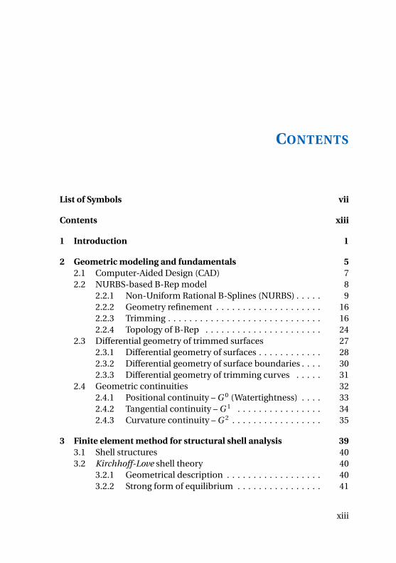
CONTENTS
List of Symbols vii
Contents xiii
1 Introduction 1
2 Geometric modeling and fundamentals 52.1 Computer-Aided Design (CAD) 72.2 NURBS-based B-Rep model 8
2.2.1 Non-Uniform Rational B-Splines (NURBS) . . . . . 92.2.2 Geometry refinement . . . . . . . . . . . . . . . . . . . . 162.2.3 Trimming . . . . . . . . . . . . . . . . . . . . . . . . . . . . . 162.2.4 Topology of B-Rep . . . . . . . . . . . . . . . . . . . . . . 24
2.3 Differential geometry of trimmed surfaces 272.3.1 Differential geometry of surfaces . . . . . . . . . . . . 282.3.2 Differential geometry of surface boundaries . . . . 302.3.3 Differential geometry of trimming curves . . . . . 31
2.4 Geometric continuities 322.4.1 Positional continuity – G 0 (Watertightness) . . . . 332.4.2 Tangential continuity – G 1 . . . . . . . . . . . . . . . . 342.4.3 Curvature continuity – G 2 . . . . . . . . . . . . . . . . . 35
3 Finite element method for structural shell analysis 393.1 Shell structures 403.2 Kirchhoff-Love shell theory 40
3.2.1 Geometrical description . . . . . . . . . . . . . . . . . . 403.2.2 Strong form of equilibrium . . . . . . . . . . . . . . . . 41
xiii
Contents
3.3 Finite element method 413.3.1 Definition of nomenclature . . . . . . . . . . . . . . . . 413.3.2 Weak form of equilibrium . . . . . . . . . . . . . . . . . 423.3.3 Discretization . . . . . . . . . . . . . . . . . . . . . . . . . . 43
3.4 Classical finite element analysis (FEA) 453.4.1 Definition of classical finite elements . . . . . . . . 453.4.2 Geometry description (finite element mesh) . . . 45
3.5 Isogeometric analysis (IGA) 483.5.1 h-,p-,h-p-, and k-refinement . . . . . . . . . . . . . . . 493.5.2 Geometry description . . . . . . . . . . . . . . . . . . . . 503.5.3 Definition of isogeometric elements . . . . . . . . . 52
4 Isogeometric B-Rep analysis 554.1 Geometrical description of shells 564.2 Weak form of equilibrium 57
4.2.1 Equilibrium along internal boundaries . . . . . . . 584.2.2 Equilibrium used for isogeometric B-Rep analysis 59
4.3 Definition of elements 604.3.1 Isogeometric (trimmed) elements . . . . . . . . . . . 604.3.2 B-Rep elements . . . . . . . . . . . . . . . . . . . . . . . . 634.3.3 B-Rep edge elements . . . . . . . . . . . . . . . . . . . . . 664.3.4 B-Rep vertex elements . . . . . . . . . . . . . . . . . . . . 68
4.4 NURBS-based Kirchhoff-Love shell formulation 684.4.1 Alternative shell formulations . . . . . . . . . . . . . . 69
4.5 B-Rep edge element formulations 694.5.1 Internal boundary conditions – penalty approach 694.5.2 Dirichlet boundary conditions – penalty approach 724.5.3 Neumann boundary conditions . . . . . . . . . . . . . 73
4.6 B-Rep vertex element formulations 74
5 Implementation of the isogeometric B-Rep analysis 775.1 Overview 775.2 Data structure of IBRA model 795.3 Generation of elements 81
5.3.1 Isogeometric (trimmed) elements . . . . . . . . . . . 825.3.2 B-Rep elements . . . . . . . . . . . . . . . . . . . . . . . . 83
5.4 Numerical integration of elements 855.4.1 B-Rep edge elements . . . . . . . . . . . . . . . . . . . . . 86
xiv
Contents
5.4.2 Isogeometric (trimmed) elements . . . . . . . . . . . 865.5 Adaptive Gaussian integration procedure (AGIP) 90
5.5.1 Full Gaussian domain . . . . . . . . . . . . . . . . . . . . 935.5.2 Trimmed Gaussian domain . . . . . . . . . . . . . . . . 95
5.6 Special aspects 965.6.1 Local refinement . . . . . . . . . . . . . . . . . . . . . . . 965.6.2 Flying nodes . . . . . . . . . . . . . . . . . . . . . . . . . . . 96
6 Analysis in Computer Aided Design 996.1 Product development process using CAx systems 100
6.1.1 Design modeling . . . . . . . . . . . . . . . . . . . . . . . 1006.1.2 Analysis modeling for classical FEA . . . . . . . . . . 1036.1.3 Analysis modeling for IBRA . . . . . . . . . . . . . . . . 103
6.2 Realization of an AiCAD worflow 1056.2.1 CAD system . . . . . . . . . . . . . . . . . . . . . . . . . . . 1066.2.2 AiCAD interface software . . . . . . . . . . . . . . . . . 1086.2.3 FE-solver . . . . . . . . . . . . . . . . . . . . . . . . . . . . . 1086.2.4 Postprocessing . . . . . . . . . . . . . . . . . . . . . . . . . 109
7 Examples and investigations 1137.1 Definition of error measures 1157.2 Infinite plate with circular hole 1157.3 Plate in bending with circular hole 1227.4 Doubly curved shell with circular hole 1277.5 Cantilever subject to end moment 1327.6 L-shaped cantilever 1387.7 Doubly curved multi-patch shell with circular hole 1397.8 Industrial application: oil sump 1417.9 Industrial application: engine bonnet 142
8 Summary and Conclusion 147
Bibliography 149
xv

We can’t solve problems byusing the same kind ofthinking we used when wecreated them.
Albert Einstein
CH
AP
TE
R
1INTRODUCTION
The usage of different geometry descriptions for design and analysis isone of the bottlenecks in a virtual product development process. Histori-cally, the independent developments in the fields computer-aided design(CAD) and computer-aided engineering (CAE) caused this "gap". The pre-dominant method in CAE for solving structural problems is the finite el-ement method (FEM). Since its origins in the 1950s FEM was developedprimarily with linear respectively quadratic polynomials defined over non-overlapping parametric domains (the elements). The standard for geom-etry description in contemporary CAD systems, however, is based on anon-uniform rational B-Splines (NURBS)-based boundary representation(B-Rep) which was mainly developed in the 1970s and 1980s (see alsoBoehm [14], Boor [15], Cohen et al. [22], Gordon et al. [35], Patrikalakis [62],Riesenfeld et al. [71], and Sederberg et al. [81]). A design-through-analysisworkflow therefore requires a geometry conversion called meshing whichis a highly complex task in itself because the meshes derived from CADmodels have to fulfill strict criteria (see also Abel Coll Sans [1], Hansen et al.[37], Knupp et al. [49], and Topping [89]). In addition, meshing leads to a
1
1 Introduction
geometry discretization error because usually a finite element mesh repre-sents just an approximation of the CAD model. The biggest disadvantage,however, is that meshing often requires manual interactions and thus itcan not be fully automatized.
To avoid the meshing, a few alternatives for the integration of design andanalysis have been suggested in the past few years. One of these approachesis the finite cell method (FCM) (see Düster et al. [32], Parvizian et al. [61],Rank et al. [67], and Schillinger et al. [76, 77]). This approach has highpotential, especially for three-dimensional structures, and it is being devel-oped continuously by Rank and his co-workers. Other approaches includethe Kantorovich method (see Kantorovich et al. [42]), implemented inScan&Solve™(see Scan&Solve [74]), or isogeometric analysis (IGA) intro-duced by Hughes et al. [40].
IGA entails the use of the same basis functions for representing CAD ge-ometries as well as for approximating solution fields. Usually, IGA is basedon NURBS (see Cottrell et al. [24] and Hughes et al. [40]) because NURBSrepresent the standard for geometry description in contemporary CADsystems. NURBS have high continuity, allow for refinement on the iden-tical geometry (see Boehm [14]) and raising the degree of the underlyingpolynomial functions (see also Cohen et al. [22], Piegl et al. [65], and Rogers[72]). NURBS basis functions show very good properties for analysis. In thepast few years, many IGA researchers have demonstrated the advantagesof these properties for analysis purposes, such as robustness and excel-lent approximation quality. IGA has been applied successfully in manyfields of engineering such as structural mechanics (see Bauer et al. [5],Belytschko et al. [10], Benson et al. [13], Cottrell et al. [24], Cottrell et al. [25,26], Hughes et al. [40], Nguyen-Thanh et al. [60], and Philipp et al. [63]),fluid mechanics (see Bazilevs et al. [8] and Hsu et al. [39]), fluid-structureinteraction (see Bazilevs et al. [6, 9], Hsu et al. [38], and Zhang et al. [93]),contact mechanics (see Dimitri et al. [29], Lorenzis et al. [54], and Temizeret al. [88]), and optimization (see Kiendl et al. [45], Qian et al. [66], and Wallet al. [91]). The usage of the basis functions from design also for analysissimplifies greatly the integration of these two tasks. However, a generaland consistent concept for creating direct and complete analysis modelsfrom CAD still is not available.
Recent publications have dealt with this shortcoming of IGA and suggestedsolutions pertaining to specific fields. Schillinger et al. [76] presented an
2
1 Introduction
integrated design-through-analysis workflow that is well suited for solvingthree-dimensional problems. Another approach for integrating design andanalysis is the use of T-Splines (see Bazilevs et al. [7] and Sederberg et al.[82, 83]) or subdivision surfaces for geometric modeling and analysis (seeBurkhart et al. [18], Cirak et al. [20], and Cirak et al. [21]). However, consid-ering NURBS-based B-Rep models as standard for geometry descriptionin CAD systems, the approaches mentioned above also require geometrictransformation.
The goal of the proposed CAD-integrated design-trough-analysis workflow,named analysis in computer aided design (AiCAD), is to use the CAD stan-dard geometry description (NURBS-based B-Rep models) for the entireworkflow, i.e. for geometric and analysis modeling as well as the analysisitself (see Breitenberger et al. [17]). AiCAD allows for unification of thedesign and analysis models and can be fully automatized and entirelyrealized within existing CAD systems. AiCAD uses the newly developed iso-geometric B-Rep analysis (IBRA) (see Breitenberger et al. [17]) for analyzingNURBS-based B-Rep models.
IBRA is a general and consequent extension of IGA, which in addition tothe basis functions also uses the B-Rep description of the CAD model.This is expressed by the extension "B-Rep", a well known term in the CADcommunity (see Mäntylä [56] and Mortenson [57]). IBRA can directly usethe design model, coming from a CAD system, for analysis, without mesh-ing or re-parametrization. Hence, IBRA allows for the creation of a directand complete analysis model from the CAD model in a consistent finite-element-like manner.
Thus far, AiCAD is realized within the integrated CAD/CAE/CAM programSiemens NX (see Siemens PLM Software [84]), within the CAD programRhinoceros (see Rhinoceros [70]), and within the Pre- and Postprocessingsoftware GiD (see GiD [34]). This demonstrates the general applicability ofthe presented concept.
This thesis provides guidelines for the realization of the AiCAD workflowin existing CAD programs and the implementation of IBRA for surfacemodels in existing FE solvers. The focus lies on a modular disassembly ofthe necessary steps and a clear definition of the data interfaces. Aspectsrelevant to practice such as the application of arbitrarily located loads,local refinement, enforcing weak boundary conditions along trimmingcurves, dealing with non-matching multi-patches including gaps and over-
3
1 Introduction
laps, and the numerical integration of trimmed surfaces are discussed aswell. For the numerical integration a new adaptive integration schemeis presented. In addition, the thesis highlights that AiCAD is very attrac-tive and can be competitive to established workflows by solving industrialproblems of shell structures.
The thesis is outlined as follows:
CHAPTER 2 explains in detail NURBS-based B-Rep surface models whichare used throughout the entire AiCAD workflow and forms the basis for theproposed isogeometric B-Rep analysis (IBRA). Important aspects of NURBS-based B-Rep models relevant for structural shell analysis are discussedsuch as geometric continuities across edges including non-watertightness,geometrical refinement, trimming, trimming tolerances, and the topologyof complex multi-patch models.
CHAPTER 3 reviews briefly the finite element method (FEM) for structuralshell problems with a focus on using different geometry discretizations. Inaddition, a classification of the finite element techniques: classical FEA,IGA, and IBRA with respect to their geometry discretization is given.
CHAPTER 4 explains the isogeometric B-Rep analysis (IBRA), in particularthe newly developed B-Rep elements, which can be used to handle dis-continuous and trimmed geometries with gaps and overlaps for structuralanalysis in a finite-element-like manner.
CHAPTER 5 describes the systematic disassembly of CAD models into fi-nite elements and defines data interfaces for an implementation of IBRAinto existing FE solvers. In addition a new adaptive numerical integrationscheme for trimmed surfaces is presented.
CHAPTER 6 describes the different steps resp. modules for the realization ofthe AiCAD workflow by combining existing CAD programs and FE-solvers.
CHAPTER 7 demonstrates the application of the proposed AiCAD workflowresp. IBRA to some academic and industrial shell problems. For theseexamples different aspects like trimming tolerances, non-watertightness,accuracy, and robustness are discussed.
CHAPTER 8 summarizes the thesis and gives an outlook to further possibleresearch.
4
Where there is matter, thereis geometry.
Johannes Kepler
CH
AP
TE
R
2GEOMETRIC MODELING AND
FUNDAMENTALS
Design or geometric modeling is used for defining the shape and other geo-metric characteristics of an object. Since every day language is not useful todescribe complex shapes, mathematical concepts and approaches are usedfor this purpose (see also Mortenson [57] and Rooney et al. [73]). Nowa-days, geometric modeling is usually computer based and is performedusing computer-aided design (CAD) systems. Geometric modeling withCAD systems is thus assumed throughout this thesis.
This chapter explains NURBS-based B-Rep models. They are the standardfor geometry description in contemporary CAD systems for mechanicalengineering and form the basis for the proposed CAD-integrated design-through-analysis workflow. Thus, important aspects relevant for structuralanalysis are discussed such as geometrical refinement, trimming, trimmingtolerances, the topology of complex multi-patch models, and geometriccontinuities across edges including non-watertightness. Moreover, thechapter reviews differential geometry of trimmed surfaces.
5
2 Geometric modeling and fundamentals
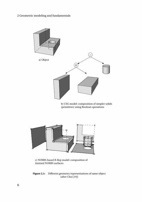
a) Object
b) CSG model: composition of simpler solids(primitives) using Boolean operations
c) NURBS-based B-Rep model: composition oftimmed NURBS surfaces
U
Figure 2.1: Different geometry representations of same object(after Choi [19])
6
2.1 Computer-Aided Design (CAD)
2.1 Computer-Aided Design (CAD)
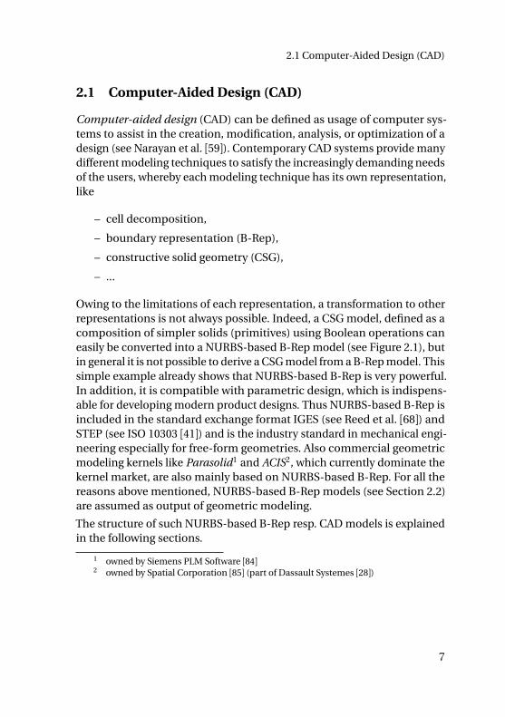
Computer-aided design (CAD) can be defined as usage of computer sys-tems to assist in the creation, modification, analysis, or optimization of adesign (see Narayan et al. [59]). Contemporary CAD systems provide manydifferent modeling techniques to satisfy the increasingly demanding needsof the users, whereby each modeling technique has its own representation,like
– cell decomposition,
– boundary representation (B-Rep),
– constructive solid geometry (CSG),
– ...
Owing to the limitations of each representation, a transformation to otherrepresentations is not always possible. Indeed, a CSG model, defined as acomposition of simpler solids (primitives) using Boolean operations caneasily be converted into a NURBS-based B-Rep model (see Figure 2.1), butin general it is not possible to derive a CSG model from a B-Rep model. Thissimple example already shows that NURBS-based B-Rep is very powerful.In addition, it is compatible with parametric design, which is indispens-able for developing modern product designs. Thus NURBS-based B-Rep isincluded in the standard exchange format IGES (see Reed et al. [68]) andSTEP (see ISO 10303 [41]) and is the industry standard in mechanical engi-neering especially for free-form geometries. Also commercial geometricmodeling kernels like Parasolid1 and ACIS2, which currently dominate thekernel market, are also mainly based on NURBS-based B-Rep. For all thereasons above mentioned, NURBS-based B-Rep models (see Section 2.2)are assumed as output of geometric modeling.
The structure of such NURBS-based B-Rep resp. CAD models is explainedin the following sections.
1 owned by Siemens PLM Software [84]2 owned by Spatial Corporation [85] (part of Dassault Systemes [28])
7
2 Geometric modeling and fundamentals
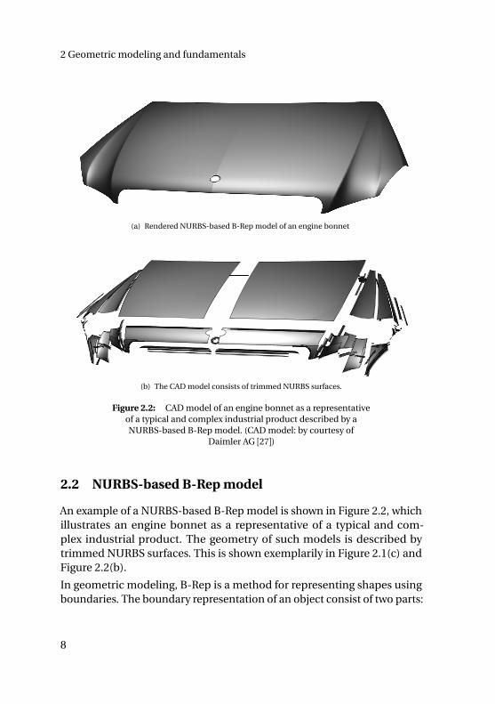
(a) Rendered NURBS-based B-Rep model of an engine bonnet
(b) The CAD model consists of trimmed NURBS surfaces.
Figure 2.2: CAD model of an engine bonnet as a representativeof a typical and complex industrial product described by aNURBS-based B-Rep model. (CAD model: by courtesy of
Daimler AG [27])
2.2 NURBS-based B-Rep model
An example of a NURBS-based B-Rep model is shown in Figure 2.2, whichillustrates an engine bonnet as a representative of a typical and com-plex industrial product. The geometry of such models is described bytrimmed NURBS surfaces. This is shown exemplarily in Figure 2.1(c) andFigure 2.2(b).
In geometric modeling, B-Rep is a method for representing shapes usingboundaries. The boundary representation of an object consist of two parts:
8
2.2 NURBS-based B-Rep model
– shape (geometry), which defines the spatial position, the curvatures,etc.
– structure (topology), which allows to make links between geometri-cal entities
The following sections explain the geometrical description i.e. trimmedNURBS and the topology of NURBS-based B-Rep models with a focus onsurface models.
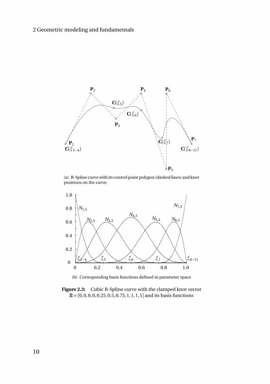
2.2.1 Non-Uniform Rational B-Splines (NURBS)
NURBS basis functions can be used for parametrizing curves in general aswell as for surfaces and solids within tensor product construction. They canbe used for modeling a large variety of shapes (see also Cohen et al. [23] andRogers [72]). The term NURBS stands for Non-Uniform Rational B-Splinesand indicates that NURBS are a generalization of B-Splines. Therefore, ashort introduction to B-Splines is given first. For a detailed description ofNURBS the reader is referred to Cohen et al. [23] and Piegl et al. [65].
B-Splines are non-interpolating, piecewise defined polynomial curves.They are defined by the following entities:
– set of control points, Pi , i = 1, ..., n
– polynomial degree p
– knot vector Ξ= [ξ1,ξ2, ...ξn+p+1]
– set of basis functions Ni , i = 1, ..., n
Knot vector
The knot vector Ξ is a set of parametric coordinates ξi arranged in as-cending order. This set divides the B-Spline resp. NURBS into sections. Ifall knots are spaced equally, the knot vector is called uniform otherwisenon-uniform. Knot values that appear more than once are called multipleknots. The intervals between two consecutive, distinct knots are callednon-zero knot spans. In case the first and last entries in knot vectors have amultiplicity of p +1 they are called clamped. Unclamped knot vectors canbe used for periodic B-Splines resp. NURBS (see Piegl et al. [65]), whichare used to describe a closed shape, like ellipse and torus.
9
2 Geometric modeling and fundamentals
P1C(ξ1−4)
P2
P3
P4
P5
P6
P7
C(ξ5)
C(ξ6)
C(ξ7)C(ξ8−11)
(a) B-Spline curve with its control point polygon (dashed lines) and knotpositions on the curve.
0 0.2 0.4 0.6 0.8 1.00
0.2
0.4
0.6
0.8
1.0
N1,3
N2,3 N3,3
N4,3N5,3 N6,3
N7,3
ξ1−4 ξ5 ξ7ξ6 ξ8−11
(b) Corresponding basis functions defined in parameter space
Figure 2.3: Cubic B-Spline curve with the clamped knot vectorΞ= [0, 0, 0, 0, 0.25, 0.5, 0.75, 1, 1, 1, 1] and its basis functions
10
2.2 NURBS-based B-Rep model
Basis functions
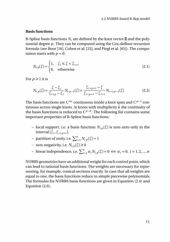
B-Spline basis functions Ni are defined by the knot vector Ξ and the poly-nomial degree p . They can be computed using the Cox-deBoor recursionformula (see Boor [16], Cohen et al. [23], and Piegl et al. [65]). The compu-tation starts with p = 0:
Ni ,0(ξ) =
(
1, ξi ¶ ξ<ξi+1
0, otherwise(2.1)
For p ¾ 1 it is
Ni ,p (ξ) =ξ−ξi
ξi+p −ξiNi ,p−1(ξ) +
ξi+p+1−ξξi+p+1−ξi+1
Ni+1,p−1(ξ) (2.2)
The basis functions are C∞ continuous inside a knot span and C p−1 con-tinuous across single knots. At knots with multiplicity k the continuity ofthe basis functions is reduced to C p−k . The following list contains someimportant properties of B-Spline basis functions:
– local support, i.e. a basis function Ni ,p (ξ) is non-zero only in theinterval [ξi ,ξi+p+1].
– partition of unity, i.e.∑n
i=1 Ni ,p (ξ) = 1
– non-negativity, i.e. Ni ,p (ξ)¾ 0
– linear independence, i.e.∑n
i=1αi Ni ,p (ξ) = 0 ⇔ αi = 0, i = 1, 2, ..., n
NURBS geometries have an additional weight for each control point, whichcan lead to rational basis functions. The weights are necessary for repre-senting, for example, conical sections exactly. In case that all weights areequal to one, the basis functions reduce to simple piecewise polynomials.The formulas for NURBS basis functions are given in Equation (2.4) andEquation (2.6).
11
2 Geometric modeling and fundamentals
(a) B-Spline surface with its control point net (dashed lines) and param-eter curves (knots)
ξ1−3
ξ4
ξ5−7
η1−3
η5−7
η4
(b) Corresponding basis functions in parameter space
Figure 2.4: Quadratic B-Spline surface with clamped knotvectors Ξ= H = [0, 0, 0, 0.5, 1, 1, 1] and its basis functions
12
2.2 NURBS-based B-Rep model
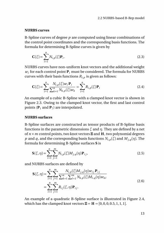
NURBS curves
B-Spline curves of degree p are computed using linear combinations ofthe control point coordinates and the corresponding basis functions. Theformula for determining B-Spline curves is given by
C (ξ) =n∑
i=1
Ni ,p (ξ)Pi . (2.3)
NURBS curves have non-uniform knot vectors and the additional weightwi for each control point Pi must be considered. The formula for NURBScurves with their basis functions Ri ,p is given as follows:
C (ξ) =n∑
i=1
Ni ,p (ξ)wi Pi∑n
k=1 Nk ,p (ξ)wk
=n∑
i=1
Ri ,p (ξ)Pi (2.4)
An example of a cubic B-Spline with a clamped knot vector is shown inFigure 2.3. Owing to the clamped knot vector, the first and last controlpoints (P1 and P7) are interpolated.
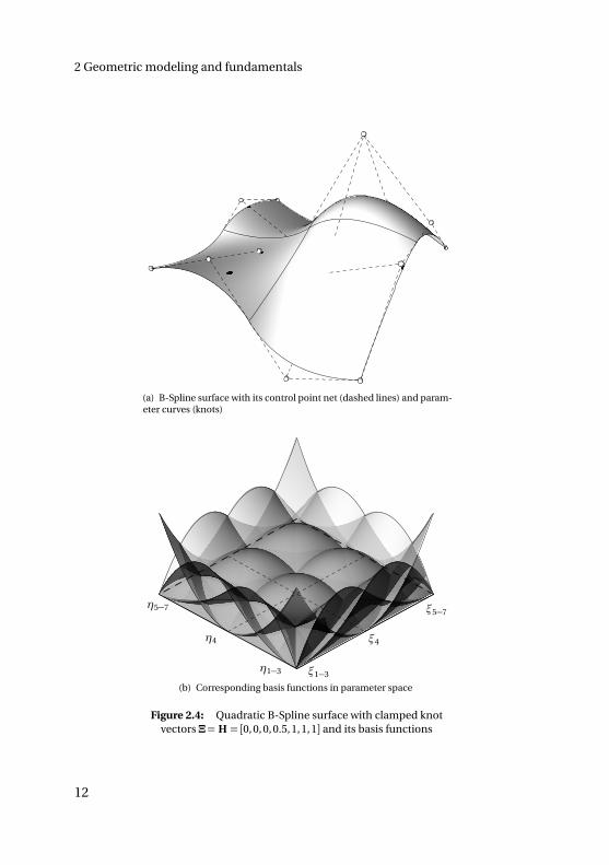
NURBS surfaces
B-Spline surfaces are constructed as tensor products of B-Spline basisfunctions in the parametric dimensions ξ and η. They are defined by a netof n×m control points, two knot vectors Ξ and H , two polynomial degreesp and q , and the corresponding basis functions Ni ,p (ξ) and M j ,q (η). Theformula for determining B-Spline surfaces S is
S (ξ,η) =n∑
i=1
m∑
j=1
Ni ,p (ξ)M j ,q (η)Pi j , (2.5)
and NURBS surfaces are defined by
S (ξ,η) =n∑
i=1
m∑
j=1
Ni ,p (ξ)M j ,q (η)wi j Pi j∑n
k=1
∑ml=1 Nk ,p (ξ)Ml ,q (η)wk l
=n∑
i=1
m∑
j=1
Ri j (ξ,η)Pi j .
(2.6)
An example of a quadratic B-Spline surface is illustrated in Figure 2.4,which has the clamped knot vectors Ξ= H = [0, 0, 0, 0.5, 1, 1, 1].
13
2 Geometric modeling and fundamentals
P1
P6
P7
P8
P9
P10
C(ξ8)
C(ξ9)
C(ξ10)C(ξ1−4)
P2
P3 P4
P5C(ξ5−7)
C(ξ11−14)
(a) Refined B-Spline curve with its control point polygon (dashed lines)and knot positions on the curve
0 0.2 0.4 0.6 0.8 1.00
0.2
0.4
0.6
0.8
1.0N4,3
N5,3N6,3
N7,3N8,3 N9,3
N10,3
ξ8 ξ10ξ9 ξ11−14
ξ5−7
N1,3
(b) Corresponding refined basis functions
Figure 2.5: Knot insertion exemplified by B-Spline curve fromFigure 2.3 with knot vector Ξ= [0, 0, 0, 0, 0.25, 0.5, 0.75, 1, 1, 1, 1].After inserting three knots at ξ= 0.1 the knot vector becomes
Ξ= [0, 0, 0, 0, 0.1, 0.1, 0.1, 0.25, 0.5, 0.75, 1, 1, 1, 1] and a C 0 continuityis introduced at the new knot. The refinement does not change the
curve’s shape.
14
2.2 NURBS-based B-Rep model
P1
P2
P3
P4
P5P6
P7
C(ξ1−5)
C(ξ6−7)
C(ξ8−9)
C(ξ10−11)C(ξ12−16)
P8
P11
P9
P10
(a) Refined B-Spline curve with its control point polygon (dashed lines)and knot positions on the curve
0 0.2 0.4 0.8 1.00.60
0.2
0.4
0.6
0.8
1.0
ξ1−5 ξ6−7 ξ8−9 ξ10−11 ξ12−16
N1,4
N2,4
N3,4N4,4
N5,4
N6,4
N7,4
N8,4N9,4
N10,4
N11,4
(b) Corresponding quartic basis functions
Figure 2.6: Degree elevation exemplified by B-Spline curve fromFigure 2.3. The polynomial degree is increased by one to four. This
results in the new knot vectorΞ= [0, 0, 0, 0, 0, 0.25, 0.25, 0.5, 0.5, 0.75, 0.75, 1, 1, 1, 1, 1]. The
refinement does not change the curve’s shape.
15
2 Geometric modeling and fundamentals
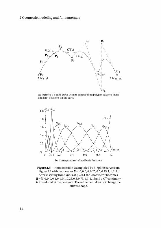
2.2.2 Geometry refinement
For the later mentioned purpose of analysis the geometry basis might needto be enriched to properly describe deformed geometries (see Section 3.5.1and Hughes et al. [40]).
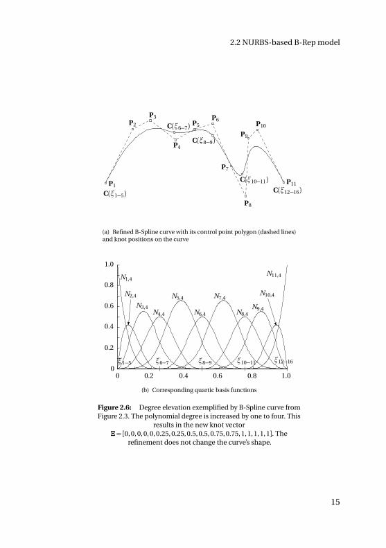
There are two ways of refining B-Spline and NURBS geometries, they arecalled degree elevation and knot insertion (see Boehm [14], Cohen et al. [22],and Piegl et al. [65]). Both refinement techniques increase the number ofcontrol points and thus impart the capability to represent a greater numberof shapes. The refinement itself does not change the initial shape of thegeometry.
The continuity of a curve can be decreased by generating knots with multi-plicity greater than one (see Section 2.2.1). In case of multiplicity equal to(p +1), the curve becomes interpolating at this knot and can be split easilyinto two curves. An example of a similar case is shown in Figure 2.5, whichillustrates the knot insertion refinement of a B-Spline curve by introduc-ing a C 0 continuity at ξ= 0.1. An example of degree elevation is shown inFigure 2.6.
For surfaces and solids refinement can be performed in the same mannerand independently for each parameter direction.
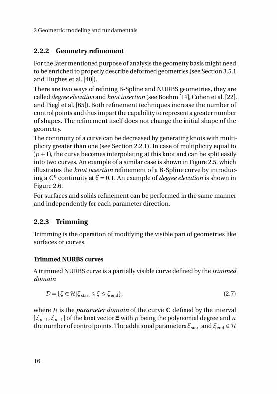
2.2.3 Trimming
Trimming is the operation of modifying the visible part of geometries likesurfaces or curves.
Trimmed NURBS curves
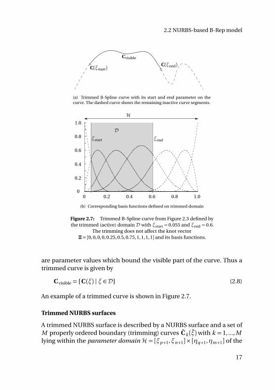
A trimmed NURBS curve is a partially visible curve defined by the trimmeddomain
D = ξ ∈H|ξstart ≤ ξ≤ ξend, (2.7)
where H is the parameter domain of the curve C defined by the interval[ξp+1,ξn+1] of the knot vector Ξwith p being the polynomial degree and nthe number of control points. The additional parametersξstart andξend ∈H
16
2.2 NURBS-based B-Rep model
C(ξstart)C(ξend)
Cvisible
(a) Trimmed B-Spline curve with its start and end parameter on thecurve. The dashed curve shows the remaining inactive curve segments.
0 0.2 0.4 0.6 0.8 1.00
0.2
0.4
0.6
0.8
1.0
ξstart ξend
D
H
(b) Corresponding basis functions defined on trimmed domain
Figure 2.7: Trimmed B-Spline curve from Figure 2.3 defined bythe trimmed (active) domain D with ξstart = 0.055 and ξend = 0.6.
The trimming does not affect the knot vectorΞ= [0, 0, 0, 0, 0.25, 0.5, 0.75, 1, 1, 1, 1] and its basis functions.
are parameter values which bound the visible part of the curve. Thus atrimmed curve is given by
C visible = C (ξ) | ξ ∈D (2.8)
An example of a trimmed curve is shown in Figure 2.7.
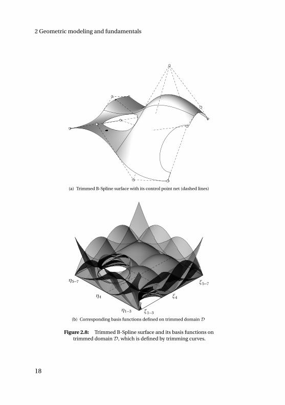
Trimmed NURBS surfaces
A trimmed NURBS surface is described by a NURBS surface and a set ofM properly ordered boundary (trimming) curves C k (ξ)with k = 1, ..., Mlying within the parameter domain H = [ξp+1,ξn+1]× [ηq+1,ηm+1] of the
17
2 Geometric modeling and fundamentals
(a) Trimmed B-Spline surface with its control point net (dashed lines)
ξ1−3
ξ4
ξ5−7
η1−3
η5−7
η4
(b) Corresponding basis functions defined on trimmed domain D
Figure 2.8: Trimmed B-Spline surface and its basis functions ontrimmed domain D, which is defined by trimming curves.
18
2.2 NURBS-based B-Rep model
surface (see also Piegl et al. [64]). Thus, a trimmed surface is a partiallyvisible surface, defined by the trimmed domain
D = (ξ,η) ∈H|∂D =M⋃
k=1
C k . (2.9)
Here, ∂D describes the boundary of the closed trimmed domain D.
In general, trimming curves C k (ξ) can be of any form, however, whendealing with NURBS entities, it is desirable to represent these with NURBS3,too
C k (ξ) =
ξk (ξ)
ηk (ξ)
=nk∑
i=1
R (k )i ,l (ξ) P ki , k = 1, 2, ..., M . (2.10)
Here, l is the polynomial degree, ξ is the curve parameter, ξk and ηk areparameters of the surface representing the trimming curve C k and P k
i arethe control points of the trimming curve in the parameter space of thesurface. The curves C k (ξ) are joined properly to form outer and innerloops. The outer loops are oriented counter-clockwise, whereas the innerloops are oriented clockwise (see also Section 2.3.3). The boundary of thesurface is given by
∂ Svisible =M⋃
k=1
∂ Sk , (2.11)
where ∂ Sk are implicitly defined curves, described by the basis functionsof the surfaces as follows
∂ Sk = S (C k (ξ)) =n∑
i=1
m∑
j=1
Ri j (C k (ξ))Pi j , k = 1, 2, ..., M . (2.12)
Figure 2.9 shows exemplarily such basis functions for the trimmed sur-face in Figure 2.8(a). Since an explicit description of the boundary ∂ Sk isneeded for geometric modeling, the trimming curves C k (ξ) are mappedonto the surface as an explicit space curve C k (ξ) (see also Renner et al.[69]):
3 within CAD systems in most cases just B-Splines are used
19
2 Geometric modeling and fundamentals
C1(ξ)
C6(ξ)C5(ξ)
C4(ξ)
C3(ξ)
C2(ξ)
C7(ξ)
(a) Explicitly defined (approximated) spacecurves C k of the trimming curves C k
R (1)i j
R (2)i j
R (4)i j
R (3)i j
R (5)i jR (6)i j
R (7)i j
(b) Implicitly defined basis functions on theboundaries
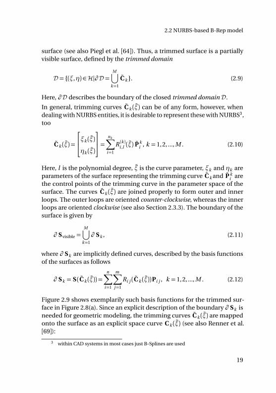
Figure 2.9: Description of the boundaries of the trimmedsurface in Figure 2.8(a) with its implicitly defined basis functions
and its explicitly defined (approximated) space curves.
Here, non-trivial mappings i.e. trimming curves which do not coincidewith parameter lines, are usually approximated by using NURBS curves ofthird order (e.g. C 3 and C 7 in Figure 2.9(a)).
A trimmed surface is given by
Svisible = S (ξ,η) | (ξ,η) ∈D. (2.13)
An example of a trimmed B-Spline surface with its basis functions, definedon a trimmed domain D, is illustrated in Figure 2.8. The correspondinguntrimmed B-Spline surface with its basis functions is shown in Figure 2.4.
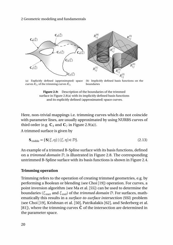
Trimming operation
Trimming refers to the operation of creating trimmed geometries, e.g. byperforming a Boolean or blending (see Choi [19]) operation. For curves, apoint inversion algorithm (see Ma et al. [55]) can be used to determine theboundaries (ξstart and ξend) of the trimmed domain D. For surfaces, math-ematically this results in a surface-to-surface intersection (SSI) problem(see Choi [19], Krishnan et al. [50], Patrikalakis [62], and Sederberg et al.[81]), where the trimming curves C of the intersection are determined inthe parameter space.
20
2.2 NURBS-based B-Rep model
d) Intersecting surfaces after trimming operations
a) Original B-Spline surface 1 b) Original NURBS surfaces 2 and 3
Boolean operations- approximation of the intersectioncurve in the parameter space (Ccurves) of each surface using an SSIalgorithm- determination of the trimmeddomain D (visible part) for eachsurface- approximation of the space curves Cby mapping the trimming curves Conto the corresponding surface
S(1)
S(2)
S(3)
c) Intersecting surfaces before trimming operations
S(1)visible
S(2)visible S(3)visible
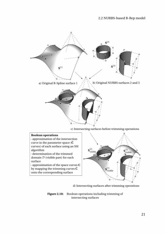
Figure 2.10: Boolean operations including trimming ofintersecting surfaces
21
2 Geometric modeling and fundamentals
Figure 2.10 shows an example of trimming operations with three intersect-ing surfaces before and after the execution of several Boolean operations.A trimming operation consists of the following steps:
– approximation of the intersection curve with the trimming curvesC k (ξ) in the parameter space of each surface using an SSI algorithm(see Krishnan et al. [50], Patrikalakis [62], and Sederberg et al. [81])
– determination of the trimmed domain D for each surface
– approximation of the space curves C k (ξ) by mapping the trimmingcurves C k (ξ) onto the corresponding surface (see Renner et al. [69])
Note that the specification of the trimmed domain (visible part) dependson the type of Boolean operation (see also Figure 2.10).
For solving the SSI problem and mapping the trimming curves onto thesurfaces most CAD systems use approximation algorithms, even if themapping could be done exactly by using polynomials of high degrees (e.g.p=27) (see Renner et al. [69]). Indeed, the use of approximation techniquesrequires the specification of tolerances but it reduces the computationalcost and increases the robustness against numerical instabilities (see Ren-ner et al. [69]).
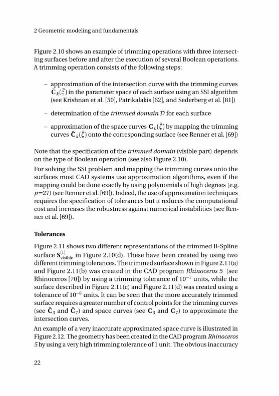
Tolerances
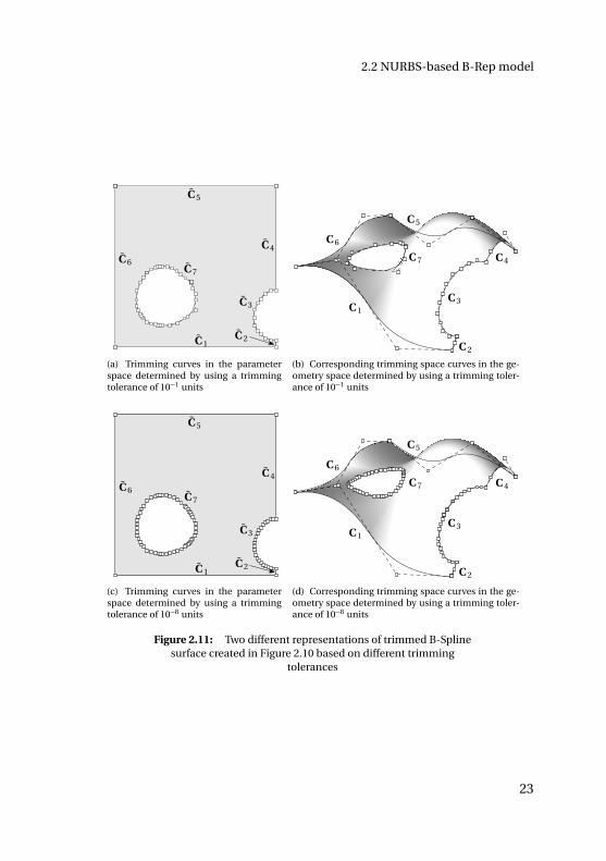
Figure 2.11 shows two different representations of the trimmed B-Splinesurface S(1)visible in Figure 2.10(d). These have been created by using twodifferent trimming tolerances. The trimmed surface shown in Figure 2.11(a)and Figure 2.11(b) was created in the CAD program Rhinoceros 5 (seeRhinoceros [70]) by using a trimming tolerance of 10−1 units, while thesurface described in Figure 2.11(c) and Figure 2.11(d) was created using atolerance of 10−8 units. It can be seen that the more accurately trimmedsurface requires a greater number of control points for the trimming curves(see C 3 and C 7) and space curves (see C 3 and C 7) to approximate theintersection curves.
An example of a very inaccurate approximated space curve is illustrated inFigure 2.12. The geometry has been created in the CAD program Rhinoceros5 by using a very high trimming tolerance of 1 unit. The obvious inaccuracy
22
2.2 NURBS-based B-Rep model
C 1C 2
C 3
C 4
C 5
C 6C 7
(a) Trimming curves in the parameterspace determined by using a trimmingtolerance of 10−1 units
C 1
C 2
C 3
C 4
C 5
C 6
C 7
(b) Corresponding trimming space curves in the ge-ometry space determined by using a trimming toler-ance of 10−1 units
C 1C 2
C 3
C 4
C 5
C 6C 7
(c) Trimming curves in the parameterspace determined by using a trimmingtolerance of 10−8 units
C 1
C 2
C 3
C 4
C 5
C 6
C 7
(d) Corresponding trimming space curves in the ge-ometry space determined by using a trimming toler-ance of 10−8 units
Figure 2.11: Two different representations of trimmed B-Splinesurface created in Figure 2.10 based on different trimming
tolerances
23
2 Geometric modeling and fundamentals
visualization mesh
inaccurate trimming space curve
last knot line before boundary
obvious inaccuracy
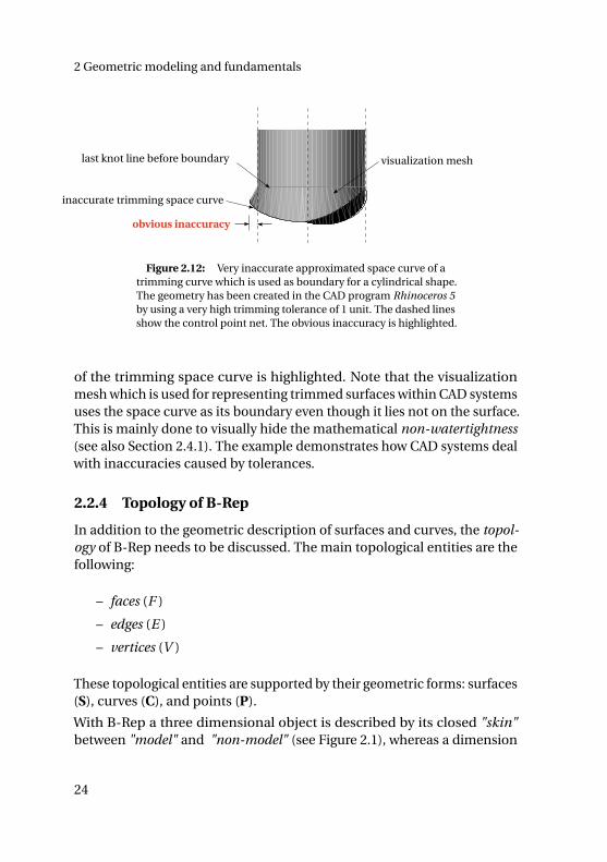
Figure 2.12: Very inaccurate approximated space curve of atrimming curve which is used as boundary for a cylindrical shape.The geometry has been created in the CAD program Rhinoceros 5by using a very high trimming tolerance of 1 unit. The dashed linesshow the control point net. The obvious inaccuracy is highlighted.
of the trimming space curve is highlighted. Note that the visualizationmesh which is used for representing trimmed surfaces within CAD systemsuses the space curve as its boundary even though it lies not on the surface.This is mainly done to visually hide the mathematical non-watertightness(see also Section 2.4.1). The example demonstrates how CAD systems dealwith inaccuracies caused by tolerances.
2.2.4 Topology of B-Rep
In addition to the geometric description of surfaces and curves, the topol-ogy of B-Rep needs to be discussed. The main topological entities are thefollowing:
– faces (F )
– edges (E )
– vertices (V )
These topological entities are supported by their geometric forms: surfaces(S), curves (C), and points (P).
With B-Rep a three dimensional object is described by its closed "skin"between "model" and "non-model" (see Figure 2.1), whereas a dimension
24
2.2 NURBS-based B-Rep model
Face 1
Face 2
Face 3
Edge 1
Edge 2
Edge 3
Edge 4Edge 5
Edge 6
Edge 7
Vertex 2
Vertex 1
Vertex 3
Vertex 4
Vertex 9
Vertex 5
Vertex 6
Vertex 7
Vertex 8
Vertex 10
Edge 8
Edge 10
Edge 9
Edge 11
Edge 12
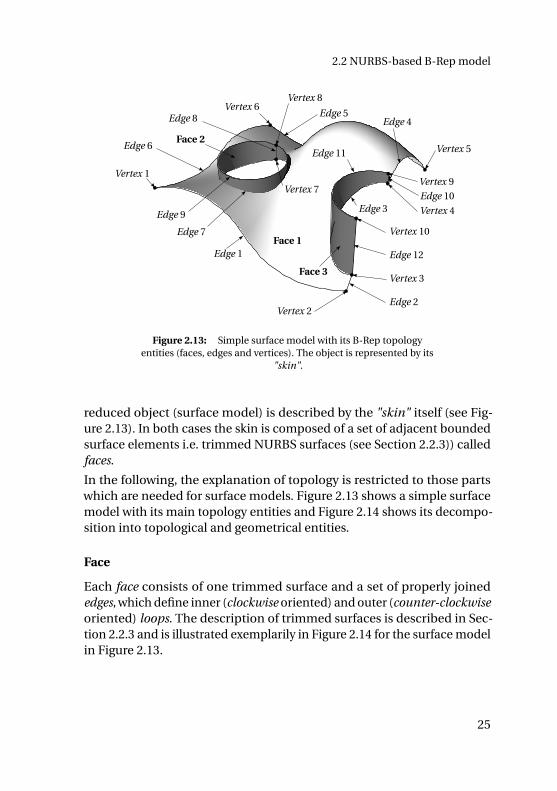
Figure 2.13: Simple surface model with its B-Rep topologyentities (faces, edges and vertices). The object is represented by its
"skin".
reduced object (surface model) is described by the "skin" itself (see Fig-ure 2.13). In both cases the skin is composed of a set of adjacent boundedsurface elements i.e. trimmed NURBS surfaces (see Section 2.2.3)) calledfaces.
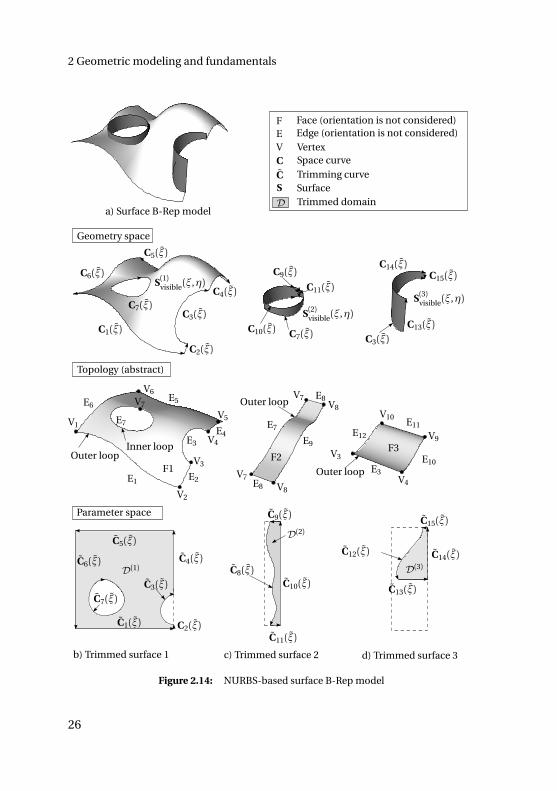
In the following, the explanation of topology is restricted to those partswhich are needed for surface models. Figure 2.13 shows a simple surfacemodel with its main topology entities and Figure 2.14 shows its decompo-sition into topological and geometrical entities.
Face
Each face consists of one trimmed surface and a set of properly joinededges, which define inner (clockwise oriented) and outer (counter-clockwiseoriented) loops. The description of trimmed surfaces is described in Sec-tion 2.2.3 and is illustrated exemplarily in Figure 2.14 for the surface modelin Figure 2.13.
25
2 Geometric modeling and fundamentals
C7(ξ)C3(ξ)
C1(ξ)
C6(ξ)
C5(ξ)
C4(ξ)
C2(ξ)
C10(ξ)
C9(ξ)
C8(ξ)
C11(ξ)
C12(ξ)
C13(ξ)
C15(ξ)
C14(ξ)
C1(ξ)
C2(ξ)
C3(ξ)
C4(ξ)
C5(ξ)
C6(ξ)
C7(ξ)
C7(ξ)
C9(ξ)
C3(ξ)C13(ξ)
C15(ξ)C14(ξ)
Geometry space
Topology (abstract)
Parameter space
C10(ξ)
C11(ξ)
Inner loop
E1
E6E5
E4E3
E2
E7
E8
E9
E8
E7E11
E10E3
E12
S(1)visible(ξ,η)
S(2)visible(ξ,η)S(3)visible(ξ,η)
Trimmed domain
E Edge (orientation is not considered)
Outer loop
Outer loop
Outer loop
Space curve
F1F2
F3
Vertex
SurfaceS
V1
V2
V4
V3
V5
V6
V7
V7
V7V8
V8V4
V9
V3
V10
VC
Trimming curveC
a) Surface B-Rep model
b) Trimmed surface 1 c) Trimmed surface 2 d) Trimmed surface 3
D(1)
D(2)
D(3)
D
F Face (orientation is not considered)
Figure 2.14: NURBS-based surface B-Rep model
26
2.3 Differential geometry of trimmed surfaces
Edge
Edges are topological entities of
– common parts of trimming curves, which bound surfaces (faces) oneither side of an edge (see Edge 3 and Edge 7 in Figure 2.13), or
– free trimming curves (see e.g. Edge 1 in Figure 2.13).
Within CAD systems an edge is described by one space curve boundedby two vertices given in spatial coordinates. The corresponding trimmingcurves for the adjacent surfaces within their parameters spaces are pro-vided by the CAD system. The parameters ξstart and ξend of the trimmeddomain D of the trimming curve within the parameter space of the surface(see also Section 2.2.3) which defines the edge need to be computed by apoint inversion algorithm (see Ma et al. [55]) using the spatial coordinatesof the vertices which bound the edge.
Vertex
Vertices given in spatial coordinates are the topological entities of pointswhere several edges meet and thus they define the boundaries of edges.
Depending on the purpose, the face-edge-vertex data model can also beaugmented by additional elements such as shells and/or loops (see topologyin Figure 2.14). For more information about B-Rep the reader is referred toMäntylä [56] and Stroud [86].
2.3 Differential geometry of trimmed surfaces
This section reviews all basics of differential geometry of trimmed surfaceswhich are used within this thesis. Remember that within this thesis the Ein-stein summation convention as well as the convention that Latin indiceslike i,j,k,l take letters 1, 2, 3 and Greek letters like α,β ,γ,δ take the values1, 2 is used. In addition, derivatives w.r.t. to a quantity i are abbreviatedby (·),i .
27
2 Geometric modeling and fundamentals
A1
A2
A3
C
Svisibleθ 1
θ 2
x 3
x 2
x 1
e3
e1e2
X surf(θ
1 ,θ2 )
θ 3
T1
T3
θ 1
X B-Rep(θ
1 )T2
∂ Svisible
Figure 2.15: Geometry description of a trimmed surface
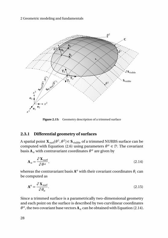
2.3.1 Differential geometry of surfaces
A spatial point X surf(θ 1,θ 2) ∈ Svisible of a trimmed NURBS surface can becomputed with Equation (2.6) using parameters θ α ∈ D. The covariantbasis Aα with contravariant coordinates θ α are given by
Aα =∂ X surf
∂ θ α, (2.14)
whereas the contravariant basis Aα with their covariant coordinates θi canbe computed as
Aα =∂ X surf
∂ θα. (2.15)
Since a trimmed surface is a parametrically two-dimensional geometryand each point on the surface is described by two curvilinear coordinatesθ α, the two covariant base vectors Aα can be obtained with Equation (2.14).
28
2.3 Differential geometry of trimmed surfaces
The third covariant base vector A 3 is defined as a normalized vector, or-thogonal to Aα as
A 3 =A 1×A 2
A 1×A 2
2
(2.16)
with the property
A 3 = A3. (2.17)
The metric tensor A of a surface can be expressed in the covariant andcontravariant basis as
A= AαβAα⊗Aβ = AαβAα⊗Aβ . (2.18)
Here, covariant metric coefficients Aαβ can be obtained with the so calledfirst fundamental form of surfaces by the scalar product of covariant basevectors (see also Klingbeil [48]):
Aαβ = Aα ·Aβ (2.19)
and the contravariant metric coefficients Aαβ can be computed by invert-ing the covariant coefficient matrix
[Aαβ ] = [Aαβ ]−1. (2.20)
The metric coefficients can be used to switch between the two differentbases
Aα = AαβAβ resp. Aα = AαβAβ . (2.21)
The explicit description of contravariant base vectors using covariant basevectors (see also Equation (2.17)) is given by
A1 =1
det[Aαβ ](A22A 1−A12A 2) (2.22)
A2 =1
det[Aαβ ](−A21A 1+A11A 2) (2.23)
with det[Aαβ ] being the determinate of the covariant metric, which can becomputed as follows:
det[Aαβ ] = A11A22−A12A21 (2.24)
29
2 Geometric modeling and fundamentals
Curvature tensor
The second fundamental form of surfaces describes the curvature prop-erties of a surface. The covariant tensor coefficients of the curvature (seealso Basar et al. [4] and Klingbeil [48]) are defined as :
Bαβ =−Aα ·A 3,β =−Aβ ·A 3,α = Aα,β ·A 3 (2.25)
2.3.2 Differential geometry of surface boundaries
A spatial point X B-Rep(θ 1) ∈ ∂ Svisible of a surface boundary can be com-puted with Equation (2.6) using parameters θ α(θ 1) ∈ ∂D. The covariantbasis A i (see Equation (2.14)) is not useful since their orientation is in-dependent of the boundary description. Thus a new orthonormal localcoordinate system Ti aligned with the boundary curve is introduced
Ti =Ti
T i
(2.26)
with Ti being the not normalized basis defined by
T2 =∂ Xsurf
∂ θ 1=A1
∂ θ 1
∂ θ 1+A2
∂ θ 2
∂ θ 1,
T3 =A1×A2,
T1 = T2× T3,
(2.27)
and T i being the length of the vectors Ti
T i =
Ti
2. (2.28)
Here, the base vector T2 represents the tangent vector of the space curve,T3 is the not-normalized vector of the surface normal and T1 is the vec-tor perpendicular to T1 and T3 pointing outwards from the surface (seeSection 2.2.3 for the correct curve direction).
For the sake of implementation, it is more elegant to rewrite the vector T1
with the pseudo parameter θ 2 by using the triple product expansion as
T1 =A1∂ θ 1
∂ θ 2+A2
∂ θ 2
∂ θ 2(2.29)
30
2.3 Differential geometry of trimmed surfaces
Trimmed domainD
ξ
η
ξ C (1)
C (2)ξ
e1
e2
e1e2
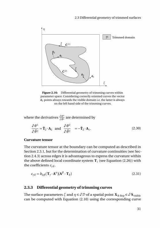
Figure 2.16: Differential geometry of trimming curves withinparameter space. Considering correctly oriented curves the vectore2 points always towards the visible domain i.e. the latter is always
on the left hand side of the trimming curves.
where the derivatives ∂ θα
∂ θ 2are determined by
∂ θ 1
∂ θ 2= T2 ·A2 and
∂ θ 2
∂ θ 2=−T2 ·A1. (2.30)
Curvature tensor
The curvature tensor at the boundary can be computed as described inSection 2.3.1, but for the determination of curvature continuities (see Sec-tion 2.4.3) across edges it is advantageous to express the curvature withinthe above defined local coordinate system Ti (see Equation (2.26)) withthe coefficients cγδ.
cγδ = bαβ (Tγ ·Aα)(Aβ · Tδ) (2.31)
2.3.3 Differential geometry of trimming curves
The surface parameters ξ and η ∈ ∂D of a spatial point X B-Rep ∈ ∂ Svisible
can be computed with Equation (2.10) using the corresponding curve
31
2 Geometric modeling and fundamentals
parameter ξ. The tangent of the trimming curve C,ξ within parameterspace can be computed as
T= C,ξ =
∂ θ 1
∂ θ 1
∂ θ 2
∂ θ 1
(2.32)
where C,ξ is the derivative of the trimming curve and the normalized tan-gent is defined by
e1 =T
T
2
. (2.33)
Assuming e1 in R3 the vector e2 ∈R3 can be computed as
e2 = e3× e1, (2.34)
with e3 ∈R3 given by
e3 =
0
0
1
. (2.35)
Figure 2.16 illustrates an example of a trimmed domain with the localorthonormal coordinate system ei .
2.4 Geometric continuities
This section deals with different orders of geometric continuity G k withk ∈ N indicating the order of continuity, across a common edge E (seeSection 2.2.4) of two adjacent faces, i.e. trimmed surfaces (see Section 2.2.3)defined by S (α)visible. The edge E as a topological entity links two boundarysubsets
∂ SE ⊂ ∂ S (α)visible, (2.36)
such that within the B-Rep description (see Section 2.2.4) they belongtogether.
32
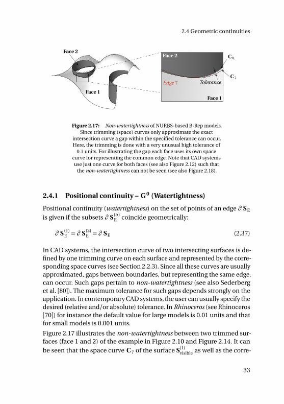
2.4 Geometric continuities
Face 1
Face 2
Face 1
Face 2
ToleranceEdge 7C 7
C 8
Figure 2.17: Non-watertightness of NURBS-based B-Rep models.Since trimming (space) curves only approximate the exact
intersection curve a gap within the specified tolerance can occur.Here, the trimming is done with a very unusual high tolerance of
0.1 units. For illustrating the gap each face uses its own spacecurve for representing the common edge. Note that CAD systemsuse just one curve for both faces (see also Figure 2.12) such that
the non-watertightness can not be seen (see also Figure 2.18).
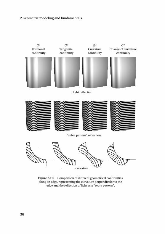
2.4.1 Positional continuity – G 0 (Watertightness)
Positional continuity (watertightness) on the set of points of an edge ∂ SE
is given if the subsets ∂ S (α)E coincide geometrically:
∂ S (1)E = ∂ S (2)E = ∂ SE (2.37)
In CAD systems, the intersection curve of two intersecting surfaces is de-fined by one trimming curve on each surface and represented by the corre-sponding space curves (see Section 2.2.3). Since all these curves are usuallyapproximated, gaps between boundaries, but representing the same edge,can occur. Such gaps pertain to non-watertightness (see also Sederberget al. [80]). The maximum tolerance for such gaps depends strongly on theapplication. In contemporary CAD systems, the user can usually specify thedesired (relative and/or absolute) tolerance. In Rhinoceros (see Rhinoceros[70]) for instance the default value for large models is 0.01 units and thatfor small models is 0.001 units.
Figure 2.17 illustrates the non-watertightness between two trimmed sur-faces (face 1 and 2) of the example in Figure 2.10 and Figure 2.14. It canbe seen that the space curve C 7 of the surface S(1)visible as well as the corre-
33
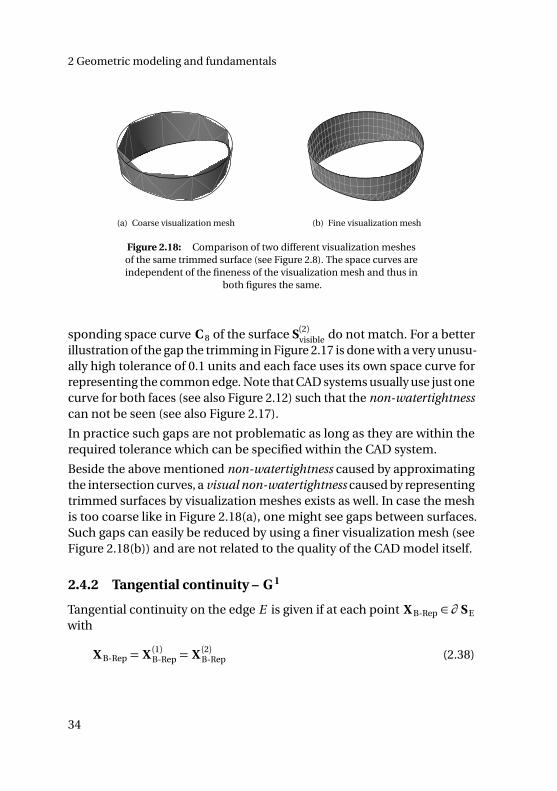
2 Geometric modeling and fundamentals
(a) Coarse visualization mesh (b) Fine visualization mesh
Figure 2.18: Comparison of two different visualization meshesof the same trimmed surface (see Figure 2.8). The space curves areindependent of the fineness of the visualization mesh and thus in
both figures the same.
sponding space curve C 8 of the surface S(2)visible do not match. For a betterillustration of the gap the trimming in Figure 2.17 is done with a very unusu-ally high tolerance of 0.1 units and each face uses its own space curve forrepresenting the common edge. Note that CAD systems usually use just onecurve for both faces (see also Figure 2.12) such that the non-watertightnesscan not be seen (see also Figure 2.17).
In practice such gaps are not problematic as long as they are within therequired tolerance which can be specified within the CAD system.
Beside the above mentioned non-watertightness caused by approximatingthe intersection curves, a visual non-watertightness caused by representingtrimmed surfaces by visualization meshes exists as well. In case the meshis too coarse like in Figure 2.18(a), one might see gaps between surfaces.Such gaps can easily be reduced by using a finer visualization mesh (seeFigure 2.18(b)) and are not related to the quality of the CAD model itself.
2.4.2 Tangential continuity – G 1
Tangential continuity on the edge E is given if at each point X B-Rep ∈ ∂ SE
with
X B-Rep = X (1)B-Rep = X (2)B-Rep (2.38)
34
2.4 Geometric continuities
the vectors T (α)1 of the locally defined coordinate systems T (α)i (see Equa-
tion (2.26)) aligned to the edge (different orientation of T (α)2 possible) pointin opposition direction.
T (1)1 =−T (2)1 (2.39)
Kinks
In the case, only the vectors T (1)2 are collinear, a kink exists with an angle
φ around T (α)2 at the corresponding position
φ =±arccos(T (1)1 · T (2)1 ) (2.40)
2.4.3 Curvature continuity – G 2
Curvature continuity on the edge E is given if at each point X B-Rep ∈ ∂ SE
besides tangential continuity also the curvature tensor, with its coefficientsc (α)αβ (see Equation (2.31)) coincides.
c (1)αβ = c (2)αβ with T (1)3 =−T (2)3
c (1)αβ =−c (2)αβ with T (1)3 = T (2)3
(2.41)
Depending on the geometric continuity, CAD models are classified to be ofstandard or high quality. The latter require a high geometrical continuitywith a low tolerance level. They are used for aesthetic purposes, such ascar bodies and consumer product outer forms. The higher geometricalcontinuity is mainly required for a better light reflection. Figure 2.19 showsthe light and zebra pattern reflection of an edge with different geometricalcontinuities, representing almost the same shape. One can see that thehigher the continuity the smoother the transition of the reflection becomes.In Figure 2.19 the "zebra pattern" reflection, which gives visual feedbackfor geometric continuities, illustrates that for G 0 the pattern is not contin-uous, for G 1 it has a kink and for G 2 and higher it is smooth. In addition,Figure 2.19 shows the curvature distribution perpendicular to the edge.
35
2 Geometric modeling and fundamentals
light reflection
"zebra pattern" reflection
G 0
Positionalcontinuity
G 1
Tangentialcontinuity
G 2
Curvaturecontinuity
G 3
Change of curvaturecontinuity
curvature
Figure 2.19: Comparison of different geometrical continuitiesalong an edge, representing the curvature perpendicular to the
edge and the reflection of light as a "zebra pattern".
36
2.4 Geometric continuities
Summary and conclusion of Chapter 2
The chapter explains NURBS-based B-Rep models which are used in in-dustry for describing complex geometrical shapes (see Figure 2.2). Thechapter explains the aspects which need to be considered for IBRA. Theseare the following:
– geometrical refinement
– description of trimmed surfaces
– trimming tolerances
– topology of complex multi-patch geometries
– geometric continuities across edges
Moreover, the chapter briefly explains the differential geometry of trimmedsurfaces as a basis for the following chapters.
37

Nature always tends to act inthe simplest way.
Daniel Bernoulli
CH
AP
TE
R
3FINITE ELEMENT METHOD FOR
STRUCTURAL SHELL ANALYSIS
This chapter briefly reviews important aspects of the finite element method(FEM) for structural shell analysis in order to differentiate
– classical finite element analysis (FEA) (see Section 3.4),
– isogeometric analysis (IGA) (see Section 3.5), and
– isogeometric B-Rep analysis (IBRA) (see Chapter 4),
w.r.t. their geometrical discretizations used for analysis. The chapter ex-plains the different element definitions used for classical FEA and IGA aswell as their shape functions, and data structures.
In addition, the different refinement strategies (h, p and k-refinement) forIGA are briefly reviewed.
39
3 Finite element method for structural shell analysis
3.1 Shell structures
Shells are thin-walled, curved structures like car bodies, roof shells or cool-ing towers. For the analysis of such structures, shell formulations are at-tractive because they concentrate on the mechanically relevant effectsand thus the computational effort can be reduced significantly. For solvingshell problems two main theories are widely used: the Reissner-Mindlin(RM) and the Kirchhoff-Love (KL) theory.
3.2 Kirchhoff-Love shell theory
Within this thesis the Kirchhoff-Love (KL) shell theory is used as basis forsolving structural shell problems. The assumptions of this theory are thefollowing:
– the director remains straight and perpendicular to the midsurfaceduring deformation
– no transverse shear deformation is taken into account
– the thickness t remains constant
– the ratio Rt of the characteristic radius R and the thickness t is larger
than 20
The geometrical description and the strong form of the static equilibriumfor KL shell problems is given in the sequel, whereas the weak form of thestatic equilibrium is described in Section 3.3.2 and Section 4.2.
3.2.1 Geometrical description
The body resp. physical domain of a KL shell can be described by theposition vector X resp. x in the reference resp. in the current configurationas follows:
X(θ 1,θ 2,θ 3) =Xsurf(θ1,θ 2) +θ 3A3,
x(θ 1,θ 2,θ 3) = xsurf(θ1,θ 2) +θ 3a3,
(3.1)
40
3.3 Finite element method
where Xsurf and xsurf are the midsurfaces in the different configurationsand θ α are the contravariant coordinates. The third contravariant coordi-nate θ 3 is the parameter for the thickness t defined in the range
− t2 ,+ t
2
,whereby t remains constant. The displacement of the physical domainbetween the two configurations can thus be described by using the dis-placement of the midsurface
usurf = xsurf− X surf. (3.2)
3.2.2 Strong form of equilibrium
The equilibrium for a geometrically nonlinear KL shell is given by the twovectorial equations in the current configuration (Basar et al. [4]) by
nα|α+p= 0,
mα|α+aα×nα = 0,(3.3)
where 2|α is the covariant derivative w.r.t. the parameters θ α, aα are thecovariant base vectors, nα (normal forces) and mα(moments) are the stressresultants derived from the Cauchy stress tensor and p is the external load.
3.3 Finite element method
Structural analysis problems, e.g. Equation (3.3) with a geometrical de-scription and appropriate boundary conditions, are usually solved with thefinite element method (FEM) by using the same discretization for geometryand solution fields (isoparametric concept – introduced by B. M. Irons [3]).
3.3.1 Definition of nomenclature
To avoid confusions in the usage of different nomenclature within FEMimportant terms are defined for this thesis as follows:
– The set of parameters A used for a function f (A) is called parameter(trimmed) domain.
– A parametric domain is the geometry defined by G(A) =∑
i f i (A)which at its turn is described by the functions f i (A) sharing the sameparameter domain A.
41
3 Finite element method for structural shell analysis
– An integration domain is a domain on which an integration scheme,e.g. Gaussian quadrature, is applied.
– With respect to the above mentioned terms a finite element is de-fined differently for classical finite element analysis (see Section 3.4.1),isogeometric analysis (Section 3.5.3) and isogeometric B-Rep analysis(Section 4.3).
3.3.2 Weak form of equilibrium
For arriving at a solution to a structural problem using approximationmethods like FEM, the internal and external forces need to be in equilib-rium in a weak sense. This can be expressed by the principle of virtualwork, which is defined as the sum of the internal and external virtual work(see also Zienkiewicz, O.C. and Taylor, R.L. and Zhu, J.Z. [94]) and is givenby
δW =δWint+δWext = 0. (3.4)
The internal and external virtual work for a KL shell in the reference config-uration on the physical domain (no boundary contributions considered –see also Section 4.2) can be formulated as follows (see also Basar et al. [4]):
δWint =−∫
Ω
N δε+M δκ
dΩ,
δWext =
∫
Ω
p δu dΩ,
(3.5)
where Ω is the midsurface of the physical domain in the reference con-figuration, N (normal force) and M (moments) are the stress resultantsderived from the 2nd Piola Kirchhoff (PK2) stress tensor, δε (virtual normalstrain) and δκ (virtual change in curvature) are the energetically conju-gated quantities derived from the virtual Green-Lagrange strain tensorall given in Voigt notation, p is the external force, and δu is the virtualdisplacement of the midsurface.
The equilibrium condition in Equation (3.4) resp. Equation (3.5) must alsobe fulfilled for the variation w.r.t. the virtual displacement field δu:
δW =∂W
∂ uδu= 0 (3.6)
42
3.3 Finite element method
3.3.3 Discretization
Applying a discretization for Equation (3.6) the equilibrium can be writtenas
δW =−R ·δuh = 0, (3.7)
which means that for an arbitrary virtual discretized displacement vectorδuh the corresponding residual force vector R must vanish. The nonlin-ear expression in Equation (3.7) is linearized to solve it with an iterativesolution approach such as the Newton-Raphson method. This results inthe linear expression
K∆u= R , (3.8)
where the tangential stiffness matrix K and the residual force R are usediteratively to obtain the displacement increment∆u until equation (3.7) issatisfied. The components of K and R are given by
Rr =−∂W
∂ ur=−
∂Wint
∂ ur−∂Wext
∂ ur=R int
r +R extr , (3.9)
Kr s =∂ Rr
∂ us=−
∂W 2
∂ ur ∂ us=−
∂W 2int
∂ ur ∂ us−∂W 2
ext
∂ ur ∂ us= K int
r s +K extr s , (3.10)
where r, s ∈N are indices used for the discretization components.
Basis functions
Following the isoparametric concept the discretized solution uh i.e. thedisplacement of the midsurface for a KL shell problem can be written as
uh = xh− X h =∑
r
Nr (xr − X r ) =
∑
r
Nr ur , (3.11)
with Nr being the basis functions, xr resp. X r the corresponding geom-etry discretization parameters in vector form, and ur the corresponding
43
3 Finite element method for structural shell analysis
variables for the displacement field uh. Considering that for the basis func-tions usually more than one parameter domain is used, the virtual workexpressions in Equation (3.5) can be computed as
δWint =−∑
k
∫
Ω(k )
N δε+M δκ
dΩ(k ),
δWext =∑
k
∫
Ω(k )p δu dΩ(k ),
(3.12)
whereΩ(k ) is the parametric domain k . Since the KL shell formulation relieson the evaluation of curvature resp. second derivatives of the shape func-tions, the formulation requires at least C 1 continuity within all parametricdomains and G 1 continuity (see also Section 4.2) across their boundaries.
The equilibrium condition in Equation (3.4) with Equation (3.5) does notconsider any virtual work contributions on boundaries of parametric do-mains and thus it requires the strong fulfillment of
– continuity on common boundaries of parametric domains i.e. tan-gential continuity G 1 including positional continuity G 0 (see alsoSection 2.4), and
– Dirichlet boundary conditions.
Neither classical finite element analysis (FEA), which usually uses Lagrangepolynomials as basis functions, nor the NURBS-based isogeometric analy-sis (IGA) fulfill these requirements. The advantage of NURBS-based IGA isthat one parametric domain i.e. a NURBS geometry (see also Section 2.2.1)resp. patch is able to represent a large amount of complex shapes andalso allows for an accurate approximation of the solution field due to thepossibility of geometry refinement (see also Section 2.2.2).
Classical FEA with its low order polynomials is mainly restricted to RM shellformulations which only require G 0 continuity across parametric domains.The latter can be achieved easily by sharing degrees of freedom (DOFs) atcommon boundaries. In contrast to that for NURBS-based IGA a strongfulfillment of G 0 across parametric domains represents a huge restrictionin geometric modeling and analysis because it requires matching patchesover the entire physical domain. Nevertheless the high continuity within
44
3.4 Classical finite element analysis (FEA)
patches allows for KL shell formulations (see Kiendl et al. [44]) as well asmatching multi-patch geometries by using the bending-strip method (seeKiendl [46]).
Chapter 4 explains how these limitations for design and analysis can beovercome by considering virtual work contributions on arbitrarily definedboundaries of parametric domains which finally allow for the direct analy-sis of surface CAD models. As reference for Chapter 4 the following sectionsbriefly explain the geometry description of surface models for classicalFEA and IGA.
3.4 Classical finite element analysis (FEA)
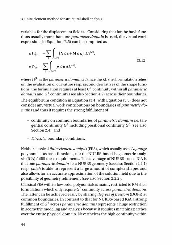
The classical finite element analysis usually uses linear polynomials forsolving RM shell problems, whereby they are used as basis for representinggeometry and solution fields (isoparametric concept). The basis functionNi of a node i (see also Figure 3.1) is given by
Ni =⋃
k
N (k )i with k ∈N (3.13)
where k is the index used for the parametric domains, which contributeto node i , and N (k )
i are the corresponding shape functions (see also Fig-ure 3.1(b)).
3.4.1 Definition of classical finite elements
In classical FEA an element is described by a parametric domain whoseparameter domain coincides with the integration domain (see also Sec-tion 3.3.1). This definition of an element usually leads to fully populatedelement stiffness matrices and allows for a simple and efficient implemen-tation.
3.4.2 Geometry description (finite element mesh)
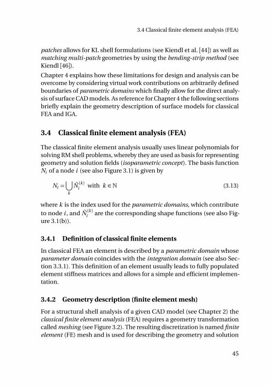
For a structural shell analysis of a given CAD model (see Chapter 2) theclassical finite element analysis (FEA) requires a geometry transformationcalled meshing (see Figure 3.2). The resulting discretization is named finiteelement (FE) mesh and is used for describing the geometry and solution
45
3 Finite element method for structural shell analysis
Node i
Ni
(a) Basis function of node i as a composition of bilinear shape functions (b) of adjacentparametric domains (elements)
N1 =14 (1+ξ)(1+η) N2 =
14 (1−ξ)(1+η)
N3 =14 (1−ξ)(1−η) N4 =
14 (1+ξ)(1−η)
ξ
η
ξ
η η
ξ
ξ
ηLocal node 1
Local node 2
Local node 3
Local node 4
for node i
(b) Bilinear shape functions of a quadrilateral element
Figure 3.1: Example of a basis function used within classical FEA
46
3.4 Classical finite element analysis (FEA)
(a) CAD (NURBS-based B-Rep) model of an oil sump
(b) A corresponding finite element mesh
Figure 3.2: Comparison of a CAD geometry and a classical FEgeometry discretization representing the same object. The
operation of creating a FE mesh from a CAD model is calledmeshing.
47
3 Finite element method for structural shell analysis
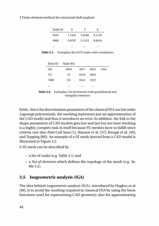
Node ID X Y Z
2016 1.2452 5.6546 8.1116
4908 9.8787 5.1315 8.8454
... ... ... ...
Table 3.1: Exemplary list of FE nodes with coordinates
Elem ID Node IDs
342 2016 2017 3015 1554
757 15 6476 3645
7588 151 6541 2415
... ... ... ...
Table 3.2: Exemplary list of elements with quadrilateral andtriangular elements
fields. Since the discretization parameters of the classical FEA use low orderLagrange polynomials, the meshing represents just an approximation ofthe CAD model and thus it introduces an error. In addition, the link to theshape parameters of CAD models gets lost and last but not least meshingis a highly complex task in itself because FE meshes have to fulfill strictcriteria (see also Abel Coll Sans [1], Hansen et al. [37], Knupp et al. [49],and Topping [89]). An example of a FE mesh derived from a CAD model isillustrated in Figure 3.2.
A FE mesh can be described by
– a list of nodes (e.g. Table 3.1) and
– a list of elements which defines the topology of the mesh (e.g. Ta-ble 3.2).
3.5 Isogeometric analysis (IGA)
The idea behind isogeometric analysis (IGA), introduced by Hughes et al.[40], is to avoid the meshing required in classical FEA by using the basisfunctions used for representing CAD geometry also for approximating
48
3.5 Isogeometric analysis (IGA)
solution fields. Usually, IGA is based on NURBS because these represent thestandard for geometry description in current CAD systems (see Chapter 2).A detailed description of NURBS basis functions and surfaces is given inSection 2.2.1. Since NURBS surfaces used for representing the shape ofan object are usually not able to represent solution fields with a satisfyingaccuracy, NURBS surfaces need to be refined resp. enriched with controlpoints (see also Section 2.2.2). Note that such a refinement neither affectsthe initial shape nor its parametrization.
3.5.1 h-,p-,h-p-, and k-refinement
Depending on the sequence of applying knot insertion and degree elevationone distinguishes between h-,p-,h-p, and k-refinement (see also Cottrellet al. [24] and Hughes et al. [40]):
– For h-refinement additional single knots are added to the knot vectorbut no degree elevation is performed. Note that each inserted knotreduces the continuity C at its position.
– p-refinement is achieved by performing degree elevation, with theresult that the polynomial degree within each non-zero knot span isincreased without modifying the continuities at knots.
– h-p-refinement is achieved by performing degree elevation after h-refinement, with the result that the polynomial degree within eachnon-zero knot span is increased without modifying the continuitiesat knots.
– k-refinement is achieved by first applying degree elevation and thenknot insertion. With this sequence one ends up with the same num-ber of non-zero knot spans as with h-refinement and the same poly-nomial degree as with p-refinement but with a higher continuitybetween non-zero knot spans than h-p-refinement.
Since high continuity is beneficial for KL shell analysis, k-refinement isassumed in the sequel.
49
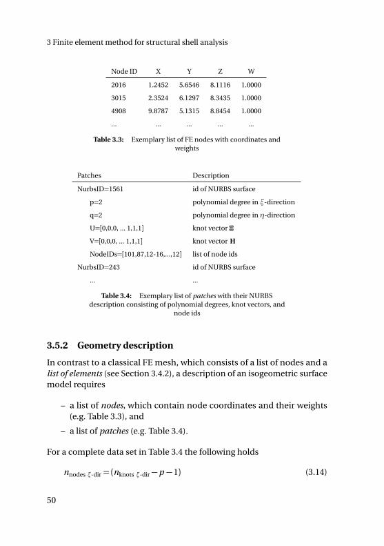
3 Finite element method for structural shell analysis
Node ID X Y Z W
2016 1.2452 5.6546 8.1116 1.0000
3015 2.3524 6.1297 8.3435 1.0000
4908 9.8787 5.1315 8.8454 1.0000
... ... ... ... ...
Table 3.3: Exemplary list of FE nodes with coordinates andweights
Patches Description
NurbsID=1561 id of NURBS surface
p=2 polynomial degree in ξ-direction
q=2 polynomial degree in η-direction
U=[0,0,0, ... 1,1,1] knot vector Ξ
V=[0,0,0, ... 1,1,1] knot vector H
NodeIDs=[101,87,12-16,...,12] list of node ids
NurbsID=243 id of NURBS surface
... ...
Table 3.4: Exemplary list of patches with their NURBSdescription consisting of polynomial degrees, knot vectors, and
node ids
3.5.2 Geometry description
In contrast to a classical FE mesh, which consists of a list of nodes and alist of elements (see Section 3.4.2), a description of an isogeometric surfacemodel requires
– a list of nodes, which contain node coordinates and their weights(e.g. Table 3.3), and
– a list of patches (e.g. Table 3.4).
For a complete data set in Table 3.4 the following holds
nnodes ξ-dir = (nknots ξ-dir−p −1) (3.14)
50
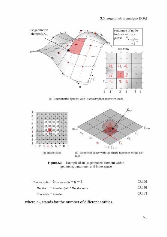
3.5 Isogeometric analysis (IGA)
ξ
η
isogeometricelement Ω4,4
top view
1 2 3 4 5 6
8 9 10
14 15 16
7
20 21 22
sequence of nodeindices within apatch
ξ
η
(a) Isogeometric element with its patch within geometry space
1 2 3 4 5 6 7 812
i
j
3
5678
z z z z z z z zz z z z z z z zz z in in in in z zz z in in in in z zz z in in in in z zz z in in in in z zz z z z z z z zz z z z z z z z
4
(b) Index space
ξ1−3
ξ4
ξ5
ξ6
ξ7−9
η1−3
η5
η6
η7−9
η4
Ω4,4
(c) Parameter space with the shape functions of the ele-ment
Figure 3.3: Example of an isogeometric element withingeometry, parameter, and index space
nnodes η-dir = (nknots η-dir−q −1) (3.15)
nnodes = nnodes ξ-dir ·nnodes η-dir (3.16)
nnode ids = nnodes (3.17)
where n2 stands for the number of different entities.
51
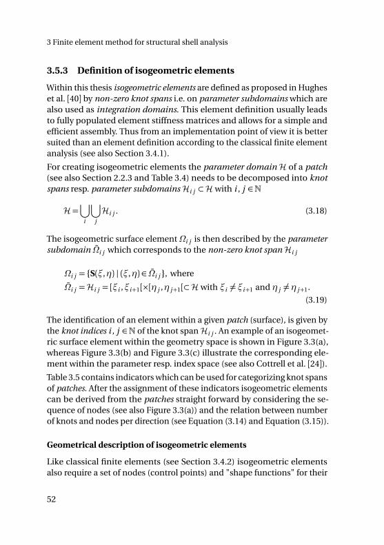
3 Finite element method for structural shell analysis
3.5.3 Definition of isogeometric elements
Within this thesis isogeometric elements are defined as proposed in Hugheset al. [40] by non-zero knot spans i.e. on parameter subdomains which arealso used as integration domains. This element definition usually leadsto fully populated element stiffness matrices and allows for a simple andefficient assembly. Thus from an implementation point of view it is bettersuited than an element definition according to the classical finite elementanalysis (see also Section 3.4.1).
For creating isogeometric elements the parameter domain H of a patch(see also Section 2.2.3 and Table 3.4) needs to be decomposed into knotspans resp. parameter subdomains Hi j ⊂H with i , j ∈N
H=⋃
i
⋃
j
Hi j . (3.18)
The isogeometric surface element Ωi j is then described by the parametersubdomain Ωi j which corresponds to the non-zero knot span Hi j
Ωi j = S(ξ,η) | (ξ,η) ∈ Ωi j , where
Ωi j =Hi j = [ξi ,ξi+1[×[η j ,η j+1[⊂H with ξi 6= ξi+1 and η j 6=η j+1.
(3.19)
The identification of an element within a given patch (surface), is given bythe knot indices i , j ∈N of the knot span Hi j . An example of an isogeomet-ric surface element within the geometry space is shown in Figure 3.3(a),whereas Figure 3.3(b) and Figure 3.3(c) illustrate the corresponding ele-ment within the parameter resp. index space (see also Cottrell et al. [24]).
Table 3.5 contains indicators which can be used for categorizing knot spansof patches. After the assignment of these indicators isogeometric elementscan be derived from the patches straight forward by considering the se-quence of nodes (see also Figure 3.3(a)) and the relation between numberof knots and nodes per direction (see Equation (3.14) and Equation (3.15)).
Geometrical description of isogeometric elements
Like classical finite elements (see Section 3.4.2) isogeometric elementsalso require a set of nodes (control points) and "shape functions" for their
52
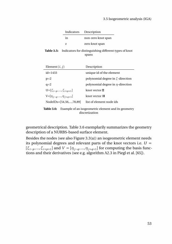
3.5 Isogeometric analysis (IGA)
Indicators Description
in non-zero knot span
z zero knot span
Table 3.5: Indicators for distinguishing different types of knotspans
Element (i , j ) Description
id=1433 unique id of the element
p=2 polynomial degree in ξ-direction
q=2 polynomial degree in η-direction
U=[ξi−p , ...,ξi+p+1] knot vector Ξ
V=[η j−q , ...,η j+q+1] knot vector H
NodeIDs=[54,56,...,78,89] list of element node ids
Table 3.6: Example of an isogeometric element and its geometrydiscretization
geometrical description. Table 3.6 exemplarily summarizes the geometrydescription of a NURBS-based surface element.
Besides the nodes (see also Figure 3.3(a)) an isogeometric element needsits polynomial degrees and relevant parts of the knot vectors i.e. U =[ξi−p , ...,ξi+p+1] and V = [η j−q , ...,η j+q+1] for computing the basis func-tions and their derivatives (see e.g. algorithm A2.3 in Piegl et al. [65]).
53
3 Finite element method for structural shell analysis
Summary and conclusion of Chapter 3
This chapter explains the difference between classical FEA and IGA w.r.t.to their geometry discretizations used for analysis and serves as referencefor IBRA (see Chapter 4). The geometrical element description used forclassical FEA and IGA, including their shape functions and possible datastructures are explained as well.
IGA in its original form provides the basis for developing element for-mulations capable of analyzing CAD models but it does not provide theframework for handling the topology of complex (trimmed multi-patch)CAD models (see also Chapter 2). This gap will be closed with the newisogeometric B-Rep analysis (IBRA) which is explained in Chapter 4 forgeometrically nonlinear KL shell problems.
54
"Das geht nicht." Dann kameiner, der wusste das nicht,und hat es gemacht.
Hilbert Meyer,Professor für Schulpädagogikan der Universität Oldenburg
CH
AP
TE
R
4ISOGEOMETRIC B-REP ANALYSIS
Isogeometric B-Rep analysis (IBRA) introduced by Breitenberger et al. [17]is a finite element approach which enables the direct analysis on surfaceCAD models (see also Section 2.2). IBRA extends isogeometric analysis(IGA), introduced by Hughes et al. [40] (see also Section 3.5), by adaptingthe basis functions as well as the B-Rep description of the CAD model forapproximating solution fields. IBRA provides a consistent framework todeal with the geometry and topology of CAD models for structural analysisin a finite-element-like manner and closes the gap between CAD modelsand the finite element method (FEM).
The chapter explains IBRA for geometrically nonlinear Kirchhoff-Love (KL)shell problems. A data structure for isogeometric (trimmed) elements as wellas for B-Rep elements is proposed. Moreover, a B-Rep element formulationbased on a penalty approach is introduced which can be used to couplediscontinuous and trimmed geometries and to enforce Dirichlet boundaryconditions.
55
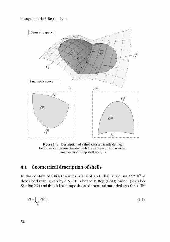
4 Isogeometric B-Rep analysis
Geometry space
Parametric space
Ω(1)
Ω(2)
Γ (1)c
Γ (1)d
Γ (2)n
Γ (2)c
Γ (2)n
Γ (1)d Γ (2)c
Ω(2)Ω(1)
Γ (1)c
H(1) H(2)
Figure 4.1: Description of a shell with arbitrarily definedboundary conditions denoted with the indices c,d, and n within
isogeometric B-Rep shell analysis
4.1 Geometrical description of shells
In the context of IBRA the midsurface of a KL shell structure Ω ⊂ R3 isdescribed resp. given by a NURBS-based B-Rep (CAD) model (see alsoSection 2.2) and thus it is a composition of open and bounded setsΩ(a ) ⊂R3
Ω =⋃
a
Ω(a ), (4.1)
56
4.2 Weak form of equilibrium
with a ∈ N (see also Figure 4.1). Each subset Ω(a ) is represented by onetrimmed surface S (a )visible and its boundary Γ (a ) by ∂ S (a )visible. The correspond-ing trimmed domains and trimming curves are denoted with Ω(a ) =D(a ) ⊂H(a ) and Γ (a ) = ∂ Ω(a ) in the parameter space, respectively (see also Sec-tion 2.3). Figure 4.1 exemplarily shows a shell in geometry and parameterspace, with a decomposition of the boundaries Γ (a ) resp. Γ (a ) into subsets:
Γ (a ) =
⋃
k
Γ (a ) kd
∪
⋃
l
Γ (a ) ln
∪
⋃
m
Γ (a ) mc
,
Γ (a ) =
⋃
k
Γ (a ) kd
∪
⋃
l
Γ (a ) ln
∪
⋃
m
Γ (a ) mc
,
(4.2)
where the following indices are used for expressing the different types ofboundary conditions:
– d for Dirichlet boundary conditions (e.g. displacement, rotation)
– n for Neumann boundary conditions (e.g. pressure load)
– c for coupling (internal) boundary conditions (preservation of conti-nuities)
Mechanical boundary formulations like cables (see Philipp et al. [63]) orbeams (see Bauer et al. [5]) are not considered in the remainder of thisthesis. An example of an internal boundary is shown in Figure 4.1 wherethe sets Ω(1) and Ω(2) share a common boundary Γc
Γc = Γ(1)c = Γ
(2)c . (4.3)
4.2 Weak form of equilibrium
In contrast to classical FEA and IGA isogeometric B-Rep analysis (IBRA)requires the consideration of virtual work contributions along domainboundaries because a strong fulfillment of Dirichlet boundary conditionson arbitrarily defined trimming curves is not possible (see also Section 3.3).
57
4 Isogeometric B-Rep analysis
The weak form of the static equilibrium in Equation (3.3) for a geometricallynonlinear KL shell including boundary terms is given by (see Basar et al.[4], Eq. 8.3.141 – other notation is used)
δW =
∫
Ω
p δu dΩ−∫
Ω
N δε+M δκ dΩ
+
∫
Γ
nΓδu+mT2δωT2
dΓ .
(4.4)
The first two integrals are the same as they are already used in Equa-tion (3.12). The third one represents the virtual work contribution on thedomain boundary with nΓ (traction force) and mT2
(moment around theboundary tangent T2) being the stress resultants derived from the 1st Piola-Kirchhoff (PK1) stress tensor using the local coordinate system as it isdefined in Equation (2.26). The term δωT2
expresses the virtual rotationaround the local base vector T2 on the boundary (see also Figure 4.5). TherotationωT2
is given by
ωT2= arcsin(ω ·T2), (4.5)
whereω is the rotation vector (see Basar et al. [4]) that is defined as
ω= T3×w, (4.6)
with w being the displacement of the tip of the local base vector t3 in thecurrent configuration, given by
w= t3−T3. (4.7)
Because the arcsin function is involved, the rotations at the shell bound-aries are restricted to be less than Π
2 .
4.2.1 Equilibrium along internal boundaries
Considering common internal boundaries as exemplarily given in Equa-tion (4.3) the equilibrium needs to be fulfilled also on those boundariesand is given by
nΓ =n(1)Γ =−n(2)Γ (4.8)
58
4.2 Weak form of equilibrium
for the traction forces and for the moments it is given by
mT2=m (1)
T2=±m (2)
T2. (4.9)
Note that the traction forces n(α)Γ point in opposite directions and the signin Equation (4.9) depends on how the tangent vectors T2 of the involvedboundary curves are oriented with respect to each other. The negative signis used in the case that both tangent vectors T2 point in the same direction.
The virtual work along a common internal boundary can thus be computedas follows
δW displacementcoupling =
∫
Γ (1)c
nΓ (δu(1)−δu(2)) dΓ (1)c , (4.10)
δW rotationcoupling =
∫
Γ (1)c
mT2(δω(1)T2
±δω(2)T2) dΓ (1)c , (4.11)
using the sign convention explained above. Applying a test function δuwhich fulfills the required continuity conditions
– G 0 continuity for Equation (4.10)
– G 1 continuity for Equation (4.11)
The corresponding virtual work term for coupling geometrical continuityalong element edges vanishes. For isogeometric B-Rep analysis (IBRA) thetest function (NURBS-based B-Rep model) is not able to meet these re-quirements thus the corresponding boundary terms need to be consideredfor analysis.
As a remark, for RM shells within classical FEA the boundary terms can beneglected because the test function fulfills the required G 0 continuity (seealso Section 3.4) by sharing all DOFs at common elements.
4.2.2 Equilibrium used for isogeometric B-Rep analysis
In the context of IBRA for KL shell problems the virtual work contributionson the boundaries (see third integral in Equation (3.5) , Equation (4.10),and Equation (4.11)) are collected within the expression δWB-Rep becausetheir geometrical description is provided by the entities of the boundary
59
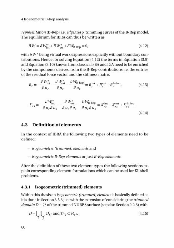
4 Isogeometric B-Rep analysis
representation (B-Rep) i.e. edges resp. trimming curves of the B-Rep model.The equilibrium for IBRA can thus be written as
δW =δW ∗int+δW ∗
ext+δWB-Rep = 0, (4.12)
with δW ∗ being virtual work expressions explicitly without boundary con-tributions. Hence for solving Equation (4.12) the terms in Equation (3.9)and Equation (3.10) known from classical FEA and IGA need to be enrichedby the components derived from the B-Rep contributions i.e. the entriesof the residual force vector and the stiffness matrix
Rr =−∂W ∗
int
∂ ur−∂W ∗
ext
∂ ur−δWB-Rep
∂ ur=R int
r +R extr +R B-Rep
r , (4.13)
Kr s =−∂W ∗
int
∂ ur ∂ us−∂W ∗
ext
∂ ur ∂ us−∂WB-Rep
∂ ur ∂ us= K int
r s +K extr s +K B-Rep
r s .
(4.14)
4.3 Definition of elements
In the context of IBRA the following two types of elements need to bedefined:
– isogeometric (trimmed) elements and
– isogeometric B-Rep elements or just B-Rep elements.
After the definition of these two element types the following sections ex-plain corresponding element formulations which can be used for KL shellproblems.
4.3.1 Isogeometric (trimmed) elements
Within this thesis an isogeometric (trimmed) element is basically defined asit is done in Section 3.5.3 just with the extension of considering the trimmeddomain D ⊂H of the trimmed NURBS surface (see also Section 2.2.3) with
D =⋃
i
⋃
j
Di j and Di j ⊂Hi j . (4.15)
60
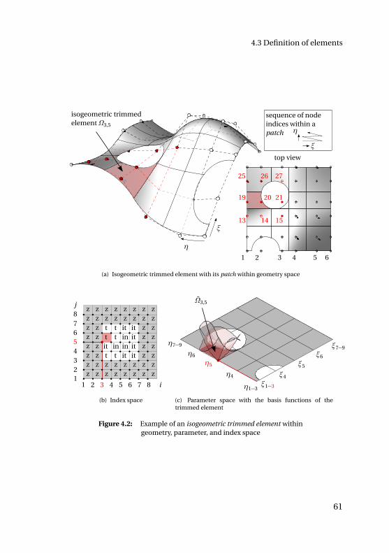
4.3 Definition of elements
ξ
η
isogeometric trimmedelement Ω3,5
top view
1 2 3 4 5 6
13 14 15
19 20 21
25 26 27
sequence of nodeindices within apatch
ξ
η
(a) Isogeometric trimmed element with its patch within geometry space
1 2 3 4 5 6 7 812
i
j
3
5678
z z z z z z z zz z z z z z z zz z t t it it z zz z it in in it z zz z t t in it z zz z t t it it z zz z z z z z z zz z z z z z z z
4
(b) Index space
ξ1−3
ξ4
ξ5
ξ6
ξ7−9
η1−3
η5
η6
η7−9
Ω3,5
η4
(c) Parameter space with the basis functions of thetrimmed element
Figure 4.2: Example of an isogeometric trimmed element withingeometry, parameter, and index space
61
4 Isogeometric B-Rep analysis
An isogeometric (trimmed) surface element Ωi j is thus described by a sub-domain Ωi j which corresponds to the trimmed domain of the non-zeroknot span Hi j with
Ωi j = Svisible(ξ,η) | (ξ,η) ∈ Ωi j , where
Ωi j =Di j ⊂ [ξi ,ξi+1[×[η j ,η j+1[⊂H with and ξi 6= ξi+1 η j 6=η j+1.
(4.16)
Note that in contrast to isogeometric elements as defined in Section 3.5.3the numerical integration of isogeometric trimmed elements can require theusage of more than just one integration domain I (h )i j (see also Section 5.4.2)such that
Hi j =⋃
h
I (h )i j (4.17)
where the following holds
Di j =⋃
h
D(h )i j with D(h )i j ⊂ I (h )i j (4.18)
An example of an isogeometric trimmed surface element within the geome-try space is shown in Figure 4.2(a), whereas Figure 4.2(b) and Figure 4.2(c)illustrate the corresponding element within the parameter resp. indexspace. The indicators applied within the index space are used for catego-rizing knot spans of the patch. Table 4.1 contains an overview of possibleindicators for such a categorization. The first three indicators describeactive elements which contribute to the virtual work expression in Equa-tion (3.5) and the rest describes inactive elements. The fine distinctionwithin active resp. inactive elements allows for a more efficient numericalintegration resp. a better visualization of analysis results.
Geometrical description of isogeometric (trimmed) elements
In addition to a set of nodes and "shape functions" (compare Table 3.4)isogeometric trimmed elements require a set of properly oriented (trimmed)curve segments which lie inside the element and define the visible domainof the element. The additional flag FaceNormal ∈ TRUE, FALSE indicates
62
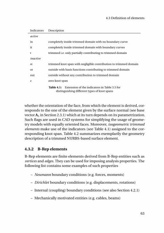
4.3 Definition of elements
Indicators Description
active
in completely inside trimmed domain with no boundary curve
it completely inside trimmed domain with boundary curves
t trimmed i.e. only partially contributing to trimmed domain
inactive
st trimmed knot span with negligible contribution to trimmed domain
ot outside with basis functions contributing to trimmed domain
out outside without any contribution to trimmed domain
z zero knot span
Table 4.1: Extension of the indicators in Table 3.5 fordistinguishing different types of knot spans
whether the orientation of the face, from which the element is derived, cor-responds to the one of the element given by the surface normal (see basevector A3 in Section 2.3.1) which at its turn depends on its parametrization.Such flags are used in CAD systems for simplifying the usage of geome-try models with equally oriented faces. Moreover, isogeometric trimmedelements make use of the indicators (see Table 4.1) assigned to the cor-responding knot span. Table 4.2 summarizes exemplarily the geometrydescription of a trimmed NURBS-based surface element.
4.3.2 B-Rep elements
B-Rep elements are finite elements derived from B-Rep entities such asvertices and edges. They can be used for imposing analysis properties. Thefollowing list contains some examples of such properties
– Neumann boundary conditions (e.g. forces, moments)
– Dirichlet boundary conditions (e.g. displacements, rotations)
– Internal (coupling) boundary conditions (see also Section 4.2.1)
– Mechanically motivated entities (e.g. cables, beams)
63
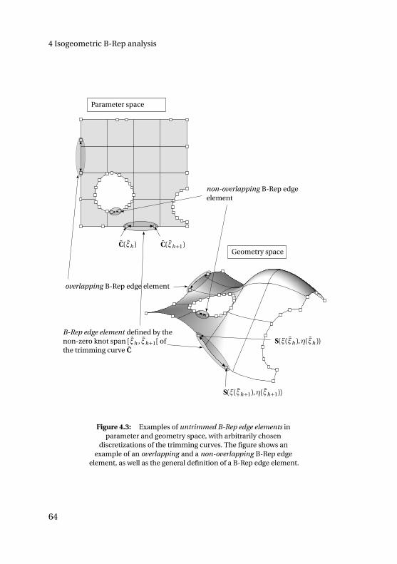
4 Isogeometric B-Rep analysis
B-Rep edge element defined by thenon-zero knot span [ξh , ξh+1[ ofthe trimming curve C
Geometry space
Parameter space
C(ξh ) C(ξh+1)
S(ξ(ξh ),η(ξh ))
S(ξ(ξh+1),η(ξh+1))
overlapping B-Rep edge element
non-overlapping B-Rep edgeelement
Figure 4.3: Examples of untrimmed B-Rep edge elements inparameter and geometry space, with arbitrarily chosen
discretizations of the trimming curves. The figure shows anexample of an overlapping and a non-overlapping B-Rep edge
element, as well as the general definition of a B-Rep edge element.
64
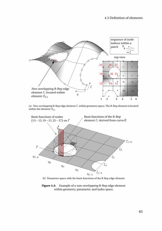
4.3 Definition of elements
ξ
η
Non-overlapping B-Rep edgeelement Γi located withinelement Ω3,5
top view
1 2 3 4 5 6
13 14 15
19 20 21
25 26 27
sequence of nodeindices within apatch
ξ
η
(a) Non-overlapping B-Rep edge element Γi within geometry space. The B-Rep element is locatedwithin the element Ω3,5
ξ1−3
ξ4
ξ5
ξ6
ξ7−9
η1−3
η5
η6
η7−9
η4
Basis functions of the B-Repelement Γi derived from curve C
1
Γ
Basis functions of nodes13−15, 19−21, 25−27 on Γ
(b) Parameter space with the basis functions of the B-Rep edge element
Figure 4.4: Example of a non-overlapping B-Rep edge elementwithin geometry, parameter, and index space.
65

4 Isogeometric B-Rep analysis
Element (i , j ) Description
id=2345 id of the element
p=2 polynomial degree in ξ-direction
q=2 polynomial degree in η-direction
U=[ξi−p ,ξi+p+1] knot vector Ξ
V=[η j−q ,η j+q+1] knot vector H
NodeIDs=[54,56,...,78,89] list of element node ids
FaceNormal=true flag used for face orientation
Indicator=t indicator from Table 4.1
Curve segments id [ξstart,ξend] curve id and active range
23 [0,0.3]
...
Table 4.2: Example of an isogeometric trimmed element and itsgeometry discretization
The basis functions of NURBS-based B-Rep elements adapt the propertiesof their underlying functional basis (see also Section 2.2.1) like
– partition of unity, i.e.∑n
i=1 Ni ,p (ξ) = 1.
– non-negativity, i.e. Ni ,p (ξ)¾ 0.
– linear independence, i.e.∑n
i=1αi Ni ,p (ξ) = 0 ⇔ αi = 0, i = 1, 2, ..., n
because they are defined on subsets of the functional parameter domain.
4.3.3 B-Rep edge elements
A B-Rep edge element Γi is a one-dimensional B-Rep element embeddedinto a surface description. It is defined by the parameter subdomain Γi
which corresponds to the non-zero knot span Hi of the trimming curve C(see also Section 2.2.3)
Γi = ∂ Svisible(ξ,η) | (ξ,η) ∈ Γi , where
Γi = C(ξ)|ξ ∈Hi = [ξi , ξi+1[⊂Ξwith ξi 6= ξi+1.(4.19)
66
4.3 Definition of elements
In this thesis, B-Rep edge elements are embedded into NURBS surfacesand make use of the basis functions from these surfaces. Figure 4.3 showsexamples of such elements. For B-Rep elements one distinguishes betweennon-overlapping and overlapping elements. Non-overlapping elementsextract the non-zero basis functions from only one underlying isogeo-metric element but overlapping elements extract them from more thanone underlying elements. Figure 4.4(b) exemplarily illustrates the basisfunctions of a non-overlapping B-Rep edge element. Usually, no explicitdescription of these basis functions is available, but this is not required forIBRA because only the evaluation at quadrature points is necessary.
B-Rep edge element Description
id=234 id of the B-Rep element
CurveID=44 id of trimming curve
Range=[0, 0.5] active range where the B-Rep element is defined
ElementID=23 id of the underlying surface element
Table 4.3: Example of a trimmed non-overlapping B-Rep edgeelement description which can be used for free edges i.e. no
coupling
B-Rep edge element Description
id=433 id of the B-Rep element
master
CurveID=165 id of the trimming curve (master)
Range=[0, 0.1] active range of master curve where the element is defined
ElementID=11 id of the underlying surface element (master)
slave
CurveID=44 id of the trimming curve (slave)
Range=[0.4, 0.3] active range of slave curve where the element is defined
ElementID=12 id of the underlying surface element (slave)
Table 4.4: Example of the description of a trimmednon-overlapping B-Rep edge coupling element
67
4 Isogeometric B-Rep analysis
Description of trimmed B-Rep edge elements
In analogy to trimmed curves (see Section 2.2.3) B-Rep elements can alsobe trimmed. The variable Range in Table 4.3 extends B-Rep edge elementsby the trimming concept. Trimmed B-Rep edge elements are more flexiblew.r.t. the definition of non-overlapping B-Rep edge elements and make arefinement of trimming curves unnecessary.
Description of trimmed B-Rep edge coupling elements
B-Rep edge coupling elements establish a connection between isogeometric(trimmed) elements of different patches. Table 4.3 describes exemplarily atrimmed B-Rep edge element. A description of a trimmed coupling B-Repedge element is given in Table 4.4.
B-Rep vertex element Description
id=24 id of the B-Rep element
u=0.86 ξ parameter which describes the position of the element
v=0.67 η parameter which describes the position of the element
ElementID=3 surface element id
Table 4.5: Example of a B-Rep vertex element description
4.3.4 B-Rep vertex elements
A B-Rep vertex element is defined by the surface parameters which describethe geometrical position of the vertex element. Table 4.5 contains theexemplarily description of such an element. A vertex element can also beextended for a pointwise coupling of patches analog to the edge couplingelements (see Section 4.3.3).
4.4 NURBS-based Kirchhoff-Love shell formulation
The element formulation for geometrically nonlinear KL problems can bederived from the internal virtual work (see also Equation (3.5)) given by
δWint =
∫
Ω
N δε+M δκ dΩ. (4.20)
68
4.5 B-Rep edge element formulations
For a detailed description of such a shell element formulation, using aNURBS discretization, the reader is referred to Kiendl [46].
4.4.1 Alternative shell formulations
Besides the NURBS-based KL shell formulation of Kiendl et al. [44] thereare also other NURBS-based shell formulations available like the RM shellformulations of Benson et al. [12] and Dornisch et al. [30, 31], the hierar-chical shell formulation of Echter et al. [33] or the blended shell of Bensonet al. [11]which can also be used for IBRA.
4.5 B-Rep edge element formulations
This section explains a B-Rep edge element formulation which can beused for coupling parameteric domains (see also Equation (4.10) and Equa-tion (4.11)). It is based on a penalty approach and can be used for geometri-cally nonlinear KL shell problems (see Breitenberger et al. [17]). Alternativeformulations are possible of course.
4.5.1 Internal boundary conditions – penalty approach
The virtual work contribution for the proposed element formulation canbe written as follows:
δW couplingB-Rep =δW disp
B-Rep+δW rotB-Rep, (4.21)
where δW dispB-Rep and δW rot
B-Rep represent the terms in Equation (4.10) andEquation (4.11).
Applying a penalty approach, the traction force nΓ in the boundary isassumed to be
nΓ =−αdisp(u(1)B-Rep−u(2)B-Rep), (4.22)
where αdisp is the penalty factor which can be seen as spring stiffness andis selected manually. Guidelines for selecting an appropriate penalty factor
69
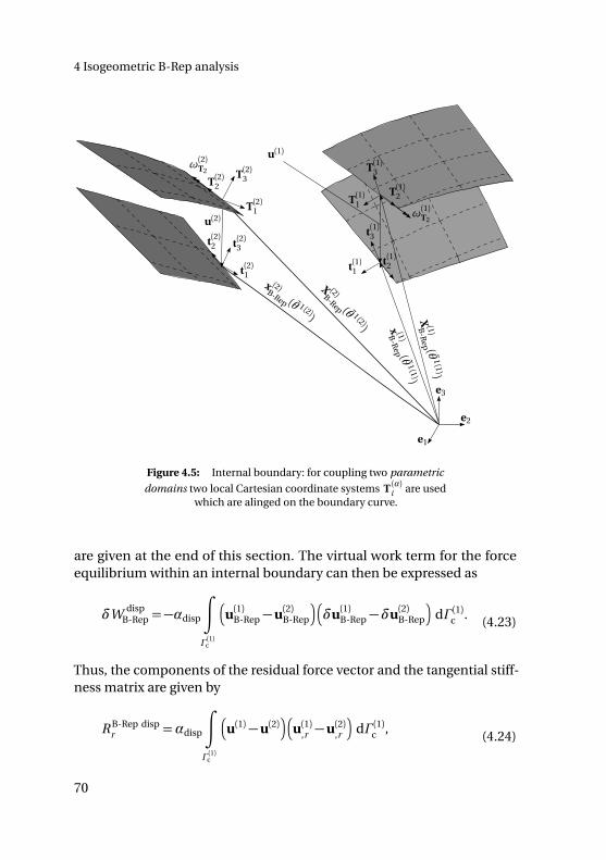
4 Isogeometric B-Rep analysis
X (2)B-Rep ( ˜θ 1 (2)) x (1)B-R
ep (θ1 (1))
x (2)B-Rep (θ 1 (2)) X(1)B
-Rep (θ
1 (1))
T(1)1
T(1)3
T(1)2
t(1)1
t(1)3
t(1)2
T(2)3
T(2)1
t(2)2
t(2)1
u(2)
T(2)2
t(2)3
u(1)
ω(1)T2
ω(2)T2
e1
e2
e3
Figure 4.5: Internal boundary: for coupling two parametric
domains two local Cartesian coordinate systems T (α)i are usedwhich are alinged on the boundary curve.
are given at the end of this section. The virtual work term for the forceequilibrium within an internal boundary can then be expressed as
δW dispB-Rep =−αdisp
∫
Γ (1)c
u(1)B-Rep−u(2)B-Rep
δu(1)B-Rep−δu(2)B-Rep
dΓ (1)c . (4.23)
Thus, the components of the residual force vector and the tangential stiff-ness matrix are given by
R B-Rep dispr =αdisp
∫
Γ (1)c
u(1)−u(2)
u(1),r −u(2),r
dΓ (1)c , (4.24)
70
4.5 B-Rep edge element formulations
K B-Rep dispr s =αdisp
∫
Γ (1)c
u(1),s −u(2),s
·
u(1),r −u(2),r
dΓ (1)c . (4.25)
Applying a penalty approach, the moment along the boundary mT2is as-
sumed to be
mT2=−αrot(ω
(1)T2−ω(2)T2
), (4.26)
where αrot is the penalty factor which can be seen as a rotational springstiffness and is selected manually as well (see also end of this section).
The virtual work term for the moment equilibrium within an internalboundary (see also Section 2.3.2) can be expressed as
δW rotB-Rep =−αrot
∫
Γ (1)c
ω(1)T2±ω(2)T2
δω(1)T2±δω(2)T2
dΓ (1)c (4.27)
and its residual force vector and the tangential stiffness matrix componentsare
R B-Rep rotr =αrot
∫
Γ (1)c
ω(1)T2±ω(2)T2
ω(1)T2,r ±ω(2)T2,r
dΓ (1)c , (4.28)
K B-Rep rotr s =αrot
∫
Γ (1)c
h
ω(1)T2,s ±ω(2)T2,s
ω(1)T2,r ±ω(2)T2,r
+
ω(1)T2±ω(2)T2
ω(1)T2,r s ±ω(2)T2,r s
i
dΓ (1)c .
(4.29)
The first and second variations of the rotation ωT2(Equation (4.5)) are
given by
ωT2,r =ω,r ·T2
p
1− (ω ·T2)2, (4.30)
71
4 Isogeometric B-Rep analysis
ωT2,r s =ω,r s ·T2
p
1− (ω ·T2)2+(ω,r ·T2)(ω ·T2)(ω,s ·T2)
1− (ω ·T2)2
32
, (4.31)
where the variations of the rotation vectorω (Equation (4.6)) and the dis-placement w (Equation (4.7)) are given by
ω,r = T3×w,r , ω,r s = T3×w,r s , (4.32)
w,r = t3,r , w,r s = t3,r s . (4.33)
The variations of t3 correspond to those of a3 and can be found in Kiendl[46].
Penalty factors
Since the penalty factor should be in the range of the usual stiffness char-acterized by the Young’s modulus E , a relative penalty factor is used, whichis defined as follows:
αrel =α
E(4.34)
A relative penalty factor in the range of 102−105 usually gives good results(see also Section 7.5 and Breitenberger et al. [17]).
For patches with C 0 continuity inside the parametric domain, this B-Repelement formulation can also be used for preserving the relative anglewithin the domain as well. One simply needs to add parameter curvesalong the knots with C 0 continuities.
4.5.2 Dirichlet boundary conditions – penalty approach
The B-Rep element formulation for Dirichlet boundary conditions can beformally written in the same way, as the coupling from the previous section,with the exception that the displacements resp. rotations for referenceboundary are set to zero. The virtual work contribution for an edge Γd canthus be written as follows:
δW DirichletB-Rep =δW disp
B-Rep+δW rotB-Rep, (4.35)
72
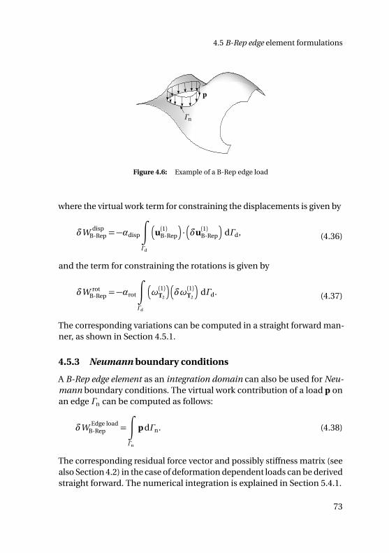
4.5 B-Rep edge element formulations
p
Γn
Figure 4.6: Example of a B-Rep edge load
where the virtual work term for constraining the displacements is given by
δW dispB-Rep =−αdisp
∫
Γd
u(1)B-Rep
·
δu(1)B-Rep
dΓd, (4.36)
and the term for constraining the rotations is given by
δW rotB-Rep =−αrot
∫
Γd
ω(1)T2
δω(1)T2
dΓd. (4.37)
The corresponding variations can be computed in a straight forward man-ner, as shown in Section 4.5.1.
4.5.3 Neumann boundary conditions
A B-Rep edge element as an integration domain can also be used for Neu-mann boundary conditions. The virtual work contribution of a load p onan edge Γn can be computed as follows:
δW Edge loadB-Rep =
∫
Γn
p dΓn. (4.38)
The corresponding residual force vector and possibly stiffness matrix (seealso Section 4.2) in the case of deformation dependent loads can be derivedstraight forward. The numerical integration is explained in Section 5.4.1.
73
4 Isogeometric B-Rep analysis
4.6 B-Rep vertex element formulations
Element formulations for vertex elements can be adapted from B-Rep edgeelements like e.g. Section 4.5.1 by using a Dirac function within the integralresp. by just evaluating the basis functions of the surface at the vertexlocation.
74

4.6 B-Rep vertex element formulations
Summary and conclusion of Chapter 4
This chapter explains the isogeometric B-Rep analysis (IBRA) which allowsthe usage of NURBS-based B-Rep (CAD) models for structural shell analysis.The newly developed B-Rep elements can be used to couple discontinuousand trimmed geometries with gaps and overlaps (see also Section 7.5).A corresponding element formulation based on a penalty approach isexplained as well. Moreover a data structure for isogeometric (trimmed)elements and B-Rep elements is proposed.
With IBRA a new method has been developed which provides the frame-work for analyzing CAD models without any modifications considering allthe aspects mentioned in Chapter 2. The implementation of IBRA and itsintegration into a CAD system is explained in the following chapters.
75

I have not failed. I’ve justfound 10,000 ways that won’twork.
Thomas A. Edison
CH
AP
TE
R
5IMPLEMENTATION OF THE
ISOGEOMETRIC B-REP ANALYSIS
This chapter explains the systematic disassembly of NURBS-based B-Repmodels (see Section 2.2) into finite elements resp. integration domains anddefines clear data interfaces for an implementation of the isogeometricB-Rep shell analysis into existing FE-solvers. In addition, a new adaptivequadrature scheme for the numerical integration of trimmed domains isintroduced. The new procedure is named adaptive Gaussian integrationprocedure and is abbreviated with AGIP. Moreover special aspects of IBRAlike local refinement, flying nodes, and clipping are discussed.
5.1 Overview
Figure 5.1 gives an overview of the required steps for analyzing CAD modelsdirectly with the isogeometric B-Rep analysis and using an existing FE solver.
77
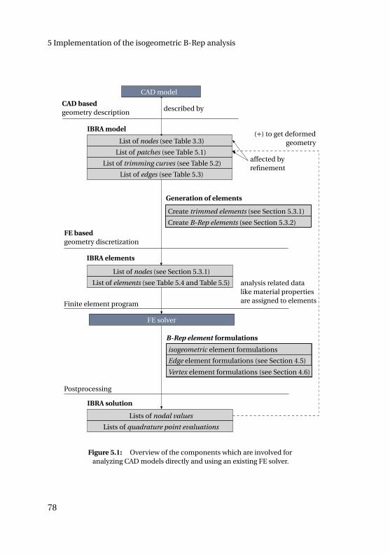
5 Implementation of the isogeometric B-Rep analysis
CAD model
described by
List of nodes (see Table 3.3)
List of patches (see Table 5.1)
List of trimming curves (see Table 5.2)
List of edges (see Table 5.3)
Create trimmed elements (see Section 5.3.1)
Create B-Rep elements (see Section 5.3.2)
Generation of elements
List of nodes (see Section 5.3.1)
List of elements (see Table 5.4 and Table 5.5)
FE solver
Finite element program
CAD basedgeometry description
FE basedgeometry discretization
B-Rep element formulations
Lists of nodal values
Postprocessing
isogeometric element formulations
Edge element formulations (see Section 4.5)
Vertex element formulations (see Section 4.6)
affected byrefinement
(+) to get deformedgeometry
IBRA model
IBRA elements
Lists of quadrature point evaluations
IBRA solution
analysis related datalike material propertiesare assigned to elements
Figure 5.1: Overview of the components which are involved foranalyzing CAD models directly and using an existing FE solver.
78
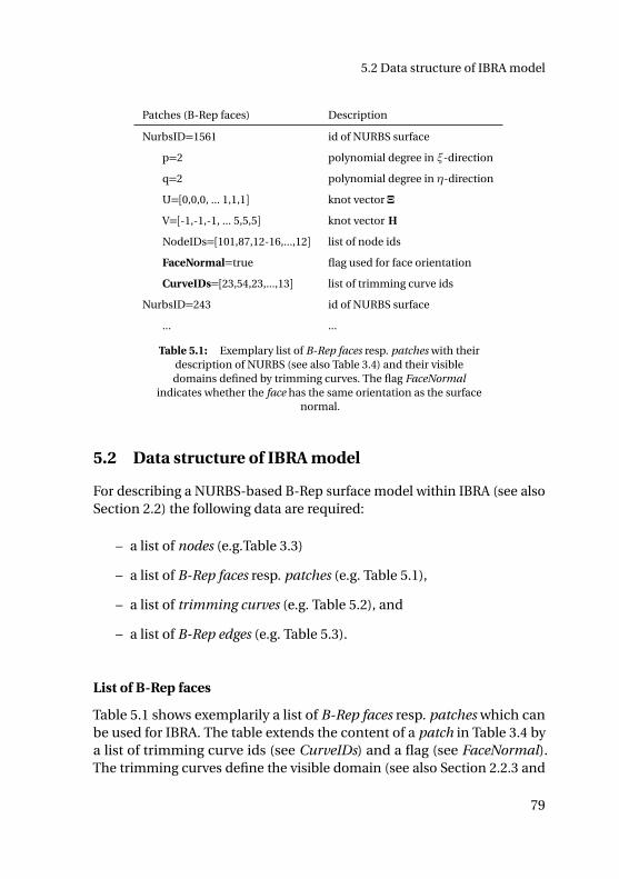
5.2 Data structure of IBRA model
Patches (B-Rep faces) Description
NurbsID=1561 id of NURBS surface
p=2 polynomial degree in ξ-direction
q=2 polynomial degree in η-direction
U=[0,0,0, ... 1,1,1] knot vector Ξ
V=[-1,-1,-1, ... 5,5,5] knot vector H
NodeIDs=[101,87,12-16,...,12] list of node ids
FaceNormal=true flag used for face orientation
CurveIDs=[23,54,23,...,13] list of trimming curve ids
NurbsID=243 id of NURBS surface
... ...
Table 5.1: Exemplary list of B-Rep faces resp. patches with theirdescription of NURBS (see also Table 3.4) and their visibledomains defined by trimming curves. The flag FaceNormal
indicates whether the face has the same orientation as the surfacenormal.
5.2 Data structure of IBRA model
For describing a NURBS-based B-Rep surface model within IBRA (see alsoSection 2.2) the following data are required:
– a list of nodes (e.g.Table 3.3)
– a list of B-Rep faces resp. patches (e.g. Table 5.1),
– a list of trimming curves (e.g. Table 5.2), and
– a list of B-Rep edges (e.g. Table 5.3).
List of B-Rep faces
Table 5.1 shows exemplarily a list of B-Rep faces resp. patches which canbe used for IBRA. The table extends the content of a patch in Table 3.4 bya list of trimming curve ids (see CurveIDs) and a flag (see FaceNormal).The trimming curves define the visible domain (see also Section 2.2.3 and
79
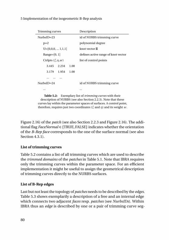
5 Implementation of the isogeometric B-Rep analysis
Trimming curves Description
NurbsID=23 id of NURBS trimming curve
p=2 polynomial degree
U=[0,0,0, ... 1,1,1] knot vector Ξ
Range=[0, 1] defines active range of knot vector
Ctrlpts (ξ,η,w ) list of control points
3.445 2.234 1.00
3.179 1.954 1.00
... ... ...
NurbsID=24 id of NURBS trimming curve
... ...
Table 5.2: Exemplary list of trimming curves with theirdescription of NURBS (see also Section 2.2.3). Note that these
curves lay within the parameter spaces of surfaces. A control point,therefore, requires just two coordinates (ξ and η) and its weight w .
Figure 2.16) of the patch (see also Section 2.2.3 and Figure 2.16). The addi-tional flag FaceNormal ∈ TRUE, FALSE indicates whether the orientationof the B-Rep face corresponds to the one of the surface normal (see alsoSection 4.3.1).
List of trimming curves
Table 5.2 contains a list of all trimming curves which are used to describethe trimmed domains of the patches in Table 5.1. Note that IBRA requiresonly the trimming curves within the parameter space. For an efficientimplementation it might be useful to assign the geometrical descriptionof trimming curves directly to the NURBS surfaces.
List of B-Rep edges
Last but not least the topology of patches needs to be described by the edges.Table 5.3 shows exemplarily a description of a free and an internal edgewhich connects two adjacent faces resp. patches (see NurbsIDs). WithinIBRA thus an edge is described by one or a pair of trimming curve seg-
80
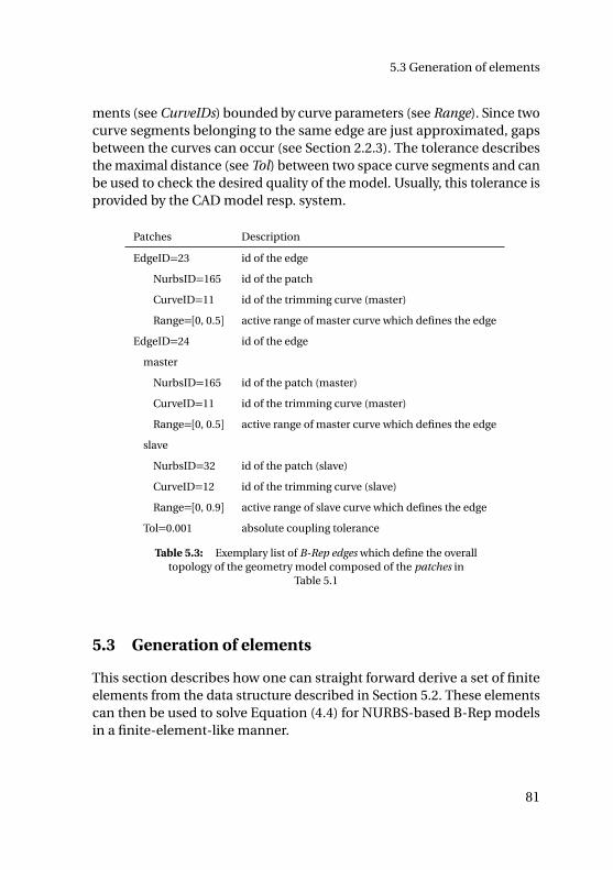
5.3 Generation of elements
ments (see CurveIDs) bounded by curve parameters (see Range). Since twocurve segments belonging to the same edge are just approximated, gapsbetween the curves can occur (see Section 2.2.3). The tolerance describesthe maximal distance (see Tol) between two space curve segments and canbe used to check the desired quality of the model. Usually, this tolerance isprovided by the CAD model resp. system.
Patches Description
EdgeID=23 id of the edge
NurbsID=165 id of the patch
CurveID=11 id of the trimming curve (master)
Range=[0, 0.5] active range of master curve which defines the edge
EdgeID=24 id of the edge
master
NurbsID=165 id of the patch (master)
CurveID=11 id of the trimming curve (master)
Range=[0, 0.5] active range of master curve which defines the edge
slave
NurbsID=32 id of the patch (slave)
CurveID=12 id of the trimming curve (slave)
Range=[0, 0.9] active range of slave curve which defines the edge
Tol=0.001 absolute coupling tolerance
Table 5.3: Exemplary list of B-Rep edges which define the overalltopology of the geometry model composed of the patches in
Table 5.1
5.3 Generation of elements
This section describes how one can straight forward derive a set of finiteelements from the data structure described in Section 5.2. These elementscan then be used to solve Equation (4.4) for NURBS-based B-Rep modelsin a finite-element-like manner.
81
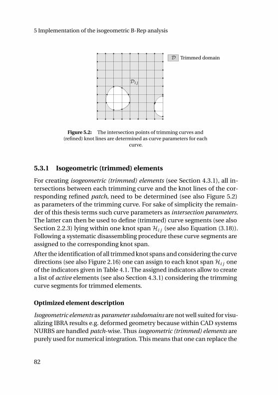
5 Implementation of the isogeometric B-Rep analysis
Trimmed domainD
Di j
Figure 5.2: The intersection points of trimming curves and(refined) knot lines are determined as curve parameters for each
curve.
5.3.1 Isogeometric (trimmed) elements
For creating isogeometric (trimmed) elements (see Section 4.3.1), all in-tersections between each trimming curve and the knot lines of the cor-responding refined patch, need to be determined (see also Figure 5.2)as parameters of the trimming curve. For sake of simplicity the remain-der of this thesis terms such curve parameters as intersection parameters.The latter can then be used to define (trimmed) curve segments (see alsoSection 2.2.3) lying within one knot span Hi j (see also Equation (3.18)).Following a systematic disassembling procedure these curve segments areassigned to the corresponding knot span.
After the identification of all trimmed knot spans and considering the curvedirections (see also Figure 2.16) one can assign to each knot span Hi j oneof the indicators given in Table 4.1. The assigned indicators allow to createa list of active elements (see also Section 4.3.1) considering the trimmingcurve segments for trimmed elements.
Optimized element description
Isogeometric elements as parameter subdomains are not well suited for visu-alizing IBRA results e.g. deformed geometry because within CAD systemsNURBS are handled patch-wise. Thus isogeometric (trimmed) elements arepurely used for numerical integration. This means that one can replace the
82
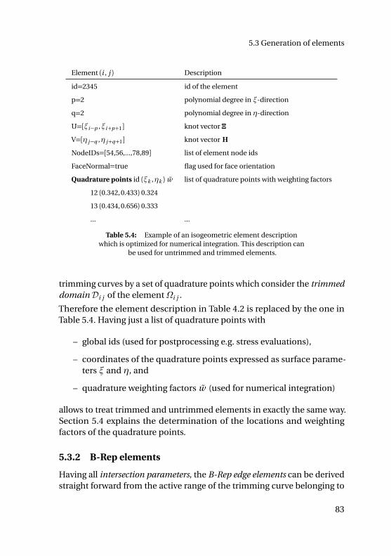
5.3 Generation of elements
Element (i , j ) Description
id=2345 id of the element
p=2 polynomial degree in ξ-direction
q=2 polynomial degree in η-direction
U=[ξi−p ,ξi+p+1] knot vector Ξ
V=[η j−q ,η j+q+1] knot vector H
NodeIDs=[54,56,...,78,89] list of element node ids
FaceNormal=true flag used for face orientation
Quadrature points id (ξk ,ηk ) w list of quadrature points with weighting factors
12 (0.342, 0.433) 0.324
13 (0.434, 0.656) 0.333
... ...
Table 5.4: Example of an isogeometric element descriptionwhich is optimized for numerical integration. This description can
be used for untrimmed and trimmed elements.
trimming curves by a set of quadrature points which consider the trimmeddomain Di j of the element Ωi j .
Therefore the element description in Table 4.2 is replaced by the one inTable 5.4. Having just a list of quadrature points with
– global ids (used for postprocessing e.g. stress evaluations),
– coordinates of the quadrature points expressed as surface parame-ters ξ and η, and
– quadrature weighting factors w (used for numerical integration)
allows to treat trimmed and untrimmed elements in exactly the same way.Section 5.4 explains the determination of the locations and weightingfactors of the quadrature points.
5.3.2 B-Rep elements
Having all intersection parameters, the B-Rep edge elements can be derivedstraight forward from the active range of the trimming curve belonging to
83
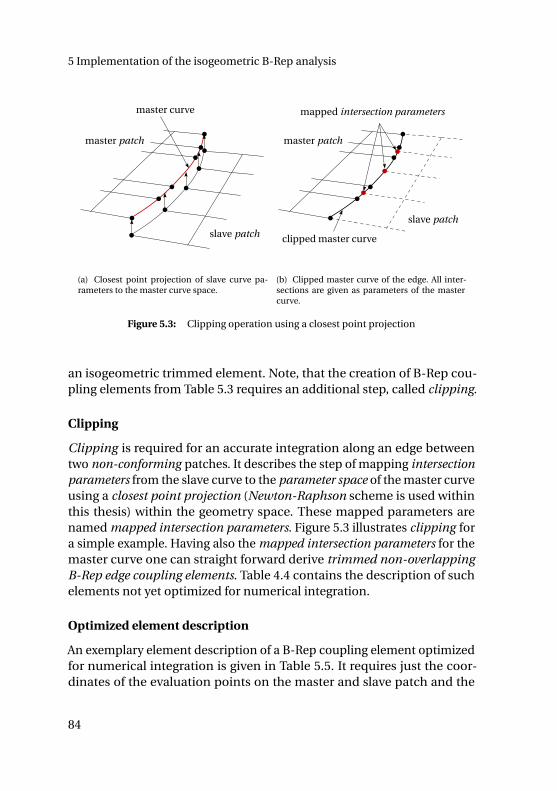
5 Implementation of the isogeometric B-Rep analysis
master curve
master patch
slave patch
(a) Closest point projection of slave curve pa-rameters to the master curve space.
clipped master curve
master patch
slave patch
mapped intersection parameters
(b) Clipped master curve of the edge. All inter-sections are given as parameters of the mastercurve.
Figure 5.3: Clipping operation using a closest point projection
an isogeometric trimmed element. Note, that the creation of B-Rep cou-pling elements from Table 5.3 requires an additional step, called clipping.
Clipping
Clipping is required for an accurate integration along an edge betweentwo non-conforming patches. It describes the step of mapping intersectionparameters from the slave curve to the parameter space of the master curveusing a closest point projection (Newton-Raphson scheme is used withinthis thesis) within the geometry space. These mapped parameters arenamed mapped intersection parameters. Figure 5.3 illustrates clipping fora simple example. Having also the mapped intersection parameters for themaster curve one can straight forward derive trimmed non-overlappingB-Rep edge coupling elements. Table 4.4 contains the description of suchelements not yet optimized for numerical integration.
Optimized element description
An exemplary element description of a B-Rep coupling element optimizedfor numerical integration is given in Table 5.5. It requires just the coor-dinates of the evaluation points on the master and slave patch and the
84
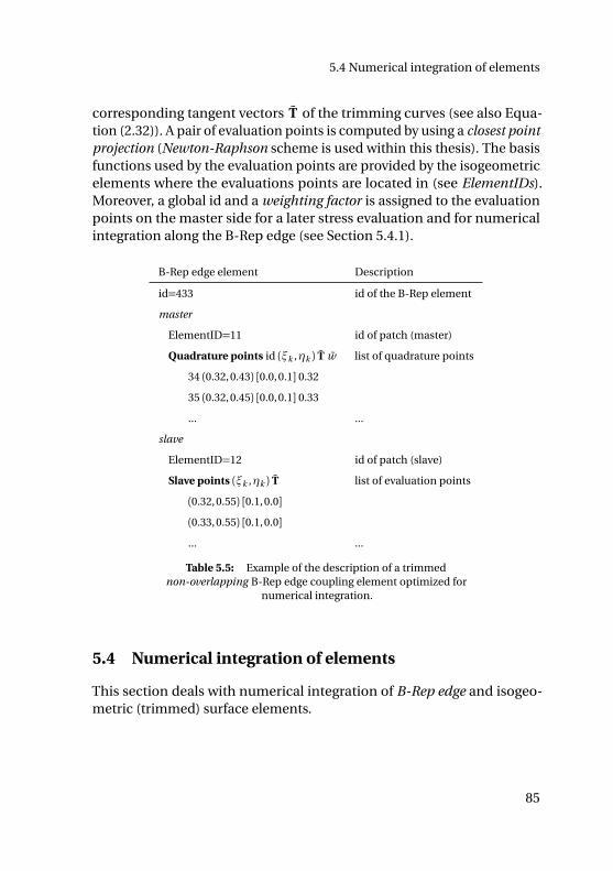
5.4 Numerical integration of elements
corresponding tangent vectors T of the trimming curves (see also Equa-tion (2.32)). A pair of evaluation points is computed by using a closest pointprojection (Newton-Raphson scheme is used within this thesis). The basisfunctions used by the evaluation points are provided by the isogeometricelements where the evaluations points are located in (see ElementIDs).Moreover, a global id and a weighting factor is assigned to the evaluationpoints on the master side for a later stress evaluation and for numericalintegration along the B-Rep edge (see Section 5.4.1).
B-Rep edge element Description
id=433 id of the B-Rep element
master
ElementID=11 id of patch (master)
Quadrature points id (ξk ,ηk ) T w list of quadrature points
34 (0.32, 0.43) [0.0, 0.1] 0.32
35 (0.32, 0.45) [0.0, 0.1] 0.33
... ...
slave
ElementID=12 id of patch (slave)
Slave points (ξk ,ηk ) T list of evaluation points
(0.32, 0.55) [0.1, 0.0]
(0.33, 0.55) [0.1, 0.0]
... ...
Table 5.5: Example of the description of a trimmednon-overlapping B-Rep edge coupling element optimized for
numerical integration.
5.4 Numerical integration of elements
This section deals with numerical integration of B-Rep edge and isogeo-metric (trimmed) surface elements.
85
5 Implementation of the isogeometric B-Rep analysis
5.4.1 B-Rep edge elements
For the numerical integration of B-Rep edge elements given in Table 4.3 andTable 4.4 a Gaussian quadrature scheme is applied with ng =maxp , q +1 quadrature points where p and q are the highest polynomial degreesoccurring within the master and slave patches, respectively. The length |Γe|of a B-Rep edge element can be computed as
|Γe|=∫
Γe
dΓe =
∫
θ 1
J1 dθ 1 =
∫
GJ1 J2 dG, (5.1)
whereΓe is the boundary segment of the B-Rep element and J1 the mappingfrom the geometry space to the parameter space
J1 =
d Xsurf
d θ 1
2
=
T2
2=
A1∂ θ 1
∂ θ 1+A2
∂ θ 2
∂ θ 1
2
. (5.2)
J2 is given as the mapping from the parameter space of the trimming curveto the Gaussian domain G = [−1, 1]
J2 =∂ ξ
∂ ξG, (5.3)
withξG being the parameter of the Gaussian space. Introducing the weight-ing factor wl
wl = J2(ξl )wl , (5.4)
with wl being the Gaussian quadrature weights, the numerical integrationof a B-Rep edge element can be computed as
|Γe| ≈ng∑
l=1
J1(ξl ) wl . (5.5)
5.4.2 Isogeometric (trimmed) elements
Since a trimmed domainDi j of an element (see also Section 5.3.1) is decou-pled from the underlying surface parametrization a Gaussian quadraturescheme can not directly be used as it is the case for untrimmed surfaces(see also Hughes et al. [40]).
86
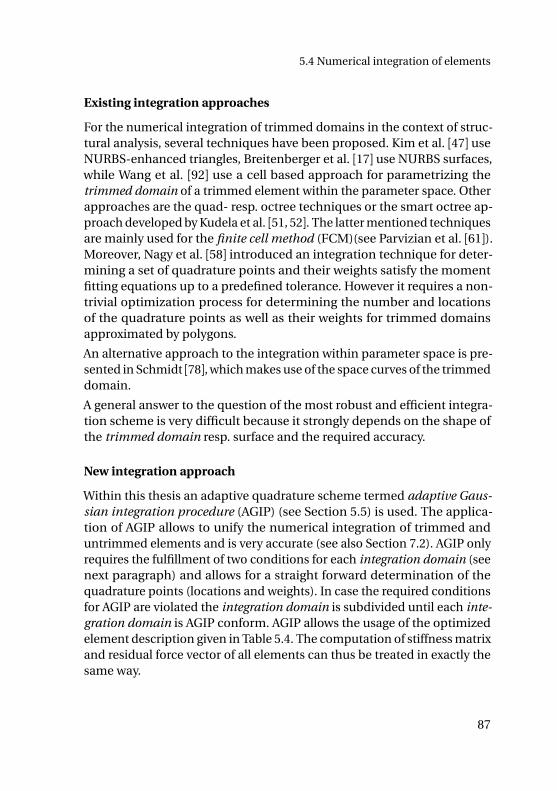
5.4 Numerical integration of elements
Existing integration approaches
For the numerical integration of trimmed domains in the context of struc-tural analysis, several techniques have been proposed. Kim et al. [47] useNURBS-enhanced triangles, Breitenberger et al. [17] use NURBS surfaces,while Wang et al. [92] use a cell based approach for parametrizing thetrimmed domain of a trimmed element within the parameter space. Otherapproaches are the quad- resp. octree techniques or the smart octree ap-proach developed by Kudela et al. [51, 52]. The latter mentioned techniquesare mainly used for the finite cell method (FCM)(see Parvizian et al. [61]).Moreover, Nagy et al. [58] introduced an integration technique for deter-mining a set of quadrature points and their weights satisfy the momentfitting equations up to a predefined tolerance. However it requires a non-trivial optimization process for determining the number and locationsof the quadrature points as well as their weights for trimmed domainsapproximated by polygons.
An alternative approach to the integration within parameter space is pre-sented in Schmidt [78], which makes use of the space curves of the trimmeddomain.
A general answer to the question of the most robust and efficient integra-tion scheme is very difficult because it strongly depends on the shape ofthe trimmed domain resp. surface and the required accuracy.
New integration approach
Within this thesis an adaptive quadrature scheme termed adaptive Gaus-sian integration procedure (AGIP) (see Section 5.5) is used. The applica-tion of AGIP allows to unify the numerical integration of trimmed anduntrimmed elements and is very accurate (see also Section 7.2). AGIP onlyrequires the fulfillment of two conditions for each integration domain (seenext paragraph) and allows for a straight forward determination of thequadrature points (locations and weights). In case the required conditionsfor AGIP are violated the integration domain is subdivided until each inte-gration domain is AGIP conform. AGIP allows the usage of the optimizedelement description given in Table 5.4. The computation of stiffness matrixand residual force vector of all elements can thus be treated in exactly thesame way.
87
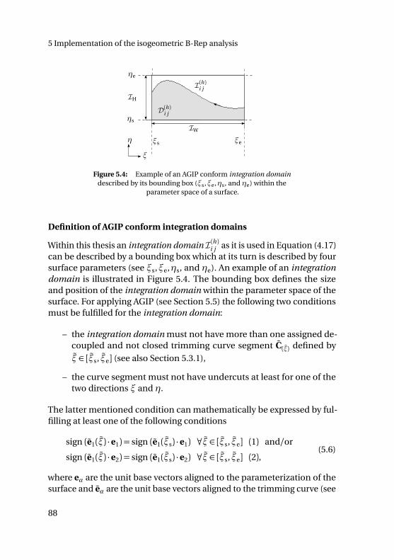
5 Implementation of the isogeometric B-Rep analysis
I (h )i j
D(h )i j
IW
IH
ξ
η
ηs
ηe
ξs ξe
Figure 5.4: Example of an AGIP conform integration domaindescribed by its bounding box (ξs,ξe,ηs, and ηe) within the
parameter space of a surface.
Definition of AGIP conform integration domains
Within this thesis an integration domain I (h )i j as it is used in Equation (4.17)can be described by a bounding box which at its turn is described by foursurface parameters (see ξs,ξe,ηs, and ηe). An example of an integrationdomain is illustrated in Figure 5.4. The bounding box defines the sizeand position of the integration domain within the parameter space of thesurface. For applying AGIP (see Section 5.5) the following two conditionsmust be fulfilled for the integration domain:
– the integration domain must not have more than one assigned de-coupled and not closed trimming curve segment C(ξ) defined by
ξ ∈ [ξs, ξe] (see also Section 5.3.1),
– the curve segment must not have undercuts at least for one of thetwo directions ξ and η.
The latter mentioned condition can mathematically be expressed by ful-filling at least one of the following conditions
sign (e1(ξ) ·e1) = sign (e1(ξs) ·e1) ∀ξ ∈ [ξs, ξe] (1) and/or
sign (e1(ξ) ·e2) = sign (e1(ξs) ·e2) ∀ξ ∈ [ξs, ξe] (2),(5.6)
where eα are the unit base vectors aligned to the parameterization of thesurface and eα are the unit base vectors aligned to the trimming curve (see
88
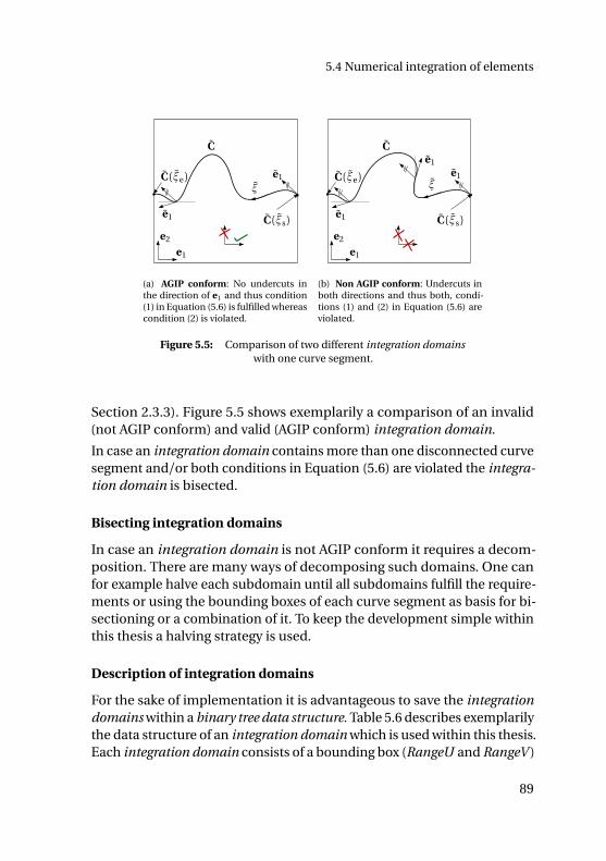
5.4 Numerical integration of elements
C
e1
e2
C (ξs)
C (ξe)ξ
e1
e1
(a) AGIP conform: No undercuts inthe direction of e1 and thus condition(1) in Equation (5.6) is fulfilled whereascondition (2) is violated.
C
e1
e2
C (ξs)
ξ
e1e1C (ξe)
e1
(b) Non AGIP conform: Undercuts inboth directions and thus both, condi-tions (1) and (2) in Equation (5.6) areviolated.
Figure 5.5: Comparison of two different integration domainswith one curve segment.
Section 2.3.3). Figure 5.5 shows exemplarily a comparison of an invalid(not AGIP conform) and valid (AGIP conform) integration domain.
In case an integration domain contains more than one disconnected curvesegment and/or both conditions in Equation (5.6) are violated the integra-tion domain is bisected.
Bisecting integration domains
In case an integration domain is not AGIP conform it requires a decom-position. There are many ways of decomposing such domains. One canfor example halve each subdomain until all subdomains fulfill the require-ments or using the bounding boxes of each curve segment as basis for bi-sectioning or a combination of it. To keep the development simple withinthis thesis a halving strategy is used.
Description of integration domains
For the sake of implementation it is advantageous to save the integrationdomains within a binary tree data structure. Table 5.6 describes exemplarilythe data structure of an integration domain which is used within this thesis.Each integration domain consists of a bounding box (RangeU and RangeV )
89
5 Implementation of the isogeometric B-Rep analysis
which indicates the size and position of the integration domain within theparameter space of the surface, a list of curve segments, an indicator fromTable 5.6, and two links to possible child domains.
Integration domain Description
RangeU=[0.1, 0.2] surface parameters ξs and ξe
RangeV=[-0.05, 0.1] surface parameters ηs and ηe
Indicator=bs indicators from Table 5.7
List of curve segments
Curve 1
CurveID=11 id of trimming curve
Range=[0, 0.5] active range of curve segment (interaction parameters)
Curve 2
CurveID=13 id of trimming curve
Range=[0, 0.4] active range of curve segment (interaction parameters)
... ...
ChildDomain1=2 id of first child domain
ChildDomain2=3 id of second child domain
Table 5.6: Example of a description of an integration domain
The indicator bs is used to describe non AGIP conform domains whichrequire a bisectioning. The indicator in and out label domains which arecompletely inside resp. outside the trimmed domain. The indicators stis used for domains with a negligible visible part and trim is used for alltrimmed integration domains which are AGIP conform. Note that bisec-tioning of integration domains is rarely required for appropriate refinedsurfaces for analysis purposes.
5.5 Adaptive Gaussian integration procedure (AGIP)
The adaptive Gaussian integration procedure (AGIP) can be used for inte-grating the trimmed domain within an AGIP conform integration domain(see Section 5.4.2) and thus it can also be used for computing stiffness
90
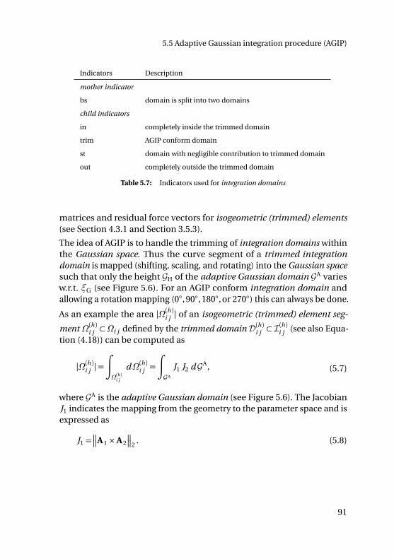
5.5 Adaptive Gaussian integration procedure (AGIP)
Indicators Description
mother indicator
bs domain is split into two domains
child indicators
in completely inside the trimmed domain
trim AGIP conform domain
st domain with negligible contribution to trimmed domain
out completely outside the trimmed domain
Table 5.7: Indicators used for integration domains
matrices and residual force vectors for isogeometric (trimmed) elements(see Section 4.3.1 and Section 3.5.3).
The idea of AGIP is to handle the trimming of integration domains withinthe Gaussian space. Thus the curve segment of a trimmed integrationdomain is mapped (shifting, scaling, and rotating) into the Gaussian spacesuch that only the height GH of the adaptive Gaussian domain GA variesw.r.t. ξG (see Figure 5.6). For an AGIP conform integration domain andallowing a rotation mapping (0, 90, 180, or 270) this can always be done.
As an example the area |Ω(h )i j | of an isogeometric (trimmed) element seg-
ment Ω(h )i j ⊂Ωi j defined by the trimmed domain D(h )i j ⊂ I (h )i j (see also Equa-tion (4.18)) can be computed as
|Ω(h )i j |=∫
Ω(h )i j
dΩ(h )i j =
∫
GA
J1 J2 dGA, (5.7)
where GA is the adaptive Gaussian domain (see Figure 5.6). The JacobianJ1 indicates the mapping from the geometry to the parameter space and isexpressed as
J1 =
A 1×A 2
2. (5.8)
91
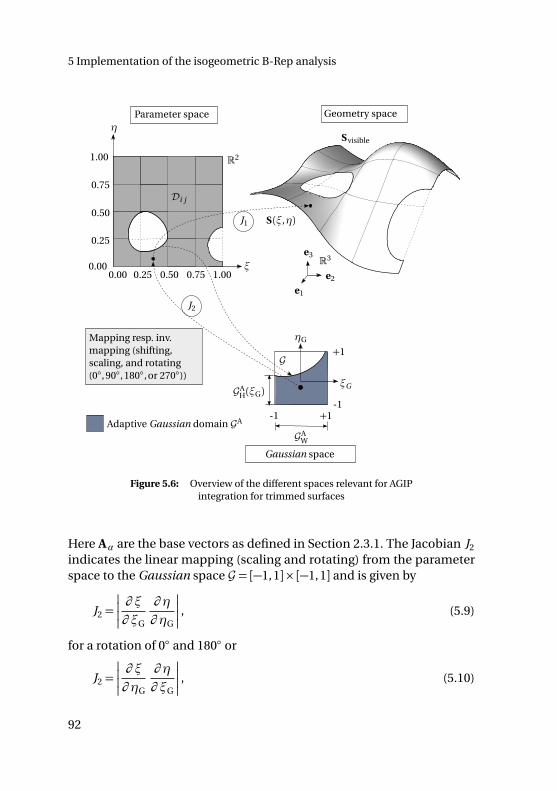
5 Implementation of the isogeometric B-Rep analysis
e1
R3ξ
η
0.00
0.25
0.50
0.75
1.00
0.00 0.25 0.50 0.75 1.00
S (ξ,η)
R2
J1
Svisible
Di j
Geometry spaceParameter space
e2
e3
-1 +1-1
ξG
ηG
+1G
Gaussian space
J2
Mapping resp. inv.mapping (shifting,scaling, and rotating(0, 90, 180, or 270))
Adaptive Gaussian domain GA
GAH(ξG)
GAW
Figure 5.6: Overview of the different spaces relevant for AGIPintegration for trimmed surfaces
Here Aα are the base vectors as defined in Section 2.3.1. The Jacobian J2
indicates the linear mapping (scaling and rotating) from the parameterspace to the Gaussian space G = [−1, 1]× [−1, 1] and is given by
J2 =
∂ ξ
∂ ξG
∂ η
∂ ηG
, (5.9)
for a rotation of 0 and 180 or
J2 =
∂ ξ
∂ ηG
∂ η
∂ ξG
, (5.10)
92
5.5 Adaptive Gaussian integration procedure (AGIP)
for a rotation of 90 and 270 with ξG and ηG being the parameters of theGaussian space. Using ng quadrature points, the area of an isogeometric
(trimmed) element segment Ω(h )i j ⊂Ωi j can be computed as
|Ω(h )i j | ≈ng∑
l=1
J1(ξAl , ηA
l ) J2(ξAl , ηA
l )wAl , (5.11)
where (ξAl , ηA
l ) are the coordinates obtained by an appropriate rotation(0, 90, 180, or 270) of the coordinates (ξA
l ,ηAl ) of the adaptive Gaussian
quadrature points determined within the Gaussian space. w Al are the corre-
sponding adaptive quadrature weights. The determination of the adaptiveGaussian quadrature points is explained in the following two sections.
For sake of implementation and simplicity Equation (5.11) is rewritten as
|Ω(h )i j | ≈ng∑
l=1
J1 wl , (5.12)
where the newly introduced weighting factor wl is given by
wl = J2 w Al . (5.13)
The weighting factor wl remains constant during analysis and thus it mustbe computed just once. The adaptive Gaussian quadrature points aremapped (rotating, scaling, and shifting) to the parameter space of thesurface and can then be used for the element description in Table 5.4.
5.5.1 Full Gaussian domain
In the special case GH is constant and equal to 2, i.e. the area of GA = 4and no rotation is performed, a full integration of the Gaussian domainG = [−1,1]× [−1,1] is performed (classical Gaussian integration). This isthe case for isogeometric untrimmed elements (see Section 3.5.3). For amore efficient numerical integration a reduced integration scheme analogto the one presented in Dornisch et al. [31] can be used for full elementslying completely inside the trimmed domain (indicator in in Table 4.1).Within this thesis only the integration scheme proposed in Hughes et al.[40] (p +1 integration points per direction) is used.
93
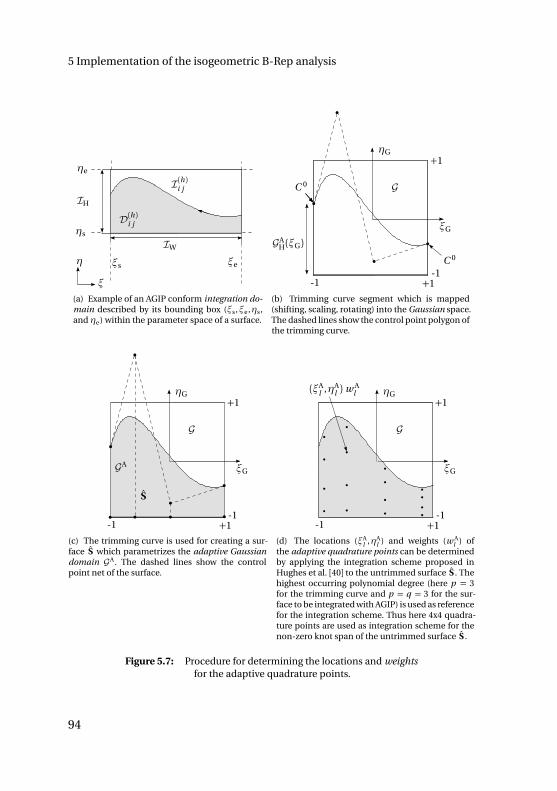
5 Implementation of the isogeometric B-Rep analysis
I (h )i j
D(h )i j
IW
IH
ξ
η
ηs
ηe
ξs ξe
(a) Example of an AGIP conform integration do-main described by its bounding box (ξs,ξe,ηs,and ηe) within the parameter space of a surface.
ξG
-1-1 +1
+1ηG
GAH(ξG)
GC 0
C 0
(b) Trimming curve segment which is mapped(shifting, scaling, rotating) into the Gaussian space.The dashed lines show the control point polygon ofthe trimming curve.
ξG
-1-1 +1
+1ηG
GA
G
S
(c) The trimming curve is used for creating a sur-face S which parametrizes the adaptive Gaussiandomain GA. The dashed lines show the controlpoint net of the surface.
ξG
-1-1 +1
+1ηG
G
(ξAl ,ηA
l ) w Al
(d) The locations (ξAl ,ηA
l ) and weights (w Al ) of
the adaptive quadrature points can be determinedby applying the integration scheme proposed inHughes et al. [40] to the untrimmed surface S . Thehighest occurring polynomial degree (here p = 3for the trimming curve and p = q = 3 for the sur-face to be integrated with AGIP) is used as referencefor the integration scheme. Thus here 4x4 quadra-ture points are used as integration scheme for thenon-zero knot span of the untrimmed surface S .
Figure 5.7: Procedure for determining the locations and weightsfor the adaptive quadrature points.
94
5.5 Adaptive Gaussian integration procedure (AGIP)
5.5.2 Trimmed Gaussian domain
In the case of trimmed Gaussian domains, i.e. the area |GA|< 4, the adaptiveGaussian quadrature points (ξA
l ,ηAl ) and the corresponding quadrature
weights wl need to be determined such that
– all quadrature points lie within the adaptive Gaussian domain
– the moment fitting equations are fulfilled
– the sum of all adaptive Gaussian quadrature weights w Al corresponds
to the area of GA i.e.∑ng
l=1 w Al = |G
A|
An efficient way to obtain an appropriate set of such quadrature points is toparametrize GA with an untrimmed NURBS surface S using the trimmingcurve segment which is mapped for each trimmed integration domaininto the Gaussian space (see also Figure 5.7). Note that C 0 continuitiesneeds to be generated at the boundaries of the trimming curve segment(see also Figure 2.5) if not already given. The surface S can then be used todetermine the adaptive quadrature points as it is explained in the followingparagraph.
Determination of the adaptive quadrature points
Using the integration scheme proposed by Hughes et al. [40] for integratingthe untrimmed surface S, a set of quadrature points A can be determined.Within this thesis the highest occurring polynomial degree of the trimmingcurve and surface, which is to be integrated with AGIP, is used as referencefor the integration scheme. Having these quadrature points the coordinates(ξA
l ,ηAl ) of the adaptive quadrature points can be computed as
(ξAl ,ηA
l ) = S(ξl ,ηl ) with (ξl ,ηl ) ∈A. (5.14)
The corresponding adaptive quadrature weights w Al are given by
w Al = J1(ξl ,ηl ) J2(ξl ,ηl ) wl , (5.15)
where wl are the Gauss quadrature weights used for integrating the sur-faces S and J1 resp. J2 represent the mapping analogously to Equation (5.8)resp. Equation (5.9).
The example in Section 7.2 underlines the accuracy of AGIP in the contextof IBRA.
95
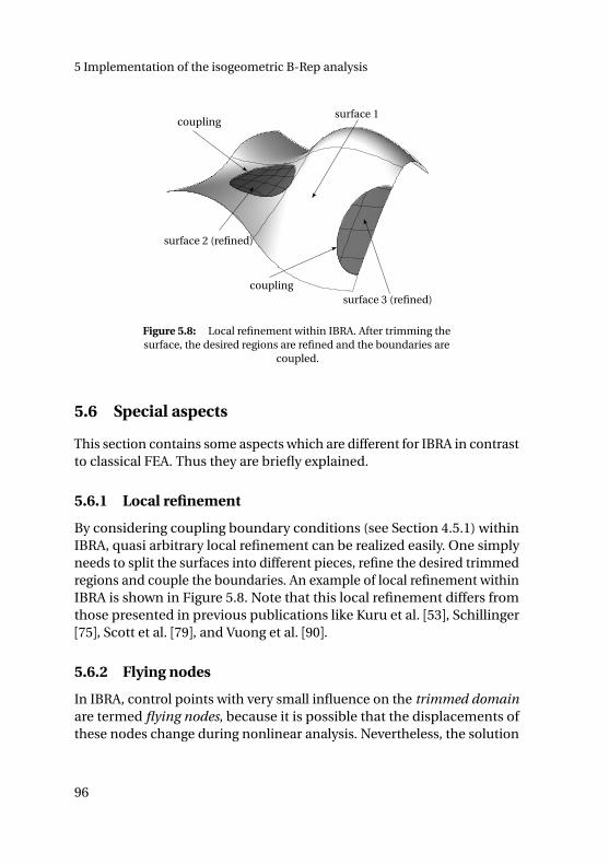
5 Implementation of the isogeometric B-Rep analysis
surface 1
surface 3 (refined)
surface 2 (refined)
coupling
coupling
Figure 5.8: Local refinement within IBRA. After trimming thesurface, the desired regions are refined and the boundaries are
coupled.
5.6 Special aspects
This section contains some aspects which are different for IBRA in contrastto classical FEA. Thus they are briefly explained.
5.6.1 Local refinement
By considering coupling boundary conditions (see Section 4.5.1) withinIBRA, quasi arbitrary local refinement can be realized easily. One simplyneeds to split the surfaces into different pieces, refine the desired trimmedregions and couple the boundaries. An example of local refinement withinIBRA is shown in Figure 5.8. Note that this local refinement differs fromthose presented in previous publications like Kuru et al. [53], Schillinger[75], Scott et al. [79], and Vuong et al. [90].
5.6.2 Flying nodes
In IBRA, control points with very small influence on the trimmed domainare termed flying nodes, because it is possible that the displacements ofthese nodes change during nonlinear analysis. Nevertheless, the solution
96
5.6 Special aspects
converges owing to the negligible contribution of the flying nodes on thetrimmed domain resp. solution.
These flying nodes are closely related to the control points in the fictitiousdomain (FCM), which also make a minor contribution to the solution.According to Schillinger [75], these points should “. . . ‘move’ as freely aspossible to permit a smooth extension of the physical solution into thefictitious domain”. This rationale can be applied to the flying nodes as well.For structural problems, the small contribution of the flying nodes has noinfluence on the solution. It only influences the conditioning of the linearsystem of equations which needs to be solved. In consequence this mightrequire an additional preconditioning step which is provided by most ofthe commercial solvers.
97

5 Implementation of the isogeometric B-Rep analysis
Summary and conclusion of Chapter 5
This chapter describes the process of creating a set of finite elements froma NURBS-based B-Rep model which is provided by a CAD system. Theelements can then be used to solve structural shell problems in a finite-element-like manner within an existing FE-solver. Possible data structuresare provided as well. In addition, a new adaptive integration scheme ispresented which allows to treat all integration domains (untrimmed andtrimmed) in exactly the same way.
All decisions made for IBRA had the goal to develop a simple and robustanalysis approach which can analyze complex CAD models without anymodifications and can be implemented easily into an existing FE-solver.
98
Simplicity is the ultimatesophistication.
Leonardo da Vinci
CH
AP
TE
R
6ANALYSIS IN COMPUTER AIDED DESIGN
The goal of an efficient design-through-analysis workflow is to simulatethe real behavior of a structure within a short time. The chosen analysisapproach must therefore deliver solutions which
– meet a specified level of reliability and
– are obtained under minimal usage of resources (human effort, com-putational cost, etc.).
In times of almost unlimited and relatively cheap computer power, one ofor probably the biggest challenge for an efficient design-through-analysisworkflow is the minimization of human effort. Because the latter is timeconsuming and thus expensive from a business point of view.
This chapter introduces a new concept for minimizing the human effort forstructural shell problems by using the proposed isogeometric B-Rep analy-sis (IBRA, see Chapter 4). The resulting CAD-integrated design-through-analysis workflow is named Analysis in Computer Aided Design (AiCAD)(see also Breitenberger et al. [17]). The implementation of an AiCAD work-
99
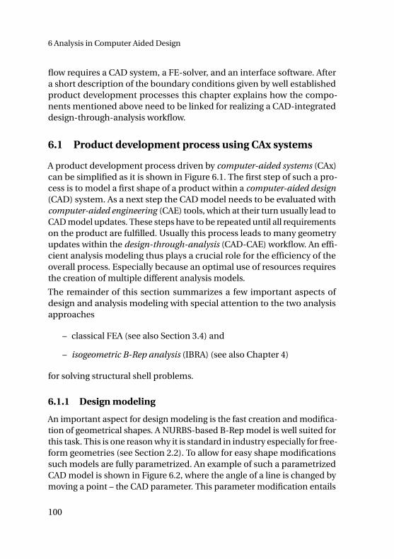
6 Analysis in Computer Aided Design
flow requires a CAD system, a FE-solver, and an interface software. Aftera short description of the boundary conditions given by well establishedproduct development processes this chapter explains how the compo-nents mentioned above need to be linked for realizing a CAD-integrateddesign-through-analysis workflow.
6.1 Product development process using CAx systems
A product development process driven by computer-aided systems (CAx)can be simplified as it is shown in Figure 6.1. The first step of such a pro-cess is to model a first shape of a product within a computer-aided design(CAD) system. As a next step the CAD model needs to be evaluated withcomputer-aided engineering (CAE) tools, which at their turn usually lead toCAD model updates. These steps have to be repeated until all requirementson the product are fulfilled. Usually this process leads to many geometryupdates within the design-through-analysis (CAD-CAE) workflow. An effi-cient analysis modeling thus plays a crucial role for the efficiency of theoverall process. Especially because an optimal use of resources requiresthe creation of multiple different analysis models.
The remainder of this section summarizes a few important aspects ofdesign and analysis modeling with special attention to the two analysisapproaches
– classical FEA (see also Section 3.4) and
– isogeometric B-Rep analysis (IBRA) (see also Chapter 4)
for solving structural shell problems.
6.1.1 Design modeling
An important aspect for design modeling is the fast creation and modifica-tion of geometrical shapes. A NURBS-based B-Rep model is well suited forthis task. This is one reason why it is standard in industry especially for free-form geometries (see Section 2.2). To allow for easy shape modificationssuch models are fully parametrized. An example of such a parametrizedCAD model is shown in Figure 6.2, where the angle of a line is changed bymoving a point – the CAD parameter. This parameter modification entails
100
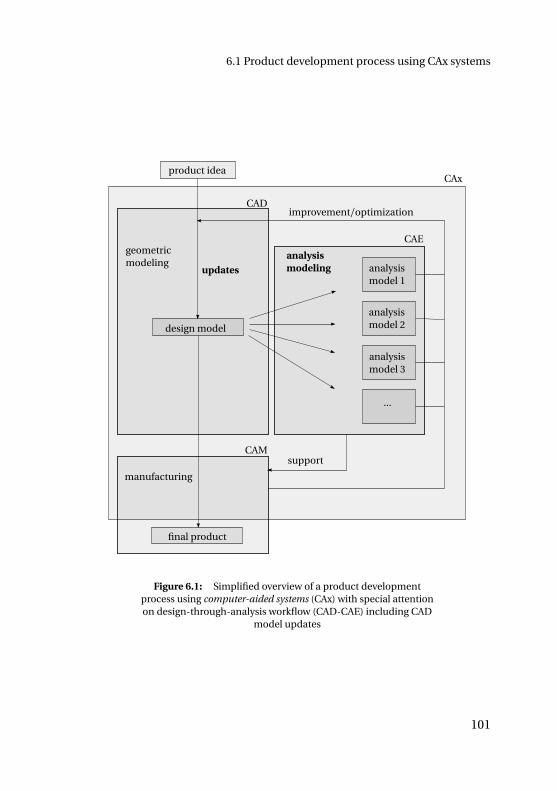
6.1 Product development process using CAx systems
product idea
CAEgeometricmodeling
final product
CAM
...
analysismodel 2
analysismodel 3
support
manufacturing
CAx
design model
analysismodel 1
improvement/optimizationCAD
analysismodelingupdates
Figure 6.1: Simplified overview of a product developmentprocess using computer-aided systems (CAx) with special attentionon design-through-analysis workflow (CAD-CAE) including CAD
model updates
101
6 Analysis in Computer Aided Design
CAD parameter
(a) Initial shape of the CAD model with the red point as CAD parameter which controls the angleof the black curve which in its turn defines the region around the hole.
Update of CADparameter
(b) Updated CAD model: the angle of the line is changed by modifying the CAD parameter (posi-tion of the red point)
Figure 6.2: Example of a CAD parameter update on a fullyparametrized CAD model within Siemens NX
102
6.1 Product development process using CAx systems
the update of the entire CAD model. Within a design-through-analysisworkflow, analysis models are therefore derived from NURBS-based B-Repmodels.
6.1.2 Analysis modeling for classical FEA
In this thesis, analysis modeling refers to the preparation of a model foranalysis itself. In industry, structural problems are solved predominantlywith classical finite element analysis (FEA), which typically uses linear orquadratic polynomials defined over non-overlapping parametric domains(the elements) for describing the geometry of the analyzed model (see alsoSection 3.4). Thus, within the standard analysis workflow, illustrated inFigure 6.3, the NURBS-based B-Rep model needs to be converted into afinite element mesh. This change of geometry description is called meshing(see Section 3.4.2).
Another step to obtain the analysis model is the introduction of analysis-related data, e.g. material properties and boundary conditions. They caneither be applied directly to the finite element mesh, e.g. by selecting theelements or nodes (option 1 in Figure 6.3), or to the CAD model (option2). In option 2, properties are assigned as attributes to the B-Rep entities(e.g. edges) and after meshing they are transferred to the finite elementmesh. This can be done automatically, option 2 is thus more convenient forthe user, especially when re-meshing of the CAD model is necessary. Theanalysis itself is performed using a finite element (FE) solver. An exampleof a CAD model with analysis related data is illustrated in Figure 6.4.
The steps in the standard design-through-analysis workflow can be per-formed by using either different programs (CAD and FE program) or byusing an integrated CAD/CAE system.
6.1.3 Analysis modeling for IBRA
In contrast to the standard analysis (CAD-CAE) workflow, in AiCAD thegeometry representation of the design and the analysis models is the same.The design model just needs to be refined for the analysis (see Section 2.2.2),which does not change the representation of the model but only its de-scription. The refinement is necessary to approximate the solution withadequate accuracy and can be assigned to the B-Rep faces as a property. In
103
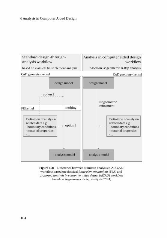
6 Analysis in Computer Aided Design
based on classical finite element analysis
Standard design-through-analysis workflow
Analysis in computer aided designworkflow
CAD geometry kernel
design model
analysis model
Definition of analysis-related data e.g.- boundary conditions- material properties- ...
FE kernel meshing
option 2
option 1
design model
analysis model
Definition of analysis-related data e.g.- boundary conditions- material properties- ...
CAD geometry kernel
isogeometricrefinement
based on isogeometric B-Rep analysis
Figure 6.3: Difference between standard analysis (CAD-CAE)workflow based on classical finite element analysis (FEA) and
proposed analysis in computer aided design (AiCAD) workflowbased on isogeometric B-Rep analysis (IBRA)
104
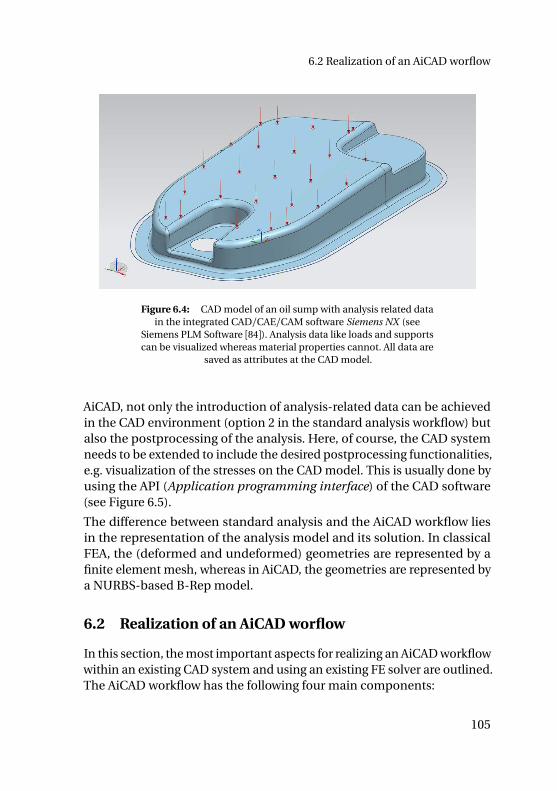
6.2 Realization of an AiCAD worflow
Figure 6.4: CAD model of an oil sump with analysis related datain the integrated CAD/CAE/CAM software Siemens NX (see
Siemens PLM Software [84]). Analysis data like loads and supportscan be visualized whereas material properties cannot. All data are
saved as attributes at the CAD model.
AiCAD, not only the introduction of analysis-related data can be achievedin the CAD environment (option 2 in the standard analysis workflow) butalso the postprocessing of the analysis. Here, of course, the CAD systemneeds to be extended to include the desired postprocessing functionalities,e.g. visualization of the stresses on the CAD model. This is usually done byusing the API (Application programming interface) of the CAD software(see Figure 6.5).
The difference between standard analysis and the AiCAD workflow liesin the representation of the analysis model and its solution. In classicalFEA, the (deformed and undeformed) geometries are represented by afinite element mesh, whereas in AiCAD, the geometries are represented bya NURBS-based B-Rep model.
6.2 Realization of an AiCAD worflow
In this section, the most important aspects for realizing an AiCAD workflowwithin an existing CAD system and using an existing FE solver are outlined.The AiCAD workflow has the following four main components:
105
6 Analysis in Computer Aided Design
– CAD system
– AiCAD interface software
– FE Solver
– eventually external postprocessing tool (e.g. HTML based)
The workflow can be seen in an abstract form independent of the im-plementation of AiCAD, as shown in Figure 6.5. In the following text, thevarious components and their tasks are briefly explained.
6.2.1 CAD system
The design component of an AiCAD workflow is realized in a CAD program,where the geometry kernel is used for the following tasks:
– geometric modeling (see section 6.1.1)
– pre- and eventually postprocessing for IBRA
Geometric modeling is the intrinsic function of the CAD program, whereaspre-and postprocessing may be seen as additional functionalities. The pre-and postprocessing in a CAD program require an API, which endows theCAD software with missing functions, such as
– assigning analysis related data to B-Rep entities (see section 6.1.3)
– assigning refinement parameters (see section 6.1.3)
– visualizing deformed geometries (see figure 6.6)
– ...
Depending on the CAD program, some of these functions are already avail-able. To give an example, the integrated CAD/CAE/CAM software SiemensNX (see Siemens PLM Software [84]) can assign analysis related data toB-Rep entities (see figure 6.4), whereas in the CAD program Rhinoceros(see Rhinoceros [70]), this needs to be realized by the API of Rhinoceros.
106
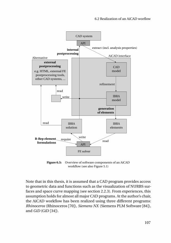
6.2 Realization of an AiCAD worflow
CAD system
API
CADmodel
IBRAmodel
refinement
generationof elements
IBRAelements
extract (incl. analysis properties)
FE solver
API
B-Rep elementformulations
IBRAsolution
readwrite
require
internalpostprocessing
read
read
write
Alternative
externalpostprocessing
e.g. HTML, external FEpostprocessing tools,other CAD systems, ...
AiCAD interface
Figure 6.5: Overview of software components of an AiCADworkflow (see also Figure 5.1)
Note that in this thesis, it is assumed that a CAD program provides accessto geometric data and functions such as the visualization of NURBS sur-faces and space curve mapping (see section 2.2.3). From experiences, thisassumption holds for almost all major CAD programs. At the author’s chair,the AiCAD workflow has been realized using three different programs:Rhinoceros (Rhinoceros [70]), Siemens NX (Siemens PLM Software [84]),and GiD (GiD [34]).
107
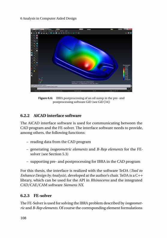
6 Analysis in Computer Aided Design
Figure 6.6: IBRA postprocessing of an oil sump in the pre- andpostprocessing software GiD (see GiD [34])
6.2.2 AiCAD interface software
The AiCAD interface software is used for communicating between theCAD program and the FE-solver. The interface software needs to provide,among others, the following functions:
– reading data from the CAD program
– generating isogeometric elements and B-Rep elements for the FE-solver (see Section 5.3)
– supporting pre- and postprocessing for IBRA in the CAD program
For this thesis, the interface is realized with the software TeDA (Tool toEnhance Design by Analysis), developed at the author’s chair. TeDA is a C++library, which can be used for the API in Rhinoceros and the integratedCAD/CAE/CAM software Siemens NX.
6.2.3 FE-solver
The FE-Solver is used for solving the IBRA problem described by isogeomet-ric and B-Rep elements. Of course the corresponding element formulations
108
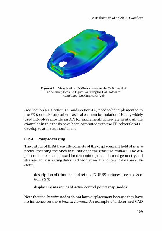
6.2 Realization of an AiCAD worflow
Figure 6.7: Visualization of vMises stresses on the CAD model ofan oil sump (see also Figure 6.4) using the CAD software
Rhinoceros (see Rhinoceros [70])
(see Section 4.4, Section 4.5, and Section 4.6) need to be implemented inthe FE-solver like any other classical element formulation. Usually widelyused FE-solver provide an API for implementing new elements. All theexamples in this thesis have been computed with the FE-solver Carat++developed at the authors’ chair.
6.2.4 Postprocessing
The output of IBRA basically consists of the displacement field of activenodes, meaning the ones that influence the trimmed domain. The dis-placement field can be used for determining the deformed geometry andstresses. For visualizing deformed geometries, the following data are suffi-cient:
– description of trimmed and refined NURBS surfaces (see also Sec-tion 2.2.3)
– displacements values of active control points resp. nodes
Note that the inactive nodes do not have displacement because they haveno influence on the trimmed domain. An example of a deformed CAD
109
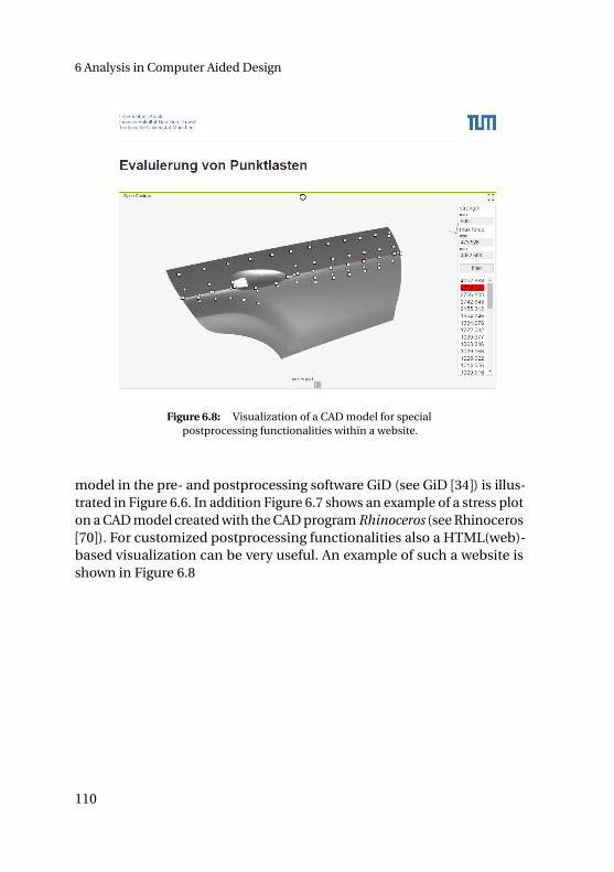
6 Analysis in Computer Aided Design
Figure 6.8: Visualization of a CAD model for specialpostprocessing functionalities within a website.
model in the pre- and postprocessing software GiD (see GiD [34]) is illus-trated in Figure 6.6. In addition Figure 6.7 shows an example of a stress ploton a CAD model created with the CAD program Rhinoceros (see Rhinoceros[70]). For customized postprocessing functionalities also a HTML(web)-based visualization can be very useful. An example of such a website isshown in Figure 6.8
110

6.2 Realization of an AiCAD worflow
Summary and conclusion of Chapter 6
This chapter describes the steps required for realizing an CAD-integrateddesign-through-analysis workflow (AiCAD) within an existing CAD sys-tem. AiCAD has been realized within three different programs: Rhinoceros(Rhinoceros [70]), Siemens NX (Siemens PLM Software [84]), and GiD (GiD[34]). This demonstrates the flexibility of the developed concept.
In addition, the difference between AiCAD and a standard design-through-analysis workflow is explained.
111

Everything should be madeas simple as possible, but notsimpler.
Albert Einstein
CH
AP
TE
R
7EXAMPLES AND INVESTIGATIONS
To highlight the accuracy, flexibility and robustness of IBRA, some well se-lected examples with increasing complexity are discussed. To demonstratethe correctness and to quantify the approximation errors of IBRA, the re-sults are compared to solutions that are either computed analytically, withisogeometric analysis (IGA), or with commercial finite element software.The examples range from geometrically linear plates in membrane actionto geometrically nonlinear shells, including weak boundary conditions(see also Section 4.5). For all examples, a linear elastic, isotropic materialis used.
This chapter can be separated into three parts. The first part deals withproblems that are discretized with one trimmed NURBS surface for investi-gating the Adaptive Gaussian Integration Procedure (AGIP) (see Section 5.5)and the influence of trimming tolerances on analysis results. The secondpart deals with B-Rep edge elements (according to Section 4.5) which areused to enforce different types of weak boundary conditions. The thirdpart deals with the application of IBRA to industrial problems.
113
7 Examples and investigations
PART 1 starts with an example of a simple plate in membrane action toshow the accuracy of the integration scheme AGIP. The second exampledeals with a geometrically linear (i.e. applying linear kinematics) plate inbending, which is used to show the robustness of AGIP against geometricdistortions. The last example within the first block deals with a geometri-cally nonlinear shell problem to demonstrate the application of IBRA alsoto mechanically challenging problems and the flexibility of IBRA in termsof trimming tolerances.
The first example of PART 2 deals with a geometrically nonlinear cantileversubjected to an end moment, a so called mainspring. This example is usedfor discussing weak coupling boundary conditions for different discretiza-tions, the influence of "dirty" geometries (gaps and overlaps) on the result,and the choice of appropriate penalty factors (according to Section 4.5.1).The second example deals with a geometrically nonlinear shell problemdiscretized with two trimmed surfaces focusing on weak coupling condi-tions.
PART 3 shows the application of IBRA to real industrial CAD models of anoil sump and an engine bonnet.
Moreover, all examples highlight the simplicity and straightforwardness ofanalysis model preparation using IBRA even for very complex geometries.All geometries for the examples are created either with the CAD programRhinoceros 5 (see Rhinoceros [70]) or the integrated CAD/CAE/CAM soft-ware Siemens NX (see Siemens PLM Software [84]). The trimming tolerance(according to Section 2.2.3) used for the examples is denoted separatelyfor each example. For some few examples, it would be possible to repre-sent the geometries exactly, i.e. without any trimming error, but this isnot the goal of the proposed method. The goal of IBRA is to use the CADmodel "as it is". For all presented examples, the geometries therefore arecreated in a CAD system, and they are analyzed directly. The analysis itselfis performed with the in-house finite element program CARAT++. Theresults of the classical finite element analysis are computed in ANSYS (seeANSYS [2]) or NASTRAN NX (see Siemens PLM Software [84]) by usingquadrilateral-dominant meshes with bi-linear quadrilaterals and trian-gular Reissner-Mindlin (RM) shell elements. For IBRA, the NURBS-basedKirchhoff-Love (KL) shell element (see Kiendl et al. [44]) is used. Note thatKL theory is not always mentioned explicitly. The postprocessing for IBRA
114
7.1 Definition of error measures
is realized with the interface software TeDA (see Section 6.2.2) used withinthe API of the CAD program Rhinoceros 5.
7.1 Definition of error measures
In order to verify the proposed technique, a few quantitative error measuresneed to be defined for the examples. The error over a parametric domainΩ can be expressed by the sum of the L 2-norms of each component of thestress tensor as follows:
er =∑
i
‖σi exact−σi num ‖L 2(Ω), (7.1)
where i represents the components x x , y y , x y . In cases where a com-puted result (e.g. displacement) at a specific point is compared to a refer-ence solution, the following relative error measure is used:
er =|uref−uIBRA||uref|
(7.2)
For a general comparison of the relative difference between two results(res 1 and res 2) the following formula is used:
dr =|ures1−ures2||ures1|
(7.3)
7.2 Infinite plate with circular hole
The first example deals with the two-dimensional linear elastic problemshown in Figure 7.1. This setup is used to solve an infinite plate with acircular hole under in-plane tension at infinity. The exact solution to thisproblem is given in Gould [36], and is solved with IGA in Hughes et al. [40].Moreover, the problem had already been solved by Kim et al. [47] using atrimmed NURBS surface. Since just another numerical integration schemeis applied (see AGIP in Section 5.5), one should obtain similar results asthose published in Kim et al. [47].
115
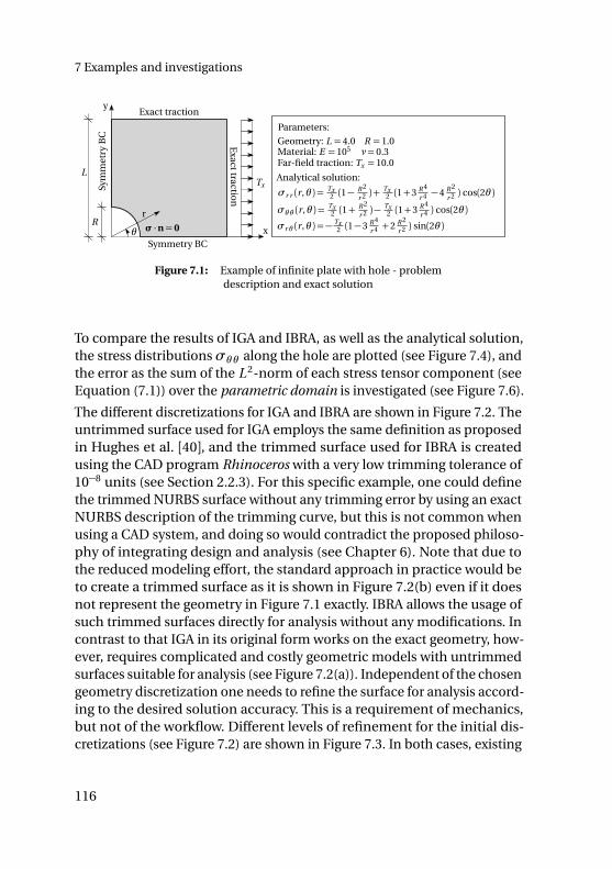
7 Examples and investigations
Far-field traction: Tx = 10.0
Geometry: L = 4.0 R = 1.0Material: E = 105 ν= 0.3
σ ·n= 0
Parameters:
Analytical solution:
σr r (r,θ ) = Tx2 (1−
R 2
r 2 ) +Tx2 (1+3 R 4
r 4 −4 R 2
r 2 ) cos(2θ )
σθθ (r,θ ) = Tx2 (1+
R 2
r 2 )−Tx2 (1+3 R 4
r 4 ) cos(2θ )
σr θ (r,θ ) =− Tx2 (1−3 R 4
r 4 +2 R 2
r 2 ) sin(2θ )
Exact traction
Exacttractio
n
r
θ x
Tx
L
R
Symmetry BC
Sym
met
ryB
Cy
Figure 7.1: Example of infinite plate with hole - problemdescription and exact solution
To compare the results of IGA and IBRA, as well as the analytical solution,the stress distributionsσθθ along the hole are plotted (see Figure 7.4), andthe error as the sum of the L 2-norm of each stress tensor component (seeEquation (7.1)) over the parametric domain is investigated (see Figure 7.6).
The different discretizations for IGA and IBRA are shown in Figure 7.2. Theuntrimmed surface used for IGA employs the same definition as proposedin Hughes et al. [40], and the trimmed surface used for IBRA is createdusing the CAD program Rhinoceros with a very low trimming tolerance of10−8 units (see Section 2.2.3). For this specific example, one could definethe trimmed NURBS surface without any trimming error by using an exactNURBS description of the trimming curve, but this is not common whenusing a CAD system, and doing so would contradict the proposed philoso-phy of integrating design and analysis (see Chapter 6). Note that due tothe reduced modeling effort, the standard approach in practice would beto create a trimmed surface as it is shown in Figure 7.2(b) even if it doesnot represent the geometry in Figure 7.1 exactly. IBRA allows the usage ofsuch trimmed surfaces directly for analysis without any modifications. Incontrast to that IGA in its original form works on the exact geometry, how-ever, requires complicated and costly geometric models with untrimmedsurfaces suitable for analysis (see Figure 7.2(a)). Independent of the chosengeometry discretization one needs to refine the surface for analysis accord-ing to the desired solution accuracy. This is a requirement of mechanics,but not of the workflow. Different levels of refinement for the initial dis-cretizations (see Figure 7.2) are shown in Figure 7.3. In both cases, existing
116
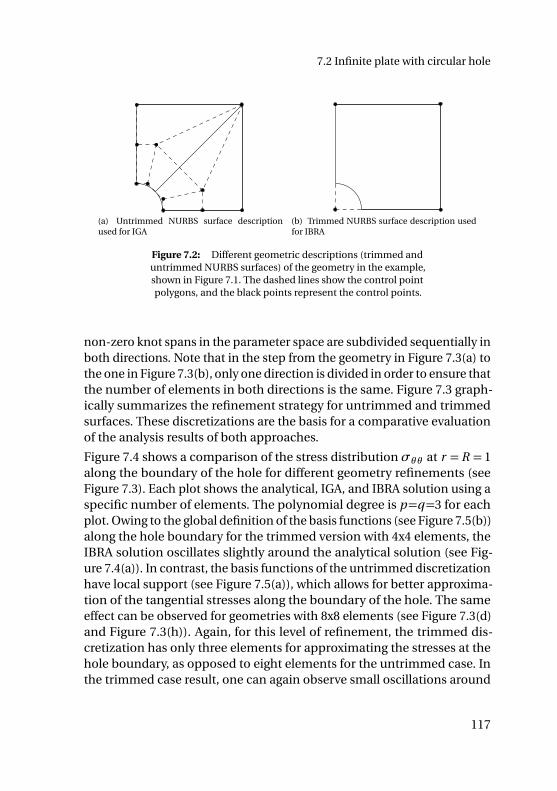
7.2 Infinite plate with circular hole
(a) Untrimmed NURBS surface descriptionused for IGA
(b) Trimmed NURBS surface description usedfor IBRA
Figure 7.2: Different geometric descriptions (trimmed anduntrimmed NURBS surfaces) of the geometry in the example,shown in Figure 7.1. The dashed lines show the control pointpolygons, and the black points represent the control points.
non-zero knot spans in the parameter space are subdivided sequentially inboth directions. Note that in the step from the geometry in Figure 7.3(a) tothe one in Figure 7.3(b), only one direction is divided in order to ensure thatthe number of elements in both directions is the same. Figure 7.3 graph-ically summarizes the refinement strategy for untrimmed and trimmedsurfaces. These discretizations are the basis for a comparative evaluationof the analysis results of both approaches.
Figure 7.4 shows a comparison of the stress distributionσθθ at r =R = 1along the boundary of the hole for different geometry refinements (seeFigure 7.3). Each plot shows the analytical, IGA, and IBRA solution using aspecific number of elements. The polynomial degree is p=q=3 for eachplot. Owing to the global definition of the basis functions (see Figure 7.5(b))along the hole boundary for the trimmed version with 4x4 elements, theIBRA solution oscillates slightly around the analytical solution (see Fig-ure 7.4(a)). In contrast, the basis functions of the untrimmed discretizationhave local support (see Figure 7.5(a)), which allows for better approxima-tion of the tangential stresses along the boundary of the hole. The sameeffect can be observed for geometries with 8x8 elements (see Figure 7.3(d)and Figure 7.3(h)). Again, for this level of refinement, the trimmed dis-cretization has only three elements for approximating the stresses at thehole boundary, as opposed to eight elements for the untrimmed case. Inthe trimmed case result, one can again observe small oscillations around
117
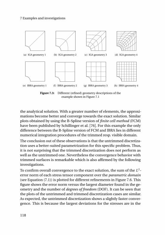
7 Examples and investigations
(a) IGA geometry 1 (b) IGA geometry 2 (c) IGA geometry 3 (d) IGA geometry 4
(e) IBRA geometry 1 (f) IBRA geometry 2 (g) IBRA geometry 3 (h) IBRA geometry 4
Figure 7.3: Different (refined) geometry descriptions of theexample shown in Figure 7.1
the analytical solution. With a greater number of elements, the approxi-mations become better and converge towards the exact solution. Similarplots obtained by using the B-Spline version of finite cell method (FCM)have been published by Schillinger et al. [76]. For this example the onlydifference between the B-Spline version of FCM and IBRA lies in differentnumerical integration procedures of the trimmed resp. visible domain.
The conclusion out of these observations is that the untrimmed discretiza-tion uses a better-suited parametrization for this specific problem. Thus,it is not surprising that the trimmed discretization does not perform aswell as the untrimmed one. Nevertheless the convergence behavior withtrimmed surfaces is remarkable which is also affirmed by the followinginvestigations.
To confirm overall convergence to the exact solution, the sum of the L 2-error norm of each stress tensor component over the parametric domain(see Equation (7.1)) is plotted for different refinements in Figure 7.6. Thisfigure shows the error norm versus the largest diameter found in the ge-ometry and the number of degrees of freedom (DOF). It can be seen thatthe plots of the untrimmed and trimmed discretization cases are similar.As expected, the untrimmed discretization shows a slightly faster conver-gence. This is because the largest deviations for the stresses are in the
118
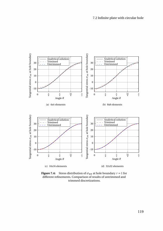
7.2 Infinite plate with circular hole
-10
0
10
20
30
0 π8
π4
3π8
π2
Tan
gen
tial
stre
ssσθθ
ath
ole
bo
un
dar
y
Angle θ
Analytical solutionTrimmedUntrimmed
(a) 4x4 elements
-10
0
10
20
30
0 π8
π4
3π8
π2
Tan
gen
tial
stre
ssσθθ
ath
ole
bo
un
dar
y
Angle θ
Analytical solutionTrimmedUntrimmed
(b) 8x8 elements
-10
0
10
20
30
0 π8
π4
3π8
π2
Tan
gen
tial
stre
ssσθθ
ath
ole
bo
un
dar
y
Angle θ
Analytical solutionTrimmedUntrimmed
(c) 16x16 elements
-10
0
10
20
30
0 π8
π4
3π8
π2
Tan
gen
tial
stre
ssσθθ
ath
ole
bo
un
dar
y
Angle θ
Analytical solutionTrimmedUntrimmed
(d) 32x32 elements
Figure 7.4: Stress distribution ofσθθ at hole boundary r = 1 fordifferent refinements. Comparison of results of untrimmed and
trimmed discretizations.
119
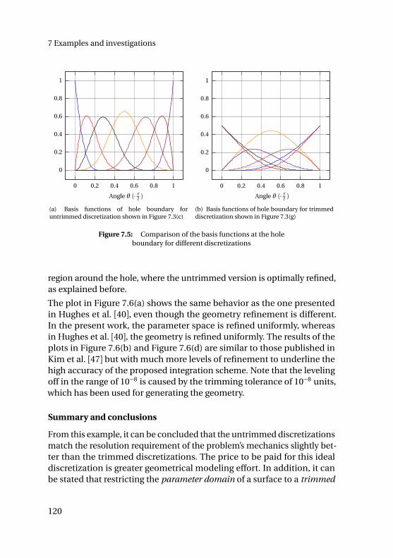
7 Examples and investigations
0
0.2
0.4
0.6
0.8
1
0 0.2 0.4 0.6 0.8 1
Angle θ (· π2 )
(a) Basis functions of hole boundary foruntrimmed discretization shown in Figure 7.3(c)
0
0.2
0.4
0.6
0.8
1
0 0.2 0.4 0.6 0.8 1
Angle θ (· π2 )
(b) Basis functions of hole boundary for trimmeddiscretization shown in Figure 7.3(g)
Figure 7.5: Comparison of the basis functions at the holeboundary for different discretizations
region around the hole, where the untrimmed version is optimally refined,as explained before.
The plot in Figure 7.6(a) shows the same behavior as the one presentedin Hughes et al. [40], even though the geometry refinement is different.In the present work, the parameter space is refined uniformly, whereasin Hughes et al. [40], the geometry is refined uniformly. The results of theplots in Figure 7.6(b) and Figure 7.6(d) are similar to those published inKim et al. [47] but with much more levels of refinement to underline thehigh accuracy of the proposed integration scheme. Note that the levelingoff in the range of 10−8 is caused by the trimming tolerance of 10−8 units,which has been used for generating the geometry.
Summary and conclusions
From this example, it can be concluded that the untrimmed discretizationsmatch the resolution requirement of the problem’s mechanics slightly bet-ter than the trimmed discretizations. The price to be paid for this idealdiscretization is greater geometrical modeling effort. In addition, it canbe stated that restricting the parameter domain of a surface to a trimmed
120
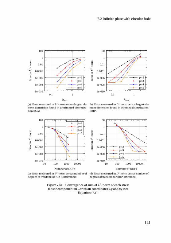
7.2 Infinite plate with circular hole
1e-010
1e-008
1e-006
0.0001
0.01
1
100
0.1 1
Err
or
inL
2-n
orm
hmax
p=2p=3p=4p=5
(a) Error measured in L 2-norm versus largest ele-ment dimension found in untrimmed discretiza-tion (IGA)
1e-010
1e-008
1e-006
0.0001
0.01
1
100
0.1 1E
rro
rin
L2
-no
rm
hmax
p=2p=3p=4p=5
(b) Error measured in L 2-norm versus largest ele-ment dimension found in trimmed discretization(IBRA)
1e-010
1e-008
1e-006
0.0001
0.01
1
100
10 100 1000 10000
Err
or
inL
2-n
orm
Number of DOFs
p=2p=3p=4p=5
(c) Error measured in L 2-norm versus number ofdegrees of freedom for IGA (untrimmed)
1e-010
1e-008
1e-006
0.0001
0.01
1
100
10 100 1000 10000
Err
or
inL
2-n
orm
Number of DOFs
p=2p=3p=4p=5
(d) Error measured in L 2-norm versus number ofdegrees of freedom for IBRA (trimmed)
Figure 7.6: Convergence of sum of L 2-norm of each stresstensor component in Cartesian coordinates x,y and xy (see
Equation (7.1))
121
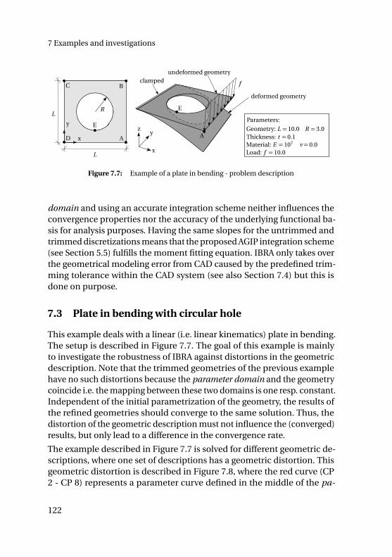
7 Examples and investigations
clamped
x
zy
f
A
E
D A
BC
L
L
R
x
y E
undeformed geometry
deformed geometry
Geometry: L = 10.0 R = 3.0
Parameters:
Material: E = 107 ν= 0.0Load: f = 10.0
Thickness: t = 0.1
Figure 7.7: Example of a plate in bending - problem description
domain and using an accurate integration scheme neither influences theconvergence properties nor the accuracy of the underlying functional ba-sis for analysis purposes. Having the same slopes for the untrimmed andtrimmed discretizations means that the proposed AGIP integration scheme(see Section 5.5) fulfills the moment fitting equation. IBRA only takes overthe geometrical modeling error from CAD caused by the predefined trim-ming tolerance within the CAD system (see also Section 7.4) but this isdone on purpose.
7.3 Plate in bending with circular hole
This example deals with a linear (i.e. linear kinematics) plate in bending.The setup is described in Figure 7.7. The goal of this example is mainlyto investigate the robustness of IBRA against distortions in the geometricdescription. Note that the trimmed geometries of the previous examplehave no such distortions because the parameter domain and the geometrycoincide i.e. the mapping between these two domains is one resp. constant.Independent of the initial parametrization of the geometry, the results ofthe refined geometries should converge to the same solution. Thus, thedistortion of the geometric description must not influence the (converged)results, but only lead to a difference in the convergence rate.
The example described in Figure 7.7 is solved for different geometric de-scriptions, where one set of descriptions has a geometric distortion. Thisgeometric distortion is described in Figure 7.8, where the red curve (CP2 - CP 8) represents a parameter curve defined in the middle of the pa-
122
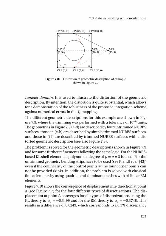
7.3 Plate in bending with circular hole
CP 1 (0, 0) CP 2 (5, 0) CP 3 (10, 0)
CP 4 CP 6 CP 5
CP 7 (0, 10) CP 8 (5, 10) CP 9 (10, 10)
(0, 5) (15, 5)(10, 5)
x
y
D A
BC
Figure 7.8: Distortion of geometric description of exampleshown in Figure 7.7
rameter domain. It is used to illustrate the distortion of the geometricdescription. By intention, the distortion is quite substantial, which allowsfor a demonstration of the robustness of the proposed integration schemeagainst numerical errors in the J1 mapping.
The different geometric descriptions for this example are shown in Fig-ure 7.9, where the trimming was performed with a tolerance of 10−8 units.The geometries in Figure 7.9 (a-d) are described by four untrimmed NURBSsurfaces, those in (e-h) are described by simple trimmed NURBS surfaces,and those in (i-l) are described by trimmed NURBS surfaces with a dis-torted geometric description (see also Figure 7.8).
The problem is solved for the geometric descriptions shown in Figure 7.9and for some further refinements following the same logic. For the NURBS-based KL shell element, a polynomial degree of p = q = 3 is used. For theuntrimmed geometry bending strips have to be used (see Kiendl et al. [43])even if the collinearity of the control points at the four corner points cannot be provided (kink). In addition, the problem is solved with classicalfinite elements by using quadrilateral-dominant meshes with bi-linear RMelements.
Figure 7.10 shows the convergence of displacement in z-direction at pointA (see Figure 7.7) for the four different types of discretizations. The dis-placement at point A converges for all types of discretizations using theKL theory to uz = −6.3499 and for the RM theory to uz = −6.3748. Thisresults in a difference of 0.0249, which corresponds to a 0.3% discrepancy
123
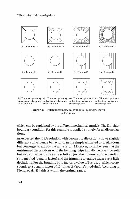
7 Examples and investigations
(a) Untrimmed 1 (b) Untrimmed 2 (c) Untrimmed 3 (d) Untrimmed 4
(e) Trimmed 1 (f) Trimmed 2 (g) Trimmed 3 (h) Trimmed 4
(i) Trimmed geometrywith a distorted geomet-ric description 1
(j) Trimmed geometrywith a distorted geomet-ric description 2
(k) Trimmed geometrywith a distorted geomet-ric description 3
(l) Trimmed geometrywith a distorted geomet-ric description 4
Figure 7.9: Different geometry descriptions of geometry shownin Figure 7.7
which can be explained by the different mechanical models. The Dirichletboundary condition for this example is applied strongly for all discretiza-tions.
As expected the IBRA solution with geometric distortion shows slightlydifferent convergence behavior than the simple trimmed discretizationsbut converges to exactly the same result. Moreover, it can be seen that theuntrimmed descriptions with the bending strips initially behaves too soft,but also converge to the same solution. Just the influence of the bendingstrip method (penalty factor) and the trimming tolerance causes very littledeviations. For the bending strip factor, a value of 5 is used, which corre-sponds to a penalty factor of 105 times E (Young’s modulus). According toKiendl et al. [43], this is within the optimal range.
124
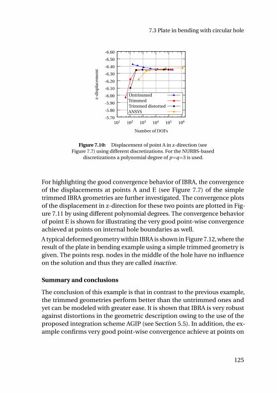
7.3 Plate in bending with circular hole
-6.60
-6.50
-6.40
-6.30
-6.20
-6.10
-6.00
-5.90
-5.80
-5.70101 102 103 104 105 106
z-d
isp
lace
men
t
Number of DOFs
UntrimmedTrimmedTrimmed distortedANSYS
Figure 7.10: Displacement of point A in z-direction (seeFigure 7.7) using different discretizations. For the NURBS-based
discretizations a polynomial degree of p=q=3 is used.
For highlighting the good convergence behavior of IBRA, the convergenceof the displacements at points A and E (see Figure 7.7) of the simpletrimmed IBRA geometries are further investigated. The convergence plotsof the displacement in z-direction for these two points are plotted in Fig-ure 7.11 by using different polynomial degrees. The convergence behaviorof point E is shown for illustrating the very good point-wise convergenceachieved at points on internal hole boundaries as well.
A typical deformed geometry within IBRA is shown in Figure 7.12, where theresult of the plate in bending example using a simple trimmed geometry isgiven. The points resp. nodes in the middle of the hole have no influenceon the solution and thus they are called inactive.
Summary and conclusions
The conclusion of this example is that in contrast to the previous example,the trimmed geometries perform better than the untrimmed ones andyet can be modeled with greater ease. It is shown that IBRA is very robustagainst distortions in the geometric description owing to the use of theproposed integration scheme AGIP (see Section 5.5). In addition, the ex-ample confirms very good point-wise convergence achieve at points on
125
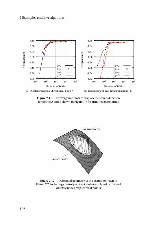
7 Examples and investigations
-6.40
-6.20
-6.00
-5.80
-5.60
-5.40
-5.20
-5.00101 102 103 104 105
z-d
isp
lace
men
t
Number of DOFs
p=2p=3p=4p=5
(a) Displacement in z-direction at point A
-1.66
-1.64
-1.62
-1.60
-1.58
-1.56
-1.54
-1.52101 102 103 104 105
z-d
isp
lace
men
t
Number of DOFs
p=2p=3p=4p=5
(b) Displacement in z-direction at point E
Figure 7.11: Convergence plots of displacement in z-directionfor points A and E shown in Figure 7.7 for trimmed geometries.
active nodes
inactive nodes
Figure 7.12: Deformed geometry of the example shown inFigure 7.7, including control point net and examples of active and
inactive nodes resp. control points
126
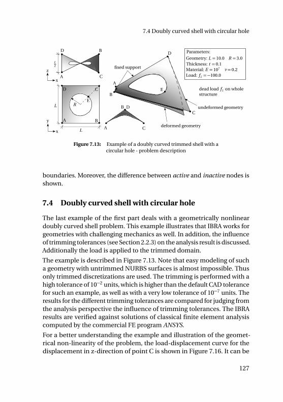
7.4 Doubly curved shell with circular hole
deformed geometry
undeformed geometry
A B
CDA
B
C
D
A
D
C
B
L
L
L2
R
fixed support
x
y
A C
B D
z
E
E
dead load fz on wholestructure
Geometry: L = 10.0 R = 3.0
Parameters:
Material: E = 107 ν= 0.2Load: fz =−100.0
Thickness: t = 0.1
x
Figure 7.13: Example of a doubly curved trimmed shell with acircular hole - problem description
boundaries. Moreover, the difference between active and inactive nodes isshown.
7.4 Doubly curved shell with circular hole
The last example of the first part deals with a geometrically nonlineardoubly curved shell problem. This example illustrates that IBRA works forgeometries with challenging mechanics as well. In addition, the influenceof trimming tolerances (see Section 2.2.3) on the analysis result is discussed.Additionally the load is applied to the trimmed domain.
The example is described in Figure 7.13. Note that easy modeling of sucha geometry with untrimmed NURBS surfaces is almost impossible. Thusonly trimmed discretizations are used. The trimming is performed with ahigh tolerance of 10−2 units, which is higher than the default CAD tolerancefor such an example, as well as with a very low tolerance of 10−7 units. Theresults for the different trimming tolerances are compared for judging fromthe analysis perspective the influence of trimming tolerances. The IBRAresults are verified against solutions of classical finite element analysiscomputed by the commercial FE program ANSYS.
For a better understanding the example and illustration of the geomet-rical non-linearity of the problem, the load-displacement curve for thedisplacement in z-direction of point C is shown in Figure 7.16. It can be
127
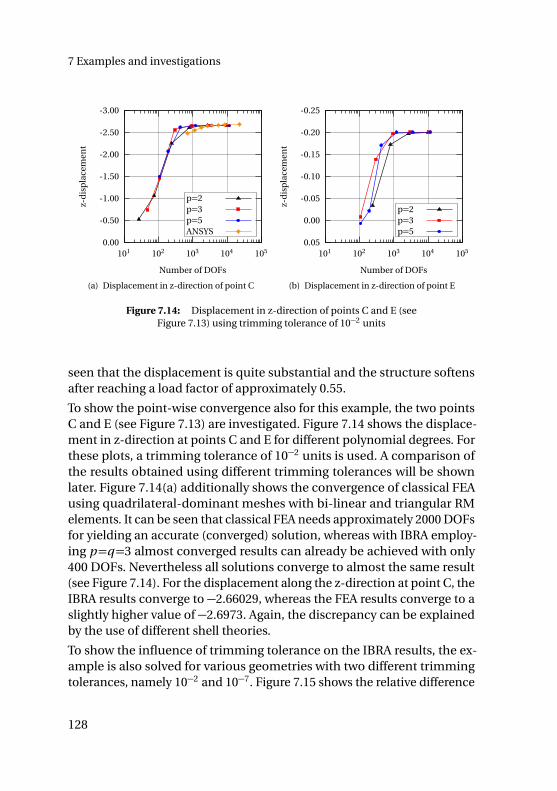
7 Examples and investigations
-3.00
-2.50
-2.00
-1.50
-1.00
-0.50
0.00101 102 103 104 105
z-d
isp
lace
men
t
Number of DOFs
p=2p=3p=5ANSYS
(a) Displacement in z-direction of point C
-0.25
-0.20
-0.15
-0.10
-0.05
0.00
0.05101 102 103 104 105
z-d
isp
lace
men
t
Number of DOFs
p=2p=3p=5
(b) Displacement in z-direction of point E
Figure 7.14: Displacement in z-direction of points C and E (seeFigure 7.13) using trimming tolerance of 10−2 units
seen that the displacement is quite substantial and the structure softensafter reaching a load factor of approximately 0.55.
To show the point-wise convergence also for this example, the two pointsC and E (see Figure 7.13) are investigated. Figure 7.14 shows the displace-ment in z-direction at points C and E for different polynomial degrees. Forthese plots, a trimming tolerance of 10−2 units is used. A comparison ofthe results obtained using different trimming tolerances will be shownlater. Figure 7.14(a) additionally shows the convergence of classical FEAusing quadrilateral-dominant meshes with bi-linear and triangular RMelements. It can be seen that classical FEA needs approximately 2000 DOFsfor yielding an accurate (converged) solution, whereas with IBRA employ-ing p=q=3 almost converged results can already be achieved with only400 DOFs. Nevertheless all solutions converge to almost the same result(see Figure 7.14). For the displacement along the z-direction at point C, theIBRA results converge to −2.66029, whereas the FEA results converge to aslightly higher value of −2.6973. Again, the discrepancy can be explainedby the use of different shell theories.
To show the influence of trimming tolerance on the IBRA results, the ex-ample is also solved for various geometries with two different trimmingtolerances, namely 10−2 and 10−7. Figure 7.15 shows the relative difference
128
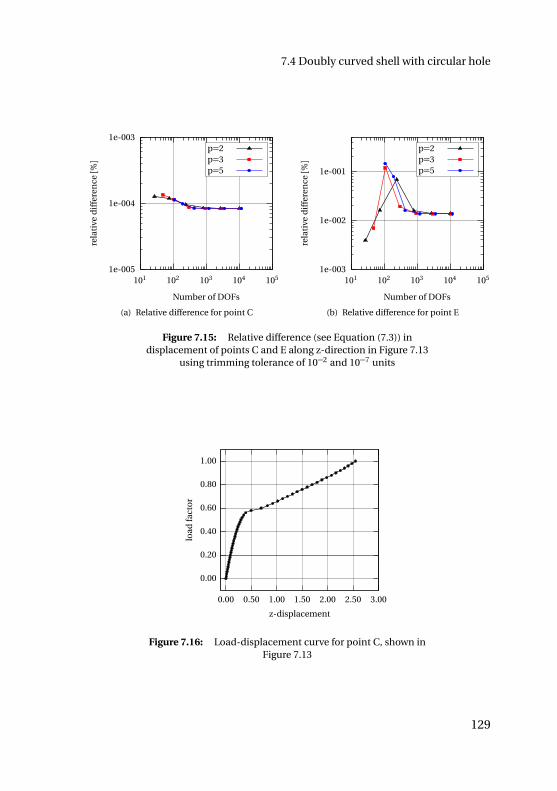
7.4 Doubly curved shell with circular hole
1e-005
1e-004
1e-003
101 102 103 104 105
r ela
tive
dif
fere
nce[%]
Number of DOFs
p=2p=3p=5
(a) Relative difference for point C
1e-003
1e-002
1e-001
101 102 103 104 105
r ela
tive
dif
fere
nce[%]
Number of DOFs
p=2p=3p=5
(b) Relative difference for point E
Figure 7.15: Relative difference (see Equation (7.3)) indisplacement of points C and E along z-direction in Figure 7.13
using trimming tolerance of 10−2 and 10−7 units
0.00
0.20
0.40
0.60
0.80
1.00
0.00 0.50 1.00 1.50 2.00 2.50 3.00
load
fact
or
z-displacement
Figure 7.16: Load-displacement curve for point C, shown inFigure 7.13
129
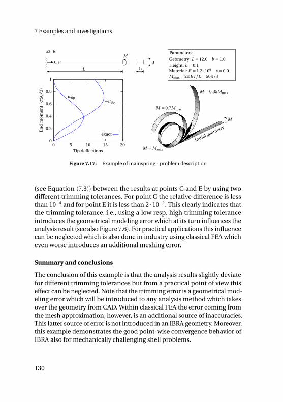
7 Examples and investigations
M
L b
hx, u
z, w
−utip
wtip
M =Mmax
M
Initial geometry
0
0.2
0.4
0.6
0.8
1
0 5 10 15 20
En
dm
om
ent(·π
50/3
)
Tip deflections
exact
M = 0.7Mmax
M = 0.35Mmax
Geometry: L = 12.0 b = 1.0
Parameters:
Material: E = 1.2 ·106 ν= 0.0Mmax = 2πE I /L = 50π/3
Height: h = 0.1
Figure 7.17: Example of mainspring - problem description
(see Equation (7.3)) between the results at points C and E by using twodifferent trimming tolerances. For point C the relative difference is lessthan 10−4 and for point E it is less than 2 ·10−2. This clearly indicates thatthe trimming tolerance, i.e., using a low resp. high trimming toleranceintroduces the geometrical modeling error which at its turn influences theanalysis result (see also Figure 7.6). For practical applications this influencecan be neglected which is also done in industry using classical FEA whicheven worse introduces an additional meshing error.
Summary and conclusions
The conclusion of this example is that the analysis results slightly deviatefor different trimming tolerances but from a practical point of view thiseffect can be neglected. Note that the trimming error is a geometrical mod-eling error which will be introduced to any analysis method which takesover the geometry from CAD. Within classical FEA the error coming fromthe mesh approximation, however, is an additional source of inaccuracies.This latter source of error is not introduced in an IBRA geometry. Moreover,this example demonstrates the good point-wise convergence behavior ofIBRA also for mechanically challenging shell problems.
130
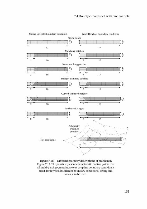
7.4 Doubly curved shell with circular hole
Single patch
Matching patches
Strong Dirichlet boundary condition Weak Dirichlet boundary condition
Non-matching patches
Straight-trimmed patches
Curved-trimmed patches
12
1
1
1
1
1
102
102
102
102
12
1
1
1
1
1
102
102
102
102
- Not applicable -
Patches with a gap
1
102
1
102
Arbitrarily-trimmedpatches
1
12
Figure 7.18: Different geometry descriptions of problem inFigure 7.17. The points represent characteristic control points. Forall multi-patch geometries, a weak coupling boundary condition is
used. Both types of Dirichlet boundary conditions, strong andweak, can be used.
131
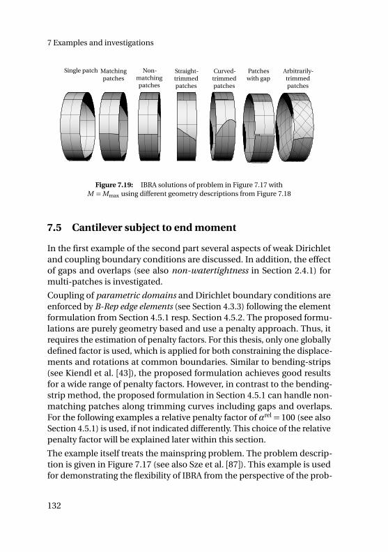
7 Examples and investigations
Single patch Matchingpatches
Non-matchingpatches
Straight-trimmedpatches
Curved-trimmedpatches
Patcheswith gap
Arbitrarily-trimmedpatches
Figure 7.19: IBRA solutions of problem in Figure 7.17 withM =Mmax using different geometry descriptions from Figure 7.18
7.5 Cantilever subject to end moment
In the first example of the second part several aspects of weak Dirichletand coupling boundary conditions are discussed. In addition, the effectof gaps and overlaps (see also non-watertightness in Section 2.4.1) formulti-patches is investigated.
Coupling of parametric domains and Dirichlet boundary conditions areenforced by B-Rep edge elements (see Section 4.3.3) following the elementformulation from Section 4.5.1 resp. Section 4.5.2. The proposed formu-lations are purely geometry based and use a penalty approach. Thus, itrequires the estimation of penalty factors. For this thesis, only one globallydefined factor is used, which is applied for both constraining the displace-ments and rotations at common boundaries. Similar to bending-strips(see Kiendl et al. [43]), the proposed formulation achieves good resultsfor a wide range of penalty factors. However, in contrast to the bending-strip method, the proposed formulation in Section 4.5.1 can handle non-matching patches along trimming curves including gaps and overlaps.For the following examples a relative penalty factor of αrel = 100 (see alsoSection 4.5.1) is used, if not indicated differently. This choice of the relativepenalty factor will be explained later within this section.
The example itself treats the mainspring problem. The problem descrip-tion is given in Figure 7.17 (see also Sze et al. [87]). This example is usedfor demonstrating the flexibility of IBRA from the perspective of the prob-
132
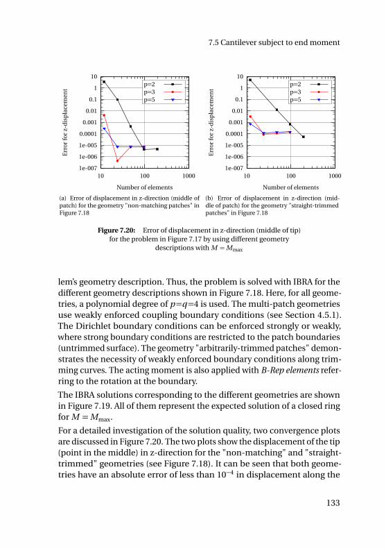
7.5 Cantilever subject to end moment
1e-007
1e-006
1e-005
0.0001
0.001
0.01
0.1
1
10
10 100 1000
Err
or
for
z-d
isp
lace
men
t
Number of elements
p=2p=3p=5
(a) Error of displacement in z-direction (middle ofpatch) for the geometry "non-matching patches" inFigure 7.18
1e-007
1e-006
1e-005
0.0001
0.001
0.01
0.1
1
10
10 100 1000
Err
or
for
z-d
isp
lace
men
t
Number of elements
p=2p=3p=5
(b) Error of displacement in z-direction (mid-dle of patch) for the geometry "straight-trimmedpatches" in Figure 7.18
Figure 7.20: Error of displacement in z-direction (middle of tip)for the problem in Figure 7.17 by using different geometry
descriptions with M =Mmax
lem’s geometry description. Thus, the problem is solved with IBRA for thedifferent geometry descriptions shown in Figure 7.18. Here, for all geome-tries, a polynomial degree of p=q=4 is used. The multi-patch geometriesuse weakly enforced coupling boundary conditions (see Section 4.5.1).The Dirichlet boundary conditions can be enforced strongly or weakly,where strong boundary conditions are restricted to the patch boundaries(untrimmed surface). The geometry "arbitrarily-trimmed patches" demon-strates the necessity of weakly enforced boundary conditions along trim-ming curves. The acting moment is also applied with B-Rep elements refer-ring to the rotation at the boundary.
The IBRA solutions corresponding to the different geometries are shownin Figure 7.19. All of them represent the expected solution of a closed ringfor M =Mmax.
For a detailed investigation of the solution quality, two convergence plotsare discussed in Figure 7.20. The two plots show the displacement of the tip(point in the middle) in z-direction for the "non-matching" and "straight-trimmed" geometries (see Figure 7.18). It can be seen that both geome-tries have an absolute error of less than 10−4 in displacement along the
133
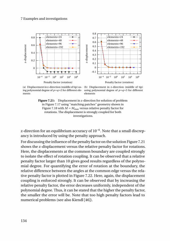
7 Examples and investigations
0
0.2
0.4
0.6
0.8
10−4 10−2 100 102 104 106
z-d
isp
lace
men
t
Penalty factor (rotation)
elements=24elements=48elements=96elements=192
(a) Displacement in z-direction (middle of tip) us-ing polynomial degree of p=q=2 for different ele-ments
-0.1
0
0.1
0.2
0.3
0.4
0.5
0.6
0.7
0.8
10−4 10−2 100 102 104 106
z-d
isp
lace
men
t
Penalty factor (rotation)
elements=24elements=48elements=96elements=192
(b) Displacement in z-direction (middle of tip)using polynomial degree of p=q=3 for differentelements
Figure 7.21: Displacement in z-direction for solution of problemin Figure 7.17 using "matching patches" geometry shown inFigure 7.18 with M =Mmax versus relative penalty factor for
rotations. The displacement is strongly coupled for bothinvestigations.
z-direction for an equilibrium accuracy of 10−6. Note that a small discrep-ancy is introduced by using the penalty approach.
For discussing the influence of the penalty factor on the solution Figure 7.21shows the z-displacement versus the relative penalty factor for rotations.Here, the displacements at the common boundary are coupled stronglyto isolate the effect of rotation coupling. It can be observed that a relativepenalty factor larger than 10 gives good results regardless of the polyno-mial degree. For quantifying the error of rotation at the boundary, therelative difference between the angles at the common edge versus the rela-tive penalty factor is plotted in Figure 7.22. Here, again, the displacementcoupling is enforced strongly. It can be observed that by increasing therelative penalty factor, the error decreases uniformly, independent of thepolynomial degree. Thus, it can be stated that the higher the penalty factor,the smaller the error will be. Note that too high penalty factors lead tonumerical problems (see also Kiendl [46]).
134
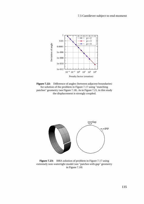
7.5 Cantilever subject to end moment
1e-012
1e-010
1e-008
1e-006
0.0001
0.01
1
10−4 10−2 100 102 104 106
Dev
iati
on
ofa
ngl
e
Penalty factor (rotation)
p = 2p = 3p = 4
Figure 7.22: Difference of angles (between adjacent boundaries)for solution of the problem in Figure 7.17 using "matching
patches" geometry (see Figure 7.18). As in Figure 7.21, in this studythe displacement is strongly coupled.
overlap
gap
Figure 7.23: IBRA solution of problem in Figure 7.17 usingextremely non-watertight model (see "patches with gap" geometry
in Figure 7.18)
135
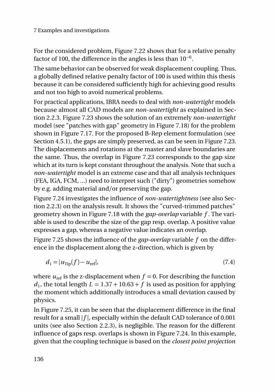
7 Examples and investigations
For the considered problem, Figure 7.22 shows that for a relative penaltyfactor of 100, the difference in the angles is less than 10−6.
The same behavior can be observed for weak displacement coupling. Thus,a globally defined relative penalty factor of 100 is used within this thesisbecause it can be considered sufficiently high for achieving good resultsand not too high to avoid numerical problems.
For practical applications, IBRA needs to deal with non-watertight modelsbecause almost all CAD models are non-watertight as explained in Sec-tion 2.2.3. Figure 7.23 shows the solution of an extremely non-watertightmodel (see "patches with gap" geometry in Figure 7.18) for the problemshown in Figure 7.17. For the proposed B-Rep element formulation (seeSection 4.5.1), the gaps are simply preserved, as can be seen in Figure 7.23.The displacements and rotations at the master and slave boundaries arethe same. Thus, the overlap in Figure 7.23 corresponds to the gap sizewhich at its turn is kept constant throughout the analysis. Note that such anon-watertight model is an extreme case and that all analysis techniques(FEA, IGA, FCM, ...) need to interpret such ("dirty") geometries somehowby e.g. adding material and/or preserving the gap.
Figure 7.24 investigates the influence of non-watertightness (see also Sec-tion 2.2.3) on the analysis result. It shows the "curved-trimmed patches"geometry shown in Figure 7.18 with the gap-overlap variable f . The vari-able is used to describe the size of the gap resp. overlap. A positive valueexpresses a gap, whereas a negative value indicates an overlap.
Figure 7.25 shows the influence of the gap-overlap variable f on the differ-ence in the displacement along the z-direction, which is given by
d1 = |uTip( f )−uref|, (7.4)
where uref is the z-displacement when f = 0. For describing the functiond1, the total length L = 1.37+ 10.63+ f is used as position for applyingthe moment which additionally introduces a small deviation caused byphysics.
In Figure 7.25, it can be seen that the displacement difference in the finalresult for a small | f |, especially within the default CAD tolerance of 0.001units (see also Section 2.2.3), is negligible. The reason for the differentinfluence of gaps resp. overlaps is shown in Figure 7.24. In this example,given that the coupling technique is based on the closest point projection
136
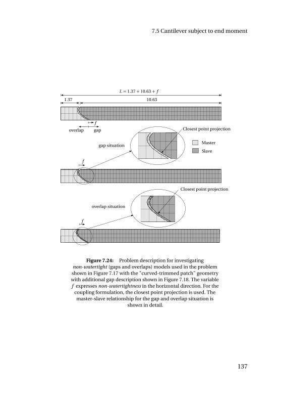
7.5 Cantilever subject to end moment
1.37
L = 1.37 + 10.63 + f
10.63
Closest point projectionf
gapoverlap
f
Master
Slave
f
gap situation
overlap situation
Closest point projection
Figure 7.24: Problem description for investigatingnon-watertight (gaps and overlaps) models used in the problemshown in Figure 7.17 with the "curved-trimmed patch" geometrywith additional gap description shown in Figure 7.18. The variablef expresses non-watertightness in the horizontal direction. For the
coupling formulation, the closest point projection is used. Themaster-slave relationship for the gap and overlap situation is
shown in detail.
137
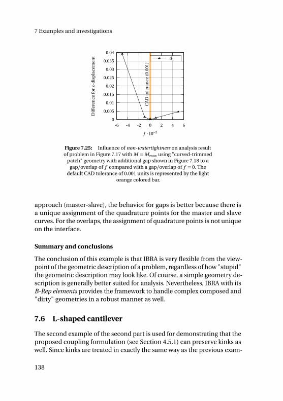
7 Examples and investigations
0
0.005
0.01
0.015
0.02
0.025
0.03
0.035
0.04
-6 -4 -2 0 2 4 6
Dif
fere
nce
for
z-d
isp
lace
men
t
f ·10−2
CA
Dto
lera
nce
(0.0
01)
d1
Figure 7.25: Influence of non-watertightness on analysis resultof problem in Figure 7.17 with M =Mmax using "curved-trimmed
patch" geometry with additional gap shown in Figure 7.18 to agap/overlap of f compared with a gap/overlap of f = 0. The
default CAD tolerance of 0.001 units is represented by the lightorange colored bar.
approach (master-slave), the behavior for gaps is better because there isa unique assignment of the quadrature points for the master and slavecurves. For the overlaps, the assignment of quadrature points is not uniqueon the interface.
Summary and conclusions
The conclusion of this example is that IBRA is very flexible from the view-point of the geometric description of a problem, regardless of how "stupid"the geometric description may look like. Of course, a simple geometry de-scription is generally better suited for analysis. Nevertheless, IBRA with itsB-Rep elements provides the framework to handle complex composed and"dirty" geometries in a robust manner as well.
7.6 L-shaped cantilever
The second example of the second part is used for demonstrating that theproposed coupling formulation (see Section 4.5.1) can preserve kinks aswell. Since kinks are treated in exactly the same way as the previous exam-
138
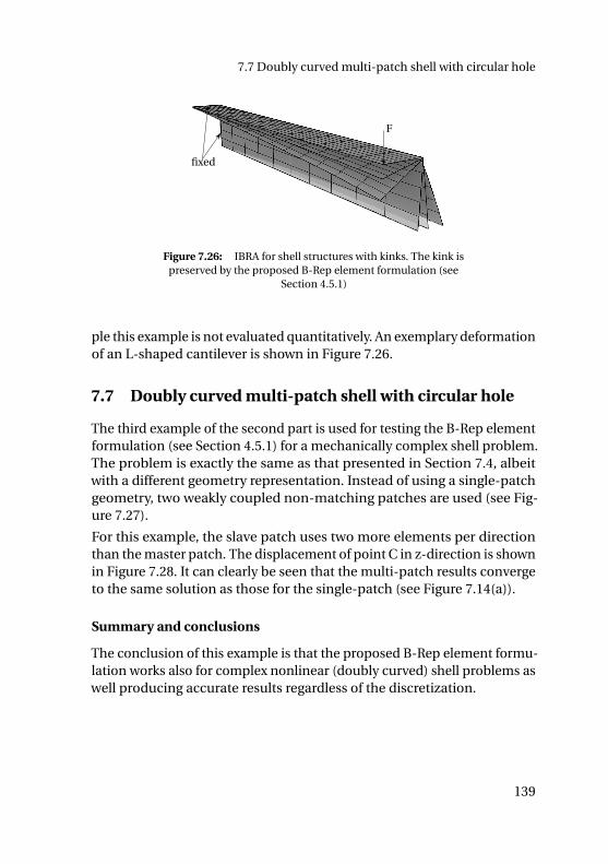
7.7 Doubly curved multi-patch shell with circular hole
F
fixed
Figure 7.26: IBRA for shell structures with kinks. The kink ispreserved by the proposed B-Rep element formulation (see
Section 4.5.1)
ple this example is not evaluated quantitatively. An exemplary deformationof an L-shaped cantilever is shown in Figure 7.26.
7.7 Doubly curved multi-patch shell with circular hole
The third example of the second part is used for testing the B-Rep elementformulation (see Section 4.5.1) for a mechanically complex shell problem.The problem is exactly the same as that presented in Section 7.4, albeitwith a different geometry representation. Instead of using a single-patchgeometry, two weakly coupled non-matching patches are used (see Fig-ure 7.27).
For this example, the slave patch uses two more elements per directionthan the master patch. The displacement of point C in z-direction is shownin Figure 7.28. It can clearly be seen that the multi-patch results convergeto the same solution as those for the single-patch (see Figure 7.14(a)).
Summary and conclusions
The conclusion of this example is that the proposed B-Rep element formu-lation works also for complex nonlinear (doubly curved) shell problems aswell producing accurate results regardless of the discretization.
139
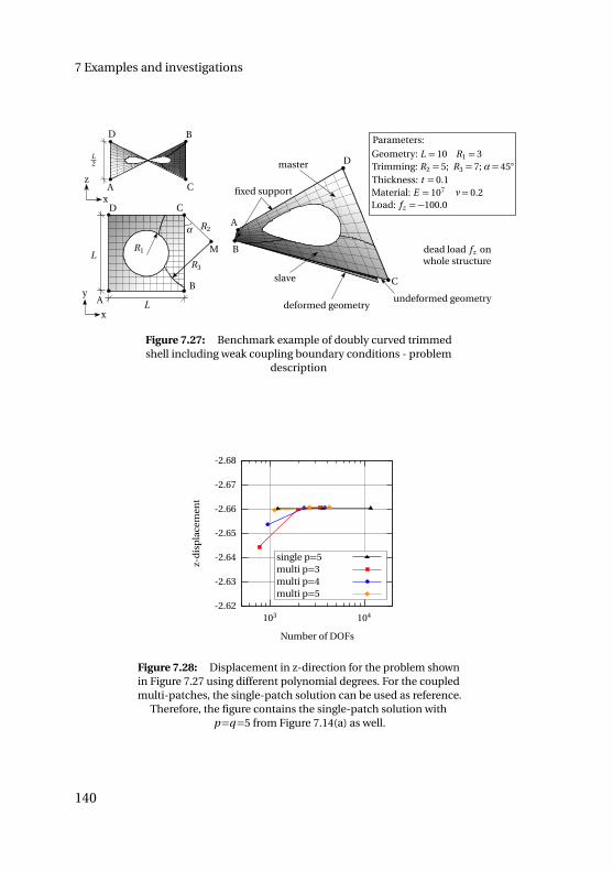
7 Examples and investigations
x
A
B
CD
A
D
C
B
deformed geometryundeformed geometry
A
B
C
D
fixed support
L
L
L2
R1
x
y
z
M
R2
R3
α
dead load fz onwhole structure
master
slave
Geometry: L = 10 R1 = 3
Parameters:
Material: E = 107 ν= 0.2Load: fz =−100.0
Thickness: t = 0.1Trimming: R2 = 5; R3 = 7; α= 45
Figure 7.27: Benchmark example of doubly curved trimmedshell including weak coupling boundary conditions - problem
description
-2.68
-2.67
-2.66
-2.65
-2.64
-2.63
-2.62103 104
z-d
isp
lace
men
t
Number of DOFs
single p=5multi p=3multi p=4multi p=5
Figure 7.28: Displacement in z-direction for the problem shownin Figure 7.27 using different polynomial degrees. For the coupledmulti-patches, the single-patch solution can be used as reference.
Therefore, the figure contains the single-patch solution withp=q=5 from Figure 7.14(a) as well.
140
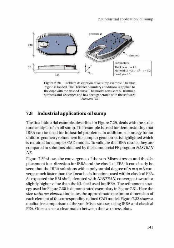
7.8 Industrial application: oil sump
Parameters:
Material: E = 2.1 ·105 ν= 0.2Load: p = 0.5
Thickness: t = 1.0
x
zy
pressure p
clamped
440
50
240A
Figure 7.29: Problem description of oil sump example. The blueregion is loaded. The Dirichlet boundary conditions is applied tothe edge with the dashed curve. The model consist of 50 trimmedsurfaces and 120 edges and has been generated with the software
Siemens NX.
7.8 Industrial application: oil sump
The first industrial example, described in Figure 7.29, deals with the struc-tural analysis of an oil sump. This example is used for demonstrating thatIBRA can be used for industrial problems. In addition, a strategy for anuniform geometry refinement for complex geometries is highlighted whichis required for complex CAD models. To validate the IBRA results they arecompared to solutions obtained by the commercial FE program NASTRANNX.
Figure 7.30 shows the convergence of the von-Mises stresses and the dis-placement in z-direction for IBRA and the classical FEA. It can clearly beseen that the IBRA solutions with a polynomial degree of p = q = 3 con-verge much faster than the linear basis functions used within classical FEA.As expected the RM shell, denoted with NASTRAN, converges towards aslightly higher value than the KL shell used for IBRA. The refinement strat-egy used for Figure 7.30 is demonstrated exemplary in Figure 7.31. Here thesize units per element indicates the approximate maximum dimension ofeach element of the corresponding refined CAD model. Figure 7.32 shows aqualitative comparison of the von-Mises stresses using IBRA and classicalFEA. One can see a clear match between the two stress plots.
141
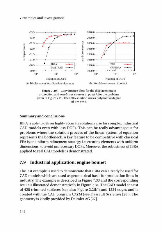
7 Examples and investigations
-63.5
-63.0
-62.5
-62.0
-61.5
-61.0
-60.5
-60.0104 105 106
z-d
isp
lace
men
t
Number of DOFs
IBRANASTRAN
(a) Displacement in z-direction of point A
1900.0
1920.0
1940.0
1960.0
1980.0
2000.0
2020.0
2040.0
104 105 106
von
-Mis
esst
ress
es
Number of DOFs
IBRANASTRAN
(b) Von-Mises stresses of point A
Figure 7.30: Convergence plots for the displacement inz-direction and von-Mises stresses at point A for the problem
given in Figure 7.29. The IBRA solution uses a polynomial degreeof p = q = 3.
Summary and conclusions
IBRA is able to deliver highly accurate solutions also for complex industrialCAD models even with less DOFs. This can be really advantageous forproblems where the solution process of the linear system of equationrepresents the bottleneck. A key feature to be competitive with classicalFEA is an uniform refinement strategy i.e. creating elements with uniformdimensions, to avoid unnecessary DOFs. Moreover the robustness of IBRAapplied to real CAD models is demonstrated.
7.9 Industrial application: engine bonnet
The last example is used to demonstrate that IBRA can already be used forCAD models which are used as geometrical basis for production lines inindustry. The example is described in Figure 7.33 and the correspondingresult is illustrated demonstratively in Figure 7.34. The CAD model consistof 428 trimmed surfaces (see also Figure 2.2(b)) and 1224 edges and iscreated with the CAD program CATIA (see Dassault Systemes [28]). Thegeometry is kindly provided by Daimler AG [27].
142
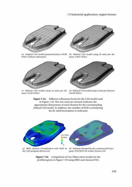
7.9 Industrial application: engine bonnet
(a) Original CAD model parametrization (10329DOFs) without refinement
(b) Refined CAD model using 20 units per ele-ment (13647 DOFs)
(c) Refined CAD model using 10 units per ele-ment (21561 DOFs)
(d) Refined CAD model using 5 units per element(44199 DOFs)
Figure 7.31: Different refinement levels for the CAD model usedin Figure 7.29. The size units per element indicates the
approximate dimensions of each element for the correspondingrefined CAD model. In addition, the number of DOFs considering
the KL shell formulation is indicated.
6850
0
von-Mises
(a) IBRA solution (Visualization with TeDA inthe CAD program Rhinoceros)
(b) Solution obtained by the commercial FE pro-gram NASTRAN NX within Siemens NX.
Figure 7.32: Comparison of von-Mises stress results for theproblem given in Figure 7.29 using IBRA and classical FEA.
143
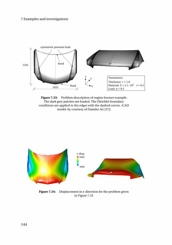
7 Examples and investigations
Parameters:
Material: E = 2.1 ·105 ν= 0.2Load: p = 0.5
Thickness: t = 1.0
1655
1355 fixed
fixed
symmetric pressure load
x
zy
Figure 7.33: Problem description of engine bonnet example.The dark grey patches are loaded. The Dirichlet boundary
conditions are applied to the edges with the dashed curves. (CADmodel: by courtesy of Daimler AG [27])
z-disp.
min
max
Figure 7.34: Displacement in z-direction for the problem givenin Figure 7.33
144
7.9 Industrial application: engine bonnet
Summary and conclusion of Chapter 7
The following list contains some important aspects elaborated within thischapter:
– Section 7.2 shows that restricting the parameter domain of a surfaceto a trimmed domain and applying an accurate integration schemeneither influences the convergence properties nor the accuracy ofthe underlying functional basis for analysis purposes. The accuracy isjust limited by the trimming tolerance (geometrical modeling error).
– Section 7.3 demonstrates the robustness of IBRA against distortionsin the geometric description as well as the good point-wise conver-gence even on trimmed boundaries.
– Section 7.4 demonstrates the influence of trimming tolerances onanalysis results (geometrical modeling error) for nonlinear shell prob-lems.
– Section 7.5 illustrates that IBRA is very flexible and able to deal with"dirty" geometries.
– Section 7.7 shows the accuracy of B-Rep coupling elements for geo-metrically nonlinear shell problems.
– The examples in Section 7.8 and Section 7.9 demonstrate that IBRAcan compete with established analysis approaches.
The various numerical examples including real industrial problems pre-sented in this chapter confirm the accuracy, flexibility, and robustness ofIBRA.
145


There is no reason anyonewould want a computer intheir home.
Ken Olsen, founder of DigitalEquipment Corporation,
1977
CH
AP
TE
R
8SUMMARY AND CONCLUSION
A new concept of a CAD-integrated design-through-analysis workflow forKirchhoff-Love (KL) shell structures, named Analysis in Computer AidedDesign (AiCAD), has been developed. AiCAD is realized within the commer-cial CAD Systems Siemens NX (see Siemens PLM Software [84]), Rhinoceros(see Rhinoceros [70]), and GiD (see GiD [34]). In contrast to other workflowsAiCAD uses the CAD geometry description, to be more specific NURBS-based B-Rep models (see Section 2.2), throughout the entire workflow.
For analyzing NURBS-based B-Rep models, the isogeometric B-Rep analysis,a new finite element technique, has been developed as well. IBRA can beseen as an extension of isogeometric analysis (IGA) introduced by Hugheset al. [40] by considering the B-Rep topology of the CAD model for theanalysis. Thus, it provides the framework for creating a direct and completeanalysis model from CAD in a consistent finite-element-like manner. Thenew type of finite elements called (isogeometric) B-Rep elements are used tohandle discontinuous and trimmed geometries with gaps and overlaps forstructural analysis and to enforce weak Dirichlet and Neumann boundaryconditions. Corresponding B-Rep element formulations are introduced.
147
8 Summary and Conclusion
Appropriate solutions for local refinement and the application of arbitrarilylocated loads within IBRA are presented as well. In addition, a new adaptiveGaussian integration procedure (AGIP) for integrating trimmed surfaces isintroduced. For applying AGIP the parameter domain of trimmed surfacesis subdivided into integration domains such that all of them can be handledby following one single procedure. The accuracy of this approach is shownby numerical examples.
Moreover a concept for implementing IBRA within an existing FE-programand realizing AiCAD within an existing CAD system is outlined and thus anew concept of bridging the gap between CAD and FEM is presented.
Various examples clearly demonstrate the power of IBRA. IBRA is flexiblefor trimming tolerances, robust against geometric distortion, and can han-dle non-watertight CAD models. These features have been demonstratedby the examples, which cover a gamut of problems ranging from simplelinear shells to real industrial problems.
The newly developed isogeometric B-Rep analysis seems to be general androbust enough to be competitive with established analysis approachesused in industry. Although the general concept has been established suc-cessfully, further research is necessary. Some interesting fields are thefollowing:
– development of alternative B-Rep element formulations for shellcoupling better suited for structural dynamics
– development of B-Rep element formulations for further applications(contact, shape optimization, FSI,...)
– defeaturing i.e. neglecting small details of the CAD model by treatingthem e.g. as rigid objects in oder to concentrate on the mechanicallyrelevant effects and thus to avoid unnecessary computational cost
There is still a long way to go until the proposed techniques are matureenough to use them in daily engineering life but the ingredients for a CAD-integrated design and analysis workflow for shell structures are provided bythis thesis.
148
BIBLIOGRAPHY
[1] Abel Coll Sans. “Robust volume mesh generation for non-watertightgeometries.” PhD thesis. Barcelona: CIMNE, May 2014.
[2] ANSYS. http://www.ansys.com.
[3] B. M. Irons. “Engineering applications of numerical integrationinstiffness methods.” In: AIAA J. 4 (1966), pp. 2035–2037.
[4] Y. Basar and W. Krätzig. Mechanik der Flächentragwerke. Theorie,Berechnungsmethoden, Anwendungsbeispiele. Braunschweig:Vieweg, 1985. ISBN: 3-528-08685-8.
[5] A. M. Bauer, M. Breitenberger, B. Philipp, R. Wüchner, andK.-U. Bletzinger. “Nonlinear isogeometric spatial Bernoulli beam.”In: Computer Methods in Applied Mechanics and Engineering 303(2016), pp. 101–127. DOI: 10.1016/j.cma.2015.12.027.
[6] Y. Bazilevs, V. M. Calo, Y. Zhang, and T. J. R. Hughes. IsogeometricFluid–structure Interaction Analysis with Applications to ArterialBlood Flow. 2006. DOI: 10.1007/s00466-006-0084-3.
[7] Y. Bazilevs, V. Calo, J. Cottrell, J. Evans, T. Hughes, S. Lipton,M. Scott, and T. Sederberg. “Isogeometric analysis using T-splines.”In: Computer Methods in Applied Mechanics and Engineering199.5-8 (2010), pp. 229–263. DOI: 10.1016/j.cma.2009.02.036.
[8] Y. Bazilevs, V. Calo, J. Cottrell, T. Hughes, A. Reali, and G. Scovazzi.“Variational multiscale residual-based turbulence modeling forlarge eddy simulation of incompressible flows.” In: ComputerMethods in Applied Mechanics and Engineering 197.1-4 (2007),pp. 173–201. DOI: 10.1016/j.cma.2007.07.016.
149
Bibliography
[9] Y. Bazilevs, M.-C. Hsu, and M. Scott. “Isogeometric fluid–structureinteraction analysis with emphasis on non-matchingdiscretizations, and with application to wind turbines.” In:Computer Methods in Applied Mechanics and Engineering 249-252(2012), pp. 28–41. DOI: 10.1016/j.cma.2012.03.028.
[10] T. Belytschko, R. W. Lewis, D. Peric, and R. L. Taylor. “Isogeometricanalysis of nearly incompressible solids.” In: International Journalfor Numerical Methods in Engineering 87.1-5 (2011), pp. 273–288.DOI: 10.1002/nme.3048.
[11] D. J. Benson, S. Hartmann, Y. Bazilevs, M.-C. Hsu, and T. Hughes.“Blended isogeometric shells.” In: Computer Methods in AppliedMechanics and Engineering 255 (2013), pp. 133–146. DOI:10.1016/j.cma.2012.11.020.
[12] D. Benson, Y. Bazilevs, M. Hsu, and T. Hughes. “Isogeometric shellanalysis: The Reissner–Mindlin shell.” In: Computer Methods inApplied Mechanics and Engineering 199.5-8 (2010), pp. 276–289.DOI: 10.1016/j.cma.2009.05.011.
[13] D. Benson, S. Hartmann, Y. Bazilevs, M.-C. Hsu, and T. Hughes.“Blended isogeometric shells.” In: Computer Methods in AppliedMechanics and Engineering 255 (2013), pp. 133–146. DOI:10.1016/j.cma.2012.11.020.
[14] W. Boehm. “Inserting new knots into B-spline curves.” In:Computer-Aided Design 12.4 (1980), pp. 199–201. DOI:10.1016/0010-4485(80)90154-2.
[15] C. de Boor. A practical guide to splines. 5. print. Vol. 27. Appliedmathematical sciences. New York: Springer, 1991. ISBN:0-387-90356-9.
[16] C. de Boor. A practical guide to splines: With 32 figures. Rev. ed.Vol. 27. Applied mathematical sciences. New York: Springer, 2001.ISBN: 0-387-95366-3.
[17] M. Breitenberger, A. Apostolatos, B. Philipp, R. Wüchner, andK.-U. Bletzinger. “Analysis in computer aided design: Nonlinearisogeometric B-Rep analysis of shell structures.” In: ComputerMethods in Applied Mechanics and Engineering 284 (2015),pp. 401–457. DOI: 10.1016/j.cma.2014.09.033.
150
Bibliography
[18] D. Burkhart, Hamann B., and Umlauf G. “Iso-geometric FiniteElement Analysis Based on Catmull-Clark Subdivision Solids.” In:Comput. Graph. Forum 29.5 (2010), pp. 1575–1784.
[19] B. K. Choi. Surface modeling for CAD/CAM. Vol. 11. Advances inindustrial engineering. Amsterdam, New York: Elsevier, 1991. ISBN:0444884823.
[20] F. Cirak, M. Ortiz, and P. Schröder. “Subdivision surfaces: a newparadigm for thin-shell finite-element analysis.” In: InternationalJournal for Numerical Methods in Engineering 47 (2000),pp. 2039–2072.
[21] F. Cirak and Q. Long. Subdivision shells with exact boundary controland non-manifold geometry. 2011. DOI: 10.1002/nme.3206.
[22] E. Cohen, T. Lyche, and L. L. Schumaker. “Degree raising forsplines.” In: Journal of Approximation Theory 46.2 (1986),pp. 170–181. DOI: 10.1016/0021-9045(86)90059-6.
[23] E. Cohen, R. F. Riesenfeld, and G. Elber. Geometric modeling withsplines: An introduction. Natick and Mass: AK Peters, 2001. ISBN:978-1568811376.
[24] J. A. Cottrell, T. J. R. Hughes, and Y. Bazilevs. Isogeometric analysis:Toward integration of CAD and FEA. Chichester et al.: Wiley, 2009.ISBN: 0470748737.
[25] J. Cottrell, T. Hughes, and A. Reali. “Studies of refinement andcontinuity in isogeometric structural analysis.” In: ComputerMethods in Applied Mechanics and Engineering 196.41-44 (2007),pp. 4160–4183. DOI: 10.1016/j.cma.2007.04.007.
[26] J. Cottrell, A. Reali, Y. Bazilevs, and T. Hughes. “Isogeometricanalysis of structural vibrations.” In: Computer Methods in AppliedMechanics and Engineering 195.41-43 (2006), pp. 5257–5296. DOI:10.1016/j.cma.2005.09.027.
[27] Daimler AG. https://www.daimler.com/.
[28] Dassault Systemes. http://www.3ds.com.
151
Bibliography
[29] R. Dimitri, L. de Lorenzis, M. Scott, P. Wriggers, R. Taylor, andG. Zavarise. “Isogeometric large deformation frictionless contactusing T-splines.” In: Computer Methods in Applied Mechanics andEngineering 269 (2014), pp. 394–414. DOI:10.1016/j.cma.2013.11.002.
[30] W. Dornisch, S. Klinkel, and B. Simeon. “IsogeometricReissner–Mindlin shell analysis with exactly calculated directorvectors.” In: Computer Methods in Applied Mechanics andEngineering 253 (2013), pp. 491–504. DOI:10.1016/j.cma.2012.09.010.
[31] W. Dornisch, R. Müller, and S. Klinkel. “An efficient and robustrotational formulation for isogeometric Reissner–Mindlin shellelements.” In: Computer Methods in Applied Mechanics andEngineering 303 (2016), pp. 1–34. DOI:10.1016/j.cma.2016.01.018.
[32] A. Düster, J. Parvizian, Z. Yang, and E. Rank. “The finite cell methodfor three-dimensional problems of solid mechanics.” In: ComputerMethods in Applied Mechanics and Engineering 197.45-48 (2008),pp. 3768–3782. DOI: 10.1016/j.cma.2008.02.036.
[33] R. Echter, B. Oesterle, and M. Bischoff. A hierarchic family ofisogeometric shell finite elements. 2013. DOI:10.1016/j.cma.2012.10.018.
[34] GiD. http://www.gidhome.com/.
[35] W. J. Gordon and R. F. Riesenfeld. “Bernstein-Bézier Methods for theComputer-Aided Design of Free-Form Curves and Surfaces.” In:Journal of the ACM 21.2 (1974), pp. 293–310. DOI:10.1145/321812.321824.
[36] P. L. Gould. Introduction to linear elasticity. 2nd ed. New York:Springer-Verlag, 1994. ISBN: 0387941002.
[37] G. A. Hansen, R. W. Douglass, and A. Zardecki. Mesh enhancement:Selected elliptic methods, foundations and applications. London:Imperial College Press, 2005. ISBN: 1-86094-487-6.
152
Bibliography
[38] M.-C. Hsu, I. Akkerman, and Y. Bazilevs. “High-performancecomputing of wind turbine aerodynamics using isogeometricanalysis.” In: Computers & Fluids 49.1 (2011), pp. 93–100. DOI:10.1016/j.compfluid.2011.05.002.
[39] M.-C. Hsu, C. Wang, F. Xu, A. J. Herrema, and A. Krishnamurthy.“Direct immersogeometric fluid flow analysis using B-rep CADmodels.” In: Computer Aided Geometric Design (2016). DOI:10.1016/j.cagd.2016.02.007.
[40] T. Hughes, J. Cottrell, and Y. Bazilevs. “Isogeometric analysis: CAD,finite elements, NURBS, exact geometry and mesh refinement.” In:Computer Methods in Applied Mechanics and Engineering 194.39-41(2005), pp. 4135–4195. DOI: 10.1016/j.cma.2004.10.008.
[41] ISO 10303. www.WikiSTEP.org: STEP (Standard for the Exchange ofProduct model data).
[42] L. Kantorovich and V. Krylov. Approximate methods of higheranalysis. Interscience Publishers, 1958.
[43] J. Kiendl, Y. Bazilevs, M.-C. Hsu, R. Wüchner, and K.-U. Bletzinger.“The bending strip method for isogeometric analysis ofKirchhoff–Love shell structures comprised of multiple patches.” In:Computer Methods in Applied Mechanics and Engineering 199.37-40(2010), pp. 2403–2416. DOI: 10.1016/j.cma.2010.03.029.
[44] J. Kiendl, K.-U. Bletzinger, J. Linhard, and R. Wüchner.“Isogeometric shell analysis with Kirchhoff–Love elements.” In:Computer Methods in Applied Mechanics and Engineering 198.49-52(2009), pp. 3902–3914. DOI: 10.1016/j.cma.2009.08.013.
[45] J. Kiendl, R. Schmidt, R. Wüchner, and K.-U. Bletzinger.“Isogeometric shape optimization of shells using semi-analyticalsensitivity analysis and sensitivity weighting.” In: ComputerMethods in Applied Mechanics and Engineering 274 (2014),pp. 148–167. DOI: 10.1016/j.cma.2014.02.001.
[46] M. J. Kiendl. Isogeometric analysis and shape optimal design of shellstructures. Aachen: Shaker, 2011. ISBN: 978-3-8440-0104-4.
153
Bibliography
[47] H.-J. Kim, Y.-D. Seo, and S.-K. Youn. “Isogeometric analysis fortrimmed CAD surfaces.” In: Computer Methods in AppliedMechanics and Engineering 198.37-40 (2009), pp. 2982–2995. DOI:10.1016/j.cma.2009.05.004.
[48] E. Klingbeil. Tensorrechnung für Ingenieure. Vol. 197/197a.BI-Hochschultaschenbücher. Mannheim [u.a.]: BI-Wiss.-Verl., 1966.ISBN: 978-3411001972.
[49] P. M. Knupp and S. Steinberg. The fundamentals of grid generation.Boca Raton [u.a.]: CRC Press, 1994. ISBN: 0-8493-8987-9.
[50] S. Krishnan and D. Manocha. “An efficient surface intersectionalgorithm based on lower-dimensional formulation.” In: ACMTransactions on Graphics (TOG) 16.1 (1997), pp. 74–106.
[51] L. Kudela, N. Zander, T. Bog, S. Kollmannsberger, and E. Rank.“Efficient and accurate numerical quadrature for immersedboundary methods.” In: Advanced Modeling and Simulation inEngineering Sciences 2.1 (2015), p. 763. DOI:10.1186/s40323-015-0031-y.
[52] L. Kudela, N. Zander, S. Kollmannsberger, and E. Rank. “Smartoctrees: Accurately integrating discontinuous functions in 3D.” In:Computer Methods in Applied Mechanics and Engineering 306(2016), pp. 406–426. DOI: 10.1016/j.cma.2016.04.006.
[53] G. Kuru, C. Verhoosel, K. van der Zee, and E. van Brummelen.“Goal-adaptive Isogeometric Analysis with hierarchical splines.” In:Computer Methods in Applied Mechanics and Engineering 270(2014), pp. 270–292. DOI: 10.1016/j.cma.2013.11.026.
[54] L. de Lorenzis, I. Temizer, P. Wriggers, and G. Zavarise. A largedeformation frictional contact formulation using NURBS-basedisogeometric analysis. 2011. DOI: 10.1002/nme.3159.
[55] Y. L. Ma and W. Hewitt. “Point inversion and projection for NURBScurve and surface: Control polygon approach.” In: Computer AidedGeometric Design 20.2 (2003), pp. 79–99. DOI:10.1016/S0167-8396(03)00021-9.
[56] M. Mäntylä. An introduction to solid modeling. Vol. 13. Principles ofcomputer science series. Rockville and Md: Computer SciencePress, 1988. ISBN: 0-88175-108-1.
154
Bibliography
[57] M. E. Mortenson. Geometric modeling. New York: Wiley, 1985. ISBN:0471882798.
[58] A. P. Nagy and D. J. Benson. “On the numerical integration oftrimmed isogeometric elements.” In: Computer Methods in AppliedMechanics and Engineering (2014). DOI:10.1016/j.cma.2014.08.002.
[59] K. L. Narayan, K. M. Rao, and Sarcar, M. M. M. Computer aideddesign and manufacturing. New Delhi: Prentice-Hall of India, 2008.ISBN: 812033342X.
[60] N. Nguyen-Thanh, J. Kiendl, H. Nguyen-Xuan, R. Wüchner,K. Bletzinger, Y. Bazilevs, and T. Rabczuk. “Rotation freeisogeometric thin shell analysis using PHT-splines.” In: ComputerMethods in Applied Mechanics and Engineering 200.47-48 (2011),pp. 3410–3424. DOI: 10.1016/j.cma.2011.08.014.
[61] J. Parvizian, A. Düster, and E. Rank. Finite cell method. 2007. DOI:10.1007/s00466-007-0173-y.
[62] N. M. Patrikalakis. “Surface-to-surface intersections.” In: IEEEComputer Graphics and Applications 13.1 (1993), pp. 89–95.
[63] B. Philipp, M. Breitenberger, I. D’Auria, R. Wüchner, andK.-U. Bletzinger. “Integrated design and analysis of structuralmembranes using the Isogeometric B-Rep Analysis.” In: ComputerMethods in Applied Mechanics and Engineering 303 (2016),pp. 312–340. DOI: 10.1016/j.cma.2016.02.003.
[64] L. Piegl and W. Tiller. “Geometry-based triangulation of trimmedNURBS surfaces.” In: Computer Aided Design 1.30 (1998), pp. 11–18.
[65] L. A. Piegl and W. Tiller. The NURBS book. 2nd ed. Berlin, New York:Springer, op. 1997. ISBN: 3-540-61545-8.
[66] X. Qian and O. Sigmund. “Isogeometric shape optimization ofphotonic crystals via Coons patches.” In: Computer Methods inApplied Mechanics and Engineering 200.25-28 (2011),pp. 2237–2255. DOI: 10.1016/j.cma.2011.03.007.
155
Bibliography
[67] E. Rank, M. Ruess, S. Kollmannsberger, D. Schillinger, and A. Düster.“Geometric modeling, isogeometric analysis and the finite cellmethod.” In: Computer Methods in Applied Mechanics andEngineering 249-252 (2012), pp. 104–115. DOI:10.1016/j.cma.2012.05.022.
[68] K. Reed, D. Harrod, and W. Conroy. The Initial Graphics ExchangeSpecification (IGES) version 5.0. Vol. 4412. NISTIR. Gaithersburg,MD: National Institute of Standards and Technology, 1990. ISBN:9781871530049.
[69] G. Renner and V. Weiß. “Exact and approximate computation ofB-spline curves on surfaces.” In: Computer-Aided Design 36.4(2004), pp. 351–362. DOI: 10.1016/S0010-4485(03)00100-3.
[70] Rhinoceros. http://www.rhino3d.com.
[71] R. F. Riesenfeld, E. Cohen, and Lyche T. “Discrete B-splines undsubdivision techniques in computer-aided geometric design andcomputer graphics.” In: Elsevier 1980 ().
[72] D. F. Rogers. An introduction to NURBS: With historical perspective.San Francisco: Morgan Kaufmann Publishers, 2001. ISBN:1-55860-669-6.
[73] J. Rooney and P. Steadman. Computer-aided Design. Milton Keynes:Open University Press, 1987. ISBN: 0273026720.
[74] Scan&Solve. http://www.intact-solutions.com.
[75] D. Schillinger. “The p- and B-spline versions of the geometricallynonlinear finite cell method and hierarchical refinement strategiesfor adaptive isogeometric and embedded domain analysis.”Dissertation. München: Technischen Universität München, 22.May2012.
[76] D. Schillinger, L. Dedè, M. A. Scott, J. A. Evans, M. J. Borden, E. Rank,and T. J. Hughes. “An isogeometric design-through-analysismethodology based on adaptive hierarchical refinement of NURBS,immersed boundary methods, and T-spline CAD surfaces.” In:Computer Methods in Applied Mechanics and Engineering 249-252(2012), pp. 116–150. DOI: 10.1016/j.cma.2012.03.017.
156
Bibliography
[77] D. Schillinger, M. Ruess, N. Zander, Y. Bazilevs, A. Düster, andE. Rank. Small and large deformation analysis with the p- andB-spline versions of the Finite Cell Method. 2012. DOI:10.1007/s00466-012-0684-z.
[78] R. Schmidt. Trimming, mapping, and optimization in isogeometricanalysis of shell structures: Zugl.: München, Techn. Univ., Diss., 2013.Vol. 20. Schriftenreihe des Lehrstuhls für Statik TU München.Aachen: Shaker, 2013. ISBN: 978-3-8440-2310-7.
[79] M. Scott, X. Li, T. Sederberg, and T. Hughes. “Local refinement ofanalysis-suitable T-splines.” In: Computer Methods in AppliedMechanics and Engineering 213-216 (2012), pp. 206–222. DOI:10.1016/j.cma.2011.11.022.
[80] T. W. Sederberg, G. T. Finnigan, X. Li, H. Lin, and H. Ipson.“Watertight trimmed NURBS.” In: ACM Transactions on Graphics27.3 (2008), p. 1. DOI: 10.1145/1360612.1360678.
[81] T. W. Sederberg and R. J. Meyers. “Loop detection in surface patchintersections.” In: Computer Aided Geometric Design 5.2 (1988),pp. 161–171.
[82] T. Sederberg, D. L. Cardon, J. Zheng, and Lyche T. “T-splineSimplication and Local Refinement.” In: ACM Trans. Graphics 2223.276-283 (2004).
[83] T. Sederberg, J. Zheng, A. Bakenov, and A. Nasri. “T-splines andT-NURCCs.” In: ACM Trans. Graphics 22 22.477-484 (2003).
[84] Siemens PLM Software. http://www.plm.automation.siemens.com.
[85] Spatial Corporation. http://www.spatial.com/.
[86] I. Stroud. Boundary representation modelling techniques. London:Springer, 2006. ISBN: 978-1-84628-312-3.
[87] K. Sze, X. Liu, and S. Lo. “Popular benchmark problems forgeometric nonlinear analysis of shells.” In: Finite Elements inAnalysis and Design 40.11 (2004), pp. 1551–1569. DOI:10.1016/j.finel.2003.11.001.
[88] I. Temizer, P. Wriggers, and T. Hughes. Three-dimensionalmortar-based frictional contact treatment in isogeometric analysiswith NURBS. 2012. DOI: 10.1016/j.cma.2011.10.014.
157
Bibliography
[89] B. H. V. Topping. Finite element mesh generation. Saxe-Coburgpublications on computational engineering. Stirling and Scotland:Saxe-Coburg Publications, 2004. ISBN: 1-874672-10-5.
[90] A.-V. Vuong, C. Giannelli, B. Jüttler, and B. Simeon. “A hierarchicalapproach to adaptive local refinement in isogeometric analysis.” In:Computer Methods in Applied Mechanics and Engineering 200.49-52(2011), pp. 3554–3567. DOI: 10.1016/j.cma.2011.09.004.
[91] W. A. Wall, M. A. Frenzel, and C. Cyron. Isogeometric structuralshape optimization. 2008. DOI: 10.1016/j.cma.2008.01.025.
[92] Y.-W. Wang, Z.-D. Huang, Y. Zheng, and S.-G. Zhang. “Isogeometricanalysis for compound B-spline surfaces.” In: Computer Methods inApplied Mechanics and Engineering 261-262 (2013), pp. 1–15. DOI:10.1016/j.cma.2013.04.001.
[93] Y. Zhang, Y. Bazilevs, S. Goswami, C. L. Bajaj, and T. J. Hughes.Patient-specific vascular NURBS modeling for isogeometric analysisof blood flow. 2007. DOI: 10.1016/j.cma.2007.02.009.
[94] Zienkiewicz, O.C. and Taylor, R.L. and Zhu, J.Z. The Finite ElementMethod, Its Basis and Fundamentals. 6th. Oxford: Elsevier, 2005.
158
Bisherige Titel der Schriftenreihe
Band Titel
1 Frank Koschnick, Geometrische Lockingeffekte bei Finiten Ele-menten und ein allgemeines Konzept zu ihrer Vermeidung, 2004.
2 Natalia Camprubi, Design and Analysis in Shape Optimizationof Shells, 2004.
3 Bernhard Thomee, Physikalisch nichtlineare Berechnung vonStahlfaserbetonkonstruktionen, 2005.
4 Fernaß Daoud, Formoptimierung von Freiformschalen - Math-ematische Algorithmen und Filtertechniken, 2005.
5 Manfred Bischoff, Models and Finite Elements for Thin-walledStructures, 2005.
6 Alexander Hörmann, Ermittlung optimierter Stabwerkmod-elle auf Basis des Kraftflusses als Anwendung plattformunab-hängiger Prozesskopplung, 2006.
7 Roland Wüchner, Mechanik und Numerik der Formfindung undFluid-Struktur-Interaktion von Membrantragwerken, 2006.
8 Florian Jurecka, Robust Design Optimization Based on Meta-modeling Techniques, 2007.
9 Johannes Linhard, Numerisch-mechanische Betrachtung desEntwurfsprozesses von Membrantragwerken, 2009.
10 Alexander Kupzok, Modeling the Interaction of Wind and Mem-brane Structures by Numerical Simulation, 2009.
11 Bin Yang, Modified Particle Swarm Optimizers and their Appli-cation to Robust Design and Structural Optimization, 2009.
Band Titel
12 Michael Fleischer, Absicherung der virtuellen Prozesskette fürFolgeoperationen in der Umformtechnik, 2009.
13 Amphon Jrusjrungkiat, Nonlinear Analysis of Pneumatic Mem-branes - From Subgrid to Interface, 2009.
14 Alexander Michalski, Simulation leichter Flächentragwerke ineiner numerisch generierten atmosphärischen Grenzschicht,2010.
15 Matthias Firl, Optimal Shape Design of Shell Structures, 2010.
16 Thomas Gallinger, Effiziente Algorithmen zur partitioniertenLösung stark gekoppelter Probleme der Fluid-Struktur-Wechselwirkung, 2011.
17 Josef Kiendl, Isogeometric Analysis and Shape Optimal Designof Shell Structures, 2011.
18 Joseph Jordan, Effiziente Simulation großer Mauerwerksstruk-turen mit diskreten Rissmodellen, 2011.
19 Albrecht von Boetticher, Flexible Hangmurenbarrieren: Einenumerische Modellierung des Tragwerks, der Hangmure undder Fluid-Struktur-Interaktion, 2012.
20 Robert Schmidt, Trimming, Mapping, and Optimization in Iso-geometric Analysis of Shell Structures, 2013.
21 Michael Fischer, Finite Element Based Simulation, Design andControl of Piezoelectric and Lightweight Smart Structures, 2013.
22 Falko Hartmut Dieringer, Numerical Methods for the Designand Analysis for Tensile Structures, 2014.
23 Rupert Fisch, Code Verification of Partitioned FSI Environmentsfor Lightweight Structures, 2014.
24 Stefan Sicklinger, Stabilized Co-Simulation of Coupled ProblemsIncluding Fields and Signals, 2014.
Band Titel
25 Madjid Hojjat, Node-based parametrization for shape optimaldesign, 2015.
26 Ute Israel, Optimierung in der Fluid-Struktur-Interaktion - Sen-sitivitätsanalyse fu ür die Formoptimierung auf Grundlage despartitionierten Verfahrens, 2015.
27 Electra Stavropoulou, Sensitivity analysis and regularizationfor shape optimization of coupled problems, 2015.
28 Daniel Markus, Numerical and Experimental Modeling forShape Optimization of Offshore Structures, 2015.
29 Pablo Suárez, Design Process for the Shape Optimization of Pres-surized Bulkheads as Components of Aircraft Structures, 2015.
30 Armin Widhammer, Variation of Reference Strategy - Generationof Optimized Cutting Patterns for Textile Fabrics, 2015.
31 Helmut Masching, Parameter Free Optimization of Shape Adap-tive Shell Structures, 2016.
32 Hao Zhang, A General Approach for Solving Inverse Problemsin Geophysical Systems by Applying Finite Element Method andMetamodel Techniques, 2016.
33 Tianyang Wang, Development of Co-Simulation Environmentand Mapping Algorithms, 2016.