Embed Size (px)
Citation preview
1
55thth Stakeholder Advisory Forum Stakeholder Advisory Forum West Texas Igneous and Bolson GAMWest Texas Igneous and Bolson GAM
March 25, 2004March 25, 2004
PEC OS
W EBB
BR EWSTER
H U D SPET H
PR ESIDIO
R EEVES
C U LBER SON
VAL VER D E
D U VAL
TERR ELL
C R OC KETT
KEN ED Y
FR IO
HAR R IS
HI L L
BELL
BEE
C L AY
POL K
ED WAR D S
JEFF D AVIS
KERR
GAIN ES
LEON
U VALD E
H ALE
D ALL AM
IRION
D IMMIT
L AMB
KIN G
BEXARKIN N EY
STAR R
H AL L
WISEJ AC K
UPTON
H ID AL GO
S U TTON
C ASS
OLD H AM
EL LIS
MED IN A
KIMBLE
Z AVAL A
KENT
R USK
LEE
LYN N
GR AY
C OKE
L A SALLE
MIL AM
ER ATH
H AR TL EY
H U N T
BR AZO R IA
SMITH
KN OX
FLOYD
L LAN O
A N D R EWS
TYL ER
TRAVISLIBER TY
J ONES
N U EC ES
R EA GAN
BOW IE
W AR D
ZAPATA
L AMAR
R EAL
N OLAN
TER R Y GAR ZA
MIL LS
C OL EMAN
EC TOR
TOM GR EEN
MASON
YOU N G
FALLS
CAMER ON
MAT AGOR D A
H AY S
BR OW N
C OOKE
JASPER
D EAF SMITH
BU R N ET
M AVER IC K
H OU STON
L AVAC A
FISH ER
C OLLIN
MOOR E
FAN N IN
M OTLEY
MAR TIN
L IVE OAK
D AL LAS
EL PASO
BAILEY
B OSQU E
H ARD IN
KLEBERG
J IM HOGG
TAYLOR
C OT TL E
POTTER
D ON LEY
GOLIAD
SAN SABA
ATASC OSA
D EN TON
C ORYEL LC R ANE
C ONC H O
BAYL OR
D E WITT
BR OOKS
PAR KER
R U N N ELS
N AVAR R O
AR C H ER
C ARSON
C ASTR O
WOOD
SC U R R Y
C R OSBY
FAYETTE
McMU L L EN
W H AR TON
BOR D EN
C AL H OUN
SH EL BY
MEN AR D
GIL LESPIE
PAR MER
WILSON
D IC KEN S
SC H LEIC H ER
GR IMES
F OAR D
PA N OLA
H ASKELL
BR ISC OE
R AN D AL L
D AW SON
MID L AN D
HOW AR D
Mc LEN N AN
GON ZA L ES
GR AYSON R ED R IVER
SW ISH ER
R OBERTS
H OC KL EY
A N DER SON
TAR R ANT
WALKER
L UBBOC K
VIC TOR IA
BASTROPJ EFFER SON
SHER MAN
WH EELER
MITC H ELL
YOAKU M
STER LIN GW IN KL ER
TRIN ITY
HEMPH ILL
W IL BA R-GER
C OMAN -C HE
WA
LL ER
KAR N ES
LIPSC OMB
JAC KSON
W IL LIAMSON
R EFU G IO
WILLAC Y
LOVIN G
AU STIN
EASTLAN D
H OPKIN S
Mc C U LL OC H
BL AN C O
H AR R ISONSTEPH EN S
AN GELIN A
CALL AH AN
C OLOR AD O
H AN SFOR D
K AU FMAN
BAN D ER A
PALO PIN TO
MON TAGU E
H AMILTO N
OC H IL TR EE
C OM AL
LIMEST ON ESABIN E
C OC H R AN
FORT BEN D
C H AMBE R S
VAN ZAN D T
WIC HITA
JOH N SON
STON EWAL L
H EN D ER SON
TITU S
FR EESTON E
MON TG OMER Y
H OOD
KEN D AL L
BR AZ OS
GAL VESTON
U P SH U R
H U TC H IN SON
L AMPAS AS
BU RL ESON
H AR D EMAN
GU AD ALU PE
CH IL D-RE SS
AR M-STR ON G
GL AS S-C OCK
N AC OG-D OC H ES
MAR ION
C ALD WELL
MAD ISON
OR AN GE
D ELTA
R AIN S
GRE GG
CAMP
MO
RR
IS
FR
ANKLIN
ROCK -W ALL
C OLLI NGS-W ORTH
THR OC K-MOR TON
SOME R-VE L
S ANA UGUS-
TI N E
S ANJAC IN TO
J IMWELL S
S HACK EL -FORD
C HE RO-KEE
NEW
TON
R OBE RT-S ON
WA SH ING-TON
AR A N-SA SS AN
P ATRIC I O
80
79
67
78
85
82
6876
69
81
75
77
87
71
72
73
74
8 4
86
83
46
47
66
53
45
54
56
50
65
38
64
41
51
16
59
42
49
39
63
48
40
61 57
44
37 55
58
62
43
60
52
36
70
29
6
14
17
35
15
9
25
3328
8
7
12
3
345
26
32
30
23
21 10
11
27
20
18
22
19
24
13
2
31
4
1
PECOS
WEBB
BREWSTER
HUDSPETH
PRESIDIO
REEVES
CULBERSON
VAL VERDE
DUVAL
TERRELL
CROC KETT
FRI O
HARRIS
HILL
BELL
BEE
KEN EDY
CLAY
POLK
EDWARDS
JEFF DAVIS
GAINES
LEON
KERR
UVALDE
HALE
DALLAM
KI NG
IRIO N
LAMB
DIMMI T
BEXARKI NNEY
STARR
HALL
JACK
CASS
WISE
SUTTON
OLD HAM
HIDALGO
ELLIS
UPTO N
ZAVALA
MEDI NA
KI MBLE
RUSK
LEE
LYNN KENT
GRAY
LA SALLE
COKE
MILAM
ER ATH
HARTLEY
HUNT
SMITH
KNOX
FLOYD
LLANO
TYLER
BRAZORIA
ANDREWS
TRAVIS LIBERTY
REAGAN
JONES
ZAPATA
LAMAR
BO WIE
NUECES
WARD
REAL
NOLAN
TERRY GARZA
COLEMAN
MILLS
ECTOR
YOUNG
TOM GREEN
MASON
FALLS
MAVERIC K
BURNET
HAYS
DEAF SMITH
JASPER
LAVACA
HOUSTON
COO KE
FISHER
BROW N
COLLIN
MOORE
MOTLEY
FANNIN
MARTIN
EL PASO
BAI LEY
DALLAS
LIVE OAK
BO SQU E
HARDIN
JIM HOGG
TAYLOR
CAMERON
POTTER
GOLIAD
CRANE
COTTLE
DONLEY
ATASCO SA
SAN SABA
DENTON
CORYELL
BAYLOR
CONCHO
BROOKS
RUNNELS
PARKER
NAVARRO
ARCHER
DE WITT
CARSON
SC URRY
MATAGORDA
CROSBY
KLEBERG
FAYETTE
SHELBY
WOOD
CASTR O
BORDEN
MENARD
WHARTON
NEWTON
PARMER
GILLESPIE
MCMULLEN
DICKENS
SCHLEICHER
FOARD
HASKELL
PAN OLA
GRIMES
MIDLAND
WILSON
RANDALL
BRISCOESW ISHER
DAWSON
GRAYSON
GONZALES
HOW ARD
RED RI VER
ROBERTS
HOCKLEY
TARRANT
AN DERSON
MCLENNAN
LUBBOCK
CALHOUN
CHEROKEE
VICTORIA
BASTROP
WALKER
SHERMAN
YOAKUM
MITCHELL
STERLING
HEMPHILL
WHEELER
KARNES
TRINITY
WINKLER
JACKSON
LIPSCO MB
LOVING
WILLIAMSON
AUSTIN
EASTLAND
REFU GIO
HOPKINS
HARRISON
BLANCO
CALLAHAN
COLORADO
ANGELINA
MCCULLOCH
STEPHENS
WILLACY
JEFFERSON
KAUFMAN
BANDERA
HANSFORD
COMANCHE
MO NTAGUE
PALO PINTO
JIM WELLS
LIMESTONE
COM AL
HAMILTON
OCHI LTREE
WILBARGER
SABI NE
COCH RAN
CHAMBERS
FO RT BEND
VAN ZANDT
HENDERSON
STONEWALL
JOHNSON
FREESTONE
MONTGOMERY
GLASSCOCK
KEN DALL
TITUS
BRAZOS
HOOD
WICHITA
AR MSTRONG
UPSHUR
ROBERTSON
HUTCHINSON
LAMPASAS
CHILDRESS
WAL LER
NACOGDOCHES
SHACKELFOR D
BURLESO N
HARDEMAN
GUADALUPE
GALVESTON
MARI ON
THR OCKM OR TON
COLLIN GSWORTH
MADI SON
CALDWELL
SAN PATRICIO
SAN JACI NTO
ARANSAS
WASHINGTON ORANGE
DELTA
RAINS
GREGG
SAN A UGUST IN
E
CAMP
MORRIS
FRAN
KLIN
SOMER-VELL
ROCK-WALL
Region F Brazos G
Panhandle
Far West Texas
Region C
East Texas
Region H
Llano Estacado
Plateau
Rio Grande
South Central Texas
Region B
Coastal Bend
Lower Colorado
North East Texas
Lavaca
P
D
K
N
B
M
L
J
O
H
I
C
E
A
GF
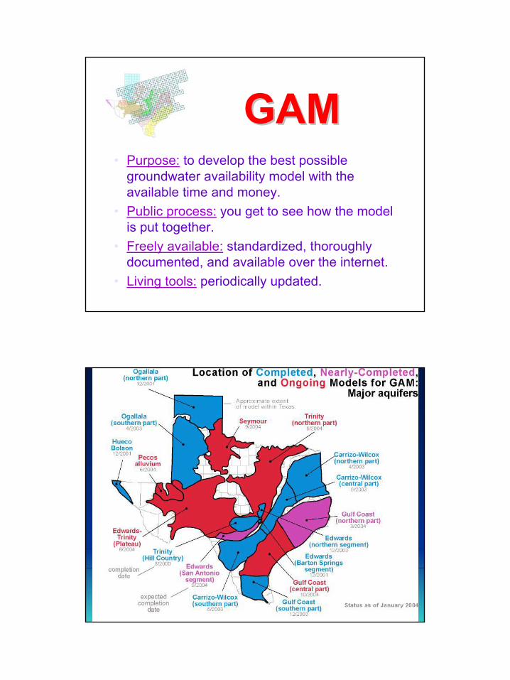
Groundwater Groundwater Availability ModelingAvailability Modeling
Contract ManagerContract Manager
• Texas Water Development Board
2
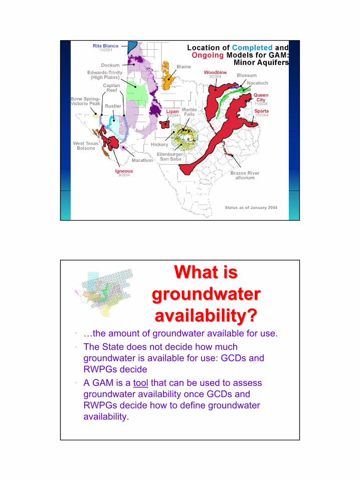
• Purpose: to develop the best possible groundwater availability model with the available time and money.
• Public process: you get to see how the model is put together.
• Freely available: standardized, thoroughly documented, and available over the internet.
• Living tools: periodically updated.
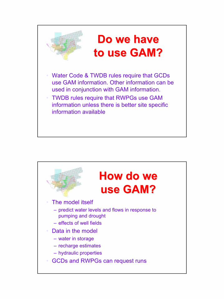
GAMGAM
3
• …the amount of groundwater available for use.• The State does not decide how much
groundwater is available for use: GCDs and RWPGs decide
• A GAM is a tool that can be used to assess groundwater availability once GCDs and RWPGs decide how to define groundwater availability.
What isWhat isgroundwatergroundwateravailability?availability?
4
• Water Code & TWDB rules require that GCDs use GAM information. Other information can be used in conjunction with GAM information.
• TWDB rules require that RWPGs use GAM information unless there is better site specific information available
Do we haveDo we haveto use GAM?to use GAM?
• The model itself– predict water levels and flows in response to
pumping and drought– effects of well fields
• Data in the model– water in storage– recharge estimates– hydraulic properties
• GCDs and RWPGs can request runs
How do weHow do weuse GAM?use GAM?
5
• GCDs, RWPGs, TWDB, and others collect new information on aquifer
• This information can enhance the current GAMs
• TWDB plans to update GAMs every five years with new info
• Please share information and ideas with TWDB on aquifers and GAMs
LivingLivingtoolstools
• SAF meetings– hear about progress on the model– comment on model assumptions– offer information (timing is important!)
• Report review– Deadline for comments on the IBGAM is April 9, 2004.
The final draft report is posted at:http://www.twdb.state.tx.us/gam/bol_ig/bol_ig.htm
• Contact TWDB (Robert Mace or Ted Angle)
Participating inParticipating inthe GAM processthe GAM process
6
Comments:Comments:Ted AngleTed Angle
(512)936(512)[email protected]@twdb.state.tx.us
www.twdb.state.tx.us/gamwww.twdb.state.tx.us/gam
Conceptual model Conceptual model
7
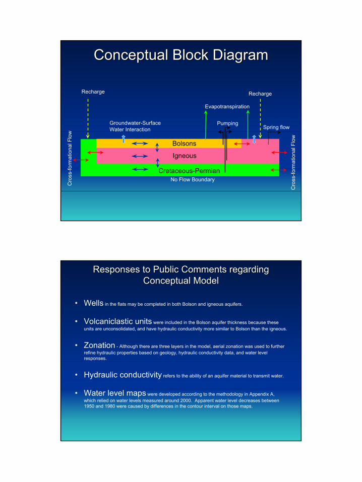
Conceptual Block DiagramConceptual Block Diagram
Bolsons
No Flow Boundary
Recharge
PumpingGroundwater-Surface Water Interaction Spring flow
Igneous
Cro
ss-fo
rmat
iona
l Flo
w
Cro
ss-fo
rmat
iona
l Flo
w
Cretaceous-Permian
Evapotranspiration
Recharge
Responses to Public Comments regarding Responses to Public Comments regarding Conceptual ModelConceptual Model
• Wells in the flats may be completed in both Bolson and igneous aquifers.
• Volcaniclastic units were included in the Bolson aquifer thickness because these units are unconsolidated, and have hydraulic conductivity more similar to Bolson than the igneous.
• Zonation - Although there are three layers in the model, aerial zonation was used to further refine hydraulic properties based on geology, hydraulic conductivity data, and water level responses.
• Hydraulic conductivity refers to the ability of an aquifer material to transmit water.
• Water level maps were developed according to the methodology in Appendix A, which relied on water levels measured around 2000. Apparent water level decreases between 1950 and 1980 were caused by differences in the contour interval on those maps.
8
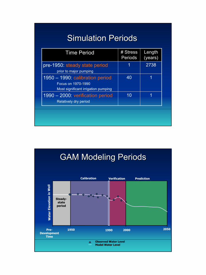
Simulation PeriodsSimulation Periods
1990 – 2000: verification periodRelatively dry period
1950 – 1990: calibration periodFocus on 1970-1990Most significant irrigation pumping
pre-1950: steady state periodprior to major pumping
Time Period Length (years)
# Stress Periods
110
140
27381
GAM Modeling PeriodsGAM Modeling Periods
Steady-state
period
Calibration Verification Prediction
Wat
er E
leva
tion
in W
ell
1950 1990 2000 2050
Observed Water LevelModel Water Level
Pre-Development
Time
9
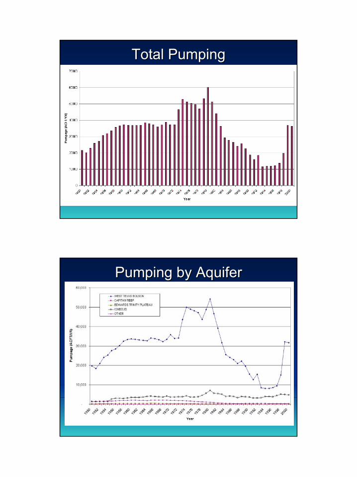
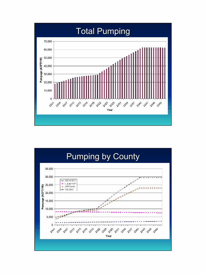
Total PumpingTotal Pumping
Pumping by AquiferPumping by Aquifer
10
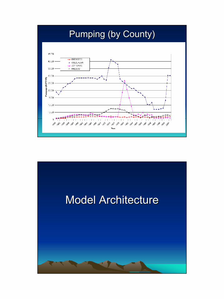
Pumping (by County)Pumping (by County)
Model ArchitectureModel Architecture
11
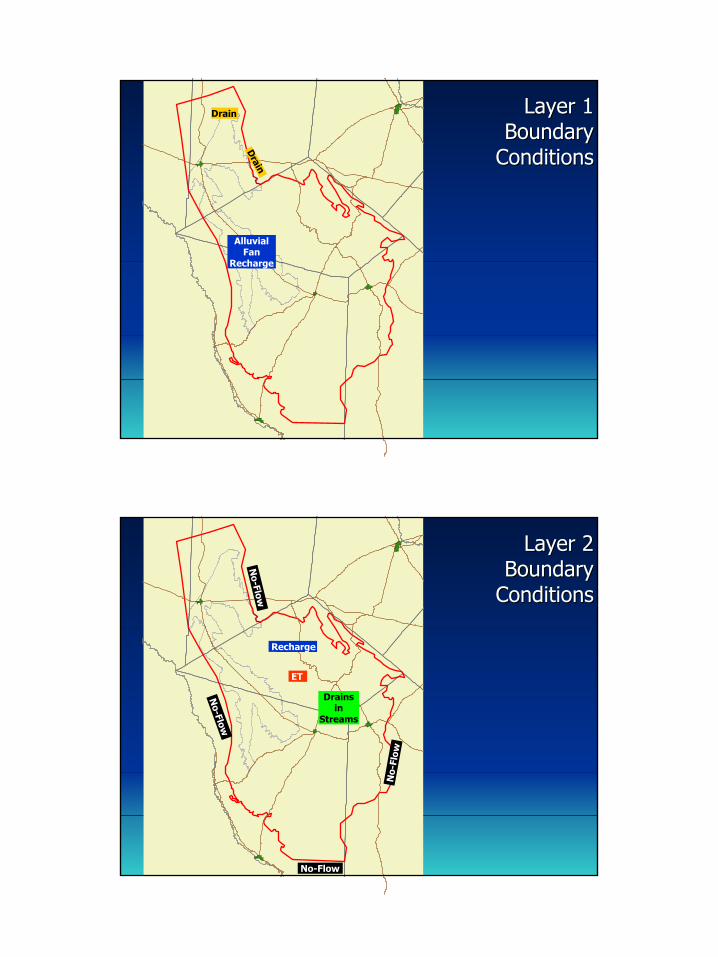
Layer 1 Layer 1 Boundary Boundary
ConditionsConditions
Alluvial Fan
Recharge
Drain
Drain
Layer 2 Layer 2 Boundary Boundary
ConditionsConditions
Drains in
Streams
Recharge
No-Flow
No-Flow
ET
No-
Flow
No-Flow
12
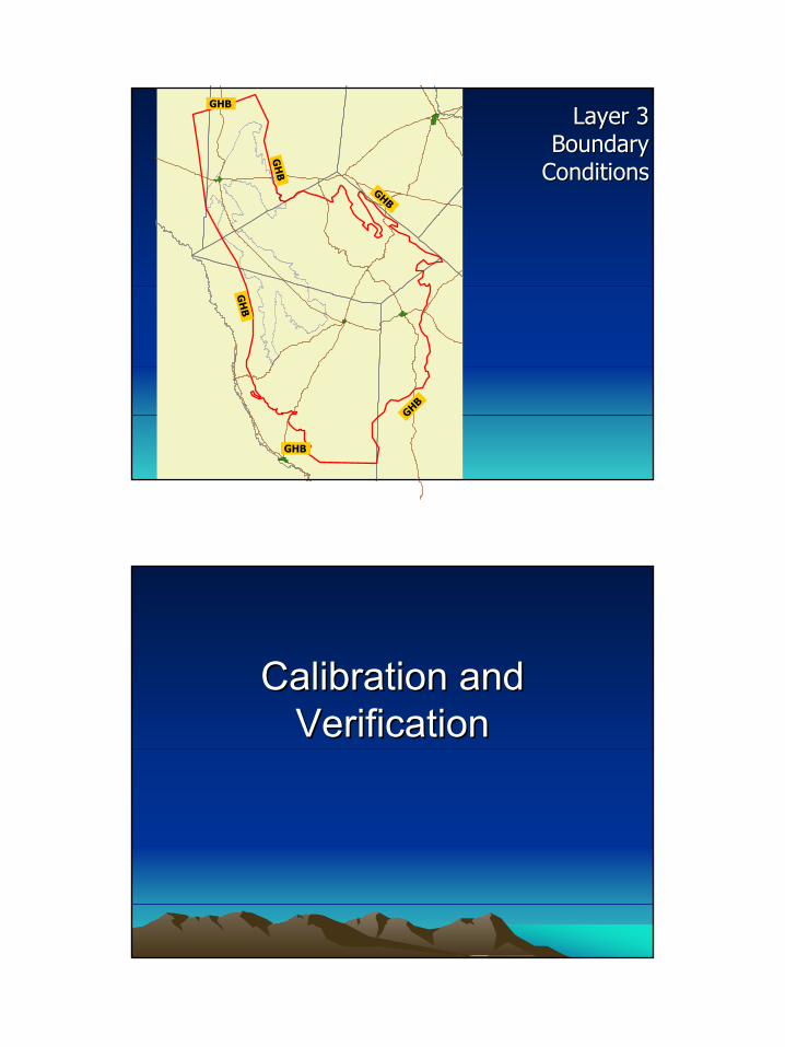
Layer 3 Layer 3 Boundary Boundary
ConditionsConditionsGHB
GH
B
GHB
GHB
GHB
GH
B
Calibration and Calibration and VerificationVerification
13
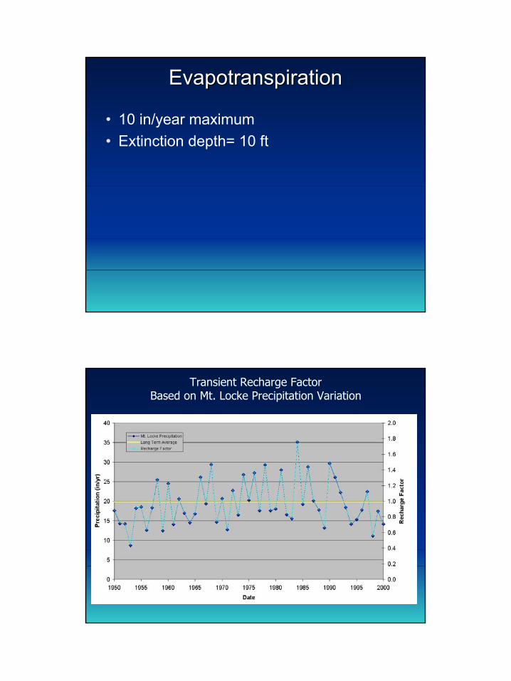
EvapotranspirationEvapotranspiration
• 10 in/year maximum• Extinction depth= 10 ft
Transient Recharge FactorBased on Mt. Locke Precipitation Variation
14
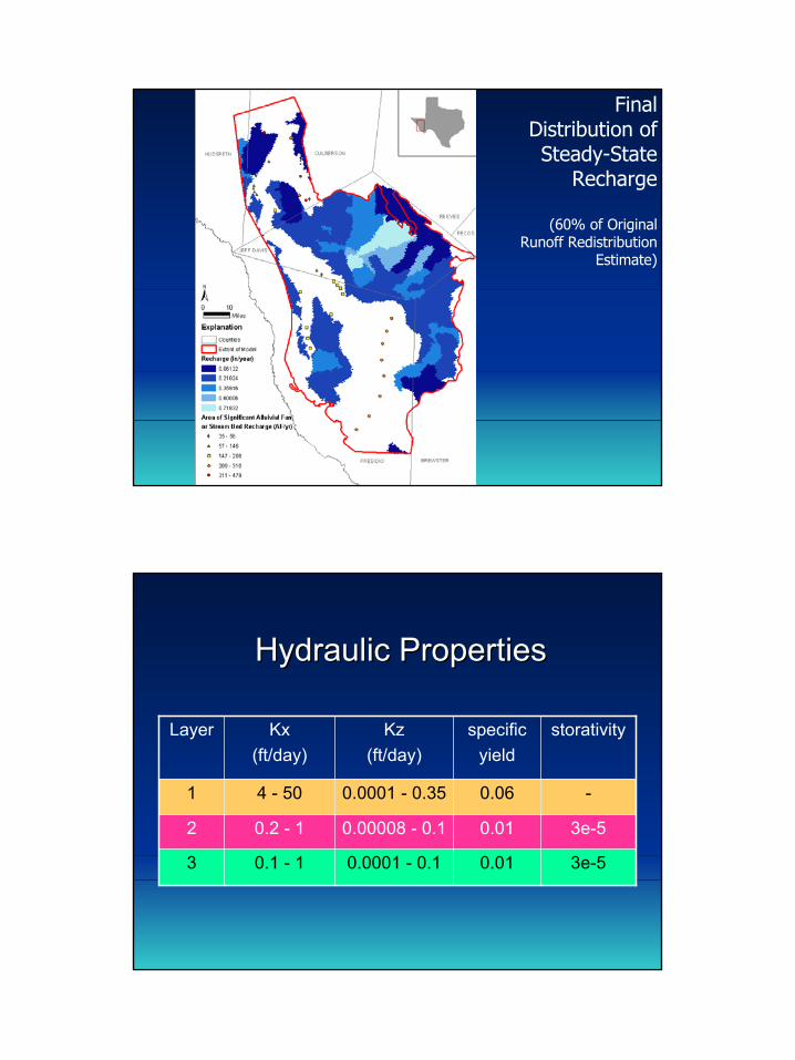
Final Distribution of Steady-State
Recharge
(60% of Original Runoff Redistribution
Estimate)
Hydraulic PropertiesHydraulic Properties
3e-50.010.0001 - 0.10.1 - 13
3e-50.010.00008 - 0.10.2 - 12
-0.060.0001 - 0.354 - 501
storativityspecificyield
Kz(ft/day)
Kx(ft/day)
Layer
15
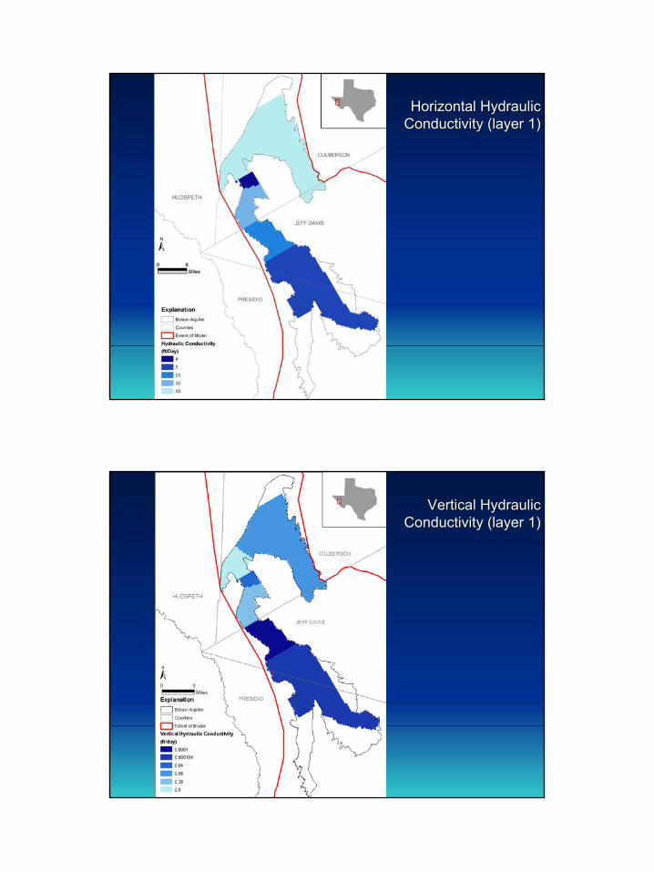
Horizontal Hydraulic Horizontal Hydraulic Conductivity (layer 1)Conductivity (layer 1)
Vertical Hydraulic Vertical Hydraulic Conductivity (layer 1)Conductivity (layer 1)
16
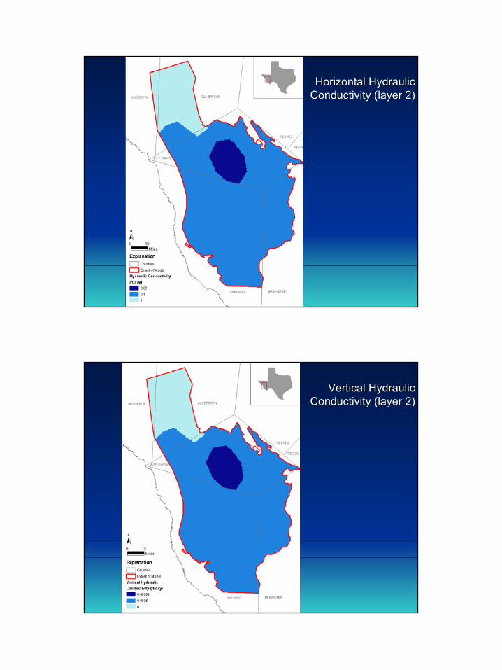
Horizontal Hydraulic Horizontal Hydraulic Conductivity (layer 2)Conductivity (layer 2)
Vertical Hydraulic Vertical Hydraulic Conductivity (layer 2)Conductivity (layer 2)
17
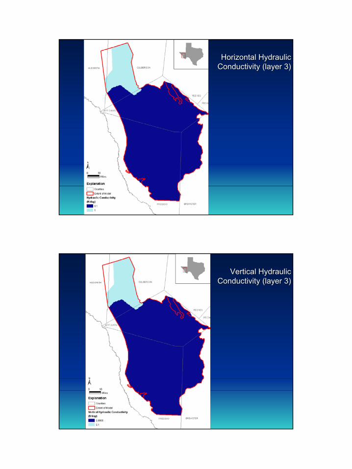
Horizontal Hydraulic Horizontal Hydraulic Conductivity (layer 3)Conductivity (layer 3)
Vertical Hydraulic Vertical Hydraulic Conductivity (layer 3)Conductivity (layer 3)
18
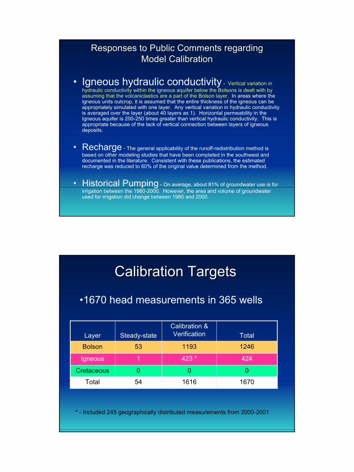
Responses to Public Comments regarding Responses to Public Comments regarding Model CalibrationModel Calibration
• Igneous hydraulic conductivity - Vertical variation in hydraulic conductivity within the igneous aquifer below the Bolsons is dealt with by assuming that the volcaniclastics are a part of the Bolson layer. In areas where the igneous units outcrop, it is assumed that the entire thickness of the igneous can be appropriately simulated with one layer. Any vertical variation in hydraulic conductivity is averaged over the layer (about 40 layers as 1). Horizontal permeability in the Igneous aquifer is 200-250 times greater than vertical hydraulic conductivity. This isappropriate because of the lack of vertical connection between layers of igneous deposits.
• Recharge - The general applicability of the runoff-redistribution method is based on other modeling studies that have been completed in the southwest and documented in the literature. Consistent with these publications, the estimated recharge was reduced to 60% of the original value determined from the method.
• Historical Pumping - On average, about 81% of groundwater use is for irrigation between the 1980-2000. However, the area and volume of groundwater used for irrigation did change between 1980 and 2000.
Calibration TargetsCalibration Targets
000Cretaceous
1670161654Total
423 *
1193
Calibration & Verification
4241Igneous
124653BolsonTotalSteady-stateLayer
•1670 head measurements in 365 wells
* - Included 245 geographically distributed measurements from 2000-2001
19
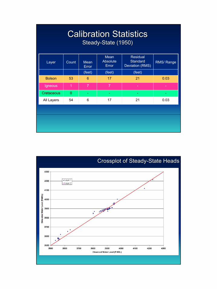
Calibration StatisticsCalibration StatisticsSteadySteady--State (1950)State (1950)
54
0
1
53
Count
(feet)(feet)(feet)
21
-
-
21
Residual Standard
Deviation (RMS)
---Cretaceous
0.03176All Layers
7
17
Mean Absolute
Error
-7Igneous
0.036Bolson
RMS/ RangeMean Error
Layer
Crossplot of SteadyCrossplot of Steady--State HeadsState Heads
20
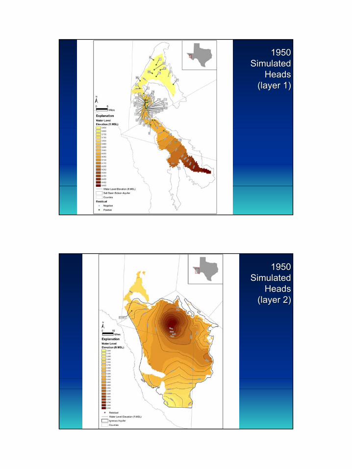
1950 1950 Simulated Simulated
HeadsHeads(layer 1)(layer 1)
1950 1950 Simulated Simulated
HeadsHeads(layer 2)(layer 2)
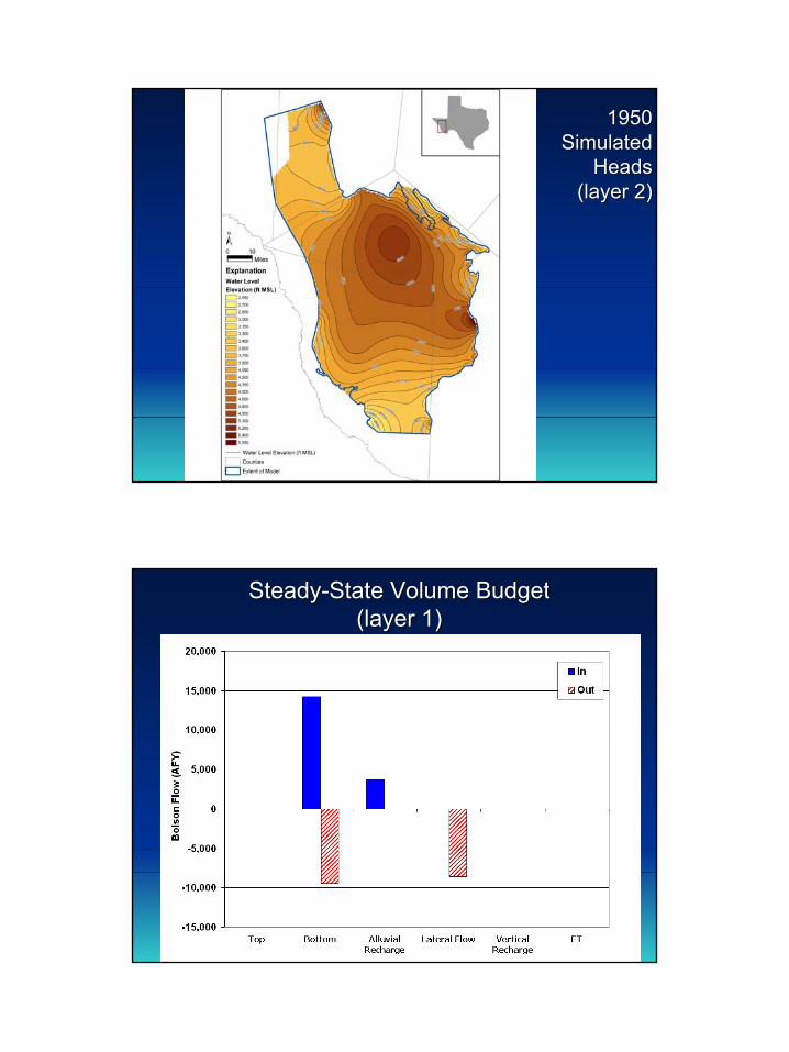
21
1950 1950 Simulated Simulated
HeadsHeads(layer 2)(layer 2)
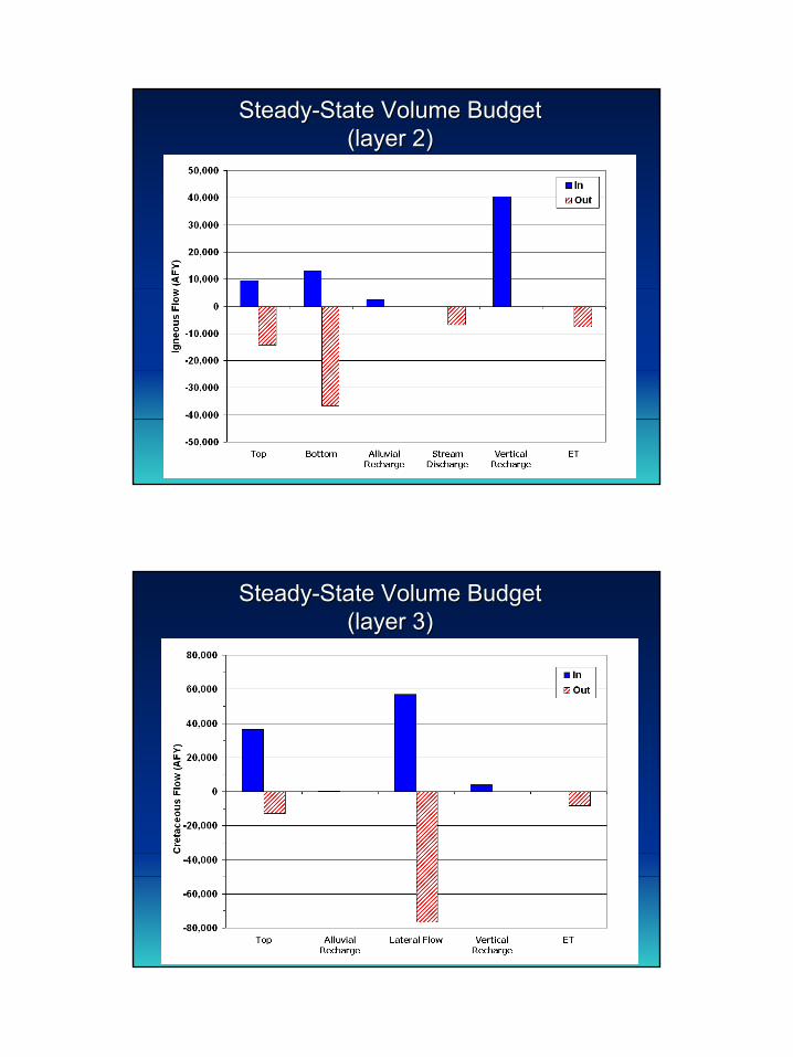
SteadySteady--State Volume Budget State Volume Budget (layer 1)(layer 1)
22
SteadySteady--State Volume Budget State Volume Budget (layer 2)(layer 2)
SteadySteady--State Volume Budget State Volume Budget (layer 3)(layer 3)
23
Calibration Calibration WellsWells
Calibration Statistics(1951(1951--1990)1990)
1017
0
122
895
Count
(feet)(feet)(feet)
34
-
35
35
Residual Standard
Deviation (RMS)
---Cretaceous
0.02287All Layers
35
27
Mean Absolute
Error
0.0317Igneous
0.04-10Bolson
RMS/ RangeMean Error
Layer
24
Crossplot of heads during calibration period (1950Crossplot of heads during calibration period (1950--1990)1990)
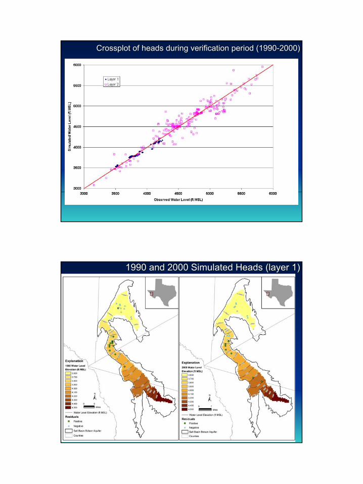
Verification StatisticsVerification Statistics(1991(1991--2000)2000)
599
301
298
Count
(feet)(feet)(feet)
109
-
150
35
Residual Standard
Deviation (RMS)
---Cretaceous
0.0464-15All Layers
105
27
Mean Absolute
Error
0.05-15Igneous
0.05-15Bolson
RMS/ RangeMean Error
Layer
25
Crossplot of heads during verification period (1990Crossplot of heads during verification period (1990--2000)2000)
1990 and 2000 Simulated Heads (layer 1)1990 and 2000 Simulated Heads (layer 1)
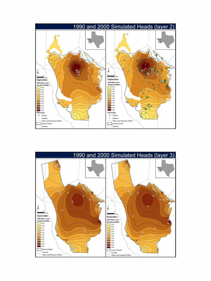
26
1990 and 2000 Simulated Heads (layer 2)1990 and 2000 Simulated Heads (layer 2)
1990 and 2000 Simulated Heads (layer 3)1990 and 2000 Simulated Heads (layer 3)
27
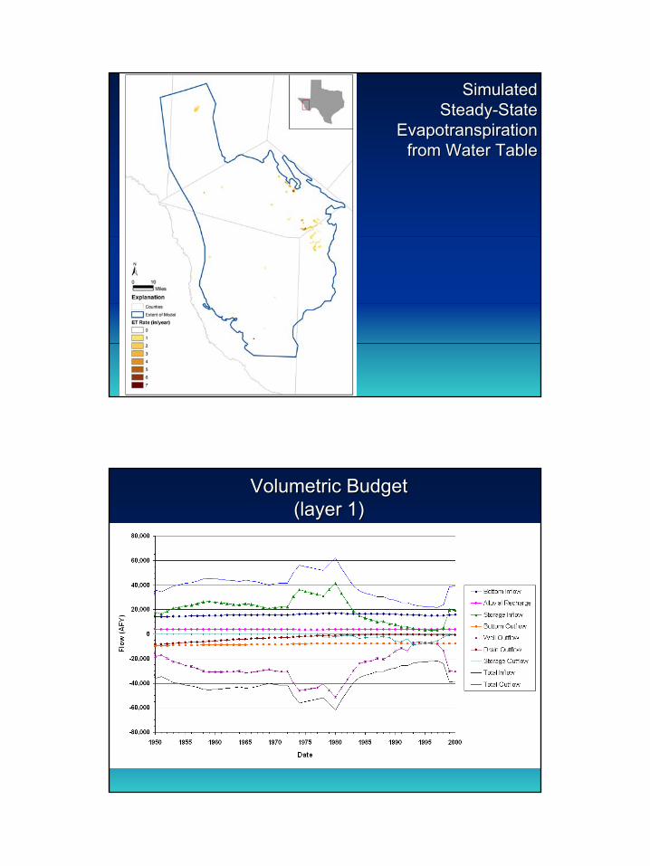
Simulated Simulated SteadySteady--State State
Evapotranspiration Evapotranspiration from Water Tablefrom Water Table
Volumetric Budget Volumetric Budget (layer 1)(layer 1)
28
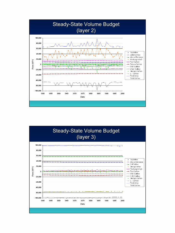
SteadySteady--State Volume Budget State Volume Budget (layer 2)(layer 2)
SteadySteady--State Volume Budget State Volume Budget (layer 3)(layer 3)
29
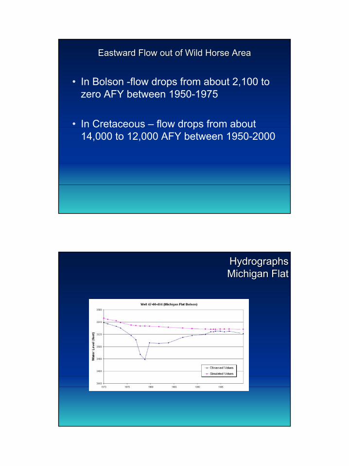
Eastward Flow out of Wild Horse AreaEastward Flow out of Wild Horse Area
• In Bolson -flow drops from about 2,100 to zero AFY between 1950-1975
• In Cretaceous – flow drops from about 14,000 to 12,000 AFY between 1950-2000
HydrographsHydrographsMichigan FlatMichigan Flat
30
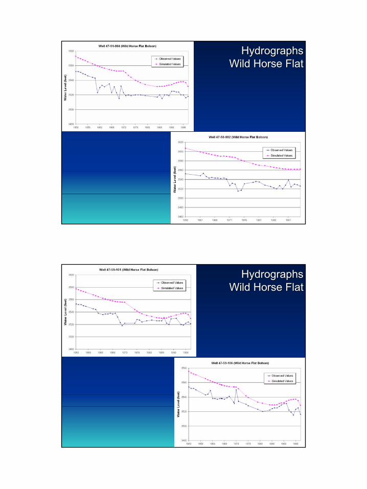
HydrographsHydrographsWild Horse FlatWild Horse Flat
HydrographsHydrographsWild Horse FlatWild Horse Flat
31
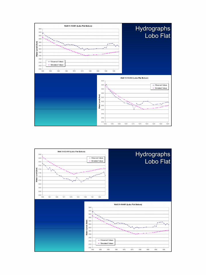
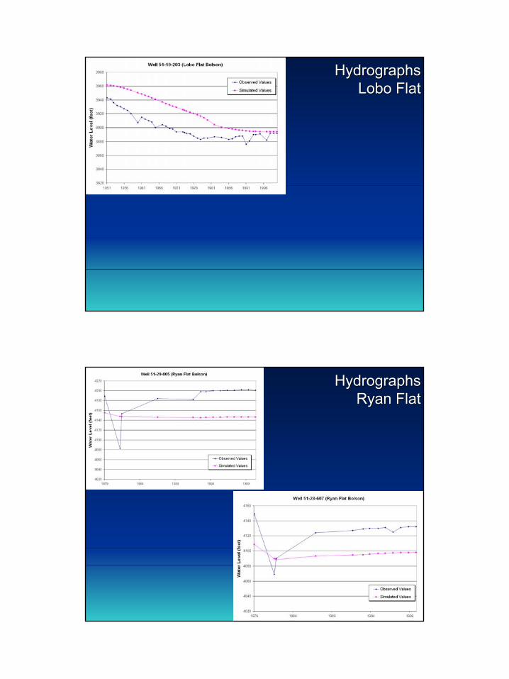
HydrographsHydrographsLobo FlatLobo Flat
HydrographsHydrographsLobo FlatLobo Flat
32
HydrographsHydrographsLobo FlatLobo Flat
HydrographsHydrographsRyan FlatRyan Flat
33
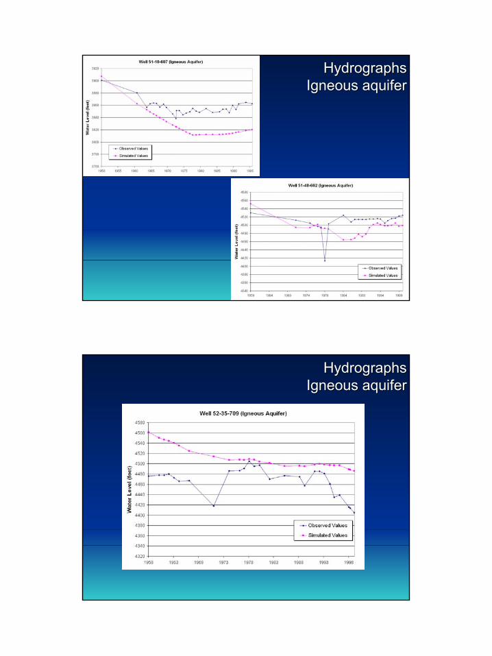
HydrographsHydrographsIgneous aquiferIgneous aquifer
HydrographsHydrographsIgneous aquiferIgneous aquifer
34
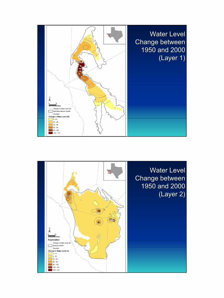
Water Level Water Level Change between Change between
1950 and 2000 1950 and 2000 (Layer 1)(Layer 1)
Water Level Water Level Change between Change between
1950 and 2000 1950 and 2000 (Layer 2)(Layer 2)
35
Water Level Water Level Change between Change between
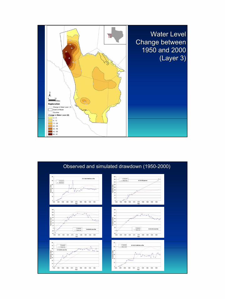
1950 and 2000 1950 and 2000 (Layer 3)(Layer 3)
Observed and simulated drawdown (1950Observed and simulated drawdown (1950--2000)2000)
36
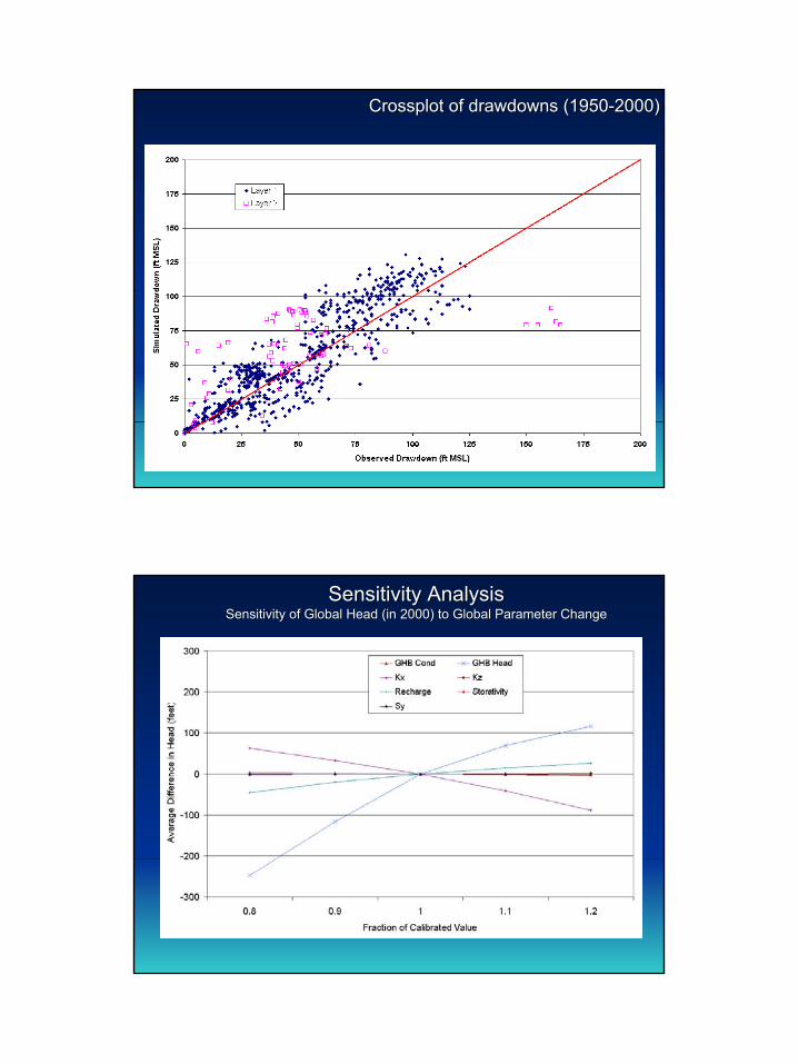
Crossplot of drawdowns (1950Crossplot of drawdowns (1950--2000)2000)
Sensitivity AnalysisSensitivity AnalysisSensitivity of Global Head (in 2000) to Global Parameter ChangeSensitivity of Global Head (in 2000) to Global Parameter Change
37
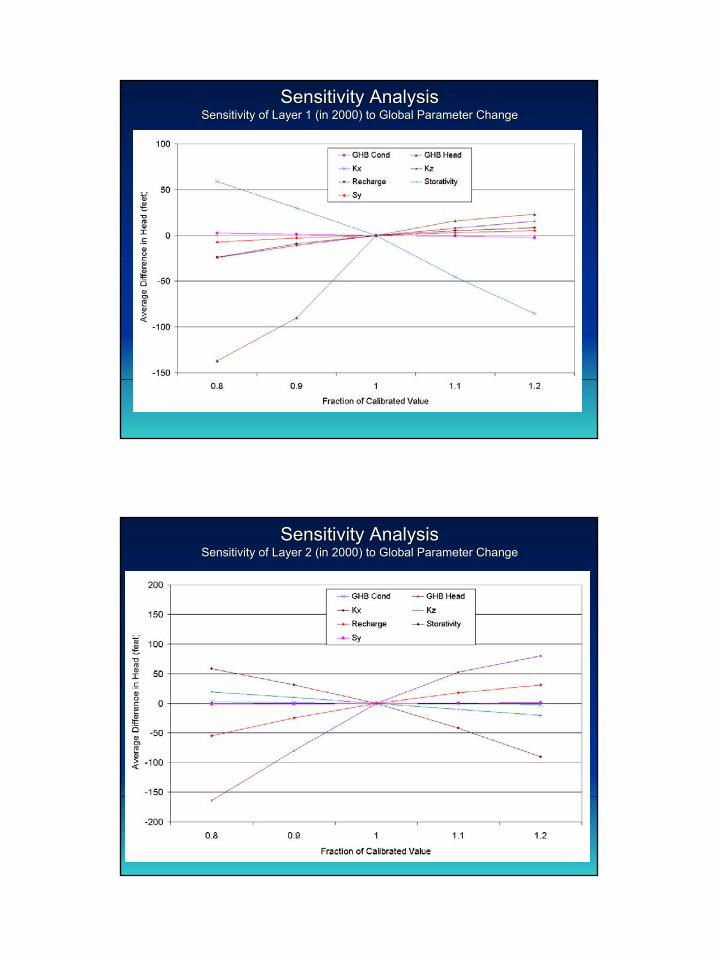
Sensitivity AnalysisSensitivity AnalysisSensitivity of Layer 1 (in 2000) to Global Parameter ChangeSensitivity of Layer 1 (in 2000) to Global Parameter Change
Sensitivity AnalysisSensitivity AnalysisSensitivity of Layer 2 (in 2000) to Global Parameter ChangeSensitivity of Layer 2 (in 2000) to Global Parameter Change
38
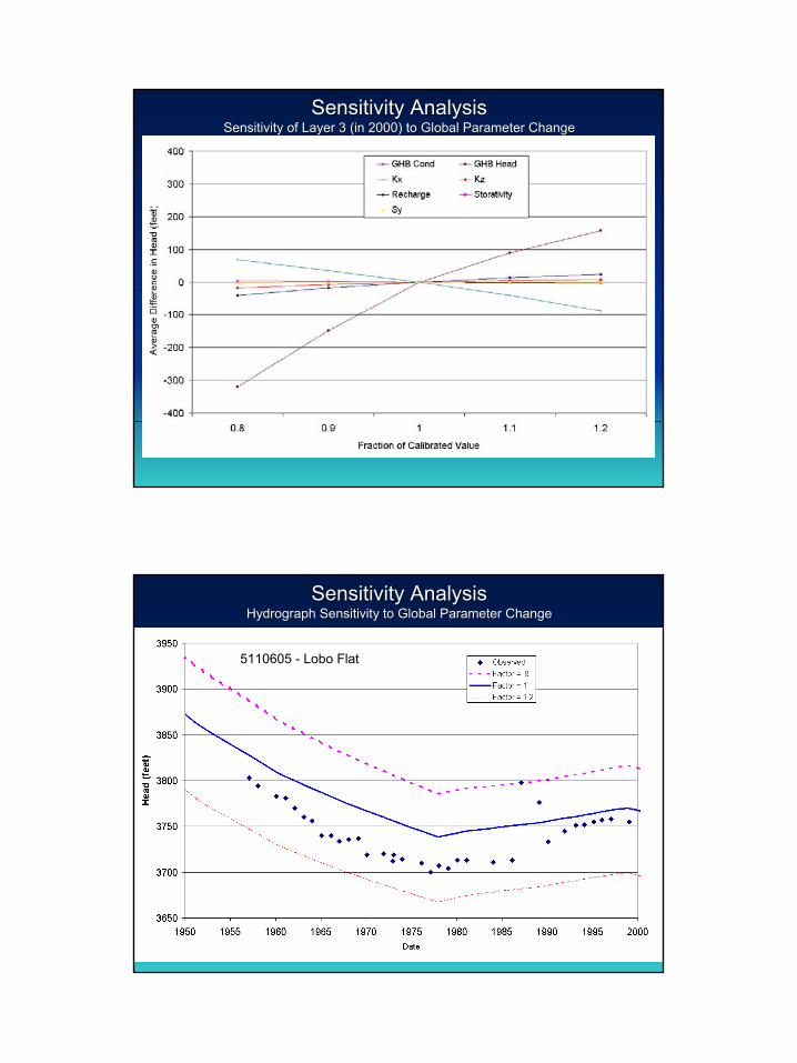
Sensitivity AnalysisSensitivity AnalysisSensitivity of Layer 3 (in 2000) to Global Parameter ChangeSensitivity of Layer 3 (in 2000) to Global Parameter Change
Sensitivity AnalysisSensitivity AnalysisHydrograph Sensitivity to Global Parameter ChangeHydrograph Sensitivity to Global Parameter Change
5110605 - Lobo Flat
39
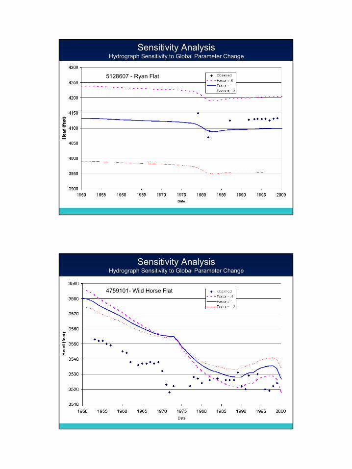
Sensitivity AnalysisSensitivity AnalysisHydrograph Sensitivity to Global Parameter ChangeHydrograph Sensitivity to Global Parameter Change
5128607 - Ryan Flat
Sensitivity AnalysisSensitivity AnalysisHydrograph Sensitivity to Global Parameter ChangeHydrograph Sensitivity to Global Parameter Change
4759101- Wild Horse Flat
40
Predictive SimulationsPredictive Simulations
Responses to Public Comments regarding Responses to Public Comments regarding Model PredictionsModel Predictions
• Culberson Co. - In 2002, the State Water Plan included estimates of future demand in Culberson Co. that were about 1/3 of the current usage. Therefore, water levels generally increase in Culberson Co. during the predictive period. For the final report, another simulation will be completed which will include the recently approved demands from Region E, which are equal to the metered amounts.
• Region E strategy – a tentative strategy was approved by Region E and included in the State Water Plan (SWP) which proposed that El Paso would pump groundwater from Ryan Flat. The existing well field is located in Jeff Davis and Presidio Counties. However, the SWP stated that all the pumping would occur in Jeff Davis Co. Region E has approved a clarification of that strategy which assumes that pumping will occur in both counties, which better represents the intent of the strategy.
41
Total PumpingTotal Pumping
Pumping by CountyPumping by County
42
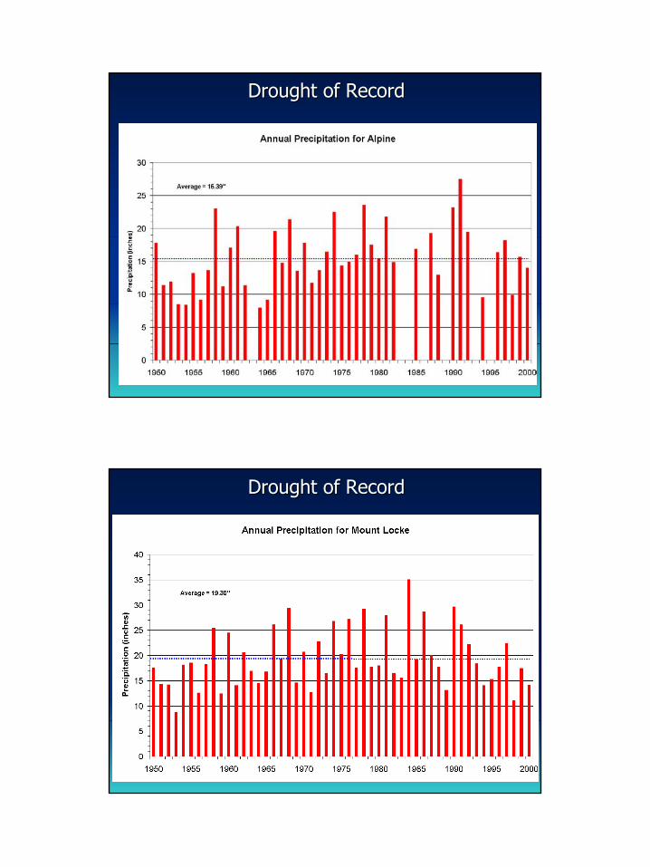
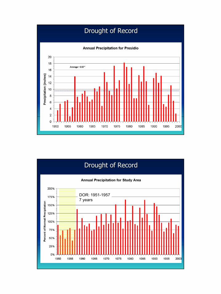
Drought of RecordDrought of Record
DOR: 1951-19577 years
Drought of RecordDrought of Record
43
Drought of RecordDrought of Record
Drought of RecordDrought of Record
DOR: 1951-19577 years
44
Drought of RecordDrought of Record
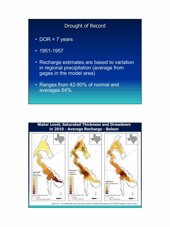
• DOR = 7 years
• 1951-1957
• Recharge estimates are based to variation in regional precipitation (average from gages in the model area)
• Ranges from 42-80% of normal and averages 64%
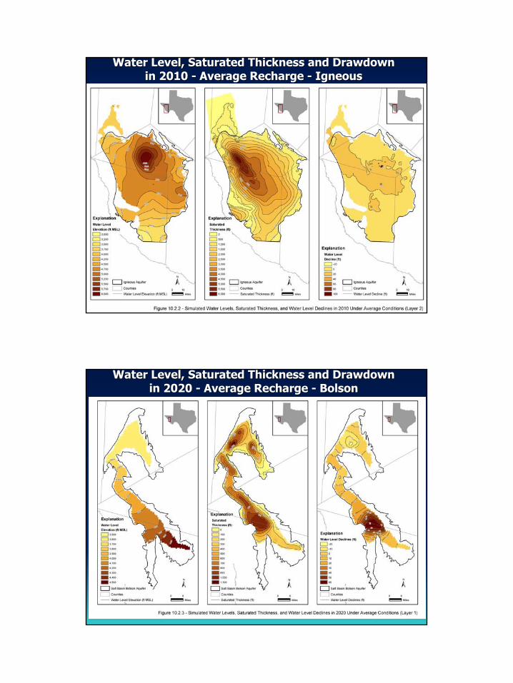
Water Level, Saturated Thickness and Drawdown Water Level, Saturated Thickness and Drawdown in 2010 in 2010 -- Average Recharge Average Recharge -- BolsonBolson
45
Water Level, Saturated Thickness and Drawdown Water Level, Saturated Thickness and Drawdown in 2010 in 2010 -- Average Recharge Average Recharge -- IgneousIgneous
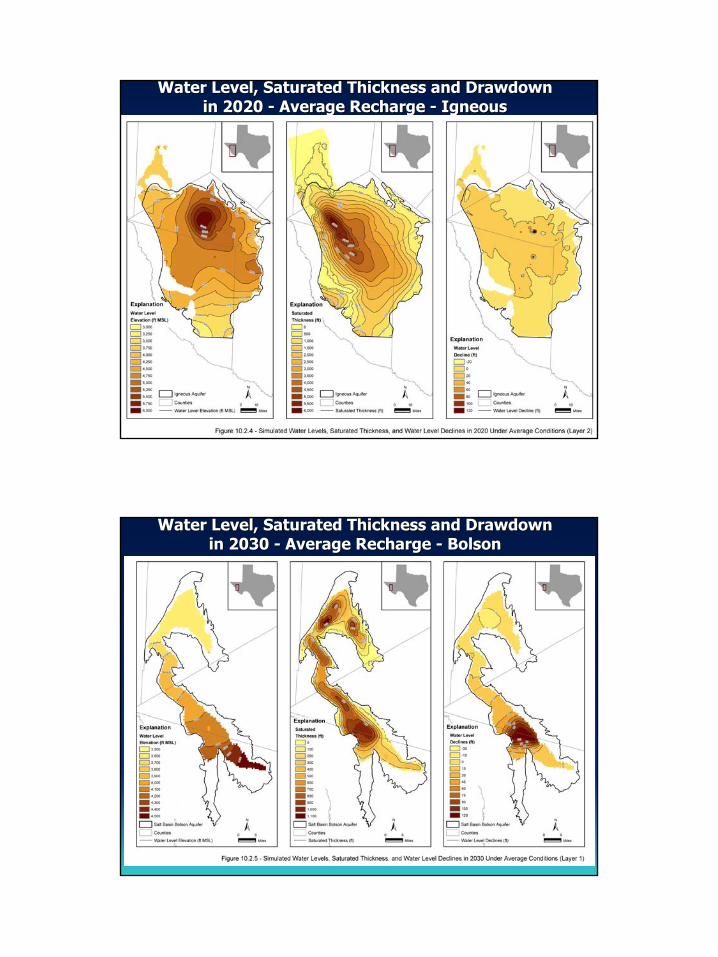
Water Level, Saturated Thickness and Drawdown Water Level, Saturated Thickness and Drawdown in 2020 in 2020 -- Average Recharge Average Recharge -- BolsonBolson
46
Water Level, Saturated Thickness and Drawdown Water Level, Saturated Thickness and Drawdown in 2020 in 2020 -- Average Recharge Average Recharge -- IgneousIgneous
Water Level, Saturated Thickness and Drawdown Water Level, Saturated Thickness and Drawdown in 2030 in 2030 -- Average Recharge Average Recharge -- BolsonBolson
47
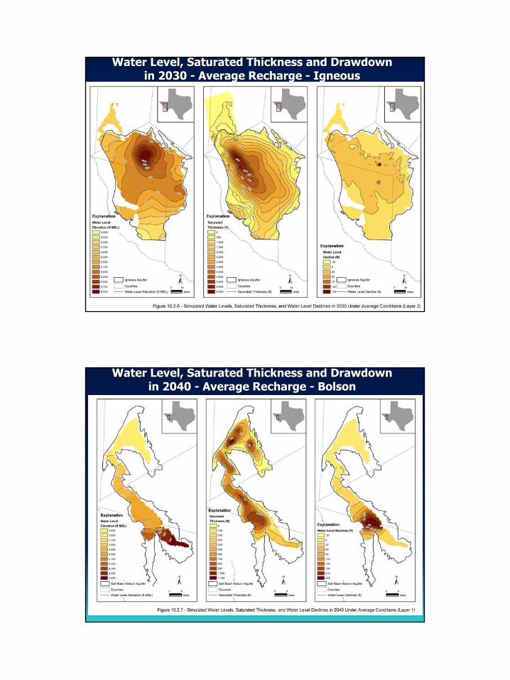
Water Level, Saturated Thickness and Drawdown Water Level, Saturated Thickness and Drawdown in 2030 in 2030 -- Average Recharge Average Recharge -- IgneousIgneous
Water Level, Saturated Thickness and Drawdown Water Level, Saturated Thickness and Drawdown in 2040 in 2040 -- Average Recharge Average Recharge -- BolsonBolson
48
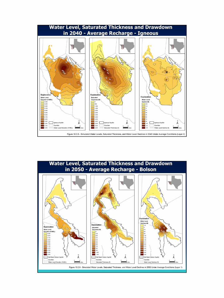
Water Level, Saturated Thickness and Drawdown Water Level, Saturated Thickness and Drawdown in 2040 in 2040 -- Average Recharge Average Recharge -- IgneousIgneous
Water Level, Saturated Thickness and Drawdown Water Level, Saturated Thickness and Drawdown in 2050 in 2050 -- Average Recharge Average Recharge -- BolsonBolson
49
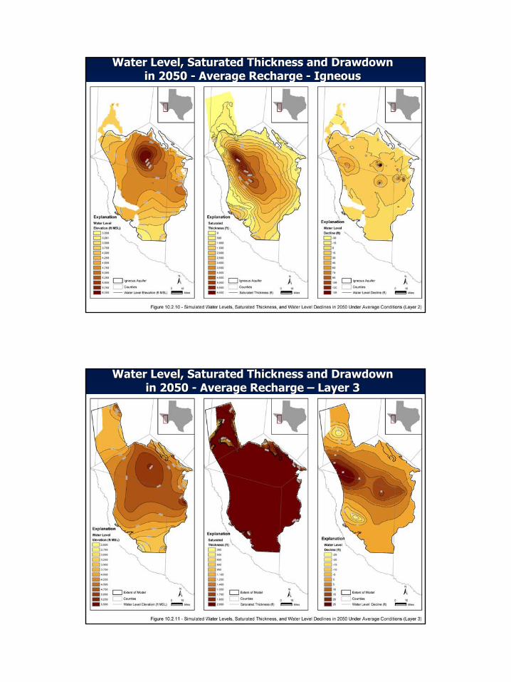
Water Level, Saturated Thickness and Drawdown Water Level, Saturated Thickness and Drawdown in 2050 in 2050 -- Average Recharge Average Recharge -- IgneousIgneous
Water Level, Saturated Thickness and Drawdown Water Level, Saturated Thickness and Drawdown in 2050 in 2050 -- Average Recharge Average Recharge –– Layer 3Layer 3
50
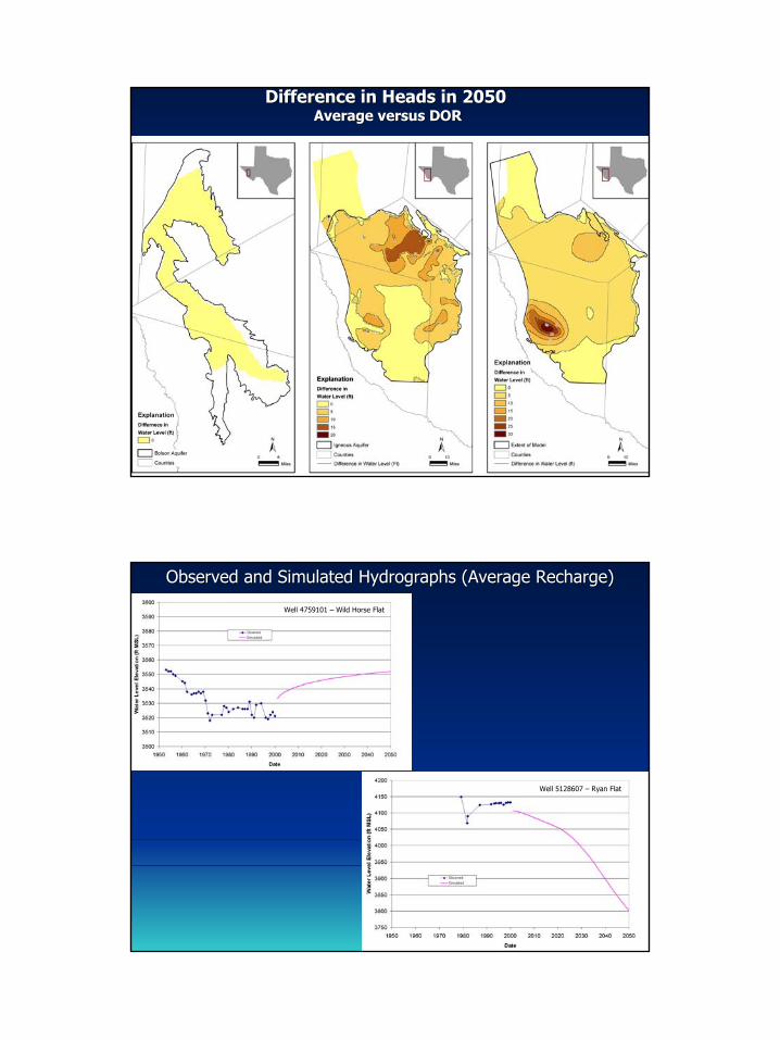
Difference in Heads in 2050 Difference in Heads in 2050 Average versus DORAverage versus DOR
Observed and Simulated Hydrographs (Average Recharge)Observed and Simulated Hydrographs (Average Recharge)
Well 4759101 – Wild Horse Flat
Well 5128607 – Ryan Flat
51
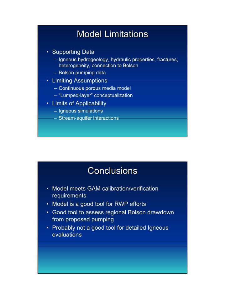
Model LimitationsModel Limitations
• Supporting Data– Igneous hydrogeology, hydraulic properties, fractures,
heterogeneity, connection to Bolson– Bolson pumping data
• Limiting Assumptions– Continuous porous media model– “Lumped-layer” conceptualization
• Limits of Applicability– Igneous simulations– Stream-aquifer interactions
ConclusionsConclusions
• Model meets GAM calibration/verification requirements
• Model is a good tool for RWP efforts• Good tool to assess regional Bolson drawdown
from proposed pumping• Probably not a good tool for detailed Igneous
evaluations
52
5th Stakeholder Advisory Forum
March 25th, 2004 West Texas Igneous and Bolson GAM
List of Attendees
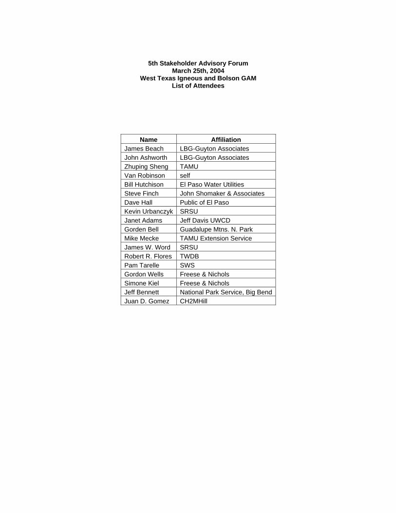
Name Affiliation James Beach LBG-Guyton Associates John Ashworth LBG-Guyton Associates Zhuping Sheng TAMU Van Robinson self Bill Hutchison El Paso Water Utilities Steve Finch John Shomaker & Associates Dave Hall Public of El Paso Kevin Urbanczyk SRSU Janet Adams Jeff Davis UWCD Gorden Bell Guadalupe Mtns. N. Park Mike Mecke TAMU Extension Service James W. Word SRSU Robert R. Flores TWDB Pam Tarelle SWS Gordon Wells Freese & Nichols Simone Kiel Freese & Nichols Jeff Bennett National Park Service, Big Bend Juan D. Gomez CH2MHill
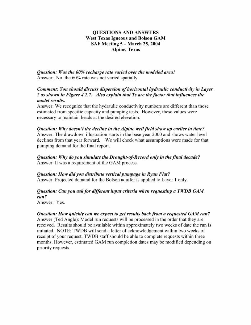
QUESTIONS AND ANSWERS West Texas Igneous and Bolson GAM
SAF Meeting 5 � March 25, 2004 Alpine, Texas
Question: Was the 60% recharge rate varied over the modeled area? Answer: No, the 60% rate was not varied spatially. Comment: You should discuss dispersion of horizontal hydraulic conductivity in Layer 2 as shown in Figure 4.2.7. Also explain that Ts are the factor that influences the model results. Answer: We recognize that the hydraulic conductivity numbers are different than those estimated from specific capacity and pumping tests. However, these values were necessary to maintain heads at the desired elevation. Question: Why doesn�t the decline in the Alpine well field show up earlier in time? Answer: The drawdown illustration starts in the base year 2000 and shows water level declines from that year forward. We will check what assumptions were made for that pumping demand for the final report. Question: Why do you simulate the Drought-of-Record only in the final decade? Answer: It was a requirement of the GAM process. Question: How did you distribute vertical pumpage in Ryan Flat? Answer: Projected demand for the Bolson aquifer is applied to Layer 1 only. Question: Can you ask for different input criteria when requesting a TWDB GAM run? Answer: Yes. Question: How quickly can we expect to get results back from a requested GAM run? Answer (Ted Angle): Model run requests will be processed in the order that they are received. Results should be available within approximately two weeks of date the run is initiated. NOTE: TWDB will send a letter of acknowledgement within two weeks of receipt of your request. TWDB staff should be able to complete requests within three months. However, estimated GAM run completion dates may be modified depending on priority requests.


![Studie Poker-Texas-Holdem[34.0][1]](https://img.pdfslide.org/doc/110x75/586b63bc1a28ab22658bbfa8/studie-poker-texas-holdem3401.jpg)